modular forms and arithmetic geometry - math.toronto.edu · modular forms and arithmetic geometry...
TRANSCRIPT
Modular forms and arithmetic geometry
Stephen S. Kudla1
The aim of these notes is to describe some examples of modular forms whose Fouriercoefficients involve quantities from arithmetical algebraic geometry. At the moment,no general theory of such forms exists, but the examples suggest that they shouldbe viewed as a kind of arithmetic analogue of theta series and that there shouldbe an arithmetic Siegel–Weil formula relating suitable averages of them to specialvalues of derivatives of Eisenstein series. We will concentrate on the case for whichthe most complete picture is available, the case of generating series for cycles onthe arithmetic surfaces associated to Shimura curves over Q, expanding on thetreatment in [40]. A more speculative overview can be found in [41].
In section 1, we review the basic facts about the arithmetic surface M associated toa Shimura curve over Q. These arithmetic surfaces are moduli stacks over Spec(Z)of pairs (A, ι) over a base S, where A is an abelian scheme of relative dimension 2and ι is an action on A of a maximal order OB in an indefinite quaternion algebraB over Q. In section 2, we recall the definition of the arithmetic Chow groupCH
1(M), following Bost, [7], and we discuss the metrized Hodge line bundle ω and
the conjectural value of 〈ω, ω〉, where 〈 , 〉 is the height pairing on CH1(M). In the
next two sections, we describe divisors Z(t), t ∈ Z>0, on M. These are defined asthe locus of (A, ι, x)’s where x is a special endomorphism (Definition 3.1) of (A, ι)with x2 = −t. Since such an x gives an action on (A, ι) of the order Z[
√−t] in the
imaginary quadratic field kt = Q(√−t), the cycles Z(t) can be viewed as analogues
of the familiar CM points on modular curves. In section 3, the complex points andhence the horizontal components of Z(t) are determined. In section 4, the verticalcomponents of Z(t) are determined using the p-adic uniformization of the fibers Mp
of bad reduction of M. In section 5, we construct Green functions Ξ(t, v) for thedivisors Z(t), depending on a parameter v ∈ R×
>0. When t < 0, the series definingΞ(t, v) becomes a smooth function on M(C). These Green functions are used in
section 6 to define classes Z(t, v) ∈ CH1(M), for t ∈ Z, t = 0, and an additional
class Z(0, v) is defined using ω. The main result of section 6 (Theorem 6.3) says
1Partially supported by NSF grant DMS-0200292 and by a Max-Planck Research Prize from the
Max-Planck Society and Alexander von Humboldt Stiftung.
1

2
that generating series
θ(τ) =∑
t∈Z
Z(t, v) qt, τ = u + iv, q = e(τ),
is the q–expansion of a (nonholomorphic) modular form of weight 32 , which we call
an arithmetic theta function. The proof of this result is sketched in section 7. Themain ingredients are (i) the fact that the height pairing of θ(τ) with various classes
in CH1(M), e.g., ω, can be shown to be modular, and (ii) the result of Borcherds,
[5], which says that a similar generating series with coefficients in the usual Chowgroup of the generic fiber CH1(MQ) is a modular form of weight 3
2 . In section 8,we use the arithmetic theta function to define an arithmetic theta lift
θ : S 32−→ CH
1(M), f → θ(f) = 〈 f, θ 〉Pet,
from a certain space of modular forms of weight 32 to the arithmetic Chow group.
This lift is an arithmetic analogue of the classical theta lift from modular formsof weight 3
2 to automorphic forms of weight 2 for Γ = O×B . According to the
results of Waldspurger, reviewed in section 9, the nonvanishing of this classicallift is controlled by a combination of local obstructions and, most importantly,the central value L(1, F ) of the standard Hecke L-function2 of the cusp form F ofweight 2 coming from f via the Shimura lift. In section 10, we describe a doublingintegral representation (Theorem 10.1) of the Hecke L-function, involving f and anEisenstein series E(τ, s, B) of weight 3
2 and genus 2. At the central point s = 0,E(τ, 0, B) = 0. In the case in which the root number of the L-function is −1, weobtain a formula (Corollary 10.2)
〈 E ′2(
(τ1
−τ2
)
, 0;B) , f(τ2) 〉Pet, τ2 = f(τ1) · C(0) · L′(12, π),
for an explicit constant C(0), whose vanishing is controlled by local obstructions.Finally, in section 11, we state a conjectural identity (Conjecture 11.1)
〈 θ(τ1), θ(τ2) 〉 ??= E ′2(
(τ1
−τ2
)
, 0;B)
relating the height pairing of the arithmetic theta function and the restriction tothe diagonal of the derivative at s = 0 of the weight 3
2 Eisenstein series. This
2Here we assume that F is a newform, so that L(1, F ) = L( 12, π), where π is the corresponding
cuspidal automorphic representation.

3
identity is equivalent to a series of identities of Fourier coefficients, (11.1),
〈 Z(t1, v1), Z(t2, v2) 〉 · qt11 qt2
2
=∑
T∈Sym2(Z)∨
diag(T )=(t1,t2)
E ′2,T (
(τ1
τ2
)
, 0;B).
Here
Sym2(Z)∨ = T =(
t1 mm t2
)
| t1, t2 ∈ Z, m ∈ 12
Z
is the dual lattice of Sym2(Z) with respect to the trace pairing. We sketch theproof of these identities in the case where t1t2 is not a square (Theorem 11.2). Asa consequence, we prove Conjecture 11.1 up to a linear combination of theta seriesfor quadratic forms in one variable (Corollary 11.3). Assuming that f is orthogonalto such theta series, we can substitute the height pairing 〈 Z(t1, v1), Z(t2, v2) 〉 forthe derivative of the Eisenstein series in the doubling identity and obtain,
〈 θ(τ1), θ(f) 〉 = f(τ1) · C(0) · L′(12, π),
in the case of root number −1. This yields the arithmetic inner product formula
〈 θ(f), θ(f) 〉 = 〈 f, f 〉 · C(0) · L′(12, π),
analogous to the Rallis inner product formula for the classical theta lift. Somediscussion of the relation of this result to the Gross-Kohnen-Zagier formula, [24],is given at the end of section 11.
Most of the results described here are part of a long term collaboration with MichaelRapoport and Tonghai Yang. I would also like to thank J.-B. Bost, B. Gross, M.Harris, J. Kramer, and U. Kuhn for their comments and suggestions.
Contents
§1. Shimura curves and arithmetic surfaces§2. Arithmetic Chow groups§3. Special cycles, horizontal components§4. Special cycles, vertical components§5. Green functions§6. The arithmetic theta series

4
§7. Modularity of the arithmetic theta series§8. The arithmetic theta lift§9. Theta dichotomy, Waldspurger’s theory§10. The doubling integral§11. The arithmetic inner product formula
§1. Shimura curves and arithmetic surfaces.
Let B be an indefinite quaternion algebra over Q and let D(B) be the product ofthe primes p for which Bp = B ⊗Q Qp is a division algebra. For the moment, weallow the case B = M2(Q), where D(B) = 1. The three dimensional Q–vectorspace
(1.1) V = x ∈ B | tr(x) = 0
is equipped with the quadratic form Q(x) = ν(x) = −x2. Here ν (resp. tr)is the reduced norm (resp. trace) on B; in the case B = M2(Q), this is theusual determinant (resp. trace). The bilinear form associated to Q is given by(x, y) = tr(xyι), where x → xι is the involution on B given by xι = tr(x)− x. Theaction of H = B× on V by conjugation, h : x → hxh−1, preserves the quadraticform and induces an isomorphism
(1.2) H∼−→ GSpin(V ),
where GSpin(V ) is the spinor similitude group of V . Since B is indefinite, i.e., sinceBR = B ⊗Q R M2(R), V has signature (1, 2). Let
(1.3) D = w ∈ V (C) | (w, w) = 0, (w, w) < 0 / C× ⊂ P(V (C)),
so that D is an open subset of a quadric in P(V (C)). Then the group H(R) actsnaturally on D, and, if we fix an isomorphism BR M2(R), then there is anidentification
(1.4) C \ R∼−→ D, z → w(z) :=
(z −z2
1 −z
)
mod C×,
which is equivariant for the action of H(R) GL2(R) on C \R by fractional lineartransformations.
5
Let OB be a maximal order in B and let Γ = O×B . In the case B = M2(Q), one
may take OB = M2(Z), so that Γ = GL2(Z). Also let
(1.5) K = (OB)× ⊂ H(Af ),
where OB = OB ⊗Z Z, for Z = lim←N
Z/NZ. Then the quotient
(1.6) M(C) = H(Q)\(
D × H(Af )/K
)
Γ\D,
which should be viewed as an orbifold, is the set of complex points of a Shimuracurve M , if D(B) > 1, or of the modular curve (without its cusp), if D(B) = 1.From now on, we assume that D(B) > 1, although much of what follows can becarried over for D(B) = 1 with only slight modifications. The key point is tointerpret M as a moduli space.
Let M be the moduli stack over Spec(Z) for pairs (A, ι) where A is an abelianscheme over a base S with an action ι : OB → EndS(A) satisfying the determinantcondition, [49], [36], [9],
(1.7) det(ι(b); Lie(A)) = ν(b).
Over C, such an (A, ι) is an abelian surface with OB action. For example, forz ∈ D C \ R, the isomorphism
(1.8) λz : BR M2(R) ∼−→ C2, b → b ·(
z1
)
=(
w1
w2
)
determines a lattice Lz = λz(OB) ⊂ C2. The complex torus Az = C2/Lz is anabelian variety with a natural OB action given by left multiplication, and hencedefines an object (Az, ι) ∈ M(C). Two points in D give the same lattice if andonly if they are in the same O×
B–orbit, and, up to isomorphism, every (A, ι) over C
arises in this way. Thus, the construction just described gives an isomorphism
(1.9) [ Γ\D ] ∼−→ M(C)
of orbifolds, and M gives a model of M(C) over Spec(Z) with generic fiber
(1.10) M = M×Spec(Z) Spec(Q),
6
the Shimura curve over Q.
Since we are assuming that D(B) > 1, M is proper of relative dimension 1 overSpec(Z) and smooth over Spec(Z[D(B)−1]). We will ignore the stack aspect fromnow on and simply view M as an arithmetic surface over Spec(Z).
The surface M has bad reduction at primes p | D(B) and this reduction can bedescribed via p-adic uniformization [9], [46]. Let Ωp be Drinfeld’s p-adic upperhalf plane. It is a formal scheme over Zp with a natural action of PGL2(Qp). LetW = W (Fp) be the Witt vectors of Fp and let
(1.11) ΩW = Ωp ×Spf(Zp) Spf(W )
be the base change of Ωp to W . Also, let Ω•W = ΩW × Z, and let g ∈ GL2(Qp) act
on Ω•W by
(1.12) g : (z, i) → ( g(z), i + ordp(det(g)) ).
Let B(p) be the definite quaternion algebra over Q with invariants
(1.13) inv(B(p)) =
−inv(B) if = p, ∞,
inv(B) otherwise.
Let H(p) = (B(p))× and
(1.14) V (p) = x ∈ B(p) | tr(x) = 0 .
For convenience, we will often write B′ = B(p), H ′ = H(p) and V ′ = V (p) when p
has been fixed. Fix isomorphisms
(1.15) H ′(Qp) GL2(Qp), and H ′(Apf ) H(Ap
f ).
Let Mp be the base change to W of the formal completion of M along its fiber atp. Then, the Drinfeld–Cherednik Theorem gives an isomorphism of formal schemesover W
(1.16) Mp∼−→ H ′(Q)\
(
Ω•W × H(Ap
f )/Kp
)
Γ′\Ω•W ,
where K = KpKp and Γ′ = H ′(Q)∩H ′(Qp)Kp. The special fiber Ωp ×Zp Fp of Ωp
is a union of projective lines P[Λ] indexed by the vertices [Λ] of the building B ofPGL2(Qp). Here [Λ] is the homothety class of the Zp–lattice Λ in Q2
p. The crossingpoints of these lines are double points indexed by the edges of B, and the actionof PGL2(Qp) on components is compatible with its action on B. Thus, the dualgraph of the special fiber of Mp is isomorphic to Γ′\B•, where B• = B × Z.
7
§2. Arithmetic Chow groups.
The modular forms of interest in these notes will take values in the arithmeticChow groups of M. We will use the version of these groups with real coefficientsdefined by Bost, [7], section 5.5. Let Z1(M) be the real vector space spanned bypairs (Z, g), where Z is a real linear combination of Weil divisors on M and g isa Green function for Z. In particular, if Z is a Weil divisor, g is a C∞ functionon M(C) \ Z(C), with a logarithmic singularity along the Z(C), and satisfies theGreen equation
(2.1) ddcg + δZ = [ωZ ],
where ωZ is a smooth (1, 1)-form on M(C), and [ωZ ] is the corresponding cur-rent. If Z =
∑
i ci Zi is a real linear combination of Weil divisors, then g =∑
i ci gi is a real linear combination of such Green functions. By construction,α · (Z, g) = (αZ, αg) for α ∈ R. The first arithmetic Chow group, with real coeffi-
cients, CH1
R(M), is then the quotient of Z1(M) by the subspace spanned by pairs
div(f) = (div(f),− log |f |2) where f is a rational function on M, and div(f) is itsdivisor. Finally, we let
(2.2) CH1(M) = CH
1
R(M) ⊗R C.
Note that restriction to the generic fiber yields a degree map
(2.3) degQ
: CH1(M) −→ CH1(M) ⊗ C
deg−→ C.
The group CH2(M) is defined analogously, and the arithmetic degree map yields
an isomorphism
(2.4) deg : CH2(M) ∼−→ C.
Moreover, there is a symmetric R–bilinear height pairing3
(2.5) 〈 , 〉 : CH1
R(M) × CH
1
R(M) −→ R.
According to the index Theorem, cf. [7], Theorem 5.5, this pairing is nondegenerate
and has signature (+,−,−, . . . ). We extend it to an Hermitian pairing on CH1(M),
conjugate linear in the second argument.
3Here the symmetry must still be checked in the case of a stack, cf. section 4 of [49].

8
Let A be the universal abelian scheme over M with zero section ε, and let
(2.6) ω = ε∗Ω2A/M
be the Hodge line bundle on M. We define the natural metric on ω by letting
(2.7) ||sz||2nat =
∣∣∣∣∣
(i
2π
)2 ∫
Az
sz ∧ sz
∣∣∣∣∣.
for any section s : z → sz, where, for z ∈ M(C), Az is the associated abelianvariety. As in section 3 of [49], we set
(2.8) || ||2 = e−2C || ||2nat
where 2C = log(4π) + γ, where γ is Euler’s constant. The reason for this choice ofnormalization is explained in the introduction to [49]. The pair ω = (ω, || ||) definesan element of Pic(M), the group of metrized line bundles on M. We write ω for
the image of this class in CH1
R(M) under the natural map Pic(M) → CH
1
R(M).
The pullback to D of the restriction of ω to M(C) is trivialized by the section α
defined as follows. For z ∈ D, let αz be the holomorphic 2–form on Az = C2/Lz
given by
(2.9) αz = D(B)−1(2πi)2 dw1 ∧ dw2
where w1 and w2 are the coordinates on the right side of (1.6). Then
(2.10) ωC =[
Γ\(D × C)],
where the action of γ ∈ Γ is given by
(2.11) γ : (z, ζ) −→ (γ(z), (cz + d)2 ζ).
Thus, on M(C), ω is isomorphic to the canonical bundle Ω1M(C), under the map
which sends αz to dz. The resulting metric on Ω1M(C) is
||dz||2 = ||αz||2 = e−2C
∣∣∣∣∣
(i
2π
)2 ∫
Az
αz ∧ αz
∣∣∣∣∣
= e−2C (2π)−2 (2π)4 D(B)−2 vol(M2(R)/OB) · Im(z)2(2.12)
= e−2C (2π)2 · Im(z)2.
9
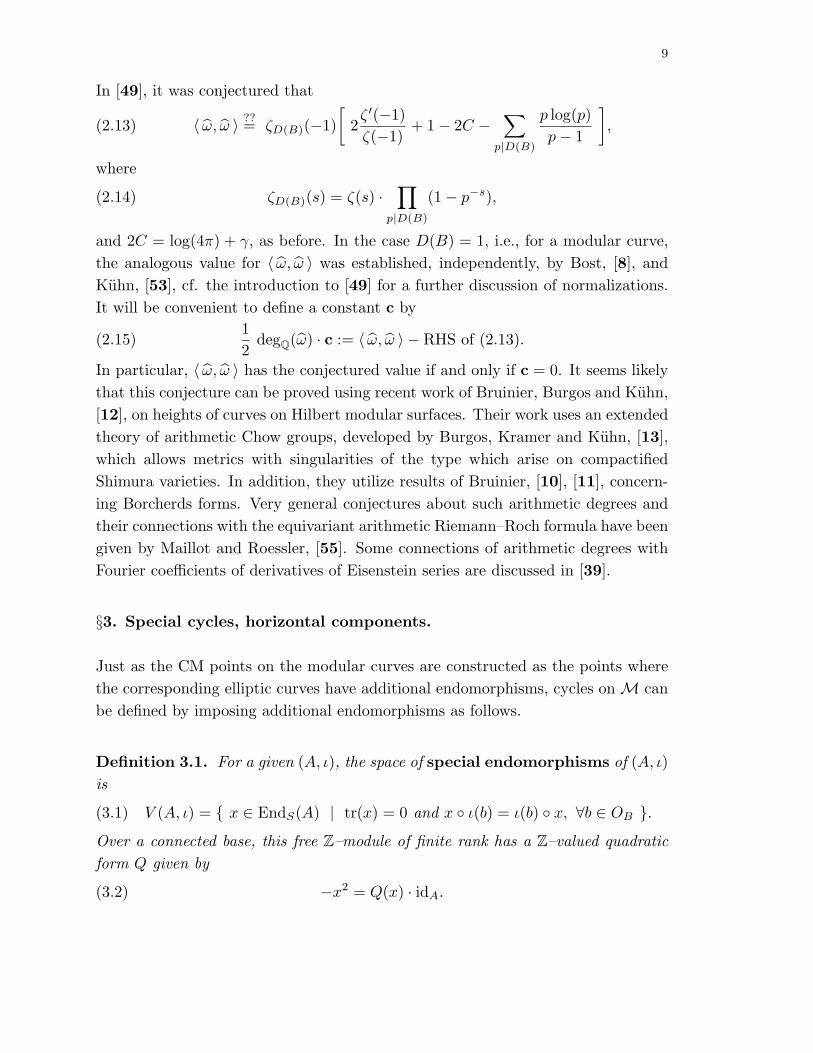
In [49], it was conjectured that
(2.13) 〈 ω, ω 〉 ??= ζD(B)(−1)[
2ζ ′(−1)ζ(−1)
+ 1 − 2C −∑
p|D(B)
p log(p)p − 1
]
,
where
(2.14) ζD(B)(s) = ζ(s) ·∏
p|D(B)
(1 − p−s),
and 2C = log(4π) + γ, as before. In the case D(B) = 1, i.e., for a modular curve,the analogous value for 〈 ω, ω 〉 was established, independently, by Bost, [8], andKuhn, [53], cf. the introduction to [49] for a further discussion of normalizations.It will be convenient to define a constant c by
(2.15)12
degQ(ω) · c := 〈 ω, ω 〉 − RHS of (2.13).
In particular, 〈 ω, ω 〉 has the conjectured value if and only if c = 0. It seems likelythat this conjecture can be proved using recent work of Bruinier, Burgos and Kuhn,[12], on heights of curves on Hilbert modular surfaces. Their work uses an extendedtheory of arithmetic Chow groups, developed by Burgos, Kramer and Kuhn, [13],which allows metrics with singularities of the type which arise on compactifiedShimura varieties. In addition, they utilize results of Bruinier, [10], [11], concern-ing Borcherds forms. Very general conjectures about such arithmetic degrees andtheir connections with the equivariant arithmetic Riemann–Roch formula have beengiven by Maillot and Roessler, [55]. Some connections of arithmetic degrees withFourier coefficients of derivatives of Eisenstein series are discussed in [39].
§3. Special cycles, horizontal components.
Just as the CM points on the modular curves are constructed as the points wherethe corresponding elliptic curves have additional endomorphisms, cycles on M canbe defined by imposing additional endomorphisms as follows.
Definition 3.1. For a given (A, ι), the space of special endomorphisms of (A, ι)is
(3.1) V (A, ι) = x ∈ EndS(A) | tr(x) = 0 and x ι(b) = ι(b) x, ∀b ∈ OB .Over a connected base, this free Z–module of finite rank has a Z–valued quadraticform Q given by
(3.2) −x2 = Q(x) · idA.

10
Definition 3.2. For a positive integer t, let Z(t) be the moduli stack over Spec(Z)of triples (A, ι, x), where (A, ι) is as before and x ∈ V (A, ι) is a special endomor-phism with Q(x) = t.
There is a natural morphism
(3.3) Z(t) −→ M, (A, ι, x) → (A, ι),
which is unramified, and, by a slight abuse of notation, we write Z(t) for the divisoron M determined by this morphism.
Over C, such a triple (A, ι, x) is an abelian surface with an action of OB ⊗Z Z[√−t],
i.e., with additional ‘complex multiplication’ by the order Z[√−t] in the imaginary
quadratic field kt = Q(√−t). Suppose that A Az = C2/Lz, so that, by (1.8),
the tangent space Te(Az) is given as BR C2 = Te(Az). Since the lift xR of x inthe diagram
(3.4)BR C2 −→ Az
xR = r(jx) ↓ x ↓ x ↓BR C2 −→ Az
commutes with the left action of OB and carries OB into itself, it is given by rightmultiplication r(jx) by an element jx ∈ OB ∩ V with ν(jx) = t. Since the map x
is holomorphic, it follows that z ∈ Dx, the fixed point set of jx on D. To simplifynotation, we will write x in place of jx. Then, we find that
(3.5) Z(t)(C) =[
Γ\Dt
],
where
(3.6) Dt =∐
x∈OB∩V
Q(x)=t
Dx.
In particular, Z(t)(C), which can be viewed as a set of CM points on the Shimuracurve M(C), is nonempty if and only if the imaginary quadratic field kt embeds inB.
The horizontal part Zhor(t) of Z(t) is obtained by taking the closure in M of theseCM–points, i.e.,
(3.7) Zhor(t) := Z(t)Q.
11
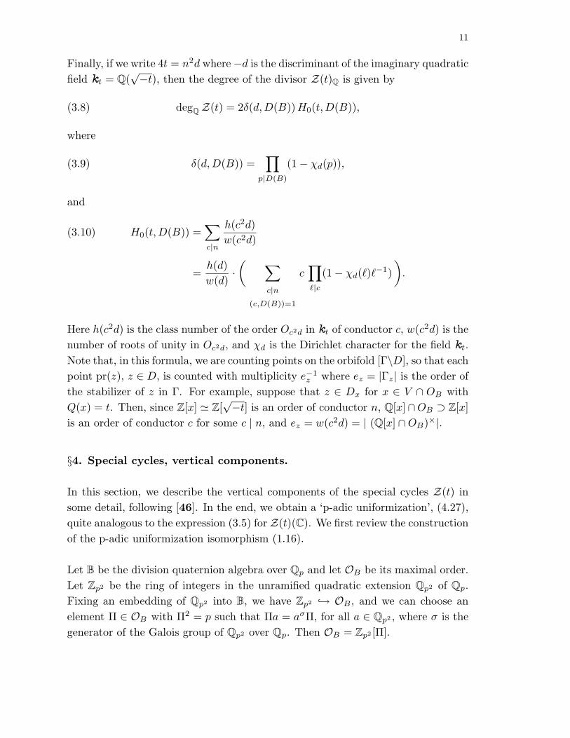
Finally, if we write 4t = n2d where −d is the discriminant of the imaginary quadraticfield kt = Q(
√−t), then the degree of the divisor Z(t)Q is given by
(3.8) degQZ(t) = 2δ(d, D(B))H0(t, D(B)),
where
(3.9) δ(d, D(B)) =∏
p|D(B)
(1 − χd(p)),
and
H0(t, D(B)) =∑
c|n
h(c2d)w(c2d)
(3.10)
=h(d)w(d)
·(
∑
c|n(c,D(B))=1
c∏
|c(1 − χd()−1)
)
.
Here h(c2d) is the class number of the order Oc2d in kt of conductor c, w(c2d) is thenumber of roots of unity in Oc2d, and χd is the Dirichlet character for the field kt.Note that, in this formula, we are counting points on the orbifold [Γ\D], so that eachpoint pr(z), z ∈ D, is counted with multiplicity e−1
z where ez = |Γz| is the order ofthe stabilizer of z in Γ. For example, suppose that z ∈ Dx for x ∈ V ∩ OB withQ(x) = t. Then, since Z[x] Z[
√−t] is an order of conductor n, Q[x]∩OB ⊃ Z[x]
is an order of conductor c for some c | n, and ez = w(c2d) = | (Q[x] ∩ OB)×|.
§4. Special cycles, vertical components.
In this section, we describe the vertical components of the special cycles Z(t) insome detail, following [46]. In the end, we obtain a ‘p-adic uniformization’, (4.27),quite analogous to the expression (3.5) for Z(t)(C). We first review the constructionof the p-adic uniformization isomorphism (1.16).
Let B be the division quaternion algebra over Qp and let OB be its maximal order.Let Zp2 be the ring of integers in the unramified quadratic extension Qp2 of Qp.Fixing an embedding of Qp2 into B, we have Zp2 → OB , and we can choose anelement Π ∈ OB with Π2 = p such that Πa = aσΠ, for all a ∈ Qp2 , where σ is thegenerator of the Galois group of Qp2 over Qp. Then OB = Zp2 [Π].

12
Recall that W = W (Fp). Let Nilp be the category of W–schemes S such that p islocally nilpotent in OS , and for S ∈ Nilp, let S = S ×W Fp.
A special formal (s.f.) OB–module over a W scheme S is a p-divisible formal groupX over S of dimension 2 and height 4 with an action ι : OB → EndS(X). The Liealgebra Lie(X), which is a Zp2 ⊗OS–module, is required to be free of rank 1 locallyon S.
Fix a s.f. OB–module X over Spec(Fp). Such a module is unique up to OB–linearisogeny, and
(4.1) End0OB
(X) M2(Qp).
We fix such an isomorphism. Consider the functor
(4.2) D• : Nilp → Sets
which associates to each S ∈ Nilp the set of isomorphism classes of pairs (X, ρ),where X is a s.f. OB–module over S and
(4.3) ρ : X ×Spec(Fp) S −→ X ×S S
is a quasi-isogeny4. The group GL2(Qp) acts on D• by
(4.4) g : (X, ρ) → (X, ρ g−1).
There is a decomposition
(4.5) D• =∐
i
Di,
where the isomorphism class of (X, ρ) lies in Di(S) if ρ has height i. The action ofg ∈ GL2(Qp) carries Di to Di−ord det(g). Drinfeld showed that D• is representableby a formal scheme, which we also denote by D•, and that there is an isomorphismof formal schemes
(4.6) D• ∼−→ Ω•W
which is equivariant for the action of GL2(Qp).
4This means that, locally on S, there is an integer r such that prρ is an isogeny.
13
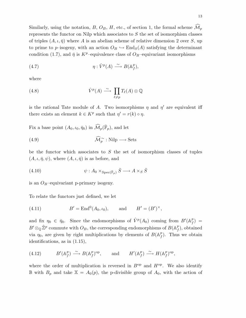
Similarly, using the notation, B, OB , H, etc., of section 1, the formal scheme Mp
represents the functor on Nilp which associates to S the set of isomorphism classesof triples (A, ι, η) where A is an abelian scheme of relative dimension 2 over S, upto prime to p–isogeny, with an action OB → EndS(A) satisfying the determinantcondition (1.7), and η is Kp–equivalence class of OB–equivariant isomorphisms
(4.7) η : V p(A) ∼−→ B(Apf ),
where
(4.8) V p(A) ∼−→∏
=p
T(A) ⊗ Q
is the rational Tate module of A. Two isomorphisms η and η′ are equivalent iffthere exists an element k ∈ Kp such that η′ = r(k) η.
Fix a base point (A0, ι0, η0) in Mp(Fp), and let
(4.9) M∼p : Nilp −→ Sets
be the functor which associates to S the set of isomorphism classes of tuples(A, ι, η, ψ), where (A, ι, η) is as before, and
(4.10) ψ : A0 ×Spec(Fp) S −→ A ×S S
is an OB–equivariant p-primary isogeny.
To relate the functors just defined, we let
(4.11) B′ = End0(A0, ι0), and H ′ = (B′)×,
and fix η0 ∈ η0. Since the endomorphisms of V p(A0) coming from B′(Apf ) =
B′⊗Q Zp commute with OB , the corresponding endomorphisms of B(Apf ), obtained
via η0, are given by right multiplications by elements of B(Apf ). Thus we obtain
identifications, as in (1.15),
(4.12) B′(Apf ) ∼−→ B(Ap
f )op, and H ′(Apf ) ∼−→ H(Ap
f )op,
where the order of multiplication is reversed in Bop and Hop. We also identifyB with Bp and take X = A0(p), the p-divisible group of A0, with the action of

14
OB = OB ⊗Z Zp coming from ι0. Note that we also obtain an identification B′p
GL2(Qp), via (4.1).
Once these identifications have been made, there is a natural isomorphism
(4.13) M∼p
∼−→ D• × H(Apf )/Kp
defined as follows. To a given (A, ι, η, ψ) over S, we associate:
X = A(p) = the p-divisible group of A,
ι = the action of OB = OB ⊗Z Zp on A(p),(4.14)
ρ = ρ(ψ) = the quasi-isogeny
ρ(ψ) : X ×Spec(Fp) S −→ A(p) ×S S
determined by ψ,
so that (X, ρ) defines an element of D•. For η ∈ η, there is also a diagram
(4.15)
V p(A0)η0∼−→ B(Ap
f )
ψ∗ ↓ ↓ r(g)
V p(A)η∼−→ B(Ap
f )
where r(g) denotes right multiplication5 by an element g ∈ H(Apf ). The coset gKp
is then determined by the equivalence class η, and the isomorphism (4.13) sends(A, ι, η, ψ) to ((X, ρ), gKp).
The Drinfeld-Cherednik Theorem says that, by passing to the quotient under theaction of H ′(Q), we have
(4.16)
M∼p
∼−→ D• × H(Apf )/Kp
↓ ↓
Mp∼−→ H ′(Q)\
(
D• × H(Apf )/Kp
)
.
Via the isomorphism D• ∼→ Ω•W of (4.6), this yields (1.16).
5This is the reason for the “op” in the isomorphism (4.12), since we ultimately want a left action
of H′(Apf).
15
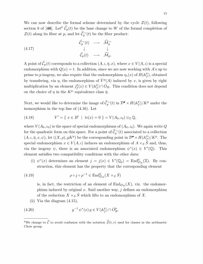
We can now describe the formal scheme determined by the cycle Z(t), followingsection 8 of [46]. Let6 Cp(t) be the base change to W of the formal completion ofZ(t) along its fiber at p, and let C ∼
p (t) be the fiber product:
(4.17)C ∼
p (t) −→ M∼p
↓ ↓Cp(t) −→ Mp.
A point of Cp(t) corresponds to a collection (A, ι, η, x), where x ∈ V (A, ι) is a specialendomorphism with Q(x) = t. In addition, since we are now working with A’s up toprime to p isogeny, we also require that the endomorphism η∗(x) of B(Ap
f ), obtainedby transfering, via η, the endomorphism of V p(A) induced by x, is given by rightmultiplication by an element jp
f (x) ∈ V (Apf )∩ OB . This condition does not depend
on the choice of η in the Kp–equivalence class η.
Next, we would like to determine the image of C ∼p (t) in D• ×H(Ap
f )/Kp under theisomorphism in the top line of (4.16). Let
(4.18) V ′ = x ∈ B′ | tr(x) = 0 = V (A0, ι0) ⊗Z Q,
where V (A0, ι0) is the space of special endomorphisms of (A0, ι0). We again write Q
for the quadratic form on this space. For a point of C ∼p (t) associated to a collection
(A, ι, η, x, ψ), let ((X, ρ), gKp) be the corresponding point in D•×H(Apf )/Kp. The
special endomorphism x ∈ V (A, ι) induces an endomorphism of A ×S S and, thus,via the isogeny ψ, there is an associated endomorphism ψ∗(x) ∈ V ′(Q). Thiselement satisfies two compatibility conditions with the other data:
(i) ψ∗(x) determines an element j = j(x) ∈ V ′(Qp) = End0OB
(X). By con-struction, this element has the property that the corresponding element
(4.19) ρ j ρ−1 ∈ End0OB
(X ×S S)
is, in fact, the restriction of an element of EndOB(X), viz. the endomor-
phism induced by original x. Said another way, j defines an endomorphismof the reduction X ×S S which lifts to an endomorphism of X.
(ii) Via the diagram (4.15),
(4.20) g−1 ψ∗(x) g ∈ V (Apf ) ∩ Op
B .
6We change to C to avoid confusion with the notation Z(t, v) used for classes in the arithmetic
Chow group.

16
Here we are slightly abusing notation and, in effect, are identifying ψ∗(x) ∈ V ′(Q)with an element of V (Ap
f ) obtained via the identification
(4.21) V ′(Apf ) ∼−→ V (Ap
f )
coming from (4.12).
Condition (i) motivates the following basic definition, [46], Definition 2.1.
Definition 4.1. For a special endomorphism j ∈ V ′(Qp) of X, let Z•(j) be theclosed formal subscheme of D• consisting of the points (X, ρ) such that ρ j ρ−1
lifts to an endomorphism of X.
We will also write Z(j) ⊂ D for the subschemes where the height of the quasi-isogeny ρ is 0. We will give a more detailed description of Z(j) in a moment.
As explained above and in more detail in [46], section 8, there is a map
(4.22) C ∼p (t) → V ′(Q) ×D• × H(Ap
f )/Kp
whose image is the set:
(4.23) () :=
(y, (X, ρ), gKp)
∣∣∣∣
(i) Q(y) = t
(ii) (X, ρ) ∈ Z•(j(y))
(iii) y ∈ g (V (Apf ) ∩ Op
B) g−1
.
Taking the quotient by the group H ′(Q), we obtain the following p-adic uniformiza-tion of the special cycle:
Proposition 4.2. The construction aboves yields isomorphisms:
Cp(t)∼−→ H ′(Q)\()
↓ ↓
Mp∼−→ H ′(Q)\
(
D• × H(Apf )/Kp
)
of formal schemes over W .
Remark 4.3. In fact, in this discussion, the compact open subgroup Kp givingthe level structure away from p can be arbitrary. In the case of interest, where

17
Kp = (OpB)×, the last diagram can be simplified as follows. Let
(4.24) L′ = V ′(Q) ∩(B′(Qp) × Op
B
),
so that L′ is a Z[p−1]–lattice in V ′(Q). Also, as in section 1, let
(4.25) Γ′ = H ′(Q) ∩(H ′(Qp) × Kp
),
so that (the projection of) Γ′ is an arithmetic subgroup of H ′(Qp) GL2(Qp).Finally, let
(4.26) D•t =
∐
y∈L′
Q(y)=t
Z•(j(y)).
Then,
(4.27)Cp(t)
∼−→[Γ′\D•
t
]
↓ ↓Mp
∼−→[Γ′\D• ]
.
Of course, we should now view these quotients as orbifolds, and, in fact, shouldformulate the discussion above in terms of stacks.
To complete the picture of the vertical components of our cycle Z(t), we need a moreprecise description of the formal schemes Z•(j) for j ∈ V ′(Qp), as obtained in thefirst four sections of [46]. Note that we are using the quadratic form Q(j) = det(j),whereas, in [46], the quadratic form q(j) = j2 = −Q(j) was used. It is mostconvenient to give this description in the space Ω•
W = ΩW ×Z. In fact, we will justconsider Z(j) ⊂ ΩW , and we will assume that p = 2. The results for p = 2, whichare very similar, are described in section 11 of [49]. Recall that the special fiber ofΩW is a union of projective lines P[Λ], indexed by the vertices [Λ] of the building Bof PGL2(Qp).
The first result, proved in section 2 of [46], describes the support of Z(j) in termsof the building.
Proposition 4.4. (i)
P[Λ] ∩ Z(j) = ∅ ⇐⇒ j(Λ) ⊂ Λ.
18
In particular, if Z(j) = ∅, then ordp(Q(j)) ≥ 0.(ii)
j(Λ) ⊂ Λ ⇐⇒ d([Λ],Bj) ≤ 12· ordp(Q(j)).
Here Bj is the fixed point set of j on B, and d(x, y) is the distance between thepoints x and y ∈ B.
Recall that the distance function on the building B is PGL2(Qp)–invariant andgives each edge length 1.
In effect, if we write Q(j) = ε pα, for ε ∈ Z×p , then the support of Z(j) lies in the
set of P[Λ]’s indexed by vertices of B in the ‘tube’ T (j) of radius α2 around the fixed
point set Bj of j.
Next, the following observation of Genestier is essential, [46], Theorem 3.1:Write Q(j) = ε pα. Then
(4.28) Z(j) =
(ΩW )j if α = 0,
(ΩW )1+j if α > 0.
where (ΩW )x denotes the fixed point set of the element x ∈ GL2(Qp) acting on ΩW ,via its projection to PGL2(Qp). Using this fact, one can obtain local equations forZ(j) in terms of the local coordinates on ΩW , cf. [46], section 3. Recall that thereare standard coordinate neighborhoods associated to each vertex [Λ] and each edge[Λ0,Λ1] of B, cf. [46], section 1. By Proposition 4.4, it suffices to compute inthe neighborhoods of those P[Λ]’s which meet the support of Z(j). For the fullresult, see Propositions 3.2 and 3.3 in [46]. In particular, embedded componentscan occur. But since these turn out to be negligible, e.g., for intersection theory,cf. section 4 of [46], we can omit them from Z(j) to obtain the divisor Z(j)pure
which has the following description.
Proposition 4.5. Write Q(j) = ε pα, and let
µ[Λ](j) = max 0,α
2− d([Λ],Bj) .
(i) If α is even and −ε ∈ Z×,2p , then
Z(j)pure =∑
[Λ]
µ[Λ](j) · P[Λ].

19
(ii) If α is even and −ε /∈ Z×,2p , then
Z(j)pure = Z(j)h +∑
[Λ]
µ[Λ](j) · P[Λ],
where the horizontal part Z(j)h is the disjoint union of two divisors projectingisomorphically to Spf(W ) and meeting the special fiber in ‘ordinary special’ pointsof P[Λ(j)], where [Λ(j)] is the unique vertex Bj of B fixed by j.(iii) If α is odd, then
Z(j)pure = Z(j)h +∑
[Λ]
µ[Λ](j) · P[Λ],
where the horizontal divisor Z(j)h is Spf(W ′) where W ′ is the ring of integers ina ramified quadratic extension of W ⊗Z Q and Z(j)h meets the special fiber in thedouble point pt∆(j) where ∆(j) is the edge of B containing the unique fixed pointBj of j.Thus Z(j)pure is a sum with multiplicities of regular one dimensional formal schemes.
In case (i), the split case, Qp(j) Qp ⊕ Qp, the element j lies in a split torus A inGL2(Qp), and Bj is the corresponding apartment in B. More concretely, if e0 ande1 are eigenvectors of j giving a basis of Q2
p, then Bj is the geodesic arc connectingthe vertices [Zp e0 ⊕ prZp e1], for r ∈ Z. The P[Λ]’s for [Λ] ∈ Bj have multiplicityα2 in Z(j), and the multiplicity decreases linearly with the distance from Bj . Thecycle Z(j) is infinite and there are no horizontal components.
In case (ii), the inert case, Qp(j) is an unramified quadratic extension of Qp, theelement j lies in the corresponding nonsplit Cartan subgroup of GL2(Qp) and Bj =[Λ(j)] is a single vertex. The corresponding P[Λ(j)] occurs with multiplicity α
2 inZ(j), and the multiplicity of the vertical components P[Λ] decreases linearly withthe distance d([Λ], [Λ(j)]).
Finally, in case (iii), the ramified case, Qp(j) is a ramified quadratic extension ofQp, the element j lies in the corresponding nonsplit Cartan subgroup of GL2(Qp)and Bj is the midpoint of a unique edge ∆(j) = [Λ0,Λ1]. The vertical componentsP[Λ0] and P[Λ1] occur with multiplicity α−1
2 in Z(j), and, again, the multiplicity ofthe vertical components P[Λ] decreases linearly with the distance d([Λ],Bj), whichis now a half-integer.

20
This description of the Z(j)’s, together with the p-adic unformization of Propo-sition 4.2, gives a fairly complete picture of the vertical components of the cyclesZ(t) in the fibers Mp, p | D(B), of bad reduction. Several interesting features areevident.
For example, the following result gives a criterion for the occurrence of such com-ponents.
Proposition 4.6. For p | D(B), the cycle Z(t) contains components of the fiberMp of bad reduction if and only if ordp(t) ≥ 2, and no prime = p with | D(B)is split in kt.
Note that the condition amounts to (i) ordp(t) ≥ 2, and (ii) the field kt embedsinto B(p)
For example, if more than one prime p | D(B) splits in the quadratic field kt =Q(
√−t), then Z(t) is empty. If p | D(B) splits in kt, and all other primes | D(B)
are not split in kt, then the generic fiber Z(t)Q is empty, and Z(t) is a verticalcycle in the fiber at p, provided ordp(t) ≥ 2. In general, if p | D(B), and kt embedsin B(p), then the vertical component in Mp of the cycle Z(p2rt) grows as r goes toinfinity, while the horizontal part does not change. Indeed, if we change t to p2rt,then, by (3.8), deg
QZ(p2rt) = deg
QZ(t), while both the radius of the tube T (prj)
and the multiplicity function µ[Λ](prj) increase.
Analogues of these results about cycles defined by special endomorphisms are ob-tained in [45] and [47] for Hilbert–Blumenthal varieties and Siegel modular varietiesof genus 2 respectively.
§5. Green functions.
To obtain classes in the arithmetic Chow group CH1
R(M) from the Z(t)’s, it is
necessary to equip them with Green functions. These are defined as follows; see[37] for more details. For x ∈ V (R), with Q(x) = 0, let
(5.1) Dx = z ∈ D | (x, w(z)) = 0 .
Here w(z) ∈ V (C) is any vector with image z in P(V (C)). The set Dx consists of
21
two points if Q(x) > 0, and is empty if Q(x) < 0. By (3.5) and (3.6), we have
(5.2) Z(t)(C) =∑
x∈OB∩V
Q(x)=t
mod Γ
pr(Dx)
where pr : D → Γ\D. For x ∈ V (R), with Q(x) = 0, and z ∈ D, let
(5.3) R(x, z) = |(x, w(z))|2|(w(z), w(z))|−1.
This function on D vanishes precisely on Dx. Let
(5.4) β1(r) =∫ ∞
1
e−ru u−1 du = −Ei(−r)
be the exponential integral. Note that
(5.5) β1(r) =
− log(r) − γ + O(r), as r → 0,
O(e−r), as r → ∞.
Thus, the function
(5.6) ξ(x, z) = β1(2πR(x, z))
has a logarithmic singularity on Dx and decays exponentially as z goes to theboundary of D. A straightforward calculation, [37], section 11, shows that ξ(x, ·)is a Green function for Dx.
Proposition 5.1. As currents on D,
ddcξ(x) + δDx= [ϕ0
∞(x)µ],
where, for z ∈ D C \ R with y = Im(z),
µ =12π
i
2dz ∧ dz
y2
is the hyperbolic volume form and
ϕ0∞(x, z) =
[4π(R(x, z) + 2Q(x) ) − 1
]· e−2πR(x,z).

22
Recall that ddc = − 12πi∂∂.
Remark. For fixed z ∈ D,
(5.7) (x, x)z = (x, x) + 2R(x, z)
is the majorant attached to z, [63]. Thus, the function
(5.8) ϕ∞(x, z) · µ = ϕ0∞(x, z) · e−2πQ(x) · µ
is (a very special case of) the Schwartz function valued in smooth (1, 1)–forms onD defined in [43]. In fact, the function ξ(x, z) was first obtained by solving theGreen equation of Proposition 5.1 with this right hand side.
Because of the rapid decay of ξ(x, ·), we can average over lattice points.
Corollary 5.2. For v ∈ R×>0, let
Ξ(t, v)(z) :=∑
x∈OB∩VQ(x)=t
ξ(v12 x, z).
(i) For t > 0, Ξ(t, v) defines a Green function for Z(t).(ii) For t < 0, Ξ(t, v) defines a smooth function on M(C).
Note, for example, that for t > 0,
(5.9)Z(t)(C) = ∅
and Ξ(t, v) = 0⇐⇒ x ∈ OB ∩ V, Q(x) = t = ∅ ⇐⇒ kt does not
embed in B.
An explicit construction of Green functions for divisors in general locally symmetricvarieties is given by Oda and Tsuzuki, [58], by a different method.
§6. The arithmetic theta series.
At this point, we can define a family of classes in CH1(M). These can be viewed
as an analogue for the arithmetic surface M of the Hirzebruch-Zagier classes TN inthe middle cohomology of a Hilbert modular surface, [29].
23
Definition 6.1. For t ∈ Z, with t = 0, and for a parameter v ∈ R×+, define classes
in CH1
R(M) by
Z(t, v) =
(Z(t),Ξ(t, v) ) if t > 0,
( 0,Ξ(t, v) ) if t < 0.
For t = 0, defineZ(0, v) = −ω − (0, log(v)) + (0, c),
where c is the constant defined by (2.15).
We next construct a generating series for these classes; again, this can be viewedas an arithmetic analogue of the Hirzebruch–Zagier generating series for the TN ’s.For τ = u + iv ∈ H, the upper half plane, let q = e(τ) = e2πiτ .
Definition 6.2. The arithmetic theta series is the generating series
θ(τ) =∑
t∈Z
Z(t, v) qt ∈ CH1(M)[[q]].
Note that, since the imaginary part v of τ appears as a parameter in the coefficientZ(t, v), this series is not a holomorphic function of τ .
The arithmetic theta function θ(τ) is closely connected with the generating seriesfor quadratic divisors considered by Borcherds, [5], and the one for Heegner pointsintroduced by Zagier, [78]. The following result, [42], justifies the terminology. Itsproof, which will be sketched in section 7, depends on the results of [49] and ofBorcherds, [5].
Theorem 6.3. The arithmetic theta series θ(τ) is a (nonholomorphic) modular
form of weight 32 valued in CH
1(M).
As explained in Proposition 7.1 below, the arithmetic Chow group CH1(M) can be
written as direct sum
CH1(M) = CH
1(M, µ)C ⊕ C∞
0 (M(C))
where CH1(M, µ)C a finite dimensional complex vector space, the Arakelov Chow
group of M for the hyperbolic metric µ, (7.7), and C∞0 (M(C)) is the space of
24
smooth functions on M(C) with integral 0 with respect to µ. Theorem 6.3 then
means that there is a smooth function of φAr of τ valued in CH1(M, µ)C and a
smooth function φ(τ, z) on H ×M(C), with∫
M(C)
φ(τ, z) dµ(z) = 0,
and such that the sum φ(τ) = φAr(τ) + φ(τ, z) satisfies the usual transformationlaw for a modular form of weight 3
2 , for Γ0(4D(B)), and such that the q–expansionof φ(τ) is the formal generating series θ(τ) of Definition 6.2. By abuse of notation,we write θ(τ) both for φ(τ) and for its q–expansion.
§7. Modularity of the arithmetic theta series.
Although the arithmetic theta series θ(τ) can be viewed as a kind of generatingseries for lattice vectors in the spaces V (A, ι) of special endomorphisms, there is noevident analogue of the Poisson summation formula, which is the key ingredient ofthe proof of modularity of classical theta series. Instead, the modularity of θ(τ) is
proved by computing its height pairing with generators of the group CH1(M) and
identifying the resulting functions of τ with known modular forms.
First we recall the structure of the arithmetic Chow group CH1
R(M), [20], [66], [7].
There is a map
(7.1) a : C∞(M(C)) −→ CH1
R(M), φ −→ (0, φ)
from the space of smooth functions on the curve M(C). Let 11 = a(1) be the
image of the constant function. Let Vert ⊂ CH1
R(M) be the subspace generated by
classes of the form (Yp, 0), where Yp is a component of a fiber Mp. The relationdiv(p) = (Mp,− log(p)2) ≡ 0 implies that (Mp, 0) ≡ 2 log(p) · 11, so that 11 ∈ Vert.The spaces a(C∞(M(C)) and Vert span the kernel of the restriction map
(7.2) resQ : CH1
R(M) −→ CH1(MQ)R
to the generic fiber. Here CH1(MQ)R = CH1(MQ) ⊗Z R.
Let
(7.3) MWR = MW(M)R = Jac(M)(Q) ⊗Z R

25
be the Mordell–Weil space of the Shimura curve M = MQ, and recall that thisspace is the kernel of the degree map
(7.4) MWR −→ CH1(M)R
deg−→ R.
Note that the degree of the restriction of the class ω to the generic fiber is positive,since it is given by the integral of the hyperbolic volume form over [Γ\D].
Finally, let C∞0 = C∞(M(C))0 be the space of smooth functions which are orthog-
onal to the constants with respect to the hyperbolic volume form.
The following is a standard result in the Arakelov theory of arithmetic surfaces,[32], [15], [7].
Proposition 7.1. Let
MW :=(
R ω ⊕ Vert ⊕ a(C∞0 )
)⊥
be the orthogonal complement of R ω ⊕ Vert ⊕ a(C∞0 ) with respect to the height
pairing. Then
CH1
R(M) = MW ⊕
(
R ω ⊕ Vert)
⊕ a(C∞0 ),
where the three summands are orthogonal with respect to the height pairing. More-over, the restriction map resQ induces an isometry
resQ : MW ∼−→ MW
with respect to the Gillet–Soule–Arakelov height pairing on MW and the negativeof the Neron–Tate height pairing on MW.
In addition, there are some useful formulas for the height pairings of certain classes.For example, for any Z ∈ CH
1(M),
(7.5) 〈 Z, 11 〉 =12
degQ(Z).
In particular, 11 is in the radical of the restiction of the height pairing to Vert, and〈 ω, 11 〉 = 1
2 degQ(ω) > 0. Also, for φ1 and φ2 ∈ C∞
0 ,
(7.6) 〈 a(φ1), a(φ2) 〉 =12
∫
M(C)
ddcφ1 · φ2.
26
Note that the subgroup
(7.7) CH1(M, µ)R = MW ⊕ Rω ⊕ Vert
is the Arakelov Chow group (with real coefficients) for the hyperbolic metric µ.
Returning to the arithmetic theta series θ(τ), we consider its pairing with various
classes in CH1
R(M). To describe these, we first introduce an Eisenstein series of
weight 32 associated to the quaternion algebra B, [49]. Let Γ′ = SL2(Z) and let Γ′
∞be the stabilizer of the cusp at infinity. For s ∈ C, let
(7.8) E(τ, s;B) = v12 (s− 1
2 )∑
γ∈Γ′∞\Γ′
(cτ + d)−32 |cτ + d|−(s− 1
2 ) ΦB(γ, s),
where γ =(
a bc d
)
and ΦB(γ, s) is a function of γ and s depending on B. This
series converges absolutely for Re(s) > 1 and has an analytic continuation to thewhole s–plane. It satisfies the functional equation, [49], section 16,
(7.9) E(τ, s;B) = E(τ,−s;B),
normalized as in Langlands theory.
The following result is proved in [49].
Theorem 7.2.(i)
2 · 〈 θ(τ), 11 〉 = −vol(M(C)) +∑
t>0
deg(Z(t)Q) qt
= E(τ,12;B).
(ii)
〈 θ(τ), ω 〉 =∑
t
〈 Z(t, v), ω 〉 qt
= E ′(τ,12;B).
27
This result is proved by a direct computation of the Fourier coefficients on the twosides of (i) and (ii). For (i), the identity amounts to the formula
(7.10) deg(Z(t)Q) qt = 2 δ(d;D(B))H0(t;D(B)) qt = E ′t(τ,
12;D(B)),
with the notation as in (3.8), (3.9) and (3.10) above. Recall that we write 4t = n2d
where −d is the discriminant of the field kt.
For example, if D(B) = 1, i.e., in the case of B = M2(Q),
(7.11) H0(t; 1) =∑
c|n
h(c2d)w(c2d)
.
Thus, 2H0(t; 1) = H(4t), where H(t) is the ‘class number’ which appears in theFourier expansion of Zagier’s nonholomorphic Eisenstein series of weight 3
2 , [14],[78]:
(7.12) F(τ) = − 112
+∑
t>0
H(t) qt +∑
m∈Z
116π
v−12
∫ ∞
1
e−4πm2vr r−32 dr q−m2
.
In fact, when D(B) = 1, the value of our Eisenstein series is(7.13)
E(τ,12; 1) = − 1
12+
∑
t>0
2 H0(t; 1) qt +∑
m∈Z
18π
v−12
∫ ∞
1
e−4πm2vr r−32 dr · q−m2
.
As in (i) of Theorem 7.2, both of these series have an interpretation in term ofdegrees of 0–cycles of CM points on the modular curve, [76]. Their relation to aregularized integral of a theta series is proved by J. Funke in [16], [17].
The computations involved in (ii) are significantly more difficult. For example, ift > 0 and Z(t)Q(C) is nonempty, then, [49], Theorem 8.8, the t-th Fourier coefficientof E ′(τ, 1
2 ;B) is
E ′t(τ,
12;B)
(7.14)
= 2 δ(d;D)H0(t;D) · qt ·[
12
log(d) +L′(1, χd)L(1, χd)
− 12
log(π) − 12γ
+12J(4πtv) +
∑
ppD
(
log |n|p −b′p(n, 0;D)bp(n, 0;D)
)
+∑
pp|D
Kp log(p)]
.

28
Here, we write D for D(B), 4t = n2d, as before, and
(7.15) Kp =
−k + (p+1)(pk−1)2(p−1) if χd(p) = −1, and
−1 − k + pk+1−1p−1 if χd(p) = 0,
with k = kp = ordp(n). Also,
(7.16) J(x) =∫ ∞
0
e−xr[(1 + r)
12 − 1
]r−1 dr.
Finally, for a prime p D,
(7.17)1
log p·b′p(n, 0;D)bp(n, 0;D)
=χd(p) − χd(p) (2k + 1)pk + (2k + 2)pk+1)
1 − χd(p) + χd(p) pk − pk+1− 2p
1 − p
The connection of this rather complicated quantity with arithmetic geometry is notat all evident. Nonetheless, the identity of part (ii) of Theorem 7.2 asserts that
(7.18) E ′t(τ,
12;B) = 〈 Z(t, v), ω 〉 qt.
Recall that the points of the generic fiber Z(t)Q correspond to abelian surfacesA with an action of OB ⊗Z Z[
√−t], an order in M2(kt). The contribution to
〈 Z(t, v), ω 〉 of the associated horizontal component of Z(t) is the Faltings heightof A. Due to the action of OB ⊗Z Z[
√−t ], A is isogenous to a product E×E where
E is an elliptic curve with CM by the order Od, and so the Faltings heights arerelated by
(7.19) hFal(A) = 2hFal(E) + an isogeny correction.
Up to some combinatorics involving counting of the points Z(t)Q, the terms on thefirst line of the right side of (7.14) come from hFal(E), while sum on p D(B) onthe second line arises from the isogeny correction. The J(4πtv) term comes fromthe contribution of the Green function Ξ(t, v) with parameter v. Finally, the cycleZ(t) can have vertical components, and the sum on p | D(B) comes from theirpairing with ω.
The analogue of (ii) also holds for modular curves, i.e., when D(B) = 1. In thiscase, there are some additional terms, as in the nonholomorphic parts of (7.12) and
(7.13). These terms are contributions from a class in CH1
R(M) supported in the
cusp, [76], [51].
29
To continue the proof of modularity of θ(τ), we next consider the height pairing ofθ(τ) with classes of the form (Yp, 0) in Vert, and with classes of the form (0, φ), forφ ∈ C∞
0 , which might be thought of as ‘vertical at infinity’.
First we consider 〈 θ(τ), (Yp, 0) 〉. For p = 2, the intersection number of a componentYp indexed by [Λ] with a cycle Z(t) is calculated explicitly in [46]. For p = 2, thecomputation is very similar. Using this result, we obtain, [42]:
Theorem 7.3. Assume that p | D(B) and that p = 2. Then, for a component Yp
of Mp associated to a homothety class of lattices [Λ], there is a Schwartz functionϕ[Λ] ∈ S(V (p)(Af )) and associated theta function of weight 3
2
θ(τ, ϕ[Λ]) =∑
x∈V (p)(Q)
ϕ[Λ](x) qQ(x),
such that〈 θ(τ), (Yp, 0) 〉 = θ(τ, ϕ[Λ]).
Next consider the height pairings with classes of the form a(φ) = (0, φ) for φ ∈ C∞0 .
Here we note that, for a class (Z, gZ) ∈ CH1
R(M),
(7.20) 〈 (Z, gZ), a(φ) 〉 =12
∫
M(C)
ωZ φ,
where ωZ = ddcgZ + δZ is the smooth (1, 1)–form on the right side of the Greenequation. The map (Z, gZ) → ωZ defines a map, [20], [66]
(7.21) ω : CH1
R(M) −→ A(1,1)(M(C)).
By the basic construction of the Green function Ξ(t, v) and Proposition 5.1, wehave
ω( θ(τ) ) =∑
x∈OB∩V
ϕ0∞(xv
12 , z) qQ(x) · µ(7.22)
: = θ(τ, ϕ0∞)(z) · µ,
where θ(τ, ϕ0∞)(z) is the theta series of weight 3
2 for the rational quadratic space V
of signature (1, 2). Thus,
(7.23) 〈 θ(τ), a(φ) 〉 =12
∫
M(C)
θ(τ, ϕ0∞)(z)φ(z) dµ(z),
30
is the classical theta lift of φ. To describe this more precisely, recall that
(7.24) ddcφ =12
∆φ · µ
where ∆ is the hyperbolic Laplacian, and consider functions φλ ∈ C∞0 (M(C))
satisfying ∆φλ + λφλ = 0 for λ > 0. Let φλi, for 0 < λ1 ≤ λ2 ≤ . . . be a basis
of such eigenfunctions, orthonormal with respect to µ. These are just the Maassforms of weight 0 for the cocompact Fuchsian group Γ = O×
B . Recalling (7.6), we
see that the classes a(φλ) ∈ CH1
R(M) are orthogonal with respect to the height
pairing and span the subspace a(C∞0 ). By (7.23), we have the following, [42].
Theorem 7.4. For a Maass form φλ of weight 0 for Γ, let
θ(τ ;φλ) :=∫
M(C)
θ(τ, ϕ0∞)(z) φλ(z) dµ(z)
be its classical theta lift, a Maass form of weight 32 and level 4D(B). Then
〈 θ(τ), a(φλ) 〉 =12
θ(τ ;φλ).
Finally, we must consider the component θMW(τ) of θ(τ) in the space MW. Recallthe isomorphism
(7.25) resQ : MW ∼−→ MW ⊂ CH1(M).
Write
(7.26) θB(τ) := resQ(θ(τ)) = −ω +∑
t>0
Z(t) qt ∈ CH1(M),
where Z(t) (resp. ω) is the class of the 0–cycle Z(t)Q (resp. the line bundle ω =resQ(ω)) in CH1(M). This series is essentially a special case of the generating func-tion for divisors considered by Borcherds, [5], [6]. Assuming that certain spaces ofvector valued modular forms have bases with rational Fourier coefficients, Borcherdsproved that his generating series are modular forms, and McGraw, [56], verifiedBorcherds assumption. The main point in Borcherds’ proof is the existence ofenough relations among the divisors in question, and such relations can be explic-itly given via Borcherds construction of meromorphic modular forms with product
31
expansions, [3], [4]. Thus, the series θB(τ) is a modular form of weight 32 valued in
CH1(M).
By (i) of Theorem 7.2, we have
(7.27) deg(θB(τ)) = E(τ,12;B),
and so, the function
(7.28) θMW(τ) := θB(τ) − E(τ,12;B) · ω
deg(ω)∈ MW
is also modular of weight 32 . Thus we obtain, [42],
Theorem 7.5. The image of θMW(τ) under the isomorphism (7.25), is given by
resQ( θMW(τ) ) = resQ
(θ(τ) − E(τ,
12;B) deg
Q(ω)−1 · ω
)
= θMW(τ) ∈ MW.
Thus, θMW(τ) is a modular form of weight 32 .
This completes the proof of the modularity of the arithmetic theta function θ(τ).
§8. The arithmetic theta lift.
The arithmetic theta function θ(τ) can be used to define an arithmetic theta lift
θ : S 32−→ CH
1(M), f → θ(f),
where S 32
is the space of cusp forms of weight 32 for Γ′ = Γ0(4D(B)), as follows.
Given a cusp form f of weight 32 for Γ′ = Γ0(4D(B)), let
(8.1) θ(f) = 〈 f, θ 〉Pet =∫
Γ′\H
f(τ) θ(τ) v32
du dv
v2∈ CH
1(M).
This construction is analogous to the construction of Niwa, [57], of the classicalShimura lift, [64], from S 3
2to modular forms of weight 2 for O×
B . Recall that we

32
extend the height pairing 〈 , 〉 on CH1
R(M) to an Hermitian pairing on CH
1(M),
conjugate linear in the second argument. By adjointness, and Theorem 7.2,
(8.2) 〈θ(f), 11〉 = 〈f, 〈θ, 11〉 〉Pet =12〈f, E(
12;B)〉Pet = 0,
and
(8.3) 〈θ(f), ω〉 = 〈f, 〈θ, ω〉 〉Pet = 〈f, E ′(12;B)〉Pet = 0.
If f is holomorphic, then, by Theorem 7.4, for any φ ∈ C∞0 (M(C)),
(8.4) 〈θ(f), a(φ)〉 = 〈 f, 〈 θ, a(φ) 〉 〉 = 〈 f, θ(φ) 〉Pet = 0,
since θ(τ ;φ) is a combination of Maass forms of weight 32 . Thus, for f holomorphic
(8.5) θ(f) ∈ MW ⊕ Vert0 ⊂ CH1(M)
where
(8.6) Vert0 = Vert ∩ ker〈 ·, ω 〉.
It remains to describe the components of θ(f) in the spaces Vert and MW. This isbest expressed in terms of automorphic representations.
§9. Theta dichotomy: Waldspurger’s theory.
We begin with a brief review of Waldspurger’s theory of the correspondence be-tween cuspidal automorphic representations of the metaplectic cover of SL2 andautomorphic representations of PGL2 and its inner forms. For a more detailedsurvey, the reader can consult [59], [70], [31], as well as the original papers [68],[69], and especially, [73].
We fix the additive character ψ of A/Q which has trivial conductor, i.e., is trivialon Z =
∏
p<∞ Zp and has archimedean component ψ∞(x) = e(x) = e2πix. Since ψ
is fixed, we suppress it from the notation.
Let G = SL2 and let G′A
be the 2–fold cover of G(A) which splits over G(Q). Let
A0(G′) = the space of genuine cusp forms for G′A.(9.1)
A00(G′) = the space of genuine cusp forms for G′A.
orthogonal to all O(1) theta series
33
For an irreducible cuspidal automorphic representation σ ⊗p≤∞σp in A00(G′),Waldspurger constructs an irreducible cuspidal automorphic representation
(9.2) π = π(σ) = Wald(σ) = Wald(σ, ψ)
of PGL2(A), which serves as a kind of reference point for the description of theglobal theta lifts for various ternary quadratic spaces. For each p ≤ ∞, there isa corresponding local construction σp → Wald(σp, ψp), and the local and globalconstructions are compatible, i.e.,
Wald(σ, ψ) ⊗p≤∞Wald(σp, ψp).
Since we have fixed the additive character ψ = ⊗pψp, we will often omit it fromthe notation.
For a quaternion algebra B over Q, let
(9.3) V B = x ∈ B | tr(x) = 0 ,
with quadratic form7 Q(x) = −x2 = ν(x), and let
(9.4) HB = B× GSpin(V ).
For a Schwartz function ϕ ∈ S(V B(A)), g′ ∈ G′A
and h ∈ HB(A), define the thetakernel by
(9.5) θ(g′, h;ϕ) =∑
x∈V B(Q)
ω(g′)ϕ(h−1x).
Here ω = ωψ is the Weil representation of G′A
on S(V (A)). For f ∈ σ and ϕ ∈S(V B(A)), the classical theta lift is
(9.6) θ(f ;ϕ) = 〈 f, θ(ϕ) 〉Pet =∫
G′Q\G′
A
f(g′) θ(g′, h;ϕ) dg′ ∈ A0(HB).
The global theta lift of σ to HB is the space
(9.7) θ(σ;V B) ⊂ A0(HB),
7Note that Waldspurger uses the opposite sign.
34
spanned by the θ(f ;ϕ)’s for f ∈ σ and ϕ ∈ S(V (A)). Here A0(HB) is the spaceof cusp forms on HB(Q)\HB(A). Then θ(σ;V B) is either zero or is an irreduciblecuspidal representation of HB(A), [73], Prop. 20, p. 290.
For any irreducible admissible genuine representation σp of G′p, the metaplectic
cover of G(Qp), there are analogous local theta lifts θ(σp, VBp ). Each of them is
either zero or is an irreducible admissible representation of HBp . The local and
global theta lifts are compatible in the sense that
(9.8) θ(σ;V B)
⊗pθ(σp;V Bp ) or
0.
In particular, the global theta lift is zero if any local θ(σp;V Bp ) = 0, but the global
theta lift can also vanish even when there is no such local obstruction, i.e., even if⊗p≤∞θ(σp;V B
p ) = 0.
For each p, let B±p be the quaternion algebra over Qp with invariant
(9.9) invp(B±p ) = ±1.
Then the two ternary quadratic spaces
(9.10) V ±p = x ∈ B±
p | tr(x) = 0
have the same discriminant and opposite Hasse invariants. A key local fact estab-lished by Waldspurger is:
Theorem 9.1. (Local theta dichotomy) For an irreducible admissible genuinerepresentaton σp of G′
p, precisely one of the spaces θ(σp;V +p ) and θ(σp;V −
p ) isnonzero.
Definition 9.2. Let εp(σp) = ±1 be the unique sign such that with
θ(σp, Vεp(σp)p ) = 0.
Examples: (i) If p is a finite prime and σp is an unramified principal series rep-resentation, then εp(σp) = +1 and θ(σp;V +
p ) is a principal series representation of
35
GL2(Qp). It is unramified if σp is unramified.(ii) For a finite prime p and a character µp of Q×
p , with µ2p = | |, there is a special
representation σp(µp) of G′p. For σp = σp(µp), with µp = | | 12 ,
θ(σp, V−p ) = 11 = 0, B−
p = Bp
θ(σp, V+p ) = 0, B+
p = M2(Qp)
Wald(σp, ψp) = unramified special σ(| | 12 , | |− 12 ) of GL2(Qp).
If µp = | | 12 , then
θ(σp, V+) = Wald(σp, ψp) = σ(µ, µ−1)
is a special representation of GL2(Qp) and θ(σp, V−p ) = 0.
(iii) If σ∞ = HDS 32, the holomorphic discrete series representation of G′
Rof weight
32 , then
θ(σ∞, V −∞) = 11 = 0, B−
∞ = H
θ(σ∞, V +∞) = 0, B+
∞ = M2(R)
Wald(σ∞, ψ∞) = DS2 = weight 2 disc. series of GL2(R).
Since we will be considering only holomorphic cusp forms of weight 32 and level 4N
with N odd and square free, these examples give all of the relevant local information.
The local root number εp( 12 ,Wald(σp)) = ±1 and the invariant εp(σp) are related
as follows. There is an element −1 in the center of G′p which maps to −1 ∈ Gp,
and Waldspurger defines a sign ε(σp, ψp), the central sign of σp, by
(9.11) σp(−1) = ε(σp, ψp)χψ(−1) · Iσp ,
[73], p.225. Then,
(9.12) εp(σp) = εp(12,Wald(σp, ψp)) ε(σp, ψp).
Note that
(9.13)∏
p
ε(σp, ψp) = 1.

36
Thus, for a given global σ ⊗pσp,
ε(12,Wald(σ, ψ)) = +1 ⇐⇒ there is a B/Q with invp(B) = εp(σp) for all p
(9.14)
⇐⇒ there is a B/Q with ⊗pθ(σp, VBp ) = 0.
The algebra B is then unique, and, if B′ B, the global theta lift θ(σ;V B′) = 0
for local reasons. On the other hand, the global theta lift for V B is
(9.15) θ(σ, V B)
⊗pθ(σp, VBp ) or
0,
and Waldspurger’s beautiful result, [73], is that
(9.16) θ(σ, V B) = 0 ⇐⇒ L(12,Wald(σ)) = 0.
§10. The doubling integral.
The key to linking Waldspurger’s theory to the arithmetic theta lift is the doublingintegral representation of the Hecke L-function, [60], [54], [52], and in classicallanguage, [18], [2]. Let G = Sp2 be the symplectic group of rank 2 over Q, andlet G′
Abe the 2–fold metaplectic cover of G(A). Recall that G = SL2 = Sp1. Let
i0 : G × G → G be the standard embedding:
(10.1) i0 :(
a1 b1
c1 d1
)
×(
a2 b2
c2 d2
)
−→
a1 b1
a2 b2
c1 d1
c2 d2
.
For g ∈ G, let
(10.2) g∨ = Ad(
1−1
)
· g,
and let
(10.3) i(g1, g2) = i0(g1, g∨2 ).
Let P ⊂ G be the standard Siegel parabolic, and, for s ∈ C, let I(s) be the inducedrepresentation
(10.4) I(s) = IndG′A
P ′A
(δs+ 32 ) ⊗pIp(s),

37
where δ is a certain lift to the cover P ′A
of the modulus character of P (A). Herewe are using unnormalized induction. For a section Φ(s) ∈ I(s), there is a Siegel–Eisenstein series
(10.5) E(g′, s,Φ) =∑
γ∈P ′Q\G′
Q
Φ(γg′, s),
convergent for Re(s) > 32 , and with an analytic continuation in s satisfying a
functional equation relating s and −s. For σ ⊗pσp a cuspidal representation inA0(G′), as above, the doubling integral is defined as follows:For vectors f1, f2 ∈ σ and Φ(s) ∈ I(s),
(10.6) Z(s, f1, f2,Φ) =∫
G′Q\G′
A×G′
Q\G′
A
f1(g′1) f2(g′2)E(i(g′1, g′2), s,Φ) dg′1 dg′2.
If f1, f2 and Φ(s) are factorizable and unramified outside of a set of places S,including ∞ and 2, then, [60], [54], [44]8,
(10.7) Z(s, f1, f2,Φ) =1
ζS(2s + 2)LS(s +
12,Wald(σ)) ·
∏
p∈S
Zp(s, f1,p, f2,p,Φp),
where Zp(s, f1,p, f2,p,Φp) is a local zeta integral depending on the local componentsat p.
Now suppose that σ∞ = HDS 32, and take the archimedean local components f1,∞ =
f2,∞ to be the weight 32 vectors. We can identify f1 and f2 with classical cusp forms
of weight 32 . Taking Φ∞(s) ∈ I∞(s) to be the standard weight 3
2 section Φ32∞(s),
we can write the Eisenstein series as a classical Siegel Eisenstein series E(τ, s,Φf )of weight 3
2 , where τ ∈ H2, the Siegel space of genus 2, and Φf (s) is the finitecomponent of Φ(s).
For a given indefinite quaternion algebra B, there is a section Φf (s) defined asfollows. For a finite prime p, the group G′
p acts on the Schwartz space S((V ±p )2)
via the Weil representation ω determined by ψp, and there is a map
(10.8) λp : S((V ±p )2) −→ Ip(0), ϕp → λp(ϕp)(g′) = ω(g′)ϕp(0).
8Note that [60] and [44] deal with the symplectic case, while the metaplectic case needed here is
covered in [54].
38
Here V ±p is the ternary quadratic space defined in (5.10). Note that a section Φp(s)
is determined by its restriction to the compact open subgroup K ′p, the inverse image
of G(Zp) in G′p. A section is said to be standard if this restriction is independent
of s. The function λp(ϕp) ∈ Ip(0) has a unique extension to a standard section ofIp(s). Fix a maximal order R±
p in B±p , and let ϕ±
p ∈ S((V ±p )2) be the characteristic
function of (R±p ∩V ±
p )2. Also let Rep ⊂ R+
p be the Eichler order9 of index p, and letϕe
p be the characteristic function of (Rep ∩ V +
p )2. We then have standard sectionsΦ0
p(s), Φ−p (s) and Φe
p(s) whose restrictions to K ′p are λp(ϕ+
p ), λp(ϕ−p ), and λp(ϕe
p)respectively. Following [46], let
(10.9) Φp(s) = Φ−p (s) + Ap(s)Φ0
p(s) + Bp(s) Φep(s),
where Ap(s) and Bp(s) are entire functions of s such that(10.10)
Ap(0) = Bp(0) = 0, and A′p(0) = − 2
p2 − 1log(p), B′
p(0) =12
p + 1p − 1
log(p).
Then let
(10.11) ΦB(s) =(
⊗p|D(B) Φp(s))
⊗(
⊗pD(B) Φ0p(s)
)
.
Using this section, we can define a normalized Siegel Eisenstein series of weight 32
and genus 2 attached to B by
(10.12) E2(τ, s;B) = η(s, B) ζD(B)(2s + 2)E(τ, s; ΦB),
where η(s, B) is a certain normalizing factor and the partial zeta function is as in(2.14). Then we have a precise version of the doubling identity, [52]:
Theorem 10.1. 10 For every indefinite quaternion algebra B over Q, the associ-ated Siegel–Eisenstein series E2(τ, s;B) of genus 2 and weight 3
2 has the followingproperty. For each holomorphic ‘newform’ f of weight 3
2 and level 4D(B) associatedto an irreducible cuspidal representation σ = ⊗pσp:
〈 E2((
τ1
−τ2
)
, s;B) , f(τ2) 〉Pet, τ2
= C(s) C(s;σ;B)L(s +12,Wald(σ)) · f(τ1),
9So R+p = M2(Zp) and x ∈ Re
p iff c ≡ 0 mod p.10At the time of this writing, we must assume that 2 D(B) and that ε2(σ2) = +1. It should not
be difficult to remove these restrictions.
39
where11 C(0) = 0, and
C(s;σ;B) =∏
p|D(B)
Cp(s;σp;Bp),
with
Cp(0;σp;Bp) =
1 if εp(σp) = −1,
0 if εp(σp) = +1,
and, if εp(σp) = +1,C ′
p(0;σp;Bp) = log(p).
Note that εp(σp) = 1 for p 4D(B), and that
(10.13) ε(12,Wald(σ)) = −
∏
p|D(B)
εp(σp).
Thus, for example, for ε( 12 ,Wald(σ)) = +1, an odd number of p | D(B) have
εp(σp) = +1.
Corollary 10.2. With the notation and assumptions of Theorem 10.1,
〈 E ′2(
(τ1
−τ2
)
, 0;B) , f(τ2) 〉Pet, τ2
= f(τ1) · C(0) ·
L′( 12 ,Wald(σ)), if εp(σp) = −1
for all p | D(B),
L( 12 ,Wald(σ)) if εp(σp) = +1× log(p), for a unique p | D(B),
0 otherwise.
§11. The arithmetic inner product formula.
Returning to the arithmetic theta lift and arithmetic theta function θ(τ), thereshould be a second relation between derivatives of Eisenstein series and arithmeticgeometry, [37]:
11These are explicit elementary factors.
40
Conjecture 11.1.
〈 θ(τ1), θ(τ2) 〉 = E ′2(
(τ1
−τ2
)
, 0;B).
Here recall that 〈 , 〉 has been extended to be conjugate linear in the second factor.Additional discussion can be found in [38], [40], [41], [51]. This conjecture amountsto identities on Fourier coefficients:
〈 Z(t1, v1), Z(t2, v2) 〉 · qt11 qt2
2(11.1)
=∑
T∈Sym2(Z)∨
diag(T )=(t1,t2)
E ′2,T (
(τ1
τ2
)
, 0;B).
If t1t2 is not a square, then any T ∈ Sym2(Z)∨ with diag(T ) = (t1, t2) has det(T ) =0. Thus, only the nonsingular Fourier coefficients of E2(τ, s, B) contribute to theright hand side of (11.1) in this case. Under the same condition, the cycles Z(t1) andZ(t2) do not meet on the generic fiber, although they may have common verticalcomponents in the fibers of bad reduction.
On the other hand, if t1t2 = m2, then the singular matrices T =(
t1 ±m±m t2
)
occur on the right side of (11.1), and the cycles Z(t1) and Z(t2) meet in the genericfiber and have common horizontal components.
The results of [37] and [46] yield the following.
Theorem 11.2. Suppose that t1t2 is not a square. In addition, assume that (11.11)(resp. (11.26)) below holds for p = 2 if 2 D(B) (resp. 2 | D(B) ). Then theFourier coefficient identity (11.1) holds.
We now briefly sketch the proof of Theorem 11.2. The basic idea is that thereis a decomposition of the height pairing on the left hand side of (11.1) into termsindexed by T ∈ Sym2(Z)∨ with diag(T ) = (t1, t2). One can prove identities betweenterms on the two sides corresponding to a given T .
Recalling the modular definition of the cycles given in section 3, the intersectionZ(t1) ∩ Z(t2) can be viewed as the locus of triples (A, ι,x), where x = [x1, x2] is a

41
pair of special endomorphisms xi ∈ V (A, ι) with Q(xi) = ti. Associated to x is the‘fundamental matrix’ Q(x) = 1
2 ((xi, xj)) ∈ Sym2(Z)∨, where ( , ) is the bilinearform on the quadratic lattice V (A, ι). Thus we may write
(11.2) Z(t1) ∩ Z(t2) =∐
T∈Sym2(Z)∨
diag(T )=(t1,t2)
Z(T ),
where Z(T ) is the locus of triples with Q(x) = T . Note that the fundamentalmatrix is always positive semidefinite, since the quadratic form on V (A, ι) is positivedefinite. On the other hand, if det(T ) = 0, then Z(T )Q is empty, since the spaceof special endomorphisms V (A, ι) has rank 0 or 1 in characteristic 0.
For a nonsingular T ∈ Sym2(Q), there is a unique global ternary quadratic spaceVT with discriminant −1 which represents T ; the matrix of the quadratic form onthis space is
(11.3) QT =(
Tdet(T )−1
)
.
The space VT is isometric to the space of trace zero elements for some quaternionalgebra BT over Q, and the local invariants of this algebra must differ from thoseof the given indefinite B at a finite set of places
(11.4) Diff(T, B) := p ≤ ∞ | invp(BT ) = −invp(B) ,
with |Diff(T, B)| even12.
The nonsingular Fourier coefficients of E2(τ, s;B) have a product formula
(11.5) E2,T (τ, s;B) = η(s;B) ζD(B)(2s + 2) · WT,∞(τ, s;32) ·
∏
p
WT,p(s; ΦBp ),
where ΦB(s) = ⊗pΦBp (s) is given by (10.11). Moreover, for a finite prime p,
(11.6) p ∈ Diff(T, B) ⇐⇒ WT,p(0, ΦBp ) = 0,
while
(11.7) ords=0 WT,∞(τ, s;32) =
0 if T > 0, and
1 if sig(T ) = (1, 1) or (0, 2).
12This is a slightly different definition than that used in [37], where ∞ is taken to be in the Diff
set for T indefinite. Hence the difference in parity.
42
First suppose that T > 0, so that ∞ ∈ Diff(T, B), since V B has signature (1, 2)and hence cannot represent T . If |Diff(T, B)| ≥ 4, then Z(T ) is empty andE ′2,T (τ, 0;B) = 0, so there is no contribution of such T ’s on either side of (11.1). If
T > 0 and |Diff(T, B)| = 2, then Diff(T, B) = ∞, p for a unique finite prime p.In this situation, it turns out that Z(T ) is supported in the fiber Mp at p. Thereare two distinct cases:
(i) If p D(B), then Z(T ) is a finite set of points in Mp.(ii) If p | D(B), then Z(T ) can be a union of components Yp of the fiber at p,
with multiplicities.
In case (i), the contribution to the height pairing on the left side of (11.1) is log(p)times the sum of the local multiplicities of points in Z(T ). It turns out that allpoints have the same multiplicity, ep(T ), so that the contribution to (11.1) has theform
(11.8) ep(T ) · |Z(T )(Fp)|.
The computation of ep(T ) can be reduced to a special case of a problem in thedeformation theory of p–divisible groups which was solved by Gross and Keating,[23]. As explained in section 14 of [37], their result yields the formula
(11.9) ep(T ) =
∑α−12
j=0 (α + β − 4j) pj if α is odd,
∑α2 −1j=0 (α + β − 4j) pj + 1
2 (β − α + 1) pα2 if α is even,
where, for p = 2, T is equivalent, via the action of GL2(Zp), to diag(ε1 pα, ε2 pβ),with ε1, ε2 ∈ Z×
p and 0 ≤ α ≤ β. The same result holds for p = 2, but with aslightly different definition, [23], of the invariants α and β of T .
On the other hand, if Diff(T, B) = ∞, p with p D(B), then
E ′2,T (τ, 0;B) = η(0;B) ζD(B)(2) · WT,∞(τ, 0;
32)
(11.10)
×W ′
T,p(0,Φ0p)
WT,p(0,Φ−p )
·(
WT,p(0,Φ−p ) ·
∏
=p
WT,(0, ΦB )
)
.
Here recall that the local sections ΦB (s) are as defined in (10.9) and (10.11). For
p = 2, formulas of Kitaoka, [35], for representation densities αp(S, T ) of binary
43
forms T by unimodular quadratic forms S can be used to compute the derivatives ofthe local Whittaker functions, and yield, [37], Proposition 8.1 and Proposition 14.6,
(11.11)W ′
T,p(0,Φ0p)
WT,p(0,Φ−p )
=12(p − 1) log(p) · ep(T ),
where ep(T ) is precisely the multiplicity (11.9)! On the other hand, up to simpleconstants13,
WT,∞((
τ1
τ2
)
, 0;32) qt1
1 qt22 ,(11.12)
and
WT,p(0,Φ−p ) ·
∏
=p
WT,(0, ΦB ) |Z(T )(Fp)|.(11.13)
Note that to obtain (11.11) in the case p = 2, one needs to extend Kitaoka’srepresentation density formula to this case; work on this is in progress.
Next, we turn to case (ii), where the component Z(T ) is attached to T withdiag(T ) = (t1, t2) and Diff(T, B) = ∞, p with p | D(B). This case is studiedin detail in [46] under the assumption that p = 2, using the p–adic uniformizationdescribed in section 4 above. First, we can base change to Z(p) and use the in-tersection theory explained in section 4 of [46]. The contribution of Z(T ) to theheight pairing is then
(11.14) χ(Z(T ),OZ(t1)
L
⊗OZ(t2) ) · log(p).
Here χ is the Euler–Poincare characteristic and, for quasicoherent sheaves F andG on M×Spec(Z) Spec(Z(p)), with supp(F)∩ supp(G) contained in the special fiberand proper over Spec(Z(p)),
(11.15) χ(FL
⊗ G) = χ(F ⊗ G) − χ(Tor1(F ,G)) + χ(Tor2(F ,G)).
Recall that, for i = 1, 2, Cp(ti) is the base change to W of the formal completionof Z(ti) along its fiber at p. Similarly, we write Cp(T ) for the analogous formalscheme over W determined by Z(T ). By Lemma 8.4 of [46],
(11.16) χ(Z(T ),OZ(t1)
L
⊗OZ(t2) ) = χ( Cp(T ),OCp(t1)
L
⊗OCp(t2)),
13Hence the notation .
44
so that we can calculate after passing to the formal situation. The same argumentswhich yield the p–adic uniformization, Proposition 4.2, of Cp(t) yields a diagram
(11.17)
Cp(T ) ∼−→ H ′(Q)\()↓ ↓
Mp∼−→ H ′(Q)\
(
D• × H(Apf )/Kp
)
where
(11.18) () :=
(y, (X, ρ), gKp)
∣∣∣∣
(i) Q(y) = T
(ii) (X, ρ) ∈ Z•(j(y))
(iii) y ∈(g (V (Ap
f ) ∩ OpB) g−1
)2
.
Proceeding as in Remark 4.3, we obtain
(11.19) Cp(T ) ∼−→[Γ′\D•
T
],
where
(11.20) D•T =
∐
y∈(L′)2
Q(y)=T
Z•(j(y)).
Here, recall from (4.25) that
(11.21) Γ′ = H ′(Q) ∩(H ′(Qp) × Kp ) =
(O′
B
[1p
] )×.
Since any y ∈ L′ with Q(y) = T spans a nondegenerate 2–plane in V ′,
(11.22) Γ′y = Γ′ ∩ Z(Q)
(Z
[1p
] )× = ±1 × pZ,
and the central element p acts on D• by translation by 2, i.e. carries Di to Di+2.Thus, unfolding, as in [46], p.216, we have
(11.23) χ( Cp(T ),OCp(t1)
L
⊗OCp(t2)) =
∑
y∈(L′)2
Q(y)=T
mod Γ′
χ(Z(j),OZ(j1)
L
⊗OZ(j2) ).
Here we have used the orbifold convention, which introduces a factor of 12 from the
±1 in Γ′y which acts trivially, and the fact that the two ‘sheets’ Z(j) = Z0(j) and
Z1(j) make the same contribution.
Two of the main results of [46], Theorem 5.1 and 6.1, give the following:
45
Theorem 11.3. (i) The quantity
ep(T ) := χ( Z(j),OZ(j1)
L
⊗OZ(j2) )
is the intersection number, [46], section 4, of the cycles Z(j1) and Z(j2) in theformal scheme Dp. It depends only on the GL2(Zp)–equivalence class of T .(ii) For p = 2, and for T ∈ Sym2(Zp) which is GL2(Zp)–equivalent to diag(ε1pα, ε2p
β),with 0 ≤ α ≤ β and ε1, ε2 ∈ Z×
p ,
ep(T ) = α+β+1−
pα/2 + 2pα/2−1p−1 if α is even and (−ε1, p)p = −1,
(β − α + 1) pα/2 + 2pα/2−1p−1 if α is even and (−ε1, p)p = 1,
2p(α+1)/2−1p−1 if α is odd.
Part (i) of Theorem 11.3, together with (11.16) and (11.23), yields
(11.24) χ(Z(T ),OZ(t1)
L
⊗OZ(t2) ) = ep(T ) ·( ∑
y∈(L′)2
Q(y)=T
mod Γ′
1),
which is the analogue of (11.8) in the present case.
On the other hand, if Diff(T, B) = ∞, p with p | D(B), the term on the rightside of (11.1) is
(11.25) E ′2,T (τ, 0;B) = c · WT,∞(τ, 0;
32) · W ′
T,p(0, Φp) ·∏
=p
WT,(0, ΦB ).
where c = η(0;B) ζD(B)(2). By [46], Corollary 11.4, the section Φp(s) in (10.9)satisfies,
W ′T,p(0, Φp) = p−2(p + 1) log(p) · ep(T )(11.26)
while∏
=p
WT,(0,Φ) ( ∑
y∈(L′)2
Q(y)=T
mod Γ′
1).(11.27)

46
can be thought of as the number of ‘connected components’ of Z(T ). Note that,the particular choice (10.10) of the coefficients Ap(s) and Bp(s) in the definition ofΦp(s) was dictated by the identity (11.16), the proof of which is based on resultsof Tonghai Yang, [74], on representation densities αp(S, T ) of binary forms T bynonunimodular forms S. To obtain (11.16) in the case p = 2, one needs to extendboth the intersection calculations of [46] and the density formulas of [74] to thiscase. The first of these tasks, begun in the appendix to section 11 of [50], is nowcomplete. The second is in progress.
Finally, the contribution to the right side of (11.1) of the terms for T of signature(1, 1) or (0, 2), which can be calculated using the formulas of [65], coincides withthe contribution of the star product of the Green functions Ξ(t1, v1) and Ξ(t2, v2) tothe height pairing. This is a main result of [37]; for a sketch of the ideas involved,cf. [38].
This completes the sketch of the proof of Theorem 11.2.
Before turning to consequences, we briefly sketch how part (ii) of Theorem 11.3is obtained. By part (i) of that Theorem, it will suffice to compute the intersec-tion number (Z(j1), Z(j2)) for j1 and j2 ∈ V ′(Qp) with j2
1 = −Q(j1) = −ε1pα,
j22 = −Q(j2) = −ε2p
β and (j1, j2) = j1j2 + j2j1 = 0. By Theorem 5.1 of[46], (Z(j1), Z(j2)) = (Z(j1)pure, Z(j2)pure), so that we may use the descriptionof Z(j)pure given in Proposition 4.5, above.
The following result, which combines Lemmas 4.7, 4.8, and 4.9 of [46], describes theintersection numbers of individual components. Recall that the vertical componentsP[Λ] of D are indexed by vertices [Λ] in the building B of PGL2(Qp).
Lemma 11.4. (i) For a pair of vertices [Λ] and [Λ′],
(P[Λ], P[Λ′]) =
1 if ([Λ], [Λ′]) is an edge,
−(p + 1) if [Λ] = [Λ′], and
0 otherwise.
(ii)

47
(Z(j1)h, Z(j2)h) =
1 if α and β are odd,0 otherwise.
(iii)
(Z(j1)h, P[Λ]) =
2 if α is even, (−ε1, p)p = −1, and Bj1 = [Λ],
1 if α is odd and d([Λ],Bj1) = 12 , and
0 otherwise.
and similarly for Z(j2)h.
The computation of the intersection number (Z(j1)pure, Z(j2)pure) is thus reducedto a combinatorial problem. Recall from Proposition 4.5 above that the multiplicityin Z(j1)pure of a vertical component P[Λ] indexed by a vertex [Λ] is determined bythe distance of [Λ] from the fixed point set Bj1 of j1 on B by the formula
µ[Λ](j1) = max 0,α
2− d([Λ],Bj1) .
In particular, this multiplicity is zero outside of the tube T (j1) of radius α2 around
Bj1 . Of course, the analogous description holds for Z(j2)pure. Our assumptionthat the matrix of inner products of j1 and j2 is diagonal implies that j1 and j2anticommute, and hence the relative position of the fixed point sets and tubes T (j1)and T (j2) is particularly convenient.
For example, consider the case in which α and β are both even, with (−ε1, p)p =1 and (−ε2, p)p = −1. These conditions mean that Qp(j1)× is a split Cartanin GL2(Qp) and Qp(j2)× is a nonsplit, unramified, Cartan. The fixed point setA = Bj1 is an apartment, and T (j1) is a tube of radius α
2 around it. Moreover,Z(j1)h = ∅, so that Z(j1) consists entirely of vertical components. The fixed pointset Bj2 is a vertex [Λ0] and T (j2) is a ball of radius β
2 around it. Since j1 and j2anticommute, the vertex [Λ0] lies in the apartment A = Bj1 . For any vertex [Λ],the geodesic from [Λ0] to [Λ] runs a distance inside the apartment A and then adistance r outside of it. By (i) of Lemma 11.4, the contribution to the intersectionnumber of the vertices with = 0 is
(11.28) −(p + 1)α
2+ (1 − p)
α/2−1∑
r=1
(α
2− r)(p − 1)pr−1 = 1 − α − pα/2.
Here the first term is the contribution of [Λ0], since
(11.29) (P[Λ0], Z(j2)v) = −(p + 1)β
2+ (p + 1)(
β
2− 1) = −(p + 1),
48
where Z(j2)v is the vertical part of Z(j2)pure. Similarly, for r > 0, there are(p − 1)pr−1 vertices [Λ] at distance r (with = 0), and each contributes
(11.30) (P[Λ], Z(j2)v) = (β
2− r + 1) − (p + 1)(
β
2− r) + p(
β
2− r − 1) = 1 − p.
Here we have used the fact that all such vertices lie inside the ball T (j2). Next,consider vertices with 1 ≤ ≤ (β −α)/2. Note that, if such a vertex [Λ] has r = α
2 ,then [Λ] ∈ T (j2). The contribution of vertices with values in this range is
(11.31) 2(1 − p)(β−α)/2
∑
=1
(α
2+
α/2−1∑
r=1
(α
2− r)(p − 1)pr−1
)
= (α − β)(pα/2−1 − 1).
Next, in the range (β −α)/2 < < β/2 and with r < β/2− − 1, [Λ] ∈ T (j2), andsuch [Λ]’s contribute
(11.32) 2(1−p)β/2−1∑
=(β−α)/2+1
(α
2+
β/2−−1∑
r=1
(α
2−r)(p−1)pr−1
)
= 2α−4pα/2−1 − 1
p − 1.
Finally, the vertices on the boundary of the ball T (j2) contribute
(11.33) α + 2β/2−1∑
=(β−α)/2+1
(α
2− (
β
2− ))(p − 1)pβ/2−−1 = 2
pα/2−1 − 1p − 1
.
Summing these contributions and adding (P[Λ0], Z(j2)h) · α/2 = α, we obtain thequantity claimed in (ii) of Theorem 11.3 in this case. The other cases are similar.
We now describe the consequences of Theorem 11.2.
Corollary 11.5. Assume that the p–adic density identity (11.11) ( resp. (11.26))holds for p = 2 when 2 | D(B) (resp. 2 D(B)). Then
〈 θ(τ1), θ(τ2) 〉 = E ′2(
(τ1
−τ2
)
, 0;B)
+∑
t1
(∑
t2
t1t2=square
c(t1, t2, v1, v2) · qt22
)
qt11 .
for some coefficients c(t1, t2, v1, v2).
The extra term on the right hand side should vanish, according to Conjecture 11.1,but, in any case, the coefficient of each qt1
1 is a modular form of weight 32 in τ2 with
only one square class of Fourier coefficients, i.e., is a distinguished form. But suchforms all come from O(1)’s, and so are orthogonal to cusp forms in A00(G′), [19].

49
Corollary 11.6. With the notation and assumptions of Theorem 10.1 and assum-ing that the p–adic density identity (11.11) holds for p = 2,
〈 θ(τ1), θ(f) 〉 = f(τ1) · C(0) ·
L′( 12 ,Wald(σ)),
L( 12 ,Wald(σ)) · log(p),
0
.
Proof.
〈 θ(τ1), θ(f) 〉 = 〈 θ(τ1), 〈 θ, f 〉Pet 〉
=⟨〈 θ(τ1), θ(τ2) 〉, f(τ2)
⟩
Pet(11.34)
=⟨E ′2(
(τ1
−τ2
)
, 0;B), f(τ2)⟩
Pet
= f(τ1) · C(0) ·
L′( 12 ,Wald(σ)),
L( 12 ,Wald(σ)) · log(p),
0
Corollary 11.7. With the notation and assumptions of Corollary 11.6,(i) If εp(σp) = +1 for more than one p | D(B), then θ(f) = 0.Otherwise(ii) If ε( 1
2 ,Wald(σ)) = +1, then there is a unique prime p | D(B) such thatεp(σp) = +1, θ(f) ∈ Vertp ⊂ Vert, and
〈 θ(f), θ(f) 〉 = C(0) · 〈 f, f 〉 · L(12,Wald(σ)) · log(p).
(iii) If ε( 12 ,Wald(σ)) = −1, then θ(f) ∈ MW and
〈 θ(f), θ(f) 〉 = C(0) · 〈 f, f 〉 · L′(12,Wald(σ)).
This result gives an analogue of Waldspurger’s theory, described in section 9 above,and of the Rallis inner product formula, [61], for the arithmetic theta lift (8.1).Of course, the result only applies to forms of weight 3
2 , and we have made quite

50
strong restrictions on the level of f . The restrictions on the level can most likely beremoved with some additional work, but the restriction on the weight is essentialto our setup.
In the case ε( 12 ,Wald(σ)) = +1, part (ii) gives a geometric interpretation of the
value L( 12 ,Wald(σ)) in terms of vertical components of M, analogous to the geo-
metric interpretation of the value of the base change L-function given by Gross inhis Montreal paper, [21].
Finally, if θ(f) = 0, let
(11.35) Z(t)(f) = Z(t, v)(f) =〈 Z(t, v), θ(f) 〉〈 θ(f), θ(f) 〉
· θ(f)
be the component of the cycle Z(t, v) along the line spanned by θ(f). Note that, byCorollary 11.6, this projection does not depend on v. The following is an analogueof the Gross-Kohnen-Zagier relation, [24], [78]. Note that it holds in both casesε( 1
2 ,Wald(σ)) = +1 or ε( 12 ,Wald(σ)) = −1.
Corollary 11.8.∑
t
Z(t)(f) · qt =f(τ) · θ(f)〈 f, f 〉 .
Thus, the Fourier coefficients of f encode the position of the cycles Z(t)(f) on theθ(f) line. Both sides are invariant under scaling of f by a constant factor.
For the related results of Gross–Kohnen–Zagier in the case ε( 12 ,Wald(σ)) = −1,
cf. [24], especially Theorem C, p. 503, the discussion on pp. 556–561, and theexamples in [78], where the analogies with the work of Hirzebruch–Zagier are alsoexplained and used in the proof! Our class θ(f)/ < f, f >, which arises as theimage of f under the arithmetic theta lift, is the analogue of the class yf in [24].To proved the main part of Theorem C of [24] in our case, namely that the πf–isotypic components, where π = Wald(σ), of the classes Z(t, v) either vanish orlie on a line, we can use the Howe duality Theorem [30], [72] for the local thetacorrespondence, cf. [42].
In [22], Gross gives a beautiful representation theoretic framework in which theGross–Zagier formula, [26], and a result of Waldspurger, [71], can be viewed to-

51
gether. He works with unitary similitude groups G = GB = GU(2), constructedfrom the choice of a quaternion algebra B over a global field k and a quadraticextension E/k which splits B. The torus T over k with T (k) = E× embeds in
GB(k) = (B× × E×)/∆k×.
For a place v of k, the results of Tunnel, [67], and Saito, [62], show that the existenceof local T (kv)–invariant functionals on an irreducible admissible representation Πv
of Gv is controlled by the local root number εv(Πv) of the Langlands L-functiondefined by a 4 dimensional symplectic representation of LG, [22], section 10. Thereis a dichotomy phenomenon. If v is a place which is not split in E/k, then the localquaternion algebras B+
v and B−v are both split by Ev, so that the torus Tv embeds
in both similitude groups G+v and G−
v . If Πv is a discrete series representation ofG+
v , then, by the local Jacquet–Langlands correspondence, there is an associatedrepresentation Π′
v of G−v , and
dim HomTv (Πv, C) + dim HomTv (Π′v, C) = 1.
For a global cuspidal automorphic representation Π of G(A) = (GL2(A)×E×A
)/A×,there is a finite collection of quaternion algebras B over k, split by E, with automor-phic cuspidal representations ΠB associated to Π by the global Jacquet–Langlandscorrespondence. When the global root number ε(Π) for the degree 4 LanglandsL-function L(s,Π) is +1, Waldspurger’s theorem, [71], says that the nonvanishingof the automorphic T (A)–invariant linear functional, defined on ΠB by integrationover A×T (k)\T (A), is equivalent to (i) the nonvanishing of the local linear func-tionals14 and (ii) the nonvanishing of the central value L( 1
2 ,Π) of the L-function.Suppose that k is a totally real number field, E is a totally imaginary quadraticextension, and Πv is a discrete series of weight 2 at every archimedean place ofk. Then, in the case ε(Π) = −1, the local root number conditions determine aShimura curve MB over k, and Gross defines a T (Af )–invariant linear functionalon the associated Mordell–Weil space MWB using the 0–cycle attached to T . Grossconjectures that the nonvanishing of this functional on the ΠB
f component of MWB
is equivalent to the nonvanishing of the central derivative L′( 12 ,Π), and that there
is an explicit expression for this quantity in terms of the height pairing of a suitable‘test vector’. In the case k = Q, this is the classical Gross–Zagier formula, [26],and in there is work of Zhang in the general case [79].
14By local root number conditions, this uniquely determines the quaternion algebra B for the
given E and Π.

52
Thus, there is a close parallel between Gross’s ‘arithmetic’ version of Waldspurger’scentral value result [71] and our ‘arithmetic’ version of Waldspurger’s results on theShimura lift. It should be possible to formulate our conjectures above for Shimuracurves over an arbitrary totally real field k. It would be interesting to find a directconnection between our constructions and the methods used by Shou-Wu Zhang,[79].
Finally, it is possible to formulate a similar theory for central value/derivativeof the triple product L-function. This is discussed in [25], cf. also [27], [28].It may be that all of these examples can be covered by some sort of arithmeticversion of Jacquet’s relative trace formula, [33], [34], [1]. Further speculationsabout ‘arithmetic theta functions’ and derivatives of Eisenstein series can be foundin [40] and [41].
References
[1] E. M. Baruch and Z. Mao, Central value of automorphic L-functions, preprint (2002).
[2] S. Bocherer, Uber die Funktionalgleichung automorpher L-Funktionen zur Siegelschen Modul-
gruppe, J. reine angew. Math. 362 (1985), 146–168.
[3] R. Borcherds, Automorphic forms on Os+2,2(R) and infinite products, Invent. math. 120
(1995), 161–213.
[4] , Automorphic forms with singularities on Grassmannians, Invent. math. 132 (1998),
491–562.
[5] , The Gross-Kohnen-Zagier theorem in higher dimensions, Duke Math. J. 97 (1999),
219–233.
[6] , Correction to: “The Gross-Kohnen-Zagier theorem in higher dimensions”, Duke
Math. J. 105 (2000), 183–184.
[7] J.–B. Bost, Potential theory and Lefschetz theorems for arithmetic surfaces, Ann. Sci. Ecole
Norm. Sup. 32 (1999), 241–312.
[8] , Lecture at Univ. of Maryland, Nov. 11, 1998.
[9] J.-F. Boutot and H. Carayol, Uniformisation p-adique des courbes de Shimura, Courbes
Modulaires et Courbes de Shimura, Asterisque, vol. 196–197, 1991, pp. 45–158.
[10] J. H. Bruinier, Borcherds products and Chern classes of Hirzebruch–Zagier divisors, Invent.
53
Math. 138 (1999), 51–83.
[11] , Borcherds products on O(2,l) and Chern classes of Heegner divisors, Lecture Notes
in Math. 1780, Springer, New York, 2002.
[12] J. H. Bruinier, J. I. Burgos Gil, and U. Kuhn, Borcherds products in the arithmetic intersec-
tion theory of Hilbert modular surfaces, in preparation.
[13] J. I. Burgos Gil, J. Kramer and U. Kuhn, Cohomological arithmetic Chow rings, preprint
(2003).
[14] H. Cohen, Sums involving the values at negative integers of L-functions of quadratic charac-
ters, Math. Ann. 217 (1975), 271–285.
[15] G. Faltings, Calculus on arithmetic surfaces, Annals of Math. 119 (1984), 387–424.
[16] J. Funke, Rational quadratic divisors and automorphic forms, Thesis, University of Maryland
(1999).
[17] , Heegner Divisors and non-holomorphic modular forms, Compositio Math. (to ap-
pear).
[18] P. Garrett, Pullbacks of Eisenstein series; applications, Automorphic Forms of Several Vari-
ables, Tanaguchi Symposium, Katata, 1983, Birkhauser, Boston, 1984.
[19] S. Gelbart and I. I. Piatetski-Shapiro, Distinguished representations and modular forms of
half-integral weight, Invent. Math. 59 (1980), 145–188.
[20] H. Gillet and C. Soule, Arithmetic intersection theory, Publ. Math. IHES 72 (1990), 93–174.
[21] B. H. Gross, Heights and special values of L-series, Number Theory (Montreal, 1985) (H.
Kisilevsky and J. Labute, ed.), CMS Conf, Proc. 7, AMS, Providence, 1987, pp. 115–187.
[22] , Heegner points and representation theory, Proc. of Conference on Special Values of
Rankin L-Series, MSRI, Dec. 2001, to appear..
[23] B. H. Gross and K. Keating, On the intersection of modular correspondences, Invent. Math.
112 (1993), 225–245.
[24] B. H. Gross, W. Kohnen and D. Zagier, Heegner points and derivatives of L-functions. II,
Math. Annalen 278 (1987), 497–562.
[25] B. H. Gross and S. Kudla, Heights and the central critical values of triple product L-functions,
Compositio Math. 81 (1992), 143–209.
[26] B. H. Gross and D. Zagier, Heegner points and the derivatives of L-series, Inventiones math.
84 (1986), 225–320.
[27] M. Harris and S. Kudla, The central critical value of a triple product L-function, Annals of
Math. 133 (1991), 605–672.
[28] , On a conjecture of Jacquet, preprint, 2001, arXiv:math.NT/0111238.
54
[29] F. Hirzebruch and D. Zagier, Intersection numbers of curves on Hilbert modular surfaces and
modular forms of Nebentypus, Invent. Math. 36 (1976), 57–113.
[30] R. Howe, θ–series and invariant theory, Proc. Symp. Pure Math., vol. 33, 1979, pp. 275–285.
[31] R. Howe and I. I. Piatetski-Shapiro, Some examples of automorphic forms on Sp4, Duke
Math. J. 50 (1983), 55–106.
[32] P. Hriljac, Heights and arithmetic intersection theory, Amer. J. Math. 107 (1985), 23–38.
[33] H. Jacquet, On the nonvanishing of some L-functions, Proc. Indian Acad. Sci. 97 (1987),
117–155.
[34] , Sur un result de Waldspurger, Ann. Scinet. Ec. Norm. Sup. 19 (1986), 185–229.
[35] Y. Kitaoka, A note on local densities of quadratic forms, Nagoya Math. J. 92 (1983), 145–152.
[36] R. Kottwitz, Points on some Shimura varieties over finite fields, J. AMS 5 (1992), 373–444.
[37] S. Kudla, Central derivatives of Eisenstein series and height pairings, Ann. of Math. 146
(1997), 545-646.
[38] , Derivatives of Eisenstein series and generating functions for arithmetic cycles, Sem.
Bourbaki no 876, Asterisque, vol. 276, 2002, pp. 341–368.
[39] , Integrals of Borcherds forms, to appear in Compositio Math.
[40] , Eisenstein series and arithmetic geometry, Proc. of the ICM, Beijing, August 2002.
[41] , Special cycles and derivatives of Eisenstein series, Proc. of Conference on Special
Values of Rankin L-Series, MSRI, Dec. 2001, to appear..
[42] , An arithmetic theta function, in preparation.
[43] S. Kudla and J. Millson, The theta correspondence and harmonic forms I, Math. Annalen
274 (1986), 353–378.
[44] S. Kudla and S. Rallis, A regularized Siegel-Weil formula: the first term identity, Annals of
Math. 140 (1994), 1–80.
[45] S. Kudla and M. Rapoport, Arithmetic Hirzebruch–Zagier cycles, J. reine angew. Math. 515
(1999), 155–244.
[46] , Height pairings on Shimura curves and p-adic uniformization, Invent. math. 142
(2000), 153–223.
[47] , Cycles on Siegel threefolds and derivatives of Eisenstein series, Ann. Scient. Ec.
Norm. Sup. 33 (2000), 695–756.
[48] S. Kudla, M. Rapoport and T. Yang, On the derivative of an Eisenstein series of weight 1,
Int. Math. Res. Notices, No.7 (1999), 347–385.
55
[49] , Derivatives of Eisenstein series and Faltings heights, preprint (2001).
[50] , Derivatives of Eisenstein series and Faltings heights II: modular curves, in prepa-
ration.
[51] , On a Siegel–Eisenstein series, in preparation.
[52] , An arithmetic inner product formula, in preparation.
[53] U. Kuhn, Generalized arithmetic intersection numbers, J. reine angew. Math. 534 (2001),
209–236.
[54] J.-S. Li, Non-vanishing theorems for the cohomology of certain arithmetic quotients, J. reine
angew. Math. 428 (1992), 177–217.
[55] V. Maillot and D. Roessler, Conjectures sur les derivees logarithmiques des fonctions L
d’Artin aux entiers negatifs, preprint (2001).
[56] W. J. McGraw, On the rationality of vector-valued modular forms, Math. Ann. (2003), DOI:
10.1007/s00208-003-0413-1.
[57] S. Niwa, Modular forms of half integral weight and the integral of certain theta functions,
Nagoya Math. J. 56 (1975), 147–161.
[58] T. Oda and M. Tsuzuki, Automorphic Green functions associated to secondary spherical
harmonics, preprint (2000).
[59] I. I. Piatetski-Shapiro, Work of Waldspurger, Lie Group Representations II, Lecture Notes
in Math. 1041, 1984, pp. 280–302.
[60] I. I. Piatetski-Shapiro and S. Rallis, L-functions for classical groups, Lecture Notes in Math.,
vol. 1254, Springer-Verlag, New York, 1987, pp. 1–52.
[61] S. Rallis, Injectivity properties of liftings associated to Weil representations, Compositio
Math. 52 (1984), 139–169.
[62] H. Saito, On Tunnell’s formula for characters of GL2, Compositio Math 85 (1993), 99–108.
[63] C. L. Siegel, Lectures on quadratic forms, Tata Institute, Bombay, 1957.
[64] G. Shimura, On modular forms of half integral weight, Ann. of Math. 97 (1973), 440–481.
[65] , Confluent hypergeometric functions on tube domains, Math. Ann. 260 (1982), 269-
302.
[66] C. Soule, D. Abramovich, J.-F. Burnol, and J.Kramer, Lectures on Arakelov Geometry,,
Cambridge Stud. Adv. Math., vol 33, Cambridge U. Press., 1992..
[67] J. Tunnell, Local ε–factors and characters of GL2, Amer. J. of Math. 105 (1983), 1277–1308.
[68] J.-L. Waldspurger, Correspondance de Shimura, J. Math. Pures Appl. 59 (1980), 1–132.
56
[69] , Sur les coefficients de Fourier des formes modulaires de poids demi-entier, J. Math.
Pures Appl. 60 (1981), 375–484.
[70] , Correspondance de Shimura, Seminare de Theorie des Nombres, Paris 1979–80,
Progr. Math., 12, Birkhauser, Boston, 1981, pp. 357–369.
[71] , Sur les valeurs de certaines fonctions L automorphes en leur centre de symetrie,
Compositio Math 54 (1985), 173–242.
[72] , Demonstration d’une conjecture de duality de Howe dans le case p-adique, p = 2,
Festschrift in honor of Piatetski-Shapiro, vol 2, Israel Math. Conf. Proc., 1990, pp. 267–234.
[73] , Correspondances de Shimura et quaternions, Forum Math. 3 (1991), 219–307.
[74] T. Yang, An explicit formula for local densities of quadratic forms, J. Number Theory 72
(1998), 309–356.
[75] , The second term of an Eisenstein series, Proc. of the ICCM, (to appear).
[76] , Faltings heights and the derivative of Zagier’s Eisenstein series, Proc. of MSRI
workshop on Heegner points, preprint (2002).
[77] D. Zagier, Nombres de classes et formes modulaires de poids 3/2, C. R. Acad. Sc. Paris 281
(1975), 883–886.
[78] , Modular points, modular curves, modular surfaces and modular forms, Lecture Notes
in Math. 1111, Springer, Berlin, 1985, pp. 225–248.
[79] Shou-Wu Zhang, Gross–Zagier formula for GL2, Asian J. of Math. 5 (2001), 183–290.