Modular Bayesian damage detection for civil structures. A proof of conceptcase-study

Andre Jesus1, Peter Brommer2, Robert Westgate3, Ki Koo3, James Brownjohn3, Irwanda Laory1

1 Civil Research Group, School of Engineering, (University of Warwick), CV4 7AL United Kingdom,andrehjesus@openmailbox.org, i.laory@warwick.ac.uk

2 Warwick Centre for Predictive Modelling, School of Engineering, and Centre for ScientificComputing (University of Warwick), CV4 7AL United Kingdom

3 College of Engineering, Mathematics and Physical Sciences, (Univ. of Exeter), EX4 4QF, UnitedKingdom

Keywords: Bayesian inference, damage detection, long suspension bridge, Gaussian process,structural health monitoring.

AbstractIn the last decades a significant portion of research in Structural Health Monitoring has been developedupon the principles of vibration-based methods, where monitored modal properties have been treated asa set of features for damage detection. Unfortunately, factors external to the structural system, such asenvironmental/operational effects, have been shown to mask relevant anomalous patterns. This paperpresents a modular Bayesian damage identification framework which considers external effects explic-itly, along with other sources of uncertainty. A calibrated finite element model of the Tamar bridgeis used in order to identify anomalous features in the bridge main/stay cables and its bearings. Dis-placements, natural frequencies, temperature and traffic monitored throughout a year are used to forma reference baseline, which is compared against a posterior identification with one month of monitoreddata. The proposed framework allows to account for observation errors, estimation of damage andmodel discrepancy of the predictive model. Multiple response Gaussian processes emulate the modelresponse surface and its discrepancy enhancing the identification task while minimising costly compu-tations. Results indicate .

1. INTRODUCTION

Throughout the past decades, SHM as matured considerably and is expected to eventually surpass visualinspection-based decision-support [1]. Early stage detection of damage in large civil infrastructures,such as suspension bridges, is a core goal of the Structural Health Monitoring (SHM) concept. Anautomated decision-making process for damage detection, implemented in SHM, can be posed as astatistical pattern recognition paradigm. As described by Farrar et al [2] the four levels of a damagedetection hierarchy are: (1) detection, (2) location, (3) extent, (4) and prognosis of existent damage.

The above mentioned problem has been more frequently addressed by interpretative methodologiesnot based on the physics of the structural system, i.e. data-based, rather than physics-based. Examplesinclude cointegration [3], blind signal separation [4], or genetic-based clustering approaches [5]. Al-though physics-based models are usually cumbersome to fine-tune, their predictive ability considerablyenhances a damage evaluation process, and their use/development agrees more reasonably with engi-neering knowledge [6, 7]. Unfortunately, a considerable number of uncertainties also need to be takeninto account in order to ensure a reliable identification. In addition to unknown structural parametersand error of a measurement setup, a model is always limited by its inadequacies to represent the realstructure, aka model discrepancy. Finally, external effects due to the environment/operational conditionsalso mask informative patterns from data, further complicating the damage evaluation process [8, 9].

9th European Workshop on Structural Health Monitoring July 10-13, 2018, Manchester, United Kingdom

Mor

e in

fo a

bout

this

art

icle

: ht

tp://

ww

w.n

dt.n

et/?

id=

2350

5

Therefore, it is important to develop highly comprehensive methodologies for probabilistic damagedetection in SHM. The Bayesian probabilistic logic is a well known basis of several inference methods,which can consider an extensive amount of uncertainties. Particularly relevant Bayesian formulations arethe classical Bayesian framework (CBF) by Beck and Katafygiotis [10], and the hierarchical Bayesianframework (HBF) by Behmanesh et al. [11]. Although the same mixture of uncertainties has beenconsidered in both frameworks, the HBF allows to enclose external effects in the variability of estimatedparameters, improving their separation from influences due to damage.

Examples of damage identification with the CBF include a laboratory reduced scale steelbridge [12] and a seven-story full-scale building slice [13], whereas the HBF application has been illus-trated in a Dowling Hall footbridge on the Tufts university campus [11, 14, 15] and a nine-story build-ing [16]. Despite the relatively well controlled environment of these specimens, difficulties have beenreported due to unidentifiable or potentially biased identifications (deviations up to 13.2% relatively to adamage reference value of 50% were observed). The HBF results also registered biases (magnitude upto 20%), despite having considered the inherent variability of structural parameters. Research suggeststhat large model discrepancy is the underlying cause of such disparity, along with its estimation as azero-mean uncorrelated Gaussian [17, 18]. Authors such as Goulet and Smith [19], or Papadimitriouand Lombaert [20] have highlighted the benefits of weakening such assumptions for structural identi-fication (st-id) and measurement system design, respectively. Finally, costly computations associatedwith damage detection should not be overlooked, given the urgent necessity of developing real-timedetection systems for large-scale civil infrastructure.

Hence, the current publication concerns the first three levels of the damage classification hierarchy,putting forward a modular Bayesian framework (MBA), which as been developed and applied by Jesuset al. [21] for st-id. This is the first implementation of the MBA for damage evaluation in SHM. Advan-tages include its comprehensiveness towards the aforementioned uncertainties, consideration of modeldiscrepancy as a Gaussian stochastic process whose correlation can be assumed, and how it allows totake into account external effects explicitly, while maintaining a relatively low computational effort.

Additionally to the presentation of the methodology, an health assessment of the Tamar long sus-pension bridge will be detailed. Advantages of such case-study include:

• a significant amount of uncertainty due to its complex behaviour and scale, e.g. because of wind,temperature, traffic, reconstruction of the bridge deck, etc.;• and the amount of continuous monitored data, and localised tests carried out through time, which

can be used to validate the current results.

There are three aspects which are relevant for management of the bridge, and which will be identifiedand assessed for existent damage. The first is the friction in the bearings of Saltash tower and the globaldeformation of the bridge. The remaining two are initial strain in the main and stay cables of the bridge.The initial strain is defined as the strain relative to when the bridge cables have been installed initially,i.e. containing all the load-history that the cables have supported since installation. Its increase couldindicate internal damage, such as broken wires, corrosion, cracks and wear.

The health assessment is based on monitoring data collected throughout a one year/month periodand simulations of the FE model. Data sets of temperature, traffic, mid-span displacements and modalproperties are analysed collectively in order to extract relevant information from the structural system ina reference and current health state. Identification results, limitations of the present study and suitabilityof the assumed damage metric will also be discussed. The current work is a proof of concept, designedto highlight the benefits of applying a comprehensive Bayesian framework to damage detection of achallenging case-study, rather than focusing on validation of the results.

The paper is summarised by a description of the methodology, detailed in Section 2., a brief over-look of the Tamar bridge SHM system and the detailed FE model under consideration, in Section 3.,the results of the damage detection and their discussion, presented in Section 4., and finally Section 5.highlights the major conclusions of the present work.

2. MODULAR BAYESIAN DAMAGE DETECTION

2.1 Modelling assumptions

The modular Bayesian approach aims to solve an equation of model calibration, which can be written as

Y e(Xe) = Y m(Xe,θ ∗)+δ (Xe)+ ε (1)

where: Y e are observations, dependent on design variables Xe; Y m are simulations of a model, dependenton the design variables and a vector of unknown fixed calibration parameters θ

∗; δ (Xe) is a discrepancyfunction that translates the difference between the model and the true process; and ε is an observationerror, that is assumed to follow a Gaussian distribution N (O,Λ). Eq. (1) is analogous to the formula-tions of the CBF and HBF, although it features the design variables Xe to allow to consider temperature,wind, loads and other external effects which influence the structural response. Note however, that unlikethe HBF, the true value of the calibration parameters is assumed as fixed.

As typically presented in Bayesian inference, the estimated parameters are assumed as randomvariables θ with an associated probability density function (PDF). On the other hand, the model dis-crepancy and the model response surface are approximated by statistical models, known as multipleresponse Gaussian processes (mrGp), whose parameters (hyperparameters φ ) have to be estimated. Theestimation of the hyperparameters, also known as Bayesian model selection [22], depends of the trainingdata and is carried out through maximum likelihood estimation (MLE) or empirical Bayes methods.

Finally, Bayes’ theorem is used to compute the posterior of the calibration parameters, which inturn is based on the prior and likelihood function built by Eq. (1). For additional details of the modellingassumptions, considered uncertainties and application of the methodology for st-id the reader is referredto the following publications [21, 23–25].

2.2 Damage identification

In this section the application of the modular Bayesian for damage detection will be detailed. In thecontext of a supervised damage detection evaluation, the most relevant sources of uncertainty in Eq. (1)are the calibration parameters and the discrepancy function. In the current work, we restrict our attentionto the calibration parameters influence. Specifically, the core idea is to establish a reference state, whenthe structural system is assumed healthy, and estimate the parameters, subsequently comparing thisreference with an estimate of the parameters for a current state.

The algorithm flowchart is depicted in Fig. 1. As can be seen, the damage detection frameworkrequires computation of a mrGp of the computer model identically to the original MBA, in Task 1.Subsequently the discrepancy function and calibration parameters posterior are estimated in a referenceand current state, Task 2 and 3, respectively. Each of the tasks iterates over module 2 and 3 from theMBA, supplying prior information of the calibration parameter and monitored data De

r or Dec. During

such computations it is advisable to supply a monitored reference dataset Der which includes as much

information as possible, e.g. seasonal variations in a one year time frame, and is acquired at the earliestpossible stage of the structure’ life-cycle. Finally, in Task 4 the uncertainties of the parameters posteriorsare propagated to a damage metric random variable DF , defined as follows

DF =θc−θr

θr(2)

where θr and θc are also random variables which represent the parameters in the reference and currenthealth state, respectively. By analysing the PDF of DF for each calibration parameter it is possible tocomprehensively evaluate damage.

Note that the assumed metric presumes that an increase of the parameter is associated with lossof its current or future performance, which might not necessarily be the case, e.g. if the parameterrepresents the stiffness or area of a structural element. Moreover, note that damage which occurs at a

Simulation Data(Xm,Θm),Y m

Output: Hyperparameters φ m

Output: Posterior of θ

Output: Hyperparameters φ δ

Update knowledge p(θ) = p(θ |Der)

Prior calibration parameters p(θ |Der)

Module 1: Gaussian Process for numerical model

Replace the numerical model with a mrGp model

Module 3: Posterior of the calibration parameters

Use Bayes theorem to calculate the posterior

p(θ |D, φ) = p(D|θ , φ)p(θ)/∫

p(D|θ , φ)p(θ)dθ

distribution for the calibration parameters

Module 2: Gaussian Process for discrepancy

function. Replace the discrepancy function with a

mrGp model.

Compute and store reference state

Current data Dec

Discrepancy function δ (x)Posterior p(θ |De

r)

Reference data Der

Prior calibration parameters p(θ)

Compute current state

Input:

Output:

Discrepancy function δ (x)Posterior p(θ) = p(θ |De

c)

Output:

Input:

Compute and store structural modelInput:

Output:Computer model Y m(X ,θ)

1- DetectionDamage evaluation

2- Location3- Extent

DF = θc−θrθr

Task 3

Task 2

Task 1

Task 4

Figure 1 : Flowchart of the MBA original approach (left) and the proposed damage detection framework (right).

location, other than the one modelled by the identified parameters, would not be readily captured. Onepossible way to surpass the last limitation would be to also examine the variability of the discrepancyfunction between the current and reference state, which would capture any anomalous trend. Howeverthe current work is limited to the analysis of the calibration parameters.

Subsequently, the probability of damage exceeding a given damage factor d f given the measureddata in both the reference and current state of the structure is defined as

p(DF ≥ d f ) = p(

θc−θr

θr≥ d f

)= p(θc−θr ≥ d f ×θr) (3)

provided that the identified parameters do not become negative. The density in Eq. (3) can be furtherdeveloped as

p(θc−θr ≥ d f ×θr) = 1−CDF(

d f ×θr− (µcθ −µ

rθ ),√(σ r

θ)2 +(σ c

θ)2

)(4)

=12− 1

2er f

d f ×θ r− (µcθ−µr

θ)√

2((σ rθ)2 +(σ c

θ)2)

(5)

where (θr,σrθ), (θc,σ

cθ), are the mean and standard deviations for the calibration parameters estimated

in the reference and current health state, respectively, CDF is the cumulative Gaussian density functionand er f is the Gauss Error function.

The probability distribution for the most probable damage factor corresponds to the 50% level ofEq. (4). As it can be observed, the uncertainty associated with such estimate is directly associated withthe uncertainty of the posteriors in the reference and current state. For the present work these have beenassumed independent, and computed with the variance formula [26].

3. SEASONAL AND OPERATIONAL DATA OF THE TAMAR BRIDGE

In this section some information related with the Tamar bridge and the monitoring systems which allowfor its health assessment will be briefly discussed. The bridge spans over the Tamar river, which sepa-rates Plymouth–Saltash, in the UK. Several environmental and operational factors have influenced thedynamic behaviour of this complex structure, and a considerable amount of related research has beendeveloped in this regard.

In addition to these effects, the Tamar bridge deck has been rebuilt in 1999-2001, changing thebehaviour of its thermal expansion, and sixteen stay cables have been added to support the deck. All ofthese new elements and their interaction with the bridge have also sparked interest in the SHM researchcommunity.

Since the greatest threat to critical infrastructure is climate change, causing ever more frequenttyphoons, tsunamis, floods, etc., it is vital to develop and calibrate models in a early reference stateof the structure, which can be used to monitor its resilience against the environment. Particularly forTamar bridge, an FE model which represents the structure after its reconstruction has been developedspecifically to analyse the above mentioned external effects.

A more in depth overview of the calibration of the Tamar bridge FE model in its reference state isdetailed in a companion publication by Jesus et al. [27].

3.1 Post-processing of monitored data

In the framework of the MBA, the selected design variables which drive Tamar’s bridge dynamic re-sponse are traffic, temperature and wind, by decreasing order of relevance [28]. However, the currentstudy is limited to traffic and temperature effects.

Having selected the factors which excite the structural behaviour it is now necessary to choosewhich responses are more informative for the identification task. It is recalled that the objective is toidentify the main and side cables initial strain and the stiffness due to friction in the bearings of thebridge. Then, one straightforward way of selecting the output responses is by performing a sensitivityanalysis with an FE model of the infrastructure. Based on the Tamar bridge FE model, it is knownthat the simulated natural frequencies are sensitive to the cables initial strain, as noted in Westgate andBrownjohn [29] analysis, and the mid-span displacements are sensitive to the stiffness of the thermalexpansion gap bearings, as shown by Westgate et al. [30].

Therefore, natural frequencies based on a set of acceleration data, mid-span displacements from atotal positioning system (TPS) reflector, cable temperature from thermocouples, and vehicle counts fromtoll gates of the Plymouth side are considered. For the reference state and current state, data was obtainedfrom 24 May 2009 to 1 March 2010, and between 9 March 2010 to 27 March 2010, respectively. Afterthese dates several sensors have stopped working and it became impossible to obtain synchronised data.Fortunately the collective sensory system worked for more than one year, and therefore large seasonalvariations are included for calibration.

After cleansing and synchronising the whole data sets 2419 and 270 common points were obtainedfor the reference/current state. For the current health state these are visualised in Fig. 2. Frequency labelsfollow the convention: L is a lateral mode shape, V is vertical mode shape, T is a torsional mode shape,TRANS is a longitudinal translation mode, S is symmetric, A is asymmetric, SS is side span and the

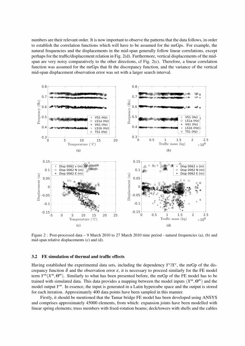
numbers are their relevant order. It is now important to observe the patterns that the data follows, in orderto establish the correlation functions which will have to be assumed for the mrGps. For example, thenatural frequencies and the displacements in the mid-span generally follow linear correlations, exceptperhaps for the traffic/displacement relation in Fig. 2(d). Furthermore, vertical displacements of the mid-span are very noisy comparatively to the other directions, cf Fig. 2(c). Therefore, a linear correlationfunction was assumed for the mrGps that fit the discrepancy function, and the variance of the verticalmid-span displacement observation error was set with a larger search interval.

(a) (b)

(c) (d)

Figure 2 : Post-processed data – 9 March 2010 to 27 March 2010 time period - natural frequencies (a), (b) andmid-span relative displacements (c) and (d).

3.2 FE simulation of thermal and traffic effects

Having established the experimental data sets, including the dependency Y e/Xe, the mrGp of the dis-crepancy function δ and the observation error ε , it is necessary to proceed similarly for the FE modelterm Y m(Xm,Θm). Similarly to what has been presented before, the mrGp of the FE model has to betrained with simulated data. This data provides a mapping between the model inputs (Xm,Θm) and themodel output Y m. In essence, the input is generated in a Latin hypercube space and the output is storedfor each iteration. Approximately 400 data points have been sampled in this manner.

Firstly, it should be mentioned that the Tamar bridge FE model has been developed using ANSYSand comprises approximately 45000 elements, from which: expansion joints have been modelled withlinear spring elements; truss members with fixed-rotation beams; deck/towers with shells and the cables

and hangers with uniaxial tension only beam elements. Additionally to thermal and traffic effects thethree aforementioned calibration parameters θ will also be generated. These are the stiffness of linearsprings, denoted as Kd , which represents friction in the thermal expansion bearings of the Saltash tower,and the initial strain εi in the two main and 16 stay cables of the bridge, respectively.

Secondly, it is necessary to highlight how temperature and traffic effects are considered. For tem-perature, a gradient is applied uniformly across all the elements, provided that the temperature of a maincable is below a notable value τc ≤ 15◦. If the temperature is above this value, different temperaturesare applied to lighted and shaded elements of the bridge as follows

τS =

{0.433τc +7.877 τc > 15τc τc ≤ 15 τL =

{1.544τc−8.798 τc > 15τc τc ≤ 15 (6)

where τS and τL represent the applied temperature in shaded (truss bridge under deck), and lighted(other components except cables) elements, respectively. Essentially, Eq. (6) represents a temperaturefork, occurring at 15◦, where lighted and shaded structural elements attain a higher/lower temperaturethan cables.

Thirdly, the effects of traffic are assumed as a set of distributed mass nodes, evenly spread lon-gitudinally across the bridge deck, and asymmetrically in the lateral direction, similarly to the modeldetailed by Westgate et al. [30]. The main differences are that in the current work temperature is alsotaken into account, and only the traffic from the Plymouth to Saltash direction has been considered.

Finally, and gathering all the above mentioned information, the simulations of the FE model havebeen generated with varying values of temperature, traffic mass, calibration parameters, and the corre-sponding natural frequencies/displacements stored. The resulting simulations are shown in Fig 3. Asexpected, by comparison with Fig. 2 there is additional variability on the model output, not only dueto the larger temperature/traffic intervals but also the varying calibration parameters. The vertical dis-placement has the larger variability and it is primarily dominated by the initial strain of the main cables,whereas the LS1a variability occurs mainly due to the stay cables initial strain. Overall the trends arealso linear and a linear correlation function was also assumed for the model mrGp.

Note that to avoid mixtures between mode shapes while running the simulations, a comparisonagainst reference mode shapes has been performed using the modal assurance criterion (MAC) at 80%.

4. BRIDGE CABLES/BEARINGS DAMAGE IDENTIFICATION

In this section the results of the application of the MBA for damage detection will be presented. Asmentioned in the introduction, the main goal of the present work is not to validate the results, but toshowcase the potentiality of the proposed approach.

4.1 Posterior distributions of reference and current health state

An identified posterior distribution of the calibration parameters for the current state is shown in Fig 4.The shown histograms display samples which were obtained with the Metropolis Hastings algorithm.The assumed prior has equivalent moments to the posterior of the reference state, and the likelihood isbuilt from the probabilistic model described in Section 2.1. The moments for the current and referencestate posteriors are shown in Table 1. It is noticeable that the variances are smaller for the current state,despite the smaller amount of data which was used for its inference. In particular the stay cables variancedecreased by 89% of its original value.

4.2 Probability of damage

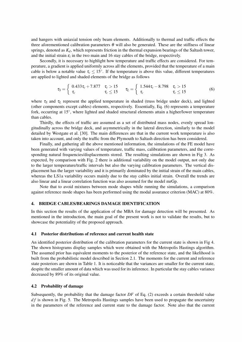
Subsequently, the probability that the damage factor DF of Eq. (2) exceeds a certain threshold valued f is shown in Fig. 5. The Metropolis Hastings samples have been used to propagate the uncertaintyin the parameters of the reference and current state to the damage factor. Note also that the current

(a) (b)

(c) (d)

Figure 3 : Simulated data – natural frequencies (a), (b) and mid-span relative displacements (c) and (d).

Mean VarianceReference Current Reference Current

Main cables 0.0012 0.0012 0.25×10−6 0.14×10−6

Stay cables 0.0024 0.0029 1.17×10−6 0.13×10−6

Bearings (kN/mm) 8.3290 6.8365 5.39 4.11

Table 1 : Posterior PDF moments for the reference and current health state.

(a) (b) (c)

Figure 4 : Prior and posterior PDFs for main (a) stay cables (b) and stiffness of bearings (c).

damage identification takes into account model discrepancy, external effects and observation error, beingtherefore challenging. If more data had been made available the estimation uncertainty visible in theplots would be expected to decrease. Another factor which also contributed to the overall amount ofuncertainty, is that the estimates of the calibration parameters have been assumed as independent.

(a) (b) (c)

Figure 5 : Probability of exceeding a certain damage factor for main (a) stay cables (b) and stiffness of bearings(c).

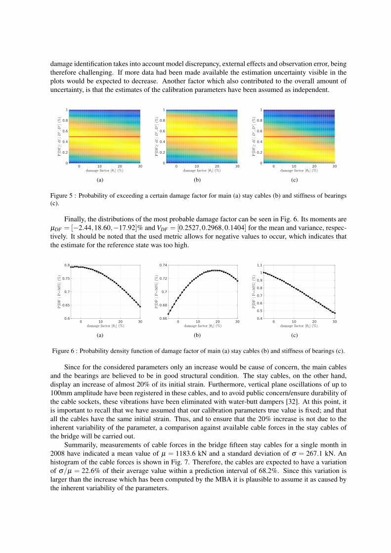
Finally, the distributions of the most probable damage factor can be seen in Fig. 6. Its moments areµDF = [−2.44,18.60,−17.92]% and VDF = [0.2527,0.2968,0.1404] for the mean and variance, respec-tively. It should be noted that the used metric allows for negative values to occur, which indicates thatthe estimate for the reference state was too high.

(a) (b) (c)

Figure 6 : Probability density function of damage factor of main (a) stay cables (b) and stiffness of bearings (c).

Since for the considered parameters only an increase would be cause of concern, the main cablesand the bearings are believed to be in good structural condition. The stay cables, on the other hand,display an increase of almost 20% of its initial strain. Furthermore, vertical plane oscillations of up to100mm amplitude have been registered in these cables, and to avoid public concern/ensure durability ofthe cable sockets, these vibrations have been eliminated with water-butt dampers [32]. At this point, itis important to recall that we have assumed that our calibration parameters true value is fixed; and thatall the cables have the same initial strain. Thus, and to ensure that the 20% increase is not due to theinherent variability of the parameter, a comparison against available cable forces in the stay cables ofthe bridge will be carried out.

Summarily, measurements of cable forces in the bridge fifteen stay cables for a single month in2008 have indicated a mean value of µ = 1183.6 kN and a standard deviation of σ = 267.1 kN. Anhistogram of the cable forces is shown in Fig. 7. Therefore, the cables are expected to have a variationof σ/µ = 22.6% of their average value within a prediction interval of 68.2%. Since this variation islarger than the increase which has been computed by the MBA it is plausible to assume it as caused bythe inherent variability of the parameters.

Figure 7 : Histogram of fifteen stay cable forces – January 2008. The dotted lines represent the mean cable forcesfor the two types of stay cables.

5. CONCLUSIONS

In this work a modular Bayesian approach has been applied for damage detection of the Tamar bridge’smain, stay cables and the stiffness of its bearings. Major conclusions can be stated as follows

• The main cables and the bearings have shown no signs of any structural anomaly.• On the other hand, the stay cables have registered a considerable increase of its initial strain,

which was however attributed to the inherent variability of the cable properties.• The estimation uncertainty of the damage factor is considerable and future efforts are target at

reducing this constraint.

Another avenue of research is the use of the discrepancy function as an indicator of the presence ofdamage. With this work the authors hope to motivate further developments of the MBA for damagedetection, and to enhance the state of the art of the SHM community.

ACKNOWLEDGMENTS

This work was supported by the Engineering and Physical Sciences Research Council (EPSRC) refer-ence number EP/N509796.

REFERENCES[1] C. R. Farrar and K. Worden. An introduction to structural health monitoring. Philosophical Transactions

of the Royal Society A: Mathematical, Physical and Engineering Sciences, 365(1851):303–315, February2007.

[2] C. R. Farrar, S. W. Doebling, and D. A. Nix. Vibration-based structural damage identification.Philosophical Transactions of the Royal Society A: Mathematical, Physical and Engineering Sciences,359(1778):131–149, January 2001.

[3] E. J. Cross, K. Worden, and Q. Chen. Cointegration: A novel approach for the removal of environmentaltrends in structural health monitoring data. Proceedings of the Royal Society A: Mathematical, Physicaland Engineering Sciences, 467(2133):2712–2732, September 2011.

[4] Nguyen Viet Ha and Golinval Jean-Claude. Damage Detection Using Blind Source Separation Techniques.In Tom Proulx, editor, Sensors, Instrumentation and Special Topics, Volume 6, pages 45–56. Springer NewYork, New York, NY, 2011.

[5] Moises Silva, Adam Santos, Eloi Figueiredo, Reginaldo Santos, Claudomiro Sales, and Joao C.W.A. Costa.A novel unsupervised approach based on a genetic algorithm for structural damage detection in bridges.Engineering Applications of Artificial Intelligence, 52:168–180, June 2016.

[6] A. Teughels and G. De Roeck. Structural damage identification of the highway bridge Z24 by FE modelupdating. Journal of Sound and Vibration, 278(3):589–610, December 2004.

[7] Edwin Reynders, Guido De Roeck, Pelin Gundes Bakir, and Claude Sauvage. Damage Identification onthe Tilff Bridge by Vibration Monitoring Using Optical Fiber Strain Sensors. Journal of EngineeringMechanics, 133(2):185–193, February 2007.

[8] E. Peter Carden and James M. W. Brownjohn. Fuzzy Clustering of Stability Diagrams for Vibration-BasedStructural Health Monitoring. Computer-Aided Civil and Infrastructure Engineering, 23(5):360–372, July2008.

[9] Hoon Sohn and Charles R Farrar. Damage diagnosis using time series analysis of vibration signals. SmartMaterials and Structures, 10(3):446–451, June 2001.

[10] J. Beck and K. Yuen. Model Selection Using Response Measurements: Bayesian Probabilistic Approach.Journal of Engineering Mechanics, 130(2):192–203, 2004.

[11] Iman Behmanesh and Babak Moaveni. Accounting for environmental variability, modeling errors, andparameter estimation uncertainties in structural identification. Journal of Sound and Vibration, 374:92–110, July 2016.

[12] Evaggelos Ntotsios, Costas Papadimitriou, Panagiotis Panetsos, Grigorios Karaiskos, Kyriakos Perros,and Philip C. Perdikaris. Bridge health monitoring system based on vibration measurements. Bulletin ofEarthquake Engineering, 7(2):469–483, May 2009.

[13] E. Simoen, B. Moaveni, J. Conte, and G. Lombaert. Uncertainty Quantification in the Assessment of Pro-gressive Damage in a 7-Story Full-Scale Building Slice. Journal of Engineering Mechanics, 139(12):1818–1830, 2013.

[14] I Behmanesh and B Moaveni. Model Updating of Structures with Temperature–Dependent PropertiesUsing a Hierarchical Bayesian Framework. In SHMII-2015, 2015.

[15] Iman Behmanesh and Babak Moaveni. Probabilistic identification of simulated damage on the DowlingHall footbridge through Bayesian finite element model updating. Structural Control and Health Monitor-ing, 22(3):463–483, March 2015.

[16] Iman Behmanesh, Babak Moaveni, and Costas Papadimitriou. Probabilistic damage identification of adesigned 9-story building using modal data in the presence of modeling errors. Engineering Structures,131:542–552, January 2017.

[17] Christopher J. Stull, Christopher J. Earls, and Phaedon-Stelios Koutsourelakis. Model-based structuralhealth monitoring of naval ship hulls. Computer Methods in Applied Mechanics and Engineering, 200(9-12):1137–1149, February 2011.

[18] Wei Zheng and Wei Yu. Probabilistic Approach to Assessing Scoured Bridge Performance and AssociatedUncertainties Based on Vibration Measurements. Journal of Bridge Engineering, 20(6):04014089, June2015.

[19] James-A. Goulet and Ian F.C. Smith. Structural identification with systematic errors and unknown uncer-tainty dependencies. Computers & Structures, 128:251–258, November 2013.

[20] Costas Papadimitriou and Geert Lombaert. The effect of prediction error correlation on optimal sensorplacement in structural dynamics. Mechanical Systems and Signal Processing, 28:105–127, April 2012.

[21] Andre Jesus, Peter Brommer, Yanjie Zhu, and Irwanda Laory. Comprehensive Bayesian structural identi-fication using temperature variation. Engineering Structures, 141:75–82, June 2017.

[22] Anis Ben Abdessalem, Nikolaos Dervilis, David Wagg, and Keith Worden. Model selection and parameterestimation in structural dynamics using approximate Bayesian computation. Mechanical Systems andSignal Processing, 99:306–325, January 2018.

[23] Marc C. Kennedy and Anthony O’Hagan. Bayesian calibration of computer models. Journal of the RoyalStatistical Society: Series B (Statistical Methodology), 63(3):425–464, 2001.

[24] Paul D. Arendt, Daniel W. Apley, Wei Chen, David Lamb, and David Gorsich. Improving Identifiabilityin Model Calibration Using Multiple Responses. Journal of Mechanical Design, 134(10):100909, 2012.

[25] Paul D. Arendt, Daniel W. Apley, and Wei Chen. Quantification of Model Uncertainty: Calibration,Model Discrepancy, and Identifiability. Journal of Mechanical Design, 134(10), October 2012.

[26] H.H. Ku. Notes on the use of propagation of error formulas. Journal of Research of the National Bureauof Standards, Section C: Engineering and Instrumentation, 70C(4):263, October 1966.

[27] Andre Jesus, Mohammad Salami, Robert Westgate, Ki-Young Koo, James Brownjohn, and Irwanda Laory.Bayesian Structural Identification of a Suspension Bridge Using Temperature and Traffic Loading. In Pro-ceedings of the 8th International Conference on Structural Health Monitoring of Intelligent Infrastructure(SHMII), Brisbane, 2017.

[28] E.J. Cross, K.Y. Koo, J.M.W. Brownjohn, and K. Worden. Long-term monitoring and data analysis of theTamar Bridge. Mechanical Systems and Signal Processing, 35(1-2):16–34, February 2013.

[29] R. J. Westgate and J. M. W. Brownjohn. Development of a Tamar Bridge Finite Element Model. InDynamics of Bridges, Volume 5, pages 13–20. Springer New York, New York, NY, 2011.

[30] Robert Westgate, Ki-Young Koo, and James Brownjohn. Effect of Solar Radiation on Suspension BridgePerformance. Journal of Bridge Engineering, 20(5):04014077, May 2015.

[31] Inc. Swanson Analysis Systems IP. ANSYS, Inc. Documentation for Release 15.0. November 2013.

[32] K. Y. Koo, J. M. W. Brownjohn, D. I. List, and R. Cole. Structural health monitoring of the Tamarsuspension bridge. Structural Control and Health Monitoring, 20(4):609–625, April 2013.