1

MODIS Observed Phytoplankton Dynamics in the

Taiwan Strait: an Absorption-based Analysis

Shaoling Shang1, Qiang Dong2, Zhongping Lee2, Yonghong Li1,

Yanshuang Xie1, Michael Behrenfeld3

1 State Key Laboratory of Marine Environmental Science, Xiamen University, Xiamen

361005, Fujian, China

2 Geosystems Research Institute, Mississippi State University, MS 39529, USA

3 Department of Botany and Plant Pathology, Oregon State University, OR 97333, USA

Corresponding author: Shaoling Shang (slshang@gmail.com)

2

Abstract 1

This study used MODIS observed phytoplankton absorption coefficient at 443 2

nm (Aph) as a preferable index to characterize phytoplankton variability in optically 3

complex waters. Aph derived from remote sensing reflectance (Rrs, both in situ and 4

MODIS measured) with the Quasi-Analytical Algorithm (QAA) were evaluated by 5

comparing them with match-up in situ measurements, collected in both oceanic and 6

nearshore waters in the Taiwan Strait (TWS). For the data with matching spatial and 7

temporal window, it was found that the average percentage error (ε) between MODIS 8

derived Aph and field measured Aph was 33.8% (N=30, Aph ranges from 0.012 to 9

0.537 m-1), with a root mean square error in log space (RMSE_log) of 0.226. By 10

comparison, ε was 28.0% (N=88, RMSE_log=0.150) between Aph derived from 11

ship-borne Rrs and Aph measured from water samples. However, values of ε as large 12

as 135.6% (N=30, RMSE_log=0.383) were found between MODIS derived 13

chlorophyll a (Chl, OC3M algorithm) and field measured Chl. Based on these 14

evaluation results, we applied QAA to MODIS Rrs data in the period of 2003-2009 to 15

derive climatological monthly mean Aph for the TWS. Three distinct features of 16

phytoplankton dynamics were identified. First, Aph is low and the least variable in the 17

Penghu Channel, where the South China Sea water enters the TWS. This region 18

maintains slightly higher values in winter (~17% higher than that in the other seasons) 19

due to surface nutrient entrainment under winter wind-driven vertical mixing. Second, 20

Aph is high and varies the most in the mainland nearshore water, with values peaking 21

in summer (June-August) when river plumes and coastal upwelling enhance surface 22

nutrient loads. Interannual variation of bloom intensity in Hanjiang River estuary in 23

June is highly correlated with alongshore wind stress anomalies, as observed by 24

QuikSCAT. The year of minimum and maximum bloom intensity is in the midst of an 25

El Nino and a La Nina event, respectively. Third, a high Aph patch appears between 26

April and September in the middle of the southern TWS, corresponding to high 27

thermal frontal probabilities, as observed by MODIS. Our results support the use of 28

satellite derived Aph for time series analyses of phytoplankton dynamics in coastal 29

3

ocean regions, whereas satellite Chl products derived empirically using spectral ratio 30

of Rrs suffer from artifacts associated with non-biotic optically active materials. 31

Keywords: absorption coefficient, phytoplankton dynamics, MODIS, Taiwan 32

Strait. 33

1 Introduction 34

While the concentration of phytoplankton pigments in the surface ocean reflect 35

both variability in phytoplankton standing stocks and physiological state (e.g. 36

Behrenfeld et al., 2005, Westberry et al., 2008), it has a clear impact on the optical 37

properties of the water, allowing its relatively straight-forward retrieval from remote 38

sensing measurements (e.g. Sathyendranath et al., 1994). The most common pigment 39

product retrieved from ocean color remote sensing is chlorophyll a concentration (Chl, 40

mg/m3; frequently used symbols throughout the manuscript are summarized in Table 41

1). However, because of the optical complexity in nearshore waters (Carder et al., 42

1989; Zhang et al., 2006) and the simple spectral ratio approach (O’Reilly et al., 2000) 43

used for the derivation of Chl, Chl product can be problematic in optically complex 44

nearshore waters. Alternatively, analytical approaches (IOCCG, 2006) based on the 45

radiative transfer theory have been developed to retrieve the spectral absorption 46

coefficient of phytoplankton (aph, m-1). Using phytoplankton absorption, instead of 47

Chl, as a superior metric of phytoplankton pigmentation is becoming increasingly 48

accepted (e.g. Cullen, 1982; Marra et al., 2007), especially from the remote sensing 49

point of view (Lee et al., 1996; Hirawake et al., 2011). This is because the direct 50

controller of ocean color is the spectral absorption and scattering properties of the 51

water media (e.g. Gordon et al., 1988) rather than pigment concentrations, although 52

the variations of the latter will change pigment absorption in a non-stable fashion (e.g. 53

Bricaud et al., 1998, Stuart et al., 1998). However, few studies based on in situ 54

measurements exist to test whether aph can be derived from satellite ocean color data 55

with less uncertainty than Chl. Such evidence is vital in order to confirm that aph can 56

function as the preferable index for characterizing phytoplankton variability in the 57

upper ocean. We here provide results conducted over the Taiwan Strait (TWS), a 58

4

shallow shelf channel that connects the South China Sea with the East China Sea (see 59

Fig. 1), to demonstrate that 1) phytoplankton absorption can be retrieved more 60

accurately than chlorophyll a in this optically complex ocean region from satellite 61

observed ocean color and 2) changes of phytoplankton absorption capture 62

phytoplankton dynamics in a vibrant and changing environment. 63

The TWS has complex hydrographic conditions determined by the relative 64

influence of the South China Sea Warm Current (SCSWC) and the Kuroshio Branch 65

Water (KBW), which are warm, saline, and oligotrophic, and the Zhe-Min Coastal 66

Water (ZMCW), which is cold, fresh, and eutrophic, and varies seasonally in response 67

to changes in the monsoonal wind (e.g. Jan et al., 2002). Several medium-sized rivers 68

(e.g. Hanjiang and Jiulongjiang Rivers) are located on the western coast (mainland 69

China) of the strait. Also along this coast, upwelling develops in summer, driven by 70

the prevailing southwest monsoon which runs parallel to the coast due to Ekman 71

transport (e.g. Hong et al., 2009). Different waters converge in a limited area with a 72

shallow bank (Taiwan Bank), a ridge (Zhangyun Ridge), and deep channel (Penghu 73

Channel), creating strong frontal phenomena (e.g. Chang et al., 2006; Li et al., 2006). 74

For this study, we first derived aph from remote sensing reflectance (Rrs, sr-1) with 75

the quasi-analytical bio-optical inversion algorithm (QAA, Lee et al., 2002; 2009). In 76

addition to QAA, there are several algorithms available for the retrieval of absorption 77

and backscattering coefficients from Rrs (IOCCG, 2006). Here we used QAA because 78

of its transparency in the analytical inversion process and simplicity in 79

implementation. We evaluated the Rrs derived aph by comparing it with match-up in 80

situ measured aph collected in both oceanic and nearshore waters in the TWS. Finally 81

we applied QAA to MODIS Rrs data for the period 2003-2009 to derive climatological 82

monthly mean aph at 443 nm (also represented as Aph for brevity) and to evaluate 83

spatio-temporal variation of the mean Aph in the TWS. 84

2 Data and methods 85

2.1 Satellite data 86

Aqua-MODIS daily Level-2 normalized water leaving radiance (nLw, 87

5

2 1 1W m nm sr− − −⋅ ⋅ ⋅ , 2005 reprocessed version) data were obtained from the NASA 88

Distributed Active Archive Center (http://oceancolor.gsfc.nasa.gov/) and were 89

subsequently converted to Rrs via the ratio of nLw to extra-terrestrial solar irradiance, 90

F0 ( 2 1W m nm− −⋅ ⋅ ) (Gordon, 2005; also see 91

http://oceancolor.gsfc.nasa.gov/DOCS/RSR_tables.html). Aqua-MODIS Level-2 Chl 92

daily data during 2003-2009, which were derived by using the OC3M empirical 93

algorithm (O’Reilly et al., 2000), were also obtained from the same source. These data 94

were further processed into Level-3 products by using Mercator projection, which was 95

implemented on SeaDAS (http://seadas.gsfc.nasa.gov/doc/tutorial/sds_tut2.html). The 96

spatial resolution of these data was 1 km by 1 km. 97

Daily wind field data were obtained from QuikScatterometer (QuikSCAT) 98

observations from 2003 to 2009 (http://podaac.jpl.nasa.gov), with a spatial resolution 99

of 0.25º by 0.25º (equivalent to ~25 km by ~25 km). Daily wind stress (T, N/m2) was 100

calculated from (Stewart, 2008): 101

210Da UCT ρ= (1) 102

where ρa=1.3 kg/m3 was the density of air, U10 (m/s) was wind speed at 10 meters 103

(the QuiSCAT measurement), and CD was the drag coefficient. CD was calculated 104

from Yelland and Taylor (1996) and Yelland et al. (1998). Wind stress vectors were 105

further decomposed into alongshore (southwesterly) and cross-shore (northwesterly) 106

components by applying a simple vector manipulation. 107

Aqua-MODIS sea surface temperature (SST, ℃) monthly mean data (4 km by 4 108

km resolution) during 2003-2009 were downloaded from 109

http://oceandata.sci.gsfc.nasa.gov/. Based on this SST data, we derived a thermal 110

frontal probability map for the TWS by following Wang et al. (2001). Briefly, we 111

calculated the SST gradients in eight directions for each clear pixel and chose the 112

average over the three absolute maxima as the horizontal gradient for this pixel. Only 113

pixels whose gradients were equal to or greater than the threshold of 0.5°C per 4 km 114

were regarded as frontal pixels. The frontal probability was then obtained by dividing 115

6

the number of times the pixel was frontal, by the accumulative number of times the 116

pixel had a valid SST value. 117

2.2 Calculation of mean and anomaly 118

To address spatio-temporal variations of properties derived from satellite 119

measurements, temporal and spatial means and anomalies were calculated for each 120

property. These properties included the non-water absorption at 443 nm (total 121

absorption coefficient without contribution from pure water; at-w(443), m-1) and Aph 122

from QAA_v5, Chl from OC3M, and QuikSCAT derived alongshore component of 123

wind stress. 124

For pixel i in month X year Y, the monthly mean of a property was obtained by 125

adding up all the available daily values in the month and then dividing them by the 126

number of days having valid values. The spatial mean of each property in month X 127

year Y ( Y X,P ) was calculated by adding up all the available monthly mean values in 128

the TWS area in the month and dividing them by the number of pixels having valid 129

retrievals. The TWS area was defined as the ocean area between the China mainland 130

coast or the 116.5ºE longitude and the 122 ºE, and between 22ºN and 25.5ºN (see Fig. 131

1, the area enclosed by the dashed grey lines, the mainland coastline and the 122 ºE). 132

For pixel i in month X, the climatological monthly mean of a property ( X,iP ) was 133

calculated by adding up all the monthly values for 2003-2009 and then dividing them 134

by the number of years (=7). The spatial mean of each property in month X ( XP ) was 135

then calculated based on this climatological monthly mean dataset following the 136

above mentioned procedure for calculation of Y X,P . 137

The spatial anomaly of a property in pixel i month X was derived from X,iP - XP . 138

The temporal anomaly of a property in month X year Y was calculated from Y X,P -139

XP . 140

7

2.3 In situ data 141

2.2.1 Remote sensing reflectance 142

In stiu Rrs was derived from measured (1) upwelling radiance (Lu, 143

2 1 1W m nm sr− − −⋅ ⋅ ⋅ ), (2) downwelling sky radiance (Lsky, 2 1 1W m nm sr− − −⋅ ⋅ ⋅ ), and (3) 144

radiance from a standard Spectralon reflectance plaque (Lplaque, 2 1 1W m nm sr− − −⋅ ⋅ ⋅ ). 145

The instrument used was the GER 1500 spectroradiometer (Spectra Vista Corporation, 146

USA), which covers a spectral range of 350-1050 nm with a spectral resolution of 3 147

nm. From these three components, Rrs was calculated as: 148

( ) / ( )rs u sky plaqueR L F L Lρ π= − ⋅ ⋅ − ∆ (2) 149

where ρ is the reflectance (0.5) of the spectralon plaque with Lambertian 150

characteristics and F is surface Fresnel reflectance (around 0.023 for the viewing 151

geometry). Δ (sr-1) accounts for the residual surface contribution (glint, etc.), which 152

was determined either by assuming Rrs(750)=0 (clear oceanic waters) or through 153

iterative derivation according to optical models for coastal turbid waters as described 154

in Lee et al. (2010). 155

2.2.2 Field-measured absorption coefficients and chlorophyll a 156

Water samples for determination of absorption coefficients and Chl were 157

collected from surface waters during 2003-2007 in the TWS. Sampling station depths 158

ranged from ~10 m to ~400 m. Measurements of chromophoric dissolved organic 159

matter (CDOM) absorption coefficient, ag(m-1), and Chl were performed according to 160

the Ocean Optics Protocols Version 2.0 (Mitchell et al., 2000), and were detailed in 161

Hong et al. (2005) and Du et al. (2010). Particulate absorption coefficient (ap, m-1) 162

was measured by the filter-pad technique (Kiefer and SooHoo, 1982) with a 163

dual-beam PE Lambda 950 spectrophotometer equipped with an integrating sphere 164

(150 mm in diameter) following a modified Transmittance–Reflectance (T-R) method 165

(Tassan and Ferrari, 2002; Dong et al., 2008). This approach was used instead of the T 166

method recommended in the NASA protocol (Mitchell et al., 2000) because some of 167

the samples were collected nearshore. These samples were rich in highly scattered 168

8

non-pigmented particles. The standard T-method will thus cause an overestimate of 169

sample absorption (Tassan and Ferrari, 1995). Detrital absorption (ad, m-1) was 170

therefore obtained by repeating the modified T-R measurements on samples after 171

pigment extraction by methanol (Kishino, 1985). aph was then calculated by 172

subtracting ad from ap, and the combination of ap and ag yields an estimation of at-w. 173

Combining all the field studies, we collected 104 sets of in situ data, with each 174

set including at-w, aph, ad, ag and Chl. This in situ dataset covered a wide range of 175

absorption properties, with at-w(443) ranging from 0.019 to 2.41 m-1, and the 176

aph(443)/at-w(443) ratio varying between 9%-86%. 177

Due to frequent cloud cover in the TWS, only 30 matching data pairs were 178

achieved of in situ absorption and Chl data collected within ±24h of MODIS overpass 179

(Fig. 1, circle symbols). By comparison, there were 88 sets of in situ absorption and 180

Chl data having match-up in situ Rrs measurements (Fig. 1, cross symbols). 181

3 Evaluation of Rrs derived absorption coefficients in the Taiwan Strait 182

Rrs from field measurements and MODIS were fed to QAA_v5 (Lee et al., 2009), 183

respectively, to derive two sets of at-w and aph. In order to evaluate the quality of Rrs 184

derived aph, we used the root mean square error both in linear scale (RMSE) and in log 185

scale (RMSE_log), and averaged percentage error (ε) as a measure to describe the 186

similarity/difference between the field measured (f) and retrieved data sets (r): 187

%100f

fr11

×

−= ∑

=

n

i i

ii

nε (3) 188

∑=

−=n

iiin

RMSE1

2)fr(1 (4) 189

2

1

1_log (log(r ) log(f ))n

i ii

RMSEn =

= −∑ (5) 190

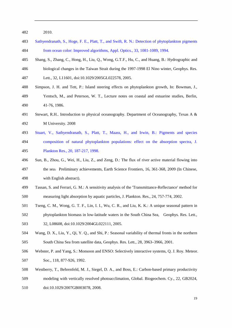
Results were given in Table 2. Fig. 2 (a & b) compares the derived and measured at-w 191

and aph values at 443 nm for the MODIS (the yellow square symbols) and the in situ 192

(the blue circle symbols) data sets, respectively. 193

Averaged percentage error (ε) and RMSE_log between in situ measured aph(412) 194

9

and MODIS aph(412) were 36.1% and 0.252, respectively, for an aph(412) range of 195

0.009–0.539 m-1. Similarly, ε was 33.8% and RMSE_log was 0.226 for an aph(443) 196

range of 0.012–0.537 m-1 (Table 2). These errors decreased when aph was derived 197

from ship-borne Rrs. For example, the ε was 28.0% and the RMSE_log was 0.150 for 198

443 nm (Table 2). Such a difference was not surprising since additional uncertainties 199

were introduced in satellite match-ups that were associated with imperfections in 200

atmospheric correction over coastal water for the MODIS Rrs (Dong, 2010) and the 201

spatio-temporal mismatch between satellite and field data (1 km2 versus 1m2, and the 202

temporal window of ±24 h) . Nevertheless, these results were better than the global 203

evaluation results reported in the IOCCG Report No.5 (IOCCG, 2006), which used 204

the earliest version of QAA (Lee et al, 2002). In that report, no satellite Rrs derived aph 205

data were evaluated and the RMSE_log between in situ Rrs derived aph(443) and field 206

measured aph(443) was 0.321 (it was 0.150 in this study). A recent evaluation of 207

SeaWiFS Rrs derived aph(443) using QAA at an European coastal site produced a 208

RMSE_log of 0.21 ( Mélin et al., 2007), which was comparable to our results. 209

The difference between in situ measured Chl and match-up Rrs derived Chl (via 210

OC3M) was much larger than found for Aph (Fig. 2c). Between in situ measured Chl 211

and MODIS Rrs derived Chl, the ε was 135.6% and RMSE_log was 0.383. Between in 212

situ measured Chl and in situ Rrs derived Chl, the ε was 162.0% and RMSE_log was 213

0.429. This analysis of match-up uncertainties clearly indicated improved 214

performance of Rrs-retrieved Aph over Chl in the TWS. One fundamental reason for 215

such results is that Rrs is largely determined by the absorption and scattering 216

properties of all the optically active materials in the water, of which phytoplankton is 217

simply one of them (Mobley, 1994; IOCCG, 2006). Higher uncertainty associated 218

with Chl is thus anticipated while trying to retrieve Chl by simple spectral ratio of Rrs 219

in marine waters where the contribution of non-phytoplankton components is 220

significant (e.g., TWS). 221

10

4 Comparison on the spatial patterns of MODIS aph(443), at-w(443) and Chl in 222

the Taiwan Strait 223

The above analysis of match-up uncertainties supports the use of Rrs derived Aph 224

as a preferable index (compared to Chl) to represent phytoplankton in the optically 225

complex coastal water of the TWS. A time series of MODIS Aph for the TWS was 226

thus derived by inputting daily MODIS Rrs into QAA_v5. Climatological monthly 227

mean Aph during 2003–2009 were then derived, along with at-w(443) from QAA_v5 228

and Chl from OC3M. Before using this multi-year monthly mean Aph dataset to 229

address phytoplankton dynamics in the TWS, we further did a comparison on the 230

spatial patterns of Aph, at-w(443) and Chl for the entire TWS. This additional analysis 231

was conducted to address a concern that the evaluation results shown in Section 3 232

were merely a comparison of discrete match-up samples in the TWS and most of the 233

Rrs data used in the analysis were in situ measurements, rather than MODIS 234

measurements. The spatial patterns of the three properties in the TWS were revealed 235

by calculating their spatial anomalies and normalizing each to their respective spatial 236

mean. The RMSD (root mean square deviation) between each pair of normalized 237

spatial anomalies was calculated as: 238

2

1

1 n

iRMSD

nδ

=

= ∑ (6) 239

where δ was the difference between each pair of normalized spatial anomalies, and n 240

was the pixel number (varies from 134000 to 148118, depending on percentage of 241

cloud cover in each month). As shown in Fig. 3, the RMSD was larger between Chl 242

and Aph (the grey bar) than between Chl and at-w(443) (the empty bar), especially 243

during the cold season when the wind was strong and the water was relatively turbid 244

due to sediment resuspension (Guo et al., 1991). This finding clearly indicates that the 245

spatial pattern of empirically derived MODIS Chl was more similar to that of MODIS 246

at-w(443) than MODIS Aph. Thus, the empirical MODIS Chl product was registering 247

the combined influence of phytoplankton pigments and other optically active 248

materials (detritus and CDOM) in the TWS, similar as that found in the South Pacific 249

11

Gyre (Lee et al., 2010). Using analytically derived Aph from MODIS measurements 250

to study phytoplankton dynamics is thus further justified. 251

5 Spatio-temporal variation of MODIS Aph in the Taiwan Strait 252

The monthly mean of each year and climatological monthly mean MODIS Aph 253

dataset were used to analyze the spatio-temporal variations of Aph during 2003-2009. 254

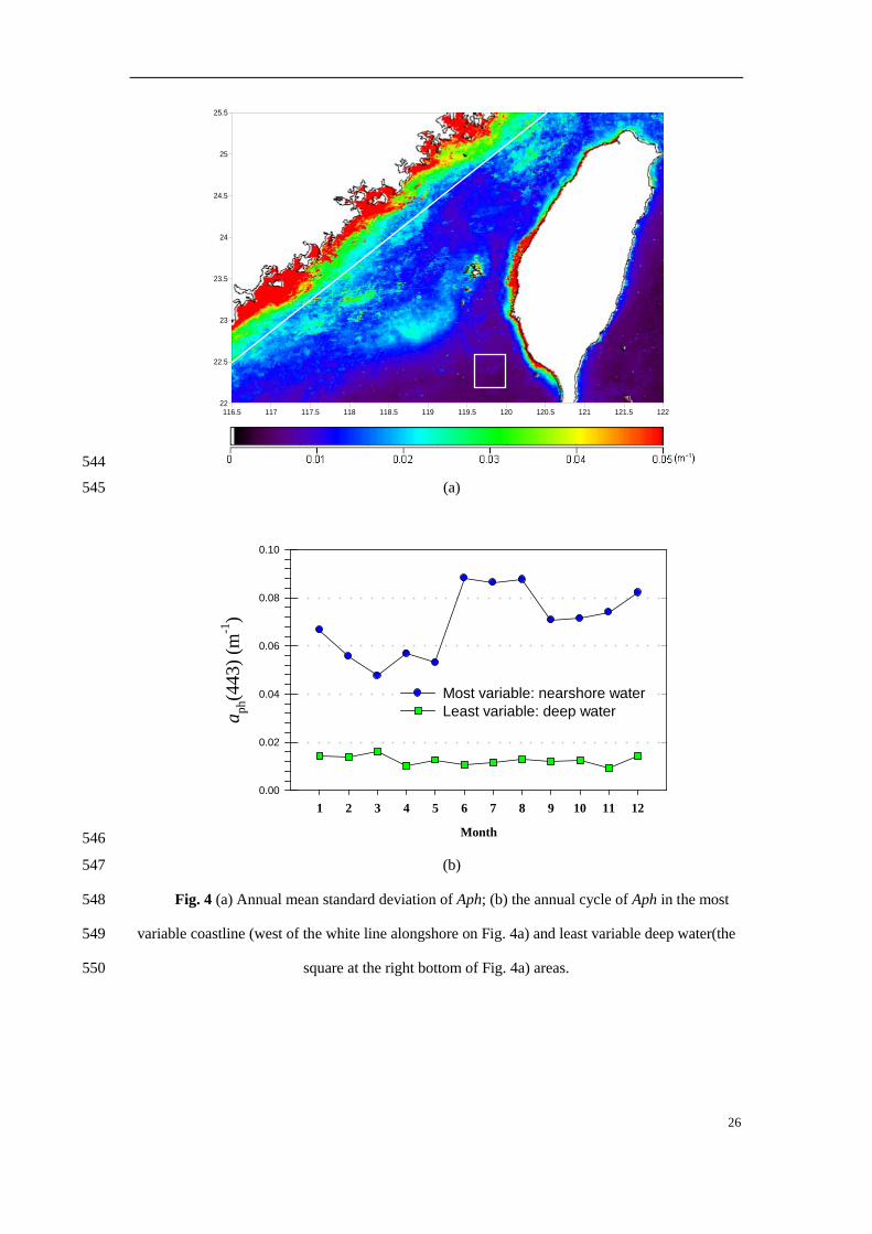
First, the annual mean Aph and its standard deviation (STD) were derived from 255

the climatological monthly mean MODIS Aph. The STD identifies a highly variable 256

area located alongshore the China mainland, and an area showing low temporal 257

variation located in the deepest zone of the TWS (i.e. the Penghu Channel), adjacent 258

to the South China Sea (Fig. 4a). 259

To investigate further the seasonality of Aph in waters of low temporal variation, 260

we chose a square in the Penghu Channel (right bottom of Fig. 4a) and derived its 261

monthly time series. Although variations are weak, Aph slightly increases during 262

December to March by about 17% over the mean level of Aph in the other months 263

(Fig. 4b). This seasonal pattern with a winter maximum is similar to in situ 264

observations of Chl, phytoplankton cell counts, and primary production at SEATS 265

(18ºN 116ºE, South East Asian Time-series Study station, Tseng et al., 2005) and the 266

entire South China Sea (Ning et al., 2004; Chen, 2005). This correspondence between 267

seasonal cycles of phytoplankton pigment in the TWS and the South China Sea is not 268

surprising since this part of the TWS is dominated by the SCSWC (Jan et al., 2002). 269

Enhanced nitrate availability in winter due to enhanced wind-driven vertical mixing is 270

thought to play a role in modulating phytoplankton dynamics in this water (Chen, 271

2005), although photoacclimation and altered grazing pressure may also be important 272

(Behrenfeld et al. 2005; Behrenfeld, 2010). 273

In contrast to the Penghu Channel water, Aph is highly variable alongshore the 274

China mainland, influenced by inputs of the Jiulongjiang and Hanjiang Rivers (see 275

locations in Fig. 1) and by upwelling in summer (Hong et al., 2009) and the Zhe-Min 276

Coastal Water in winter (Jan et al., 2002). In the nearshore band west of the white line 277

on Fig. 4a, Aph ranges from 0.048 m-1 in March to 0.088 m-1 in June (Fig. 4b). 278

12

Overall, Aph peaks in summer (June-August) at a value 64% higher than the 279

minimum Aph observed in spring (March-May). Summer is the season of peak river 280

flow, which accounts for 44% of the annual discharge (Sun et al., 2009; http://bai- 281

ke.baidu.com/view/23372.html). Summer is also the season of southwesterly wind, 282

which drives coastal upwelling (Hong et al., 2009). Nearshore phytoplankton blooms, 283

as indexed by the high Aph values, are thus supported by the availability of nutrients 284

provided by both river plumes and upwelling. 285

A close-up view of this nearshore water in May-August (Fig. 5a) clearly 286

demonstrates the combined impacts of river plumes and upwelling in summer. Out of 287

each estuary, there is a tongue of high Aph (generally ≥0.1 m -1) advecting 288

northeastward. This feature is most distinct in June (Fig. 5a). In the vicinity of 289

Hanjiang River estuary (also nearby the Dongshan Island), a broad area of especially 290

high Aph is found, relative to values for the Jiulongjiang River estuary. This 291

difference is, in part, due to the volume of Hanjiang River annual flow at 258 x 109 m3, 292

which is ~80% higher than the Jiulongjiang River (142×109 m3) (Sun et al., 2009). In 293

addition, a significant upwelling center is located in the vicinity of Dongshan Island 294

(Hong et al., 2009). These combined factors (upwelling and stronger river plume) 295

result in stronger blooms for the Hanjiang River estuary area. 296

To investigate the interannual variation of bloom intensity for such an upwelling 297

enhanced bloom in the Hanjiang River estuary area, we used the monthly mean of 298

each year Aph data to derive an annual areal bloom index (ABI). ABI was calculated 299

as the sum of Aph in pixels having Aph≥0.1 m-1 for all valid observations in a month 300

(Aph of 0.1 m-1 corresponds to ~1.7 mg/m3 Chl in the TWS (Dong, 2010)). The ABI 301

within a square representing the Hanjiang River estuary (see location on the June 302

image of Fig. 5a; its area is 9400 km2) in June of each year during 2003-2009 is 303

shown in Fig. 5b (the empty circle), along with the percentage of valid pixels to 304

retrieve the ABI (the grey bar), the alongshore wind stress anomaly (the solid circle), 305

and the Multivariate ENSO Index (MEI, 306

http://www.cdc.noaa.gov/people/klaus.wolter/MEI/) (the red and blue curve). The 307

13

ABI peaks in 2008 and is the lowest in 2004, and is well correlated with the 308

alongshore wind stress anomaly (r2=0.67, n=7). More positive alongshore wind stress 309

anomalies correspond to stronger southwesterly winds, which drive enhanced 310

upwelling, offshore advection of river plumes, and stronger phytoplankton blooms 311

(and vise versa). However, the ABI in 2009 is 152 m-1, even lower than the ABI in 312

2003 (776 m-1). The alongshore wind stress anomaly is positive in 2009 and negative 313

in 2003, suggesting bloom favoring conditions in 2009 compared to 2003. This 314

abnormally low number in 2009 is in part due to missing satellite data in the Hanjiang 315

River estuary area owing to heavy cloud cover. In total, there are 7771 pixels in the 316

square for ABI estimation. As the grey bar in Fig. 5b shows, during most of the year, 317

more than 80% of the pixels in the square have valid retrievals; while in 2009, only 29% 318

of the pixels had valid Aph data. Therefore, additional uncertainties of satellite data 319

due to bad weather conditions must be noted, necessitating careful examination of the 320

data. If we remove data from 2009 where ABI values are abnormally low in number, 321

the r2 between ABI and the alongshore wind stress anomaly increases to 0.97 (n=6). 322

Interestingly, variations of the ABI show coincidence with ENSO activities, 323

illustrated by the match of the empty circles (ABI) and the red and blue curve (MEI) 324

(Fig. 5b). Positive MEI (red curve) indicates occurrence of El Nino while negative 325

MEI (blue curve) corresponds to La Nina. The year of the lowest ABI (2004) is in the 326

midst of an El Nino event (2000-2005), and the year of the highest ABI (2008) is in 327

the midst of a La Nina event (2007-2009). Such an ABI difference between El Nino 328

and La Nina years might be more significant, if it is influenced by potential 329

differences in cloud cover between El Nino and La Nina years, since 78% of the total 330

pixels have valid retrievals in 2008 while the percentage of valid retrievals is as high 331

as 86% in 2004 (see the grey bar in Fig. 5b). It has been acknowledged that the 332

relationship between the Asian monsoon and ENSO is mutual but selectively 333

interactive (e.g. Webster and Yang 1992). However, which factor is the underlying 334

cause and which is the effect remain unclear (e.g. Kinter III, et al., 2002). Here we 335

have observed a strong coastal bloom in 2008, when the southwest monsoon is the 336

14

strongest (during 2003-2009) and a La Nina event is occurring. We have also 337

observed a weak bloom in 2004, when the southwest monsoon is the weakest (during 338

2003-2009) and an El Nino event is at its mid-point. Further study of regional scale 339

ecosystem variability should advance understanding of the monsoon-ENSO 340

interaction. 341

Spatial anomalies of Aph also highlight a distinctly high Aph patch generally 342

located in the middle of the southern TWS, appearing in the period of April to 343

September (Fig. 6a). This patch is likely associated with (1) shelf break upwelling in 344

the vicinity of the Taiwan Bank (Li et al, 2000), (2) island stirring around Penghu 345

Islands (Simpson and Tett, 1986) and (3) upwelling associated with Zhangyun Ridge 346

(Pi and Hu, 2010). Frontal probabilities derived from MODIS SST during 2003-2009 347

are grater than 60% in the area corresponding to this Aph patch (Fig. 6b). Since 348

vertical temperature gradients are smaller during cold seasons, these fronts can only 349

be well developed in the surface water during warm seasons (April-September). 350

Fronts provide powerful physical forcings to inject nutrients from deep water into the 351

surface, thus facilitating phytoplankton growth. 352

353

6 Conclusion 354

The current study provided both an assessment of algorithm performance and a 355

description of phytoplankton dynamics in the optically complex TWS. Based on our 356

analysis of 104 in situ measurements in the TWS, we found that the QAA algorithm 357

provided a satisfactory assessment of aph from both MODIS and ship borne Rrs. We 358

further derived climatological monthly mean Aph (2003-2009) from MODIS Rrs with 359

QAA and found a variety of seasonal patterns for Aph in the TWS. The most 360

interesting result is that the phytoplankton bloom in the vicinity of Hanjiang River 361

estuary, which is enhanced by upwelling in summer, shows an order of magnitude 362

variation during 2003-2009. This interannual variability is highly correlated with 363

alongshore wind stress anomalies and ENSO activities, and demonstrates ecological 364

responses to changing in environmental forcings, documented here for the first time 365

15

by using satellite Aph data. This dynamics was not revealed when satellite Chl 366

product was employed, as there are large uncertainties in the spectral-ratio derived 367

Chl in nearshore waters (Zhang, 2006). It should be noted, however, that Aph is not a 368

full reflection of variability in phytoplankton pigmentation because of the package 369

effect (Bricaud et al., 1998), even though they are directly related to each other. Some 370

uncertainties also remain in our satellite aph products due to issues with variable cloud 371

cover that may introduce biases in our results, especially in winter. Repeated 372

observations from multi-sensors and geostationary satellites may help resolve such 373

problems in the future. 374

375

Acknowledgements 376

This work was supported jointly by the High-tech R & D program of China 377

(#2008AA09Z108), NSF-China (#40976068), the National Basic Research Program 378

of China (#2009CB421200 and 2009CB421201), the China Scholarship Council, and 379

the Program of ITDU (#B07034). Suport for M. Behrenfeld was provided through the 380

National Aeronautics and Space Administration (#NNX08AF73A). We thank the 381

crew of the R/V Yanping II, and J. Wu, X. Ma, X. Sui, W. Zhou, W. Wang, M. Yang, 382

C. Du and G. Wei for their help in collecting in situ data and Drs. Allen Milligan and 383

Toby Westberry for helpful discussions during our analysis. 384

385

References 386

Behrenfeld, M. J., Boss, E., Siegel, D. A., and Shea, D. M.: Carbon-based ocean productivity and 387

phytoplankton physiology from space, Global Biogeochem. Cy., 19, GB1006, 388

doi:10.1029/2004GB002299, 2005. 389

Behrenfeld, M. J.: Abandoning Sverdrup’s Critical Depth Hypothesis on phytoplankton blooms, 390

Ecology, 91, 977-989, 2010. 391

Bricaud, A., Morel, A., Babin, M., Allali, K., and Claustre, H.: Variations of light absorption by 392

suspended particles with chlorophyll a concentration in oceanic (case 1) waters: Analysis and 393

implications for bio-optical models, J. Geophys. Res., 103, 31033-31044, 1998. 394

16

Carder, K. L., Steward, R. G., Harvey, G. R., and Ortner, P. B.: Marine humic and fulvic acids: 395

their effects on remote sensing of ocean chlorophyll, Limnol. Oceanogr., 34, 68-81, 1989. 396

Carder, K. L., Chen, F. R., Lee, Z., Hawes. S. K., and Kamykowski, D.: Semianalytic 397

Moderate-Resolution Imaging Spectrometer algorithms for chlorophyll a and absorption with 398

bio-optical domains based on nitrate-depletion temperatures, J. Geophys. Res., 104, 399

5403-5421, 1999. 400

Chang, Y., Shimada, T., Lee, M. A., Lu, H. J., Sakaida, F., and Kawamura, H.: Wintertime sea 401

surface temperature fronts in the Taiwan Strait, Geophys. Res. Lett., 33, L23603, 402

doi:10.1029/2006GL027415, 2006. 403

Chen, L.: Spatial and seasonal variations of nitrate-based new production and primary production 404

in the South China Sea, Deep-Sea. Res. Pt I, 52, 319-340, 2005. 405

Cullen, J. J.: The deep chlorophyll maximum: Comparing vertical profiles of chlorophyll a, Can. J. 406

Fish. Aquat. Sci., 39, 791-803, 1982. 407

Dong, Q., Hong, H., Shang, S.: A new approach to correct for pathlength amplification in 408

measurements of particulate spectral absorption by the quantitative filter technique, Journal 409

of Xiamen University (Natural Science), 47, 556-561, 2008 (In Chinese, with English 410

abstract). 411

Dong, Q.: Derivation of Phytoplankton Absorption Properties from Ocean Color and Its 412

Application, Ph. D., Xiamen University (China), 2010. 413

Du, C., Shang, S., Dong, Q., Hu, C., and Wu, J.: Characteristics of Chromophoric Dissolved 414

Organic Matter in the nearshore waters of the western Taiwan Strait, Estuar. Coast. Shelf. S., 415

88, 350-356, 2010. 416

Gordon, H. R., Brown, O. B., Evans, R. H., Brown, J. W., Smith, R. C., Baker, K. S., and Clark, D. 417

K.: A semianalytic radiance model of ocean color, J. Geophys. Res., 93, 10909-10924, 1988. 418

Gordon, H. R.: Normalized water-leaving radiance: revisiting the influence of surface roughness, 419

Appl. Optics., 44, 241-248, 2005. 420

Guo, L., Hong, H., Chen, J., and Hong, L.: Distribution and variation of suspended matter in the 421

southern Taiwan Strait, In: Hong, H., Minnan-taiwan bank fishing ground upwelling 422

ecosystem study, 273-281, 1991 (In Chinese, with English abstract). 423

17

Hirawake, T., Takao, S., Horimoto, N., Ishimaru, T., Yamaguchi, Y., and Fukuchi, M.: A 424

phytoplankton absorption-based primary productivity model for remote sensing in the 425

Southern Ocean, Polar Biology (accepted). 426

Hong, H., Wu, J., Shang, S., and Hu, C.: Absorption and fluorescence of chromophoric dissolved 427

organic matter in the Pearl River Estuary, South China, Mar. Chem., 97, 78-89, 2005. 428

Hong, H., Zhang, C., Shang, S., Huang, B., Li, Y., Li, X., and Zhang, S.: Interannual variability of 429

summer coastal upwelling in the Taiwan Strait, Cont. Shelf. Res., 29 , 479-484, 2009. 430

Jan, S., Wang, J., Chern, C.S., and Chao, S.Y.: Seasonal variation of the circulation in the Taiwan 431

Strait, J. Marine. Syst., 35, 249-268, 2002. 432

Kiefer, D. A., and SoohHoo, J. B.: Spectral absorption by marine particles of coastal waters of 433

Baja California, Limnol. Oceanogr., 27, 492-499, 1982. 434

Kinter III, J., Miyakoda, K., and Yang, S.: Recent change in the connection from the Asian 435

monsoon to ENSO, J. Climate, 15, 1203-1215, 2002. 436

Kishino, M., Takahashi, M., Okami, N., and Ichimura, S.: Estimation of the spectral absorption 437

coefficients of phytoplankton in the sea, B. Mar. Sci., 37, 634-642, 1985. 438

Lee, Z., Carder, K. L., Marra, J., Steward, R. G., and Perry, M. J.: Estimating primary production 439

at depth from remote sensing, Appl. Optics., 35(3), 463-474, 1996. 440

Lee, Z., Carder, K. L., and Arnone, R. A.: Deriving inherent optical properties from water color: a 441

multiband quasi-analytical algorithm for optically deep waters, Appl. Optics., 41, 5755-5772, 442

2002. 443

Lee, Z.: Remote sensing of inherent optical properties: fundamentals, tests of algorithms, and 444

applications, In: Stuart, V., International Ocean-Colour Coordinating Group, No. 5, IOCCG, 445

Dartmouth, Canada, 2006. 446

Lee, Z., Carder, K. L, Arnone, R. A, and He, M.: Determination of primary spectral bands for 447

remote sensing of aquatic environments, Sensors, 7, 3428-3441, 2007. 448

Lee, Z., Lubac, B., Werdell, J., and Arnone, R.: An update of the Quasi-Analytical Algorithm 449

(QAA_v5), http://www.ioccg.org/groups/Software_OCA/QAA_v5.- pdf, 2009. 450

Lee, Z., Ahn, Y., Mobley, C., and Arnone, R.: Removal of surface-reflected light for the 451

measurement of remote-sensing reflectance from an above-surface platform, Opt Express, 452

18

18(25), 26313-26342, 2010. 453

Lee, Z., Shang, S., Hu, C., Lewis, M., Arnone, R., Li, Y., and Lubac, B.: Time series of 454

bio-optical properties in a subtropical gyre: Implications for the evaluation of inter-annual 455

trends of biogeochemical properties, J. Geophys. Res. 115, C09012, 456

doi:10.1029/2009JC005865, 2010. 457

Li, C., Hu, J., Jan, S., Wei, Z., Fang, G. H., and Zheng, Q.: Winter-spring fronts in Taiwan Strait, J. 458

Geophys. Res., 111, C11S13, doi:10.1039/2005JC003203, 2007. 459

Li, L., Guo, X., and Wu, R.: Oceanic fronts in southern Taiwan Strait, Journal of Oceanography in 460

Taiwan Strait, 19, 147-156, 2000 (In Chinese, with English abstract). 461

Maritorena, S., Siegel, D. A., and Peterson, A. R.: Optimization of a semianalytical ocean color 462

model for global-scale applications, Appl. Optics., 41, 2705-2714, 2002. 463

Marra, J., Trees, C. C., and O’Reilly, J.E.: Phytoplankton pigment absorption: A strong predictor 464

of primary productivity in the surface ocean, Deep-Sea. Res. Pt I, 54, 155-163, 2007. 465

Mélin, F., Zibordi, G., and Berthon, J.F.: Assessment of satellite ocean color products at a coastal 466

site, Remote. Sens. Environ., 110, 192-215, 2007. 467

Mitchell, B. G., Bricaud, A., and Carder, K.: Determination of spectral absorption coefficients of 468

particles, dissolved material and phytoplankton for discrete water samples, In: Fargion, G.S. 469

and Mueller, J.L., Ocean optics protocols for satellite ocean color sensor validation, revision 470

2, Greenbelt, Maryland: NASA Goddard Space Flight Space Center, 125-153, 2000. 471

Ning, X., Chai, F., Xue, H., Cai, Y., Liu, C., and Shi, J.: Physical-biological oceanographic 472

coupling influencing phytoplankton and primary production in the South China Sea, J. 473

Geophys. Res., 109, C10005, doi:10.1029/2004JC002365, 2004. 474

O'Reilly, J. E., Maritorena, S., Siegel, D., and O'Brien, M. C.: Ocean color chlorophyll a 475

algorithms for SeaWiFS, OC2, and OC4: version 4, In: Hooker, S. B. and Firestone, E. R., 476

SeaWiFS postlaunch technical report series, volume 11, SeaWiFS postlaunch calibration and 477

validation analyses, part 3, Greenbelt, Maryland: NASA Goddard Space Flight Center, 9-23, 478

2000. 479

Pi, Q. and Hu, J.: Analysis of sea surface temperature fronts in the Taiwan Strait and its adjacent 480

area using an advanced edge detection method, Science China, Earth Science, 53, 1008-1016, 481

19

2010. 482

Sathyendranath, S., Hoge, F. E., Platt, T., and Swift, R. N.: Detection of phytoplankton pigments 483

from ocean color: Improved algorithms, Appl. Optics., 33, 1081-1089, 1994. 484

Shang, S., Zhang, C., Hong, H., Liu, Q., Wong, G.T.F., Hu, C., and Huang, B.: Hydrographic and 485

biological changes in the Taiwan Strait during the 1997-1998 El Nino winter, Geophys. Res. 486

Lett., 32, L11601, doi:10.1029/2005GL022578, 2005. 487

Simpson, J. H. and Tett, P.: Island steering effects on phytoplankton growth, In: Bowman, J., 488

Yentsch, M., and Peterson, W. T., Lecture notes on coastal and estuarine studies, Berlin, 489

41-76, 1986. 490

Stewart, R.H.. Introduction to physical oceanography. Department of Oceanography, Texas A & 491

M University. 2008 492

Stuart, V., Sathyendranath, S., Platt, T., Maass, H., and Irwin, B.: Pigments and species 493

composition of natural phytoplankton populations: effect on the absorption spectra, J. 494

Plankton Res., 20, 187-217, 1998. 495

Sun, B., Zhou, G., Wei, H., Liu, Z., and Zeng, D.: The flux of river active material flowing into 496

the sea：Preliminary achievements, Earth Science Frontiers, 16, 361-368, 2009 (In Chinese, 497

with English abstract). 498

Tassan, S. and Ferrari, G. M.: A sensitivity analysis of the 'Transmittance-Reflectance' method for 499

measuring light absorption by aquatic particles, J. Plankton. Res., 24, 757-774, 2002. 500

Tseng, C. M., Wong, G. T. F., Lin, I. I., Wu, C. R., and Liu, K. K.: A unique seasonal pattern in 501

phytoplankton biomass in low-latitude waters in the South China Sea, Geophys. Res. Lett., 502

32, L08608, doi:10.1029/2004GL022111, 2005. 503

Wang, D. X., Liu, Y., Qi, Y. Q., and Shi, P.: Seasonal variability of thermal fronts in the northern 504

South China Sea from satellite data, Geophys. Res. Lett., 28, 3963–3966, 2001. 505

Webster, P. and Yang, S.: Monsoon and ENSO: Selectively interactive systems, Q. J. Roy. Meteor. 506

Soc., 118, 877-926, 1992. 507

Westberry, T., Behrenfeld, M. J., Siegel, D. A., and Boss, E.: Carbon-based primary productivity 508

modeling with vertically resolved photoacclimation, Global. Biogeochem. Cy., 22, GB2024, 509

doi:10.1029/2007GB003078, 2008. 510

20

Yelland, M. J. and Taylor, P. K.: Wind stress measurements from the open ocean, J. Phys. 511

Oceanogr., 26, 541-558, 1996. 512

Yelland, M. J., Moat, B. I., Taylor, P. K., Pascal, R. W., Hutchings, J., and Cornell, V. C.: Wind 513

stress measurements from the open ocean corrected for airflow distortion by the ship, J. Phys. 514

Oceanogr., 28, 1511-1526, 1998. 515

Zhang, C.Y.: Response of chlorophyll a to marine environment variability at multiple temporal 516

scale in the Taiwan Strait. Ph.D., Xiamen University (China), 2006. 517

Zhang, C., Hu, C., Shang, S., Muller-Karger, F. E., Li, Y., Dai, M., Huang, B., Ning, X., and Hong, 518

H.: Bridging between SeaWiFS and MODIS for continuity of chlorophyll-a concentration 519

assessments off Southeastern China, Remote. Sens. Environ., 102, 250-263, 2006. 520

521

522

21

Table 1 Symbols, abbreviations and description 523

524

Symbol Description Unit

ABI Areal Bloom Index m-1

aph Absorption coefficient of phytoplankton; aph(412)

means aph at 412 nm; aph(443) means aph at 443 nm

m-1

Aph aph(443) m-1

at-w Total absorption without pure water contribution;

at-w(443) means at-w at 443 nm

m-1

Chl Chlorophyll a concentration mg/m3

MEI Multivariate ENSO Index

QAA Quasi-analytical Algorithm (Lee, et al. 2002)

RMSE Root mean square error

Rrs Remote sensing reflectance sr-1

TWS Taiwan Strait

525

22

Table 2 Error statistics between derived and in situ absorption coefficients and Chl data* 526

527

Band (nm) RMSE RMSE_log ε (%) R2 n

Derived from field measured Rrs (N=88)

at-w(λ)

412 0.269 0.155 26.1 0.80 88 443 0.197 0.135 23.1 0.87 88 488 0.079 0.117 22.4 0.93 88 531 0.040 0.169 37.7 0.91 88

aph(λ)

412 0.086 0.145 26.9 0.86 88 443 0.093 0.150 28.0 0.87 88 488 0.066 0.189 43.0 0.90 88 531 0.051 0.348 116.1 0.85 88

Chl 5.067 0.429 162.0 0.80 88 Derived from MODIS Rrs (N=30)

at-w(λ)

412 0.076 0.150 25.9 0.76 30 443 0.063 0.127 21.1 0.91 30 488 0.021 0.109 20.2 0.91 30 531 0.011 0.142 25.7 0.91 30

aph(λ)

412 0.078 0.252 36.1 0.87 25 443 0.070 0.226 33.8 0.86 25 488 0.019 0.265 34.8 0.87 28 531 0.012 0.267 63.5 0.88 26

Chl 2.063 0.383 135.6 0.81 30

* N is the number of data tested, while n is the number of valid retrievals. 528

529

23

530 531

Fig. 1 Map of the Taiwan Strait; ZMCW: Zhe-Min Coastal Water; SCSWC: South China Sea 532

Warm Current; KBW: Kuroshio Branch Water; the red cross and blue circle symbols show the 533

locations where field measured Rrs and MODIS Rrs have match-up in situ observed absorption 534

coefficients, respectively; the grey lines indicate the boundaries of the research area of this study. 535

536

116o E 118o E 120o E 122o E21o N

23o N

25o N

27o N

ChinaMainland

Taiwan

South China Sea

East China SeaMinjiangRiver

HanjiangRiver

JiulongjiangRiver

Taiwan Bank

DongshanIsland

Zhangyun Ridge

Penghu Islands

PenghuChannel

KBWSCSWC

ZMCW

24

537

Fig. 2 Scatter plot of Rrs (in situ: blue circles; MODIS: yellow squares) derived (a) at-w(443), 538

(b) aph(443) and (c) Chl versus field measured data.539

0.01 0.10 1.000.01

0.10

1.00

0.01 0.1 1 10 100

Der

ived

0.01

0.1

1

10

100

Measured0.01 0.10 1.00

0.01

0.10

1.00(c) Chl (mg/m3)(b) aph(443) (m-1)(a) at-w(443) (m-1)

25

540 Fig. 3 Root mean square deviation between normalized spatial anomaly of aph(443) and that of 541

Chl (the grey bar), and normalized spatial anomaly of at-w(443) and that of Chl (the empty bar). 542

543

Month

1 2 3 4 5 6 7 8 9 10 11 12

RM

SD

0.0

0.4

0.8

1.2

1.6

26

544

(a) 545

546

(b) 547

Fig. 4 (a) Annual mean standard deviation of Aph; (b) the annual cycle of Aph in the most 548

variable coastline (west of the white line alongshore on Fig. 4a) and least variable deep water(the 549

square at the right bottom of Fig. 4a) areas.550

Month

1 2 3 4 5 6 7 8 9 10 11 12

a ph(4

43) (

m-1

)

0.00

0.02

0.04

0.06

0.08

0.10

Most variable: nearshore waterLeast variable: deep water

116.5 117 117.5 118 118.5 119 119.5 120 120.5 121 121.5 12222

22.5

23

23.5

24

24.5

25

25.5

27

551

(a) 552

553

(b) 554

Fig. 5 (a) close-up view of Aph in the nearshore water (west of the white line alongshore on 555

Fig. 4a) in May-August; (b) The interannual variation of Aph percentage of valid retrievals and 556

alongshore wind stress anomaly in the area of Hanjiang River estuary in June during 2003-2009 557

and the MEI. 558

559

560

May

Jun

Jul

Aug

Hanjiang

MEI

0.5

1.5

-1.5

-0.5 AB

I (m

-1)

1500

1000

500

Year

Valid

dat

a pe

rcen

t (%

)

40

60

80

ABI

Win

d st

ress

ano

mal

y (N

/M2 )

-0.05

0.00

0.05

2003 2004 2005 2006 200920082007

28

561

(a)562

563

(b) 564

Fig. 6 (a) Spatial anomaly of Aph in the TWS in April-September; (b) thermal frontal 565

probability in April-September. 566

Apr

Sep

May Jun

AugJul

Apr

Sep

May Jun

AugJul

Apr

Sep

May Jun

AugJul

Apr

Sep

May Jun

AugJul

Apr

Sep

May Jun

AugJul