MODIS Level 1B Algorithm Theoretical Basis Document

MODIS Characterization Support Team

Jack Xiong, Gary Toller, Junqiang Sun, Brian Wenny, Amit Angal, and William Barnes

Version 4

June 14, 2013

Prepared For: National Aeronautics and Space Administration

ii

Table of Contents 1. INTRODUCTION 1 1.1 OVERVIEW 1 1.2 HISTORICAL PERSPECTIVE 1 1.3 DOCUMENT CONTEXT AND SCOPE 2 1.4 RELEVANT DOCUMENTS 2 2. INSTRUMENT DESCRIPTION 3 2.1 OVERVIEW 3 2.2 SOLAR DIFFUSER (SD) AND SOLAR DIFFUSER STABILITY MONITOR (SDSM) 8 2.3 ON-BOARD BLACKBODY (BB) 9 2.4 SPECTRO-RADIOMETRIC CALIBRATION ASSEMBLY (SRCA) 10 3. CALIBRATION ALGORITHM FOR THE THERMAL EMISSIVE BANDS (TEB) 10 3.1 PRE-LAUNCH CHARACTERIZATION AND CALIBRATION 10 3.2 ON-ORBIT CALIBRATION ALGORITHM 12 3.3 SPECIAL CONSIDERATIONS IN THE TEB CALIBRATION ALGORITHM 15 3.3.1 Band 21 Calibration 15 3.3.2 Terra MODIS PC Bands Optical Leak 16 3.3.3 Aqua MODIS Bands 33, 35, and 36 On-Orbit Calibration 18 3.3.4 Moon in the SV PORT 18 3.4 UNCERTAINTY 19 4. CALIBRATION ALGORITHM FOR THE REFLECTIVE

SOLAR BANDS (RSB) 21 4.1 PRE-LAUNCH CHARACTERIZATION and CALIBRATION 21 4.2 ON-ORBIT CALIBRATION ALGORITHM 22 4.3 RESPONSE VERSUS SCAN ANGLE (RVS) 24 4.4 SPECIAL CONSIDERATIONS IN THE RSB CALIBRATION ALGORITHM 25 4.4.1 SWIR Crosstalk Correction 25 4.4.2 B26 De-Striping Algorithm 26 4.4.3 Aqua Band 6 Consideration 26 4.4.4 Moon in the SV Port 27 4.5 UNCERTAINTY 27 5. LEVEL 1B DATA PRODUCTS AND CALIBRATION ALGORITHM IMPLEMENTATION 27 5.1 L1B DATA PRODUCTS 27 5.2 L1B ALGORITHM IMPLEMENTATION 28 5.3 L1B DATA PRODUCT RETRIEVAL 30 6. SUMMARY 30

iii

7. REFERENCES 31 8. APPENDIX A: MODIS SPECIFICATIONS AND DESIGN PARAMETERS 36 9. APPENDIX B: L1B TEB SCALED INTEGERS 37 10 APPENDIX C: L1B RSB SCALED INTEGERS 37 11. APPENDIX D: UNCERTAINTY INDEX IN THE L1B PRODUCTS 38 12. APPENDIX E: ACRONYMS AND ABBREVIATIONS 38

Figures Figure 1 MODIS Scan Cavity and On-Board Calibrators 5 Figure 2 Schematic of the Optical System 6 Figure 3 MODIS’ Focal Plane Assemblies: 6 Figure 4a The Primary Mirror Scan Angles of the Ground Calibration Sources, Space, and Earth. 7 Figure 4b AOIs Corresponding to Primary Mirror Scan Angles 8 Figure 5 MODIS RSB Calibrator: Solar Diffuser 9 Figure 6 Solar Diffuser Stability Monitor 9 Figure 7 On-Board Blackbody Calibration Source 9 Figure 8 Specto-Radiometric Calibration Assembly 10 Figure 9 Blackbody Calibration Source (BCS) 11 Figure 10 Lunar Responses for Band 31 and 33 17 Figure 11 Band 35 Images Before and After PC Crosstalk Correction 17 Figure 12 Earth View Radiance Uncertainties at a Typical EV Radiance 20 Figure 13 MODIS Reflective Solar Bands Pre-launch Calibration Source: SIS-100 21 Figure 14 TEB L1B Flow Diagram 29 Figure 15 RSB L1B Flow Diagram 30

Tables Table 1 MODIS Measured Characteristics 4 Table 2 L1B Uncertainty Index (UI) Mapped to TEB Uncertainty in Percent 20

1

1. INTRODUCTION

1.1. Overview The MODerate-resolution Imaging Spectroradiometer (MODIS) is a key instrument for the NASA’s Earth Observing System (EOS) and, subsequently, Mission To Planet Earth (MTPE) programs. The EOS was designed to provide global observations and scientific understanding of land cover changes and global productivity, sea surface temperature, atmospheric and climate changes, and natural hazards [Xiong et al., 2009]. MODIS [Xiong et al., 2005a] is a passive imaging spectroradiometer with 490 detectors, arranged in 36 spectral bands that are sampled across the visible and infrared spectrum. It is a high signal-to-noise instrument designed to satisfy a diverse set of oceanographic, terrestrial, and atmospheric science observational needs. The near-daily global coverage of MODIS, combined with its continuous operation, broad spectral coverage, and relatively high spatial resolution, makes the MODIS instruments central to the objectives of NASA’s EOS and MTPE programs. MODIS observations and science data products are applied to many of the areas identified as EOS science topics, such as land surface composition, land surface biological activity, surface temperature, snow and sea-ice extent and character, ocean and lake physics and biogeochemical activity, aerosol properties, and cloud properties. The MODIS Proto-Flight Model (PFM) was launched December 18, 1999 on-board the Terra spacecraft in a 10:30 AM (local time, descending node) orbit. The Aqua Flight Model (FM-1) was launched onboard the Aqua spacecraft into a 1:30 PM (local time, ascending node) orbit on May 4, 2002. The MODIS development was managed by NASA’s Goddard Space Flight Center (GSFC) in Greenbelt, Maryland. The MODIS instruments were designed, built, and tested by Raytheon / Santa Barbara Remote Sensing (SBRS) in Goleta, California. The MODIS Characterization Support Team (MCST), working under the direction of the MODIS Team Leader, is responsible for the characterization and radiometric calibration of the MODIS instruments [Xiong et al., 2006]. MCST developed the Level 1B (L1B) software that converts instrument response in digital numbers (DN) to calibrated, geo-located top of the atmosphere (TOA) radiances for all bands and Earth reflectance factors for the 20 reflective solar bands (RSB). The MODIS data products provided by the MODIS Science Team support the Earth science community at large, interdisciplinary investigators, and the MODIS Science Team members' own investigations. 1.2. Historical Perspective The MODIS was designed to continue global monitoring similar to the observations initiated with the Nimbus 7 Coastal Zone Color Scanner (CZCS), the Advance Very High Resolution Radiometer (AVHRR), the High Resolution Infrared Spectrometer (HIRS), the Landsat Thematic Mapper (TM), and the Orbview-2 Sea-viewing Wide Field of View Sensor (SeaWiFS). The selection of MODIS spectral bands and the development of many of the MODIS science data products rely on the experiences and lessons learned from predecessor missions. This continuity allows many previously existing data records to be extended with improved coverage

2

and quality. New features incorporated into MODIS include a thin-cirrus cloud detection channel, low gain bands to detect surface fires, and high gain bands for ocean chlorophyll fluorescence-line height discrimination. Additional information about the MODIS instrument development, MODIS requirements, and program development is presented by Barnes et al [2003]. Key MODIS specifications and design parameters are listed in Appendix A. 1.3. Document Context and Scope

This ATBD describes how MODIS operates in space and provides the equations implemented by the L1B software to generate the MODIS MOD02 (Terra) and MYD02 (Aqua) data products. It is a summary document that presents the formulae and error budgets used to transform MODIS DN to radiance and reflectance. It describes the current (Collection 6), post-launch MODIS calibration process and supersedes previous ATBDs [Barker et al. (Version 1), 1994] [MCST (Version 2), May 1997] [MCST (Version 3), December 14, 2005]. Analysis of instrumental on-orbit performance by MCST and investigation of L1B products by the Science Team have resulted in several L1B software updates and improvements. This ATBD corresponds to the Version 6.0 Terra and Aqua software releases. Prior to 2006, the MCST and the Science Data Support Team (SDST) provided software deliveries to the Goddard Distributed Archive and Analysis Center (GDAAC). Subsequently, the MODIS Adaptive Processing System (MODAPS) assumed the data production role formerly undertaken by the GDAAC. Product files are currently distributed using the Level 1 and Atmosphere and Archive Distribution System available at http://ladsweb.nascom.nasa.gov. The MODIS calibrated data product results from the application of the formulae and the determination of corresponding uncertainties described in this document and the referenced support documents. The support documents present details of how the instrument data are transformed from digital counts to (1) reflectance factors and radiances for the reflective solar bands and (2) radiances for the thermal emissive bands. Items (1) and (2) are the focus of this document and of the on-line production processing efforts. Changes in the center wavelengths for the solar reflecting bands and relative spatial shifts for the pixels along scan and the bands along track are evaluated off-line by the MCST. The instrument is described in section 2 of this document. The key calibration equations applied by the L1B algorithms to the thermal emissive band (TEB) and the reflective solar band (RSB) data are presented in sections 3 and 4, respectively. These sections also describe MODIS instrumental effects handled within L1B and discuss the associated uncertainties in Terra/MODIS and Aqua/MODIS processing. An overview of the L1B calibration algorithm is given in section 5 and a summary follows in section 6. 1.4. Relevant Documents

Documents containing more complete derivations and explanations of the implementation of

3

these algorithms include [EOS, 1994], [MCST (1997)], [Guenther et al., 1996], [Isaacman et al., 2003] and [Toller et al., 2008 and 2013]. Pre-launch sensor characterization publications include [GSFC, 1993], [SBRS, 1993], [SBRS, 1994], [Guenther et al., 1995], and [Barnes et al., 1998]. The L1B approach to calibration is described in the MODIS Level 1B In-Granule Calibration Code (MOD_PR02) High-Level Design [MCST, 2012a]. Program file specifications and metadata are described in the MODIS Level 1B Product Data Dictionary [MCST, 2012b]. The product format and the scaling algorithms used to generate the calibrated products are presented in the MODIS Level 1B Product User's Guide [MCST, 2012c]. The MCST web site:[MCST Home Page, 2013] contains abundant Terra MODIS and Aqua MODIS mission information. . Data flow diagrams for the reflective solar and thermal emissive band algorithms, L1B input files, data products, and a discussion of the look-up tables (LUTs) that provide the parameters needed to generate L1B are summarized in Isaacman, et al., 2003. Detailed LUT documentation is also available from the MODIS LUT Information Guide [MCST, 2012d]. Solar and lunar position vectors together with the MODIS geolocation product are used within the L1B algorithm. A separate ATBD exists for the MODIS geolocation algorithms [Nishihama et al., 1997]. 2. INSTRUMENT DESCRIPTION

2.1. Overview MODIS is a passive cross-track-scanning imaging radiometer designed to take measurements in spectral regions that have been included in a number of heritage sensors. MODIS uses a two-sided beryllium paddle-wheel scan mirror that continuously rotates at 20.3 rpm (a scan period of 1.478s per mirror side). The instrument field of view (FOV) is ±55

o from the nadir. Viewing the

Earth from a sun-synchronous near polar orbit at an altitude of 705km, the two sides of the scan mirror alternately produce a swath of 2330km along scan by 10km (at nadir) along track. Both Terra and Aqua MODIS are able to provide near-global coverage in 2 days, enabling comprehensive short- and long-term studies of the Earth’s land, oceans, and atmosphere. MODIS [Xiong et al., 2005a] has 36 spectral bands with wavelengths from 0.41 to 14.5μm. The center wavelength and band-pass of each band were carefully selected to optimize measurements of key features of the Earth’s land, ocean, and atmosphere. MODIS bands 1-19 and 26 are the reflective solar bands (RSB) that provide images from daylight reflected solar radiation and bands 20-25, and 27-36 are the thermal emissive bands (TEB) that provide day and night images of thermal emissions. The measured characteristics in Table 1 can be compared to the MODIS design specifications provided in Appendix A. MODIS bands 1-2 have a nominal nadir resolution of 250m with 40 detectors per band along-track, bands 3-7 have a nadir resolution of 500m with 20 detectors per band along-track, and

4

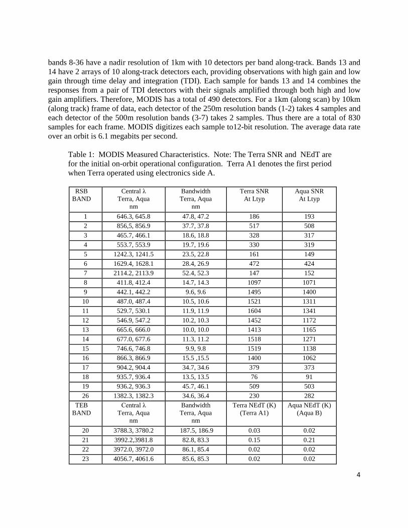
bands 8-36 have a nadir resolution of 1km with 10 detectors per band along-track. Bands 13 and 14 have 2 arrays of 10 along-track detectors each, providing observations with high gain and low gain through time delay and integration (TDI). Each sample for bands 13 and 14 combines the responses from a pair of TDI detectors with their signals amplified through both high and low gain amplifiers. Therefore, MODIS has a total of 490 detectors. For a 1km (along scan) by 10km (along track) frame of data, each detector of the 250m resolution bands (1-2) takes 4 samples and each detector of the 500m resolution bands (3-7) takes 2 samples. Thus there are a total of 830 samples for each frame. MODIS digitizes each sample to12-bit resolution. The average data rate over an orbit is 6.1 megabits per second. Table 1: MODIS Measured Characteristics. Note: The Terra SNR and NEdT are for the initial on-orbit operational configuration. Terra A1 denotes the first period when Terra operated using electronics side A.

RSB BAND

Central λ Terra, Aqua

nm

Bandwidth Terra, Aqua

nm

Terra SNR At Ltyp

Aqua SNR At Ltyp

1 646.3, 645.8 47.8, 47.2 186 193 2 856,5, 856.9 37.7, 37.8 517 508 3 465.7, 466.1 18.6, 18.8 328 317 4 553.7, 553.9 19.7, 19.6 330 319 5 1242.3, 1241.5 23.5, 22.8 161 149 6 1629.4, 1628.1 28.4, 26.9 472 424 7 2114.2, 2113.9 52.4, 52.3 147 152 8 411.8, 412.4 14.7, 14.3 1097 1071 9 442.1, 442.2 9.6, 9.6 1495 1400

10 487.0, 487.4 10.5, 10.6 1521 1311 11 529.7, 530.1 11.9, 11.9 1604 1341 12 546.9, 547.2 10.2, 10.3 1452 1172 13 665.6, 666.0 10.0, 10.0 1413 1165 14 677.0, 677.6 11.3, 11.2 1518 1271 15 746.6, 746.8 9.9, 9.8 1519 1138 16 866.3, 866.9 15.5 ,15.5 1400 1062 17 904.2, 904.4 34.7, 34.6 379 373 18 935.7, 936.4 13.5, 13.5 76 91 19 936.2, 936.3 45.7, 46.1 509 503 26 1382.3, 1382.3 34.6, 36.4 230 282

TEB BAND

Central λ Terra, Aqua

nm

Bandwidth Terra, Aqua

nm

Terra NEdT (K) (Terra A1)

Aqua NEdT (K) (Aqua B)

20 3788.3, 3780.2 187.5, 186.9 0.03 0.02 21 3992.2,3981.8 82.8, 83.3 0.15 0.21 22 3972.0, 3972.0 86.1, 85.4 0.02 0.02 23 4056.7, 4061.6 85.6, 85.3 0.02 0.02

5

24 4473.2, 4448.3 90.2, 92.2 0.13 0.11 25 4545.4, 4526.3 91.1, 90.4 0.05 0.04 27 6770.5, 6786.8 239.1, 187.9 0.10 0.10 28 7342.9, 7349.3 320.6, 314.9 0.05 0.05 29 8528.7, 8555.3 344.1, 359.2 0.02 0.02 30 9734.1, 9723.7 297.2, 301.1 0.11 0.07 31 11018.9, 11026.2 516.3, 531.1 0.03 0.02 32 12032.1, 12042.3 520.7, 521.5 0.04 0.03 33 13365.0, 13364.7 307.6, 310.9 0.13 0.08 34 13683.3, 13685.9 324.1, 341.7 0.23 0.12 35 13913.2, 13925.2 327.7, 332.7 0.23 0.15 36 14195.6, 14215.2 284.9, 327.9 0.43 0.23

Figure 1 shows the MODIS scan cavity and the on-board calibrators. The on-board calibrators (OBCs) include a solar diffuser (SD) and solar diffuser stability monitor (SDSM), a blackbody (BB) and a space view (SV) port, and a spectro-radiometric calibration assembly (SRCA).

Figure 1: MODIS scan cavity and on-board calibrators The optical system schematic is shown in Figure 2. The scan mirror reflects energy to the fold mirror. The aft optics consist of a two mirror off-axis telescope, and a series of dichroic beam splitters and band pass filters that separate the radiation onto four focal plane assemblies (FPAs). These are designated, according to their spectral regions, as: visible (VIS), near infrared (NIR), short and middle wave infrared (SMIR), and long wave infrared (LWIR).

6

Figure 2: Schematic of the optical system

Figure 3: MODIS’ focal plane assemblies

7

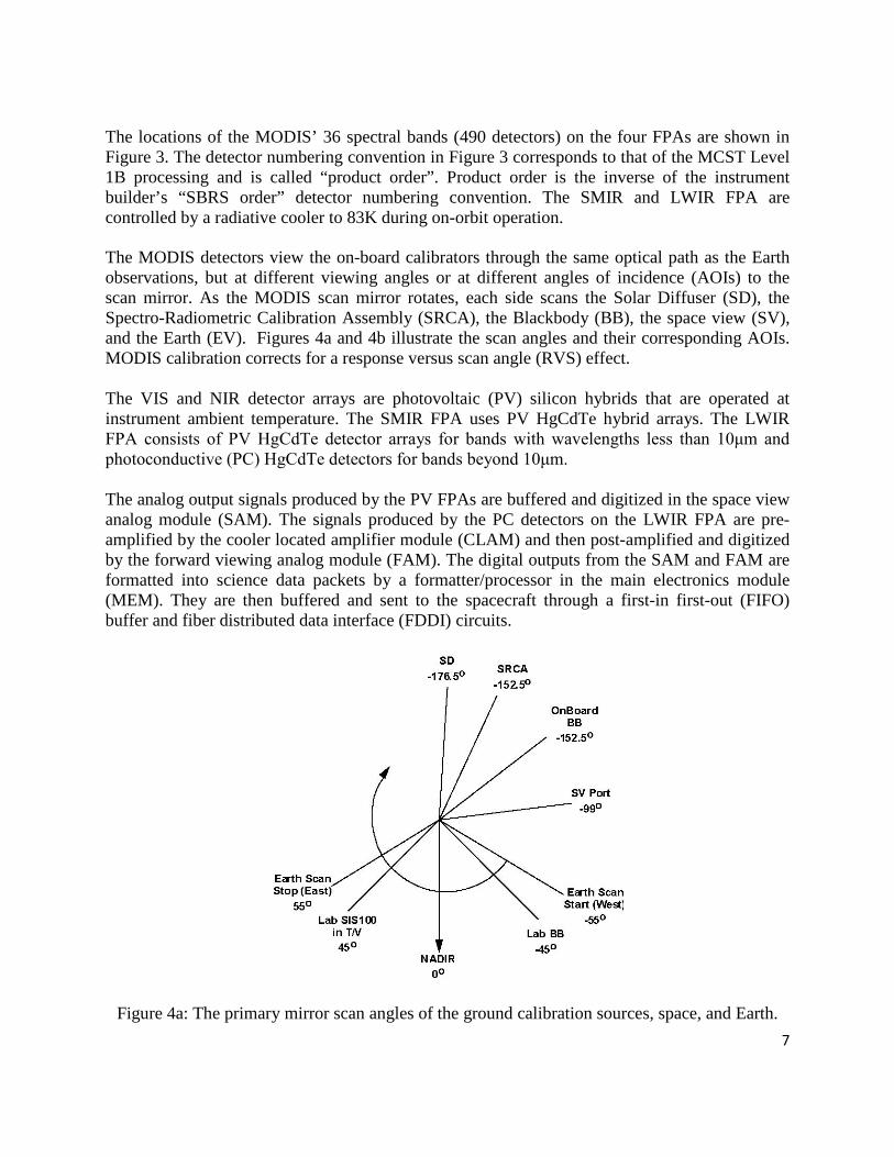
The locations of the MODIS’ 36 spectral bands (490 detectors) on the four FPAs are shown in Figure 3. The detector numbering convention in Figure 3 corresponds to that of the MCST Level 1B processing and is called “product order”. Product order is the inverse of the instrument builder’s “SBRS order” detector numbering convention. The SMIR and LWIR FPA are controlled by a radiative cooler to 83K during on-orbit operation. The MODIS detectors view the on-board calibrators through the same optical path as the Earth observations, but at different viewing angles or at different angles of incidence (AOIs) to the scan mirror. As the MODIS scan mirror rotates, each side scans the Solar Diffuser (SD), the Spectro-Radiometric Calibration Assembly (SRCA), the Blackbody (BB), the space view (SV), and the Earth (EV). Figures 4a and 4b illustrate the scan angles and their corresponding AOIs. MODIS calibration corrects for a response versus scan angle (RVS) effect. The VIS and NIR detector arrays are photovoltaic (PV) silicon hybrids that are operated at instrument ambient temperature. The SMIR FPA uses PV HgCdTe hybrid arrays. The LWIR FPA consists of PV HgCdTe detector arrays for bands with wavelengths less than 10μm and photoconductive (PC) HgCdTe detectors for bands beyond 10μm. The analog output signals produced by the PV FPAs are buffered and digitized in the space view analog module (SAM). The signals produced by the PC detectors on the LWIR FPA are pre-amplified by the cooler located amplifier module (CLAM) and then post-amplified and digitized by the forward viewing analog module (FAM). The digital outputs from the SAM and FAM are formatted into science data packets by a formatter/processor in the main electronics module (MEM). They are then buffered and sent to the spacecraft through a first-in first-out (FIFO) buffer and fiber distributed data interface (FDDI) circuits.

Figure 4a: The primary mirror scan angles of the ground calibration sources, space, and Earth.

8

Figure 4b: The angles of incidence (AOIs) corresponding to primary mirror scan angles for the observed elements.

2.2. Solar Diffuser (SD) and Solar Diffuser Stability Monitor (SDSM) The SD and SDSM shown in Figures 5 and 6 operate together as a system for calibrating the reflective solar bands (RSB) with wavelengths from 0.41 to 2.2 μm. The diffuser is made of space-grade Spectralon™, a proprietary thermoplastic formulation of polytetrafluoroethylene (PTFE). The SD bi-directional reflectance factor (BRF) was characterized pre-launch with National Institute of Standards and Technology (NIST) traceable reflectance standards. The SD on-orbit degradation is tracked by the SDSM during each periodic (initially weekly, currently every 3 weeks) calibration sequence. The SDSM itself is a ratioing radiometer which monitors on-orbit SD BRF variation (degradation) by alternatively viewing diffusely reflected Sun light from the SD panel and direct Sun light through an attenuation screen with a nominal 1.44% transmission. The screen is used to keep the signals from the SD and sun view at nearly the same level. The SDSM has nine filtered detectors embedded in a small solar integrating sphere (SIS) that monitors the SD degradation in the wavelength range from 0.41 to 0.94 μm . The specified MODIS RSB uncertainties are ± 2% reflectance and ± 5% absolute radiance. The reflectance calibration of the RSB from the SD measurements can be converted to a radiance calibration based on published values for the solar spectral irradiance. Two illumination levels of SD calibration are provided via a deployable 8.5% transmission screen. The screen must be in place for calibrating the high gain bands (B8-16 for ocean color observations) since they saturate when viewing direct sun exposure of the SD.

9

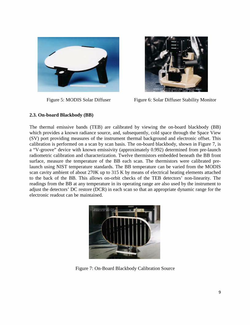
Figure 5: MODIS Solar Diffuser Figure 6: Solar Diffuser Stability Monitor 2.3. On-board Blackbody (BB) The thermal emissive bands (TEB) are calibrated by viewing the on-board blackbody (BB) which provides a known radiance source, and, subsequently, cold space through the Space View (SV) port providing measures of the instrument thermal background and electronic offset. This calibration is performed on a scan by scan basis. The on-board blackbody, shown in Figure 7, is a “V-groove” device with known emissivity (approximately 0.992) determined from pre-launch radiometric calibration and characterization. Twelve thermistors embedded beneath the BB front surface, measure the temperature of the BB each scan. The thermistors were calibrated pre-launch using NIST temperature standards. The BB temperature can be varied from the MODIS scan cavity ambient of about 270K up to 315 K by means of electrical heating elements attached to the back of the BB. This allows on-orbit checks of the TEB detectors’ non-linearity. The readings from the BB at any temperature in its operating range are also used by the instrument to adjust the detectors’ DC restore (DCR) in each scan so that an appropriate dynamic range for the electronic readout can be maintained.

Figure 7: On-Board Blackbody Calibration Source

10

Figure 8: Spectro-Radiometric Calibration Assembly 2.4. Spectro-radiometric Calibration Assembly (SRCA) The Spectro-radiometric Calibration Assembly (SRCA) is depicted in Figure 8. It is primarily used for spatial (all 36 bands) and spectral (RSB only) characterization. It also monitors radiometric response changes (RSB only) on-orbit. This device consists of a modified Czerny-Turner monochromator that includes a motor-driven grating/mirror assembly, a filter wheel assembly, incandescent sources, including a SIS with four 10W and two 1W lamps and a separate IR source, and collimating optics located at the exit slit of the monochromator. In spectral mode the SRCA is a monochromator while in spatial modes it becomes a transfer optic by replacing the grating with a plain mirror [Young, 1995a]. The SRCA spectral radiance is self-calibrated on-orbit using known and pre-launch calibrated spectral peaks in a didymium glass filter located at the exit slit of the monochrometer. In the spatial registration mode, the entrance port of the monochromator is open and the exit slit of the monochromator is replaced with specially designed spatial reticles, one for along scan and another for along track [Young, 1995b]. The images of the reticles are projected onto the MODIS FPAs to provide instrument spatial registration information. 3. CALIBRATION ALGORITHM FOR THE THERMAL EMISSIVE BANDS (TEB) 3.1 Pre-launch Characterization and Calibration (TEB) Each of the MODIS instruments went through a series of pre-launch comprehensive, system-level, spatial, spectral, and radiometric calibrations and characterizations. The TEB radiometric calibration was performed in a thermal vacuum (TV) environment. To cover the anticipated range of on-orbit operational conditions, three different temperature plateaus (nominal, cold, and

11

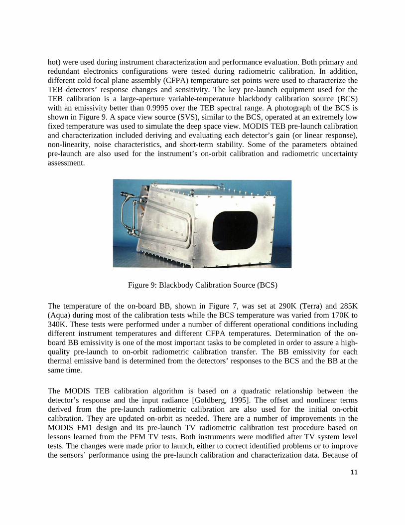
hot) were used during instrument characterization and performance evaluation. Both primary and redundant electronics configurations were tested during radiometric calibration. In addition, different cold focal plane assembly (CFPA) temperature set points were used to characterize the TEB detectors’ response changes and sensitivity. The key pre-launch equipment used for the TEB calibration is a large-aperture variable-temperature blackbody calibration source (BCS) with an emissivity better than 0.9995 over the TEB spectral range. A photograph of the BCS is shown in Figure 9. A space view source (SVS), similar to the BCS, operated at an extremely low fixed temperature was used to simulate the deep space view. MODIS TEB pre-launch calibration and characterization included deriving and evaluating each detector’s gain (or linear response), non-linearity, noise characteristics, and short-term stability. Some of the parameters obtained pre-launch are also used for the instrument’s on-orbit calibration and radiometric uncertainty assessment.

Figure 9: Blackbody Calibration Source (BCS) The temperature of the on-board BB, shown in Figure 7, was set at 290K (Terra) and 285K (Aqua) during most of the calibration tests while the BCS temperature was varied from 170K to 340K. These tests were performed under a number of different operational conditions including different instrument temperatures and different CFPA temperatures. Determination of the on-board BB emissivity is one of the most important tasks to be completed in order to assure a high-quality pre-launch to on-orbit radiometric calibration transfer. The BB emissivity for each thermal emissive band is determined from the detectors’ responses to the BCS and the BB at the same time. The MODIS TEB calibration algorithm is based on a quadratic relationship between the detector’s response and the input radiance [Goldberg, 1995]. The offset and nonlinear terms derived from the pre-launch radiometric calibration are also used for the initial on-orbit calibration. They are updated on-orbit as needed. There are a number of improvements in the MODIS FM1 design and its pre-launch TV radiometric calibration test procedure based on lessons learned from the PFM TV tests. Both instruments were modified after TV system level tests. The changes were made prior to launch, either to correct identified problems or to improve the sensors’ performance using the pre-launch calibration and characterization data. Because of

12

these changes, additional post launch efforts were required to assure on-orbit calibration and characterization quality. MODIS uses a double-sided scan mirror to make observations of the Earth scenes in a ±55° scan angle range about the nadir. For each mirror side, this (scan angle) range corresponds to 1354 EV frames of data with angles of incidence (AOI) on the scan mirror ranging from 10.5° to 65.5° (see Figure 4b). Since the sensor response changes with scan mirror AOI whereas the calibration is performed at a single AOI, it is essential to accurately characterize the sensor’s response versus scan-angle (RVS). For the Terra MODIS (PFM), there are no valid pre-launch RVS measurements for the TEB. Initially, the Terra MODIS TEB RVS values were derived using scan mirror witness-sample reflectance measurements (by the National Physical Lab, Great Britain) and the coupling parameters derived from the Aqua MODIS (FM1) TEB RVS measurements. Currently, the Terra MODIS thermal emissive bands use the RVS values derived from on-orbit deep space maneuvers [Xiong et al 2005a]. 3.2 On-orbit Calibration Algorithm (TEB) The MODIS TEB on-orbit calibration is performed for each band, detector, and mirror side during nominal operations [Xiong, et al., 2002a]. During MODIS on-orbit nominal operation, the blackbody temperature is controlled at 290K (Terra) and 285K (Aqua). The BB temperature setting for each instrument corresponds to the BB temperature at which most of the pre-launch calibration and characterizations were performed in the thermal vacuum environment. Calibration is scan angle dependent and is performed on a scan-by-scan basis. During each scan, the sensor views the on-board calibrator (OBC) blackbody (BB) at a known temperature (or radiance) and deep space through the instrument space view (SV) port to measure the instrument’s thermal background and electronic offset. The calibration coefficients determined are then used for the Earth view (EV) scene radiance retrieval. There are 50 frames (samples) of data collected in each scan when viewing both the BB and SV sectors. The instrument response is provided in 12-bit digital numbers (DN). When the sensor views the BB via its scan mirror, the total path radiance includes the radiance from the BB emission (L

BB), the radiance due to the

scan mirror emission (LSM

), the scan cavity emission (LCAV

) reflected from the BB, and the thermal background (L

BKG). Thus the BB view path radiance (L

BB_Path) is

(3.1) where L

BB_Path is the BB view path radiance.

RVSBB

is the normalized system response versus scan angle when the sensor views the BB.

13

εBB

is the emissivity of the BB.

εCAV

is the emissivity of the scan cavity.

LBB

is the radiance from the BB emission.

LSM

is the radiance from the scan mirror emission.

LCAV

is the radiance of the scan cavity reflected from the BB.

LBKG

is the radiance from the thermal background.

The RVS for each band and mirror side was determined pre-launch and normalized to the value at the BB view. The term (1-RVS

BB) is equivalent to the emissivity of the scan mirror at the BB

view angle. This term, in general, varies with the scan angle or the angle of incidence (AOI) to the scan mirror. The cavity contribution is reflected from the BB with a reflectivity of (1-ε

BB).

This term becomes smaller with higher BB emissivity. For simplicity, we do not specify the mirror side, the spectral band, and the detector indices throughout this algorithm derivation. Similarly, when the sensor views deep space (“zero” radiance) through the SV port, the total path radiance can be expressed as,

. (3.2) where L

SV_Path is the SV view path radiance.

RVSSV

is the normalized system response versus scan angle when the sensor views deep space. L

SV_Path includes only a scan mirror term and the background term. Note that the scan mirror

terms in equation 3.1 and equation 3.2 are not the same since the RVS is a function of the AOI to the scan mirror. The path radiance difference between equations 3.1 and 3.2 is related to the sensor’s response difference between the EV and SV given by;

(3.3) where <DN

BB> and <DN

SV> represent the frame average of the sensor’s BB and SV digital

response during each scan. During the BB warm-up and cold-down (WUCD) cycles, the BB temperature varies from instrument ambient temperature (~270K) to 315K. This process starts with an initial cool-down from BB nominal operating temperature to the instrument ambient. During the warm-up process, a few intermediate temperature plateaus between instrument ambient and 315K are added, allowing TEB detectors’ noise characterization to be performed at different radiance or

14

temperature levels. Once the BB temperature has reached 315K, a complete and continuous cool-down process is followed. Finally, the BB temperature is brought back to its nominal setting. Using WUCD data, a quadratic fit of BB path radiance difference vs. response difference (dn

BB)

is written as,

. (3.4) where a

0, b

1, and a

2 are the quadratic polynomial coefficients. Note that we purposely use b

1

instead of a1 in the calibration equation to emphasize the on-orbit scan-by-scan computation of

the linear coefficient from the sensor’s response to the BB. The radiance term, e.g. LBB

, is computed using the Planck equation averaged over the detector’s relative spectral response, RSR(λ).

(3.5) where λ is the wavelength of the emission incident to the given detector. RSR(λ) is the relative spectral response of the detector. Planck symbolizes the Planck black body equation. Similar expressions apply to L

SM and L

CAV. The temperatures of the blackbody, scan mirror, and

instrument cavity are determined from the instrument’s telemetry using conversion coefficients. Equation 3.4 is used to calculate the TEB calibration coefficient, b

1, which is the dominant term

in this quadratic algorithm. The offset and non-linear terms account for the fitting process residues or errors and small detector non-linearities over the dynamic range. They are provided in the LUTs with values determined from pre-launch calibration and updated from on-orbit BB WUCD cycles. Currently in the L1B algorithms (for both Terra and Aqua MODIS), the a

0 term is set to zero for

B33-B36. These bands typically view scenes at temperatures (see Table 1) much lower than the BB’s lowest ambient temperature of about 270K. Other parameters, such as emissivity, relative spectral response (RSR) and response versus scan-angle (RVS), determined from pre-launch calibration, are also included in the L1B LUTs. The same quadratic algorithm approach is used for the Earth view (EV) radiance retrieval process. Using the sensor’s EV and Space View (SV) response, equation 3.4 becomes

15

2

EV EV SV EV SM 0 1 EV 2 EVRVS L + (RVS - RVS ) L = a + b dn + a dn• • • • (3.6) where dn

EV is the sensor’s EV response in digital number (DN

EV) with the average response to

the space view (<DNSV

>) from the same scan subtracted, that is,

. (3.7) Once the EV radiance is retrieved, the top of the atmosphere (TOA) brightness temperature of the scene can be determined using the Planck equation. 3.3 Special Considerations in the TEB Calibration Algorithm The TEB algorithm described above applies to both the Terra MODIS L1B and the Aqua MODIS L1B. However, there are circumstances that do not work well with the general algorithm that assumes all detectors are functional and that all bands behave similarly. In order to achieve high quality calibration for all the bands, modifications are made to deal with cases that cannot be calibrated with the general algorithm. Keeping separate L1B code for Terra and Aqua MODIS makes it easy to address the special features in each instrument and to update the code and the LUTs for each sensor as required. Special considerations are required for the band 21 calibration (fire detection band), for the algorithm to remove Terra MODIS photo-conductive (PC) bands’ optical leak, for the approach used to retain the Aqua MODIS bands 33, 35, and 36 on-orbit calibration when the blackbody temperature is above their saturation limits, and for the presence of the moon in the SV port. Most of these issues were identified from pre-launch testing and characterized prior to the instruments’ launches. On-orbit observations continue to track the potential changes and to monitor the performance of these special algorithms or approaches. 3.3.1 Band 21 Calibration MODIS band 21 has low gain photovoltaic (PV) detectors with a specified center wavelength at 3.96μm, a typical scene temperature of 335K, and a maximum scene temperature of 500K. This mid-wave spectral band is used primarily for fire detection. At a typical blackbody temperature of 285K for Aqua MODIS and 290K for Terra MODIS, the sensor’s response, dn

BB, of B21 is

very small. The linear calibration coefficient, b1, calculated from the on-board BB, fluctuates

widely from scan to scan because of this low signal-to-noise ratio. Thus, the general scan-to-scan calibration method cannot provide an accurate and stable calibration for B21. Instead of computing B21 gain on a scan-by-scan basis, a set of fixed linear coefficients is put into a LUT and used in the L1B code for B21 calibration. These linear coefficients are monitored and updated, if necessary, using on-orbit scheduled BB WUCD cycles. B21 has less stringent

16

calibration uncertainty requirements. The offset and nonlinear terms of B21 have been set to zero in the TEB calibration algorithm. Since the MODIS TEB calibration is detector and mirror-side dependent, there are 20 coefficients for the 10 detectors and two mirror sides (L1B did not apply any mirror side difference in B21 prior to version 5). This fixed coefficient LUT approach is specifically designed for B21, and used in both Terra and Aqua MODIS calibration. 3.3.2 Terra MODIS PC Bands Optical Leak MODIS bands 31-36 utilize photo-conductive (PC) detectors located on the LWIR CFPA. The other TEB bands use photovoltaic (PV) detectors. During pre-launch PFM instrument characterization, an optical leak (or crosstalk) from B31 to the other PC bands was identified. This problem was verified on-orbit from Earth scenes and lunar observations. Examples of Terra MODIS lunar view responses for band 31 and 33 are shown in Figure 10. The plot of band 31 response (detector 5) shows a smooth profile. The response profile of band 33 shows a small side peak that is due the optical leak from band 31 as discerned from the frame offset between the two bands. The frame offset is related spectral band location on the focal plane (see Figure 3). In order to remove the optical leak from the contaminated instrument responses (dn) for these PC bands (bands 32-36) when the sensor views the BB and the EV sectors, a special correction algorithm was developed and implemented in the Terra MODIS L1B code. It is designed to make the correction by subtracting the contributions from band 31 into the other PC bands. Assume dn

corr is the correct response if there were no B31 optical leak, dn

cont is the response with

the optical leak, and xtalkB31 → B

is the crosstalk coefficient from B31 to a given PC band. The crosstalk coefficients for each PC band are in the L1B LUT for on-board calibration and EV retrieval. The correction algorithm (using B32 as an example) is given by,

where

is the digital response for band 32 before correction for band 31 optical leak.

is the digital response for band 32 after correction for band 32 optical leak F is the data frame number.

is the data frame offset between band 31 and band 32.

is the optical leakage coefficient for band 31 into band 32.

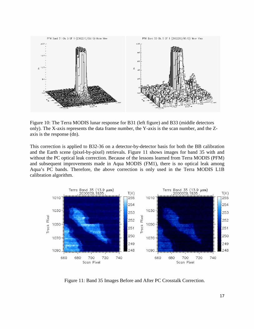
17

Figure 10: The Terra MODIS lunar response for B31 (left figure) and B33 (middle detectors only). The X-axis represents the data frame number, the Y-axis is the scan number, and the Z-axis is the response (dn). This correction is applied to B32-36 on a detector-by-detector basis for both the BB calibration and the Earth scene (pixel-by-pixel) retrievals. Figure 11 shows images for band 35 with and without the PC optical leak correction. Because of the lessons learned from Terra MODIS (PFM) and subsequent improvements made in Aqua MODIS (FM1), there is no optical leak among Aqua’s PC bands. Therefore, the above correction is only used in the Terra MODIS L1B calibration algorithm.

Figure 11: Band 35 Images Before and After PC Crosstalk Correction.

18

3.3.3 Aqua MODIS Bands 33, 35, and 36 On-orbit Calibration On-orbit, the BB can be heated from instrument ambient to 315K. However Aqua MODIS bands 33, 35, and 36 saturate before the BB temperature reaches 315K. The saturation temperatures can vary due to instrument background and DC Restore (DCR). When the BB temperature is above the saturation limits, the scan-by-scan calibration approach of equation 3.4 can no longer be used for these three bands. In order to keep Earth view data calibrated in this situation, a revised algorithm was developed and implemented for Collection 6. To account for the CFPA temperature fluctuation and to minimize the uncertainty in the estimation of the default b1, the new algorithm calculates the CFPA temperature dependent default b1 to calibrate these bands when TBB>Tsat. The algorithm is based on the linear relationship between b1 and the LWIR CFPA temperature for bands 33, 35, and 36. The default b1 is calculated by b1 = b1baseline,LUT [1 + c1LUT (TLWIR - T baseline,LUT)],

where the LWIR FPA temperature TLWIR is measured scan-by-scan. Other inputs to the L1B code are provided by a set of LUTs, including:

– b1baseline: The b1baseline coefficient is the supposed b1 coefficient at Tsat when the LWIR temperature is Tbaseline. Since the BB WUCD and CFPA oscillation are two independent processes, b1baseline is actually calculated from the b1 measured at Tsat with CFPA temperature TLWIR,Tsat, and scaled to Tbaseline based on the same linear relationship.

b1baseline = b1,Tsat / [1 + c1 (TLWIR,Tsat - T baseline,LUT)],

where b1,Tsat is the default b1 calculated at TBB=Tsat (within ±0.25 K), as in the previous method;

– TLWIR,Tsat: is the average LWIR FPA temperature estimated from scans when TBB=Tsat (within ±0.25 K);

– c1: is the rate of change of relative b1 as a function of LWIR FPA temperature; c1 is calculated for each BB WUCD event through the fitting of b1 and TLWIR to a set of three-orbit data two days prior to the BB WUCD;

– Tbaseline: is a baseline LWIR FPA temperature estimate and is currently set at 83K for Bands 33, 35-36;

Three sets of LUTs are used by L1B to calculate the calibration coefficients for bands 33, 35, and 36 during the saturation periods. These LUTs are updated, when necessary, with the most recent on-orbit detector response. The saturation temperatures for these bands are in a LUT that is updated as needed based on WUCD data. 3.3.4 Moon in the SV Port Typically, the SV signal is subtracted as in equation 4.3. However, the SV digital counts are unreliable if the Moon is in the SV port. Prior to 9/11/02 such data was flagged as unusable.

19

Subsequently, L1B was upgraded to handle this event by including only a specified number of the dimmest frames in the calculation of the average background. A QA flag is set for the scan whenever this is done, and a metadata field reports the percentage of pixels affected. 3.4 Uncertainty (TEB) MODIS L1B data products also include uncertainty indices that are computed for all pixels. The TEB uncertainty algorithm is based on the on-orbit calibration and scene radiance retrieval equations. It calculates the uncertainty using on-orbit observations and some input parameters determined from pre-launch calibration and characterization. The TEB calibration total uncertainty can be computed by combining the contributions from all the factors involved in the calibration and retrieval. In order to establish an uncertainty coefficient for each term, a partial derivative with respect to each individual term is calculated [Wenny et al. (2012)]. In collection 6, the uncertainty components were broken down into 14 contributing factors. The total TEB uncertainty is expressed in equation 3.9.

∑

+

+

+

+

+

+

+

+

+

=

−

i

EV

PCXEV

EV

bEV

EV

dnEV

EV

dnEV

EV

TcavEV

EV

TsmEV

EV

TBBEV

EV

EV

EV

EV

EV

EV

EV

RVSEV

EV

RVSEV

EV

aEV

EV

aEV

EV

iEV

LdL

LdL

LdL

LdL

LdL

LdL

LdL

LdL

L

dL

L

dL

L

dL

L

dL

LdL

LdL

LdL

BBEVBB

CAVBBEVSV

22

1

22222

222222

2

2

0

)3632(21 + + + +

λεε

(3.9)

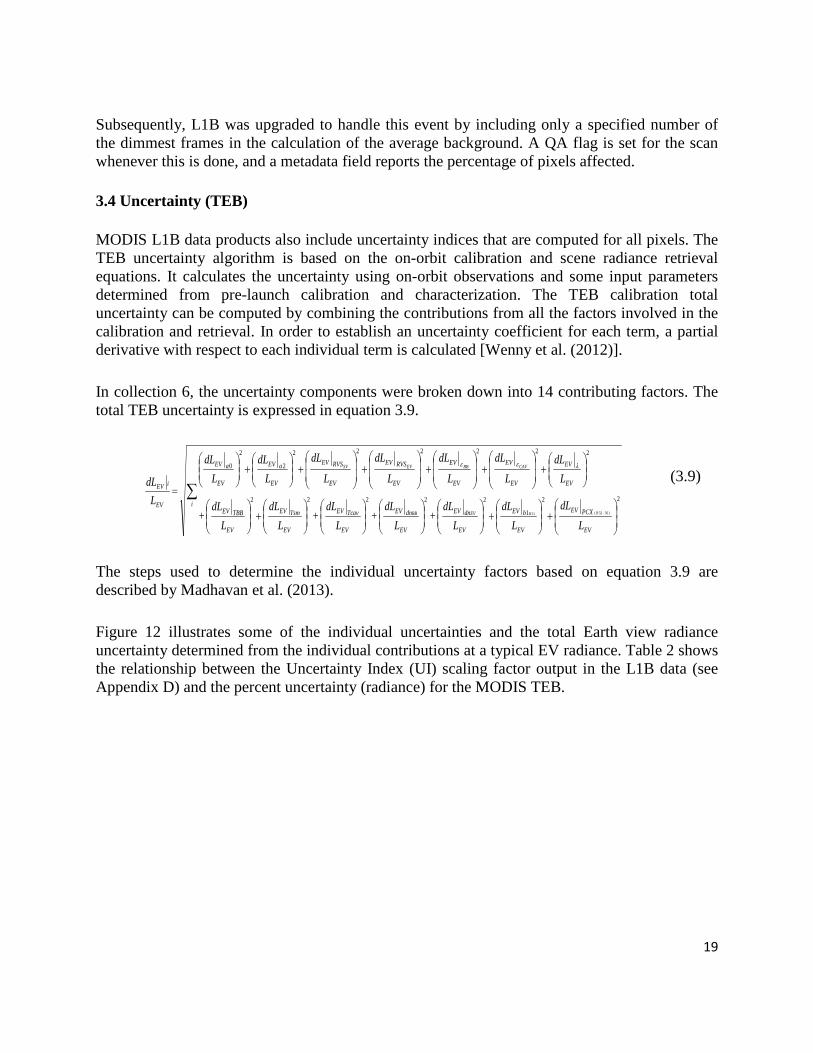
The steps used to determine the individual uncertainty factors based on equation 3.9 are described by Madhavan et al. (2013). Figure 12 illustrates some of the individual uncertainties and the total Earth view radiance uncertainty determined from the individual contributions at a typical EV radiance. Table 2 shows the relationship between the Uncertainty Index (UI) scaling factor output in the L1B data (see Appendix D) and the percent uncertainty (radiance) for the MODIS TEB.

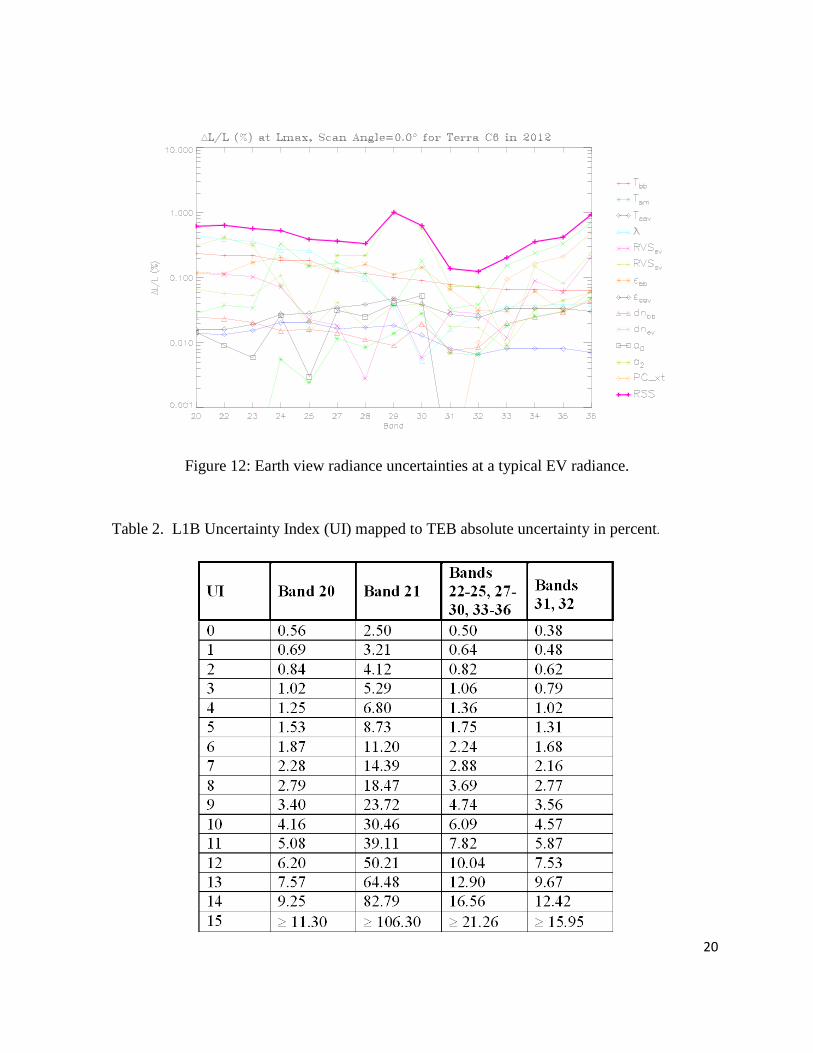
20

Figure 12: Earth view radiance uncertainties at a typical EV radiance. Table 2. L1B Uncertainty Index (UI) mapped to TEB absolute uncertainty in percent.

21

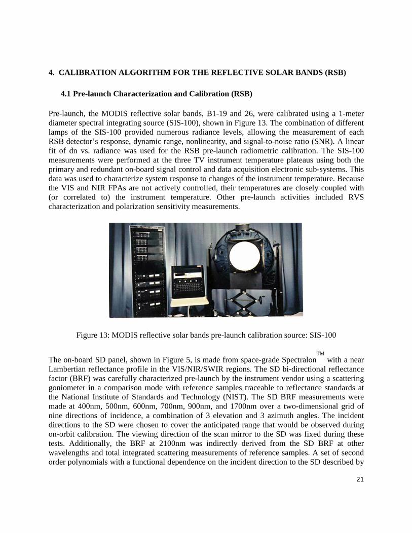
4. CALIBRATION ALGORITHM FOR THE REFLECTIVE SOLAR BANDS (RSB) 4.1 Pre-launch Characterization and Calibration (RSB) Pre-launch, the MODIS reflective solar bands, B1-19 and 26, were calibrated using a 1-meter diameter spectral integrating source (SIS-100), shown in Figure 13. The combination of different lamps of the SIS-100 provided numerous radiance levels, allowing the measurement of each RSB detector’s response, dynamic range, nonlinearity, and signal-to-noise ratio (SNR). A linear fit of dn vs. radiance was used for the RSB pre-launch radiometric calibration. The SIS-100 measurements were performed at the three TV instrument temperature plateaus using both the primary and redundant on-board signal control and data acquisition electronic sub-systems. This data was used to characterize system response to changes of the instrument temperature. Because the VIS and NIR FPAs are not actively controlled, their temperatures are closely coupled with (or correlated to) the instrument temperature. Other pre-launch activities included RVS characterization and polarization sensitivity measurements.

Figure 13: MODIS reflective solar bands pre-launch calibration source: SIS-100

The on-board SD panel, shown in Figure 5, is made from space-grade SpectralonTM

with a near Lambertian reflectance profile in the VIS/NIR/SWIR regions. The SD bi-directional reflectance factor (BRF) was carefully characterized pre-launch by the instrument vendor using a scattering goniometer in a comparison mode with reference samples traceable to reflectance standards at the National Institute of Standards and Technology (NIST). The SD BRF measurements were made at 400nm, 500nm, 600nm, 700nm, 900nm, and 1700nm over a two-dimensional grid of nine directions of incidence, a combination of 3 elevation and 3 azimuth angles. The incident directions to the SD were chosen to cover the anticipated range that would be observed during on-orbit calibration. The viewing direction of the scan mirror to the SD was fixed during these tests. Additionally, the BRF at 2100nm was indirectly derived from the SD BRF at other wavelengths and total integrated scattering measurements of reference samples. A set of second order polynomials with a functional dependence on the incident direction to the SD described by

22

solar zenith angle θ and solar azimuth angle φ was determined from these pre-launch measured BRF values. For each RSB, a second order polynomial was interpolated from the surface fits at surrounding wavelengths. 4.2 On-orbit Calibration Algorithm (RSB) Based on the desire of the MODIS science community, the top of the atmosphere (TOA) scene reflectance factor was chosen as the primary L1B data product for the MODIS reflective solar bands (RSB). The on-orbit calibration of the reflectance factor [Xiong et al., 2002b] is based on solar observations via the instrument’s on-board solar diffuser (SD). Using a simple linear algorithm, the Earth view (EV) reflectance factor, ρ

EVcos(θ

EV), is related to

the detector’s response by

(4.1) where

is the EV scene reflectance. θ

EV is the solar zenith angle of the EV pixel.

m1 is a calibration coefficient determined from on-orbit SD observations .

is the Earth-Sun distance (in AU) at the time of the EV scene observation.

is the sensor’s digital response to the EV scene with background subtracted and instrument effects corrected. Instrument effect corrections include normalizing the sensor’s viewing angle and correcting for the instrumental temperature dependence via

(4.2) where

is the instrument temperature correction coefficient determined pre-launch. is the difference between the instrument temperature at the time of EV observation and

its reference value,

is the instrument temperature at the time of EV observation.

is the instrument temperature reference value, chosen pre-launch and used for deriving

.

23

RVSEV

is the system level response at the scan angle of an EV pixel. The dark background subtracted response, dn

EV, is computed by

dnEV

= DNEV

- < DNSV

> (4.3) where DN

EV is the EV digital response (raw data) and < DN

SV> is the average SV digital

response. The SD calibration coefficient m

1 is determined by

(4.4) where ρ

SD is the SD pre-launch BRF.

is the corrected detector response to the SD. d

ES_SD is the Earth-Sun distance in AU at the time of the SD measurements.

ΓSDS

is the SD screen (SDS) vignetting (transmission) function. Δ

SD is the SD degradation factor.

Except for the SD degradation factor, Δ

SD, and the SD screen (SDS) vignetting function, Γ

SDS,

equation 4.4 is the same as equation 4.1 when it is applied to the SD observations. The SD reflectance and MODIS optics transmission deteriorate on-orbit due to their exposure to sunlight [Xiong, et al., 2001 and Xiong et al., 2002c]. The SD degradation rate is tracked by the solar diffuser stability monitor (SDSM) during each SD calibration. The SDSM alternately measures the response of the SD view and a direct Sun view through an attenuation screen of 1.44% nominal transmittance so that the responses from both views are closely matched. Nine individually filtered detectors in the SDSM monitor the SD degradation. The SD/Sun ratios were normalized to ratio at 936 nm (SDSM D9) In January 2009 (Terra MODIS) and April 2009 (Aqua MODIS), the assumption of negligible degradation in SDSM D9 was dropped and the SDSM correction was derived and applied [Sun et al. 2012]. For high gain bands (bands 8-16), a retractable solar diffuser screen (SDS) is placed in front of the SD to attenuate the direct sunlight and to avoid saturation. The SDS attenuation is represented by the vignetting (transmission) function Γ

SDS. The vignetting function is set to unity

for bands 1-7, 17-19, and 26 when these bands are calibrated without the SDS. Note that beginning July 2, 2003 the Terra RSB calibration includes the SDS, so the vignetting function is no longer set to unity.

24

The RSB calibration coefficients, m1, are provided to the L1B software through LUTs. These

coefficients are band, detector, sub-sample, and mirror side dependent. They are updated based on regularly scheduled SD/SDSM observations. The MODIS L1B RSB software also produces a radiance product. From the reflectance factor, the Earth view radiance can be calculated by

(4.5) where E

Sun is the solar irradiance at d = 1 AU, computed at mid-granule. SunE /π is written as a

global attribute in the L1B product so that the users can readily convert the RSB reflectance product to the radiance product. 4.3 Response Versus Scan Angle (RVS) The MODIS scan mirror scans the Earth view (EV), SD, SRCA, BB, and SV sectors sequentially. As shown in Figure 4b, the EV AOI varies from 10.5o to 65.5o with the nadir at the center, AOI 38o. For the SD, SV, and SRCA, the AOI is 50.25o, 11.2o, and 38o, respectively. The RVS of the MODIS scan mirror for both Terra and Aqua MODIS RSB were measured before launch. The measurements showed that the prelaunch RVS could be approximated as detector independent, but was wavelength (band) dependent. It showed a strong mirror side (MS) dependence, especially for Terra MODIS shorter wavelength bands. The on-orbit RVS variation can be tracked by the onboard calibrators, the lunar observations, and EV MS ratios. It may be dependent on detector, wavelength and MS. The MODIS RSB RVS is always normalized at the AOI of the SD. Thus, the RVS represents the ratio of the gain at a particular AOI to that at the AOI of the SD. The gain of the MODIS electronic and optical system at the AOI of the SD and that of the SV is inversely proportional to the SD calibration coefficients and lunar coefficients, respectively. Thus, RVS on-orbit variation at the AOI of the SV can be derived from the ratio of these two coefficients for both MS1 and MS2. The gain at any other AOI cannot be easily determined for MODIS RSB. However, the MS ratio of the gain for any band, detector, or AOI can be derived from the MS ratio of the instrument’s response. From EV observations, the MODIS MS response ratio at any selected AOI can be derived. Although the Earth’s surface is not smooth, the EV radiance can be approximated as coming from the same light source for the two mirror sides of the scan mirror when averaged over a large number of scans. The MODIS MS response ratio at the AOIs of the SV, nadir, and SD can also be derived from the lunar, the SRCA, and the SD observations, respectively. The MS ratio of the RVS on-orbit variation can be calculated from the MS ratio of the two mirror sides’ responses. For each MS, we only know the RVS on-orbit variation at the AOI of the SD and that of the SV, although we know the MS ratio of the RVS on-orbit variation for all AOI. Knowing the RVS variation at the AOI of the SD and the SV, a linear approximation can be applied for the RVS on-orbit variation as a function of the AOI. In principle, the approximation can be applied to the RVS on-orbit variation for either of the two mirror sides. But for Terra MODIS, the MS differences were already observed in prelaunch measurements and differences exist when the

25

linear approximation is applied to the other mirror side. It is believed that it would be better to apply the linear approximation to the Terra RSB MS1 RVS on-orbit variation. Thus, for Terra MODIS RSB MS1, the RVS on-orbit variation at any AOI is calculated from the RVS at the AOI of the SD and that of SV with a linear approximation for the AOI dependence. Then the MS1 RVS can be obtained by multiplying the prelaunch MS1 RVS and the RVS on-orbit variation. Since the MS ratio of the instrument’s response represents the MS ratio of the RVS, Terra MODIS RSB MS2 RVS can be calculated using the MS1 RVS and the MS ratio of the instrument’s response obtained from SD, SRCA, lunar, and EV observations. In Terra MODIS L1B collection 5, the RVS is detector independent, i.e., the RVS depends only on band, MS, AOI, and time. Data are averaged over detectors before they are applied to calculate the RVS. During the early mission, the RVS detector difference was negligible compared to the 2% specified uncertainty in reflectance for MODIS RSB calibration. However, the AOI dependence of the detector difference has increased noticeably in the last few years. Starting with Terra MODIS L1B collection 6, the RVS is derived for each individual detector, band and MS. It is also AOI and time dependent. In collection 5, the time-dependence RVS was only applied to several short-wavelength bands initially but other RSB were gradually included later. In collection 6, the time-dependent RVS has been applied to all RSB except SWIR bands for consistency. In collection 5, the calculated RVS are fit to a quadratic form whereas a quartic fit is used for selected bands in C6. The fitted time-dependent coefficients are applied to calculate the RVS in MODIS L1B products. Collection 6 RVS LUT and algorithm enhancements are presented by Sun et al. (2012) and by Toller et al (2013). Major methodology improvements include the use of EV response trending using time-invariant desert sites for the VIS bands, detector dependent RVS in selected bands to reduce striping, time-dependent RVS for chosen bands, and an extension of the RVS MS2 computation methodology used in Terra collection 5 to additional Terra and Aqua MODIS bands 4.4 Special Considerations in the RSB Calibration Algorithm The general RSB algorithm described above applies to the Terra MODIS L1B as well as to the Aqua MODIS L1B. Each L1B code has its own set of LUTs which are instrument specific. There are only minor differences between the two sets of software. 4.4.1 SWIR Crosstalk Correction Pre-launch and on-orbit characterization of both Terra and Aqua MODIS have shown small but non-negligible out-of-band (OOB) response in the sensors’ short-wave infrared bands (SWIR). In general, the Aqua SWIR bands’ OOB responses (including the thermal leaks) were much smaller than those for the Terra MODIS. In order to minimize the impact due to OOB response, a simple linear correction algorithm has been developed, tested, and implemented in the L1B codes for both Terra and Aqua MODIS.

26

For Terra MODIS, the SWIR band EV data and SD calibration dataset are corrected by the following expression using MODIS band 28: '

' 28( ) ( ) _ _1( ) ( )EV SWIR EV SWIR SWIR EV Bdn BDSM dn BDSM x oob BDSM dn BDM•= − (4.6) where BDSM is a band, detector, sub-sample, and mirror side index (respectively) used in the RSB

calibration. '' ( )EV SWIRdn BDSM is the response of the receiver SWIR band after correction for OOB crosstalk.

( )EV SWIRdn BDSM is the response of the receiver SWIR band before correction for OOB crosstalk.

_ _1( )SWIRx oob BDSM is the thermal leak correction coefficient.

28( )EV Bdn BDM is the response of the sender band, band 28 in this case. Because there is no sub-sample in B28 (1km spatial resolution band with 10 detectors), B28 detector 1 is matched with B5, B6 and B7 detectors 1 and 2 (both sub-samples), B28 detector 2 is matched with B5, B6 and B7 detectors 3 and 4, etc. The same algorithm is also used in Aqua MODIS L1B with the sending band 28 replaced by band 25. The choice of the sending band is based on OOB characterization, on-orbit observations, and science test results. The correction coefficients are derived from on-orbit observations. In addition to the thermal leak, the SWIR bands also have electronic crosstalk that has made this problem difficult to characterize and correct. In order to distinguish the electronic crosstalk among the SWIR detectors from that coming from the MWIR detectors, a special instrument activity to collect the Earth scene RSB (including SWIR bands) data during spacecraft nighttime is used. This is designated the nighttime day mode (NTDM). The thermal leak correction coefficients are derived by fitting the SWIR responses to the corresponding sending band. 4.4.2 B26 De-striping Algorithm A de-striping algorithm was furnished by the atmospheric group at the University of Wisconsin. It only applies to MODIS band 26. It is a simple linear approach developed to remove the difference (striping) among the 10 detectors in band 26. The coefficients are derived from the L1B EV scaled integers of band 26 and band 5 after the SWIR crosstalk correction algorithm [Moeller, C., 2001]. 4.4.3 Aqua Band 6 Consideration Prior to launch, the majority of the Aqua Band 6 detectors were known to be non-functional. This information is communicated to L1B from the LUTs. As with all non-functional detectors, the bad channels are not used in the data products.

27

4.4.4 Moon in the SV Port Typically, the SV signal is subtracted as in equation 4.3. However, the SV digital counts are unreliable if the Moon is in the SV port. When this occurs, the SV digital counts are sorted and a few (defined in the LUT) of the lowest readings are used. If no valid SV digital count is obtained, the RSB use the on-board BB as the background, replacing the SV readings, except for the SWIR bands. 4.5 Uncertainty (RSB) MODIS L1B data products also include uncertainty indices that are computed for all pixels. The RSB uncertainty algorithm is based on characterization of the EV scene reflectance. The RSB reflectance total uncertainty can be expressed as (4.7) The first term on the right side is the calibration uncertainty, calculated from the uncertainty of the SD/SDSM calibration, the lunar calibration, and EV response trending. The second term is the uncertainty of the temperature correction, and the last term addresses the scene dependent uncertainty due to instrument noise. In Collection 6, the calibration coefficients are derived from the SD/SDSM calibration and the RVS are derived from the SD/SDSM and lunar observation with support from EV mirror side ratio for most MODIS RSB. But for Terra bands 1-4 and 8-9 and Aqua bands 8-9, the EV response trending over selected desert sites are also used to derive the calibration coefficients and RVS LUT besides the aforementioned data. Then the uncertainty of the calibration can be calculated from the uncertainty of the SD/SDSM calibration, lunar calibration, and EV response trending. The determination of the individual RSB uncertainties at Ltyp are described by Sun et al. (2012). 5. LEVEL 1B DATA PRODUCTS AND ALGORITHM IMPLEMENTATION 5.1 L1B Data Products The sensors’ raw data are transmitted to ground stations, such as the one at White Sands in New Mexico, through the Tracking Data Relay Satellite System (TDRSS) and then sent to the EOS Data and Operations System (EDOS). At the Goddard Space Flight Center Distributed Active Archive Center (GDAAC), the sensor’s original binary data files (Level 0) from the EDOS are reformatted, attitude and ephemeris data are incorporated, and the data is separated into 2-hour Level 0 files. Starting in 2006, the GDAAC passed these Terra and Aqua 2-hour Level 0 files to the MODIS Adaptive Processing System (MODAPS) which produces Level 1A (L1A) granules

( ) [ ]2

22

1

1

2

)(/

)/()cos()cos(

+∆⋅+

=

EV

EVInstInst

EVEVEV

EVEV

dndn

TkRVSmRVSm δ

δδ

θρθρδ

28

using EOS specific Hierarchical Data Format (HDF). Each L1A granule contains 5 minutes of data, consisting of the sensor’s response in digital numbers (DNs) as well as other engineering and telemetry information. These are the principal inputs to the Level 1B (L1B) process. Other inputs include a geolocation file and a set of L1B Look-Up Tables (LUTs) that provide parameters determined during pre-launch and on-orbit calibration and characterization. The MODIS L1B products are distributed through the Level 1 and Atmosphere and Archive Distribution System available at http://ladsweb.nascom.nasa.gov. L1B output consists of calibrated Earth View (EV) data for all 36 spectral bands, organized in three HDF files corresponding to MODIS’ three spatial resolutions, and associated metadata files. These files serve as the common input for all higher-level science algorithms. The L1B process also produces a separate file containing on-board calibration data sets and key instrument telemetry. The latter does not contain the EV sector data and is primarily used by MCST analysts to perform instrument on-orbit calibration and to monitor the instrument’s status. The Level 1B calibrated EV data products include top of the atmosphere (TOA) reflectance factors for the RSBs, TOA radiances for both the RSBs and TEBs, associated uncertainty indices and data quality flags. To reduce file size, the calibrated Earth view data are stored as 16-bit unsigned integers coupled with associated scale and offset terms in three separate HDF files (see Appendices B and C). This approach allows the user to reconstruct calibrated radiance values for all MODIS bands as well as calibrated reflectance values for the Reflective Solar Bands (RSBs). Associated uncertainty values are included as unsigned 8-bit integers with coefficients provided to reconstruct the percent uncertainty. A scan-by-scan 32-bit data quality flag and a granule level 8-bit detector quality flag for each of the 490 detectors are included as part of each file’s metadata. 5.2 L1B Algorithm Implementation MODIS L1B software provides calibration for all TEB and RSB detectors. Calibration is performed for each band, detector, sub-sample (for the sub-kilometer resolution bands 1-7), and mirror side (BDSM), and thus is on a pixel-by-pixel basis for all MODIS detectors. The radiometric calibration algorithm is divided into two major modules in the L1B software: one for the thermal emissive bands and the other for the reflective solar bands. The RSB calibration uses some processed data from TEB calibration and is therefore performed after the TEB calibration. Both TEB and RSB calibration modules in the L1B process are executed after L1B pre-processing in which the calibration coefficients are either calculated from on-orbit data sets or determined from the associated LUT inputs. Figure 14 [Xiong et al., 2005b] is a simplified flow diagram that illustrates the core of the TEB calibration algorithm: computing the EV radiance, converting radiance to a scaled integer (SI), and computing the uncertainty index (UI). For each scan of EV data, this process loops through bands, detectors, and frames. The data quality flags are assigned for each scan of the data. An optical crosstalk (PCX) correction algorithm, which applies only to bands 32-36, is included in

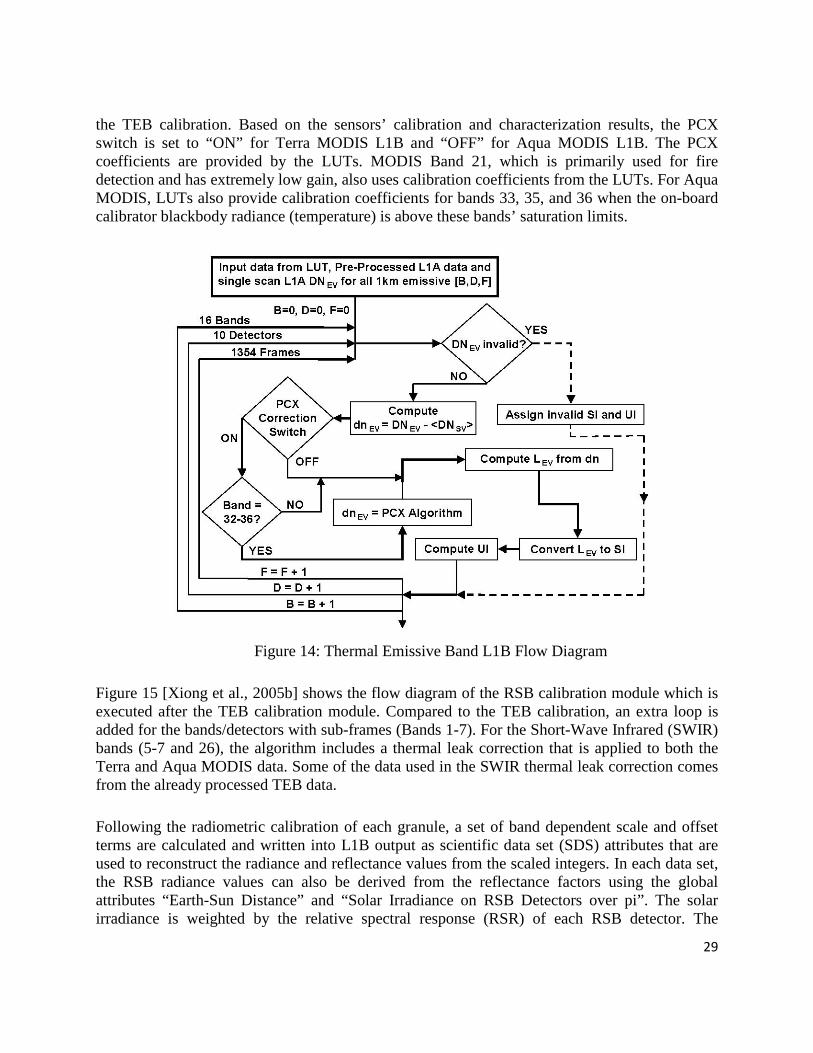
29

the TEB calibration. Based on the sensors’ calibration and characterization results, the PCX switch is set to “ON” for Terra MODIS L1B and “OFF” for Aqua MODIS L1B. The PCX coefficients are provided by the LUTs. MODIS Band 21, which is primarily used for fire detection and has extremely low gain, also uses calibration coefficients from the LUTs. For Aqua MODIS, LUTs also provide calibration coefficients for bands 33, 35, and 36 when the on-board calibrator blackbody radiance (temperature) is above these bands’ saturation limits.

Figure 14: Thermal Emissive Band L1B Flow Diagram

Figure 15 [Xiong et al., 2005b] shows the flow diagram of the RSB calibration module which is executed after the TEB calibration module. Compared to the TEB calibration, an extra loop is added for the bands/detectors with sub-frames (Bands 1-7). For the Short-Wave Infrared (SWIR) bands (5-7 and 26), the algorithm includes a thermal leak correction that is applied to both the Terra and Aqua MODIS data. Some of the data used in the SWIR thermal leak correction comes from the already processed TEB data. Following the radiometric calibration of each granule, a set of band dependent scale and offset terms are calculated and written into L1B output as scientific data set (SDS) attributes that are used to reconstruct the radiance and reflectance values from the scaled integers. In each data set, the RSB radiance values can also be derived from the reflectance factors using the global attributes “Earth-Sun Distance” and “Solar Irradiance on RSB Detectors over pi”. The solar irradiance is weighted by the relative spectral response (RSR) of each RSB detector. The

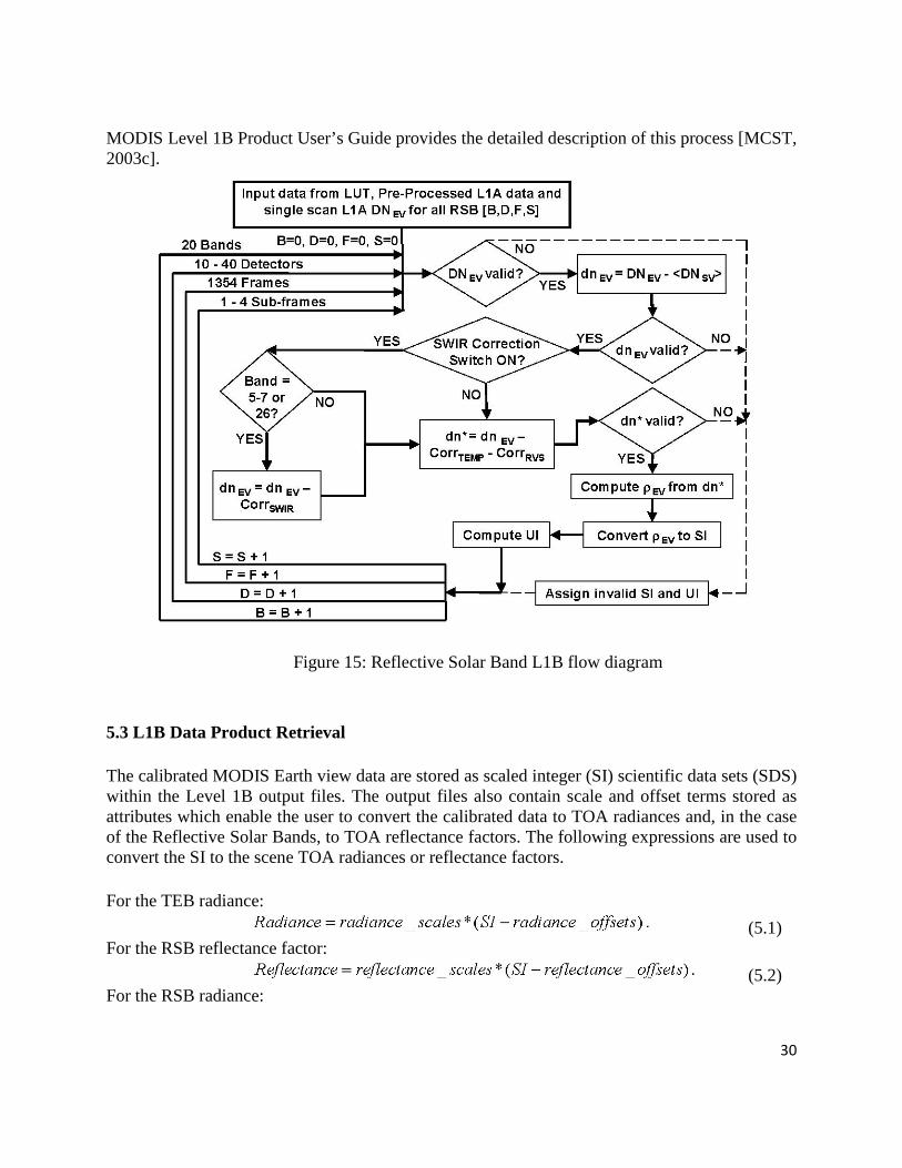
30

MODIS Level 1B Product User’s Guide provides the detailed description of this process [MCST, 2003c].

Figure 15: Reflective Solar Band L1B flow diagram 5.3 L1B Data Product Retrieval The calibrated MODIS Earth view data are stored as scaled integer (SI) scientific data sets (SDS) within the Level 1B output files. The output files also contain scale and offset terms stored as attributes which enable the user to convert the calibrated data to TOA radiances and, in the case of the Reflective Solar Bands, to TOA reflectance factors. The following expressions are used to convert the SI to the scene TOA radiances or reflectance factors. For the TEB radiance: (5.1) For the RSB reflectance factor: (5.2) For the RSB radiance:

31

For the thermal emissive bands, the radiance scale and offset terms are used to reconstruct the radiance values calculated within the Level 1B TEB calibration algorithm. For the reflective solar bands, the reflectance scales and offsets may be used to reconstruct the reflectance factors calculated within the RSB calibration algorithm, but use of the radiance scales and offsets for the reflective solar bands will result in only approximate radiance retrievals. This is due to the fact that the reflective radiance scales are derived using a band-averaged value of the solar irradiance, which actually varies from detector to detector due to the individual detector’s relative spectral response (RSR) function. An alternative method to derive RSB radiances, which yields more precise results, is to use the global attributes “Earth-Sun Distance” and “Solar Irradiance on RSB Detectors over pi” to reconstruct the radiances directly from reflectance values. This method is given by equation 5.3. To cover a broad range of uncertainty in percentage for the retrieved EV products, an exponential approach is used. Two SDS attributes, “specified_uncertainty” and “scaling_factor” in equation 5.4, are used to convert the Uncertainty Index (UI) back to the percentage uncertainty. Additional information is provided in the MODIS Level 1B Product User’s Guide [MCST, 2003c].

(5.4) 6. SUMMARY MODIS, a key instrument for the NASA’s EOS and MTPE missions, is currently operating on both the Terra and Aqua spacecraft, providing continuous global data sets from complementing morning and afternoon observations of the Earth’s land, oceans, and atmosphere. MODIS has 36 spectral bands covering spectral regions from the VIS to LWIR (0.41 to 14.5μm), taking observations at 250m, 500m, and 1km nadir spatial resolutions. Ongoing monitoring of instrument operation and performance of comprehensive calibration and characterization has shown both Terra and Aqua MODIS are performing well. The mature, validated MODIS L1B algorithms are used to generate calibrated L1B products. Updates that account for changes in sensor performance are implemented via numerous L1B LUTs. The two MODIS instruments are identical in many aspects, allowing a common calibration approach for generation of the L1B data products with special treatments added in the code to account for differences in the two sensors. For additional information on the MODIS instrument calibration and characterization, current instrument status, L1B code changes, and LUT updates, please use the MODIS Characterization Support Team (MCST) web page (http://mcst.gsfc.nasa.gov/).

32

7. REFERENCES Barker, J., J. Harnden, H. Montgomery, P. Anuta, G. Kavaran, E. Knight, T. Bryant, A. McKay, J. Smid, and D. Knowles, MODIS Level 1 Geolocation, Characterization and Calibration Algorithm Theoretical Basis Document, Version 1, Goddard Space Flight Center, Greenbelt, MD., 1994. Barnes, W. L., T. S. Pagano, and V. V. Salomonson, Pre-launch characteristics of the Moderate Resolution Imaging Spectroradiometer (MODIS) on EOS-AM1, IEEE Trans. Geosci. Remote Sensing, 36, pp. 1088-1100, 1998. Barnes, W., X. Xiong, B. Guenther, and V. Salomonson, Development, Characterization and Performance of the EOS MODIS Sensors, Proceedings of SPIE – Earth Observing Systems VIII, W. L. Barnes, ed., 5151, pp.337-345, 2003. EOS, Functional and Performance Requirements Specification For the Earth Observing System Data and Information System (EOSDIS) Core System, NASA, 1994. Goldberg, I. L., Two-point calibration of non-linear PC HgCdTe channels, Infrared Phys. Technol., 36, 1995. GSFC, Specification for the Moderate-Resolution Imaging Spectroradiometer (MODIS), GSFC 422-20-02, Rev. A, March 24, 1993. Guenther, B., H. Montgomery, P. Abel, J. Barker, W. Barnes, P. Anuta, J. Baden, L. Carpenter, E. Knight, G. Godden, M. Hopkins, M. Jones, D. Knowles, S. Sinkfield, B. Veiga, N. Che, L. Goldberg, M. Maxwell, T. Zukowski, T. Pagano, N. Therrien, and J. Young, MODIS Level 1B Algorithm Theoretical Basis Document [MOD-02], GSFC, Greenbelt Maryland, 1995. Guenther, B. W. Barnes, E. Knight, J. Barker, J. Harnden, G. Godden, H. Montgomery, and P. Abel, MODIS Calibration: A Brief Review of the Strategy for the At-Launch Calibration Approach, J. Atmos. Ocean. Tech., 13, 274-285, 1996. Isaacman, A. G. Toller, B. Guenther, W. Barnes, and X. Xiong, MODIS Level 1B Calibration and Data Products, Proceedings of SPIE – Earth Observing Systems VIII, 5151, 552-562, 2003. http://dx.doi.org/10.1117/12.507957 Madhavan, S., A. Wu, K. Chiang, and Z. Wang, “MODIS TEB Uncertainty Algorithm Collection 6 Update”, MCST memo M1153, Feb. 8, 2013. MCST Home Page, http://mcst.gsfc.nasa.gov, accessed June 14, 2013. MCST, MODIS Level 1B Algorithm Theoretical Basis Document, Version 2, Goddard Space Flight Center, Greenbelt MD, May 1997.

33

MCST, MODIS Level 1B Algorithm Theoretical Basis Document, Version 3, Goddard Space Flight Center, Greenbelt MD, December 2005. MCST, MODIS Level 1B In-Granule Calibration Code (MOD_PRO2) High-Level Design, applicable to Level 1B code version 6.1.14 (MODIS/Terra) and version 6.1.17 (Terra/Aqua), http://mcst.gsfc.nasa.gov/content/l1b-documents, Goddard Space Flight Center, Greenbelt MD, 2012a. MCST, MODIS Level 1B Product Data Dictionary, MODIS Characterization Support Team, “MODIS Level 1B Products Data Dictionary- applicable to Level 1B code Version 6.1.14, file specifications Version 6.1.14. (MODIS/Terra) and to Level 1B code Version 6.1.17, file specifications Version 6.1.17 (MODIS/Aqua)”, MCM-02-2.3.1-PROC-L1BPDD-U-01-0107-REV D, http://mcst.gsfc.nasa.gov/content/l1b-documents, Goddard Space Flight Center, Greenbelt MD, 2012b. MCST, MODIS Level 1B Product User’s Guide, MCM-PUB-01-U-0202-Rev D, applicable to Level 1B code version 6.1.14 (MODIS/Terra) and version 6.1.17 (Terra/Aqua), http://mcst.gsfc.nasa.gov/content/l1b-documents, Goddard Space Flight Center, Greenbelt MD, 2012c. MCST, MODIS LUT Information Guide, applicable to Level 1B code version 6.1.14 (MODIS/Terra) and version 6.1.17 (Terra/Aqua), http://mcst.gsfc.nasa.gov/content/l1b-documents, Goddard Space Flight Center, Greenbelt MD, 2012d. Moeller, C., MODIS B26 Performance Part III, Influence of B5 (1.2 μm) on B26 (1.38 μm), MODIS Science Team Meeting, 12/17/2001. Nishihama, M., R. Wolfe, D. Solomon, F. Patt, J. Blanchette, A. Fleig, and E. Masuoka, MODIS Level 1A Earth Location: Algorithm Theoretical Basis Document Version 3.0, NASA Goddard Space Flight Center, Greenbelt MD, 1997. SBRS, Operational In-Flight Calibrations Procedures, CDRL 404, Hughes Santa Barbara Research Center, Santa Barbara California, 1993. SBRS, Moderate Resolution Imaging Spectroradiometer (MODIS) Program Calibration Management Plan, SBRC, Goleta, California, 1994. Sun, J., A. Angal, X. Xiong, H. Chen, X. Geng, A. Wu, T. Choi, and M. Chu, "MODIS Reflective Solar Bands Calibration Improvements in Collection 6", Proc. SPIE 8528, Earth Observing Missions and Sensors: Development, Implementation and Characterization II, 85280N, 2012. Toller, G., X. Xiong, K. Chiang, J. Kuyper, J. Sun, L. Tan, and W. Barnes, Status of Earth

34

Observing System Terra and Aqua MODIS Level 1B Algorithm, J. Appl. Remote Sens., Vol. 2, 023505, http://dx.doi.org/10.1117/1.2839442 , 2008. Toller, G., X. Xiong, J. Sun, B. N. Wenny, X. Geng, J. Kuyper, A. Angal, H. Chen, S. Madhavan, and A. Wu, Terra and Aqua Moderate-resolution Imaging Spectroradiometer Collection 6 Level 1B Algorithm, J. Appl. Remote Sens., Vol. 7(1), 073557 (May 22, 2013), doi: 10.1117/1.JRS.7.073557, http://dx.doi.org/10.1117/1.JRS.7.073557 , 2013. Wenny, B.N., A. Wu, S. Madhavan, Z. Wang, Y. Li, N. Chen, K. Chiang, and X. Xiong, MODIS TEB calibration approach in collection 6, Proceedings of SPIE- Sensors, Systems and Next-Generation Satellites XVI, Vol. 8533, doi 10.1117/12.974231, 2012. Xiong, X., J. Esposito, J. Sun, C. Pan, B. Guenther, and W. Barnes, Degradation of MODIS Optics and Its Reflective Solar Bands Calibration, Proceedings of SPIE – Sensors, Systems, and Next Generation Satellite V, 4540, 62-70, 2001. Xiong, X., K. Chiang, B. Guenther, and W. L. Barnes, MODIS Thermal Emissive Bands Calibration Algorithm and On-orbit Performance, Proceedings of SPIE – Optical Remote Sensing of the Atmosphere and Clouds III, 4891, 392-401, 2002a. Xiong, X., J. Sun, J. Esposito, B. Guenther, and W. Barnes, MODIS Reflective Solar Bands Calibration Algorithm and On-orbit Performance, Proceedings of SPIE – Optical Remote Sensing of the Atmosphere and Clouds III, 4891, 392-401, 2002b. Xiong, X., A. Wu, J. Esposito, J. Sun, N. Che, B. Guenther, W. Barnes, Trending Results of MODIS Optics On-orbit Degradation, Proceedings of SPIE – Earth Observing Systems VII, 4814, 2002c. Xiong, X., and W. Barnes, MODIS calibration and characterization, Earth Science Satellite Remote Sensing, J. Qu, W. Gao, M. Kafatos, R. Murphy, and V. Salomonson, eds., Vol. I, Chapter 4, Springer-Verlag, New York, 2005a. Xiong, X., A. Isaacman, and W. Barnes, MODIS level 1B products, Earth Science Satellite Remote Sensing, J. Qu, W. Gao, M. Kafatos, R. Murphy, and V. Salomonson, eds., Vol. II, Chapter 6, Springer-Verlag, New York, 2005b. Xiong, X., and W. Barnes, MODIS Calibration and Characterization, Earth Science Satellite Remote Sensing, Data, Computational Processing, and Tools, J. J. Qu, W. Gao, M. Kafatos, R. E. Murphy, and V. V. Salomonson, eds., Vol. II, Springer-Verlag, New York, 77-97, 2006. Xiong, X., B. N. Wenny, and W. L. Barnes, Overview of NASA Earth Observing Systems Terra and Aqua Moderate Resolution Imaging Spectroradiometer Instrument Calibration Algorithms and On-orbit Performance, J. Appl. Remote Sens., Vol. 3, 032501, doi:10.1117/1.3180864, 2009.

35

Young, J. B., SRCA Spectral Calibration Methodology, PL3095-No4744, March 20, 1995a. Young, J. B., SRCA along track SBR Modeling/algorithm, PL3095-No4214, August 24, 1995b.

36

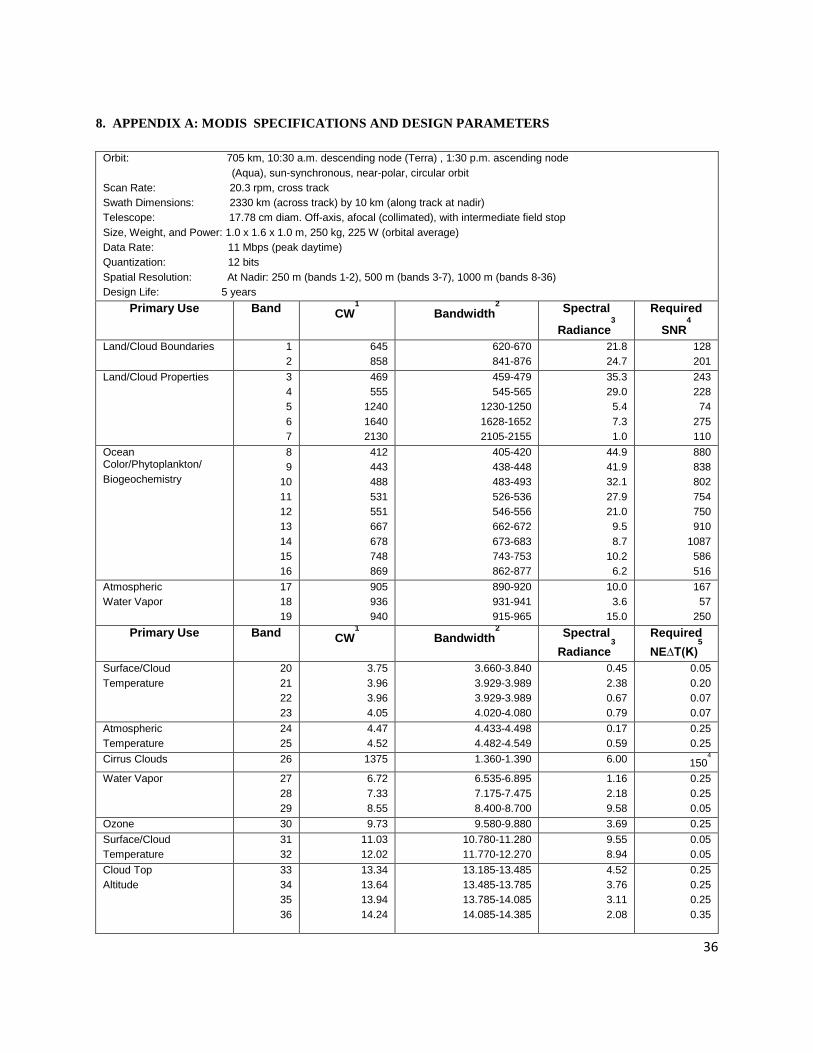
8. APPENDIX A: MODIS SPECIFICATIONS AND DESIGN PARAMETERS

Orbit: 705 km, 10:30 a.m. descending node (Terra) , 1:30 p.m. ascending node (Aqua), sun-synchronous, near-polar, circular orbit Scan Rate: 20.3 rpm, cross track Swath Dimensions: 2330 km (across track) by 10 km (along track at nadir) Telescope: 17.78 cm diam. Off-axis, afocal (collimated), with intermediate field stop Size, Weight, and Power: 1.0 x 1.6 x 1.0 m, 250 kg, 225 W (orbital average) Data Rate: 11 Mbps (peak daytime) Quantization: 12 bits Spatial Resolution: At Nadir: 250 m (bands 1-2), 500 m (bands 3-7), 1000 m (bands 8-36) Design Life: 5 years

Primary Use Band CW1 Bandwidth

2 Spectral

Radiance3

Required

SNR4

Land/Cloud Boundaries 1 2

645 858

620-670 841-876

21.8 24.7

128 201

Land/Cloud Properties 3 4 5 6 7

469 555

1240 1640 2130

459-479 545-565

1230-1250 1628-1652 2105-2155

35.3 29.0 5.4 7.3 1.0

243 228 74

275 110

Ocean Color/Phytoplankton/ Biogeochemistry

8 9

10 11 12 13 14 15 16

412 443 488 531 551 667 678 748 869

405-420 438-448 483-493 526-536 546-556 662-672 673-683 743-753 862-877

44.9 41.9 32.1 27.9 21.0 9.5 8.7

10.2 6.2

880 838 802 754 750 910

1087 586 516

Atmospheric Water Vapor

17 18 19

905 936 940

890-920 931-941 915-965

10.0 3.6

15.0

167 57

250 Primary Use Band CW

1 Bandwidth

2 Spectral

Radiance3

Required NE∆T(K)

5

Surface/Cloud Temperature

20 21 22 23

3.75 3.96 3.96 4.05

3.660-3.840 3.929-3.989 3.929-3.989 4.020-4.080

0.45 2.38 0.67 0.79

0.05 0.20 0.07 0.07

Atmospheric Temperature

24 25

4.47 4.52

4.433-4.498 4.482-4.549

0.17 0.59

0.25 0.25

Cirrus Clouds 26 1375 1.360-1.390 6.00 1504

Water Vapor 27 28 29

6.72 7.33 8.55

6.535-6.895 7.175-7.475 8.400-8.700

1.16 2.18 9.58

0.25 0.25 0.05

Ozone 30 9.73 9.580-9.880 3.69 0.25 Surface/Cloud Temperature

31 32

11.03 12.02

10.780-11.280 11.770-12.270

9.55 8.94

0.05 0.05

Cloud Top Altitude

33 34 35 36

13.34 13.64 13.94 14.24

13.185-13.485 13.485-13.785 13.785-14.085 14.085-14.385

4.52 3.76 3.11 2.08

0.25 0.25 0.25 0.35

37

Appendix A Notes 1. Central Wavelength (nm for bands 1-19, 26; μm for bands 20-25, 27-36) 2. Units: Bands 1 to 19, nm; Bands 20-36 μm

3. (W/m2 μm sr) Typical Earth scene radiance, L

typ

4. SNR = Signal-to-noise ratio {Performance goal is 30% -40% better than required.} 5. NE∆T = Noise-equivalent temperature difference

9. APPENDIX B: L1B TEB SCALED INTEGERS In the L1B code, the TEB radiance produced for each Earth view (EV) pixel is expressed in a 32-bit floating-point format. It is output as a 16-bit scaled integer (SI) in the Scientific Data Sets (SDS) of the Hierarchical Data Format (HDF) for the L1B data products. The dynamic range of valid data in SI is [0, 32767] and any values greater than 32767 represent invalid data. To convert the SI back to the calibrated radiance for a given pixel, simply use the following expression:

(9.1) where

(9.2) and

(9.3) The values of radiance_scales(B) and radiance_offsets(B) are computed inside L1B based on the L

MAX(B) and L

MIN(B) values of each band stored in the L1B LUTs. They are written as

attributes to the SDS. 10. APPENDIX C: L1B RSB SCALED INTEGERS In L1B, the RSB product is Earth view reflectance, expressed in a 32-bit floating-point format for each pixel. As with the TEB radiance, the RSB reflectance is output as a 16-bit SI in the SDS of the HDF. The reflectance can be calculated from the SI by ( ) reflectance_scale(B) [SI - reflectance_offset(B)],EV EVCosρ θ = (10.1) where ρ Cos(θ

EV) is the EV scene reflectance factor for the EV pixel at solar zenith angle θ

EV.

reflectance_scale(B) and reflectance_offset(B) are written as attributes to the SDS. With the reflectance, the RSB radiance can be obtained by

(10.2)

38

where Esun

is the solar irradiance. The quantity Esun

/π for each detector is written as a global attribute to the SDS.

11. APPENDIX D: UNCERTAINTY INDEX IN THE L1B PRODUCTS After the radiometric uncertainty calculation, a Root-Sum-Square (RSS) approach is completed and the uncertainty is written to the L1B products in terms of the Uncertainty Index (UI) for each pixel, with an integer ranging from 0 to 15. The UI is computed in the L1B using the following expression:

The use of nonlinear log scaling allows a broad range of uncertainty to be covered while an adequate resolution for small uncertainties is still retained. Table 2 lists the band dependent scaling_factor[B] and specified_uncertainty[B] values. They are provided from LUT inputs. The RSS uncertainty is computed dynamically for each pixel in each scan as described above. 12. APPENDIX E: ACRONYMS AND ABBREVIATIONS a0 Temperature-dependent Offset for TEB Calibration a2 Temperature-dependent Quadratic Coefficient for TEB Calibration A/D Analog-to-Digital Converter AM-1 Ante Meridian EOS Platform (Terra) AOI Angle of Incidence Aqua FM1 satellite that houses MODIS ATBD Algorithm Theoretical Basis Document AU Astronomical Unit AVHRR Advanced Very High Resolution Radiometer b

1 Linear Gain Term for TEB Calibration

BB OBC Blackbody BCS Blackbody Calibration Source BDSM Band, Detector, Subframe (sample), Mirror side BRDF Bi-Directional Reflectance Distribution Function BRF Bi-Directional Reflectance Factor CFPA Cold Focal Plane Assembly CLAM Cooler Located Amplifier Module CZCS Coastal Zone Color Scanner DAAC Distributed Active Archive Center DC Direct Current DCR DC Restore DN Digital Number. Raw signal recorded including SV with DCR. dn DN Corrected for Electronic Background (i.e., DN-SV)

39

dn* dn**

DN Corrected for Instrumental Effects and Electronic Background For RSB, dn* as Scaled to the SI Within a Defined Dynamic Range so that a Single Set of Calibration Parameters Applies to Every Detector in a Band

ECAL Electronics Calibration EM Engineering Model Esun RSR-Weighted Solar Irradiance EV Earth view FAM Forward Viewing Analog Module FDDI Fiber Distributed Data Interface FIFO First-In First-Out FM-1 Flight Model-1 (Aqua) FPA Focal Plane Assembly Frame Number 1-1354. Linearly Related to Scan Angle. An Along-Scan Pixel. GDAAC Goddard DAAC Granule A Data Processing Time Unit (5 minutes) HIRS High Resolution Infrared Spectrometer IFOV Instantaneous Field of View IR Infrared K Kelvin L Radiance L1B Level 1B (calibrated, geo-located data) LUT Look-Up Table LWIR Long Wavelength Infrared m

1 Reflectance Calibration Linear Term

MCST MODIS Characterization Support Team MEM Main Electronics Module MODAPS MODIS Adaptive Processing System MODIS Moderate-Resolution Imaging Spectroradiometer MTPE Mission To Planet Earth MWIR Medium Wavelength Infrared NASA National Aeronautics and Space Administration NIR Near Infrared NIST National Institute of Standards and Technology nm Nanometers (10

-9 meters)

NOAA National Oceanic and Atmospheric Administration OBC On-Board Calibrator OOB Out-of-Band PC Photoconductive PFM Proto-Flight Model (Terra) PM-1 Post Meridian EOS Platform (Aqua) PV Photovoltaic RSB Reflective Solar Band (1-19,26) RSR Relative Spectral Response RSS RVS

Root Sum Squared (Uncertainty in the Level 1B Product) Response Versus Scan Angle

SAM Space View Analog Module

40

SBRS Santa Barbara Remote Sensing Scan 1.4771 second cross-track sweep SD Solar Diffuser SDS Solar Diffuser Screen; also Science Data Set SDSM Solar Diffuser Stability Monitor SDST Science Data Support Team SI Scaled Integer SiPD Silicon Photodiode SIS Solar Integrating Sphere SNR Signal-to-Noise Ratio SpMA Spectral Measurement Assembly (used in TV) SRCA Spectro-radiometric Calibration Assembly SV Space View SWIR Short Wavelength Infrared TBD To Be Determined TDI Time Delay Integration TEB Terra

Thermal Emissive Band (20-25, 27-36) AM-1 satellite that houses MODIS

TM Thematic Mapper TOA Top of the Atmosphere TV Thermal Vacuum UI Uncertainty Index VIS WUCD

Visible Warm-up, cool-down