modified logistical creep strain prediction method : a...
TRANSCRIPT

Ryerson UniversityDigital Commons @ Ryerson
Theses and dissertations
1-1-2011
Modified Logistical Creep Strain PredictionMethod : A Constitutive Creep Strain Model Of ANickel Based Super-AlloyAmir SeifRyerson University
Follow this and additional works at: http://digitalcommons.ryerson.ca/dissertationsPart of the Aerospace Engineering Commons
This Thesis is brought to you for free and open access by Digital Commons @ Ryerson. It has been accepted for inclusion in Theses and dissertations byan authorized administrator of Digital Commons @ Ryerson. For more information, please contact [email protected].
Recommended CitationSeif, Amir, "Modified Logistical Creep Strain Prediction Method : A Constitutive Creep Strain Model Of A Nickel Based Super-Alloy"(2011). Theses and dissertations. Paper 1633.

MODIFIED LOGISTICAL CREEP STRAIN PREDICTION METHOD
A CONSTITUTIVE CREEP STRAIN MODEL OF A NICKEL BASED SUPER-ALLOY
By
Amir Seif
Bachelor of Aerospace Engineering
2011
A thesis
Presented to Ryerson University
In partial fulfillment of the
Requirements for the degree of
Master of Applied Science
In the Program of
Aerospace Engineering
Toronto, Ontario, Canada, 2011
©Amir Seif 2011

Author's Declaration
I hereby declare that I am the sole author of this thesis or dissertation.
I authorize Ryerson University to lend this thesis or dissertation to other institutions or individuals
for the purpose of scholarly research.
~~
I further authorize Ryerson University to reproduce this thesis or dissertation by photocopying or by
other means, in total or in part, at the request of other institutions or individuals for the purpose of
scholarly research.
11

iii
MODIFIED LOGISTICAL CREEP STRAIN PREDICTION METHOD
A CONSTITUTIVE CREEP STRAIN MODEL OF A NICKEL BASED SUPER-ALLOY
MASTER OF APPLIED SCIENCE
2011
AMIR SEIF
AEROSPACE ENGINEERING
RYERSON UNIVERSITY
In turbine blade design, all three stages of creep are of concern. Moreover, for most commonly
employed materials, creep rupture data is readily available where as long term creep strain data is not
[1]. Recently, effort has been expended by many researchers in the development of material models
incorporating all three stages of creep at varying stress and temperatures. Several developed models
are complex or burdened by large numbers of material fitting constants. There is need for the
development of a constitutive creep strain prediction formulation that is simplistic and requires
minimal empirical data.
In this thesis, the creep strain model proposed by Holmstrom et al., called the Logistic Creep Strain
Prediction (LCSP) method was modified and used to model all three stages of creep of the well
known nickel based super alloy Inconel 718 [1]. The LCSP is robustness and accurate, and
possesses a simplistic formulation ideal for algebraic manipulation and differentiation making it a
very attractive solution.

iv
ACKNOWLEDGEMENTS
I would like to thank, first and foremost, my Academic Supervisor Doctor Kamran Behdinan for
taking an interest in me and guiding me through this process. I am forever grateful to Doctor
Jeffrey W. Yokota for encouraging me to pursue Postgraduate studies. I recognize Doctor Jason V.
Lassaline for his long standing support of my academic career and his guidance. I wish to
acknowledge my RIADI Supervisor Chao Zhang for instilling an interest in creep phenomenon and
creep modeling. Finally, a special thanks to my personal computer programmer Mohammed Buttu
for his contribution and consultation in this research endeavour. All of the distinguished persons
mentioned above have given me support and guidance that is invaluable.

v
DEDICATION
I‟d like to dedicate this endeavour to my parents Faisal and Pierrette Seif. They nurtured me and
told me I could do whatever I set my mind too. Thanks Mom and Dad. I‟d also like to dedicate
my efforts to my beautiful wife, Hana Alziadeh, for her endearing love and support. It‟s just a
memory now Dad!

vi
TABLE OF CONTENTS
Chapter 1 Introduction .................................................................................................................................................. 1
1.1 Research Motivation & Goals ........................................................................................................................ 1
1.2 The Concept of creep ...................................................................................................................................... 2
1.3 Primary/Secondary Creep ............................................................................................................................... 4
1.4 Tertiary Creep ................................................................................................................................................... 7
Chapter 2 Literature Survey .......................................................................................................................................... 9
2.1 Historical Background ..................................................................................................................................... 9
2.2 Rabotnov-Kachanov Method ....................................................................................................................... 12
2.3 Theta θ Projection Method ........................................................................................................................... 14
2.4 Omega (Ω) Method ........................................................................................................................................ 16
2.5 Logistic Creep Strain Prediction (LCSP) Method ..................................................................................... 17
Chapter 3 Theory & Application ............................................................................................................................... 19
3.1 ANSYS User-Programmable Features ........................................................................................................ 19
3.2 LCSP Limits & constraints ........................................................................................................................... 20
3.3 LCSP user-defined creep equations ............................................................................................................. 22
Chapter 4 Procedure .................................................................................................................................................... 24
4.1 Material Data Collection................................................................................................................................ 24
4.2 Creep Strain Curve Fitting ............................................................................................................................ 26
4.3 Fortran Compiling and Linking ................................................................................................................... 29
4.4 CATIA V5 Geometry Creation.................................................................................................................... 29
4.5 Workbench Meshing ...................................................................................................................................... 30
4.6 APDL Creep Analysis Input Files ............................................................................................................... 32
Chapter 5 Results & Discussion ................................................................................................................................. 32
Chapter 6 Conclusion .................................................................................................................................................. 42
Chapter 7 Recommendations & Future work .......................................................................................................... 44
References .......................................................................................................................................................................... 65

vii
LIST OF TABLES
TABLE 1 SPECIFIC FITTING OPTIONS FOR MATERIAL CONSTANTS .............................................................................. 29 TABLE 2 MATLAB LCSP CURVE FITTING RESULTS......................................................................................................... 33 TABLE 3 MATERIAL CONSTANT .............................................................................................................................. 33 TABLE 4 MATERIAL CONSTANT ........................................................................................................................ 34 TABLE 5 MATERIAL CONSTANT .......................................................................................................................... 34 TABLE 6 LARSON-MILLER PARAMETER ............................................................................................................. 34 TABLE 7 IS TAKEN FROM ADVANCED MECHANICS OF MATERIALS [4 PP. 630-31] ...................................................... 45

viii
LIST OF FIGURES
FIGURE 1 IS A TYPICAL METAL CREEP CURVE, DISPLAYING ALL THREE STAGES [4]....................................................... 3 FIGURE 2 ILLUSTRATES THE TYPE OF CURVE EQUATION 1.4 PRODUCES [4] ................................................................. 7 FIGURE 3 P – PRIMARY, S – SECONDARY, T – TERTIARY CREEP STAGES. ..................................................................... 11 FIGURE 4 ORIGINAL CREEP CURVES FROM YEOM ET AL [3] ........................................................................................ 25 FIGURE 5 LISTS ELEMENT COMPOSITIONAL PERCENTAGE IN THE IN718 SAMPLES .................................................... 25 FIGURE 6 POISSON'S RATIO (LEFT PLOT, SECOND COLUMN DIGITIZED DATA TABLE ON RIGHT) FROM AEROSPACE
STRUCTURAL METALS HANDBOOK [2] AND MODULUS OF ELASTICITY (HIGH TEMP METALS COMPANY WEBSITE, FIRST COLUMN TABLE ON RIGHT) [23] ............................................................................................... 26
FIGURE 7 CATIA SMOOTH AXI-SYMMETRIC CROSS-SECTION SKETCH ......................................................................... 30 FIGURE 8 SURFACE GEOMETRY OF CATIA AXI-SYMMETRIC MODEL ........................................................................... 31 FIGURE 9 AXI-SYMMETRIC SMOOTH SPECIMEN MESH ............................................................................................... 32 FIGURE 10 MATLAB GENERATED PLOT OF MATERIAL CONSTANT BETA VERSUS STRESS ........................................... 35 FIGURE 11 EXAMPLE OF A LOGISTIC FUNCTION ............................................................................. 36 FIGURE 12 MATLAB GENERATED PLOT OF MATERIAL CONSTANT XO VERSUS LOGARITHMIC STRESS ...................... 37 FIGURE 13 MATLAB GENERATED PLOT OF MATERIAL CONSTANT P VERSUS STRESS ................................................. 38 FIGURE 14 COMPARATIVE CREEP CURVE PLOT (109 KSI & 1112 °F) ........................................................................... 39 FIGURE 15 COMPARATIVE CREEP CURVE PLOT (123 KSI & 1112 °F) ........................................................................... 39 FIGURE 16 COMPARATIVE CREEP CURVE PLOT (138 KSI & 1112 °F) ........................................................................... 39 FIGURE 17 COMPARATIVE CREEP CURVE PLOT (58 KSI & 1292 °F) ............................................................................. 40 FIGURE 18 COMPARATIVE CREEP CURVE PLOT (65 KSI & 1292 °F) ............................................................................. 40 FIGURE 19 COMPARATIVE CREEP CURVE PLOT (80 KSI & 1292 °F) ............................................................................. 40 FIGURE 20 SNAP SHOT OF EXCEL TABULATED DIGITIZED CREEP STRAIN AND RESPECTIVE TIME DATA (YEOM ET
AL.)[3] .................................................................................................................................................................. 47

ix
LIST OF APPENICES
APPENDIX A: TABLES AND CHARTS .............................................................................................................................. 45 APPENDIX B: ANSYS SOURCE CODE ............................................................................................................................. 48 APPENDIX C: MATLAB SOURCE CODE .......................................................................................................................... 55

x
NOMENCLATURE
- or : Creep strain
- or : Creep strain rate
- : Stress
- T: Temperature
- t: Time
- : Rupture time
- : Damage parameter
- : Rate of damage
- : Deviatoric Stress
- : Equivalent stress
- : Rupture stress
- : First principle stress
- : Theta projection constants where i = 1,2,3,4
- : Omega method material parameter
- : Imaginary initial strain
- , , , : Logistic Creep Strain Prediction Material Parameters
- : Incremental stress
- : Incremental strain
1
CHAPTER 1 INTRODUCTION
1.1 RESEARCH MOTIVATION & GOALS
In the aviation industry gas turbines push their components to the very limit of their thermal
capacity. The ever increasing demand on the design of engines with greater thermal performance
has spurred a major need in the development of models expressing all three stages of creep. The
first two stages of creep for design are no longer adequate. Since, long term creep strain data is not
as common as long term rupture time data, a need for the development of constitutive creep strain
models has been incited. Models that are capable of predicting long term creep strain data from
short term experiments, with a simple formulation. This research was motivated by the need of a
constitutive formulation that encompassed the entire creep strain curve at varying stress levels and
temperatures. The criterions of the development effort focused on a simplistic formulation,
encompassing all three creep stages, requiring minimal empirical data and containing a minimal
number of material fitting parameters. The criterions are derived from what is termed the goals of
applicability. The goals of applicability are concerned with the following qualities:
- Ease of application
- Cost of application
- Versatility
Ease of application was met by the simplistic formulation of the modified LCSP and the minimal
number of material fitting constants. Cost of application is met by the fact that the model for
Inconel 718 could be developed from whatever empirical data could be found from the literature.
Versatility is met by the evidence that the material constants of the modified LCSP are connected to
the mechanisms of creep rather than the specific material. The implied connection of the material
fitting constants and the mechanisms of creep would reason that the proposed model can be easily
applied to other similar materials. The modified LCSP presented in this thesis fills the need of a
constitutive creep strain prediction model, encompassing all three stages of creep. The modified
LCSP also has the potential of giving greater understanding of the mechanisms of creep through
state variable type material constants due to the constraints applied to them. Since a vast majority of
proposed constitutive models have yet to be widely accepted or standardized through batteries of
benchmarking exercises, most commercial Finite Element Method (FEM) software packages do not
include full creep strain curve modeling in the default instillation. Most FEM packages such as

2
ANSYS or ABACAS offer the user the ability to customize a user defined subroutine. In this
research, the modified LCSP will be written into an ANSYS User-Programmable Feature (UPF).
The user subroutine is an example of the modified LCSP‟s easy application and versatility. The UPF
is discussed in greater detail in Chapter 3, section 3.1.
1.2 THE CONCEPT OF CREEP
The advancement of technology and the need for stronger materials for high temperature
applications has driven researchers to study material behaviour at high temperature. Moreover, the
need to understand the critical modes of failure at high temperature and the ability to predict failure
is at the forefront of many engineering problems. A long standing interest has existed in creep
phenomenon and its initial observation is obscured in the pages of human history. If someone were
to try pinpointing a time in history as the beginning of major interest in the analysis of creep, one
might choose the work of French engineer L. J. Vicat in 1834 as a beginning. Vicat‟s primary
interest was in the application of wire for load-carrying members in suspension bridges. His
observations lied within what is now accepted as the primary creep stage of the creep curve (Figure
1) [2].
At the beginning of the twentieth century, Phillips (1905) and Andrade (1910) introduced the
concept of the full creep curve with the creep curves for iron and several other materials. Creep
phenomenon is broken up into three stages, namely primary, secondary and tertiary. The three
stages correspond to a decreasing, constant and increasing strain rate respectively. A typical creep
strain versus time curve is presented in Figure 1.

3
Figure 1 is a typical metal creep curve, displaying all three stages [2]
Since the achievements of Phillips and Andrade, the reminder of the twentieth century to the
present is littered with the work of many in the study of creep behaviour. The insurgence of the
industrial revolution required machinery that could operate at high temperatures for greater thermal
efficiency. The advancements in aircraft technologies during the two Great World Wars required
engine components that could handle greater temperatures as humanity moved into the jet age.
During the late 1950‟s to the 1960‟s interest in nuclear power generation peaked another great surge
in interest in the studies of creep analysis [2].
At present, there is great interest in creep modeling that incorporates all three stages of creep in a
single unified model. This interest is driven by the demands of turbo-machinery technology which
is found in both aircraft and power generation industries. Many researchers have developed and
studied a plethora of modeling techniques, some of which will be discussed in the literature survey.
The remainder of this introduction is intended as a summary of the twentieth century equations and
models describing individual creep stages or multiple stages at once. A literal description of the
mechanisms and mechanics of the creep phenomenon will also be presented. There will, however,
be little or no effort to present a detailed derivation of any equations in this section. This section is
merely intended to introduce the concept and is in no way exhaustive. The equations presented in
this section are intended to give an awareness of some of the commonly accepted fundamental

4
mathematical relations of the various stages of creep. Detailed derivation is left to the literature
survey section detailing full creep curve modeling techniques, the primary interest of this thesis.
Since the creep phenomenon is a complex material behaviour, its analysis is often based on curve-
fitting of experimental creep data. Typically, an effort is made to describe creep strain or creep
strain rate as a function of stress , temperature T, and time . The relations and models
producing constitutive equations are most commonly derived by one of three methods [2; 3],
- Phenomenological (macroscopic, empirical): Derivation of empirical formulas that model
experimental data
- Physical (microscopic): Derivation of equations based on metallurgical creep mechanisms
- Physical-Phenomenological (micro-macroscopic): As its name implies these types of
equations combine the first two types. These formulations are dominated by state variables
representing prevailing creep mechanisms.
Table 7 is duplicated in APPENDIX A: Tables AND CHARTS
from Advance Mechanics of Materials of empirical one-dimensional creep formulas [2]. Table 7 is a
good summary of the generally accepted equations and concepts developed over the twentieth
century.
The proceeding sections of the introduction will briefly give a literal description of the mechanisms
controlling the different stages of creep. The literal description will be followed by a discussion of
some of the basic mathematical relations describing the stage. First the Primary/Secondary stages
will be discussed as they are similar in mechanism. Finally, the introduction will finish off with a
discussion on the tertiary creep stage.
1.3 PRIMARY/SECONDARY CREEP
Dislocation creep theory is based on the principle of crystallographic dislocation of a material‟s
atoms arranged in a crystal structure or lattice. The atoms dislocate by means of gliding along their
slip planes, but are not restricted to glide only. The atoms can climb, meaning they are not forced to
only move along their slip planes. Dislocation theory is the premise that a material is hardened with
deformation and softened with time [3]. The primary and secondary creep stages are characterized
by this process of simultaneous hardening and softening. The concept was first coined by Bailey
and Orowan.

5
At high temperatures roughly one-third of the absolute material melting temperature, dislocations
obtain a new degree of freedom. This degree of freedom is climb. The climb mechanism allows for
the gradual freeing of dislocations previously created by increasing strain. The strain dependent
dislocation or glide dislocation can be halted by obstacles such as other dislocations or second-phase
particles. The dislocation is said to recover if it undergoes a climb mechanism, releasing the
dislocation to slide to the next obstacle. The glide mechanism is the principal creep mechanism of
the primary stage. The glide-climb mechanism is dubbed the hardening-recovery mechanism.
Hardening is the process of the dislocation being restrained by an obstacle and recovery is the
freeing of the dislocation by climb.
Empirical evidence would suggest the dislocations are arranged in a network. Creep consists of
continuous events of recovery and hardening within this network. Network consistency is ensured
by the repulsive and attractive forces among the dislocations.
The stress and high temperature subjected dislocations lengthen and therefore increase in density.
This causes strain and hardening to increase. At the initiation of the stress the glide mechanism is
predominate such that there is initially a large number of loosely connected dislocations. This
results in a high initial creep strain rate. Eventually, the number of loosely held dislocations is
reduced over time which gives the primary stage‟s characteristic decreasing strain rate (hardening).
The decreasing strain rate or hardening process is countered by the recovery mechanism (softening).
The climb trend is increasing with increasing dislocation density over time. Finally, equilibrium is
achieved by both mechanisms of hardening and softening. The effect is a steady state creep rate or
the beginning of the secondary creep stage.
The objective of mathematical descriptions of material phenomenon is to accurately relate
empirically determined values of creep strain, stress, temperature and time. The developed
mathematical relation can take the form of a single equation or a system of equations. Historically,
efforts have been centered to the fitting of single portions of the creep curve.
The primary creep stage, characterized by a monotonic decrease in creep strain rate, strain ε can be
described simplistically by the time-hardening-theory.
Equation 1.1
The variables and are constant uniaxial stress and temperature respectively. The parameters A, n
and m are temperature dependent material constants determined from uni-axial stress creep tests.

6
Furthermore, differentiating Equation 1.1 with respect to time (t), the creep rate can be
determined as,
Equation 1.2
If time is substituted from Equation 1.1 into Equation 1.2, we get the relation,
Equation 1.3
Equation 1.3 is referred to as the strain-hardening-theory [4].
Both time-hardening and strain-hardening theories are default models provided in Ansys mechanical
modeling software. Among the two theories mentioned above, Generalized Exponential,
Generalized Graham, Generalized Blackburn, Modified Time-Hardening, and Modified Strain-
Hardening are the available default primary creep models available in Ansys 12 Finite Element
Method (FEM) software package.
Secondary stage creep is similar in behaviour to pure plastic behaviour. Moreover, creep
deformations “of metals will usually be uninfluenced if a hydrostatic pressure is superimposed” [4].
A similar behaviour observed of pure plastic deformations and, as such, creep can be described by
methods employing the mathematical theories of plasticity. The secondary stage can also be
described by its characteristic constant strain rate, at constant stress level and temperature.
For uni-axial tensile tests all at the same temperature but different stress levels, the constant creep
strain rate of the secondary stage can be described as a function of the stress level σ [2 p. 635]:
Equation 1.4
Equation 1.4 ignores primary and tertiary stages and is only applicable to situations when a
component exhibits a curve that appears dominated by a secondary creep stage. In this instance
creep strain is approximated by straight lines such as those in Figure 2.

7
Figure 2 illustrates the type of curve Equation 1.4 produces [2]
Models employing formulations such as Equation 1.4 are termed steady-state creep models.
Equation 1.3 or the strain-hardening-theory can be used to model both primary and secondary
stages together. Available default creep models in Ansys 12 are, Generalized Garofalo, Exponential
Form, or Norton.
1.4 TERTIARY CREEP
The final stage of creep before rupture is the tertiary stage. This stage is characterized by an
exponentially increasing creep strain rate. The increasing strain rate is related to the damage
accumulation within the internal crystalline structure of the material. The dislocation mechanisms of
the primary/secondary stages cause cavities (microscopic cracks) on the grain boundaries. These
cavities are initially small and have negligible effect on the strain rate. However, with increasing time
and creep strain the cracks grow and meet to form larger cavities. Eventually, the growing creep
damage becomes a prominent factor in the behaviour of the strain rate. It is at this point the
characteristic exponentially increasing strain rate of the tertiary stage can be observed [3; 4].
Other forms of damage may arise such as void formation from a certain stress history. Less certain,
but still of interest is the effect of oxidation on or below the surface causing microscopic cavities [3].
Hence, was born an interest and study of damage mechanics and specifically continuum damage
mechanics (CDM) methods. However, there has been little benchmarking to date on CDM
methods and therefore it is often difficult to “establish the accuracy of the numerical formulations”

8
[5]. Since it is difficult to establish the accuracy of such methods, commercial general-purpose Finite
Element (FE) codes leave it to the individual users to incorporate in-house FE codes.
Among some of the modeling methods explored in this paper are Theta-Projection, Omega, and
Typical Katchanov-Robotnov (CDM) and Logistic Creep Strain Prediction methods. The
descriptions of the methods are left to the section within the literature survey entitled continuum
damage mechanics Methods.

9
CHAPTER 2 LITERATURE SURVEY
Initially, the literature survey served to familiarize the author with not only previously proposed
creep models encompassing the entire creep strain curve, but also the mechanics and basic
mathematical relations of the creep phenomenon. It became apparent at the beginning of this study
that the subject of creep was immense and that a focus was going to be required. A literature survey
that encompassed a review of the major historical mathematical relations developed in twentieth
century would be a task in itself. The primary goal of this research project is the development of a
procedural method in modeling a material‟s entire creep strain evolutionary curve. This was to be
done by choosing an appropriate existing creep model that fits the development criterions outlined
previously. As a consequence this literature review reflects the main formulations of interest that
were considered for use in this thesis.
2.1 HISTORICAL BACKGROUND
There has been a great deal of interest within the past century in the study of creep behaviour and
development of modelling techniques. Arguably the first researcher to introduce the concept of the
creep strain curve with all three stages as it is known today was Andrade [6]. Initially, many
scientists approached the analysis of creep modeling within its individual stages. One of the most
well known formulations is the Norton-Bailey relation:
Equation 2.1
Where and are material constants and R, T and are the global constant, absolute temperature
and applied constant stress respectively. However, as remarked by Batsoulas, “the use of this
relation in the design means that (i) the creep curve is a straight line, (ii) the initial and tertiary creep
are neglected, and (iii) the rate of secondary creep, (and the creep life, ) is, essentially defined as
the exclusive designing parameter”[3]. As might be imagined this is simply unacceptable in most, if
not all serious creep analysis of modern components. The majority of relations developed early in
this century till relatively recently have tackled one or two stages of the creep and not the entire
curve. Batsoulas lists several of these concerning the first and second creep stages. Herein, only a
few representing some of the more well known relations will be reproduced.
Andrade‟s Relation

10
Equation 2.2
Mott and Nabarro‟s relation
Equation 2.3
McVetty and Garofalo‟s relation
Equation 2.4
Andrade, Nabarro, Garofalo and many other notable scientists are found in the literature for their
contributions to the understanding of creep. As some of their postulated relations became accepted
researchers of the present are modifying the old to create more robust and accurate all
encompassing relations. Some of the relations accepted as fundamental formulations are found in
popular Finite Element Method (FEM) software packages such as a generalized Garofalo relation in
ANSYS 12.
Recently, there have been efforts by some researchers to compile and provide benchmarks of some
of the past proposed creep strain models [3; 7; 8]. Figure 3 is a table taken from the European Creep
Collaborative Committee‟s (ECCC) publication entitled, Recommendations and Guidance for the
Assessment of Creep Strain and Creep Strength Data [8; 9]. The table is a modest compilation of
models most commonly used by organizations currently active in the ECCC.

11
Figure 3 P – Primary, S – Secondary, T – Tertiary creep stages.
In the past two or three decades, a shift was made to model the creep curve in its entirety. Either, it
was to be modelled by macroscopic phenomenological curve fitting techniques, or continuum
damage mechanics (CDM) approaches incorporating state variables corresponding to the dominant
physical procedures of damage [3]. Three methods listed in Figure 3 were of particularly interest,
the Rabotnov-Kachanov, Theta and Omega models. Additionally, one other model is presented and
described in addition to the aforementioned methods. The Logistic Creep Strain Prediction (LCSP)
model developed by Holmstrom and Auerkari is the final model studied in this paper. The LCSP
model is a phenomenological model or a non-linear asymmetric transition function with regulated
steepness, as described by its authors [10]. A detailed description of the Rabotnov-Kachanov,
Theta, Omega and LCSP models is provided in the ensuing subsections of the literature survey.

12
2.2 RABOTNOV-KACHANOV METHOD
Kachanov has been dubbed the founder and developer of classical Continuum Damage Mechanics
or CDM as it is referred to. His original work has been revised and adapted by many researchers
with considerable success to many applications [3; 7; 11; 12; 13].
Initially, Kachanov introduced the concept of CDM for the case of creep damage [13]. He
represented the accumulation of damage as the loss in material cross-section, due to cavitation [14].
His initial concept took the form,
Equation 2.5
is Kachanov‟s damage parameter he called the „continuity‟. The state variable „continuity‟ is
defined as the ratio of the remaining effective area ( ) to the initial area ( ). This continuity state
variable could be taken a step further to relate to initial stress ( ) and effective stress ( ) as,
Equation 2.6
In Equation 2.6, the effective stress is increasing due to increasing damage or decreasing effective
area ( ). Later Rabotnov would modify Kachanov‟s state variable „continuity‟ concept with the
damage parameter . The new damage parameter is defined as,
Equation 2.7
Equation 2.6 can be re-written to reflect Rabotnov‟s modification as,
Equation 2.8
Eventually, with the combined effort of Kachanov, Rabotnov, and Hayhurst and co-workers, the
damage rate ( ) would be expressed in terms of applied stress and current state of damage ( ) as,
Equation 2.9
The constants , , and are material constants. Two more fundamental equations can be derived
using the conditions that at , at ( is time and is time to failure).
Integrating Equation 2.9 using the conditions described above gives,
Equation 2.10
Finally, the instantaneous damage state can be derived as,
Equation 2.11

13
In 1958 Kachanov proposed a modified Norton‟s creep rate equation utilizing his effective stress for
the applied stress used in the original Norton‟s equation [14]. The modified Norton‟s steady state
creep rate equation took the form,
Equation 2.12
Equation 2.12 is suitable for uni-axial secondary/tertiary creep modeling.
A commonly used single-state variable constitutive multi-axial stress equation based on the original
Kachanov type equation takes the form [12],
Equation 2.13
Here, and are the deviatoric and equivalent stresses respectively and , and are material
constants. Researchers such as Hyde, Becker, Sun and many others have found success in a variety
of applications employing Kachanov adaptations such as Equation 2.13 in their work [12].
Accompanying Equation 2.13 is the rate of change of the damage parameter which takes the form
[7],
Equation 2.14
Where , and are continuum damage material constants. In Equation 2.14, is a rupture
stress that can be calculated by [7],
Equation 2.15
In Equation 2.15 is a material constant that ranges from 1 (maximum first principle stress
dominant) to 0 (equivalent or Von Mises stress dominant) [7].
Equation 2.13 to Equation 2.15 can be applied to multi-axial stress cases that lie primarily in the
secondary/ tertiary creep stages. The equations can be modified to incorporate the primary creep
stage [7].
As it stands, the Kachanov based equations 2.13 to 2.15 have a total of 9 material constants. This
formulation does not even include the primary creep region.
The Kachanov style formulation represented in this section was eliminated during the selection
process on several accounts. The number of material constants required implies the need for a great
deal of material data for accurate modeling of creep strain curve family. The model would not be
easily integrated into a FEM software package. It was concluded that a Kachanov style model would

14
not best achieve the development criterions of the proposed constitutive modeling procedural
method.
2.3 THETA Θ PROJECTION METHOD
The Theta Projection (TP) method is a parametric method used to obtain approximations of long-
term creep strain or time data from short term experimental creep data [15]. The TP method is one
that has gained some favour among researchers as a promising constitutive creep formulation. The
TP method expresses creep strain evolution with respect to time in the form,
Equation 2.16
Where is creep strain, is time to specific creep strain, terms are experimentally determined
material constants [16]. The method attempts to perform two functions, empirically fitting
experimental strain-time data and provide insight into the processes characteristic of creep damage
mechanics [16]. Though this method is not explicitly a CDM approach, it does however have
similar attributes as it relies on the failure mechanisms of both primary and tertiary creep.
The first group of terms in Equation 2.16 model‟s the primary stage and the second group of terms
models tertiary. Any constant secondary creep stage is considered an inflection in the curve. In
other word, the first group is representative of the primary stages characteristic hardening process.
The second group is representative of the tertiary stages mechanism of accumulated damage or
softening. The balancing of the two groups of terms results in an equilibrium being achieved. This
equilibrium is representative of the secondary stage. Furthermore, though the TP method does not
contain any damage parameter, it is reminiscent of the Kachanov damage state variable concept.
The creep strain rate can be defined by differentiating Equation 2.16 to give,
Equation 2.17
The theta terms can be expressed as functions of applied constant stress and temperature as,
Equation 2.18
The theta terms vary approximately linearly with respect to stress and temperature [16]. It has been
shown that the TP method is capable of predicting creep rupture strains as a function of stress and
temperature.
Equation 2.19
The TP method is a favourable creep strain evolution formulation. It has become more widely used
as its advantage and flexibility have become appreciated [3; 15; 16; 17]. Despite the fewer number of

15
material constants than a Kachanov style CDM method, there still exists a modeling formulation
incorporating some well established relations with fewer material constants. Moreover, the TP
method appears more dependent on empirical data to accurately model a family of creep curves. It
was believed that the TP method would be dependent on the number of points defining a single
curve of a family of curves in order to adequately model its shape. Furthermore, several curves at
multiple conditions would be required with a great deal of data to extrapolate/interpolate other
curves within that same family of curves. It was concluded that a model with even fewer material
constants was required and a model that could utilize master curve data such as the Larson-Miller
relation to specified creep strains and creep rupture time. For the abovementioned reasons, the TP
method was eliminated as the modeling choice.

16
2.4 OMEGA (Ω) METHOD
Developed by the Materials Properties Council (MPC) and presented by Prager, the MPC Omega
method is founded on the premise that the current creep strain rate along with a brief history of
creep strain rates is adequate to predict past and future creep behaviour of a component [12]. The
MPC Omega (Ω) method has received some interest from several researchers [12; 18].
The Ω method relies on the premise that a materials ability to resist a given stress decreases with
increasing creep damage. Creep strain rate is therefore defined by,
Equation 2.20
Where is the imaginary initial creep strain rate, is creep strain (at some time), is the omega
material parameter. A small primary creep region results in a that is near the minimum creep
strain rate (secondary creep stage).
The factor material parameter omega is implicitly a function of stress, mechanical damage and
micro-structural changes [18]. Integrating Equation 2.20 with respect to time gives a relation with
strain and time t.
Equation 2.21
Finally, at large values of , such as those at creep rupture. The value of the exponential term in
Equation 2.21 can be considered negligible. Moreover, creep rupture time can be approximated
as [18],
Equation 2.22
The imaginary initial strain rate and omega parameters are stress and temperature dependent.
The determination of the appropriate fitting function that relates stress and temperature for either
parameter is material dependent (i.e. polynomial, exponential). For instance, Jong-Taek Yeom et al.
initially chose an exponential power law to express the material parameter with respect to stress and
temperature. It was found that the developed power law expressions did not fit the material
parameters accurately, and a hyperbolic sine formulation was used to describe imaginary initial strain
rate and omega parameters as functions of stress and temperature [18].
At first glance the MPC method appeared very promising. However, of concern was the fact that
the type of curve required to fit the material parameters (polynomial, exponential, etc.) is material
17
dependent. This would be a serious disadvantage when trying to develop a creep model that can be
somewhat standardized for multiple materials for application in a user-defined creep model in a
FEM software package. The number of constants and the accuracy of the MPC model are not in
question, but the concern over curve fitting issues even among similar materials disqualified this
model as a choice for the development of the proposed constitutive creep strain procedural method.
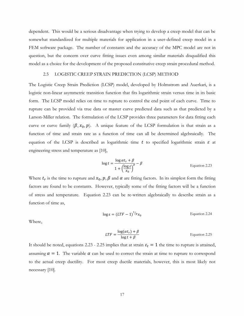
2.5 LOGISTIC CREEP STRAIN PREDICTION (LCSP) METHOD
The Logistic Creep Strain Prediction (LCSP) model, developed by Holmstrom and Auerkari, is a
logistic non-linear asymmetric transition function that fits logarithmic strain versus time in its basic
form. The LCSP model relies on time to rupture to control the end point of each curve. Time to
rupture can be provided via true data or master curve predicted data such as that predicted by a
Larson-Miller relation. The formulation of the LCSP provides three parameters for data fitting each
curve or curve family ( , , ). A unique feature of the LCSP formulation is that strain as a
function of time and strain rate as a function of time can all be determined algebraically. The
equation of the LCSP is described as logarithmic time to specified logarithmic strain at
engineering stress and temperature as [10],
Equation 2.23
Where is the time to rupture and , , and are fitting factors. In its simplest form the fitting
factors are found to be constants. However, typically some of the fitting factors will be a function
of stress and temperature. Equation 2.23 can be re-written algebraically to describe strain as a
function of time as,
Equation 2.24
Where,
Equation 2.25
It should be noted, equations 2.23 - 2.25 implies that at strain the time to rupture is attained,
assuming . The variable can be used to correct the strain at time to rupture to correspond
to the actual creep ductility. For most creep ductile materials, however, this is most likely not
necessary [10].

18
Moreover, differentiating Equation 2.25 with respect to time gives the algebraic expression for creep
strain rate as,
Equation 2.26
Where is determined by Equation 2.24, and
Equation 2.27
And
Equation 2.28
The LCSP method is attractive for several reasons. First, if we assume the model is reduced
to a total of three fitting material constants that can be determined by a minimal amount of actual
data or master curve data. Furthermore, the formulation is easily manipulated algebraically from one
form to another, which is ideal for characterizing creep in terms of creep strain or creep strain rate.
The LCSP‟s robust and simplistic nature made it the ideal constitutive model for application in this
research.

19
CHAPTER 3 THEORY & APPLICATION
3.1 ANSYS USER-PROGRAMMABLE FEATURES
ANSYS provides thirteen creep formulations for implicit analysis. The Norton law and Blackburn
model are examples of the models available in ANSYS implicit creep analysis [19]. Despite the
many included implicit creep analysis tools, some users may wish to use a customized creep equation
that has already been validated through testing. Or perhaps, the application of a damage parameter
is required for a certain application. The creep laws that come preinstalled assume creep is to be
used in design rather than failure analysis and as a consequence the available creep laws are meant to
model primary and secondary creep only.
In order to surmount this limitation ANSYS provides a means of allowing the user the ability to
customize a user defined creep subroutine via ANSYS User-Programmable Features (UPF). Since,
ANSYS has an open architecture it allows the user to write their own routines or subroutines in C or
FORTRAN. The routines or subroutines can either be linked to ANSYS or used externally as
commands [20]. Therefore, using UPF‟s the user can tailor the ANSYS program to their specific
needs.
The UPF of particular interest in this research is the usercreep.F subroutine. The usercreep
subroutine is activated by “the TB command with the CREEP option and with TBOPT =100” [20].
For the usercreep subroutine, a uniaxial creep law can be used which will be generalized to the
multi-axial state by the general time-dependent viscoplasticity material formulation implemented in
ANSYS.
The original ANSYS instillation provides a usercreep.F file, as source code based on the strain
hardening law TBOPT = 1 [19]. The usercreep.F source code provided with the original installation
is reproduced in Appendix B, Source Code 1.
Available variables for use in the subroutine are effective creep strain or time, effective stress, and
temperature. Also available is hydrostatic pressure [19]. The TBDATA command used in creating a
material model input file is used to input the creep material constants right after the TB, CREEP, , ,
,100 command is given. Other temperature dependent material properties such as Modulus of
Elasticity are also input in this way. For specifics on material property input, the user manuals
provided with the ANSYS installation can be reviewed. Moreover, an example of a material
property input file is provided in Appendix B, Source Code 3.

20
Three outputs are required by ANSYS for the calculation of creep strain from the subroutine. First,
the incremental creep strain designated „delcr‟ is required. The last two outputs required are, “the
derivatives of the incremental creep strain with respect to effective stress and creep strain, which are
dcrda(1) and dcrda(2), respectively” [19]. It is crucial that these derivatives are calculated correctly as
ANSYS requires them to calculate the material tangent stiffness matrix. Miscalculating the
derivatives can negatively impact the convergence behaviour and accuracy of the subroutine. In the
case that the model to be used is complex and the derivative cannot be evaluated directly, it is
suggested that numerical differentiation be used [19]. Therefore from first principles, dcrda(1)
would take the form,
Equation 3.1
The value of stress increment ( ) is a very small arbitrarily chosen number that may require
adjustment to achieve acceptable accuracy. The value of dcrda(2) would take a similar form to
Equation 3.1 with creep strain increment ( ) in place of stress increment.
ANSYS UPF usercreep.F subroutine was implemented using the LCSP method as the means of
constructing and analysing creep material properties of all three stages of the creep strain curve of
Inconel 718. The derivation of the equations used in the source code which is reproduced in
Appendix B, Source Code 2, will be covered in the next section entitled LCSP. The specific
equations used to calculate the values of incremental creep strain, dcrda(1) and dcrda(2) are derived
in the next section.
3.2 LCSP LIMITS & CONSTRAINTS
Upon careful observation of the original LCSP formulation, two limitations can be identified. The
original LCSP formulation, time to specified strain is reiterated below for convenience.
Equation 2.23
The condition of creep strain ( ) equal to zero, would imply time to specified strain ( ) is also zero.
However, if zero is subbed into the left side of Equation 2.23, a complex value results. In order to
avoid the calculation of a complex value, a value of one is added to each value of time to specified
strain such that Equation 2.23 can be re-written as,

21
Equation 3.2
Although, typically researchers and engineers are not concerned with cases where rupture time is
zero, for completeness the same logic was applied to rupture time ( ) and Equation 3.2 is re-written
to take the form,
Equation 3.3
The final constraint of the original LCSP involves the denominator of the right side of Equation
2.23. It is possible to calculate a complex value in the denominator in two situations. In both cases
the value of the material constant p, which is fractional, has an even denominator (eg. If p = 3.5 =
7/2). A complex value will be calculated if is negative which will result from any creep strain
value less than 1. Finally, a negative value of the material constant can produce a complex value
in the denominator of Equation 2.23. Therefore, a value of one is added to each value of creep
strain such that Equation 3.3 is further modified to give,
Equation 3.4
Furthermore, to avoid the calculation of a complex value or infinity a lower limit is imposed on the
material constant , specifically,
Equation 3.5
In this research, MATLAB software and FORTRAN are used as a mathematical computer aid and
programming language of the subroutine respectively. In both software packages the command log
is the natural logarithm (ln). Therefore, all logarithms of the LCSP are interpreted as natural
logarithms. This was done primarily for aesthetic purposes of the programming of any m code or
FORTRAN programming.
Finally, the LCSP method was developed with the fitting of creep strain as a percent, but ANSYS
calculates strain as a fraction. Therefore, fractional strain is multiplied by one hundred percent and
Equation 3.4 takes it‟s finally form as,
Equation 3.6

22
In its final modified form (Equation 3.6), creep strain ( ), is interpreted as fractional strain.
Moreover, Equation 3.6 can be algebraically rearranged for creep strain as,
Equation 3.7
Where LTF is now,
Equation 3.8
The creep strain rate is found by taking the derivative of Equation 3.7 with respect to time, which
follows,
Equation 3.9
In Equation 3.9 creep strain can be calculated via Equation 3.7 and k1 and k2 are,
Equation 3.10
And,
Equation 3.11
3.3 LCSP USER-DEFINED CREEP EQUATIONS
As mentioned previously, ANSYS requires three outputs from the user subroutine for analysis. The
first of these outputs is incremental creep strain or delcr, which from Equation 3.9 takes the form,
Equation 3.12
Here is incremental time, which in ANSYS is the sub-step time size. The last two outputs are the
derivatives of incremental creep strain with respect to stress and strain. It is apparent that the
evaluation of the derivatives would be complex and therefore it was decided that numerical
differentiation would be employed.
The numerical differentiation of incremental creep strain with respect to stress, dcrda(1), is defined
by Equation 3.1. Since creep strain in Equation 3.12 can be replaced by Equation 3.7 which implies
that Equation 3.12 is a function of stress and temperature solely. Therefore, the derivative of
incremental creep strain with respect to creep strain, dcrda(2), is equal to zero. Equations 3.1, 3.12
and the fact that dcrda(2) is equal to zero are the three required output of the ANSYS usercreep

23
subroutine that was compiled and linked into ANSYS. The usercrrep.F file is presented in
APPENDIX B: ANSYS Source Code
.

24
CHAPTER 4 PROCEDURE
The procedure of the proposed constitutive creep strain modeling method involved several steps.
They are listed and discussed in order within this chapter under their respective subchapters. This
chapter includes the following subchapters,
- Material Data Collection
- Creep Strain Curve Fitting
- FORTRAN Compiling and Linking
- CATIA V5 Geometry Creation
- Workbench Meshing
- APDL Creep Analysis Input Files
4.1 MATERIAL DATA COLLECTION
The proposed model was to be based on creep strain and rupture data that could be found in the
literature. As a starting point, the Aerospace Structural Metals Handbook was consulted for a
commonly used material in Turbine Blade design. A well know nickel based super alloy employed in
Turbo-Machinery, Inconel 718 (IN718), was found to be well documented [21].
Data was collected for IN718 under the following heat treatment [21; 18]:
- Annealing for 1 hour at 1750°F - 1800°F then air cooled
- Two Step aging treatment
∙ 8 hours at 1325°F then furnace cooled to 1150°F at 100-108°F/hour
∙ Held at 1150°F for an additional 8 hours and finally air cooled
The above heat treatment is the most commonly used treatment procedure with regards to optimum
creep properties [22]. Creep strain data was digitized from creep curves presented by Yeom et al
[18]. Modulus of Elasticity was taken from the High Temp Metals Inc website and poison‟s ratio was
taken from the Aerospace Structural Metals Handbook [21; 23]. OriginPro 8 SRO v8.0724 was used
to digitize all required data which is then output to text files by the program. The text files can then
be read into Excel. Figure 4 is the illustrated original creep strain curves taken [18] from Yeom et al
for IN718 [18]. The digitized data points for the Creep Strain Curves are provided in APPENDIX
A: Tables AND CHARTS
, Figure 20.

25
Figure 4 Original creep curves from Yeom et al [18]
The chemical composition of the material in Yeom‟s research was the following,
Figure 5 lists Element compositional percentage in the IN718 Samples
Finally, to complete the material model the following two charts are the mechanical properties of
IN718 used for this thesis project.

26
Figure 6 Poisson's Ratio (left plot, second column digitized data table on right) from Aerospace Structural Metals
Handbook [21] and Modulus of Elasticity (High Temp Metals company website, first column table on right) [23]
The table in Figure 6 is a snap shot of the table created in Excel.
4.2 CREEP STRAIN CURVE FITTING
The LCSP is fitted in the form of time as a function of the creep strain (Equation 3.6). Three
material constants result from each stress/temperature case. MATLAB Version 7.10.0.499 64-bit
(win64) was used for all curve fitting procedures.
The MATLAB curve fitting tool uses x and y data in the form of,
Equation 4.1
In order to use Equation 3.6 within the MATLAB curve fitting tool graphical user interface (GUI),
the equation was re-written as,
Equation 4.2
Where,
Equation 4.3
And,
Equation 4.4
Values of x and y were calculated using the digitized creep strain and corresponding time data
(APPENDIX A: Tables AND CHARTS

27
, Figure 20) in Excel. Since the creep strain data is to rupture, the last time data point was taken to
be the rupture time of each curve.
The x and y data for each creep curve at specified stress and temperature was read into MATLAB
from Excel and the curve fitting tool was opened in MATLAB with the command „cftool‟. Data is
selected within the Data tab of the cftool GUI. From the „Data‟ tab the x and y data was loaded
from the MATLAB workspace where data was earlier read from excel. Next, fit options and the
data to be fitted are selected. The specific options chosen in the „Fit Editor‟ accessed through the
fitting button are as follow,
- Select new fit
- Populate fit name in the „Fit name‟ field
- Selected desired data from the „Data set‟ drop down menu
- Custom Equations is selected from the drop down menu of „Type of fit‟
- Under Custom Equations, the „New‟ button is selected to create new custom equation
- In the „New Custom Equations‟ window under „General Equations‟ tab right side of
Equation 4.2 is input into the field to the right of the equal sign, the appropriate rupture time
was subbed in and then ok was selected.
- Back in the Fit Editor, „Fit options‟ button is pressed and the following options are selected
in the „Fit Options‟ window:
∙ Robust: Off
∙ Algorithm: Trust-Region
∙ Lower: 0
Each creep curve at specified temperature and stress is fitted using the steps and options listed
above. Once all creep curves where created, m-code representing the fitting of all the curves was
generated by selecting the Generate M-file option from the file drop down menu in the „Curve
Fitting Tool‟ window. This serves three purposes,
- Document the fitting procedure
- Incorporate generated m-function into Excel data reading m-code
- Saves fitting information in a MATLAB Structure Array that can be retrieved for further use
The generated code for curve fitting is modified slightly to output structural arrays containing the
goodness of the fit (R-squared value) and the values of the three material constants of each

28
respective creep strain curve. The m-code reading and writing the Excel data and the generated
modified curve fitting m-function is reproduced in APPENDIX C: MATLAB SOURCE CODE
, Source Code 5 and Source Code 6 respectively.
The next phase of curve fitting was done to fit relations to the material constants as functions of
stress level. Temperature dependence was accounted for by determining the relations as a function
of stress level at a particular temperature. Similar procedure was followed for the fitting of the
material constants versus stress level at specified temperature as the curve fitting procedure of the
creep strain curves. In the case of the material constant fitting, the material constants were the y
values and their corresponding stress level was the x values. The values of x and y were again read
in from Excel. The values of the material constants (x) are the values that had just been written in
by MATLAB from the first curve fitting procedure of the creep strain curves.
Also, curve fitted was a relation describing the Larson-Miller Parameter versus logarithmic stress
level. The Larson-Miller Parameter relation is used in the user defined creep subroutine to calculate
rupture time. The Larson-Miller Parameter (LMP) is defined as,
Equation 4.5
Where T is temperature in degrees Fahrenheit and stress is in kilo-pound per square inch (ksi). The
value of C is a constant that is typically 20 for metals. The LMP was calculated for each creep curve.
For curve fitting x data is represented by and corresponding y values are the respective LMP
value. The values are again read into MATLAB from Excel.
The curve fitting of the material constants and LMP is analogous to that of the creep strain curves
with a few notable differences. The differences are tabulated below.

29
Table 1 Specific Fitting Options for Material Constants
Material Constant Type of Fit Option
Fit Options Custom Equation
Input Robust Algorithm
β exp2 Off Trust-
Region N/A
P poly2 Off N/A N/A
xo Custom Equations Off Trust-
Region a/(1+exp(b*x+c))+d
LMP fourier2 Off Trust-
Region N/A
N/A not applicable.
The fitting equations of the material constants and the LMP were chosen based on known
constraints ( ) and the observable pattern of the resulting data points.
4.3 FORTRAN COMPILING AND LINKING
In order to be capable of utilizing the UPF features in ANSYS, the incumbent must have the proper
software and setup requirements. For this it is recommended that they refer to the specific user‟s
manuals such as the Guide to ANSYS User Programmable Features provided with every version of
ANSYS [24]. Several other sources provided insightful information regarding UPF‟s [25; 26].
The method of compiling and linking the usercreep.F will not be detailed here as this information
can be found for each individual version of ANSYS being used. The usercreep.F subroutine code
used for this work can be found in Appendix B.
4.4 CATIA V5 GEOMETRY CREATION
The two-dimensional axi-symmetric model of the smooth specimen for use in ANSYS was
constructed in CATIA Version 5 Release 20. The model geometry is derived from a smooth
cylindrical specimen with dimensions of a 25 mm (0.9843 inches) gauge section and 6 mm (0.2362

30
inches) diameter [18]. Figure 7 is an illustration of the CATIA geometry later imported into ANSYS
Workbench 12.
Figure 7 Catia Smooth Axi-Symmetric Cross-Section Sketch
4.5 WORKBENCH MESHING
The CATIA surface part, Figure 8, was imported as an igs geometry file into ANSYS Workbench
Version 12 for meshing.

31
Figure 8 Surface Geometry of Catia Axi-Symmetric Model
The two-dimensional model is simple and therefore default settings where kept for meshing. Only
one option was used, Face Sizing of the surface of the model with an element size of 1.0E-2 inches.
The resulting mesh is adequate for the simplicity of the model. The mesh is illustrated in Figure 9.

32
Figure 9 Axi-Symmetric Smooth Specimen Mesh
From the meshed model an input file was written to transfer the mesh into ANSYS classical.
4.6 APDL CREEP ANALYSIS INPUT FILES
The ANSYS analysis options and commands are written in ANSYS Parametric Design Language
(APDL) text files. APDL presents the advantage of documenting the analysis details as well as
automation of the analysis, simplifying consistent reruns of the analysis. It is a quick efficient way of
avoiding the need to setup the analysis each and every trial run through the Graphical User Interface
(GUI). The example of an input file for the case of 109 ksi and 1112 °F is provided in APPENDIX
B: ANSYS Source Code
CHAPTER 5 RESULTS & DISCUSSION
This chapter is a summary and discussion of the results of the work performed. The first results to
be discussed are the curve fitting of the creep strain curves and their resulting material constants.
This is followed by the results of the equations relating the material constants with stress level and
the LMP with logarithmic stress. The measure of accuracy is presented by the R-squared value or
also known as the coefficient of determination as calculated by MATLAB for each curve fit. In
MATLAB the R-squared value is described as the goodness of the fit. The last results to be
presented, is a comparison of the analytical creep strain curves as generated by ANSYS and the
LCSP usercreep subroutine against the original empirical curves.

33
The resulting material constants of the MATLAB curve fitting procedure for the LCSP fitting of the
creep strain curves are tabulated in Table 2 below.
Table 2 MATLAB LCSP Curve Fitting Results
Temperature Stress B p xo R-Square
1112 109 3.114E-03 -1.531E+00 8.834E-02 0.999
1112 123 -4.942E-04 -1.511E+00 2.138E-01 0.993
1112 138 -8.918E-02 -2.792E+00 7.036E-01 0.988
1292 58 1.489E-01 -2.340E+00 3.425E-01 0.990
1292 65 1.074E-02 -2.617E+00 4.496E-01 0.972
1292 80 7.584E-03 -2.008E+00 5.301E-01 0.986
It should be noted that „B‟ is actually the material constant β. Table 2 was generated from the data
output by MATLAB into an Excel spreadsheet. Given the very high R-Square values for each of the
curves approximated by the modified LCSP formulation, is evidence of the methods considerable
accuracy. The apparent accuracy and robustness of the method with minimal empirical data usage is
attractive for application to user-defined creep models, incorporating all three stages of creep, within
Finite Element Method (FEM) software packages.
In order to interpolate between creep curves at varying stress and temperature, it was necessary to
determine functions of stress and temperature for each material constant. The relations and their R-
Squared fitting accuracies are presented in Tables 3 - 5.
Table 3 Material Constant B(σ) a*exp(b* σ) + c*exp(d* σ)
Temperature 1112 1292
a -1.0821E-14 4.0165E+08
b 2.1575E-01 -3.7441E-01
c 4.8801E-03 0.0000E+00
d -3.6150E-03 0.0000E+00
R-Squared ≈1 9.9465E-01

34
Table 4 Material Constant xo(σ) a/(1+exp(b* σ +c))+d
Temperature 1112 1292
a 7.499E-01 3.572E-01
b -6.224E+01 -2.462E+01
c 1.314E+02 4.373E+01
d 6.478E-02 1.932E-01
R-Squared 9.990E-01 9.993E-01
Table 5 Material Constant p(σ) p1*σ2 + p2*σ + p3
Temperature 1112 1292
p1 -2.994E-03 3.644E-03
p2 6.961E-01 -4.878E-01
p3 -4.183E+01 1.370E+01
N/A N/A N/A
R-Squared ≈1 ≈1
The functions fitted to the material constants β and p was chosen intuitively from the observable
graphical pattern of the material constants plotted versus stress at specified temperature. The
function fitted to xo was chosen partially via the observable graphical pattern of the parameter
plotted versus stress. Also considered in the choice of the function, was the imposed constraints of
the modified LCSP.
Also, the Larson-Miller parameter was described by a function of logarithmic base 10 stress. The
Larson-Miller parameter is used to determine the rupture time of the new creep strain curve. The
Larson-Miller Parameter as a function of stress is presented in Table 6.
Table 6 Larson-Miller Parameter
LMP(σ) a0 + a1*cos(log10(σ)*w) + b1*sin(log10(σ)*w) + a2*cos(2*log10(σ)*w) + b2*sin(2*log10(σ)*w)
a0 3.595E+04
a1 1.357E+03
b1 3605
a2 1669
b2 72.87
w 7.627
R-Squared ≈1
Some notable observations were made concerning the pattern of the relations of the material
constants to stress. β versus stress at 1112°F tends towards some small value above zero as stress

35
drops (infinite rupture). As stress increases β tends toward negative infinity (no rupture life). In
contrast, β versus stress at 1292°F tends toward positive infinity as stress decreases (infinite rupture)
and tends toward some horizontal asymptote just below zero as stress increases (no rupture life).
An illustration of the described behaviour is presented in Figure 10,
Figure 10 MATLAB Generated Plot of Material Constant Beta Versus Stress
The inverse in the trend indicates the possibility that β is actually related to stress by a logistic
function, which is characterized by two horizontal asymptotes. Figure 11 is an example of a logistic
function plot,

36
Figure 11 Example of a logistic function
The horizontal asymptotes are inductive of an upper and lower limit on β which are governed by
minimum rupture life (zero rupture life) and infinite rupture life. More empirical creep strain curves
at other stress levels would be required to produce more values of β to confirm this pattern. A
stress low enough to produce large life and a stress high enough to produce nearly immediate
rupture is required to acquire a true sense of the relationship of material constant β and stress.
The graphical relationship of the material constant is considerably more apparent than that of β.
The plot in Figure 12 illustrates the observed logistical relationship of material constant with
stress.

37
Figure 12 MATLAB Generated Plot of Material Constant xo versus Logarithmic Stress
The effect of temperature seems to manifest as shifting and compression/stretching of the logistical
function.
The material constant p, displays a polynomial relation of power two. Figure 13 illustrates the
polynomial relation of material constant p with respect to stress level.

38
Figure 13 MATLAB Generated Plot of Material Constant p versus Stress
The characteristic point of inflection in a polynomial function of power two (quadratic relation) is
indicative of the material constant p controlling the inflection characterizing the transition of
primary creep to tertiary creep. Therefore, the quadratic relation of p with stress implies that the
material constant p has some effect on curve shape and specifically on the length and presence of a
secondary stage. Temperature appears to manifest itself in the concavity of the quadratic relation.
The last and most important results to be presented is the analytical results of the ANSYS User-
creep LCSP based subroutine generated creep strain curves compared against the empirical data
points. Creep strain versus time data was output into text files through the Time History Post-
Processor for each of the six cases analyzed. The creep strain curves of the six cases are illustrated
in Figure 14 - 19.

39
Figure 14 Comparative Creep Curve Plot (109 ksi & 1112 °F)
Figure 15 Comparative Creep Curve Plot (123 ksi & 1112 °F)
Figure 16 Comparative Creep Curve Plot (138 ksi & 1112 °F)
0.00%
2.00%
4.00%
6.00%
8.00%
10.00%
0 1000 2000 3000
Cre
ep
Str
ain
in P
erc
en
t
Time in Hours
Creep Strain Curve at 109 ksi and 1112 °F
Ansys User Defined Model Output (LCSP)
Empirical Data Points
0.00%
2.00%
4.00%
6.00%
8.00%
10.00%
0 100 200 300 400
Cre
ep
Str
ain
in P
erc
en
t
Time in Hours
Creep Strain Curve at 123 ksi & 1112 °F
Ansys User Defined Model Output (LCSP)
Empirical Data Points
0.00E+00
1.00E-02
2.00E-02
3.00E-02
4.00E-02
5.00E-02
6.00E-02
7.00E-02
0 5 10 15 20
Cre
ep
Str
ain
in P
erc
en
t
Time in Hours
Creep Strain Curve at 138 & 1112 °F
Ansys User Defined Model Output (LCSP)
Empirical Data Points

40
Figure 17 Comparative Creep Curve Plot (58 ksi & 1292 °F)
Figure 18 Comparative Creep Curve Plot (65 ksi & 1292 °F)
Figure 19 Comparative Creep Curve Plot (80 ksi & 1292 °F)
0.00%
5.00%
10.00%
15.00%
20.00%
25.00%
0 100 200 300 400
Cre
ep
Str
ain
in P
erc
en
t
Time in Hours
Creep Strain Curve at 58 ksi & 1292 °F
Ansys User Defined Model Output (LCSP)
Empirical Data Points
0.00%
2.00%
4.00%
6.00%
8.00%
10.00%
12.00%
0 50 100
Cre
ep
Str
ain
in P
erc
en
t
Time in Hours
Creep Strain Curve at 65 ksi & 1292 °F
Ansys User Defined Model Output (LCSP)
Empirical Data Points
0
0.05
0.1
0.15
0.2
0.25
0 10 20 30
Cre
ep
Str
ain
in P
erc
en
t
Time in Hours
Creep Strain Curve at 80 ksi & 1292 °F
Ansys User Defined Model Output (LCSP)
Empirical Data Points

41
The figures - 16 demonstrated the most significant divergence with R-Squared values of
approximately .916, .936 and .787 respectively. The remaining figures 17 - 19, possessed R-Squared
values of approximately .844, .982, and .958. Several sources of error were noted. First, it was
observed that the LCSP is highly sensitive to the model used to predict rupture time which is used
to determine the end point of each curve [10]. Slight deviations of predicted rupture time result in
either stretched or compressed creep curves such as figures 14 and 16 respectively. Moreover,
empirical data scatter that is slightly irregular such as Figure 16 are difficult to quantify, such that
they do not conform to the expected creep curve shape. Finally, it should be noted that there is also
combined error. The fitting error of the original curve fits is compounded with the fitting error of
the material constant relations and the Larson Miller relation. Furthermore, the element formulation
and calculations internally performed within ANSYS have their own error to contend with.
It should be noted no attempt was made to characterize the relationship between the material
constants and temperature. This was done for two reasons. First, since data for only two
temperatures was acquired from the literature, only a linear relation with temperature can be inferred
which may be misleading. Moreover, typically in ANSYS material parameters are described with
respect to stress at a given temperature and ANSYS is allowed to interpolate between temperatures
internally. Finally, temperature interpolation is not suggested for the reasons stated earlier. More
data would be required to better understand the relation between the material constants and
temperature. Therefore, the model of IN718 developed in this paper is not suggested for use when
temperature interpolation or extrapolation is required.

42
CHAPTER 6 CONCLUSION
In summary, a modified Logistic Creep Strain Prediction (LCSP) method was developed and applied
to the material IN718. The formulation maintains a simplistic formulation that encompasses all
three stages of creep without limitations that the original LCSP method contained. In this thesis
several modifications and constraints were proposed eliminating limitations the original formulation
contained. Specifically, the modelling limitation on a minimum of 1 percent creep and minimum of
1 hour for effective creep modeling. The modified LCSP formulation of this thesis suffers no
minimums in its modelling capabilities. Furthermore, the proposed modifications and constraints
present evidence of a possible insight into the mechanisms of creep rather than simply being
material fitting constants. The research performed was guided by the following development
criterions:
- Minimal empirical data requirements
- Simplistic formulation
- Easy commercial FEM software integration
The development criterions are derived from what was termed the goals of applicability. Reiterating
the goals of applicability, a model‟s applicability is founded on the principles of
- It‟s easy application
- Cost of application
- Versatility
From this research, several things can be concluded. First, the LCSP modeling technique devised by
Holmstrom et al. is a robust method that, with some modification, accurately predicts the creep
strain curve of super alloys such as IN718. The modified LCSP formulation proposed in this thesis,
offers a creep strain prediction method that encompasses all three stages of creep while maintaining
a simplistic formulation. The modified LCSP, once again, does not contain any of the limitations
the original formulation contained. Moreover, the modified formulation gives some insight into the
mechanisms of creep rather than simply define the shape of a specific creep curve for a specified
material. Furthermore, application of the modified modelling method to IN718 in an ANSYS user-
defined creep strain subroutine is evidence of the simplicity, robustness and versatility of the
modified LCSP modeling method developed in this work.

43
Finally, the development of the modified LCSP modelling method accomplishes all the development
criterions set out at the beginning of this endeavour. The modified LCSP model does not need a
great deal of empirical data to describe any particular creep strain curve. In fact, a few points from
within each stage present in the curve which can be acquired from master curve data such as the
LMP for time to specified strain can be used. The modified LCSP is a simplistic formulation not
requiring complex variable data such as deviatoric stress or activation energies. It is easily
algebraically manipulated from one form to another. Its formulation includes, in this case, a total of
three material fitting constants, such that the fourth fitting constant α from the original formulation
is assumed to equal 1. The value of α is set to one as is suggested by Holmstrom et al [10]. As for
the very last of the criterions, easy commercial FEM software integration, the LCSP was shown to
be easily integrated via a user-defined subroutine that was compiled and linked into ANSYS 12. The
simplistic nature of the LCSP formulation made it easy to manipulate it into a form similar to the
already standard creep material models pre-installed in ANSYS 12. In conclusion, despite any
compounded error, the fact that only two of the modelled case has R-Squared values lower than .9 is
evidence of the accuracy and robustness of the proposed formulation. The modified LCSP model
proposed achieves the requirements of a model robust and accurate describing all three stages of
creep at varying stress and temperature. The ease, of which the modified LCSP was integrated into
a FEM package (ANSYS), is a testament to its simplicity and versatility. It presents itself as a viable
modeling technique to be utilized for creep analysis requiring the incorporation of all three stages of
creep. While, still maintaining the criterions outlined in this thesis.

44
CHAPTER 7 RECOMMENDATIONS & FUTURE WORK
Several recommendations can be made with regard to the work performed in this thesis. Despite
the fact that the LCSP method requires little empirical data for anyone specific creep strain curve.
In order to accurately assess the relationship between material constant and stress, creep strain
curves at extremes (extreme low: rupture life < 15 hours; extreme high: rupture life > 5000 hours)
should be included amongst a few more creep strain curves in-between. Also, as a standard of good
practice the influence of temperature on creep material constants should include more than two
temperatures to avoid the assumed linear relation between them.
Furthermore, the interesting observation of the possible representation of creep stages by specific
material constants as remarked earlier should be studied further. This could be done by observing
the behaviour of the relation of the material constants and creep strain curve shape, and the
presence or lack of particular stages of creep.
Finally, the proposed model and the application of the LCSP model should be extended to the study
of notched acuity and multi-axial states of stress. Moreover, many researchers have studied notched
behaviour using other methods of creep strain modeling, that include all three stages of creep [13;
22; 27; 28; 29; 30]. This would be the natural step forward in the complete development of a well
rounded creep material modeling method.

45
APPENDIX A: TABLES AND CHARTS
Table 7 is taken from Advanced Mechanics of Materials [2 pp. 630-31]

46

47
Figure 20 snap shot of Excel tabulated digitized creep strain and respective time data (Yeom et al.)[18]

48
APPENDIX B: ANSYS SOURCE CODE
Source Code 1: Original Usercreep.F Source (TBOP = 1)
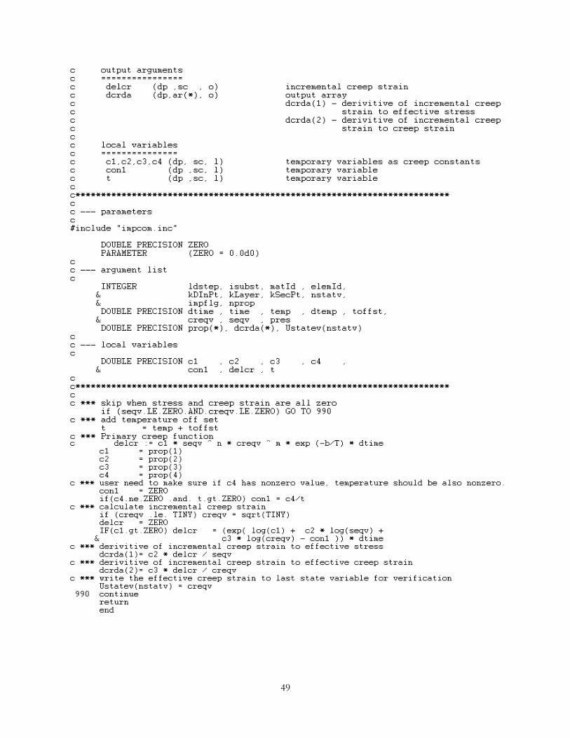
49

50
Source Code 2: LCSP Usercreep.F Source (TBOP = 100)
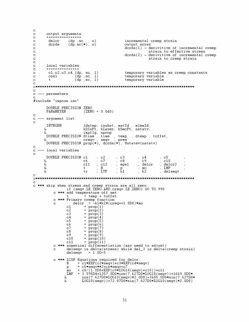
51

52
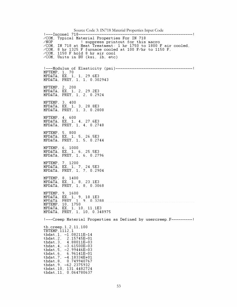
53
Source Code 3: IN718 Material Properties Input Code

54
Source Code 4: APDL Input File (Case of 109 ksi and 1112 °F

55
APPENDIX C: MATLAB SOURCE CODE
Source Code 5: Excel Data Reading & Result Writing M-code

56

57
Source Code 6: LCSP Generated Modified Curve Fitting Function

58

59

60

61

62

63

64

65
REFERENCES
1. Energy Materials: Robust prediction of full creep curves from minimal data and time to rupture model. Holmstrom, S. and Auerkari, P. 4, Kemistintie : Institute of Materials, Minerals and Mining and W. S. Maney & Son Ltd, 2006, Vol. 1.
2. Boresi, P. Arthur. Advanced Mechanics of Materials Sixth Edition. Hoboken : John Wiley & Sons, Inc, 2003. 0-471-43881-2.
3. Journal Of Materials Science: Review, Mathematical description of the mechanical behaviour of metallic materials under creep conditions. Batsoulas, N. D. 10, Patras : Chapman & Hall, 1997, Vol. 32. 0022-2461.
4. Betten, Josef. Creep Mechanics. Berlin : Springer-Verlag Berlin Heidelberg, 2008. 5. Computational Materials Science: Benchmarks for finite element analysis of creep continuum damage mechanics. Becker, A.
A., et al. pg. 34-41, Nottingham : Elsevier Science B. V., 2002, Vol. 25. 6. On the Viscous Flow in Metals and Allied Phenomena. C., Andrade E. N. DA. London : The Royal Society of
London, 1910. 7. Computational Materials Science: Benchmarks for finite element analysis of creep continuum damage mechanics. Becker, A.
A., et al. pg. 34-41, Nottingham : Elsevier Science B. V., 2002, Vol. 25. 0927-0256. 8. ECCC Recommendations and Guidance for the assessment of Creep Strain Data. Holdsworth, S. R. 5, United
Kingdom : ECCC (European Creep Collaborative Committee), 2003, Vol. 5. 9. International Journal of Damage Mechanics: A Damage Mechanics Model for Creep and Oxygen Embrittlement in Metals.
Deng, Xiaomin, Ma, Fashang and Sutton, A. Michael. Columbia : Sage Publications, 2005, Vol. 14. 1056-7895.
10. Energy Materials; Robust prediction of full creep curves from minimal data and time to rupture model. Holmstrom, S. and Auerkari, P. 4, Kemistintie : Maney Publishing, 2006, Vol. 1. 1748-9245.
11. Materials Science and Engineering A: Time-independent formulation for creep damage modeling in metals based on void and crack evolution. Esposito, Luca and Bonora, Nicola. 15, s.l. : Elsevier, 2009, Vols. 510 - 511. 0921-5093.
12. Uniaxial high-temperature creep property predictions made by CDM and MPC omega techniques for ASME SA 455 steel. Manu, C. C., Birk, A. M. and Y., Kim I. 4, Tarrytown : Pergamon, 2009, Vol. 16. 1350-6307.
13. Nuclear Engineering and Design: A review of creep analysis and design under multi-axial stress states. Yao, Hua-Tang, et al. s.l. : Elsevier, 2007, Vol. 237. 0029-5493.
14. Jadaan, M. Osama. Deterministic Multiaxial Creep and Creep Rupture Enhancements for CARES/Creep Integrated Design Code. s.l. : National Aeronautics and Space Administration (NASA), 1968.
15. Journal of Materials Engineering and Performance; Creep Constitutive Model and Component Lifetime Estimation: The Case of Niobium-Modified 9Cr-1Mo Steel Weldments. Lewis, Gladius and Shaw, M. Kevin. New York : Springer, 2010, Vol. Online First. 1059-9495.
16. International Journal of Pressure Vessels and Piping. Law, M., Payten, W. and Snowden, K. Northern Ireland : Elsevier Science Ltd., 1998, Vol. 75. 0308-0161.
17. International Journal of Pressure Vessels & Piping; Creep damage simulation of thick-walled tubes using the θ projection concept. Loghman, A. and Wahad, M. A. Northern Ireland : Elsevier, 1996, Vol. 67. 0308-0161.
18. Metals and Materials International: Creep Strain and Creep-Life Prediction for Alloy 718 Using the Omega Method. Yeom, Jong-Taek, et al. 6, Seoul : Springer, 2003, Vol. 9.
19. Imaoka, Sheldon. User Creep Subroutine. s.l. : ANSYS Inc, 2007. Memo Number: STI074A. 20. Guide to ANSYS User Programmable Features, ANSYS Release 10.0. Canonsburg : ANSYS, Inc, 2005. 21. Klopp, D. William. Ni-4100:IN718 (Code 4103). Aerospace Structural Metals Handbook. West Lafayette :
Purdue Research Foundation, 1995. 22. Cullen, T.M. and Freeman, J.W. Nasa Contractor Report (NASA CR-268): The Mechanical Properties of
Inconel 718 Sheet Alloy at 800, 1000, and 1200. Washington, D.C. : National Aeronautics and Space Administration, 1965.
23. High Temp Metals 800-500-2141 - Inconel 718 Technical Data. High Temp Metals. [Online] High Temp Metals, Inc., July 29, 2011. [Cited: Febuary 15, 2011.] http://www.hightempmetals.com/techdata/hitempInconel718data.php.
24. Programmer's Manual for ANSYS Release 12.0. s.l. : SAS IP Inc, 2009.

66
25. Developing an ANSYS Creep Model for Polypropylene from Experimental Data. Proceedings of International ANSYS Conference. Dropik, M., Johnson, D. and Roth, D. s.l. : N/A, 2002.
26. Shults, Carlos. Implicit Delayed Norton Creep Implememnted. s.l. : PADT Inc. 27. Nuclear Engineering and Design; Long-term creep rupture behavior of smoothed and notched bar specimens of low-carbon
nitrogen-controlled 316 stainless steel (316FR) and their evalution. Takahashi, Yukio, Hiroshi, Shibamoto and Kazuhiko, Inoue. s.l. : Elsevier, 2008, Vol. 238. 0029-5493.
28. Materials Science and Engineering A. Yu, Q. M., et al. s.l. : Elsevier, 2009, Vol. 520. 0921-5093. 29. Inouye, F. T., et al. Application of Alloy 718 in M-1 Engine Components. Washington : National Aeronautics
and Space Administration (NASA), 1967. 30. Notch effects on creep behaviour of CMSX-4 superalloy single crystals. Lukas, P., Preclik, P. and Cadek, J. s.l. :
Elsevier, 2001, Vol. 298. 0921-5093. 31. International Journal of Pressure Vessels and Piping: A comparison of creep models for nickel base alloys advanced energy
systems. Swindeman, R.W. and Swindeman, M.J. Lancaster : Elsevier, 2008, Vol. 85. 0308-0161. 32. Transactions of The Indian Institute of Metals: A Stochastic model for evolution of creep damage in engineering materials.
Roy, N., Ghosh, R.N. and Bose, S.C. 2-3, Jamshedpur : TIIM, 2010, Vol. 63. 33. Engineering Failure Analysis: Uniaxial High-Temperature creep property predictions made by CDM and MPC omega
techniques for ASME SA 455 Steel. Manu, C.C., Birk, A.M. and Kim, I.Y. s.l. : Elsevier, 2009, Vol. 16. 1350-6307.
34. Metallurgical and Materials Transactions A: Creep-Behavior Modeling of the Single-Crystal Superalloy CMSX-4. MacLachlan, D. W. and Knowles, D. M. Cambridge : TMS and ASM International, 2000, Vol. 31A.
35. ACTA PHYSICA SINICA: A STATISTICAL THEORY OF CREEP FRACTURE. HUI-YING, Xu and XIU, XING. 8, Beijing : National Natural Science Fundation of China, 1997, Vol. 6.
36. Materials Letters: Study of standard heat treatment on mechanical properties of Inconel 718 using ball indentation technique. Ghosh, Sabita, Yadav, Sandip and Goutam, Das. s.l. : Elsevier, 2008, Vol. 62. 2619-2622.
37. Strain: An Advanced Creep Model Allowing for Hardening and Damage Effects. Calı, C., Cricrı, G. and Perrella, M. s.l. : Blackwell Publishing Ltd., 2010, Vol. 46.
38. Ansys Element Reference 12.1. Canonsburg : SAS IP, Inc., 2009.