Applied Mathematics, 2017, 8, 537-549 http://www.scirp.org/journal/am

ISSN Online: 2152-7393 ISSN Print: 2152-7385

DOI: 10.4236/am.2017.84043 April 28, 2017

Modified Function Projective Synchronization of Complex Networks with Multiple Proportional Delays

Xiuliang Qiu1, Honghua Bin2*, Licai Chu2

1Chengyi University College, Jimei University, Xiamen, China 2School of Science, Jimei University, Xiamen, China

Abstract This paper deals with the modified function projective synchronization prob-lem for general complex networks with multiple proportional delays. With the existence of multiple proportional delays, an effective hybrid feedback control is designed to attain modified function projective synchronization of net-works. Numerical example is provided to show the effectiveness of our result.

Keywords Complex Networks, Modified Function Projective Synchronization, Proportional Delays, Hybrid Feedback Control

1. Introduction

In recent decades, synchronization as a popular research topic of complex networks has been widespread concern around the world [1] [2] [3] [4]. With the deepening of research on complex networks synchronization problems, the concept and theory of synchronization have been greatly developed, and many different types of synchronization concepts have been found and put forward. such as complete synchronization [5], cluster synchronization [6], lag synchro- nization [7], generalized synchronization [8], quasi-synchronization [9], phase synchronization [10], anti-synchronization [11], projective synchronization [12], function projective synchronization [13] [14].

Modified function projective synchronization(MFPS) has been proposed and extensively investigated in the latest. MFPS means that the drive and response systems could be synchronized up to a desired scaling function matrix [15]. It is easy to see that the definition of MFPS encompasses projective synchronization

How to cite this paper: Qiu, X.L., Bin, H.H. and Chu, L.C. (2017) Modified Func-tion Projective Synchronization of Com-plex Networks with Multiple Proportional Delays. Applied Mathematics, 8, 537-549. https://doi.org/10.4236/am.2017.84043 Received: March 24, 2017 Accepted: April 25, 2017 Published: April 28, 2017 Copyright © 2017 by authors and Scientific Research Publishing Inc. This work is licensed under the Creative Commons Attribution International License (CC BY 4.0). http://creativecommons.org/licenses/by/4.0/

Open Access

X. L. Qiu et al.

538

and function projective synchronization. The MFPS of general complex networks can reveal that the nodes of complex networks could be synchronize up to an equilibrium point or periodic orbit with a desired scaling function matrix. Because the unpredictability of the scaling function in MFPS can additionally enhance the security of communication, MFPS has attracted the interest of many researchers in various fields. On the basis of an adaptive fuzzy nonsingular terminal sliding mode control scheme, a general method of MFPS of two different chaotic systems with unknown functions was investigated in [16]. The work in [17] gives MFPS of a class of chaotic systems. MFPS of a classic chaotic systems with unknown disturbances was investigated by adaptive integral sliding mode control [18]. Ref. [19] investigates the adaptive MFPS of a class of complex four-dimensional chaotic system with one cubic cross-product term in each equation. Ref. [20] investigates the MFPS of two different chaotic systems with parameter perturbations.

A simple general scheme of MFPS in complex dynamical networks (CDNs) is investigated in this paper, considering that external disturbances and unmodeled dynamics are always unavoidably in the practical evolutionary processes of synchronization, MFPS in CDNs with proportional delay and disturbances will be investigated by the proposed scheme.The rest of this paper is organized as follows. Some definitions and a basic lemma are given in Section 2. In Section 3, the synchronization of the complex networks with proportional delays by the pinning control method is discussed by the way of equivalent system. Finally, computer simulation is performed to illustrate the validity of the proposed method in Section 4.

2. Preliminaries

Consider a generally controlled complex dynamical networks consisting of N identical linearly coupled nodes with multiple proportional delays by the following equations:

( ) ( )( ) ( ) ( )1

, 1, 2, , , 1,N

i i ij j ij ij

t t g q t t i N t=

= + + = ≥∑x f x x u (2.1)

where 1, 2, , , 1,i N t= ≥ ( )T1 2, , , n

i i i inx x x= ∈x R denotes the state vector of the ith node, : n n→f R R is a continuously differentiable vector function determining the dynamic behavior of the nodes, ( ) n

i t ∈u R is the control input.

( ) N Nijg ×= ∈G R is the coupling configuration matrix representing the topolo-

gical structure of the network, where 0ijg > if there is a connection between node i and node j; otherwise 0ij jig g= = , and the diagonal elements of matrix G are defined by

1,, 1, 2, , ,

N

ii ijj j i

g g i N= ≠

= − =∑ (2.2)

, , 1, 2, ,ijq i j n= are proportional delay factors and satisfy

{ }1 ,

0 1, minij iji j nq q q

≤ ≤< ≤ = . Furthermore, the complex network described in (2.1)

possess initial conditions of ( ) [ ]0 , ,1i ix t x t q= ∈ , ( )0 1, 2,3, ,ix i N= are constants.

X. L. Qiu et al.

539

Definition 1. (MFPS) The network (2.1) with proportional delays is said to achieve modified function projective synchronization if there exists a continu- ously differentiable scaling function matrix ( )tM such that

( ) ( ) ( )lim 0, 1, 2, , ,itt t t i N

→+∞− = =x M x (2.3)

where ⋅ stands for the Euclidean vector norm, ( ) ( )( )it diag tα=M is a modified function matrix, and each modified function ( )i tα is a continuously differential function and is bounded as ( )i itα δ≤ < ∞ , ( ) 0i tα ≠ , iδ is a finite constant, and ( ) nt ∈x R can be an equilibrium point, or a periodic orbit, or an orbit of a chaotic attractor, which satisfies ( ) ( )( )t t=x f x .

Considering the actual evolutionary processes of synchronization, external disturbances and unmodeled dynamics are always unavoidable. MFPS in CDNs with disturbances will be investigated further as follows:

( ) ( )( ) ( ) ( ) ( )1

, 1, 2, , , 1,N

i i ij j ij i ij

t t g q t t t i N t=

= + + + = ≥∑x f x x d u (2.4)

where ( )T1 2, , , n

i i i inx x x= ∈x R denotes the state vector of the ith node, : n n→f R R is a continuously differentiable vector function determining the

dynamic behavior of the nodes, ( ) ni t ∈u R is the control input and ( ) n

i t ∈d R is the mismatched terms, which could exist in many perturbation, noise disturbance. ( ) N N

ijg ×= ∈G R is the coupling configuration matrix represent- ing the topological structure of the network, and the diagonal elements of matrix G are defined by Equation (2.2).

In the following, some necessary assumptions are given. Assumption 1. The derivative of scaling function ( )i tα is bounded, that is

( ) *i t aα ≤ (2.5)

for all t R+∈ , where *a R+∈ is the upper limit of the ( ) , 1, 2, ,i t i Nα = .

Assumption 2. The norm of the mismatched terms ( ) ( )1, 2, ,i t i N=d are bounded, that is

( ) *i it d≤ < ∞d (2.6)

where *id R+∈ is the upper limit of the norm of ( )id t .

In this paper, 1 2,M M denote the upper limit of the norm of ( ) ( )( )t tM f y , ( ) ( )t tM y , respectively. nI= ⊗Q G , ⊗ represent the Kroncecker product, ( )maxλ A denotes the maximum eigenvalue for symmetric matrix A .

Lemma 1. [21] For any vector , n∈x y R and positive definite matrix n n×∈S R , the following matrix inequality holds:

T T T 12 −≤ +x y x Sx y S y (2.7)

3. MFPS in Complex Networks with Multiple Proportional Delays

In this section, a hybrid feedback control method for realizing modified function projective synchronization in complex dynamical networks with multiple proportional delays is proposed.

X. L. Qiu et al.

540

Let ( ) ( )eti it =y x , then a couple of networks (2.1) and (2.4) is equivalently

transformed into the following couple of complex networks with constant delay and time varying coefficients

( ) ( )( ) ( ) ( )1

e , 1, 2, , ,N

ti i ij j ij i

jt t g t t i Nτ

=

= + − + =

∑y f y y U

(3.1)

and

( ) ( )( ) ( ) ( ) ( )1

e , 1, 2, , ,N

ti i ij j ij i i

jt t g t t t i Nτ

=

= + − + + =

∑y f y y D U

(3.2)

where 0t ≥ , ( )elog 0ij ijqτ = − ≥ , ( ) ( ) ( ) ( )e , et ti i i it t= =D d U u , and

( ) ( ) [ ]( ), 0 ,i iy s x s C τ= ∈ − , in which ( ) [ ]0 , , 0i ix s x s τ= ∈ − , { }1 ,max iji j n

τ τ≤ ≤

= .

Definition 2. The network (3.2) is said to achieve modified function projec- tive synchronization if there exists a continuously differentiable scaling function matrix ( )tM such that

( ) ( ) ( ) ( )lim lim 0, 1, 2, , ,i it tt t t t i N

→+∞ →+∞= − = =e y M y (3.3)

where ⋅ stands for the Euclidean vector norm, ( ) ( )( )it diag tα=M is a modified function matrix, and each modified function ( )i tα is a continuously differential function and is bounded as ( )i itα δ≤ < ∞ , ( ) 0i tα ≠ , iδ is a finite constant, and ( ) nt ∈y R can be an equilibrium point, or a periodic orbit, or an orbit of a chaotic attractor, which satisfies ( ) ( )( )ett t=y f y .

Theorem 1. Suppose Assumptions 1 and 2 hold. For a given synchronization scaling function matrix ( )tM , if there exist positive constants 1

ik , 2ik and

3ik which satisfy 1 *

1i ik d M≥ + , 22ik M≥ and

T3

max1

2 2ik λ

≥ +

QQ , CDNs

with disturbance (3.2) can realize modified function projective synchronization via the control law :

( ) ( )( ) ( ) ( )( ) ( )1 2 3e , 1, 2, , ,ti i i i i i it t k k sgn t k t i N−= − − + − =U f y e e (3.4)

where ( )sgn ⋅ denotes the sign function. Proof. Define

( ) ( ) ( ) ( ) , 1, 2, , ,i it t t t i N= − =e y M y (3.5)

where ( )tM is a modified function matrix. It follows from (3.2) and (2.2) that

( ) ( )( ) ( ) ( ) ( )

( ) ( ) ( ) ( )( )1

e

e , 1, 2, , ,

Nt

i i ij j ij i ij

t

t t g t t t

t t t t i N

τ=

= + − + +

− − =

∑e f y e D U

M s M f y

(3.6)

Construct the Lyapunov function

( ) ( ) ( ) ( ) ( )T T

1 1

1 1e d ,2 2 ij

N Ntti i i it

i iV t t t v v v

τ−

−= =

= +∑ ∑∫e e e e (3.7)

The time derivative of V(t) along the trajectories of system (3.6) is

X. L. Qiu et al.

541

( ) ( ) ( ) ( ) ( ) ( ) ( ) ( ) ( )

( ) ( ) ( ) ( ) ( ) ( )

( ) ( )( ) ( ) ( ) ( ) ( ) ( ) ( ) ( )( )

T T T T

1 1 1 1

T T T

1 1 1

T

1 1

1 1 1e e2 2 2

1 1e2 2

e e e

N N N Nt t

i i i i i i i ij i iji i i i

N N Nt

i i i i i ij i iji i i

N Nt t t

i i ij j ij i ii j

V t t t t t t t t t

t t t t t t

t t g t t t t t t t

τ τ

τ τ

τ

− −

= = = =

−

= = =

−

= =

= − + + − − −

≤ + − − −

= + − + + − −

∑ ∑ ∑ ∑

∑ ∑ ∑

∑ ∑

e e e e e e e e

e e e e e e

e f y e D U M y M f y

( ) ( ) ( ) ( )

( ) ( )( ) ( ) ( ) ( ) ( ) ( ) ( )( )

( ) ( ) ( ) ( ) ( ) ( )

( ) ( ) ( ) ( )( ) ( ) ( ) ( ) ( ) ( )( )

T T

1 1

T

1

T T T

1 1 1 1

T 1 2 3

1

1 12 2

e

1 12 2

e e

N N

i i i ij i iji i

Nt

i i i ii

N N N N

i ij j ij i i i ij i iji j i i

Nt t

i i i i i i ii

t t t t

t t t t t t t t

t g t t t t t

t t k k sgn t k t t t t t

τ τ

τ τ τ

= =

−

=

= = = =

− −

=

+ − − −

= + + − −

+ − + − − −

= + − − − − −

∑ ∑

∑

∑∑ ∑ ∑

∑

e e e e

e f y D U M y M f y

e e e e e e

e D e e M y M f y

( ) ( ) ( ) ( ) ( ) ( )

( ) ( ) ( ) ( )( ) ( ) ( ) ( ) ( )( )

( ) ( ) ( ) ( ) ( ) ( ) ( ) ( )

T T T

1 1 1 1

T 1 2

1

3 T T T T

1 1 1 1 1

1

1 12 2

e e

1 12 2

N N N N

i ij j ij i i i ij i iji j i i

Nt t

i i i i ii

N N N N N

i i i i ij j ij i i i ij i iji i j i i

N

i

t g t t t t t

t t k k sgn t t t t t

k t t t g t t t t t

τ τ τ

τ τ τ

= = = =

− −

=

= = = = =

=

+ − + − − −

= + − − − −

− + − + − − −

≤

∑∑ ∑ ∑

∑

∑ ∑∑ ∑ ∑

∑

e e e e e e

e D e M y M f y

e e e e e e e e

e ( ) ( ) ( ) ( ) ( ) ( ) ( )( )

( ) ( ) ( ) ( ) ( ) ( ) ( ) ( )

T 1 2

3 T T T T

1 1 1 1 1

e e

1 12 2

t ti i i i

N N N N N

i i i i ij j ij i i i ij i iji i j i i

t t k k t t t t

k t t t g t t t t tτ τ τ

− −

= = = = =

+ − − + +

− + − + − − −∑ ∑∑ ∑ ∑

D M y M f y

e e e e e e e e

(3.8)

Because chaos systems and the scaling function are bounded, ( )ty and ( )i tα are bounded. Furthermore, f is a continuously vector function, there

exists a positive constants 1M satisfying ( ) ( )( ) 1t t M≤M f y . Because Assumption 1 holds, there exists a positive constant 1M satisfying

( ) ( ) 2t t M≤M y . Because Assumption 2 holds, there exists a positive constant *id satisfying ( ) ( )* 1, 2, ,i it d i N≤ =D :

( ) ( ) ( ) ( )

( ) ( ) ( ) ( ) ( ) ( )

( ) ( ) ( ) ( ) ( )

( ) ( )

T * 1 2 3 T1 2

1 1

T T T

1 1 1 1

T * 1 2 3 T1 2

1 1

T

1 1 1

e e

1 12 2

e

12

N Nt t

i i i i i i ii i

N N N N

i ij j ij i i i ij i iji j i i

N Nt

i i i i i i ii i

N N

i ij j iji j i

V t t d k k M M k t t

t g t t t t t

t d M k M k k t t

t g t

τ τ τ

τ

− −

= =

= = = =

−

= =

= = =

≤ − − + + −

+ − + − − −

= + − + − −

+ − +

∑ ∑

∑∑ ∑ ∑

∑ ∑

∑∑

e e e

e e e e e e

e e e

e e

( ) ( ) ( ) ( )T T

1

12

N N

i i i ij i iji

t t t tτ τ=

− − −∑ ∑e e e e

(3.9)

Tanking 1 *1i ik d M≥ + and 2

2ik M≥ , 1, 2, ,i N= , we obtain

( ) ( ) ( ) ( ) ( )

( ) ( ) ( ) ( )

3 T T

=1 1 1

T T

1 1

1 12 2

N N N

i i i ij j iji i j

N N

i i i ij i iji i

V t k t t t g t

t t t t

τ

τ τ

= =

= =

≤ − + −

+ − − −

∑ ∑∑

∑ ∑

e e e e

e e e e

(3.10)

X. L. Qiu et al.

542

where ( )3 3 3 31 2min , , , Nk k k k= .

Let ( ) ( ) ( ) ( )( )TT T T1 2, , , nN

Nt t t t= ∈e e e e R . Then by Lemma 1, we have

( ) ( ) ( ) ( ) ( )( ) ( ) ( ) ( )

( ) ( ) ( ) ( ) ( ) ( )

( ) ( )

3 T T

T T

3 T T T T

T3 T

max

1 12 2

1 12 2

12 2

ij

ij ij

V t k t t t t

t t t t

k t t t t t t

k t t

τ

τ τ

λ

≤ − + −

+ − − −

≤ − + +

≤ − + +

e e e Qe

e e e e

e e e QQ e e e

QQ e e

(3.11)

Taking T

3max

12 2

k λ

≥ +

QQ , we obtain

( ) 0.V t ≤ (3.12)

According to the Lyapunov stability theory, the error system (3.6) is asymptotically stable. This completes the proof.

Corollary 1. Suppose Assumptions 1 hold. For a given synchronization scaling function matrix ( )tM , if there exist positive constants 1

ik , 2ik , 3

ik ,

which satisfy 11ik M≥ , 2

2ik M≥ and T

3max

12 2ik λ

≥ +

QQ , CDNs without

disturbance (3.1) can realize modified function projective synchronization via the control law :

( ) ( )( ) ( ) ( )( ) ( )1 2 3e , 1, 2, , ,ti i i i i i it t k k sgn t k t i N−= − − + − =U f y e e (3.13)

where ( )sgn ⋅ denotes the sign function. By Theorem 1, it is easy to see that a similar proof holds for ( ) ( )0 1, 2, ,i t i N= =D . Thus, the proof is omitted here.

Though the proposed error feedback control method is very simple, Choosing the appropriate feedback gains 1

ik , 2ik and 3

ik is still difficult. Thus, finding appropriate gains 1

ik , 2ik and 3

ik to achieve synchronization is still a challenging problem. In the following, an adaptive scheme is established in order to select the appropriate gains 1

ik , 2ik and 3

ik to realize MFPS in CDNs with or without disturbances.

Theorem 2. Suppose Assumptions 1 and 2 hold. For a given synchronization scaling function matrix ( )tM , CDNs with disturbance (3.2) can realize modified function projective synchronization via the control law :

( ) ( )( ) ( ) ( )( ) ( )( ) ( ) ( )1 2 3 , 1, 2, , ,ti i i i i i it t k t k t sgn t k t t i N−= − + − − − =U f y e e e (3.14)

( ) ( ) ( )( )1 1 T , 1, 2, , ,i i i ik t l t sgn t i N= =e e

(3.15)

( ) ( ) ( )( )2 2 Te , 1, 2, , ,ti i i ik t l t sgn t i N−= =e e

(3.16)

( ) ( ) ( )3 3 T , 1, 2, , ,i i i ik t l t t i N= =e e

(3.17)

where ( )sgn ⋅ denotes the sign function. 1 20, 0i il l> > and 3 0il > are arbi- trary positive constants. Proof. Construct the Lyapunov function

X. L. Qiu et al.

543

( ) ( ) ( ) ( ) ( ) ( )( )

( )( ) ( )( )

2T T 1 11

1 1 1

2 22 2 3 32 3

1 1

1 1 1 1e d2 2 2

1 1 1 1 ,2 2

ij

N N Ntti i i i i it

i i i iN N

i i i ii ii i

V t t t v v v k t kl

k t k k t kl l

τ−

−= = =

= =

= + + −

+ − + −

∑ ∑ ∑∫

∑ ∑

e e e e (3.18)

The time derivative of V(t) along the trajectories of (3.6) is

( ) ( ) ( ) ( ) ( ) ( ) ( ) ( ) ( )

( )( ) ( ) ( )( ) ( ) ( )( ) ( )

( ) ( ) ( ) ( ) ( ) ( )

T T T T

1 1 1 1

1 1 1 2 2 2 3 3 31 2 3

1 1 1

T T T

1 1 1

1 1 1e e2 2 2

1 1 1

1 1e2 2

N N N Nt t

i i i i i i i ij i iji i i i

N N N

i i i i i i i i ii i ii i i

N N Nt

i i i i i ij i iji i i

V t t t t t t t t t

k t k k t k t k k t k t k k tl l l

t t t t t t

τ τ

τ τ

− −

= = = =

= = =

−

= = =

= − + + − − −

+ − + − + −

≤ + − − −

+

∑ ∑ ∑ ∑

∑ ∑ ∑

∑ ∑ ∑

e e e e e e e e

e e e e e e

( )( ) ( ) ( )( ) ( ) ( )( ) ( )

( ) ( )( ) ( ) ( ) ( ) ( ) ( ) ( ) ( )( )

( ) ( ) ( ) ( ) ( )

1 1 1 2 2 2 3 3 31 2 3

1 1 1

T

1 1

T T 1 1 11

1 1 1

1 1 1

e e e

1 1 12 2

N N N

i i i i i i i i ii i ii i i

N Nt t t

i ij j ij i ii j

N N N

i i i ij i ij i i ii i i i

i

k t k k t k t k k t k t k k tl l l

t z t g t t t t t t t

t t t t k k kl

τ

τ τ

= = =

−

= =

= = =

=

− + − + −

= + − + + − −

+ − − − + −

+

∑ ∑ ∑

∑ ∑

∑ ∑ ∑

e f e D U M y M f y

e e e e

( ) ( )

( ) ( )( ) ( ) ( ) ( ) ( ) ( ) ( )( )

( ) ( ) ( ) ( ) ( ) ( )

( ) ( )

2 2 2 3 3 32 3

1 1

T

1

T T T

1 1 1 1

1 1 1 2 2 2 31 2 3

1 1 1

1 1

e

1 12 2

1 1 1

N N

i i i i i iii i

Nt

i i ii

N N N N

i ij j ij i i i ij i iji j i i

N N N

i i i i i i i ii i ii i i

k k k k k kl l

t z t t t t t t t

t g t t t t t

k k k k k k k kl l l

τ τ τ

=

−

=

= = = =

= = =

− + −

= + + − −

+ − + − − −

+ − + − + −

∑ ∑

∑

∑∑ ∑ ∑

∑ ∑ ∑

e f D U M y M f y

e e e e e e

( )

( ) ( ) ( ) ( )( ) ( ) ( ) ( ) ( ) ( )( )

( ) ( ) ( ) ( ) ( ) ( )

( ) ( ) ( )

( )

3 3

T 1 2 3

1

T T T

1 1 1 1

1 1 1 2 2 2 3 3 31 2 3

1 1 1

T

1

e

1 12 2

1 1 1

i

Nt t

i i i i i i ii

N N N N

i ij j ij i i i ij i iji j i i

N N N

i i i i i i i i ii i ii i i

N

i ii

k

t t k k e sgn t k t t t t t

t g t t t t t

k k k k k k k k kl l l

t

τ τ τ

− −

=

= = = =

= = =

=

= + − − − − −

+ − + − − −

+ − + − + −

=

∑

∑∑ ∑ ∑

∑ ∑ ∑

∑

e D e e M y M f y

e e e e e e

e D ( ) ( ) ( ) ( ) ( )( ) ( ) ( ) ( ) ( )

( ) ( ) ( ) ( ) ( )( ) ( ) ( )

( ) ( ) ( ) ( ) ( ) ( )( ) ( ) ( )

( ) ( )

T T

1 1 1

T 1 2 T 3 T

1 1 1

T T

1 1 1

T

1

12

1 e2

e

1 12 2

N N Nt

i ij j ij i ii j i

N N Nt

i ij i ij i i i i i i ii i i

N N Nt

i i i ij j iji i j

N

i ii

t t t t t t g t t t

t t k k t sgn t k t t

t t t t t y t t g t

t t

τ

τ τ

τ

−

= = =

−

= = =

−

= = =

=

− − + − +

− − − − + −

≤ + + + −

+ −

∑∑ ∑

∑ ∑ ∑

∑ ∑∑

∑

e M y M f y e e e e

e e e e e e

e D M y M f e e

e e ( ) ( ) ( ) ( ) ( ) ( )

( ) ( ) ( ) ( )( )( ) ( ) ( ){ }

( ) ( ) ( ) ( ) ( ) ( ) ( ) ( )

T 1 2 T 3 T

1 1 1

T 1 2

1

T T T 3 T

1 1 1 1 1

e

e

1 12 2

N N Nt

i ij i ij i i i i i ii i i

Nt

i i i ii

N N N N N

i ij j ij i i i ij i ij i i ii j i i i

t t k k t k t t

t t t y t k t t k

t g t t t t t k t t

τ τ

τ τ τ

−

= = =

−

=

= = = = =

− − − + −

= + − + −

+ − + − − − −

∑ ∑ ∑

∑

∑∑ ∑ ∑ ∑

e e e e e

e D M f M y

e e e e e e e e

(3.19)

X. L. Qiu et al.

544

Because chaos systems and the scaling function are bounded, ( )ty and ( )i tα are bounded. Furthermore, f is a continuously vector function, there

exists a positive constants 1M satisfying ( ) ( )( ) 1t t M≤M f y . Because As- sumption 1 holds, there exists a positive constant 2M satisfying ( ) ( ) 2t t M≤M y . Because Assumption 2 holds, there exists a positive constant *

id satisfying ( ) ( )* 1, 2, ,i it d i N≤ =D :

( ) ( ) ( ) ( )

( ) ( ) ( ) ( )

( ) ( ) ( ) ( )

T * 1 21 2

1

T T

1 1 1

T 3 T

1 1

e

12

12

Nt

i i i ii

N N N

i ij j ij i ii j i

N N

i ij i ij i i ii i

V t t d M k M k

t g t t t

t t k t t

τ

τ τ

−

=

= = =

= =

≤ + − + −

+ − +

− − − −

∑

∑∑ ∑

∑ ∑

e

e e e e

e e e e

(3.20)

Tanking 1 *1i ik d M≥ + and 2

2ik M≥ , = 1, 2, ,i N, we obtain

( ) ( ) ( ) ( ) ( )

( ) ( ) ( ) ( )

T T

1 1 1

T 3 T

1 1

12

12

N N N

i ij j ij i ii j i

N N

i ij i ij i ii i

V t t g t t t

t t k t t

τ

τ τ

= = =

= =

≤ − +

− − − −

∑∑ ∑

∑ ∑

e e e e

e e e e

(3.21)

where ( )3 3 3 31 2min , , , Nk k k k= .

Let ( ) ( ) ( ) ( )( )TT T T1 2, , , nN

Nt t t t= ∈e e e e R . Then by Lemma 1, we have

( ) ( ) ( ) ( ) ( )

( ) ( ) ( ) ( )

( ) ( ) ( ) ( ) ( ) ( ) ( )

( ) ( )

T T

T 3 T

T T T 3 T

T3 T

max

12

12

1 12 2

12 2

ij

ij ij

V t t t t t

t t k t t

t t t t k t t

k t t

τ

τ τ

λ

≤ − +

− − − −

≤ + −

≤ + −

e Qe e e

e e e e

e QQ e e e e e

QQ e e

(3.22)

Taking T

3max

32 2

k λ

= +

QQ , we obtain

( ) ( ) ( )T .V t t t≤ −e e (3.23)

According to the Lyapunov stability theory, the error system (3.6) is asymptotically stable. This completes the proof.

Corollary 2. Suppose Assumptions 1 hold. For a given synchronization scaling function matrix ( )tM , CDNs without disturbance (3.1) can realize modified function projective synchronization via the control law (3.14)-(3.17).

By Theorem 2, it is easy to see that a similar proof holds for ( ) ( )0 1, 2, ,i t i N= =D . Thus, the proof is omitted here.

4. Computer Simulation

In this section, the chaotic Lorenz system is taken as nodes of CDNs to verify the effectiveness of the proposed scheme in Corollary 2.

X. L. Qiu et al.

545

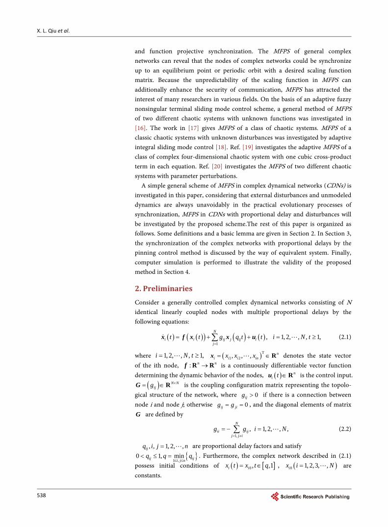
Consider the following single Lorenz system:

( )( )

1 2 1

2 3 1 2

3 1 2 3

x a x x

x b x x xx x x cx

= −

= − − = −

(4.1)

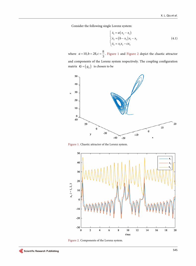
where 810, 28,3

a b c= = = . Figure 1 and Figure 2 depict the chaotic attractor

and components of the Lorenz system respectively. The coupling configuration matrix ( )ijg=G is chosen to be

Figure 1. Chaotic attractor of the Lorenz system.

Figure 2. Components of the Lorenz system.

X. L. Qiu et al.

546

1 0 11 1 00 1 1

− = − −

G

Complex networks with proportional delays can be described as follows:

( )( )( )

( ) ( )( )( )( ) ( ) ( )

( ) ( ) ( )

( ) ( )2 11 3

2 3 1 21

31 2 3

10

28 , 1, 2,3

83

i ii

i i i i ij j ij ij

ii i i

x t x tx tx t x t x t x t g q t t ix t

x t x t x t=

− = − − + + =

−

∑ x u

(4.2)

where the controllers ( )i tu satisfied: ( ) ( )eti it =U u , ( )i tU can be designed

by using Theorem 2 as follows:

( )( ) ( )( )

( )( ) ( ) ( )

( ) ( ) ( )

( ) ( )( )( )( )( )( )( )( )

( )( )( )( )

2 1 1 11 2 3

3 1 2 2 2

331 2 3

10

28 e

83

i i i it

i i i i i i i i i

iii i i

y t y t sgn e t e tt y t y t y t k t k t sgn e t k t e t

e tsgn e ty t y t y t

− = − − − + − − − −

U

with

( ) ( ) ( )( )

( ) ( ) ( )( )

( ) ( )

31 1

1

32 2

1

33 3 2

1

e

i i ij ijj

ti i ij ij

j

i i ijj

k t l t sgn t

k t l t sgn t

k t l t

=

=

=

=

=

=

∑

∑

∑

e e

e e

e

where ( ) ( )eti it =y x , ( ) ( ) ( ) ( )i it t t t= −e y M y , 1, 2,3.i =

In this numerical simulation, we take the initial states as ( ) [ ]T1 0 3 4 4x = − ,

( ) [ ]T2 0 4 1 4x = − , ( ) [ ]T3 0 2 0 5x = − , ( ) [ ]T0 5 3 5x = − . We take ( )11 0 1k = ,

( )12 0 2k = , ( )1

3 0 3k = , ( )21 0 4k = , ( )2

2 0 5k = , ( )23 0 6k = , ( )3

1 0 12k = ,

( )32 0 15k = , ( )3

3 0 16k = , ( )33 0 16k = and

( ) 2π 2π 2π4 sin , 4 cos , 4 sin10 10 10

t t tt diag = + + +

M . The numerical results are

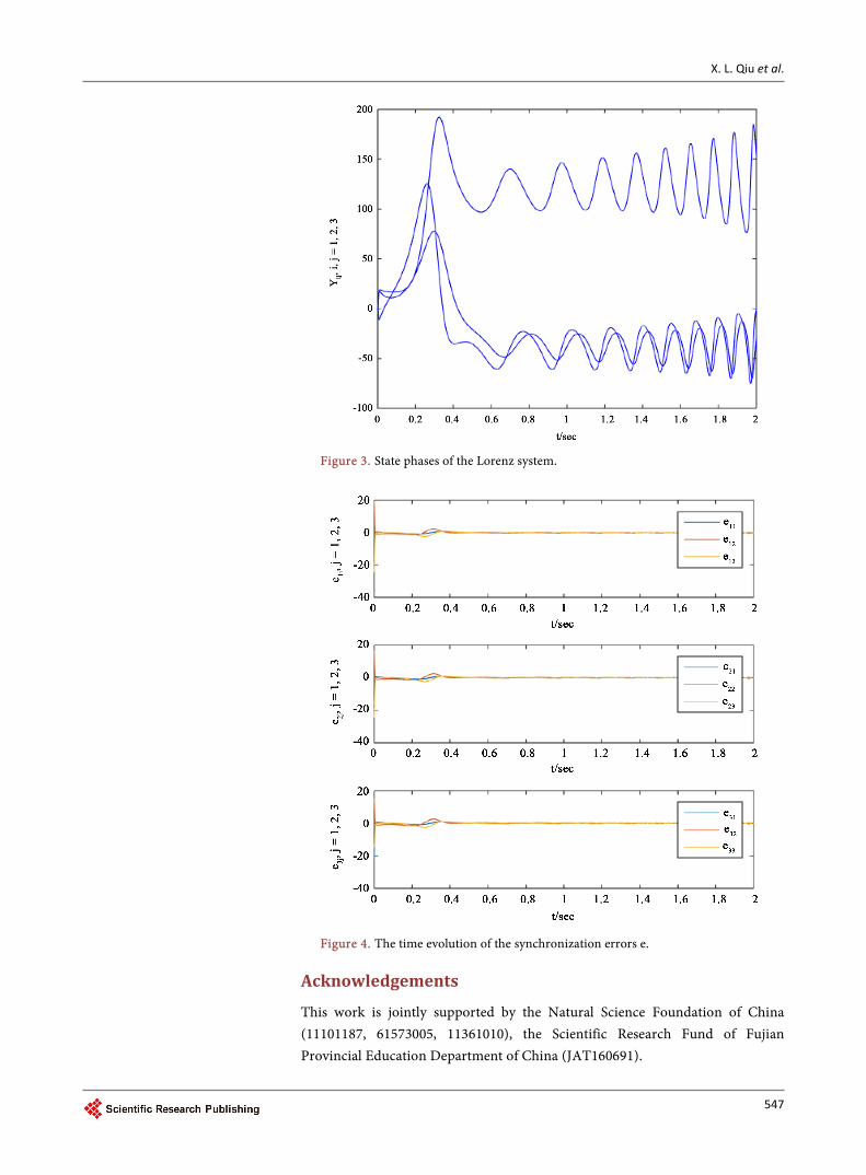
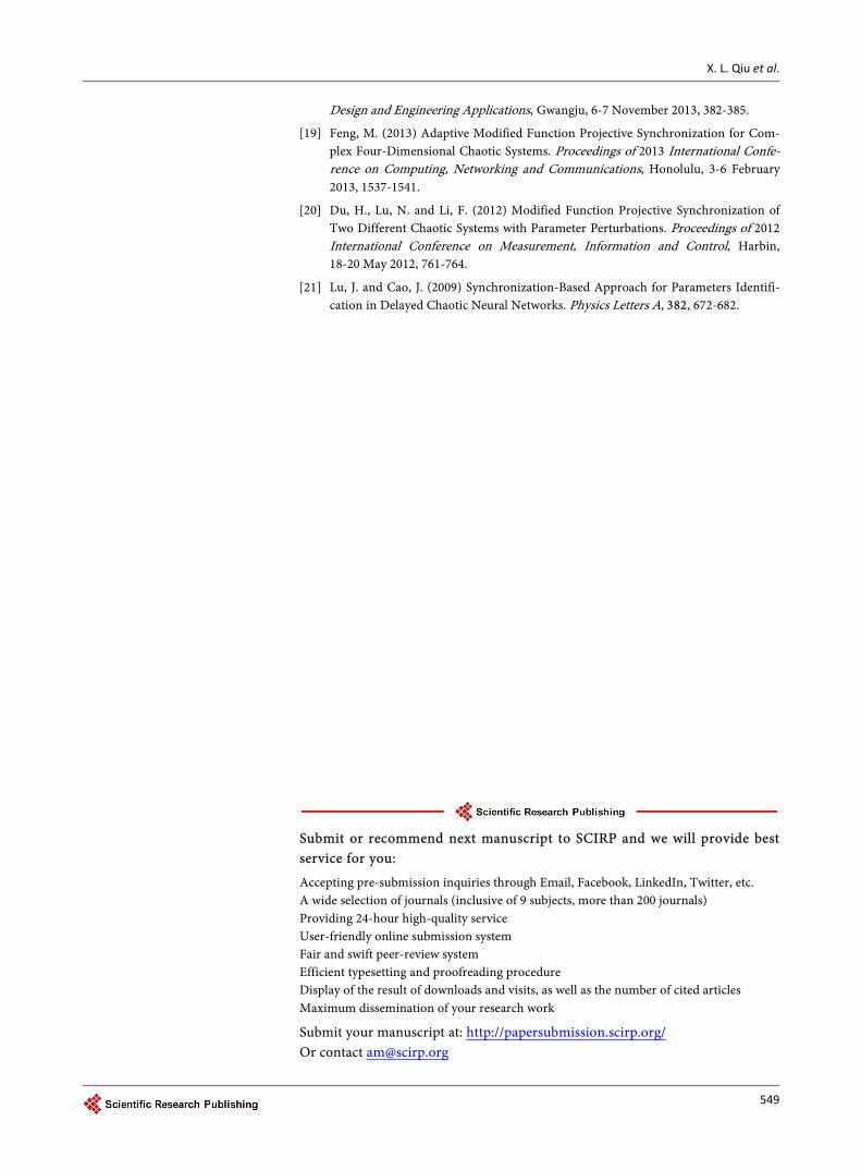
presented in Figure 3 and Figure 4. Figure 3 displays the state phases of the Lorenz system. The time evolution of the synchronization errors is depicted in Figure 4, which displays ( ) 0t →e with t →∞ . These results show that function projective synchronization takes place with the desired scaling function in complex networks (4.2).

5. Concluding Remarks

In this paper, function projective synchronization schemes for complex net- works with proportional delays are given by a error feedback control method. Numerical simulation is provided to show the effectiveness of our result.

X. L. Qiu et al.

547

Figure 3. State phases of the Lorenz system.

Figure 4. The time evolution of the synchronization errors e.

Acknowledgements

This work is jointly supported by the Natural Science Foundation of China (11101187, 61573005, 11361010), the Scientific Research Fund of Fujian Provincial Education Department of China (JAT160691).

X. L. Qiu et al.

548

References [1] Ott, E., Grebogi, C. and Yorke, J.A. (1990) Controlling Chaos. Physical Review Let-

ters, 11, 1196-1199. https://doi.org/10.1103/PhysRevLett.64.1196

[2] Gang, H. and Qu, Z.L. (1994) Controlling Spatiotemporal Chaos in Coupled Map Lattice Systems. Physics Letters A, 72, 68-73. https://doi.org/10.1103/PhysRevLett.72.68

[3] Carroll, T.L. and Pecora, L.M. (1990) Synchronization in Chaotic Systems. Physical Review Letters, 64, 821-824. https://doi.org/10.1103/PhysRevLett.64.821

[4] Yang, T. (2004) A Survey of Chaotic Secure Communication Systems. International Journal of Computational Vision and Robotics, 2, 81-130.

[5] Lu, J.Q. and Cao, J.D. (2005) Adaptive Complete Synchronization of Two Identical or Different Chaotic (Hyperchaotic) Systems with Fully Unknown Parameters. Chaos, 15, 4-9. https://doi.org/10.1063/1.2089207

[6] Wang, T., Li, T., Yang, X., Fei, S. (2012) Cluster Synchronization for Delayed Lur’e Dynamical Networks Based on Pinning Control. Neurocomputing, 83, 72-82.

[7] Shahverdiev, E.M. and Sivaprakasam, S. (2002) Lag Synchronization in Time De-layed Systems. Physics Letters A, 292, 320-324. https://doi.org/10.1016/S0375-9601(01)00824-6

[8] Rulkov, N.F., Sushchik, M.M. and Tsimring, L.S., et al. (1995) Generalized Syn-chronization of Chaotic Oscillators. Physical Review Letters, 51, 980-994.

[9] Wang, L., Qian, W. and Wang, Q. (2015) Bounded Synchronization of a Time Va-rying Dynamical Network with Nonidentical Nodes. International Journal of Sys-tems Science, 46, 1-12. https://doi.org/10.1080/00207721.2013.815825

[10] Rosenblum, M.G., Pikovsky, A.S. and Kurths, J. (1996) Phase Synchronization of Chaos in Directionally Coupled Chaotic Systems. Physical Review Letters, 761, 804- 807.

[11] Kim, C., Rim, S., Kye, W., Yu, J.R. and Park, Y. (2003) Anti-Synchronization of Chaotic Oscillators. Physics Letters A, 320, 39-46. https://doi.org/10.1016/j.physleta.2003.10.051

[12] Mainieri, R. and Rehacek, J. (1999) Projective Synchronization in Three-Dimen- sional Chaotic Systems. Physical Review Letters, 82, 3042-3045.

[13] Tang, X., Lu, J. and Zhang, W. (2007) The FPS of Chaotic System Using Backstep-ping Design. International Journal of Dynamics and Control, 5, 216-219.

[14] Chen, Y. and Li, X. (2009) Function Projective Synchronization between Two Iden-tical Chaotic System. Chaos, Solitons & Fractals, 42, 2399-2402. https://doi.org/10.1016/j.chaos.2009.03.120

[15] Du, H., Zeng, Q. and Wang, C. (2010) Modified Function Projective Synchroniza-tion of Chaotic Systems. Nonlinear Analysis: Real World Applications, 11, 705-712.

[16] Park, J., Lee, J. and Won, S. (2013) Modified Function Projective Synchronization for Two Different Chaotic Systems Using Adaptive Fuzzy Nonsingular Terminal Sliding Mode Control. 13th International Conference on Control, Automation and Systems, Gwangju, 20-23 October 2013, 28-33. https://doi.org/10.1109/iccas.2013.6703858

[17] Li, J. and Li, N. (2011) Modified Function Projective Synchronization of a Class of Chaotic Systems. Acta Physica Sinica, 60, 147-149.

[18] Wei, D., Hong, W., et al. (2013) Modified Function Projective Synchronization of a Classic Chaotic Systems with Unknown Disturbances Based on Adaptive Integral Sliding Mode Control. 2013 Fourth International Conference on Intelligent Systems

X. L. Qiu et al.

549

Design and Engineering Applications, Gwangju, 6-7 November 2013, 382-385.

[19] Feng, M. (2013) Adaptive Modified Function Projective Synchronization for Com-plex Four-Dimensional Chaotic Systems. Proceedings of 2013 International Confe-rence on Computing, Networking and Communications, Honolulu, 3-6 February 2013, 1537-1541.

[20] Du, H., Lu, N. and Li, F. (2012) Modified Function Projective Synchronization of Two Different Chaotic Systems with Parameter Perturbations. Proceedings of 2012 International Conference on Measurement, Information and Control, Harbin, 18-20 May 2012, 761-764.

[21] Lu, J. and Cao, J. (2009) Synchronization-Based Approach for Parameters Identifi-cation in Delayed Chaotic Neural Networks. Physics Letters A, 382, 672-682.

Submit or recommend next manuscript to SCIRP and we will provide best service for you:

Accepting pre-submission inquiries through Email, Facebook, LinkedIn, Twitter, etc. A wide selection of journals (inclusive of 9 subjects, more than 200 journals) Providing 24-hour high-quality service User-friendly online submission system Fair and swift peer-review system Efficient typesetting and proofreading procedure Display of the result of downloads and visits, as well as the number of cited articles Maximum dissemination of your research work

Submit your manuscript at: http://papersubmission.scirp.org/ Or contact am@scirp.org