modification of the mml turbulence model for adverse ... · pdf filemodification of the mml...
TRANSCRIPT

NASA Technical Memorandum 106544
Modification of the MML Turbulence Model for Adverse Pressure Gradient Flows
Julianne M. Conley Lewis Research Center Cleveland, Ohio
April 1994
• National Aeronautics and Space Administration
NASA Technical Memorandum 106544
Modification of the MML Turbulence Model for Adverse Pressure Gradient Flows
Julianne M. Conley Lewis Research Center Cleveland, Ohio
April 1994
• National Aeronautics and Space Administration
https://ntrs.nasa.gov/search.jsp?R=19940028441 2018-05-21T00:03:32+00:00Z

MODIFICATION OF THE MML TURBULENCE MODEL FOR ADVERSE·
PRESSURE GRADIENT FLOWS
A Thesis
Presented to
The Graduate Faculty of The University of Akron
In Partial FulfiIlment
of the Requirements for the Degree
Master of Science
Iulianne M. Conley
December, 1993
MODIFICATION OF THE MML TURBULENCE MODEL FOR ADVERSE·
PRESSURE GRADIENT FLOWS
A Thesis
Presented to
The Graduate Faculty of The University of Akron
In Partial FulfiIlment
of the Requirements for the Degree
Master of Science
Iulianne M. Conley
December, 1993

ABSTRACT
Computational ft.uid dynamics is being used increasingly to predict ft.ows for
aerospace propulsion applications, yet there is still a need for an easy to use, computa
tionally inexpensive turbulence model capable of accurately predic~g a wide range
of turbulent flows. The Baldwin-Lomax model is the most widely used algebraic
model, even though it has known difficulties calculating flows with strong adverse'
pressure gradients and large regions of separation. The modified mixing length model
(MML) was developed specifically to handle the separation which occurs on airfoils
and has given significantly better results than the Baldwin-Lomax model. The success
of these calculations warrants further evaluation and development of MML.
The objective of this work was to evaluate the performance of MML for zero
and adverse pressure gradient flows, and modify it as needed. The Proteus Navier
Stokes code was used for this study and all results were compared with experimental
data and with calculations made using the Baldwin-Lomax algebraic model, which is
currently available in Proteus.
The MML model was first evaluated for zero pressure gradient flow over a flat
plate. then modified to produce the proper boundary layer growth. Additional modifi
cations, based on experimental data for three adverse pressure gradient ft.ows, were
also implemented. The adapted model, called MMLPG (modified mixing length
model for pressure gradient flows), was then evaluated for a typical propulsion ft.ow
problem, ft.ow through a transonic diffuser. Three cases were examined: flow with no
shock. a weak shock and a strong shock.
ii

-The results of these calculations indicate that the objectives of this study have
been met. Overall, MMLPG is capable of accurately predicting the adverse pressure
gradient flows examined in this study, giving generally better agreement with experi
mental data than the Baldwin-Lomax model.
iii
-The results of these calculations indicate that the objectives of this study have
been met. Overall, MMLPG is capable of accurately predicting the adverse pressure
gradient flows examined in this study, giving generally better agreement with experi
mental data than the Baldwin-Lomax model.
iii

TABLE OF CONTENTS
Page
. LIST OF TABLES ...... . . . . . . . . . . . . . . . . . . . . . . . . . . . . . . . . . . . . . . . . . .. vi
LIST OF FIG'URE.S ................ . . . . . . . . . . . . . . . . . . . . . . . . . . . . . . .. vii
LIST OF SYMBOLS ..... . . . . . . . . . . . . . . . . . . . . . . . . . . . . . . . . . . . . . . . . .. x
CHAPTER
I. INTRODUCTION. . . . . . . . . . . . . . . . . . . . . . . . . . . . . . . . . . . . . . . . . . . . .. 1
1.1 Motivation and Objectives .................................... 1
1.2 Overview ................................................. 3
II. BACKGROUND ............................................... 4
2.1 The Proteus Navier-Stokes Code. . . • . . . . . • . . . . . . . . . .... • . . . . . . . . . . 4
2.2 Algebraic Turbulence Modeling and the Baldwin-Lomax Model .. • . . .. 5
2.3 The Modified Mixing Length Turbulence Model. . • • . • . . . • . . . . . • . . . • 9
lIT. EVALUATION AND MODIFICATION OF MML. . . . • . . . . . . . . • • . . . . .• 14
3.1 Optimization of Shear Stress Estimate .......................... 14
3.2 Evaluation and Modification for Zero Pressure Gradient Flows ....... 20
3.3 Modifications for Adverse Pressure Gradient Flows. . . . . . • • . . . . • . .. 25
3.4 Final Model ............................................... 33
3.5 Averaging for Multiple Boundaries. . . . . . . . . . . . . . • . • . . • . • . . . . . .. 38
IV. ADVERSE PRESSURE GRADIENT TEST CASES. . . . • . . . . . . . • . . • . .. 39
4.1 Weak Shock Case ............... ~ ......................... . 41
4.2 No Shock Case . . . . . . . . . . . . . . . . . . . . . . . . . . . . . . . . . . . . . . . . . . . . 46
4.3 Strong Shock Case . . . . . . . . . . . . . . . . . . . . . . • . . . . . • . . . • . . • . . . .. 49
iv

V. SUMMARY AND CONCLUSIONS . . . . . . . . . . . . . . . . . . . . . . . . . . . . . . . 56
REFERENCES .................................................... 60
APPENDICES •........•........•.............. ~ . . . . . . . . . • . . . . . . .. 64
APPENDIX 1: GOVERNING EQUATIONS OF PROTEUS. . . . . . . . . . . . . . .. 65
APPENDIX 2: ARTIFICIAL VISCOSITY AND GRID CONVERGENCE ..... 70
APPENDIX 3: THE BALDWIN-LOMAX TURBULENCE MODEL ••.•..•.. 78
.... "",
v
LIST OF TABLES
Table Page
1. Parameters used in pressure gradient modifications. • . . . • . . . . . . • . • . . . .. 30
2. Computational times for flat plate flows. . . • . . . . . . . . . . . . . . . . . . . . . . . .• 37
3. Shock location and Mach number, weak: shock case .......... . . . . . . . . . 45
4. Maximum Mach number, no shock case .........•................... 48
5. Shock location and Mach number, strong shock case ........•.......... 52
6. TIme differencing schemes in Proteus . . • . . . . . . . . . . . • . . . . . . . . . . . . . .. 69
vi
LIST OF FIGURES
Figure Page
1. F(y) profiles for attached and separated flow conditions •................ 8 (a) Attached flow (b) Separated flow .
2. Dimensionless mixing length distribution across a turbulent boundary layer, taken from reference 20 . . . . . . . . . . . . . . . . . . . . . . . . . . . . . . . . . . . . . . . .. 11
·3. Mixing length profJle for the MML modelS .••...•.•.••.•...••.•••••• 13
4. Estimation of 'tw using equation (3.3) ....•...•..•.............•.•.. 16
5. nlustration of flow over a flat plate. ............................••. 18
6. Computational grid for zero pressure gradient flat plate case ...... '. . . . • . .. 18
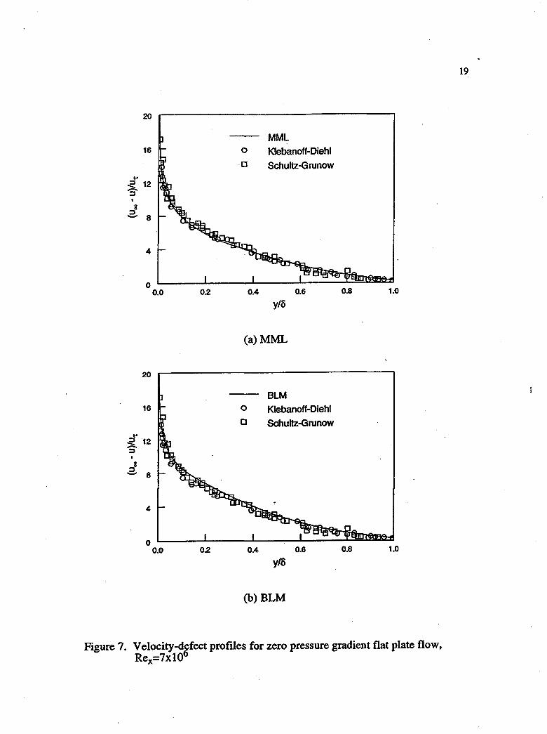
7. Velocity-defect profiles for zero pressure gradient flat plate flow, Rex=7xl06. . . . . . . . . . . . . . . . . . . . . . . . . . . . . . . . . . . . . . . . . . . . . . . . . . . . . . . . . . .. 19
(a) MML (b) BLM
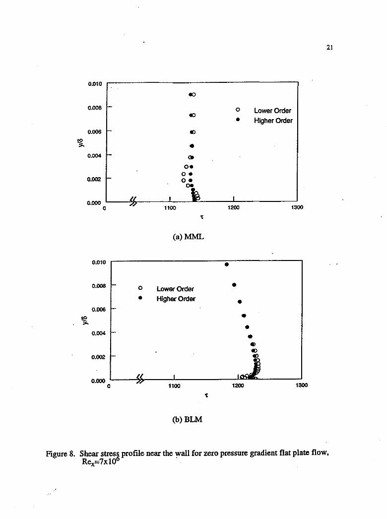
8. Shear stress profile near the wall for zero pressure gradient flat plate flow, Rex=7xl06 ................................................... 21 (a) MML (b) BLM
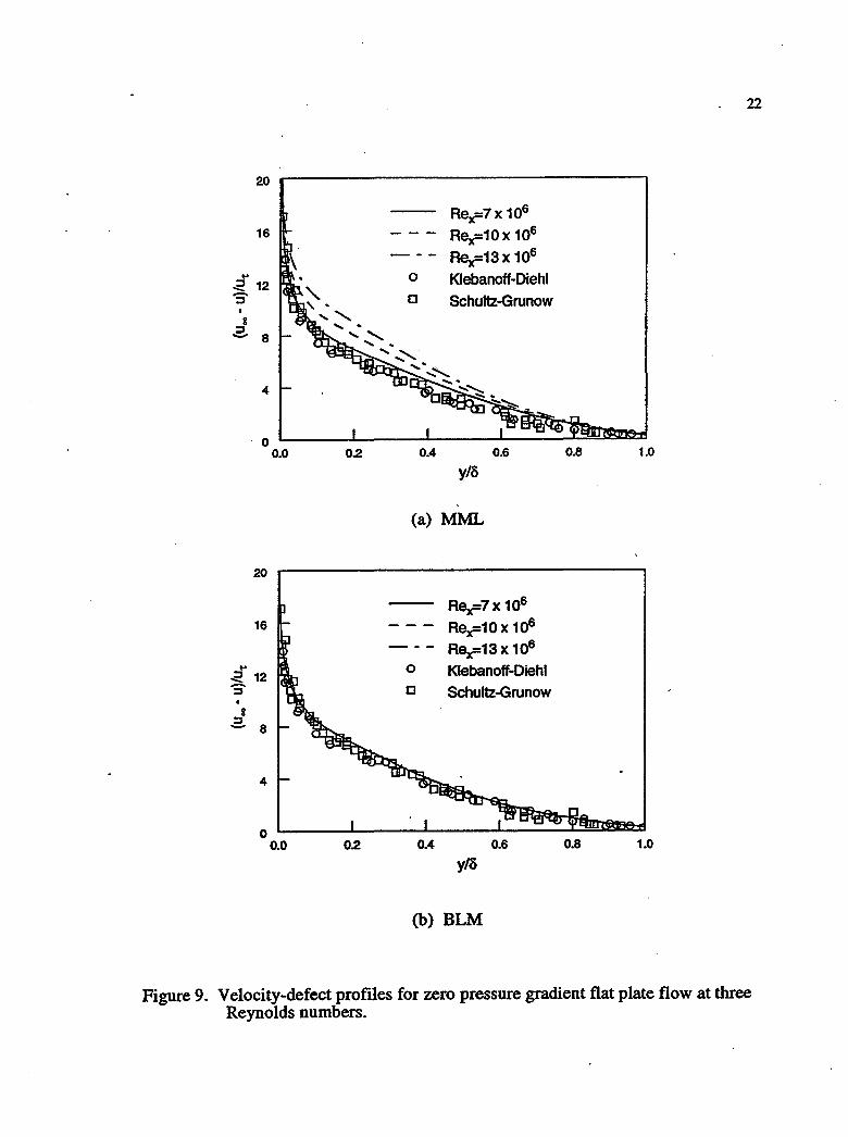
9. Velocity-defect profiles for zero pressure gradient flat plate flow at three Reynolds numbers . . • . . . . . . . . . . . . . . . . • . . . . . . • • . • . . . . . . . . . . . . . .. 22 (a) MML' (b) BLM
10. Turbulent viscosity for zero pressure gradient flat plate flow at three Reynolds numbers. . . . . . . . . . . . . . . . . . . . . . . : . . . . . . . . . . . . . . . . . . . . . . . . . . . .. 24 (a) MML
. (b) BLM
11. Velocity-defect for zero pressure gradient flat plate flow calculated using the modified MML of section 3.2 ........... . . . . . . . . . . . • . . . . . . . . . . . .. 26
vii
LIST OF FIGURES
Figure Page
1. F(y) profiles for attached and separated flow conditions •................ 8 (a) Attached flow (b) Separated flow .
2. Dimensionless mixing length distribution across a turbulent boundary layer, taken from reference 20 . . . . . . . . . . . . . . . . . . . . . . . . . . . . . . . . . . . . . . . .. 11
·3. Mixing length profJle for the MML modelS .••...•.•.••.•...••.•••••• 13
4. Estimation of 'tw using equation (3.3) ....•...•..•.............•.•.. 16
5. nlustration of flow over a flat plate. ............................••. 18
6. Computational grid for zero pressure gradient flat plate case ...... '. . . . • . .. 18
7. Velocity-defect profiles for zero pressure gradient flat plate flow, Rex=7xl06. . . . . . . . . . . . . . . . . . . . . . . . . . . . . . . . . . . . . . . . . . . . . . . . . . . . . . . . . . .. 19
(a) MML (b) BLM
8. Shear stress profile near the wall for zero pressure gradient flat plate flow, Rex=7xl06 ................................................... 21 (a) MML (b) BLM
9. Velocity-defect profiles for zero pressure gradient flat plate flow at three Reynolds numbers . . • . . . . . . . . . . . . . . . . • . . . . . . • • . • . . . . . . . . . . . . . .. 22 (a) MML' (b) BLM
10. Turbulent viscosity for zero pressure gradient flat plate flow at three Reynolds numbers. . . . . . . . . . . . . . . . . . . . . . . : . . . . . . . . . . . . . . . . . . . . . . . . . . . .. 24 (a) MML
. (b) BLM
11. Velocity-defect for zero pressure gradient flat plate flow calculated using the modified MML of section 3.2 ........... . . . . . . . . . . . • . . . . . . . . . . . .. 26
vii
12. Local skin friction coefficient for zero pressure gradient flat plate flow; MML of section 3.2 used. . . . . . . . . . . . . . . . . . . . . . . . . . . . . . . . . . . . . . . . . . . . . . . 27
13. Mixing length profiles at three pressure gradients.2S ••••••••••••••••••• 28
14. Velocity-defect for zero pressure gradient flow calculated using the modified" ~ of section 3.3 .....•..•.••.....•....•....•••.•..•...• " •.••• 30
15. Velocity-defect for mild pressure gradient flow ...........•........... 31 (a) Modified MML of section 3.3 (b) BLM
16. Velocity-defect for strong pressure gradient flow .....................• 32 (a) Modified MML of section 3.3 (b)BLM
17. Velocity-defect profiles computed using MMLPG (a) Zero pressure gradient flow. . . . . • • . • • . . . . • • . • . • . . . • . . . . . . • . . .• 35 (b) Mild pressure gradient flow. • • . . • . • . . • . . . . . . . . . • •. • • . • . • • • • . .• 35 (c) Strong pressure gradient flow . . . . . . . . . . . . . • . . . . . • . . . . . . . . • • . .. 36
18. nlustration of the Sajben diffuser geometry ......•........•....... : .. 40
19. Computational grid for the Sajben diffuser .........................• 40
20. Static pressure history at two locations on the top wall: just upstream and just downstream of the normal shock . . . . . . . . • . . . . . • . . . • . . . . • . . • . . . . . . . 43 (a) MMLPG (b) BLM2
21. Static pressure distribution on the top and bottom walls of the Sajben diffuser, weak: shock case ......... '. . . . . . . . . . . . . . . . . . . . . . . . . . . . . . . . . . . . . . 44 (a) Topwall (b) Bottom wall
22. Static pressure distribution on the top and bottom walls of the Sajben diffuser, no shock case •••••••••• -••••••••• : ••••••••••••••••••••••••••• •• 47 (a) Topwall (b) Bottom wall
23. Shock static pressure on top wall for the Sajben diffuser, strong shock case .. SO
24. Static pressure distribution on the top and bottom walls of the Sajben diffuser, strong shock case. . . . . . . . . . . . . . . . . . . . . . . . . . . . . . . . . . . . . . . . . . . . .. 51 (a) Topwall (b) Bottom wall
viii

· 25. Velocity profiles for the strong shock case ........................... 54
(a) xIH = 2.88 (b) xIH = 4.61 (c) xIH = 6.34 (d) xIH = 7.49
26. Turbulent viscosity ratio, 1lt/J1, for the Sajben diffuser, strong shock case . .. 55 (a) MMLPG (b) BLMI (c) BLM2
27. Comparison of weak shock static pressure distributions, computed using MMLPG and three different amounts of artificial viscosity •.•.••........ 75 (a) Top Wall (b) Bottom Wall
28. Comparison of no shock static pressure distributions, computed using MMLPG and two different grids. . . . . . . . . . . • . . • . . . . . • • • . . . . . . . . . . . . . . . . . . . 77 (a) Top Wall (b) Bottom Wall
ix
a, b, C
A+
cf
cp
CI
,C2
Ccp
CKIeb
Cwk 01,02
E,F
ET
EV,Fv
fI' f2
F(y)
FKIeb
Fmax
Fwake
GI
G2
G3
LIST OF SYMBOLS
parameters used to compute shear stress
van Driest damping constant = 26
local skin friction coefficient
specific heat at constant pressure
MML parameter; controls mixing length saturation level
MML parameter; controls curvature of blending region
Baldwin-Lomax turbulence model constant = 1.6
Baldwin-Lomax turbulence model constant = 0.3
Baldwin-Lomax turbulence model constant = 0.25
parameters used in turbulence model averaging for multiple walls
inviscid ftux vectors
total energy per unit volume
viscous flux vectors
parameters used in turbulence model averaging for multiple walls
function in Baldwin-Lomax turbulence model (equation (C.7»
Klebanoff intermittency factor
parameter in Baldwin-Lomax turbulence model
parameter in Baldwin-Lomax turbulence model (equation (C.6»
MMLPG parameter; controls mixing length saturation level
MMLPG parameter; controls curvature of blending region
MMLPG parameter; controls slope of inner layer mixing length
x
p
Pt
Pr
Q
R
Rex t
T
u,v
1lt
V
x,y
+ y
* y
Ymax
MMLPG parameter; nondimensional boundary layer thickness
MMLPG parameters; used to compute 04
MMLPG parameters; used to compute displacement thickness
throat height of Sajben diffuser
coefficient of thennal conductivity
turbulent mixing length
static pressure
total pressure
Prandtl number
heat fluxes in the x and y directions
vector of dependent variables (equation (A.2»
ratio of exit static pressure to inlet total pressure for Sajben diffuser
Reynolds number based on x-coordinate
time
static temperature
velocities
freestream x-velocity
shear velocity
total velocity
difference between maximum and minimum total velocities
Cartesian coordinates
y coordinate nondimensionalized by shear length scale
shear length scale (equation (2.7»
parameter in Baldwin-Lomax turbulence model
Clauser's equilibrium parameter
boundary layer thickness
xi

1C
displacement thickness
second- and fourth- order artificial viscosity coefficients in constant coefficient model
implicit artificial viscosity coefficient
parameters determining type of time differencing used
von Karman constant = 0.4
constants in nonlinear coeffi~ient artificial viscosity model
second coefficient of viscosity
molecular viscosity
computational coordinate directions
density
pressure gradient scaling parameter in nonlinear coefficient artificial viscosity model (equation (B.9»
spectral radius in nonlinear coefficient artificial viscosity model (equation (B.6»
't shear stress
'tl, 't2 shear stress at interior grid points
'tXXt ~ 'txy elements of shear stress tensor (equation (A.3»
vorticity
Subscripts
cap capping or saturation value
e edge of boundary layer
eff effective
i, j indexes in the x and y directions
xii

inner
max
min
outer
t
w
x,y
Superscripts
+
inner region of boundary layer
maximum
minimum
outer region of boundary layer
turbulent
wall
differentiation with respect to Cartesian coordinate directions
nondimensionalized by the shear length scale
xiii
inner
max
min
outer
t
w
x,y
Superscripts
+
inner region of boundary layer
maximum
minimum
outer region of boundary layer
turbulent
wall
differentiation with respect to Cartesian coordinate directions
nondimensionalized by the shear length scale
xiii

1
1
1
1
1
1
1
1
1
1
1
1
1
1
1
1
1
1
1
1
1
1
1
1
1
1
1
1
1
1
1
1
1
1
1
1
1
1
1
1
1
1
1
1
1
1
1
1
1
1
1
1
1
1
1
1
1
1
1
1
1
1
1.1 Motivation and Objectives
CHAPTER I
INTRODUCTION
Computational Fluid Dynamics (CFD) is a valuable tool for calculating the
turbulent flow fields that occur in engineering fluid flow problems. Some of the
characteristics of turbulent flow include random fluctuations in fluid properties, the
enhancement of mixing, diffusion and dissipation, and the presence of eddies of
various sizes. Turbulent flow is, therefore, very difficult to predict theoretically.
Experiments provide much useful infonnation about turbulent flow fields but are
costly and time consuming, so CFD is being used increasingly to reduce or optimize
the amount of experimental testing which must be done.
Most CFD codes solve the equations of conservation of mass, momentum
(Navier-Stokes) and energy and, in principle, completely describe the details'ofturbu
lent flow. However, except for very simple problems, these equations cannot be
solved exactly due to the limited capabilities 'of computation'aI resources. Most
engineering problems are primarily concerned with mean fluid properties and not with
the details of the turbulent fluctuations; the mean properties can: therefore be
computed using the ReynQlds-averaged fonn of the Navier-Stokes equations. 1 In
Reynolds averaging, the conservation equations are averaged over a time scale that is
large compared to the largest time scale of the fluctuating motion. 1,2,3 The averaging
procedure introduces new terms which represent the turbulent transport of mean
momentum, heat and mass. The resulting averaged equations are not closed and
1

2
empirical information, in the form of a turbulence model, must be used to close the
system.
A turbulence model is a mathematical model consisting of an equation or set
of equations which determines the turbulent transport terms in the mean flow
equations and hence closes the system of equations. 1 Turbulence models give an
approximate description of the flow by describing the overall effect of turbulence on
the mean flow, rather than describing the details of the turbulent motion. Since turbu
lent transport processes depend on factors such as geometry, swirl effects and
buoyancy, turbulence models, which are usually developed based on hypotheses about
a certain flow or range of flows, usually have a limited range of applicability.
Typically, a model which is complex and consists of a large number of equations is
difficult to use and is computationally expensive. Often this increase in "cost" is not
proportional to the improvements in the computation.
For most engineering applications, a turbulence model should be easy to
implement, computationally inexpensive and applicable to a wide range of flows.
Algebraic turbulence models, also called zero-equation models, are simple and
inexpensive, however they generally have only a narrow range of applicability. The
most widely used algebraic model, the Baldwin-Lomax model (BLM},4 fits this
description, but it is known to have difficulties calculating adverse pressure gradient
and separated flows,5-12 the regime it was designed to handle.
In 1989, the modified mixing length model (MML) was developed and used io
calculate separated flows over airfoils, flowfields that BLM was unable to accurately
predict.5 It is based on Prandtl's mixing length hypothesis3 and uses a mixing length
that is dependent on the local wall shear stress. The objective of this work is to
continue the development of MML to e~pand its range of applicability to include
boundary layer flows with adverse pressure gradients.
3
1.2 Overview
Chapter II gives some background infonnation on the Proteus Navier-Stokes
code; which" was used to make all of the calculations in this work. It also describes the
implementation of turbulence into the governing equations and describes problems
encountered with BLM, the current algebraic turbulence model in Proteus. Chapter II
also describes the original formulation of MML. Chapter III reports calculations
made with MML for zero pressure gradient flow over a flat plate, and then describes
the modifications made to improve these results for both zero and adverse pressure
gradient flows. The resulting modified version of MML is called MMLPG. Chapter
IV compares MMLPG and BLM for three transonic diffuser flow test "cases: flow with
a weak shock, strong shock, and no shock. Chapter V contains a summary of this
work and a discussion of the conclusions drawn.
CHAPTER II
BACKGROUND
2.1 The Proteus Navier-Stokes Code
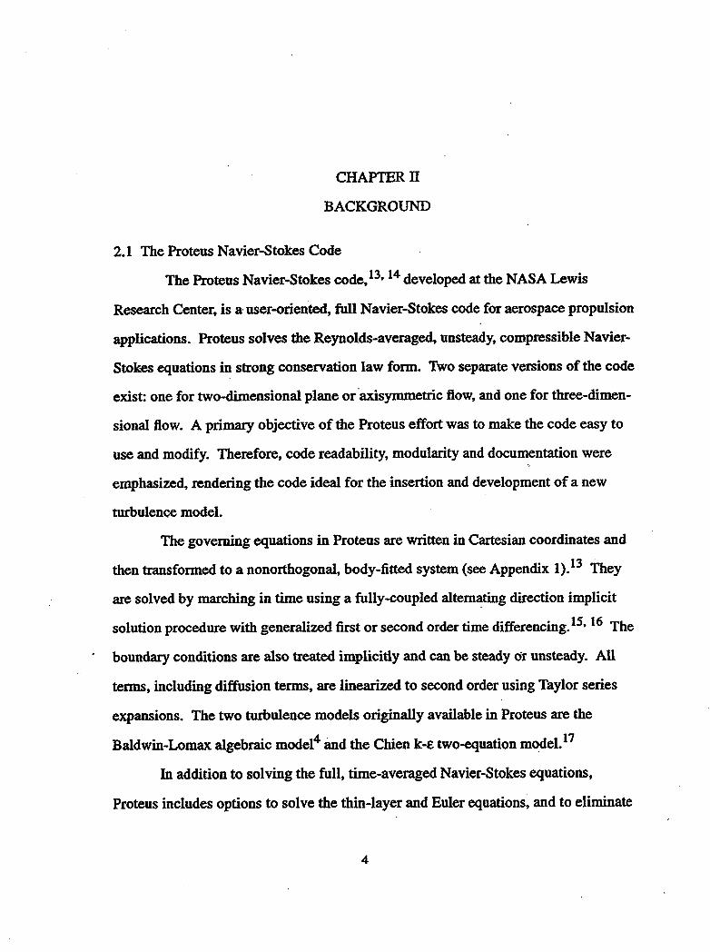
The Proteus Navier-Stokes code,13. 14 developed at the NASA Lewis
Research Center, is a· user-oriented, full Navier-Stokes code for aerospace propulsion
applications. Proteus solves the Reynolds-averaged, unsteady, compressible Navier
Stokes equations in strong conservation law form. Two separate versions of the code
exist: one for two-dimensional plane or 'axisymmetric flow, and one for three-dimen
sional flow. A primary objective of the Proteus effort was to make the code easy to
use and modify. Therefore, code readability, modularity and documentation were
emphasized, rendering the code ideal for the insertion and development of a new
turbulence model.
The governing equations in Proteus are written in Cartesian coordinates and
then transformed to a nonorthogonal, body-fitted system (see Appendix 1).13 They
are solved by marching in time using a fully-coupled altem~ting direction implicit
solution procedure with generalized first or second order time differencing.15• 16 The
boundary conditions are also treated implicitly and can be steady fir unsteady. All
tenns, including diffusion tenns, are linearized to second order using Taylor series
expansions. The two turbulence models originally available in Proteus are the
Baldwin-Lomax algebraic model4 and the Chien k-£ two-equation model. 17
In addition to solving the full, time-averaged Navier-Stokes equations,
Proteus includes options to solve the thin-layer and Euler equations~ and to eliminate
4
CHAPTER II
BACKGROUND
2.1 The Proteus Navier-Stokes Code
The Proteus Navier-Stokes code,13. 14 developed at the NASA Lewis
Research Center, is a· user-oriented, full Navier-Stokes code for aerospace propulsion
applications. Proteus solves the Reynolds-averaged, unsteady, compressible Navier
Stokes equations in strong conservation law form. Two separate versions of the code
exist: one for two-dimensional plane or 'axisymmetric flow, and one for three-dimen
sional flow. A primary objective of the Proteus effort was to make the code easy to
use and modify. Therefore, code readability, modularity and documentation were
emphasized, rendering the code ideal for the insertion and development of a new
turbulence model.
The governing equations in Proteus are written in Cartesian coordinates and
then transformed to a nonorthogonal, body-fitted system (see Appendix 1).13 They
are solved by marching in time using a fully-coupled altem~ting direction implicit
solution procedure with generalized first or second order time differencing.15• 16 The
boundary conditions are also treated implicitly and can be steady fir unsteady. All
tenns, including diffusion tenns, are linearized to second order using Taylor series
expansions. The two turbulence models originally available in Proteus are the
Baldwin-Lomax algebraic model4 and the Chien k-£ two-equation model. 17
In addition to solving the full, time-averaged Navier-Stokes equations,
Proteus includes options to solve the thin-layer and Euler equations~ and to eliminate
4

the energy equation by assuming constant stagnation enthalpy. Artificial viscosity is
used to minimize the odd-even decoupling resulting from the use of central spatial
differencing for the convective terms, and to control pre- and post-shock oscillations
in supersonic flow. 13 Two artificial viscosity models are available: a combination
implicit/explicit constant coefficient model,18 and an explicit nonlinear coefficient
model designed specifically for flows with shock waves.19 The artificial viscosity is
discussed in more detail in Appendix 2. At the NASA Lewis Research Center the
5
code is typically run either on the CRAY X-MP or CRAY Y-MP computer, and is
highly vectorized. For all calculations made herein, the two-dimensionallaxisymmet
~c version of the code was run on the CRAY Y-MP computer.
2.2 Algebraic Turbulence Modeling and the Baldwin-Lomax Model
Accurate modeling of turbulence is essential to the computation of complex
propulsion flow fields. Several types of turbulence models are available, ranging
from zero-equation algebraic models to mUlti-equation Reynolds-stress models.
Algebraic models are the most algorithmically simple and computationally inexpen
sive models and were therefore chosen as the focus of this effort.
Proteus, along with the majority of Navier-Stokes codes, uses the Boussinesq
assumption,3 which states that the turbulent stresses behave like the molecular viscous
stresses and therefore are proportional to the mean velocity gradient. The resulting
total shear stress for a two-dimensional flow is given by13
(2.1)
The effective viscosity is defined as JLeff = JL + JL" where JL is the molecular viscosity
and JL, is the turbulent, or "eddy" viscosity. The same analogy applies to the heat flux
and the normal stresses, which are both defined in Appendix I, such that an effective
second coefficient of viscosity is defined as Aeff = A + At and an effective thennal
conductivity coefficient is defined as keff = k + kt.
Most algebraic turbulence models are based on Prandtl's mQc.ing length
hypothesis which builds on the Boussinesq assumption.1 Prandtl made an analogy
between molecular motion and turbulent ft.ow. In molecular motion, the molecular
viscosity is proportional to the average velocity and the mean free path of the
. molecules. In turbulent ft.ow, Prandtl assumed that the turbulent viscosity is propor
tional to the characteristic velocity of the fluctuating motion and to a typical length,
called the "mixing length", of this motion. In other words,
6
(2.2)
where Vt is the turbulent velocity scale and the mixing length, 1, is·the transverse
distance over which ft.uid particles maintain their original momentum. Prandtl further
assumed that the turbulent velocity scale is equal to the mixing length times the veloc
ity gradient so that
(2.3)
The quantity 11 dUI is the velocity scale, where u is the component of velocity in the dy. .
primary ft.ow direction and y is the coordinate perpendicular to the primary ft.ow direc-
tion.
The current algebraic turbulence model in Proteus, the Baldwin-Lomax model
(BLM), is given in Appendix 3. It is the most well-known and widely used algebraic
turbulence model. An extension of the Cebeci-Smith model,20 which requires knowl
edge of the outer edge of the boundary layer, the Baldwin-Lomax model was devel
oped to handle separated flows while avoiding the necessity of finding this outer edge.
7
Several references report problems with BLM in regions of strong pressure
gradient and in flows with large regions of separation. Yu6 reports problems calculat
ing surface pressures on the outboard wing region of a wing-body configuration when
the angle of attack is high and separation occurs. Visbal and Knight7 report that the
BLM outer fonnulation is unsuitable for separated supersonic flow and also is unable
to predict the recovery of the boundary layer downstream of reattachment. Degani &
SchiW report that BLM is unsuitable in regions of cross flow separation due to
ambiguities in computing the outer length scale. Mente~ reports that BLM underesti
mates the displacement thickness for the increasingly adverse pressure gradient flow
of Samuel & ]oube~l and that it also gives an incorrect prediction of the adverse
pressure gradient flow of Driver.22 Potapczu!2 reports problems with BLM in
predicting the separation and unsteady behavior on airfoils with and without leading
edge ice accretion. Stock and Haase10 report that BLM does not predict the correct
trends for Il, or the Reynolds stresses in adverse pressure gradient ~d separated
flows.
There are several reasons why BLM has problems computing flows with large
pressure gradients and large regions of separation. The primary difficulty occurs in
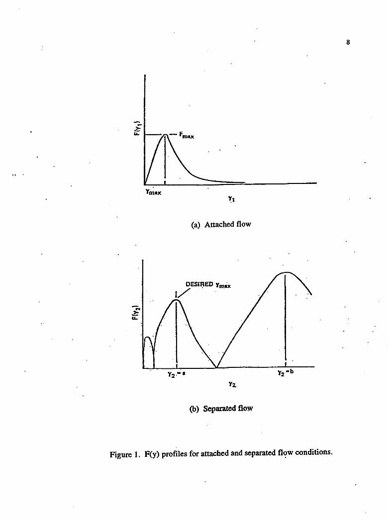
finding the maximum of the F(y) function (defined Appendix 3), which has two or
more peaks in regions of separated flow. This behavior is shown in figure 1 taken
from reference 5. As the relative magnitudes of the local maxima change~ ymax
. (defined in Appendix 3), may suddenly jump, producing unrealistic discontinuities in
the turbulent viscosity. Selection of the global maxima often results in a gross over
prediction of the turbulent viscosity. Some authors 7• 23 have found that choosing the
outermost peak produces better results, while others have elected to use the innermost
peak.S To account for upstream turbulence history effects, Visbal and Knight7 used
7
Several references report problems with BLM in regions of strong pressure
gradient and in flows with large regions of separation. Yu6 reports problems calculat
ing surface pressures on the outboard wing region of a wing-body configuration when
the angle of attack is high and separation occurs. Visbal and Knight7 report that the
BLM outer fonnulation is unsuitable for separated supersonic flow and also is unable
to predict the recovery of the boundary layer downstream of reattachment. Degani &
SchiW report that BLM is unsuitable in regions of cross flow separation due to
ambiguities in computing the outer length scale. Mente~ reports that BLM underesti
mates the displacement thickness for the increasingly adverse pressure gradient flow
of Samuel & ]oube~l and that it also gives an incorrect prediction of the adverse
pressure gradient flow of Driver.22 Potapczu!2 reports problems with BLM in
predicting the separation and unsteady behavior on airfoils with and without leading
edge ice accretion. Stock and Haase10 report that BLM does not predict the correct
trends for Il, or the Reynolds stresses in adverse pressure gradient ~d separated
flows.
There are several reasons why BLM has problems computing flows with large
pressure gradients and large regions of separation. The primary difficulty occurs in
finding the maximum of the F(y) function (defined Appendix 3), which has two or
more peaks in regions of separated flow. This behavior is shown in figure 1 taken
from reference 5. As the relative magnitudes of the local maxima change~ ymax
. (defined in Appendix 3), may suddenly jump, producing unrealistic discontinuities in
the turbulent viscosity. Selection of the global maxima often results in a gross over
prediction of the turbulent viscosity. Some authors 7• 23 have found that choosing the
outermost peak produces better results, while others have elected to use the innermost
peak.S To account for upstream turbulence history effects, Visbal and Knight7 used
8
Ymax
(a) Attached flow
OES1J:lED Ymax 1/ .'
-£ u.
(b) Separated flow
Figure 1. F(y) profiles for attached and separated fl<?w conditions.
8
Ymax
(a) Attached flow
OES1J:lED Ymax 1/ .'
-£ u.
(b) Separated flow
Figure 1. F(y) profiles for attached and separated fl<?w conditions.

BLM with relaxation. They also found that the BLM constants Ccp and CK1eb (see
Appendix 3) should vary with Mach number. Sakowski et alII expounded upon this
by finding a relation for Ccp as a function of Mach number and pressure gradient, but
encountered problems caused by the vanishing of the Van Driest factor when 'tw ' the
local shear stress at the wall, approaches zero. To remedy this, they used the local
shear in place of'tw. Launder and Pridden24 report several modifications to the Van
Driest facto~ for pressure gradient flows, many of which incorporate the local shear
stress instead of 'two
A simpler, yet effective, approach was used by Potapczuk, 5 who developed a
modified mixing length (MML) model that does not require a boundary layer thick
ness, but also avoids all problems associated with the determination of a maximum
F(y). This model is described in detail in the following section.
2.3 The Modified Mixing Length Turbulence Model
The modified mixing len~ (MML) model was developed by Potapczu!2 to
fill the need for an algebraic model to handle turbulent flow with large separated
regions. The particular problem of interest was an ainoil at angle of attack with and
without leading edge ice accretions. Previous calculations made with BLM gave poor
results and the source of the problem was the function F(y), which had mUltiple peaks . . .
for this flow case.
The MML model avoids the need to seek a maximum of some ad hoc function.
In accordance with Prandtl's mixing length theory, the MML model determines the
mixing length using the wall shear stress and the nonnal distance from the wall, with
the maximum mixing length capped off at a given value. Thus, it is a two layer
model, such that the length scale depends on conditions near the surface and remains
9
10
constant in the separated region~ This assumption is valid since there is no substantial
enhancement of turbulence in separated regions. The turbulent viscosity is given by
(2.4)
where the velocity gradient in equation (2.3) has been replaced by the vorticity magni
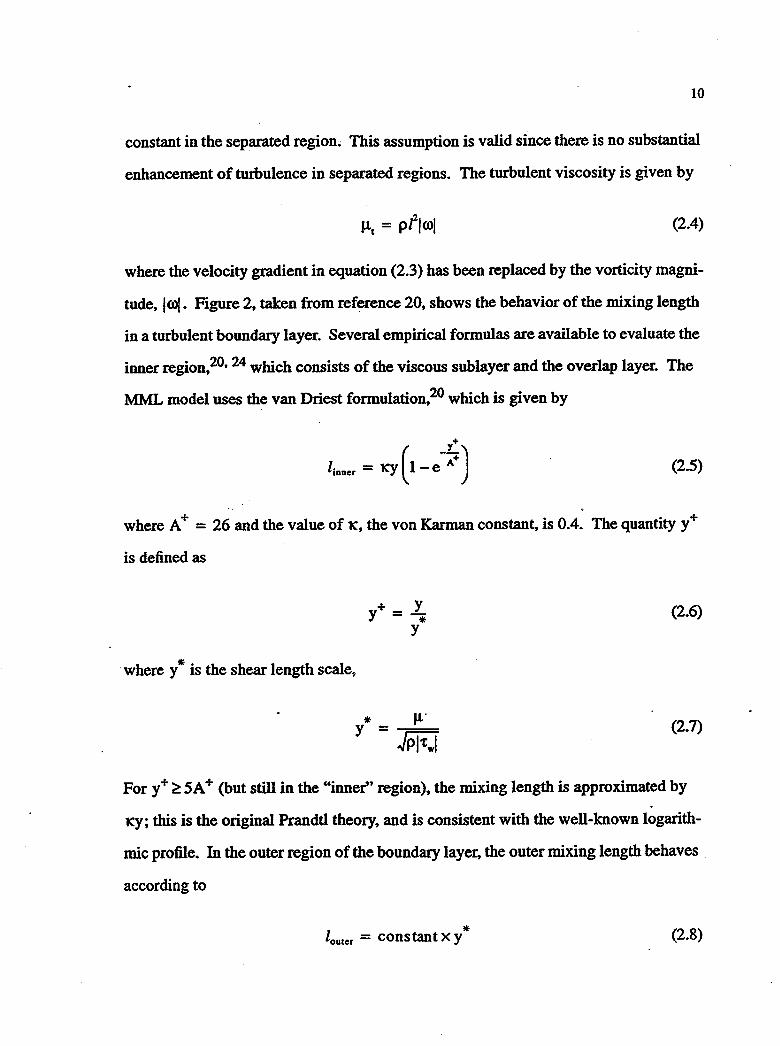
tude, lcol. Figure 2, taken from reference 20, shows the behavior of the mixing length
in a turbulent boundary layer. Several empirical formulas are available to evaluate the
inner region,20, 24 which consists of the viscous sublayer and the overlap layer. The
MML model uses the van Driest formulation,20 which is given by
- ( ::) linDcr - 'ICY l-e (2.5)
where A + = 26' and the value of le, the von Karman constant, is 0.4: The quantity y +
is defined as
where y * is the shear length scale,
* J1" y =-== Jpl'twl
(2.6)
(2.7)
For y+ ~ SA + (but still in the "inner" region), the mixing length is approximated by
ley; this is the original Prandtl theory, and is consistent with the well-known logarith
mic profile. In the outer region of the boundary layer, the outer mixing length behaves
according to
* loutcr = constant X y (2.8)
10
constant in the separated region~ This assumption is valid since there is no substantial
enhancement of turbulence in separated regions. The turbulent viscosity is given by
(2.4)
where the velocity gradient in equation (2.3) has been replaced by the vorticity magni
tude, lcol. Figure 2, taken from reference 20, shows the behavior of the mixing length
in a turbulent boundary layer. Several empirical formulas are available to evaluate the
inner region,20, 24 which consists of the viscous sublayer and the overlap layer. The
MML model uses the van Driest formulation,20 which is given by
- ( ::) linDcr - 'ICY l-e (2.5)
where A + = 26' and the value of le, the von Karman constant, is 0.4: The quantity y +
is defined as
where y * is the shear length scale,
* J1" y =-== Jpl'twl
(2.6)
(2.7)
For y+ ~ SA + (but still in the "inner" region), the mixing length is approximated by
ley; this is the original Prandtl theory, and is consistent with the well-known logarith
mic profile. In the outer region of the boundary layer, the outer mixing length behaves
according to
* loutcr = constant X y (2.8)

11
o.oa
0.07
0.06
I/o 0.05
0.0';
0.03
0.02
OOo-~O~.I'--;;-~~~~--~--~--~~~~~--~ 0.2 . 0.3 0.4 0.5 0.6 07 0.8 0.9 1.0
y/o
Figure 2. Dimensionless mixing length distribution across a turbulent boundary layer, taken from reference 20.
11
o.oa
0.07
0.06
I/o 0.05
0.0';
0.03
0.02
OOo-~O~.I'--;;-~~~~--~--~--~~~~~--~ 0.2 . 0.3 0.4 0.5 0.6 07 0.8 0.9 1.0
y/o
Figure 2. Dimensionless mixing length distribution across a turbulent boundary layer, taken from reference 20.
12
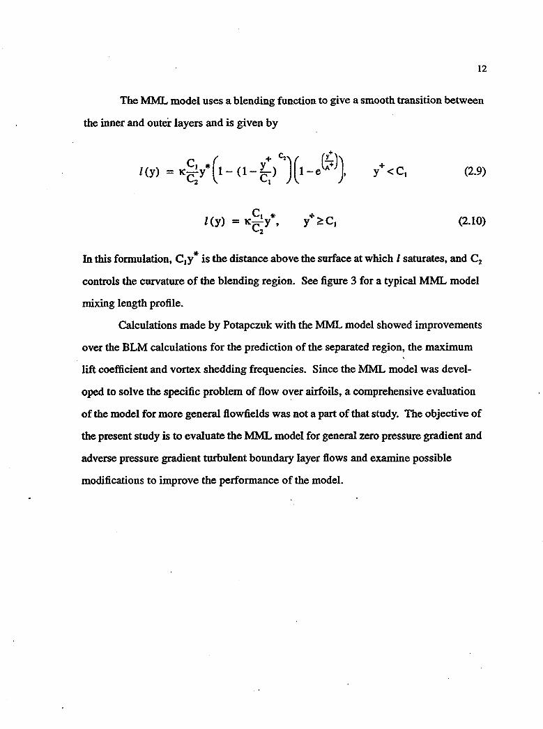
The MML model uses a blending function to give a smooth transition between
the inner and outer layers and is given by
C1 * y A+ (
+ <;)( (l)) l(y) = lC
C2 Y 1- (I-C1
) l-e , (2.9)
+ Y ~Cl (2.10)
In this formulation. Cly* is the distance above the surface at which I saturates. and C2
controls the curvature of the blending region. See figure 3 for a typical MML model
mixing length profile.
Calculations made by Potapczuk with the MML model showed improvements
over the BLM calculations for the prediction of the separated region. the maximum
lift coefficient and vortex shedding frequencies. Since the MML model was devel
oped to solve the specific problem of flow over airfoils. a comprehensive evaluation
of the model for more general flowfields was not a part of that study. The objective of
the present study is to evaluate the MML model for general zero pressure gradient and
adverse pressure gradient turbulent boundary layer flows and examine possible
modifications to improve the performance of the model.
12
The MML model uses a blending function to give a smooth transition between
the inner and outer layers and is given by
C1 * y A+ (
+ <;)( (l)) l(y) = lC
C2 Y 1- (I-C1
) l-e , (2.9)
+ Y ~Cl (2.10)
In this formulation. Cly* is the distance above the surface at which I saturates. and C2
controls the curvature of the blending region. See figure 3 for a typical MML model
mixing length profile.
Calculations made by Potapczuk with the MML model showed improvements
over the BLM calculations for the prediction of the separated region. the maximum
lift coefficient and vortex shedding frequencies. Since the MML model was devel
oped to solve the specific problem of flow over airfoils. a comprehensive evaluation
of the model for more general flowfields was not a part of that study. The objective of
the present study is to evaluate the MML model for general zero pressure gradient and
adverse pressure gradient turbulent boundary layer flows and examine possible
modifications to improve the performance of the model.

.10
l/f>
.os
i = let I I I I
I I I I I I
I I l
saturation length scale -""-------- ---
)'/0
Figure 3. Mixing length profile for the MML modeLS
13
.10
l/f>
.os
i = let I I I I
I I I I I I
I I l
saturation length scale -""-------- ---
)'/0
Figure 3. Mixing length profile for the MML modeLS
13
CHAPTER III
EVALUATION AND MODIFICATION OF MML
The MML model. described in Chapter II, was modified so that it could better
calculate turbulent boundary layer flows with zero and adverse pressure gradients.
The first step in this process was to optimize the computation of the wall shear stress
used in MML. Next, MML was used to calculate a turbulent boundary layer with zero
pressure gradient. These results exhibited poor agreement with experimental data, so
modifications were made to MML to remedy this problem. Then modificati~ns corre
sponding to two adverse pressure gradient flows of Bradshaw25 were successfully
incorporated into MML. Finaliy, all of the modifications were combined into one
general model, called MMLPG.
,
3.1 Optimization of Shear Stress Estimate
Since the MML turbulence model is a function of the wall shear stress. it is
important to accurately calculate this quantity. The wall shear stress is given by
(3.1)
The molecular viscosity. J.1. is a very small quantity compared to the velocity gradient,
(~)w • which is strongly dependent on several fact~rs such as the finite difference
scheme used, the grid spacing and the numerical features of the code. It is important
to minimize·the sensitivity of these factors because smaIl changes in the estimate of
(ou) may actually produce large changes in 'two A more global approach is to use a oYw
14
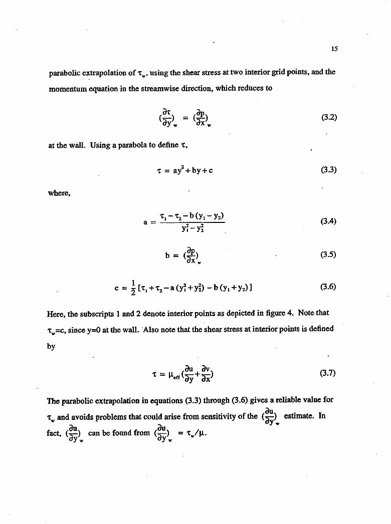
15
parabolic extrapolation of 'tw ' using the shear stress at two interior grid points, and the
momentum equation in the streamwise direction, which reduces to
(3.2)
at the wall. Using a parabola to define 't,
2 't = ay +by+c (3.3)
where,
(3.4)
(3.5)
(3.6)
Here, the subscripts 1 and 2 denote interior points as depicted in figure 4. Note that
'tw=c, since y=O at the wall. Also note that the shear stress at interior points is defined
by
(3.7)
The parabolic extrapolation in equations (3.3) through (3.6) gives a reliable value for
'tw and avoids problems that could arise from sensitivity of the (~u) estimate. In au au Yw
fact, (cr) can be found from (cr) = 'tw/Ji· Yw Yw
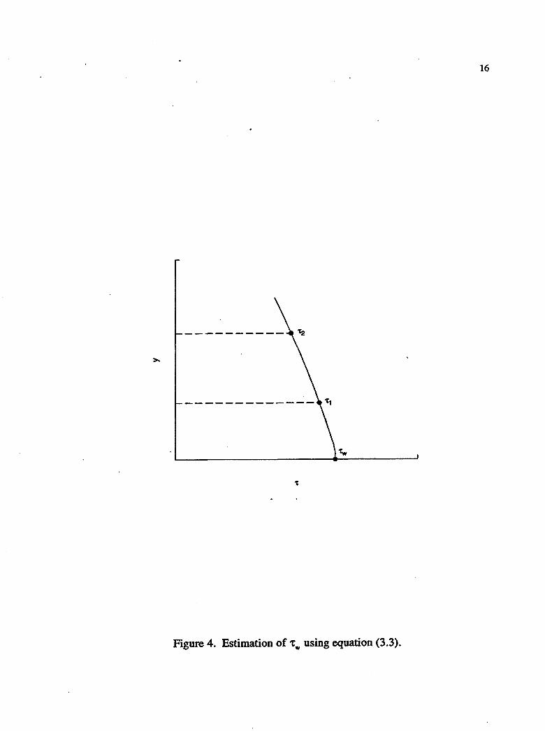
16
Figure 4. Estimation of 'tw using equation (3.3).
16
Figure 4. Estimation of 'tw using equation (3.3).

Modifications were made to the Proteus code to calculate the shear stress
profile in the boundary layer. These modifications made use of the generalized grid
transformations in Proteus such that
17
(3.8)
where ~y = 'Ilx = 0 for an orthogonal grid. 13 The derivatives in the above equation
are calculated in Proteus using 3-point, second-order central differencing. To see if
higher order differencing would improve the calculation, 5-point, fourth-order central
differencini6 was also used to calculate the velocity gradients.
The test case of incompressible, zero pressure gradient, turbulent flow over a
fiat plate, as shown in figure 5, was used to evaluate the shear stress calculations. The
grid, shown in figure 6,' had 51 points in both the streamwise and normal directions
and had grid points clustered at the wall to resolve the boundary layer and at the
upstream boundary to resolve the imposed boundary condition. In addition, it was
evaluated to insure grid indepence for zero pressure gradient flow. The reference
velocity, temperature, pressure and length used in Proteus were 33.53 mis, 288.3 K,
101.3 kPa and 1.98 m, respectively. At the upstream boundary, the velocity profile,
which was computed using the correlation of Musker,27 was held fixed. The flow was
computed using both MML and BLM, using both higher and lower order differencing
of the velocity gradients in the shear stress computation. The MML constants were
chosen as Cl=3000 and C2=5, which were found to give good results at Rex=7xl06.
Both turbulence models produced good agreement with experimental velocity-defect
profiles,28 as shown in figure 7, which shows calculations at RCx=7xl06 made with
the lower order differencing of the velocity gradients. The quantity Ut in figure 7 is
the shear velocity, given by Ut = J (It wI / p). The accuracy of the finite differencing

18
Figure 5. lliustration of flow over a flat plate.
Figure 6. Computational grid for zero pressure gradient flat plate case.
18
Figure 5. lliustration of flow over a flat plate.
Figure 6. Computational grid for zero pressure gradient flat plate case.
20
MMl 16 0 Klebanoff-Oiehl
[J Schultz-Grunow to'
~ 12 -::s I
8 ::s - 8
4
0 0.0 0.2 0.4 0.6 0.8 1.0
y/r,
(a)MML
20
BlM 16 0 Klebanoff-Oiehl
[J Schultz-Grunow to' ~ 12 -::s
I
8 ::s - 8
4
0 0.0 0.2 0.4 0.6 0.8 1.0
yffl
(b) BLM
Figure 7. Velocity-dgfect profiles for zero pressure gradient flat plate flow, Rex=7xlO
19
20
MMl 16 0 Klebanoff-Oiehl
[J Schultz-Grunow to'
~ 12 -::s I
8 ::s - 8
4
0 0.0 0.2 0.4 0.6 0.8 1.0
y/r,
(a)MML
20
BlM 16 0 Klebanoff-Oiehl
[J Schultz-Grunow to' ~ 12 -::s
I
8 ::s - 8
4
0 0.0 0.2 0.4 0.6 0.8 1.0
yffl
(b) BLM
Figure 7. Velocity-dgfect profiles for zero pressure gradient flat plate flow, Rex=7xlO
19

.20
produced no noticeable improvement in the velocity profiles, but there were slight
differences in the shear stress profile very close· to the wall, which can be observed in
the plots of figure 8. The higher-order differencing produced a smoother shear stress
profile near the wall, and thus subsequent calculations will make use of the higher
order calculation of the velocity gradients.
Near separated regions of flow, 'tw approaches zero which will cause y* and
thus the mixing length to become infinitely large. To avoid this problem, the follow
ing.local average used by PotapczuI2 was incorporated:
(3.9)
The subscripts in equation (3.9) refer to grid points in the streamwise direction along
the wall.
3.2 Evaluation and Modification for Zero Pressure Gradient Flows
In reference 5, a series of cases were run for flow over a NACAOO 12 airfoil at
. conditions near stall using both BLM and MML. The MML constants' Cl=2000 and
C2=5 were chosen based on correlations with experimental data. The Baldwin-Lomax
model tended to suppress the trailing-edge separation, which occurs on the top surface
of the airfoil, by over-predicting J1, throughout the separated region. On the other . . hand, MML predicted high values of J1, only near the separation point, thus allowing
the reverse flow to develop downstream. In the current study, MML was evaluated for
turbulent flow over a flat plate at zero pressure gradient, as described below.
In the preliminary analysis presented in section 3.1, the constants C1 = 3000
and C2 = 5 were found to give good agreement for Rex = 7xl06. At other locations on
the plate, i.e., at other Reynolds numbers, the BLM velocity-defect profiles correctly
exhibit similarity but the MML profiles do not, as shown in figure 9. In a turbulent
21
0.010
O.OOS 0 Lower Order «> e Higher Order
0.006 ~
C/O >. •
0.004 CIt
oe oe
0.002 oe De
0.000 () 1300
't
(a)MML
0.010 • 0.008 0 Lower Order •
e Higher Order • 0.006
C/O >. •
• 0.004 • • ~
0.002 ~
0.000 0 1100 1200 1300
't
(b)BLM
Figure 8. Shear stres~ profile near the ~all for zero pressure gradient flat plate flow, Rex=7xlO .
. -
22
20
Re -7x 10⁶ X-
16 - -- Re -10x 106 X-
\ --- Rex==13 X 106
to 0 Klebanoff-Diehl ~ 12 - c Schultz-Grunow ;:,
8 ..... . ;:, - 8 ..... , ..... .
..... -0-........... ,
4
'0 0.0 0.2 0.4 0.6 0.8 1.0
ylt>
(a) MML
20
Rex=7x 10⁶
16 --- Rex=10x 106
--- Rex=13 x 106
to 0 Klebanoff-Diehl ~ 12 - c Schultz-Grunow ;:,
8 ;:, - 8
4
0 0.0 0.2 0.4 0.6 0.8 1.0
y/t>
(b) BLM
Figure 9. Velocity-defect profiles for zero pressure gradient flat plate flow at three Reynolds numbers.
23
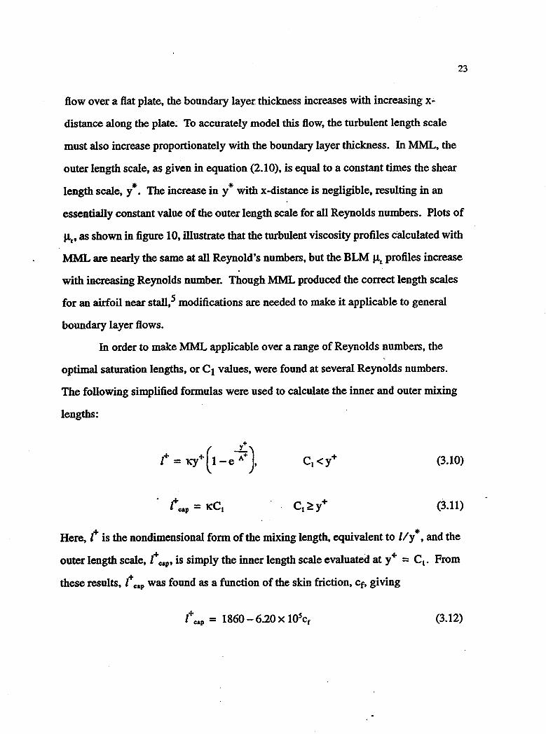
flow over a flat plate, the boundary layer thickness increases with increasing x
distance along the plate. To accurately model this flow, the turbulent length scale
must also increase proportionately with the boundary layer thickness. In MML, the
outer length scale, as given in equation (2.10), is equal to a constant times the shear
length scale, y*. The increase in y* with x-distance is negligible, resulting in an
essentially constant value of the outer length scale for all Reynolds numbers. Plots of
J.1t , as shown in figure 10, illustrate that the turbulent viscosity profiles calculated with
MML are nearly the same at all Reynold's numbers, but the BLM J.1t profiles increase
with increasing Reynolds number. Though MML produced the correct length scales
for an airfoil near stall,S modifications are needed to make it applicable to general
boundary layer flows.
In order to make MML applicable over a range of Reynolds numbers, the
optimal saturation lengths, or Cl values, were found at several Reynolds numbers.
The following simplified formulas were used to calculate the inner and outer mixing
lengths:
(3.10)
. ~ . + 1 cap = KCl . C l ~ Y (3.11)
Here, t is the nondimensional form of the mixing length, equivalent to l/y *, and the
outer length scale, t cap, is simply the inner length scale evaluated at y+ = C l - From
these results, tcap was found as a function of the skin friction, cf, giving
(3.12)
23
flow over a flat plate, the boundary layer thickness increases with increasing x
distance along the plate. To accurately model this flow, the turbulent length scale
must also increase proportionately with the boundary layer thickness. In MML, the
outer length scale, as given in equation (2.10), is equal to a constant times the shear
length scale, y*. The increase in y* with x-distance is negligible, resulting in an
essentially constant value of the outer length scale for all Reynolds numbers. Plots of
J.1t , as shown in figure 10, illustrate that the turbulent viscosity profiles calculated with
MML are nearly the same at all Reynold's numbers, but the BLM J.1t profiles increase
with increasing Reynolds number. Though MML produced the correct length scales
for an airfoil near stall,S modifications are needed to make it applicable to general
boundary layer flows.
In order to make MML applicable over a range of Reynolds numbers, the
optimal saturation lengths, or Cl values, were found at several Reynolds numbers.
The following simplified formulas were used to calculate the inner and outer mixing
lengths:
(3.10)
. ~ . + 1 cap = KCl . C l ~ Y (3.11)
Here, t is the nondimensional form of the mixing length, equivalent to l/y *, and the
outer length scale, t cap, is simply the inner length scale evaluated at y+ = C l - From
these results, tcap was found as a function of the skin friction, cf, giving
(3.12)

400
300
:1. ";,t 200
100
Rex =7x10⁶
Rex = 10x106
Rex = 13x106
o L-____ ~~ ____ ~ ____ ~~ ______ ~ ______ ~
0.0 0.5 1.0 1.5 2.0 2.5
y/a
(a) MML
~ ~-------------------------------------,
,..---- ..
300 "' Rex = 7x10⁶
Rex = 10x106
Rex = 13x106
:1. ";,t 200
.,,-------
100
o L-____ ~L-____ -l ______ _1 __ _=~~~-=-~~.J
0.0 0.5 1.0 1.5 2.0 2.5
yta
(b) BLM
Figure 10. Turbulent viscosity for zero pressure gradient flat plate flow at three Reynolds numbers.
24

25
The velocity-defect profiles of figure 11 show that equations (3.10) and (3.12) with
t = min (t, t cap) , allow the mixing length to grow proportionately with the bound
ary layer thickness. The modified MML is better than BLM at predicting the local
skin friction coefficient, cr, as shown in figure 12; the wiggles at the upstream bound
ary are a result of the imposed upstream boun<;lary condition.
3.3 Modifications for Adverse Pressure Gradient Flows
Two equilibrium pressure gradient flows of Bradshaw25 were used' to modify
MML for adverse pressure gradients effects. Equilibrium turbulent flows are flows
which have a constant value of Clauser's equilibrium parameter,2
(3.13)
In addition, they correspond to a power-law velocity profile distribution, Ue oc xa,
where the magnitude of the-exponent, a, indicates the strength of the pressure gradi
ent. They also exhibit similarity when plotted in velocity-defect coordinates. Three
flows were examined in the experimental study of Bradshaw;25 these were flows with
zero, mild, and strong pressure gradients. The corresponding values of the exponent,
a, are 0, -0.15, and -0.255, respectively; the corresponding values of f3 are 0, 1 and 5.
The modifications to the turbulence model are based on the trends exhibited in
the mixing length at the three pressure gradients as shown in figure 13 taken from
Bradshaw25. Note that for all three pressure gradients, th~ maximum mixing length is
approximately 0.080, the saturation distance from the wall is approximately 0.40, and
the slope of the curves near the wall increases with the strength of the pressure gradi
ent. These three features were used to develop the following model:
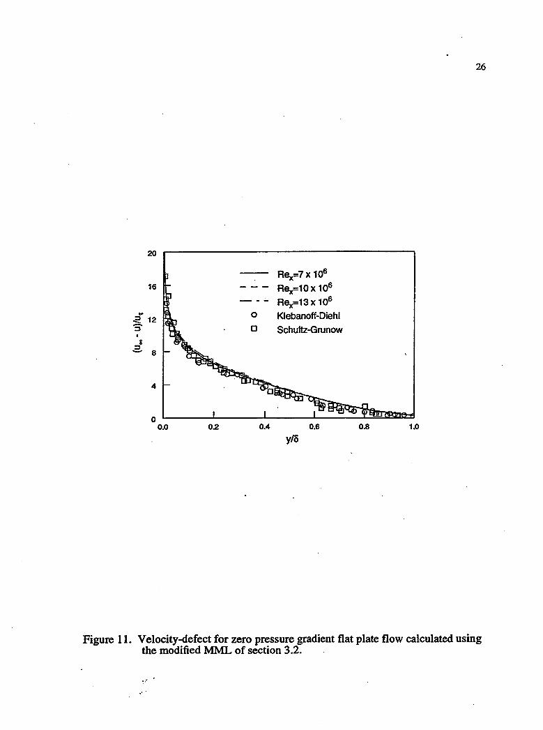
26
20
R¥7x10⁶
16 - -- Re -10x 106 x-
- -- Re -13 x 106 X-
too 0 Klebanoff-Oiehl ~ 12 - 0 Schultz-Grunow :::J
8 :::J - 8
4
0 0.0 0.2 0.4 0.6 0.8 1.0
y/a
Figure 11. Velocity-defect for zero pressure gradient flat plate flow calculated using the modified MML of section 3.2 .
. " "
26
20
R¥7x10⁶
16 - -- Re -10x 106 x-
- -- Re -13 x 106 X-
too 0 Klebanoff-Oiehl ~ 12 - 0 Schultz-Grunow :::J
8 :::J - 8
4
0 0.0 0.2 0.4 0.6 0.8 1.0
y/a
Figure 11. Velocity-defect for zero pressure gradient flat plate flow calculated using the modified MML of section 3.2 .
. " "
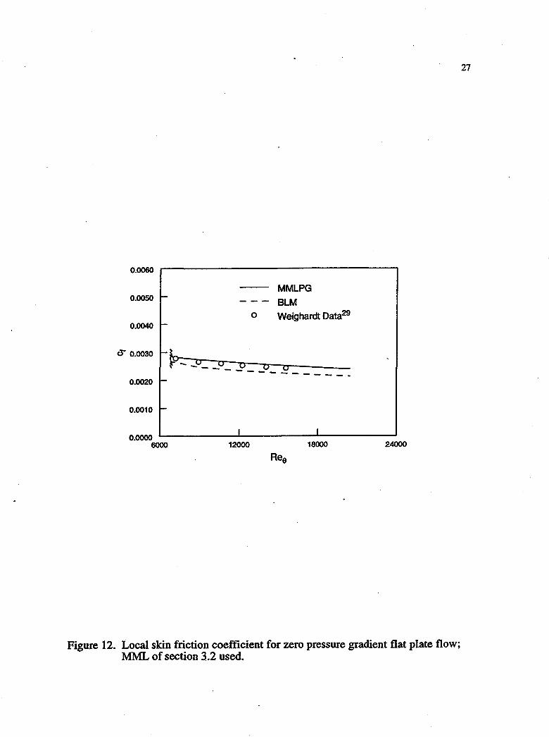
0.0060
0.0050
0.0040
is 0.0030
0.0020
0.0010
o - -
MMlPG
BlM o Weighardt Data29
o 0 0 -- -- ------
0.0000 '--------'------....... ------..1 6000 12000 18000 24000
Figure 12. Local skin friction coefficient for zero pressure gradient flat plate flow; MML of section 3.2 used.
27
0.0060
0.0050
0.0040
is 0.0030
0.0020
0.0010
o - -
MMlPG
BlM o Weighardt Data29
o 0 0 -- -- ------
0.0000 '--------'------....... ------..1 6000 12000 18000 24000
Figure 12. Local skin friction coefficient for zero pressure gradient flat plate flow; MML of section 3.2 used.
27
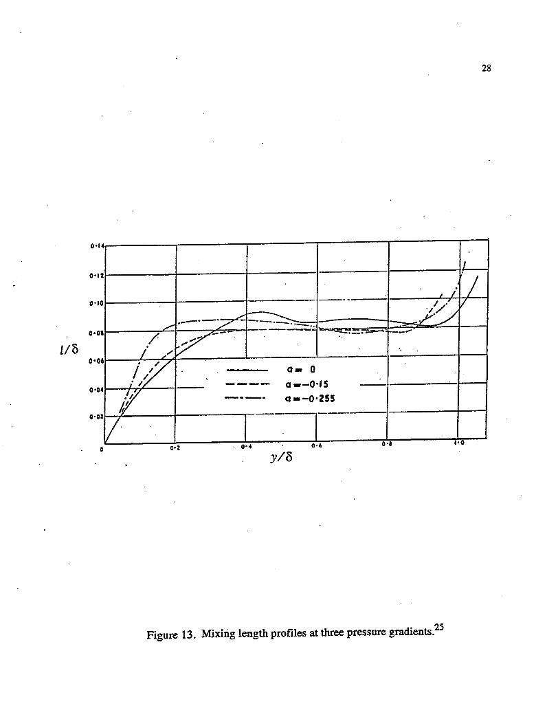
28
o· 14
0'1 t 1/
LIB
0 ----- f ; / ---I -' V
,,/ .---Z--=~ ,- /.~ . . --....;. .... • / V-- --___ Oi ~:__. ;::.:..-0. -_ .... ,..,..- .
/ /' " " 6
',f/ / 1 G- O
4 / 1/ - ---- a --0-'5 --
!/ -----. 0--0-255 1/
'V
0-0
0-0
0-0
0'0
o o-z o • I 0
yla
Figure 13. Mixirig length profiles at three pressure gradients.25

+ y>G1
29
(3.14)
(3.15)
A new parameter, G3' has been introduced and the constants C1 and C2 in the original
MML model have been replaced by the functions Gl and G2' where
(3.16)
(3.17)
Here, G4 is essentially a nondimensional boundary layer thickness which is a function
of 13 and cf, and G3 controls the slope of mixing length curve and is a function of 13.
The following correlation was assumed for G4:
(3.18)
Separate values of the parameters G3, Gs, and G6, corresponding to each of the three
pressure gradients, were found and are given in table 1. This results in essentially
three separate models, one for each pressure gradient, depending on which set of
parameters is used. The results of these-modifications are compared with Baldwin
Lomax calculations in the velocity-defect plots of figures 14 through 16. (Note: The
Baldwin-Lomax. results for the zero pressure gradient case are given in figure 9.) The
reference conditions used are the same as those given in section 3.1. For the two
adverse pressure gradient cases, the turbulent velocity profiles at the upstream bound
ary were computed using a cubic spline fit of the Bradshaw experimental data and
held fixed; the appropriate pressure gradient was imposed at the freestream boundary.
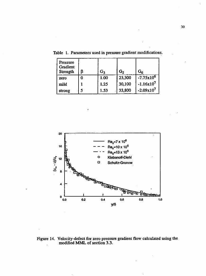
Table 1. Parameters used in pressure gradient modification~.
Pressure Gradient Strength f3 G3 GS G6 zero 0 1.00 23,300 -7.75xl0fJ
mild 1 1.25 30,100 -1.16xl07
strong 5 1.53 33,800 -2.09xl07
~o
Re -.7 x 106 x--
16 --- Rex=10x 106
- -- Rex=13 x 106
~ 0 Klebanoff-Oiehl ~ 12 -:::I 0 Schultz-Grunow • B
:::I - 8
4
0 0.0 0.2 0.4 0.6 0.8 1.0
y/6
Figure 14. Velocity-defect for zero pressure gradient flow calculated using the modified MML of section 3.3.
30
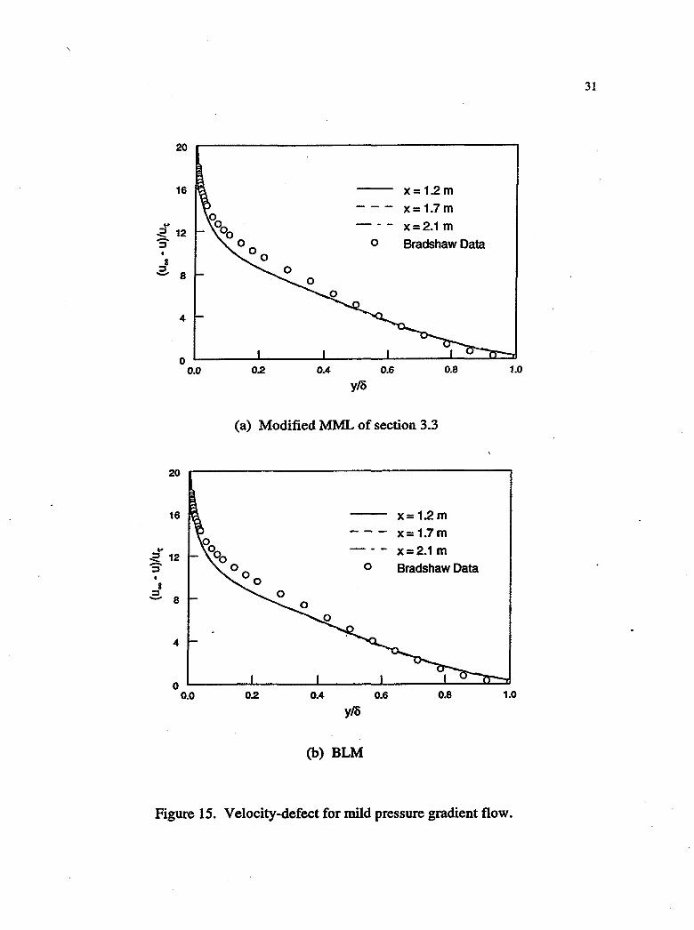
20
16
to ~ 12 -:J
8 :J - 8
4
0 0.0
o
0.2 0.4
y/a 0.6
x= 1.2 m x= 1.7 m x=2.1 m Bradshaw Data
0.8
(a) Modified MML of section 3.3
1.0
20 r-------------------------------------~
16
to ~ 12 -:J • 8
:J - 8
4
o 0.0
o
0.2 0.4
yJa
(b) BLM
0.6
X= 1.2 m x= 1.7m x=2.1 m Bradshaw Data
0.8 1.0
Figure 15. Velocity-defect for mild pressure gradient flow.
31
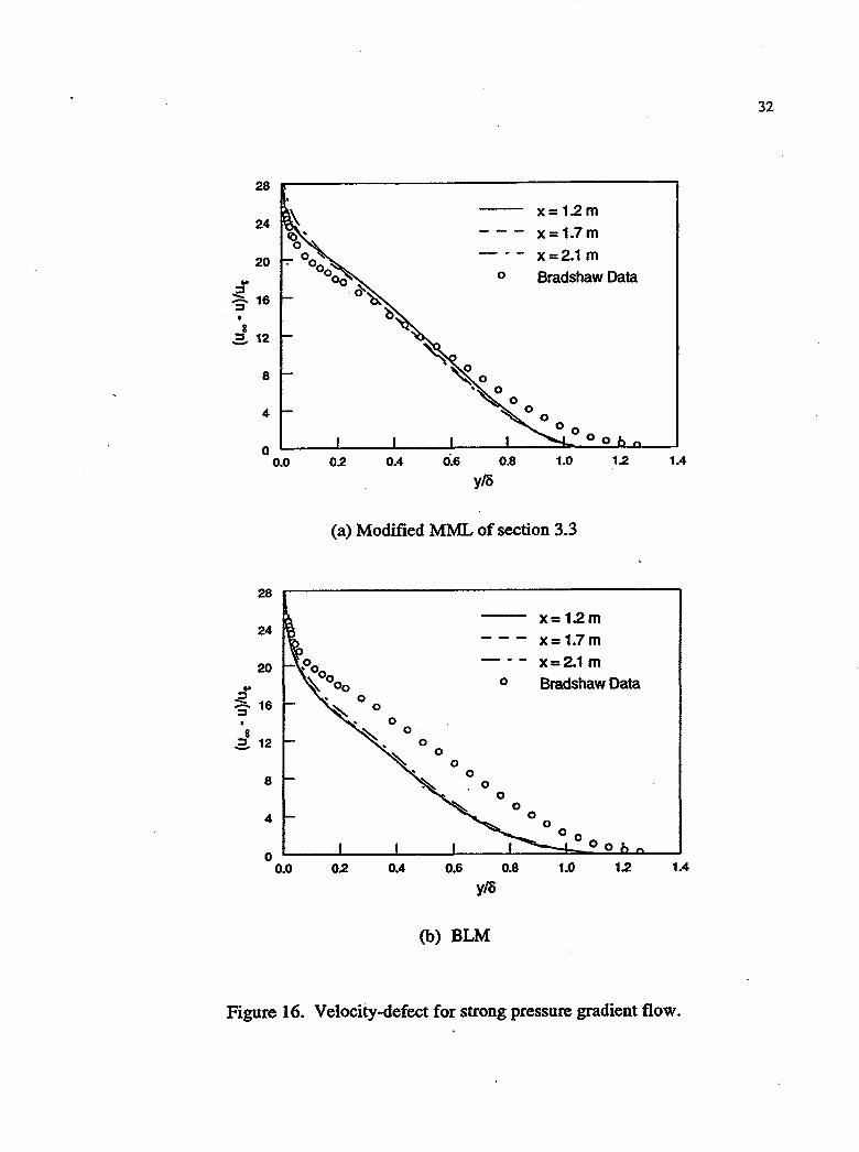
28
24
20
:r :::::=.. 16 ::l
8 a 12
8
4
0 0.0
28
24
20
8 ::l 12 -.
8
4
o 0.0
o
0.2 0.4 0.6 0.8
y/r)
X= 1.2 m x= 1.7m x=2.1 m Bradshaw Data
1.0 1.2
(a) Modified MML of section 3.3
X= 1.2m --- X= 1.7m --- x=2.1 m
0 Bradshaw Data 0
~ 0 0
~ 0 0
~ 0
0
~ 0
0 0
0 0
0
0.2 0.4 0.6 0.8 1.0 1.2
y/r)
(b) BLM
1.4
1.4
Figure 16. Velocity-defect for strong pressure gradient flow.
32
28
24
20
:r :::::=.. 16 ::l
8 a 12
8
4
0 0.0
28
24
20
8 ::l 12 -.
8
4
o 0.0
o
0.2 0.4 0.6 0.8
y/r)
X= 1.2 m x= 1.7m x=2.1 m Bradshaw Data
1.0 1.2
(a) Modified MML of section 3.3
X= 1.2m --- X= 1.7m --- x=2.1 m
0 Bradshaw Data 0
~ 0 0
~ 0 0
~ 0
0
~ 0
0 0
0 0
0
0.2 0.4 0.6 0.8 1.0 1.2
y/r)
(b) BLM
1.4
1.4
Figure 16. Velocity-defect for strong pressure gradient flow.
32
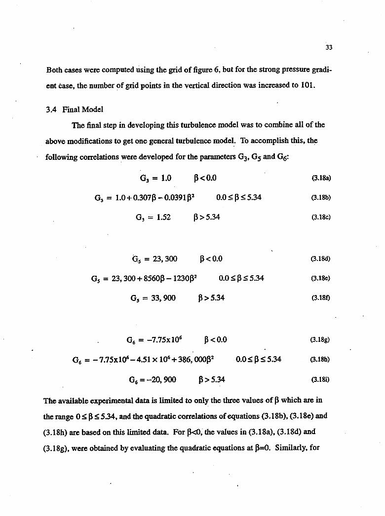
33
Both cases were computed using the grid of figure 6, but for the strong pressure gradi
ent case, the number of grid points in the vertical direction was increased to 101.
3.4 Final Model
The final step in developing this turbulence model was to combine all of the
. above modifications to get one general turbulence model: To accomplish this, the
following correlations were .developed for the parameters G3' GS and G6:
G3 = 1.0 ~<O.O
G3 = 1.0 + 0.307(i - 0.0391 (i2 0.0 ~ (i ~ 5.34
(i >5.34
Os = 23,300 (i<0.0
Gs = 23,300 + 8560(i - 1230(i2 0.0 ~ (i ~ 5.34
Gs = 33, 900 (i > 5.34
G6 = -7.75xl06 (i<0.0
G6 = -7.75xl06-4.51 X 10⁶ + 3S6, OOO(i2 0.0 ~ (i ~ 5.34
G6 =-20,900 ~>5.34
(3.18a)
(3. 18b)
(3. 18c)
(3.18d)
(3. 18e)
(3.18f)
(3.18g)
(3. 18b)
(3.18i)
The available experimental data is limited to only the three values of (i which are in
the range 0 ~ (i ~ 5.34, and the quadratic correlations of equations (3.1Sb), (3.1Se) and
(3.1Sh) are based on this limited data. For (i<0; the values in (3. 1 Sa), (3.1Sd) and
(3.ISg), were obtained by evaluating the quadratic equations at (i=0. Similarly, for
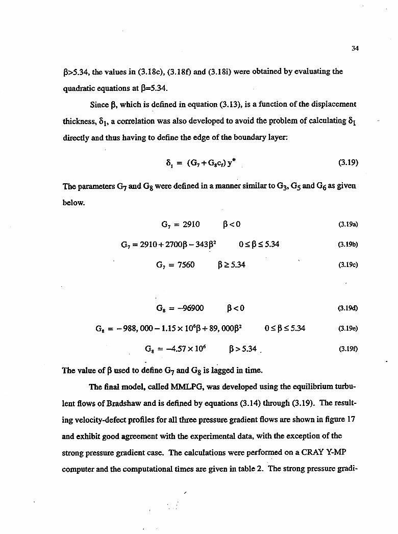
34
(3)5.34, the values in (3.18c), (3.18f) and (3.18i) were obtained by evaluating the
quadratic equations at (3=5.34.
Since (3, which is defined in equation (3.13), is a function of the displacement
thickness, ai, a correlation was also developed to avoid the problem of calculating al
directly and thus having to define the edge of the boundary layer:
(3.19)
The parameters G7 and Gs were defined in a manner similar to G3, Gs and G6 as given
below.
G7 = 2910 (3 <0
G7 = 2910+ 2700(3 - 343(32 0 ~ (3 ~ 5.34
G7 = 7560 (3 ~ 5.34
Gs = -96900 (3 < 0
Gs = - 988,000 -1.15 x 10⁶(3 + 89,000(32 O~ (3 ~5.34
Gs = -4.57 X 10⁶ (3 > 5.34 .
The value of (3 used to define G7 and Gs is lagged in time.
(3.19a)
(3. 19b)
(3.19c)
(3.19d)
(3. 1ge)
(3.19t)
The final model, called MMLPG, was developed using the equilibrium turbu
lent flows of Bradshaw and is defined by equations (3.14) through (3.19). The result
ing velocity-defect profiles for all three pressure gradient flows are shown in figure 17
and exhibit good agreement with the experimental data, with the exception of the
strong pressure gradient case. The calculations were performed on a CRAY Y-MP
computer and the computational times are given in table 2. The strong pressure gradi-

35
20
Re -7x 10⁶ x-
16 - -- Re -10x 106 X-
- -- Rex=13 X 106
to 0 Klebanoff-Diehl .~ 12 - 0 Schultz-Grunow ::s
8 ::s - 8
4
0 0.0 0.2 0.4 0.6 0.8 1.0
yta
(a) Zero pressure gradient flow.
20
16 X= 1.2 m X= 1.7 m
to x=2.1 m ~ 12 - Bradshaw Data ::s • 8 ::s - 8
4
0 0.0 0.2 0.4 0.6 0.8 1.0
yta
(b) Mild pressure gradient flow.
Figure 17. Velocity-defect profiles computed using MMLPG.
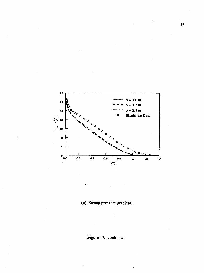
8
28 r---------------------------------------~
24
20 o
X= 1.2 m x=1.7m x=2.1 m Bradshaw Data
.2. 12
8
4
o L-____ L-____ L-____ L-____ L-__ ~~ __ ~~~~
0.0 0.2 0.4 0.6 0.8 1.0 1.2 1.4
yta
(c) Strong pressure gradient.
Figure 17. continued.
36
8
28 r---------------------------------------~
24
20 o
X= 1.2 m x=1.7m x=2.1 m Bradshaw Data
.2. 12
8
4
o L-____ L-____ L-____ L-____ L-__ ~~ __ ~~~~
0.0 0.2 0.4 0.6 0.8 1.0 1.2 1.4
yta
(c) Strong pressure gradient.
Figure 17. continued.
36

37
Table 2. Computational times for fiat plate fiows.
(a) Zero Pressure Gradient
sec.liter.l Model Iterations grid point
BLM 2000 2.02xl0-~
MMLPG 2000 2.ooxl0-s
(b) Mild Pressure Gradient
sec JiterJ Model Iterations grid point
BLM 3000 2. 14x 1 0-.:)
MMLPG 3000 2.17zl0-S
(c) Strong Pressure Gradient
sec.liter.l Model Iterations grid point
BLM 18,000 2.14xl0-=>
MMLPG 10,000 1.96xlO-S
38
ent case took considerably longer to reach convergence because the code had difficul
ties resolving oscillations induced at the upstream boundary, which was a fixed
velocity profile as mentioned in section 3.3.
3.5 Averaging for Multiple Boundaries
If both walls in a given coordinate direction are solid surfaces, the turbulent
mixing lengths are computed separately at each surface and then averaged. The
Sajben diffuser, which is described in Chapter IV, has solid walls at the upper and
lower vertical boundaries, and is a typical example of a geometry which would require
averaging of the mixing length. The averaging formula of Appendix 3 (equation C.9), .
which was used to average the Fwake function in the Baldwin-Lomax model, is also
used here to average the mixing length:
I = I1fl + 12f2 fl +f2
(3.20)
If the lower and upper boundaries in the vertical direction, are solid surfaces, as in the
Sajben diffuser, then II and 12 are the mixing lengths at the lower and upper bound
aries, respectively. The functions fl and f2 are defined in equation C.IO of Appendix
3.
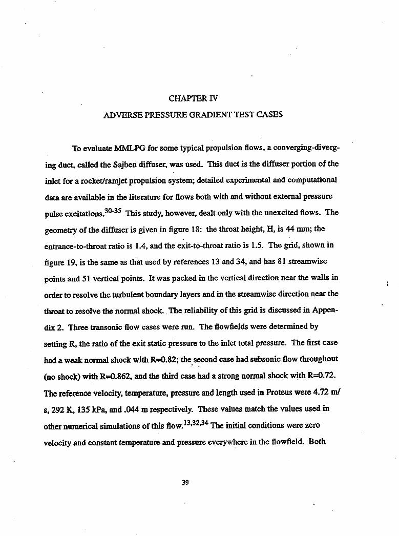
CHAPTER IV
ADVERSE PRESSURE GRADIENT TEST CASES
To evaluate MMLPG for some typical propulsion flows, a converging-diverg
ing duct, called the Sajben diffuser, was used. This duct is the diffuser portion of the
inlet for a rocket/ramjet propulsion system; detailed experimental and computational
data are available in the literature for flows both with and without external pressure
pulse excitations.30-3S This study, however, dealt only with the unexcited flows. The
geometry of the diffuser is given in figure 18: the throat height, H, is 44 mm; the
entrance-to-throat ratio is 1.4, and the exit-to-throat ratio is 1.5. The grid, shown in
figure 19, is the same as that used by references 13 and 34, and has 81 streamwise
points and 51 vertical points. It was packed in the vertical direction near the walls in
order to resolve the turbulent boundary layers and in the streamwise direction near the
throat to resolve the normal shock. . The reliability of this grid is discussed in Appen
dix 2. Three transonic flow cases were run. The flowfields were determined by
setting R, the ratio of the exit static pressure to the inlet total pressure. The first case
had a weak normal shock with R=O.82; the. s~ond case had subsonic flow throughout
(no shock) with R=O.862, and the third case had a strong normal shock with R=O.72.
The reference velocity, temperature, pressure and length used in Proteus were 4.72 mI
s, 292 K, 135 kPa, and .044 m respectively. These values match the values used in
other numerical simulations of this flow. 13,32,34 The initial conditions were zero
velocity and constant temperature and pressure everywJ:tere in the flowfield. Both
39
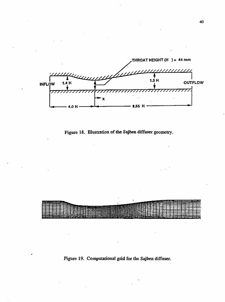
40
)= 44mm
..... --4.0 H --~-------- 8.65 H -------......
Figure 18. nlustration of the Sajben diffuser geometry.
Figure 19. Computational grid for the Sajben diffuser.
40
)= 44mm
..... --4.0 H --~-------- 8.65 H -------......
Figure 18. nlustration of the Sajben diffuser geometry.
Figure 19. Computational grid for the Sajben diffuser.

cases were run using MMLPG and two implementations of the Baldwin-Lomax
model.
Two slightly different implementations of BLM were used because it was
discovered, during the course of these calculations, that a slight change in the BLM
coding, which occurred in the update of Proteus from Version 1.014 to 2.0,13 can
effect turbulent calculations. References 14 and 34 give results for the weak and no
shock cases calculated with Version 1.0 of Proteus and using BLM. These calcula-
41
tions were repeated in the current study using the current version of Proteus, Version
2.0, and slightly different results were obtained. (These results will be presented later
in this chapter.) Discrepancies in the results were caused by differences in the imple
mentation of the BLM model, more specifically, in the Fwalce function. Version 2.0 of
Proteus computes Fwake using equation (C.6) in Appendix 3, and version 1.0 of
Proteus computes F wake as
(4.1)
which is the formulation stated in the original paper by Baldwin and Lomax.4 The
BLM implementations using equations (4.1) and (C.6) will be referred to as BLMI
and BLM2, respectively.
4.1 Weak Shock Case
The weak shock case was used as an example case in the Proteus User's
Manual~ 13.14 and therefore was run first in order to gain familiarity with running this
type of flow. It was computed as described in reference 13: First the exit pressure
was gradually reduced to R = 0.1338 to establish supersonic flow throughout the
diffuser; then it was gradually raised to R = 0.82, the desired ratio to establish the
42
weak normal shock, and iterated until the solution was no longer changing apprecia
bly with time. A plot of the static pressure on the top wall at two locations, one
upstream and one downstream of the normal shock, as the solution progresses is given
in figure 20. This indicates that pressure reaches a steady state level, which, for
practical engineering purposes, can be considered a converged solution. A closer
examination of the results indicates that the solution oscillates slightly about a mean
steady level. This may be caused by inherent unsteadiness in the flow; Salmon et al30
mention that very low-amplitude, self-sustaining oscillations were observed experi
mentally. It is more likely that the oscillations present in this calculation are numeri
cal in nature, which is common for flows with shock waves. The oscillations
originating at the shock may not be damped out by the artificial viscosity and there
fore tend to migrate upstream. The artificial viscosity used in Proteus to calculate this
flow was second- and fourth-order explicit, both using the nonlinear coefficient model
of Jameson et al; 19 the respective smoothing coefficients are 1(2 and 1<4, as given in
Appendix 2. For the entire calculation, 1(2 was set to 0.1; K.t was set to .005 for the
first 6000 iterations, while the exit pressure was changing, and decreased to .0004 for
the remaining 3000 iterations, which were at a constant exit pressure. More details
about the effects of the artificial viscosity on this solution are included in Appendix 2.
The static pressure distribution on the top and bottom walls is given in figure
21. The small discrepancies just downstream of the shock are due to insufficient
streamwise grid distribution. The shock location on the upper wall and the shock
Mach number at the edge of the upper wall boundary layer are given in table 3. Both
MMLPG and BLM2 do a good job of predicting the pressure distribution on the wall
and the location of the shock. Each case was run for 9000 iterations and calculations
made using MMLPG, BLMI and BLM2 required 3.44 x 10⁻⁵ sec/iteration/grid point,

43
1.2
xIH=.93 1.0 xIH=2.1
0.8 -.e-Q. ""------
0.6 I
, 0.4
, "- ..... ---- --- -
0.2 0 2000 4000 6000 8000 10000
Iteration Number
(a) MMLPG
1.2
xIH=.93 1.0 xIH=2.1
0.8 -..e-Q. 1\./------
0.6 I
, 0.4
, "- I .....
..... _------0.2
0 2000 4000 6000 8000 10000
Iteration Number
(b) BLM2
Figure 20. Static pressure history at two locations on the top wall: just upstream and just downstream of the normal shock.

1.0
0.9 I : 0 I f I j 1
0.8 .----.j ... - ·-· .. ----j--T'-----· I ! I
_ 0.7 .e-o.
0.6
0.5
0.4
0.3 -5.0
1.0
0.9
0.8
_ 0.7 .e-o.
0.6
0.5
0.4
0.3 -5.0
! I I I .
-2.5
-2.5
0.0 2.5
xlH
(a) Top wall
0.0 2.5
xIH
(b) Bottom wall
o
5.0
o
5.0
.- ·--·-r-· ...... -· .. -I
MMLPG BLM1 BLM2 Hsieh Data
7.5 10.0
MMLPG BLM1 BLM2 Hsieh Data
7.5 10.0
Figure 21. Static pressure distribution on the top and bottom walls of the Sajben diffuser, weak shock case.
44
1.0
0.9 I : 0 I f I j 1
0.8 .----.j ... - ·-· .. ----j--T'-----· I ! I
_ 0.7 .e-o.
0.6
0.5
0.4
0.3 -5.0
1.0
0.9
0.8
_ 0.7 .e-o.
0.6
0.5
0.4
0.3 -5.0
! I I I .
-2.5
-2.5
0.0 2.5
xlH
(a) Top wall
0.0 2.5
xIH
(b) Bottom wall
o
5.0
o
5.0
.- ·--·-r-· ...... -· .. -I
MMLPG BLM1 BLM2 Hsieh Data
7.5 10.0
MMLPG BLM1 BLM2 Hsieh Data
7.5 10.0
Figure 21. Static pressure distribution on the top and bottom walls of the Sajben diffuser, weak shock case.
44
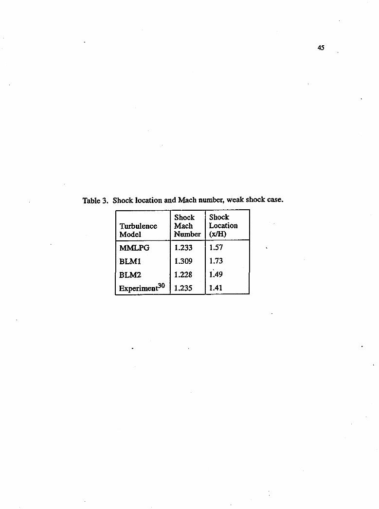
45
Table 3. Shock location and Mach number, weak shock case.
Shock Shock Turbulence Mach Location Model Number (xIH)
MMLPG 1.233 1.57
BLMI 1.309 1.73
BLM2 1.228 1.49
Experimen~O 1.235 1.41
45
Table 3. Shock location and Mach number, weak shock case.
Shock Shock Turbulence Mach Location Model Number (xIH)
MMLPG 1.233 1.57
BLMI 1.309 1.73
BLM2 1.228 1.49
Experimen~O 1.235 1.41
3.90 x 10⁻⁵ sec/iteration/grid point and 3.36 x lO-s sec/iteration/grid point, respec
tively on the CRAY Y-MP computer.
4.2 No Shock Case
46
The second diffuser test case did not have a normal shock wave. To compute
this case .. the exit pressure was gradually lowered to R=0.862 then iterated until the
solution stopped changing. A steady state solution was reached with subsonic flow
throughout the entire diffuser. The Proteus default artificial viscosity, which uses the
constant coefficient model of Steger18 with both fourth-order explicit and second- .
order implicit artificial viscosity, was used; the smoothing coefficients, £E(4) and £[
(defined in Appendix 2), had values of 1.0 and 2.0, respectively.
The static pressure distribution on the top and bottom walls is given in figure
22 and shows that MMLPG is clearly better than BLMI and BLM2 at predicting the
pressure distribution, though it still predicts a larger pressure drop than that given by
the experimental data. The MMLPG results are similar to the calculations of Hseih et
al33 who attributed the lower throat pressure to the fact that the experiment was highly
sensitive to small perturbations in exit pr~ssure. The maximum Mach numbers in the
diffuser are given in table 4. Though no experimental data is available to compare
these values, the MMLPG results are in best agreement with the calculations of
Georgiadis3S who used the PARC Navier-Stokes code36 for the same geometry. Each
case was run for 9000 iterations and calculations using MMLPG, BLMI and BLM2
required 3.45xl0-S sec/iteration/grid point, 2.90xl0-S secliteration/grid point and
3.36xlO-S secliteration/grid point, respectively, on the CRAY Y-MP computer.
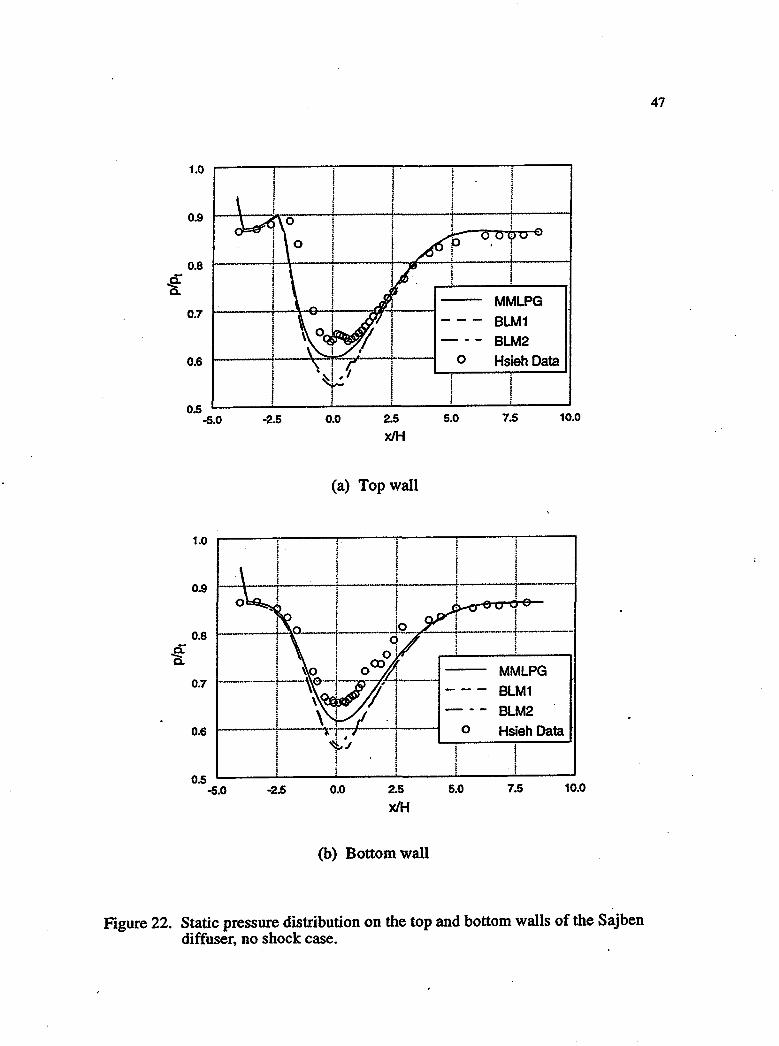
1.0
0.9
0.8
~ 0-
MMLPG 0.7 - -- BLM1
- -- BLM2 0.6 0 Hsieh Data
0.5 -5.0 -2.5 0.0 2.5 5.0 7.5 10.0
x/H
(a) Top wall
1.0 "f i
0.9 -
0.8
~ 0-
MMLPG 0.7 --- BLM1
- -- BLM2 0.6 0 Hsieh Data
I . , 0.5
1
-5.0 -2.5 0.0 2.5 5.0 7.5 10.0
xIH
(b) Bottom wall
Figure 22. Static pressure distribution on the top and bottom walls of the Sajben diffuser, no shock case.
47
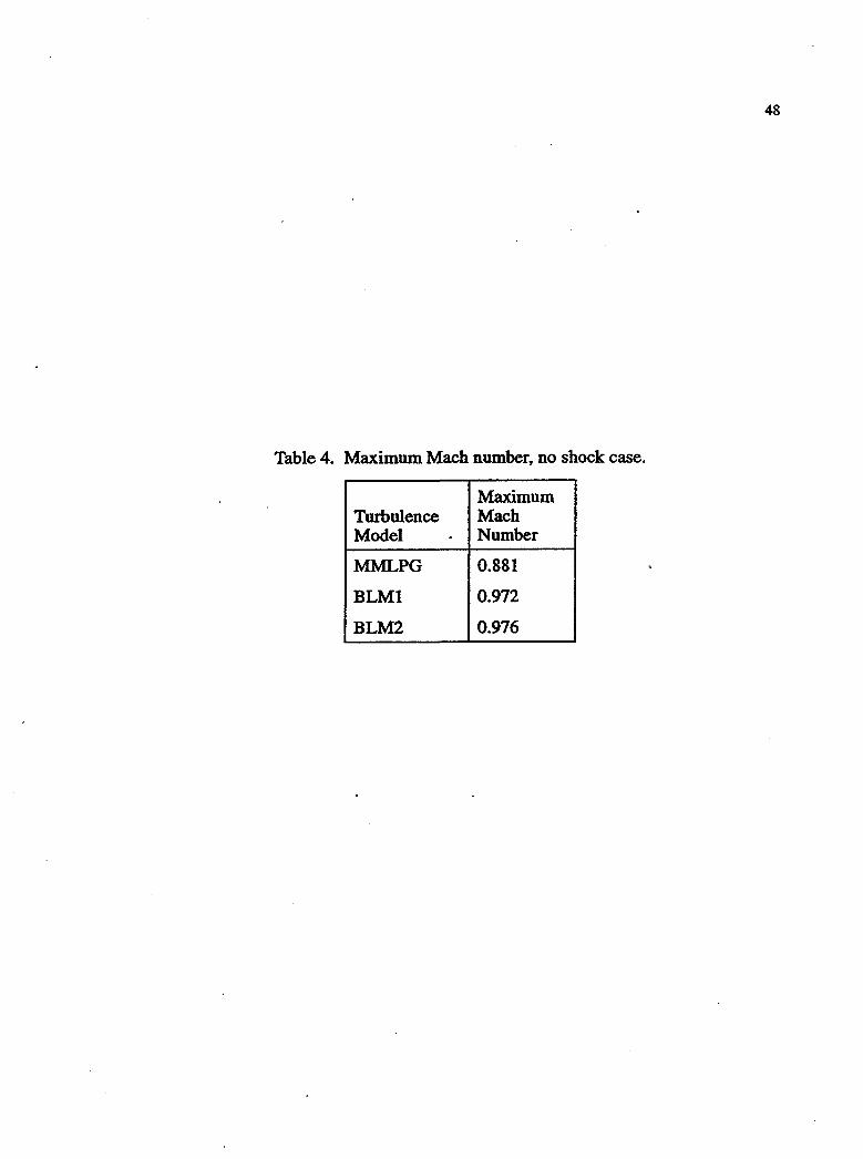
48
Table 4. Maximum Mach number, no shock case.
Maximum Turbulence Mach Model . Number
MMLPG 0.881
BLMI 0.972
BLM2 0.976
48
Table 4. Maximum Mach number, no shock case.
Maximum Turbulence Mach Model . Number
MMLPG 0.881
BLMI 0.972
BLM2 0.976

49
4.3 Strong Shock Case
The final diffuser flow computed was the case with a strong normal shock
positioned in the throat. This case was run in a manner similar to the weak shock
case: First the exit pressure was gradually lowered to R=O.1338 to achieve supersonic
flow throughout the diffuser; then it was gradually raised to R=O.72 to establish the
strong normal shock in the throat region, then iterated there until the solution stopped
changing appreciably with time. Proteus was run in both steady and unsteady modes
to try to simulate the experimentally observed self-excited oscillations of217 Hz.30
Unsteady mode in Proteus is achieved by calculating a global time step whereas
steady mode uses a local time step to speed up the computation. Neither calculation
simulated the experimentally observed oscillatory behavior, but instead produced very
small numerical oscillations in the flow properties. (The artificial viscosity used for
the strong shock calculations was the same as that used for the weak shock calcula
tion.) Figure 23 shows the static pressure on the top wall at the experimental shock
location and illustrates the behavior of these small oscillations; the calculation shown
was run in unsteady mode with MMLPG.
The static pressure on the top and bottom walls are presented'in figure 24 and
the shock location and Mach number at the edge of the top wall boundary layer are
given in table 5. Both BLM2 and MMLPG predicted the shock ldcation too far
downstream, while BLMI predicted it too far upstream. The experiment predicted a
region of separation on the top wall just downstream of the shock with the flow
reattaching at x/H=6.0. MMLPG predicted a very small region of separation on the
top wall which reattached at xIH=3.6. BLM2 predicted very small regions of separa
tion on both the top and bottom walls which reattached at xIH=3.8 and x/H=6.2,
respectively, and BLMI predicted a separation along the bottom wall that did not
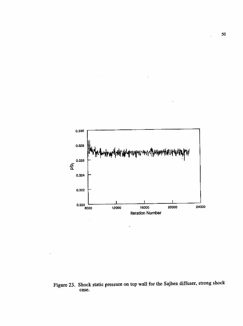
50
0.330
0.328
0.326 -~ 0.324
0.322
0.320 8000 12000 16000 20000 24000
Iteration Number
Figure 23. Shock static pressure on top wall for the Sajben diffuser, strong shock case.
50
0.330
0.328
0.326 -~ 0.324
0.322
0.320 8000 12000 16000 20000 24000
Iteration Number
Figure 23. Shock static pressure on top wall for the Sajben diffuser, strong shock case.

~ Q.
~ Q.
1.0
0.9
0.8
0.7
0.6
0.5
0.4
0.3
. I I I I I I ! I ! I i I ! ! ·················· .. ··t······ .. ······· .. ······!_········· ......... _.+_ ................ _ ... -t ........................ .
I I I I I ................................................... .;. ....................... + ..................... · .. f· .... •• ...... ·-· ....... .!· ......... ·-...... _ .. .. Ii! i j
I j I J ! .................. _ .... + .............. ·· .. · .. + .... ·· .. ··· ...... ·_··i .. · .......... · .. ··.. ·f··=·_7 .. -:o .. , '" .................. . i I I ~'-o-O i I ! !.Il ~ II
................... _ .... ,................ .. ...... , ...... _ ................. L •.• /....... ._ .................... _ ...... _ ..... _ .. _ ..... _ .. , , . g6 ~ • • ~ $ $
I ! lIS i i ! ,
..... _ .................. -1"._ .......... _ ..... '1' .... ··· ........ ··e· .. · .. · ....... - MMLPG ! i 9 t ; $
......................... 1 ......................... 1............ .. ... J., .... .. f ~ ~ I ! ! i f ! !
....... ~ ................................. ~ ........... _ ........................... ~ .......... _........................ I
I , f ~
o
BLM1
BLM2 Hsieh et al.
0.2 -5.0
~ ~
-2.5 0.0 2.5
xIH 5.0 7.5 10.0
1.0
0.9
0.8
0.7
0.6
0.5
0.4
0.3
0.2 -5.0 -2.5
(a) Top wall
0.0 2.5
xlH
(b) Bottom wall
5.0 7.5 10.0
Figure 24. Static pressure distribution on the top and bottom walls of the Sajben diffuser, strong shock case.
51
~ Q.
~ Q.
1.0
0.9
0.8
0.7
0.6
0.5
0.4
0.3
. I I I I I I ! I ! I i I ! ! ·················· .. ··t······ .. ······· .. ······!_········· ......... _.+_ ................ _ ... -t ........................ .
I I I I I ................................................... .;. ....................... + ..................... · .. f· .... •• ...... ·-· ....... .!· ......... ·-...... _ .. .. Ii! i j
I j I J ! .................. _ .... + .............. ·· .. · .. + .... ·· .. ··· ...... ·_··i .. · .......... · .. ··.. ·f··=·_7 .. -:o .. , '" .................. . i I I ~'-o-O i I ! !.Il ~ II
................... _ .... ,................ .. ...... , ...... _ ................. L •.• /....... ._ .................... _ ...... _ ..... _ .. _ ..... _ .. , , . g6 ~ • • ~ $ $
I ! lIS i i ! ,
..... _ .................. -1"._ .......... _ ..... '1' .... ··· ........ ··e· .. · .. · ....... - MMLPG ! i 9 t ; $
......................... 1 ......................... 1............ .. ... J., .... .. f ~ ~ I ! ! i f ! !
....... ~ ................................. ~ ........... _ ........................... ~ .......... _........................ I
I , f ~
o
BLM1
BLM2 Hsieh et al.
0.2 -5.0
~ ~
-2.5 0.0 2.5
xIH 5.0 7.5 10.0
1.0
0.9
0.8
0.7
0.6
0.5
0.4
0.3
0.2 -5.0 -2.5
(a) Top wall
0.0 2.5
xlH
(b) Bottom wall
5.0 7.5 10.0
Figure 24. Static pressure distribution on the top and bottom walls of the Sajben diffuser, strong shock case.
51

52
Table 5. Shock location and Mach number, strong shock case
Shock Shock Turbulence Mach Location Model Number (x/H)
MMLPG 1.626 3.13
BLM1 1.411 2.11
BLM2 1.665 2.90
Experiment30 1.353 1.98
52
Table 5. Shock location and Mach number, strong shock case
Shock Shock Turbulence Mach Location Model Number (x/H)
MMLPG 1.626 3.13
BLM1 1.411 2.11
BLM2 1.665 2.90
Experiment30 1.353 1.98

53
reattach. The separated behavior is illustrated in figure 25, which gives the velocity
profiles at four locations downstream of the shock. These peculiar results can be
attributed to the behavior of the turbulent viscosity as shown in figure 26. MMLPG
and BLM2 compute much higher values of J..lt than does BLM1; this is due to the large .
increase in vorticity downstream of the shock. In BLM1, as given in equation (4.1),
the second formula results in Fwake being inversely proportional to the vorticity
magnitude, and this helps to reduce the value of J..lt for this model. Each case was run
for 10,000 iterations and the steady calculations using MMLPG, BLMI and BLM2
required 3.54xlO-5 sec/iteration/grid point, 3.83xlO-5 sec/iteration/grid point, and
3.82xlO-S sec/iteration/grid point, respectively, on the CRAY Y-MP computer.

1.4
1.2
1.0
~ 0.8
>-0.6
0.4
0.2
~oc -
'""
- --- -- - -
0 -
--- - - ""'-I 0 -0 ,
0 ,0 ,g J 0
0 J 0 1 0
MMLPG 0 I BLM1
1 0 BLM2 Ig Hsieh et al. I 0
0.0 -100
_ .... ~ o§ _ o;;cfo-o -go I ~
o 100 200 300 400 500
u (m/s)
(a) x/H = 2.88
1.6
1.4
1.2
1.0
~ >- 0.8
MMLPG BLM1
BLM2
0.6 0 Hsieh etal.
0.4
0.2 .,
,/
0.0 -200 -100 0 100 200 300 400
u (m/s)
(c) x/H = 6.34
1.6
1.4
1.2
1.0
J: ">. 0.8
0.6
0.4
0.2
0.0 -200
1.6
1.4
1.2
1.0
J: ">. 0.8
0.6
0.4
0.2
0.0 -100
0
.... .,
MMLPG BLM1
o
,~, . , , I ", I
I ~ • 0
\~ BLM2 • 0
Hsieh et al. ....' Yg --::~ 0
cP
54
-100 o 100 200 300 400
u (m/s)
(b) x/H = 4.61
MMLPG
BLM1 BLM2
0
... .,
0 100 200 300 400
u (m/s)
(d) x/H = 7.49
Figure 25. Velocity profiles for the strong shock case.
1.4
1.2
1.0
~ 0.8
>-0.6
0.4
0.2
~oc -
'""
- --- -- - -
0 -
--- - - ""'-I 0 -0 ,
0 ,0 ,g J 0
0 J 0 1 0
MMLPG 0 I BLM1
1 0 BLM2 Ig Hsieh et al. I 0
0.0 -100
_ .... ~ o§ _ o;;cfo-o -go I ~
o 100 200 300 400 500
u (m/s)
(a) x/H = 2.88
1.6
1.4
1.2
1.0
~ >- 0.8
MMLPG BLM1
BLM2
0.6 0 Hsieh etal.
0.4
0.2 .,
,/
0.0 -200 -100 0 100 200 300 400
u (m/s)
(c) x/H = 6.34
1.6
1.4
1.2
1.0
J: ">. 0.8
0.6
0.4
0.2
0.0 -200
1.6
1.4
1.2
1.0
J: ">. 0.8
0.6
0.4
0.2
0.0 -100
0
.... .,
MMLPG BLM1
o
,~, . , , I ", I
I ~ • 0
\~ BLM2 • 0
Hsieh et al. ....' Yg --::~ 0
cP
54
-100 o 100 200 300 400
u (m/s)
(b) x/H = 4.61
MMLPG
BLM1 BLM2
0
... .,
0 100 200 300 400
u (m/s)
(d) x/H = 7.49
Figure 25. Velocity profiles for the strong shock case.

(a) MMLPG
lWJ..1]max = 4,600
-----------------~-~ ~
(b) BLM1
If..1t1J..1]max = 21,000
(c) BLM2
55
Figure 26. Turbulent viscosity ratio, J.liJl, for the Sajben diffuser, strong shock case.
(a) MMLPG
lWJ..1]max = 4,600
-----------------~-~ ~
(b) BLM1
If..1t1J..1]max = 21,000
(c) BLM2
55
Figure 26. Turbulent viscosity ratio, J.liJl, for the Sajben diffuser, strong shock case.

CHAPTER V
SUMMARY AND CONCLUSIONS
The objective of this work was to modify the MML algebraic turbulence
model to increase its range of applicability to include zero and adverse pressure gradi
ent boundary layer flows. To accomplish this objective, modifications were made
based on experimental data for zero and adverse pressure gradient flat plate flows.
The resulting model, called MMLPG, successfully predicted the flat plate flows and
also successfully predicted three transonic diffuser flows. This indicates that the
objective of this work has been met.
In order to provide meaningful solutions for turbulent flows, CFD codes
require good turbulence models. Algebraic models are the simplest and the most
computationally inexpensive of turbulence models, and so were chosen as the focus of
this study. Proteus, which was used to make all of the calculations in this work, is a
Reynolds averaged Navier-Stokes code for aerospace propulsion flows and contains
the Baldwin-Lomax algebraic turbulence model as a default. The Baldwin-Lomax
model is known to have problems calculating cer.tain flowfields, namely flows with
strong pressure gradients and large separated regions. A promising newer model, the
MML model, produced significantly better results than the Baldwin-Lomax model for
separated airfoil flows,S but it was not evaluated for other types of flows. The objec
tive of the current work was to continue development of MML to increase its range of
applicability to include boundary layer flows with zero and adverse pressure gradi
ents.
56
57
To accomplish this objective, MML was installed in Proteus and first used to
calculate zero pressure gradient flow over a flat plate. These results indicated that the
original MML model was not allowing for the proper boundary layer growth with
increasing Reynolds number. To remedy this behavior, a relationship was found for
the saturation length scale as a function of the local skin friction coefficient. This
modified version of MML allowed for the proper boundary layer growth and therefore
produced the correct velocity-defect profiles. Next, MML was modified to calculate
adverse pressure gradient flows using the experimental data of Bradshaw for zero,
mild and strong adverse pressure gradient flows. These modifications were combined
into one generalized model, called MMLPG. This new model accurately predicted the
zero and adverse pressure gradient flows and exhibited better agreement with experi
mental data than the Baldwin-Lomax model.
To more thoroughly evaluate MMLPG for other adverse pressure gradient
flows, this model was also used to calculate three transonic diffuser flow cases: flow
with a weak shock, flow wit~ no shock, and flow with a strong shock. These are flows
typically encountered in aerospace propulsion applications. The MMLPG results
were compared with results calculated using two slightly different implementations of
the Baldwin-Lomax model, referred to as BLMI and BLM2. The differences in the
two models arise from the calculation of the Fwake function, as discussed in Chapter
N.
For the weak shock case, MMLPG and BLM2 did equally well in predicting
the shock Mach Number and location, and also in predicting the static pressure distri
bution on the top and bottom walls. However, BLMI over-predicted the shock Mach
number and location and did not match the wall static pressures in the throat region of
the diffuser. For the no shock case, MMLPG was Significantly better than either of the
58
Baldwin-Lomax models at predicting the static pressures on the walls and MMLPG
also predicted a maximum Mach number that was in close agreement with the results
of Georgiadis.35
The strong shock diffuser flow was beyond the capabilities of all three
models. Both MMLPG and BLM2 over-predicted the shock Mach number and
location, as well as the pressure distribution on the walls, while the BLMI results
were in reasonable agreement for these quantities. None of the models were able to
correctly predict the shock-induced separation on the top wall; in fact, BLMI
predicted no separation at all on the top wall yet predicted a very large, unattached
separation on the bottom wall. The primary reason the MMLPG and BLM2 results
differ greatly from the BLMI results is explained by the turbulent viscosity values.
MMLPG and BLM2 gave maximum turbulent viscosity values of 23,000 and 21,000
times the molecular viscosity, respectively, while BLMI gave a maximum turbulent
viscosity of only 4,600 times the molecular viscosity. The turbulent viscosity is
proportional to the vorticity, which becomes very large just downstream of the normal
shock, however, the FWake function used in BLMI is inversely proportional to the
vorticity resulting in a lower overall turbulent viscosity. The poor performance of all
of the models for this case can also be attributed to the fact that all of the models are
equilibrium turbulence models being used to calculate a flow which is clearly
nonequilibrium. The poor performance of MMLPG for the strong shock case is also
explained by the derivation of the model, which is based on experimental data for ~
values between 0 and 5, while this flow encountered ~ values as high as 12,000.
Considering that MMLPG did well at calculating the less severe no shock and weak
shock flows indicates that it is most likely applicable to other propulsion flows at
these less severe types of conditions.
59
The flat plate and transonic diffuser results indicate that the modified version
of the MML model, MMLPG, is capable of accurately predicting turbulent flows with.
and without adverse pressure gradients. Thus, the objective of this work, which was
to evaluate the original MML model and modify it to increase its range of applicabil
ity to include adverse pressure gradient flows, has been met. Future work should
include continued validation of the model for these types of flows as well as continued
development of the model to better account for stronger adverse pressure gradient
flows both with and without separation.

REFERENCES
1. Rodi, W., Turbulence Models and Thelr Application in Hydraulics, Brookfield Publishing, Brookfield, Vermont, 1984.
2. White, F. M., Viscous Fluid Flow, McGraw-Hill, Inc., New York, 1991.
3. Anderson, D. A., Tannehill, J. C., and Pletcher, R. H., Computational Fluid Mechanics and Heat Transfer, McGraw-Hill, New York, 1984.
4. Baldwin, B. and Lomax, H., "Thin Layer Approximation and Algebraic Model for Separated Turbulent Flows," AIAA Paper 78-257, January 1978.
5. Potapczuk, M. G., "Navier-Stokes Analysis of Airfoils with Leading Edge' Ice Accretions," Ph.D. Dissertation, University of Akron, May 1989.
6. Yu, N. J., Allmaras, S. R., and Moschetti, K. G., "Navier-Stokes Calculations for Attached and Separated Flows Using Different Turbulence Models," AIAA Paper 91-1791, June 1991.
7. Visbal, M. and Knight, D., "The Baldwin-Lomax Turbulence Model for TwoDimensional Shock-WavelBoundary-Layer Interactions," AIAA Journal, Vol. 22, No.7, July 1984, pp. 921-928.
8. Degani, D. and Schiff, L. B., "Computation of Turbulent Supersonic Flows around Pointed Bodies Having Crossflow Separation," Journal of Computational Physics, Vol. 66, 1986, pp. 173-196.
9. Menter, F. R., "Performance of Popular Turbulence Models for Attached and Separated Adverse Pressure Gradient Flows," AIAA Journal, Vol. 30, No.8, August 1992,pp.2066-2072.
10. Stock, H. W. and Haase, W., "The Determination of Turbulent Length Scales in Algebraic Turbulence Models for Attached and Slightly Separated Flows Using Navier-Stokes Methods," AIAA Paper 87-1302, June 1987.
11. Sakowski, B., Darling, D., Roach, R. L. and van de Wall, A., "Evaluation and Application o'fthe Baldwin-Lomax Turbulence Model in Two-Dimensional,
60
61
Unsteady, Compressible Boundary Layers with and without Separation in Engine Inlets," AIAA Paper 92-3676, July 1992.
12. Chima, R. V., Giel, P. W. and Boyle, R. J., "An Algebraic Turbulence Model for Three-Dimensional Viscous Flows," NASA TM 105931, January 1993.
13. Towne, C. E., Schwab, J. R. and Bui, T. T., "Proteus Two-Dimensional NavierStokes Computer Code, Version 2.0, Vols. 1-3," NASA TM 106336, 106337, 106339, October 1993.
14. Towne, C. E., Schwab, J. R., Benson, T. J. and Suresh, A., "PROTEUS TwoDimensional Navier-Stokes Computer Code, Version 1.0, Vols. 1-3," NASA TM 102551-102553, March 1990.
15. Briley, W. R., McDonald, R., "Solution of the Multidimensional Compressible Navier-Stokes Equations by a Generalized Implicit Method," Journal o/Computational Physics, Vol. 24, 1977, pp. 373-397.
16. Beam, R. M. and Warming, R. E, "An Implicit Factored Scl\eme for the Compressible Navier-Stokes Equations," AlAA Journal, Vol. 16, No.4, April 1978, pp. 393-402.
17. Chien, K. Y., "Prediction of Channel and Boundary-Layer Flows with a LowReynolds-Number Turbulence Model," AlAA Journal, Vol. 20, No.1, January 1982, pp. 33-38.
18. Steger, J. L., "Implicit Finite-Difference Simulation of Flow about Arbitrary TwoDimensional Geometries," AlAA Journal, Vol. 16, No.7, July 1978, pp. 679-686.
19. Jameson, A., Schmidt, W. and Turkel, E., "Numerical Solutions of the Euler Equations by Finite Volume Methods Using Runge-Kutta Time-Stepping Schemes," AIAA Paper 81-1259, June 1981.
20. Cebeci, T. and Smith, A. M. 0., Analysis of Turbulent Boundary Layers, Academic Press, New York, 1974.
21. Samuel, A. E. and Joubert, P. N., "A boundary layer developing in an increasingly adverse pressure gradient,"journal of Fluid Mechanics, Vol. 66, Part 3, 1974, pp. 481-505.
22. Driver, D. M., "Reynolds Shear Stress Measurements in a Separated Boundary Layer," AIAA Paper 91-1787, 1991.
23. Kirtley, K. R., "A Coupled, Parabolic-Marching Method for the Prediction of Three-Dimensional Viscous Incompressible Turbomachinery Flows," Ph. D. Thesis, Pennsylvania State University, December, 1987.
24. Launder, B. E. and Priddin, C. H., "A Comparison of Some Proposals for the Mixing Length Near a Wall," International Journal of Heat and Mass Transfer, Vol. 16, 1973, pp. 700-702.
62
25. Bradshaw, P., "The Turbulence Structure of Equilibrium Boundary Layers," NPL Aero Report 1184, January, 1966.
26. Fletcher, C. A. J., Computational Techniques of Fluid Dynamics, Vol. 1, SpringerVerlag, Berlin, 1985.
27. Musker, A. J., "Explicit Expression for the Smooth Wall Velocity Distribution in a Turbulent Boundary Layer," AIAA Journal, Vol. 17, No.6, June 1979, pp. 655-657.
28. Clauser, F. H., "Turbulent Boundary Layers in Adverse Pres~ure Gradients," Journal of Aeronautical Sciences, February 1954, pp. 91-108.
29. Weighardt, K., "Flat Plate Flow. uoo=33 m/sec," Proceedings, AFOSR-IFPStanford Conference on Computation of Turbulent Boundary Layers-1968, Vol. II, Ed. by Coles, D.E. and Hirst, E. A., 1968, pp. 98-123.
30. Salmon, J. T., Bogar, T. J. and Sajben, M., "Laser Doppler Velocimeter Measurements in Unsteady, Separated, Transonic Diffuser Flows," AIAA Journal, Vol. 21, No. 12, 1983,pp. 1690-1697.
31. Bogar, T. J., Sajben, M. and KroutH, J. C., "Characteristic Frequencies of Transonic Diffuser Flow Oscillations," AIAA Journal, Vol. 21, No.9, 1983, pp. 1232-1240. .
32. Hsieh, T., Bogar, T. J. and Coakley, T. J., "Numerical Simulation and Comparison with Experiment for Self-Excited Oscillations in a Diffuser FloW," AIAA Journal, Vol. 25, No.7, 1987, pp. 936-943.
33. Hsieh, T., Wardlaw, A. B. Jr., Collins, P. and Coakley, T., "Numerical Investigation of Unsteady Inlet Flowfields," AIAA Journal, Vol. 25, No.1, January 1987, pp.75-81.
34. Bui, T. T., "Implementation/Validation of a Low Reynolds Number Two-Equation Turbulence Model in the Proteus Navier-Stokes Code - Two-Dimensionall Axisymmetric," NASA TM 105619, April 1992.

35. Georgiadis, N. J., "An Evaluation of Turbulence Models for Propulsion Flows," Master's Thesis, University of Akron, May 1993.
36. Cooper, G. K. and Sirbaugh, J. R., "PARC Code: Theory and Usage," Arnold Engineering Development Center Report AEDC-TR-89-15, December 1989.
63
37. Wassel, A. T., and Catton, I., "Calculation of Turbulent Boundary Layers Over Flat Plates With Different Phenomenological Theories of Turbulence and Variable Turbulent Prandtl Number," International Journal of Heat and Mass Transfer, Vol. 16, 1973,pp. 1547-1563.
38. Schlicting, H., Boundary-Layer Theory, McGraw-Hill Book Company, New York, 1968.
39. Hoffman, K. A., Computational Fluid Dynamics for Engineers, Engineering Education System, Austin, Texas, 1989.
40. Pulliam, T. H., "Artificial Dissipation Models for the Euler Equations," AlAA Journal, Vol. 24, No. 12, December 1986, pp. 1931-1940. ,

APPENDICES
64
APPENDICES
64

APPENDIX 1
GOVERNING EQUATIONS OF PROTEUS
The governing equations of Proteus are the compressible Navier-Stokes
equations. The equations given below are taken from reference 13, but may also be
found in several references.2,3,38 Since the two-dimensional/axisymmetric version of
the Proteus code was used for all calculations discussed in this work, the two-dimen
sional, planar equations are given here. (For the axisymmetric version of the
equations, which are somewhat more complex, consult reference 13.)
1. Cartesian Coordinates
In Cartesian coordinates, the continuity, x-momentum, y-momentum and
energy equations are written in strong conservation law form, using vector notation:
where
oQ oE of oEv oFv - +-+- =- +ot ox oy ox oy
p
Q = pu pv
ET
65
(A.I)
(A.2)

E=
F=
Ev =
Fv =
pu
pU2+p pUV
(Er+P)u
pv puv
pV2+p
(Er + p) Y-
o 'txx 'txy
u'txx + v'txy - qx
0 'txy 'tyy
u'tXy + v'tyy - qy
66
(A.2a)
(A.2b)
(A.2c)
(A.2d)
In equation (A.2), the dependent variables are p, pu, pv and Er. the inviscid flux
vectors are E and F, and the viscous flux vectors are Ev and F yo The normal and
shear stresses, and the heat ,flux are given by
(A.3)
2. Equation of State
oT q = -k-
y oy
67
In addition to the above equations, an equation of state is needed to relate the
pressure to the dependent variables. Proteus contains the equation of state for an ideal
gas:
p = pRT (A.4)
where R is the ideal gas constant. For a calorically perfect gas, this is equivalent to
(A.5)
3. Generalized Grid Transformation
The governing equations in section 1.0 are written in Cartesian coordinates
and are not well-suited for nonrectangular geometries and grids with unequal
spacing.13, 39 To overcome these difficulties, the following generalized grid transfor
mation is used to transform the governing equations from physical (x, y) coordinates
to rectangular orthogonal computational (~, 11) coordinates.
~ = ~ (x, y)
11 = 11 (x, y) (A.6)
The resulting spatial computational domain is square, and has uniform spacing. The
chain rule is used to transform the partial derivatives in the Cartesian form of the

68
governing equations, (A.l)-(A.3); for details, refer to Towne et al. 13 The transformed
equations are written as
where
Q=Q J
and J is the Jacobian of the transformation,
4. Time Differencing
(A.7)
(A.8)
(A.8a)
(A.8b)
(A.8c)
(A.8d)
(A.9)
The generalized time differencing scheme of Beam & Warming16 is used to
approximate the time derivative in equation (A.7):
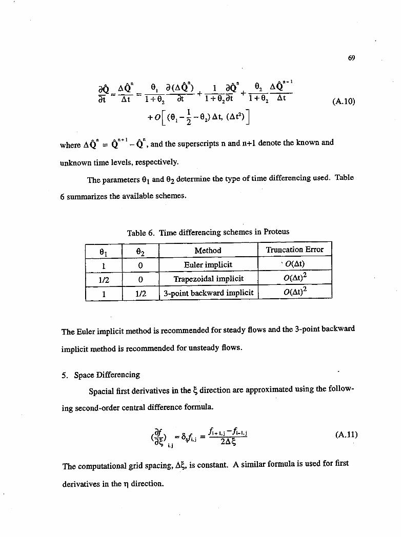
69
dO /)..00
91 d (/)..00
) I dOD 92 /)..00
-
1
- =< -- = -- + --- + -----'7-dt /)..t I +92 at I +92 dt 1 +92 /)..t (A.IO)
+ O[ (9 1 - 4 -92) Llt, (/)..t2) ]
An ,,0+1 AD
where /).. Q = Q - Q , and the superscripts n and n+ I denote the known and
unknown time levels, respectively.
The parameters 61 and 62 determine the type of time differencing used. Table
6 summarizes the available schemes.
Table 6. Time differencing schemes in Proteus
91 92 Method Truncation Error
I 0 Euler implicit ", O(/)..t)
112 0 Trapezoidal implicit O(/)..t) 2
1 112 3-point backward implicit 0(/)..t)2
The Euler implicit method is recommended for steady flows and the 3-point backward
implicit method is recommended for unsteady flows.
5. Space Differencing
Spacial first derivatives in the ~ direction are approximated using the follow
ing second-order central difference formula.
(A. 11)
The computational grid spacing, /)..~, is constant. A similar formula is used for first
derivatives in the Tl direction.

APPENDIX 2
ARTIFICIAL VISCOSITY AND GRID CONVERGENCE
High frequency nonlinear instabilities can appear as the Proteus solution
develops. For example, physical phenomena, such as shock waves, can cause instabil
ities when they are captured by the finite difference algorithm. In addition, high
Reynolds number flows may have oscillations resulting from the odd-even decoupling
inherent in the use of central spatial differencing of the convective terms. Artificial
viscosity may be used to suppress these oscillations. The two artificial viscosity
models in Proteus are the constant coefficient model of Steger18 and the nonlinear
coefficient model of Jameson et al. 19 The implementation of these models in general
ized nonorthogonal coordinates was taken from Pulliam.40 .
1. Constant Coefficient Model
The constant coefficient model uses a combination of explicit and implicit
smoothing. The standard explicit artificial viscosity uses fourth-order differences.
Second-order explicit artificial viscosity, which provides more smoothing, is also
available in Proteus, however it is rarely used because it introduces a large error. The
implicit smoothing is second order and is used to extend the linear stability bound of
the fourth-order explicit smoothing.
The explicit artificial viscosity is implemented in the Proteus alternating
direction implicit (ADI) algorithm15 by adding the following terms to the right-hand
side source term for the first ADI sweep.
70
71
where ei2) and eE(4) are the second- and fourth-order explicit artificial viscosity
coefficients. The symbols V and Il are the backward and forward first difference
operators for the first ADI sweep such that
V'!;Qj = Qj-Qj-l
Il!;Qi = Q i+1 - Qi
'V!;Il!;Qi = Q i+1 - 2Qi + Qi-l
(V!;Il!;)2Qi = Qi+2 -4Qi+l + 6Qi -4Qi-l +Qi-2
Similar formuias are used in the 11 direction.
(B.2)
The implicit artificial viscosity is implemented by adding the following terms
to the left-hand side of the governing equation.
(B.3a)
(B.3b)
Equation (B.3a) is added for the first ADI sweep and equation (B.3b) is added for the
second ADI sweep. The constant e] is the implicit artificial viscosity coefficient.
The optimum values of the coefficients ei2), ei4) and e] vary from problem
to problem. They should be small so as not to corrupt the physical solution, yet large
enough to damp any instabilities. The Proteus User's Guide13 recommends starting
values of eE(4) =1.0, ei2)=1.0 and e[=2.0.
72
2. Nonlinear Coefficient Model
The nonlinear coefficient artificial viscosity is explicit and contains second
and fourth-order differences. The following terms are added to the right-hand side of
the governing equations.
V; { [ ( j) i + 1 + ( j) J (e~2) a; Q - et) a; v ;a; Q) )
+ Vll {['IIJ. + 'IIJ.J (e~2) allQ - e~4) ~ V llallQ).} J + 1 J J
The difference operator a; v ;a; Qi is defined by
and the expression '" is given by
where 'II x and 'II y are spectral radii defined by
(B.4)
(B.S)
(B.6)
(B.7)
The second- and fourth- order nonlinear artificial viscosity coefficients are a
function of the pressure field. In the ~ direction, they are given by
(B.8a)
(B.8b)
where

73
(Ji = IPi+1- 2Pi+Pi-l! Pi+l +2Pi+Pi-l
(B.9)
Similar formulas are used in the 11 direction.
The parameter (J is a pressure gradient scaling parameter which increases the
amount of second-order smoothing relative to fourth-order near shock waves. The
parameters 1C2 and 1C4 are user-specified constants. As with the constant coefficient
model, the optimum values of 1(2 and 1'4 are problem dependent. Typical values range
from 1(4=0.005 and 1(2=0.01 for flows with no shocks, to 1'4=0.0004 and 1C2=0.1 for
flows with shocks. 13 Pulliam gives 1(2=0.25 and K4=0.01 as typical values for an
Euler analysis. 13, 40
3. Comments on Artificial Viscosity
As previously mentioned, artificial viscosity is generally used to minimize
oscillations which occur when computing high Reynolds number flows and flows with
shock waves. Since the artificial viscosity terms do not represent anything physical,
the coefficients should be as small as possible so as not to corrupt the solution, yet
large enough to damp the nonphysical instabilities. Optimum values of the artificial
viscosity coefficients vary from problem to problem; the coefficients used to calculate
the flows presented in Chapters III and IV were selected based on values used for
similar cases, as given in the Proteus User's Manual. 13 Some representative test cases
were evaluated to insure that the chosen artificial viscosity did not corrupt the physi
cal characteristics of the flow.
The flat plate flows presented in Chapter III were run using the constant
coefficient model with £i4)=1.0, £E(2)=0.0 and £] =2.0. For these flows, it was possi
ble to run Proteus with zero artificial viscosity, however the solutions took two to four
times longer to "converge," or reach a point where the solution stopped changing

appreciably with time. Upon close examination, these solutions did not agree as
closely with experimental data as the solutions computed using artificial viscosity.
74
For the diffuser flows computed in Chapter IV, the artificial viscosity effects
were examined for the weak shock case. As mentioned in Chapter IV, the nonlinear
coefficient model was used. A value of 1C2=0.1 was used for the entire calculation,
with 1C4=0.00S while the exit pressure was changing (i.e, for the first 6000 iterations),
and 1C4=0.0004 for the remaining 3000 iterations, which were at a constant exit
pressure. It was not possible to compute this flow without artificial viscosity, so the
effects of doubling and halving the smoothing coefficients was examined.· The static
pressure distribution on the top and bottom walls for this comparison (computed using
MMLPG) is given in figure 27. The solution computed using half of the original
artificial viscosity was nearly identical to the original solution, indicating that the
originally chosen artificial viscosity is reasonable for this flow. Doubling the artificial
viscosity gave a less desirable result in that the normal shock was smeared over a
greater number of grid points.
4. Grid Convergence
Grid convergence is an important factor in the accuracy of a CFD calculation.
:rhe grids used to make the flat plate and transonic diffuser calculation~ were assessed
to insure their grid independence. For the zero pressure gradient flat plate calcula
tions, a 101xlOl grid was initially chosen. The size of this grid was systematically
reduced in each direction in order to find the coarsest grid that would give a solution
which would not change if additional grid points were added. The SlxSl grid
described in Chapter III was chosen based on this study.
The grid used to make the transonic diffuser calculations had been used previ
ously by others, 13, 34 so it is probable that this grid gives a reliable solution. As an
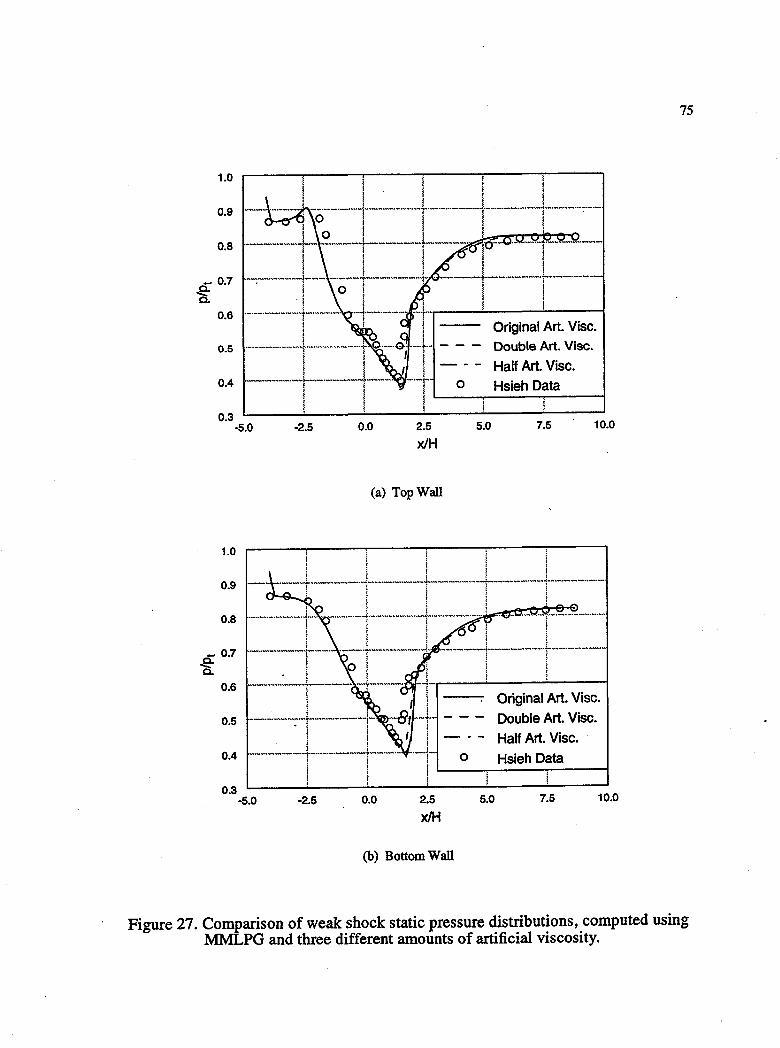
1.0 I
0.9
I i I ! I I I I ............. _ ...... + .. _ ... _ .............. -4 ......................... 1 .......... _ ........ _ .•• ;._ .................... .
. 0 ! ! ! !. I I . , I ! 0 I ! ! ! _ ... _ ... _ ... _ ... _.-1-.. - -"'-'--+-'-'''--'_.-1--.. _-_ ... _. 0.8
_ 0.7 .e-o.
I I I I I "-;"-"'--'-"-i'-"'-' -"-'''-'+'--'''-'''-'-'''i'' .• _ •.• _--+._-_ .... _._ ... _ .. j_._ •.• _ •.. __ ._ ... i O! !! . j! I I
0.6 I! I I .................. _ ................ .,........................ • ..... 1· .. ·..-.. • .. " .. _ .. · ... ..
~ ~ f . I
....... -... -.......... J ...... --................ ~. O····.-Q. ·_··t··· - - -if, ~ ! ! ! ! ! I - --f i i
"-'--"'-'''-'''-''!-'-''-'''-''-'1'''-'''-'' . _···-t ! ! ! II ~ t I ~ t
0.5
0.4 o
0.3 -5.0 -2.5 0.0 2.5
xlH 5.0
(a) TopWall
1.0 i i
0.9
0.8
Original Art. VisCo Double Art. Visco
Half Art. VisCo Hsieh Data
7.5 10.0
_ 0.7
..... _ ........ _.-... _::_:~_ .. ~ .... _.:.~!:,!.-~ .. _~_-.,~ .. :::,~·.:.~ ... _:.:,!,':.:_~~:.~.,.·_=_,~.~_::.~.,.·_f:, .. -=J~i= _ -~ - -_ .... _ ............ _ .. -J ........... _ .... -... ................... .L. ..... _ ..... _ ........... _ ..
I 0 I !! ..e-o. 0.6 -_··· __ ·_···t .. _· __ ···· ·-1 .. _·--·_- .'
f
==t--L 0.5
0.4
0.3 -5.0
~ i f f
-2.5 0.0 2.5
x/H
(b) Bottom Wall
o
5.0
Original Art. Visco Double Art. Visco Half Art. Visco Hsieh Data
7.5 10.0
75
Figure 27. Comparison of weak shock static pressure distributions, computed using MMLPG and three different amounts of artificial viscosity.

76
added check, the number of grid points in each direction was doubled, and the result
ing 162xl0l grid was used to compute the no shock flow using MMLPG. A compari
son of these results with the results obtained using the 81 x51 grid of Chapter IV is
given in figure 28 and indicates that the 81x51 grid is reliable.
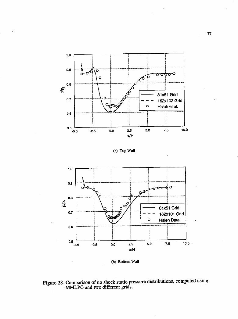
0: Q.
~ a.
1.0 1 !
0.9
0.8
0.7
0.6
! \ \ !
I I I I -··· .... · .. · .... · .. ·~.-... --.-.· .. - .. ·l ........ · .. -· ... --·-+ ........................ +_ .... _ ..... _ ... .. oil I !
i ! ! ! ! !
! ! !
! ! \ ·-....... · .. ~-·-· .. · .... · .. · .... t·· .. · .. · .. · .. ·-· .. · .... · .. · .... · .. t .. · .. · .... · .. · .... · .. ·---.. · .. ~· .. · .... · til i I ! ! ! ! ! ! ! .. ·· .................... 1 .......... · .. o ...... t .. · .... ·· .. · .... · ! i j 01 I .n'I.~K':.i., ! ! !
......... -.-... --... ~ .. - .. -..... -... - ......... · ........ · ................. · .. - ... _ .. ·f ...... · ........ · ........ • .. _ ........ · .. L ........... _ .......................... -~ ............ - ..... - .. -iii ! :
I I I I I
o ! I .
......... - ........ 4. ......................................... ;.. ........ --....................... .
I f
I I
81x51 Grid
162x102 Grid o Hsieh etal.
0.5 -5.0
! i ~ j ~
-2.5 0.0 2.5
xlH 5.0 7.5 10.0
1.0
0.9
0.8
0.7
0.6
0.5 -5.0 -2.5
(a) TopWall
0.0 2.5
x/H
(b) Bottom Wall
81x51 Grid
162x101 Grid
o Hsieh Data
5.0 7.5 10.0
Figure 28. Comparison of no shock static pressure distributions, computed using MMLPG and two different grids.
77
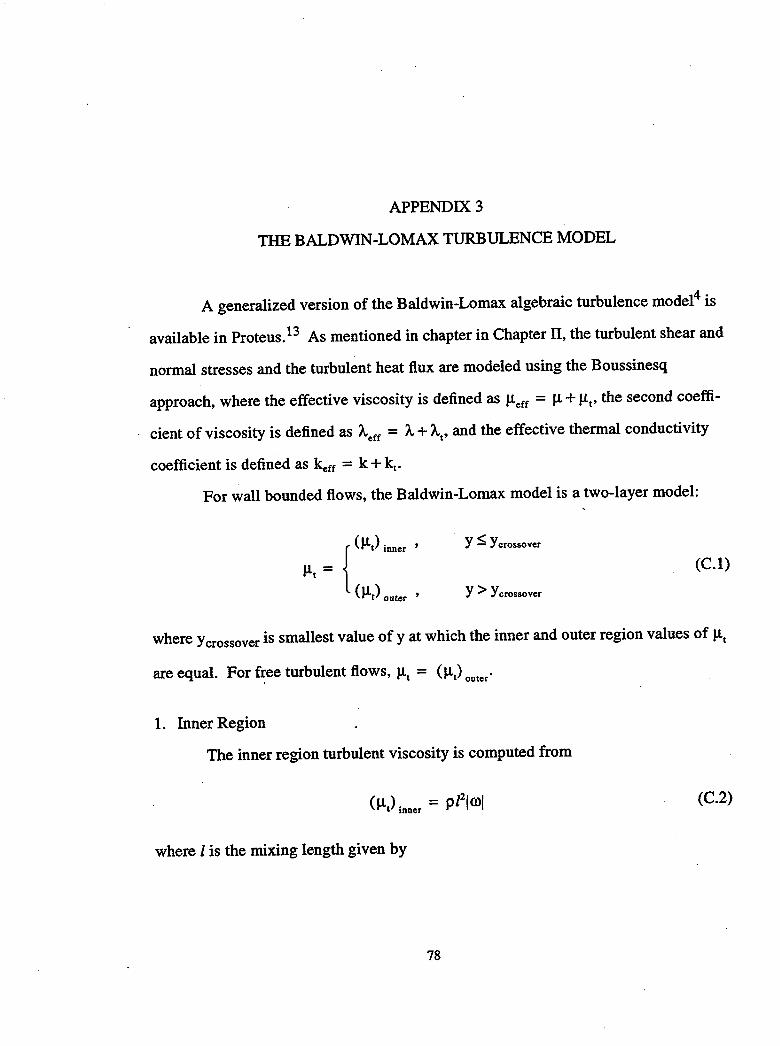
APPENDIX 3
THE BALDWIN-LOMAX TURBULENCE MODEL
A generalized version of the Baldwin-Lomax algebraic turbulence model4 is
available in Proteus.13 As mentioned in chapter in Chapter II, the turbulent shear and
normal stresses and the turbulent heat flux are modeled using the Boussinesq
approach, where the effective viscosity is defined as J..teff = J..t + J..t t ' the second coeffi
cient of viscosity is defined as Aeff = A + At' and the effective thermal conductivity
coefficient is defined as keff = k + k t •
For wall bounded flows, the Baldwin-Lomax model is a two-layer model:
y ~ Ycrossover
(C.l)
y > y crossover
where Y crossover is smallest value of Y at which the inner and outer region values of J..tt
are equal. For f~ee turbulent flows, J..lt = (J..lt) outer'
1. Inner Region
The inner region turbulent viscosity is computed from
(C.2)
where 1 is the mixing length given by
78

79 .
(C.3)
The quantity 1001 is the magnitude of the total vorticity, defined for two-dimensional
planar flow as
2. Outer Region
lOll = Idv _ dul ax ~
In the outer region, the turbulent viscosity is given by
(C.4)
(C.5)
where K is the Clauser constant, taken as 0.0168 and Ccp is a constant taken as 1.6.
The quantity Fwake is computed from
Fwake =
1 YmaxFmax ,
C V2 Ymax
wk diffr max
where the constant Cwk is 0.25 and
for wall bounded flows
(C.6)
for free turbulent flows
where V is the total velocity vector. The quantity Fmax is the maximum value of
for wall bounded flows F(y) = (C.7)
ylrol , for free turbulent flows
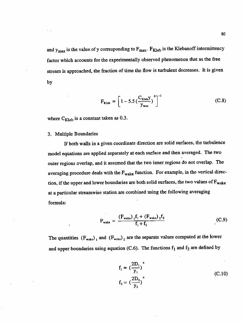
80
and y max is the value of y corresponding to Fmax' FKleb is the Klebanoff intermittency
factor which accounts for the experimentally observed phenomenon that as the free
stream is approached, the fraction of time the flow is turbulent decreases. It is given
by
F - [1 55 (CKleby) 6J-1 Kleb - -. -y--max
(C.8)
where CKleb is a constant taken as 0.3.
3. Multiple Boundaries
If both walls in a given coordinate direction are solid surfaces, the turbulence
model equations are applied separately at each surface and then averaged. The two
outer regions overlap, and it assumed that the two inner regions do not overlap. The
averaging procedure deals with the Fwake function. For example, in the vertical direc
tion, if the upper and lower boundaries are both solid surfaces, the two values of Fwake
at a particular streamwise station are combined using the following averaging
formula:
(C.9)
The quantities (Fwake) 1 and (Fwake) 2 are the separate values computed at the lower
and upper boundaries using equation (C.6). The functions fl and f2 are defined by .
(C.10)

81
The constant n is set equal to 2.0, Yl and Y2 are the normal distances to the bottom and
top surfaces, respectively, and Dl and D2 are the normal distances from the two
surfaces to the location of Ivlmax • In addition, the y/Ymax value used in equation (C.8)
for FKleb is computed for both surfaces and the minimum value is used. These values
of FKleb and Fwake are then used in equation (C.S) to compute (J.1t) •
outer
4. Turbulent Values of A. and k
The turbulent second coefficient of viscosity is defined as
(C.Il)
The turbulent thermal conductivity coefficient is defined using the Reynolds
analogy as
(C.12)
and cp is the specific heat at constant pressure and P't is the turbulent Prandtl number.
In Proteus, the turbulent Prandtl number may be equal to a constant or computed using
the empirical formula of Wassel and Catton.37 For the cases described herin, Prt was
constant with the Proteus default value of 0.91.

REPORT DOCUMENTATION PAGE I Form Approved
OMB No. 0704-0188 Public reporting burden for this collection of information is estimated to average 1 hour per response, including the time for reviewing instructions, searching existing data sources, gathering and maintaining the data needed, and completing and reviewing the collection of information. Send comments regarding this burden estimate or any other aspect of this collection of information, including suggestions for reducing this burden, to Washington Headquarters Services, Directorate for Information Operations and Reports, 1215 Jefferson Davis Highway, Suite 1204, Arlington, VA 22202-4302, and to the Office of Management and Budget, Paperwork Reduction Project (0704·0188), Washington, DC 20503.
1. AGENCY USE ONLY (Leave blanK) 12. REPORT DATE 13. REPORT TYPE AND DATES COVERED
April 1994 Techrrical~emorandum
4. TITLE AND SUBTITLE 5. FUNDING NUMBERS
~odification of the MML Turbulence ~odel for Adverse Pressure Gradient Flows
6. AUTHOR(S) WU-505-62-52
Julianne~. Conley
7. PERFORMING ORGANIZATION NAME(S) AND ADDRESS(ES) 8. PERFORMING ORGANIZATION REPORT NUMBER
National Aeronautics and Space AdDlinistration Lewis Research Center E-8690
Cleveland, Ohio 44135-3191
9. SPONSORINGIMONITORING AGENCY NAME(S) AND ADDRESS(ES) 10. SPONSORINGIMONITORING AGENCY REPORT NUMBER
National Aeronautics and Space AdDlinistration NASA TM-I06544 Washington, D.C. 20546-0001
11. SUPPLEMENTARY NOTES This report was subDlitted as a thesis in partial fulfillment of the requirements for the degree ~aster of Science to the University of Akron, Akron, Ohio, December 1993. Responsible person, Julianne ~. Conley, organization code 2660, (216) 433-2188.
12a. DISTRIBUTION/AVAILABILITY STATEMENT 12b. DISTRIBUTION CODE
Unclassified - UnliDlited Subject Category 34
13. ABSTRACT (Maximum 200 words)
Computational fluid dynamics is being used increasingly to predict flows for aerospace propulsion applications, yet there is still a need for an easy to use, computationally inexpensive turbulence model capable of accurately predicting a wide range of turbulent flows. The Baldwin-Lomax model is the most widely used algebraic model, even though it has known difficulties calculating flows with strong adverse pressure gradients and large regions of separation. The modified mixing length model (MML) was developed specifically to handle the separation which occurs on airfoils and has given significantly better results than the Baldwin-Lomax model. The success of these calculations warrants further evaluation and development of MML. The objective of this work was to evaluate the performance of MML for zero and adverse pressure gradient flows, and modify it as needed. The Proteus Navier-Stokes code was used for this study and all results were compared with experimental data and with calculations made using the Baldwin-Lomax algebraic model, which is currently available in Proteus. The MML model was first evaluated for zero pressure gradient flow over a flat plate, then modified to produce the proper boundary layer growth. Additional modifications, based on experimental data for three adverse pressure gradient flows, were also imple-mented. The adapted model, called MMLPG (modified mixing length model for pressure gradient flows), was then evaluated for a typical propulsion flow problem, flow through a transonic diffuser. Three cases were examined: flow with no shock, a weak shock and a strong shock. The results of these calculations indicate that the objectives of this study have been met. Overall, MMLPG is capable of accurately predicting the adverse pressure gradient flows examined in this study, giving generally better agreement with experimental data than the Baldwin-Lomax model.
14. SUBJECT TERMS
Navier-Stokes; Turbulent boundary layer; Two-dimensional flow; Mixing length flow theory; Pressure gradients; Flat plates; Computational fluid dynaDlics
17. SECURITY CLASSIFICATION 18. SECURITY CLASSIFICATION 19. SECURITY CLASSIFICATION OF REPORT OF THIS PAGE OF ABSTRACT
Unclassified Unclassified Unclassified
NSN 7540-01-280-5500
15. NUMBER OF PAGES 96
16. PRICE CODE A05
20. LIMITATION OF ABSTRACT
Standard Form 298 (Rev. 2-89) Prescribed by ANSI Std. Z39-18 298-102