modern power-systems-analysis-d-p-kothari-i-j-nagrath-130414214412-phpapp01

nrp : // n I g n e reo. m cg raw-n | | L co m/s ites/O0 7 o 4g4gg 4

F ri

In simple language, the book provides a modern introduction to powersystem operation, control and analysis.

Key Features of the Third

New chapters added on

) .Power System Security) State Estimation) Power system compensation including svs and FACTS) Load Forecasting) Voltage Stability

New appendices on :

> MATLAB and SIMULINK demonstrating their use in problem solving.) Real time computer control of power systems.

From the Reviewen.,

The book is very comprehensive, well organised, up-to-date and (aboveall) lucid and easy to follow for self-study. lt is ampiy illustrated w1h solvedexamples for every concept and technique.

iltililttJffiillililil

€il

o'A--fvrt=

€o=,o-

va-coFTt-

r 9--

TIrd

sr-

-oI ro

- ' J - - - -u ; ; DaEi r -4 iEut i l r l ruwEt

Rm Anllueisr y r r r T r l r u t r t g r l ,s-

ThirdEditior;

Ff llf J( ^r*I- ^..!L' r r \(J l l td,f l

lJ Nagrath

lMrll--=i

Modern Porroer SYstem

Third Edition

About the Authors

D P Kothari is vice chancellor, vIT University, vellore. Earlier, he wasProfessor, Centre for Energy Studies, and Depufy Director (Administration)Indian Institute of Technology, Delhi. He has uiro t."n the Head of the centrefor Energy Studies (1995-97) and Principal (l gg7-g8),Visvesvaraya RegionalEngineering college, Nagpur. Earlier lflaz-s: and 19g9), he was a visitingfellow at RMIT, Melbourne, Australia. He obtained his BE, ME and phDdegrees from BITS, Pilani. A fellow of the Institution Engineers (India), prof.Kothari has published/presented 450 papers in national and internationaljournals/conferences. He has authored/co-authored more than 15 books,including Power system Engineering, Electric Machines, 2/e, power systemTransients, Theory and problems of Electric Machines, 2/e., and. BasicElectrical Engineering. His research interests include power system control,optimisation, reliability and energy conservation.

I J Nagrath is Adjunct Professor, BITS Pilani and retired as professor ofElectrical Engineering and Deputy Director of Birla Institute of Technologyand Science, Pilani. He obtained his BE in Electrical Engineering from theuniversity of Rajasthan in 1951 and MS from the Unive.rity of Wi"sconsin in1956' He has co-authored several successful books which include ElectricMachines 2/e, Power system Engineering, signals and systems and.systems:Modelling and Analyns. He has also puulistred ,"rr.ui research papers inprestigious national and international journats.

Modern Power SystemAnalysis

Third Edition

D P Kothari

Vice ChancellorVIT University

VelloreFormer Director-Incharge, IIT Delhi

Former Principal, VRCE, Nagpur

I J Nagrath

Adjunct Professor, and Former Deputy Director,Birla Ins1i1y7" of Technologt and Science

Pilani

Tata McGraw Hill Education private LimitedNEW DELHI

McGraw-Hill OfficesNew Delhi Newyork St Louis San Francisco Auckland Bogot6 Caracas

Kuala Lumpur Lisbon London Madrid Mexico city Milan MontrealSan Juan Santiago Singapore Sydney Tokyo Toronto

Information contained in this work has been obtained by Tata McGraw-Hill, from

sources believed to be reliable. However, neither Tata McGraw-Hill nor its authors

guarantee the accuracy or completeness of any information published hereiir, and neittier

Tata McGraw-Hill nor its authors shall be responsible for any errors, omissions, or

damages arising out of use of this information. This work is publi 'shed-with the

understanding that Tata McGraw-Hill and its authors are supplying information but are

not attempting to render enginecring or other professional services. If such seryices are

required, the assistance of an appropriate professional should be sought

Tata McGraw-Hill

O 2003, 1989, 1980, Tata McGrtrw I{ill Education Private I-imited

Sixteenth reprint 2009RCXCRRBFRARBQ

No part of this publication can be reproduced in any form or by any -"un,without the prior written permission of the publishers

This edition can be exported from India only by the publishers,Tata McGraw Hill Education Private Limited

ISBN-13: 978-0-07-049489-3ISBN- 10: 0-07 -049489 -4

Published by Tata McGraw Hill Education Private Limited,7 West Patel Nagat New Delhi I l0 008, typeset in Times Roman by Script Makers,Al-8, Shop No. 19, DDA Markct, Paschim Vihar, New Delhi l l0 063 and printed at

Gopaljee Enterprises, Delhi ll0 053

Cover printer: SDR Printcrs

Preface to the Third Edition

Since the appearance of the second edition in 1989, the overall energy situationhas changed considerably and this has generated great interest in non-conventional and renewable energy sources, energy conservation and manage-ment, power reforms and restructuring and distributed arrd dispersed generation.Chapter t has been therefore, enlarged and completely rewritten. In addition,the influences of environmental constraints are also discussed.

The present edition, like the earlier two, is designed for a two-semestercourse at the undergraduate level or for first-semester post-graduate study.

Modern power systems have grown larger and spread over larger geographi-cal area with many interconnections between neighbouring systems. Optimalplanning, operation and control of such large-scale systems require advancedcomputer-based techniques many of which are explained in the student-orientedand reader-friendly manner by means of numerical examples throughout thisbook. Electric utility engineers will also be benefitted by the book as it willprepare them more adequately to face the new challenges. The style of writingis amenable to self-study. 'Ihe wide range of topics facilitates versarile selectionof chapters and sections fbr completion in the semester time frame.

Highlights of this edition are the five new chapters. Chapter 13 deals withpower system security. Contingency analysis and sensitivity factors aredescribed. An analytical framework is developed to control bulk power systemsin such a way that security is enhanced. Everything seems to have a propensityto fail. Power systems are no exception. Power system security practices try tocontrol and operate power systems in a defensive posture so that the effects ofthese inevitable failures are minimized.

Chapter 14 is an introduction to the use of state estimation in electric powersystems. We have selected Least Squares Estimation to give basic solution.External system equivalencing and treatment of bad data are also discussed.

The economics of power transmission has always lured the planners totransmit as much power as possible through existing transmission lines.Difficulty of acquiring the right of way for new lines (the corridor crisis) hasalways motivated the power engineers to develop compensatory systems.Therefore, Chapter 15 addresses compensation in power systems. Both seriesand shunt compensation of linqs have been thoroughly discussed. Concepts ofSVS, STATCOM and FACTS havc-been briefly introduced.

Chapter 16 covers the important topic of load forecasting technique.Knowing load is absolutely essential for solving any power system problem.

Chapter 17 deals with the important problem of voltage stability. Mathemati-cal formulation, analysis, state-of-art, future trends and challenges arediscussed.

Wl Prerace ro rne lhlrd Edrtion

MATLAB and SIMULINK, ideal programs for power system analysis areincluded in this book as an appendix along with 18 solved examples illustratingtheir use in solvin tive tem problems. The help rendered

by Shri Sunil Bhat of VNIT, Nagpur in writing this appendix is thankfullyacknowledged.

Tata McGraw-Hill and the authors would like to thank the followingreviewers of this edition: Prof. J.D. Sharma, IIT Roorkee; Prof. S.N. Tiwari,MNNIT Allahabad; Dr. M.R. Mohan, Anna University, Chennai; Prof. M.K.Deshmukh, BITS, Pilani; Dr. H.R. Seedhar, PEC, Chandigarh; Prof. P.R. Bijweand Dr. Sanjay Roy, IIT Delhi.

While revising the text, we have had the benefit of valuable advice andsuggestions from many professors, students and practising engineers who usedthe earlier editions of this book. All these individuals have influenced thisedition. We express our thanks and appreciation to them. We hope this support/response would continue in the future also.

D P Kors[mI J Nlcn+rn

Preface to the First

Mathematical modelling and solution on digital computers is the only practicalapproach to systems analysis and planning studies for a modern day powersystem with its large size, complex and integrated nature. The stage has,therefore, been reached where an undergraduate must be trained in the latesttechniques of analysis of large-scale power systems. A similar need also existsin the industry where a practising power system engineer is constantly faced withthe challenge of the rapidly advancing field. This book has bedn designed to fulfilthis need by integrating the basic principles of power system analysis illustratedthrough the simplest system structure with analysis techniques for practical sizesystems. In this book large-scale system analysis follows as a natural extensionof the basic principles. The form and level of some of the well-known techniquesare presented in such a manner that undergraduates can easily grasp andappreciate them.

The book is designed for a two-semester course at the undergraduate level.With a judicious choice of advanced topics, some institutions may also frnd ituseful for a first course for postgraduates.

The reader is expected to have a prior grounding in circuit theory and electricalmachines. He should also have been exposed to Laplace transform, lineardifferential equations, optimisation techniques and a first course in controltheory. Matrix analysis is applied throughout the book. However, a knowledgeof simple matrix operations would suffice and these are summarised in anappendix fbr quick reference.

The digital computer being an indispensable tool for power system analysis,computational algorithms for various system studies such as load flow, fault levelanalysis, stability, etc. have been included at appropriate places in the book. Itis suggested that where computer facilities exist, students should be encouragedto build computer programs for these studies using the algorithms provided.Further, the students can be asked to pool the various programs for moreadvanced and sophisticated studies, e.g. optimal scheduling. An important novelfeature of the book is the inclusion of the latest and practically useful topics likeunit commitment, generation reliability, optimal thermal scheduling, optimalhydro-thermal scheduling and decoupled load flow in a text which is primarilymeant for undergraduates.

The introductory chapter contains a discussion on various methods ofelectrical energy generation and their techno-economic comparison. A glimpse isgiven into the future of electrical energy. The reader is also exposed to the Indianpower scenario with facts and figures.

Chapters 2 and 3 give the transmission line parameters and these are includedfor the sake of completness of the text. Chapter 4 on the representation of powersystem components gives the steady state models of the synchronous machine andthe circuit models of composite power systems along with the per unit method.

W preface ro rhe Frrst Edition

Chapter 5 deals with the performance of transmission lines. The load flowproblem is introduced right at this stage through the simple two-bus system andbasic concepts of watt and var control are illustrated. A brief treatment of circle

concept of load flow and line compensation. ABCD constants are generally wellcovered in the circuit theory course and are, therefore, relegated to an appendix.

Chapter 6 gives power network modelling and load flow analysis, whileChapter 7 gives optimal system operation with both approximate and rigoroustreatment.

Chapter 8 deals with load frequency control wherein both conventional andmodern control approaches have been adopted for analysis and design. Voltagecontrol is briefly discussed.

Chapters 9-l l discuss fault studies (abnormal system operation). Thesynchronous machine model for transient studies is heuristically introduced tothe reader.

Chapter l2 emphasises the concepts of various types <lf stability in a powersystem. In particular the concepts of transient stability is well illustrated throughthe equal area criterion. The classical numerical solution technique of the swingequation as well as the algorithm for large system stability are advanced.

Every concept and technique presented is well supported through examplesemploying mainly a two-bus structure while sometimes three- and four-busillustrations wherever necessary have also been used. A large number ofunsolved problems with their answers are included at the end of each chapter.These have been so selected that apart from providing a drill they help thereader develop a deeper insight and illustrate some points beyond what is directlycovered by the text.

The internal organisation of various chapters is flexible and permits theteacher to adapt them to the particular needs of the class and curriculum. Ifdesired, some of the advanced level topics could be bypassed without loss ofcontinuity. The style of writing is specially adapted to self-study. Exploiting thisfact a teacher will have enough time at his disposal to extend the coverage ofthis book to suit his particular syllabus and to include tutorial work on thenumerous examples suggested in the text.

The authors are indebted to their colleagues at the Birla Institute ofTechnology and Science, Pilani and the Indian Institute of Technology, Delhifor the encouragement and various useful suggestions they received from themwhile writing this book. They are grateful to the authorities of the Birla lnstituteof Technology and Science, Pilani and the Indian Institute of Technology, Delhifor providing facilities necessary for writing the book. The authors welcomeany constructive criticism of the book and will be grateful for any appraisal bythe readers.

I J NlcRArHD P KorHlnr

A Perspective IStructure of Power Systems I0Conventional Sources of Electric Energy I3Renewable Energy Sources 25Energy Storage 28Growth of Power Systems in India 29Energy Conservbtion 3IDeregulation 33Distributed and Dispersed Generation 34Environmental Aspects of Electric Energy Generation 35Power System Engineers and Power System Studies 39Use of Computers and Microprocessors 39Problems Facing Indian Power Industry and its Choices 40References 43

2. Inductance and Resistance of Transmission Lines

1.

vn

I1 . 11 . 21 . 3r .41 . 51 . 61 . 7r . 81 . 91 . 1 01 . 1 1T . I 21 . 1 3

2 . 12.22 .3

2.42 .52.62.72.82.92 . 1 02 . l I2 . r 2

Introduction 45Definition of Inductance 45Flux Linkages of an IsolatedCurrent-CtrryingConductor 46Inductance of a Single-Phase Two-Wire Line 50Conductor Types 5IFlux Linkages of one Conductor in a Group 53Inductance of Composite Conductor Lines 54Inductance of Three-Phase Lines 59Double-CircuitThree-PhaseLines 66Bundled Conductors 68Resistance 70Skin Effect and Proximity Effect 7IProblems 72References 75

45

3. Capacitance of Transmission Lines

3.1 Introduction 763.2 Electric Field of a Long Straight Conductor 76

Contents

Preface to First Edition

Introduction

76

fW . contents .3.3 Potential Diff'erence between two Conductors

of a Group of Parallel Conductors 773.4 Capacitance of a Two-Wire Line 783.5 Capacitance of a Three-phase Line

with Equilateral Spacing B0

6.4 Load Flow Problem 1966.5 Gauss-Seidel Method 2046.6 Newton-Raphson (NR) Method 2136.7 Decoupled Load Flow Methods 222

6.9 Control of Voltage Profile 230Problems 236D ^ t - - ^ - - - . ) 2 0

I I Y J E I E T L L C J L J 7

7. Optimal System Operation 242

7.I Introduction 2421.2 Optimal Operation of Generators on a Bus Bar 2437.3 Optimal Unit Commitment (UC) 2507.4 ReliabilityConsiderations 2531.5 Optimum Generation Scheduling 2597.6 Optimal Load Flow Solution 2707.7 Optimal Scheduling of Hydrothermal System 276

Problems 284References 286

8. Automatic Generation and Voltage Control 291'l

8.1 Introduction 2908.2 Load Frequency Control (Single Area Case) 2918.3 Load Frequency Control and

Economic Despatch Control 305Two-Area Load Freqlrency Control 307Optimal (Two-Area) Load Frequency Control 3I0Automatic Voltage Control 318Load Frequency Control with GenerationRate Constraints (GRCs) 320Speed Governor Dead-Band and Its Effect on AGC 321Digital LF Controllers 322DecentralizedControl 323Prohlents 324References 325

9. Symmetrical Fault Analysis 327

9.1 Introduction 3279.2 Transient on a Transmission Line 3289.3 Short Circuit of a Synchronous Machine

(On No Load) 3309.4 Short Circuit of a Loaded Synchronous Machine 3399.5 Selection of Circuit Breakers 344

UnsymmetricalSpacing BI3.7 Effect of Earth on Transmission Line capacitance g3"

o l t - t l - - l a r . ^ / r .J.o rvleln(Jo or \rlvll-, (vlooll led) yl

3.9 Bundled Conductors 92Problems 93References 94

4. Representation,of Power System Components

4.1 Introduction g5

4.2 Single-phase Solution of BalancedThree-phase Networks 95

4.3 One-Line Diagram and Impedance orReactance Diagram 98

4.4 Per Unit (PU) System 994.5 Complex Power 1054.6 Synchronous Machine 1084.7 Representation of Loads I2I


5. Characteristics and Performance of powerTransmission Lines

5.1 Introduction 1285.2 Short Transmission Line 1295.3 Medium Transmission Line i375.4 The Long Transmission Line-Rigorous Solution I 395.5 Interpretation of the Long Line Equations 1435.6 Ferranti Effect 1505.1 Tuned Power Lines 1515.8 The Equivalent Circuit of a Long Line 1525.9 Power Flow through a Transmission Line I585.10 Methods ol 'Volrage Control 173


6. Load Flow Studies

6.1 lntrotluction 1846.2 Network Model Formulation I85

95

1288.48 . 58 . 68 . 7

8 . 88 . 98 . 1 0

t84

rffi#q confenfsI

9.6 '

Algorithm for Short Circuit Studies 3499.7 Zsus Formulation 355


Symmetrical Com

10.1 Introduction 36910.2 SymmetricalComponentTransformation 37010.3 Phase Shift in Star-Delta Transformers 37710.4 Sequence Impedances of Transmission Lines 37910.5 Sequence Impedances and Sequence Network

of Power Systern 38110.6 Sequence Impedances and Networks of

Synchronous Machine 38110.7 Sequence Impedances of Transmission Lines 38510.8 Sequence Impedances and Networks

of Transformers 38610.9 Construction of Sequence Networks of

a Power System 389Problems 393References 396

ll. Unsymmetrical Fault Analysis

1 1.1 Introduction 39711.2 Symmetrical Component Analysis of

UnsymmetricalFaults 398, 11.3 Single Line-To-Ground (LG) Fault 3gg

11.4 Line-To-Line (LL) Fault 40211.5 Double Line-To-Ground (LLG) Fault 40411.6 Open Conductor Faults 41411.1 Bus Impedance Matrix Method For Analysis

of Unsymmetrical Shunt Faults 416Problems 427References 432

12. Power System Stability

12.1 Introduction 43312.2 Dynamics of a Synchronous12.3 Power Angle Equation 44012.4 Node Elimination TechniqueI2.5 Simple Systems 45112.6 Steady State Stability 45412.7 Transient Stability 459I2.8 Fq'-ral Area Criterion 461

Machine 435

444

12.10 Multimachine Stabilitv 487


13. Power System Security

13.1 Introduction 51013.2 System State Classification 51213.3 Security Analysis 51213.4 Contingency Analysis 51613.5 Sensitivity Factors 52013.6 Power System Voltage Stability 524

References 529

14. An Introduction to state Estimation of Power systems 531

l4.l Introduction 531I4.2 Least Squares Estimation: The Basic

Solution 53214.3 Static State Estimation of Power

Systems 538I4.4 Tracking State Estimation of Power Systems 54414.5 Some Computational Considerations 54414.6 External System Equivalencing 545I4.7 Treatment of Bad Dara 54614.8 Network observability and Pseudo-Measurements s4914.9 Application of Power System State Estimation 550

Problems 552References 5.13

397

433

55015. Compensation in Power Systems

15.1 Introduction 55615.2 Loading Capability 55715.3 Load Compensation 55715.4 Line Compensation 55815.5 Series Compensation 55915.6 Shunt Cornpensators 562I5.7 Comparison between STATCOM and SVC 56515.8 Flexible AC Transmission Systems (FACTS) 56615.9 Principle and Operation of Converrers 56715.10 Facts Controllers 569

References 574

16. Load Forecasting Technique

16.1 Introduction 57516.2 Forecasting Methodology 577

timation of Average and Trend Terms 577Estimation of Periodic Components 581Estimation of y., (ft): Time Series Approach 582Estimation of Stochastic Component:Kalman Filtering Approach 583Long-Term Load Predictions UsingEconometric Models 587Reactive Load Forecast 587References 589

Voltage Stability

11.1 Introduct ion 59117.2 Comparison of Angle and Voltage Stability 59217.3 Reactive Power Flow and Voltage Collapse 59311.4 Mathematical Formulation of

Voltage Stability Problem 59311.5 Voltage Stability Analysis 59717.6 Prevention of Voltage Collapse 600ll.1 State-of-the-Art, Future Trends and Challenses 601

References 603

Appendix A: Introduction to Vector and Matrix Algebra

Appendix B: Generalized Circuit Constants

Appendix C: Triangular Factorization and Optimal Ordering

Appendix D: Elements of Power System Jacobian Matrix

Appendix E: Kuhn-Tucker Theorem

Appendix F: Real-time Computer Control of power Systems

Appendix G: Introduction to MATLAB and SIMULINK

Answers to Problems

Index

I.T A PERSPECTIVE

Electric energy is an essential ingredient for the industrial and all-rounddevelopment of any country. It is a coveted form of energy, because it can begenerated centrally in bulk and transmitted economically over long distances.Further, it can be adapted easily and efficiently to domestic and industrialapplications, particularly for lighting purposes and rnechanical work*, e.g.drives. The per capita consumption of electrical energy is a reliable indicatorof a country's state of development-figures for 2006 are 615 kwh for Indiaand 5600 kWh for UK and 15000 kwh for USA.

Conventionally, electric energy is obtained by conversion fiom fossil fuels(coal, oil, natural gas), and nuclear and hydro sources. Heat energy released byburning fossil fuels or by fission of nuclear material is converted to electricityby first converting heat energy to the mechanical form through a thermocycleand then converting mechanical energy through generators to the electricalform. Thermocycle is basically a low efficiency process-highest efficienciesfor modern large size plants range up to 40o/o, while smaller plants may haveconsiderably lower efficiencies. The earth has fixed non-replenishable re-sources of fossil fuels and nuclear materials, with certain countries over-endowed by nature and others deficient. Hydro energy, though replenishable, isalso limited in terms of power. The world's increasing power requirements canonly be partially met by hydro sources. Furthermore, ecological and biologicalfactors place a stringent limit on the use of hydro sources for power production.(The USA has already developed around 50Vo of its hydro potential andhardly any further expansion is planned because of ecological considerations.)

x Electricity is a very inefficient agent for heating purposes, because it is generated bythe low efficiency thermocycle from heat energy. Electricity is used for heatingpurposes for only very special applications, say an electric furnace.

16.41 6 . 51 6 . 6

16.7

r6 .8

17. 591

605

617

623

629

632

634

640

Introduction

with the ever increasing per capita energy consumption and exponentially_ _ _ _ _ _ _ - - ^ D v ^ , v t 6 J v u r r J L u r l p [ r u l t i l t l u g x p o n g n l l a

rising population, technologists already r* the end of the earth,s ncs non-

llfenislable fuel reso.urces*.

-The oil crisis of the 1970s has dramatically

intense pollution in their programmes of energygenerating stations are more easily amenable tocentralized one-point measures can be adopted.

development. Bulk powercontrol of pollution since

drawn attention to this fact. In fact, we can no lontor generation of electricity. In terms of bulk electric energy generation, adistinct shift is taking place across the world in favour of coalLJin particular

*varying estimatcs have bccn put forth for rescrvcs ol 'oi l , gas and coal ancl l issionablernaterials' At the projected consumption rates, oil and gases are not expected to lastmuch beyond 50 years; several countries will face serious shortages of coal after 2200A'D' while fissionable materials may carry us well beyond the middle of the nextcentury. These estimates, however, cannot be regarded as highly dependable.

Cufiailment of enerry consumption

The energy consumption of most developcd corrntries has alreacly reachecl alevel, which this planet cannot afford. There is, in fact, a need to find ways andmeans of reducing this level. The developing countries, on the other hand, haveto intensify their efforts to raise their level of energy production to provide basicamenities to their teeming millions. of course,- in doing ,o th"y need toconstantly draw upon the experiences of the developed countries and guardagainst obsolete technology.

rntensification of effofts to develop alternative sources ofenerw including unconventional sources like solan tidalenergy, etc.

Distant hopes are pitched on fusion energy but the scientific and technologicaladvances have a long way to go in this regard. Fusion when harnessed couldprovide an inexhaustible source of energy. A break-through in the conversionfrom solar to electric energy could pr*io" another answer to the world,ssteeply rising energy needs.

Recyclingr of nuclear wastes

Fast breeder reactor technology is expected to provide the answer for extendingnuclear energy resources to last much longer.

D e velopm ent an d applicati on of an ttpollu tion techn ologries

In this regard, the developing countries already have the example of thedeveloped countries whereby they can avoid going through the phases of

consumption on a worldwide basis. This figure is expected to rise as oil supply

for industrial uses becomes more stringent. Transportation can be expected to

go electric in a big way in the long run, when non-conventional energy

resources are we[ developed or a breakthrough in fusion is achieved.To understand some of the problems that the power industry faces let us

briefly review some of the characteristic features of generation and transmis-

sion. Electricity, unlike water and gas, cannot be stored economically (except

in very small quantities-in batteries), and the electric utility can exercise little

control over the load (power demand) at any time. The power system must,therefore, be capable of matching the output from generators to the demand at

any time at a specified voltage and frequency. The difficulty encountered in this

task can be imagined from the fact that load variations over a day comprises

three components-a steady component known as base load; a varying

component whose daily pattern depends upon the time of day; weather, season,

a popular festival, etc.; and a purely randomly varying component of relativelysmall amplitude. Figure 1.1 shows a typical daily load curve. The characteris-

tics of a daily load curve on a gross basis are indicated by peak load and the

time of its occurrence and load factor defined as

average load = less than unitymaximum (peak) load

Fig. 1.1 Typical dai ly load curve

The average load determines the energy consumption over the day, while

the peak load along with considerations of standby capacity determines plant

capacity for meeting the load.

100BE B ocotr6 6 0:o

El + oxo

mterconnection,rgreajly aids in jacking uF tn,a factors at er in&viJJp i of the.station .staff.excess Power of a plant audng tight"toaa periods is evacuated through long i Tariff structures may be such as to influence the load curve and to improve

distance high voltage transmissionlo"r, *hl" "

h"""itr;;;pj;;,:;";# | s"j:9.fi",.:''

I.Ah igh load fac to rhe lps ind rawngmoreenergy* 'nu , ' u "n ,n , .u * I ' , iuvrl,; ur (xawrrg more energy lrom a given installation. IAs individuar road centris have rJir o*n

"r,#u","'.i.,ii, ;;;ilnffi | Tt:"9:"lT:f:,_Tj_.:llT:11,:::."1:,1.j:ij:::.,j:j:*T:jgeneral have a time dJveniry, which when ;61il ;&;';;"irili,jij I o:rynd.. o_l the units produced and therefore on th€ tuel charges and the wages

power. '"*-- Prur rwervcs

] Tariff should consider the pf (power factor) of the load of the consumer.

If it is low, it takes more current for the same kWs and hence Z and DDiversity Factor i i;;;;.i." and distribution) losses are conespondingly increased. The

rhis is denned as the sum of individual maximum demands on the consumers, i ::m:r,:_".*'Ji:[1t z%""l,i""irT3H::Tgl""rii:'J],f;fi:_'J""1trdivided by ,r," **i-u--i;#"#UH:ffiTTfi,1"ff":"il:ffi: I :#:*'::i,:"ff"Hf,.j,f.',.d1:$:"*Yil'.:fff:fii*,:.;iff;"T.?itl,i::::*1":i""1".:1t:i1;ft;," ,."'.::"'?; ;3:":ffii"T,"-jT,ffiH: i tr;'3f:l ;xl#1rJ,ffi?,1?Til'jl[,"ff"tJ'trJ; ili"tH i:s,?"i:"::19'c,.r"d transmission prant. rf au the demands

"r-" ;;" ,;"'11'f,;: i

-:,':T":.-"::i,"":"^::::":--":J _ ;;ff; ;;"";;'--

-- *i.e. unitv divenitv ru"to', tr,"'iotJ ;;';";;;il.;;;;;;ilTffi? i lil m tharee,lfe ::"T:l:_^,:Tl it1:Y_T^:*more. Luckily, rhe factor is much higher trran unity,

"il*t, f-;;#; I tlil a pf penalty clause may be imposed on the consumer.

loads. , (iiD the consumer may be asked to use shunt capacitors for improving theA high diversity factor could be obtained bv; I po*er factor of his installations.1' Giving incentives to farmers and/or some industries to use electricity inthe night or l ighr load periods.uru ruEirr ur UBI|L roao pef loos.

2 using daylight saving as in many other counfies. Llg4" 1'1 L------

3' staggering the offrce timings A factory to be set up is to have a fixed load of 760 kw gt 0.8 pt. The

4' Having different time zones in the country like USA, Australia, etc. L electricrty board offeri to supplJ, energy at the following alb;ate rates:5' Having two-part tariff in which consumer has to pay an amount (a) Lv supply at Rs 32ftvA max demand/annum + 10 paise/tWh

dependent on the maximum demand he makes, plus u "h.g;

fo. "u"t

(b) HV supply at Rs 30/kvA max demand/annum + l0 paise/kwh.unit of energy consumed. sometimes consumer ii charged o? tt" u"si, i rne lrv switchgear costs Rs 60/kvA and swirchgear losses at full loadof kVA demand instead of kW to penalize to"O. of to'* lo*", tin"tor. I amount to 5qa- Intercst depreciation charges ibr the snitchgear arc l29o of the

other factors used frequently are:plant capacity foctor

enuy 3re: capital cost. If the factory is to work for 48 hours/week, determine the more

e.conomical tariff.- Actual energy produced 7@

m a x i m u m p o s s i b l e e ' m s o f u t i o n M a x i m u m d e m a n d = 0 3 = 9 5 0 k v A@ased on instarelptant capaciiyy

-

Loss in switchgear = 5%

_ Average demand 950Installed capacity .. InPut dematrd = j- = 1000 kvA

Plant use f(tctor I "ost

of switchgear = 60 x 1000 = Rs 60,000_ _ --_ Actual energy produced (kWh)

-. . -,:- -- ' Annual charges on degeciation = 0.12 x 60,000 = Rs 7,200plant capacity (kw) x Time (in hours) th" plunr h^ b;i" il;;ti"" Annual fixed charges due to maximum demand corresponding to tariff (b)

Tariffs= 30 x 1.000 = Rs 30,000

The cost of electric power is normally given by the expression (a + D x kW Annual running charges due to kwh consumed+ c x kWh) per annum, where 4 is a rixea clarge f_ ,f," oiifif,'ina"p".a"* = 1000 x 0.8 x 48 x 52 x 0.10of the power output; b depends on the maximum demand on tir" syrie- ano i

= Rs 1.99.680

t

Total charges/annum = Rs 2,36,gg0

Max. demand corresponding to tariff(a) j 950 kVA

Annual running charges for kWh consumed

= 9 5 0 x 0 . 8 x 4 8 x 5 2 x 0 . 1 0= Rs t,89,696

Total = Rs 2,20,096Therefore, tariff (a) is economical.

B0 Hours afoo

Fig. 1.2 Load duration curveAnnual cost of thermar plant = 300(5,00,000 - p) + 0.r3(zrg x r07 _ n)

Total cost C = 600p + 0.038 + 300(5,00,000 _ p)

+ 0.t3(219 x 107 _ E)

For minimum cost, 4Q- = 0dP

A region has a maximum demand of 500 MW at a road factor of 50vo. TheIoad duration curve can be assumed to be a triangle. The utility has to meetthis load by setting up a generating system, which is partly hydro and partrythermal. The costs are as under:Hydro plant: Rs 600 per kw per annum and operating expenses at 3p

per kWh.Thermal plant: Rs 300 per kw per annum and operating expenses at r3p

Determine the :ffily:f hydro prT!, rhe energy generated annually byeach, and overall generation cost per kWh.

Solution

Total energy generated per year = 500 x 1000 x 0.5 x g760

- 219 x 10' kwhFigure 1.2 shows the load duration

curve. Since operating cost of hydro plantis low, the base load would be suppliedfrom the hydro plant and peak load fromthe thermal plant.

Ler the hydro capacity be p kW andthe energy generared by hydro plant EkWh/year.Thermal capacity = (5,00,000 _ p) kWThermal energy = (2lg x107 _ E) kwhAnnual cost of hydro plant

= 6 0 0 P + 0 . 0 3 E

I500,000 - P

Introduction WII

.'.600 +0.03

or

l"'

4E-too- o.r3dE = odP dP

d E = 3 m d Pd E = d P x t

From triangles ADF and ABC,

5,00,000-P _ 30005,00,000 8760

P = 328, say 330 MW

Capacity of thermal plant = 170 MW

Energy generated by thermal plant =170x3000x1000

= 255 x106 kwh

Energy generated by hydro plant = 1935 x i06 kwh

Total annual cost = Rs 340.20 x 106/year

overall generation cost = ###P

x 100

= 15.53 paise/kWh

l 50.50 =installed capacity

Installed capacity = += 30 MW0.5

A generating station has a maximum demand of 25 MW, a load factor of 6OVo,

a plant capacity factor of 5OVo, and a plant use factor of 72Vo. Find (a) thedaily energy produced, (b) 'the reserve capacity of the plant, and (c) themaximum energy that could be produced daily if the plant, while running asper schedule, were fully loaded.

Solution

Load factor = average demand

maximum demand

0.60 = average demand

25Average demand = 15 MW

average demandPlant capacity factor =

;#;;..0".,,,

Reserve capacity of the plant = instalred capacity - maximum demand= 3 0 - 2 5 = 5 M W

Daily energy produced = flver&g€ demand x 24 = 15 x 24= 360 MWh

Energy corresponding to installed capacity per day= 2 4 x 3 0 _ 7 2 0 M W h

axlmum energy t be produced

_ actual energy produced in a dayplant use factor

= :9 = 5oo MWh/day0.72

From a load duration curve, the folrowing data are obtained:Maximum demand on the sysrem is 20 Mw. The load supplied by the two

units is 14 MW and 10 MW. Unit No. 1 (base unit) works for l00Vo of thetime, and Unit No. 2 (peak load unit) only for 45vo of the time. The energygenera tedbyun i t I i s 1x 108un i ts ,andtha tbyun i t z is7 .5 x 106un i ts .F indthe load factor, plant capacity factor and plant use factor of each unit, and theload factor of the total plant.Solution

Annual load factor for Unit 1 = 1 x 1 0 8 x 1 0 0:81.54Vo14,000 x 8760

The maximum demand on Unit 2 is 6 MW.

Annual load factor for Unit 2 = 7 . 5 x 1 0 6 x 1 0 0 = 14.27Vo6000 x 8760

Load factor of Unit 2 for the time it takes the load

7 . 5 x 1 0 6 x 1 0 06000 x0.45x8760

= 3I .7 I7o

Since no reserve is available at Unit No. 1, its capacity factor is thesame as the load factor, i.e. 81.54vo. Also since unit I has been runningthroughout the year, the plant use factor equals the plant capacity factori .e . 81 .54Vo.

Annual plant capacity f'actor of Unit z = lPgx 100

l o x g 7 6 o x l o o = 8 ' 5 6 7 o

7 . 5 x 1 0 6 x 1 0 0

Introduction NI

The annual load factor of the total plant =1 . 0 7 5 x 1 0 E x 1 0 0= 6135%o20,000 x 8760

Comments The various plant factors, the capacity of base and peak load

units can thus be found out from the load duration curve. The load factor of

than that of the base load unit, and thus the

cosf of power generation from the peak load unit is much higher than that

from the base load unit.

i;;;";-l' - ' - . - - * - " iThere are three consumers of electricity having different load requirements at

different times. Consumer t has a maximum demand of 5 kW at 6 p.m. and

a demand of 3 kW at 7 p.m. and a daily load factor of 20Vo. Consumer 2 has

a maximum demand of 5 kW at 11 a.m.' a load of 2 kW at 7 p'm' and an

average load of 1200 w. consumer 3 has an average load of I kw and his

maximum demand is 3 kW at 7 p.m. Determine: (a) the diversity factor, (b)

the load factor and average load of each consumer, and (c) the average load

and load factor of the combined load.

Solution(a) Consumer I M D 5 K W

a t 6 p mM D 5 K Wat 11 amM D 3 K Wa t T p m

Maximum demand of the system is 8 kW at 7 p'm'

sum of the individual maximum dernands = 5 + 5 + 3 = 13 kw

DiversitY factor = 13/8 = 7.625

Consumer 2

Consumer 3

3 k wa t T p m2 k wa t T p m

LFZOVoAverage load1\2 kWAverage load1 k w

(b) Consumer I Average load 0'2 x 5 = I

Consumer 2 Average load 1.2 kW,

Consumer 3 Average load I kW,

(c) Combined average load = I + l'2 +

kW, LF= 20Vo

L F = l ' 2 * 1 0 0 0 - 2 4 V o

5

IL F =

5 x 1 0 0 - 3 3 . 3 V o

l = i . 2 k W

Combined load factor

Load Forecasting

As power plant planning and construction require a gestation period of four to

eight years or even longer for the present day super power stations, energy anrl

load demand fnrecasting plays a crucial role in power system studies.

= + x 1 0 0 = 4 0 V o

Plant use factor of Unit 2 =1 0 x 0 . 4 5 x 8 7 6 0 x 1 0 0

= 19.027o

ffiil,ftffi| Modern power Syslem nnatysisI

This necessitates long range forecasting. while sophisticatedmethods exist in literature [5, 16, 28], the simple extrapolationquite adequate for long range forecasting. since weather has ainfluence on residential than the industrial component, it mayprepare forecast in constituent parts to obtain total. Both power

uru ractors rnvolved re ng an involvedprocess requiring experience and high analytical ability.

Yearly forecasts are based on previous year's loading for the period underconsideration updated by factors such as general load increases, major loadsand weather trends.

In short-term load forecasting, hour-by-hour predictions are made for the

decade of the 21st century it would be nparing 2,00,000 Mw-a stupendoustask indeed. This, in turn, would require a corresponding developmeni in coalresources.

T.2 STRUCTURE OF POWER SYSTEMS

Generating stations, transmission lines and the distribution systems are the maincomponents of an electric power system. Generating stations and a distributionsystem are connected through transmission lines, which also connect one power

* 38Vo of the total powerof electricity in India wasless than 200 billion kWh

required in India is for industrial consumption. Generationaround 530 billion kWh in 2000-2001 A.D. compared toin 1986-87.

system (gtid,area) to another. A distribution system connects all the

a particular area to the transmission l ines.

For economical and technological reasons (which will be discussed

probabilistictechnique ismuch more

be better toand energy

loads in

in detail

electrically connected areas or regional grids (also called power pools). Each

area or regional grid operates technically and economically independently, but

these are eventually interconnected* to form a national grid (which may even

form an international grid) so that each area is contractually tied to other areas

in respect to certain generation and scheduling features. India is now heading

for a national grid.The siting of hydro stations is determined by the natural water power

sources. The choice of site for coal fired thermal stations is more flexible. The

following two alternatives are possible.

l. power starions may be built close to coal tnines (called pit head stations)

and electric energy is evacuated over transmission lines to the load

centres.

Z. power stations may be built close to the load ceutres and coal is

transported to them from the mines by rail road'

In practice, however, power station siting will depend upon many factors-

technical, economical and environmental. As it is considerably cheaper to

transport bulk electric energy over extra high voltage (EHV) transmission

lines than to transport equivalent quantities of coal over rail roqd, the recent

trends in India (as well as abroad) is to build super (large) thermal power

stations near coal mines. Bulk power can be transmitted to fairly long

distances over transmission lines of 4001765 kV and above. However, the

country's coal resources are located mainly in the eastern belt and some coal

fired stations will continue to be sited in distant western and southern regions.

As nuclear stations are not constrained by the problems of fuel transport

and air pollution, a greater flexibility exists in their siting, so that these

stations are located close to load centres while avoiding high density pollution

areas to reduce the risks, however remote, of radioactivity leakage.

*Interconnection has the economic advantage of reducing the reserve generation

capacity in each area. Under conditions of sudden increase in load or loss of generation

in one area, it is immediately possible to borrow power from adjoining interconnected

areas. Interconnection causes larger currents to flow on transmission lines under faulty

condition with a consequent increase in capacity of circuit breakers. Also, the

centres. It provides capacity savings by seasonal exchange of power between areas

having opposing winter and summer requirements. It permits capacity savings from

time zones and random diversity. It facilitates transmission of off-peak power. It also

gives the flexibility to meet unexpected emergency loads'

lntroduction

In India, as of now, abou t 7 5vo of electric power used is generated in thermalplants (including nuclear). 23vo frommostly hydro stations and Zvo.come from

:^:yft.s and.others. coal is the fuer for most of the sream plants, the rest

substation, where the reduction is to a range of 33 to 132 kV, depending on the

transmission line voltage. Some industries may require power at these voltage

level.The next stepdown in voltage is at the distribution substation. Normally, two

distribution voltage levels are employed:

l. The primary or feeder voltage (11 kV)

2. The secondary or consumer voltage (440 V three phase/230 V single

phase).The distribution system, fed from the distribution transformer stations,

supplies power to ttre domestic or industrial and commercial consumers.

Thus, the power system operates at various voltage levels separated by

transformer. Figure 1.3 depicts schematically the structure of a power system.

Though the distribution system design, planning and operation are subjects

of great importance, we are compelled, for reasons of space, to exclude them

from the scope of this book.

1.3 CONVENTIONAL SOURCES OF ELECTRIC ENERGY

Thermal (coal, oil, nuclear) and hydro generations are the main conventional

sources of electric energy. The necessity to conserve fosqil fuels has forced

scientists and technologists across the world to search for unconventional

sources of electric energy. Some of the sources being explored are solar, wind

and tidal sources. The conventional and some of the unconventional sources and

techniques of energy generation are briefly surveyed here with a stress on future

trends, particularly with reference to the Indian electric energy scenario-

Ttrermal Power Stations-Steam/Gas-based

The heat released during the combustion of coal, oil or gas is used in a boiler

to raise steam. In India heat generation is mostly coal based except in small

sizes, because of limited indigenous production of oil. Therefore, we shall

discuss only coal-fired boilers for raising steam to be used in a turbine for

electric generation.The chemical energy stored in coal is transformed into electric energy in

thermal power plants. The heat released by the combustion of coal produces

steam in a boiler at high pressure and temperature, which when passed through

a steam turbine gives off some of its internal energy as mechanical energy. The

axial-flow type of turbine is normally used with several cylinders on the same

shaft. The steam turbine acts as a prime mover and drives the electric generator

(alternator). A simple schematic diagram of a coal fired thermal plant is shown

in Fig. 1.4.The efficiency of the overall conversion process is poor and its maximum

value is about 4OVo because of the high heat losses in the combustion gases and

a O Generating stations

.qi-aji, '-qff-9-a, at 11 kV - 25 kv

Tie lines toother systems

Largeconsumers

Small consumersFig. 1.3 schematic diagram depicting power system structure

Transmission level(220 kv - 765 kV)

E r t ^ - r ^ - - h - . - ^ - ^

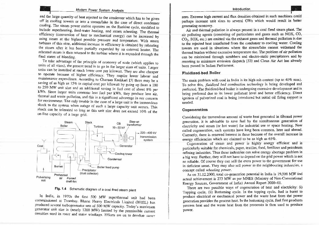
and the large quantity of heat rejected to the condenser which has to be givenoff in cooling towers or into a streamlake in the case of direct condensercooling' The steam power station operates on the Rankine cycle, modified to

\vv'yvrDrwrr ur r'.lr. r.u Inecnanlcal energy) can be increased byusing steam at the highest possible pressure and temperature. with steam

Ah Step-upuE transformer

10-30 kv /

turbines of this size, additional increase in efficiency is obtained by reheatingthe steam after it has been partially expanded by an ext;;; i"ui"r. rn"reheated steam is then returned to the turbine where it is expanded through thefinal states of bleedins.

To take advantage of the principle of economy of scale (which applies tounits of all sizes), the present trend is to go in foilarger sizes of units. Largerunits can be installed at much lower cost per kilowatt. Th"y are also cheaperto opcrate because of higher efficiency. Th"y require io*", labour andmaintenance expenditure. According to chaman Kashkari [3] there may be asaving of as high as l|vo in capital cost per kilowatt by going up from a 100to 250 MW unit size and an additional saving in fuel cost of ubout gvo perkwh. Since larger units consume less fuer pJr kwh, they produce ress air,thermal and waste pollution, and this is a significant advantage in our concernfor environment' The only trouble in the cai of a large unit is the tremendousshock to the system when outage of such a large capacity unit occurs. Thisshock can be toleratecl so long as this unit sizeloes not exceed r}vo of theon-line capacity of a large grid.

rntroduction Effi

perhaps increase unit sizes to several GWs which would result in better

generating economy.Air and thermal pollution is always present in a coal fired steam plant. The

COz, SOX, etc.) are emitted via the exhaust gases and thermal pollution is due

to the rejected heat transferred from the condenser to cooling water. Cooling

towers are used in situations where the stream/lake cannot withstand the

thermal burden without excessive temperature rise. The problem of air pollution

can be minimized through scrubbers and elecmo-static precipitators and by

resorting to minimum emission dispatch [32] and Clean Air Act has already

been passed in Indian Parliament.

Fluidized-bed Boiler

The main problem with coal in India is its high ash content (up to 4OVo max).

To solve this, Jtuidized bed combustion technology is being developed and

perfected. The fluidized-bed boiler is undergoing extensive development and is

being preferred due to its lower pollutant level and better efficiency. Direct

ignition of pulverized coal is being introduced but initial oil firing support is

needed.

Cogeneration

Considering the tremendous amount of waste heat generated in tlbrmal power

generation, it is advisable to save fuel by the simultaneous generation of

electricity and steam (or hot water) for industrial use or space heating. Now

called cogeneration, such systems have long been common, here and abroad.

Currently, there is renewed interest in these because of the overall increase in

energy efficiencies which are claimed to be as high as 65Vo.

Cogeneration of steam and power is highly energy efficient and is

particularly suitable for chemicals, paper, textiles, food, fertilizer and petroleum

refining industries. Thus these industries can solve energy shortage problem in

a big way. Further, they will not have to depend on the grid power which is not

so reliable. Of course they can sell the extra power to the government for use

in deficient areas. They may aiso seil power to the neighbouring industries, a

concept called wheeling Power.As on 3I.12.2000, total co-generation potential in India is 19,500 MW

-and

actual achievement is 273 MW as per MNES (Ministry of Non-Conventional

Energy Sources, Government of India) Annual Report 200H1.

There are two possible ways of cogeneration of heat and electricity: (i)

Topping cycle, (ii) Bottoming cycle. In the topping cycle, fuel is burnt to

produce electrical or mechanical power and the waste heat from the power

generation provides the process heat. In the bottoming cycle, fuel first produces

process heat and the waste heat from the process6s is then used to produce

power.

Stack

Coolirrg tower

-Condenser

mil l

Burner

Preheatedair Forced

draft fan

Flg. 1.4 schematic diagram of a coar fired steam prant

In India, in 1970s the first 500 Mw superthermal unit had beencommissioned at Trombay. Bharat Heavy Electricals Limited (BHEL) hasproduced several turbogenerator sets of 500 MW capacity. Today;s maximumgenerator unit size is (nearly 1200 Mw) limited by the permissible currentcjensities used in rotor and stator windines. Efforts are on to develoo srDer.

- Coal-fired plants share environmental problems with some other types offossil-fuel plants; these include "acid rain" and the ,,greenhouse,,

effect.

Gas Turbines

With increasing availability of natural gasuangladesh) primemovers based on gas turbines have been developed on thelines similar to those used in aircraft. Gas combustion generates hightemperatures and pressures, so that the efficiency of the las turbine iscomparable to that of steam turbine. Additional advantage is that exhaust gasfrom the turbine still has sufficient heat content, which is used to raise steamto run a conventional steam turbine coupled to a generator. This is calledcombined-cycle gas-turbine (CCGT) plant. The schernatic diagram of such aplant is drawn in Fig. 1.5.

Steam

Fig. 1.5 CCGT power station

CCGT plant has a fast start of 2-3 min for the gas turbine and about20 minutes for the steam turbine. Local storage tanks Jr gur

"ui-u" ured in

case of gas supply intemrption. The unit can take up to ITVo overload for shortperiods of time to take care of any emergency.

CCGT unit produces 55vo of CO2 produced by a coal/oil-fired plant. Unitsare now available for a fully automated operation for 24h or to meet the peakdemands.

In Delhi (India) a CCGT unit6f 34Mw is installed at Indraprastha powerStation.

There are culrently many installations using gas turbines in the world with100 Mw generators. A 6 x 30 MW gas turbine station has already been putup in Delhi. A gas turbine unit can also be used as synchrono.r, .ornp"nsatorto help maintain flat voltage profile in the system.

HI

The oldest and cheapest method of power generation is that of utilizing thepotential energy of water. The energy is obtained almost free of nrnning costand is completely pollution free. Of course, it involves high capital cost

requires a long gestation period of about five to eight years as compared tofour to six years for steam plants. Hydroelectric stations are designed, mostly,as multipurpose projects such as river flood control, storage of irrigation anddrinking water, and navigation. A simple block diagram of a hydro plant isgiven in Fig. 1.6. The vertical difference between the upper reservoir and tailrace is called the head.

Surge chamberHead works

Spillway

Valve house

Reservoir Pen stock

Power house

Tailrace pond

Fig. 1.6 A typical layout for a storage type hydro plant

Hydro plants are of different types such as run-of-river (use of water as itcomes), pondage (medium head) type, and reservoir (high head) type. Thereservoir type plants are the ones which are employed for bulk powergeneration. Often, cascaded plants are also constructed, i.e., on the sa.me waterstream where the discharge of one plant becomes the inflow of a downs6eamplant.

The utilization of energy in tidal flows in channets has long been thesubject of researeh;Ttrsteehnical and economic difficulties still prevail. Someof the major sites under investigation are: Bhavnagar, Navalakhi (Kutch),Diamond Harbour and Ganga Sagar. The basin in Kandala (Gujrat) has beenestimated to have a capacity of 600 MW. There are of course intense sitingproblems of the basin. Total potential is around 9000 IvftV out of which 900MW is being planned.

A tidal power station has been constructed on thenorthern France where the tidal height range is 9.2 mestimated to be 18.000 m3/sec.

Different types of turbines such as Pelton. Francis and Kaplan are used forstorage, pondage and run-of-river plants, respectively. Hydroelectric plants are

La Rance estuary inand the tidal flow is

Generator

W - Modern power system Anarvsist -

p = g p W H W

whereW = discharge m3ls through turbinep = densiry 1000 kg/m3

11= head (m)

8 = 9.81 mlszProblems peculiar to hydro plant which inhibit expansion are:

1. Silting-reportedly Bhakra dead storage has silted fully in 30 years2. Seepage

3. Ecological damage to region4. Displacement of human habitation from areas behind the dam which will

fill up and become a lake.5. These cannot provide base load, must be used for peak.shaving and energy

saving in coordination with thermal plants.India also has a tremendous potential (5000 MW) of having large number of

micro (< 1 Mw), mini (< 1-5 Mw), and, small (< 15 Mw) Mrl plants inHimalayan region, Himachal, up, uttaranchal and JK which must be fullyexploited to generate cheap and clean power for villages situated far away fromthe grid power*. At present 500 MW capacity is und"r construction.

In areas where sufficient hydro generation is not available, peak load may behandled by means of pumped storage. This consists of un ,rpp". and lowerreservoirs and reversible turbine-generator sets, which cun ulio be used asmotor-pump sets. The upper reservoir has enough storage for about six hoursof full load generation. Such a plant acts as a conventional hydro plant duringthe peak load period, when production costs are the highest. The iurbines aredriven by water from the upper reservoir in the usual manner. During the lightload period, water in the lower reservoir is pumped back into the ipper oneso as to be ready for use in the next cycle of the peak ioad p.rioo. rn"generators in this period change to synchronous motor action and drive theturbines which now work as pumps. The electric power is supplied to the setsfrom the general power network or adjoining thermal plant. The overallefficiency of the sets is normarly as high ut 60-7oEo. The pumped sroragescheme, in fact, is analogous to the charging and discharging or u battery. Ithas the added advantage that the synchronous machin", tu1 be used assynchronous condensers for vAR compensation of the power network, ifrequired. In-a way, from the point of view of the thermal sector of the system,

* Existing capacity (small hydro) is 1341 MW as on June 200I. Total estimatedpotential is 15000 MW.

daily load demand curve.Some of the existing pumped storage plants are I100 MW Srisailem in Ap

and 80 MW at Bhira in Maharashtra.

Nuclear Power Stations

With the end of coal reserves in sight in the not too distant future, the immediatepractical alternative source of large scale electric energy generation is nuclearenergy. In fact, the developed countries have already switched over in a big wayto the use of nuclear energy for power generation. In India, at present, thissource accounts for only 3Vo of the total power generation with nuclear stationsat Tarapur (Maharashtra), Kota (Rajasthan), Kalpakkam (Tamil Nadu), Narora(UP) and Kakrapar (Gujarat). Several other nuclear power plants will becommissioned by 20I2.In future, it is likely that more and more power will begenerated using this important resource (it is planned to raise nuclear powergeneration to 10,000 MW by rhe year 2010).

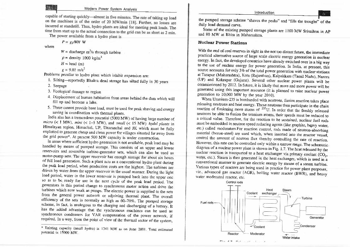
When Uranium-235 is bombarded with neutrons, fission reaction takes placereleasing neutrons and heat energy. These neutrons then participate in the chainreaction of fissioning more atoms of 235U. In order that the freshly releasedneutrons be able to fission the uranium atoms, their speeds must be ieduced toa critical value- Therefore, for the reaction to be sustained, nuclear fuel rodsmust be embedded in neutron speed reducing agents (like graphite, hqavy water,etc.) called moderators.For reaction control, rods made of n'eutron-absorbingmaterial (boron-steel) are used which, when inserted into the reactor vessel,control the amount of neutron flux thereby controlling the rate of reaction.However, this rate can be controlled oniy within a narrow range. The schemadc,diagram of a nuclear power plant is shown in Fig. 1.7. The heit released by the'uclear reaction is transported to a heat exchanger via primary coolant (coz,water, etc.). Steam is then generated in the heat exchanger, which is used in aconventional manner to generate electric energy by means of a steam turbine.Various types of reactors are being used in practice for power plant pu{poses,viz., advanced gas reactor (AGR), boiling water reactor (BwR), und h"uuywater moderated reactor. etc.

Water intake

Control rods

Fue l rods_

W Modern Po*", system An"tysis

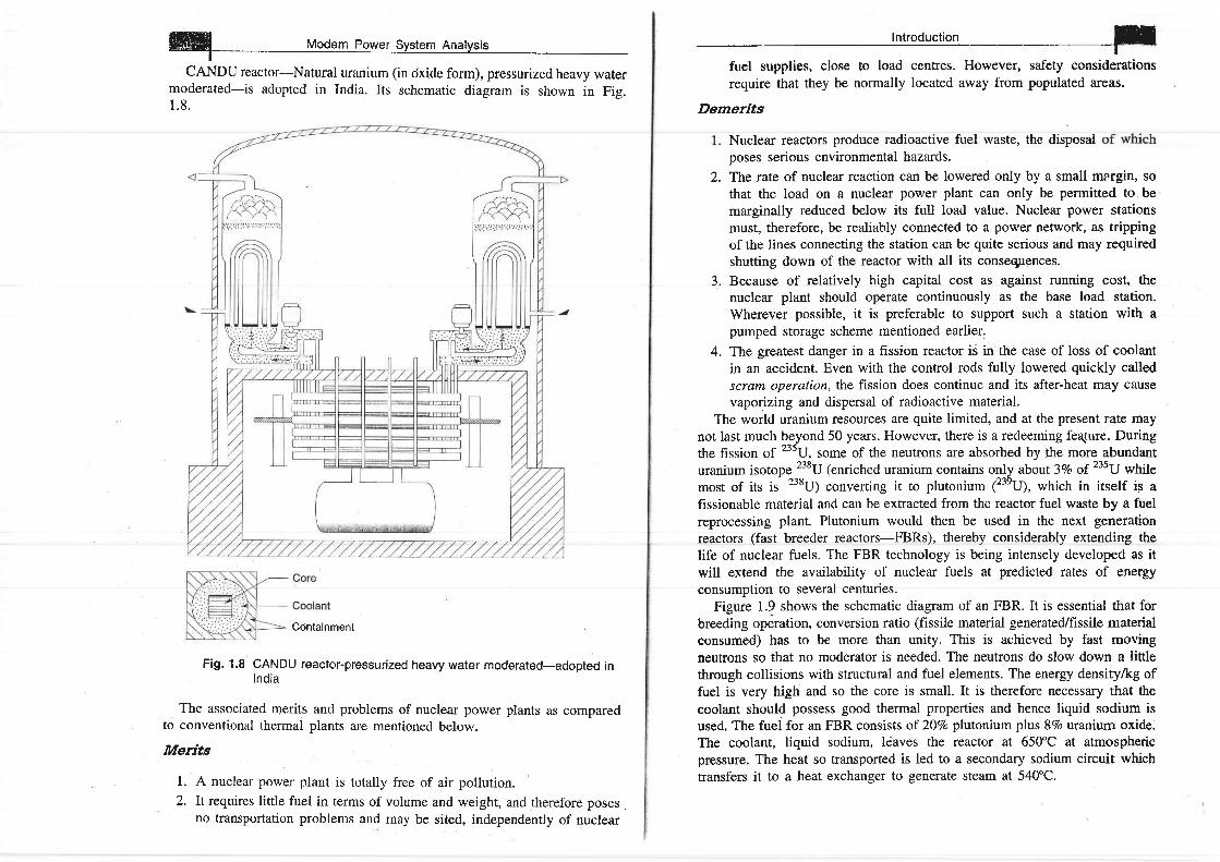
CANDU reactor-Natural uranium (in cixide form), pressurized heavy watermoderated-is adopted in India. Its schematic diagram is shown in Fig.1 . 8 .

Containment

Fig. 1.8 CANDU reactor-pressurized heavy water rnoderated-adopted inIndia

The associated merits and problems of nuclear power plants as comparedto conventional thermal plants are mentioned below.

Merits

1. A nuclear power plant is totally free of air pollution.2. It requires linle fuel in terms of volume and weight, and therefore poses .

no transportation problems and may be sited, independently of nuclear

i i i r ioc iucr ion -

require that they be normally located away from populated areas.

Demerits

Nuclear reactors produce radioactive fuel waste, the disposalposes serious environmental hazards.

The rate of nuclear reaction can be lowered only by a small margin, sothat the load on a nuclear power plant can only be permitted to bemarginally reduced below its full load value. Nuclear power stationsmust, therefore, be realiably connected to a power network, as trippingof the lines connecting the station can be quite serious and may requiredshutting down of the reactor with all its consequences.

Because of relatively high capital cost as against running cost, thenuclear plant should operate continuously as the base load station.Wherever possible, it is preferable to support such a station with apumped storage scheme mentioned earlier.

The greatest danger in a fission reactor is in the case of loss of coolantin an accident. Even with the control rods fully lowered quickly calledscrarn operation, the fission does continue and its after-heat may causevaporizing and dispersal of radioactive material.

The world uranium resources are quite limited, and at the present rate maynot last much beyond 50 years. However, there is a redeeming feqture. Duringthe fission of 235U, some of the neutrons are absorbed by lhe more abundanturanium isotope 238U

lenriched uranium contains only about 3Vo of 23sU whilemost of its is 238U) converting it to plutonium ("nU), which in itself is afissionable material and can be extracted from the reactor fuel waste by a fuelreprocessing plant. Plutonium would then be used in the next generationreactors (fast breeder reactors-FBRs), thereby considerably extending thelife of nuclear fuels. The FBR technology is being intensely developed as itwill extend the availability of nuclear fuels at predicted rates of energyconsumption to several centuries.

Figure 1.9 shows the schematic diagram of an FBR. It is essential that forbreeding operation, conversion ratio (fissile material generated/fissile materialconsumed) has to be more than unity. This is achieved by fast movingneutrons so that no moderator is needed. The neutrons do slow down a littlethrough collisions with structural and fuel elements. The energy densitylkg offuel is very high and so the core is small. It is therefore necessary that the

coolant should possess good thermal properties and hence liquid sodium isused. The fuel for an FBR consists of 20Vo plutonium phts 8Vo uranium oxide.The coolant, liquid sodium, .ldaves the reactor at 650"C at atmosphericpressure. The heat so transported is led to a secondary sodium circuit whichtransfers it to a heat exchanger to generate steam at 540'C.

2.

3 .

4.

t Modprn pnrr rar erro lam Anal . ,^ l^_ r r t y y v r r . r v r r v r v y g l g t t l n t t d t v s t s

with a breeder reactor the release of plutonium, an extremely toxicmaterial, would make the environmental considerations most stringent.

An experimental fast breeder test reacror (FBTR) (40 MW) has -been

builtat Kalpakkam alongside a nucrear power plant. FBR technology i,

"*f..l"Jconventional thermal plants.

- Core

Coolant

Containment

Fig. 1.9 Fast breeder reactor (FBR)

An important advantage of FBR technology is that it can also use thorium(as fertile material) which gets converted to t33U which is fissionable. Thisholds great promise for India as we have one of the world's largest depositsof thoriym-about 450000 tons in form of sand dunes in Keralu una along theGopalpfur Chatrapur coast of Orissa. We have merely 1 per cent of the world's

suited for India, with poor quality coal, inadequare hydro potentiaiilentifulreserves of uranium (70,000 tons) and thorium, and many years of nuclearengineering experience. The present cost of nuclearwlm coal-ttred power plant, can be further reduced by standardising pl4ntdesign and shifting from heavy wate,r reactor to light water reactor technology.

Typical power densities 1MWm3) in fission reactor cores are: gas cooled0.53, high temperature gas cooled 7.75, heavy warer 1g.0, boiling iut., Zg.O,pressurized water 54.75, fast breeder reactor 760.0.

Fusion

Energy is produced in this process by the combination of two light nuclei toform a single heavier one under sustained conditions of exiemely hightemperatures (in millions of degree centigrade). Fusion is futuristic. Genera-tion of electricity via fusion would solve the long-tenn energy needs of theworld with minimum environmental problems. A .o--"i.iul reactor isexpected by 2010 AD. Considering radioactive wastes, the impact of fusionreactors would be much less than the fission reactors.

In case of success in fusion technology sometime in the distant future or abreakthrough in the pollution-free solar energy, FBRs would become obsolete.However, there is an intense need today to develop FBR technology as aninsurance against failure to deverop these two technologies. \

In the past few years, serious doubts have been raised.about the safetyclaims of nuclear power plants. There have been as many as 150 near disasternuclear accidents from the Three-mile accident in USA to the recentChernobyl accident in the former USSR. There is a fear.that all this may purthe nuclear energy development in reverse gear. If this happens there could beserious energy crisis in the third world countries which have pitched theirhopes on nuclear energy to meet their burgeoning energy needs. France (with78Vo of its power requirement from nuclear sources) and Canada are possiblythe two countries with a fairty clean record of nuclear generation. India needsto watch carefully their design, construction and operating strategies as it iscommitted to go in a big way for nuclear generation and hopes to achieve acapacity of 10,000 MW by z0ro AD. As p.er Indian nuclear scientists, ourheavy water-based plants are most safe. But we must adopt more conservativestrategies in design, construction and operation of nuclear plants.

World scientists have to adopt of different reaction safety strategy-may beto discover additives to automatically inhibit feaction beyond cr;ii"at ratherthan by mechanically inserted control rods which have possibilities of severalprimary failure events.

Magnetohydrodynamic (MHD) Generation

In thermal generation of electric energy, the heat released by the fuel isconverted to rotational mechanical energy by means of a thermocvcle. The

ry Modern Power System Anatysis

mechanical energy is then used to rotate the electric generator. Thus twostages of energy conversion are involved in which the heat to mechanicalenergy conversion has inherently low efficiency. Also, the rotating machinehas its associated losses and maintenance problems. In MHD technology,

cornbustion of fuel without the need for mechanical moving parts.In a MHD generator, electrically conducting gas at a very high temperature

is passed in a strong magnetic fleld, thereby generating electricity. Hightemperature is needed to iontze the gas, so that it has good eiectricalconductivity. The conducting gas is obtained by burning a fuel and injectinga seeding materials such as potassium carbonate in the products ofcombustion. The principle of MHD power generation is illustrated in Fig.1.10. Abotrt 50Vo efficiency can be achieved if the MHD generator is operatedin tandem with a conventional steam plant.

Gas flow

at 2,500 'C

Strong magneticfield

Fig. 1.10 The pr inciple of MHD power generat ion

Though the technological feasibility of MHD generation has been estab-lished, its economic f'easibility is yct to be demonstrated. lndia had started aresearch and development project in collaboration with the former USSR toinstall a pilot MHD plant based on coal and generating 2 MW power. InRussia, a 25 MW MHD plant which uses natural gas as fuel had been inoperation for some years. In fact with the development of CCGT (combinedcycle gas turbine) plant, MHD development has been put on the shelf.

Geothermal Power Plants

In a geothermal power plant, heat deep inside the earth act as a source ofpower. There has been some use of geothermal energy in the form of steamcoming from underground in the USA, Italy, New Zealand, Mexico, Japan,Philippines and some other countries. In India, feasibility studies of 1 MWstation at Puggy valley in Ladakh is being carried out. Another geothermalfield has been located at Chumantang. There are a number of hot springs inIndia, but the total exploitable energy potential seems to be very little.

Ttre present installed geothermal plant capacity in the world is about 500MW and the total estimated capacity is immense provided heat generated in the

Introduction wI

volcanic regions can be utilized. Since the pressure and temperatures are low,the efficiency is even less than the conventional fossil fuelled plants, but thecapital costs are less and the fuel is available free of cost.

I.4 RENEWABLE ENERGY SOURCES

To protect environment and for sustainable development, the importance ofrenewable energy sources cannot be overemphasized. It is an established andaccepted tact that renewable and non-conventional forms of energy will playan increasingly important role in the future as they are cleaner and easier touse and environmentally benign and are bound to become economically moreviable with increased use.

Because of the limited availability of coal, there is considerable interna-tional effort into the development of alternative/new/non-conventionaUrenew-able/clean sources of energy. Most of the new sources (some of them in facthave been known and used for centuries now!) are nothing but themanifestation of solar energy, e.g., wind, sea waves, ocean thermal energyconversion (OTEC) etc. In this section, we shall discuss the possibilities andpotentialities of various methods of using solar energy.

Wind Power

Winds are essentially created by the solar heating of the atmosphere. Severalattempts have been made since 1940 to use wind to generate electric energyand development is still going on. However, technoeconomic feasibility hasyet to be satisfactorily established.

Wind as a power source is attractive because it is plentiful, inexhaustibleand non-polluting. Fnrther, it does not impose extra heat burden on theenvironment. Unlbrtunately, it is non-steady and undependable. Controlequipment has been devised to start the wind power plant whenever the windspeed reaches 30 kmftr. Methods have also been found to generate constantfrequency power with varying wind speeds and consequently varying speedsof wind mill propellers. Wind power may prove practical for small powerneeds in isolated sites. But for maximum flexibility, it should be used inconjunction with other methods of power generation to ensure continuity.

For wind power generation, there are three types of operations:

1. Small, 0.5-10 kW for isolated single premises

2. Medium, 10-100 kW for comrnunities i

3. Large, 1.5 MW for connection to the grid.The theoretical power in a wind stream is given by

P = 0.5 pAV3 W

density of air (1201 g/m' at NTP)

mean air velocity (m/s) and

p =

V _

where

A = swept area (rn").

2. Rural grid systems are likely to be 'weak, in these areas. sinceretatrvely low voitage supplies (e.g. 33 kV).

3. There are always periods without wind.In India, wind power plants have been installed in Gujarat, orissa,

Maharashtra and Tamil Nadu, where wind blows at speeds of 30 kmftr duringsummer' On the whole, the wind power potential of India has been estimatedto be substantial and is around 45000 Mw. The installed capacity as onDec. 2000 is 1267 Mw, the bulk of which is in Tamil Nadu- (60%). Theconesponding world figure is 14000 Mw, rhe bulk of which is in Europe(7UVo).

Solar Energy

The average incident solar energy received on earth's surface is about600 W/rn2 but the actual value varies considerably. It has the advantage ofbeing free of cost, non-exhaustible and completely pollution-free. On the otherhand, it has several crrawbacks-energy density pei unit area is very row, it isavailable for only a part of the day, and cl,oud y and, hazy atmosphericconditions greatly reduce the energy received. Therefore, harnessing solarenergy for electricity generation, challenging technological problems exist, themost important being that of the collection and concentration of solar energyand its conversion to the electrical form through efficient and comparativelyeconomical means.

Total solarenergy potent ia l in India is 5 x lOls kwh/yr.Up ro 31.t2.2000.462000 solar cookers, 55 x10am2 solar thermai system collector area, 47 MWof SPV power, 270 community lights, 278000 solar lanterns (PV domesticlighting units), 640 TV (solar), 39000 PV street lights and 3370 warer pumps

MW of grid connected solar power plants were in operation. As per oneestimate [36], solar power will overtake wind in 2040 and would become theworld's overall largest source of electricity by 2050.

Direct Conversion to Electricity (Photovoltaic Generation)

This technology converts solar energy to the electrical form by means of siliconwafer photoelectric cells known as "Solar Cells". Their theoretical efficiency isabout 25Vo but the practical value is only about I5Vo. But that does not matteras solar energy is basically free of cost. The chief problem is the cost andmaintenance of solar cells. With the likelihood of a breakthrough in the largescale production of cheap solar cells with amorphous silicon, this technologymay compete with conventional methods of electricity generation, particularlyas conventional fuels become scarce.

Solar energy could, at the most, supplement up to 5-r0vo of the totalenergy demand. It has been estimated that to produce 1012 kwh per year, thenecessary cells would occupy about 0.l%o of US land area as against highwayswhich occupy 1.57o (in I975) assuming I07o efficiency and a daily insolationof 4 kWh/m'. .\

In all solar thermal schentes, storage is necessary because of the fluctuatingnature of sun's energy. This is equally true with many other unconventionalsources as well as sources l ike wind. Fluctuating sources with fluctuatingloads complicate still further the electricity supply.

Wave Energy

The energy conient of sea waves is very high. In India, with several hundredsof kilometers of coast line, a vast source of energy is available. The power inthe wave is proportional to the square of the anrplitude and to the period ofthe motion. Therefore, rhe long period (- 10 s), large amplitude (- 2m) wavesare of considerable interest for power generaticln, with energy fluxescommonly averaging between 50 and 70 kW/m width of oncoming wave.Though the engineering problems associated with wave-power are formidable,the amount of energy that can be harnessed is large and development work isin progress (also see the section on Hydroelectric Power Generation, page 17).Sea wave power estimated poterrtial is 20000 MW.

Ocean Thermal Energy Conversion (OTEC)

The ocean is the world's largest solar coilector. Temperature difference of2O"C between \,varrn, solar absorbing surface water and cooler 'bottorn' water

At present, two technologies are being developed for conversion of solarenergy to the electrical form.-'In one technology, collectors with concentratorsare employed to achieve temperatures high enough (700'C) to operate a heatengrne at reasonable efficiency to generate electricity. However, there areconsiderable engineering difficulties in building a single tracking bowi with adiarneter exceeding 30 m to generate perhaps 200 kw. The scheme involveslarge and intricate structures invoiving

lug" capital outlay and as of today isf'ar from being competitive with

"otru"titional Jlectricity generation.

The solar power tower [15] generates steam for electricity procluction.]'here is a 10 MW installation of such a tower by the Southern CaliforniaEdison Co' in USA using 1818 plane rnirrors, each i m x 7 m reflecting directracliation to thc raisecl boiler.

Electricity may be generated from a Solar pond by using a special .lowtemperature' heat engine coupled to an electric generator. A solar pond at EinBorek in Israel procluces a steady 150 kW fiorn 0.74 hectare at a busbar costof about $ O. tO/kwh.

Solar power potential is unlimited, however, total capacity of about 2000MW is being planned.

Introduction

ffiffi| Modem Pow'er system Anatysis

can occlrr. This can provide a continually replenished store of thermalwhich is in principle available fbr conversion to other energy forms.refers to the conversion of some of this thermal energy into work and

lntroduction

solar. The most widely used storage battery is the lead acid battery. inventedby Plante in 1860. Sodiuttt-sulphur battery (200 Wh/kg) and other colrbina-tions of materials are a-lso being developed to get more output and storage perunit weisht.

Fuel Cells

A fuel cell converts chemical enerry of a fuel into electricity clirectly, with nointermediate cotnbustion cycle. In the fuel cell, hyclrogen is supplied to thenegative electrode and oxygen (or air) to the positive. Hydrogen and oxygenare combined to give water and electricity. The porous electrodes allowhydrogen ions to pass. The main reason ';rhy fuel cells are not in wide use istheir cost (> $ 2000/kW). Global electricity generating capacity from full cellswil l grow from just 75 Mw in 2001 ro 15000 MW bv 2010. US. Germanv andJapan may take lead for this.

Hydrogen Energy Systems

Hydrogen can be used as a medium for energy transmission and storage.Electrolysis is a well-established commercial process yielding pure hydrogen.Ht can be converted very efficiently back to electi'icity by rneans of fuel ceils.Also the use of hydrogen a.s fuel for aircraft and automcbiles could encouraseits large scale production, storage and distriburion.

1"6 GROWTH OF POWER SYSTEII{S IN INDIA

India is fairly rich in natural resources like coal and lignite; while sorne oilreserves have been discovered so far. intense exploration is being undertakeriin vitrious regitlns of thc country. India has immense water power l.csourcesalso of which only around25To have so farbeen uti l iseci, i.e., oniy 25000 t\,IWhas so far been commissioned up to the end of 9th plan. As per a recent reportof t lre CEA (Ccntlal Flectricit,v Authority), the total potential of h1,dro poweris 84,040 Iv{W at ('L't% load factor. As regards nuclear power, India is cleflcientin uranium, but has rich deposits of thorir-im rvhich can be uti l ised at a futureclatc in l 'ast brccclor rci.tctor.s. Since indepcndcncc, thc coulltry has nndetremendous progress in the development of electric energy and today it has thelargest system among the developing countries.

When lndia attained independence, the installecl capacity was as low as1400 MW in the early stages of the growth of power system, the major portionof generation was through thermal stations, but due to economical reasons.hydro development received attention in areas like Kerala, Tamil Nadu. UttarPradesh and Punjab.

In the beginning of the First Five Year Plan (1951-56), the rotal installedcapacity was around 2300 MV/ (560 MW hydro, 1004 MW thermal, 149 MWthrough oil stations and 587 MW through non-utilities). For transporting this

energyOTECthence

50,000 Mw.A proposed plant using sea iemperature difference would be situated 25 km

cast ol 'Mianii (USA), where the temperature cli l ' l 'eronce is 17.5"C.

Biofuels

The material of plants and animals is called biomass, which may betransformed by chemical and biological processes to produce intermediatebiofuels sttch as methane gas, ethanol liquid or charcoal solid. Biomass isburnt to provide heat for cooking, comfort heat (space heat), crop drying,tactory processes and raising steam for electricity production and transport. InIndia potent ia l I ' t t l b io-Energy is 17000 MW and that fbr agr icul tunr l wirstc isabout 6000 MW. There are about 2000 community biogas plants and tamilysize biogas plants are 3.1 x 106. Total biomass power harnessed so far is222 MW.

Renewable energy programmes are specially designed to meet the growingenergy needs in the rural areas for prornoting decentralized and hybriddcvelopment st.l as to stem growing migration of rural population to urbanareas in search of better living conditions. It would be through this integrationof energy conservation efforts with renewable energy programmes that Indiawould be able to achieve a smooth transition from fossil fuel economy tosustainable renewable energy based economy and bring "Energy for ali" forec;uitable and environrnental friendly sustainable development.

1.5 ENERGY STORAGE

'l 'here is a lol ol problenr in storing clectricity in largc quantit ies. Enclgy

wliich can be converted into electricity can be stored in a number of ways.Storage of any nature is l rowever very cost ly arrc l i ts cconomics must beworked out properly. Various options available are: pLrmped storage, c:onl-pressed air, heat, hydrogen gas, secondary batteries, flywheels and supercon-duct ing coi ls.

As already mentioned, gas turbines are normally used for meeting peakloads but are very expensive. A significant amount of storage capable ofinstantancous use would be better way of meeting such peak loads, and so farthe most important way is to have a pumped storage plant as discussed earlier.Other methods are discuss-ed below very briefly.

Secondary Batteries

Large scale battery use is almost ruled out and they will be used for batterypowered vehicles and local fluctuating energy sources such as wind mills or

power to the loadwere constructed.

centres, transmission lines of up to 110

HEIntroduction FI

regions of the country with projected energy requirement and peak load in the

year 2011-12 [19]' io ororrcrt crcncreri At the

During the Fourth Five Plan, India started generating nuclear power'

Tarapur i\uclear Plant 2 x 210 MW units were comrnissioned in April-May

. This station uses two boiling water reactors of American design. By

commissioned bY 2012.

The growth of generating capacity so

2012 A.D. are given in Table 1'1'far and future projection for 2011-

Tabte 1.1 Growth of Installed capacity in lndia (ln MW)

Year Hydrtt Nuclear Thermal DieseI Total

Northern region

308528

(49674) .,.

MW* 9

Western region299075(46825)

1970-7t1978-791984-852000-01

398

=2700 MWrenewable

r47042864042240

101630

6383l 1378t427125141

420890

10952720

7503t63722707471060

\'./

Fig. 1.11 Map of India showing five regional projected energy requirement in

MkWh and park load in MW for year 2011-12'

The emphasis during the Second Plan (195 6-61) was on the development of

basic ancl heavy inclustries and thus there was a need to step up power

generation. The total installed capacity which was around 3420 MW at the end

of tn" First Five year Plan became 5700 MW at the end of the Second Five

year plan. The introduction of 230 kv transmission voltage came up in Tarnil

Pattern of utlization of electrical energy in 1997-98 was: Domestic

{O.6g\o,commercial 6.91 7o, inigation 30.54Vo, industry 35'22Vo and others is

6.657o.It is expected to remain more or less same in 2004-05'

To be self-sufficient in power' BHEL has plants spread out all over the

country ancl these turn out an entire range of power equipment, viz' turbo sets'

hydro sets, turbines for nuclear plants, tiigft pi".ture boilers, power transform- -

ers, switch gears, etc. Each plant specializes in a range of equipment' BHEL's

first 500 MW turbo-generator was cornmissioned at singrauli' Today BIIEL

is considered one of the major power plant equipment manufacturers in the

world.

T.7 ENERGY CONSERVATION

Energy conservation is the cheapest new source of energy' we should resort

to various conservation measures such as cogeneration (discussed earlier), and

lu

,r32 I Modern power Svstem Analvsis

use energy efficient motors to avoid wasteful electric uses. We can achieveconsiderable electrical power savings by reducing unnecessary high lightinglevels, oversized motors, etc. A 9 W cornpact fluorescent lamp (CFL) may beused instead of 40 w fluorescent tube or 60 w lamp, all having the same

Load Management

As mentioned earlier by various 'load management' schemes. It is possible to

shift demanrl away frorn peak hours (Section I .1.). A more direct method

would be the control of the load either through rnodified tariff structure that

encourageschedules or direct electrical control of appliance in the form of remote timer

controlled on/off switches with the least inconvenience io the customer.

Various systems for load rnanagement are described in Ref. [27]. Ripple

control has been tried in Europe. Remote kWh meter reading by carrier

sysrems is being tried. Most of the potential for load control lies in the

domestic sector. Power companies are now planning the introduction of

system-wide load management schemes.

1.8 DEREGULATION

For over one hundred years, the electric power industry worldwide operated as

a regulated industry. In any area there was only one company oI government

agency (mostly state-owned) that produced, transmitted, distributed and sold

electric power and services. Deregulation as a concept came in early 1990s. It

brought in changes designeci to enc<.rutage competition.

Restructuring involves disassembly of the power industry and reassembly

into another form or functional organisation. Privatisation started sale by a

government of its state-owned electric utility assets, and operating economy,

to private companies. In some cases, deregulation was driven by privatization

needs. The state wants to sell its electric utility investment and change the

rules (deregulation) to make the electric industry more palatable for potential

investors, thus raising the price it could expect from the sale. Open access rs

nothing but a common way for a govenlment to encourage competition in the

electric industry and tackle monopoly. The consumer is assured of good

quality power supply at competitive price.The structure for deregulation is evolved in terms of Genco (Generation

Company), Transco (Transrnission Company) and ISO (Independent System

Operator). It is expected that the optimal bidding will help Genco to maximize

its payoffs. The consumers are given choice to buy energy from different retail

energy suppliers who in turn buy the energy from Genco in a power market.

(independent power producer, IPP).The restructuring of the electricity supply industry that norrnally accompa-

nies the introduction of competiiion provides a fertile ground for the growth

of embedded generation, i.e. generation that is connected to the distribut-icn

system rather than to the transmission systetn.

The earliest reforms in power industries were initiated in Chile. They were

followed by England, the USA, etc. Now India is also implementing the

restructuring. Lot of research is needed to clearly understand the power system

operation under deregulation. The focus of, research is now shifting towards

a year. Everyone should be made aware through print or electronic media howconsumption levels can be reduced without any essential lowering of comfort.Rate restructuring can have incentives in this regard. There is no conscious-ness on energy accountabil ity yet etnd no sense of urgency as in developedcountries.

Transmission and distribution losses shoulcl not exceed 2OVo. This can beachieved by employing series/shunt compensation, power factor improvementmethods, static var compensators, HVDC option and FACTS (flexible actechnology) devices/controllers.

Gas turbirre combined with steam turbine is ernployed for peak loadshaving. This is more efficient than normal steam turbine and has a quickautomated starl and shut doivn. It improves the load factor of the steamstaflon.

Energy storage can play an important role where there is time or ratemismatch between supply and demand of energy. This has been discussed inSection 1.5. Pumped storage (hyclro) scheme has been consiclered in Section1 . 3 .

Industry

In India where most areas have large number of sunny days hot water forbath arrd kitchen by solar water heaters is becoming common for commercialbuildings, hotels even hospitals.

In India where vast regions are deficient in electric supply and, are subjectedto long hours of power shedding mostly random, the use of small diesel/petrolgenerators and inverters are very conmon in commercial and domestic use.These are highly wasteful energy devices. By proper planned maintelance thedowntime of existin g large stations can be cut down. Plant utilization factorsof existing plants must be improved. Maintenance must be on schedule ratherthan an elner-qency. Maintenance manpower training should be placed on warfooting. These actions wil l also improve the load factor of most powerstations, which would indirectly contribute to energy conservation.

lntroduction

W Modern po*", Syster Anulyri,

finding the optimal bidding methods which take into account local optimaldispatch, revenue adequacy and market uncertainties.

India has now enacted the Electricity Regulatory Comrnission's Act, 1998and the Electricity (Laws) Amendment Act, 1998. These laws enable settinguo ofState Electricity Regulatory Comrnissions (SERC) at srate level. 'fhe

mainpurpose of CERC is to promote efficiency, economy and competition in bulkelectricity supply. orissa, Haryana, Andhra Pradesh, etc. have started theprocess of restructuring the power sector in their respective states.

1.9 DISTRIBUTED AND DISPERSED GENERATION

Distributed Generation (DG) entails using lnany srnall generators of 2-50 MWoutput, installed at various strategic points throughout the area, so that eachprovides power to a small number of consumers nearby. These may be solar,mini/micro hydel or wind turbine units, highly efficient gas turbines, smallcombincd cycle plitnts, sincc thcse aro the rnost ccon<lnrical choiccs.

Dispersed generation referes to use of still smaller generating units, of lessthan 500 kW output and often sized to serve individual homes or businesses.Micro gas turbines, fuel cells, diesel, and small wind and solar PV seneratorsmake up this category.

Dispersed generation has been used for clecades as an emergency backuppower source. Most of these units are used only fbr reliability reinfbrcement.Now-a-days inverters are being increasingly used in domestic sector as anemergency supply during black outs.

The distributed/dispersed generators can be stand alone/autonomous orgrid connected depending upon the requirement.

At the time of writing this (200i) there still is and will probably always besome economy of scale f-avouring large generators. But the margin ofeconomy decreased considerably in last 10 years [23]. Even if the power itselfct lsts a bi t r t t t l rc th i tn ccn(r 'a l stat ion powcr, there is no nccd <t f t ransrnissionlines, and perhaps a reduced need fbr distribution equipment as well. Anothermaior advantage of dispersed gene.ration is its modularity, porlability andrelocatabil ity. Dispersed generators also include two new types of tbssil fuelunits-fuel cells and microgas turbines.

The main challenge today is to upgrade the existing technologies and toproniote developrnent, demonstration, scaling up and cornmercialization ofnew and emerging technologies for widespread adaptation. In the rural sectormain thrust areas are biomass briquetting, biomass-based cogeneration, etc. Insolar PV (Photovoltaic), large size solar cells/modules based on crystallinesilicon thin films need to be developed. Solar cells efficiency is to be improvedto 15%o to be of use at commercial level. Other areas are developrnent of higheificiency inverters. Urban and industrial wastes are used for various energyapplications including power generation which was around 17 Mw in 2002.

Introduct ion

There are already 32 million improved chulhas. If growing energy needs in therural areas are met by decentralised and hybrid ener-qy systems (distributed/

dispersed generation), this can stem growing migration of rural population to

urban areas in search of better living conditions. Thus, India will be able to

able-energy based econolny iind bring "Energy for all" for equitable,environment-friendly, and sustainabie development.

1.10 ENVIRONMENT/\L ASPECTS OF ELECTRIC ENER,GY

GENERATION

As far as environmental and health risks involved in nuclear plants of variouskinds are concerned, these have already'been discussed in Section 1.3. Theproblerns related to large lrydro plants have also been dwelled upon in Section1.3. Therefore, we shall now focus our attention on fossil fuel plant includinggas-based plants.

Conversion of clne lornr ol' energy or another to electrical tortn hasunwanted side effects and the pollutants generated in the process have to be

disposed off. Pollutants know no geographical boundary, as result thepollution issue has become a nightmarish problem and strong national andinternational pressure groups have sprung up and they are having a definite

impact on the development of energy resources. Governmental awareness has

created numerous legislation at national and international levels, w[ich powerengineers have to be fully conversant with in practice of their profession andsurvey and planning of large power projects. Lengthy, t ime consumingprocedures at governrnent level, PIL (public interest litigation) and demonstra-tive protests have delayed several projects in several countries. This has ledto favouring of small-size projects and redevelopment of existing sites. But

with the increasing gap in electric dernand and production, our country has tomove forward fbr several large thermal, hydro and nuclear power projects.

Entphasis is l rc ing la id on cor]scrvi l t ior t issucs. curtui l tnent of t ransnt issi t tnlosses, theft, subsidized power supplies and above all on sustainabledevektpnrenl wittr uppntpriata technolog-)' whercver feasible. It has to be

particularly assured that no irreversible damage is caused to environmentwhich wouid affect the living conditions of the future generations. Irreversibledamages like ozone layer holes and global warming caused by increase in CO2

in the atmosphere are already showing up.

Atmospheric Pollution

We shall treat here only pollutrorr as caused by thermal plants using coal as

feedstock. Certain issues concerning this have already been highlighted in

Section 1.3. The fossil fuel based generating plants fonn the backbone ofpower generation in our country and also giobally as other options (like

nuclear and even hydro) have even stronger hazards associated with them.

f f i f f i | r r ^ r ^ - - n ^ . . . ^ - ^ . , - r - - a - - r . - - ,w_ tviouern row-er uystem Anaiysts

Also it should be understood that pollution in large cities like Delhi is causedmore by vehicrtlar traffic and their emission. In Delhi of course Inderprasthaand Badarpur power stations contribute their share in certain areas.

Problematic pollutants in emission of coal-based generating plants are.

lntroduction

Oxides of Carhon (CO, COt)

CO is a very toxic pollutant but it gets converted to CO'., in the open atmosphere

(if available) surrounding the plant. On the other hand CO2 has been identified

developing countries.

Ifydrocarbons

During the oxidation process in cornbustion charnber certain light weight

hydrocarbon may be formed. Tire compounds are a major source of

photochemical reaction that adds to depleti,rn of ozone layer.

Particulates (fIY ash)

Dust content is particularly high in the Indian coal. Particulates come out of

the stack in the form of fly ash. It comprises fine particles of carbon, ash and

other inert materials. In high concentrations, these cause poor visibility and

respiratory diseases.Concentration of pollutants can be reduced by dispersal over a wider area

by use of high stacks. Precipitators can be used to remove particles as the flue

gases rise up the stack. If in the stack a vertical wire is strung in the middle

and charged to a high negative potential, it emits electrons. These electrons

are captured by the gas molecules thereby becoming negative ions. These ions

accelerate towards the walls, get neutralized on hitting the'walls and the

particles drop down the walls. Precipitators have high efficiency up to 99Vo for

large particles, but they have poor performance for particles of size less than

0.1 pm in diameter. The efficiency of precipitators is high with reasonable

sulphur content in flue gases but drops for'low sulphur content coals; 99Vo for

37o sulphur and 83Vo for 0.5Vo sulphur.Fabric filters in form of bag lnuses have also been employed and are

located before the flue gases enter the stack.

Thermal Pollution

Steam fronr low-pressure turbine has to be liquefied in a condenser and

reduced to lowest possible temperature to maximize the thermodynamic

efficiency. The best efficiency of steam-cycle practically achievable is about

4\Vo.It means that 60Vo of the heat in steam at the cycle end must be removed'

This is achieved by following two methods'

1. Once through circulation through condenser cooling tubes of sea or river

water where available. This raises the temperature of water in these two

sources and threatens sea and river life around in sea and downstream

in river. ThesE, are serious environmental objections and many times

cannot be overruled ard also there may be legislation against it.

2. Cooling tov,ers Cool water is circulated rottnd the condenser tube to

remove heat from the exhaust steam in order to condense it. The

a

a

o

a

2

NO.r, nitrogen oxides

CO

coz. Certain hydrocarbonso ParticulatesThough the account that follows will be general, it needs to be mentioned

here that Indian coal has comparatively low sulphur content but a very highash content which in some coals may be as high as 53Vo.

A brief account of various pollutants, their likely impact and methods ofabatements are presented as follows.

Oxides of Sulphur (SOr)

Most of the sulphur present in the fossil fuel is oxidized to SO2 in thecombustion chamber before being emitted by the chimney. In atmosphere itgets further oxidized to HrSOo and metallic sulphates which are the majorsource of concern as these can cause acid rain, impaired visibility, damage tobuildings and vegetation. Sulphate concenffations of 9 -10 LElm3 of airaggravate asthma, lung and heart disease. It may also be noted that althoughsulphur does not accumulate in air, it does so in soil.

Sulphur emission can be controlled by:o IJse of fuel with less than IVo sulphur; generally not a feasible solution.o LJse of chemical reaction to remove sulphur in the form of sulphuric

acid, from combustion products by lirnestone scrubbers or fluidized bedcombustion.

. Removing sulphur from the coal by gasification or floatation processes.It has been noticed that the byproduct sulphur could off-set the cost of

sulphur recovery plant.

Oxides of Nitrogen (NO*)

Of these NOz, nitrogen oxides, is a major concern as a pollutant. It is solublein water and so has adverse aff'ect on human health as it enters the lungs oninhaling and combining with moisture converts to nitrous and nitric acids,which dannge the lungs. At ievels of 25-100 parts per million NO, can causeacute bronchitis and pneumonia.

Emission of NO_, can be controlled by fitting advanced technology burnerswhich can assure more complete combustion, thereby reducing these oxidesfrom being emitted. These can also be removed from the combustion productsby absorption process by certain solvents going on to the stock.

Gfrfudffi-ffii Mociern Power Systeq AnaiysisI

circulating water gets hot in the process. tt is pumped to cooling towerand is sprayed through nozzles into a rising volume of air. Some of thewater evaporates providing cooling. The latent heat of water is 2 x 106J/kg and cooling can occur fast, But this has the disaclvantage of raising

unoest raoteJ teve ls ln thc su l r f t lund lng areas.course the water evaporated must be macle up in the system by adctingfresh water from the source.

Closed cooling towers where condenr;ate flows through tubcs ancl air isblown in these tubes avoids the humidity problem but at a very high cost. InIndia only v,et towers are being used.

Electromagnetic Radiation from Overhead Lines

Biological effects of electromagnetic radiation from power lines and evencables in close proximity of buildings have recently attracted attention andhave also caused some concern. Power frequency (50 or 60 Hz) and even theirharmonics are not considered harmful. Investigations carried out in certainadvanced countries have so far proved inconclusive. The electrical andelectronics engineers, while being aware of this controversy, must know thatmany other environmental agents are moving around that can cause far greaterharm to human health than does electromagnetic radiation.

As a piece of information it may be quoted that directly under an overheadline of 400 kV, the electric f ield strength is 11000 V/m and magneric fluxdensity (depending on current) may be as much as 40 ptT. Electric fieldstrength in the range of 10000-15000 v/m is considered safe.

Visual and Audible Impacts

These environmental problems are caused by the following factors.l. Right of way acquires land underneath. Not a serious problern in India

at present. Could be a problem in future.2. Lines converging at a large substation mar the beauty of the lanclscape

around. Underground cables as alternative are too expensive a proposi-tion except in congestecl city areas.

3' Radio interference (RI) has to be taken into account and countered bvvarlous means.

4. Phenomenon of corona (a sort of electric discharge around the hightension line) produces a hissing noise which is auclible when habitationis in close proximity. At the to'wers great attention must be paid totightness of joints, avoidance of sharp edges and use of earth screenshielding to lirnit audible noise to acceptable levels.

5' Workers inside a power plant are subjected to various kinds of noise(particularly near the turbines) and vibration of floor. To reduce thisuoise to tolerable level foundations and vibration filters have to bedesigned properly and simulation studies carried out. The worker nlustbe given regular medical examinations and sound medical advice.

sffilntrcCuction EEF

T.TT POWER SYSTEM ENGINEERS AND POWERSYSTEM STUDIES

The power system engineer of the first decade of the twenty-first century has

abreast of the recent scientific advances and the latest techniques. On theplanning side, he or she has to make decisions on how much electricity togenerate-where, when, and by using what fuel. He has to be involved inconstruction tasks of great magnitude both in generation and transmission. Hehas to solve the problems of planning and coordinated operation of a vast andcomplex power network, so as to achieve a high degree of economy andreliability. In a country like India, he has to additionally face the perennialproblem of power shortages and to evolve strategies for energy conservationand load management.

For planning the operation, improvement and expansion of a power system,a power system engineer needs load flow studies, short circuit studies, andstability studies. He has to know the principles of economic load despatch andload frequency control. All these problems are dealt with in the next fewchapters after some basic concepts in the theory of transmission lines arediscussed. The solutions to these problems and the enormous contributionmade by digital cornputers to solve the planning and operational problems ofpower systems is also investigated.

I.I2 USE OF COMPUTERS AND MICR.OPROCESSOiTS

Jlhe f irst rnethos l ir l solving various powcr system problenis were AC and DCnetwork analysers developed in early 1930s. AC analysers were used for loadflorv and stability studies whereas DC were preferred for short-circuit studies.

Analogue compLrters were developed in 1940s and were used in conjunc-tion with AC network analyser to solve various problems for off--line studies.In 1950s many analogue devices were developed to control the on-linetunctions such as genelation r--ontrol, Ii'equency and tie-line controt.

The 1950s also saw the advent of digital computers which were first usedto solve a. load flow problem in 1956. Power system studies by computersgave greater flexibility, accuracy, speed and economy. Till 1970s, there wasa widespread use of computers in system analysis. With the entry of micro-processors in the arena, now, besides main frame compLlters, mini, micro andpersonal computers are all increasingly being used to carry out various powersystern studies and solve power system problems for off-line and on-lineapplications.

Off-line applications include research, routine evaluation of systemperformance and data assimilation and retrieval. It is mainly used for planningand arralysing some new aspects of the system. On-line and real timeapplications include data-logging and the monitoring of the system state.

rytrfi\ tutodern power Svstem Anaivsis-----r-----A large central computer is used in central load despatch centres for

cc<ln<lmic and securc control of' largc integrated systems. Microprocessors anclcomputers installed in generating stations control various local processes suchas starting up of a generator from the cold state, etc. Table 1.2 depicts the time

microprocessors. some of these problems are tackled in this book.

Table 1.2

Tirne scale Control Problems

'.1g.r.,'"" Fseveral super thermal stations such as at Singrauli (Uttar Pradesh), Farakka

(West Bengal), Korba (Madhya Pradesh), Rarnagundam (Andhra Pradesh) and

Neyveli (Tamil Nadu), Chandrapur (Maharashtra) all in coal mining areas,2000 MW*. Manv more super thermal

plants would be built in future. Intensive work must be conducted on boiler

furnaces to burn coal with high ash content. Nationai Thennal Power

Corporation (NTPC) is in charge of these large scale generation projects.

Hydro power will continue to remain cheaper than the other types for the

next decade. As mentioned earlier, India has so far developed only around

l87o of its estimated total hydro potential of 89000 MW. The utilization of

this perennial source of energy would involve massive investments in dams,

channels and generation-transrnission system. The Central Electricity Author-

ity, the Planning Commission and the Ministry of Power are coordinating to

work out a perspective plan to develop all hydroelectric sources by the end of

this century to be executed by the National Hydro Power Corporation

(NHPC). NTPC has also started recently development of hydro plants.

Nuclear energy assumes special significance in energy planning in India.

Because of limited coal reserves and its poor quality, India has no choice but

to keep going on with its nuclear energy plans. According to the Atomic

Energy Commission, India's nuclear power generation will increase to 10000

MW by year 2010. Everything seems to be set for a take off in nuclear powel'

production using the country's thorium reserves in breeder reactors.

In India, concerted efforts to develop solar energy and \other

non-

conventional sources of energy need to be emphasized, so that the growing

clemancl can be met and depleting fbssil fuel resources may be conserved. To

meet the energy requirement, it is expected that the coal production will have

to be ipclcascd to q)orc than .150 nril l ion totts itt 200'+ -2005 lts cotttpltrcd to

180 mill ion tonnes in 1988.A number of 400 kV lines are operating successfully since 1980s as

mentioned alreacly. This was the firsi step in working towards a national grid.

There is a need in future to go in for even higher voltages (800 kV). It is

expecred rhat by the year 2Ol1-12,5400 ckt krn of 800 kV lines and 48000

ckt kni gf 400 kV lines would be in operation. Also l ines may be serics and

shunt compensated to carry huge blocks of power with greater stability. There

is a need for constructing HVDC (High Voltage DC) links in the country since

DC lines can carry considerably more power at the same voltage and require

fewer conductors. A 400 kV Singrauli-Vindhyachal of 500 MW capacity

first HVDC back-to-back scheme has been commissioned by NPTC (National

power Transmission Corporation) followed by first point-to-point bulk

EHVDC transmission of 1500 MW at -+

500 kV over a distance of 91-5 km

from Rihand to Delhi, Power Grid recently commissioned on 14'Feb. 2003 a

'k NTPC has also built seven gas-based combined cycle power stations such as Anta

and Auraiya.

Mil l iseconds

2 s -5 minutes10 min-few hours

- do-few hours-l weekI month -6 monthsI yr- 10 years

Relaying and system voltage control andexcitation controlAGC (Automatic generation conrrol)ED (Economic despatch)Security analysisUC (Unit commitment)Mai ntcrrancc schedLrl i ngSystern planning(modification/extension)

1.13 PROBLEMS FACING INDIAN POWER INDUSTR.YAND ITS CHOICES

The electricity requilements of .[ndia have giown tremendously anC thedemand has been running ahead of supplyl Electricity generation andtransmission proccsscs in India arc vcry inef f ic icnt in c<l lnpar ison wit l r thoseof some developed countries. As per one estimate, in India generating capacityis utilized on an average for 360t) hours out of 8760 hclurs in a year, r,vhile inJapan it is rrsed lbr 5 t00 hours. l l ' the uti l ization lactor could be increascd, itshould be possible to avoid power cuts. The transmission loss in 1997-98 ona national basis was 23.68Vo consisting of both technical losses in transmis-sion l ines ancl transfonners, and also non-technical losses caused by energythefts and meters not being read correctiy. It should be possible to achieveconsiderable saving by leducing this loss to 1570 by the end of the Tenth FiveYear Plan by r-rsing well known ways and nreans and by adooting soundcommercial practices. Further, evcry attempt should be made to improvesystem load factors by flattening the load curve by giving proper tariffincentives and taking other administrative m.easures. As per the CentralElectricity Authority's (CEA) sixteenth annual power survey of India report,the all India load factor up to 1998-99 was of the order of 78Vo.In future itis l ikely to be 7I7o. By 200i,5.07 lakh of vil lages (86Vo) have been electrif iedand 117 lakh of pumpsets have been energized.

Assuming a very modest average annual energy growth of 5Vo, India'selectrical energy requirement in the year 2010 will be enormously high. Adifficult and challenging task of planning, engineering and constructing newpower stations is imrninent to rneet this situation. The governnlent has bLrilt

2000 MW Talcher-Kolar + 500 kV HVDC bipoleenabling excess power from East to flow to South.HVDC line is expected by Z0ll-I2.

At the time of writing, the whole energy sce

t

real time control of power system. It may also be pointed out that this book willalso help in training and preparing the large number of professionals trained incomputer aided power system operation and control that would be required tohandle v

REFEREN CES

Books

l. Nagrath, I.J. and D.P. Kothari, Electric Machines, Tata McGraw-Hill. New Delhi.3rd edn, 1997.

2. Eilgerd, O.1., Basic Electric Power Engineering, Reading, Mass., 1977.3. Kashkari, C., Energy Resources, Demand and Conservation with Special Reference

to India, Tata McGraw-Hill, New Delhi, 1975.4. Parikh, Kirit, .sacond India studies-Energy, Macmillian, New Delhi, 1976.5. Sullivan, R.L, Power System Planning, McGraw-Hill, New york, 1977.6. S. Krotzki, B.G.A. and W.A. Vopat, Power Station Engineering and Economy,

McGraw-Hill, New York. 1960.7 . Car,T.H., Electric Power Stations, vols I and lI, Chapman and Hall, London, 1944.8. Central Electricity Generating Board, Modern Power Station Practice, 2nd edn,

' Pergamon, L976.9t Golding, E.W., The Generation o.f' Electricitlt b1t Wind Power, Ctnpman and Hall,

London, 1976. i10. McMillan, J.T., et. al., Energy Resoorces and Supp\t, Wiley, London, 1976.I L Bennet, D.J., The Elements oJ' Nuclear Poveer, Longman, 1972.12. Berkowitz, D.A:,. Power Generation and Environmental change, M.I.T. press,

Cambridge, Mass., 1972.13. Steinberg, M.J. and T.H. Smith, Econonr-loading of Power Plants and Electric

Systems, Wiley, New York, 1943.14. Power System Planning and Operations: Future Problems and Research Needs.

EPRI EL-377-SR, February 1977.15. Twidell, J.w. and A.D. weir, Renewuble Energy Resources, E. and F. N, spon,

London. 1986.16. Mahalanabis, A.K., D.P. Kothari and S.l. Ahson, Conxputer Aided Power,S),srenr

Analysis and Control, Tata McGraw-Hill, New Delhi, 1988.17. Robert Noyes (Ed.), Cogeneration of Steam and Electric Power, Noyes Dali Corp.,

usA, 1978.18. weedy, B.M. and B.J. cory, Electric Power svstems,4th edn, wiley, New york,

1998.19. cEA 12 Annual survey of Power Report, Aug. 1985; l4th Report, March l99l;

16th Electric Power Survey of India, Sept 2000.20. Kothari, D.P. and D.K. sharma (Eds), Energy En.gineering. Theory and practice,

S. Chand, 2000.21. Kothari, D.P. and I.J. Nagrath, Basic Electrical Engineering, 2nd edn, Tata

McGraw-Hill, New Delhi, 2002. (Ch. 15).

transmission system thus7000 ckt km of + 500 kV

is so clouded with

future. However, certain trends that will decide the future developments ofelectric power industry are clear.

Generally, unit size will go further up from 500 MW. A higher voltage (76511200 kV) will come eventually at the transmission level. There is little chancefor six-phase transmission becoming popular though there are few such lines inUSA. More of HVDC lines will do-. in operation. As populhtion has alreadytouched the 1000 million mark in India, we may see a trend to go towardunderground transmission in urban areas.

Public sector investment in power has increased from Rs 2600 million inthe First Plan to Rs 242330 million in the Sevenrh Plan (1985 -90). Shortfallin the Sixth Plan has been around 26Vo. There have been serious powershortages and generation and availability of power in turn have lagged toomuch from the industrial, agricultural and domestic requiremeni. Hugeamounts of funds (of the order of Rs. 1893200 million) will be required if wehave to achieve power surplus position by the time we reach the terminal yearto the XI Plan (201I-2012). Otherwise achieving a rarget of 975 billion unitsof electric power will remain an utopian dream.

Power grid is planning creation of transmission highways to conserveRight-of-way. Strong national grid is being developed in phased manner. In20Ol the interregional capacity was 5000 MW. It is Lxpecred that by 2OlI-12,it will be 30000 Mw. Huge investment is planned to the tune of us $ 20billion in the coming decade. presenr figures for HVDC is 3136 ckt km,800 kV is 950 ckt km, 400 kV is 45500 ckt krn and.220/132 kv is 215000ckt km. State-of-the art technologies which are, being used in India currentlyare HVDC bipole, HVDC back-to-back, svc (static var compensator),FACTs (Flexible AC Transmissions) devices etc. Improved o and M(Operation and Maintenance) technologies which are being used tgda y arehotline maintenance, emergency restoration system, thermovision scanning,etc.

Because of power shortages, many of the industries, particularly power-intensive ones, have installed their own captive power plants.* Curcently 20Voof electricity generated in lndia comes from the captive power plants and thisis bound to go up in the future. Consortium of industrial .onru-.rs should beencouraged to put up coal-based captive plants. Import should be liberalizedto support this activity.

x Captive diesel plants (and small diesel sets for commercial and domestic uses) arevery uneconomical from a national point of view. Apart from being lower efficiencyplants they use diesel which should be conserved for transportation sector.

ffiffi N4odern power System Alqtysis ,

20. Kothari, D.P. and D.K. Sharma (Eds), Energy Engineering. Theory and practice,

S. Chand, 2000.21. Kothari, D,P. and I.J. Nagrath, Basic Electrical Engineering, 2nd edn, Tata

McGraw-Hill, New Delhi, 2002. (Ch. l5).22. Wehenkel, L.A. Automatic Learning Techniques in Power Systems, Norwell MA:

Kiuwer, i997.23. Philipson, L and H. Lee Willis, (Jnderstanding Electric Utilities and Deregulation,

Marcel Dekker Inc, NY. 1999.

Papers

24. Kusko, A., 'A Prediction of Power System Development, 1968-2030', IEEESpectrum, Apl. 1968, 75.

25. Fink, L. and K. Carlsen, 'Operating under S/ress and Strain',IEEE Spectrum,Mar.r978.

26. Talukdar, s.N., et. al., 'Methods for Assessing energy Management options', IEEETrans., Jan. 1981, PAS-100, no. I , 273.

27. Morgen, M.G. and S.N. Talukdar, 'Electric Power Load Management: someTechnological, Economic, Regularity and Social Issues', Proc. IEEE, Feb. L979,vo l . 67 , no .2 ,241 .

28. Sachdev, M.S.,'Load Forecasting-Bibliography, IEEE Trans., PAS-96, 1977,697.29. Spom, P., 'Our Environment-Options on the Way into the Future', ibid May

1 9 7 7 , 4 9 .30. Kothari D.P., Energy Problems Facing the Third World, Seminar to the Bio-

Physics Workshop, 8 Oct., 1986 Trieste Italy31. Kothari, D.P,'Energy system Planning and Energy conservation', presented at

Y Y I V N n t i n n n l f n n v o n t i n n n ^ F l l l t r N I ^ r ' , n - l h i E - k l O Q Os v J t t r L , r \ w w y v t t l l , I w u , I 7 Q L ,

32. Kothari, D.P. et. a1., 'Minimization of Air Pollution due to Thermal Plants'. ,I1E(India), Feb. 1977, 57, 65.

33. Kothari, D.P, and J. Nanda, 'Power Supply Scenario in India' 'Retrospects andProspects', Proc. NPC Cong., on Captive Power Generation, New Delhi, Mar.1986 .

34. National Solar Energy Convention, Organised by SESI, 1-3 Dec. 1988, Hyderabad.35. Kothari, D.P., "Mini and Micro Flydropower Systems in India", invited chapter in

the book, Energy Resources and Technology, Scientific Publishers, 1992, pp 147-1 5 8 .

36. Power Line, vol.5. no. 9, June 2001.37. United Nations.' Electricity Costs atxd Tariffs: A General Study; 1972.38. Shikha, T.S. Bhatti and D.P. Kothari, "Wind as an Eco-friendly Energy Source to

meet the Electricity Needs of sAARC Region", Proc. Int. conf. (icME 2001),BUET, Dhaka, Bangladesh. Dec. 2001, pp 11-16.

39. Bansal, R. C., D.P. Kothari & T. S. Bhatti, "On Some of the Design Aspects ofWind Energy Conversion Systems", Int. J. of Energy Conversion and Managment,Vol. 43, 16, Nov. 2002, pp.2175-2187.

40. l). P. Kothari and Amit Arora, "Fuel Cells in Transporation-Beyond Batteries",Proc. Nut. Conf. on Transportation Systems, IIT Delhi, April 2002, pp. 173-176.

41. Saxena, Anshu, D. P. Kothari et al, "Analysis of Multimedia and HypermediaforComputer Simulation and Growtft", EJEISA, UK, Vol 3, 1 Sep 2001, 14-28.

j^a

2.I INTRODUCTION

The four parameters which affect the performance of a transmission line as an

e l e m e n t o f a p o w e r S y s t e m a r e i n d u c t a n c e , c a p a c i t a n c e , r e s i s t a n c e a n d, .rL..++ ̂̂ nrrrrnrAnce which is normally due to leakale over line

illffilf?; L*",,;i;;.";;r""i"J ii overhead transmission lines' rhisr -r- --' i+r- +ha caricq line narameters, 1'e' lnductance and resistance'

ffiffir"##r'"* #;;t; oi.itiuu,.d atong the line and thev together

i"; th" ,"ri., imPedance of the line'

Inductar,c. i, ;;f; the most dominant line parameter from a power system

e n g i n e e r , s v i e w p o i n t . A s w e s h a l l s e e i n l a t e r c h a p t e r s , i t i s t h e i n d u c t i v ereactance which limits the transmission capacity of a line'

2,2 DEFINITION OF INDUCTANCE

Voltage induced in a circuit is given by

, = V Y

", ,ti" flux linkages of the circuit in weber-turns (Wb-T)'

This can be written in the formdrb d i , d i . ,

e = , - : L - : vdt dr dr

ance of the circ'lit in henrys' which in

near magnetic circuit, i'e'' a circuit

Ies vary linearly with current such that

(2. r )

(2.2)

+f ,,il Modern po**, Syrtm An"lyri,

L = ! HI

or

lnductance and Resistance of Transmission Lines ffffi-

Fig. 2.1 Flux linkages due to internal flux (cross-sectional view)

where

H, = magnetic field intensity (AT/m)

/y = current enclosed (A)By symmetry, H, is.constant and is in direction of ds all alongi the circular

path. Therefore, from Eq. (2.8) we have

(2.e)

(2.10)

(2.rr)

(2.r2)

M r n = ) t ,

,rL Iz

The voltage drop in circuit 1 due to current in circuit 2 is

V, = jwMnlz = 7t l\12 V

A = LI e.4)where ) and I arc the rms values of flux linkages and current respectively.These are of course in phase.

Replacing i + Eq. (2.1) by ir, we get the steady state AC volrage drop

due to alternating flux linkages as

Y= jwLI = jt^r) V e.5)-On similar lines, the mutual inductance between two circuits is defined as the

flux linkages of one circuit due to current in another, i.e.,

(2.6)

(2.7)The concept of mutual inductance is required while considering the coupling

between parallel lines and the influence of power lines on telephone lines.

2.3 FLUX LINKAGES OF AN ISOTATED CURRENT.CARRYTNG coNqucroR

Transmission lines are composed of parallel contluctors which, for all practicalpurposes, can be considered as infinitely long. Let us first develop expressionsfor flux linkages of a long isolated current-canying cylindricat conductor withreturn path lying at infinity. This system forms a single-turn circuit, flux linkingwhich is in the form of circular lines concentric to the conductor. The total fluxcan be divided into two parts, that which is internal to the conductor and theflux external to the conductor. Such a division is helpful as the internal fluxprogressively links a smaller amount of current as we proceed inwards towardsthe centre of the conductor, while the external flux always links the total currentinside the conductor.

Flux Linkages due to Internal Flux

Figure 2.1 shows the cross-sectional vi,ew of a long cylindrical conductorcarrying current 1.

The mmf round a concentric closed circular path of radius y internal to theconductor as shown in the figure is

2rryH, =1,A s s r r m i n o r r n i f o r m c r r r r e n f d c n s i f v *

, " = ( - ) t : [ 4 ) ,' \ r r r ' ) \ r " )

From Eqs. (2.9) and (2.10), we obtain

H,. =)!- AT/mt 2 T r "The flux density By, y metres from the centre of the conductors is

r ntIBu=pHu= :+ Wb/m2

z ztr-where p is the permeability of the conductor.Consider now an infinitesimal tubular element of thickness dy and length one

metre. The flux in the tubular element dd = Bu dy webers links the fractionaltrrrn (Iril - yzly'l resulting in flux linkages of

(2.3)

*For power frequency of 50 Hz, it is quite reasonable to assume uniform currentdensity. The effect of non-uniform current density is considered later in this chapterwhile treating resistance.

,---f\-]y, '.rt t, -?5

t l l

i r ' i \ \i + - - - - r - l - l -1 t i !\ \ . I t ' lt . r t t -

- i r - . " r1 /

{nr.ds =Iy (Ampere's law) (2,8)

Integrating, we get the total internal flux lin

^^,=I#fdy: f fwat^ (2.14)

For a relative permeability lf,, = | (non-magnetic conductor), 1t = 4n xl0-'[Vm. therefore

f -

and

^rn =T*10-/ wb-T/m

Lint= ]xto-7 rVmz

Flux Linkage due to Flux Between Two Points Externalto Conductor

Figure 2.2 shows two points P, and Prat distances D, and Drftoma conductorwhich carries a cunent of 1 amperes. As the conductor is far removed from thereturn current path, the magnetic field external to the conductor is concentriccircles around the conductor and therefore all the flux between P, and Pr lineswithin the concentric cylindrical surfaces passing through P, and P2.

Fig.2.2 Flux l inkages due to flux between external points

Magnetic field intensity at distance y from the conductor is

lnductance and Resistance of rransmission Lines ffi.$t-The flux dd contained in the tubular element of thickness dy is

dd = +dy Wb/m length of conductor

The flux dQbeing external to the conductor links all the current in the conductorwhich together with the return conductor at infinity forms a single return, suchthat its flux linkages are given by

d ) = 1 x d 6 = F I d ,' 2ny

Therefore, the total flux linkages of the conductor due to flux between pointsP, and Pr is

p D " , , f n

\," = | ' tn' dy - -t"- I ln "2 wb-T/m

,1Dt 2 n.v 2r Dr

where ln stands for natural logarithm*.

Since Fr=I, F = 4t x10-7

Modern Pqwer System Analysis

(2.r3)

(2.1s)

(2.16)

Thepoints

or

- n) rz= 2 x l } - t l ln =L wb/m

Drinductance of the conductor contributed bvP, and Pr is then

Lrz = 2 x I0-1 fn -? fV*Dl

L,n = 0.461 los.D' mH,/kmL L " D l

(2.r7)

the flux included between

(2.18)

(2.1e)

(2.20)

external flux are

H.,= I

AT/m' Zr ry

Flux Linkages due to Flux up to an External Point

Let the external point be at distance D from the centre of the conductor. Fluxlinkages of the conductor due to external flux (from the surface of the conductorup to the external point) is obtained from Eq. (2.17) by substitutin E D t = r andDz = D, i 'e',

) . * , = 2 x 7 0 - 1 l l n Dr

Total flux linkages of the conductor due to internal and

) = ) i n , * ) " * ,

= I x 1 o - 7 + Z x r o - : . I I n 22 r

*Throughout the book ln denotes natural logarithmlogarithm to base 10.

PI, P2

(base e), while log denotes

W Modern Power systgm Analysis

- . ^ - t + r n 2 )= 2 x 1 0 - , / [ - 4 r )

x ro_71 t" *J_r,

I-et ,t - ,r-r/4 = 0.7788r

\ = 2 x ro4r h + wb-T/mr l

Inductance of the conductor due to flux up to an external

(2.Zra)

point is therefore

L= 2x 1o-7 n I w^ (z.zrb)r

Here r' can be regarded as the radius of a fictitious conductor with nointernal inductance but the same total inductance as the actual conductor.

2.4 INDUCTANCE OF A SINGLE.PHASE TWO.WIRE LINE

Consider a simple two-wire line composed of solid round conductors carryingcurrents 1, and 1, as shown in Fig. 2.3.|n a single-phase line,

1 1 + I r = Q

I z = - I t

D - r z

D

D + r z

Fig. 2.3 Single-phase two-wire l ine and the magnetic f ield due to current inconductor 1 only

It is important to note that the effect of earth's presence on magnetic fieldgeometry* is insignificant. This is so because the relative permeability of earthis about the same as that of air and its electrical conductivitv is relativelv small.

*The electric field geometry will, however, be very much affected as we shall seelater while dealing with capacitance.

- - lnductance and Flesistanae of Transmission Lines li$Bfrf--

To start with, let us consider the flux linkages of the circuit caused by currentin conductor 1 only. We make three observations in regard to these flux

linkages:

1. External flux from 11 to (D - ,) links all the current It in conductor 1.

2. External flux from (D - r) to (D + rr) links a current whose magnitudeprogressively reduces from Irto zero along this distance, because of theeffect of negative current flowing in conductor 2.

3. Flux beyond (D + 12) links a net cunent of zero.For calculating the total inductance due to current in conductor 1, a

simplifying assumption will now be made. If D is much greater than rt and 12(which is normally the case for overhead lines), it can be assumed that the fluxfrom (D - r) to the centre of conductor 2 links all the current ^Ir and the fluxfrom the centre of conductor 2 to (D + rr) links zero current*.

Based on the above assumption, the flux linkages of the circuit caused by

current in conductor 1 as per Eq. (2.2Ia) are

(2.22a)

The inductance of the conductor due to current in conductor 1 only is then

) r = 2 x 1 0 - 7 1 , l n - Lr\

Lt= 2 x 10-7 l" +f ' 1

(2.22b)

Similarly, the inductance of the circuit due to current in conductor 2 is

L z = 2 x 1 0 - 7 h D .

'

r,2 (2'23)

r lo inc rha c r rncr r rns i f inn fhenrern fhe f l r rx l inkaoes and l i kewise fhe ind t tc fancesv u r r r E r u v u s r v r r ! a r v v ^ v ^ ^ ^ t

of the circuit caused by current in each conductor ccnsidered separately may beadded to obtain the total circuit inductance. Therefore, for the complete circuit

L = L t + 4 = 4 x 1 0 - ' l n

If r/r= r'z= /; then

L= 4 x 10- ' ln D/ / Wm

L - 0.92t log Dlr' mHlkm

FVm (2.24)

Transmission lines are infinitely long compared to D in practical situationsand therefore the end effects in the above derivation have been neglected.

2.5 CONDUCTOR TYPES

So far we have considered transmission lines consisting of single solidcylindrical conductors for forward and return paths. To provide the necessaryflexibility for stringing, conductors used in practice are always stranded except

*Kimbark [l9] has shown that the results based on this assumption are fairlyaccurate even when D is not much larger than 11 and 12.

(2.25a)

(2.zsb)

52 | Vodern Power System AnalysisI

fo, .r.ry small cross-sectional areas. Stranded conductors are composed ofstrands of wire, electrically in parallel, with alternate layers spiralled inopposite direction to prevent unwinding. The total number of strands (M) inconcentrically stranded cables with total annular space filled with strands ofuniform diameter (rD is given by

N = 3 x ' - 3 x + l (2.26a)where x is the number of layers wherein the single central strand is counted asthe first layer. The overall diameter (D) of a stranded conductor is

P - ( 2 x - r ) d (2.26b)Aluminium is now the most commonly employed conductor material. It has

the advdntages of being cheaper and lighter than copper though with lessconductivity and tensile strength. Low density and low conductivity result inlarger overall conductor diameter, which offers another incidental advantage inhigh voltage lines. Increased diameter results in reduced electrical stress atconductor surface for a given voltage so that the line is corona free. The lowtensile strength of aluminium conductors is made up by providing centralstrands of high tensile strength steel. Such a conductor is known as alurniniumconductor steel reinforced (ACSR) and is most commonly used in overheadtransmission l ines. Figure 2.4 shows the cross-sectional view of an ACSRconductor wrth 24 strands of aluminium and 7 strands of steel.

Steel strands

Aluminiumstrands

Fig.2.4 Cross-sectional view of ACSR-7 steel strands, 24 aluminium strands

In extra high voltage (EHV) transmission line, expanded ACSR conductorsare used. These are provided with paper or hessian between various layers ofstrands so as to increase the overall conductor diameter in an attempt to reduceelectrical stress at conductor surface and prevent corona. The most effectiveway of constructing corona-free EHV lines is to provide several conductors perphase in suitable geometrical configuration. These are known as bundledconductors and are a common practice now for EHV lines.

l n e l r r n + a n a ^ ^ ^ - f a t ^ ^ l ^ . ^ - - - ^ t r - ^ - - - ^ : - - ! - , r . | - ^rrrLrL.vtclt tutt ct ' t tu nt 'st l ' lat lug ut I lal lsrnlsslon Unes ! 5.* "

l*2.6 FIUX LINI{AGES OF ONE CONDUCTOR IN A GROUP

As shown in Fig. 2.5, consider a group of n pnallel round conductors carryingphasor currents Ip 12,-, I, vvhose sum equals zero. I)istances of these

an expression for the total flux linkages of thel t u l t , . . t u n . us oDtam

ith conductor of the groupconsidering flux up to the point P only.

Fig. 2.5 Arbitrary group of n parallel round conductors carrying currents

The flux linkages of ith conductor due to its own current 1, (self linkages) aregiven by [see F,q. (2.21)]

on(,

3

2

-4I

(2.27)

The flux linkages of conductor i due to current in conductor 7 1rlf"r to Eq.(2 .17) l i s

) i i= 2 x 10-7 t, h! Wb-T/mr i

5,,= 2 x l;-il,fn a Wb-T/mDij

) i = Xir + ) iz + .. . + ) i i *. . . * ) in

= 2 x rca ( r , t ' * + 4u ! - +. . .+ 1,\ ^ D t

' D , z

(2.28)

where Du is the distance of ith conductor from 7th conductor carrying current1r. From F,q. (2.27) and by repeated use of Eq. (2.28), rhe rotal flux linkagesof conductor i due to flux up to point P are

, D iln

rl.

+... + In

The above equation can be reorganized as

)i = 2xro'[[r, h+ + hn[* .+ I ,m]+. .+

+ (/, ln

But, I, - - (1, +

D r + I r h D z + . . . + I i k D , + . . + I n ^ O , )

Iz +... + In-).

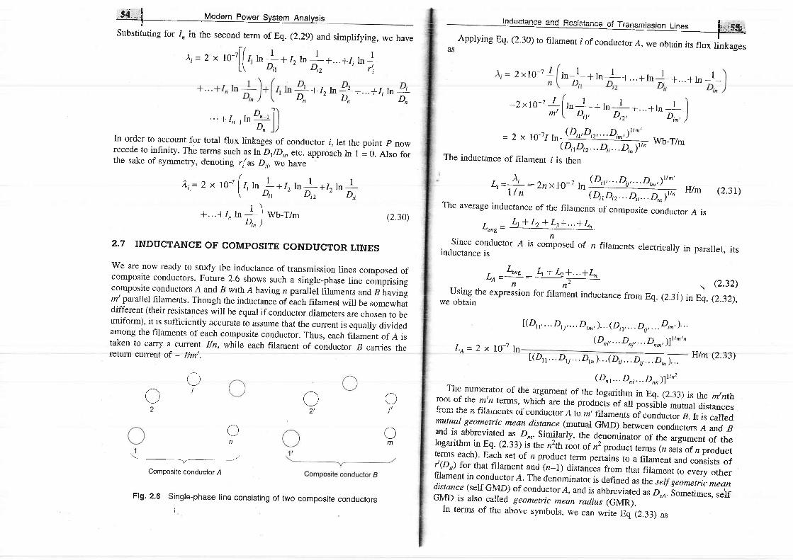
Substiiuti'g for /n in the second term of Eq. (2.29)and simplifying, we havef /

)i = 2 * to-tl I t, ml * L, h L_.+...+1, rn a' L ( ' D i r ' - " " ' D i z " " ' ' ' ' ^ ' r t i

l nduc tanec anr l F laa io ranaa ^ i T - - -^ - - ! . f . ., rs rq r rug ur I ra l l smlss fon L lnes k , . . . i<Er- I

- - -

a / 1 l A \ t ^ c r I

u, Applying Eq. (2-30) ro filamenr i of conductor A, weobtain its flux tintages

zxfir ! h+a6J-a. . . * rn l * . . . * rn I

, (-2xto-7 4 l t " ] -* 6-J-1. . . * ln t )^, \ Dir,

^^' Diz,

| " ' ' 'r D,^, )

= 2 x lo-716 (P,r:D,r,...D,t

Wb_T/m(D,rD,r. . . D,,. . . D,n)r' "The inductance-of filament f is then

L i = ] -! : 2nx70-t,n (Dn' " ' D,, ' " ' D,^')1/^'

* I , ln =e+. . .* l i ln at-

. . . * I , - r1n Dr - t 1 )' 4 ) )

In order to account for total flux linkages of conductor i, let the point p nowrecede to infinity. The terms such as ln D1/Dn, etc. approach ln t = o. Also forthe sake of symmetry, denoting ,.{^ D,,,- wi have

l i= z x 1or I t rn** r r ' , ' ! -+1, ln -1U Dt

' D,2

-" --- Dii

+...+I^t" +)

wb-r/m

(D,rD,r . . .D, , .D ' * FVm (2.3r)7 / n

(2.30)

2.7 INDUCTANCE OF COMPOSITE CONDUCTOR LINES

We are now ready to study the inductance of transmission lines composed ofcomposite conductors. Future 2.6 shows such a single-phase line comprisingcomposite conductors A and B with A having n paraliel filaments and B havingmt parallel filaments. Though the inductance of each filament will be somewhatdifferent (their resistances will be equal if conductor diameters are chosen to beunttorm), it is sufficiently accurate fo assum.e that the current is equally dividedamong the filaments of each composite conductor. Thus, each filament of A istaken to carry a current I/n, while each filament of conductor B carries thereturn current of - Ihnt.

o

Composite conductor A

Fig. 2.6 single-phase line consisting of two composite conductors

The average inductance of the filaments of composite conductor A is

L u u , = L t + L 2 + 4 + " ' + L n

Since conductor a is co#posed of n filaments electrically in parallel, itsinductance is

, _ L u , , _ \ + 1 2 + . . . + L ,_A = -

*ru"rorr:rr"rh" .*pr"f,rion for rir"#i"t indu*ance from Eq. (2.31)i" E;. 3'::r',

Le=2 x 10-7 ln

l ( D n , . . . D r j , . . . D r . , ) . . . ( D ^ , . . . p r j , . . . D , ^ , ) . . .

(Dnr, .. . Dnj, ... Dr^,17r/ntn

[ (Dn . . . Du . . . D rn ) . . . (D i t . .n , t . 4 .Htm (2.33)

( D n t . . . D n i . . . D r n ) ] r , n '

11? x-.::ir:l :f ,he,arsumenr of the logarithm in Eq. (2.33) is rhe m,nth

t:?,T,:!"^: u.]-tl-*'of conductor Ati m' iri"L.il "il"#il#:ili:ffi;

l:#1:# *: jr:lr* ry n2.th int of nz p,;d;;;._,i; ff ffiilil:;yflr,""1i) T:l

set of n product term pertains to "

fii";;;;rrj"",i,sts of

I!:::::1li:*Ti:r{. rnl denominaror is defin"o u, ;;;w;;:;;:;,1;::;!:{Kr,"-li:t:t:y?

of conduc tor A, and ,s auureviate; ;, "J

"r';#;;;":::"*

oo

2o

2l I

r )m

GMD is also called geometric mean radius (GMR).lf

In terms of the above symbols, we can write Eq (2.33) as

56 ,1 todern Fower System AnalysisI

L t=2x 10 -7h + - I i lmDr.t

(2.34a)

'^ ^Hn^

Note the similarity of the above relation with Eq. (2.22b), which gives theinductance of one conductor of a single-phase line for the special case of twosolid, round conductors. In Eq. (2.22b) r\ is the self GMD of a singleconductor and D is the mutual GMD of two single conductors.

The inductance of the composite conductor B is determined in a similarmanner, and the total inductance of the line is

L = L e + L n (2.3s)

A conductor is composed of seven identical copper strands, each having aradius r, as shown in Fig. 2.7. Frnd the self GMD of the conductor.

-- D^^ = 2..fir

Fig.2.7 Cross-section of a seven-strand conductor

Solution The self GMD of the seven strand conductor is the 49th root of the49 distances. Thus

D, = (V)7 (D1zD'ruD rp r)u (zr)u )t'on

Substituting the values of various distances,

p..- ((tJ.7788r)7 (2212 x 3 x 22f x 22rx 2r x 2r)u)t 'o'

srngre layer oI alurrunlumconductor shown in Fig. 2.8 is 5.04 cm. The diameter of each strand is 1.6g cm.Determine the 50 Hz reactance at I rn spacing; neglect the effect of the centralstrand of steel and advance reasons for the same.

Solution The conductivity of steel being much poorer than that of aluminiumand the internal inductance of steel strands being p-times that of aluminiumstrands, the current conducted by the central strands of steel can be assumed tobe zero.

Diameter of steel strand = 5.04 -2 x 1.68= 1.68 cm.Thus, all strands are of the same diameter, say d. For the arrangement of

strands as given in Fig. 2.8a,

D t z = D r c = d

D r t = D n = J l d

D u = 2 d

D r = (l(+)- dTil,eilf')

(b) Line composed of two ACSR conductors

Inductance and Resistance of Transmission Lines

(a) Cross-section of ACSR conductor

, _2r(3(0.7788)) t t7 _ 2. t77 rus - 6U+e Fig. 2.8

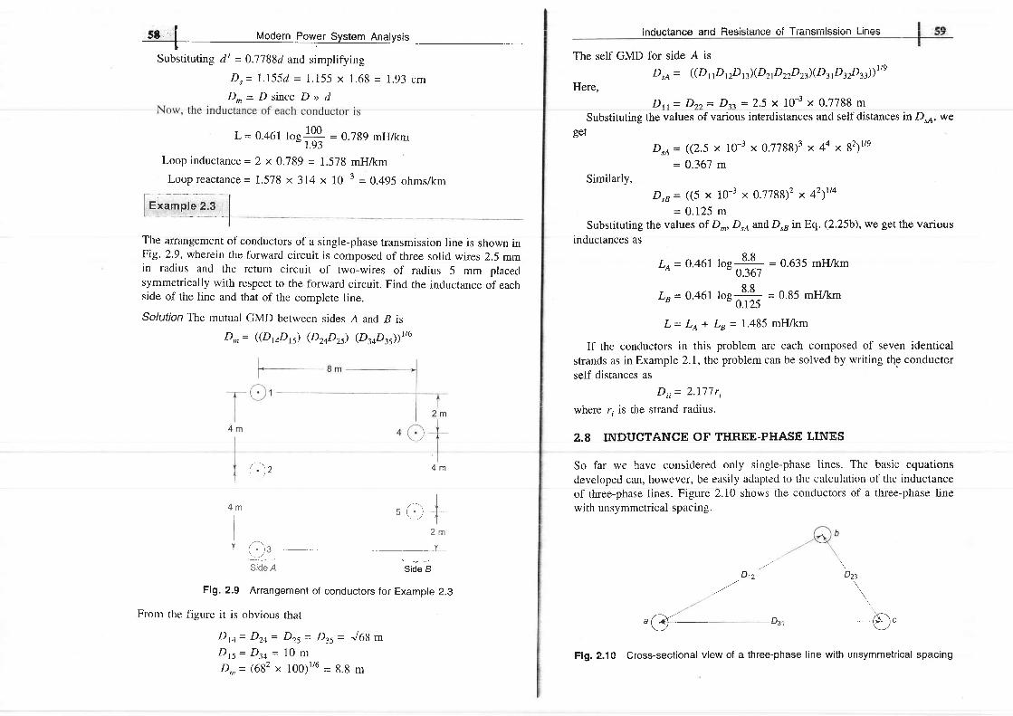
I5t I Modern Power Svstem Analvsis

Substituting d' = 0.7188d and simplifying

D , = l . l 5 5 d = 1 . 1 5 5 x 1 . 6 8 = 1 . 9 3 c m

D ^ = D s i n c e D > > d

L= 0.46t toe 1P - 0.789 mH/km" 1.93Loop inductance - 2 x 0.789 = 1.578 mHlkm

Loop reactance = 1.578 x 314 x 10-3 - 0.495 ohms/lcm;;;,;,; I

lnductance and Resistance oi Transmission Lines

The self GMD fbr side A is

D,A = ((D nD nD n)(DztDzzDn)(D3tDtrDtr))''eHere.

D,, = Doc = Dat = 2.5 x 10-3 x 0.7788 mSubstituting the values of various interdistances and self distances in D16, we

get

D,A= (2.5 x 10-3 x 0.778U3 x 4a x 8\tte= 0.367 m

D,B= ((5 x 10-3 x 0.778q2 ,4 ' ) t 'o= 0 .125 m

Substituting the values of D^, D6 and Dr, in Eq. (2.25b), we get the various

inductances as

L^ = 0.461 los 8'8 = 0.635 mHlkm^ " 0.367

L. = 0.461 toe 8'8 = 0.85 mH/<mD -

0J25

L = Lt + Ln = 1.485 mH/km

If the conductors in this problem are each composed of seven identicalstrands as in Example 2.1, the problem can be solved by writing t[e conductcr

self distances as

Di i= 2 '177r t

where r, is the stranci raciius.

2.8 INDUCTANCE OF THREE.PHASE LINES

So far we have considered only single-phase lines. The basic equationsdeveloped can, however, be easily adapled to the calculation of the inductanceof three-phase lines. Figure 2.10 shows the conductors of a three-phase linewith unsymmetrical spacing.

Similarly,

The arrangement of conductors of a single-phase transmission line is shown inFig.2.9, wherein the forward circuit is composed of three solid wires 2.5 mmin radius and the return circuit of two-wires of radius 5 mm placedsymmetrically with respect to the forward circuit. Find the inductance of eachside of the line and that of the complete line.

Solution The mutual GMD between sides A and B is

D.= ((DMD$) (Dz+Dz) 1D3aD3))tt6

( ) z 4 m

l i4 m s ( t l II " ' " ' t

Side A Side B

Fig. 2.9 Arrangement of conductors for Example 2.3

From the figure it is obvious that

D t q = D z q = D z s - D . u = J O a mD r s = D y = 1 0 mD^= (682 x 100) l /6 = 8.8 m

DzsDn

Fig. 2.10 Cross-sectional view of a three-phase l ine with unsymmetrical spacing

Ugdern Power System A

Assume that there is no neutral wire, so that

I r , + I r + I r - 0Unsymmetrical spacing causes the flux linkages and therefore the inductance ofeach phase to be different resulting in unbalanced receiving-end voltages even

en senolng-e tages and llne currents are balanced. AIso voltages will beinduced in adjacent communication lines even when line currents are balanced.This problem is tackled by exchanging the positions of the conductors at regularintervais aiong the line such that each conductor occupies the original positionof every other conductor over an equal distance. Such an exchange of conductorpositions is called transposition. A complete transposition cycle is shown inFig.2.11. This alrangement causes each conductor to have the same averageinductance over the transposition cycle. Over the length of one transpositioncycle, the total flux linkages and hence net voltage induced in a nearbytelephone line is zero.

b1

lnductance and Resistance of Transmission Lines

But, 1, I I, = - /n, hence

Ao= 2 x 10-7 Iok (D"D ' t rDt ' ) ' ' '

r'a

D"o (DtzDnDrr)t'' - equivalent equilateral spacing

Lo= 2x t0-7 h + = 2 x fO-? fn{ : r FVmf ' o D ,

This is the same relation as Eq. (2.34a) where Dn, = D"o, the mutual GMDbetween the three-phase conductors. lf ro = 11, = r6t we have

L o = L O = L ,It is not the present practice to transpose the power lines at regular intervals.

However, an interchange in the position of the conductors is made at switchingstations to balance the inductance of the phases. For all practical purposes thedissynrnrctry can bc neglectcd and the inductancc of an untransposecl l ine canbe taken equal to that of a transposed line.

If ttre spacing is equilateral, then

D " o = Dand

L o = 2 x l 0 - 7 m I f m nra

If ro = 11, = r,-, it follows from F,q. (2.37) that

L o = L t r = L ,

Fig. 2.11 A complete transposition cycle

To find the average inductance of each conductor of a transposed line, theflux linkages of the conductor are found for each position it occupies in theiransposeci cycie. appiying Eq. (2.s0) to conciuctor a of Fig. z.lI, for section1 of the transposition cycle wherein a is in position 1, b is in position 2 andc is in position 3, we get

)ur = 2 x to-r f , , , r " * I I , ,m]-* l In -1 j *o-r r , r ,\ " ' ' r , " D r ,

( D t , )

For the second section

- ( | | \

For the tr,ira ,".* := 'x to-?[r" k + * 16 tn

b: . '' t" ],;i wu v-

)o3 = z x ro-71 r" h !t 16 tn*+ r.,n l-l *o-rr-\ f',, " D, uzr /

Average flux linkages of conductor a are

(2.36)

(2.37)

Show that over the length of one transposition cycle of a power line, the totalf lux l inkages of a nearby telephone line are z,ero, ftrr balanced three-phasecurrents.

b(l) ci'-)\ 7

c'l

r c t l I , , h ! r , , t n\ 4 ,

()T2

- 1 u

(DnDrD l t ) t / 3+ 1 . l n

(D t2D2 . )3 t ) t / 3F19.2.12 Effect of transposit ion on Induced voltage of a telephone l ine

) t 2 = 2 x t o t l , " L n 5 * r 6 t n + * 1 . 1 n + l w b _ r i m ( 2 . 3 s )( " D o z

- o - - D u , D , , )

" v ' ' t

The net flux linkages of the telephone line are) , = ) , t - ) t z

= 2 x to-r( t" h D:, * 16 tn? *r" ,"+) wb-rim (2.40)

rhe emf induced ," ,n! ,.,"p'#ir" t* "3Jti,

" -

D" )

E,= Zr f ) , \ lmfjnder balanced load conditions, ), is not very large because there is acancellation to a great extent of the flux linkages due to Io, 16 and 1r. Suchcancellation does not take place with harmonr.

"u.r.nts which are multiples of

three and are therefore in phase. Consequently, these frequencies, if present.may be very troublesome.

lf the power line is f'ully transposed with respect to the telephone line

),, = )" (I) * 4, (tr) * ),,(III)3

where ),r(I), )/r(II) ancl ),,(III) are the flux linkages of the telephone line r, inthe three transposition sections of the power line.

Writing for ),,(l), ,\/2(II) and ),r([l) by repeared use of Eq. (2.3g), we have

A , t = 2 x l 0 - / ( t n + 1 6 + 1 , , ) l n(Dn tDu tD , . i t t 3

Similarly,

= 2 x 1 0 4 ( 1 , + . I b + 1 , ) l n(Dn2Db2D, , r ) t , ,

) r= 2 x 10-711, + I t , + I , ) ln (D"2Db2D, ) r t :' (DorDarD,r)r , ,

If Io + Iu + I, = 0, ), = 0, i.e. voltage induced in the telephone loop is zeroover one transposition cycle of the power line.

It may be noted here that the condition Iu+ Iu+ I, = 0 is not satisfied for- (i) rpwer frequency L-G (line-to-ground fault) currents. where

I o + I u * I r = J [ o

62 | Modern Power Svstem Anatrrq ic.

solution Referring to Fig. 2.r2, the flux linkages of the conductor r, of thetelephone line are

, " ^ * + 1 , l n * . 1

t " * Wb-T/m (2.38)

Similarly,

(2.4r)


(ii) third and multiple of third harmonic currenrs under healthy .ondirion,where

1, , (3 )+ IoQ)+ I , (3 )= 31(3)

The harmonic line currents are troublesome in two wavs:(i) Induced ernf is proportional to the frequency.

(ii) Higher frequencies come within the audible range.Thus there is need to avoid the presence of such harmonic currents on power

Iine from considerations of the performance of nearby telephone lines.It has been shown above that voltage induced in a telephone line running

parallel to a power line is reduced to zero if the power line is transposed andprovided it carries balanced currents. It was also shown that ptwer linetransposition is ineffective in reducing the induced telephone line uoitug. whenpower line currents are unbalanced or when they contain third harmonics.Power line transposition aparrfrom being ineffective introduces mechanical andinsulation problems. It is, therefore, easier to eliminate induced voltages bytransposing the telephone line instead. In fact, the reader can easily verify thateven when the power line currents are unbalanced or when t-h"y cgntainharmonics, the voltage induced over complete transposition cycle (called abarrel) of a telephone line is zero. Some induced voltage will always be presenton a telephone line running parallel to a power line because in actu4l practicetransposition is never completely symmetrical. Therefore, when the lines runparallel over a considerable length, it is a good practice to transpose both powerand telephone lines. The two transposition cyeles ^re staggered. and thetelephone line is transposed over shorter lengths compared to the power line.

rc-7

i,."rp," i u I- f

A three-phase, 50 Hz,15 km long line has four No. 4/0 wires (1 cm dia) spacedhorizontally 1.5 m apart in a plane. The wires in order are carrying currents 1o,Iu and I, and the fourth wire, which is a neutral, carries ,".o iu.."nt. Thecurrents are:

Io= -30 + 750 A

Iu= -25 + j55 A

I "= 55 - j105 AThe line is untransposed.

(a) From the fundamental consideration, find the flux linkages of the neutral.Also find the voltage induced in the neutral wire.

(b) Find the voltage drop in each of the three-phase wires.

I64 I Modern Power System Analysis

t

a b c n(:; (. 1 ,r"n.'f(') (:)

t-r.s n.' --. -t--1.5 m -l*- r.s n1 -l

Fig. 2.13 Arrangement of conductors for Example 2.5

Solution (a) From Frg.2.I3,

Don= 4.5 m, Dbn = 3 m, Drn = 1.5 mFlux linkages of the neutral wire n are

- ( I 1 r \) - = 2 x 1 0 - 7 1 1 - l n

' + 1 ^ l n ' * l l n ' l w b - T / m

\ " D o n " D r n D , n )

Substituting the values of D,,n, Dg, and D,.n, and simplifying, we get

An= - 2 x lO-' 0.51 I, + 1.1 Iu + 0.405 1") Wb-TimSince I, = - (Io+ I) (this is easily checked from the given values),

2,, = - 2 x l0-' (1.1051o + 0.695I) Wb-T/mThe voltage induced in the neutral wire is then

Vn= jw),n x 15 x 103 V

=- j314 x 15 x 103 x Z x 10-7(1 J05Io+ 0.695 I) y

Vn= - j0.942 (1.105 Io + 0.695 I) V

Substituting the values of 1, and 16, and simplifying

Vn= 0.942 x 106 = 100 V

(b) From Eq. (2.30), the flux linkages of the conductor a are

( r I r \)o= 2x ro-?[ r,rn l* ru rn**r rn * | wu-r-

\ r 'o " D 2D)The voltage drop/metre in phase a can be written as

a v , , = 2 x r 0 - 7 i w ( , - r n I + 1 ^ l n l * 1 - l n I ) t r , o

\ . " f ' o ' '

D c

2 D )

Since Ir= - (lr,+ Iu), and further since ro= rb= rr= r, the expression forAVo can be written in simplified form

Avo= 2 x to-ty, (r, rn !* romz) v/m

Similarly, voltage drop/petre of phases b and c can be written as

AVo= 2 x r;a iulbo_ #

A V , = 2 x t o t / , ( 1 , f n 2 + 1 , " + )Using matrix notation, we can present the result in compact form


) , r = 2 x I o - 7 ( , r n t - l 6 t ) = 2 x\ D t D r )

In2

ln Dlr l

ln2

voltage p o s e 4 r s c a ulated below:

Avo = j2xra- lx 3r4 x rs x rd(6 !9e (-30+ j50)+0.6e3(-25+is5))

= - (348.6 + j204) V

Flux linkages of conductor 7,

\ ,2= 2 x 10-71 lnD 'D^

A single-phase 50 Hz power line is supported on a horizontal cross-ann. Thespacing between the conductors is 3 m. A telephone line is supportedsymmetrically below the power line as shown in Fig. 2.14. Find the mutualinductance between the two circuits and the voltage induced per kilometre in thetelephone line if the current in the power line is 100 A. Assume the telephoneIine current to be zero.Solution Flux linkaees of conductor Z,

ro-1 I h D'D1

or

Fig.2.14 Power and telephone lines for Example 2.6

Total flux linkage of the telephone circuit

D2

Dr

\)d/

, '-Yt'- \-l-l I

" l*-O.e t

) , = \ , r - \ r z = 4 x 1 0 - ' l l n

66 i Modern power System AnalysisI

A4pt= 4 x tl-i n ! Ul^Dl

lnductanee and Resistance of Transmission Lines

each other. (The reader can try other configurations to verity that these will lead

to low D..) Applying the method of GMD, the equivalent equilateral spacing is

D rn (DnbDbrD.n)' ' t (2.42)

a and b in section I of the

transposition cYcle

= (DpDp)rr+ - 7DP)tt2

Dt,=mutual GMD between phases b and c in section 1 of the

transposition cYcle

= (DP)r;z

D,o=mutual GMD between phases c and a in section I of the

r- transPosition cYcle

= (2Dh)v2

Hence D"o 2rt6Drt2pr/3htt6 (2'43)

It uray be notecl here that D"u t'eurains the sallle in each section of the

transposition cycle, as the conductors of each parallel circuit rotate cyclically,

so do D,,h, Dbrand D,.,,. The reader is advised to verify this for sections 2 and

3 of the transposition cycle in Fig' 2'15'

Self GMD in section 1 of phase a (i.e., conductors a and a/) rs

Drr,= (r 'qy'q)t 'o = (r'q)'/z

Serr GMD "t *;:;=' ,*;;';:^':'ffi'1'are

respectiverv 'i

Drr= (y 'qr 'q) ' ' ' = (r 'q) ' ' t

Equivalent self GMD D, = (Dr,,DrbD,,)rt3

= (r')t' 'qtt3hrt6 (2.44)

Dr= Q.12 + 2 \ t /2 = (5 .2 I ) t /2

D2= (L92 + Z\r /2 = (7.61)t /2

vot= o.g2r bs (Jsf) t"= 0.0758 mH/kmr ' - \ 5 2 1 )

Voltage induced in the telephone circuit V,= jttMr,I

lV,l = 314 x 0.0758 x l0-3 x 100 _ 2.3,/9 Vlkm

2.9 DOUBI"E.CIRCUIT THREE.PHASE LINES

It is common practice to build double-circuit three-phase lines so as to increasetransmission reliability at somewhat enhanced cost. From the point of view ofrrower transfer from one end of the l ine to the other (see Sec. 12.3), it isdesirable to build the two lines with as low an inductance/phase as possible. Inorder to achieve this, self GMD (D") should be made high and mutual GMD(D') should be made low. Therefore, the individual conductors of a phaseshould be kept as far apart as possible (for high self GMD), while the distancebetween phases be kept as low as permissible (for low mutual GMD).

Figure 2.15 shows the three sections of the transposition cycle of two parallelcircuit three-phase lines with vertical spacing (it is a very commonly usedconfiguration).

c b ' b

Section 1

Because of the cyclic rotation of conductors of each parallel circuit over the

transposition cycle, D. also remains the same in each transposition section. The

reader should verify this for sections 2 and 3 in Fig. 2.15.

The inductance Per Phase is

L= 2x 10-7 lo D ' ,n

Ds

= z x ,ot ,n't'u '|l'ltl"tlt)u( r ' ) t ' ' q r /3hr t6Section 2

Fig. 2.15 Arrangement of conductors of a double-circuit three-phase l ine

It may be noted here that conductors a and a' in parallel compose phase aand sirnilarly b and b'compose phase b and, c and c'compose phase c. in orderto achieve high D" the conductors of two phases are placed diametricallyopposite to each other and those of the third phase are horizontally opposite to

\ 0 ,oSection 3

o

= 2 x 1 0 - 7 h

The self inductance of each circuit

( 2,,u(q')" ' [a)"' ] rvpnur.rrn (2.4s)[ ' \ r ' ) \ q )

is given by

(2) ' ' ' p

rLr= 2 x 10-7 ln

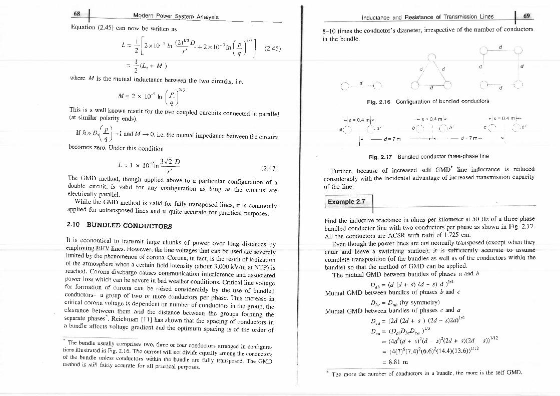
(2.47)

lnductance and Resisiance of Transmission Lines

8-10 times the conductor's diameter, irrespective of the number of conductors

in the bundle.

d i t t , d

Configuration of bundled conductors

= ,(t,

+ M )

where M is the mutual inductance between the two circuits. i.e.

M = z x 1 o - 7 ^ ( z \ ' ' '\ q )

This is a well known result for the two coupled curcuits connected in parallel(at similar polarity ends).

/ \rf h >> o,[ L

l-l una M '--+0, i.e. the mutuar impedance between the cucuits\ q )becomes zero. Under this condition

" I J2DL = I x 1 0 - ' l n " ' ;

The GMD method, though applied above to a particular configuration of adouble circuit, is valid for any configuration as long as the circuits areelectrically parallel.While the GMD method is valid.for fully transposed lines, it is commonly

applied for untransposed lines and is quite u.rrrui" for practical purposes.

2 1n El rT l . t r r r r : rn AAr?s.rv sv l r r - r r r .q .Lr te tJM,rUUl-L, t (S

It is economical 10 transmit large chunks of power over long dista'ces byemploying EHV lines. However, the line voltages that can be used are severelylimited by the phenomenon of corona. corona,ln fact, is the result of ionizationof the atmosphere when a certain field intensity (about 3,000 kv/m at NTp) isreached' Corona discharge causes communication interference and associatedpower loss which can be severe in bad weather conditions. Critical line voltagefor formation of corona can be raised considerably by the use of bundledconductors-a group of two or more conductoru p". phase. This increase incrit ical corona voltage is clepenclcnt on number of concluct<lrs in thc group, thcclearance between them and the distance between the groups forming theseparate phases*. Reichman [11] has shown that the spacing of conductors ina bundle affects vortage gradient and the optimum spacing is of the order of

n no\,v be written as

L =! [ , " ,u

' ̂ c[ .2 *2xro-7rn ( t) '^ l , r .ou,

r-\ d /-\\ . / -

F ig . 2 .16

f "=o .am l ,, ( ) I ou ' ,

-] s = 0.4 m""

be) I On '

---1-)d \_..

d l

I(}

4 m! .

'/^' :' 6 /

- s = 0 .

" \ '

- The bundle usually comprises two, three or four conductors arranged in configura-tions illustrated in Fig' 2.16. The current will not divide equally among the conductors

of the bundle unless conductors within the bundle are ruly transposed. The GMDmethod is still fairly accurate for all practical purposes.

l-_- d =7 m---*]*- d =7 m--- >l:I

Fig.2.17 Bundled conductor three-phase line

Further, because of increased self GMD- line inductance is reduced

considerably with the incidental advantage of increased transmission capacity

of the line.

Find the inductive reactance in ohms per kilometer at 50 Hz of a three-phase

bundled conductor line with two conductors per phase as shown in Fig. z.ri.

All the conductors are ACSR with radii of 1.725 cm'

Even though the power lines are not normally transposed (except when they

enter and leave a switching station), it is sufficiently accurate to assume

complete transposition (of the bundles as well as of the conductors within the

bundle) so that the method of GMD can be applied'

The mutual GMD between bundles of phases a and b

D o b = @ @ + s ) ( d - i d ) r t 4

Mutual GMD between bundles of phases b and c

Dh, = D,,,, (bY sYmmetrY)

Mutual GMD between bundles of phases c uruJ a

D,n = Qd (2d + s ) (2d - t)Zd)tt+

D,o= (DrPaPro)t ' t

= @f@ + s)z(d - s)2(2a + i(Zd - t))tt"

= GQ)6 Q .q2 6.0)2 (14.4)(13.6))', ' ' ,2

= 8 . 8 1 m

Equation (2.45) can

The more the number of conductors in a bundle, the more is the self GMD'

7 0 I n l l a r l a r n D n r e , o ' e r r a + ^ - ^ - ^ r - , ^ .

D.,= (r 'sr ' r ) ' 'o= (rk)r /z = (0.77gg x 1.725 x l0-2 x 0.4\ t /z= 0.073 m

Inductive reactance per phase


A = cross-sectional area, ln2The effective resistance given by Eq. (2.48) is equal ro the DC resistance of theconductor given by Eq. (2.49) only if the current distribution is uniformthroughout the conductor.

r small changes in temperature, the resistance increases with temperaturein accordance with the relationship

R,= R (1 + oor) (2.s0)where R = resistance at temperature 0"C

ao = temperature coefficient of the conductor at 0"CEquation (2.50) can be used to find the resistance Ro at a temperature /2, ifresistance Rr1 at temperature tl is known

8.8r0.073

= 0.301 ohm/kmIn most cases' it is sufficiently accurate to use the centre to centre dista'ces

between bundles rather than mutual GMD between bundles for compu ting D"n.with this approximation, we have for the example in handD r n = e x T x l 4 y r r t - g . g 2 m

Xr= 3I4 x 0.461 x 10-3 los 8 '82" 0.073

= 0.301 ohmlkmThus the approximate method yielcls almost the same reactance value as theexact method' It is instructive to compare the inductive reactance of a bundled

conductor l ine with an equivalent (on heuristic basis) single conductor l ine. Forthe example in hand, the equivalent line will have d = 7 m and conductordiameter (for same total cross-sectional area) as JT x 1.i25 cm

Xr= 314 x 0.461 x l0-3 6n (7 x7 x l4)t /3

0.7799 x J2 xl.725x 10-3= 0.531 ohm/km

This is 7-6'4rvo higher than the colresponding value for a bundled conductorl l t l A A c o l r a n . l " - ^ l - r ^ l - - . r ri i i iv' -\ i diiuduJ liuirit€c out' iower reactance of a bundled conductor l ineincreases its transmission capacity.

2.TT RESISTANCE

Though the contribution of line resistance to series line impedance can beneglected in most cases' it is the main source of line power loss. Thus whileconsidering transmission line economy, the presence of line resistance must beconsidered.The effective AC resistance is given by

O _ average power loss in conductor in wattsohms (2.48)

where 1is the rms current in the conductoi in amperes.Ohmic or DC resistance is given by the formula

n lRn - ' " ohlns' ' A

p = resistivity of the conductor, ohm_m/ = length, m

2.T2 SKIN EFFECT AND PROXIMITY EFFECT

The distribution of current throughout the cross-section of a conductor isuniform only when DC is passing through it. on the contrary when AC isflowing through a conductor, the current is non-uniformly distributed over thecross-section in a manner that the current density is higher at the surface of theconductor compared to the current density at its centre. This effect becornesInore pronounced as frequency is increased. This phenonlenon is cil led stirrqffect.It causes larger power loss for a given rms AC than the loss when theSairr€ vaiue of DC is flowing ihrough the conciuctor. Consequently, the effectiveconductor resistance is more fbr AC then fbr DC. A qualitative explanation ofthe phenomenon is as follows.

Imagine a solid rottnd conductor (a round shape is considered forconvenience only) to be composed of annular filaments of equal cross-sectionalarea. The flux linking the filaments progressively decreases as we movetowards the outer filaments fbr the simple reason that the flux inside a filamentdoes not link it. The inductive reactance of the inraginary filaments thereforedecreases outwards with the result that the outer filaments conduct more ACthan the inner filaments (filaments being parallel). With the increase offrequency the non-uniformity of inductive reactance of the filaments becomesmore pronounced, so also the non-uniformity of current distribution. For largesolid conductors the skin effect is quite significant even at 50 Hz. Theanalytical study of skin effect requires the use of Bessel's functions and isbeyond the scope of this book.

Apart fronl the skin effect, non-uniformity of current distribution is alsocaused by proximity eJJ'ect. consider a two-wire line as shown in Fig. 2.1g.Each line conductor can be divided into sections of equal cross-sectionat area(say three sections). Pairs aat, bbt and, cct can form three loops in parallel. The

(2 .s 1)

where(2.49)

I72 | Modern Power System Anaiysis

t

flux linking loop aat (and therefore its inductance) is the least and it increasessomewhat for loops bbt and ccl. Thus the density of AC flowing through theconductors is highest at the inner edges (au') of the conductors and is the leastat the outer edges (cc').This type of non-uniform AC current distributionDecomes more pronounceo as me olstance Detween conouctors ls reouceo. LlKe

skin effect, the non-uniformity of current distribution caused by proximity effect

also increases the effective conductor resistance. For normal spacing ofoverhead lines, this effect is always of a negligible order. However, forunderground cables where conductors are located close to each other, proximityetfect causes an appreciable increase in effective conductor resistance.

F ig . 2 .18

Both skin and proximity effects depend upon conductor size, fiequency,

distance between conductors and permeability of conductor material.

PROB LE IVI S

Derive the formula for the internal inductance in H/m of a hollowr;onductor having inside radius r, and outside radius r, and also determinethe expression for the inductance in H/rn of a single-phase line consistingof the hollow conductors described above with conductors spaced adistance D apart.

Calculate the 50 Hz inductive reactance at I m spacing in ohms/km of acable consisting of 12 equal strands around a nonconducting core. Thediameter of each strand is 0.25 cm and the outside diameter of the cableis 1.25 cm.

A concentric cable consists of two thin-walled tubes of mean radii r andIt respectively. Derive an expression for the inductance of the cable perunit length.

A single-phase 50 Hz circuit comprises two single-core lead-sheathedcables laid side by side; if the centres of the cables are 0.5 m apart andeach sheath has a mean diameter of 7.5 cm, estimate the longitudinalvoltage induced per km of sheath when the circuit carries a current of800 A.

2.5 Two long parallel conductors carry currents of + 1 and - 1. What is themagnetic field intensity at a point P, shown in Fig. P-2.5?


Fig. p-2.5

2.6 Two three-phase lines connected in parallel have selt'-reactances of X, andX2. If the mutual reactance between them is Xp, what is the effectivereactance between the two ends of the line?

2.7 A single-phase 50 Hz power line is supported on a horizonral cross-arm.The spacing between conductors is 2.5 m. A telephone line is alsosupported on a horizontal cross-arm in the same horizontal plane as thepower l ine. The condttctors of the telephrlnc l ine are of solid copperspaced 0.6 m between centres. The distance between the nearestconductors of the two lines is 20 m. Find the mutual inductance betweenthe circuits and the voltage per kilometre induced in the teiephone line for150 A current flowing over the power line.

2.8 A telephone line runs parallel to an untrasposed three-phase transmissionline, as shown in Fig. P-2.8. The power line carries balanced current of400 A per phase. Find the mutual inductance between the circuits andcalculate the 50 Hz voltage induced in the telephone line ptsr km.

a b c h b

( r ( r ( , , .l L

f ^ 5 m - - - + + + - - 5 m - - - f - 1 5 m - - - * 1 r n . _ _

Fig. P-2.8 Telephone l ine paral lel to a power l ine

2.9 A 500 kV line has a bundling arrangement of two conductors per phaseas shown in Fic. P-2.9.

Fig. P-2.9 500 kV, three-phase bundled conductor l ine

Compute the reactance per phase of this line at 50 Hz Each conductorcarries 50Vo of the phase current. Assume full transposition.

b

2 . 1

2 .?

2 . 3

2 . 4

lgq e r1-tgrygf .!yg!U_ An 4ygp2.10 An overhead line 50 kms in length is to be constructed of conductors 2.56

cm in diameter, for single-phase transmission. The line reactance must notexceed 31.4 ohms. Find the maximum permissible spacing.

2.11 In Fig. P-2.1 I which depicts two three-phase circuits on a steel tower therecal cenre tlnes.

three-phase circuit be transposed by replacing a by b and then by c, sothat the reactances of the three-phases are equal and the GMD method ofreactance calculations can be used. Each circuit remains on its own sideof the tower. Let the self GMD of a single conductor be 1 cm. Conductorsa and at and other corresponding phase conductors are connected inparallel. Find the reactance per phase of the system.

b b '

o c )l - 1o m- - l

r.___zsm___l') .)

Fig. P-2.11

)-.12 A double-circuit three-phase l ine is shown in Fig. P-2.I2. The conductorsa, a/l b, bt and c, c/ belong to the same phase respectively. The radius ofeach conductor is 1.5 cm. Find the inductance of the double-circuit line inmH/km/phase.

l t

I- l - 1 m

I

b /

I4 m

Il-4 m

II

i-----z.sm ---j


REFERE N CES

l . Electric'tt l Transrnission and Distributiort Book, Westinghouse Electric andManufacturing Co., East Pittsburgh, Pennsylvania, 1964.

2. Waddicor, H., Principles of Electric Power Transmission, 5th edn, Chapman andHall, London, 1964.

3. Nagrath, I.J. and D.P. Kothari, Electric Machines, 2nd edn, Tata McGraw-Hill,New Delhi, 1997.

4. Stevenson, W.D., Elements of Power System Analvsis,4th edn, Mccraw-Hill, NewYork, 1982.

5. Edison Electric Institute, EHV Transmission Line Reference Book, 1968.6. Thc Aluminium Association, Aluminium Electrical Conductor Handboo,t. New

York, 1971.

1. Woodruff. L.F., Principles of Electric Pov,er Trun.snissiorr, John Wiley & Sons,New York, 1947.

8. Gross, C.A., Power System Analysis, Wiley, New York, 1979.9. Weedy, B.M. and B.J. Cory Electric Power Systems,4th edn, Wiley, New york,

1998 .

10. Kimbark, E.W., Electrical Transmission of Power and Signals, John Wiley, NewYork, 1949.

Paper

I l . Reichman. J. , 'Bundled Conductor Vol tage Gradient Calculat ions," AIEE Trans.1959, Pr I I I . 78: 598.

c '

C)o

a) [r\..,_/ \. _./1 m - l - , r - l

Fig. P-2.12 Arrangement of conductors for a double-circuit three-phase line

2.13 A three-phase line with equilateral spacing of 3 m is to be rebuilt withhorizontal spacing (.Dn = ZDn - ZDrr).The conducrors are to be fullytransposed. Find the spacing between adjacent conductors such that thenew line has the same inductance as the original line.

2.14 Find the self GMD of three arrangernents of bundled conductors shown inFig. 2.16 in terms of the total cross-sectional area A of concluctors (samein each case) and the distance d between them.

a /

l l

> l <I

a b

(_) ( )

i ' 1 m - i - 1 m

Capacitance of Transmission Lines

tV," = 6eav :6-- -q-dv V

t L | . ' ,

) , , ,r r L / t ' \ V

Fig. 3.1 Electr ic f ield of a lclng straight conductor

As the potential difference is independent of the path, we choose the path of

integration as PrPP2 shown in thick line. Since the path PP2lies along an

equipo',entral,Vrris obtained simply by integrating along PyP, t.e.

3.1 INTRODUCTION

The capacitance together with conductance forms the shunt admittance of atransmission line. As mentioned earlier the conductance is the result of leakageover the surface of insulators and is of negligible order. When an alternatingvoltage is applied to the l ine, the l ine capacitance draws a leading sinusoidalcurrent called the charging current which is drawn even when the line is opencircuited at the far end. The line capacitance being proportional to its length, thecharging current is negligible for l ines less than 100 km long. For longer l inesthe capacitance becomes increasingly important and has to be accounted for.

3.2 ELECTRIC FIELD OF A LONG STRAIGHT CONDUCTOR

Imagine an infinitely long straight conductor far removed from other conductors(including earth) carrying a unifbrrn charge of 4 coulomb/metre length. Bysymmetry, the equipotential surfaces will be concentric cylinders, while the linesof electrostatic stress will be radial. The electric field intensitv at a distance vfrom the axis of the conductor is

,= Q v /^2nky

where ft is the permittivity* of the medium.

As shown in Fig. 3.1 consider two pclints P, and P, located at clistances D,and Dr respectively from the conductor axis. The potential difference Vn(between P, and Pr) is given by

* In SI units the pennittivity of free space is ko = 8.85 x 10-12 F/m. Relativepermittivity for air is ft, = klko = 1.

( 3 . 1 )

3.3 POTENTIAL DIFFERENCE BETWEEN TWO CONDUCTORS

OF A GROUP OF PARALLEL CONDUCTORS

Figure 3.2 shows a group of parallel charged conductors. It is assumed that the

conductors are far removed from the ground and are sufficiently removed from

each other-, i.e. the conductor radii are much smaller than the distances between

them. The spacing commonly used in overhead power transmission lines always

meets these assumptions. Further, these assumptions imply that the charge on

each conductor remains uniformly distributed around its periphery and length.

vrz= l:, ' trav:ht"?u

i,o - --

n n

Fig. 3.2 A group of paral lel charged conductors

7S 'l Modern power System Analysis

The potential difference between any two conductors of the group can then beobtained by adding the contributions of the individual charged conductors:byrepeated application of Eq. (3.1). so, the potential difference betweenconductors a and b (voltage drop from a to b) is

v (3.2)

Each term in Eq. (3.2) is the potential drop from a to b caused by charge onone of the conductors of the group. Expressions on similar lines could bewritten for voltage drop between any two conductors of the group.

If the charges vary sinusoidally, so do the voltages (this is the case for ACtransmission line), the expression of Eq. (3.2) still applies with charges/metrelength and voltages regarded as phasor quantities. Equation (3.2) is thus validfor instantaneous quantities and for sinusoidal quantities as well, wherein allcharges and voltages are phasors.

3.4 CAPACITANCE OF A TWO.WIRE LINE

Consider a two-wire line shown in Fig. 3.3 excited from a single-phase source.The line develops equal and opposite sinusoidal charges on the two conductorswhich can be represented as phaso$ Qo Nd qb so that eo = _ eu.

l ' . - ^Capacitance of Transmission Lines | 79r-

or

Cot0.0121

trtF/km (3.4b)log (D / (ror)t tz)

*lcln tn +.

qo tn *;. n, h ++..

qn " +)

The associated line charging current is

I,= ju.Co6Vnu Allvn

(3.4c)

(3.5)

(3.6)

(3.7)

(a) L ine-to- l inecapaci tance

l ---r )oi . . - -

Cnnc",C . n = C b r = 2 C " a

(b) L ine-to-neutra lcapaci tance

F ig . 3 .4

As shown in Figs. 3.a @) and (b) the line-to-line capacitance can beequivalently considered as two equal capacitances is senes. The voltage acrossthe lines divides equally between the capacitances such that the neutral point nis at the ground potential. The capacitance of each line to neutral is then givenby

l*- --- --Jl - l

Fig. 3.3 Cross-sectional view of a two_wire l ine

The potential difference Vo6 can be written in terms of the contributionsmade by qo and q6 by use of Eq. (3.2) with associated assumptions (i.e. Dlr islarge and ground is lar away). Thus,

V , =' 0t) (3.3)

Since Qr,= - qu, we have

vob= !+mL27rk rorb

The line capacitance Cnh is then

C,= Co,= Cb, = 2Cou= ,!#A

pflkm

"O___l [__{b

pFkm

, l ; t ( n " h D * " ^ + )

The assumptions inherent in the above derivation are:(i) The charge on the surface of each conductor is assumed to be uniformly

distributed, but this is strictly not correct.If non-uniforrnity of charge distribution is taken into account, then

0.0242C,

rcn( L+( 4- , ) " ' )- [ 2 r \ 4 r ' ) )

Qo

Vot

lf D/2r >> 1, the above expression reduces to that of Eq. (3.6)and the errorcaused by the assumption of uniform charge distribution is negligible.

(ii) The cross-section of both the conductors is assumed to be circular, whilein actual practice stranded conductors are used. The use of the radius of thecircumscribing circle for a stranded conductor causes insignificant error.

" a b -

In (D / ( ror) t tz1F/m length of line Q.aa)

q0 | Modern pb*gl Jysteq 4!gly..!s

3.5 CAPACITANCE OF A THREE-PHASE LINE WITHEOUILATERAL SPACING

Figure 3.5 shows a three-phase line composed of three iclentical concluctors of

(3.e)

(3. r 0)Since there i l re no othcr charges in the vicinity, thc sunr of 'clrar_{es on the threeconductors is zero. Thus q6 * Qr=- Qu, which when substi tuted in Eq. (3.10)vields

A\_-/b

Fig. 3.5 cross-section of a three-phase l ine with equi lateral spacing

Using Eq. (3.2) we can write the expressions for Vu,, and V,,.. as

vub= *(0"

6 2 * t1,, tn t , r, ,, +)

(3.8)

vn ,= i ! * (n "6P- tq1 , tn#* r , ̂r j )

Adding Eqs. (3.8) and (3.9), we get

v,,t, * v,,, = , 'oolrr,,

,, D + (qu ' l ,1, )t,, ; ]

V,,h I Vn, = !+ r" 2zTTk r

With balanced three-phase voltages appliedphasor diagrarn ol ' I ,r ig. 3.(r that

Vou I Vor= 3Von

Substi tut ing for (Vot,+ V,,,) trom Eq. (3.12)

v^_- 4o tn227Tk r

The capacitance of line to neutral immediately follows as

/- Qo 2 Tlc" Von ln (D/r)

( 3 . 1 1 )

to the line, it follows from the

i n Eq. (3 .11) , we ger

(3.r2)

(3 .13)

(3. l4a)

s 1 ^ - 4

a

es Lg-For air medium (k, = l),

T '

,,=#ffi p,Flkm

1o (line charging) = ju,CnVnn

(3.14b)

\ D

(3 .1s)

Vac,/Vab + Vac= 2 rt cos 30" V"n

= 3 V " n

\V'o

IF

vb

Vr

Fig. 3.6 phasor diagram of baranced three-phase vortages

3.6 CAPACITANCE OF A THREE.PHASE LINE WITHUNSYMMETRICAL SPACING

For the first,section of the transposition cycle

vob = +(eo t rn ! *qur tn f + e , r rn } ) (3 . r6a)zTvc \ r - ' Drz Dr, )

\

Vca 1

v",

a/

,''h1 " ,t "

, " III

III tvun

n " .

6 D

30

! b

. l

E2' I Modern Power System Analysist Capacitance of Transmission Lines I m

t

* l r " ho -3L+aa tnL (3 .18)

(3 .1e)

D rn = (D nDnDT)tl3

Fig. 3.7 Cross-section of a three-phase(ful ly transposed)

l ine with asymmetrical spacing

For the second section of the transposition cycle

- t e.zt" +l (3.16b)z T r K \ f u z t u t z )

For the third section of the transposition cycle

vob= |- . ( r"r ln -&r- * q6rtn-!- i e, t t "+l (3.16c)

z i ' ! \ D y D r , )

If the voltage drop along the line is neglected, Vno is the same in each

transposition cycle. On similar lines three such equations can be written for

Vbr= Vut, I -120. Thrce more equations can be written equating to zero the

summation of all line charges in each section of the transposition cycle. From

these nine (independent) equations, it is possible to determine the nine unknoWn

charges. The rigorous solution though possible is too involved.

With the usual spacing of conductors sufficient accuracy is obtained by

assuming

(3.20)

As per Eq. (3.12) for balanced three-phase voltages

Vnt i Vor= '3Vnn

and also (qu + qr) = - qo

Use of these relationships in Eq. (3.20) leads ro

l/ ̂ .. - Qo ln D"n

o n - Z n k - " rThe capacitance of line to neutral of the transposed line

C. = 3s-: -2nk F/m to neutral" Von ln (D"o / r)

For air medium 'o;=

-'uut-\-n = -- p,F/km to neutral" log (D,o /r)

It is obvious that for equilateral spacing D,, = D, the above (approximate)formula gives the exact resdlt presented earlier.

The line charging current for a three-phase line in phasor form isIo Qine charging) = jut,,Vnn Alkm (3.23)

3.7 EFFECT OF EARTH ON TRANSMISSION LINECAPACITANCE

In calculating the capacitance of transrnission lines, the presence of earth wasignored, so far. The effect of earth on capacitance can be conveniently takeninto account by the method of images.

Method of Images

The electric field of transmission line conductors must conforrn to the presenceof the earth below. The earth for this purpose may be assumed to be a perfectty

r / - - l ( ^ r ^ D " n ' , t j'o,= l f i ln,

tn;*n, r" ,* )

Adding Eqs. (3.18) and (3.19), we get

vot # vo, = *( , ,6 2rt r (qt-r q")rn t

' )

r , / r ^ \ f -

% )

(3.2r)

is then giveh by

(3.22a)

(3.22b)Q a t = Q a 2 = Q a 3 = Q " i Q u t = Q a z = Q u z = Q o ,

4 c t = Q , ' 2 = 4 , 3 = 4 r ' (3. t7)

This assumption of equai charge/unit length of a line in the three sections of thetransposition cycle requires, on the other hand, three diff'erent values of Vnudesignated as Vo61, Vo62and Voo, in the three sections. The solution can beconsiderably simplified by taking Vou as the average of these three voltages, i.e.

v ,q ,@vg)= ! {v , ,u r+ vour+ vooz)J

or ' I l- ( DtzD?tDy .1*o" rn I r ' )/ nb =

6 q1aln' 'n

[ ,, ) '

" ' \ Dt2D23D3t )

( DrrDr^D^, \1+ q ^ l n l - : l l

\ DnDnD3t ))

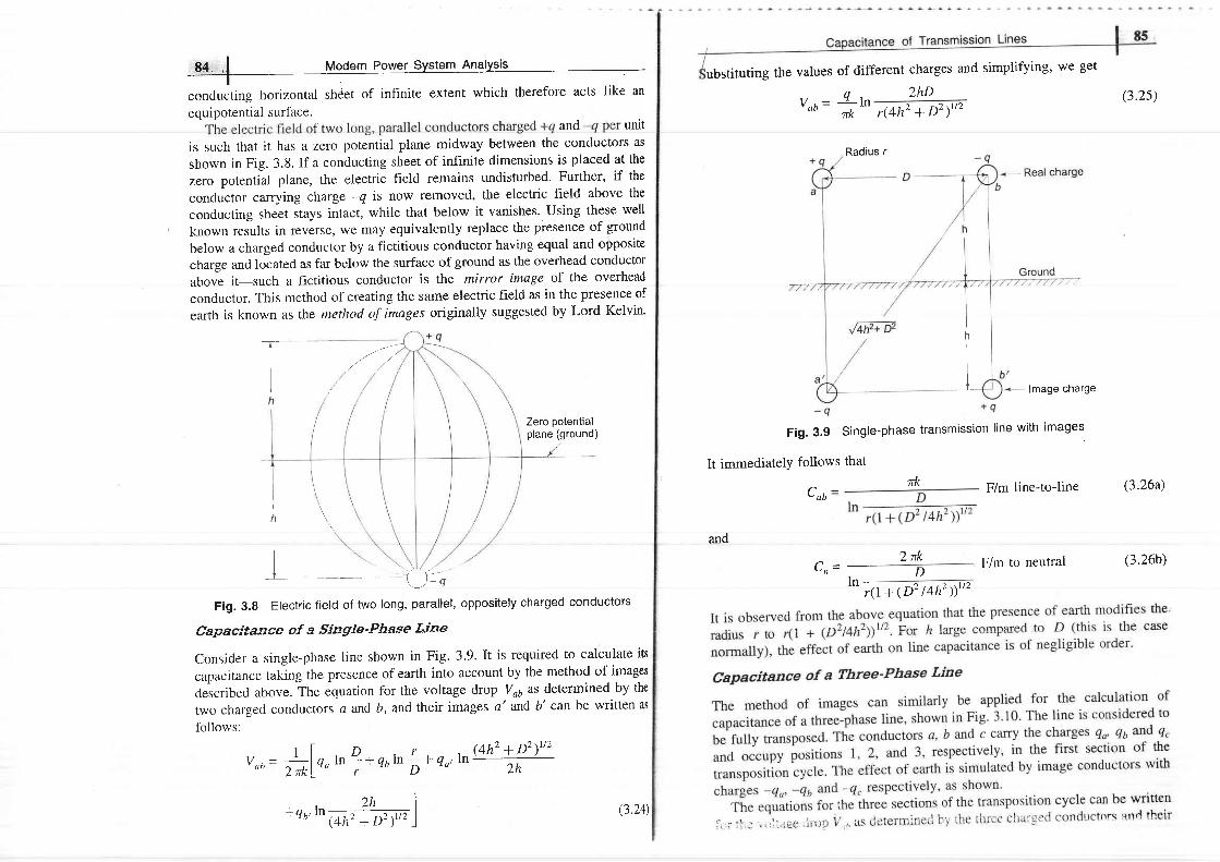
E4 | Modern Power SYstem AnalYsis

conducting horizontal shdet of infinite extent which therefore acts like an

equipotential surface.and unit

is such that it has a zero potential plane midway between the conductors as

shown in Fig. 3.8. If a conducting sheet of infinite dimensions is placed at the

zero potential plane, the electric field remains undisturbed. Further, if the

conductor carrying charge -q is now removed, the electric field above the

conducting sheet stays intact, while that below it vanishes. Using these well

known results in reverse, we may equivalently replace the presence of ground

below a charged conductor by a fictitious conductor having equal and opposite

charge and located as far below the surface of ground as the overhead conductor

above it-such a fictitious conductor is the mirror image of the overhead

conductor. This method of creating the same electric field as in the presence of

earth is known as the method of images originally suggested by Lord Kelvin.

Zero potentialp lane (ground)

Fig. 3 .8 Electr ic f ield of two long, paral lel, oppositely charged conductors

Capacitance of a Single'Phase Line

Consider a single-phase line shown in Fig. 3.9.lt is required to calculate its

capacitance taking the presence of earth into acoount by the method of images

described above. The equation for the voltage drop Vo6 as determined by the

two charged conductors a and, b, and their images a'and b' can be written as

follows:

lmage charge

F i g ' 3 . 9 S i n g | e - p h a s e t r a n s m i s s i o n I i n e w i t h i m a g e s

It immediatelY follows that

w a b - F/m line-to-line (3.26a)

2hDV o b =

r(4hz + D2)'tz

Radius r

(3.2s)

F/m to neutral (3.26b)

'l rn

rk

l--t ,

h \ ,

It__

h

III

/'7

irk

and

C n = - 2nkD

ln

v ub = *1, " m 2 + nrrn i* e,,, t"gt#Y

*q,,tnGFfUl

41+tO' t4h21st t2

ubstituting the values of different charges and simplifying' we get

(3.24)

86 ,* | Modern power Svstem Analvsis

images. with conductor a in position 1, b in position2, and c in position 3,

ln r - ln

h,

(3.27)

Similar equations for Vo6 can be written for the second and third sections of thetransposition cycle. If the fairly occurate assumption of constant charge per unitlength of the conductor throughout the transmission cycle is made, the averagevalue of Vou for the three sections of the cycle is given by

Capacitanee of Transmission Lines

The equation for the average value of the phasor %. ir found in a similarmanner. Proceeding on the lines of Sec. 3.6 and using Vou * Vo, = 3Von andQo * Qt * Qc = 0, we ultimately obtained the following expression for thecapacitance to neutral.

F/m to neutral (3.29a)

12 7rl(

tn D'u - rr( rn"n"\'),)!t \r ( (hrlhhs)' ' ' )

0.0242C, pPttcm to neutral (3.29b)

lon D'n - ron@"httu')'!t- - o

r - - o

(4h24 ) t t 3

(3.28)

Comparing Eqs. (3.22a) and (3.29a), it is evident that the effect of earth is toincrease the capacitance of a line. If the conductors are high above earttrcompared to the distances among them, the effect of earth on the capacitanceof three-phase lines can be neglected.

Calculate the capacitance to neutrallkm of a single-phase line composed ofNo. 2 single strand conductors (radius = 0.328 cm) spaced 3 m apart and,7.5m above the ground. compare the results obtained by Eqs. (3.6), (3.7) and(3.26b).Solution (1) Neglecting the presence of earth tEq. (3.6)l

^ 0.0242 n,C , = 3 1 f i t k mlog -

o.oi+z=ff i=o'00817 P'Flkm- 0.328

By the rigorous relationship [(Eq. (3.7)]

cn o.0242

where D, = (DnDnDrr)"t

"'(+.(#-')"')Since

+ =915, the effect of non-uniformity of charge distribution is almost

negligible.

C" = 0.00817 pFkm

Flg. 3.10 Three-phase l ine with images

c'- o:o?? = o'0082 P'Fkm" 2.9s3Note: The presence of earth increases the capacitance by approximately 3

parts in 800.

r r l

_uu I Modern powel€ysteryr_Anslygls-

(2) Considering the eff'ect of earth and neglecting non-uniformity of chargedistribution [Eq. (3.26b)]

0.0242

Capacitance of Transmission Lines | 89-----------l

b c a

d = 8 m -

- h = 6 m

Fig. 3.11 Cross-section of a double-circuit three-phase line

Solution As in Sec. 3.6, assume that the charge per conductor on each phaseis equal in all the three sections of the transposition cycle. For section / of thetransposition cycle

V,,n(l) =

(3.30)

r ( l * (

300,Jto4 o32BJLo4

/4h") )

- 897

0.0242tog(440/0.525)

Example 3.2

A three-phase 50 Hz transmission line has flat horizontal spacing with 3.5 mbetween adjacent conductors. The conductors are No. 2/0 hard-drawn sevenstrand copper (outside conductor diameter = 1.05 cm). The voltage of the lineis 110 kV. Find the capacitance to neutral and the charging current perkilometre of line.Solution D"o= (3.5 x 3.5 x '7)t 't = 4.4 m

v l _ 1 0 6n" - u,Cn

- 314. o.oos%

= 0.384 x 106 O/km to neutral

charging cunent - +- (l 19l ]e) x l-000

Xn 0.384x 106= 0.1I Aftm

For section II of the transposition cycle

v"b Gr) = ,lAln.("i* r" #)+ c, (rn; .'" *)

+ a , ( r n j . , " : ) ] ( 3 3 r )

For section III of the transposition cycle

vtu (rrr) = *lr. ('" j .^ i)+ a, (rn I. ̂ I)

+a.(rn;.r"f)f ,"r,Average value of Vo6 over the transposition cycle is given by

v,* (av s) = iL*[n.'n (ttrj+* r, ̂ (###)]

z*l*(" i* ' ' ;)+c,(rn; . '"f )*n.(,n j+r";)]

The six conductors of a double-circuit three-phase line having an overall radiusof 0.865 x 10-2 m are arranged as shown in Fig. 3.11. Find the capacitivereactance to neutral and charging current per kilometre per conductor at110 kV, 50 Hz.

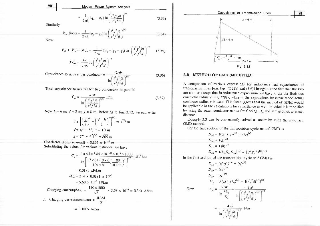
90 | Modern power System Analysis

i 'B' jh

, ' f 'd

Capacitance to neutral per conductor = 2dc

vou* vo,= 3von= fien"- Qt- q,)tn (ffi) ' ' ' (3.3s)

3von=*r " ( :# )

Capacitance of Transmission Lines I gf-

l ' . h = 6 m

Fig. 3.12

3.8 METHOD OF GMD (MODTFTED)

A comparison of various expressions for inductance and capacitance oftransmission lines [e.g. Eqs. (2.22b) and (3.6)] brings our rhe facr that the rwoare sirnilar except that in inductance expressions we have to use the tictit iousconductor radius rt = 0.7788r, while in the expressions for capacitance actualconductor radius r is used. This fact suggests that the method of GDM wouldbe applicable in the calculations for capacitance as well provided it is modifiedby using the outer conductor radius for finding D,, the self geometric meandistance.

Exarnple 3.3 can be conveniently solved as under by using the rnodifledGMD method.

For the first section of the transposition cycle mutual GMD is

Dub= ((ts) (ts))tta _ l iglttzDb' = Qil'''

Drr, = ( jh)'''

D "n

(D"pop,o)r,t = [(i, grjh)r,t)t,,

ln the first section of the transposition cycle self GMD is

D,o = ?f rf )rt4 = ?f)'''

D'l' = QAt''

Dr, = (At''

D, = (D,oDroD,,)''3 = l?3f Arl3fitz2d( 2nk

=fi,^-,,)h(ffi)"' (3.33)

(3.36)

(3.37)

Now h= 6 m; d = 8 m; -/ = 8 m. Referring to Fig. 3.I2, we can writef , . . ? . , , , 1 2 1 ' 1 / 2

r = l f / ) - + ( o - h \ " 1 : J i mL \ 2 ) \ 2 ) )

f = ( j '+ h2)r t2 = l0 m

g = (72 + 42)rt2 =J65 -Conductor radius (overall) = 0.865 x 10-2 mSubstituting the values for various distances. we have

4 rx7 x 8 .85 x 10-12 x 106 x 1000pF /km

Total capacitance to neutral for two conductors in parallel

C n =4 r k

1n f r z *os *s to f r oo ) 3 - l ' / 3[ 1 0 0 x 8 \ 0 . 8 6 s / |

= 0.018 I 1F/kmQC,= 314 x 0 '0181 x 10-6

= 5.68 x 10-6 Ulkm

Charging current/phase = "t#*

x 5.6g x 10{ = 0.361

Charging current/conductor = 0'361L

cn

4 ltk= 0.1805 A/km

Now C n =

F/m

a i , ' l t I

FThis result obviously checks with the fundamentally derived expression inExample 3.3.

3.9 BUNDTED CONDUCTORS

LsLPROB IE M S

:::f ::i::t"^tll:; j;;:i;g;:;fi IH#,",iHffi T,.$l;:i,h*jA bundled conductor line is shown in Fig. 3.13. The conductors of any onebundle are in parallel, and it is assumed that the charge per bundle dividesequally among the conductors of the bundle as Drr> r/. Also Drr- d x D*+ d x D12for the same reason. The results obtained-with these urru'rnptions arefairly accurate for usual spacings. Thus if the charge on phase a is qo, theconductors a and a'have a charge of qolz each; similarly the charge is equallydivided for phases b and c.

[ ? 1 F - q - - i F d +aQ I O,, oQ I eu, "6 iec/____ _DP ---->f-

Dzs ---------

l' Dy -- '..l

Fig' 3'13 Cross-section of a bundled conductor three-phase transmission l ine

Now, writing an equ'ation for the voltage from conductor a to condu ctor b,we get

vob= * lotn,(rn4.*ro- ,

*o.Sq"lr" o-u* rn 4. )- - \ D, Dt,)

or

/r t + . qn tng .n " t nD r r \v,,h =

,* l r , ,n ' . r

ro , . , Dtz Dzt )

applied voltage is baranced three-phase, 50 Hz. Take the voltage of phasea as reference phasor. All conductors have the same radii. Also find thecharging current of phase a. Neglect the effect of grouno.

Fig. p-3.1

3'2 A three-phase double-circuit line is shown in Fig. p-3.2.The diameter ofeach conductor is 2.0 cm. The line is transffio and carries balancedload' Find the capacitance per phase to neutral of the line.

Q c '

Qu,

aQ

o Q

T2 m

,fI

I2 m

_t

Considering the line to be transposed and proceeding in the usual manner, thef inal resul t wi l l be

',= ^ffi p,Fkmto neutral

where Do, = (DnDnD3)In

It is obvious from Eq. e.aD that the method of modified GMD is equallyvalid in this case (as it should be).

3'3 A three-phase, 50 Hz overhead line has regularly transposed conductorsequilaterally spaced 4 m apart The "upu.Itun.e

of such a line is 0.01tFkm'Recalculate the capacitanc. p"i kilometre to neutral when theconductors are in the same horizontai prane with successive spacing of4 m and are regularly transposed.3'4 consider the, 500 kv, three-phase bundled conductor line as shown inFig' P-2'9' Find the capacitivi reactance to neutral in ohms/km at 50 Hz.3.5 A three-phase trernsnri.ssion rinc has r,rat, horizontar spacing with 2 rnbetween adjacent conductors. The radius of each conductor is 0.25 cm. Ata certain instant the charges on the centre conductor and on one of theoutside conductors are identical and voltage drop between these identi-cally charged conductors is 775 v.xegtecithe effect of ground, and findthe value of the identical charge in coulomblkm at the instant specified.

3'6 Find the 50 Hz susceptance to neutral per kilometre of a double-circuitthree phase line with transposition as shown in Fig. p_3.6. Given D = Jmand radius of each of the six conductors is 1.3g cm.

(3.3e)

(3.40)

94 i - Modern Po*", Syrt"r An"lysi.t

6 6 6 5 6 5l'- o - +-- o-*_ D >)<-- D 'l-- o-J

3 . 8

. P-3.6 Double circuit three-phase l ine with f lat spacing

3.7 .{ single conductor power cable has a conductor of No. 2 solid copper(radius = 0.328 cm). Paper insulation separating the conductor from theconcentric lead sheath has a thickness of 2.5 mm and a relativepermittivity of 3.8. The thickness of the lead sheath is 2 mm. Find thecapacitive reactance per kilometre between the inner conductor and thelead sheath.

Find the capacitance of phase to neutral per kilometre of a three-phaseline having conductors of 2 cm diameter placed at the corners of a trianglewith sides 5 m, 6 m and 7 m respectively. Assume that the line is fullytransposed and carries balanced load.Derive an expression for the capacitance per metre length between twolong parallel conductors, each of radius,r, with axes separated by adistance D, where D ,, r, the insulating medium being air. Calculate themaximum potential difference permissible between the conductors, if theelectric lield strength between them is not to exceed 25 kY lcm, r being0.3 cm and D = 35 cm.

REFERE N CES

Books

l . Stevenson, w.D., Elements of Power System Analysis,4th edn, McGraw-Hill, NewYork, 1982.

Cotton, H., and H. Barber, The Transmission and Distribution of ElectricalEnergy,3rd cdn, Hodder and Stoughton, 1970.Starr, A.T., Generation, Transmission and Utilization of Electric Power, Pitman,1962.

Papers

Parton, J.E. and A. Wright, "Electric Stresses Associated with Bundle Conduc-tors", International Journal of ELectrical Engineering Education 1965,3 :357.Stevens, R.A. and D.M. German, "The Capacitance and Inductance of OverheadTransmission Lines", International Journal of Electrical Engineering Education,1 9 6 5 , 2 : 7 1 .

4.I INTRODUCTION

A complete diagram of a power system representing all the three phasesbecomes too complicated for a system of practical size, so much so that it mayno longer convey the information it is intended to convey. It is much morepractical to represent a power system by means of simple symbbls for eachcomponent resulting in what is called a one-line diagram.

Per unit system leads to great simplification of three-phase networksinvolving transformers. An impedance diagram drawn on a per unit basis doesnot require ideal transfbrrners to be included in it.

An important element of a power system is the synchronous machine, whichgreatly influences the system behaviour during both steady state and transientconditions. The synchronous machine model in steady state is presented in thischapter. The transient model of the machine will be presented in Chapter 9.

4.2 Single-Phase Solution of Balanced Three-Phase Networks

The solution of a three-phase network under balanced conditions is easilycarried out by solving the single-phase network corresponding to the ref'erencephase. Figure 4.1 shows a simple, balanced three-phase network. The generatorand load neutrals are therefore at the same potential, so that In = 0. Thus theneutral impedance Zn does not affect network behaviour. For the referencephase a

En= (Zc+ ZL)I '

3 . 9

2 .

3 .

AT .

5 .

( 4 . 1 )

The currents and voltages in the other phases have the same magnitude butare progressively shifted in phase by 120". Equation (4.1) conesponds to thesingle-phase network of Fig. 4.2 whose solution completely determines thesolution of the three-phase network.

Modern power System Alelygis

Ia

\;\ e ,*c) t L_-l - .*-' -

zn In=otrb

16 Z1

Ic

Representation of Pgryer System Components

If the transformer is YIA connected as in-Fig. 4.4a, the delta side has to bereplaced by an equivalent star connection as shown dotted so as to obtain thesingle-phase equivalent of Fig. 4.4b. An important fact has, however, to be

AN m0 lrne culTent /Ahave a certain phase angle shift- from the star side values Vorand Io(90" forthe phase labelling shown). In the single-phase equivalent (Vew, I) arerespectively in phase with (Von, /o). Since both phase voltage and line currentshift through the same phase angle from star to delta side, the transformer perphase impedance and power flow are preserved in the single-phase equivalent.In most analytical studies, we are merely interested in the magnitude of voltagesand currents so that the single-phase equivalent of Fig. 4.4b is an acceptableproposition. Wherever proper phase angles of currents and voltages are needed,correction can be easily applier after obtaining the solution through a single-phase transformer equivalent.

(a) Y/A transformer with equivalent star connection

-l

,",lrJ'ZL

!:Fig. 4.1 Balanced three-phase network

Ea

Fig' 4.2 Single-phase equivalent of a balanced three-phase network of Fig. 4.1

Z6

€ l >

Ia

->, AIa

(a) Three-phase Y/y transformer

(b) Single-phase equivalent of 3-phase y/y transformer

n _

(b) Single-phase equivalent of Y/A transformer

Fig.4.4

It may be noted here that irrespective of the type of connection, thetransformation ratio of the single-phase equivalent of a three-phase transformeris the same as the line-to-line transformation ratio.

' See Section 10.3.

Fig. 4.3

Y r

iv--

qr

, Fig. 4.5 One-l ine representation of a simple power system

Generator No. 1 : 30 MVA, 10.S kV, X ' = 1 .6 ohms1 Generator No. 2 : 15 MVA, 6 .6 kV, X ' = 1 .2 ohms

Generator No. 3 : 25 MVA, 6 .6 kV, X '= 0 .56 ohmsTransformer 11 (3 phase) : 15 MVA, 33/1 1 kV, X = 15.2 ohms per phase on high tension sideTransformer Tr(3 phase): 15 MVA, 3316.2 kV, X= 16 ohms per phase on fr ign tension sideTransmission l ine: 20.5 ohms/phaseLoad A : 15 MW, 1 1 kV, 0.9 lagging power factorLoad B: 40 MW, 6.6 kV, 0 .85 lagging power fac tor

Note: Generators are specif ied in three-phase MVA, l ine-to-l ine voltage and per phasereactance (equivalent star). Transformers are specif ied in three-phase MVA, l ine-to-l inetransformation rat io, and per phase (equivalent star) impedance on one side. Loads arespecified in three-phase MW, line-to-line voltage and power factor.

I- r_-1 --i--t I--ntrn^'"1'"rr' f- I '-litr-d-'r,n'rq J-'rn,A,n-?fi-d\ 1 r- i , I

tro IYli i Modern Power System AnalysisI

4.3 ONE.IINE DIAGRAM AND IMPEDANCE OR REACTANCEDIAGRAM

A one-line diagram of a powersystem shows the main connections and

showrr depending on the information required in a system study, e.g. circuitbreakers need not be shown in a load flow study but are a must for a piotectionstudy. Power system networks are represented by one-line diagrams usingsuitable symbols fbr generators, motors, transformers and loads. It is aconvenient practical way of network representation rather than drawing theactual three-phase diagram which may indeed be quite cumbersome andconfusing for a practical size power network. Generator and transformerconnections-star, delta, and neutral grounding are indicated by symbols drawnby the side of the representation of these elements. Circuit breakers arerepresented as rectangular blocks. Figure 4.5 shows the one-line diagram of asimple power system. The reactance data of the elements are given below thediagram.

T2. tF

f t - f l l F t la t '

__'l r-YA

r l

- >Fr-F. + : : - - ,F_. . - : -J ; - f f i

G e n l ' I

T r a n s f o r m e r l l ' L i n e ' r ' T r a n s f o r m e r T 2 - - t C ; / C " ' S

Load A Load g

Representation of Power System Components t

99

The impedance diagram on single-phase basis for use under balanced operating

conditions can be easily drawn from the one-line diagram. For the system of

Fie. 4.5 the impedance diagram is drarvn in Frg. 4.6. Single-phase transtbrmer

equivalents are shown as ideal transformers with transformer impedances

have been neglected. This is a fairly good approximation for most power system

studies. The generators are represented as voltage sources with series resistance

and inductive reactance (synchronous machine model wil l be discussed in Sec.

4.6). The transmission line is represented by a zi-model (to be discussed in

Chapter 5). Loads are assumed to be passive (not involving rotating machines)

and are represented by resistance and inductive reactance in series. Neutral

grounding impedances do not appear in the diagram as balanced conditions are

assumed.Three voltage levels (6.6. I 1 ancl 33 kV) are present in this system. The

throughout this book.

4.4 PER UNIT (PU) SYSTEM \

It is usual to express voltage, current, voltamperes and impedance of an

electrical circuit in per unit (or percentage) of base or ret'erence values of these

quantities. The per unit* value of any quantity is defined as:

the actual value in anY units

the base or reference value in the same units

The per unit method is particularly convenient in power systems as the various

sections of a power system are connected through translormers and have

different voltage levels.Consider first a single-phase system. Let

Base voltamPerss = (VA)s VA

Base voltage = Vu V

Then(4.2a)

*Per cent value = per unit value

Per cent value is not convenient

computations.

T1

I(( 'l

L

Y o

A -

Base current /u = -[4)e\ /v B

A

x 100.for use

Fig. 4.6 lmpectance diagram of the power system of Fig. 4.5

as the factor of 100 has to be carried in

t i r . n ' l.,rvq..i l Mooern Hower system AnalysisI

I

(4.e)(4.2b)

Z(ohms) x (kVA),

Base impedance z, = Y-4-: Vi ohms" I B (VA)"

If the actual impedance is Z (ohms), its per unit value is given by

Z (oltrns) x (MVA)''er unit imPedance Z (Pu) =

@

, r t r t 2 - , i n ^ n

z(pu) = J--- Z(ohms) x (vA)'

ZB V;

For a power system, practical choice of base values are:

Base megavoltamperes = (MVA)B

or

Base kilovoltamperes = (kVA)B

Base kilovolrs = (kv)a

Base current 1,1,000 x (MVA)u

(kV)a

when MVA base is changecl trom (MVA)r, oto to (MVA)a' n'*' andtV base

s changed from (kv)r, oro tJ (kV)n, new' the nt* p"t unit impedance from Eq'

.4.9) is given bY

Z(pu)n"* =z(pu)o.,. ffi"ffi

ohms

(4.3)

(4.4)

(4.s)

(4.6)

(4.7)

(4 .10)

(4.11a)

Base impedance z- - 1'ooq] GV)r,u _ __Ia

_ GV)3 _ 1,000 x (kv)1(MVA)B (kvA)8

Per Unit Representation of a Transformer

It has been said in Section 4.2 that a three-phase transformer forming part of

a three-phase system can be represented ty a single-phase transformer in

obtaining per phase solution of the system' The deltaconnected winding of the

transformer is replaced by an "quiuaient

star so that the transformation ratio of

the equivalent single-phase transformer is always the line-to-line voltage ratio

of the three-Phase transformer'

Figure4.Tarcpresentsasingle-phasetransfgrmlr intermsofpr imaryandsecondary leakagi reactances Zp artd Z, and an ideal transformer of ratio 1 : a'

The magnetizing impedance is neglected. Let us choose-a voltampere base of

(vA)a and voltage bases on the two sides of the transformer in the ratio of

transformation, i.e.

V r s - !Vt, a

(a) Representation of single-phase transformer'-'

(mignetizing impedance neglected)

(b) Per unit equivalent circuit of single-phase transformer

Fig. 4.7

Z(ohms) x (kVA)u

(kV)? x 1,000In a three-phase system rather than obtaining the per unit values using per phasebase quantities, the per unit values can be obtained directly Uy u.ing three-phase base quantities. Let

Three-phase base megavoltamperes = (MVA,)BLine-to-line base kilovolts = (kV)BAssuming star connection (equivalent star can always be found),

Per unit impedance z (pu) - Z (ohms) x (MVA),

(kv)"

Base current Ir- l 'ooox(MVA)u

oJr 1rv;u

Base impedance 7o - l 'ooox(kv)u

" J 3 r B

_ GD3 _ 1,ooo x (kv)2, ̂ L_-(MVA)' G"Ab

: onms

-{_J--->

zs 12

(4.8)

-W I todern Power Srrstem -A-nalr-rsieY - v r v . v r . ; , r r r q t y s t r

I

Therefore = a (as (VA)a is common)I' 2 8

Representation of Power System Uomponents [,.t'ff.l-

zz(pu)= +-++o'1'' zzu zB zru

(4.1 i b)

( 4 . 1 1 c )

From Fig. 4.7a we can write

V z = ( V t - I f l p ) a - l r Z , (4.12)We shall convert Eq. (4.12) into per unit form

Vz(pu) Vzn = [Vr(pu) V w - I r(pu)I 6Zo(pu)Zru]a-Ir(pu)IruZ,(pu)Z*

Dividing by vzn throughout and using base relations (4. rra, b, c), we get

Vz(pu) = Vr(pu) - I,(pu)Zr(pu) _ Ir(pu)Z,(pu) (4.13)

N o w + = + = ,Ir 12orI'o I 'u

I r ( p u ) = 1 2 ( p u ) = 1 ( p u )

Equation (4.13) can therefore be written as

Vz@u) = Vr(pu)- (pu)Z(pu)

Z(pu)=Z,,(pu)+ Z,(pu)Equation (4.I4) can be represented by the simple equivalent circuit of Fig.

4'7b which does not require an ideal transfurmet. Coniia.rable simplif icationhas therefore been achieved by the per unit method with a common voltamperebase and voltage bases on the two sides in the ratio of transformation.

Z(pu) can be determined directly from the equivalent impedance on primaryor secondary side of a transformer by using the appropriaie impedancl base.

On primary side:

Z r = Z p + Z , / a 2

Z(pu) = +: ! -+L*I' z r u Z r o z , o " a 2

But a2Ztn = Zzr

Zr(pu) = Zo(pu) + Z,(pu) - Z(pu)

On secondary side:

zz= Z, + o2zo

Vrn z Vza. L a D - - -

1,, 1,,

where

(4.r4)

Thus the per unit impedance of a transformer is the same whether computedfrom primary or secondary side so long as the voltage bases on the two sidesare in the ratio of transformation (equivalent per phase ratio of a three-phasetransformer which is the same as the ratio of line-to-line voltage rating).

The pu transformer impedance of a three-phase transformer is convenientlyobtained by direct use of three-phase MVA base and line-to-line kV base inrelation (4.9). Any other impedance on either side of a transformer is convertedto pu value just like Zo or Zr.

Per Unit Impedance Diagram of a Power System

From a one-line diagram of a power system we can directly draw the impedancediagram by following the steps given below:

1. Choose an appropriate common MVA (or kVA) base for the system.

2. Consider the system to be divided into a number of sections by thetransfbrmers. Choose an appropriate kV base in one of the sections.Calculate kV bases of other sections in the ratio of transformation.

3. Calculate per unit values of voltages and impedances in eqch section andconnect them up as per the topology of the one-line diagram. The resultis the single-phase per unit impedance diagram.

The above steps are illustrated by the fallowing examples.

j Example 4 1

Obtain the per unit impedance (reactance) diagram of the power system of Fig.4 .5 .Solution The per phase impedance diagram of the power system of Fig. 4.5has been drawn in Fig. 4.6. We shall make some further simplifyingassumptions.

1. Line capacitance and resistance are neglected so that it is represented asa series reactance only.

2. We shall assume that the impedance diagram is meant for short circuitstudies. Current drawn by static loads under short circuit conditions canbe neglected. Loads A and B are therefore ignored.

Let us convert all reactances to per unit form. Choose a common three-phaseMVA base of 30 and a voltage base of 33 kV line-to-line on the transmissionline. Then the voltage base in the circuit of generator 1 is 11 kV line-to-line andthat in the circuits of generators 2 and 3 is 6.2 kV.

The per unit reactances of various components are calculated below:

(4.1s)

Transmission line: 2o.5x3o

GT2

Transform er T,: -l-!,? I l_0_

= 0.564

= 0.418

Flepresentation of power System eomponents I iliffijI-

Example 4.I, we now calculate the pu values of the reactances of transfonnersand generators as per relation (4.10):

Transformer Z : 0.209 x

Transformer Tt:

Generator 1:

Generator 2:

Generator 3:

1 6 x 3 0aiT

= 0.44

1.6 x 30u t7- = o'396

1.2 x 30tazr

= o'936

0.56 x 30AZI-

= 0'437

Transformet Tr:

Generator 1:

0.22 x ff =0.++

0.43s x (10'5i1 =0.3e6( l l ) '

G e n e r a t o r 2 : 0 . 4 1 3 r * * ( 6 ' 6 1 2 - = 0 . 9 3 6I ) 6 .2 ) '

Generator 3: 0.3214 * i9 x (6'6)1

= 0.431/.r 6.21'

obviously these values are the same as obtained already in Exampre 4.r.

4.5 Complex Power

Consider a single-phase load fed from a source as in Fig. 4.9. Let

v - t v t 1 6r _ t n t ( 6 _ 0 )

The reactance diagram of the system is shown in Fig. 4.g.{-)frL_/-X-fX-)<1J U - _ "

U 0 0 0 . _ - - J - -

64 0.44 I i

Fig. 4.9 Reactance criagram of the system of Fig. 4.5 (roads neglected)Et' Ez and E, are per unit values of voltages to which the generators are

iJ"',ltl3;3llllrlt"" in a short circuit study, these wil be raken ui t /.,"pu (no

volta_ee of I I kV in the circuit of generatorthe circuit of generators 2 and 3

"; ,r; i;

Example 4.2

The reactancc data of gencrators and transtbrmers are usually specified in pu(or per cent) values, based on equiprnent ratings rather than in actual ohmicvalues as given in Exampl e 4.7; *iit" rhe transmirr;;; hne irnpedances nray be

;"";:,[J:Ti]#?l-et us rc-sotve rJxarnpre 4.1 b; assuming rhe rbuowing

Transformer T,: 0.209Transformer T): 0.220Generator Gr: 0.435Generator Gr: 0.413Generator G3: 0.3214

With a base MVA of 30. baseI md b:ise voltage of 6.1 k\; in

Source

Fig. 4.9 Complex power flow in a single-phase load

When d is positive, the current lags behind voltage. This is a convenientchoice of sign of 0 in power systems where loads have mostly lagging powerfactors.

Complex power flow in the direction of current indicated is siven bvS = V I *

= l V l l l l l 0= lV l l1 l cos d+ j l v l l1 l s in 0= P + ie @.17)

or

(a)

t S l = ( p 2 + e \ t , ,

Modern Power system AnatysisI

Here

S - complex power (VA, kVA, MVA)

lSl = apparent power (VA, kVA, MVA); it signifies rating ofI

P = lVl l1l cos 0 - real (active) power (watts, kW, MW)

Q = lVl l1l sin 0 = reactive power- voltamperes reactive (VAR)

= kilovoltamperes reactive (kVAR)

= megavoltamperes reactive (MVAR)

It irnmediately follows from Eq. (4.17) that Q, the reactive power, is positivefor lagging current (lagging power factor load) and negative for leading cunent(leading power factor load). With the direction of current indicated in Fig. 4.9,.9 = P + iQ is supplied by the source and is absorbed by the load.

Eqr-ration (4.17) can be represented by the phasor diagram of Fig.4.10 where, n

0 = Lan'' i1 = positive for lagging currentP

:gative fbr leading current

nepresentation ot power system eompqlents l.i; ffiiT-

As per Eq.(4.19), Kirchhoff's current law applies to complex power (alsoapplies separately to real and reactive powers).

In a series RL load carrying current {V = l ( R + j x r )

P = I"R = active power absorbed by load

Q - IzXr = r-eactive power absorbed by loadIn case of a series RC load carrying current I

P _ I 2 R

O - - IzX, qreactive power absorbed is negative)Consider now a balanced three-phase load represented in the form of an

equivalent star as shown in Fig. 4.L2. The three-phase complex power fed intoload is given by

S = 3vpl-t = 3 lvpt l6pl; : JT lvrl zOrti (4.20)If

I r = l l i l I ( 6 p - A

Then .S = ,'5 lvLl lILl I 0

- Ji tvLt vLt cos d + iJT t 0 = P + i Q @ . 2 1 )

Here

Fig. 4.12 Complex power fed to three-phase load

tsl = Ji tvrt ttrlP - Ji tvLl tILt cos d

e = Ji lvLl tILt sin d

d - power factor angle

lf vL, the line voltage, is expressed in kv; and Iy,the line current in amperes,s is in kvA; and if the line current is in kiloamperes, s is in MvA.

(4 .18)

(4.1e)

Fig. 4.10 Phasor representation of complex power (lagging pf load)

If two (or more) loads are in parallel as in Fig. 4.ll

s = v F _ v ( i + i )

f Yr i . . r ' r ' ! - (pr+ pr ) + j (e t+ ez)

In terms of load impedance Z,

f, _ v , _ l vL l l6Pr L - z J i z

Substituting for I, in Eq. (4.20)

" - V'l'r - r

tr V,. is in kV, ,S is now given in MVA. Loadcalculated from

, _ l v r l ' _ l v l" - Jt-

-T1O

4.6 SYNCHRONOUSMACHINE

The synchronous machine is the most important element of a power system. Itconverts mechanical power into electrical form and feeds it into the powernetwork or, in the case of a motor, it draws electrical power from the networkand converts it into the mechanical form. The machine excitation which iscontrollable determines the flow of VARs into or out of the machine. Books onelectrical machines 11-51 may be consulted for a detailed account of thesynchronous machine. We shall present here a simplified circuit model of themachine which with suitable modifications wherever necessary (under transientconditions) will be adopted throughout this book.

Figure 4. 13 shows the schematic cross-sectional diagram of a three-phasesynchronous generator (alternator) having a two pole structure. The stator hasa balanced three-phase winding-aat, bbt and cct. The winding shown is aconcentrated one, while the winding in an actual machine is distributed acrossthe stator periphery. The rotor shown is a cylindrical" one (round rotor or non-salient pole rotor) with rotor winding excited by the DC source. The rotorwinding is so arranged on rotor periphery that the field excitation producesnearly sinusoidally distributed flux/pole (d) in the air gap. As the rotor rotates,three-phase emfs are produced in stator winding. Since the machine is abalanced one and balanced loading will be considered, it can be modelled onper phase basis for the reference phase a.

T n o m q n h i n c r r r i f h m n r a f h q n f r r r n n n l e c f h p q l r n r r e A p f i n p A c f n r n f r r r o r o n p a f cv l / v r vo , L l l v quv v v sv r l l l vu JL r uvLu r v r vyvo lo

electrically for every pair of poles. The frequency of induced emf is given by

f =ff i nzwhere

. High-speed turbo-generators have cylindrical rotors and Iow spped hydro-generators

have salient pole rotors.

= rotor speed (synchronous speed) in rpm= number of poles

winding

Fig. 4.13 Schematic diagram of a round rotor synchronous generator

On no load the voltage EJ induced in the reference phase a lags 90" behind

dywhich produces it and is proportional to dyif the magnetic circuit is assumedto be unsaturated. This phasor relationship is indicated in Fig. 4.14. Obviouslythe terminal vclltage V, = Er

Il - E f = V t

Fig.4.14 Phasor relationship between fuand E,

As balanced steady load is drawn from the three-phase stator winding, thestator currents produce synchronously rotating flux Q/poIe (in the direction ofrotation of the rotor). This flux, called armature reaction flux, is thereforestationary with respect to field flux Qy.It intuitively fbllows that Qo is in phasewith phase c current 1o which causes it. Since the magnetic circuit has been

N

P

(4.22a)

impedance Z if required can be

(4.22b)

Qr

Field winding -..

1)xr\Xp>{

o--F

v lI

-T-

:t- F

I

lot-t-

I

\,'. \ '\r \lQ

NN

Phasor diagramand voltages as

,liO* | Modern powsr Syglem_Anatygis

urrurnJd to be unsaturated, the superposition principle is applicable so that theresultant air gap flux is given by the phasor sum

d' = d1+ Q,, @,3)Further assuming that the armature leakage reactance and resistance are

re eml whtch equals the termin tage V,.

Rapr"."n,",ion of po*"r' Syrr"r Cornp.on"n,, NEffit -

The circuit of Fig. 4.L6 can be easily modified to include the effect ofarmature leakage reactance and resistance (these are series effects) to give thecomplete circuit model of the synchronous generator as in Fig. 4.I7. The total

+ x l = X s l s c synchronous reactance of the machine.Equation (4.24) now becomes

V, = Et - jlo X, - IoRa

Fig. 4.16

This model of the synchronous machine can be further modified to accountfor the effect of magnetic saturation where the principle of super-position doesnot hold.

Fig- 4.17 circuit model of round rotor synchronous generator

Armature resistance Rn is invariably neglected in power system studies.Therefore, in the place of the circuit model of Fig. 4.I7, the simplified circuitmodel of Fig. 4.18 will be used throughout this book. The corresponding phasordiagram is given in Fig. 4.i9. The fieici induceci emi Ey ieacis the terminalvoltage by the torque (load) angle d This, in fact, is the

-condition for acrive

power to flow out of the generator. The magnitude of power delivered dependsupon sin d

In the motoring operation of a synchronous machine, the current 1,, reversesas shown in Fig. 4.20, so that Eq. @.25) modifies ro

Ef = V, - jIoX, (4.26)

which is represented by the phasor diagram of Fig. 4.2I.It may be noted thatV, now leads lby d, This in fact is the condition for power to flow into motorterminals.

under loaded (balanced) conditions showing fluxes, currentsphasors is drawn in Fig. 4.15. (4.2s)

j lX"= - E"

Fig. 4.1S phasor diagram of synchronous generator

Hered - power factor angle6 - angle by which Et leads v, called load angre or torque angle

We shall see in Sec.5.10 that dmainly determines the power delivered bythe generator and the magnitude of E, (i.e. excitation) determines the VARsdelivered by it.

Because of the assumed linearity of the magnetic circuit, voltage phasor E,Eo and v, are proportional to flux phasors dr, doand d, respectively; furthei,voltage phasors lag 90' behind flux phasori. It therefore easily follows fromFig.4.15 that phasor AB =- Eois proportionalto (o (and therefore Io) and is90' leadin g d" @r 1,). With the direction of phasor AB indicated on the diagram

AB = jlo Xo

where X" ir the constant of propotionality.I n t e r r n c n F t h p q l r n r r o r l o f i - i r i ^ - ^ s v l i - ^ ^ r r - - - - - ^ r r - 4 t - - r r tquvvv uvruul rurr vL , l ra , wE ual t ur r€ut ly wl - l [c) u le l0 i lowlng

expression for voltages without the need of invoking flux phasors.V, = Ef - jloXo (4.24)

whereEf = uolrage induced by field flux Q, alone

= uo load emfThe circuit model of Eq. (4.24) is drawn in Fig. 4.16 wherein X, is

interpreted as inductive reactance which accounts for the effect of armaturereaction thereby avoiding the need of resorting to addition of fluxes l&[email protected])1.

&

the'i I Modern Power System Analysis

The flow of reactive power ancl terminal voltage of a synchronous machine

is mainly controllecl by means of its excitation. This is discussed in detail in

Section 5.10. Voltage and reactive power flow are often automatically regulated

u y Y U I L 4 S \ / I v S u r q l v r o \ u v v v v v e ^ v ^ r v r

and by automatic tap changing devices on transformers.

- Representation of Power System Components FIIS':

lvtl ll,,l cos d = constant = active power output

Fig .4 .22Synchronousmach ineconnected to in f in i tebus

It rneans that since lV,l is fixed, the projection l/ol cos dof the phasor Io on V'

remains constant, whiie the excitation is varied' Phasor diagrams corresponding

to high, medium and low excitations are presented in Fig' 4'23' T\e phasor

diagram of Fig. 4.23(b)colresponds to the unity power factor case' It is obvious

frot the phasor diagram that for this excitation

lEJ l cos 5= lV)

E1

-l it"x'---"' /

0

(a) Overexcited

cI

| - - - ' - / 6 6 6 6

l x "I

( ;

It

4.18 Simpl i f iedround rotogenerator

E1

Fig. ircuit model ofsynchronous

Fig. 4.20 Motoring oPeration ofsYnchronous machine

Ia

(b)Normal exci tat ion

(c) Underexcited

Phaso rd iag ramsc fsynch ronousgene ra to r f eed ingcons tan tpower as excitation is varied

j IJ 'E f '

1I

JV t ' ,

Fig. 4.21 Phasor diagram of motoringoPeration

Normally, a synchronous generator operates in parallel with other generators

connected to the power system. For simplicity of operation we shall consider a

generator connected to an inJinite bus as shown in Fig' 4'22' As infinite bus

means a large system whose voltage and frequency remain constant independent

of the power exchange between the synchronous machine and the bus' and

independent of the excitation of the synchronous machine.

consider now a synchronous generator feeding constant active power into an

infinite b's bar. As the machine excitation is varied, armature current In and its

angle g, t.e. power factor, change in such a manner as to keep

Fi1.4.23

This is defined as normal excitttt i ttrt Forthe ovetexciterl case (Fig' a'23a)' i 'e'

|,8,.1 cos 6>|v),1, lags behind V, so thatthe generator feeds positive reactive

p o w e r i n t o t h e b u s ( o r d r a w s n e g a t i v e r e a c t i v e p o w e r f r o m t h e b u s ) ' F o r t h e

Fig. 4.19 Phasor diagram of synchro-nous generator

., I"

;iiii I Modern Power system Analysist

underexcited case (Fig. 4.23c), i.e. lErl cos 6 < lV), 1o leads V, so that thegenerator feeds negative reactive power into the bus (or draws positive reactive

Figure 4.24 shows the overexcited and underexcited cases of synchronousmotor (connected to infinite bus) with constant power drawn from the infinitebus. In the overexcited case, Io leads Vu i.e. the motor draws negative reactivepower (or supplies positive reactive power); while in the underexcited case .Iolags V, r.e. the motor draws positive reactive power (or supplies negativereactive power).

E1

(a) Overexcited

V1--

(b) Underexcited

Fig.4 .24 Phasor diagrams of synchronous motor drawing constant power asexcitat ion is varied

From the above discussion we can draw the general conclusion that asynchronous machine (generating or motoring) while operating at constantpower supplies positive reactive power into the bus bar (or draws negativer c q e t t v c n r t r x / c r f r n r n f h c h r r c h q r \ r r r h a n n r r c r c v n i f a r l A n r r n r l a r o w n i f p r l m q n l " i - oI v v v v s U Y v r r v r r v Y v l v l \ v l L v v . / l l l u l l u v t v n v l t v u l l l 4 v l l l t l v

on the oih.. hand, feeds negative reactive power into the bus bar (or drawspositive reactive power from the bus bar).

Consider now the power delivered by a synchronous generator to an infinitebus. From Fig. 4.19 this power is

P = lVtl llol cos 0

The above expression.can be written in a more useful form from the phasorgeometry. From Fig. 4.19

lnA _ rl,lx,sin (90" + 0)

- sin 6

^ # . . . . . . . ' @ , ^ ^ l L ^ " j a ^ { - A l 4 ^ l i ^ / \ ^ ^ A a A u t _ ^ ^ -

Representation of Power System Components I iilis'.$T.._

or

ln , ll1,l cos e: E: sin 6 (4.27)

(4.2e)

(4.28)

The plot of P versus { shown in Fig. 4.25, is called the power angle curve.The maximum power that can be delivered occurs at 6 = 90" and is given by

For P ) P** or for 6> 90' the generator falls out of step. This problem (the

stability) will be discussed at length in Chapter 12.

Fig. 4.25 Power angle curve of a synchrcnous generator

Power Factor and Power Control

While Figs 4.23 and 4.24 illustrate how a synchronous machine power factorchanges with excitation for fixed power exchange, these do not give us a clueregarding the quantitative values of llnl and d This can easily be accomplishedby recognizing from Eq. (4.27) that

lEll sin 6 -llolX, cos d

PX"= # = constant (for constant exchange of power to

lyrl , infinite bus bar) (4.30)

Figure 4.26 shows the phasor diagram for a generator delivering constantpower to infinite bus but with varying excitation. As lEtl sin dremains constant,the tip of phasor Ermoves along a line parallel to y, as excitation is varied. The

direction of phasor 1o is always 90o lagging jI"X, and its magnitude is obtainedfrom (l1olX5)/X5. Figurc 4.27 shows the case of limiting excitation with d= 90".For excitation lower than this value the generatff becomes unstable.

Modern Power System Analysis Ftepreseniation of Fqwer System Components |

1!1

Salient Pole Synctrronous Generator

A salient polefrom a round

synchronous machine, as shown in Fig.rotor machine by constructional features

4.29, is distinguishedof field poles which

/.{1\ 3

Iaz

Effect of varying excitation of generator delivering constant power

to inf ini te bus bar

employed in machines coupled to hydroelectric turbines which are inherently

slow-speed ones so that ttre synchronous machine has rnultiple pole pairs as

different from machines coupled to high-speed steam turbines (3,000/1,500

rpm) which have a two- or four-pole structure. Salient pole machine analysis is

made through the two-reaction theory outlined below.

Direct axis

I

' l

Fig. 4.29 Sallent pole synchronous machine (4-pole structure)

In a round rotor machine, armatLlre current in phase with f ield induced emf

Ey or in quadrature (at 90") to S, produces the same flux linkages per arnpere

ai the air gap is uniform so that the armature reaction reactance offered to in-

phase or quadrature current is the same (X,, + X1 = Xr), In a salient polel - , - - - 1 - - - ^ ^ - : - L ^ - - . f t i ^ + L ^ l ^ ^ ^ + ^ l ^ - ^ + L ^

machrne at gap ls non-unllorTn arong IULOI'ljcrlPilury. rL ls Lllc rtrilsL .lruug trrtr

axis of main poles (called direct axis) and is the largest along the axis of the

interpolar region (called quadrature oxis). Armature current in quadrature with

El produces flux along the direct axis and the reluctance of flux path being low(because of small air gap), it produces larger flux linkages per ampere and

hence the machine presents larger armature reaction reactance X, (called direct

axis reactance) to the flow of quadrature component Il of armature current 1o.

On the other hand, armature current in phase with { produces flux along the

quadrature axis and the reluctance of the flux path being high (because of large

62

Fig. 4.26

/ , "

V1

Fig. 4.27 Case of l imit ing excitat ion of generator del ivering constant power

to inf ini te bus bar

Similar phasor diagrams can be drawn for synchronous motor as well for

constant input power (or constant load if copper and iron losses are neglected

and mechanical ioss is combined with load).

Another important operating condition is variable power and fixed excita-

tion. In this case lV,l and lE1tr are fixed, while d and active power vary in

accordance with Eq. (a.28). The corresponding phasor diagram for two values

of d is shown in Fig. 4.28. It is seen from this diagranr that as d increases,

current magnitude increases and power t'actor improves. lt will be shtlwn in

Section 5.10 that as dchanges, there is no significant change in the flow of

reactive Power' Locus of Er -

E r ' ,--4,

, - - ' l \ - - - j l u z X ", n ' l / -

Operation of synchronous generator with variable power and f ixed

excitationFig. 4.28

4 r i 5 I I r l , l - r -

ffil Mod"rn Po*r. syrt"t Rn"tyri,

interpolar air gap), it produces smaller flux linkages per ampere and hence themachine presents smaller armature reaction reactance Xu (guadrature axisreactance a X) to the flow of inphase component Io of armature current /o.

Since a salient pole machine offers different reactances to the flow of Il and1o cornponents of armature current Io, a circuit model cannot be drawn. Thephasor diagram of a salient pole generator is shown in Fig. 4.30.It can be easilydrawn by following the steps given below:

Fig. 4.30 Phasor diagram of salient pole synchronous generator

1. Draw % *d Io at angle 0

2. Draw IoRo. Draw CQ = .il,X,t(L to 1,,)

3. Make lCPl - llol Xq and draw the line OP which gives the direction of Eyphasor

4. Draw a I from Q to the extended line OP such that OA = EfIt can be shown by the above theory that the power output of a salient pole

generator is given by

lv,l' (xo - xn)sin 26 (4.31)

2XdXq

The first term is the same as for a round rotor machine with X, = Xa andconstitutes the major part in power transfer. The second term is quite small(about I0-20Vo) compared to the first term and is known as reluctance power.

P versus d is plotted in Fig. 4.31. It is noticed that the maximum power

output occurs at 6 < 90' (about 70'). Furt1t"r 34 (change in power per unit' d 5 '

change in power angle for small changes in power angle), called thesynchronizing power.cofficient,in the operating region (r< 70') is larger ina salient pole niachin.: than in a round rotor machine.

Representation of power

Resultant

Fig. 4.31 power angre curve for sarient pore generator

In this book we shall neglect the effect of sariency and takeX ' = X ' t

in all types of power system studies considered.During a machine transient, the direct axis reactance changes with time

acquiring the following distinct values during the complete transieht.X/ = subtransient direct axis reactanceXh = transient direct axis reactance

X,r = steady state direct axis reactanceThe significance and use of these three values of direct axis reactance will

be elaborated in Chapter 9.

Operating Chart of a Synchronous Generator

while selecting a large generator, besides rated MVA and power factor, thegreatest allowable stator and rotor currents must also be considered as theyinfluence mechanical stresses and temperature rise. Such timiting parameters inthe operation are brought out by means of an operating chart or- performancechart.

For simplicity of analysis, the saturation effects, saliency, and resistance iueignored and an unsaturated value of synchronous reactance is considered.Consider Fig. 4.32, the phasor diagram of a cylindrical rotor machine. Thelocus of constantllolx,V) and hence MVA is a circle centered at M. The locusof constant lEtl (excitation) is also a circle centered at O. As Mp is proportionalto MVA,QP is proportional to MVAR and Me to MW, all to the same scalewhich is obtained as follows.

lv , l lE, l, = - 1 ; - s i n d +

I \ , / l n r l o r n D n r r r a r Q r r c i a m A n a l r r c i cr Y r v u ! r r r I v Y Y v r v ) ' s r v r r | , r r r q r t u r u

Fig.4.32 Phasor diagram of synchronous generator

For zero excitation. i.e. lE.l = 0- i IoXr '= Y,

or

Io = jV,lX,

i.e. llol =lV)lXr leading at 90" to OM which corresponds to VARs/phase.Consider now the chart shown in Fig. 4.33 which is drawn for a synchronous

machine having Xt = 1.43 pu. For zero excitation, the current is 1 .01I.43 - 0.Jpu, so that the length MO conesponds to reactive power of 0.7 pu, fixing bothactive and reactive power scales.

With centre at 0 a number of semicircles are drawn with radii equal todifferent pu MVA loadings. Circles of per unit excitation are drawn from centreM with 1.0 pu excitation corresponding to the fixed terminal voltage OM . Linesmay also be drawn from 0 conesponding to various power factors but forclarity only 0.85 pf lagging line is shown. The operational limits are fixed asfbllows.

Taking 1.0 per unit active power as the rnaximum allowable powel', ahorizontal l imirl ine ubc is drawn through b at 1.0 pu. It is assumed that themachine is rated to gire 1.0 per unit active power at power factor 0.85 laggingand this tixes point c. Limitation of the stator current to the corresponding valuerequires the limit-line to become a circular arc cd about centre 0. At point d therotor heating becomes more important and the arc de is fixed by the maximumexcitation current allowable, in this case assumed to be lEtl = 2.40 pu (i.e.2.4times ly,l). The remaining l imit is decided by loss of synchronism at leadingpower factors. The theoretical lirnit is the line perpendicular to MO at M (i.e.d= 90o), but in practice a safety margin is brought in to permit a further smallincrease in load belore instabil ity. ln Fig. 4.33, a 0.1 pu margin is employedand is shown by the curve afg which is drawn in the following way.

Fig. 4.33 operating chart for rarge synchronous generator ,

Consider a point h onthe theoretical limit on the lETl = 1.0 pu excitations arc,the pcrwer Mh is reduced by 0.1 pu to Mk; the op"ruiing point must, however,still be on rheon the desired limiting curve. This is repeated for other excitations giving thecurve afg. The complete working area. shown shaded. is gfabcde. ,{ workingpoint placed within this area at once defines the MVA, Mw, MVAR, current,power factor and excitation. The load angle 6 can be measured as shown in thefigure.

4.7 REPRESENTATION OF LOADS

Load drawn by consutners is the toughest parameter to assess scientifically. Themagniiude of the ioad, in iact, changes continuously so that the load forecastingproblern is truly a statistical one. A typical daily load curve is shown inFig' 1.1. The loads are generally composed of industrial and domesticcomponents. An industrial load consists mainly of large three-phase inductionnlotors with sulficient load constancy and predictable duty .y.lr, whereas thedomestic lclad mainly consists of lighting, heating and many single_phasedevices used in a random way by houscholders. The design un6 upJrotion ofpower systems both economically and electrically are greatly influenced by ttrpnature and magnitude of loads.

- 2.O pu excitation

. 0.85 pf lagging

i\E

a-o(E

C]'

(Uo

c)F

0.7

\I

, t l , - , - - -M 9 o . s

Leading

0 .5 1 .0

>- Reactive power (pu) lagging

lN

ILocus 11, I X"(circle centre M)

. s a I._IaZ I Modern Power Svstem Anatr-rsic

In representation of loads for various system studies such as load flow andstability studies, it is essential to know the variation of real and reactive powerwith variation of voltage. Normatly in such studies the load is of compositenature with both industrial and domestic components. A typical composition of

Representation of p JlfZJ.t

Sotution

Base MV A = 645, 3_phase

Base kV = 24, line-to_line

Load volt )L

ASa= i

= 1 pu

Synchronous reactance X, = +# = 1.344 pu" ( 2 4 ) z - ' r -

Full load (MVA) = I pu, 0.9 pf lagging

Load current = generator current

Io= 7 pu, 0.9 pf lagging

= 0.9 - 7 0.436 pu

(a) Excitation emf (see Fig. 4.Ig)

Ef = V,+ j XJ"

= 1 1 0 " + j 1 . 3 4 4 ( 0 . 9 - j 0 . 4 3 6 )

= 1 . 5 8 6 - j l . 2 l = 1 9 9 1 3 7 . 1 "

E, (actual) = 1 .99 x 24 = 47.76 kV (line)

6= 3j .1" ( leading)

(b) Reactive power drawn by load

Q = VJ,, sin r/

= 1 x I x 0.436 = 0.436 pu or 0.436 x M5= 281 MVAR

The generator of Example 4.3 is carrying full load at rated voltage but itsexcitation emf is (i) increased by 20vo and (ii) reducedby 20vo.Calculate in each case

(a) load pf(b) reactive power drawn by load(c) load angle 6

Solution

Full load, 1 x 0 . 9 = 0 . 9 p u

r .99

Induction motorsSynchronous motorsLighting and heating

55-757o5:75Vo20-30Vo

Though it is always better to consider the P-V and Q-V characteristics ofeach of these loads for simulation, the analytic treatment would be verycumbersome and complicated. In most of the analytical work one of thefollowing three ways of load representation is used.

(i) Constant Power Representation

This is used in load flow studies. Both the specified MW and MVAR are takento be constant.

(ii) Constant Current Representation

Here the load current is given by Eq. (4.17), i.e.

I = P : i Q - t n' V { <

- " ' l ( 6 - 0 )

where V = lVl 16and 0= tan-l QlP is the power factor angle. It is knownas constant current representation because the magnitude of current is regardedas constant in the .study.

(iii) Constant Impedance Representation

This is quite olten used in stability studies. The load specified in MW andMVAR at nominal voltage is used ro compure the load impedance (Eq. (4.?2b)).Thus I "

z = ! : - w * - l v l 2 - tI - P = J O -

P - J Q : Twhich then is regarded as constant throughout the study.f l-

--- .---l

l Fvattrt l i a e II

F ^ s r . . l s r v z r v I

t - -T

A synchronous generator is rated 645 MVA , 24 kv,0.9 pf lagging. It has asyrrchronous reactance l.z o. The generator is feeding full load-at 0.9 pflagging at rated voltage. Calculate:

(a) Excitation emf (E1) and power angle 6(b) Reactive power drawn by the load

Carry out calculations in pu form and convert the result to actual values.P _

Ef=

lM I ftrodern Power System Analysis

(i) Et is

V , = 7

d by 20Vo at same real load. Now

As per Eq. (a.28)

l E , l l v , lP = ' ' s i n dx,

0.9 = (2'388xr ) ,i ' d\ 1.344 )

sin d= 0.5065

6 = 30.4"

= 0 .89 - j0 .79 = 1 .183 l - 4L2"

(a) pf = cos 4I.2" = 0.75 lagging

(b) Reactive power drawn bY load

Q = lV,lllol sin /

= 1 x 1 . 1 8 3 x 0 . 6 5 9

= 0.78 pu or 502.8 MVAR

(ii) E, decreased by 20o/o or

Ef= 1 .99 x 0 .8 = 1 .59

Substituting in Eq. (i)

o e = ( L 2 \ L ) , i n 6\ 1.344 )

which gives

6 - 49.5"

I n =t.59149,5"-rlo"

4'r Figure P-4'l shows the schematic diagram of a radial transmissionsystem' The ratings and reactances of the various components are shownrherein. A load of 60 MW at 0.9- power factor ragging is tapped from the66 kv substation which is to be mainraineo alt oo kv. calcurate rheterminal voltage of the synchronous machine. Represent the transmissionline and the transforrners by series reactances ontu. .

(b)

or Q = 0.024 x 645 = 15.2 MVAR

PROB IEIvI S

11t220 kv

V1 100 MVAX = 10o/o

Fig. p_4.1

4.2 Draw the pu inrpedance diagram fbr the power system shown in nig. e-4.2. Neglect resistance, and use a base of ioo vrre , 220 kv in 50 () rine.The ratings of the generator, motor and transformers areGenerator 40 MVA, 25 kV, Xu = 20VoMotor 50 MVA, I I kV, X,t = 30VoY-Iltransformer, 40 MVA, 33 y_220 y kV, X = I5VoY-l transformer, 30 MVA, ll L_220 y kV, X = l5*o

(i)

or

or

2.388130.4"-110"jr.344

220t66 kV

dh 160 kv

_-__-EF_-----l___> 60 MW5 F

| 0.9 pf tagging100 MVA V2X = Bo/o

- 1 f 1 M ) Y\ ' )/I

U-vGi-r+1,-__iF--r-F ,50o -.*fF-., l_. l l - - Y Y - I [ y ^

2

Fig. p-4.2

A synchronous generator is rated 60 MVA, 1r kv. It has a resistanceRo = 0-l pu and xo 7 r.65 pu. It is feeding into an infinite bus bar ar11 kV delivering a cirrrent 3.15 kA at 0.g ff hgging.(a) Determine E, and angte d(b) Draw a phasor diagram for this operation.(c) Bus bar voltage fails to 10 kv while the mechanical power input togenerator and its excitation remains unchanged. wtrat is the valueand pf of the current delivered to the bus. In this case assume the

.i1.344

= 0 . 9 - j 0 . 0 2 4

= 0.9 l-1.5"

= 1; unity pf

tation of Power

x 0.9 x sin 1.5 = 0.024

(a) pf = cos 1.5"

4.3

I

126 | Modern Power System AnalysisT

generator resistance to be negligible.4.4 A 250 MVA, 16 kV rated generator is feeding into an infinite bus bar at

15 kV. The generator has a synchronous reactance of 1.62pu.lt is foundthat the machine excitation and mechanical power input are adiusted togive E, = 24 kY and power angle 6 = 30o.(a) Determine the line current and active and reactive powers fed to the

bus bars.(b) The mechanical power input to the generator is increased by 20Vo

from that in part (a) but its excitation is not changed. Find the newline current and power factor.

(c) With reference to part (a) current is to be reduced by 20Vo at thesame power factor by adjusting mechanical power input to thegenerator and its excitation. Determine Ey, 6 and mechanical powerrnput.

(d) With the reduced current as in part (c), the power is to be deliveredto bus bars at unity pf, what are ttre corresponding values of El andd and also the rnechanical power input to the generator.

4.5 The generator of Problern 4.4 is feeding 150 MVA at 0.85 pf lagging toinfinite bus bar at 15 kV.(a) Determine Ey and d for the above operation. What are P and Q fed

to the bus bars?(b) Now E, is reduced by l0o/o keeping mechanical input to generator

same, find new dand Q delivered.(c) Et is now maintained as in part (a) but mechanical power input to

generator is adjusted till Q = 0. Find new d and P.(d) For the value of Eyin part (a) what is the maximum Qthat can be

delivered to bus bar. What is the corresponding 6and {,? Sketch thephasor diagram for each part.

Answers

4 . 1 1 2 k V

4.3 (a) 26.8 kV (l ine), 42.3" leading(c) i . i3 l -28.8" kA; 0.876 lag

4.4 (a) 0.5ll"l- 25.6" kA; 108 MW, 51.15 MVAR(b) 6.14 kA, 0.908 lagging(c ) 1 .578, 13 .5o , 53 .3 MW(d) 18 .37 kv , '35 .5" , 96 MW

4.5 (a) 25.28 kV, 20.2 ' ,127.5 MW, 79.05 MVAR(b) 33.9", 54 14 MVAR(c) 41.1", 150.4 MW(d) 184.45,MVAR, 53.6", - 7 0.787 pu

- Representation oflgygr_gyg!"_!L_qg[p!g$q

REFERE I.ICESBooks

l ' Nagrath, I'J. and D.P- Kothari, Electric Machines, 2nd edn Tata McGraw-Hill,New Delhi, 7997.

2' van E' Mablekos, Electric Machine Theory for Power Engineers,Harperlno Raw,New York, 1980.

3. Delroro, v., Electric Machines and power systems, prentice_Hall, Inc., NewJe rsey ,1985 .

4' Kothari, D.P. and I.J. Nagrath, Theory and. Problems of Electric Machines, 2ndEdn, Tata McGraw-Hill, New De\hi, 2002.

5. Kothari, D.p. and I.J. Nagrath, Basic Electicar Engineering, 2nd Edn., TataMcGraw-Hill, New Delhi. 2002.

Paper

6' IEEE Cornittee Report, "The Effect of Frequency and Voltage on power SystemLoad", Presented at IEEE winter po,ver Meeting, New york, 1966.

5.1 INTRODUCTION

This chapter deals primarily with the characteristics and performance oftransmission lines. A problem of major importance in power systems is the flowof load over transmission lines such that the voltage at various nodes ismaintained within specified limits. While this general interconnected systemproblem will be dealt with in Chapter 6, attention is presently focussed onperformance of a single transmission line so as to give the reader a clearunderstanding of the principle involved.

Transmission lines are normally operated with a balanced three-phase load;the analysis can therefore proceed on a per phase basis. A transmission line ona per phase basis can be regarded as a two-port network, wherein the sending-end voltage Vr and current 15 are related to the receiving-end voltage Vo andcurrent 1o through ABCD constants" as

ehara-cteristics and Perforr"nance of povrer Transmission Lines

The following nomenclature has been adopted in this chapter:z = series impedance/unit length/phase

y = shunt admittance/unit length/phase to neutral

;=;l_*#:,T.":Jff::C = cepacitance/unit length/phase to neutral

/ = transmission line length

Z = zl = total series impedance/phase

Y = ll = total shunt admittance/phase to neutralNote: Subscript ,S stands for a sending-end quantity and subscript R stands fora receiving-end quantity

5.2 SHORT TRANSMISSION LINE

For short lines of length 100 km or less, the total 50 Hz shunt admittance*QwCl) is small enough to be negligible resulting in the simple equivalent circuito f F ig . 5 .1 .

Fig. 5.1 Equivalent circuit of a short l ine

This being a simple series circuit, the relationship between sending-endreceiving-end voltages and currents can be immediately written as:

l y r l I l z f l vo l

Lr,J =

Lo rJLr-.J (5'3)The phasor diagram for the short line is shown in Fig. 5.2 for the lagging

current case. From this figure we can writelV5l = l(ly^l cos /o + lllR)z + (lV^l sin dn + lllxyzlr/2

lv5 l= [ tvRP+ l l t2 (Rz + f ) *z tvR| i l (Rcos Q^+ X s in fu) r l2 (5.4)

(s r)

/ < t \

These constants can be determined easily for short and medium-length linesby suitable approximations lumping the line impedance and shunt admittance.For long lines exact analysis has to be carried out by considering thedistribution of resistance, inductance and capacitance parameters and the ABCDconstants of the line are determined therefrom. Equations for power flow on aline and receiving- and sending-end circle diagrams will also be developed inthis chapter so that various types of end conditions can be handled.

*R"f'.. to Appenclix B.

ly r l lA Bl Iy* lL1 ,J Lc p lL roJ

Also the following identity holds for ABCD constants:A D - B C = l

I t 2

tvRP

-;- -For overhead transmission lines, shunt admittance is mainly capacitive susceptance

(iwcl) as the line conductance (also called leakance) is always negligible.

= tvnt f r * ?JlJr cos /o + 4#rin Qp t" L l V R l / A , I / i - "

-{w

. r l /r lJ

1il2 1n2 + x2

The last term is usually of negligible order.

Characteristics and Performance of Power Transmission Lines J"#,--1l / l R cos /^+l1l X sin d^ x 100

I yRl

In the above derivation, Q*has been considered positive for a lagging load.

(s.7)

(s.8)

(5.e)

Expanding binomially and retaining first order terms, we get

(s.s)The above equation is quite accurate for the normal load range.

Fig. 5.2 Phasor diagram of a short line for lagging current

Voltage Regulation

Voltage regulation of a transmission line is defined as the rise in voltage at thereceiving-end, expressed as percentage of full load voltage, when full load at aspecified power factor is thrown off, i.e.

Per cent regutation = ''^?)-:'Yu'x

100 (5.6)lvRLl

where lVool = magnitude of no load receiving-end voltage

lVprl = magnitude of full load receiving-end voltage

I vs l=l v^ rfr . ff

cos /^ + ff

sin f^)'''

l V 5 l = l V ^ l + l X ( R c o s / o + X s i n / o )

(for leading load)

Voltage regulation becomes negative (i.e. load voltage is more than no loadvoltage), when in Eq. (5.8)

X sin Qo> R cos /p, or tan </o (leading) >+X

It also follows from Eq. (5.8) that for zero voltage regulation

per cenr regularion - | !!4 9"-t !t:l n x tin 4-r x 100lvRl

tan /n= X =cot d

i .e . , / ^ ( tead ing= [ - e

where d is the angle of the transmission line impedance. This is, however, anapproximate condition. The exact condition for zero regulation is determined asfollows:

Fig. 5.3 Phasor diagram under zero regulation condition

Figure 5.3 shows the phasor diagram under conditions of zero voltageregulation, i.e.

lV5 I = lVpl

or OC= OA

sn /AOD _ AD - AClz -_ llllzl

oA lyR | zlvRl

(at a specified power factor)

For short line, lV^61 = lVsl, lVsl = lVpl

Per cent regutation = 'u1|, '%'

lvRl

' ,

or IAOD= sin-r U!4z lvR l

lt follows from the geometry of angles at A, that for zero voltaee regulation,

/p (leading) =

Characteristics and Performance of Power Transmission Lines 133

or new value of lVr | = 11.09 kV

Figure 5.4 shows the equivalent circuit of the line with a capacitive reactance

placed in parallel with the load.

R + j x

l l !

l - - , L - - - l

Fig. 5 .4

Assuming cos y''^ now to be the power factor of load and capacitive reactance

taken together, we can write

(11.09 - 10) x 103 = l1n | (R cos d^+ X sin dn)

Since the capacitance does not draw any real power, we have

5000l / o l =

10 x cos /^

Solving Eqs. (i) and (ii), we get

cos dn= 0'911 lagging

and

l l a l = 5 4 9 A

Now

I c = I n - I

= 549(0.911 - j0 '412) -707(0.107 - j0.70'7)

= 0.29 + j273'7

Note that the real part of 0.29 appears due the approximation in (i) Ignoring it,

we have

I, = j273.7 A

' Y : l t l - l o x l o o o' ^ L 3 w x c l l . I 2 7 3 ' 7

o r C - 8 1 P ' F

(c) Efficiency of transmission;

(5.10)

From the above discussion it is seen that the voltage regulation 6f a line isheavily dependent upon load power factor. voltage regulation improves(decreases) as the power factor of a lagging load is increased and it becomeszero at a leading power factor given by Eq. (5.10).

A single-phase 50 Hz generator supplies an inductive load of 5,000 kw at apower factor of 0'707 lagging by means of an overhead transmission line20 km long. The line resistance and inductance are 0.0195 ohm and 0.63 mHper km' The voltage at the receiving-end is required to be kept constant at 10kv.

Find (a) the sending-end voltage and voltage regulation of the line; (b) thevalue of the capacitors to be placed in parailet viittr the load such that theregulation is reduced to 50vo of that obtained in part (a); and (c) compare thetransmission efficiency in parrs (a) and (b).Solution The line constants are

R = 0.0195 x 20 = 0.39 f)

X = 3I4 x 0.63 x 10-3 x Z0 = 3.96 e(a) This is the case of a short line with I = Ia= 1, given by

l 1 l = - - 5 0 0 0 = 7 0 7 A10x0.70i

From Eq. (5.5),

l V 5 l = l V o l + l 1 l ( R c o s Q * + X s i n / ^ )= 10,000 + 707(0.39 x 0.701 + 3.96 x 0.707,\ y

= 72.175 kV

Voltage regulation = pfTL-- l9- x roo :Zt.j7vo1 0

(b) Voltage regularion desired = ?+t = l0.9Vo

lys t- 10

(i)

(ii)

t 0= 0.109

Case (a)

Case (b)

characteristics and Pedormance of Power Transmission Lines LI{Sf*

Per unit transformer impedance,

5000r/= - g7.7%o' 5000 + (549)2 x 0.39 x 10-3

- '

/u Lrr6f.L uJ prdvrtg , uapacltor ln parallel wlth the load, thereceiving-end power factor improves (from 0.707 iug to 0.911 lag), the linecurrent reduces (from 707 A to 549 A), the line voitage regulation decreases(one half the previous value) and the transmission

"ffi"i"nJy i-proves (from

96'2 to 97 '7vo)' Adding capacitors in parallel with load is a powerful methodof improving the performance of a transmission system and will be discussedfurther towards the end of this chapter.

= f

(O.OU + 7O.36) = (0.02 + /0.12) O/phase

Zr=(0 .02+ j0 .12 )x5 _ (0 .5+13 .75)x5

6.q2 Q'2

A substation as shown in Fig. 5.5 receives 5 MVA at 6 kv, 0.g5 lagging powerfactor on the low voltage side of a transforner from a power station through acable having per phase resistance and reactance of 8 and 2.5 ohms, respectively.Identical 6.6/33 kV transfoffners are installed at each end of the line. The6'6 kV side of the transfonners is delta connected while the 33 kV side is starconnected. The resistance and reactance of the star connected windings are 0.5and 3'75 ohms, respectively and for the delta connected windings arJ0.06 and0.36 ohms. what is the voltage at the bus at the power station end?

6.6/33 kV 33/6.6 kV

Fig. 5.5

Solution lt is convenient here to employ the per unit method. Let us choose,Base MVA = 5

Base kV = 6.6 on low voltage side

= 33 on high voltage side

Cabie impeciance = (8 + jZ.S) e/phase

_ ( 8 + r 2 . s ) x s(33)'

: = (0'037 + io'0r15) Pu

Equivalent star impedance of 6.6 kv winding of the transformer

= (0.0046 + j0.030) pu

Total series impedance = (0.037 + j0.0115) + 2(0.0046 + j0.030)

= (0.046 + j0.072) pu

Given: Load MVA = 1 pu

Loadvol tage = + = 0.91 pu6.6

Load current = -.1- = 1.1 pu0.91

Using Eq. (5.5), we get

lVs | = 0.91 + 1.1(0.046 x 0.85 + 0.072 x 0.527)

= 0.995 pu

= 0.995 x 6.6 - 6.57 kV (line-to-line)

Input to a single-phase short line shown in Fig. 5.6 is 2,000 kw at 0.8 laggingpower factor. The line has a series impedance of (0.4 + j0.a) ohms. If the loadvoltage is 3 kV, find the load and receiving-end power f'actor. Also tind thesupply voltage.

2,000 kw Iat 0.8 pf *Vslassins

LFig. 5.6

Solution It is a problem with mixed-end conditions-load voltage and inputpower are specified. The exact solution is outlined below:Sending-end active/reactive power = receiving-end active/reactive power +

activ ekeactive line lossesFor active power

lys I l1 l cos ds= lVRl l l l cos /a + l1 l2p ( i )

For reactive power

lys I l / l s in g55= lVp l l1 l s in Qo+ l t l2X ( i i )

I

I3 k vI

__1

'F6, I Modern Power System Anatysis

Squaring (i) and (ii), adding and simplifying, we getlvrl2 l l l2 = lVnlz l l l2 + zlvRl l l l2 (l1lR cos /o

+ tItX sh /n) + tlta @2 + f) (i i i)

the numerical values given

l Z l 2 = ( R 2 + f ) = 0 . 3 2

lys l l1 l - 2 ,oo-ox1o3 - 2 ,500 x 1030.8

lVs I l1l cos /, - 2,000 x 103

lys l l l l s in /5= 2 ,500 x 103 x 0 .6 = 1 ,500 x 103

From Eqs. (i) and (ii), we get

, n 2 0 0 0 x 1 0 3 - 0 . 4 l t Pl 1 l c o s P o = F

l1l sin /o1 5 0 0 x 1 0 3 - 0 . 4 t I f

3000Substituting all the known values in Eq. (iii), we have

(2,500 x 103;2 = (3,000)' til2 + 2 x 3,000 t|210.4* 29W "19! p'{lt

L 3000+0.4x 1s00xlq1r0.4112

l+ o.zz t t ta3000 JSimplifying, we get

0 .32 Vf - 11 .8 x 106 l l l2+ 6 .25 x 1012 = 0

which upon solution yields

t | _ 7 2 5 A

Substituting for l1l in Eq. (iv), we ger

cos Qp = 0.82

Load Pn = lVRl lll cos /a = 3,000 x 725 x 0.82

= 1,790 kW

Now

lV5 | = l1 l cos ds = 2,000

2000

Characteristics and Performance of Power Transmission Lines l. l3?.,-{I-

5.3 MEDIUM TRANSMISSION I,INE

For lines more than 100 km long, charging currents due to shunt admittance100 km to 250 km leneth. it is

sufficiently accurate to lump all the line admittance at the receiving-end

resulting in the equivalent diagram shown in Fig. 5.7.

Starting frorn fundamental circuit equations, it is fairly straightforward to

write the transmission line equations in the ABCD constant form given below:

[:] =l'*;'llVl

Fig. 5.7 Medium line, localized load-end capacitance

Nominal-f Representation

If all the shunt capacitance is lumped at the middle of the line, it leads to the

nominal-Z circuit shown in Fig. 5.8.

Fig. 5.8 Medium line, nominal-T representation

For the nominal-Z circuit, the following circuit equations can be written:

Vc= Vn+ Io(Zl2)

Is = In + VrY = In -r Wo+ IR(Z|L)Y

Vs = Vc + it (ZiZ)

Substituting for Vg and 1, in the last equation, we get

( s .1 1 )

(iv)

(v)

vs = vn + I^ (zt2) + (zD) [r^(t . +)+

YvR)

= vn( , . t { )+ r nz( t . t f )l V 5 l =

725x0.8:3.44 kY

Rearranging the results, we get the following equations

(s .12+

2

Nominal- zr Representation

In this methoc the total line capacitance is divided into twoare lumped at the sending- and receiving-ends resultingrepresentation as shown in Fie. 5.9.

equal parts whichin the nominal- zr

l . - r

Characteristics and Performance of Power Tralq4lqslon Lines [l$kt

MVA at 0.8 lagging power factor to a balanced load at 132 kV. The lineconductors are spaced equilaterally 3 m apart. The conductor resistance is 0.11ohmlkm and its effective diameter is 1.6 cm. Neglect leakance.

= 0.0094 pFlkrrr

Fig. S.9 Medium line, nominal_7r representation

From Fig. 5.9, we have

_ t lI s = I n + - V o Y +

2 V s y

R = 0.11 x 250 = 27.5 C)

X - ZrfL = 2rx 50 x I .24 x 10-3 x 250 = 97.4 Q

Z= R + jX = 27.5 + j97^4 = I0I.2 174.T Q

Y = jutl = 314 x 0.0094 x 10{ x 250 lg0"

= 7.38 x 104 lW U

r^ = #9 l-- i6.g"o = 109.3 I -369" A"13 xl32

vo (per phase) = (I32/d, ) 10" = 76.2 l0 kv/ 1 \

vs= [ t ++YZ l vR+ z I *\ 2 ) "r 1I i +: x 7.38 x io-a 190"x10r.2134.2"\to.z\ 2 )+ 101.2 174.2" x 109.3 x 10-3 l-36.9"

76.2 + 2.85 l1&.2 ' + 11.06 137.3"

82.26 + j7.48 - 825 15.2"

82.6 xJl - 143 kv

1 + 0.0374 ll&.2" = 0.964 + 70.01

rv^or (rine no load) = ffid:;#

= 148.3 kvt z l

Voltage regulation = W#2 x 100 - l2.3vo

5.4 THE LONG TRANSMISSION LINE-RIGOROUS SOLUTION

For lines over 250 km, the fact that the parameters of a line are not lumped butdistributed uniformally throughout its length, must be considered.

V s =

1 s =

vo + eo *,)vov>z = vn(r.*

r ** tvoy

+ t ; t r r - ( t+ |vz)

vov ( t + t ^vz ) . + ( , + )vz )

f / 1 \

I ( '* i4 z l,u.r|

' r - ' t ' , / | . , l l -" | (5.13)

LrU+; r t ) [ t * r " ) ]L1nrnominal-zand nominal-rrwith the above constants arether. The reader should verify this fact by applying star_either one.

att oto

lV5 | (line) =

I + L Y Z =2

d thaeachion t

l noted

3nt to eormati<

J b e

vale

nsfc

uld t

lurvatrans

houequ:a tr

It slnotdelt

Finally, we have

Using theregulation

nominai- z- method, findof a 250 km, three-phase,

the sending-end voltage50 Hz, transmission line

and voltagedelivering 25

-149 1 mooetn Po*", Sv sisI

Fig. 5.10 Schematic diagram of a long l ine

Figure 5.10 shows one phase and the neutral return (of zero impedance) ofa transmission line. Let dx be an elemental section of the line at u dirtunr.

"from the receiving-end having a series impedance zdx and a shunt admittanceyd-r. The rise in voltage* to neutral over the elemental section in the directionof increasing "r is dV". We can write the following differential relationshipsacross the elemental section:

dVx = Irzdx o, Y- = ZI,

d,lx = v*ldx o, !1' = yvx

It may be noticed that the kind of connection (e.g. T or r) assumed for theelemental section, does not affect these first order differential relations.

Differentiating Eq. (5.14) with respecr ro -tr, we obtain

drv , d I .-d-T = i''

Substituting the value of + from Eq. (5.15), we gerdx

d 2 vEa

= rZv'This is a linear differentiai equation whose general solution can be written

as follows:

where

V * = C p I * * C r e - 1 x

7= ,lWand C, and C, are arbitrary constants to be evaluated.

Differentiating Eq. (5.17) with respect to x:

*-_-Here V' is the complex expression of the rms voltage, whose magnitude and phase

vary with distance along the line.

characteristics and Performance of Power Transmission Lines

C 1 7 e ) r ' - C z l e - ) ' - 2 1 . ,

9 t , r , -C , , - ' , ' ,Z, Z,

(5.20)

The constants C, and C2 may be evaluated by using the end conditions, i.e.when .r = 0, Vr= Vn and 1r= In. Substituting these values in Eqs. (5.17) and(5.19) gives

Vn= Cr + Cz

r^= ! (c t - cz)Lc

which upon solving yield

(5 .1e)

(s.2r)

(s.14)

(s.1s)

(5.16)

(s.r7)

(s .18)

, r= *

(vn+ zJn)

1C r =

2 U n - Z J * )

with 9r ant c, as determined above, Eqs. (5.r7) and (5.19) yield thesolution for V.- and 1. as

,,= (Yn+/o),,. *(h.? ),-,.,. -_ (bITk),,. _ (w*),-,.

Here Z, is called the charqcteristic impedance of the line and 7is called thepropagatton constant.

Knowing vp, In and the parameters of the line, using Eq. (5.21) complexnumber rms values of I/, and I, at any distance x along the line can be easilyfound out.

A more convenient form of expression fbr voltage and current is obtained byintroducing hyperbolic functions. Rearranging Eq. (5.21), we get

( o 7 * + o - 7 ' \ / +v*=vnt+ l+ r^2 , (e :J : : )\ 2 / " ' (

2 )

I . = VoL( " *

- . t - " ) * , " ( e1 ' + e - t '

\" " 2 " \ 2 ) " \ 2 )

These can be rewritten after intloducing hyperbolic functions, asVr= Vn cosh 1r + I^2, sinh 1r (5,22)

I,= Io cosh rr + V- -l-.i

(s.23)

Characteristics and Performance of Power Transmission Lines ffi-

sinh 7/ - | .+*4* . .=Jyz(H+) (s.28a)3 ! ) ! \ ^ ' 6 . ) \

This series converges rapidly for values of 7t usually encountered for powerl ines and can he convenie-nflw qrrrrrnwi-o.l.r ^l-^i^-.^ -r,L- --

when x = l, Vr= V, Ir= Is

Hl =l;::,, ':::i;:l;;tHere

A = D - c o s h 7 /

B = Z, sinh 7/

c = J-sinh :r/Z,

A = D = l * Y Z2

B x, z (t .+)

c x Y ( r * V \\ 6 )

The above approximation is computationally convenient and quite accurate forlines up to 400/500 km.

Method 3

cosh (o/ + i7t) - tat"iot +-'-?t'-iot 1

Z _=

;(e" tpt +

expressions for ABCD constanis art

sinh (o/ + jpl) - , a t " i 0 t _e :de - ip t

*In case [vs 1s ] is known , fvn Inl can be easily found by inverting Eq. (5.23).

Hl =l-i, -:l [:] (s.2s)

Evaluation of ABCD Constants

The ABCD constants of a long line can be evaluated fiorn the results given inF4. 6.24). It must be noted that 7 -Jw is in general a complex number andcan be expressed as

^ 7 - a + j p (s.26)The hyperbolic function of.complex numbers involved in evaluating ABCDconstants can be computed by any one of the three methods given uJtow.

Method I

cosh (cr./ + j1l) = cosh ul cos gl+ j sinh a/ sn pt (5.27)

sinh (a/ + jQl) = sinh al cos gl + j cosh a/ sn pt

Note that sinh, cosh, sin and cos of real numbers as in Eq. (5.27) can belooked tp in standard tables.

Method 2

(s.24)

: ){r",

tpt -

(s.28b)

e-"1 l-Bt1

(s.2e)t-d l-Bt1

(5.30)

5.5 INTERPRETATION OF THE LONG LINE EOUATIONS

As already said in Eq. (5.26), 7is a comprex number which can be expressedas

7 = a + j p

The real part a is called the attenuation constant and the imaginary part Biscalled the phase constant. Now v, of Eq. (5.2r) can be writtin as ^

V, = IVR+ Z, lR l r . , , r i tgx+n

* lVn-Z , ln l o - -c ,x , - t t / , x -e2)^ | 2 | | z I 'where

Qr= I (Izn + I&,)

dz= I (Vn- InZ,)The instantaneous voltage v*(t) can be written from Eq. (5.30) as

v* (t) = xd Ol!- + 3/tl ,o' ,i@t+r,,.+o,)L t 2 l

cosh 7/ = r + +* #*. .=(t .+)

144 | nrodern Power System Analysis

, nlV^ - ZrI * l ^-* - j(at-/ tx+t '1+Jll tr le-*ett ' ' - tLt-rh) I (5.31)

The instantaneous voltage consists of two terms each of which is a function

of two variables-time and distance. Thus they represent two travelling waves,


- A t ( f + 4 0

S e n d i n g e n d x = /

Fig. 5.12 Reflected wave

If the load impedance Zr = + = 2,, i.e. the line is terminated in its. I R

characteristic impedance, the reflected voltage wave is zero (vn- zJn= 0).A line terminated in its characteristic impedance is called the infinite line.

The incident wave under this condition cannot distinguish between a termina-tion and an infinite continuation of the line.

Power system engineers normally caII Zrthe surge impedance. It has a valueof about 400 ohms for an overhead line and its phase angle normally variesfrom 0" to - 15o. For underground cables Z. is roughly one-tenth of the valuefor overhead lines. The term surge impedance is, however, used ih connectionwith surges (due to lightning or switching) or transmission lines. where the linesloss can be neglected such that

( ; , . , 1 r l / 2 i / 1

z, = z,= l : i : r) ( ;)" ' . , , purc rcsist ' 'cc

SLtrge Impetlance Loading (SIL) of a transmission line is.defined as thepower delivered by a line to purely resistive load equal in value to the surgeimpedance of the line. Thus for a line having 400 ohms surge impedance,

Now

At any instant of time t, v.rl is sinusoidally distributed along the distance

from the receiving-end with amplitude increasing exponentially with distance,

as shown in Fig. 5.11 (a > 0 for a line having resistance).

Envelop eox

u-rAfB

S e n d i n g e n d x = /- x = 0 R e c e i v i n g

end-'- ' Direction of

travelling wave

Fig. 5.11 lncident wave

After t-ime At, the distribution advances in distance phase by (u'Atlfl. Thus

this wave is travelling towarcls the receiving-end and is the incident v'ave'Line

losses cause its arnplitucle to decrease exponentially in gcling l}onr tht: sendirlg

to the receiving-end.Now

Vx= Vr l * VxZ

"',, - JIlh-?\,* "or{'l + gx + h)

u,r= Elt+tlu^ cos (az - 0x+ dz)

(s.32)

(5.33)

(s.34)

After time At the voltage distribr-rtion retards in distance phase by (uAtl4.

This is the reflecterl wave travelling trom the receiving-end to the sending-end

with amplitude decreasing exponentially in going from the receiving-end to the

sending-end, as shown in Fig' 5.12.At any point along the line, the voltage is the sum of incident and reflected

voltage waves present at the point tEq. (5.32)1. The same is true of current

waves. Expressions for incident and reflected current waves can be similarly

written down by proceeding from Eq. (5.21).If Z" is pure resistance, current

waves can be simply obtained from voltage waves by dividingby Zr.

where lVol is the line-to-line receiving-end voltage in kV. Sometirnes, it isfound convenient to express line loading in per unit of SIL, i.e. as the ratio ofthe power transmitted to surge impedance loading.

At any time the voltage and current vary harmonically along the linc withrespect to x, the space coordinate. A complete voltage or current cycle along theline corresponds to a change of 2r rad in the angular argument Bx. Thecorresponding line length is defined as the wavelength.

It 0 i.s expressed in radlm,

SIL = JT -y!- tv, I x t00o kwJ3 x aoo

lvo I x looo k

= 2.5 lyRl2 kw (s.3s)

-iAd I Modern Po*g!Sy$e!l Anelysis

) - Z n / g m ( s . 3 6 )

Now for a typical power transmission line

g (shunt conductancelunit length) = 0

' = *fu=

velocitv of light

The actual velocity of the propagation

somewhat less than the velocity of l ight'

., = 1" lot = 6,000 km" - 5 0 -

Practical transmission lines are much shorter than this (usually a few

hundred kilometre s). It needs to be pointed out heye that the vyaves tlrau'tt in

F i g s , 5 . 1 1 a n d 5 . ] ' 2 a r e f o r i t l u s t r a t i o n o n l y a n d d o n o t p e r t a i n n a r e a lpower transmission line'

A three-phase 50 Hz transmission line is 400 km long' The voltage at the

sending.en d ts 220kV. The line parameters are r = o.!25 ohnr/km, x = 0.4 ohm/

tm ani y = 2.8 x 10-6 rnho/km'

Find the following:

( i )Thesending-enclcurrentandrebeiv ing-endvol tagewhenthereisno- load

Solution The total line parameters are:

R - 0.125 x 400 = 50.0 f)

X = O.4 x 400 = 160'0 fl

Y = 2.8 x 10-6 x 400 lg)" - l'12 x IA-3 lxf U

Z = R + i X = ( 5 0 ' 0 + j 1 6 0 ' 0 ) = 1 6 8 ' 0 1 7 2 ' 6 " Q

YZ = l. l2 x 1O-3 /90" x 168 172'6"

= 0 .188 1162 '6"

(i) At no-load

Vs= AVn' ls = CVa

A and C are comPuted as follows:

l l

A = l * t Y Z = l + * x 0 . 1 8 8 1 1 6 2 ' , 6 "

/ L - ) 2

= 0.91 + j0.028

147

(s.42)

of wave along the line would be

7= (yz)1/2 = Qu,C(r + juL))rt2

- iu (LQ''' (r- t i)' ' '

7= a+ jg = ju\Lc), , , ( t - t#)

Now time for a phase change of 2n is 1f s, where/= cul2r is the frequency

in cycles/s. During this time the wave travels a distance equal to ). i.e. one

wavelensth.

r ( C \ l t za - - l - l

2 \ L )

0 = a (Lq'' '

C _2ffi0

\Velocity of propagation of wave, , = -4=: f^ m/s

' "'

r i f

which is a well known result.For a lossless transmission line (R = 0, G = 0),

,= 7yz)''' - iu(LC)tlz

such that e. = A, 0 = . (Lq'''

) - 2 1 1 0 - , ? n = , = : 1 , , - m

and

v = fA = ll(LC)rlz m|s

For a single-phase transmission line

L= l to ,n D2 r r '

(s.37)

(s.38)

(5.3e)

(s.40)

(s.41)

ln D/r

v = 4' ( P o l ^ D 2 * o ) t / 2

'

I t ; , . t - ' l t "nG )

Since r and rt are quite close to each other, when log is taken, it is sufficiently

accurate to assume that ln q, = h D/r.

' lvnhn' = #:#

= 242 kY

115 l= lc l lVRl = 1.09 x 10-3x ry * 103 = 152 A"J3

It is to be noted that under no-load conditions, the receiving-end voltage(242 kV) is more than the sending-end voltage. This phenomenon is known asthe Ferranti elfect and is discussed at length in Sec. 5.6.(ii) Maximum permissible no-load receiving-end voltage = 235 kv.

, r , l V " l 2 2 0^ , = l% l : f f i =0 .e36

Now

1A = l + L Y Z

2

1 ^= 1 + -; t ' , . i2.8 x 10-6 x (0.125 + 70.4)z

= (1 - 0._56 x t0-6P1 + j0.t75 x r0-6P

,l th of the real part. lzll can beSince thc i rnaginary part wi l l bc less than,

approxirnated as

. r14E -f Modern Power Svstem Analvsis

lAl = 0.91

C = Y(l + YZ/6) =

= 1.09 x 10-3 I

Characteristics. and Performance of Power Transmission Lines I 14g^t-

simplifying, we obtain the maximum permissible frequency as

f = 57.9 Hz

If in Example 5.5 the line is open circuited with a receiving-end voltag e of 220kV, find the rms value and phase angle of the following:

(a) The incident and reflected voltages to neutral at the receiving-end.(b) The incident and reflected voltages to neutral at 200 km from the

receiving-end.(c) The resultant voltage at 200 km from the receiving-end.

Note: Use the receiving-end line to neutral voltage as reference.

solution From Example 5.5, we have following line parameters:

r = 0.725 Qlkm; x = 0.4 Olkm; y = j2.g x 10{ Uncm

z = (0.125 + j0.4) Olkm = 0.42 172.6 CI/km

y- 1yz)t'2 = (2.8 x 10-6 x 0.42 /.(g0 + 72.6))t/2

= 1 .08 x 10-3 lg I .3

= (0.163 + i1.068) x tO--r - 0+ j {J

a= 0 .163 x tO-3 ; f= 1 .06g x l0 -3(a) At the receiving-end;

For open circuit 1n = 0 ;

Incident vcrltage - Vn I ?cl n -2

- 220/J3 = 63.512

Reflected voltage - vR-zclR -

)

= 63.51 10" kV (to neurral)

At 200 km from the receiving-end:

l / l

Incident voltage = :!u+urlt lxl2 lr :2oo rm

= 63.51 exp (0.163 x l0-3 x 200)x exp 01.068 x 10-3 x 200)

lA l= | - 0 .56 x l rJ6P = 0.936

p _ r-0.9360 .56 x l0 6

/= 338 km

= 0.88

V,,

VR

10" kV (to neurral)

;;,, ,A, = 220250

IA - l * ; x i 1 . l 2 x l 0 - 3 x

Neglecting the imaginary part, we can write

(b)

L ( t o+160 , . I )J0 \ s0 )

tAl = 1 - +" r . r2 x1o-3 x 160 x

&= 0.88

ffi0'. I Modern Po*e, System Anatysisf

= 65.62 112.2" kV (to neutral)

Reflected voltage - Ys-"-'ur-itt'l

2 l ' , , ,n ,u -

characteristics and performance of power Transmission Lines I rsr/ v ^ , \ -

I i. u"'J and turns rhrough a positive angle pr (represenred by phasor oB);

while the reflected voltage wave decreases in magnitude exponentiaily-Y-E- --u,

= 6I.47 l-12.2" kV (to neutral)

(c) Resultant voltage at 200 km from the receiving-end

- 65.62 112.2" + 61.47 I - 12.2"

= 124.2 + j0.877 = 124.2 10.4"

Resultant line-to-line voltage at 200 km

= 124.2 x J3 - 215.1 kV

5.6 FERRANTI EFFECT

As has been illustrated in Exarnple 5.5, the eff'ect of the line capacitance is tocause the no-load receiving-end voltage to be more than the sending-endvoltage. The effect becomes more pronounced as the line length increases. Thisphenomenon is known as the Ferranti. effect. A general explanation of thiseffect is advanced below:

Substituting x = / and In = 0 (no-load) in Eq. (5.21), we have

t / -7 5 -Vn

,at4gt * (< A2\\ J . - t J I

- lncreasino /-\.-

Locus of V5 wlth /

DVpfor I = 0

It is apparent from the geometry of this figure that the resultant phasor voltageVs QF) is such that lVol > lysl.

A simple explanation of the Ferranti effect on an approximate basis can beadvanced by lumping the inductance and capacitance parameters of the line. Asshown in Fig.5.14 the capacitance is lumpld at the ieceiving-end of the line.

Fig. 5.14

Here Ir= , V,

(-+-.\ juCt )

Since c is small compared to L, uLl can be neglected in comparisoh to yc,tl.Thus

Vn ,-at --ifl

2 Now

Magnitude of voltage rise _ lvrltJ CLf

15 - jVruCl

Vn= Vs - Is QwLl) = V, + V,tj CLlz= vs0+ Jc t t2)

=olv.rt+

(s.M)

(s.4s)

Increasing /

F ig . 5 .13

The above equation shows that at I = 0, the incident (E,o) and reflected (E o)voltage waves are both equal to V^/2. With reference to Fig. 5.13, as Iincreases, the incident voltage wave increases exponentially in magnitude

where v = 7/J LC. i1 the velocity of propagation of the electromagnetic wave

along the line, which is nearly equal to trr" velocity of light.

5.7 TUNED POWER LINES

Equation (5-23) characterizes the performance of a long line. For an overheadline shunt conductance G is always negligible and it is sufficiently accurate toneglect line resistance R as well. with this approximation

7- Jyz = jalLC

cosh 7/ = cosh jwlJTC = cos Lt,lrc

\En= Ero= Vpl2

;fiTi I I uooern power system Rnarysis

sinh ?/ = sinh jalJ-LC = j sin wtJLC

Hence Eq. (5.23) simplifies to

cos ulJ LC jZ, sin utJET .r sin a'tJ LC cos utE

Z,

eharacteristics and performance of power Tr@t -

Z = Z, s inhl / =

= ! .o,nh..,tt2

_1 = Y ganh1il2) t(-tU 2)

_ _ ___{ l

(5.48)

N o w i f a l J t C = h r , n = I , 2 , 3 , . . .lV5l = lVpl

llsl = llal

i.e. the receiving-end voltage and current are numerically equal to thecolresponding sending-end values, so that there is no voltage drop on load. Sucha line is called a tuned line.For 50 Hz, the length of line for tuning is

1- --!r_.2nrf J LC

Since ll^frc = y, the velocity of light

Fig. 5.15 Equivarent-z network of a transmission rine

For a zr-network shown in Fig. 5.15 [refer ro Eq. (5.13)].

,,1 _ | (t. It,t,) z, .Jru.

,Lr,J - Lr,(, +!v,2,) (r*ir,r,)lL,_)

According to exact solurion of a long line [refer to Eq. (5.23)].

fi:I = filH;':"! l'lt,^tL 1, _, I z, ___.. . cosh 7/

JLl^ JFor exact equivalence, we must have

Z/= Z, sin h 7/

f * *Y tZ=cosh 7 /2From Eq. (5.50)

Z' = ,l-:. sinn 1/ = Z, tlnh '' : z[*init rr 1vY tJyz -(

7t )11-"'' -sln!-24 is thc fitct.r by which thc scrics irupcdunce ol'the no'ri'al-z

must be multiplied to obtain the z parameter of the equivalent-a Substituting7 from Eq. (5.50) in Eq. (5.51), we gerI

1 * ; YtZ, sitrh 7/ = cosh fl

r= +@))= , i^,^,?rx.. .= 3,000 km, 6,000 km,...

(s.47)

(s.4e)

(s.s0)

(s.51)

(5.52)

It is too long a distance of transmission frorn the point of view of cost andefficiency (note that line resistance was neglected in the above analysis). Fora given line, length and freouency tuning can be aehieved by increa-sing L orC, i.e. by adding series inductances or shunt capacitances at several placesalong the line length. The method is impractical and uneconomical for powerfrequency l ines ancl is adopted for tclephony where higher frecluencies areemployed.

A method of tuning power lines which is being presently experimented with,uses series capacitors to cancel the effect of the line inductance and shuntinductors to neutralize line capacitance. A long line is divided into severalsections which are individuatly tuned. However, so far the practical method ofimproving line regulation and power transfer capacity is to add series capacitorsto reduce line inductance; shunt capacitors under heavy load conditions; andshunt inductors under light or no-load conditions.

5.8 THE EOUIVALENT CIRCUIT OF A LONG LINE

So far as the end conditions are concerned, the exact equivalent circuit of atransmission line can be established in the form of a T- or zr-network.The parameters of the equivalent network are easily obtained by comparing theperfbrmance equations of a z--network and a transmission line in terms of endquantities. L v , -

2 (s.53)

Wl Modern Power System AnqlysisI

d ( t a n h f l l 2 \ .rnus I is thc lactor by which thc shunt aclmittancc anr ol ' the

\ i l / z )nominal-n-must be multiplied to obtain the shunt parameter (Ytl2) of theequivalent- z.

/ 1 \ lNote that Ytl | + +Y' Z' I : j- sinh 7/ is a consistent equation in terms of the

\ 4 ) 2 ,

above values of Y/and Z/.

For a line of medium length tuth-l!/2 - 1 and

sinh 7/ = 1 so that thefll2 1t

equivalent- n- network reduces to that of nominal-n-.

Fig. 5.16' Equivalent-T network of a transmission l ine

Equivalent-T network parameters of a transmission line are obtained on

similar lines. The equivalent-T network is shown in Fig. 5.16.

As we shall see in Chapter 6 equivalent-r (or nominal-r) network is easily^ . 1 ^ ^ + ^ l + ^ l ^ ^ . 1 { ' l ^ , r , o t r r . l i o o o - . 1 i o f } r o r e f ' n r o r r n i r r p r c q l l . , p m n l n r r e r l< f l l IWPLVLT L \ J l \ - r a t . l l l L rW JLUUM q l l u l o t l l t v l v l v l v t ( 4 l r l v v rL tq r r J v r ^ lH rvJ vs '

Z= 10-' 190" U

Leceiving-end load is 50 MW at ?20 kV,0.8 pf lagging.

1o = ,=-+ - l-36.9" = 0.164 l-36.9" kAJ3 x220x0.8

A 50 Hz transmission line 300 km long has a total series impedance of 40 +j125 ohms and a total shunt admittance of 10-3 mho. The receiving-end load is50 MW at220 kV with 0.8 lagging power factor. Find the sending-end voltage,current, power and power factor using

(a) short line approximation,

(b) nominal-zrmethod,

(c) exact transmission line equation lBq. (5.27)1,

(d) approximation [Eq. (5.28b)].Compare the results and comment.Solution Z = 40 + iI25 - 131.2 172.3" Q

VR= +20 - lz710 kvV J

(a) Short line approximation:

Vs = t27 + 0.164 /._36.9 x 131.2 172.3= 145 14.9

lYsltin" = 25L2 kV

Is= In= 0.764 /_-36.9 kASending-end power factor = cos (4.9" + 36.9" _ 41.g.)

= 0.745 laggrng

Sending-end power _ JT x 251.2 x 0.764 x 0.745= 53.2 MW

x@) Nominal-trmethod:

A = D = l + ! y z = . I '2

I + _x l0-r lg0" x l3l .2 / .72.3"

= 1 + 0.0656 L162.3 = 0.93g /_L2"B = Z = I 3 L . 2 1 7 2 . 3 "

c = v ( r + ! v z ) = y + l f z\ 4 / 4

= 0.00 | 190" + I . t0-6 1J g0. x 131.2 L72.3"4= 0.001 /.90

7s = 0'938 1r.2 x r27 + r3r.2 172.3" x 0.164 L-36.9"= 719.7 /7.2 + 21.5 135.4" = 73j.4 /.6.2

lVsllin" = 238 kV

1s = 0.001 Z90 x 127 + 0.93g Zl.Z x 0.164 /._ 36,9"= 0.127 l9A + 0.154 l_35.7" = 0.13 /.16.5"

Sending-end pf = cos (16.5. _ 6.2) = 0.9g4 leacl ing

Sending-endpower= JT * 23g x 0.13 x 0.gg4= 52.7 MW

(c) Exact transmission line equarions (Eq. (5.29)).

fl = al + jpt =JyZ

The

Exirmple 5.7

155 | - Modern Power System 4nalysis-

= Jro- t lgo"* l3 t .z l7z.3" = 0.0554 + i0 .3577

= 0 .362 18L2"

cosh (al + i 0l) = !k"' lgt + e*t l-Bt1

' gl = a.5'fi1 (radians)- r'6.4,g"

eo.0s54 1e0.49") = 1.057 lzo.49" = 0.99 + j0.37

e4'oss4 l-20.49" = 0.946 l- 20.49" = 0.886 - j0.331

gosh 7/ = 0.938 + iO.O2 = 0.938 11.2"

sinh 7/ = 0.052 + 70.35 = 0.354 181.5"

E l3nnn" .,^L..= 1- : - t----- = soz.2I l- 8.85'

" l Y Y 1 0 - ' 1 9 0 "

A= D =cosh f l =O:938 1L .2 "

t =7::: ,lr ul"u"'

t- 8 8s" x 0 354 tsr s'

Vs = 0.938 11.2" x 127 10" + 128.2 172.65" x 0.164 l-36.9"-'

= 119.13 11.2" + 2L03 135.75"

= 136.97 16.2" kV

lVs hin. = 81,23--W

C = Lsinh .y/ f x 0.354 181.5"z, 362.211- 8.85"

= 9.77 x 104 190.4" .\

Is=9.J7 x lO-a 190.4" x 127 + 0.938 11.2" x0.164 l -36.9

= 0.124 190.4" + 0.154" - 35.7"

= 0.1286 115.3" kA

Sending-end pf = cos (15.3' - 6.2" - 9.1") = 0.987 leading

Sending-end power = Jt x 237.23 x 0.1286 x 0.987

= 52.15 MW

(d) Approximation (5.28b):

A '= D = | + |

Yz)


= 0.938 ll.2 (already calculated in part (b))

B = z ( t * ! Z \ = Z + | y f\ 6 ) 6

-{- x 1o-3 lgo" x (13l.D2 1144.6.6

= 731.2 172.3 +

= 131.2 172.3" + 2.87 l-125.4"

= 128.5 172.7'

c= y(w!Z') = o.oo1 tetr +\ 6 )

= 0.001 l9O"

]x to{ lrgo xr3t.2 172.3"6

Vs = 0.938 11.2" x 127 10" + 128.5 172.7'x 0.164

= ll9.I3 11.2" + 21.07 135.8" - 136.2 + it4.82= 137 16.2" kV

I Ys I rin" = 237 .3 kY

/s = 0.13 116.5" (same as calculated in part (b))

Sending-end pf = cos (16.5' - 6.2 = 10.3") = 0.984 leading

Sending-end power = Jl * ?313 x 0.t3 x 0.984

= 52.58 MW'fhe results are tabulated below:

I -36.9"

Now

Short lineuppntximatktn

Nominal-r Exact Approximation( s.28h)

l ys lhn" 25I .2 kvI, 0J& l-36.9" kAp.f, 0.745 laggingP" 53.2 MW

238 kV 237.23 kVo.I3 116.5" kA 0.1286 1t5.3" kA0.984 leading 0.987 leading52.7 MW 52.15 MW

?37.3 kV0.13 1t6.5" kA0.984 leading52.58 MW

Comments

We find from the above example that the results obtained by the nominal- zrmethod and the approximation (5.28b) are practically the same and are veryclose to those obtained by exact calculations (part (c)). On the other hand theresults obtained by'the short line approximation are in considerable error.Therefore, ftlr a line of this length (about 300 knr), it is sufficiently accurate touse the nominal- r (or approximation (5.28b)) which results in considerablesaving in computational eflort.

15El I Modern Power System Analysis

5.9 POWER FLOW THROUGH A TRANSMISSION LINE

So far the transmission line performance equation was presented in the form of

voltase and current relationships between sending-and receiving-ends. Since

loads are more often expressed in terms of real (wattslkW) and reactive (VARs/

kVAR) power, it is convenient to deal with transmission line equations in the

form of sending- and receiving-end complex power and voltages. While the

problem of flow of power in a general network will be treated in the next

chapter, the principles involved are illustrated here through a single transmis-

sion line (2-nodel2-bus system) as shown in Fig. 5.17.

Sp = Pp +lQP

Fig.5.17 A two-bus system

Let us take the receiving-end voltage as areference phasor (Vn=lVRl 10")

and let the sending-end voltage lead it by an angle 6 (Vs = lVsl 16). Tlp- angle

d is known as the torque angle whose significance has been explained in

Chapter 4 and will further be taken up in Chapter 12 while dealing with the

problem of stability.The complex power leaving the receiving-end and entering the sending-end

of the transmission line can be expressed as (on per phase basis)

Sn = Pn + .iQn -- Vn fn

Ss= Ps + iQs = YsI;

Receiving- and sending-end currents can, however, t" .*pr"rsed in terms of

receiving- and sending-end voltages [see Eq. (5'1)] as

(s.s6)

(s.s7)

characteristics and performance of power Transmission Lines

= 'ul'll^' t(/r -d) - l-4v^t2 l1p - ay

t, = I ?l,r,f tur - u) -lll*lf t@ + 6)

sn= lvRt t0 ti+l vstt13- a-l!lrv^tz{1-*t]

Similerly,

S s = iQs

In the above equations so and s, are per phase complex voltamperes, while v*and vr are expressed in per phase volts. If yR and 7, are expressed in kv line,then the three-phase receiving-end complex por., is given by

so (3-phase vA) = t {l#%+191 t( s -r, - l4l tvot2 x to6 ,, ,, , i'-/ - L Jt *JT lBl

.-'"'-lEl 3 L\tl- a)F

s^ (3-phase MVA) = T# 4p - , -l*lvop t1p - a1

(s.se)

(s.60)

Let A, B, D, the transmission Jine constants, be written as

A = lAl la, B = lBl lP, D = lDl lo (since A = D)

Therefore, we can write

r 1 r , _ 0 ) _ l A l r v " r 4 a _ 0 )t^=

l ; l tv5t t (

rBl' ( '

r,= i+l v,t t(a+ 6- ,-l+lvRt t-pSubstituting for 1o in Eq. (5.54)'we get

This indeed is the same as Eq. (5.59). The same result holds for sr. Thus wesee that Eqs. (5.58) and (5.59) give rhe three-phase MVA if vs ina vo *"expressed in kV line.

If Eq' (5'58) is expressed in real and imaginary parts, we can write the realand reactive powers at the receiving_end as

r* = JI]l-v^]cos (/ - a - l{l rv^r' cos (B- a) (5.61)" t B t v - / l r l "

/ 1 l y s l l y * l . , n ^ l A l . _ _ . "Qn= ff

sin 1/ - 6t - lliivni'?

sin (/- a) (s.62)similarly, the real and reactive powers at sending-end are

p, = I ?l v,P cos (o- o)- lvsllv'l

' lB l J tB i cos (0*A (5 '63 )

Qs = l*l 'ur,t sin (p - a) - tvsttvRt 'pr I f |

. ' . , l - s r t l

( /1+ b) 6 .e )

It is easy to see from Eq. (5.61) that the received power po will be maximumat

6 = 0such that

Po (max) = 'u:' l l^' -t Attv'P v)

:.

I Bt lB- c,os (/1 _ a) (5.65)

The corresponding en @t max po ) is

o ̂ = -l4LYry !t .A n = - - f f f : - s i n ( 0 - u )

/ E E A \( J . J + /

(5.s5)

t,r= ivr,=

-* vR

, r=* r , - * ro

I

f60 | Modern Po*e, Sy.t"r Analysir _

Thus the load must draw this much leading MVAR in order to receive themaximum real power.Consider now the special case of a short line with a series impedance Z. Now

A - D = I l 0 : B = Z = l z l l e

Substituting these in Eqs. (5.61) to (5.64), we get the simplified results forthe short line as

t -Equation (5.72) can be further simplified by assuming cos 6 = r,since disnormally small*. Thus

Let lvtl - lvRl = lAv1, the magnitude of voltage drop across the rransmissionline.

n^= #tavl (s.74)

The above short line equation will also apply for a long line when the lineis replaced by its equivalent-r (or nominal- r) and the shunt admittances arelumped with the receiving-end load and sending-end generation. In fact, thistechnique is always used in the load flow problem to be treated in the nextchapter.

From Eq.(5.66), the maximum receiving-end power is received, when 6 = 0

so that P^ (rnax) = lv]\Yol Ytc's //tz t tz l

po- Yr i l l o l cos (g -6 \ - l vRP cosolz l tz l

go= lv ' ) lY* l -s in (d- b)- lv* l '

, inolz l t z l

for the receiving-end and for the sending-end

ps= lI:1.o, e-tl1' lunl .o, @+6)" lz l tz l

e, _ ry_srn d_ 'u:'lI.' sin (d* ovo l z l l z l

- \

Now cos d= RllZl,

Pp (max) = 'tr',|,o' -l'r-t o

several importanr conclusions that easily follow from Eqs. (5.71 ) to (5.74)are enumerated below:I' For R = 0 (which is a valid approximation for a transmission line) thereal power transferred to the receiving-end is proportional to sin 6 (= 6forsmall values of d ), while the reactiu. po*", is proportional to themagnitude of the voltage drop across the line.

2. The real power received is maximum for 6 = 90o and has a varuelvsllvRvx. of course, d is restricted to varues weil below 90o fromconsiderations of stability to be discussed in Chapte t 12.

3. Maximum real power transferred for a given line (fixed X) can beincreased by raising its voltage level. lt is from this consideration thatvoltage levels are being progressively pushed up to transmit larger chunksbf power over ronger distances wananted ty l*g; ;irtlln"rutirrgstations.

For very long lines voltage level cannot be raised beyond the limits placed' 4'1'present-day high voltage technoiogy. To increase power transmitted insuclt citscs, t ltc only choicc is to reduce the l ine reactance. This isaccomplished by adding series capacitors in the line. This idea will bepursued further in chapter 12. Series capacitors woulcl of c<lurse incrcos!.the severity of line over voltages under switching conditions.

4. As said in 1 above, the vARs (lagging reactive power) derivered by a lineis proportional to the line voltage drop and is independent of d Therefore,in a transmission system if the vARs demand of the load is large, thevoltage profile at that point t-ends to sag rather sharply. To maintain adesired voltage profile, the vARs demanJ of the load must be met locallyby employing positive vAR generators (condensers). This will bediscussed at length in Sec. 5.10.

A somewhat more accurate yet approximate result expressing iine voltagedrop in terms of active and rlactive powers can be written directly fromEq. (5.5), i .e.lAVl= l ln l R cos Q + l lo l X sn Q

lvRl*small

dis necessary from considerations of system stability which will be discussedat length in Chapter 12.

Normally the resistance of a transmission line is small compared to itsreactance (since it is necessary to maintain a high efficiency of transmission),so that 0 = tan-t xlR = 90"; where z = R + jx.The receiving-end Eqs. (5.66)and (5.67) can then be approximated as

(5.66)

(s.67)

(s.68)

(s.6e)

(5.70)

(s.1r)

(s.12)

ir i

I

II

162 | "odern

power Svstem Analvsis

= R!ry * XQnlvRl

This result reduces to that of Eq. (5.74) if R = 0.


Case (a): Cable impedance = 70.05 pu.Since cable resistance is zero, there is no real power loss in the cable. Hence

Pcr t Pcz= Por * Poz = 40 pu

(s.75)

j Example 5.8

An interconnector cable links generating stations 1 and 2 as shown in Fig. 5.18.The desired voltage profi le is f lat, i.e.lVrl=lVzl = 1 pu. The total demands atthe two buses are

S p r = 1 5 + 7 5 P u

Soz= 25 + 715 PuThe station loads are equalized by the flow of power in the cable. Estimate

the torque angle and the station power factors: (a) for cable z = 0 + 70.05 pu,and (b) for cable Z - 0.005 + 70.05 pu. It is given rhat generator G, cangenerate a maximum of 20.0 pu real power.

Pot= Pcz = 20 pu

The voltage of bus 2 is taken as ref'erence, i.e. V, 10" and1 is V1 16r. Further, for flat voltage profile lVll = lV2l - L

Real power flow from bus I to bus 2 is obtained fromrecognizing that since R = 0, 0= 90".Hence

D _ D l v t l l v lPs= Pn = -f sin 6,

- l x l) = -SlI l d,

0.05

or 4 = I4.5"

v r = I l L 4 ' 5 "

From Eq. (5.69)

voltage of bus

Eq. (s.68) by

Solution The powers at the various points insystem are defined in Fig. 5.18(a).

the fundamental (two-bus)

@I

Sn.' = P61+ jQ61

l v l t51

Jp2 = I-p2+ J\Jp2

I

^ ' l v , l ' l v , l l v l -Qt=

X cosd t

-

":

-,: x 0.e68 = 0.638 puU,\ ,J U.UJ

(a )From Eq. (5.67)

f l v t l l v , l

2o= -Tcos d'

Reactive power loss* in the cable is

c) tv12X

- - Qs = - 0.638 Pu

SDI = 15 +/5

__>

S n = 5 - l

(c )

Fig. 5.18 Two-bus system

{ zo.ro + i16.12V 2 = 1 . 0 l o "

QL= Qs - en _ 2es _ 1.276 pu

Total load on station 1 = (15 + i5) + (5 + j0.638)

= 20 + j5.638

Power factor at starion I = cos [run-' t'f:t') = 0.963 lagging

\ 2 0 )

Total load on station 2 - (25 + jls) - (5 - j0.638)

= 2 0 + i 1 5 . 6 3 8

(b)

G)

1 5 + j 5

Q - . - D - . r i Av u 1 - , D 1 ' l \ 1 D 1

25 + j1S

Reactivc powcr loss can also be cornputed as l/l2X =:t +(9.!1q)1

" o.os= t.z7 pu.I

164 I toctern power Svstem ,Analvsis

Power factor ar station 2 = coS (ron*r 15'638 ')

= O.zgs lagging\ 2 0 )

The station loads, load demands, and line flows are shown in Fig.5.1g(b).

ir-;- t { iz i, r" r p "" rt " "r v.Case (b): Cable impedance = 0.005 +70.05 = 0.0502 lB4.3 pu. In rhis casethe cable resistance causes real power loss which is not known a priori. The realload flow is thus not obvious as was in the case of R = 0. we specify thegeneration at station I as

P c r = 2 0 P uThe consideration for fixing this generation is economic as we shall see inChapter 7.

The generation at station 2 will be 20 pu plus the cable loss. The unknownvariables in the problem are

P62, 6p Qcp Qcz

characteristics and Performance of power Transmission Lines 165

6r = 14.4"Substituting dr in Eqs. (ii), (iii) and (iv), we ger

Qct= 5.13, Qc2 = 16.12, PGz = 20.10

It may be noted that the realGz(Pcz - 20.10).

^ ' - - ^ D ' " ' ^ '

power loss of 0. i pu is supplied by

The above presented problem is a two-bus load flow problem. Explicitsolution is always possible in a two-bus case. The reader should try the casewhen

Q c z = 7 1 0 a n d l V 2 l = ' -

The general load flow problem will be taken up in Chapter 6. It will be seenthat explicit solution is not possible in the general case and iterative techniqueshave to be resorted to.

A 275 kV transmission line has the following line constants:

A = 0.85 15": B - 200 175"

(a) Determine the power at unity power factor that can be received if thevoltage profile at each end is to be maintaine d at 275 ky .

\

(b) What type and rating of compensation equipment would be required if theload is 150 MW at unity power factor with the same voltage profile asin part (a).

(c) With the load as in part (b), what r,vould bc thc receiving-end voltage ifthe compensation equipment is not installed?

Solution (a) Given lV5l = lVal = 215 kY; e, = 5o, C = J5". Since the poweris received at unity power factor,

Q n = o

Substituting these values in Eq. (5.62), we can write

Let us now examine as to how many system equations can be formed.From Eqs. (5.68) and (5.69)

Pct - Por = ', = #cos

d- V#*s@+ 61)

5 = -= cos 84.3" - ^-= cos (84.3" + 4) (i)U.U)UZ U.U)UZ

ecr- eot= es= f f r t^ t - t r r , \ i ,s in (d+ 4)

Qcr - S = ;j- sin 84.3" - =+-sin (84.3" * Ur) (ii)0.0502 0.0502

From Eqs. (5.66) and (5.67)

P o z - P - P - l v t l l v z l l v ' PGz= Pn= - f f cos (d- 6r) - -1 : -cose

2s - Pc2= *;rcos

(84.3" - A,l - #rcos

84.3o (ii i)

eor- ecz= en= Uffiri, (o- 6t> - ,Yl!rr",l z l

15 - Qcz= #,

sin (84.3" - 4) #, sin 84.3" (v)

Thus we have four equations, Eqs. (i) to (iv), in four unknowns p52, 51, e61,Q62.Even though these are non-linear algebraic equations, solution is possiblein this case. Solving Eq. (i) for d,, we have

o - !5x]75- sin (75"- d) -200

0 = 3 7 8 s i n ( 7 5 " - A - 3 0 2which gives

6- ) ) "

From Eq. (5.61)

ij; x Q75)2 sin (75"- 5")

Pn= 275^x275 cos (75o - 22") - 9 85 * (2712 cos 70o" 200 200

- 227.6 - 109.9 = 117.7 D{W

150= 215zq7cos

(75o - 5 ) -200

1 5 0 = 3 7 8 c o s ( 7 5 " - 4 - 1 1 0

or 5 = 28.46"

From Eq. (5.62)

166 | todern power Svstem AnalvsisI

(b) Now lV5l = lVpl = 275 kV

Power dernanded by load = 150 MW at UPF

P n = P R = 1 5 0 M W ; Q o = 0

0 = !:y-*t sin (75'- .5) - *tvot2 sin 70' (ii)200 200

From Eq. (ii), we gets in (75" - A=0 .00291VR1

characteristics and Performance of Power Transmission Lines Ifil

150 = 1.375 lynt (1 _ (0.002912 lv^121u2 _ 0.00l45tyRl2Solving the quadratic and retaining the higher value of lv^|, we obtain

lVal = 244.9 kV

Note: The second and lower value solution of lVol though feasible, isimpractical as it corresponds to abnormally low voltage and efficiency.

It is to be observed from the results of this problem that larger power canbe transmitted over a line with a fixed voltage profile by installingcompensation equipment at the receiving-end capable of feeding positive VARsinto the line.

Circle Diagrams

It has been shown above that-the flow of active and reactive power over atransmission line can be handled computationally. It will now be shown that theIocus of complex sending- and receiving-end power is a circle. Since circles areconvenient to draw, the circle diagrams are a useful aid to visualize the loadflow problem over a single transmission.

The expressions for complex number receiving- and sending-end powers arereproduced below from Eqs. (5.58) and (5.59).

0.85 .^- - , ),*

x (275)'cos 70o

en= "#

sin (75. - 28.46") - 0'85 x e75)2 sin 70o200

- 274.46 - 302 = - 2l.56 MVARThus in order to maintain2T5 kV at a receiving-end, en= -27.56 MVAR mustbe drawn along with the real power of Po = 150 MW. The load being 150 MWat unity power factor, i.e. Qo = 0, compensation equipment must be installedat the receiving-end. With reference to Fig. 5.19, we have

- 2 7 . 5 6 + Q c = 0

or Qc = + 27.56 MVAR

i.e. the compensation equipment nnust feed positive VARs into the line. Seesubsection 5.10 for a more detailed explanation.

150 - j27.56 150 + /0

sR=- lfl rv^r' 4/r- r. +P 4r- b)

n= l+l vs( t(r- o)- +3 4/r+ o

(s.s8)

(5.5e)

(s.16)

Fig . 5 .19

(c) Since no compensation equipment is provided

P n = 1 5 0 M W , Q n = 0Now,

The units for Sp and S, are MVA (three-pha,se) with voltages in KV line.As per the above equations, So and ,9, are each composed of two phasorcomponenfs-6ne a constant phasor and the other a phasor of fixed magnitudebut variable angle. The loci lor S^ and S, would, therefore, be circles drawnfrom the tip of constant phasors as centres.

It follows from Eq. (5.58) that the centre of receiving-end circle is locatedat the tip of the.phasor.

l V 5 l = 2 7 5 k V , l V a l = ?

Substituting this data in Eqs. (5.61) and (5.62), we have

150 = t ' :\! '"os (75" - A - ggtv^t2 cos 70"200 200

-l+l vRP t(r - a)I B l ' \

in polar coordinates or in terms of rectangular coordinates,Horizontal coordinate of the centre

(i)= -l| lrv-f cos (//- a) MW (s.77)

e. - '1 , , ,

. I

.d6Eif _ Modern power System Analysis .,.,,

Vertical coordinate of the centre

= -i{-ltv*t2 sin (tJ- a) MVARl B l

The radius of the receiving-end circle is

t y s l l y R l M V A

tB l

l A l l t 2

lall u"l

Reference linefor angle 6

Fig. 5.20 Receiving-end circle diagram

F'or constant lVol, the centre Co rernains fixed and concentric circles resultfor varying l7rl. However, for the case of constant ll{l and varying lvol thecentrcs o1'circles movc along the l ine OCoaru),have racl i i in accordance to l tzr llvRtABt.

Similarly, it follows from Eq. (5.59) that the centre of the sending-end circleis located at the tip of the phasor

characteristics and performance of power Transmission Lines t69Vertical coordinate of the centre

= l+ilvrt2 sin (F - a) MVARt B t

The radius of the sending-end circle is

(5.78) (s .81 )

The sending-end circle diagram is shown in Fig. 5.2I.Thecenrre is located bydrawing OC, at angle rt? - a) from the positive MW-axis. From the centre the

sending-end circle is drawn with a .uoi.rr${e(same as in the case oflB t \receiving-end). The operating point N is located by measuring the torque angled(as read from the recefving-end circle diagram) in ttre direction indicated fromthc re'f i 'rcncc' I inc.

l4l,u,,' t(0.- a)I B l

in the polar coordinates or in terms of rectangular coordinales.Horizontal coordinate of the centre

C5

Roforonco lino- for angle d

Radius lYsl lVnllB l

Phasor 55 = P5 +ie5

1--Qs

+Fig. 5.21 Sending-end circle diagram

i,i,=',!"i =u':;=o

The corresponding receiving- and sending-end circle diagrams have been clrawnin Figs 5.22 and 5.23.

(s.7e)

MVAR MVAR

= B-ltv;2 cos (f - a) Mw (s.80)

Pa= oKQn= KM

Fig.5-22 Receiving-end circre diagram for a short rine

MVAR

P s = o LQ s = L N

L

Fig. 5.23 Sending-end circle diagram for a stror.t line

oJl: use of circle diagrams is i$ustrated by means of the rwo examples given

A 50 Hz, three-phasg, 275 kY,400 km transmission line has the followingparameters:

characteristics and Performance of power Transmission Lines [giMt -

Resistance = 0.035 Olkm per phaseInductance = 1.1 mHlkm per phase

Capacitance = 0.012 pFlkm per phase

If the line is supplied at 275 kV, determine the MVA rating of a shunt

the receiving-end when the line is delivering no load. Use nominal- zr method.Solution

R = 0 . 0 3 5 x 4 0 0 = 1 4 QX = 314 x 1.1 x l0-3 x 400 = 138.2 OZ = 14 + 7138 - 138.1 184.2" QY= 314 x 0.012 x 10-6 x 400 lg0" - 1.507 x 10-3 /_W U

A= ( t+Lvz\ = 1 + - l - x t .507 x 10-3 x r3g. i l r i4 .z"\ 2 ) 2

= (0.896 + 70.0106) = 0.896 lj.l 'B = Z - 1 3 8 . 7 1 8 4 . 2 "

lV5 | = 275 kV, lVpl = 275 kV

Radius of receiving-end circle - lysllyRl -275x275 - 545.2MVA

tBl 138.7Location of the cenre of receiving-end circle,

l4:l1 ,, 275x275x0.896 = 488.5 MVAI B I

i l l = 138J

= ' rdd ' ) r l l \

l@ - a) = 84.2" - 0.7" = 83.5"

i , \ /A P

_ > M W

488.5 MVA

.tuou.rrro

Cp

Fi1.5.24 Circle diagram for Example 5.10

From the circle diagram of Fig. 5.24, + 55 MVAR must be drawn from thereceiving-end of the line in order to maintain a voltage of 275 kV. Thus ratingof shunt reactor needed = 55 MVA.

lvnl2tzl

lvsl2

lzl

55 MVAR

Example 5.11

X12,:jl Modern power System Analysis

A - 0.93 11.5", B = Il5 l l7"If the receiving-end voltage is 2'r-5 kV, determine:

(a) The sending-end voltage required if a load of 250 MW at 0.g5 lagging pfis being delivered at the receiving-end.

(b) The maximum power that can be delivered if the sending-end voltage isheld at 295 kV.

(c) The additional MVA that has to be provided at the receivihg-end whendelivering 400 MVA at 0.8 lagging pt the suppty voltage beingmaintained at 295 kV.

Solution In Fig. 5.25 the centre of the receiving-end circle is located at

l4li t' - 2t5x275x0'93 - 611.6 MVAl B l

R ' - t t 5

cos- l 0.85 = 31.8"

l @ - a ) = 7 7 o - 1 . 5 " = 7 5 . 5 "

Characteristics and Performance of Power Transmission Lines | ,i?3-;-t-

(a) Locate OP conesponding to the receiving-end load of 250 MW at 0.85lagging pf (+ 31.8). Then

, ^ o r^ l ys l l yR l 275 lvs l

l V s l = 3 5 5 . 5 k V

(b) Given lV5 | = 295 kV.

Radius of circle diagram - t".l?" - 705.4 MVA

1 1 5Drawing the receiving-end circle (see Fig. 5.25) and the line C^Q parallel tothe MW-axis, we read

PR-o = RQ = 556 MW

(c) Locate OPt conesponding to 400 MVA at 0.8 lagging pf (+ 36.8"). DrawP/S parallel to MVAR-axis to cut the circle drawn in part (b) at S. For thespecified voltage profile, the line load should be O^S. Therefore, additionalMVA to be drawn from the line is

P/S = 295 MVAR or 295 MVA leading

5.10 METHODS OF VOLTAGE CONTROL

Practically each equipment used in power system are rated for a cprtain voltagewith a permissible band of voltage variations. Voltage at various buses must,therefore, be controlled within a specified regulation figure. This article willdiscuss the two methods by means of whieh voltage at a bus can be controlled.

lvslt6 lvRlt j

MVAR

I

a) Ip"-.io, P^ iio* |

Fig. 5.26 A two-bus system

Consider the two-bus system shown in Fig. 5.26 (akeady exemplified in Sec.5.9). For the sake of simplicity let the line be characterized by a seriesreactance (i.e. it has negligible resistance). Further, since the torque angle d issmall under practical conditions, real and reactive powers delivered by the linefor fixed sending-end voltage lVrl and a specified receiving-encl voltage l{ | canbe-written as below from Eqs. (5.71) and (5.73).

Fig. 5.25 Circle diagram for Example S.11(5.82)

ef, = 'li, ,, u, r - r v,i rl' X

Equation (5.83) upon quadratic solution* can also be written as

rr{ r = }vrt

. +tys | (1 - 4xesn Avrtzlt/zSince the real power demanded by the loacl must be delivered by the line,

Pn= Povarying real power demand p, is met by consequent changes in the rorqueangle d.

It is, however' -to be noted that the received reactive power of the line mustremain fixed at esn as given by Eq. (5.g3) for fixed rv, I and specified r4r. il"line would, therefore, operate with specified receiving-end voltage for only onevalue of Qo given by

Qo = QsnPractical loads are generally lagging in nature and are such that the vARdemand Qn may exceed et*.rt easily follows from Eq. (5.g3) that for or; ot-the receiving-end voltage must change from the specified value 'n'i somevalue lTol to meet the demanded VARs. Thus

Q ^ = o ^ = l v * l ''Jo= Qn =

;i ( lYsl - lVol) for (QD> QsR)

The modified lVol is then given by

rvlql = lvrt

- +ty3

(1 - 4xeRltvrt )r,,

nsmtssion Lines l"ffieReactive Power Injection(5.83)

(5.84)

(s.85)

It follows from the above discussion that in order to keep the receiving-endvoltage at a specified value l{1, a fixed amount of VARs tai I *;;; drawn

Qn, a local VAR generator (controlled reactive power source/compensatingequipment) must be used as shown in Fig. 5.27. fle vAR balance equation at

from the line-. To accomplish this under conditions

the receiving-end is now

Oi * Qc= QoFluctuations in Qo ue absorbed by the local vAR generator o6 such that

the vARs drawn from the line remain fixed at esn. The receiving-end voltagewould thus remain

{1ed at l4l (this of "ourr"lrrumes

a fixed sending_endvoltage lVrl). L,ocal VAR compensation can, in fact, be made automatic byusing the signal from the VAR meter installed at the receiving-end of the line.

Fig. s-zr use of rocar vAR generator at the road bus

Trryo types of vAR generators are employed in practic e-static type androtating type. These are discussed below.

Static VAR grenerator

crrmparison of Eqs. (5.84) ancl (5.85) rcvcals thut r^r. n. - n - .,-),s ,!,.,receiving-end voltage is r{r, butior bo= Oo; A:,"'

YD- vR- vp' tttt:

tvo | < t4lThus a VAR demand larger than Qf is met by a consequent fall in receiving-11d ":t!q,"

from the specified value. similarly, if the vAR demand is less thanQ"*, i t fo l lows that

tyRt > tr4lIndeed, under light load conditions, the charging

"upu.lance of the line may

cause the VAR demand to become negative resuliing in the receiving-endvoltage exceeding the sending-end voltage (this is the Ferranti effect alreadyillustrared in Section 5.6).

In order to regulate the line voltage under varying demands of VARs, the twomethods discussed below are employed.

'Negative sign in the quadratic solution is rejected because otherwise the solution

would not match the specified receiving-end voltage which is only slightly less thanthe sending-end vortage (the difference is ress thai nqo).

It is nothing but a bank of three-phasestatic capacitors and/or inductors. Withreference to Fig. 5.28, if lV^l is in line kV,and Xg is the per phase capacitive reac_tance of the capacitor bank on an equiva_Ient star basis, the expression for theVARs fed into the line can be derived asunder.

l I c

Fig. 5.28 Static capacitor bank

r,=iH kA

'of course, sincc t{t is spccificcl within a buntl, Ql rury vrry withil a corresponding

band.

: iii,',1,1 Modern power system Anarysis

iQcG-Phase)- 3ry (- IF)J3

- i 3x # .HMVA

tFigure 5'29 shows a synchronous motor connected to the receiving-end busbars and running at no load. since the motor o.u*, n.grigible real power from$",.t":::H:,.,:o,^fl !:T-? T*ly in pr,use.

", ; th" ,yn.r,ronous reachnce

:j 3:^t1o1 wtr,icrr i, usium"a to have ;rr,r*,n ;r;:r*::':il;t v P

QsQ-Phase)- + MVARXC

If inductors are employed instead, vARs fed into the line are

Q{3-phase )= - 'F ' ' t uo*XL

Under heavy load conditions, when positive VARs are needed, capacitor banksare employed; while under light load conditions, when negative vARs areneeded, inductor banks are switched on.The following observations can be rnade for.static vAR generators.

(i) Capacitor and inductor banks can be switched on in steps. However,stepless (smooth) VAR control can now be achieved using SCR (SiliconControlled Rectifier) circuitrv.

I- _ (lvRl - IEGD/0. ,. ̂.C _ J5;E- KA

iec= 3tvRl4o G i l_ J 3

= 3W(- lYRr- r rc l )J3 ( _jxsJl )

= jlVpt(tE6t _ IVRt)lXs MVA

ec= tVRt (EGt _ tVRt)lXs MVAR (5.8g)It immediately follows from the above relationship that the machine feedspositive vARs into the line when rEGt > tv^r (werexcited case) and injectsnegarive VARs if lEGlcontinuously adjustable by adjusting machine

"Jtution which controls tE6l.rn contrast to statrc vAR generators, the following observations are made inrespect of rotating VAR generators. .,

(i) These can provide both positive and negative vARs which are continu_ously adjustable.(ii) vAR inje*ion ar a given excirarion is ress s

. .vol rage. As I rzo r d e Jeas e s and (r E 6r - r v^ rr

t i,Lt

tlt""r"" J"-:ff i::: {.:::smaller reduction in Qc compared to the .0.r. or static capacitors.From rhe observarions -ua"

ibr_"" in ,.rp..t of ,tuti. ""d;;;;;ing

vARgenerators, it seems that rotating vAR g.n"ruro* would be preferred. However,economic considerations, install.t ion and 'rai 'r.rrun.. problerns l imit theiril]ffi'ir'$ t:L::"::ch

buses in the svstem *r,"i"' a taige u.oun,-.or vAR

Control by Transformers

The vAR injection method discussed above lacks the flexibility and economyof voltage control by transformer tap changing. The transformer tap changingis obviously rimited to a narrow range of voltage control. If the vortagecorrection needed exceeds this range, tap changing Is used in conjunction withthe VAR injection method.Receiving-end voltage which tends to sag owing to vARs demanded by theload, can be raised by simultaneousry .t,uogir; th. taps of sending_andreceiving-end transformers. Such tap changes niust"be made ,on_road,

and canbe done either manua'y or automaiically,-the oo*io.,o"r being ca'ed a TapChanging Under Load ifCUf_l transformer.

(s.86)

(s.87)

(ii) Since Qg is proportional to the square of terminal voltage,capacitor bank, their effectiveness tends to decrease as theunder full load conditions.

(iii) If the system voltage contains appreciable harmonics, rhe fifth being themost troublesome, the capacitors may be overloaded considerably.

(iv) capacitors act as short circuit when switched on.(v) There is a possibility of series resonance with the line incluctance

particuia.riy at harmonic frequencies.

Rotating VAR grenerator

It is nothing but a synchronous motor running at no-load and having excitationadjustable over a wide range. It feeds positive VARs into the l ine uncleroverexcited conditions and f'eeds negative VARs when underexcited. A machinethus running is called a synchronous condenser.

lvnl

for a givenvoltage sags

Fig. 5.29 Rotating VAR generation

z = R + j x

,tig;'J Modern Power System AnalysisI

Consider the operation of a transmission line with a tap changing transformerat each end as shown in Fig. 5.30. Let /5 and r^ be the fractions of the nominaltransformation ratios, i.e. the tap ratio/nominal ratio. For example, a trans-

kV input has rr - I2lll =

1 : fsnl

Fig. 5.30 Transmission l ine with tap changing transformer at each end

With reference to Fig. 5.30 let the impedances of the transformer be lumpedtn Z along with the line impedance. To compepsate for voltage in the line andtransformers, let the transformer taps be set at off nominal values, rr and ro.With reference to the circuit shown. we have

trnrVs= t^nrVo+ IZ (s.8e)From Eq. (5.75) the voltage drop ref'erred to the high voltage side is given by

tAvl = !I,!jIQs-t on,r lVol

lAVl - tsn, lTsl - ton2lVol

Characteristics and Performance of Power Transmission Lines fi.l7!J,I

l.{Vl which is to be compensated. Thus merely tap setting as a method ofvoltage drop compensation rvould give rise to excessively large tap setting ifcompensation exceeds certain limits. Thus, if the tap setting dictated by Eq.

setting range (usually not more than + 20Vo), it would be necessary tosimultaneously inject VARs at the receiving-end in order to maintain thedesired voltage level.

Compensation of Transmission Lines

The perfonnance of long EHV AC transmission systems can be improved byreactive compensation of series or shunt (parallel) type. Series capacitors andshunt reactors are used to reduce artificially the series reactance and shuntsusceptance of lines and thus they act as the line compensators. Compensationof lines results in improving the system stability (Ch. 12) and voltage conffol,in increasing the efficiency of power transmission, facilitating line energizationand reducing temporary and transient overvoltages.

Series compensation reduces. the series impedance of the line which causesvoltage drop and is the most important factor in finding the maximum powertransmission capability of a line (Eq. (5.70)). A, C and D constants arefunctions of Z and therefore the also affected by change in the value of. Z, butthese changes are small in comparison to the change in B as B = Z for thenominal -rr and equals Z (sinh 4ll) for the equivalent zr. .,

The voltage drop AV due to series compensation is given by

AV = 1R cos S, + I(X,. - X.) sin ,!, (s.e4)Here X, = capacitive reactance of the series capacitor bank per phase ancl

X, is thc total incluctive rcactance of the line/phasc. In practice, X. may be soselected that the factor (XL - X.) sin Q, becomes negative and equals (inmagnitude) R cos /, so that AV becomes zero. The ratio X=IXL is called"compensation factor" and when expressed as a percentage is known as the"percentage compensation".

The extent of effect of compensation depends on the number, location andcircuit arrangements of series capacitor and shunt reactor stations. Whileplanning long-distance lines, besides the average degree of compensationrequired, it is required to find out the most appropriate location of the reactorsand capacitor banks, the optimum connection scheme and the number ofintermediate stations. For finding the operating conditions along the line, theABCD constants of the portions of line on each side of the capacitor bank, andABCD constants of the bank may be first found out and then equivalentconstants of the series combination of line-capacitor-line can then be arrived atby using the formulae given in Appendix B.

In India, in states like UP, series compensation is quite important since superthermal plants are located (east) several hundred kilometers from load centres(west) and large chunks of power must be transmitted over long distances.Series capacitors also help in balancing the voltage drop of two parallel lines.

Now

(s.e0)

(s.e1)

In order that the voltage on the HV side of the two transformers be of the

same order and the tap setting of each transformer be the minimum, we choose

t s t n = 1 ( 5 . 9 2 )

SubstitutinE tn= l ltt in Eq. (5.91) and reorganising, we obtain

t rn r lv r l - tonr lvo l + RPR+xQR

t * n r l V o l

.r( , RPR +xgo ) _ n2 lvRl

" [ ' " r " rWW )- " , W(s.93)

For complete voltage drop compensation, the right hand side of Eq. (5.93)

should be unity.It is obvious from Fig. 5.30 that rr > 1 and tn 1 I for voltage drop

compensation. Equation (5.90) indicates that /^ tends to increase* the voltage

-This is so because fn < 1 increases the line current / and hence voltage drop.

r-hOt" l uodern Power Svstem Analysis

When series compensation is used, there are chances of sustained overvoltage

to the ground at the series capacitor terminals. This overvoltage can be the

power limiting criterion at high degree of compensation. A spark gap with a

high speed contactor is used to protect the capacitors under overvoltage

trons.Under light load or no-load conditions, charging current should be kept less

than the rated full-load current of the line. The charging current is approxi-

mately given by BrltA where B. is the total capacitive susceptance of the line

and lVl is the rated voltage to neutral. If the total inductive susceptance is Br due

to several inductors connected (shunt compensation) from line to neutral at

appropriate places along the line, then the charging current would be

Characteristics and Performance of Power Transmission Lines

kW at a leading power factor. At what value of P is the voltage regulatiorzero when the power factor of the load is (a) 0.707, (b) 0.85?

5 . 2 A l o n g l i n e w i t h A = D = 0 . 9 l 1 . 5 " a n d B = 1 5 0 1 6 5 " C I h a s a t t h e l o a rend a transformer having a series impedance Zr = 100 167" Q. The loar

form of

and evaluate these constants.

5.3 A three-phase overhead line 200 km long has resistance = 0.16 Qlkrn anconductor diameter of 2 cm with spacing 4 m, 5 m and 6 m transpose(Find: (a) the ABCD constants using Eq. (5.28b), (b) the V,, 1,, pf,,'Iwhen the line is delivering full load of 50 MW at 132 kV and 0.8 lagginpf, (c) efficiency of transmission, and (d) the receiving-end voltagregulation.

5.4 A short 230 kV transmission line with a reactance of 18 O/phase supplira load at 0.85 lagging power factor. For a line current of 1,000 A ttreceiving- and sending-end voltages are to be maintained at 230 k\Calculate (a) rating of synchronous capacitor required, (b) the loacurrent, (c) the load MVA. Power drawn by the synchronous capacittmay be neglected. .\

5.5 A 40 MVA generating station is connected to a 'three-phase line havin

Z = 300 175" Q Y = 0.0025 19tr U.

The power at the generating station is 40 MVA at unity power factor aa voltage of L20 kV. There is a load of 10 MW at unity power factor athe mid point of the line. Calculate the voltage and load at the distant encof the line. Use nominal-T circuit for the line.

5.6 The generalized circuit constants of a transmission line are

A - 0 . 9 3 + 7 0 . 0 1 6

B = 2 0 + j I 4 0

The load at the receiving-end is 60 MVA, 50 H4 0.8 power factorlagging. The voltage at the supply end is 22O kV. Calculate the loadvoltage.

Find the incident and reflected currents for the line of Problem 5.3 at thereceiving-end and 200 km from the receiving-end.

If the line of Problem 5.6 is 200 km long and delivers 50 MW at22OkYand 0.8 power tactor lagging, determine the sending-end voltage, current,power factor and power. Compute the efficiency of transmission,characteristic impedance, wavelength, and velocity of propagation.

For Example 5.7 find the parameters of the equivalent-n circuit for theline.

r81

ff] = [1 ",]l';l

(s.es)

Reduction of the charging current is by the factor of (1 - Br lBc) and 81lBg is

the shunt compensation factor. Shunt compensation at no-load also keeps the

receiving end voltage within limits which would otherwise be quite high

because of the Ferranti Effect. Thus reactors should be introduced as load is

removed,f<lr proper voltage control'As mentioned earlier, the shunt capacitors are used across an inductive load

so as to provide part'of the reactive VARs required by the load to keep the

voltage within desirable limits. Similarly, the shunt reactors are kept across

capacitive loads or in light load conditions, as discussed above, to absorb some

of the leading VARs for achieving voltage control. Capacitors are connected

eithcr clirectly to a bus or through tcrtiary wincling of the main transformer and

are placed along the line to minimise losses and the voltage drop.

Ii may be noted that for the same voltage boost, the reactive power capacity

of a shunt capacitrtr is greater than that of a series capacitor. The shunt

capacitor improves the pf of the load while the series capacitor has hardly any

impact on the pf. Series capacitors are more effective for long lines for

irnprovement of system stability.Thus, we see that in both series and shunt compensation of long transmission

lines it is possible to transmit large amounts of power efficiently with a flat

voltage profile. Proper type of compensation should be provided in proper

quantity at appropriate places to achieve the desired voltage control. The reader

is enceuraged to read the details about the Static Var Systems (SVS) in

References 7, 8 and 16. For complete treatment on 'compensation', the reader

may refer to ChaPter 15.

PROB !.EMS

A three-phase voltage of 11 kV is applied to a line having R = 10 f) and

X = 12 ft p"t conductor. At the end of the line is a balanced load of P

I ,he,= (Bc- Br) lvl = BclV f[r +)

5 .7

5 . 8

5 .95 . 1

,,1€? il uooern power system hnalysis-T-

5.10 An interconnector cable having a reactance of 6 O links generatingstations 1 and 2 as shown in Fig. 5.18a. The desired voltage profile is lVtl= lVzl = 22 kY. The loads at the two-bus bars are 40 MW at 0.8 laggingpower factor and 20 MW at 0.6 lagging power factor, respectively. The

torque angle and the station power factors.

5.11 A 50 Hz, three-phase,275 kV, 400 km transmission line has followingparameters (per phase).

Resistance = 0.035 Qlkm, Inductance=1mFl/km

Capacitance = 0.01 p,Flkm

If the line is supplied at 275 kV, determine the MVA rating of a shuntreactor having negligible losses that would be required to maintain 275

kV at the receiving-end, when the line is delivering no-load. Use nominal-zr method.

5.12 A,three-phase feederhaving a resistance of 3 Q and areactance of 10 f)supplies a load of 2.0 MW at 0.85 lagging power factor. The receiving-end voltage is maintained at 11 kV by means of a static condenserdrawing 2.1 MVAR from the line. Calculate the sending-end voltage andpower factor. What is the voltage regulation and efficiency of the feeder?

5.13 A three-phase overhead line has resistance and reactance of 5 and 20 Q,respectively. The load at the receiving-end is 30 MW, 0.85 power factorlagging at 33 kV. Find the voltage at the sending-end. What will be thekVAR rating of the compensating equipment inserted at the receiving-endso as to maintain a voltage of 33 kV at each end? Find also the maximumload that can be transmitted.

5.I4 Construct a receiving-end power circle diagram for the line of Example5.7. Locate the point coresponding to the load of 50 MW at 220 kV with0.8 lagging power factor. Draw the circle passing through the load point.

Measure the radius and determine therefrom lVrl. Also draw the sending-end circle and determine therefrorn the sending-end power and powerfactor.

5.15 A three-phase overhead line has resistance and reactance per phase of 5and 25 f), respectively. The load at the receiving-end is 15 MW, 33 kV,0.8 power factor lagging. Find the capacity of the compensationequipment needed to deliver this load with a sending-end voltage of 33kv.Calculate the extra load of 0.8 lagging power factor which can be

delivered with the compensating equipment (of capacity as calculatedabove) installed, if the receiving-end voltage is permitted to drop to

28 kV.

characteristics and Performance of power Transmission Lines 183

REFERE N CES

Books

l. Tron'smission Line Reference Book-345 kV and Above, Electric Power ResearchInstitute, Palo Alto calif, 1975.

2. Mccombe, J. and F.J. Haigh, overhead-Iine practice, Macdonalel, London, 1966.3. Stevenson, w.D., Elements of Power Sy.stem Analysis,4th edn, McGraw-Hill. New

York, 1982.4. Arrillaga, J., High Vohage Direct Curuent Transmission, IF,E Power Engineering

Series 6, Peter Peregrinus Ltd., London, 1983.5. Kirnbark, E.w., Direct current Transmission, vol. 1, wiley, New york, 1971.6. IJhlmann, E., Power Transmission by Direct current, Springer-verlag, Berlin-

Heidelberg, 1975.7. Miller, T.J.E., Reactive Power control in Electric systems, wiley, New york

t982.8. Mathur, R.M. (Ed.), Static Compensators for Reactive

Pub., Winnipeg, 1984.9. Desphande, M.V., Electrical Power System Design,

Delhi, 1984.

Power Control, Context

Tata McGraw-Hill. New

Papers

10. Dunlop, R.D., R. Gutman and D.p. Marchenko, "Analyt ical Development ofLoadability Characteristics for EHV and UHV Transmission Lines", IEEE Trans.PAS, 1979,98: 606.

11. "EHV Transmission", (special Issue), IEEE Trans, June 1966, No.6, pAS-g5.12. Goodrich, R.D., "A Universal Power circle Diagram", AIEE Trans., 1951, 7o:

2042.Indulkar, c.s. Parmod Kumar and D.p. Kothari, "sensitivity Analysis of aMulticonductor Transmission Line", Proc. IEEE, March 19g2, 70: 299.Indulkar, c.s., Parmod Kumar and D.P.Kothari, "some studies on carrierPropagation in overhead rransmission Lines", IEEE Trans. on pAS, No. 4, 19g3,102: 942.Bijwe, P.R., D.P. Kothari, J. Nanda and K.s. Lingamurthy, "optimal voltageControl Using Constant Sensitivity Matrix", Electric Power System Research, Oct.1986, 3 : 195.Kothari, D.P., et al. "Microprocessors controlled static var s5istems", proc. Int.conf. Modelling & Simulation, Gorakhpur, Dec. 1985, 2: 139.

1 3 .

14.

1 5 .

1 6 .

6.1 INTRODUCTION

With the background of the previous chapters, we are now ready to study the

operational features of a composite power system. Symmetrical steady state is'

in fact, the most important mode of operation of a power system. Three major

problems encountered in this mode of operation are listed beiow in their

hierarchical order.

1. Load flow problem

2. Optimal load scheduling problem

3. Systems control ProblemThis chapter is devoted to the load flow problem, while the other two

problems will be treateil in later chapters. Lt-rad llow study in power systetn

parlance is the steady state solution of the porver system network. The main

information obtained from this study comprises the magnitudes and phase

angles of load bus voltages, reactive powers at generator buses, real and

reactine power flow on transmission lines, other variables being specified. This

information is essential for the continuous monitoring of the current state of the

systern and for analyzing the effectiveness of alternative plans for future system

expansion to meet increased load demand.

Before the advent of digital computers, the AC calculating board was the

only means of carrying out load flow studies. These studies were, therefore,

tedious and time consuming. With the availability of fast and large size digital

computers, all kinds of power system studies, inciuding load flow, can now be

carried out conveniently. In fact, some of the advanced level sophisticated

studies which were almost impossible to carry out on the AC calculating board

have now become possible. The AC calculating board has been rendered

obsolete for all practical purposes.

6.2 NETWORK MODEL FORMULATION

The load flow problem has, in fact, been already introduced in Chapter 5 with

the help of a f'undamental systent, i.e. a two-bus problem (see Example 5.8)'

Eor4 lq4d flqW llq4ypfufg4l life power system comprising a large number

of buses, it is necessary to proceed systematically by first formulating the

network model of the sYstern.A power system comprises several buses which are interconnected by rneans

of transmission lines. Power is injected into a bus from generators' while the

loads are tapped from it. Of course, there may be buses with only generators

and no-loads, and there may be others with only loads and no generators.

Further, VAR generators may also be connected to some buses. The surplus

power at some of the buses is transported via transmission lines to buses

deficient in power. Figure 6.1a shows the one-line diagram of a four-bus system

with generators and loads at each bus. To arrive at the network model of a

po*"i system, it is sufficiently accurate to represent a short line by a series

impedance and a long line by a nominal-zr model. (equivalent-7T may be used

foi very long lines). Often, line resistance may be neglected with a small loss

in accuracy but a great deal of saving in computation time.

For systematic analysis, it is convenient to regard loads as negative

generators and lump together the generator and load powers at the buses. Thus

at the ith bus, the net complex power injected into the bus is given by

S ; = P i + j Q i = ( P c i - P o ) + j ( Q c i - Q o )

where the corrrplex power supplied by the generators is

S c i = P o t + i Q a i

ancl the ccltnplex power drawn by the loads is

Sp i= Por+ iQo i

The real ancl reactive powers injected inttl thc itlt bus arc thcn

P i = P o i - P ^ i = 1 , 2 , " ' ' f l ( 6 ' 1 )

Q i = Q c i - Q o i

Figure 6.lb shows the network model of the sample power system prepared

on the above lines. The equivalent power source at each bus is represented by

a shaded circle. The equivalent power source at the ith bus injects current Jr into

the bus. It may be observed that the structure of a power system is such that

all the Sources are always connected to a common ground node.

The network model of Fig. 6.lb has been redrawn in Fig. 6.lc afier lurnping

the shunt admittances at the buses. Besides the ground node, it has four other

nocies (buses) at which the current from the sources is injected into the network.

The line admittance between nodes i and k is depicted by !ip= Jri'Further, the

mutual admittance between lines is assumed to be zero'

.Line transformers are represented by

tion by series and shunt impedances,a series impedance (or for accurate representa-

i.e. inverted L-network).

apitying Kirchhoff s current law (KCL) at nodes r,2,3 and 4,respectively,we get the following fbur equations:

Jt = Vrlro + (Vr - V) ln * (Vr - Vr) ),:Jz= Vz)zo + (Vz- Vr) ln + (Vz_ V) yzt + (Vz_ Vq) yzq

s= vztgo + (y: - v) ln + (Vt _ V) lzz + (Vt_ Vq) yzqJq= Vayqo + (Vq - Vr) lzc * (Vq _ V) yzq

Rearranging and writing in matrix form, we get

(yrc * tn* f n ,

- l n - \ z 0

. , ( l z o * l n- Yrz * hz * lzq,

- lzt - !z+

_ !* (y:o * yrg- t 2 3 * r z t * y y ,

- l u

0 -Jz+ - lzq

Equation (6.3) can be recognized, to be of the standard form

(b) Equivalent circuit

(c) Power network of Fig. 6.1 (b) lumped and redrawn

Fig. 6.1 Sample four-bus system

Y l t = Y r c = - l n i Y v = Y q t = - ) r + = 0

Y z q = Y + z = - l z q i Y y = y q z = - l y

Each admittance y,, (i = r,2,3, 4) is calred the serf admittance (or drivingpoint admittance) of node i and equals the algebraic sum of all the admittancesterminaring on the node. Each ofi-diagonal ierm v* (i, k = r, 2, 3, 4) is themutual admittance (transfer admittance) between noim i and ft and equals thenegative of the sum of all admittances connected directly between these nodes.Further, Yr* = Yri.using index notation, Eq. (6.a) can be written in compact form as

n

J i= D yp vp i i = r ,2 , . . . , f lk = l

or, in matrix form

"Inus = Isus Vnus

(Yqa * yzq

* Yz+)

Comparing Eqs. (6.3) and (6.4), we can write

(6.4)

Y r r = ) r o * l n + l nYzz= lzo * l tz t lzt + lzqY t t = ) : o * l n * l z z * l z qYu= lqo * lzq * lyYtz= Yzt = - lni YZt = YZZ = - lZt

(a) One-line diagram

Fig. 6.1 Sample four bus system

(6.s)

(6.6

Sor Soz

v1

,?-blrs system. Furthermore, yi* = 0 if buses i d k are not connected(e.9. YA = 0). since in a power network each bus is connected only to a fewother buses (usually to two or three buses), the ys.y5 of a rarge network is verysparse' i'e' it has a large number of zero elementi.-itrougtr tf,i, prop"rty is notevident in a small system like the sample system under consideration, in asystem containing hundreds of buses, the sparsity may be as high as 90vo.Tinney and associates [22] at Bonnevile Power Authority were the first toexploit the sparsity feature of zsu5 in greatly reducing numerical computationsin load flow studies and in minimizing the memory required as only non-zeroterms need be stored.

Equation (6.6) can also be written in the form

u rhanp V J^ - ^+^^ aL^ - - ^ ^ :'vrrvrv -BUS \re,'ulsD urc llralnx or DUS admlttance and is known as busadmittance matrix. The dimension of the y"u5 matrix is (n x n) where n is thenumber of buses' [The total number of nocles ii e m = n + | including the ground(reference) node.lAs seen above, yru, is a symmetric except when phase shifting

transformers are involved, so that onlyn v + t )

terms are to be stored for an2

1.,.^L{"

involved algorithms. Furthermore, the impedance matrix is a fuil matrix.**The bus impedance matrix, however, is most useful for short circuit studiesas will be seen in Chapters 10 and 11.Note: In the sample system of Fig. 6.1. the

arDrrrary manner, although in more sophisticated studies of large powersystems, it has been shown that certain ordering of nodes produfes fasterconvergence and solutions. Appendix c deals with the topics of sparsity andoptimal ordering.

6.3 FORMATION OF fsus BY SINGULARTRANSFORMATION

GraphVnus = Zausleus

where

Zsu5 (bus impedance matrix) = fsLsfbr a network of fbur buses (fbur inclependent nodes)

(6.7)

(6.8)

-flmmetric rnus yields symmetric Zsus. The diagonal erements of Zuu, arecalled driving point imped,ances of the nodes, and th! off-diagonal elements arecalled transfer impedances of the nodes. Zsus need not be obtained byinverting rnus.while y"u, is a sparse matrix,-Auris a full matrix. i.e., zeroelements of I'ru, become non-zero in the .o,,.rp"o"niing Zsu, erements.

It is t' be stressed here that yBus/zBus constitute models of the passiveportions of the power network.

Bus admittance matrix is often used in sorving road flow problem. It halgained widespread application owing to its simpticity of data preparation andthe ease with which the bus admittance matrix can be formed ano moOfied fornetwork changes-addition of lines, regulating transformers, etc. (see Examples6'2 and6'7)' of course, sparsity is one of its greatest advantages as it heavilyreduces computer'memory and time requirernents. In contrast to this, the

zss" can be referred to ground or slack bus. In the former case, it is usuallynecessary l'o creal'e at least one strong artificial tie to ground to avoid numericaldifficulties when obtaining Zsg5, because in absence of this, rr* is ilr-conditioned oreven singular' A large shunt admittance inserted at the slack bus most simply achievesthe desired result [20].**The

disadvantages of the conventional impedance matrix may be overcome bymaking use of LU factors of the admittance matrix and bf employing compacr sroragescheme' Piecewise methods or tearing techniques (dialoptics) have recently beenapplied to overcome the disadvantages of excessiv, ,rorug. requirements Ilg].***For convenience, direction is so assigned as to coincide with the assu'redpositive direction of the element current.

i90 l Modern power System Anatysis

O r @

oFig. 6.2 Linear graph of the circuit in Fig. 6.1c

here that each source and the shunt admittance connected across it arerepresented by a single element. In fact, this combination represents the mostgeneral network element and is described under the subheading "primitiveNetwork".

A connected s'bgraph containing all the nodes of a graph but having noclosed paths is called a tree. The elements of a tree are called branches or ffeebranches. The number of branches b that form a tree are given by

b = m * 1 - n ( n u m b e r o f b u s e s ) ( 6 . 9 )Those elements of the graph that are not included in the tree are called links (orlink branches) and they form a subgraph, not necessarily connected, called

- Branch- - Linke = 9m = 5b = m - 1 = 5 - ' l = 4 = nl = e - b = 5

@(a) Tree (b) Co- tree

Fig. 6.3 Tree and cotree of the oriented connected graph of Fig. 6.2

cotree. The number of links / of a connected graph with e elements isI = e - b = e - m + l

Note that a tree (and therefbre, cotree) of a graph is not unique.

Primitive Network

vr , = Er- E,

where E, and E" are the voltages of the element nodes r and s, respectively.It may be remembered here that for steady state AC performan.., ull element

variables (vr* E, 8", irr,7r.,) are phasors and element parameters (zrr, .rr") ar€complex numbers.The voltage relation for Fig. 6.4a can be written as

v r r * € r r = Z r r i ^

Similarly, the current relation for Fig. 6.4b isi r , * j r , = l r r v^

(a) lmpedance form (b) Admittance form

( 6 . 1 1 )

(6.r2)

rnv 7

o------------- - --------+

\ .e

@c

! r . ,= | /7r ,

A set of unconnected elements is defined asperformance equations of a primitive network erre

In impedance form

I

y r " = E - E "

a primitive network. Thegiven below:

Fig. 6.4 Representation of a network element

The forms of Figs. 6.4a and, b are equivalent wherein the parallel source currenrin admittance form is related to the series voltage in impedance form byJ r ,= -

Y rs€ rs

Also

(6.10)

V + E = Z I (6 .13)

'f{W';l Modern Power svstem Anatvsis

In admittance formI + J = W (6.14)

Load Fiow Stucjies i flH:<

v = AV,'J' I(6.16)

where the bus incidence matrix A isHere V and.I are the element voltage and current vectors respectively, and rl andE are the source vectors. z and Y are referred to as the primitive iadmittance matrices, respectively.'These are related as Z = Y-r.If there is nomutual coupling between elements, Z and Y are diagonal where the diagonalentries are the impedances/admittances of the network elements and arereciprocal.

NeturorkVariables in Bus Frame of Reference

Linear network graph helps in the systematic assembly of a network model. Themain problem in deriving mathematical models for large and complex powernetworks is to select a minimum or zero redundancy (linearly independent) setof current or voltage variables which is sufficient to give the information aboutall element voltages and currents. One set of such variables is the b treevoltages.* It may easily be seen by using topological reasoning that thesevariables constitute a non-redundant set. The knowledge of b tree voltagesallows us to compute all element voltages and therefore, all bus currentsassuming all element admittances being known.

Consider a tree graph shown in Fig. 6.3a where the ground node is chosenas the reference node. This is the most appropriate tree choice for a powernetwork. With this choice, the b tree branch voltages become identical with thebus voltages as the tree branches are incident to the ground node.

Bus Incidence Matrix

For the specific system of Fig. 6.3a, we obtain the following relations tetweenthe nine element voltages and the four bus (i.e. tree branch) voltages V1, V2, V3and Va.

Vut = Vt

V t z = V z

Vut = Vt

Vuq= Vq

V t s = V t -

V ta= V t -

V n = V t -

V t s = V q -

V t g = V t -or, in matrix form

*Another useful set of network variables are the / link (loop) currents which

constitute a zero redundancy set of network variables [6].

1 0 0 0

0 1 0 0

0 0 1 0

0 0 0 1

0 0 1 _ l

0 - l 1 0l - l 0 00 - 1 0 1

- l 0 1 0

This matrix is rectangular and therefore singular.as per the following rules:

e

I234)67

branches

links

8

9

(6.r7)

Its elements a,oare found

and oriented away from the ftth

to but oriented towards the ftth

aik = 1 if tth element is incident tonode (bus)

= - | if tth element is incident

node

= 0 if the ith element is not incident to the kth nodeSubstituting Eq. (6.16) into Eq. (6.14), we get

I + J = y A V s u 5Premultiplying by Ar,

A r I + A r J = A r y A V " u ,F,ach component of the n-dimensional vector ATI is theelement currents leaving the nodes 7,2, ..., n.

Therefore, the application* of the KCL must result inA r I = o

( 6 . 2 0 )Similarly, each component of the vector ATJ

"unbe recognized as the algebraicsum of all source currentsinjected into nodes r,2, ...,n. These components aretherefore the bus currents**. Hence we can write

*For node l, Arl gives

iro + ir, - l:r= 0-The reader shoulci verify this for another node.**For

node l, AT"/ givesj61 =current injected into bus 1because other elements connected to bus t have no sources.

(6 . l8 )

(6.1e)algebraic sum of the

Vn

v2v2v2vr

(6.15)

i,il9:4iitl Modern Power Svstem Analvsis- . -

J - - - - - - - " - - ' f - - -

I

ArJ = JsusEquation (6.19) then is simplified to

,/eus = ATYAV",,,,

- - J - - - . ^ ^ _ - . - - r r ^ ' v r r r r g v l ' v a

the same nodal current equation as (6.6). The bus admittance matrix can thenbe obtained from the singular transformation of the primitive Y, i.e.

Yeus = ATYA

Load Flow Studies I ftt^

I

v - l T v , rr B U S = A I A

(6.2r)

(6.22)

(6.23)

0

- ! ' tn

A computer programme can be developed to write the bus incidence matrixA from the interconnection data of the directed elements of the power systetn.Standard matrix transpose and multiplication subroutines can then be used tocompute Yu* fiorn Eq. (6.23).

*"*'^-"r

, Example 6.1 |I

Find the Y6u" using singular transformation for the system of Fig. 6.2.

Solution

Y -

Using A fiom

* y r : )(yzo * yn- Jtz * lzt * t-zq,

- lzt

- ) r : ,. ()'lo f- .yr'- .t'23 * lzt * Jy,

- }'l

0 _ ! z c

The elements of this matrix, of course, agree with those previously calculatedin Eq. (6.3)

)ro

Figure 6.5 shows the one-line diagram of a simple four-bus system. Table 6.1gives the line impedances identified by the buses on which these terminate. Theshunt admittance at all the buses is assumed negligible.

(a) Find Yuu. assuming that the line shown dotted is not connected.(b) What modifications need to be carried out in Yuu, if the line shown dotted

is connected.

Fig. 6.5 Sample system for Example 6.2

Table 6.1

!zo

-Vro

!qo

l t n

v-,J Z )

!n

Y.-n

ln IJ1'3

Eq.

)ro0

00

00

!n0

- . Y r r

00

0jqo

- ft+

0

0

lzq

0

& p u

0.050 . 1 00 . 1 50 . 1 00.05

x p u

0 . 1 50.300.450.E00 . 1 5

(6.17), we get

0 0

lzo 0

0 J n

0 0

0 l y- jzz lzz- l r z 0-

!24 0

0 l n

Line,bus to bus

t-21-32-32434

Y A =

trrrr.F,b"iFl

'f|/0.!:l Modern Power Svstem Anatvcis-tTable 6.2

f.siffi

where V, is the voltage at the ith bus with respect to ground and ,/, is the sourcecurrent injected into the bus.

The load flow problem is handled more conveniently by use of "/, rather than,I,t. Therefore, taking the complex conjugate of Eq. (6.24), we have

(6.25a)

Substituting for J, = Y*Vr from Eq. (6.5), we can write

Line

r-2G p u

2.0

1 . 02.0

B , p u- 6.0-

J . \ ,

- 2.0- 3.0- 6.0

2-32434 t

k : lsolution (a) From Table 6.1, Table 6.2 is obtained from which yuu, for thesystem can be written as

added between buses 7 and 2.Ytz, n"* = Yrz, on - (2 - j6) = Yzr. o"*Xrr, n"* = ytt,ora + (2 - j6) (iv)Y2z, n"* = Yzz, ot,t + (2 - j6)

Modified Y"u, is written below

6.4 LOAD FLOW PROBLEM

The complex power injected by the source into the ith bus of a power sysremI S

Qi (reactive power) = - Irn

In polar form

V; = ll/,1si6t

Y r* = lY'ol eio'r

Real and reactive powers can now be expressed as

n

P, (real power) = lvil D lvkl lYikl cos (0,0 +k : l

i = r ,

AP i - jQ i=Vf L Y i l ,Vp i

k : l

Equating real and imaginary parts

IP; (real power) = Re ]Vi

t

i = l 2 n (6.2sb)

(6.26a)

(6.26b)

(6.27)

6,);

(6.28)

6t - 6');

2 , . . . , f l

Qi Qeactive power) - - lvil D lvkl lYikl sin (e,1 + 6t -k : l

i = 1 , 2 , . . . , f l

Equations (6.27) and (6.28) represent 2n power flow equations at n buses ofa power system (n real power flow equations and n reactive power flowequations). Each bus is characterized by four variables; P;, Qi, l7,l and 6iresulting in a total of 4n variables. Equations (6.27) and (6.28) can be solvedfor 2n variables if the remaining 2n variables are specified. Practicalconsiderations allow a power system analyst to fix a priori two variables ateach bus. The solution for the remaining 2n bus variables is rendered difficultby the fact that Eqs. (6.27) and (6.28) are non-linear algebraic equations (busvoltages are involved in product form and sine and cosine terms are present)and therefore, explicit solution is not possible. Solution can only be obtained byiterative numerical techniques.

(6.24)

:flg.,0iil toaern power system Anatvsis

Depending upon which two variables are specified a priori, the buses areclassified into three categories.

(I) PQ Bus

r rr rrrro rJyw vr LruD, Lrrc ucr puwers ri ano ai arc known (po, and Qpi arc known

l."l 1:1t"t:i:.t" g ancl p, and egile specified). The *tnn*i, ars f l/,t and

6,. A pure load bus (no generating f*ifty-at the bus, i.e., pcr= eci=0) is aPp bus.

(2) PV Bus/Generator Bus/voltagre controlled Bus

At this type of bus P' and eo, are known a priori and rv,r and. p,(hence p6;)are specified. The unknowns are e, (hence eo,) and 6,.

' ' \

(3) Slack Bus/Swing Bus/Reference Bus

state variables. These adjustable independent variables are called controlparameters. Vector J can then be partitioned into a vector u of confrolparameters and a vector p of fixed parameters.

In a load flow study real and reactive powers (i.e. complex power) cannotbe fixed a priori at alr the buses as the net complex power flow into thenetwork is not known in advance, the system power loss being unknown till theload flow study is complete. It is, therefore, n.."rrury to have one bus (i.e. theslack bus) at which complex power is unspecified so that it supplies thedifference in the total system load plus losses and the sum of the complexpowers specified at the rcrnaining buses. By the same reasoning the slack busmust be a generator bus. The complex power allocated to this bus is determinedas part of the solution. In order that the variations in real and reactive powersof the slack bus during the iterative process be a snrall percentage of itsgenerating capacity, the bus connectecl to the largest generating station isnormally selected as the slack bus. Further, for corivenience the slack bus isnumbered as bus 1.

Equations (6.27) and (6.28) are referred to as stutic load ftow equations(SLFE)' By transposing all the variables on one side. these equations can bewritten in the vector form

f ( x , y ) - o

,f = vector function of dimension 2n

x = d_ependent or state vector of dimen sion 2n(2n unspecified variables)

Control parameters may be voltage magnitudes at pV buses, real powers p,, etc.The vector p includes all the remaining parameters which are uncontrollable.

For SLFE solution to have practical significance, all the state and controlvariables must lie within specified practical limits. These limits, which aredictated by specifications of power system hardware and operating constraints,are described below:

(i) Voltage magnirude lV,l must satisfy the inequalitylv,l^tn < lvi l ( lv,l_* (6.31)

The power system equipment is designed to operate at fixed voltages withallowable variations of t (5 - l})Vo of the rated values.(ii) Certain of the 6,s (state variables) must satisfy the inequality constraint

16,- 6ft1 S l6i- 6rln,o (6.32)This constraint limits the maximum permissible power angle of transmissionline connecting buses i and ft and is imposed by considerations of systemstability (see Chapter 12).

\ -

(iii) owing to physical limitations of p and/or e generation sources, po, andQci Ne constrained as follows:

(6.30)

(6.33)

(6.34)

(6.35)

(6.36)

Pc,, ^in 1 Pc, S Pc,. ,n*

Qci, ^rn 1 Qci S Qc,, ^u**

(6.2e)

It is, of course, obvious that the total generation of real and reactive power mustequal the total load demand plus losses, i.e.

D Po,= t Po,+ P,l t

D Q c i = l Q o t + Q ri i

where Ptand Qpare system real and reactive power loss, respectively. Optimalsharing of active and reactive power generation between sources will bediscussed in Chapter 7.

-Voltage ata PV bus can be maintained constant only if conrollable esource is

available at the bus and the reactive generation required is within prescribed limits.

where

) = vector of independent variables of dimension 2n(2n independent variabres which are specified. i prrori)

ffi#ilfl,.l.i| Mod".n Po*"t sv"ttt An"lvtitI

"Ihe load flow problem can now be fully defined as follows:

Assume a certain nominal bus load configuration. Specify P6i+ iQci at all

the pQbuses (this specifies P, + iQi at these buses); specify Pcr (this specifies

P,) and lV,l at all the PV buses. Also specify lVll and 6, (= 0) at the slack bus'T.L,,- r- .,--iolrlac nf thp rrer-fnr u ere snecifie.d The 2n SLFE can now be solved

(iteratively) to determine the values of the 2n vanables of the vector x

comprising voltages and angles at the PQ buses, reactive powers and angles at

fhe pV buses and active and reactive powers at the slack bus. The next logical

step is to comPute line flows.'

So far we have presented, the methods of assembling a Yeus matrix and load

flow equations and have defined the load flow problern in its genpral form with

definitions of various types of buses. It has been demonstrated that load flow

equations, being essentially non-linear algebraic equations, have to be solved

through iterative numerical techniques. Section 6.5 presents some of the

algorithms which are used for load flow solutions of acceptable accuracy for

systems of practical size.At the cost of solution accuracy, it is possible to linearize load flo-w

equations by making suitable assumptions and approximations so that f'ast and

eiplicit solutions become possible. Such techniques have value particularly for

planning studies, where load flow solutions have to be carried out repeatedly

but a high degree of accuracy is not needed.

An Approximate Load Flow Solution

Let us make the following assumptions and approximations in the load flow

Eqs. (6.27) and (6.28). '

(i) Line resistances being smaii are rreglecie,C (shiint conductance of overhead

lines is always negligible), i.e. P7, the active power loss of the system is

zero. Thus in Eqs. (6'21) and (6.28) 1it = 90' and 1ii - - 90o '

(ii) (6, - 6r) is small (< r/6) so that sin (6, - 6o) = (6r - 6r). This is justified

from considerations of stability (see Chapter 72)'

(i i i) AII buses other than the slack bus (numbered as bus 1) are PV buses, i.e.

voltage magnitucles at all the buses including the slack bus are specified.

Equations (6.27) and (6.28) then reduce to

P i = l V i l lvk l lYik l (6 i - 6r) ; i = 2,3, . . . , n (6.37)

n

et=- 'u , '

E

rvkr ly ik r cos (6 , - 6u) +rv , r2 ry , , r ; i = r ,2 , . . . , n (6 .39)

Since lv,ls are specified, Eq. (6.37) represents a set of linear algebraic

equationi in 6,s r,vhich are (n - l) in number as 6, is specified at the slack bus

(6, = 0). The nth equation corresponding to slack bus (n = l) is redundant as

the reat power injected at this bus is now fully specified as

Wffi

n n

Pr = .I

Po,- D Po,; (Pr= 0). Equations (6.37) can be solved explicirlyi : 2 i : 2

(non-iteratively) for 62, 61, ..., d, which, when substituted in Eq. (6.3g), yields

madehaveo..ouiLii*i;:;ffi ,"(;:;'iLT,",",T:,:T:J"#il-,1',T,7simultaneously but can be solved sequentially [solution of Eq. (6.3g) followsimmediately upon simurtaneous sorution of Eq. (6.37)). Since the sorution isnon-iterative and the dimension is retlucecr to (rr-l) from Zrt, it iscomputationally highly economical.

consider the four-bus sample system of Fig. 6.6 wherein line reactances areindicated in pu. Line resistances are considerld negligible. The magnitude of allthe four bus vortages are specified to be r.0 pu. itJuu, powersLe specifiedin the table below:

53=- 2 +7O,--r J

j0 .15

jo.2

iP,tslVzl= 'l.o

.S.= I + i^,,-. - I Uz

Fig. 6.6 Four-bus lossless sample system

2

Realdemand

Reactive

demandReal

generationReactive

generatrcn

1234

Por = 1 .0 Qot = 0 .5Poz = 7.0 Qoz = 0.4Poz = 2.0 Qoz = 1.0Poq = 2.0 Qoq = 7.0

061 (unspecified)

Q62 (unspecified)

O63 (unspecified)

06a (unspecified)

P c l = ' -Pcz = 4'0P c t = oP c q = on

\-,/--rk : 1

Figure 6.6 indicates bus injections fbr the data specified in the table.As bus voltages are specified, all the buses must have controllable e sources.

Il_r::t:: "_bviyus from the data rhar buses 3 and 4 have onry e sources. Further,

slnce ffie system is assumeci lossless, the real power generation at bus I isknown a priori to be

Pct = Por * Poz * pot * poo_ pcz = 2.0 puTherefore, we have 7 unknowns instead of 2 x 4 = 8 unknowns. In the presentproblem the unknown state and control variables are {, e, 60, ect, ecz, eczand Qc+.

Using the above Y"u, and bus powers as shown in Fig. 6.6, approximateload flow Eqs. (6.37) are expressed as (all voltage magnitudes are equal to 1.0pu)

'yili.\ Modern Power System Analysis

I

Though the reali63ses are zero, the presence of the reactive losses requiresthat the total reactive generation must be more than the total reactive demand(2.9 pu).From the data given, Yru5 can be written as follows:

4 4

er=D eo , - D ep i

_ r .+r+ _ L,> = u.JJ4 pu (v i i i )Now, let us find the line flows. Equation (5.6g) can be written in the form

( l z l = X , 0 = 9 0 " )

2 + j0.ET1 3

0.891 +/O. 04

0.891 -7O. 04

,385 -70. 015 0.492 -70. 018

0.385 +,p. 01S

1.s02 - i0 . 113

1.502 + 10. 113

2

t, jD.4

1.103 - j0.0s2

4 1.103 +p. 092

Pz= 3 = 5 (6- 6) + 10 (6- 4) + 6 .667 (6- 6q)Pt =- 2 - 6 .667 (6- 4) + l0 (4 - 6)P + = - 2 - 1 0 ( 4 - 4 ) + 6 . 6 6 7 ( 6 q : 6 )

Pik = - Pki - lvi]-lvkl

sin ({ - 6o)x,o

where P* is the real power flow from bus j to bus k.

pn = - pz, = + sin (d, - q)- sin-1.23" = 0.492 pu0 . 1 5

\ r - r / 0 . 1 :

Ptz = - Pzr = -1- s in (4 - 6) = - $n 4 '41oL'L

0.2 02 = - 0 '385 Pu ( ix)

Pru=- Pqt= + s in ( { - 6o) = 10 s in 5 .11o = 0 .g91 pu0.1Real power flows on other lines can be similarly calculated.

For reactive power flow, Eq. (5.69) can be written in the general form( l Z l = X , 0 = 9 0 o )

e i * =W - l v i - l l vk l cos ( , { - 6o) "

Xik Xikwhere Q* ir the reactive power flow from bus i to bus ft.

Q p = Q , z r = + - I

_1, 0.2 i.,

cos (d, _ hl = 0.015 pu

@

* l i't ',t,

Taking bus 1 as a reference bus, i.". 4 = 0, and solving (ii), (iii) and (iv), weget

4. --O.0ll rad = 4.4I"

4 = - 0 . 0 7 4 r a d = - 4 . 2 3 ' ( v )

6 q = - 0 . 0 8 9 r a d = - 5 . 1 1 '

Substituting 6s in Eqs. (6.38), we have

Qr = - 5 cos 4.4I" - 6.667 cos 4.23" - 10 cos 5.11' + 21.667

Qz = - 5 cos 4.41" - 10 cos 8.64" - 6.667 cos 9.52o + 21.667

Qz = - 6.667 cos 4.23o - 10 cos 8.64' + 16.667

Qq = - l0 cos 5.11" - 6.667 cos 9.52o + 16.667

OI'

Qr = 0'07 Pu

Qz = 0'22 Pu

Qz = 0'732 Pu

Q+ = 0.132 PuReactive power generation at the four buses are

Qa = Qt + 0.5 = 0.57 pu

Qcz = Qz + 0.4 = 0.62 ptr

Qa = Qs + 1.0 = 1.L32 pu

Qc+ = Q+ + 1.0 = 1.132 pu

n:n l |Fig. 6.7 Load flow solution for the four'-bus system

Qrc = Qu = # #

cos (d1 , O = 0 .018 puI

(ii)

(iii )

(iv)

(vi)

(vii),

.2Oftril Modern Power System AnalysisI

eA = e+t = + - -1- .o, (6r - 64) = 0.04 pu*+ ' 0 .1 0.1Reactive power flows on other lines can be similarly calculated.

Generations and load demands at all the buses and all the line flows are

6.5 GAUSS.SEIDEL METHOD

The Gauss-Seidel (GS) method is an iterative algorithm for solving a set of

non-linear algebraic equations. To start with, a solution vector is assumed,

based on guidance from practical experience in a physical situation. One of the

equations is then used to obtain the revised value of a particular variable by

substituting in it the present values of the remaining variables. The solution

vector is immecliately updatecl in respect of this variable. The process is then

repeated for all the variables thereby completing one iteration. The iterative

process is then repeated till the solution vector converges within prescribed

accuracy. The convergence is quite sensitive to the starting values assumed'

Fortunately, in a load flow study a starting vector close to the final solution can

be easily identified with previous experience.To explain how the GS method is applied to obtain the load flow solution,

let it be assumed that all buses other than the slack bus are PB buses. We shall

see later that the method can be easily adopted to include PV buses as well. The

slack bus voltage being specified, there are (n - 1) bus voltages starting values

of whose magnitudes and angles are assumed. These values are then updated

through an iterative process. During the course of any iteration, the revised

voltage at the ith bus is obtained as follows:

I en*.

carried out at the end of a complete iteration, the process is known as the Gaussiterative method. It is much slower to converge and may sometimes fail to doso.

Algorithm for Load Flow Solution

Presently we shall continue to consider the case where all buses other than theslack are PQ buses. The steps of a computational algorithm'are given below:

1. With the load profile known at each bus (i.e. P^ and 0p; known),allocate* Po, and. Q5; to all generating stations.While active and reactive generations are allocated to the slack bus, theseare permitted to vary during iterative computation. This is necessary asvoltage magnitude and angle are specified at this bus (only two variablescan be specified at any bus).

With this step, bus iniections (P, + jQ) are known at all buses other thanthe slack bus.

2. Assembly of bus' admittance matrix rsus: with the line and shuntadmittance data stored in the computer, Yru, is assembled by using therule for self and mutual admittances (Sec. 6.2). Alternatively yru, isassembled using Eq. (6.23) where input data are in the form of primitivematrix Y and singular connection matrix A.

3. Iterative computation of bus voltages (V;; L = 2, 3,..., n): To start theiterations a set of initial voltage values is assumed. Since, in a powersystem the voltage spread is not too wide. it is normal practice ro use aflat voltage start,** i... initialiy ali voltages are set equal to (r + 70)except the voltage of the slack bus which is fixed. It should be noted that(n - l) equations (6.41) in cornplex numbers are to be solved iterativelyfor findin1 @ - 1) complex voltages V2, V3, ..., V,. If complex numberoperations zlre Dot available in a computer. Eqs (6.41) can be convertedrnto 2(n - 1) equations in real unknowns (ei, fr or lV,l, 5) by writing

Vr = €i + ifi = lV,l ei6' (6.42)

A significant reduction in the computer time can be achieved byperforming in advance all the arithmetic operations that do not changewith the iterations.

Define

i = 2 , 3 , . . . , f t (6.43)

'Active and reactive generation allocations are made on econorfc considerations

discussed in Chapter 7..*A

flat voltage start means that to start the iteration set the voltage magnitudes andangles at all buses other than the PV buses equal to (i + l0). The slack bus angle isconveniently taken as zero. The voltage magnitudes at the PV buses and slack bus areset equal to the specified values.

J, = (P, - jQ)lvi [from Eq. (6.25a)]

From Eq. (6.5)

, [ Iv , = * l L , _ f v , o v o l,,'

L T:i ISubstituting fbr J, from Eq. (6.39) into (6.40)

t^ . , - l

v, = *l '':jq - t Yit' vr' l

" = 2' 3""' n

Y" I vr* ilt II k * t I

(6.3e)

(6.40)

(6.4r)

The voltages substituted in the right hand side of Eq. (6.41) are the most

recently calcuiated (updated) values for the corresponding buses. During each

iteration voltages at buses i = 2,3, ..., n are sequentially updated through use

of Eq. (6.41). Vr, the slack bus voltage being fixed is not required to be

updated. Iterations are repeated till no bus voltage magnitude changes by more

than a prescribed value during an iteration. The computation process is then

said to converge to a solution.

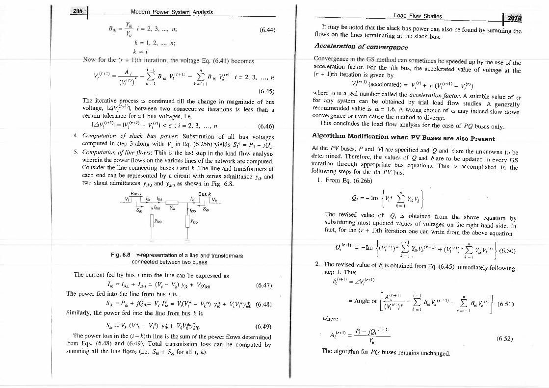
206 | Modern power Svstem Anatvsis

(6.44)

I*r l .d

flows on the lines terminating at the slack bus.

Acceleration of convergence

acceleration factor. For the tth(r + l)th iteration is given by

up by the use of thebus, the accelerated value of voltage at the

y(r+r) (accelerated) = V,Q'* a(v.G+r) - V,Ql,where a is a real number called the acceleration factor. A suitable value of afor any system can be obtained by trial load flow sfudies. A generallyrecommended value is a = 1.6. A wrong choice of o. may indeed slow downconvergence or even cause the method to diverge.

This concludes the load flow analysis for thJ case of pe buses onry.

Algorithm Modification when pv Buses are arso present

At the PVbuses, p andrv]r are specified and e ancr dare the unknowns to bedetcnnincd.'l'hererirre, the values of e and d are to be updated in every GSiteration through appropriate bus equations. This is accomplished in thefollowing steps for the ith pV bus.l. From Eq. (6.26b)

f " )ei = - Im j yr* D, y,ovof

L f t : l )

The revised value of ei is obtained from the above equation bysubstituting most updated values of voltages on rhe right hand side. Infact, for the (.r + 1)th iteration one can write from the above equationI

g.(r+t) = -Ln ],r, ',)

- i y,rv,,(,*t) a 1y.r,1- D y,kvk,,,I ,u.ro,I L r , f ! , " )2' The revised value of {.is obtained from Eq. (6.45) immediately following

step 1. Thus

6Q+r) _ ay!+r)

= Ansle "t fei]l- - i Bovo(,+r) - D B,ovo,,,l (6.s1)

L ( t1 ' ' ' ) * , r : r k : ,+r Jwhere

. ^ ( r + t ) - P - i ? t ' r t tr 1 . ; . =__

, u _

6 .52 )

The algorithm for pe buses remains unchanged.

1 7 ( r + l ) - A i ' S

- r t ( , n

v i ' - t B , o v o , , * t , - f r , o v l , , i = 2 , 3 , . . . , n( V l " ) i l t k = i r l

(6.4s)The iterative process is continued till the change in magnitude of busvoltage, lav.('*r)|, between two consecutive iterations is less than acertain tolerance for all bus voltages, i.e.

IAV.G*r)l _ 1y.t+r) _ V,e)l < 6, ; i = 2, 3, ..., n

4.

5 .

computation of slack bus power: substitution of all bus voltagescomputed in step 3 along with V, in Eq. (6.25b) yields Sf = pr- jeycomputttt ion ofl ine .f lows: This is thc last step in thc loacl f low analysiswherein the power flows on the various lines of the network are computed.Consider the line connecting buses i and k. The line and transformers ateach end can be represented by a circuit with series admittance y* andtwo shunt admittances 1l;ro and )no as shown in Fig. 6.8.

Bus i Bus k

(6.46)

(6.47)

(6.48)

(6.4e)

l*io sm

Fig. 6.8 7i'-representation of a line and transformersconnected between two buses

The current fed by bus i into the line can be expressed asIit = Iitt + Iirc = (Vi - V) !it,+ V,y,oo

The power fed into the line from bus i is.

S* = Pir* jQiF Vi lfr= Vi(Vf - Vr\ yft+ V!,*y,f,Similarly, the power fed into the line from bus k is

Sri = Vk (V*k- Vf) yfo+ VoVfyi,l,

The power loss in the (t - t)th line is the sum of the power flows determinedfrorn Eqs. (6.48) and (6.49). Total transmission loss can be computed bysununing all the line llows (i.e. 5';a + Sri fbr all i, /<).

7 Voltage magnitude limits I Vr I min and I Vi I max'lor '-(J o

b n"u"iiu" pow"t limits Qi min and Q; max for PV buses

F i g . 6 . 9 F | o w c h a r t f o r l o a d f l o w s o | u t i o n b y t h e G a u s s . S e i d e |iterative method using YBUS

l'fiffi

demand at any bus must be in the range e^rn - eû*.If ai any stageduring the computatibn, Q at any bus goes outside ttreJe timits, it is fixedAt Qîn or Qô, as the case may be. and thedropped, i.e. the bus is now treated like a pe bus. Thus step 1 abovebranches out to step 3 below.

3. ff 9.('+r) a 0;,6;n, set e,Q*r) - er,r^n and treat bus f as a pe bus.compute 4-(r+1) and y(r+t) from Eqs. (6.52) and (6.45), respectively. IfOtu..:, ') Qt, ̂ , set O-(r+l) = ei,^*and treat bus i as a pebus. Compure4.Q+r) -6 y(r+l) from Eqs. (6.52) and (6.45), respecrively.Now all the computational steps are summarized in the detailed flow chartof Fig. 6.9 which serves as a basis for the reader to write his owncomputer programme. It is assumed that out of n buses, the first is slackas usual , then2,3, . . . , m are PVbuses and the remaining m + l , . . . , f tare PQ buses.

For the sample system of Fig. 6.5 the generators are connected at all the fourbuses, while loads are at buses 2 and 3. Values of real and reactive powers arelisted in Table 6.3. All buses other than the slack are pe typd.

Assuming a flat voltage start, f)nd the voltages and bus angles at the threebuses at the end of the first GS iteration.

Solution

Table 6.3 lnput data

Bus

1 Primitive Y matrix2 Bus incidence matrix A3 Slack bus vol tage ( lY1l , 61)4 Real bus powers Pi for i= 2,3 '4,"" 'n5 Reactive bus powers Qi, for I = m + 1" -{fO buses)

Vf I for i = 2,....,m (PV buses)

Ie 6.4Exampl

Retnarks

Slack busPQ busPp busPp bus

The l"ur for the sample system has been calculated earlier in Example 6.2b(i.e. the dotted line is assumed to be connected). In order to approach theaccuracy of a digital computer, the computations given below have beenperformed on an electronic calculator.

T ) - - - - - - r - - - , , i-Dus voltages at rne eno or tne llrst rteratron are calculated using Eq. (6.a5).

I2J

4

Pp PU

0.5- 1 .0

0 .3

0u pu

- 0.20 .5

- 0 . 1

Vt' Pur .u 10"

v t z = + { W - Y z t v t - Y " v ! - 'r^'iI

tg. Yr,. r.i"g Eq. (6.2

Make initial assumptions Vio for I = m + 1,"',n and O;0 for i = 2!: 'm

Compute the parameters A; for i = ̂ t 1,"n .and B;p'for i = 1'2"

-.;; i: 1 ,2,-'...,n (except k = i ) from Eqs (6'43) and (6'44)

Set iteration count r = 0

l 1 0 . 5 + i 0 . 2 ' )- - - - - 1 - ' - r - ' - - 1 . 0 4 ( - z + j 6 ) - ( - 0 . 6 6 6 + j 2 ) _ ( _ t + f l l-

Y z z I t - i O - ' - ' \ - ' r - / \ v ' v v v ' r !

|

fei.fii,',1 Modern Power System Analysis -I

4.246 - jrr.04 = 1.019 + 70.046 pu3.666 - jLr

(vl) * T#-frL+re - e 2 + i6) (to4 + io)- (- 0.666 + j2) (t + 70) _ (_ 1+

r)j3) (t. io) j l

= t( +'z^?e;t - itt' lzs J = , (r.rstz+ 70.033e)( 3 . 6 6 6 _ j t t ) -or 612 = 1.84658o = 0.032 rad

. ' . v) = 1.04 (cos 6)* j s in dj)

= 1.04 (0.99948 + j0.0322)

= L03946 + 70.03351

, ( o

v l = - l - j ' 1 - = i Q t - y . v . - y _ v t _ v , , 0 I' t = 1 114tr

- Y"v' - Yszv; - Yrovl, l[ - r _ 7 0 . s-

3.666-in L ,f;; - (- t + i3) 1'04

- (- 0.666 + j2) (1.03s46 + 70.03351) _ (_ z + io)f

I [ 0 . 3 + i o . r= il tf:;

- (- I + i3) (1.03e4 + 70.0335)

- (- 2 + j6) (r.03t7 _ yo.08e3z) IJ

_ 2.967r _ j8.99623 - i g

= 0 ' 9 9 8 5 - 7 O ' 0 0 3 1

",,il1;,;llii,""rrirhe

permissibte limits on ez (reactive power injection) are

1 - -" Ytt

_ 1Yzt

- r.04 (- 1 + 13)

Load Flow Studies

- Yo, vJ

I

- (- 0.666 + j2) (1.019 + ;0.046) - (- 2 * i6) |

= ''!'-,-1"'.9?' = 1.028 - 70.087 pu3.666 - jrr

I- (- 2 + j6) (1.028 - jo.o87) |)

- 1.025 - 70.0093 pu

- r^rr\l

19 + 70.046)

2.99r - j9.2s33 - j e

In Example 6.4,let bus 2 be a PV bus now with lV2l = 1.04 pu. Once again

assuming a flat voltage start, find Qz, 6., V3, V4 at the end of the first GS

iteration.Given: 0.2 < Q, < l.

From Eq. (6.5), ii e", (Note fz= 0, i.e. Vl - I.04 + i0)n, =_ : [J .,:,,,:.

A,,i". ^r!:, J, ^.,,?,: : :;: !:: ^+ (- 0.666 + j2) + (- I + i3)l )

= - Im {- 0.0693 - j0.20791 - 0.2079 pu

' O" = 0'2079 Pu

From Eq. (6.51)

r.0317 -

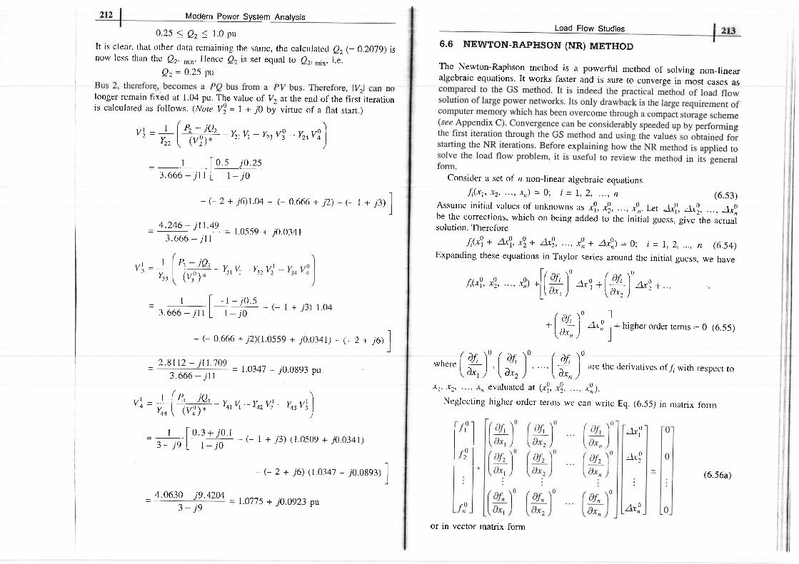
Modern Power System Analysis

0.25 < Qz < i .0 pu

It is clear, that other data remaining the same, the calcul ated e2 (= 0.2079) isnow less than the Qz, ̂ in.Hence e, it set equal to ez, _in, i.e.

Qz = 0'25 Pu

a - p - - - u v r v r v r v , t f

2 t v q L t l l v

longer remain fiied at I.04 pu. The value of V, ar the end of the first iterationis calculated as follows. (Note VL = t + 70 bf virrue of a flat start.)

I a a r { E l a . . , O r . , - r : ^ ^Lwqv I t v yy \ ) t ,U (J lU l i

6.6 NEWTON-RAPHSON (NR) METHOD

The Newton-Raphson method is a powerful method of solving non-linearalgebraic equations. It works faster and is sure to converge in most cases as

vL = l-( 'r, ^!?, - yztvt - yztv? - yrovl)' z

Y r , [ ( Y 3 ) - - z t | - z r J - ' "

" )

_ [ o . s - j o . z s3 .666 - j r l L t - r ,

(* 2 + i6)1.04 - (- 0.666 + .i2) - (-

- 4'246- j lr-,? = t.05.59 + io.o3413 . 6 6 6 - j t l

(

vj = : l':-:* -. Y,,v, - Y,,vJ" r,, [ (Y,')'

[_t;u.t _ (_ r + j3) toa3 . 6 6 6 - j r r L r - ; o *

Consider a set of n non-linear algebraic equations

f i ( \ , x 2 , . . . , x n ) = 0 ; i = I , 2 , - . . , nr + i 3 ) ] Assur.c initial vulucs of u'know's as *l: *'), ..., r"r. Let J.r(1, Jg, ..., J_rl

be the corrections, which on being added to the initial guess, givelhe actualsolution. Therefore

Jt@\+ fut l , *ur+ Axl , . . , , x0,+ Axf ;1 = g; i = 1,2, . . . , n (6.54)Expanding these equations in Taylor series around the initial guess, we have

f;(x01, xor,

(6.ss)

Neglecting higher order terins we can write Eq. (6.55) in matrix fbrm

(6.s3)

- (- 0.666 + j2X1.0s5e + 70.0 341) - (- 2 + j6) ]

,,r).[[*)' a*0, .(#)' Axt +

/ ^ - \ 0 I

*[ -l!t] o-i l* n,rn-, order re,,ns - o\ux, ) l

whcrefg) ' , ( ! f , ) ' . . f9 ) '\ d"r / ( Dr, )

' ' [ ,", ,/

are the derivatives of It with respect to

x1, x2, . . . , x, evaluated at (x! , *1, . . . , *0,) .

vL = ;;W,# - Yo,v, - Yo,u| - v*v))

= +,t"=#

- (- I +,r3) (r '0s0e + i0'0341)

_ 2 . 8 t t 2 - j n . 7 0 93.666 - j r r

/,.0630 - j9 .42M _3 - j e

1.0347 - 70.0893 pu

-1

- (- 2 + j6) (r.034i - j0.08e3) I

1.0775 + j0.0923 pu

f''' lI ' r l

a'l'

Llxi

Ax:

or in vector matrix form

(6.56a)

2ll I Modern Power Svstem Analvsis-

l ( , + . f , A*, * 0 (6.56b)

,f is k,o*n as the Jacobian matrix (obtained by differentiating the functionvector f with respect to x and evaluating it at r01. Equation (6.56b) can bewritten as

: l _ J

Approximate values of corrections /-r0 can be obtained from Eq (6.57). These

being a set of linear algebraic equations can be solved efficiently bytriangularization and back substitution (see Appendix C).

Updated values of x are then

t l ="0 + AxI

or, in general, for the (r + 1)th iteration

" ( r + l ) _ r ( r ) + A x Q )(6.s8)

Iterations are continued till Eq. (6.53) is satisfied to any desired accuracy, i.e.

(6.63a)

at Alvml = 0. We

(6.62c)

mth bus

First, assume that all buses are PQ buses. At any PQbus the load flow solutionrnust satisfy the following non-linear algebraic equations

lJ iG" ) ) l < e (a spec i f ied va lue) ; i = 1 ,2 , . . . , n

NR Algorithm for Load flow Solution

fip= Pi (specified) - Pi (calculated) = APi

.f ie= Qi(specif ied) - Qi @alculated) - AQi

(6.5e)

(6.60a)

(6.60b)

(6 .61a)

(6 .61b)

J'ip (lV, 6) = I'i (sPccificcl) - Pi = 0

fiq (1v1, 6) = Qi (specified) - Qi = o

where expressions for P, and Q, are given in Eqs. (6.21) and (6.28). For a trial

set of variables lV;1, 6;, the vector of residuals /0 of Eq. (6.57) comesponds to

while the vector of corrections y'xo corresponds to

alvil, a,i

Equation (6.51) for obtaining the approximate corrections vector can be writtenfor the load flow case as If the mth br-rs is also a

can now wnte

II

fth busl, lPi

aQii thbus l np, l= l T : tT ' I

L- ---J t -- - --- - ---rH' ' l - l46^

AlV^

I (6.62a)

jmtn ous

m

It is to be immediately observed that the Jacobian elements corresponding to theith bus residuals and mth bus corrections are a 2 x 2 matrix enclosed in the boxin Eq. (6.62a) where i and m Ne both PQ buses.

Since at the slackbus (bus number l), Prand Qr are unspecified and lV,l,Q are fixed, there are no equations corresponding to Eq. (6.60) at this bus.Hence the slack bus does not enter the Jacobian in Eq. (6.62a).

consider now the presence of PV buses. If the ith bus is a pv bus, e, isunspecified so that there is no equation corresponding to Eq. (6.60b) for thisbus. Therclbrc, the Jacobian eleurents of the lth bus become a sinele rowpertaining to AP,, i.e.

r thbusF l=(6.62b)

PV bus, lVrl becomes fixed so thmth bus

2L6 | rtrodern Power System Analysis

Also if the ith bus is a PQ bus while the mth bus is a PV bus, we can then write

(6.62d)

It is convenient for numerical solution to normalize the voltage corrections

alv^ ll v ^ l

as a consequence of which, the corresponding Jacobian elements become

l ztzt

N inr= N^ i = 0

l , ^ = J ^ ; = O ( 6 . 6 6 )

corresponding to a parricular vecror of variables tqlv2lq64lval6lr, thevector of residuars [aP2 aez ah ap4 ae4 Apr], and the Jacobian (6 x 6in this example) are computed. Equation rc.an is then solved bytriangularization and back substitution procedure to obtain the vector of

f n v t A t r l | 1 rcorrections I oo, # oo1464 + /,6r l . corrections are then added to

L lv2l J a lVor I

update the vector of variables.

2(Pa) 3(PVl

(6.63b)

Expressions for elements of the Jacobian (in normalized form) of the loadflow Eqs. (6.60a and b) are derived in Appendix D and are given below:

Case I m t l

H,^= Li^= a^fi - b*et 6.64)

Nr*=- J i r r= a .er+ bJt

Yi^= G* + jB,*

Vi= e, + j f ,

(a* i ib) = (Gi- + jBi*) @* + jk\

case 2 I,,==t- n, - Biirvirz

Mii= Pi + G,, lV, lz I A A < \\ \ J ' \ ' J , '

J ti = Pi - Giilvil'

L i ;= Qi - B i i lv i lz

An important observation can be made in respect of the Jacobian by

examination of the Y"u5 matrix. If buses i and m are not connected, Yi^= 0 (Gi^= Bi^ - 0). Hence from Eqs. (6.63) and (6.64), we can write

Il 2IY

o

f , zJc0

Fig. 6.10 Sample five-bus network

-'-* Bus No.2 3 4 5

Jacobian(Evaluated at trial values of variables)

[:_]l a l v 4 l ll]ql-l

i_it_lt

Correctionsin variables

Hzz Nzz Hzs Hzn Nza

Jzz Lzz Jzs Jz+ Lz+

Hsz Nsz Hss Hss

Hqz Nn Haa Naz. H+s

Jqz Lqz Jcc Lu J+s

Hss H5a Nsq Hss

t

(6.67)

,re I rrrrodcrn Power Svstem AnalvsisL L V I-T--

Iterative Algorithm

Omitting programming details, the iterative algorithm fbr the solution of the

load flow problem by the NR method is as follows:

L W'ith voittge ancl angle (usually f'= €I) at sabsence of anY tltherat atl PQ buses and d at all PV buses' In the

information flat voltage start is recommended'

2. Compute AP,(for PV and PB buses) and AQ,(for aII PQ buses) from

Eqs. (6.60a and b). If all the values are less than the prescribed toletance,

stop the iterations, calculate P, and Q, and print the entire solution

including line flows.

3. If the convergence criterion is not satisfied, evaluate elements of the

Jacobian using Eqs. (6.64) and (6.65).

4. Solve Eq. (6.67) for corrections of voltage angles and magnitudes'

5. Update voltage angles and magnitudes by adding the corresponding

changes to the previous values and return to step 2'

Note: 1. In step 2, if there are limits on the controllable B sources at PV

buses, Q is computed each time and if it violates the limits, it is made equal to

the limiting value and the corresponding PV bus is made a PQ bus in that

iteration. If in the subsequent computation, Q does come within the prescribed

limits, the bus is switched back to a PV bus.

2. If there are limits on the voltage of a PQ bus and if any of these limits

is violated, the corresponding Pp bus is made a PV bus in that iteration with

voltage fixed at the limiting value.

Consider the three-bus system of Fig. 6.11. Each of the three lines has a series

impedance of 0.02 + 1O.OS pu and a total shunt admittance of 70'02 pu' The

specifiecl quantities at the _b"!91j9!qulated below:

R e a l l o a d R e a c t i v e l o a d R e a l p o w e r R e a c t i v e V o l t a g e

Lcad Ftor; Studies I i:ig,:-

Find the load flow solution using the NR method. Use a tolerance of 0.01 forpower mismatch.Solution Using the nominal-rc model for transmission lines, I"u, for the givensystem is obtained as follows:

eacn l tne

1,sen. "= I

^ -z .g4r - j11 .7& - r2 . r3 l -75 .96"nes o.oz+jo.og

Each off-diagonal term = - 2.94I + jll.764Each self term = 2l(2.941 - j11.764) + j0.011

= 5.882 - j23.528 = 24.23 l-75.95"

0 +,O

2

Fig. 6.11 Three-bus system for Example 6.6

Pz = lVzl lvl lY2l cos (0r1 + 6r - $) + lVrlz lyrrl cos 0zz + lvzl l\llYrr l cos (Qzt+ q- 6)

Pt = lVl lvl l\rl cos (dr, + 6r - 6r) + lVrl lv2l l\zl x cos (ez + h- 6r) + lV,rlz lyrrl cos 0r,

Qz =- ivz i iv l tyz l s in (gr+ dt - h) - lvz lz ly22l x sn 4z_lv2 llv3l lY.,.l sin (0r, + bz - 6)

Substituting given and assumed values of different quantities, we get the valuestrf Powers rts

PB. = -0.23 pu

To start iteration choose 4= t +70 and ,4 = 0. From Eqs. (6.27) and (6.2g),we get

Bus

2.0 1 . 0 Unspecified Unspecified V'=1.94 * ;g(slack bus)

0.0 Unspecified(PO hus)

0.6 Q c t = ? l v l l = 1 . 0 4(PV bus)

Control lablc rcact ivo powor sourcc ls avai lablc nt bt ts 3 wi th the ct lnstraint

0 < Q c t S 1 . 5 P u

demand

PD

demand generation power specification

Qo PG generation O6

0.0 1 . 00.5

0.0l 5

3 1 .04 lO "1.5 +7O.6

O } n r ' l i l a d a - n D a r r r a r C r r a l a m A n a h r a i at t v . l r v r u u E r r r r V Y Y E r \ ) y o l g l t r n r r q r y o r o

t

P3 = 0.12 pu

Qor= - 0 '96 PuPower residuals as per Eq. (6.61) are

- rt (calcu

(- 0.23) = 0.73

Aror- -1.5 - (0.12) = - ! .62

tQT= 1 - (- o'e6) - t 'e6The changes in variables at the end of the first iteration are obtained as follows:

0P, 0P, 0P,06, 061 alv2l0P, aP, 7Pu06, 061, 0lv2laQ, }Qz aQ,06, 06: ' 'av|

Jacobian elements can be evaluated by differentiating the expressions given

above fr>r Pr, Py Qz with respectto 6r, d1 and lVrl and substi tut ing the given

and assumed values at the start of iteraticln. The chanses in variables are

obtained as

Load Ftow Studies i zzrt i ^ - - i .

S z = 0 . 5 + j 1 . 0 0 | -

S r = - 1 . 5 - j 0 . 1 5

Transmission loss = 0.031

Line flows

The

The

the real part of line flows

0.1913r2E00 0.839861E'00-l0.0 0.6s4697 E00 |

-0.673847 E00 0.0 Jthe imaginary part of line flows-0.5994&E00 _0.r9178zE00]

0.0 0.39604s800 I-0.37sr6s800 0.0 I

Rectangular Power-Mismatch Version

This version uses e, ancl .f ,the rear ancr imaginary parts of the v.ltagesresllectivcly, as variables' ' fhe

number of equations and variables is greaterthan thart t irr Eq. (6.6r), by the nurnber <tt pi buses. Since at pv buses e,and.f; can vary but ,,' +.f,' - lviP, a voltage-magnitude squarecl misn-latch equationis required tbr each PV bus. with sparsity programming, this increase in orderis of hardly any significance. Indeed each iteration is rnarginally faster than forEq' (6'67) since there are no time-consunring sine ancl cosine terms. It nray,however, be noted that even the polar version avoids these as far as possible9f using rectangular arirhemetic in constructing Eqs (6.64) and (6.65).However' thc rcct:tttgtrl l tr vcrsion sccnls to bc slighiiy t.r, rcliable but faster inconvergence than the polar version.

The total number of non-linear power flow equations considered in this casearc fixed iurd cqual 2 (trl). These lbllow fr.o'i Eqs. (6.26a) and (6.26b) andare

following matrix shows

I o oI-0.r8422eE00L-0.826213^800

following matrix shows

I o.oI

l|0.60s274800L0.224742E00

I t d j l l - 2 4 . 4 i - t 2 . 2 3 s . 6 4 - 1 - r [ 0 . i 3 f [ - 0 . 0 2 3 - 1| ^ r I | . ^ ^ ^ ^ ^ - l | - ^ l | ^ ^ . - . 1I A a i l : l - t / . . 2 5 / . 4 . e ) - J . u ) l | - t . o z l : l - u . u o ) 4 |

[nrv,r ' - ] L-uu 3.0s zz.s4) L r .qol I ooar l

l a ) l I a i - l l - ^4 I t -0 .1 [ 002 .3 I [ 0023 .1I a ] l : l I l * l ̂ 4 l : l o l * l - 0 0 6 s 4 1 : l - 0 0 6 s 4 1Itv,t ' j L 'y,roJ lnrv.,r ' .1 L' i I oosoJ I r .08eJ

We can now calculate fusing Eq. (6.28)]

Qtt = 0.a671

Qo\= Q\ + Qrt = 0.4677 + 0.6 = 1.0677

which is within l imits.If' the sanre problem is solved using a digital computer, the solution

converges in three iterations. The final results are given below:

Vz= 1.081 l- 0.024 rad

Vt = I.M l- 0.0655 rad

Qu = - 0 . I5 + 0 .6 = 0 .45 (w i th in l in r i t s )

Sr = 1.031 * j ( - 0.791)

P, (specifi"d) -I{ e,(epG11, - f,B,t) + fihrG* -t epB,o} : 0k : l

i = l , 2 , . . . , n

i = slack(s)

nr t .

B; (specifi"d) -) lf,koG,o - ftB,t1- e;(.f*Gi* * eoB,oy]} = gk = l

(6.68)

(lbr each PQ bus) (6.69)

222 | Modern Porgl Jyllem AnatysisI

l(l (specified)2 - @i2 + f,') = 0 (for each PV bus) (6.70)

Using the NR method, the linearised equations in the rft iteration of iterativeprocess can be written as

Jr J2

Load Flow Studies

necessary motivation in developing the decoupled load flow (DLF) method, inwhich P-6 and Q-V problems are solvecl separately.

Decoupled Newton Methods

F o r i * j

Juj= - Jqij = Gij ei fi

Jz i j= J t , j=- B i je i+ Gi l f i 6 .72)

Jsij= Jo,j = O

F o r i = , r

t;^"'::: .-::::!-

tlr,,, -!' u,u-' l,) i J:,

Jsii= 2"i J6ii = 2fi

a, and b, are the components of the current flouring into node i, i.e.,

a,+ jb,= frCo * jBi)@r+ jf*)k : l

(6.74)

Steps in solution procedure are similar to the polar coordinates case, exceptthat the initial estimates of real and imaginary parts of the voltages at the PQbuses are made and the corrections required are obtained in each iteration using

The corrections are then applied to e andf and the calculations are repeated tillconvergence is achieved. A detailed flow chart describing the procedure forload flow analysis using NR method is given in Fig. 6.12.

F E F F A A ' ? h I E h ' A A

O. I L'|aUL,UTL|1L' L('AL' .F LL'VV IVI.EI.tsI(-,L'Ii

An important characteristic of any practical electric power transmission systemoperating in steady state is the strong interdependence between real powers andbus voltages angles and between reactive powers and voltage magnitudes. Thisinteresting property of weak coupling between P-6 and Q-V variable.s gave the

In any conventional Newton method, half of the elements of the Jacobeanmatrix represent the weak coupling referred to above, and therefore may beignored' Any such approximation reduces the true quadratic convergence togeometric one, but-there are compensating computational benents.i largenumber of decoupled algorithms have been dlveloped in the literature.However, only the most popular decoupled Newton veision is presented heret1e l .

In Eq. (6.67), the elements to be neglected are submatrices [1v] and [,/]. Theresulting decoupled linear Newton equations become

tApl = lHl lA6l

I^Qt - tLt l4!1L t v t J

where it can be shown thatgU = Lij = lvil lvjl (CU sin

AQ

AIVPJ3 J4

Js J6

(6.73)

(6.7s)

H i i = - 8 , , l V i P -

Li i= - 8,, lV, lz +

6u - B,i cos {r)i * j

(Eq. (6.6s))

(Eq. (6.6s))

Qi

Qi

(6.76)

(6.77)

(6.78)

(6.7e)

(6.80)

Equations (6.76) and (6.77) can be constructed and solved simultaneouslywith each other at each iteration, updating the [H] and [r] matrices in eachiteration using Eqs (6.78) to (6.80). A better opproo.h is to conduct eachiteration by frst solving Eq. (6.76) for 44 *o use the updared 6 inconstructing and then solving Eq. (6.77) for Alvl. This will result in fasterconvcl'geuce than in the sirnultaneous mode.

The main advantage of the Decoupred Load Flow (DLF) as compared to theNR method is its reduced memory requirements in storing the Jacotean. Thereis not much of an advantage from the point of view of speed since the time periteration of the DLF is almost the same as that of NR method and it alwaystakes more number of iterations to converge because of the approximation.

Fast Decoupled Load Flow (FDLF)

Further physically justifiable simplifications may be carried out to achieve somespeed advantage without much loss in accuracy of solution using the DLFmodel described in the previous subsection. This effort culminated in thedevelopmenr of the Fast Decoupled Load Frow (FDLF) merhod by B. stott in1974l2ll. The assumptions which are valid in normal power ryr,"n1 operationare made as follows:

'*i I vodern Power Svstem Analvsis

- : : , : - , t

I

I zas-With these assumptions, the entries of the [1{ and [L] submatrices will becomeconsiderably simplified and are given by

I Aduance iteration countI r = r + 1

Determine J-1.'. comPute Aefr) 2n6

Lfiv)

Are allmax A within

tolerance2

and ? =i: =-''i,,,11,,u" :: ,::(6.82)

(6.83)

(6.84)

(6.8s)

(6.86)

(6.87)

c-mpute ano--lprint line flows,l

power loss, Ivoltages, I

elci ----.]

Matrices [/fl and [L] are squiue mafrics with dimension (npe + npy) and nrnrespectively.

Equations (6.76) and (6.77) can now be written as

LAPI = ltyjt lvjl Bfi AA

tAQl= [%t tv j t B,, i j , [#]

Determine maxchange in powermax APr,AO

where 8t,,, B(are elements of [- B] matrix.Further decoupling and logical simplification of the FDLF algorithm is achievedby:

1. Omitting from [B/] the representation of those network elements thatpredominantly affect reactive power flows, i.e., shunt reactances andtransformer off-nominal in-phase taps;

2. Neglecting from [B//] the angle shifting effects of phase shifters;3. Dividing each of the Eqs. (6.84) and (6.85) by lv,l and setting lVrl = I pu

in the equations;

4. Ignoring series resistance in calculating the elements of tdll which thenbecomes the dc approximation power flow matrix.

With the above modifications, the resultant simplified FDLF equationsbecome

I last node')

Computeel,),1v112

-' ls -\

gt'r ioi)

IAP| lyl I = [B'] [L6]

tAQl tr4 I - LB" I t^lytl

Fig . 6 .12

In Eqs. (6.86) and (6.87), both [B/] and lBttf are real, sparse and have thestructures of [I{ and [L], respectively. Since they contain only admittances,they are constant and need to be inverted only once at the beginning of thestudy. If phase shifters are not present, both [B'l and lB"] are alwayssymmetrical, and their constant sparse upper triangular factors are calculatedand stored only once at the beginning of the solution.

Equations (6.86) and (6.87) are solved alternatively.always employing themost recent voltage values. One iteration implies one solution for [4fl, toupdate [d] and then one solution for IA lVl] to update [Vl] to be called l-dandl - V i t e r a f i o n S e n a r a f e . c r l n v e . r s e n c e t c e t c a r e a n n l i e d f h r t h e r c q l q n A r c q o t l v c

" - r * ^ * ' - - - ^ ^ ' - ^ o - ^

power mismatches as follows:

max [APf I €pi max lAQl S eo

where eo and €e are the tolerances.

A flow chart giving FDLF algorithm is presented in Fig.6.13.

cos 6, : 1;

s i n { r : 0

G,, sin 6,, < B4;

Qi < B i i l v i l z

ComputeLlVi,12 = 1V, scnd 12- l%

tl2

and

(6 .81) (6.88)

,bZC I Modern power Svstem Analvsis

Consider the three-bus system of Example 6.6. Use (a) Decoupled NR method

(a) Decoupled NR method:Equations to be solved are (see Eqs. (6.76) and (6.77)).Substituting relevant values in Eqs. (6.78) - (6.80) we get

Hzz= 0'96 + 23.508 - 24.47

Hzt= Hzz= 1.04 (- Brz) = - 1.04 x 11.764 = - 12.23

H t t = - Q t - B n 0 . 0 q 2

= [- Bsr t\P - 42 tv3t - Bzz t\P] - Bn (r.0a1.2

= - f 1.764 x (1.04)2 - 1t .764 x 1.04 + ( l .oq2

x 2 x 2 3 . 5 0 8 - 2 5 . 8 9

Load Ftow Studies I ##

(Start )

Calculate 6i.1 = 6[+ 66[

(i)

(ii)

Lzz = Qz - Bzz = t + 23.508 - 24.508

[ 0.731 _ [ 24.47 _r2.2311\6t\1

l-t.oz) -

L- n.23 zs.ssJ[64trl

tLQzl - lz4.srl f+uJ"'l' L 't;(-i)l JSolving Eq. (i) we get

L6;') = - 0.0082 - 0.0401 - - 0.002

Aa{tr = - 0.018 - 0.08 - - 0.062

Qz= - lvzl lvtl lYzl sin (0r, + 6r - 6r) - lvzlz V2zl sin 82lvzl lhl llrrl sin (9zt + 6, - q)

= - 1.04 x 12.13 sin (104.04 + 0 - 0.115) -24.23

sin(-75.95) - 1.04 x 12.13 sin (104.04 + .115 - 3.55")

- - 1 2 . 2 4 + 2 3 . 5 0 5 - 1 2 . 3 9

Qz= - l '125A r - l - 1 / 1 1 a < \ ^ 1 ? r Et - t v 2 - r -

\ - r . r L J ) = L . I L J

Substituting in Eq. (ii)

f o r i = 1 , 2 , . . . , n , i - s

1. (6.60a)= PV bus

------ X

- ' - - I

r c E q . l. ,n, I: u s - l

; Afr/,R

Calculate slibus power i

all l ine flovand print

- - re \ -

<'- fr= 1 --

l slacker andflows

e+

Read LF data and form Ysr.

Solve for A6f using Eq.(6 .86) i =1,2 , . . . , n , i * s

Lz.rz5r - [24.5r] [alY"( ') l lL tu,a, l

Flg. 6.13

;'..ng I Modern Power System Analysis -

AN 9 l= 0.086

lvftt - lvlo)t+atv|'tt = 1.086 pu

Q(rl can be similarly calculated using Eq. (6.28).

The matrix equations for the solution of load flow by FDLF method are [seeEqs. (6.86) and (6.87)l

lui:.

complete an iteration. This is because of the sparsity of the network matrix andthe simplicity of the solution techniques. Consequently, this method requiresless time per iteration, With the NR method, the elements of the Jacobian areto be computed in each iteration, so the time is considerably longer. For typicallarge systems, the time per iteration in the NR rnethod is roughly equivalent to7 times that of the GS method [20]. The time per iteration in both these methodsincreases almost directly as the number of buses of the network.

The rate of convergence of the GS method is slow (linear convergencecharacteristic), requiring a considerably greater number of iterations to obtaina solution than the NR method which has quadratic convergence characteristicsand is the best among all methods from the standpoint of convergence. Inaddition, the number of iterations for the GS method increases directly as thenumber of buses of the network, whereas the number of iterations for the NRmethod remains practically constant, independent of system size. The NRmethod needs 3 to 5 iterations to reach an acceptable solution for a largesystem. In the GS method and other methods, convergence is affected by thechoice of slack bus and the presence of series capacitor, but the sensitiviry ofthe NR method is minimal to these factors which cause poor convergence.

Therefore, for large systems the NR method is faster, more accurate andmore reliable than the GS method or any other known method. In fact, it worksfor any size and kind of pro6lem and is able to solve a wider variety of ill-conditioned problems t23). Its programming logic is considerably morecomplex and it has the disadvantage of requiring a large computei memory evenwhen a compact storage scheme is used for the Jacobian and admittancematrices. In fact, it can be made even faster by adopting the scheme ofoptimally renumbered buses. The method is probably best suited for optimalload flow studies (Chapter 7) because of its high accuracy which is restrictedonly by round-off errors.

The chief advantage of the GS method is the ease of programming and mostefficient utilization of core menrory. It is, however, restricted in use of smallsize system because of its doubtful convergence and longer time needed forsolution of large power networks.

Thus the NR method is decideclly more suitable than the GS method for allbut very small systems.

For FDLF, the convergence is geometric, two to five iterations are normallyrequired for practical accuracies, and it is more reliable than the formal NRmethod. This is due to the fact that the elements of [81 and [Btt] are fixedapproximation to the tangents of the defining functions LP/lVl and L,QAV l, andare not sensitive to any 'humps' in the ciefining iunctions.

fi LP/lVl and A^QIIV I are calculated efficiently, then the speed for iterationsof the FDLF is nearly five times that of the formal NR or about two-thirds thatof the GS method. Storage requirements are around 60 percent of the formalNR, but slightly more than the decoupled NR method.

-Brr1l af',f-8,, )Lz4" l

(iii)

and

lffil= r-Bzzt tatrt')tl (iv)

fil6411oqrl23.508.1la4" l

I o.tz I| -t.oz It -|

- l -

| 1.04 IL: - 1'5571

Solving Eq. (v) we get

46;r) -

A6t'' =

6') -lz.rzsl -

alvtl =l v t t =

- 0.003- 0.068- 0.003 rad; {tl

[23.508] tatvitl0.09

1.09 pu

Now Q3 can be calculated.These values are used to compute bus

iteration. Using the values of 'LAPAVll andsolved alternatively, using the most recentwithin the specified limits.

0.068 rad

power mismatches for the next

lAQAl\l the above equations arevalues, till the solution converges

(v)

6.8 COMPARISON OF IOAD FLOW METHODS

In this section, GS and NR methods are compared when both use liu5 as the

network model. It is experienced that the GS method works well when

programmed using rectangular coordinates, whereas NR requires more memory

when rectangular coordinates are used. Hence, polar coordinates are preferred

for the NR method.

ilai:i;'l ,odern power system AnatvsisI

Changes in system configurations can be easily taken into account andthough adjusted solutions take many more iteration.s, each one of them takesless time and hence the overall solution time is still low.

system, buses with generators are usually made PV (i.e. voltage control) buses.Load flow solution then gives the voltage levels at the load buses. If some of

lines for specified voltage limits cannot meet the reactive load demand (reactiveline flow from bus i1o bus ft is proportional to lAvl = lvil - lvkD.This situation

tAvt - tEtht - tv! = -ffi O,

tv';t= lErhl+ #l

n,

=tv i t * hn,

Flg. 6.1S

Since we are considering a voltage rise of a few percent, lV(l can be furtherapproximated as

lV|l = lV,l+ ffiO,

Thus the VAR injection of +jQc causes the voltage at the jth bus to riseapproximately by (XhllViDQ.. The voltages at other load buses wili also riseowing to this injection to a varying but smaller extent.

Control by Transformers

Apart from being VAR generators, transformers provide a convenient means ofcontrolling real power' and reactive power flow along a transmission line. As

The FDLF can be employed in optimization studies and is specially used forthe load bus voltages work out to be less than the specified lower voltage limit,i t is indicative of the fact that the reer-fivc n^rr/ar ff^.,, ^-*^^ie, ^r4-^-^--:--:-

estudies, as in contingency evaluationenhancement analysis.

for system security assessment and

Note: When a series of load flow calculations are performed, the finalvalues of bus voltages in each case are normally used as the initial voltages ofthe next case. This reduces the number of iterations, particularly when there areminor changes in system conditions.

6.9 CONTROL OF VOLTAGE PROFILE

Control by Generators

Control of voltage at the receiving bus in the fundamental two-bus system wasdiscussed in Section 5.10. Though the same general conclusions hold for aninterconnected system, it is important to discuss this problem in greater detail.

At a bus with generation, voltage can be conveniently controlled byadjusting generator excitation. This is illustrated by means of Fig. 6.14 wherethe equivalent generator at the ith bus is modelled ty a synch.onou, reactance(resistance is assumed negligible) and voltage behind synchronous reactance. Itimmediately follows upon application of Eqs. (5.71) and (5.73) that

Pa i+ jQe t6ilVilt

t i

Xei

P c i = | v,l -Epl.;;,' -'-i,xo,

eci= #r-,vi t+tEcit)

W i t h / P t i A \ - - , { l r / l , / f ^ : , - ^ - L - - r r - - r , f tYYrtrr \rGi - iVcil ano i 't lr i Loi glven bY-ihe ioaci i jow soiution- these velrres

(6.8e)

(6.e0)(6 .e1)

','d&r1'l Modern Power Svstem A-nalvsis- l

has already been clarified, real power is controlled by means of shifting thephase of voltage, and reactive power by changing its magnitude. Voltagemagnitude can be changed by transforrners provided with tap changing underIoad (TCUL) gear. Transformers specially designed to adjust voltage magnitude

smail values are calleo re rnxers.Figure 6.16 shows a regulating transformer for control of voltage rnagnitude,

which is achieved by adding in-phase boosting voltage in the line. Figure 6.17ashows a regulating transformer which shifts voltage phase angle with noappreciable change in its magnitude. This is achieved by adding a voltage inseries with the line at 90" phase angle to the corresponding line to neutralvoltage as illustrated by means of the phasor diagram of Fig. 6.17b. Here

VLn= (Von * tV6) = Q - jJT) Von= dVon 6.92)

where a = (1- jJ- l t )=71-tan-t J1t

since r is small.The presence of regulating transformers in lines modifies the l/uur matrix

thcrcby rn<i l i fy ing the loacl f low solut ion. Consic ler a l ine, connect ing twobuses, having a regulating transformer with off'-nominal turns (tap) ratio aincluded at one end as shown in Fig. 6.18a. It is quite accurate to neglect thesmall impedance of the rr:gulating translonucr, i.c. it is rcgardcd as an iclcaldevice. Figure 6.18b gives the corresponding circuit 4epresentation with linerepresented by a series admittance.

-_o A/

Since the transformer ls assumed to be ideal, complex power output from itequals complex power input, i.e.

51 =V , / i = c rv l for

For the transmission line

I\= ! @V1 - V2)

or

Ir = dl'a lo:lzyV, - cfyVz

Also

Iz= l (Vz- oV,) = - WVr + lVz

(6.e4)

(6.es)Equations (6.94) and (6.95) cannot be represented by a bilateral network.

The I matrix representation can be written down as follows liom Eqs. (6.94)and (6.95).

n. ,%n

C...,%n.___ Jl"r<_t c,

(b)

(a)

JI ( V " n + t V " r ) = a V " ,/^ ic raal nr rmhor\

Flg. 6.16 Regulating transformer for control of voltage magnitude Fig. 6.17 Regulating transformer for control of voltage phase angle

I Modern power System AnalysisI

Bus,1 Bqs 2

neffitingtransformer

(a)

ao.O t,o* a,r.,.r __ f#

( i ) V/V\ = l .M or a - l /1.04(ii) V/V\ = d3 or d = s-i3o

Solution (i) With regulating transformer in line 3-4, the elements of the6.2 are modified as under.corresponding submatrix in (v) of Exa

sz v2aV'l <L I

. - - - . - O-- f__1--* -<- I

l''r Y 12

(b)

Fig. 6.18 Line with regulating transformer and its circuit representation

The entries of f matrix of Eq. (6.96) would then be used in writing, the rru,matrix of the complete power network.

For a voltage regulating transformer a is real, i.e. d = e, therefore, Eqs.(6.94) and (6.95) can be represenred by the zr-network of Fig. 6.19.

Fis.6.1e :jiiil:':3;:i;ffiTH#*:

with orr-nominar tap settins or

If the line shown in Fig. 6.18a is represented by a zr-network with shuntadmittance yu at each end, additional shunt admittancelol2ysappears at bus 1and yo at bus 2.

The above derivations also apply for a transformer with off-nomin al tapsetting' where a = (k[nuJ(kD,r:up, a real value.

The four-bus system of Fig. 6.5 is now modified to include a regulatingtransformer in line 3-4 near bus 3. Find the modified rru5 gf the system for-With

off-nominaf ,up **ing transformers at each end of the line as shown inFig. 6.20, we can write.

t c

Fig. 6.20 Off-nominal transformers at both line ends (a., , a, real)

I t - Y l f v i l - [ I i - lL- , y) lv t ) - Ut )

ly . i 1=[o , o I [ - '4 . l l r l I l t /q o I f4 lL v ; l - l o q ) L v , ) ' L , ; l : [ o v " , ) ] , 1

Substituting (ii) in (i) and solving we get

| 4t -"!-',vf [q 1: ['"1L-otory 4y ) LV2 J ltz )

- - l o?v -aqzt f'= l-^*, d; )Note: Solve it for the case when ao &2 are complex.

3 4-r.92+ js.777

3 - j e

(6.e6)

j2)

j6)

aJ

r- j3)-(0.666 --(2 - j6)1T Gz+

3

4

j6)

4

i3" e2 +

3 - j e3- j e

3.e

(i) .

( i i )

/ i i i \

Thus

(iv)

5 1 6j10.s47

r.92js.777

of Example 6.2 is

j2)

i n (

3

Modified submatrix (v)

4

.3r135.887

. l

236 | Modern power System AnqtysisI

6.10 CONCLUSION

In this chapter, perhaps the most important power system study, viz. load flowhas been introduced and discussed in detail. Important methods available have

methods is the best, because the behaviour of different load flow methods isdictated by the types and sizes of the problems to be solved as well as theprecise details to implementation. Choice of a particular method in any givensituation is normally a compromise between the various criteria of goodness ofthe load flow methods. It would not be incorrect to say that among the existingmethods no single load flow method meets all the desirable requirements of anideal load flow method; high speed, low storage, reliability for ill-conditionedsystems, versatility in handling various adjustments and simplicity in program-ming. Fortunately, not all the desirable features of a load flow method areneeded in al l s i tuat ions.

Inspite of a large number of load flow methods available, it is easy to seethat only the NR and the FDLF load flow methods are the most important onesfbr general purpose load flow analysis. The FDLF method is clearly superior tothe NR method from the point of view of speed as well as storage. Yet, the NRmethod is stili in use because of its high versatility, accuracy and reliability andas such is widely being used for a variety of system optimization calculations;it gives sensitivity analyses and can be used in modern dynamic-response andoutage-assessment calculations. Of course newer methods would continue to bedeveloped which would either reduce the computation requirements for largesystems or which are more amenable to on-line implementation.

PROB TE IVI S

For the power system shown in Fig. P-6.1, obtain the bus incidence matrixA. Take ground as reference. Is this matrix unique? Explain.

(-)

Fig. p-6='!

F<rr the network shown in Fig. P-6.2, obtain the complex bus bar voltageat bus 2 at the end of the first iteration..use the GS method. Lineimpedances shown in Fig. P-6.2 are in pu. Given:

Load Flow Studies

Bus I is slack bus with Vr = 1.0 10"Pz+ iQz = -5.96 + j1.46

lVTl = 1102

Assume:

\ = 1.02/0" and vi -710"1 2 3t-'

o ottooo tt.-o.oz

.7orr:"

Fig. P-6.2

6.3 For the system of Fig. P-6.3 find the voltage at the receiving bus at theend of the first iteration. Load is 2 + 70.8 pu. voltage at the sending end(slack) is 1 + /0 pu. Line admittance is 1.0 - 74.0 pu. Transformerreactance is 70.4 pu. off-nominal turns ratio is lll.04. Use the GStechnique. Assume Vn = l l0.

c>+J=---F"dFig. P-6.3

6.4 (a) Find the bus incidence matrix A for the four-bus sysrem in Fig. p-6.4.Take ground as a reference.

(b) Find the primitive admittance matrix for the system. It is givbn rhat allthe lines are charactenzed by a series impedance of 0.1 + j0.7 akrnand a shunt admittance of 70.35 x 10-5 O/km. Lines are rated at220kv.

(c) Find the bus admittance matrix for the system. Use the base values22OkV and 100 MVA. Express all impedances and admittances in perunit.6. r

6.5

1

1 1 0 k m

3

Fig. P-6.4

Consider the three-bus system of Fig. P-6.5. The pu line reactances areindicated on the figure; the line resistances are negligible. The magnitudeof all the three-bus voltages are specified to be 1.0 pu. The bus powersare specified in the following table.

6 .2

.?38 i I Modern Power Svstem AnatvsisI

3

Fig. P-6.5

.ffi Z-r----rvz-- () ir o -- |y = _ j 5 . 0

' ,\,lJ

, = -is'o

\ /v e l 1 3

Fig. P-6.7 Three-bus sample system containing aregulating transformer

6.8 Calculate V3for the system of Fig. 6.5 for the first iteration, using the dataof Example 6.4. Start the algorithm with calculations at bus 3 rather thanat bus 2.

6.9 For the sample system of Example 6.4 with bus I as slack, use thefbllowing nrcthuds to obtairr a load flow solution.(a) Gauss-Seidel using luur, with acceleration factor of 1.6 and

tolerances of 0.0001 for the real and imaginary components ofvoltuge.

(b) Newton-Raphson using IBUS, with tolerances of 0.01 pu for changesin the real and reactive bus powers.

\Note: This problem requires the use of the digital computer.

6.10 Perform a load flow study for the system of Problem 6.4. The bus powerand voltage specifications are given in Table P-6.10.

Table P-6.10

Bus power, puBus Voltage magnitude, pu Bus type

y = - j 5 0 , l

Real

demandReactive

demandReal

Seneratrcn

Reactive

generation

I Por = 1.0 Qot = 0.6 PGr = ? ect (unspecified)' ',r2 = 0 Qoz = 0 Pcz = 1.4 pn, lunspecified)3 Po: = 1.0 Qot = l.O Pa = 0 go. lunsp"cified)

Carry out the complete approximate load flow solution. Mark generations,load demands and linc f-lows on thc one-line diagram.

6.6 (a) Repeat Problem 6.5 with bus voltage specifications changed as below:l V t l = 1 . 0 0 p u

lV2l = 1.04 pu

lV3l = 0.96 pu

Your results should show that no significant change occurs in realpower flows, but the reactive flows change appreciably as e issensitive to voltage.

(b) Resolve Problem 6.5 assuming that the real generation is scheduled asfollows:

Pct = 1.0 pu, Pcz = 1.0 pu, Pct = 0The real demand remains unchanged and the desired voltage profile isflat, i.e. lvrl = lv2l = lv3l = 1.0 pu. In this case the results will showthat the reactive flows arc essentially unchangccl, but thc rcal f lgwsare changed.

6.7 Consider the three-bus system of problem 6.5. As shown in Fig. p-6.7where a regulating transforrner (RT) is now introcluced in the ljne l-2near bus 1. Other system data remain as that of Problem 6.5. Considertwo cases:(i) RT is a magnitude regulator with a rario = VrlVl = 0.99,

(ii) RT is a phase angle regr-rlaror having a ratio = V/Vi = ",3"(a) Find out the modified )/ur5 matrix.

(b) Solve the load flow equations in cases (i) and (ii). compare theload flow picture with the one in Problem 6.5. The reader shouldverify that in case (i) only the reactive flow will change; whereasin case (ii) the changes will occur in the real power flow.

Compute the unspecified bus voltages, all bus powers and all l ine flows.Assume unlimited Q sources. Use the NR method.

REFERE N CES

I2a-)4

Unspecified0.95- 2.O- 1 .0

UnspecifiedUnspecified

- 1 . 0- 0 .2

1.021 . 0 1

UnspecifiedUnspecified

SlackPVPQPQ

Books

l . Mahalanabis, A.K., D.P. Kothari and S.I.

Analysis and Control, Tata McGraw-Hill,

Ahson, Computer Aided Power System

New Delhi . 1988.

, u.r., L,teclrrc Lnergy System Theom: An Introduction, 2nd Ed, McGraw_Hill, New York. 19g2.6. stagg, G.w. and A.H. EI-Abiad, computer Methods in power system Anarysis,McGraw-Hill, New york, 196g.7 ' Rose' D'J' and R'A willough (Eds), sparse Matrices and their Applications,

Plenum, New york, 1972.8' Anderson, P'M., Analysis of Faulted Power systems, The Iowa state universityPress, Ames, Iowa, 1923.9' Brown, H'8., sorution of Large Networks by Matix Methods, John w1rey, New, York, 1975.

l0' Knight' rJ'G', Power system Engineering and Mathematics, pergamon press, NewYork 1972.11. Shipley, R.B., Introduction to Matrices and power systems, John w1ey, NewYork, 1976.12' Hupp, H.H., Diakoptics and Networks, Academic press, New york, 1971.l3' Arrillaga, J. and N.R. watson, computer Modeiling of Erectricar power sltstems,2nd edn, Wiley, New york, 2001.14' Nagrath, I.J. and D.p. Kothari, power system Engineering, Tata McGraw_Hilr,

New Delhi, 1994.l5' Bergen, A.R., power system Anarysis, prentice-Hail, Engrewood criffs, N.J. r9g6.l6' Anillaga' J and N'R' watson, computer Modelting of Electrical power systems,2nd edn. Wiley, N.y. 2001.

Papers

' 2A0" ' l Modprn pnr r ra r e r ra ra* A^^r - . - , -_ - r____ . - . - - - ' , , , v ' rv r eyor r r i l l A1 ta tys ls

2' weedy, B.M. and B.J. cory, Erectricar power- systents,4th Ed., John wiley, NewYork, 1998.Gross, C.A., power System Analysis, 2nd 8d..,Sterling, M.J.H., power System Control, IEE.

17. Happ, H.H., 'Diakoptics-The solution of system problems by Tearing ,, proc. ofthe IEEE, Juty t974, 930.

l8' Laughton' M'A', 'Decontposition Techniques in power system Network Load FlowAnalysi.s usi'g the Nodar Impcdance Matrix,, proc. IEE, 196g, r15, s3g19' stott, B., 'Decouprecr

Newron Load FIow,, IEEE Trans., 1972, pAS_91, 1955.20. stott, B., 'Review of Load-Frow carcuration Method, , proc. IEEE, Jury 1974,916.21' stott, B., and o. Alsac, 'Fast Decoupled Load Flow,, IEEE Trans., 1974,pAS_93:

859 .22' Tinney' w'F" and J'w. walker, 'Direct solutions of sparse Network Equations byOptimally Ordered Triangular Factorizaiions,, proc. IEEE. Nnvernhe" 1oA1

55 :1801 ' v "

23' Tinney, w.F. and c.E. Hart, 'power Flow sorution by Newton,s Method,, ,EEETrans., November 1967, No. l l , pAS_g6:1449.

24' ward, J.B. and H.w. Hare, 'Digitar computer Sorution of power problems,, AIEETrans., June 1956, pt III, 75: 39g.

Power Frow Argorithms with Reference to Indian power systems,, proc. of IIsymp.on Power plant Dynamics ancr contror, Hyderabad, 14_i6 Feb. rg:/g, zrg.26. Tinney, W.F. and W.S. Mayer, .Solution

Triangular Factorization', IEEE Trans. on Auto contor, August 1973, yor. AC_lg,J J J .

27 ' Saro, N. and w.F Tinney, 'Techniques for Exproiting Sparsity

Admittance Matrix', IEEE Trans. pAS, I)ecember L963, g2, 44.28' sachdev, M.s. and r.K.p. Medicherla, 'A second order Load Flow

IEEE Trans., pAS, Jan/Feb 1977, 96, Lgg.29. Iwamoto, S.and y. Tamura, ,A Fast Load Flow Method' IEEE Trans., pAS. Sept/Oct. 197g, 97, 15g6.30. Roy, L., 'Exact Second Order Load Flow,, proc. of

Dermstadt, Yol. 2, August lg7g, 7Il.31' Iwamoto, s' and Y. Tamura, 'A Load Flow calculation Method for Ill-conditioned

Power Systems', IEEE Trans pAS, April lggl , 100, 1736.32. Happ, H.H. and c.c. young, 'Tearing Argorithms for Large scare Network

Problems', IEEE Trans pA,S, Nov/Dec Ig71, gO, 2639.33. Dopazo, J.F.O.A. Kiltin and A.M. Sarson, ,stochastic

Load Flow s,, .IEEE Trans.PAS, 1975 ,94 ,2gg .

34' Nanda' J'D'P' Kothari and s.c. srivastava, "Some Important observations onFDLF'Algorithm", proc. of the IEEE, May 19g7, pp.732_33. \

35. Nanda, J., p.R., Bijwe, D.p. Kothari and D.L. stenoy, .,second order Decoupred

Load Flow', Erectric Machines and power systems, vor r2, No. 5, 19g7, pp. 301_312.

36' Nanda J'' D'P' Kothari and S.c. srivastva, "A Novel second order Fast DecoupledLoad Flow Method in Polar coordinatcs", Electic Machines and power,s.ysrems,Vol. 14, No. 5, 19g9, pp 339_351

37. Das, D., H.s. Nagi and D.p. Kothari, .,A Novel Method for solving RadiarDistribution Networks", proc. IEE, ptc, v.r. r4r, no. 4. Jury r994. pp. zgr_zgg.

38' Das, D', D'P' Kothari and A. Kalam. "A Simple and Efficient Method for LoadFlow sorurion of Radiar Distribution Nerworks',, Inr. J. of EpES, r995, pp. 335_346.

John Wiley, New york, 19g6.England, 1978.

of Network

Technique',

Retaining Non linearitv'.

the Sixth pSCC Conf.

7.1 INTRODUCTION

The optimal system operation, in general, involved the consideration ofeconomy of operation, system security, emissions at certain fossil-fuel plants,optimal releases of water at hydro generation, etc. All these considerations maymake for confl icting requirements and usually a compromise has fo he made foroptimal system operation. ln this chapter we cor..;ider the economy of operationonly, also called the ec'omonic di.spcttch problem.

The main aim in the economic dispatch problern is to rninimize thc total costof generating real power (production cost) at various stations while satisfyingthe loads and the losses in the transmission l inks. For sirnplicity we consicler thepresence of thermal plants only in the beginning. In the later part of this chapterwe will consider the presence of hydro plants which operate in conjunction withthermal plants. While there is negligible operating cost at a hydro plant, thereis a l imitation ol availabil ity ol 'watcr' over a pcriod of t inre which nrust bc usedto save maximum fuel at the thermal plants.

In the load flow problem as detailed in Chapter 6, two variables are specifiedat each bus and the solution is then obtained for the rernaining variables. Thespecified variables are real and reactive powers at PQ buses, real powers andvoltage magnitudes at PV buses, and voltage magnitude and angle at the slackbus. The additional variables to be specified for load flow solution are the tapsettings of regulating transformers. If the specified variables are allowed to varyin a region constraineci by practicai consicierations (upper anci iower i imits onactive and reactive generations, bus voltage limits, and range of transformer tapsettings), there results an infinite number of load flow solutions, each pertainingto one set of values o1'specified variables. The 'best' choice in sorne sense ofthe values of specified variables leads to the 'best' load flow solution. Economyof operation is naturally predominant in determining allocation of generation toeach station for various system load levels. The first problem in power system

Optimal System Operation A3

pariance is caiied the 'unii commitment' (UC) probiem and the second is callecithe 'load scheduling' (LS) problem. One must first solve the UC problem beforeproceeding with the LS problem.

Throughout this chapter we shall concern ourselves with an existinginstallation, so that the economic considerations are that of operating (running)cost and not the capitai outiay.

7.2 OPTIMAL OPERATION OF GENERATORS ON A BUS BAR

Before we tackle the unit commitment problem, we shall consider the optimaloperation of generators on a bus bar.

Generator Operating Cost

The major component of generator operating cost is the fuel input/hour, whilemaintenance coutributes only to a small extent. The fuel cost is meaningtul incase of thermal and nuclear stations, but for hydro stations where the energystorage is 'apparently free', the operating cost as such is not meaningful. Asuitable meaning will be attached to the cost of hydro stored energy in Section7.7 of this chapter. Presently we shall concentrate on fuel fired stations.

o (vw)min (MW)maxPower output, MW -'- --

Fig.7.1 Input-output curve of a generatrng unit

The input-output curve of a unit* can be expressed in a million kilocaloriesper hour or directly in terms of rupees per hour versus output in megawatts. Thecost curve can be determined experimentai ly. A typical curve is shown inFig. 7.1 where (MW)o'in is the minimum loading limit below which it isuneconomical (or may be technically infeasible) to operate the unit and(MW)n,u, is the maximunr output l imi t . The inpL l t -output curve hasdiscontinuities at steam valve openings which have not been indicated in thefigure. By fitting a suitable degree polynomial, an analytical expression foroperating cost can be written as

lIII

t -L \

- al)

; Pt r o. c 86 o8 b =e 5g EoO 6

f

LL

A unit consists of a boiler, turbine and generator.

_ Q ;

2

The slope of the cost curve, i.".43 is called the incremental Juel cost (lQ,dPo,

and is expressed in units of rupees per megawatt hour (Rs/lvIWh). A typical plot

of incremental fuel cost versus power output is sho.wn in Fig. 7.2.If the cost

curve is approximated as a quadratic as in Eq. (7.1), we have

| . . - - A - - - ! - - A - ^ r - - ^ : -

.L4+ | MOOern rower DySIeIrl ArlalyI

Ci(Pc) Rs/hour at outPut Pc,

where the suffix i stands for the unit number. It generatly suffices to fit a second

degree polynomial, i.e.

Considerations of spinning reserve, to be explained later in this section, require

that

D Po,, ̂*) Po

marsin. i.e. Eq. (7.6) must be a strict inequality.

Since the operating cost is insensitive to reactive loading of a generator, thernanner in which the reactive load of the station is shared among various on-

line generators does not afl'ect the operating economy'.The question that has now to be answered is: 'What is the optimal manner

in which the load demand Po must be shared by the generators on the bus?'

This is answered by minimizing the operating cost

k

c = D ci(pci)f : l

under the equality constraint of meeting the load demand, i.e.(

f - \ D lL

' G i - P o = Oi : t

where k = the number of generators on the bus.Further, the loading of each generator is constrained by the inequality

constraint of Eq. (7.5).Since Ci(Pc) is non-linear and C, is independent of P6t (i+ i), this is a

separable non-linear programming problem. \If it is assumed at present, that the inequality constraint of Eq. Q.q is not

effective, the problem can be solved by the method of Lagrange multipliers.

Define the Lagrangian as

b,Pc, + d, Rs/hour (7.r)

(7.2)

(7.3)

(7.4)

of the ith generator

Equat ion (7 .10) can

dC^ \dPoo

(7.6)

(7.7)

(7.8)

(7.e)

( 7 . 1 o )

(units: Rs/TvIWh),

be written as

( lc) i= aiP"t + bt

(MW )min (MW ) maxPower output, MW

Fig.7.2 Incremental fuel cost versus power output for the unit whoseinput-output curve is shown in Fig. 7.1

i.e. a linear relationship. For better accuracy incremental fuel cost may be

expressed by a number of short line segments (piecewise lineanzation).

Altcrnativcly, wc can fit a polynomial of suitable degree to represent IC curve

in the inverse form

Pc;i= a, + {),( lC)i + 1,QC)', + . . .

Optimal Operation

[,et us assulne that it is known a priltr i which generutors itre t<l rt ln to ntcct a

p:.rrt icular load clenrand on the statton. Ubvtously

f -

where X is the Lagrange multiplier.Minimization is achieved by the condition

o f , = odPo,

dCo r

' i - ) i i = 1 , 2 , . . . , kdPc,

where lci is the incremental costd4,,

a Iurctio' ol'.gencra,il;,":':t

:":d4( i l - d r - -

lII

-i. I(J

ooo c

E B, d >o oE t roEE()

i t (Pci)-^[f "",

-""]

DPr,,, , ' ',,* ) P,

where Pci, ,r.,,"* is the rated real power capacity of the ith generator and Po is

the total power demand on the station. Further, the load on each generator is to

irc constrained within lower and upper limits, i.e.

Pcr, .in 1 Po, 1 Po,, rn.*, I = L, 2, "', k (7.s)*The

effect of reactive loading on generator losses is of negligible order.

(7 . r l )

Computer solution fbr optimal loa<ling of generators can be obtainediteratively as follows:

1. Choose a trial value of ), i.e. IC = (IC)o.2. Solve for P", (i = 1, 2, ..., k) from Eq. (7.3).

3. If ItPc,- Pol < e(a specified value), the optimal solution is reached.

Otherwise,

4. Increment (lC) bv A (1"), t I: I

f l Po,- ,rl < 0 or decrement (/c) by A(tr)

if [D Pc, - Pr] r 0 and repeat from step 2. This step is possible becauseP.-, is monotonically increasing function of (1g).

consider now the effecr of the inequality constraint (7.5). As (1c) isincreased or decreased in the iterative process, if a particular generator loadingP", reaches the limit PGi,^o or P6;, min, its loading from now on is held fixedat this value and the balance load is then shared between the remaininggenerators on equal incremental cost basis. The fact that this operation isoptimal can be shown by rhe Kuhn-Tucker theory (see Appendix n;.

Incremental fuel costs in rupees per MWh for a plant consisting of two unitsare:

dt

i * - o . 2 o p c t + 4 0 . 0G 1

-dcz- = o.2,pcz+ 3o.odPo,

Assume that both units are operating at all times, and total load varies from 40MW to 250 MW, and the maximum and minimum loads on each unit are to beI25 and 20 MW, respectively. How will the load be shared between the twounits as the system load vanes over the full range? What are the correspondingvalues of the plant incremental costs?Solution At light loads, unit t has the higher incremental fuel cost and will,therefore, operare at its lower limit of zo Mw, for which dcrldpcr is Rs 44 perMWh. When the ourput of unit 2is20 MW, dczldpcz= Rs 35 p"i UWt. Thus,with an increase in the plant output, the additional load should be borne bv unit

n - . : - ^ r A - ^ ^ r - - - ^ . . L - ^ -

cost of the plant colresponds to that of unit 2 alone. When rhe plant load is 40Mw, each unit operates at its minimum bound, i.e.2o Mw wiitr plant \ = Rs35/I4Wh.

When dczldPcz= Rs 44/MWh,

0.25PG2+ 30 - 44

or pnt = JI- = 56 MW0.25

The total plant output is then (56 + 20) = 76 MW. From this point onwards,the values of plant load shared by the two units are found by assuming variousvalues of \. The results are displayed in Table 7.1.

Table 7-1 Output of each unit and plant output for various values of) for Example 7.1

Plant ),

RszMWh

354450556061.2565

40.076.0

130.0175.0220.0\231.25250.0

Figure 7.3 shows the plot of the plant .tr versus plant output. It is seen fromTable 7.7 that at .\ = 61.25, unit 2 is operating at its upper limit and therefore,the additional load must now be taken by unit 1, which then determines theplant ).

60+t - -l c cI

8 5 0o

@ ^

i = 4 5a >E P 4 0t -EOc J c

Plant output, MW

Fig.7.3 Incremental fuel cost versus plant output, as found in Example 7.1

Unit I Unit 2Pcz, NfW

Plant OutputPcl, MW

t :Hzut " l.Z.48: i Mocjern Power System nnaiysis

To find the load sharing between the units for a plant output of say 150 MW,we find from the curve of Fig. 7.3, that the corresponding plant X is Rs 52,22per MWh. Optimum schedules for each unit for 150 MW plant load can nowbe found as

Net saving caused by optimum scheduling is772.5 - 721.875 = 50.625 Rs/lr

Total yearly saving assuming continuous operation

This saving justifies the need for optimalinstalled for controlling the unit loadings

load sharing and the ddvices to beautomaticallv.

0 . 2 P a * 4 0 - 5 2 . 2 2 ;

0.25PG2 + 30= 52.22;

Pcr + Pcz= 150 MW

Proceeding on the above lines, unit outputs for various plant outputs arecomputed and have been plotted in Fig. 7.4. Optimum load sharing for any plantload can be directlv read from this fieure.

P c t = 6 1 ' 1 1 M W

Pcz = 88'89 MW

100 150 200 250Plant output, MW -_-->

unit versus plant output for Example 7.1

For the plant described in ExampleT.l find the saving in fuel cost in rupees perhour for the optimal scheduling of a total load of 130 MW as compared to equaldistribution of the same load between the two units.Solution Example 7.I reveals that unit I should take up a load of 50 MW andunit 2 should supply 80 MW. If each unit supplies 65 MW, the increase in costfor unit 1 is

1 6 5 r n n n . , ^ \ r n r r . ' t n Z| \U .L I ' r : r t *U) |J I l n r = (U. I fn tJso '

Similarly, for unit 2,

J*co.rs" ", + 30) dpor= (0. r25PGz+ :oro;1"

Let the two units of the svstem studiedcurves.

in Example 7.1 have the following cost

Cr = 0.lPto, + 40Pc + 120 Rs/hr

Cz= 0.l25Pzcz + 30Po, + 100 Rsftrr

220 MW

Monday

12l l1 2 6

(noon) PM (night) AMTime -----

Fig. 7.5 Daily load cycle

Let us assume a daily load cycle as given in Fig. 7.5. Also assume that a costof Rs 400 is incurred in taking either unit off the line and returning it to serviceafter 12 hours. Consider the 24 hour period from 6 a.m. one morning to 6 a.m.the next morning. Now, we want to find out whether it would be moreeconomical to keep both the units in service for this 24hour period or to removeone of the units from service for the 12 hours of light load.

For the twelve-hour period when the load is 220 MW, referring to Table 7.1of Example 7.1, we get the optimum schedule as

Pcr= 100 MW' Pcz = 120 MW

Total fuel cost for this period is

[ 0 . 1 x 1 0 0 2 + 4 0 x 1 0 0 + 1 2 0 + 0 . 1 2 5 x 1 2 0 2 + 3 0 x 7 2 0 + 1 0 0 ] x 1 2

= Rs. 1,27,440

I tzsI

= 100

E r uo

E 5 0f

250

t 200II3 150

E 100o

J

500 5 0

Flg.7.4 Output of each

165; l f \ r 1 r l F n ^ a D ^ t L -

t ' t U I ' 6 y l l = l l L . J l \ S / I [" ' l so

Sunday

- - 721.875 Rs/hr

ltgtiFl Modern power svstem nnAVsis- - t

If both units operate in the light load period (76 MW from 6 p.m. to 6 a.m.)also, then from the same table, we get the optimal schedule as

Pcr = 20 MW, Pcz = 56 MW

Total fuel cost for this period is then(0.1 x 20' + 40 x 20 + 120 + 0.125x 5 6 + 3 0 x 5 6 + 1 0 0 ) x 1 2

= Rs 37,584

Thus the total fuel cost when the units are operating throughout the 24 hourperiod is Rs I,65,024.

If only one of the units is run during the light load period, it is easily verifiedthat it is economical to run unit 2 and to put off unit 1. Then the total fuel costduring this periot:tXf ':

762 + 3o x 76+ 100) x rz = Rs 37,224Total fuel cost for this case = L,27,440 + 37,224

= Rs 1,64,664

Total operating cost for this case will be the total fuel cost plus the start-up costof uni t l , i .e.

1,64,6& + 400 = Rs 1,65,064

Comparing this with the earlier case, it is clear that it is economical to run boththe units.

It is easy to see that if the start-up cost is Rs 200, then it is economical torun only 2 in the light load period and to put off unit 1.

7.3 OPTTMAL UNrT COMMTTMENT (UC)

As is evident, it is not economical to run all the units available all the time. Todetermine the units of a plant that should operate for a particular load is theproblem of unit commitment (UC). This problem is of importance fbr thermalplants as for other types of generation such as hydro; their operating cost andstart-up times are negligible so that their on-off status is not important.

A simple but sub-optimal approach to the problem is to impose priorityordering, wherein the most efficient unit is loaded first to be'followed by theless efficient units in order as the Ioad increases.

A straightforward but highly time-consuming way of finding the mosteconomical combination of units to meet a particular load demand, is to try allpossible combinations of units that can supply this load; to divide the loadoptimally among the units of each combination by use of the coordinationequaiions, so as to finci the most economicai operating cost of the combination;then, to determine the combination which has the least operating cost among allthese. Considerable computational saving can be achieved by using branch andbound or a dynamic programming method for comparing the economics ofcombinations as certain combinations neet not be tried at all.

t -

Dynamic Programming Method

In a practical problem, the UC table is to be arrived at for the complete loadcycle. If the load is assumed to increase in small but finite size stensl dvnaminprograrrurung can be used to advantage for computing the uc table,wherein it is not necessary to solve the coordination equations; while at thesame time the unit combinations to be tried are much reduced in number. Forthese reasons, only the Dp approach will be advanced here.

The total number of units available, their individual cost characteristics andthe load cycle on the station are assumed to be known a priori.Further, it shallbe assumed that the load on each unit of combination of units changei'insuitably small but uniform steps of size /MW (e.g. I MW).

Starting arbitrarily with any two units, the most iconomical combination isdetermined for all the discrete load levels of the combined output of the twounits. At each load level the most economic answer may be to run either unitor both units with a certain load sharing between the two. The most economicalcost curve in discrete form for the two units thus obtained, can be viewed asthe cost curve of a single equivalent unit. The third unit is now added and theprocedure repeated to find the cost curve of the three combined units. It may benoted that in this procedure the operating combinations of third and first, alsothird and second are not required to be worked out resulting in considerablesaving in computational effort. The process is repeated, till all available unitsare exhausted. The advantage of this approach is that having oitiined thegPli-u.| way,of loading ft units, it is quite easy ro determine the Jptimal mannerof loading (ft + 1) units.

Let a cost function F" (x) be defined as follows:F,y (x) = the minimum cost in Rs/hr of generating .r MW by N units,

fN 0) = cost of generating y MW by the Nth unit

F*-{x - y) - the minimum cosr of generating (.r - y) Mw by the remain_ing (1/ - t) units

Now the application of DP results in the following recursive relation

FN @) = Tn Vn9) * Fu-r @ - y)| (7.r2)Using the above recursive relation, we can easily determine the combination

of units, yielding minimum operating costs for loads ranging in convenient stepsfrom the minimum.permissible load of the smallest unit to the sum of thecanae i f ies n f q l l q r ro i io l - lo r r - i+o i - +L ;^ - -^^^ -^ .1^ - 1 -1 r .$vs^rqurv uurrD. rrr Lrr lD PruuttJs ure total nunlmum oDerating eostand the load shared by each unit of the optimal combination are ;il.u,i"determined for each load level.

The use of DP for solving the UC problem is best illustrated by means of anexample. Consider a sample system having four thermal generating units withparameters listed in Table 7.2.It is required to determinr th. most-economicalunits to be committed for a load of 9 MW. Let the load changes be in steps ofI MW.

. Modern Pow

Table 7.2 Generating unit parameters for the sample system

Capacity (MW) Cost curve pararneters (d = 0)

Unit No.

The effect of step size could be altogether eliminated, if the branch andbound technique [30] is employed. The answer to the above problem usingbranch and bound is the same in terms of units to be committed, i,e. units 1 and2, but with a load sharing of 7 .34 MW and 1.66 MW, respectively and a total

graung cost oI I<s z,y.zL /J/nour.

In fact the best scheme is to restrict the use of the DP method to obtain theUC table for various discrete load levels; while the load sharing amongcommitted units is then decided by use of the coordination Eq. (7.10).

For the example under consideration, the UC table is prepared in steps- of IMW. By combining the load range over which the unit commitment does notchange, the overall result can be telescoped in the form of Table 7.3.

Table 7.3 Status* of units for minimumoperating cost (Unit commitmenttable for the sample system)

Load rangeUnit number

r 2 3 4l-56-r3t4-181948

*l = unit running; 0 = unit not running. \

' The UC table is prepared once and for all for a given set of units. As the loadcycle on the station changes, it would only mean changes in starting andstopping of units with the basic UC table remaining unchanged.

Using the UC table and increasing load in steps, the most economical stationoperating cost is calculated for the complete range of station capacity by usingthe coordination equations. The result is the overall station cost characteristicin the form of a set of data points. A quadratic equation (or higher orderequation, if necessary) can then be fitted to this data for later use in economicload sharing among generating stations.

7.4 RELIABILITY CONSIDERATIONS

With the increasing dependence of industry, agriculture and day-to-dayhousehold comfort upon the continuity of electric supply, the reliability ofpower systems has assumed great importance. Every eleciric utilify is normailyunder obligation to provide to its consumers a certain degree of continuigl andquality of service (e.g. voltage and frequency in a specified range). Therefore,economy and reliability (security) must be properly coordinated in arriving atthe operational unit commitment decision. In this section, we will see how thepurely economic UC decision must be modified through considerations ofreliability.

1234

NowFt@) = ft@)

fr(9) = f{9)= LorP'ot+ btPcr

= ollss x 92 + 23.5 x9 = Rs 242.685lhour

From the recursive relation (7.12), computation is made for F2(0), Fz(l),

Fz(2), ..., Fz(9).Of these

FzQ) = min tt6(0) + Ft(9)1, VzG) + Ft(8)l'

VzQ) + Ft(7)1, VzQ) + Fr(6)l' Vz@) + F1(5)l'

t6(5) + Fr(4)1, VzG) + Ft(3)1, VzT + Fr(2)1,

tfr(s) + F,(1)1, vzg) + Fr(O)l)

On computing term-by-term and compdng, we get

FzQ) = Vz(2) + Ft(1)) = Rs 239.5651how

Similarly, we can calculate Fz(8), Fz(1), ..., Fz(l), Fz(O).

Using the recursive relation (7.12), we now compute Fl(O), F:(1), ...' F3(9).

Of these

Fse)= min {t6(0) + Fr(9)f, t6(1) + Fl8)1, ...'[6(9) + rr(0)]]

= [6(0) + FzQ)l = Rs 239.565ftour

Proceeding similarly, we get

FoQ) = [f4(0) + Fr(9)] = Rs 239.565lhour

Examination of Fr(9), Fz(9), Fl(9) and Fa(9) leads to the conclusion that

optimum units to be lommitted for a 9 MW load are 1 and 2 sharing the load

ur Z l,tW and 2 MW, respectively with a minimum operating cost of Rs

239.565/hour.It must be pointed out here, that the optimai iiC tabie is inclependent of 'u\e

numbering of units, which could be completely arbitrary. To verify, the reader

rnay solvethe above problem once again by choosing a different unit numbering

scheme.

If a higher accuracy is desired, the step size could be reduced (e.g. *

t*r,

with a considerable increase in computation time and required storage capacity.

1 . 01 .01 .01 . 0

12.012.012.012.0

0.771.602.002.50

23.526.530.032.0

0 00 01 01 1

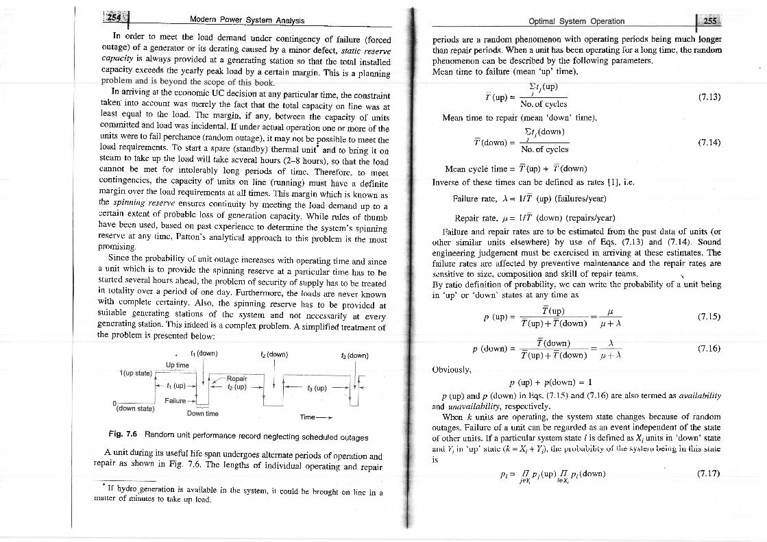
In order to meet the load demand under contingency of failure (forcedoutage) of a generator or its derating caused by a minor defect, static reservecapacity is always provided at a generating station so that the total installedcapacity exceeds the yearly peak load by a certain margin. This is a planning

In arriving at the economic UC decision at any particular time, the constrainttaken into account was merely the fact that the total capacity on line was atleast equal to the load. The margin, if any, between the capacity of unitscommitted and load was incidental. If under actual operation one or more of theunits were to fail perchance (random outage), it may not be possible to meet theload requirements. To start a spare (standby) thermal unit* and to bring it onsteam to take up the load will take several hours (2-8 hours), so that the loadcannot be met for intolerably long periods of time. Therefore, to meetcontingencies, the capacity of units on line (running) must have a definitemargin over the load requirements at all times. This margin which is known asthe spinning reserve ensures continuity by meeting the load demand up to acertain extent of probable loss of generation capacity. While rules of thumbhave been used, based on past experience to determine the system's spinningreserve at any time, Patton's analytical approach to this problem is the mostpromising.

Since the probability of unit outage increases with operating time and sincea unit which is to provide the spinning reserve at a particular time has to bestarted several hours ahead, the problem of security of supply has to be treatedin totality over a period of one day. Furthefinore, the loads are never knownwith complete certainty. Also, the spinning reserve has to be provided atsuitable generating stations of the system and not necessarily at everygenerating station. This indeed is a complex problem. A simplified treatment ofthe problem is presented below:

f1(down) f2 (down) f3 (down)

Time-------->

Fig. 7.6 Random unit performance record neglecting scheduled outages

A unit during its useful life span undergoes alternate periods of operation andrepair as shown in Fig. 7.6. The lengths of individual operating and repair

periods are a random phenomenon with operating periods being much longerthan repair periods. When a unit has been operating for a long time, the randomphenomenon can be described by the following parameters.Mean time to failure (mean 'up' time),

Mean time to repair (mean 'down' time),

Et, (down)Z (down)

No. of cycles

No. of cycles

z(up) * z(down)

Z(down)

(7 .13)

(7.r4)

(7.rs)

(7.16)

Mean cycle time = f (up) + Z(down)

Inverse of these times can be defined as rates [1], i.e.

Failure rate, A = IIT (up) (failures/year)

Repair rate, trt = llT (down) (repairs/year)

Failure and repair rates are to be estimated from the past data of units (orother similar units elsewhere) by use of Eqs. (7.13) and (7.I4). Soundengineering judgement must be exercised in arriving at these estimates. Thefailure rates are affected by preventive maintenance and the repair rates arescnsitive to size, composition and skill of repair teams. .rBy ratio definition of probability, we can write the probabiliiy of a unit beingin 'up' or 'down' states at any time as

r(up) _ l.tp (up) =

P (down) =

p + A

)Z(up) * Z(down) tr+ A

Obviously,

p (up) + p(down) = 1

p (up) and p (down) in Eqs. (7.15) and (7.16) are also termed as availabilityand unavailability, respectively.

When ft units are operating, the system state changes because of randomoutages. Failure of a unit can be regarded as an event independent of the stateof other units. If a particular system state i is defined as X, units in 'down' state

1 r , ' ( t - - - t - l r \ / . r z \ ! l - - - - - - - 1 - - l - : 1 : - - - ^ t L 1 ^ ^ l - ^ : - ^ 2 - t L l

an0 I j ln Up. Stale \K = i + I ) t urs PIUDaUITILy Ur urtr systel l l Utr l tr$ t t l ul IS Slaltr

is

pt = {r,r;(ul),{*

ot(down).

If hy^dro.generation is available in the system, it could be brought on line in amatter of minutes to take up load.

(7.r7)

gW Modern Power system AnalysisI

Patton's Security Function

A breach of system security is defined as some intolerable or undesirablecondition. The only breach of security considered here is insufficient generation

probability that the available generation capacity (sum of capacitiescbmmitted) at a particular hour is less than the system load at thatdefined as [25]

S = Ep,r,

where

of unitstime, is

( 7 . 1 8 )

p, = probability of system being in state i [see Eq. (7.17)]

r, = probability that system state i causes breach of syStemsecurlty.

When system load is deterministic (i.e. known with complete certainty), r, = 1if available capacity is less than load and 0 otherwise. S indeed, is aquantitative estimate of system insecurity.

Though theoretically Eq. (7.18) must be summed over all possible systemstates (this in fact can be very large), from a practical point of view the sumneeds to be caried out over states reflecting a relatively small number of uniqson forced outage, e.g. states with more than two units out may be neglected asthe probability of their occurrence will be too low;

Security Constrained Optimal Unit Commitment

Once the units to be committed at a particular load level are known from purelyeconomic considerations, the security function S is computed as per Eq. (7.18).This figure should not exceed a certain maximum'tolerable insecurity level(MTIL). MTIL for a givcn system is a management decision which is guidedby past experience. If the value of S exceeds MTIL, the economic unitcommitment schedule is modified by bringing in the next most economical unitas per the UC table. S is then recalculated and checked. The process iscontinued till ^t < MTIL. As the economic UC table has some inherent spinningreserve, rarely more than one iteration is found to be necessary.

For illustration, reconsider the fbur unit example of Sec. 7.3. Let the dailyload curve for the system be as indicated in Fig. 7.7. The economically optimalUC fbr this load curve is immediately obtained by use of the previouslyprepared UC table (see Table 7.3) and is given in TabIe 7.4.

Let us now check if the above optimal UC table is secure in every period ofthe ioaci curve.

For the minimum load of 5 MW (period E of Fig. 7.7) according to optimalUC Table 7.4., only unit 1 is to be operated. Assuming identical failure rate )of l/year and repair rate pr, of 99/year for all the four units, let us check if thesystem is secure fcrr the period E. Further assume the system MTIL to be 0.005.Unit I can be only in two possible states-operating or on forced outage.

WWt

the sample system for the loadcurve of Fig. 7.7

Unit number

t 2 3 4ABCDEF

100000

II0I00

Therefore,

where

Time in hours ------------>

Flg.7.7 Daily load curye

2S =

,? p i t i : p1r1* p2r2

Pr = P(up) = ffi

= 0.99, rr = 0 (unit I = 12 MW > 5 MW)

pz= p(down) =p + ̂

= 0.01 , rz = t (with unit I down loaddemand cannot be met)

Hence

S= 0.99 x 0 + 0.01 x 1 = 0.01 > 0.005 (MTIL)

Thus unit I alone supplying 5 MW load fails to satisfy tne prescribedsecurity criterion. In order to obtain optimal and yet secure UC, it is necessaryto run the next most economical unit, i.e. unit 2 (Table 7.3) along with unit 1.

0 L0

(noon)

ifl5 "#Wl Mooern power System Rnarysis

With both units I and 2 operating, security function is contributed only bythe state when both the units are on forced outage. The states with both unitsoperating or either one failed can meet the load demand of 5 MW and so donot contribute to the security function. Therefore,

S = p (down; x p (down) x 1 = 0.0001This combination (units 1 and 2both committed) does meet the prescribed

MTIL of 0.005, i.e. ^S < MTIL.Proceeding similarly and checking security functions for periods A, B, c, D

and F, we obtain the following optimal and secure UC table for the samplesystem for the load curve given in Fig. 7.7.

Table 7.5 Optimal and secure UC table

Unit numberPeriod

I

* Unit was started due to security considerations.

Start-up Considerations

The UC table as obtained above is secure and economically optimal over eachindividual period of the load curve. Such a table may require that certain unitshave to be started and stopped more than once. Therefore, start-up cost must betaken into consideration from the point of view of overall economy. Forexample, unit 3 has to be stopped and restarted twice during the cycle. Wemust, therefore, examine whether or not it will be more economical to avoid onerestarting by continuing to run the unit in period C.

Case a When unit 3 is not operating in period C.Total fuel cost for periods B, c and D as obtained by most economic loadsharing are as under (detailed computation is avoided)

= 1,690.756 + 1,075.356 + 1.690.756 = Rs 4.456.869

Start-up cost of unit 3 = Rs 50.000 (say)

Iotal operatrng cost = Rs 4,506.868

Case b When all three units are running in period C, i.e. unit 3 is not stoppeclat the end of period B.

Total operating costs = I,690.756 + 1,0g1.704 + 1,690.756

E#nft#= Rs 4,463.216 (start-up cost = 0)

Clearly Case b results in overall economy. Therefore, the optimal and secureUC table for this load cycle is modified as under, with due consideration to theoverall cost.

Unit numberPeriod

III

I

I

I

III

I

I

I

1 l1 0

l'l' 0

l 00 00 0

*Unit was started due to start-up considerations.

7.5 OPTIMUM GENERATION SCHEDUTING

From the unit commitment table of a given plant, the fuel cost curve of the plantcan be determined in the form of a polynomial of suitable degree by the methodof least squares fit. If the transmission losses are neglected, the total systemload can be optimally divided among the various generating plants using theequal incremental cost criterion of Eq. (2.10). It is, howrurr, on."alistic toneglect transmission losses particularly when long distance transmission ofpower is involved.

A modern electric utility serves over a vast area of relatively low loaddensity. The transmission losses may vary from 5 to ISVo of the total load, 4'dtherefore, it is essential to account for lcsses while developing an economic loaddispatch policy. lt is obvious that when losses are present, we can no longer usethe simple 'equal incremental cost' criterion. To illustrate the point, consider atwo-bus system with identical generators at each bus (i.e. the same IC curves).Assume that the load is located near plant I and plant 2 has to deliver powervia a lossy line. Equal incremental cost criterion would dictate that each plantshould carry half the total load; while it is obvious in this case that the ptunt1 should carry a greater share of the load demand thereby reducing transmissio'losses.

In this section, we shall investigate how the load should be shared amongr r q r i r r r r a n l q n f c . r r l r o - l ; - ^ l ^ - - ^ ^ L ^ s n ^ , - r yr$rrvsu l.rquLor vYuvrr uuv rvirDsr 4rE .1uuuurrttrg t()f, Ine ODJgCtfVg fS tO mirufiUzethe overall cost of generation

c = ,\-rci(Pc')

at any time under equality constraint of meeting the load demand withtransmission loss, i.e.

ABCDEF

I

10100

t<

ABCDEF

I00000

(7.7)

- P I - = 0

where

k = tatalr number of generating plants

Pci= generation of lth plant

Pp = sum of load demand bt all buses (system load demand)

Pr= total system transmission loss

To solve the problem, we write the Lagrangian as

k

DP", - P,i : l

(7.re)

(7.23)

(7.20)

It will be shown later in this section that, if the power factor of load at eachbus is assumed to remain constant, the system loss P, can be shown to be afunction of active power generation at each plant, i.e.

Pr= Pt(Pcp P52, . . . , P51r) (7.2r)Thus in the optimization problem posed above, Pci Q = I,2, ..., k) are the onlycontrol variables.

For optimum real power dispatch, ')

(7.22)

Rearranging Eq. (7 .22) and recognizing that changing the output of only oneplant can affect the cost at only that plant, we have

t=tr,(Pc)-^[t"" , - Po-".]i : l

A L = d C , - \ r , 1 P t -

oPo, dPGt- ^+ A

#*:O' i = r ' 2 ' "" k

= ) or #Li=

) , i = r ,2, . . . , k

where

L i =Q-APL iAPGi )

(7.24)

is called the penalty factor of the ith plant.The Lagrangian multiplier ) is in rupees per megawatt-hour, when fuel cost

is in rupees per hour. Equation (7.23) impiies that minimuqr ftrei eost isobtained, when the incremental fuel cost of each plant multiplied by its penaltyfactor is the same for all the plants.

The (k + 1) variables (P6r, P62,..., Pct, )) canbe obtained from k optimaldispatch F,q. (7.23) together with the power balance Eq,. (1.19). The parrialderivative )PLIAPGi is referred to as the incremental transmission loss (ITL),,associated with the lth generating plant.

Equation (7.23) can also be written in the alternative form(IC) i - An- QTL)i f i = 1,2, . . . , k (7.2s)

This equation is referred to as the exact coordination equation.Thus it is elear tha-t to solve the optimum lead seheduling problem; it is

necessary to compute ITL for each plant, and therefore we must determine thefunctional dependence of transmission loss on real powers of generating plants.There are several methods, approximate and exact, for developing a transmis-sion loss model. A full treatment of these is beyond the scope of this book.One of the most important, simple but approximate, methods of expressingtransmission loss as a function of generator powers is through B-coeffrcients.This method is reasonably adequate for treatment of loss coordination ineconomic scheduling of load between plants. The general form of the lossformula (derived later in this section) using B-coefficients is

P. = II pG^B*,pGn

m:7 n:I

where

PG^, PGr= real power generation at m, nth plants

B^n= loss coefficients which are constants under certain assumedoperating conditions

If P6"s are in megawatts, B*n are in reciprocal of megawatts*. Cemputations, ofcourse, may be carried out in per unit. Also, B*r= Bn^. ,:

Equation (7.26) for transmission loss may be written in the rnatrix form as

(7.26)

(7.27)Pr= PIBPI

Where

It may be noted that B is a symmetric matrix.For a three plant system, we can write the expression for loss as

PL= Bn4, + Bzz4, + Bzz4, + 28rrpcrpcz + ZBnpGzpG3+ 2BrrPorpo, e.ZS)

wiih the system Dower ioss moriei as per Eq. e.z6), we c.an now write

Ap ^ f t o_, I

* = ftl?lPo,"a^^'o')*B^,

{in pu) = B^n (in Mw-t) x Base MVA

ffif Modern Po*er system Anatysis

It may be noted that in the above expression other terms are independent of Po,and are, therefore, left out.

Simplifying Eq. (7.29) and recognizing that B, = Bir, we can write

a P k-+ =D zBijpcj)Fo, j:l

Assuming quadratic plant cost curves as

Ci(Poi)= *o,4,+ b,p. ,+ d,

We obtain the incremenlal cost as

dc,dP'

= atPo'+ b'

Substinrting APL|&G' and dcildPci from above in

k k

4. Calculate p, =If pciBijpcj.j : l J=l

5. Check if power balance equation (?. t o) is satistied

l s llLPot

- PD - pr.l' t (a specified value)l n * t I

If yes, stop. Otherwise, go to step 6.(7.30a)

(7.30b)

the coordination

6. Increase ) by A) (a suitable

decrease ) by AA

repeat from step 3.

step size)' tt [*

pc, - ^ -

")

step size); if (8", - po - p,

< 0 o r

) > 0 ,

Eq. (7.22), we have

k

a iPc i+ b ,+ S lzn , , ro , : ^ (1 .3 I )J : l

Collecting all terrns of P, and solving for Po, we obtaink

(ai + 2M,,) Pci= - )D ZBijpGj -bi + ^' - l

J * T

t-r &n ' t -

l - a - ) ' 2 8 , , P

^ ) L " " i i ' G i

] : I

, , * r B = ;

i - 7 ' 2 ' " ' ' k ( 7 ' 3 2 )

)

(a suitable

Example 7,4 '

A two-bus system is shown in Fig. 7.8. If 100 Mw is transmited from plant1 to the load, a transmission loss of 10 MW is incurred. Fin( the requiredgeneration for each plant and the power received by load when tie system ,\ isRs 25llvlWh.

The incremental fuel costs of the two plants are given below:dC

A* - o'ozPcr + 16'o Rs,Mwh

:f: - o'o4PG2+ 2o.o Rs/lvIWh

Pc,

For any particular value of \, Eq. (7.32) can be solved iteratively byassuming initial values of P6,s(a convenient choice is P", = 0; i = l, 2, ..., k).Iterations are stopped when Po,s converge within specified accuracy.

Equation (7.32) along with the Dower balance F,q,. (7.19) for a pa-rtieularioaci ciemanci Po are soiveci iteratively on the following lines:

1. Initially choose ) = )0.

2 . A s s u m e I t G i = 0 ; I = 1 , 2 , . . . , k .3. Solve Eq. (7.32) iteratively for Po,s.

6 ^ r - - r : - -outuuonTherefore

Hence

Fig. 7.8 A two-bus system for Example 7.4

since the ioad is at bus z a\one, p", v,.r,! not have any effect ort Fr.

B z z = 0 a n d B n = 0 = B z ,

Pl-=

For Po, -

B nPbr

100 MW, Pr = 10 MW, i.e.

(i)

" l Mod"rn Po*"r. Syrt"r An"lyri,I

10 = Bn (100)2

Brr= 0'001 MW-r

Equation (7.31) for plant 1 becomesA.A2P;1+2^;B1P;1 +2^aBr2P62 = ^-76 (ii)

and for plant 2

0 . 0 4 P c 2 + 2 A B r r P " r + Z ) B u P c r = ) - 2 0 ( i i i )

Substituting the values of B-coefficients and ) - 25, we get

Pct = 128'57 MW

Pcz= 125 Mw

The transmission power loss is

Pr = 0.001 x (128.57)' = 16.53 MW

and the load is

Po = Pct * Pcr- Pt- = 128.57 + I25 - 16.53 - 237.04 MW

Consider the system of Example 7 .4 with a load of 237 .04 MW at bus 2. Findthe optimum load distribution between the two plants for (a) when losses areincluded but not coordinated, and (b) when losses are also coordinated. Alsofind the savings in rupees per hour when losses are coordinated.Solution Case a If the transmission loss is not coordinated, the optimumschedules are obtained by equating the incremental fuel costs at the two plants.Thus

0 . 0 2 P - + 1 6 = 0 . O 4 P c z + 2 0

The power delivered to the load isPct * Pcz= 0.001P4r + 237.04

Solving Bqs. (i) and (ii) for P61 nncl P6.2, we get

Pcr = 275.18 MW; and Prr2 = 37.59 MW

Case b This case is already solved in Example 7.4. Optimum plant loadingswith loss coordination are

Pct= 128,57 MW; Pcz = 125 MW

Loss coordination causes the load on plant I to reduce from 275.18 MW to128.57 MW. Therefore, saving at plant I due to loss coordination is

(i)

(i i )

Kgi:",+ 16)dPc, : o.MPl,r +r6Pctli),'r',

= Rs 2,937.691hr

At plant 2 the load increases from 37.59 MW to 125 MWcoordination. The saving at plant 2 is

due to loss

= - Rs 2,032.431hr

The net saving achieved by coordinating losses while scheduling the receivedload of 237.04 MW is r'

2,937.69 - 2,032.43 = Rs g,OtS.Ztm,

Derivation of Transmission Loss Forrnula

An accurate method of obtaining a general formula for transmission loss hasbeen given by Kron [4]. This, however, is quite complicated. The aim of thisarticle is to give a simpler derivation by making certain assumptions.

Figure 7.9 (c) depicts the case of two generating plants connected to anarbitrary number of loads through a transmission network. One line within thenetwork is designated as branch p.

Im,agine that the total load current 1, is supplied by plant 1 only, as inFig. 7.9a. Let the current in line p & Irr.Define

\ (7.33)

(c)

Flg. 7.9 Schematic diagram showing two plants connected througha power network to a number of loads

S i r n i i n r i v w i t h n i e n t ) q i n r n c c t r n n i r r i n o t h e f n t e l l n q d n n r a n t t ' E i c ? o k \ r ' a ^ a -r^_-^ , vs^rvrr r \ r r5 . , . rv) , wv v( l t l

define

I ^nMrz= i= e.34)

t D

Mo1 wrd Mp2 are called curcent distribution factors. The values of currentdistribution factors depend upon the impedances of the lines and theirinterconnection and are independent of the current Ip.

fW Modern power Sygtem Anatysist

When both generators t and 2 are supplying current into the network as inFig.7.9(c), applying the principle of superposition the current in the line p canbe expressed as

where 1ot and Io2 are the currents supplied by plants I and 2, respectively.At this stage let us make certain simplifying assumptions outlined below:(1) All load currents have the same phase angle with respect to a common

refere{ce. To understand the implication of this assumption consider the loadcurrent at the ith bus. It can be written as

VDil I (6t- d) = lloil l1i

where {. is the phase angle of the bus voltage and /, is the lagging phase angleof the load. Since { and divary only through a narrow range at various buses,it is reasonable to assume that 0, is the same for all load currents at all times.

(2) Ratio X/R is the same for all network branches.These two assumptions lead us to the conclusion that Ip1 and I, fFig.7 .9(a))

have the same phase angle and so have Ioz and 1o [Fig. 7.9(b)], such that thecurrent distribution factors Mr, and Mr, are real rather than complex.

Let, . Ict = llcrl lo, and lcz = 1162l lo2

where a, and 02 are phase angles of 1", and lor, respectiveiy with respectto the common reference.

From Eq, (7.35), we can write

llrl2 - (Moll6l cos a1 + Mpzllo2lcos oz)2 a (Mrll6lstn o;

Mr2lls2lsn oz)2 (7.36)

Expanding the simplifying the above equation, we get

ll,,l2 = Mzrrllorlz + tutf,zllczlz + 2MolMrzllctl llGzlcos (a1 - oz)

l l . r l= = '? ' : I I .J - -&z-sr $lvt lcos/ ,

' vL J l lvr lcosf"

p

Substituting for llrl2 fromEq. (7.37), and l1o,l and llurl from Eq. (7.38),'weobtain

D2D r Gr rLu|rn,"-

- 1v31"*fr) p

*Wl,r,rMpzRplVllv2lcos /, cos Q, 7

P

* P3'' tvzP("o, dritT M32RP (7 '3s)

Equation (7 3e) "T,o:

;:;::::;:,PczB,z + 4,8,,

8 . . -'n- WGoshfDmS,nop

f f i D M " M " R o (7.40)

Bn = T.M' , rR.lV , l ' ( cos 6) ' 7

YL Y

The terms Bs, Bp and 82, are called loss cofficients or B-cofficients.lfvoltages are line to line kV with resistances in ohms, the units of B-coefficientsare in MW-I. Further, with Po, and Po, expressed in MW, P, will also be inMK

The\,bove results can be extended to the general case of ft plants withtransrnishur loss expressed as

k k

P, =Df PG^B^.PG.m:l n: l

where

cos (a,, - on)

Brz

Now

(7.37)

(7.38)

where Pot and Po, are the three-phase real power outputs of plants I and 2 atpower factors of cos (t, and cos Q2, and yl and V2 are the bus voltages at theplants.

ff Ro is the resistance of branch p, the total transmission loss is given by*

(7.41)

(7.42)'The general expression for the power system with t plants is expressed as

P F3' T,*3,R,t. .-r4r-lu|*ry' r -

1yf 1*r6f L' 'nt"P ' ' ' tVr, l2 1cosff i Lu'

8 r,,, =l v - l l v , l cosQ- cosQ-

It can be recognized as

cos(a, - on)

lcosQ*cosQ,

Pcn

ilV,

Pc^

lV*

P'o4oo * zDpG^B^npGnm,n: l

;!l

e, = lstrp( Re

Pr= f t rB, * . . .*

i?ffil ruodern power system nnatysisI

The following assumptions including those mentioned already are necessary,if B-coefficients are to be treated as constants as total load and load sharingbetween plants vary. These assumptions are:

1, All load currents maintain a constant ratio to the total current.

2. Voltage magnitudes at all plants remain constant.

3. Ratio of reactive to real power, i.e. power factor at each plant remainsconstant.

4. Voltage phase angles at plant buses remain fixed. This is equivalent toassuming that the plant currents maintain constant phase angle withrespect to the common reference, since source power factors are assumedconstant as per assumption 3 above.

In spite of the number of assumptions made, it is fortunate that treating B-coefficients as constants, yields reasonably accurate results, when the coeffi-cients are calculated for some average operating conditions. Major systemchanges require recalculation of the coefficients.

Losses as a function of plant outputs can be expressed by other methods*, butthe simplicity of loss equations is the chief advantage of the B-coefficientsmethod.

Accounting for transmission losses results in considerable operatingeconomy. Furthermore, this consideration is equally important in future systemplanning and, in particular, with regard to the location of plants and buildingof new transmission lines:

Figure 7.10 shows a system having trrvo plants 1 and 2 connected to buses 1 and2, respectively. There are two loads and a network of four branches. Thereference bus with a voltage of l.0l0o pu is shown on the diagram. The branchcunents and impedances are:

I o = 2 - 7 0 . 5 P u

Iu= 1 .6 - j0 .4 Pu

Zo = 0.015 + 70.06 pu

Zo = 0.015 + 70.06 pu

I , = 7 - j 0 . 2 5 P u

Id = 3.6 - 70.9 Pu

Z, = 0.OI + 70.04 pu

Za = 0.Ol + 70.04 pu

Calculate the loss formula coefficients of the system in pu and in reciprocalmesawat fs i f t he hase i s 100 MVA^ ^ ^ - D -

*For more accurate methods and exact expression for 0P,./0P6i, references 122,231

may be consulted.

..-#

r !nrr!-na! ffi i

- i i

l r"Y

Ref busv =1 10" pu

l ,oY

I ro"o r

Fig. 7.10 Sample system of Example 7.6

Solution As all load currents maintain a constant ratio to the total current, wehave

rd _ 3.6_ jo.g _ o. t8z6

I, + Id 4.6 - j l . l5

r- i0.25: - " - - - - -0 .21744.6 - j1.1s

l b - - -1 ' '

- - - - t ' ' b

I"

I , + l d

Mor= L, Mtr - - 0.2174, Mrr = 0.2774, Mu = 0.7826

M,,2= 0, Mnz = 0.7826, Mrz = 0.2174, Mrtz = 0,7826

Since the source currents are known, the voltages at the source buses can becalculated. However, in a practical size network a load flow study has to bemade to find power factors at the buses, bus voltages and phase angles.The bus voltages at the plants are

Vr = 1.0 + (2 - j0.5) (0.015 + 70.06)

= 1.06 + jO.I725 = 1.066 16.05" pu

Vz= 7 + (1.6 - jO.4) (0.015 + 70.06)= 1.048 + jO.O9 = 1.051 14.9" pu

The current phase angles at the plants are (1, = Io, 12= 16r Ir)

ot= tan-t +! . : - l4oi o2: tan-r -^O

9t : - l4o- 2 2 . 6

cos (or- ot) = cos 0o = 1

The plant power factors are

pfi = cos (6.05" + l4') = 0.9393

ffiffi Mociern Power Svstem Ana[,sis

Pfz = cos (4.9 + 14") - 0.946The loss coefficients are lBq. Q.a\l

- 0.02224 pu

0.0 | 5 x (0.7 82q2 + 0.0 1 x (0.217 q2 + 0.01 x (0.7 82q2(1.051)2 x(0.946)2

= 0.01597 pu

D _ e0.2174)L0.7826X0.015) + 0.01x (0.217a)2 + 0.01 x(0.7826)2D t2 = rJ66 . Lotl x 0.9393 x 0.946

= 0.00406 puFor a base of 100 MVA, these loss coefficients must be divided by 100 toobtain their values in units of reciprocal megawatts, i.e.

h 0.02224Drr = LLL+ - 0 .02224 x lo2 Mw- l

100

8.t., = 0'01597 = 0.01597 x 1o-2 Mw-l100

Br.t = 0'0M06 = 0.00406 x lo-z Mw-l100

7.6 OPTIMAL LOAD FLOW SOLUTION

The problem of optimal real power dispatch has been treated in the earliersection using the approximate loss formula. This section presents the moregeneral problem clf real attd reactive povrer flow so as to minirnize theinstantaneous operating costs. It is a static optimization problem with a scalarobjective function (also called cost function).

The solution technique given here was first given by Dommel and Tinney[34]. It is based on load flow solution by the NR method, a first order gradientadjustment algorithm for minimizing the objective function and use of penaltyfunctions to account for inequality constraints on clepenclent variables. Theproblem of unconstrained optirnal load flow is first tackJed. Later the inequalityconstraints are introduced, first on control variables and then on dependentvariables.

Optimal Power Flow without Inequality Constraints

The objective function to be minimized is ihe operating cost

Bzz

] =

t r4n I4 i

a. slack bus

4 lO ]

for each pe bus

OPtimal System Operation ffiffi$ffi

p l

c = f ci(Pci)

e -f tUilvj i ly,,tcos(0,, -j :1

3Q, + Ltvinvjlllzulsin (0u l

j :r

and

A4 -

Llvllvj l ly,, lcos(9,, * 6i - 4)= 0 for each pv busj :7

It is to be notecl that at the ith busP t = P c i - P o i

Q i = Q c i - Q uwhere Po, and ep; are load demands at bus i.Equarions (7.43), (7.44) and (7.45) can be expressed in vector form

[Eq. (7.a3)l I' f (x, y) =

| _tn. \7qql for each r0 bus

| \

lEq. Q.a, for each pV bus i ;

where the vector of dependent variables is

l-t y, tl I.= l r , j f o reachrouus f

Ld, for each pV bus_Jand the vector of independent variables is

,1,,,j t"each PV busf n f h a q l - ^ . r o f ^ * , , . t ^ + : ^ - - rq v v v v r t - l r u r u l a l L l u l l , [ f l e O D l e Q t l V e t l t n e f i n n m r r c f i _ ^ 1 , - A ^ d ^ ^ _ r -

p o w e r . r r r u D l l l l w l L l L l g L l l E S r a c K D u S

The vector of independent variabres y can be partitioned into two parts_avector u of control variables which are to be variea to achieve optimum valueof the objective function and a vector p of fixed or disturbange or unconhollable

(7.43)

(7.44)

(7.4s)

(7.46)

(7.47)

(7.48a)

(7.48b)

(7.7)subject to the load flow equations [see

ffi@ Modern Power Svstem Analvsis

puru-"t"rs. Control parameters* may be voltage magnitudes on PV buses, P6t

buses with controllable power, etc.

The optimization problem** can now be restated as

min C (x' u)

at

(7.4e)

subject to equalitY constraints

.f (x, u, p) = 0 (7'50)

To solve the optimization problem, define the Lagrangian function as

L (x, u, p)= C (x, u7+ Arf (x, u, P) (7'51)

where ) is the vector of Lagrange multipliers of same dimension as f (x, u, p)

The necessary conditions to minimize the unconstrained Lagrangian function

are (see Appendix A for differentiation of matrix functions).

af, = 0c * ly1 ' )_o0x 0x L}x J

0L = 0c * ly1 ' )_o0u 0u Ldu-J

, a ru;

= f (x, u, P) = o

Equation (7.54) is obviously the same as the equality

(7.s2)

(7.s3)

(7.s4)

constraints.' The

tS ^a L as needed in Eqs. (i.52) and (7.53) are ratherexpressions for

; 0uinvolved***. It may however be observed by comparison with Eq. (6.56a) that

Y= Jacobian matrix [same as employed in the NR method of load flow0xsolution; the expressions for the elements of Jacobian are given in Eqs. (6.64)

and (6.65)1.Equations (7.52), 0.53) and (7.54) are non-linear algebraic equations and

can only be solved iteratively. A simple yet efficient iteration scheme, that can

by employed, is the steepest descent method (also called gradient method).

-Slack bus voltage and regulating transformer tap setting may be employed as

additional control variables. Dopazo et all26ltuse Qo, as control variable on buses'

with reactive Power control'**rr *L^ .. , .*^- .pal nnrrrcr lncc ic to he minimized- the obiective function is

l I L rMJ D l v r r l l v s r r v

C = P r ( lV l , 6 )

Since in this case the net injected real powers are fixed, the minimization of the real

injected power P, at the slack bus is equivalent to minimization of total system loss,

This is known as optimal reactive power flow problem'***The

original pup". of Dommel and Tinney t34l may be consulted for details'

feasible solution point (a set of values of x which satisfies Eq. (7.5a) for givenu and p; it indeed is the load flow solution) in the direction of steepest desceht(negative gradient) to a new feasible solution point with a lower value ofobjeetlve funstion. By repeating the-.se moves in *rc dkestisn +f the negadvegradient, the minimum will finally be reached.

The computational procedure for the gradient method with relevant details isgiven below:

Step I Make an initial guess for u, the control variables.

Stey 2 - Jind a feasible load flow solution from Eq. (7.54) by the NR iterativemethod. The method successively improves the Solution x as follows.

* (r +r) - ,(r) + Ax

where A-r is obtained by solving the set of linear equations (6.56b) reproducedbelow:

rhe end resurts "^-,

J,;; $; Iti.[l]'*u,,on or x and the racobian matri,...Step 3 Solve Eq. (7.52) for

(7.s5)I

Step 4 Insert ) from Eq. (7.55) into Eq. (7.53), and compute the gradient

l#r,"',rl]4" - - r (*('), y)

r , ^ - - r r - l

\ = - i ( { \ ' l a cL\dx l J 0x

(7.s6)

It may be noted that for computing the gradient, the Jacobian J - + is already0x

known from the load flow solution (step 2 above).

step 5 rf v -c equals zero within prescribed tolerance, the minimum hasbeen reached. Otherwise,

Step 6 Find a new set of control variables

where

unew= l.l.^6* L,il

L,u = - o"V-C,

Here A,u is a step in the negative direction of the gradient. The step size isadjusted by the positive scalar o..

Y.c, = oc *l 9L1' t0u L0u )

(7.57\

(7.s8)

#*ff" f

uooern Power Svstem Analvsis

Steps 1 through 5 are straightforward and pose no computational problems.Step 6 is the critical part of the algorithm, where the choice of a is veryimportant. Too small a value of a guarantees the convergence but slows downthe rate of convergence; too high a value causes oscillations around the

Inequality Constraints on Control Variables

Though in the earlier discussion, the control variables are assumed to beunconstrai""o,

1.j":T.1",::tutt

are, in fact, always contrained,

(7.se)e.g. Pc,, ,nin 1 Po, S Pct, **These inequality constraints on control variables can be easily handled. If thecorrection Au,inBq. (7 ,57) causes uito exceed one of the limits, a, is set equalto the corresponding limit, i.e.

to the constraint limits, when these limits are violated. The penalty functionmethod is valid in this case, because these constraints are seldom rigid limitsin the strict sense, but are in fact, soft limits (e.g. lvl < 1.0 on a pebus really

ry v-should not exceed 1.0 too much and lvl = 1.01 may still be

The penalty method calls for augmentation of the objective function so thatthe new objective function becomes

C t = C ( x , u ) * f U t

where the penalty W, is introduced for each violated inequality constraint. Asuitable penalty function is defined as

w, = {7i@i - xi,ô)2 i whenever xi ) xi,rnax

' [ 71G,-xi ,^ i )z i wheneverxr(ry,min Q'64)

where Tiis Treal positive number which controls degree of penalty and is calledthe penalty factor.

Xmln

Fig. 7.11 Penalty function

A plot of the proposed penalty function is shown in Fig. 7.11, which clearlyindicates how the rigid limits are replaced by soft limits.The necessary conditions (7.52) and (7.53) would now be modified as givenbelow, while the conditions (7.54), i.e. load flow equations, remain unchanged.

(7.6s)

(7.66)

(7.63)

i f u,,oro * Au, ) ui,^^

7f u,,oro * Au, 1ui,în

otherwise

(7.60)

(7.6r)

After a control variable reaches any of the limits, its component in thegradient should continue to be computed in later iterations, as the variable maycome within limits at some later stage.

In accordance with the Kuhn-Tucker theorem (see Appendix E), thenecessary conditions for minimization of I, under constraint (7.59) arc:

0 L : 00u,of .oou, -

o r , o0r,

-

Thereforer now, in step 5 of the computational algorithm, the gradient vectorhas to satisfy the optimality condition (7.61).

Inequality Constraints on Dependent Variables

Often, the upper and lower limits on dependent variables are specified as

r m i r , S x S r * u ^

e.g. lUn,in < lVl < lYl -.o ofl a PQ bus (7.62)

Such inequality constraints can be conveniently handled by the penalty

function method. The objective function is augmented by penalties forinequality constraints violations. This forces the solution to lie sufficiently close

^ t r ZU W :'Ihe vecto obtained from Eq. (7.64) would contain only one non-zero.0x

term corresponding to the dependent variable x;; while #

= 0 as the penalty

functions on dependent variables are independent of the control variables.

7f u, ,*n <ui <ui ,^^,

if u, - ui,^*

ui : u i .û*

a x _ a c , \ - a w j , f a f l ' ,T- = __l_ )d x o x 4 a r * L a " i ) - o

l

a x _ A C , s d w ; , f A f 1 ' ,- : - = - - L

)d u o u ' + a " * L a " l ' r : o

' Modern Power System Analysis

By choosing a higher value fot 1,,the penalty function can be made steeper

so that the solution lies closer to the rigiA fimits; the convergence, however, will

become poorer. A good scheme is to start with a low value of 7 j and to increase

imization process, if the solution exceeds a certain tolerance

limit.This section has shown that the NR method of load flow can be extended to

yield the optimal load flow solution that is feasible with respect to all relevant

inequality constraints. These solutions are often required for system planning

and operation.

7.7 OPTIMAL SCHEDULING OF HYDROTHERMAL SYSTEM

The previous sections have dealt with the problem of optimal scheduling of a

Dower system with thermal plants only. Optimal operating policy in this case

can be completely determined at any instant without reference to operation at

other times. This, indeed, is the static optimization problem. Operation of a

system having both hydro and thermal plants is, however, far more complex as

hydro plants have negligible operating cost, but are required to operate under

constraints of water available for hydro generation in a given period of time.

The problem thus belongs to the realm of dynamic optimization. The problem

of minimizingthe operating cost of a hydrothermal sYstem can be viewed as one

of minimizing the fuel cost of thermal plants under the constraint of water

availability (storage and inflow) for hydro generation over a given period of

operation.J (water inflow)

Fig. 7.12 Fundamental hydrothermal system

For the sake of simplicity and understanding, the problem formulation and

solution technique are illustrated through a simplified hydrothermal system of- _ _ - - - - ^ _ 1 - - _ Q

Fig. 7 .I2. This system consists of one hydro and one thermai piant suppiying

power to a centralized load and is referred to as a fundamental system.

Optimization will be carried out with real power generation as control

variable, with transmission loss accounted for by the loss formula of Eq. (7.26),

Mathematical Formulation

For a certain period of operation 7 (one year, one month or one day, depending.upon the requirement), it is assumed that (i) storage of hydro reservoir at the

reservoir (after accounting for irrigation use) and load demand on the systemare known as functions of time with complete certainty (deterministic case). Theproblem is to determine q(t),,the water discharge (rate) so as to minimize thecost of thermal generation.

rTCr=

JoC (Por( t ) )dt

under the following constraints:(i) Meeting the load demand

Pcr(r) * Pca (t) - Pr(t) - PoG) = 0; te 10,71 (7.68)This is called the power balance equation.(ii) Water availability

X (T)- x, (o) -l' t@ at + lrqgl dt =oJ O J O _

where J(t) is the water inflow (rate), X'(t) water storage, and X/(0) , Y (T) arcspecified water storages at the beginning and at the end of the optimizationinterval.(iii) The hydro generation Pcrlt) is a function of hydro dischaige and waterstorage (or head), i.e.

Pcn( r )= f (X ' ( t ) ,q ( t ) ) (7.70)The problem can be handled conveniently by discretization. The optimizationinterval Z is subdivided into M subintervals each of time length 47. Over eachsubinterval it is assumed that all the variables remain fixed in value. Theproblem is now posed as

: u^r^4-r:....*r"$^-r'(pt) - n^(EL ,rfrrrt,

under the following constraints:(i) Power balance equation

Pt *P t r -P I -P t =0where

(7.72t

Ptr = thermal generation in the mth interval

Ptn = hydro generation in the zth interval

PI =transmission loss in the rnth interval

(7.67)

(7.6e)

\ t . l r )

ffiffifj- Modern Power System Analysisn

n t n m t 2 | . r n n m I D t n m t 2= D77\r57 ) t LDTHTGH -f Dpy\r6p )

PI = load demand in the mth interval

(ii) Water continuity equationy^ _ yt(m_r) _ f AT + q^ AT = 0

X ^ = water storage at the end of the mth interval

J* -- water inflow (rate) in the mth interval

q^ = water discharge (rate) in the ruth interval

The above equation can be written as

Y - X^-r - J* + q^ = 0; m = I ,2, , . . , M (7,73)

where Y = X/*IAT = storage in discharge units.InEqs. (7.73), Xo and XM are the specified storages at the beginning and

end of the optimization interval.(iii) Hydro generation in any subinterval

Ptn = ho{I + o.5e (Y + Y)l (7.74)

where

ho=9.8r x ro-rhto

fto = basic water head (head corresponding to dead storage)

* P3, = 9.81 x 1o-2 hk@^ -,p ) Mw

where

(q^ - p) = effective discharge in m3ls

hry, = average head in the mth interval

Now

LT(X^ +X^-r)

Optimal System Operation ffiffil -

(7.76)

e = water head correction factor to account for head variation withstorage

In the above problem formulation, it is convenient to choose water dischargesin all subintervals except one as independent variables, while hydro genera-tions, thermal generations and water storages in all subintervals are treated asdependent variables. The fact, that water discharge in one of the subintervalsis a dependent variable, is shown below:Adding Eq. (7.73) for m = l, 2, ..., M leads to the following equation, knownas water availability equation

xM - "o-D

J^ +la^ = o (7.7s)m m

Because of this equation, only (M - l) qs can be specified independently andthe remaining one can then be determined from this equation and is, therefore,a dependent variable. For convenience, ql is chosen as a dependent variable, forwhich we can write

M

qt = xo - xM * DJ^ -Dn^

Solution Technique

The problem is solved here using non-linear programming technique inconjunction with the first order gradient method. The Lagrangian L isformulated by augmenting the cost function of Eq. (7.7L) with equaliryconstraints of Eqs. (7 .72)- (7.74) through Lagrange multipliers (dual variables)\i \i'and )i. Thus,

.c, =D tc(%r) - xT (4r+ 4, - ry- ffi + M (y - y-t-r* +

qr) * ^T tp1, - h, (r + 0.5e(y * it11* @^ - p)rj (7 .77)The dual variables are obtained by equating to zero the partial derivatives

of the Lagrangian with respect to the dependent variables yielding the followingequations

A P A r , r D m t / r t . \rJ)e ut/\ I CT) ,z I n Uf t | ^= - - - A r l l - -

l - u7Pt dPt '[- 7Pt )0 /78)

[The reader may compare this equation with Eq. (7.23)]

can be expressed* as

(q* - p)

l f f i= 7ro*2 A

whereA = draa. of cross-section of the reservoir at the given storage

h' o = basic water head (head corresponding to dead storage,

hk= hL l l + o .Se(x '+ X"- t ) l

where

ATAhto

.

Now

4n= ho {! + o.Se(x^ + x^-t)l @^ - P)where

ho= 9.87 x l0-3hto #r, -M-^r['-ffi)='

p = non:effective discharge (water discharge needed to run h dro

(7.7e)

ffil Modern Power system Analysisa

( -+) = )7,- Ar*' - \r p.sh"r(q* - p)l - )i*t 1o.5ho eI ax^ )^**t\ /

* U

(q^ *'- DI - oand using Eq. (7.73) in Eq. (7.77), we get

(pt-) = )rr- t\n" f l + 0.5e (zy + Jt - zqt +d)= 0 (7.81)laq' )

The dual variables for any subinterval may be obtained as follows:

(i) Obtain { from Eq. (7.78).

(ii) Obtain )! from Eq. (7.79).

(iii) Obtain )1, from Eq. (7.81) and other values of ry (m * 1) from Eq.'

(7.80).The gradient vector is given by the partial derivatives of the Lagrangian with

respect to the independent variables. Thus

(+) =\f.- ^Zh" {r + 0.5e (2Y-t + J^ - 2q^ + p)} (7.82)\ oq )m+r

For optimality the gradient vector should be zero if there are no inequalityconstraints on the control variables.

Algorithm

Assume an initial set of independentsubintervals except the first.

Obtain the values of dependent variables(7.73), (7.74), (7.72) and (7.76).

variables q* (m*I) for all

3. Obtain the dual variables )f, \f, )i @ = 1) and )rr using Eqs. (7.78),(739), (7.80) and (7.81).

4. Obtain the gradient vector using Eq. (7.82) and check if all its elementsare equal to zero within a specified accuracy. If so, optimum is reached.If not, go to step 5.

5. Obtain new values of control variables using the first order gradientmethod, i.e.

ek*=q ;a - {++ ) ;m=r (7 .83 )\ oq* )

where cr is a positive scalar. Repeat from step 2In the solution technique presented above, if some of the control variables

(water discharges) cross the upper or lower bounds, these are made equal totheir respective bounded values. For these control variables, step 4 aboveis checked in accordance with the Kuhn-Tucker conditions (7.61) given inSec. 7.6.

Y, Ptu, F\r, qt using Eqs.

(7.80)

iently by augmenting the cost function iith p"nulty functionr ur air";;;i"Sec. 7.6.

The method outlined above is quite general and can be directly extended toa slzstem having multihas the disadvantage

hydro and multi-ther+nal plan+s. The method, however,of large memory requirement, since the independent

variables, dependent variables and gradients need to be stored simultaneously.A modified technique known as decomposition [24) overcomes this difficulty.In this technique optimization is carried out over each subinterval and thecomplete cycle of iteration is repeated, if the water availability equation does.not check at the end of the cvcle.

Consider the fundamental hydrothermal system shown in Fig. 7.I2. Theobjective is to find the optimal generation schedule for a typical dav, whereinload varies in three steps of eight hours each as 7 Mw, 10 Mw and 5 Mw,respectively. There is no water inflow into the reservoir of the hydro plant. Theinitial water storage in the reservoir is 100 m3/s and the final water storageshould be 60m3/s, i.e. the total water available for hydro generation during theday is 40 m3/s.

Basic head is 20 m. Water head correction factor e is given to.be 0.005.Assume for simplicity that the reservoir is rectangular so that e does not ehangewith water storage. Let the non-effective water discharge be assumed as2 m3/s.Incremental fuel cost of the thermal plant is

dc - r.opcr + 25.0 Rsft'dPcr

Further, transmission losses may be neglected.The above problem has been specially constructed (rather ovelsimplified) to

illustrate the optimal hydrothermal scheduling algorithm, which is otherwisecomputationally involved and the solution has to be worked on the digitalcomputer. Steps of one complete iteration will be given here.

Since there are three subintervals, the control variables re q2 and q3. Let usassume their initial values to be

q2 = 75 m3ls

15 m2ls

The value of water diseharge in the first subinterval can be immediateiy foundout using Eq. (7.76), i.e.

er = LOO - 60 - (15 + 15) = 10 m3ls

It is given that X0 = 100 m3/s and X3 = 60 m3/s.From Eq. (7.73)

W Modern po

Xt = f + Jr - gt = 90 m3ls

f = X r + 1 2 - q 2 = 7 5 m 3 / s

The values of hydro generations in the subintervals can be obtained usingEq. (7.7q as follows:

Pb , t=9 ,81 x 10-3 x20 [ l + 0 .5 x 0 .005 1x r + X0 ; ) {q ' - p )

= 0.1962 {I + 25 x 104 x 190} x 8

= 2.315 MW

4n =0 .1962 { I + 25 x lOa x 165} x 13

= 3.602 MW

PZa=0.1962 { l + 25 x 10a x 135} x 13

= 3.411 MWThe thermal generations in the three intervals are then

pLr = pL- pl, = J - 2.515 = 4.685 MW

4r = Pto- PL, = 10 - 3.602 = 6.398 MW

Fcr=p| , - 4" = J - 3 .41I = 1.589 MWFrom Eq. (7.78), we have values of )i as

dc(P€) _ \mA D m

- ' t lV G T

or

Calculating ),

Also from Eq.

From Eq. (7.81

\l' = A\hn i i + o.5e (?)(0 + i l

- 29.685 x 0.1962 {l + 25

- ,8.474

From Eq. (7.E0) for m = 1 and 2, we have

^ l- z q ' + o l

x loa (2oo - 2o + 2)l

) T = P [ , + 2 5for all the three subintervals, we have

[^i I [2e 685]l r ? l = l r r . l s a lLr? j fzo.ssrJ(7.79), we can write

lril hil lzs.68s1| ̂ 3 | = | ̂ ? l: I I r:ea I for ttre lossless case

Lri I Ld I Lze .sag J)

xt, - x3 - )l {o.Shoe (qt - p)l _

x?, - ll - ^Z {0.5 hoe (q, _ p)l _Substituting various values, we get

) t r=8.q14 -29.685 (0.5 x0.1962x 0.005 x 8 l _ 31.398 {0.5 x0.1962 x 0.005 x 13)

= 8.1574

)t, = 9.1574 - 31.398 (0.5 x 0.tg6} x 0.005 x t3)- 26.589 (0.5 x 0.1962 x 0.005 x t3) = 7.7877

Using Eq. (7.82), the gradient vector is

(#)= ^7- f t n"{1 + 0.5 x 0.005 (2 x eo - 2 x 15 + z) l

= 8.1574 - 31.398 x 0.1962 ,{l + 25 x 10a x l52l= - 0.3437

( ar . l - r3lrf )-

A:2- strn, fl + 0.5e (2X2 + f - zqt + p)I

lf:i= [[] -,'l-:::Ij : fli lliland from Eq. {7.76)

4'r*= 100 - 60 - (15.172 + 14.510) = 10.31g m3lsThe above computation brings us to the starting point of the next iteration.

Iterations are carried out till the gradient vector U"comes zero within specifiedtolerance.

S! 1O.Sn"e @, - p)l = 0)3, 1o.5ho, (qt - p)] = o

- 7.7877 - 26.589 x 0.1962 {I + 25 x 10a x t22}= 0.9799

If the tolerance fbr gradient vector is 0.1, then optimal conditions are not yetsatisfied, since the gradient vector is not zero, i.i. (< 0.1); hence the seconditeration will have to be carried out starting with the following new values ofthe control variables obtained from Eq. (7-g3)

lnk_l=la[,oLl#lLq:"*J= L;i;l-1+lLoq" )

Let us take a = 0.5, then

ffil uodern Power Slrstem Analvsis

PROB iEii/iS

7.1 For Example 7.1 calculate the extra cost incurred in Rsftr, if a load of220 MW is scheduled as Pct= Pcz = 110 MW.

7.2 A constant load of 300 Mw is supplied by two 200 Mw generators, Iand 2, for which the respective incremental fuel costs are

dcr

P o , = o ' l O P G l + 2 0 ' 0

dczdPo,

- o'lzPc2 + 15'o

with powers Pc in MW and costs c in Rsar. Determine (a) the mosteconomical division of load between the generators, and (b) the saving inRs/day thereby obtained compared to equal load sharing betweenmachines.

7.3 Figure P-7.3 shows the incremental fuel cost curves of generators A andB. How would a load (i) more than ZPo, (ii) equal to 2p6, and (iii) lessthan ZPo be shared between A and B if both generators are running.

(MW)mtn P6

Flg. P-7.3

7.4 Consider the following three IC curves

P G r = - 1 0 0 + 5 0 ( I Q t - 2 A q i

Pcz= - 150 + 60 (IQz - 2.5 AqZ

Pct= - 8.0 + 4a Qq3 - 1.8 Aqi

where ICs are in Rs/IVIWh and P6s are in MW.The total load at a certain hour of the day is 400 MW.

transmission loss and develop a computer programme forgeneration scheduling within and accuracy of + 0.05 MW.Note: All P6s must be real positive.

Neglectoptimum

Hffiffi

miiiions of iriiocaiories per hour can be expressed as a function of poweroutput Poin megawatts by the equation

0.00014 + O.$ft + r2.0po+ 150Find the expression for ineremental fuel eost in rupees per megawatt houras a function of power output in megawaffs. AIso find a good linearapproximation to the incremental fuel cost as a function of Fo.Given: Fuel cost is Rs Zhmltion kilocalories.

7.6 For the system of Example 7.4, the system ) is Rs 26a4wh. Assumefurther the fuel costs at no load to be Rs 250 and Rs 350 per hr,respectively for plants I and 2.(a) For this value of system ),, what are the values of p61, po, and,

received load for optimum operation.(b) For the above value of received load, what are the optimum values

of Pot and Por, if system losses are accounted for but notcoordinated.

(c) Total fuel costs in RsArr for parrs (a) and (b).7.7 FigureP-7.7 shows a system having two plants I and 2 connected to buses

1 and 2, respectively. There are two loads and a network of threebranches. The bus 1 is the reference bus with voltage of 1.0 I 0" pu. Thebranch currents and impedances are

I o = 2 - 7 0 . 5 p u

L = 1 6 - i O 4 n r r- o

1, = 1.8 - i0.45 pu

Zo= 0.06 + j0..24 pu

Zt = 0.03 + J0.12 pu

Z, = 0.03 + /0.I2 pu

Calculate the loss formula coefficients 6f the system in per unit and inreciprocal megawatts, if the base is 100 MVA

Ref bus

Flg. P-7.7 Sample system for probtem p-7.7

W uoo"rn po*", syrt"r Anutyri,

7.8 Fot the power plant of the illustrative example used in Section 7.3. obtainthe economically optimum unit commitment for the daily load cycle givenin Fig. P-7.8.

Correct the schedule to meet security requirements.

8 1 2 16 20 24Time in hours ---------'

Flg. P-7.8 Daily load curve for problem p-7.9

7.9 Repeat Example 7.3 with a load of 220 Mw from 6 a.m. to 6 p.m. and40 MW from 6 p.-. to 6 a.m.

7.10 Reformulate the optimat hydrothermal scheduling problem considering theinequality constraints on the thermal generation and water storageemploying penaity functions. Find out the necessary equations andgradient vector to solve the problem.

REFERE N CES

Books

1. Billinton,R., Power System Reliability Evaluation, Gqrdon and Breach, New york,t970.Billirrton, R., R.J. Ringlee and A.J. Wood. Power System Reliabitity Calculations,The MIT Press, Boston, Mass, 1973.Kusic, G.L., computer Aided Power system Analysis, prentice-Hall, Nerv Jersey,1986 .Kirchmayer, L.K., Economic operation of Power systems, John wiley, New york,I 9 ) 6 .

Kirchmayer, L.K., Economic control of Interconnected systems, wiley, New york,1959.Knight, u.G., Power systems Engineering and Mathematics, pergamon press, NewYork. 1972.

i "E , o

2.

5 .

4 .

5 .

0

w/. r\cuenswanoer, J.}(-, Modern power systems, International rext Book co., New

York, 1971.8' singh, c. and R. Billinton, system Reliabitity, Modelling and Evaluation,

Hutchinson of London, 1977.9. sullvan, R.L., power system pianning, McGraw-Hil, New york, 1977.

10' Wood, A'J' and B.F' Wollenberg, Power Generation, operation and Control, Zndedn., Wiley, New york, 1996

11' Mahalanabis, A.K., D.p. Kothari and s.I. Ahson, computer Aided power systemAnalysis and control, Tata McGraw-Hill, New Delhi. r9gg.

12. Bergen, A.R., power system Anarysis, prentice-Hall, rnc., Ncw Jersey, 19g6.13' Billinton, R. and R.N. Allan, Reliability Evaluation of power System, plenum

Press, New york, 1984.14. Sterling, M.J.H., power System Control,I.E.E., England, 197g.15. Khatib, H., "Economics of power systems Reriability,', Technicopy. r9g0.16. warwick, K. A.E. Kwue and R. Aggarwar (Eds), A.r. Techniques in power

System.s, IEE, UK, 1997.17. Momoh, J.A., Electic power System Applications of Optimization,Marcel Dekker,

Inc., New York., 2001.18' Yong-Hua Song (Ed.), Modern optimization Techniques in power Systems,Kluwer

Academic Publishers, London, 1999.19' Debs, A.S., Modern power systems contror and operation, KAp, New york,

1988 .20. Berrie, T,W., Power System Economics,IEE, London, 19g3.2r. Berrie, T.w., Electricity, Economics and pranning, rEE, London, rp92.

D o n o - or q l ,E r ; ,

22. Meyer, w.s. and v.D. Albertson, ..Improved Loss Formula compuration by

optimally ordered Erimination Techniques',, IEEE Transm pAs, 1971, 90: 716.23. Hill, E.F. and w.D. stevenson, J.R., ..A New Method of Determining Loss

Coefficients", IEEE Trans. pAS, July 196g, g7: 154g.24' Agarwal, S'K. and I.J' Nagrath, "optimal Schcduling of Hydrothermal Systems,,,

Proc. IEEE, 1972, 199: 169.25' Aytb, A'K' and A.D. Patton, "Optimal Thermal Generating Unit Commitment,,,

IEEE Trans., July-Aug 1971, pAS_90: 1752.26' Dopazo, J'F. et al., "An optimization Technique for Real and Reactive power

Allocation", Proc, IEEE, Nov 1967. 1g77.27. Happ, H.H., "optimal power Dispatch-A Comprehensive survey,,, IEEE Trans.

1977, PAS-96: 841.28. Harker, 8.c., "A primer on Loss Formula", AIEE Trans, r95g, pt ilr,77: 1434.29' IEEE Commitfee Report, "Economy-security Functions in power -system opou-

t ionS". IEEE ,snpr in l Pt th l i rn t inn 15 f \ rJn oao ( D\r rD Lr-, J v r r v 7 w 7 . w E Y Y r \ , l \ e w I o r K , I y l ) .30. Kothari, D.p., "optimal Hydrothermal Scheduling and Unit commitment,. ph. D.

Thesis, B.I.T.S, Pilani, 1975.31' Kothari, D.P. and I.J. Nagrath, "security Constrained Economic Thermal Generat-

ing Unit Commitment,, J.I.E. (India), Dec. 197g, 59: 156.32' Nagrath, I.J. and D.P. Kothari, "optimal Stochastic Scheduling of Cascaded Hydro-

thermal Systems", J.I.E. (India), June 1976, 56: 264.

ffi Modern power svstem Analvsis

2 2 D ^ " l L ^ - I ^ r ^ l . . / \ - r : - ^ l t 1 ^ - t - ^ l ^ f D - - ^ r i - - ^ n - - - - - - F r - - - - r r r n n h a rJJ . r vDwr rw t r t J . v r c l . t r . , tP t l r r r . u \ .V t l L fU l U l I \ | jAL ; | IY t r fUWEf f IUW , IEDL l fQnS , I yO6 ,

PAS. 87 :40 .34. Dommel, H.w. and w.F. Trinney, "optimal power Flow solution", IEEE Trans.,

October 1968, PAS. 87: 1866.35. Sasson, A.M. and H.M. Itlerrill, "Sonne Applications of Optimization Techniques

to Power System Problems", Proc. IEEE, July 1974,62: 959.36. wu, F. et al., "A Two-stage Approach to solving optimal power Flows", proc.

1979 PICA Conf. pp. 126-136.37. Nanda, J., P.R. Bijwe and D.P. Kothari, "Application of Progressive Optimality

Algorithm to Optimal Hydrothermal Scheduling Considering Deterministic andStochastic Data", International Jountal of Electrical Power and Energy Systems,January 1986, 8: 61.

38. Kothari, D.P. et al., "Some Aspects of Optimal Maintenance Scheduling ofGenerating lJnits", "/./.E (India), August 1985, 66: 41.

39' Kothari, D.P. and R.K. Gupta, "Optimal Stochastic Load FIow Studies", J.I.E.(India), August 1978, p. 34.

40. "Description and Bibliography of Major Economy-security Functions-Part I, il,and III", IEEE committee Report,IEEE Trans. Jan 1981. pAS-r00, zlr-235.

41. Bijwe, P.R., D.P., Kothari, J. Nanda, and K.S. Lingamurthy, .,Optimal VoltageControl using Constant Sensiiivity Matrix", Electric Power System Research, Vol.II, No. 3, Dec. 1986, pp. 195-203.

42. Nanda, J., D.P. Kothari and K.S. Lingamurthy, "Economic-emission Load Dispatchthrough coal Programming Techniques", IEEE Trans. on Energy conversion, vol.3, No. 1, March 1988, pp. 26-32.

43. Nanda, J.D.P. Kothari and s.c. srivastava, "A New optimal power DispatchAlgorithm using Fletcher's QP Method", Proc. IEE, pte, vol. 136. no. 3, May1989 , pp . 153 -161 .

44. Dhillon, J.S., S.C. Parti and D.P. Kothari, "stochastic Economic Emission LoadDispatch", Int. J. of Electric Power system Research, Yol. 26, No. 3, 1993, pp.179 - 183 .

45. Dhillon, J.S., S.C. Parti and D.P. Kothari, "Multiobjective Optimal Thermal PowerDispatch", Int. J. of EPES, Vol. 16, No.6, Dec. L994, pp.383-389.

46. Kothari, D.P. and Aijaz Ahmad, "An Expert system Approach to the unitcommitment hoblem", Energy conversion and Management", vol. 36, No. 4,Apri l 1995, pp. 257-261.

47 - Sen, Subir, D.P. Kothari and F.A Talukdar, "Environmentally Friendly ThermalPower Dispatch - An Approach", Int. J. of Energy Sources, Vol. 19, no. 4, May1997, pp.397-408.

48. Kothari, D.P. and A. Ahmad, "Fuzzy Dynamic Programming Based optimalGenerator Maintenance Scheduling Incorporating Load Forecasting", in Advancesin Intelligent systems, edited by F.c. Morabito, IoS press, ohmsha, 1997, pp./.J5 - /4U.

49. Aijaz Ahmad and D.P. Kothari, "A Review of Recent Advances in GeneratorMaintenance scheduling", Electric Machines and Power systems, yol 26, No. 4,1998, pp. 373-387.

50. Sen S., and D.P. Kothari, "Evaluation of Benefit of Inter-Area Energy Exchangeof Indian Power System Based on Multi-Area Unit Commitment Approach", Int.J . of EMPS, Vol .26, No. 8, Oct . 1998, pp. 801-813.

mal

< | Q a n Q ^ - i n D I f ^ + L ^ - j . . / \ - . : - - tv v r r . u . r q r r s v . l . nu lua t l l , \ _ rp l , l l l l a l

Review, "Int. J. EPES, Vol. 20, No.52. Kulkarni, P.S., A.G. Kothari and D.p.

Dispatch using Improved BpNN", /nf.3t - 4_7

53. Aryu, L.D., S.C. Chaude and D.P. Kothari, "Economic Despatch Accounting LineFlow Constraints using Functional Link Network," Int. J. of Electrical Machine &Power Systems, 28, l, Jan 2000, pp. 55-6g.

54. Ahmad, A. and D.P. Kothari, "A practical Model for GeneratorScheduling with rransmission constraints", Int. J. of EMps, vol. 2g,

Approach forNo. 2, Nov.

Thermai Generadng'tjnir Commitment-A7, Oct. 1998, pp. 443-451.Kothari, "Combined Econonic and EmissionJ. of EMPS, Vol. 28, No. l, Jan 2000, pp.

MaintenanceNo. 6, June

2000, pp. 501 -514.

55. Dhillon, J.s. and D.P. Kothari, "The surrogate worth rrade offMutliobjective Thermal power Dispatch hobelm". EpsR, vol. 56,2000, pp. 103-110.

56. Son, S. and D.P. Kothari, "Large Scale Thermal Generating Unit Commitment: ANew Model", in The Next Genera\ion of Electric Power (Jnit Commitment Models,edited by B.F. Hobbs et. al. KAp, ,Boston, 2001, pp. Zll-225-

57. Dhillon, J.s., s.c. Parti and D.p. \ Kothari , ,,Fuzzy Decision Making in Multi

objective Long;term scheduling of Hydrothermal system,,, rnt. t. oy erns, vol.23, No. l , Jan 2001, pp. lg-29.

58. Brar, Y.s., J.s. Dhillon and D.p. Kothari, "Multi-objective Load Dispatch byFuzzy Logic based Searching Weightage Pattern," Electric power SystemsResearch, Vol. 63, 2002, pp. 149-160.

59. Dhillion, J.s., S.c. Parti and D.p. Kothari, "Fuzzy Decision-mgking in stochasticMultiobjective short-term Hydrothermal scheduling," Ip,B proc.tcTD, vol. l4g, z,March 2fi02, pp l9i-200.

60' Kothari, D.P., Application of Neural Netwdrks to Power Systems (Invited paper),Proc. Int. Conf., ICIT 2000, Jan. 2000, pp. 62l_626.

R1.,

8.T .INTRODUCTION

Power system operation considcrcd so far was under conditions of stcady load.However, both active and reactive power demands are never steady and theycontinually change with the rising or falling trend. Steam input to turbo-generators (or water input to hydro-generators) must, therefore, be continuouslyregulated to match the active power demand, failing which the machine speedwill vary with consequent change in frequency whieh may be highlyundesirable* (maximum permissible change in power fiequency is t 0.5 Hz).Also the excitation of generators must be continuously regulated to match thereactive power demand with reuctive generation, otherwise the voltages atvarious system buses may go beyond the prescribed limits. In modern largeinterconnected systems, manual regulation is not feasible and thereforeautomatic generation and voltage regulation equipment is installed on eachgenerator. Figure 8.1 gives the schematic diagram of load frequency andexcitation voltage regulators of a turbo-generator. The controllers are set for aparticular operatirrg condition and they take care of small changes in loaddenrand without fiequency and voltage exceeding the prescribed limits. Withthe passage of time, as the change in lcad demand becomes large, thecontrcllers must be reset either nianually or automatically.

It has been shown in previous chapters that for small changes active poweris dependent on internal machine angle 6 and is inderrendent of bus voltage:whiie bus voitage is dependent on machine excitation (therefore on reactive- " -

Change in frequency causes change in speed of the consumers' plant affectingproduction processes. Further, it is necessary to maintain network frequency constantso that the power stations run satisfactorily in parallel, the various motors operatingon the system run at the desired speed, correct time is obtained from synchronousclocks in the system, and the entertaining devices function properly.

caused by momentary charge in generafor speecl, tI'r.r.tnr*,-i;;?t;qffi; ;;excitation voltage controls are non-interactive for small changes and can bemodelled and analysed independently. Furthermore, excitation voltage eontrol isF : t c l : t c f i n r r i n r r r h i n h t h c - , r i ^ r f i r r r o n , r n . . r , r h r ^ 6 ^ , r r i - + ^ - ^ . 1 : - r L ^ e ^ $ r L - - ^ - ^ - - ^ -r r r v v r r r v r r L r r v r r r c r J v r r r l t t w v r J r r J r - ( l r r r u r l L U u l t L t r l c u r 5 l l l a ! u l u l c ; g g i r t c f a l o r

field; while the power frequency control is slow acting with major time constantcontributed by the turbine and generator moment of inertia-this time constantis much larger than that of the generator tield. Thus, the transients in excitationvoltage control vanish much faster and do not affect the dynamics of powerfrequency control.

Fig. 8.1 schematic diagram of load frequency and excitationvoltage regulators of a turbo-generator

Change in load demand can be identified as: (i) slow varying changes inmean demand, and (ii) fast random variations around the mean. The regulatorsmust be dusigned to be insensitive to thst random changes, otherwise the systemwill be prone to hunting resulting in excessive wear and tear of rotatinsmachines and control equipment.

8.2 LOAD FREOUENCY CONTROL (STNGLE AREA CASE)

Let us consider the problem of controlling the power output of the generatorsof a closely knit electric area so as to maintz,in the scheduled frequency. All thegenerators in such an area constitute a coherent group so that all the generators^ - ^ ^ l - I ^ l - - - - . - l ^ - - - - ^ L - - - . r - - ^ . _ _ _ : - , . r .speeo iip anci siow riowii togetiier rnarntarnrng thelr reiarrve power angies. Suchan area is defined as a control area. Tire boundaries of a coqtrol area willgenerally coincide with that of an individual Electricity Board Company.

To understand the load fiequency control problem, let us consider a singleturbo-generator system supplying an isolated load.

IP+JQ

W Modern power system Analys,s

Turbine Speed Governing System

Figure 8.2 shows schematically the speed governing system of a steam turbine.The system consists of the following components:

Steam

Speed changer

Mainpiston

AI

rHydraulic amplifier(speed control mechanism)

Fig.8,2 Turbine speed governing systemReprinted with permission of McGraw-Hilt Book Co., New York, from Olle l. Elgerd:Electric Energy System Theory: An lntroduction, 1g71, p. 322.

(i) FIy ball speed governor: This is the heart of the system which senses thechange in speed (frequency). As the speed increases the fly balls move outwardsand the point B on linkage mechanism moves downwards. The reverse happenswhen the speed decreases.

G) Hydraulic amplifier: It comprises a pilot valve and main pistonalrangement. Low power level pilot valve movement is converted into highpower level piston valve movement. This is necessary in order to open or closethe steam valve against high pressure steam.

(xl) Lintcage mechanism: ABC is a rigid link pivoted at B and cDE isanother rigid link pivoted at D. This link mechanism provides a movement tothe control valve in proportion to change in speed. It also provides a feedback

,,fr9rn the steam valve movement (link 4).

turbine. Its downward movement opens the upper pilot valve so that more steemis admitted to the turbine under steady conditions (hence more steady power

. The reverse

Model of Speed Governing System

Assume that the system is initially operating under steady conditions-thelinkage mechanism stationary and pilot valve closed, stearn valve opened by adefinite magnitude, turbine running at constant speed with turbin" po*"r outputbalancing the generator load. Let the operating conditions be characteizedby

"f" = system frequency (speed)

P'c = generator output = turbine output (neglecting generator loss)

.IE = steam valve setting

We shall obtain a linear incremental model around these operatingconditions.

Let the point A on the linkage mechanism be moved downwards by a smallamount Aye.It is a command which causes the turbine power output to changeand can therefore be written as

Aye= kcAPc

--t-\

Pilotvalue

oilHigh

pressure (8.1)

(8.2)

where APc is the commanded increase in power. \The command signal AP, (i.e. Ayi sets into rnotion a bequence of events-the pilot valve moves upwards, high pressure oil flows on to the top of the mainpiston moving it downwards; the steam valve opening consequently increases,the turbine generator speed increases, i.e. the frequency goes up. Let us modelthese events mathematically.

Two factors contribute to the movement of C:

(i) Ayecontributer - [?J Aya or - krAyo(i.e. upwards) of - ktKcApc\ r l l

(ii) Increase in frequency ff causes the fly balls to move outwards so thatB moves downwards by a proportional amount k'z Af. The consequent

movemen t of Cwith A remaining fixed at Ayo - . (+) orO, - + kAf

(i.e. downwards)The net movement of C is therefore

AYc=- k tkcAPc+ kAfThe movement of D, Ayp, is the amount by which the pilot valve opens. It iscontributedby Ayg and AyB and can be written as

Ayo=(h) Ayc+(;h) *,

= ktayc + koAys (g.3)The movement ay.o-d,epending upon its sign opens one of the ports of the pilotvalve admitting high pressure'o' into thJ

"ynnJ.ithereby moving the mainpiston and opening the steam valve by ayr. certain justifiable simprifyingassumptions, which ean be rnade at this .tugl, ur",

(i) Inertial reaction forces of main pistoi and steam valve are negligiblecompared to the forces exertecl on the iirton by high pressure oil.(ii) Because of (i) above, the rate of oil admitted to the cylinder isproportional to port opening Ayo.The volume of oil admitted to the cylinder is thus proportional to the timeintegral o,f ayo. The movement ay"i.s obtained by dividing the oil volume bythe area of the cross-section of the-piston. Thus

Avn= krfoeayrlat

It can be verified from the schematic diagram that a positive movemen t ayo,causes negative (upward) movement ayulccounting for the n"gutiu" ,ign usedin Eq. (8.4).Taking the Laplace transform of Eqs. (g.2), (g.3) and (g.4), we ger

AYr(s)=- k&cApc(") + krAF(s)Ayp(s)= kzAyd,s) + koAyug)

ayu(g=-ks l o rUnEliminating Ayr(s) and Ayo(s), we can write

AY u(s) - k'ktk'AP' (s) - k,krAF(s)

(oo '' t ')

\ "'tr ,/

-lor,<,r-*^or",].i#)

(8.4)

(8.5)

(8.6)

(8.7)

(8 .8 )

where

n= klct_K2

= speed regulation of the governor

K., = +y

- gain of speed governor

. r . l ", rs = ;-; = tlme constant of speed governor- K q k S r - -

controt E1

E ^ , , ^ r i ^ - / o o \ : - . r . - triyLr.Lru' \o.o., rs rcpfesenleo ln tne ronn of a block diagram in Fig. 9.3.

4Y5(s)

4F(s)

Steam valve-=-&

Flg. 8.3 ,Block diagram representation of speed governor system

The speed governing system of a hydro-turbine is more involved. Anadditional feedback loop provides temporary droop compensation to preventinstability. This is necessitated by the targe inertia or the penstoct gut" whichregulates the rate of water input to the turbine. Modelling of a hyjro-turbineregulating system is beyond the scope of this book.

Turbine Model

Let us now relate the dynamic response of a steam turbine in tenns of changesin power ouFut to changes in steam valve opening ̂ 4yr. Figure g.4a shows atwo stage steam turbine with a reheat unit. The dynamic *ponr" is targelyinfluenced by two factors, (i) entrained steam betwein the inlet stbam valve andfirst stage of the turbine, (ii) the storage action in the reheater which causes theoutput of the low pressure stage to lag behind that of the high pressure stage.'fttus,

the turbine transfer function is characterized by two time constants. Forease of analysis it will be assumed here that the turbinl can be modelled to haveSsingle equivalent time constant. Figure 8.4b shows the transfer function modelof a sream turbine. Typicaly the time constant { lies'in the range o.i ro z.ssec.

AYg(s)-FAPds)

(b) Turbine transfer function model

Flg. 8.4

Ks91 + fsss

(a) Two-stage steam turbine

#ph-Si rrrroarrn po*", s),rt"r An"ly.i,I

Generator Load Model

The increment in power input to the generatbr-load system isAPG _ APD

whele AP6 = AP,, incremental turbineincremental loss to be negligible) and App is the load increment.

This increment in power input to the syrtem is accounted for in two ways:(i) Rate of increase of stored kinetic energy in the generator rotor. At

scheduled frequency (fo ), the stored energy isWk, = H x p, kW = sec (kilojoules)

where P, is the kW rating of the turbo-generator and H is defined as its inertiaconstant.

The kinetic energy being proportional to square of speed (frequency), thekinetic energy at a frequency of (f " + Arf ) is given by

=nr,(r.T)Rate of change of kinetic energy is therefore

$rr*"r =fffrr"n(ii) As the frequency changes, the motor load changes being sensitive to

speed, the rate of change of load with respect to frequ"n.y, i.e. arot\ycan beregarded as nearly constant for small changes in frequency Af ard can beexpressed as

Automatlc Generation and Voltage Control I

=tAP6g)_ aPo(,)r.[#j (s.13)

2HBf" = pow€r system time constant

Kp, = +

=power system gain

Equation (8.13) can be represented in block diagram form as in Fig. g.5.

laeo(s)^Po(s) 16---ffioro,

Flg. 8.5 Block diagram representation of generator-load model

complete Block Diagrram Representation of Load FrequenryControl of an Isolated Power System

(8.e)

(8.10)

( 8 . 1 1 )

positivo for a

@PDl? f lA f=BAfwhere the constant B can be determined empirically, B ispredominantly motor load.Writing the power balance equation, we have

A P c - a P ^ = T H P ' d (, r= - f . ] * <of l+ B Af

Dividing throughoutby p, and rearanging, we get

AP(s)=trPn15;

AP6(s)

Flg. 8.6 Block diagram model of load frequency control(isolated power system)

Steady States Analysis

The model of Fig. 8.6 shows that there are two important incremental inputs tothe load frequency control system - APc, the change in speed changer setting;and APo, the change in load demand. Let us consider,,.4,.simple situatiqn in

A P 6 $ u ) - A P ; q ; u ) = 1 d / A ' ^ ' n ' 7 ' - - - \

f dt (Afi + B(ptt) af (8.i2)

Taking the l,aplace transforrn, we can write AF(s) as

4Fis; - AP,G) -4PoG)

B * - ' - s

Modern

which the sneerl .hqnrro' hoo .. g.-.^) ^-.-.

r.han.,oo 't::; ;-::--::^ '(rr cr rr^tr(r ucttrng \7'e' af c = o) and the load demand

:,:il?: ; 3l i: T: :: a2 rr e e g o,, * ;, 2 ; ;; ;*;:r;;ffi; *' #ff:Tiil:steady change in system frequen-cy for a sudd.n .hung", ffi;ffi"ffi;ti'l;anaount *, (, e.Apog):+)is obtained as follows:

aF@)l*,(s):o : - AP^^f

K I ( = 1r ^ s o r r , . I

It is also rccognized that Ko, =

in frequency). Now

4=-(#6)o,.

7 / B , w h e r e B - Y ^ai

/P' (in Pu MWunit change

(8 .16)

fi roa(JL

8. rog. c

102 atl i \ d A ^ t | |\r,, ruu-lo Loao

(ii) 60% Load101

1000

Percent Load

Flg. 8.7 Steady "*-l?39-frequency

qharacteristic of a speedgovernor system

. rL^ ^L^- -^ Ir'E .1uuy' cquauon glves tne steady state changes in frequency caused bychanges in load demand. Speed regulation R is-naturally so adjusted thatchanges in frequency are small (of the order of 5vo from no load to ruu load).Therefore, the linear incremental relation (g.16)ican be applied from no load tofull load' with this understanding, Fig. 8.7 shows the linear relationshipbetween frequency and load for free governor operation with speed changer setto give a scheduled frequency of r00% at full toao. The .droop,

or slope of this(

relationship is -l I 'l

- \ B+( t /R) )

Power system parameter B is generaily much smalrer* than r/R (a typicalvalue is B = 0.01 pu Mwalz and l/R = U3) so that B can be neglected incomparison. Equation (8.16) then simplifies to

rhe droop "r,,fl", fjfli;], curve isspeed governor regulation.

(8.17)thus mainly determined by R, the

MW. let the change in load= 50 Hz). Then

ap,=_ *"r: (r^;)o",

Decrease in system load = BAf= (uffi)*,Of course, the contribution of decrease in system load is much less than theincrease in generation. For typical values of B and R quoted earlier

APo = 0.971 APo

Decrease in system load = 0.029 ApDconsider now the steady effect of changing speed changer setting

(Or"<rl- +)with

load demand remaining fixed (i.e. Apo= 0). The sready

state change in frequency is obtained as follows.

*For 250 MW machine with an operating load of 125

be i%o for IVo change in frequency (scheduled frequency

a-:?:r?: :2.5 NNVtHzaf 0.s

: #: o'ol Pu Mwgz'=(#)b

W uodern Power system Analysis

IAF@lap,{s):o:

r t v (t t s g t t f t ^ p s A D

x u ' c ( 8 . 1 8 )s(1+ T,rs) ( l * 4s)

I4,flr*uoyro,":

I AP',:g

xl-

_ t( 1

K

\I- l

r l

p, /R

AP,

* zors) + KseKt

KreKrKp,

+ K.sKtKps / R(8.1e)

(8.20)

IfKrrK, =l

Ar= ( | \rc"" \ B + l l R )If the speed changer setting is changed by AP, while the load demand

changes by APo, the steady frequency change is obtained by superposition, i.e.

(8 .21)

According to Eq. (8.2I) the frequency change caused by load demand can becompensated by changing the setting of the speed changer, i.e.

APc- APo, for Af = Q

Figure 8,7 depicts two load frequency plots-one to give scheduledfrequency at I00Vo rated load and the other to give the same frequency at 6O7orated load.

A 100 MVA synchronous generator operates on full load at at frequency of 50Hz. The load is suddenly reduced to 50 MW. Due to time lag in governorsystem, the steam valve begins to close after 0.4 seconds. Determine the changein frequency that occurs in this time.Given H = 5 kW-sec/kVA of generator capacity.Solution Kinetic energy stored in rotating parts of generator and turbine

= 5 x 100 x 1.000 = 5 x 105 kW-sec

Excess power input to generator before the steam valve

begins to close = 50 MW

Excess energy input to rotating parts in 0.4 sec

= 50 x 1,000 x 0.4 = 20,000 kW-sec

Stored kinetic energy oo (frequency)2Frequency at the end of 0.4 sec

= 5o x I soo,ooo + zo,ooo )t"= 5r rfz\ 500,000 )

Ar = ( ".

ru) 'o" - APo)

Autor"tic G"n"r"tion and Volt"g" Conttol F

Two generators rated 200 MW and 400 MW are operating in parallel. The

droop characteristics of their governors are 4Vo and 5Vo, respectively from no

load to full load. Assuming that the generators are operating at 50 Hz at no

load, how would a load of 600 MW be shared between them? What will be the

system frequency at this load? Assume free governor operation.Repeat the problem if both governors have a droop of 4Vo.

Solution Since the generators are in parallel, they will operate at the same

frequency at steady load.Let load on generator 1 (200 MW) = x MWand load on generator 2 (400 MW) = (600 - x) MW

Reduction in frequency = AfNow

a f _x

af6 0 0 - x

Equating Af in (i) andv -

6 0 0 - x =

System frequency = 50 - 0'0-1150 x 231 = 47 .69 Hz'

200

It is observed here that due to difference in droop characteristics of

governors, generator I gets overloaded while generator 2 is underloaded.

It easily follows from above that if both governors have a droop of.4Vo, they

will share the load as 200 MW and 400 MW respectively, i.e. they are loaded

corresponding to their ratings. This indeed is desirable from operational

considerations.

Dynamic Response

To obtain the dynamic response giving the change in frequency as function of

the time for a step change in load, we must obtain the Laplace inverse of Eq.(8.14). The characteristic equation being of third order, dynamic response can

r ' r | 1 - ! - - - I f - , - - - ^ ^ ^ t C : ^ - - - * ^ - : ^ ^ 1 ^ ^ ^ ^ t I ^ . - , ^ , , ^ - + L ^ ^ L ^ - ^ ^ + ^ - - i ^ + i nOnfy Dg ODIalneU luf A SPtrUfffU ll| ' l l l l( ' l lua1'I Ua1DE. II(rwsYsIr LfIs r,Il<ll4ivLsllDrlv

equation can be approximated as first order by examining the relative

magnitudes of the time constants involved. Typical values of the time constants

of load frequency control system are rdlated as

0.04 x 50200

0.05 x 50400

(ii), we get

231 MW (load on generator- / A t r l t f / 1 ^ - l ^ -JOy lvlw (IUau ull Btrrltrriltur

(i)

(ii)

r)L )

T r r 4 T , < T o ,

Typically* t, = 0.4 sec, Tt = 0.5 sec and

Flg' 8.8 First order approximate brock diagram of roadfrequency controt of an isolated area

Irning Tro = T, =reduced to thlt of F'ig.

AF(s)l*r(s):o =

Ar (,)= -ft{' - *,[-,,a[n#)]] *, g 22)Taking R = 3, Kp, = llB = 100, e, = 20, Apo = 0.01 pu

Af (t) = - 0.029 (I - ,-t:tt ',

Aflrt"udystare = - 0.029 Hz

0: Iuld

K*\ =1), the block diagram of Fig. 8.6 is8.8, from which we can write

- to, .-. APo

(1+ Kps lR)+ Zp.s "

s

- - "o{1:- =xaP,, l ,+^+ro'1L R 4 , J

Dynamic response_of change in frequency for a step change in load(APo= 0.01 pu, 4s = 0.4 sec, | = 0.5 sLc, Io. = 2b sec, (" = 100,R = 3 )

The plot of change in frequency versus time for first order approximadongiven above and the exact response are shown in Fig. a.g.

^rirst order

approximation is obviously a poor approximation.

Gontrol Area Concept

So far we have considered the simplified case of a single turbo-generatorsupplying an isolated load. Consider now a practical system with e number ofgenerating stations aird loads. It is possible to divide an extended power system(say, national grid) into subareas (may be, State Electricity Boards) in whichthe generators are tightly coupled together so as to form a coherent group, i.e.all the generators respond in unison to changes in load o, ,p"rJ changersettings. Such a coherent area is called a control area in which the frequencyis assumed to be the same throughout in static as well as dynamic conditions.For purposes of developing a suitable control strategy, a control area can bereduced to a single speed governor, turbo-generator and load system. All thecontrol strategies discussed so far are, therefore, applibable to an independentcontrol area.

Proportional Plus fntegral Control

It is seen from the above discussion that with the speed governing sysreminstalled on each machine, the steady load frequency charartitirti" fi agivenspeed changer setting has considerable droop, e.g. for the system being used forthe illustration above, the steady state- droop in fieo=ueney will be 2.9 Hz [seeEq. (8.23b)l from no load to tull load (l pu load). System frequencyspecifications are rather stringent and, therefore, so much change in frequencycannot be tolerated. In fact, it is expected that the steady change in frequencywill be zero. While steadystate frequency can be brought back io the scheduled

Time (sec)------->

-1tI

Io

First order approximatiorl

(8.23a)

(8.23b)

"For a 250 MW machine quoted earlier, inertia constanr

, = 4 : . 2 * 5 = = 2 o s e c' Bf o 0.01x 50

Il = SkW-seclkVA

ffil Modern Power system AnalysI

vaiue by adjus'ring speed changer setting, the system could under go intolerable

dynamic frequency changes with changes in load. It leads to the natural

suggestion that the speed changer setting be adjusted automatically by

monitoring the frequency changes. For this purpose, a signal from Af is fed

througfan integrator to the s diagram

configuration shown in Fig. 8.10. The system now modifies to a proportional

plus integral controller, which, as is well known from control theory, gives zero

steady state error, i.e. Af lrt""d" ,,ut, = 0.

Integralcontroller

APp(s)

AP6(s)

Frequency sensor

Fig. 8.10 Proportional plus integral load frequency control

The signal APr(s) generated by the integral control must be of opposite sign

to /F(s) which accounts for negative sign in the block for integral controller.

Now

( l * f , r s ) ( l +4s )

RKo,s(l+ {rs)(l+ 4s)

obviousry

+ {'s)(1 + 4sXl f zo's)R * Ko' (KiR f s)

Af l"t"^dy state = , so/F(s) : o

In contrast to Eq. (8.16) we find that the steady state change in frequency

has been reduced to zero by the additio4 of the integral controller. This can be

argued out physically as well. Af reaches steady state (a constant value) onlyrr.,lrsrr Ap^ - Ap- = .ons-fant Becarrs-e of fhe intes!'atins actiOn Of thew l M l u r c - H r D - v v u u l q r ! .

controller, this is only possible if Af = 0.In central load frequency control of a given control area, the change (error)

in frequency is known as Area Contol Error (ACE). The additional signal fed

back in the modified control scheme presented above is the integral of ACE.

l+t-r8-I I t - +

t l

Kn,AF(s1 =

(r + %"s). (* * +).Ko,

"+

APe(s)

-1+II

torx

AF(s)

Automatic Generation and Voltage Controlt-

in ihe above scheme ACE being zero uncier steaciy conditions*, 4 logicaldesign criterion is the minimization of II,CZ dr for a step disturbance. Thisintegral is indeed the time error of a synchronous electric clock run from thepower supply. Infact, modern powersystems keep Eaekofintegra+e4tinae errsrall the time. A corrective action (manual adjustment apc, the speed changersetting) is taken by a large (preassigned) station in the area as soon as the timeerror exceeds a prescribed value.

The dynamics of the proportional plus integral controller can be studiednumerically only, the system being of fourth order-the order of the system hasincreased by one with the addition of the integral loop. The dynamic responseof the proportional plus integral controller with Ki = 0.09 for a step loaddisturbance of 0.01 pu obtained through digital computer are plotted in Fig.8.11. For the sake of comparison the dynamic response without integral controlaction is also plotted on the same figure.

Flg. 8.11 Dynamic response of load frequency controller with and withoutintegral control action (APo = 0.01 pu, 4s = 0.4 sec, Ir = 0.5sec, Ips = 20 sec, Kp. = 100, B - B, Ki= 0.-09)

8.3 IOAD FREOUENCY CONTROL AND ECONOMICDESPATCH CONTROL

Load freouencv control with inteorel eonfrnl ler qnhierrAe ?a?^ craolrr ora+oI

_ _ J _ _ _ _ _ _ _ _ , . _ _ _ _ - - - _ O ' v u l v r v o t v s u J D l 4 l g

frequency elTor and a fast dynamic response, but it exercises no control over therelative loadings of various generating stations (i.e. economic despatch) of thecontrol area. For example, if a sudden small increase in load (say, 17o) occurs

'Such a control is known as isochronous control, but it has its time (integral of

frequency) error though steady frequency error is zero.

(8.24)

(8.25)

1i..l1r_::ltrol area, the road

-frequency conrior ,changes the speed changerDcrurgs or tne governors of all generating units of the area so that, together,these units match the load and the frequenry returns tp the scheduled value (thisaction takes place in a few seconds). However, in the,process of this change theIoadings of u@units change in a manner independent ofeconomi@ In fact, some units in the pro""r, may evenget overloaded. Some control over loading of individual units cafi be Lxercisedby adjusting the gain factors (K,) includeJin the signal representing integral ofthe area cogtrol error as fed to individual unitr. However, this is notsatisfactory.

lr. EDC - Economic despatch controllerCEDC - Central economic despatch computer

Flg. 8-12 Control area load frequency and economic despatch control

Reprinted (with modification) with permission of McGraw-Hill Book Company,New York from Olle I. Elgerd: Electric Energy Systems Theory: An Introd.uction,I971, p . 345.

"fnce ot

Speed

Automatic f

_T---command signai generated'oy the centrai economic despatch computer. Figure8'12 gives the schematic diagram of both these controlsior two typi.ut units ofa control area. The signal to change the speed chan3er setting is lonstructed inaccordance with economic despatch error, [po (desired) - pJactual)]. suitabrymodified by the signal representing integral ncg at that instant of time. Thesignal P6 (desired) is computed by the central economic despatch computer(CEDC) and is transmitted to the local econornic despatch controller (EDC)installed at each station. The system thus operates with economic desfatch erroronly for very short periods of time beforJ it is readjusted.

8.4 TWO-AREA LOAD FREOUENCY CONTROL

An extended power system can be divided into a number of load frequencycontrol areas interconnected by means of tie lines. Without loss of generality weshall consider a two-area case connected by a single tie line as lilusnated inFig. 8.13.

Fig. B.i3 Two interconnected contror areas (singre tie rine)

The control objective now is to regulate the frequency of each area and tosrnnultaneously regulate the tie line power as per inter-area power contracts. Asin the case of frequency, proportional plus integral controller will be installedso as to give zero steady state error in tie line power flow as compared to thecontracted power,

It is conveniently hssumed that each control area canbe represented by anequivalent turbine, generator and governor system. Symbols used with suffix Irefer to area 7 and those with suffi x 2 refer to area 2.

In an isolated control area case the incremental power (apc _ apo) wasaccounted for by the rate of increase of stored kinetic energy and increase inarea load caused by increase in fregueircy. since a tie line t *rport, power inor out of an area, this fact must be accounted for in the incremental powerbalance equation of each area.

Power transported out of area 1 is .eiven bv

Ptie, r = ''rrl''l sin ({ - q

X,,where

q'q - power angles of equivalent machines of the two areas.

(8.26)

I

308 | Modefn Power System AnalysisI

For incremental changes in { and 6r, the incre.mental tie line power can beexpressed as

AP,i,, r(pu) = Tp(Afi - 462)

where

T, = 'Y:t'-Yf cos (f - E) - synchronizing coefficient

PrrXrz

Since incremental power angles are integrals of incremental frequencies, wecan write Eq. (8.27) as

AP,i,, r = 2*.(l Afrdt - I Urat)

where Afi nd Af,, arc incremental frequency changes of areas 1respectively.

Similarly the incremental tie line power out of area 2 is given by

aPt;", z = 2ilzr([ yrat - [

ayrat)

where

rzr = tYr:J cos ({ - E): [S]t i z: ar2rrz (s.30)L L P r z x z r

L " \ P r r )

With reference to Eq. (8.12), the incremental power balance equation forarea 1 can be written as

APo, - APor = + *w)+ nrz|r* AP,,",tJr" or

(8.27)

(8.28)

and 2,

(8.2e)

It rnay be noted that all quantit ies other than fiequency are in per unit inE q . ( 8 . 3 l ) .

Taking the l-aplace transf'orm of Eq. (8.31) and reorganizing, we get

AF(s) = IAP61G) - APr,(s) - APt i" , ,1r ; ] " t$-

$.32)I + 4, , t , !

where as defined earlier [see Eq. (8.13)]

Kp31 = I/81

Tpil = LHr/BJ"

Compared to Eq. (8.13) of the isolated control area case, the only change isthe appearance ol the signal APri"J (s) as shown in Fig. 8.14.

' - l ' ^ L i - - f h o T - ^ l - ^ a f * o n o f n r m ^ f E ^ / a t a \ t h a c i o n o l , 4 P / " \ i c n l r f o i n e r lI4Arr rS r r rw ls l / l4vv L l4 l lDrurr r r ur LY. \v .L9) , l l rv or6rrs^ " , t ie . I \ . r /

AS

AP,i.,1(s) = ffroor(s)

- /4 (s)l

( 8 . 3 1 )

(8.33)

(8.34)

Automatic Generation and Vortage contror Fil

I APti".r(s)

Fig. 8 .14

The corresponding block diagram is shown in Fig. g.15.

+APti",r(s)

AF1(s) -iE= --n7ri"l

Fig. 8.15

For the control area 2, Ap6", r(s) is given by tEq. (g.Zg)l

apt i " ,z(s) = - :grrr ,

[AFr(s) - 4F, (s) ] (g:35)

which is also indicated Uy ,i. block diagram of Fig. 8.15. \Let us now turn our attention to ACE (area control error; in the presence of

a tie line. In the case of an isolated control area, ACE is the change in areafrequency which when used in integral control loop forced the steady statefrequency elror to zero. In order that the steady state tie line power error in atwo-area control be made zero another integral control loop (one for each area)must be introduced to integrate the incremental tie line power signal and feedit back to the speed changer. This is aeeomplished by a single integrating bloekby redef ining ACE as a linear combination of incremental frequenry and tie linepower. Thus, fbr control area I

ACEI = APu" . r+ b rAf ,

where the constant b, is called area frequency bias.Equation (8.36) can be expressed in the Laplace transform as

ACEl(s) = APo., r(s) + b1AF1g)

Similarly, for the control are a 2, ACE2 is expressed asACEr(s) = APti".z(s) + b2AF,(s)

Combining the basic block diagrams of the two control areas correspondingto Fig. 8.6, with AP5rg) and Apr2(s) generated by integrals of respectiveACEs (obtained through signals representing changes in tie line power and localfrequency bias) and employing the block diagrams of Figs. g.t+ to g.15, weeasily obtain the composite block diagram of Fig. g.16.

(8.36)

(8.37)

(8.38)

WIU&| Modern Power svstem Analvsis

Let the step changes in loads APo, and APrrbe simultaneously applied incontrol areas 1 and 2, respectively. When steady conditions are reached, theoutput signals of all integrating blocks will become constant and in order forthis to be so, their input signals must become zero. We have, therefore, fromFie. 8.16

APu", , + b rAfr= O finput of integrating block - KtL)

- \ , r )

APti", , + brAfr= o finpot of integrating block - K'z)

- \ r l

Afr - Afz =o finpurot integrating block -'4'\- \ s )

From Eqs. (8.28) and (8.29)

A P n " , , = - T r , - . I . = c o n s t a n t

A P . i " , z , T z t ; a r 2

Hence Eqs. (8.39) - (8.41) are simultaneously satisfied only for

(8.39a)

(8.3eb)

(8.40)

(8.41)

(8.42)and

Thus, under steady condition change in the tie line power and frequency ofeach area is zero. This has been achieved by integration of ACEs in thefeedback loops of each area.

Dynamic response is difficult to obtain by the transfer function approach (asused in the single area case) because of the complexity of blocks-and multi-input (APop APor) and multi-output (APri",1, Ap6",2, Afr Afr) situation. Amore organized and more conveniently carried out analysis is through the statespace approach (a tirne domain approach). Formulation of the state space modelfor the two-area system will be illustrated in Sec. 8.5.

The results of the two-area system (APri", change in tie line power and, Af,change in frequency) obtained through digital computer study are shown in theform of a dotted line in Figs. 8.18 and 8.19. The two areas are assumed to beidentical with system parameters given by

Trs= 0.4 sec, 7r = 0.5 sec, ?r, = 20 sec

K o r = 1 0 0 , R = 3 , b = 0 . 4 2 5 , & = 0 . 0 9 , 2 f l r 2 = 0 . 0 5

8.5 OPTTMAL (TWO-AREA) LOAD FREOUENCY CONTROL

Modern control theory is applied in this section to design an optimal loadfrequency controller for a two-a3ea system. In accordance with modern controlterminology APcr arrd AP62 will be referred to as control inputs q and u2.lnthe conventional approach ul and uzwere provided by the integral of ACEs. In

.Yo(U-o!togo y ,E F8 6:pEo 6=a c)- ( d

E 9g t uQ c le . >( g ( )o oF AO E5 ** ob 6t r ( ' )E gH'.s* 35 u= oa ' 5' 8 9o o .* , nE O -o oo o

@

d<;

l!

EoooooG'

6

ooEoE(D()(UCL.nooor\aicitlr

tt)

.9d

A P r i " , r = A P , : " , 2 = 0

A f i = A f z = 0

a(\.gq

<.1

t

l +5 l

- l d

trJooiraIilS A

No

o-

u I f|:-

* l io l . a

v'itl r

itZ I rrrrodern Power System Analysis-

modern control theory approach ur and u2 wtll be created by a linear

combination of all the system states (full state feedback). For formt'lating the

state variable rnodel for this purpose the conventional feedback loops areresented bv a se block as shown in

Fig. 8.17. State variables are defined as the outputs of all blocks baving either

an integrator or ar tirne, constanf.. We immediately notice that the systern has nine

state variables.

-1-+-r+--i, -f-.'f--\

Optimal case (full state feedback)

' With integralcontrol action

change in tie l ine power due to step load (0.01 pu) change in area 1

Automatic Generation and Voltage controt M&f*

Comparing Figs. 8.16 and 8.17,

xt = Aft

.r2 - AP,;1

xq = Af.

x5 = AP52

XS = JACE it

t, = JACE, dt

Itt-,I1 8

- l

t'-2

-3

1

8. '

+III

o

o

X

(

Fig.

AL

IN

Iox

IL

r;+-.1 I -21.--+-_'--';-;;7-1=a.-1-1=--1

/ ' 8 ' - - - ' 12 14 16 18 20

/ Time (sec)-----

t t 1 = A P g ,

w 1 = A P "

For block 1

x1 + T.rr i , =L P

. 1h l - 4 l

' p s l

For block 2

x .2+ T i l i z= x t

or *z= -+-r**n

For block 3

t r+ { , s r i : = -L r r+ r ,' R , r r

or * t= - ^h r , -

t* ,** , ,For block 4

X n *+

or iq=

For block 5

x s t

o r i s =

For block 6

x s *

u2 = /)Pa

w2 = APp,

K^ t ( xz - h - w )

, Kp r t , - Kp r t - , Kp r t* f x z - ; - x t - ; - w t ( 8 . 4 3 )

t ps l t p t l t p t l

(8.445

(8.45)

(8.46)

(8.47)

with integral control action

Optimal case (full state feedback)

Fig. 8.19 Change in frequency of area 1 due to step load (0.01 pu)

change in a.rea 1

Before presenting the optimal design, we must formulate the state model.

This is achieved below by writing the differential equations ciescribing each

individual block of Fig. 8.17 in terms of state variables (note that differential

equations are written by replacing s UV *1.' d t '

Torz*+= Krrz(xs + ar2x7 - wz)

I Knrz at?K or2 Ko*2' \ A ' 1 - - . { < - T - - - y ' - a - _ - W ^

Tprz -

Tps2 ''

Tps2 '

Tpsz z

7,2i5 - x6

l 1Y I - V

4 < t 4 l

Ttz r

T,z u

. lI ,szx6

- -; x4 + u2I \2

o r i o= -# *o - * *u'2 t sg2 t sg2

(8.48)

'3i4',"1 Modern Power System AnatysisT

For block 7

i t = 2 i T t z x t - 2 i T r 2 x aFor block 8

is= brx, + x.iFor block 9

(8.4e)

(8.5O-)

(8.s 1)

(8.s2)

i9= b2xa- anxt

The nine equations (8.43) to (8.51) can be organized in the following vectormatrix form

A _

where

x _ l x r

u = f u t

w = l w t

while the matrices

* = A x + B u + F w

x2 ... xg)r = state vector

u2fT = control vector

w2fT = clisturbance vector

A, B and F are defined below:

2 3 4 5Y' tPsl

0 0 0Tprt

- 1 1 o oTt Ttr

o - 1 o oTrst

0 0 - 1 K p ' zTprz Tprz

o o i o --1-Ttz

II

Tpst,

0

1Rr4er

0

0

0

2 irrzbL

0

7 8 9

- b L o oTprt

0 0 0

0 0 0

atzKprz 0 0

Tprz

0 0 0

6

789

o o - 1 0RzTrsz

0 0 -2i lr2 00 0 0 00 0 b 2 0

[ o o I o o oI T

Br = | -ss1

l o o o o o +I a c o )L 'O -

17,,

ITreZ

000

0

01

-a tz

0 0

0 00 00 0

- Kp r t

0Tprt

0 0 . lII

0 0 lI

J

,;T

(8.s7b)

"

'-- co","".t""constructed as under from the state variables x, and -rn only.

u t = - K i r x s = - K i r I e C n , A r

uz=- K i {s=- K iz la .Cerarln the optimal control scheme the control inputs u, and uz are generated by

means of feedbacks from all the nine states with feedback constants to bedetermined in accordance with an optimality criterion.

Examination of Eq. (8.52) reverals that our model is not in the standard formemployed in optimal control theory. The standard form is

i = A x + B uwhich does not contain the disturbance term Fw present in Eq. (g.52).Furthermore, a constant disturbance vector p would drive some of the systemstates and the control vector z to constant steady values; while the cost functionemployed in optimal control requires that the system state and control vectorshave zero steady state values for the cost function to have a minimum.

For a constant disturbance vector w, the steady state is reached when

* = 0in Eq. (8.52); which then gives

0=A.rr " + Burr+ Fw (8.s3)Defining x and z as the sum of transient and steady state terms, we can write

,x = x' * Ir" (8.54)

n = ut * z', (8.55)Substituting r and z from Eqs. (8.54) and (8.55) in Eq. (8.52), we have

i' = A (r/ + x"r) + B(at + usr) + FwBy virtue of relationship (8.53), we get

* ' = Axt + But (g.56)This represents system model in terms of excursion of state and conhol

vectors fiom their respective steady state values.For full state feedback, the control vector z is constructed by a linear

combination of all states. i.e.

u = - K x ( 8 . 5 7 a )where K is the feedback matrix.Now

t t t+ I t r r= - l ( ( r /+ r r " )

For a stable system both r/ and ut go to zero, therefore

ur, = _ Kx*

Hence

tt /= - Ikl


Examination of Fig. 8.17 easily reveals the steady state values of state andcontrol variables for constant values of disturbance inputs w, andwr. These are

I l r r = X 4 " r = / 7 r " = 0

Automatic Generation

b ? o0 0

0 0

0 0

0 0

0 0

0 0 0 0 0 00 0 0 0 0 0

4 0 0 - a n b z 0 00 0 0 0 0 00 0 0 0 0 0

4 0 00 0 00 0 0

-arzbz 0 00 0 00 0 0

Q+a?) o o0 1 00 0 1

(8.63)for which the system remains stable.

the system dynamics with foedback is

0

0

0

0

0

0

u l r , = w l

r5 r r= x6 r r= l v2

uzr, = wz

(8.s8)

Igr, = COnstant

I9r, = Constant

The values of xr* and xe* depend upon the feedback constants and can bedetermined from the following steady state equations:

utrr= kttxtr, + . . . + f t t8r8", * kt*sr, = wl

r,t2ss = k2txlr, + ... + kzgxgr., * kz*gr, = wz (8.se)The feedback rnatrix K in Eq. (8.57b) is to be determined so that a certain

performance index (PI) is minimized in transferring the system from anarbitrary initial state x' (0) to origin in infinitie tirne (i.e. x' (-) = 0). Aconvenient PI has the quadratic form

' Pr = ;ll '.'' Qx' + u'r Ru' dt

The manices Q arrd R are defined for the problem in hand through thefollowi ng design consiclerations:

(i) Excursions of ACEs about the steady values (r,t + brx\; - arrxt, + bzx,q)are minimized. The steady values of ACEs are of course zero.

(ii) Excursions of JnCg dr about the steady values (xts, xte) are nrinimized.

The steacly values of JeCg dt are, of course, constants.(i i i) Excursions o1'the contt 'ol vector (ut1, ut2) about the steady value are

rninirnized. The steady value of the control vector is, of course, a constant.' This nrinimization is intended to indirectly l imit the control effbrt within

the physical capability of components. For example, the steam valvecatmot be opened more than a certain value without causing the boilerpresisure to drop severely.

With the above reasoning, we can write the PI as

= symmetric matrix

R - kI = symmetric matrix

K = R-rBrS

The acceptable solution of K is thatSubstituting Eq. (8.57b) in Eq. (8.56),defined bv

i' = (A - BIgx, (g.64)Fol stability all thc cigenvalues of the matrix (A - Bn should have negative

real parts.For illustration we consider two identical control areas with the following

syste|ll parameters:

4r* = 0'4 scc; T'r = 0.5 sec; 7'r* = 20 sec

/l = 3: (n* = l/ lJ = 100

b = O.425; Ki = 0.09; up = I ; 2 i ln = 0.05

f, [ 0.52tt6 l. l4l9 0.68 l3 - 0.0046 -0.021 | -0.0100 -0.743 7 0.gggg0.00001^ =

L-o.tl046-0.o2tl-0.0100 0.5286 t.t4rg 0.6813 0.74370.0000 0.gggsl

(8.60)

pr= * fU-+ + h,.r,,)2 + (- tt,2xt, + brxta)z + (.r,? + ,,])2 J t t '

+ kfu'l + u,|11 atFrom the PI of Eq. (8.51), Q md R can be recognized as

(8 .61)

'*Refer Nagrath and Gopal [5].

iiii'f:l Modern power rystem in4gs

As the control areas extend over vast geographical regions, there are twoways of obtaining full state information in each area for control purposes.

(i) Transport the state information of the distant area over communicationchannels. This is, of course, expensive.

8.6 AUTOMATIC VOLTAGE CONTROL

Figure 8.20 gives the schematic diagram of an automatic voltage regulator ofa generator. It basically consists of a main exciter which excites the alternatorfield to control the output voltage. The exciter field is automatically controlledthrough error e = vr"r - vr, suitably amplified through voltage and poweramplifiers. It is a type-0 system which requires a constant error e for aspecifiedvoltage at generator terminals. The block diagram of the system is given in

Fig. 8.20 Schematic diagram of alternator voltage regulator scheme

Fig. 8.21. The function of important components and their transfer functions isgiven below:Potential transformer: It gives a sample of terminal voltage v..Dffirencing device; It gives the actuating error

c= vR.f - vr '_-

The error initiates the corrective action of adjusting the alternator excitation.Error wave form is suppressed carrier modulated, tt" carrier frequency beingthe system frequency of 50 Hz.

Change in voltagecaused by load

Load change

Fig. 8.21 Brock diagram of arternator vortage regurator scheme

Error amplifier: It demodulates and amplifies the error signal. Its gain is Kr.scR power amplffier and exciter fierd: It provides the n"."rriry poweramplification to the signal for controlling thl exciter n"ro.- arr*;"g ,rr"amplifier time constant to be small enoughio be neglected, the ovelail fansferfunction of these two is

K,

l* T"rs

where T"y is the exciter field time constant.

Alternator; Its field is excited by the main exciter voltage vu. Under no roadit produces a voltage proportional to field current. The no load transfer functionis

Ks

7 * T * s

where

T*= generator field time constant.The load causes a voltage drop which is a complex function of direct andquadrature axis currents. The effect is only schematically reBresented hv hlock

G.. The exact load model of the alternator is beyond ,t" ,iop" ;rhtJ;;:stabitizing transformer: T4*d

-lq are large enough time constants to impair

the system's dynamic response. Itjs weil known that the dynami. r"rpoor" ofa control system can be improved by the internal derivative feedback loop. Thederivative feedback in this system is provided by means of a stabi yzingtransformer excited by the exciter output voltage vE. The output of the

tG1+Iers

skrt

LoAD

Potential

I320' l Modern Power System Analysis

I

stabiliz,ing transformer is fccl ncgativcly at the input terminals of thc SCR power

amplifier. The transfer function of the stabilizing transfo"mer is derived below.

Since the secondary is connected at the input ternfnals of an amplifier, it can

be assumed to draw zero current. Now

d tvr = Rr i., + LrJilL' d t

' r r= MYdt

Taking the Laplace transform, we get

%, (s) _VuG) R, * s,Lt

sK",

sMlRt

l * I r ssM

1+ { , sAccurate state rrariable models of loaded alternator around an operating point

are available in literature using which optimal voltage regulation schemes can

be devised. This is, of course, beyond the scope of this book.

8.7 LOAD FREOUENCY CONTROL WITH GENERATION

RATE CONSTRAINTS (GRCs)

The l<-racl frcquency control problcm discussed so far does not consicler the effect

of the restrictions on the rate of change of power generation. In power systems

having steam plants, power generation can change only at a specified maximum

rate. The generation rate (fiom saf'ety considerations o1 the equipment) for

reheat units is quit low. Most of the reheat units have a generatiol rate around

3%olmin. Some have a generation rate between 5 to 7jo/o/min. If these

constraints arc not consirlcrcd, systertt is l ikely to c:ha.sc largc tttottrclttrry

disturbances, Thrs results in undue wear and tear of the controller. Several

methocls have been proposecl to consider the effect of GRCs for the clesign of

automatic generation controllers. When GRC is considered, the systeln dynamic

rnodel becomes non-linear and linear control techniques cannot be applied for

the optimization of the controller setting.If the generation rates denoted by P", are included in the state vec:tor, the

systerm order will be altered. Instead of augntenting them, while solving the

stare equations, it may be verified at each step if the GRCs are viclated.

Another way of consiciering GRCs for both areas is to arjri iinriiers io ihe

governors [15, 17] as shown in Fig. 8.22, r.e., the maximum rate of valve

opening or closing speed is restricted by the limiters. Here 2", tr,r,, iS the power

rate limit irnposed by valve or gate control. In this model

lAYEl . - - gu,nr (8.6s)

Automatic Generation and Voltage Control Jffif------_-----lE

The banded values imposed hy the limiters are selected to resffict the generationrate by l}Vo per minute.

I

I.g 9t",

u ' t + /_+(

-t*9r"'--l

Fig.8.22 Governor model with GRC

The GRCs result in larger deviations in ACEs as the rate at which generationcan cha-nge in the area is constrained by the limits imposed. Therefore, theduration for which the power needs to be imported increases considerably ascornpared to the case where generation rate is not constrained. With GRCs, Rshould be selected with care so as to give the best dynamic response. In hydro-thennal system, the generation rate in the hydro area norrnally remains belowthe safe limit and therefore GRCs for all the hydro plants can be.ignored.

8.8 SPEED GOVERNOR DEAD-BAND AND ITS EFFECTON AGC

The eff'ect of the speed governor dead-band is that for a given position of thegovernor control valves, an increase/decrease in speed can occur before theposition of the valve changes. The governor dead-band can materially affect thesystem response. ln AGC studies, the dead-band eff'ect indeed can besignificant, since relativcly small signals are under considerations.

TlLe speed governor characterristic. though non-lirrear, has been approxinraaedby linear characteristics in earlier analysis. Further, there is another non-iinearity introduced by the dead-band in the governor operation. Mechanicalf'riction and backlash and also valve overlaps in hydraulic relays cause thegovernor dead-band. Dur to this, though the input signal increases, the speedgovernor may not irnmediately react until the input reaches a particular value.Similar a.ction takes place when the input signal decreases. Thus the governordead-band is defined as the total rnagnitude of sustained speed change withinwhich there is no change in valve position. The limiting value of dead-band isspecified as 0.06Vo. It was shown by Concordia et. al [18] that one of theeffects of governor dead-band is to increase the apparent steady-state speedregulation R.

Al -

lFFf Modrrn Po*., svrt.t Analuri,

The effect of the dead-band may be included in the speed governor controlloop block diagram as shown in Fig. 8.23.Considering the worst case forthedead-band, (i.e., the system starts responding after the whole dead-band istraversed) and examining the dead-band block in Fig. 8.23,the following set of

ly define the behaviourolthe dead.band [9]-

Speed governor

Dead-band

Flg. 8.23 Dead-band in speed-governor control loop

u(r +1) = 7(r) 1: "(r+1)

_ x, 1 dead-band

- "(r+l)

_ dead-band; if x('+l) - ,(r) I g

- "(r+1).

tf Xr*l _ xt < 0

(r is the step in the computation)

Reference [20] considers the effect of governor dead-band nonlinearity by usingthe describing function approach [11] and including the linearised equations inthe state space model.

The presence of governor dead-band makes the dynamic response oscillatory.It has been seen [9J that the governor dead-band does not intluence theselection of integral controller gain settings in the presence of GRCs. In thepresence of GRC and dead band even for small load perturbation, the systembecomes highly non-linear and hence the optimization problem becomes rathercomplex.

8.9 DIGITAL LF CONTROLLERS

In recent years, increasingly more attention is being paid to the question ofdigital implementation of the automatic generation control algorithrns. This ismainly due to the facts that digital control turns out to be more accurate andrc l iqh lc nnrnnaef in q ize less cens i f i ve to nn ise end dr i f t nnd more f lex ih le T tr v ^ r E v ^ v t

may also be implemented in a time shared fashion by using the computersystems in load despatch centre, if so desired. The ACE, a signal which is usedfor AGC is available in the discrete form, i.e., there occurs sampling operation

; between the system and the controller. Unlike the continuous-time system, thecontrol vector in the discrete mode is constrained to remain constant between

(8.66)

Discrete-Time Control Model

The continuous-time dynamic system is described by a set of linear differentialequations

x = A x + B u + f p (8.67)where f u, P are state, conhol and disturbance vectors respectively and A,Band f are constant matrices associated with the above vectors.

The discrete-time behaviour of the continuous-time system is modelled by thesystem of first order linear difference equations:

x ( k + 1 ) = Q x ( k ) + V u ( k ) + j p & ) (8.68)where x(k), u(k) and p(k) are the state, control and disturbance vectors and arespecified at t= kr, ft = 0, 1,2,... etc. and ris the sampling period. 6, t l,nd7 Te the state, control and disturbance transition matrices and they areevaluated using the following relations.

d= eAT

{ = ( { r _ l n - t rj = ( e A r - D A - t f

where A, B and, I are the constant matrices associated with r, ,,LO p vectorsin the conesponding continuous-time dynamic system. The matri x y'r can beevaluated using various well-documented approaches like Sylvestor's expansiontheorem, series expansion technique etc. The optimal digital load frequencycontroller design problem is discussed in detail in Ref [7].

8.10 DECENTRALIZED CONTROL

In view of the large size of a modern power system, it is virtually impossibleto implement either the classical or the modern LFC algorithm in a centralizedmanner. ln Fig. 8.24, a decentralized control scheme is shown. x, is used to findout the vector u, while x, alone is employed to find out u". Thus.

Flg. 8.24 Decentralized control

i,i2[,:*.1 Modern Power System Analysis -4

x - (x1 x2)'

u t = - k t x t

u 2 - - k z x z

been shown possible using the modal control principle. Decentralized orhierarchical implementation of the optimal LFC algorithms seems to have beenstudied more widely for the stochastic case since the real load disturbances aretruely stochastic. A simple approach is discussed in Ref. [7].

It may by noted that other techniques of model simplification are availablein the literature on alternative tools to decentralized control. These include themethod of "aggregation", "singular perturbation", "moment matching" andother techniques [9] for finding lower order models of a given large scalesystem.

PROB IE I/I S

Two generators rated 200 MW and 400 MW are operating in parallel.The droop characteristics of their governors are 47o and 5Vo respectivelyfrom no load to full load. The speed changers are so set that the generatorsoperate at 50 Hz sharing the full load of 600 MW in the ratio of theirratings. If the load reduces to 400 MW, how will it be shared among thegenerators and what will the s)/stem frequency be? Assume free governoroperatlon.

The speed changers of the governors are reset so that the load of 400 MWis shared among the generators at 50 Hz in the ratio of their ratings. Whatare the no load frequencies of the generators?

Consider the block diagram model of lcad frequency control given in Fig.8.6. Make the following approximatron.

(1 + Z.rs) (1 + Z,s) =- t + (7rg + T,),s = 1 + Z"c.r

Solve for Af (l) with parameters giveu below. Given AP, - 0.01 pu

T"q= 0.4 + 0.5 = 0.9 sec; 70, = 20 sec

K r r K , = 1 ; K p r = 1 0 0 ; R = 3

Coinpare with the exact response given in Fig. 8.9.

For the load frequency control with proportional plus integral controllero c o l r n ' r n . i - T i i c e 1 n n h f a i n e n A s n r A c c i n n f n r t h a c f e n r l r r c f r f p e r r n r i nc l J o r l v Y Y l l l l ( L L 6 . v . r v t v u L a r r r

cycles, i.". f'41t)d r; for a urrit step APr. What is the corresponding timet ^ "

, 1 ,

l i rn l *m

error in seconds (with respect to 50 Hz).lComment on the dependence oferror in cycles upon the integral controller gain K,.

Automatic Generation and voltage Control ffi

I n,n,, tf^461dv - aF(s) ' 1' af (t)dr : liq, * '4F(s) : hm/F(")]L JO , t JO s-0 S s+0

8.4 For the two area load frequency control of Fie. 8.16 assume that intecontroller blocks are replaced by gain blocks, i.e. ACEI and ACE are fedto the respective speed changers through gains - K, and - Ko. Derive anexpression for the steady values of change in frequency and tie line powerfor simultaneously applied unit step load disturbance inputs in the twoareas.

8.5 For the two area load frequency control employing integral of area controlerror in each area (Fig. 8.16), obtain an expression for AP6"$) for unitstep disturbance in one of the areas. Assume both areas to be identical.Comment upon the stability of the system for parameter values givenbelow:

4e = 0'4 sec; Z, = 0'5 sec;

K p r = 1 0 0 ; R = 3 ; K i = l ; b

a r 2 = I ; 2 t T r , = 0 . 0 5

lHint: Apply Routh's stability criterionthe system.l

Zp. = 20 sec

= 0.425

to the characteristic equation of8 . 1

8 .2

REFERE N CES

Books

l . Elgcrd, O.1., Elccu'ic Energv.Sv,s/clr T'lrcorv: An ltttnxlut' l ion. 2nd cdn. McCraw-

Hill, New York, 1982.

2. Weedy, B.M. and B.J. Cory Electric Pow'er Systems,4th edn, Wiley, New York,

I 998 .

Cohn, N., Control of Generation and Power Flou, on Interconnected Systents,

Wi ley, New York, i971.

Wood, A.J., and B.F. Woolenberg, Power Generation, Operation and Control,2nd

edn Wi ley, New York, 1996.

Nagarth, I.J. and M. Gopal, Control Systems Engineering, 3rd edn. New Delhi,

200 l .

Handschin, E. (Ed.), Real Time Control of Electric Power Systems, Elsevier, New

York 1972.

Mahalanabis, A.K., D.P. Kothari and S.I Ahson, Computer Aided Power Systent

Analysis and Control, Tata McGraw-Hill, New Delhi, 1988.

Kirclrrnayer, L.K., Economic Control of lnterconnected Systems, Wiley, New York,

t959.

Jamshidi, M., Inrge Scale System.s: Modelling and Control, North Holland, N.Y.,

1 9 8 3 .

a1

4.

5 .

6 .

7 .

8 .

9 .

8 . 3

10. Singh, M.G. and A. Titli, Systems Decomposition, Optimization and ControlPergamon Press, Oxford, 197g.

I I' Siljak, D'D., Non-Linear Systems: The Parametcr Analysis antl Design, Wiley,N.Y. 1969.

.t,apers

12. Elgerd, o.I. and c.E..Fosha, "The Megawatt Frequency control problem: A NewApproach via optimal control Theory", IEEE Trans., April 1970, No. 4, pAS g9:556.

13' Bhatti, T'S., C.S Indulkar and D.P. Kothari, "Parameter optimization of powerSystems for Stochastic Load Demands" Proc. IFAC. Bangalore, December 19g6.

l4' Kothari, M'L., P.S. Satsangi and J. Nanda, "sampled-Data Automatic GenerationControl of Interconnected Reheat Thermal Systems Considering Generation RateConstraints", IEEE Trans., May 19g1, pAS_100; 2334.

15' Nanda, J', M.L. Kothari and P.S. Satsangi, "Automatic Generation Control of anInterconnected Hydro-thermal system in continuous and Discrete Modes consid-ering Generation Rate constraints' IEE proc., prD, No. l, January 19g3, 130 : 17.

16' IEEE committee Report, 'Dynamic Models for Steam and Hydro-turbines in power

system studies" IEEE Trans., Nov/Dec. rg73, pAS-92, 1904.l7' Hiyama, T', "Optimization of Discrete-type Load Frequency Regulators Consider-

ing Generation-Rate constraints" proc.lE4 Nov. g2, r2g, pt c, 2g5.I8. concordia, c., L.K. Kirchmayer and E.A. Szyonanski, ..Effect of speed Governor

Dead-band on Tie Line Power and Frequency Control performan ce,, AIEE Trans.Aug. 1957, 76,429.

19' Nanda, J', M.L. Kothari and P.S. Satsangi, "Automatic Control of Reheat ThermalSystem Considering Generation Rate Constraint and Covernor Dead-band,,. J.I.E.(India), June 1983, 63,245.

20. Tripathy, s.9., G.s. Hope and o.p. Marik, , ,optimisatiorr of Load-frcqucncy

C<lntrol Parameters for Power systems with Reheat Steam Turbines and GovernorDead-band Nonlinearity", proc. IEE, January rgg2, rzg, pt c, No. r, r0.

21. Kothari, M.L., J. Nanda, D.p. Kothari and D. Das,.,Discrete-mode AGC of a.two_area Reheat Thermal system with New Area control Error,,, IEEE Trans. onPower System, Vol. 4, May 19g9, 730

22' Daq D. J. Nanda, M.L. Kothari and D.p. Kothari, ,.AGC of a Hydro_Thermalsystem with New ACE considering GRC", Int. J. EMps,1g, No. 5, rggo, 46r.

23' Das, D', M.L' Kothari, D.P. Kothari and J. Nanda, "Variable Structure Controlstrategy to AGC of an Intcrconncctcd Rcheat Thermal systcm,,, prctc. IEE, r3g,p t D , 1991 , 579 .Jalleli, Van Slycik et. al.. "lJndersfanding Autonnatic Generation Control,,, IEEETrans. on P.S., Vol 07, 3 Aug. 92, 1106_1122.Kothari, M.L., J. Nanda, D.p. Kothari and D. Das, ,,Discrete Mode AGC of a twoArea Reheat Thermal System with a NACE considering GRC,,, J.LE. (rndia), vol.72, Feb. 1992, pp Zg7-303.Bakken, B.H. and e.s. Grande,"AGC in a Deregulated power system,,, IEEETrans. on Power Systems, 13, 4, Nov. 199g, pp. 1401_1406.

24.

25 .

26.

9.1 INTRODUCTION

So far we have dealt with the steady state behaviour of power system undernormal operating conditions and its dynamic behaviour under small scaleperturbations. This chapter is devoted to abnormal system behaviour underconditions of symmetrical short circuit (symmetrical three-phase.fault*). Suchconditions are caused in the system accidentally through insulation failure ofequipment or flashover of lines initiated by a lightning stroke or throughaccidental faulty operation. The system must be protected against flow of heavyshort circuit currents (which can cause peffnanent damage to major equipment)by disconnecting the faulty part of the system by means of circuit breakersoperated by protective relaying. For proper choice of circuit breakers andprotective relaying, we must estimate the magnitude of currents that would flowunder short circuit conditions-this is the scope of fault analysis (study).

The majority of system faults are not three-phase faults but faults involvingone line to ground or occasionally two lines to ground. These are unsymmetricalfaults requiring special tools like symmetrical components and form the subjectof study of the next two chapters. Though the symmetrical faults are rare, thesymmetrical fault analysis must be carried out, as this type of fault generallyleads to most severe fault current flow against which the system must beprotected. Symmetrical fault analysis is, of course, simpler to carry out.

A power network comprises synchronous generators, ffansfonners, lines andloads. Though the operating conditions at the time of fault are important, theloads can be neglected during fault, as voltages dip very low so that currentsdrawn by loads can be neglected in comparison to fault currents.

*Symmetrical faultimpedance.

may be a solid three-phase short circuit or may involve are

325 | Modern Power System Analysist

The synchronous generator during short circuit has a characteristic time-varying behaviour. In the event of a short circuit, the flux per pole undergoesdynamic change with associated transients in damper and field windings. Thereactance of the circuit model of the machine changes in the first few cyclesfrom a low subtransient reaetanec to a higher transient value, finally settling ata s'iitt higher synchronous (steady state) value. Depending upon the arcintemrption time of circuit breakers, a suitable reactance value is used for thecircuit model of synchronous generators for short circuit analysis.

In a modern large interconnected power system, heavy currents flowingduring a fault must be interrupted much before the steady state conditions areestablished. Furthermore, from the considerations of mechanical forces that acton circuit breaker components, the maximum current that a breaker has to carrymomentarily must also be determined. For selecting a circuit breaker we must,therefore, determine the initial current that flows on occulTence of a shortcircuit and also the current in the transient that flows at the time of circuitintemrption.

9.2 TRANSIENT ON A TRANSMISSION LINE

Let us consider the short circuit transient on a transmission line. Certainsimplifying assumptions are made at this stage.

(i) The line is led I 'rorn a constant voltagc soLrrcc (tlte case whcn the l ine isfed from a realistic synchronons ma.chrne wil l tre treated in Sec. 9.3).

(i i) Short circuit takes place when the l ine is unloaded (the case of shortcircuit on a loaded line will be treated later in this chapter).

(iii) Line capacitance is negligible and the line can be represented by a lumpedRZ series circuit.

, , F . Lr+V\'\-'

. lv = JI vsin (o,t + *) rV)

Ii _

Fig. 9.1

With the above assumptions the l ine can be representecl by the circuit rnoclelof Fig. 9.1 . The short circuit is assumed to take place at t = 0. The parameter<r controls the instant on the voltage wave when short circuit occLrrs. It is knownfrom circuit theory that the current after short circuit is composed of two parts,1. t r .

t - - I " + I . t

whcre

i, = steady state current

tffiffiI

42V= --*sin (cr,rf + a_ Al z l

ir = transient current [it is such that t(0) = t(0) + L(0) = 0 being aninductive circuit; it decays correspondingio the tim6 constant iRl.

= - i,(6)e-$tL)t

= 9Y s in (d - a )g- . (RtDttz l

Thus short circuit current is given by

z = (Rz + Jr\tt"(t: tan-l +)

Synrnretrical shortcircuit current

DC otT- set curnent

A plot of i* i, and'i = i, + i, is shown in Fig. 9.2.rnpower system terrninology,the sinusoidal steady state current is called the symmetrical short circuitcurrent and the unidirectional transient component is called the DC off-setcurrent, which causes the total short circurit current to be unsymmetrical till thetransient decays.

It easily follows fiom F'ig.currcnt i,,,,,, corresponds to theshort time is neglected,

9.2 that the maximum momenro) short circuitfirst penk. If the clecay of trnnsient current in this

(e.1)

(e.2)

(e.3)

- Jrv'sin (d- c) * E'lzl tzl

Since transmission l ine resistance is small. 0 - 9C,.

. Jiv JTvIm* = rzr

cosa+ rzl

This has the maximum possible value for o. = 0, i.e. short circuit occurringwhen the voltage wave is going through zero. Thus

i,n,n lrnu* possible) = '# e.4)

= twice the maxirnum of symmetrical short circuit current(doubling effect)

For the selection of circuit breakers. momentary short circuit current is takencorresponding to its maxirnum possible value (a sat'e choice).

.w

ffiffif Modern Power System Analysis

T h e n e v f n t r e c f i n n i c t u r h q f i c f h c r . r r r r c n f f n h c i n f e r r r r n f p r l ? t A a h q o h a a ne l / l vs

pointed out earlier, modern day circuit breakers are designed to intemrpt thecunent in the first few cycles (five cycles or less). With reference to Fig, 9.2it means that when the current is intemrpted, the DC off-set (i,) has not yet died

the value of the DC off-set at the time of intemrption (this would be highlycomplex in a network of even moderately large size), the symmetrical shortcircuit current alone is calculated. This figure is then increased by an empiricalrnultiplying factor to account for the DC off-set current. Details are given inSec. 9.5.

Fig. 9.2 Waveform of a short circuit current on a transmission line

9.3 SHORT CTRCUTT OF A SYNCHRONOUS MACHTNE (ONNO LOAD)

Under steady state short circuit conditions, the armature reaction of asynchronous generator produces a demagnetizing flux. In terms of a circuit this

b,a#&

reactance when combined with the leakage reactance Xi of the machine is calledsynchronous reactance X4 (direct axis synchronous reactance in the case ofsalient pole machines). Armature resistance being small can be neglected. The

ne ls snown ln rrg.on per phase basis.

(a) Steady state short circuit modelof a synchronous machine

(b) Approximate circuit model duringsubtransient period of short circuit

X1

(c) Approximate circuit model duringtransient period of short circuit

Fig. 9.3

Consider now the sudden short circuit (three-phase) of a synchronousgenerator initially operating under open circuit conditions. The machineundergoes a transient in all the three phase finally ending up in steady stateconditions described above. The circuit breaker must, of course, intemrpt thecurrent much before steady conditions are reached. Immediately upon shortcircuit, the DC off-set currents appear in all the three phases, each with adifferent magnitude since the point on the voltage wave at which short circuitoccurs is different for each phase. These DC off-set currents are accounted forseparately on an empirical basis and, therefore, for short circuit studies, weneed to concentrate our attention on syimmetrical (sinusoidal) short circuitcurrent only.Immediately in the event of a short circuit, the symmetrical.shortcircuit current is limited only by the leakage reaitance of the machine. Since theair gap flux cannot change instantaneously (theorem of constant flux linkages),to counter the demagnetization of the armature short circuit current, currentsappear in the field winding as well as in the damper winding in a direction tohelp the main flux. These currents decay in accordance with the winding timeconstants. The time constant of the damper winding which has low leakageinductance is much less than that of the field winding, which has high leakage

Mocjern Power Sysiem nnaiysis

inductance. Thus during the initial part of the short circuit, the damper and fieldwindings have transfurnrer currents induced in them so that in the circr,rit modelthcir reactances--X, of field winding and Xa* of damper winding-appear inparallelx with Xo as shorvn in Fig. 9.3b. As the danqpqlruadlag cullqqls 4!qfirst to die out, Xr* effectively becomes open circuited and at a later stage X1becomes open circuited. The rnachine reactance thus chauges from the parallelcombination of Xo, Xy and Xu. during the initial period of the short circuit toX,,and Xrinparallel (Fig.9.3c) in the rniddle per:iod of the short circuit, andfinally to X,, in steady state (Fig. 9.3a). The reactance presented by the machinein the initial period of the short circuit, i.e.

X. -r- - 1_- : X'jL ( 1 1 x , , + U X J + l l x d , , ) "

(e.5)

is called the subtrunsient reoctutxc:e <>f the nrachine. While the reactanceeffective after the darnper winding currents have died out, i.e.

X' , t= X, + (X,, l l X,) (e.6)

is called the transient reactance of the machirre. Of course, the leactance understeacly conditions is the synchronous reactance of the machine. Obviousiy Xf7 <X'd < Xu. The machine thus offers a time-varying reactance which changes frontXttoto Xtaand finally to Xn.

Subtransient oeriod

Steady state period

Extrapolation ofsteady valrre

Extrapolation of transient envelope

(a) Symmetrical short circuit armature current in synchronous machine

Fig. 9.4 (Contd.)

Time

iActual envelope

I

b

lI

III

E aq)

f,()g' o 0t

a

o

oEEa

*Unity turn ratio is assumed here.

symmerrical Fault Analysis I'lt,5ffit

Steady state current amPlitude

(b) Envelope of synchronous machine symmetrical short circuit current

Fig. 9.4

If we examine the oscillograrn of the short circuit current of a synchronous

machine after the DC ott-set cuitents have been rettroved trom it, we will tind

the current wave shape as given in Fig. 9.4a. The envelope of the current wave

shape is plotted in Fig. 9.4b, The short circuit current can be divided irtto three

periods-initial subtransient period when the current is large as tire tnachine

offers subtransient reactance, the middle transient period where the machine

offers transient reactance, and finally the steady state period w\n the machine

ofters synchronous reactance. :If the transient envelope is extrapolated backwards in tinre, the difference

betwecn the tlansicrrt ancl subtransiertt envelopes is the cunent Ai/ ' (corre-

sponding to the clamper winding current) which decays fast according to the

clamper winding time constant. Similarly, the difference Ai/ between the steady

state 1nd transicnt envelopes decays in accordance with the field time constant.

In terms of the oscillogram, the cunents and reactances discussed above, we

can wrlte

l Es l

Y ,

tltt = 32.: Y+J2 X,J

where

l1l = steady state current (rms)

!//l = transient current (rms) excluding DC component

lltl = subtransient current (rms) excluding DC component

Xa = direct axis synchronous reactance

I

I

0)

Tlme

l I l =

l l l =

oat;

\t z.

obt;

\ I L

_ l E 8 lxtd

(9.7a)

(e.7b)

(9.7c)

Modern Power Svstenn Anelveie

Xtd= direct axis transient reactanceX'j = direct axis subtransient reactance

lErl = per phase no load voltage (rms)Oa,Ob,Oc = intercepts shorvn iLEigs- 9Aa and, b_The intercept Ob for finding transient reactance can be determined

accurately by means of a logarithmic plot. Both Ai, and al decavexponentially as

Aitt = Ai( exP (- t/q,)

Ait = Ai6 exp 1_ t/r7)where r4, and rf are respectively damper, and field winding time constants withTd* 4 ry At time / 2' r4*, Aitt practicalry dies out and we can writelog (Aitt+ At,)1, , , - log Ai' = - Aint ,/ ry

Fig. 9.5

Ai,l,:o : Aito exp(-r / ,t )1,:o : Ai,o : ob

Table 9.1 Typical values of synchronous machine reactances(All values expressed in pu of rated MVA)

Trl*

tl c-

a b*+gO)o

o r f

Type ofmachine

Turbo-alternator Salient pole(Turbine (Hydroelectric)

generator)

Synchronous

compensator(Condenser/

capacitor)

Synchronous

motors*

X, (or X,)X

.̂t

xdxtix2xoru

l .00--2.00 .9-1 .s0.12-0.350.r-0.25_ x,d0.04-0.140.003-0.008

0.6-1 .50.4-1.00.2-0.50.13-0.35_ x,d0.02-0.20.003-0.01s

r .5-r2.50.95-1.50.3-0.60.18-0.380.17-0.370.025-0.160.004-0.01

0 . 8 - 1 . 1 00.65-0.80.3-0.350.18-0 .20.19-0.350.05-0.070.003-0.012

ro = AC resistance of the armature winding per phase.* High-speed units tend to have low reactance and low speed units high reactance.

Fault

pon ii'ragn-tir rutlrarion

f:T:jr:lltlq j? ",l"ilirion), rhe values tf reactances normally rie withincertain predictable limits for different types of machines. Tabie 9.r givestypical values of machine reactances which can be userj in fault calculations andin stability studies.

Normally both generator and motor subtransient reactances are used todetermine the momentary current flowing on occurrence of a short circuit. Todecide the intemrpting capacity of circuit breakers, except those which openinstantarreously, subtransient reactance is used for generators and transientreactance for synchronous motors. As we shall see later the transient reactancesare used for stability studies.

The machine model to be employed when the short circuit takes place fromloaded conditions will be explained in Sec. 9.4.The method of computing short circuit currents is illustrated through

examples given below.

'ii#I:

n

s

For the radial network shown in Fig. 9.6, a three-phase fault occurs at F.Determine the fault current and the line voltage at l l kv bus under faultconditions.

1O MVA15% reactance

11 kV

10 MVA \12.5oh reactance \

ne : 3o km, z = (0.27 + jo.3e a/ km

r NO 2: 5 MVA, 8oh reaclance

riO.0B) o / kmz xn caote

/ F

Fig. 9.6 Radial network for Example g.1

Solution Select a system base of 100 MVA.V6ltage bases are: I I kV-in generators, 33 kV for overhead line and 6.6 kVfor cable.

Reactance of G, =

Reactance of G2 -

Reactance of Z, =

Power System Analysis

Reactance of Tr= ;WY4 = 71.6 pu)

overhead line impedance - Z (in ohms) x MVA""'"(kvBur" )2

30x(0 .27+ j0 .36)x100

Q'2

- (0.744 + 70.99) pu

cable impedanc" = 3(9-1!t,rJr0,q, q21tlq = (0.93 + 70.55) pu(6.6) '

Circuit model of the system for fault calculations is shown in Fig. 9.7. Since

the system is on no load prior to occurrence of the fault, the voltages of the two

generators are identical (in phase and magnitude) and are equal to 1 pu. The

generator circuit can thus be replaced by a single voltage source in series with

the parallel combination of generator reactances as shown.

Fig. 9.7

Total impedance = (j1.5 ll j1.25) + (t1.0) + (0.744 + i0.99) + (i1.6) +

(0.93 + 70.55)

-1 .674 + j4 .82 = 5 .1 170 .8 " pu

Isc = ' '? t t = 0'196 I - 70'8" Pu

5.r170.8"

18u." = to*.10; = 8,750 AJ3 x6 .6

Isc = 0.196 x 8,750 = 1,715 A

Total irnpedance between F and 11 kV bus

i

55)

I tIl

11 kV bus

j| .0 (o.744 +i0.99) i1.6 (0.93 +70.

6 6 d . I | , 6 6 6 ' I IT1 Line T2 Cable

I

Symmetrical Fault Analysis |

337I

= (0.93 + j05s) + (71.6) + (0.744 + i0.99) + (t1.0)

= I.674 + j4.14 = 4.43 176.8" pu

Voltage at 11 kV bus = 4.43 167.8" x 0.196 l- 70-8"

= 0;88 I :T ptt = ft88 x 11 = 9;68 kV

A 25 MVA, 11 kV generator with Xl = 20Vo is connected through a

transformer, line and a transfbrmer to a bus that supplies three identical motors

as shown in Fig. 9.8. Each motor has Xj = 25Vo and Xl = 3OVo on a base of

5 MVA, 6.6 kV. The three-phase rating of the step-up transformer is 25 MVA,

11/66 kV with a leakage reactance of l0o/o and that of the step-down

transformer is 25 MVA, 6616.6 kV with a leakage reactance of l0%o. The bus

voltage at the motors is 6.6 kV when a three-pha.se fault occurs at the point F.

For the specified fault, calculate

(a) the subtransient current in the fault,

(b) the subtransient current jn the breaker .8,

(c) the momentary current in breaker B, and

(d) the current to be interrupted by breaker B in five cycles.

Given: Reactance of the transmission line = l5%o on a base of 25 MVA, 66

kV. Assurne that the system is operating on no load when the fdul" occurs.

Flg. 9.8

Sotution Choose a system base of 25 MVA.

For a generator voltage base of 11 kV, line voltage base is 66 kV and motor

voltage base is 6.6 kV.(a) For each motor

X',j* = j0.25 x

Line, transtbrmers and generator reactances are already given on proper base

values.The circuit model of the system for fault calculations is given in Fig. 9.9a.

The system being initially on no load, the generator and motor induced emfs are

identical. The circuit can therefore be reduced to that of Fig. 9.9b and then to

Fis. 9.9c. Now

+ = i1.25 pu

fiffirel Modern power System Anatysis!

Isc=3>< - - l -+=+ - - j4 .22puj1.25 j0.55 r

Base cun'ent in 6.5 kV circui, - 25 x 1,000 = 2.187 A

Issc= o,;; * r4rrlt]frf* o(b) From Fig. 9.9c, current through circuit breaker B is

I s c (B ) - 2x -++ . ] _ : - i 3 .42' j1.25 j0.55 r -. -

110 ' jo.2+

= 3.42 x 2,187 = 7,479.5 A

j0.15 j0.1

110"

110 '

(b) i0.55

Fig. 9.9

(c) For finding momentary current through the breaker, we must add theDC off-set current to the symmetrical subtransient current obtained in part (b).Rather than calculating the DC off-set current, allowance is made for it on anempirical basis. As explained in Sec. 9.5,

rcuit breaker) (c)

F tll?9 ;< to"

i0.55

momentary curreni ihrough breaker B -- 1.6 x 7,4i9.5

- 17,967 A

(d) To compute the current to be intemrpted by the breaker, motorsubtransient reactance (X!j = j0.25) is now replaced by transient reactance(X a = /0.3O).

XI (motor) = 70.3 x

The reactances of the circuit of Fig. 9.9c now modify to that of Fig. 9.9d.Current (symmetrical) to be intemrpted by the breaker (as shown by arrow)

1 " 1= 2 x ^

+ = 3 . 1 5 1 5 p uj l .s jO.ss

Allowance is made for the DC off-set value by multiplying with a factor of 1.1(Sec. 9.5). Therefore, the current to be interrupted is

1 .1 x 3 .1515 x 2 .187 = 7 .581 A

9.4 SHORT CIRCUIT OF A LOADED SYNCHRONOUSMACHINE

In the previous article on the short circuit of a synchronous machine, it wasaBsumed that the machine was operating at no load prior to the occurrence ofshort circuit. The analysis of short circuit on a loaded synchronous machine iscomplicated and is beyond the scope of this book. We shall, howevbr, presenthere the methods of computing short circuit current when short circuit occursunder loaded conditions.

r l : - - - ^ f \ 1 / . | ^ L ^ . - , ^ + L ^ ^ i - ^ . , i + * ^ A ^ l ^ flr rBtlc >. Lv Slluws Llrg urrUurt lrlu(lEl ur a

synchronous generator operating under steady con-ditions supplying a load current /" to the bus at aterminal voltage of V ". E, is the induced emf underloaded condition and Xa is the direct axis synchro-nous reactance of the machine. When short circuitoccurs at the terminals of this machine, the circuitmodel to be used for computing short circuitcurrent is given in Fig. 9.11a for subtransientcurrent, and in Fig. 9.1lb for transient current. Theinduced emfs to be used in these models are givenbY

E,l= v" + i lTtj

EL- V'+ i l"Xto

The voltage E!is known as the voltage behind the subtransient reactance andthe voltage E!is known as the voltage behind the transient reactance.Infact,if 1o is zero (no load case), EJ= Etr= Er, the no load voltage, in which casethe circuit model reduces to that discussed in Sec. 9.3.

25T

= J r . ) pu

Fig. 9.10 Circuit model ofa loadedmachine

(e.8)(e.e)

340 | Modern po*s1_qqe!l inslygsI

t / o

Fig . 9 .11

Synchronous motors have internal emfs and reactances similar to that of agenerator except that the current direction is reversed. During short circuitconditions these can be replaced by similar circuit moclels eicept that thevoltage behind subtransient/transient reactance is eiven bv

E'lr= v" - jI"xUE'*= v" - jI"4

Whenever we are dealing with short circuit of an interconnected system, thesynchronous machines (generators and motors) are replaced by their corre-sponding circui t moclels having vol tage behincl srrhtransient ( t ransient) reac-tance in series with subtransient (transient) reactance. The rest of the networkbeing passive rentains unchanged.

II Example 9.3r^_._ , . ...- .: ".._ . ._ .

A synchronous generator and a synchronous motor each rated 25 MVA, I I kVhaving l5Vo subtransient reactance are connected through transfbrmers and aline as shown in F'ig. 9.12a. The transfbrmers are ratecl 25 MVA. lll66kV and66lll kV with leakage reactance of l\Vo each. The line has a reactance of lTToon a base of 25 MVA, 66 kv. The motor is drawing 15 Mw at 0.9 power factorleading and a terminal voltage of 10.6 kV when a symmetrical three-phase faultoccurs at the motor terminals. Find the subtransient culrent in the generator,motor and fault.

(a) Circui t model for comput ingsubtransient current

t" j0.1 j0.1 j0.1t ; .6'f,1,'. 'dtI-. - ' l trd-.I

. ,1 i0 .15' )r+ l

I(b) Prefault equivalent circuit

(b) Circuit model for computingtransient current

Gen t Tt'| | ' ! L ine) l r ;

(a) One- l ine diagram for tho systom of Example 9 3

F-ti

II

(c) Equivalent circuit during fault

F i 9 . 9 " 1 2

_Symmetrical Fault Arralysis

solution Aii reactances are given on a base of 25 MVA andvoiiages.

I 36.9" pu

I 36.9"

Current in fault

appropriatgi

:t

(e .10)(e .11 )

Prefault voltage V" = J'9 = 0.9636 l0 pul 1

Load = 15 NfW, 0.8 pflEading

= l: = 0.6 pu, 0.8 pf leading25

prefault currenl I" = _9{__ _ 136.9. = 0.77g30.9636 x 0.8

Voltage behind subtransient reactance (generator)

E", - 0.9636 I tr + j0.45 x 0.1783- 0.7536 + 70.28 pu

Voltage behind subtransient reactance (motor)

El,, - 0.9636 /_ tr -i0.15 x 0.7783 /_ 36.9"= 1.0336 - .70.0933 pu

The plefurult .equivalent circuit is shown in Fig.9. l2b. Uncler fhrr l tecl c.ncl i-t i on ( l r i g . 9 . l 2c )

. , , 0.7536+ i0.21t00I ' ; , - - " - = 0 . 6 2 2 6 _ j 1 . 6 7 4 6 p u" i 0.45

1.03 i6 - ro oc)? 1I',l, =

i 0 .1s

Base

Now

IJ= I : i + 1, , , ,=_ jg .5653 pu

cttrre nt (gen/moto I = 44q1 = 1.3 12.2 AJ 3 x l l

I 'J - 1,312.0 (0.6226 - j1.6746) = (816.4 _ jL,tgt.4) AI'J= 1,312.2 (.- 0.6226 - j6.8906) = (- 816.2 _ jg,O4L8) A1 t - - j t t , 2 3 g A

short circuit (sc) current computation through theThevenin Theorem

An alternate method ol' cornputing short circuitapplication of the Thevenin theorem. This method is

currents is through thefaster and easily adopted

I

342 | Modern Po*er System AnalysisI

to ,yrtl-atic computation for large networks. While the method is perfectlygcncrerl, i t rs i l lustratcd hcrc tlrrough a sinrplc cxanrplc.

Consider a synchronous generator feeding a synchronous motor over a line.Figure 9.I3a shows the circuit model of the system under conditions of steady

As a first step the circuit model is replaced by the one shown in Fig. 9.13b,wherein the synchronous machines are represented by their transient reactances(or subtransient reactances if subtransient currents are of interest) in series withvoltages behind transient reactances. This change does not disturb the prefaultcurrent I" and prefault voltage V" (at F).

As seen from FG the Thevenin equivalent circuit of Fig. 9.13b is drawn inFig. 9.13c. It comprises prefault voltage V" rn series with the passive Theveninimpedance network. It is noticed that the prefault current 1" does not appear inthe passivc Thcvcnin irnpcdancc nctwork. It is thcretore t<l be rcmcnrbcrcd thatthis current must be accounted for by superposition after the SC solution isobtained through use of the Thevenin equivalent.

Consider now a lault at 1,' thlough an irnpedance Zl . l i igure 9.13d shows theThevenin equivalent of the system feeding the fault impedance. We canimmediately wr i te

AI^ +X(xlh, +x + xi

Xle(e.14)

, l ' - - V "'

jXrn + Zt

Current caused by fault in generator circuit

Postfault currents and voltages are obtained as follows by superposition:I{= I" + alr

I{=- I" + AI^ (in rhe direction of AI^) (9.15)Postfault voltage

vf -=

vo + (- , rxn, I f ) = v" + Av eJ6)where Av = -ix^tf is the voltage of the fault point F/ on the Thevenin passive

fffl:liiwith respect to the reference bus ct-;;;..d by the flow

-of faurt

ince the prefault current flowing out oft curent out of F. is independeniof load

on is summarized in the following fourStep I: Obtain steady state solution of loaded systemstep 2: Replace reactances of synchronous machinestransient values. Short circuit uit

"rr sources. TheThevenin network.

'Step 2 at the fault point by negarive of

ies with the fault impedanc". 6o_pur"rterest.r are obtained by adding results of Steps

The following assumptions can be safery made in SC computations reading:ation:ragnitudes are I pu.tre zero.to actual conditions as under normalnity.

ruc cnanges ln current caused by shortcircuit are quite large, of the order of 10_20

(load flow study).by their subtransienUresult is the passive

x'd^ fAI, - - (xhs +x + xl^

(b) G(a ) G

tion 2.Let us illustrate the above method b,

Fi9'e't+

recalculating the results of Example 9.3.

F is the fault point onthe passive Theveninnetwork

(c) (d)

Fig. 9.13 Computation of SC current by the Thevenin equivalent

(e.r2)

(e.13)

Modern Power System Anatysts

The circuit model for the system of Example 9'3 for computation of postfault

condition is shown in Fig' 9'14'

_ 0.9636x 70.60= - 78.565 pu

Change in generator current due to fault'

AI^=- l8.s6s t io '+ - - i2 '141 Pu, , B _ r " . " "_ j0 .60

Change in motor current due to fault'

At^=- 78.565 x j.$*i -- - i6'424 Ptt

To these changes we add ttre prefault current to obtain the subtransient

current in machines. Thus

I' l= I" + AIr - (0.623 - j1.67$ Pu

In = - I " + AI^= (- 0.623 - 76.891) Pu

which are the same (and shoutd be) as calculated already

we have thus solved Example 9.3 alternatively through th9 Thevenin

theorem ond ,up.rposition. This, in4eecl, is a powerful method for large

networks.

9.5 SELECTION OF CIRCUIT BREAKERS

. Iwoot thcc i rcu i tb rcakcr ra t ingswhic l r rcc ;u i rc thcc t rn lp t l t t t t iono fSCcur ren t

are: rated momentary current and rated symmetrical interruptirtg c:nrrent'

Syrnmetrical SC current is obtained by using subtransient reactances for

synchronous rnachines. Momcntary current irms) is then calculated by

multiplying the symmetrical -o-"nory current by a factor of 1'6 to account for

the presence of DC off-set current'

Symmetrical current to be intcrrupted is computed by r'rsing subtransient

reactances tor synchronous generators and transient reactances for synchronous

motors-induction motors are neglected*. The DC off-set value to be added to

obtain the current to be interrupted is accounted for by multiplying the

symmetrical SC current by a factor as tabulated below:

Multiplying Factor

, Q r r r n m a l r i n a l E ^ . . t + A - - r . - - ! -

If sc MVA (explained below) is more than 500, the above multiplyingiactorsare increased by 0.1 each. The multiplying factor for air breakers rated 600 vor lower is 1.25.

The current that a circuit breaker can intemrrng voltage over a certain range, i.e.

Amperes at operating voltage

Rated intemrpting MVA (three-phase) capacity

= '6ty(tif le)lrated x 11(line)lrated inremrpting cunentwhere V(line) is in kV and 1 (line) is kA.

Thus, instead of_computing the sc current to be intemrpted, we cbmputethree-phase SC MVA to be intemrpted, where

r --' '

SC MVA (3-phase) _ Jt x prefault line voltage in kVx SC current in kA.

If voltage and current are in per unit values on a three-phase basisSC MVA (3-phase) = lylp,. .roul, x 11116 x (MVA)uur. (e.r7)

Circuit Breaker SPeed

8 cycles or slower

5 cycles

3 cyclcs

2 cycles

attempts, currents contributed

accounted for.

1 . 0

1 . 11 . 2

1 . 4

by induction motors during a short

O h v i o r r s l r r r q f o A l \ / \ / A i - + ^ * , - - . : - - - -' - 'L 'Yru 'uJrJ ' ic i iuu lv tvA in ie i rupi i i lg capacl ty of a c i rcui t breaker is to bernurc thln (or cclual to) thc sc MVA required to be intemupted.For the selection of a circuit breaker for a particular location, we must find.the maximum possible SC MVA to be intemrpted with respect to type andlocation of fault and generating capacity (also synchronous rnotorl load)

connected to the system. A three-phase fault though rare is generally the onewhich gives the highest SC MVA and a circuit breaker must be capable ofinterrurpting it. An exception is an LG (line-to-ground) f.ault close to asynchronous generator*. In a simple system the fault location which gives thehighest sc MVA may be obvious but in a large system various possiblelocations must be tried our to obtain the highest st nava requiring Lp"ur"aSC computations. This is ilustrated by the examples that follow.

Iii"'n" r.; IThree 6.6 kv generators A, B and c, each of I0o/o leakage reactance and MVAratings 40, 50 and 25, respectively are interconnected electrically, as shown in

t ' In some recent

circuit have been

tThis will be explained in Chapter 1 l.

15:!"'l .";: I

{d46..t| Modern Power System Analysis-TFig. f.i5, by a tie bar through curent timiting reactors, each of I2Vo reactance

baiecl upon the rating ofthe machine to which it is connected. A threc-phase

feeder is supplied from the bus bar of generator A at a line voltage of 6'6 kV'^ f n 1 a

Q/phase. Estimate the maximum MVA that can be fed into a symmetrical short

circuit at the far end of the feeder.

currents can then be calculated by the circuit model of Fig. g.l6acorrespondingto Fig. 9.13d. The circuit is easily reduced ro rhat of Fig. 9.16b, where

7-(0.069 + j0.138)+ j0.r2s i l 00.15 + jo.22| j0.44)

= 0.069 + j0.226 = 0.236173

SC MVA = Volf = V"('+') = + pu (since Vo = 1 pu)\ Z ) Z

Fig. 9.15

Sotution Choose as base 50 MVA, 6.6 kV'

Feeder imPedance

= %

=(o.o6e+/0.138)pu

Gen A reactance - o'1[50 = 0.125 Pu40

Gen B reactance = 0.1 Pu

GenCreac tance=0 .1 * 425

Reactor A reactan." = o't ''I tn40

Reactor B reactance = 0.12 Pu

(MVA)Ba."

= 212 MVA0.236

Consider the 4-bus system of Fig. 9.17. Buses 1 and 2 aregenerator buses and3 and 4 are load buses. The generators are rated l l kv, 100 MVA, withtransient reactance of l07o each. Both the transformers are 1ll110 kV, 100MVA with a leakage reactance of 5Vo. The reactances of the lines to a base of100 MVA, 110 kv are indicated on the figure. obtain the short circuit solutionfor a three-phase solid fault on bus 4 (load bus).

Assume prefault voltages to be 1 pu and prefault currents to be zero.(G)

Fig. 9.17 Four-bus system of Example g.5

Solution Changes in voltages and currents caused by a short circuit can becalculated from the circuit model of Fig. 9.18. Fault current 1/ is calculated bysystematic network reduction as in Fig. 9.19,

IZ

50

Reactor C reactance = 0.12 x 50

= 0.2 pu

= 0 .15 pu

- 0.24 pu

(0.069 +i0.138)

(a )

j0.2

j0.12 jo.24

Tie bar

1

yo = 1Z0o(

Fig. 9 .16

(b)

lo* !o;E

,^o I Moclern Power Svstem AnalYsis

I

1 4

tt = -*= = - jt.37463 puj0.13s60

t,= rs x i: i3;:: = - j3 837or puj0.37638

12= r, x {: i :::: = - j3.53 762 pu- ' ' j0.37638

Let us now compute the voltage changes fclr buses l,2and 3. From Fig.9 . l 9 b , w c g i v c

AVr- 0 - ( /0.15) (- j3.8370r) = - 0.57555 pu

AV, = 0 - (iO.l.s) (- . i3.53762) = - 0.53064 puNow

jo 1 , ) ,7

D': _ jo.2[ 0 t , i0.1

A ,l , zs2

t, i,- t ,10.15

II r - ---rnTl

4+ ib . rs Izt

\i ro ' rso)

r -f- i.0.11I t - - - ' A t i A ' -l,

i 0 1 ' ' : , , , t , . ( ^ . -

t i o t s

l l4 T

( t v l = t o ( a )*

i r t

(c )

l ' ' l

I F ' t t II 2 i I 0 6 ' )( r l r

io. t \P ' ' r ) , }o ' rs

-l(b) ( . )v l = t .o

i rfr '

(, - l

, -J 10.04166tt*)

-i( ) V ? = 1 . 0\..t .

I l lI

(e )

+I

,-j ;0. '' uuuo

l( ) v? = t .o

Tr

V , ' = l + l V t = 0 . 4 2 4 4 . 5 p u

V ) , = l + A V z = 0 . 4 6 9 3 6 p u

. v ,J -vJ/ l- t =

,of tr .o.t = J0'17964 pu

AVy= 0 - [( /0.15) (- j3.83701) + Q0.15) (/0.17964)l

= - 0.54fi(r0 pu

Vt t= I - 0 .54860 = 0.4514 pu

vlo= oThe determination of currents in the remaining lines is left as an exercise to

tltcr rr'ldcr.Short circuit study is complete with the computation of SC MVA at bus 4.

(SC MVA)^ = 7 .37463 x 100 = 737.463 MVAIt is obvious that the heuristic network reduction procedure adopted above is

not practical for a real power network of even moderate size. It is, therefore,essential to adopt a suitable algorithm fbr carrying out short circuit study on adigital computer. This is discussed in Sec. 9.6.

9.6 ALGORITHM FOR SHORT CIRCUIT STUDIES

So far we have carried out short circuit calculations for simple systems whosel l i tss ivc t tctworks can be easi ly reduced. In th is scct ion wc extcnd our study to

Now

Fig. 9.19 Systentat ic reduction of the network of Fig' 9'18

i*.3€0 -l Modern Power System Analysis

large ,tyrt"-r. In orcler to apply the four steps of short circuit computationdeveloped earlier to large systems, it is necessary to evolve a systematic generalalgorithm so that a digital computer can be used.

Gen 2

Fig. 9.20 n-bus system under steady load

Consider an n-bus system shown schematically in Fig.9.20 operating at steadyload. The first step towards short ciicuit computation is to obtain prefaultvoltages at all buses and currents in all lines through a load flow study. Let usindicate the prefault bus voltage vector as

_ Symmetr.ic- , . . . . . ,*" , , ;a l Faul t Anat l rs is

4V = Z"urJfwhere

. 7 - ' l ' -otn I

i I

= bus impedance matrix of the e.2DZnn ) passive Thevenin network

rth bus

(e.20)

(e.22)

(e.23)

(e.24)

u// = bus current injection vectorSince the network is injected with current - 1/ only at the rth bus, we have

0

0

Let us assume that the rth bus is faulted through a fault impedance Zf . The

postfault bus voltage vector will be given by

V{ur= VBus + AV

:r f , f

I , : - I '

:

Substituting Eq. (9.22) in Eq. (g.20), we have for rheAV, = - ZrJf

By step 4, the voltage at the nh bus under fault is

v!= vor+ avo, - vor - Z ,J fHowever, this voltage must equal

Vd = 7f 1f

We have from Eqs. (9.23) and (g.24)

zftf - vo,_ z,Jf

or f= V:Zr, + Zf

At the rth bus (from Eqs (9.20) and (g.22))

AV, = - Z,Jf

v{= v?- Z,Jf, i = 1,2, . . . ,substituting for // from Eq. (9.25). we have

vI= vf - : zl';rv!

z * + L

/ -

(e.18)

(e.1e)where AV is the vector of changes in bus voltages caused by the fault.

As'step 2, we drawn the passive Thevenin network of the system withgenerators replaced by transient/subtransient reactances with their emfs shorted(Fie.9.21).

Fig. 9.21 Network of the system of Fig. 9.20 for computing changes inbus voltages caused by the fault

(e.2s)

(e.26)

(e.27)

network . _ - - . r r .vv \ , r r rv u ( r r vur raegcs o I mls

Now

Fi1.9.22

f", = &#; (prefault generator output = Pci + iQci) (9.30)v,u

E'Gi = V, + jXt"/t)", (9'31)

From the SC study, Vf ,is obtained. It then follows from Fig. 9.22(b) that

I rcaSiimmetrica! Fault ,Analysis | -?53

First of all the bus admittance matrix for the network of Fig. 9.18 is formedas fol lows:

-r - - j28.333

352 i rtllodern Power System Analysis

F o r i = r i n E q . ( 9 . 2 7 )

(e.28)

In the above relationship V,o'r, the prefault bus voltages are assumed to be

known from a load flow study. Zuu, matix of the short-circuit study network

of Fig. 9.21 can be obtained by the inversion of its furr5 matrix as in Example

9.6 or the Zru, building algorithm presented in Section 9.7.It should be

observed here that the SC study network of Fig. 9.2I is different from the

corresponding load flow study network by the fact'that the shunt branches

corresponding to the generator reactances do not appear in the load flow study

network. Further, in formulating the SC study network, the load impedances are

ignored, these being very much larger than the impedances of lines and

ginerators. Of course synchronous motors must be included in Zuur tormula-

tion for the SC study.Postfault currents in lines are given by

f u= yu (vri- vt) Q.29)For calculation of postfault generator current, examine Figs. 9.22(a) and (b).

From the load flow study (Fie. 9.22(a))Prefault generator output = PGr + iQci

- lY r . > = Y r t = _ - 1 7 5 . 0 0 0t L L t

j 0 . 2

- lY3= Yy =

; r* - i6.667

- 1Yrq= Yq=

J ,3 . l = i10 .000

Yzz= . : -++-+++:^ = - j28 .333j0.15 j0.1s " j j .r j0.2

Yzt= Yn= += j10.000j0.1

- lYzq= Yn=

F; - i6.667

Y - . = I + I = - i 1 6 . 6 6 7' 3 3 - j 0 . 1 5

' j o . 1

Ytq= Yqt = 0.000

v - I - IYqq=

,- *

,."" -- i76'667

I1-t-

II- - r

(b )(a )

By inversion we get Z",tt as

rrc,=tfr!

i ir;rnr;;.; I

(e.32)

j0.0s97

j0.0903

j0.0780

jo.o719

j0.0719

j0.0780

j0.13s6

j0.0743

Now, the postfault bus voltages can be obtained using Eq. (9.27) as

To illustrate the algorithm discussed above, we shall recompute the short circuit

solution for Example 9.5 which was solved earlier using the network reduction

technioue.

V { = V o - Z t o V Pr r Z o o a

,2.tr!A | ^/lndarn Pnrrrar Qrratarn AnalrrcicJ J ' I l Y l V V V l l l I V l t v l V t v l v l l l , r l r s r t v r e

I

The prlfault condition being no load, V0r= Voz= V03- Voo= 1pu - r 1.000, J - _ -

2,,{or Zzz)

m a l r i a a l| | t g l t t v q l

E a tq u

1.00j0.0903

= - j I L074 I97 pu

r .o - i99199 x 10 =0 .4248pui 0 .1356

vrz= v: - ?': r, ' ,L L z o o r

i 0 . 0 7 1 0= 1 .0 - o - : : x 1 .0 = 0 .4698 pu

j0 .1356

7

v{= v\ - 1* vfZoo

i0.0743= 1 .0 - ' - : : _ : 1 .0 = 0 .4521 puj0. r3s6

vi = o'oUsing Eq. (9.25) we can obtain the fault current as

7r= .r-^0.9^o=- =, j7.3j463puj0.13s6

These values agree with those obtained earlier in Example 9.5. Let us alsocalculate the short circuit current in lines 1-3, 1-2, l-4,2-4 and 2-3.

,r v,r -v{ 0.4248-0.4521[ 1 2 = - : - - j o ' 1 8 2 P uz.n i0.15

- r v,r -v{ 0.4248- 0.4698tr rz= - '_- '2- : - _ j0 .225 puzrz . i0 .2

r r yr -v{ _ o.4z4v-o, t4 - - i4.248 pu4q jo' l

. r u'l - v{ 0.46e8 - oI i q = ' -

q - - - = - j 3 . 1 3 2 p uzz+ i0'15

--r v{ -v^ 0.4698 -0.4521I-Izt= tiutt =

TO- = - ./0.177 Pu

For the example on hand this method may appear more involved comparedto the heuristic network reduction method employed in Example 9.5. This,

however, is a systematic method and can be easily adopted on the digital

computer for practical networks of large size. Further, another important feature

of the method is that having computed Zu's, we can at once obtain all the

required short circuit data for a fault on any bus. For example, in this particular

system, the fault current for a fault on bus I (or bus 2) will be

By Inventing Y"u"

/nus = Yrus Vsus

or Vsus = [Y"ur]-t /eus = Znus /eus

or Zsvs = [Yuur]-t

The sparsity of fsu, may be retained by using an efficient inversion technique

[1] and nodal impedance matrix can then be calculated directly from thefactorized admittance matrix. This is beyond the scope of this book.

Current Iniection Technique

Equation (9.33) can be written in the expanded form

V1 : 211\ * Z tz lz 1 . . . * ZnIn

v2:22111 + 22212 +. . . + zzn ln

(e.34)

(e.33)

(e.35)

V, : Zntl l * 2,,21r * . . .+ Z,,nl, ,

It immediately follows from Eq. (9.34) that

z - v ' l" i i -

I r l , r : r z : . . . : r n = oI 1 - r 0

Also Zi, - Ziii (Znvs is a symmetrical matrix).As per Eq. (9.35) if a unit current is injected at bus (node) 7, while the other

buses ere kept opon circuited, the bus voltages yield the values of theTth columnof Zuur. However, no organized computerizable techniques are possible forfinding the bus voltages. The technique had utility in AC Network Analyzers'where the bus voltages could be read by a voltmeter.

Consider the network of Fig. 9.23(a) with three buses one of which is areference. Evaluate Zsus.

Sotution Inject a unit current at bus I keeping bus 2 open circuit, i.e., Ir = I.

and Ir= 0 as in Fig. 9.22(b). Calculating voltages at buses I and 2, wehave

Z t t = V t = 7

Z z t = V z = 4

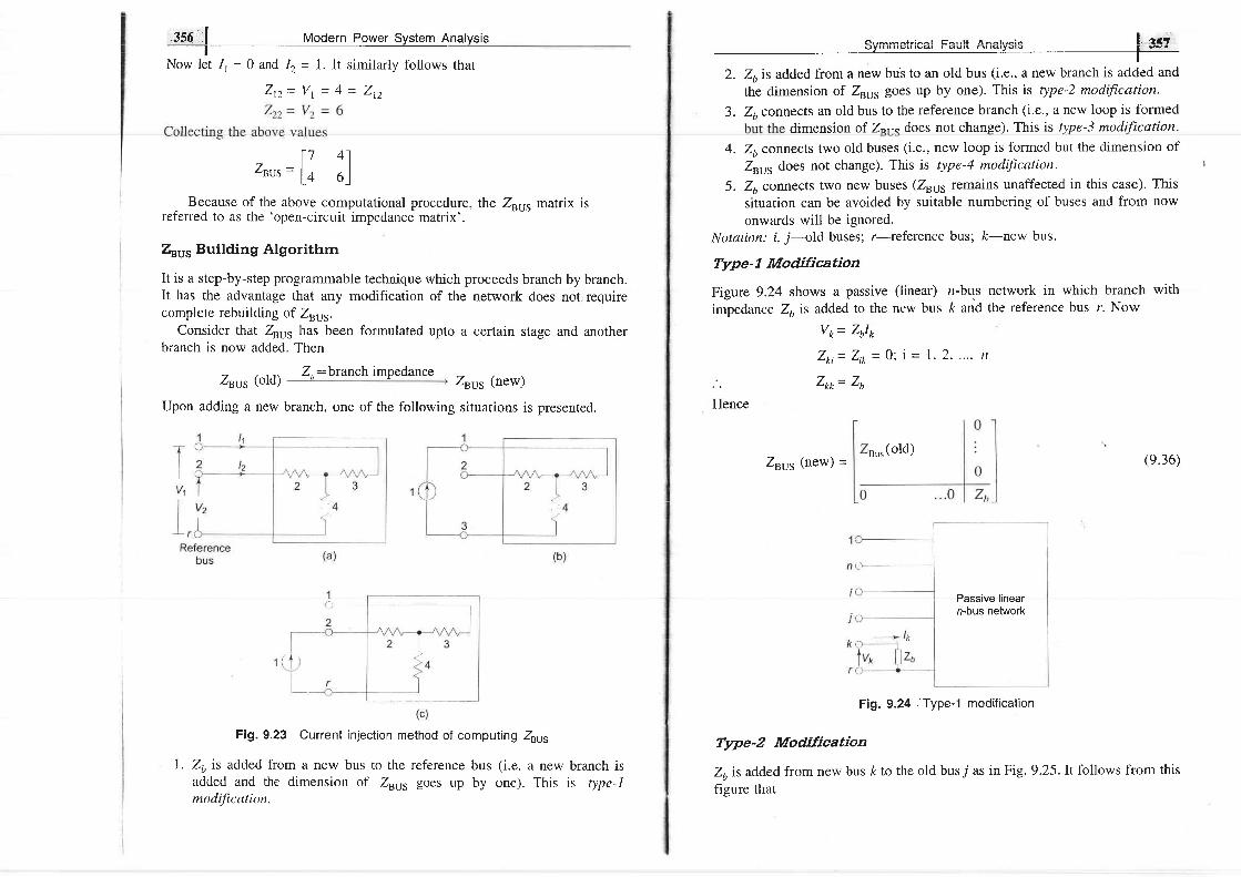
. f

356 | Modern Power System Analysis

Now let It = 0 and 12 = 1. It similarly fbllows that

Z t z = V t = 4 = Z n

Because of the above computational procedure, the Zru, matrix isreferred to as the 'open-circuit impedance matrix'.

Z"vs Building Algo4ithm

It is a step-by-step programmable technique which proceeds branch by branch.It has the advantage that any modification of the network does not requirecomplcte rebuilding of Z"ur.

Consider that Zrur has been formulated upto a certain stage and anotherbranch is now added. Then

Zrur (old)Zo:branch impedance

Zsus (new)

Upon adding a new branch, one of the following situations is presented.

Fig. 9.23 Current injection method of computing Zru.

26 is added from a new bus to the reference bus (i.e. a new branch isadded and the dimension of Zry5 goes up by one). This is type-Imodificution.

Symmetrical Fault Analysis !, f5l

, 4r,the dimension of Zsu5 goes up by one). This is type-2 modification.

3. Zuconnects an old bus to the reference branch (i.e., a new loop is formeddimension of 2o,," does not change). This is type-3 modification.

4. Zuconnects two old buses (i.e., new loop is formed but the dimension of

Zuu, does not change). This rs type-4 rnodittcation.

5. Zu connects two new buses (Zeus remains unaffected in this case). This

situation can be avoided by suitable numbering of buses and from now

onwards will be ignored.Notation: i, j-old buses; r-lsfelence bus; k-new bus.

Type- 1 Modification

Figure 9.24 shows a passive (linear) n-bus network in which branch with

impedance 2,, is added to the new bus k and the reference bus r. Now

Hence

V*= ZJ*

Z r i = Z * = 0 ; i = 1 , 2 . . . . . t t

Zm= Zu

Fig. 9.24 , Type-1 modification

Type-2 Modification

Zo is added from new bus ft to the old bus 7 as in Fig. 9.25.It follows from this

figure that

l7 41Zvus=

l+ 6 l

s,," (old)Zsvs (new) - (e.36)

t .

Passive linearn-bus network

35S;,1 MorJern Powcr Srrctarn anatrroio

1O_

n

Passive linearn-bus network

Fig. 9.25 Type-Z modification

Vo= Zdo + V,

= Zr,I*+ ZiJr+ Zlzlz +... + Zii ei* I) + ... + ZinlnRearranging,

V * = 4 l t + Z l z l z + . . . + 2 , , 1 , + . . . + Z i , l n + ( Z i i + Z ) l k

Consequently

Zrj

zzjZsvs(old) I : (e.38)

o I lzyziz...zi, I zii + z, )lI*

lr

Eriminate { in the 3":';,,iiy';;;?::"i"t i.I" a;y>;i:ation

(e' 3 I )'1

or 'o= -12 (\1Ir+ Zi2Iz+ "' + ZlnI) (9'39)

NowV;= 2;111+ Z,r I , + " ' + Z'nIn + Z; / r (e.40)

(e.42)

Zti

Zzj

:

Znj

(e.37)

Substituting Eq. (9.40) in Eq. (9.39)

,, = lr^

- h(z* 1 rr]a * lr,,

-

"h rz uz,,>)r,

+ + lr^- ̂ i{zu

2,,1)r, (s.4t)

Equation (9.37) can be written in matrix form as

. | t"fZsLr5 (new) = znvs(old - ;+;l : ltz't"Zv)

" j jT "u l z , , lzjj + zb

IYpe-3 Modification

zu connects an old bus (l) to the reference bus (r) as in Fig. 9.26. This casefollows from Fig.9.25 by connecting bus ft to the reference bus r, i.e. by settingv * = o '

Type- Modification

zo connects two old buses as in Fig. 9.27 . Equations can be written as follows

for all the network buses.

Fig. 9.27 TYPe-4 modification

Vi= Z;11, + Z, l r+ " ' + Zr i ( I i + / ) + ZU Qi-

Similar equations follow for other buses.

J

Passivelinearn-buSnetwork

( l ;+ lp

Fig. 9.26 Type-3 modification/o) + ...+ ZiJ"(9.43)

360 | Modern power System Analysis

I he voltages of the buses i and j are, however, constrained by the equation(Fig. 9.27)

Symmetrical Fault Analysis I fOt

Step I: Add branch 2,, - 0.25 (from bus I (new) to bus r)

Step

ZBUS = t}.25l (i)

Add branch Zzt = 0.1 (from bus 2 (new) to bus I (old)); type-Z

V,= Z,r lo+ Vi

o r 21111 + \212+ . . . + Z i t (1 ,+ I ) * Z i i ( I i - I ) + . . . +

(e.44)zi,In

= Z t l *+ Z , r l , + Z , r l " + . . . + Z lU,+ IearTangtng

_ I

0 = ( Z i t - 2 1 ) I r + . . . + ( Z t i - Z ) I i + e u - Z ) I i+...+ (Z* - 21,) In + (Zu * Zii * Zii - Zi - Z) 11, e.45)

Collecting equations similar to Eq. (9.43) and Eq. (9.45) we can writevl

V

vn

0

(9.46)

Eliminating 1o in Eq. (9.46) on lines similar to whar was donemodification, it follows that

l'"lZ,,

with the use of fbur relarionships Eqs (9.36), (9.37), (9.42) and (9.47) busimpedance matrix can be built by a step-by-step procedure (bringing in onebranch at a t in le) as i l l t rstratc ' t l in l ixrrrnple 9.8. This pror.cdrrr-c

-hcing a

mechanical one can be easily computerized.When the network undergoes changes, the modiflcation proceclures can be

cttrployccl to rcvisc thc bLrs irtrpcdance rnatrix ul 'thc nctwol'k. Thc opeling o1a line (Ztt) is equivalent to adding a branch in parallel to it with impedance- 2,, (see Example 9.8).

j Example 9.8

For the 3-bus network

III

!,--0.25 l , '(--

IlI

Ref bus r

F ig . 9 .28

zsvs=',lZ:11, 31i] (ii)Step 3: Add branch ,rt = 0.1 (from bus 3 (new) to bus I (old)); type-Z

modification

lo.2s o.zs 0.2s1zsvs =

| o.zs o.3s o.2s

| (i i i)

lo.2s 0.2s 0.3s..lStep 4: Add branch zz, (from bus 2 (old) to bus r); type-3 modification

10.2s o.zs 0.25'l [0.25-lZet)s =

| o.zs 0.3s 0.2s | | o.ts I to.zs 0.3s 0.251

Lo.2s o.2s o3sl o'3s + o " Ln.trj

[0.14s8 0.1042 0.14s8-l= I o.ro+z o.r4s8 o. lo42 |

fo.tott o.ro42 o.24s8lStep 5: Acld branch iz-r = 0.1 (from bus 2 (olct) to brrs 31old)): type-4modification

[o. l4s8 0.1042 0.l4s8l

zsvs = l o.'oo, 0.1458 o.to42l-

| 0 .1 + 0 .1458 + 0 .2458-2xO. lO4210.l4s8 O.tO42 0.24s8 )

[-0 1042.l

= I

0.0417 | [-o.to+z 0.0411 -0.0417]

[-o.o+tz-l

lo.r3e7 0.1103 0.12501

= | 0.1ro3 o.I3e7 0.1250

I| 0.1250 0.1250 0.17sol

Oltenirtg o tinu (l ine 3-2): This is equivalent to connecting an intpeclance - 0.I

between bus 3 (old) and bus 2 (old) i.e. type-4 modification.

Zsus= Zuur(olcl) - (-01)+ol?5 #

Z131,s (new) = Zsuts (old) -

lzit - z1t) ... (zi, - zi))

z b + z i i * Z i i - z z i j

Zsus

Ii,J o r.

I

shown in Fig. 9.28 buildr 9 l zI

' i r l

lL-, tr ili -, -- 6"11-. I0 .1 3 o . t

filf.lid, Modern Power System Anatysis- r - r -^ r r ^ . . t r Ana* ra io f f i r

:)ymmelrlual raul l rurqryo's r**

Now

I- | 0.1042 0.14s8 0.1042l; (same as in step 4)0.1458 0.1042 0.2458 |

For the power system shown in Fig. 9.29 the pu reactances are shown therein.For a solid 3-phase fault on bus 3, calculate the following

(a) Fault current(b) V\ and vt(c) I t ,r , I ' \ , uxl I l ,(d) 1fr, and If,

Assume prefault voltage to be I pu.0.2 0-.09 1

a n d i l = ( F Z E - ) = 0 . 2 8 6' i 2 - [ ^ z u )

These two voltages are equal because of the symmetry of the given power

network(c) From Eq. (9.29)

and

But

| f f r

Jt -

or 1f -

(b) As per Eq. (9.26)

rr.f -v i -

\, //

o '' \ ,/'0.,\ /\.. ,/. ,

l l3 ' '

Fig. 9.29

[ 0.0147-lt l

| -0.0147

| 10.0147 - 0.0147 0.0s001

L o.osoo_J

(d)

Iri = Y,j (vl - vl)

Irtz= +(0.286 - 0.286; = gj0.1 '

I \ t= t | t= f r ro .186-o)- - i2.86

As per Eq. (9.32)

, r E' or-vrfr Gr - ixtic + ixr

E'Gr = 1 Pu (Prefault no load)

J I - F 0 .1c) | i-,,

IL.= 1-0'286-- =- j2 '86Gt- io .2+ io .os

SimilarlY

I fcz= i2.86

Solution The Thevenin passive network for this system is drawn in Fig. 9.28with its Zru, given in Eq. (iv) of Example 9.8.(a) As per Eq. (9.25)

PROB LE M S

A transmission line of inductance 0.1 H ancl resistance 5 ohms is suddenly

short circuited at t =0 at the bar end as shown in Fig' P-9'1' Write the

expression for short circuit current i(r). Find approximately the value of

the first current maximum (maximum momentary current)'

[Hint: Assume that the first current ntaximum occurs at the same time as

the first current maximum of the symmgtricl.:non ttrcuit current')

V:2,, + Zl

Yo- : . _1 - - - - j s . j lzn j0.175

vl - --Zt--yu' z r r + z l ' r

9 . 1

564,'l rr]logern power System AnalvsisI

errrnrnorrinal Farrlt Analvsis I geS

v y r r r r l v t " v E ' ' | - - " - " - - J

I

9 .3

i 0 . 1 H S O

I ' 64-A-' v^/v\

i

f l u =1OO sin (100 n f + 15.)

Fig. p-9.1

9 '2 (a) What should the instant of short circuit be in Fig. p-9.1 so that theDC off-set current is zero?

(b) what should the instant of short circuit be in Fig. p-9.1 so rhar theDC off-set current is maximum?

For the system of Fig. 9.8 (Example 9.2) find the symmetrical currents tobe interrupted by circuit breakers A and B for a fault ar (i) p and (ii) e.For the system in Fig. p-9.4 the ratings of the various componenrs are:

Fig. P-9.5

A s y n c h r o n o u s g e n e r a t o f r a t e d 5 0 0 k V A , 4 4 0 v , 0 . l p u s u b t r a n s i e n t."u"'tun". is supptying a passive load of 400 kW at 0.8 lagging powel

factor. Calculate tfr" in'itiui symmetrical rms current for a three-phase fault

at generator terminals.

A generator-transformer unit is connected to a line through a circuit

breaker. The unit ratings are:

Generator: 10 MVA, 6.6 kV; X,,d= 0.1 pu, Xi= o,2o pu and

X,r = 0'80 Ptt

T r a n s f o r m e r : 1 0 M V A , 6 . 9 1 3 3 k V , r e a c t a n c e 0 . 0 8 p u

The system is operating no load at a line voltage of 30 kv, when a three-

phase tault occurs on ih" tin" just beyond the circuit breaker' Find

(a) the initial symmetrical rms current in the breaker'

iui tt. maximum possible DC off-set currenr in rhe breaker,

(c) the momentary current rating of the breaker'

(d) the current,o U. intemrpted by the breaker and the intemrpting kVA'

9.6

9.79.4

Generator:

Motor:

25 MVA, 12.4 kV, l\Vo subtransient reactance20 MVA, 3.8 kV, l5%o subtransient reactance

Transformer T,: 25 MVA, 11/33 ky, gVo reactanceTransfbrmer Tr: 20 MVA, 33/3.3 kV, I \Vo reactanceLine: 20 ohms reactance

The system is loaded so that the motor is drawing 15 Mw at 0.9 loadingpower factor, the motor terminal voltage being 3.1 kv. Find thesubtransient current in generator and motor for a fault at generator bus.lHint: Assume a suitable voltage base fbr the generator. The voltage basefor transformers, line and motor would then be given by the transforma_t i0n r i l t i< ls. Fr l r cxanrplc, i f 'wc choosc gcrrcrator. vol tagc basc as I I kv,the line voltage base is 33 kv and motor voltage base is 3.3 kv. per unitreactances are calculated accordingly.]

T, 1 T 2

Fig. p-9.4

Two synchronous motors are connected to the bus of a large systemthrough a short transmission line as shown in Fig. p-9.5. The ratings ofvanous components are:

Motors (each): 1 MVA, 440 v,0.1 pu transient reactanceLine: 0.05 ohm reacranceLarge system: Short circuit MVA at its bus at 440 V is g.

when the motors are operating at 440 v, calculate the short circuitcuffent (symmetrical) fed into a three-phase fault at motor bus.

and(e) the sustained short circuit current in the breaker'

The system shown in Fig' P-9'8 is delivering 50 MVA at

l a g g i r r g p 0 w 0 r l . i t c t t t r i l l t t l l t b r r s w h i c h r t r i r y b e r e g i r r d e c lParticulars of various system components are:

Generator; 60 MVA, 12 kV' X,/ = 0'35 Pu

Transtbrmers (each): 80 MVA, 12166 kV' X = 0'08 pu

Line: Reactance 12 ohms' resistanc: negligible'

Calculate the syrnmetrical current that the circuit breakers A and B will

be called upon to interrupt in the event of a three-phase fault occurring at

F near the circuit breaker B'

9 . 811 kv, 0.8i ls inf ini te.

9.5

Line

Fig. P-9.8

*Sf-,S tgdern power Svstem Anatvsist . -

9'9 A two generatorstaticln supplies a f'eeder through a bus as shown in Fig.P-9'9' Additional power is fed to the bus throJgh a transfoilner from alarge system which may be regarded as infinite. A reactor X is included

:,'jT:^"1^:t::1u1.',f"'Ter and,1"-!T to limit the SC rupruring capacity of4v<rl\er rr ru JJJ rvtyA (Iault close to breaker). Find theinductive reactance of the reactor required. system data are:

-bus 2 of the system. Buses 1 and 2 are connected through a transformerand a transmission line. Per unit reactances of the various components are:

Generator (connected to bus bar 1) 0.25

Transmission line 0.28

The power network can be represented bi a gene ator with a reactance(unknown) in series.

With the generator on no load and with 1.0 pu voltage at each busunder operating condition, a three-phase short circuit occurring on bus 1causes a current of 5.0 pu to flow into the fault. Determine the equivalentreactance of the power network.

9.12 Consider the 3-bus system of Fig. P-9.I2. The generators are 100 MVA,with transient reactance IjVo each. Both the transforners are 100 MVAwith a leakage reactance of 5%t. The reactance of each of the lines to abase of 100 MVA, 110 KV is 707o. Obtain the short circuit solution fora three-phase solid short circuit on bus 3.

Assume prefault voltages to be 1 pu and prefault currents to be zero.

Generator Gr:Generator Gr:Transformer Tr:Transformer T2:

Assume that all reactances are given on appropriate voltage bases. choosea base of 100 MVA.

ti Tz

25 MVA, 757o reactance50 MVA, 20Vo reactance100 MVA;8Vo reacrance40 MVA; l\Vo reactance.

Fig. p_9.9

9'10 For the three-phase power network shown in Fig. p-9.10,the various components are:

T11 1 / 1 1 0 k V

G)^T" T

f l rn kv\-x-x-x-" '2

the ratings of

j 0 .1

Fig. p-9.10

Generators Gr: 100 MVA, 0.30 pu reactanceGz: 60 MVA, 0.18 pu reactance

Transformers (each): 50 MVA, 0.10 pu reactanceInductive reactor X: 0.20 pu on a base of 100 MVALines (each): 80 ohms (reactive); neglect resistance.

with the network init iaily unroaded and a rine vortage of 110 kv, asymmetrical short circuit occurs at mid point F of rine r-.calculate the short circuit MvA to be intemrpted by the circuit

breakers A and B at the ends of the line. what would these values be, ifthe reactor X were eliminated? Comment.

Fault

Fig. P-9.12

9.13 In the system configuration of Fig. P-9.12, the system impedance data aregiven below:

Transient reactance of each generator = 0.15 pu

Leakage reactance of each transformer = 0.05 pu

Ztz = i0.1, zp - i0.12, 223 = 70.08 PuFor a solid 3-phase fault on bus 3, find all bus voltages and sc currentsin each component.

365 j Modern Power System Analysist

9.14 For the fault (solid) location shown in Fig. P-9.I4, find the sc currents inlines 1.2 and 1.3. Prefault system is on no-load with 1 pu voltage andprefault currents are zero. Use Zuu, method and compute its elements bythe current injection technique.

'r-[b- 111 110 kV 0.5 pu reactance

-lQ9 0.1 pu reactance

Fig. P-9.14

REF ERE N CE S

Books

l . BIr rwt t . H.L) . . Sol t t t io t r t t . f I .ar ,g,e Netwrtrk l ty Mutr i r Mct lutds, Wi lcy, Ncw York,

tL)'7 5.

2. f . lc t rct tswartdu' , j . i t . , Mtt t i t : t ' t t i ' tnv 'u ' 5 'vs ' /e l l , l , i r r tcrr tat i t t r ta j ' i 'cxtbook

eorrrp lny,

New York , 1971 .'3.

Stagg, G.W. and A.H. El-Abiad. Computer Methods in Power Systems Analysis,

McCraw-H i l l Book Co . , Ncw York , 1968 .

4. Anderson, P.M., Analysis of Faulted Power Systems,Iowa State Press, Ames, Iowa,

1973 .( ' f r r t 'kc. l - , . . ( ' in ' t t i t Arr t t l . t , , t ' i , t o. f 'A l t t rnul i t t ,q Ctrr rcr t l l ' t twrr S\ , . r ' / r , r l . r . Vol . I ,

New York . 1943 .

Stcvcrrson, W.D. Jr . , Eletr rcnt .s of Powcr Systems Anuly-s is,4th cdn, Mc( i rz

Ncw York , l 9 t l 2 .

Paper

"7. Brown. H.E. et al. "Digital Calculation o[ Three-Phase Short Circuits by Matrix

Methods", AIEE Trani., 1960, 79 : 1277.

10.1 INTRODUCTION

In our work so far, we have considered both normal and abnormal (shortcircuit) operett ions of power systern Llncler cornpletely balanced (symmetrical)co l t t l i t io t ts . LJ l r r lc r suc l t o l tc t 'a t io t t t l tc systcr l r i ru l tcdanccs in cac l r phasc areidentical and the thrce-phase voltages and currents throughout the system areco l l tp lc tc ly h l t l i tncct l . i .c . thcy huvc crpr i r l nurgr r i tu t lcs in c l rch phusc und t rcprtrgrcs.sivcly displaced in t irne phase by 120' (phase u leads/laes phase b by120 ' and phase i r leads/ l lgs ph i tse c by 120") . In a b : r l lnced systenr , lna lys iscan proceed on a single-phase basis. The knowledge of voltage and current inone phase is sufficient to completely determine voltages and currents in theother two phases. Real and reetctive powers are simply three times thecorresponding per phase values.

Unbalanced system operation can result in an otherwise balanced system dueto unsymmetrical fault , e.g. l ine-to-ground fault or l ine-to-l ine fault . Thesef 'aults atrc, i t t lhct, ol ' lnot 'e conlnrol l occurrence+ thalt the syrnntetr ic:al ( three-phase) fault . Systern operation may also become unbalanced when loads areunbalanced as in the presence of lar-ee single-phase loads. Analysis underunbalancetl conditions has to be carried out on a three-phase basis. Alterna-tively, a nlore convenient method of analyzing unbalanced operation is throughsymtnetr ical components where the three-phase voltages (and currents) whichmay be unbalanced are transfbrmed into three sets of balanced voltages (and

* Typical relative frequencies of occurrence of different kinds of faults in a powersyst(: l l t ( i rr ordcr ol ' dccrcasing scvcri ty) are:

l l

I

- r .

6 .

Three-phase (3L) faultsDouble line-to-ground (LLG) faultsI)outr lc l i rrc ( l-1,) l i rultsSingle l ine-to-ground (LG) faults

5Volj%o| 5t/o

7jVo

currents) called symmetrical components. Fortunately, in such a transformationthe impedances presented by various power system elements (synchronousgenerators, transformers, lines) to symmetrical components are decoupled fromeach other resulting in independent system networks for each component

anced set). This is the basic reason for the simolicitv of the svmmetricalcomponent method of analysis.

TO.2 SYMMETRICAL COMPONENT TRANSFORMATION

A set of three balanced voltages (phasors) Vo, V6, V" is charactertzed by equalmagnitudes and interphase differences of 120'. The set is said to have a phasesequence abc (positive sequence) if Vulags Voby l2O" and V. lags Vuby I20".The three phasors can^then be expressed in terms of the reference phasor Vo as

Vo = Vo, V6 = a"Va, V, = aVowhere the complex number operator cr is defined as

sL - air20"It has the following properties

symmetrica! compo1gnlg ! .a?.,{fi-i

above. ThusVo-- Vot * Voz I Voo (10.s)

b - Y b L - v b z

Vr= VrI * Vrz * Vro ( r0.7)

The three phasor sequences (positive, negative and zero) are called the

symmetrical components of the original phasor set Vo, V6,V,. The addition ofsymmetrical components as per Eqs. (10.5) to (10.7) to generate Vo, Vr, V, isindicated by the phasor diagram of Fig. 10.1.

V61=crV61 V6fo?V11

Fig. 10.1 Graphical addition of the symmetrical components to obtainthe set of phasors V", V6, V" (unbalanced in general)

Let us now express Eqs. (10.5) to (10.7) in terms of reference phasors Voy

Vo2 and Voe. Thus

V o = V o t * V o z l V o o

Vu= a .2Vo r+ aVo r * Voo

V"= c -Vo l+ o2vo r * Voo

These equations can be expressed in the matrix form

, * 2 : e i 2 4 o ' : e - i l A o " _ *

(o ' ) * : o

a 3 : l

l + a l a 2 : 0

( 1 0 . 1 )

(r0.2)

If the phase sequence is acb (.negative sequence), then

Vo= Vo, Vu= tuVo, Vr= &Vo

Thus a set of balanced phasors is fu'lly characterized by its reference phasor(say V,) and its phase sequence (positive or negative).

Suffix 1 is commonly used to indicate positive sequence. A set of (balanced)positive sequence phasors is written as

Vo1, V61 - &Vu1, Vrr = aVot

Similarly, suffix 2 is used to indicate negative sequence. A set of (balanced)negative sequence phasors is written as

Vo2, V62= dVn2, Vrz= Q'Voz (10.3)

A set of three voltages (phasors) equal in magnitude and having the same phaseis said to have zero sequence. Thus a set of zero sequence phasors is writtenAS

Vng, V6g = Vo1, Vr1 = Vo1 (10.4)

Consider now a set of three voltages (phasors) Vo, V6, V, which in general maybe unbalanced. According to Fortesque's theorem* the three phasors can be

(10.8)

(10.e)(10.10)

* The theorem is a general one and applies to the case of n phasors [6],

ffi#d : Modern Po*et sytttt Analysi,-__r_-

and Io = il'

where I' = A-rI'

(10.19)

(10.20)

(10.21)(r0.22)(r0.23)

(ro.24)

(ro.2s)

(r0.26)

Vp = AV,

1,"1v, =

l'u | = vector of original Phasors

Lv, )

Iu' l% = | Voz | = vector of symmetrical components

Lu"'.1[ ' I r - l

A - 1 " o n t II a o 2 t - l

We can wrire Eq. (10.12) asV, = 4-'V,

ComputinE ,{r and utilizing relations (10.1), we get

[ t d o ' ]

o - ' = * l r c r 2 a I' L t r r lIn expanded form we can write Eq. (10.14) as

IVor =

,<V"+ c-Vu+ a2VS

voz = ! f r"+ ozvu+ o%)3I

Vuo= ;

V ,+ Vr , * r , )

( 1 0 . 1 1 )

(10.12)

(10 .13)

(10.14)

( r0.1s)

(10.16)

(10.17)

(10 .18)

l ' ' l [ r , ' II r = l I u l ; a n a

I , = l I o , I

L I , ) L r , o_ iOf course A and A-r are the same as given earlier.

In expanded form the relations (10.19) and (10.20) can be expressed asfollows:

(i) Construction of current phasors from their symmetrical components:Io= Iot * Ioz * Ioo

I a = o 2 l o t t d o z r l o o

I r= do t+ az lo r * I oo(ii) Obtaining symmetrical components of current phasors:

1I o t= * e "+ du+ o2 l r )

;t , r .=

i ( Io+ az lu+ aI , )

; .I r o = , Q o + I u + I r )

Certain observations can now be made regarding a three-phase system withneutral return as shown in Fig. 10.2.

Equations (10.16) to (10.18) give the necessary relationships for obtainingsymmetrical components of the original phasors, while Eqs. (10.5) to (10.7)give the relationships for obtaining original phasors frorn the symmetricalcomponents.

The symmetrical component transformations though given above in terms ofvoltages hold for any set of phasors and therefore automatically apply for a setof currents. Thus

Fig. 10.2 Three-phase system with neutral return

The sum of the three line voltages will always be zero. Therefore, the zerosequence component of line voltages is always zero, i.e.

ln

Vao V""

vobo = trr**

vu,+ v"o) = o (10.27)

On the other hand, the sum of phase voltages (line to neutral)'may not be zeroso that their zero sequence component Vn, may exist.

Since the sum of the three line currents equals the current in the neutralwire. we have

(10.28)

i.e. the current in the neutral is three times the zerc sequence line current. If theneutral connection is severed.

I o o = ! U " + 1 6 + r " ) = ! +

I o o = l r , = o3

t.e. in the absence of a neutral connection thealways zero.

B --_____}_----

Flg. 10.3

Solution Io + I" * Is = Qor

10130" + l5l- 60o + Ic = O

Ic= - 16.2 + j8.0 = 18 1154" A

(ro.2e)

zero sequence line current is

(10 .31)

FromPower Invariance

We shall now show that the symmetrical component transformation is powerinvariant, which means that the sum of powers of the three symmetricalcomponents equals the three-phase power.Total complex power in a three-phase circuit is given by

S = f p $ = 4 1 , + V u t t + V , t ! (10.30)

ors = [A v,,]'t'lAl,l.

= v! 'qr'q. tINow

[ r o ? ' T to 1 6 . = l t a " t l l a

[r r I JLa,. . s=31y t i ,=341 . ,

(10.33)

A delta connected balanced resistive load is connected across an unbalancedthree-phase supply as shown in Fig. 10.3. With currents in lines A and Bspecified, find the symmetrical components of line currents. Also find thesymmetrical components of delta currents. Do you notice any relationshipbetweeri symmetrical components of line and delta currents ? Comment.

Eqs. (10.24) to (10.26)1

Itr= :0Ol3O" + 751(-60" + l2O" )5

= 10.35 + j9.3 = 14142" A

+ I8l(154" + 240"))

( i)

151(- 60o + 240") + I8l(154' + 120"))

4.651248" A (ii)

/c) = 0 (ii i)

IIez= ;Q0130' +

J

= --1.7 - j4.3 =

IIao= t^ (lo + IR +

J

From Eq. (10.2)

Im= 141282" AInz= 4'6518" AI a o = o Ar r l l -1 0 0l

n ' . r l : r | o r o l - t , ( 1 0 . 3 2 )c - l l L 0 0 l l

Icr = 141162" AIcz = 4.651128" AI c o = o A

Check:

Ia= Iat * I,rz* I,to = 8'65 + j5 = 10130"

Converting delta load into equivalent star, we can redraw Fig. 10.3 as in Fig.10.4.

la= 3V^1, + 3V"r!), + 3V"oI),

= sum of symmetrical component powers

I Example 10.1 |-T

_\

$,$i.M Modern power system anatysisI

Delta currents are obtained as follows

Qrrmmatriaal l-amnnnanla tffiffi

Positive and negative sequence voltages and currents undergo a phase shift inpassing through a star-delta transformer which depends upon the labelling ofterminals. Before considering this phase shift, we need to discuss the standardpolarity marking of a single-phase transformer as shown in Fig. 10.5. Thetransformer ends marked with a dot have the same polarity. Therefore, voltageVun, is in phase with voltage V..,. Assuming that the small amount ofmagnetizing current can be neglected, the prirnary current 1r, entering the dottedend cancels the demagnetizing ampere-turns of the secondary current 1, so thatI, and 12 with directions of flow as indicated in the diagram are in phase. If thedirection of 1, is reversed, 1, and 1, will be in phase opposition.

veB= Io U^- Ir)

I tB= zAB)R - tUo-

ru)

Similarly,

r nc= I e r - I r )5

Ice= ! f r r - Io )5

Substituting the values of Io, Iu and Ir,

I en = ! Oozzo" -r5l- 60") =

rnc= lOsz-

60" - rllr54")

rcn= !W2154"

- rol3o") =

we have

6186 A

= lO.5l- 41.5" A

8.31173" A

The symmetrical components of delta currents are

1Iem= ;(6186" + IO.5l(- 4I .5 '+ l2O") + 8.31(173" + 240"))( iv)

J

= 8172" A

II,qaz= :6186" + 1051(- 41.5" + 240") + 8.31(173" + 120")) (v)

J

= 2.71218" A

Ieno= 0

Incr, Ircz, IBC,,lsn1, Iga2 and 1.oo can be found by using Eq. (10.2).

Comparing Eqs. (i) and (iv), and (ii) and (v), the following relationshipbetween symmetrical components of line and delta currents are immediatelyobserved:

t 'IeBr= +130" (vi i)

V J

Ienz= \ z-zo" (viii)! J

The reader should verify these by calculatrng Io', and l*2from Eqs. (vii) and(viii) and comparing the results with Eqs. (iv) and (v).

Flg. 10.5 Polarity marking of a single-phase transformer\

Consider now a star/delta transformer with terminal labelling as indicated inFig. 10.6 (a). Windings shown parallel to each other are magnetically coupled.Assume that the transformer is excited with positive sequence voltages andcarries positive sequence currents. With the polarity marks shown, we canimmediately draw the phasor diagram of Fig. 10.7. The following interrelation-ship between the voltages on the two sides of the transformer is immediatelyobserved from the phasor diagram

VtBt= x Vabr l3V, -r - phase transformation ratio (10.34)

As per Eq. (10.34), the positive sequence line voltages on star side lead thecorresponding voltages on the delta side by 30" (The same result wo,'ld applyto line-to-neutral voltages on the two sides). The same also applies for linecurrents.

If the delta side is connected as in Fig. 10.6(b) the phase shrft reverses (thereader should draw the phasor diagram); the delta side quantities lead the starside quantities by 30".

(vi)

A __--______

ar System Analys'is Symmetricat Componentg | 3?9I

correspotxding positive sequence quantities on the LV side by 30'. The reverse

is the case for negative sequence quantities wherein HV quantities lag the

corresponding LV quantities by 30".

vsc2

l- /\

o a

(a) Star side quantities lead delta side quantities by 30o

(b) Delta side quantities lead star side quantities by 30o

Fig. 10.6 Labelling of star/delta transformer

Fig. 10.7 Positive sequence voltages on a star/delta transformer

Instead, if the transformer of Fig. 10.6(a) is now excited by negativesequence voltages and currents, the voltage phasor diagram will be as in Fig.10.8. The phase shift in comparison to the positive sequence case now reverses,i.e., the star side quantities lag the delta side quantities by 30'. The result forFig. 10.6(b) also correspondingly reverses.

It shall from now onwards be assumed that a star/delta transformer is solabelled that the po,sitive sequence quantities on the HV side lead their

vcea Vcrcz Vesz

Fig. 10.8 Negative sequence voltages on a star/delta transformer

IO.4 SEOUENCE IMPEDANCES OF TRANSMISSION LINES

Figure 10.9 shows the circuit of a fully transposed line carrying unUalanceclcurrents. The return path for 1,, is sufficiently away for the mutual effect to beignored. Let

X" = sell 'reactance o1'each line

X. = mutual reactance of any line pair

The fbllowing KVL equations can be written down from Fig. 10.9.

Vo - V'o= jXJo + jX*Iu + .ixmlc

l r= l "+ l o+ 1 "-(-

V6

Vec'l

vc

Fig. 10.9

Modern PgwgfSy$gln Snalysis Svmmetrienl cnmnonent( tflIlFffiT

t, Z1 12 22o-------{__]- -o

"----f--}- ---o

4 - r[: jxJo

l', - V!: iXJ"or in rnatrix form

+ jxh + jx*["

+ jxmlb + jxJ"(10.3s)

(10.36)

(10.37)

(10.38)

(10.3e)

(10.40)

(r0.42)

(10.43)

(r0.44)

(10.4s)

(or negative)

(a) Positive sequencenetwork

(b) Nagative sequencenetwork

ls Zso---)--f---_l.-

@)Zero sequencenetwork

^ a

Ib

I"

vIvi

vb

v"I// -- - / n -

v ! ) :r// -- , ' s -

V,r

= J x^x,x.x_x*x,

or A (I/, -

or v,Now

A-I ZA :

0

X, -X*

0

z t 0 0

0 2 2 00 0 z o

wherein

Zr: j(X, - X,r) : positive sequence impedance

Zz: j(X, - X^) : negative sequence impedance

Zo: i(X, + 2X) : zero ,tequence impedance

We conclude that a fully transposed transmission has:/ t ; \ o ^ r r o l ^ ^ o . i + i " o ^ - l - ^ ^ ^ + i - - ^ : ^ - ^ ) ^ - ^ ^ -\ r , , vyuar pvrr l ryu ( t r l r l u t / ts4Lrvg st rqu{r r ruE r rup€ual lu t is .

(ii) zero sequence impedance much larger than the positive

F ig . 10 .10

The decoupling between sequence networks of a fully transposed transmis-sion holds also in 3-phase synchronous machines and 3-phase transformers.This fact leads to considerable simplications in the use of symmetricalcomponents rnethod in unsymmetrical fault analysis.

In case of three static unbalanced impedances, coupling appears betweensequence networks and the method is no more helpful than a straight forward3-phaso unalysis.

10.5 SEQUENCE IMPEDANCES AND SEOUENCE NETWORKOF POWER SYSTEM

Power system slernsnfs-transmission lines, transformers and. synchronousnlachines-have a three-phase symmetry because of which when'currents of aparticular sequence are passed through these elements, voltage drops of thesame sequence appear, i.e. the elements possess only self impedancos- tosequence currcnts. Each eleurent can therelbre be represented by tlreedecoupled sequence networks (on single-phase basis) pertaining to positive,negative and zero sequences, respectively. EMFs are involved only in a positivesequence network of synchronous machines. For finding a particular sequenceimpedance, the element in question is subjected to currents and voltages of thatsequence only. With the element operating under these conditions, the sequenceimpedance can be determined analytically or through experimental test results.

With the knowledge of sequence networks of elements, complete positivel'negative and zero sequence networks of any power systern can be assembled.As will be explained in the next chapter. these networks are suitablyinterconnected to simulate different unsymmetrical faults. The sequencecurrents and voltages during the fault are then calculated from which actualfar"rlt currents and voltases can be found.

10.6 sEQuENCg I;IpTDANCES AND NETWoRKs oFSYNCHRONOUS MACHINE

Figure 10.11 depicts an unloaded synchronous rlachine (generator or motor)grounded through a reactor (impedance Z).8o, E6and E, are the induced emfs

zIo

zuIs

A-IZAI,

jx,JX^jx^

jx^jx,jx^

l*, - ',:J L :

Thus Eq. (10.37) can be written as

| 41 l'tr( I I x"- x^

l " l - l ' t l : ' I oL r r o J l r r t J L o

0 o ll-r, Ix, - x,,, o ll r, | (l o.4l)

o x, *zx^ )j,l

l[ /' .l

ll ,, IlLr, i

sequence impedance (it is approximately 2.5 times).It is further observed that the sequence circuit equations (10.42) are in

decouplecl fbnn, i.c. thcrre arc no rnutual scqucncc inducternccs. F)quation(10.42) can be represented in network form as in Fig. 10.10.

3S2 I _ Modern power System Anatysis--]-

of the three phases. when a fault (not shown in the figure) takes place atmachine terminals, currents 1,,, I,,and /. f low in the l ines. whenever the faultinvolves ground, current In= In+ Iu + ^I" flows to ne'tral from ground

"i^I^'.

negative and zero sequence culrents, respectively. Because of windingsymmetry currents of a particular sequence produce voltage drops of thatsequence only. Therefore, there is a no coupling between the equivalent circuitsof various sequences*.

uence voltage.Hrvvvvs yyrrrr r(rLrl l 4rr.1IyJIs (\_napler i l ) , we must

know the equivalent circuits presentecl by the *u.hin" to the flow of positive,

Symmetrigel_qg4pe!e$s _

the short circuit occurs l irrnr kradccl conditiorts, thc voltagt: behind appropriltc

reactance (subtransient, transient or synchr:onous) constitutes the positive

Figure lO.IZa shows the three-phase posit ive sequence network ntodel of a

synchronous machine. Z, does not appear in the model as Iu = 0 for positive

sequence currents. Since it is a balanced network it can be represented by the

single-phase network model of Fig. 10.12b for purposes of analysis. The

reference bus for a positive sequence network is at neutral potential. Further,since no current flows from ground to neutral, the neutral is at ground potential.

l a t> a

(I

II

(a)Three-phase model

Fig. 10.12 Positive sequence network of synchronous machine

With reference to Fig. 10.12b, the positive sequence voltage of terminal c

with respect to the reference bus is given by

V , , l = E , , - Z l l , , l (10.4e)

Negative Sequence Impedance and Network

It has already been said that a synchronous rnachine has zero negative sequence

induced voltages. With the flow of negative sequence currents in the stator a

rotating field is created which rotates in the opposite direction to that of the

positive sequence field and, therefore, at double synchronous speed with respect

to rotor. Currents at double the stator frequency are therefore induced in rotor

field and damper winding. In sweeping over the rotor surface, the negative

sequence mmf is alternately presented with reluctances of direct and quadrature

axes. The negative sequence impedance presented by the machine with

consideration given to the damper windings, is often defined as

la

-*)e ".n'-----

( t +\=\'-..t:.6 d-n>_- u

\ t 6--> -----b

L----- ____l_"Fig' 10'11 Three-phase synchronous generator with grounded neutral

Positive Sequence Impedance and Network

Since a synchronous machine is clesigned with symmetrical windings, it inducesemfs of positive sequence only, i.e. no negatrve or zero sequence voltages areincl t rced in i t ' Whcn thc t t t l tc l t inc curr ics posi t ivc scqucncc curr .cnts gl ly, th isntode of operation is the balanced mocle discussed ailength in Chapter 9. Thearmature reaction field caused by positive sequence currents rotates at'synchronous speed in the salne clirection as the ,otu., i.e., it is stationary withrespect to field excitation. The machine equivalently offers a direct axisreactance whose value reduces from subtransicnt reactance (X,a) to transientreactance (Xtr) and finally to steady state (synchronous) reactanJe (Xa), as theshort circuit transient progresses in time. If armature resistance is assumednegligible, the positive sequence impedance of the machine is

ln't, b

lc't

Reference bus

(b) Single-phase model

21= jXtj (if I cycle transient is of interest)

= jX'a Gf 3-4 cycle transient is of interest)

= jXa (if steady state value is of interest) xt: + x,!Z . t = j ; l Z 2 l < l Z r l

2

(10.46)

(10.47)

(10.48)If the machine short circuit takes place from unloaded conditions, the

terminai voltage constitutes the positive sequence voltage; on the other hand. if Negative sequence network models of a synchronous machine, on a three-phase and single-phase basis are shown in Figs. 10.13a and b, respectively. The

reference bus is of course at neutral potential which is the same as ground

potential.

(10.s0)

*'fhis can be shown to be so by synchronous machine theory, [5].

fl$4.:rl Mooern powLr System nnarysist -

From Fig' 10.13b the negative sequence voltage of terminal a with respecrto reference bus is

Voz= - Zzloz

symmetricat Components FjSiffi

Zs= 3Zra Zos (10.53)in order for it to have the same voltage from a to reference bus. The referencebus here is, of course, at ground potential.

From Fig. 10.14b zero sequence voltage of point c with respect to the

Voo = - Z{oo (10.54) .

Order of Values of Sequence Impedances of aSynchronous Generator

Typical values of sequence impedances of a turbo-generator rated 5 MVA, 6.6kV, 3;000 rpm are:

Zr = lZ%o (subtransient)

Zr = 20Vo (transient)

Zr = 7l0Vo (synchronous)

Zz= I2Vo

Zo= 5Vo

For typical values of positive, negative and zero sequence reactances of asynchronous machine refer to Tablu 9.1.

IO.7 SEOUENCE IMPEDANCES OF TRANSMISSIO\ LINES

A fully transposed three-phase line is completely symmetrical and therefore theper phase impedance offered by it is independent of the phase sequence of abalanced set of currents. In other words, the impedances offired by ii to positiveand negative sequence culrents are identical. The expression foi its per phaseinductive reactance accounting for both self and mutual linkages ias beenderived in Chapter 2.

When only zero sequence currents flow in a transmission line, the currentsin each phase are identical in both magnitude and phase angle. part of thesecurrents return via the ground, while the rest return throu h the overheadground wires. The ground wires being grounded at several towers, the returncurrents in the ground wires are not necessarily uniform along the entire length.The flow of zero sequence currents through the transrnission iln"r, ground wiresand ground creates a magnetic field pattern which is very different from thatcaused by the flow of positive or negative sequence currents where the currentsh , r . r o ^ ^ L ^ ^ ^ - J : f f ^ - ^ - ^ ^ ^ f t ^ n orrqYv (r Prrd'Ds' urrrsrtrI lutr UI ILV an(l tne fetufn Cuffent lS ZefO. T\e ZefOsequence impedance of a transmission line also accounts for the groundimpedance (zo = z.to + 3zri.since the ground impedance heavily depends onsoil conditions, it is esseniial to make some simplifying assumptions io obtainanalytical results. The zero sequence impedance of transmission lines usuallv

(10.s1)

laz a

(b) Single-phase model

Flg. 10.13 Negative sequence network of a synchronous machine

Zero Sequence Impedance and Network

we state once again that no zero sequence voltages are induced in asynchronous machine. The flow of zero sequence currents creates three mmfswhich are in time phase but are distributed in space phase by 120". Thetesultant air gap field caused by zero sequence currents is therefore zero.Hence, the rotor windings present leakage reactance only to the flow of zerosequence currents (Zos < Zz < Z).

/66

Reference bus

(a)Three-phase model

Iao -a

(b)S ing le -phase mode l

1o.14 Zero sequence network of a synchronous machine

Zero sequence network models on a three- and single-phase basis are shownin Figs. 10.14a and b. In Fig. r0.l4a, the cu'ent flowing in the inpedance znbetween neutral and ground is In = 3lno. The zero sequence voltage of t"r-inula with respect to ground, the reference bus. is therefore

Vr1= - 3znioo - Zorlno =,r, (32, + Z0)loo e0.52)wh11e Zo, is the zero sequence impedance per phase of the machine.

Since the single-phase zero sequence network of Fig. 10.14b carries only perphase zero sequence current, its total zero sequence impedance must be

3Sd I Modern Power System Anatysis

ranges fromZ to 3.5 times the positive sequence impedance*. This ratio is onthe higher side for double circuit lines without ground wires.

10.8 SEOUENCE IMPEDANCES AND NETWORKS OF

It is well known that ahnosl all present day installations have three-phasetransformers since they entail lower initial cost, have smaller space require-ments and higher efficiency.

The positive sequence series impedance of a transformer equals its leakageimpedance. Since a transformer is a static device, the leakage impedance doesnot change with alteration of phase sequence of balanced applied voltages. Thetransformer negative sequence impedance is also therefore equal to its leakagereactance. Thus. for a transformer

Z t= Zz= Z r "ukug "

Symmetria

ter" -"*"- -"-t--t "

transformers

the zero'sequence networks of various types of transformer

important observations are made:

current only if there is cunent florv on the secondary side.

(ii) Zero sequence currents can flow in the legs of a star connection only if

the star point is groundecl which provicies the necessary return path for

zero sequence culrents. This fact is illustrated by Figs. 10.15a and b.

Before consideringconnections, three

( r 0.55)

- ':o

__----, a

{.->

(a) Grounded star

Assuming such transformer connections that zero sequence cunents can flowon both sides, a transformer offers a zero sequence impedance which may differslightly from the corresponding positive and negative sequence values. It is,however, normal practice to assume that the series impedances of all sequencesare equal regardless of the type of transformer.

The zero sequence magnetizing current is somewhat higher in a core typethan in a shell type transformer. This difference does not matter as themagnetizing curent of a transformer is always neglected in short circuitanalysis.

Above a certain rating (1,000 kvA) the reactance and impedance of atransformer are almost equal and are therefore not distinguished.

*We can easily compare the forward path positive and zero sequence impedances ofa transmission l ine with ground return path inf ini tely away. Assume that each l ine hasa self inductance, L and mutual inductance M between any two lines (completelysymmetrical case). The voltage drop in line a caused by positive sequence currents is

VAnt= uL lnr+ uMI , , r+ aMI , .1

- [uL+ (& + a) aMllo, = a(L-tu|)Ior

Positive sequence reactance = a(L- fuI)The voltage drop in line a caused by zero sequence currents is

VAno= aLloo+ utMluo+ uMlrs

= a(L + 2M)Ino

Zero sequence reactance = w(L + 2WObviously, zero sequence reactance is much more than positive sequence reactance.

This result has already been derived in Eq. (10.45).

r ' l/co = 0 --f-'

/oo= o

(a) Ungrounded star

Fig. 10.15 Flow of zero sequence currents in a star connection

(iii) No zero sequence currents can flow in the lines connecte.d to a delta

connection as no return path is available for these culrents. Zero sequence

currents can, howevet, flow in the legs of a delta-such currents are

caused by the presence of zero sequence voltages in the delta connection.

This fact is i l l t rstrated bY Fig. 10.16'

/ a o = 0 a

Fig. 10.16 Flow of zero Sequence currents i i ' , a delta connection

Let us now consider various types of transformer connections.

Case I; Y-Y transformer bank with any one neutrttl grounded.

If any one of the two neutrals of a Y-Y transformer is ungrounded, zero sequence

currents cannot flow in the ungrounded star and consequently, these cannot flow

in the grounded star. Hence, an open circuit exists in the zero sequence network

between H and L, i.e. between the two parts of the system connected by the

transformer as shown in Fig. 10.17.

/ao= 0

Zg---tll d---

LY-Ytransformer bank with one neutral grounded and its zero

sequence network

Case 2: Y-Y transforrner bank both neutrals grounded

When both the neutrals of a Y-Y transformer are grounded, a path through thetransformer exists for zero sequence currents in both windings via the twogrounded neutrals. Hence, in the zero sequence network 11and L are connectedby the zero sequence irnpedance of the transformer as shown in Fig. 10.1g.

Case 3: Y-A transformer bank with grounded y neutral

Reference bus

o---4TdL=-oH Z s L

Fig. 10.18 Y-Ytransformer bank withsequence network

neutrals grounded and its zero

Reference bus

ffi

(see Fig. 10.19). If the star neutral is grounded through 2,, an impedance 3Zn

appears in series with Z, in the sequence network-

Casb Y-A tran rmer bank with ungrounded star

This is the special case of Case 3 where the neutral is grounded through

Zn = oo. Thereiore no zero sequence curent can flow in the transformer

windings. The zero sequence network then modifies to that shown in Fig. 10.20.

Reference bus

"ifr6LH 2 ;

Fig. 10.20 Y-l transformer bank with ungrounded star and itszero sequence network

Case 5: A-A transformer bank

Since a delta circuit provides no return path, the zero sequence currents cannot

flow in or out of A-A transformer; however, it can circulate in the delta

windings*. Theretore, there is an open circuit between H anE L and Zo is

connected to the reference bus on both ends to account for any circulating zero

sequence current in the two deltas (see Frg. 10.2I).

Fig. 10.21 A-Atranstormer bank and its zero sequence network

10.9 CONSTRUCTION OF SEOUENCE NETWORKS OF APOWER SYSTEM

In the previous sections the sequence networks for various power system

elements-synchronous machines, transformers and lines-have been given.

Using thesq, complete sequence networks of a power system can be easily

constructed. To start with, the positive sequence network is constructed by

*Such circulating currents would exist only if zero sequence voltages are somehow

induced in either delta winding.

{ L

----------o

L

d-E-;1a ---_.^--r-

-I

Fig. 10.19 Y-1 transformer bank with grounded yneutral and its zerosequence network

If the neutral of star side is grounded, zero sequence currents can flow in starbecause a path is available to ground and the balancing zero sequence currentscan flow in delta. Of course no zero sequence currents can flow in the line onthe delta side. The zero sequence network must therefbre have a path from theline 1{ on the star side through the zero sequence impedance of the transformer


examination of the one-line diagrarn of the system. It is to be noted that positivesequence voltages are present in synchronous machines (gcnerators and motors)only. The transition li'orr-r positil'e sequence network to negative sequencenetwork is straightforward, Since the positive and negative sequence irnped-

, ) \ r r r r v D q r t u L t o t r J l t r t t t l v t J r r , r r r v L r l t l J v r r a r r

neclessary in positive sequence network to obtain negatit'e sequence networkin respect of synchronous machines. Each machine is represented byneg;ttive sequence impedance, the negative sequence voltage being zero.

The reference bus for positive and negative sequence networks is the systemneutral. Any impedance connected between a neutral and ground is not includedin these sequence networks as neither of these sequence currents can flow insuch an impedance.

Zero sequence subnetworks for various parts of a system can be easilycombined to form complete zero sequence network. No voltage sources arepresent in the zero sequence network. Any impedance included in generator ortransformer neutral becomes three tirnes its value in a zero sequence network.Special care needs to be taken of transforners in respect of zero sequencenetwork. Zero sequence networks of all possible transformer connections havebeen dealt with in the preceding section.

The procedure for drawing sequence networks is illustrated through thefollowing examples.

f-"-- - - :---- '

r Example 10.2 1t _ _ _ _ _ _ : _ - l

A 25 MVA, 1l kV, three-phase generator has a subtransient reactance of 20Vo.Tlrc gcrrcr i t tor suppl ics two rr totors ov0r ' r , r t ransnr ission l inc wiLh tral ts lo l l r rc l 'sat both ends as shown in the one-line diagram of Fig. I0.22. The motors haverated inptrts of 15 and 7.5 MVA, both 10 kV with 25Vo subtransient reactance.The three-phase transformers are both rated 30 MVA, I0.8/L2I kV, connectionA-Y with leakage reactance of 70Vo each. The series reactance of the line is100 ohms. Draw the positive and negative sequence networks of the systemwith reactances marked in per unit.

e

ffiMVA base in all other circuits and the following voltage bases.

Transmission line voltase base = 11 x 121 - 123.2 kY10.8

Reactance of motor I = 0.25 x = 0.345 pu

Motor voltage base = 123.2 x ++ = 11 kV121

The reactances of transformers, line and motors are converted to pu valueson appropriate bases as follows:

Transformer reactance = 0.1 x =. f++) = 0.0s05 pu30 \ 11 /

Line reacl loo x 25:ance= f f i

=o .164pu

2 s / 1 0 \ 2- x t - |1 5 \ l l l

The

Reactance of motor 2 - 0.25 x ?1, rf -Lo )t = 0.69 pu7 . 5 \ l l /

required positive sequence network is presented in Fig. 10.23.

Reference busI

Es( )+ l

ioz: ),

I

Enrt( )+ l

I.r : t !

i o345 : - r

i ) Eara

l +

--,1

i i o6e

t

p u910'' (-t, ) 'r'

. ( 2 ) ,q \ - / r \' Motor ,,1

I

I t s' r t - o

IYA

. P -----r--'--- 9d ,-6 6X-L-g ,.I-6XU -,

"xfi r- - In

i oo8o5 j0'164 i 00805

Fig. 10.23 Positive sequence network for Example 10.3

Reference bus

i 0.0805 j4164 loo8o5

Fig. 10.24 Negative sequence network for Example 10.3

Since all the negative sequence reactances of the system are equal to the

positive sequence reactances, the negative sequence network is identical to the

Fig. 10.22

Assume that the negative sequence reactancesubtransient reactance. Omit resistances. Selectgenerator circuit.

of each machine isgenerator rating as

equal to itsbase in the

' rti..;;:1 . ::i.l

3,42'l l-4odern Pov"'ei' Svstem Analvsis

positive sequence network but for the omission of voltage sources. The negativesequence network is drawn in Fig. 10.24.

For the power system whose one-line diagram is shown in Fig. 10.25, sketchthe zero sequence network.

F ig . 10 .25

Solution The zero sequence network is drawn in Fig. 10.26.

Reference bus

Zrt Z6(line) 272

Fig. 10.26 Zero sequence network of the system presented in Fig. 10.25

i - - i - - - - - _ - * - ;

1 Example 10.4 |-*-" 1Draw the zero sequence netrvork for the system described in Example 10.2.Assume zero sequence reactances for the generator and motors of 0.06 per unit.Current limiting reactors of 2.5 ohms each are connected in the neutral of thegenerator and motor No. 2. The zero sequence reactance of the transmissionline is 300 ohms.Solution The zero sequence reactance of the transfonner is equal to itspositive sequence reactance. Hence

Transformer zero sequence reactance : 0.0805 puGenerator zero seqllence reactances: 0.06 pu

Zero sequence reactance of motor 1 : 0.06 x

T2T1

32n

Zost

symmetricat compblents ffi-------_-1

Zero sequence reactance of motor 2 - 0.06 " +. (i+)'

= 0.164 pu

Reactance of current limiting reactors = ''.1.i3t = 0.516 pu(1 1) ' ,

Reactance of current limiting reactor included in zero sequence network'= 3 x 0.516 - - 1 .548 pu

Zero sequence reactance of transmission line = ry:21(r23.D2

= 0.494 pu

The zero sequence network is shown in Fig. 10.27.

j1-548

io06

Fig. 1O.27 Zero sequence network of Example 10.5

PROB IEIvIS

10.1 Compute the following in polar form

(i) o2-t 1ii; I- a - "?

(iii) 3 d + 4cy + 2 (iv) ja

10.2 Thlee identical resistors are star connected and rated 2,500 V, 750 kVA.This thre.e-phase unit of resistors is connected to the I side of a A-Ytransformer. The following are the voltages at the resistor load

lVo6l = 2,000 Y; lVu,l = 2,900 V; lV,ol = 2,500 V

Choose base as 2,500 V, 750 kVA and determine the line voltages andcurrents in per unit on the delta side of the transforrner. It may be assumedthat the load neutral is not connected to the neutral of the transformersecondary.

10.3 Determine the symmelrical components of three voltages

Vo= 2001ff, Vt = 2001245" and V, = 2001105' y

Reference bus

j1. i l8

jo164

26(line)

: 0.082

Power System Analysis

10.4 A single-phase resistive load of 100 kVA is connected across iines bc of

a balanced supply of 3 kV. Compute the symmetrical components of the

line currents.

10.5 A delta connected resistive load is connected across a balanced three-

pnase supply

250 f)B

Fig. P-10.5 Phase sequence ABC

of 400 V as shown in Fig. P-10.5. Find the symmetrical components of

line cunents and delta currents.

10.6 Three resistances of 10, 15 and 2O ohms are connected in star across a

three-phase supply of 200 V per phase as shown in Fig. P-10.6. The

supply neutral is earthed while the load neutral is isolated. Find the

currents in each load branch and the voltage of load neutral above earth.

Use the method of symmetrical components'la

I r

"-"*' "' Generator 2: 25 MVA, 11 kV, Xtt = ZOVo

Three-phase transformer (each): 20 MVA, ll Y1220 Y kV, X = I5Vo

The negative sequence reactance of each synchronous machine is equal

machine is 8Vo. Assume that the zero sequence reactances of lines are

25OVo of their positive sequence reactances.

t B c 1 t bI- te _L__ _l

1--ls

Fig. P-10.6

10.7 The voltages at the terminals of a balanced load consisting of three 20

ohm X-connected resistors arc 2OO4O", 100 1255.5'and 200 llsf V.

Find the line currents from the symmetrical components of the line

voltages if the neutral of the load is isolated. What relation exists between

the syrnrnetrical components of the line and phase voltages'/ Find the

power expanded in three 20 ohm resistors from the symmetrical

components of currents and voitages.

10.8. Draw the positive, negative and zero sequence impedance networks for

the power system of Fig. P-10.8.

Choose a base of 50 MVA, 220 kV in the 50 0 transmission lines, and

mark all reactances in pu. The ratings of the generators and transformers

are:

X = 5o/oat machine,l rating at machine 2 rating

Fig. P-10.8

For the power system of Fig. P-10.9 draw the positive, negative and zero

sequence networks. The generators and transformers are rated as follows:

Generator l :25 MVA, 11 kV, Xtt=0.2, X2 = 0.15, Xo = 0.03 pu

Generator 2: 15 MVA, 11 kV, Xt =0.2, Xz= 0.15, X0 = 0.05 pu

Synchronous Motor 3: 25 MVA, 11 kV, Xt = 0-2, Xz= 0-2, Xo = 0.1 pu

Transformer l: 25 MVA, I 1 Lll20 Y kV, X = IIVo

2: 12.5 MVA, 11 LlI20 Y kV, X = l07o

3: 10 MVA, I2O Ylll Y kV, X - IjVo

Choose a base of 50 MVA, I I kV in the circuit of generator l.

Fig. P-10.9

Note: Zero sequence reactance of each line is 250Vo of its positive

sequence reactance.

r0.9

'0.:-"t

T1

\ 7

j,,W voo"in po*",, syrt"r Rn"tu"i,

10.10 Consider the circuit shown in Fig. P-10.10. SupposeVo, = L00 l0

vbn = 60 160

X r = 1 2 Q

X o b = X b r = X * = 5 d )

Fig. P-10.10

16, and 1, without using symmetrical component.16, and 1" using symmetrical component.

REFERE N CES

Books

l. wagncr, c.F. and R.D. Evans, symmetrit:al componenfs, McGraw-Hill, Ncw york

, 1933.2. Clarke, E., Circuit Analysis of Alternating Current Power Systems, Vol. 1. Wiley,

Ncw York, 1943.3. Austin Stigant, 5., Master Equations and Tables for Symmetrical Component Fault

Studies, Macdonald, London, 1964.4. stcvenson, w.D., Elcments oJ' Power Sy.stem Analysis,4th edn, McGraw-Hill, New

York, 1982.5. Nagrath, I.J. and D.P. Kothai, Electric Machines,2nd edn., Tata McGraw-Hill,

New Delhi, 1997.

Paper

6. Fortescue, C.L., "Method of Symmetrical Coordinates Aonlies to the Solution ofPolyphase Networks', AIEE, 1918,37: 1O27.

II.I INTRODUCTION

Chapter 9 was devoted to the treatment of symmetrical (three-phase) faults ina power system. Since the system remains balanced during such faults, analysiscould conveniently proceed on a single-phase basis. In this chapter, we shalldeal with unsymmetrical faults. Various types of unsymmetrical faults thatoccur in power systems are:

Shunt Wpe Faults

(i) Single line-to-ground (LG) fault

(ii) Line-to-line (LL) fault

(iii) Double line-to-ground (LLG) fault

Series Type Faults

(i) Open conductor (one or two conductors open) fault.It was stated in Chapter 9, that a three-phase (3L) fault being the most severe

must be used to calculate the rupturing capacity of circuit breakers, even thoughthis type of fault has a low frequency of occurrence, when compared to theunsymmetrical faults listed above. There are, however, situations when an LGfault can cause greater fault current than a three-phase fault (this may be sowhen the fault location is close to large generating units). Apart fiom tliS,unsymmetrical fault analysis is important for relay setting, single-phaseswitching and system stability studies (Chapter 12).

The probability of two or more simultaneous faults (cross-country faults) ona power system is remote and is therefore ignored in system design forabnormal conditions.

(a) Calculate Io,(b) Calculate Io,

*g9,S. I Modern power System Anatysis

The method of symmetricar cclmponents presented in chapter 10, is apowerful tool for study of unsymmetrical faults and witl be fully exploited inthis chapter.

UNSYMMETRICAL FAULTS

Consider a general power network shown in Fig. 11.1. It is assumed that ashund type fault occurs at point F in the system, is a result of which currenmIo, 16, /, flow out of the system, and vo, v6, v"are voltages of lines a, b, c withrespect to ground.

Fig. 11.1 A general power network

Let us also assume that the system is operating at no load before theoccurrence of a fault. Therefore, the positive sequence voltages of allsynchronous machines will bc identical and will equal the prefault voltage at F.Let this voltage be labelled as Eo.

As seen from F, the power system will present positive, negative and zerosequence networks, which are schematically represented by Figs. Il.2a, b andc. The reference bus is indicated by a thick line and the point F is identified oneach sequence network. Sequence voltages at F and sequence currents flowingout of the networks at F are also shown on the sequence networks. Figures1 1.3a, b, and c respectively, give the Thevenin equivalents of the three sequencenetworks.

Recognizing that voltage Eo is present only in the positive sequence networkand that there is no coupling between sequence networks, the sequence voltagesat F can be expressed in terms of sequence currents and Thevenin sequenceimpedances as

Unsymmetrical Fault Analysis

Fig. 11 .2 Sequence networks as seen Fig. 11.3 Thevenin equivalents of thefrom the fault point F sequence netWorks as seen

from the fault point F

Depending upon the type of fault, the sequence cunents and voltages areconstrained, leading to a particular connection of sequence networks. Thesequence curents and voltages and fault currents and voltages can then beeasily computed. We shall now consider the various types of faults enumeratedearlier.

11.3 STNGIE LINE-TO-GROUND (tG) FAULT

Figure 11.4 shows a line-to-ground fault at F in a power system through a faultimpedance ZI. The phases are so labelled that the fault occurs on phase a.

Fig. 11.4 Single l ine-to-ground (LG) fault at F

(a )Vat

(b)(b)

(c)(c)

lao

1r",1 lt"1 lt, 0 o l|-r",'ll r " , l = l o l - l o 2 2 o l l , * lLv"o) Lo l Io o zo ) l r "o )

Vao

_l

( 1 1 . 1 )

At the fault point F, the currents out of the power system and the line to groundvoltages are constrained as follows:

Unsvmmetrical Fault Anatvsis fffiH

r = E o'at (zr * zz * z) +3zr

Fault current /o is then given byI u = o

I r = 0

vo = zlloThe symmetrical components of the fault currents are

Expressine Eq ,r':l; ,';',.*1;,ij;.*.ar componenrs, we haveVot * Voz * Voo = ZfIo = 3zflor

As per Eqs. (11.5) and (11.6) all sequence currents are equal and the sumof sequence voltages equals 3zf lot Theiefore, these equations suggest a seriesconnection of sequence networks through an impedan ie 3zf ut rrio"*n in Figs.11.5a anci b.

la,t= laz = t"o= t h

l"s= I,,1= t t,

(zr * zz * zo) +32The above results can also be obtained directly from Eqs. (11.5) and (11.6)

by using Vop Vo2 and Voe from Eq. (11.1). Thus(Eo- IolZ) + (- IorZr) + (- I"&d = 3Zf lot

I (4+ 4+ Zo) + 3z f l lo r= Eo

Ior =(zr * zz -t Z) +3zr

The voltage of line b to ground under fault condition is

Vu= &Vor+ aVo2* Voo

= o,2 (n' - ̂ +)* 4-',+). (-" +)Substituting for /o from Eq. (11.8) and reorganizing, we ger

3rl2 zr + Z2(& - a) + zo(& - D( Z r * 2 2 + Z o ) + 3 Z t

be similarly obtained.

(rr.2)1 1 .3 )

(11 .4 )

(11 .5 )

(11 .6 )

. (11 .7 )

(11 .e )

Eo

Va= Eo

The expression for V, can

/ a \(b )

Fig' 11'5 Connection of sequence network for a single l ine-to-ground (LG) fault

In terms of the Thevenin equivalent of sequence networks, we can write fromFig . 11 .5b .

Fault Occurring Under Loaded Conditions

When a fault occurs under balanced load conditions, positive sequence currentsalone flow in power system before the occurrence of the fault. Therefore,negative and zero sequence networks are the sanle as without loacl. The positivesequence network must of course carry the load current. To account for loadcurrent, the synchronous machines in the positive sequence network arereplaced by subtransient, transient or synchronous reactances (depending uponthe time after the occulTence of fault, when currents are to be determined) andvoltages behind appropriate reactances. This change does not disturb the flowof prefault positive sequence currents (see Chapter 9). This positive sequencenetwork would then be used in the sequence network conhection of Fig. 11.5afor computing sequence currents under fault

In case the positive sequence network is replaced by its Thevenin equivalentas in Fig. 11.5b, the Thevenin voltage equals the prefault voltage Vi atthe faultpoint F (under loaded conditions). The Thevenin impedance is th6 impedancebetween F and the reference bus of the passive positive sequence network (withvoltage generators short circuited).

i '4ot',,1 Modern Po@is

fni, i, illustratecl by a two machine system in Fig. 11.6. It is seen fiom thisfigure that while the prefault currents flow in the actual positive sequencenetwork <lf Fig. 11.6a, the samc do not exist in its Thevenin equivalent networkof Fig' 11.6b. Therefore, when the Thevenin equivalent of positive sequencenetwork is used fot calculatlng fault eurre+ts, the positive sequenee eurrentswithin the network are those due to fault alone and we must superimpose onthese the prefault currents. Of course, the positive sequence current into thefault is directly the correct answer, the prefault current into the fault being zero.

(c)

Fig. 11.6 Positive sequence network and its Thevenin equivalent beforeoccurrence of a fault

The above remarks are valid for the positive sequenie network, independentof the type of fault.

t7.4 LrNE-TO-LrNE (LL) FAULT

Figure I 1.7 shows a line-to-line fault at F in a power system on phases b andc through a fault impedance Zf . The phases can always be relabelled, such thatthe fault is on phases b md c.

b

l6

Fig. 11.7 Line-to-l ine (Lt) fault through impedance Z/

fault can be expressed as

(b)

The currents and voltages at the

[ 1 " : oI

I o = l I ulI, : -Ir

The symmetrical components of

Il ,t '_ithe

Vo- Vr= IoZf

fault currents are

( 1 1 . 1 0 )

from whlch we get

Io2= - Io l

1.,0 = 0

The symmetrical components of voltages at F under fault are

Writing the

3voz= v, + (tr + ,l) vo - ull Iu

from which we get

3(va- voz) - (a - &1zrtu - iJi y' toNow

I v,,f , [t a o'f l ' ' Il r " , l = i l t a 2 " l l r ,

LV"o) L r 1 I l L " , - z r ra )first two equations, we have

3vot= vo + (a+ &) vu - &zf tu

( 1 1 . 1 1 )

( 1 1 . 1 2 )

( 1 1 . 1 3 )

( 1 1 . 1 4 )

16= (& - a) Io t ( : Ioz= - Io t , 1oo = 0) . r

= - j J t I " r ( 11 .15)Substituting 16 from Eq. (11.15) in Eq. (11.14), we get

Vot - Voz= Zf Iot ( 1 1 . 1 6 )

Equations (11.11) and (11.16) suggest parallel connection of positive andnegative sequence networks through a series intpedance V as shown in Figs.11.8a and b. Since loo= 0 as per Eq.(11.12),the zero sequence network isunconnected.

Vaz

_1laz

Fig. 11.8 Connection of sequence networks for a l ine-to-l ine (LL) fault

In terms of the Thvenin equivalents, we get from Fig. 11.8b

F

lat

( 1 1 . 1 7 )

t

From Eq. (11.15), we get

- jJi n,4 + 2 2 + Z l

\ .

Knowing l,-trwe carl calsqld{e v,,, and, vorfromwhich vsltages at the fault,

I ' - - ! - J ' - u ou L

Z , * 2 " + z ft + 2 2 +( 1 1 .18)

be found.

(1 1 .19)

( r 1 .20)

If the fault occurs from loaded conditions, the positive sequence network canbe modified on the lines of the later portion of Sec. 1r.3.

11.5 DOUBLE LrNE-TO-cRouND (Lrc) FAULT

Figure 1 1.9 shows a doubre line-to-ground fault at F in a power system. Thefault may in general have an impedance Zf as shown.

tra - aY / u = 9

b - - , . . \ .

_.__ |r"l t'o z! t'"o| ___ _,__r:]tr"

Fig. 11.9 Double l ine-to-ground. (LLG) fault through impedance Zl

The current and voltage (to ground) conditions at the fault are expressed asI o = o l

ot i", + Io, + I"o =o|

V,,= V, = Zf (lt, + Ir) = 37rf 1,,r,The symmetrical components of voltages are given by

l ! : '1 [r a " ' ] lr. ll ! : ' l= * l ' a2 o l lvu I1"v,, , ) , l_ l

I r l l ,ur)f iom which i t fol lows rhat

v,,t = V.z = Llv,, + (a + r11V,,13 " '

v,,o= 1""

+ 2vu)From Eqs. (11.22a) and (t I.Z2b)

voo- vot= tr,

- ,r- &1 vu= vt = 3zfloo

(rr.21)

( I l .22a)

(rr.22b\

Unsymmetrical Fault Analysis I SQt*--_1or

Voo= Vot * 3Zf Ino ( l 1 .23)

From Eqs. (11.19), (l l .22a) and (11.23), we can draw the connection ofsequence networks as shown in Figs. 11.10a and b. The reader may verify thisby writing mesh and nodal equations for these figures.

(b)

Fig. 11.10 Connection of sequence networks for a double l ine-to-ground(LLG) fault

ln terms of the Thevenin equivalents, we can write from Fig. 11.10b

I . = E o

, l - @

En(11 .24)

zt + z2(zo *3zI ) I (22 + zo + 3zt )The above result can be obtained analytically as follows:

Subst i rut ing for Vut, Vuz and V,* in terms of E, , in Eq. (11.1) andpremultiplying both sides by Z-t (inverse of sequence impedance matrix), weget

IIVssI

+I

Vaz

: 1laz

Ea

Z1

l t ; ' o l [ r , , -z t rut II o z;' o lln,-2,r", II o o z; ' l l E,, - 2,r,,, +3zf I,,nl'=17'

;, ilt?l l';"1I o o z o t ) L o ) L r , o _ J

(rr.2s)

From Eq. (11.22a), we haveEo- Z t lo t=- Zz loz

Substituting loz= - (Ior + Io) fsee Eq. (11.19)]

Eo- Zr lot= Zz(Ior + Ios)

or

I ^ = E o - ( z t + z ' \ '' u o - , - l , " 1 " '

Substituting this value of Ioo in Eq. (rr.26) and simplifying, we finally get

f " l

=

If the fault takes place from loaded conditions, the positive sequence networkwill be modified as discussed in Sec. 11.3.

r- --- ----- - - li e+tflP.f ;;!utrl,,r|

Figure 1 1.1 1 shows a synchronous generator whose neutral is grounded througha reactanca Xn.The generator has balanced emfs and sequence reactances X1,X., and Xu such that X, = Xz > Xo.

406t'l Modern powe1_syglgll 4!g!yg!s

1-.gltiitiUying both sides by row marrix tl 1 1l and using Eqs. (11.19) and(1I.20), we ger

xn Ea

----l'FJf[\--| """ .--\"/: : / )+)- )

bc

Fig' i i . i i Syne hronous generator grounded through neutral reactance

(a) Draw the sequence networks of the generator as seen from the terminals.(b) Derive expression for fault current for a solid line-to-ground fault on

phase a.

be more than the three-phase fault current.

Fig. 11.12 Sequence networks of synchronous generator grounded throughneutral impedance

(d) Write expression for neutral grounding reactance,current is less than the three-phase fault current.

Solution (a) Figure 11.12 gives the se-quence networks of the generator. As statedearlier voltage source is included in thepositive sequence network only.

(b) Connection of sequence networks for asolid LG fault (ZI = 0) is shown in Fig.11.13, from which we can write the faultcurrent as

ll)rc - 3 l E , lzx t+& , *3X , ,

\O<

lx,?il .

Negative

such that the LG fault

(i)

(c) If the neutral is solidly grounded

llol LG = = 3l E"l

2 \ + x cFor a solid three-phase fault (see Fig.

I Eo l _ 3 lE " ll I ) r r = ; : : t

Comparing (ii) and (iii), it is easy tol lo l Lc> l lo l3L

An important observation is made here that,when the generator neutral is solidlygrounded, LG fault is more severe than a 3I_fault. It is so because, Xo * Xr = X, ingenerator. However, for a line Xo D Xt = Xz,so that for a fault on a line sufficiently awayfrorn generator, 3L fault will be ntore severethan an LG fault.

lqs= 1131.

F ig . 11 .13 LG fau t t

nE " ( ) I

f t l

\ lq lXt'4 I

7 iL _ _ l

Fig. 11.14 Three-phasefauft

(ii)

1 1 . 1 4 )

(iii)

see that

usqelrl@(d) with generator neu,tral grounded through reactance, comparing Eqs. (i)

and (iii), we have for LG faurt current to be less than 3L fault3 l E , l

24 + Xo +3X,

2X, + Xo + 3Xn> 3Xl

*^, I(xr - xo)J

F i g . 1 1 . 1 5

Solution (Note: All values are given in per unit.)Since the two identicar generators operate in paralrer,

Two 11 kV, 20 MVA, three-phase, star connected generators operate in parallelas shtrwn in Fig ' l l '15, thc posi t ive, negat ivc and-zero sequence reactances ofeach being, respectively, j0.1g, j0.r5,7o.10 pu. The star point of one of thegenerators is isolated and that of the other is earthed through a 2.0 ohm resistor.A single line-to-ground fault occurs at the terminals of one of the generators.Estimate (i) the faurt current, (ii) current in grounding resistor, and (iii) thevoltage across grounding resistor.

408

(iv)

i;;;ili",i:rl

Xr.o = = i0.0g, Xr"q= t-'# = j0.075

Since the star point cf the second generator is isolated, its zero sequencereactance does not come into picture. Therefore,

Z o " q = 7 O . 1 0 + 3 R n = j 0 . 1 0 + 3 x 4 : + = 0 . 9 9 + i 0 . 1( l l ) ' , r -

For an LG fault , using Eq. (11.1g), we ger

3E

j 0 . 1 8

Iy (fault current for LG fault) - Io = 3lo, =Xt"o + Xz"qlZo",

- a . 1 . - . 4 s ^ & g . . . - ' r } . } . * ' * . 3 a - - - } l ! - } - } . } ' Q t p t |

Unsymmetrical Fault Analysis l'i

tltrffi3 x 1 f

J

= 0.965 = 6 .13 kV

For the system of Example 10.3 the one-line diagram is redrawn in Fig. I 1.16.On a base of 25 MVA and I 1 kV in generator circuit, the positive, nega"tiue andzero sequence networks of the system have been drawn already in Figs. 10.23,10.24 and 10.27- Before the occurrence of a solid LG at bus g, the motors areloaded to draw 15 and 7.5 MW at 10 kV, 0.8 leading power factor. Ifiprefaultcurrent is neglected, calculate the fault current and subtransient current in allparts of the system.

(a) Ir=I f - :

J - ' A A A r : A A 4 E , . n rj 0.0e + j0.07 s+ j0.1 + 0.9e 0.99 + j0.26s

= 2.827 - j0.756

(b) Cunent in the grounding resisror = If = 2.g27 _ j0.756

llrl = 2.926 x -:L- = 3.07 kA" J 3 x l l

(c) Voltage across grounding resisror = * e.g2i - j0.756)12r

- 0.932 - j0.249

What voltage behind subtransientsequence network il prefault current

Xo = 0.06 pu Tz e

(H+----2 . 5 A - d ) ( | Xo = 300 fl

Fig. 11.16 one-r ine diagram of the system of Exampre 11.3

solution The sequence networks given in Figs. 10.23, 10.24 and r0.2i areconnected in Fig. 11.17 to simulate a solid LG fault at bus g (see Fig. 11.16).[ f n re fo r r l t n r r f f an fo a ra nan lo^+^ . ivu r r v r r lD q rv r r vS l vvL ( / \ I

E'l= E',!,t = E',1,2 = vj (prefault voltage at g)

= 1+ = o.eoe pu

reactances must be used in a posit iveis to be accounted fbr'/

. l ' ' .E"o( )

fl0 2: l

( io'szsdt rb-6T--___

410 I Modern Power System AnalysisI

I

l- io.t+z

------+ -i0.136-i0.1 36

*_-- - j0.311

.447

i 0.608 11.712

I -p.oo,

Fig. 11.17 Connection of the sequence networks of Example 1 1.3.Subtransient currents are shown on the diagram in pu for a solidline-to-ground fault at g

The positive sequence network can now be easily replaced by its Thevenin

e q u i v a l e n t a s s h o w n i n F i g . 1 1 . 1 8 .

Reference bus

T

r

--'>

0.99 +i0.607

Now

. Unsymmetrical Fautt Anatysir mblT-Zz= Zr = j0 .16 pu

Fiom the scquence network connection

Vff _ J' o r -

7 3 7 ; 4

= q'901 = - jo.Ml puj2.032

Ioz= Ioo= Ior = - j0.447 pu

Fault current = 3loo = 3 x (- j0.447) = - jL341 pu

The component of Io, flowing towards g from the generator side is

j0.447 x !: ?:= = - 70.136 puj0.7ss

and its component flowing towards g from the motors side is

- jo.Ml * i,?s?-s= = - j0.311 puj0.7ssSimilarly, the component of Io2from the generator side is - j0.136 pu and

its component from the motors side is -70.311. All of Iosflows towards g fromtnotor 2.

Fault currents from the generator towards g are

I r,1 [ r I rl [-ro.r30l l-i0.2721l l l . l l l l

I r u l = l a z G r l l - i o . r r 6 l = l 7 0 . 1 3 6 l p uLr .J lo u2 rJL o j L jo . r36 j

and to g fiom motors are

[ t . . ] [ t I l l f - ro. l t t1 [ - . r l ,06elI t o l - | a 2 a r l l - r o . s u l : l - i o . r 3 6 l p ul " l l ^ l l " l l ' l 'L/,J la e" I )L- j0.447J L- j0.136_l

The positive and negative sequence components of the transmission linecunents are shifted -90" and +90o respectively, from the correspondingcomponents on the generator side of Tr, i.e.

Positive sequence current = - j(-jO.136) - - 0.136 puNegative sequence current - j(- j0.I36) = 0.136 puZero sequence current = 0 ('.' there are no zero secluence currents

on the transmission line, see Frg. ll.17)Line a current on the transmission line

= - Q . 1 3 6 + 0 . 1 3 6 + 0 = 0

Iu and I, can be similarly calculated.

4l:iN Modern power System Anatvsis

Let us now calculate the voltages behind subtransient reactances to be usedif the load currents are accounted for. The per unit motor currents are:

25x0 .909x0 .8136.86 = 0.66 + j0.495 pu

25x0 .909x0 .8= 0.4125 136.86'= 0.33 + j0.248 pu

Total cuffent drawn by both motors = 0.99 + j0.743 puThe voltages behind subtransient reactances are calculated below:Motor 1: tr'^'

= lllt- r:';:: ="ri;Yilii.il r"Motor 2: E!"2

= l.l:t-, l';:::iir:tfi il r"Generator, E'{ = 0.909 + j0.525 x I.2375136.86"

= 0.52 + j0.52 = 0.735145. pu

It may be noted that with these voltages behind subtransient reactailces, theThevcnin equivalent circuit will still be the same as that of Fig. 11.19.Therefore, in calculating fault currents taking into account prefault loadingcondition, we need not calculate EIy E/ft and E(. Using the Thevenineqtrivalent approach, we can first calculate currents cauied by fault to which theload currents can then be added.

Thus, the actual value of positive sequence current from the generator. ^ - - . ^ - l ^ r l - - f ^ - - l r ! -ruw:lrus ule Iault ls

0.99 + -j0.743 -j0.136 = 0.99 + j0.607and the actual value of positive sequence current from the motors to the faultl s '

-0.99 -j0.743 -j0.311= - 0.99 -jr.054In this problem, because of large zero sequence react ance, load current is

comparable with (in fact, more than) the fault current. In a large practicalsystem, however, the reverse will be the case, so that it is normal practice toneglect load current without causing an appreciable error.

For Example I1.2, assume that the grounded generator is solidly grounded. Findf } r o f ^ " 1 + n r r * a * # ^ - J , , ^ l r ^ - ^ ^ f e L ^ l - ^ ^ t r r ^ - - - r - - - - r r . r a .rrrv rcr lrrL t-tursrr l auLr vurLi l$tr ul t t l9 lr€art l ly pl lase IOf a l fne-to-l lne laUlt On

terminals of the generators. Assume solid fault (Zf - 0).Solution For the LL fault, using Eq. (11.I7) and substituting the values ofX,"u and Xr"u from Example 11.2, we get

Unsymmetricat Fault Anglysis lll4#hF

Ft u at a l -

x*q* Xr", i0.09 + i0.075

Using Eq. (11.15), we have

1y (fault current) = Io = -i

Now

= _ j6.06

3X- j6 .06) : -10 .496

Vot = Voz = Eo - Iorxleq = 1'0 - (- j6.06)

= 0.455

V o o = - I ^ / ' o - g

Voltage of the healthy phase,

Vo= Vo t * Vnz* Voo = 0 .91

u0.0e)

("' /oo = 0)

3or Example 11.2, assume that the grounded generator is solidly grounded. Find.he fault current in each phase and voltage of the healthy phase for a doubleine-to-ground fault on terminals of the generator. Assume solid fault (Zf - 01.)olution Using Eq. (1I.24) and substituting the values of Zp* Zr"rand Z*,rom Example 1l .2,we get (note Zf =0, Z0"q=j0.1)

t + 7 0I _r a l -

' ' r - - - ; 7 < ?10.075 x i 0.10io.oe. {: Yj:

^ J:: l:- j0.075 + j0. i0

Vot= Vo2= Vo1= Eo- Ior Zr .q= 1 - ( - j7 .53) ( /O.09)

= 0.323

_ V o z -Zr.,

Voo

Zo.,

0.323I _r a 2 -

t -t a 0 -

- j4.306j0.07s

0.323 .^ A^= t 1 / 1

j0.10

Iu= rllot + alo, + Ioo

= (-0.5 -/0.866) (-j7.53) + (-O.5 + _i0.866) U4.306) + j3.23

= - 10.248 + j4.842 - 11.334 1154.74'

I r= e l , r , + oz lor* Ino

= (-0.s + 70.866) (-j7.s3) + (-0.5 -j0.866) (j4.306) + j3.23

4!4" 1 Modern Power System AnalysisI

- 10.248 + j4.842 - 71.334125.28"

Voltage of the healthy phase,

Vo= 3Vat = 3 x 0.323 = 0.969

11.6 OPEN CONDUCTOR FAULTS

An open conductor fault is in series with the line. Line currents and seriesvoltages between broken ends of the conductors are required to be determined,

lc c i c '

Fig. 11.19 Currents and voltages in open conductor fault

Figure 1 1.19 shows currents and voltages in an open conductor fault. The endsof the system on the sides of the fault are identified as F, F', while theconductor ends are identified as ua /, bb / and cc'. The set of series currents andvoltages at the fault are

l - l I f v . ll ' , I l ' " " ' l

r - l t , l : v : l v . . , l' p l - , 1 ' ' P I

o o ' l

L / , I L V , , , )The symmetrical components of currents and voltages are

[ /.' I 1v,,,,,,1t. = | I^. l: v" :l v^-," I" l " ' l | " " ' l

L/.,, J lVou'o )

The sequence networks can be drawn for the power system as seen from FF/and are schematically shown in Fig. ll.2O. These are to be suitably connecteddepending on the type of fault (one or two conductors open).

Two Conductors Open

Figure lI.2l represents the fault at FF /with conductorscurrents and voltages due to this fault are expressed as

Voo '= 0

1 6 = I r - Q

b and c open. The

(rr.27)(11 .28)

Unsymmetrical Fault Analysis |

,415

Positive sequencenetwork

Negative sequencenetwork

Fig. 11.20 Sequence networks for open conductor laull at FF/

[n terms of symtnctrical cotnponents, we can wrlte

Zero sequencenetwork

F I F '

III

c " c 'I

Fig 11.21 Two conductors open

' t D

Vonl * Voo,2* Vno,g = O

I o t = I o 2 = I n o - + 1 "

Fig.11.22 Connection of sequencenetworks for two conductorsopen

Onc Con-luctor Open

1V o o l = V o o r 2 = V o o r y = * V o o ,

J

I o t * I n + I o o = 0

Equations (11.33) and (1I.34) suggest a parallelnetworks as shown in Fie. 1I.24.

la

F

a

t c ' , c /, c + -i

Fig. 11.23 One conductor open

tt'6 il Modern Power System Anatysist

Equations (11.29) and (11.30) suggest a series connection of sequencenetworks as shown in Fig. II.22. Sequence currelrts and voltages can now becomputed.

For one conductor open as in Fig. 11.23, the circuit conditions require

V b b , = V r r , = O ( 1 1 . 3 1 )

Io = O (11.32)

In terms of symmetrical components these conditions can be expressed as

(11 .33)

(11 .34)

connection of sequence

lao

Fig. 11.24 Connection of sequencenetworks for one conductoropen

II.7 BUS IMPEDANCE MATRIX METHOD FOR ANALYSIS OFUNSYMMETRICAL SHUNT FAULTS

Bus impedance method of fault analysis, given for symmetrical faults inChapter 9, can be easily extended to the case of unsymmetrical faults. Considerfbr example an LG fault on the rth bus of a n-bus system. The connection ofsequence networks to simulate the fault is shown in Fig. I1.25. The positivesequence network has been replaced here by its Thevenin equivalent, i,e.

prefault voltage Vf_. of bus r in series with the passive positive sequence

network (all voltage sources short circuited). Since negative and zero sequenceprefault voltages are zero, both these are passive networks only.

Reference busfor passivepositivesequencenetwork

Fig. 11.25 Connection of sequence networks for LG faulton the r th bus (positive sequence networkrepresented by its Thevenin equivalent)

It may be noted that subscript a has been dropped in sequence currents andvoltages, while integer subscript is introduced for bus identification. Super-scripts o and /respectively, indicate prefault and postfault values.

For the passive positive sequence network

Vr-"us = Zr-nus Jr-"utwhere

V t - u u s = positive sequence bus voltage vector (1 1.36)

Zr-nus

and

- positive sequence bus impedance matrix

/ 1 1 2 ? \\ L r . J t )

bus cunent injection vector (l1.38)

( 1 1 . 3 5 )

Z-tr l: l

Zt-nn )

[/'-' Il t t . ' | = posi t ive sequencel : lr l

[--lt lI V""'z I

L-'i-- ' ryl

Jr-sus =

t4l8 | todern power Svstem AnalvsisI

Thus the passive positive seguence network presents an impedance Zr_ r, to thepositive sequence current I{_r.

For the negative sequence network

Vz-uus = Zz_sus Jz_nus (11.41)

The negative sequence network is injected with current lfr_, at the rth busonly. Therefore,

nly at the

(1 1 .3e)

sequence

( 1 1.40)

As per the sequence network connection, current - IJr_, is injected ofaulted rth bus of the positive sequence network, we have therefore

subst i tut ing Eq.(11.39) in Eq. (11.35), we can wrire the posi t ivevoltage at the rth bus of the passive positive sequence network as

V,-, ' = - Zr-rrlfr-,

0

0

-,i{ ,0

(1r.42)

The negative sequence voltage at the rth bus is then given by

Y r , = - z r r r l f , IThus, the negative sequence network offers an impedance Zr_rrto the negativesequence current ltr_,

Sirnilarly, fbr the zero scqucnce network

Vu-uu, = Zo-sus J,,-",r, ( 1 1 . 4 4 )

Jo-sus =

00

-r {^ u - r

0

(r 1.46)Zrr_,.,. to the zero

Jz-sus =

( l 1 .43 )

( l l .4s)

and Vo_, = - Zs_,.rlf s_,.,That is, the zero s.equence network off'ers zrn intpeclancesequence cuffent l'-*r.

From the Sequence network connection of Fig. 11.25, we can now

- r f- t 2 - r

vro-, (rr.47)2r-,, * zz-,, I Zo-r, +3zf

Zl-rr, Zr-r, and Zo-n

other types of faults can be simila*Seomputed using

in place of Zr, Zrand Zoin Eqs. (1I .7) , (11.17) and

write

ue

(11.24) with E, - Vi-,.Postfault sequence voltages at any bus can now be computed by superposing

on prefault bus voltage, the voltage developed owing to the injection of

appropriate sequence current at bus r'.

Foi passive positive^sequence network, the voltage developed at bus i owing

to the injection of - IIr-, at bus r is

Vt-r=- Zr- ,J f r - ,

Hence postfault positive sequence voltage at bus I is given by

V l - ,= V i - , - Z r - , , f r - , ; i = l ' 7 ' " ' ' t t

whereprefault positive sequence voltage at bus i

Zr-,, = irth component of Zt-"ut

Since the prefault negative sequence bus voltages

negative sequence bus voltages are given by

V f ' - ' = 0 + V z - r

- - - z r - , r l ' f r - ,

where

are zero, the postfault

l r - , , = i r t l t co l l lpo l lc l t t o l ' Z t - t , , t

Similarly, the postfault zero sequence bus voltages are given by

Vd- ' = - Zu- ' ' l fu - ' ' ; j = l ' 2 ' " ' ' t I

where

= irth component t l f Z9- sLr.

With postfault sequence voltages known at the buses, sequence currents in

lines can be comPr'rted as:

For line uv, having sequence adrnittarlces yl -ur, Jz',u, and yo-r,

f , - r r = l t - u , ( V f t - u - v [ - r )

I f r - r r= !2 - , , r , (V t - , , - V5- r , )

I i , r -ur= Jo-u, (Vio-, - Vfo-r l

Knowing sequence voltages and currents, phase voltages and currents can be

easily computed by the use of the symmetrical component transformation

Vr, = AV"

Ir, = AI,

( 1 1 . 4 8 )

( l r .49)

( l r . s0)

( i l . s 1 )

( r r.s2)

'i[di;,l Modern powSr Jy$ern_4nglysis

It appears at first, as if this method is more laborious than computing faultcurrents from Thevenin impedances of the sequence networks, as it requirescomputation of bus impedance matrices of all the three sequence networks. Itmust, however, be pointed out here that once the bus impedance matriceq havebeen assembled, fault analysis can be conveniently carried out for all the buses,which, in fact, is the aim of a fault study. Moreover, bus impedance matricescan be easily modified to account for changes in power network configuration.

For Example 10.3, positive, negative and zero sequence networks have beendrawn in Figs. 70.23, 10.24 and 10:27. Using the bus impedance method offault analysis, find fault currents for a solid LG fault at (i) bus e and (ii) busI Also find bus voltages and line currents in case (i). Assume the prefaultcurrents to be zero and the prefault voltages to be 1 pu.Solution Figure 11.26 shows the connection of the sequence networks ofFigs. 10.23, 10:24 and 10.27 for a solid LG fault at bus e.

Negative sequencenetwork iO'345

@ @

i 0.6e

i0.0805

Zero sequencenetwork

JU.4v+ /U.UUUs v/

Fig. 11.26 Connection of the sequence networks of Example 1 1 .6 for an LGfault at bus e

Refer to Fig. 11.26 to find the elements of the bus admittance matrices of thethree sequence nefworks. as follows:

@{@

I Positive sequence E"*

anetwork

10.345

@ @

Unsymmetrical Fault nnarvsis liffiffi

l _+ _+^- =_ j t j .422Yr-aa= io.z io.o'os

Yr-re- Yr-a"= to;;t

: jr2-4zz

Yr-n= Yt_,,= #*

.# - - i78.s1e

Yr-"f -- *h:

i6.0s1

Y . * I + I = - i 1 6 . 7 6 9- t-88 j0.085 j0.345 j0.69

vr I -BUS _vI 2 _ B U S _

vr o-dd -

d e f-t7.422 12.422 0

t2.422 - 18.519 6.097

0 6.097 - 1 8.5 19

0 0 12.422

I0

0

12.422-16.769

Ij1.608

= _ j0.62I

v - Y , - - - 1 = - i 1 4 . 4 4 6' o - e e - ' t t - t t - j 0 . 0 8 0 5

' j 0 . 4 9 4

1Y r - r r =

j t h = - i o ' 5 8 4

Yo-ar= o 'o

-.1Yo-,r= jofu

= j2.024

Yo-fs = 0.0

o6

0f0

d e-0.621 0

vI O_BUS _ 0 -r4.M6 2.024 0

0 2.024 -14.446 0

0 0 0 -0.584

lnverting the three matrices above renders the fbllowing three bus impedance

matrices

orl" r r l

Analysis

The fault current with LG fault on

i l=e

The fault curent with

0

0.07061

0.00989

0

bus c is

3 x 1j 0J7 636 + j 0.r7 636 + j 0.07 061

LG fault on bus /'is

_ _ 3 x 1.i0.t82gg + iOlAZgg +/O"O?Gi

0

0.00989

0.07061

0

0

0

0

r.71233

= - j7.086 pu

a)

(i)

Irr

= - 76 .871 puBus voltages and line currents in case (i) can

Eqr. (11.49)-(tI.sZ). Given below is a samplevoltage at bus f and current in line efFrorrr Eq. (11.49)

VI-a= Vi_a- Zr_0"- Ifr_"

= t.0 - j0.t2s7s(- ' 7'0ttb ) = 0.703 pu\ " 3 )

Vft-t= Vi-t - Z, tu- I f , . ,

= r.o - jo.ns4j (-r, orru )

= o.zzs p,

VJ r - " = V"r - " - Zr_"o- lJ r_"

= 1.0 - i0.17638 (- j2.363) = 0.584 puvI-r= vi-s - z,-r"-I{-,

= 1.0 - j0.08558 (- j2.363) = 0.798 puvfz-f = - zr-.fJfr-"

= - ./0.11547 x (- j2.362) = - 0.272 puVfo-r= - Zo-f"Ifo-, =- j0.00989 x (- j2.362)

= _ 0.023 pu

j0.436s9

(ii)

easily be computcd usingcalculation for computing

- - 0.417 pu

VL" = - Zu,,Ifo-, = - j0.0706 x (- j2.362)

- - 0.167 pu

Vfz-r=- 4-r" l l r1 =-j0.08558 x(- j2.362)

= - 0.202 pl

V f u s = - Z u r J f u " = O

Using Eq. (11.52), the currents in variouscornputed as follows:

II+= Yr-p UI+- vI+, )- - j6.097 (0.728 - 0.s84)

= _ 70.88

I f ,-0"= Yr4" (Vf ,-a - Vf ,-r)

= - j12.422 (0.703 - 0.584) = - jL482

I,,t= If t-f" * If t-,t, = - 70.88 + (- ,tl .482)

- - i2.362

which is the same as obtained earlier [see Eq. (i)l where If, = 3lut.

IJrsf = YFcf (vf '-, - vf '-)

- j12.422 (-0.798 - 0.728) = - i0.88

Notice that as per Fig. 11.26, it was required to be the same as llr-s".

Iz-f" = Yr-r, (Vfr-r - Vf ,-r)

= - j6.097 (- 0.212 + 0.417) = - 7O.884

IL- tr.= nt-1a (Vtt-1 - Vfrr,)

= - j2.024 (- 0.023 + 0.167) = - jO.29I pu

Ittn (a) = IJr-f" * It)-r, + {*

= - j0.88 + (- 70.88) + (- j0.291)

- - jz.osSirnilarly, other currents can be computed.

A single line to ground fault (on phase a) occurs on the bus I of the system ofFig. 11.27. Find

parts of Fig. 1I.26 can be

qU;l Modern Power System Anatysis

Ftg. 11.27

(a) Current in the fault.(b) sc current on the transmission line in all the three phases. :(c) SC current in phase a of the generator.(d) Voltage of the healrhy phases of the bus 1.

Given: Rating of each machine 1200 kvA, 600 v with x, = x, = rTvo,xo = 5vo. Each three-phase transformer is rated rz0o kvA, 600 v - nlgrooV-Y with leakage reactance of SVo, The reactances of the transmission line arexr = Xz = 20vo and Xo = 40vo on a base of 1200 kVA, 3300 V. The reactancesof the neutral grounding reactors are 5Vo on the kVA and voltage base of themachine.

Note: Use Z"u, method.

Solution Figure 11.28 shows the passive positive sequence network of thesystem of Fig.l1.27. This also represents the negative sequence network for thesystem. Bus impedance matrices are computed below:

I

Unsymmetrlcal Fault Analysis f,r'4l#-T

i t-0.105 0.0451zr-ws = rLo.o+s o.1o5.J:

Zz-.sus

sequence network of the system is drawn in Fig. II.29 and its busmatnx ls ted below.

( i )

Tero

0 .15

0.05

0 . 1 5

0.05

0.05 0.4

Fig. 11.29

Bus 1 to ref'erence bus

Zo-sus = i [0.05]

Bus 2 to bus I

0.05

l-0.0s'Lo.os

.1[0.04s 0.0051Zo-sus = JZIO.OO5 0.0451

0.05

Bus I to reference bus

Zt_svs = j[0.15]

Bus 2 to Bus I

0.2 0.05

F lg . 11 .28VO

fr_,

Zr-8r , .= , fo '15, t - r lO. tS

Bus 2 to reference bus

zLBr, .= , [o '15rs - "/Lo.rs

o l 5 t

;;;l

Reference bus

Reference bus

l-0.05 0.051Zo-nus = /Lo.os 0.451

Bus 2 to reference bus

7zO-BUS -

or

As per Eq. (11.47)

I I - t =Z; t r * Zz_ t r * Zo_r , +3Z l

unloaded before fault)But V", = I Pu (sYstemThen

-j1.0= - j3.92 pu

,0.105+0.105+0.045

I f r - t = l t r ; = f - ^ 2 P u

(a) Fault current, I\ = 3If ,-, =

O) Vfvr = Vo r-, = Zt-rr lfr-t

= 1.0 - 70.105 x - j3.92 = 0.588; Vot; = |

0.051 ; l-0.051_ l l _ l to .os o .4s l

0.4s1 0.45 + 0.0s 10.451 -

(ii)

0.1s1 r l-O.tsto35J- **

"" Lo.rt.l [o'ls o'3s]

Vf t-r= Vor-r- Zr-rJfr-ri Vora = 1.0 (system unloaded before fault)= 1.0 - j0.M5 x - j3.92 = 0.g24

vtr; = - zr-trfr-t= -70.105 x - j3.92 = 0.412

V{-z= - Zr-r, Ifr-,

- - j0.045 x - j3.92 = _ 0.176vfo-t = - zurrlL,

- - j0.045 x - j3.92 = _ 0.176vt-z= - Zuy IL,

= - 7O.005 x - j3.92 = - 0.02I{-rz= yvrz (VI_r - Vfr_r)

= - 1- (0.588 - 0 .824)= j l . r8j0.2

Ifr-rr= !z-n U{-t - Vfr-r)

= * . r - 0 .412 + 0.176) = i1 .18j 0 . 2 '

If o_r, = lo_tz (Vf u, - Vfur)

= ;,

(- 0'176 + o.o2o) = io.3s

I ro_tz= j l .18 + 71.18 + j0.39 _ j2.75

7 f . , - - i l t a . / 1 A I r o r . ' 1 - r o / 7 ^ f r . . n ^ ^- D_t .z _ J r . ru 4 -av _r J r . ro z_ tLv + Jv .Jy

= _ j07g

If,-rz= jl.18 lI20 + 71.1g lZ4V + il.3g= j0.79

r l(c) 4-c =

,o; (1 - o's88) t-33"

- - - 1 . 3 7 - i 2 . 3 8

rLc= .:= to - (- 0.412)) t3o"j0.1s

r.37 - i2.38

IIo-c= 0 (see Fig' 1I'29)

If o_c= et37 - j2.38) + (1.37 - i2.38)

= _ j4.76

Current in phases b andt:c of the generator can be similarly calculated.

(d) Vfo-r = ZVf vr + Vf ,-, + Vf ur

= 0.588 1240" - 0.4L2 1120" - 0.176

= - 0.264 - j0.866 = 0.905 l- 107"

VIr-t= Vf ,-t + Vfr-, + Vfu'

= 0.588 ll20' - 0.412 1240" - 0.176

- - 0.264 + i0.866 = 0.905 1107"

PROB LEIVIS

11.1 A 25 MVA, 11 kv geaerator has a x"o= 0'2 pu' Its negative and zero

sequence reactances are respectively 0.3 and 0.1 pu. The neutral of the

generatoi is solidly grounded. Determine the subtransient current in the

generator and the line-to-line voltages for subtransient conditions when

an LG f'ault occurs at the generator terminals. Assume that before the

occuffence of the fault, the generator is operating at no load at rated

voltage. Ignore resistances.

11.2 Repeat Problem 11.1 for (a) an LL fault; and (b) an LLG fault.

11.3 A synchronous generator is rated 25 MVA, 11 kV. It is star-connected

with the neutral point solidly grounded. The generator is operating at no

load at rated voltage. Its reactances are Xt' = Xz = 0.20 and Xo = 0'08r r^r^ i - r^+^ + l^^ - . ,m,-o+einol or r l r f ronc icnt l ine et r r re.nfs for ( i ) S inSle

pu. \ -aruula lLE L l ls DJr luuvl r rv4r ouvuera - - - -o--

line-to-ground fault; (ii) double line fault; (iii) double line-to-ground

fault; and (iv) symmetrical three-phase fault. Compare these currents

and comment.

ll.4 For the generator of Problem I 1.3, calculate the value of reactance to be

included in the generator neutral and ground, so that line-to-ground fault

11'5 Two 25 MVA, 11 kv synchronous generators are connected to acommon bus bar which supplies a feeder. The star point of one of thegenerators is grounded through a resistance of 1.0 ohm, while that of theother generator is isolated. A line-to-ground fault occurs at the far endof the feeder. Determine: (a) the fault current; (b) the voltage to groundof the sound phases of the feeder at the fault point; and r.l

"orilg" bi

the star point of the grounded generator with iespect to ground.The impedances to sequence currents of each generator and feeder are

given below:

lW:il Mqdern power Syst€m Anatysis

current equals the three-phase fault current. What will be the value ofthe grounding resistance to achicvc thc samc conclit ion,l

with the reactance value (as calculated above) included betweenneutral and ground, calculate the double l ine fault current ancl r lsodouble line-to-ground faul

t*t. sub-^prelault current ignored.

7.5 MVA3.3/0,6 kvX = 10o/o

fauft X'= Xz= 2oo/oXo = 5o/oXn = 2'5o/o

Yr6i*

F ig . P- l1 .8

n.g A double line-to-ground fault occurs on lines b and c at point F in the

system of Fig. i-tf.q. Find the subffansient current in phase c of

machine 1, assuming prefault currents to be zero. Both machines are

rated 7,200 kvA,600 v with reactances of x//= xz=lUvo and xo=

5%. l lac5 thrcc-phirsc trtnslorutcr is rutcd 1.200 kVA. 600 V-A/3.300

V-ts with leakage reactance of 5Vo. The reactances of the transmission

line are X,=X,-=20vo andXo= 4oTo on a base of 1,200 kVA, 3,300V'

The reactances of the neutral grounding reactors are 5Vo on the kVA

base of the machines.

Positive sequence

Negative sequence

Zero sequence

Generator(per unit)

jo.2

i 0 . 1 5j0.08

Feeder(ohms/phase)

j0.4

j0.4

j0.8rI'6 Determine the fault currents in each phase following a double line-to-

ground short circuit at the terminals of a star-connected synchronousgenerator operating initially on an open circuit voltage or i.o pu. Thepositive, negative and zero sequence reactance of the generator are,respectively, 70.35, j0.25 and j0.20, and its star point is isolated fromground.

11'7 A three-phase synchronous generator has positive, negative and zerosequence reactances per phase respectively, of 1.0, 0.g and 0.4 ohm. Thewinding resistances are negligible. The phase sequence of the generatoris RYB with a no load voltage of I I kV between lines. A short circuitoccurs between lines I and B and earth at the generator terminals.

Calculate sequence currents in phase R and current in the earth returncircuit, (a) if the gencrator neutral is solidly earthecl; ancl (b) i l thegenerator neutral is isolated.

Use R phase voltage as reference.11.8 A generator supplies a group of identical motors as shown in Fig.

P-11'8. The motors are rated 600 V, 9O%o efficiency at full load unitypower factor with sum of their output ratings being i rrrrW. The motorsa f e s h a r i n o e n r r q l l r r o l ^ o . l ^ € . / t l \ t r r r ^ t - ^ . ^ r - - - ' .s rvsu \^ ' r lvrvv i l r laL€u v ' r 'age, u.6 power tactorlagging and 90vo efficiency whea an LG fault occurs on the low voltageside of the transformer.

Specify completely the sequence networks to simulate the fault so asto include the effect of prefault current. The group of motors can betreated as a single equivalent motor.

_r_rr* "1_

xl

0.35

Xz xo

0.250.30 0.20

0.050.040.80

i^ vn6l,_L

-:

Flg . P '11 .9

1 1.10 A synchronous machine 1 generating 1 pu voltage is connected through

a Y/Y transformer of reactance 0.1 pu to two transmission lines in

parallel. The other ends of the lines are connected through a YN

transformer of reactance 0.1 pu to a machine 2 generating 1 pu voltage'

For both transformers X, = Xz = Xo'

Calculate the current fed into a double line-to-ground fault on the line'side terminals of the transformer fed from machine

'2. The star point of

machine I and of the two transiormers. are soiiriiy grourrded. The

reactances of the machines and lines referred to a common base are

Machine 1

Machine 2

Line (each) 0.40 0.40

Modern power

ll'll iltr"::,i"il"ti .1T:-Toow.er nerwork with two generators connecredil"lili 1:' " : : i::, {:,il.: f: " 9,,.* ; ;il;; ; ;".il:i i.H flffi ,:i:T "tl' :

j. "."11'::::1.r: un i n ri ni te fr u s il; *'' ;ffi # Hffi ff #,f

i,:il".5.T1",ffi,1,iJl.:^::l:l;,-i""i;ffi*"#,J'#::,irfrfl:f{",,":t'

The pot+-: q"geEye uno zero seque;r1:#;:"#viltr'om vv'rv\,rerr,-" in pEr fiit *:" ""*"t-;;;il#,Positive Negative Zero

Generator I 0.15 0.15 0.0gGeneraror 2 0.25 0.25 oo (i.e. neutral isolated)Each rransformer 0.15 0.15 0.15Inf inite bus 0.15 0.15 0.05Line 0.20 0.20 0.40

l.] P_-....*,the sequence networks of the power ;;_(b) with borh generarors and infinite bus op"rutinf "a

r.o pu voltage onno road, a rine-to-grouncr faurt occurs at .ne of the terminars of thestar-connected winding of the transformer A. caiculate the currentsflowing (i) in the fauli; and (ii) through rhe transformer A.6L-_' ,q\--7 | )r I

I_ ]L I, - x l J | l

I t z 2 , H " . . '/ \ Y -- _ t

Fig . p -11 .11

rl'r2 A star connected synchronous generator feeds bus bar r of a powersystem. Bus bar I rs connected to bus bar 2 thro'gh a star/crertalt'itnsl0t'ttlcl' ilt scrics with a transmission line. The power networkconnected to bus bar 2 can be, "quiuutently' represented by a star_connected generator with equar positive incr ncg.tivc sc(rr.r0rccsrcactances. Alr star pornts are solidry connected to ground. The per unitsequence re:lct*nces of v'rious corrlponents are given berow:

pol;itive Nc,,gutivt: Zt:roGenerator 0.20 0. l5 0.05Transfbrmer OJZ 0.12 0.12Transmission Line 0.30 0.30 0.50PowerNerwork X X 0.10

Under no load condition with 1.0 go voltage at each bus bar, a currentof 4'0 pu is fed to a three-phase short circ-uit on bus bar Z.Deitrmhethe positive sequence reactance X of the equivarent generator of the,, . power network.

For the same initial conditions, find the faurt current for single line_to-ground fault on bus bar l.

' I lncrr rnmatr ina l Farr l t Anahra io lL . 'A+\ l

Generator: Xr = Xz = 0.1 pui Xo = 0.05 pu

X, (Brounding reactance) = 0.02 puTransformer: Xr: Xr:Xt = 0J?u

X, (grounding reactance) = 0.04 puForm the positive, negative and zero sequence bus impedance matrices.For a solid LG fault at bus 1, calculate the fault current and itscontributions from the generator and ffansformer.

1 , L 2_f6l-Y €fff

rTft-YA

Fig . P-11 .13

Hint: Notice that the line reactances are not given. Therefore it isconvenient to obtain Zt, svs directly rather than by inverting Ir, sus.Also ro,

"us it singular and zs, BUS cannot be obtained from it. In such

situations the method of unit current injection outlined below can beused.

For a two-bus case

Injecting unit current at bus 1 (i.e. Ir = tr, !2= 0), we get

Z n = V t

Zzt = Vz

Sirni lar ly in jcct ing rrui t currcut ut bus 2 1i .c. / r = 0, lz = l ) , we getZ tz = V l

7:tz = Vz

Zou5 could thus bc dircctly obtained by this technique.ll. l4 Consider the 2-bus system of Example 11.3. Assume that a solid LL

fault occurs on busf Determine the fault current and voltage (to ground)of the healtlry phase.

11.15 Write a computer programme to be employed for studying a solid LGfault on bus 2 of the sy'stem shown in Fig. 9.17. our aim is to find thefault current and all bus voltages and the line currents following thefault. use the impedance data given in Example 9.5. Assume alltransformers to be YlA type with their neutrals (on HV side) solidlygrounded.

li;,1=17,',7,',)l';,1

Assume that the positive and negative sequence, reactances of thegenerators are equal, while their zero sequence reactance is one-fourthof their positive sequence reactance. The zero sequence reactances of thelines are to be taken as 2.5 times their positive sequence reactances. Setall prefault voltages = 1 pu.

REFERE N CES

Books

1. Stevenson, W.D., Elements of Power System Analysis,4th edn., McGraw-Hill,

New York, 1982.

2. Elgerd, O.I., Electric Energy Systems Theory: An Introduction, 2nd edn.,

McGraw-Hill, New York, 1982.

3. Gross, C.A., Power System Analysis, Wiley, New York, 1979.

4. Ncuenswander, J.R., Modern Power Systems, International Textbook Co., Ncw

York, 1971.

5. Bergan, A.R. and V. Vittal, Power System Analysis,2nd edn., Pearson EducationAsia, Delhi, 2000.

6. Soman, S.A, S.A. Khaparde and Shubha Pandit, Computational Methods forLarge Sparse Power Systems Analysis, KAP, Boston, 2002.

Papers

7. Brown, H.E. and C.E. Person, "Short Circuit Studies of Large Systems by the

Impedance Matrix Method", Proc. PICA, 1967, p. 335.

8. Smith, D.R., "Digital Simulation of Simultaneous Urrbalances Involving Open

and Faultcd Conductors", IEEE Trans. PnS, 1970, 1826.

12

T2.T INTRODUCTION

The stability of an interconnected power system is its ability to return to normalor stable operation after having been subjected to some form of disturbance.Conversely, instability means a condition denoting loss of synchronism orfalling out of step. Stability considerations have been recognized as an essentialpart of power system planning for a long time. With interconnected systemscontinually growing in size and extending over vast geographical regions, it isbecoming increasingly more difficult to maintain synchrortism bdtween variousparts of a power system. '.

The dynamics of a power system are characterised by its basic features givent j E l t w .

1. Synchronous tie exhibits the typical behaviour that as power transfer isgradually increased a maximum limit is reached beyond which the systemcannot stay in synchronism, i.e., it falls out of step.

2. The system is basically a spring-inertia oscillatory system with inertia onthe mechanical side and spring action provided by the synchronous tie whereinpower transfer is proportional to sin d or d (for small E, 6 being the relativeinternal angle of machines).

3. Because of power transfer being proportional to sin d, the equationdetermining system dynamics is nonlinear for disturbances causing largevariations in angle d, Stability phenomenon peculiar to non-linear systems asdistinguished from linear systems is therefore exhibited by power systems(stable up to a certain magnitude of disturbance and unstable for largerdisturbances).

Accordi^rgly power system stability problems are classified into three basictypes*-steady state, dynamic and transient.

*There are no universally accepted precise definitions of this terminology. For a

definition of some important tenns related to power system stability, refer to IEEE

Standard Dictionary of Electrical and Electronic Terms, IEEE, New York, 19i2.

il

' l

434 .'l Modern power System Analysis

Th"t study of steady state stability is basically concerned with thedetermination of the upper limit of machine loadings beiore losing synchronism,provided the loading is increased gradually.

Dynamic instability is more probable than steady state instability. Smalldisturbances are esntinuaHy oeeurring irr a po*.. system r"#"ti"* i"loadings, changes in turbine speeds, etc.) which are small enough not to causethe system to lose synchronism but do excite the system into the"itate of naturaloscillations. The system is said to be dynamically stable if the oscillations donot acquire more than certain amplitude and die out quickly (i.e., the system iswell-damped). In a dynamically unstable system, the oscillation amplitude islarge and these persist for a long time (i.e., the system is underda-p"a;. rni,kind of instability behaviour constitutes a serious threat to system security andcreates very difficult operating conditions. Dynamic stability can be signifi-cantly improved through the use of power system stabilizers. Dynamic systemstudy has to be carried out for 5-10 s and sometimes up to 30 s. computersimulation is the only effective means of studying dynamic stability problems.The same simulation programmes are, of course, appiicable to transient stabilitystudies.

Following a sudden disturbance on a power system rotor speeds, rotorangular differences and power transfer undergo fast changes whose magnitudesare dependent upon the severity of disturbance. For a large disturbanc",

"hung..in angular differences may be so large as to .:ause the machines to fall out ofstep' This type of instability is known as transient instability and is a fastphenomenon usually occurring within I s fbr a generator close to the cause ofdisturbance. There is a large range of disturbancei which may occur on a powersystem, but a fault on a heavily loaclecl l ine which requires opening thc l ipc t<lclear the fault is usually of greatest concern. The tripping of a loadJd generatoror the abrupt dropping of a large load may also cause instability.

The effect of short circuits (faults), the most severe type of disturbance towhich a power system is subjected, must be determined in nearly all stabilitystudies' During a fault, electrical power from nearby generators is reduceddrastically, while power from remote generators is scarcely af1'ecte4. ln somecases' the system may be stable even with a sustained fault, whereas othersystems will be stable only if the fault is cleared with sufficient rapidity.Whether the system is stable on occurrence of a fault depends not only on thesystem itself, but also on the type of fault, location of fauit, rapidity of clearingand method of clearing, i.e., whether cleared by the sequential opening of twoor more breakers or by simultaneous opening and whether or not the faulted lineis reclosed. The transient stability limit is atmost always lower than the steadystate limit, but unlike the latter, it may exhibit different values depending on thenature, location and magnitude of disturbance.

Modern power systems have many interconnected generating stations, eachwith several generators and many loads. The machineJlocated a-t any one pointln a system normally act in unison. It is, therefore, common practice in stability

D n r r r n ' Q r r a + ^ - O r ^ L : l : r - . I - ^ -

machines which are not separated by lines of high reactance are lumpedtogether and considered as one equivalent machine. Thus a multimachinesystem can often be reduced to aq equlyalg4t fery lq4qhrue system- IfSynchronlsm ii lost, ttre rn'achinei of eaitr gioup stay together although they goout of step with other groups. Qualitative behaviour of machines in an actualsystem is usually that of a two machine system. Because of its simplicity, thetwo machine system is extremely useful in describing the general concepts ofpower system stability and the influence of various t'actors on stability. It willbe seen in this chapter tbata two machine system can be regarded as a singlemachine system connected.to infinite system.

Stability study of a multimachine system must necessarily be carried out ona digital computer.

I2.2 DYNAMICS OF A SYNCHRONOUS MACHINE

The kinetic energy of the rotor at synchronous machine is

JJ,^ x 10-6 MJ

where

But

whorc

We shall

-/ = rotor moment of inertia in kg-m2

aro, = synchronous speed in rad (mech)/s

u.r,n = rotor speed in rad (elect)/s

P = nuurbel o1'rnaclrine poles

= moment of inertia in MJ-s/elect rad

detine the inertia constant H such that

K E = 12

M = J ( ? \ ' u , x 1 0 - 6\ P / ' ,

G H = K E = ! u % M J2

KE = +(t(?)'c.,. xro-.)*

- L M ,2 ' ,

G = machine rating (base) in MVA (3-phase)

H = inertict constant in MJ/I4VA or MW-s/MVA

' . : - : i l{36 i Mociern Power Sysiem nnaiysis

I

It immediately follows that

M = 2GH = GH MJ-s/elect rad

(ts lt f

= ffi 14J-s/elect degree

180-f

M is also called the inertia constant.Taking G as base, the inertia constant in pu is

M (pu) = + s2lelect radnf

(r2.r)

(r2.2)

H ) , ,= ffi

s'lelect degree

The inertia constant H has a characteristic value or a range of values foreach class of machines. Table 12.1 lists some typical inertia constants.

, Table 12.1 Typical inertia constants of synchronous machines*

Type oJ Mat:hine Intertia Con.slunt H

Stored Energy in MW Sec per MVA**

Turbine GeneratorCondensing

Non-CondensingWater wheel Gencrzttor

Slow-speed (< 200 rpm)High-speed (> 200 rpm)

Synchlor rous Corrdcr rscr '+ + 4

LargeSma l l

Synclrrcnous Motor with load varying l i 'ortr1.0 to 5.0 and highcr lor hcavy l ' lywhccls

It is observed from Table 12.1 th'at the value of H is considerably higher forsteam turbogenerator thzrn tbr watc:r wheel generator. Thirty to sixty per cent ofthe total inertia of a steam turbogenerator unit is that of the priine mover,whereas only 4 -I5Vo of the inertia of a hydroelectric generating unit is that ofthe waterwheel, including water.

1,800 rpm3,000 rpm3,000 rpni

9-67-44-3

L - J

2-4

t . 2 5l .00

2.00

* Rcprinted with permission of the Westinghous Electric CorporationElectrical Transmission and Distribution Reference Book.

+* Where range is given, the first figure applies to the smaller MVA sizes.*tc+ Hydrogen-Cooled,25 per cent less.

from

Power System Stability I 437I

e Swing Equation

;ure 12.1 shows the torque, speed and flow of mechanical and electrical

wers in a synchronous machine. It is assumed that the windage, triction and

n-loss torque is negligible. The differential equation governing the rotor

namics can then be written as

- d 'o^J - : ; t =T^- r" Nt

ot-'here

0*T*

T,

= angle in rad (mech)= turbine torque in Nm; it acquires

machine= electromagnetic torque developed

for a motoring machine

o _ >t m

mechanical pt lwer inPut

electrical power outPttt

( r2 .3 )

a negative value for a motoring

in Nm; it acquires negative value

Fig. 12.1 Flow of mechanical and electrical powers in a synchronous machine

While the rotor undergoes dynamics as per Eq. (12'3), the rotor' speed

changes by insignificant magnitude for the time period of interest (1s) [Sec.

0.i. Equation (12.3) can therefore be converted into its more convenient. - L - . . , . . - , = * : * * r ! : a * n r ^ r ( ' n e r r . l t n r c n r a i n c n n s t : t n t a t t h g S V n C h f O n O U Sl n r l t a r T n r m n v 2 \ \ l l l l l l l l y l l l c l t r l t r l J U U U U L v l v l l r q r t l ! v r r u r q r r r

, v v r v r t v r r l t v J - I

peed (ur,.). Multiplying both sides of Eq. ( 12.3) by u),,^' we can write

J6"n, t ' :t);"

x lo-(' - P^ P,. Mwd t t

where

MWMW; stator copPer

( t 2 . 4 )

loss is assumedl n

t n

p' t t t -

Dt - , -

negligible.

Rewriting Eq. (12.4)

/ ) \ 2 s 2 a

ul;) u.r, x 1o-6) ff

- P^ P, Mw

where 0, = angle in rad (elect)

n o d ' \ , = , - p ( 1 2 . 5 )ol Mi;- = P,,- P"

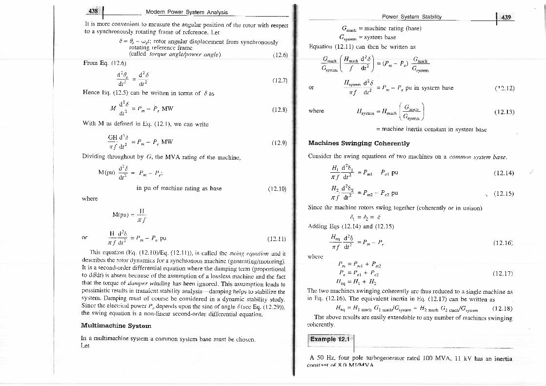
43S I Modern power Svstem Analvsist - -

It is more convenient to measure the angular position of the rotor with respectto a synchronously rotating frame of reference. Let

o = (a;,?;[' ;"':?: f#

u l ar di s P 1 ac e me n t fro m s y n c hron o u s l y

(r2.6)

(r2.7)

(called torque angle/power angle)From Eq. (12.6)

drg, _ d26,Jt2 dt2

Hence Eq. (12.5) can be written in terms of d as

, , d 2 6 'M - : = P ^ - P e M w

ot-

With M as defined in Eq. (12.1), we can write

GH d2d

f V - P * - P " M wDividing throughoutby G, the MVA rating of the machine,

a

M(pu) + = P*- P,;dt'

in pu of machine rating as base

where

(12.8)

(r2.9)

(12.r0)

M(Pu) = +lrj

H d z bor ^ - = P* - P , pu ( IZ .1 I )n f d t "

This equation (Eq. (12.1D)l}q.(12.1 1)), is called the stving ecluatioy and itdescribes the rotor dynamics fbr a synchronous machine (generating/motoring).It is a second-order differential equation where the darnping term (proportionalto d6ldt) is absent because of the assumption of a lossless machine ancl the factthat the torque of damper winding has been ignored. This assumption leads topessimistic results in transient stability analysis-dampinghelps to stabilize thesystem. Damping must of course be considered in a dynamic stability study.Since the electrical power P, depends upon the sine of angle d(see Eq. (12.29)),the swing equation is a non-linear second-order differential equation.

Multimachine System

In a multimachine system a common system base must be chosen.Let

_ Power System Stabitity _ I +Sl-

Grnu"h = machine rating (base)

Gryrt",o = system base

Equation (12.11) can then be written as

+-" (Yry*l = (p- - p.) g'""Gsystem \- / dt' )

\ "t c'

Grrr,.*

= machine inertia constant in system base

Machines Swinging Coherently

Consider the swing equations of two machines or a common system base.

or { " " " ' o ' ! = ' -P

"f dl

= P*- P"PU in sYstem base

where Hryr,"* = H-u"h t'+*l**" \.. Gt""'n /

Hr d261

"f a;

= P*r - P"t Pu

H2 d262

" f A;

= P*2- P"zPu

Since the machine rotors swing together (coherently or in unison)

6 , = [ r = [

Adding Eqs (12.14) and (12.15)

H"q d26

trf dtz = P*- P"

whcrcP r r = P * r + P n

P r = P " l * P r z

H " q = H r + H ,

ffimel"L2rl1

( t : . r2)

(r2.r3)

( r2 .14)

. (12. rs )

( r2 .16"

( r2 . r7 )

The two machines swinging coherently are thus reduced to a single machine asin Eq. (12.16). The equivalent inertia in Eq. (12.17) can be wrirten as

H"q, = Hl ,nu.h Gl ^ach/Grystem * Hz ^u"h G2 -u"h/G.yr,.. (12.18)

The above results are easily extendable to any number of machines swingingcoherently.

A 50 Hz, four pole turbogenerator rated 100 MVA, 11 kv has an inertiag6nsf an f n f R O MI / I \ / IVA

Find the stored energy in the rotor at synchronous speed.If the mechanical input is suclcJenly raised to 80 MW fbr an electrical loadof 50 MW, tind rotor acceleration, neglecting rrlechanical and electricallosses.

(c) If the acceleration calculated in part (b) is maintained for 10 cycles, findthe change in torque angle and rotor speed in revolutions per minute at theend of this period.

)olution(a) Stored energy = GH = 100 x g = g00 MJ

( b ) P , = 8 0 - 5 0 = 3 0 M W = M 4dt'

r, CH 800. 1 - -

180/ 180 x 50

4 d 2 6+'j 6,2

= 3o

or

r ) c

(c) 10 cycres = "lT

- 337 '5 elect deg/s2

Change in d= !{ZZI.S) x (0.2)2 = 6.75 elect degrees

= 6 0 x 3 3 7 ' 5 . o 1 ^ E !

2x360J = z6'12r {PnVs

. ' . Rotor speed at the end of l0 cvcles

- r2ox5o + 'z8. tz5 x 0 .24

= 1505.625 rpm

I2.3 POWER ANGLE EQUATION

In solving the s'uving equation (Eq (12.10)),certain simplifying assumpticns areusually made. These are:

1. Mechanical power input to the machine (P*) remains constant during theperiod of electromechanical transient of interest. In other words, it means thatthe effect of the turbine governing loop is ignored being much slower than thespeed of the transient. This assumption leads to pessimistic result-governingloop helps to stabil ize the sysrem.

'2. Rotor speed changes are insignificant-these have already been ignoredin formulating the swing equation.

(a)

(b)

t4/s' I torJern Power Srrctarn Anarrraio--

4 MJ-r/elect deg

teryer-Svele m-qtsqllv--

3. Effect of voltage regulating loop during the transient is ignored, as a

consequence the generated machine emf remains constant. This assumption also

leads to pessimistic results-voltage regulator helps to stabil ize the system.

Before the swing equation can be solved, it is necessary to determine the

dependence of the electrical powel otttput (P,,) upon the rotor angle.

Simplified Machine Model

For a nonsalient pole machine, the per phase induced emf-terminal voltage

equation under steady conditions is

where

E =V + jXolu+ jXol,,; X,r) X,r

I = I a + I s

( r2 . Ie )(r2.20)

(12.2r)

' (12.22)

and usual symbols are used.Under transient condition

X a - X ' a 1 X a

but

X'o = Xn since the main fleld is on the d-axis

Xtd < Xo ; but the difference is less than in Eq' (I2.I9)

Equation (12.19) during the transient modifies to

Et =V + jxt lo+ jXnln

=V + jXq(I - I) + jXotlo

= (Y + jxp + j(X'a - Xq)Id

The phasor diagram colresponding to Eql (12.21) and (12.22) is drawn in

Fig. 12.2.Since under transient condition, X'a 1X, but Xn remains almost unaffected,

it is fairly valid to assttme that

x'a = xq (r2.23)

Fig. 12.2 Phasor diagram-sal ient pole machine

,firZlll r"orrr r atysis _equation (12.22)now becomes

E , = V + j X n I

= V + jXotl (r2.24)The machine modalso applies to a cylindrical rotor machine where

- - - - - D '

X,l = X*/(transientsynchronous reactance)

The simplified machine of Fig. 12.3 will be used in all stabilitv studies.

P.ower Angle'Cunre

For the purposes of stability studies lEl1, transient emf of generator motor,remains constant or is the independent variable determined by the voltageregulating loop but v, the generator determined terminal voltage is a dependentvariable' Therefore, the nodes (buses) of the stability study network pertain tothe ernf terminal in the machine model as shown in rig. 12.4, while the machinereactance (Xu) is absorbed in the system network as clifferent from a load flowsttlcly' Fttrther, lhe loirt ls (othcr thrrn l iu'gc s;ynchronous ri it i tt ir.s) wil l bc r.cpiacetlby equivalent static admittances (connected in shunt between transmissionnetwork buses and the reference bus). This is so because load voltages varycltlr ing a stabil ity stutly (in a loacl l low stucly, the.se remain constant within analrow bancl).

,/

System network

Fig. 12.3 Simpli f ied machine model

Fig. 12.5 Two-bus stability study network

For the 2-bus system of Fig. 12.5

f Y , , Y "1Ynus = I - j ' - : ' l ; Y ,z= Yzr

LY^ Yr,[ I

Complex power into bus is given by

P i + j Q i - E l f

At bus I

Pr + jQr - Er' (YyE1)* + E, (YpEil*

But

(r2.2s)

(r2.26)

E ' t = l E i l l 6 ; E / = l E ' z l 1 4 .

Y,u = Gr t + jBt i Yrz = lYrzl l0 p

Since in solution of the swing equation only real power is involved, we havefrom Eq. (12.26)

I r t = l E l i 2 G t r + l E r t I i E i i i y , r l c o s ( , t i - , h - 0 , 2 ) u 2 . 2 7 )A similar equation will hold at bus 2.

Let

l E l l z G , = P ,

lEt ' l lEzt I lY7l = Pn,*

4 - 6 = 6and Qn = x/2 -1

Then Eq. (12.27) can be written as

Pr = P, * P,n"* sin (6 - 1); Power Angle Equation (IZ.ZB)

For a purely reactive network

Gtt = 0 (. ' . P. = 0); lossless network

} t z = n 1 2 , : . J = 0

P , = P ^ * s i n 6

Power Svstem Stabilitv [ECAC,+'T*

\ t 2

o @

O f r

Fig. 12.4

(12.29a)

I

I

where P^^, = lE'' I lE'' | '' - x '

simplified power angle equation

Yl aZ t

+= - P^ Pn'u* sin dpu7rI dt-

where X = transfer reactance between nodes (i.e., between E{'Ihe graphical plot of power angle equation (Eq.(12.29)) is

Fig. 12.6.

p " lI

DI max

(Ps6+APe).-....t-----*

Peo

- Generator

Fig. 12.6 Power angle curve

The swing equation (Eq. (12.10)) can now be written as

j0.5

i0.5

lE' l t61 lo"

(b)

F|g .12 .7As imp|esys temwi th i t s reac tanced iagram

0.5Xrz =0 '25 + 0 '1 + -

= 0.6

Consider now a more complicated case wherein a 3-phase fault occurs at the

midpoint of one of the lines in which case the reactance diagram becomes that

of Fig. 12.8 (a).

Star-Delta Conversion

Converting the star at the bus 3 to delta, the network transforms to that of

Fig. 12.8(b) wherein

(,

j0.25at(- U

(r2.29b)

and Ei)

shown in

(12.30)

which, as already stated, is a non-linear second-order differential equation withno damping.

T2.4 NODE ELIMINATION TECHNIOUE

In stability studies, it has been indicated that the buses to be considered are

those which are excited by the internal machine voltages (transient emf's) and

not the load buses which are excited by the terminal voltages of the generators.

Therefore, in Y"u, formulation for the stability study, the load buses must be

eliminated. Three methods are available for bus elimination. These are

illustrated by the simple system of Fig. 12.7(a) whose reactance diagram is

drawn in Fig. I2.7(b).In this simple situation, bus 3 gets easily eliminated by

parallel combination of the lines. Thus

o

(a)

lE/lt61ttr

446 L Modern power System Anatysis

lE/lt6

CD

(c)

F ig . 12.8

v _ 0.25 x 0.35 + 0.35 x 0.5 + 0.5 x0.25

= 1 . 5 5

This method for a complex network, however, cannot be mechainzed forpreparing a computer programme.

Thevenin's Equivalent

With ref'crcncc lo Fig. l2.ti(a), tho Thcvcnirr's ccluivalcnt lbr thc networkportion to the left of terminals a b as drawn in Fig. 12.8(c) wherein bus t hasbeen modified to 1/.

l u tPower System Stability ,

- _

This method obviously is cumbersome to apply for a network of even smallcomplexity and cannot be computenzed.

Node Elimination Technique

Formulate the bus admittances for the 3-bus system ofnetwork is redrawn in Fig. 12.9 wherein instead ofadmittances are shown. For this network.

Fig. 12.8(a). Thisreactance branch.

(r ra

(r2.31)

(r2.32)

of Eq. (12.31),

@ o

ruus

The bus 3 is to be eliminated.In general for a 3-bus system

f ' 'I fr' Y" t"lIu'Ilh | = lY^ Y, vu llv, ILlrl Lv,, Yn rrrJL%l

Since no source is connected at the bus 3I t = o

or Yr rVr+ Yr rVr+ Yr rVr=O

o r v z = - ? r r - ? r ,Yrt Y.,

Substituting this value of V3 in the remaining two equationsthereby eliminating Vy

I t =Y,Vt * YrzVz+ Yt tV t

=(", - Y,rYr, ) u +( y," - !+)v"- ( . ^ t t Y r ,

' [ ' t ' Y r , ) ' '

, r 0.25v r h =

0 2 5 + 0 - , 5 l E t l l 5

= 0.417 | Et I 16

0.35x0.25xrh =

035+025 - o '146

Xt2 =0 .146 + 0 .5 = 0 .646*

*This value is different from that obtained by star delta transformation aslonger lEtl I { in fact i t is 0.417 lEtl 16.

Itlow

Fig. 12.9

V* is no

In compact form

Ynus (reduced) =lt,i, ' l, l, '1lY'r, Y'r, )

Y ' t l = Y " - r y'33

Y'12 = Y'21= Ytz -

v t , = y r r - Y r t Y tt 22 - 'zz yT

In general, in eliminating node n

Yo^(old)Y,,(old)Yo, (new) = Yry (old)

Applying Eq. ( 12.34) to the example in hand

l-t.gztYsu5 (reduced) = ; 1 0.646L

It then follows that

X , t = : - = 1 . 5 4 8 ( = 1 . 5 5 )o.646

In the systenr shown in Fig. 12,10, a three-phase static capacitive reactor ofreactance 1 pu per phase is connected through a switch at motor bus bar.Calculate the limit of steady state power with and without reactor switch closed.Recalculate the power limit with capacitive reactor replaced by an inductivereactor of the same value.

to be 1.0 pu.

Solution

l E r l l E ^ l I . Z x I=f f i=m=o '49Pu

(2) Equivalent circuit with capacitive reactor is shown in Fig. 12.71 (a).

j1.o jo.l i0.25 io.1 i1.o p'e65

lEnl = 1.2 -i1.0 = lEml = 1.0

(a) (b)

Flg . 12 .11

Converting star to delta, the network of Fig. 12.11(a) is reduced to that of

Fig. 12.11(b) where

7X( t rans fer ) - /1 .35X/1 .1+/1 .1X(_J1.0)+( - /1 .0 )XJ1.35 . .-j1.0

= j0.965

. 1 .2x1Steady state power limit =

ffi = 1-244 pu

(3) With capacitive reactance replaced by inductive reactance, we get

equivalent circuit of Fig. 12.12. Converting ster to delta, we have

trasfer reactance of

i1.35 i1.1

Fig.12.12

_ j1.35 x.r1.l + "11.1x ll.0 + 11.0 x.t1.35

i 1.0

- j3.e35

YrtYt,

Ytt

(12.33)

Q23aa)

(r2.34b)

(r2.34c)

(r2.3s)

the

the

Fig . 12 .10

7X(transfer)

-!5o' l ""attt t"-t,

Steady state power timit - ' : ' ! ] = 0.304 pu3.935

Example 12.3

The generator of Fig. 12.7(a) is delivering 1.0 pu power to the infinite bus (lVl= 1'0 pu), with the generator terminal voltage of v,r = 1.0 pu. calculate thegenerator emf behind transient reactance. Find the maximu- io*". that can betransferred under the following conditions:

(a) System healthy(b) One line shorted (3_phase) in rhe middle(c) One line open.

. Plot all the three power angle curves.

Solution

L,et Vt = lV,l la = | laFrom power angle equation

t v t l l v I_ - - - s tn o=p"X

( t " t )

[ 0 2 5 + o J J s r n < t = I

or r r = 20.5"

Current into infinite bus.

Power System Stability hiffi

As already calculated in this section,

Xn = l '55

= !".!;!! = 0.6e4 pu

or P, = 0.694 sin d (ii)

(c) One line open:

It easily follows from Fig. 12.7(b) that

X r z = 0 . 2 5 + 0 . 1 + 0 . 5 = 0 . 8 5

P* . *= t i t ^o ] t = r .2650.85

or P" = I.265 sin 6 (iii)

The plot of the three power angle curves (Eqs. (i), (ii) and (iii)) is drawn inFig. 12.13. Under healthy condition, the system is operated with P,, = P, = 1.0pu and 6o= 33.9", i.e., at the point P on the power angle curve 1.79 sin d Asone line is shorted in the middle, Po, remains fixed at 1.0 pu (governing systemact instantaneously) and is further assumed to remain fixed throughout thetransient (governing action is slow), while the operating point instantly shifts to

Q on thc curvc 0.694 sin dat d= 33.9". Noticc thut bccuusc of machine inertiu,the rotor angle can not change suddenly.

1 . 7 9

1.265

Pn=1 'O

0.694

0

0.694 s in 6

33.90I

900 A

Fig. 12.13 Power angle curue,s-

I2.5 SIMPLE SYSTEMS

Machine Connected to Infinite Bus

Figure 12.14 is the circuit model of a single machine connected to infinite busthrough a line of reacthnce Xr.In this simple case

l V , l l a - l V l l 0 "

jx

| 120 .5 - I l 0i0.3s

= l + j 0 . 1 8 = 1 . 0 1 6 1 1 0 . 3 "Voltage behind transient reactance,

E t = t l t r + . j 0 . 6 x ( l + 7 0 . 1 g )= 0.892 + j0.6 - 1.075 133.9"

(a) System healrhy

p^u* = lv )-l Et | - 1x 1.075 - ., F,.\ ,-,x , ,

- c ,5

= t ' t9 PU

P, = I '79 sin d

(b) One line shorred in the middle:

I _

(i)

I

Xtransf.er =X'a* X,

From Eq. (12.29b)

,, ='4U sin d= p.u* sin dXt urrrf..

The dynamics of this sysrem are describecl in Eq. (12.11) as

-#ft= P^- P" Pu

P r l = - P r z = P "

The swing equations for the two machines can now be written as

t L _ _ r ( P ^ r _ P " r ) _ _ " ( p . - + \d t z

- " ' i f f , ) : u t t r r , l

(r2.36)

lE/lt6

Fi1.12.14 Machine connected to infinite bus

Two Machine System

The case of two finite machines connected through a line (X") is illustrated inFig. 12.15 where one of the machines must be generating und th" other mustbe motoring. Under steady condition, before the system goes into dynamics and

Fig. 12.15 Two-machine svstem

P * t = - P * z = P . (12.38a)the mechanical input/output of the two machines is assumed to remain constantat these values throughout the dynamics (governor action assumed slow).During steady state or in dynamic condition, the electrical power output of thegenerator must be absorbed by the motor (network being lossless). Thus at alltime

(12.38b)

(12.39a)

t -

Power System Stability I lt5'

d 2 6 " . ( P - r - P " r \ ( r - - n - )and it ="f

l2?:)= "tlH')Subtracting Eq. (12.39b) from Eq. (12.39a)

d2@,;6) =^r( ' : j r ! , ] , . - - P,)dtz

.J \ HrH, )

H"q d26o r - * . , = P n - P ,

7r I (lt-

w h e r e 6 = 4 - 6 .

rr - HtH,"eq Hl + Hz

The electrical power interchange is given by expression

p" = ,E!4!- ,in6' X'0, + x, + xd2

(r2.39b)

(r2.40)

(r2.4r)

(r2.42)

(r2.43)

(12.44)

The swing equation Eq. (12.41) and the power angle equation F;q- (12.aa)

have the same form as for a single machine connected to infinite bus. Thus a

two-machine system is equivalent to a single machine connected to infinite bus.

Because of this, the single-machine (connected to intinite bus) qYstem would be

studied extensively in this chapter.

In the system of Example 12.3, the generator has an inertia constant of 4 MJ/

MVA, write the swing equation upon occurrence of the fault. What is the initial

angular acceleration? If this acceleration can be assumed to remain constant for

Lt = 0.05s, find the rotor angle at the end of this time interval and the new

acceleration.

Solution

Swing equation upon occurrence of fault

H d ' 6 _ o D1 g 0 f d v

- r m - ' e

4 d,26 ,

* " t # = l - 0 ' 6 9 4 s i n 6

t4 = z2so (1 - 0.6e4 sin d;.d t "

,.4#jirf vooern power sysrem AnatysisI

Initial rotor angle do = 33.9" (calculated in Example 12.3)

a 2 s l; l = 2250 ( l - 0.694 sin 33.9")d t ' l , - n+

#l * = 0; rotor speed cannot change suddenlyC l l l r : o +

A, ( in A,t = 0.05s) = x 1379 x (0.05)2

7"

+ 4,6 = 33.9 + 1.7" = 35.6"

I2

t .

66 t =

a26 l. , | = 2250 (l - 0.694 sin 35.6")d r l

l r = 0 .05s

- l34I elect deg/s2Observe that as the rotor angle increases, the electrical power output of the

generator increases and so the acceleration of the rotor reduces.

12.6 STEADY STATE STABILITY

The steady state stability limit of a particular circuit of a power system isdefinecl as the maximutn power that can be transmitted tri fhe receivino en;without loss of synchronism.

v'r6 vrru

Consider the sirnple system of Fig. 12.14 whose clynamics is describect byequations

M* = P^ P" MW; Eq. (12.8)d l

M H= 7

ln Pu sYstem

and p, = !4)! ) ,in 6'= p^u*sin dx,t

For determination of steady state stability, the direct axis reactance (X.r) ant,voltage behind X4 are used in the above equahons.

The plot of Eq. (12.46) is given in Fig. 12.6. Let the system be operaringwith steady power transfer of P^ = P^with torque angle d as indicated in thefigure. Assume a small increment AP in the electric power with the input fromthe prime mover remaining fixed at p*(governor r.rforrr" is slow compared to

(12.4s)

(12.46'

L ltc..:']i;E!!";1&tffi

Linearizing about the operating point Qo (P"0, 4) *" can write

LP,= ( * ) . o ,

The excursions of A d are then described by

no 9i+' - P^ - (P,o + aP,') = - L,P,d,r

M d'+' *d r

(r2.47)

where

The systemequation

P ddt

stability to small changes is determined from the characteristic

Mp, +[#], =o

whosc two roots are

f / t \ t r , . 1 ( \ f {

P = + l - \ u 1 t 0 o ) o l -L M I

As long as (0P/0 0o it positive, the roots are purely imaginary and conjugate

and the system behaviour is oscillatory about do. Line resistance and damper

windings of machine, which have been ignored in the above modelling, cause

the system oscillations to decay. The system is therefore stable for a small

increment in power so long as

(a P,/aa| > o (12.48)

When (0 P/AD, is negative, the roots are real, one positive and the other

negative but of equal magnitude. The torque angle therefore increases without

bound upon occurrcncc ol a small powcr incretrtent (disturbancc) and the

synchronism is soon lost. The system is therefore unstable for

@ Pe/aDo < 0

@p/A[ois known as synchronizing cofficienr. This is also called stffiess

(electrical) of synchronous machine.Assuming lEl and lVl to remain constant, the system is unstable, if

l E l l v l c o s d ^ < o

X

po*e, systm st"uititv b{dffir-

o r 4 > 9 0 "The maximum power that can be transmitted without loss of stabili

(12.4e)

and is given by( r 2.s0)

(12.sr)l E n v l

If the system is operating below the limit of steady stability condition (Eq.12'48), it may continue to oscillate for a long time if the iamping is low.Persistent oscillations are a threat to system security. The study oi systemdamping is rhe study of dynamical stability.

The above procedure is also applicable for complex systems whereingovernor action and excitation control are also accounted for. The describingdi f ferent ia l equat ion is l inear izecl about the opcrat ing point . Concl i t iep fbrsteady state stability is then determined from the corresponding characteristicequation (which now is of order higher than two)

It was assumed in the above account that the internal rnachinc voltagelEl remains constant (i.e., excitation is held constant). The result is that asloading increases, the terminal voltage lv,l dips heavily which cannot betoleratcd in practice. Thereforc, we must consicler the steady state stability limitby assuming that excitation is adjusted for every load increase to keeplv,l constanr. This is how the system will be operaied practically. It may beunderstocd that we are still not considering the effect of automatic excitationcontrol.

steady state stabil ity l imit with lv,l anrt lvl constant is consiclered inExample 12.6.

A synchronous generator of reactance 1.20 pu is connected to an infinite busbar (l Vl = 1.0 pr) through transformers and a line of total reactance of 0.60 pu.The generator no load voltage is I .20 pu and its inertia constant is H = 4 MW-silvIVA. The resistance and machine damping may be assumed negligible. Thesystem frequency is 50 Hz.

Calculate the frequency of natural oscillations if the generator is loaded to(1) 50Vo and (ii) 80Vo of its maximum power limit.

Solution

(i) For 50Vo loading

I ae1 L2xrl - - e | _ ____ cos 30 "L 06 Jro" 1.8

= 0.577 MW (pu)/elect rad

H 4M(pu) =

o*ro =

t rx5o s?/crcct ratr

From characteristic equation

-+i(WiY")u == i4.76

P^u*

P=tr[(*),,"1*)'

FrequencY of oscillations =

(ii) For 807o loading

4.76 railsec

4'76 - 0.758 Hz2r

s i n d o = + = 0 . 8 o r 6 = 5 3 . 1 "P-u*

rqa) - r 'Zxr cos 53.1"\ 05 ) r r , 1 .8

= 0'4 MW (Pu)/elect rad

p =!, (q+k)* =* i3s6

Frequency of oscillations = 3.96 radlsec

Psm do - i t

' max

? q 6

')*

Find the steady state power limit of a system consisting of a generator

equivalent reactance 0.50 pu connected to an infinite bus through a series

rcactance gf 1.0 pu. The terminal voltage of the generator is held at 1.20 pu and

the voltage of the infinite bus is 1.0 pu.

Solution

The system is shown in Fig. 12.16. Let the voltage of the infinite bus be taken

as reference.= 0 . 5 o r 4 = 3 0 o

Then

Now

V = 7 . 0 / - f f ,

I _

lE4t6

E = Vt + jXdI = 1.2 l0 + j0.5

or

Now

0 = 73.87"

Vt = 1.2 /.73.87" = 0.332

r _ 0.332+.ir.rs2_r= t. t52 + j0.669

E -0.332 + jr .r52 + 70.5 (1.152 + j0.668)- 0.002 + j1.728 = 1.728 I90.

Steady state power limit is given by

p ^ u - l E l l V l 1 . 7 2 8 x L*= V;-+V

= -- i5 = l '152 Pu

If instead, the generator emf is held fixed at a value of r.2pu, the steadystate power limit would be

P*"* = i# = o'8 Pu

It is observed that regulating the generator emf to hold the terminal generator', 'oltage at r.2 pu raises thepowerli.it frorn 0.g pr'ro r.r52pu; this is howthe voltage regulating loop helps in power system stab'ity.

Xa= O'5

IVt= 1.219

m Analysis

Vt = ! .2 l0

1 . 2 1 0 - 7 . 0jI

V = 1.0100

Flg. 12.16

.E = l .g l0 _ 0.5 = (t .g cos e_ 0.5) + 71.g sin 0Steady state porver rimit is reached when E has an angle of 6= 90o, i.e., its realpart is zero. Thus,

1 . 8 c o s 0 - 0 . 5 = 0

r .2 lg - 1 .0rI

L IJ

Power Srrstem Stahilitu EsE

A knowledge of steady state stability limit is important for various reasons. Asystem can be operated above its transient stability limit but not above itssteady-tatelimit. Nowrwith increased fault el,earing speedsjt is possible tomake the transient limit closely approach the steady state limit.

As is clear from Eq. (12.51), the methods of improving steady state stabilitylimit of a system are to reduce X and increase either or both lEl and I Vl. If thetransmission lines are of sufficiently high reactance, the stability limit can beraised by using two parallel lines which incidently also increases the reliabilityof the system. Series capacitors are sometimes employed in lines to get bettervoltage regulation and to raise the stability limit by decreasing the linereactance. Higher excitation voltages and quick excitation system are alsoemployed to improve the stability limit.

I2.7 TRANSIENT STABITITY

It has been shown in Sec. L2.4 that the dynamics of a single synchrono,rsmachine connected to infinite bus bars is governed by the nonlinear differentialequation

+ j t .152

, , d '6M iF

=P^- P"

where P, = P-* sin d

- _ d 2 6or M --+ - P*- P** sind

ot-(r2.s2)

As said earlier, this equation is known as the swing equation. No closed formsolution exists for swing equation except for the simple case P- = 0 (not apractical case) which involves elliptical integrals. For small disturbance (say,gradual loading), the equation can be linearized (see Sec. 12.6) leading to theconcept of steady state stability where a unique criterion of stability(APrlAd>0) could be established. No generalized criteria are available* fordetermining system stability with large disturbances (called transient stability).The practical approach to the transient stability problem is therefore to list allimportant severe disturbances along with their possible locations to which thesystern is likely to be subjected according to the experience and judgement ofthe power system analyst. Numerical solution of the swing equation (orequations for a multimachine case) is then obtained in the presence of suchdisturbances giving a plot of d vs. r called the swing curve. If d starts todecrease after reaching a maximum value, it is normally assumed that thesystem is stable and the oscillation of daround the equilibrium point will decay

tRecent literature gives methods of determining transient stability throughLiapunov and Popov's stability criteria, b:rt these have not been of partical use so far.

ffiffif Modern power System AnatysisI

and finally die out. As already pointed out in the introduction, important severedistulbances are a short circuit or a sudden loss of load.

For ease of analysis certain assumptions and simplifications are always made(some of these have already been made in arriving at the swing equation (Eq./ 1 / l < . t \ \ a r r 1 1 -

consequences upon accuracy of results.1. Transmission line as well as synchronous machine resistance are

ignored. This leads to pessimistic result as resistance introduces damping termin the swing equation which helps stability. In Example I2.11, line iesistancehas been taken into account.

2. Damping term contributed by synchronous machine damper windings isignored. This also leads to pessimistic results for the transient stability limit.

3. Rotor speed is assumed to be synchronous. In fact it varies insignifi-cantly during the course of the stability transient.

4. Mechanical input to machine is assumed to remain constant durins thetransient, i.e., regulating action of the generator loop is ignored. This leais topessimistic results.

5. Voltage behind transient reactance is assumed to remain constant, i.e.,action of voltage regulating loop is ignored. It also leads to pessimistic results.

6. Shunt capacitances are not difficult to account for in a stability study.Where ignored, no greatly significant error is caused.

7. Loads are modelled as constant admittances. This is a reasonablvaccurate representation.

Note: Since rotor speed and hence frequency vary insignificantly, the networkparameters remain fixed during a stability study.

A digital computer programme to compute the transient following suddendisturbance aan be suitably modified to include the effect of governlr actionand excitation control.

Upon occulTence of a severe disturbance, say a short circuit, the powertransfer between machines is greatly reduced, causing the machine torqueangles to swing relatively. The circuit breakers near the fault disconnect the

Power S','stem StabilitY ffiffi

p"rrnon.ntly till cleared manually. Since in the majority of faults the first

ieclosure will be successful, the chances of system stability are greatly

enhanced by using autoreclose breakers.

Fig.12.17

In the case of a perrnanent fault, this system completely falls apart. This will

not be the case in a multimachine system. The steps listed, in fact, apply to a

system of any size.

1. From prefault loading, determine the voltage behind transient reactance

and the torque angle 16o of the machine with reference to the infinite bus.

2. For the specified fault, determine the power transfer equation Pr(A during

^ault. In this system P" = 0 for a three-phase fault' ' '

From the swing equation starting with fi as obtained in step 1, calculate

das a function of time using a numerical technique of solving thetnon-

linear differential equation.

After clearance of the fault, once again determine P, (A and solve further

for d (r). In this case, P"(A = 0 as when the fault is cleared, the system

gets Cisconnected.

After the transmission line is switched on, again find P" (0 and continue

to calculate d (r).

If 6 (t) goes through a maximum value and starts to reduce, the system is

regarded as stable. It is unstable if d(r) continues to increase. Calculation

is ceased after a suitable length of time.

An important numerical method of calculating d(t) from the swing equation

will be giurn in Section 12.9. For the single machine infinite bus bar system,

stability can be conveniently determined by the equal area criterion presented

in the following section.

I2.8 EOUAL AREA CRITERION

In a system where one machine is swinging with respect to an infinite bus, it

is possible to study transient stability by means of a simple criterion, without

resorting to the numerical solution of a swing equation.

5 .

4.

5 .

6.

Consider the swing equation

&rt ,"= accelerating powerd26 I

AF =

*@^- P '1 =

M = !rf

ln pu system (r2.s3)

Fig. 12.1g prot of 6 vs tfor stabre and unstabre systems

lf the system is unstable dcontinues to increase indefinitely with time and themachine loses synchronism. on the other hand, if the system is stable, 6(t)performs oscillations (nonsinusoidal) whose amplitude decreases in actualpraetice because of darnping terms (not included in the swing equation). Thesetwo situations are shown in nig. 12.1g. since the system is non_linear, thenature of its response 160l is not unique and it may exhibit instability in afashion different from that indicated in Fig. rz.rg,depending upon the natureand severity of disturbance. However. experience indicates ihai the response6!'l j" a power system generally falls in the two broad categories as shown inthe figure' It can easily be visualized now (this has also been stated earlier) thatfor a stable system, indication of stability will be given by observation of thefirst swing where dwill go to a maximum and will Jturt to reduce. This fact canbe stated as a stability criterion, that the system is stable if at some timed 6

= od t

and is unstable, if

d 6- - > 0<lt

for a sufticiently long time (more than 1 s will genera'y do).

(r2.s4)

(12.ss)

Multiplying both sides of the swing equation * [t#),

we get

The stability criterion for power systems stated above can be converted intca simple and easily applicable form for a single machine infinite bus system.

2P" d6M d t

Ifrtegrating, we have

(r2.s6)

where do is the initial rotor angle before it begins to swing due to disturbance.From Eqs. (12.55) and (12.56), the condition for stability can be written as

6

o r [ r " a d - o6,,

The condition of stability can therefore be stated as: the system is stable if theareaunder Po(accelerating power) -dcurve reduces to zero at some value ofd In other words, the positive (accelerating) area under Po- 6curve must equalthe negative (decelerating) area and hence the name 'equal area' criterion of

lstability.To illustrate the equal area criterion of stability, we now consider several

types of disturbances that may occur in a single machine infinite bus barsystem.

Sudden Change in Mechanical Input

Figure 12.t9 shows the transient model of a single machine tied to infinite busbar. The electrical power transmitted is given by

(r2.s7)

-->

Pm

Infinitebus bar

lv l r0o

F ig . 12 .19

ffifftl| Modern Power svstem nnarys,s

l E t l l v lP, =

u, # sin d- P** sind,

n d T ^ e

Under steady operating condition

P.o = Pro = P** sin do

Flg. 12.20 P"- 6 diagram for sudden increase in mechanical input togenerator of Fig. 12.19

This is indicated by the point ainthe Pr- 6 diagram of Fig. 12.20.Let the mechanical input to the rotor be suddenly increased to Pn (by

opening the steam valve). The accelerating power 1o = P*t - P, causes'therotor speed to increase (u> a,,r) and so does the rotor angle. At angle 6r,,Po= P*r- Pr(= P-* sin 4) = O (state point atb)but the rotor angle continuesto increase as t., ) ur.Po now becomes negative (decelerating), the rotor speedbegins to reduce but the angle continues to increase till at angle 6., a= ur onceagain (state point at c. At c), the-decelerating area A, equals the accelerating

bc

area A, (areas are shaded), j.e., J ,, Od = 0. Since the rotor is decelerating,6o

the speed reduces below ur and the rotor angle begins to reduce. The state pointnow traverses the P, - 6 curve in the opposite direction as indicated by arrowsin Fig. 12.20.It is easily seen that the system oscillates about the new steadystate point b (6= 4) with angle excursion up to 6 *d 4.on the two sides.These oscillations are similar to the simple harmonic motion of an inertia-springsystem except that these are not sinusoidal.

As the oscillations decay out because of inherent system damping (notmodelled),.the system settles to the new steady state where

P^t = P, = Prn.* sin dl

6 b f i 6 2%

?' i ( 's

Q < ( 4

4n

A r = ) ( P n - P " ) d 6

A z = i < r , - P ^ ) d 66l

be possible to find angle d2 such that

rg condition is finally reached when 41

own in Fig.l2.2L Under this condition,

hat

6 . = 6 ^ o = T - 6 t = n'-sin-l +:

(12.58)

Fig. 12.21 Limiting case of transient stability with mechanical input

suddenlY increased

Any turther increas e in P ̂ , means that the area available for A, is less than A1'

so that the excess kinetic energy causes d to increase beyond point c and the

decelerating power changes over to accelerating power, with the system

consequently becoming uistable. It has thus been shown by use of the equal

area criterion that there-is an upper limit to sudden increase in mechanical input

(P^r- Po,s), for the system in question to remain stable'' 'ii

',,uy'ulso be not"i from Fig. 12.21that the system will remain stable even

though the rotor may oscillate beyo-nd -{^=.90"' so long as the equal area

criterion is met. The condition of d = 90" is meant for use in steady state

stability only and does not apply to the transient stability case'

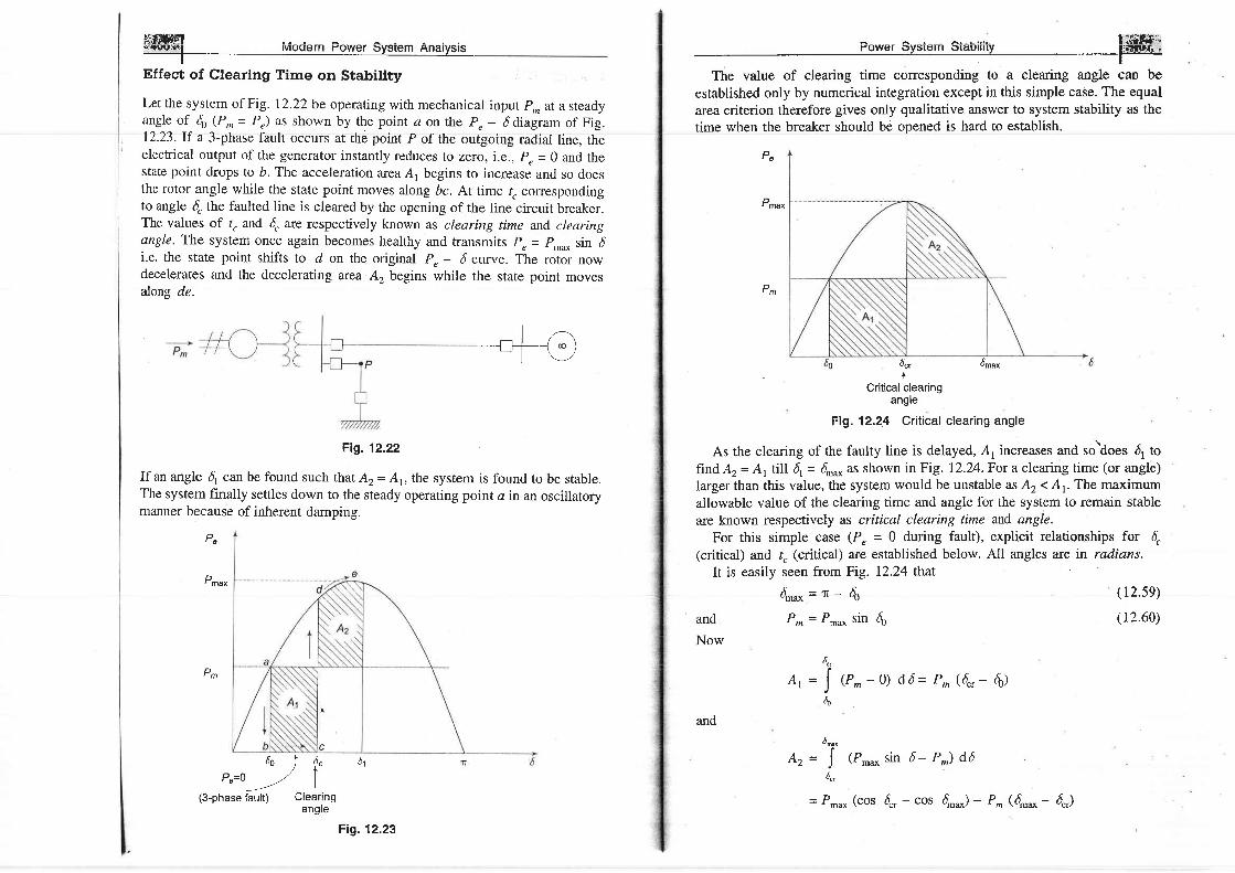
trs#ffi r._r_..._ A{i..fuu.xdr ruooern Fower uvslem Anarvsrs-

Effect of Clearing Time on Stability

Let the system of Fig. 12.22 be operating with mechanical input P^ at a steadyangle of d0 (Pn,= P") as shown by the point a on the Pr- 6 cliagram of Fig.12.23.If a 3-phase fault occurs at the point P of the outgoing radial line, theelectrical output of the generator instantly reduces to zero, i.e,, p, = 0 and thestate point drops to b. The acceleration area A, begins to increase and so doesthe rotor angle while the state point moves along bc. At time /. correspondingto angle 6, the faulted line is cleared by the opening of the line circuit breaker.The values of /, attd 4 are respectively known as clearing time and, clearingangle. The system once again becomes healthy and transmits p, = p,ou,. sin di.e. the state point shifts to d on the original P, - d curve. The rotor nowdecelerates and the decelerating area A, begins while the state point movesalong de.

F19.12.22

If an angle fi can be found such that A2= Ap the system is found to be stable.The systern finally settles down to the steady operating point a rn an oscillatorymanner because of inherent damping.

| /'-\- l l \

|-t___j co )- l \ - /

Pe

D, max

Pm

6 e l f . "

P"=o -.--/ i(3-phase fault) Clearing

61

angle

Fig. 12.23

l':fiffn#;i;Power a

t rresponding to a clearing angle can beestablished only by numerical integration except in this simple case. The equalarea criterion therefore gives only qualitative answer to system stability as thetime whgn the breaker should be opened is hard to establish.

Pe

D' max

I d", 6r"*+

Critical clearingangle

Fig. 12.24 Critical clearing angle

As the clearing of the faulty line is delayed, A, increases and so\oes d, tofind A2 = Ar till 6r = 6^ as shown in Fig. 12.24. For a clearing time (or angle)larger than this value, the system would be unstable as A, < Ar The maximumaiiowabie vaiue of the clearing time and angle for the system to remain stabieare known respectively as critical clearing time and angle.

For this simple case (P, = 0 during fault), explicit relationships for 6,(critical) and t" (critical) are established below. All angles are in radians.

It is easily seen from Fig. 12.24 that

Pm

4 n u * = T - d ;

and P*= Pr* sin 6o

Now

A t = (P^ --0) d 6 = P^ (4, - 6)

A z = (P** sin d- P^) d6

( 12.59)

(r2.60)

uct

Jh

6 ^ ^

J6,,

and

= P.u* (cos d, - cos d-*) - P* (6^o - 6"i)

ffil uoo"rn po*"r system AnatvsisFor the system to be stable, A2= A1, which yields

cos {. = !^ (5,^^" -Prn*

\ -tniu( d) + cos 4o"*

where 4, = critical clearing angleSubstituting Eqs. (1259) and (12.60) in Eq. (12.61), we get

4r = cos-t [(r, _ Z6l sin do _ cos 6o]During the period the fault is persisting, the swing equation is

d,2 d rf

d,r, =

1r: P^: P, = o

Integrating twice

P*tz + $

/cr = critical clearing time

4, = critical clearing angleFrom Eq. (12.6a)

6 = -,rf-2H

0" ,=# P ;2 " , 160

(r2.61)

(r2.62)

(12.63)

(12.64)

(r2.6s)

where

where d, is given by the expression of Eq, (12.62)An explicit relationship I 'rrr clctenninirtg r., i , porisiblc in this case as tluringthe faulted condition p" = o and so trre ,wing equation can be integrated inclosed form. This will not be the case in mosi other situations.

Sudden Loss of One of parallel Lines

consider now a single machine tied to infinite bus through two parallel l ines asin Fig. 12.25a. circuit model of the sysrem is given in Fig. r2.25b.Let us study the transient stability of the ,yir"rn when one of the lines issuddenly switched off with the system operating at a steady road. Beforeswitching off, power angle curve is given by

P " r = l E ' l l v l

xa i xt l lx2 sin d= Pm*l sin d

Immediately on switching off line 2, power angre curve is given by

P"n = g:+ sin d= pmaxr sin d,\d -T rt7

2H(6, , - 4 )TrfP*

,, /__\ l_Lr__l I Infinite, .774 ) | I - l bus

P m t t \ - - l I V V O "L r l

IVVO"

(b)

Fi1.12.25 Single machine tied to infinite bus through two par:allel l ines

Both these curves are plotted in Fig. 12.26, wherein P-u*n ( P_u*r as (Yo * Xr)> (Ya + Xr ll X).The system is operating initially with a steady power transferPr= P^ at a torque angle 4 on curve I.

Immediately on switching off line 2, the electrical operating point shifts tocurve II (point b). Accelerating energy corresponding to area A, is put into rotorfollowed by decelerating energy for 6 > q. Assuming that an area A2corresponding fo decelerating energy (energy out of rotor) can be found suchthat At = Az, the system will be stable and will finally operate at ccorresponding to a new, rotor angle 6, > 60" This is so because a single lineoffers larger reactance and larger rotor angle is needed to transfer the samesteady power.

Fig.12.26 Equal area criterion applied to the opening of one of the twolines in parallel

W

(a)

/

," (both lines in)

ffiffi-4l Mod"rn po*rr. surt* nrryr',

4 = 4 o * _ T _ 6 ,which is the same condition as in the previous example.

Sudden Short Circuit on One of parallel Lines

Case a: Short circuit at one end of line

Let us now assume the disturbance to be a short circuit at the generator end ofline 2 of a double circuit line as shown in Fig. 12.27a. We shall assume thefault to be a three-phase one.

Power Sy-t-- St"blllry-

via the healthy line (through higher linereactance X2 in place of Xl ll Xz)7; with power angle curve

sln sin d

obviously, P-o[ ( P-"*r. The rotor now starts to decelerate as shown inFig. 12.28. The system will be stable if a decelerating area A, can be foundequal to accelerating area A, before d reaches the maximum allowable value4o*.At areaA, depends upon clearing time /. (corresponding to clearing angle{), clearing time must be less than a certain value (critical clearing time) forthe system to be stable. It is to be observed that the equal area criterion helpsto determine critical clearing angle and not critical clearing time. Criticalclearing time can be obtained by numerical solution of the swing equation(discussed in Section 12.8).

P"y, prefault (2 lines)

P6n1, postfault (1 line)

? t 6

Ffg. 12.28 Equal area criterion applied to the system of Fig. 12.24a,I system normal, ll fault applied, lll faulted line isolated.

It also easily follows that larger initial loading (P.) increases A, for a givenclearing angle (and time) and therefore quicker fault clearing would be neededto maintain stable operation.

Case b: Short circuit away from line ends

When the fault occurs away from line ends (say in the middle of a line), thereis some power flow during the fault though considerably reduced, as differentfrom case a where Pen = 0. Circuit model of the system during fault is nowshown in Fig. 12.29a. This circuit reduces to that of Fig. 12.29c through onedelta-star and one star-delta conversion. Instead, node elimination technique ofSection 12.3 could be employed profitably. The power angle curve during faultis therefore given by

P" t= | E l l v l

s in d= Pmaxr r s in d'1r'II

X2

, (b)

F19.12.27 Shoft circuit at one end of the l ine

Before the occurrence of a fault, the power angle curve is given by'--

p"t = ,)4,'rlr,,,a, sin d= p_*, sin d' xi + xltx2which is plotted in Fig. 12.25.

Upon occulrence of a three-phase fault at the generator end of line 2 (seeFig. I2.24a), the generator gets isolated from the power system for purposes ofpower flow as shown by Fig. 12.27b. Thus during the period the fauit lasts,

The rotor therefore accelerate, .i;t:;i"s dincreases. synchronism will belost unless the fault is cleared in time.

The circuit breakers at the two ends of the faulted line open at time tc(corresponding to angle 4), the clearing time, disconnecting the faulted line.

ffiil Modern Power svstem Analvsis+ t * F ; 4 - l ' ! ' v e v " ' ' - ' - v ' v , - ' - " ' '

" ' - ' , - ' -

I

ls#z#i

system operation is shown in Fig. 12.30, wherein it is possible to find an area

A, equal-to A, for q. < 4nu*. At the clearing angle d. is increased, area

ai increat"t und to nna Az = Ar, 4. increases till it has a value 4n*' t6"-ooi*,,- ollnrvohle fnr stahilitv This case of critical clearine angle is shown

in Fig. 12.3L

Pe

Fig. 12.31 Fault on middle of one line of the system of Fig. t2.l4a, case ofcritical clearing angle

Annlvins eoual area eriterion to the case of critical clearing angle of Fig. 12.31'

we can wnte

4, dntn'

j (P^- 4n*u sinfldd= J {r^*r sind- P^) d660 6,,

(c)

Fig. 12.29

P"rand P,u as in Fig. 12.28 and Per as obtained above are all plotted in Fig.

I2.3O. Accelerating area A, corresponding to a given clearing angle d is less

Pe

Fig. 12.30 Fault on middle of one line of the system of Fig. 12.24awith d" < {,

X6x,t

(b)

Xr

where

4,,* =T - sin-r (:t_)V maxIII ./

Integrating, we get

l6*(P^a + Pmaxrr cos d) | * (P'*,,1 cos d +

1 6 o

or

(r2.66)

= Q

P^ (6", - 6) * P.u*u (cos '[. - cos do)

I P* (6** - 6"r) * P-om (cos fi* - cos 4J = 0

Pr1, prefault (2 l ines)

P6111, postfault (1 line)

xcG @

,.a P"'Prefault (2 l ines)

P"11;, postfault (1 l ine)

P"11, during fault

t

cos {r = :otd",*4naxtn

- PmaxII

critical clearing angle can be calculated from Eq. (12.67) above. The angles in:lt::t1|on

are in radians. The equation mooiiies as below if the angJes areln oegrees.

cos {. - ft

r.(6 ^i* - do ) - Pmaxrr cos do * prnu*ru cos d,ou*

Pmaxltr - Prnaxn

Case c: Reclosure

If the circuit breakers of line 2 are reclosed successfully (i.e., the fault was atransient one and therefore vanished on clearing the faurty line), the powertransfer once again becomes

P"N = P"r= p*u*I sin dSince reclosure restores power transfer, the chances of stable operati'nimprove. A case of stable operation is indicated by Fig. 12.32.

For critical clearing angle

(Clearing angle) \(Angle of reclosure )

Fig- 12-32 Faurt in middre of a rine of the system of Fig. 12.27awhere trrj tr, + r; T = time betw,een clearing ancl reclosure.

(12.67)

4 = 4r* = 1T - sin-l 1p_/p*.*r;tuc r

6 r c

J @r,- Pmaxrr sin 0 dd = J (p.*m sin d_ pm) d,6

60 6r,

dru,t

+ J (P,*r sin d_ p^) d66.-

i0.s

Give the system of Fig.P as shown.

12,33 where a three-phasc fault is applied at rhe point

Infinitebus

vFlloo

Flg. 12.33

Find the critical clearing angle for clearing the fault with simultaneous openingof the breakers I and 2. T\e reactance values of'various components areindicated on the diagram. The generator is delivering 1.0 pu power at the instanrpreceding the fault.

Solution

With reference to Fig. 12.31, three separate power angle curves are involved.

f. Normal operation (prefault)

Xr=0.2s+f f i+0 .05

= 0.522 pu

p,t=rysind: ffirino

= 2.3 sin d (i l

Prefault operating power angle is given by

1.0 = 2.3 sin 6or 6o =25.8" = 0.45 radians

IL During fault

It is clear from Fig. 12.31 that no power is ffansferred during fault, i.e.,

,0.:"o

= o

t r i n 1n 1A

iffi Modern power System Anatysis

rrr. Post fault operation (fault cleared by openingr the faultedIiae)

UE

= - 1.5 (cos 2.41 - cos 6,) - (2.41 - 6")

= 1.5 cos 6", + 6r, - I.293

Setting A = Az and solving

6r, - 0.45 = 1.5 cos 6r, + 6r, - 1.293

or cos {,. = 0.84311.5 - 0.562

or 4, = 55.8"

The corresponding power angle diagrams are shown in Fig. 12.35.

Find the critical clearing angle for the system shown in Fig. 12.36 for a three-phase fault at the point P. The generator is delivering 1.0 pu power underprefault conditions.

n l.2xl.0Perrr= ff

sin d= 1.5 sin 6 (iii)

Pe

Pn=1 'O

66=0.45 rad 6^rr=2.41 rdd

Fig. 12.35

T T t o - o o i * " * - ^ * : ^ ^ : L l ^ ^ - - l ^ C f ^ - - - - - - ^ .rrrw urour.rLurr psl l luDDlulc al i lBrtr Omax l()f afea Al = A2 (Sge f lg.

given by

4 o u * = r - s i n - l I = 2 . 4 L r a d i a n s1.5

Applying equal area criterion for critical clearing angle {Ar = P^ (6", - 6)

= 1.0 (6", - 0.45) = 6c, - 0.45

dr*

A z = ! { r , n - p ^ ) d , 66,,

2 .41I= | (1 .5 s in 6 - 1 ) dd

J6.,

r 2 . 4 1

= - 1 . 5 c o s d _ d l| 6",

i0.1 5 i 0.1s

lnfinitebus

lvF1.otoo

.10.15 jo.15

Flg. 12.36

Solution

f, Prefault operation Transfer reactance between generator and infinitebus is

& = 0.25 + 0.17 +0 .15+0 .28+0 .15= 0.71

12.35) is

P- , = r 'Zx l s in d= 1 .69 s inc ' 0.71(i)

2

6

The operating power angle is given by

1.0 = 1.69 sin ,fr

or do = 0.633 rad

IL Durtng fault The positive sequence reactance diagram during fault ispresented in Fig. 12.37a.

lF,l=1.2 Pu

j0.25J 000 L / 000 L--- - - - - - - - r 000 \ -

j0 .15 j0.14 j0.14 j0.'15

jo .17

++

0 '

) E1=t.z V=1.0

(a) Positive sequence reactance diagram during fault

j0.25 j0.145 j0.145 ', j0.17

lE'l=1.2 V=1.OlOo

(b) Network after ddlta-star conversion

l9l=1'z V=1.0100

(c) Network after star-delta conversion

. Ftg. 12.32

Converting delta to star*, the reactance network is changed to that of Fig.12.37(b). Further, upon converting star to delta, we obtain the reactancenetwork of Fig. .r2.37(c). The transfer reactance is given 6y

(0.2s + 0.145) 0.072s + (0.145 + 0.17) 0.0725 + (0.25 + 0.145)

X u = (0.14s + 0.17)0.075

_ 2.424

p - = lal! sin d = 0.495 sin 6r eI - i.+Z+

uur v - v.a/,

Postfault operation (faulty line switched off)

Xr l =0 .25 + 0 .15 + 0 .28 + 0 .15 + 0 .17 = 1 .0

*Node elirnination technique would be'used for complex network.

fir.

(ii)

Power System Stabilit-v Mi#ffir*Perrr=U! sin d = r'2 sin 6' l

With reference to Fig. 12.30 and Eq. (12.66), we have

(iii)

To find the cqitical clearing angle, areas A1 and A, arc to be equated.6",

At = l.o (6,,- 0.633) - , J o.+e5 sin d dd60

and

dmaxf

Az = | 1 .2 s in ddd- 1.0 (2.155 - 4)- J

6-cr

Now

A t = A z

or

6r, = 0.633 ---

o

2.155

= [ t.Z rin 6 d6 - 2.t55 + 6,,J '6cr

or - 0.633 + 0.495 cos olo' = - 1.2 cos ol"tt -2.155lo.orr la.,

or - 0.633 + 0.495 cos 6,, - 0.399 = 0.661 + 1.2 cos 6", - 2.155

or cos 6r, = 0.655

U 6r, = 49.I"

A generator operating at 50 Hz delivers 1 pu power to an infinite bus througha transmission circuit in which resistance is ignored. A fault takes placereducing the maximum power transferable to 0.5 pu whereas before the fault,this power was 2.0 pu and after the clearance of the fault, it is 1.5 pu. By theuse of equal area criterion, determine the critical clearing angle.

Solution

All the three power angle curves are shown in Fig. 12.30.

J.63

0.495 sin d ddJ

,'ffi| Mod"rn Po*.. sEl!"-n An"lytit

Ilere P-"*r =2.0 pu, Pmaxl = 0.5 pu and Pmaxrrr = 1.5 pu

Initial loading P^ = 1.0 pu

Applying Eq.

cos {, -

( p \

6r,ro= zr sin I tffiJ

E 7 - s i n l 1 : 2 . 4 ! r a d1.5

(r2.67)

1.0(2.41 - 0.523) - 0.5 cos 0.523 + 1.5 cos 2.41 = o ???1.5 -- 0.5

6r, = 70'3"

T2.9 NUMERICAT SOTUTION OF SWING EOUATION

In most practical systems, after machine lumping has been done, there are still

more than two machines to be considered from the point of view of system

stability. Therefore, there is no choice but to solve thp swing equation of each

machine by a numerical technique on the digital computer. Even in the case of

a single machine tied to infinite bus bar, the critical clearing time cannot be

obtained from equal area criterion and we have to make this calculation! . . r r - - r r - - - - - - - l - - - - - : - - - - - - - L l ^ , z F L ^ - ^ | - ^ - L l ^ + i ^ ^ + ^ l * ^ + L ^ l -

numerlca[y mrougn swulg equauulr. t rttrIc aIU ssvtrIi lr JuPurDtruilL('(l l l lELlluLlD

now available for the solution of the swing equation including the powerful

Runge-Kutta method. He.re we shall treat the point-by-point method of solution

which is a conventional, approximate method like all numerical methods but a

well tried and proven one. We shall illustrate the point-by-point method for one

machine tied to infinite bus bar. The procedure is, however, general and can be

applied-to every machine of a multimachine system.Consider the swing equation

d26 1 --; T

= ; e * - P ^ * s i n d ) :

P o l M ;

(* - 9H orin pu system M = +)\ 7t iTf)

The solution c(r) is obtained at discrete intervals of time with interval spread

of At uniform throughout. Accelerating power and change in speed which are

continuous functions of time are discretrzed as below:1. The accelerating power Po computed at the beginning of an interval is

assumed to remain constant from the middle of the preceding interval to the

middle of the interval being considered as shown in Fig. t2.38.

r>2 n-1

Discrete solution

n

Continuous solutionU

un-|/2

u13/2un-I/T-+tsn4l2

n-2 p3l2 n-'l r>112 n

6n-z

n-2 n-1 n

Fig. 12.38 Point-by-point solut ion of swing equation

In Fig. L2.38, the numbering on tl\t axis pertains to the end of intervals. Atthe end of the (n -l)th interval, the acceleration power is

Pa (n_r)-- Pm- P-* sh 4-r Q2.68)

where d_1 has been previously calculated. The change in velocit! (a= d6ldt),caused by the Pa@-r), assumed constant over At from (n-312) to (n-ll2) is

tAf

- tAf

$n-i

J-Af

wn-'2- wn-3t2= (Lt /M) Pa@-r)

The change in d during the (n-l)th interval is

L6r-t= 6r-1 - 6n-2= A'tun4'2

and during the nth interval

L6r- 6n- 6n-t= / \ tun-112

(12.6e)

(12.70a)

(12.70b)

2.The angular rotor velocity u= d6ldt (over and above synchronous velocity

t

,ir Yirtvt r t Ar lr.rl b r )

Subtracting Eq. (12.70a\ from Eq. (12.70b) and using Eq. (12.69), we get

L'6,= A6,-t +

Using this, we can write

(12.7r)

6n = 6n-t + L,6n G2.72)

The process of computation is now repeated to obtain Pa61, L6r*tand d*t. Thetime solution in discrete form is thus carried out over the desired length of time,normally 0.5 s. Continuous form of solution is obtained by drawing a ;moothcurve through discrete values as shown in Fig. 12.38. Greater accuracy ofsolution can be achi.eved by reducing the time duration of intervals.

The occurrence or removal of a fault or initiation of any switching eventcauses a discontinuity in accelerating power Po.lf such a discontinuity occursat the beginning of an interval, then the average of the values of Po before and

after the discontinuity must be used. Thus, in computing the increment of angleoccurring durirrg the first interval after a fault is applied at t = 0, Eq. (I2.7I)

becomes

7, ,6 , = (Ar ) t

*Pao+, M 2

where Pos* is the accelerating power immediately after occurrence of fault.Immediately before the fault the system is in steady state, so that Poo- = 0 andds is a known value. If the fault is cleared at the beginning of the nth interval,

in calculation for this interval one should use for Pa@-r) the value llP"6-r>-+ Po6_9*), where Pa@_r)- is the accelerating power immediately before clearingand Po6_r)+ is that immediately after clearing the fault. If the discontinuityoccurs at ihe miciciie of an intervai, no speciai proceciure is neecled. Theincrement of angle during such an interval is calculated, as usual, from thevalue of Po at the beginning of the interval.

The procedure of calculating solution of swing equation is illustrated in thefollowing example.

A 20 MVA, 50 Hz generator delivers 18 MW over a double circuit line to aninfinite bus. The generator has kinetic energy of 2.52 MJA4VA at rated speed.The generator transient reactance is X/o = 0.35 pu. Each transmission circuithas R = 0 and a reactance of 0.2 pu on a 20 MVA bgq-e. lE/l = 1.1 pu andinfinite bus voltage V = 7.0 10". A three-phase short circuit occurs at the midpoint of one of the transmission lines. Plot swing curves with fault cleared bysimrrltaneous opening of breakers at both ends of the line at2.5 cycles and 6.25cycles after the occuffence of fault. Also plot the swing curve over the periodof 0.5 s if the fault is sustained.

(A r )2 DM

r a ( .n - I )

power System Stabilitv [i{8il;r

Q ^ t , , 1 ; ^ ^ E ^ f ^ - ^ ^ - * 1 , , + L ^ ^ + ^ - L . . ^ + ^ - - ^ r l . ^ l - ^ - t ^ - - - r - - - r - a -\rvtu.,v,t nsluls ws Lal l aPPt.y ult t stEP-Uy-slt tP l I IculUU, Wtr l l t rC(l t() Calculate

the inertia constant M and the power angle equations under prefault andpostfault conditions.

Base MVA = 20

IneRia coflstant, Mepu\ =180 /

1.0 x L52180 x 50

I I Prefault

= 2.8 x 10+ s2le\ect degree

& = 0 . 3 5 + 0 ' 2 = 0 . 4 5' 2

Pd= Pr.*r sin d

! , . l x t . r= -'.-;;sin d = 2.M sin 5 (i)

Prefault power transf'er = + = 0.9 pu20

Initial power angle is given by

2 . 4 4 s i n 4 = 0 . 9

or 6o= 21.64" \

II During fault A positive sequence reactance diagram is shown in Fig.12.39a. Converting star to delta, we obtain the network of Fig. 12.39b, in which

, , 0.35 x 0. i + A.2x0. i + 0.35x0.2 1 A-trtr = - 0l

-= I..Z) pu

P.u = Pmaxtt sin d

- 1'1x 1 r;n d = 0.88 sin 61.25

(ii)

Fig. 12.39

lil. Postfault With the faulted line switched off,

J;=:::,J;2 -055

1 . 1 x 1 . I= : : : t ' - ' s in d = 2 .0 s in d

Let us choose Al = 0.05 s

The recursive relationshi'ps for step-by-step swingreproduced below.

Pa(n_r)= P^ - P** sin 4_r

L6n= L6n-t * (Lt)z

o 'M

' a(n-l)

6n= 6n-t + A,6n

curve calculation are

(iv)

(v)

(vi)

Since there is a discontinuity in P, and hence in Po, the average value of pomust be used for the first interval.

P"(0-) = 0 pu and Po (0*) = 0.9 - 0.88 sin 2I.64" = 0.576 pu

Po(ouu.,us"l = 9t#ZQ = 0.288 puL

Sustained Fault

Calculations are carried out in Table 12.2 in accordance with the recursiverelationship (iv), (v) and (vi) above. The second column of the table shows P-*the maximum power that can be transferred at time r given in the first column.Pn * in the case of a sustained fault undergoes a sudden change at t = 0* andremains constant thereafter. The procedure of calculations is illustrated belowby calculating the row corresponding to t = 0.15 s.

(0 ' l sec) = 31 .59"

P."* = 0.88

sin d (0.1 s) = 0.524

P, (0.1 s) = P,,,u* sin 6 (0.1 s) = 0.88 x 0.524 - 0.46IP, (0.1 s) = 0.9 - 0.46I - 0.439

( At\2YP, (0.1 s) = 8.929 x 0.439 - 3.92

M

6 (0.1s s) = Ad (0.1 s) + qL P, (0.1 s)M U \

= J.38" + 3.92" = 11.33"d (0.15 s) = d (0.1 s) + Ad (0.15 s)

= 31.59" + 11.30' = 42.89"

which it is obvious that the systern is unstable'

fault clearedat 2.5 cycles

I t l l t l l l i io 0 .1 0 .2 0 .3 0 .4

_ r l

f (s) --0 .5 0 .6

Fig. 12.40 Swing curyes for Example 12.10 for a sustained fault and for

clearing in 2.5 and 6.25 cYcles

! A A n ^ i - . l - . , ^ a i a * r r a t i n n c n { c r r r i n n n r r n / a f n r q t r c t a i n a r l f a t t l ta a D l e a Z . Z f U l l l l ' - U y - P u l l l t t / v l l l P u t q r r v r r o v r e r ' r r r V v u '

/ f = 0.05 s

t; 100oE@

o 8 0o)c(5

o

i o oP

t P^u sin 6 P"=Prrr,*sin6 P,,= 0'9- P,

sec pu Pu Pu

a 6 6

deg deg

2.440.88

0.880.880.880.880.880.880.880.880.880.88

0.3680.368

0.00.576

2.574.8r3.922.68r.450.550 . 1 80.4261.302.87

2.577.38

1 1 . 3 01 3 . 9 815.4315.98r6 . r616 .58r7 .8820.75

2r .642r.6474.2131.5942.8956.8772.3088.28

r04.44r2r.02138.901s9.65

0+o^u,0.050 . 1 00 . t 50.200.250.300.350.400.450.50

0324

0.3610.46r0.5980.7360.8380.8790.8520.1540.578

0.3680.410.5240.6800.8370.9530.9990.9680.8560.657

0.2880.5390.4390.3010.1630.060.0210.0480.1450.32r

I Modern po@isf -

F.at t l t F laae^ 'J : - o E n-- - t - -- su.a vtcrete.t tlt A,i, fryCIeS

Time to clear f'ault = 2.5 = 0.05 s50

P-u^ suddenly to 2.0 at t = 0.05-. Since the

be assumed to remain constant fr-om 0.025 s to 0.075 s. The rest of theprtrcedure is the same ancl complete calculations are shown in Table 12.3. Theswing curve is plotted in Fig. 12.40 from which we find that the generatorundergoes a maximum swing of 37.5" but is stable as c5 finaily begins todecrease.

Table 12'3 Computations of swing curyes for fautt cleared at2.s cvcles(0.05 s), At = 0.05 s

6

deg

P,,,,,^

pu

.sin. 5 Pr,=P,rr.,*,tin5 pr,= 0.9- pu

pu pu

A 6

deg

00 .

T

ouu,

0.050.05+0.05uus0 . 1 0

0 . i 5o.200.25

0.300.35o.40

0.450.50

2.44 0.3680.88 0.368

0.3680.88 0 .412.00 0.41

0.00.5760.288

0.540.080.31

- 0.086- 0.22- 0.29- 0.29- 0.22- 0.089

0.08

0.225

0.90.324

0.360.82

0.986

I . t 2T . I 9r . t 9

I . t 20.9890.82

0.615

2.57 2.57

21.6421.6421.64

24.2124.2124.2129.54

34.1036.7037.7234.1629.6424.3319.7317.13

2.00

Z.UU2.002.002.00

2.002.002.C0

0.493

0.560.s910.597

0.5610.4940.410.337

2.767 5.33- 0.767 4.56- 1.96 2.60- 2.s8 0.02- 2.58 - 2.56- 1 .96 _ 4 .52- 0 .79 _ 5 .31

0.71 - 4 .602.0 - 2.6

Fault Cleared in 6.25 Cycles

Time to clear fault = ua?t = 0.125 ss0

l t r

progressively greater clearing time till the torque angle d increases withoutbound. In this example, however, we can first find the critical clearing angleusing Eq. (12.67) and then read the critical clearing time from the swing curvecorresponding to the sustained fault case. The values obtained are:

Critical clearing angle = 118.62

Critical clearing time = 0.38 s

Table 12.4 Computations of swing curve for fault cleared at6.25 cycles (0.125s), Af = 0.05 s

P,no

pu

sin 6 P"=P^ *sin6 Po= 0.9- P" 4 6 6

deg deg

0 2.440+ 0.88ouu,0.05 0.880.10 0 .880.15 2 .O00.20 2.000.25 2.000.30 2.000.35 2.000.40 2.00A A ? ' \ N

u .4J Z .W

0.50 2.oo

0.3680.3680.3680.410.5240.6800.7670.780.7340.6130.430u. z-1-1

0.90.324

0.36ro.46t1 . 3 61 . 5 31 . 5 61.46r .220.86u.4c)0

0.00.5760.2880.5390.439

- 4.46- 0.63- 0.66- 0.56- 0.327

0.04u.4-J4

2.574.813.92

- 4 . 1 0- 5 .66- 5 .89- 5.08- 2.92

0.35-r .6 /

. 2 r .&21.64

2.57 z t .U7.38 24.2r

11 .30 3 t .597.20 42.89r.54 50.09

- 4 .35 51 .63- 9.43 47.28

- 12.35 37.85- 12.00 25.50- u. t -J l_J.)u

5 .37

T2.TO MULTIMACHINE STABITITY

From what has been discussed so far, the following steps easily follow fordetermining multimachine stability.

1. From the prefault load flow data determine E/ovoltage behind transient. reactance for all generators. This establishes generator emf magnitudes

lEll which remain constant during the study and initial rotor angle6f = lEt. Also record prime mover inputs to generators, P*o - PoGk

2. Augment the load flow network by the generator transient reactances.Shift network buses behind the transient reactances.

3. End Inus for various network conditions*during fault, post fault(faulted line cleared), after line reclosure.

4. For faulted mode, find generator outputs from power angle equations(generalized forms of Eq. (12.27)) and solve swing equations step,bystep (point-by-point method).

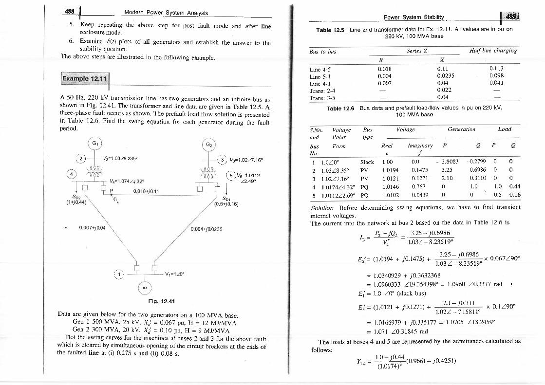
4ffi | Modern power System Analysis

5. Keep repeating the above step for post fault mode and after linereclosure mode.

6. Examine d(r) plots of all generators and establish the answer to thestability question.

The above stgps are illustrated in the following example.

A 50 Hz, 220 kV transmission line has two generators and an infinite bus asshown in Fig. 12.4I. The transformer and line data are given in Table I2.5. Athree-phase fault occurs as shown. The prefault load flow solution is presentedin Table 12.6. Find the swing equation fbr each generator cluring the faultperiod.

o Vz=1.0328.2350 o(

l-l- i

Se).5+j(

F1.O217.16o

)vs=1.o l l z22.490

6)

) v i

[5,

t-I'

i6,u

oFig. 12.41

Data are given below for the two generators on a 100 MVA base.Gen 1 500 MVA, 25 kV, XJ = 0.067 pu, H = 12 MJAyIVAGen 2 300 MVA, 20 kV, X,j = 0.10 pu, H = 9 MJA4VA

Plot the swing curves for the machines at buses 2 and 3 for the above faultwhich is cleared by simultaneous opening of the circuit breakers at the ends ofthe faulted line at (i) 0.275 s and (ii) 0.0g s.

l,,m220kV,100 MVA base

Bus to bus Series Z HaIf line charging

Line 4-5Line 5-1Line 4-ITrans;2-4Trans: 3-5

0 .0180.0040.007

0 . 1 r0.02350.04o.0220.04

0 . 1 1 30.0980.041

Tabfe 12.6 Bus data and prefault load-flow values in pu on 220 kV,100 MVA base

S.No. Voltageand Polar

Bus FormNo.

BusUpe

Voltage Generation Load

Real Imaginarye f

| 1.010" Slack

2 t.0318.35" PV

3 t .0217.16 PV

4 1.017414.32" PQ

5 1 . 0 1 1 2 1 2 . 6 9 " P Q

0.0 - 3.8083

0.1475 3.250.1271 2 .10

0.167 0

0.0439 0

-0.2199 0 00.6986 0 00 . 3 1 1 0 0 01.0 1.0 0.440 0 .5 0 .16

1.00t.01941 . 0 1 2 11.01461.0102

Solution Before determining swing equations, we have to find transient

internal voltages.The current into the network at bus 2 baseci on the <iata in Tabie i2.6 is

r -_ Pr - iQ , _ 3 .25- i0 .6986'z

v : r .o3 l - 8 .23519"

E{= (1.0194 + j0.1475) +3.2s - j0.6986

x 0.06719Vr.03 l-8.23519'

= 1.0340929 + j0.3632368= 1.0960333 119.354398" = 1.0960 lo.337l tad I

El = I.0 l0' (slack bus)

E4 - Q.0I2r + j0.1271) + 2 .1 - j 0 .31 r x 0.1 l9O"r .021- 7 .15811 '

= 1.0166979 + j0.335177 = 1.0705 lI8'2459"

- 1.071 10.31845 rad

The loads at buses 4 and 5 are represented by the admittances calculated as

follows:

yr r.= ''9

.!.:,0! (0.9661 - jo.4zsr)6 (1.0174)"

;;'#;;"J###::il::H,:T:|, :::,::::^'l:,::,1,:nt reactanles of the machines we wlr,we wlll,therefore' now designate as buses 2 and3, the fictitious internal nodes betweenthe internal voltages and the transient reactances of the machines. Thus we get

Y-^ =- 2 2 - @ = - i r r . 2 3 6

Yzq= j11.236 = yqz

Ytt =

io'04+io] = - i7'143

Yzs = j7.I43 = yst

Y u = Y t q + y q t * y q s +* Yzq

= 0.9660877 - j0.4250785 + 4.245 - j24.2571 + 1.4488 _i8 .8538+ j0 .041 + rO.113_ j r t .235g

_ 6.6598977 _ j44.6179

Yss= Yrs* Ysq* Ysr * 9 * Ur ,

* r " ,2 2

' ' 35- 0.4889 - j0.1565 + r.4488 - j8.8538 + 7.039r _ j41.335+ /O.1 13 + j0.098 _ j7.t42}_ 8.97695s _ js7.297202

The complete augmented prefault lzuu, matrix is show n.iri'Table 12.1.Table 12.T The augmented prefaurt bus admittance matrix for Ex. 12.11,admittances in pu

I a,grr,Power System Stability _ .

During Fault Bus Matrix

Since the fault is near bus 4, it must be short circuited to ground. The Ynusduring the fault conditions would, therefore, be obtained by deleting 4th rowand 4th column from the above augmented prefault Y".r. rnatrix. Reduced faultmatrix (to the generator internal nodes) is obtained by eliminating the new 4throw and column (node 5) using the relationship

Y*iqn"*1 = Y*j@tat - Y t n(oltt) ynj(old

)/ Y rn @ta)

The reduced faulted matrix ()'eus during fault) (3 x 3) is given in Table I2.8,which clearly depicts that bus 2 decouples from the other buses during the faultand that bus 3 is directly connected to bus 1, showing that the fault at bus 4reduces to zero the power pumped into the system from the generator at bus 2and renders the second generator at bus 3 to -eive its power radially to bus 1.

Table 12.8 Elements of Yrus (during fault) and Ysus (post fault)for Ex. 12.11, admittances in pu.

Reduced during fault Yu^

Bus

v 0.5 _ j0 .16

prefaulr "r"

*Trl rr.off (0'488e - i0'1s647)

Load admittances, al

Bo, Bo,') )

L

I2aJ

s.7986-j35.63010

- 0 .0681+ 75.1661

0- jrr.236

0

- 0 .0681 + j5 .166 l0

0.1362'- j6.2737

Reduced post Jault Yurt

I2-J

r.3932 - jr3.873r- 0.2214 + j7.6289- 0.0901 + j6.0975

- 0.2214 + j7.6289 - 0.0901 + j6.O9750.s - j7.7898 0

0 0 .1591 - j6 .1168

B u s

Post Fault Bus Matrix

Once the fault is cleared by removing the line, simultaneously opening thecircuit breakers at the either ends of the line between buses 4 and 5, the prefaultY"u5 has to be modified again. This is done by substituting Yqs = Ysq - 0 andsubtracting the series admittance of line 4-5 and the capacitive susceptance ofhalf the line from elements Yoo and Ytt.

Y++lporrfault) = Y++(prefault) - Yqs- 84512

= 6.65989 - j44.6179 - 1.448 + 78.853 - j0.113

= 5.2III - j35.8771

Similarly, Ysr(oo*, rault) = 7.528I - i48.5563

The reduced post fault Y"u5 is shown in the lower half to Table 12.8. It maybe noted that 0 element appears in 2nd and 3rd rorvs. This shows that,

234

rr.284_j6s.473 0

0- j7.1428

0

0 + j7.1428

4.245 + j24.257

j11.23s9

06.6598_j44.617

-1.4488 + j8.8538

0 _i1r.23sg

0 6-4.245 + j24.257 jl l .2359

-7.039 + j41.355 0

-7.039 +j4 r .35s

0j7.t428-1.4488+j8.85388.9769

+ j57.2972

{92 | Modern power System Anatysis

- L . . ^ : ^ ^ l r - . r r - -lrrryr'ruarry' tlle generarors I an0 Z are not Interconnected when line 4-5 isremoved.

During Fault Power Angle Equation

P r z = 0

P,3= Re [YrrEr,El* * El* \F(]; since yy= 0= E{2 Gn + lEi l lEi l l rr , l cos (6zr _ Lzt)= (1.071)2 (0. 1362) + I x 1.071x 5.1665 cos (d3 _ 90.755")

P"3 = 0.1561 + 5.531 s in (h - 0 .755)

Postfault Power Angle Equations

p"z= lE/P G22 + lElt lEll ly2Ll cos (dr, _ 0zr)= 1.0962 x 0.5005 + I x 1.096 x 7.6321 cos ({ - 9I.662")= 0.6012 + 8.365 sin (d, _ I.662)

p,3 = tE{ 2q3 + Ell tElt t\l cos ( 6r, _ 0rr)- 7.0712 x 0.1591 + 1 x 1.07r x 6.09g cos (dr - 90.g466")= 0.1823 + 6.5282 sin (d, _ 0.9466")

Swing Equations-During Fault

Power System Stanitity I 491,1

It rnay be noted that in the above swing equations, P,, ntay be written in

general as follows:

Pn= Pr, - Pr. - P,r,n* sin (6- 7)

Solution of Swing Equation

The above swing equations (during fault followed by post fault) can be solved

by the poinrby-point method presented earlier or by the Euler's method

presented in the later part of this section. The plots of E and 4 are given in

Fig. 12.42 for a clearing time of 0.21 5 s and in Fig. 12.43 for a clearing time

of 0.08 s. For the case (i), the machine 2 is unstable, while the machine 3 is

stable but it oscillates wherein the oscillations are expected to decay if effect

of damper winding is considered. For the case (ii), both machines are stable but

the machine 2 has large angular swings.

(0.275s fault cleared at)

F\g.12.42 Swing curves for machines 2 and 3 of Example 12.1 for

clearing at 0.275 s.

If the fault is a transient one and the line is reclosed, power angle and swing

equations are needed for the period after reclosure. These can be computed from

the reduced Ysus matrix after line reclosure.

#=ff (P^z-P,z)=

= t:9/ e.2s - o) elecr deg/sz

1 2

d ,q _ 180 fa ' r = k

( P n - P " t )

= t * : / e . r - {0 .1s61 + 5.531 s in (6t -0 .7ss)} l

9

= Y

l .g43g - 5.531 sin (d, - 0.755")l elect d,eg/sz

Swing Equations-Postfault

#={ f p .2s-10.60r z + 8.365 s in (d) - t .662") }J erect deg/s2

dtd, 180 f-* =*12.10-{0.1823 + 6.5282 sin(d3 _ 0.g466.)}lelect deg/szdt' 9

Machine 1 is reference (lnfinite bus)

494 |

Modern power System Analysis

500Machine 1 is reference (lnfinite bus)

Machine 2

i l l t l_ L _ _ I _ | _0 .8 0 .9 1 .0

Fault clearedafter 4 cycles

Fig. 12.43 Swing curves for machines 2 and 3 ofExample 12.11 for clearing at 0.0g s

Gonsideration of Automatic voltage Regulator (AVR) andSpeed Governor Loops

state variable Formulation of swing Equations

The swing equation for the hh generator is

Power System Stabilitv l,,4PFr

. i *= #(P"or - Pco) , k = 1 ,2 , . . . , mr7.2

Initial state vector (upon occurrence of fault) is

xoLk= fr= lEot

(t2.74)

(Eo*) usingrotor angle

1 0 0

at)c)oL

q,o)

!

o(tc

x " z k = 0

The state form of swing equations (Eq. (12.74)) can be solved by the many

available integration algorithms (modified Euler's method is a convenient

choice).

Computational Algorithm for Obtaining Swing Currzes Using

Modified Euler's Method

l. Carry out a load flow studY

voltages and powers.

(prior to disturbance) using specified

2. Compute voltage behind transient reactances of generators

Eq. (9.31). This fixes generator. emf magnitudes and init ial

lreference slack bus voltag" Y?).

Compute, Ysu5 (during fault, post fault, line reclosed).

Set time count r = 0.

Compute generator power outputs using appropriatg ts"us with the help

of the geniral form of Eq. (12.27). This givet Pg},for / 1 /').

Note: After the occurrence of the fault, the period is divided into uniform

discrete time intervals (At) so that t ime is counted as /(0), t(l), ...... A

typical value ol' l t is 0.05 s.

aJ .

4.5 .

6. Compute t( i [ ; ' } , i \7' ) ,k

7. Corttputc thc I ' i ls l stutc

- - 1 ,2 , . . . , m l f iom Eqs. (12 .74) .

cst i r r t i r lc 's l iu ' t = , { t+ l ) 'prr

(r2.73)

For the multimachine case, it is more convenient to organise Eq. (12.73) isstate variable form. Define

x r k = 6 r = l E * '

xz*= 6 t

i t * = x z t

+ = + (p 'oo- p " ) ; k - r ,2 , . . . , f f id t ' H k '

u

, [ , 0 * r , = , t l o + i [ , 0 ) a t I = | . 2 . . . . . r r t

,ff') - *V) + *$'o) At

8. Cortrpute the first estimates of E^('+t)

BQ+D = E? lcos x,(i*r)+ 7 sin *\lf '))

g. Compute P8;'); (appropriate Y"u5 and Eq. (12.72))'

10. compute [t ;{ in') , i t :o*t ' ) , k = r,2, . . . , mf fromEqs. (12.74).

1 1. Compute the average values of state derivatives

i[ i ,) , urr= ][ iu,cl +; l [*t) ]k = 1 , 2 , . . . , f f i

iL'),*, = *I*\:| + ,tt'i" lThen

1 ' t ALL. Lompute tne lrnal state estimates for | = t\r+t)-

*;Iu" = *([) + ill) uus, at

,&*r) - ,([l + if).^,rat k = 7'2' "'' frt

Compute the final estimate for Eo at t = r('*l) using

BQ+t) = l4llcos xf;+r) + 7 sin *f1r)

14. Print (",9*t), *;:o*D ); k = I,2, ..., m15. Test for time limit (time for which swing curve is to be plotted), i.e.,

checki f r> rnnur. I f not , r - r+ r and repeat f romstep5 above.Otherwise print results and stop.

The swing curves of all the machines are plotted. If the rotor angle of amachine (or a group of machines) with r"rp".t to other machines increaseswithout bound, such a machine (or grouf of machines) is unstable andeventually falls out of step.

The computational algorithm given above can be easily modified to includesimulation of voltage regulator, field excitation response, saturation of fluxpaths and governor action

Stability Study of Large Systems

To limit the computer memory and the time requirements and for the sake ofcomputational efficiency, a large multi-machine system is divided into a studysubsystem and an external system. The study subsystem is modelled in detailwhereas approximate modelling is carried out for the external subsystem. Thetotal study is rendered by ihe modern technique of dynamic equivalencing. Inthe external subsysteln, nutnber <lf rnachines is drastically recluced using variousmethods-coherency based rnethods being most popurar and widely used byvanous power ut i l i t ies in the wor ld.

I2.T7 SOME FACTORS AFFECTING TRANSIENT STABILITY

We have seen in this chapter that the two-machine system can be equivalentlyreduced to a single machine connected to infinite bus bar. The qualitativeconclusions regarding system stability drawn from a two-machine or anequivalent one-machine infinite bus system can be easily extended to amultimachine system. In the last article we have studied ihe algorithm fordetermining the stability of a multimachrne system.

It has been seen that transient stability is greatly affected by the type andlocation of a fault, so that a power system analyst must at the very outset of astability study decide on these two factors. In ou,

"*u-ples we have selected

a 3-phase fault which is generally more severe from point of view of powertransfer' Given the type of fault and its location let us now consider other

Power System Stabitity |

491;,,

factors which affect transient stability and therefrom draw th" .on"llsions,regarding methods of improving the transient stability lirnit of a system andmaking it as close to the steady state limit as possible.

For the case of one machine connected to infinite bus, it is easily seen from

the angle through which it swings in a given time interval offering thereby amethod of improving stability but this cannot be employed in practice becauseof economic reasons and for the reason of slowing down the response of thespeed governor loop (which can even become oscillatory) apart from anexcessive rotor weight.

With reference to Fig. 12.30, it is easily seen that for a given clearing angle,the accelerating area decreases but the decelerating area increases as themaximum power limit of the various power angle curves is raised, therebyadding to the transient stability limit of the system. The maximum steady powerof a system can be increased by raising the voltage profile of the system andby reducing the transfer reactance. These conclusions along with the varioustransient stability cases studied, suggest the following method of improving thetransient stability limit of a power system.

1. Increase of system voltages, use of AVR.2. Use of high speed excitation systems.

3. Reduction in system transf-er reactance.

4. Use of high speed reclosing breakers (see Fig. 12.32). Mo&rn tendencyis to employ single-pole operation of reclosing circuit breakers.

When a fault takes place on a system, the voltages at all buses are reduced.At generator terminals, these are sensed by the automatic voltage regulatorswhich help restore generator terminal voltages by acting within the excitationsystem. Modern exciter systems having solid state controls quickly respond tobus voltage reduction and can achieve from one-half to one and one-h'alf cycles(l/2-l]) gain in crit ical clearing times fbr three-phase taults on the HT busof the generator transformer.

Reducing transfer reactance is another important practical method ofincreasing stability limit. Incidentally this also raises system voltage profile.The reactance of a transmission line can be decreased (i) by reducing theconductor spacing, and (ii) by increasing conductor diameter (see Eq. (2.37)).Usually, however, the conductor spacing is controlled by other features such aslightning protection and minimum clearance to prevent the arc from one phasemoving to another phase. The conductor diameter can be increased by usingmaterial of low conductivity or by hollow cores. However, norrnally, theconductor configuration is fixed by economic considerations quite apart fromstability. The use of bundled conductors is, of course, an effective means ofreducing series reactance.

Compensation for line reactance by series capacitors is an effective andeconomical method of increasing stability limit specially for transmission

'4lI I Modern power System Analysis

distances of more than 350 km. The ciegree of series compensation, however,accentuates the problems of protective relaying, normal voltage profiles, andovervoltages drrring line-to-ground faults. Series cornpensation becomes moreeffective and economical if part of it isof compensation upon the occurrence cS witehed series eapaeitors simultaneotand raise the transient stability limit tclimit. Switching shunt capaciiors on olstability limits (see Example 12.2) but the MVA rating of shunt capacitorsrequired is three to six times the rating of switched series capacitors for thesame increase in stability limit. Thus series capacitors are preferred unlessshunt elements are required for olher pu{poses, siy, control of voltage profile.

Increasing the number of parallel lines between transmission points is quiteoften used to reduce transfer reactance. It adds at the same time to reliabilityof the transmission system. Aclditional line circuits are not likely to proveeconomical unit I aftet all feasible improvements have been carried out in thefirst two circuits.

As the majority of faults are transient rn nature, rapid switching and isolationof unhealthy lines followed by reclosing has been shown earliei to be a greathelp in improving the stability marginr. ih. modern circuit breaker technologyhas now made it possible fbr line clearing to be done as fast as in two cycles.Further, a great majority of transient faults a'e line-to-ground in nature. It isnatural that methods have been developed for selective single pole opening andreclosing which further aid the stability limits. With ,"f"r".,"" to Fi;. lz.r7, ifa transient LG fault is assumed to occur on the generator bus, it is immedi ately

::.1,:l_., ol,lnt the fault there will now be a definite amount of power rransfer,

n d d r + + ^ s ^ ^ L L - - - -ab uurereni rrom zero power transfer for the case of a three-phase fault. Alsowhen the circuit breaker pole corresponding to the faulty line is opened, theother two lines (healthy ones) remain intact so that considlrable power transfercontinues to take place via these lines in comparison to the case of three-poleswitching when the power transfer on fault clearing will be reduced to zero. Itis, therelbre, easy to see why the single pole swiiching and reclosing aids instability problem and is widely adopted. These facts arelilustrated by means ofExample 12'12. Even when the stability margins are sufficient, single poleswitching is adopted to prevent large swings and consequent vortage dips.Single pole switching and reclosing is, of course, expensiu. in t..*s of relayingand introduces the as.socjatec! problerns of overvoltages caused by single poleopening owing to line capacitances. Methods are available to nullify thesecapacitive coupling effects.

Recent Trends

Recent trends in design of large alternators tend towards lower short circuitratio (scR = r/x), which is achieved by reducing machine air gap withconsequent savings in machine mmf, size, weight and cost. Reduction in the

II : . - ^ I r .I.1.':/tlltt, i::

stze of rotor reduces inertia constant, Iowering thereby the stability margin. Theloss in stability margin is made up by such features as lower reactance lines,faster circuit breakers and faster cxcitation systenrs as tliscussetl alreacly, anda faster system valving to be discussed later in this article.

A stage has now been reached in technology whereby the methods ofirnprovinE=stability; discussetl above, have been pushed to their limits, e.g.,clearing times of circuit breakers have been brought down to virnrallyirreducible values of the order of two cycles. With the trend to reduce machineinertias there is a constant need to determine availability, feasibility andapplicability of new methods for maintaining and/or improving system stability.A brief account of some of the recent methods of maintaining stability is givenbelow:

HVDC Links

Increased use of HVDC links ernploying thyristors would alleviate stabilityproblems. A dc link is asynchronous, i.e., the two ac system at either end donot have to be controlled in phase or even be at exactly the same frequency asthey do for an ac link, and the power transmitted can be readily controlled.There is no risk of a fault in one system causing loss of stability in the othersystem.

Breakingr Resistors

For improving stability where clearing is delayed or a large tn)a i, suddenlylost, a resistive load called a breaking resistor is connected at or near thegenerator bus. This load compensates for at least sonre of the reduction of loadon the generators and so reduces the acceleration. During a f-ault, the resistorsare applied to the terminals of the generators through circuit breakers by meansof an elaborate control scheme. The control scheme determines the amount ofresistance to be applied and its duration. The breaking resistors remain on fora matter of cycles b<lth during fault clearing and after system voltage isrestored.

Short Circuit Current Limiters

These are generally used to limit the short circuit duty of distribution lines.These may also be used in long transmission lines to modify favourably thetransfer impedance during fault conditions so that the voltage profile of thesystem is somewhat improved, thereby raising the system load level durins thefault.

Turbine Fast Valuing or Bypass Valuing

The two methods just discussed above are an attempt at replacing the sysremload so as to increase the electrical output of the generator during faultconditions. Another recent method of improving the stability of a unit is todecrease the mechanical input power to the turbine. This can be accornplished

by rneans of fast valving. where the differenee between mechanical input andreduced electrical output of a generator under a fault, as sensed by a controlscheme, initiates the closing of a turbine valve to reduce the power input.Briefly, during a fast valving operation, the interceptor valves are rapidly shut(in 0.1 to 0.2 sec) and immediately reopened. This procedure increases thecritical switching time lons enoushstable for faults with stuck-breaker clearing times. The scheme has been put touse in some stations in the USA.

FUII Load Rejection Technique

Fast valving combined with high-speed clearing time will suffice to maintainstability in most of the cases. However, there are still situations where stabilitvis difficult to maintain. In such cases, the normal procedure is to automaticallytrip the unit off the line. This, however, causes several hours of delay beforethe unit can be put back into operation. The loss of a major unit for this lengthof tirne can seriously jeopardize the remaining system.

To remedy these situations, a full load rejection scheme could be utilizedafter the unit is separated from the system. To do this, the unit has to beequipped with a large steam bypass system. After the system has recoveredfrom the shock caused by the fault, the unit could be resynchronized andreloaded. The main disadvantage of this method is the extra cost of a largebypass system.

The systetn shown in Fig. 12.44 is loaded to I pu. Calculate the swing curveand ascertain systern stability for:

(i) LG fault three pole switching followecl hy reclosure. l inc louncl healthy.(ii) LG fault single pole switching fbllowed by reclosure, line found healthy.

Switching occurs at 3.75 cycles (0.075 sec) and reclosure occllrs at 16.25cycles (0.325 sec). All values shown in the figure are in pu. -

l . r . l= . , ,?_ Xr= 0.1

r--- - --lJ I-, t 0.15 |7 lI 0 ' 1 p 0 ' 3 0 .1 |L --z -rfd]-ui-r

i-dT L_r6TT\_ I

(b) Negative sequence network

Fig. 12.45

For an LG fault at P the sequence networks will be connected in series-asshown in Fig. 12.46. A star-delta transformation reduces Fig. 12.38 to that ofFig. 12.47 from which we have the transfer reactance

Xr2(LG faulQ = 0.4 + 0.4 + nOII' 'O = 1.450.246

I

I.- t .

lE l=1 '2 ( )I

r - r d 600 '4

Fig.12.46 Connection of sequence networks for an LG fault

f-( , r

Fig.12.47 Transfer impedance for an LG fault

When the circuit breaker poles corresponding to the faulted line are opened(it corresponds to a single-line open fault) the connection of sequence networksis shciwn in Fig. 12.48. From the reduced network of Fig. 12.49 the rransferreactance with faulted line switched off is

t T - t

I - t -

; . i ) l _ Cao

'' l]o t go '' | =

l xo = 0.0e15| | p 1 ' o | | IL----.-' I i-rT60 t;,'r";*u1n""

networl

P o'4

H = 4.167 - ' .Xr = o 3Oj ?*f -h'Ir-!.&-f!X t = 0 ' 1 5 ' L ( /

xo= o.t AY-l

Fig. 12.44

Solution The sequence networks of the system are drawn and suitably reducedin Figs. I2.45a, b and c.

I l ' Xn ' l r

tI r / - f t r f \ r _ _ _ J

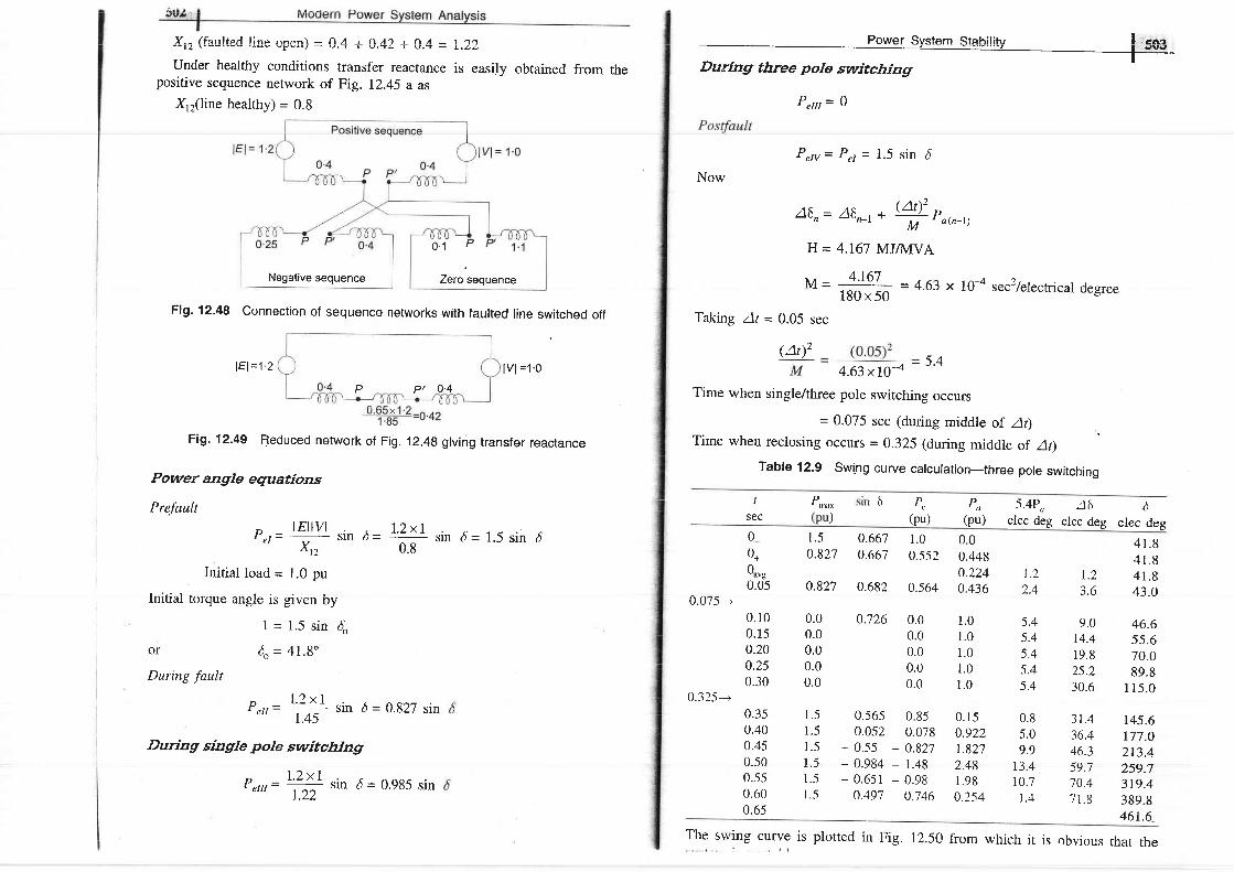
Y.^ (fett l ter l l ine nnen\ - 0 A t A A1 r ( l A - 1 . .- ^ l l \ - * - - - - v . - | v . a L - r V . . + _ L . . / - L

Under healthy conditions transfer reactance is easily obtained from thepositive sequence network of Fig. 12.45 a as

Xrr(line healthy) = 0.8

Zero sequence

Flg.12-48 Connection of sequence networks with faulted line switched off

lEl=1'z lv l =1 'o

Fig. 12.49 Reduced network of Fig. 12.49 giving transfer reactance

I .o.ro

Pettt = 0

Now

PrN= Pd = 1.5 sin d

46,- A6n-, + @LP^,- ,,M

' a ( n - l )

H = 4.167 MJA{VAo '1 P

1,1= JU- - 4.63 x 10a sec2lelectrical degree180 x 50

Taking At = 0.05 sec

(at)'5.4

4.63xI0-4

Time when single/three pole switching occurs

= 0.075 sec (during middle of At) .,Time when reclosing occurs = 0.325 (during middle of at)

Table 12.9 swing curye calculation-three pole switchingPower angle eguations

PreJault

p,= rE vr sin d=X, ,

Initial load = 1.0 pu

Initial torque angle is given by

or

During fault

1 = 1.5 sin 5o

6o = 47.8"

7.2x1- S l I l d = l . ) s t n b0.8

L

sec

P,u,o P,,(pu))

1.5 0.6670.827 0.667

0.827 0.682

0.0 0.7260.00.00.00.0

1.5 0.5651.5 0.0521.5 - 0 .551.5 - 0.9841.5 - 0 .651r .5 0 .497

.5.4P,, ifielec deg elec deg

6 P "(pu)

6elec deg

0.075---+0 . 1 00 . 1 50.20o.250.30

0.325--+0.3s0.400.450.500.s50.600.65

r .0 0 .00.552 0.448

0.2240.564 0.436

0.0 1 .00 .0 1 .00 .0 1 .00 .0 1 .00 .0 1 .0

0 .85 0 .150.078 0.922

- 0.827 r.827- r .48 2.48- 0 .98 1 .98

0.146 0.254

4 1 . 84 1 . 8

1 . 2 4 1 . 83.6 43.0

9.0 46.6r4.4 55.619.8 70.02s.2 89.830.6 I 15 .0

31.436.446.359.710.47 1 . 8

0o*ouu,0.05

1.2N A

F l . Z x l'",, = lff

sin d = 0.827 sin

I)uring single pole switching

Perrr = +#

sin d = 0.985 sin

5.45.45.45.45.4

0.85.09.9

13.410.7t . 4

r45.6177.O2r3 .4259.73r9.4389.8461.6

Negative sequence

P P/ o:4

The swing curve is plotted in Fig. 12.50 from which it is obvious that rhe

\4gqe!_lg',gf tyq]g1_ Analysis Power System Stability |

505;I

0.40 l .s 0.998 1.5 - 0 .5 - 2 .70 .45 1 .5 1 .0 1 .5 - 0 .5 - 2 .70 .50 1 .5 1 .0 1 .5 - 0 .s - 2 .7 - 2 .6 89 .50.55 1.5 0.9985 1.5 - 0 .5 -2.7 86.9

2.8 86.60 .1 89 .4

r I , r l - - , r - r ] . . . r ro ' 5 1 . 0

Time (sec)

Fig. 12.50 swing curue for three pole switching with reclosure

Table 12.10 swing curve calculation-single pole switching

- 10 .3 73 .7- 12.r 63.4- 1 3 . 0 5 1 . 3- 12 .6 38 .3- 10.7 25.7- 7.4 15.0- 3 . r 7 . 6

1.7 4.56.2 6.29.9 r2.4

12.2 22.3l3 . l 34 .512.5 47.610.9 60.18 .6 7 r .O6.0 79.63 .3 \ 95 .6' gg .g

The swing curve is plotted in Fig. 12.51from which it follows that the sysremis stable.

Single pole switch off

/'/ ' Reclosure (fault cleared)| ' /

i - l - - r

0 5Time (sec)

Fig. 12.51 Swing curve for single pole switching with reclosure

I300 !

II

250 Ii

2oo i-II

tIIL

6q)

g)oEoL(.)q)

J)to

\Iir pote i

switch off i

/ / l

MACHINE UNSTABLE

0 .65 1 .50 .70 1 .50 .75 1 .50.80 1.50.85 1.50.90 1.50.95 1.51 .00 1 .5r .05 r .51 . 1 0 1 . 51 . 1 5 1 . 51 .20 1 .5r .25 1 .51 .30 1 .51 .35 1 .5r .40 1.51 .45 1 .51 .50 1 .5

0.96 t.44 - 0.44 - 2.40 . 8 9 4 1 . 3 4 - 0 . 3 4 - 1 . 80 . 7 8 1 t . l 1 - 0 . 1 7 - 0 . 90.62 0.932 0.068 0.4'0.433 0.6s 0.35 r .90.2s9 0.39 0.61 3.30 .133 0 .2 0 .8 4 .30 .079 0 .119 0 .881 4 .80 .107 0 .161 0 .839 4 .50.214 0.322 0.678 3.70.38 0.57 0.43 2.30.566 0.84 0. 16 0.90 . 7 3 8 1 . 1 1 - 0 . 1 1 - 0 . 60.867 1.3 - 0 .3 - 1 .60.946 t.42 - 0.42 - 2.30.983 1.48 - 0 .48 - 2 .60.997 1.5 - 0.s - 2.7

1 5 0

100

I

SEC

I',uu^

(pu),s:itt h

BO

60

A

III

o)oo)o)

oC)L

ooo)

ra

t,,,(pu)

l'r, 5'4P,,(pu) elec deg

A belec deg

belec deg

0o ,

f

oory

0.050.075---

0 . 1 00 . 1 5o.20o.250.30

4325---+0.35

1 .5 0 .661 1 .00.827 0.667 0.s52

0.827 0.682 0.s64

0.00.4480.224 1.20.436 2.4

0.285 1.50.230 r.20 .166 0 .90.107 0.60.060 0.3

0.485 - 2.6

4 t . 8 04 1 . 8

r .2 41.83.6 43.0

5.1 46.66.3 5r .77.2 58.01.8 65.28 .1 73 .0

5 . 5 8 1 . 1(Contd... .)

0.98s 0.7260.98s 0.7840.985 0.8480.98s 0.9080.985 0.956

1 .5 0 .988

0 .7Ls0.770.8340.8930.940

1 .485

MACHINE STABLE

t 2 . l

t 2 .3

12.4

t2 .5

1 2 . 6

t 2 .1

506 | Modern po@is

PROB TEIlIS

A two-pole, 50 Hz, 11 kv turboalternator has a rating of 100 Mw,powel factor 0.85 lagging. The rotor has a moment of inertia of a 10,000

12.2 Two turboalternators with ratings given below are interconnected via ashort transmission line.Machine 1: 4 poIe, 50 Hz, 60 MW, power factor 0.g0

moment of inertia 30,000 kg-rn,lagging,

Machine 2 pole, 50 Hz, 80 MW, power factor 0.85 lagging,moment of inertia 10,000 kg--'

Calculate the inertia constant of the single equivalent machine on a baseof 200 MVA.

Power station t has four identical generator sets each rated g0 MVA andeach having an inertia constant 7 MJA4VA; while power station 2 hasthree sets each rated 200 MVA, 3 MJA4VA. The stations are locatldclose together to be regarded as a single equivalent machine for stabilitystudies. Calculate the inertia constant of the equivalent machine on 100MVA base.

A 50 Hz transmission l ine 500 km long with constants given below tiesup two large power areas

I ina

from its prefault position, determine the maximum load that could betransferred without loss of stability.

I2.8 A synchronous generator is feeding 250 MW to a large 5O Hz networkover a double circuit transmission line. The maximum steady state Dowerthat can be transmitted over the line with both circuits in operation is500 MW and is 350 MW with any one of the circuits.A solid three-phase fault occurring at the network-end of one of the linescauses it to trip. Estimate the critical clearing angle in which the circuitbreakers must trip so that synchronism is not lost.What further information is needed to estimate the critical clearing time?

12.9 A synchronous generator represented by a voltage source of 1.05 pu inseries with a transient reactance of 70.15 pu and in inertia constant F/ =4.0 sec, is connected to an infinite inertia system through a transmissionline. The line has a series reactance of70.30 pu, while the infinite inertiasystem is represented by a voltage source of 1.0 pu in series with atransient reactance of 70.20 pu.

The generator is transmitting an acti're power of 1.0 pu when a three-phase fault occurs at its terminals. If the fault is cleared in 100 millisec,determine if the system will remain stable by calculating the swingcurve.

12.10 For Problem 12.9 find the critical clearing time from the swin! currre fora sustained fault.

l2. l l A synchrt)nous generator representcd by a vol tage of l . l5 pu in ser ieswith a transient reactance is c<lnnected to a large power system withvol t t tgc 1.0 pu throt lgh l powcr rrc lwork. Thc cquivalcnt t larrs ienttransf'er reactance X between voltage sources is 70.50 pu.After the occurrence of a three-phase to grouncl fault on one of the l inesof the power network, two of the line circuit breakers A and B operatesequentially as follows with corresponding transient transfer reactancegiven therein.(i) Short circuit occurs at 6 = 30", A opens instantaneously to make X

= 3.0 pu.(ii) At 6 = 60o, A recloses, X = 6.0 pu.

(i i i) At 5=75o, A reopens.(iv) At d = 90o, B also opens to clear the fault making X = 0.60 puCheck if the systenr wil l operate stably.

12.12 A 50 Hz synchronous generator with inertia constant H = 2.5 sec anda transient reactance of 0,20 pu feeds 0.80 pu active power into aninfinite bus (voltage I pu) at 0.8 lagging power lactor via a network withan equivalent reactance of 0.25 pu.

A three-phase fault is sustained for 150 millisec across generatorterminals. Determine through swing curye calculation the torqu e angle 6,250 millisec, after fault initiation.

F i n d t h e s f c : t r l v s l z f e c f e h i l i t r r l i m i t i f l l , / | - l l / | - t n l l t , \ / / . . ^ - ^ + ^ - + r, . - - ' . , , J r r r J r r r r r r r , , , r , t t _ | v R t

_ , \ r v A V \ L t , | t : l t d l l l r .

What will the steady state stability limit be if line capacitance is alsoneglected? What will the steady state stability limit be if line resistanceis also negloctcd' / Cornnrcl t t on t l rc rcsul ts.A power deficient area receives 50 MW over a tie line from anotherarea. The maximum steady state capacity of the tie line is 100 MW. Findthe allowable sudden load that can be switched on without loss ofstability.

A synchronous motor is drawin g 30vo of the maximum steady statepower from an infinite bus bar. If the load on motor is suddenlyincreased by 100 per cent, would the synchronism be lost? If not, whatis the maximum excursion of torque angle about the new steady stater<ltor position.

The transfer reactances between a generator and an infinite bus baroper i l t ing i r f 200 kV trnder var ious condi t ions on fhe interconnector aro:

R = 0.11 f) /km

C = 0.009 lFlkm

Pretault

During fault

Postfhult

L - 1.45 mH/kmG = 0

S0 0 per phase

m O per phase

2ffi {) per phase

12.13 A 50 Hz, 500 MVA,400 kV generator (with transformer) is connectedto a 400 kV infinite bus bar through an interconnector. The generatorhas F1 - 2.5 MJA4VA, voltage behind transient reactance of 450 kV andis loaded 460 MW. The transfer reactances between generator and bus

Power System Stabitity I

5(D

12. Kundur, P., Power System Stability and Control, McGraw-Hill, New York, 1994.13. Chakrabarti, A., D.P. Kothari and A.K. Mukhopadhyay, Performance Operation

and Cqntrol of EHV Power Transmission Systems, Wheeler Publishing, NewDelh i , 1995.

14. Padiyar, K.R., Povter System Stability and Control, Znd

lcatlons, Hy

15. Sauer, P.W. and M.A. Pai, Power System Dynamics and Stabiliry, Prentice-Hall,New Jersey, 1998.

Papers

16. Cushing, E.W. et al., "Fast Valving as an Aid to Power System TransientStability and Prompt Resynchronisation and Rapid Reload After Full L,oadRejection", IEEE Trans, L972, PAS 9I 1624.

t

17. Kimbark, E.W., "Improvement of Power System Stability", IEEE Trans., 1969,PAS-88: 773.

18. Dharma Rao, N. "Routh-Hurwitz Condition and Lyapunov Methods for theTransient Stability Problem", Proc. IEE, 1969, 116: 533.

19. Shelton, M.L. et al., "BPA 1400 MW Braking Resistor", IEEE Trans., 1975,94:602.

Nanda, J., D.P. Kothari, P.R. Bijwe and D.L. Shenoy, "A New Approach forDynamic Equivalents Using Distribution Factors Based on a Moment Concept",Proc. IEEE Int. Conf. on Computers, Systems and Signal Processi4g, Bangalore,Dec. 10-12, 1984. \

Dillon, T.S., 'Dynamic Modelling and Control of Large Scale System", Int.Journal of Electric Power and Energy Systems, Jan. 1982, 4: 29.Fatel, R., T.S. Bhatti and D.P. Kothari, "Improvement of Power System Transientstability using Fast valving: A Review", Int. J. of Electric Power componentsand Systems, Vol. 29, Oct 2001, 927-938.Patel, R., T.s. Bhatti and D.P. Kothari, "MATLAB/simulink Based rransientStability Analysis of a Multimachine Power System, IJEEE, Vol. 39, no. 4, Oct.2002, pp 339-355.

Patel R., T.S. Bhatti and D.P. Kothari, "A Novel scheme of Fast valvingControl", IEEE Power Engineering Review, Oct.2002, pp. 4446.Patel, R., T.S. Bhani and D.P. Kothari, "Improvement of Power system Transientstability by coordinated operation of Fast valving and Braking Resistor", Toappear in IEE proceeriings-Gen., Trans and Distribution.

During fault

Postfault

1 .0 pu0.75 pu

Calculate the swing curve using intervals of 0.05 sec and assuming thatthe fault,is cleared at 0.15 sec.

I2.I4 Plot swing curves and check system stability for the fault shown on thesystem of Example 12.10 for fault clearing by simultaneous opening ofbreakers at the ends of the faulted line at three cycles and eight cyclesafter the fault occurs. Also plot the swing curye over a period of 0.6 secif the fault is sustained. For the generator assume H = 3.5 pu, G = 1 puand carry out the computations in per unit.

12.15 Solve Example 12.10 for a LLG fault.

REFERE N CES

Books

1 Stevenson, W.D., Elements of Power System Analysis,New York, 1982.

Elgerd, O.I., Electic Energy Systems Theory: AnMcGraw-Hill, New York, 1982.

4th edn., McGraw-Hill,

iniroduciion, 2nd edn.,

The Iowa3. Anderson, P.M. and A.A. Fund, Power System Control and Stability,State University Press, Ames, Iowa, 1977.

4. stagg, G.w. and A.H. o-Abiad, computer Methods in Power system Analysis,Chaps 9 and 10, McGraw-Hil l Book Co., New York, 1968.

5. Crary, S.8., Power System Stability, Vol. I (Steady State Stability), Vol. II(Transient Stability), Wiley, New York, 1945-1947.Kimbark, E.W., Power System Stability, Vols 1, 2 and 3, Wiley, New york, 1948,Veuikorz, Y.A., Transient Phenomena in Electrical Power System (translated fromthe Russian), Mir Publishers, Moscow, 1971.

8. Byerly, R.T. and E.w. Kimbark (Eds.), stability of l^arge Electric power

Systems, IEEE Press, New York, 1974.9. Neuenswander, J.R., Modern Power Systems,International Text Book Co., 1971.

t0. Pai, M.A., Power System Stability Annlysis by the Direct Method of Lyapunov.,North-Holland, System and Control Services, Vol. 3, 1981.

I 1. Fouad, A.A and V. Vittal, Power System Transient Stability Analysis using theTransient Energy Function Method, Prentice-Hall, New Jersy, 1992.

20.

2 r .

22.

23.

. AL + .

25.6.

7 .

13.1 INTRODUCTION

In Chapter 7, we have been primarily concerned with the economical operationof a power system' An equally important factor in the operation of a powersystem is the desire to maintain system security. System security involvespractices suitably designed to keep the system operating when components fail.Besides economizing on fuel cost and minimizrngemission of gases (co, cor,Nox, sor), the power systern should be operationally ,.secure,,.

An operation_ally "secure" power system is one with low probability of, systern black out(collapse) or equipment damage. If the pro."r, uf cascading failures continses.the systern as a whole or its tnajor parts may completely collapse. This isnormally referred to as system blackout. All these aspects require securityconstrained power system opt imizat ion (SCO).

Since security and economy normally have conflicting requirements, it isinappfopriate to treat them separately. The fina.l aim of economy is the securitylunction of the utility company. The energy management system (EMS) is tooperate the system at minimum cost, with the guaranteed alleviation ofemergency conditions. The emergency condition will depend on the severity oft io lat ions of operat ing l i rn i ts (branch f ' lows and bus vol tage l imi ts) . The mostsevere violations result fiom contingencies. An irnportant part of security study,therefbre, moves around the power system's ability to withstanrj the effects ofcontingencies. A particular system state is said to be secure only with referenceto one or more specific contingency cases, and a given set of quantitiesmonitored for violation. Most power systems are operated in such a way thatany single contingency will not leave other.o-pon"nts heavily overloaded, sothat cascading failures are avoided.

Power System Security I

Sll

Most of the security related functions deal with static "snapshots" of thepower system. They have to be executed at intervals compatible with the rateof change of system state. This quasi-static approach is, to a large extent, theonly practical approach at present, since dynamic analysis and optimization areconslder4bly mole {!fficu!! 4nd cqmpurallo44lly 1aqte lime corrsulurg,

System security can be said to comprise of three major functions that arecarried out in an energy control centre: (i) system monitoring, (ii) contingencyanalysis, and (iii) comective action analysis.

System monitoring supplies the power system operators or dispatchers withpertinent up-to-date information on the conditions of the power system on realtime basis as load and generation change. Telemetry systems rneasure, monitorand transmit the data, voltages, currents, current flows and the status of circuitbreakers and switches in every substation in a transrnission network. Further,other critical and important information such as frequency, generator outputsand transformer tap positions can also be telemetered. Digital computers in acontrol centre then process the telemetered data and place them in a data baseform and inform the operators in case of an overload or out of limit voltage.Important data are also displayed on large size monitors. Alarms or warningsmay be given if required.

State estimation (Chapter 14) is normally used in such systems to combinetelemetered data to give the best estimate (in statistical sense) of the currelttsystem condition or "state". Such systems otten work with supervi$ory controlsystems to help operators control circuit breakers and operate switches and tapsremotely. These systems together are called SCADA (supervisory control anddata acquisit ion) systelns.

The second ma-ior security function is contingency analysis. Modernoperation computers have contingency analysis programs stored in them. Theseloresee possiblc systetn troubles (outages) before they occur. They study outageevents and alert the operators to any potential overloads or serious voltageviolat i t lns. For exalnple, the s i rnplest f i r rm of cont ingency analysis can be puttogether with a standard LF program as studied in Chapter 6, along withprocedures to set up the load flow dafa for each outage to be studied by theLF plogram. This allows the system operators to locate def'ensive operatingstates where no single contingency event will generate overloads and/or voltageviolation:;. This analysis thus evolves operating constraints which may becntpioycd in thc l iD (ccotrolnic dispatch) and UC (uni t cornnr i t rnclr t ) prograrrr .Thus contingency analysis carrics out ornergcncy identil ' ication ancl "what if ' 'simulations.

The third major security function, corrective action analysis, permits theoperator to change the operation of the power system if a contingency analysisprogram predicts a serious problem in the event of the occurrence of a certainoutage. Thus this provides preventive and post-contingency control. A simpleexample of corrective action is the shifting of generation from one station toanother. This may result in change in power flows and causing a change inloading on overloaded lines.

j5!2,1 Modern Po@is

Threse three ftrnctions together consist oi a very compiex set of toois that heipin the secure operation ol'a power system.

T3.2 SYSTEM STATE CLASSIFICATION

Dyliacco [13] and further clarified by Fink and Carlsen l23l in order to definerelevant EMS (Energy Management System) functions. Stott et. al [15] havealso presented a more practical static security level diagram (see Fig. 13.1) byincorporating correctively secure (Level 2) and correctable emergency (Level4)security levels.

In the Fig. 13.1, arrowed linep represent involuntary transitions betweenLevels 1 to 5 due to contingencies..The removal of violations from Level 4normally requires EMS directed "corrective rescheduling" or "remedial action"bringing the system to Level 3, from where it can return to either Level I or2 by further EMS, directed "preventive rescheduling" depending upon thedesired operational security objectives.

Levels I and 2 represent normal power system operation. Level t has theideal security but is too conservative and costly. The power system survives anyof the credible contingencies without relying on any post-contingency correctiveaction. Level2 is more economical, but depends on post-contingency correctiverescheduling to alleviate violations without loss of load, within a specifiedperiod of time. Post-contingency operating limits might be different from theirpre-contingency values.

13.3 SECURITY ANALYSIS

System security can be broken down into two major functions that are carriedout in an operations control centre: (i) security assessment, and (ii) securitycontrol. The tormer gives the security level of the system operating state. Thelatter determines the appropriate security constrained scheduling required tooptimally attain the target security level.

The security functions in an EMS can be executed in 'real time' and 'study'

modes. Real time application functions have a particular need for computingspeed and reliability.

'fhe static securit.v level of a power system is characterised by the presence

or rrtherwise of emergency operating conditions (limit violations) in its actual(pre-contingency) or potential (post-contingency) operating states. Systemsecurity assessment is the process by which any such violations are detected.

Sy st e m e.:^ s € s s tlt€rrt involv e s two func tions :

(i) system monitoring and (ii) contingency analysis. System monitoring providesthe operator of the power system with pertinent up-to-date information on thecurrent condition:; clf the power system. In its simplest form, this just detectsviolations in the actual system operating state. Contingency analysis is much

I srr

=o-3

o-ocoo

oooo

ooL

o-o

p b .6 q

ooo)

oo

ooo

L

f()oU)C)(Eo

Eooo

o

oo_

at

.d,lr

P c 9 cE O = O

d H d 8

occ)o)c

oo

9 c

6 H

g >. F O E=-E fiE 8 E

z E C gg#EE( ' 5 o 3

xo 9 .' E b

.= g,

g) 'Ec c

F O( g ( J

b o d8 b b: 5 8d d ' 5( l ) - . o

. = 9 =

los i5 c o( t ) . =

H E ' =e o y

=ee

o-o

8 s 9o o ' : =L - A

, ^ k a t , ^ i :* ' u o * 9o c f r o ) c ,> o x > oA z C . A i lJ 3 ( D J 3

o0)o)

Eo)o-o([()q)L

C)

r ' / ^ Y

ea i

9 cF . O

d 8

6-L

oc)a

o

: : 0( l ) -> o_9 !)

- Ea dg E

oog,c

co(J

E E8 E( ! 6

B Er: .9q Fo oo o _

E; .^Et-E. ; E b

abg

o,coL

q)o.oozEoo.o-=o

Eoo

- o =

g H €' = O -o _ o xo - - c . Y

! ie= 9 8

,.sfe ;l Modern power Svstem Analvsis

Only a small proportion of work on optimal power flow (OPF) has taken intoaccount the security constraints. The most successful applications have been tothe security constrained MW dispatch OPF sub-problem. The contingency-constrained voltageivar rescheduling problem, as of the writing of this text, stillremains to be solved to a satisf desree.

The total number of contingency constraints imposed on SCO is enormous.The SCO or contingency constrained OPF problem is solved with or withoutfirst optimizing with respect to the base case (precontingency) constraints. Thegeneral procedure adopted is as follows:

(i) Contingency analysis is carried out and cases with violations or nearviolations are identified.

(ii) The SCO problem is solved.(iii) The rescheduling in Step 1 might have created new violations, and

therefore step 1 should be repeated till no violations exist.Hence, SCO represents a potentially massive additional computing effort.An excellent comprehensive overview of various available methods ispresented by Stott et. al [15].

There is still great potential for further improvement in power systemsecurity control. Better problem formulations, theory, computer solutionmethods and implementation techniques are required.

T3.4 CONTINGENCYANALYSIS

In the past many widespread blackouts have occurred in interconnected powersystems. Therefore, it is necessary to ensure that power systems should beoperatec! mosf economic:r!ly such that povrer is cle!i.rerecl reliably. Reliableoperation implies that there is adequate power generation and the same can betransmitted reliably to the loads. Most power systems are designed with enoughredundancy so that they can withstand all rnajor tailure events. Here we shallsttrdy thc possiblc consccprcnccs :rncl rcrncdial actions rcquircd by two nrainf a i lure events; l ine.orr tages ancl generat ing rrni t fa i lures.

To explain the probleln briefly, we consider the five-bus system of Ref'erenceL I0J. The base case load llow results lbr the example are given in t ig. 13.2 and,sl t r rw i r f ' low <tf 24.7 MW and 3.6 MVAR on the l ine f }om bus 2 to hus 3. L.ctt ls l lsst l l l lc that at prcscnl , we i l rc only intcrestecl in the MW loading of the l ine.Let us examine what will happen if the line from bus 2 to bus 4 were to open*.' l ' l rc

rcsul t ing l inc l ' lows artc l vol tagcs ulc shown in l r ig. 13.3. t t nray be notcdthat the flow on the line 2-3 has increased to 31.5 MW and that most of theother line flows are also changed. It may also be noted fhat bus voltagemagnitudes also get aff'ected, particularly at bus 4, the change is almost2To lessfrom 1.0236 to 1.0068 pu. Suppose the line from bus 2 to bus 5 were to open.Figure 13.4 shows the resulting flows and voltages. Now the inaximum changet:fgl.g.j

",jus 5 which is almost 107o less.

xSimulation of line outage is more complex than a generator outage, since lineoutage results in a change in system configurations.

I sraiPower System Security _

SLACK BUSf + o * y st +s *y ts

1 .02421-5 .0 " 31 .O6 tO" 1 4 1 . 0 2 3 6 t - 5 . 3 "

--.>40.7 + j1.2 _ 39.5 _i3.0:_ + 18 .9 - y5 .2 _16.9 +13.2-< _

,f 88.e -y8.6,l

+ -Ja.a--/e.8 i 6 . 3 - j 2 .3

I z+.2 *js.a ----/ --zt.s-i5.9

t'L?:'-q''---'

t- az.s *

1.0474t-2

1.0610" 1

!G-)) ,zo +1to

t40 +i30

Fig. 13.2 Base Case AC

SLACK BUS

*oo *ito

Line flow for sample 5 bus system

l+-u '-" ' '.i;n;l--+s- 53.7 -i7.2 -* 5'

i1 .o17gt -6 .2"Y

*S4.9 +17.3

:63 .1 + j 1O.2

{ + s * y t s1.01071- 5.9" 3

->48.6 + j5.2 -46.7 - j5.3<- + 38.5 -10.6 -38.4 -i1.1 :-

+ --

3a? -/'e r

f + o + 7 s

4 1.00682 - 6.6"

{ - r .o -7 a.s

i r .s - ; t . r-<-- - 61.6 - i8.9 5

1 .O114 t -6 .4 "

loo *lt o

AC Load Flow (Line between 2 and 4 is open)

t a s r r t s I ao ,7s

- 52.s -i 13.0 +

+ 81 .8 -i 5.5

t- eo.o *

1.0468t-2.

rlr { 2s +ilo\

l J . /

t40 +i30

Fig. 13.3 Post outage

SLACK BUS

( c )

| +s,s * 1tz.t

':: )ll ':t't'

- 50.8994t-16.?

120 + i10 'f oo *yr o

between 2 and 5 is open)

| 0.se35/ - 6.s" o 11 '06 t0 " 1 l ' 54 .4 + i 1 i . 3 - s2 .1 - i 9 .7 - | - s1 .4 + i7 .3 - s1 .1_1_ _r

tl;f+ 8 0 . e + 1 3 . 2 1 | I t l _ q q . z _ j 1 z . s

Fig. 13.4 Post outage AC Lcad Flow (Line

5LAUK HUS

e t 4 s + l 1 5

| 1 .oo61t _ s .7" 311 . 0 6 t 0 " 1 l ^ I'l_ -!.6 + 1t.s _ 4s.9 _j7.6 <_i __22.4 _ j2.6

{nze+ i z1 .7 l L - - - i - 1 - II - - - V _21.5_ j4 .8

Give Alarm signal

;'518 | rr,rodern Po@is- t -

l + o * 1 s

4 1 . O 0 4 3 t - 6 . 1 "_22 .3 + j0.7 <_

{ t.s - 1t.t

-25.2- j4 .4 +

I ---t i ' ' '"

1- rzo .g -1 ts . t l ( - ' - _ -l l r

2..]--u+ _+ _53.6 +16.81.o24st -3 .7 . i

Yl ,zo +1 lo

<- -52.5 -16.5f - z s - 7 s . s

5o 9956/_-7 .1"

{ o o * i r o

lost generation isGive Alarm signalFig. 13.5 Post outage AC Load Flow (Generator 2 outage,

picked up by generator 1)

Figure 13.5 is an example of generator outage ancl is selected to explain thetact that generator outages can also result in changes in line flows and busvoltages. In the example showr in Fig. 13.5 all the generation lost from bus 2is picked up on the generator at bus 1. Had there been more thanZgenerarorsin the sample system say at bus 3 also, it was possible the loss of lenerationon bus 2 is made up by an increase in generation at buses 1 and 3. Thedifferences in Iine flows ancl bus voltages vrould show how the lost gener.ationis shared by the remaining units is quite significant.

It is important to know which line or unit outages will render line flows orvoltages to cross the lirnjts. To find the eff'ects of outages, contingency analysistechniques are empioyeci. Contingency analysis models single failure events( i 'e ' one- l inc outagcsi orol lc uni t outugcs) or nrul t ip lc ccpr ipnrcnt f i r i lurc cvc^ts(failure of multiple unit or lines or their combination) one after another until all"credible outages" are considered. For each outage, all lines ancl voltages in thenetrvork are checked against their respective limits. Figure 13.6 depicts a flowchart illustrating a simple method for carrying out a contingency analysis.

One of the important problems is the selection of "all credible outages,,.Execution time to analyse several thousand outages is typically I min based oncomputer and analytical technology as of 2000. An erpproxirnate rnodel suclr asDC load flow may be used to achieve speedy solution if voltage is aisorequired, then full AC load flow analysis has to be carried out.

- - ' t A - . .

1;no*rifii.iuior".""-i;{offi 'l

l'r'.,o ' ''l''''

_ _ l,rr\=_ ves jciventarnviolation? ->*-t_-qJ-T-

,*" I, N oI

' - - - iAil

--\

FIg. 13.6 A simple technique for contingency analysis

620j;:f uodern Power System AnatysisI

^ a ? f r E r r a r E ? r t r E l t

I J .C D I I IYDI I IV I I Y .FAUI -L ' I ( s

A .security analysis program is run in a load dispatch centre very quickly to helpthe operators. This can be attempted by carrying out an approximate analysisand using a computer system having multiple processors or vector processors

y anarysts. I ne s may uate an equrvalentshould be used for neighbours connected through tie-linos. We can eliminate allnon-violation cases and run complete exact program for "critical" cases only.This can be achieved by using techniques such as "contingency selection" or"contingency screening", or "contingency ranking". Thus it will be easy towarn the operation staff in advance to enable them to take corrective action ifone or more outages wiil result in serious overloads or any violations. One ofthe simplest ways to present a quick calculation of possible overloads is toemploy network (linear) sensitivity factors. These factors give the approximatechange in l ine flows for changes in generation in the system and can becalculated from the DC load flow. They are mainly of two types:

1. Generation shift factors

2. Line outage distribution factors

Briefly we shall now describe the use of those factors without deriving them.Reference [7] gives their deri iation.

The generation shift factorsl cr.,; are defined as:

limits and those violating their limit can be informed to the operator for

necessary control action.The generation shift sensitivity factors are linear estimates of the change in

line flow with a change in power at a bus. Thus, the effects of simultaneous

principle of superposition.Let us assume that the loss of the ith generator is to be made up by governor

action on all generators of the interconnected system and pick up in proportion

to their maximum MW ratings. Thus, the proportion of generation pick up from

unit k (k * i) would be

where,

4t = Change in MW power flow on hne I whention, AP", takes place at the ith bus

Here, it is assumed that LPotis fully compensated by an equal and oppositechange in generation at the slack (reference) bus, with all other generatorsremaining fixed at their original power generations. The factor al,then gives thesensitivity of the /th line flow to a change in generation at ith bus. Let us nowstudy the outage of a large generating unit and assume that all the lostgeneration (Pod would be supplied by the slack bus generation. Then

APo, - -P1i

where

Pn,,,,,u,^ = maximum MW rating for rnth generator

g*i= proportionality factor for pick up on kth unit when ith unit fails.

Now, for checking the /th line flow, we may write

j, = ff * 0r; APo, - E,lau, \ri LPotl

In Eq. (13.8) it is assumed that no unit will violate its maximdm limit. For

unit limit violation, algorithm can easily be modified.

Similarly the line outage distribution factors can be used for checking if the

line overloads when solllc of the lines are lost.

The line outage distribution factor is defined as:

d , , ,= *J i

where

dt,i = line outage distributionoutage of ith line.

Aft = change in MW flow on /th iine'

fi - precontingency line flow on ith line

lf precontingency line flows on lines / and i, tlre power flow on line / with line

i out can be found out employing "d" factors.

(13 .4 )

a change in genera-

(13 .7 )

(13 .8 )

(13 .10)

( 13.e)

factor when monitoring /th line atter an

(13.s)and the new power flow on each line could be calculated using a precalculatedset of " d' factors as given below.

ft = f i * dti APc, for all lines V / (13.6)

where, ft - power flow on /th line after the failure of ith generator

f i = power flow on /th line before the failure or precontingencypower flow

Here,

fi ^d foi =precontingency or preoutage flows on lines / and i respectively

?,= ff *d,, , f ,o

fr = power flow on /th line with ith line out.

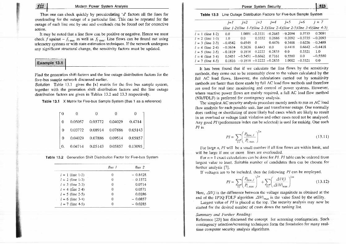
iii l Modern Poa

Thus one can check quickiy by precaiculating 'd' factors ali the lines foroverloading for the outage of a particular line. This can be repeated fbr theoutage of each line one by one and overloads can be found out for correctiveaction.

It may be noted that a line flow can be positive or negative. Hence we mustcheck / agarnst - Jt ̂ u* as well as h **. Llne tlows can be louncl out usmgtelemetry systems or with state estimation techniques. If the network undergoesany significant structural change, the sensitivity factors must be updated.

Find the generation shift factors and the line outage distribution factors for thefive-bus sample network discussed earlier.Solution Table 13.1 gives the [x] matrix for the five bus sample system,together with the generation shift distribution factors and the line outagedistribution factors are given in Tables I3.2 and 13.3 respectively.

Table 13.1 X Matrix for Five-bus Sample System (Bus 1 as a reference)

0.05057 0.03772 0.04029 0.4714

0.03772 0.08914 0.07886 0.05143

0.04029 0.07886 0.09514 0.05857

0.04714 0.05143 0.05857 0.13095

Table 13.2 Generation Shift Distribution Factor for Five-bus System

Bus I Bus 2

J "srr

j= l j=2 j=3 j=4 j=5 j=6 j = 7

(line 1-2)(line l-3)(Iine 2-3)(line 2-4)(line 2-5)(line 3-4)(line 4-5)

( l ine l -2) 0.0 1.0001 -0.3331 -0.2685 -0.2094 0.3735 0.2091

= 3 (line 2-3) -0.4542 0.4545 0 0.4476 0.3488 -0.6226 -0.3488- J \ r r \ r w L - J ) - v

= 4 (hne 2-4) -0.3634 0.3636 0.4443 0.0 0.4418 0.6642 -O.44r8

= 5 ( l ine 2-5) -0 .1819 0.1818 0.2222 0.2835 0.0 0 '3321 1.0= 6 ( l ine 3-4) 0 .5451 -0 .5451 -0 .6662 0.7161 0.5580 0.0 -0 .5580

= 7 ( l ine 4-5) 0 .18 i6 -0 .1818 -0 .2222 -0 .2835 1.0002 -0 .3321 0 '0

It has been found that if we calculate the line flows by the sensitivity

methods, they come out to be reasonably close to the values calculated by the

full AC load flows. However, the calculations carried out by sensitivity

methods are faster than those made by full AC load flow methods and therefore

are used for real time monitoring and control of power systems. However,

where reactive power flows are mainly required, a full AC load flow method(NR/FDLF) is preferred for contingency analysis.

The simplest AC security analysis procedure merely needs to run an AC load

flow analysis for each possible unit, line and transformer outage. One normally

does ranking or shortlisting of most likely bad cases which are likely to result

in an overload or voltage limit violation and other cases need not be analysed.Any good P1(performance index can be selected) is used for rankirig. One such

P/ is

0

0

0

0

0.

( 1 3 . 1 1 )

For large n, PI will be a small number if all line flows are within limit, and

will be large if one or more lines are overloaded.For rr = I exact calculations ciur be done fbr P1. P1 table can be ordered from

largest value to least. Suitable number of candidates then can be chosen for

further analysis [7].If voltages are to be included, then the following PI can be employed.

l = 1 ( l i n e 1 - 2 )

/ = 2 ( l i n e 1 - 3 )

/ = 3 ( l i n e 2 - 3 )

I = 4 ( l i n e 2 - 4 )

/ = 5 ( l i n e 2 - 5 )

/ = 6 ( l i n e 3 - 4 )

I = l ( l i n e 4 - 5 )

- 0.8428- o. t572

o.07140.05710.0286

- 0.0857- 0.0285

(13.12)

Here, Alvil is the difference between the voltage magnitude as obtained at the

end of the lPlQ FDLF algorithm Alvl-u* it the value fixed by the utility.Largest vaiue oi Pi is piaceci at the top. The security arraiysis trray rrow -ue

started for the desired numbel of cases down the ranking list.

$ummary and Further Reading:Reference [25] has discussed the concept for screening contingencies. Such

contingency selection/screening techniques fonn the foundation for many real-

time computer security analysis algorithms.

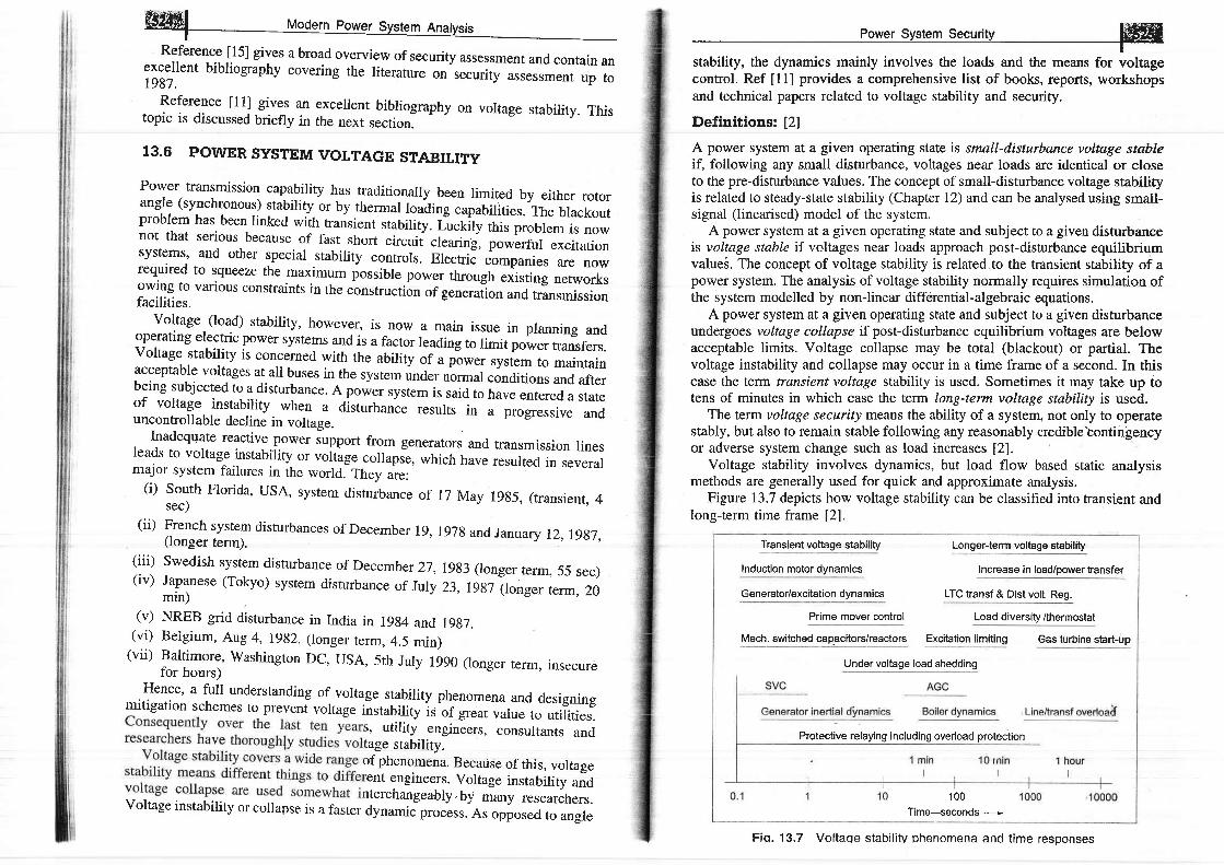
Reference [15] gives a broad overview of security assessment and contain an

;;;;t]r", bibliography covering the literature on"security assessmenr up to

Reference [11] gives an excellent bibliography on voltage stability. Thistopic is discussed briefly in the next section.

13.6 POWER SYSTEM VOITAGE STABILITY

Power transmissiol tuglgility has traditionally been Iimited by either rotorangle (synchronous) stability or by thermal loaoing capabilities. The blackoutproblem has been linked with transient stability. L-uckily this ;roblem is nownot that serious because of fast short circuii clearing; po*Lrru excitationsystems, and other special stability controls. ElectriJ *rnpuni"s are nowrequired to squeeze the maximum possible power through "ii.G

networksowing to various constraints in the construction of generation and transmissionfacilities.voltage (load) stability, however, is now a main issue in planning andoperating electric power systems and is a factor reading to limit po-w; transfers.voltage stability is concerned with the ability of a power system to maintainacceptable voltages at all buses in the system under normal conditions and afterbeing subjected to a disturbance. A power system is said to have entered a stateof voltage instability when a disturbante resurts in a pro!."rriu" anduncontrollable decline in voltageInadequate reactive.-power support from generators and transmission linesleads to voltage.instability ot uoitug" collapse, which have resulted in severalmajor system failures in the world. Th"y -",

(i) south Florida, usA, system disturbanc e of 17 May r9g5, (transient, 4sec)(ii) French system disturbances of Decembe r 19, r97g and Januar y 12, rgg7,(longer term).

(iii) swedish system disturbance of December 27, rgg3 (longer term, 55 sec)(iv) Japanese (Tokyo) system disturbance of July 23, 1gg7 irorg", term, z0min)(v) NREB grid disturbance in India in 19g4 and r9g7.

(vi) Belgium, Aug 4, 1992. (longer term, 4.5 min)(vii) Baltimore, washington DC, usA, 5th July 1990 (longer rerm, insecurefor hours)

Hence, a full understanding of voltage stability phenomena and designingmitigation schemes to prevent voltase instabilitv is nf o,raqr'or,,o +^,.+:r:a:^^', ;,ilir; ;;,:;; ffiri#il;";;age stability.lf phenomena. Becadse of this, voltage'ent engineers. Voltage instabilitv andrterchangeably.by many ."r"ur"h..r.voltage instability or co[apse is a faster dynamic-process. As opposed to angle

l#GrffiEIE!F}ILfr

stability, the dynamics mainly involves the loads and the means for voltagecontrol. Ref [11] provides a comprehensive list of books, reports, workshopsand technical papers related to voltage stability and security.

Definitions: [2]

A power system at a given operating state is small-disturbance voltage stableif, following any small disturbance, voltages near loads are identical or closeto the pre-disturbance values. The concept of small-disturbance voltage stabilityis related to steady-state stability (Chapter 12) and can be analysed using small-signal (linearised) model of the system.

A power system at a given operating state and subject to a given disturbancets voltage stable if voltages near loads approach post-disturbance equilibriumvaluei. The concept of voltage stability is related to the ffansient stability of apower system. The analysis of voltage stability normally requires simulation ofthe system modelled by non-linear diffdrential-algebraic equations.

A power system at a given operating state and subject to a given disturbanceundergoes voltage collapse if post-disturbance equilibrium voltages are belowacceptable limits. Voltage collapse may be total (blackout) or partial. Thevoltage instability and collapse may occur in a time frame of a second. In thiscase the term transient voltage stability is used. Sometimes it may take up totens of minutes in which case the term long-term voltage stability is used.

The term voltage security means the ability of a system, not only to operatestably, but also to remain stable following any reasonably crediblebontingencyor adverse system change such as load increases [2].

Voltage stability involves dynamics, but load flow based static analysismethods are generally used for quick and approximate analysis.

Figure 13.7 depicts how voltage stability can be classified into transient andlong-term time frame l2l.

Transient voltage stability Longer-term voltage stability

Induction motor dynamics Increase in load/power transfer

Generator/excitation dvnamics LTC transf & Dist volt. Reg.

Prime mover control Load diversity /thermostat

Mech. switched capacitors/reactors Excitation limiting Gas turbine start-up

Under voltage load shedding

100Time-seconds -

Protective relaying including overload protection

Fiq. 13.7 Voltage stabi l i tV phenomena and t ime responses

;;;''',h.;A#";rvr^rvlv vv'Yvr Pr'lurs tu a large system over long transmission lines. Voltage':::i:y,"::,*:,','31^

^,?::^s,112itiu and ,oto."ungl" stability is basicauy

Effective counter Measures to prevent or contain voltageInstability

(i) Generator terminal voltage shourd be raised.(ii) Generator transformer tap value may be increased.

(iii) Q-injection should be carried out at an appropriate location.(iv) Load-end oLTc (on-load tap changer) should be suitably used.(v) For under voltage conditions, strategic load shedding should be resorted

to'System reinforcement may be carried out by instpiling new transmissionlines between generation and load centres. series and shunt compensation maybe carried out and svcs (static var compensation) may be installed. Generationrescheduling and s_tarting-up of gas ,rrui-"* ,.y i" .,*.i.,t out.Practical aspects of Q-flow problems leading to voltage collapse in EHv lines:( i) For lons l ine.s uri fh 'r-^^nrrnu^r L--^^-"-!' s'vv'Lr.,'e' uus's, recelvlng_end or road voltages

increase for light load conditions and decrease for heavy load conditions.(ii) For radial transmission lines, if any loss of a line takes place, reactancegoes up, I2x loss increases resulting in increase in voltage drop. Thisshould be suitably compensated by local e injection. of course thisinvolves cost. If there is a shortage of rocal q ,ourrr, then import of e

wffi;Ewe

desirable.

Unity power factor

Nosepoint (knee)

t\ Loaw of V6 and Pr"r;

same for const Z loadfor other types of load,V degradation is faster.

PplP6zy

0.2 0 .4 0 .6 0 .8 1 .0 1 .2 1 .4 1 .6

Fig. 13.8 PV curves with different load power factors

Only the operating points above the critical points represent satisfactoryoperating conditions. At the 'knee' of the V-P curve, the voltage drops rapidlywith an increase in load demand. Power-flow solution fails to convefge beyondthis limit indicating instability. Operation at or near thel stability limit isimpractical and a satisfactory operating condition is ensured by permittingsufficient "power margin".

SPfti*f uooern po@isI

Voltage stability problems normaliy occur in heavily stressed systems.voltage stability and rotor angle (or synchronous) stability are more or lessinterlinked' Rotor angle stability, .a3-.wex as voltage stability is affected byreactive power control. voltage stability is concern"o *itt, load areas and load

Senerator stability.In a large inter-connected system, voltage coilapse of a loadarea is possible without lois of synchroni* or any generators.The slower forms of voltage instability are often analysed as steady-stateproblems' 'snapshots'

in time following an outage or during load buildup aresimulated' In addition to post-disturbancl load floivs, two other load flow basedmethods are widely used: P-V curves and e-v curves. pV curves are used forespecially for radial systems.

/ curves (Fig. 13.g), eV curves (Fig.'ig. 13.8) and methods to quantify noseputed. Power flow analysis cletermines

as vanous svstem parameters and ""lT:ir'#n#'f |HI'I,:IJHI#voltage exist for each value of load. The uppe. on" indicates stable ;;i;;;whereas lower one is the unacceptable value (multiple load flow). At limitingl!ug" of voltage stability i.e. at nose point single ioad flow solution exists.Nearer the nose point, lesser is the staLility maigin,

1400

1200

1000P> P, > P, , iN MW

System characteristics

Capacitorcharacteristics

0.9 0 .95 1.0 1 .05

Vin pu

Fig. 13.9 System and shunt capacitor steady-state Q-V characteristics,capacitor MVAr shown at rated voltage

j+Allowable range

ffuo. Boo

Voltage Collapse

Voltage collapse is the process by which the seguence of events accompanyingvoltage instability le_ads to unacceptable voltag6 profile in a significant part ofthe power system. It may be manifested in ieverat different"ways. Voltagecollapse may be characterised as follows:

(iii) The voltage collapse generally manifests itself as a slow decay of voltage.It is the result of an accumulative process involving the actions andinteractions of many devices, controlJ, and protective iyrt"*r. The timeframe of collapse in such cases would be of the order of several minutes.Voltage collapse is strongly influenced by system conditions andcharacteristics.

(iv) Reactive compensation can be made most effective by the judicious choiceof a mixture of shunt capacitors, static var system and possiblysynetuonous condensers.

Methods of Improvlng Voltage Stabllity

voltage stability can be improved by adopting the following rneans:(i) Enhancing the localised reactive power support (SVC) is more efl,ective

and C-banks are lnore economical. ra-tS devices or synchronouscondenser may also be used,

(ii) Compensating the line length reduces net reactance and power flowincreases.

(iii) Additional transmission linc muy be crectccl. It also improves reliability.(iv) Enhancing excitation of generator, system voltage improves and e is

supplied to the system.(v) HVDC tie may be used between regional grids.

(vi) By resorting to strategic load shedding, voltage goes up as the reactive. burden is reduced.

Future Trends and Challenges

( i \ Ontirnql oif i -- n'F EA/- 'n- ,{^*,:^^^\- . / urrrrr6 vr I nv r i , \r lvv. l tvgD.

(ii) Better and probabilistic load modelling.(iii) Develop techniques and models for study of non-linear dynamics of largr

siz.e systems. For example, new methods to obtain network equivalentrsuitable for voltage stability analysis.

M

;(v) Post-disturbance MwA4vAR margins should be ffanslated to pre-

disturbance operating limits that operators can monitor.(vi) Training in voltage stability basis (a training simulator) for control centre

and power plant operators should be i

SUIvIMARY

Power system security (including voltage stability) is likey to challengeplanneqs, analysts; researchers and operators for the foreseeable future. As loadgrows, and as new transmission lines and new generations would beincreasingly difficult to build or add, more and more utilities will face thesecurity challenge.

Deregulation and socio-economic ffends compounded by technologicaldevelopments have increased the likelihood of voltage instability.

Luckily many creative persons are working tirelessly to find new methodsand innovative solutions to meet this challenge.

REFERE N CES

Books

L l.J. Narguth and D.P. Kothari, Pttnter System Engincering,'fata Mc0raw.Hill, NewDclhi, 1994.

2, C.W, Taylor, Power System Voltag,e Stabiliry, McGraw-Hill, New york, 1994.3. P. Kundur, Power System Stability and Contol, Sections 2.12, ll.2 and Chapter

14, McGraw-Hill, New York, 1994.

4, T,J.E, Miller, Editor, Reactive Power Control in Electric Syslens, John Wiley andSons, New York, 1982.

5. A. chakrabarti, D.P. Kothari and A.K. Mukhopadhyay, Perforurutnce, operationand Control of EHV Power Transmission Systems, Wheeler Publishing, NewDelhi. 1995.

6. T.V. Cutsem and C. Vournas, Voltage Stability of Electric Power Syslerns, KluwerAcademic Publishers, London, 1998.

7. A.J. Wood and W.F. Wollenberg, Power Generation, Operation, and Control, ZndEdn, John Wiley, New York, 1996.

E. John J. Gratnger and W.D. Stevenson, Power SystemAnalysis, McGraw-Hill, NewYork, 1994.

9. G.L. Kusic, Computer-Aided Power Systems Analysis, Prentice-Hall, New Jersey,1986.

10. G.W. Stagg and A.H. El-Abiad, Computer Methods in Power System Analysis,McGraw-Hill, New York, 1968.

Papers

11. v. Ajjarapu and B. Lee, "Bibliography on voltage stability", IEEE Trans. onPower Systems, Vol. 13, No. 1, February 1998, pp lI5-125,

12. L.D. Arya, "Security Constrained Power System Optimization", PhD thesis, IITDelhi, 1990.

13. T.E. Dyliacco, "The Adaptive Reliability Control System", IEEE Trans. on pAS,

Vol. PAS-86, May 1967, pp 517-531(This is a key paper on system security and energy control system)

14. A.A. Fouad, "Dynamic Security Assessment Practices in North America", IEEETrans. on Power Systems, Vol. 3, No. 3, 1988, pp 1310-1321.

15. B. Stott, O. Alsac and A.J. Monticelli, "security Analysis and Optimization", proc

IEEE, VoL 75, No. 12, Dec. 1987, pp 1623-1644.16. Special issue of Proc. IEEE, February 2000.17. P.R. Bijwe, D.P. Kothari and L.D. Arya, "Alleviation of Line Overloads and

voltage violations by corrective Rescheduling", IEE proc. c, vol. 140, No. 4,July 1993, pp 249-255.

18. P.R. Bijwe, D.P. Kothari and L.D. Arya, "Overload Ranking of Line Outages withpostourage generation rescheduling", Int. J. of Electric Machines and PowerSystems, Yol. 22, No. 5, 1994, pp 557-568.

19. L.D. Arya, D.P. Kothari et al, "Post Contingency Line Switching for OverloadAlleviation or Rotation", Int J. of EMPg Vol 23. No. 3, 1995, pp 345-352.

20. P.R. Bijwe, S.M. Kelapure, D.P. Kothari and K.K. Saxena, "Oscillatory StabilityLirnit Enhancement by Adaptive Control Rescheduliig, Int. J. of Electric Powerand Energy Systems, Vol. 21, No. 7, 1999, pp 507-514.

21. L.D. Arya, S.C. Chaube and D.P. Kothari, "Line switching for AlleviatingOverloads under Line Outage Condition Taking Bus Voltage Limits into Account",Int. J. of EPES, Yol. 22, No. 3, 2000, pp 213-ZZl.

22. P.R. Bijwe, D.P. Kothari and S. Kelapure, "An Effective Approach to VoltageSecurity and Enhancement", 'Int. J. of EPES, Yol. 22, No 7, 2000, pp 4g3-4g6.

23. L. Fink and K. carlsen, "operating under sttress and Strain", IEEE spectrum,March 1978, pp. 48-50.

24. S.M. Kelapure, "Voltage Security Analysis and Enhancement", Ph.D. thesis, IITDelhi,2000.

25. G.C. Ejebe, et. al, "Fast Contingency Screening and Evaluation for Voltagesecurity Analysis", IEEE Trans. on Power systems, vol. 3, No. 4, Nov. l9gg, pp1582-1590.

26. T. Van Cutsen, Voltage Instability: "Phenomena, Counter measures, and AnalysisMethods", Proc. IEEE, Vol. 88, No. 2, Feb. 2000, pp 208-227.

t4

T4.I INTRODUCTION

State estimation plays a very important role in the monitoring and control ofmodern power systems. As in case of load flow analysis, the aim of stateestimation is to obtain the best possible values of the bus voltage magnitudesand angles by processing the available network data. Two modifications are,however, introduced now in order to achieve a higher degree of accuracy of thesolution at the cost of some additional computations. First, it is recognised thatthe numerical values of the data to be processed for the state estimation aregenerally noisy due to the errors present. Second, it is noted that there are alarger number of variables in the system (e.9. P, Q line flows) which can bemeasured but arc not utilised in the load flow analysis. Thus, the processinvolves imperfect measurements that are redundant and the process ofestimating the system states is based on a statistical criterion that estimates thetrue value of the state variables to minimize or maximize the selected criterion.A well known and commonly used criterion is that of minimizing the sum of thesquares of the differences between the estimated and "u1le" (i.e. measured)values of a function.

Most state estimation programs in practical use are formulated asoverdetermined systems of non-linear equations and solved as weighted least-squares (WLS) problems.

State estimators may be both static and dynamic. Both have been developedfor power systems. This chapter will introduce the basic principles of a static-state estimator.

ln a power system, the state variables are the voltage magnrtudes and phaseangles at the buses. The inputs to an estimator are imperfect (noisy) powersystem measurements. The estimator is designed to give the "best estimate" ofthe system voltage and phase angles keeping in mind that there are errors in themeasured quantities and that there may be redundant measurements. The outputdata are then used at the energy control centres for carrying out several

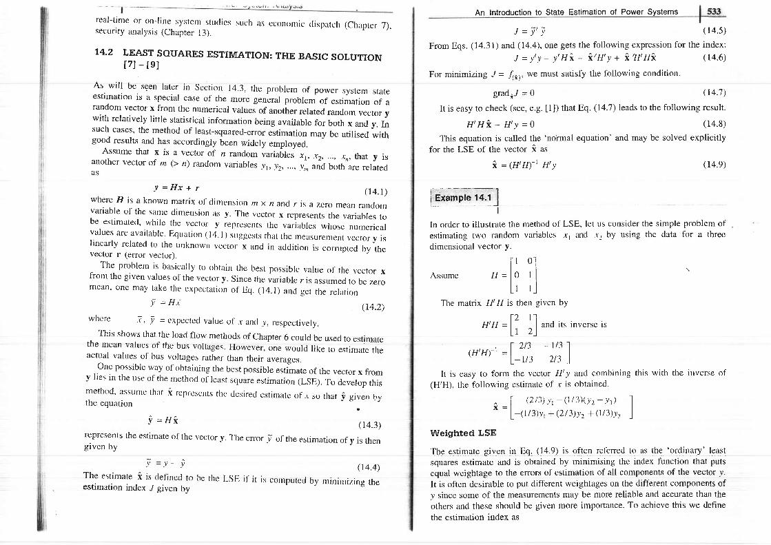
::if.-jl:t or,01-li,r:, systeT^studics such as cconornic clisplrch (Chaprcr 7),

strLur l -y analysts (Lnapter lJ) .

r4-2 LEAST souARES ESTIMATION: THE BAsrc soluTroNI7 l - I e I

A l r rns wilf be seen iater in Section r4.3, the probrem of power system stateestirnation is a special case of the more general problem of estimation of arandom vector x from the numerical values of anotirer related random vector ywith relatively little statistical information being available for both x and y. Insuch cases, the method of least-squared-error estimation may be utilised withgood results and has accordingly been widely employed.

Assume that x is a vector of n random variabres x1t x2, ..., x' that y isanother vector of m (> n) random variables !1, J2, ..., J^ and both are relatedas

where H is a known matrix of dimension mx n ancl r is a zero mean rancklmvariable of the same din-rension as y. The vector x represents the variables tobe estimated, while the vector y represents the variables whose numericalvalues are avai lable. Equat ion ( l4. l ) suggests that the measurement vector y islinearly related to the unknown vector x and in addition is corrupted by thevector r (error vector).

The problem is basically to obtain thc best possible value of the vector xfrom the given values of the vector y. Since the variable r is assumed to be zeromean, one may take the expectat ion of Eq. (14.1) ancl get the relat ion

! = H x + r

f = Hx

j ' = Hf,

( r4 .1 )

(r4.2)

(r4.3)

whcre I , , = cxpcctccl value ol' x iurd y, respec:tively.This shows that the load flow methods of chapter 6 could be used to estimate

the mean values of the bus voltages. Howeu"r, tn. woulcl like to estimate theactual values of bus voltages rather than their averages.One possible way of obtaining the best possible estimate of the vector x fromy lies in the use of the method of least square estimation (LSE). To develop this

rneth<td, assllme that i rcpresettts the desirecl estirnate of ,r so that y given bythe equation

represents the estimate of the vector y. The effor ! of the estimation of y is thengiven bv

(r4.4)The estimate i is definecl to irc thc I-sE if i t is cornputccl by rninirnizing theestimation index J given by

An lntroduction to State Estimation of Power Systems

J = 7 ' V ( 1 4 . 5 )

From Eqs. (14.31) and (14.4), one gets the following expression for the index:

J = y t ! - y ' H * . - i < ' H ' y + * . ' H t H * .

For minimizing J = f$), we must satisfy the tollowing condition.

gradoJ = 0

It is easy to check (see, e.g. [1]) that Eq. (1a.7) leads to the following result.

H t H * , - H ' y - O (14 .8 )

This equation is called the 'notmal equation' and may be solved explicitly

for the LSE of the vector i as

*. = (H,Il)-t Ht y (14.e)

E;il;il]r . iln orcler to illustrate the method of LSE, let us consider the simple problem of

estimating two random variables x, and .rz by using the data for a thret:

dimensional vector y.

Weighted LSE

mI ..

l nq g rs l l l l | : . i l t r E i l v€ i l ! r l D9. \ !+ ,2 ) l s u l re r r l r - rs r rsu r \ , ( r i ) r r ru \ r r \ . r r r r (uJ r1 ,61 i r

squares estimate and is obtained by minimising the index function that puts

equal weightage to the effors of estimation of all components of the vector y.

It is often desirable to put. dift'erent weightages on the ditt'erent components ofy since some of the measurements may be more reliable and accurate than the

others and these should be given more importance. T'o achieve this we define

the estimation index as

( r4.6)

\ r + . t )

l-' 0.1A s s u m e H = 1 0 l l

L r r lThe matrix Ht F1 is then given bY

u'u =12 I I una its inverse is

L l 2 )

(H'm-' =f ''':' -:':1l- u3 213 1

It is easy to form the vector Hty and combining this with the itrverse of(H'H), the following estimate of x is obtained.

f r r t l a t - . / 1 t 1 \ / r - l

^ | \ L t r ) / r - \ r r t ) \ / 2 - Y z ) |* = L-( t /3)yr*(2/3)yr1(r /3)v- , l

/ | / ( \\ r + . J , ,

rvtouern Power

where W is a real symmetric weighting matrix of dimension m x ru. This isoften chosen as a diagonal matrix for simplicity.

It is relatively straightforward to extend the method of LSE to the weightedform of "I and to derive the foilowing form of the normal equation.

H | W H ? _ H ' W y _ 0 G 4 . I l a )This leads to the desired weighted least squares estimate (WLSE)

I = l 'wf

*. = (H,W H)-t H,W yThis pertains to minimization as the hessian

definite.Some Properties:

Rewriting Eq. (14.i lb) as

i = k y

k = (H'W H)-' Ht W .

( 1 4 . 1 1 b )2H|WH is a non-negative

(I4.I2a).

(r4.rzb)

/ 1 4 1 n \\ r . i . r v i ,

(14.r3)

(14.r4)

( 1 4 . 1 5 a )

(14.1sb)

where

Here the matrix k depends on the value of H and the choice of w.using Eqs. (14.1) and (r4.lzb) it is easy to get the relation as follows.

r =f::;,7, ,,,wH) x + kr

Or X =r + k r

a n d E { i } = E { x l

ln IJq. (14.14) it is assumed that the error r is statistically independent ofcolumns of H and the vector r has a zero mean. An estimate that satisfiedEq. (l 4)4) is called an unbiased estimate. This implies that the estimation errorls zero on an averase.

x = k r

The covariance of the error of estimation is therefore given byP, = KRK

where R is the covarianee o1 the error vector r. Note that the covariance p" isa lneasure of the accuracy of the estirnaiion and a smaiier trace of this matrixindicates a better estimate. Eq. (14.15b) suggests that the best possible choiceof the weighting matrix is to set w - R-1. The optimum value of the errorcovariance'matrix is then given by

P, - (HtR-rH)- l ( 1 4 1 5 c )

Assume that in the Example I4.1, we want to obtain the WLSE of the variablex by choosing the following weighting matnx

t---*-- **1 Et<ample 14;2

An lntroduction to State Estimation of Power Systems l" ,3iiSl:-T--

[o.r It lw = l I IL o.tj

The matrir HLWH ts

H,wH -l'' ' o'tl10.1 1. lJ

and the matrix HtW is obtained as

H' |w=fo ' t o o t - lL 0 1 0 . 1 j

The weighted least squares estimate of the vector x is then obtained as (fromEq. ( la .11b))

^ [ (lr/21) y, - (r}/Zt) y, (t0/2t) yr I* =

L- ellr) y, (2ot2r) y, (r/2\ y, )If this result is compared with the result in Example I4.1, the effect of

introducing the weighting on the estimate is apparent. Note that the choice ofW in this case suggests the data for y2 is considered more valuable and thisresults in the components of x being more heavily dependent on )2.

The matrix ft is in this case found to be (Eq. (1a.12b))

rc=lrr/21 -ro/2r ro/zrf

L- r lzt 20/21 r /21 JIf the covariance of the measurement error is assumed to be R = L the

covariance of the estimation error is obtained as (Ref. Eq. (14.15c))

P,= (1tr47) | *:_

.::1L-67 r34 )

The choice of W above yields unacceptably large estimation error variances.Let us now choose the weighting matrix W = I. The matrix Kis then obtained

AS

* = l ' ' 3 - 1 / 3 t / 3 f

L- U3 2/3 1/3JThe error covariance matrix is then given by

D / r / n \ [ 6 - 3 ]r - x = \ L t > )

L _ E 6 JThe error variances are now seen to be much smaller as is to be expected.

Non-linear Measurements

The case of special interest to the power system state estimation problemcorresponds to the non-linear measurement model.

I536 | Modern Power System Analysis

II

! = h ( x ) + r (14 .16)

where h(x) represents an rz dimensional vector of nonlinear functions of thevariable x. It is assumed that the components of the vector h(x) are continuousin their arguments and therefore may be differentiated r.vith respect to thecomponents of x. The problem is to extend the method of least squares in orderto estimate the vector x from the data for the vector y with these two variablesbeing related through Eq. (14.16).

To mimic our treatment of the linear measurement case, assume that irepresents the desired estimate so that the estimate ol the measLlrement y couldbe obtained using the relation

I = h( i )This yields the error of estimation of the vectol y

j = y _ h ( 3 )

In ordcr to obtain the WLSE of ,,r, we nrust cho<lse the index of estimationJ as follows.

J = U - h ( f i ) l ' W l J - h ( i ) l (14 .18)

The necessary condition for the index ,I to have a minimum at .x, is given byEq. (14 .1e) .

t y - h ( x ) l H ( i ) = o (r4.re)

where H (fr) is the Jacobian of h (x) evaluated at i. In general this non-linear

equation can not be solved for the desired estimate, i. n way out of thisdifficulty is to make use of the linearisa-tion technique. Let us assume that ana priori estimate xu of the vector x is available (say from the load flowsolution).

Using Taylor series approximation, we get

(1.4.17a)

(r4.r7b)

(14.20)

r11.22)

! = h ( x d + H u & - x 1 ) + r

where 1/o stands for the Jacobian evaluated at x = x9 and the noise term r isnow assurned to include the effects of the higher order terms in the'Taylorseries. Equation (14.20) can be rewritten as:

A ) ' = y - h ( x o ) = H s A x + r ( 1 4 . 2 I )

where Ay is the p^-rturbed measurement and Ax is the perturbed value of thevector r. An \\LSE of .r is then ea^silv obtained a-s discussed earlier and thisleads to the desired expression for the lineaized solurion of the non-linearestjmat.ion problem.

. i . = .rrr - [H,, ' I+'HQ]- t H() ' ] l ' {-r - h t . t , , ,)}

I r is nor l ikelv that the est imate . i obtained from Eq. (11.22 r is going to bet - r f I r tuc i r use s i l t . 'c . i r t tener. r i . t l t r ' . r i , t ' r t t t ' t c 's t i r lute . l ' , . r I l )J \ - I l r r t h ' c lose t i r thf

(Dt-irnal ydue rf rhe \ect()r x. Hrt,*'ever, F,q. (14.22) prot' ides us wirh a very

An lrylfgduction to_State Estimation of Power Systems I S3TI

useful result in the sense that it shows a mechanism for improving on the initialestimafe by making use of the available nleasurements. Having obtained newestimate i , the process of linearisation is repeated as many times as desired andthis leads to the {qllq*tng 4erylle {qryq qf the qqb]ro4 of thq 4on-linearestimation problem.

i ( t + 1)= i ( t ) + K( t ) {y - h t t ( / ) l }where the matrix K(D is deflned as

K(t) - LH/ wHil-' al wThe index / represents the iteration number and H lrepresents the value of theJacobian evaluated at x = i (l). Usualiy the iterative process is terminatedwhenever the norm of the difference of two successive values of the estimatei 1t + l) - .i (/) reaches a pre-selecred rhreshold level.

A flowchart for implementing the iterative algorithm is shown in Fig. 14.7.A major source of computation in the algorithm lies in the need to update theJacobian at every stage of iteration. As discussed earlier in Chapter 6 (see Eqs.(6.86) and (6.87)) it is often possible to reduce the computations by holding rhevalue of H a constant, possibly after / exceeds 2 or 3. T,ris is in general,permissible in view of the fact that the change in estimate tends to be rathersmall after a couple of iterations.

(r4.23)

(r4.24)

i ,00"," ) eq. (+..227 /

Ic"l:: '1: -,=n ) \, * ! -_I \,, l l

-''!'./ ls

: - \ - . - 2 a . ,No

r Yes\

Stcp

r ig . r+.1

',:83--E-, I todern power System AnalvsisI

Consider the simple case o1'a scalar variable x and assunle that the relationship_x ls glven Dy

Y = x 3 + r

The Jacobian H, is easily obtained in this case and the iterative algorithm takesthe explicit form

i (t + 1) = i (t) + t3 i (Dl-z {y - t i (Dl3}where we have used W = 1.

Let the correct value of x/ be eclual to 2 and assume that due to the effectof r the measured value of y is found to be 8.5. Also, assume that the initialestimate x (0) is taken to be equal to 1. The table below gives the results of thefirst few iterations.

, (t)

1 . 03 .5

2.562 . t 6

It is apparent that the algorithm would yield the correct solution after severaliterations.

14.3 STATIC STATE ESTIMATION OF POWER SYSTEMSlrol-lr2l

As noted earlier, for a system with N buses, the state vector x may be definedas thc 2N - | vccl t l r t l l ' l l tc N -- | vol lagc anglcs 62, . . . , 6" and thc N vol tagemagnitudes /1, v2, ..., v". The load flow data, depending on type of bus, aregenerally comrpted by noise and the problem is that of processing an adequateset of available data in order to estimate the state vector. The readily availabledata may not provide enough redundancy (the large geographical area overwhich the system is spread often prohibits the telemetering of all the availabletnedsurements to the central computing station). The redundancy factor, definedas the ratio m./n should have a value in the range 1.5 to 2.8 in order that thecomputed value of the state may have the desired accuracy. It may be necessaryto irleh-rde the data for the power flows in both the directions of some of the tielines in order to increase the redundancy factor. In fact, some 'psuedo

measurements' which represent the computed values of such quantities as theactive and reactive injections at some remote buses may also be includerl in thevector y (k).

An tntroduction to State Estimation of Power Systems | 539_r-It is thus apparent that the problem of estimation of the power system state

'is a non-linear problenn and may be solved using either the batch pr:ocessing or

sequential processing formula [see Section 3.3 of Reference 1]. Also, if the

svstem is assumed to have reached a steady-state condition. the voltage angles

problem is then a static problem and the methods of Sec. 14.2 may be used. if

so desired. To develop explicit solutions, it is necessary to start by noting the

exact forms of the model equations for the components of the vector y (k).

Let P, arfi Qi denote the active and reactive power injections of ith bus.

These are related to the components of the state vector through the following

equations.

I Yj | | Vjl lYij I cos (- 6t + 6, * 4ti) (r4.2s)

(r4.26)

l v iP lY , , l cos 9 , ,(r4.27)

I viP I Y,, I sin Iij(14.28)

l , N Qn . . . Q7,J - 1, 7s,

b i n l l v 1 l , . . . . , I y N I l /

(r4.2e)

The Jacobian H will theh have the form

Ht Hz

H3 H4

Hs H6

H7 Hs

/ru-r oo IN

where /" is the iclentity matrix of dimension N, H, is the N x (N - l; submatrix

of the partial derivatives of the active power injections wrt 6's, H2 is the

N

P,= Dj - - r

0I2a_)

N

e , = - D | % l I v j l l Y i j l s i n ( - 6 , + 5 t + 0 ; )j : 1

where I IU I repre5ents the uragnitude and l/U - represents the angle of the

admittance of the line connecting the lth and 7th buses. The active and reactive

components of the power flow from the ith to the 7th bus, on the other hand are

given by the tbllowing relations.

P,j= | vi l I Vjl I Yij I cos (d, - 6i * 0,) -

Q , j = l % l I V j l l Y i j l s i n ( d ' - 6 i * 0 t ) -

Let us assume that fhe vector y has the general form

J = lPt . . . PN Qt . . . Qru Prz . . . Pu -

)2

H _ (14.30)

54q f Modern PoT

N x N sub-matrix of the partial-derivatives of the active power injections wrt| 7l' and so on. Jacobian H will also be a sparse matrix since I is a sparsematrix.

Two special cases of interest are those corresponding to the use of only theactive and reactive iniections and the use of onlflows in the vector y. In the first case, there are a total of 2N components ofy compared to the 2N - 1 components of the state x. There is thus almost noredundancy of measurements. However, this case is very close to the case ofload flow analysis and therefore provides a good measure of the relativestrengths of the methods of load flow and state estimation. In the second case,it is possible to ensure a good enough redundancy if there are enough tie linesin the system. One can obtain two measurements using two separate meters atthe two ends of a single tie-line. Since these two data should have equalmagnitudes but opposite signs, this arrangement also provides with a readycheck of meter malfunctioning. There are other advantages of this arrangementas will be discussed later.

The Injections Only Algorithm

In this case, the model equation has the form

! = h l x l + r

with the components of the non-linear function given by

Qa32a)N

- D t v * _ i l l v j l l y N _ i , ; l s i n ( 6 , - 6 i + 7 i i )j : 1

i = N + 1 , N + 2 . . . , 2 N (r4.32b)The elements of the sub-matrices Hp H2, H, and Ho are then determined

easily as follows.

Ht ( i , j ) = lV i l lV j l lY i j I s in ( r { . - 6 t + 0 t )

i = 1 , 2 , . . . , N ,j = I , 2 , " ' , N - 1

Hz Q, i ) = lv i l lYi j I cos (d, - 6 i * 0;) i = 7,2, . . . , N,j = 1 , 2 , " ' , N '

r f / r ! \ | r t I I t r | | r , | / C a - n \ . n AI a 3 \ t t J ) =

- | y i l I v j l I I U I C O S \ O i - . O j + A i j ) I = I , Z ) . . . , l Y ,

j = I , 2 , " ' , N - 1

H q ( i , j ) = l V i l l Y i j l s i n ( { - 6 i + 0 , ) i = I , 2 , . . . , N ,j = I , 2 , " ' , N '

(r4.33)

An tntroduction to State Estimation of Power Systems I 541'I

Equation (14.33) may be used to determine the Jacobian at any specified value

of the system state vector. The injections only state estimation algorithm is then

obtained directly from the results of sec 14.2. Since the problem is non-linear,

it is convenient to employ the iterative algorithm given in Eq. (14.22).

ine. the submatrices H., and H^ become null

with the result that the linearised model equation rnay be approximated as:

^ fH , o - l

rr we parrition,J";,1:' ,,o*^::::

'

f Ay,1 lAr r l l ro lAv =

l^'r 'r. j ' '= Lor"l,

'= L; j

(r4.34)

(14 .35)(r4.36)

(14 .31)

then, Eq. (14.34) may be rewritten in the decoupled form as the following two

separate equations for the two partitioned components of the state vector

A l p = H 1 A x 5 + r o

Alq= H4 Axr, + rn

Based on these two equations, we obtain the following nearly decoupled state

estimation algorithms.

i u Q + r ) = x d 0 + t H i 0 w p H t U ) l - ' H , ( D { t o - h r l i U ) l }

where the subscripts p and q are used to indicate the partitions of the weighting

matrix W and the non-linear function h (.) which correspond to the vectors yp

*rd lerespectively. As mentioned earlier, if the covariances R* 11d

Rn of the

effors r, and r(t are assumed known, one should select Wo = R o' and Wn =

R q " i'Note that Eqs. (14.37) and (14.38) are not truly decoupled because the

partitions of the non-linear function depend on the estimate of the entire state

vector. It may be possible to assume that vi U) = I for all i and 7 while'

Eq. (14.37) is being used in order to estimate the angle part of the state vector.

similarly one may assume 6i U) = 0o for all i and 7 while using Eq. (14.38)

in order to estimate the_yllltage part of the state vector. Such approximations

allow the two equations to be completely decoupled but may not yield very good

solutions. A better way to decouple the two equations would be to use the load

flow sglutions for x, and x6 as therr suppose<iiy consnnt vaiues in Eq. (14.37)

and Eq. (14.38) respectively. There are several forms of fast decoupled

estimation algorithms based on such considerations (see e.g. [13], tl4l).A flow

chart for one scheme of fast decoupled state estimation in shown in Fig. I4.2.

h , [ x ) = Dj : 1

. l = 0 , 1 , 2 , . . . \ (14 .37)

l V i l l V j l l Y i j l c o s ( 6 , - 6 i + 0 i ) , i = I , . . . , N i, (/ + 1) = i, Q) + tHl u) w, Hq (j)l-' nl u) wo ur- hq ti (j)llj = 0 | 2 ( 1 4 . 3 8 )

542 | Modern Po*er System AnalysisAn Introduction to State Estimation of Power Systems | 543

1_-

* 1 1

Fig . 14 .3

I

j Example 14.4

In order to illustrate an application of the injections only algorithm, consider the

"imple 2-bus system shown in Fig. 14.3.Assuming loss less l ine , 0 , j=90" . A lso le t Yr r= jzz=2and yn= yz t=

. The power relations in this case would be

P t = - | Y r | | V 2 l l Y r r l s i n EP z = l V t l l V z l I Y , r l s i n 6 ,

Q t = i r i l i i V r i ' - | y n l l y l | | V r l c o s $Q z = l Y z z l l V r l ' - l y t 2 l l y r | | v r l c o s 6

I f we choose the in i t ia l values lVf l= lV; l= 1, 6o2=0", the correspondingpower values are P f = Pf - 0, Qf = Qi = 1. The value of the Jacobian matrixevaluated at the above nominal values of the variables turns out to be

Application of the LSE then yields the following expressions for the

estimates of the perturbations in the three state variables around their chosen

initial values:

- AP, - AP,

= 0.78 AQz - 0.26 AQr

AV' = g39 AQ' + 0 '14 AQr

These equations should be used in order to translate the measured values of

thc pcrturhat ions in the act ive ancl react ive power in ject ions into the ist inrates

of the perturbations of the state variables.It is interesting to note that for lhe sirnple example, partit ions Hranrl Htare

null matrices so that the decoupied state estimators are the same as those given

above.

The Line Only Algorithm

This algorithm has been developed in order to avoid the need for solving a non-

linear estimation problem. which as seen earlier, requires some approximation

or other. ln the line tlow only algorithm, the data tor the active and reactive tie

line flows are processed in order to generate the vector of the voltage difference

across fte tie-lines. Let z denote this vector. A model equation for this vector

may be expressed as

z= Bx + r - ( r4 .39)

where B is the node-elernent incidence rnatrix and r- is the vector of the errors

in the voltage el-ata. Since this is a linear equation. one may use the WLSE

technique to generate the estimate as

*, = lB, wBl- | Bt wz (r4.40)where the weighting rnatrix may be set equai to the inverse of the covariance

of rrif this is known. The main problem with Eq. (14.40) is that the vector zis not directly measurable but needs to be generated frorn the tie line flow data.

I , o , r l l i 1 i * 1 t ) - * ( j ) l l = , ' jAi,

AT,

l so n , ^ t

, 2 a n 2 >t \ u - \

\\r---'

1"",I

, \(3'9)Fig. 14.2

r++ | Moctern power System AnalysisI

V,tdenotes the voltage across the line connecting the ith ancl theTth buses, thefollowine relation holds.

Vi i= Zi i [@i i - - j Qi ; tV7- Vi Y, i ]

Here Z,.,stands for the impedance of the l ine.This shows that the vector z is related to the vectors x and

ashion and one ffidy use the notation

z = g (x, y) 04.42)In view of this non-linear relation, Ecl. (14.40) may be expressecl in the form

i = LB, Wnyr B,W I ( i , y) (14.43)This, being a non-linear relationship, can not be solved except through a

numerical approach (iterative solution). The iterative form of Eq. (14.43) isi (j + r) = lBt wBll H w s [i (i), y],

- / = 0 , 1 , 2 , . . .(r4.44)

Note that the original problem of estimation of x from the data for z is a linearproblem so that the solut ion given by Eq. (14.40) is the opr inral solrr t ion.However, the data for z need to be generated using the non-linear transforma_tion in Eq' (14.42), which in turn has necessitatecl the use of iterative Eq.(14.44)' Compared to the injections only iterative algorithm, the pr-ese1talgorithm has the advantage of a constant gain matrix [8, W B]-t gr I4z. Thisresult in a considerable computational simplif ication. The concept of decoupledestimation is easily extencled to the case of the l irre flows [15].

T4.4 TRACKING STATE ESTIMATION OF POWERSYSTEMS t16l

Tracking the state estimation of a given power system is important for real t irnemonitoring of the system. As is well known, the voltages of all real system varyrandomly with time and should therefore be considered to be stochasticprocesses' It is thus necessary to make use of the sequential estimationtechniques of Ref. [1] in order to obtain the state estimate at any given timepoint. The power relations in Eqs. (14.25) and, (74.26) are still valid bur mustbe rewritten after indicating that the voltage rnagnitudes and angles are newfunctions of the discrete time index ft.

I4.5 SOME COMPUTATIONAL CONSIDERATIONS

B r r f h t h e q t a f i n q n d f h e t r q o l z l n o o c f i m o f i n - ^ 1 - ^ * i + L * ^ a i ^ , r ^ 6 1 ^ - r i - r L ^ - - - ^ - - r : - -r r u v r \ r r 1 6 v r ) r r r r r q l r u l r C t r 5 \ J l t L l l l l . l J P I E i ) t ' f l t t r l t l l l t l l € p I C L : C U l l l g

sections are computationally intensive, particularly for large power networkswhich may have nlore than 200 important buses. It is, therefore, very importantto pay at tent ion fo such computat ional issues as i l lcondi t ioning, computerstorage and tinne requirements. However, we need to first consider the questionof existence of a solution of the state estimation problem.

An lntroduction to state Estimation of power systems | 545T-

Network Obsenrability [17]

Consider the static WLSE formula lEq.(14.l lb)l which serves as the srartingpoint fbr all the algorithrns. lnverse of information matrix Mn,, = Ht wHshould exist otherwise there is no state estimate. This will happen if rank of f/ls equal to n (no. ot state vartables). Since one can always choose a non-singular l4l, so if lt1 has a rank n, the power network is said to be observable.

Problem of lll-conditioning

Even if the given power system is an observable system in terms of themeasurements selected for the state estimation purposes, there is no guaranteethat the required inversion of the information matrix will exist. Duringmultiplications of the matrices, there is some small but definite error introduceddue to the finite word length and quantisation. Whether or not these errorscreate ill-conditioning of the information matrix may be determined from aknowledge of the condition number of the matrix. This number is defined as theratio of the largest and the smallest eigen values of the inforrnation rnatrix. Themaftix M becomes more and more ill-conditioned as its condition numberincreases in magnitude. Some detailed results on power system state estimationusing Cholesky factorization techniques may be fbund in tl8l. Factorizationhelps to reduce ill-conditioning but may not reduce the computational burden.A techrrique to reduce computational burden is describecl in Ref. []91.

14.6 EXTERNAL SYSTEM EOUTVAIENCTNG [20]

One of the widely practiced methods used for computational simplification is todivide the given system into three subsystems as shown in Fig. 14.4. One ofthese is referred to as the 'internal' subsystem and consists of those buses inwhich we are really interested. The second subsystem consists of those buseswhich are not of direct interest to us and is referred to as the 'external,subsystem' Finally, the buses which provide links between these internal andexternal subsystems constitute the third subsystem referred to as the 'boundary'subsystem. For any given power network, the identification of the threesubsystems may be done either in a natural or in an artiflcial way.

,/ -t,

/ \ ,

(14.41)

\ " , /

Internalsystem

Boundarysystem

Flg. 14.4

fl6 -l Modern PoI

To illustrate the simplification of the state estimation algorithm, consider the

linearised measurement equation for the injections only case. Since the system

is partitioned into three subsystems, this equation may be written as

A y i H,, H,, o A * ,

A * ,

A * ,

It may be noted that the internal me ..rrerrrert vector Ayt is not completely

inclepenclent of the external subsystem state Axu since Ay, depends on the

boundary subsystetn state Axr, and Ax6 depends on Axr.

An lntroduction to state Estimation of Power systems I

t{7

Bad Data Detection [231

A convenient tool fcr detecting the presence of one or more bad data in the

vector y at any given point of t ime is based on the'Chi Square Test'. To

appreciate this, flrst nc:te that the trrethod t-ll least square ensures that the

rflLW Ta : 1r (t)l- /ltgr haritrminimum

value when x - i. Since the variable r is random, the minimum value ,I.in is

also a random quantity. Quite often, r may be assumed to be a Gaussian

variable and then .I*1n would follow a chi square distribution with L = m - n

degrees of freedom. It turns out that the mean of ./,o1n is equal to L and its

variance is equal to 2L. This implies that if all the data processed for state

estimatiorr are reliable, then the computed value of ../r,r,n should be close to the

average value (=L). On the other hand, if one or ntore of the data for )' tre

unreliable, then the assumptiorrs of the least squares estimation are violated and

the computed value of J*1n will deviate significantly from I.

It is thus possible to develop a reiiable schetrre for the detection of bad data

in y by computing the value of [y - h(i)l 'w ly - h(r)], i being the estimate

obtained on the basis of the concerned y. If the scalar so obtained exceeds some

threshold Ti - c L, c: being a suitable nuutber, we conclude that the vector y

includes some bad data. (Note that the data for the. cornponent y;, i - 1,2, ...,

nr wil l be consiclerecl bacl if i t deviates from the tnean of r ', by more than t 3e,.

where o, is the standard deviation of r;). Care must be exercised while choosing

the value of threshold parameter c.If it is close to 1, the test maf produce many'talse alal1s' ancl il it is tt-rt-r large, the test worrld fail to detect nlany bad data.

To select an appropriate value of c, we may start by choosing the

significance level d of the test by the relation'

I ' lJ (x) > cLlJ (.r) lbllows chi squale distribution) = 6/

We rnay select, fbr example, d = 0.05 which corresponds to a 5Vo false alarm

sitrrlt ign. [t is thcn possible to find the valr.re of c hy making use of the table

X@).Once the valuc of c is determined, it is simple to cary out the test

whether or not .l(x\ exceeds cL.Identification of Bad Data [231

Once the presence of bad data is detected, it is iraperative that these be

identified so that they could be removed from the vector of measurements beforeit is processed. One way of doing this is to evaluate the components of the

measurement residual !, = y, - h, (.x\, i = 1,2,..., m. If we assLlme that the

residuals have the Gaussian distribution with zero mean and the varLance 4,then the magnitucie of the resiciuai y, shouici iie in the range - 3o i ( )i ( 3or with

95Vo confidence ievel. Ihus, if any one of tlte cotnputed residual turns out to

be significantly larger in magnitude than three times its standard devia,tion, then

corresponding data is taken to be a bad data. If this happenS for more than one

con)potrctr( o l '_y, thcn thc con' lponcnt lurv ingl thc largcst rcsidual is assunted to

be thc bad data and is removed from y. The estimation algorithm is re-run with

the remaining data and the bad data detection and identification tests are

Ayr,

ay"

Hu, Huu Ho,

0 Hra H""

, o l

, " ]

(r4.4s)

(r4.46)

(14.47)

( r4.48)

Ayr= Ayt,i + Aynr,+ Ayu, + ru

where Ayo" represents the injections intc the boundary buses from the external

buses, Ay66is the injection from the boundary buses znd Ay6, is the injection

fiom the internal buses. It is assurned that the term Ayu, (= Ht,, Axr), may be

approximated as n A*, where A It estimated from the relation

H = Ayt,nlAxl,

The conrponent Ayu" may be estimated if the terms Ayy, and Ayuo ne

computed as H,,, Ax,and H1,1, Ax1, and then subtracted from the measured value

of Ayo. This woulc! result in part of Eq. (14.45) to be rewritten as

l^;,)=l',;;, ',;:;)l*,1 . [;]whcrc Ht,, = H t,t,t U pcrprcscrnts fhc cff-ccf ivc Jacohiltn if the hottnclitry

subsystern that accounts for the eff'ects of the external subsystern on the

boundary subsystem. Equation (14.48) has a lower dimension than the original

tncasurclncrt t cclLr l t ion und worr l r l t l tcrc lorc i r tvolvcr lcss ct l t t t l l t r ( . t l io l ls . Tl tc

concept of external system equivalencing may be employed with the line or

rnixed Cata situations also.

14.7 TREATMENT Ol.- BAD DATA 127,221

The ability to detect and identify bad measurements is extremely valuable to a

load dispatch centre. One or more of the data may be affected by rnalfunction-

ing of either the measuring instruments or the data transmission system or both.

Transtlucers rnay have becn wilcd incorrcctly or t lto l.rattsduccr itscll rttay be

malfunctioning so that it simply no longer gives accurate readings.

If such faulty daia are included in the vector Ay, the estimation algorithm

will yielcl unreliable estimates of the state. It is therefbre important to develop

techniques for detecting the presence of faulty data in the measurement vector

at any given point of time, to identify the fauity data and eliminate these from

the vector y befble it is processcd lbr state estinration. [t is alstl ilttpoltant to

rnodify the estirnation algorithms in a way that will permit tnore reliable state

est imat ion in the p!esence of bad data.

,548 ,! Modern power System AnalysisI

performed again to find out if there are additional bad data in the measurementset. As we will see later bad rneasurement clata are detected, eliminated andreplaced by pseudo or calculated values.

of Bad Data

The procedures described so far in this section are quite tedious and timeconsuming and rnay not be utilized to remove all the bad data which may bepresent in the vector y at a given point of time. It may often be desirable on theother hand to modify the estimation algorithms in a way that will minimise theinfluence of the bad data on the estimates of the state vector. This would bepossible if the estimation index J(x) is chosen to be a non-quadratic function.The reason that the LSE algorithm does not perform very well in the presenceof bad data is the fact that because of the quadratic nature of J(x), the indexassumes a large value for a data that is too far removed from its expected value.To avoid this overemphasis on the effoneous data ancl at the same time to retainthe analytical tractability of the quadratic: perlbrmance index, let us choose

/ ( i ) = s ' ( t ) w sG) (14.49a)

where 8(t) is a non-linear function of the residual !. There may be severalpossible choices for this f'unction. A convenient form is the so-called 'quadratic

flat' form. In this case, the components of the function g (y) are defined by thefollowing relation.

gi ( j ) = l i , for j , lo, 1 a,

= ai , f tx ' l , /o,> u,

where a, is a pre-selected constant threshold level. Obviously, the perform-ance indcx ./("r) may bc cxpressed as

m

I( i) = Dy, c;); - I. - - I

and each component has a quadratic nature for small values of the residual buthas a constant magnitude for residual magnitudes in excess of the threshold.Figure 14.5 shows a typicai variation of J, (.r) for the quadratic and the non-quadratic choices.

\

(r4.49b)

(14.s0)

An tntroduction to State Estimation of Power Systems I 549.t -

The main advantage of the choice of the form (14.49) for the estimation

index is that it is sti l l a quadratic in the function g(.i) and so the LSE theory

may be mimicked in order to derive the following iterative formuia for the state

estimate.

Hr(D CTWCH Q)Tfl (D WCtfiDI(74.5ra)

where the matrix C is diagonal and its elements are computed as

Ct= l , fot l ; lo, S ai

= 0, for l i lo,> a '

(14.s 1b)

Comparing this solution with that given in Eq. (14.22), it is seen that the

main effect of the particular choice of the estimation index in Eq. (14.49) is to

ensure that the data producing residuals in excess of the threshold level will not

change the estimate. This is achieved by the production of a null value for the

matrix C for large values of the residual.

I4.8 NETWORK OBSERVABILITY AND PSEUDO-

MEASUREMENTS

A minimum amount of data is necessary for State Estimation (SE) to be

effective. A more analytical way of determining whether a given data is enough

for SE is called observability analysis. It forms an integral part olany real time

state estimator.The ability to perform state estimation depends on whether

.sufficient measurements are well distributed throughout the system. When

sufficient measurements are available SE can obtain the state vector of the

whole system. In this case the network is observable. As explained earlier in

Sec. 14.5 this is true when the rank of measurentent Jacobian tlratrix is equal

to the number of unknown state variables. The rank of the measurement

Jacobian matrix is dependent on the locations and types of available

rneasurements as well as on the network topology.

An auxiliary problem in state estimation is where to add additional data or

pseudo measurements to a power system in order to improve the accuracy of the

calculated state i.e. to improve observability. The additional measurements

represent a cost for the physicat transducers, remote terminal or telemetry

sy.stem, and software data processing in the central computer. Selection of

pseudo measurements, filling of missing data, providing appropriate weightage

are the functions of the observability analysis algorithm.I I - - r - - I l - - - : - ^ C ^ ^ t ^ - i - ^ + l ^ - T f ^ - . ' ^ i " ^ + L ^ ^ ^ - ^ . . ' ^ - . '

UbsefvaDll l ty Can De CIICCKCU UUtrr lB l i lulul lzi t tLl tr l l . I l 4IrJ Prv\rr r .rvtrrr.rrr lr YvrJ

small or zero during factoization, the gain matrix may be singular, and the

system may not be observable.To finil the value ol an injection without nteasuring it, we tlrust know the

power system beyond the measurements currently being made. For example, we

pormally know the generated MWs and MV ARs at generators through

telemetry channels (i.e. these measurements would generally be known to theFig. 14.5

i ,t,

state estimator). If these channels are out, we can perhaps communicate with theoperators in the plant control room by telephone and ask for these values andenter them manually. Similarly, if we require a load-bus MW and MVAR fora pseudo measurement' we could use past records that show the relationshipbetween an individual load and the total qyrtemload. We canestimate the tstalsystetn load quite accurately by f)nding the total power being generated andestimating the line losses. Further, if we have just had a telernetry failure, wecould use the most recently estimated values fiom the estimator (a.ssgming thati',' is run periodic:ally) as pseudo rlreasureftlents. Thus, if required, we can give

. the state estimator with a reasonable value to use as a pseudo measurement atany bus in the system.

Pseudo measurements increase the data redundancy of SE. If this approachis adapted, care must be taken in assigning weights to various types ofmeasurements. Techniques that can he usecl to cleternrine the rnctcr or. pseu4gmeasurement locations fbr obtaining a complete observability of the sysrem areavailable in Ref. [251. A review of the principal observability analysis andmeter placcrncnt alg ' r i thrns is avuirahrc in I (cr ' . [261.

T4.9 APPLICATION OF POWER SYSTEM STATEESTIMATION

In real-time environment the state estimator consists of different modules suchas network topology processor, observability analysis, state estimation and baddata processing. The network topology processor is required for ail powersystem analysis. A conventional network topology program uses circuit breakerstatus information and network connectivity data to determine the connectivityof the network.

Figtrrc 1r4.6 is it schcrnatic cliagtarn showing the info.rnation flow betweenthe varior-rs functions to be performed in an operations control centre compurersystem. The system gets information from remote terminal unit (RTU) thatcncodc l l lcasLlrcll lcnt t l 'ul lsduccr 0r-rtputs ancl opcnccl/closccl staLus inlbmrationinto digital signals which are sent to the operation centre over communicationscircuits. Control centre can also transmit commands such as raiseflower togenerators and open/close to circuit breakers and switches. The analogmeasurements of generator output would be rJirectly used by the AGC program(Chapter 8). However, rest of the data will be processed by the state estimatorbefbre being used fbr other functions such as OLF (Optimal Loacl Flow) etc.

Before running the SE, we must know how the transmission lines arer - n n n e n f p r l f n f l r o l n ^ ' l ^ ^ J r - - - - - - - -L\ / L r ru r \ / cu ( r r rL r l i c r r rs r .u . ( r l . ,usc l i l .e . ne lworK topo logy , lh rs kceps 6nchanging and hcnce l.hc currertt r.clentetered breaker'/switch stertus must be usedto restructure the electrical system model. This is called the network tr,tpop.tgyprogram or system status proce,\.tor or netwc;rk configurator.

, l' I

I

An introduction to state Estimation of powqr systems I FSIt -

o

oooL

cooEoaU)L

o=oo

qsf

E;ll-

Io(!

(E

o(L

II

II

II

I

I

il_

In lL U I> i

I

IIII

I,tll 6 ci o !

LLI .

L

- - 9F G. Y t= t h

drx

o ga

aL

n ^v v

a. n F

A - Lq ' = . oo 0 - ( E

Io

oEoL

fa(!o)Eo)o

trot-

FatrJ

]U

FCn

II

t , -L

oaU)o

X H; o -ii' >,z 8

F

o1fo

EooU)

U)

C O eN ' E C

b 8 gE E . EE E E6 E oF O

o

U ' E

b A !l ol mI

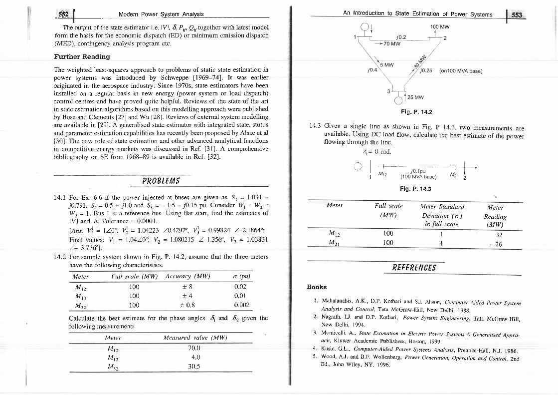
ilr l Modern PoI

The output of the state estimator i.e. lvl, 6, P,j, Q,jtogether. with latest modelform the basis for the economic dispatch (ED) or minimum emission dispatch(MED), contingency analysis program etc.

Further Readin

The weighted least-squares approach to problems of static state estimation inpower systems was introduced by Schweppe 11969-741. It was earlieroriginated in the aerospace industry. Since 1970s, state estimators have beeninstalled on a regular basis in nern' energy (power system or load dispatch)control centres and have proved quite helpful. Reviews of the state of the artin state estimation algorithms based on this modelling approach were publishedby Bose and Clements [27] and Wu [28]. Reviews of external system modellingare available in 1291. A generalised state estimator with integrated state, stutusand parameter estimation capabilities has recently been proposed by Alsac et al

[30]. The new role of state estimation and other advanced analytical functionsin competitive energy markets was discussed in Ref. [31].A comprehensivebibliography on SE from 1968-89 is available in Ref. [32].

PROB LEMS

14.1 For Ex. 6.6 if the power injected at buses are given as Sr = 1.031 -

j0.791, Sz = 0.5 + 71.0 and 'S3 = - 1.5 - j0.15 pu. Consider Wt= Wz=Wz = l. Bus I is a reference bus. Using flat start, find the estimates oflV,l and {. Tolerance = 0.0001.

lAns: Vl = l/0", V', = t.04223

Final values: Vt - 1.04./.0", V2l- 3.736"1.

14.2 For sample system shown in Fig.have the followine characteristics.

Meter Full scale (MW) Accuracy (MW) o (pu)

F ig . P .14 .2

Given a single line as shown in Fig. p 14.3, two measurements areavailable. using DC load flow, calculate the best estimate of the powerflowing through the line.

14.3

4= 0 rad.

/1 |

( ,r-1-- t t----- [lr y0 .1pu1

Mt2 (1oo MVA base) Mzt l -2

Fig. P. 14.3

Meter Full scale

(MW)Meter Standard

Deviation ( o )in full scale

Meter

Reading(Mw)

10.4297", V\ = 0.9982q l-2.1864";= 1.080215 l-1.356, Va - 1.03831

P. 14.2, assume that the three meters

Mrz

Mzr100100

14

32- 2 6

Mrz

M t t

Mzz

100r00100

+ 8+ 4

+ 0.8

0.020.010.002

the phase angles 4 *d d2 given the

REFEREN CES

Books

l. Mahalanabis, A.K., D.P. Kothari and S.L Ahson, Computer Aidetl pr;wer SystemAnalysis and Control, Tata McGraw-Hill, New Delhi, 19gg.

2. Nagrath, I.J. and D.P. Kothari, Power System Engineering, Tata McGraw-Hill.Ncw Dclhi, I q94.

3. Mtrnticclli' A., State li.rtinrution in Eler:tric: Power Sysrems A Gcnerali.recl Apprct-at:h, Kluwcr Academic Publishers, Boston, 1999.

4. Kusic, G'L., Computer-Aided Power Systems Analysis, Prentice-Hall, N.J. 19g6.5. Wood, A'J. and B.F. Wollenberg, Power Generation, Operation and Control. Znd

Ed., John Wiley, NY, 1996.

Calculate the best estimate forf , ' 1 1 , . . . , : n m n n f t ,| 1 - r l l \ . , W | | l 5 | I lU { lDL l l t / l I lU l l L , )

Meter Meusured value (MW)

M t z

Mrz

Mt,

70.04.0

30.5

An lntroduction to State Estimation of Power

'lIIj

t -

;554.;l Modern Power System Analysls

6. Grainger, J.J. and W.D. Stevenson, Power System Analysis, McGraw-Hill, NY',

1994.

7. Deautsch, R., Estimation Theory, Prentice-Hall Inc' NJ, 1965

g. Lawson, C.L. and R.J. Hanson, Solving Least Squares Problens, Prentice-Hall.

inc., NJ., i974.g. Sorenson, H.W., Parameter Estimation, Mercel Dekker, NY, 1980'

Papers

10. Schweppe, F.C., J. Wildes, D. Rom, "Power System Static State Estimation, Parts

l, ll and lll", IEEE Trans', Vol. PAS-89, 1970, pp 120-135'

ll. Larson, R.E., et. al., "State Estimation in Power Systems", Parts I and II, ibid-,

pp 345-359.

lZ. Schweppe, F.C. and E.J. Handschin, "static State Estimation in Electric Power

System", Proc. of the IEEE, 62, 1975, pp 972-982'

13. Horisbcrgcr, H.P., J.C. Richarcl and C. Rossicr, "A Fast Dccouplcd Static Statc

Estimator for Electric Power Systems", IEEE Trans. Vol. PAS-95, Jan/Feb 1976,

pp 2O8-215.Monticelli, A. and A. Garcia, "Fast Decoupled Estimators", IEEE Trans' Power

Sys/, 5, May 1990, pP 556-564.

Dopazo, J.F. et. al., "State Calculation of Power Systems from Line Flow

Measurcments, Parts I and l l" , IEEE Trans., 89, pp. 1698-1708, 91, 1972, pp

1 4 5 - 1 5 1 .

16. Dcbs, A.S. ancl R.E. Larson, "A Dynamic Estimator for Tracking the State of a

Power System", IEEE Trans' 89, 1970, pp 1670-1678'

iZ. K1u-pholz, G.R. et. al., "Power System Observability: A Practical Algorithm Using

Nctwork Topology", IEEE Trans. 99' 1980' pp 1534-1542'

lg. Sirnoes-Costa, A and V.H. Quintana, "A Robust Numerical Technique for Power

System State Estimation", IEEE Trans. 100, 1981, pp 691-698'

19. Simgcs-Costa, A and V.H. Quintana, "An Orthogonal Row Processing Algorithm

for Power System Sequential State Estimation", IEEE Trans., 100, 1981' pp

3 '79r-3799.

20. Debs, A.S., "Estimation of External Network Equivalents from Internal System

Data", IEEE Trans., 94, 1974, pp 1260-1268'

21. Garcia. A., A. Monticelli and P. Abreu, "Fast Decoupled State Estimation and Bad

Dara Processing", IEEE Trans. PAS-98, Sept/Oct 1979, pp 1645-1652.

22. Handschin, E. et. al., "Bad Data Analysis for Power System State Estimation",

IEEE Trans., PAS-94, 1975, pp 329-337-. t2 r.^-r:6 rJ r or nl "Flqd T)cre Detecfion and ldenti f icat ion". Int. J. EleC. POWer,4 J . r \ V 6 l r r r t L t . r . e L . @ e . ,

Vol. 12, No. 2, April 1990, PP 94-103'

24. Me-Jjl, H.M. and F.C. Schweppe, "Bad Data Suppression in Power System State

Estimation", IEEE Trans. PAS-90, 1971' pp 2718-2725'

25. Mafaakher, F., et. al, "Optimum Metering Design Using Fast Decoupted

Estimator", IEEE Trans. PAS-98, 7979, pp 62-68.

1 4 .

1 5 .

ii

I

An Introduction to State Estrmation of Power Systems I 555_T--

26. Clements, K.A., "Observability Methods and optimal Meter Placement", Int. J.

Elec. Power, Vol. 12, no. 2, April 1990, pp 89-93.

27. BoSe, A. and Clements, K.A., "Real-time Modelling of Power Networks", IEEE

Proc., Special Issue on Computers in Power Svstem Operations, Vol. 75, No. 12,

Dee 1987;aP 76ff7=1ffi2:

28. Wu, F.F., "Power System State Estimation: A Survey", Int: J. Elec. Power and

Energy Syst., Vol. 12, Jan 1990, pp 80-87.

29. Wu, F.F. and A. Monticelli, "A Critical Review on External Network Medelling

for On-line Security Analysis", Int. J. Elec. Power and Energy Syst., Vol. 5, Oct

1983, pp 222-235.

30. Alsac, O., et. aI., "Genetalized State Estimation", IEEE Trans. on Power Systems,

Vol. 13, No. 3, Aug. 1998, pp 1069-1075.

31. Shirmohammadi, D. et. al., "Transmission Dispatch and Congestion Management

in the Emerging Energy Market Structures", IEEE Trans. Power System., Vol 13,

No. 4, Nov 1998, pp 1466-1474.

32. Coufto, M.B. et. aI, "Bibliography on Power System State Estimation (1968-

1989)", IEEE Trans. Power Sysr., Vol.7, No.3, Aug. 1990, pp 950-961.

15.1 INTRODUCTION

For reduction of cost and improved reliability, most of the world,s electricpower systems continue to be intercorof diversity of loads, availability of sorto loads at minimum cost and pollrderegulated electric service environmeto the competitive environment of reli

Now-a-days, greater demands have been placed on the transmission network,and these demands will continue to rise because of the increasing number ofnonutil i ty generators and greater competit ion among uti l i t ics the'rselves. It isnot easy to acquire new rights of way. Increased demands on transmission,absence of long-term planning, and the need to provide open access togenerating companies and customers have resulted in less security and reducedquality of supply.compensation in power systems is, therefore, essential to alleviate some ofthese problems' series/shunt compensation has been in use for past many yearsto achieve this objective.In a power system, given the insignificant erectricar storage, the powergeneration and load mttst balance at all t imes. To some extent, the electricalsystem is self'-regulating. If generation is less than roacl, voltage ancl frequencyd'op, and thereby reducing the road. However, there is only a few percentmargin for such self-regulation. lf ,,^r+--^ :- :_,-

support, rhen load increase with con"se;:;iilTi: ,:t#'j|i;l:ffL;system collapse' Alternatively, if there isinadequate reactive power, the systemrnay havc voltage collapse.This chapter is devotecl to the stucly of various methods .f compensatingpower systems and various types clf compensating crevices, cailccr .,,,rrj",rru,urr,to alleviate the problems of power system outlined above. These compensators

Compensation in lglver Systems | 55?I

can be connecteci in the system in two ways, in series and irr shunt at ihe line

ends (or even in the midPoint)'

Apart from the well-known technologies of compensation, the latest

technology of Flexible AC Transmission System (FACTS) will be introduced

towards the end of the chaPter.

15.2 LOADING CAPABILITY

There are three kinds of limitations for loading capability of transmission

system:(i) Thermal (ii) Dielectric (iii) Stability

Thermal capabitity of an overhead line is a function of the ambient

temperature, wind conditions, conditions of the conductor, and ground

clearance.There is a possibility of converting a single-circuit to a double-circuit line to

increase the loading caPabil itY.

Dieletric Limitations From insulation point of view, many lines are designed

very conservatively. For a given nominal voltage rating it is often possible to

increase normal operating voltages by l07o (i.e. 400 kV - 440 kV). One should,

however, ensure that dynamic and transient overvoltages are within limits. [See

Chapter 13 of Ref. 71.

Stability Issues. There are certain stability issues that limit the tlansmission

capability. These include steady-state stability, transient stability, dynamic

stability, frequency collapse, voltage collapse and subsynchronous resonance.

Several goocl books l, l , 2, 6,7 ,8) are available on these topics. The FACTS

technology can certainly be used to overcome any of the stability limits, in

which case the final limits would be thermal and dielectric'

15.3 LOAD COMPENSATION

Load compensation is the management of reactive pcwer to improve power

quality i.e. V profile and pf. Here the reactive power flow is controlled by

installing shunt compensating devices (capacitors/reactors) at the load end

bringing about proper balance between generated and consurned reactive power.

This is most effective in improving the power transfer capability of the system

ancl its voltage stabil ity. It is desirable both economically and technically to

operate the system near uriity power factor. This is why some utilities impose

a penalty on low pf loads. Yet another way of irnproving the system

performa-nee is to operate it under near balanced conditions so as to reduce the

ho* of legative sequence currents thereby increasing the system's load

capabil ity and reducing power loss'

A transmission l ine has thrcc cr i t ical loadings ( i ) natural loading ( i i ) steady-

stare stabil ity l imit and (i i i) thermal l imit loading. For a compensated l ine the

natural loading is the lowest and before the thermal loading limit is reached,

steady-state stability limit is arrived.

Ideal voltage profile for a transmission line is flat, which can onlyby loading the line with its surge impedance loading while this

esJI

T5.4 LINE COMPENSATIONcompensated, it will behave as a purely resistive element and would. causeseries resonance even at fundamental frequency. The location of seriescapacitors is decided by economical factors and severity of fault currents. Seriescapacitor reduces line reactance thereby level of fault currents.

on on vanous lssues ln in series and shuntcompensators now follows.

15.5 SERIES COMPENSATION

A capacitor in series rvith a line gives control over the effective reactancebetween line ends. This effective reactance is eiven bv

X r = X - X ,

whereXl = line reactance

Xc = capacrtor reactance

It is easy to see that capacitor rcduccs the cffectivc l ine rcactance*.This results in improvement in performance of the system as below.

(i) Voltage drop in the line reduces (gets compensated) i.e. minimization ofend-voltage variations.

(ii) Prevents voltage collapse.(i i i) Steady-stttte power transfer increases; it is inverscly proportional to Xl.(iv) As a result of (ii) rransient stability limit increasbs.

The benefits of the series capacitor compensator are associated with a problem.The capacitive reactance Xg fbrms a series resonant circuit with the total seriesreactance

X = Xt * X*.n * Xoun,

The natural frequency of oscillation of this circuit is given by.

f ^ - |rL

2 rJ rc

be achievedmay not be

achievable, the characteristics of the line can be modiso that

(i) Ferranti effect is minimized.(ii) Underexcited operation of synchronous generators is not required.

(iii) The power transfer capability of the line is enhanced. Modifying thecharacteristics of a line(s) is known as line compensation.

Various compensating devices are:o Capacitors. Capacitors and inductors. Active voltage source (synchronous generator)

When a number of capacitors are connected in parallel to get the desiredcapacitance, it is known as a bank of capacitors, similarly a Uant< of incluctors.A bank of capacitors and/or inductors can be adjusted in steps by switching(mechanical). .

Capacitors and inductors as such are passive line compensators, whilesynchronous generator is an active compensator. When solid-state devices areused for switching off capacitors and inductors, this is regardecl as activecompensation.

Before proceeding to give a detailed account of line compensator, we shallbriefly discuss both shunt and series compensation.

Shunt compensation is more or less like load compensation with all theadvantages associated with it and discussed in Section 15.3. It needs to bepointed out here that shunt capacitors/inductors can not be distributeduniformally along the line. These are normally connected at the end of the lineand/or at midpoint of the l ine.

Shunt capacitors raise the load pf which greatly increases the powertransmitted over the line as it is not required to carry the reactive power. Thereis a limit to which transmitted power can be increased by shunt compensationas it would require very iarge size capacitor bank, which would be impractical.For increasing power transmitted over the line other and better means can beadopted. For example, series compensation, higher transmission voltage, HVDCetc.

When switched capacitors are employed for compensation, these shculd bedisconnected irnmediately under l ight loacl conclit ions to avoicl er.cessive voltagerise and ferroresonance in presence of transformers.

The purpose of series compensation is to cancel part of the series inductivereactance of the line using series capacitors. This helps in (i) increase ofmaximum power transfer (ii) reduction in power angle for a given amount ofpower transfer (iii) increased loading. From practical point of view, it is

' 2 n

where l= system frequency

xReactive voltage drops of a series reactance added in a line is I2xIt is positive if X is inductive and negative if X is capacitive. So a series capacitivereactance reduces the reactance voltage drop of the line, which is an alternative wavof saying that

X ' t = \ - X , -I

iitit i

I

f c < fwhich is subharmonic oscillation.

Even though series compensation has often been found to be cost-effective

compared to shunt compensation, but sustained oscillations below the funda-

mental system frequency can cause the phenomenon, referred to aS

subsynchronous resonance (SSR) first observed in 1937, but got world-wide

attention only in the 1970s, after two turbine-generator shaft failures occurred

at the Majave Generating station in Southern Nevada. Theoretical studies

pointed out that interaction between a series capacitor-compensated line,

oscillating at subharmonic frequency, and torsional mechanical oscillation of

turbine-generator set can result in negative damping with consequent mutual

reinforcement of the two oscillations. Subsynchronous resonance is often not a

major problem, and low cost countermeasures and protective measures can be

applied. Some of the corrective measures are:

(i) Detecting the low levels of subharmonic currents on the line by use of

sensitive relays, which at a certain level of currents triggers the action to

bypass the series capacitors.

(ii) Modulation of generator field current to provide increased positive

damping at subharmonic frequency'

Series incluctors are neeclecl for line compensation under light load conditions to

counter the excessive voltage rise (Ferranti effect).

As the line load and, in particular the reactive power flow over the line

varies, there is need to vary the compensation for an acceptable voltage profile.

The mechanical switching arrangement for adjusting the capacitance of the

capacitor bank in series with the line is shown in Fig. 15.1. Capacitance is

variecl by opening the switchos of individual capacitances with the capacitance

C1, being started by a bypass switch. This is a step-u'ise arrangement. The

whole bank can also be bypassed by the starting switch under any emergent

conclitions on the line. As the switches in series with capacitor are current

carrying suitable circuit breaking arrangement are necessary. However, breaker

switched capacitors in series are generally avoided these days the,capacitor is

either fixed or thvristor switched.

I , ,

' technology, the capacitance of the series capacitance bank can be controlledmuch more effectively; both stepwise and smooth control. This is demonsffatedby the schematic diagram of Fig. 15.2 wherein the capacitor is shunted by two

nstors ln antlcurrent in positive half cycle and the other in negative half cycle.

In each half cycle when the thyristor is fired (at an adjustable angle), itconducts current for the rest of the half cycle till natural current zeto. Duringthe off-time of the thyristor current is conducted by the capacitor and capacitorvoltage is vr. During on-time of the thyristor capacitor is short circuited i.e.v, = 0 and current is conducted by the thyristor. The same process is repeatedin the other half cycle. This means that v, can be controlled for any given i,which is equivalent of reducing the capacitance as C = vJi.By this schemecapacitance can be controlled smoothly by adjusting the firing angle.

l - -+ { - -_ -__-a , .Cur renu imi t ins| | r' reactor^ o ' l l " " il-1<-------r l

C r i---. i

t 7,c -----]

Fig. 15.2

Thyristors are now available to carry large current and to withstand (duringoff-time) large voltage encountered in power systems. The latest device calleda Gate Turn Off (GTO) thyristor has the capability that by suitable firingcircuit, angle (time) at which it goes on and off can both be controlled.

This means wider range and finer control over capacitance. Similarly confrolis possible over series reactor in the l ine.

All controlled.".?nd uncontrolled (fixed) series compensators require aprotective arrangement. Protection can be provided externally either by voltagearrester or other voltage limiting device or an approximate bypass switcharrangement. In no case the VI rating of the thyristors should be exceeded.

Depending on (i) kind of solid-state device to be used (ii) capacitor and/orreactor compensation and (iii) switched (step-wise) or smooth (stepless)control, several compensatron schemes have been devised and are in use. Someof the more common compensation schemes are as under.

(i) Thyristor Controlled Series Cappcitor (TCSC)(ii) Thryristor\Switched Series Capacitor (TSSC)

(iii) Fllyristor controlled Reactor with Fixed capacitor (TCR + FC)(iv) GTO thyristor Coniiolled Series Capacitor (GCSC)

Modern Power System AnalYsis

rL =degree of compensation

X

= 25 to J5Vo (recommended)

i'r;

*562i I Modern Power System AnalysisI

(v) Thyristor Controlied reactor (TCR)

Capacitor and/or reactor series compensator act to modify line impedance.

An altcrnativo approach is to introducc a controllable voltagc sourcc in series

with the line. This scheme is known as static synchronous series compensator

(SSSC). SSSC has the capabitity to induce both capacitive and inductive

voltage ln senes wrtn [lne, wrdenrng me operatmg reglon o

It can be used for power flow control both increasing or decreasing reactive

flow on the line. Further this scheme gives better stability and is more effective

in damping out electromechanical oscillations.

Though various types of compensators can provide highly effective power

flow control, their operating characteristics and compensating features are

different. These differences are related to their inherent attributes of their

control circuits; also they exhibit different loss characteristics.

From the point of view of almost maintenance free operation impedance

modifying (capacitors and/or reactors) schemes are superior. The specific kind

of compensator to be employed is very much dependent on a particular

application.

15.6 SHUNT COMPENSATORS

As already explained in Sec. 15.4 and in Ch. 5 (Sec. 5.10) shunt compensators

are connected in shunt at various system nodes (major substations) and

sometimes at mid-point of lines. These serve ihe purposes of voltage control and

load stabilization. As a result of installation of shunt compensators in the

system, the nearby generators operate at near unity pf and voltage emergencies

mostly clo not arise. The two kinds of compensators in use are:

(1) Static var compensators (SVC): These are banks of capacitors (some-

t imes incluctors also fgr use under l ight load condi t ions)

(ii) STATCOM: static synchronous compensator

(iii) Sync hronous condenser: It is a synchronous motor running at no-load

and having excitation adjustable over a wide range. It f'eeds positive

VARs into the line under overexcited conditions and negative VARS

when underexcited. (For details see Sec. 5.10.)

It is to be pointed out here that SVC and STATCQM are stgtic var

generators which are thyristor controlled. In this section SVC will be detailed

while STATCOM forrns a part of FACTS whose operafion is explained in

S e c . 1 5 . l O .

Statia VAR Compensator (SVC)

These comprise capacitor bank fixed or switched (controlled) or fixed capacito

bank and switched reactor bank in parallel. These compensators draw reactiv(leading or lagging) power* from the line thereby regulating voltage, improv

*A rcrrct l r rcc cor)ncctcd in shunt to t inc at vol tage V draws react ive power Vzl ]

It is negative (leading) if reactance is capacitive and positive (lagging) if reactance is

induct ive.

called static var switches or systems. It means that terminology wiseSVC = SVS

and we will use these interchangeably.

Basic SVC Configrurations (or Desigrns)

Thyristors in antiparallel can be used to switch on a capacitor/reactor unit instepwise control. When the circuitary is designecl ro adjust the firing angle,capacitor/reactor unit acts as continuously variable in the power circuit.

Capacitor or capacitor and incluctor bank can be varied stepwise orcontinuously by thyristor control. Several important SVS configurations havebeen devised and are applied in shunt line compensation. Some of the staticcompensators schemes are discussed in what follows.

(i) Sutu.rutcd reuctlr

This is a multi-core reactor with the phase windings so arranged as to cancelthe principal harmonics. It is consiclered as a constant voltageieactive source.It is almost maintenance free but not very flexible with reipect to operatingcharacteristics.

(ii)'fhyristor-coilrroll,cd reuctor (T'CR)

A thyristor-controlled-reactor (Fig. 15.3) compensator consists of a combina-tion of six ptrlse or twelve pluse thyristor-controllecl reactprs with a fixe<t shuntcapacitor bank. The reactive power is changect by adjusting the thyristor firingangle. TCRs are characterised by continuous control, no transients andgencration of harmonics'k. The control systenr consists of voltage (and current)

Power I- - Line oi.rt

transformer I-? {-rf '-- lneaitr i

I

Fixedcaoacitor

I i] l.:

) t lII

I

I n"r.to,f =..'x',rnc.- -I

u v v v

I

I Neutral

Fig. 15.3 Thyristor controlledreactor (TCR) with fixed capacitor*Though ) -connected TCR's are

since it is better configuration.used here, it is better to use A-connected TCR,s


measuring devices, a controller for error-signal conditioning, a Iinearizingcircuit and one or more synchronising circuits.(iii) Thyristor switcherl capacitor (fSC)

It consists of only a thyristor-switched capacitor bank which is split into anumDer o unrts o equal ratrngs to achreve a stepwise con

| ;

fe"system (e.9. line faults, load rejection etc) TSC/TCR combinations arecharacterised by continuous contrdl, no transients, low generations of harmon-ics, low losses, redundancy, flexible control and operation.

in Tab le 15 .1 .

Table 15.1 Comparison of Static Var Generators' 0 d 6 '

/

Type ofVar

Generator

TCR.FC( 1 )

TSC-(TSR)(2)

TCR-TSC(3)

Dampingreactor

- Fig. 15.4 Thyristor switched capacitor (TSC)

As such they are applied as a discretly variable reactive power source, wherethis type of voltage support is deemed adequate. All switching takes place whenthe voltage across the thyristor valve is zero, thus providing almost transienttree switching. Disconnection is eff'ected by suppressing the firing plus to thethyristors, which will block when the current reaches zero. TSCs are,charetcLorisccl by stcp wisc control, no transients, vcry low htlrnronics, lowlosses, redundancy and flexibility.

(iv) Combined TCR and TSC Compensator

A combined TSC and TCR (Fig. 15.5) is the optimum solution in majority ofcases. With this, continuous variable reactive power is obtained tirroughout thecott t l ; lc tcr conl lo l r lngc. Fru' t l tc l rnorc l i r l l control o1'bot l r induct ive andcapacitive parts of the cornpensator is obtained. This is a very advantageous

---{Neutral

l lCapacitor

T5.7 COMPARISON BETWEEN STATCOM AND SVC

I t m q w h e n n t e r l t h o t i - t h o n n r , - , ' l l ; - ^ ^ - ^ * ^ - , - f : ^ - ^ r - r - - r t t" ' *J r r rqL r r r Lr rv r rv l r l la l l r l r t /q . r \ ,Pgr4t r l rE rd l rBc u l u le v - l

characteristic and functional compensation capability of the STATCOM and thesVC aie similar l2l. However, the basic operating principles of theSTATCOM, which, with a converter based var generator, functions as a shunt-connected synchronous voltage source, are basically different from those of theSVC, since SVC functions as a shunt-connected, controlled reactive admittance.This basic operational difference renders the STATCOM to have overall

VI and VQcharacteristics

Loss Vs varoutput.

Hannorr icgeneration

Max. theoret.delayTrrns i r :n lbehaviourunder systentvoltagr:disturbances

Max comp. currentis proportional tosystem voltage.Max cap. var outputdecreases with thesquare of the voltagedecrease.High losses at zerooutput. Lossesdecrease smoothlywith cap. output,increirse withinductive output

In tcrna l ly h igh(large pu TCR)Requires significantfilteringl/2 cycle

Poor (FC ('iluscs

transient over-voltages in responseto step disturbances)

Max. Comp. current is Same as inproportional to system (1) or (2)voltage.Max. cap. var outputdecreases with thesquare of the voltagedecrease.Low losses at zero Low losses atouput. Losses increase zero output.step-like with cap. Losses increaseoutput step-like with

cup. output,smoothly withind. output

hrtcrnal ly vcry low Internal ly lowResonance may (small punecessirate tuning TCR) Filteringreactors requiredI cycle I cvcle

Cun bc l rcut ra l . Sanrc as in (2)(Capacitors can beswitched out to minimisetrattsicnt ovcr-volt ages)

a

Neutral

Fig. 15.5 A combined TCR/TSC compensator

tto .t lvlooern Power Systenr Analystst

superior functional characteristics, better performance, and greater applicationflexibility as compared to SVC. The ability of the STATCOM to maintain fullcapacitle output current at low system voltage also makes it rnore effectivethan the SVC in improving the transient (first swing) stability.Comparison between series and shunt compensation:

(i) Series capacitors are inherently self regulating and a control system is notrequired.

(ii) For the same performance, series capacitors are often less costly thanSVCs and losses are very low.

(iii) For voltage stability, series capacitors lower the critical or coliapsevoltage.

(iv) Series capacitors possess adequate timc-ovellt-rad capability.(v) Series capacitors and switched series capacitors can be used to controi

loading of paralled lines to minimise active and reactive losses.

Disadvantages of series compensation:

(i) Series capacitors are line connected and compensation is removed foroutages and capacitors in parallel lines may be overloaded.

(ii) During tru.,vy ioading, the voltage on one side of the series capacitor maybe out-of range.

(iii) Shunt reactors may be needed for light load compensation.(iv) Subsynchronous resonance may call for expensive countermeasures.

Advantages of SVC

(i) SVCs control voltage directly.

(ii) SVCs control temporary overvoltages rapidly.

Disadvantages of SVC

(i) SVCs have limited ovcrload capability.

(ii) SVCs are expensive.

The best design perhaps is a combination of series and shunt compensation.Because of higher initial and operating costs, synchronous condensers arenormally not competitive with SVCs. Technically, synchronous condensers arebetter than SVCs in voltage-weak networks. Following a drop in networkvoltage, the increase in condenser reactive power output is ilrslantaneous. Mostsynchrono.us condenser applications are now associated with HVDC installa-l lons.

15.8 FLEXTBLE AC TRANSMTSSTON SYSTEMS (FACTS)

The rapid development of power electronics technology provides excitingopportunities to develop new power system equipment for better utilization of

*FACTS technology have been proposed and implemented. FACTS devices ca1be effectively used for power flow conffol, load sharing among parallelcorridors, voltage regulation, enhancement of transient stability anO mitlgation

enable a line to carry power closer to its thermal rating. Mechanical switchinghas to be supplemented by rapid response power electronics. It may be notedthat FACTS is an enabling technology, and not a one-on-one substitute formechanical switches.

FACTS employ high speed thyristors for switching in or out transmissionline cornponents such as capacitors, reactors or phase shifting transformer forsome desirable performance of the systems. The FACTS technology is not asingle high-power controller, but rather a collection of controllers, wtrictr can beapplied individually or in coordination with others to conffol one or more of thesystem parameters.

Before proceeding to give an account of some of the important FACTScontrollers the principle of operation of a switching converter will be explained,which forms the heart of these controllers.

15.9 PRINCIPLE AND OPERATION OF CON\ZERTERS

Controllable reactive power can be generated by dc to ac switching converterswhich are switched in synchronism with the line voltage with whicn tfr" reactivepower is exchanged. A switching power converter consists of an array of solid-state switches which connect the input terminals to the output terminals. It hasno internal storage and so the instantaneous input and output power are equal.Further the input and output terminations are complementar|, that is, if the inputis terminated by a voltage source (charged capacitor or battery), output ii acuffent source (which means a voltage source having an inductive impedance)and vice versa. Thus, the converter can be voltage sourced (shunted by acapacitor or battery) or current sourced (shunted by an inductor).

Single line diagram of the basic voltage sourced converter scheme forreactive power generation is drawn in Fig. 15.6. For reactive power flow busvoltage V and converter terminal voltage V, are in phase.

Then on per phase basis i

r = v - v 4x ' i

' F h a r a a ^ + ; " ^ - ^ ' . ' ^ - ^ - , ^ f ^ ^ J ^ ^ : ^

r u v l v c v L t v l y P r J w 9 r E ^ U r r 4 r r B t r l 5

' O = v I = v ( v - v o )

X

563 l Modern PoI

System bus V---__i--' i ' Coupling transformer

I

. J ,X

:l J, Transformer leakage reactance

Vd.

Fig. 15.6 Static reactive power generator

The switching circuit is capable of adjusting Vo, the output voltage of theconverter. For Vo 1 V,1 lags V and Q drawn from the bus is inductive, whilefor Vo > V, I leads V and Q drawn from the bus is leading. Reactive power

drawn can be easily and smoothly varied by adjusting Voby changing the on-time of the solid-state switches. It is to be noted that transformer leakagereactance is.quite small (0.1-0.15 pu), which means that a amall difference ofvoltage (V-Vo) causes the required ,1 and Q flow. Thus the converter acts likea static synchronous condenser (or var generator).

A typical converter circuit is shown in Fig. 15.7. It is a 3-phase two-level,six-pulse H.bridge with a diode in antiparallel to each of the six thyristors(Normally, GTO's are used). Timings of the triggering pulses ate insynchronism with the bus voltage waves.

[ 1 '

K

Va"

C

Fig. 15.7 Three-phase, two-level six-pulse bridge

-

capacitor is zero. Also at dc (zero fiequency) the capacitor does not supply any

reactive power. Thereibre, the capacitor voltage cloes not change and the

capacitor establishes only a voltage level for the converter. The switching

causes the converter to interconnect the 3-phase lines so that reactive current

can flow between thent.

The converter draws a small amount of real power to provide for the internal

loss (in switching). If it is required to feed reai power to the bus, the capacitor

is replace,l by a storage battery. For this the circuit switching has to be

modified ro create a phase difference dbetween Vsand Vwith Vsleading V'

The above explained converter is connected in shunt with the line. On sirnilar

lines a converter can be constructed with its terminals in series with the line.

It has to carry the line current and provide a suitable magnitude (may also be

phase) voltage in series with the line. In such a connection it would act as an

impedance modifier of the line.

15.10 FACTS CONTROLLERS

The development of FACTS controllers has followed two different approaches.

The first approach employs reactive impedances or a tap changing ffansformer

with thyristor switches as controlled elements, the second approach employs

self-commutated static converters as controlled voltage sources.

ln general, FACTS controllers can be divided into tour categories.

(i) series (ii) shunt (iii) combined series-series (iv) combined series-shunt

controllers.The general symbol for a FACTS controller is given in Fig. 15.8(a). which

shows a thyristor arrow inside a box. The series controller of Fig. 15.8b could

be a variable impedance, such as capacitor, reactor, etc. or a power electronics

based variable source. All series controllers inject voltage in series with the

line. If the voltage is in phase quadrature with the line, the series controller only

supplies or consumes variable reactive power. Any other phase relationship will

involve real power also.Tlte shunt controllers of Fig. 15.8c may be variable impedance, variable

source or a combination of these. All shunt controllers inject current into the

system at the point of connection. Combined series-series controllers of Fig.

15.8d could be a combination of separate series controllers which are conffolled

in a coordinated manner or it could be a unified controller.

Combined series-shunt controllers are either controlled in a coordinated

ma-nner as in Fig. 15.8e or a unified Power Flow Controller with series and

shunt elements as in Fig. 15.8f. For unified controller, there can be a real power

exchange between the series and shunt controllers via the dc power link.

Storage source such as a capacitor, battery, superconducting magnet, or any

other source of energy can be added in parallel through an electronic interface

to replenish the converter's dc storage as shown dotted in Fig. 15.8 (b). A

Vo" Vot Vo,

ff.*J Modern power System Analysis

controller with 'storage is much more effective for conffolling the systemdynamics than the corresponding controller without storage.

Compensation in power Systems tffi*ffilT-

Llne Line

(a)GeneralsymbolforFACTS controller (FC)

l u n " l[,--TT- I

lFcl-T-

(c) Shunt controller

Line

ac l ines

Flg. 15.8 Different FACTS controllers

The group of FACTS controllers employing switching converter-basedsynchronous voltage sources include the STATic synchronous COMpensator(STATCOM), the static synchronous series compensator (SSCC), the unifiedpower flow controller (UPFC) and the latest, the Interline Power FlowController (IPFC).

STATCOM

STATCOM is a static synchronous generator operated as a shunt-connectedstatic var compensator whose capacitive or inductive output current can be^ - - - ^ - - ^ l l - l ! t a ,i;orrrr-oiieo rnoepenoent oi rhe ac system voltage. The STATCOM, like itsconventional countetpart, the SVC, controls transmission voltage by reactiveshunt compensation. It can be based on a voltage-sourced oi curtent-sourcedconverter. Figure 15.9 shows a one-line diagram of srATCoM based on avoltage-sourced converter and a current sourced converter. Normally a voltage-source converter is preferred for most converter-based FACTS controllers.STATCOM can bc designed to be an active filter to absorb system harmonics.

(a) /

(b)

Fig. 15.9 (a) STATCOM based on voltage-sourced and (b) current-sourcedconverters.

. A combination of STATCOM and any energy source to supply or absorbpowei is called static synchronous generator (SSG). Energy source may be abattery, flywheel, superconducting magnet, large dc storage capacitor, anotherrectifi erlinverter etc.

Statlc Synchronous Series Compensator (SSCC)

It is a series connected controller. Though it is like STATCOM, bu(its outputvoltage is in series with the line. It thus controls the voltage across the line andhence its impedance.

Interline Power FIow Controller (IPFC)

This is a recently introduced controller 12,3]. It is a cornbination of two ormore static synchronous series conlpensators which are coupled via a commondc link to facilitate bi-directional flow of real power between the ac terminalsof the SSSCs, and are controlled to provide independent reactive seriescompensation for the control of real power flow in each line and maintain thedesired distribution of reactive power flow among the lines. Thus it manages acomprehensive overall real and reactive power management for a multi-linetransmission system.

Unified Power FIow Controller (UPFC)

This controller is connected as shown in Fig. 15.10. It is a combination ofSTATCOM and SSSC which are coupled via a iommon dc lin-k to -allowbi-directional flow of real power between the series output terminals of theSSSC and the shunt output terminals of the STATCOM. These are controlled

fo provide concurrent real and reactive series line compensation without anexternal energy source. The.UPFC, by means of angularly unconsffained seriesvoltage injection, is able to control, concurrently/simultaneously or selectively,the transmission line voltage, impedance, and angle or, alternatively, the real

(d) Unified series-series controller

!-.I i t

FCH Coordinatedcontrol

(e) Coordinated seriesand shunt controller

(f) Unified series-shunt controller

dc powerl ink

<-oc

rr$il#4 ModernI

and reactive line flows. The UPFC may also provide independently controllabteshunt reactive compensation.

STATCOM

Fig. 1S.10 Unified power Flow Controiler UpFC

Th yri s t or- co n tro I I e d p h a s e - sh ifti n g Tra n sfo rm er (TCp s r)

This controller is also called Thyristor-controlled Phase Angle Regulator(TCPAR). A phase shifting transformer controlled by thyristor switches to givea rapidly variable phase angle.

Th yristor- Con troll e d VoI tdgre R egu tra tor flCVR)

A thyristor controlled transformer which can provide variable in-phase voltagewith continuous control.

Interphase Power Controller (IpC)

A series-connected controller of active and reactive power consisting, in eachphase, of inductive and capacitive branches subjected to separately phase-shifted voltages. The active and reactive power can be set inpedendently byadjusting the phase shifts and/or the branch impedances, using mechanical orelectronic switches.

Thyristor Controlled Braking Resistor ICBR)

It is a shunt-connected thyristor-switched resistor, which is controlled to aidstabilization of a power system or to minimise power acceleration of agenerating unit during a disturbance.

Thyristor-controlled Voltage Limiter FCVL)

A thyristor-switched metal-oxide varistor (Mov) used to limit theacross its terminals durins transient conditions

'TIVDC

It may be noted that normally HVDC and FACTS are compleme ntarytechnologies. The role of HVDC, for economic reasons, is to interconnect acsystem?,where a reliable ac interconnection would be too expensive. HVDC

l l " r ' . - r ' i :

stability and cnnffol line flows. Voltage source converter based (self-commutated) HVDC system may have the same features as those ofSTATCOM or UPFC. This system also regulates voltage and provides system

A comparative perfonnance of major FACTS controllers in ac system isgiven in Table 15.2 U4l.

Table 15.2 A comparative performance of major FACTS controller

Type of FACTS

Controller

Load

flow control

Transient

stability

Oscillation

Damping

V

controlSVC/STATCOMTCSCSSSCTCPARUPFC

X

X X

XXX

XXX

X X X

X X X

xx

X X

X X X

xxxxxxX X X

X

X X X

X X

XX

X X

X X

XXX

voltage

* a;v-slrong influence; xx-average influence; x-smail infruence

sutyffvtARySince the 1970s, energy cost, environmental restrictions, right-of-*ay difficul-ties, along with other legislative sociai and cost problems huu. postponed theconstruction of both new generation and transmission systems in India as wellas most of other countries. Recently, because of adoption of power reforms orrestructuring or deregulation, competitive electric energy markets are beingdeveloped by mandating open access transmission services.

In the late 1980s, the vision of FACTS was formulated. In this various powerelectronics based controllers (compensators) regulate power flow and transmis-sion voltage and through fast control aciion, mitigate dynamic disturbances.Due to FACTS, transmission line capacity was enhanced. Two types of FACTScontrollers were developed. One employed conventional thyristor-switchedcapacitors and react<lrs, and quadrature tap-changing transformers such as SVCand TCSC. The second category was of self-commutated switching convertersas synchronous voltage sources, e.g. STATCOM, SSSC, UPFC and IpFC. Thetwo groups of FACTS controllers have quite different operating and perform-ance characteristics. The second group uses self-commutated dc to ac converter.The converter, supported by a de power supply or energy storage de.,,ice canalso exchange real power with the ac system besides conmolling reactive powerindependently.

The increasing use of FACTS controllers in future is guaranteed. Whatbenefits are required for a given system would be a principal justification forthe choice of a FACTS controller. Its final form and operation will, ofcourse,depend not only on the successful development of the necessary control and

r:5?4i I Modern power System AnalysisI

communieation teehnologies and protocols, but also on the final structure of ihreevolving newly restructured power systems.

REFERE N CES

Books

I ' Chakrabarti, A', D.P. Kothari and A.K. Mukhopadhyay, Performance Operationand Control of EHV Power Transmission Systems. Wheeler, New Delhi, 1995.

2. Hingorani, N.G. and Laszlo Gyugyi, (Jnderstanding FACTS. IEEE press, NewYork, 2000.

3. Song, Y.H' and A.T. Johns, Flexible AC Transmission Systems,IEE, Lbndon, 1999.4. Miller, T'J.E., Reactive Power Control in Electric Systems, John Wiley and Sons,

NY, lgg2.5. Nagrath' I.J. and D.P. Kothari, Electric Machines, 2nd edn, Tata McGraw-Hill.

New Delhi, 1997.6. Taylor, c.w., power system vortage stability, McGraw-Hill, singapore, 1994.7. Nagrath, I.J and D.P. Kothari, power S),stem Engineering, TataMcGraw_Hill, New

Delhi, 1994.8. Indulkar, C.S. and D.P. Kothari, Power System Transients A Statistical Approach,

Prentice-Hall of India, New Delhi, 1996.9. Mathur, R.M' and R.K. Verma, Thyristor-Based FACTI; Controllers for Electrical

Transmission Systems. John Wiley, New york, 2002.

Papers

I0- Edris- A-, "FACTS Technologv Development: An Update".\EEE Pott'er Engirteer-ing Rerieu'. \'ol. 20. lVlarch 2@1i. pp f9.

1l - I l iceto F- and E. Cinieri, "Comparative Analysis of Series and Shunt CompensationSchemes for Ac Transmission svstems". IEEE Trans. pAs 96 6). rg77. pp lglg-l8-10.

12. Kimbark. E.W.. "Hou, to Impror,e S.r'srem Stabilir-i, u,ithout RiskingSuhs-rtchnrnous R('s(')nitncc"'. IEEE lr.-rrs. P.-tJ-. 96 t-i,I. Sept/Oc.t 1977. pp 160.S-1 9 .

13. CIGRE/ 'wG 38-01. .srrzric l/ar Conrp<,r-rdrorr. CIGRE/. prrr-is.l{ . Ptrvlr. f) . . "Llsc'of HDVC and F.ACTS". IEEE procc'edings. vol.

pp 235-245.15. Kinrbark, E.W. "A New Look At Shunt Compensation., IEEE

102. No. l . Ja-n 1983. nn 212-2!8

i 986.\8. 2, Feb. 2000,

Trans. Vol PAS-

16.1 INTRODUCTION

Load forecasting plays an important role in power system planning, operationand control. Forecasting means estimating active load at various load busesahead of actual load occurrence. Planning and operational applications of loadforecasting requires a certain 'lead time' also called forecasting iritervals.Nature of forecasts, lead times and applications are summarised in Table 16.1"

Table 16.1

Nature of

forecast

Lead time Application

Very short term

Short term

Medium term

Long term

A few seconds toseveral minutes

Half an hour toa ferv hours

A few days toa t'ew' rveeksA t'ew months toa few years

Generation, distribution schedules,contingency analysis for systemsecunfyAllocation of spinning reserve;operarionilI planning ild unitcommitment; maintenance scheduling

Planning for seasonal peak-wrnter. summerPlanning generationgrowth

A good t'orecast reflecting current and future r.rends, tempered wi.Ji goodjudgement, is the key to all planning, indeed. to financial success. The accuracyof a forecast is crucial to any electric utility, since it determines the timing andcharacteristics of major system additions. A forecast that is too low can resultin low revenue from sales to neighbouring utilities or even in load curtailment.Forecasts that are too high can result in severe financial problems due toexcessive investment in a plant that is not fully utilized or operated at low

capacity factors. No forecast obtained from analytical proceclures can be strictly

r"ii.d upon the judgement of the forecaster, which plays a crucial role in

ariving at an acceptable forecast.

Choosing a forecasting technique for use in establishing future load

requirements is a nontrivial task in itself. ing on nature o

variations, one particular methcd may be superior to another.

The two approaches to load forecasting namely total load approach and

component approach have their own merits and demerits. Total load approach

has the merit that it is much smoother and indicative of overall growth trends

and easy to apply. On the other hand, the merit of the component approach is

that abnormal conditions in growth trends of a certain component can be

detected, thus preventing misleading forecast conclusions. There is a continuing

need, however, to improve the methodology for forecasting power demand more

accurately.The aim of the present chapter is to give brief expositions of some of the

techniques that have been developed'in order to deal with the various load

forecasting problems. All of these are based on the assumption that the actual

load supplied by a given system matches the demands at all points of time (i.e.,

there has not been any outages or any deliberate shedding of load). It is then

possible to make a statistical analysis of previous load data in order to set up

a suitable model of the demand pattern. Once this has been done, it is generally

possible to utilize the identified load model for making a prediction of the

estirnated demand for the selected lead time. A major part of the forecasting

task is thus concerned with that of identifying the best possible model for the

past load behaviour. This is best achieved by decomposing the load demand at

any given point of tirne into a number of distinct components. The load is

dependent on the industrial, commercial and agricultural activities as well as the

weather condition of the system/area. The weather sensitive component depends

on temperarure, cloudiness, wind velocity, visibility and precipitation. Recall

the brief discussions in Ch. 1 regarding the nature of the daily load curve which

has been shown to have a constant pari corresponding to the base load and other

variable parts. For the sake of load forecasting, a simple decomposition may

serve as a cdnvenient starting point. Let y(k) represent the total load demand

(either for the whole or a part of the system) at the discrete time k = l, 2,3,

....It is generally possible to decompose y(k) into two parts of the form

Load Forecasting Technique Llif,iffiI

T6.2 FORECASTING METHODOLOGY

Forecasting techniques may be divided into three broad classes. Techniquesmay be based on extrapolation or on correlation or on a combination of both.

rrnlnlstlc,

Extrapolation

Extrapolation techniques involve fitting trend curves to basic historical dataadjusted to reflect the growth trend itself. With a trend curve the forecast isobtained by evaluating the trend curve function at the desired future point.Although a very simple procedure, it produces reasonable results in someinstances. Such a technique is called a deterministic extrapolation since randomerrors in the data or in analytical model are not accounted for.Standard analytical functions used in trend curve fitting are [3].

(i) Straight line(ii) Parabola'

(iii) S-curve(iv) Exponential(v) Gempertz

! = a + b x

! = a + b x + c * 2! = a + b x + c i + d x 3! = c e &! = In-r 7a + ced''1

y(k)= ya(k) + y"(k)

where the subscript d indicates the deterministic part and the subscript s

indicates the stochastic part of the demand. If k is considered to be the present

time, then y(k + j), j > 0 would represbnt a future load demand with the index

7 being the lead time. For a chosen value of the indexT, the forecasting problem

is then the same as the problem of estimating the value of y(k +/) by processing

adequate data fbr the past load dernand.

' The most corlmon curve-fitting technique for fitting coefficients andexponents (a4) of a function in a given forecast is the method of least squares.If the uncertainty of extrapolated results is to be quantified using statisticalentities such as mean and variance, the basic technique becomes probabilisticextrapolation. With regression analysis the best estimate of the modeldescribing the trend can be obtained and used to forecast the trend.

Correlation

Correlation techniques of forecasting relate system loads to various demo-graphic and economic factors. This approach is advantageous in forcing theforecaster to understand clearly the interrelationship between load growthpatterns and other measurable factors. The disadvantage is the need to forecastdemographic and economic factors, which can be more difficult than forecastingsystem load. Typically, such factors as population, employment, buildingpermits, business, weather data and the like are used in correlation techniques.

No one forecasting method is effective in all situations. Forecastingtechniques must be used as tools to aid the planner; good judgement a:rdexperience can never be completely replaced.

16.3 ESTIMATION OF AVERAGE AND TREND TERMS

The simplest possible form of the deterministic part of y(k) is given by

( 1 6 . 1 )

ya &) = !-a + bk + e(k) (r6.2)


where larepresents the average or the mean value of yd(k), bk represents the'trend' term that grows linearly with k and e(k) represents the error of

modelling the complete load using the average and the trend terms only. Thequestion is one of estimating the values of the two unknown model parameters

la aldb !o ensure a good model. As seen in Ch, 14, when little orlo st1listical

information is available regarding the error term, the method of LSE is helpful.

If this method is to be used forestimating yo and b,the estimation index "/isdefined using the relation

J - E{ez(D} (16 .3 )

where E(.) represents the expectation operation. Substituting for e(A) from

Eq. (16.2) and making use of the first order necessary conditions for the index

J to have its minimum value with respect to ya md b, it is found that the

following conditions must be satisfied l2).

Since the expectation operation does not affect the constant quantities, it is

easy to solve these two equations in order to get the desired relations.

E {ya - ya&) + bkI= 0

E {bkz - ya(k)k + tdkl - 0

ta= E{yd&) l - b {E(k ) }

b - lE{ya&)kl - yo E{kllt4{k2l

(16.4a)

(16.4b)

(16.5a)

(16.5b)

(16.6a)

(16.6b)

If y(k) is assumed to be stationary (statistics are not time dependent) one may

involve the ergodic hypothesis and replace the expectatiori operation by the time

averaging fonnula. Thus, if a total of N data are assumed to be avai.labLe for

determining the time averages, the two relations may be equivalently expressed

as follows.

These two relations may be fruitfully employed in order to estimate the average

and the trend coefficient for any given load data.Note that Eqs. (16.6a) and (16.6b) are not very accurate in case the load

data behaves as a non-stationary process since the ergodic hypothesis does not

holcl for such cases. It may still be possible to assume that the data over a finite

window is stationary and the entire set of data may then be considered as thejuxtaposition of a number of stationary blocks, each having slightly different

statistics. Equations (16.6a) and (16.6b) may then be repeatecl over the different

blocks in order to compute the average and the trend coefficient for each

window of data.

Load Forecasting Technique kt5f,*AI

ln order to illustrate the nature of results obtainable from Eqs' (16'6a) and

(16.6b), consider the clata shown in the graphs of Fig. 16'l which give the

iopurerion in millionT. Th= cash values of the agricirttural and the jndust+ial

ooiput, in millions r.rf rupees and the amount of electrical energy consumpdon

(toaA demand) in MWs 1n Punjab over a period of seven years starting from

1968. A total of g5 data have been generated from the graphs by sampling the

graphs at intervals of 30 days. These have been substituted in Eqs' (16'6a) and

if O.OUI in order to compute the avetage and the trend coefficients of the four

variables. The results are given in Table 16'2'

Table 16.2

Variable Average Trend Cofficient

itIIli t

TI

l

PopulationIndustrial output

Agricultural output

Load demand

13 millionRs 397 millionRs 420.9 million855.8 MW

o.20.540.78r .34

- peprJlation in millions

lndustry in millions of ruPees

--- Agriculture millions of rupees

- Load demand in MW- - -/ /

t , ,

i 1 6

I t

the data

ffi4 Modern power System AnalysisI

600

72

-t--tr in "-ert-

the load model maY be assumed to be

y(k) - fu3,+e(k)i : l

where the coefficient b,needto be estimated from the past load d

model above is obviously a non-linear function of the time index

need L coefficients to be estimated. A much simpler approach

modelling of the load is to introduce an exponential form

{ 'III,I

ItII

;: 400

3

120

(16.8a)

/< and wouldto non-linear

(16.8b)k (hours) -_---

192 216 240 264 288 312 336k (hours) ---------

Fig. 16.2 Hourly load behaviour of Delhi over two consecutive weeks

Caution

The 85 data, used in Example 16. r, are generally not adequate for makingstatistical caiculations so that the vaiues given ubour may not be entirelyadequate. In addition, the statistical characteristics of the set of variablesconcerned may have changed (i.e., the data may in fact be non-stationary) andthis also mav inffoduce some error in the results. Finally, the graphs in Fig. 16.1are actually based on half yearly data obtained from the planning commissiondocument and an interpolation process has been employed in order to generatethe monthly data. This may add some unspecified errors to the data which willalso affect the accuracy of the estimates.

Prediction of ya &+j)

Once the model for the deterministic component of the load has beendetermined, it is simple to make the prediction of its future value. For the simplemodel in Eq. (76-2), the desired prediction is computed using the relation

v ' (k + i ) = T , + h (k + i \/ 4 \ r / J A " U ' - J l ( i6 .7)

More General Forms of Models

Before leaving this section, it may be pointed out that the load model may begeneralized by including second and higher order terms on the right hand side

y(k)= c exp [bk]+ e(k)

which involves only two unknown coefficients. Besides reducing the number of

unknowns, th" exponential model has the additional advantage of being readily

transformed into u linru, form. All that is required is to take the natural log of

the given data. In either case, the method of LSE is easily extended to estimate

the model parameters from the given historical data.

|6,4ESTIMATIoNoFPERIoDIGcoMPoNENTS

The deterministic part of the load may contain some periodic components in

;ilri'.o,',; tn" uurrage and the porynomial rerms. consider for example the

curve shown in Fig. tZ.Z wtrich givei the variation of the active power supplied

by a power utility over a period of t*o weeks. It is observed that tlrg daily load

variations are repetitive from day to day except for some random fluctuations'

It is also seen that the curve for sundays differ significantly from those of the

week days in view that Sundays are holidays. I,,]rTt out that the curve ior ihe

entire weekly period starting fiom, say, the mid night of one Sunday till the mid

night of the next Sunday behaves as a clistinctty periodic waveform with

superposed random variations'

If it is assumed that the load data are being sampled at an hourly interval,

then there are atotal of 168 load data in one period so that the load pattern may

be expressed in terms of a Fourier series with the fundamental frequency ul

i.f"g'.q" ut to Z7rl\68rads. Arsuitable model for the load y(k) is then given by

y(k) = y + t [a, sin iuk + b, cos iuk] + e(k) (15'9)

i= l

where L represents the total number of harmonics present and a; and b; are the

amplitudes of respectively the sinusoidal and the cosinusoidal components' only

rlnrrrinqnt t',ormonics nee-d to be included in the model'( l t J l l l l l l g r r ! l rq^ r^ \

Once the harmonic load model is identified, it is simple to make a prediction

of the future load ya(k + 7) using the relation

600tIi.

400

3E 2ooo

J

01

9a&+ / ) = h ' (k + l ) i (k ) (16.10)

'eifrz#d Modern Po@is

!6.5 ESTIMATION OF YS(^ft): TiME SERIES APPROACH

Auto-regressive Models

The sequence y,(ft) is said to satisfy an AR model of order n i.e.it is [AR(n)],if it can be expressed asn

y,(k) = Do,r,(k - i) + w(k)

i _ l

lie inside the unit circle in the e-plane.The problem in estimating the value of n is refer-red rn qc tha ntnhtaw )^s

i,&) = -D a, y, (k- i)i : l

The variance d of w(k) is then estimated using the relationN

n 2 - ( 1 l n n F - Z r r t- \ r ' l ' ) / , - rc \ t r )

k: l

Load Forecasting Technique Hffi-T--h v 2

15(ft) = -t a, y, (k - r) +D b, w(k- ) + w(k) (16.14)j:l

Estimation of two structural parameters n and rn as well as model parametersap bi and the variance d of the noise term w(k) is required. Moie complex

i:l

(16 .16)where a(k) represents the increment of the load demand at time k and u1@)represents a'disturbance term which accounts for the stochastic perturbations iny,(k).The incrementai ioaci itseif is assumeri to remain constant on an averageat every time point and is modelled by the equation

z(k +l) = z(k) + ur(k)where the term uz&) represents a stochastic disturbance term.

( 1 6 . 1 1 )

(16.r2)

( r6 . l3)

can be represented. The identification problem is solved off-line. Theacceptable load model is then utilized on-line for obtaining on-line loadforecasts. ARMA model can easily be modified to incorporate the temperature,rainfall, wind velocity and humidity data [2]. In some cases, it is desirable toshow the dependence of the load demand on the weather variables in an explicitmanner. The time series models are easily generalized in order to reflect thedependence of the load demand on one or more of the weather variables.

16.6 ESTIMATION OF STOCHASTIC COMPONENT:KALMAN FILTERING APPROACH

The time series approach has been widely employed in dealing with the loadforecasting problem in view of the relative simplicity of the model forms.However, this method tends to ignore the statistical information about the loaddata which may often be available and may lead to improved load forecasts ifutilized properly. In ARMA model, the model identification problem is not thatsimple. These difficulties may be avoided in some situations if the Kalmanfiltering techniques are utilized. , '

Application to Short-term Forecasting

An application of the Kalman filtering algorithm to the load forecastingproblem has been first suggested by Toyada et. al. [11] for the very short-termand short-term situations. For the latter case, for example, it is possible to makeuse of intuitive reasonings to suggest that an acceptable model for load demandwould have the form

v,(k) = y'(k) + v(li) ( 16 .15)where y,(ft) is the observed value of the stochastic load at time ft, y,(k) is thetrue value of this load and u(fr) is the error in the observed load. In addition.the dynamics of the true load may be expressed as

y,(k +I) = y{k) + z(k) + u1&)

Auto-Regressive Moving-Average Models

In some cases, the AR model may not be adequate to represent -the observed

Ioad behaviour unless the order n of the model is made very hrgfi. In such a caseARMA (n, m) model is used.

(16.r7)

In order to make use of the Kalman filtering techniques, the noise termsu(k), uz&) and u(k) are assumed to be zero mean independent white Gaussiansequences. Also, the model equations are rewritten in the form

x (ft+l) = Fx(k) + Gu(k)

a-.,.".lm

to use the solution of Eq. (16.18a) for the vector x (k+ d)to get the result

f ;g+ d)= pdi ( tc t tc) (16.199)In order to be able to make use of this algorithm for generating the forecast

of thg load v-(k + d\. it is necessarv fhaf the nnisc cfeficrinc qnr{ o^-o nr}ra-

information be available. The value of R(ft) may often be estimated from aknowledge of the accuracy of the meters employed. However, it is very unlikelythat the value of the covariance Q(k) will be known to start with and willtherefore have to be obtained by some means. An adaptive version of theKalman filtering algorithm may be utilized in order to estimate the noisestatistics alongwith the state vector x(k) tZ). Now let it be assumed that bothR(k) and Q(k) are known quantities. Let it also be assumed that the initialestimate i (0/0) and the covariance P"(0/0) are known. Based on these a prioriinformation, it is possible to utilize Eq. (16.19a)-(16.19e) recursively toprocess the data for yr(l), yr(z), ..., yr(k) to generate the filtered estimate ,(klk). Once this is available, Eq. (16.19g) may be utilized to ger,erate the desiredload forecast.

To illustrate the nature of the results obtainable through the allorithm justdiscussed, the data for the short term load behaviour for Delhi have beenprocessed. A total of 1030 data collected at the interval of 15 minutes have bee.nprocessed. It has been assumed that, in view of the short time interval overwhich the total data set lies, the deterministic part of the load may be assumedto be a constant mean term. Using the sample average Formula (16.7) (withb = 0), we get y = 220 Mw. The data for yr(k) have then been generated bysubtracting the mean value from the measured load data.

To process these stochastic data, the following a priori information havebeen used:

The results of application of the prodietion Algonthnn (16.19) are shown inFig. 16.3. It is noted that the elror of 15 minutes ahead load prediction is around8 MW which is about 3Vo of the average load and less than 2Vo of the dailymaximum load.

(16.18a)

v(k

where the vectors x(ft) and u(ft) are defined asx(k) = ly,(k) = (Df and u(k) = fur(k) uz&))r

The matrices 4 G and h' are then obtained from Eqs. (16.15)-(16.17) easilyand have the following values.

"= [1 1-l, c = [1 o1, r= lt lLo u ' Lo 1 l ' Lo l

Based on model (16.18), it is possible to make use of the Kalman filteringalgorithm to obtain the minimum variance estimate of the vector x (k) based onthe data y,(k): {y,(1), ),,(2) ... y,(k)}. This algorithm consisrs of the followingequations.

i (k/k) = i (ktt< - 1) + K" (k) ty"(ft) -

i(ktk -1)= F i((k-L)/(k-r))

h'ft(k/k-I)l (16.19a)

k

K,(k) = P,(k/k-l) hlh' P,(klk-I)h + R(k)l-r

P-(k/k)= V - K,(k) h') P,(k/k-l)

P,(k/k - l)= FP,(k-l/k-l)F'+ GQG-DG',

where,

Q(k) = covariance of u(k)

R(ft) = covariance of y(ft)

ft(klk) = filtered estimate of x(ft)

ft (k/k-L) = single step pretliction of x(ft)

K.r(k) = filter gain vector of same dimension as a(ft)

Pr(k/k) = filtering error covariance

Pr(k/k-l) = prediction error covariance

Fronr Eq. (16.18b) obtain the predict ion i ( (k+1) lk)From this the one step ahead load fbrecast is obtained as

Y " ( f t + I ) = h ' i ( ( k + l ) l k ) (16.1e0It may be noted that filtering implies removal of disturbance or stochastic

term with zero mean.It is also possible to obtain a multi-step ahead prediction of the load from the

multi-step ahead prediction of the vector x (k). For example, if the prediction

(16.19b)

(16 .19c)

(16 .19d)

(16.19e)

R(k) = 3.74,

i (oro) = [;]

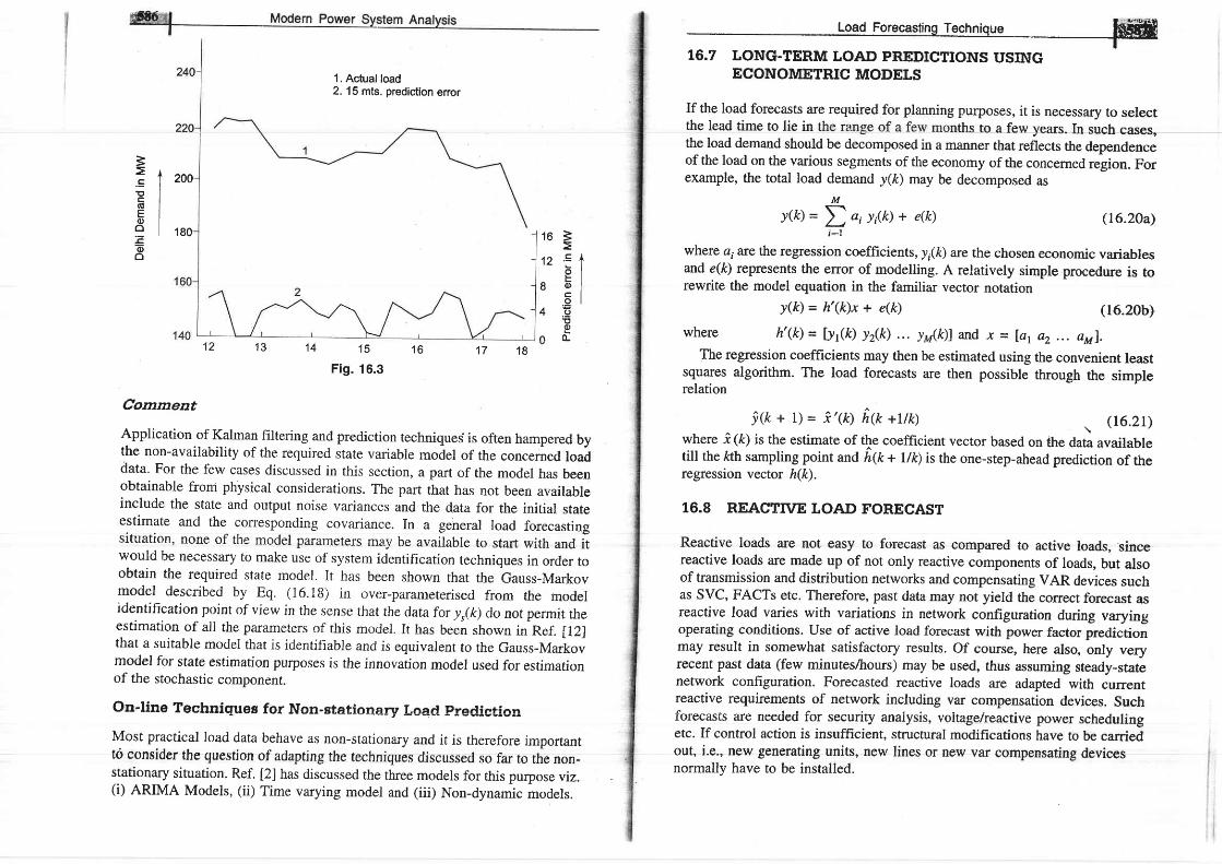
1. Actual load2. 15 mts. prediction error

200

180

i 3 1 4 1 5 1 6 1 7 1 8Fig. 16.3

Comment

Application of Kalman filtering and prediction techniques is often hampered bythe non-availability of the required state variable model of the concerned loaddata' For the few cases discussed in this section, a part of the model has beenobtainable from physical considerations. The part that has not been availableinclude the state and output noise variances and the data for the initiai stateestimate and the conesponding covariance. In a general load forecastingsituation, none of the model parameters may be available to start with and itwould be necessary to make use of system identification techniques in order toobtain the required state model. It has been shown that the Gauss-Markovmodel described by Eq. (16.18) in over-parameterised from the modelidentification point of view in the scnse that the data for y,(k) dr: not permit theestimation of ali the parameters of this model. It has been shown in Ref. [12]that a suitable model that is identifiable and is equivalent to the Gauss-Markovmodel for state estimation purposes is the innovation model usecl for estimationof the stochastic component.

on'line Techniques f,or Non-stationanl Load predietion

Most practical load data behave as non-stationary and it is therefore imponantto consider the question of adapting the techniques cliscussecl so f,ar to the non-stationary situation. Ref. [2] has discussed the three models for this purpose viz.(i) ARIMA Models, (ii) Time varying model and (iii) Non-dynamic models.

I - , - r6 rsHs

ECONOMETRTC MODELS

If the load forecasts are required for planning purposes, it is necessary to selectthe lead time to lie in thrro aJeulyears-In sucLcases-the load demand should be decomposed in a manner that reflects the dependenceof the load on the various segments of the economy of the concerned region. Forexample, the total load demand y(ft) may be decomposed as

M

y (k )=D" ,y , ( k )+ e (k )i : l

where aiare the regression coefficients, y,(k) are the chosen economic variablesand e(k) represents the error of modelling. A relatively simple procedure is torewrite the model equation in the tamiliar vector notation

y(k )=h ' (k )x+ e(k ) (16.20b)

where h'(k)= [yr(ft) yz(k) ... yu&)] and x = far a2... ayl.The regression coefficients may then be estimated using the convenient least

squares algorithm. The load forecasts are then possible through the simplerelation

i (k + 1) = i ' (k) i t(k +I lk)\ (16.21)

where i (k) is the estimate of the coefficient vector based on the data availabletill the ftth sampling point ana fr6 + Uk) is the one-step-ahead prediction of theregression vector h(k).

16.8 REACTTVE LOAD FORECAST

Reactive loads are not easy to forecast as compared to active loads, sincereactive loads are made up of not only reactive components of loads, but alsoof transmission and distribution networks and compensating VAR devices suchas SVC, FACTs etc. Therefore, past data may not yield the correct forecast asreactive load varies with variations in network configuration durin g varyingoperating conditions. Use of active load forecast with power factor predictionmay result in somewhat satisfactory results. Of course, here also, only veryrecent past data (few minutes/hours) may be used, thus assuming steady-statenetwork configuration. Forecasted reactive loads are adapted with currentreactive requirements of network including var compensation devices. Suchf - - - | | arorecasts are neeoed ior secunty anaiysls, voitageireactive power schedulingetc. If control action is insufficient, sffuctural modifications have to be carriedout, i.e., new generating units, new lines or new var compensating devicesnormally have to be installed.

3

E Ic lO IE IO Io lE(Do

(16.2Oa)1 6 =

1 2 . = 19 lL I

I o lc lo l

4 E'1C

En f L

mitul Modrrn Po*"r Syrt"r An"turi.

s u tut ttil ARyLoad forecasting is the basic step in power system planning. A reasonably self-contained account of the various techniques for the load prediction of a modern

prediction problems. Applications of time series, Gauss-Markov and innovationmodels in setting up a suitable dynamic model for the stochastic part of the loaddata have been discussed. The time series model identification problem has alsobeen dealt with through the least squares estimation techniques developed inChapter 14.

In an interconnected power system, load forecasts are usually needed at allthe important load buses. A great deal of attention has in recent years beengiven to the question of setting up the demand models for the individualappliances and their impact on the aggregated demand. It may often benecessary to make use of non-linear forms of load models and the question ofidentification of the non-linear models of different forms is an important issue.

Finally, a point may be made that no particular method or approach willwork for all utilities. All methods are strung on a common thread, and that isthe judgement of the forecaster. In no way the material presented here isexhaustive. The intent has been to introduce some ideas currentlv used inforecasting system load requirements.

Future Trends

Forecasting electricity loads had reached a comfortable state of performance inthe years preceding the recent waves of industry restructuring. As discussed inthis chapter adaptive time-series techniques based on ARIMA, KalmanFiltering, or spectral methods are sufficiently accurate in the short term foroperational purposes, achieving errors of l-2%o. However, the arrival ofcompetitive markets has been associated with the expectation of greaterconsumer participation. Overall we can identify the following trends.

(i) Forecast errors have significant implications for profits, market shares,and ultimately shareholder value.

(ii) Day ahead, weather-based, forecasting is becoming the rnost crucialactivity in a deregulated market.

(iii) Information is'becoming commercially sensitive and increasingly tradesecret.

(iv) Distributed, embedded and dispersed generation rhay increase.

A recent paper [7] takes a selective look at some of the forecasting issues whichare now associatecl with decision-making in a competit ive market. Forecastingloads and prices in the wholesale markets are mutually intertwined activities.Models based on simulated artificial agents may eventually become asimportant on supply side as artificial neural networks have already become

li':l;{lrJ.

**and integration with conventional time-series methods in order to provide amore precise forecasting.

REVIEW QUESTIONS

L6.7 Which method of load forecasting would you suggest for long term andwhy?

16.2 Which method of load forecasting would you suggest for very short termand why?

16.3 What purpose does medium term forecasting serve?

16.4 How is the forecaster's knowledge and intuition considered superior to anyload forecasting method? Should a forecaster intervene to modify aforecast, when, why and how?

16.5 Why and what are the non-stationary components of load changes duringvery short, short, medium and long terms?

REFTRT N CES

Books

1. Nagrath I.J. and D.P. Kothari, Power System Engineering,Tata McGraw-Hill, NewDelhi, 1994.

2. Mahalanabis, A.K., D.P. Kothari and S.I. Ahson, Computer Aided Power SystemAnalysis and Control, Tata McGraw-Hill, New Delhi, 1988.

3. Sullivan, R.L., Power System Planning, McGraw-Hill Book Co., New York, 1977.4. Pabla, A.5., Electricol Power Systems Planning, Macmillan lndia Ltd., New Delhi,

1998.

5. Pabla, 4.5., Electric Power Distribution,4th Edn, Tata McGraw-Hill, New Delhi.1997.

6. Wang, X and J.R. McDonald (Eds), Modern Power System Planning, McGraw-Hill, Singapore, 1994.

Papers

7. Bunn, D.W., "Forecasting Loads and Priees in Competitive Power Mark-ets"- Prac-of the IEEE, Vol. 88, No. 2, Feb 2000, pp 163-169.

8. Dash, P.K. et. al., "Fuz,zy Neural Network and Fuzzy Expert System for LoadForecasting", Proc. IEE, Yol. 143, No. l, 1996, 106-114.

9. Ramanathan, R. ef. a/., "Short-run Forecasts of Electricity Loads and Peaks". lntJ, Forecasring, Vol. 13, 1997, pp 161-174.

@ Mod"rn po*", syrt"r An"ly.i.

10. Mohammed, A. et. al., "Short-term Load Demand Modelling and Forecasting AReview," IEEE Trans. SMC, Vol. SMC-12, No. 3, lggl, pp 370_3g2.

ll. Tyoda, J. et. al., "An Application of State Estimation to Short-term LoadForecasting", IEEE Trans., Vol. pAS-89, 1970, pp l67g-16gg.

12. Mehra, R.K., "On-line Identification ofto Kalmann Filtering", IEEE Trans. Vol. AC-16, lg7l, pp lZ_21.

77

T7.T INTRODUCTION

Voltage control and stability problems are very much familiar to the electricutility industry but are now receiving special attention by every power systemanalyst and researcher. With growing size alongwith economic and environ-mental pressures, the possible threat of voltage instability is becomingincreasingly pronounced in power system networks. In recent years, voltagiinstability has been responsible for several major network collap$s in NewYork, France, Florida, Belgium, Sweden and Japan [4, 5]. Research workers,R and D organizations and utilities throughout the world, are busy inunderstanding, analyzing and developing newer and newer strategies to cope upwith the menace of voltage instability/collapse.

Voltage stability* covers a wide range of phenomena. Because of this,voltage stability means different things to different engineers. Voltage stabilityis sometimes also called load stability. The terms voltage instability and voltagecollapse are often used interchangeably. The voltage instability is a dynamicprocess wherein contrast to rotor angle (synchronous) stability, voltagedynamics mainly involves loads and the means for voltage control. Voltagecollapse is also defined as a process by which voltage instability leads ro verylow voltage profile in a significant part of the system. Voltage instability limitis not directly correlated to the network maximum power transfer limit.

A CIGRE Task Force [25] has proposed the following definitions for voltagestability.

Small-disturban-ce voltage stability

A power system at a given operating state is small-disturbance voltage stableif, following any small disturbance, voltages near loads do not change or remain

*The problem of voltage stability has already been briefly rackled in Ch. 13. Hereit is again discussed in greater details by devoting a full chapter.

close to the pre-disturbance values. The concept of small-disturbance voltagestability is related to steady-state stabiiity and can be analysed using small-signal (linearised) model of the system.

Voltage Stability

to a certain disturbance, the voltages near loads approach the post-disturbanceequilibrium values.

The concept of voltage stability is related to transient stability of a powersystem. The analysis of voltage stability normally requires simulation of thesystem modelled by non-linear differential-algebraic equations.

Voltage Collapse

Following voltage instability, a power system undergoes voltage collapse if thepost-disturbance equilibrium voltages near loads are below acceptable limits.Voltage collapse may be total (blackout) or partial.

Voltage security is the ability of a system, not only to operate stably, butalso to remain stable following credible contingencies or load increases.

Although voltage stability involves dynamics, power flow based staticanalysis methods often serve the purpose of quick and approximate analysis.

T7.2 COMPARISON OF ANGTE AND VOLTAGE STABILITY

The problern of rotor angle (synchronous) stability (covered in Ch. 12) is wellunderstood and documented t3l. However, with power system becomingoverstressed on accourrt of economic and resource constraint on addition ofgeneration, transfofiners, transmission lines and allied equipment, the voltageinstability has become a serious problem. Therefore, voltage stability studieshave attracted the attention of researchers and planners worldwide and is anactive area of research.

Real power is related to rotor angle instability. Similarly reactive power iscentral to voltage instability analyses. Deficit or excess reactive power leads tovoltage instability either locally or globally and any increase in loadings maylead to voltage collapse.

Voltage Stability Studies

The voltage stability can be studied either on static (slow time frame) ordynamic (over long time) considerations. Depending on the nature of distur-bance and system/subsystem dynamics voltage stability may be regarded a slowor fast phenomenon.

Static Voltage Analysis

Load flow analysis reveals as to how system equilibrium values (such asvoltage and power flow) vary as various system parameters and controls arechanged. Power flow is a static analysis tool wherein dynamics is not explicitly

lEq!tl#*l,rc'tr

considered. Many of the indices used to assess voltage stability are related toNR load flow study. Details of static and dynamic voltage stability will beconsidered further in Section 17.5.

Some Counter Measures

n counter measures to avord voltage r lty are:

(i) generator terminal voltage increase (only limited control possible)

(ii) increase of generator transformer tap

(iii) reactive power injection at appropriate locations

(iv) load-end OLTC blocking

(v) strategic load shedding (on occurrence of undervoltage)Counter measures to prevent voltage collapse will be taken up in

Section 17.6.

T7,3 REACTIVE POWER FLOW AND VOLTAGE COLLAPSE

Certain situations in power system cause problems in reactive power flowwhich lead to system voltage collapse. Some of the situations that can occur arelisted and explained below.

(1) Long Transmission Lines.' In power systems, long lines with voltageuncontrolled buses at the receiving ends create major voltage problemsduring light load or heavy load conditions.

(ii) Radial Transmission Lines: In a power system, most of the parallel EHVnetworks are composed of radial transmission lines. Any loss of an EHVline in the network causes an enhancement in system reactance. Undercertain conditions the increase in reactive power delivered by the line(s)to the load for a given drop in voltage, is less than the increase in reactivepower required by the load for the same voltage drop. In such a case asmall increase in load causes the system to reach a voltage unstable state.

(iii) .Sftortage of Local Reactive Power: There may occur a disorganisedcombination of outage and maintenance schedule that may cause localisedreactive power shortage leading to voltage control problems. Any attemptto import reactive power through long EHV lines will not be successful.Under this condition, the bulk system can suffer a considerable voltagedrop.

I7.4 MATHEMATICAL FORMULATION OF VOLTAGEcrrrr,lltE l.? Trnl't l ittD/^t T Eriltrit .l l.l.EDllrr I I r.ClLr.Cr!.GrlVl

The slower forms of voltage instability are normally analysed as steady stateproblems using power flow sirnulation as the primary study method. "Snap-shots" in time following an outage or during load build up are simulated.Besides these post-disturbance power flows, two other power flow based

I 's-ls{methods are often used; pv curves and ve curves. (see also sec. 13.6) Thesetwo methods give steady-state loadability limits which are related to vohagsstability. conventional load flow programs can be used for approxilmateanalysis.

P-V. curvesare useful for conceptual analysis of voltage stability and for

The model that will be employed here to judge voltage stability is based ona single line performance. The voltage performun"" of this simile system isqualitatively similar to that of a practical system with many voltage sources,Ioads and the network of transmission lines.

Consider the radial two bus system of Fig. 17.1. This is the same diagrarnas that of Fig. 5.26 except that symbols are simplified. Here Eis 75 and yisvn and E and v are magnitudes with E leading v by d, Line angle" p: tunliXlR and lzl = X.

Fig. 17.1

In terms of P and e,the system loacl encl voltage can be expressed as [l].

V

-'<- Locus of V66 and Pr",

Nose of the curve

0.9 pf lead

0.8 pflag

Fig.17.2 PV curves for various power factors

As in the case of single line systerrr, ,r, a general power system, voltageinstability occurs above certain bus loading and certain Q injections. Thiscondition is indicated by the singularity of the Jacobian of Load Flow equationsand level of voltage instability is assessed by the minimum singular value.

Certain results that are of significance for voltage stability are as under.o Voltage stability limit is reached when

It is seen from Eq. (17.1) that Vis a double-valued function (i.e. ithas twosolutions) of P for a particular pf which determines e in terms of p. The pVcurves for various values of pf are plotted in Fig. 17 .2. For each value of pf,the higher voltage solution indicates stable voltage case, while the lowervoltage lies in the unstable voltage operation zone. -fhe

changeover occurs atv".t (critical) and Pro*. The locus of v.r,-p^u* points for variJus pfs is drawnin dotted line in the figure. Any attempt to iniiease the load abov"

"-* causes

a reversal of voltage and load. Reducing voltage causes an increasing currentto be drawn by the load. In turn the larger reactive line drop causes the voltageto dip further. This being unstable operation causes the system to suffer voltagecollapse. This is also brought out by the fact that in upper part of the curve

( r7.2)

where S = complex power at load bus

Yrt= load bus admittance

', V = load bus voltage

Nearer the magnitude in Eq. (17.2) to unity, lesser the stability margin.o The loading limit of

'a transmission line can. be determined from

lsl = v"3 lx"; ( r7 .3)X".i is the critical system reactance beyond which voltage stability is lost. It canbe expressed as

, - z z x - z : - _ i r - 1 - : , , _ < \

L z - i ' l r z o x - E ) ' - 4 x 2 G 2 + o \ l e 7 . t )

i n f l ra l ^ . ' ,o - ^^* / . . ^ . ,+^L l^ - - , - - \ dP^rr lrrv rvwwr panL \u'Dr.rurc pdtL) , , , > U (feduclng lOad meansg V

F zX"n= * ( - tan Q+sec Q)

2 P

o = EY.o, a- 11X X

ff. 0 and

d V

We have so far considered how the PV characteristics with constant loadpower factor affect the voltage stability of a system. A more meaningfulcharrcteristic for certain aspects of voltage stability is the QV characteristic,which brings out the sensitivity and variation of bus voltage with respect toreactive power injections (+ve or -ve).

Consider once again the simple radial system of Fig. 17.1. For p flow it issufficiently accurate to assume X > R i.e. 0 = 90".It then follows that

(r7.4)

reducing voltage and vice-versa). It may be noted here that the type of loadassumed in Fig' 17.2 is constant impedance. In practical syste-.

-tir" type of

loads are mixed or predomirrantly constant power type such that system voltagedegraclationis inore and voltagelnstability occurs much prior to the theoreticalpower limit.

(17.s)

or

Taking

a

V" - EV cos 6+ QX = 0 (r7.6)

(17.7)

The QV characteristic on normalized basrs (etf**. VIE) for various valuesof P/P^ are plotted in Fig. 17.3.The system is voltage stable in the regionwhere dQldv is positive, while the voltage stability limit is reached at d,eldV= 0 which may also be termed as the critical operating point.

derivative wrt V gives

dQ = Ecos 6 -2Vd V X

various values of plp^^r.

The limiting value of the reactive power transfer atvoltage stability is given by

oD, max

Pr", is the maxlmumpower transfer at upf

1 . 0

0.75

Unstable. . PIP^" ,= 9 .5operation

0 0.2 0 .6 0 .8 1 .0VIE

Fig- 17.3 QV characteristics for the system of Fig. 17.1 tor

the limiting stage of

Q,n^ = t-"o '26 (17 .8 )

The inferences drawn from the simple radial system qualitatively apply to apractical size system. Other factors that contribute to system voltage collapseare: strength of transmission system, power transfer levels, load chaiacteristics,generator reactive power limits and characteristics of reactive power compen-sating devices.

Other Criteria of Voltage Stability

(i) 34 ..it.rion: (E'=generator voltage; V=load voltage). Using this crite-

rion, the voltage stability limit is reached when

cos d {#.#}+sin dff i -}=o ( r7.e)

Using ihe decoupiing principle 1.". dP = 0, we setd V

+=."'r[#.+]o r I sc=cos d loO +11

L d V X J

or Ers6 = E cos 5l !9 + 2Y]L d V X J

Voltage stability is achieved when

E cos , (# . +)

> Ers, (short circuit MVA of power source)

(17.10), . . \ dz(lU - cntenon

d Vvoltage instability occurs when the system Z is such that

d v M- = o o o r - = udZ dV

Application of this criterion gives value of(iii) Ratio of source to load reactance is

stability

Xsource a o2

X load

z";.very important

(r7.1r)

\dnd for voltage

(17.r2)

a indicates the off-nominal tap ratio of the OLTC transformer at the load end.

T7.5 VOLTAGE STABILITY ANALYSIS

The voltage stability analysis for a given system state involves examiningfollowing two aspects.

(i) Proximity to voltage instabitity: Distance to instability may be measuredin terms of physical quantities, such as load level, rea power flow througha critical interface, and reactive power reserye. posiible contingenciessuch as a line outage, loss of a generating unit or.a reactiu. po*"rio*..must be given due consideration.

(ii) iuiechanism of voitage instabiiity: How and why does voltage instabititytake place? What are the main factors leading to instability?'ulhat are thevoltage-weak areas? What are the most effective ways to improv"

"of,ug,stability?

.ffiiffi| . Modern Power System Analysis

The static analysis techniques permit examination of a wide range of system

conditions and can descriUe the nature of the problem and give the main

contributing factors. Dynamic analysis is useful for detailed study of specific

voltage coliapse situations, coordination of protection and controls, and testing

of remedial rneasures. Dynamic simulations further tell us whether and how the

steady-state equilibrium point wr

Modelling Requirements of various Power system components

Loads

Load modelling is very critical in voltage stability analysis. Detailed

subiransmission system representation in a voltage-weak area may be required'

This may includeiransformer ULTC action, reactive power compensation' and

voltage regulatorsIt is essential. to consider the voltage and frequency dependence of loads'

Induction motors should also be modelled'

Generators and their excitation controls

It is necessary to consider the droop chatacteristics of the AVR, load

compensation, SVSs (static var system), AGC, protection and controls should

also be modelled appropriately l4l.

Dynamic AnalYsis

'lhe general structu rc of the systcm moclel for voltage stability analysis is

similar to that for transient stability analysis. overall system equations may be

cxprefihcd as

* = f ( X , nand a set of algebraic equations

I (X, V) = YxV

with a set of known initial conditions (Xo' Ve)'

where X = system state vector

Y = but voltage vector

1= current injeition vector

Ilv = rletwork node admittance matrix'

Equations (17.13) and (17'14) can be s

oi tt e numerical integration methods

analysis nrethocls clescribed in Ch' 6' T

,ninutes. As the special models repl

ieading to voltage collapse have bee

differential equations is considerably

models. Stiffness is also called synchrc

Static AnalYsis

The static approach captures .snapshots of system conditions at various dme

frames along the time-domain trajectory. At each of these time frames' X in

ii h?lrJdil. frame. Thus, the overau system equations redPce to purely

algebraic equations allowing 'h.t..Ytt :f ,t'1tit Tlv:i: ::*:1,::t"t' vlp qnrt vo"'?'J"6;ffiffi;;;g."riuulirv is determrned- by computin s .vP and vQ

curves at selected load buses. Special techniques using static analysis havb been

reported in literature. Methods based on VQ sensitivity such as eigenvalue (or

modal) analysis have been devised. These methods give stability-related

information from a system-wide perspective and also identify areas of potential

problems t13-151.

Proximity to InstabilitY

proximity to small-disturbance voltage instability is determined by increasing

il;^";ruiion in steps until,the system becomes unstable or the load flow fails

to converge. Refs. t16-181 discuss special techniques for determining the point

of voltage collapse and proximity to volage instability'

The Continuation Power-flow Analysis

The Jacobian matril becomes singular at the voltage stability limit. A! a result'

conventional toad-flow algorith*, rnuy have convergence problems at operating

conditions near the stability limit. The continuation power-flow analysis

overcomes this problem by reformulating the load-flow equations so that they

remain well-conditioned at all possible loading conditions. This allows the

solution of load-flow problem forioth upper *d lo*"t portions of the P-V

*fi"t:lltinuation-method of power-flow analysis is ,obrrrt and flexible and

with convergence difficulties' However'

suming. Hence the better approach is to

flow irethod (NR/FDLF) and continua-

:ase, LF is solved using a conventional

ns for successively increasing load levels

Hereafter, the continuation method is

ns. Normally, the continuation method is

I exactly at and past the critical point'

Voltage StabilitY with HVDC Links

High voltage direct current* (HVDC).litt -tl:1r:t.:d

for extremely long distance

f f a n s m i s s i c l n a n c l f t r r a s y n c h r o n o u s i n t e r c o n n e c t i o n s . A n H V D C l i n k c a n b e

(r7.r3)

(r7.r4)

*For dctai lcd accountof HVDC, the reader maY refer to [3]'

f00 | Modern power System Anatysis

either a back-to-back rectifier/inverter link or can includetransmission. Multi-terfninal HVDC links are also feasible.

The technology has come to such a level that HVDCconnected even at voltage-weak points in power systems.present unfavourable "load" characterisfics fo fhe nnrr/rrconverter consumes reactive power equal to 50-60vo of the dc power.

HVDC-related voltage control (voltage stability and fundamental frequencytemporary over voltages) may be studied using a transient stability program.Transient stability is often interrelated with voltage stability. Ref. t2i .onJia.r,this problem in greater detail.

17.6 PREVENTION OF VOLTAGE COLLAPSE

(i) Application of reactive power-compensating devices.Adequate stability margins should be ensured by proper selection ofcompensation schemes in terms of their size, ratingr-und locations.

(ii) control of network voltage and generator reactive outputSeveral utilities in rhe world such as EDF (France), ENEL (Italy) aredeveloping special schemes for control of network voltages and reactivepower.

(iii) Coordination of protections/controlsAdequate coordination should be ensured between equipment protections/controls based on dynamic simulation studies. Tripping of equipment toavoid an overloaded condition should be the last alternative. Controlledsystem s€paration and adaptive or irrtelligent control could also be used.

(iv) Control of transfurmer tap chan.gersT'ap changers can be controlled, either locally or centrally, so as to reducethe risk of voltage collapse. Microprocessor-based OLTC controls offeralmost unlimited flexibility for implementing ULTC control strategies soas to take advantage of the load characteristics.

(v) Under voltage load sheddingFor unplanned or extreme situations, it may be necessary to useundervoltage load-shedding schemes. This is similar to under ir"q1r"rr.yload shedding, which is a common practice to deal with extreme situations-resulting from generation deficiency.Strategic load shedding provides cheapest way of preventing widespreadVOl taSg COl lanse Lnar l sher ld ino cn l ,a -oo o l rn , , r , r L^ r^^ : - ^^ ) ^^ - - - -_ -___r _ uvrrvrrrvJ orr\_rr l l \ . t ug ugsrBlrtru su as t()differentiate berween faults, transient voltage dips unJ lo* voltageconditions leading to voltage collapse.

(vi) Operators' role

Operators must be able to recognise voltage stabiiity-related symptomsand take required remedial actions to prevenr voltage collapse. On-line

I' Voltase Stability __{-tr*g

monitoring and analysis to identify potential voltage stability problemsand appropriate remedial measures are extremely helpful.

T7.7 STATE-OF-THE.ART, FUTURE TRENDS ANDCHALLENGES

The present day transmission networks are getting more and more stressed dueto economic and environmental constraints. The trend is to operate the existingnetworks optimally close to their loadability limit. This consequently means thatthe system operation is also near voltage stability limit (nose point) and thereis increased possibility of voltage instability and even collapse.

Off-line and on-line techniques of determining state of voltage stability andwhen it enters the unstable state, provide the tools for system planning and realtime control. Energy management system (EMS) provide a variety of measuredand computer processed data. This is helpful to system operators in takingcritical decisions inter alia reactive power management and control. In thisregard autornation and specialized software relieve the operator of good part ofthe burden of system management but it does add to the complexity of thesystem operation.

Voltage stability analysis and techniques have been pushed forward byseveral researchers and several of these are in commercial use as outlined inthis chapter. As it is still hot topic, considerable research effort is being devotedto it. ,

Pw et al. l8l considered an exponential type voltage dependent load modeland a new index called condition number for static voltage stability prediction.Eigenvalue analyses has been used to find critical group of buses responsiblefor voltage collapse. Some researchers [26] have also investigated aspects ofbifurcations (local, Hopf, global) and chaos and their implications on powersystem voltage stability. FACTS devices can be effectively used for controllingthe occurrence of dynamic bifurcations and chaos by proper choice of errorsignal and controller gains.

Tokyo Electric Power Co. has developed a pP-based controller forcoordinated control of capacitor bank switching and network transformer tapctranging. HVDC power control is used to improve stability.

More systematic approach is still required for optimal siting and sizing ofFACTS devices. The availability of FACTS controllers allow operation close tothe thermal limit of the lines without jeopardizing security. The reactive powercompensation close to the load centres and at the critical buses is essential forovercoming voltage instability. Better and probabilistic load modelling [11]should be tried. It will be worthwhile developing techniques and models forstudy of non-linear dynamics of large size systems. This may require exploringnew methods to obtain network equivalents suitable for the voltage stabilityanalysis. AI is another approach to centralized reactive power and voltagecontrol. An expert system [9] could assist operators in applying C-banks so that

long distance dc

terminals can beHVDC links mav

a00.l,*l Modern Pot

generators operate near upf. The design of suitable protective measures in theevent of voltage instability is necessary.

So far, computed PV curves are the most widely used method of estimatingvoltage security, providing MW margin type indices. Post-disturbance MW orMVAr margins should be translated to predisturbance operating limits thatoperators can monitor. Both control centre and power.plant operators should betrained in the basics of voltage stability. For operator training simulator [10] areal-time dynamic model of the power system that interfaces with EMS controlssuch as AGC is of great help.

Voltage stability is likely to challenge utility planners and operators for theforeseable future. As load grows and as new transmission and load areageneration become increasingly difficult to build, rnore and more utilities willface the voltage stability'challenge. Fortunately, many creative researchers andplanners are working on new analysis methods and an innovative solutions tothe voltage stability challenge.

A load bus is composed of induction motor where the nominal reactive poweris I pu. The shunt compensation is K,n. Find the reactive power sensitivity atthe bus wrt change in voltage.Solution

Qrcot= Qno V2 [given] '

Qcomp= - Krt V2

Qn"t= Qnua t Qcomp

Qn r= v' - Krn vz lQoo^ =.'. Here,

[-ve sign denotes inductivereactive power injection.l

1.0 givenl

dQn"t = 2v-2v K..,dv

i ' ,

Sensitivity increases or decreases with Krn as well as the magnitude of thevoltage. Say at V - 1.0 pu, Krn = 0.8

dQn t - 2 - 1 . 6 = 0 . 4 p u .dv

Find the capacity of a static VAR compensator to be installed at ax 5Vo voltage fluctuation. The short circuit capacity is 5000 MVA.Solution For the switching of static shunt compensator,

Example:,17.2

bus with l l .

I . .

AQ = reactive power variation(i.e. the size of the compensator)

Srr. = system short circuit capacity

Then AV =

AQ = AVSsk

= 1 ( 0 . 0 5 x 5 0 0 0 )

= + 250 MVARThe capacity of the static vAR compensator is +250 MVAR.

REFERE N CES

Books

1. Chakrabarti, A., D.P. Kothari and A.K. Mukhopadhyay, Perfurmance, Operationand Control of EHV Power Transmission Systerts, Wheeler Publishing, NewDelhi, 1995.

2. Taylor, c.w., Power system voltage stability, McGraw-Hill, New york, 1994.3. Nagrath, I.J. and D.P. Kothari, Power System Engineering, Tata McGraw-Hill,

New Delhi, 1994.4. Kunclur, P., Powcr Sy,stem Stubility atul Control, McGraw-Hill, New york, 1994.5. Padiyar, K.R., Power System Dynamics: Stability and Control, John Wilev.

Singapore, 1996.

6. Cutsem, T Van and Costas Vournas, Voltage Stabitity of Electric power Systems,Kluwer Int. Series, 1998.

Papers

7 . Concordia, C (Ed.), "special Issue on Voltage Stability and Collap se,', Int. J. ofElectrical Power and Energy systems, voi. i5, no. 4, August 1993.Pai, M.A. and M.G.O, Grady,"Voltage Collpase Analysis with Reactive Generationand voltage Dependent cons,traints", J. of Elect Machines and power systems,Vol . 17, No. 6 , 1989, pp 379-390.cIGRE/ Task Forcc 38-06-0l,"Expcrt Systems Applied to voltage and varControl/ / , 1991."operator Training simulator", EpRI Final Report EL-7244, May 1991, preparedby EMPROS Systems International.Xu, W and Y Mansour, "Voltage Stability using Generic Dynamic Load Models",IEEE Trans. on Power Systems, Vol 9, No l, Feb 1994, pp 479493.

trgd,.

8 .

9 .

1 0 .

1 5 .

Modern Pot

. . . t ? i - d - t ! l ! - F L - - - - , - - - - ^ L - -

IZ. VerTna, tl.lt., L.IJ. Arya ano u.r. I\.oman, 'Yoltage JlaDrtrty DnnansEulenr uy

Reactive Power Loss Minimization", JIE (I), Vol. 76, May 1995, pp.4449.

13. IEEE, special Publication 90 TH 0358-2 PWR, "Voltage Stability of Power

Systems: Concepts, Analytical Tools, and Industry Experience" 1990.

14. Flatabo, N., R. Ogncdal and T. Carlsen, "Voltagc Stabi l i ty Condit ion , in a Power

Tiansmisiion System calculated by Sensilivity Methods", IEEE Tians. VoI.

PWRS-5, No. 5, Nov 1990, pp 12-86-93.

Gao, 8., G.K. Morison and P. Kundur, "Voltagc Stability Evaluation Using Modal

Analysis", IEEE Trans. Vol. PWRS-7, No. 4, Nov. 1992, pp 1529-1542.

Cutsem, T. Van, "A Method to Compute Rbactive Power Margins wrt Voltage

Collapse", IEEE Trans., Vol. PWRS-6, No. 2, Feb 1991, pp 145-156.

Ajjarapu, V. and C. Christy, "The continuation Power Flow: A Tool for Steady

State Voltage Stability Analysis", IEEE PICA Conf. Proc., May 1991, pp 304-311.

Ldf, A-P, T. Sined, G. Anderson and D.J. Hill, "Fast Calculation of a Voltage

Stability Index", IEEE Trans., Vol. PWRS-7, No. 1, Feb 1992, pp 54-64.

Arya, L.D., S.C. Chaube and D.P. Itothari, "Line Outage Ranking based on

Estimated Lower Bound on Minimum Eigen Value of Load Flow Jacobian", JIE

(1), Vol. 79, Dec 1998, pp 126-129.

Bijwe, P.R,, S.M. Kelapure, D,P. Kothari and K.K. Saxena, "Oscillatory Stability

Limit Enhancement by Adaptive Control Rescheduling", Int J. of Electrical Power

and Energy Systems, Vol. 21, No. 7, 1999, pp 507-514.

Arya, L.D., S,C, Chaube and D.P. Kothari, "Linc Switching for Al leviat ing

Overloads under Line Outage Condition taking Bus Voltage Limits into Account",

Int J. of Electric Power and Energy System, YoL 22, No. 3, 2000, pp 213-221.

Bijwc, P.R., D.P. Kothari and S. Kclapure, "An Efficient Approach to Voltage

Sccurity Analysis and Enhancement", Int J. of EP and,ES., Vol. 22, No. 7, Oct.

2000, pp 483486.

Arya, L.D., S.C., Chaube and D.P. Kothari, "Reactive Power Optimization using

Static Stability Index (VSD", Int J. of Electric Power Components and Systems,

Vol. 29, No. 7, July 2001, pp 615-628.

Arya, L.D., S.C. Chaube and D.P. Kothari, "Line Outage Ranking for Voitage

Limit Violations witti Conective Rescheduling Avoiding Masking", Int. J. of EP

and ES, Vol. 23, No. 8, Nov. 2001, pp 837-846.

CIGRE Task Foice 38-02-10, "Cigre Technical Brochure: Modelling of Voltage

Collapse Includihg Dynamic Phenomena", Electa, No. 147, April 1993, pp' 7l-77.

Mark J. Laufenberg and M.A. Pai, "Hopf bifurcation control in power system with

static var compensators", Electrical Power and Energy Systems, Vol. 19, No. 5,

1997, pp 339-347.

T6,

1 7 .

1 8 .

19 .

'20.

24.

25 .

26.

2 t ,

. )

23.

AppnNDrx A

In this appendix, our aim is to present definitions and elementary operations ofvectors and matrices necessary for power system analysis.

VECTORS

A vector x is defined as an ordered set of numbers (real or complex), i.e.

, (A-1)

xp ...t xn are known as the components of the vector r. Thus the vector x isa n-dimensional column vector. Sometimes transposed form is found to be moreconvenient and is written as the row vector.

rT A fx1, x2, ..., xrf

Some Special Vectors

The null vector 0 is one whose each component is zero, i.e.

(A-2)

The sum vector i has each of its components equai to unity, i.e.

A

. flTY'-tI

0x.= 0The multiplication of two vectors x and y of same dimensions results in a

very important product known as inner or j9g!g! pfodqcij.e.

*tv AD",y,Aytxi : l

Also, it is interesting to note that

xTx = lx 12

cos d 4 "tY' l x l l y l ,

wtere Q is angle between vectors, lxl and lyl are the geometric lengths ofvectors x and y, respectively. Two non-zero vectors are said to be orthJgonral,if

* ty= o (A-6)

The unit 'tector ethe.rest of the componentb are zero, i.e.

0

0

1

0

0

kth component

Some Fundamental Vector Operations

A€ k :

(A_3)

(A-4)

(A-5)

Two vectors x and y are known as equal if, and only if, .yk= !*for k = r,2,. . . , n . Then we sav

x = y

The product of a vector by a scalar is carried out by multiplying eachcomponent of the vector by that scalar, i.e.

If a vector y is to be added to or subtracted from another vector x of the samedimension, then each component of the resulting vector will consist of additionor subtraction of the corresponding components of the vectors x and vr,i.e.

T h e f n l l n u r i n c n r n n A r f i o o ^ * ^ ^ - - + : ^ ^ l ^ l ^ r ^ r L - - - ' ' -Y v r r r 6 y r v P v r ! a v D 4 r v 4 y I - , u U < r U I t r L U u r c v e L : t 0 r a r g e D r a :

x * ! = y + xx + ( v + ' z ) = ( x + y ) + z

ar @zx) - (afiz)x(a r+ e )x - dF+ a2x

MATRICES

Definitions

Matrix ' '

'\n m x n (ot m' n) matrix is an ordered rectangular array of elements whichmay be real numbers, complex numbers, functions or operators. The matrix

(A-7)

is a rectangular array of mn elements.

. . o,t

!"notes the (i, i)th element, i.e. the element located in the ith row and the

7th column. The matrix A has m rows ano n coiumns and is said to be of orderm x n .

When m = rt, i.e. the number of rows is equal to that of columns, the matrixis said to be a square matrix of order n.

An m x 1 matrix, i.e. a matrix having only one column is called a columnvector. An I x n matix, i.e. a matrix having only one row is called a rorevector.

*Sometimes inner product is also represented by the following alterr ative forms

x . y , ( x , y ) , ( x , y ) .

. ,1 r\!r

's.t

frffi-H Modern Power Svstem Analvsis

Diagronal matrix

A diagonal matrix is a square matrix whose elements off the main diagonal area l l z e r o s ( a i j = 0 f o r i + j ) .

NUII matrix

If all the elements of the square matrix are zero, the matrix is a nuII or zeromatrix.

(A-8)

Unit (identity). matrix

A unit matrix / is a diagonal matrix with all diagonal elements equal to unity.If a unit matrix is multiplied by a constant (),), the resulting matrix is a diagonalmatrix with all diagonal elements equal to 2. This matrix is known as a scalarmaffix.

= 3 x 3 s c a l a r m a t r i x

Determinant of a matrix

For each square matrix, there exists a determinant which is formed by takingthe determinant of the elements of the matrix.

T

det (A) = tAt = 213 2l l-l 2l , l-1 3l'1, +l- r- t1 I 4l* | 1 2l

= 2 ( 8 ) + ( ' 6 ) + ( - 5 ) = 5

l -1- l

l 2

(A-e)

(A-10)

ll:Lll;lL - ^ J

= 4 x 4 u n i t m a t r i x

Transpose of a matrix

'l.h-.e transpose of matrixA denoted by At is the matrix formed by interchanglng

the rows and columns of A.

Note that (Ar)r = A

Symmetrtc matrix

A square matrix is symmetric, if it is equal to its transpose, i.e.A T = A

Notice that the matrix A of Eq. (A-9) is a symmeffic matrix.

Minor

The mino, Mij of an n x n rnatrix is the determinant of (n - l) x (n - 1) matrixformed by deleting the ith row and the 7th column of the n x n matrix.

Cofactor

The cofactor AU of element a,, of the matrix A is defined as

aU = Gl)'*t M,i

Adjoint matrix

The adjoint matrix of a square matrix A is found by replacing each element auof matrix A by its cofactor A,, and then transposing.

For example, if A is given by Eq. (A-9), then

l-tl 1l 2l rl 2l - 1

1

3

l3lzt-Il-I

a o J A =

MotJel lr Powor S

6

7-5

- \ l_;l) l

(A-11)

A square matrix is called singular, if its associated determinant is zero, andnon-singular, if its associated determinant is non-zero.

ELEMENTARY MATR.IX OPERATIONS

Eguality of matrices

Two matrices A(m x n) and B(m x n) are said to be equal, if the only if

a i = b i j f o r i = 7 , 2 , . . . , f f i , . i = 1 , 2 , . . . , f l

Then we write

A = B

Multiplication of a matrix by a scalar

A matrix is multiplied by a scalar a if all the mn elements are multiplied bya. i.e.

(A- 12)

Addition (or suhtraction) of matrices

To add (or subtract) two matrices of the same older (same number of rows, andsame number of columns), simply add (or subtract) the corresponding elementsnf the f rxrn rnefr ;cce i e r r rhen f rxrn rnqfr i / -ec A enA I l n f lhe cqrnc o, rAcr qrc

added, a new matrix C results such that

C - A + B ;

whose ryth elernent equals

cij= aij * bij

l - - - - - -_ -__ - i r1r ,Example I Il : r

I

i - ? O - r f ) - 1 1

I A A = i' - - l z - r l " - L o 3 . 1then,

Appendix A I ,6tlI -1 5 - 1 - l

C = A + B = l ' IL2 2)

Addition and subtraction are defined only for matrices of the same order.The fbllowing laws hold lbr addition:

(+ fhe cammatatLve ln+y: A + B -B + ,{ :

(ii) The associative law: A +- (B + C) = (A + B) + CFurther

( A t B ) r = A r + B r

Matrix Multiplication

The product of two matrices A x B is defined if A has the same number ofcolumns as the number of rows in B. The natrices are then said to beconform.able.If amatrix A is of order mx n and B is an n x q matrix, theproduct C = AB will be an m x q matrix. The element c,, of the product is givenbv

, l

r ,cii =

)_rai*0*ik : l

Thus the elements cu are obtained by multiplying the elements of the ith rowofA with the corresponding elements of theTth column of B and then summingthese element productp.

For example

where

c t t = a t t b t , + a r r b ^

c tz= anbn + ar rb2

c z l = u z l b t , + a r r b 2 1

czz= aztbtz + crrb2

If the product AB is defined, the product BA may or may not be defined.Even if BA is defined, the resulting products of AB and, BA are not, in general,equal. Thus, it is important to note that in general matrix multiplication is notcommutative, i.e.

A B + B A

The associarive and distributive larr-s hold for matrix mulriplicarion (wtrenthe 'aryprrtixiate erpernirnys .are def;tv.4)- re.

Asscrica'rv &rrt': 4{B [ = A(BC) = -tBC

Distibutive law:. A(B + C) - AB + AC

(A-13)

1"" arzl lbn b,r l_

[ ' ' r cnlLau azz)Lbn brrJ Lr^ czrl

tffiWl Modern PoI

[ 1 - 1 3 ]

Lo z r l

Find AB and BA.A and B are conformable (A has two columns and B has two rows), thus we

have

l -1 -1 3 l| | r--1 0t

4 8 = 1 2 4 9 l t B A = l , , '' " - L ; ; ; l " ^ - l - 4 1 )

A matrix remains unaffected, if a null matrix, defined by Eq. (A-8) is addedto it, i.e.

A + 0 = A

If a null matrix is multiplied to another matrix A, the result is a null matrix

A 0 = 0 A = 0

Also

A - A = 0

Note that equation AB = 0 does not mean that either A or B necessarily has

to lre a null matrix, e.g.

[ r , l [ 3 o l = f o 0 lL0 0J L-l 0l Lo 0J

Multiplication of any matrix by a unit matrix results in the original maffix,l . e .

A I - I A = A

The transpose of the product of two matrices is the product of theirtransposes in reverse order, i.e.

6Dr = BrArThe concept of matrix multiplication assists in the solution of simultaneous

linear algebraic equations. Consider such a Set of equations

at f t + anxz+ . . . + abJn = c t

aL lx t + azzxz+ . . . + azr t r= c2

:

Q^ lX l * C^*z+ . . . + A - rJn = C^

I,j].qffil*ll.,i95I3n

orn

D " * t = c i i i = 1 , 2 , . . . , m

i:l

Using the rules of matrix multiplication defined above. Eqs (A-14) canlewritten in the compact notation as

A x = c (A-1s)where

It is clear that the vector:mntrix Eq. (A-15) is a useful shorthandrepresentation of the set of linear algebraic equations (A-14).

Division does not exist as such in matrix algebra. However, if A is a squarenon-singular matrix, its inverse (A-l) is defined by the relation

A _ I A _ A A _ I _ I (A-16)

The conventional method for obtaining an inverse is to use the followingrelation

A-; _ adj A

det A

It is easy to prove that the inverse is uniqueThe following are the important properties charactenzing the inverse:

(AB)-r = 3-t4-l

(A-tf = (Ar)-r

14-r1-t = 4

(A-18)

Matrix Inversion

(A-17)

I f A(A-14) is given by Eq. (A-9), then from Eqs. (A-10), (A-1I), (A-17), we get

ffd-ffi.:| Modern power System Rnatysis

A-1 -+:if : i _;l:f:i; i,:_ildet A t L-r -s 5j L -; -; l.J

SCALAR AI\rD VE CTOFFUNCTI O]NIS

A scalar function of n scalar variables is defined asy ! f \ r , x2 , . . . , xn)

It can be written as a scalar function of a vector variable x, i.e.y - f(x)

where x is an n-dimension vector,

(A-1e)

(A-20)

In general, a scalar function could be a function of severy - f ( x , u , p )

where x, u and p are vectors of various dimensions.A vector function is defined as

y - f ( x , u , p )

DERTVATNTES OF SCALAR AND \ZECTOR FUNCTIONS

(A-23)

A derivafit'e of a scalar funcritrn 1A-lt)) s,ith re-sper.r tr) u \.eL-R)r r.ariable -r isdefind as

al vector variables, e.g.

(A-2r)

In general, a vector function is a function of several vector variables, e.g.

- a f

0r,af

0*,

oJorn -

A t0x

(A-24)

It may be noted that ihe derivative of a scaiar function with respect to a vectorof dimension n is a vector of the same dimension.

The derivative of a vector function (A-22) with respect to a vector variabler is defined as

ofa0x

0*,}fz0*,af-0*,

0*,0fz0*,af;0*,

(A-zs)

o*n?fz0rn

.. af;o*n

Consider now a scalar function defined ast - ff@, u, p)

= 21fi(x, u, p) + Lzfz(*, u, p)

Let us fincf j{ . According ro Eq. (A-24),a^

(A-26)

(A-27)

+ ... + 2*f*(4, u, ) 6-2g)

we can write

f (x, u, p) (A-2e)

(A-24), we can writeLet us now find

L J m \ r r U r P ) J

d s ^ i .-. According to Eq.ox

l a " lLar, J

fijfilftf.f Modern Power'system AnatystsI

}ft 0f, af^ AppnNDrx B

We can represent, as we saw in Chapter 5, a three-phase transmission line* bya circuit with two input terminals (sending-end, where power enters) and twooutput terminals (receiving-end, where power exits). This two-terminal paircircuit is passive (since it does not contain any electric energy sources), linear.(impedances of its elements are independent of the amount of current flowingthrough them), and bilateral (impedances being independent of direction ofcurrent flowing). It can be shown that such a two-terminal pair network can berepresented by an equivalent T- or zr-network.

Consider the unsymmetrical T-network of Fig. B-1, which is equivalenr tothe general two-terminal pair network.

0*, 0*,Ofi }fz0r, 0r,

0*,af^0*,

)r

^2

0*n 0r, o*n

REFERE N CES

l, Shiplcy, R,8,, Intoduction to Matric:r:s andr976.

2. Hadley, G., Linear Algebra, Addison-Wesley3. Bellman, R., Introduction to Matrix Analysis,

1960.

Power Sy,rtems, Wiley, New

Pub. Co. Inc., Reading, Mass.,McGraw-Hill Book Co.. New

VJI UJ2

(A-30)

York,

1961.

York,

Flg. B-1

For Fig. B-1,

1 s -

or

I s =

* :

Unsymmetrical T-circuit equivalent to a generalnair networkr - " " - - - ' - " _

the following circuit equations can be writtenI^+ Y(Vo+ I^Zr)

Y V * + ( l + Y Z r ) I *

V*+ I^Zr+ IrZ,

V^ + I^2, + ZrWn+ I^2,, + I^YZ.Z,

two-terminal

(B-1)

.+iqY

*A transformer is similarlyterminals.

s lp

Vg

Z1 22

Y Vp

represented by a circuit with two input and two ouput

tlCtf I Modern porelsyslern inal,sis

or

V5 = (1 + YZr) V* + (2, + Z" + yZrZr)IoEquations (B-1) and (B-2) can be simplified by letting

A - l + Y Z , B = 2 . , + Z r + y Z r Z ,

C = Y D = l + y Z ,

A D - B C = 1 (B-s)

Fig. B-2 :#:::representation

of a two-rerminar pair network using

ABCD CONSTANTS FOR VARIOUS SIMPLE NETWORKS

We have already obtained the ABCD constants.of an unsymmetrical T-network.The ABCD constants of unsymmetrical a-network shown in Fig. B-3 may beobtained in a similar manner and are given below:

-

A = l + Y r Z

B = Z,C = Y r + Y r + Z Y r y z

D = I + Y r Z

(B-2)

(B-3)

using these, Eqs. (B-1) and (B-2) can be written in matrix form as

lyrl lA Bllv*1Lr,.J

= Lt olj^l ,t-0,

This equation is the same as Eq. (5.1) and is valid for any linear, passive andbilateral two-terminal pair network. The constants A, B, C and D are called thegeneralized circuit constants or the ABCD constants of the network, and theycan be calculated for any such two-terminal pair network.

It may be noted that ABCD constants of a two-terminal pair network arecomplex numbers in general, and always satisfy the following relationship

Also, for any symmetrical network the constants A and, D are equal. From Eq.(B-4) it is clear that A and D are dimensionless, while B has the dimensions ofimpedance (ohms) and c has the dimensions of admittance (mhos).

The ABCD constants are extensively used in power system analysis. Ageneral two-terminal pair network is often represented as in Fig. B_2.

(B-6)

Fig. B-3 Unsymmetrical zr-circuit

A series impedance often represents short transmission lines and transform-ers. The ABCD constants for such a circuit (as shown in Fig. B-4) canimmediately be determined by inspection of Eqs. (B-1) and (B-2), as follows:

A = 1

B = Z

C = 0

D = l

Fig. B-4 Series impedance

Another simple circuit of Fig. B-5 consisting of simple shunt admittance canbe shown to possess the following ABCD constants

A = 7

B = 0

C = Y

D = I

/E l_a \\s-u,,

Fig. B-5 Shunt admittance r

It may be noted that whenever ABCD constants are computed, it should bechecked that the relation AD-BC = 1 is satisfied. For examole, using Eq.(B-8) we get

A D - B C = 1 x 1 - 0 x Y = 1

(B-7)

:fflfuii'l Modern power: System nnatysis

II ABCD constants of a circuit are given, its equivalent I- or a-circuit canbe determined by solving Eq. (B-3) or (8-6) respectively, for the values ofseries and shunt branches. For the equivalent n-circuit of Fig. B-3, we liuu.

(B-e)

, r =#

ABCD CONSTANTS OF NETWORKS IN SERIES AND FANEr,r,Ur,

Whenever a power system consists of series and parallel combinations ofnetworks, whose ABCD constants are known, the overall ABCD constants forthe system may be determined to analyze the overall clperation of the system.

Fig. 8-6 Networks in series

Consider the two networks in series, as shown in Fig. 8-6. This combinationcan be reduced to a single equivalent network as follows:For the first network. we hal'e

t ,

, , Append8B l , ;621+I

tr= (ArBr+ ArBr)/(8, + Br)

B= BrBzl (Bt+ Br)

C= (Cr * Cr) + (Ar - Ar) (Dz- D)l(Br * Ur)

(B-13)

Fig. B-7 Networks in parallel

Measurement of ABCD Gonstants

The generuIized circuit constants rnay be computed for a transmission linewhich is being designed from a knowledge of the system impedance/admittanceparameters using expressions such as those cleveloped above. If\the line isalready built, the generalized circuit constants can be measured by making afew ordinary tests on the line. Using Eq. (B-4), these constants can easily beshown to be ratios of either voltage or current at the sending-end to voltage orcurrent ai the receiving-end of the network with the receiving-end open or short-circuited. When the network is a transformer, generator, or circuit havinglumped parameters, voltage and current measurements at both ends of the linecan be made, and the phase angles between the sending and receiving-endquantities can be found out. Thus rhe ABCD constants can be determineC.

It is possible, also, to measure the rnagnitudes of the required voltages andcurrents sinrultaneously at both ends of a transmission line, but there is nosimple method to find the difference in phase angle between the quantities at thetwo ends of the line. Phase difference is necessary because the ABCD constantsare complex. By measuring two impedances at each end of a transmission line,however', the generalized circuit constants can be computed.

The following impedances are to be measured:7 - o o - ' l . i - - o - . l i * ^ o ' l ^ - ^ ^ . . ' i + L - ^ ^ ^ : . , : - - ^ - l ^ - ^ - ^ : - ^ - . : - - r

"so - rvrrulrS-vr:\r uuPv\r(rrrlvs wrlrl r9L9rvlttE-trlru uP(,il-ull'uulteo

Zss = sending-end impedance with receiving-end short circuitedzno = receiving-end impedance with sending-end cpen-circuiteciZns = receiving-end impedance with sending-end short-circuited

The impedances measured from the sending:end can be determined in termsof the ABCD constants as follows:

[u,l _ | o, ",

'l [u,l

Lr, J -

1., o, )lt, )For the second network, we can write

I y*

I I A, Brll vo]I t = t | | |l r r ) l _c , D rJ l r * l

From Eqs. (B-10) and (B-11), we can write

[u ' l _ lo ' u '11o, u' l [u^]L+ I

- 1., n,ll.c, or)j^ l

(B- 10)

( B - 1 1 )

f A ,A , + B tC . , A tBz + qD2 l [ y * I= llcrAz + D1C2 CrB' - t DrD, J l t o l

If two networks are connected in parallel as shown in Fig. B-7, the ABCDconstants of the combined network ca-n be found out similarly with some simplemanipulations of matrix algebra. The results are presented below:

From Eq. @- ), with 1R = 0,

Z s o = V s l l s = A l C

and with VR = 0,

Vn= DVs + BIt

In= CVs + AIt

From Eq. (8-16), with Is = 0,

Z n o = V R | I R = D / C

and when Vs = 0,

Zns= VRl lR= BIA

When the impedances are measured from the receiving-end, the direction of

current flow is reversed and hence the signs of all current terms in Eq. (5.25).

We can therefore rewrite this equation as

AppENDIX C

We know that the nodal maffix Yu.r, and its associated Jacobian are very

sparse, whereas their inverse matrices are full. For large power systems the'sparsity

of these matrices may be as high as 98Vo and must be exploited. Apart

fiom reducing storage and time of computation, sparsity utilization limits the

round-off computational errors. In fact, straight-foru'ard application cf the

iterative procedure tor system studies like load flow is not possible for large

systems unless the sparsity of the Jacobian is dealt with effectivet).

GAUSS ELIMINATION

One of the recent techniques of solving a set of linear algebraic equations,

called triangular factorizatiott, replaces the use of matrix inverse which is

highly inefficient for large sparse systems. In triangularization the elements of

.u.h ,o* below the main diagonal are made zero and the diagonal element of

each row is normalized as soon as the processing of that row is completed- It

, is possible to proceed columnwise but it is computationally inefficient and is

theref,re not used. After triangularization the solution is easily obtained by

hack sub.stitution. The technique is illustrated in the example below'

Consider the linear vector-maffix equation

(B- 14)

(B-16)

(B- 17)

(B- 18)

Solving Eqs. (B-14), (B-15), (B-17) and (B-18) we can obtain the values ofthe ABCD constants in terms of the measured impedances as follows.

A D - B C

C _

p =

[using Eq. (B-5)]1AC

I C 1

A C , A A 2

AC

o=(ffi)'''By substituting this value of A in Eqs. (B-14),

value of C so obtained in Eq. (B-17), we get

( z\ 1 l /2r > - . 7 , - '

ID = L R S l z * o - z n r )

(Zss(Zno - Zo))' ' '

Z^o

(B- 1e)

(B-18) and substituting the

(B-20)

(B-21)

(B-22)(zso(z^o - zo))t' '

REFERE N CE

The Transmi,ssion and Distribution of Electrical Energy,

New Delhi. 1970.

l'L3

1' l [ ' t I,l1,,I =t;l

l . Cotton, H. and H, Barber,

3rd edn., B.I. Publishers,

Procedure

1. Divide row 1 by the self-element of the row, in this case2.

2. Eliminate the element (2, 1) by multiplying the modified row 1, byelement (2, I) and subtract it from row 2.

3' Divide the modified row 2 by its self-element (f); and stop.

Following this procedure, we get the upper triangular equation as

[ r + l [ ' ' - l t + ll z i l t = t o _ + ll o ? : r l l _ l - l , rL t ) L x z l L t J

Upon back substituting, that is first solving for x2 and then for 11, we get

o - + 1x 2 = - - 7 : - - j

2

- - I _ I Y - I _ 1 1 _ 3 \ - 5

Check

br + xz= 2(*) - t r = t

3x, + 5rz- 3(+) - s(f) = oThus, we have demonstrated the use of the basic Gauss elimination and back

substitution procedure for a simple system, but the same procedure applies toany general system of linear algebraic equations, i.e.

A x = b (c-1)An added advantage of row processing (elimination of row elements below

the main diagonal and normalization of the self-element) is that it is easilyamenable to the use of low storage compact storage schemes-avoiding storageof zero elements.

GAUSS ELIMINATION USING TABLE OF FACTORS

Where repeated solution of vector-matrix Pq. (C-1j with cons tant Abut varyingvalues of vector D is required, it is computationally advantageous to split thematrix A into triangular f'actor (termed as 'Table of factors' or 'LU

decomposition') using the Gauss elimination technique. If the matrix A issparse, so is the table of factors which can be compactly stored thereby not onlyreducing core storage requirements, but also the computational effort. Gausselimination using the table of factors is illustrated in the following example.

Consider the following system of linear equations:

(Z)xt + Q)x2 + (3)x, = $

( 2 ) x r + ( 3 ) x z + ( 4 ) x t = )

( 3 ) x r + ( 4 ) x r + ( 7 ) 4 = 1 4

(c-2)

For computer solution, maximum efficiency is attained when elimination is

carried out by rows rather than the more tamiliar column order. The successivereduced sets of equations are as follows:

( l )xr + ( t )*z+ (*)r t = *(Z)xt+ (3)x2 + (4)xt = )

(3)xr + (4)xz + (7)x3 = 14

(1 ) . r , + ( i l r r+ ( | ) x t - z

(2)xz + (1)x, = l

( 3 ) x r + ( 4 ) x 2 + ( 7 ) 4 = 1 4

(1)x ,+ ( t r ) r r+ (* ) " , -3

(1 )x2+ ( * ) r , -+

( 3 ) x r + ( 4 ) x 2 + Q ) x t = 1 4

( l )x r + ( t ) r r+ (J )x , = 3

( l )x2+ ( * ) " r ' = + , i

( t ) , r + ( * ) r , - s

(1)x, + ( t )rr+ (*)" , = J

( t )xr+ ( t)* t - +(*)rt = +

(1)x, + (tr)*r+ (*)r,

(1)x, + (I)*t (c-8)

x 3 =

These steps are referred to as 'elimination' operations. The solution r maybe immediately determined by 'back substitution' operation using Eq. (C-8).

(c-3)

(c-4)

(c-s)

(c-6)

(c_'7\

_ J

32

I

The solution for a new set of values for b can be easily obtained by usinga table of factors prepared by a careful examination of eqs. 1c-l) to (c-g). wecan write the table of factors F as below for the example in hand.

fnfzt

The row elements of F below the diagonal are the multipliers of thenormalized rows required for the elimination of the row element, e.g. fzz = *,the multiplier of normalized row 2 l&q. (c-6)l to eliminate the element (3,2),i'e- (])x2. The diagonal elements of F are the mulripliers needed to normalizethe rows after the row elimination has been completed, e.g. .fzz = ! , the factorby which tow 2 of Eq. (C-4) must be multiplied to normalize the row. Theelements of F above the diagonal can be immecliately written down byinspection of Eq. (C-8). These are needed for the back substitution process.

In rapidly solving Eq. (C-1) by use of the table of factors F, succesiive stepsappear as columns (left to right) in Table C.l below:

Table C.l

- 5 - ( ;X ; ) : iand for heading 3, 3

lt = fszlz

= (+x+) = IIn fact, operation (C-10) represents row normalization and (C-11) represents

elimination and back substitution procedures.

Optimal Ordering

In power system studies, the matrix A is quite sparse so that the number of non-zero operations and non-zero storage required in Gauss elimination is verysensitive to the sequence in which the rows are processed. The row sequencethat leads to the least number of non-zero operations is not, in general, the sameas the one which yields least storage requirement. It is believed that theabsolute optimum sequence of ordering the rows of a large network matrix (thisis equivalent to renumbering of buses) is too complicated and time consumingto be of any practical value. Therefore, some simple yet effective schemes havebeen evolved to achieve near optimal ordering with respect to both the criteria.Some of the schemes of near optimal ordering the sparse matrices, which arefully symmetrical or at least symmetric in the pattern of non-zero off-diagonalterms, are described below [4].

Scheme I

Number the matrix rows in the order of the fewest non-zero terms in each row.If more than one unnumbered row has the same number of non-zero terms.number these in anv order.

Scheme 2

Number the rows in the order of the fewest non-zero terms in a row at each stepof elimination. This scheme requires updating the count of non-zero terms aftereach step.

Scheme 3

Number the rows in order of the fewest non-zero off-diagonal terms generatedin the renraining rows at each step of elimination. This scheme also involves anupdating procedure.

I he chotce ot scheme ts a trade-otf between speed of execution and thenumber of times the result is to be used. For Newton's method of load flowsolution, scheme 2 seems to be the best. The efficiency of scheme 3 is notsufficiently established to offset the increased time required for its execution.

f t , f tz

fu fzz

32

r l 3' ) . r a

L

n l lL T T (c-e)

1 , 35/2

II

xII1

The heading row (i, j) of Table C-1 represents the successive elimination andback substitution steps. Thus,

represents normalization of row 1represents elimination of element (2, l)

h69t 4

l , I39

T4

2 , 1 2 , 2 3 , I 3 , 23 3 3 33 3t2 3/2 3t2

14 t4 5 5 t4

1 , 2a a

33 t )

1

2 , 3aJ

31

7 , 72 , L2,2 represents nonnalization of row 23, L; 3,2 represent elimination of elements (3, 1) an,J (3,2) respectively3. 3 represents normalization of row 32,3 represents elimination of element (2,3) by back substitutionr, 3; 7, 2 reprelent elimination of elements (1, 3) and (r, z) respectively by

back substitution.The solution vector at any stage of development is denoted by

Ut lz y3Jr = y

The modification of solution vector fiom column to column (left to right) iscarried out for the headin g (i, j) as per the operations defined below:

! i= f i i j i t t j = i (c- 10)

(c-11)! i= ! r - f i / i l t i + i

Thus for heading 3, z

l t = l t - f n ) z

Mffi# Modern pot -

Scheme I is useful for problems requiring only a single solution with nqiteration.

Compact Storage Schemes

The usefulness of the Newton's method depends largely upon conservingcomputer storage ucmg the nu oI non-zero computatlons.'l'o ettectthese ideas on the computer, elimination of lower triangle elements is carriedout a row at a time using the concept of compact working row. The non-zeromodified upper triangle elements and mismatches are stored in a compact andconvenient way. Back substitution progresses backwards through the compactupper triangle table. A properly programmed compact storage scheme results inconsiderable saving of computer time during matrix operations.

Naturally, there are as many compact working rows and upper trianglestorage schemes as there are programmers. One possible scheme for a generalmatrix stores the non-zero elements of successive rows in a linear array. Thecolumn location of these non-zero elements and the location where the next rowstarts (row index) is stored separately. The details of this and various otherschemes are given in [2].

REFERE N CES

Singh, L.P., Advanced Power System Analysis and Dynamics, 2nd edn., Wiley

Eastern, New Delhi, 1986.

Agarwal, S.K., 'Optimal Power Flow Studies', Ph.D. Thesi.r, B.I.T.S.r Pilani,

r970.

Tinney, W.F. and J.W. Walker, "Direct Solutions of Sparse Network Equations by

Optintally Ordered Triangular Factorizations", Proc. IEEE, Nov. 1967,.55: 1801.

Tinney, W.F. and C.E. Hart, "Power Flow Solution by Newton's Method", IEEE

Trans., Nov. 1967, No. l l , PAS-86: 1449.

AppBNDrx I)

Expressions to be used in evaluating the elements of the Jacobian matrix of apower system are derived below:

From Eq. (6.25b)

fr*rrk:r

A \exp (- i6,)L lY,/ exp (i?il lVll exp (7dn) (D-l)

k:r

Differentiating partially with respect to 6* (m * i)

+- i+ = Tvil exp (-r4) (Yi^l exp Q0,^) tv^t exp (j5^))06^ - a6^

P, - jiQ,= t',

l . = lvil

3 .

4.-- j(ei - jf) (a^ + jb^) (D-2)

where

Y,^= G,* + jB,^

V i= € i+ j f i '

(a^ * jb*) = (c* * jBi) @^ + jf^)

Although the polar form of the NR method is being used, rectangularcomplex arithmetic is employed for numerical evaluation as it is faster.

From Eq. (D-2), we can write

# = ( a J i - b ^ e ) = H i ^

#= - (a^ei+ b, f , )= J i^

t v rOt lc I t I rOWgf

For the case of m = i. we have

* -i* = - jtvitexp (- j6,)i ty,ni exp (j4) tV1,t exp Qfi)06, " 06, k:l

+ jlV,l exp (- j6 ) (tytil exp Q?,,)tV;t exp (id))

l r ' q - " "

I f . l r . $

= l%l exp (- j6,)ilY,pl exp (i0*) lvpl exp (7d')k:l

+ lV,lzlY,, l exp (7d,,)

= \Ft - lQ) + i t * (D-s)= - j(Pi - jQ) + jlV,l'(G,, + jB,,)

From Eq. (D.3), we can write

(D-3)

# = - Qli- Bii lv;12 = H"

ao.; t

= P i - G ' i tv i l2 = J '

Now differentiate Eq. (D-1) partially with respect to lV^l (m r i). We have

a4 0Q,-- = lvil exp (- j6) (lYi*l exp (j0,^) exp Qd^))a l v ) " a l v ^ l ' L

Multiplying by lV^l on both sides,

aPt I

AO.

a t v ^ t v ^ t - i f f i w ^ t- lvil exp (- j6) lY,^l exp (j1i)'tV*l exp (i6^)

= (ei- jf,) (a^ + jb*) (D-4)

It follows from Eq. (D-4) that

! ! r r* t= aê,+ b, f i= Niâ lv^ l

-!,?: ,tv^l = a,,fi - bê, = L,â l v . l

Now for the case of m = i. we have

aPt - j-P.- exp e ji lf tyat exp (j0*) tvet exp (jQ,)a l v i l " 7 l v i l , . .

o : ,

+ lV,l exp (- j6) lyi exp Q0,,) exp (/4)

Multiplying by lV,l on both sides

an Ao'- - t l v , l - i " " , l v , l

a lv i l ' " aw i l

It follows from Eq. (D-5) that

oPi-' av,l

\v'l = Pt * GiilViP = Nii

, e t _ , = L tavil

lvil = Qi - Biilvil

The above results are'summattzed below:

Case 7

Case 2

m * i

Hi^= Li*= aJ,- b*e,

N i *=- J i *= d*€ i+ b" f t

Yi*= Gt^ + jBt*

V i = e i + j f i

(a* * jb^) = (Gi^ + jBi^) @* + jk)

m = i

H , = - Q i - B i i l v i l z

Ni i= P,+ G,, lV, lz

Jii - Pi- Gii lvr

L i i= Qr - B i i l v i l z

(D-6)

(D-7)

(D-8)

REFERE N CES

Tinney, W.F. and C.E. Hart "Power Flow Solution by Newton's Method", IEEETrans., Nov 1967, No. 11, PAS-86: 1449.

Van Ness, J.E., "Iteration Methods for Digital Load Flow Studies", Trans. AIEE,Aug 1959, 78A: 583.

AppBNDrx E

The Kuhn-Tucker theorem makes it possible to solve the general non-linearprogramming problem with several variables wherein the variables are alsoconstrained to satisfy certain equality and inequality constraints.

We can state the minimization problem with inequality constraints for thecontrol variables as

nln / (x' u)

subject to equality constraints

g ( x , u , P ) = o

and to the inequality constraints

u - u ^ u 1 0

u^1- - u < 0

The Kuhn-Tucker theorem [] gives the necessary conditions for the minimum,assuming convexity for the functions (E-1)-(E-4), as

A.C = 0 (gradient with respect to u, x, )) (E-5)

where .C is the Lagrangian formed as

-C=f (x , u )+ )Tg(x ,u ,p )+ o f *u* { , -uû* )+ oT* ,n1r - in -z )

and (E-6)

(E-7)

Equations (E-7) are known as exclusion equations.The multipliers a,rr* and @,rri,, ?re the dual variables associated with the

upper and lower limits on control variables. They are auxiliary variables similarto the Lagrangian multipliers ) for the equality constraints case.

If z, violares a limit, it can either be upper or lower limit and not both

simultaneously. Thus, either inequality constraint (E-3) or (E-4) is active at a

time, that is, either ei.^^ of oi.min exists, but never both. Equation (E-5) can

be written as

AL0x Ax

\ * o - 0 (E-e)

In Eq. (E-9),

oL = 0f +rq)'d u 0 u ' \ a u l

It is evident that a computed from Eq. (E-9) at any feasible solution, with

) from Eq. (E-8) is identical with negative gradient, i.e.

di= Qi.û* t f Ui- ui,*o ) 0

ai= - Ai,-io if ,r, ,t, - ui ) 0

a L , .# = g ( x , u , p ) = oO A

d = - K

= negative of gradient with respect to u

if ur, ,n;o < ui < ui, ̂

t f u , = u i , ^ *

tf u, - ili, în

(E-10)

(E-11)

(E-12)

(E- l )

(E-2)

(E-3)(E-4)

At the optimum,state that

a must also satisfy the exclusion equations (E-7), which

, \ff ,i, ,rt, < ui < ui, ,n"*

lf u, = ui, ,iru*

Q i = - Q , r n i n S 0 l f u i = 4 i , * i n

which can be rewritten in ternts of the gradient using Eq. (E-11) as follows:

o x = o0u,

o f , . o0u,

of , roout

REFERE N CE

1 . Kuhn, H.W. and A.W. Tucker, "Nonlinear Programming", Proceedings of the

Second.Berkeley Symposium on Mathematical Statistics and Probability, Univer-

sity of California Press, Berkeley, 1951.

d i = 0

di= di , -* 2 0

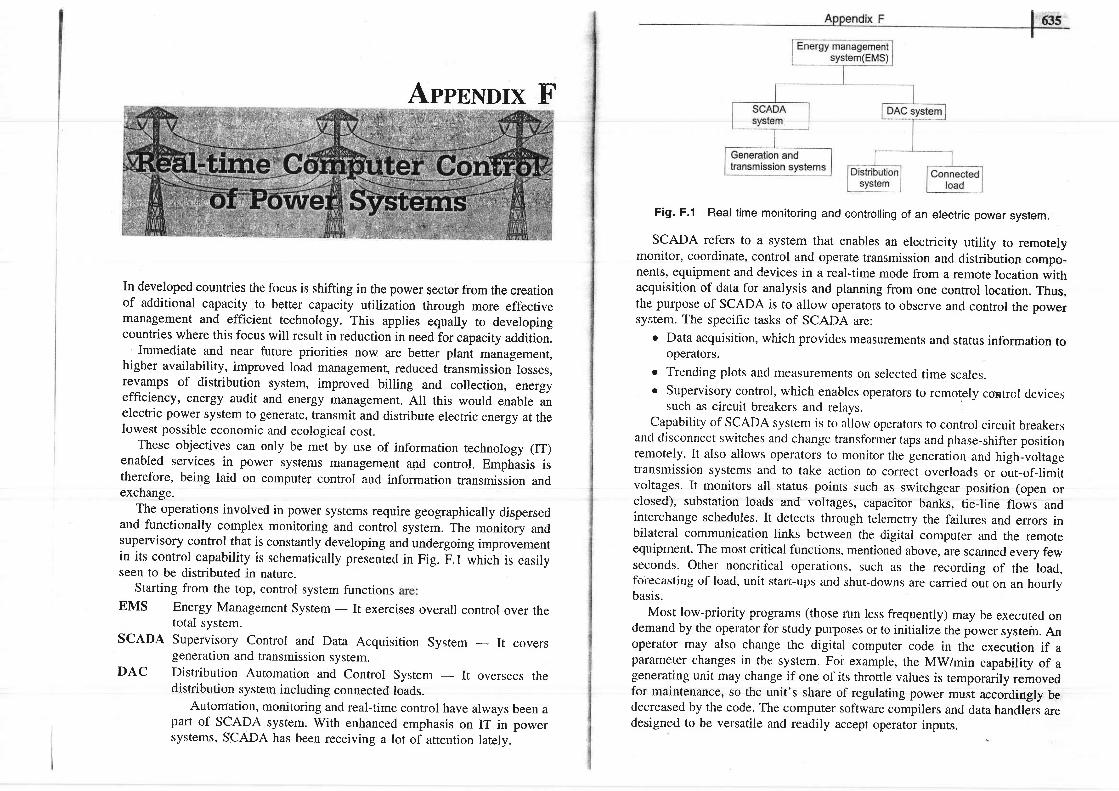
AppnNDrx F

In developed countries the focus is shifting in the power sector from the creationof additional capacity to better capacity utilization through more effectivemanagement and efficient technology. This applies equally to developingcountries where this focus will result in reduction in need for capacity addition.

Immediate and near future priorities now are better plant management,higher availability, improved load management, reduced transmission losses,revamps of distribution system, improved billing and collection, energyefficiency, energy audit and energy management. All this would enable anelectric power system to generate, transmit and distribute electric energy at thelowest possible economic and ecological cost.

These objectives can only be met by use of information technology (IT)enabled services in power systems management and control. Emphasis istherefore, being laid on computer control and information transmission andexchange.

The operations involved in power systems require geographically dispersedand functionally complex monitoring and control system. The monitory andsupervisory control that is constantly developing and undergoing improvementin its control capabil ity is schematically presented in Fig. F.1 which is easilyseen to be distributed in nature.

Starting from the top, control system functionsEMS Energy Management System - It exercises overall control over the

total system.scADA Supervisory control and Data Acquisition system - It covers

generation anci transmission system.DAC Distribution Automation and Control System - It oversees the

distribution system including connected loads.Automation, monitoring and real-time control have always been a

part of scADA system. with enhanced emphasis on IT in powersystems, scADA has been receiving a lot of attention lately.

Fig. F.l Real time monitoring and controlling of an electric power system.

SCADA refers to a system that enables an electricity utitity ro remotelymonitor, coordinate, control and operate transmission and distribution compo-nents, equipment and devices in a real-time mode from a remote location withacquisition of data for analysis and planning from one con[ol location. Thus,the purpose of SCADA is to allow operators to observe and control the powersystem. The specific tasks of SCADA are:

o Data acquisition, which provides measurements and status information tooperators.

. Trending plots and measurements on selected time scales.

. Supervisory control, which enables operators to remotely co:rtrcl devicessuch as circuit breakers and relays.

Capability of SCADA system is to allow operators ro control circuit breakersancl disconnect switches and change transformer taps and phase-shifter positionremotely. It also allows operators to monitor the generation and high-voltagetransmission systems and to take action to ccrrect overloads or out-of-limitvoltages. It monitors all status points such as switchgear position (open orclosed), substation loads and voltages, capacitor banks, tie-line flows andinterchange schedules. It detects through telemetry the failures and errors inbilateral communication links between the digital computer and the remoteequipment. The most critical functions, mentioned above, are scanned every fewseconds. Other noncritical operations, such as the recording of the load,foiecasting of load, unit start-ups and shut-downs are carried out on an hourlvbasis.

Most low-priority programs (those run less frequently) may be executed ondemand by the operator for study purposes or to initialize thepower system. Anoperator may also change the digital computer code in the execution if aparameter changes in the system. For example, the MWmin capability of agenerating unit may change if one of its throttle values is temporarily removedfor maintenance, so the unit's share of regulating power must accordingly bedecreased by the code. The computer software compilers and data handlers aredesigned to be versatile and readily accept operator inputs.

DAC is a lower level version of SCADA applicable in distribution system(including loads), which of course draws power from the transmission/subtransmission levels. Obviously then there is no clear cut demarcationbetween DAC and SCADA.

In a distribution network, computerisation can help manage load, maintainquality, detect theft and tampering and thus reduce system losses. Cornputeri-sation also helps in centralisation of data collection. At a central load dispatch'centre, data such as culTent, voltage, power factor and breaker status aretelemetered and displayed. This gives the operator an overall view of the entiredistribution network. This enables him to have effective control on the entirenetwork and issue instructions for optimising flow in the event of feederoverload or voltage deviation. This is carried out through switching inlout ofshunt capacitors, synchronous condensers and load management. This wouldhelp in achieving better voltage profile, loss reduction, improved reliability,quick detection of fault and restoration of service.

At a systems level, SCADA can provide status and measurements fordistribution feeders at the substation. Dictribution automation equipment canmonitor selectionalising devices like switches, intemrpters and fuses. It can alsooperate switches for circuit reconfuration, control voltage, read customers'meters, implement time-of-day pricing and switch customer equipment tomanage load. This equipment significantly improves the functionality ofdistribution control centres.

SCADA can be used extensively fbr compilation of extensive data andmanagement of distribution systems. Pilferage points too can be zeroed in on,as the flow of power can be closely scrutinised. Here again, trippings due tohuman effors can be avoided. Modern metering systems using electronic meters,automatic meter readers (AMRs), remote meteripg and spot billing can go along way in helping electric utility. These systbms can bring in additionalrevenues and also reduce the time lag between billing and collection.

Distribution automation through SCADA systems directly leads to increasedreliability of power for consumers and lower operating costs for the utility. Itresults in fbrecasting accurarte clenrand and supply management, taster restora-tion of power in case of a tailure and ahernative routing of power in anemergency,

A kt 'y l 'c i l turc l r l l ' thcstr $ystc l l ls is lhc rur lo lc l contnr l l i rc i l i ty l l r l t l l lows lnstcrexecution of decisions. Manual errors and oversights are eliminated. Besides online and rcal-time inlbnnution, the systenr provides periodic reports that help inthe analysis of performance of the power system. Distributi'on automationcombines distribution network monitoring functions with geographical mapping,f ^ . - f e l ^ ^ - r . l ^ - ^ - - l r 1 t | ! t ' , t . 'rilur! luL;aLtuil, ailu su un, 1.() tmprove availaDtlty. tr aISo lntegrates loadmanagement, load despatch and intelligent metering.

Data Acquisition Systems and Man-Machine Interface

The use of computers nowadays encompasses all phases of power systemoperation: planning, forecasting, scheduling, security assessment, and control.

IAn energy control centre manages these tasks and provides optimal operationof the system. A typical control centre can perform the following functions:

(i) Short, medium and long-term load forecasting (LF)(ii) System planning (SP)

(iii) Unit commitment (UC) and maintenance scheduling (MS)

(v) State estimation (SE)(vi) Economic dispatch (ED)

(vii) Load frequency control (LFC)

The above monitoring and control functions are performed in the hierarchicalorder classified according to time scales. The functions perfotmed in the controlcentre are based on the availability of a large information base and requireextensive software for data acquisition and processing.

At the generation level, the philosophy of 'distributed conffol' hasdramatically reduced the cabling cost within a plant and has the potential ofreplacing traditional control rooms with distributed CRT/keyboard stations.

Data acquisition systems provide a supporting role to the applicationsoftware in a control centre. The data acquisition system (DAS) collects rawdata from selected points in the power system and converts these data intoengineering units. The data are checked for limit violations and status changesand are sent to the data base for processing by the application software. Thereal-time data base provides structured information so that application programsneeding the information have direct and efficient access to it. ,

The Man-Machine interface provides a link between the operator and thesoftware/lrardware used to control/monitor the power system. The interfacegenerally is a colour graphic display system. The control processors interfacewith the control interface of the display system. The DAS and Man-Machineinterface support the following functions:

(i) Load/Generation Dispatching(ii) Display and CRT control

( i i i ) Datt Base Maintcnancc( iv) Alarrn Handl ing(v) Supervisory control

(v i I l ) rograrnnr ing lbnct ions(vii) DaLa logging

(vi i i ) Event logging(ix) Real-time Network Analysis

With the introduction of higher size generating units, the monitoringr r t z r t r i r a r n a n f < ' h o r r a f r n i a r r h i - ^ o . r r o - * l ^ ^ + . ^ l - ^ I - ^ - l ^ - a ^ : - . - - ^ - . ^ r L - - r - - ^rvyurrvruvrr ro r rqvw 6vuw up ur y \ ryvvr pr4rrLD ( r rD(J. I l l u lu t t t tu l r r rp l 'uvc u le Ixant

performance, now all the utilities have installed DAS in their generating unitsof sizes 200 MW and above. The DAS in a thermal power station collects thefollowing- inputs from various locations in the plant and converts thern intoengineering'units.

l,@E+l Modern Po@isI

Analog Inputs

(i) Pressures, flows, electrical parameters, etc.(ii) Analog input of 0-10 V DC

(iii) Thermocouple inputs(iv) RTD input

Digital Inpurs:

(i) Contract outputs(ii) Valve position, pressure and limit switches

All these process inputs are brought from the field through cables to theterminals. The computer processes the information and ,uppli", to the Man-Machine interface to perform the following functions.

(i) Display on CRT screen(ii) Graphic disptay of plant sub-systems

(iii) Data logging(iv) Alarm generation(v) Event logging

(vi) Trending of analogue variables(vii) Performance calculation

(viii) Generation of control signals

Some of the above functions are briefly discussed as follows.

The DAS software contains programs to calculate periodically the efficiencyof various equipment like boiler, turbine, generator, condenser, fans, heaters,etc.

| -^^a a D J t ,

"

power system engineers who are adopting the low-cost and relatively powerfulcomputing devices in implementing their distributed DAS and control systems.

Computer control brings in powerful algorithms with the following advan-

and so in raw materialsand modifiability, (iv)effectiveness.

paurly ururzauon rn generailon, (u) savings in energydue to increased operational efficiency, (iii) flexibiliiyreduction in human drudgery, (v) improved operator

Intelligent database processors will become more cornmon in power systemssince the search, retrieval and updating activity can be speeded up. Newfunctional concepts from the field of Artificial Intelligence (AI) will beintegrated with power system monitoring, automatic restoration of powernetworks, and real-time control.

Personal computers'(PCs) are being used in a wide range of power systemoperations including power station control, loacl management, SCAOe systems,protection, operator training, maintenance functions, administrative dataprocessing, generator excitation control and control of distribution networks. ITenabled systems thus not only monitor and control the grid, but also improveoperational efficiencies and play a key part in maintaining the security of thepower system.

RFFERE N CESI . Power Line Maga7ine,yol.7, No. l , October 2002, pp 65_71.2. A.K' Mahalanabis, D.P. Kothari and S.I. Ahson, Computer Aided power System

Analysis and Control, TMH, New Delhi, 199g.3. IEEE Tutorial course, Fundamentals of supervisory control system, l9gr.4. IEEE Tutorial course, Energy control centre Design, 19g3.

AppBNDrx G

MATLAB has been developed by MathWorks Inc. It is a powerful softwarepackage used for high performance scientific numerical computation, dataanalysis and visualization. MATLAB stands for MATrix LABoratory. Thecombination of analysis capabilities, flexibility, reliability and powerfulgraphics makes MATLAB the main software package for power systemengineers. This is because unlike other programming languages where you haveto declare rnatrices and operate on them with their indices, MATLAB providesmatrix as one of the basic elements. It provides basic operations, as we will seelater,like addition, subtraction, multiplication by use of simple mathematicaloperators. Also, we need not declare the type and size of any variable inadvance. It is dynamically decided depending on what value we assign to it. ButMATLAB is case sensitive and so we have to be careful about the case ofvariables while using them in our prograrns.

MATLAB gives an interactive environment with hundreds of reliable andaccurate builrin functions. These functions help in providing the solutions to avariety of mathematical problems including matrix algebra, linear systems,differential equations, optimization, non-linear systems and many other types ofscientific and technical computations. The most important feature of MATLABis its programming capability, which supports both types of programming-object oriented and structured programming and is very easy to learn and useand allows user developed functions. It facilitates access to FORTRAN and Ccodes by means of external interfaces. There are several optional toolboxes forsimulating specializeel problems of rJifferent areas anrd er-tensions to link upNIATLAB and other programs. SIMULINK is a program build on top ofMATLAB environment, which along with its specialized products, enhances thepower of MATLAB for scientific simulations and visualizations.

For a detailed description of commands, capabilities, MATLAB functionsand many other useful features, the reader is referred to MATLAB lJser'sGuide/lvlanual.

F;;ff$:

You can start MATLAB by double clicking on MATLAB icon on your Desktopof your computer or by clicking on Start Menu followed by 'programs' and thenciicking appropriate program group such as 'MATLAB

Release 12,. you willvisualize a screen shown in Fis. G.1.

Flg. G. l

The command prompt (characterised by the symbol >>)'is the one afterwhich you type the commands. The main menu contains the submenus such asEile, Edit, Help, etc. If you want to start a new program file in MATLAB(denoted by .m extension) one can click on File followed by new and select thedesired M'file. This will open up a MATLAB File Editor/Debugger windowwhere you can enter your program and save it for later use. You can run thisprogram by typing its name in front of command prompt. Let us now learn somebasic commands.

Matrix Initialization

A matrix can be initialized by typing its name followed by = sign and anopening square bracket after which the user supplies the values and closes thesquare brackets. Each element is separated from the other by one or morespaces or tabs. Each row of matrix is separated from the other by pressing Enterkey at the end of each row or by giving semicolon at its

"na. potiowing

examples illustrate this.

7 2 -9

- 3 2 - 5 1

The above operation can also be achieved by typing

Click on this to changethe cunent directory

Command prompt

Simulink browser

64?,..1 Modern Po@sist

If we do not give a semicolon at the end of closing square brackets,MATLAB displays the value of matrices in the command winCow. If you donot want MATLAB to disptay the results, just type semicolon(;) at the endof the statement. That is why you rvill find that in our programmes, wheneverwe want to display value of variables say voltages, we have just typed the nameof the variable without semicolon at the end, so that user will see the valuesduring the program. After the program is run with no values of the variablesbeing displayed, if the user wants to see the values of any of these variables inthe program he can simply type the variable narne and see the values.

Common Matrix Operations

First let us declare some matrices

Addition

Adds matrices A and B and stores them in matrix C

Subtraction

Subtracts matrix B from matrix A and stores the result.in D

Multiplication

Multiplies two conformable matrices A and B and stores the result in E

Inverse

This calculates the inverse of matrix A by calculating the co-factors and storesthe result in F.

Transpose

Single quote ( / ) operator is used to obtain transpose of matrix. In case thematrix elernent is complex, it stores the conjugate of the element while takingthe transpose, e.g.

or> > G t = [ 1 3 ; 4 5 ; 6 3 ] 'also stores the transpose of matrix given in square brackets in matrix Gl

In case one does not want to take conjugate of elements while takingtranspose of complex matrix, one should use . 'operator instead of ' operator.

t em*,

This stores determinant of matrix A in H.

VaIues

obtains eigen values of rnatrix A and stores tlrem in K.

G.2 SPECIAL MATRICES AND PRE.DEFINED VARIABLESAND SOME USEFUL OPERATORS

MATLAB has some preinitialised variables. These variables can directlyused in programs.

pi

be

iI't

t

I

This gives the value of n

converts degrees d rnto radians and stores it in variable r.

inf

You can specify a variable to have value as oo.

iandj

These are predefined variables whose value is equitl to sqrt (- 1). This is usedto define complex numbers. One can specify complex maffices as well.

The above statement defines complex power S.A word of caution here is that if we use i and j variables as loop counters

then we cannot use them for defining complex numbers. Hence you may findthat in some of the programs we have used i I and.i 1 as loop variables insteadof i and 7.

eps

This variabie is preinitiiized to 2-s2.

Identity Matrix

To generate an identity matrix and store it in variabte K give the followingcommand

A= [1 5

? 6

5 4

#ffif Modern po*er System Analysis

So K after this becomes

K = [ 1 0 00 1 0

0 0 1 l

Zeros Matrix

generates a 3 x 2 matrix whose all elements are zero and, stores them in L.Ones Matrix

generates a 3 x 2 matrix whose all elements are one and stores them in M.: (Colon) operator

This is an important operator which can extract a submatrix from a givenmatrix. Matrix A is given as below

7 8

9 1 0

3 1

e 3 r 2 l

This command extracts all columns of matrix A corresponding to row Z andstores them in B.S o B b e c o m e s 1 2 6 9 l , } l tNow try this command.

The above cofirmand extracts all the rows corresponding to column 3 of matrixA and stores them in matrix C.So C becomes

l 7931 l

Now try this command

This command extracts a submatrix such that it contains all the elementscorresponding to row number 2 to 4 and column number 1 to 3.

S o D = [ 2 6 9

5 4 3

9 3 1 l

[-ait+

" (.. oPERATOR)

This operation unlike complete matrix multiplication, multiplies element of one

matdx WitlreOnrespond'rng; eiement of other matrixlaving same index. However

in latter case both the matrices must have equal dimensions.We have used this operator in calculating complex powers, at the buses.

Say V = [0.845 + j*0.307 0.921 + j*0.248 0.966 + 7*0.410]And I = [0.0654 - j*0.432 0.876 - j*0.289 0.543 + j*0.210]'

Then the complex power S is calculated as

Here, conj is a built-in t'unction which gives complex conjugate of its argument.

So S is obtained as [- 0.0774 + 0.385Li 0.7404 + 0.4852t 0.6106 + 0.0198i]

Note here, that if the result is complex MATLAB automatically assigns i in the

result without any multiplication sign(*). But while giving the input as complex

number we have to use multiplication (*) along with i or 7.

G.4 COMMON BUILT.IN FUNCTIONS

sum

sum(A) gives the sum or total of all the elements of a given matrix A.

min

This function can be used in two forms

(a) For comparing two scalar quantities

if either a or b is complex number, then its absolute value is taken for

comparison

(b) For finding minimum amongst a matrix or ilray

e .g . i f A = [6 -3 ;2 -5 ]

>> min (A) results in - 5

abs

If applied to'a scalar, it gives the(magnitude). For example,

> > x = 3 + j * 4

abs(x) gives 5

absolute positive value of that element

If applied to a matrix, it results in a matrix storing absolute values of all the

elementS of a given matrix.

G,5 CONTROL STRUCTURES

IF Statement

The general from of the IF statement isI F e x p r e s s i o n

s t a t e m e n t sE L S E e x p r e s s i o n

s t a t e m e n t sE L S E I F

s ta tementsE N D

Expression is a logical expression resul t ing in an answer, t rue,( l ) or'false'(0). The logical expression can consist of

(i) an expression containing relational operators tabulated along with theirmean ings in Tab le G. l .

Table G.1

Relational Operator Meaning

Greater thanGreater than or Equal toLess thanLess than or Equal toEqual toNot equal to

(i i) or many logical expressions combincd with Logical operators. Variouslogical operators and their meanings are given in Table G.2.

Table G.2

Logical Operator Meaning

ANDOR

NOT

FOR Loops

This repeats a block of statements precletermined number of times.The most common {&m of FOR loop used isf o r k = a : b t c ,

s ta tementsendwhere k is the loop variable which is initialised to value of initial variable a.If the final value (i'e. c) is not reached, the statements in the body for the loop

&

t - ' _ _I 041/

comes to an end when k reaches or exceeds the final value c. For example,f o r i - 1 : 1 : 1 0 ,

a ( i ) - 1e n dThis initializes every element of a to 1. If increment is of 1, as in this case, thenthe increment part may as well be omitted and the above loop could be writtenAS

f o r i - 1 : 1 0 ,a ( i ) = 1

e n d

While Loop

This loop repeats a block of statements till the condition given in the loop is truew h i l e e x p r e s s i o n

s t a t e m e n t se n d

For example,

j - 1

w h i l e i < = 1 0a ( i ) = 1i = i + 1 ;

e n d '

This loop makes first ten elements of array a equal to l.

break statement

This staternent allows one to exit prerr'aturely from a for or while loop.

G.6 HOW TO RUN THE PROGRAMS GIVEN IN THISAPPENDIX?

1. Copy these programs into the work subfolder under MATLAB foider.2. Just type the name of the program without'.m' extension and the program

will run.

3. If you wanL to copy them in some other folder say c:\power, then aftercopying those fi les in c:\power. change the work folder to e :\power. youcan do this by clicking on toolbar containing three periods ... which is onthe right side to the Current Directory on the top rilht corner.

4. You can see or edit these programs by going through Fite - open menuand opening the appropriate file. However do not save those programs,unless you are sure that you want the changes you have made to theseorisinal files.

ffiffi| Modern Power system Analysis

5. You can see which are the variables already defined by typing whos infront of command prompt. That is why you will normally find a clearcommand at the beginning of our programs. This clears all the variablesdefined so far from the memory, so that those variables do not interfere

G.7 SIMULINK BASICS

SIMULINK is a software package developed by MathWorks Inc. which is oneof the most widely used software in academia and industry for modeling andsimulating dynamical systems. It can be used for modeling linear and nonlinearsystems, either in continuous time frame or sampled time frame or even a hybridof the two. It provides a very easy drag-drop type Graphical user interface tobuild the models in block diagram form. It has many built-in block-librarycomponents that you can use to model complex systems. If these built-in modelsare not enough for you, SIMULINK allows you to have user defined blocks aswell. However, in this short appendix, we will try to cover some of the verycommon blocks that one comes across while simulating a system. You can tryto construct the models given in the examples.

How to Start?

You can start SIMULINK by simply clicking the simulink icon in the tools baror by typing Simulink in front of the MATLAB command prompt >>. Thisopens up SIMULINK'hbrary browser, which should look similar to the oneshown in Fig. G2. There may be other tool boxes depending upon the licenseyou have, The plus sign that you see in the right half of the window indicatesthat there are more blocks available under the icon clicking on the (+) sign willexpand the library. Now for building up a new model click on.File and selectNew Model. A blank model window is opened. Now all you have to do is toselect the block in the SIMULINK library browser and drop it on your modelwindow. Then connect them together and run the simulation. That is all.

An Example

Let us try to simulate a simple model where we take a sinusoidal input,integrate it and observe the output. The steps are outlined as below.

1. Click on the Sources in the SIMULINK library browser window.

2. You are able to see various sources that SIMULINK provides. Scrolldown and you will see a Sine Wave sources icon.

3. Click on this sources icon and without releasing the mouse button dragand drop it in your model window which is currently named as 'untitled'.

4. If you double-click on this source, you will be able to see Blockparameters for sine wave which includes amplitude, frequency, phase, etc.Let not change these parameters right now. So click on cancel to go back.

Fig. G.2

Similarly click on continuous library icon. You can now see variousbuilt-in blocks such as derivative, integrator, transfer-function, state-space etc. Select integrator block and drag-drop it in your model window.

Now click on sinks and drag-drop scope block into your model. This isone of the most common blocks used for displaying the values of theblocks.

7. Now join output of sine-wave source to input of Integrator bloc(. This can' be done in two ways. Either you click the left button and drag mouse fromoutput of sine-wave source to input of Integrator block and leave leftbutton or otherwise click on right button and drag the mouse to formconnection from input of integrator block to output of sine,wave source.

8. Now in the main menu, click on Simulation and click Start. Thesimulation runs and stops after the time specified by giving ready promptat bottom left'corner.

9. Now double-click on scope to see the output. Is something wrong? Theresult is a sine wave of magnitude 2. Is there something wrong withSIMULINK software?

No, we have in fact forgotten to specify the integration constAnt!Integration of sin ?is - cos d+ C. At 0=0, C - - 1. If we do not specifyany initial condition for output of the integrator, simulink assumes it to be0 and calculates the constant. So it calculates

f l Hi U ccrlrnni".Sl oircrctc'. S furtmsaroUosUnu

, H nmr'oeri .fi sgn*aryrtan

i H s * ':. fl sar:er

f,l crrtrd 9y*en tooDox

Dbcret

Fqdin t l$hr

Ma['

Nmlle

Sign* t SJ,s{emt

Si*r1

:l

5 .

6.

ffi Modern Po

- cos 0+ C = 0 at r = 0 givinl C = 1. So the equation for output becomes- cos 0 + l. Thus naturally, it starts from 0 at t = 0 and reaches its peakvalue of 2 at 0= n, i.e. 3.I4.

10. To rectifv this error. double click on Inte block and in the initialconditions enter - 1 which should be the output of the block at t = 0. Nowrun the simulation again and see for yourself that the result is correct.

Some Commonly used Blocks

1. Integrator We have already described its use in the above example.

2. Transfer function Using this block you can simulate a transfer functionof the form Z(s) = N(s)/D(s), where N(s) and D(s) are polynomials in s.You can double click the block and enter the coefficients of s in numeratorand denominator of the expression in ascending order of s which are to beenclosed inside square brackets and separated by.a space.

3. Sum You can find this block under Math in Simulink block. By default,it has two inputs with both plus signs. You can modify it to have requirednumber of inputs to be surnmed up by specifying a string of + or- depending upon the inputs. So if there are 3 inputs you can give the listof signs as + - - . This will denote one positive input and two inputs with- signs which are often used to simuiate negative feedback.

4. Gain This block is also found under Math in Simdlink block. It is usedto simulate static eain. It can even have fractional values to act asattenuator.

5. Switch This block is available under Non-linear block in Simulink. Ithas 3 inputs with the top irrput being numbered 1. When the input number2 equals or exceeds the threshold value specified in the properties of thisblock, it allows input number 1 to pass through, else it allows inputnumber 3 to pass through.

6. Mux and Demux These blocks are available under Signals and systemsblock in Simulink. The Mux block combines its inputs into a single outputand is mostly used to form a vector out of input scalar quantities. Demuxblock does the reverse thing. It splits the vector quantity into multiplescalar outputs.

7. Scope We have already described its use. However; if you are plottinga large number of points, click on properties toolbar and select DataHistory tab. Then uncheck the Limit data points box so that all points areplotted. Also when the rvaveform does not appear smooth, in the generaltab of properties toolbar, select sample time instead of decimation in thesample time box and enter a suitable value like le-3 (10-3). The scopethen uses the value at sample-time interval to plot.

8. Clock This block is used to supply time as a source input and isavailable in Sources block under Simulink.

,*rr-rr r^tin Sources block under Simulink. We have made use of this block instability studies to provide constant mechanical input.

generate a sine wave of any amplitude, frequency and phase.

The reader is encouraged to work out, the examples given in thisAppendix to gain greater insight into the software.

G.8 SCRIPT AND FUNCTION FILES

Types of m-files

There are two types of m-files used in Matlab programming:

(i) Script m-file - This file needs no input parameters and does not returnany values as output parameters. It is just a set of Matlab statementswhich is stored in a file so that one can execute this set by just typing thefile name in front of the command prompt, eg. prograrnmes in G2 to Gl8are script files.

(ii) Function m-files - This file accepts input agruments and return values asoutput parameters. It can work with variables which belong to theworkspace as well as with the variables which are local to the functions.These are useful for making your own function for a\ particularapplication, eg. PolarTorect.m in Gl is a function m-file.

The basic structure of function m-file is given below:(a) Function definition line - This is the first line of a function. It specifies

function name, number and order of input variables.

Its syntax is- function [output variables] = function-name (list of inputvariables)

(b) First line of help - Whenever help is requested on this funciton or lookfor is executed MATLAB displays this line.

Its syntax is - Vo function-name help(c) Help text - Whenever help is requested on the function-name help text

is displayed by Matlab in addition to first help line.

Its syntax is - Vo function-name (input variables)(d) Body of the function - This consists of codes acting on the set of input

variables to produce the output variables.Tlccr nqn fhrrs r lcwelnn h ic /hcr nrr rn r t rn t r rqrnc end f i ' rnnf innc qnA qAA fham fn fha

LarvrII uv ulv

existing library of functions and blocks.

G.9 SOME SAMPLE EXAMPLES SOLVED BY MATLAB

In this section 18 solved examples of this book are solved again usingMATLAB/SIMULINK to encourage the reader to solve more power systemproblems using MATLAB.

ffil uodern power Systefn nnalysis

Ex G.I

% This funct ionYo The argument% This funct ion

conve r t s po1 a rt o t h i s f u n c t i o nhas been used i

t o r ec tangu la r coo rd ina tesi s 1 ) Magn i t ude & ? )Ang le i s . i n deg rees

append i xfunc t i on rec t=po la rTo rec t ( a ,b )rec t=a*cos (b *p i / 1S0 )+ j *a *s i n (b *p i / l g0 ) ;

function is used in solution of many of the examples solved later.

Ex G.2 (Example S.O)

% Th l s i l l u s t ra tes t he Fe r ran t i e f f ec t% I t s imu la tes t he e f f ec t by va ry i ng t he l eng th o f l i ne f r om% zero( rece iv ing end) to 5000km in s teps of 10 km% and p lo t s t he send ing end vo l t age phaso r% Th i s co r responds t o F ig . 5 .13 and da ta f r om Examp le 5 .6c l ea rVR=220e3/sqr t (3) ;a 1 p h a = 0 . 1 6 3 e - 3 ;be ta=1 .068e -3 ;I =5000 ;

k = 1 ;f o r i = 0 : 1 0 : 1 ,

V S = ( V R / z ) * e x p ( a ' l p h a * i ) * e x p ( j * b e t a * j ) + ( V R / Z ) * e x p ( - a l p h a * i ) * e x p ( j * b e t a * j ) ;X (k ) = rea l (VS) ;Y ( k ) = i m a g ( V S ) ;

' k=k+1 ;endp 1 o t ( X , Y )

Ex. G.3 (Example 8.7)

% Th i s P rog ram i l l us t ra tes t he use o f d i f f e ren t l i ne mode l s as% in Examp ' l e 5 .7c l e a rf=50| =300

7=4Q+j* lZ5Y= I e -3PR=50e6/3YR=?20e3/ (sqrt (3) )p f1 oad=0 .8IR=PR/ (VR*p f1 oad )z=7 /1y=Y l1

% Now we ca l cu la te t he send ing -end vo l t age , send . i ng -end cu r ren t% a n d s e n d i n g - e n d p f . b y f o l l o w i n g m e t h o d s f o r v a r i o u s l e n g t h s o F I i n e

' Appendix G ffiT -

% va ry ing l i ne l eng ths f r om 10 t o 300 km i n s teps o f 10 km% and compare t hem as a f unc t i on o f l i ne l eng ths .% The methods are% l ) Sho r t L i ne app rox ima t i om

Nomina l -P I me thod% 3 ) E x a c t t r a n s m i s s i o n l i n e e q u a t i o n s% 4 ) App rox ima t i on o f exac t equa t i onsi =1.

f o r I = 1 0 : 1 0 : 3 0 0 ,

% S h o r t I i n e a p p r o x i m a t i o nVs_sho r t l ' i ne ( i ) =Yq+ (2 *1 ) * I RI s s h o r t l i n e ( i ) = 1 Pspf_shor t l i ne ( i ) =cos (ang1 e (vs_shor t l i ne ( i ) -ang l e ( I s_shor t l ine ( i ) ) ) )Spower_shor t l ' i ne ( i ) =rea l (Vs shor t l i ne ( j ) *con j ( Is_shor t l i ne ( i ) ) )

%Nomi na l PI method4=1+ ( y *1 ) * ( z *1 ) /ZD=AB=z* lC=y* t * ( l + ( y *1 ) * ( z *1 ) / a )Vs_nomi na l p i ( i ) =A*VR+B*I RI s_nom'i na' l pi ( i ) =C*VR+D*l RS p f _ n o m i n a l p i ( i ) = c o s ( a n g 1 e ( V s _ n o m i n a l p ' i ( i ) - a n g t e ( I s _ n o m i n a l p i ( i ) ) ) )Spower_nomi na' l pi ( i ) =real (Vs_nomi nal pi ( i ) *conj ( I s_norpi na I pN.i ) ) )

% Exac t t r ansm jss ion L ine Equa t j onsLc=sqrt(z/y)garnma=sqrt (y*z)Vs_exact ( i )=cosh(gamma* l ) *VR + Zc*s inh (ganrma*1 )* IRIs_exac t ( i ) = ( I l l c ) * s i nh (gamma*1 ) + cosh (gamma* l ) * IRSpf_exact ( i ) =cos (ang1 e (Vs_exact ( i ) -ang1 e ( I s_exact ( j ) ) ) )Spower_exact ( i ) =real (Vs_eiact ( i ) *conj (Is_exlct ( i ) ) )

% Approx imat ion of above exact equat ions4 = 1 + ( y * l ) * ( z * t ) / ZD=Ag = ( z * 1 ) * ( t + ( y * l ) * ( z * t ) / 6 )C= ( y * l ) * ( 1+ (y * l ) * ( z *1 ) / 6 )Vs_aPProx ( i ) =A*VR+B*IR

I s_approx ( i ) = [ * !P+P* 1 PSpf_approx ( i ) =cos (ang1 e (Vs_approx ( I ) -ang I e ( I s_approx ( i ) ) ) )Spower_appnox( i ) =rea1 (Vs_approx ( ' i ) *con j ( Is_approx( i ) ) )p o i n t ( j ) = ii = i + L

end% The reader can uncomment any of the four p lo t s ta tements g iven be low% by removing the percenlage s ign against that s ta tement% for ex. in the p lo t s ta tement uncommented be low% i t p l o t s t he send ing end vo ' l t ages f o r sho r t l i ne mode l i n r ed

% by nominal p i -mode1 in green , by exact parameters moder% and by approx. p i model in b luep l o t ( po ' i n t , abs (Vs_sho r t l i ne ) , ' r ' , po i n t , abs (Vs_nomi na . l p i ) ,

,( V s _ e x a c t ) , ' b ' , Dpo i n t , abs (Vs_approx) , , k , )

, po i n t , abs . . .

, po i n t , abs. . .

Ex G.4 (Eiample 6,2)

% This program forms yBUS by Singular Transformat ion& The da ta f o r t h i s p rog ram i s a p r im i t i ve adm i t t ance ma t r i x y% wh i ch i s t o be g i ven i n t he f o i l ow ing f o rma t and s to red i n yda ta .% G r o u n d i s g i v e n a s b u s n o 0 .% I f t he e lemen t i s no t mu tua l ] y coup led w i t h any o the r e l emen t ,% the( ' the ent ry cor respondi ng to 4 th and 5th co i umn of ydata% has ' I o be ze ro

i n b l a c k

' , po i n t , abs . . .

%

% e lement no I connected I y (se l f ) lMutua l l y I v (mutua l )? | F r o m I T o I t c o u p l e d t o l% | Busno I Busno I%yda ta= [ I

2345

% fo rm p r im i t i ve% to s ta r t w i t h

t 2 L / ( 0 . 0 5 + ; * 9 . 1 5 ;I 3 t / ( 0 . 1 + j * 0 . 3 )2 3 t / ( 0 . 1 s + j * 0 . 4 s )? 4 1 / ( 0 . 1 0 + j * 9 . 3 9 ;3 4 1 / (O .05+ j *0 . 15)

y mat r ix f rom th is da ta andi n i t i a l i z e i t t o z e r o .

0000o l ;

00000

%

%

%

%

%

%

%

%

%

%yo

%

el ements=max (ydata ( : , 1) )ypr i mi t i ve=zeros (e1 ements , e1 ements )% Process ydata matr . ix rowwjse to form

el ement no I connected Il F r o m l T o II Busno I eusno I

y ( s e l f )

1 2 L / (O .Os+ j *0 . 15) 01 3 r / ( o . i + j * 0 . 3 ) 02 3 t / ( 0 . r 5 + j * 0 . 4 5 ) 02 4 t / (o .19+3 *0 .30) 0? , A 1 l l n n c ' : + ^ 1 r \v r r / \ v . s 3 r . . ; " U . I C , f U

lMutua l l y I y (mutua l )I coupl ed to I

0000o j ;

ypr imi t i ve

coupl ed wi th any other e l ementi n 5 th co l umn of ydata above)the i th row i s made equal to y(mutua. l )

n o w i t h w h i c h j t h e l e m e n t i s m u t u a l l y c o u p l e d

f o r i = 1 : e l e m e n t s ,yp r i m i t i ve ( i ,

. i ) =yda ta ( i , 4 )% A l s o ' i f t h e e l e m e n t i s m u t u a l l yeo (whose e lemen t no i s i nd i ca ted% the co r respond ing co lumn no i n

t5

ydata=[ 12345

i f ( y d a t a ( i , S ) - = g ;j i s i h e e l e m e n t

j=yda ta ( j , 5 )Ymu tua i = ; ' da ta ( i , 6 )y p r i m i t i v e ( i , j ) = y m u t u a l

endend

% Form Bus ' inc idence matr ix A f rom ydata

% Fo l1ow jng s ta temen t g i ves max imum no . o f e l emen ts by ca l cu la t i ng t he% max imum ou t o f a l l e l emen ts (deno ted by : ) o f f i r s t co lumn o f yaa tae l ements=max (ydata ( : , l ) ) \% th i s g i ves no . o f buses wh i ch i s no th ing bu t t he max imum en t r y% ou t o f ?nd and 3 rd co lumn o f yda ta wh i ch i s ' f r om ' and , t o ' ao l r r n ,b u s e s = m a x ( m a x ( y d a t a ( z , Z ) ) , m a x ( y d a t a ( : , 3 ) ) ) ;

ffi__f--

buses=max(max(ydata (2 , : ) ) ,max (ydata (3 , : ) ) )A=zeros (e'l emen t s , bu ses )

f o r i =1 :e l emen ts% y d a t a ( i , ? ) g i v e s t h e , f r o m ' b u s n o .% fhe ent ry cor rosponding to co lumn corrosponding to th is bus% i n A m a t r i x i s m a d e 1 i f t h i s i s n o t g r o u n d b u i

i f y d a t a ( i , 2 1 - = gA ( i , y d a t a ( i , Z ; ; = 1 .end

% y d a t a ( i , 3 ) g i v e s t h e ' t o ' b u s n o .% The en t r y co r rospond ing t o co lumn co r respond ing t o t h i s bus% i n A m a t r i x i s m a d e 1 i f t h i s i s n o t g r o u n d b u s

i f yda ta ( ' i , 3 ; -= 9A ( i , y d a t a ( i , 3 ; ; = - iend

end

Y B U S = A ' * y p r i m i t i v e * A

Ex G.5 (data same as Example 6.2)

This program forms yBUS by,adding one erement a t a t . imeThe da ta f o r t h i s p rog ram i s a p r im i t i ve adm i t t ance ma t r i x ywh i ch i s t o be g i ven i n t he f o l l ow ing f o rma t and s to red i n yda taGround i s g i ven as bus no . 0I f t he e lemen t i s no t mu tua l l y coup led w i t h any o the r e l emen t ,then the ent ry cor responding to 4 th and 5th co iumn of ydatahas to be zeroThe da ta mus t be a r ranged i n ascend ing o rde r o f e l emen t no .

ffi,W uooern Power System nnavsis

YBUS=zeros (buses , buses) ;

f o r r ow=1 :e lemen ts ,% i f yda ta ( row ,5 ) i s ze ro t ha t means t he co r respond ing e lemen t% i s no t mu tua l l y coup led w i t h any o the r e l emen t

nppencix o Hffi-

Y B U S ( k , l ) = Y B U S ( k , l ) - y s m ( 2 , 2 ) ;Y B U S ( l , k ) = Y B U S ( k , l ) ;YBUS ( i 1 , k ) = YBUS ( i 1 , k )Y B U S ( k , i 1 ) = Y B U S ( i 1 , k ) ;YBUS(II,I) = YBtll(j!,L)YBUS ( l , j 1 ) = YBUS ( j 1 , I ) ;Y B U S ( i 1 , . | ) = Y B U S ( i 1 , 1 )YBUS ( . | , i 1 ) = YBUS ( j 1 , . | ) ;Y B U S ( j 1 , k ) = Y B U S ( j 1 , k )Y B U S ( k , j l ) = Y B U S ( j 1 , k ) ;

endi f i 1 = = 0 & j 1 - = 0 & k - = 0 & l - = 0

Y B U S ( j 1 , j 1 ) = Y B U S ( i 1 , i 1 ) + y s m ( 1 , 1 ) ;Y B U S ( k , k ) = Y B U S ( k , k ) + y s m ( 2 , 2 ) ;Y B U S ( l , l ) = Y B U S ( 1 , . | ) + y s n ( ? , 2 ) ;Y B U S ( k , l ) = Y B U S ( k , l ) - y s m ( 2 , 2 ) ;Y B U S ( l , k ) = Y B U S ( k , l ) ;Y B U S ( j 1 , . | ) = Y B U S ( i 1 , 1 ) + y s m ( 1 , 2 ) ;Y B U S ( . l , j 1 ) = Y B U S ( i l , l ) ;Y B U S ( j 1 , k ) = Y B U S ( i 1 , k ) - y s m ( 1 , 2 ) ;Y B U S ( k , j 1 ) = Y B U S ( i 1 , k ) ;

endi f i 1 - = 0 & j l = = Q & k - = 0 & l - = 0

Y B U S ( i 1 , j 1 ) = Y B U S ( i 1 , ' i 1 ) + y s m ( 1 , 1 ) ;Y B U S ( k , k ) = Y B U S ( k , k ) + y s n ( 2 , 2 ) ;Y B U S ( l , l ) = Y B U S ( 1 , ' l ) + y s n ( z , 2 ) ;Y B U S ( k , l ) = Y B U S ( k , l ) - y s m ( 2 , 2 ) ;Y B U S ( l , k ) = Y B U S ( k , l ) ;Y B U S ( i 1 , k ) = Y B U S ( i 1 , k ) + y s m ( 1 , 2 ) ;Y B U S ( k , i 1 ) = Y B U S ( ' i l , k ) ;Y B U S ( i 1 , . | ) = Y B U S ( i 1 , 1 ) - y s m ( 1 , 2 ) ;YBUS ( l , ' i 1 ) = YBUS ( i 1 , . | ) ;

endj f i 1 - = 0 & j 1 - = Q & k = = 0 & l - = 0

Y B U S ( i 1 , i 1 ) = Y B U S ( i 1 , i 1 ) + y s m ( 1 , l . ) ;Y B U S ( j 1 , i 1 ) = Y B U S ( i 1 , i 1 ) + y s m ( 1 , 1 ) ;Y B U S ( l , l ) = Y B U S ( 1 , . | ) + y s m ( 2 , 2 ) ;Y B U S ( i 1 , j 1 ) = Y B U S ( i 1 , i 1 ) - y s m ( 1 , l . ) ;Y B U S ( j 1 , j 1 ) = Y B U S ( i 1 , i 1 ) ;Y B U S ( j 1 , 1 ) = Y B U S ( j 1 , 1 ) + y s m ( I , 2 ) ;Y B U S ( . l , j 1 ) = Y B U S ( i 1 , 1 ) ;Y B U S ( i 1 , . | ) = Y B U S ( i 1 , . | ) - y s m ( 1 , 2 ) ;Y B U S ( l , j l ) = Y B U S ( i 1 , 1 ) ;

end

i f i 1 - = 0 & j l - = Q & k - = 0 & l = = 0Y B U S ( i 1 , i 1 ) = Y B U S ( i 1 , i 1 ) + y s m ( 1 , 1 ) ;Y B U S ( j 1 , j l ) = Y B U S ( j 1 , i 1 ) + y s m ( 1 , 1 ) ;Y B U S ( k , k ) = Y B U S ( k , k ) + y s m ( 2 , 2 ) ;Y B U S ( i 1 , j 1 ) = Y B U S ( i 1 , j 1 ) - y s m ( 1 , 1 ) ;

+ y s m ( 1 , 2 ) ;

+ v s m ( 1 . 2 ) :

j f yda ta ( row ,5 ) == 0i 1 = y d a t a ( r o w , 2 ) ;j 1 = y d a t a ( r o w , 3 ) ;

i f i 1 - = 0 & j l - = 0Y B U S ( i 1 , ' i 1 ) = Y B U S ( j 1 , j 1 ) + y d a t a ( r o w , 4 ) ;Y B U S ( i 1 , j l ) = Y B U S ( i 1 , j 1 ) - y d a t a ( r o w , 4 ) ;Y B U S ( j 1 , i 1 ) = Y B U S ( i 1 , j l ) ;Y B U S ( j 1 , j 1 ) = Y B U S ( j 1 , j 1 ) + y d a t a ( r o w , 4 ) ;

endi f i l = = 0 & j l - = Q

Y B U S ( i 1 , j 1 ) = Y B U S ( i 1 , i 1 ) + y d a t a ( r o w , 4 ) ;endi f i l - = 0 & j l = = Q

Y B U S ( j 1 , j 1 ) = Y B U S ( j 1 , j 1 ) + y d a t a ( r o w , 4 ) ;end

endeo i f yda ta ( row ,5 ) i s NOT ze ro t ha t means t he co r respond ing e lemen t% i s m u t u a l l y c o u p l e d w i t h e l e m e n t g i v e n i n y d a t a ( r o w , 5 )

i f y d a t a ( r o w , 5 ) - = g

i 1 = y d a t a ( r o w , 2 ) ;j 1 =yda ta ( row ,3 ) ;% mu tua lw i t h g i ves t he e lemen t no w i t h wh i ch t he cu r ren t e l emen t% i s mu tua l l y coup led w j t h k and 1 g l ve t he bus nos be tween% wh ich t he mu tua l l y coup led e lemen t i s connec tedmu tua l * . i 11=yda ta ( i 1 ,5 ) ;;q=ydata (mutua l w i th ,2) ;1 =yda ta (mu tua l w i t h ,3 ) ;

zs I=I /ydata( row,4) ;zs?=L/ydata (mutual w' i th,4) ;zm = l / yda ta ( row ,6 ) ;

756= [zs 1 zmzn zs?l;

ysm='i nv (zsm) ;% Fo l ' l ow ing i f b l ock g i ves t he necessa ry mod i f i ca t i ons i n YBUS% when none o f t he buses i s r e fe rence (g round ) bus .i f i l - = 0 & j l - = 0 & k - = 0 & l - = 0

Y B U S ( ' i 1 , i 1 ) = Y B U S ( i i , i 1 ) + y s m ( 1 , 1 ) ;Y B U S ( j 1 , j l ) = Y B U S ( j 1 , j l ) + y s m ( 1 , 1 ) ;Y B U S ( k , k ) = Y B U S ( k , k ) + y s m ( 2 , 2 ) ;Y B U S ( l , l ) = Y B U S ( l , l ) + y s n ( Z , 2 ) ;Y B U S ( i I , j 1 ) = Y B U S ( i 1 , j 1 ) - y s m ( 1 , 1 ) ;Y B U S ( j 1 , i 1 ) = Y B U S ( i 1 , j 1 ) ;

- y s m ( 1 , 2 ) ;

- y s m ( 1 , 2 ) ;

W Mooern power system A_nalysis

Y B U S ( j 1 , i 1 ) = y B U S ( i t , j t ) ;Y B U S ( i 1 , k ) = Y B U S ( i 1 , k ) + y s m ( 1 , 2 ) ;YBUS (k , i 1 ) = YBUS ( i 1 , k ) ;Y B U S ( i 1 , k ) = y B U S ( i 1 , k ) _ y s m ( 1 , 2 ) ;Y B U S ( k , i l ) = Y B U S ( j 1 , k ) ;

end

YBUS

Ex G.6

% T h i s ' i s p r o g r a m f o r g a u s s s i e d e r L o a d f r o w . T h e d a t a i sc l e a rn = 4V = [ 1 . 0 4 1 . 0 4 1 t ]

Y = [ 3 - i * 9 - 2 + i * 6 - l + 5 * 3 0- 2 + i * 6 3 6 6 6 _ j * 1 1 _ 0 . 6 6 6 + j * 2 _ t + 3 * 3- 1 + ; * 3 - 0 . 6 6 6 + j * 2 3 . 6 6 6 - j * 1 1 _ Z + i * 60 - 1 + 3 ' * 3 - 2 + t r * 6 3 - j " 9 1

t y p e = o n e s ( n , 1 )typechanged=zeros (n , 1 ) Q l i m i tmax=zeros (n , 1 iQ l im i tm i n=zeros (n , l )Vmagf i xed=zeros (n , 1 )tYpe(2)=2Ql i mi tmax (2) =1 . gQ1 i m i tm i n (2 ) =9 . 2Vmagf i xed(2) =1.04d i f f=10; noof i te r=1Vprev=V;w h i l e ( d i f f > O . 0 0 0 0 1 | n o o f i t e r = = 1 ) ,abs (V)abs (Vprev)%pauseVprev=V;P = [ i n f 0 . 5 - 1 0 . 3 ] ;Q = [ i n f 0 0 . 5 - 0 . 1 ] ;$ = [ i n f + j * i n f ( 0 . 5 - j * 0 . 2 ) ( - 1 . 0 + j * 0 . 5 ) ( 0 . 1 - 1 * g . 1 ) ] ;f o r i = Z i n ,

i f t y p e ( i ) = = 2 l t y p e c h a n g e d ( i ; = = 1 ,

",llilil;:il;l#ii#ll, ill ).Q, imi tmi n(i ) ),Q( j ) =Q l im i tm i n ( i ) ;

e l s e

Q ( ' i ) = Q l i m i t m a x ( i ) ;endt Y P e ( i ) = 1 ;

f r om Examp le 6 .5

lFitlilE4lq.ffi.Appendix c NilFffi

T-typechanged ( i ) =1 t

e l setype ( i ) =2;

endend

sumyv=0;f o r k = L : n ,

i f ( i - = k )sumyv=sumyv+Y ( i , k ) *V (k) ;

endendv ( i ) = (1 /Y ( i , i ) ) * ( ( p ( i ) - j *Q ( i ) ) / con j ( v ( i ) ) - sumyv ) ;i f t ype ( i ; ==2 & t ypechanged ( i ) -=1 ,

V ( i )=pe1 a rTo rec t (Vmag f i xed ( i ) , ang1 e (V ( i ) ) *1g0 /p i ) ;end

enddi f f=max (abs (abs (U (Zzn) ) -abs (Vprev (Z: n) ) ) ) ;noof i ter=noof i ter+ l ;endV


% Programc l e a r ;% n s tands

for load f low by Newton-Raphson Method.

for number o f busesn = 3 ;% Y , v o l t a g e s a t t h o s e b u s e s a r e i n i t j a l j s e dv = [ 1 . 0 4 1 . 0 1 . 0 4 ] ;% Y i s Y B u sY=[ 5 .88228- j ' t23 .50514 -2 .9427+ j *L t . t6 t6

-2 .9427 +j*Lt .7 67 6 5 .88228_j*23 .505L4-? .9427 + j *L l .7 67 6 -2 .9427 + j * t t .7 6 t6

%Bus types are jn i t ia l j sed in type ar ray to%bus.%code 2 stands for PV bust y p e = o n e s ( n , 1 ) ;%when Q l ' imj ts are exceeded for a pV bus Bus type is changed to pQ%temporari 1 yL a n a ' l o m o n f i n f # . r ^ o a h r n a n ' l . i a - ^ + . ^ 1 i -' e " , L , , e I v r u J p s L r s r v s u r ) J t r L L u r r l r c d s g r r 5 D u s s t a t u s%is t empora r i l y changed f r om pQ to pV .O the rw i se i t i s ze rotypechanged=zeros (n , 1) ;% s ince max and m in Q l ' im i t s a re checked on l y f o r pv buses ,% max & m in Q l im l t s f o r o the r t ypes o f buses can be se t t o any va lues .% here we have set them to zeros for convenienceQl imi tmax=zeros (n , 1) ;Q1 im i tm i n=ze ros (n , l ) ;Vmagf i xed=zeros (n , 1) ;

-Z .9427 + j * 7 I . t 67 6-2 .9427 + j* I I .7 67 65 .88228- j *23 .5051a1;code 1 which stands for PQ

W Modern Power system AnalysisI

t I to to ta l no . o f equat ions (eqcount )fo r ceq=1:eqcount ,

fo r cco l=1 :eqcount ,

v s J \ e e y / t s J r v v v r \ u J J v e v r u u J \ v w w r l l r ,

bm=i mag (Y (assoeqbus (ceq) , assocol bus (cco: l ) ) *V (as soco l bus (cco l ) ) ) ;e i =rea l (V (assoeqbus (ceq) ) ) ;f i = imag (V (assoeqbus ( ceq ) ) ) ;

i f a s s o e q v a r ( c e q ) = = ' P " ' & a s s o c o l v a i ( c c o 1 ) = = ' d ' ,

i f assoeqbus ( ceq ) -=assoco l bus ( cco l ) ,H=am*f i -bm*ei ;

e l s e11 = -Q (as soeqbus ( ceq ) ) i mag (Y ( assoeqbus ( ceq ) , assoco l bus ( ceq ) ) . . .

* abs (V (assoeqbus ( ceq ) ) ) ^2 ) ;endJacob ( ceq , cco l ) =H

endi f a s s o e q v a r ( c e q ) = = ' P ' & a s s o c o l v a r ( c c o 1 ) = = ' V ' ,

' i f assoeqbus (ceq) -=assocol bus (cco l ) ,N=am*e i+bm* f i ;

e l seN=P (assoeqbus (ceq) ) +real (Y (assoeqbus (ceq) , assocol bus (ceq) ) . . .

* abs (V (assoeqbus ( ceq ) ) ) ^2 ) ;endJacob ( ceq , cco l ) =11

endi f a s s o e q v a r ( c e q ) = = ' Q ' & a s s o c o l v a r ( c c o 1 ) = = ' d ' ,

i f assoeqbus ( ceq ) -=assoco l bus ( cco l ) ,J = a m * e i + b m * f i ;

e l s eJ=P (as soeqbus ( ceq ) ) r ea l ( Y (assoeqbus ( ceq ) , assoco l bus ( ceq ) )

*abs (V (assoeqbus ( ceq ) ) ) ^2 ) ;endJ a c o b ( c e q , c c o l ) = J

endi f a s s o e q v a r ( c e q ) = = ' Q ' & a s s o c o l v a r ( c c o 1 ) = = ' V ' ,

1 f assoeqbus ( ceq ) - - assoco l bus ( cco l ) ,L=am*f i -bm*ei '

e l s eL=Q(assoeqbus ( ceq ) ) - . . .

i m r n / V / ' c c ^ o ^ h , , . t / ^ o ^ \ ' e . ^ ^ ^ ' 1 h , , . / ^ ^ ^ \ \ * . h . / \ , 1 . . . ^ ^ ^ h , , - / ^ ^ ^ \ \ \ ' \ D \ .r f f f u v \ r \ . u J J v s q v u J \ l s Y / r q J J v u v l p u J \ L s Y / r / , q w J \ r \ q J J v E V U U J \ L g r { , , l l L l ,

endJacob ( ceq , cco l ) =L

en0end

en0

%New Upda te vec to r i s ca l cu la ted f r om Inve rse o f t he Jacob ian

pauseupdate=i nv (Jacob) *mi smatch ' ;noofeq=L;

i f t y p e ( i ; = = 1newchi nangV=update (noofeq) ;newangV=ang1 e (V ( i ) ) +newchi nangV ;newchi nmagV=update(noofeQ+l )*abs (V ( i ) ) ;newmagV=abs (V ( ' i ) ) +newch j nmagV;V ( j ) =po l arTorect (newmagV, newangV*180/p i ) ;noofeq=noofeq+l ;

e l senewchi nangV=update (noofeq) ;newangV=ang1 e (V ( ' i ) ) +newctr i nangV ;V ( i )=po l a rTo rec t ( abs (V ( i ) ) , newangV* l8O /p i ) ;noofeq=noofeq+l ;

endend

% Al I the fo l I owi ng var i ab l es /ar rays are c l eared f rom% memory. Th is is because the ' i r d imensions may change due to% bus sw i t ched and once upda tes a re ca l cu la ted , t he va r i ab les9r are o f no use as they are be ing re formulated at the% end of each i tera t ' ion \c l ea r m isma tch Jacob upda te assoeqva r assoeqbus assoco l va f assoco lbus ;d i f f =m ' i n ( abs (abs (V (2 : n ) ) - abs (Vp rev (2 : n ) ) ) ) ;noof i ter=noof i ter+1 ;end

Ex. G.8 (Table 7.1)

% MATLAB Program for opt ' imum loading of generators% The data are f rom Example 7 .1% r t f i nds l amda by t he a lgo r i t hm g i ven on t he same pd9€ , once t he demandrk i s spec ' i f i ed% We have t aken t he demand as 231 .25MW co r rospond ing t o t he l as t bu t one% r o w o f T a b l e 7 . 1 a n d c a l c u l a t e d l a m d a a n d t h e l o a d s h a r l n g% n i s no o f gene ra to rsn=2% Pd s tands for load demand.% a lpha and be ta a r rays deno te a lpha be ta coe f f j c i en t s% fo r g i ven gene ra to rs .

Pd=?31.25a l pha= [0 .20

0.251beta= [40

301% i n i t i a l g u e s s f o r l a m d aI amda=20

m't n't mum%are stored in arrays% I n r e a l l i f e l a r g e% ar ray to in f us ing

ffil Modern po

I amdaprev=l amda% to le rance is eps and increment in lamda is de l ta lamdaeps=1de' l ta l amda=0.25

Hffim 1 n " l n f icos t=0 ;f o r j = 0 : n ,

f o r i = 0 : n ,

f o r I = 0 : n ,

u n i t = [ 0 0 0 0 ] ;% Here we e l imna te s t ra i gh taway t hose comb ina t i ons wh i ch% dont make up the

% n MW demand or such combinat ions where maximum generat ion

% o n l n d i v i d u a l% gene ra t i on i s exceed ing t he max imum capac i t y o f any o f t he

% generatorsi f ( ' i + j+k+ ' l ) ==n & i cPgmax (1 ) & i <Pgmax (2 ) & kcPgmax (3 ) & I < . . .Pgmax (4)

i f i - = 0u n i t ( 1 , 1 ) = i ;% F tnd ou t t he cos t o f gene ra t i ng t hese un i t s and% qdd ' i t up to to ta l costcos t=cos t+0 . 5 *a l pha ( I ) * i * i +be ta ( I ) * i ;

endi f 3 -=g

u n i t ( L , 2 ) = i ;c o s t = c o s t + 0 . 5 * a l p h a ( 2 ) * j * j + b e t a ( 2 ) * i ; \

endi f k -=0

u n i t ( 1 , 3 ) = k ;

cos t=cos t+0 .5 *a l ph r (3 ) * k *k+be ta (3 ) * k ;endi f l - = 0

u n i t ( 1 , 4 ) = l ;cos t=cos t+0 .5 *a1 pha (a ) * l * l +be ta (4 ) * l ;

end% If the total cost i s comi ng out to be I ess than

% m i n i m u m o f t h e c o s t i n% p rev ious comb ina t ' i ons t hen make m in equa l t o cos t and

% cuni t (s tand for commit ted un i ts ) equal to un ' i ts

% c o m m i t t e d i n t h i s i t e r a t i o nt ( d e n o t e d b Y v a r i a b l e u n i t s )i f c o s t < m i n

c u n ' i t - u n ' i t im i n = n n c . f :r r r . | | e v v v t

e l s ec o s t = 0 ;

endend

end

mum | ' r mt ts o t each generat i ng unPgmin and Pgmax.

s c a l e p r o b l e m s , w e c a n f i r s t i n i t i a l s e t h e P g m a xfor I oop and

L a m d a i s ' )

I oad sha red by two un j t s ' i s ' )

% Pgnin ar ray to zero us ing Pgmin=zeros(n,1) command% L a t e r w e c a n c h a n g e t h e l ' i m i t s i n d i v ' i d u a l l yPgmax=[125 I25]Pgmin=120 Z0)Pg - -1O0*ones (n ,1 )wh i l e abs ( sum(PS) -ed ; ' g t t

f o r i = 1 : n ,Ps ( i ) = (1 amda-be ta ( i ) ) / a l pha ( i ) ;i f P g ( i ) > P s m a x ( i )

P g ( i ) = P s m a x ( i ) ;endi f P s ( i ) . P g m l n ( i )

P g ( i ) = P g m i n ( i ) ;end

endi f ( s u m ( P g ) - P d ) . 0

l amdap rev= l amda ;lamda=l amda+del ta1 amda;

e l s eI amdaprev= I amda ;lamda=l amda-del ta l amda;

ende n dd i s p ( ' T h e f i n a l v a l u e o f1 amdaprevd i s p ( ' T h e d i s t r i b u t i o n o fPg

Ex. G.9 (Table 7.2)

% MATLAB Program for opt imum uni t commit tment by Brute Force methodf t The da ta fo r th ls p rogram cor responds to Tab le 7 .2

c I ear ;% a lpha and be ta a r rays denote a lpha be ta coef f i c ien ts fo r g iven genera torsa l p h a = 1 0 . 7 7 1 . 6 0 2 . 0 0 2 . 5 0 1 ' ;b e t a = 1 2 3 . 5 2 6 . 5 3 0 . 0 3 2 . 0 1 ' ;P g m i n = [ 1 1 I 1 ] ' ;Pgmax=ll? 12 12 I2l ': '

n=9% n denotes total MW to be commi tted

end

,f,f6.'l Modern Po@

end

E

f o r i = 1 : n ,s i gma=B (i , : ) *Pg-B ( i , i ) *Pg ( i ) ;

end, d i s p ( ' c u n i t d i s p l a y t h e n o o f c o m m j t t e d u n i t s o n e a c h o f

t o r s ' )d i s p ( ' I f c u n i t f o r a p a r t i c u ) a r g e n e r a t o r i s 0 j t m e a n s

for I amda

the four genera-

t h e u n i t i s n o tcommdi sp ( ' The to ta l no o f un i ts to be commi t ted are ' )c u n i t

Ex G.lO (Ex. 7.A)

c l ea r% MATLAB Program for opt imum loading of generators% Th i s p rog ram f i nds t he op t ima l l oad ing o f gene ra to rs i nc l ud ing% penal ty factors% I t imp lemen ts t he a lgo r i t hm g i ven j us t be fo re Examp le 7 .4 .% The data for th is program are taken f rom Example 7 .4% Here we g i ve demand Pd and a lpha , be ta and B -coe f f i c i en t st l , {e ca lcu la te load shared by each generator% n is no of generatorsn=2? Pd s tands for I oad demand% alpha and beta ar rays denote a lpha beta coef f ic jents for g iven% generators

Pd=237 .04;a l ph6= [0 .020

0 . 0 a 1 ;beta= [16

2ol i 'I i n i t i a l g u e s sI amda=20;I amdaprev= I amda;% to l e rance i s eps and i nc remen t i n l amda j s de l t a l amdae p s = 1 ;de l t a l amda=O.25 ;% the m in imum and max imum l im i t s o f each gene ra t i ng un i t%are s tored in ar rays Pgmin and Pgmax.% In ac tua l l a rge sca le p rob lems , we can f i r s t i n i t i a l i se t he Pgmax a r ray% to i n f us ing f o r l oop% and Pgmin a r ray t o ze ro us ing Pgmin=ze ros (n ,1 ) command% La te r we shou ld can change the l im i t s i nd i v ' i dua11yPqmax=f200 200. l :P g m i n = [ 0 0 ] ;B = [ 0 . 0 0 1 0

0 0 l ;P g = z e r o s ( n , 1 ) ;noo f i t e r=0 ;PL=0 ;P g = z e r o s ( n , 1 ) ;

Pg ( i ) = (1- (beta ( i ) / l amda) - (2*s i sna)) / (a l pha ( i ) / l amda+z*B ( i , i ) ) ;I

i f P g ( i ) ' P g m a x ( j )Pg ( i ) =Pgmax ( i ) ;

endi f P g ( i ) < P g m i n ( i )

P s ( i ) = P s m i n ( i ) ;end

endPL=Pg ' *B*Pg ;

i f ( sum(Pg) -Pd -PL )<01 amdaprev=l amda;I amda=l amda+del tal amda;

e l seI amdaprev=1 amda;I amda=l amda-del tal amda;

endnoofi ter=noofi ter+1 ;P g ;endd i sp ( ' The

noof i terd i s p ( ' T h e

1 amdaprevd i sp ( ' The

Pgd i s p ( ' T h e

P L

Ex. G.II

% I r i th is% F is . 8 .8s' imul at i onTsg= .4Tt=0.5Tps=20Kps=100R=3Ksg= 1gKt=0. IK i =0 .09

no o f i t e ra t i ons requ i red a re ' )

f i na l va l ue o f ' lamda

i s ' )

opt ' ima1 I oadi ng of generators i ncl udi ng penal ty facto,rs ' is ' )

I osses are ' )

example the parametersa r e i n i t i a l i z e d T h i sbo th f o r F igs . G .3 and

for a l l the b locks for the system inprogram has to be run prior to theG . 4 .

Tranefer Fcn Tranefer Fcn 1

SS1 Moo"rn po*b, syrt"r Rn"trrri, .

Ksg KpsTps.s + 1

Conetant

Fig. G.3 First order approximation for load frequency control

Ex. G.12

The system of Fig. 8.10 is simulated using simulink as wasExample G. l l .

Flg. G.4 Proportional plus Integral load frequency control


% Prog ram fo r bu i ] d i r r g o f Zbus by add i t ' i on o f b ranch o r l . i nk% Zpr imary=[e lementno f rom to va lue

. s + 1

done in

%%yo

% -- l% Here care shou ld be taken tha t to beg in w i th an% reference and both f rom and to nodes should notc l e a rzpri mary= [

1 I 0 0 . 2 52 2 I 0 . 13 3 1 0 . 14 2 0 0 . 2 5s 2 3 0 . 1 1

[el ements co1 umns] =size(zpr imary)t To beg in w i th zbus mat r ix i s a nu l l mat r i x

e lemen t i s addedbe new nodes

to

KsgTsg.s + 1

KpsTps.s + 1

Transfer Fcn Transfer Fcnl I Transfer Fcn2

lffiwffiflI

I currentbusno indicates maximum no. of buses added unt i l nowcurrentbusno=0

for count=1:e lements ,[ rows co1 s ] =s jze(zbus)f rom=zpr i mary (count, 2)

to=zpr i mary (count,3)val ue=zpr i mary (count, 4)

% newbus var iab le ind ica tes% newbus bus may or may not

newbus=max ( f rom, to)

the maximum of the two busesal ready be a par t o f ex i s t i ng zbus

bus to reference bus

% re f va r i ab le i nd i ca tes t he m in imum o f t he two buses% & not necessar j ly the re ference bus% re f bus mus t a lways ex i s t i n t he ex i s t i ng zbus

ref=mi n (from, to)% Mod j f i ca t i on o f t ype l% A new e lement is added f romi f newbus >currentbusno & re f

zbus= [zbus ze ros ( rows , 1 )z e r o s ( 1 , c o l s ) v a l u e l

cu rrentbusno=newbu scont i nue

end

new==0

% Modi f icat ion o f type?% A new e lement is added f rom new bus to o ld busbusi f newbus >currentbusno & re f -=0

zbus= [zbus zbus ( : , r e f )zbus ( re f , : ) va l ue+zbus ( re f , re f ) ]

cu rrentbu sno=newbu scon t i nue

\

other than re ference

end% Modi f i ca i ton o f type3% A new e lement is added between an o ld bus and re ference busi f newbus <=currentbusno & re f==O

zbus=zbus -1 / ( zbus (newbus , newbus )+va l ue ) * zbus ( : , newbus ) * zbus (newbus , : )con t i nue

end% Mod ' i f i ca t j on o f t ype4% A new e lement is added betwen two o ld busesi f newbus <= currentbusno & ref -=0

zbus=zbus - L / (va lue+zbus ( f rom, f rom)+zbus ( to , to) -2 * z b u s ( f r o m , t o ) ) * ( ( z b u s ( : , f r o m ) - z b u s ( : , t o ) ) * ( ( z b u s ( f r o m , ; | - z b u S ( t o r : ) ) ) )

con t i nueendend

Wl uodgin Power System Rnatysis

Ex. G.14 (Example 12,10)

t Program fo r t rans ' ien t s tab i ' l i t y o f s ing le mach ine connected to ln f in i te% bus th is p rogram s imu la tes Example 12 .10 us jng po in t by po in t methodc l eart - 0t f=0t f i na l =0 .5

t c=O. 125ts teP=9 . 95l4=? .5? /( 180*50)j = 2

de1 ta=21. .64*p i /180ddel ta=0t ime ( 1 ) =9

a n g ( 1 ) = 2 I . 6 4Pm=0 .9Pnaxbf=2.44Pmaxdf=0.88Pmaxaf=2.00

whi I e t< t f i na l ,' i f ( t = = t f ) ,

Pam' i nus=0.9-Pmaxbf*s i n (de l ta)Papl us=O.9-Pmaxdf*s ' in (de l ta)Paav= ( Pam'i nus+Pap1 us ) /2

' Pa=Paavendi f ( t = = t c ) ,

Pami nus=0.9-Pmaxdf*s i n (de l ta)Papl us=0. 9-Pmaxaf*s j n (de l ta)Paav= (Pamj nus+P aplus) /2Pa=Paav

end

i f ( t > t f & t < t c ) ,Pa=Pm-Pmaxdf*s i n (de l ta)

endi f ( t > t c ) ,

Pa=Pm-Pmaxaf*s i n (de l ta)end

t , P addel ta=c ide l ta+ ( ts tep* ts tep*pa/M)

de l t a - ( de l t a *180 /p j +dde l t a ) *p i / 180

de ' l tadeg=de1 ta*180/P ' it= t+ ts teppauset i m e ( i ) = 1a n g ( i ) = d e l t a d e g

j = j + 1

end

a x i s ( [ 0 0 . 6 0 1 6 0 ] )

Ex. G.15

Here the earlier Example G.l4 is solved again using SIMULINK.Before running simulation shown in Fig. G.5 integrater t has to be initializedto prefault value of 4 i.e. 4. Thit can be done by double-clicking on integrater

1 block and changing the initial value from 0 to 6s (in radius). Also double clickthe switch block and change the threshold value from 0 to the fault clearing time(in sec.).

Ex. G.16 (Ex. 12.11)

v" Th'ts program simul ates transi ent stab'i 1 i ty of mul t imachi ne systems% The data is f rom Examp' le 12.11c l ear a l Iformat long%Step 1 In ' i t ia l i sa t ion w i th load f low and mach ' ine da taf = 5 0 ; t s t e p = 9 . 9 1 . 6 = [ 1 2 9 J , ;P g n e t t e r m = [ 3 . 2 5 2 . 1 0 ] ' ;Qgnet te rm=[ 0 .6986 0 .3110] ' ;X g = [ 0 . 0 6 7 0 . 1 0 ] ' ;% Note the .use of . ' operator here% This does a t ranspose wj thout tak ing the conjugate o f each e lement

y g = [ p o ' l a r T o r e c t ( 1 . 0 3 , 8 . 2 3 5 ) p o l a r f o r e c t ( 1 . 0 2 , 7 . 1 6 ) ] . '% n is no of generators o ther than s l ack busn=2 i%Step 2V0con i=co r i (V0 ) ;Ig0=conj ( (Pgnet tem+j*Qgnet term) . /UO) ;Edash0=V0+j " (Xg. * Ig0) ;Pg0= rea ' l (Edash0 . *con j ( I g0 ) ) ;x1 r=ang l e (Edash0 ) ;% l n i t ' i a l i sa t i on o f s ta te vec to rPg r=Pg0;% Pg_ro1us l .=PgO;x Z r = [ 0 0 ] , ;x t d o t r = [ 0 0 ] , ;

x2do t r= [o o ] , ;

x l do t rp l r t l = [ 0 0J ' ix2dot rp l r t l= J0 0J ' i

SStep 3% Here in th is example we have no t rea l l y ca lcu la ted YBus But -sne% can write seParate Program.yBusdf= [1f986-j*35-6301 0 -0.0681+i*5.1661

- j * 1 1 . 2 3 6 00-0 .068 l+ j *5 . 1661

YBuspf= [I .3932- j *13 .8731

-0.2?I++j*7 .6289-0 .090 l+ i *6 .0975

%Step 4

0

-0.2214+j*7 .62890.5+j *7 .7898

0

0. 1362- j *6 .2737f i

-0 .090 l+ j *6 .0975

00.1591= j *6 .11681 ;

ofd]

. oEc

.go

P

Eo()occo. c )o.Eo(u

E Lc Lg oe o ,O Co ' o / -

L

ots

F=_o(Uo

c.9oc(gL

F

u?(56

IL

.soo

% Set the va ]ues fo r in i t ia l t ime t (occurance o f fau l t ) and% tc i s t ime a t wh ich fau l t i s c learedt=0; tc=0.08 ; t f i na l = 1 .0 ;r = 1 ;Edash_r=Edash0 ; Edash_rpl us 1=Edash0 ;w h i l e t < t f i n a l ,%Step 5 Compute Generator Powers using appropriate YBus% the YBus chosen in the fo l low ing s tep is se t accord ing to the cur ren t% t imei f t <= tc YBus=YBusdf ; e lse YBus=YBuspf ;end% Note that here we obtain the currents in iected at generator bus% by mult ip ' ly ing the correspond' ing row of the Ybus wjth the ve\tor of% vo l tages beh ind the t rans ien t reac tances . Th is shou ld a lso jnc lude

% s lack bus vo l t age% and hence the ent rY 1 aPPears% generator bus vo ' l tages

I = Y B u s ( 2 : m + 1 , : ) * [ 1E d a s h r l ;

Pg_r=rea1 (Edash_r . *con i ( I ) ) ;

j n t he bus vo l t age vec to r i n add i t i on t o

%Step 6 compute xldot-r and xZdot-rx ldot_r=x2_r;f o r k = 1 : m ,

xZdot - r ( k , 1 ) = (p i * f /H (k) ) * (PgO ( k) -Pg-r ( k ) ) ;end

%Step 7 Compute f i rs t s ta te est imates for t= t ( r+1)

x 1_rp1 us I =xl_r+x ldot-r*tsteP ;xZ_rpl us 1=x2_r+x2dot_r*tsteP ;

%Step 8 Compute f i rs t es t imates o f E ' - r+1

Edash rp l us1=abs (Edash0 ) . * ( cos ( x1 - rp1 us l )+ i * s i n ( x l - r p l us l ) ) ;%Step 9 Compute Pg for t= t ( r+1)

I = Y B u s ( 2 : m + 1 , : ) * [ 1Edash_rp' l us 1l ;

Pg_rp ' l us1=rea l (Edash_rp1 us1.*coni ( I ) ) ;

%Step 10 Compu te S ta te -den i va t i ves ' a t t = t ( r+1 )

(I'L

o)oc

(\'=o)

E

cat,

IU

-1 ,

W Mod"rn po*",. sy.t.r An"ryri,x l d o t _ r p l r t l = J 0 0 J , ixZdot_rpl r r l=10 0J , if o r k = 1 : m ,

Iffi

x ldo t_rp l us l (k , 1 ) =x2_rp ' l us l ( k , l ) ;x2dot . rp l us l (k ; l )=p i * f /H (k ) * (pqg (

%step 11 compute average varues o f s ta te der iva t ivesx I dotav_r= (x ldot_r+x1dot_rp'l usl) / ?.0 ;x2dotav_r= (x2dot_r+xZdot_rp1 usl) /2.0 ;%step L2 Compute f jnal State est t 'mates fbr t=t(r+1)x l_rp l us 1=xl_r+xldotav_r*tstep ;x2_rpl usl ixZ r+x2dotav_r*tstep ;%step 13 Compute f ina l es t imate fo r Edash a t t= t ( r+1)Edash_rp1 us 1=abs (Edash0) . * (cos (x l_ rp l us 1 ) + j *s i n (x t_ rp1 us l ) ) ;%Step 14 Pr in t S ta te Vec tor

x?_r=x?_rpl usl;x l_ r=x l_ rp1 us l ;Edash_r=Edash_rp' l us I ;

%Step 15t i m e ( r ) = 1 ;f o r k = l : m ,

ang ( r , k ) = (x t_ r (k ) *180) /p i ;e n dt= t+ ts tep ;r - r+1 ;endp l o t ( t i m e , a n g )

Ex. G. 17 (Example IZ,II)

%Example 72 .11 iE so lved us ing SIMULINK% T h e c o d e g i v e n b e l o w s h o u l d b e r u n p r i o r t o s i m u ' l a t i o n s h o w n i n F i g . G . 6 .c l ear a l Ig l o b a 1 n r y y rg l o b a l P m f H E y n g gglobal r td dtr %conversjon factor rad/degree91 obal Ybf Ydf yaf

f=50;ngg=2;r = 5 ;n b u s = r ;

r td=180/p i ;d t r=p i /180 i

9o Gen .g e n d a t a = [ 1

23

R a X d ' H0 0 i n f0 0 . 0 6 7 1 2 . 0 00 0 . 1 0 0 9 . 0 0 l ;

E E i l $ n E

'Fl8 8

tt

Es3-8 .=o l l

ctoc.9U'c,6Fo.=.c,ctG'E=

q(J

dtIL

o

oa

o.tt

o

N

oooIlf

U'

Eoo>6

IIJ

6

iltl Modern Power svstem Anatvstsydf ' I5. 7986-J *35.6301

0-0 .0681+ i *5 . 1661

- Appendix G EI

Complex

Product 21

E2

0- j * 1 1 . 2 3 6

0

-0 .0681+J*5 .166100.1362- j *6 .27371 i

Yaf= [1 . 3 9 3 2 - j * 1 3 . 8 7 3 1

-0.22L4+j*7 .6289-0 .0901+ j *6 .0975

-0 .22I4+j*7 .6?89 -0.0901+j * 6 .097 50 .5+ j *7 .7898 0

0 0 . 1 5 9 1 - j * 6 . 1 1 6 8 1 ;

f c t = i n p u t ( ' f a u l t c l e a r i n g t i m e f c t = ' ) ;

&Dampi ng factorsdamp2=O. 0 ;damp3=0 . 0;

%I ni t i a l generator Ang' l esd2-0,3377*rtdld3=0.31845*r td ;

%In i t ia l PowersPn2=3.25;Pm3=2 . 10;

%Generator Internal Vol tagesEl .= 1 .0 ;E 2 = 1 . 0 3 ;E 3 = 1 . 0 2 ;

%Mach ine Iner t ia Constan ts ;H2=gendat a (2 ,4 ) t113=gendata (3 ,4 ) ;

&Mach l ne Xd ' ;1661=gendata (2 ,3 ) ;1661=gendata (3 ,3 ) ;

Note : For the simulation for multimachine stability the'two summation boxessum 2 & sum 3 give the net acceleating powers Po2 and Por. T}ire gains of thegain blocks Gl, G2 G3 and G4 are set equal to pi*fAlZ, dampZ, pi*f/Fl3 anddamp3, respectively. The accelerating power P" is then integrated twice foreach mahcine to give the rotor angles 4 ^d 4. Th" initial conditions forintegrator biocks integrater i, integrator 2,integrator 3 anci integrator 4 are setto 0, d2/r+d, 0 and d3lrtd, respectively. The gain blocks G5 and G6 convert theangles $ and d, into degrees and hence their gains are set to rtd. The electricalpower P"2ts calculated by using two subsystems 1 and 2.The detailed diagramfor subsystem 1 is shown in Fig. G.7. Subsystem I gives two outputs (i)complex voltage Etl6 and (ii) current of generator 12 which is equal to

Flg. G.7 Multimachine transient Stability : Subsystem 1

Yaf (2,1)

ffi vodern power syster Rnalysis

E/-61 *Yar (2,1) + Erlq*Yq{z,z) + ErlErYar (2,3). The switches are used toswitch between prefault and post fault conditions for each machine and theirthreshold values are adjusted to fct, i.e. the fault clearing time.

c l ea r% T h i s% w h i c h% l I g l l% lIszl% l . lv o l . lY o l l g n l% l r L l ly o

l r L 2 l% l . lv o l . l% l I L m l

II

= l y n lI Yn+12III

II Yn+m1

Y f u l l = _ j * 5 0 7 * 50 - j * 7 . 5 j * 2 . 5

j * 5 j * ? . 5 - j * 1 2 . 5 1

[ r o w c o l u m n s ] = s j z e ( Y f u l l )n=2Y A A = Y f u l l ( 1 : n , 1 : n )Y A B ; Y f u l l ( 1 : n , n + 1 ; c o l u m n s )YBA=Yfu l 1 (n+1 : r ows , n+L : co l umns )YBB=Yfu l 1 (n+1: rows, n+1 : co1 ums)% This g ives the reduced matr ix

Yreduced=YAA-YAB* i nv (YBB) *YBA

matri x for stabi ' l

i tyand re ta i ns on l y t he

Y ln+ l YLn+Z .YZn+l YZn+Z.

Y n n + 1 Y n n + 2

Program f i ndse l imna tes t he

I Y l l Y L ?

iIY21. Y?r

reducedI buses

. Y l n. YZn

. Ynn

theI oad

s tud i esgenerator

Y1n+ml I V1Yln+ml I V2

t l

buses

2.1 Lirt =

2.2 0.658 ohmlkm

2.3 L= F loR w^2 r r

2.4 260.3 Vlkm

2.5 He = - .,:I , AT/mz (directed upwards)n 3nd

2 .6 X= (X t -Xn) (X2-Xn)

\ * x2 -zxn2.7 0.00067 m}J/krlt, 0.0314 V/r<Tl2.8 0.W44 /-t4C, ml{lkm, 0.553 /.l40 Vlkm2.9 0.346 ohmtkm 2.rc 1.48 m

2.ll 0.191 ohmlkm/phase 2.12 0.455 mlllkm/phase2.13 2.38 m2.14 (i) 0.557 dtt2 Att4 (ii) 0.633 d2t3 A16 er) 0.746 d3t4 Ar/8

Chapter 3

3.1 n^ _ 2 rk lVl(ln (r/ 2D)130"_!n (DlLr)l_30o) -,ru 2h(D/r)ln(r/2nffi t'tm,

Io = 2rfqo/90" A0.0204 p,FlkrrrO OlO? t tF l1r 'm rn na ' l . -^r

/ r^ , rut r Lv uvuLl4 l

5,53 x 10{ mhoslkm8.72 x l0-3 1fi/xm

ro-7 x *Vlr,:

-,lt-+n,e| -,,,)+arlr?]

rs to Problems

3.3 0.0096 pFlkm3.5 3.08 x iO-s coulomb/km3.7 8.54 x 103 ohmslkrn3.9 71.24 kv

CHAPTER 2

YnZ Y n n + mYn+Lm

Yn+mn+m

VnVn +1Vn +1

V n * m

1- x2

3 .23"43 .63 .8

Chapter 4

4.1 12 kV

W Modrrn Po*"r. syrt"t An"lv.i.

Chapter 5

5.1 (a) 992.75 kW (b) No solution possible5.2 At -0.91I .5o, B '=239.9166.3" , C '= 0.001 1102.6, Dt =0.851I .96

(b) 165.44 ky,0.2441-28.3" kA, 0.808 lagging, 56.49 MW(c) 7O.8Vo (d) 28.L5Vo

5.4 (a) 273.5 MVA (b) l,IT4 A (c) 467.7 MVA5.5 133.92 kV , 23.12 MW 5.6 202.2 kV5.7 At x = 0, irr = 0.3L4 cos Q,st -21.7"), irz=0.117 cos (utt + 109"),

At x = 200 km, it = 0.327 cos (c..r/ - 9.3o), irz = 0.t12 cos (,*t + 96.6)5.8 135.817.8o kV, 0.138115.6o kA, 0.99 leading, 55.66 MW, 89.8Vo,

373.L1 - t.5o, 3,338 km, 1,66,900 km/sec

5.g v - 12g.3172.60, Y' - 0.000511g9.5".2

5.10 7.12", pfr = 0.7 lagging, pfz= 0.74 \agging5.11 47.56 MVAR lagging5.I2 10.97 kV, 0.98 leading, - 0.27Vo,86.2Vo5.13 51.16 kV, 38.87 MVAR leading, 40 MW5.I4 238.5 kV, P,+ jQ, = 53 - jI0, pf - 0.983 leading5"15 17.39 MVAR leading, 3.54 MW

Chapter 6

6.1 For this network tree is shown in Fig. 6.3a;A is given by Eq. (6.17). Thematrix is not unique. It depends upon the orientation of the elements.

6.2 V) = 0.9721- 8.15" 6.3 V) = 1.26 l:74.66"

6.a @)

IE

(b)

j0.3049

j0.1694

j0.1948

j0.3134

0.807 _ js.6s

0.645 _ j4,517

0.968 - j6.776

0.968 _ j6.776

0.880 _ j6.160

6.5 Pn = - 0.598 pu, PB = 0.2 pu, pzs = 0.796 puQn= Qzr = 0.036 pu, Qn= Qn= 0.004 pu, ezz= ezz= 0.064 pu

6.6 (a) Pn = - 0.58 pu, P* = 0.214 pu, pzl = 0.792 puQn = - 0.165 pu, ezt _ 0.243 pu, en = 0.204 puQy = - 0.188 pv, Qzt = 0.479 pu, en= - 0.321 pu

(b) Pn = - 0.333 Pu, Pzz= 0.664 pu, Pr: = - 0.333 pu' on= Qzr = 0 '011pu, QB= Qzr = 0.011 pu, ezt= en=g.g44 pu

(c)

t z } 4

I l- -ito s/s3" i5 I

I tul lst87" -ilo js I

J L js js _j l0j

f-iro.rors j5.o5o5 js6.7 (a) (i)

| ;s.osos -j10 jsL j5 js _j10

t

234

--:-)

6

7

I9

U

I

0

0

I

0

00

0 0 1- l 0 0

l - 1 00 - l 0- l 0 l

U

0I0

U

Q r

0I

f h \ / i \ D - n < n n - . . n n A ^ A\.r,, \i,, i 12: v.iJVU pu, ts13 = U.LUZ pu, pzZ = 0.794 puQn= 0.087 pu, Qzt = - 0.014 puQn= QzF 0.004 pu, Qzz = Qsz = 0.064 pu

/ / : : \ I ) t \ . oE\ u , , f 12 : - u .ooJpu ,

Pn = 0.287 pu, Pzt = 0.711 puQn = 0.047 Pu,Qn = 0.008 ptr, Qzt = 0.051 pu

6.8 Vrt = I.025 - y0.095 = l.AZ9/.- 5.3. pu

- l

1

0

1

0

4 Mooern power slrstem nnatysii

Chapter 7

7.1 Rs 22.5/hr7.2 (a) Pcr = 140.9 MW, 159.1 MW

7.3

7.47 .57.6

7.8

7.7

S4VlIl$ =

(i) Gen A will share more load than Gen B(ii) Gen A and Gen B will share load of po each(iii) Gen B will share more load than Gen A.Pcr = 148 MW, Pez, = L42.9 MW, Pct = 109.1 MW( d c l d P d = 0 . 1 7 5 P c + 2 3(a) Pq = 138.89 MW, Pcz = 150 MW, Po = 269.6 MW0) Pcr = 310.8 MW, Pcz = 55.4 MW(c) For part (a): Cr = Rs 6,465.141hr

Forpart (b): Cr = Rs 7,708.15/hrBn = 0.03387 pu or 0.03387 x ITa MW-lBrz = 9.6073 x 10-5 pu or 9.6073 x 10-7 MW-tBzz = 0.02370 pu or 0.02370 x 10-2 MW-r.Economically optimum UC

Load (MW) Unit Number

1 2 3 4

0-44-88-r2t2-16r6-2020-24

Optimal and secure UC

Period Unit Number

t 2 3 4

044-88-12I2_16l6-2020-24

7.9 Total operating cost (both units in service for24 hrs) = Rs 1,47,960Total operating cost (unit tr put off in light load period) = Rs 1,45,g40

1 1 1 1r 1 1 01 1 0 01 1 1 01 0 0 01 1 0 0

20l46

l44

1 0

1 1 1 11 ' 1 1 01 1 0 0 .1 1 , 1 01 1 0 0r t 0 0

RL.,-iiiis;E:lit+i(Atlldt

I--

8.1 Load on 123 MW, Load on G2 = 277 MW, 50.77 H)..2

8.2 Af (t) = - 0.029 - 0.04ea.58' cos (1.254t + 137.g")8.3 1/(50K) sec9.4 aPtie. |

-

_ ll R2)an (K iz+D0 / K p, 1 * K ipl +l / Rt)+ (K, r

8.5 APt i . , r (s) = - tOOf O'zt t t0.9t L80s5 1

System is found to be unstable.

Chapter 9

9. r9.29.3

it = 3.14 sin (314t - 66.) + 2.97e sor, ;"* = 5A(a) 81" (b) - 9'(1) Ie = 2.386 kA, .IB -

9.4 8.87 kA, 4.93 kA9.6 6.97 kA9.7 (a) 0.9277 kA (b) 1.312 kA (c)

(e) 0.1959 kA8.319 kA

1.75 kA (ii) IA = 4.373 kA, IB = |.ZS ta9.5 26.96 kA

1.4843 kA (d) 1.0205 kv, 53.03 MVA

9.9 2.39 pu9.89 .109 , 1 2

132.1, 47.9; 136.9, 45.6 gJt 0.6 pu{ - - j8,006 pu, 1{: = - 74.004 pu

Chapter 10

10.1 (i) 1.7321270" (ii) zl0" (ii i) 1 .7321150. (iv) tl2r0"lO.2 IA= jl.l6 pu, Vtn = 1.171109.5" pu

l l - n O < 2 . / 4 . < A o - - - Y 'v BC - v.zirz_- oJ.+- pu, VCB = U.9952_Il3. lo pu.19 3 Vor = l97.Vl- 3.3" V, Voz J 20.Zll51.lo V, V"o = 21.61110.63" V10.4 lor = 19.23_1. 3V A, Ioz = Ig.23lISV A,1oo = 0 A1 0 . 5 1 , , = 2 7 - 8 7 , / 3 f f A t , - - ' t ? . / - A A o . l o A r n a

^ r ^ A Z - L J 1 - a - ' . Z J I l , l A 0 = U A

Iobr = 16.1 A, Iab2 = 7.5/_-75" A, Iob1= l.,S/lS e,10.6 Io = 16.16 + j1.335 A, Iu= _ 9.24 _"1\O.AO e,

Ic - - 6.93 + j9.32 A, lVN,l = lVosl = 40.75 yt0.7 1,500.2 w

Il

ffi4 Modern Power System Anal'sis

Chapter 11

1 1.1 - i6.56 kA, lV6,l - 12.83 kV, lvobl = 6.61 kV, ly"rl = 6'61 kV

= I = -2./1

(b) V*= Vo, = 0'816 pu, 116l = l lr l = 5'69 pu

11.3 (i) - i6.2.5 (i i) - 4.33 (i i i) 6'01 (iv) - /5 pu

In order of decreasing magnitude of line currents the faults can be listed

AS

(a) LG (b) LLG (c) 3-Phase (d) LL

Il.4 0.1936 ohm, 0.581 ohm, - 4.33 pu, j5 pu

1 1 . 5 ( a ) 3 . 5 1 p u ( b ) V t , = I . | 9 1 _ 1 5 9 . 5 " p o , V , = I , 6 8 1 | 2 9 . 8 " p t 1(c) 0.726 Pu

1 1 . 6 I u = - I r = - 2 . 8 8 7 P u

||.7 (a) Iv = _ 5.79 + j5.01 kA, 18 = 5.79 + j5.01 kA, ,IG = j10.02 kA

(b) /n - - IY = - 6'111 kA, Ic= 0

1 1.8 In, = 0 Io^ = - 73'51 PuIus = - 72.08 pu Ib^= - jl.Z PiuIrB = 72.08 pu I,^ = - jl.Z Pu

11.9 5,266 A11.10 j2.0 pt

11.1 1 / = - j6.732 Pt, Io(A) = - i4.779 pu,

/a(A) = - i0.255 po, 1" (A) - - j0'255 prt

l|lz 0.42 ptt, - j9'256 Pu11.13 -ill.l52 pu, -i2.478 pu, -Jl -239 pn'1.14 4.737 Pu, 1 Pur 1.15 f, = - i12.547 pu, Ifrr(b) = - i0.0962 pu

Chapter 12

l2.I 4.19 MJA4VA, 0.0547 MJ-sec/elec deg

12.2 4.315 MJA4VA 12.3 40'4 MJiTVIVA

12.4 140.1 MW, 130.63 MW, 175.67 MW

r2.5 72.54 MW!2.7 L27.3 MW

12.6 4 = 58'

12.8 53'. We need to know the inertia constant M to determine /.'

ABCD constants 61,7for various simple networks 618in power flow equations lS9measurement of 621of networks in series and parallel 620

AC calculating board lB4Accelerationfactor 207Accelerating power 462Acid rain 16Adjoint matrix 609Admittance matrix (see Bus admittance

matrix)Advanced gas reactor (AGR) 19Algorithm

for building the Zru, 355for load flow solution

by GS method 205by NR method 214by FDLF 223

for optimum generationscheduling 262

for optimal hydrothermalscheduling 280

for optimal loading of generatorson a bus 246

for optimal load flow solution 273for short circuit current

computation 343for short circuit studies 349for static state estimation of

power systems 540for transient stability, analysis

of large system 4gSAlternator (sea Synchronous machines)Aluminum conductor steel reinforced

(ACSR) conductors 52A * a a a ^ - + - ^ 1 ^ - ^ - / a ^ F \ 4 A f ,

Arvc Lrr l l l l ( I El lul \ f \ \- .8, JU+

Armature leakage reactance 331Armature reaction 109, 110, 330Attenuationconstant 143Augmented cost function 279Automatic generation conirol (see Load

frequency control)Automatic voltagc controi 318

Index

12.9 The system is stable

l2.Il The system is unstable

12.13 The system is stable

12.10 70.54", 0.1725 sec

t2.t2 63.36"12.14 The system is stable

B-coefficients 261.267Bad data detection 547Bad data

detection 547identification 547suppression 548treatment 546

Base load 3Base value 99Bharat Heavy Electricals

Lrd (BHEL) 14,31Boiling water reactor 19Breaking resistors for

improving stabiliry 499Branch 190Breakers (see Circuit breakers)Brown, H. E. 368Bundled conductors, \

capacitivereactance 92inductive reactance 68

Busgenerator 198Ioad 198PQ 198PV 198reference 198slack

Bus admittance matrix 188formulation of 187. 189

Bus impedance matrixbuilding algorithm 355for unsymmetrical fault analysis 416i n c r r a * ^ + - l ^ ^ l f ^ . . f r - - - ! - - - ' - E rr r r DJrr r r t ls t t rucu la tu i l . a l |a lys ls JJ I

Bus incidence matrix I92

Capacitance^ ^ f ^ - - 1 ^ - i - - - t - tu4ruuliluon oy memoo oI modrlred

geometric mean distances 9leffect of earth on 83effect of non-uniform

charge distribution 79effect of stranded conductors 79l ine-to-l ine 78line-to-neutral 79

12.15 The system is unstable for both three pole and single pole switching

tndex

of parallel circuit three-phaselines 88

of three-phase lines: withequilateral spacing 80

with unsymmetrical spacing 81a two-wire line(see also Reactance) 78

Central Electricity Authority (CEA) ZgCharpcteristic (surge) impedance l4l

qf .lines and cables 145Chaiging current 76, 180Circle diagrams 167Circuit breakers 327, 329

autoreclose 460rated intemrpting capacity of 344rated momentary current of 344selection of 344

Circulating currents 389Cogeneration 15Coherent group 291,303Compact storage scheme 189,628Comparison of angle and voltage

stability 592Compensation

series 779,498, ,Sgshunt 179,498,562

Compensatorcombined TCR and TSC .564shunt 562static synchronous series (SSCC) 571

Complex power 105Composite conductors

capacitance 9linductance 54

Computational flow chart for load flowsolution using

FDLF 227GS method 20SNR method 224

ConductorsACSR 52Bundled 52,68expanded ACSR 52iypes 5 i

Conductance 45Constraints

equality 272, 632inequality 632

on control variables 274on dependent variables 274

for hydro-thermal scheduling. problems 277

Contingencyanalysis 51rankins 520screening 520selection 515

' direct method 515indirect method 515

Contingency analysisby dc model 520by distribution factors 521modelling for 5I4

Contingency evaluation(see contingency analysis)

Controlarea 291,303,306by transformers 23Iintegral 304isochronous 305of voltage profile 230of WAfiS and VARS along a

transmission line 230optimal 310parameters 199,272proportioiral pft"s-fuBral 303suboptimal 318

Control area concept 303Control strategy 303Control variables 199, 632Control vector 199Controller

interline power flow (IpFC) 571interphase power (IPC) 572unified power flow (UPFC) 571

Converters 567Ccxrrdinatisn equations 2frCorona 52,68Cost function 251,270i , t ^ e - ^ ^ 1 n n\ -u l l ( i ( ' L>V

Covariance matrix 535Critical clearing angle and time 467Current distribution factors 265Current limiting reactors 346

DAC (Distribution Automation andControl System) 634

Damper winding 438DC network analyser 39Data acquisition systems (DAS) 636

Digiral LF controllers 322Direct axis reactance llgDisturbance parameters 271, 272Distribution factors

generation_shift SZ0Iine-outage 520

Diversity factor 4Dommel, H. W. 270Doubling effect 3ZgDouble line-to-ground (LLG) fault 404Driving point (self) admittance lg7Dual variables 279,632Dynamic programming

applied to unit commitment 251

Economic dispatch (see also optimumgeneration scheduling) 306

Electricity Board ZglElements 189Energy conservation 3lEnergy control centre 637

!MS.(Energymanagement system) 634Energy sources

conventional 13hydroelectric power generation l7nuclear power stations lgthermal power stations 13

biofuels 28biomass 28gas turbines 16geotbermal power plants 24magnetohydrodynam i c (MHDI

generation 23OTEC 27renewable Zssolar energy 26wave energy 27wind power stations 25

Energy storage Zgfuel cells 29hydrogen Zgpumped storage planf lgsecondary batteries 2g

Equal area criterion 461Equal incremental fuel cost criterion 246

the medium length linenominal_ zr representation l3gnominal-Trepresentation 137

short transmission line l}gsynchronous generator llg

Error amplifier 3lgError signat 319Estimation methods

least squares 532weighted least-squares 533

Estimation of periodic components 5g lExact coordination equation 26IExpectation 532External system equivalencing 545

Facrors affecting srability 496FACTS controllers 569Failure rate 255Fast breeder reactor 22Fast decoupled load flow 223Fasr valving 49,9Faults

balanced (see symmetrical faultanalysis)

calculation using Zsus 351,417

open conductor 414unbalanced

series type 397shunt type 397

Ferranri effect 150Field erciretion l0gField rriading 32gFlat voltage starr 205,209,21gFlexible AC transmission systems

(F-ACTS) 566Fluidized-bed boiler 15Flux linkages

external 49internal 46of an isolated current carrying

conductor 46

,Fly ball speed governor Zgz

rorecastlngmethodology 577Fortescue,C.L. 370,3t6Frequency bias 309Fuel cost ofgenerators 243

@ !no.*Full load ri,iection technique for ; ,,

improving system stability 500

Fusion 23Gauss elimination 623

constants)Generator (see Synchronous generator)

Generator load model 296Generator operating cost 243Geometric mean distance (GMD)

mutual 55self 55

Geometric mean radius (GMR) 55

Governors, characteristics 298dead band 32Ifree operation 301model with GRC 32I

Gradient method 272Graph

connected 189linear 189oriented 189

. theory 189Greenhouse effect 16Growth of installed capacity in India 30

Growth of power systems in India 29

HVDC 572Hydraulic'amplifier 292

Hydroelectric power generation l7

Hyperbolic'functions 142, 143

Ideal transformer 99Illconditioning 229, 545Impedance

driving point 187transfer 187

Impedance diagram 98Incidence matrix (see Bus incidence

matrix)Incident waves I44lncremental fuel cost 244Incremental transmission loss 260

Inductionmotors 122,344lnductance

definition 45due to internal flux 46mutual 46of composite conductor lines 54

of double circuit threc-phase line 66

of single phase two wire line 50

of three-phase lines 59Inequality constraints

on control variables 274

Inertia constant 436Infinite bus Ll2Infinite line 145Inner product 607Input-output curve of a unit 243

Interrupting capacity of breakers 345

Interconnected power systems 10

Interference with communicationcircuits 6l-63

Irrverse of matrix 6L3Iterative algorithm for NR method for load

flow studies 218

Jacobian matrix 2I4,272elements of 2I4,629

Kalman filtering approach 583application to short term load

forecasting 583Kimbark, E.W. 508Kinetic energy 435Kirchhoff's current law (KCL) 186.

Kirchmayer, Leon K. 325Kron, G. 265Kuhn Tucker theorem (theorY) 632

Lagrangian function 279, 632Lagrange multiplier 219, 632Laplace transformation 294Leakage reactance 331Leakance 129Lcast squares estimation 532

the basic solution 532Linear graph (see GraPh)Line charging current (see capacitance)Link 190Line-to-line (LLXault 402Line compensation

L - . - ^ - : ^ ^ ^ ^ - ^ ^ l + ^ - - 1 ? O / ' l O Quy ugrr r rJ ualP4r / r turJ r t 7 , 1 /v

by shunt capacitors 179,498Load

angle (see also power angle;torque angle) 1 10

bus 198oontro I Icompcnsation 557

delta connected 374

representation 122symmerrical (balanced) lO7unbalanced 394

Loading capability 557Load factor 3Load flow problem 196Load flow methods

comparison of 229continuation 599decoupled 222FDLF 223Gauss 205Gauss-Seidel204Newton-Raphson 213decoupled 223rectangularversion Z2I

Load forecasting 9Load forecasting techniques

estimation of average andtrend terms 577

estimation of periodiccomponents 581

incorporation of weather variables 5g3time series approach 592

autoregressive models Sgzautoregressive moving-average

models 582Load frequency conrrol (LFC) and

economic dispatch control 305decentralizedcontrol 323digital 322single area case 29Itwo area 307with cRC 320

Load management 33Load prediction

on-line techniques 586A D f l t A ^ ^ ) ^ r ^ E o z

A l \ l lY l . l 1 r r l uug l l t Joo

non-dynamic model 596time varying model 5g6' long term 587

using econometric models 5g7Long transmission line equations l4Z

cvaluntion of ABCD con$tsnts l42hypcrbolic form of l4Z

generation 260assumptions in calculating 266,269equation for 267

Maintenance 32Magnetohydrodynamic (MHD)

generation 23Magnetomotive force around closed

path 47MATLAB

examples 651introduction to 640programs 652programming 640

Matricesaddition of 610associative law 6l lcommutative law 611equality of 610multiplication of 611

associative law 6lIdistributive law 611

singular and nonsingular(see also matrix) 610

Matrixdefinition

'607

diagonal 608element of 607identity 609null 608symmetric 609transpose of 609unit 508zero (see a/so Bus admittance matrix:

Bus impedance matrix;m o t r i ^ ^ ^ \ z A orrElr rvgJrf Ul.,O

Medium transmission line 137Method of images g3Methods of voltage control 173Mini hydel plants 18Micro hydel plants lgModel

generator load 42of speed governing system 2g3turbine Z9S

Modil'icd Euler's method for stabilityanalysis 495

Losses as function of

Modification of Z for networkBUS

changbs 360Mutual (transfer) admittance I87Mutual coupling 46

National Thermal Power Corporation(NTPC) 4r

Negative sequence components 370Negative sequence impedance 383

of passive elements 383of synchronous machines 386

table 334of transformers 390of transmission lines 390

Negative sequence networksin fault analysis 399examples 409of power systems 386of unloaded generators 388of Zr* elements 417

Networkbranch 190model formulation for SLFE 185node 90observability 545, 549primit ive 191

Nodes 190Node elimination technique for stability

study 444Nominal- t circuit of medium

transmission line 138Nominal-T representation of medium

transmission linc 137Non-linear programming problem 632Non-linear programming technique 279

Nuclear reactors 2I

Objective function 270, 27I, 275Off-nominal turn (tap) ratio or off-nominal

tap setting 234One linc diugrtnr 98On-l ine

- + ^ + ^ ^ . + 1 . - ^ + i ^ - < A AJ l c t l l y \ , D L l l l l d l l u t l J 1 a

techniques for non-stationaryload prediction 586

ARMA models 5E6rime r-ar1-ing mcxlel -s36

Apaaror a 370

Wn l cstrrdla 310ft'dmrl hrsd fltrrr' srrludon :?0

Optimal (two area) load frequencycontrol 310

Optimal ordering I89, 627Cptimal operation of generators on a bus

Optimal operating strategy 242Optimal reactive power flow

problem 272Optimal scheduling of hydrothermal ,

system 276Optimal unit commitment 250Optimal security constrained unit

commitment 256Optimum generation scheduling 259Optimum real power dispatch (sZe

optimum generation scheduling)

Parameter estimation 552Parameters of overhead lines 45Patton, A.D. 254,256Penalty factor 260,275Penalty function 270, 275Percent value 99Per unit system

change of base 101definitioir of 99selection of base 100

Performance chart of synchronousmachines 119

Performance index GI) 316Phase constants 143Phase shift in star-delta

transformers 377Planning commission 4Lz'-equivalent

for long line 152for medium length line 138

zrmodel for transformer with off-nominalturns ratio 234

Plant capacity tactor 4Plnnt use factor 4Photovoltaic generation 2lPi lct vulve 292Point-by-point solution of swing

equation 481Positive sequence components 370Positive sequence impedance

of pa-ssive elements i8lof syfrrwus nrchirc,s 3E3

table 334

of transformerof transmission

Positive sequencein fault studies

390lines 389

networks398

of Zsu5 elements 417Power

accelerating 46?angle 437

_ apparent 106by symmetric components 374complex 105factor 105, 1 12, Il5flow through a transmission line 158in three-phase circuits Il2maximum transmitted I59real and reactive (see also Reactor

power; Real power ) 106Power angle curve 1I5,444Power system

compensation 556engineer 39state estimation 538structure 10studies 39

Primitive impedance (admittance)matrix I92

Primitive network (see Network) I9lPropagationconstant l4lProportional plus integral control 303Proximity effect 7 LPumped storage scheme 18

Qurdrrturc axis synchronousreactance I17

Rcuctivc powcr 106control of flow: by machine

excitation ll3, I14injection of 175<ll ' synchronous machincs

with ovcr cxcitut iou l 14with under excitat ion 114- - - l - - r ! - - - , r ^ : - ^ ^ , , : r l ^ . . . . 1 r - - . ^ - l - - , . . l 1 4 4t -c tauunsntp wi l ,u vurruBc rcvsl L I J

s ign o f l 06

Real power 106

f'ormulas for 159, 160

in sr nchrtrn(lus nt&('hin('s I l-5. I l9

Real dme computer control of

Ww'q $-r-Silems 6Y

direct axis 118. 121leakage, of transformers 101of bundled conductors

inductive 67quadrature axis Ll7subtransient 332synchronous 111,332transient 332

Reactance diagram 98Reactive load forecast 587Reclosure 474Reference bus 198Reflected waves 144Regulating transformers (s ee Transformer,

regulating)Regulating constant (R) 294Regulation of voltage 130Reheat turbine model 295Reliability considerations for economic

dispatch 253Reluctance power . 118Repair rate 255Reserve 254 \

Resistance of lines 7ORotating VAR generator 176Rigid limits 275

Salient pole synchrono-us generator ll7Saturated reactor 563SCADA 634Scalar product 607Sctr lnr and v0ctor functions 614

derivatives of 614Security analysis 256Scnsit ivi ty luctors

generation shift factors 520line outage distribution factors 520

Seqtience impedancesl irr synchronous machines 3t i5ol passive elements 383of transformers 386of transmission l incs 3E5table lbr typical values of 334

Sequence impedances andsequence networks

ul ptr$ E'r s\stL'nl issof syrrchrowus mar.+tiffi 3t5of transformers 390

Reactance

i

lndex lndex

Sequence netviork connections forunsymmetrical faults 4OO, 403,4A5

Sequen,:e networksconstruction of sequence networks

Short circuit current limiters 499Short circuit megavoltamperes 345Short circuit ratio (SCR) 498Short term load forecasting

estimating of stochasticcomponent 583

innovation model approach 588using Kalman filtering

approach 583using the periodic load model 581

Short transmission line equations 12,9Short transmission line equivalent

circuit 129Shunt capacitors

effect upon voltage regulation 132for power factor correction 133for voltage control 175

Simulink 640basics 648example 648

Single line-ro-ground (LG) fault 399Skin effect 71Slack bus 198Soft l imit 275Solid LG fault 407Sparse matrix 188Sparsity 188, I 89, 623Speed changer 293Speed governing system 293Speed regulation constant (see regulation

constant)Spinning reserve 245, 254Stabi l i ry

analysis for multimachine system 497definition 433dynamic 434study 461steady state 454transient, defined 434

clearing angle 466clearing time 466critical clearing angle 467critical clearing time 467equal area criterion 461point-by-point merhod 4gl

some factois affecting 496voltage 591

Stability limitsteady srate 456

Start up cost 250Statcbm 562State electricity boards 303State estimation

external system equivalencing 545of power systems 538

the injections oniy algorithm 540the line only algorithm 543

nonlinear measurements 535problems of illconditioning 545stochastic component 583

State variable model 3lzState variables 199,312, 494Static load flow equarions (SLFE) 198Static reserve capacity 254Static VAR generator 175, 565Static VAR sysrem 562,565State-vector 198Steady stare srabiliry 454-Step-by-step fofmulation of bus

impedance matrixaddition of a branch 357addition of a link 359

Stiffness of sy,nchroneus machine 455Steepest descent method (see Gradient

method)Suboptimal conrrol 318Substation

bulk powcr 13distr ibution l3

Superconductingmachine l4Surge impbdance (see also characteristic

impedance) 145SVC (Static var compensator) 562.565Swing bus (see Slack bus)Swing curve 459,495

determination using modified Euler'smarhn - | , { n<t l l vL t l vu a7J

step-by-step determination of 481Swing equation 438, 480, 494

state variable form 495Switching

single pole 500three pole 500

Symmetric marrix 609

Symmetrical comPonetsdefinition of 369of unsymmetrical Phasors 372power in terms of 374

algorithm for large sYstems ustng

zBUs 350selection of circuit breakers 344

short circuit current computationthrough the Thevenin'stheorem 341

short circuit of a synchronous machineon load 339on no load 330

transient on a transmission line 320

Symmetrical short circuitcurrent 329, 331

Synchronising powercoefficient I 18, 308, 455

Synchronous reactance 33 I

Synchronous machinearmature reaction 108construction 108dynamics of 435equiva lent c i rcu i t l l lexcitat ion 1 13inertia constants of 435leakage reactance 331ioad angle of I 10operating (performance) chart ll9

-' n(qr. of values of sequence impedances

of 385per unit reactance, table 334phasor diagrams 112

T circuit of medium length line 137

Taylor series expansion 213TCUL (tap changing under load) (see

transformers)Thevenin's theorem

in calculation of three-phase faultcurrents 341, 35O

in caleulation of unsymmetrical faultcurrents 416

Three phase circuitspower in lO7voltage and current in 107

Three phase faults (see Faults)Thyristor controlled braking resistor 577.

Thyristor controlled phase shifting

transformer (TCPST) 572Thyristor controlled reactor (TCR) 563

Thyristor controlled voltage regulatort.T.rl!.f D \ {?t\ r L v r\,, J t -

TSC) 564Tie line power 307Tolerance 206Torque angle (see also Power angle) 438

Tracking state estimation of powersystems 544

Transformerscontrol (see regulating below) 231off-norninal tapes 234per unit representation of lOlphase shift in Y-A 377phase shifting 232polarity markings 377regulat ing 232

equivalent circuit of 234for magnitude control 232for phase angle control 233sequence impedances of 385TCUL 177.232

Triangularisation and back \

substi tut ion 623Transient reactance 332Transient stability

definition of 433digital computer solution method 610

equal area cri terion 461Euler modified method 495mult igeneratorcase 487numcrical solut ion of swing cquation

for single generator case 480Transmissioncapabil i ty 12Transmission level l3Transmission loss (see Losses as function

of plant generation) '

Transmission loss formula 261derivation of 264

Transposition of transmission lines 60t n l r a l a n n a n q n q n i f q n n e f l , Il v vs l s r r vv

to balance inductance 6lTree 190Tuned power lines 15tTurbine fast valving 499Turbine model 295Turbine speed governing system 292Two-area load frequency control 307

Two reaction theory Il7

Unit comrnitment 250branch and bound technique 250,

252

dynamic programming method Z5lreliability (security)

considerations 253securityconstrained 256stait-up consideration Z5g

Unit matrix 609Unsyrirmetrical faults (see also Faults)

analysis u,sing Zsu5 rhbthod 416symmetriCal component analysis

of 398Use of computers and microprocessors

in power systems', 39VAR (see also Reactive power)Variance 582Vector

column 607control (see control vector)disturbance 27lequation 271null 605of fixed parameters Ig9orthogonal 607row 607state (see State vector)sum 606unit 606

Velocity of propagation 146Voltage

collapse 528, 592prevention of 526,593, 600

control by transformers i'77control by VAR injecrion I75eff'ect of capacitors on l3Z, 175

equations: for long line 142for medium transmission lines137 -t39

for short transmission lines l/g

stability 524, 592methods for improVing 5Zg

Voltage controlled bus 198Voltage regulation 130Voltage stability 591

analysis 592, 5glcriteria of 596with IdVDC links 599

Watts (see qlso Real power) 106Wavelength 145Waves, incident and reflected 144, I45Weighted least squares estimation 533Weighting marrix 534Y"r, (see Bus admittance matrix)Y-A transfonners 96

phase shift in 377single-phase equivalent of 96zero sequence networ[s of 397

Z^.,^ (see Bus impedance matrix)BUS

./'Zero sequence components 371Zero sequence impedance

of circuit elements 384of synchronous machines 384

table' 334of transformers 387of transmission lines 3g5

Zero sequence networksin fault studies 399of delta connected loads 389of transformers 387of unloaded generators 384of Y-connecred loads 397

Index