modern physics for engineers jasprit
TRANSCRIPT

Modern Physics for Engineers
Jasprit Singh
W I LEY- VCH
WILEY-VCH Verlag GmbH & Co. KGaA

This Page Intentionally Left Blank

Modern Physics for Engineers

This Page Intentionally Left Blank

Modern Physics for Engineers
Jasprit Singh
W I LEY- VCH
WILEY-VCH Verlag GmbH & Co. KGaA

All books published by Wiley-VCH are carefully produced. Nevertheless, authors, editors, and publisher do not warrant the information contained in these books, including this book, to be free of errors. Readers are advised to keep in mind that statements, data, illustrations, procedural details or other items may inadvertently be inaccurate.
Library of Congress Card No.: Applied for
British Library Cataloging-in-Publication Data: A catalogue record for this book i s available from the British Library
Bibliographic information published by Die Deutsche Bibliothek Die Deutsche Bibliothek lists this publication in the Deutsche Nationalbibliografie; detailed bibliographic data is available in the Internet at <http://dnb.ddb.de>.
0 1999 by John Wiley & Sons, Inc.
0 2004 WILEY-VCH Verlag GmbH & Co. KGaA, Weinheim
All rights reserved (including those of translation into other languages). No part of this book may be reproduced in any form - nor transmitted or translated into machine language without written permission from the publishers. Registered names, trademarks, etc. used in this book, even when not specifically marked as such, are not to be considered unprotected by law.
Printed in the Federal Republic of Germany Printed on acid-free paper
Printing Strauss GmbH, Morlenbach Bookbinding Litges & Dopf Buchbinderei Grnbl-l, Heppenheim
ISBN-13: 978- 0-47 1-33044-8 ISBN-10: 0-471-33044-2

CONTENTS
PREFACE
INTRODUCTION
1 CLASSICAL VIEW OF THE UNIVERSE
1.1 INTRODUCTION
1.2 SCIENTIFIC METHOD
1.3 OVERVIEW OF CLASSICAL PHYSICS: BASIC INTERACTIONS
1.4 CLASSICAL PARTICLES
1.4.1 Newtonian Mechanics
1.5 CLASSICAL WAVE PHENOMENA
1.5.1 Boundary Conditions and Quantization
1.6.1 Propagation of a Wavepacket 1.6 WAVES, WAVEPACKETS, AND UNCERTAINTY
1.7
1.8 CHAPTER SUMMARY
SYSTEMS WITH LARGE NUMBER OF PARTICLES
1.9 PROBLEMS
QUANTUM MECHANICS AND 2 THE UNIVERSE
2.1 INTRODUCTION 2.1.1 Need for Quantum Mechanics
SOME EXPERIMENTS THAT DEFIED CLASSICAL PHYSICS
2.2.1 Waves Behaving as Particles: Blackbody Radiation 2.2.2 Waves Behaving as Particles: Photoelectric Effect
2.2
xiii
xv
1
2
2
4
11 11
12 13
14 16
21
25
25
28
29 29
29 31 32
V

vi
2.3
2.4
2.5
2.6
2.7
2.8
2.9
2.10
2.2.3 Particles Behaving as Waves: Specific Heat of Metals 2.2.4 Particles Behaving as Waves: Atomic Spectra
2.3.1 De Broglie's Hypothesis WAVE-PARTICLE DUALITY: A HINT IN OPTICS
SCHRODINGER EQUATION
THE WAVE AMPLITUDE
2.5.1 Normalization of the Wavefunction 2.5.2 Probability Current Density 2.5.3 Expectation Values
2.6.1 Equations of Motion: The Ehrenfest Theorem
2.7.1 What Are We Trying To Do?
SOME MATHEMATICAL TOOLS FOR QUANTUM MECHANICS
2.8.1 Boundaty Conditions on the Wavefunction 2.8.2 Basis Functions 2.8.3 Dirac &Function and Dirac Notation
CHAPTER SUMMARY
PROBLEMS
WAVES, WAVEPACKETS, AND UNCERTAINTY
HOW DOES ONE SOLVE THE SCHRODINGER EQUATION?
CONTENTS
3 PARTICLES THAT MAKE UP OUR WORLD
3.1 INTRODUCTION
3.2 NATURE OF PARTICLES
3.3 SIMPLE EXPERIMENT WITH lDENTlCAL PARTICLES
3.3.1 Pauli Exclusion Principle
3.4 WHEN WAVES BEHAVE AS PARTICLES
3.4.1 Second Quantization of the Radiation Field
3.5 CLASSICAL AND QUANTUM STATISTICS
3.6
3.7 BLACKBODY SPECTRAL DENSITY
3.8 CHAPTER SUMMARY
STATISTICS OF DISCRETE ENERGY LEVELS
3.9 PROBLEMS
34 37
41 42
43
47 47 48 49
50 51
54 54
59 59 60 62
64
64
69
70
70
71 72
74 75
76
82
84
87
88

CONTENTS
4 PARTICLES IN PERIODIC POTENTIALS
4.1
4.2
4.3
4.4
4.5
4.6
4.7
4.8
4.9
4.10
4.1 1
INTRODUCTION
FREE PARTICLE PROBLEM AND DENSITY OF STATES
4.2.1 Density of States for a Three-Dimensional System 4.2.2 Density of States in Sub-Three-Dimensional Systems
PARTICLE IN A PERIODIC POTENTIAL: BLOCH THEOREM
CRYSTALLINE MATERIALS
4.4.1 Periodicity of a Crystal 4.4.2 Basic Lattice Types 4.4.3 The Diamond and Zinc Blende Structures 4.4.4 Hexagonal Close Pack Structure 4.4.5 Ferroelectric Crystals 4.4.6 Notation to Denote Planes and Points in a Lattice:
Miller Indices 4.4.7 Artificial Structures: Superlattices and Quantum Wells 4.4.8 Wave Diffraction and Braggs Law
KRONIG-PENNEY MODEL FOR BANDSTRUCTURE
4.5.1 Significance of the k-Vector
APPLICATION EXAMPLE: METALS, INSULATORS,
SEMICONDUCTORS AND SUPERCONDUCTORS
4.6.1 Polymers 4.6.2 Normal and Superconducting States
4.7.1 Direct and Indirect Semiconductors: Effective Mass 4.7.2 Modification of Bandstructure by Alloying
BANDSTRUCTURES OF SOME MATERIALS
INTRINSIC CARRIER CONCENTRATION
ELECTRONS IN METALS
CHAPTER SUMMARY
PROBLEMS
vii
89
90
90 93 94
98
100 100 101 104 104 104 107
110 111
111 116
117
121 122
123 123 128
131
137
139
139

CONTENTS ... V l l l
5 PARTICLES IN ATTRACTIVE POTENTIALS
5.1
5.2
5.3
5.4
5.5
5.6
5.7
5.8
5.9
INTRODUCTION
5.2.1 Square Quantum Well 5.2.2 Application Example: Semiconductor Heterostructures 5.2.3 Particle in a Triangular Quantum Well 5.2.4 Application Example: Confined Levels in
Semiconductor Transistors
THE HARMONIC OSCILLATOR PROBLEM
5.3.1 Application Example: Second Quantization
ONE-ELECTRON ATOM AND
5.4.1 Application Example: Doping of Semiconductors 5.4.2 Application Example: Excitons in Semiconductors
FROM THE HYDROGEN ATOM TO THE PERIODIC TABLE:
NON-PERIODIC MATERIALS: STRUCTURAL ISSUES
NON-PERIODIC MATERIALS: ELECTRONIC STRUCTURE
5.7.1 Defects in Crystalline Materials and Trap States
CHAPTER SUMMARY
PROBLEMS
PARTICLE IN A QUANTUM WELL
of Wavefields
THE HYDROGEN ATOM PROBLEM
A QUALITATIVE REVIEW
6.1 INTRODUCTION
6.2 GENERAL TUNNELING PROBLEM
6.3 TIME-INDEPENDENT APPROACH TO TUNNELING
6.3.1 Tunneling Through a Square Potential Barrier
146
147
147 148 151 155 156
160 162
169
173 178
181
184
186 187
189
189
193
194
195
197 198

CONTENTS
6.4
6.5
6.6
6.7
6.8
IMPORTANT APPLICATION EXAMPLES
6.4.1 Ohmic Contacts 6.4.2 Field Emission Devices 6.4.3 Scanning Tunneling Microscopy 6.4.4 Tunneling in Semiconductor Diodes 6.4.5 Radioactivity
TUNNELING THROUGH MULTIPLE BARRIERS:
RESONANT TUNNELING
6.5.1 Application Example: Resonant Tunneling Diode
TUNNELING IN SUPERCONDUCTING JUNCTIONS
CHAPTER SUMMARY
PROBLEMS
7 APPROXIMATION METHODS
7.1 INTRODUCTION
7.2 STATIONARY PERTURBATION THEORY
7.2.1 Application Example: Stark Effect in Quantum Wells 7.2.2 Application Example: Magnetic Field Effects in Materials 7.2.3 Application Example: Magnetic Resonance Effects
7.3.1 Coupling of Identical Quantum Wells 7.3.2 Application Example: Hydrogen Molecule Ion 7.3.3 Coupling Between Dissimilar Quantum Wells 7.3.4 H2Molecule 7.3.5 Application Examples: Ammonia Molecules
7.3.6 Application Example: Atomic Clock
7.4.1 Application Example: Exciton in Quantum Wells
7.5.1 Crystal Growth from Vapor Phase 7.5.2 Catalysis
7.3 COUPLING IN DOUBLE WELLS
and Organic Dyes
7.4 VARIATIONAL METHOD
7.5 CONFIGURATION ENERGY DIAGRAM
7.6 CHAPTER SUMMARY
ix
202 202 206 208 209 21 1
216
219
22 1
224
224
229
230
23 1 233 235 24 1
243 245 247 249 250 25 1
252
254 257
258 260 26 1
26 1
7.7 PROBLEMS 26 1

X CONTENTS
8 SCATTERING AND COLLISIONS
8.1
8.2
8.3
8.4
8.5
8.6
8.7
8.8
8.9
8.10
INTRODUCTION
TIME-DEPENDENT PERTURBATION THEORY
OPTICAL PROPERTIES OF SEMICONDUCTORS
CHARGE INJECTION AND QUASI-FERMI LEVELS
8.4.1 Quasi-Fermi Levels
CHARGE INJECTION AND RADIATIVE
8.5.1 Application Example: Phosphors and
COLLISIONS AND BORN APPROXIMATION
8.6.1 Application Example: Alloy Scattering 8.6.2 Application Example: Screened Coulombic Scattering
SCATTERING AND TRANSPORT THEORY
8.8.1 Ionized Impurity Limited Mobility 8.8.2 Alloy Scattering Limited Mobility 8.8.3 Lattice Vibration Limited Mobility 8.8.4 High Field Transport 8.8.5 Very High Field Transport: Avalanche Breakdown
CHAPTER SUMMARY
PROBLEMS
RECOMBINATION
Fluorescence
TRANSPORT: VELOCITY FIELD RELATlON
9 SPECIAL THEORY OF RELATIVITY
9.1 INTRODUCTION
9.2 CLASSICAL MECHANICS I N MOVING REFERENCE FRAMES
9.3.1 Michelson-Morley Experiment 9.3.2 Lorentz's Proposal
9.4.1 Relativity of Time
9.3 LIGHT IN DIFFERENT FRAMES
9.4 EINSTEIN'S THEORY
266
267
267
269
278 278
280 283
285 289 29 1
294
30 1 30 1 304 304 308 311
3 14
3 14
319
320
320
322 322 324
326 326

CONTENTS
9.4.2 Relativity of Length 9.4.3 Relativistic Velocity Addition and Doppler Effect
9.5 LORENTZ TRANSFORMATION
9.6 RELATIVISTIC DYNAMICS
9.6.1 Conservation of Momentum: Relativistic Momentum
9.6.2 Conservation of Energy: Relativistic Energy
9.7.1 Optical Gyroscope 9.7.2 Rest Mass and Nuclear Reaction 9.7.3 Cosmology and Red Shift
9.7 APPLICATION EXAMPLES
9.8 CHAPTER SUMMARY
9.9 PROBLEMS
APPENDICES
A
C
FERMI GOLDEN RULE
BOLTZMANN TRANSPORT THEORY
B. 1 BOLTZMANN TRANSPORT EQUATION
B.l .I Diffusion-Induced Evolution of f k(r) B.1.2 External Field-Induced Evolution of f k(r) B.1.3 Scattering-Induced Evolution of f k(r)
B .2 AVERAGING PROCEDURES
QUANTUM INTERFERENCE DEVICES
C. 1 INTRODUCTION
C.2 PARTICLE-WAVE COHERENCE
c .3
C.4 SUPERCONDUCTING DEVICES
FREE ELECTRONS IN MAGNETIC FIELDS
xi
328 329
33 1
335 335
337
339 339 34 1 342
343
343
347
353
353 354 354 355
362
364
364
364
366
369
373 INDEX

This Page Intentionally Left Blank

PREFACE
Over the last few years there have been several important changes in the under- graduate curricula in both Engineering and Physics departments. In engineering schools there is an increased emphasis on design type courses which squeeze the time students have for fundamental courses. In physics departments there is an increased need to make a stronger connection between the material studied and modern technological applications. This book is motivated by these changes.
This book deals with important topics from the fields of quantum mechan- ics, statistical thermodynamics, and material science. It also presents a discussion of the special theory of relativity. Care is taken to discuss these topics not in a dis- jointed manner but with an intimate coupling. My own experience as a teacher is that applied science students are greatly motivated to learn basic and even esoteric concepts when these concepts are closely connected to applications from real-life technologies. This book strives to establish such connections wherever possible.
The material of the text can be covered in a single semester. The text is de- signed to be highly applied and each concept developed is folfowed with discussions of several applications in modern technology.
The emphasis in this text is not on tedious mathematical derivations for the solutions of various quantum problems. Instead we focus on the results and their physical implications. This approach allows us to cover several seemingly complex subjects which are of great importance to applied scientists.
I believe the level of the text is such that it can be taught in the physics, electrical engineering or material science departments of most schools. For physics students, the book may be suitable in the sophomore year, while in the engineering schools it may be used for seniors or even for entering graduate students.
I a m extremely grateful to Greg Franklin, my editor, for his support and encouragement. He was able to get valuable input from a number of referees whose comments were most useful. I also wish to extend my gratitude t o the following reviewers for their expert and valuable feedback: Professor Arthur Gossard of the Materials Department a t the University of California, Santa Barbara; Professor Karl Hess of the Beckman Institute of Advanced Science and Technology at the University of Illinois; and Dr. Michael Stroscio of the Army Research Office.
The figures, typing, cover design, and formatting of this book were done by Teresa Singh, my wife. She also provided the support without which this book would not be possible.
J ASPRIT SINGH Ann Arbor, M I
... X l l l

This Page Intentionally Left Blank

INTRODUCTION
MODERN PHYSICS AND TECHNOLOGY
Modern technologies are changing our lives a t an unprecedented pace. New ma- terials, information technologies of communication and computation, and break- throughs in medical technologies are bringing new opportunities to us. For stu- dents of applied physics and engineering these technologies offer both challenges and opportunities. On one hand, these developments offer solutions t o complex problems-problems that seemed unsolvable a decade ago. On the other hand, the amount of knowledge needed t o understand and contribute t o new developments is also growing tremendously. This places a considerable burden on students.
Modern technologies seem so “magical” that they almost lull us into believ- ing that one simply needs t o wave a magic wand and new devices and systems will appear. I t is easy to forget that these new inventions are based on well-established fundamental principles of physics derived through the application of the scientific method. Most of these principles have been known to humanity for only about a hundred years or less. Quantum mechanics, quantum statistics, theory of relativity, and structure of materials provide us the basis for modern technologies. Yet all of this understanding was developed in the twentieth century.
This book deals with the basic principles of modern physics that have led to revolutionary new technologies. Our focus is on the basic principles of quantum mechanics and material science and how these principles have been exploited to generate modern technologies. The emphasis in this text is not on tedious mathe- matical derivations for the solutions of various quantum problems. Instead we focus o n the results and their physical implications. In Chapter 9 we present a treatment of the special theory of relativity along with some important applications.
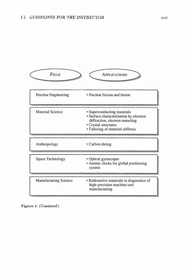
In Figs. 1 and 2 we show an outline of some of the applications we link to the basic principles discussed in this text. As one can see, a number of different fields have benefited from modern physics. The connection between basic principles and applications is a very important one-one that is used by applied scientists as they go about inventing new technologies. I t is important for students of applied physics and engineering to appreciate this connection.
1.1 Guidelines for the Instructor
This book can be used for engineering students as well as for physics majors. For engineering students there are two possible roles of this book, depending on the un- dergraduate curricula a t a particular university. In some schools a modern physics course is offered in the physics department for undergraduate engineering students. This book should be particularly attractive for such a course, since there is a close
xv

XVI
Figure 1: Applied fields and applications discussed in this textbook.
INTRODUCTION
I. 1. GUIDELINES FOR THE INSTRUCTOR
Figure 1: (Continued).
xvii
xviii lNTROD UCTION
connection between basic principles and applications. For such students the instruc- tor should cover the first six chapters and Chapter 9 in some detail and pick selected topics from Chapters 7 and 8. For example, the coupled well problem could be dis- cussed from Chapter 7. A physical discussion of optical processes could be discussed from Chapter 8. Derivations of Fermi golden rule (Appendix A) or Boltzmann trans- port theory (Appendix B) should be avoided for students at this level.
The book would be very useful for students who are seniors or entering grad- uate students in the electrical engineering, material science, or chemical engineering departments. For such students the first couple of chapters could be covered rather quickly (some sections could be given as reading assignments). Topics in Chapters 7 and 8 as well as Appendices A and B could be covered in detail.
Finally, for physics majors the book could be used for a modern physics course. The book covers most topics of relevance to such a course and provides an important link to technical applications. Such a link is normally not provided to physics majors, but given the changes occurring in the physics profession, will most likely be appreciated by them.
The system of units used throughout the text is the SI system-a system that is widely used by technologists. The text contains nearly 100 solved examples, most of which are numerical in nature. It also contains about 200 end-of-chapter problems.
SOME IMPORTANT REFERENCES
Review of Classical Physics
R. Resnick, D. Hafliday, and K. S. Krane, Physics, Wiley, New York, 1992.
0 R. A. Serway, Physics for Scientists and Engineers, Saunders, Philadelphia, 1990.
H . D. Young, University Physics, Addison-Wesley, Reading, MA, 1992.
Quantum Mechanics
0 K. Krane, Modern Physics, Wiley, New York, 1996
P. A. Lindsay, Introduction to Quantum Mechanics for Electrical Engineers, 3rd edition, McGraw-Hill, New York, 1967.
Special Relativity
0 R. Resnick, Introduction to Special Relativity, Wiley, New York, 1996.
0 K. Krane, Modern Physics, Wiley, New York, 1996
0 E. F. Taylor and J . A. Wheeler, Spacetime Physics, Freeman, New York, 1992.

1.1. GUIDELINES FOR THE INSTRTJCTOR xix
General
0 R. P. Feynman, R. B. Leighton and M . Sands, The F e y n m a n Lectures of Physics, Vol. 111, Addison-Wesley Publishing Company, Reading, M A , 1964. This and the accompanying volumes are a musf read.

This Page Intentionally Left Blank
CHAPTER 1
CLASSICAL VIEW OF THE UNIVERSE
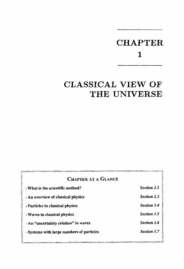
CHAPTER AT A GLANCE
. What is the scientific method?
. An overview of classical physics
Section 1.2
Section 1.3
$ . Particles in classical physics
. Waves in classical physics P
Section 1.4
Section 1.5
? . An “uncertainty relation” in waves Section 1.6
Section 1.7 I . Systems with large numbers of particles

2 CHAPTER 1. CLASSICAL VIEW OF THE UNIVERSE
1.1 INTRODUCTION
The term classical physics sounds old, but it is the term used for the physics in existence until the beginning of the twentieth century. This is the physics that was developed by scientists such as Archimedes, Newton, Maxwell, Boltzmann, . . . and even though the developements due to quantum physics and relativistic physics have ushered in the more accurate modern physics, classical physics continues to be used in a vast array of applications quite successfully.
Classical physics, it turns out, gives us an approximate description of how our world behaves. This approximation is usually adequate for a very large class of problems. However, on some levels, the inaccuracies of classical physics are man- ifested quite dramatically. Modern physics can be classified as a much better ap- proximation and is suitable for cases where classical concepts fail.
In this chapter we will take a quick tour of important classical concepts. I t is important to keep in mind that modern physics reduces to classical physics when certain conditions are met. These conditions may be stated as, “mass of the particle is large,” or “potential energy is slowly varying in space,” etc. Thus i t is important to understand the classical concepts.
We start this chapter with an overview of the approach known as the scien- tific method. This approach must be followed in the understanding and development of any physics related concept. This is the method that has brought physics to the present level-a level where enormously complex physical phenomena are well un- derstood.
1.2 SCIENTIFIC METHOD
Physics is the branch of science that attempts to answer the questions related to the ‘hows’ and ‘whys’ of our physical universe. In this great attempt, some very rigorous paths are t o be taken. There must be a logical flow between one assertion and the next. I t may be fine to explain the twinkling of stars to a child by claiming there are angels lowering and raising their lanterns. But this is not the approach we can follow in physics.
While there are still phenomena we cannot explain by simply invoking our understanding of physics, it is quite remarkable that a great range of observations can now be explained through modern physics. Physics has developed from explain- ing how cannon balls fly and pulleys work to what happens inside a white dwarf star or what happens to protons when they are smashed into each other a t close t o the speed of light.
I t is important t o understand the approach known as the scientific method, which has allowed us to understand our universe so well. This approach has been used by intellectual giants like Galileo, Newton, Maxwell, Einstein, Feynman, etc. It is also an approach used by thousands of basic and applied scientists around the world. The scientific method is used by the electrical engineer when he or she is trying to build a gigabit memory chip. It is used by the biophysicist who is assembling a special molecule t o attack cancer cells. Or by the mechanical engineer developing a more crash-safe car. The scientific method allowed Galileo to do his

1.2. SCIENTIFIC METHOD 3
famous experiment to show that objects with different masses drop to the earth with the same velocity. I t also allowed Copernicus to show that the earth went around the sun. It allowed Newton to describe how gravity worked and Einstein to come up with the theory of relativity. It ushered in the quantum age and the information age based on computers.
Let us examine the components of the scientific process. Fig. 1.1 gives an overview of this approach. Here are the building blocks: 0 Observation: This is the core of the scientific method. Careful measurements of a physical phenomenon set the stage for most scientific endeavors. Sometimes the experiment may be motivated by a theoretical prediction based on existing knowledge. In the scientific method no one can argue against a fundamentally sound experiment. The experiment can never be subverted to fit an existing line of thought. 0 Postulates: The scientific method now starts, with the ultimate aim to explain experiments and to predict phenomena. The method sets up some postulates which seem reasonable to the scientists. These postulates are the starting points from which the theory describing the phenomena springs forth. At the most fundamental level the postulates do not have any proofs, in the sense that they cannot be derived from other laws. 0 Physical Laws: Next, physical laws are set up, which describe how physical quantities evolve from one value to another in space and time. These equations of motion along with the powerful language of mathematics allow the scientist to relate experiments and the scientific formalism. These laws not only should be able to explain existing observations, but also must predict phenomena that can then be observed by properly designed experiments. It is also very important to keep in mind what a good scientific method tries to do: 0 Make assumptions that are absolutely necessary. If we are building a formalism for how an airplane flies we must not assume anything about whether a cockroach evolved 10 million years ago or 100 million years ago! 0 Accept the guidance of experiments. A good scientist should not retain a formalism which explains everything except one lonely experiment. It is this lonely experiment that may ultimately advance our knowledge. 0 Consider our present understanding as an approximation. it is important to realize that when a scientist writes down certain laws or equations of motion, he or she is only describing how the real world behaves in an approximate way. This is because the laws may describe nature quite well in some regimes but may not be able to describe things well in a different regime. And even though we know a great deal of the rules of nature, we don’t know all the rules. And some rules may manifest themselves under conditions that are almost impossible to realize in a controlled manner in a laboratory.
It sometimes happens that a certain set of laws or rules work quite well for a long period in our history. Then something is observed which does not fit into the scheme we have developed. One then looks for a broader set of rules. These new rules must explain all the previous observations, along with the new ones. One of the most dramatic instances of such a development is the subject of this book. Toward the end of the nineteenth century, a series of remarkable experiments were conducted that completely baffled existing physics. This created a tremendous excitement among

4 CHAPTER 1. CLASSICAL V I E W OF T H E UNIVERSE
Figure 1.1: An overview of the scientific method
the physicists who then gradually built what we now call modern physics. Before we start our discussions of modern physics we need to review classical physics, which is the name often given to physics existing up to the beginning of the twentieth century.
1.3 OVERVIEW OF CLASSICAL PHYSICS: BASIC INTERACTIONS
In classical physics our physical universe is distinctly divided into two categories- particles and waves. When we talk about particles, we do not necessarily refer to point particles or very tiny particles. The earth is a particle; so are a car, a refrigerator, and a tennis ball. T h e laws which describe particles and those which describe waves are very different, and we have no problem distinguishing a particle from a wave. In Fig. 1.2 we show an overview of classical concepts. We have particles which are represented by masses, momentum, position, etc., and waves which are described by amplitude, wavelength, phase, etc. We also have an important branch of physics which deals with systems of large numbers of particles. This field is known as thermodynamics.
In classical physics particles interact with each other via two kinds of in- teractions. As shown in Fig. 1.2, the first kind of interaction is the gravitational interaction. If we have two particles of masses ml and m2 placed a t a separation of

1.3. OVERVIEW OF CLASSICAL PHYSICS: BASIC INTERACTIONS 5
Figure 1.2: An overview of the classical concepts that govern our universe.
r , they have an attractive force given by
77211712 - F G-T 7-2
where G is a coefficient with a value 6.67 x lo-" N.m2/kg2. The second form of interaction between particles is the electromagnetic
interaction. A manifestation of this interaction is that if we have two particles with charges q1 and 92 separated by a distance r , there is a force felt by each particle given by (see Fig. 1.3)
where

6 CHAPTER 1. CLASSICAL VIEW OF THE UNIVERSE
Figure 1.3: Coulombic force between two charged particles.
The potential energy of the system is
If a charged particle is moving in an electric field E and a magnetic field B with a velocity v, it sees a force given by (see Fig. 1.4a)
F = q v x B (1.4)
Another manifestation of the electromagnetic interaction is that a magnetic field is produced by an electric current I . The current is just the motion of charged particles. If, for example, the current is flowing in a circular loop as shown in Fig. 1.4b, the magnetic field a t the center is
with po = 47r x Ns2/C2
The direction of the field is given by the right-hand rule, i.e., if you hold the wire in the right hand with the thumb pointing along the current direction, the fingers point in the field direction.
A number of interesting interactions arise from the equations described above. These include the attraction or repulsion between current-carrying wires, torque on a current-carrying wire in a magnetic field, etc. All these disparate looking phenomena were placed into a single coherent picture by James Clark Maxwell. The classical electromagnetic phenomena is described completely by the Maxwell equations.
The properties of electromagnetic fields in a medium are described by the four Maxwell equations. Apart from the electric (E) and magnetic (B) fields and velocity of light, the effects of the material are represented by the dielectric constant, permeability, electrical conductivity, etc. We start with the four Maxwell equations
dB
a D at
V X E + - = 0 at V x H - - = J

1.3. OVERVIEW OF CLASSICAL PHYSICS: BASIC INTERACTIONS 7
Figure 1.4: (a) Force on a charged particle moving with velocity (b) Magnetic field produced by a current.
in a magnetic field.
where E and H are the electric and magnetic fields, D = rE, B = pH, and J and p are the current and charge densities. In electromagnetic theory i t is often convenient to work with the vector and scalar potentials A and 4, respectively, which are defined through the equations
B = V x A
T h e first and fourth Maxwell equations are automatically satisfied by these definitions. T h e potentials A and 4 are not unique but can be replaced by a new set of potentials A' and 4' given by
A ' = A + V x & + - - dX
at
The new choice of potentials does not have any effect, on the physical fields
I t can be shown tha t the equations for the vector and scalar potential have E and B.

8
the form (for p = pa)
CHAPTER 1. CLASSICAL VIEW OF THE UNIVERSE
It is useful to establish the relation between the vector potential A and the optical power. The time-dependent solution for the vector potential solution of Eqn. 1.9 with J = 0 is
A(r , t ) = A0 {exp [i(k . r - w t ) ] + c.c.} (1.10)
with 2 k 2 = €pow
Note that in the MKS units ( < o ~ o ) - ' / ~ is the velocity of light c (3 x lo8 ms-'). The electric and magnetic fields are
a A E = -- at
= 2wAo sin(k. 1: - w t )
= 2k x A0 sin(k . r - w t )
B = V x A
(1.11)
The Poynting vector S representing the optical power is
S = E X H 4
PO (1.12) = -uk2 IAoI2 s in2 (k . r - w t ) k
where u is the velocity of light in the medium (= c/&) and k is a unit vector in the direction of k. Here EI is the relative dielectric constant. The time-averaged value of the power is
= 2 v w 2 lAo12 k (1.13)
since (kl = w / v (1.14)
(1.15)
The electromagnetic spectrum spans a vast array of wavelengths. In Fig. 1.5 we identify the important regimes of this spectrum.