modern algebra lecture notes
TRANSCRIPT
Modern Algebra Lecture NotesDr. Monks - University of Scranton - Fall 2021
Contents
0 Introduction 20.1 Logic . . . . . . . . . . . . . . . . . . . . . . . . . . . . . . . . . . . . . . . . . . . . . . 20.2 Appendix B: Sets, Functions, Numbers . . . . . . . . . . . . . . . . . . . . . . . . . . . 130.3 Appendix D: Equivalence Relations . . . . . . . . . . . . . . . . . . . . . . . . . . . . 160.4 Appendix C: Math Induction . . . . . . . . . . . . . . . . . . . . . . . . . . . . . . . . 18
1 Arithmetic in Z Revisited 191.1 Integers . . . . . . . . . . . . . . . . . . . . . . . . . . . . . . . . . . . . . . . . . . . . . 191.2 Divisibility in Z . . . . . . . . . . . . . . . . . . . . . . . . . . . . . . . . . . . . . . . . 211.3 Primality in Z . . . . . . . . . . . . . . . . . . . . . . . . . . . . . . . . . . . . . . . . . 22
2 Congruence in Z and Modular Arithmetic 242.1 Congruence in Z . . . . . . . . . . . . . . . . . . . . . . . . . . . . . . . . . . . . . . . 242.2 Arithmetic in Zn . . . . . . . . . . . . . . . . . . . . . . . . . . . . . . . . . . . . . . . . 262.3 Algebra in Zn . . . . . . . . . . . . . . . . . . . . . . . . . . . . . . . . . . . . . . . . . 27
3 Rings 283.1 Definition and Examples of Rings . . . . . . . . . . . . . . . . . . . . . . . . . . . . . . 283.2 Algebra in Rings . . . . . . . . . . . . . . . . . . . . . . . . . . . . . . . . . . . . . . . . 333.3 Ring Homomorphisms . . . . . . . . . . . . . . . . . . . . . . . . . . . . . . . . . . . . 35
4 Arithmetic in F[x] 374.1 Polynomials . . . . . . . . . . . . . . . . . . . . . . . . . . . . . . . . . . . . . . . . . . 374.2 Divisibility in F[x] . . . . . . . . . . . . . . . . . . . . . . . . . . . . . . . . . . . . . . . 404.3 Primality (Irreducibilty) in F[x] . . . . . . . . . . . . . . . . . . . . . . . . . . . . . . . 424.4 Polynomial Functions . . . . . . . . . . . . . . . . . . . . . . . . . . . . . . . . . . . . . 45
5 Congruence in F[x] and Congruence Class Arithmetic 465.1 Congruence in F[x] . . . . . . . . . . . . . . . . . . . . . . . . . . . . . . . . . . . . . . 465.2 Arithmetic in F[x]p . . . . . . . . . . . . . . . . . . . . . . . . . . . . . . . . . . . . . . 485.3 Finite fields . . . . . . . . . . . . . . . . . . . . . . . . . . . . . . . . . . . . . . . . . . . 49
6 Ideals and Quotient Rings 506.1 Congruence in Rings . . . . . . . . . . . . . . . . . . . . . . . . . . . . . . . . . . . . . 506.2 Arithmetic in R/I . . . . . . . . . . . . . . . . . . . . . . . . . . . . . . . . . . . . . . . 51
7 Groups 537.1 Groups . . . . . . . . . . . . . . . . . . . . . . . . . . . . . . . . . . . . . . . . . . . . . 537.2 Properties of Groups . . . . . . . . . . . . . . . . . . . . . . . . . . . . . . . . . . . . . 567.3 SubGroups . . . . . . . . . . . . . . . . . . . . . . . . . . . . . . . . . . . . . . . . . . . 58
c© 2021 KEN MONKS PAGE 1 of 71
Modern Algebra Lecture Notes
7.4 Group Homomorphisms . . . . . . . . . . . . . . . . . . . . . . . . . . . . . . . . . . . 607.5 (Section 8.1) Congruence and Lagrange’s Theorem . . . . . . . . . . . . . . . . . . . . 617.6 (Section 7.5) Symmetric and Alternating Groups . . . . . . . . . . . . . . . . . . . . . 63
8 Appendix: Some Useful Proof Recipes 64
0 Introduction
This is not a complete set of lecture notes for Math 448, Modern Algebra I. Additional material willbe covered in class and discussed in the textbook. These notes are currently under developmentas a port from a previous version, so typos and formatting errors are inevitable. Check backfrequently for updates.
0.1 Logic
In this section, we give an informal overview of logic and proofs. For a more formal introductionsee any logic textbook.
Proofs and Formal Axiom Systems
Definition. A Formal Proof System (or Formal Axiom System) consists of
1. A set of expressions S, called the statements.2. A set of rules R, called the rules of inference.
Each rule of inference has zero or more inputs called premises and one or more outputs calledconclusions. Most premises and all conclusions of a rule of inference are statements in the system.1
There also may be conditions on when a particular rule of inference can be used.
Definition. An axiom is a conclusion of a rule of inference that has no premises.
Definition. A statement Q in a formal axiom system is provable from premises P1, . . . ,Pn if
1. Q is one of the premises P1, . . . ,Pn, or
2. Q is a conclusion of a rule of inference whose premises are provable from P1, . . . ,Pn.
In particular, if Q is an axiom, then Q is provable from no premises at all!
Definition. If Q follows from no premises in a formal axiom system, we say that Q is provable inthe system. A provable statement is called a theorem.
And finally, the definition we’ve all been waiting for!
Definition. A proof of a statement in a formal axiom system is a finite sequence of applications ofthe rules of inference (i.e., inferences) that show that the statement is a theorem in that system.
1Other common premises are variable declarations, constant declarations, and subproofs.
c© 2021 KEN MONKS PAGE 2 of 71
Modern Algebra Lecture Notes
Notation. If Q is provable from premises P1, . . . ,Pn in a formal system we can denote this symbol-ically as
P1, . . . ,Pn ` Q
It is also commonplace to refer to such an expression as a theorem. To prove such a theorem is togive a proof of Q in the same formal system where additionally the premises are ‘Given’ as axioms.
Variables, Expressions, and Statements in Mathematics
Term Description
set A set is a collection of items.
element The items in a set are called its elements (or members).
expression An expression is an arrangement of symbols which represents an element of aset
type The set of elements that an expression can represent is called the type of theexpression.
value The element of the domain that the expression represents is called a value ofthat expression.
variable A variable is an expression consisting of a single symbol
constant A constant is an expression whose domain contains a single element.
statement A statement (or Boolean expression) is an expression whose domain is{ true, false}.
truth value The value of a statement is called its truth value.
solve To solve a statement is to determine the set of all elements for which thestatement is true.
solution set The set of all solutions of a statement is called the solution set.
equation An equation is a statement of the form A = B where A and B are expressions.
inequality An inequality is a statement of the form A ⋆ B where A and B are expressionsand ⋆ is one of ≤, ≥, >, <, or ,.
Remarks:
• An element is either in a set or it is not in a set, it cannot be in a set more than once.
• It is not necessary that we know specifically which element of the domain an expressionrepresents, only that it represents some unspecified element in that set.
• We do not have to know if a statement is true or false, just that it is either true or false.
• If a statement contains n variables, x1, . . . xn, then to solve the statement is to find the set ofall n-tuples (a1, . . . , an) such that each ai is an element of the domain of xi and the statementbecomes true when x1, . . . , xn are replaced by a1, . . . , an respectively. In this situation, eachsuch n-tuple is called a solution of the statement.
• In formal mathematics, ‘true’ means ‘provable’.
c© 2021 KEN MONKS PAGE 3 of 71
Modern Algebra Lecture Notes
Substitution and Lambda Expressions
Definition. We can prefix an expression E to form the expression “λx,E” (or “x 7→E”) to indicatethat all occurrences2 of x in E are a variable that represents the same unspecified object of the sametype as x. These prefixed expressions are called lambda expressions (or anonymous functions).
Definition. Lambda expressions can be applied to an expression a having the same type as x toform a new expression, (λx,E)(a) which has the same type as E. These can be further simplified tothe expression obtained by replacing all occurrences3 of x in E with a.
Remark. If we give a name to a lambda expression, e.g., define f to be λx,E then the expression(λx,E)(a) is just the usual notation for function application f (a).4
Definition. Two lambda expressions are said to be equivalent if they simplify to the same orequivalent things when applied to any argument.
Remark. Renaming all occurrences of x in λx,E with a new identifier always produces a lambdaexpression that is equivalent to the original. Another common situation where we can simplify alambda expression λx,E is when the expression E does not contain x. In this situation (λx,E)(a)simplifies to just E for every a, and thus we can say that λx,E simplifies to just E in that case.
Rules of Inference in Mathematics
Most rules of inference in mathematics are stated as assertions that something can be proven inthe given system. Frequently these are given as lambda expressions. Such a lambda expressiongenerate an entire family of specific rules of inference, one for each application of the expression.Because this is so common, we usually omit the lambda prefixes, and use the convention that anyfree variables that appear free in the premises or conclusion of a rule of inference can be replacedwith an expression of the same type to form a particular instance of that rule of inference.
2These refer to free occurrences - see below.3See footnote 2. Also no free identifier in a should become bound as a result of the substitution.4Indeed, in precalculus they usually write f (x) = x3 instead of writing f = (λx, x3), but the latter is usually what they
mean.
c© 2021 KEN MONKS PAGE 4 of 71

Modern Algebra Lecture Notes
Template Notation for Rules of Inference
Notation. A rule of inference having premises P1, . . . ,Pk and conclusions Q1, . . . ,Qn can be ex-pressed in template notation or recipe notation as
Rule Name Here
P1 (show)...
Pk (show). . . . . . . . . . . . . . . . . . . . . . . . . . . . . . . . . . .Q1 (conclude)...
Qn (conclude)
In this notation, the rule looks like a template that we can fill in to create our proofs. In particular,the lines marked with a (show) need to be justified with a rule of inference that is supplied asa reason for that line, and those marked with (conclude) can be justified with the given rule ofinference.
Some rules of inference have a premise of the form
(P1, . . . ,Pk ` Q)
This is not a statement in the formal system itself, but rather the assertion that Q can be provenfrom P1, . . . ,Pk in the formal system. We call an expression of this form a subproof or environment.Such a premise is satisfied by including a subproof in a proof that shows that Q can be provedfrom the given premises (which do not need to be justified by a rule of inference). We denote thisin recipe notation as an indented ‘assume-block’ as illustrated below.
Example 1. Suppose we have a rule of inference that justifies the following.
φ or ψ, (φ ` ρ), (ψ ` ρ) ` ρ
where φ, ψ, and ρ are any mathematical statements. Then we would express this rule in recipenotation as
Proof by Cases
φ or ψ (show)Assume φρ (show)←Assume ψρ (show)←
. . . . . . . . . . . . . . . . . . . . . . . . . . . . . . . . . . .ρ (conclude)
c© 2021 KEN MONKS PAGE 5 of 71
Modern Algebra Lecture Notes
In this, everything between an Assume and the following ← (the ‘end assumption’ symbol) is asubproof that demonstrates the corresponding premise in the rule of inference. We indent suchassumption blocks in our proofs. Subproofs can be nested, and the level of indentation correspondsto the level of nesting. Assumptions (lines that start with Assume) do not need to be justified bya rule of inference. We say that they are given. Lines marked with (show) must be justified. Linesmarked with (conclude) are justified by the rule itself.
Note that we do include the word "Assume " in the proof itself, but not the words "show" or"conclude" which are just instructions to the proof author (as opposed to the reader) for how tojustify the indicated lines.
Natural Deduction
We now turn our attention to a formal axiom system that is based on one first formulated byGerhard Gentzen in 1934 as a formal system that closely imitates the way mathematicians actuallyreason when writing traditional expository proofs.
Propositional Logic
The Statements of Propositional Logic
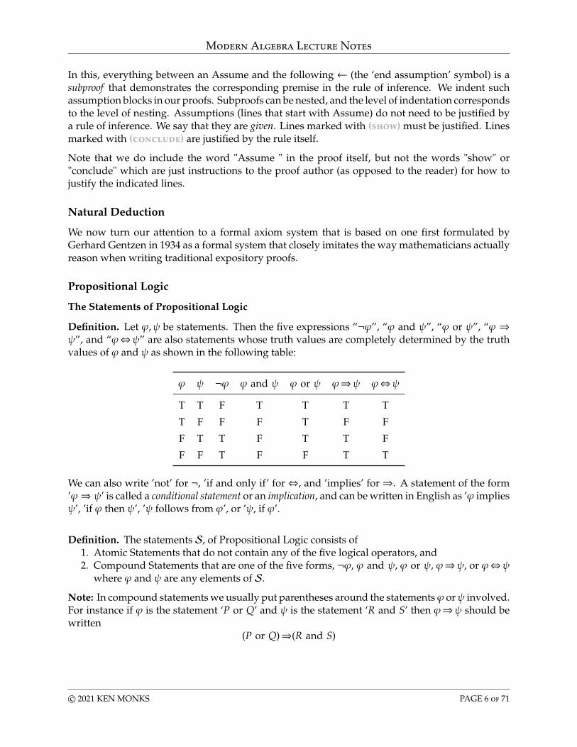
Definition. Let φ,ψ be statements. Then the five expressions “¬φ”, “φ and ψ”, “φ or ψ”, “φ ⇒ψ”, and “φ⇔ψ” are also statements whose truth values are completely determined by the truthvalues of φ and ψ as shown in the following table:
φ ψ ¬φ φ and ψ φ or ψ φ⇒ψ φ⇔ψ
T T F T T T T
T F F F T F F
F T T F T T F
F F T F F T T
We can also write ’not’ for ¬, ’if and only if’ for⇔, and ’implies’ for⇒. A statement of the form’φ⇒ ψ’ is called a conditional statement or an implication, and can be written in English as ’φ impliesψ’, ’if φ then ψ’, ’ψ follows from φ’, or ’ψ, if φ’.
Definition. The statements S, of Propositional Logic consists of1. Atomic Statements that do not contain any of the five logical operators, and2. Compound Statements that are one of the five forms, ¬φ, φ and ψ, φ or ψ, φ⇒ψ, or φ⇔ψ
where φ and ψ are any elements of S.
Note: In compound statements we usually put parentheses around the statementsφ orψ involved.For instance if φ is the statement ‘P or Q’ and ψ is the statement ‘R and S’ then φ⇒ψ should bewritten
(P or Q)⇒(R and S)
c© 2021 KEN MONKS PAGE 6 of 71
Modern Algebra Lecture Notes
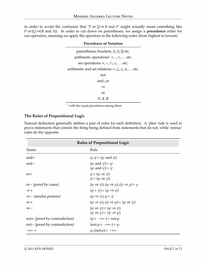
in order to avoid the confusion that ‘P or Q⇒R and S’ might actually mean something likeP or (Q⇒(R and S)). In order to cut down on parentheses, we assign a precedence order forour operators, meaning we apply the operators in the following order (from highest to lowest).
Precedence of Notation
parentheses, brackets, (), {}, [] etc.
arithmetic operations∗ ∧, ·,+, . . . etc.
set operations ×,−,∩,∪, . . . etc.
arithmetic and set relations =,⊆,≤,,, . . . etc.
not
and , or
⇒⇔∀,∃,∃!
∗ with the usual precedence among them
The Rules of Propositional Logic
Natural deduction generially defines a pair of rules for each definition. A ’plus’ rule is used toprove statements that contain the thing being defined from statements that do not, while ’minus’rules do the opposite.
Rules of Propositional Logic
Name Rule
and+ φ,ψ ` (φ and ψ)
and− (φ and ψ) ` φ(φ and ψ) ` ψ
or+ φ ` (φ or ψ)ψ ` (φ or ψ)
or− (proof by cases) (φ or ψ), (φ⇒ ρ), (ψ⇒ ρ) ` ρ⇒+ (φ ` ψ) ` (φ⇒ ψ)
⇒− (modus ponens) (φ⇒ ψ), φ ` ψ⇔+ (φ⇒ ψ), (ψ⇒ φ) ` (φ⇔ ψ)
⇔− (φ⇔ ψ) ` (φ⇒ ψ)(φ⇔ ψ) ` (ψ⇒ φ)
not+ (proof by contradiction) (φ ` →←) ` notφ
not− (proof by contradiction) (notφ ` →←) ` φ→←+ φ, (notφ) ` →←
c© 2021 KEN MONKS PAGE 7 of 71
Modern Algebra Lecture Notes
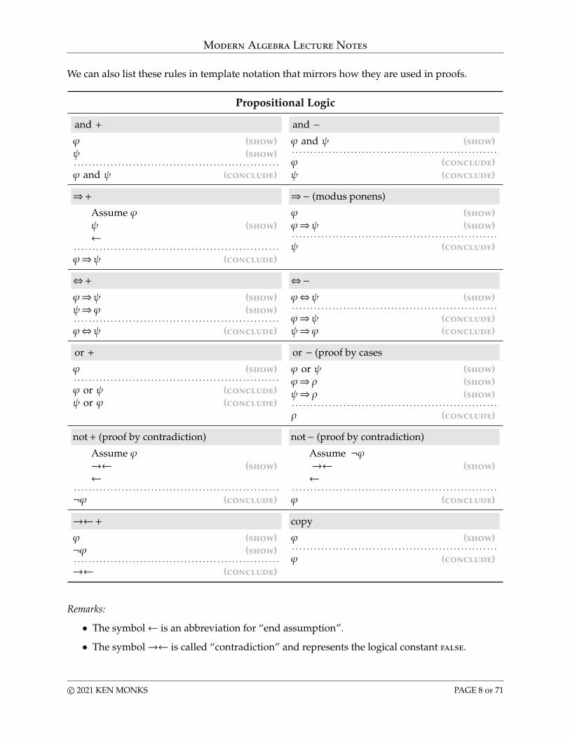
We can also list these rules in template notation that mirrors how they are used in proofs.
Propositional Logic
and + and −φ (show)ψ (show). . . . . . . . . . . . . . . . . . . . . . . . . . . . . . . . . . . . . . . . . . . . . . . . . . . . . . . .φ and ψ (conclude)
φ and ψ (show). . . . . . . . . . . . . . . . . . . . . . . . . . . . . . . . . . . . . . . . . . . . . . . . . . . . . . . .φ (conclude)ψ (conclude)
⇒+ ⇒− (modus ponens)
Assume φψ (show)←
. . . . . . . . . . . . . . . . . . . . . . . . . . . . . . . . . . . . . . . . . . . . . . . . . . . . . . . .φ⇒ψ (conclude)
φ (show)φ⇒ψ (show). . . . . . . . . . . . . . . . . . . . . . . . . . . . . . . . . . . . . . . . . . . . . . . . . . . . . . . .ψ (conclude)
⇔+ ⇔−φ⇒ψ (show)ψ⇒φ (show). . . . . . . . . . . . . . . . . . . . . . . . . . . . . . . . . . . . . . . . . . . . . . . . . . . . . . . .φ⇔ψ (conclude)
φ⇔ψ (show). . . . . . . . . . . . . . . . . . . . . . . . . . . . . . . . . . . . . . . . . . . . . . . . . . . . . . . .φ⇒ψ (conclude)ψ⇒φ (conclude)
or + or − (proof by cases
φ (show). . . . . . . . . . . . . . . . . . . . . . . . . . . . . . . . . . . . . . . . . . . . . . . . . . . . . . . .φ or ψ (conclude)ψ or φ (conclude)
φ or ψ (show)φ⇒ρ (show)ψ⇒ρ (show). . . . . . . . . . . . . . . . . . . . . . . . . . . . . . . . . . . . . . . . . . . . . . . . . . . . . . . .ρ (conclude)
not+ (proof by contradiction) not− (proof by contradiction)
Assume φ→← (show)←
. . . . . . . . . . . . . . . . . . . . . . . . . . . . . . . . . . . . . . . . . . . . . . . . . . . . . . . .¬φ (conclude)
Assume ¬φ→← (show)←
. . . . . . . . . . . . . . . . . . . . . . . . . . . . . . . . . . . . . . . . . . . . . . . . . . . . . . . .φ (conclude)
→←+ copy
φ (show)¬φ (show). . . . . . . . . . . . . . . . . . . . . . . . . . . . . . . . . . . . . . . . . . . . . . . . . . . . . . . .→← (conclude)
φ (show). . . . . . . . . . . . . . . . . . . . . . . . . . . . . . . . . . . . . . . . . . . . . . . . . . . . . . . .φ (conclude)
Remarks:
• The symbol← is an abbreviation for “end assumption”.
• The symbol→← is called “contradiction” and represents the logical constant false.
c© 2021 KEN MONKS PAGE 8 of 71
Modern Algebra Lecture Notes
• The word Assume is actually entered as part of the proof itself, it is not just an instruction inthe recipe like ’(show)’ and ’(conclude)’.
• The inputsAssume- and “←” are not themselves statements that you prove or are given, butrather are inputs to rules of inference that may be inserted into a proof at any time. There isno useful reason however, to insert such statements unless you intend to use one of the rulesof inference that requires them as an input.
• The statement following an Assume is the same as any other statement in the proof and canbe used as an input to a rule of inference.
• Statements in an Assume-← block can be used as inputs to rules of inference whose conclu-sion is also inside the same block only. Once a Assume is closed with a matching←, only theentire block can be used as an input to a rule of inference. The individual statements withina block are no longer valid outside the block. We usually indent and Assume-← block tokeep track of what statements are valid under which assumptions.
Definition. A compound statement of propositional logic is called a tautology if it is true regardlessof the truth values the atomic statements that comprise it. (Its "truth table" contains only T’s.)
It can be shown that a statement can be proved with Propositional Logic if and only if the statementis a tautology.
Formal Proof Style
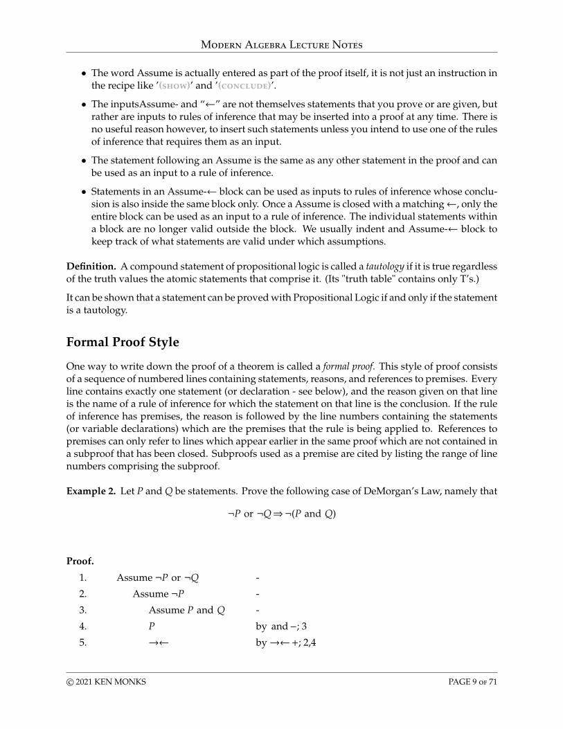
One way to write down the proof of a theorem is called a formal proof. This style of proof consistsof a sequence of numbered lines containing statements, reasons, and references to premises. Everyline contains exactly one statement (or declaration - see below), and the reason given on that lineis the name of a rule of inference for which the statement on that line is the conclusion. If the ruleof inference has premises, the reason is followed by the line numbers containing the statements(or variable declarations) which are the premises that the rule is being applied to. References topremises can only refer to lines which appear earlier in the same proof which are not contained ina subproof that has been closed. Subproofs used as a premise are cited by listing the range of linenumbers comprising the subproof.
Example 2. Let P and Q be statements. Prove the following case of DeMorgan’s Law, namely that
¬P or ¬Q⇒¬(P and Q)
Proof.
1. Assume ¬P or ¬Q -
2. Assume ¬P -
3. Assume P and Q -
4. P by and−; 3
5. →← by→←+; 2,4
c© 2021 KEN MONKS PAGE 9 of 71
Modern Algebra Lecture Notes
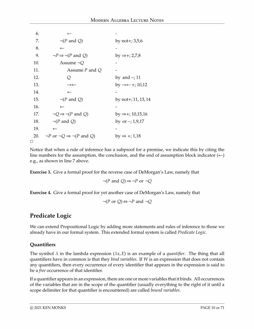
6. ← -
7. ¬(P and Q) by not+; 3,5,6
8. ← -
9. ¬P⇒¬(P and Q) by⇒+; 2,7,8
10. Assume ¬Q -
11. Assume P and Q -
12. Q by and−; 11
13. →← by→←+; 10,12
14. ← -
15. ¬(P and Q) by not+; 11, 13, 14
16. ← -
17. ¬Q⇒¬(P and Q) by⇒+; 10,15,16
18. ¬(P and Q) by or−; 1,9,17
19. ← -
20. ¬P or ¬Q⇒ ¬(P and Q) by⇒ +; 1,182Notice that when a rule of inference has a subproof for a premise, we indicate this by citing theline numbers for the assumption, the conclusion, and the end of assumption block indicator (←)e.g., as shown in line 7 above.
Exercise 3. Give a formal proof for the reverse case of DeMorgan’s Law, namely that
¬(P and Q)⇒¬P or ¬Q
Exercise 4. Give a formal proof for yet another case of DeMorgan’s Law, namely that
¬(P or Q)⇔¬P and ¬Q
Predicate Logic
We can extend Propositional Logic by adding more statements and rules of inference to those wealready have in our formal system. This extended formal system is called Predicate Logic.
Quantifiers
The symbol λ in the lambda expression (λx,E) is an example of a quantifier. The thing that allquantifiers have in common is that they bind variables. If W is an expression that does not containany quantifiers, then every occurrence of every identifier that appears in the expression is said tobe a free occurrence of that identifier.
If a quantifier appears in an expression, there are one or more variables that it binds. All occurrencesof the variables that are in the scope of the quantifier (usually everything to the right of it until ascope delimiter for that quantifier is encountered) are called bound variables.
c© 2021 KEN MONKS PAGE 10 of 71
Modern Algebra Lecture Notes
Predicate logic extends propositional logic by defining two additional quantifiers.
Definition. The symbols ∀ and ∃ are quantifiers. The symbol ∀ is called “for all”, “for every”, or“for each”. The symbol ∃ is called “for some” or “there exists”.
We will encounter more quantifiers beyond just these two and λ.
Statements
Every statement of Propositional Logic is still a statement of Predicate Logic. In addition we definethe following statements.
Definition. If x is any variable and W is a lambda expression5 that simplifies to a statement whenapplied to any expression having the same type as x, then (∀x,W(x)) and (∃x,W(x)) are bothstatements.
We say that the scope of the quantifier in (∀x,W(x)) and (∃x,W(x)) is everything inside the outerparentheses. Sometimes these parentheses are omitted when the scope is clear from context. Alloccurrences if x throughout the scope are said to be bound by the quantifier.
Variable declaration
Before using a free identifier for the first time in any expression in our proofs we should tell thereader what that identifier represents. There are four ways to introduce a new free identifier.
1. It can be declared to be a variable (a variable declaration).
2. It can be declared to be a constant (a constant declaration).
3. It can be defined as temporary new notation, usually as an abbreviation for a larger expression(a notational definition).
4. It can occur free in an expression preceding the proof itself, such as in the statement of thetheorem, in a premise that is given, or declared globally prior to the start of the proof (globallydeclared).
Bound variables do not have to be declared. They can be any identifier you like, as long as thatidentifier is not in the scope of more than one quantifier that binds it.
Rules of Inference
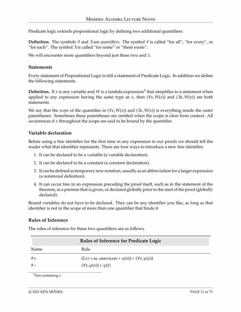
The rules of inference for these two quantifiers are as follows.
Rules of Inference for Predicate Logic
Name Rule
∀+ (Let s be arbitrary ` φ(s)
) ` (∀x, φ(x))
∀− (∀x, φ(x)) ` φ(t)
5Not containing x.
c© 2021 KEN MONKS PAGE 11 of 71
Modern Algebra Lecture Notes
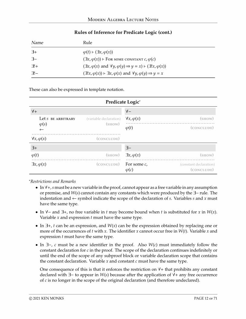
Rules of Inference for Predicate Logic (cont.)
Name Rule
∃+ φ(t) ` (∃x, φ(x))
∃− (∃x, φ(x)) ` For some constant c, φ(c)
∃!+ (∃x, φ(x) and ∀y, φ(y)⇒ y = x) ` (∃!x, φ(x))
∃!− (∃!x, φ(x)) ` ∃x, φ(x) and ∀y, φ(y)⇒ y = x
These can also be expressed in template notation.
Predicate Logic∗
∀+ ∀−Let s be arbitrary (variable declaration)φ(s) (show)←
. . . . . . . . . . . . . . . . . . . . . . . . . . . . . . . . . . . . . . . . . . . . . . . . . . . . . . . .∀x, φ(x) (conclude)
∀x, φ(x) (show). . . . . . . . . . . . . . . . . . . . . . . . . . . . . . . . . . . . . . . . . . . . . . . . . . . . . . . .φ(t) (conclude)
∃+ ∃−φ(t) (show). . . . . . . . . . . . . . . . . . . . . . . . . . . . . . . . . . . . . . . . . . . . . . . . . . . . . . . .∃x, φ(x) (conclude)
∃x, φ(x) (show). . . . . . . . . . . . . . . . . . . . . . . . . . . . . . . . . . . . . . . . . . . . . . . . . . . . . . . .For some c, (constant declaration)φ(c) (conclude)
∗Restrictions and Remarks• In∀+, s must be a new variable in the proof, cannot appear as a free variable in any assumption
or premise, and W(s) cannot contain any constants which were produced by the ∃− rule. Theindentation and← symbol indicate the scope of the declaration of s. Variables s and x musthave the same type.
• In ∀− and ∃+, no free variable in t may become bound when t is substituted for x in W(x).Variable x and expression t must have the same type.
• In ∃+, t can be an expression, and W(x) can be the expression obtained by replacing one ormore of the occurrences of t with x. The identifier x cannot occur free in W(t). Variable x andexpression t must have the same type.
• In ∃−, c must be a new identifier in the proof. Also W(c) must immediately follow theconstant declaration for c in the proof. The scope of the declaration continues indefinitely oruntil the end of the scope of any subproof block or variable declaration scope that containsthe constant declaration. Variable x and constant c must have the same type.
One consequence of this is that it enforces the restriction on ∀+ that prohibits any constantdeclared with ∃− to appear in W(s) because after the application of ∀+ any free occurrenceof c is no longer in the scope of the original declaration (and therefore undeclared).
c© 2021 KEN MONKS PAGE 12 of 71
Modern Algebra Lecture Notes
Equality
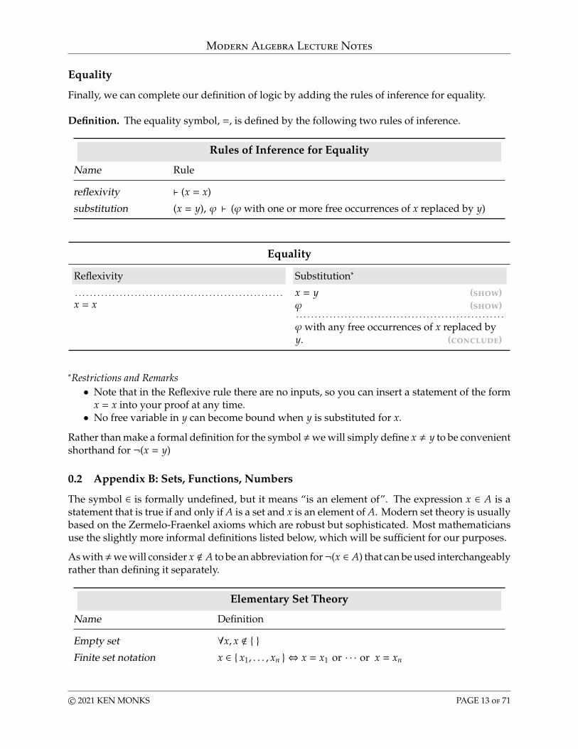
Finally, we can complete our definition of logic by adding the rules of inference for equality.
Definition. The equality symbol, =, is defined by the following two rules of inference.
Rules of Inference for Equality
Name Rule
reflexivity ` (x = x)
substitution (x = y), φ ` (φ with one or more free occurrences of x replaced by y)
Equality
Reflexivity Substitution∗
. . . . . . . . . . . . . . . . . . . . . . . . . . . . . . . . . . . . . . . . . . . . . . . . . . . . . . . .x = x
x = y (show)φ (show). . . . . . . . . . . . . . . . . . . . . . . . . . . . . . . . . . . . . . . . . . . . . . . . . . . . . . . .φ with any free occurrences of x replaced byy. (conclude)
∗Restrictions and Remarks• Note that in the Reflexive rule there are no inputs, so you can insert a statement of the form
x = x into your proof at any time.• No free variable in y can become bound when y is substituted for x.
Rather than make a formal definition for the symbol,we will simply define x , y to be convenientshorthand for ¬(x = y)
0.2 Appendix B: Sets, Functions, Numbers
The symbol ∈ is formally undefined, but it means “is an element of”. The expression x ∈ A is astatement that is true if and only if A is a set and x is an element of A. Modern set theory is usuallybased on the Zermelo-Fraenkel axioms which are robust but sophisticated. Most mathematiciansuse the slightly more informal definitions listed below, which will be sufficient for our purposes.
As with,we will consider x < A to be an abbreviation for¬(x ∈ A) that can be used interchangeablyrather than defining it separately.
Elementary Set Theory
Name Definition
Empty set ∀x, x < { }Finite set notation x ∈ { x1, . . . , xn } ⇔ x = x1 or · · · or x = xn
c© 2021 KEN MONKS PAGE 13 of 71
Modern Algebra Lecture Notes
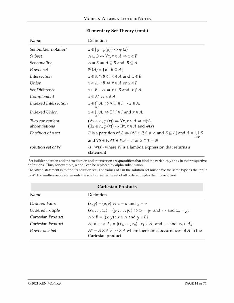
Elementary Set Theory (cont.)
Name Definition
Set builder notation∗ x ∈ { y : φ(y)}⇔ φ (x)
Subset A ⊆ B⇔ ∀x, x ∈ A⇒ x ∈ B
Set equality A = B⇔ A ⊆ B and B ⊆ A
Power set P (A) = {B : B ⊆ A }Intersection x ∈ A ∩ B⇔ x ∈ A and x ∈ B
Union x ∈ A ∪ B⇔ x ∈ A or x ∈ B
Set Difference x ∈ B − A⇔ x ∈ B and x < A
Complement x ∈ A′ ⇔ x < A
Indexed Intersection x ∈ ⋂i∈I
Ai ⇔ ∀i, i ∈ I⇒ x ∈ Ai
Indexed Union x ∈ ⋃i∈I
Ai ⇔ ∃i, i ∈ I and x ∈ Ai
Two convenientabbreviations
(∀x ∈ A, φ (x))⇔ ∀x, x ∈ A⇒ φ(x)(∃x ∈ A, φ (x))⇔ ∃x, x ∈ A and φ(x)
Partition of a set P is a partition of A⇔ (∀S ∈ P,S , ∅ and S ⊆ A) and A =⋃
S∈PS
and ∀S ∈ P,∀T ∈ P,S = T or S ∩ T = ∅
solution set of W {s : W(s)}where W is a lambda expression that returns astatement
∗Set builder notation and indexed union and intersection are quantifiers that bind the variables y and i in their respectivedefinitions. Thus, for example, y and i can be replaced by alpha substitution.∗∗To solve a statement is to find its solution set. The values of s in the solution set must have the same type as the inputto W. For multivariable statements the solution set is the set of all ordered tuples that make it true.
Cartesian Products
Name Definition
Ordered Pairs(x, y)= (u, v)⇔ x = u and y = v
Ordered n-tuple (x1, . . . , xn) =(y1, . . . , yn
)⇔ x1 = y1 and · · · and xn = yn
Cartesian Product A × B ={(
x, y)
: x ∈ A and y ∈ B}
Cartesian Product A1 × · · · × An = {(x1, . . . , xn) : x1 ∈ A1 and · · · and xn ∈ An}Power of a Set An = A × A × · · · × A where there are n occurrences of A in the
Cartesian product
c© 2021 KEN MONKS PAGE 14 of 71
Modern Algebra Lecture Notes
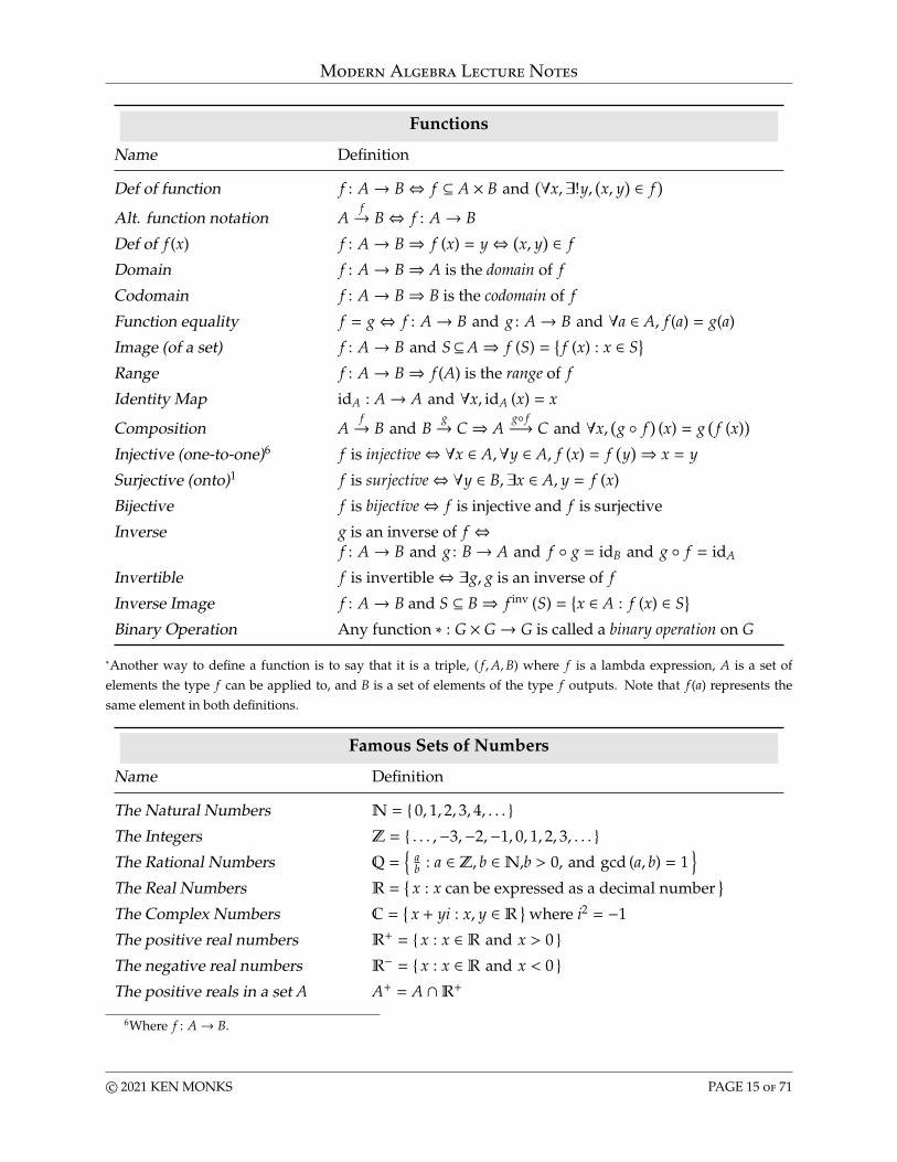
Functions
Name Definition
Def of function f : A→ B⇔ f ⊆ A × B and(∀x,∃!y,
(x, y) ∈ f
)Alt. function notation A
f→ B⇔ f : A→ B
Def of f (x) f : A→ B⇒ f (x) = y⇔ (x, y) ∈ f
Domain f : A→ B⇒ A is the domain of f
Codomain f : A→ B⇒ B is the codomain of f
Function equality f = g⇔ f : A→ B and g : A→ B and ∀a ∈ A, f (a) = g(a)
Image (of a set) f : A→ B and S⊆A⇒ f (S) ={f (x) : x ∈ S
}Range f : A→ B⇒ f (A) is the range of f
Identity Map idA : A→ A and ∀x, idA (x) = x
Composition Af→ B and B
g→ C⇒ Ag◦ f−→ C and ∀x,
(g ◦ f
)(x) = g
(f (x))
Injective (one-to-one)6 f is injective⇔ ∀x ∈ A,∀y ∈ A, f (x) = f(y)⇒ x = y
Surjective (onto)1 f is surjective⇔ ∀y ∈ B,∃x ∈ A, y = f (x)
Bijective f is bijective⇔ f is injective and f is surjective
Inverse g is an inverse of f ⇔f : A→ B and g : B→ A and f ◦ g = idB and g ◦ f = idA
Invertible f is invertible⇔ ∃g, g is an inverse of f
Inverse Image f : A→ B and S ⊆ B⇒ f inv (S) ={x ∈ A : f (x) ∈ S
}Binary Operation Any function ∗ : G × G→ G is called a binary operation on G
∗Another way to define a function is to say that it is a triple, ( f ,A,B) where f is a lambda expression, A is a set ofelements the type f can be applied to, and B is a set of elements of the type f outputs. Note that f (a) represents thesame element in both definitions.
Famous Sets of Numbers
Name Definition
The Natural Numbers N = { 0, 1, 2, 3, 4, . . . }The Integers Z = { . . . ,−3,−2,−1, 0, 1, 2, 3, . . . }The Rational Numbers Q =
{ab : a ∈ Z, b ∈N,b > 0, and gcd (a, b) = 1
}The Real Numbers R =
{x : x can be expressed as a decimal number
}The Complex Numbers C =
{x + yi : x, y ∈ R }where i2 = −1
The positive real numbers R+ = { x : x ∈ R and x > 0 }The negative real numbers R− = { x : x ∈ R and x < 0 }The positive reals in a set A A+ = A ∩R+
6Where f : A→ B.
c© 2021 KEN MONKS PAGE 15 of 71
Modern Algebra Lecture Notes
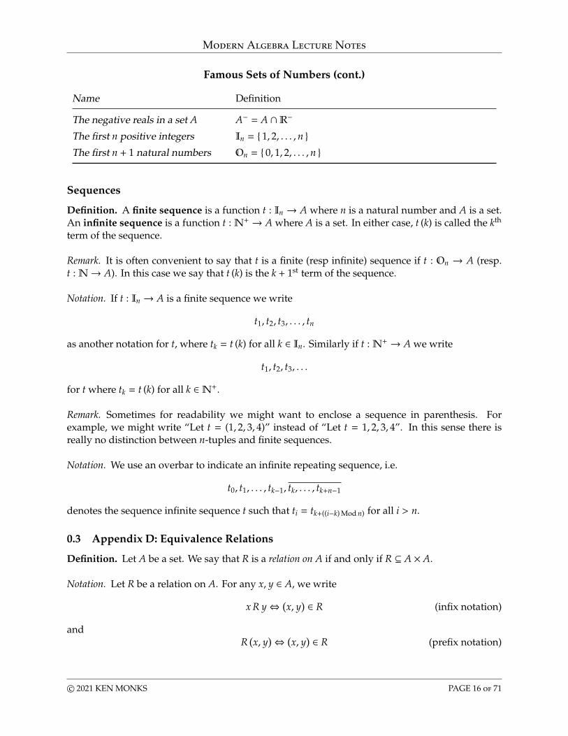
Famous Sets of Numbers (cont.)
Name Definition
The negative reals in a set A A− = A ∩R−
The first n positive integers In = { 1, 2, . . . , n }The first n + 1 natural numbers On = { 0, 1, 2, . . . , n }
Sequences
Definition. A finite sequence is a function t : In → A where n is a natural number and A is a set.An infinite sequence is a function t :N+ → A where A is a set. In either case, t (k) is called the kth
term of the sequence.
Remark. It is often convenient to say that t is a finite (resp infinite) sequence if t : On → A (resp.t :N→ A). In this case we say that t (k) is the k + 1st term of the sequence.
Notation. If t : In → A is a finite sequence we write
t1, t2, t3, . . . , tn
as another notation for t, where tk = t (k) for all k ∈ In. Similarly if t :N+ → A we write
t1, t2, t3, . . .
for t where tk = t (k) for all k ∈N+.
Remark. Sometimes for readability we might want to enclose a sequence in parenthesis. Forexample, we might write “Let t = (1, 2, 3, 4)” instead of “Let t = 1, 2, 3, 4”. In this sense there isreally no distinction between n-tuples and finite sequences.
Notation. We use an overbar to indicate an infinite repeating sequence, i.e.
t0, t1, . . . , tk−1, tk, . . . , tk+n−1
denotes the sequence infinite sequence t such that ti = tk+((i−k) Mod n) for all i > n.
0.3 Appendix D: Equivalence Relations
Definition. Let A be a set. We say that R is a relation on A if and only if R ⊆ A × A.
Notation. Let R be a relation on A. For any x, y ∈ A, we write
x R y⇔ (x, y) ∈ R (infix notation)
andR(x, y)⇔ (x, y) ∈ R (prefix notation)
c© 2021 KEN MONKS PAGE 16 of 71
Modern Algebra Lecture Notes
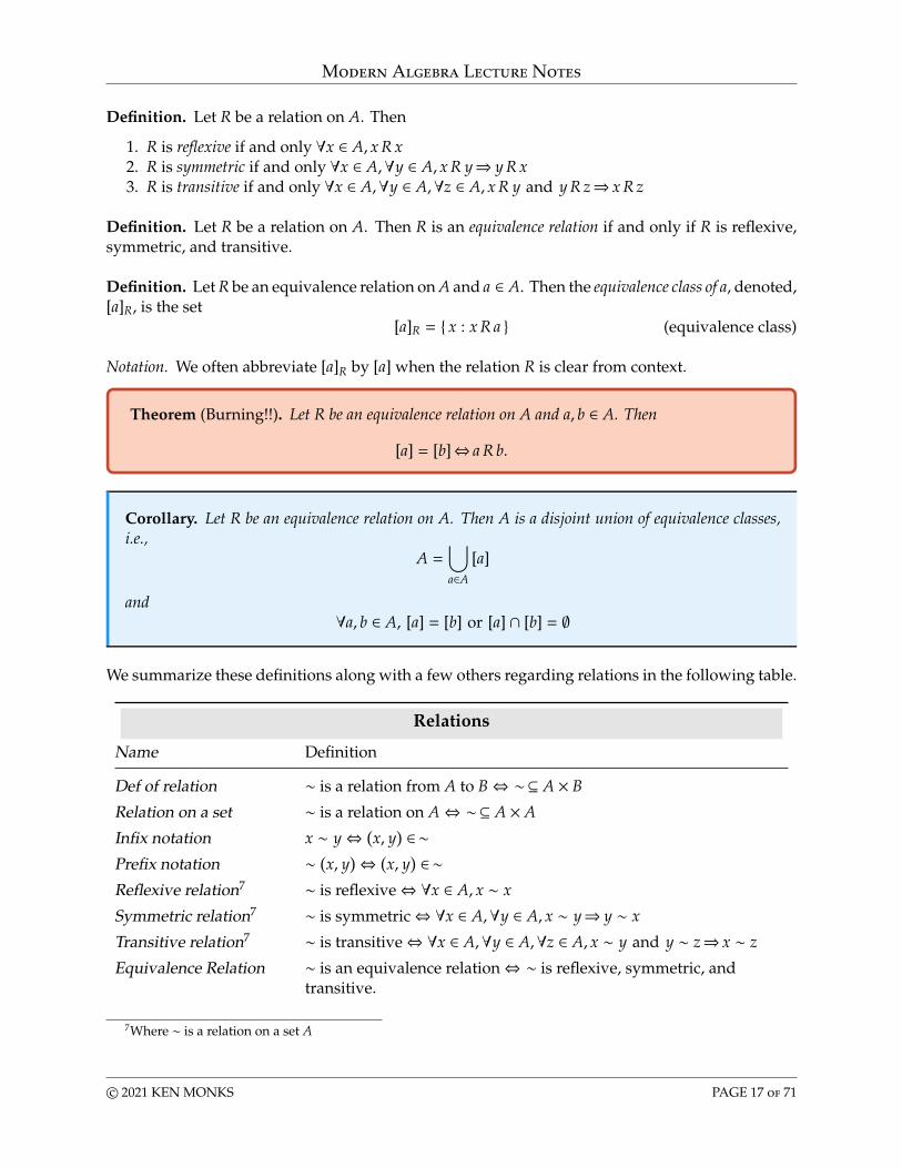
Definition. Let R be a relation on A. Then
1. R is reflexive if and only ∀x ∈ A, x R x2. R is symmetric if and only ∀x ∈ A,∀y ∈ A, x R y⇒ y R x3. R is transitive if and only ∀x ∈ A,∀y ∈ A,∀z ∈ A, x R y and y R z⇒ x R z
Definition. Let R be a relation on A. Then R is an equivalence relation if and only if R is reflexive,symmetric, and transitive.
Definition. Let R be an equivalence relation on A and a ∈ A. Then the equivalence class of a, denoted,[a]R, is the set
[a]R = { x : x R a } (equivalence class)
Notation. We often abbreviate [a]R by [a] when the relation R is clear from context.
Theorem (Burning!!). Let R be an equivalence relation on A and a, b ∈ A. Then
[a] = [b]⇔ a R b.
Corollary. Let R be an equivalence relation on A. Then A is a disjoint union of equivalence classes,i.e.,
A =⋃a∈A
[a]
and∀a, b ∈ A, [a] = [b] or [a] ∩ [b] = ∅
We summarize these definitions along with a few others regarding relations in the following table.
Relations
Name Definition
Def of relation ∼ is a relation from A to B⇔ ∼⊆ A × B
Relation on a set ∼ is a relation on A⇔ ∼⊆ A × A
Infix notation x ∼ y⇔ (x, y) ∈∼Prefix notation ∼ (x, y)⇔ (x, y) ∈∼Reflexive relation7 ∼ is reflexive⇔ ∀x ∈ A, x ∼ x
Symmetric relation7 ∼ is symmetric⇔ ∀x ∈ A,∀y ∈ A, x ∼ y⇒ y ∼ x
Transitive relation7 ∼ is transitive⇔ ∀x ∈ A,∀y ∈ A,∀z ∈ A, x ∼ y and y ∼ z⇒ x ∼ z
Equivalence Relation ∼ is an equivalence relation⇔ ∼ is reflexive, symmetric, andtransitive.
7Where ∼ is a relation on a set A
c© 2021 KEN MONKS PAGE 17 of 71

Modern Algebra Lecture Notes
Relations (cont.)
Name Definition
Equivalence Class∗ ∼ is an equivalence relation and a ∈ A⇒ [a]∼ = { x ∈ A : x ∼ a }∗We often abbreviate [a]∼ by [a] when the relation ∼ is clear from context.
0.4 Appendix C: Math Induction
The Natural Numbers
It is possible to define the Natural Numbers and addition, multiplication, and < for those numbersfrom scratch. One famous way of doing that was developed by Giuseppe Peano at the end of the19th century. It defines constants 0, +, ·, σ andN.
Peano Postulates
Name Axiom
(N0) existence of zero 0 ∈N(N1) existence of successors ∀n, σ(n) ∈N(N2) uniqueness of predecessor ∀n,∀m, σ(n) = σ(m)⇒ m = n
(N3) zero is first ∀n, 0 , σ(n)
(N4) induction P (0) and (∀k,P (k)⇒P (σ(k)))⇒∀n,P (n)
(A0) additive identity ∀n,n + 0 = n
(A1) successor addition ∀n,∀m,m + σ(n) = σ(m + n)
(M0) multiplication by zero ∀n,n · 0 = 0
(M1) successor multiplication ∀n,∀m,m · σ(n) = m +m · n(I) order ∀n,∀m,m ≤ n⇔ ∃k,m + k = n
In all of the axioms the quantified variables have natural number type, so that in particular we canonly apply the ∀− rule for expressions which also are type natural number. In N4 above and in thefollowing, P (n) is a statement about a natural number variable n (i.e., P is a lambda expression thatreturns a statement when applied to a natural number variable n). Axiom N4 is called mathematicalinduction, or simply induction. While not strictly necessary, the following definitions are useful.
Definition (base ten representation). We define the usual base ten representations of naturalnumbers such that 1 = σ(0), 2 = σ(1), 3 = σ(2), 4 = σ(3),. . . and so on.
Definition (less than). ∀m,∀n,m < n⇔m ≤ n and m , n.
c© 2021 KEN MONKS PAGE 18 of 71
Modern Algebra Lecture Notes
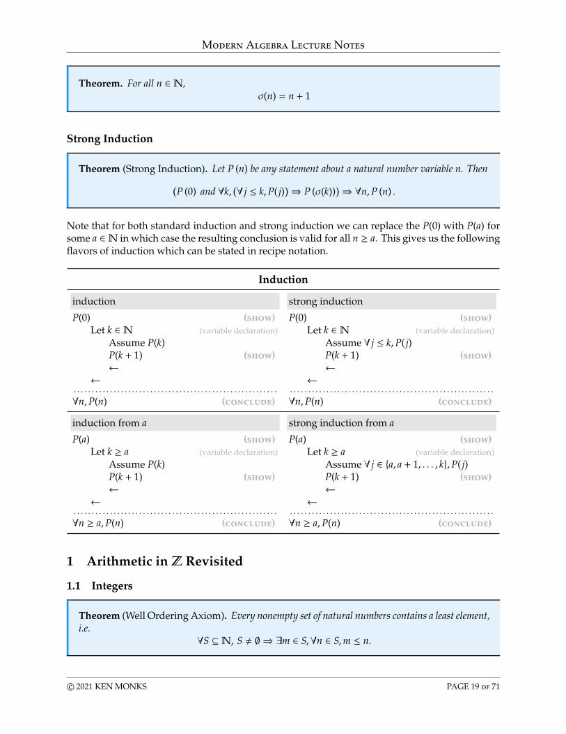
Theorem. For all n ∈N,σ(n) = n + 1
Strong Induction
Theorem (Strong Induction). Let P (n) be any statement about a natural number variable n. Then(P (0) and ∀k,
(∀ j ≤ k,P( j))⇒ P (σ(k))
)⇒ ∀n,P (n) .
Note that for both standard induction and strong induction we can replace the P(0) with P(a) forsome a ∈N in which case the resulting conclusion is valid for all n ≥ a. This gives us the followingflavors of induction which can be stated in recipe notation.
Induction
induction strong induction
P(0) (show)Let k ∈N (variable declaration)
Assume P(k)P(k + 1) (show)←
←. . . . . . . . . . . . . . . . . . . . . . . . . . . . . . . . . . . . . . . . . . . . . . . . . . . . . . . .∀n,P(n) (conclude)
P(0) (show)Let k ∈N (variable declaration)
Assume ∀ j ≤ k,P( j)P(k + 1) (show)←
←. . . . . . . . . . . . . . . . . . . . . . . . . . . . . . . . . . . . . . . . . . . . . . . . . . . . . . . .∀n,P(n) (conclude)
induction from a strong induction from a
P(a) (show)Let k ≥ a (variable declaration)
Assume P(k)P(k + 1) (show)←
←. . . . . . . . . . . . . . . . . . . . . . . . . . . . . . . . . . . . . . . . . . . . . . . . . . . . . . . .∀n ≥ a,P(n) (conclude)
P(a) (show)Let k ≥ a (variable declaration)
Assume ∀ j ∈ {a, a + 1, . . . , k},P( j)P(k + 1) (show)←
←. . . . . . . . . . . . . . . . . . . . . . . . . . . . . . . . . . . . . . . . . . . . . . . . . . . . . . . .∀n ≥ a,P(n) (conclude)
1 Arithmetic in Z Revisited
1.1 Integers
Theorem (Well Ordering Axiom). Every nonempty set of natural numbers contains a least element,i.e.
∀S ⊆N, S , ∅ ⇒ ∃m ∈ S,∀n ∈ S,m ≤ n.
c© 2021 KEN MONKS PAGE 19 of 71
Modern Algebra Lecture Notes
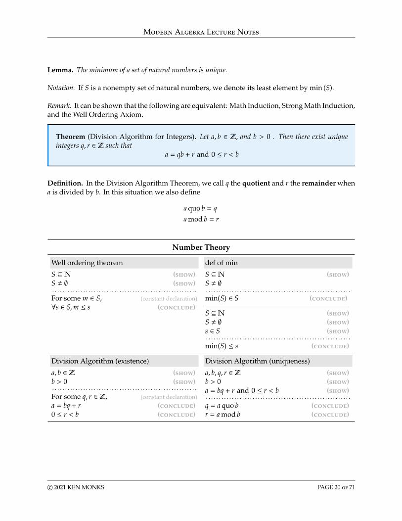
Lemma. The minimum of a set of natural numbers is unique.
Notation. If S is a nonempty set of natural numbers, we denote its least element by min (S).
Remark. It can be shown that the following are equivalent: Math Induction, Strong Math Induction,and the Well Ordering Axiom.
Theorem (Division Algorithm for Integers). Let a, b ∈ Z, and b > 0 . Then there exist uniqueintegers q, r ∈ Z such that
a = qb + r and 0 ≤ r < b
Definition. In the Division Algorithm Theorem, we call q the quotient and r the remainder whena is divided by b. In this situation we also define
a quo b = qa mod b = r
Number Theory
Well ordering theorem def of min
S ⊆N (show)S , ∅ (show). . . . . . . . . . . . . . . . . . . . . . . . . . . . . . . . . . . . . . . . . . . . . . . . . . . . . . . .For some m ∈ S, (constant declaration)∀s ∈ S,m ≤ s (conclude)
S ⊆N (show)S , ∅. . . . . . . . . . . . . . . . . . . . . . . . . . . . . . . . . . . . . . . . . . . . . . . . . . . . . . . .min(S) ∈ S (conclude)
S ⊆N (show)S , ∅ (show)s ∈ S (show). . . . . . . . . . . . . . . . . . . . . . . . . . . . . . . . . . . . . . . . . . . . . . . . . . . . . . . .min(S) ≤ s (conclude)
Division Algorithm (existence) Division Algorithm (uniqueness)
a, b ∈ Z (show)b > 0 (show). . . . . . . . . . . . . . . . . . . . . . . . . . . . . . . . . . . . . . . . . . . . . . . . . . . . . . . .For some q, r ∈ Z, (constant declaration)a = bq + r (conclude)0 ≤ r < b (conclude)
a, b, q, r ∈ Z (show)b > 0 (show)a = bq + r and 0 ≤ r < b (show). . . . . . . . . . . . . . . . . . . . . . . . . . . . . . . . . . . . . . . . . . . . . . . . . . . . . . . .q = a quo b (conclude)r = a mod b (conclude)
c© 2021 KEN MONKS PAGE 20 of 71
Modern Algebra Lecture Notes
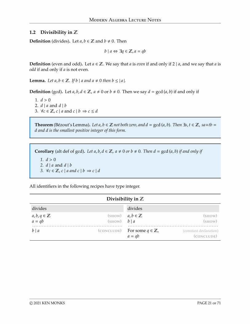
1.2 Divisibility in Z
Definition (divides). Let a, b ∈ Z and b , 0. Then
b | a⇔ ∃q ∈ Z, a = qb
Definition (even and odd). Let a ∈ Z. We say that a is even if and only if 2 | a, and we say that a isodd if and only if a is not even.
Lemma. Let a, b ∈ Z. If b | a and a , 0 then b ≤ | a |.
Definition (gcd). Let a, b, d ∈ Z, a , 0 or b , 0. Then we say d = gcd (a, b) if and only if
1. d > 02. d | a and d | b3. ∀c ∈ Z, c | a and c | b ⇒ c ≤ d
Theorem (Bézout’s Lemma). Let a, b ∈ Znot both zero, and d = gcd (a, b). Then∃s, t ∈ Z, sa+tb =d and d is the smallest positive integer of this form.
Corollary (alt def of gcd). Let a, b, d ∈ Z, a , 0 or b , 0. Then d = gcd (a, b) if and only if
1. d > 02. d | a and d | b3. ∀c ∈ Z, c | a and c | b ⇒ c | d
All identifiers in the following recipes have type integer.
Divisibility in Z
divides divides
a, b, q ∈ Z (show)a = qb (show). . . . . . . . . . . . . . . . . . . . . . . . . . . . . . . . . . . . . . . . . . . . . . . . . . . . . . . .b | a (conclude)
a, b ∈ Z (show)b | a (show). . . . . . . . . . . . . . . . . . . . . . . . . . . . . . . . . . . . . . . . . . . . . . . . . . . . . . . .For some q ∈ Z, (constant declaration)a = qb (conclude)
c© 2021 KEN MONKS PAGE 21 of 71
Modern Algebra Lecture Notes
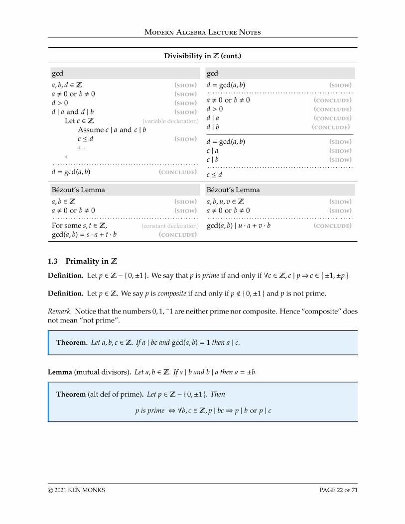
Divisibility in Z (cont.)
gcd gcd
a, b, d ∈ Z (show)a , 0 or b , 0 (show)d > 0 (show)d | a and d | b (show)
Let c ∈ Z (variable declaration)Assume c | a and c | bc ≤ d (show)←
←. . . . . . . . . . . . . . . . . . . . . . . . . . . . . . . . . . . . . . . . . . . . . . . . . . . . . . . .d = gcd(a, b) (conclude)
d = gcd(a, b) (show). . . . . . . . . . . . . . . . . . . . . . . . . . . . . . . . . . . . . . . . . . . . . . . . . . . . . . . .a , 0 or b , 0 (conclude)d > 0 (conclude)d | a (conclude)d | b (conclude)
d = gcd(a, b) (show)c | a (show)c | b (show). . . . . . . . . . . . . . . . . . . . . . . . . . . . . . . . . . . . . . . . . . . . . . . . . . . . . . . .c ≤ d
Bézout’s Lemma Bézout’s Lemma
a, b ∈ Z (show)a , 0 or b , 0 (show). . . . . . . . . . . . . . . . . . . . . . . . . . . . . . . . . . . . . . . . . . . . . . . . . . . . . . . .For some s, t ∈ Z, (constant declaration)gcd(a, b) = s · a + t · b (conclude)
a, b,u, v ∈ Z (show)a , 0 or b , 0 (show). . . . . . . . . . . . . . . . . . . . . . . . . . . . . . . . . . . . . . . . . . . . . . . . . . . . . . . .gcd(a, b) | u · a + v · b (conclude)
1.3 Primality in Z
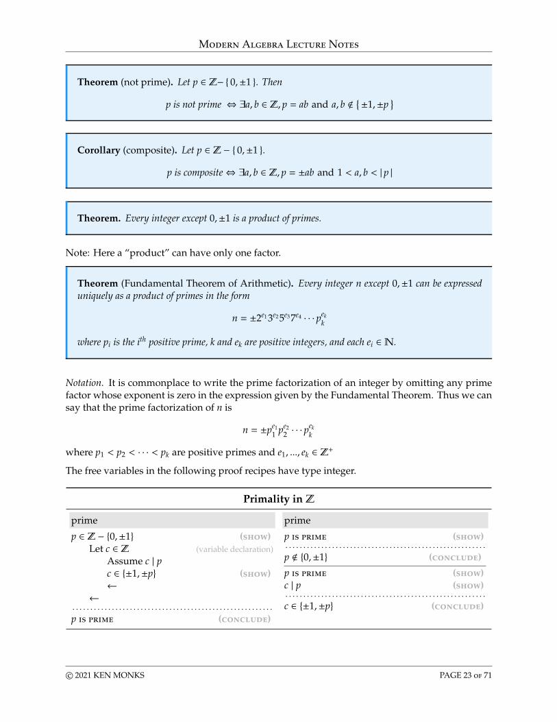
Definition. Let p ∈ Z − { 0,±1 }. We say that p is prime if and only if ∀c ∈ Z, c | p⇒ c ∈ {±1,±p}
Definition. Let p ∈ Z. We say p is composite if and only if p < { 0,±1 } and p is not prime.
Remark. Notice that the numbers 0, 1, −1 are neither prime nor composite. Hence “composite” doesnot mean “not prime”.
Theorem. Let a, b, c ∈ Z. If a | bc and gcd(a, b) = 1 then a | c.
Lemma (mutual divisors). Let a, b ∈ Z. If a | b and b | a then a = ±b.
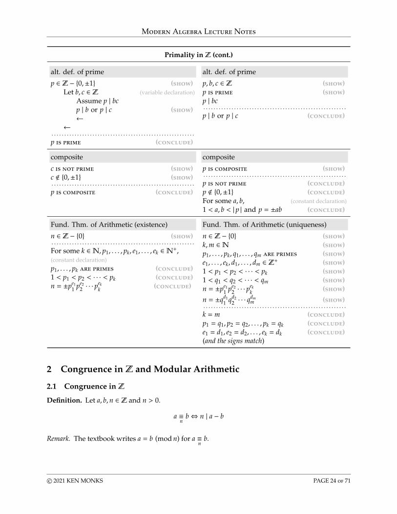
Theorem (alt def of prime). Let p ∈ Z − { 0,±1 }. Then
p is prime ⇔ ∀b, c ∈ Z, p | bc⇒ p | b or p | c
c© 2021 KEN MONKS PAGE 22 of 71
Modern Algebra Lecture Notes
Theorem (not prime). Let p ∈ Z− { 0,±1 }. Then
p is not prime ⇔ ∃a, b ∈ Z, p = ab and a, b <{±1,±p
}
Corollary (composite). Let p ∈ Z − { 0,±1 }.
p is composite⇔ ∃a, b ∈ Z, p = ±ab and 1 < a, b < | p |
Theorem. Every integer except 0,±1 is a product of primes.
Note: Here a “product” can have only one factor.
Theorem (Fundamental Theorem of Arithmetic). Every integer n except 0,±1 can be expresseduniquely as a product of primes in the form
n = ±2e13e25e37e4 · · · pekk
where pi is the ith positive prime, k and ek are positive integers, and each ei ∈N.
Notation. It is commonplace to write the prime factorization of an integer by omitting any primefactor whose exponent is zero in the expression given by the Fundamental Theorem. Thus we cansay that the prime factorization of n is
n = ±pe11 pe2
2 · · · pekk
where p1 < p2 < · · · < pk are positive primes and e1, ..., ek ∈ Z+
The free variables in the following proof recipes have type integer.
Primality in Z
prime prime
p ∈ Z − {0,±1} (show)Let c ∈ Z (variable declaration)
Assume c | pc ∈ {±1,±p} (show)←
←. . . . . . . . . . . . . . . . . . . . . . . . . . . . . . . . . . . . . . . . . . . . . . . . . . . . . . . .p is prime (conclude)
p is prime (show). . . . . . . . . . . . . . . . . . . . . . . . . . . . . . . . . . . . . . . . . . . . . . . . . . . . . . . .p < {0,±1} (conclude)
p is prime (show)c | p (show). . . . . . . . . . . . . . . . . . . . . . . . . . . . . . . . . . . . . . . . . . . . . . . . . . . . . . . .c ∈ {±1,±p} (conclude)
c© 2021 KEN MONKS PAGE 23 of 71
Modern Algebra Lecture Notes
Primality in Z (cont.)
alt. def. of prime alt. def. of prime
p ∈ Z − {0,±1} (show)Let b, c ∈ Z (variable declaration)
Assume p | bcp | b or p | c (show)←
←. . . . . . . . . . . . . . . . . . . . . . . . . . . . . . . . . . . . . . . . . . . . . . . . . . . . . . . .p is prime (conclude)
p, b, c ∈ Z (show)p is prime (show)p | bc. . . . . . . . . . . . . . . . . . . . . . . . . . . . . . . . . . . . . . . . . . . . . . . . . . . . . . . .p | b or p | c (conclude)
composite composite
c is not prime (show)c < {0,±1} (show). . . . . . . . . . . . . . . . . . . . . . . . . . . . . . . . . . . . . . . . . . . . . . . . . . . . . . . .p is composite (conclude)
p is composite (show). . . . . . . . . . . . . . . . . . . . . . . . . . . . . . . . . . . . . . . . . . . . . . . . . . . . . . . .p is not prime (conclude)p < {0,±1} (conclude)For some a, b, (constant declaration)1 < a, b < | p | and p = ±ab (conclude)
Fund. Thm. of Arithmetic (existence) Fund. Thm. of Arithmetic (uniqueness)
n ∈ Z − {0} (show). . . . . . . . . . . . . . . . . . . . . . . . . . . . . . . . . . . . . . . . . . . . . . . . . . . . . . . .For some k ∈N, p1, . . . , pk, e1, . . . , ek ∈N+,(constant declaration)p1, . . . , pk are primes (conclude)1 < p1 < p2 < · · · < pk (conclude)n = ±pe1
1 pe22 · · · p
ekk (conclude)
n ∈ Z − {0} (show)k,m ∈N (show)p1, . . . , pk, q1, . . . , qm are primes (show)e1, . . . , ek, d1, . . . , dm ∈ Z+ (show)1 < p1 < p2 < · · · < pk (show)1 < q1 < q2 < · · · < qm (show)n = ±pe1
1 pe22 · · · p
ekk (show)
n = ±qd11 qd2
2 · · · qdmm (show)
. . . . . . . . . . . . . . . . . . . . . . . . . . . . . . . . . . . . . . . . . . . . . . . . . . . . . . . .k = m (conclude)p1 = q1, p2 = q2, . . . , pk = qk (conclude)e1 = d1, e2 = d2, . . . , ek = dk (conclude)(and the signs match)
2 Congruence in Z and Modular Arithmetic
2.1 Congruence in Z
Definition. Let a, b,n ∈ Z and n > 0.
a ≡n
b⇔ n | a − b
Remark. The textbook writes a = b (mod n) for a ≡n
b.
c© 2021 KEN MONKS PAGE 24 of 71
Modern Algebra Lecture Notes
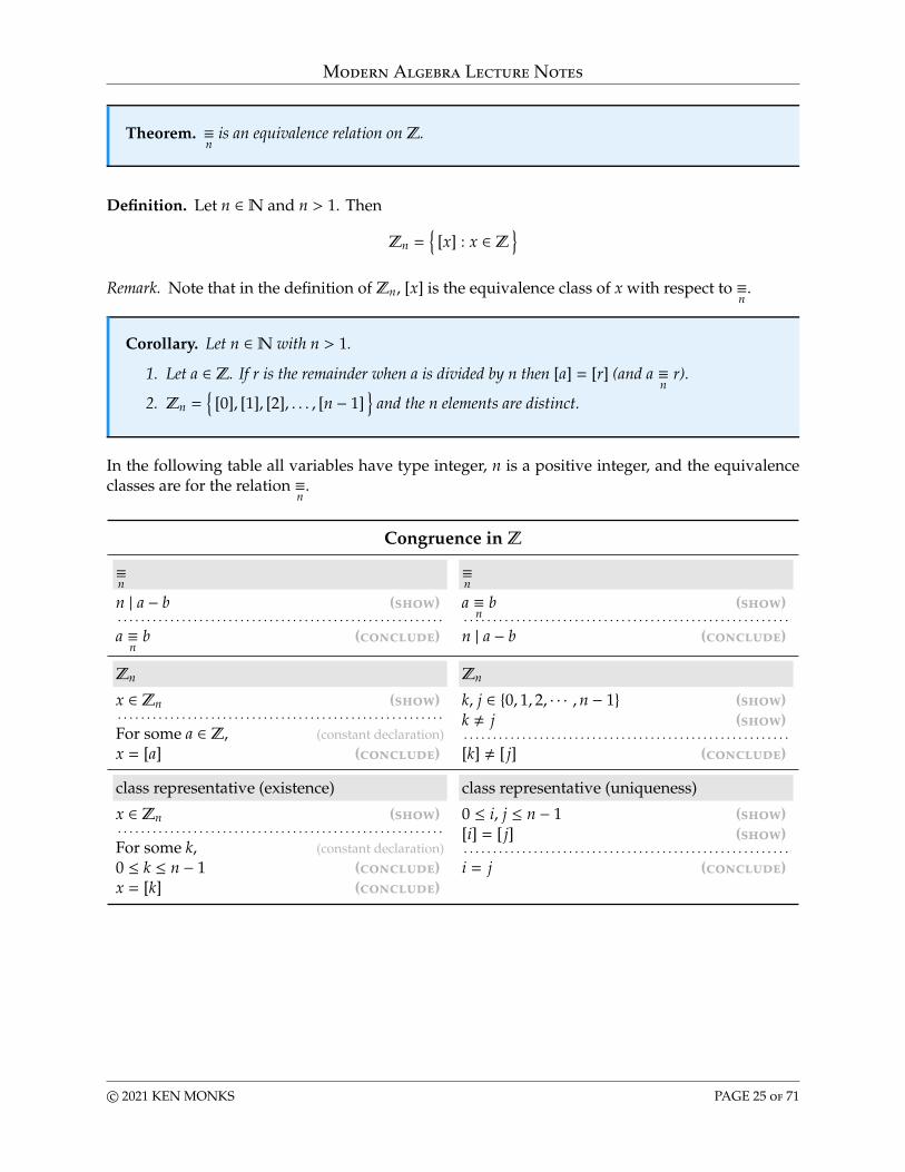
Theorem. ≡n
is an equivalence relation on Z.
Definition. Let n ∈N and n > 1. Then
Zn ={
[x] : x ∈ Z}
Remark. Note that in the definition of Zn, [x] is the equivalence class of x with respect to ≡n
.
Corollary. Let n ∈N with n > 1.
1. Let a ∈ Z. If r is the remainder when a is divided by n then [a] = [r] (and a ≡n
r).
2. Zn ={
[0], [1], [2], . . . , [n − 1]}
and the n elements are distinct.
In the following table all variables have type integer, n is a positive integer, and the equivalenceclasses are for the relation ≡
n.
Congruence in Z
≡n
≡n
n | a − b (show). . . . . . . . . . . . . . . . . . . . . . . . . . . . . . . . . . . . . . . . . . . . . . . . . . . . . . . .a ≡
nb (conclude)
a ≡n
b (show). . . . . . . . . . . . . . . . . . . . . . . . . . . . . . . . . . . . . . . . . . . . . . . . . . . . . . . .n | a − b (conclude)
Zn Zn
x ∈ Zn (show). . . . . . . . . . . . . . . . . . . . . . . . . . . . . . . . . . . . . . . . . . . . . . . . . . . . . . . .For some a ∈ Z, (constant declaration)x = [a] (conclude)
k, j ∈ {0, 1, 2, · · · ,n − 1} (show)k , j (show). . . . . . . . . . . . . . . . . . . . . . . . . . . . . . . . . . . . . . . . . . . . . . . . . . . . . . . .[k] , [ j] (conclude)
class representative (existence) class representative (uniqueness)
x ∈ Zn (show). . . . . . . . . . . . . . . . . . . . . . . . . . . . . . . . . . . . . . . . . . . . . . . . . . . . . . . .For some k, (constant declaration)0 ≤ k ≤ n − 1 (conclude)x = [k] (conclude)
0 ≤ i, j ≤ n − 1 (show)[i] = [ j] (show). . . . . . . . . . . . . . . . . . . . . . . . . . . . . . . . . . . . . . . . . . . . . . . . . . . . . . . .i = j (conclude)
c© 2021 KEN MONKS PAGE 25 of 71
Modern Algebra Lecture Notes
2.2 Arithmetic in Zn
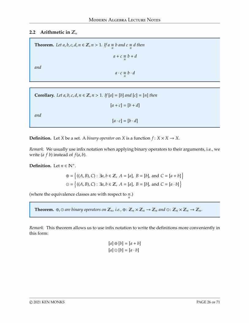
Theorem. Let a, b, c, d,n ∈ Z,n > 1. If a ≡n
b and c ≡n
d then
a + c ≡n
b + d
anda · c ≡
nb · d
Corollary. Let a, b, c, d,n ∈ Z,n > 1. If [a] = [b] and [c] = [n] then
[a + c] = [b + d]
and[a · c] = [b · d]
Definition. Let X be a set. A binary operator on X is a function f : X × X→ X.
Remark. We usually use infix notation when applying binary operators to their arguments, i.e., wewrite (a f b) instead of f (a, b).
Definition. Let n ∈N+.
⊕ ={
((A,B),C) : ∃a, b ∈ Z, A = [a], B = [b], and C = [a + b]}
� ={
((A,B),C) : ∃a, b ∈ Z, A = [a], B = [b], and C = [a · b]}
(where the equivalence classes are with respect to ≡n
.)
Theorem. ⊕,� are binary operators on Zn, i.e., ⊕ : Zn ×Zn → Zn and � : Zn ×Zn → Zn.
Remark. This theorem allows us to use infix notation to write the definitions more conveniently inthis form:
[a] ⊕ [b] = [a + b][a] � [b] = [a · b]
c© 2021 KEN MONKS PAGE 26 of 71
Modern Algebra Lecture Notes
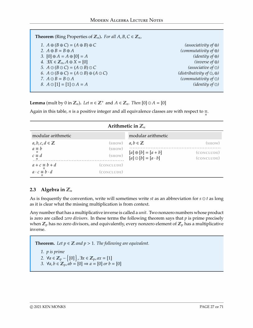
Theorem (Ring Properties of Zn). For all A,B,C ∈ Zn,
1. A ⊕ (B ⊕ C) = (A ⊕ B) ⊕ C (associativity of ⊕)2. A ⊕ B = B ⊕ A (commutativity of ⊕)3. [0] ⊕ A = A ⊕ [0] = A (identity of ⊕)4. ∃X ∈ Zn,A ⊕ X = [0] (inverse of ⊕)5. A � (B � C) = (A � B) � C (associative of �)6. A � (B ⊕ C) = (A � B) ⊕ (A � C) (distributivity of �,⊕)7. A � B = B � A (commutativity of �)8. A � [1] = [1] � A = A (identity of �)
Lemma (mult by 0 in Zn). Let n ∈ Z+ and A ∈ Zn. Then [0] � A = [0]
Again in this table, n is a positive integer and all equivalence classes are with respect to ≡n
.
Arithmetic in Zn
modular arithmetic modular arithmetic
a, b, c, d ∈ Z (show)a ≡
nb (show)
c ≡n
d (show). . . . . . . . . . . . . . . . . . . . . . . . . . . . . . . . . . . . . . . . . . . . . . . . . . . . . . . .a + c ≡
nb + d (conclude)
a · c ≡n
b · d (conclude)
a, b ∈ Z (show). . . . . . . . . . . . . . . . . . . . . . . . . . . . . . . . . . . . . . . . . . . . . . . . . . . . . . . .[a] ⊕ [b] = [a + b] (conclude)[a] � [b] = [a · b] (conclude)
2.3 Algebra in Zn
As is frequently the convention, write will sometimes write st as an abbreviation for s � t as longas it is clear what the missing multiplication is from context.
Any number that has a multiplicative inverse is called a unit. Two nonzero numbers whose productis zero are called zero divisors. In these terms the following theorem says that p is prime preciselywhenZp has no zero divisors, and equivalently, every nonzero element ofZp has a multiplicativeinverse.
Theorem. Let p ∈ Z and p > 1. The following are equivalent.
1. p is prime2. ∀a ∈ Zp −
{[0]},∃x ∈ Zp, ax = [1]
3. ∀a, b ∈ Zp, ab = [0]⇒ a = [0] or b = [0]
c© 2021 KEN MONKS PAGE 27 of 71
Modern Algebra Lecture Notes
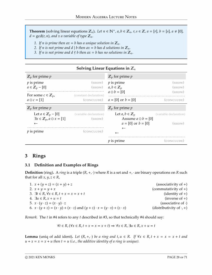
Theorem (solving linear equations Zn). Let n ∈ N+, a, b ∈ Zn, r, s ∈ Z, a = [r], b = [s], a , [0],d = gcd(r,n), and x a variable of type Zn.
1. If n is prime then ax = b has a unique solution in Zn.2. If n is not prime and d | b then ax = b has d solutions in Zn.3. If n is not prime and d ∤ b then ax = b has no solutions in Zn.
Solving Linear Equations in Zn
Zp for prime p Zp for prime p
p is prime (show)a ∈ Zp − [0] (show). . . . . . . . . . . . . . . . . . . . . . . . . . . . . . . . . . . . . . . . . . . . . . . . . . . . . . . .For some c ∈ Zp, (constant declaration)a � c = [1] (conclude)
p is prime (show)a, b ∈ Zp (show)a � b = [0] (show). . . . . . . . . . . . . . . . . . . . . . . . . . . . . . . . . . . . . . . . . . . . . . . . . . . . . . . .a = [0] or b = [0] (conclude)
Zp for prime p Zp for prime p
Let a ∈ Zp − [0] (variable declaration)∃x ∈ Zp, a � x = [1] (show)←
. . . . . . . . . . . . . . . . . . . . . . . . . . . . . . . . . . . . . . . . . . . . . . . . . . . . . . . .p is prime (conclude)
Let a, b ∈ Zp (variable declaration)Assume a � b = [0]a = [0] or b = [0] (show)←
←. . . . . . . . . . . . . . . . . . . . . . . . . . . . . . . . . . . . . . . . . . . . . . . . . . . . . . . .p is prime (conclude)
3 Rings
3.1 Definition and Examples of Rings
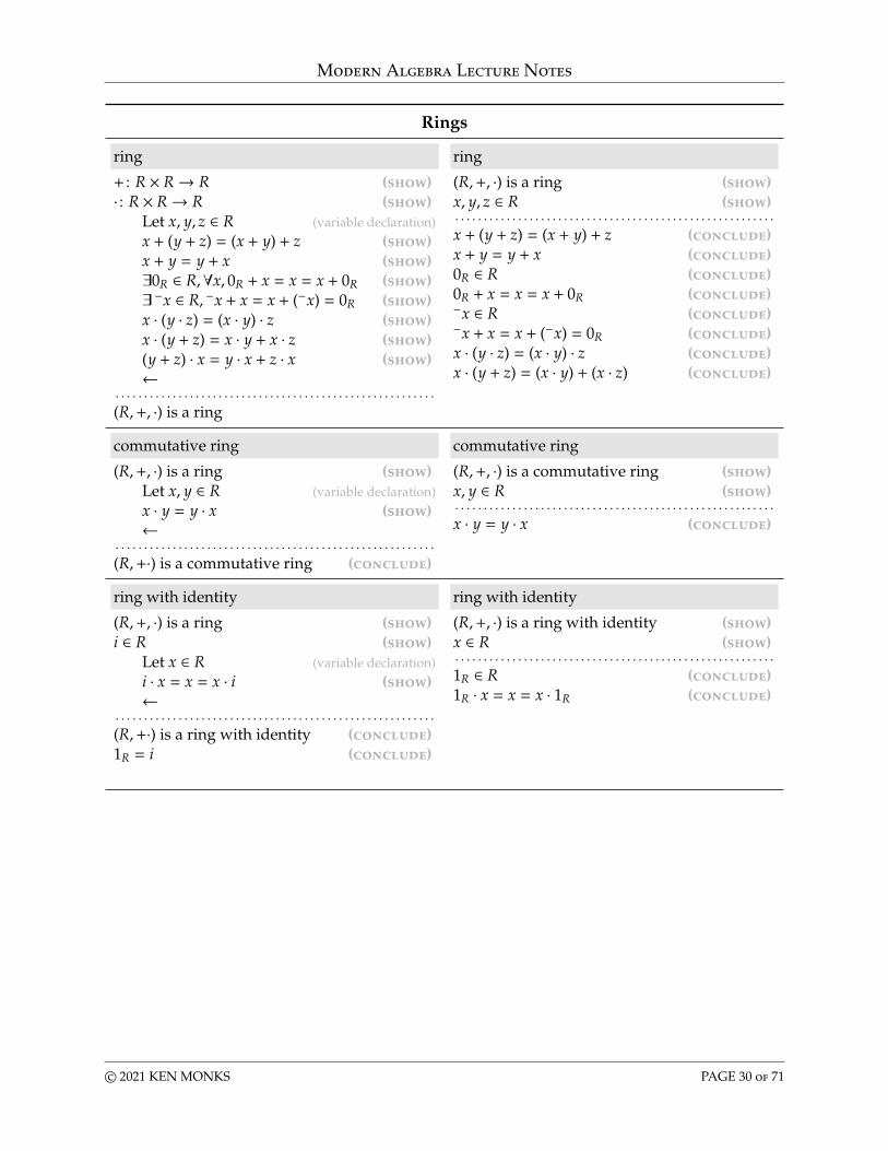
Definition (ring). A ring is a triple (R,+, ·) where R is a set and +, · are binary operations on R suchthat for all x, y, z ∈ R,
1. x + (y + z) = (x + y) + z (associativity of +)2. x + y = y + x (commutativity of +)3. ∃t ∈ R,∀x ∈ R, t + x = x = x + t (identity of +)4. ∃u ∈ R, x + u = t (inverse of +)5. x · (y · z) = (x · y) · z (associative of ·)6. x · (y + z) = (x · y) + (x · z) and (y + z) · x = (y · x) + (z · x) (distributivity of ·,+)
Remark. The t in #4 refers to any t described in #3, so that technically #4 should say:
∀t ∈ R, (∀x ∈ R, t + x = x = x + t)⇒ ∀x ∈ R,∃u ∈ R, x + u = t
Lemma (uniq of add ident). Let (R,+, ·) be a ring and t,u ∈ R. If ∀x ∈ R, t + x = x = x + t andu + x = x = x + u then t = u (i.e., the additive identity of a ring is unique).
c© 2021 KEN MONKS PAGE 28 of 71
Modern Algebra Lecture Notes
Notation. We write 0R for the unique additive identity of a ring (R,+, ·).
Notation. We also usually abbreviate a · b as ab.
Notation. We often refer to the ring (R,+, ·) as the ring R.
Lemma (uniq of add inv). Let (R,+, ·) be a ring and u, v, x ∈ R. If u+x = 0R = x+u and v+x = 0R = x+vthen u = v (i.e. the additive inverse of x in a ring is unique)
Notation. We write −x for the additive inverse of x in a ring R.
Definition (of subtraction). Let (R,+, ·) be a ring and a, b ∈ R. Then a − b is defined to bea +(−b).
Types of Rings
Definition (commutative ring). A ring (R,+, ·) is a commutative ring if and only if∀a, b ∈ R, ab = ba.
Definition (ring with identity). A ring (R,+, ·) is a ring with identity if and only if ∃i ∈ R,∀x ∈R, ix = x = xi.
Lemma (uniq of mult ident). Let (R,+, ·) be a ring and u, v ∈ R. If
∀x ∈ R,ux = x = xu and vx = x = xv
then u = v (i.e. the multiplicative identity for a ring is unique).
Notation. If R is a ring with identity we write 1R for the unique multiplicative identity of R.
Lemma (uniq of mult inverse). Let (R,+, ·) be a ring with identity 1R and x,u, v ∈ R. If
ux = 1R = xu and vx = 1R = xv
then u = v (i.e. a multiplicative inverse of an element of a ring is unique).
Notation. If R is a ring with identity we write x−1 for the unique multiplicative inverse of x in R.
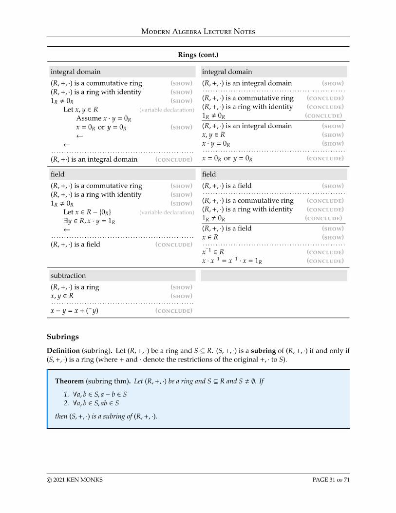
Definition (integral domain). A ring (R,+, ·) is an integral domain if and only if it is a commutativering with identity 1R , 0R and ∀a, b ∈ R, ab = 0R ⇒ a = 0R or b = 0R.
Definition (field). A ring (R,+, ·) is a field if and only if is a commutative ring with identity 1R , 0Rand ∀a ∈ R − { 0R } ,∃x ∈ R, ax = 1R (i.e., every nonzero element has a multiplicative inverse).
c© 2021 KEN MONKS PAGE 29 of 71
Modern Algebra Lecture Notes
Rings
ring ring
+ : R × R→ R (show)· : R × R→ R (show)
Let x, y, z ∈ R (variable declaration)x + (y + z) = (x + y) + z (show)x + y = y + x (show)∃0R ∈ R,∀x, 0R + x = x = x + 0R (show)∃ −x ∈ R, −x + x = x + (−x) = 0R (show)x · (y · z) = (x · y) · z (show)x · (y + z) = x · y + x · z (show)(y + z) · x = y · x + z · x (show)←
. . . . . . . . . . . . . . . . . . . . . . . . . . . . . . . . . . . . . . . . . . . . . . . . . . . . . . . .(R,+, ·) is a ring
(R,+, ·) is a ring (show)x, y, z ∈ R (show). . . . . . . . . . . . . . . . . . . . . . . . . . . . . . . . . . . . . . . . . . . . . . . . . . . . . . . .x + (y + z) = (x + y) + z (conclude)x + y = y + x (conclude)0R ∈ R (conclude)0R + x = x = x + 0R (conclude)−x ∈ R (conclude)−x + x = x + (−x) = 0R (conclude)x · (y · z) = (x · y) · z (conclude)x · (y + z) = (x · y) + (x · z) (conclude)
commutative ring commutative ring
(R,+, ·) is a ring (show)Let x, y ∈ R (variable declaration)x · y = y · x (show)←
. . . . . . . . . . . . . . . . . . . . . . . . . . . . . . . . . . . . . . . . . . . . . . . . . . . . . . . .(R,+·) is a commutative ring (conclude)
(R,+, ·) is a commutative ring (show)x, y ∈ R (show). . . . . . . . . . . . . . . . . . . . . . . . . . . . . . . . . . . . . . . . . . . . . . . . . . . . . . . .x · y = y · x (conclude)
ring with identity ring with identity
(R,+, ·) is a ring (show)i ∈ R (show)
Let x ∈ R (variable declaration)i · x = x = x · i (show)←
. . . . . . . . . . . . . . . . . . . . . . . . . . . . . . . . . . . . . . . . . . . . . . . . . . . . . . . .(R,+·) is a ring with identity (conclude)1R = i (conclude)
(R,+, ·) is a ring with identity (show)x ∈ R (show). . . . . . . . . . . . . . . . . . . . . . . . . . . . . . . . . . . . . . . . . . . . . . . . . . . . . . . .1R ∈ R (conclude)1R · x = x = x · 1R (conclude)
c© 2021 KEN MONKS PAGE 30 of 71
Modern Algebra Lecture Notes
Rings (cont.)
integral domain integral domain
(R,+, ·) is a commutative ring (show)(R,+, ·) is a ring with identity (show)1R , 0R (show)
Let x, y ∈ R (variable declaration)Assume x · y = 0Rx = 0R or y = 0R (show)←
←. . . . . . . . . . . . . . . . . . . . . . . . . . . . . . . . . . . . . . . . . . . . . . . . . . . . . . . .(R,+·) is an integral domain (conclude)
(R,+, ·) is an integral domain (show). . . . . . . . . . . . . . . . . . . . . . . . . . . . . . . . . . . . . . . . . . . . . . . . . . . . . . . .(R,+, ·) is a commutative ring (conclude)(R,+, ·) is a ring with identity (conclude)1R , 0R (conclude)(R,+, ·) is an integral domain (show)x, y ∈ R (show)x · y = 0R (show). . . . . . . . . . . . . . . . . . . . . . . . . . . . . . . . . . . . . . . . . . . . . . . . . . . . . . . .x = 0R or y = 0R (conclude)
field field
(R,+, ·) is a commutative ring (show)(R,+, ·) is a ring with identity (show)1R , 0R (show)
Let x ∈ R − {0R} (variable declaration)∃y ∈ R, x · y = 1R←
. . . . . . . . . . . . . . . . . . . . . . . . . . . . . . . . . . . . . . . . . . . . . . . . . . . . . . . .(R,+, ·) is a field (conclude)
(R,+, ·) is a field (show). . . . . . . . . . . . . . . . . . . . . . . . . . . . . . . . . . . . . . . . . . . . . . . . . . . . . . . .(R,+, ·) is a commutative ring (conclude)(R,+, ·) is a ring with identity (conclude)1R , 0R (conclude)(R,+, ·) is a field (show)x ∈ R (show). . . . . . . . . . . . . . . . . . . . . . . . . . . . . . . . . . . . . . . . . . . . . . . . . . . . . . . .x−1 ∈ R (conclude)
x · x−1 = x−1 · x = 1R (conclude)
subtraction
(R,+, ·) is a ring (show)x, y ∈ R (show). . . . . . . . . . . . . . . . . . . . . . . . . . . . . . . . . . . . . . . . . . . . . . . . . . . . . . . .x − y = x + (−y) (conclude)
Subrings
Definition (subring). Let (R,+, ·) be a ring and S ⊆ R. (S,+, ·) is a subring of (R,+, ·) if and only if(S,+, ·) is a ring (where + and · denote the restrictions of the original +, · to S).
Theorem (subring thm). Let (R,+, ·) be a ring and S ⊆ R and S , ∅. If
1. ∀a, b ∈ S, a − b ∈ S2. ∀a, b ∈ S, ab ∈ S
then (S,+, ·) is a subring of (R,+, ·).
c© 2021 KEN MONKS PAGE 31 of 71
Modern Algebra Lecture Notes
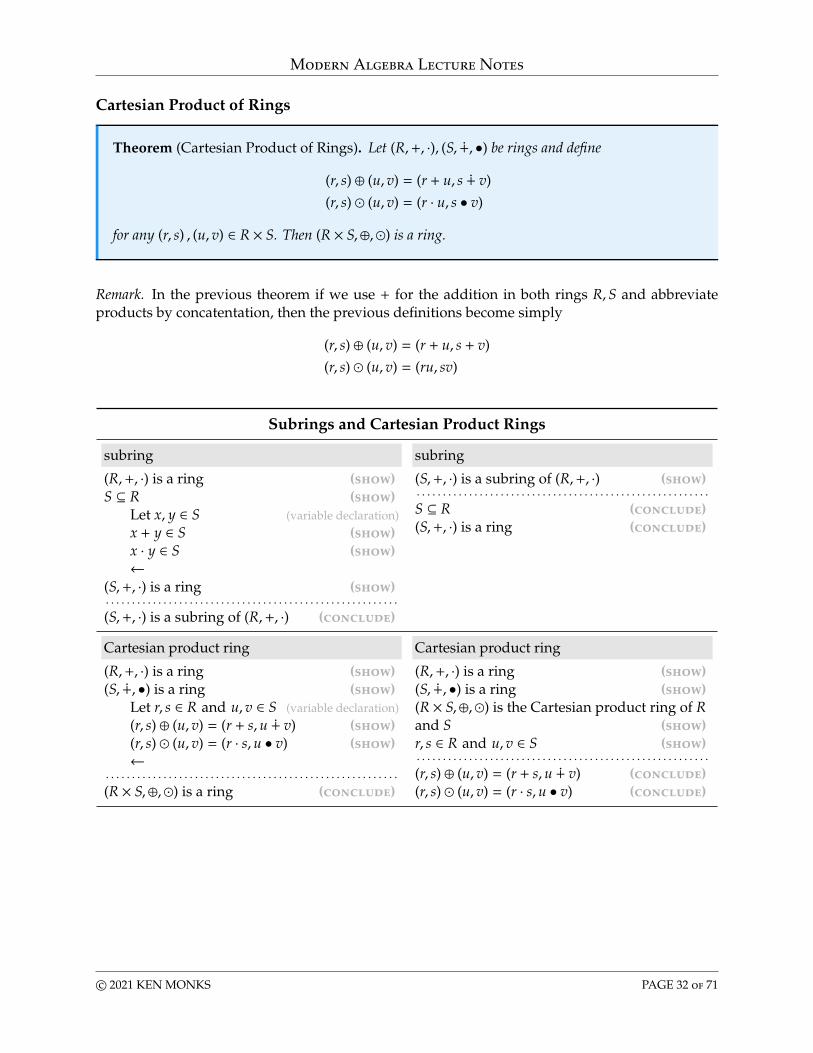
Cartesian Product of Rings
Theorem (Cartesian Product of Rings). Let (R,+, ·), (S,∔, •) be rings and define
(r, s) ⊕ (u, v) = (r + u, s ∔ v)(r, s) � (u, v) = (r · u, s • v)
for any (r, s) , (u, v) ∈ R × S. Then (R × S,⊕,�) is a ring.
Remark. In the previous theorem if we use + for the addition in both rings R,S and abbreviateproducts by concatentation, then the previous definitions become simply
(r, s) ⊕ (u, v) = (r + u, s + v)(r, s) � (u, v) = (ru, sv)
Subrings and Cartesian Product Rings
subring subring
(R,+, ·) is a ring (show)S ⊆ R (show)
Let x, y ∈ S (variable declaration)x + y ∈ S (show)x · y ∈ S (show)←
(S,+, ·) is a ring (show). . . . . . . . . . . . . . . . . . . . . . . . . . . . . . . . . . . . . . . . . . . . . . . . . . . . . . . .(S,+, ·) is a subring of (R,+, ·) (conclude)
(S,+, ·) is a subring of (R,+, ·) (show). . . . . . . . . . . . . . . . . . . . . . . . . . . . . . . . . . . . . . . . . . . . . . . . . . . . . . . .S ⊆ R (conclude)(S,+, ·) is a ring (conclude)
Cartesian product ring Cartesian product ring
(R,+, ·) is a ring (show)(S,∔, •) is a ring (show)
Let r, s ∈ R and u, v ∈ S (variable declaration)(r, s) ⊕ (u, v) = (r + s,u ∔ v) (show)(r, s) � (u, v) = (r · s,u • v) (show)←
. . . . . . . . . . . . . . . . . . . . . . . . . . . . . . . . . . . . . . . . . . . . . . . . . . . . . . . .(R × S,⊕,�) is a ring (conclude)
(R,+, ·) is a ring (show)(S,∔, •) is a ring (show)(R × S,⊕,�) is the Cartesian product ring of Rand S (show)r, s ∈ R and u, v ∈ S (show). . . . . . . . . . . . . . . . . . . . . . . . . . . . . . . . . . . . . . . . . . . . . . . . . . . . . . . .(r, s) ⊕ (u, v) = (r + s,u ∔ v) (conclude)(r, s) � (u, v) = (r · s,u • v) (conclude)
c© 2021 KEN MONKS PAGE 32 of 71
Modern Algebra Lecture Notes
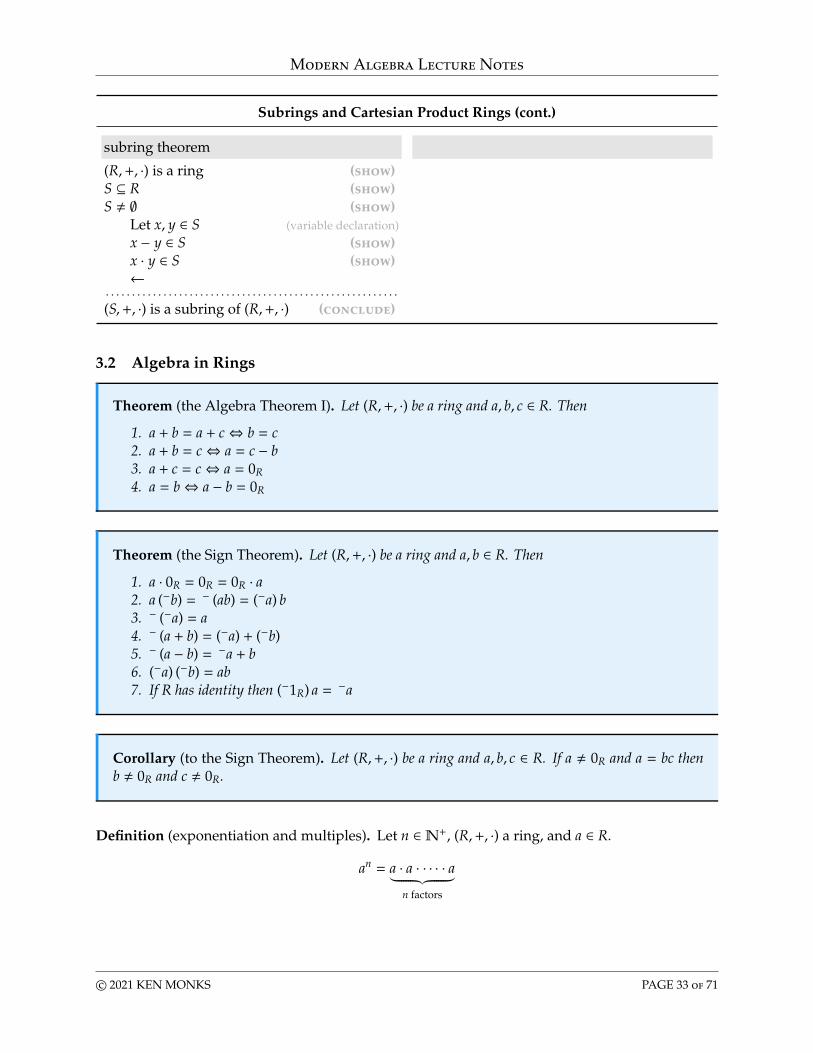
Subrings and Cartesian Product Rings (cont.)
subring theorem
(R,+, ·) is a ring (show)S ⊆ R (show)S , ∅ (show)
Let x, y ∈ S (variable declaration)x − y ∈ S (show)x · y ∈ S (show)←
. . . . . . . . . . . . . . . . . . . . . . . . . . . . . . . . . . . . . . . . . . . . . . . . . . . . . . . .(S,+, ·) is a subring of (R,+, ·) (conclude)
3.2 Algebra in Rings
Theorem (the Algebra Theorem I). Let (R,+, ·) be a ring and a, b, c ∈ R. Then
1. a + b = a + c⇔ b = c2. a + b = c⇔ a = c − b3. a + c = c⇔ a = 0R4. a = b⇔ a − b = 0R
Theorem (the Sign Theorem). Let (R,+, ·) be a ring and a, b ∈ R. Then
1. a · 0R = 0R = 0R · a2. a (−b) = − (ab) = (−a) b3. − (−a) = a4. − (a + b) = (−a) + (−b)5. − (a − b) = −a + b6. (−a) (−b) = ab7. If R has identity then (−1R) a = −a
Corollary (to the Sign Theorem). Let (R,+, ·) be a ring and a, b, c ∈ R. If a , 0R and a = bc thenb , 0R and c , 0R.
Definition (exponentiation and multiples). Let n ∈N+, (R,+, ·) a ring, and a ∈ R.
an = a · a · · · · · a︸ ︷︷ ︸n factors
c© 2021 KEN MONKS PAGE 33 of 71
Modern Algebra Lecture Notes
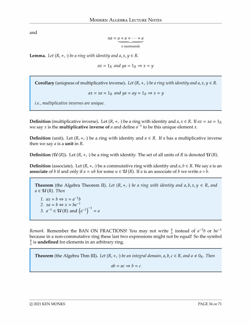
andna = a + a + · · · + a︸ ︷︷ ︸
n summands
Lemma. Let (R,+, ·) be a ring with identity and a, x, y ∈ R.
ax = 1R and ya = 1R ⇒ x = y
Corollary (uniqness of multiplicative inverse). Let (R,+, ·) be a ring with identity and a, x, y ∈ R.
ax = xa = 1R and ya = ay = 1R ⇒ x = y
i.e., multiplicative inverses are unique.
Definition (multiplicative inverse). Let (R,+, ·) be a ring with identity and a, x ∈ R. If ax = xa = 1Rwe say x is the multiplicative inverse of a and define a−1 to be this unique element x.
Definition (unit). Let (R,+, ·) be a ring with identity and a ∈ R. If a has a multiplicative inversethen we say a is a unit in R.
Definition (U (R)). Let (R,+, ·) be a ring with identity. The set of all units of R is denotedU (R).
Definition (associate). Let (R,+, ·) be a commutative ring with identity and a, b ∈ R.We say a is anassociate of b if and only if a = ub for some u ∈ U (R). If a is an associate of b we write a � b.
Theorem (the Algebra Theorem II). Let (R,+, ·) be a ring with identity and a, b, x, y ∈ R, anda ∈ U (R). Then
1. ax = b⇔ x = a−1b2. xa = b⇔ x = ba−1
3. a−1 ∈ U (R) and(a−1)−1= a
Remark. Remember the BAN ON FRACTIONS! You may not write ba instead of a−1b or ba−1
because in a non-commutative ring these last two expressions might not be equal! So the symbolba is undefined for elements in an arbitrary ring.
Theorem (the Algebra Thm III). Let (R,+, ·) be an integral domain, a, b, c ∈ R, and a , 0R. Then
ab = ac⇒ b = c
c© 2021 KEN MONKS PAGE 34 of 71
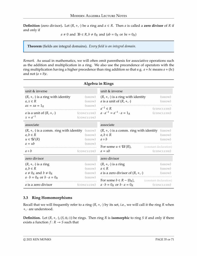
Modern Algebra Lecture Notes
Definition (zero divisor). Let (R,+, ·) be a ring and a ∈ R. Then a is called a zero divisor of R ifand only if
a , 0 and ∃b ∈ R, b , 0R and (ab = 0R or ba = 0R)
Theorem (fields are integral domains). Every field is an integral domain.
Remark. As usual in mathematics, we will often omit parenthesis for associative operations suchas the addition and multiplication in a ring. We also use the precendence of operators with thering multiplication having a higher precedence than ring addition so that e.g. a+ bc means a+ (bc)and not (a + b)c.
Algebra in Rings
unit & inverse unit & inverse
(R,+, ·) is a ring with identity (show)a, x ∈ R (show)ax = xa = 1R (show). . . . . . . . . . . . . . . . . . . . . . . . . . . . . . . . . . . . . . . . . . . . . . . . . . . . . . . .a is a unit of (R,+, ·) (conclude)x = a−1 (conclude)
(R,+, ·) is a ring with identity (show)a is a unit of (R,+, ·) (show). . . . . . . . . . . . . . . . . . . . . . . . . . . . . . . . . . . . . . . . . . . . . . . . . . . . . . . .a−1 ∈ R (conclude)a · a−1 = a−1 · a = 1R (conclude)
associate associate
(R,+, ·) is a comm. ring with identity (show)a, b ∈ R (show)u ∈ U (R) (show)a = ub (show). . . . . . . . . . . . . . . . . . . . . . . . . . . . . . . . . . . . . . . . . . . . . . . . . . . . . . . .a � b (conclude)
(R,+, ·) is a comm. ring with identity (show)a, b ∈ R (show)a � b (show). . . . . . . . . . . . . . . . . . . . . . . . . . . . . . . . . . . . . . . . . . . . . . . . . . . . . . . .For some u ∈ U (R), (constant declaration)a = ub (conclude)
zero divisor zero divisor
(R,+, ·) is a ring (show)a, b ∈ R (show)a , 0R and b , 0R (show)a · b = 0R or b · a = 0R (show). . . . . . . . . . . . . . . . . . . . . . . . . . . . . . . . . . . . . . . . . . . . . . . . . . . . . . . .a is a zero divisor (conclude)
(R,+, ·) is a ring (show)a ∈ R (show)a is a zero divisor of (R,+, ·) (show). . . . . . . . . . . . . . . . . . . . . . . . . . . . . . . . . . . . . . . . . . . . . . . . . . . . . . . .For some b ∈ R − {0R}, (constant declaration)a · b = 0R or b · a = 0R (conclude)
3.3 Ring Homomorphisms
Recall that we will frequently refer to a ring (R,+, ·) by its set, i.e., we will call it the ring R when+, · are understood.
Definition. Let (R,+, ·), (S,⊕,�) be rings. Then ring R is isomorphic to ring S if and only if thereexists a function f : R→ S such that
c© 2021 KEN MONKS PAGE 35 of 71

Modern Algebra Lecture Notes
1. ∀a, b ∈ R, f (a + b) = f (a) ⊕ f (b)2. ∀a, b ∈ R, f (a · b) = f (a) � f (b)3. f is bijective
Such a map f is called an isomorphism.
Notation. For rings R,S, we write R � S to mean R is isomorphic to S.
Lemma. The identity map is a ring isomorphism.
Theorem. � is an equivalence relation on any set of rings.
Definition. Let (R,+, ·) , (S,⊕,�) be rings and f : R → S. The map f is a homomorphism (or ringhomomorphism) if and only if
1. ∀a, b ∈ R, f (a + b) = f (a) ⊕ f (b)2. ∀a, b ∈ R, f (a · b) = f (a) � f (b)
Remark. An isomorphism is a bijective homomorphism.
Remark. Note that in most situations we use +,· for the addition and multiplication (and conca-tentation for ·) in both R and S so that requirements #1,#2 in the defintions of isomorphism andhomomorphism above would be written:
1. ∀a, b ∈ R, f (a + b) = f (a) + f (b)2. ∀a, b ∈ R, f (a · b) = f (a) · f (b)
in this notation.
Theorem (composition of homomorphisms). The composition of ring homomorphisms is a ringhomomorphism.
Corollary. The composition of ring isomorphisms is a ring isomorphism.
Theorem (inverse of an isomorphism). If f is a ring isomorphism then f−1 is a ring isomorphism.
c© 2021 KEN MONKS PAGE 36 of 71
Modern Algebra Lecture Notes
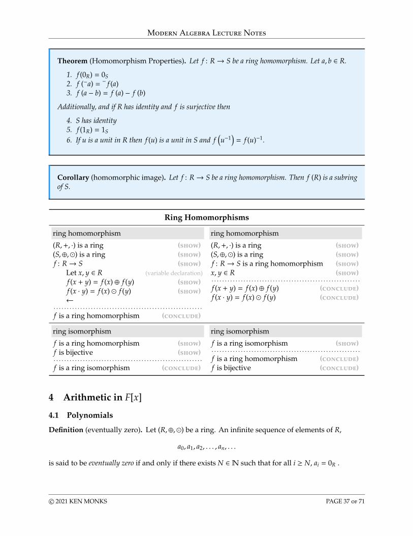
Theorem (Homomorphism Properties). Let f : R→ S be a ring homomorphism. Let a, b ∈ R.
1. f (0R) = 0S2. f (−a) = − f (a)3. f (a − b) = f (a) − f (b)
Additionally, and if R has identity and f is surjective then
4. S has identity5. f (1R) = 1S
6. If u is a unit in R then f (u) is a unit in S and f(u−1)= f (u)−1.
Corollary (homomorphic image). Let f : R→ S be a ring homomorphism. Then f (R) is a subringof S.
Ring Homomorphisms
ring homomorphism ring homomorphism
(R,+, ·) is a ring (show)(S,⊕,�) is a ring (show)f : R→ S (show)
Let x, y ∈ R (variable declaration)f (x + y) = f (x) ⊕ f (y) (show)f (x · y) = f (x) � f (y) (show)←
. . . . . . . . . . . . . . . . . . . . . . . . . . . . . . . . . . . . . . . . . . . . . . . . . . . . . . . .f is a ring homomorphism (conclude)
(R,+, ·) is a ring (show)(S,⊕,�) is a ring (show)f : R→ S is a ring homomorphism (show)x, y ∈ R (show). . . . . . . . . . . . . . . . . . . . . . . . . . . . . . . . . . . . . . . . . . . . . . . . . . . . . . . .f (x + y) = f (x) ⊕ f (y) (conclude)f (x · y) = f (x) � f (y) (conclude)
ring isomorphism ring isomorphism
f is a ring homomorphism (show)f is bijective (show). . . . . . . . . . . . . . . . . . . . . . . . . . . . . . . . . . . . . . . . . . . . . . . . . . . . . . . .f is a ring isomorphism (conclude)
f is a ring isomorphism (show). . . . . . . . . . . . . . . . . . . . . . . . . . . . . . . . . . . . . . . . . . . . . . . . . . . . . . . .f is a ring homomorphism (conclude)f is bijective (conclude)
4 Arithmetic in F[x]
4.1 Polynomials
Definition (eventually zero). Let (R,⊕,�) be a ring. An infinite sequence of elements of R,
a0, a1, a2, . . . , an, . . .
is said to be eventually zero if and only if there exists N ∈N such that for all i ≥ N, ai = 0R .
c© 2021 KEN MONKS PAGE 37 of 71
Modern Algebra Lecture Notes
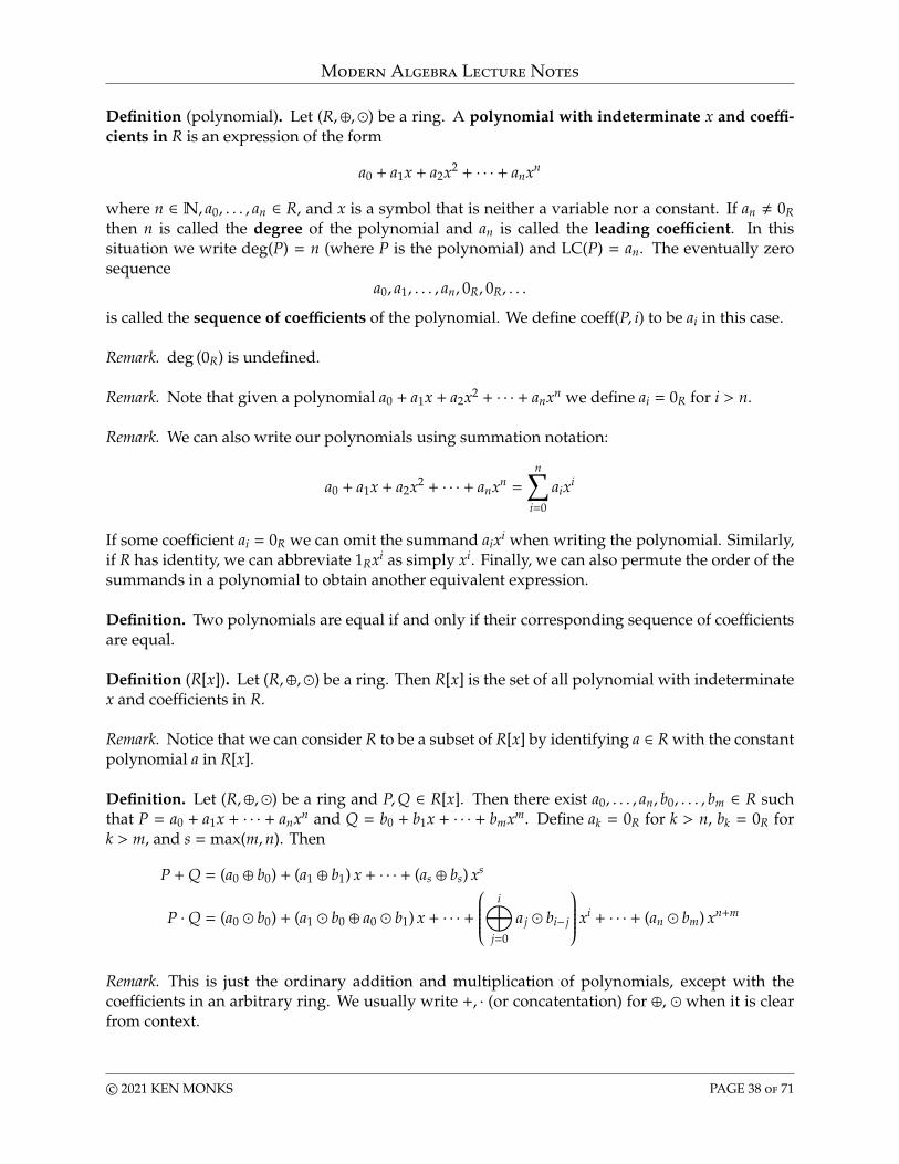
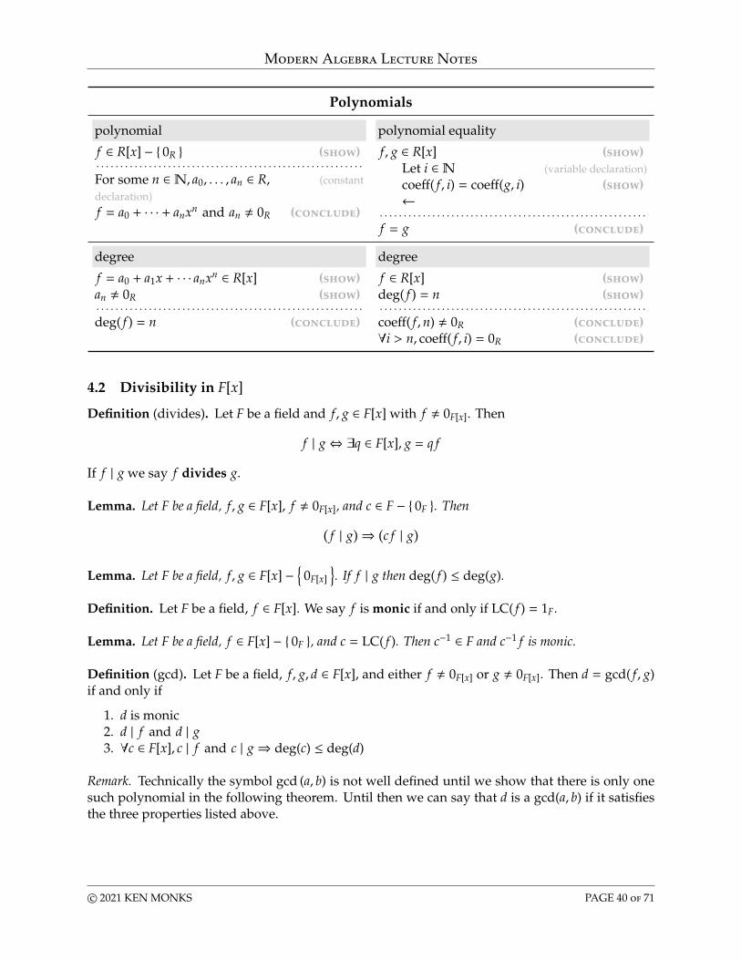
Definition (polynomial). Let (R,⊕,�) be a ring. A polynomial with indeterminate x and coeffi-cients in R is an expression of the form
a0 + a1x + a2x2 + · · · + anxn
where n ∈ N, a0, . . . , an ∈ R, and x is a symbol that is neither a variable nor a constant. If an , 0Rthen n is called the degree of the polynomial and an is called the leading coefficient. In thissituation we write deg(P) = n (where P is the polynomial) and LC(P) = an. The eventually zerosequence
a0, a1, . . . , an, 0R, 0R, . . .
is called the sequence of coefficients of the polynomial. We define coeff(P, i) to be ai in this case.
Remark. deg (0R) is undefined.
Remark. Note that given a polynomial a0 + a1x + a2x2 + · · · + anxn we define ai = 0R for i > n.
Remark. We can also write our polynomials using summation notation:
a0 + a1x + a2x2 + · · · + anxn =
n∑i=0
aixi
If some coefficient ai = 0R we can omit the summand aixi when writing the polynomial. Similarly,if R has identity, we can abbreviate 1Rxi as simply xi. Finally, we can also permute the order of thesummands in a polynomial to obtain another equivalent expression.
Definition. Two polynomials are equal if and only if their corresponding sequence of coefficientsare equal.
Definition (R[x]). Let (R,⊕,�) be a ring. Then R[x] is the set of all polynomial with indeterminatex and coefficients in R.
Remark. Notice that we can consider R to be a subset of R[x] by identifying a ∈ R with the constantpolynomial a in R[x].
Definition. Let (R,⊕,�) be a ring and P,Q ∈ R[x]. Then there exist a0, . . . , an, b0, . . . , bm ∈ R suchthat P = a0 + a1x + · · · + anxn and Q = b0 + b1x + · · · + bmxm. Define ak = 0R for k > n, bk = 0R fork > m, and s = max(m,n). Then
P +Q = (a0 ⊕ b0) + (a1 ⊕ b1) x + · · · + (as ⊕ bs) xs
P ·Q = (a0 � b0) + (a1 � b0 ⊕ a0 � b1) x + · · · + i⊕
j=0
a j � bi− j
xi + · · · + (an � bm) xn+m
Remark. This is just the ordinary addition and multiplication of polynomials, except with thecoefficients in an arbitrary ring. We usually write +, · (or concatentation) for ⊕, � when it is clearfrom context.
c© 2021 KEN MONKS PAGE 38 of 71
Modern Algebra Lecture Notes
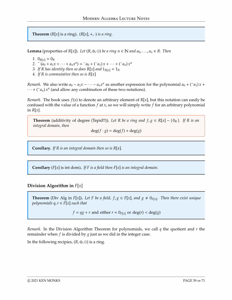
Theorem (R[x] is a ring). (R[x],+, ·) is a ring.
Lemma (properties of R[x]). Let (R,⊕,�) be a ring n ∈N and a0, . . . , an ∈ R. Then
1. 0R[x] = 0R2. − (a0 + a1x + · · · + anxn) = −a0 + (−a1) x + · · · + (−an) xn
3. If R has identity then so does R[x] and 1R[x] = 1R4. If R is commutative then so is R[x]
Remark. We also write a0 − a1x − · · · − anxn as another expression for the polynomial a0 + (−a1) x +· · · + (−an) xn (and allow any combination of these two notations).
Remark. The book uses f (x) to denote an arbitrary element of R[x], but this notation can easily beconfused with the value of a function f at x, so we will simply write f for an arbitrary polynomialin R[x].
Theorem (additivity of degree (Tepid!!)). Let R be a ring and f , g ∈ R[x] − { 0R }. If R is anintegral domain, then
deg( f · g) = deg( f ) + deg(g)
Corollary. If R is an integral domain then so is R[x].
Corollary (F[x] is int dom). If F is a field then F[x] is an integral domain.
Division Algorithm in F[x]
Theorem (Div Alg in F[x]). Let F be a field, f , g ∈ F[x], and g , 0F[x]. Then there exist uniquepolynomials q, r ∈ F[x] such that
f = qg + r and either r = 0F[x] or deg(r) < deg(g)
Remark. In the Division Algorithm Theorem for polynomials, we call q the quotient and r theremainder when f is divided by g just as we did in the integer case.
In the following recipies, (R,⊕,�) is a ring.
c© 2021 KEN MONKS PAGE 39 of 71
Modern Algebra Lecture Notes
Polynomials
polynomial polynomial equality
f ∈ R[x] − { 0R } (show). . . . . . . . . . . . . . . . . . . . . . . . . . . . . . . . . . . . . . . . . . . . . . . . . . . . . . . .For some n ∈N, a0, . . . , an ∈ R, (constantdeclaration)f = a0 + · · · + anxn and an , 0R (conclude)
f , g ∈ R[x] (show)Let i ∈N (variable declaration)coeff( f , i) = coeff(g, i) (show)←
. . . . . . . . . . . . . . . . . . . . . . . . . . . . . . . . . . . . . . . . . . . . . . . . . . . . . . . .f = g (conclude)
degree degree
f = a0 + a1x + · · · anxn ∈ R[x] (show)an , 0R (show). . . . . . . . . . . . . . . . . . . . . . . . . . . . . . . . . . . . . . . . . . . . . . . . . . . . . . . .deg( f ) = n (conclude)
f ∈ R[x] (show)deg( f ) = n (show). . . . . . . . . . . . . . . . . . . . . . . . . . . . . . . . . . . . . . . . . . . . . . . . . . . . . . . .coeff( f ,n) , 0R (conclude)∀i > n, coeff( f , i) = 0R (conclude)
4.2 Divisibility in F[x]
Definition (divides). Let F be a field and f , g ∈ F[x] with f , 0F[x]. Then
f | g⇔ ∃q ∈ F[x], g = q f
If f | g we say f divides g.
Lemma. Let F be a field, f , g ∈ F[x], f , 0F[x], and c ∈ F − { 0F }. Then(f | g)⇒ (c f | g)
Lemma. Let F be a field, f , g ∈ F[x] −{
0F[x]
}. If f | g then deg( f ) ≤ deg(g).
Definition. Let F be a field, f ∈ F[x]. We say f is monic if and only if LC( f ) = 1F.
Lemma. Let F be a field, f ∈ F[x] − { 0F }, and c = LC( f ). Then c−1 ∈ F and c−1 f is monic.
Definition (gcd). Let F be a field, f , g, d ∈ F[x], and either f , 0F[x] or g , 0F[x]. Then d = gcd( f , g)if and only if
1. d is monic2. d | f and d | g3. ∀c ∈ F[x], c | f and c | g⇒ deg(c) ≤ deg(d)
Remark. Technically the symbol gcd (a, b) is not well defined until we show that there is only onesuch polynomial in the following theorem. Until then we can say that d is a gcd(a, b) if it satisfiesthe three properties listed above.
c© 2021 KEN MONKS PAGE 40 of 71
Modern Algebra Lecture Notes
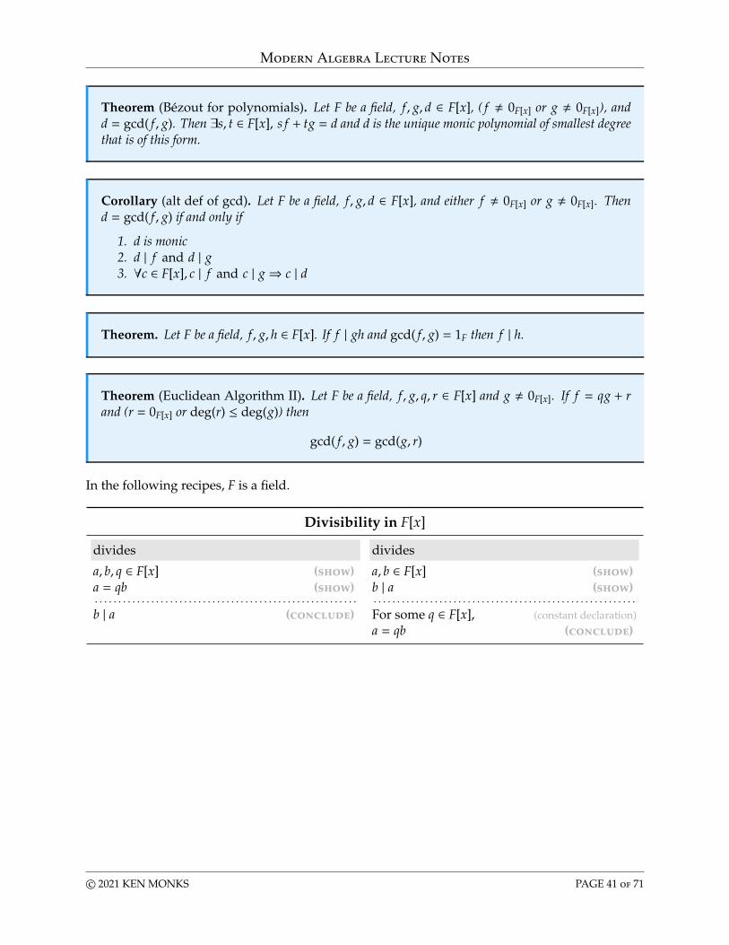
Theorem (Bézout for polynomials). Let F be a field, f , g, d ∈ F[x], ( f , 0F[x] or g , 0F[x]), andd = gcd( f , g). Then ∃s, t ∈ F[x], s f + tg = d and d is the unique monic polynomial of smallest degreethat is of this form.
Corollary (alt def of gcd). Let F be a field, f , g, d ∈ F[x], and either f , 0F[x] or g , 0F[x]. Thend = gcd( f , g) if and only if
1. d is monic2. d | f and d | g3. ∀c ∈ F[x], c | f and c | g⇒ c | d
Theorem. Let F be a field, f , g, h ∈ F[x]. If f | gh and gcd( f , g) = 1F then f | h.
Theorem (Euclidean Algorithm II). Let F be a field, f , g, q, r ∈ F[x] and g , 0F[x]. If f = qg + rand (r = 0F[x] or deg(r) ≤ deg(g)) then
gcd( f , g) = gcd(g, r)
In the following recipes, F is a field.
Divisibility in F[x]
divides divides
a, b, q ∈ F[x] (show)a = qb (show). . . . . . . . . . . . . . . . . . . . . . . . . . . . . . . . . . . . . . . . . . . . . . . . . . . . . . . .b | a (conclude)
a, b ∈ F[x] (show)b | a (show). . . . . . . . . . . . . . . . . . . . . . . . . . . . . . . . . . . . . . . . . . . . . . . . . . . . . . . .For some q ∈ F[x], (constant declaration)a = qb (conclude)
c© 2021 KEN MONKS PAGE 41 of 71
Modern Algebra Lecture Notes
Divisibility in F[x] (cont.)
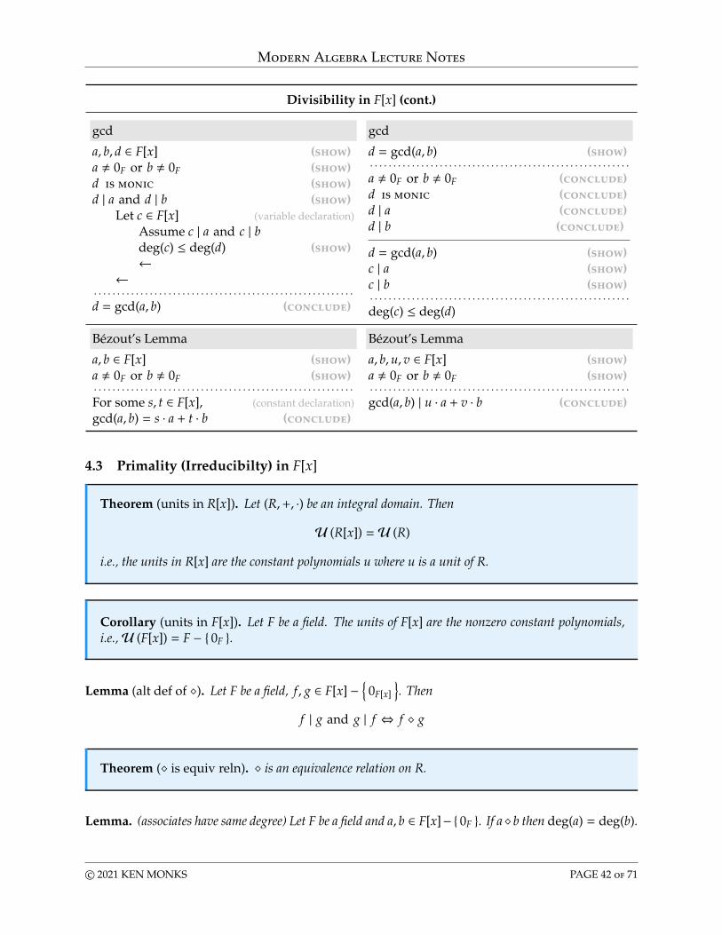
gcd gcd
a, b, d ∈ F[x] (show)a , 0F or b , 0F (show)d is monic (show)d | a and d | b (show)
Let c ∈ F[x] (variable declaration)Assume c | a and c | bdeg(c) ≤ deg(d) (show)←
←. . . . . . . . . . . . . . . . . . . . . . . . . . . . . . . . . . . . . . . . . . . . . . . . . . . . . . . .d = gcd(a, b) (conclude)
d = gcd(a, b) (show). . . . . . . . . . . . . . . . . . . . . . . . . . . . . . . . . . . . . . . . . . . . . . . . . . . . . . . .a , 0F or b , 0F (conclude)d is monic (conclude)d | a (conclude)d | b (conclude)
d = gcd(a, b) (show)c | a (show)c | b (show). . . . . . . . . . . . . . . . . . . . . . . . . . . . . . . . . . . . . . . . . . . . . . . . . . . . . . . .deg(c) ≤ deg(d)
Bézout’s Lemma Bézout’s Lemma
a, b ∈ F[x] (show)a , 0F or b , 0F (show). . . . . . . . . . . . . . . . . . . . . . . . . . . . . . . . . . . . . . . . . . . . . . . . . . . . . . . .For some s, t ∈ F[x], (constant declaration)gcd(a, b) = s · a + t · b (conclude)
a, b,u, v ∈ F[x] (show)a , 0F or b , 0F (show). . . . . . . . . . . . . . . . . . . . . . . . . . . . . . . . . . . . . . . . . . . . . . . . . . . . . . . .gcd(a, b) | u · a + v · b (conclude)
4.3 Primality (Irreducibilty) in F[x]
Theorem (units in R[x]). Let (R,+, ·) be an integral domain. Then
U (R[x]) =U (R)
i.e., the units in R[x] are the constant polynomials u where u is a unit of R.
Corollary (units in F[x]). Let F be a field. The units of F[x] are the nonzero constant polynomials,i.e.,U (F[x]) = F − { 0F }.
Lemma (alt def of �). Let F be a field, f , g ∈ F[x] −{
0F[x]
}. Then
f | g and g | f ⇔ f � g
Theorem (� is equiv reln). � is an equivalence relation on R.
Lemma. (associates have same degree) Let F be a field and a, b ∈ F[x]−{ 0F }. If a� b then deg(a) = deg(b).
c© 2021 KEN MONKS PAGE 42 of 71
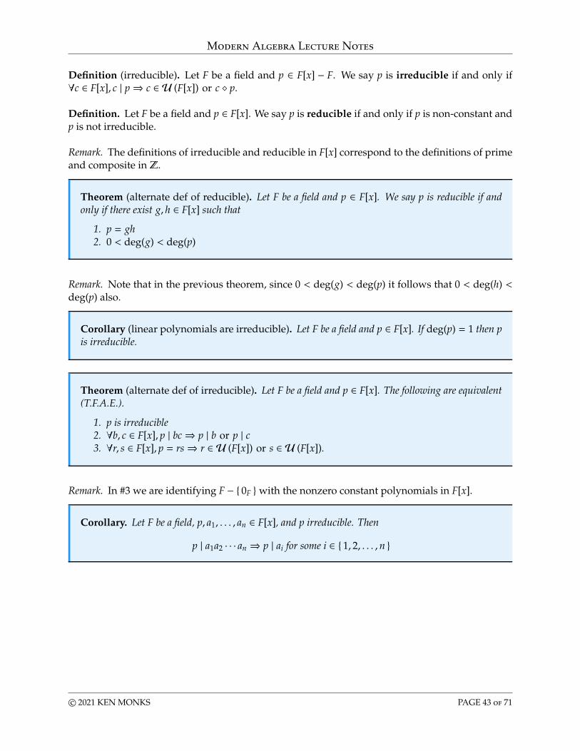
Modern Algebra Lecture Notes
Definition (irreducible). Let F be a field and p ∈ F[x] − F. We say p is irreducible if and only if∀c ∈ F[x], c | p⇒ c ∈ U (F[x]) or c � p.
Definition. Let F be a field and p ∈ F[x]. We say p is reducible if and only if p is non-constant andp is not irreducible.
Remark. The definitions of irreducible and reducible in F[x] correspond to the definitions of primeand composite in Z.
Theorem (alternate def of reducible). Let F be a field and p ∈ F[x]. We say p is reducible if andonly if there exist g, h ∈ F[x] such that
1. p = gh2. 0 < deg(g) < deg(p)
Remark. Note that in the previous theorem, since 0 < deg(g) < deg(p) it follows that 0 < deg(h) <deg(p) also.
Corollary (linear polynomials are irreducible). Let F be a field and p ∈ F[x]. If deg(p) = 1 then pis irreducible.
Theorem (alternate def of irreducible). Let F be a field and p ∈ F[x]. The following are equivalent(T.F.A.E.).
1. p is irreducible2. ∀b, c ∈ F[x], p | bc⇒ p | b or p | c3. ∀r, s ∈ F[x], p = rs⇒ r ∈ U (F[x]) or s ∈ U (F[x]).
Remark. In #3 we are identifying F − { 0F }with the nonzero constant polynomials in F[x].
Corollary. Let F be a field, p, a1, . . . , an ∈ F[x], and p irreducible. Then
p | a1a2 · · · an ⇒ p | ai for some i ∈ { 1, 2, . . . , n }
c© 2021 KEN MONKS PAGE 43 of 71
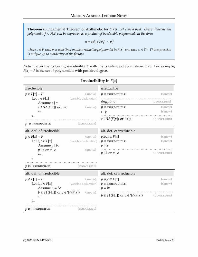
Modern Algebra Lecture Notes
Theorem (Fundamental Theorem of Arithmetic for F[x]). Let F be a field. Every nonconstantpolynomial f ∈ F[x] can be expressed as a product of irreducible polynomials in the form
n = cpe11 pe2
2 pe33 · · · p
ekk
where c ∈ F, each pi is a distinct monic irreducible polynomial in F[x], and each ei ∈N. This expressionis unique up to reordering of the factors.
Note that in the following we identify F with the constant polynomials in F[x]. For example,F[x] − F is the set of polynomials with positive degree.
Irreducibility in F[x]
irreducible irreducible
p ∈ F[x] − F (show)Let c ∈ F[x] (variable declaration)
Assume c | pc ∈ U (F[x]) or c � p (show)←
←. . . . . . . . . . . . . . . . . . . . . . . . . . . . . . . . . . . . . . . . . . . . . . . . . . . . . . . .p is irreducible (conclude)
p is irreducible (show). . . . . . . . . . . . . . . . . . . . . . . . . . . . . . . . . . . . . . . . . . . . . . . . . . . . . . . .deg p > 0 (conclude)
p is irreducible (show)c | p (show). . . . . . . . . . . . . . . . . . . . . . . . . . . . . . . . . . . . . . . . . . . . . . . . . . . . . . . .c ∈ U (F[x]) or c � p (conclude)
alt. def. of irreducible alt. def. of irreducible
p ∈ F[x] − F (show)Let b, c ∈ F[x] (variable declaration)
Assume p | bcp | b or p | c (show)←
←. . . . . . . . . . . . . . . . . . . . . . . . . . . . . . . . . . . . . . . . . . . . . . . . . . . . . . . .p is irreducible (conclude)
p, b, c ∈ F[x] (show)p is irreducible (show)p | bc. . . . . . . . . . . . . . . . . . . . . . . . . . . . . . . . . . . . . . . . . . . . . . . . . . . . . . . .p | b or p | c (conclude)
alt. def. of irreducible alt. def. of irreducible
p ∈ F[x] − F (show)Let b, c ∈ F[x] (variable declaration)
Assume p = bcb ∈ U (F[x]) or c ∈ U (F[x]) (show)←
←. . . . . . . . . . . . . . . . . . . . . . . . . . . . . . . . . . . . . . . . . . . . . . . . . . . . . . . .p is irreducible (conclude)
p, b, c ∈ F[x] (show)p is irreducible (show)p = bc. . . . . . . . . . . . . . . . . . . . . . . . . . . . . . . . . . . . . . . . . . . . . . . . . . . . . . . .b ∈ U (F[x]) or c ∈ U (F[x]) (conclude)
c© 2021 KEN MONKS PAGE 44 of 71
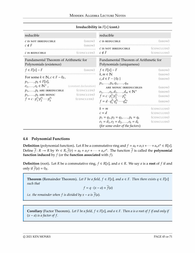
Modern Algebra Lecture Notes
Irreducibility in F[x] (cont.)
reducible reducible
c is not irreducible (show)c < F (show). . . . . . . . . . . . . . . . . . . . . . . . . . . . . . . . . . . . . . . . . . . . . . . . . . . . . . . .c is reducible (conclude)
c is reducible (show). . . . . . . . . . . . . . . . . . . . . . . . . . . . . . . . . . . . . . . . . . . . . . . . . . . . . . . .c is not irreducible (conclude)c < F (conclude)
Fundamental Theorem of Arithmetic forPolynomials (existence)
Fundamental Theorem of Arithmetic forPolynomials (uniqueness)
f ∈ F[x] − F (show). . . . . . . . . . . . . . . . . . . . . . . . . . . . . . . . . . . . . . . . . . . . . . . . . . . . . . . .For some k ∈N, c ∈ F − 0F,p1, . . . , pk ∈ F[x],e1, . . . , ek ∈N+ , (constant declaration)p1, . . . , pk are irreducible (conclude)p1, . . . , pk are monic (conclude)f = c · pe1
1 pe22 · · · p
ekk (conclude)
f ∈ F[x] − F (show)k,m ∈N (show)c, d ∈ F − { 0F } (show)p1, . . . , pk, q1, . . . , qmare monic irreducibles (show)
e1, . . . , ek, d1, . . . , dm ∈N+ (show)f = c · pe1
1 pe22 · · · p
ekk (show)
f = d · qd11 qd2
2 · · · qdmm (show)
. . . . . . . . . . . . . . . . . . . . . . . . . . . . . . . . . . . . . . . . . . . . . . . . . . . . . . . .k = m (conclude)c = d (conclude)p1 = q1, p2 = q2, . . . , pk = qk (conclude)e1 = d1, e2 = d2, . . . , ek = dk (conclude)(for some order of the factors)
4.4 Polynomial Functions
Definition (polynomial function). Let R be a commutative ring and f = a0 + a1x+ · · ·+ anxn ∈ R[x].Define f : R → R by ∀r ∈ R, f (r) = a0 + a1r + · · · + anrn. The function f is called the polynomialfunction induced by f (or the function associated with f ).
Definition (root). Let R be a commutative ring, f ∈ R[x], and a ∈ R. We say a is a root of f if andonly if f (a) = 0R.
Theorem (Remainder Theorem). Let F be a field, f ∈ F[x], and a ∈ F. Then there exists q ∈ F[x]such that
f = q · (x − a) + f (a)
i.e. the remainder when f is divided by x − a is f (a).
Corollary (Factor Theorem). Let F be a field, f ∈ F[x], and a ∈ F. Then a is a root of f if and only if(x − a) is a factor of f .
c© 2021 KEN MONKS PAGE 45 of 71
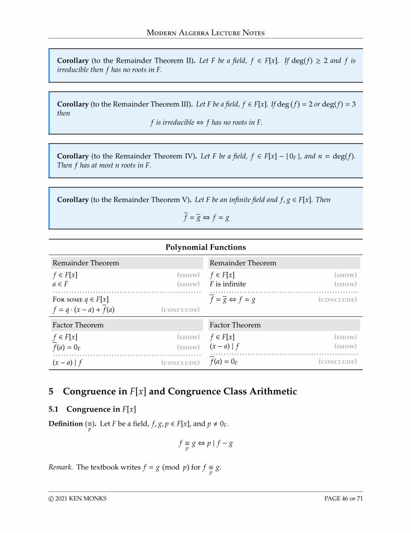
Modern Algebra Lecture Notes
Corollary (to the Remainder Theorem II). Let F be a field, f ∈ F[x]. If deg( f ) ≥ 2 and f isirreducible then f has no roots in F.
Corollary (to the Remainder Theorem III). Let F be a field, f ∈ F[x]. If deg(
f)= 2 or deg( f ) = 3
thenf is irreducible⇔ f has no roots in F.
Corollary (to the Remainder Theorem IV). Let F be a field, f ∈ F[x] − { 0F }, and n = deg( f ).Then f has at most n roots in F.
Corollary (to the Remainder Theorem V). Let F be an infinite field and f , g ∈ F[x]. Then
f = g⇔ f = g
Polynomial Functions
Remainder Theorem Remainder Theorem
f ∈ F[x] (show)a ∈ F (show). . . . . . . . . . . . . . . . . . . . . . . . . . . . . . . . . . . . . . . . . . . . . . . . . . . . . . . .For some q ∈ F[x]f = q · (x − a) + f (a) (conclude)
f ∈ F[x] (show)F is infinite (show). . . . . . . . . . . . . . . . . . . . . . . . . . . . . . . . . . . . . . . . . . . . . . . . . . . . . . . .f = g⇔ f = g (conclude)
Factor Theorem Factor Theorem
f ∈ F[x] (show)f (a) = 0F (show). . . . . . . . . . . . . . . . . . . . . . . . . . . . . . . . . . . . . . . . . . . . . . . . . . . . . . . .(x − a) | f (conclude)
f ∈ F[x] (show)(x − a) | f (show). . . . . . . . . . . . . . . . . . . . . . . . . . . . . . . . . . . . . . . . . . . . . . . . . . . . . . . .f (a) = 0F (conclude)
5 Congruence in F[x] and Congruence Class Arithmetic
5.1 Congruence in F[x]
Definition (≡p
). Let F be a field, f , g, p ∈ F[x], and p , 0F.
f ≡p
g⇔ p | f − g
Remark. The textbook writes f = g(mod p
)for f ≡
pg.
c© 2021 KEN MONKS PAGE 46 of 71
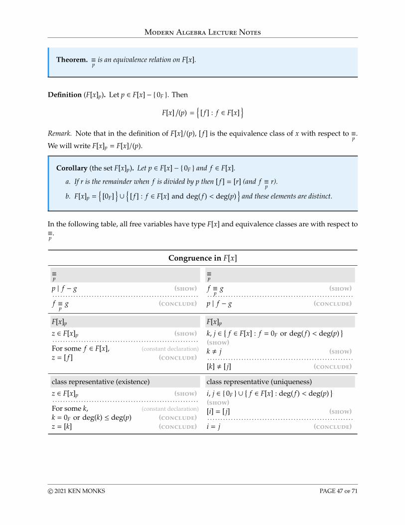
Modern Algebra Lecture Notes
Theorem. ≡p
is an equivalence relation on F[x].
Definition (F[x]p). Let p ∈ F[x] − { 0F }. Then
F[x]/(p) =
{[ f ] : f ∈ F[x]
}Remark. Note that in the definition of F[x]/(p), [ f ] is the equivalence class of x with respect to ≡
p.
We will write F[x]p = F[x]/(p).
Corollary (the set F[x]p). Let p ∈ F[x] − { 0F } and f ∈ F[x].
a. If r is the remainder when f is divided by p then [ f ] = [r] (and f ≡p
r).
b. F[x]p ={
[0F]}∪{
[ f ] : f ∈ F[x] and deg( f ) < deg(p)}
and these elements are distinct.
In the following table, all free variables have type F[x] and equivalence classes are with respect to≡p
.
Congruence in F[x]
≡p
≡p
p | f − g (show). . . . . . . . . . . . . . . . . . . . . . . . . . . . . . . . . . . . . . . . . . . . . . . . . . . . . . . .f ≡
pg (conclude)
f ≡p
g (show). . . . . . . . . . . . . . . . . . . . . . . . . . . . . . . . . . . . . . . . . . . . . . . . . . . . . . . .p | f − g (conclude)
F[x]p F[x]p
z ∈ F[x]p (show). . . . . . . . . . . . . . . . . . . . . . . . . . . . . . . . . . . . . . . . . . . . . . . . . . . . . . . .For some f ∈ F[x], (constant declaration)z = [ f ] (conclude)
k, j ∈ { f ∈ F[x] : f = 0F or deg( f ) < deg(p)}
(show)k , j (show). . . . . . . . . . . . . . . . . . . . . . . . . . . . . . . . . . . . . . . . . . . . . . . . . . . . . . . .[k] , [ j] (conclude)
class representative (existence) class representative (uniqueness)
z ∈ F[x]p (show). . . . . . . . . . . . . . . . . . . . . . . . . . . . . . . . . . . . . . . . . . . . . . . . . . . . . . . .For some k, (constant declaration)k = 0F or deg(k) ≤ deg(p) (conclude)z = [k] (conclude)
i, j ∈ { 0F } ∪{
f ∈ F[x] : deg( f ) < deg(p)}
(show)[i] = [ j] (show). . . . . . . . . . . . . . . . . . . . . . . . . . . . . . . . . . . . . . . . . . . . . . . . . . . . . . . .i = j (conclude)
c© 2021 KEN MONKS PAGE 47 of 71
Modern Algebra Lecture Notes
5.2 Arithmetic in F[x]p
Theorem (polynomial modular arithmetic). Let F be a field, f , g, h, i, p ∈ F[x], and deg(p) > 0. Iff ≡
ph and g ≡
pi then
f + g ≡p
h + i
andf · g ≡
ph · i
Definition. Let F be a field, f , q, r, p ∈ F[x], and deg(p) > 0. If f = pq + r, and either r = 0F ordeg(r) < deg(p)) then we define
f Mod p = r
Definition. Let F be a field, p ∈ F[x], and deg(p) > 0.
⊕ ={
((A,B),C) : ∃ f , g ∈ F[x],A = [ f ],B = [g] and C = [ f + g]}
� ={
((A,B),C) : ∃ f , g ∈ F[x],A = [ f ],B = [g] and C = [ f · g]}
(where the equivalence classes are with respect to ≡p
).
Theorem. ⊕, � are binary operators on F[x]p.
Remark. This theorem allows us to use infix notation to write the definitions more conveniently inthis form: [
f] ⊕ [g] = [ f + g
][f] � [g] = [ f · g]
Theorem (F[x]p is a ring). Let F be a field, p ∈ F[x], and deg(p) > 0. Then(F[x]p,⊕,�
)is a
commutative ring with identity, and 1F[x]p = [1F].
Notation. As in Zn, we will often abbreviate [ f ] ∈ F[x]p as f . We will also often abbreviate ⊕ as +and � as ×, ·, or concatenation.
Theorem (F is a subring of F[x]p). Let F be a field, p ∈ F[x], deg(p) > 0, and define
F∗ = { [c] : c ∈ F }
Then F∗ is a subring of F[x]p which is isomorphic to F.
c© 2021 KEN MONKS PAGE 48 of 71
Modern Algebra Lecture Notes
Remark. We often identify c ∈ F with [c] ∈ F[x]p and simply say that F is a subring of F[x]p.
Theorem (units in F[x]p). Let F be a field, p, f ∈ F[x], deg(p) > 0. Then
[ f ] ∈ U(F[x]p
)⇔ gcd( f , p) = 1F
Arithmetic in F[x]p
modular arithmetic modular arithmetic
a, b, c, d, p ∈ F[x] (show)a ≡
pb (show)
c ≡p
d (show). . . . . . . . . . . . . . . . . . . . . . . . . . . . . . . . . . . . . . . . . . . . . . . . . . . . . . . .a + c ≡
pb + d (conclude)
a · c ≡p
b · d (conclude)
a, b ∈ F[x] (show). . . . . . . . . . . . . . . . . . . . . . . . . . . . . . . . . . . . . . . . . . . . . . . . . . . . . . . .[a] ⊕ [b] = [a + b] (conclude)[a] � [b] = [a · b] (conclude)
5.3 Finite fields
Theorem (F[x]p for irreducible p). Let F be a field, p ∈ F[x], deg(p) > 0. The following areequivalent (T.F.A.E.).
1. p is irreducible.2. F[x]p is a field.3. F[x]p is an integral domain.
Definition. Let F be a field, p, f ∈ F[x], deg(p) > 0, n ∈N+, a0, . . . , an ∈ F, and f = a0+a1x+ · · ·+anxn.Define f : F[x]p → F[x]p by
∀r ∈ F[x]p, f (r) = [a0] + [a1] r + · · · + [an] rn
Remark. If we identify F with F∗ ⊆ F[x]p, then this function f is just an extension of our originalfunction f from F to F[x]p.
Theorem (extension field). Let F be a field, p ∈ F[x], and p irreducible. Then F[x]p is an extensionfield of F which contains a root of p.
c© 2021 KEN MONKS PAGE 49 of 71
Modern Algebra Lecture Notes
Corollary (existence of extension fields). Let F be a field, f ∈ F[x], and deg(p) > 0. There existsan extension field K of F containing a root of f .
6 Ideals and Quotient Rings
6.1 Congruence in Rings
Definition (ideal). Let R be a ring and I ⊆ R. Then I is an ideal of R if and only if
1. I is a subring of R2. ∀r ∈ R,∀a ∈ I, ra ∈ I and ar ∈ I
Theorem (ideal generated by c1, . . . , cn ∈ R). Let R be a commutative ring with identity andc1, . . . , cn ∈ R. The set
I = { r1c1 + r2c2 + · · · + rncn : r1, . . . , rn ∈ R }is an ideal of R.
Definition (principle and finitely generated ideals). The ideal I in the previous theorem is calledthe ideal generated by { c1, . . . , cn }. If n = 1 then I is called a principal ideal. Since { c1, . . . , cn } is afinite set, we say that I is finitely generated.
Definition (congruence modulo ideals). Let R be a ring, a, b ∈ R, and I an ideal of R.
a ≡I
b⇔ a − b ∈ I
Remark. The textbook writes a = b (mod I) for a ≡I
b.
Theorem. ≡I
is an equivalence relation on R.
Definition (R/I). Let R be a ring and I and ideal of R. Then
R/I ={
[r] : r ∈ R}
Remark. Note that in the definition of R/I, [r] is the equivalence class of r with respect to ≡I.
Theorem (equivalence class mod I). Let R be a ring, a ∈ R, and I an ideal of R. Then
[a] = { a + i : i ∈ I }
c© 2021 KEN MONKS PAGE 50 of 71
Modern Algebra Lecture Notes
Definition. Let R be a ring, a ∈ R, and I an ideal of R. The set
a + I = { a + i : i ∈ I } = [a]
is called the left coset of a mod I. The notation a + I is called coset notation for the equivalenceclass [a].
Remark. I hate coset notation.
Ideals and Quotient Rings
ideal ideal
I v R (show)Let r ∈ R and a ∈ I (variable declaration)ra ∈ I (show)ar ∈ I (show)←
. . . . . . . . . . . . . . . . . . . . . . . . . . . . . . . . . . . . . . . . . . . . . . . . . . . . . . . .I is an ideal of ring R (conclude)
I is an ideal of ring R (show). . . . . . . . . . . . . . . . . . . . . . . . . . . . . . . . . . . . . . . . . . . . . . . . . . . . . . . .I v R (conclude)I is an ideal of ring R (show)a ∈ I (show)r ∈ R (show). . . . . . . . . . . . . . . . . . . . . . . . . . . . . . . . . . . . . . . . . . . . . . . . . . . . . . . .ar ∈ I (conclude)ra ∈ I (conclude)
congruence mod an ideal congruence mod an ideal
I an ideal of ring R (show)a, b ∈ R (show)a − b ∈ I (show). . . . . . . . . . . . . . . . . . . . . . . . . . . . . . . . . . . . . . . . . . . . . . . . . . . . . . . .a ≡
Ib (conclude)
I an ideal of ring R (show)a, b ∈ R (show)a ≡
Ib (show)
. . . . . . . . . . . . . . . . . . . . . . . . . . . . . . . . . . . . . . . . . . . . . . . . . . . . . . . .a − b ∈ I (conclude)
6.2 Arithmetic in R/I
Theorem (modular arithmetic in R/I). Let R be a ring, a, b, c, d ∈ R, and I an ideal of R. If a ≡I
b
and c ≡I
d then
a + c ≡I
b + d
andac ≡
Ibd
Definition. Let R be a ring and I an ideal of R. Define
⊕ ={
((A,B),C) : ∃a, b ∈ R, A = [a], B = [b], and C = [a + b]}
� ={
((A,B),C) : ∃a, b ∈ R, A = [a], B = [b], and C = [a · b]}
(where the equivalence classes are with respect to ≡I).
c© 2021 KEN MONKS PAGE 51 of 71
Modern Algebra Lecture Notes
Theorem. ⊕,� are binary operators on R/I.
Remark. This theorem allows us to use infix notation to write the definitions more conveniently inthis form:
[a] ⊕ [b] = [a + b][a] � [b] = [a · b]
or equivalently in left coset notation:
(a + I) ⊕ (b + I) = (a + b) + I(a + I) � (b + I) = ab + I
Theorem (R/I is a ring). Let R be a ring and I an ideal of R. Then (R/I,⊕,�) is a ring.
Definition (quotient ring). Let R be a ring and I an ideal of R. Then (R/I,⊕,�) is called a quotientring.
Theorem (properties of quotient rings). Let R be a ring and I an ideal of R.
1. If R is commutative then so is R/I.
2. If R has identity then so does R/I and 1R/I = [1R]
Notation. As in Zn, and F[x]p we will often abbreviate [a] as a. We will also often abbreviate ⊕ as+ and � as ×, ·, or concatentation.
Homomorphisms and Quotient Rings
Definition (kernel). Let f : R→ S be a ring homomorphism. The kernel of f is the set
Ker( f ) ={
x ∈ R : f (x) = 0S}
Theorem (Ker is an ideal). Let f : R→ S be a ring homomorphism. Ker( f ) is an ideal of R.
Theorem (injectivity vs Kernel). Let f : R→ S be a ring homomorphism.
f is injective⇔ Ker( f ) = { 0R }
c© 2021 KEN MONKS PAGE 52 of 71
Modern Algebra Lecture Notes
Definition (quotient map). Let R be a ring, I an ideal of R, and define f : R→ R/I by ∀r ∈ R, f (r) =[r]. The map f is called the quotient map (or natural homomorphism).
Theorem. A quotient map is a surjective ring homomorphism.
Theorem (First Isomorphism Thm). Let f : R→ S be a surjective ring homomorphism. Then
S � R/Ker( f )
Arithmetic in Quotient Rings
Kernel Kernel
f : R→ S a ring homomorphism (show)a ∈ Ker f (show). . . . . . . . . . . . . . . . . . . . . . . . . . . . . . . . . . . . . . . . . . . . . . . . . . . . . . . .f (a) = 0R (conclude)
f : R→ S a ring homomorphism (show)f (a) = 0R (show). . . . . . . . . . . . . . . . . . . . . . . . . . . . . . . . . . . . . . . . . . . . . . . . . . . . . . . .a ∈ Ker f (conclude)
Quotient Ring
f : R→ S a ring homomorphism (show)f is surjective (show). . . . . . . . . . . . . . . . . . . . . . . . . . . . . . . . . . . . . . . . . . . . . . . . . . . . . . . .S � R/Ker f (conclude)
7 Groups
7.1 Groups
Definition (group). Let G be a set and ∗ : G × G→ G a binary operator. The pair (G, ∗) is a groupif and only if
1. ∀a, b, c ∈ G, a ∗ (b ∗ c) = (a ∗ b) ∗ c (associative)2. ∃e ∈ G,∀a ∈ G, a ∗ e = a = e ∗ a (identity)3. ∀a ∈ G,∃d ∈ G, a ∗ d = e = d ∗ a (inverses)
Remark. We will often abbreviate abbreviate a ∗ b by ab. We will also often refer to the group (G, ∗)as simply G.
Remark. The e in condition #3 refers to any e satisfying condition #2, so technically it should bewritten
∀e ∈ G, (∀a ∈ G, a ∗ e = a = e ∗ a)⇒ (∀a ∈ G,∃d ∈ G, a ∗ d = e = d ∗ a)
c© 2021 KEN MONKS PAGE 53 of 71
Modern Algebra Lecture Notes
Types of Groups
Definition (abelian group). A group (G, ∗) is abelian if an only if ∀a, b ∈ G, a ∗ b = b ∗ a (i.e., ∗ iscommutative).
Definition (finite group). A group (G, ∗) is finite if and only if G is a finite set.
Definition (cardinality). If S is a finite set, the # (S) denotes the number of elements in the finiteset S. Two sets (finite or infinite) have the same cardinality if an only if there is a bijection betweenthem.
Remark. The book writes |S | for the number of elements in S, but we will use #(S).
Definition (order of a group). If (G, ∗) is a finite group then #(G) is called the order of the group.
Examples of Groups
Theorem (additive group of a ring). Let (R,+, ·) be a ring. Then (R,+) is a group.
Theorem (group of units in a ring). Let (R,+, ·) be a ring with identity. Then (U (R) , ·) is a group.
Corollary (group of units in a field). Let (F,+, ·) be a field. Then (F − { 0F } , ·) is a group.
Definition (permutation). Let T be a set. A permutation of T is a bijection f : T→ T.
Definition (In). Let n ∈N. Define In = { 1, 2, . . . , n }.
Definition (symmetric group). Let n ∈N+. Then
Sn ={α : α is a permutation of In
}i.e. Sn is the set of all permutations of In.
Theorem (symmetric group). The pair (Sn, ◦) is a group.
Notation (table notation). Let f ∈ Sn. We can describe f in table notation by defining
f =
1 2 · · · n
a1 a2 · · · an
⇔ ∀i ∈ In, f (i) = ai
c© 2021 KEN MONKS PAGE 54 of 71
Modern Algebra Lecture Notes
Theorem (cardinality of Sn). #(Sn) = n!
Definition (symmetry operation). Let X ⊆ Rn. A symmetry operation of X is a bijection f : X→ Xwhich preserves the distances between points, i.e., ∀a, b ∈ X, d(a, b) = d( f (a), f (b)).
Remark. Note: in geometry a symmetry operation is called an isometry.
Definition. Let X ⊆ Rn. Then
Sym(X) ={α : α is a symmetry operation of X
}i.e., Sym(X) is the set of all symmetry operations of X.
Theorem (group of symmetries). The pair (Sym(X), ◦) is a group.
Definition (dihedral group). Let Pn be a regular n-gon in R2. Define
Dn = Sym (Pn)
(Dn, ◦) is called a dihedral group.
Theorem (direct product). Let (G, ∗) and (H, ·) be groups and define � : (G×H)× (G×H)→ G×Hby
(a, b) � (c, d) = (a ∗ c, b · d)
for all (a, b), (c, d) ∈ G ×H. Then (G ×H,�) is a group.
Definition (direct product group). The group (G ×H,�) is called the direct product of the groupsG and H.
c© 2021 KEN MONKS PAGE 55 of 71
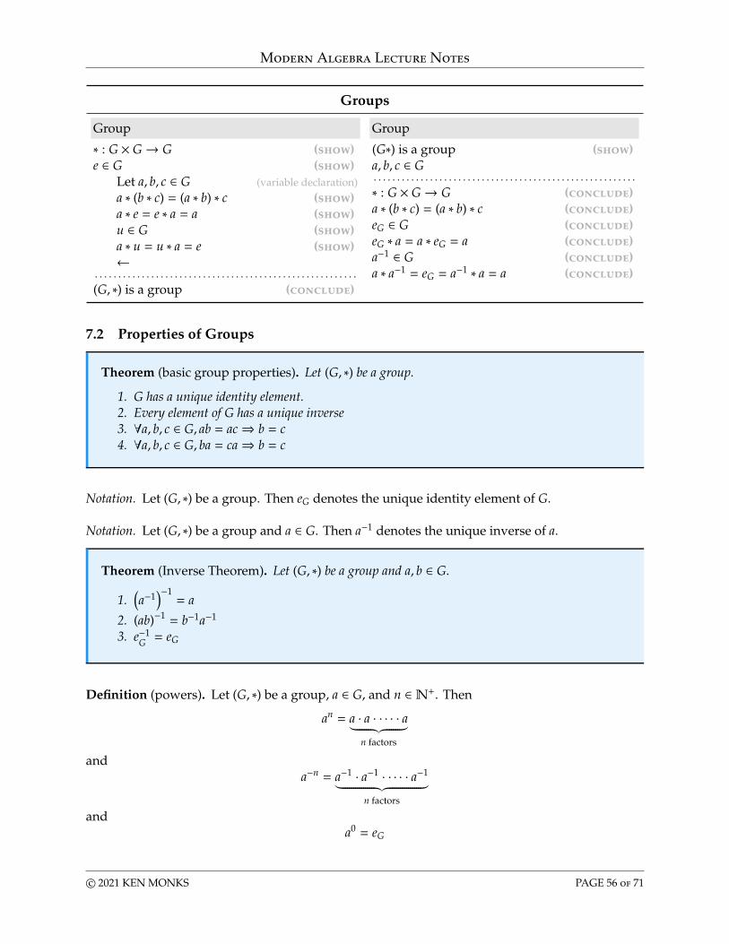
Modern Algebra Lecture Notes
Groups
Group Group
∗ : G × G→ G (show)e ∈ G (show)
Let a, b, c ∈ G (variable declaration)a ∗ (b ∗ c) = (a ∗ b) ∗ c (show)a ∗ e = e ∗ a = a (show)u ∈ G (show)a ∗ u = u ∗ a = e (show)←
. . . . . . . . . . . . . . . . . . . . . . . . . . . . . . . . . . . . . . . . . . . . . . . . . . . . . . . .(G, ∗) is a group (conclude)
(G∗) is a group (show)a, b, c ∈ G. . . . . . . . . . . . . . . . . . . . . . . . . . . . . . . . . . . . . . . . . . . . . . . . . . . . . . . .∗ : G × G→ G (conclude)a ∗ (b ∗ c) = (a ∗ b) ∗ c (conclude)eG ∈ G (conclude)eG ∗ a = a ∗ eG = a (conclude)a−1 ∈ G (conclude)a ∗ a−1 = eG = a−1 ∗ a = a (conclude)
7.2 Properties of Groups
Theorem (basic group properties). Let (G, ∗) be a group.
1. G has a unique identity element.2. Every element of G has a unique inverse3. ∀a, b, c ∈ G, ab = ac⇒ b = c4. ∀a, b, c ∈ G, ba = ca⇒ b = c
Notation. Let (G, ∗) be a group. Then eG denotes the unique identity element of G.
Notation. Let (G, ∗) be a group and a ∈ G. Then a−1 denotes the unique inverse of a.
Theorem (Inverse Theorem). Let (G, ∗) be a group and a, b ∈ G.
1.(a−1)−1= a
2. (ab)−1 = b−1a−1
3. e−1G = eG
Definition (powers). Let (G, ∗) be a group, a ∈ G, and n ∈N+. Then
an = a · a · · · · · a︸ ︷︷ ︸n factors
anda−n = a−1 · a−1 · · · · · a−1︸ ︷︷ ︸
n factors
anda0 = eG
c© 2021 KEN MONKS PAGE 56 of 71
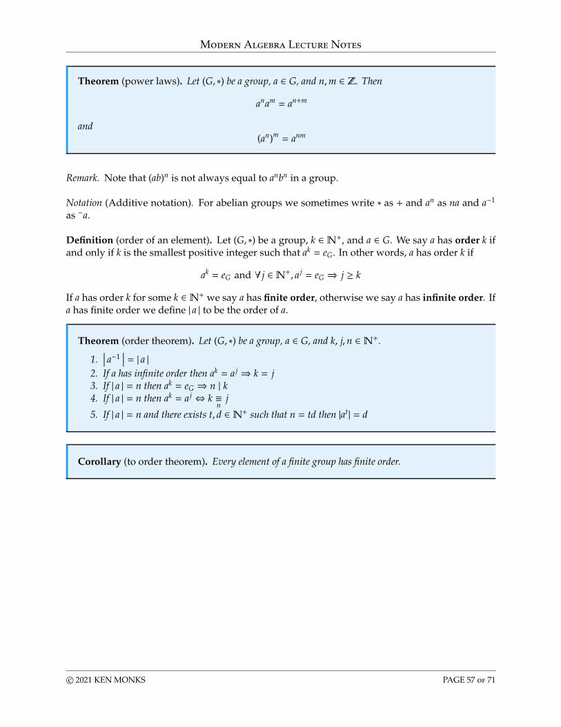
Modern Algebra Lecture Notes
Theorem (power laws). Let (G, ∗) be a group, a ∈ G, and n,m ∈ Z. Then
anam = an+m
and(an)m = anm
Remark. Note that (ab)n is not always equal to anbn in a group.
Notation (Additive notation). For abelian groups we sometimes write ∗ as + and an as na and a−1
as −a.
Definition (order of an element). Let (G, ∗) be a group, k ∈ N+, and a ∈ G. We say a has order k ifand only if k is the smallest positive integer such that ak = eG. In other words, a has order k if
ak = eG and ∀ j ∈N+, a j = eG ⇒ j ≥ k
If a has order k for some k ∈N+ we say a has finite order, otherwise we say a has infinite order. Ifa has finite order we define | a | to be the order of a.
Theorem (order theorem). Let (G, ∗) be a group, a ∈ G, and k, j,n ∈N+.
1.∣∣∣ a−1∣∣∣ = | a |
2. If a has infinite order then ak = a j ⇒ k = j3. If | a | = n then ak = eG ⇒ n | k4. If | a | = n then ak = a j ⇔ k ≡
nj
5. If | a | = n and there exists t, d ∈N+ such that n = td then |at| = d
Corollary (to order theorem). Every element of a finite group has finite order.
c© 2021 KEN MONKS PAGE 57 of 71

Modern Algebra Lecture Notes
Properties of Groups
order of an element order of an element
n ∈N+ (show)a ∈ G (show)an = eG (show)
Let m ∈N+ (variable declaration)Assume am = eGn ≤ m (show)←
←. . . . . . . . . . . . . . . . . . . . . . . . . . . . . . . . . . . . . . . . . . . . . . . . . . . . . . . .a has order n (conclude)
a has order n in group G (show). . . . . . . . . . . . . . . . . . . . . . . . . . . . . . . . . . . . . . . . . . . . . . . . . . . . . . . .an = eG (conclude)a has order n in group G (show)am = eG (show). . . . . . . . . . . . . . . . . . . . . . . . . . . . . . . . . . . . . . . . . . . . . . . . . . . . . . . .n | m (conclude)
7.3 SubGroups
Definition (subgroup). Let (G, ∗) be a group and H ⊆ G. Then (H, ∗) is a subgroup of (G, ∗) if andonly if (H, ∗) is a group (where ∗ denotes the restriction of the original ∗ to H).
Definition (proper subgroup). Let (H, ∗) be a subgroup of (G, ∗). Then (H, ∗) is a proper subgroupof (G, ∗) if and only if H , G and H , { eG }.
Notation (v). We sometimes write “H v G” as a shorthand for “H is a subgroup of G”.
Theorem (subgroup theorem). Let (G, ∗) be a group, H ⊆ G, and H , ∅. Then (H, ∗) is a subgroupof (G, ∗) if and only if
1. ∀a, b ∈ H, ab ∈ H2. ∀a ∈ H, a−1 ∈ H
Theorem (subgroup theorem II). Let (G, ∗) be a group and H ⊆ G a finite nonempty set. Then(H, ∗) is a subgroup of (G, ∗) if and only if
∀a, b ∈ H, ab ∈ H
Lemma (subgroup identity). Let H v G. Then eG ∈ H and eH = eG.
Definition (center). Let (G, ∗) be a group. The center of G is the set
Z(G) ={
a ∈ G : ∀g ∈ G, ag = ga}
Theorem (center is a subgroup). The center of a group is a subgroup of the group.
c© 2021 KEN MONKS PAGE 58 of 71
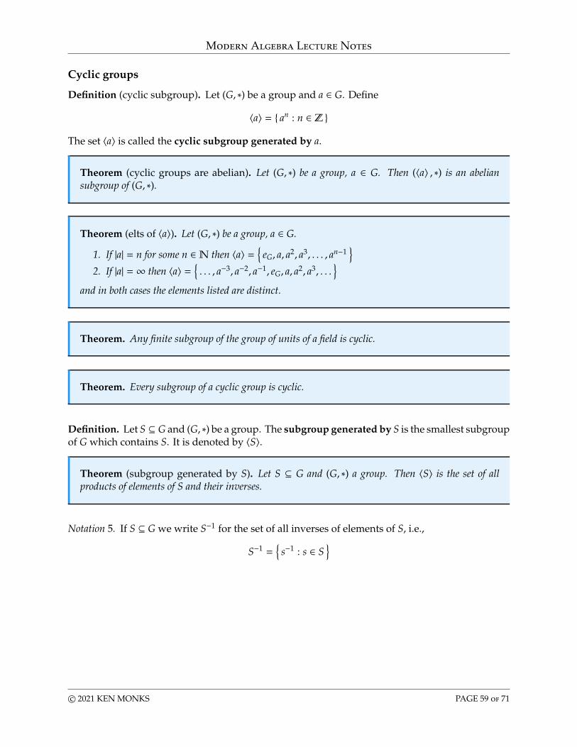
Modern Algebra Lecture Notes
Cyclic groups
Definition (cyclic subgroup). Let (G, ∗) be a group and a ∈ G. Define
〈a〉 = { an : n ∈ Z }
The set 〈a〉 is called the cyclic subgroup generated by a.
Theorem (cyclic groups are abelian). Let (G, ∗) be a group, a ∈ G. Then (〈a〉 , ∗) is an abeliansubgroup of (G, ∗).
Theorem (elts of 〈a〉). Let (G, ∗) be a group, a ∈ G.
1. If |a| = n for some n ∈N then 〈a〉 ={
eG, a, a2, a3, . . . , an−1}
2. If |a| = ∞ then 〈a〉 ={. . . , a−3, a−2, a−1, eG, a, a2, a3, . . .
}and in both cases the elements listed are distinct.
Theorem. Any finite subgroup of the group of units of a field is cyclic.
Theorem. Every subgroup of a cyclic group is cyclic.
Definition. Let S ⊆ G and (G, ∗) be a group. The subgroup generated by S is the smallest subgroupof G which contains S. It is denoted by 〈S〉.
Theorem (subgroup generated by S). Let S ⊆ G and (G, ∗) a group. Then 〈S〉 is the set of allproducts of elements of S and their inverses.
Notation 5. If S ⊆ G we write S−1 for the set of all inverses of elements of S, i.e.,
S−1 ={
s−1 : s ∈ S}
c© 2021 KEN MONKS PAGE 59 of 71
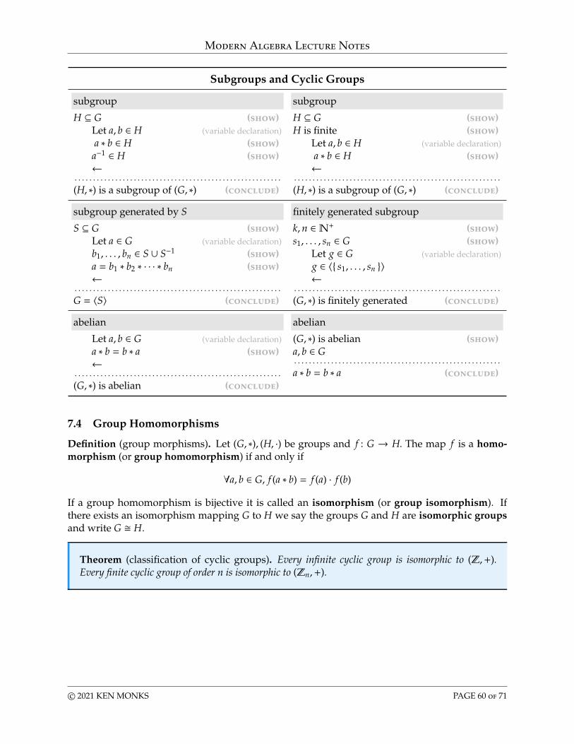
Modern Algebra Lecture Notes
Subgroups and Cyclic Groups
subgroup subgroup
H ⊆ G (show)Let a, b ∈ H (variable declaration)a ∗ b ∈ H (show)
a−1 ∈ H (show)←
. . . . . . . . . . . . . . . . . . . . . . . . . . . . . . . . . . . . . . . . . . . . . . . . . . . . . . . .(H, ∗) is a subgroup of (G, ∗) (conclude)
H ⊆ G (show)H is finite (show)
Let a, b ∈ H (variable declaration)a ∗ b ∈ H (show)←
. . . . . . . . . . . . . . . . . . . . . . . . . . . . . . . . . . . . . . . . . . . . . . . . . . . . . . . .(H, ∗) is a subgroup of (G, ∗) (conclude)
subgroup generated by S finitely generated subgroup
S ⊆ G (show)Let a ∈ G (variable declaration)b1, . . . , bn ∈ S ∪ S−1 (show)a = b1 ∗ b2 ∗ · · · ∗ bn (show)←
. . . . . . . . . . . . . . . . . . . . . . . . . . . . . . . . . . . . . . . . . . . . . . . . . . . . . . . .G = 〈S〉 (conclude)
k,n ∈N+ (show)s1, . . . , sn ∈ G (show)
Let g ∈ G (variable declaration)g ∈ 〈{ s1, . . . , sn }〉←
. . . . . . . . . . . . . . . . . . . . . . . . . . . . . . . . . . . . . . . . . . . . . . . . . . . . . . . .(G, ∗) is finitely generated (conclude)
abelian abelian
Let a, b ∈ G (variable declaration)a ∗ b = b ∗ a (show)←
. . . . . . . . . . . . . . . . . . . . . . . . . . . . . . . . . . . . . . . . . . . . . . . . . . . . . . . .(G, ∗) is abelian (conclude)
(G, ∗) is abelian (show)a, b ∈ G. . . . . . . . . . . . . . . . . . . . . . . . . . . . . . . . . . . . . . . . . . . . . . . . . . . . . . . .a ∗ b = b ∗ a (conclude)
7.4 Group Homomorphisms
Definition (group morphisms). Let (G, ∗), (H, ·) be groups and f : G → H. The map f is a homo-morphism (or group homomorphism) if and only if
∀a, b ∈ G, f (a ∗ b) = f (a) · f (b)
If a group homomorphism is bijective it is called an isomorphism (or group isomorphism). Ifthere exists an isomorphism mapping G to H we say the groups G and H are isomorphic groupsand write G � H.
Theorem (classification of cyclic groups). Every infinite cyclic group is isomorphic to (Z,+).Every finite cyclic group of order n is isomorphic to (Zn,+).
c© 2021 KEN MONKS PAGE 60 of 71
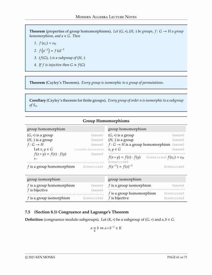
Modern Algebra Lecture Notes
Theorem (properties of group homomorphisms). Let (G, ∗), (H, ·) be groups, f : G→ H a grouphomomorphism, and a ∈ G. Then
1. f (eG) = eH
2. f(a−1)= f (a)−1
3. ( f (G), ·) is a subgroup of (H, ·)4. If f is injective then G � f (G)
Theorem (Cayley’s Theorem). Every group is isomorphic to a group of permutations.
Corollary (Cayley’s theorem for finite groups). Every group of order n is isomorphic to a subgroupof Sn.
Group Homomorphisms
group homomorphism group homomorphism
(G, ∗) is a group (show)(H, ·) is a group (show)f : G→ H (show)
Let x, y ∈ G (variable declaration)f (x ∗ y) = f (x) · f (y) (show)←
. . . . . . . . . . . . . . . . . . . . . . . . . . . . . . . . . . . . . . . . . . . . . . . . . . . . . . . .f is a group homomorphism (conclude)
(G, ∗) is a group (show)(H, ·) is a group (show)f : G→ H is a group homomorphism (show)x, y ∈ G (show). . . . . . . . . . . . . . . . . . . . . . . . . . . . . . . . . . . . . . . . . . . . . . . . . . . . . . . .f (x ∗ y) = f (x) · f (y) (conclude) f (eG) = eH(conclude)f (x−1) = f (x)−1 (conclude)
group isomorphism group isomorphism
f is a group homomorphism (show)f is bijective (show). . . . . . . . . . . . . . . . . . . . . . . . . . . . . . . . . . . . . . . . . . . . . . . . . . . . . . . .f is a group isomorphism (conclude)
f is a group isomorphism (show). . . . . . . . . . . . . . . . . . . . . . . . . . . . . . . . . . . . . . . . . . . . . . . . . . . . . . . .f is a group homomorphism (conclude)f is bijective (conclude)
7.5 (Section 8.1) Congruence and Lagrange’s Theorem
Definition (congruence modulo subgroups). Let (K, ∗) be a subgroup of (G, ∗) and a, b ∈ G.
a ≡K
b⇔ a ∗ b−1 ∈ K
c© 2021 KEN MONKS PAGE 61 of 71
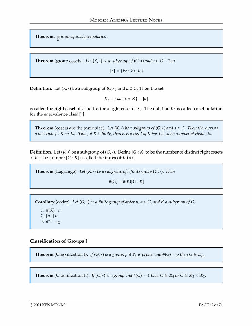
Modern Algebra Lecture Notes
Theorem. ≡K
is an equivalence relation.
Theorem (group cosets). Let (K, ∗) be a subgroup of (G, ∗) and a ∈ G. Then
[a] = { ka : k ∈ K }
Definition. Let (K, ∗) be a subgroup of (G, ∗) and a ∈ G. Then the set
Ka = { ka : k ∈ K } = [a]
is called the right coset of a mod K (or a right coset of K). The notation Ka is called coset notationfor the equivalence class [a].
Theorem (cosets are the same size). Let (K, ∗) be a subgroup of (G, ∗) and a ∈ G. Then there existsa bijection f : K→ Ka. Thus, if K is finite, then every coset of K has the same number of elements.
Definition. Let (K, ∗) be a subgroup of (G, ∗). Define [G : K] to be the number of distinct right cosetsof K. The number [G : K] is called the index of K in G.
Theorem (Lagrange). Let (K, ∗) be a subgroup of a finite group (G, ∗). Then
#(G) = #(K)[G : K]
Corollary (order). Let (G, ∗) be a finite group of order n, a ∈ G, and K a subgroup of G.
1. #(K) | n2. | a | | n3. an = eG
Classification of Groups I
Theorem (Classification I). If (G, ∗) is a group, p ∈N is prime, and #(G) = p then G � Zp.
Theorem (Classification II). If (G, ∗) is a group and #(G) = 4 then G � Z4 or G � Z2 ×Z2.
c© 2021 KEN MONKS PAGE 62 of 71
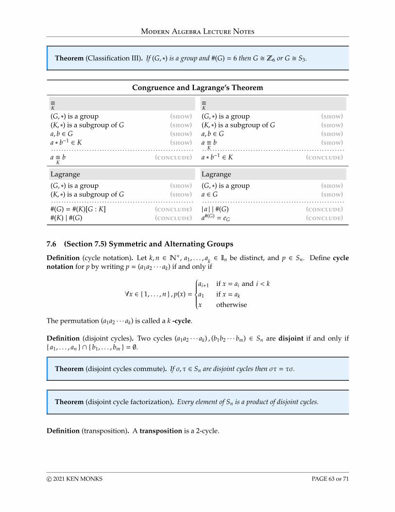
Modern Algebra Lecture Notes
Theorem (Classification III). If (G, ∗) is a group and #(G) = 6 then G � Z6 or G � S3.
Congruence and Lagrange’s Theorem
≡K
≡K
(G, ∗) is a group (show)(K, ∗) is a subgroup of G (show)a, b ∈ G (show)a ∗ b−1 ∈ K (show). . . . . . . . . . . . . . . . . . . . . . . . . . . . . . . . . . . . . . . . . . . . . . . . . . . . . . . .a ≡
Kb (conclude)
(G, ∗) is a group (show)(K, ∗) is a subgroup of G (show)a, b ∈ G (show)a ≡
Kb (show)
. . . . . . . . . . . . . . . . . . . . . . . . . . . . . . . . . . . . . . . . . . . . . . . . . . . . . . . .a ∗ b−1 ∈ K (conclude)
Lagrange Lagrange
(G, ∗) is a group (show)(K, ∗) is a subgroup of G (show). . . . . . . . . . . . . . . . . . . . . . . . . . . . . . . . . . . . . . . . . . . . . . . . . . . . . . . .#(G) = #(K)[G : K] (conclude)#(K) | #(G) (conclude)
(G, ∗) is a group (show)a ∈ G (show). . . . . . . . . . . . . . . . . . . . . . . . . . . . . . . . . . . . . . . . . . . . . . . . . . . . . . . .| a | | #(G) (conclude)a#(G) = eG (conclude)
7.6 (Section 7.5) Symmetric and Alternating Groups
Definition (cycle notation). Let k,n ∈ N+, a1, . . . , ak ∈ In be distinct, and p ∈ Sn. Define cyclenotation for p by writing p = (a1a2 · · · ak) if and only if
∀x ∈ { 1, . . . , n } , p(x) =
ai+1 if x = ai and i < ka1 if x = ak
x otherwise
The permutation (a1a2 · · · ak) is called a k -cycle.
Definition (disjoint cycles). Two cycles (a1a2 · · · ak) , (b1b2 · · · bm) ∈ Sn are disjoint if and only if{ a1, . . . , an } ∩ { b1, . . . , bm } = ∅.
Theorem (disjoint cycles commute). If σ, τ ∈ Sn are disjoint cycles then στ = τσ.
Theorem (disjoint cycle factorization). Every element of Sn is a product of disjoint cycles.
Definition (transposition). A transposition is a 2-cycle.
c© 2021 KEN MONKS PAGE 63 of 71
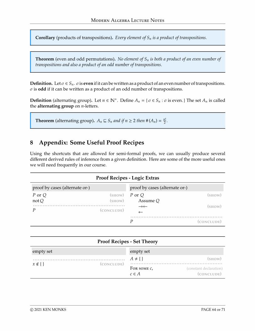
Modern Algebra Lecture Notes
Corollary (products of transpositions). Every element of Sn is a product of transpositions.
Theorem (even and odd permutations). No element of Sn is both a product of an even number oftranspositions and also a product of an odd number of transpositions.
Definition. Letσ ∈ Sn. σ is even if it can be written as a product of an even number of transpositions.σ is odd if it can be written as a product of an odd number of transpositions.
Definition (alternating group). Let n ∈ N+. Define An = { σ ∈ Sn : σ is even. } The set An is calledthe alternating group on n-letters.
Theorem (alternating group). An v Sn and if n ≥ 2 then # (An) = n!2 .
8 Appendix: Some Useful Proof Recipes
Using the shortcuts that are allowed for semi-formal proofs, we can usually produce severaldifferent derived rules of inference from a given definition. Here are some of the more useful oneswe will need frequently in our course.
Proof Recipes - Logic Extras
proof by cases (alternate or-) proof by cases (alternate or-)
P or Q (show)not Q (show). . . . . . . . . . . . . . . . . . . . . . . . . . . . . . . . . . . . . . . . . . . . . . . . . . . . . . . .P (conclude)
P or Q (show)Assume Q→← (show)←
. . . . . . . . . . . . . . . . . . . . . . . . . . . . . . . . . . . . . . . . . . . . . . . . . . . . . . . .P (conclude)
Proof Recipes - Set Theory
empty set empty set
. . . . . . . . . . . . . . . . . . . . . . . . . . . . . . . . . . . . . . . . . . . . . . . . . . . . . . . .x < { } (conclude)
A , { } (show). . . . . . . . . . . . . . . . . . . . . . . . . . . . . . . . . . . . . . . . . . . . . . . . . . . . . . . .For some c, (constant declaration)c ∈ A (conclude)
c© 2021 KEN MONKS PAGE 64 of 71
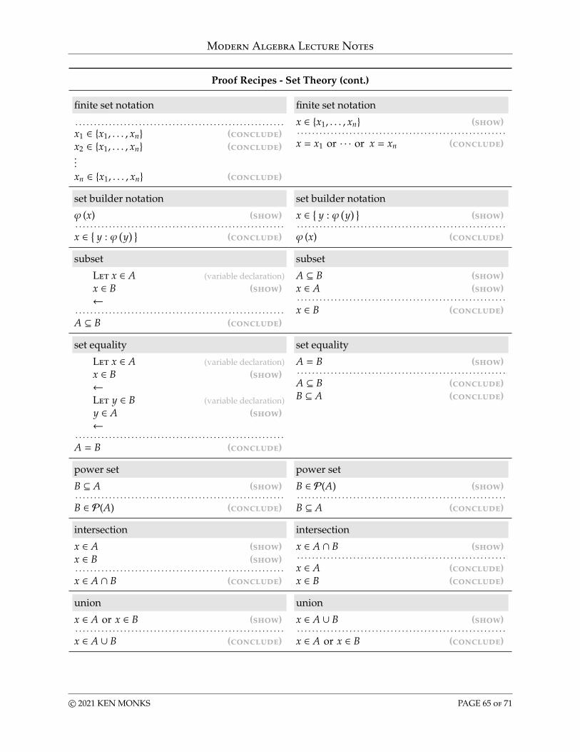
Modern Algebra Lecture Notes
Proof Recipes - Set Theory (cont.)
finite set notation finite set notation
. . . . . . . . . . . . . . . . . . . . . . . . . . . . . . . . . . . . . . . . . . . . . . . . . . . . . . . .x1 ∈ {x1, . . . , xn} (conclude)x2 ∈ {x1, . . . , xn} (conclude)...xn ∈ {x1, . . . , xn} (conclude)
x ∈ {x1, . . . , xn} (show). . . . . . . . . . . . . . . . . . . . . . . . . . . . . . . . . . . . . . . . . . . . . . . . . . . . . . . .x = x1 or · · · or x = xn (conclude)
set builder notation set builder notation
φ (x) (show). . . . . . . . . . . . . . . . . . . . . . . . . . . . . . . . . . . . . . . . . . . . . . . . . . . . . . . .x ∈ { y : φ
(y) }
(conclude)
x ∈ { y : φ(y) }
(show). . . . . . . . . . . . . . . . . . . . . . . . . . . . . . . . . . . . . . . . . . . . . . . . . . . . . . . .φ (x) (conclude)
subset subset
Let x ∈ A (variable declaration)x ∈ B (show)←
. . . . . . . . . . . . . . . . . . . . . . . . . . . . . . . . . . . . . . . . . . . . . . . . . . . . . . . .A ⊆ B (conclude)
A ⊆ B (show)x ∈ A (show). . . . . . . . . . . . . . . . . . . . . . . . . . . . . . . . . . . . . . . . . . . . . . . . . . . . . . . .x ∈ B (conclude)
set equality set equality
Let x ∈ A (variable declaration)x ∈ B (show)←Let y ∈ B (variable declaration)y ∈ A (show)←
. . . . . . . . . . . . . . . . . . . . . . . . . . . . . . . . . . . . . . . . . . . . . . . . . . . . . . . .A = B (conclude)
A = B (show). . . . . . . . . . . . . . . . . . . . . . . . . . . . . . . . . . . . . . . . . . . . . . . . . . . . . . . .A ⊆ B (conclude)B ⊆ A (conclude)
power set power set
B ⊆ A (show). . . . . . . . . . . . . . . . . . . . . . . . . . . . . . . . . . . . . . . . . . . . . . . . . . . . . . . .B ∈ P(A) (conclude)
B ∈ P(A) (show). . . . . . . . . . . . . . . . . . . . . . . . . . . . . . . . . . . . . . . . . . . . . . . . . . . . . . . .B ⊆ A (conclude)
intersection intersection
x ∈ A (show)x ∈ B (show). . . . . . . . . . . . . . . . . . . . . . . . . . . . . . . . . . . . . . . . . . . . . . . . . . . . . . . .x ∈ A ∩ B (conclude)
x ∈ A ∩ B (show). . . . . . . . . . . . . . . . . . . . . . . . . . . . . . . . . . . . . . . . . . . . . . . . . . . . . . . .x ∈ A (conclude)x ∈ B (conclude)
union union
x ∈ A or x ∈ B (show). . . . . . . . . . . . . . . . . . . . . . . . . . . . . . . . . . . . . . . . . . . . . . . . . . . . . . . .x ∈ A ∪ B (conclude)
x ∈ A ∪ B (show). . . . . . . . . . . . . . . . . . . . . . . . . . . . . . . . . . . . . . . . . . . . . . . . . . . . . . . .x ∈ A or x ∈ B (conclude)
c© 2021 KEN MONKS PAGE 65 of 71
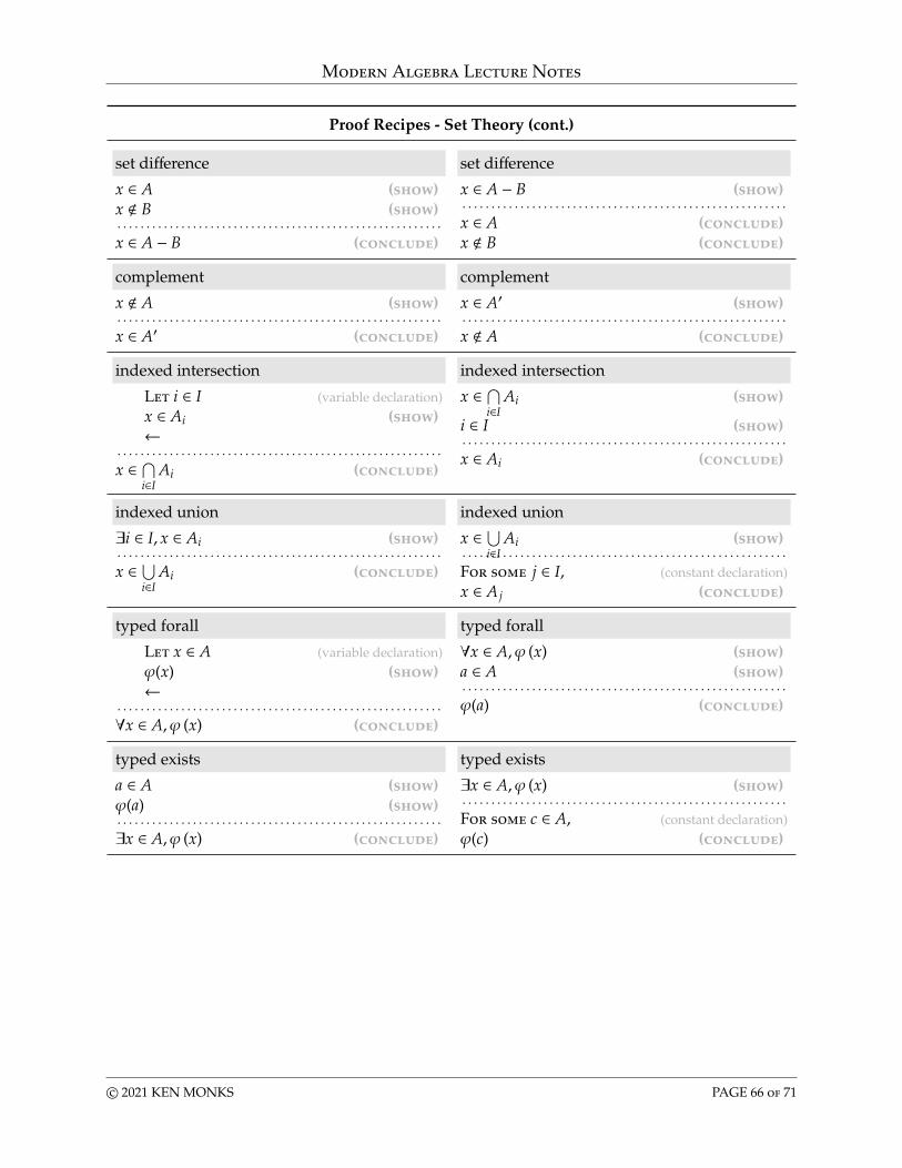
Modern Algebra Lecture Notes
Proof Recipes - Set Theory (cont.)
set difference set difference
x ∈ A (show)x < B (show). . . . . . . . . . . . . . . . . . . . . . . . . . . . . . . . . . . . . . . . . . . . . . . . . . . . . . . .x ∈ A − B (conclude)
x ∈ A − B (show). . . . . . . . . . . . . . . . . . . . . . . . . . . . . . . . . . . . . . . . . . . . . . . . . . . . . . . .x ∈ A (conclude)x < B (conclude)
complement complement
x < A (show). . . . . . . . . . . . . . . . . . . . . . . . . . . . . . . . . . . . . . . . . . . . . . . . . . . . . . . .x ∈ A′ (conclude)
x ∈ A′ (show). . . . . . . . . . . . . . . . . . . . . . . . . . . . . . . . . . . . . . . . . . . . . . . . . . . . . . . .x < A (conclude)
indexed intersection indexed intersection
Let i ∈ I (variable declaration)x ∈ Ai (show)←
. . . . . . . . . . . . . . . . . . . . . . . . . . . . . . . . . . . . . . . . . . . . . . . . . . . . . . . .x ∈ ⋂
i∈IAi (conclude)
x ∈ ⋂i∈I
Ai (show)
i ∈ I (show). . . . . . . . . . . . . . . . . . . . . . . . . . . . . . . . . . . . . . . . . . . . . . . . . . . . . . . .x ∈ Ai (conclude)
indexed union indexed union
∃i ∈ I, x ∈ Ai (show). . . . . . . . . . . . . . . . . . . . . . . . . . . . . . . . . . . . . . . . . . . . . . . . . . . . . . . .x ∈ ⋃
i∈IAi (conclude)
x ∈ ⋃i∈I
Ai (show). . . . . . . . . . . . . . . . . . . . . . . . . . . . . . . . . . . . . . . . . . . . . . . . . . . . . . . .For some j ∈ I, (constant declaration)x ∈ A j (conclude)
typed forall typed forall
Let x ∈ A (variable declaration)φ(x) (show)←
. . . . . . . . . . . . . . . . . . . . . . . . . . . . . . . . . . . . . . . . . . . . . . . . . . . . . . . .∀x ∈ A, φ (x) (conclude)
∀x ∈ A, φ (x) (show)a ∈ A (show). . . . . . . . . . . . . . . . . . . . . . . . . . . . . . . . . . . . . . . . . . . . . . . . . . . . . . . .φ(a) (conclude)
typed exists typed exists
a ∈ A (show)φ(a) (show). . . . . . . . . . . . . . . . . . . . . . . . . . . . . . . . . . . . . . . . . . . . . . . . . . . . . . . .∃x ∈ A, φ (x) (conclude)
∃x ∈ A, φ (x) (show). . . . . . . . . . . . . . . . . . . . . . . . . . . . . . . . . . . . . . . . . . . . . . . . . . . . . . . .For some c ∈ A, (constant declaration)φ(c) (conclude)
c© 2021 KEN MONKS PAGE 66 of 71
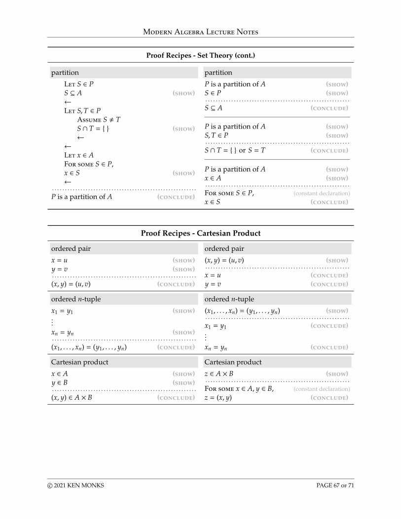
Modern Algebra Lecture Notes
Proof Recipes - Set Theory (cont.)
partition partition
Let S ∈ PS ⊆ A (show)←Let S,T ∈ P
Assume S , TS ∩ T = { } (show)←
←Let x ∈ AFor some S ∈ P,x ∈ S (show)←
. . . . . . . . . . . . . . . . . . . . . . . . . . . . . . . . . . . . . . . . . . . . . . . . . . . . . . . .P is a partition of A (conclude)
P is a partition of A (show)S ∈ P (show). . . . . . . . . . . . . . . . . . . . . . . . . . . . . . . . . . . . . . . . . . . . . . . . . . . . . . . .S ⊆ A (conclude)
P is a partition of A (show)S,T ∈ P (show). . . . . . . . . . . . . . . . . . . . . . . . . . . . . . . . . . . . . . . . . . . . . . . . . . . . . . . .S ∩ T = { } or S = T (conclude)
P is a partition of A (show)x ∈ A (show). . . . . . . . . . . . . . . . . . . . . . . . . . . . . . . . . . . . . . . . . . . . . . . . . . . . . . . .For some S ∈ P, (constant declaration)x ∈ S (conclude)
Proof Recipes - Cartesian Product
ordered pair ordered pair
x = u (show)y = v (show). . . . . . . . . . . . . . . . . . . . . . . . . . . . . . . . . . . . . . . . . . . . . . . . . . . . . . . .(x, y) = (u, v) (conclude)
(x, y) = (u, v) (show). . . . . . . . . . . . . . . . . . . . . . . . . . . . . . . . . . . . . . . . . . . . . . . . . . . . . . . .x = u (conclude)y = v (conclude)
ordered n-tuple ordered n-tuple
x1 = y1 (show)...xn = yn (show). . . . . . . . . . . . . . . . . . . . . . . . . . . . . . . . . . . . . . . . . . . . . . . . . . . . . . . .(x1, . . . , xn) = (y1, . . . , yn) (conclude)
(x1, . . . , xn) = (y1, . . . , yn) (show). . . . . . . . . . . . . . . . . . . . . . . . . . . . . . . . . . . . . . . . . . . . . . . . . . . . . . . .x1 = y1 (conclude)...xn = yn (conclude)
Cartesian product Cartesian product
x ∈ A (show)y ∈ B (show). . . . . . . . . . . . . . . . . . . . . . . . . . . . . . . . . . . . . . . . . . . . . . . . . . . . . . . .(x, y) ∈ A × B (conclude)
z ∈ A × B (show). . . . . . . . . . . . . . . . . . . . . . . . . . . . . . . . . . . . . . . . . . . . . . . . . . . . . . . .For some x ∈ A, y ∈ B, (constant declaration)z = (x, y) (conclude)
c© 2021 KEN MONKS PAGE 67 of 71
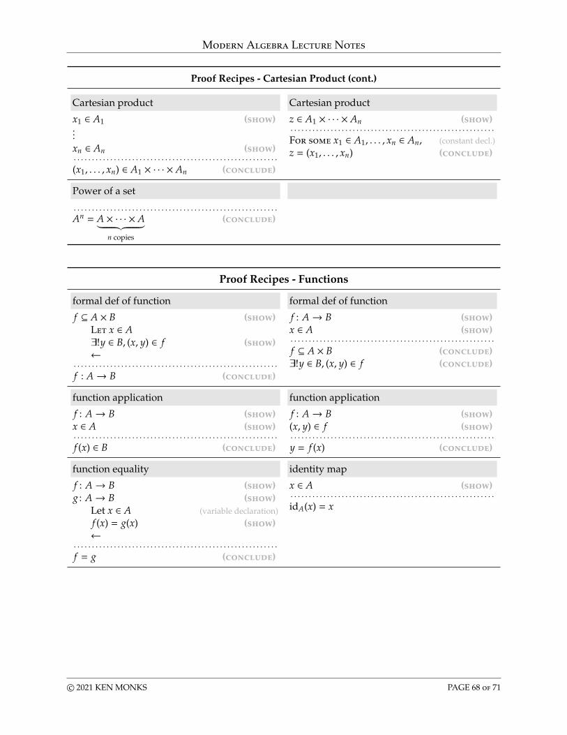
Modern Algebra Lecture Notes
Proof Recipes - Cartesian Product (cont.)
Cartesian product Cartesian product
x1 ∈ A1 (show)...xn ∈ An (show). . . . . . . . . . . . . . . . . . . . . . . . . . . . . . . . . . . . . . . . . . . . . . . . . . . . . . . .(x1, . . . , xn) ∈ A1 × · · · × An (conclude)
z ∈ A1 × · · · × An (show). . . . . . . . . . . . . . . . . . . . . . . . . . . . . . . . . . . . . . . . . . . . . . . . . . . . . . . .For some x1 ∈ A1, . . . , xn ∈ An, (constant decl.)z = (x1, . . . , xn) (conclude)
Power of a set
. . . . . . . . . . . . . . . . . . . . . . . . . . . . . . . . . . . . . . . . . . . . . . . . . . . . . . . .An = A × · · · × A︸ ︷︷ ︸
n copies
(conclude)
Proof Recipes - Functions
formal def of function formal def of function
f ⊆ A × B (show)Let x ∈ A∃!y ∈ B, (x, y) ∈ f (show)←
. . . . . . . . . . . . . . . . . . . . . . . . . . . . . . . . . . . . . . . . . . . . . . . . . . . . . . . .f : A→ B (conclude)
f : A→ B (show)x ∈ A (show). . . . . . . . . . . . . . . . . . . . . . . . . . . . . . . . . . . . . . . . . . . . . . . . . . . . . . . .f ⊆ A × B (conclude)∃!y ∈ B, (x, y) ∈ f (conclude)
function application function application
f : A→ B (show)x ∈ A (show). . . . . . . . . . . . . . . . . . . . . . . . . . . . . . . . . . . . . . . . . . . . . . . . . . . . . . . .f (x) ∈ B (conclude)
f : A→ B (show)(x, y) ∈ f (show). . . . . . . . . . . . . . . . . . . . . . . . . . . . . . . . . . . . . . . . . . . . . . . . . . . . . . . .y = f (x) (conclude)
function equality identity map
f : A→ B (show)g : A→ B (show)
Let x ∈ A (variable declaration)f (x) = g(x) (show)←
. . . . . . . . . . . . . . . . . . . . . . . . . . . . . . . . . . . . . . . . . . . . . . . . . . . . . . . .f = g (conclude)
x ∈ A (show). . . . . . . . . . . . . . . . . . . . . . . . . . . . . . . . . . . . . . . . . . . . . . . . . . . . . . . .idA(x) = x
c© 2021 KEN MONKS PAGE 68 of 71
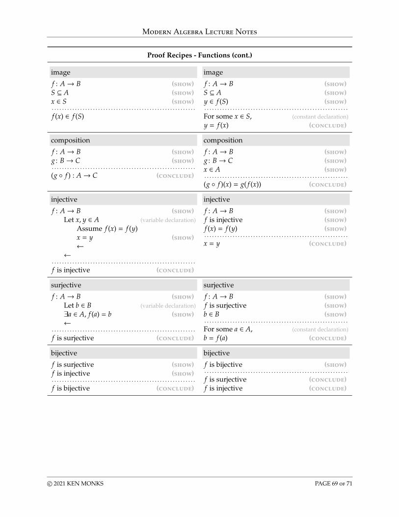
Modern Algebra Lecture Notes
Proof Recipes - Functions (cont.)
image image
f : A→ B (show)S ⊆ A (show)x ∈ S (show). . . . . . . . . . . . . . . . . . . . . . . . . . . . . . . . . . . . . . . . . . . . . . . . . . . . . . . .f (x) ∈ f (S)
f : A→ B (show)S ⊆ A (show)y ∈ f (S) (show). . . . . . . . . . . . . . . . . . . . . . . . . . . . . . . . . . . . . . . . . . . . . . . . . . . . . . . .For some x ∈ S, (constant declaration)y = f (x) (conclude)
composition composition
f : A→ B (show)g : B→ C (show). . . . . . . . . . . . . . . . . . . . . . . . . . . . . . . . . . . . . . . . . . . . . . . . . . . . . . . .(g ◦ f ) : A→ C (conclude)
f : A→ B (show)g : B→ C (show)x ∈ A (show). . . . . . . . . . . . . . . . . . . . . . . . . . . . . . . . . . . . . . . . . . . . . . . . . . . . . . . .(g ◦ f )(x) = g( f (x)) (conclude)
injective injective
f : A→ B (show)Let x, y ∈ A (variable declaration)
Assume f (x) = f (y)x = y (show)←
←. . . . . . . . . . . . . . . . . . . . . . . . . . . . . . . . . . . . . . . . . . . . . . . . . . . . . . . .f is injective (conclude)
f : A→ B (show)f is injective (show)f (x) = f (y) (show). . . . . . . . . . . . . . . . . . . . . . . . . . . . . . . . . . . . . . . . . . . . . . . . . . . . . . . .x = y (conclude)
surjective surjective
f : A→ B (show)Let b ∈ B (variable declaration)∃a ∈ A, f (a) = b (show)←
. . . . . . . . . . . . . . . . . . . . . . . . . . . . . . . . . . . . . . . . . . . . . . . . . . . . . . . .f is surjective (conclude)
f : A→ B (show)f is surjective (show)b ∈ B (show). . . . . . . . . . . . . . . . . . . . . . . . . . . . . . . . . . . . . . . . . . . . . . . . . . . . . . . .For some a ∈ A, (constant declaration)b = f (a) (conclude)
bijective bijective
f is surjective (show)f is injective (show). . . . . . . . . . . . . . . . . . . . . . . . . . . . . . . . . . . . . . . . . . . . . . . . . . . . . . . .f is bijective (conclude)
f is bijective (show). . . . . . . . . . . . . . . . . . . . . . . . . . . . . . . . . . . . . . . . . . . . . . . . . . . . . . . .f is surjective (conclude)f is injective (conclude)
c© 2021 KEN MONKS PAGE 69 of 71
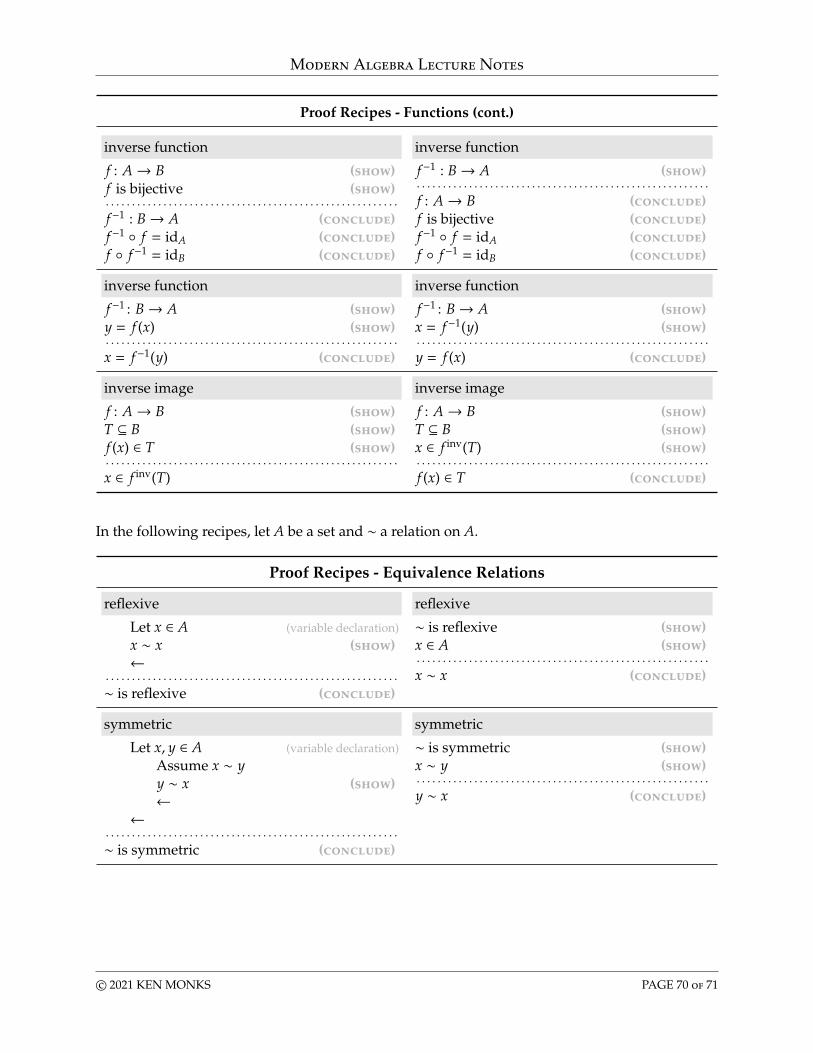
Modern Algebra Lecture Notes
Proof Recipes - Functions (cont.)
inverse function inverse function
f : A→ B (show)f is bijective (show). . . . . . . . . . . . . . . . . . . . . . . . . . . . . . . . . . . . . . . . . . . . . . . . . . . . . . . .f−1 : B→ A (conclude)f−1 ◦ f = idA (conclude)f ◦ f−1 = idB (conclude)
f−1 : B→ A (show). . . . . . . . . . . . . . . . . . . . . . . . . . . . . . . . . . . . . . . . . . . . . . . . . . . . . . . .f : A→ B (conclude)f is bijective (conclude)f−1 ◦ f = idA (conclude)f ◦ f−1 = idB (conclude)
inverse function inverse function
f−1 : B→ A (show)y = f (x) (show). . . . . . . . . . . . . . . . . . . . . . . . . . . . . . . . . . . . . . . . . . . . . . . . . . . . . . . .x = f−1(y) (conclude)
f−1 : B→ A (show)x = f−1(y) (show). . . . . . . . . . . . . . . . . . . . . . . . . . . . . . . . . . . . . . . . . . . . . . . . . . . . . . . .y = f (x) (conclude)
inverse image inverse image
f : A→ B (show)T ⊆ B (show)f (x) ∈ T (show). . . . . . . . . . . . . . . . . . . . . . . . . . . . . . . . . . . . . . . . . . . . . . . . . . . . . . . .x ∈ f inv(T)
f : A→ B (show)T ⊆ B (show)x ∈ f inv(T) (show). . . . . . . . . . . . . . . . . . . . . . . . . . . . . . . . . . . . . . . . . . . . . . . . . . . . . . . .f (x) ∈ T (conclude)
In the following recipes, let A be a set and ∼ a relation on A.
Proof Recipes - Equivalence Relations
reflexive reflexive
Let x ∈ A (variable declaration)x ∼ x (show)←
. . . . . . . . . . . . . . . . . . . . . . . . . . . . . . . . . . . . . . . . . . . . . . . . . . . . . . . .∼ is reflexive (conclude)
∼ is reflexive (show)x ∈ A (show). . . . . . . . . . . . . . . . . . . . . . . . . . . . . . . . . . . . . . . . . . . . . . . . . . . . . . . .x ∼ x (conclude)
symmetric symmetric
Let x, y ∈ A (variable declaration)Assume x ∼ yy ∼ x (show)←
←. . . . . . . . . . . . . . . . . . . . . . . . . . . . . . . . . . . . . . . . . . . . . . . . . . . . . . . .∼ is symmetric (conclude)
∼ is symmetric (show)x ∼ y (show). . . . . . . . . . . . . . . . . . . . . . . . . . . . . . . . . . . . . . . . . . . . . . . . . . . . . . . .y ∼ x (conclude)
c© 2021 KEN MONKS PAGE 70 of 71
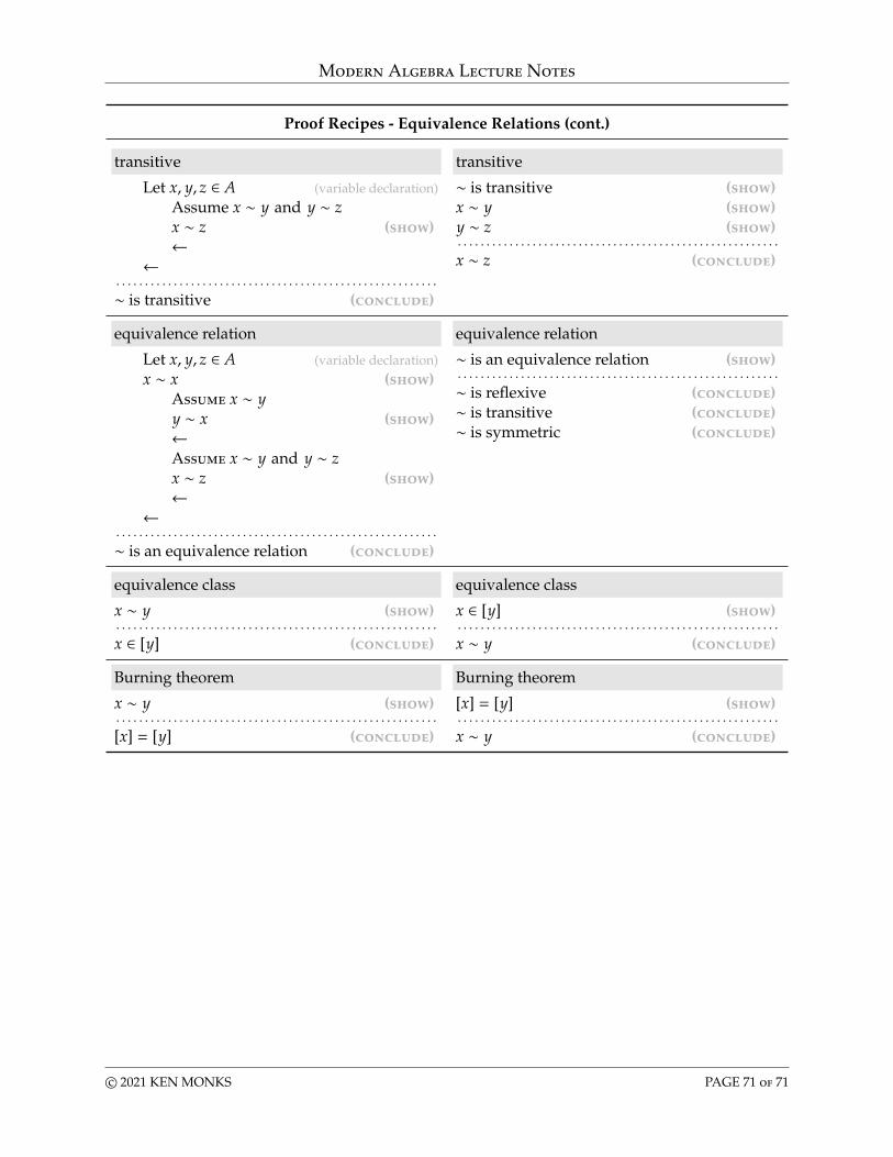
Modern Algebra Lecture Notes
Proof Recipes - Equivalence Relations (cont.)
transitive transitive
Let x, y, z ∈ A (variable declaration)Assume x ∼ y and y ∼ zx ∼ z (show)←
←. . . . . . . . . . . . . . . . . . . . . . . . . . . . . . . . . . . . . . . . . . . . . . . . . . . . . . . .∼ is transitive (conclude)
∼ is transitive (show)x ∼ y (show)y ∼ z (show). . . . . . . . . . . . . . . . . . . . . . . . . . . . . . . . . . . . . . . . . . . . . . . . . . . . . . . .x ∼ z (conclude)
equivalence relation equivalence relation
Let x, y, z ∈ A (variable declaration)x ∼ x (show)
Assume x ∼ yy ∼ x (show)←Assume x ∼ y and y ∼ zx ∼ z (show)←
←. . . . . . . . . . . . . . . . . . . . . . . . . . . . . . . . . . . . . . . . . . . . . . . . . . . . . . . .∼ is an equivalence relation (conclude)
∼ is an equivalence relation (show). . . . . . . . . . . . . . . . . . . . . . . . . . . . . . . . . . . . . . . . . . . . . . . . . . . . . . . .∼ is reflexive (conclude)∼ is transitive (conclude)∼ is symmetric (conclude)
equivalence class equivalence class
x ∼ y (show). . . . . . . . . . . . . . . . . . . . . . . . . . . . . . . . . . . . . . . . . . . . . . . . . . . . . . . .x ∈ [y] (conclude)
x ∈ [y] (show). . . . . . . . . . . . . . . . . . . . . . . . . . . . . . . . . . . . . . . . . . . . . . . . . . . . . . . .x ∼ y (conclude)
Burning theorem Burning theorem
x ∼ y (show). . . . . . . . . . . . . . . . . . . . . . . . . . . . . . . . . . . . . . . . . . . . . . . . . . . . . . . .[x] = [y] (conclude)
[x] = [y] (show). . . . . . . . . . . . . . . . . . . . . . . . . . . . . . . . . . . . . . . . . . . . . . . . . . . . . . . .x ∼ y (conclude)
c© 2021 KEN MONKS PAGE 71 of 71