models used in variance swap pricing - final analysis report · models used in variance swap...
TRANSCRIPT
Models Used in Variance Swap PricingFinal Analysis Report
Jason Vinar, Xu Li, Bowen Sun, Jingnan ZhangQi Zhang, Tianyi Luo, Wensheng Sun, Yiming Wang
Financial Modelling Workshop 2011
Presentation – Jan 15, 2011
Team Three (U of Minnesota) Models Used in Variance Swap Pricing Jan 15, 2011 1 / 47

Report Summary
Variance Swap Introduction (Tianyi Luo)I Definition and Pay-offI Pricing Methods Intro: Rule of Thumb, Replication and SimulationI Models of Volatility Skew: Stochastic Volatility Inspired and
7-Parameter Skew
Model Parametrization (Tianyi Luo)
Constructing The Volatility Surface (Wensheng Sun)
Analysis of Rule of Thumb Pricing (Jingnan Zhang)
Analysis of Continuous and Discrete Replication (Bowen Sun)
Analysis of Pricing Using Simulation (Qi Zhang, Yiming Wang)
Discussion of Future Work (Xu Li)I Variance Swap with Stochastic Interest RateI The Bound of Value of Variance Swap
Team Three (U of Minnesota) Models Used in Variance Swap Pricing Jan 15, 2011 2 / 47
What is variance swap?
A variance swap is an instrument which allows investors to trade futurerealized volatility against current implied volatility.
It is a popular way to add volatility exposure to a portfolio since
It comes without the directional risk of the underlying security.
The variance swap quotes are based on the implied volatility while thefinal pay-off is based on the realized volatility.
The additivity of variance allows the investor to easily take a forwardvolatility position.
Team Three (U of Minnesota) Models Used in Variance Swap Pricing Jan 15, 2011 3 / 47

The Pay-off
The pay-off of the variance swap can be expressed as:
P = N(σ2R − Kvar )
where N is notional amount, Kvar is the strike quoted in annualizedvariance, and σ2R is the realized variance over the life of the contractdefined as
σ2R =252
D
D∑i=1
(lnSi
Si−1)2
with D being the number of trading days during the contract.
Team Three (U of Minnesota) Models Used in Variance Swap Pricing Jan 15, 2011 4 / 47
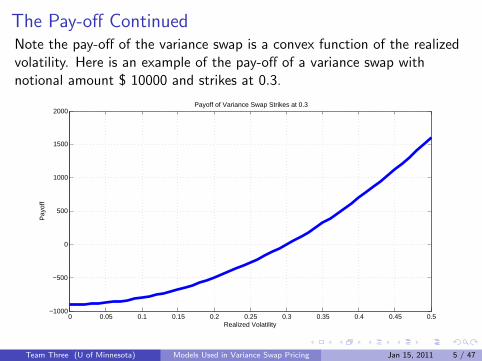
The Pay-off ContinuedNote the pay-off of the variance swap is a convex function of the realizedvolatility. Here is an example of the pay-off of a variance swap withnotional amount $ 10000 and strikes at 0.3.
0 0.05 0.1 0.15 0.2 0.25 0.3 0.35 0.4 0.45 0.5−1000
−500
0
500
1000
1500
2000
Realized Volatility
Pay
off
Payoff of Variance Swap Strikes at 0.3
Team Three (U of Minnesota) Models Used in Variance Swap Pricing Jan 15, 2011 5 / 47
Pricing Method: Rule of Thumb
The rule of thumb pricing includes the following two methods:
90% put: take 90% of the forward price as the strike and plug thatinto the volatility function.
25% delta put: search for the strike that has a -25% delta (on the putside) and plug that strike into the volatility function.
These two methods are empirically based and were justified bypractitioners for non-steep volatility skew. They are used as quick ways toestimate the fair strike of variance swap. Under different scenarios, theserule of thumb might not be accurate enough thus other pricing methodswould be suggested.
Team Three (U of Minnesota) Models Used in Variance Swap Pricing Jan 15, 2011 6 / 47
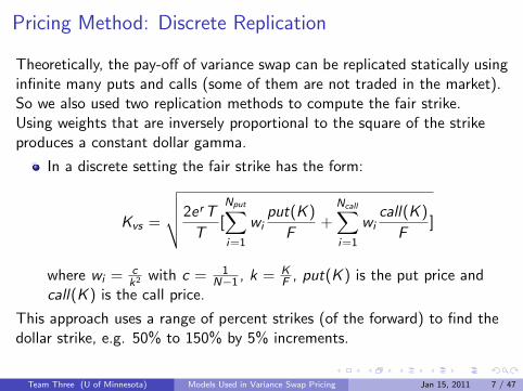
Pricing Method: Discrete Replication
Theoretically, the pay-off of variance swap can be replicated statically usinginfinite many puts and calls (some of them are not traded in the market).So we also used two replication methods to compute the fair strike.Using weights that are inversely proportional to the square of the strikeproduces a constant dollar gamma.
In a discrete setting the fair strike has the form:
Kvs =
√√√√2erT
T[
Nput∑i=1
wiput(K )
F+
Ncall∑i=1
wicall(K )
F]
where wi = ck2 with c = 1
N−1 , k = KF , put(K ) is the put price and
call(K ) is the call price.
This approach uses a range of percent strikes (of the forward) to find thedollar strike, e.g. 50% to 150% by 5% increments.
Team Three (U of Minnesota) Models Used in Variance Swap Pricing Jan 15, 2011 7 / 47

Pricing Method: Continuous Replication
In a continuous setting, the fair strike is calculated as the following:
Kvs =
√2erT
T[
∫ F
0
1
k2
put(K )
Fdk +
∫ ∞F
1
k2
call(K )
Fdk]
This approach requires a parametrized volatility surface, gaps andnon-exist strikes should be filled and extrapolated. Intuitively, the accuracyof this approach depends highly on the reliability of volatility surface. Thederivation of the theoretical strike will be included in our final report.
Team Three (U of Minnesota) Models Used in Variance Swap Pricing Jan 15, 2011 8 / 47

Pricing Method: Local Volatility & Monte Carlo Simulation
With a parametrized implied volatility surface, we can construct the localvolatility surface used Monte Carlo simulation. Conceptually, this isdefined as:
σlocal(s, t) = f (σimp(K ,T ))
After the translation, we simulate the underlying index with daily timesteps.Using the fact that
payoff =N∑i=1
(lnSi+1
Si)2 − Kvs
and at time zero, the contract has no value, we can solve for a fair strike.We will be giving more on this method in the later part of our presentation.
Team Three (U of Minnesota) Models Used in Variance Swap Pricing Jan 15, 2011 9 / 47

Modelling Vol Skew: SVIWe will use Gatheral’s Stochastic Volatility Inspired (SVI) and7-Parameter Skew Model to model the volatility skew.
Define k = ln(K/F ), where K is the strike and F is the forward price.Gatheral’s SVI Model reads
σimp(F ,T ,K ) =
√a + b[ρ(k − m) +
√(k − m)2 + σ2]
T
−2.5 −2 −1.5 −1 −0.5 0 0.5 1 1.5 2 2.50.2
0.25
0.3
0.35
0.4
0.45
0.5
0.55
0.6
0.65
Moneyness k=log(K/F)
Impl
ied
Vol
Illustration of the SVI Model
This is an illustration with a = 0.026, m = 0, b = 0.1, ρ = 0.6, σ = 0.6Team Three (U of Minnesota) Models Used in Variance Swap Pricing Jan 15, 2011 10 / 47

Modelling Vol Skew: 7-Parameter SkewThe 7-Parameter Skew Model reads
σimp(F ,T ,K ) =
ALeλLk + β4 if k < kL
β1 + kβ2√T
+k2Rβ32T if kL ≤ k ≤ KR
ARe−λRk + β6 if kR < k
−2.5 −2 −1.5 −1 −0.5 0 0.5 1 1.5 2 2.5
0.18
0.2
0.22
0.24
0.26
0.28
0.3
0.32
0.34
Moneyness k=log(K/F)
Impl
ied
Vol
Illustration of the Skew Model
This is an illustration with β1 = 20% implied vol at the at the moneyforward, β2 = −0.1, β3 = 0.5, β4 = 50%, β5 = −0.75, β6 = 15%, β7 = 1.
Team Three (U of Minnesota) Models Used in Variance Swap Pricing Jan 15, 2011 11 / 47
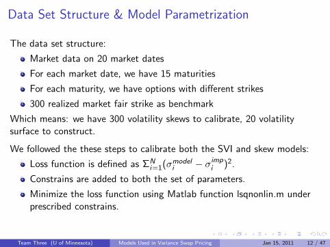
Data Set Structure & Model Parametrization
The data set structure:
Market data on 20 market dates
For each market date, we have 15 maturities
For each maturity, we have options with different strikes
300 realized market fair strike as benchmark
Which means: we have 300 volatility skews to calibrate, 20 volatilitysurface to construct.
We followed the these steps to calibrate both the SVI and skew models:
Loss function is defined as ΣNi=1(σmodel
i − σimpi )2.
Constrains are added to both the set of parameters.
Minimize the loss function using Matlab function lsqnonlin.m underprescribed constrains.
Team Three (U of Minnesota) Models Used in Variance Swap Pricing Jan 15, 2011 12 / 47
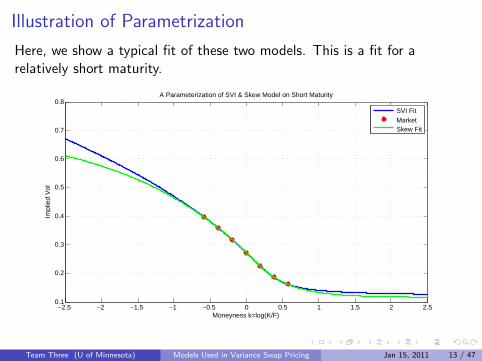
Illustration of Parametrization
Here, we show a typical fit of these two models. This is a fit for arelatively short maturity.
−2.5 −2 −1.5 −1 −0.5 0 0.5 1 1.5 2 2.50.1
0.2
0.3
0.4
0.5
0.6
0.7
0.8
Moneyness k=log(K/F)
Impl
ied
Vol
A Parameterization of SVI & Skew Model on Short Maturity
SVI FitMarketSkew Fit
Team Three (U of Minnesota) Models Used in Variance Swap Pricing Jan 15, 2011 13 / 47

Illustration of Parametrization
This is a fit for a relatively long maturity.
−2.5 −2 −1.5 −1 −0.5 0 0.5 1 1.5 2 2.5
0.2
0.25
0.3
0.35
0.4
0.45
0.5
Impl
ied
Vol
Moneyness k=log(K/F)
A Parameterization of SVI & Skew Model on Long Maturity
SVI FitMarketSkew Fit
Team Three (U of Minnesota) Models Used in Variance Swap Pricing Jan 15, 2011 14 / 47
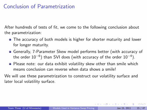
Conclusion of Parametrization
After hundreds of tests of fit, we come to the following conclusion aboutthe parametrization:
The accuracy of both models is higher for shorter maturity and lowerfor longer maturity.
Generally, 7-Parameter Skew model performs better (with accuracy ofthe order 10−6) than SVI does (with accuracy of the order 10−4).
Please note: our data exhibit volatility skew other than smile whichmeans conclusion can reverse when data shows a smile!
We will use these parametrization to construct our volatility surface andlater local volatility surface.
Team Three (U of Minnesota) Models Used in Variance Swap Pricing Jan 15, 2011 15 / 47
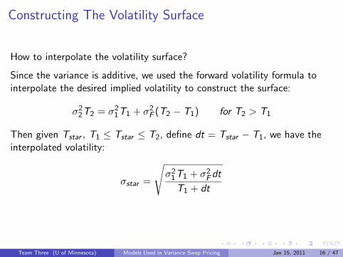
Constructing The Volatility Surface
How to interpolate the volatility surface?
Since the variance is additive, we used the forward volatility formula tointerpolate the desired implied volatility to construct the surface:
σ22T2 = σ21T1 + σ2F (T2 − T1) for T2 > T1
Then given Tstar , T1 ≤ Tstar ≤ T2, define dt = Tstar − T1, we have theinterpolated volatility:
σstar =
√σ21T1 + σ2Fdt
T1 + dt
Team Three (U of Minnesota) Models Used in Variance Swap Pricing Jan 15, 2011 16 / 47

Constructing The Volatility Surface
A Visual Illustration: Step 1
T
k
σ
Team Three (U of Minnesota) Models Used in Variance Swap Pricing Jan 15, 2011 17 / 47

Constructing The Volatility Surface
A Visual Illustration: Step 2
T
k
σ
T_star
Team Three (U of Minnesota) Models Used in Variance Swap Pricing Jan 15, 2011 18 / 47

Constructing The Volatility Surface
A Visual Illustration: Step 3
T
k
σ
T_lower
T_star
Team Three (U of Minnesota) Models Used in Variance Swap Pricing Jan 15, 2011 19 / 47
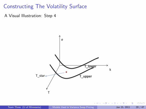
Constructing The Volatility Surface
A Visual Illustration: Step 4
T
k
σ
T_upper
T_lower
T_star
Team Three (U of Minnesota) Models Used in Variance Swap Pricing Jan 15, 2011 20 / 47
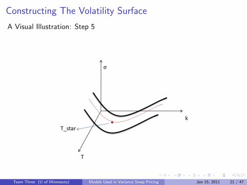
Constructing The Volatility Surface
A Visual Illustration: Step 5
T
k
σ
T_star
Team Three (U of Minnesota) Models Used in Variance Swap Pricing Jan 15, 2011 21 / 47

Constructing The Volatility Surface
A Visual Illustration: Step 6
T
k
σ
T_star
Team Three (U of Minnesota) Models Used in Variance Swap Pricing Jan 15, 2011 22 / 47

Constructing The Volatility Surface
A Visual Illustration: Step 7
• Surface
T
k
σ
Team Three (U of Minnesota) Models Used in Variance Swap Pricing Jan 15, 2011 23 / 47

Constructing The Volatility Surface
Extrapolate Out of The Maturity Range
In constructing local volatility surface, we need to use daily time stepwhich might be less than the smallest maturity and our desired varianceswap maturity might be longer than the longest the data provided, so weneed to extrapolate out of the maturity range the data specified. We didthe following:
Assign σ(kstar ,Tstar ) = σ(kstar ,T (1)) if Tstar < T (1)
Assign σ(kstar ,Tstar ) = σ(kstar ,T (end)) if Tstar > T (end)
Team Three (U of Minnesota) Models Used in Variance Swap Pricing Jan 15, 2011 24 / 47

Constructing The Volatility Surface
We built a MATLAB function to calculate the volatility surface:
surface = vol surf (para,T ,Model ,T star ,K star)
para: parameter set from the calibration (a matrix)
T: data maturity range (a column vector)
Model: SVI or skew (string)
T star: specified maturity (an arbitrary m by 1 vector)
k star: specified moneyness (an arbitrary n by 1 vector)
surface: interpolated volatility surface (an m by n matrix)
In conclusion, this function searches the neighbouring maturity slices T1
and T2, evaluates σ1 and σ2 and then interpolates in between to giveσ(kstar ,Tstar ).
Team Three (U of Minnesota) Models Used in Variance Swap Pricing Jan 15, 2011 25 / 47

Constructing The Volatility Surface
This is how the volatility surface look like:
−3 −2 −1 0 1 2 30
5
10
0.1
0.2
0.3
0.4
0.5
0.6
0.7
0.8
Maturity
Moneyness = log(K/F)
Volatility Surface
Impl
ied
Vol
atili
ty
Team Three (U of Minnesota) Models Used in Variance Swap Pricing Jan 15, 2011 26 / 47
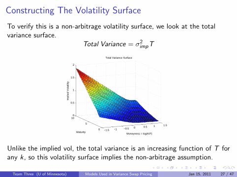
Constructing The Volatility Surface
To verify this is a non-arbitrage volatility surface, we look at the totalvariance surface.
Total Variance = σ2impT
−1.5 −1 −0.5 0 0.5 1 1.5
0
5
100
0.5
1
1.5
2
Moneyness = log(K/F)
Total Variance Surface
Maturity
Impl
ied
Vol
atili
ty
Unlike the implied vol, the total variance is an increasing function of T forany k, so this volatility surface implies the non-arbitrage assumption.
Team Three (U of Minnesota) Models Used in Variance Swap Pricing Jan 15, 2011 27 / 47

Test of Rule of Thumbs
To get a quick view of the fair strike for variance swaps, one can use eitherof the following rule of thumb calculations. We can price variance swaps
using rule of thumb:
90% put: take 90% of the forward strike as the strike and plug thatinto the volatility function
25% delta put: search for the strike that has a -25% delta (on the putside) and plug that strike into the volatility function
Review that we already have two models:
Gatherals SVI Model
Skew Model
We are going to show comparisons of these roles of thumb calculations tothe market prices in hopes of creating a guide line for the use of these twomethods.
Team Three (U of Minnesota) Models Used in Variance Swap Pricing Jan 15, 2011 28 / 47

Test of Rule of Thumbs
Next, we apply these two rules into SVI Model and Skew ModelRespectively and compare model data with market data over bothmaturity and calendar time (market date), then do statistics analysis.
The guideline will cover the following dimensions:
Time to maturity or Calendar Time
Type of volatility surface
Rule of Thumb Method
Review that we already have two models:
Gatherals SVI Model
Skew Model
After determining the guidelines, we also wanted to check theappropriateness of the 90% and 25% values used in the respectivemethods and make a recommendation for better levels given the timeseries data available.
Team Three (U of Minnesota) Models Used in Variance Swap Pricing Jan 15, 2011 29 / 47

Test of Rule of Thumbs
Here we calculate volatility derived from market data of 10/27/2010 asexample:
1 1
Figure: Rule of thumb in SVI model (left) and skew model (right)
Two Figures above have applied rule of thumb into SVI Model and SkewModel with same market date, therefore the same strike is taken.
Team Three (U of Minnesota) Models Used in Variance Swap Pricing Jan 15, 2011 30 / 47
Test of Rule of Thumbs
From previous graphs, we find:
The shape of two Figures is similar which means choice of volatilitysurface does not seem to show a big difference, and Market Fair Priceis almost higher than other two ways, we notice when the Maturitygoes increasing, both rules approximate to same volatility.
It shows how each method performs relative to the time to maturityfor fixed market date. 25% Delta put performs very well formaturities less than 2 years and turns out not so well when maturityis increasing to large period of time.
Moreover, the 90% Strike does not work well at all due to the poormatch of the market data.
At 10 years maturity, the difference is 4 vol points of 25% Delta Put,however at 2 years, the difference is very tiny, how does this spread?We need to do different version for calendar time of market dateinstead of Maturity.
Team Three (U of Minnesota) Models Used in Variance Swap Pricing Jan 15, 2011 31 / 47

Test of Rule of ThumbsExpiration date of 12/21/2012 = 2Y
1
Expiration date of 12/21/2013 = 3Y
1
Team Three (U of Minnesota) Models Used in Variance Swap Pricing Jan 15, 2011 32 / 47

Test of Rule of Thumbs
We did similar plot on longer maturity. The conclusion is:
When maturity goes further, 90% Forward rules seems plausible than25% rule. While, for short maturities, the 25% Delta Put matchesmarket better.
90% forward rule is good for long maturity, but lower than market.
25% Delta Put is good for short maturity, but lower than market.
There are no significant differences between Skew Model and SVIModel using these two rules of thumb.
Team Three (U of Minnesota) Models Used in Variance Swap Pricing Jan 15, 2011 33 / 47

Test of Rule of Thumbs
We also sampled from the market fair strike and our model strike pricerandomly and then F-test is performed on the random samples. And wefind that the statistical analysis is in line with our assumption from graphsbefore.
The 90% strike does not seems to work for any maturity in our datasample though it does perform better than 25% for the long maturity,but not good enough to use.
The 25% delta put works very well for short term maturity varianceswaps, but becomes ineffective when the maturity goes longer than 2years.
Given the reservation stated in 1 and 2, each pricing method worksequally well with either volatility model.
Team Three (U of Minnesota) Models Used in Variance Swap Pricing Jan 15, 2011 34 / 47

Conclusion of Discrete & Continuous Replication
Discrete and continuous replication is theoretically true to price thevariance swap. Commonly, discrete replication uses a range of percentstrikes to find the dollar strike. Usually we use 50%-150%. We also didtrials on 10%-190%, 30%-170%, 70%-130% and 90%-110%.
Statistical analysis shows that:
Discrete Replication + SVI is better than Discrete Replication + Skew
Continuous Replication + SVI and Continuous Replication + skew areequivalent.
Team Three (U of Minnesota) Models Used in Variance Swap Pricing Jan 15, 2011 35 / 47
Conclusion of Discrete & Continuous Replication
Discrete and continuous replication is theoretically true to price thevariance swap. Commonly, discrete replication uses a range of percentstrikes to find the dollar strike. Usually we use 50%-150%. We also didtrials on 10%-190%, 30%-170%, 70%-130% and 90%-110%.
Statistical analysis shows that:
Discrete Replication + SVI is better than Discrete Replication + Skew
Continuous Replication + SVI and Continuous Replication + skew areequivalent.
Team Three (U of Minnesota) Models Used in Variance Swap Pricing Jan 15, 2011 36 / 47

Transfer Implied Volatility to Local Volatility
The formula that transfer implied volatility to local volatility reads:
σ(s, t)2loc =∂w∂T
1 − kw∂w∂k + 1
4(−14 − 1
w + k2
w2 )(∂w∂k )2 + 12∂2w∂k2
where k = ln( SF ) and w = σ2impT . Derivatives are found numerically: we
use forward approximation to calculate the first order derivative andcentral approximation to calculate the second derivative.
Team Three (U of Minnesota) Models Used in Variance Swap Pricing Jan 15, 2011 37 / 47

Monte Carlo Simulation
We assume underlying asset follows the stochastic equation:
dSt
St= µ(t)dt + σ(S , t)dWt
where µ(t) = r(t) − q(t) and σ(S , t) is the local volatility. Every step ofsimulation we generate a new normal distributed random number and plugin local volatility and local drift term to produce a new underlying price.And the final price can be obtained using:
payoff =N∑i=1
(lnSi+1
Si)2 − Kvs
Team Three (U of Minnesota) Models Used in Variance Swap Pricing Jan 15, 2011 38 / 47

Monte Carlo Simulation & Error Analysis
To reach a more accurate pay-off, we should simulate large number ofpaths of price evolution.
Then, take the expectation of the total number of pay-off, which will bethe fair volatility strike that let the initial value of the variance swap equalto zero.
We finally compare the simulated value to market price:
Percentage Error = abs(simulated value-market data) / market data
Team Three (U of Minnesota) Models Used in Variance Swap Pricing Jan 15, 2011 39 / 47

Monte Carlo Simulation & Error Analysis
Team Three (U of Minnesota) Models Used in Variance Swap Pricing Jan 15, 2011 40 / 47

Discussion of Future Work:Variance Swap with Stochastic Rate
So far, the work we have been done is under the assumption that heunderlying price process is an Ito process with a deterministic short rate.we have shown that rule of thumbs and the discrete model and continuousmodel work well in this setting for a relative short maturity, that is, lessthan 2 years for rule of thumbs and 3 to 5 years for the discrete andcontinuous models.
Team Three (U of Minnesota) Models Used in Variance Swap Pricing Jan 15, 2011 41 / 47

Variance Swap with Stochastic Interest Rate
The market has a stochastic interest rate;
The value of an equity variance swap depends on the interest ratevolatility;
Long-dated variance swaps will be sensitive to the interest ratevolatility;
Long-dated variance swaps do happen;
Price becomes more complicated.
Team Three (U of Minnesota) Models Used in Variance Swap Pricing Jan 15, 2011 42 / 47

Variance Swap with Stochastic Interest Rate
The rest is an upper bound of the fair strike developed by Per Horfelt andOlaf Torn.
P(t,T ) bond price at time t that matures at T .
S(t) stock price at time t.
dP(t,T )
P(t,T )= r(t)dt + σP(t,T ) dW1(t), (1)
dS(t)
S(t)= r(t) dt + σS(t) dW2(t). (2)
r(t) is the continuous compounded short rate at time t, Q is a risk-neutralmeasure, (W1,W2) is a 2-dim Q-Wiener process with joint correlation ρ.
Team Three (U of Minnesota) Models Used in Variance Swap Pricing Jan 15, 2011 43 / 47

Discussion of Future Work:The Bound of Value of Variance Swap
Introduce
β(t) = exp(
∫ t
0r(θ) dθ),
The solution of (1) is
P(t,T )
P(0,T )= β(t) exp(
∫ t
0σP(θ,T )dW1(θ) − 1
2
∫ t
0σ2P(θ,T ) dθ). (3)
It follows
β(t) =1
P(0, t)exp(−
∫ t
0σP(θ,T )dW1(θ) +
1
2
∫ t
0σ2P(θ,T ) dθ). (4)
Team Three (U of Minnesota) Models Used in Variance Swap Pricing Jan 15, 2011 44 / 47
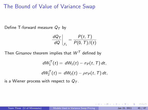
The Bound of Value of Variance Swap
Define T-forward measure QT by
dQT
dQ
∣∣∣∣Ft
=P(t,T )
P(0,T )β(t)
Then Girsanov theorem implies that W T defined by
dW T1 (t) = dW1(t) − σP(t,T ) dt,
dW T2 (t) = dW2(t) − ρσP(t,T ) dt,
is a Wiener process with respect to QT .
Team Three (U of Minnesota) Models Used in Variance Swap Pricing Jan 15, 2011 45 / 47
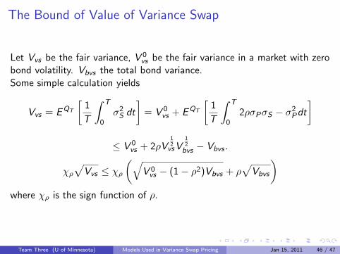
The Bound of Value of Variance Swap
Let Vvs be the fair variance, V 0vs be the fair variance in a market with zero
bond volatility. Vbvs the total bond variance.Some simple calculation yields
Vvs = EQT
[1
T
∫ T
0σ2S dt
]= V 0
vs + EQT
[1
T
∫ T
02ρσPσS − σ2Pdt
]
≤ V 0vs + 2ρV
12vsV
12bvs − Vbvs .
χρ√
Vvs ≤ χρ
(√V 0vs − (1 − ρ2)Vbvs + ρ
√Vbvs
)where χρ is the sign function of ρ.
Team Three (U of Minnesota) Models Used in Variance Swap Pricing Jan 15, 2011 46 / 47

References
More Than You Ever Wanted To Know About Volatility Swaps
Just What You Need To Know About Variance Swaps
The Volatility Surface: A practitioner’s guide
The Fair Value of a Variance Swap - a question of interest
Team Three (U of Minnesota) Models Used in Variance Swap Pricing Jan 15, 2011 47 / 47