modelling the overall personal income distribution in the usa
TRANSCRIPT

Working Paper Series
Modelling the overall personal income distribution in the USA from 1994 to 2002 Ivan O. Kitov
ECINEQ WP 2005 – 07

ECINEQ 2005-07
November 2005
www.ecineq.org
Modelling the overall personal income distribution in the USA from 1994 to 2002
Ivan O. Kitov*
Russian Academy of Sciences
Abstract Numerical modelling of the personal income distribution (PID) in the USA from 1950 to 2003 is accomplished based on a microeconomic model for the personal income evolution. It is shown that the overall PID demonstrates the existence of some fixed hierarchical income distribution structure in the USA. The PIDs normalized to the total population and corrected for the per capita nominal GDP growth coincide for years from 1994 to 2002. The observed inflation plays a role of some specific mechanism returning the PIDs to the initial shape. The structure of the PID is accurately simulated by using a microeconomic model with some simple assumptions related to the distribution of capabilities to earn money and sizes of earning means – two measurable parameters introduced in the model. The evolution of the overall PID is also well predicted depending on nominal GDP growth from 1994 to 2002.
KEYWORDS: personal income distribution, mean income,
microeconomic modeling, USA, real GDP, macroeconomics JEL Classification: D01, D31, E17, J1, O12
* Contact details: VIC, P.O. Box 1250, Vienna 1400, Austria; email - [email protected]

Introduction
This paper is devoted to the numerical modelling of the personal income distribution in the USA
from 1950 to 2003. Kitov (2005b) has formally introduced a microeconomic model for the personal
income evolution depending on economic growth. Personal income distribution (PID) is one of the
key economic parameters. The history of the income measurements in the USA started in 1948
when the first Annual Social and Economic Supplement, ASEC, (former Annual Demographic
Survey, ADS, or March Supplement) to the Current Population Survey (CPS) included a question
about the income (The U.S. Census Bureau 1996). Tables of income by detailed socioeconomic
characteristics published by the US census Bureau (2004a) span the time interval from 1994 to
2003. The tables include information on the number of people with income in narrow intervals of
$2500 starting from zero income and current losses up to a highest income of $100,000. They also
provide mean incomes in five years intervals of age groups, except for the youngest group, which
spans the time interval from 15 to 24 years of age. Thus, detailed data on personal income are
available for the last 10 years and the aggregated data are available for a longer period of 35 years -
from 1967 to 2001. The aggregated data sets are used in the following papers.
An important issue for the analysis conducted below is accuracy of the income
measurements. There are two principal sources of inaccurate measurement - sampling error and
non-sampling error as presented by the US Census Bureau (2002). The first is related to the
difference between the CPS sample and the complete coverage of the population. Statistical
accuracy of this type of error can be estimated and included into analysis. The second includes all
1
other potential sources of error including undercoverage, definition difficulties, variations in
interpretation of questions, etc. The U.S. Census Bureau constantly improves accuracy of the
personal income measurements. This process includes extension of the number of interviewed
households, covering some specific groups such as Hispanic origin, etc. The last major change in
the procedure occurred in 2002, when the total number of the surveyed units became 99,000.
Between 1994 and 2001 there were 60,000 units in the basic CPS and additional 21,000 units for
the March Survey, i.e. 81,000 in total. These changes make it sometimes difficult to compare
income data sets obtained in different years.
Despite some shortcomings in the personal income data set, this represents the longest,
and the most detailed and accurate source of income information for any numerical analysis.
1. Personal income distribution in the USA
The personal income distributions for years from 1994 to 2002 are displayed in Figure 1. The
number of people with income inside original $2500 wide intervals is merged in wider intervals of
$10,000. The distributions show an increasing number of people with income above $20,000 and a
decreasing number below this value. This is an expected result of population growth, real economic
growth and inflation. The first of the three processes potentially leads to the upward displacement
of the curves as a whole if the population added every year is distributed over income in the same
way as before. The US population grows approximately by 1% yearly due to excess of births over
deaths, and positive migration.
The latter two processes, however, result in the distribution curve change. Inflation
observed in the USA last ten years was between 1.2% in 1998 and 2.4% in 2001. The effect of
inflation results in receipt of a higher nominal income. Because subsequent years provide
population counts in the same income bins, one can expect that people in lower income bins would
eventually migrate in higher income bins. Moreover, the people in the highest routinely counted
income bins, eventually, migrate to the zone above the highest limit of the survey, i.e. above
$100,000. Thus, more and more people were outside the published detailed counting. This effect,
apparently, forced the Census Bureau to introduce some new income intervals for higher incomes
after 2000. These intervals, however, are $50,000 wide, i.e. twenty times wider than the standard
intervals. The observed effect of the inflation is a decreasing population in lower income bins and
an increasing population in higher income bins. This is exactly what one observes in Figure 1.
2

The real economic growth leads to the effect similar to that caused by inflation. More goods
and services produced by the economy result in an increase in the total income, which by definition
is GDP (GDP=GDI). People earn more and migrate with time to higher income bins. In some rare
years of the economy contraction, incomes drop and people fall back into lower income bins.
The aggregate effect of the three processes described above divide the distribution into two
zones – less than the mean income and above the mean income, as seen in Figure 1. The mean
income increases from $23,278 in 1994 to $32,222 in 2002 (in current dollars). So, the turning
point between the two zones is somewhere between these values.
One can present the original PIDs in some normalized form. A natural normalization is
according to the total population. This representation avoids population change effects and allows
for the population density distribution. As shown below, this distribution better characterizes a
hierarchy of the personal income distribution in a developed economy. Figure 2 illustrates
evolution of the population density distribution as a function of income.
A series of corrections has been applied to the original PID. Information on real and
nominal GDP growth and total population change in the USA is used to reduce the distributions to
that of the 1994 PID. A well-known procedure of the reduction is the adjustment for inflation.
Because the March Supplement of the CPS gives numbers of people with incomes in bins of $2500,
one has to correct the distribution for changing dollar value, which represents the scale contraction
caused by the inflation. For example, in order to correct for 10 per cent inflation, one has to
compress the scale by 1.1. In this case, the bin between $50,000 and $52,500 transforms into the
bin from $45,450 to $47,727, with the center shifted from $51,125 to $46,588. Comparison of the
starting year distribution, the PID for 1994 in this case, and the subsequent years' distributions
corrected for the inflation reveals the change of the real PID. Figure 3 displays results of the
correction for inflation during time period from 1994 to 2002 applied to the population density
distribution. Evolution of the distributions shows an increase of relative number of people with
higher real incomes. This observation is consistent with the observed real economic growth during
the studied period of time. Due to very weak real GDP growth in 2001, the curve for 2000 is very
close to that for 2002. One can observe the scale contraction resulted from the corrections described
above - the centers of the measurement intervals monotonically drift to the zero point with time.
The same correction procedure has been applied to changes of nominal and real economic
growth, both absolute and per capita. In the case of zero population change and inflation, a
3

correction for the real economic growth could potentially reveal changes in distribution of the total
personal income among the same people. This type of correction is similar to that of correction of
the density distribution for per capita nominal GDP growth. The density distribution is not affected
by the population changes and the correction for the nominal GDP growth effectively compensates
for the inflation effect. Figures 4 and 5 compare effects of a correction for the nominal GDP growth
on the original personal income distribution and a correction for the nominal per capita GDP
growth on the density income distribution. This correction addresses the question of redistribution
of the extra income generated by inflation and real economic growth among the increasing
population. Are the extra money distributed evenly over the income groups or some selected
groups obtain more from the redistribution?
The personal income distributions in Figure 4 are almost parallel. This indicates that
potentially only population growth forces the 1994 curve to move upwards. Because the curves are
parallel, relative increase of population in every income bin is the same, and the personal income
distribution among the newcomers is exactly the same as among the experienced people. In other
words, the hierarchy in the PID is rigid over time and generations. This principal conclusion of the
paragraph is even better illustrated by Figure 5 where the population density curves for the studied
years coincide.
Hence, one can interpret inflation as a mechanism compensating the distortion of the PID
caused by the real economic growth. The observed inflation rate is exactly equal to the rate needed
to return the PID density distribution to its original shape. In other words, inflation eats out of the
poor people advantages obtained from the economic growth.
2. Modelling the overall personal income distribution
Using the model described in Kitov (2005b), we start the personal income modelling with some
theoretical examples. The initial model is constrained so as to reproduce the real observations, but
only general details are important at this stage. The model is characterized by a number of external
and internal parameters. The external parameters include GDP growth rate: real and nominal, total
and per capita and population distribution - total and single year of age. The internal parameters of
the model are the initial critical work experience, Tcr(0), and the initial dissipation factor, α. The
former internal parameter can be obtained from the observations and the latter only from some
calibration process.
4

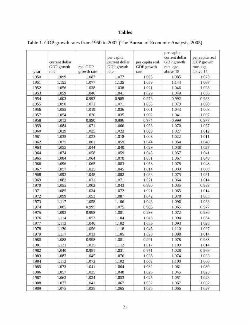
GDP growth rates during the period from 1950 to 2002 are presented in table 1. The total
increase of the nominal and real GDP is 35.7 and 5.7, respectively. The per capita GDP corrected
for population above 15 years has changed by factors 17.5 and 2.5, respectively. The latter value
indicates that the real GDP growth per a person of age above 15 changed only by 2.5 times during
the 52 years after 1950. It is 2.28 less than the total change of real GDP. Actual economic
development is not as fast as seems from some economic news.
Thus, the observed growth of the real GDP is half due to the population growth or extensive
factors. Figure 6 illustrates single year population estimates for some selected calendar years as
obtained from the U.S. Census Bureau (2004b). Total population in the USA grows eventually
from 152,200,000 in 1950 to 286,200,000 in 2001. Total population of age above 15 grew during
the same period from 111,300,000 to 225,670,000. The relative share of a given single year age
population also changes in time. Figure 7 depicts the same population distributions normalized to
the corresponding peak year for a single year population. The age of the largest population evolves
in time and is currently 45 years. Populations peaked at this age provides the highest share of
population with almost the highest attained income. In other words, the current population
conditions in the USA correspond to a very effective one case for income earning. When the peak
surpasses the critical time, Tcr (also growing in time), in several years from now, the conditions will
deteriorate eventually, but not severely. There will be only 10% drop of the relative share of the
population with the peak income in next 15 years. The next five years, however, are favorable. The
Figures demonstrate also the importance of the single year population distribution for the model.
Variations of population counts within the 10 year age groups used by the U.S. Census Bureau for
averaging of income readings can cause substantial variations in estimates, especially in the
youngest age group, where the personal income increases exponentially. Fortunately, the single
year population estimates are available from 1950, with a varying accuracy, however. We estimate
the accuracy of the estimates for a single year of age as 5% to 7%. In wider intervals, the accuracy
is higher and may be of 1% to 2%.
In the model, the population of every single year of age for every calendar year is divided
by 292=841. The resulting value represents a share of population with the same income evolution
history, because only 841 different combinations of SL are available. One should keep in mind that
combinations (S=2, L=30) and (S=30, L=2) are quite different due to the fact that the means size L
defines the time constant of dissipation. People in each of the 841 groups have the same income
5

equal to the product of the current GDP level relative to the start point of the calculations and time
dependent function (1-exp(-αT/L), where T is the work experience of the particular age group. For
example, the age group of 50 year-olds has the work experience of 35 years. L is the value of the
real earning means’ size in the group relative to the initial value. Actually, there are as many age
groups as listed in the tables of the U.S. Census Bureau. The model includes only the age groups
from 15 to 75 years. This age interval is used in the calculations of the average income covering the
time period from 1967 to 2001. This limitation affects, however, the modelling of the overall
personal income distribution because not all the people counted by the Census Bureau are counted
in the model.
The internal parameters Tcr and α depend on time. We have conducted a series of
calculations for various time intervals between 1950 and 2002. The best estimates for the year 1950
are Tcr=23.5 years and α=0.097, respectively. These values can be reduced to any year other than
1950 by using the per capita real GDP growth (see Table 1).
Figure 8 presents some examples of the overall PID for the years of 1980, 1990, and 2002.
Evolution of the PID reproduces some principal features of the observed distributions: a drop of
population density level at lower incomes, and an increase of population density at higher income.
The point where the two processes compensate each other is situated between $20K and $30K. The
curves are obtained from corresponding dimensionless curves scaled with a factor of 70000. This
means that 1 unit of the dimensionless scale costs $70,000 for the year of 1980. The scaling factor
evolves in time with the per capita nominal GDP growth. In the year 2002, the scaling factor is
about 105,000 and the theoretical personal income distribution in current dollars extends to
$103,000.
Figures 9 through 11 compare the observed and predicted distributions for the years 1994,
1998, and 2001. The observed distributions in $10K wide intervals are interpolated by splines in
order to get a continuous distribution. The predicted distributions are obtained from a model with
the following parameters: start year = 1960, Tcr(1960)=26.5, α=0.087. Because the calculation are
carried out in current dollars, the initial value of the Pareto threshold is equal to 0.43 and develops
in time as the per capita nominal GDP growth in order to obtain the number of people in the current
dollar bins. The conversion factor between dimensionless units of the model and current dollars in
the year of 1960 is 10,500. This means that the whole 1960 theoretical PID can be placed into
$10,500 income range, and the whole 1980 PID spans from $0 to $40,000 because the per capita
6

nominal GDP grew by 3.8 times from 1960 to 1980. There are no people in the highest income
groups of the theoretical distribution, however, because none reached 100% of their potential
income during the period of income growth.
The PID for the year 1994 is presented in Figure 9. The predicted distribution coincides
with the observed one in the range between $5K and $35K. The latter value is very close to the
Pareto threshold situated between $35K and $45K. Beginning from the Pareto threshold the
distributions diverge because of different character of decay described in the model (see Kitov
(2005) for details). The observed distribution drops with income by a power law. The predicted
distribution decays slowly just above the threshold, but then the rate of the decay grows very fast
and it intercepts the observed distribution somewhere near the $60K income point. Since the scale
is semi-logarithmic, the curves apparent divergence is higher than the actual one on a linear scale.
Figures 10 and 11 illustrate the development of the distributions and corresponding Pareto
threshold. The threshold moves towards the higher limit of the income range with time. It was
somewhere around $45K in 1998, and near $55K in 2001. Because the Pareto threshold quickly
moves to the $100,000 mark as a result of the observed intensive economic growth in the USA, one
can expect that the distribution in the range from $0 to $100,000 will not contain the Pareto
distributed portion of the overall distribution and will not correctly represent the personal income
distribution. Even now the distribution contains only a narrow range where the power law reigns.
The predicted and observed PID describing the population between 15 and 75 years of age
are consistent. These distributions, however, are less sensitive to the model parameters than other
fine characteristic described in the following paper.
3. Discussion and conclusion
The above analysis of the overall PID demonstrates the existence of some fixed hierarchical
structure of the personal income distribution in the USA. The PIDs normalized to the total
population above 15 years of age and corrected for the per capita nominal GDP growth coincide for
years from 1994 to 2002. Thus, the observed inflation plays a role of some specific mechanism
returning the PIDs to the initial shape when disturbed by the real economic growth.
The structure of the personal income distribution can be simulated by using the
microeconomic model presented in Kitov (2005b) with some simple assumptions related to the
distribution of capabilities to earn money and sizes of earning means. In the lower income zone, the
7

observed and predicted distributions coincide up to an income interpreted as the Pareto distribution
threshold or the minimum possible income in the Pareto distribution. The Pareto part of the actual
PID is considered to be a result of the self-organized criticality and does not need any additional
modelling except the prediction of the portion of the total population in the Pareto zone. This
portion of the total population is of about 10 per cent and its distribution over work experience is
also exactly predicted by the microeconomic model (Kitov 2005a).
The evolution of the overall PID is also well predicted depending on nominal GDP growth
from 1994 to 2002. This includes the prediction of the subcritical zone width and relevant change
of the PID slope with time. One can easily predict the future PIDs as a function of GDP growth and
population changes.
On the other hand, the observed accurate prediction of the US PIDs for years between 1994
and 2002 demonstrates validity of the microeconomic model and general concept inherently related
to the personal income as the only source of the economic growth. More support for the model is
expected in further papers addressing some fine features of the PIDs for the same years from 1994
to 2002 and aggregated income measures available for a longer interval starting in 1967.
Acknowledgements
The author is grateful to Dr. Wayne Richardson for his constant interest in this study, help and
assistance, and fruitful discussions. The manuscript was greatly improved by his critical review.
8
References
Kitov, I.O. (2005a) “Evolution of the personal income distribution in the USA: High incomes”, paper accepted for presentation at the first meeting of the Society for the Study of Economic Inequality (ECINEQ), Palma de Mallorca, July 20-22, 2005 Kitov, I.O. (2005b) “A model for microeconomic and macroeconomic development”, (in preparation) U.S. Bureau of Economic Analysis (2005) “Current-Dollar and "Real" Gross Domestic Product”, Table, Last modified 05.26.05. http://bea.gov/bea/dn/gdplev.xls U.S. Census Bureau (1996) “CPS Help-Census/DSD/CPSB”, Last modified: May 22, 1996; http://www.bls.census.gov/cps/ads/shistory.htm U.S. Census Bureau (2004a) "Detailed Income Tabulations from the CPS". Tables, Last Revised: August 26 2004; http://www.census.gov/hhes/income/dinctabs.html U.S. Census Bureau (2002) “Source and Accuracy of the Data for the March 2002 CPS” http://www.bls.census.gov/cps/ads/2002/S&A_02.pdf U.S. Census Bureau (2004b) "Population Estimates; Age", Tables, Last Revised: 4-December-2004 03:44:43 p.m.; http://www.census.gov/popest/age.html
9

Figures
Fig.1. Personal income (current dollars) distributions in the USA from 1994 to 2002. Odd years are skipped for the sake of clarity. Absolute number (thousands) of people with income in $10K bins (includes current losses)are shown.
10

Fig.2. Personal income distributions shown in Fig.1 divided by the corresponding midyear population.
11
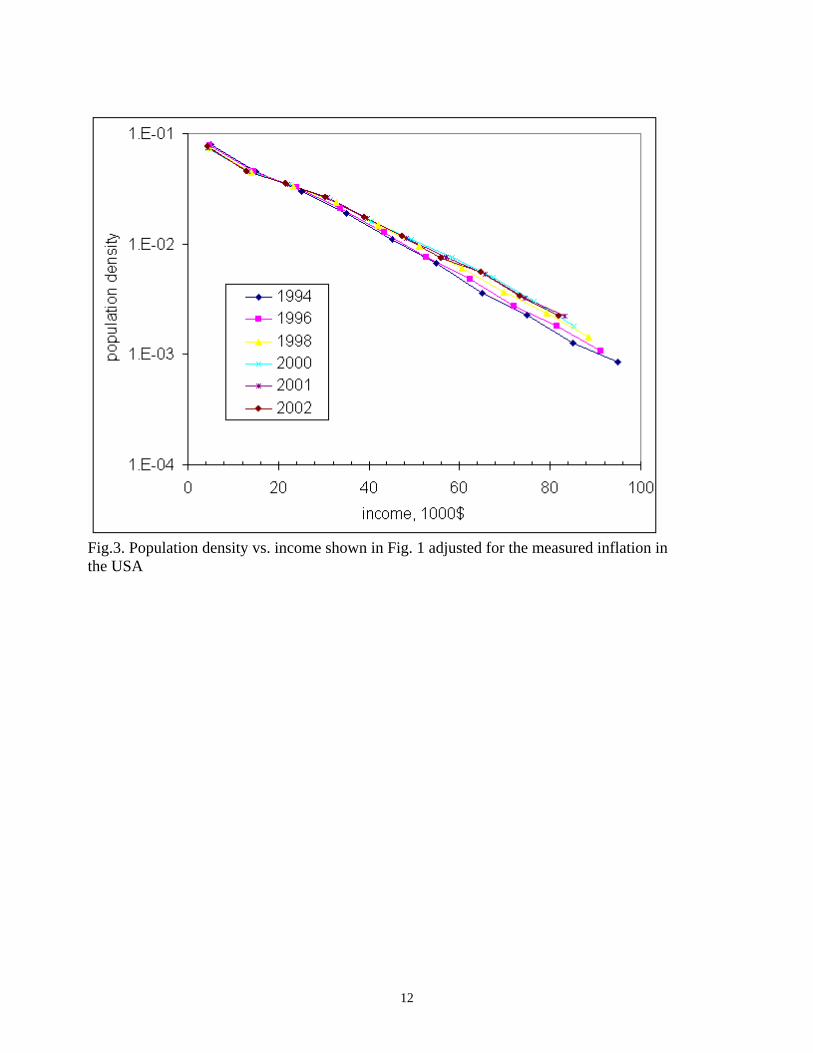
Fig.3. Population density vs. income shown in Fig. 1 adjusted for the measured inflation in the USA
12

Fig.4. Personal income distribution shown in Fig. 1 adjusted for the measured nominal GDP growth.
13

Fig.5. Population density vs. income adjusted for the measured per capita nominal GDP growth. Exponential and power law branches are distinguished and corresponding trend lines are shown.
14

Fig.6. Population estimates for the calendar years of 1950, 1960, 1970, 1980, 1990, and 2001 (The US Census Bureau (2004b)).
15

Fig. 7. Normalized population estimates for the calendar years of 1950, 1960, 1970, 1980, 1990, and 2001.
16

Fig. 8. Predicted evolution of the personal income distribution for the years between 1980 and 2002.
17

Fig. 9. Comparison of the predicted and observed personal income distributions for the year 1994. The Pareto threshold is between $35K and $45K.
18

Fig. 10. Comparison of the predicted and observed personal income distributions for the year 1998. The Pareto threshold is between $45K and $55K.
19

Fig. 11. Comparison of the predicted and observed personal income distributions for the year 2001. The Pareto threshold is between $55K and $65K.
20
Tables
Table 1. GDP growth rates from 1950 to 2002 (The Bureau of Economic Analysis, 2005)
year
current dollar GDP growth rate
real GDP growth rate
per capita current dollar GDP growth rate
per capita real GDP growth rate
per capita current dollar GDP growth rate. age above 15
per capita real GDP growth rate. age above 15
1950 1.099 1.087 1.077 1.065 1.085 1.073 1951 1.155 1.077 1.135 1.059 1.144 1.067 1952 1.056 1.038 1.038 1.021 1.046 1.028 1953 1.059 1.046 1.041 1.029 1.049 1.036 1954 1.003 0.993 0.985 0.976 0.992 0.983 1955 1.090 1.071 1.071 1.053 1.079 1.060 1956 1.055 1.019 1.036 1.001 1.043 1.008 1957 1.054 1.020 1.035 1.002 1.041 1.007 1958 1.013 0.990 0.996 0.974 0.999 0.977 1959 1.084 1.071 1.066 1.053 1.070 1.057 1960 1.039 1.025 1.023 1.009 1.027 1.012 1961 1.035 1.023 1.018 1.006 1.022 1.011 1962 1.075 1.061 1.059 1.044 1.054 1.040 1963 1.055 1.044 1.040 1.029 1.038 1.027 1964 1.074 1.058 1.059 1.043 1.057 1.041 1965 1.084 1.064 1.070 1.051 1.067 1.048 1966 1.096 1.065 1.083 1.053 1.078 1.048 1967 1.057 1.025 1.045 1.014 1.039 1.008 1968 1.093 1.048 1.082 1.038 1.075 1.031 1969 1.082 1.031 1.071 1.021 1.064 1.014 1970 1.055 1.002 1.043 0.990 1.035 0.983 1971 1.085 1.034 1.072 1.021 1.065 1.014 1972 1.099 1.053 1.087 1.042 1.078 1.033 1973 1.117 1.058 1.106 1.048 1.096 1.038 1974 1.085 0.995 1.075 0.986 1.065 0.977 1975 1.092 0.998 1.081 0.988 1.072 0.980 1976 1.114 1.053 1.104 1.043 1.094 1.034 1977 1.113 1.046 1.102 1.036 1.093 1.028 1978 1.130 1.056 1.118 1.045 1.110 1.037 1979 1.117 1.032 1.105 1.020 1.098 1.014 1980 1.088 0.998 1.081 0.991 1.078 0.988 1981 1.121 1.025 1.112 1.017 1.109 1.014 1982 1.040 0.981 1.031 0.971 1.028 0.969 1983 1.087 1.045 1.076 1.036 1.074 1.033 1984 1.112 1.072 1.102 1.062 1.100 1.060 1985 1.073 1.041 1.064 1.032 1.061 1.030 1986 1.057 1.035 1.048 1.025 1.045 1.023 1987 1.062 1.034 1.053 1.025 1.051 1.023 1988 1.077 1.041 1.067 1.032 1.067 1.032 1989 1.075 1.035 1.065 1.026 1.066 1.027
21

1990 1.058 1.019 1.048 1.009 1.049 1.010 1991 1.033 0.998 1.023 0.988 1.025 0.990 1992 1.057 1.033 1.045 1.021 1.046 1.023 1993 1.050 1.027 1.039 1.015 1.039 1.016 1994 1.062 1.040 1.052 1.030 1.052 1.030 1995 1.046 1.025 1.036 1.015 1.036 1.015 1996 1.057 1.037 1.047 1.027 1.045 1.026 1997 1.062 1.045 1.052 1.035 1.051 1.034 1998 1.053 1.042 1.043 1.032 1.041 1.030 1999 1.060 1.044 1.050 1.035 1.049 1.034 2000 1.059 1.037 1.048 1.026 1.046 1.024 2001 1.032 1.008 0.998 0.974 0.997 0.974 2002 1.035 1.019 1.024 1.008 1.022 1.006
Total
increase 35.69 5.67 18.94 3.01 17.55 2.79
22