Modelling Soil Water and Solute Dynamics

Assoc. Prof. Dr. Ahmad M. Manschadi

Water & Nitrogen

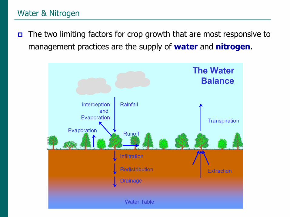
The two limiting factors for crop growth that are most responsive to

management practices are the supply of water and nitrogen.

Soil Water Balance

Basis of a soil water balance is the simple statement of the

conservation of water in soil

change in soil water content

= water in – water out

= precipitation + irrigation + runon

- runoff – drainage – transpiration – evaporation

This can be applied over any block of soil and any time scale

Soil Water Balance

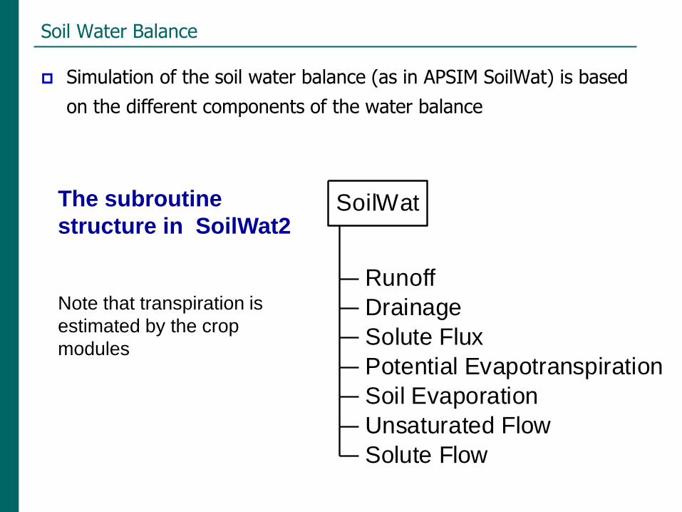
Simulation of the soil water balance (as in APSIM SoilWat) is based

on the different components of the water balance

Runoff

Drainage

Solute Flux

Potential Evapotranspiration

Soil Evaporation

Unsaturated Flow

Solute Flow

SoilWatThe subroutine

structure in SoilWat2

Note that transpiration is

estimated by the crop

modules

Soil Water Balance

Characterizing soil water properties

0

30

60

90

120

150

180

0.0 0.1 0.2 0.3 0.4 0.5

Volumetric soil water

De

pth

(c

m)

Total porosity

SAT

DUL

LL15

air_dry

LL crop 1

LL crop 2

Specified in terms of:

SAT (saturation)

DUL (drained upper limit)

LL15 (lower limit;

biological activity

ceases)

LLcrop (not a true soil

property)

Air Dry

Soil Water - Runoff

Precipitation has to be partitioned into what infiltrates into the top

soil layer and what runs off

Runoff is calculated using the USDA Soil Conservation Service (SCS)

procedure known as curve number technique

Based on total precipitation for the day – no allowance for number of

storms or rainfall intensity

Curve numbers have been derived from experimental data and depend

on:

- soil type

- land use (row crops, contoured, terraced)

- antecedent rainfall condition

Soil Water - Runoff

Surface residues affect movement of water during runoff events.

Curve number is adjusted according to amount of crop and residue

cover

0

10

20

30

40

50

60

70

80

0 20 40 60 80 100

Cover (%)

Curve

Number

Effect of cover on

runoff curve number

where bare soil curve

number is 75 and

total reduction in

curve number is 20

at 80% cover.

Soil Water - Evaporation

Soil evaporation occurs in two stages –

In 1st stage, the soil is sufficiently wet for water to be transported to the

surface to keep up with potential atmospheric evapotranspiration (based on

Priestly and Taylor approach)

In 2nd stage, transport of water to the surface can’t meet potential.

In SoilWat2 this behaviour is described by two parameters:

U – the cumulative evaporation (mm) before actual evaporation falls

below potential

CONA – 2nd stage evaporation is described as square root of time

(days) since 2nd stage commenced and CONA is the coefficient

Water lost by evaporation is only removed from the surface layer which can

be dried out to the Air Dry moisture content

Soil Water - Evaporation

Cumulative soil evaporation through time for

U = 6 mm and CONA = 3.5

0

2

4

6

8

10

12

14

16

18

0 2 4 6 8 10

Time (t)

Cumulative

Evaporation

(mm) U

t 1

The evaporation loss is linear against time until cumulative loss

exceeds U, beyond which it is calculated as CONA * (t –t1)1/2.

Soil Water - Saturated Water Flow

Cascading water balance model

When soil water content in any layer exceeds DUL, a fraction

(SWCON) of the excess drains to the next layer

FLUX = SWCON x (SW_dep – DUL_dep)

SWCON is the fraction of the water that drains. It can be set to

have different values in each layer.

Typically in clay soils SWCON has low values (0.2) while in a free

draining sand a higher value would be used (0.7)

Any water in excess of SAT automatically cascades to the next layer

Soil Water - Unsaturated Water Flow

When water content is below DUL, movement of water depends on

water content gradient between adjacent layers and the soil’s

diffusivity.

FLOW = DIFFUSIVITY x SOIL WATER GRADIENT

Unsaturated flow can move water either up or down in the profile

(saturated flux is only downwards).

But it can’t move water out of the bottom layer. In SoilWat2

drainage from the deepest layer can only occur when this layer wets

up above DUL.

Soil Water – Solute Movement

Solutes are moved together with water for both saturated and

unsaturated flow.

Nitrate-N is a mobile ion whereas ammonium-N is considered to

be immobile. Other solutes that are to be redistributed as mobile

must be specified in the SoilWat2 INI file (eg chloride, TDS)

SoilWat2 uses a simple “mixing” algorithm to calculate the

redistribution of solutes between layers. All water and solute

entering a layer is completely mixed with water and solute already

present to derive an average concentration.

The water that leaves the layer is at a concentration that is

proportional to this average concentration.

Soil Water

There are other approaches!

Soil physicists describe soil water behaviour in terms of soil water

potential and the movement of water in terms of

differential equations (Richards’ Equation)…… which can be

solved simultaneously.

An APSIM module (SWIMSOIL) is available and provides an

efficient numerical solution of Richards’ Equation.

It’s main users would be those interested in surface soil condition

and solute movement (e.g simulating soil/groundwater salinity).

Not generally used for agronomic applications

SWIM Module – Soil Water Infiltration and Movement

Developed by CSIRO Division of Land & Water

Based on a numerical soluation of the Richards´ equation and the advection-

dispersion equation

Components of soil water and solute balances (SWIM ver 2.1; Verburg et al. 1996)

SWIM Module

SWIM simulates

One-dimensional layered soil profile (vertically inhomogenous but

horizontally uniform

Saturated/unsaturated conditions

Surface ponding (high rainfall intensities)

Surface runoff (remove excess water)

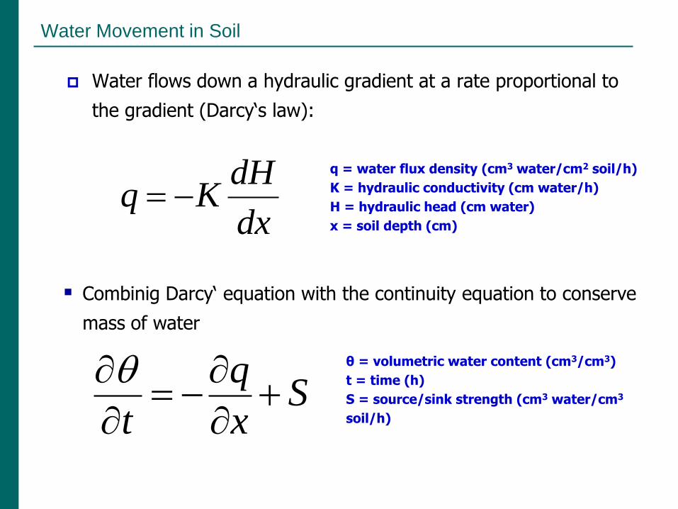
Water flows down a hydraulic gradient at a rate proportional to

the gradient (Darcy‘s law):

dx

dHKq

q = water flux density (cm3 water/cm2 soil/h)

K = hydraulic conductivity (cm water/h)

H = hydraulic head (cm water)

x = soil depth (cm)

Combinig Darcy‘ equation with the continuity equation to conserve

mass of water

qS

t x

θ = volumetric water content (cm3/cm3)

t = time (h)

S = source/sink strength (cm3 water/cm3

soil/h)

Water Movement in Soil

Water Movement in Soil

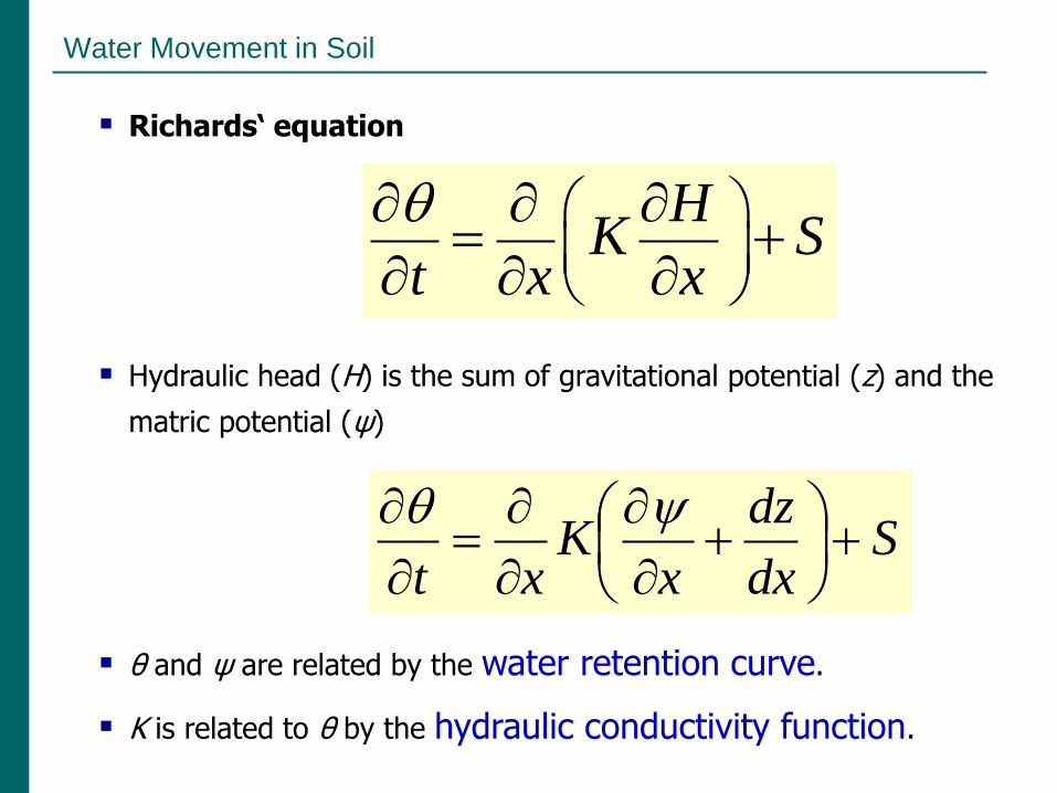
Richards‘ equation

HK S

t x x

Hydraulic head (H) is the sum of gravitational potential (z) and the

matric potential (ψ)

Sdx

dz

xK

xt

θ and ψ are related by the water retention curve.

K is related to θ by the hydraulic conductivity function.

Water Movement in Soil

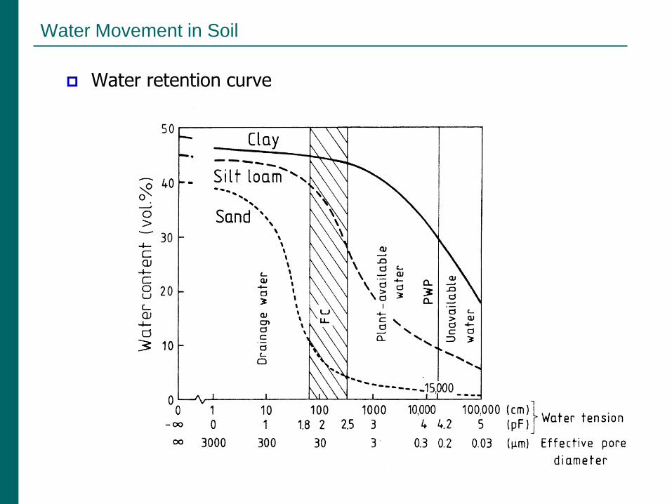
Water retention curve

bars kPa (=J/kg) MPa cm of H2O

-0.01 -1 -0.001 -10

-0.1 -10 -0.01 -102

-0.33 -33 -0.033 -337

-1 -100 -0.1 -1020

-10 -1000 -1 -10,204

-15 -1500 -1.5 -15,306

~PWP

~FC

Units of Soil Matric Potential

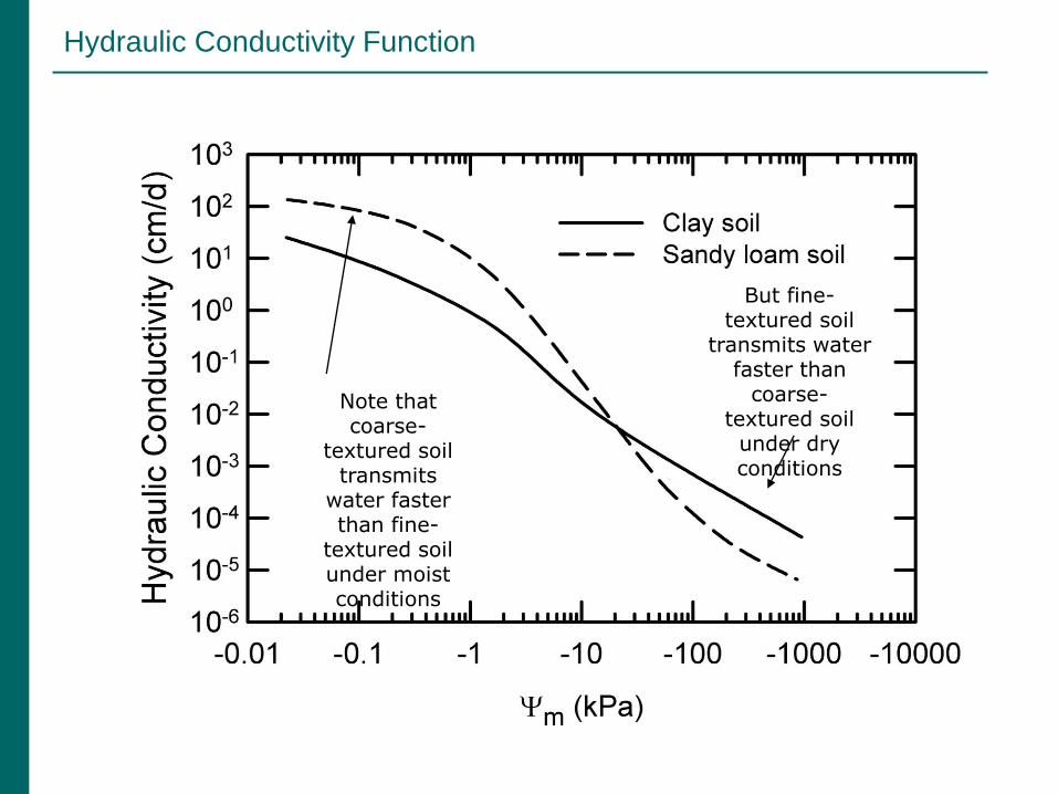
But fine-textured soil

transmits water faster than

coarse-textured soil under dry conditions

Note that coarse-

textured soil transmits

water faster than fine-

textured soil under moist conditions

Hydraulic Conductivity Function

Hydraulic Conductivity & Soil Water Potential

The soil profile is represented by a series of nodes

Water retention curve:

Instead of relating θ and ψ directly, SWIM uses a normalised

parameter S, effective saturation

( )

( )

rS

s r

S = effective saturation (cm3/cm3)

θr = residual vol. water content

(cm3/cm3)

θs = saturated vol. water content

(cm3/cm3)

Campbell equation (CropSyst):

S(Ψ) = (Ψ / Ψe)-1/b

Ψe = air entry potential (cm)

SWIMSOIL Parameters

User-defined water retention and hydraulic conductivity functions

HYPROPS generates a hydraulic property table

This table is used by SWIMSOIL

Log10 ǀΨǀ

Volumetric water content θ

Slope of θ vs. Log10 ǀΨǀ

Log10 K

Slope of Log10 K vs. Log10 ǀΨǀ

Solute Transport

The Advection-Dispersion Equation

At macroscopic level: solute transport is a function of vol. Soil water

content, solute concentration in solution, adsorbed concentration

At microscopic level: differencess in pore water velocities lead to

unequal solute movement in the direction of flow

Solute transport goverened by ADVECTIVE and DISPERSIVE

Advection (convection): movement of a solute with flowing water;

depends on water flux

Dispersion: quantifies the effects of mechanical dispersion and

diffusion

Diffusion: movement of solute molecules from higher to lower

concentrations (little or no water flow); diffusion coefficient, tortuosity

(ratio of actual to shortest path length for diffusion)

Solute Transport

Solute transport parameters in SWIM

Solute_name: TDS, Cl, NO3, NH4 etc.

slupf: factor for solute uptake (TDS=0)

slos: osmotic pressure per unit solute concentration

(TDS=1.14); multiplied by solute concentration to

calculate osmotic potential

d0: diffusion coefficient in water (TDS=0.21)

disp: used for calculating dispersion (TDS=1)

a& athc: used for calculating tortuosity

ground_water_conc: solute concentration in GW (ppm)

Default_tds_conc: irrigation solute concentration (ppm)

Plant Water Uptake

Based on Campbell (1985) method: soil-plant-atmosphere

continuum is a resistance network

Soil matric potential, xylem potential

Soil resistance of layer: a functionn of K, RLD, water uptake rate

Root resistance: resistance per unit length of root & root length density

of each soil layer

Required input parameters

min_xylem_potential (cm)

root_radius (mm)

root_conductance