modelling residential building costs in new zealand: a
TRANSCRIPT

Research ArticleModelling Residential Building Costs in New Zealand ATime-Series Transfer Function Approach
Linlin Zhao 1 Jasper Mbachu2 and Zhansheng Liu1
1College of Architecture and Civil Engineering Beijing University of Technology Beijing 100124 China2Faculty of Society and Design Bond University Gold Coast Queensland QLD 4226 Australia
Correspondence should be addressed to Linlin Zhao linlinsucsinacom
Received 4 June 2019 Revised 25 September 2019 Accepted 1 October 2019 Published 27 January 2020
Academic Editor Ana C Teodoro
Copyright copy 2020 Linlin Zhao et al )is is an open access article distributed under the Creative Commons AttributionLicense which permits unrestricted use distribution and reproduction in any medium provided the original work isproperly cited
Cost estimating based on a building cost index plays an important role in project planning and cost management by providingaccurate cost information However an effective method to predict the building cost index of New Zealand is lacking )is studyproposes a transfer functionmethod to improve the forecasting accuracy of the building cost index In this study the New Zealandhouse price index is included in the transfer function models as an explanatory variable to produce cost forecasts )e proposedmethod is used to estimate the building cost index of residential buildings including one-story houses two-story houses and townhouses in New Zealand To demonstrate the effectiveness of the proposedmethod this study compares the cost forecasts generatedfrom the transfer function models and the autoregressive integrated moving average (ARIMA) models )e results indicate thatthe proposed transfer function method can achieve better outcomes than ARIMA models by considering the time-lag causalitybetween building costs and New Zealand house prices )e proposed method can be used by industry professionals as a practicaltool to predict project costs and help the professionals to better capture the inherent relationships between cost and house prices
1 Introduction
In todayrsquos highly competitive market companies are seekingeffective methods to accurately predict project costs since anaccurate cost estimate is important to the commercialsuccess of a project [1] Project cost estimates are needed byclients consultants and contractors for purposes such asproject feasibility studies financial evaluation of alternativesand the formulation of initial budgets and tender prices [2]Accurate forecasting of a building projectrsquos cost is crucial toadequately managing resources [3] Moreover inaccuratecost estimates constitute one of the main reasons for projectcost overruns [4] )e construction cost index has beenwidely used in the construction industry for generating costestimates [5] )e cost index provides information regardingcost changes in the industry which are caused by changes inthe prices of materials labour and equipment )e con-struction cost index can reflect fluctuations in constructioncosts [6] In fact accurate prediction of the cost index plays
an important role in preparing cost estimates [7 8]Moreover understanding cost index trends and the asso-ciated factors that influence these trends allows industryprofessionals to properly perform the tasks of cost planningand management Due to the importance of the cost indexexploring effective tools for forecasting changes in the costindex has prompted a large body of scholarly research
Building costs in New Zealand increased considerablyduring the period 2002ndash2012 [9] )e fluctuations of costindex usually result in inaccurate estimations As accuracyplays an important role in preparing budgets and bids inmost building projects industry professionals and organi-zations have long shown interest in finding an effective toolto accurately predict the building cost index Howevertraditional approaches are often regarded as not effective[10] )e objective of this study is to provide a reliableforecasting tool for predicting the construction cost index)is study proposes a transfer function method to forecastthe building cost index of New Zealand )e transfer
HindawiMathematical Problems in EngineeringVolume 2020 Article ID 7028049 18 pageshttpsdoiorg10115520207028049
function method incorporates the cost-influencing variablesinto the model to quantify their effect on the movement ofthe cost index
Time-series analysis is a classic and powerful approachused in predicting the future of stochastic processes )etransfer function model is another method of time-seriesforecasting incorporating more variables (including morepredicting information) into the model for producing moreaccurate forecasts ARIMA can only include the cost variableand its past values into the model which ignores the fact thatthe variables can be influenced by other factors [11 12] )isis one of the main reasons why transfer function models canhave comparative advantages over ARIMA models )isstudy takes into account the influence of house prices in atransfer function model for building cost forecasting )eproposed method was applied to forecast the cost index ofresidential buildings in New Zealand including one-storyhouses two-story houses and town houses )e ARIMAmodel was also used in forecasting to demonstrate the ef-fectiveness of the proposed transfer function model
)e rest of this study is organized as follows Section 2discusses previously related works Section 3 illustrates theproposed transfer function method and ARIMA modelSection 4 presents the application of the proposed methodand ARIMA model to the cost series and the effectivenessassessment of the proposed transfer function method )eresults are discussed in Section 5 Section 6 presents theconclusions of this study
2 Literature Review
21e ForecastingMethods In the last few decades severalmethods for deriving forecasting models of the constructioncost index have been proposed )e most common usedtechniques include time-series analysis methods [13] causalmethods [7 14] artificial neutral network algorithms [2 15]and case-based reasoning [16 17] Time-series analysismethods including exponential smoothing autoregressiveand moving average autoregressive integrated moving av-erage (ARIMA) and seasonal ARIMA have been widelyused in the forecasting of time series [18 19] Time-seriesanalysis methods forecast future values based on past valuesand corresponding errors Causal methods are based on theview that cause decides the effect and that future values canbe predicted that are dependent on explanatory variablesCausal methods include Granger causality multiple re-gression analysis and cointegration [20] Additionally newprediction methods have been recently proposed includingartificial intelligent models [15] grey system [21] fuzzy setsand evidence theory [22 23]
)e time-series analysis method has been used to predictchanges in the construction cost index )is method ana-lyzes index patterns from the past and then extrapolatesthese patterns into predictions of future trends [24] Studiesfocusing on forecasting of the construction cost index werepreviously conducted In study [5] univariate time-seriesmodels such as HoltndashWinter exponential smoothingmethod simple moving average ARMA and ARIMA wereused to predict the construction cost index Moreover
according to study [25] the ARIMAmodel is the best modelfor one-step-ahead predictions of the construction costindex (CCI) while HoltndashWinter ES is suitable for makingmultiple-step-ahead predictions of the cost index
In addition to the time-series analysis method causalmethods have been used to forecast the construction costindex )e principle of regression methods is that variationin the cost index is tightly related to other variables [12]Hence future values of the cost index can be obtained basedon information provided by the predictive variables Study[26] adopted an integrated regression model for predictingthe construction tender price index Study [8] employed acointegrated vector autoregression model for predicting theconstruction cost index Similarly study [27] presented aregression model that incorporates economic and financialvariables for forecasting movements of tender price in HongKong Study [12] used a dynamic regression model thatincludes several economic indicators to predict cost fluc-tuation )e results demonstrated the effectiveness of theregression method as compared to other methods In factthe regression method builds relationships between the costindex and the variables that influence it Hence this methodcan evaluate causes of cost variations Consequently todevelop effective risk strategies industry professionals canevaluate the effects of the factors that influence project costIn study [28] the vector error correction model (VECM)that incorporated the producer price index (PPI) was used toforecast the construction cost index )e results indicatedthat the VECM can provide accurate cost index forecastsAdditionally study [12] employed a dynamic regressionmodel to predict the cost index Study [29] developed re-gression models for company-level cost flow forecastingStudy [30] presented a regression model for predicting costsof public building projects
In study [31] three different methods were used topredict the cost index which included exponentialsmoothing multiple regressions and artificial neutral net-works (ANNs) )e results indicated that the ANN methodgenerated the least accurate forecasts Study [32] concludedthat the ANN model has the potential of predicting long-term forecasts Recent studies have been performed in whichtwo forecasting techniques were combined into one modelFor example study [33] used a forecast combination modelthat adaptively identifies the best forecast and optimizesvarious combinations of commonly used project costforecasting models to improve the accuracy of project costforecasts Taking interests and benefits into account accu-rate predictions and simple implementations are alwaysrequired [13]
22 e Cost-Influencing Factor House Price Changes insome variables are usually influenced by changes in othervariables the latter variables are called leading indicators[34] Leading indicators have been successfully used inforecasting For example in [35] the study used financialand economic indicators in forecasting US recessions )eapplication of leading indicators is based on the view thatrepetitive sequences occur in the business cycle )e cycles
2 Mathematical Problems in Engineering
include booms and busts in various activities but thesebooms and busts do not happen at exactly the same time forall economic activities some activities are leading and somelagging Although a leading indicators model is usuallyreferred to as ldquoa method without a theoryrdquo existing literatureand empirical evidence give clues as to the selection ofappropriate indicators
In [36 37] the studies pointed out that housing supplyusually exhibits a lag )erefore house prices shouldinfluence future housing supply since developersrsquo deci-sions about whether to increase the housing supply fre-quently depend on present house prices Based on thefindings of [38] house prices affect changes in buildingconstruction costs through the effect of the derived de-mand for housing Moreover in [39] the study alsoprovided evidence that building construction costs aresensitive to housing prices
23 Gaps in the Literature A construction cost index isusually used in cost estimates To improve the accuracy ofthe cost estimates several forecasting methods have beenproposed to predict the construction cost index Manystudies have been conducted focusing on the forecasting ofthe cost index )e current study proposes the transferfunction model to improve the forecasting accuracy of thebuilding cost index of New Zealand )e method has neverbeen used to forecast the cost index Moreover house pricehas been included into the transfer function model to im-prove the accuracy of cost forecasting )is study is the firstthat incorporates the time-lag causality between house priceand building cost variables into the model in order to im-prove the forecasting accuracy
When a time series is examined questions usually ariseabout the relationship and impact of other series on it overtime If the relationship or impact is important a dynamicmodel incorporating the relationship or impact is neces-sary A transfer function model was introduced to relate theendogenous response series to the exogenous series )etransfer function model combines the advantages of uni-variate time-series analysis and causal methods whichconsiders the data-series pattern and incorporates ex-ploratory variables into the model Unlike the black boxmethod such as artificial neutral networks (ANNs) and themethod that is difficult to decide the model parameters likethe vector error correction model (VECM) the transferfunction method has mathematical function and cross-correlation function can be used to decide the model pa-rameters Examples of transfer function applicationsabound in business economics and engineering Inbusiness it is used widely in modelling sales and adver-tising [40] In economics the transfer function was used forpredicting business cycles It has also modelled the effect ofpersonal disposal income on real nondurable consumptionin the UK [41] According to [42] statistical and engi-neering process controls are associated with modelling thetransfer functions between inputs and outputs )e transferfunction method can be used as an effective tool forforecasting in many complicated situations
3 Methodology
31 Data )e building cost index of residential buildings inNew Zealand including one-story houses two-story housesand town houses was obtained from the QV cost builder)e building cost index (BCI) is defined as the average costper square metre of the building )e BCI includes rawmaterial costs labour costs and equipment costs )ebuilding cost index of New Zealand including residentialbuildings commercial buildings industrial buildings andeducational buildings is published quarterly in New Zealandby the QV cost builder )e New Zealand house price indexwas employed in this study and obtained from the ReserveBank of New Zealand Changes in house prices can bemeasured in many ways )e house price index produced bythe Reserve Bank of New Zealand has become a favouredbenchmark in recent years )e 72 observations used werequarterly observations starting with the first quarter of 2001through until the last quarter of 2018 )e training sample isfrom 2001Q1 to 2014Q4 (totally 56 observations) while thevalidation sample is from 2015Q1 to 2018Q4 )e four dataseries including the building cost index of the one-storyhouse (HBC1) two-story house (HBC2) and town house(HBC3) and the house price index of New Zealand (AHP)are plotted in Figure 1 It is evident from the graph that thefour data series are autocorrelated and highly unlikelystationary
32 Seasonal ARIMAModel )e seasonal ARIMA model inits seasonal form is usually given as in equation (1) denotedas ARIMA(pdq)(PDQ)s p d and q refer to the autore-gressive order differencing order and moving average termof the nonseasonal part of the model respectively while PD and Q have the same role for the seasonal part of themodel and s indicates the number of seasons
φp(B)emptyP(B)(1 minus B)d 1 minus B
s( 1113857
Dzt θq(B)ϑQ(B)at (1)
where
φp(B) 1 minus φ1B minus φ2B2
minus middot middot middot minus φpBp
θq(B) 1 minus θ1B minus θ2B2
minus middot middot middot minus θqBq
emptyP(B) 1 minus empty1Bs
minus empty2B2s
minus middot middot middot minus emptyPBPs
ϑQ(B) 1 minus ϑ1Bs
minus ϑ2B2s
minus middot middot middot minus ϑQBQs
Bzt ztminus 1
Bszt ztminus s
(2)
and φ1φ2 φp are the parameters of the nonseasonalautoregressive terms of the model θ1 θ2 θq are theparameters of the nonseasonal moving average terms of themodel empty1 empty2 emptyP are the parameters of the seasonalautoregressive terms of the model ϑ1 ϑ2 ϑQ are theparameters of the seasonal moving average terms of themodel B is the backshift operator d and D indicate regularand seasonal differencing respectively at is a white noiseprocess and zt is the data series
Mathematical Problems in Engineering 3
Autocorrelation function (ACF) and partial autocorre-lation function (PACF) are usually used to identify anARIMA model providing systematic guidance about theunderlying correlated behaviour of the series In fact theprocedure follows five steps (i) stationarity examination (ii)model identification (iii) parameter estimation (iv) modelverification and (v) forecasting
33 Transfer Function Method )e transfer functionmethod combines time-series analysis and causal method[43] It can obtain output variables based on input variablesat different time periods [44] )e model developmentprocess is based on study [45]
)e general transfer function is shown as
zt μ +Cω(B)
δ(B)B
bz
(x)t + at (3)
where
ω(B) 1 minus w1B minus w2B2
minus middot middot middot minus wsBs
δ(B) 1 minus δ1B minus δ2B2
minus middot middot middot minus δrBr
(4)
and zt represents the stationary Yt values z(x)t represents the
stationary Xt values μ is a constant term C is a scale pa-rameter b is the order of delay that is the time delay betweenchanges in Xt and the impact on Yt s is the order of re-gression and r represents the order of decay
331 Stationary Transformation If the time series is sto-chastic the variables are usually centered or differenced toattain a condition of stationarity In general it is necessary toapply differencing to either the input series z
(x)t or the output
series zt or both in order to achieve stationarity [45]Moreover the input series z
(x)t or the output series zt does
not need to be differenced in the same way )e ACFs of thedata series are shown in Figure 2 which indicate they arenonstationary variables )erefore they need to be differ-enced to be a stationary variable for further modelling
332 Prewhitening Time Series z(x)t and zt It is recognised
that autocorrelation in the input series may contaminate thecross-correlation between the input and output series [46]Autocorrelation is a major reason for spurious relationshipsFor example two unrelated time series that are internallyautocorrelated sometimes by chance can produce signifi-cant cross-correlations )us a prewhitening filter is sug-gested to neutralize this autocorrelation [47] )is filter cantransform the input series into white noise It is formulatedfrom the ARIMA models )e first step in the prewhiteningprocess is to select an ARIMAmodel describing the z
(x)t series
)e ARIMA model to describe z(x)t is expressed as
φp(B)emptyP BL
1113872 1113873z(x)t θq(B)ϑQ B
L1113872 1113873αt (5)
So
αt φp(B)emptyP BL( 1113857z
(x)t
θq(B)ϑQ BL( ) (6)
)is inverse filter developed from Xt is then applied tothe Yt series substituting zt for z
(x)t in the above equation
)en βt is obtained as
βt φp(B)emptyP BL( 1113857zt
θq(B)ϑQ BL( ) (7)
333 Determining Model Orders )e order of b r and sdetermines the structure of the transfer function )e
HBC1HBC2
HBC3AHP
2001
Q1
2001
Q3
2002
Q1
2002
Q3
2003
Q1
2003
Q3
2004
Q1
2004
Q3
2005
Q1
2005
Q3
2006
Q1
2006
Q3
2007
Q1
2007
Q3
2008
Q1
2008
Q3
2009
Q1
2009
Q3
2010
Q1
2010
Q3
2011
Q1
2011
Q3
2012
Q1
2012
Q3
2013
Q1
2013
Q3
2014
Q1
2014
Q3
2015
Q1
2015
Q3
2016
Q1
2016
Q3
2017
Q1
2017
Q3
2018
Q1
2018
Q3
0
500
1000
1500
2000
2500
3000
Figure 1 Time-series plots
4 Mathematical Problems in Engineering
cross-correlation function between αt and βt can be usedto tentatively determine the model orders b s and r )ecross-correlation subjected to the identical transformationremains the same After both Xt and Yt series are pre-whitened direct estimation of the orders is made possiblefrom the examination of the cross-correlation function (CCF)[45])e shape of the cross-correlation between the two seriesexplores the orders (b r and s) of the transfer function )ecross-correlation function at lag k can be described as
rk αt βt( 1113857 1113936
nminus ktb αt minus α( 1113857 βt+k minus β1113872 1113873
1113936ntb αt minus α( 1113857
21113960 1113961
121113936
ntb βt+k minus β1113872 1113873
21113876 1113877
12 (8)
where α is the mean of αt values and β is the mean of βt
valuesTo interpret the cross-correlation function (CCF) it is
supposed that there are no spikes at negative lags If therewere this indicates that zt has an effect on z
(x)t In that case
ndash10
ndash05
00
05
10A
CF
2 7 129 143 8 134 5 10 15 166 111Lag number
CoefficientUpper confidence limitLower confidence limit
(a)
155 10 166 148 93 11 1341 72 12Lag number
ndash10
ndash05
00
05
10
ACF
CoefficientUpper confidence limitLower confidence limit
(b)
105 15 166 7 8 93 11 12 13 142 41Lag number
ndash10
ndash05
00
05
10
ACF
CoefficientUpper confidence limitLower confidence limit
(c)
153 4 5 6 148 9 10 11 13 161 72 12Lag number
ndash10
ndash05
00
05
10
ACF
CoefficientUpper confidence limitLower confidence limit
(d)
Figure 2 (a) ACF of HBC1 (b) ACF of HBC2 (c) ACF of HBC3 (d) ACF of AHP
Mathematical Problems in Engineering 5
the transfer function cannot be used )ere can be nofeedback from Yt to Xt In other words Xt in the transferfunction model must be exogenous One of the assumptionsof the transfer function is that the relationship proceedsfrom Xt to Yt A spike at negative lags can possibly occurindicating a feedback simultaneity or a reverse effect Anapparent spike at negative lags may result from the failure toprewhiten that fails to trim out contaminating autocorre-lation within the input series or may be due to the reverseeffect or feedback in the relationship No such spikes existthe next step is to identify the lag at which the first spikeoccurs in the cross-correlation plot)is lag is b the numberof periods before Xt begins to influence Yt
Furthermore the practice has suggested that after thefirst spike a clear dying-down pattern (exponential or si-nusoidal) may exist in the CCF )e value of s is the numberof lags that lie between the first spike and the beginning ofthe dying-down pattern Sometimes s is not obvious due tothe beginning of the dying-down pattern being questionableIn some cases the value of s is somewhat arbitrarily de-termined In addition the value of r is determined by ex-amining the dying-down pattern after lag b+ s Specificallyif the sample cross-correlation is dying down in an oscil-latory or compound exponential fashion it is reasonable toassign r 2 If it is dying down in a damped exponentialfashion it is reasonable to set r 1 )e value of r is zero ifthere is no decay Fine tuning the identification process mayrequire some trial and error with a view toward examiningthe parameters for significance and minimising the errors
334 Estimation and Diagnosis Checking After determin-ing the values of b r and s the model parameters can beestimated by least squares To minimize sums of squaredresiduals the iterations continue until they do not improvesignificantly)e next step is to evaluate the model adequacyby examining the model residuals )e residuals can beexamined by their ACF and PACF as well as the LjungndashBoxQ test )e autocorrelation function and partial autocor-relation function of the residuals are employed If no spikesexist in either residual autocorrelation function (RACF) orresidual partial autocorrelation function (RPACF) it isreasonable to conclude that the residuals are independentwhich meets the model assumption [45] Otherwise if thereare spikes in either RACF or RPACF this indicates thatresiduals are dependent New parameters should be incor-porated into the model to account for those spikes
A comparative evaluation of alternative models is nec-essary by examining the residuals or their error measuressuch as sums of squared residuals mean absolute errors andmean absolute percentage errors )e comparison also in-cludes the evaluation of the forecasts produced by thosemodels )e MAPE is usually employed for investigating theforecasts against the validation sample
4 Data Analysis
)e development process of ARIMA models and transferfunction models for the building cost index and the
forecasting performance of the models are discussed in thissection To compare the forecasting performance of pro-posed ARIMA models and transfer function models theMAPE is introduced It can be expressed as
MAPE 1113936
ni1 yi minus 1113954y( 1113857yi
11138681113868111386811138681113868111386811138681113868
ntimes 100 (9)
where yi is the actual observed value 1113954y is the forecastingvalue and n is the number of forecasting values
41 SeasonalARIMAModel )e observations that are s timeintervals apart are similar if the seasonal period is s [48] Inthis study s 4 quarters )us for example the observedvalue in the second quarter of one year will be alike to orcorrelated with that in the second quarter of the followingyear However it should be noted that the value in thesecond quarter is also correlated with that in the immedi-ately preceding quarter the first quarter)erefore there aretwo relationships going on simultaneously (i) betweenobservations for successive quarters within the same yearand (ii) between observations for the same quarter in suc-cessive years It is necessary to develop two time-seriesmodelsmdashone for modelling the correlation between suc-cessive quarters within the years and one for describing therelationship between same quarters in successive yearsmdashandthen combine the two )e model development process forseasonal models is similar to that used for regular time-seriesmodels First the difference operations can also be used tomake time-series data stationary For seasonal data bothregular difference and seasonal difference (nablaszt zt minus ztminus s)can be used
411 ARIMA Model for Building Cost Index of One-StoryHouse in New Zealand (HBC1) For the building cost datafor the one-story house in New Zealand denoted as HBC1with quarterly seasonality a regular first difference and aseasonal difference were applied nablanabla4zt nabla(zt minus ztminus 4)
zt minus ztminus 1 minus ztminus 4 + ztminus 5 Finally when the data were differ-enced twice the autocorrelation function (ACF) it indicatesthat the data are stationary as the spikes fade out at bothseasonal and nonseasonal lags as shown in Figure 3(a)Having transformed the data to stationary it is ready toidentify the model )e patterns of the ACF and PACFshown in Figures 3(a) and 3(b) provide guidance to identifythe stationary seasonal model From Figure 3(a) showing theACF for the stationary time series HBC1 it can be seen thatthere is a significant negative spike at lag 4 after which theseasonal autocorrelation pattern cuts off It indicates that amoving average model is applied to the four-quarter sea-sonal pattern Moreover it can also be seen that there is asignificant autocorrelation at lag 1 and lag 3 after which theACF cuts off )is indicates the first-order and third-ordermoving average terms in the regular time-series model
ARIMA(013)(011)4 was obtained to model the time-series data HBC1 Moreover the LjungndashBox chi-squarestatistics indicate that for all lags there is no significantautocorrelation remaining in the residuals as shown inFigure 4(a) )e residual tests confirm that the model
6 Mathematical Problems in Engineering
10
05
00
ndash05
ndash10
ACF
2 3 4 5 6 7 8 9 10 11 12 13 14 15 161Lag number
CoefficientUpper confidence limitLower confidence limit
(a)
10
05
00
ndash05
ndash10
Part
ial A
CF
2 3 4 5 6 7 8 9 10 11 12 13 14 15 161Lag number
CoefficientUpper confidence limitLower confidence limit
(b)
10
05
00
ndash05
ndash10
ACF
2 3 4 5 6 7 8 9 10 11 12 13 14 15 161Lag number
CoefficientUpper confidence limitLower confidence limit
(c)
10
05
00
ndash05
ndash10
Part
ial A
CF
2 3 4 5 6 7 8 9 10 11 12 13 14 15 161Lag number
CoefficientUpper confidence limitLower confidence limit
(d)
10
05
00
ndash05
ndash10
ACF
2 3 4 5 6 7 8 9 10 11 12 13 14 15 161Lag number
CoefficientUpper confidence limitLower confidence limit
(e)
10
05
00
ndash05
ndash10
Part
ial A
CF
2 3 4 5 6 7 8 9 10 11 12 13 14 15 161Lag number
CoefficientUpper confidence limitLower confidence limit
(f )
Figure 3 Continued
Mathematical Problems in Engineering 7
10
05
00
ndash05
ndash10
ACF
2 3 4 5 6 7 8 9 10 11 12 13 14 15 161Lag number
CoefficientUpper confidence limitLower confidence limit
(g)
10
05
00
ndash05
ndash10
Part
ial A
CF
2 3 4 5 6 7 8 9 10 11 12 13 14 15 161Lag number
CoefficientUpper confidence limitLower confidence limit
(h)
Figure 3 (a) ACF of stationary HBC1 (b) PACF of stationary HBC1 (c) ACF of stationary HBC2 (d) PACF of stationary HBC2 (e) ACF ofstationary HBC3 (f ) PACF of stationary HBC3 (g) ACF of stationary AHP (h) PACF of stationary AHP
ndash10
ndash05
00
05
10
ACF
2 3 4 5 6 7 8 9 10 11 12 13 14 15 161Lag number
CoefficientUpper confidence limitLower confidence limit
(a)
ndash10
ndash05
00
05
10
ACF
2 3 4 5 6 7 8 9 10 11 12 13 14 15 161Lag number
CoefficientUpper confidence limitLower confidence limit
(b)
Figure 4 Continued
8 Mathematical Problems in Engineering
provides a fairly effective description of the dynamics inHBC1 data
412 ARIMA Model for Building Cost Index of Two-StoryHouse in New Zealand (HBC2) )e building cost of a two-storey house in New Zealand is denoted as HBC2 Based onthe ACF and PACF shown in Figures 3(c) and 3(d) theestimated seasonal ARIMA model for forecasting buildingcost of a two-storey house in New Zealand is found to beARIMA(010)(002)4 )e residuals shown in Figure 4(b)indicate that the model is adequate )e forecast error fortwo-year-ahead forecasts measured by the MAPE and RMSEis illustrated in Table 1 )e values of the MAPE and RMSEare 2177 and 6176 respectively
413 ARIMA Model for Building Cost Index of Town Housein New Zealand (HBC3) )e building cost of a town housein New Zealand is denoted as HBC3 Seasonal ARIMAmodels are fitted to stationary building cost series of a townhouse and the cost series require a regular difference and aseasonal difference to achieve stationarity According toFigures 3(e) and 3(f ) the seasonal ARIMA model isARIMA(010)(100)4 )e final ARIMA model estimatedand selected for forecasting future building cost of a townhouse in New Zealand is ARIMA(010)(100)4)emodel isadequate and consistent with the underlying theory as theresiduals shown in Figure 4(c)
42 Transfer Function Model )e transfer function modelswill be developed below In all cases only the first 56
observations were used which indicates the data set up to2014Q4 were used to specify the models Based on theapproach in [45] the transfer function model can beidentified After some initial analysis the New Zealandhouse price series (AHP) was used as the input variable )eACF and PACF of AHP are shown in Figures 3(g) and 3(h)Using the proposed identification method the ARIMAmodel for New Zealand house price (AHP) can be expressedas
(1 minus 0827B) Xt minus Xtminus 1( 1113857 at (10)
)e model residuals were checked for independence)ere is no significant autocorrelation at the 5 level )eresults of the transfer function models for the residentialbuilding costs in New Zealand are shown in Table 2
421 Transfer Function Model for Building Cost Index ofOne-Story House in New Zealand Building cost index of aone-storey house in New Zealand denoted as HBC1 couldbe influenced by the New Zealand house prices Buildingcosts and house prices are positively correlated so that anincrease in house prices leads to an increase in the buildingcosts and vice versa )us finding a mathematical rela-tionship between these two variables in the transfer functionform can be particularly valuable )e preliminary identi-fication of series with the ACF and PACF to test for sta-tionarity and seasonality was performed With theobservation of slow damping of the ACF correlogram theregular first differencing and seasonal differencing of orderfour were required to bring about stationarity After regular
ndash10
ndash05
00
05
10
ACF
2 3 4 5 6 7 8 9 10 11 12 13 14 15 161Lag number
CoefficientUpper confidence limitLower confidence limit
(c)
Figure 4 (a) ACF of the noise residuals of the ARIMAmodel for HBC1 (b) ACF of the noise residuals of the ARIMAmodel for HBC2 (c)ACF of the noise residuals of the ARIMA model for HBC3
Mathematical Problems in Engineering 9
and seasonal differencing of the HBC1 series the series isstationary
As shown in Figure 5(a) the first spike which is placedout of its acceptance region is at lag zero after which theCCF damping down is in an oscillation pattern )us b iszero s is zero and r 2 (oscillation pattern) )e modelparameters were estimated and then C 0414 δ1
minus 0959 and δ2 minus 0894 )en the model can be expressedas
zHBC1t
C
1 minus δ1B minus δ2B2( 1113857z
(AHP)t + at
0414
1 + 0959B + 0894B2( )z
(AHP)t + at
(11)
)e model residuals should be examined to meet theassumption of error independence According toFigures 6(a) and 6(b) it can be inferred that the residuals arenot a white noise process therefore to redevelop the modelis necessary After examining the pattern of RACF andRPACF a moving average term and a seasonal movingaverage term should be included in the model )e movingaverage parameters are θ1 0298 and ϑ1 0251 respec-tively )erefore the model can be expressed as
zHBC1t
C
1 minus δ1B minus δ2B2( 1113857z
(AHP)t + 1 minus θ1B( 1113857 1 minus ϑ1B
41113872 1113873εt
0414
1 + 0959B + 0894B2( )z
(AHP)t
+(1 minus 0298B) 1 minus 0251B4
1113872 1113873εt
(12)
In order to access the model expressed in the aboveequation the autocorrelation function of themodel residualswas considered)e residuals shown in Figure 7 suggest thatthe residuals satisfy the condition of a white noise processMoreover the results of the LjungndashBox test also indicate theabsence of the autocorrelation in the residuals )ereforethe model in equation (12) is adequate
422 Transfer Function Model for Building Cost Index ofTwo-Story House in New Zealand Building cost of a two-storey house in New Zealand is denoted as HBC2 )e ACFand PACF were used to test stationarity and seasonality ofthe data series With the observation of slow damping of theACF correlogram the regular first differencing was required
Table 1 Univariate ARIMA models for cost series
Cost series Model Parameters Estimate t-StatisticsLjungndashBox
Statistics df p value
HBC1
ARIMA(013)(011)4 θ1 0335 2379 2477 14 0375θ3 minus 0297 minus 2022ϑ1 0447 3177
R2 096 RMSE 3560 MAPE 1644 MAE 2495 BIC 7453
HBC2 ARIMA(010)(002)4 ϑ2 minus 0394 minus 2848 6035 16 0988R2 0943 RMSE 6176 MAPE 2177 MAE 3741 BIC 8392
HBC3 ARIMA(010)(100)4 empty1 0594 5483 8168 17 0963R2 0969 RMSE 4575 MAPE 1576 MAE 2892 BIC 7719
Table 2 Transfer function parameters in the different cost series
Cost seriesModel order
TF model parameters Estimate t-Statistics p valueb s r
HBC1
0 0 2 C 0414 2189 0034δ1 minus 0959 minus 9110 0δ2 minus 0894 minus 8434 0θ1 0298 2007 0051ϑ1 0311 2630 0211
R2 0960 RMSE 3583 MAPE 1690 MAE 2563 BIC 7543
HBC2
3 1 1 C minus 1341 minus 2969 0005ω1 1257 3596 0001δ1 0429 2103 0041
R2 0932 RMSE 5955 MAPE 2476 MAE 4356 BIC 8405
HBC3
3 0 2 C 1088 3327 0002δ1 minus 0790 minus 4529 0δ2 minus 0645 minus 3698 0001
R2 0952 RMSE 4762 MAPE 1850 MAE 3473 BIC 7961
10 Mathematical Problems in Engineering
to bring about stationarity After the first regular differ-encing of HBC2 series the series is stationary
First this ARIMA model was used to filter the buildingcost for a two-storey house )en the cross-correlationbetween these two prewhitened series was computed asshown in Figure 5(b) )e first significant spike appears atlag 3)e orders of the transfer function b 3 s 1 and r 1can be identified )e ordinary least-square method was
used to estimate the model parameters)e transfer functionis shown as
zHBC2t
minus 1341(1 + 1257B)
1 minus 0429BB3z
(AHP)t + at (13)
)e model residuals should be examined to meet theassumption of error independence According toFigures 6(c) and 6(d) it can be inferred that the residuals are
CoefficientUpper confidence limitLower confidence limit
AHP with HBC1
ndash10
ndash05
00
05
10CC
F
1ndash6 ndash3 ndash2 40ndash5 2 3 5ndash4 6ndash1
Lag number
(a)
CoefficientUpper confidence limitLower confidence limit
AHP with HBC2
ndash10
ndash05
00
05
10
CCF
1ndash6 ndash3 ndash2 40ndash5 2 3 5ndash4 6ndash1
Lag number
(b)
CoefficientUpper confidence limitLower confidence limit
AHP with HBC3
ndash10
ndash05
00
05
10
CCF
ndash5 ndash4 ndash3 ndash2 30 2 4 5ndash1 1 6ndash6
Lag number
(c)
Figure 5 (a) CCF of AHP and HBC1 (b) CCF of AHP and HBC2 (c) CCF of AHP and HBC3
Mathematical Problems in Engineering 11
CoefficientUpper confidence limitLower confidence limit
ndash10
ndash05
00
05
10
ACF
2 134 116 7 9 14 168 1253 101 15Lag number
(a)
CoefficientUpper confidence limitLower confidence limit
2 7 12 1363 8 94 11 141 5 15 1610Lag number
ndash10
ndash05
00
05
10
Part
ial A
CF
(b)
CoefficientUpper confidence limitLower confidence limit
ndash10
ndash05
00
05
10
ACF
3 84 136 11 15 161 9 127 1452 10Lag number
(c)
CoefficientUpper confidence limitLower confidence limit
2 7 125 63 8 9 10 114 13 14 15 161Lag number
ndash10
ndash05
00
05
10
Part
ial A
CF
(d)
CoefficientUpper confidence limitLower confidence limit
ndash10
ndash05
00
05
10
ACF
3 12 15136 7 82 10 161 9 1454 11Lag number
(e)
CoefficientUpper confidence limitLower confidence limit
2 3 4 5 6 7 8 9 10 11 12 13 14 15 161Lag number
ndash10
ndash05
00
05
10
Part
ial A
CF
(f )
Figure 6 (a) ACF of the noise residuals of the transfer function model for HBC1 (b) PACF of the noise residuals of the transfer functionmodel for HBC1 (c) ACF of the noise residuals of the transfer function model for HBC2 (d) PACF of the noise residuals of the transferfunction model for HBC2 (e) ACF of the noise residuals of the transfer function model for HBC3 (f ) PACF of the noise residuals of thetransfer function model for HBC3
12 Mathematical Problems in Engineering
a white noise process )e residuals shown in Figures 6(c)and 6(d) suggest that the residuals are white noise More-over the results of the LjungndashBox test also indicate theabsence of the autocorrelation in the residuals )ereforethe model in equation (13) is adequate
423 Transfer Function Model for Building Cost Index ofTown House in New Zealand Building cost of a town housein New Zealand is denoted as HBC3With the observation ofslow damping of the ACF correlogram the regular firstdifferencing and seasonal differencing of order four wererequired to bring about stationarity After regular andseasonal differencing of the HBC3 series the series is sta-tionary as shown from the ACF In the identification of thetransfer function model it is necessary to apply the sameprewhitening transformation to both the input and outputseries)us the ARIMAmodel for house price (AHP) is alsoapplied to the building cost series of a town house Howeverbefore the prewhitening progress the cost series has beentransformed to stationary by a regular difference and aseasonal difference
Figure 5(c) shows the first significant spike is at lag 0 onthe cross-correlation function indicating no delay time )eorders of the transfer function b 3 s 0 and r 2 can beidentified )e ordinary least-square method was used toestimate the model parameters )e transfer function isshown as
zHBC3t
C
1 minus δ1B minus δ2B2( 1113857B3z
(AHP)t + at
0089
1 minus 1614B + 0849B2( )B3z
(AHP)t + at
(14)
)e residuals were checked for autocorrelation and thechi-square values for all the lags were found to be notsignificant at the 5 level as shown in Figures 6(e) and 6(f ))is suggests that the model residuals do not have problemswith autocorrelation and indeed white noise
43 Forecast Evaluation )e above proposed models wereevaluated for their out-of-sample forecasting performance)e models were developed using data from 2001Q1 to2014Q4 and then forecasts were made for the following 16quarters (2015Q1ndash2018Q4) )e model comparison wascarried out in a meaningful and systematic way )e MAPEvalues for the transfer function models and seasonal ARIMAmodels for the period 2015Q1ndash2018Q4 are presented inTable 3 )e results clearly indicate that the transfer functionmethod outperforms the seasonal ARIMA models for allbuilding cost series considered )e improvement of fore-casting accuracy from the adoption of the transfer functionmodel is best illustrated by observing the error measure-ments For the building cost index of a one-story house(HBC1) in New Zealand there is a reduction of about 391
CoefficientUpper confidence limitLower confidence limit
ndash10
ndash05
00
05
10A
CF
2 3 4 5 6 7 8 9 10 11 12 13 14 15 161
Lag number
(a)
CoefficientUpper confidence limitLower confidence limit
ndash10
ndash05
00
05
10
Part
ial A
CF
2 3 4 5 6 7 8 9 10 11 12 13 14 15 161
Lag number
(b)
Figure 7 (a) ACF of the noise residuals of the remodel for HBC1 (b) PACF of the noise residuals of the remodel for HBC1
Mathematical Problems in Engineering 13
2001
Q1
2001
Q2
2001
Q3
2001
Q4
2002
Q1
2002
Q2
2002
Q3
2002
Q4
2003
Q1
2003
Q2
2003
Q3
2003
Q4
2004
Q1
2004
Q2
2004
Q3
2004
Q4
2005
Q1
2005
Q2
2005
Q3
2005
Q4
2006
Q1
2006
Q2
2006
Q3
2006
Q4
2007
Q1
2007
Q2
2007
Q3
2007
Q4
2008
Q1
2008
Q2
2008
Q3
2008
Q4
2009
Q1
2009
Q2
2009
Q3
2009
Q4
2001
0Q
120
010
Q2
2001
0Q
320
010
Q4
2001
1Q
120
011
Q2
2001
1Q
320
011
Q4
2001
2Q
120
012
Q2
2001
2Q
320
012
Q4
2001
3Q
120
013
Q2
2001
3Q
320
013
Q4
2001
4Q
120
014
Q2
2001
4Q
320
014
Q4
2001
5Q
120
015
Q2
2001
5Q
320
015
Q4
2001
6Q
120
016
Q2
2001
6Q
320
016
Q4
2001
7Q
120
017
Q2
2001
7Q
320
017
Q4
2001
8Q
120
018
Q2
2001
8Q
320
018
Q4
0
500
1000
1500
2000
2500
$ (m
2 )
HBC1HBC1 (TF)
HBC1 (ARIMA)
Year (quarter)
(a)
2001
Q1
2001
Q2
2001
Q3
2001
Q4
2002
Q1
2002
Q2
2002
Q3
2002
Q4
2003
Q1
2003
Q2
2003
Q3
2003
Q4
2004
Q1
2004
Q2
2004
Q3
2004
Q4
2005
Q1
2005
Q2
2005
Q3
2005
Q4
2006
Q1
2006
Q2
2006
Q3
2006
Q4
2007
Q1
2007
Q2
2007
Q3
2007
Q4
2008
Q1
2008
Q2
2008
Q3
2008
Q4
2009
Q1
2009
Q2
2009
Q3
2009
Q4
2001
0Q
120
010
Q2
2001
0Q
320
010
Q4
2001
1Q
120
011
Q2
2001
1Q
320
011
Q4
2001
2Q
120
012
Q2
2001
2Q
320
012
Q4
2001
3Q
120
013
Q2
2001
3Q
320
013
Q4
2001
4Q
120
014
Q2
2001
4Q
320
014
Q4
2001
5Q
120
015
Q2
2001
5Q
320
015
Q4
2001
6Q
120
016
Q2
2001
6Q
320
016
Q4
2001
7Q
120
017
Q2
2001
7Q
320
017
Q4
2001
8Q
120
018
Q2
2001
8Q
320
018
Q4
0
500
1000
1500
2000
2500
$ (m
2 )
HBC1HBC1 (TF)
HBC1 (ARIMA)
Year (quarter)
(b)
Figure 8 Continued
Table 3 Comparison of model performance (MAPE)
Cost series ARIMA TFHBC1 2091 1273HBC2 2935 1365HBC3 5766 1161
14 Mathematical Problems in Engineering
in the MAPE from the seasonal ARIMA model to thetransfer function model For the building cost index of atwo-story house in New Zealand (HBC2) the reductionfrom using the transfer function model is even more pro-nounced there is a 535 reduction in the MAPE from theARIMA model to the transfer function model For thebuilding cost index of a town house in New Zealand (HBC3)the transfer function model provides a 799 MAPE re-duction over the seasonal ARIMA model Note that thetransfer function models are for all three cost series su-perior to the seasonal ARIMA models )e building costindex of HBC1 HBC2 and HBC3 and their forecastsgenerated from ARIMA and transfer function models areshown in Figure 8
5 Results and Discussion
)e fluctuations in the building cost index are problematicfor cost estimation)eARIMAmodels completely take intoaccount the dynamic process of cost series the seasonalityand the serial correlation in the residuals to obtain precisecost forecasts Although the model can dynamically describethe time-series data it cannot investigate the causality be-tween independent variables and dependent variables Basedon the current state of knowledge and the existing literaturebuilding costs are influenced not only by the constructionindustry but also by other factors such as house priceseconomic conditions population incomes and businessloans)e inclusion of explanatory variables into the modelscan forecast building cost more accurately)eNew Zealandhouse price index was selected as an explanatory variable forpredicating building cost in this study
)e analysis results suggest that the simplest model is notalways the most appropriate one for predicting particularly
when additional information is available Univariate modelslike ARIMA can be used as a benchmark in comparingforecasting performance When explanatory variables areavailable they can be included in the model to improveforecasting accuracy Multivariate models can then berealised to improve forecasting performance )e transferfunction model can describe more about the characteristicsof the output than a univariate model by describing thedynamic relationship between the input and output vari-ables Inclusion of New Zealand house prices in the transferfunction models significantly improves forecasting accuracy)is is consistent with the findings of [49] which indicatedthat model inclusion of an exogenous variable can improvethe forecasting performance Housing is one kind ofbuilding construction product that connects the buildingconstruction sector to the housing sector So the buildingcosts are subject to changes in house prices New Zealandhouse prices stimulate the changes in building costs al-though building costs are usually viewed as fundamentals)e findings are also supported by the studies of [38 50]
6 Conclusion
)is study proposed the transfer functionmethod to forecastthe building cost index of New Zealand to improve theaccuracy of the cost estimates that help in developing ac-curate budgets and preventing under- or overestimation AnARIMAmodel was also used as a benchmark method Basedon the BoxndashJenkins model development process transferfunction models and seasonal ARIMA models for buildingcost indices of one-storey houses two-storey houses andtown houses in New Zealand were developed )e effec-tiveness of the transfer function models was compared withthat of the univariate ARIMA models )e results indicated
2001
Q1
2001
Q2
2001
Q3
2001
Q4
2002
Q1
2002
Q2
2002
Q3
2002
Q4
2003
Q1
2003
Q2
2003
Q3
2003
Q4
2004
Q1
2004
Q2
2004
Q3
2004
Q4
2005
Q1
2005
Q2
2005
Q3
2005
Q4
2006
Q1
2006
Q2
2006
Q3
2006
Q4
2007
Q1
2007
Q2
2007
Q3
2007
Q4
2008
Q1
2008
Q2
2008
Q3
2008
Q4
2009
Q1
2009
Q2
2009
Q3
2009
Q4
2001
0Q
1
HBC1HBC1 (TF)
HBC1 (ARIMA)
Year (quarter)
2001
0Q
220
010
Q3
2001
0Q
420
011
Q1
2001
1Q
220
011
Q3
2001
1Q
420
012
Q1
2001
2Q
220
012
Q3
2001
2Q
420
013
Q1
2001
3Q
220
013
Q3
2001
3Q
420
014
Q1
2001
4Q
220
014
Q3
2001
4Q
420
015
Q1
2001
5Q
220
015
Q3
2001
5Q
420
016
Q1
2001
6Q
220
016
Q3
2001
6Q
420
017
Q1
2001
7Q
220
017
Q3
2001
7Q
420
018
Q1
2001
8Q
220
018
Q3
2001
8Q
4
0
500
1000
1500
2000
2500
$ (m
2 )
(c)
Figure 8 (a) Building cost index of HBC1 and its forecasts generated from ARIMA and transfer function models (b) building cost index ofHBC2 and its forecasts generated from ARIMA and transfer function models (c) building cost index of HBC3 and its forecasts generatedfrom ARIMA and transfer function models
Mathematical Problems in Engineering 15
that the predictive accuracy of the transfer function model issuperior to that of the ARIMA model since the transferfunction model achieved lower MAPE and RMSE
)e transfer functionmodel was developed from a fusionof time-series analysis regression analysis and cross-cor-relation analysis Cross-correlation analysis was used toexplore the potential optimal parameters Time-seriesanalysis was used to identify the cost index patterns Re-gression analysis was utilized to identify the underlyingmapping between influencing factors and the cost index)etransfer function models that contain an exogenous variable(more information) are better at forecasting than the simplerARIMA models )e causality between building cost andhouse prices was modelled in the transfer function method)e inclusion of house prices in the model significantlyreduces the forecasting error of the transfer functionmodelsrelative to seasonal ARIMA models )is study has shownthat the inclusion of an explanatory variable input within theframework leads to an improvement in forecastingperformance
)is study makes important contributions to three areas)e main contribution of this study is to enhance cost es-timation accuracy and guide industry practitioners in thepreliminary design stage )e proposed transfer functionmodel can be a useful tool for industry professionals togenerate cost estimates that can help in pricing bidding andassessing construction projects Second the inclusion ofNew Zealand house prices in the transfer function modelsignificantly improves the cost forecasting performance )efindings indicate that the inclusion of cost-influencingfactors into the model can significantly improve the fore-casting accuracy of the building cost index of New Zealand)e findings contribute to the present body of knowledge oncost estimation and may serve as a valuable guide for futuremodel development )ird the results of this study provethat New Zealand house price is a significant influencingfactor of residential building cost )e results also demon-strate that variations in house prices can result in fluctua-tions in residential building costs )e results may helpindustry professionals understand the underlying relation-ship between the construction industry and housing marketof New Zealand
)e developed models are based on the building costindex of New Zealand However the model developmentprocess can be used in other regions )e accuracy of long-term forecasting of the cost index using the transfer functionmodel may be impaired due to uncertainty in the dynamicenvironment Hence the use of intelligent methods for long-term prediction of the cost index is a future researchdirection
Abbreviations
ACF Autocorrelation functionAHP House price index of New ZealandANNs Artificial neutral networksARIMA Autoregressive integrated moving averageARMA Autoregressive moving averageBCI Building cost index
CCF Cross-correlation functionCCI Construction cost indexES Exponential smoothingHBC1 Building cost index of a one-story house in New
ZealandHBC2 Building cost index of a two-story house in New
ZealandHBC3 Building cost index of a town house in New
ZealandMAPE Mean absolute percentage errorPACF Partial autocorrelation functionPPI Producer price indexRACF Residual autocorrelation functionRMSE Root mean square errorRPACF Residual partial autocorrelation functionUK United KingdomVECM Vector error correction model
Data Availability
)e data used to support the findings of this study areavailable from the corresponding author upon request
Conflicts of Interest
)e authors declare no conflicts of interest
Authorsrsquo Contributions
L Z and J M conceptualized the idea L Z performed themethodology prepared the original draft and acquired thefund Z L developed the software L Z and Z L performedvalidation J M supervised the work and reviewed andedited the paper
Acknowledgments
)is research was funded by the China Scholarship Councilthrough the research project (grant no 201206130069)Massey University (grant no 09166424) and Beijing Uni-versity of Technology (grant no 004000514119067) )eAPC was funded by the three grants )e authors would liketo thank the Reserve Bank of New Zealand and Ministry ofBusiness Innovation and Employment for providing data toconduct this research In addition the authors would like tothank all practitioners who contributed to this project
References
[1] J Gido and J P Clements Successful Project ManagementCengage Learning Stamford CT USA 6th edition 2015
[2] R Sonmez ldquoConceptual cost estimation of building projectswith regression analysis and neural networksrdquo CanadianJournal of Civil Engineering vol 31 no 4 pp 677ndash683 2004
[3] Y Takano N Ishii andMMuraki ldquoDetermining bidmarkupand resources allocated to cost estimation in competitivebiddingrdquo Automation in Construction vol 85 pp 358ndash3682018
[4] E W Merrow Concepts Strategies and Practices for SuccessJohn Wiley amp Sons Hoboken NJ USA 2011
16 Mathematical Problems in Engineering
[5] B Ashuri and J Lu ldquoTime series analysis of ENR constructioncost indexrdquo Journal of Construction Engineering and Man-agement vol 136 no 11 pp 1227ndash1237 2010
[6] Y Elfahham ldquoEstimation and prediction of construction costindex using neural networks time series and regressionrdquoAlexandria Engineering Journal vol 58 no 2 pp 499ndash5062019
[7] S Hwang ldquoDynamic regression models for prediction ofconstruction costsrdquo Journal of Construction Engineering andManagement vol 135 no 5 pp 360ndash367 2009
[8] J X Xu and S Moon ldquoStochastic forecast of construction costindex using a cointegrated vector autoregression modelrdquoJournal of Management in Engineering vol 29 no 1pp 10ndash18 2013
[9] MBIE NZ Sector Report 2013mdashConstruction Ministry ofBuilding Innovation and Employment Wellington NewZealand 2013
[10] A Jrade A Conceptual Cost Estimating Computer System forBuilding Projects Concordia University Montreal Canada2000
[11] M-Y Cheng and A F V Roy ldquoEvolutionary fuzzy decisionmodel for cash flow prediction using time-dependent supportvector machinesrdquo International Journal of Project Manage-ment vol 29 no 1 pp 56ndash65 2011
[12] S Hwang ldquoTime series models for forecasting constructioncosts using time series indexesrdquo Journal of ConstructionEngineering and Management vol 137 no 9 pp 656ndash6622011
[13] R Zhang B Ashuri Y Shyr and Y Deng ldquoForecastingconstruction cost index based on visibility graph a networkapproachrdquo Physica A Statistical Mechanics and Its Applica-tions vol 493 pp 239ndash252 2018
[14] D J Lowe M W Emsley and A Harding ldquoPredictingconstruction cost using multiple regression techniquesrdquoJournal of Construction Engineering and Managementvol 132 no 7 pp 750ndash758 2006
[15] H-L Yip H Fan and Y-H Chiang ldquoPredicting the main-tenance cost of construction equipment comparison betweengeneral regression neural network and Box-Jenkins time se-ries modelsrdquo Automation in Construction vol 38 pp 30ndash382014
[16] G Morcous H Rivard and A M Hanna ldquoCase-basedreasoning system for modeling infrastructure deteriorationrdquoJournal of Computing in Civil Engineering vol 16 no 2pp 104ndash114 2002
[17] N-J Yau and J-B Yang ldquoCase-based reasoning in con-struction managementrdquo Computer-Aided Civil and Infra-structure Engineering vol 13 no 2 pp 143ndash150 1998
[18] R G Brown Smoothing Forecasting and Prediction of Dis-crete Time Series Courier Dover Publications Mineola NYUSA 2004
[19] G P Zhang and M Qi ldquoNeural network forecasting forseasonal and trend time seriesrdquo European Journal of Oper-ational Research vol 160 no 2 pp 501ndash514 2005
[20] B Pfaff Analysis of Integrated and Cointegrated Time Serieswith R Springer Berlin Germany 2008
[21] Y-H Lin and P-C Lee ldquoNovel high-precision grey fore-casting modelrdquo Automation in Construction vol 16 no 6pp 771ndash777 2007
[22] H Zheng Y Deng and Y Hu ldquoFuzzy evidential influencediagram and its evaluation algorithmrdquo Knowledge-BasedSystems vol 131 pp 28ndash45 2017
[23] X Zhou X Deng Y Deng and S Mahadevan ldquoDependenceassessment in human reliability analysis based on D numbers
and AHPrdquo Nuclear Engineering and Design vol 313pp 243ndash252 2017
[24] M-Y Cheng N-D Hoang and Y-W Wu ldquoHybrid intel-ligence approach based on LS-SVM and differential evolutionfor construction cost index estimation a Taiwan case studyrdquoAutomation in Construction vol 35 pp 306ndash313 2013
[25] B Ashuri S M Shahandashti and J Lu ldquoEmpirical tests foridentifying leading indicators of ENR construction cost in-dexrdquo Construction Management and Economics vol 30no 11 pp 917ndash927 2012
[26] S T Ng S O Cheung M Skitmore and T C Y Wong ldquoAnintegrated regression analysis and time series model forconstruction tender price index forecastingrdquo ConstructionManagement and Economics vol 22 no 5 pp 483ndash493 2004
[27] J MWWong and S T Ng ldquoForecasting construction tenderprice index in Hong Kong using vector error correctionmodelrdquo Construction Management and Economics vol 28no 12 pp 1255ndash1268 2010
[28] S M Shahandashti and B Ashuri ldquoForecasting engineeringnews-record construction cost index using multivariate timeseries modelsrdquo Journal of Construction Engineering andManagement vol 139 no 9 pp 1237ndash1243 2013
[29] H L Chen ldquoDeveloping cost response models for company-level cost flow forecasting of project-based corporationsrdquoJournal of Management in Engineering vol 23 no 4pp 171ndash181 2007
[30] A Hammad S Ali G J Sweis and R J Sweis ldquoStatsticalanalysis on the cost and duration of public building projectsrdquoJournal of Management in Engineering vol 26 no 2pp 105ndash113 2010
[31] W P Trefor ldquoPredicting changes in predicting changes inconstruction cost indexes using neural networksrdquo Journal ofConstruction Engineering and Management vol 120 no 2pp 306ndash320 1994
[32] G-H Kim S-H An and K-I Kang ldquoComparison of con-struction cost estimating models based on regression analysisneural networks and case-based reasoningrdquo Building andEnvironment vol 39 no 10 pp 1235ndash1242 2004
[33] K Byung-Cheol and H K Young ldquoImproving the accuracyand operational predictability of project cost forecasts anadaptive combination approachrdquo Production Planning ampControl vol 29 no 9 pp 743ndash760 2018
[34] N Kulendran and S F Witt ldquoLeading indicator tourismforecastsrdquo Tourism Management vol 24 no 5 pp 503ndash5102003
[35] M Qi ldquoPredicting US recessions with leading indicators vianeural network modelsrdquo International Journal of Forecastingvol 17 no 3 pp 383ndash401 2001
[36] M-C Chen and I-C Tsai ldquoA cobweb theory of house priceincorporating investor behaviorrdquo Academia Economic Papersvol 35 pp 315ndash344 2007
[37] J Janssen B Kruijt and B Needham ldquo)e honeycomb cyclein real estaterdquo e Journal of Real Estate Research vol 9pp 237ndash251 1994
[38] I-C Tsai ldquoHousing supply demand and price constructioncost rental price and house price indicesrdquo Asian EconomicJournal vol 26 no 4 pp 381ndash396 2012
[39] T Sunde and P-F Muzindutsi ldquoDeterminants of house pricesand new construction activity an empirical investigation ofthe Namibian housing marketrdquo e Journal of DevelopingAreas vol 51 no 3 pp 390ndash407 2017
[40] S Makridakis S C Wheelwright and V McGee ForecastingMethods and Applications Wiley Hoboken NJ USA 2ndedition 1983
Mathematical Problems in Engineering 17
[41] T C Mills Time Series Techniques for Economists CambridgeUniversity Press New York NY USA 1990
[42] G E P Box G M Jenkins and G C Reinsel Time SeriesAnalysis Forecasting and Control Wiley Hoboken NJ USA1994
[43] Y Hasanah M Herlina and H Zaikarina ldquoFlood predictionusing transfer function model of rainfall and water dischargeapproach in Katulampa damrdquo in Proceedings of the 3rd In-ternational Conference on Sustainable Future for HumanSecurity SUSTAIN 2012 pp 317ndash326 Kyoto Japan No-vember 2012
[44] T Cook ldquoAn application of the transfer function to aneconomic-base modelrdquo e Annals of Regional Sciencevol 13 pp 81ndash92 1979
[45] G E P Box and G M Jenkins Time Series Analysis Fore-casting and Control Holden Day Inc San Francisco CAUSA 1976
[46] R Yaffee and M McGee Introduction to Time Series Analysisand Forecasting with Applications of SAS and SPSS AcademicPress Inc Cambridge MA USA 2000
[47] G E Box G Jenkins and G Reinsel Time Sereis AnalysisWiley Hoboken NJ USA 4th edition 2008
[48] S Bisgaard and M Kulahci Time Series Analysis and Fore-casting by Example John Wiley amp Sons Inc Hoboken NJUSA 2011
[49] R Ashley ldquoOn the usefulness of macroeconomic forecasts asinputs to forecasting modelsrdquo Journal of Forecasting vol 2no 3 pp 211ndash223 1983
[50] A Grimes and A Aitken ldquoHousing supply land costs andprice adjustmentrdquo Real Estate Economics vol 38 no 2pp 325ndash353 2010
18 Mathematical Problems in Engineering
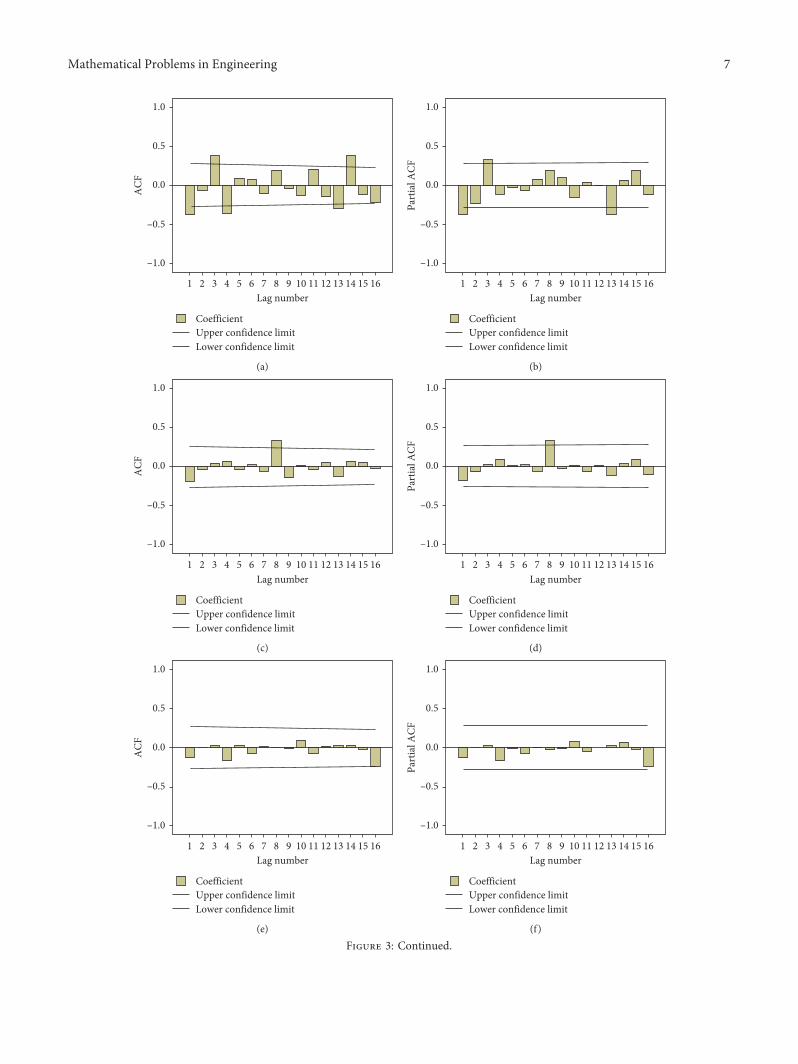
10
05
00
ndash05
ndash10
ACF
2 3 4 5 6 7 8 9 10 11 12 13 14 15 161Lag number
CoefficientUpper confidence limitLower confidence limit
(a)
10
05
00
ndash05
ndash10
Part
ial A
CF
2 3 4 5 6 7 8 9 10 11 12 13 14 15 161Lag number
CoefficientUpper confidence limitLower confidence limit
(b)
10
05
00
ndash05
ndash10
ACF
2 3 4 5 6 7 8 9 10 11 12 13 14 15 161Lag number
CoefficientUpper confidence limitLower confidence limit
(c)
10
05
00
ndash05
ndash10
Part
ial A
CF
2 3 4 5 6 7 8 9 10 11 12 13 14 15 161Lag number
CoefficientUpper confidence limitLower confidence limit
(d)
10
05
00
ndash05
ndash10
ACF
2 3 4 5 6 7 8 9 10 11 12 13 14 15 161Lag number
CoefficientUpper confidence limitLower confidence limit
(e)
10
05
00
ndash05
ndash10
Part
ial A
CF
2 3 4 5 6 7 8 9 10 11 12 13 14 15 161Lag number
CoefficientUpper confidence limitLower confidence limit
(f )
Figure 3 Continued
Mathematical Problems in Engineering 7
10
05
00
ndash05
ndash10
ACF
2 3 4 5 6 7 8 9 10 11 12 13 14 15 161Lag number
CoefficientUpper confidence limitLower confidence limit
(g)
10
05
00
ndash05
ndash10
Part
ial A
CF
2 3 4 5 6 7 8 9 10 11 12 13 14 15 161Lag number
CoefficientUpper confidence limitLower confidence limit
(h)
Figure 3 (a) ACF of stationary HBC1 (b) PACF of stationary HBC1 (c) ACF of stationary HBC2 (d) PACF of stationary HBC2 (e) ACF ofstationary HBC3 (f ) PACF of stationary HBC3 (g) ACF of stationary AHP (h) PACF of stationary AHP
ndash10
ndash05
00
05
10
ACF
2 3 4 5 6 7 8 9 10 11 12 13 14 15 161Lag number
CoefficientUpper confidence limitLower confidence limit
(a)
ndash10
ndash05
00
05
10
ACF
2 3 4 5 6 7 8 9 10 11 12 13 14 15 161Lag number
CoefficientUpper confidence limitLower confidence limit
(b)
Figure 4 Continued
8 Mathematical Problems in Engineering
provides a fairly effective description of the dynamics inHBC1 data
412 ARIMA Model for Building Cost Index of Two-StoryHouse in New Zealand (HBC2) )e building cost of a two-storey house in New Zealand is denoted as HBC2 Based onthe ACF and PACF shown in Figures 3(c) and 3(d) theestimated seasonal ARIMA model for forecasting buildingcost of a two-storey house in New Zealand is found to beARIMA(010)(002)4 )e residuals shown in Figure 4(b)indicate that the model is adequate )e forecast error fortwo-year-ahead forecasts measured by the MAPE and RMSEis illustrated in Table 1 )e values of the MAPE and RMSEare 2177 and 6176 respectively
413 ARIMA Model for Building Cost Index of Town Housein New Zealand (HBC3) )e building cost of a town housein New Zealand is denoted as HBC3 Seasonal ARIMAmodels are fitted to stationary building cost series of a townhouse and the cost series require a regular difference and aseasonal difference to achieve stationarity According toFigures 3(e) and 3(f ) the seasonal ARIMA model isARIMA(010)(100)4 )e final ARIMA model estimatedand selected for forecasting future building cost of a townhouse in New Zealand is ARIMA(010)(100)4)emodel isadequate and consistent with the underlying theory as theresiduals shown in Figure 4(c)
42 Transfer Function Model )e transfer function modelswill be developed below In all cases only the first 56
observations were used which indicates the data set up to2014Q4 were used to specify the models Based on theapproach in [45] the transfer function model can beidentified After some initial analysis the New Zealandhouse price series (AHP) was used as the input variable )eACF and PACF of AHP are shown in Figures 3(g) and 3(h)Using the proposed identification method the ARIMAmodel for New Zealand house price (AHP) can be expressedas
(1 minus 0827B) Xt minus Xtminus 1( 1113857 at (10)
)e model residuals were checked for independence)ere is no significant autocorrelation at the 5 level )eresults of the transfer function models for the residentialbuilding costs in New Zealand are shown in Table 2
421 Transfer Function Model for Building Cost Index ofOne-Story House in New Zealand Building cost index of aone-storey house in New Zealand denoted as HBC1 couldbe influenced by the New Zealand house prices Buildingcosts and house prices are positively correlated so that anincrease in house prices leads to an increase in the buildingcosts and vice versa )us finding a mathematical rela-tionship between these two variables in the transfer functionform can be particularly valuable )e preliminary identi-fication of series with the ACF and PACF to test for sta-tionarity and seasonality was performed With theobservation of slow damping of the ACF correlogram theregular first differencing and seasonal differencing of orderfour were required to bring about stationarity After regular
ndash10
ndash05
00
05
10
ACF
2 3 4 5 6 7 8 9 10 11 12 13 14 15 161Lag number
CoefficientUpper confidence limitLower confidence limit
(c)
Figure 4 (a) ACF of the noise residuals of the ARIMAmodel for HBC1 (b) ACF of the noise residuals of the ARIMAmodel for HBC2 (c)ACF of the noise residuals of the ARIMA model for HBC3
Mathematical Problems in Engineering 9
and seasonal differencing of the HBC1 series the series isstationary
As shown in Figure 5(a) the first spike which is placedout of its acceptance region is at lag zero after which theCCF damping down is in an oscillation pattern )us b iszero s is zero and r 2 (oscillation pattern) )e modelparameters were estimated and then C 0414 δ1
minus 0959 and δ2 minus 0894 )en the model can be expressedas
zHBC1t
C
1 minus δ1B minus δ2B2( 1113857z
(AHP)t + at
0414
1 + 0959B + 0894B2( )z
(AHP)t + at
(11)
)e model residuals should be examined to meet theassumption of error independence According toFigures 6(a) and 6(b) it can be inferred that the residuals arenot a white noise process therefore to redevelop the modelis necessary After examining the pattern of RACF andRPACF a moving average term and a seasonal movingaverage term should be included in the model )e movingaverage parameters are θ1 0298 and ϑ1 0251 respec-tively )erefore the model can be expressed as
zHBC1t
C
1 minus δ1B minus δ2B2( 1113857z
(AHP)t + 1 minus θ1B( 1113857 1 minus ϑ1B
41113872 1113873εt
0414
1 + 0959B + 0894B2( )z
(AHP)t
+(1 minus 0298B) 1 minus 0251B4
1113872 1113873εt
(12)
In order to access the model expressed in the aboveequation the autocorrelation function of themodel residualswas considered)e residuals shown in Figure 7 suggest thatthe residuals satisfy the condition of a white noise processMoreover the results of the LjungndashBox test also indicate theabsence of the autocorrelation in the residuals )ereforethe model in equation (12) is adequate
422 Transfer Function Model for Building Cost Index ofTwo-Story House in New Zealand Building cost of a two-storey house in New Zealand is denoted as HBC2 )e ACFand PACF were used to test stationarity and seasonality ofthe data series With the observation of slow damping of theACF correlogram the regular first differencing was required
Table 1 Univariate ARIMA models for cost series
Cost series Model Parameters Estimate t-StatisticsLjungndashBox
Statistics df p value
HBC1
ARIMA(013)(011)4 θ1 0335 2379 2477 14 0375θ3 minus 0297 minus 2022ϑ1 0447 3177
R2 096 RMSE 3560 MAPE 1644 MAE 2495 BIC 7453
HBC2 ARIMA(010)(002)4 ϑ2 minus 0394 minus 2848 6035 16 0988R2 0943 RMSE 6176 MAPE 2177 MAE 3741 BIC 8392
HBC3 ARIMA(010)(100)4 empty1 0594 5483 8168 17 0963R2 0969 RMSE 4575 MAPE 1576 MAE 2892 BIC 7719
Table 2 Transfer function parameters in the different cost series
Cost seriesModel order
TF model parameters Estimate t-Statistics p valueb s r
HBC1
0 0 2 C 0414 2189 0034δ1 minus 0959 minus 9110 0δ2 minus 0894 minus 8434 0θ1 0298 2007 0051ϑ1 0311 2630 0211
R2 0960 RMSE 3583 MAPE 1690 MAE 2563 BIC 7543
HBC2
3 1 1 C minus 1341 minus 2969 0005ω1 1257 3596 0001δ1 0429 2103 0041
R2 0932 RMSE 5955 MAPE 2476 MAE 4356 BIC 8405
HBC3
3 0 2 C 1088 3327 0002δ1 minus 0790 minus 4529 0δ2 minus 0645 minus 3698 0001
R2 0952 RMSE 4762 MAPE 1850 MAE 3473 BIC 7961
10 Mathematical Problems in Engineering
to bring about stationarity After the first regular differ-encing of HBC2 series the series is stationary
First this ARIMA model was used to filter the buildingcost for a two-storey house )en the cross-correlationbetween these two prewhitened series was computed asshown in Figure 5(b) )e first significant spike appears atlag 3)e orders of the transfer function b 3 s 1 and r 1can be identified )e ordinary least-square method was
used to estimate the model parameters)e transfer functionis shown as
zHBC2t
minus 1341(1 + 1257B)
1 minus 0429BB3z
(AHP)t + at (13)
)e model residuals should be examined to meet theassumption of error independence According toFigures 6(c) and 6(d) it can be inferred that the residuals are
CoefficientUpper confidence limitLower confidence limit
AHP with HBC1
ndash10
ndash05
00
05
10CC
F
1ndash6 ndash3 ndash2 40ndash5 2 3 5ndash4 6ndash1
Lag number
(a)
CoefficientUpper confidence limitLower confidence limit
AHP with HBC2
ndash10
ndash05
00
05
10
CCF
1ndash6 ndash3 ndash2 40ndash5 2 3 5ndash4 6ndash1
Lag number
(b)
CoefficientUpper confidence limitLower confidence limit
AHP with HBC3
ndash10
ndash05
00
05
10
CCF
ndash5 ndash4 ndash3 ndash2 30 2 4 5ndash1 1 6ndash6
Lag number
(c)
Figure 5 (a) CCF of AHP and HBC1 (b) CCF of AHP and HBC2 (c) CCF of AHP and HBC3
Mathematical Problems in Engineering 11
CoefficientUpper confidence limitLower confidence limit
ndash10
ndash05
00
05
10
ACF
2 134 116 7 9 14 168 1253 101 15Lag number
(a)
CoefficientUpper confidence limitLower confidence limit
2 7 12 1363 8 94 11 141 5 15 1610Lag number
ndash10
ndash05
00
05
10
Part
ial A
CF
(b)
CoefficientUpper confidence limitLower confidence limit
ndash10
ndash05
00
05
10
ACF
3 84 136 11 15 161 9 127 1452 10Lag number
(c)
CoefficientUpper confidence limitLower confidence limit
2 7 125 63 8 9 10 114 13 14 15 161Lag number
ndash10
ndash05
00
05
10
Part
ial A
CF
(d)
CoefficientUpper confidence limitLower confidence limit
ndash10
ndash05
00
05
10
ACF
3 12 15136 7 82 10 161 9 1454 11Lag number
(e)
CoefficientUpper confidence limitLower confidence limit
2 3 4 5 6 7 8 9 10 11 12 13 14 15 161Lag number
ndash10
ndash05
00
05
10
Part
ial A
CF
(f )
Figure 6 (a) ACF of the noise residuals of the transfer function model for HBC1 (b) PACF of the noise residuals of the transfer functionmodel for HBC1 (c) ACF of the noise residuals of the transfer function model for HBC2 (d) PACF of the noise residuals of the transferfunction model for HBC2 (e) ACF of the noise residuals of the transfer function model for HBC3 (f ) PACF of the noise residuals of thetransfer function model for HBC3
12 Mathematical Problems in Engineering
a white noise process )e residuals shown in Figures 6(c)and 6(d) suggest that the residuals are white noise More-over the results of the LjungndashBox test also indicate theabsence of the autocorrelation in the residuals )ereforethe model in equation (13) is adequate
423 Transfer Function Model for Building Cost Index ofTown House in New Zealand Building cost of a town housein New Zealand is denoted as HBC3With the observation ofslow damping of the ACF correlogram the regular firstdifferencing and seasonal differencing of order four wererequired to bring about stationarity After regular andseasonal differencing of the HBC3 series the series is sta-tionary as shown from the ACF In the identification of thetransfer function model it is necessary to apply the sameprewhitening transformation to both the input and outputseries)us the ARIMAmodel for house price (AHP) is alsoapplied to the building cost series of a town house Howeverbefore the prewhitening progress the cost series has beentransformed to stationary by a regular difference and aseasonal difference
Figure 5(c) shows the first significant spike is at lag 0 onthe cross-correlation function indicating no delay time )eorders of the transfer function b 3 s 0 and r 2 can beidentified )e ordinary least-square method was used toestimate the model parameters )e transfer function isshown as
zHBC3t
C
1 minus δ1B minus δ2B2( 1113857B3z
(AHP)t + at
0089
1 minus 1614B + 0849B2( )B3z
(AHP)t + at
(14)
)e residuals were checked for autocorrelation and thechi-square values for all the lags were found to be notsignificant at the 5 level as shown in Figures 6(e) and 6(f ))is suggests that the model residuals do not have problemswith autocorrelation and indeed white noise
43 Forecast Evaluation )e above proposed models wereevaluated for their out-of-sample forecasting performance)e models were developed using data from 2001Q1 to2014Q4 and then forecasts were made for the following 16quarters (2015Q1ndash2018Q4) )e model comparison wascarried out in a meaningful and systematic way )e MAPEvalues for the transfer function models and seasonal ARIMAmodels for the period 2015Q1ndash2018Q4 are presented inTable 3 )e results clearly indicate that the transfer functionmethod outperforms the seasonal ARIMA models for allbuilding cost series considered )e improvement of fore-casting accuracy from the adoption of the transfer functionmodel is best illustrated by observing the error measure-ments For the building cost index of a one-story house(HBC1) in New Zealand there is a reduction of about 391
CoefficientUpper confidence limitLower confidence limit
ndash10
ndash05
00
05
10A
CF
2 3 4 5 6 7 8 9 10 11 12 13 14 15 161
Lag number
(a)
CoefficientUpper confidence limitLower confidence limit
ndash10
ndash05
00
05
10
Part
ial A
CF
2 3 4 5 6 7 8 9 10 11 12 13 14 15 161
Lag number
(b)
Figure 7 (a) ACF of the noise residuals of the remodel for HBC1 (b) PACF of the noise residuals of the remodel for HBC1
Mathematical Problems in Engineering 13
2001
Q1
2001
Q2
2001
Q3
2001
Q4
2002
Q1
2002
Q2
2002
Q3
2002
Q4
2003
Q1
2003
Q2
2003
Q3
2003
Q4
2004
Q1
2004
Q2
2004
Q3
2004
Q4
2005
Q1
2005
Q2
2005
Q3
2005
Q4
2006
Q1
2006
Q2
2006
Q3
2006
Q4
2007
Q1
2007
Q2
2007
Q3
2007
Q4
2008
Q1
2008
Q2
2008
Q3
2008
Q4
2009
Q1
2009
Q2
2009
Q3
2009
Q4
2001
0Q
120
010
Q2
2001
0Q
320
010
Q4
2001
1Q
120
011
Q2
2001
1Q
320
011
Q4
2001
2Q
120
012
Q2
2001
2Q
320
012
Q4
2001
3Q
120
013
Q2
2001
3Q
320
013
Q4
2001
4Q
120
014
Q2
2001
4Q
320
014
Q4
2001
5Q
120
015
Q2
2001
5Q
320
015
Q4
2001
6Q
120
016
Q2
2001
6Q
320
016
Q4
2001
7Q
120
017
Q2
2001
7Q
320
017
Q4
2001
8Q
120
018
Q2
2001
8Q
320
018
Q4
0
500
1000
1500
2000
2500
$ (m
2 )
HBC1HBC1 (TF)
HBC1 (ARIMA)
Year (quarter)
(a)
2001
Q1
2001
Q2
2001
Q3
2001
Q4
2002
Q1
2002
Q2
2002
Q3
2002
Q4
2003
Q1
2003
Q2
2003
Q3
2003
Q4
2004
Q1
2004
Q2
2004
Q3
2004
Q4
2005
Q1
2005
Q2
2005
Q3
2005
Q4
2006
Q1
2006
Q2
2006
Q3
2006
Q4
2007
Q1
2007
Q2
2007
Q3
2007
Q4
2008
Q1
2008
Q2
2008
Q3
2008
Q4
2009
Q1
2009
Q2
2009
Q3
2009
Q4
2001
0Q
120
010
Q2
2001
0Q
320
010
Q4
2001
1Q
120
011
Q2
2001
1Q
320
011
Q4
2001
2Q
120
012
Q2
2001
2Q
320
012
Q4
2001
3Q
120
013
Q2
2001
3Q
320
013
Q4
2001
4Q
120
014
Q2
2001
4Q
320
014
Q4
2001
5Q
120
015
Q2
2001
5Q
320
015
Q4
2001
6Q
120
016
Q2
2001
6Q
320
016
Q4
2001
7Q
120
017
Q2
2001
7Q
320
017
Q4
2001
8Q
120
018
Q2
2001
8Q
320
018
Q4
0
500
1000
1500
2000
2500
$ (m
2 )
HBC1HBC1 (TF)
HBC1 (ARIMA)
Year (quarter)
(b)
Figure 8 Continued
Table 3 Comparison of model performance (MAPE)
Cost series ARIMA TFHBC1 2091 1273HBC2 2935 1365HBC3 5766 1161
14 Mathematical Problems in Engineering
in the MAPE from the seasonal ARIMA model to thetransfer function model For the building cost index of atwo-story house in New Zealand (HBC2) the reductionfrom using the transfer function model is even more pro-nounced there is a 535 reduction in the MAPE from theARIMA model to the transfer function model For thebuilding cost index of a town house in New Zealand (HBC3)the transfer function model provides a 799 MAPE re-duction over the seasonal ARIMA model Note that thetransfer function models are for all three cost series su-perior to the seasonal ARIMA models )e building costindex of HBC1 HBC2 and HBC3 and their forecastsgenerated from ARIMA and transfer function models areshown in Figure 8
5 Results and Discussion
)e fluctuations in the building cost index are problematicfor cost estimation)eARIMAmodels completely take intoaccount the dynamic process of cost series the seasonalityand the serial correlation in the residuals to obtain precisecost forecasts Although the model can dynamically describethe time-series data it cannot investigate the causality be-tween independent variables and dependent variables Basedon the current state of knowledge and the existing literaturebuilding costs are influenced not only by the constructionindustry but also by other factors such as house priceseconomic conditions population incomes and businessloans)e inclusion of explanatory variables into the modelscan forecast building cost more accurately)eNew Zealandhouse price index was selected as an explanatory variable forpredicating building cost in this study
)e analysis results suggest that the simplest model is notalways the most appropriate one for predicting particularly
when additional information is available Univariate modelslike ARIMA can be used as a benchmark in comparingforecasting performance When explanatory variables areavailable they can be included in the model to improveforecasting accuracy Multivariate models can then berealised to improve forecasting performance )e transferfunction model can describe more about the characteristicsof the output than a univariate model by describing thedynamic relationship between the input and output vari-ables Inclusion of New Zealand house prices in the transferfunction models significantly improves forecasting accuracy)is is consistent with the findings of [49] which indicatedthat model inclusion of an exogenous variable can improvethe forecasting performance Housing is one kind ofbuilding construction product that connects the buildingconstruction sector to the housing sector So the buildingcosts are subject to changes in house prices New Zealandhouse prices stimulate the changes in building costs al-though building costs are usually viewed as fundamentals)e findings are also supported by the studies of [38 50]
6 Conclusion
)is study proposed the transfer functionmethod to forecastthe building cost index of New Zealand to improve theaccuracy of the cost estimates that help in developing ac-curate budgets and preventing under- or overestimation AnARIMAmodel was also used as a benchmark method Basedon the BoxndashJenkins model development process transferfunction models and seasonal ARIMA models for buildingcost indices of one-storey houses two-storey houses andtown houses in New Zealand were developed )e effec-tiveness of the transfer function models was compared withthat of the univariate ARIMA models )e results indicated
2001
Q1
2001
Q2
2001
Q3
2001
Q4
2002
Q1
2002
Q2
2002
Q3
2002
Q4
2003
Q1
2003
Q2
2003
Q3
2003
Q4
2004
Q1
2004
Q2
2004
Q3
2004
Q4
2005
Q1
2005
Q2
2005
Q3
2005
Q4
2006
Q1
2006
Q2
2006
Q3
2006
Q4
2007
Q1
2007
Q2
2007
Q3
2007
Q4
2008
Q1
2008
Q2
2008
Q3
2008
Q4
2009
Q1
2009
Q2
2009
Q3
2009
Q4
2001
0Q
1
HBC1HBC1 (TF)
HBC1 (ARIMA)
Year (quarter)
2001
0Q
220
010
Q3
2001
0Q
420
011
Q1
2001
1Q
220
011
Q3
2001
1Q
420
012
Q1
2001
2Q
220
012
Q3
2001
2Q
420
013
Q1
2001
3Q
220
013
Q3
2001
3Q
420
014
Q1
2001
4Q
220
014
Q3
2001
4Q
420
015
Q1
2001
5Q
220
015
Q3
2001
5Q
420
016
Q1
2001
6Q
220
016
Q3
2001
6Q
420
017
Q1
2001
7Q
220
017
Q3
2001
7Q
420
018
Q1
2001
8Q
220
018
Q3
2001
8Q
4
0
500
1000
1500
2000
2500
$ (m
2 )
(c)
Figure 8 (a) Building cost index of HBC1 and its forecasts generated from ARIMA and transfer function models (b) building cost index ofHBC2 and its forecasts generated from ARIMA and transfer function models (c) building cost index of HBC3 and its forecasts generatedfrom ARIMA and transfer function models
Mathematical Problems in Engineering 15
that the predictive accuracy of the transfer function model issuperior to that of the ARIMA model since the transferfunction model achieved lower MAPE and RMSE
)e transfer functionmodel was developed from a fusionof time-series analysis regression analysis and cross-cor-relation analysis Cross-correlation analysis was used toexplore the potential optimal parameters Time-seriesanalysis was used to identify the cost index patterns Re-gression analysis was utilized to identify the underlyingmapping between influencing factors and the cost index)etransfer function models that contain an exogenous variable(more information) are better at forecasting than the simplerARIMA models )e causality between building cost andhouse prices was modelled in the transfer function method)e inclusion of house prices in the model significantlyreduces the forecasting error of the transfer functionmodelsrelative to seasonal ARIMA models )is study has shownthat the inclusion of an explanatory variable input within theframework leads to an improvement in forecastingperformance
)is study makes important contributions to three areas)e main contribution of this study is to enhance cost es-timation accuracy and guide industry practitioners in thepreliminary design stage )e proposed transfer functionmodel can be a useful tool for industry professionals togenerate cost estimates that can help in pricing bidding andassessing construction projects Second the inclusion ofNew Zealand house prices in the transfer function modelsignificantly improves the cost forecasting performance )efindings indicate that the inclusion of cost-influencingfactors into the model can significantly improve the fore-casting accuracy of the building cost index of New Zealand)e findings contribute to the present body of knowledge oncost estimation and may serve as a valuable guide for futuremodel development )ird the results of this study provethat New Zealand house price is a significant influencingfactor of residential building cost )e results also demon-strate that variations in house prices can result in fluctua-tions in residential building costs )e results may helpindustry professionals understand the underlying relation-ship between the construction industry and housing marketof New Zealand
)e developed models are based on the building costindex of New Zealand However the model developmentprocess can be used in other regions )e accuracy of long-term forecasting of the cost index using the transfer functionmodel may be impaired due to uncertainty in the dynamicenvironment Hence the use of intelligent methods for long-term prediction of the cost index is a future researchdirection
Abbreviations
ACF Autocorrelation functionAHP House price index of New ZealandANNs Artificial neutral networksARIMA Autoregressive integrated moving averageARMA Autoregressive moving averageBCI Building cost index
CCF Cross-correlation functionCCI Construction cost indexES Exponential smoothingHBC1 Building cost index of a one-story house in New
ZealandHBC2 Building cost index of a two-story house in New
ZealandHBC3 Building cost index of a town house in New
ZealandMAPE Mean absolute percentage errorPACF Partial autocorrelation functionPPI Producer price indexRACF Residual autocorrelation functionRMSE Root mean square errorRPACF Residual partial autocorrelation functionUK United KingdomVECM Vector error correction model
Data Availability
)e data used to support the findings of this study areavailable from the corresponding author upon request
Conflicts of Interest
)e authors declare no conflicts of interest
Authorsrsquo Contributions
L Z and J M conceptualized the idea L Z performed themethodology prepared the original draft and acquired thefund Z L developed the software L Z and Z L performedvalidation J M supervised the work and reviewed andedited the paper
Acknowledgments
)is research was funded by the China Scholarship Councilthrough the research project (grant no 201206130069)Massey University (grant no 09166424) and Beijing Uni-versity of Technology (grant no 004000514119067) )eAPC was funded by the three grants )e authors would liketo thank the Reserve Bank of New Zealand and Ministry ofBusiness Innovation and Employment for providing data toconduct this research In addition the authors would like tothank all practitioners who contributed to this project
References
[1] J Gido and J P Clements Successful Project ManagementCengage Learning Stamford CT USA 6th edition 2015
[2] R Sonmez ldquoConceptual cost estimation of building projectswith regression analysis and neural networksrdquo CanadianJournal of Civil Engineering vol 31 no 4 pp 677ndash683 2004
[3] Y Takano N Ishii andMMuraki ldquoDetermining bidmarkupand resources allocated to cost estimation in competitivebiddingrdquo Automation in Construction vol 85 pp 358ndash3682018
[4] E W Merrow Concepts Strategies and Practices for SuccessJohn Wiley amp Sons Hoboken NJ USA 2011
16 Mathematical Problems in Engineering
[5] B Ashuri and J Lu ldquoTime series analysis of ENR constructioncost indexrdquo Journal of Construction Engineering and Man-agement vol 136 no 11 pp 1227ndash1237 2010
[6] Y Elfahham ldquoEstimation and prediction of construction costindex using neural networks time series and regressionrdquoAlexandria Engineering Journal vol 58 no 2 pp 499ndash5062019
[7] S Hwang ldquoDynamic regression models for prediction ofconstruction costsrdquo Journal of Construction Engineering andManagement vol 135 no 5 pp 360ndash367 2009
[8] J X Xu and S Moon ldquoStochastic forecast of construction costindex using a cointegrated vector autoregression modelrdquoJournal of Management in Engineering vol 29 no 1pp 10ndash18 2013
[9] MBIE NZ Sector Report 2013mdashConstruction Ministry ofBuilding Innovation and Employment Wellington NewZealand 2013
[10] A Jrade A Conceptual Cost Estimating Computer System forBuilding Projects Concordia University Montreal Canada2000
[11] M-Y Cheng and A F V Roy ldquoEvolutionary fuzzy decisionmodel for cash flow prediction using time-dependent supportvector machinesrdquo International Journal of Project Manage-ment vol 29 no 1 pp 56ndash65 2011
[12] S Hwang ldquoTime series models for forecasting constructioncosts using time series indexesrdquo Journal of ConstructionEngineering and Management vol 137 no 9 pp 656ndash6622011
[13] R Zhang B Ashuri Y Shyr and Y Deng ldquoForecastingconstruction cost index based on visibility graph a networkapproachrdquo Physica A Statistical Mechanics and Its Applica-tions vol 493 pp 239ndash252 2018
[14] D J Lowe M W Emsley and A Harding ldquoPredictingconstruction cost using multiple regression techniquesrdquoJournal of Construction Engineering and Managementvol 132 no 7 pp 750ndash758 2006
[15] H-L Yip H Fan and Y-H Chiang ldquoPredicting the main-tenance cost of construction equipment comparison betweengeneral regression neural network and Box-Jenkins time se-ries modelsrdquo Automation in Construction vol 38 pp 30ndash382014
[16] G Morcous H Rivard and A M Hanna ldquoCase-basedreasoning system for modeling infrastructure deteriorationrdquoJournal of Computing in Civil Engineering vol 16 no 2pp 104ndash114 2002
[17] N-J Yau and J-B Yang ldquoCase-based reasoning in con-struction managementrdquo Computer-Aided Civil and Infra-structure Engineering vol 13 no 2 pp 143ndash150 1998
[18] R G Brown Smoothing Forecasting and Prediction of Dis-crete Time Series Courier Dover Publications Mineola NYUSA 2004
[19] G P Zhang and M Qi ldquoNeural network forecasting forseasonal and trend time seriesrdquo European Journal of Oper-ational Research vol 160 no 2 pp 501ndash514 2005
[20] B Pfaff Analysis of Integrated and Cointegrated Time Serieswith R Springer Berlin Germany 2008
[21] Y-H Lin and P-C Lee ldquoNovel high-precision grey fore-casting modelrdquo Automation in Construction vol 16 no 6pp 771ndash777 2007
[22] H Zheng Y Deng and Y Hu ldquoFuzzy evidential influencediagram and its evaluation algorithmrdquo Knowledge-BasedSystems vol 131 pp 28ndash45 2017
[23] X Zhou X Deng Y Deng and S Mahadevan ldquoDependenceassessment in human reliability analysis based on D numbers
and AHPrdquo Nuclear Engineering and Design vol 313pp 243ndash252 2017
[24] M-Y Cheng N-D Hoang and Y-W Wu ldquoHybrid intel-ligence approach based on LS-SVM and differential evolutionfor construction cost index estimation a Taiwan case studyrdquoAutomation in Construction vol 35 pp 306ndash313 2013
[25] B Ashuri S M Shahandashti and J Lu ldquoEmpirical tests foridentifying leading indicators of ENR construction cost in-dexrdquo Construction Management and Economics vol 30no 11 pp 917ndash927 2012
[26] S T Ng S O Cheung M Skitmore and T C Y Wong ldquoAnintegrated regression analysis and time series model forconstruction tender price index forecastingrdquo ConstructionManagement and Economics vol 22 no 5 pp 483ndash493 2004
[27] J MWWong and S T Ng ldquoForecasting construction tenderprice index in Hong Kong using vector error correctionmodelrdquo Construction Management and Economics vol 28no 12 pp 1255ndash1268 2010
[28] S M Shahandashti and B Ashuri ldquoForecasting engineeringnews-record construction cost index using multivariate timeseries modelsrdquo Journal of Construction Engineering andManagement vol 139 no 9 pp 1237ndash1243 2013
[29] H L Chen ldquoDeveloping cost response models for company-level cost flow forecasting of project-based corporationsrdquoJournal of Management in Engineering vol 23 no 4pp 171ndash181 2007
[30] A Hammad S Ali G J Sweis and R J Sweis ldquoStatsticalanalysis on the cost and duration of public building projectsrdquoJournal of Management in Engineering vol 26 no 2pp 105ndash113 2010
[31] W P Trefor ldquoPredicting changes in predicting changes inconstruction cost indexes using neural networksrdquo Journal ofConstruction Engineering and Management vol 120 no 2pp 306ndash320 1994
[32] G-H Kim S-H An and K-I Kang ldquoComparison of con-struction cost estimating models based on regression analysisneural networks and case-based reasoningrdquo Building andEnvironment vol 39 no 10 pp 1235ndash1242 2004
[33] K Byung-Cheol and H K Young ldquoImproving the accuracyand operational predictability of project cost forecasts anadaptive combination approachrdquo Production Planning ampControl vol 29 no 9 pp 743ndash760 2018
[34] N Kulendran and S F Witt ldquoLeading indicator tourismforecastsrdquo Tourism Management vol 24 no 5 pp 503ndash5102003
[35] M Qi ldquoPredicting US recessions with leading indicators vianeural network modelsrdquo International Journal of Forecastingvol 17 no 3 pp 383ndash401 2001
[36] M-C Chen and I-C Tsai ldquoA cobweb theory of house priceincorporating investor behaviorrdquo Academia Economic Papersvol 35 pp 315ndash344 2007
[37] J Janssen B Kruijt and B Needham ldquo)e honeycomb cyclein real estaterdquo e Journal of Real Estate Research vol 9pp 237ndash251 1994
[38] I-C Tsai ldquoHousing supply demand and price constructioncost rental price and house price indicesrdquo Asian EconomicJournal vol 26 no 4 pp 381ndash396 2012
[39] T Sunde and P-F Muzindutsi ldquoDeterminants of house pricesand new construction activity an empirical investigation ofthe Namibian housing marketrdquo e Journal of DevelopingAreas vol 51 no 3 pp 390ndash407 2017
[40] S Makridakis S C Wheelwright and V McGee ForecastingMethods and Applications Wiley Hoboken NJ USA 2ndedition 1983
Mathematical Problems in Engineering 17
[41] T C Mills Time Series Techniques for Economists CambridgeUniversity Press New York NY USA 1990
[42] G E P Box G M Jenkins and G C Reinsel Time SeriesAnalysis Forecasting and Control Wiley Hoboken NJ USA1994
[43] Y Hasanah M Herlina and H Zaikarina ldquoFlood predictionusing transfer function model of rainfall and water dischargeapproach in Katulampa damrdquo in Proceedings of the 3rd In-ternational Conference on Sustainable Future for HumanSecurity SUSTAIN 2012 pp 317ndash326 Kyoto Japan No-vember 2012
[44] T Cook ldquoAn application of the transfer function to aneconomic-base modelrdquo e Annals of Regional Sciencevol 13 pp 81ndash92 1979
[45] G E P Box and G M Jenkins Time Series Analysis Fore-casting and Control Holden Day Inc San Francisco CAUSA 1976
[46] R Yaffee and M McGee Introduction to Time Series Analysisand Forecasting with Applications of SAS and SPSS AcademicPress Inc Cambridge MA USA 2000
[47] G E Box G Jenkins and G Reinsel Time Sereis AnalysisWiley Hoboken NJ USA 4th edition 2008
[48] S Bisgaard and M Kulahci Time Series Analysis and Fore-casting by Example John Wiley amp Sons Inc Hoboken NJUSA 2011
[49] R Ashley ldquoOn the usefulness of macroeconomic forecasts asinputs to forecasting modelsrdquo Journal of Forecasting vol 2no 3 pp 211ndash223 1983
[50] A Grimes and A Aitken ldquoHousing supply land costs andprice adjustmentrdquo Real Estate Economics vol 38 no 2pp 325ndash353 2010
18 Mathematical Problems in Engineering
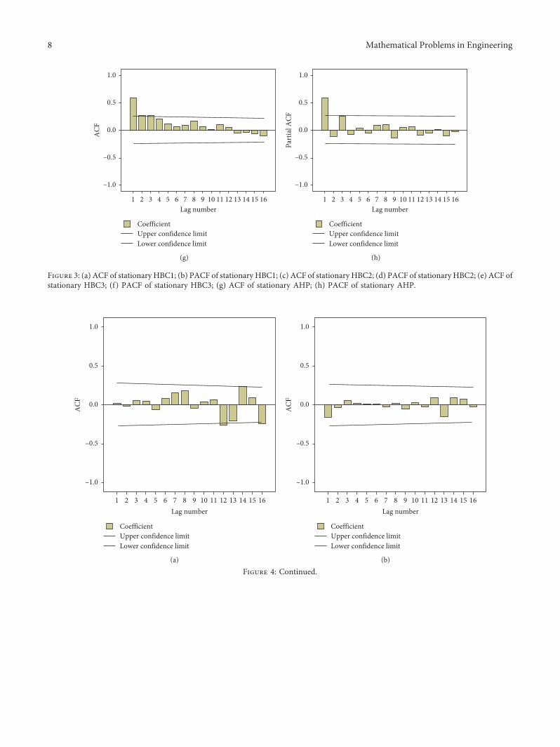
10
05
00
ndash05
ndash10
ACF
2 3 4 5 6 7 8 9 10 11 12 13 14 15 161Lag number
CoefficientUpper confidence limitLower confidence limit
(g)
10
05
00
ndash05
ndash10
Part
ial A
CF
2 3 4 5 6 7 8 9 10 11 12 13 14 15 161Lag number
CoefficientUpper confidence limitLower confidence limit
(h)
Figure 3 (a) ACF of stationary HBC1 (b) PACF of stationary HBC1 (c) ACF of stationary HBC2 (d) PACF of stationary HBC2 (e) ACF ofstationary HBC3 (f ) PACF of stationary HBC3 (g) ACF of stationary AHP (h) PACF of stationary AHP
ndash10
ndash05
00
05
10
ACF
2 3 4 5 6 7 8 9 10 11 12 13 14 15 161Lag number
CoefficientUpper confidence limitLower confidence limit
(a)
ndash10
ndash05
00
05
10
ACF
2 3 4 5 6 7 8 9 10 11 12 13 14 15 161Lag number
CoefficientUpper confidence limitLower confidence limit
(b)
Figure 4 Continued
8 Mathematical Problems in Engineering
provides a fairly effective description of the dynamics inHBC1 data
412 ARIMA Model for Building Cost Index of Two-StoryHouse in New Zealand (HBC2) )e building cost of a two-storey house in New Zealand is denoted as HBC2 Based onthe ACF and PACF shown in Figures 3(c) and 3(d) theestimated seasonal ARIMA model for forecasting buildingcost of a two-storey house in New Zealand is found to beARIMA(010)(002)4 )e residuals shown in Figure 4(b)indicate that the model is adequate )e forecast error fortwo-year-ahead forecasts measured by the MAPE and RMSEis illustrated in Table 1 )e values of the MAPE and RMSEare 2177 and 6176 respectively
413 ARIMA Model for Building Cost Index of Town Housein New Zealand (HBC3) )e building cost of a town housein New Zealand is denoted as HBC3 Seasonal ARIMAmodels are fitted to stationary building cost series of a townhouse and the cost series require a regular difference and aseasonal difference to achieve stationarity According toFigures 3(e) and 3(f ) the seasonal ARIMA model isARIMA(010)(100)4 )e final ARIMA model estimatedand selected for forecasting future building cost of a townhouse in New Zealand is ARIMA(010)(100)4)emodel isadequate and consistent with the underlying theory as theresiduals shown in Figure 4(c)
42 Transfer Function Model )e transfer function modelswill be developed below In all cases only the first 56
observations were used which indicates the data set up to2014Q4 were used to specify the models Based on theapproach in [45] the transfer function model can beidentified After some initial analysis the New Zealandhouse price series (AHP) was used as the input variable )eACF and PACF of AHP are shown in Figures 3(g) and 3(h)Using the proposed identification method the ARIMAmodel for New Zealand house price (AHP) can be expressedas
(1 minus 0827B) Xt minus Xtminus 1( 1113857 at (10)
)e model residuals were checked for independence)ere is no significant autocorrelation at the 5 level )eresults of the transfer function models for the residentialbuilding costs in New Zealand are shown in Table 2
421 Transfer Function Model for Building Cost Index ofOne-Story House in New Zealand Building cost index of aone-storey house in New Zealand denoted as HBC1 couldbe influenced by the New Zealand house prices Buildingcosts and house prices are positively correlated so that anincrease in house prices leads to an increase in the buildingcosts and vice versa )us finding a mathematical rela-tionship between these two variables in the transfer functionform can be particularly valuable )e preliminary identi-fication of series with the ACF and PACF to test for sta-tionarity and seasonality was performed With theobservation of slow damping of the ACF correlogram theregular first differencing and seasonal differencing of orderfour were required to bring about stationarity After regular
ndash10
ndash05
00
05
10
ACF
2 3 4 5 6 7 8 9 10 11 12 13 14 15 161Lag number
CoefficientUpper confidence limitLower confidence limit
(c)
Figure 4 (a) ACF of the noise residuals of the ARIMAmodel for HBC1 (b) ACF of the noise residuals of the ARIMAmodel for HBC2 (c)ACF of the noise residuals of the ARIMA model for HBC3
Mathematical Problems in Engineering 9
and seasonal differencing of the HBC1 series the series isstationary
As shown in Figure 5(a) the first spike which is placedout of its acceptance region is at lag zero after which theCCF damping down is in an oscillation pattern )us b iszero s is zero and r 2 (oscillation pattern) )e modelparameters were estimated and then C 0414 δ1
minus 0959 and δ2 minus 0894 )en the model can be expressedas
zHBC1t
C
1 minus δ1B minus δ2B2( 1113857z
(AHP)t + at
0414
1 + 0959B + 0894B2( )z
(AHP)t + at
(11)
)e model residuals should be examined to meet theassumption of error independence According toFigures 6(a) and 6(b) it can be inferred that the residuals arenot a white noise process therefore to redevelop the modelis necessary After examining the pattern of RACF andRPACF a moving average term and a seasonal movingaverage term should be included in the model )e movingaverage parameters are θ1 0298 and ϑ1 0251 respec-tively )erefore the model can be expressed as
zHBC1t
C
1 minus δ1B minus δ2B2( 1113857z
(AHP)t + 1 minus θ1B( 1113857 1 minus ϑ1B
41113872 1113873εt
0414
1 + 0959B + 0894B2( )z
(AHP)t
+(1 minus 0298B) 1 minus 0251B4
1113872 1113873εt
(12)
In order to access the model expressed in the aboveequation the autocorrelation function of themodel residualswas considered)e residuals shown in Figure 7 suggest thatthe residuals satisfy the condition of a white noise processMoreover the results of the LjungndashBox test also indicate theabsence of the autocorrelation in the residuals )ereforethe model in equation (12) is adequate
422 Transfer Function Model for Building Cost Index ofTwo-Story House in New Zealand Building cost of a two-storey house in New Zealand is denoted as HBC2 )e ACFand PACF were used to test stationarity and seasonality ofthe data series With the observation of slow damping of theACF correlogram the regular first differencing was required
Table 1 Univariate ARIMA models for cost series
Cost series Model Parameters Estimate t-StatisticsLjungndashBox
Statistics df p value
HBC1
ARIMA(013)(011)4 θ1 0335 2379 2477 14 0375θ3 minus 0297 minus 2022ϑ1 0447 3177
R2 096 RMSE 3560 MAPE 1644 MAE 2495 BIC 7453
HBC2 ARIMA(010)(002)4 ϑ2 minus 0394 minus 2848 6035 16 0988R2 0943 RMSE 6176 MAPE 2177 MAE 3741 BIC 8392
HBC3 ARIMA(010)(100)4 empty1 0594 5483 8168 17 0963R2 0969 RMSE 4575 MAPE 1576 MAE 2892 BIC 7719
Table 2 Transfer function parameters in the different cost series
Cost seriesModel order
TF model parameters Estimate t-Statistics p valueb s r
HBC1
0 0 2 C 0414 2189 0034δ1 minus 0959 minus 9110 0δ2 minus 0894 minus 8434 0θ1 0298 2007 0051ϑ1 0311 2630 0211
R2 0960 RMSE 3583 MAPE 1690 MAE 2563 BIC 7543
HBC2
3 1 1 C minus 1341 minus 2969 0005ω1 1257 3596 0001δ1 0429 2103 0041
R2 0932 RMSE 5955 MAPE 2476 MAE 4356 BIC 8405
HBC3
3 0 2 C 1088 3327 0002δ1 minus 0790 minus 4529 0δ2 minus 0645 minus 3698 0001
R2 0952 RMSE 4762 MAPE 1850 MAE 3473 BIC 7961
10 Mathematical Problems in Engineering
to bring about stationarity After the first regular differ-encing of HBC2 series the series is stationary
First this ARIMA model was used to filter the buildingcost for a two-storey house )en the cross-correlationbetween these two prewhitened series was computed asshown in Figure 5(b) )e first significant spike appears atlag 3)e orders of the transfer function b 3 s 1 and r 1can be identified )e ordinary least-square method was
used to estimate the model parameters)e transfer functionis shown as
zHBC2t
minus 1341(1 + 1257B)
1 minus 0429BB3z
(AHP)t + at (13)
)e model residuals should be examined to meet theassumption of error independence According toFigures 6(c) and 6(d) it can be inferred that the residuals are
CoefficientUpper confidence limitLower confidence limit
AHP with HBC1
ndash10
ndash05
00
05
10CC
F
1ndash6 ndash3 ndash2 40ndash5 2 3 5ndash4 6ndash1
Lag number
(a)
CoefficientUpper confidence limitLower confidence limit
AHP with HBC2
ndash10
ndash05
00
05
10
CCF
1ndash6 ndash3 ndash2 40ndash5 2 3 5ndash4 6ndash1
Lag number
(b)
CoefficientUpper confidence limitLower confidence limit
AHP with HBC3
ndash10
ndash05
00
05
10
CCF
ndash5 ndash4 ndash3 ndash2 30 2 4 5ndash1 1 6ndash6
Lag number
(c)
Figure 5 (a) CCF of AHP and HBC1 (b) CCF of AHP and HBC2 (c) CCF of AHP and HBC3
Mathematical Problems in Engineering 11
CoefficientUpper confidence limitLower confidence limit
ndash10
ndash05
00
05
10
ACF
2 134 116 7 9 14 168 1253 101 15Lag number
(a)
CoefficientUpper confidence limitLower confidence limit
2 7 12 1363 8 94 11 141 5 15 1610Lag number
ndash10
ndash05
00
05
10
Part
ial A
CF
(b)
CoefficientUpper confidence limitLower confidence limit
ndash10
ndash05
00
05
10
ACF
3 84 136 11 15 161 9 127 1452 10Lag number
(c)
CoefficientUpper confidence limitLower confidence limit
2 7 125 63 8 9 10 114 13 14 15 161Lag number
ndash10
ndash05
00
05
10
Part
ial A
CF
(d)
CoefficientUpper confidence limitLower confidence limit
ndash10
ndash05
00
05
10
ACF
3 12 15136 7 82 10 161 9 1454 11Lag number
(e)
CoefficientUpper confidence limitLower confidence limit
2 3 4 5 6 7 8 9 10 11 12 13 14 15 161Lag number
ndash10
ndash05
00
05
10
Part
ial A
CF
(f )
Figure 6 (a) ACF of the noise residuals of the transfer function model for HBC1 (b) PACF of the noise residuals of the transfer functionmodel for HBC1 (c) ACF of the noise residuals of the transfer function model for HBC2 (d) PACF of the noise residuals of the transferfunction model for HBC2 (e) ACF of the noise residuals of the transfer function model for HBC3 (f ) PACF of the noise residuals of thetransfer function model for HBC3
12 Mathematical Problems in Engineering
a white noise process )e residuals shown in Figures 6(c)and 6(d) suggest that the residuals are white noise More-over the results of the LjungndashBox test also indicate theabsence of the autocorrelation in the residuals )ereforethe model in equation (13) is adequate
423 Transfer Function Model for Building Cost Index ofTown House in New Zealand Building cost of a town housein New Zealand is denoted as HBC3With the observation ofslow damping of the ACF correlogram the regular firstdifferencing and seasonal differencing of order four wererequired to bring about stationarity After regular andseasonal differencing of the HBC3 series the series is sta-tionary as shown from the ACF In the identification of thetransfer function model it is necessary to apply the sameprewhitening transformation to both the input and outputseries)us the ARIMAmodel for house price (AHP) is alsoapplied to the building cost series of a town house Howeverbefore the prewhitening progress the cost series has beentransformed to stationary by a regular difference and aseasonal difference
Figure 5(c) shows the first significant spike is at lag 0 onthe cross-correlation function indicating no delay time )eorders of the transfer function b 3 s 0 and r 2 can beidentified )e ordinary least-square method was used toestimate the model parameters )e transfer function isshown as
zHBC3t
C
1 minus δ1B minus δ2B2( 1113857B3z
(AHP)t + at
0089
1 minus 1614B + 0849B2( )B3z
(AHP)t + at
(14)
)e residuals were checked for autocorrelation and thechi-square values for all the lags were found to be notsignificant at the 5 level as shown in Figures 6(e) and 6(f ))is suggests that the model residuals do not have problemswith autocorrelation and indeed white noise
43 Forecast Evaluation )e above proposed models wereevaluated for their out-of-sample forecasting performance)e models were developed using data from 2001Q1 to2014Q4 and then forecasts were made for the following 16quarters (2015Q1ndash2018Q4) )e model comparison wascarried out in a meaningful and systematic way )e MAPEvalues for the transfer function models and seasonal ARIMAmodels for the period 2015Q1ndash2018Q4 are presented inTable 3 )e results clearly indicate that the transfer functionmethod outperforms the seasonal ARIMA models for allbuilding cost series considered )e improvement of fore-casting accuracy from the adoption of the transfer functionmodel is best illustrated by observing the error measure-ments For the building cost index of a one-story house(HBC1) in New Zealand there is a reduction of about 391
CoefficientUpper confidence limitLower confidence limit
ndash10
ndash05
00
05
10A
CF
2 3 4 5 6 7 8 9 10 11 12 13 14 15 161
Lag number
(a)
CoefficientUpper confidence limitLower confidence limit
ndash10
ndash05
00
05
10
Part
ial A
CF
2 3 4 5 6 7 8 9 10 11 12 13 14 15 161
Lag number
(b)
Figure 7 (a) ACF of the noise residuals of the remodel for HBC1 (b) PACF of the noise residuals of the remodel for HBC1
Mathematical Problems in Engineering 13
2001
Q1
2001
Q2
2001
Q3
2001
Q4
2002
Q1
2002
Q2
2002
Q3
2002
Q4
2003
Q1
2003
Q2
2003
Q3
2003
Q4
2004
Q1
2004
Q2
2004
Q3
2004
Q4
2005
Q1
2005
Q2
2005
Q3
2005
Q4
2006
Q1
2006
Q2
2006
Q3
2006
Q4
2007
Q1
2007
Q2
2007
Q3
2007
Q4
2008
Q1
2008
Q2
2008
Q3
2008
Q4
2009
Q1
2009
Q2
2009
Q3
2009
Q4
2001
0Q
120
010
Q2
2001
0Q
320
010
Q4
2001
1Q
120
011
Q2
2001
1Q
320
011
Q4
2001
2Q
120
012
Q2
2001
2Q
320
012
Q4
2001
3Q
120
013
Q2
2001
3Q
320
013
Q4
2001
4Q
120
014
Q2
2001
4Q
320
014
Q4
2001
5Q
120
015
Q2
2001
5Q
320
015
Q4
2001
6Q
120
016
Q2
2001
6Q
320
016
Q4
2001
7Q
120
017
Q2
2001
7Q
320
017
Q4
2001
8Q
120
018
Q2
2001
8Q
320
018
Q4
0
500
1000
1500
2000
2500
$ (m
2 )
HBC1HBC1 (TF)
HBC1 (ARIMA)
Year (quarter)
(a)
2001
Q1
2001
Q2
2001
Q3
2001
Q4
2002
Q1
2002
Q2
2002
Q3
2002
Q4
2003
Q1
2003
Q2
2003
Q3
2003
Q4
2004
Q1
2004
Q2
2004
Q3
2004
Q4
2005
Q1
2005
Q2
2005
Q3
2005
Q4
2006
Q1
2006
Q2
2006
Q3
2006
Q4
2007
Q1
2007
Q2
2007
Q3
2007
Q4
2008
Q1
2008
Q2
2008
Q3
2008
Q4
2009
Q1
2009
Q2
2009
Q3
2009
Q4
2001
0Q
120
010
Q2
2001
0Q
320
010
Q4
2001
1Q
120
011
Q2
2001
1Q
320
011
Q4
2001
2Q
120
012
Q2
2001
2Q
320
012
Q4
2001
3Q
120
013
Q2
2001
3Q
320
013
Q4
2001
4Q
120
014
Q2
2001
4Q
320
014
Q4
2001
5Q
120
015
Q2
2001
5Q
320
015
Q4
2001
6Q
120
016
Q2
2001
6Q
320
016
Q4
2001
7Q
120
017
Q2
2001
7Q
320
017
Q4
2001
8Q
120
018
Q2
2001
8Q
320
018
Q4
0
500
1000
1500
2000
2500
$ (m
2 )
HBC1HBC1 (TF)
HBC1 (ARIMA)
Year (quarter)
(b)
Figure 8 Continued
Table 3 Comparison of model performance (MAPE)
Cost series ARIMA TFHBC1 2091 1273HBC2 2935 1365HBC3 5766 1161
14 Mathematical Problems in Engineering
in the MAPE from the seasonal ARIMA model to thetransfer function model For the building cost index of atwo-story house in New Zealand (HBC2) the reductionfrom using the transfer function model is even more pro-nounced there is a 535 reduction in the MAPE from theARIMA model to the transfer function model For thebuilding cost index of a town house in New Zealand (HBC3)the transfer function model provides a 799 MAPE re-duction over the seasonal ARIMA model Note that thetransfer function models are for all three cost series su-perior to the seasonal ARIMA models )e building costindex of HBC1 HBC2 and HBC3 and their forecastsgenerated from ARIMA and transfer function models areshown in Figure 8
5 Results and Discussion
)e fluctuations in the building cost index are problematicfor cost estimation)eARIMAmodels completely take intoaccount the dynamic process of cost series the seasonalityand the serial correlation in the residuals to obtain precisecost forecasts Although the model can dynamically describethe time-series data it cannot investigate the causality be-tween independent variables and dependent variables Basedon the current state of knowledge and the existing literaturebuilding costs are influenced not only by the constructionindustry but also by other factors such as house priceseconomic conditions population incomes and businessloans)e inclusion of explanatory variables into the modelscan forecast building cost more accurately)eNew Zealandhouse price index was selected as an explanatory variable forpredicating building cost in this study
)e analysis results suggest that the simplest model is notalways the most appropriate one for predicting particularly
when additional information is available Univariate modelslike ARIMA can be used as a benchmark in comparingforecasting performance When explanatory variables areavailable they can be included in the model to improveforecasting accuracy Multivariate models can then berealised to improve forecasting performance )e transferfunction model can describe more about the characteristicsof the output than a univariate model by describing thedynamic relationship between the input and output vari-ables Inclusion of New Zealand house prices in the transferfunction models significantly improves forecasting accuracy)is is consistent with the findings of [49] which indicatedthat model inclusion of an exogenous variable can improvethe forecasting performance Housing is one kind ofbuilding construction product that connects the buildingconstruction sector to the housing sector So the buildingcosts are subject to changes in house prices New Zealandhouse prices stimulate the changes in building costs al-though building costs are usually viewed as fundamentals)e findings are also supported by the studies of [38 50]
6 Conclusion
)is study proposed the transfer functionmethod to forecastthe building cost index of New Zealand to improve theaccuracy of the cost estimates that help in developing ac-curate budgets and preventing under- or overestimation AnARIMAmodel was also used as a benchmark method Basedon the BoxndashJenkins model development process transferfunction models and seasonal ARIMA models for buildingcost indices of one-storey houses two-storey houses andtown houses in New Zealand were developed )e effec-tiveness of the transfer function models was compared withthat of the univariate ARIMA models )e results indicated
2001
Q1
2001
Q2
2001
Q3
2001
Q4
2002
Q1
2002
Q2
2002
Q3
2002
Q4
2003
Q1
2003
Q2
2003
Q3
2003
Q4
2004
Q1
2004
Q2
2004
Q3
2004
Q4
2005
Q1
2005
Q2
2005
Q3
2005
Q4
2006
Q1
2006
Q2
2006
Q3
2006
Q4
2007
Q1
2007
Q2
2007
Q3
2007
Q4
2008
Q1
2008
Q2
2008
Q3
2008
Q4
2009
Q1
2009
Q2
2009
Q3
2009
Q4
2001
0Q
1
HBC1HBC1 (TF)
HBC1 (ARIMA)
Year (quarter)
2001
0Q
220
010
Q3
2001
0Q
420
011
Q1
2001
1Q
220
011
Q3
2001
1Q
420
012
Q1
2001
2Q
220
012
Q3
2001
2Q
420
013
Q1
2001
3Q
220
013
Q3
2001
3Q
420
014
Q1
2001
4Q
220
014
Q3
2001
4Q
420
015
Q1
2001
5Q
220
015
Q3
2001
5Q
420
016
Q1
2001
6Q
220
016
Q3
2001
6Q
420
017
Q1
2001
7Q
220
017
Q3
2001
7Q
420
018
Q1
2001
8Q
220
018
Q3
2001
8Q
4
0
500
1000
1500
2000
2500
$ (m
2 )
(c)
Figure 8 (a) Building cost index of HBC1 and its forecasts generated from ARIMA and transfer function models (b) building cost index ofHBC2 and its forecasts generated from ARIMA and transfer function models (c) building cost index of HBC3 and its forecasts generatedfrom ARIMA and transfer function models
Mathematical Problems in Engineering 15
that the predictive accuracy of the transfer function model issuperior to that of the ARIMA model since the transferfunction model achieved lower MAPE and RMSE
)e transfer functionmodel was developed from a fusionof time-series analysis regression analysis and cross-cor-relation analysis Cross-correlation analysis was used toexplore the potential optimal parameters Time-seriesanalysis was used to identify the cost index patterns Re-gression analysis was utilized to identify the underlyingmapping between influencing factors and the cost index)etransfer function models that contain an exogenous variable(more information) are better at forecasting than the simplerARIMA models )e causality between building cost andhouse prices was modelled in the transfer function method)e inclusion of house prices in the model significantlyreduces the forecasting error of the transfer functionmodelsrelative to seasonal ARIMA models )is study has shownthat the inclusion of an explanatory variable input within theframework leads to an improvement in forecastingperformance
)is study makes important contributions to three areas)e main contribution of this study is to enhance cost es-timation accuracy and guide industry practitioners in thepreliminary design stage )e proposed transfer functionmodel can be a useful tool for industry professionals togenerate cost estimates that can help in pricing bidding andassessing construction projects Second the inclusion ofNew Zealand house prices in the transfer function modelsignificantly improves the cost forecasting performance )efindings indicate that the inclusion of cost-influencingfactors into the model can significantly improve the fore-casting accuracy of the building cost index of New Zealand)e findings contribute to the present body of knowledge oncost estimation and may serve as a valuable guide for futuremodel development )ird the results of this study provethat New Zealand house price is a significant influencingfactor of residential building cost )e results also demon-strate that variations in house prices can result in fluctua-tions in residential building costs )e results may helpindustry professionals understand the underlying relation-ship between the construction industry and housing marketof New Zealand
)e developed models are based on the building costindex of New Zealand However the model developmentprocess can be used in other regions )e accuracy of long-term forecasting of the cost index using the transfer functionmodel may be impaired due to uncertainty in the dynamicenvironment Hence the use of intelligent methods for long-term prediction of the cost index is a future researchdirection
Abbreviations
ACF Autocorrelation functionAHP House price index of New ZealandANNs Artificial neutral networksARIMA Autoregressive integrated moving averageARMA Autoregressive moving averageBCI Building cost index
CCF Cross-correlation functionCCI Construction cost indexES Exponential smoothingHBC1 Building cost index of a one-story house in New
ZealandHBC2 Building cost index of a two-story house in New
ZealandHBC3 Building cost index of a town house in New
ZealandMAPE Mean absolute percentage errorPACF Partial autocorrelation functionPPI Producer price indexRACF Residual autocorrelation functionRMSE Root mean square errorRPACF Residual partial autocorrelation functionUK United KingdomVECM Vector error correction model
Data Availability
)e data used to support the findings of this study areavailable from the corresponding author upon request
Conflicts of Interest
)e authors declare no conflicts of interest
Authorsrsquo Contributions
L Z and J M conceptualized the idea L Z performed themethodology prepared the original draft and acquired thefund Z L developed the software L Z and Z L performedvalidation J M supervised the work and reviewed andedited the paper
Acknowledgments
)is research was funded by the China Scholarship Councilthrough the research project (grant no 201206130069)Massey University (grant no 09166424) and Beijing Uni-versity of Technology (grant no 004000514119067) )eAPC was funded by the three grants )e authors would liketo thank the Reserve Bank of New Zealand and Ministry ofBusiness Innovation and Employment for providing data toconduct this research In addition the authors would like tothank all practitioners who contributed to this project
References
[1] J Gido and J P Clements Successful Project ManagementCengage Learning Stamford CT USA 6th edition 2015
[2] R Sonmez ldquoConceptual cost estimation of building projectswith regression analysis and neural networksrdquo CanadianJournal of Civil Engineering vol 31 no 4 pp 677ndash683 2004
[3] Y Takano N Ishii andMMuraki ldquoDetermining bidmarkupand resources allocated to cost estimation in competitivebiddingrdquo Automation in Construction vol 85 pp 358ndash3682018
[4] E W Merrow Concepts Strategies and Practices for SuccessJohn Wiley amp Sons Hoboken NJ USA 2011
16 Mathematical Problems in Engineering
[5] B Ashuri and J Lu ldquoTime series analysis of ENR constructioncost indexrdquo Journal of Construction Engineering and Man-agement vol 136 no 11 pp 1227ndash1237 2010
[6] Y Elfahham ldquoEstimation and prediction of construction costindex using neural networks time series and regressionrdquoAlexandria Engineering Journal vol 58 no 2 pp 499ndash5062019
[7] S Hwang ldquoDynamic regression models for prediction ofconstruction costsrdquo Journal of Construction Engineering andManagement vol 135 no 5 pp 360ndash367 2009
[8] J X Xu and S Moon ldquoStochastic forecast of construction costindex using a cointegrated vector autoregression modelrdquoJournal of Management in Engineering vol 29 no 1pp 10ndash18 2013
[9] MBIE NZ Sector Report 2013mdashConstruction Ministry ofBuilding Innovation and Employment Wellington NewZealand 2013
[10] A Jrade A Conceptual Cost Estimating Computer System forBuilding Projects Concordia University Montreal Canada2000
[11] M-Y Cheng and A F V Roy ldquoEvolutionary fuzzy decisionmodel for cash flow prediction using time-dependent supportvector machinesrdquo International Journal of Project Manage-ment vol 29 no 1 pp 56ndash65 2011
[12] S Hwang ldquoTime series models for forecasting constructioncosts using time series indexesrdquo Journal of ConstructionEngineering and Management vol 137 no 9 pp 656ndash6622011
[13] R Zhang B Ashuri Y Shyr and Y Deng ldquoForecastingconstruction cost index based on visibility graph a networkapproachrdquo Physica A Statistical Mechanics and Its Applica-tions vol 493 pp 239ndash252 2018
[14] D J Lowe M W Emsley and A Harding ldquoPredictingconstruction cost using multiple regression techniquesrdquoJournal of Construction Engineering and Managementvol 132 no 7 pp 750ndash758 2006
[15] H-L Yip H Fan and Y-H Chiang ldquoPredicting the main-tenance cost of construction equipment comparison betweengeneral regression neural network and Box-Jenkins time se-ries modelsrdquo Automation in Construction vol 38 pp 30ndash382014
[16] G Morcous H Rivard and A M Hanna ldquoCase-basedreasoning system for modeling infrastructure deteriorationrdquoJournal of Computing in Civil Engineering vol 16 no 2pp 104ndash114 2002
[17] N-J Yau and J-B Yang ldquoCase-based reasoning in con-struction managementrdquo Computer-Aided Civil and Infra-structure Engineering vol 13 no 2 pp 143ndash150 1998
[18] R G Brown Smoothing Forecasting and Prediction of Dis-crete Time Series Courier Dover Publications Mineola NYUSA 2004
[19] G P Zhang and M Qi ldquoNeural network forecasting forseasonal and trend time seriesrdquo European Journal of Oper-ational Research vol 160 no 2 pp 501ndash514 2005
[20] B Pfaff Analysis of Integrated and Cointegrated Time Serieswith R Springer Berlin Germany 2008
[21] Y-H Lin and P-C Lee ldquoNovel high-precision grey fore-casting modelrdquo Automation in Construction vol 16 no 6pp 771ndash777 2007
[22] H Zheng Y Deng and Y Hu ldquoFuzzy evidential influencediagram and its evaluation algorithmrdquo Knowledge-BasedSystems vol 131 pp 28ndash45 2017
[23] X Zhou X Deng Y Deng and S Mahadevan ldquoDependenceassessment in human reliability analysis based on D numbers
and AHPrdquo Nuclear Engineering and Design vol 313pp 243ndash252 2017
[24] M-Y Cheng N-D Hoang and Y-W Wu ldquoHybrid intel-ligence approach based on LS-SVM and differential evolutionfor construction cost index estimation a Taiwan case studyrdquoAutomation in Construction vol 35 pp 306ndash313 2013
[25] B Ashuri S M Shahandashti and J Lu ldquoEmpirical tests foridentifying leading indicators of ENR construction cost in-dexrdquo Construction Management and Economics vol 30no 11 pp 917ndash927 2012
[26] S T Ng S O Cheung M Skitmore and T C Y Wong ldquoAnintegrated regression analysis and time series model forconstruction tender price index forecastingrdquo ConstructionManagement and Economics vol 22 no 5 pp 483ndash493 2004
[27] J MWWong and S T Ng ldquoForecasting construction tenderprice index in Hong Kong using vector error correctionmodelrdquo Construction Management and Economics vol 28no 12 pp 1255ndash1268 2010
[28] S M Shahandashti and B Ashuri ldquoForecasting engineeringnews-record construction cost index using multivariate timeseries modelsrdquo Journal of Construction Engineering andManagement vol 139 no 9 pp 1237ndash1243 2013
[29] H L Chen ldquoDeveloping cost response models for company-level cost flow forecasting of project-based corporationsrdquoJournal of Management in Engineering vol 23 no 4pp 171ndash181 2007
[30] A Hammad S Ali G J Sweis and R J Sweis ldquoStatsticalanalysis on the cost and duration of public building projectsrdquoJournal of Management in Engineering vol 26 no 2pp 105ndash113 2010
[31] W P Trefor ldquoPredicting changes in predicting changes inconstruction cost indexes using neural networksrdquo Journal ofConstruction Engineering and Management vol 120 no 2pp 306ndash320 1994
[32] G-H Kim S-H An and K-I Kang ldquoComparison of con-struction cost estimating models based on regression analysisneural networks and case-based reasoningrdquo Building andEnvironment vol 39 no 10 pp 1235ndash1242 2004
[33] K Byung-Cheol and H K Young ldquoImproving the accuracyand operational predictability of project cost forecasts anadaptive combination approachrdquo Production Planning ampControl vol 29 no 9 pp 743ndash760 2018
[34] N Kulendran and S F Witt ldquoLeading indicator tourismforecastsrdquo Tourism Management vol 24 no 5 pp 503ndash5102003
[35] M Qi ldquoPredicting US recessions with leading indicators vianeural network modelsrdquo International Journal of Forecastingvol 17 no 3 pp 383ndash401 2001
[36] M-C Chen and I-C Tsai ldquoA cobweb theory of house priceincorporating investor behaviorrdquo Academia Economic Papersvol 35 pp 315ndash344 2007
[37] J Janssen B Kruijt and B Needham ldquo)e honeycomb cyclein real estaterdquo e Journal of Real Estate Research vol 9pp 237ndash251 1994
[38] I-C Tsai ldquoHousing supply demand and price constructioncost rental price and house price indicesrdquo Asian EconomicJournal vol 26 no 4 pp 381ndash396 2012
[39] T Sunde and P-F Muzindutsi ldquoDeterminants of house pricesand new construction activity an empirical investigation ofthe Namibian housing marketrdquo e Journal of DevelopingAreas vol 51 no 3 pp 390ndash407 2017
[40] S Makridakis S C Wheelwright and V McGee ForecastingMethods and Applications Wiley Hoboken NJ USA 2ndedition 1983
Mathematical Problems in Engineering 17
[41] T C Mills Time Series Techniques for Economists CambridgeUniversity Press New York NY USA 1990
[42] G E P Box G M Jenkins and G C Reinsel Time SeriesAnalysis Forecasting and Control Wiley Hoboken NJ USA1994
[43] Y Hasanah M Herlina and H Zaikarina ldquoFlood predictionusing transfer function model of rainfall and water dischargeapproach in Katulampa damrdquo in Proceedings of the 3rd In-ternational Conference on Sustainable Future for HumanSecurity SUSTAIN 2012 pp 317ndash326 Kyoto Japan No-vember 2012
[44] T Cook ldquoAn application of the transfer function to aneconomic-base modelrdquo e Annals of Regional Sciencevol 13 pp 81ndash92 1979
[45] G E P Box and G M Jenkins Time Series Analysis Fore-casting and Control Holden Day Inc San Francisco CAUSA 1976
[46] R Yaffee and M McGee Introduction to Time Series Analysisand Forecasting with Applications of SAS and SPSS AcademicPress Inc Cambridge MA USA 2000
[47] G E Box G Jenkins and G Reinsel Time Sereis AnalysisWiley Hoboken NJ USA 4th edition 2008
[48] S Bisgaard and M Kulahci Time Series Analysis and Fore-casting by Example John Wiley amp Sons Inc Hoboken NJUSA 2011
[49] R Ashley ldquoOn the usefulness of macroeconomic forecasts asinputs to forecasting modelsrdquo Journal of Forecasting vol 2no 3 pp 211ndash223 1983
[50] A Grimes and A Aitken ldquoHousing supply land costs andprice adjustmentrdquo Real Estate Economics vol 38 no 2pp 325ndash353 2010
18 Mathematical Problems in Engineering
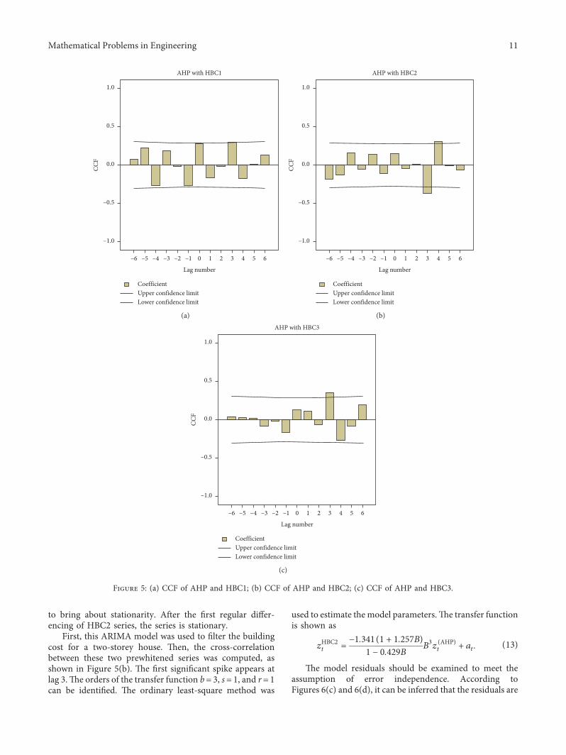

CoefficientUpper confidence limitLower confidence limit
ndash10
ndash05
00
05
10
ACF
2 134 116 7 9 14 168 1253 101 15Lag number
(a)
CoefficientUpper confidence limitLower confidence limit
2 7 12 1363 8 94 11 141 5 15 1610Lag number
ndash10
ndash05
00
05
10
Part
ial A
CF
(b)
CoefficientUpper confidence limitLower confidence limit
ndash10
ndash05
00
05
10
ACF
3 84 136 11 15 161 9 127 1452 10Lag number
(c)
CoefficientUpper confidence limitLower confidence limit
2 7 125 63 8 9 10 114 13 14 15 161Lag number
ndash10
ndash05
00
05
10
Part
ial A
CF
(d)
CoefficientUpper confidence limitLower confidence limit
ndash10
ndash05
00
05
10
ACF
3 12 15136 7 82 10 161 9 1454 11Lag number
(e)
CoefficientUpper confidence limitLower confidence limit
2 3 4 5 6 7 8 9 10 11 12 13 14 15 161Lag number
ndash10
ndash05
00
05
10
Part
ial A
CF
(f )
Figure 6 (a) ACF of the noise residuals of the transfer function model for HBC1 (b) PACF of the noise residuals of the transfer functionmodel for HBC1 (c) ACF of the noise residuals of the transfer function model for HBC2 (d) PACF of the noise residuals of the transferfunction model for HBC2 (e) ACF of the noise residuals of the transfer function model for HBC3 (f ) PACF of the noise residuals of thetransfer function model for HBC3
12 Mathematical Problems in Engineering
a white noise process )e residuals shown in Figures 6(c)and 6(d) suggest that the residuals are white noise More-over the results of the LjungndashBox test also indicate theabsence of the autocorrelation in the residuals )ereforethe model in equation (13) is adequate
423 Transfer Function Model for Building Cost Index ofTown House in New Zealand Building cost of a town housein New Zealand is denoted as HBC3With the observation ofslow damping of the ACF correlogram the regular firstdifferencing and seasonal differencing of order four wererequired to bring about stationarity After regular andseasonal differencing of the HBC3 series the series is sta-tionary as shown from the ACF In the identification of thetransfer function model it is necessary to apply the sameprewhitening transformation to both the input and outputseries)us the ARIMAmodel for house price (AHP) is alsoapplied to the building cost series of a town house Howeverbefore the prewhitening progress the cost series has beentransformed to stationary by a regular difference and aseasonal difference
Figure 5(c) shows the first significant spike is at lag 0 onthe cross-correlation function indicating no delay time )eorders of the transfer function b 3 s 0 and r 2 can beidentified )e ordinary least-square method was used toestimate the model parameters )e transfer function isshown as
zHBC3t
C
1 minus δ1B minus δ2B2( 1113857B3z
(AHP)t + at
0089
1 minus 1614B + 0849B2( )B3z
(AHP)t + at
(14)
)e residuals were checked for autocorrelation and thechi-square values for all the lags were found to be notsignificant at the 5 level as shown in Figures 6(e) and 6(f ))is suggests that the model residuals do not have problemswith autocorrelation and indeed white noise
43 Forecast Evaluation )e above proposed models wereevaluated for their out-of-sample forecasting performance)e models were developed using data from 2001Q1 to2014Q4 and then forecasts were made for the following 16quarters (2015Q1ndash2018Q4) )e model comparison wascarried out in a meaningful and systematic way )e MAPEvalues for the transfer function models and seasonal ARIMAmodels for the period 2015Q1ndash2018Q4 are presented inTable 3 )e results clearly indicate that the transfer functionmethod outperforms the seasonal ARIMA models for allbuilding cost series considered )e improvement of fore-casting accuracy from the adoption of the transfer functionmodel is best illustrated by observing the error measure-ments For the building cost index of a one-story house(HBC1) in New Zealand there is a reduction of about 391
CoefficientUpper confidence limitLower confidence limit
ndash10
ndash05
00
05
10A
CF
2 3 4 5 6 7 8 9 10 11 12 13 14 15 161
Lag number
(a)
CoefficientUpper confidence limitLower confidence limit
ndash10
ndash05
00
05
10
Part
ial A
CF
2 3 4 5 6 7 8 9 10 11 12 13 14 15 161
Lag number
(b)
Figure 7 (a) ACF of the noise residuals of the remodel for HBC1 (b) PACF of the noise residuals of the remodel for HBC1
Mathematical Problems in Engineering 13
2001
Q1
2001
Q2
2001
Q3
2001
Q4
2002
Q1
2002
Q2
2002
Q3
2002
Q4
2003
Q1
2003
Q2
2003
Q3
2003
Q4
2004
Q1
2004
Q2
2004
Q3
2004
Q4
2005
Q1
2005
Q2
2005
Q3
2005
Q4
2006
Q1
2006
Q2
2006
Q3
2006
Q4
2007
Q1
2007
Q2
2007
Q3
2007
Q4
2008
Q1
2008
Q2
2008
Q3
2008
Q4
2009
Q1
2009
Q2
2009
Q3
2009
Q4
2001
0Q
120
010
Q2
2001
0Q
320
010
Q4
2001
1Q
120
011
Q2
2001
1Q
320
011
Q4
2001
2Q
120
012
Q2
2001
2Q
320
012
Q4
2001
3Q
120
013
Q2
2001
3Q
320
013
Q4
2001
4Q
120
014
Q2
2001
4Q
320
014
Q4
2001
5Q
120
015
Q2
2001
5Q
320
015
Q4
2001
6Q
120
016
Q2
2001
6Q
320
016
Q4
2001
7Q
120
017
Q2
2001
7Q
320
017
Q4
2001
8Q
120
018
Q2
2001
8Q
320
018
Q4
0
500
1000
1500
2000
2500
$ (m
2 )
HBC1HBC1 (TF)
HBC1 (ARIMA)
Year (quarter)
(a)
2001
Q1
2001
Q2
2001
Q3
2001
Q4
2002
Q1
2002
Q2
2002
Q3
2002
Q4
2003
Q1
2003
Q2
2003
Q3
2003
Q4
2004
Q1
2004
Q2
2004
Q3
2004
Q4
2005
Q1
2005
Q2
2005
Q3
2005
Q4
2006
Q1
2006
Q2
2006
Q3
2006
Q4
2007
Q1
2007
Q2
2007
Q3
2007
Q4
2008
Q1
2008
Q2
2008
Q3
2008
Q4
2009
Q1
2009
Q2
2009
Q3
2009
Q4
2001
0Q
120
010
Q2
2001
0Q
320
010
Q4
2001
1Q
120
011
Q2
2001
1Q
320
011
Q4
2001
2Q
120
012
Q2
2001
2Q
320
012
Q4
2001
3Q
120
013
Q2
2001
3Q
320
013
Q4
2001
4Q
120
014
Q2
2001
4Q
320
014
Q4
2001
5Q
120
015
Q2
2001
5Q
320
015
Q4
2001
6Q
120
016
Q2
2001
6Q
320
016
Q4
2001
7Q
120
017
Q2
2001
7Q
320
017
Q4
2001
8Q
120
018
Q2
2001
8Q
320
018
Q4
0
500
1000
1500
2000
2500
$ (m
2 )
HBC1HBC1 (TF)
HBC1 (ARIMA)
Year (quarter)
(b)
Figure 8 Continued
Table 3 Comparison of model performance (MAPE)
Cost series ARIMA TFHBC1 2091 1273HBC2 2935 1365HBC3 5766 1161
14 Mathematical Problems in Engineering
in the MAPE from the seasonal ARIMA model to thetransfer function model For the building cost index of atwo-story house in New Zealand (HBC2) the reductionfrom using the transfer function model is even more pro-nounced there is a 535 reduction in the MAPE from theARIMA model to the transfer function model For thebuilding cost index of a town house in New Zealand (HBC3)the transfer function model provides a 799 MAPE re-duction over the seasonal ARIMA model Note that thetransfer function models are for all three cost series su-perior to the seasonal ARIMA models )e building costindex of HBC1 HBC2 and HBC3 and their forecastsgenerated from ARIMA and transfer function models areshown in Figure 8
5 Results and Discussion
)e fluctuations in the building cost index are problematicfor cost estimation)eARIMAmodels completely take intoaccount the dynamic process of cost series the seasonalityand the serial correlation in the residuals to obtain precisecost forecasts Although the model can dynamically describethe time-series data it cannot investigate the causality be-tween independent variables and dependent variables Basedon the current state of knowledge and the existing literaturebuilding costs are influenced not only by the constructionindustry but also by other factors such as house priceseconomic conditions population incomes and businessloans)e inclusion of explanatory variables into the modelscan forecast building cost more accurately)eNew Zealandhouse price index was selected as an explanatory variable forpredicating building cost in this study
)e analysis results suggest that the simplest model is notalways the most appropriate one for predicting particularly
when additional information is available Univariate modelslike ARIMA can be used as a benchmark in comparingforecasting performance When explanatory variables areavailable they can be included in the model to improveforecasting accuracy Multivariate models can then berealised to improve forecasting performance )e transferfunction model can describe more about the characteristicsof the output than a univariate model by describing thedynamic relationship between the input and output vari-ables Inclusion of New Zealand house prices in the transferfunction models significantly improves forecasting accuracy)is is consistent with the findings of [49] which indicatedthat model inclusion of an exogenous variable can improvethe forecasting performance Housing is one kind ofbuilding construction product that connects the buildingconstruction sector to the housing sector So the buildingcosts are subject to changes in house prices New Zealandhouse prices stimulate the changes in building costs al-though building costs are usually viewed as fundamentals)e findings are also supported by the studies of [38 50]
6 Conclusion
)is study proposed the transfer functionmethod to forecastthe building cost index of New Zealand to improve theaccuracy of the cost estimates that help in developing ac-curate budgets and preventing under- or overestimation AnARIMAmodel was also used as a benchmark method Basedon the BoxndashJenkins model development process transferfunction models and seasonal ARIMA models for buildingcost indices of one-storey houses two-storey houses andtown houses in New Zealand were developed )e effec-tiveness of the transfer function models was compared withthat of the univariate ARIMA models )e results indicated
2001
Q1
2001
Q2
2001
Q3
2001
Q4
2002
Q1
2002
Q2
2002
Q3
2002
Q4
2003
Q1
2003
Q2
2003
Q3
2003
Q4
2004
Q1
2004
Q2
2004
Q3
2004
Q4
2005
Q1
2005
Q2
2005
Q3
2005
Q4
2006
Q1
2006
Q2
2006
Q3
2006
Q4
2007
Q1
2007
Q2
2007
Q3
2007
Q4
2008
Q1
2008
Q2
2008
Q3
2008
Q4
2009
Q1
2009
Q2
2009
Q3
2009
Q4
2001
0Q
1
HBC1HBC1 (TF)
HBC1 (ARIMA)
Year (quarter)
2001
0Q
220
010
Q3
2001
0Q
420
011
Q1
2001
1Q
220
011
Q3
2001
1Q
420
012
Q1
2001
2Q
220
012
Q3
2001
2Q
420
013
Q1
2001
3Q
220
013
Q3
2001
3Q
420
014
Q1
2001
4Q
220
014
Q3
2001
4Q
420
015
Q1
2001
5Q
220
015
Q3
2001
5Q
420
016
Q1
2001
6Q
220
016
Q3
2001
6Q
420
017
Q1
2001
7Q
220
017
Q3
2001
7Q
420
018
Q1
2001
8Q
220
018
Q3
2001
8Q
4
0
500
1000
1500
2000
2500
$ (m
2 )
(c)
Figure 8 (a) Building cost index of HBC1 and its forecasts generated from ARIMA and transfer function models (b) building cost index ofHBC2 and its forecasts generated from ARIMA and transfer function models (c) building cost index of HBC3 and its forecasts generatedfrom ARIMA and transfer function models
Mathematical Problems in Engineering 15
that the predictive accuracy of the transfer function model issuperior to that of the ARIMA model since the transferfunction model achieved lower MAPE and RMSE
)e transfer functionmodel was developed from a fusionof time-series analysis regression analysis and cross-cor-relation analysis Cross-correlation analysis was used toexplore the potential optimal parameters Time-seriesanalysis was used to identify the cost index patterns Re-gression analysis was utilized to identify the underlyingmapping between influencing factors and the cost index)etransfer function models that contain an exogenous variable(more information) are better at forecasting than the simplerARIMA models )e causality between building cost andhouse prices was modelled in the transfer function method)e inclusion of house prices in the model significantlyreduces the forecasting error of the transfer functionmodelsrelative to seasonal ARIMA models )is study has shownthat the inclusion of an explanatory variable input within theframework leads to an improvement in forecastingperformance
)is study makes important contributions to three areas)e main contribution of this study is to enhance cost es-timation accuracy and guide industry practitioners in thepreliminary design stage )e proposed transfer functionmodel can be a useful tool for industry professionals togenerate cost estimates that can help in pricing bidding andassessing construction projects Second the inclusion ofNew Zealand house prices in the transfer function modelsignificantly improves the cost forecasting performance )efindings indicate that the inclusion of cost-influencingfactors into the model can significantly improve the fore-casting accuracy of the building cost index of New Zealand)e findings contribute to the present body of knowledge oncost estimation and may serve as a valuable guide for futuremodel development )ird the results of this study provethat New Zealand house price is a significant influencingfactor of residential building cost )e results also demon-strate that variations in house prices can result in fluctua-tions in residential building costs )e results may helpindustry professionals understand the underlying relation-ship between the construction industry and housing marketof New Zealand
)e developed models are based on the building costindex of New Zealand However the model developmentprocess can be used in other regions )e accuracy of long-term forecasting of the cost index using the transfer functionmodel may be impaired due to uncertainty in the dynamicenvironment Hence the use of intelligent methods for long-term prediction of the cost index is a future researchdirection
Abbreviations
ACF Autocorrelation functionAHP House price index of New ZealandANNs Artificial neutral networksARIMA Autoregressive integrated moving averageARMA Autoregressive moving averageBCI Building cost index
CCF Cross-correlation functionCCI Construction cost indexES Exponential smoothingHBC1 Building cost index of a one-story house in New
ZealandHBC2 Building cost index of a two-story house in New
ZealandHBC3 Building cost index of a town house in New
ZealandMAPE Mean absolute percentage errorPACF Partial autocorrelation functionPPI Producer price indexRACF Residual autocorrelation functionRMSE Root mean square errorRPACF Residual partial autocorrelation functionUK United KingdomVECM Vector error correction model
Data Availability
)e data used to support the findings of this study areavailable from the corresponding author upon request
Conflicts of Interest
)e authors declare no conflicts of interest
Authorsrsquo Contributions
L Z and J M conceptualized the idea L Z performed themethodology prepared the original draft and acquired thefund Z L developed the software L Z and Z L performedvalidation J M supervised the work and reviewed andedited the paper
Acknowledgments
)is research was funded by the China Scholarship Councilthrough the research project (grant no 201206130069)Massey University (grant no 09166424) and Beijing Uni-versity of Technology (grant no 004000514119067) )eAPC was funded by the three grants )e authors would liketo thank the Reserve Bank of New Zealand and Ministry ofBusiness Innovation and Employment for providing data toconduct this research In addition the authors would like tothank all practitioners who contributed to this project
References
[1] J Gido and J P Clements Successful Project ManagementCengage Learning Stamford CT USA 6th edition 2015
[2] R Sonmez ldquoConceptual cost estimation of building projectswith regression analysis and neural networksrdquo CanadianJournal of Civil Engineering vol 31 no 4 pp 677ndash683 2004
[3] Y Takano N Ishii andMMuraki ldquoDetermining bidmarkupand resources allocated to cost estimation in competitivebiddingrdquo Automation in Construction vol 85 pp 358ndash3682018
[4] E W Merrow Concepts Strategies and Practices for SuccessJohn Wiley amp Sons Hoboken NJ USA 2011
16 Mathematical Problems in Engineering
[5] B Ashuri and J Lu ldquoTime series analysis of ENR constructioncost indexrdquo Journal of Construction Engineering and Man-agement vol 136 no 11 pp 1227ndash1237 2010
[6] Y Elfahham ldquoEstimation and prediction of construction costindex using neural networks time series and regressionrdquoAlexandria Engineering Journal vol 58 no 2 pp 499ndash5062019
[7] S Hwang ldquoDynamic regression models for prediction ofconstruction costsrdquo Journal of Construction Engineering andManagement vol 135 no 5 pp 360ndash367 2009
[8] J X Xu and S Moon ldquoStochastic forecast of construction costindex using a cointegrated vector autoregression modelrdquoJournal of Management in Engineering vol 29 no 1pp 10ndash18 2013
[9] MBIE NZ Sector Report 2013mdashConstruction Ministry ofBuilding Innovation and Employment Wellington NewZealand 2013
[10] A Jrade A Conceptual Cost Estimating Computer System forBuilding Projects Concordia University Montreal Canada2000
[11] M-Y Cheng and A F V Roy ldquoEvolutionary fuzzy decisionmodel for cash flow prediction using time-dependent supportvector machinesrdquo International Journal of Project Manage-ment vol 29 no 1 pp 56ndash65 2011
[12] S Hwang ldquoTime series models for forecasting constructioncosts using time series indexesrdquo Journal of ConstructionEngineering and Management vol 137 no 9 pp 656ndash6622011
[13] R Zhang B Ashuri Y Shyr and Y Deng ldquoForecastingconstruction cost index based on visibility graph a networkapproachrdquo Physica A Statistical Mechanics and Its Applica-tions vol 493 pp 239ndash252 2018
[14] D J Lowe M W Emsley and A Harding ldquoPredictingconstruction cost using multiple regression techniquesrdquoJournal of Construction Engineering and Managementvol 132 no 7 pp 750ndash758 2006
[15] H-L Yip H Fan and Y-H Chiang ldquoPredicting the main-tenance cost of construction equipment comparison betweengeneral regression neural network and Box-Jenkins time se-ries modelsrdquo Automation in Construction vol 38 pp 30ndash382014
[16] G Morcous H Rivard and A M Hanna ldquoCase-basedreasoning system for modeling infrastructure deteriorationrdquoJournal of Computing in Civil Engineering vol 16 no 2pp 104ndash114 2002
[17] N-J Yau and J-B Yang ldquoCase-based reasoning in con-struction managementrdquo Computer-Aided Civil and Infra-structure Engineering vol 13 no 2 pp 143ndash150 1998
[18] R G Brown Smoothing Forecasting and Prediction of Dis-crete Time Series Courier Dover Publications Mineola NYUSA 2004
[19] G P Zhang and M Qi ldquoNeural network forecasting forseasonal and trend time seriesrdquo European Journal of Oper-ational Research vol 160 no 2 pp 501ndash514 2005
[20] B Pfaff Analysis of Integrated and Cointegrated Time Serieswith R Springer Berlin Germany 2008
[21] Y-H Lin and P-C Lee ldquoNovel high-precision grey fore-casting modelrdquo Automation in Construction vol 16 no 6pp 771ndash777 2007
[22] H Zheng Y Deng and Y Hu ldquoFuzzy evidential influencediagram and its evaluation algorithmrdquo Knowledge-BasedSystems vol 131 pp 28ndash45 2017
[23] X Zhou X Deng Y Deng and S Mahadevan ldquoDependenceassessment in human reliability analysis based on D numbers
and AHPrdquo Nuclear Engineering and Design vol 313pp 243ndash252 2017
[24] M-Y Cheng N-D Hoang and Y-W Wu ldquoHybrid intel-ligence approach based on LS-SVM and differential evolutionfor construction cost index estimation a Taiwan case studyrdquoAutomation in Construction vol 35 pp 306ndash313 2013
[25] B Ashuri S M Shahandashti and J Lu ldquoEmpirical tests foridentifying leading indicators of ENR construction cost in-dexrdquo Construction Management and Economics vol 30no 11 pp 917ndash927 2012
[26] S T Ng S O Cheung M Skitmore and T C Y Wong ldquoAnintegrated regression analysis and time series model forconstruction tender price index forecastingrdquo ConstructionManagement and Economics vol 22 no 5 pp 483ndash493 2004
[27] J MWWong and S T Ng ldquoForecasting construction tenderprice index in Hong Kong using vector error correctionmodelrdquo Construction Management and Economics vol 28no 12 pp 1255ndash1268 2010
[28] S M Shahandashti and B Ashuri ldquoForecasting engineeringnews-record construction cost index using multivariate timeseries modelsrdquo Journal of Construction Engineering andManagement vol 139 no 9 pp 1237ndash1243 2013
[29] H L Chen ldquoDeveloping cost response models for company-level cost flow forecasting of project-based corporationsrdquoJournal of Management in Engineering vol 23 no 4pp 171ndash181 2007
[30] A Hammad S Ali G J Sweis and R J Sweis ldquoStatsticalanalysis on the cost and duration of public building projectsrdquoJournal of Management in Engineering vol 26 no 2pp 105ndash113 2010
[31] W P Trefor ldquoPredicting changes in predicting changes inconstruction cost indexes using neural networksrdquo Journal ofConstruction Engineering and Management vol 120 no 2pp 306ndash320 1994
[32] G-H Kim S-H An and K-I Kang ldquoComparison of con-struction cost estimating models based on regression analysisneural networks and case-based reasoningrdquo Building andEnvironment vol 39 no 10 pp 1235ndash1242 2004
[33] K Byung-Cheol and H K Young ldquoImproving the accuracyand operational predictability of project cost forecasts anadaptive combination approachrdquo Production Planning ampControl vol 29 no 9 pp 743ndash760 2018
[34] N Kulendran and S F Witt ldquoLeading indicator tourismforecastsrdquo Tourism Management vol 24 no 5 pp 503ndash5102003
[35] M Qi ldquoPredicting US recessions with leading indicators vianeural network modelsrdquo International Journal of Forecastingvol 17 no 3 pp 383ndash401 2001
[36] M-C Chen and I-C Tsai ldquoA cobweb theory of house priceincorporating investor behaviorrdquo Academia Economic Papersvol 35 pp 315ndash344 2007
[37] J Janssen B Kruijt and B Needham ldquo)e honeycomb cyclein real estaterdquo e Journal of Real Estate Research vol 9pp 237ndash251 1994
[38] I-C Tsai ldquoHousing supply demand and price constructioncost rental price and house price indicesrdquo Asian EconomicJournal vol 26 no 4 pp 381ndash396 2012
[39] T Sunde and P-F Muzindutsi ldquoDeterminants of house pricesand new construction activity an empirical investigation ofthe Namibian housing marketrdquo e Journal of DevelopingAreas vol 51 no 3 pp 390ndash407 2017
[40] S Makridakis S C Wheelwright and V McGee ForecastingMethods and Applications Wiley Hoboken NJ USA 2ndedition 1983
Mathematical Problems in Engineering 17
[41] T C Mills Time Series Techniques for Economists CambridgeUniversity Press New York NY USA 1990
[42] G E P Box G M Jenkins and G C Reinsel Time SeriesAnalysis Forecasting and Control Wiley Hoboken NJ USA1994
[43] Y Hasanah M Herlina and H Zaikarina ldquoFlood predictionusing transfer function model of rainfall and water dischargeapproach in Katulampa damrdquo in Proceedings of the 3rd In-ternational Conference on Sustainable Future for HumanSecurity SUSTAIN 2012 pp 317ndash326 Kyoto Japan No-vember 2012
[44] T Cook ldquoAn application of the transfer function to aneconomic-base modelrdquo e Annals of Regional Sciencevol 13 pp 81ndash92 1979
[45] G E P Box and G M Jenkins Time Series Analysis Fore-casting and Control Holden Day Inc San Francisco CAUSA 1976
[46] R Yaffee and M McGee Introduction to Time Series Analysisand Forecasting with Applications of SAS and SPSS AcademicPress Inc Cambridge MA USA 2000
[47] G E Box G Jenkins and G Reinsel Time Sereis AnalysisWiley Hoboken NJ USA 4th edition 2008
[48] S Bisgaard and M Kulahci Time Series Analysis and Fore-casting by Example John Wiley amp Sons Inc Hoboken NJUSA 2011
[49] R Ashley ldquoOn the usefulness of macroeconomic forecasts asinputs to forecasting modelsrdquo Journal of Forecasting vol 2no 3 pp 211ndash223 1983
[50] A Grimes and A Aitken ldquoHousing supply land costs andprice adjustmentrdquo Real Estate Economics vol 38 no 2pp 325ndash353 2010
18 Mathematical Problems in Engineering
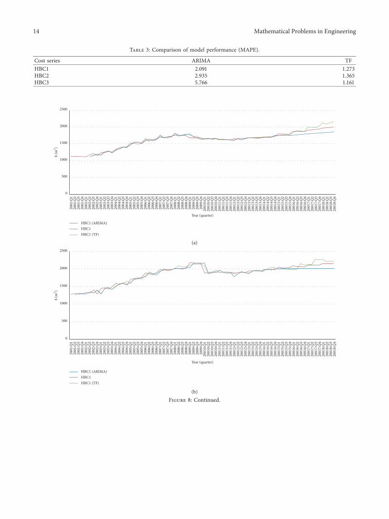
2001
Q1
2001
Q2
2001
Q3
2001
Q4
2002
Q1
2002
Q2
2002
Q3
2002
Q4
2003
Q1
2003
Q2
2003
Q3
2003
Q4
2004
Q1
2004
Q2
2004
Q3
2004
Q4
2005
Q1
2005
Q2
2005
Q3
2005
Q4
2006
Q1
2006
Q2
2006
Q3
2006
Q4
2007
Q1
2007
Q2
2007
Q3
2007
Q4
2008
Q1
2008
Q2
2008
Q3
2008
Q4
2009
Q1
2009
Q2
2009
Q3
2009
Q4
2001
0Q
120
010
Q2
2001
0Q
320
010
Q4
2001
1Q
120
011
Q2
2001
1Q
320
011
Q4
2001
2Q
120
012
Q2
2001
2Q
320
012
Q4
2001
3Q
120
013
Q2
2001
3Q
320
013
Q4
2001
4Q
120
014
Q2
2001
4Q
320
014
Q4
2001
5Q
120
015
Q2
2001
5Q
320
015
Q4
2001
6Q
120
016
Q2
2001
6Q
320
016
Q4
2001
7Q
120
017
Q2
2001
7Q
320
017
Q4
2001
8Q
120
018
Q2
2001
8Q
320
018
Q4
0
500
1000
1500
2000
2500
$ (m
2 )
HBC1HBC1 (TF)
HBC1 (ARIMA)
Year (quarter)
(a)
2001
Q1
2001
Q2
2001
Q3
2001
Q4
2002
Q1
2002
Q2
2002
Q3
2002
Q4
2003
Q1
2003
Q2
2003
Q3
2003
Q4
2004
Q1
2004
Q2
2004
Q3
2004
Q4
2005
Q1
2005
Q2
2005
Q3
2005
Q4
2006
Q1
2006
Q2
2006
Q3
2006
Q4
2007
Q1
2007
Q2
2007
Q3
2007
Q4
2008
Q1
2008
Q2
2008
Q3
2008
Q4
2009
Q1
2009
Q2
2009
Q3
2009
Q4
2001
0Q
120
010
Q2
2001
0Q
320
010
Q4
2001
1Q
120
011
Q2
2001
1Q
320
011
Q4
2001
2Q
120
012
Q2
2001
2Q
320
012
Q4
2001
3Q
120
013
Q2
2001
3Q
320
013
Q4
2001
4Q
120
014
Q2
2001
4Q
320
014
Q4
2001
5Q
120
015
Q2
2001
5Q
320
015
Q4
2001
6Q
120
016
Q2
2001
6Q
320
016
Q4
2001
7Q
120
017
Q2
2001
7Q
320
017
Q4
2001
8Q
120
018
Q2
2001
8Q
320
018
Q4
0
500
1000
1500
2000
2500
$ (m
2 )
HBC1HBC1 (TF)
HBC1 (ARIMA)
Year (quarter)
(b)
Figure 8 Continued
Table 3 Comparison of model performance (MAPE)
Cost series ARIMA TFHBC1 2091 1273HBC2 2935 1365HBC3 5766 1161
14 Mathematical Problems in Engineering
in the MAPE from the seasonal ARIMA model to thetransfer function model For the building cost index of atwo-story house in New Zealand (HBC2) the reductionfrom using the transfer function model is even more pro-nounced there is a 535 reduction in the MAPE from theARIMA model to the transfer function model For thebuilding cost index of a town house in New Zealand (HBC3)the transfer function model provides a 799 MAPE re-duction over the seasonal ARIMA model Note that thetransfer function models are for all three cost series su-perior to the seasonal ARIMA models )e building costindex of HBC1 HBC2 and HBC3 and their forecastsgenerated from ARIMA and transfer function models areshown in Figure 8
5 Results and Discussion
)e fluctuations in the building cost index are problematicfor cost estimation)eARIMAmodels completely take intoaccount the dynamic process of cost series the seasonalityand the serial correlation in the residuals to obtain precisecost forecasts Although the model can dynamically describethe time-series data it cannot investigate the causality be-tween independent variables and dependent variables Basedon the current state of knowledge and the existing literaturebuilding costs are influenced not only by the constructionindustry but also by other factors such as house priceseconomic conditions population incomes and businessloans)e inclusion of explanatory variables into the modelscan forecast building cost more accurately)eNew Zealandhouse price index was selected as an explanatory variable forpredicating building cost in this study
)e analysis results suggest that the simplest model is notalways the most appropriate one for predicting particularly
when additional information is available Univariate modelslike ARIMA can be used as a benchmark in comparingforecasting performance When explanatory variables areavailable they can be included in the model to improveforecasting accuracy Multivariate models can then berealised to improve forecasting performance )e transferfunction model can describe more about the characteristicsof the output than a univariate model by describing thedynamic relationship between the input and output vari-ables Inclusion of New Zealand house prices in the transferfunction models significantly improves forecasting accuracy)is is consistent with the findings of [49] which indicatedthat model inclusion of an exogenous variable can improvethe forecasting performance Housing is one kind ofbuilding construction product that connects the buildingconstruction sector to the housing sector So the buildingcosts are subject to changes in house prices New Zealandhouse prices stimulate the changes in building costs al-though building costs are usually viewed as fundamentals)e findings are also supported by the studies of [38 50]
6 Conclusion
)is study proposed the transfer functionmethod to forecastthe building cost index of New Zealand to improve theaccuracy of the cost estimates that help in developing ac-curate budgets and preventing under- or overestimation AnARIMAmodel was also used as a benchmark method Basedon the BoxndashJenkins model development process transferfunction models and seasonal ARIMA models for buildingcost indices of one-storey houses two-storey houses andtown houses in New Zealand were developed )e effec-tiveness of the transfer function models was compared withthat of the univariate ARIMA models )e results indicated
2001
Q1
2001
Q2
2001
Q3
2001
Q4
2002
Q1
2002
Q2
2002
Q3
2002
Q4
2003
Q1
2003
Q2
2003
Q3
2003
Q4
2004
Q1
2004
Q2
2004
Q3
2004
Q4
2005
Q1
2005
Q2
2005
Q3
2005
Q4
2006
Q1
2006
Q2
2006
Q3
2006
Q4
2007
Q1
2007
Q2
2007
Q3
2007
Q4
2008
Q1
2008
Q2
2008
Q3
2008
Q4
2009
Q1
2009
Q2
2009
Q3
2009
Q4
2001
0Q
1
HBC1HBC1 (TF)
HBC1 (ARIMA)
Year (quarter)
2001
0Q
220
010
Q3
2001
0Q
420
011
Q1
2001
1Q
220
011
Q3
2001
1Q
420
012
Q1
2001
2Q
220
012
Q3
2001
2Q
420
013
Q1
2001
3Q
220
013
Q3
2001
3Q
420
014
Q1
2001
4Q
220
014
Q3
2001
4Q
420
015
Q1
2001
5Q
220
015
Q3
2001
5Q
420
016
Q1
2001
6Q
220
016
Q3
2001
6Q
420
017
Q1
2001
7Q
220
017
Q3
2001
7Q
420
018
Q1
2001
8Q
220
018
Q3
2001
8Q
4
0
500
1000
1500
2000
2500
$ (m
2 )
(c)
Figure 8 (a) Building cost index of HBC1 and its forecasts generated from ARIMA and transfer function models (b) building cost index ofHBC2 and its forecasts generated from ARIMA and transfer function models (c) building cost index of HBC3 and its forecasts generatedfrom ARIMA and transfer function models
Mathematical Problems in Engineering 15
that the predictive accuracy of the transfer function model issuperior to that of the ARIMA model since the transferfunction model achieved lower MAPE and RMSE
)e transfer functionmodel was developed from a fusionof time-series analysis regression analysis and cross-cor-relation analysis Cross-correlation analysis was used toexplore the potential optimal parameters Time-seriesanalysis was used to identify the cost index patterns Re-gression analysis was utilized to identify the underlyingmapping between influencing factors and the cost index)etransfer function models that contain an exogenous variable(more information) are better at forecasting than the simplerARIMA models )e causality between building cost andhouse prices was modelled in the transfer function method)e inclusion of house prices in the model significantlyreduces the forecasting error of the transfer functionmodelsrelative to seasonal ARIMA models )is study has shownthat the inclusion of an explanatory variable input within theframework leads to an improvement in forecastingperformance
)is study makes important contributions to three areas)e main contribution of this study is to enhance cost es-timation accuracy and guide industry practitioners in thepreliminary design stage )e proposed transfer functionmodel can be a useful tool for industry professionals togenerate cost estimates that can help in pricing bidding andassessing construction projects Second the inclusion ofNew Zealand house prices in the transfer function modelsignificantly improves the cost forecasting performance )efindings indicate that the inclusion of cost-influencingfactors into the model can significantly improve the fore-casting accuracy of the building cost index of New Zealand)e findings contribute to the present body of knowledge oncost estimation and may serve as a valuable guide for futuremodel development )ird the results of this study provethat New Zealand house price is a significant influencingfactor of residential building cost )e results also demon-strate that variations in house prices can result in fluctua-tions in residential building costs )e results may helpindustry professionals understand the underlying relation-ship between the construction industry and housing marketof New Zealand
)e developed models are based on the building costindex of New Zealand However the model developmentprocess can be used in other regions )e accuracy of long-term forecasting of the cost index using the transfer functionmodel may be impaired due to uncertainty in the dynamicenvironment Hence the use of intelligent methods for long-term prediction of the cost index is a future researchdirection
Abbreviations
ACF Autocorrelation functionAHP House price index of New ZealandANNs Artificial neutral networksARIMA Autoregressive integrated moving averageARMA Autoregressive moving averageBCI Building cost index
CCF Cross-correlation functionCCI Construction cost indexES Exponential smoothingHBC1 Building cost index of a one-story house in New
ZealandHBC2 Building cost index of a two-story house in New
ZealandHBC3 Building cost index of a town house in New
ZealandMAPE Mean absolute percentage errorPACF Partial autocorrelation functionPPI Producer price indexRACF Residual autocorrelation functionRMSE Root mean square errorRPACF Residual partial autocorrelation functionUK United KingdomVECM Vector error correction model
Data Availability
)e data used to support the findings of this study areavailable from the corresponding author upon request
Conflicts of Interest
)e authors declare no conflicts of interest
Authorsrsquo Contributions
L Z and J M conceptualized the idea L Z performed themethodology prepared the original draft and acquired thefund Z L developed the software L Z and Z L performedvalidation J M supervised the work and reviewed andedited the paper
Acknowledgments
)is research was funded by the China Scholarship Councilthrough the research project (grant no 201206130069)Massey University (grant no 09166424) and Beijing Uni-versity of Technology (grant no 004000514119067) )eAPC was funded by the three grants )e authors would liketo thank the Reserve Bank of New Zealand and Ministry ofBusiness Innovation and Employment for providing data toconduct this research In addition the authors would like tothank all practitioners who contributed to this project
References
[1] J Gido and J P Clements Successful Project ManagementCengage Learning Stamford CT USA 6th edition 2015
[2] R Sonmez ldquoConceptual cost estimation of building projectswith regression analysis and neural networksrdquo CanadianJournal of Civil Engineering vol 31 no 4 pp 677ndash683 2004
[3] Y Takano N Ishii andMMuraki ldquoDetermining bidmarkupand resources allocated to cost estimation in competitivebiddingrdquo Automation in Construction vol 85 pp 358ndash3682018
[4] E W Merrow Concepts Strategies and Practices for SuccessJohn Wiley amp Sons Hoboken NJ USA 2011
16 Mathematical Problems in Engineering
[5] B Ashuri and J Lu ldquoTime series analysis of ENR constructioncost indexrdquo Journal of Construction Engineering and Man-agement vol 136 no 11 pp 1227ndash1237 2010
[6] Y Elfahham ldquoEstimation and prediction of construction costindex using neural networks time series and regressionrdquoAlexandria Engineering Journal vol 58 no 2 pp 499ndash5062019
[7] S Hwang ldquoDynamic regression models for prediction ofconstruction costsrdquo Journal of Construction Engineering andManagement vol 135 no 5 pp 360ndash367 2009
[8] J X Xu and S Moon ldquoStochastic forecast of construction costindex using a cointegrated vector autoregression modelrdquoJournal of Management in Engineering vol 29 no 1pp 10ndash18 2013
[9] MBIE NZ Sector Report 2013mdashConstruction Ministry ofBuilding Innovation and Employment Wellington NewZealand 2013
[10] A Jrade A Conceptual Cost Estimating Computer System forBuilding Projects Concordia University Montreal Canada2000
[11] M-Y Cheng and A F V Roy ldquoEvolutionary fuzzy decisionmodel for cash flow prediction using time-dependent supportvector machinesrdquo International Journal of Project Manage-ment vol 29 no 1 pp 56ndash65 2011
[12] S Hwang ldquoTime series models for forecasting constructioncosts using time series indexesrdquo Journal of ConstructionEngineering and Management vol 137 no 9 pp 656ndash6622011
[13] R Zhang B Ashuri Y Shyr and Y Deng ldquoForecastingconstruction cost index based on visibility graph a networkapproachrdquo Physica A Statistical Mechanics and Its Applica-tions vol 493 pp 239ndash252 2018
[14] D J Lowe M W Emsley and A Harding ldquoPredictingconstruction cost using multiple regression techniquesrdquoJournal of Construction Engineering and Managementvol 132 no 7 pp 750ndash758 2006
[15] H-L Yip H Fan and Y-H Chiang ldquoPredicting the main-tenance cost of construction equipment comparison betweengeneral regression neural network and Box-Jenkins time se-ries modelsrdquo Automation in Construction vol 38 pp 30ndash382014
[16] G Morcous H Rivard and A M Hanna ldquoCase-basedreasoning system for modeling infrastructure deteriorationrdquoJournal of Computing in Civil Engineering vol 16 no 2pp 104ndash114 2002
[17] N-J Yau and J-B Yang ldquoCase-based reasoning in con-struction managementrdquo Computer-Aided Civil and Infra-structure Engineering vol 13 no 2 pp 143ndash150 1998
[18] R G Brown Smoothing Forecasting and Prediction of Dis-crete Time Series Courier Dover Publications Mineola NYUSA 2004
[19] G P Zhang and M Qi ldquoNeural network forecasting forseasonal and trend time seriesrdquo European Journal of Oper-ational Research vol 160 no 2 pp 501ndash514 2005
[20] B Pfaff Analysis of Integrated and Cointegrated Time Serieswith R Springer Berlin Germany 2008
[21] Y-H Lin and P-C Lee ldquoNovel high-precision grey fore-casting modelrdquo Automation in Construction vol 16 no 6pp 771ndash777 2007
[22] H Zheng Y Deng and Y Hu ldquoFuzzy evidential influencediagram and its evaluation algorithmrdquo Knowledge-BasedSystems vol 131 pp 28ndash45 2017
[23] X Zhou X Deng Y Deng and S Mahadevan ldquoDependenceassessment in human reliability analysis based on D numbers
and AHPrdquo Nuclear Engineering and Design vol 313pp 243ndash252 2017
[24] M-Y Cheng N-D Hoang and Y-W Wu ldquoHybrid intel-ligence approach based on LS-SVM and differential evolutionfor construction cost index estimation a Taiwan case studyrdquoAutomation in Construction vol 35 pp 306ndash313 2013
[25] B Ashuri S M Shahandashti and J Lu ldquoEmpirical tests foridentifying leading indicators of ENR construction cost in-dexrdquo Construction Management and Economics vol 30no 11 pp 917ndash927 2012
[26] S T Ng S O Cheung M Skitmore and T C Y Wong ldquoAnintegrated regression analysis and time series model forconstruction tender price index forecastingrdquo ConstructionManagement and Economics vol 22 no 5 pp 483ndash493 2004
[27] J MWWong and S T Ng ldquoForecasting construction tenderprice index in Hong Kong using vector error correctionmodelrdquo Construction Management and Economics vol 28no 12 pp 1255ndash1268 2010
[28] S M Shahandashti and B Ashuri ldquoForecasting engineeringnews-record construction cost index using multivariate timeseries modelsrdquo Journal of Construction Engineering andManagement vol 139 no 9 pp 1237ndash1243 2013
[29] H L Chen ldquoDeveloping cost response models for company-level cost flow forecasting of project-based corporationsrdquoJournal of Management in Engineering vol 23 no 4pp 171ndash181 2007
[30] A Hammad S Ali G J Sweis and R J Sweis ldquoStatsticalanalysis on the cost and duration of public building projectsrdquoJournal of Management in Engineering vol 26 no 2pp 105ndash113 2010
[31] W P Trefor ldquoPredicting changes in predicting changes inconstruction cost indexes using neural networksrdquo Journal ofConstruction Engineering and Management vol 120 no 2pp 306ndash320 1994
[32] G-H Kim S-H An and K-I Kang ldquoComparison of con-struction cost estimating models based on regression analysisneural networks and case-based reasoningrdquo Building andEnvironment vol 39 no 10 pp 1235ndash1242 2004
[33] K Byung-Cheol and H K Young ldquoImproving the accuracyand operational predictability of project cost forecasts anadaptive combination approachrdquo Production Planning ampControl vol 29 no 9 pp 743ndash760 2018
[34] N Kulendran and S F Witt ldquoLeading indicator tourismforecastsrdquo Tourism Management vol 24 no 5 pp 503ndash5102003
[35] M Qi ldquoPredicting US recessions with leading indicators vianeural network modelsrdquo International Journal of Forecastingvol 17 no 3 pp 383ndash401 2001
[36] M-C Chen and I-C Tsai ldquoA cobweb theory of house priceincorporating investor behaviorrdquo Academia Economic Papersvol 35 pp 315ndash344 2007
[37] J Janssen B Kruijt and B Needham ldquo)e honeycomb cyclein real estaterdquo e Journal of Real Estate Research vol 9pp 237ndash251 1994
[38] I-C Tsai ldquoHousing supply demand and price constructioncost rental price and house price indicesrdquo Asian EconomicJournal vol 26 no 4 pp 381ndash396 2012
[39] T Sunde and P-F Muzindutsi ldquoDeterminants of house pricesand new construction activity an empirical investigation ofthe Namibian housing marketrdquo e Journal of DevelopingAreas vol 51 no 3 pp 390ndash407 2017
[40] S Makridakis S C Wheelwright and V McGee ForecastingMethods and Applications Wiley Hoboken NJ USA 2ndedition 1983
Mathematical Problems in Engineering 17
[41] T C Mills Time Series Techniques for Economists CambridgeUniversity Press New York NY USA 1990
[42] G E P Box G M Jenkins and G C Reinsel Time SeriesAnalysis Forecasting and Control Wiley Hoboken NJ USA1994
[43] Y Hasanah M Herlina and H Zaikarina ldquoFlood predictionusing transfer function model of rainfall and water dischargeapproach in Katulampa damrdquo in Proceedings of the 3rd In-ternational Conference on Sustainable Future for HumanSecurity SUSTAIN 2012 pp 317ndash326 Kyoto Japan No-vember 2012
[44] T Cook ldquoAn application of the transfer function to aneconomic-base modelrdquo e Annals of Regional Sciencevol 13 pp 81ndash92 1979
[45] G E P Box and G M Jenkins Time Series Analysis Fore-casting and Control Holden Day Inc San Francisco CAUSA 1976
[46] R Yaffee and M McGee Introduction to Time Series Analysisand Forecasting with Applications of SAS and SPSS AcademicPress Inc Cambridge MA USA 2000
[47] G E Box G Jenkins and G Reinsel Time Sereis AnalysisWiley Hoboken NJ USA 4th edition 2008
[48] S Bisgaard and M Kulahci Time Series Analysis and Fore-casting by Example John Wiley amp Sons Inc Hoboken NJUSA 2011
[49] R Ashley ldquoOn the usefulness of macroeconomic forecasts asinputs to forecasting modelsrdquo Journal of Forecasting vol 2no 3 pp 211ndash223 1983
[50] A Grimes and A Aitken ldquoHousing supply land costs andprice adjustmentrdquo Real Estate Economics vol 38 no 2pp 325ndash353 2010
18 Mathematical Problems in Engineering