MODELING OF LNG POOL SPREADING AND VAPORIZATION

A Thesis

by

OMAR MANSOUR ABDELHAFEZ MOHAMED BASHA

Submitted to the Office of Graduate Studies of

Texas A&M University

in partial fulfillment of the requirements for the degree of

MASTER OF SCIENCE

Approved by:

Co-Chairs of Committee, Sam Mannan

Luc Véchot

Committee Member, Eyad Masad

Head of Department, M. Nazmul Karim

December 2012

Major Subject: Chemical Engineering

Copyright 2012 Omar Mansour Abdelhafez Mohamed Basha

ii

ABSTRACT

In this work, a source term model for estimating the rate of spreading and vaporization

of LNG on land and sea is introduced. The model takes into account the composition

changes of the boiling mixture, the varying thermodynamic properties due to preferential

boiling within the mixture and the effect of boiling on conductive heat transfer. The heat,

mass and momentum balance equations are derived for continuous and instantaneous

spills and mixture thermodynamic effects are incorporated. A parameter sensitivity

analysis was conducted to determine the effect of boiling heat transfer regimes, friction,

thermal contact/roughness correction parameter and VLE/mixture thermodynamics on

the pool spreading behavior. The aim was to provide a better understanding of these

governing phenomena and their relative importance throughout the pool lifetime. The

spread model was validated against available experimental data for pool spreading on

concrete and sea. The model is solved using Matlab for two continuous and

instantaneous spill scenarios and is validated against experimental data on cryogenic

pool spreading found in literature.

iii

DEDICATION

To my parents

iv

ACKNOWLEDGEMENTS

I am deeply grateful to my advisor, Dr. Luc N. Véchot, for all his feedback and his

guidance throughout this process. I would like to acknowledge my committee members:

Dr. Sam M. Mannan and Dr. Eyad Masad. Thanks to all the members and staff of the

Process Safety Group at Texas A&M University at Qatar. I would like to acknowledge

Dr. Simon Waldram for introducing me to the field of process safety and his guidance

and help. I want to acknowledge the long term, not only financial, support provided by

BP Global Gas SPU for the LNG safety research being conducted at Texas A&M

University at Qatar (TAMU at Qatar), and the support of Qatar Petroleum in the form of

the facilities used for experiments at RLESC and the provision of staff to work with the

TAMU at Qatar’s LNG research team.

v

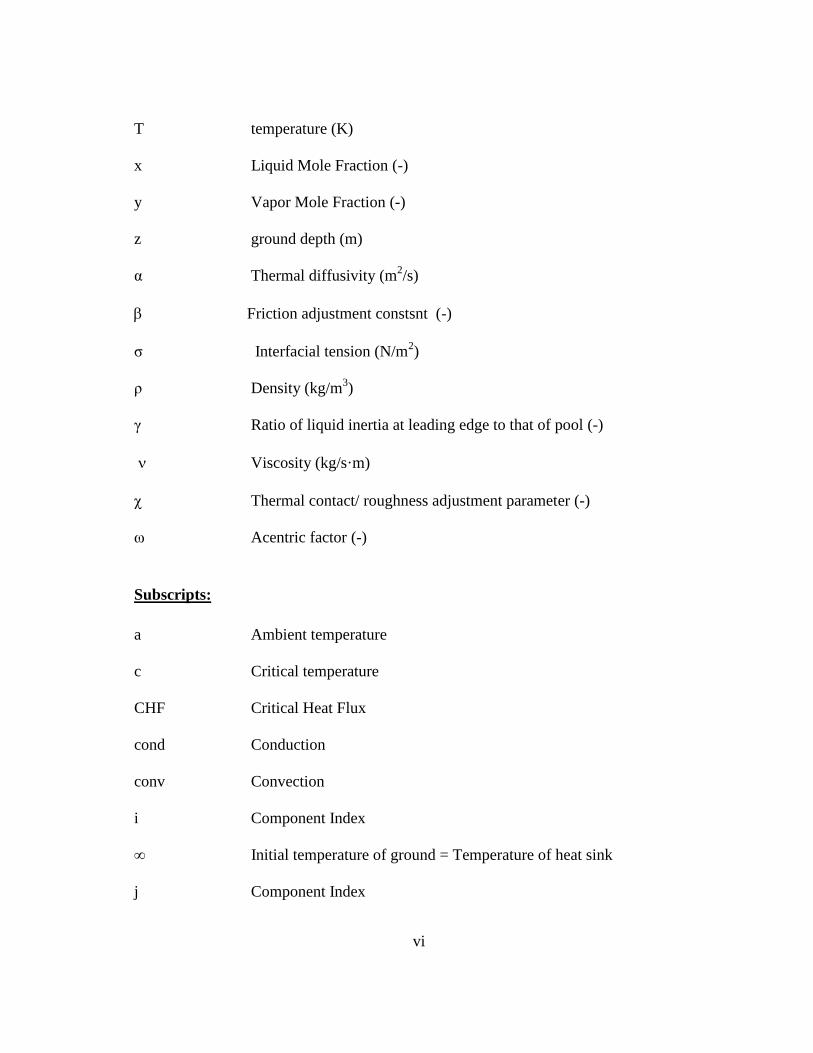
NOMENCLATURE

A Pool area (m)

CHF Critical Heat Flux

Cp Specific heat Capacity of mixture component (J/kg-K)

CF friction coefficient (m/s2)

g acceleration due to gravity (m/s2)

h pool height (m)

hs Heat Transfer Coefficient (W/m2-K)

k Thermal Conductivity (W/m-K)

ΔHvap latent heat of vaporization (J/kg)

Lc Length Scale (m)

m LNG mass (kg)

Nu Nusselt Number (-)

ONB Onset of Nucleate Boiling

P Pressure (Pa)

q Heat flux (W/m2)

Q Heat transfer to the pool (W)

R Universal Gas Constant (J/K-mol)

r radius (m)

t time (s)

vi

T temperature (K)

x Liquid Mole Fraction (-)

y Vapor Mole Fraction (-)

z ground depth (m)

α Thermal diffusivity (m2/s)

Friction adjustment constsnt (-)

σ Interfacial tension (N/m2)

ρ Density (kg/m3)

γ Ratio of liquid inertia at leading edge to that of pool (-)

Viscosity (kg/s·m)

χ Thermal contact/ roughness adjustment parameter (-)

ω Acentric factor (-)

Subscripts:

a Ambient temperature

c Critical temperature

CHF Critical Heat Flux

cond Conduction

conv Convection

i Component Index

∞ Initial temperature of ground = Temperature of heat sink

j Component Index

vii

L Liquid

long Long wave radiation from the pool

min Leidenfrost temperature

r Reduced property

rad Solar radiation

s Surface of substrate

Sat Saturated Pressure

Total Total Pressure

V Vapor

vf Vapor Film

VLE Vapor Liquid Equilibrium

W Water

viii

TABLE OF CONTENTS

Page

ABSTRACT…………. ......................................................................................................ii

DEDICATION ................................................................................................................ iii

ACKNOWLEDGEMENTS .............................................................................................. iv

NOMENCLATURE ........................................................................................................... v

TABLE OF CONTENTS ............................................................................................... viii

LIST OF FIGURES ............................................................................................................ x

LIST OF TABLES ......................................................................................................... xiii

CHAPTER I INTRODUCTION ....................................................................................... 1

1.1. Background ........................................................................................................ 1

1.2. Previous accidents involving LNG .................................................................... 3

1.2.1. Shipping and transportation of LNG ............................................................ 3 1.2.2. Land based incidents .................................................................................... 4

CHAPTER II BACKGROUND ON POOL SPREADING AND VAPORIZATION ...... 9

2.1. Introduction ........................................................................................................ 9 2.2. LNG pool vaporization..................................................................................... 11

2.2.1. Heat transfer from the ground .................................................................... 11 2.2.2. Conduction heat transfer ............................................................................ 12

2.2.3. Boiling regimes for cryogenic liquids ........................................................ 14 2.2.4. Effect of composition on vaporization rate ................................................ 17

2.3. LNG pool spread modeling .............................................................................. 20

CHAPTER III PREVIOUS EXPERIMENTS ON LNG POOL SPREADING .............. 22

3.1. Summary of Experiments on liquefied gases ................................................... 22

CHAPTER IV CURRENT STATE OF THE ART ........................................................ 29

4.1. Introduction ...................................................................................................... 29 4.2. Early spread models ......................................................................................... 29

ix

4.3. PHAST ............................................................................................................. 32 4.4. Supercritical pool spread model ....................................................................... 33 4.5. CFD models...................................................................................................... 34

4.5.1. FLACS by GexCon .................................................................................... 34

CHAPTER V METHODOLOGY ................................................................................... 36

5.1. Introduction ...................................................................................................... 36 5.2. Governing equations ........................................................................................ 37

5.2.1. Mass balance .............................................................................................. 38 5.2.2. Momentum balance .................................................................................... 38

5.2.3. Heat transfer to the pool and boiling regimes ............................................ 39

5.2.4. LNG pool/ vapor properties – vapor liquid equilibrium ............................ 44

5.2.5. Differences between pool spread on land and water .................................. 47

CHAPTER VI ANALYSIS OF GOVERNING PHENOMENA .................................... 49

6.1. Introduction ...................................................................................................... 49 6.2. Definition of the base case ............................................................................... 50

6.3. Friction and gravity terms ................................................................................ 51 6.4. Effect of thermal contact/ roughness ................................................................ 54

6.5. Heat transfer and boiling mechanism ............................................................... 56 6.6. Vapor liquid equilibrium (VLE) effects ........................................................... 66 6.7. Conclusion of sensitivity analysis .................................................................... 72

CHAPTER VII MODEL VALIDATION ....................................................................... 74

7.1. Introduction ...................................................................................................... 74 7.2. Validation for spills on land ............................................................................. 74 7.3. Validation for spills on sea ............................................................................... 76

CHAPTER VIII CONCLUSION .................................................................................... 77

CHAPTER IX FUTURE WORK .................................................................................... 80

REFERENCES ................................................................................................................ 81

x

LIST OF FIGURES

Page

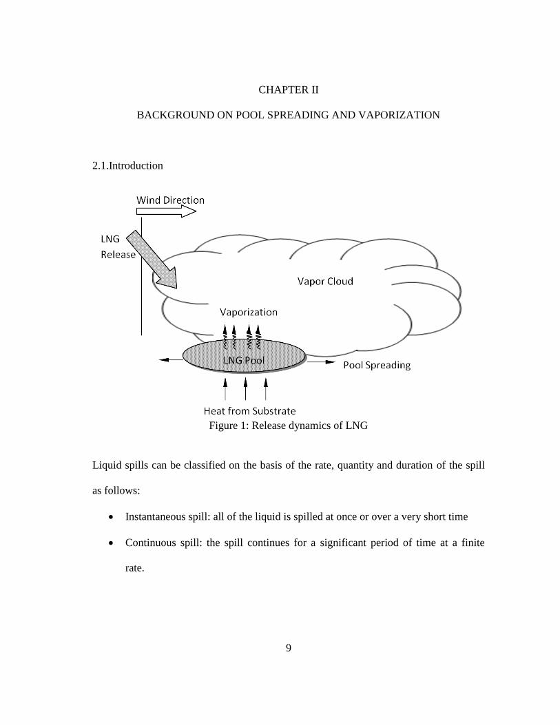
Figure 1: Release dynamics of LNG .................................................................................. 9

Figure 2: Event tree for an LNG spill .............................................................................. 10

Figure 3: Evaporation rate as a function of time for a continuous release of a cryogenic

liquid. (Jensen, 1983) ....................................................................................... 13

Figure 4: Boiling heat flux curve ..................................................................................... 15

Figure 5: 90 mol% Methane 10mol% Ethane mixture VLE phase envelope .................. 18

Figure 6: Boiling temperature and vapor composition of 90 mol% methane 10mol%

ethane mixture.................................................................................................. 19

Figure 7: Forces acting on the spreading pool ................................................................. 21

Figure 8: Previous experiments conducted using LNG ................................................... 22

Figure 9: Cryogenic spread on land ................................................................................. 37

Figure 10: Box model ....................................................................................................... 37

Figure 11: Boiling heat flux curves for LNG components ............................................... 40

Figure 12: Algorithm for Heat transfer as implemented in the proposed model ............. 44

Figure 13: Algorithm for thermodynamic effects as implemented in the proposed

model ............................................................................................................. 48

Figure 14: Webber 1991 model with 1-D ideal conduction: gravity and friction

comparison ..................................................................................................... 52

Figure 15: Effect of friction on gravitational driving force.............................................. 53

Figure 16: The effect of friction on pool radius ............................................................... 54

Figure 17: Effect of varying thermal contact parameter on pool radius while maintaining

frictional effects (Base Case: =3) ................................................................. 55

xi

Figure 18: Effect of varying thermal contact parameter on pool radius while ignoring

frictional effects (Base Case: =3) ................................................................. 56

Figure 19: Effect of boiling heat transfer on pool radius for a continuous spill .............. 59

Figure 20: Effect of boiling heat transfer on heat flux at center of the pool for a

continuous spill .............................................................................................. 60

Figure 21: Effect of boiling heat transfer on temperature at center of the pool for a

continuous spill .............................................................................................. 60

Figure 22: Effect of boiling on overall heat flux into pool for a continuous spill............ 61

Figure 23: Effect of boiling heat transfer on pool radius for an instantaneous spill ........ 62

Figure 24: Effect of boiling heat transfer on heat flux at center of the pool for an

instantaneous spill .......................................................................................... 63

Figure 25: Effect of boiling heat transfer on temperature at center of the pool for an

Instantaneous spill .......................................................................................... 63

Figure 26: Effect of boiling on overall heat flux into pool for a continuous spill............ 64

Figure 27: Comparing 1-D conduction with varying parameter to boiling heat

transfer ........................................................................................................... 65

Figure 28: Effect of incorporating VLE effects on pool radius for a continuous spill..... 67

Figure 29: Effect of incorporating VLE effects on pool composition for a continuous

spill ................................................................................................................. 67

Figure 30: Effect of incorporating VLE effects on pool density for a continuous spill ... 68

Figure 31: Effect of incorporating VLE effects on pool latent heat for a continuous

spill ................................................................................................................ 68

Figure 32: Effect of incorporating VLE effects on pool radius for an Instantaneous

spill ................................................................................................................. 69

Figure 33: Effect of incorporating VLE effects on pool composition for an Instantaneous

spill ................................................................................................................. 70

Figure 34: Effect of incorporating VLE effects on pool density for an Instantaneous

spill ................................................................................................................ 70

xii

Figure 35: Effect of incorporating VLE effects on pool latent heat for an Instantaneous

spill ................................................................................................................. 71

Figure 36: Model validation vs experimental data for a 17 tonne/hr continuous LNG

release on concrete ......................................................................................... 75

Figure 37: Model validation vs experimental data for a 14 tonne/hr continuous LNG

release on soil ................................................................................................. 75

Figure 38: Model validation vs experimental data for a continuous release of 0.15 m3/s

of LNG on sea ................................................................................................ 76

xiii

LIST OF TABLES

Page

Table 1: Typical composition of LNG ............................................................................... 2

Table 2: LNG hazardous properties ................................................................................... 2

Table 3: Accidents involving maritime transport of LNG from 1995 to 2009

(Forsman, 2011) .................................................................................................. 4

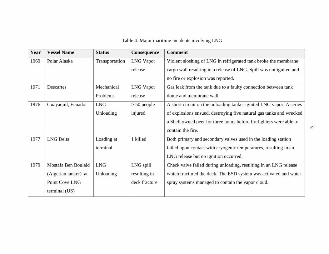
Table 4: Major maritime incidents involving LNG ........................................................... 5

Table 5: Major land based incidents involving LNG ......................................................... 6

Table 6: Spills of liquefied gases into bunds .................................................................... 23

Table 7: Experimental setup for bund experiments.......................................................... 23

Table 8: Spills of liquefied gases onto water ................................................................... 25

Table 9: Experimental setup of spills on water ................................................................ 27

Table 10: LNG properties used in simulation .................................................................. 51

Table 11: Concrete properties used in simulation ............................................................ 51

1

CHAPTER I

INTRODUCTION

1.1. Background

Liquefied Natural Gas (LNG) is natural gas that has been cooled down to its liquid state

at atmospheric pressure. LNG is produced primarily in the Middle East and Russia and is

then transported all around the world using tankers and continental pipelines. Over the

last few years Qatar has become a key player in the LNG industry. The liquefaction

process of natural gas allows a 600 fold reduction in the volume of the gas being

transported at ambient pressure. The resulting liquid which is mainly composed of

methane presents some hazardous properties linked to its flammable nature and its

cryogenic state. Typical composition ranges for LNG and the hazardous properties

associated with LNG are shown in Tables 1 and 2 respectively.

Upon a release on land or sea, LNG (boiling point = -162°C) will boil vigorously and

generate a vapor cloud that will disperse. If within the flammable range, the vapor cloud

may ignite and cause fires and explosions. Although governmental regulations have been

imposed and new technologies have been designed and incorporated into the design and

operating procedures of LNG facilities, risks associated with catastrophic events like a

total loss of containment of an LNG tanker or storage tank must be studied to determine

the potential impact on the employees, the facility, the public and the environment.

2

Table 1: Typical composition of LNG

Chemical Chemical Formula Lean Rich

Methane CH4 99% 87%

Ethane C2H6 < 1% 10%

Propane C3H8 > 1% 5 %

Butane C4H10 > 1% > 1%

Nitrogen N2 0.1% 1%

Other Hydrocarbons C5+ Trace Trace

Table 2: LNG hazardous properties

Properties LNG

Toxic No

Carcinogenic No

Flammable Vapor Yes

Forms Vapor Clouds Yes

Asphyxiant Yes

Extreme Cold Temperature Yes

Flash point (°C) -188

Boiling point (°C) -160

Flammability Range in Air, % LEL = 5.5% and UEL 14% (at 25°C)

Auto ignition Temperature 0C 540

Behavior if Spilled Evaporates, forming a partly visible clouds

Modeling the spread and vaporization of an LNG pool is a key element in the

consequence analysis and risk assessment of a possible spill on water or land. This

represents an important part of the source term (LNG vapor release rate) which is

subsequently used for vapor dispersion modeling. While atmospheric dispersion of

flammable vapor has been extensively studied, LNG source term modeling, including

pool spreading and vaporization has received less attention both experimentally and

theoretically.

3

In this work, a source term model for estimating the rate of spreading and vaporization

of LNG and cryogenic mixtures on unconfined land and sea is proposed. The model

takes into account the composition changes of a boiling liquid mixture, the varying

thermodynamic properties due to preferential boiling within the mixture and the effect of

boiling on conductive heat transfer. A parameter sensitivity analysis was conducted to

determine the effect of boiling heat transfer regimes, friction, thermal contact/roughness

correction parameter and VLE/mixture thermodynamics on the pool spreading behavior.

The aim was to provide a better understanding of these governing phenomena and their

relative importance throughout the pool lifetime. The model was validated against

available experimental data for pool spreading on concrete and sea.

1.2. Previous accidents involving LNG

Transportation and handling of LNG in import/export facilities has over 60 years of

development. Accidents involving LNG often resulted in huge financial and commercial

impacts; this section provides a summary of the recorded incidents involving LNG.

1.2.1. Shipping and transportation of LNG

Most of the incidents involving LNG occurred during maritime transport, but there has

been insufficient data collection to draw conclusions regarding the safety of LNG

maritime transport. Nonetheless, most of these incidents are not specific to LNG itself

but are more connected to the practices of the maritime transport industry. Table 3

summarizes shipping accidents that involved LNG from 1995 to 2009. When compared

4

to oil carriers, LNG tanks seem slightly less incident prone, but when forecasting the

expected increase in demand and transportation of LNG over the coming decade, this

may very well change. Some of the more significant incidents are highlighted in Table 4.

1.2.2. Land based incidents

Most land based incidents involve a vapor release that was somehow ignited resulting in

a wide variety of consequences. These incidents have highlighted the importance of

being able to contain LNG vapor from spreading and keeping LNG activities at a safe

distance from other plant facilities, particularly combustion, compression and air intake

equipment. Moreover, it shows that released LNG vapor on land will probably not travel

far before getting ignited. Table 5 highlights the major land based incidents associated

with LNG.

Table 3: Accidents involving maritime transport of LNG from 1995 to 2009

(Forsman, 2011)

Cause Number of

accidents

% of

Total

Killed/

Missing

LNG Released

(m3)

Collision 50 26% 0 7

Contact 8 4% 0 1

Fire/Explosion 26 13% 29 1

Foundered 14 7% 24 2

Hull/ Mchy. Damage 63 32% 0 2

Miscellaneous 1 1% 0 0

Wrecked/ Stranded 33 17% 0 1

Total 195 100% 53 14

5

Table 4: Major maritime incidents involving LNG

Year Vessel Name Status Consequence Comment

1969 Polar Alaska Transportation LNG Vapor

release

Violent sloshing of LNG in refrigerated tank broke the membrane

cargo wall resulting in a release of LNG. Spill was not ignited and

no fire or explosion was reported.

1971 Descartes Mechanical

Problems

LNG Vapor

release

Gas leak from the tank due to a faulty connection between tank

dome and membrane wall.

1976 Guayaquil, Ecuador LNG

Unloading

> 50 people

injured

A short circuit on the unloading tanker ignited LNG vapor. A series

of explosions ensued, destroying five natural gas tanks and wrecked

a Shell owned peer for three hours before firefighters were able to

contain the fire.

1977 LNG Delta Loading at

terminal

1 killed Both primary and secondary valves used in the loading station

failed upon contact with cryogenic temperatures, resulting in an

LNG release but no ignition occurred.

1979 Mostafa Ben Boulaid

(Algerian tanker) at

Point Cove LNG

terminal (US)

LNG

Unloading

LNG spill

resulting in

deck fracture

Check valve failed during unloading, resulting in an LNG release

which fractured the deck. The ESD system was activated and water

spray systems managed to contain the vapor cloud.

5

6

Table 5: Major land based incidents involving LNG

Year Place Status Consequences Comment

1944 Cleveland,

Ohio

Construction

failure

128 killed, 225

injured

LNG storage tanks experienced material failures resulting in overflowing of

LNG into surrounding dikes. The vapor cloud was ignited. A second tank

failed after 20 minutes resulting in more LNG release and a longer fire time. It

is estimated that the pool fire extended to 0.5 miles around failed tank.

1966 Raunheim

, Germany

Accidental

venting

1 killed, 75

injured

LNG was being passed through a vaporizer. The liquid level control loop failed

resulting in overflow and around 500 kg of LNG was vented out of the

vaporizer. The vapor cloud drifted towards the control room resulting in a fire

and explosion.

1968 Portland,

US

Human

malfunction

4 killed Natural gas from the inlet lines leaked into an LNG tank through a valve that

was supposed to be closed off, but the flange used to close the valve had been

removed for the testing leaving the valve slightly opened. Natural Gas

accumulated inside the tank got ignited resulting into.

1973 Staten

Island,

NY,US

Human

malfunction

40 killed An LNG storage tank was emptied, warmed and purged of the combustible

gases using nitrogen, and then filled with fresh re-circulating air. This was not

done properly and while repairs were being done on the tank, a fire was ignited

resulting in the tank roof getting fractured and collapsing. The 40 workers

inside died from asphyxiation.

1977 Arzew, On terminal 1 killed A terminal worker was frozen to death during loading. A valve rupture sprayed

6

7

Table 5: Major land based incidents involving LNG

Year Place Status Consequences Comment

Algeria the worker with LNG.

1978 Das

Island,

UAE

On terminal LNG spill A bottom pipe connection of an LNG tank failed resulting in a spill. It was

stopped by closing the internal valve. The resulting vapor cloud dissipated

without igniting.

1983 Bontang,

Indonesia

Over

pressure

3 killed A blind left in the flare line resulted in the over pressurization of the main

liquefaction column which was a vertical shell and tube heat exchanger. The

heat exchanger failed and popped and debris was projected as far as 50m

killing 3 workers.

1985 Pinson,

Alabama

Loading

vessel

6 injured The welding on a patch plate on an aluminum vessel failed during loading. The

plate was projectile towards the control room, blowing the windows. The

escaping gas was ignited.

1988 Everett,

WA, US

On terminal Vapor release Operation of LNG transfer was improperly interrupted resulting in a flange

gasket to blow and 114 m3 of LNG were released. The spill was contained and

a stable atmosphere prevented the vapor cloud from propagating.

1989 Thurley,

UK

Human

malfunction

2 workers got

burned

Valves were opened for draining out natural gas, but one was left open before

operation. LNG was released as a high pressure jet burning 2 workers. The

resulting vapor cloud was ignited 30s into the spill covering an area of 40 by

25 m.

7

Table 5 Continued

8

Table 5: Major land based incidents involving LNG

Year Place Status Consequences Comment

1993 Bontang,

Indonesia

Leakage to

sewer

system

Vapor release During a pipe modification project, LNG leaked into the underground sewer

system. LNG underwent rapid vapor expansions that ruptured the pipes.

2004 Skikda,

Algeria

Explosion

and fire

27 killed, 5

injured

A leak occurred that was pulled into a high pressure steam boiler. The resulting

mixture ignited rapidly resulting in an explosive fire and a fireball that

damaged surrounding LNG facilities, killing 27 people.

8

Table 5 Continued

9

CHAPTER II

BACKGROUND ON POOL SPREADING AND VAPORIZATION

2.1.Introduction

Figure 1: Release dynamics of LNG

Liquid spills can be classified on the basis of the rate, quantity and duration of the spill

as follows:

Instantaneous spill: all of the liquid is spilled at once or over a very short time

Continuous spill: the spill continues for a significant period of time at a finite

rate.

10

The distinction is made between these scenarios based on a number of factors like the

size of the spill, the properties of the spilled liquid and the surrounding environmental

conditions. Figure 1 shows the factors involved in the release dynamics of an LNG spill.

Once a release occurs it will usually follow the event tree shown in Figure 2.

Figure 2: Event tree for an LNG spill

A pool will form from an LNG spill, the behavior of the pool and its dynamics depend

on the release scenario and surrounding conditions.

If immediate ignition occurs to the LNG spill a pool fire will develop. This will pose a

direct hazard to the surroundings due to direct fire contact and thermal radiation.

11

In the case where no immediate ignition occurs, the LNG spill will boil-off generating

dense gas which is then dispersed by atmospheric turbulence. The cloud will pose

flammability and explosion hazards for long distances unless it is diluted below its lower

flammability limit. The extent of the vapor cloud hazard depends on the pool spill rate,

the pool size and the stability of the surrounding atmosphere.

For LNG spills of significantly long duration, a constant spill rate could results in a

steady-state pool when the discharge rate into the pool equals the vaporization rate from

the pool.

2.2.LNG pool vaporization

When LNG is spilled onto the ground, heat transfer from the substrate will result in an

immediate boil-off. The spill rate, duration of spill, ambient temperature and ground

temperature and porosity would determine the LNG boiling regime.

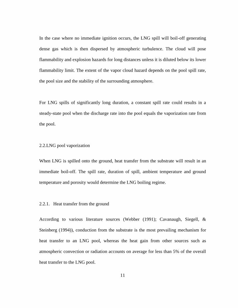
2.2.1. Heat transfer from the ground

According to various literature sources (Webber (1991); Cavanaugh, Siegell, &

Steinberg (1994)), conduction from the substrate is the most prevailing mechanism for

heat transfer to an LNG pool, whereas the heat gain from other sources such as

atmospheric convection or radiation accounts on average for less than 5% of the overall

heat transfer to the LNG pool.

12

2.2.2. Conduction heat transfer

For spills over land, the heat transfer to the pool is generally considered to be transient

due to conductive cooling of the substrate.

1-D conduction is usually used when modeling heat conduction from the ground. The

model is based on assuming a uniform semi-infinite medium on which the pool spreads;

the heat flow rate is given by:

( ) ' '

' 0.5

0

2( )

R t

cond

r drQ

t t

(1)

Where r’ is the pool radius at time t’ when the new pool segment first comes into contact

with fresh ground:

0.5

( )

( )

s Bh T T

(2)

Nonetheless it is important to remember that since the substrate is being cooled by the

LNG, a continuous spill would have to eventually reach a maximum evaporation rate,

Jensen (1983) shows the following behavior. It is understood that at the latter stages of a

spill, the heat transfer from the soil becomes sufficiently low, eventually allowing for

heat transfer from the air to become increasingly important. He shows that there is an

inverse proportionality between the evaporation rate and the square root of time

according to the following correlation:

sq

t

(3)

13

vap

T cs

H

(4)

A limitation of the above derivation is that it initially results in infinite evaporation rates.

Nonetheless a correction is applied by integrating the area differentials of the above

equation:

1 2

8 8 8...

( 1)n nQ dA dA dA

ndt n dt dt

(5)

To achieve adecaying behavior as shown in Figure 3:

Figure 3: Evaporation rate as a function of time for a continuous release of a cryogenic

liquid. (Jensen, 1983)

The point td in the above graph corresponds to the time when the pool has reached its

maximum area. These results seem reasonable and the conclusion that the evaporation

rate would eventually reach a minimum asymptotic value is ok for continuous spills. For

14

Instantaneous spills it also seems reasonable that a similar, yet steeper profile would

exist for the evaporation rate.

2.2.3. Boiling regimes for cryogenic liquids

There are three main pool boiling regimes, as shown in Figure 4, which are functions of

the temperature difference between the LNG and the ground, known as the temperature

superheat:

1. Nucleate boiling: The LNG is in direct contact with the substrate and bubbles form

at distinct intervals.

2. Transitional boiling: There is enough superheat to support vigorous boiling with

large distinct bubbles, but not enough to maintain a stable vapor film. At this stage,

these large bubbles prevent full thermal contact of the fluid with the surface.

3. Film boiling: There is enough superheat from the substrate to maintain a stable

vapor film, thus the LNG is separated from the substrate by a vapor film.

15

Figure 4: Boiling heat flux curve

When spreading a cryogenic liquid onto the ground, which initially is at ambient

temperature, a large temperature difference between the liquid and the ground exists and

vigorous boiling will occur. This boiling generates vapor bubbles or a vapor film at the

liquid-ground interface which tends to limit the heat transfer. Three boiling regimes can

occur depending on the temperature difference between the liquid and the ground: film,

transition and nucleate. These complex phenomena make the heat transfer process

during boiling difficult to predict.

Experimental measurement of the boiling curve of cryogenic liquids, such as liquid

nitrogen (Berenson, 1962) and LNG (Reid & Wang, 1978) are reported in literature. It

Free

Convection FilmTransitionNucleate

CHF

ONB

ΔTCHF

ΔTMin

Leidenfrost

(Min)

I II III IV

q (

W∙m

-2)

T =Twall - Tb(K)

16

has also been reported that LNG will boil in the transitional regime if it has a higher

composition of heavier hydrocarbons, if it with a higher content of heavier components

tends to boil in the transitional boiling regime (Woodward & Pitblado, 2012). Significant

work is still to be done in modeling the boiling of cryogenic liquids. Liu et al. (2011)

developed a methodology using Computational Fluid Dynamics (CFD) to simulate the

boiling process of liquid nitrogen. This approach is promising and may be extrapolated

to calculate the boiling curve for cryogenic liquid mixtures like LNG.

As shown in Figure 4, during the initial stages of the spill when the temperature

superheat is relatively high, the pool will be in the film boiling regime and a thin vapor

film would be fully developed between the spilled liquid and the substrate over the entire

heating surface. The superheat will then start to decrease due to the transient cooling of

the ground; until it reaches the minimum superheat Tmin also known as the Leidenfrost

temperature, during this period the heat flux will decrease accordingly until it reaches

the minimum value qmin. Once the superheat temperature becomes lower than Tmin the

pool will enter into the transitional boiling regime, the transitional boiling regime is

usually short lived and involves vigorous boiling and relatively large bubbles due to the

breakup of the film, the heat flux will then start to increase due to the increased contact

area between the surface and the fluid after the film breakup. The heat flux will increase

until it reaches a value of maximum heat flux which corresponds to the critical value qc,

the corresponding temperature is known as the critical superheat and is denoted Tc. As

the superheat continues to decrease and drops below the critical superheat, nucleate

17

boiling will start and the heat flux will continue decreasing with the superheat

temperature. During Nucleate boiling, nucleation sites, which are gas or vapor filled

cavities, appear on the surface of the substrate and develop to allow vapor bubbles to

form. Nucleation can occur on both a solid surface and in a homogenous liquid. The

maximum heat flux will occur in the nucleate boiling region, but then decreases sharply

as the bubbling becomes so rapid that the liquid is prevented from getting enough

contact time with the substrate, this is where the transitional regime starts.

1/4

min ( ) 0.16 0.24L pL L

C L

w pw w

C kT T T

C k

(6)

2.2.4. Effect of composition on vaporization rate

Being a mixture of different volatile components, LNG will exhibit preferential boiling.

Lighter components will boil off before the heavier ones, resulting in an accumulation of

the heavier hydrocarbons within the LNG pool. This change in composition will in turn

affect the thermo-physical properties of the LNG pool as it become enriched with the

heavier components. It is important to realize that despite methane being the dominant

component in LNG, the evaporation rate of an LNG mixture will be different than that of

pure methane, particularly during the later stage of boil-off when the methane

composition decreases. The vapor liquid equilibrium of a mixture composed of 90 mol%

methane and 10% ethane is shown in Figure 5.

18

Figure 5: 90 mol% Methane 10mol% Ethane mixture VLE phase envelope

From the above VLE diagram, it is seen that the dew point is very steep for pure

methane, while the bubble point is flat. This means that during the initial stages of the

spill, the vapor will consist almost completely of methane and the liquid boiling point

temperature will change very slowly as exhibited by the flat bubble point curve.

Similarly analyzing the other end of the VLE diagram, it is noticeable that the dew point

becomes flat whereas the bubble point becomes very steep, this means that during the

later stages of the pool life, the vapor composition will not change while the boiling

temperature will rapidly increase. These observations have been further verified by

plotting the boiling temperature and vapor composition of the mixture over time as

shown in Figure 6 (Conrado & Vesovic, 2000):

19

Figure 6: Boiling temperature and vapor composition of 90 mol% methane 10mol%

ethane mixture

As predicted, the boiling temperature of the LNG-like mixture remains unchanged

during the initial stages and the vaporization rate of the mixture is almost identical to

that of pure methane. During the later stages of boiling, and as the LNG becomes

increasingly ethane rich, the boiling temperature increases steeply as predicted by the

VLE diagram. Therefore as the temperature driving force decreases towards the end of

the spill, heat transfer goes from film boiling toe transition boiling stage. This boiling

regime is due to the increased content of ethane in the LNG after most of the methane

has boiled off during the early stages of the spill. Not considering preferential boil-off

would result in underestimating the evaporation time by about 20% (Conrado &

Vesovic, 2000). Therefore, when modeling LNG, thermodynamic properties that reflect

the behavior of all the compounds in the mixture should be used rather than those of

pure methane.

20

The above conclusions were confirmed by Boe (1998), by performing laboratory scale

experiments using liquefied methane-ethane and methane-propane mixtures on boiling

water. The results confirmed that the addition of ethane or propane in a predominantly

methane mixture will affect the boil off rate in a similar manner to the above. Methane

rich mixtures exhibited high initial boil off rates, by adding methane of propane to a

97% methane mixture, the boil off rates increased by a factor of 1.5-2. Moreover, the

same conclusion regarding the breakdown of film boiling due to increased contact

between the mixture and the substrate which would lead to an enhanced heat flux and

lower temperature difference. This ultimately results in the breakdown of the continuous

vapor film.

These conclusions were also observed by Drake et al. (1975) which indicated that LNG

has a higher boil off rate than pure methane. He conducted a series of laboratory scale

experiments with mixtures composed of 98% methane and 2%ethane which is very

similar to that of lean LNG. These results were compared to experiments conducted with

82-89% methane mixtures containing ethane-propane ratios between 4-5, which is

similar to the composition of rich LNG. His results showed that increasing the amount

of heavier hydrocarbons will lead to faster vaporization, and an increased rate of boiling.

2.3.LNG pool spread modeling

As the spilled liquid starts spreading, it will go through several flow regimes due to

changes in the dominant forces governing the spread. The forces governing the pool

21

spreading process are gravity, surface tension, inertia and viscous friction as shown in

Figure 7. These different regimes are the basis to many of the models that will be

discussed later. There are three main regimes:

1. Gravity-Inertia regime: Gravitational forces are equal to inertial forces.

2. Gravity-viscous regime: Gravitational forces are equal to viscous resistance

(More applicable for spills on water)

3. Surface tension regime: Viscous drag forces are equal to the surface tension.

(More applicable for spills on land, or spills on water during ice formation)

Figure 7: Forces acting on the spreading pool

Each of these regimes could be solved by equating the dominant forces for each regime

and obtaining an analytical solution. Since the lifetime of an LNG spill is relatively

short, it will spend the entirety of its lifetime in the gravity inertia regime.

Gravity

OO

OWWO

Inertia

Surface Tension

Viscous Friction

u

x

t

hgh

x

uh

x

22

CHAPTER III

PREVIOUS EXPERIMENTS ON LNG POOL SPREADING

3.1.Summary of Experiments on liquefied gases

Numerous experiments of various scales have been conducted using LNG, these

experiments are necessary to collect a large database of data that can be used to verify

models and distinguish among their accuracy and applicability. a comparison of the scale

of the most important experiments are shown in Figure 8. Tables 6 to 9 provide a

detailed summary of the experiments and the instrumentation used to collect data.

Figure 8: Previous experiments conducted using LNG

1 10 100 1000 10000 100000

Esso

US CG

Maplin

Burro

Coyote

Falcon

Single tank

Spill Volume (Tonnes)

23

Table 6: Spills of liquefied gases into bunds( Puttock, Blackmore, & Colenbrander, 1982)

Experiment Year Spilled Volume (m3) Spill Rate (m

3/min) Duration (min) No. of tests

Air Products 1966-1967 Oxygen - 0.04-0.15 30-250 11

AGA/TRW 1968 LNG 0.2 - 0.2 18

Gaz de France 1972 LNG Max 3 - - > 40

Gaz de France 1972 LNG - 0.16 4.5 1

Battelle/ AGA 1974 LNG 0.4-51 - 0.3-0.5 42 (14 w/

Ignition)

23

24

Table 7: Experimental setup for bund experiments

Experiment Type of Spill Surface Bund Size

(m2)

Additional Info Instrumentation (Sensors)

Conc. Temp Meteo. Photo

Air Products Continuous Soil 1 Water spray used 6 5 4 -

AGA/TRW Continuous - Wet Clay

- Dry Clay

- Steel

2 - - - 3 1

Gaz de France Instantaneous Soil 9 – 200 Tipping Bucket - - - -

Gaz de France Continuous Soil 200 - - - - -

Battelle/ AGA Instantaneous - Wet Soil

- Dry Soil

- Polyurethane

3 – 450 - 36 26 9 -

24

25

Table 8: Spills of LNG and other gases onto water ( Puttock, Blackmore, & Colenbrander, 1982)

Experiment Year Spilled Volume (m3) Spill Rate (m

3/min) Duration (min) No. of tests

Bureau of Mines

1970 LNG 0.04-0.5 - - 51

1970 LNG - 0.2-0.3 - 4

1972 LNG - 0.2-1.3 Max 10 13 (7 useless)

Esso/API 1971 LNG 0.09-10.2 - 0.1-0.6 17

Shell (Gadila) 1973 LNG 27-198 2.7-19.8 10 6

Shell Maplin Sands

1980 Propane - 2-5 4-8 11 (3

w/Ignition)

1980 LNG - 1-5 1.5-10 13 (4 w/

Ignition)

1980 Propane 15-25 - - 3 (1w/Ignition)

25

26

Experiment Year Spilled Volume (m3) Spill Rate (m

3/min) Duration (min) No. of tests

1980 LNG 5-20 - - 7 (3 w/ Ignition)

China Lake – Avocet 1978 LNG 4.5 4 - 4

China Lake – Burro 1980 LNG 40 12-18 2.2-3.5 8

China Lake – Coyote 1981 LNG 3-28 6-19 0.2-2.3 5 (w/Ignition)

10 RPT tests

China Lake-

Frenchman Flat

1984 Ammonia/

LNG

350 - - -

26

Table 8 Continued

27

Table 9: Experimental setup of spills on water

Experiment Type of spill Surface Setup Additional

Info.

Instrumentation (Sensors)

Conc Temp Meteo Photo

Bureau of Mines Instantaneous Water 60 m pond Tipping Bucket 0 0 1 5

Bureau of Mines Continuous Water 60 m pond - 12 0 1 5

Bureau of Mines Continuous Water 70 m lake with

20 m walls

- 30 0 1 1

Esso/API Instantaneous Sea From Barge Jet 7 m high,

300 upwards

18 2 9 2

Shell ‘Gadila’ Continuous Sea From Ship Jet 18 m high,

Moving ship

0 0 2 3

Shell Maplin Sands Continuous Water 300 m pond 3 m above

200 70 45 7

27

28

Experiment Type of spill Surface Setup Additional

Info.

Instrumentation (Sensors)

Conc Temp Meteo Photo

Shell Maplin Sands Instantaneous Water surrounded by

sand

surface

Shell Maplin Sands Instantaneous Water

Sinking Barge

Shell Maplin Sands Instantaneous Water

China Lake – Avocet Continuous Water Irregular

surface for 25 m

downwind of

source, them 7

m elevation

over 80 m from

source.

Jet Submerged

1 m into splash

plate

11 24 17 1

China Lake – Burro Continuous Water

90 100 76 4 China Lake – Coyote

Continuous Water

China Lake-

Frenchman Flat

Continuous Water

Table 9 Continued

29

CHAPTER IV

CURRENT STATE OF THE ART

4.1.Introduction

In the scenario of a spill of a cryogenic liquid on land, the following parameters will

determine the behavior of the pool spread:

1. The type and volume of the release, i.e. instantaneous or continuous;

2. The volatility of the spilled material and its initial temperature (degree of sub-

cooling).

3. The thermal (temperature, thermal diffusivity, thermal conductivity) and

mechanical (roughness, porosity) properties of the substrate;

4. The presence of any bunds or wall to contain the spill.

A multitude of pool spread models have been developed since the early 70’s, although

most of them employ the same principles derived for oil spill applications; many have

been adjusted to account for LNG applications. The following section will discuss some

of the more widely used models.

4.2.Early spread models

Earlier models by Hoult (1972) and Fay (1971) were generally derived from the steady-

state Bernoulli equation assuming axisymmetric spread on water:

30

drgh

dt

(7)

These models assume that gravity is the only driving force for pool spread, while

ignoring the effect of friction and preferential boil. It is derived from the balance of the

liquid inertia and gravitational force assuming the ground is smooth. Although these

models may seem reasonable for oil spills or other heavy liquids, they cannot be applied

to cryogenic liquids where the effect of gravity decreases with time. Moreover, the pool

radius is dependent on another unknown variable which is the average height of the pool.

These models, although used to represent the gravity inertia regime, do not represent a

pure gravity-inertia regime but rather the gravity-front resistance.

Another early model developed by Raj (1974) was derived by equating the inertial

resistance forces to gravitational forces as follows:

Inertial resistance:

22

2( )l

d rF C r h

dt

(8)

31

Gravitational forces:

2

GF rh g

(9)

Nonetheless this will yield a similar result to the previously mentioned models by

reaching the conclusion that spreading is strictly gravity driven

2

2

d r gh

dt Cr

(10)

A setback of these modesl involves the improper repersentation of the gravity inertiea

regime, by including a negative sign for the inertial resistance equation, this resulted in a

widely used misconception that has been propagated throughout later models (Webber,

1996). Moreover, a basic counterargument against these approaches has also been that

they ignore frictional resistance to spreading. These issues were addressed by Webber

(1991) who expressed inertial forces as the differences between the gravitational drive

and the resistance as follows:

2

2

4F

d r ghC

dt r

(11)

This effect of gravity was then examined by ABSG & FERC (2004) by comparing

theBriscoe & Shaw (1980) model which ignores the effect of friction to that of Webber

(1991) mentioned above. Reaching the conlusion that frictional effects are much more

significant for large short duration spills, but their effect declines for longer duration

spills.

32

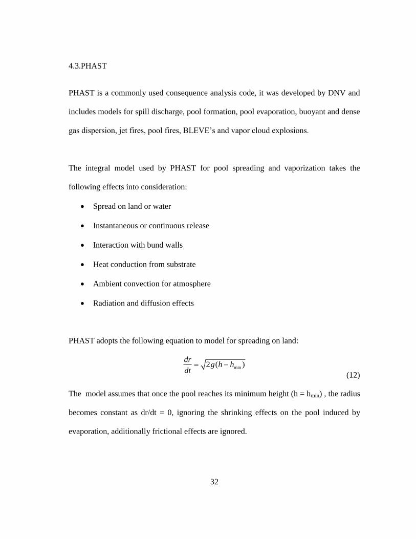
4.3.PHAST

PHAST is a commonly used consequence analysis code, it was developed by DNV and

includes models for spill discharge, pool formation, pool evaporation, buoyant and dense

gas dispersion, jet fires, pool fires, BLEVE’s and vapor cloud explosions.

The integral model used by PHAST for pool spreading and vaporization takes the

following effects into consideration:

Spread on land or water

Instantaneous or continuous release

Interaction with bund walls

Heat conduction from substrate

Ambient convection for atmosphere

Radiation and diffusion effects

PHAST adopts the following equation to model for spreading on land:

min2 ( )

drg h h

dt

(12)

The model assumes that once the pool reaches its minimum height (h = hmin) , the radius

becomes constant as dr/dt = 0, ignoring the shrinking effects on the pool induced by

evaporation, additionally frictional effects are ignored.

33

4.4.Supercritical pool spread model

Fay (2007) claimed that the above gravity inertia based models are not entirely

applicable to cryogenics due to their unique thermo-physical properties, the proposed

model is based on the idea that the vigorous boiling of LNG means that bubbles will

occupy a significant volume of the overall pool volume, therefore reducing the density.

This reduction in density will both affect the amount of LNG submerged in water for

water based spills, and increase the predicted diameter for land based spills. Moreover,

this supercritical model argues that equating viscous and gravitational effects as done by

Webber might not necessarily be applicable to LNG as it will eventually ride on a thin

film of LNG vapor that is at a much lower viscosity than that of water, which then

enables the treatment of the LNG pool as inviscid flow. According to the model the pool

volume changes are modeled as follows:

2 2 2( ) ( )p evap evap

L

L L

dV G GR u t

dt

(13)

The above relation has been derived through an energy balance equation the pool’s

kinetic energy to the initial potential energy; it argues that gravitational effects should

not be a parameter for a continuous release since it is overcome by the initial potential

energy of the release. The major disadvantage of this model is that it tries to account for

the mechanical effects of boiling by incorporating bubble volume, but fails to account

for their heat effects as the vaporization rate is fixed. Moreover, although it accounts for

density changes due to bubble volumes, the model does not also incorporate similar

changes due to preferential boiling.

34

4.5.CFD models

CFD codes have yet to achieve full confidence in dealing with LNG release and

dispersion modeling. So far only one CFD tool (FLACS) has passed the MEP (model

evaluation protocol) for the NFPA-59A standard, whereas countries like France and the

Netherlands have moved away from using CFD for Risk assessment of atmospheric

dispersion. At the moment, CFD modeling is highly dependent on the user, and different

users modeling the same scenario could possibly end with varying results. Moreover,

although CFD could arguably provide a better mathematical accuracy, the computational

time required compared to integral models is disparaging.

4.5.1. FLACS by GexCon

The FLACS source term model is based on the shallow layer equations presented by

Hansen et al. (2007), despite recent enhancements to their code, they still rely heavily on

shallow water modeling to predict their pool size and evaporation rate. The 2-D shallow

layer model implemented by FLACS relies on the following coupled momentum and

heat equations:

, ,

i ij g i i

j

u uu F F

t x

(14)

( )Li L c rad g evap

i l

mu q q q q

t x

(15)

35

For spills on water, the conduction heat effects used by FLACS attempt to take into

account the effect of the transition and boiling regimes, it uses the correlations derived

by Conrado & Vesovic (2000). Moreover, it takes into account the effect of turbulent

mixing that is expected to accompany LNG spills on sea as derived by Hissong (2007),

who introduces a turbulence factor to model the instability of the thin film during film

boiling and the increased contact between the LNG and water due to excessive

turbulence disturbing the separating thin film.

The above equations are then solved explicitly using a 3rd

order Runge-Kutta solver to

obtain the evaporation and geometrical parameters for the spill.

Despite being tested for liquid hydrogen spills as shown by FLACS literature, this

shallow layer model has yet to be verified for LNG. Moreover, FLACS will model LNG

using an analogue with fixed thermo physical properties, thus ignoring preferential boil

off and property changes of the spilled LNG throughout the pool lifetime.

36

CHAPTER V

METHODOLOGY

5.1.Introduction

In this work, a model is developed that accounts for both the mixture and cryogenic

natures of LNG. The model takes into account the composition changes of a boiling

mixture due to preferential boil-off and the effect of different boiling modes on

conductive heat transfer. The heat, mass and momentum balance equations are derived

for different spill scenarios and the model is solved using Matlab.

Unlike currently available models, the uniqueness of this model lies in its incorporation

of these complexities to determine the pool behavior and vaporization rate throughout

the spill lifetime. Additionally, a purely analytical approach is implemented without

relying on any empirical constants or adjustments.

As a mixture, LNG will experience preferential boil-off, which in turn will influence the

mixture density, temperature (and therefore heat transfer driving force), viscosity and

almost all of the remaining properties as it is continuously changing in composition.

Moreover, being a boiling liquid, both the mechanical and heat effects will differ

depending on the boiling regime it is currently in. Once these complexities are

understood and accounted for, they can then be applied to a wide variety of scenarios

and conditions.

37

5.2.Governing equations

A box model approach has been used to model the spill behavior, the basic idea of the

model is shown in Figures 9 and 10. In this model a circular pool with average height is

used to predict the behavior of the spill and the height and radius are recalculated for

each time step after solving the momentum and heat balance equations.

Figure 9: Cryogenic spread on land

Figure 10: Box model

38

5.2.1. Mass balance

The volume of the pool is calculated using a mass balance that accounts for the added

LNG from the source and the vaporized LNG form the pool at each time step.

0

vap

c

mV V V t

(16)

The average height of the liquid pool is then calculated by:

2pool

Vh

r

(17)

5.2.2. Momentum balance

The momentum balance is based on a gravity-inertia regime, with the addition of a

resistance term corresponding to the friction at the base of the pool:

– Inertial forces Gravitational forces Friction

(18)

The equation describing the spreading rate of the pool is then given by (Webber , 1991):

2

2

1F

r hg C

t r

(19)

The adjustment constant is a multiplicative constant derived from the self-similar

solutions of the shallow layer equations for a radial spread of a fixed volume of liquid as

shown by Webber (2012). Other models account for this multiplicative difference by

deriving the ratio of the liquid inertia of the leading edge to that of the pool bulk

(Briscoe & Shaw (1980) ). A value of 0.25 is used for γ as shown by Webber et al

39

(1987). The frictional resistance terms were calculated using the correlations provided

by Webber (1991).

5.2.3. Heat transfer to the pool and boiling regimes

Equation (19) is coupled to the following equation describing the vaporization rate:

vap

dm Q

dt H

(20)

The heat flux into the pool will be determined by the boiling regime, the behavior of the

boiling pool will follow the trend shown in Figure 4. The maximum heat flux and critical

temperature for nucleate boiling can be estimated using the following equation (Conrado

& Vesovic (2000)):

1/2 1/4

max 0.16 [ ( )]cr VL V L Vq q H g

(21)

1/32/3 1/2

1/2

1/3

2/3

10( / ) 1 10

( )0.625( )

1 10

L pL L

L

w pw w w pw w

cr cr L

vs

L vs

C kv k

C k C kT q T

(22)

The minimum heat flux and temperature indicating the transition to film boiling regime

can also be estimated using the following equation (Kalininet al., 1976; Opschoor,

1980):

40

1/3

min min0.18 1Lv

v v v

gq k T

v

(23)

Figure 11 shows the boiling heat flux curves for the LNG components. LNG is expected

to lie somewhere between methane and ethane. No correlations have been developed for

mixtures.

Figure 11: Boiling heat flux curves for LNG components

The correlation provided by Klimenko (1981) was used to determine the heat flux into

the pool during the film boiling:

_ _cond film S film a Lq h T T

(24)

41

The heat transfer coefficient for film boiling is expressed as a function of the Nusselt

number, thermal conductivity of the vapor film and a characteristic length as follows:

_

S Vf

S film

C

Nu kh

L

(25)

The Length scale factor:

2( )

C

L V

Lg

(26)

The criteria to determine Laminar or Turbulent flow in the vicinity of the vapor film is

as follows:

8 1/3

1Laminar Region :         10 , 0.19( Pr)SAr Nu Ar f

(27)

8 1/3

1Turbulent Region :         10 , 0.19( Pr)SAr Nu Ar f

(28)

Where:

1.53

2(2 )

( )

V

V L V

Arg

(29)

Pr PV V

V

C

k

(30)

Where 1f and 2f are functions of the thermal properties of the liquid pool, determined as

follows:

42

1/3

1 1.4

Laminar Region :          0.89

1.4

LV

pL

LV

LVpL

pL

Hfor

C T

HH

C T forC T

(31)

1/2

1 2

Turbulent Region :          0.71

2

LV

pL

LV

LVpL

pL

Hfor

C T

HH

C T forC T

(32)

The correlation provided by Opschoor (1975) was used to calculate the heat transfer for

the nucleate regime, whereas the heat flux for the transitional regime is determined

using a linear approximation between qCHF and qMin.

The change from transition to nucleate boiling happens at the critical superheat

corresponding to the TCHF point on Figure 4. Kalinin et al. (1976) proposed the

following correlation:

1/32/3 1/2

1/2

1/3

2/3

,

,

10( / ) 1 10

( )0.625( )

1 10

L pL L

L

w pw w w pw w

CHF CHF L

v s

L v s

C kk

C k C kT q T

(33)

The condition for nucleate boiling to occur is:

CHFT T

(34)

43

A similar condition is applied to determine whether transition boiling occurs by

determining the minimum temperature required for film boiling. This is calculated using

the correlation from Kalinin et al. (1976):

1/4

( ) 0.16 0.24L pL L

Min C L

w pw w

C kT T T

C k

(35)

The condition for transition boiling to occur is:

MinT T

(36)

Else film boiling is present. The algorithm used to implement boiling heat transfer is

shown in Figure 12.

Unlike 1-D conduction, the Drichlet boundary condition used to determine the ground

temperature is not valid when boiling is considered, as the thermal resistance between

the ground surface and the liquid pool should be accounted for. A Neumann type

boundary condition was therefore applied to calculate the ground surface temperature.

An in-house model was developed under Matlab to account for the change of surface

temperature based on the heat transfer correlations for the boiling regimes cited above.

0 0 0

t t t t t t

x

xT T n T T q

k

(37)

44

Figure 12: Algorithm for Heat transfer as implemented in the proposed model

5.2.4. LNG pool/ vapor properties – vapor liquid equilibrium

The use of pure fluids or constant property analogues to represent LNG may not provide

an accurate representation of its mixture thermodynamics (Conrado & Vesovic, 2000).

Varying the thermo physical properties and composition throughout the pool spread

period have to be accounted for. LNG will behave differently than pure methane, or in

fact a pure cryogen, as transient changes in the composition may affect the physical

properties of the mixture. Vapor Liquid Equilibrium (VLE) relations can be used to

predict such properties and were incorporated in the pool spreading model as follows.

Since the system will always be at low pressure, Raoult’s law was used to calculate the

partial pressure of each component in the vapor phase.

Calculate

ΔTΔT > TMin ΔT > TCHF

Film

Transition

Nucleate

Yes

No Yes

No

45

,i i sat i totalx P y P

(38)

The saturation properties for each of the pure components were calculated using the

Antoine Equation.

10log

BP A

C T

(39)

Where A, B and C are component specific empirical constants.

The enthalpy of vaporization was determined as the difference between the vapor and

liquid enthalpies:

Vap V LH H H

(40)

The enthalpy of each of the phases is calculated as the sum of the ideal gas and residual

enthalpies:

ig residual

phase phase phaseH H H

(41)

For the gas phase, the ideal gas enthalpy was determined using the following mixing

law:

0

( , )

, ,( )

Tsat

ig ig ref T P

V i P i formation i

i T

H x C dT H (42)

The reference state was taken to be at 298 K and 1 atm.

46

The ideal gas heat capacity of each of the components was determined using the

Shomate equation:

2 3

2Pi

EC A B T C T D T

T

(43)

Where A, B, C, D and E are empirical constants obtained from the NIST Database.

The residual enthalpy of the vapor phase was ignored because the system will be at low

pressure.

The enthalpy of the liquid phase was determined similar to Equation 23, an ideal

solution mixing rule was used and the mixing energy was neglected as follows:

, ,

ig res mix

L L L i L i L i L i

i i

H H H x H H x H (44)

The pure component liquid enthalpy was then determined as follows:

0

, ,

Tsat

ig res ig vap

L i i i P i i

T

H H H C dT H (45)

The pure component residual enthalpy was taken to be equal to the negation of the

vaporization energy, because the saturated vapor is assumed to behave as an ideal gas at

the temperature of interest.

The heat of vaporization of the pure components was determined using the Pitzer

correlation:

47

0.354 0.456

, , ,(7.08(1 ) 10.95(1 )vap

i c i r i r i iH RT T T

(46)

The heat of vaporization of the mixture is then calculated using Equation 40 and used to

determine the vaporization rate from the spreading pool.

The algorithm used to implement mixture thermodynamics is shown in Figure 13.

5.2.5. Differences between pool spread on land and water

In this work, the major difference between the pool spread models on land and on sea

involved accounting for the disturbance of the water surface by introducing an effective

gravitational acceleration parameter g’ as shown by (Webber, 1991):

' w l

w

g g

(47)

48

Figure 13: Algorithm for thermodynamic effects as implemented in the proposed model

Rault’s law:

Vapor

composition

Determine gas

phase heat

capacity

Liquid

Composition,

Temperature

Low PressureàIgnore Gas

Residual Enthalpy

Determine gas

phase enthalpy

Determine liquid

enthalpy using

Ideal solution

mixing rule

Similar components, low Temp. à Mixing energy neglected

Determine

Vaporization

energy: Pitzer

Correlation

Liquid Residual

Enthalpy = - Vaporization

energy

Low Pressure System

Liquid Enthalpy=

Residual + Ideal

Vapor Enthalpy=

Residual + Ideal

Determine

Enthalpy of

vaporization=

Liquid Enthalpy –

Vapor Enthalpy

48

49

CHAPTER VI

ANALYSIS OF GOVERNING PHENOMENA

6.1.Introduction

The pool spreading model developed in this work was used to identify the relative

importance of the phenomena involved in the pool spreading process of a cryogenic

liquid mixture like LNG. The purpose of this analysis was to gain a better perspective of

the effect of these phenomena and how their effect varies throughout the lifetime of the

spreading pool. This should provide a better idea so as to optimize the modeling

processes and approaches required when conducting a sensitivity analysis.

A base case was defined before conducting the sensitivity analysis. The purpose of this

Base Case was to be used as a reference simulation. The base case was compared to

several simulations which included or not the phenomena involved in the pool spreading

process of a cryogenic liquid mixture. The base case was selected so as to represent the

most commonly used approaches in modeling the mechanical and heat effects involved

in the pool spreading process. Mechanical effects were modeled using a gravity-inertia

balance, whereas heat effects were modeled using an adjusted simple 1-D conduction.

The effect of the following phenomena was studied in this analysis:

1. Friction and gravity terms

2. Thermal contact/ roughness adjustment parameter

50

3. Boiling heat transfer

4. Mixture thermodynamics

6.2.Definition of the base case

The Base Case was defined as follows:

The liquid spreading is LNG. The properties of the LNG mixture are shown in

Table 10.

LNG spreads on concrete. The physical properties for concrete were extracted from

Briscoe & Shaw (1980) as shown in Table 11.

The pool spreads according to a gravity inertia regime as represented by Webber

(1991), as shown in Equation 19.

1-D conduction is used to represent heat transfer, as shown in equation 49.

( ) ' '

0.5 ' 0.5

0

( ) 2

( ) ( )

r t

a b

vap vap

k T Tdm Q r dr

dt H H t t

(48)

The simulations were run for two scenarios:

A 1000 m3 instantaneous spill.

A 10 m3/s continuous spill for 100 seconds.

These scenarios have been adopted from Briscoe and Shaw (1980).

51

Table 10: LNG properties used in simulation

Density 450 kg/m3

Molecular Weight 16.043 kg/kmol

Latent Heat of vaporization 8.8 kJ/mol

Composition

Methane: 89.9 %, Ethane: 6 %,

Propane: 2.2 %, Butane: 1.5 %,

Nitrogen: 0.4 %

Table 11: Concrete properties used in simulation

Density 2300 kg/m3

Specific Heat 961.4 J/kg-K

Thermal Conductivity 0.92 W/m-K

Thermal Diffusivity 4.16 x 10-7

m2/s

6.3.Friction and gravity terms

Frictional effects are an important parameter in the momentum balance implemented in

many of the currently available models. Yet the applicability of implementing frictional

effects for boiling liquids has been questioned (Brambilla et al., 2009). Frictional effects

of boiling cryogenics are usually corrected for by incorporating empirical constants to

better predict the spreading behavior of LNG. These empirical constants are either

based on experimental work developed for LNG as is the case with Briscoe & Shaw

(1980), or based on mathematical derivations for the spread of boiling water as with

52

Webber (1991), which brings their validity and versatility for application into question.

In this section, the relative importance of frictional effects on the gravitational driving

force is investigated. This was done by comparing both terms of the gravity inertia

regime as shown in Equation 49.

22

2

/4 rdr dtg hd r

dt r h

Gravity Friction

(49)

When compared to the gravitational driving force, the effect of friction is seen to be

significant towards the later stages of the pool lifetime as shown in Figure 14 .

Figure 14: Webber 1991 model with 1-D ideal conduction: gravity and friction

comparison

0 50 100 150 200 250 3000

0.5

1

1.5

2

Time (s)

Ter

m (

m s

-2)

Friction

Gravity

53

Therefore, when the momentum balance is coupled with 1-D conduction to model the

pool behavior, frictional effects are expected to be significant towards the later stages of

the pool lifetime.

Moreover, adding or removing the frictional term will affect the value of the

gravitational driving force of the pool as shown in Figure 15. As expected, when friction

is removed from the gravity inertia balance equation, the gravitational driving force

increases throughout the pool lifetime.

Figure 15: Effect of friction on gravitational driving force

Similarly when comparing the pool radius for both cases, the pool will spread faster

when the friction term is removed, but will have a shorter lifespan due to the larger area

100

101

102

103

104

0

1

2

3

4

5

6

7

Time step (-)

Gra

vit

y t

erm

(m

s-2)

Gravity with Friction

Gravity without Friction

54

in thermal contact with the substrate as shown in Figure 16. Nonetheless, although these

effects are not overly significant, the addition or removal of friction will completely

change the pool’s overall behavior, as the addition of friction will result in a smaller pool

that lasts longer.

Figure 16: The effect of friction on pool radius

6.4.Effect of thermal contact/ roughness

When trying to model the boiling heat transfer observed with LNG using 1-D

conduction, an empirical constant () has been employed to adjust for perfect thermal

contact as shown by Briscoe & Shaw (1980) (equation 49) and Jensen (1983) (Equation

4). A value of = 3 has been commonly used based on laboratory scale experiments of

55

liquid Nitrogen on a galvanized Iron plate (Burgess & Zabetakis, 1962). The validity of

this constant to applications involving different spill scenarios and different substrates

has not been questioned. Therefore a sensitivity analysis was conducted to determine

the effect of this parameter on the pool spread model, Figures 17 and 18 show the effect

of varying this parameter for the two cases with and without friction.

Figure 17: Effect of varying thermal contact parameter on pool radius while maintaining

frictional effects (Base Case: =3)

0 50 100 150 200 250 300 350 400 4500

50

100

150

200

250

300

350

Time (s)

Rad

ius

(m)

Friction = 1

Friction = 2

Friction = 3

Friction = 6

56

Figure 18: Effect of varying thermal contact parameter on pool radius while ignoring

frictional effects (Base Case: =3)

The 1-D conduction model seems to be very sensitive to this parameter which implies

that perhaps further investigation is required to determine its validity and applicability to

LNG on different substrates. Better experimental data would be required to increase

confidence in the applicability of these empirical parameters for LNG spill scenarios.

6.5.Heat transfer and boiling mechanism

In this section, the base case which assumes 1-D conduction (with = 3) was compared

to the pool spread model incorporating the boiling correlations described in Section 2.1

above. Other effects such as mixture thermodynamics have not been repressed for the

sake of this comparison to help capture the true effect of implementing different heat

0 50 100 150 200 250 300 350 4000

50

100

150

200

250

300

350

400

Time (s)

Rad

ius

(m)

No Friction = 1

No Friction = 2

No Friction = 3

No Friction = 6

57

transfer mechanisms. Figure 19 to 27 show the effect of implementing boiling heat

transfer on the pool spread and heat flux for both a continuous and instantaneous spill. It

is important to note that frictional effects were ignored when boiling heat transfer

correlations are used since direct contact between the ground and the spreading pool is

limited throughout the pool’s lifetime by either a vapor film or bubbling; nonetheless

they were included in the Base Case.

Due to the high initial superheat, the pool will initially be in the film boiling regime, but

there are two possible mechanisms that can lead to a change of the boiling regime to

nucleate boiling. First, the cooling of the substrate may reduce the temperature

difference between the liquid and the substrate and promote film collapse. Second,

preferential boiling of the lighter hydrocarbons, will increase the content of heavier

components in the pool, which would destabilize the film (Conrado & Vesovic, 2000).

It is important to recall that although mechanical effects could also promote film

collapse and the transition between boiling regimes, these effects have not been

considered as they have not been extensively studied in literature. Instead, film stability

and transition between boiling regimes is governed solely by heat effects, primarily the

temperature superheat difference between the substrate and the spreading LNG.

Implementing boiling correlations will results in higher values of the maximum pool

radius and pool lifetime for both continuous and instantaneous spills, this is because heat

transfer and subsequently the vaporization rate will be limited by film boiling. The

58

complexity of the boiling process of LNG on land or sea renders its complete description

difficult. Thus the modeling of the boiling of an LNG mixture requires more theoretical

and experimental efforts. Moreover, further work is needed to increase confidence in the

validity of the correlations used to calculate the heat transfer for the different boiling

regimes and the values of TCHF or Tmin in the case of an LNG mixture.

For a continuous spill, implementing boiling heat transfer will result in a 50 m difference

in estimating the maximum pool radius, this difference is maintained throughout the pool

decay period. Although the difference in pool diameter is not significant during the pool

development period and 1-D conduction provides a reasonably close estimate using a

much simpler correlation, the difference becomes important towards the end of the pool

lifetime, as implementing boiling mechanisms will predict a pool that lasts longer by

about 60s or 125% longer than that predicted using 1-D conduction. Properly estimating

the pool lifetime from the source term will have an important effect on predicting

subsequent effects, particularly in the case of the formation of a vapor cloud.

59

Figure 19: Effect of boiling heat transfer on pool radius for a continuous spill

Moreover, when comparing the heat flux curves as shown in Figures 20 and 22, there is

an initial order of magnitude in difference between the two models during the very early

stages of pool contact, this difference decreases with time, but heat flux from 1-D

conduction remains higher throughout the pool lifetime. In this scenario, the pool will

remain in film boiling due to its relatively short lifetime. Additionally when comparing

the ground temperature profiles as shown in Figure 21, implementing the boiling heat

transfer mechanism will provide a more accurate representation of how the ground

temperature changes, in contrast to 1-D conduction which is limited by its use of a

Drichilet boundary condition to estimate the ground temperature.

0

50

100

150

200

250

300

350

0 50 100 150 200 250 300 350

Ra

diu

s (m

)

Time (s)

With Boiling Heat Transfer

Base Case

60

Figure 20: Effect of boiling heat transfer on heat flux at center of the pool for a

continuous spill

Figure 21: Effect of boiling heat transfer on temperature at center of the pool for a

continuous spill

1

10

100

1 10 100

Hea

t F

lux

(k

W/m

2)

Time (s)

1-D Conduction

Boiling

100

120

140

160

180

200

220

240

260

280

300

0 50 100 150 200 250 300

Tem

per

atu

re (

K)

Time (K)

Boiling

1-D Conductoin

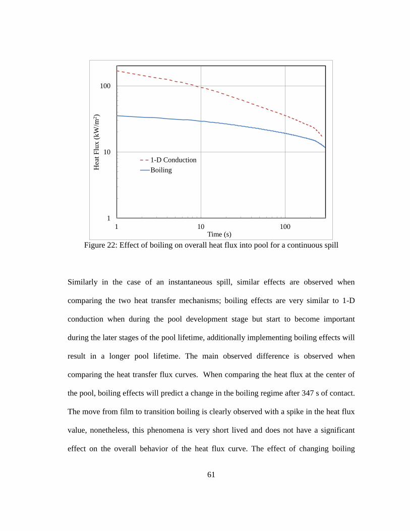
61

Figure 22: Effect of boiling on overall heat flux into pool for a continuous spill

Similarly in the case of an instantaneous spill, similar effects are observed when

comparing the two heat transfer mechanisms; boiling effects are very similar to 1-D

conduction when during the pool development stage but start to become important

during the later stages of the pool lifetime, additionally implementing boiling effects will

result in a longer pool lifetime. The main observed difference is observed when

comparing the heat transfer flux curves. When comparing the heat flux at the center of

the pool, boiling effects will predict a change in the boiling regime after 347 s of contact.

The move from film to transition boiling is clearly observed with a spike in the heat flux

value, nonetheless, this phenomena is very short lived and does not have a significant

effect on the overall behavior of the heat flux curve. The effect of changing boiling

1

10

100

1 10 100

Hea

t F

lux

(k

W/m

2)

Time (s)

1-D Conduction

Boiling

62

regimes becomes more significant when considering the larger picture as shown in

Figure 26 which shows the overall heat flux of the pool instead of the local effect at the

center of the pool shown in Figure 24. In this case the multiple spikes towards the end of

the curve shows how different areas of the pool will reach the transition boiling regimes

at different times due to varying contact times as the pool is spreading. Moreover, when

comparing the temperature profiles, the point of film breakup and switch to transitional

boiling regime is clearly observed and represented by a sudden drop in temperature as

the liquid is now in direct contact with the ground instead of having an insulating vapor

layer between them.

Figure 23: Effect of boiling heat transfer on pool radius for an instantaneous spill

0

20

40

60

80

100

120

140

160

180

0 100 200 300 400 500 600

Ra

diu

s (m

)

Time (s)

With Boiling Heat Transfer

Base Case

63

Figure 24: Effect of boiling heat transfer on heat flux at center of the pool for an

instantaneous spill

Figure 25: Effect of boiling heat transfer on temperature at center of the pool for an

Instantaneous spill

1

10

100

1 10 100

Hea

t F

lux

(k

W/m

2)

Time (s)

1-D Conduction

Boiling

100

120

140

160

180

200

220

240

260

280

300

0 100 200 300 400 500 600

Tem

per

atu

re (

K)

Time (K)

Boiling

1-D Conductoin

64

Figure 26: Effect of boiling on overall heat flux into pool for a continuous spill

Although representing heat transfer effects using boiling heat transfer correlations

compared to adjusted 1-D conduction does not provide a significant difference, it offers

a more accurate representation of the spill scenario and provides a better understanding

of the dynamics of the ground-liquid heat transfer interaction. When comparing the

effects of varying the parameter on 1-D conduction to boiling heat transfer as shown in

Figure 27, it is clear that the commonly implemented adjusted 1-D conduction with =3

provides a reasonable representation of the pool behavior. Nonetheless, it is important to

realize that the boiling heat transfer correlations are based on pure thermo physical

properties of the spilled substance and the substrate and do not employ any empirical

adjustment parameters such as the parameter used in 1-D conduction. Although boiling

1

10

100

1 10 100

Hea

t F

lux

(k

W/m

2)

Time (s)

1-D Conduction

Boiling

65

heat transfer correlations will, as is the case with any thermo physical model, employ

empirical parameters at the very basic levels, these parameters have not been

implemented to adjust the nature of these predictions as is the case with the parameter.

This difference in the nature of the boiling heat transfer correlations provides better

confidence in their applicability to a wider range of spill scenarios on different substrates

or even involving different cryogens.

Figure 27: Comparing 1-D conduction with varying parameter to boiling heat transfer

0

50

100

150

200

250

300

350

0 100 200 300 400

Ra

diu

s (m

)

Time (s)

X = 1

X = 2

X = 3

X = 6

Boiling

66

6.6.Vapor liquid equilibrium (VLE) effects

Here, the base case was compared to the model incorporating VLE effects. VLE and

mixture thermodynamics were implemented as described in Section 2.2.4 to determine

the temperature, thermo physical properties and vapor and liquid compositions

throughout the pool’s lifetime. The initial composition of the LNG mixture used is

shown in Table 1. In this comparison, heat transfer effects were modeled using 1-D

conduction to obtain an absolute effect of mixture thermodynamics on the pool

spreading process.

As shown by Figure 28 incorporating mixture and thermodynamic effects will not result

in a significant enhancement to the pool spread model for continuous spills. This is

primarily due to the continuous supply of fresh LNG into the pool which will maintain a

high methane content as shown in Figure 29, yet once the continuous spill stops at 100s

and the effect of preferential boil-off starts being more significant, the pool density and

latent heat will start to increase due to the higher fractions of heavier hydrocarbons in the

pool as shown in Figure 30 and 31. This in turn will affect the pool radius and the

deviation of pool radius from 1-D conduction can be observed to begin after 100s which

is the end time of the continuous spill as shown in Figure 28.

67

Figure 28: Effect of incorporating VLE effects on pool radius for a continuous spill

Figure 29: Effect of incorporating VLE effects on pool composition for a continuous

spill

0

50

100

150

200

250

300

0 50 100 150 200 250 300 350

Ra

diu

s (m

)

Time (s)

Base Case

With VLE Effects

0

0.1

0.2

0.3

0.4

0.5

0.6

0.7

0.8

0.9

1

0 50 100 150 200 250 300 350

Mo

le F

ract

ion

Time (s)

MethaneEthanePropaneButane

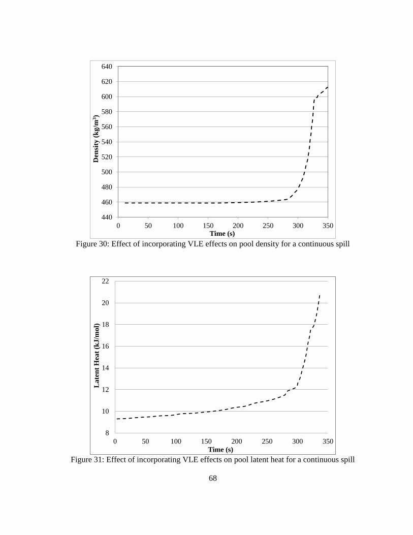
68

Figure 30: Effect of incorporating VLE effects on pool density for a continuous spill

Figure 31: Effect of incorporating VLE effects on pool latent heat for a continuous spill

440

460

480

500

520

540

560

580

600

620

640

0 50 100 150 200 250 300 350

Den

sity

(k

g/m

3)

Time (s)

8

10

12

14

16

18

20

22

0 50 100 150 200 250 300 350

La

ten

t H

eat

(kJ

/mo

l)

Time (s)

69

Similarly, for instantaneous spills, VLE effects are significant only for the pool decay

period. Implementing VLE will predict a longer pool lifetime by about 80s or about

120% longer than using a simple LNG analogue as shown in Figure 32. This is primarily

due to the immediate effect of preferential boil off on the pool’s composition and thermo

physical properties as shown in Figures 33to 35 since there is no continuous supply or

replenishment of the lighter methane as is the case with a continuous spill. The effect of

incorporating VLE on the pool radius is parallel to the change in the pool composition

due to preferential boiling. Similarly, the density and the latent heat will increase as the

fraction of heavier hydrocarbons starts increasing in the pool.

Figure 32: Effect of incorporating VLE effects on pool radius for an Instantaneous spill

0

20

40

60

80

100

120

140

160

0 100 200 300 400 500 600

Ra

diu

s (m

)

Time (s)

Base Case

With VLE Effects

70

Figure 33: Effect of incorporating VLE effects on pool composition for an Instantaneous

spill

Figure 34: Effect of incorporating VLE effects on pool density for an Instantaneous spill

0

0.1

0.2

0.3

0.4

0.5

0.6

0.7

0.8

0.9

1

0 100 200 300 400 500 600

Mo

le F

ract

ion

Time (s)

MethaneEthanePropaneButane

440

460

480

500

520

540

560

580

600

620

640

0 100 200 300 400 500 600

Den

sity

(k

g/m

3)

Time (s)

71

Figure 35: Effect of incorporating VLE effects on pool latent heat for an Instantaneous

spill

Although, the overall effect of implementing VLE is not very significant it offers a

multitude of thermo physical properties throughout the pool lifetime and provides a

unique perspective on the pool’s dynamics throughout its lifetime. This is a reasonable

and important enhancement to available models since it increases the understanding of

the underlying behaviors and phenomena without exerting a huge computational load.

8

10

12

14

16

18

20

22

0 100 200 300 400 500 600

La

ten

t H

eat

(kJ

/mo

l)

Time (s)

72

6.7.Conclusion of sensitivity analysis

The following conclusions can be drawn from this sensitivity analysis:

1. 1-D conduction models were found to be very sensitive to the thermal contact

correction parameter, which brings into question the versatility of applying 1-D

conduction to represent heat transfer under different scenarios. Further

experimental work is required if adjusted 1-D conduction is to be used with

LNG.

2. Frictional effects within the Base Case seem to have a noticeable effect on the

pool spreading process and become important during the later stages of the pool

spread. However, this is not applicable in the case of LNG, as its unique nature

as a cryogen, prevents the use of conventional frictional terms which may simply

overestimate the friction as stated by (Brambilla et al., 2009). In this model, the

use of boiling heat transfer correlations while ignoring frictional effects seem to

be in reasonable agreement with the Base Case that employs adjustable

parameters to correct for frictional and heat effects.

3. The model which includes the boiling effects provided results close to the

current 1-D conduction model with a correction factor =3. .It provides a better

representation of the pool boiling behavior, the ground temperature change and

the transitions between the different boiling regimes during the pool spreading.

73

4. VLE and mixture effects seem to have a negligible effect on the pool spreading

process during methane rich periods of the pool’s lifetime, but become

increasingly significant during the methane poor periods as the effect of

preferential boiling becomes more observed. Additionally, implementing VLE

effects will provide a detailed insight on the varying thermo physical properties

throughout the pool’s lifetime.

74

CHAPTER VII

MODEL VALIDATION

7.1.Introduction

When trying to validate the model for spills on land and sea, there are very few well

instrumented data for medium and large scale experiments in literature. Such lack of

data presents some limitations when used to validate the complex phenomena involved

in the pool spreading process. More experimental investigations at significantly larger

scales on land and sea are necessary to properly validate the existing LNG pool

spreading models. Nonetheless, two sets of data for land and sea were selected from the

literature and compared to the full present model incorporating mixture thermodynamics,

VLE effects and varying boiling heat transfer regimes was validated.

7.2.Validation for spills on land

Moorehouse and Carpenter (1982) conducted a series of experiments on soil and

concrete involving continuous releases of LNG at a rate of 17 tonnes/hr on soil and 14

tonnes/hr on concrete. The model was compared to a set of experiments conducted on

concrete with thermal conductivity and diffusivity of 1.7 W/m-K and 5x10-7

m2/s. As

shown by Figures 36 and 37, the model is able to reproduce the data reasonably well.

Nonetheless it is important to consider that the measured data is only for the pool

development stage of the release and is therefore governed primarily by momentum

effects, and may not be used to properly validate the modelling of heat effects into the

spreading pool.

75

Figure 36: Model validation vs experimental data for a 17 tonne/hr continuous LNG

release on concrete

Figure 37: Model validation vs experimental data for a 14 tonne/hr continuous LNG

release on soil

0

2

4

6

8

10

12

14

16

18

0 50 100 150 200 250 300 350

Rad

ius

(m)

Time (s)

Moorehouse and Carpenter

Curve1

0

2

4

6

8

10

12

0 50 100 150 200

Ra

diu

s (m

)

Time (s)

Moorehous and Carpenter

Model

76

7.3.Validation for spills on sea

The Esso 11 experiments included a continuous release of 0.15 m3/s of LNG on sea, the

experimental data was extracted from Hissong (2007). As shown in Figure 38 the model

seems to validate reasonably well with the experimental data, yet the validation suffers

from the same uncertainty as that on land as the experimental data only measures the

very early stages of pool development. Moreover the availability of only four

experimental points weakens the credibility of the data to be used for validation

purposes.

Figure 38: Model validation vs experimental data for a continuous release of 0.15 m3/s

of LNG on sea

0

5

10

15

20

25

30

35

0 10 20 30 40

Rad

ius

(m)

Time (s)

Esso 11

Model

77

CHAPTER VIII

CONCLUSION

In this work, a pool spread model was developed by incorporating boiling heat transfer

and mixture thermodynamic effects to a gravity inertia momentum balance. The aim was

to develop an analytical model that represents the unique properties of LNG as

accurately as possible without relying on any empirical or adjustment parameters.

A sensitivity analysis was conducted to determine the relative importance of boiling heat

transfer, friction, thermal contact/roughness adjustment parameter and VLE effects on

the rate of pool spreading and decay. The purpose of the sensitivity analysis was to

determine the effect of increasing the complexity of the currently available models and

to analyse the sensitivity of these models to the empirical constants incorporated.

Modelling conduction using boiling heat transfer rather than 1-D conduction seems to

have a significant effect on pool spreading, particularly towards the later stages of the

pool spread as these effects start to become increasingly significant. On the other hand,

implementing VLE and mixture effects into the model seems to have a negligible effect

when compared to using fixed LNG thermo physical properties for continuous spills, but

are significant for instantaneous spills. This is due to delayed effect of preferential boil

off in continuous spills due to the continuous supply of fresh LNG into the pool, unlike

78

the case for an instantaneous spill where the effect of preferential boil off occurs much

quicker.

The addition of friction to the gravity inertia balance was investigated to better

understand its relative importance on the mechanical aspects of the pool spread model,

this is because frictional effects have been ignored in the developed model due to the

implementation of boiling heat transfer which assumes that the leading edge of the pool

will always be in film boiling and therefore sliding on a thin frictionless vapour film.

Results show that friction seems to have a noticeable effect on the pool spreading

process modelled using the Base Case, and will affect the pool lifetime and spread rate,

particularly towards the later stages of the pool lifetime. This is explained by the fact

that as the modelled pool spreads faster due to lack of friction, it will get thinner at a

faster rate and will be in contact with more ground which increases the amount of heat

conducted into the pool. These two effects will results in a pool with a shorter lifetime

and a larger maximum diameter. However, this is not applicable then dealing with LNG

due to its cryogenic nature, and the use of conventional frictional terms as will in fact

over estimate these frictional effects as shown by (Brambilla et al., 2009).

Finally, the effect of the thermal contact/roughness correction parameter was studied.

The thermal contact/roughness correction parameter is an empirical parameter that has

usually been introduced to early spread models such as Briscoe & Shaw (1980) and

79

Jensen (1983) to correct the 1-D conduction to match experimental data for LNG. When

varied, the 1-D conduction equation was found to be very sensitive to this parameter

which brings into question its applicability to a wide range of spreading scenarios and

substrates.

The model was validated against experimental data found in literature. The model seems

to validate well with the available data, but since all of the data found was only for the

development region of the pool this brings into question the confidence they provide in

validating this model. A more reliable set of experimental data are required to properly

validate and understand the governing phenomena involved in pool spread models.

80

CHAPTER IX

FUTURE WORK

Further work is needed to understand substrate effects on the boiling behaviour of LNG.

The effect of surface roughness, porosity, thermal conductivity and other parameters on

the boiling process needs to be studied to properly determine their effect on bubble

nucleation and film breakup. Additionally, CFD modelling of these phenomena may be

required to provide additional insight on the effect of these parameters. Nonetheless, the

author of this report strongly believes that experimental work, both lab and large scale, is

crucial to gain a better understanding and develop more accurate correlations when

dealing with LNG. Although modelling efforts are important, there has been a lack of

experimentally backed insight during recent years, particularly when it comes to dealing

with the boiling phenomena of LNG. Experimental work at medium and large scale is

currently being planned to be conducted at the Ras Laffan Emergency and Safety

College, which could be a huge step forward to help properly and comprehensively

validate the model and provide a better understanding of its governing phenomena.

81

REFERENCES

ABSG, & FERC. (2004). Consequence assessment methods for incidents involving

releases from liquefied natural gas carriers.

Berenson, P. J. (1962). Experiments on pool-boiling heat transfer. International Journal

of Heat and Mass Transfer, 5, 985–999.

Boe, R. (1998). Void fraction measurements in boiling cryogenic mixtures using gamma

densitometer. International Journal of Heat and Mass Transfer, 41(10), 1167–

1175.

Brambilla, S., & Manca, D. (2009). Accidents involving liquids: A step ahead in

modeling pool spreading, evaporation and burning. Journal of Hazardous

Materials, 161(2-3), 1265–1280. doi:10.1016/j.jhazmat.2008.04.109

Briscoe, F., & Shaw, P. (1980). Spread and Evaporation of Liquid. Progress in Energy

and Combustion Science, 6(2), 127–140.

Burgess, D., & Zabetakis, M. G. (1962). Fire and explosion hazards associated with

liquefied natural gas (p. 34). Washington, DC: U.S. Dept. of the Interior, Bureau of

Mines, Report 6099.

Cavanaugh, T. A., Siegell, J. H., & Steinberg, K. W. (1994). Simulation of Vapor

Emissions From Liquid Spills. Journal of Hazardous Materials, 38(1), 41–63.

doi:10.1016/0304-3894(93)E0111-E

Conrado, C., & Vesovic, V. (2000). The influence of chemical composition on

vaporisation of LNG and LPG on unconfined water surfaces. Chemical Engineering

Science, 55(20), 4549–4562. doi:10.1016/S0009-2509(00)00110-X

Drake, E. M., Jeje, A. A., & Reid, R. C. (1975). Transient boiling of liquefied cryogens

on a water surface: I. Nitrogen, Methane and Ethane. International Journal of Heat

and Mass Transfer, 18(12), 1361–1368. Retrieved from

http://www.sciencedirect.com/science/article/pii/0017931075902495

Fay, J. A. (1971). Physical processes in the spread of oil on a watersurface. Proceedings

of The Joint Conference on Prevention and Control of Oil Spills (p. 463467).

Fay, J. A. (2007). Spread of large LNG pools on the sea. Journal of Hazardous

Materials, 140(3), 541–551. doi:10.1016/j.jhazmat.2006.10.024

82

Forsman, B. (2011). North European LNG Infrastructure Project : A Feasibility Study

for an LNG filling station infrastructure and test of recommendations (p. 20).

Hansen, O., Melheim, J., & Storvik, I. (2007). CFD-modeling of LNG dispersion

experiments. AIChE Spring National Meeting, 2007, (April). Retrieved from

http://www.gexconus.com/doc/olav/LPS_Houston_Hansen_2007.pdf

Hissong, D. W. (2007). Keys to modeling LNG spills on water. Journal of Hazardous

Materials, 140(3), 465–477. doi:10.1016/j.jhazmat.2006.10.040

Hoult, D. (1972). Oil spreading on the sea. Annual Review of Fluid Mechanics, 341(1).

Retrieved from

http://www.annualreviews.org/doi/pdf/10.1146/annurev.fl.04.010172.002013

Jensen, N. O. (1983). On cryogenic liquid pool evaporation. Journal of Hazardous

Materials, 8(2), 157–163. doi:10.1016/0304-3894(83)80054-5

Kalinin, E. K., Berlin, I. I., Kostyuk, V. V., & Nosova, E. M. (1976). Heat transfer in

transition boiling of cryogenic liquids. Advances in Cryogenic Engineering, 21,

273–277.

Klimenko, V. V. (1981). Film boiling on a horizontal plate — new correlation.

International Journal of Heat and Mass Transfer, 24(1), 69–79. doi:10.1016/0017-

9310(81)90094-6

Liu, Y., Olewski, T., Vechot, L., Gao, X., & Mannan, S. (2011). Modelling of a

cryogenic liquid pool boiling using CFD code. 14th Annual Symposium, Mary Kay

O’Connor Process Safety Center “Beyond Regulatory Compliance: Making Safety

Second Nature” (pp. 512–524).

Luketa-Hanlin, A. (2006). A review of large-scale LNG spills: Experiments and

modeling. Journal of Hazardous Materials, 132(2-3), 119–140.

doi:10.1016/j.jhazmat.2005.10.008

Moorhouse, J., & Carpenter, R. J. (1986). Factors affecting vapour evolution rates from

liquefied gas spills. North western Branch Papers, Institution of Chemical

Engineers, 1, 4.1–18.

NFPA 59A Standard for the Production, Storage, and Handling of Liquefied Natural Gas

(LNG) (2009).

Opschoor, G. (1975). Investigations into the spreading and evaporation of burning

LNG-spills on water and the heat radiation from LNG-fires on water (No. CTI-

TNO 75-03777, I.O.W.-subproject 4, report 4). Apeldoorn.

83

Opschoor, G. (1980). Spreading and evaporatoin of LNG spills and burning LNG spills

on water. Journal of Hazardous Materials, 3(3), 249–266. doi:10.1016/0304-

3894(80)85004-7

Puttock, J. S., Blackmore, D. R., & Colenbrander, G. W. (1982). Field experiments on

dense gas dispersion. Journal of Hazardous Materials, 6,13–41.

Raj, and A.S. Kalelkar, (1974) “Assessment Models in Support of the Hazard

Assessment Handbook”, U.S. Coast Guard Report No. CG-446-3, Report

submitted by Arthur D. Little, Inc., to Department of Transportation, U.S. Coast

Guard, Contract No. DOT-CG24655A, January 1974.

Raj, P. K. (1981). Models for cryogenic liquid spill behavior on land and water. Journal

of Hazardous Materials, 5(1-2), 111–130. doi:10.1016/0304-3894(81)85009-1

Reid, R. C., & Wang, R. (1978). The boiling rates of LNG on typical dike floor

materials. Cryogenics, 18(7), 401–404. doi:http://dx.doi.org/10.1016/0011-

2275(78)90033-4

Webber, D. M. (1987). “Heat conduction under a spreading pool”, UKAEA Report

SRD/HSE R 421.

Webber, D. M. (1991). Source terms. Journal of Loss Prevention in the Process

Industries, 4(1), 5–15. doi:10.1016/0950-4230(91)80002-C

Webber, D. M. (1996). Letter to the editor. Journal of Hazardous Materials, 45(1), 79–

80. doi:10.1016/0304-3894(95)00043-7

Webber, D. M. (2012). On models of spreading pools. Journal of Loss Prevention in the

Process Industries, 25, 923–926.

Woodward, J. L., & Pitblado, R. (2012). LNG Risk Based Safety - Modeling and

Consequence Analysis (p. 374). Wiley-AIChE.