Modelling of iron-filled magneto-active polymers with

a dispersed chain-like microstructure

Prashant Saxenaa,b, Jean-Paul Peltereta, Paul Steinmanna

aChair of Applied Mechanics, University of Erlangen–Nuremberg,Paul-Gordan Straße 3, Erlangen 91052, Germany

bCenter for Integrative Genomics, University of Lausanne,Genopode Building, 1015 Lausanne, Switzerland

Abstract

Magneto-active polymers are a class of smart materials commonly manufacturedby mixing micron-sized iron particles in a rubber-like matrix. When cured in thepresence of an externally applied magnetic field, the iron particles arrange them-selves into chain-like structures that lend an overall anisotropy to the material. Ithas been observed through electron micrographs and X-ray tomographs that thesechains are not always perfect in structure, and may have dispersion due to the con-ditions present during manufacturing or some undesirable material properties. Wemodel the response of these materials to coupled magneto-mechanical loading inthis paper using a probability based structure tensor that accounts for this imper-fect anisotropy. The response of the matrix material is decoupled from the chainphase, though still being connected through kinematic constraints. The latter isbased on the definition of a ‘chain deformation gradient’ and a ‘chain magneticfield’. We conclude with numerical examples that demonstrate the effect of chaindispersion on the response of the material to magnetoelastic loading.

Keywords: Nonlinear magnetoelasticity; anisotropy; chain dispersion; finite elementmethod

1 Introduction

Magneto-active polymers (MAPs) are smart materials in which the mechanical and themagnetic properties are coupled with each other. Typically these elastomers are composedof a rubber matrix filled with magnetisable iron particles. The magnetisable particles areusually between 1-5 µm in diameter and kept between 0-30% by volume of the entiremixture [4, 27, 36, 39]. The application of an external magnetic field causes the magneti-sation of iron particles and the resulting particle-particle and particle-matrix interactions

Corresponding author: Paul SteinmannEmail: paul.steinmann@ltm.uni-erlangen.dePh: +49 9131 8528501, Fax: +49 9131 8528503

1

lead to phenomena such as magnetostriction and a change in the overall material stiff-ness [16, 66]. These elastomers have received considerable attention in recent times dueto their potential uses in a variety of engineering applications, such as variable stiffnessactuators [6] and vibration suppression by energy absorption [39, 70].

Mathematical modelling of the coupling of electromagnetic fields in deformable con-tinua has been an area of active research in the past. In particular, we note the con-tributions of Landau and Lifshitz [42], Livens [43], Tiersten [64], Brown [9], Pao andHutter [51], Maugin and Eringen [48], Maugin [46], and Eringen and Maugin [22]. Theadvancement of MAP (along with electro-active polymer) fabrication in the laboratorysetting, and hence their wider availability in recent decades, has led to another surge inresearch in this area. Furthermore, as opposed to metallic alloys and ceramics, newly de-veloped polymer based materials can undergo very large deformations. This has resultedin focused explorations in the nonlinear regime of their response.

Recent developments in this field, based on the classical works mentioned above,are largely due to Brigadnov and Dorfmann [8], Dorfmann and Ogden [19, 21], andKankanala and Triantafyllidis [37]. The former’s (Dorfmann and coworkers) work isbased on the definition of a ‘total’ energy density function that implicitly accounts formagnetic and coupled energy stored in the polymer; while the latter’s approach is tominimise a generalised potential energy with respect to internal variables, thereby yieldingthe relevant governing equations and boundary conditions. It is shown that any oneof the magnetic induction, magnetic field, or magnetisation vectors can be used as anindependent input variable and the other two obtained through constitutive relations.Based on these formulations, several nonlinear deformation problems have been studiedby, for example, Dorfmann and Ogden [20], Ottenio et al. [50], Bustamante et al. [13],and Danas et al. [16]. Steigmann [62] and Maugin [47] have discussed several importantissues concerning the modelling of coupled magneto-electro-elasticity using continuumapproaches. Further newer developments pertain to using implicit theories [12] and rate-dependent theories [55, 56] for modelling more general effects, but are beyond the scopeof this work.

MAPs can exhibit isotropic or anisotropic properties depending on the kind of fabri-cation process used. If the elastomers are cured in the presence of an external magneticfield, the magnetisable particles tend to form chain-like arrangements lending an overalldirectional anisotropy to the material. Experiments on such materials [66] have shownthat anisotropic MAPs tend to have stronger coupling with the external magnetic fieldand are therefore more likely to be used in engineering applications.

The modelling of soft elastomers with a directional anisotropy is a subject of researchin its own right. For example, averaging approaches have been adopted by Galipeauand Ponte Castaneda [24] and Yin et al. [71] to capture the microscopic behaviour ofaligned magnetisable particles in soft carrier. In contrast, Rudykh and Bertoldi [52] di-rectly represented the chain-type microstructure using a laminate structure. Anothercommon method of incorporating anisotropy, and that adopted within this work, is byusing structural tensors. As described by Spencer [61] and Zheng [72], these can be cou-pled with the right Cauchy–Green deformation tensor to obtain scalar invariants throughsymmetry arguments. The invariants are then used as an independent input in the en-ergy density function defining the material properties. This method has been used by,among others, Shams et al. [58] for modelling pre-stressed elastic solids, Holzapfel and

2

Gasser [31] for modelling fibre-reinforced composites, and Bustamante [10] and Danaset al. [16] for modelling MAPs with a directional anisotropy. One needs to choose at leasta minimum number of invariants for completeness [18] and take care while performingenergy decomposition for numerical implementation of incompressible materials [54]. An-other approach towards this problem is by decoupling the response of the matrix and theanisotropic part, thereby considering different kinematic variables and energies for each.This has been used by Klinkel et al. [40] in the case of anisotropic elasto-plasticity andby Nedjar [49] for modelling anisotropic visco-elasticity. Based on this latter approach,Saxena et al. [56] recently presented a model for nonlinear magneto-viscoelasticity ofanisotropic MAPs.

Recent experiments have shown another rather important feature in the microstruc-ture of anisotropic iron-filled MAPs, namely that the particle chains formed due to thecuring of an MAP under an external magnetic field are not all aligned in the same di-rection. The chains combined together have an average alignment in the direction of themagnetic field applied during curing, but individual chains do have an observable dis-persion that may possibly influence the macroscopic response of the material. Modellingof this phenomenon and demonstration of the effect of chain dispersion on the overallmacroscopic response of an MAP are the main contributions of this paper. We notethat, mathematically, this phenomenon is similar to the dispersion of fibres in biologicaltissues as is discussed in the papers by Gasser et al. [25], Holzapfel and Ogden [32] onthe modelling of blood vessels, and Federico and Herzog [23] on articular cartilage. Inthese works, the authors considered a generalised structure tensor based on a probabilitydensity function that accounts for the dispersion of embedded fibres.

Numerical methods, and in particular finite element analysis, have been widely usedin the study of magneto-sensitive materials in order to understand and predict boththeir micro- and macroscopic behaviour. The formation of particle chains in magneto-rheological fluids, effectively characterising the pre-cured state of an MAP, has been inves-tigated by Ly et al. [44] and Simon et al. [60]. For the case of solid carriers, Boczkowskaet al. [5], Chen et al. [15] and Vogel et al. [68] have studied the movement of mag-netic particles in elastomers. A coupled scalar magnetic potential formulation has beenutilised to predict both the magnetic and deformation fields at the macroscopic level,where consideration of the surrounding free space is necessary. For example, Kannan andDasgupta [38] adopted this approach to study the magnetostrictive behaviour of MAPsand their application in mini-actuators, Zheng and Wang [73] investigated the magneti-sation of a ferromagnetic plate and Bermudez et al. [3] demonstrated its application toelectromagnets. Furthermore, the shear behaviour of a magnetised block in free spacehas been considered by Marvalova [45] and Bustamante et al. [13], the latter of whichalso investigated its contractile behaviour.

The remainder of this paper is arranged in the following manner: In section 2 weoutline the fundamental aspects of continuum mechanics pertaining to magnetoelasticity.Following this, in section 3 we provide a motivation and the mathematical formulation ofthe dispersed magnetisable particle chains that comprise the MAP microstructure. Wethen detail a decoupled energy model for quasi-incompressible media in section 4, andthe associated energy model for the free space. In section 5, we briefly present the finiteelement formulation used for performing the numerical computations. Analytical andfinite element examples, used to demonstrate the behaviour captured by the constitutive

3

model, are presented in sections 6 and 7 respectively. Lastly, some concluding remarksare presented in section 8.

2 Kinematics, balance laws and boundary conditions

We consider a body composed of a quasi-incompressible magnetoelastic material which,in a state of no stress and no deformation, occupies the reference configuration B0 witha boundary ∂B0. In this state, the free space surrounding the body is denoted by S0

and the entire domain by D0 = B0 ∪ S0. On a combined mechanical and magnetic staticloading, the body occupies the spatial configuration Bt at time t with the boundary ∂Bt.The corresponding configurations for the free space and entire domain are denoted by St

and Dt = Bt ∪ St respectively. A deformation function ϕ maps the points X ∈ D0 to thepoints x ∈ Dt by the relation x = ϕ(X). The deformation gradient tensor is given by atwo-point tensor F = ∇0ϕ, ∇0 being the differential operator with respect to X. Thedeterminant of F is given by J = detF such that the condition J > 0 is always satisfied.For the case of an incompressible material, as presented in section 6, the constraint J ≡ 1is enforced.

It is assumed that the material is electrically non-conducting and that there are noelectric fields. Let σ be the symmetric total Cauchy stress tensor [19] that takes intoaccount magnetic body forces, ρ be the mass density, fm be the mechanical body forceper unit deformed volume, a be the acceleration, b be the magnetic induction vector inDt, and h be the magnetic field vector in Dt. The balance laws are expressed as [9, 48]

∇ · σ + fm = ρa, σt = σ in Bt; ∇× h = 0, ∇ · b = 0 in Dt. (1)

Here ∇ denotes the differential operator with respect to x in Dt. Equation (1)1 is thestatement of balance of linear momentum, equation (1)2 is the statement of balance of an-gular momentum, equation (1)3 is a specialisation of the Ampere’s law, and equation (1)4is the statement of impossibility of the existence of magnetic monopoles. The magneticvectors are connected through the standard constitutive relation [48]

b = µ0[h+m], (2)

where m is the magnetisation vector in Bt (and vanishes in St) and µ0 is the magneticpermeability of vacuum. If σmech is the purely mechanical stress tensor, then it is relatedto the total stress σ by the relation

σ = σmech +1

µ0

[b⊗ b− 1

2[b · b]i

]+ [m · b]i−b⊗m. (3)

Here i is the second order identity tensor in Dt and use has been made of expression forthe magnetic body force as f = [∇b]t ·m [22, and included references].

The total (second) Piola–Kirchhoff stress and the Lagrangian forms of h,b, and mare defined by using the pullback operations [21, 46]

S = JF−1 · σ · F−t, H = Ft ·h, B = JF−1 · b, M = Ft ·m. (4)

4

The above relations are used to rewrite the balance laws as

∇0 ·(S · Ft

)+ ρfm = ρa, St = S in B0; ∇0 ×H = 0, ∇0 ·B = 0 in D0, (5)

along with the relation for magnetic quantities

J−1C ·B = µ0 [H+M] . (6)

At a boundary ∂Bt, which can be the bounding surface of the magnetoelastic bodyor a surface of discontinuity within the material, the jump conditions

n× JhK = 0, n · JbK = 0, (7)

need to be satisfied by the magnetic vectors. Here n denotes the unit outward normal to∂Bt, and J•K = [•]out− [•]in represents jump in a quantity across the boundary. The totalCauchy stress must satisfy

σ · n = ta + tm, (8)

where ta and tm are, respectively, the mechanical and magnetic contributions to thetraction per unit area on ∂Bt. In the reference configuration, the boundary conditions atthe boundary ∂B0 are given by

N× JHK = 0, N · JBK = 0, F · S ·N = tA + tM , (9)

where N is the unit outward normal to ∂B0 and related to n through Nanson’s formulan da = JF−t ·N dA, where da and dA represent the infinitesimal current and referenceareas, respectively. The vectors tA and tM are the mechanical and magnetic contributionsto the traction per unit area on ∂B0.

3 Magneto-active polymer microstructure and chain

dispersion

In order to understand the particle chain alignment and resulting anisotropy in magneto-active polymers, we analyse the electron micrographs of MAP samples documented byJolly et al. [36] and Boczkowska and Awietjan [4]. It is observed that the MAPs curedunder the effect of a magnetic field develop a preferred direction due to the alignment ofiron particles in chain-like formations. Under (presumably) near ideal curing conditions,the chains are quite uni-directional as can be seen in figure 2(a) of [4]. However, if onevaries the matrix material or the particle volume fraction (figures 1(c) and 2(c,d,e) of[4]), we observe that the particle chains do have an observable dispersion.

To reaffirm this observation, samples of magneto-active polymers were prepared andtheir microstructure subsequently analysed using X-ray computed tomography. Iron par-ticles coated with silicon-dioxide were mixed with ELASTOSILr and the mixture wascured for sixteen hours in the presence of a magnetic field created by permanent magnets.The volume fraction of iron particles was taken to be 2% and 10%. Dispersion of theformed particle chains is quite prevalent in the samples shown in figure 1. Overall, itis hypothesised that the final microstructure was influenced by a multitude of factors

5

(a) (b)

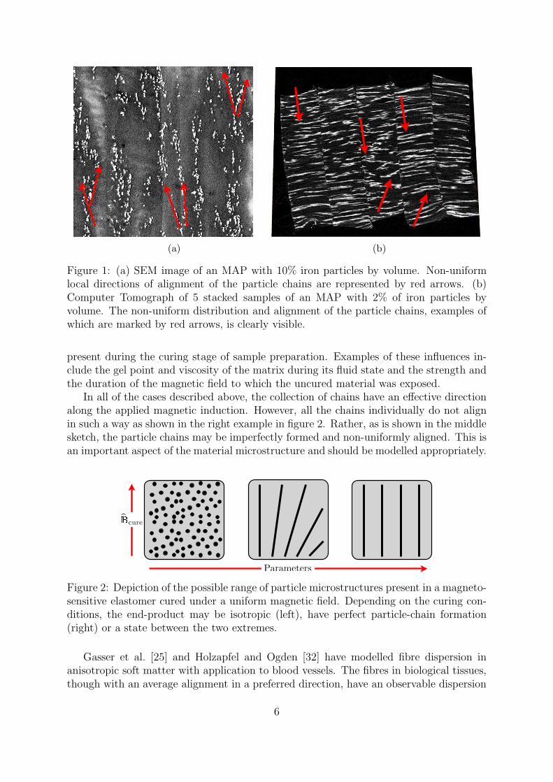
Figure 1: (a) SEM image of an MAP with 10% iron particles by volume. Non-uniformlocal directions of alignment of the particle chains are represented by red arrows. (b)Computer Tomograph of 5 stacked samples of an MAP with 2% of iron particles byvolume. The non-uniform distribution and alignment of the particle chains, examples ofwhich are marked by red arrows, is clearly visible.

present during the curing stage of sample preparation. Examples of these influences in-clude the gel point and viscosity of the matrix during its fluid state and the strength andthe duration of the magnetic field to which the uncured material was exposed.

In all of the cases described above, the collection of chains have an effective directionalong the applied magnetic induction. However, all the chains individually do not alignin such a way as shown in the right example in figure 2. Rather, as is shown in the middlesketch, the particle chains may be imperfectly formed and non-uniformly aligned. This isan important aspect of the material microstructure and should be modelled appropriately.

pcure

Parameters

Figure 2: Depiction of the possible range of particle microstructures present in a magneto-sensitive elastomer cured under a uniform magnetic field. Depending on the curing con-ditions, the end-product may be isotropic (left), have perfect particle-chain formation(right) or a state between the two extremes.

Gasser et al. [25] and Holzapfel and Ogden [32] have modelled fibre dispersion inanisotropic soft matter with application to blood vessels. The fibres in biological tissues,though with an average alignment in a preferred direction, have an observable dispersion

6

that significantly affects their mechanical properties. A similar analysis for collagenfibre distribution in bone cartilage has been performed by Federico and Herzog [23]. Inthe following text, we use similar concepts to approach the problem of particle-chaindistribution in magnetorheological elastomers.

A unit direction vector M is characterised by means of Eulerian angles θ ∈ [0, π] andφ ∈ [0, 2π] in a three-dimensional coordinate system e1, e2, e3 such that

M(θ, φ) = sin θ cosφ e1 + sin θ sinφ e2 + cos θ e3. (10)

If the unit vector M(θ, φ) represents the direction of a particle chain, then the overallgeneralised structure tensor G for the material can be defined as

G =1

4π

∫

ω

ξ(M(θ, φ))M(θ, φ)⊗M(θ, φ) dω, (11)

where ω is the unit sphere, dω = sin θ dθ dφ and ξ is a probability density functiondefining orientation of the particle chains such that ξ(M) is normalised according to therelation

1

4π

∫

ω

ξ(M(θ, φ)) dω = 1. (12)

In the ideal case of absolute anisotropy when all the particle chains are aligned along justone direction (say M = e3), then the probability density function ξ approaches the limitof a Dirac-Delta and the structure tensor G reduces to

G = M⊗M. (13)

For true material characterisation, the probability density function ξ can be nu-merically approximated using experimental data obtained through three-dimensionalcomputerised-tomography (CT) scans of the material specimens. For some simple cases,it can also be approximated through two-dimensional electron-microscopy (SEM or TEM)images. In this paper, for the sake of simplicity, we employ symmetry arguments andassume a transversally isotropic distribution of particle chains around an axis such thatthe probability ξ simply depends on the angle θ with no dependence on φ. Following [25]we assume the function ξ to be given by the π-periodic von Mises probability distributionfunction

ξ (θ) = 4

√b

2π

exp (b [cos 2θ + 1])

erfi(√

2b) . (14)

where the parameter b ∈ [0,∞]. This causes the structure tensor G to reduce to thefollowing simple form

G = κI+ [1− 3κ]M⊗M (15)

as has been shown by Gasser et al. [25]. HereM is the direction of average chain alignmentand κ ∈ [0, 1/3] is a parameter given by

κ =1

4

π∫

0

ξ(θ) sin3θ dθ, (16)

7

and describes the ‘degree of anisotropy’ of the material. The parameters κ and b have aone-to-one mapping through the relations (14) and (16). A visual interpretation of thepresented dispersed microstructure model and its parameters, specifically in the contextof a magneto-sensitive material, is provided in figure 3. Figure 4 presents 3-D plots ofthe von Mises probability distribution as given in equation (14) for different values of thedispersion parameter κ.

M

κ “

1

3κ “ 0.05 κ “ 0

Figure 3: Description of material structure assumed by the material model. For a givenaverage chain directionM, the upper and lower limiting values for κ respectively representan isotropic and perfectly transversely isotropic material. For the isotropic case, this mayimply that either the particles do not form chain-like structures, or the particle chainsare completely randomly orientated. An intermediate value of κ assumes that partialorganisation of particle chains towards M has taken place during curing.

κ = 0κ = 0.05κ = 0.1κ = 1/3

Figure 4: Probability density distribution plotted on a unit sphere according to equa-tion (14) corresponding to two extreme and two intermediate values of the dispersionparameter κ.

4 Constitutive modelling

In general, we consider the total magnetoelastic energy of the material to depend on thedeformation gradient, the magnetic field vector and the structure tensor, that is

Ω0 = Ω0(F,H,G). (17)

It can be shown that, using symmetry arguments, the dependence on F is simplifiedthrough a dependence on the right Cauchy–Green deformation tensor C = Ft · F. For

8

this case, the total Piola–Kirchhoff stress and the magnetic induction are given by theconstitutive relations [21]

S = 2∂Ω0

∂C, B = −∂Ω0

∂H. (18)

4.1 Decoupled energy model

In order to take into account the response of the magnetoelastic chains, we follow theapproach presented in a recent paper [56] that is based on the modelling of fibre-reinforcedsolids by Klinkel et al. [40]. We define a chain-deformation gradient Fc such that

Fc = F ·G = κF+ [1− 3κ]F ·A. (19)

where we have defined A = M ⊗ M. Indeed, we note that if one defines the chaindeformation gradient as an average over chains in all the directions

Fc =1

4π

∫

ω

ξ [F ·M]⊗M dω, (20)

we arrive at the expression in (19) on using the condition (11). In the limit κ → 0 for apurely anisotropic material with no dispersion, this reduces to Fc = F ·A thus capturingthe one-dimensional deformation in the chain anisotropy direction. We note that hereand henceforth, a superscript ‘c’ refers to the quantities associated with the chain phase.

For future use, we define Cc = [Fc]t · Fc, also expressed as

Cc = G ·C ·G = κ2C+ κ[1− 3κ][C ·A+A ·C] + [1− 3κ]2[C : A]A, (21)

and present the identity

∂Cc

∂C= G⊗G = κ2

I4 +κ

2[1− 3κ]

[I⊗A+ I⊗A+A⊗I+ I⊗A

]+ [1− 3κ]2A⊗A. (22)

Here we define the non-standard tensor products of two second order tensors as [P⊗Q]ijkl =PikQjl and [P⊗Q]ijkl = PilQjk, and I4 = [I⊗I+ I⊗I] /2 is the fourth order symmetricidentity tensor.

The Lagrangian magnetic field in the average chain direction is given by

H

c = G ·H = κH + [1− 3κ][M ·H]M, (23)

and we note the identity∂Hc

∂H= G. (24)

The dependence of the total energy density on the structure tensorG is now consideredimplicitly through Cc and Hc. Thus Ω0 = Ω0(C,Cc,H,Hc) and the Piola–Kirchhoffstress is given in the case of incompressibility by

S = 2∂Ω0

∂C+ 2κ2 ∂Ω0

∂Cc+ 2κ[1− 3κ]

[A · ∂Ω0

∂Cc+

∂Ω0

∂Cc·A]+ 2[1− 3κ]2

[∂Ω0

∂Cc: A

]A− pC−1,

(25)

while the magnetic induction is given as

B = −∂Ω0

∂H−G · ∂Ω0

∂Hc . (26)

9

4.2 Dealing with material incompressibility

The energy density function is initially decomposed into two parts, namely those at-tributed to the matrix and the particle chain, such that

Ω0 = Ωmat0 (C,H) + Ωc

0(C,Cc,H,Hc). (27)

However, following the discussion by Sansour [54], only the matrix part is decomposedfurther into volumetric and isochoric parts [59] such that

Ω0 = Ωvol0 (J) + Ωiso

0 (C,H)︸ ︷︷ ︸Ωmat

0

+Ωc0(C,Cc,H,Hc). (28)

A multiplicative split of the deformation gradient into volumetric and isochoric contribu-tions

F = F · F with F := J1

3 I, F := J−1

3F (29)

is also assumed [59], from which the isochoric part of the right Cauchy–Green deformation

tensor is given as C = Ft·F. Such decompositions are typically utilised not only to capturethe decoupled behaviour of rubber-like materials but also to support their numericalmodelling. In view of the material description given by equation (28), for the case of aquasi-incompressible material equation (18)1 is transformed to

S = 2

[∂Ωiso

0

∂C:∂C

∂C+

∂Ωc0

∂C

]− pJC−1 (30)

with the hydrostatic pressure defined as

p = −∂Ωvol0 (J)

∂J. (31)

4.3 Dealing with surrounding free space

In addition to the stored energy in the material due to elastic deformation and mag-netisation, an additional energy contribution arises due to the presence of the magneticfield permeating and surrounding the elastic body. Depending on its constitutive modeland consequent magnetisation, this may be a negligible quantity inside the elastic body.However, this energy must certainly be accounted for in the free space as it quantifiesits Maxwell stress and free space induction. We therefore formally write the total storedpotential energy Ω0 as

Ω0 (C,H) = W0 (C,H) +M0 (C,H) (32)

where W0 is the elastic and magnetic energy stored in the elastic body and M0 =

−1

2µ0JC

−1 : H ⊗ H is the energy stored in the free space [67]. It should be noted

that, for the examples shown later, the free space energy within the elastic media isignored and the above reduces to

Ω0 (C,H) ≡ W0 (C,H) if X ∈ B0 and Ω0 (C,H) ≡ M0 (C,H) if X ∈ S0. (33)

10

5 Finite element formulation

Under the assumption of quasi-static conditions and the presence of no free-currents, wedenote the displacement by u = x−X and define a scalar magnetic potential1 Φ [7, 41].The referential magnetic field, being curl-free, is related to the magnetic potential (afictitious quantity) by

H = −∇0Φ (34)

with the following conditions on the solid boundary and truncated far-field boundary∂S∞

JΦK = 0 on ∂B0, Φ = Φ on ∂S∞. (35)

We define a total potential energy functional

Π = Πint +Πext (36)

on the domain D0, composed of a magnetoelastic subdomain B0 and the surrounding freespace S0. The total internal potential energy is given by

Πint =

∫

D0

Ω0 (C,H) =

∫

B0

W0 (C,Cc,H,Hc) +

∫

S0

M0 (C,H) , (37)

where, from equations (28) and (32), W0 denotes the total potential energy per unitvolume due to the magnetoelastic material’s deformation and magnetisation, while M0

quantifies the magnetic energy stored in the free field. The total external potential energyis

Πext = −∫

B0

u · b0 −∫

Γt0

u · tA−∫

∂Sb∞

Φ [BA ·N∞], (38)

where b0, tA represent the referential mechanical body forces and surface tractions re-spectively, and BA is the magnetic induction prescribed on the far-field boundary ∂Sb

∞.

Using the principle of stationary potential energy, the equilibrium solution to equa-tion (36) can be determined. The stationary point is that at which all directional deriva-tives of the total potential energy disappear. The expression for the Gateaux derivativeof the total energy is

δΠ (u, δu,Φ, δΦ) = δuΠ (u,Φ) + δΦΠ (u,Φ)

=d

dǫΠ (u+ ǫδu,Φ)

∣∣∣∣ǫ=0

+d

dγΠ (u,Φ + γδΦ)

∣∣∣∣γ=0

= 0,(39)

1An alternative to the scalar potential formulation, which is used due to its simple numerical implan-tation, is the vector potential formulation [11, 41, 57] for which a relationship between B and a vectorpotential field A, namely B = ∇0 ×A, is assumed.

11

which yields δΠ = δΠint + δΠext. Using equations (33) and (37), the variation of theinternal potential energy is expressed concisely as

δΠint = δuΠint + δΦΠ

int =

∫

D0

δE : S−∫

D0

δH ·B, (40)

and that of the external potential energy is

δΠext = −∫

B0

δu · b0 −∫

Γt0

δu · tA−∫

∂Sb∞

δΦ [BA ·N∞]. (41)

Here we define the variations of the Green-Lagrange strain tensor, the deformation gra-dient and magnetic field respectively as

δE = sym[FT · δF

], δF = ∇0δu, δH = −∇0δΦ. (42)

As is detailed by Bustamante and Ogden [11] for the case involving both a solid andfree-space domain, the above collectively represents the equivalent weak form of thedivergence-free condition for both the stress and magnetic induction (equations (1)1,4)for the magneto-elastostatic case. Furthermore, the continuity of the normal tractionand magnetic induction (given in equation (7)2) at the material interfaces is also embed-ded within this formulation. However, it remains to be ensured that the compatibilityconditions for the deformation and the continuity of tangential magnetic field (equation(7)1) are satisfied.

As the material laws are nonlinear, an iterative procedure such as the Newton-Raphsonmethod must be utilised to determine the stationary point. The nonlinear system ofequations can be linearised using a first-order Taylor expansion about the current solution.Linearisation of equation (40) with respect to the motion and scalar magnetic potentialrenders the contributions [63, 69]

∆δΠint = ∆u

[δuΠ

int + δΦΠint]+∆Φ

[δuΠ

int + δΦΠint], (43)

=

∫

D0

[sym

[δFT ·∆F

]: S+ δE : H : ∆E− δH ·P : ∆E

]

+

∫

D0

[−δE : PT ·∆H−∆H ·D ·∆H

],

(44)

with ∆ (•) representing value increments. The material tangents, namely the referentialelasticity tensor, the fully-referential magneto-elasticity tensor and the rank-2 magnetictensor, are defined as

H = 4∂2Ω0 (C,H)

∂C⊗ ∂C, P = −2

∂2Ω0 (C,H)

∂C⊗ ∂H,

P

T = −2∂2Ω0 (C,H)

∂H⊗ ∂C, D = −∂2Ω0 (C,H)

∂H⊗ ∂H.

(45)

Overall, the linear Taylor expansion of equation (40), with the use of equation (43),can be expressed as

0 = δuΠ +∆uδuΠ+∆ΦδuΠ

0 = δΦΠ +∆uδΦΠ +∆ΦδΦΠ.(46)

12

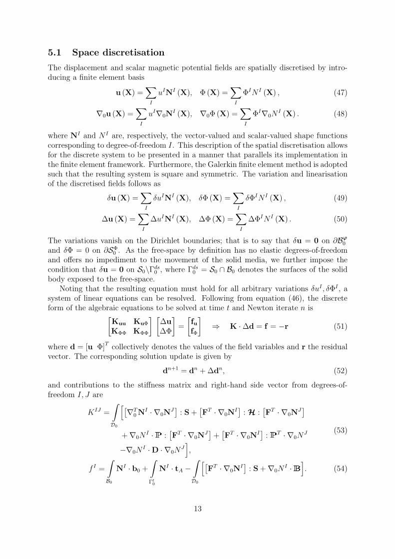
5.1 Space discretisation

The displacement and scalar magnetic potential fields are spatially discretised by intro-ducing a finite element basis

u (X) =∑

I

uINI (X), Φ (X) =∑

I

ΦIN I (X) , (47)

∇0u (X) =∑

I

uI∇0NI (X), ∇0Φ (X) =

∑

I

ΦI∇0NI (X) . (48)

where NI and N I are, respectively, the vector-valued and scalar-valued shape functionscorresponding to degree-of-freedom I. This description of the spatial discretisation allowsfor the discrete system to be presented in a manner that parallels its implementation inthe finite element framework. Furthermore, the Galerkin finite element method is adoptedsuch that the resulting system is square and symmetric. The variation and linearisationof the discretised fields follows as

δu (X) =∑

I

δuINI (X), δΦ (X) =∑

I

δΦIN I (X) , (49)

∆u (X) =∑

I

∆uINI (X), ∆Φ (X) =∑

I

∆ΦIN I (X) . (50)

The variations vanish on the Dirichlet boundaries; that is to say that δu = 0 on ∂Bϕ

0

and δΦ = 0 on ∂SΦ0 . As the free-space by definition has no elastic degrees-of-freedom

and offers no impediment to the movement of the solid media, we further impose thecondition that δu = 0 on S0\Γds

0 , where Γds0 = S0 ∩ B0 denotes the surfaces of the solid

body exposed to the free-space.Noting that the resulting equation must hold for all arbitrary variations δuI , δΦI , a

system of linear equations can be resolved. Following from equation (46), the discreteform of the algebraic equations to be solved at time t and Newton iterate n is

[Kuu KuΦ

KΦΦ KΦΦ

] [∆u

∆Φ

]=

[fufΦ

]⇒ K ·∆d = f = −r (51)

where d = [u Φ]T collectively denotes the values of the field variables and r the residualvector. The corresponding solution update is given by

dn+1 = dn +∆dn, (52)

and contributions to the stiffness matrix and right-hand side vector from degrees-of-freedom I, J are

KIJ =

∫

D0

[[∇T

0NI · ∇0N

J]: S+

[FT · ∇0N

I]: H :

[FT · ∇0N

J]

+∇0NI ·P :

[FT · ∇0N

J]+[FT · ∇0N

I]: PT · ∇0N

J

−∇0NI ·D · ∇0N

J],

(53)

f I =

∫

B0

NI · b0 +

∫

Γt0

NI · tA −∫

D0

[[FT · ∇0N

I]: S+∇0N

I ·B]. (54)

13

5.2 Mesh-motion in the free-space

As the energies given in equation (37) are defined in terms of referential quantities, anexpression for the displacement u is required for the entire computational domain. Morepointedly, it is necessary that some artificial measure of deformation be provided withinthe free-space S0 such that an associated, invertible deformation gradient (which mapsthe configuration used for computation to the physically relevant spatial configuration)can be defined and spatial quantities derived from M0 can be computed.

Moving mesh approaches adapted from the modelling of fluid systems with movingboundaries (the “ALE” class of fluid formulations) can be utilised in magneto-elasticproblems [14, 53]. Johnson and Tezduyar [35] describes a typical approach to performingthis update, and the one that is used in this work. Once the deformation field in the solidmedia is computed, we solve a linear elasticity problem

∫

S0

∇δu∗ : σ∗ = 0 with σ∗ = K∗ (X) : ε∗ , ε∗ =

1

2

[∇u∗ + (∇u∗)T

]. (55)

The motion of the mesh in the free-space is thus governed by a fictitious stiffnesstensor defined at each integration point and the assumed Dirichlet boundary conditions.There exist a number of viable choices to define an effective stiffness to the elasticityproblem [34, 35] and we choose to point-wise define the isotropic elasticity tensor

K∗ (X) =

1

dhI4 (56)

where dh is a measure of the longest diameter of the cell encompassing X. As for theboundary conditions, we use the precomputed displacement of the solid media as thedriving Dirichlet boundary conditions for the artificial problem. This has the additionalbenefit that the interface mesh between the free-space and solid domains (on Γds

0 ) is alwayssynchronised. To ensure the exterior shape of the far-field domain remains the same, wefix all pseudo-elastic degrees-of-freedom on these surfaces. In the case where half of thedomain is modelled, as is the case for the problem demonstrated in section 7.2, onlysymmetry conditions (that is that no out-of-plane displacement may occur) are enforcedon the cut-plane.

6 Extension and inflation of a hollow cylinder

In order to illustrate the physical behaviour predicted by the model presented in the pre-ceding sections, we now present some calculations related to standard loading conditions.This section presents a problem of inflation and extension of a magnetoelastic tube thathas been solved analytically.

We consider an infinitely long circular cylindrical tube made of an incompressiblemagnetoelastic material with a directional anisotropy. We work in cylindrical polar co-ordinates, which in the reference configuration B0 are denoted by (R,Θ, Z) and in thedeformed configuration by (r, θ, z). Let the internal and external radii of the tube inB0 be given by A and B, which become a and b in Bt after deformation. The tube isdeformed by a combination of inflation and axial stretching as is depicted in figure 5.

14

N

N

Pin

Figure 5: Cylinder being inflated through internal pressure Pin and extended in axialdirection through force N . Dotted curves in colour denote the direction of average align-ment of particle chains and the applied magnetic field.

We will consider the external magnetic field being applied in azimuthal direction by anelectric current density through the axis of the tube. In this case, the magnetic field inthe azimuthal direction decays with increasing distance from the axis and is given byhθ = h0/r where r is the radius.

The deformation is given (due to incompressibility) by

r =[a2 + λ−1

z

[R2 − A2

] ]1/2, z = λzZ, θ = Θ, (57)

where λz is the uniform axial stretch. Using the constraint of incompressibility, theprincipal stretches in the azimuthal and the radial directions are given by

λθ = λ =r

R, λr = λ−1λ−1

z , (58)

respectively. For this case, the deformation gradient is given by F = diag(λr, λθ, λz).

6.1 Energy density functions

Following the discussion in section 4.2, the energy density function is additively decom-posed into the energy of the matrix phase and that of the chain phase. We consider thefollowing prototype functions for each of these components

Ωmat0 =

n1

α

[exp

(α [C : I− 3]2

)− 1]

︸ ︷︷ ︸Ω

m,E0

+n2[H⊗H] : I+ n3[H⊗H] : C−1

︸ ︷︷ ︸Ω

m,ME0

, (59)

Ωc0 =

n4

α

[exp

(α[Cc : I−G2 : I]2

)− 1]

︸ ︷︷ ︸Ω

c,E0

+n5[Hc ⊗Hc] : I+ n6[H

c ⊗Hc] : C−1

︸ ︷︷ ︸Ω

c,ME0

. (60)

The magnetoelastic component is quadratic in terms of the spatial magnetic field vector,and the use of the Fung-type energy function for the elastic part ensures that the chainsare stress-free in the undeformed configuration.

15

In the case of incompressibility C = C and we need only consider the functionsprovided in equation (59) and equation (60). For such a case, the constitutive relationfor the Piola–Kirchhoff stress is given as

S = 2β1I− 2n3[C−1 ·H]⊗ [C−1 ·H] + 2β2κ

2I+ 2β2[1− κ][1− 3κ]M⊗M

−2n6[C−1 ·Hc]⊗ [C−1 ·Hc]− pC−1, (61)

where

β1 = 2n1 [C : I− 3] exp(α [C : I− 3]2

), (62)

β2 = 2n4[Cc : I−G2 : I] exp

(α[Cc : I−G2 : I]2

). (63)

The magnetic induction is given by

B = −2n2H− 2n3C−1 ·H− 2n5G ·Hc − 2n6G ·C−1 ·Hc. (64)

These quantities are given in the spatial configuration as

σ = 2[β1 + β2κ2]b− 2n3h⊗ h+ 2β2[1− κ][1− 3κ]m⊗m

− 2n6[b−1 · g · h]⊗ [b−1 · g · h]− pi,

(65)

andb = −2n2b · h− 2n3h− 2n5g · b−1 · g · h− 2n6g · b−2 · g · h, (66)

where we have defined the push-forward of the structure tensor to the spatial configurationas g = F ·G · Ft.

It is to be noted here that, due to this particular choice of energy functions, Ωc0 defined

for the particle chain direction results in a Cauchy stress and magnetic induction thatare similar to those produced by Ωmat

0 , but aligned in the chain direction. The degree ofreinforcement in the chain direction is defined by the parameter κ, which measures thestrength of anisotropy.

6.1.1 Uniaxial deformation

In order to provide an understanding of the behaviour of the chosen energy densityfunction, we first consider a simple example of uniaxial deformation at a point. Theaverage chain alignment, the applied magnetic field and the applied deformation areall in the same direction, say e1 = 1, 0, 0t. Thus we consider the case when F =diag(λ, λ−1/2, λ−1/2), H = H1, 0, 0t, and M = 1, 0, 0t. For this test case, the totalCauchy stress and the developed magnetic induction in the direction of loading are givenby

σ11 = 2[β1 + β2[1 + 4κ2 − 4κ]

]λ2 − 2[β1 + β2κ

2]1

λ

− 2

[n3 + n6[1 − 2κ]2

1

λ2

]H2

1 ,(67)

andb1 = −2

[n2λ

2 + n3 + [1− 2κ]2[n5 +

n6

λ2

]]H1, (68)

16

where

β1 =2n1

[λ2 +

2

λ− 3

]exp

(α

[λ2 +

2

λ− 3

]2),

β2 =2n4

[[1− 2κ]2[λ2 − 1] + 2κ2

[1

λ− 1

]]

× exp

(α

[[1− 2κ]2[λ2 − 1] + 2κ2

[1

λ− 1

]]2).

(69)

It is seen from equation (67) that stress increases in general with an increase in thestretch λ. As the dispersion parameter κ increases from 0 to 1/3, the overall magnitudeof β2 decreases for λ > 1 and increases for λ < 1 while β1 remains unaffected. The lastterm in equation (67) provides a positive stress contribution from the magnetic field forthe case when the effective coefficient comprising of the terms n3 and n6 is negative. Thestress contribution from the magnetic field has a quadratic dependence on H1 as observedby Varga et al. [66, fig. 6] at least for the case of small strains. Clearly the magneticcontribution to the stress is highest when the chains are perfectly aligned at κ = 0 anddecreases with an increase in the chain dispersion.

The magnetic induction from equation (68) is developed in the same direction as theapplied magnetic field when the overall coefficients constituted of the parameters n2, n3, n5

and n6 are negative. Magnetic induction has a linear dependence on the magnetic fieldH1. As κ changes from 0 to 1/3, the magnetic induction decreases in value thus providingmaximum response in the case of perfectly aligned chains.

The above stated observations can also be derived from the plots of equations 67 and68 as shown in figure 6. The graphs are plotted for the values of the parameters listed intable 1 and H1 = 2× 105 A/m.

Table 1: Baseline values of the material parameters.

µ0 µe α n1, n4 n2, n3, n5, n6

4π × 10−7 N/A2 3× 104 N/m2 0.15 0.5 µe -0.5 µe

The proposed energy function corresponds to a material that shows a much higherresistance to extension in comparison to a compressive deformation as is seen from fig-ure 6a. As observed from figure 6b, a high magnetic induction is developed both duringcompression and extension when the chains are perfectly aligned. In the case of isotrop-ically distributed particles (κ = 1/3), the magnetic response during extension is morepronounced in comparison to that during compression.

6.2 Anisotropy in azimuthal direction

We now use the energy density function presented in the previous section to the problemof inflation and extension of a tube as presented in figure 5. As is depicted in figure 5,we consider the average particle-chain alignment to be in the azimuthal direction. Thus,

M = 0, 1, 0t , m = F ·M = 0, λ, 0t. (70)

17

0.5 1 1.5 2

0

1

2

3

Stretch λ [N/D]

Stressσ11[M

Pa]

κ = 0 κ = 0.1 κ = 1

3

(a) Stress σ11

0.5 1 1.5 2

0.5

1

1.5

Stretch λ [N/D]

Mag

netic

induction1[T

]

κ = 0 κ = 0.1 κ = 1

3

(b) Magnetic induction b1

Figure 6: Variation of stress and magnetic induction for a uniaxial deformation case fordifferent values of the dispersion parameter κ.

The structure tensor is given by G = diag(κ, [1− 2κ], κ).Using the expressions in equation (65), the three principal components of the total

Cauchy stress in this case are given by

σrr = −p + 2[β1 + β2κ2]λ2

r, (71)

σθθ = −p+ 2[β1 + β2κ

2 + β2[1− κ][1− 3κ]]λ2 − 2n3h

2θ − 2n6[1− 2κ]2h2

θ, (72)

σzz = −p + 2[β1 + β2κ2]λ2

z, (73)

and the azimuthal component of the magnetic induction from equation (66) is expressedas

bθ = −2n2λ2hθ − 2n3hθ − 2n5[1− 2κ]2λ4hθ − 2n6[1− 2κ]2λ2hθ. (74)

The equilibrium equation ∇ · σ = 0 gives

dσrr

dr=

1

r[σθθ − σrr] , (75)

rdσrr

dr= 2[β1 + β2κ

2][λ2 − λ2r] + 2β2[1− κ][1− 3κ]λ2 − 2n3h

2θ − 2n6[1− 2κ]2h2

θ. (76)

Thus the above differential equation can be integrated with respect to r to calculateσrr as a function of r while σθθ is given as

σθθ = rdσrr

dr+ σrr. (77)

The principal stress in the axial direction (σzz) can be rewritten, using some algebraicmanipulations as

σzz =1

2r

d

dr(r2σrr)−

1

2[σθθ − σrr] + [σzz − σrr]. (78)

18

Thus the total axial force acting on the cylinder can be computed from

N =

2π∫

0

b∫

a

σzz r dr dθ = π[a2Pin − b2Pout

]+ 2π

b∫

a

[[σzz − σrr]−

1

2[σθθ − σrr]

]r dr.

(79)

Here Pin is the pressure in the inside of the tube (r < a) and Pout is the external pressurein the region r > b. In deriving the above, we have also used the boundary conditions onthe lateral surfaces of the tube that are given by the balance of traction as

σrr = σ∗

rr − Pin on r = a, and σrr = σ∗

rr − Pout on r = b, (80)

where σ∗

rr obtains the value −µ0h2θ/2 at r = a and r = b. We note that expressions similar

to equation (75) and equation (79) have been obtained in the context of magnetoelasticityearlier by Dorfmann and Ogden [20].

The values of the material parameters used to perform the calculations are taken fromtable 1. The geometry of the tube is taken such that B/A = 1.4 while the following valuesof the applied magnetoelastic deformation are taken

λa = a/A = 2, λz = 1.5, H0 = 2× 105A/m. (81)

Here we have defined a reference value H0 for the azimuthal magnetic field so that at aradius r, hθ is given by

hθ(r) = H0A/r. (82)

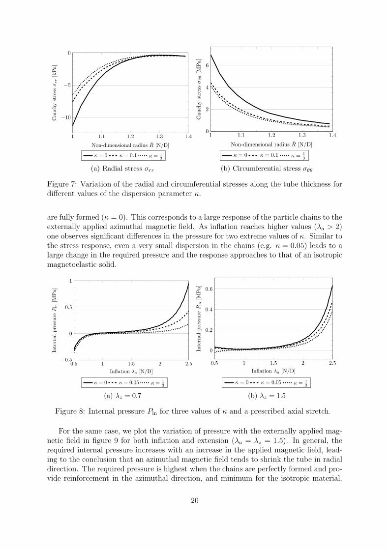
We now plot σrr and σθθ as a function of the non-dimensional radius R = R/A infigure 7 for the magnetoelastic coupled loading specified in equation (81) but for differentvalues of κ to observe how the dispersion of chains affects the internal stresses. Theradial stress is maximum (a negative value indicating compression) at the inner surfaceof the tube and decreases along the thickness direction reaching a minimum value close tothe outer surface. The circumferential stress is two orders of magnitude higher than theradial stress since both the chains and the applied magnetic field provide reinforcementin this direction. In this case also, the maximum stress occurs at the inner surface whichreduces through the thickness with a minimum occurring at the outer surface.

In both the cases, the maximum value of stress is obtained for κ = 0 when the chainsare ideally formed. However, even for a small change (when κ = 0.1), the responsechanges rapidly and converges towards that of the matrix (κ = 1/3).

Given the deformed geometry and the applied magnetic field, one can compute theinternal pressure required to maintain the deformation using the boundary condition(80). In figures 8 and 9 we plot the pressure as a function of inflation for two valuesof λz (representing contraction and extension in the axial direction) and three values ofthe dispersion parameter κ. As expected, the pressure Pin increases with the inflationλa, with the increase in stiffness being exponential as is a typical response for a Fungtype material. The negative values for λa < 1 in the case of λz = 0.7 suggest that anexternal compressive pressure is required to maintain that geometry. Interestingly verylittle variation with the value of κ is observed in this region. However, when the tube isin extension (λz = 1.5), the pressure rises both for inflation and deflation when the chains

19

1 1.1 1.2 1.3 1.4

−10

−5

0

Non-dimensional radius R [N/D]

Cauchystress

σrr[kPa]

κ = 0 κ = 0.1 κ = 1

3

(a) Radial stress σrr

1 1.1 1.2 1.3 1.40

2

4

6

Non-dimensional radius R [N/D]

Cau

chystress

σθθ[M

Pa]

κ = 0 κ = 0.1 κ = 1

3

(b) Circumferential stress σθθ

Figure 7: Variation of the radial and circumferential stresses along the tube thickness fordifferent values of the dispersion parameter κ.

are fully formed (κ = 0). This corresponds to a large response of the particle chains to theexternally applied azimuthal magnetic field. As inflation reaches higher values (λa > 2)one observes significant differences in the pressure for two extreme values of κ. Similar tothe stress response, even a very small dispersion in the chains (e.g. κ = 0.05) leads to alarge change in the required pressure and the response approaches to that of an isotropicmagnetoelastic solid.

0.5 1 1.5 2 2.5−0.5

0

0.5

1

Inflation λa [N/D]

Internal

pressure

Pin

[MPa]

κ = 0 κ = 0.05 κ = 1

3

(a) λz = 0.7

0.5 1 1.5 2 2.5

0

0.2

0.4

0.6

Inflation λa [N/D]

Internal

pressure

Pin

[MPa]

κ = 0 κ = 0.05 κ = 1

3

(b) λz = 1.5

Figure 8: Internal pressure Pin for three values of κ and a prescribed axial stretch.

For the same case, we plot the variation of pressure with the externally applied mag-netic field in figure 9 for both inflation and extension (λa = λz = 1.5). In general, therequired internal pressure increases with an increase in the applied magnetic field, lead-ing to the conclusion that an azimuthal magnetic field tends to shrink the tube in radialdirection. The required pressure is highest when the chains are perfectly formed and pro-vide reinforcement in the azimuthal direction, and minimum for the isotropic material.

20

0 1 2 3

20

25

30

Magnetic field H0 [105 A/m]

Internalpressure

Pin

[kPa]

κ = 0 κ = 0.05 κ = 1

3

Figure 9: Internal pressure Pin for three values of the parameter κ. The deformationparameters were λa = 1.5, λz = 1.5.

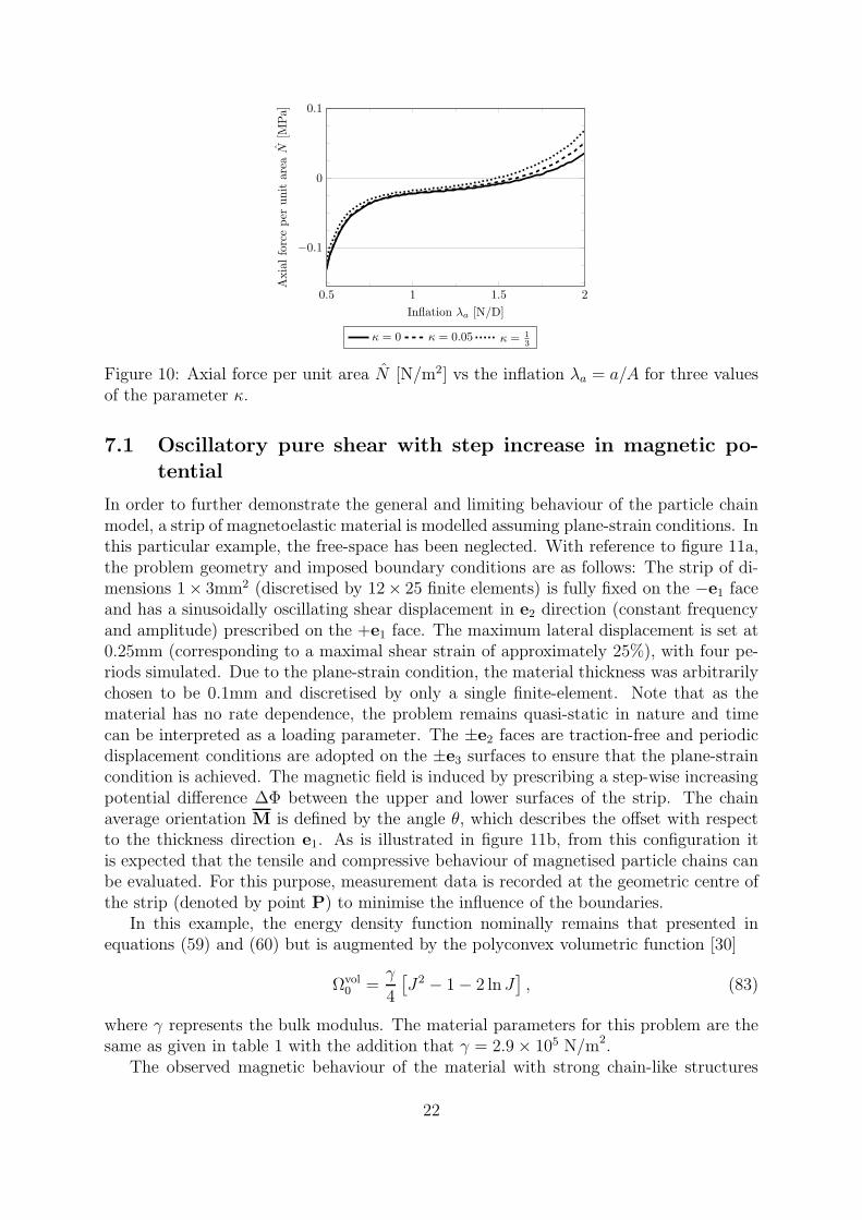
We compute the total axial force per unit area N = N/[π[b2−a2]] required to maintainthe deformed geometry using equation (79) and plot this value in figure 10 to observe theeffect of chain dispersion. The applied loading conditions are that λz = 1 andH0 = 2×105

A/m. As the tube is inflated, it tends to shorten in length and an extensional axial forceis required to maintain the original length. Thus the force N increases with inflation.The axial load is at a minimum in the case of perfect anisotropy when all chains arealigned in the azimuthal direction. As dispersion increases, the particle chains start toprovide a contribution in the axial direction and one observes an increase in the axial forcenecessary to maintain the same level of deformation. Similar to the pressure response, asignificant variation with κ is observed only for the case of inflation λa < 1 and not incontraction λa < 1.

7 Finite element examples

The finite element problem has been implemented using a total Lagrangian approachwithin an in-house code developed using the open-source FE library deal.II [1, 2]. Theuse of continuous linear shape functions for the purpose of discretising the magnetic po-tential Φ ensure that its gradient is curl-free, thereby satisfying equation (7)1. Similarly,continuous trilinear shape functions chosen for the displacement ϕ ensure that the com-patibility conditions for the deformation are naturally satisfied. For the first problemshown in section 7.1, a direct solver, namely UMFPACK [17], was used to solve the lin-ear system of equations given by equation (51). In section 7.2 where a larger geometryis considered, the entire linear system is solved using the stabilised biconjugate gradientmethod [28] in conjunction with an algebraic multi-grid preconditioner [26, 29].

21

0.5 1 1.5 2

−0.1

0

0.1

Inflation λa [N/D]

Axialforceper

unitarea

N[M

Pa]

κ = 0 κ = 0.05 κ = 1

3

Figure 10: Axial force per unit area N [N/m2] vs the inflation λa = a/A for three valuesof the parameter κ.

7.1 Oscillatory pure shear with step increase in magnetic po-

tential

In order to further demonstrate the general and limiting behaviour of the particle chainmodel, a strip of magnetoelastic material is modelled assuming plane-strain conditions. Inthis particular example, the free-space has been neglected. With reference to figure 11a,the problem geometry and imposed boundary conditions are as follows: The strip of di-mensions 1× 3mm2 (discretised by 12× 25 finite elements) is fully fixed on the −e1 faceand has a sinusoidally oscillating shear displacement in e2 direction (constant frequencyand amplitude) prescribed on the +e1 face. The maximum lateral displacement is set at0.25mm (corresponding to a maximal shear strain of approximately 25%), with four pe-riods simulated. Due to the plane-strain condition, the material thickness was arbitrarilychosen to be 0.1mm and discretised by only a single finite-element. Note that as thematerial has no rate dependence, the problem remains quasi-static in nature and timecan be interpreted as a loading parameter. The ±e2 faces are traction-free and periodicdisplacement conditions are adopted on the ±e3 surfaces to ensure that the plane-straincondition is achieved. The magnetic field is induced by prescribing a step-wise increasingpotential difference ∆Φ between the upper and lower surfaces of the strip. The chainaverage orientation M is defined by the angle θ, which describes the offset with respectto the thickness direction e1. As is illustrated in figure 11b, from this configuration itis expected that the tensile and compressive behaviour of magnetised particle chains canbe evaluated. For this purpose, measurement data is recorded at the geometric centre ofthe strip (denoted by point P) to minimise the influence of the boundaries.

In this example, the energy density function nominally remains that presented inequations (59) and (60) but is augmented by the polyconvex volumetric function [30]

Ωvol0 =

γ

4

[J2 − 1− 2 lnJ

], (83)

where γ represents the bulk modulus. The material parameters for this problem are thesame as given in table 1 with the addition that γ = 2.9× 105 N/m2.

The observed magnetic behaviour of the material with strong chain-like structures

22

(a) Material configuration with boundary condi-tions. For this problem, D0 ∩ S0 = 0.

(b) Illustration of offset chain deforma-tion upon deformation

Figure 11: Problem description, boundary conditions and expected behaviour of mi-crostructure. The upper surface ∂B2

0 undergoes oscillatory displacement u = u (t) e2,while a magnetic potential difference between the upper and lower surfaces is prescribed.When the material is sheared to the right, chains will be placed in tension. When thematerial is sheared to the left, (offset) chains may experience compression.

differed greatly to that of an isotropic medium. For both cases, away from the traction-free boundaries and regardless of the motion, the magnetic field (related to the primaryfield Φ) remains vertically aligned between the upper and lower surfaces. However, thepredicted magnetic induction upon incorporation of the particle chain model is no longeraligned with the magnetic field, but rather reorientated towards the direction of theparticle chains. Furthermore, the direction of the total magnetic induction is measurablyinfluenced by the deformation as the particle chains undergo length change and rotation.

7.1.1 Variation of dispersion parameter κ

Firstly, we demonstrate the effect of the dispersion parameter κ on the material behaviourfor a fixed chain orientation θ = 0. The history of the component of the true stressaligned in the thickness direction for the elastic components of the stored energy functionis plotted in figure 12 for one full period of deformation. It is shown that elastic stressesproduced in the chain phase increase towards that of the matrix contribution as thedispersion is reduced. When the particles are randomly dispersed, the chain stress isnegligible. It is observed that in the limiting case of κ = 0, the chain stress exceeds thatof the matrix as the effective chain stretch computed from Cc : I − G2 : I = λ2

c − 1 isgreater than the matrix exponent C : I− 3 = λ2

1 + λ22 + λ2

3 − 3 for which λ2 < 1, λ3 = 1.Furthermore, due to their alignment, the stress contributions σ11 suggests that only tensiledeformation has occurred within the particle chains.

Similarly, the stress contribution from the magnetoelastic components of the chainenergy function increases as the value of the dispersion parameter is reduced. Figure 13aalso highlights that the chain magnetoelastic stresses are proportional to the square ofthe spatial magnetic field magnitude and, for this chain orientation, are unaffected by thedeformation. Contrary to the previous result, for near perfectly developed particle chains,the chain and matrix stresses are equal. The stress magnitude is reduced considerablyas the degree of anisotropy is lowered, but the chains remain effective force generatorsfor relatively large values of κ. A similar trend is observed in the magnetic inductiongenerated though the thickness direction and shown in figure 13b.

23

0 0.05 0.1 0.15 0.2 0.250

1

2

3

4

Time [N/D]

σE 11[kPa]

κ = 1

3κ = 1

10κ = 1

3000Matrix

Figure 12: Variation of chain dispersion parameter. Cauchy stress magnitude in the +e1direction (aligned with chain reference direction) for elastic components (matrix, chain)of the energy density function. As the stress in the elastic components is dependent onlyon the deformation, results for a single full oscillation are shown. The values for thematrix component were recorded for the case for which κ = 1

3000, and the time scale has

been non-dimensionalised.

0 0.25 0.5 0.75 10

2

4

6

8

Time [N/D]

σM

E

11

[kPa]

κ = 1

3κ = 1

10κ = 1

3000Matrix

(a) Cauchy stress σ11

0 0.25 0.5 0.75 10

0.05

0.1

0.15

0.2

Time [N/D]

M

E

1[T

]

κ = 1

3κ = 1

10κ = 1

3000Matrix

(b) Spatial magnetic induction b1

Figure 13: Variation of chain dispersion parameter. Cauchy stress and spatial magneticinduction magnitude in the +e1 direction (aligned with chain reference direction) formagnetoelastic components of the energy density function. Within the given time-frame,four full periods of mechanical oscillation and three ramped increases in the scalar po-tential difference take place. Note that the results for the matrix and κ = 1

3000are near

identical.

7.1.2 Chain orientation

We now consider a variable chain orientation by changing the value for θ while maintaininga constant dispersion parameter κ = 1

3000. As is illustrated in figure 11b, it is now expected

that chains may experience both tensile and compressive deformation during loading.

24

This precise behaviour is observed in figure 14. Introducing an angular offset producestensile stresses in the chain for the first half-period of deformation, while compression isexperienced during the second half. Due to the geometry of the problem, the peak valueof the measured component of the stress is greater in magnitude during tension thancompressive loading of the chains. For θ = 30, the chains are nearly aligned with thedirection of principal stretch, invoking the largest stress response of the tested cases. Asthe chains become more horizontally aligned, they undergo less deformation and exhibitlower stresses. In the limiting case of θ = 90, there is no contribution to the stress fromthe chains.

0 0.05 0.1 0.15 0.2 0.25

−5

0

5

10

Time [N/D]

σE 11[kPa]

60 45 30 0 Matrix

Figure 14: Variation of chain orientation. Cauchy stress magnitude in the +e1 direction(aligned with chain reference direction) for elastic components (matrix, chain) of theenergy density function. The values for the matrix component were recorded for the casefor which θ = 0.

As is shown in figure 15a, a similar dependence on deformation is observed for themagnetoelastic contributions to the stress. Significant deformation of the chains producesa deviation of the value of stress away from a mean value (computable at F = I). Dueto the form of the energy function (specifically its dependence on C−1), the generatedmagnetoelastic stress is reduced when the chains are stretched, and increased when theyare shortened. From a microscopic viewpoint, this is sensible as for the most part thecloser the magnetisable particles are to one another, the larger their force-generationproperties are. This variance in stress is again greatest when the chains are most alignedwith the direction of principal strain.

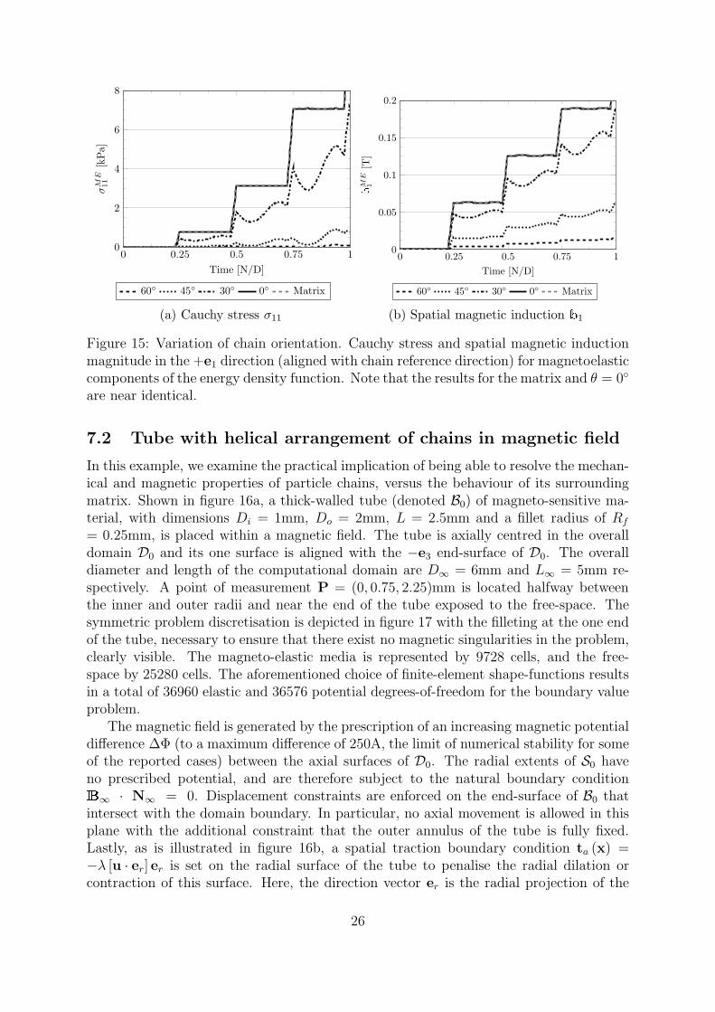
Similar trends are observed for the magnetic induction shown in figure 15b. Increasingthe offset angle reduced contribution from the magnetoelastic components of the energydensity function to the first component of the magnetic induction. These contributionswere also influenced by the chain stretch. Comparing figure 15a to figure 15b, it isobserved that the magnetoelastic contribution to the stress, which is dependent on |hc|2,is significantly more sensitive to the chain orientation than that of the magnetic induction,which has a linear dependence on h.

25

0 0.25 0.5 0.75 10

2

4

6

8

Time [N/D]

σM

E

11

[kPa]

60 45 30 0 Matrix

(a) Cauchy stress σ11

0 0.25 0.5 0.75 10

0.05

0.1

0.15

0.2

Time [N/D]

M

E

1[T

]

60 45 30 0 Matrix

(b) Spatial magnetic induction b1

Figure 15: Variation of chain orientation. Cauchy stress and spatial magnetic inductionmagnitude in the +e1 direction (aligned with chain reference direction) for magnetoelasticcomponents of the energy density function. Note that the results for the matrix and θ = 0

are near identical.

7.2 Tube with helical arrangement of chains in magnetic field

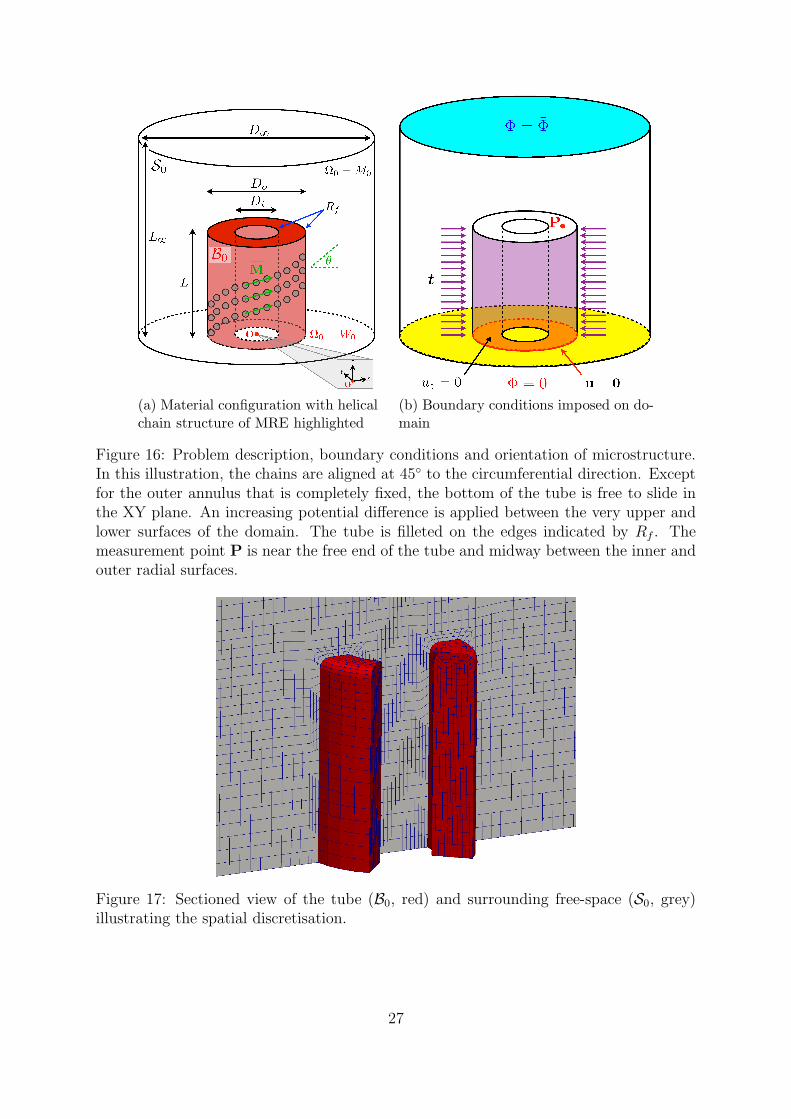
In this example, we examine the practical implication of being able to resolve the mechan-ical and magnetic properties of particle chains, versus the behaviour of its surroundingmatrix. Shown in figure 16a, a thick-walled tube (denoted B0) of magneto-sensitive ma-terial, with dimensions Di = 1mm, Do = 2mm, L = 2.5mm and a fillet radius of Rf

= 0.25mm, is placed within a magnetic field. The tube is axially centred in the overalldomain D0 and its one surface is aligned with the −e3 end-surface of D0. The overalldiameter and length of the computational domain are D∞ = 6mm and L∞ = 5mm re-spectively. A point of measurement P = (0, 0.75, 2.25)mm is located halfway betweenthe inner and outer radii and near the end of the tube exposed to the free-space. Thesymmetric problem discretisation is depicted in figure 17 with the filleting at the one endof the tube, necessary to ensure that there exist no magnetic singularities in the problem,clearly visible. The magneto-elastic media is represented by 9728 cells, and the free-space by 25280 cells. The aforementioned choice of finite-element shape-functions resultsin a total of 36960 elastic and 36576 potential degrees-of-freedom for the boundary valueproblem.

The magnetic field is generated by the prescription of an increasing magnetic potentialdifference ∆Φ (to a maximum difference of 250A, the limit of numerical stability for someof the reported cases) between the axial surfaces of D0. The radial extents of S0 haveno prescribed potential, and are therefore subject to the natural boundary conditionB∞ · N∞ = 0. Displacement constraints are enforced on the end-surface of B0 thatintersect with the domain boundary. In particular, no axial movement is allowed in thisplane with the additional constraint that the outer annulus of the tube is fully fixed.Lastly, as is illustrated in figure 16b, a spatial traction boundary condition ta (x) =−λ [u · er] er is set on the radial surface of the tube to penalise the radial dilation orcontraction of this surface. Here, the direction vector er is the radial projection of the

26

(a) Material configuration with helicalchain structure of MRE highlighted

(b) Boundary conditions imposed on do-main

Figure 16: Problem description, boundary conditions and orientation of microstructure.In this illustration, the chains are aligned at 45 to the circumferential direction. Exceptfor the outer annulus that is completely fixed, the bottom of the tube is free to slide inthe XY plane. An increasing potential difference is applied between the very upper andlower surfaces of the domain. The tube is filleted on the edges indicated by Rf . Themeasurement point P is near the free end of the tube and midway between the inner andouter radial surfaces.

Figure 17: Sectioned view of the tube (B0, red) and surrounding free-space (S0, grey)illustrating the spatial discretisation.

27

current position x = ϕ (X) onto the original tube outer surface, and the value of thepenalty parameter λ = 250N/mm3. As the integration of the traction was performed onthe reference domain, we define an equivalent Cauchy stress such that ta (x) = σ · n ≡[ta ⊗ n] · n. Thereafter, Nanson’s formula is used to define tA, the equivalent referentialtraction, such that tA dA = ta da = [ta ⊗ n] · JF−t · n dA. The linearisation of thevariation of the total potential energy, given in equation (43), was augmented with theadditional non-symmetric term

∆δΠext = −∫

Γt0

δu ·[∂ta∂u

·∆u+∂ta∂F

·∆F

](84)

to account for the deformation-dependent traction and normal.The tube is composed of a media similar to that used in section 7.1, with the exception

that we substitute an incompressible neo-Hookean material

Ωm,E0 =

µe

2

[I1 − 3

], (85)

where µe is the shear modulus, for the elastic part of the matrix energy density functionpreviously described in equation (59), and additionally utilise the volumetric energy func-tion provided in equation (83). The baseline material coefficients2 are given in table 2.

Table 2: Baseline values of the material parameters.

µe γ α n2, n5 n3, n6

30kPa 1490kPa 1 0.5µ0 −µ0

For this problem, we identify the material parameter n4 =µc

2as being related to the

small-strain chain shear modulus. The particle chains are assumed to, in the general case,be arranged in a helical formation within the media. The chain or helix angle θ is givenwith respect to the point-wise azimuthal tangent vector eθ, such that the average chaindirection M = M (X). The baseline chain parameters are listed in table 3.

Table 3: Baseline values of the chain parameters.

κ θ n4

µe1

300045 1

10000

A typical result of the fields for the magnetic quantities is presented in figures 18and 19. The magnetic field is aligned axially with the tube, with a strength weaker than

2 Numerical issues related the presence of a non-negligible Maxwell stress contribution have beenindicated previously [14]. As a first approximation, it is sometimes convenient to ignore the Maxwellcontributions [53]. For this problem of a compliant elastomer in the presence of a strong magnetic field,a large bulk modulus γ was required in order to maintain numerical stability. However, the use of lineardisplacement ansatz to represent quasi-incompressible media in some scenarios may lead to artificialvolumetric locking behaviour being exhibited [33]. Comparison of a selection of the results presentedlater with those derived using higher-order finite-elements produced, in the worst case, displacementfields with less than 8% difference between them. This suggested that the problem, while completelyfictitious, nonetheless remained locking free.

28

that of the far-field value present in the bulk of the material. A significant perturbation inthe scalar potential gradient is present at the end of the tube, ensuring that equation (7)2is satisfied. If there exists no particle chains, or M is aligned perpendicular to the appliedmagnetic field, then the resulting magnetic induction is aligned with h. However, as isshown in figure 18c, the magnetic induction is offset towards M should the dispersionparameter be sufficiently low. With the chosen material coefficients the tube compressesaxially and expands radially inwards. In figure 19b it is shown that the presence andalignment of the mechanically weak chains generate additional forces that not only furthershorten the tube, but also induces a significant degree of torsion in it.

h∞

(a) Contours of magneticfield strength. The blacklines outline the cross-section of the tube.

(b) Magnetic induction (ei-ther without particle chains,with κ = 1

3or with θ = 0)

(c) Magnetic induction (withparticle chains; parametersgiven in table 3)

Figure 18: Magnetic quantities (shown in B) at maximum scalar potential difference.The direction of the far-field magnetic field is indicated in figure 18a.

Hereafter, in a parametric study we investigate the influence of various material pa-rameters on the displacement recorded at P.

7.2.1 Variation of dispersion parameter

The introduction of the helically orientated particle chains of sufficient consistency signifi-cantly influence the mechanical response of the magneto-sensitive tube. As was previouslydescribed, magnetostriction of the media is induced by application of the magnetic field.However, if the chains are strongly formed, twist can be also induced in the tube. Giventhat the material remains compliant in the direction of the chains, the chains shortensignificantly in the direction of M thereby causing rotation of the material.

Figure 20 quantifies the resulting twist and shortening recorded at P under increasingmagnetic load. For the chosen material models, parameters and boundary conditions, thetotal displacement and magnetic field strength are quadratically related. Although the

29

(a) Displacement field either without par-ticle chains, with κ = 1

3or with θ = 0

(b) Displacement field with particle chains(parameters given in table 3)

Figure 19: A comparison of the displacement fields generated by ignoring or includingthe influence of particle chains. Vectors are coloured and scaled relative to the magnitudeof the displacement.

total twist is directly proportional to the dispersion parameter, the overall reduction inlength of the specimen remains largely independent of κ. Associated with the decrease inthe dispersion parameter is a marginal stiffening upon deformation in the axial direction.This is not completely offset by the increase in force generation properties in the axialdirection and therefore leads to decreased shortening of the tube. It should be noted thata significant twist is measured even when the particles constituting the chains are nothighly organised.

7.2.2 Variation of chain orientation

The chain orientation influences not only the degree of magnetisation of the particlechains, but also the line of action of the resulting force developed due to particle-particleinteractions. It is demonstrated visually in figure 21 that modification of the orientationangle, for strongly formed but compliant chains, affects both the amount of twist andcontraction induced in the tube.

Interestingly, as can be deduced from figure 21a, there exists some non-trivial optimal

30

0 10 20 30 40 500

2

4

6

8

Far-field magnetic field strength [kA/m]

Angleof

twist[deg]

κ = 1

3κ = 1

4κ = 1

6

κ = 1

12κ = 1

30κ = 1

3000

(a) Angle of twist

0 10 20 30 40 50−40

−30

−20

−10

0

Far-field magnetic field strength [kA/m]

Axialdisplacement[µm]

κ = 1

3κ = 1

30κ = 1

3000

(b) Axial displacement

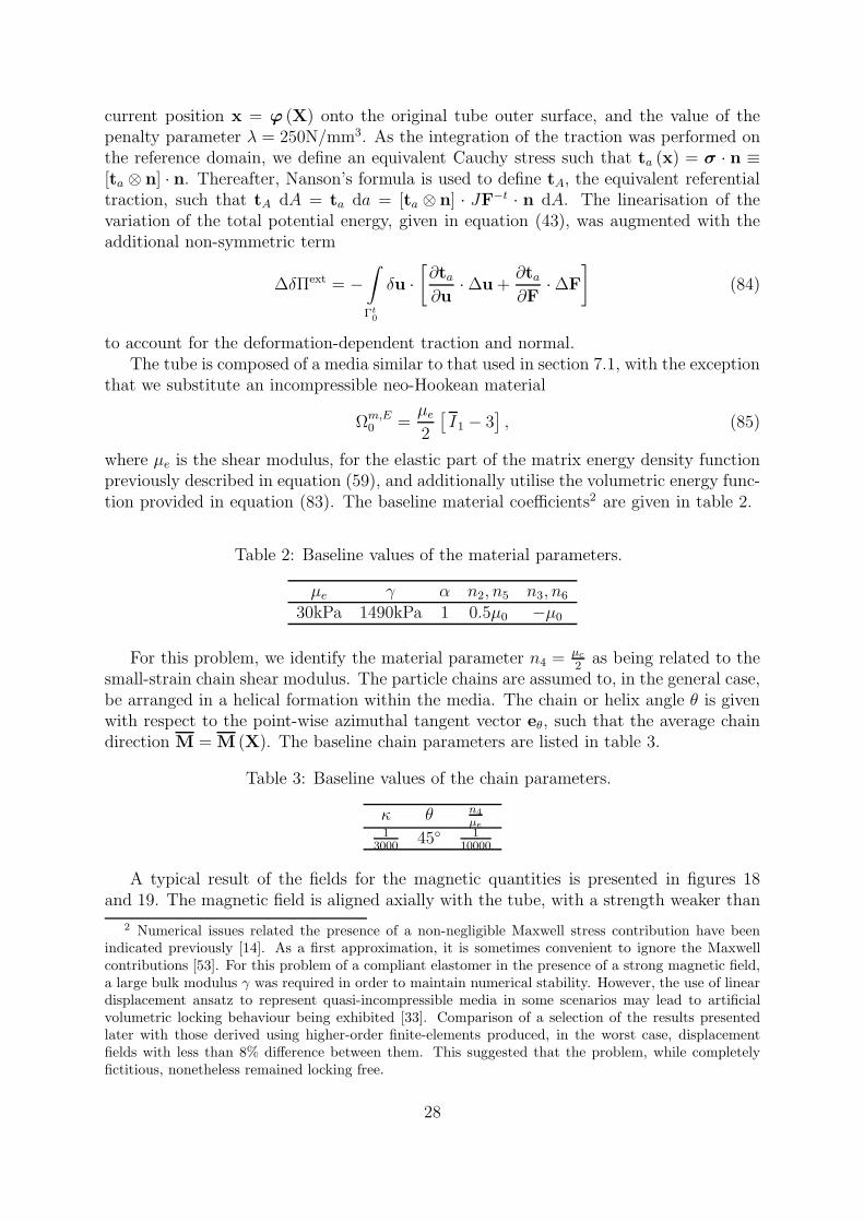
Figure 20: Influence of dispersion parameter on deformation at measurement point P

when the chains are mechanically weak (n4

µe= 1

10000). We consider the deformation field

shown in figure 19b to have undergone positive angle of twist.

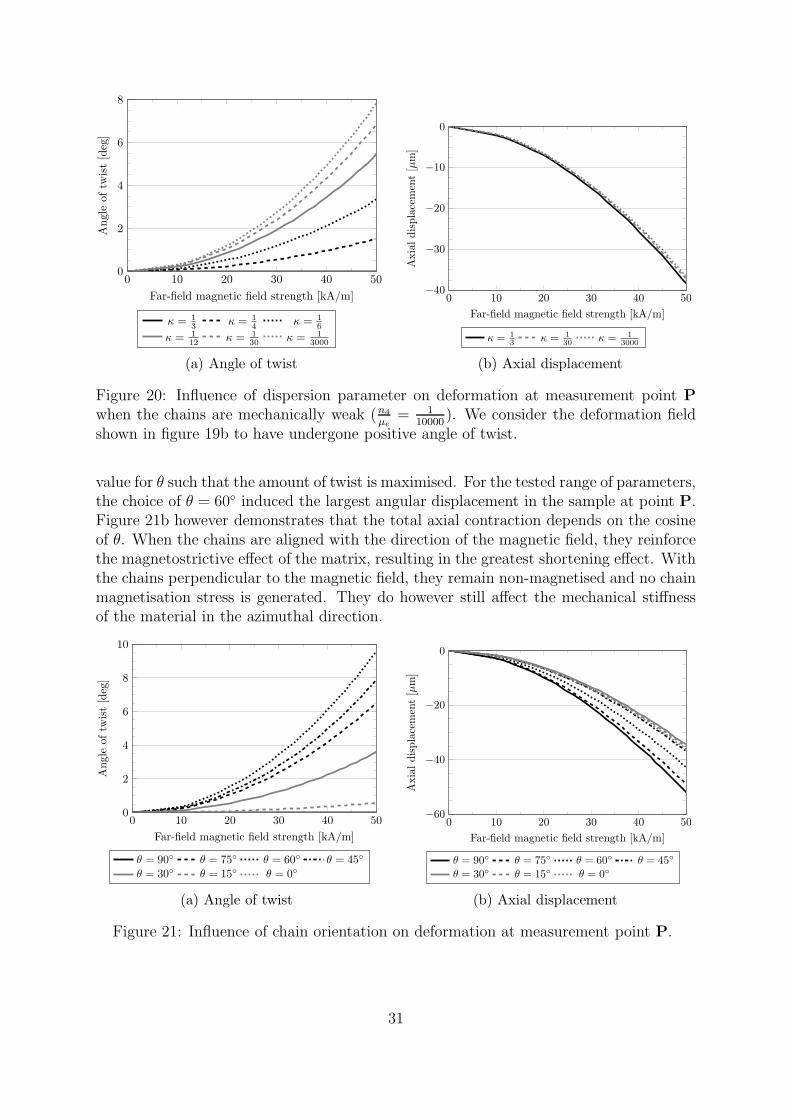
value for θ such that the amount of twist is maximised. For the tested range of parameters,the choice of θ = 60 induced the largest angular displacement in the sample at point P.Figure 21b however demonstrates that the total axial contraction depends on the cosineof θ. When the chains are aligned with the direction of the magnetic field, they reinforcethe magnetostrictive effect of the matrix, resulting in the greatest shortening effect. Withthe chains perpendicular to the magnetic field, they remain non-magnetised and no chainmagnetisation stress is generated. They do however still affect the mechanical stiffnessof the material in the azimuthal direction.

0 10 20 30 40 500

2

4

6

8

10

Far-field magnetic field strength [kA/m]

Angle

oftw

ist[deg]

θ = 90 θ = 75 θ = 60 θ = 45

θ = 30 θ = 15 θ = 0

(a) Angle of twist

0 10 20 30 40 50−60

−40

−20

0

Far-field magnetic field strength [kA/m]

Axialdisplacement[µm]

θ = 90 θ = 75 θ = 60 θ = 45

θ = 30 θ = 15 θ = 0

(b) Axial displacement

Figure 21: Influence of chain orientation on deformation at measurement point P.

31

7.2.3 Variation of chain elastic modulus

Previously the examined conditions were such that µc ≪ µe, inferring that the chainsprovide little mechanical reinforcement to the material. However, given that the typicalcomposition of such a material involves the ordered deposition of metallic particles in asoft substrate, it is more likely that in commercially applicable materials the differencebetween µc and µe is less extreme and µc ≥ µe. The actual ratio of these effective shearmoduli not only depends on the particulate composition, but also the inter-particle spaceoccupied by the compliant matrix. Towards the limit when µc ≫ µe, it can be assumedthat the micron-sized particles are in contact and effectively form very stiff reinforcingchains.

As is shown in figure 22, the ratio of the chain to matrix shear modulus plays asignificant role in the deformation of the tube resulting from magnetic loading alone. Itis observed that when the chain shear modulus is very large in comparison to that ofthe matrix, the induced direction of twist is opposite to that caused when the chains arecompliant. This is as the increased stiffness in chain direction ensures that direction ofdeformation is locally restricted primarily to transverse plane of isotropy. Associated withthis increase in chain stiffness is a reduction in the total twist and axial shortening. When

this ratio of stiffnesses isµc

µe= 2

n4

µe≈ 10, the magnetically-generated contractile force

in the circumferential direction is nearly perfectly balanced by the additional stiffnessprovided by the particle chains in this direction.

0 10 20 30 40 50

0

2

4

6

8

Far-field magnetic field strength [kA/m]

Angleof

twist[deg]

n4

µe

= 1

10000

n4

µe

= 1

10

n4

µe

= 1

2

n4

µe

= 1n4

µe

= 2 n4

µe

= 5 n4

µe

= 10 n4

µe

= 100

(a) Angle of twist

0 10 20 30 40 50−40

−30

−20

−10

0

Far-field magnetic field strength [kA/m]

Axialdisplacement[µm]

n4

µe

= 1

10000

n4

µe

= 1

10

n4

µe

= 1

2

n4

µe

= 1n4

µe

= 2 n4

µe

= 5 n4

µe

= 10 n4

µe

= 100

(b) Axial displacement

Figure 22: Influence of chain shear modulus on deformation at measurement point P.

Given that the influence of the chain stiffness has such a significant impact on thematerial deformation, we revisit the scenario described in section 7.2.1, but now prescribemechanically stiff chains. Figure 23 illustrates that a decrease in the dispersion parameteris associated with a notable decrease in axial shortening due to the increased materialstiffness. However, contrary to what has been observed previously, it is also correlatedwith a decrease in the amount of (negative) twist induced in the tube. At some non-trivial value of κ (which has not been resolved here), the force-generation properties of therelatively dispersed chain structures overcome the mechanical reinforcement. However,

32

as the chains become less dispersed the angular displacement of the tube is reducedsignificantly due to the increased stiffness in the circumferential direction.

0 10 20 30 40 50−2

−1.5

−1

−0.5

0

Far-field magnetic field strength [kA/m]

Angle

oftw

ist[deg]

κ = 1

3κ = 1

4κ = 1

6

κ = 1

12κ = 1

30κ = 1

3000

(a) Angle of twist

0 10 20 30 40 50−40

−30

−20

−10

0

Far-field magnetic field strength [kA/m]

Axialdisplacement[µm]

κ = 1

3κ = 1

4κ = 1

6

κ = 1

12κ = 1

30κ = 1

3000

(b) Axial displacement

Figure 23: Influence of dispersion parameter on deformation at measurement point P

when the chains are mechanically stiff (n4

µe= 100).

7.2.4 Variation of bulk and chain material coefficients

Depending on the experimental conditions and organisation of the particle micro-structuredeveloped during curing, the MRE may be expected to demonstrate different mate-rial behaviour [16, 65], namely axial contraction or elongation. The former effect hasbeen shown thus far, but in this section we will demonstrate that modification of themagneto-elastic material coefficients used in table 2 for the prototype energy functioncauses the material to exhibit different behaviours. In each instance, we vary boththe chain and bulk magneto-static and magneto-elastic material coefficients3 (by set-ting n2 + n3 = n5 + n6 = −0.5µ0) such that the magnetic induction within the materialremains qualitatively and quantitatively similar.

In figure 24 the outcome of using the material coefficients listed in table 4 are illus-trated. It is apparent both axial contraction and elongation of the tube can be modelledusing the energy density function. With reference to Danas et al. [16, fig. 5], the choiceof chain material coefficients is assumed to be linked to the microstructure and thereforedictate their magnetostrictive behaviour. In case 7, the magneto-elastic component isremoved, with no twist being induced and axial extension of the tube occurring due tothe influence of the free-space Maxwell stress. In contrast to the previous results andthose demonstrated in cases 1–6, positive values for n6 cause the chains to elongate andinduce a negative angle of twist.

Figure 25 demonstrates that an alteration of the coefficients governing the chain be-haviour can significantly alter that behaviour of the tube under a magnetic field. For the

3 Note that the convexity/concavity of the energy density function has not been examined.

33

0 10 20 30 40 50−5

0

5

10

Far-field magnetic field strength [kA/m]

Angleof

twist[deg]

Case 1 Case 2 Case 3 Case 4 Case 5Case 6 Case 7 Case 8 Case 9

(a) Angle of twist

0 10 20 30 40 50

−50

0

50

100

Far-field magnetic field strength [kA/m]

Axialdisplacement[µm]

Case 1 Case 2 Case 3 Case 4 Case 5Case 6 Case 7 Case 8 Case 9

(b) Axial displacement

Figure 24: Influence of material coefficients on deformation at measurement point P whenthe chains are mechanically weak (n4

µe= 1

10000). The material coefficients for each case are

listed in table 4.

Table 4: Chain and bulk material coefficients for cases in parameter study where n2 = n5

and n3 = n6.

Case n2, n5 n3, n6 Case n2, n5 n3, n6

1 µ0 −1.5µ0 6 −0.25µ0 −0.25µ0

2 0.75µ0 −1.25µ0 7 −0.5µ0 03 0.5µ0 −µ0 8 −0.75µ0 0.25µ0

4 0.25µ0 −0.75µ0 9 −µ0 0.5µ0

5 0 −0.5µ0

parameters listed in table 5, the axial deformation trends remain qualitatively similar tothose shown in figure 24. However, the force generation properties of the chains differ and,in some cases, the chain model no longer produces a force that reinforces the bulk modelleading to smaller displacements. This can be verified by comparing the twist directionsbetween the two sets of results. For comparable bulk properties, the twist direction haschanged although the compressive behaviour of the bulk remains largely the same.

Table 5: Chain and bulk material coefficients for cases in parameter study where n2 = n6

and n3 = n5.

Case n2, n6 n3, n5 Case n2, n6 n3, n5

1 µ0 −1.5µ0 6 −0.25µ0 −0.25µ0

2 0.75µ0 −1.25µ0 7 −0.5µ0 03 0.5µ0 −µ0 8 −0.75µ0 0.25µ0

4 0.25µ0 −0.75µ0 9 −µ0 0.5µ0

5 0 −0.5µ0

Although not presented here, using the parameters given in table 4 but mechanicallystrong chains (e.g. with n4

µe= 100) leads to material having both angular and axial

34

0 10 20 30 40 50

−5

0

5

Far-field magnetic field strength [kA/m]

Angleof

twist[deg]

Case 1 Case 2 Case 3 Case 4 Case 5Case 6 Case 7 Case 8 Case 9

(a) Angle of twist

0 10 20 30 40 50

−20

0

20

40

60

Far-field magnetic field strength [kA/m]

Axialdisplacement[µm]

Case 1 Case 2 Case 3 Case 4 Case 5Case 6 Case 7 Case 8 Case 9

(b) Axial displacement

Figure 25: Influence of material coefficients on deformation at measurement point P whenthe chains are mechanically weak (n4

µe= 1

10000). The material coefficients for each case are

listed in table 5.

deformation characteristics similar to those shown in figure 25.

8 Conclusions and discussion

Dispersion of the particle-chains in magneto-active polymers is an undesirable but preva-lent phenomenon as shown by several experiments, such as the ones presented in figure 1.Thus, it needs to be appropriately accounted for while constructing material models forthese functional elastomers. In this paper, we have presented a procedure to model theeffects due to dispersion of iron-particle chains in magneto-active elastomers. Based onsimilar developments in biomechanics, a probability-based structure tensor G that ac-counts for imperfect distribution of chains is defined and is used as an input to the energydensity function. This is based on a parameter κ ∈ [0, 1/3] that defines the degree ofanisotropy. Additionally, as a simplification, we decompose the energies of the matrixand the chain phases – the latter based on the definition of a ‘chain deformation gradient’Fc and a ‘chain magnetic field’ Hc.

As is seen from the parametric studies in sections 6 and 7, the proposed model is ableto capture the dependence of material response on the degree of anisotropy parameterκ. As κ → 0, one obtains a perfectly anisotropic material and leads to stiffening ofthe material in the anisotropy direction. On the other hand, as κ → 1/3, the materialtends to become isotropic and the response of the chain phase and the matrix phasetend to align. Moreover, as is exemplified in figure 22, even for the case of perfect chainformation, one can obtain completely different magnetoelastic responses from the samegeometry by making the chains stiffer or weaker than the bulk matrix. It has beenextensively demonstrated that very different behaviours can be elicited from a materialby appropriately modifying the constitutive model parameters.

A future course of research will be to employ image processing techniques to extract3-D chain distribution parameters from the X-ray CT scans. This data will then be used

35

to provide numerical values to the structure tensor at every mesh point and appropriatelymodel the material. Furthermore, using the models of rate-dependence and the experi-mental data on testing with magnetoelastic loading, a future aim is to provide physicallyand mathematically consistent material models for these smart polymers.

Acknowledgements

The support of this work by the European Research Council (ERC) through the AdvancedGrant MOCOPOLY is gratefully acknowledged by the authors. The authors also thankMr. Bastian Walter for MRE sample preparation and providing the images shown infigure 1.

References

[1] W. Bangerth, R. Hartmann, and G. Kanschat. deal.II – a general purpose objectoriented finite element library. ACM Trans. Math. Softw., 33(4):24/1–24/27, 2007.

[2] W. Bangerth, T. Heister, L. Heltai, G. Kanschat, M. Kronbichler, M. Maier,B. Turcksin, and T. D. Young. The deal.ii library, version 8.0. arXiv preprinthttp: // arxiv. org/ abs/ 1312. 2266v3 , 2013.

[3] A. Bermudez, R. Rodrıguez, and P. Salgado. A finite element method forthe magnetostatic problem in terms of scalar potentials. SIAM Journal onNumerical Analysis, 46(3):1338–1363, 2008. doi: 10.1137/06067568X. URLhttp://epubs.siam.org/doi/abs/10.1137/06067568X.

[4] A. Boczkowska and S. F. Awietjan. Smart composites of urethane elastomers withcarbonyl iron. Journal of Materials Science, 44(15):4104–4111, May 2009. ISSN0022-2461. doi: 10.1007/s10853-009-3592-7.

[5] A. Boczkowska, L. Czechowski, M. Jaroniek, and T. Niezgoda. Analysis of magneticfield effect on ferromagnetic spheres embedded in elastomer pattern. Journal ofTheoretical and Applied Mechanics, 48(3):659–676, 2010.

[6] H. Bose, R. Rabindranath, and J. Ehrlich. Soft magnetorheological elastomers asnew actuators for valves. Journal of Intelligent Material Systems and Structures, 23(9):989–994, 2012. doi: 10.1177/1045389X11433498.

[7] A. Bossavit. Computational Electromagnetism. Variational Formulations, Comple-mentarity, Edge Elements, volume 2 of Electromagnetism Series. Academic Press,San Diego, 1 edition, 1998. ISBN-13: 978-0121187101.

[8] I. A. Brigadnov and A. Dorfmann. Mathematical modeling of magneto-sensitiveelastomers. International Journal of Solids and Structures, 40(18):4659–4674,September 2003. ISSN 00207683. doi: 10.1016/S0020-7683(03)00265-8. URLhttp://linkinghub.elsevier.com/retrieve/pii/S0020768303002658.

36

[9] W. F. Brown. Magnetoelastic interactions. In C. Truesdell, editor, Springer Tractin Natural Philosophy. Springer-Verlag, Berlin Heidelberg New York, 1966.

[10] R. Bustamante. Transversely isotropic nonlinear magneto-active elastomers. ActaMechanica, 210(3-4):183–214, July 2010. ISSN 0001-5970. doi: 10.1007/s00707-009-0193-0.

[11] R. Bustamante and R. Ogden. Nonlinear magnetoelastostatics: Energy functionalsand their second variations. Mathematics and Mechanics of Solids, 18(7):760–772,2012. doi: 10.1177/1081286512448347.

[12] R Bustamante and K R Rajagopal. On a new class of electroelastic bodies. I. Pro-ceedings of the Royal Society A, 469(November 2012):20120521, 2013.

[13] R. Bustamante, A. Dorfmann, and R. W. Ogden. Numerical solu-tion of finite geometry boundary-value problems in nonlinear magnetoe-lasticity. International Journal of Solids and Structures, 48(6):874–883,March 2011. ISSN 00207683. doi: 10.1016/j.ijsolstr.2010.11.021. URLhttp://linkinghub.elsevier.com/retrieve/pii/S0020768310004208.

[14] R. Bustamante, A. Dorfmann, and R.W. Ogden. Numerical solutionof finite geometry boundary-value problems in nonlinear magnetoelastic-ity. International Journal of Solids and Structures, 48(6):874–883, 2011.ISSN 0020-7683. doi: http://dx.doi.org/10.1016/j.ijsolstr.2010.11.021. URLhttp://www.sciencedirect.com/science/article/pii/S0020768310004208.

[15] W. Chen, L. Sun, X. Li, and D. Wang. Numerical investigation on themagnetostrictive effect of magneto-sensitive elastomers based on a magneto-structural coupling algorithm. Smart Materials and Structures, 22(10):105012–1–105012–15, 2013. doi: 10.1088/0964-1726/22/10/105012. URLhttp://stacks.iop.org/0964-1726/22/i=10/a=105012.

[16] K. Danas, S. V. Kankanala, and N. Triantafyllidis. Experiments and modeling ofiron-particle-filled magnetorheological elastomers. Journal of the Mechanics andPhysics of Solids, 60:120–138, 2012. doi: 10.1016/j.jmps.2011.09.006.

[17] T. A. Davis. Algorithm 832: Umfpack v4.3 – an unsymmetric-pattern multifrontalmethod. ACM Transactions on Mathematical Software (TOMS), 30:196–199, 2004.doi: 10.1145/992200.992206.

[18] M. Destrade, B. Mac Donald, J. G. Murphy, and G. Saccomandi. At leastthree invariants are necessary to model the mechanical response of incom-pressible, transversely isotropic materials. Computational Mechanics, 52(4):959–969, April 2013. ISSN 0178-7675. doi: 10.1007/s00466-013-0857-4. URLhttp://link.springer.com/10.1007/s00466-013-0857-4.

[19] A. Dorfmann and R. W. Ogden. Nonlinear magnetoelastic deformations. QuarterlyJournal of Mechanics and Applied Mathematics, 57(7):599–622, 2004.

37

[20] A. Dorfmann and R. W. Ogden. Some problems in nonlinear magnetoelasticity.Journal of Applied Mathematics and Physics (ZAMP), 56(4):718–745, 2005.

[21] L. Dorfmann and R. W. Ogden. Nonlinear Theory of Electroelastic and Magnetoe-lastic Interactions. Springer, New York Heidelberg Dordrecht London, 2014.

[22] A. C. Eringen and G. A. Maugin. Electrodynamics of Continua, Vol. 1. Springer-Verlag, 1990.

[23] S. Federico and W. Herzog. On the anisotropy and inhomogeneity of permeabilityin articular cartilage. Biomechanics and Modeling in Mechanobiology, 7(5):367–78,October 2008. ISSN 1617-7940. doi: 10.1007/s10237-007-0091-0.

[24] E. Galipeau and P. Ponte Castaneda. The effect of particle shapeand distribution on the macroscopic behavior of magnetoelastic compos-ites. International Journal of Solids and Structures, 49(1):1–17, 2012.ISSN 0020-7683. doi: http://dx.doi.org/10.1016/j.ijsolstr.2011.08.014. URLhttp://www.sciencedirect.com/science/article/pii/S0020768311003076.

[25] T. C. Gasser, R. W. Ogden, and G. A. Holzapfel. Hyperelastic modelling of arteriallayers with distributed collagen fibre orientations. Journal of the Royal Society,Interface, 3(6):15–35, February 2006. ISSN 1742-5689. doi: 10.1098/rsif.2005.0073.

[26] M.W. Gee, C.M. Siefert, J.J. Hu, R.S. Tuminaro, and M.G. Sala. ML 5.0 smoothedaggregation user’s guide. Technical Report SAND2006-2649, Sandia National Labo-ratories, 2006.

[27] J. M. Ginder, S. M. Clark, W. F. Schlotter, and M. E. Nichols. Magnetostrictive phe-nomena in magnetorheological elastomers. International Journal of Modern PhysicsB, 16(17-18):2412–2418, 2002.

[28] M. A. Heroux. Aztecoo user’s guide. Technical Report SAND2004-3796, SandiaNational Laboratories, 2007.

[29] M. A. Heroux, R. A. Bartlett, V. E. Howle, R. J Hoekstra, J. J. Hu, T. G. Kolda,R. B. Lehoucq, K. R. Long, R. P. Pawlowski, E. T. Phipps, A. G. Salinger, H. K.Thornquist, R. S. Tuminaro, J. M. Willenbring, A. Williams, and K. S. Stanley. Anoverview of the Trilinos project. ACM Transactions on Mathematical Software, 31:397–423, 2005. doi: 10.1145/1089014.1089021.

[30] G. A. Holzapfel. Nonlinear solid mechanics. John Wiley & Sons Ltd., West Sussex,England, 2007. ISBN 0 471 82304 X.

[31] G. A. Holzapfel and T. C. Gasser. A viscoelastic model for fiber-reinforced com-posites at finite strains : Continuum basis, computational aspects and applica-tions. Computational Methods in Applied Mechanics and Engineering, 190:4379–4403, 2001.

[32] G. A. Holzapfel and R. W. Ogden. Constitutive modelling of arteries. Proceedingsof the Royal Society A, 466(2118):1551–1597, March 2010. ISSN 1364-5021. doi:10.1098/rspa.2010.0058.

38

[33] T. J. Hughes. The Finite Element Method: Linear Static and Dynamic FiniteElement Analysis. Dover Publications Inc., New York, USA, 2000. ISBN 978-0486411811.

[34] H. Jasak and Z Tukovic. Automatic mesh motion for the unstructured fi-nite volume method. Transactions of Famena, 30(2):1–20, 2006. URLhttp://www.scopus.com/inward/record.url?eid=2-s2.0-33847351298&partnerID=40&md5=1a

[35] A.A. Johnson and T.E. Tezduyar. Mesh update strategies in parallel finite elementcomputations of flow problems with moving boundaries and interfaces. Com-puter Methods in Applied Mechanics and Engineering, 119(1-2):73–94, 1994. URLhttp://www.scopus.com/inward/record.url?eid=2-s2.0-0028534257&partnerID=40&md5=f7b

[36] M. R. Jolly, J. D. Carlson, and B. C. Munoz. A model of the behaviour of mag-netorheological materials. Smart Materials and Structures, 5(5):607–614, October1996. ISSN 0964-1726. doi: 10.1088/0964-1726/5/5/009.

[37] S. V. Kankanala and N. Triantafyllidis. On finitely strained magnetorheological elas-tomers. Journal of the Mechanics and Physics of Solids, 52(12):2869–2908, December2004. ISSN 00225096. doi: 10.1016/j.jmps.2004.04.007.

[38] K S Kannan and A Dasgupta. A nonlinear galerkin finite-element theory for modelingmagnetostrictive smart structures. Smart Materials and Structures, 6(3):341, 1997.URL http://stacks.iop.org/0964-1726/6/i=3/a=011.

[39] Lance Ong-Siong Co Ting Keh, Jianfeng Zang, and Xuanhe Zhao.Magneto-rheological foams capable of tunable energy absorption. In2013 Proceedings of IEEE Southeastcon, pages 1–3. Ieee, April 2013.ISBN 978-1-4799-0053-4. doi: 10.1109/SECON.2013.6567490. URLhttp://ieeexplore.ieee.org/lpdocs/epic03/wrapper.htm?arnumber=6567490.

[40] S. Klinkel, C. Sansour, and W. Wagner. An anisotropic fibre-matrix material modelat finite elastic-plastic strains. Computational Mechanics, 35(6):409–417, December2004. ISSN 0178-7675. doi: 10.1007/s00466-004-0629-2.

[41] A. Kovetz. Electromagnetic theory. Oxford University Press, Oxford and New York,2000.

[42] L. D. Landau and E. M. Lifshitz. Electrodynamics of Continuous Media. PergamonPress, 1960.

[43] G. H. Livens. The theory of electricity. Cambridge University Press, 2 edition, 1962.

[44] H. V. Ly, F. Reitich, M. R. Jolly, and H. T. Banks. Simulations of particle dy-namics in magnetorheological fluids. Journal of Computational Physics, 155(1):160–177, 1999. ISSN 0021-9991. doi: http://dx.doi.org/10.1006/jcph.1999.6335. URLhttp://www.sciencedirect.com/science/article/pii/S0021999199963350.

[45] B. Marvalova. Modelling and Simulation, chapter Modelling of MagnetosensitiveElastomers, pages 245–260. I-Tech Education and Publishing, 2008. ISBN: 978-3-902613-25-7.

39

[46] G. A. Maugin. Continuum Mechanics of Electromagnetic Solids. North-Holland,1988.

[47] G. A. Maugin. On modelling electromagnetomechanical interactions in deformablesolids. International Journal of Advances in Engineering Sciences and Applied Math-ematics, 1:25–32, 2009.

[48] G. A. Maugin and A. C. Eringen. On the equations of the electrodynamics ofdeformable bodies of finite extent. Journal de Mecanique, 16(1):101–146, 1977.

[49] B. Nedjar. An anisotropic viscoelastic fibre-matrix model at finite strains: Con-tinuum formulation and computational aspects. Computer Methods in Applied Me-chanics and Engineering, 196(9-12):1745–1756, February 2007. ISSN 00457825. doi:10.1016/j.cma.2006.09.009.

[50] M. Ottenio, M. Destrade, and R. W. Ogden. Incremental magnetoelastic deforma-tions, with application to surface instability. Journal of Elasticity, 90(1):19–42, 2008.doi: 10.1007/s10659-007-9120-6.

[51] Y. H. Pao and K. Hutter. Electrodynamics for moving elas-tic solids and viscous fluids. Proceedings of the IEEE, 63(7):1011–1021, 1975. ISSN 0018-9219. doi: 10.1109/PROC.1975.9878. URLhttp://ieeexplore.ieee.org/lpdocs/epic03/wrapper.htm?arnumber=1451808.

[52] S. Rudykh and K. Bertoldi. Stability of anisotropic magnetorheologicalelastomers in finite deformations: A micromechanical approach. Jour-nal of the Mechanics and Physics of Solids, 61(4):949–967, 2013. ISSN0022-5096. doi: http://dx.doi.org/10.1016/j.jmps.2012.12.008. URLhttp://www.sciencedirect.com/science/article/pii/S0022509613000045.

[53] E. Salas and R. Bustamante. Numerical solution of some boundary valueproblems in nonlinear magneto-elasticity. Journal of Intelligent Mate-rial Systems and Structures, 2014. doi: 10.1177/1045389X14522533. URLhttp://jim.sagepub.com/content/early/2014/02/10/1045389X14522533.abstract.

[54] C. Sansour. On the physical assumptions underlying the volumetric-isochoric splitand the case of anisotropy. European Journal of Mechanics - A/Solids, 27(1):28–39,January 2008. ISSN 09977538. doi: 10.1016/j.euromechsol.2007.04.001.

[55] P. Saxena, M. Hossain, and P. Steinmann. A theory of finite deformation magneto-viscoelasticity. International Journal of Solids and Structures, 50(24):3886–3897,2013. doi: 10.1016/j.ijsolstr.2013.07.024.

[56] P. Saxena, M. Hossain, and P. Steinmann. Nonlinear magneto-viscoelasticity oftransversally isotropic magneto-active polymers. Proceedings of the Royal Society A,470:20140082, 2014.

[57] Mark D. Semon and John R. Taylor. Thoughts on the magnetic vector potential.American Journal of Physics, 64(11):1361–1369, 1996. doi: 10.1119/1.18400. URLhttp://scitation.aip.org/content/aapt/journal/ajp/64/11/10.1119/1.18400.

40

[58] M. Shams, M. Destrade, and R. W. Ogden. Initial stresses in elasticsolids : Constitutive laws and acoustoelasticity. Wave Motion, 48(7):552–567, 2011. ISSN 0165-2125. doi: 10.1016/j.wavemoti.2011.04.004. URLhttp://dx.doi.org/10.1016/j.wavemoti.2011.04.004.

[59] J. C. Simo, R. L. Taylor, and K. S. Pister. Variational and projection methods forthe volume constraint in finite deformation elasto-plasticity. Computer Methods inApplied Mechanics and Engineering, 51:177–208, 1985. doi: 10.1016/0045-7825(85)90033-7.

[60] T. M. Simon, F. Reitich, M. R. Jolly, K. Ito, and H. T. Banks.The effective magnetic properties of magnetorheological fluids. Math-ematical and Computer Modelling, 33(1–3):273–284, 2001. ISSN 0895-7177. doi: http://dx.doi.org/10.1016/S0895-7177(00)00244-2. URLhttp://www.sciencedirect.com/science/article/pii/S0895717700002442.Computation and control VI proceedings of the sixth Bozeman conference.

[61] A. J. M. Spencer. Theory of invariants. In A. C. Eringen, editor, Continuum Physics,Vol. I, pages 239–353. Academic, New York, 1971.

[62] D. J. Steigmann. On the Formulation of Balance Laws for Electromag-netic Continua. Mathematics and Mechanics of Solids, 14(4):390–402, Septem-ber 2009. ISSN 1081-2865. doi: 10.1177/1081286507080808. URLhttp://mms.sagepub.com/cgi/doi/10.1177/1081286507080808.

[63] P. Steinmann. Mechanics and Electrodynamics of Magneto- and Electro-elasticMaterials, chapter Computational Nonlinear Electro-Elasticity – Getting Started.Springer Vienna, 2011. doi: 10.1007/978-3-7091-0701-0 5.

[64] H. F. Tiersten. Coupled magnetomechanical equations for magnetically saturatedinsulators. Journal of Mathematical Physics, 5(9):1298–1318, 1964.

[65] Z. Varga, G. Filipcsei, and M. Zrınyi. Smart composites with controlled anisotropy.Polymer, 46:7779–7787, 2005. doi: 10.1016/j.polymer.2005.03.102.

[66] Z. Varga, G. Filipcsei, and M. Zrinyi. Magnetic field sensitive functional elas-tomers with tuneable elastic modulus. Polymer, 47(1):227–233, January 2006. ISSN00323861. doi: 10.1016/j.polymer.2005.10.139.

[67] F. Vogel, R. Bustamante, and P. Steinmann. On some mixedvariational principles in magneto-elastostatics. International Jour-nal of Non-Linear Mechanics, 51(0):157 – 169, 2013. ISSN 0020-7462. doi: http://dx.doi.org/10.1016/j.ijnonlinmec.2012.12.005. URLhttp://www.sciencedirect.com/science/article/pii/S0020746212001989.

[68] F. Vogel, J-P. Pelteret, S. Kassmair, and P. Steinmann. Magnetic force and torqueon particles subject to a magnetic field. European Journal of Mechanics A/Solids,2014. Accepted.

41

[69] D. K. Vu, P. Steinmann, and G. Possart. Numerical modelling of non-linear electroe-lasticity. International Journal for Numerical Methods in Engineering, 70:685–704,2007. doi: 10.1002/nme.1902.

[70] M. Yalcintas and H. Dai. Vibration suppression capabilities of magnetorheologicalmaterials based adaptive structures. Smart Materials and Structures, 13(1):1–11,2004.

[71] Y.M. Yin, L.Z. Sun, and J.S. Chen. Magneto-elastic modeling of com-posites containing chain-structured magnetostrictive particles. Journalof the Mechanics and Physics of Solids, 54(5):975–1003, 2006. ISSN0022-5096. doi: http://dx.doi.org/10.1016/j.jmps.2005.11.007. URLhttp://www.sciencedirect.com/science/article/pii/S002250960500222X.

[72] Q.-S. Zheng. Theory of representations for tensor functions - A unified invariant ap-proach to constitutive equations. Applied Mechanics Review, 47(11):545–587, 1994.

[73] X-J. Zheng and X. Wang. Analysis of magnetoelastic interaction ofrectangular ferromagnetic plates with nonlinear magnetization. Interna-tional Journal of Solids and Structures, 38(48–49):8641–8652, 2001. ISSN0020-7683. doi: http://dx.doi.org/10.1016/S0020-7683(01)00100-7. URLhttp://www.sciencedirect.com/science/article/pii/S0020768301001007.

42