modelling of flows through hydraulic · pdf filemodelling of flows through hydraulic...
TRANSCRIPT
MODELLING OF FLOWS
THROUGH HYDRAULIC STRUCTURES
AND INTERACTION WITH SEDIMENT
A thesis submitted to the Cardiff University
In candidature for the degree of
Doctor of Philosophy
by:
Shervin Faghihirad
B.Sc., M.Sc.
Cardiff School of Engineering
Cardiff University
April 2014

DECLARATION
This work has not previously been accepted in substance for degree and is not concurrently
being submitted in candidature for any degree.
Signed........................................................................................................................(candidate)
Date........................................................................................................................
STATEMENT 1
This thesis is the result of my own investigations, except where otherwise stated.
Other sources are acknowledged by footnotes giving explicit references. A bibliography is
appended.
Signed........................................................................................................................(candidate)
Date........................................................................................................................
STATEMENT 2
I hereby give consent for my thesis, if accepted to be available for photocopying and for
interlibrary loan, and for the title and summary to be made available to outside organisations.
Signed........................................................................................................................(candidate)
Date........................................................................................................................
i
ABSTRACT
A three-dimensional layer integrated morphodynamic model has been developed to predict
the hydrodynamic, sediment transport and morphological processes in a regulated reservoir.
The model was based on an existing sediment transport model, with improvements being
made. A bed evolution module based on the mass balance equation has been developed to
determine the bed level change due to sediment transport. The horizontal eddy viscosity
coefficient was equated to the depth averaged eddy viscosity, based on the horizontal velocity
distribution while the vertical eddy viscosity coefficient was evaluated using the layer
integrated form of the - equations. This scheme enhances the accuracy of the computed
velocity and suspended sediment concentration distributions.
The highly accurate ULTIMATE QUICKEST scheme was used to represent the advective
terms in solving the advective-diffusion equation for suspended sediment transport. An
explicit finite difference scheme has been developed for the bed sediment mass balance
equation to calculate bed level changes. The numerical model was verified against laboratory
data obtained from experiments in a trench and a partially closed channel.
A physical model was constructed to represent the flow, sediment transport and
morphodynamic processes in Hamidieh regulated reservoir. The physical model was
designed based on the Froude similarity law and was undistorted. The model sediment size
was determined in such a manner that the same ratio of particle fall velocity to shear velocity
is maintained for both the model and prototype reservoir. Stokes law was used in calculating
the particle fall velocity. The physical model results confirmed that the normal water surface
elevation in the reservoir should increase by up to 25 cm in order to reach the nominal flow
discharge diverted to the intakes.
The numerical model was then applied to the scaled physical model of the reservoir and the
associated water intakes and sluice gates. Various scenarios were tested to investigate the
effects of different situations of diverting flow and sediment transport regimes, as well as to
establish how these operations affect the morphodynamic processes in the reservoir and the
vicinity of hydraulic structures. The model predictions agreed with measured data generally
well. The numerical model results revealed the possibility of forming sedimentary islands in
the regulated reservoir and it is uneconomical to set up a dredging zone near the one of the
intakes. In summary, the integrated numerical and physical modelling approach showed
many benefits and could help to optimize time and budget for design hydraulic structures.
Key words: morphodynamic numerical model, turbulent flow, regulated reservoir, three-
dimensional flow, laboratory tests.
ii
ACKNOWLEDGEMENTS
I would like to express my sincere gratitude to my supervisors Professor Binliang Lin and
Professor Roger A. Falconer for the help, guidance and support they were given during this
research project. The author wishes to thank the Water Research Institute in Iran for assisting
in the laboratory physical model tests.
I am eternally grateful to my parents, my wife and my son for their continuous love,
enormous support and encouragement.
iii
Table of Contents Chapter One-Introduction 1
1.1 The essence of the research 1
1.2 Reservoirs 2
1.2.1 General synthesis 2
1.2.2 Regulated reservoirs 4
1.3 Goals 6
1.4 The structure of thesis 7
Chapter Two-Literature Review 8
2.1 Introduction 8
2.2 Hydrodynamic numerical models 8
2.3 Sediment transport numerical models 15
2.4 Morphodynamic numerical models 20
2.5 Model applications to reservoir 25
2.6 Physical models 28
2.7 Summary 32
Chapter Three-Physical Modelling (Theory and Experimental Study) 34
3.1 Introduction 34
3.2 Hydraulic simulation theory 34
3.3 Undistorted model attitudes 36
3.4 Introduction to Hamidieh regulated reservoir study 43
3.5 Project background 43
3.6 Model design and testing 47
3.6.1 Designing scale 47
3.6.2 Construction and material 50
3.6.3 Measuring systems 52
3.7 Scenarios and results of physical model 55
3.7.1 Flow and hydrodynamic section 55
3.7.2 Sediment transport and morphodynamic section 62
3.7.3 Considering scale effects for Hamidieh physical model 70
3.8 Conclusion 71
3.9 Summary 74
Chapter Four-Numerical Modelling (Governing Equations and Solutions) 75
4.1 Introduction 75
4.2 Governing hydrodynamic equations 75
iv
4.2.1 Layer integrated hydrodynamic equations 76
4.2.2 Depth integrated hydrodynamic equations 79
4.2.3 Boundary conditions for the hydrodynamic model 80
4.2.4 Gates simulation 81
4.2.4.1 Validation of the numerical technique 82
4.2.4.2 Results in the validated example 83
4.3 Turbulence model 84
4.3.1 Mixing length model 85
4.3.2 model 87
4.3.2.1 Layer integrated model 88
4.3.2.2 Boundary conditions for the turbulence model 89
4.4 Sediment transport 91
4.4.1 Suspended sediment transport model (3D) 91
4.4.1.1 Boundary conditions for suspended the sediment transport model 93
4.4.2 Bed load transport 96
4.5 Bed level change equation 96
4.6 Discretization and numerical solution for hydrodynamic equations 97
4.6.1 Representation of closed boundary conditions 101
4.7 Discretization and numerical solution for sediment transport equations 103
4.8 Discretization and numerical solution for bed Level change equation 105
4.9 Summary 110
Chapter Five-Model Verification 111
5.1 Introduction 111
5.2 Test Case 1: flow, sediment transport and bed level changes in a trench 111
5.2.1 A sensitive analysis on vertical layers 115
5.3 Test Case Two: partially closed channel 118
5.3.1 Hydraulic conditions 118
5.3.2 Boundary conditions and input parameters 118
5.3.2.1 Fluid velocities 118
5.3.2.2 Sediment concentration and transport rate 119
5.3.3 Model results 119
5.3.3.1 Flow pattern and fluid velocity 119
5.3.3.2 Sediment concentration 122
5.3.3.3 Sediment transport 125
5.3.3.4 Bed level changes 126
v
5.4 Summary 128
Chapter Six-Model Application 129
6.1 Introduction 129
6.2 A case study (Hamidieh Regulated Reservoir) 129
6.2.1 Objectives 130
6.3 Numerical model study 131
6.4 Flow and hydrodynamic simulation 132
6.5 Sediment transport simulation 140
6.6 Morphodynamic 144
6.7 Conclusion and discussion for the results of numerical model 149
6.8 Summary 151
Chapter Seven-Conclusions and recommendations 152
7.1 Summary of the research 152
7.2 The main findings of the research 153
7.3 The novelties of the research 155
7.4 Recommendation for further study 156
References 158
vi
List of Figures Figure 1.1 Number and purpose of registered dams in ICOLD 3
Figure 1.2 The distributed single-purpose dams related to objectives 3
Figure 1.3 The distributed multiple-purpose dams related to objectives 4
Figure 3.1 Relation between sieve diameter and fall velocity for naturally worn
quartz particles falling alone in quiescent distilled water of infinite
extent (U.S. Inter-Agency Committee on Water Resources,
Subcommittee on Sedimentation, 1957)
41
Figure 3.2 Bed shape criteria (Zwamborn 1969) 42
Figure 3.3 Location map of Hamidieh town 44
Figure 3.4 Aerial photo of current situation of Hamidieh regulated reservoir 44
Figure 3.5 The layout of current situation of Hamidieh regulated reservoir and
associated structures (WEOKP 2001)
45
Figure 3.6 Pictures of existing hydraulic structures of Hamidieh regulated
reservoir
45
Figure 3.7 Plan view of Hamidieh regulated reservoir and associated structures 46
Figure 3.8 Two intakes physical model 51
Figure 3.9 The installation stage of the physical model 51
Figure 3.10 Constructing bed topography for the reservoir model 52
Figure 3.11 Completed physical model 52
Figure 3.12 Tail gate for regulating and measuring water level, gage mark in
trapezoidal channel and digital limnimeter for measuring head
water on weir
53
Figure 3.13 Putting gage marks in the physical model 54
Figure 3.14 Mechanical current meter system (A.OTT KEMPTEN, type:
, NO.52051-meter support on rod of 9 mm diameter)
54
Figure 3.15 Sediment injection system and accessories (gearbox, shaft and
storage box)
54
Figure 3.16 Hydrometer analysis for sediment samples 55
Figure 3.17 Determination of sediment concentration 55
Figure 3.18 Location of velocity measuring points in vicinity of Azadegan
intake
56
Figure 3.19 Location of velocity measuring points in the vicinity of Chamran
intake
57
Figure 3.20 Flow pattern in a regulatory condition at normal water level
(20.20m) in the Hamidieh reservoir (Test No. 5 explained in Table
3.5)
58
Figure 3.21 Location of permeable groins on the opposite bank 61
Figure 3.22 Location of permeable guide wall for Chamran intake 61
Figure 3.23 Obstruction of reservoir width by a permeable wall 62
Figure 3.24 Locations of sediment concentration and gradation sampling points
(CAZ=Concentration in Azadegan Intake, CCH=Concentration in
63

vii
Chamran Intake and CRR, CRM and CRL=Concentration in the
reservoir)
Figure 3.25 Changes sediment dischrage in reservoir and sediment discharge
entry to different hydraulic structures
64
Figure 3.26 The dredging zone in front of Azadegan intake before running the
sediment transport scenarios
66
Figure 3.27 The dredging zone in front of Azadegan intake after tests 67
Figure 3.28 Scour zone in front of the right sluice gates 68
Figure 3.29 Scouring zone in front of the left side sluice gates 68
Figure 3.30 Bed level changes after 48.5 hours in 6 section profiles (scenario
S.1)
69
Figure 3.31 Morphological changes in Hamidieh regulated reservoir (physical
model) after sediment transport experiments
70
Figure 3.32 The Proposed layout for Chamran Intake 72
Figure 4.1 Coordinate system for layer integrated equations 76
Figure 4.2 Coordinate system for wave profile 80
Figure 4.3 Plan and section views of channel 82
Figure 4.4 Submerged gate flow 83
Figure 4.5 Relationship between bed level above base line and depth below
datum
96
Figure 4.6 Finite-difference notation for closed boundary 102
Figure 4.7 Computational space staggered grid system 106
Figure 4.8 Plotted warm-up period ( = initial time steps and = total
computational time)
109
Figure 5.1 The layout of model trench 111
Figure 5.2 Comparisons of velocity profiles in the trench 113
Figure 5.3 Comparisons of sediment concentration profiles in the trench 114
Figure 5.4 Bed level profiles in the trench after 15 hours (Present N.M =Present
Numerical Model)
115
Figure 5.5 Comparisons of velocity profiles in the trench for sensitive analysis 116
Figure 5.6 Comparisons of sediment concentration profiles in the trench for
sensitive analysis
117
Figure 5.7 Schematic view of partially closed channel 118
Figure 5.8 The velocity field 120
Figure 5.9 Streamline pattern along the channel 121
Figure 5.10 Comparison of depth averaged velocities along streamline B for
different models
122
Figure 5.11 Comparison of depth averaged velocities along streamline C for
different models
122
Figure 5.12 Sediment concentration distribution obtained from the present
model
123
Figure 5.13 Sediment concentration distribution obtained from ESMOR 123

viii
Figure 5.14 Concentration profiles in streamline A 124
Figure 5.15 Concentration profiles in streamline B 124
Figure 5.16 Concentration profile in recirculation zone 125
Figure 5.17 Suspended sediment transport in streamline B 126
Figure 5.18 Suspended sediment transport in streamline C 126
Figure 5.19 The rate of bed level change (mm/hr) obtained using the present
model
127
Figure 5.20 Erosion (interval=4mm/hr) in ESMOR model 127
Figure 5.21 Sedimentation (interval=2mm/hr) in ESMOR model 127
Figure 6.1 Plan view of Hamidieh regulated dam and associated structures 130
Figure 6.2 The initial bathymetry of Hamidieh, physical model scale 133
Figure 6.3 Numerical model predicted flow pattern and speed contours for
scenario S.1
135
Figure 6.4 Model predicted velocity distributions and measured velocities at
0.6D from water surface for scenario S.1 (Az=Azadegan Intake,
Ch=Chamran Intake, Nu=Numerical, Ph=Physical and TD=Total
Depth (i.e. calculated by 3D layer-integrated numerical model
along whole depth))
135
Figure 6.5 Numerical model predicted flow pattern and speed contours for (a)
Scenario S.2 and (b) Scenario S.3
138
Figure 6.6 Eddy viscosity results (Eddy_H= depth integrated horizontal eddy
viscosity and Eddy_VL1…5= layer integrated vertical eddy
viscosity for each layer) for hydrodynamic scenario S.1
139
Figure 6.7 Pattern of suspended sediments concentrations (SSC), scenario S.4 142
Figure 6.8 Pattern of suspended sediments concentrations (SSC), scenario S.5 142
Figure 6.9 Pattern of suspended sediments concentrations (SSC), scenario S.6 143
Figure 6.10 Bed level changes after 48.5 hours in 6 section profiles (scenario
S.7)
146
Figure 6.11 Initial bathymetry for scenarios S.8 and S.9 147
Figure 6.12 Computed bathymetry after 8 hours for scenario S.8 148
Figure 6.13 Computed bathymetry after 8 hours for scenario S.9 148
ix
List of Tables Table 3.1 Criteria for rough turbulent flow 38
Table 3.2 Ratios of hydraulic and sediment parameters 49
Table 3.3 Suspended sediment size frequency distribution in prototype and the
model
49
Table 3.4 Velocity values obtained from physical model and converted to
prototype
57
Table 3.5 Results of hydraulic experiments, Discharge (m3/s), Bay opening
(m2) and Water surface Elevation (m) (data transferred to
prototype)
59
Table 3.6 Sediment grain size for different hydraulic and sediment transport
scenarios
65
Table 3.7 Hydraulic model parameters of sluice gates' testing scenarios 67
Table 3.8 Main hydraulic and sediment parameters for morphodynamic
scenario
69
Table 4.1 The characteristics of validation scenario for gates simulation 82
Table 4.2 Results of the improved numerical model 83
Table 4.3 Results of the analytic solution 84
Table 4.4 Mixing length model assessment 87
Table 4.5 Standard model assessment 91
Table 5.1 The maximum rates for erosion and deposition in different
numerical models
128
Table 6.1 Hydrodynamic parameters of scenario S.1 132
Table 6.2 Comparison between velocity values obtained from numerical and
physical models for scenario S.1
134
Table 6.3 The characteristic for extra hydrodynamic scenarios 137
Table 6.4 Main parameters for sediment transport scenarios 141
Table 6.5 SSC measured and predicted at sampling points 143
Table 6.6 Main hydraulic and sediment parameters for morphodynamic
scenarios
145

x
Notations
cross-sectional area
a reference level
B channel width
C Chézy - coefficient
vegetation drag coefficient
eddy viscosity coefficient
suspended sediment concentration in the prototype
coefficient of approach velocity
air/fluid resistance coefficient
grain roughness coefficient
, , , empirical constants in turbulence model
D representative sediment grain size
dimensionless particle parameter
hydraulic diameter
Dr sediment particle size scale ratio
20% particle diameter
50% particle diameter
90% particle diameter
Coriolis parameter
f Darcy–Weisbach friction factor
Froude number
force scale ratio
grain (Densimetric) Froude number
gravitational acceleration
total depth of flow
depth of flow
bed roughness length
scale ratio (inverse of scale 1 : )
lh layer thickness
layer thicknesses in the x-direction for pervious and current time
step

xi
layer thicknesses in the y-direction for pervious and current time
step
Manning coefficient
nr Manning’s roughness scale ratio
p(=UH) discharges per unit width in the x direction
p porosity of the sediment material
q(=VH) discharges per unit width in the y direction
source discharge per unit horizontal area
xbxs qq ,, total sediment load transport rates per unit width in the x direction
ybys qq ,, total sediment load transport rates per unit width in the y direction
discharge scale ratio
suspended sediment load discharge in the model
water discharge in the model
bed load transport rate
Reynolds number
grain size Reynolds number
hydraulic radius
slope of the energy gradient
equilibrium concentration at a reference level
bed load concentration
effective correlation the shape factor
specific gravity
dimensionless bed-shear stress parameter (or transport stage
parameter)
time scale ratio
U,V depth averaged velocity components in the x and y directions
respectively
depth averaged shear velocity
effective particle velocity
velocity of bed load particles
components of velocity in the
shear velocity
xii
depth averaged flow speed (=√
velocity scale ratio
Weber number
wind speed
, wind velocity components in the x, y directions, respectively
settling (fall) velocity
dimensionless suspension parameter
bed level
distance to the wall at the first grid point
contraction coefficient
relaxation coefficient
momentum correction factor for a non-uniform vertical velocity
profile
specific weight of water
specific weight of sediment particles
sHt
storage term
siltation height
, horizontal and vertical eddy viscosities, respectively
sediment mixing coefficient in x, y, z direction, respectively
water surface elevation above datum
turbulent velocity
turbulent length scale
a new turbulence length scale
von Karman’s constant
dynamic viscosity
kinematic viscosity
fluid density
air density
sediment density
Schmidt numbers is the horizontal and vertical directions
respectively

xiii
components of the stress tensor in the zx and zy plane,
respectively
bed shear stress
critical bed shear stress

1
Chapter One
Introduction
1.1 The essence of the research
The central concern of the dissertation is to study hydraulic flows and sediment phenomena
through hydraulic structures in a regulated reservoir. The flow patterns in and around most
hydraulic structures are complex, three-dimensional, and highly turbulent. Furthermore, the
use of a three-dimensional (3-D) numerical model instead of a two-dimensional (2-D), depth-
averaged one is strongly recommended where sediment concentration changes in the vertical
profile are considerable such as near intakes and sluice gates. For these reasons, in order to
understand the impact of hydraulic structures on the hydrodynamic, sediment transport
processes and morphological changes in regulated reservoirs it is often necessary to
investigate these processes in three dimensions. The main goal of this research is to refine
existing numerical (3-D) model and develop a proposed mathematical scheme for predicting
the bed level changes in the vicinity of hydraulic structures where complex geometry, flow
pattern, turbulence and sediment concentration distribution have important effects on the
simulation results.
The type of the research is an application research and how uses a mathematical knowledge
in order to simulate natural process correctly for a real case study. In design a real and
complex water regulated reservoir both physical and numerical models are used. Currently,
physical models are still widely used as an essential tool to obtain information about the
above processes. Generally speaking, physical models need a long time to construct and are
expensive to run, particularly if large scale models are involved. Numerical models offer the
possibility to test various scenarios which are difficult to test in a physical model and this
ability will be used for the future operation of the regulated reservoir. Besides, the project
cost can be reduced and more options considered.

2
1.2 Reservoirs
1.2.1 General synthesis
Dams have been constructed worldwide to reduce risks associated with flood hazards, to
harness energy for industry and commerce, and to help secure a reliable source of water for
domestic, industrial and/or agricultural use.
Most of the existing dams are single-purpose dams, but the number of multipurpose dams is
increasing. According to the most recent publication of the World Register of Dams (ICOLD,
http://www.icold-cigb.org/GB/Dams/role_of_dams.asp), irrigation is by far the most common
purpose of dams. Among the single purpose dams, 50 % are for irrigation, 18% for
hydropower (production of electricity), 12% for water supply, 10% for flood control, 5% for
recreation and less than 1% for navigation and fish farming.
Presently, irrigated land covers about 277 million hectares (ICOLD, http://www.icold-
cigb.org/GB/Dams/role_of_dams.asp), i.e. about 18% of world's arable land but it is
responsible for around 40% of crop output and employs nearly 30% of population spread
over rural areas. With the large population growth expected for the next decades, irrigation
must be expanded to increase the food production capacity. It is estimated that 80% of
additional food production by the year 2025 will need to come from irrigated land (ICOLD,
http://www.icold-cigb.org/GB/Dams/role_of_dams.asp). Even with the widespread measures
to conserve water by improvements in irrigation technology, the construction of more
reservoirs will be required.
Runoff waters are a natural resource. For developing countries, storing water is often vital
and in many cases, the only means to conserve economically this natural resource
(http://icold-cigb.org/GB/World_register/general_synthesis.asp). Reservoirs mainly give
guarantee of water supply for irrigation, domestic and industrial use during droughts and
reduce negative impacts of floods. Figures 1.1, 1.2 and 1.3 present the purpose of dams
constructed worldwide and their attitudes. Referenced dams can be broken in two main
categories:
Single-purpose dams (26938) or 71.6% dams.
Multi-purpose dams (9321) or 24.8% dams.
Those data are gathered by International Commission on Large Dams (ICOLD,
http://www.icold-cigb.org/GB/World_register/general_synthesis.asp) and a basic criterion is
a structural dam not less than 15 meters higher than its foundation.
Demand for water is steadily increasing and would reach 2-3 percent per year over the
coming decades. With their present aggregate storage of about 14913 , dams clearly

3
make a significant contribution to the efficient management of the finite water resources that
are unevenly distributed and subject to large seasonal fluctuations. Many more dams need to
be built to ensure proper use of these resources, in accordance with ICOLD policy (ICOLD,
http://www.icold-cigb.org/GB/World_register/general_synthesis.asp) set out in the "Position
Paper Dams and Environment".
Figure 1.1 Number and purpose of registered dams in ICOLD
Figure 1.2 The distributed single-purpose dams related to objectives
13468
4914
3205 2603
1338
112 39
1259
5617
3775 3984 4579
2810 547 1342 827
0
2000
4000
6000
8000
10000
12000
14000
16000
I H S C R N F X
Single
Multiple
Codes: I Irrigation H Hydropower S Water Suply C Flood Control R Recreation N Navigation F Fish breeding X Others 37641 dams data corresponding to registered dams only
50%
18%
12%
10%
5%
1%
5% Irrigation(13468)
Hydropower(4914)
Water supply(3205)
Flood control(2603)
Recreation(1338)
Navigation/fish farming(151)
Others(1295)
4
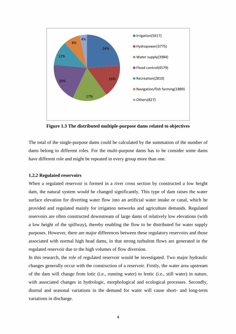
Figure 1.3 The distributed multiple-purpose dams related to objectives
The total of the single-purpose dams could be calculated by the summation of the number of
dams belong to different roles. For the multi-purpose dams has to be consider some dams
have different role and might be repeated in every group more than one.
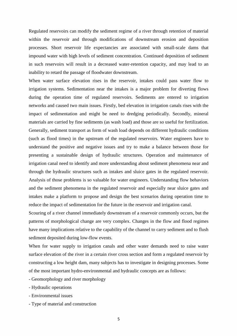
1.2.2 Regulated reservoirs
When a regulated reservoir is formed in a river cross section by constructed a low height
dam, the natural system would be changed significantly. This type of dam raises the water
surface elevation for diverting water flow into an artificial water intake or canal, which be
provided and regulated mainly for irrigation networks and agriculture demands. Regulated
reservoirs are often constructed downstream of large dams of relatively low elevations (with
a low height of the spillway), thereby enabling the flow to be distributed for water supply
purposes. However, there are major differences between these regulatory reservoirs and those
associated with normal high head dams, in that strong turbulent flows are generated in the
regulated reservoir due to the high volumes of flow diversion.
In this research, the role of regulated reservoir would be investigated. Two major hydraulic
changes generally occur with the construction of a reservoir. Firstly, the water area upstream
of the dam will change from lotic (i.e., running water) to lentic (i.e., still water) in nature,
with associated changes in hydrologic, morphological and ecological processes. Secondly,
diurnal and seasonal variations in the demand for water will cause short- and long-term
variations in discharge.
24%
16%
17%
20%
12%
8% 4%
Irrigation(5617)
Hydropower(3775)
Water supply(3984)
Flood control(4579)
Recreation(2810)
Navigation/fish farming(1889)
Others(827)
5
Regulated reservoirs can modify the sediment regime of a river through retention of material
within the reservoir and through modifications of downstream erosion and deposition
processes. Short reservoir life expectancies are associated with small-scale dams that
impound water with high levels of sediment concentration. Continued deposition of sediment
in such reservoirs will result in a decreased water-retention capacity, and may lead to an
inability to retard the passage of floodwater downstream.
When water surface elevation rises in the reservoir, intakes could pass water flow to
irrigation systems. Sedimentation near the intakes is a major problem for diverting flows
during the operation time of regulated reservoirs. Sediments are entered to irrigation
networks and caused two main issues. Firstly, bed elevation in irrigation canals rises with the
impact of sedimentation and might be need to dredging periodically. Secondly, mineral
materials are carried by fine sediments (as wash load) and those are so useful for fertilization.
Generally, sediment transport as form of wash load depends on different hydraulic conditions
(such as flood times) in the upstream of the regulated reservoirs. Water engineers have to
understand the positive and negative issues and try to make a balance between those for
presenting a sustainable design of hydraulic structures. Operation and maintenance of
irrigation canal need to identify and more understanding about sediment phenomena near and
through the hydraulic structures such as intakes and sluice gates in the regulated reservoir.
Analysis of those problems is so valuable for water engineers. Understanding flow behaviors
and the sediment phenomena in the regulated reservoir and especially near sluice gates and
intakes make a platform to propose and design the best scenarios during operation time to
reduce the impact of sedimentation for the future in the reservoir and irrigation canal.
Scouring of a river channel immediately downstream of a reservoir commonly occurs, but the
patterns of morphological change are very complex. Changes in the flow and flood regimes
have many implications relative to the capability of the channel to carry sediment and to flush
sediment deposited during low-flow events.
When for water supply to irrigation canals and other water demands need to raise water
surface elevation of the river in a certain river cross section and form a regulated reservoir by
constructing a low height dam, many subjects has to investigate in designing processes. Some
of the most important hydro-environmental and hydraulic concepts are as follows:
- Geomorphology and river morphology
- Hydraulic operations
- Environmental issues
- Type of material and construction
6
- Economical and social investigations
- Downstream ecology and eco-morphodynamic
- Water quality
- Sediment regime changes
- Morphological changes in the reservoir
- Useful life of a regulated reservoir
In this research, efforts will be focused on simulating hydraulic behavior, sediment transport
and morphological changes in regulated reservoirs by making a combination between
physical and numerical modelling.
1.3 Goals
The primary objective of this research programme is to study the hydrodynamic, sediment
transport and morphodynamic processes in the vicinity of hydraulic structures of a regulated
reservoir. Fluid flows in nature are three dimensional and usually turbulent. In many cases the
geometry of the flow boundaries is also very complex. Solving the governing equations of
water and sediment motion in these conditions is very difficult. Numerical modelling of fluid
flow is generally based on the principles of conservation of mass and momentum. In many
cases, the flow is governed by the Reynolds-averaged Navier-Stokes equations, which
describe the three-dimensional turbulent motion of the incompressible fluid. In many water
bodies where the width of the flow is large compared to its depth, the vertical acceleration of
water is negligible compared to the gravitational acceleration. In this condition, the pressure
distribution along the depth can be assumed to be hydrostatic and the equations of motion can
be integrated along the depth to obtain two-dimensional depth averaged equations. The
sediment is generally classified as being either cohesive (mud) or non-cohesive (sand and
silt), and with these two types of sediment being described by difficult formulations. As a
result of fluid flow over loose material, sediment particles will move from one location to
another. This movement of the bed material causes the geometry and the bathymetry to
change in the region. This may subsequently cause the flow field to change again which in
turn affects the sediment transport rate. The typical equation for representing bed level
change due to sediment transport in rivers and reservoirs is based on the assumption of
conservation of sediment mass. It is generally a nonlinear equation.
In this study, an existing numerical model will be modified and enhanced to include the
capability in predicting the effects of hydraulic structures such as sluice gates and intakes on
7
the hydraulic regime and bed level. The refined model will be validated and verified against
experimental data.
The main objectives of this research are as follows:
- To study of hydraulic flows and sediment transport phenomena in the vicinity of
hydraulic structures.
- To determine the effect of hydraulic structures such as sluice gates and intakes on the
flow regime for different hydraulic conditions.
- To investigate the distributions of the concentration of sediments and the different fluxes
between upstream and downstream reaches.
- To study the morphological changes in the reservoir and especially in the vicinity of
hydraulic structures.
- To make a combination between numerical and physical modelling on designing
procedure of a complex hydraulic structure.
1.4 The structure of thesis
The thesis has seven chapters. Chapter 2 comprises a literature review on numerical and
physical models and their applications to reservoirs. Chapter 3 describes physical model
theories and criteria for determining an appropriate scale for a hydraulic model briefly.
Chapter 3 also presents an experiment study which comprises project background, model
design, different hydraulic scenarios, model construction, results and discussions. Chapter 4
explains the governing equations of the hydrodynamic (including turbulence), sediment
transport and morphodynamic process, respectively. In this chapter different boundary
conditions and simplifications of 2D and 3D numerical models are also discussed.
Turbulence has an important role on the above processes and it is discussed in a single
section. Besides, mathematical solutions for the different equations (hydrodynamic, sediment
transport and bed level change equation) are given in detail in chapter 4. In chapter 5, the
capability of the numerical model is evaluated with two sets of experimental data by van Rijn
(1986 and 1987). Chapter 6 presents the application of the numerical model to the experiment
explained in chapter 3 and comparisons made between the physical and numerical model
results. Finally, Chapter 7 summarises the main findings. The possible limitations of the
study are considered and future research is suggested in the last chapter.
8
Chapter Two
Literature Review
2.1 Introduction
This chapter presents a general overview of the literature relating to modelling flows through
hydraulic structures and interaction with sediments. In the recent years numerical modelling
of the hydrodynamic process in the vicinity of hydraulic structures has become one of the key
research interests in the field of river and dam engineering. Because of the complexity of this
subject, our knowledge of this process is still limited in terms of model accuracy in
describing the process. With recent progress in computing science and numerical methods
many researchers have focused on developing numerical models or improving and enhancing
existing numerical models to predict the hydrodynamic and sediment transport behaviors in
the vicinity of hydraulic structures and the role of cross structures. A large number of
physical and numerical models have been developed and deployed for predicting the
fundamental physical parameters involved in such processes. These models which have
usually been verified and validated against experimental or field data can be applied to a
range of case studies. A numerical morphodynamic model often consists of a number of sub-
modules, including the hydrodynamic, sediment transport and bed level change modules.
This literature review is divided into seven sections. Section 2.2 introduces various existing
hydrodynamic numerical models and their abilities whilst Section 2.3 describes sediment
transport numerical models. Section 2.4 emphasizes morphodynamic numerical models and
explains the main features and key points related to the subject. In Section 2.5 the application
of these numerical models (hydrodynamic, sediment transport and morphodynamic) to
reservoirs is investigated. Section 2.6 describes different physical models investigations.
Section 2.7 is a summary of the review.
2.2 Hydrodynamic numerical models
It has been a common practice to divide the mathematical flow models into different classes
according to the dimensionality of the problem involved. For example, a flow in which the

9
motion is predominantly confined to one direction as may occur in a straight channel is called
one-dimensional flow. Consequently, the continuity equation that describes this motion in a
mathematical model is formulated in one independent space variable.
Similarly, the flow in a well-mixed shallow estuary or reservoir is predominantly two-
dimensional, whereas the flow near structures (with separation and reattachment) essentially
is three-dimensional.
One-dimensional (1D) flow simulations are of interest in situation where the flow field shows
little variation over the cross-section. Examples are river flows and flow in irrigation network
systems.
Two-dimensional depth-averaged (2DH) flow simulations are of particular interest in
situations where the flow field shows no significant variations in vertical direction and where
the fluid density is constant. Examples are tidal flow in well-mixed estuaries, seas and
shallow reservoirs and wind-driven circulation in shallow flows.
Two-dimensional flow simulations in the vertical plane (2DV) are of interest in situations
where the flow is uniform in one horizontal (lateral) direction, but with significant variations
in the vertical direction. Examples are the flow across a trench navigation channel, wind-
driven circulation perpendicular to the coast, narrow reservoirs and flow over long-term sand
dunes.
Three-dimensional (3D) flow simulations are of particular interest in situations where the
flow field shows significant variations in vertical and horizontal directions. Examples are salt
intrusion in estuaries, fresh water discharge in bays, thermal stratifications in lakes and seas,
water flow near hydraulic structures, wind-driven circulations in lakes, seas and oceans, etc.
Sometimes, for reasons of simplicity, a flow model makes use of the assumption that the
vertical pressure distribution is hydrostatic. This restricts the range of applications of the
model because it cannot be used to compute the flow in the vertical direction. Strictly
speaking, such a model is not a three-dimensional model. It is more close to a two-
dimensional model, even though it has three independent space variables.
There are many one-dimensional models and most new ones would be pointed here. FLOWS
model developed by Delft University of Technology (DUT 1983), HEC-RAS was developed
at the Hydrologic Engineering Center (HEC), U.S. Army Corps of Engineers. The new
version of HEC-RAS system contains four one-dimensional river analysis components for:
(1) steady flow water surface profile computations; (2) unsteady flow simulation; (3)
movable boundary sediment transport computations; and (4) water quality analysis (HEC
2008). HEC-RAS is designed to perform one-dimensional hydraulic calculations for a full
10
network of natural and constructed channels. The major hydraulic capability of the HEC-
RAS contains steady flow water surface profiles, unsteady flow simulation, sediment
transport/movable boundary computation and water quality analysis.
The one-dimensional (1D) hydrodynamic model ISIS has been extensively used for designing
river engineering and irrigation schemes and mapping flood risks. ISIS Flow is used for
modelling steady and unsteady flows in networks of open channels and flood plains
(Halcrow/HR Wallingford 1999). In ISIS, free surface flow is represented by the Saint
Venant equations. Two methods are available for flow problems: the Direct Method and the
Pseudo Time-stepping Method. Muskingum and Muskingum-Cunge based flood routing
methods are also provided. In addition to channels and flood plains, ISIS Flow contains units
to represent a wide variety of hydraulic structures including several types of sluices and
weirs, jagged topped weirs and head losses through bridges. Closed conduits and culverts are
represented by cross sections and several standard shapes are available. Other units include
reservoirs (to represent flood storage areas, for example) and junctions.
Advances in personal computer capability and computational software technology are making
detailed analysis more routine in almost all branches of engineering. In channel and river
engineering, two-dimensional (2D), depth averaged models are beginning to join one-
dimensional models in common practice. These models are useful in studies where local
details of velocity and depth distributions are important. Examples include bridge design,
river training and diversion works, contaminant transport, and fish habitat evaluation (Steffler
and Blackburn 2002).
With possible high velocities and slopes, and relatively shallow depths, river and stream
models present a particularly difficult computational challenge. This fact is likely a
significant factor in the lag of application of shallow water models in rivers compared to
coastal and estuarine problems. There are a number of commercial and public domain 2D
models available. They are based on a variety of numerical schemes and offer a range of
graphical pre and post processor modules. The fundamental physics is more or less common,
however. All 2D models solve the basic mass conservation equation and two (horizontal)
components of momentum conservation. Outputs from the model are two (horizontal)
velocity components and a depth at each point or node. Velocity distributions in the vertical
direction are assumed to be uniform and pressure distributions are generally assumed to be
hydrostatic. 2D model schemes based on finite difference, finite volume, and finite element
methods are available.
11
Two-dimensional flow models were first developed and applied for flows in estuaries
(Leendertse 1967). They were based on a finite difference method with a staggered grid
arrangement that leads to a conservative and monotone (non-oscillatory) solution for
subcritical flow regimes. This kind of model has been widely used to simulate coastal flows
and flows in lowland rivers (e.g., Vreugdenhil and Wijbenga 1982; Li and Falconer 1995).
However, as these schemes become unstable for critical and supercritical flow conditions,
they are unsuitable to model flows in channels with steeper slopes.
The depth-integrated two-dimensional (2-D) tidal circulation model (DIVAST), developed
originally by Falconer (1980, 1986) and subsequently refined (Falconer and Chen 1991; Li
and Falconer 1995), has been applied extensively to several U.K. and overseas estuarine and
coastal water bodies by the Environmental Hydraulics Research Group at Bradford
University and several external organizations and universities. Much experience has been
gained in applying DIVAST to a range of basins, particularly with regard to the treatment of
the advection, diffusion, bed stress and free surface stress terms, as well as flooding, drying
and the solute transport equation.
Turbulence causes the appearance in the flow of eddies with a wide range of length and time
scales that interact in a dynamically complex way. Given the importance of the avoidance or
promotion of turbulence in engineering applications, it is no surprise that a substantial
amount of research effort is dedicated to the development of numerical methods to capture
the important effects due to turbulence. The methods can be grouped into following three
categories (Versteeg and Malalasekara 2007):
- Turbulence models for Reynolds-averaged Navier-Stokes (RANS) equations: attention
is focused on the mean flow and the effects of turbulence on mean flow properties. Prior to
the application of numerical methods the Navier-Stokes equations are time averaged. Extra
terms appear in the time-averaged (or Reynolds-averaged) flow equations due to the
interactions between various turbulent fluctuations. These extra terms are modelled with
classical turbulence models: among the best known ones are the model and the
Reynolds stress model. The computing resources required for reasonably accurate flow
computations are modest, so this approach has been the mainstay of engineering flow
calculations over the last three decades.
- Large eddy simulation: this is an intermediate form of turbulence calculations which
tracks the behavior of the large eddies. The method involves space filtering of the unsteady
Navier-Stokes equations prior to the computations, which passes the large eddies and rejects
the smaller eddies. The effects on the resolved flow (mean flow plus large eddies) due to the

12
smallest, unresolved eddies are included by means of a so-called sub-grid scale model.
Unsteady flow equations must be solved, so the demands on computing resources in terms of
storage and volume of calculations are large, but (at the time of writing) this technique is
starting to address CFD problems with complex geometry.
- Direct numerical simulation (DNS): these simulations compute the mean flow and all
turbulent velocity fluctuations. The unsteady fine that they can resolve the Kolmogorov
length scales at which energy dissipation takes place and with time steps sufficiently small to
resolve the period of the fastest fluctuations. These calculations are highly costly in terms of
computing resources, so the method is not used for industrial flow computations.
Enhancing the ability of the numerical model in simulating turbulence concept is considered
in different CFD (Computational Fluid Dynamic) codes specifically.
Three two-dimensional depth-averaged models: CCHE2D developed at the National Center
for Computational Hydro-science and Engineering (NCCHE), University of Mississippi;
RMA-2 from the U. S. Army Corps of Engineers; and FESWMS-2DH from the U. S. Federal
Highway Administration were used to simulate flow in river bends.
CCHE2D is an unsteady, turbulent flow model with non-uniform sediment and conservative
pollutant transport capabilities. An efficient element scheme of Wang and Hu (1992) is
incorporated to numerically solve the two-dimensional depth-averaged shallow water flow
equations. The numerical scheme requires a structured grid with quadrilateral elements. A
working element is formed around each node. The working element consists of a central node
(the node at which the variables are calculated) and eight surrounding nodes. Quadratic
interpolation functions are used to approximate the variables and their derivatives. The
solution progresses element by element. For details of the scheme are given by Wang and Hu
(1992). A fully implicit scheme is used to solve the discretized set of nonlinear equations.
The model employs three turbulence closure schemes: the first one is based on depth-
averaged parabolic eddy viscosity model; the second one uses depth-integrated mixing length
model; and lastly a depth-averaged model is utilized to evaluated the turbulence
viscosity. The last two turbulence closure schemes are particularly useful for flow in the
vicinity of hydraulic structures and in areas of re-circulating flows. The model allows for
wetting and drying of the solution domain using critical depth criteria. A node is considered
dry if the flow depth is below the user specified critical depth. Complete details about the
model are given by Jia and Wang (1999) and Khan et al. (2000).
13
RMA-2 is an unsteady, turbulent flow model originally developed by Norton et al. (1973) for
the U. S. Army Corps of Engineers. The model has been under continuous development by
Resources Management Associates (RMA) and Waterways Experiment Station (WES). The
model uses fully implicit Galerkin weighted residual technique to solve the two-dimensional
depth-averaged shallow flow equations. The water depth and velocity are discretized using
linear and quadratic interpolation respectively requiring six nodes triangular or eight nodes
quadrilateral elements. A mesh may contain a combination of triangular and quadrilateral
elements. The turbulent eddy viscosity (in the form of dynamic turbulent viscosity) is left as
user input parameter and depends on the mesh size. The wetting and drying is achieved either
through critical depth criteria or marsh porosity. In case of user specified critical depth
criteria, an element is considered dry if water depth at any of its node falls below the critical
depth.
FESWMS-2DH is also an unsteady, turbulent flow model. The model was developed by
Froehlich (1989) for the U. S. Federal Highway Administration. FESWMS-2DH uses theta-
implicit Galerkin weighted residual technique with mixed interpolation (as described above)
to discretize the two-dimensional depth-averaged flow equations. The mesh can contain six
nodes triangular, nine nodes quadrilateral and eight nodes quadrilateral elements. The user
can select one of the following two methods to handle wetting and drying of the elements.
The first method checks the submergence of each element, if an element is not fully
submerged it is eliminated from the analysis. The second method uses critical depth specified
by the user to check the status of an element. If all the nodes of an element are below the
specified critical depth the element is considered dry.
Depth-integrated 2D hydrodynamic models based on a regular grid have been used for many
years for predicting free surface flows, but they are generally computationally more
expensive and less flexible when dealing with channel networks and hydraulic structures. The
increasing availability of digital topographic data in recent years provides this type of models
with scope for wider application. For flood modelling, 2D models based on the mass balance
equation and with the raster grid have been developed and increasingly used (Horritt and
Bates 2001). Such models discretize the floodplain according to a regular grid with each
floodplain pixel in the grid treated as an individual storage cell. The inter-cell fluxes are
treated using uniform flow formulae.
Coupled 1D and 2D models have been developed in recent years and successfully applied to
large and complex river systems (Verwey 2001 and Dhondia and Stelling 2002). However,
there are still a number of issues, including a huge difference in the computational resource

14
requirements between the 1D and 2D models. For example, in modelling flood inundation in
an urban area, it was found that the computational time required for a 2D model can be 1000
times higher than that required for a 1D model (Wicks et al. 2004). Lin et al. (2006) tried to
enhance the capability of the ISIS modelling system by integrating a revised version of the
DIVAST 2D model. The model has been tested for idealized test cases, followed by
application to the Thames Estuary and the urbanized region of Greenwich. The new model
has generally performed well in comparison with other similar models.
Water flow in rivers, lakes, estuaries or coastal is primarily driven by tide, wind, bed-level
gradients, density gradients or wave actions, it is also strongly affected by the complex
geometry and bathymetry of the water body. A few years ago, quasi three-dimensional
models were used to predict flow fields in the estuaries and coastal waters which are
combination of two-dimensional horizontal model with a vertical velocity profile (see van
Rijn 1987). Three-dimensional models are now increasingly attractive for predicting the
hydrodynamic parameters in river and estuarine waters. Most three-dimensional numerical
models recently developed are based on a splitting method for horizontal and vertical
directions. Falconer has developed a three-dimensional numerical model to study wind driven
circulation in shallow homogeneous lakes (see Falconer et al. 1991). The finite difference
method was used to discretize the governing equations in this model.
For water bodies with relatively simple geometry and bathymetry, it is economical and
possible to develop conformal or orthogonal grids for a finite difference model. However, for
the most natural rivers with very complex shoreline and bathymetry, the better way to
simulate the water flows is to apply a non-orthogonal (boundary-fitted) curvilinear grid to the
hydrodynamic numerical model. The Curvilinear Hydrodynamics in 3 – Dimensions (CH3D)
by Waterways Experiment Station (WES) of the U.S. Army Corps of Engineers, USA is one
of the most suitable models applied to those rivers with complex river banks and bathymetry
(see Chapman 1993). The CH3D model is a fully three-dimensional model with well-tested
sediment transport and hydrodynamic algorithms. As its name implies, CH3D allows
curvilinear river geometry with complex bathymetry.
Manson (1994) developed a three-dimensional river flow using the fractional step projection
method on a Cartesian grid, and using a method similar to that proposed by Viollet (see
Manson 1994). Pender et al. (1995) subsequently verified this model against experimental
data. Lin and Falconer (1997) developed a three dimensional model for estuarine waters
based on a layer integrated modelling approach. In this model the depth integrated equations
were first solved in a Cartesian co-ordinate system using the finite difference method. With
15
the water elevations, obtained from these equations, the three-dimensional momentum and
continuity equations were then solved to obtain the velocity components in three-dimensions.
Again the finite difference method was used for the second part. Hakimzadeh and Falconer
(2007) enhanced an existing 3D layer-integrated model to predict more accurately the
secondary tide induced circulation through the water column, associated with marinas and
enclosed coastal embayment, where the aspect ratio is large or small. Two different
turbulence models were also considered, particularly in the horizontal plane, including the
mixing length and models. In this study some modifications were made in this
numerical model in order to predict the flow, sediment transport in river flow environments
2.3 Sediment transport numerical models
The transport of sediment particles by a flow of water can be in the form of bed-load, or
suspended load, or both, depending on the size of the bed material particles and the flow
conditions. The suspended load may also contain some wash load, which is generally defined
as that portion of the suspended load which is governed by the upstream supply rate and not
by the composition and properties of the bed material. Sediment transport plays an important
role in the evolution of river beds, estuaries, and the coastlines; consequently it exerts a
considerable influence on the evolution of the topography of the earth’s surface. Therefore,
the mechanism of sediment transport is of great interest to hydraulic engineers, coastal
engineers, geologists, hydrologists, geographers, and so on. Integrated modelling of sediment
transport from river to marine environment requires a quantitative and universally applicable
law governing the motion of the transported sediment in all flow situations ranging from pure
current to complex flow in the wave-current situation including irregular and sometimes
breaking waves. The equation of sediment transport correlated with local flow parameters
such as bed shear stress and near bed velocity is highly demanded by hydrodynamic modelers
who are able to precisely determine these flow parameters by solving the Reynolds equations
in rivers, estuaries and coastal waters.
Mathematical sediment transport models can be divided based on dimensionality, the same as
hydrodynamic numerical models, or based on the model capabilities of calculation suspended
load and bed load sediments.
One-dimensional (1-D) modelling of sediment transport in streams has seen extensive
development over the past decades. In rivers, using one-dimensional numerical models has
many benefits such as short computational time, simple equations and less input data, but
with many restrictions. For example when we need to understand sediment profile or
16
sediment distribution in plan, using 1D sediment transport numerical models do not have any
meaning. Steady and stepwise quasi-steady 1-D models, such as HEC-6 (Thomas 1982),
Han’s (1980) model, Chang’s (1982) model, van Niekerk et al.’s (1992) model and others,
have been widely tested and applied to sedimentation studies in reservoirs and rivers in which
the long wave assumption is valid and the long-term results are mainly considered (Wu et al.
2004). Many unsteady flow models (e.g., Cunge et al. 1980; Tsai and Yen 1982; Rahuel et al.
1989) have been developed and applied to river estuaries and other situations where the
unsteadiness of flow prevails. With a lot of enhancement and refinement, 1-D models
continue to have their place in engineering applications.
One of the components of the new version of HEC-RAS system contains sediment
transport/movable boundary computations, with details being given below (HEC 2008):
Sediment Transport/Movable Boundary Computations: This component of the modelling
system is intended for the simulation of one-dimensional sediment transport/movable
boundary calculations resulting from scour and deposition over moderate time periods
(typically years, although application to single flood events will be possible).
The sediment transport potential is computed by grain size fraction, thereby allowing the
simulation of hydraulic sorting and armoring. Major features include the ability to model a
full network of streams, channel dredging, various levee and encroachment alternatives, and
the use of several different equations for the computation of sediment transport.
The model is designed to simulate long-term trends of scour and deposition in a stream
channel that might result from modifying the frequency and duration of the water discharge
and stage, or modifying the channel geometry. This system can be used to evaluate deposition
in reservoirs, design channel contractions required to maintain navigation depths, predict the
influence of dredging on the rate of deposition, estimate maximum possible scour during
large flood events, and evaluate sedimentation in fixed channels.
The sediment transport add-on module for ISIS Professional allows us to predict the sediment
transport rates and patterns of erosion/deposition in river channels. The module has been
applied to many natural and engineered channels around the world and has been used to study
sedimentation problems for both uniform and graded sediments.
The module is able to predict sediment transport rates, bed elevations and amounts of
erosion/deposition throughout a channel system. In summary, this is achieved with the
following calculations at each time step:
- The ISIS hydraulic engine calculates the hydraulic variables of flow, stage, velocity in the
usual way;
17
- Starting at the upstream end of the system, the sediment transport module engine then loops
around the nodes calculating the sediment transport capacity and solving the sediment
continuity equation for depth of erosion/deposition;
- Finally the module updates the channel conveyance tables to allow for any calculated
deposition or erosion ready for the next time step.
Many mathematical studies carried out for simulation of both suspended and bed load
transport in the flow. van Rijn (1984, part I & part II) proposed methods for calculating
suspended and bed load. The motion of the bed load particles is assumed to be dominated by
gravity forces, while the effect of turbulence on the overall trajectory is assumed to be minor
importance. For the suspended load, a near bed sediment concentration is used as a reference
concentration. Numerical suspended sediment transport models can be classified as follows:
- One dimensional model
- Depth integrated (or depth averaged) models
- Two-dimensional vertical models
- Three-dimensional models
A number of numerical models, including: two-dimensional depth-integrated (e.g. Galppatti
and Vreugdenhil 1985; Celic and Rodi 1988) and three dimensional sediment transport
models (e.g. O'Connor and Nicholson 1988; Lin and Falconer 1996) have been developed to
simulated these transport processes. van Rijn (1986) presented a two-dimensional vertical
mathematical model for calculating suspended sediment in non-uniform flows. This
numerical model is based on the width-integrated convection-diffusion equation for the
sediment particles including settling effects. The local fluid velocities and mixing coefficients
are described by a so-called Profiled model, which is based on the application of flexible
profiles to represent the vertical distribution of basic variables. Wang and Adeff (1986)
developed 2-D and 3-D finite element model using the Petrov-Galerkin method for sediment
transport in rivers and estuaries. O'Connor and Nicholson (1988) used the characteristics
method to represent the advective terms of the sediment transport equation and also
undertook laboratory measurements to validate the numerical model. The process of
advective and diffusive transport are three-dimensional, although most currently used
estuaries, coastal and reservoirs models are primarily two-dimensional in plan. These models
involve solving depth-integrated or depth-averaged 2-D sediment transport equations to
describe the governing suspended sediment transport (e.g. Galppatti and Vreugdenhil 1985;
Falconer and Owen 1990). Considering that 2-D models need much less data and computer
resources in comparison with 3-D models, these models are still very useful for many

18
practical engineering applications. However, in 2-D sediment transport models, only the
depth averaged sediment concentration is available. The value of the near-bed reference
concentration which is required to compute the sediment erosion or deposition rate must be
related to the depth averaged concentration. A common assumption made to related the
reference sediment concentration with the depth averaged concentration is equal to the
corresponding value in the equilibrium state. This implies that vertical sediment transport
profile adjusts instantly to the equilibrium profile, with this approach therefore being limited
to situations where the differences between the local true sediment profile and the local
equilibrium profile are relatively small. The current research focuses on understanding
sediment behavior in the vicinity of hydraulic structures and for this reason 2-D models may
not be suitable, because the sediment profile in that area is generally not in an equilibrium
condition.
For those situations where flow conditions change rapidly, it is more appropriate and accurate
to use a 3-D model in which the local sediment distribution is calculated using the advective-
diffusion equation and the erosion or deposition of sediment is directly related to the near bed
reference concentration. van Rijn (1987) and van Rijn et al. (1990) investigated the influence
of the basic physical parameters and developed a model for suspended sediment transport in
gradually varying steady flows, in which the flow velocities were computed using a two-
dimensional depth averaged model in combination with a logarithmic velocity profile. Olsen
and Skoglund (1994) used a 3-D turbulence model to predict the steady flow and
sediment transport in a sand trap. A layer integrated 3-D numerical model was developed to
predict suspended sediment fluxes by Lin and Falconer (1996). The hydrodynamic equations
of the model were solved using a combine layer integrated and depth integrated scheme, with
a two layer turbulence mixing model being used to represent the eddy viscosity distribution.
The transport of suspended sediment was solved in the model by using a splitting algorithm,
which split the original 3-D advective-diffusion equation into a 1-D vertical equation and a
2-D horizontal equation. An implicit finite volume method used in the vertical sub-equation
was able to maintain stability for very small layer thicknesses and the ULTIMATE
QUICKSET scheme was used to give highly accurate approximations of horizontal advection
process. The model was tested against analytic solutions and laboratory measurements for
different types of flow and boundary conditions, and has also been applied to predict
suspended sediment fluxes in the Humber Estuary, UK.
The program called Sediment Simulation In Intakes with Multiblock option, or ―SSIIM‖ was
developed by Olsen (2002). The program is made for use in
19
River/Environmental/Hydraulic/Sedimentation Engineering. Initially, the main motivation for
creating the program was to simulate the sediment movements in general river/channel
geometries. This has been shown to be difficult to do in physical model studies for fine
sediment. The main strength of SSIIM compared to other CFD program is the capability of
modelling sediment transport with moveable bed in a complex geometry. This includes
multiple sediment sizes, sorting, bed load and suspended load, bed forms and effects of
sloping beds (Olsen 2011).
The SSIIM program solves the Navier-Stokes equations with the k-ε model on a three-
dimensional almost general non-orthogonal grid, then uses a control volume discretization
approach together with the power-law scheme or the second order upwind scheme. The
SIMPLE method is used when calculating the pressure coupling. An implicit solver is used to
produce the velocity field in the geometry. Consequently, these velocities are used when
solving the convection-diffusion equations for different sediment sizes.
Ruether et al. (2005) used SSIIM model to predict the flow field and the sediment transport at
the Kapunga water intake in Tanzania. The 3-D numerical model was used to predict the
suspended sediment distribution in the flow approaching a water intake. In this research, a
ratio namely performance ratio was proposed by calculating from the sediment concentration
in the river upstream of the intake and passing into the water intake. This ratio makes a
platform for comparing and verifying results between the numerical model and
measurements. Intake performance can be assessed by a performance ratio PR, defined by
equation as follows:
A performance ratio of unity indicates the maximum possible sediment exclusion, whereas a
performance ratio of zero indicates no concentration reduction between the river and the
canal. A performance ratio less than zero indicate that an intake is aggravating sediment
concentrations.
It was found that the calculated performance ratios at the Kapunga water intake showed an
accuracy of 15–20% when compared with the measurements. A sensitivity analysis in this
study showed that a more accurate discretization scheme is more important than doubling the
number of grid cells. The use of the second-order upstream scheme instead of the first-order
method reduced the average deviation by about 8%, whereas the doubling of the number of
grid cells improved the result by only about 3%. When using the combination of these two
20
measures, the best results were obtained. The study also showed that the results are not very
sensitive to the variation of the bed roughness. Three different approaches were investigated;
with regard to the average performance ratio, the method of van Rijn (1984, part I) showed
the best agreement with the measurements.
In addition, many sediment transport numerical models have an ability to predict
morphological changes and those can compute bed level changes. These models will be
discussed in the next section.
2.4 Morphodynamic numerical models
The central concern of morphodynamics is the evolution of bed levels of rivers, reservoirs
and estuarine and other water bodies where fluid flows interact with sediments fluxes.
Numerical morphological models usually involve coupling between a hydrodynamic model, a
sediment transport model and a model for bed level change, which expresses the balance of
sediment volume and its continual redistribution with time.
In modelling reservoirs and rivers, in order to understand the impact of hydraulic structures
on the hydrodynamic and sediment transport processes and morphological changes it is often
necessary to investigate these processes in three dimensions. The main goal of the current
research is to present a proposed scheme for computing bed level changes in the vicinity of
hydraulic structures where complex geometry, flow pattern and sediment concentration
distributed have important effect on the simulation results.
Currently, physical models are still widely used as an essential tool to obtain information
about these processes. Generally speaking, physical models need a long time to construct and
are expensive to run, particularly if large scale models are involved. Use of the numerical
model offers the possibility to test various scenarios which are difficult to test in a physical
model; the cost can also be reduced and more options considered.
The three dimensionality of turbulence and the effect of turbulence on the sediment transport
and morphological process in the vicinity of hydraulic structures form a complex problem
which is an open research field yet. Theoretical aspects of one-dimensional morphodynamic
models were studied by de Vries (1981). De Vriend (1985, 1986) worked on the theoretical
basis of the behavior of two-dimensional geo-morphological models. In the 1980s and 1990s,
depth-averaged two dimensional (2DH) models were developed. Originating mainly in river
engineering (e.g. Struiksma, 1985) the models often had sophisticated quasi-three-
dimensional (quasi-3D) extensions to allow for spiral flow in bends. Later they were used in

21
coastal areas where waves also play a crucial role in driving currents. For reviews of several
such models, see de Vriend et al. (1993) and Nicholson et al. (1997).
van Rijn(1987) used a 2-D width-averaged numerical model to simulate bed level changes in
dredged trenches. The numerical model predictions agreed closely with the bed levels
measured from physical model tests. In a similar study performed by Martinez et al. (1999) a
2-D depth-averaged model was used to determine the evolution of bed elevations, as well as
the suspended sediment concentrations, using a finite element model. Olsen (1999) applied a
2-D depth-averaged numerical model to calculate bed level changes in a reservoir which was
flushed by flood flows. Péchon and Teisson (1996) presented a morphological model based
on a three-dimensional (3D) flow description, where the near-bed velocity was coupled with
a local transport formula. This model produced rather irregular results, which were at least
partly due to the assumption of local equilibrium transport.
Olsen and Kjellesvig (1999) studied 3-D numerical modelling of bed changes in a sand trap.
They found that the numerical model results compared well with similar measurements
obtained from physical model studies. Gessler et al. (1999) developed a 3D model for
predicting river morphology, which includes separate solvers for bed load transport and 3D
suspended transport. It considers several size fractions of sediment and keeps track of the bed
composition and evolution during each time step. Kolahdoozan and Falconer (2003)
developed a three-dimensional (3-D) layer-integrated morphological model for estuarine and
coastal waters and compared the numerical model predictions with experimental
measurements in a laboratory model harbour. They used mixing length theory in simulating
turbulence, and recommended that a fine mesh should be used in areas of severe erosion or
deposition. Kocyigit et al. (2005) presented the application and refinement of a 2-D, depth-
integrated, numerical model for predicting changes in bed level in an idealized model square
harbour with an asymmetric entrance. The model predictions were compared with physical
model results, obtained from a scaled hydraulic model in a laboratory tidal basin. They
reported that under-prediction of the volume of erosion was thought to be due to the model
not predicting the lateral movement of sediment.
Olsen (2003) and Rüther and Olsen (2003, 2005a, b) developed a fully 3D model with an
unstructured grid. They showed first results from a simulation of meander evolution using no
initial perturbation. Their work focused on the formation of alternate bars and the initiation of
meandering starting from a completely straight channel.
DHI group developed MIKE 21C software that is a generalized mathematical modelling
system for the simulation of the hydrodynamics of vertically homogenous flows, and for the

22
simulation of sediment transport and morphodynamic in river environments. The modelling
system has the capability of utilizing either a rectilinear grid, or a curvilinear computational
grid. The modelling system is composed of a number of modules relevant to sediment and
morphology studies in rivers including: a hydrodynamic module, an advection-dispersion
module, a sediment transport module, a flow resistance module, a bank erosion module and a
large scale morphological module. The model components can run simultaneously, thus
incorporating dynamic feedback from changing hydraulic resistance, bed topography and
bank lines to the hydrodynamic behavior of the river (MIKE 21C River morphology, M21C-
SD/0400215/HE, 2004,DHI).
The DELFT3D package developed by WL|Delft Hydraulics is a model system that consists of
a number of integrated modules which together allow the simulation of hydrodynamic flow
(under the shallow water assumption), computation of the transport of water-borne
constituents (e.g., salinity and heat), short wave generation and propagation, sediment
transport and morphological changes, and the modelling of ecological processes and water
quality parameters. The main advantages of this 3D model are the following: (1) three
dimensional hydrodynamic processes and the adaptation of non-equilibrium sediment
concentration profiles are automatically accounted for in the suspended sediment
calculations; (2) the density effects of sediment in suspension (which may cause density
currents and/or turbulence damping) are automatically included in the hydrodynamic
calculations; (3) changes in bathymetry can be immediately fed back to the hydrodynamic
calculations; and (4) sediment transport and morphological simulations are simple to perform
and do not require a large data file to communicate results between the hydrodynamic,
sediment transport, and bottom updating modules (Lesser et al. 2004).
TELEMAC-3D is a three-dimensional finite element model developed by Patrick Sauvaget of
the Laboratoire d' Hydraulique de France. The modelling system contains a number of
modules that are assembled for individual simulations. The TELEMAC-3D’s prominent
applications can be found in free surface flow, in both seas and rivers; the software can take
the following processes into account (TELEMAC modelling system 2007):
• Influence of temperature and/or salinity on density,
• Bottom friction,
• Influence of the Coriolis force,
• Influence of weather elements: air pressure and wind,
• Consideration of the thermal exchanges with the atmosphere,
• Sources and sinks for fluid moment within the flow domain,

23
• Simple or complex turbulence models (K-Epsilon) taking the effects of the Archimedean
force (buoyancy) into account,
• Dry areas in the computational domain: tidal flats,
• Current drift and diffusion of a tracer, with generation or disappearance terms.
The code is applicable to many fields. The main ones are related to the marine environment
through the investigations of currents being induced either by tides or density gradients, with
or without the influence of such an external force as the wind or the air pressure. It can be
applied either to large extent areas (on a sea scale) or to smaller domains (coasts and
estuaries) for the impact of sewer effluents, the study of thermal plumes or even sedimentary
transport. As regards the continental waters, the study of thermal plumes in rivers, the
hydrodynamic behavior or natural or man-made lakes can be mentioned as well. In its basic
release, the code solves the three-dimensional hydrodynamic equations with the following
assumptions:
• Three-dimensional Navier-Stokes equations with a free surface changing in time,
• Negligible variation of density in the conservation of mass equation (incompressible fluid),
• Pressure-hydrostatic assumption (that assumption results in that the pressure at a given
depth is the sum of the air pressure at the fluid surface plus the weight of the overlying
water body),
• Boussinesq approximation for the momentum (the density variations are not taken into
account in the gravity term).
Both TELEMAC-3D and DELFT3D codes are open source now and researchers can use and
enhance the codes directly for any applications.
Because the flow field and the resulting transport rate is a nonlinear function of bed level, the
sediment conservation equation is physically a nonlinear conservation equation for the bed
level. The same situation occurs in other physics contexts, such as mass conservation
equation in hydraulics and aerodynamics as well as traffic flow in highway systems
(Whitham 1974). A common feature of these conservation laws is that shock waves, i.e.
discontinuities of the respective physical quantities, will develop when particle velocity
approaches celerity. Several decades of research effort has been devoted to the development
of numerical solution techniques for obtaining accurate and stable simulations of shock
behavior. These researchers focus on to propose robust numerical schemes for solving bed
level change equation in order to be achieved against instability especially for long-term
simulations.
24
As reviewed in Nicholson et al. (1997), many state-of-art morphodynamic models use
classical shock capturing schemes for bed level simulation. For example, Johnson and
Zyserman (2002) apply a second-order accurate modified Lax-Wendroff scheme (Abbott
1978). The Delft Hydraulics model Delft2D-MOR (Roelvink and van Banning 1994;
Roelvink et al. 1994) uses a FTCS (Forward Time, Central Space) explicit scheme with
corrections of the transport rate to compensate negative numerical diffusion resulting from
the scheme. The HR Wallingford model PISCES (Chesher et al. 1993) uses a one-step Lax-
Wendroff scheme. STC (Service Technique Central des Ports Maritimes et des Voies
Navigables) model uses a two-step Lax-Wendroff scheme (Tanguy et al. 1993). The
University of Liverpool model (O'Connor and Nicholson, 1988, 1995) also uses a modified
Lax–Wendroff scheme with effects of gravity on the sediment transport rate. The Lax-
Wendroff scheme suffers from dispersion resulting in spurious oscillations occurring in the
numerical results; see, for example, Hudson et al. (2005). Various techniques, including flux-
limiter methods, have been used to try to eliminate the spurious oscillations. Unfortunately,
the spurious oscillations could not be eliminated and overpowered the numerical results for
long computational runtimes as also pointed out by Damgaard and Chesher (1997) and
Damgaard (1998).
Long et al. (2008) investigate the stability and performance of several finite difference
schemes. They study the evolution (in one horizontal direction) of an initial mound of
sediment in an analytically tractable case with a rigid lid, in order to compare the
performance of various schemes. Two schemes based on the Weighted Essentially Non-
Oscillatory (WENO) formulation of Liu et al. (1994) are found to provide reasonably
accurate reproduction of a simple shock structure in one horizontal dimension. Then, an
Euler-WENO scheme, based on first order explicit time stepping together with a WENO
scheme for spatial discretization, is applied in two examples based on depth integrated, free
surface flows. In the first example, a phase resolving sediment transport model is used to
study evolution of periodic sand bars in the presence of waves at the resonant Bragg
frequency. Finally, the evolution of periodic alternating bars in an otherwise rectangular
channel is considered.
Long et al. (2008) found that new shock capturing schemes such as WENO (Weighted
Essentially Non-Oscillatory) and TVD (Total Variation Diminishing) schemes are more
appropriate for morphodynamics. Tests showed that the Euler-WENO scheme and the TVD-
WENO scheme would be able to simulate bed level deformation with very good accuracy and
stability in comparison to classical schemes. The Euler-WENO scheme is preferred to the
25
TVD-WENO scheme because the TVD-WENO scheme requires much more computational
cost.
It is also demonstrated briefly that the Euler-WENO scheme is successful in phase resolving
sediment transport models under waves. Investigation of alternating bar systems due to
channel instabilities shows the Euler-WENO scheme is also capable of modelling 2D
morphology change.
A numerical scheme for realistic morphology calculations needs to be stable for extremely
long integration times, and also needs to be robust when used in conjunction with a variety of
strategies for accelerated morphology updating. They have not addressed these questions
systematically in their research (Long et al. 2008). Preliminary calculations for the 1-D
Gaussian bump case have been performed using the ’online’ formulation as defined by
Roelvink (2006) with morphology factors up to 100. For that simple case, the shock front
structure is preserved accurately for this level of accelerated updating. They also proposed
that much work remains to be done to evaluate this sort of application for the WENO scheme.
Now days, researchers try to use physical and numerical model to understand hydraulic and
sediment behavior simultaneously. Stephan and Hengl (2010) used a physical model test
which aimed at improving the sediment transport through the backwater of a hydropower
plant to reduce the flood risk of the town of Hallein. In addition, the morphodynamic 3D
model SSIIM was applied to this case in order to investigate if a 3D model may reproduce
erosion and deposition pattern for such a complex situation. The numerical results when
using the default values for the transport formula show a good agreement for the main
erosion and deposition pattern but not for the absolute bed levels.
2.5 Model applications to reservoir
For the mathematical modelling of sediment deposition in reservoirs, Lopez (1978)
approximates the partial derivatives of the flow continuity and momentum equations with the
Preissmann implicit scheme of finite differences, whereas an explicit scheme is used for
solving the sediment continuity equation. For one and quasi-two-dimensional models, there
are some classical works, such as Alvim (1987) and Cogollo and Villela (1988), the latter
based on the mathematical model of Lopez (1978), for the prediction of sedimentation in
Urra II reservoir, Sinu River, Colombia.
Dhamotharan et al. (1981) utilized a one dimensional unsteady numerical model to establish
the important reservoir sedimentation variables for trap efficiency as a Peclet number, using
depth and turbulent diffusion coefficient, and a Courant number. Ziegler and Nisbet (1995)
26
simulated 30 years of cohesive sediment transport (from 1961 to 1991) with the SEDZL
model, in the Watts Bar reservoir - Tennessee, which is a part of the Tennessee Valley
Authority reservoir system. Bathymetry data from 1946, 1951, 1956, 1961 and1991, done in
64 cross-sections of the reservoir were used to calibrate the model. Although a quantitative
comparison with the actual bathymetry resulted in an error of 46%, the simulation was
considered satisfactory by the authors. This software was also used in the study of fine
sediment transport in other aquatic systems, such as Fox River - Wisconsin (Gailani et al.
1991), Pawtuxet River - Rhode Island (Ziegler and Nisbet 1994), and Lake Irie (Lick et al.
1994).
A study with FLUVIAL-12 was developed by Chang et al. (1996) to analyze the efficiency of
flushing operations in reservoirs along the North Fork Feather River, U.S.A. The study
pointed to a deficiency in electric energy generation due to sedimentation in the near future.
The three-dimensional model CH3D-SED was described by Gessler et al. (1999). The model
simulated non-cohesive sediment transport in open channels with an application in the project
Deep Draft Navigation, in the Lower Mississippi River. Olsen (1999) applied the three-
dimensional model SSIIM to predict sedimentation in the Kali Gandaki Hydropower
Reservoir, Nepal. Results from a physical model built in scale 1:50 (12m long and 6m wide)
and from the numerical model estimated that the reservoir volume of 0.4 million cubic meters
would be filled in a short period of time if flushing operations were not run.
Other numerical models have been successfully applied to river and reservoir morphology,
such as FAST3D at the University of Karlsruhe (Demuren 1991); HEC-6 from the U.S. Army
Corps of Engineers (Nicklow and Mays 2000); and Delft3D, with application to Senbiri
reservoir, Toshibetsu river, Japan (Sloff et al. 2004).
Fang and Rodi (2000) used a 3D model to simulate flow and sediment transport in the Three
Gorges Project (TGP) reservoir in the Yangtze River. Olsen (2000) used a 3D model to
compute the flow field and bed level changes during reservoir flushing. Khosronejad and
Salehi Neishabouri (2006) used a vertical two-dimensional finite volume model to study the
effects of various parameters on quantity of sediment released from a reservoir in the
reservoir flushing process. Khosronejad et al. (2008) developed a fully three-dimensional
hydrodynamic model, using a finite volume method to solve the Reynolds averaged Navier-
Stokes equations, and combined with a three-dimensional sediment transport model. The
hydrodynamic model was based the equations of mass and momentum conservation along
with a standard turbulence closure model. The sediment transport model was based on
the equation of convection/diffusion of sediment concentration and sediment continuity

27
equation for calculating the sediment concentration and bed level change in the reservoir
flushing process, respectively. Both the hydrodynamic and sediment transport models was
developed in a boundary-fitted curvilinear coordinate system. The grid is adaptive in the
vertical direction, and changes according to the calculated bed level. The hydrodynamic
section of the model was verified using experimental and direct numerical simulations data,
and the sediment concentration calculations compare well with the experimental results. Also
a physical model study was carried out to verify the results of bed evolution at the upstream
of a sluice gate. Good agreement was found between bed evolution in the numerical and
physical models.
Souza et al. (2010) compares laboratorial sedimentation experiments in a shallow reservoir
and predictions using a 2D numerical model with depth-averaged Navier-Stokes equations
and a sediment transport code. The reservoir in operation, with a width of 1.5m and length of
3.00m, is used for the laboratory tests. Velocity measurements where conducted with the
laser sheet crossing the side walls and a CCD (Charged Coupling Devices) camera positioned
under the bed of the reservoir. Two prismatic channels, 2.0m long, 0.15m wide and0.25m
high, originally supplied water to the reservoir. The experiments were conducted using only
the left supply channel. The sand supply structure, with an elevated reservoir, had a volume
of 0.40 with its bottom positioned 1.50m above the reservoir. A pressurized air system fed
the channels with a constant sediment discharge of 0.002kg/s. The PIV (Particle Image
Velocimetry) technique could not be applied, evidently, during the sedimentation process.
The images were taken with the CCD camera positioned beneath the reservoir, so the sand
deposition did not permit the acquisition of flow images. Therefore, instantaneous and mean
velocity fields were obtained in several reservoir regions during the water flow, before the
addition of sand at the inlet. The numerical simulation was conducted using MIKE21C
(Olesen 1987; Talmon 1992) which uses mass and momentum equations reduced to 2D
vertically integrated Navier-Stokes equations in this study. Three-dimensional effects of
secondary flows are kept in simplified form through the addition of a helical flow tool to the
model, described by de Vriend (1981). A number of sediment transport equations were tested
which is described in Souza (2006). The Engelund and Fredsøe formulation best reproduced
the experimental results. Flows without sediment transport or without bed dunes could be
simulated using Smagorinski’s turbulence model, while flows with sediment occurring over
dunes needed the use of a constant turbulent viscosity. The similarity obtained between
experimental data and numerical results, for both flow pattern and sediment deposition,
28
confirms that the models and numerical codes used in this work are useful for the analysis
and prediction of reservoir sedimentation (Souza et al. 2010).
As can been seen from above descriptions, little works focused on understanding
hydrodynamic and morphodynamic behavior in the vicinity of hydraulic structures (River
regulated structures) and this field has some complexity that need to more investigations in
the numerical model. My experiences in the physical model and some difficulties to run the
hydraulic model encourage me to study and develop an enhanced numerical model for this
case.
2.6 Physical models
Physical modelling is based on dimensional analysis knowledge. Dimensional analysis is a
most useful tool in experimental fluid mechanics, allowing for the implicit formulation of
criteria for dynamic similarity in a simple and direct manner (Kobus 1980). It is based on the
-theorem of Buckingham (1914), as described by, for example, Raghunath (1967), Yalin
(1971), Novak and Cabelka (1981), Spurk (1992) and Hughes (1993).
A physical problem with n independent parameters can be reduced to a product
of independent, dimensionless parameters with r as the minimum
number of reference dimensions (length [L], mass [M] or time [T]) required describing the
dimensions of these n parameters. Similarity requires that each of these dimensionless
parameters quantitatively agree between model and real-world prototype. The dimensionless
parameters include the geometrical ratios as well as the force ratios such as Fr (Froude
number), Re (Reynolds number), W (Weber number), C (Cauchy number) and E (Euler
number).
These dimensionless parameters allow for a general presentation of results and since they are
related as a function of dimensionless parameters, no scale ratios are required to up-scale
them. The number of necessary tests is normally reduced since the number of physical
parameters characterizing the phenomenon is reduced from to . However, in contrast
to inspectional analysis, the relative importance of the dimensionless parameters on the
phenomenon remains unknown. The dimensional analysis results in arbitrariness in
determining the conditions of similitude if the phenomenon includes more than six
parameters and it is strongly criticized, for example, by Le Méhauté (1990). Nevertheless, it
is widely applied in hydraulic modelling. It is recommended using dimensional analysis only

29
if the level of theoretical understanding of a phenomenon allows no inspectional analysis
(Heller 2011).
Depending upon the sediment supply from the watershed and flow intensity in terms of
velocity and turbulence, river flows usually carry sediment particles within a wide range of
sizes. When the water flows into a reservoir, the coarser particles deposit gradually and form
a delta in the headwater area of the reservoir that extends further into the reservoir as
deposition continues. Sediment transport from riverine sediments can be investigated via
physical and mathematical models. This can give practitioners an insight of the potential
transport processes, which affect the movement of sediments across the sediment-water
interface (Vanoni 1975). A general objective of physical modelling is to fill the gaps in the
existing knowledge of transport processes of non-cohesive sediments in the vicinity of
hydraulic structures and to find suitable parameterizations of those processes which will lead
to improvements in hydraulic structure operations.
The lifetime of man-made reservoirs often depends on the magnitude of sedimentation.
Reservoirs play a significant role on the retention of water and sediments during floods,
which contribute to the protection of the population and the land downstream (Chanson and
James 1999). In addition, the accumulation of the sediments in reservoirs can affect intake
and outlet devices and reduce the storage capacity (Boillat and De Cesare 1994).
As water intakes are designed to extract and deliver water, it is necessary to test a series of
design considerations in order to arrive at a desirable concept that can obtain and deliver the
water economically with the least environmental impact (ASCE 1982). Therefore,
environmental hydraulic engineers are faced with a number of challenges while selecting and
designing water intakes. These are site access, site hydrologic conditions, ease of
construction, operation and maintenance without which an intake may be designed and
constructed but may not be efficiently operable due to lack of adequate water supply (Knauss
1987) or may be adversely operated due to degraded environment (PIANC 1991).
Physical model experiments have been applied to study the performance of reservoirs and
related hydraulic structures; this includes the adaptation of them as part of study process for
sediment control measures at intakes (Nakato and Ogden 1998). Physical model are useful in
predicting river morphological changes related to an intake (Neary et al. 1994). However,
physical models are only able to determine sediment control qualitatively (Atkinson 1995);
this is due to the scaling effect. As sediment particles are modelled in proportion to the main
model scale ratio, those appear so fine which may become cohesive and exhibit different
properties from the prototype sediment particles. Therefore, only the coarser sediments can
30
be scaled. Yalin (1971) suggested that the use of lightweight sediment is impossible to satisfy
all the physical scaling laws, particularly, when water is used as the fluid in the model. These
may cause the sediment particles in the model to represent coarse material in the prototype.
The sediment, therefore, moves in the model as bed load and any correctly designed device
for sediment exclusion shows in result reported in Atkinson (1989) illustrate this problem.
This is particularly noticeable when sediment control at intakes is studied (Avery 1989).
Grain size gradation can also be found a problem associated with physical models. As the
sediment material in rivers can range from fine sand to gravels or even boulders, it is not
practical to model such a range. In fact, a physical model with more than one sediment size
fraction is exceptional and may not be economical.
When modelling river cross or parallel structures such as groins, dikes and intakes; to
investigate their impacts on the river regime, it is imperative to note that when the river bed
and banks are composed of non-cohesive coarse material with a wide range of sediment grain
sizes, the median grain size could be many times greater than the sediment in motion under
normal conditions. In these circumstances, the performance of the structures can only be
determined by the material in motion. However, the single sediment size to be selected for
modelling must represent prototype bed material to model bed morphology and roughness
correctly. This represents inaccuracies involved in the modelling of sediment in motion,
which may lead to inaccurate performance of modelling river structures (Atkinson et al.
1993).
A hydraulic model cannot reproduce an equal ratio of all the prototype forces and satisfy
perfect similarity. Also practical limitations of available space, funds and bed materials make
it necessary in many studies to deviate from the desired scale ratios. Therefore, it depends on
the engineer to use his knowledge, experience and even intuition to determine what laws of
similarity must be satisfied and what special modelling techniques must be applied. The
engineer must first determine the type of problem to be studied, dominant natural process to
be simulated and the type of data to be obtained from the model. This information will dictate
the type of model to be used, the space to be reproduced and the range of scales suitable for
the study.
There are generally two types of river models, which are fixed-bed and moveable-bed. The
fixed-bed model is constructed of concrete, pea gravel or some other material that cannot be
moved by the force of the fluid in the model. The moveable-bed model has usually fixed
bank-lines and overbank areas with a moveable-bed of crushed-coal, sand, light weight
31
material and some other materials that can be moved by the forces developed in the model
stream (Ivicsisc 1975).
In addition, models may be constructed with the same horizontal and vertical scales
(undistorted) or with different horizontal and vertical scales (distorted). Even though it is
desirable in most cases to have an undistorted model, in some cases distortion is necessary. It
necessitates as the prototype area is so large that if the vertical scale was made the same as
the horizontal scale, the changes in water surface elevation would be of such small magnitude
that accuracy would be lost (French 1986).
Where hydraulic performance of river channels as well as the cross-structures to be predicted,
it is appropriate to apply models with fixed-bed. These are used mainly when problems of
water levels and flow patterns are only investigated (Chadwick and Morfett 1986).
Physical models are still particularly attractive for investigating non-cohesive sediment
transport processes, since many aspects of sediment transport processes are still unclear
(Shen 1990). Physical models are attractive but there are difficulties associated with scaling
and they may not represent the prototype situation. Several other difficulties are often
encountered during laboratory studies associated with sediment transport research. One of the
main problems is the degree of turbidity, which can be high in sediment-laden flows and can
cause difficulties in direct observation and measurement of sediment fluxes. Chien and Wan
(1998) stated that the trend in recent years towards using plastic granular material in flume
experiments is an attempt to circumvent this difficulty. They suggested that additional
experimental studies of the deposition process under various complicated dynamic conditions
should be conducted alongside the development of physical modelling techniques and the use
of lightweight modelling materials.
Kocyigit et al. (2005) used a lightweight material called Cation Resinto to represent the bed
sediments in laboratory model experiments. The use of this material was aimed at
overcoming the difficulties in observing the erosion or deposition phenomena caused by the
small magnitude of the flow velocities. A series of laboratory tests were undertaken in a
square scaled model harbour, in which bed level changes due to tidal motion were measured.
Mefford et al. (2008) published a physical model study report on Robles Diversion Dam High
Flow and Sediment Bypass Ventura, California. This research was carried out in the Bureau
of reclamation’s Water Resources Research Laboratory, Colorado. Robles Diversion Dam is
located on the Ventura River, approximately 14 river miles from the Pacific Ocean. A 1:20
Froude-scale model of the proposed facility was tested to determine the interaction of flows
and bed load sediments near the facility following decommissioning and removal of Matilija
32
Dam located about two river miles upstream. The HFB (High Flow Bypass) spillway was
proposed to enhance sediment movement through the diversion pool thereby reducing the
impacts of elevated bed load levels resulting from the upstream dam removal. A new
auxiliary fish way and 1.5ft dam raise associated with the HFB was also proposed to improve
upstream fish passage at the diversion dam during HFB operation. The primary objectives of
the model study were to evaluate the HFB spillway's effectiveness for reducing the impact of
future increases in sediment load on canal operation and fish passage.
Noor Shahidan and Abu Hasan (2010) investigated the usability of mathematical and physical
model for simulation of sediment pattern near the Ijok intake, Ijok River Perak. Ijok Intake is
facing sedimentation problem at the inlet that reduced the flow capacity into Ijok Canal.
CCHE2D (a two-dimensional numerical model) was used in the study, while a physical
model was designed and constructed with a 1:15 undistorted scale at REDAC (River
Engineering and Urban Drainage Research Center) physical laboratory in University Sains
Malaysia. A comparative study using both models was performed by running simulations
without and with an intake structure. Results proved that sediments were accumulated in front
of the intake structure, where good agreement was obtained between the numerical and
physical simulations. Further simulation with design work of dike structure was carried out
using the CCHE2D model, and result showed that proposed dike could reduce and control
sedimentation near the intake structure. This research demonstrated that combination of
physical and mathematical model can give advantages in analyzing the river sedimentation
problem near an intake structure or design mitigation works. As can been seen from the
above literature, the role of physical model is undeniable for simulating the hydrodynamic
and sediment transport processes.
2.7 Summary
Previous researches in hydrodynamic, sediment transport and morphodynamic processes
concerning numerical and physical models have been reviewed in this chapter.
The application of numerical models on simulating hydrodynamic, sediment transport and
morphodynamic phenomena for different real case studies could improve and enhance
existing methods. Lessons obtained from the numerical simulation of a real case study are
very valuable. Besides, this approach needs to investigate accuracy of the mathematical
model seriously. Making a comparison between numerical and physical modelling results
could reveal joint key features in a same case study. Those are so useful in calibrating and
motivating the abilities of the mathematical scheme. This method proposes to design

33
combined hydraulic structures (such as intakes, sluice gates in a regulated reservoir) in order
to find and cover strengths and weaknesses of numerical and physical schemes. Making a
combination between numerical and physical modelling also prepares a platform to reduce
the cost of designing procedure for a real case study and prevent to construct large scale
physical model and run more laboratory tests. Besides this combination enhance our
knowledge and abilities for better operation and management of hydraulic structures for the
future.
As can been seen from the literature review presented in this chapter, physical and numerical
modelling in the design of hydraulic structures can be jointly used. Little works focused on
implementing this idea for a real case study comprehensively.
Attempts have been made to investigate procedures for developing a 3-D morphodynamic
model to predict natural and hydraulic processes in the vicinity of hydraulic structures
accurately. In the current study, A combined numerical and physical modelling approach will
be adopted to study the design procedure of hydraulic structures and to assess economic
objectives. The essence and complexity of hydraulic flow, sediment transport and
morphological changes in the adjacent of hydraulic structures dictate us for simulating these
phenomena in three dimensions. For this reason, developing an accurate 3-D numerical
model is the focal point of my study.
34
Chapter Three
Physical Modelling (Theory and Experimental Study)
3.1 Introduction
The present chapter comprises two main parts including physical model theory and an
experimental study. The first part including sections 3.2 to 3.4 describes key points of
physical model theory related to flow and sediment transport. The second part including
sections 3.5 to 3.12 explains an experimental study that is carried out to investigate the flow
and sediment transport processes in a regulated reservoir, i.e. the Hamidieh Reservoir, located
in Iran.
3.2 Hydraulic simulation theory
A physical scale model is similar to its real-world prototype and involves no scale effects if it
satisfies mechanical similarity according to the following three criteria (Yalin 1971, Kobus
1980):
geometric similarity
kinematic similarity
dynamic similarity
Geometric similarity requires similarity in shape, i.e. all length dimensions in the model are
( ⁄ where the subscripts p and m refer to prototype (full-scale) and model
parameters respectively and describes characteristic length) times shorter than of real-world
prototype. Model lengths, areas and volumes therefore scale with and , respectively, in
relation to the prototype.
Kinematic similarity implies geometric similarity and in addition indicates a similarity of
motion between model and prototype particles. It requires constant ratios of time, velocity,
acceleration and discharge in the model and its prototype at all times.
Dynamic similarity requires in addition to geometric and kinematic similarities that all force
ratios in the two systems are identical.

35
In fluid dynamics, the most relevant forces are (Hughes 1993):
Inertial force = mass acceleration = (
) = (3-1)
Gravitational force = mass gravitational acceleration = g (3-2)
Viscous force = dynamic viscosity (velocity / distance) area = (
) = (3-3)
The parameters in Eqs. (3-1) to (3-3) are fluid density , characteristic length L, characteristic
velocity V, gravitational acceleration g and dynamic viscosity .
Dynamic similarity requires constant ratios of all forces, namely
= = …= constant. A direct
consequence is that the corresponding ratios among the various forces in Eqs. (3-1) to (3-3)
must be identical in the model and real-world prototype (Kobus 1980). The inertial force is
normally the most relevant in fluid dynamics and is therefore included in all common force
ratio combinations:
Froude number Fr = ⁄
(3-4)
Reynolds number Re = ⁄ =
(3-5)
In Eq. (3-5), the kinematic viscosity
is used instead of the dynamic viscosity .
In open channel flows, the presence of the free-surface mean that gravity effects are
important. The Froude number is always significant. Secondary scale ratios such as velocity,
time and discharge can be derived from the constancy of the Froude number.
Froude scaled modelling is typically used when friction losses are small and the flow is
highly turbulent: e.g. spillways, over flow weirs, flow past bridge piers. It is also used in
studies involving large waves: e.g. breakwater or ship models.
In river modelling, gravity effects and viscous effects are basically the same order of
magnitude. For example, in uniform equilibrium flows, the gravity force component
counterbalances exactly the flow resistance and the flow conditions are deduced from the
continuity and momentum equations.
In practice, river models are scaled with a Froude similitude ( ) and viscous
scale effects must be minimized. The model flow must be turbulent with the same relative
roughness as for the prototype (Chanson 1999):
(3-6)
(3-7)

36
where the Reynolds number is defined in terms of the hydraulic diameter (i.e.
and
, where is the cross-sectional area and is the wetted perimeter of the cross-
section)
For internal flows or flow through intake structures, the viscous force may be dominant and
the Reynolds similarity therefore applies i.e. . A serious disadvantage of the
Reynolds similarity is its inconvenient scaling ratios such as for velocity (Hughes 1993).
A phenomenon with a velocity of 1 m/s in a real-world prototype has to be modelled with a
model velocity ( ⁄ )1= 25*1=25 m/s at a scale 1:25. For those reasons, Froude similarity
is generally used for simulating hydraulic phenomena in rivers and reservoirs.
3.3 Undistorted model attitudes
Undistorted models are those in which all geometric lengths are scaled by the same ratio, and
the first several items in this section are simply scaled as products of the geometric length
ratio. Since the significant processes in most open channel flow problems are dominated by
the forces of gravity and inertia, the remaining ratios are the consequence of requiring that the
Froude numbers of the model and prototype be equal:
(3-8)
Resistance scaling
The modelling of flow resistance is not a simple matter. Often the geometric similarity of
roughness height and spacing is not enough. For example, it is observed sometimes that a
model does not reproduce the flow patterns in the prototype because the model is too 'smooth'
or too 'rough'. In some cases (particularly with a large scale ratio), the model flow is not as
turbulent as the prototype flow. A solution is to use roughness elements (e.g. mesh, wire,
vertical rods) to enhance the model flow turbulence, hence to simulate more satisfactorily the
prototype flow pattern.
Another aspect is the scaling of the resistance coefficient. The flow resistance can be
described in terms of the Darcy friction factor or an empirical resistance coefficient (e.g.
Chezy or Gauckler-Manning coefficients).
In uniform equilibrium flows, the momentum equation implies:
√ √
(3-9)

37
where the subscripts r refer to scale ratio, = hydraulic diameter, = hydraulic slope
and = Darcy friction factor.
For an undistorted model, a Froude similitude (equations (3-8) and (3-9)) implies that the
model flow resistance is similar to that in the prototype:
(3-10)
Most prototype flows are fully-rough turbulent and the Darcy friction factor is primarily a
function of the relative roughness.
Another approach is based upon the Gauckler-Manning coefficient. The Chezy equation
implies that, in gradually-varied and uniform equilibrium flows, the following scaling
relationship holds:
√
( )
⁄ √ (3-11)
For an undistorted scale model, equation (3-11) becomes:
( )
⁄ (3-12)
In summary, a physical model (based upon a Froude similitude) has proportionally more
resistance than the prototype. If the resistance losses are small (e.g. at a weir crest), the
resistance scale effects are not considered. In the cases of river and harbour modelling,
resistance is significant. The matter may be solved using distorted models.
Fixed bed models
For river or channel studies in which the motion of the bed is unimportant a fixed bed model
can be used. In practice, an important rule, in model studies is that the model Reynolds
number should be kept as large as possible, so that the model flow is rough turbulent
(if prototype flow conditions are rough turbulent which is generally occurred).
Various criteria for rough turbulent flow in open channels have been proposed and some of
these are listed in Table 3.1.
The most reliable criteria are those, in which Reynolds number is specified in terms of the
shear velocity, , and the equivalent roughness size, , e.g. (Henderson 1966).
(3-13)
Shear velocity is the ratio of bed shear stress/fluid density and is given by
=
√ (3-14)
where is gravitational acceleration, is the hydraulic radius and is the slope of the
energy gradient.
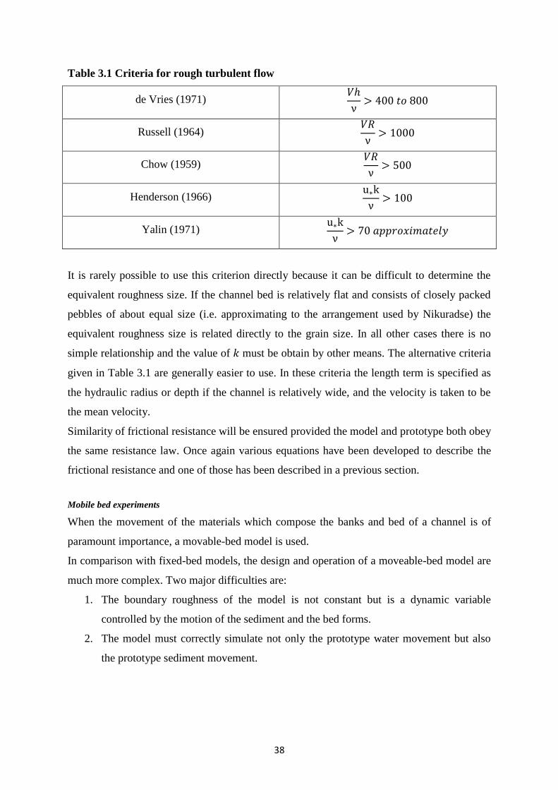
38
Table 3.1 Criteria for rough turbulent flow
de Vries (1971)
Russell (1964)
Chow (1959)
Henderson (1966)
Yalin (1971)
It is rarely possible to use this criterion directly because it can be difficult to determine the
equivalent roughness size. If the channel bed is relatively flat and consists of closely packed
pebbles of about equal size (i.e. approximating to the arrangement used by Nikuradse) the
equivalent roughness size is related directly to the grain size. In all other cases there is no
simple relationship and the value of must be obtain by other means. The alternative criteria
given in Table 3.1 are generally easier to use. In these criteria the length term is specified as
the hydraulic radius or depth if the channel is relatively wide, and the velocity is taken to be
the mean velocity.
Similarity of frictional resistance will be ensured provided the model and prototype both obey
the same resistance law. Once again various equations have been developed to describe the
frictional resistance and one of those has been described in a previous section.
Mobile bed experiments
When the movement of the materials which compose the banks and bed of a channel is of
paramount importance, a movable-bed model is used.
In comparison with fixed-bed models, the design and operation of a moveable-bed model are
much more complex. Two major difficulties are:
1. The boundary roughness of the model is not constant but is a dynamic variable
controlled by the motion of the sediment and the bed forms.
2. The model must correctly simulate not only the prototype water movement but also
the prototype sediment movement.
39
Sediment scaling
Sediment transport scaling is a complex problem. It is generally assumed that perfect
similitude in both the bed-load and suspended load sediment transport may not be achieved.
Therefore a compromise between a bed-load or a suspended load dominated model must be
chosen.
Similarity in sediment transport models is obtained by fulfilling similitude in the following
dimensionless parameters (Kamphuis1996; Hughes1993):
Grain (or Densimetric) Froude number:
(3-15)
where = bottom shear velocity (√ ), = submerged sediment specific weight
[ ], = medium grain size and = specific gravity.
Grain size Reynolds number:
(3-16)
where is water viscosity. These two parameters make reference to forcing ( ) and resting
( ) forces acting on a sand particle as represented on Shields diagrams.
Kamphuis (1996) and Hughes (1993) classified bed-load scale models in terms of the
requirements they fulfill. The best bed-load model can maintain similitude in grain
(densimetric) Froude number, Relative density of the sediment and Relative length number.
Grain (densimetric) Froude number similitude results in geometrical scaling of the
median, , sediment size:
(3-17)
Several authors have proposed different scaling relations assuming suspended load dominates
the transport (see Hughes, 1993 for a comprehensive review). These relations determine the
scaling using the sediment settling velocity instead of the sediment size and require similitude
in both the relative fall speed and relative density.
Zwamborn (1966, 1967 and 1969) has developed a set of similarity criteria for movable-bed
models which have been validated by model-prototype correlations. The similarity criteria
are:
1. Flow in natural rivers is always fully turbulent. To ensure that the flow in the model is
also fully turbulent, the Reynolds number (ks is length scale) for the model should
exceed 600.
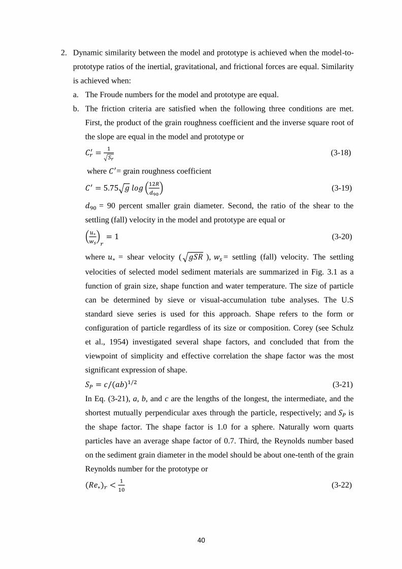
40
2. Dynamic similarity between the model and prototype is achieved when the model-to-
prototype ratios of the inertial, gravitational, and frictional forces are equal. Similarity
is achieved when:
a. The Froude numbers for the model and prototype are equal.
b. The friction criteria are satisfied when the following three conditions are met.
First, the product of the grain roughness coefficient and the inverse square root of
the slope are equal in the model and prototype or
√ (3-18)
where = grain roughness coefficient
√ (
) (3-19)
= 90 percent smaller grain diameter. Second, the ratio of the shear to the
settling (fall) velocity in the model and prototype are equal or
(
) (3-20)
where = shear velocity (√ ), = settling (fall) velocity. The settling
velocities of selected model sediment materials are summarized in Fig. 3.1 as a
function of grain size, shape function and water temperature. The size of particle
can be determined by sieve or visual-accumulation tube analyses. The U.S
standard sieve series is used for this approach. Shape refers to the form or
configuration of particle regardless of its size or composition. Corey (see Schulz
et al., 1954) investigated several shape factors, and concluded that from the
viewpoint of simplicity and effective correlation the shape factor was the most
significant expression of shape.
(3-21)
In Eq. (3-21), a, b, and c are the lengths of the longest, the intermediate, and the
shortest mutually perpendicular axes through the particle, respectively; and is
the shape factor. The shape factor is 1.0 for a sphere. Naturally worn quarts
particles have an average shape factor of 0.7. Third, the Reynolds number based
on the sediment grain diameter in the model should be about one-tenth of the grain
Reynolds number for the prototype or
(3-22)
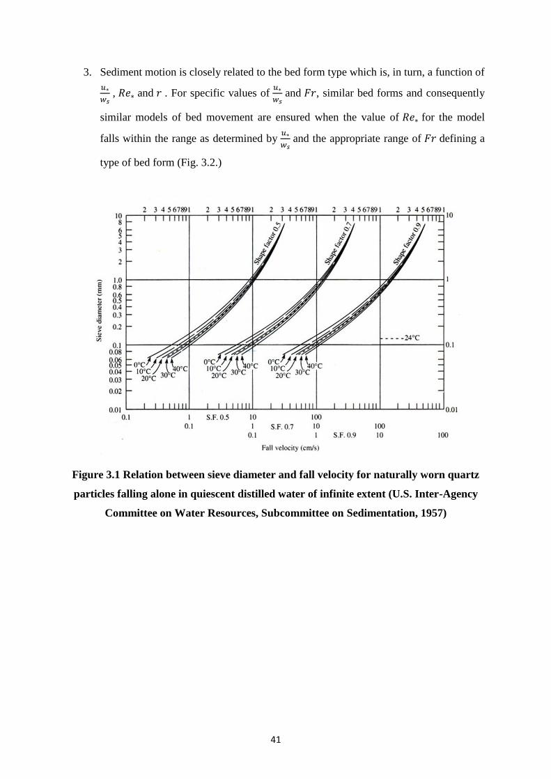
41
3. Sediment motion is closely related to the bed form type which is, in turn, a function of
, and . For specific values of
and , similar bed forms and consequently
similar models of bed movement are ensured when the value of for the model
falls within the range as determined by
and the appropriate range of defining a
type of bed form (Fig. 3.2.)
Figure 3.1 Relation between sieve diameter and fall velocity for naturally worn quartz
particles falling alone in quiescent distilled water of infinite extent (U.S. Inter-Agency
Committee on Water Resources, Subcommittee on Sedimentation, 1957)
42
Figure 3.2 Bed shape criteria (Zwamborn 1969)
𝑢
𝑤
𝑅𝑒 𝑢 𝑑
𝜈
43
3.4 Introduction to Hamidieh regulated reservoir study
A physical model was constructed to represent the flow, sediment transport and
morphodynamic processes in Hamidieh regulated reservoir. The experiments, including
designing scale, constructing and measuring tests of the physical model were carried out in
the Water Research Institute in Iran by the author. Efforts were made to simulate the
hydrodynamic, sediment transport and morphological processes in one model. The physical
model was designed based on Froude similarity (undistorted), with non-cohesive material
being used. Although a physical model cannot answer all of the hydraulic questions, it can
reveal some key features.
In the next sections, details are given of the criteria for surface water physical model
simulations, and the application to the Hamidieh regulated reservoir to investigate fluid,
sediment interactions and to optimize the operation of the intake structures. Designing the
scale of the model, hydraulic testing programme and scientific judgments will be presented in
the following sections.
3.5 Project background
Hamidieh regulated reservoir is located 11 km away from Hamidieh Town. It has been
constructed along the Karkheh River, downstream of Karkheh reservoir dam (Figure 3.3).
Figure 3.4 also shows an aerial photo of current situation of Hamidieh regulated reservoir and
relative hydraulic structures. Currently, there are two water intakes, namely Ghods and
Vosaileh. Vosaileh water intake channel, located on the left side of the Hamidieh dam body
(regarding to flow direction) is 10.8 km long with a maximum discharge of 60 ⁄ , while
Ghods, located on the right side, of dam body operates with a 25 km long channel, with a
maximum carrying capacity of 13 ⁄ (WEOKP, 2001). The layout of current situation of
Hamidieh regulated reservoir including dam body, irrigation channels, Ghods and Vosaileh
intakes is presented in Figure 3.5. Figure 3.6 shows pictures about existing hydraulic
structures of Hamidieh regulated reservoir.

44
Figure 3.3 Location map of Hamidieh town
Figure 3.4 Aerial photo of current situation of Hamidieh regulated reservoir
Vosaileh
Intake
Ghods
Intake
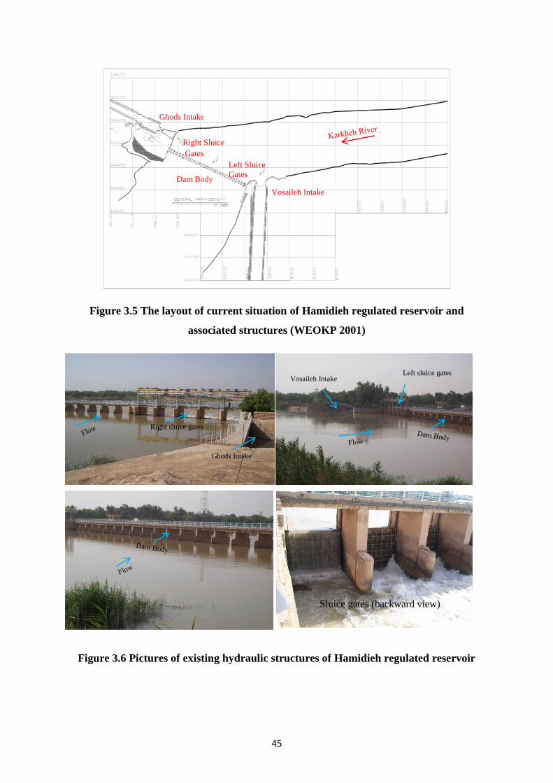
45
Figure 3.5 The layout of current situation of Hamidieh regulated reservoir and
associated structures (WEOKP 2001)
Figure 3.6 Pictures of existing hydraulic structures of Hamidieh regulated reservoir
Vosaileh Intake
Ghods Intake
Dam Body
Right Sluice
Gates
Left Sluice
Gates
Ghods Intake
Right sluice gates
Left sluice gates Vosaileh Intake
Sluice gates (backward view)
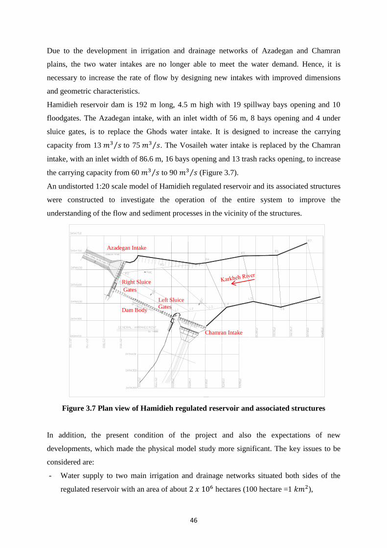
46
Due to the development in irrigation and drainage networks of Azadegan and Chamran
plains, the two water intakes are no longer able to meet the water demand. Hence, it is
necessary to increase the rate of flow by designing new intakes with improved dimensions
and geometric characteristics.
Hamidieh reservoir dam is 192 m long, 4.5 m high with 19 spillway bays opening and 10
floodgates. The Azadegan intake, with an inlet width of 56 m, 8 bays opening and 4 under
sluice gates, is to replace the Ghods water intake. It is designed to increase the carrying
capacity from 13 ⁄ to 75 ⁄ . The Vosaileh water intake is replaced by the Chamran
intake, with an inlet width of 86.6 m, 16 bays opening and 13 trash racks opening, to increase
the carrying capacity from 60 ⁄ to 90 ⁄ (Figure 3.7).
An undistorted 1:20 scale model of Hamidieh regulated reservoir and its associated structures
were constructed to investigate the operation of the entire system to improve the
understanding of the flow and sediment processes in the vicinity of the structures.
Figure 3.7 Plan view of Hamidieh regulated reservoir and associated structures
In addition, the present condition of the project and also the expectations of new
developments, which made the physical model study more significant. The key issues to be
considered are:
- Water supply to two main irrigation and drainage networks situated both sides of the
regulated reservoir with an area of about hectares (100 hectare =1 ),
Chamran Intake
Azadegan Intake
Dam Body
Right Sluice
Gates
Left Sluice
Gates
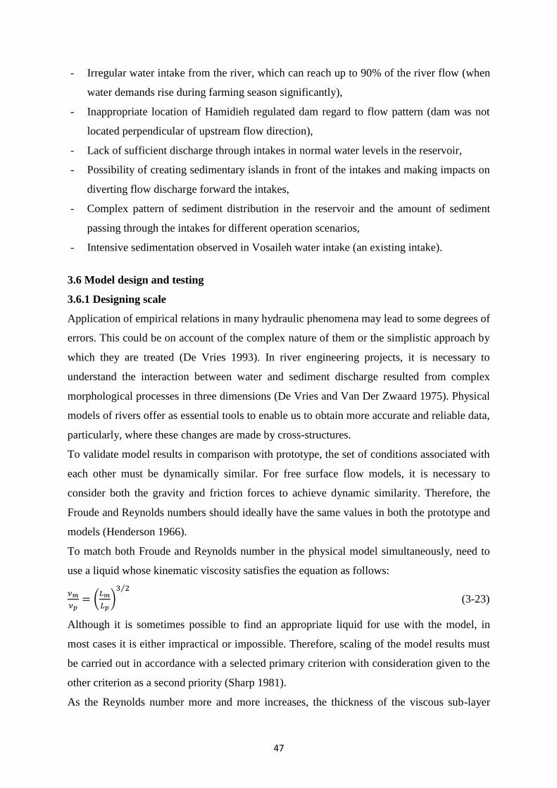
47
- Irregular water intake from the river, which can reach up to 90% of the river flow (when
water demands rise during farming season significantly),
- Inappropriate location of Hamidieh regulated dam regard to flow pattern (dam was not
located perpendicular of upstream flow direction),
- Lack of sufficient discharge through intakes in normal water levels in the reservoir,
- Possibility of creating sedimentary islands in front of the intakes and making impacts on
diverting flow discharge forward the intakes,
- Complex pattern of sediment distribution in the reservoir and the amount of sediment
passing through the intakes for different operation scenarios,
- Intensive sedimentation observed in Vosaileh water intake (an existing intake).
3.6 Model design and testing
3.6.1 Designing scale
Application of empirical relations in many hydraulic phenomena may lead to some degrees of
errors. This could be on account of the complex nature of them or the simplistic approach by
which they are treated (De Vries 1993). In river engineering projects, it is necessary to
understand the interaction between water and sediment discharge resulted from complex
morphological processes in three dimensions (De Vries and Van Der Zwaard 1975). Physical
models of rivers offer as essential tools to enable us to obtain more accurate and reliable data,
particularly, where these changes are made by cross-structures.
To validate model results in comparison with prototype, the set of conditions associated with
each other must be dynamically similar. For free surface flow models, it is necessary to
consider both the gravity and friction forces to achieve dynamic similarity. Therefore, the
Froude and Reynolds numbers should ideally have the same values in both the prototype and
models (Henderson 1966).
To match both Froude and Reynolds number in the physical model simultaneously, need to
use a liquid whose kinematic viscosity satisfies the equation as follows:
(
) ⁄
(3-23)
Although it is sometimes possible to find an appropriate liquid for use with the model, in
most cases it is either impractical or impossible. Therefore, scaling of the model results must
be carried out in accordance with a selected primary criterion with consideration given to the
other criterion as a second priority (Sharp 1981).
As the Reynolds number more and more increases, the thickness of the viscous sub-layer
48
decreases and finally it has no covering effect in the end. Additionally the tenacity has no
influence on the flow resistance anymore. Only the size of the relative roughness has to be
considered for the calculation of the friction coefficient. Flow in natural channels are usually
within the ''hydraulically rough" range (see Eq. 3-30) so that the roughness coefficient only
depends upon the relative roughness, and the magnitude of the Reynolds number is of no
importance (Kobus 1980). Therefore, the model conditions are derived from the Froude
number similarity criterion as gravity provides the driving force in river mechanics.
Accordingly, satisfaction of the Froude law will make the model operate at a much smaller
Reynolds number than the prototype, but care must be taken to ensure that the model operates
within the same flow regime as the prototype; as energy losses associated with laminar and
turbulent flow cannot be easily scaled (Yalin 1971).
For Froude number similarity with a scale ratio of hydraulic parameters may be derived
(Table 3.2). However, it is important to simulate sediment transport processes as accurately
as possible, as this reflects the sediment behavior in the prototype. French (1986), following
Zwamborn (1966), argues that when particle in solution for mass transport of sediment is not
large enough or investigation is concerned with transport en-masse, the dependence on the
particles’ Reynolds number is limited for suspended sediment load and ⁄ )
may be a more appropriate parameter to obtain satisfactory scales. Therefore, values must
be the same in both the model and prototype as
(
) (3-24)
where = particles fall velocity (m/s)
= shear velocity (m/s)
= von Karman’s constant = 0.407
Stokes’ law states that if the particles' Reynolds number (
) is small, is expressed as
(3-25)
where = specific weight of sediment particles ( )
= specific weight of water ( )
= dynamic viscosity ( )
D = representative sediment grain size (m)
At a high value of , the fall velocity increases and only little material is kept in suspension
and their distribution becomes non-uniform over the water depth; while at a low value of ,
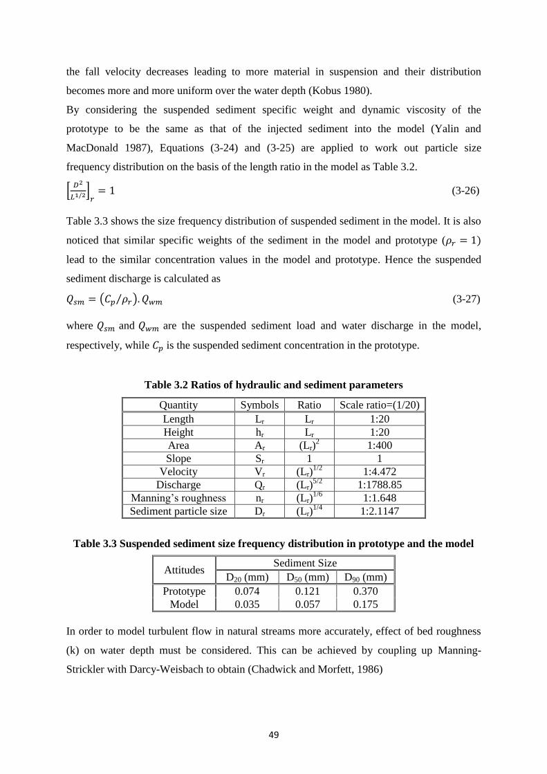
49
the fall velocity decreases leading to more material in suspension and their distribution
becomes more and more uniform over the water depth (Kobus 1980).
By considering the suspended sediment specific weight and dynamic viscosity of the
prototype to be the same as that of the injected sediment into the model (Yalin and
MacDonald 1987), Equations (3-24) and (3-25) are applied to work out particle size
frequency distribution on the basis of the length ratio in the model as Table 3.2.
*
+ (3-26)
Table 3.3 shows the size frequency distribution of suspended sediment in the model. It is also
noticed that similar specific weights of the sediment in the model and prototype (
lead to the similar concentration values in the model and prototype. Hence the suspended
sediment discharge is calculated as
( ⁄ ) (3-27)
where and are the suspended sediment load and water discharge in the model,
respectively, while is the suspended sediment concentration in the prototype.
Table 3.2 Ratios of hydraulic and sediment parameters
Quantity Symbols Ratio Scale ratio=(1/20)
Length Lr Lr 1:20
Height hr Lr 1:20
Area Ar (Lr)2
1:400
Slope Sr 1 1
Velocity Vr (Lr)1/2
1:4.472
Discharge Qr (Lr)5/2
1:1788.85
Manning’s roughness nr (Lr)1/6
1:1.648
Sediment particle size Dr (Lr)1/4
1:2.1147
Table 3.3 Suspended sediment size frequency distribution in prototype and the model
Attitudes Sediment Size
D20 (mm) D50 (mm) D90 (mm)
Prototype 0.074 0.121 0.370
Model 0.035 0.057 0.175
In order to model turbulent flow in natural streams more accurately, effect of bed roughness
(k) on water depth must be considered. This can be achieved by coupling up Manning-
Strickler with Darcy-Weisbach to obtain (Chadwick and Morfett, 1986)
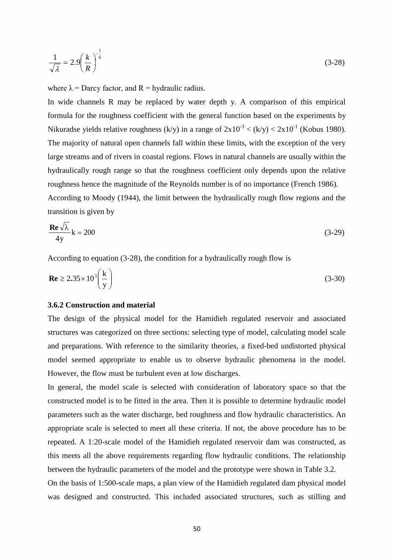
50
6
1
9.21
R
k
(3-28)
where λ = Darcy factor, and R = hydraulic radius.
In wide channels R may be replaced by water depth y. A comparison of this empirical
formula for the roughness coefficient with the general function based on the experiments by
Nikuradse yields relative roughness (k/y) in a range of 2x10⁻³
< (k/y) < 2x10⁻¹
(Kobus 1980).
The majority of natural open channels fall within these limits, with the exception of the very
large streams and of rivers in coastal regions. Flows in natural channels are usually within the
hydraulically rough range so that the roughness coefficient only depends upon the relative
roughness hence the magnitude of the Reynolds number is of no importance (French 1986).
According to Moody (1944), the limit between the hydraulically rough flow regions and the
transition is given by
200ky4
Re
(3-29)
According to equation (3-28), the condition for a hydraulically rough flow is
y
k10352 3
.Re (3-30)
3.6.2 Construction and material
The design of the physical model for the Hamidieh regulated reservoir and associated
structures was categorized on three sections: selecting type of model, calculating model scale
and preparations. With reference to the similarity theories, a fixed-bed undistorted physical
model seemed appropriate to enable us to observe hydraulic phenomena in the model.
However, the flow must be turbulent even at low discharges.
In general, the model scale is selected with consideration of laboratory space so that the
constructed model is to be fitted in the area. Then it is possible to determine hydraulic model
parameters such as the water discharge, bed roughness and flow hydraulic characteristics. An
appropriate scale is selected to meet all these criteria. If not, the above procedure has to be
repeated. A 1:20-scale model of the Hamidieh regulated reservoir dam was constructed, as
this meets all the above requirements regarding flow hydraulic conditions. The relationship
between the hydraulic parameters of the model and the prototype were shown in Table 3.2.
On the basis of 1:500-scale maps, a plan view of the Hamidieh regulated dam physical model
was designed and constructed. This included associated structures, such as stilling and

51
sedimentation basins as well as Azadegan and Chamran water intakes. A laboratory setup
was then established based on the designed dimensions of the physical model and associated
structures at the Water Research Centre in Iran.
The water discharge was adjusted by a pump control system through an inlet channel and an
outlet channel linked to a storage tank. The reservoir bed topography was made by concrete
and masonry. Both the two intakes (Chamran and Azadegan) and all of the gates were
constructed by wood. Different workshops such as those for carpentry, painting, ironing and
turning were involved for constructing and assembling the whole system of this large
physical model. It took more than 5 months for construction and installation of the Hamidieh
physical model. Figures 3.8 to 3.11 show the constructing stages of this hydraulic model.
a) Chamran Intake b) Azadegan Intake
Figure 3.8 Two intakes physical model
Figure 3.9 The installation stage of the physical model
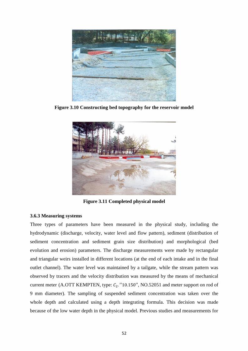
52
Figure 3.10 Constructing bed topography for the reservoir model
Figure 3.11 Completed physical model
3.6.3 Measuring systems
Three types of parameters have been measured in the physical study, including the
hydrodynamic (discharge, velocity, water level and flow pattern), sediment (distribution of
sediment concentration and sediment grain size distribution) and morphological (bed
evolution and erosion) parameters. The discharge measurements were made by rectangular
and triangular weirs installed in different locations (at the end of each intake and in the final
outlet channel). The water level was maintained by a tailgate, while the stream pattern was
observed by tracers and the velocity distribution was measured by the means of mechanical
current meter (A.OTT KEMPTEN, type: , NO.52051 and meter support on rod of
9 mm diameter). The sampling of suspended sediment concentration was taken over the
whole depth and calculated using a depth integrating formula. This decision was made
because of the low water depth in the physical model. Previous studies and measurements for
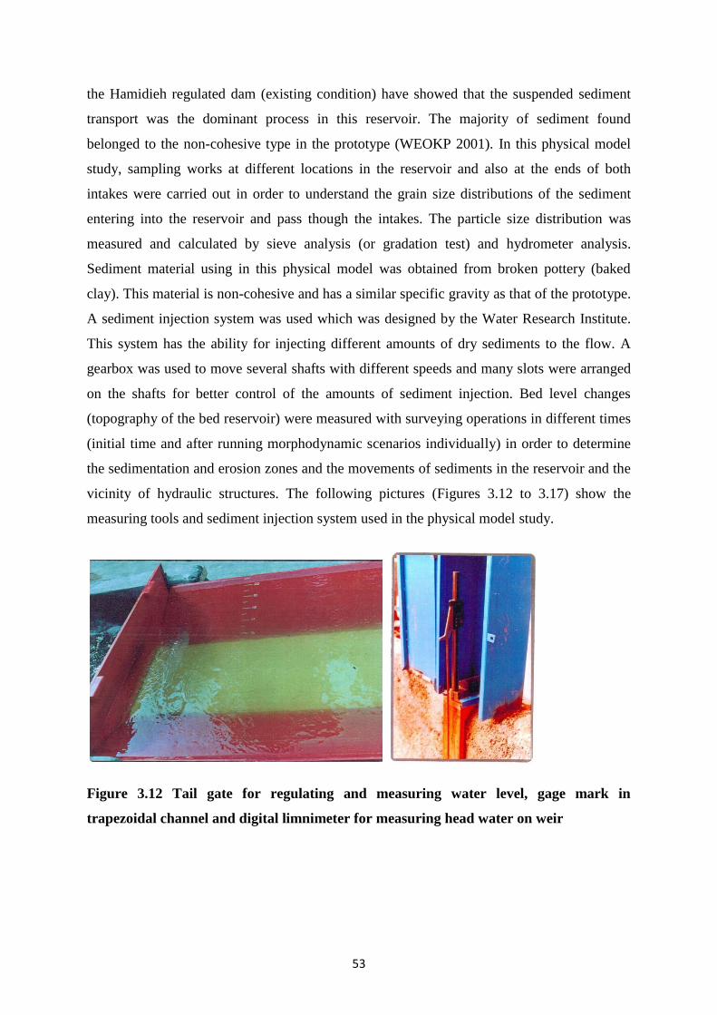
53
the Hamidieh regulated dam (existing condition) have showed that the suspended sediment
transport was the dominant process in this reservoir. The majority of sediment found
belonged to the non-cohesive type in the prototype (WEOKP 2001). In this physical model
study, sampling works at different locations in the reservoir and also at the ends of both
intakes were carried out in order to understand the grain size distributions of the sediment
entering into the reservoir and pass though the intakes. The particle size distribution was
measured and calculated by sieve analysis (or gradation test) and hydrometer analysis.
Sediment material using in this physical model was obtained from broken pottery (baked
clay). This material is non-cohesive and has a similar specific gravity as that of the prototype.
A sediment injection system was used which was designed by the Water Research Institute.
This system has the ability for injecting different amounts of dry sediments to the flow. A
gearbox was used to move several shafts with different speeds and many slots were arranged
on the shafts for better control of the amounts of sediment injection. Bed level changes
(topography of the bed reservoir) were measured with surveying operations in different times
(initial time and after running morphodynamic scenarios individually) in order to determine
the sedimentation and erosion zones and the movements of sediments in the reservoir and the
vicinity of hydraulic structures. The following pictures (Figures 3.12 to 3.17) show the
measuring tools and sediment injection system used in the physical model study.
Figure 3.12 Tail gate for regulating and measuring water level, gage mark in
trapezoidal channel and digital limnimeter for measuring head water on weir
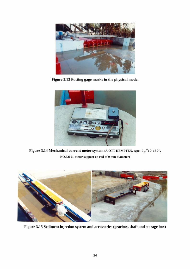
54
Figure 3.13 Putting gage marks in the physical model
Figure 3.14 Mechanical current meter system (A.OTT KEMPTEN, type: ,
NO.52051-meter support on rod of 9 mm diameter)
Figure 3.15 Sediment injection system and accessories (gearbox, shaft and storage box)

55
Figure 3.16 Hydrometer analysis for sediment samples
Figure 3.17 Determination of sediment concentration
3.7 Scenarios and results of physical model
3.7.1 Flow and hydrodynamic section
Experiments were undertaken with different water discharges to simulate three different
conditions containing regulatory conditions, high flow and flooding
Similarity of frictional resistance will be ensured provided the model and prototype both obey
the same resistance law. The Manning equation is probably most widely used. However, the
model roughness must be considered in conjunction with the reduction in Reynolds number
(Sharp 1981). The roughness coefficient in the prototype was estimated in the range of 0.023
to 0.025 (refer to proposing for various types of channels by Chow 1959), these
were converted to 0.014 to 0.015 in the physical model (( )
⁄
, refer to Table 3.2), which could easily be obtained by a plane concrete surface.
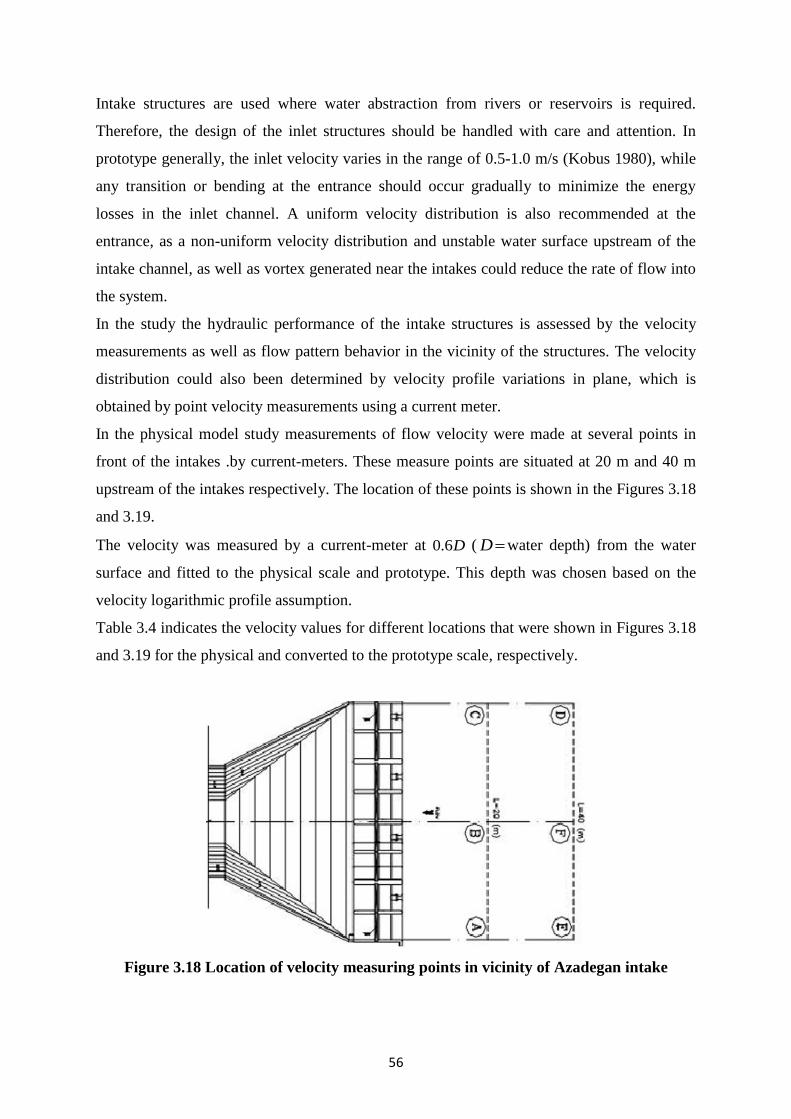
56
Intake structures are used where water abstraction from rivers or reservoirs is required.
Therefore, the design of the inlet structures should be handled with care and attention. In
prototype generally, the inlet velocity varies in the range of 0.5-1.0 m/s (Kobus 1980), while
any transition or bending at the entrance should occur gradually to minimize the energy
losses in the inlet channel. A uniform velocity distribution is also recommended at the
entrance, as a non-uniform velocity distribution and unstable water surface upstream of the
intake channel, as well as vortex generated near the intakes could reduce the rate of flow into
the system.
In the study the hydraulic performance of the intake structures is assessed by the velocity
measurements as well as flow pattern behavior in the vicinity of the structures. The velocity
distribution could also been determined by velocity profile variations in plane, which is
obtained by point velocity measurements using a current meter.
In the physical model study measurements of flow velocity were made at several points in
front of the intakes .by current-meters. These measure points are situated at 20 m and 40 m
upstream of the intakes respectively. The location of these points is shown in the Figures 3.18
and 3.19.
The velocity was measured by a current-meter at D6.0 ( D water depth) from the water
surface and fitted to the physical scale and prototype. This depth was chosen based on the
velocity logarithmic profile assumption.
Table 3.4 indicates the velocity values for different locations that were shown in Figures 3.18
and 3.19 for the physical and converted to the prototype scale, respectively.
Figure 3.18 Location of velocity measuring points in vicinity of Azadegan intake
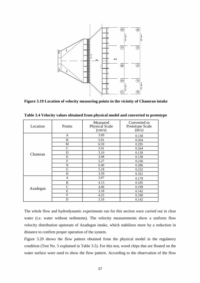
57
Figure 3.19 Location of velocity measuring points in the vicinity of Chamran intake
Table 3.4 Velocity values obtained from physical model and converted to prototype
Location Points Measured
Physical Scale (cm/s)
Converted to Prototype Scale
(m/s)
Chamran
A 3.09 0.138
B 5.91 0.264
M 6.59 0.295
C 5.91 0.264
D 3.10 0.139
E 3.08 0.138
F 5.27 0.236
N 6.40 0.286
G 5.18 0.232
H 3.59 0.161
Azadegan
A 3.97 0.178
B 4.13 0.185
C 4.46 0.199
E 3.18 0.142
F 4.25 0.190
D 3.18 0.142
The whole flow and hydrodynamic experiments run for this section were carried out in clear
water (i.e. water without sediments). The velocity measurements show a uniform flow
velocity distribution upstream of Azadegan intake, which stabilizes more by a reduction in
distance to confirm proper operation of the system.
Figure 3.20 shows the flow pattern obtained from the physical model in the regulatory
condition (Test No. 5 explained in Table 3.5). For this test, wood chips that are floated on the
water surface were used to show the flow pattern. According to the observation of the flow
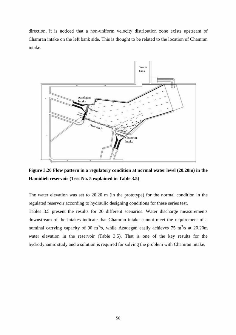
58
direction, it is noticed that a non-uniform velocity distribution zone exists upstream of
Chamran intake on the left bank side. This is thought to be related to the location of Chamran
intake.
Figure 3.20 Flow pattern in a regulatory condition at normal water level (20.20m) in the
Hamidieh reservoir (Test No. 5 explained in Table 3.5)
The water elevation was set to 20.20 m (in the prototype) for the normal condition in the
regulated reservoir according to hydraulic designing conditions for these series test.
Tables 3.5 present the results for 20 different scenarios. Water discharge measurements
downstream of the intakes indicate that Chamran intake cannot meet the requirement of a
nominal carrying capacity of 90 m3/s, while Azadegan easily achieves 75 m
3/s at 20.20m
water elevation in the reservoir (Table 3.5). That is one of the key results for the
hydrodynamic study and a solution is required for solving the problem with Chamran intake.
Water
Tank
Chamran
Intake
Azadegan
Intake

59
Table 3.5 Results of hydraulic experiments, Discharge (m3/s), Bay opening (m
2) and
Water surface elevation (m) (data transferred to prototype)
Test
No.
System
Operation
Hamidieh
Reservoir
Az.
intake
Ch.
intake
Under
sluice
Az.
intake
Right
sluice
gates
Left
sluice
gates
Remarks
1 Discharge 48.29 6.97 36.14 5.18 - - *
Bay opening - 4.60 13.14 4.48 - -
WS. Elevation 20.20 19.30 19.70 - - -
2 Discharge 88.67 27.69 54.17 6.81 - - *
Bay opening - 14.40 22.50 4.48 - -
WS. Elevation 20.20 19.36 19.77 - - -
3 Discharge 113.02 43.14 62.73 7.15 - - *
Bay opening - 27.90 33.75 4.48 - -
WS. Elevation 20.20 19.56 19.83 - - -
4
Discharge
Bay opening
166.99 103.89 63.20 - - - *
WS. Elevation 20.20 20.00 20.00 - - -
5 Discharge 179.66 107.99 71.67 - - - *
Bay opening - 144 52.8 - - - **
WS. Elevation 20.20 20.00 20.00 ***
6 Discharge 194.21 40.26 63.27 4.10 38.58 48.00 *
Bay opening - 14.40 27.75 4.48 6.51 9.11
WS. Elevation 20.20 19.46 19.83 - - -
7 Discharge 159.55 74.86 73.54 4.65 - 6.50 *
Bay opening - 36.00 49.2 2.24 - 1.04
WS. Elevation 20.25 20.00 20.00 - - -
8 Discharge 167.04 74.02 81.67 4.65 - 6.7 *
Bay opening - 34.2 49.8 2.24 - 1.04
WS. Elevation 20.30 20.00 20.00 - - -
9 Discharge 179.81 74.02 94.34 4.65 - 6.8 *
Bay opening - 28.80 50.40 2.24 - 1.04
WS. Elevation 20.35 20.00 20.00 - - -
10 Discharge 186.33 76.50 98.10 4.65 - 7.08 *
Bay opening - 29.70 52.80 2.24 - 1.04
Elevation 20.40 20.00 20.00 - - -
11 Discharge 189.17 80.40 95.56 4.71 - 8.50 ****
Bay opening - 43.20 50.40 2.24 - 1.30
WS. Elevation 20.45 20.20 20.20 - - -
12 Discharge 186.56 84.53 88.75 4.78 - 8.50 ****
Bay opening - 46.80 49.80 2.24 - 1.30
Elevation 20.40 20.00 20.00 - - -
13 Discharge 174.47 79.44 82.43 4.7 - 7.90 ****
Bay opening - 43.20 49.20 2.24 - 1.30
WS. Elevation 20.35 20.00 20.00 - - -
14 Discharge 147.81 67.02 68.37 4.68 - 7.74 ****
Bay opening - 45.00 49.2 2.24 - 1.30
WS. Elevation 20.30 20.00 20.00 - - -

60
Continued-Table 3.5 Results of hydraulic experiments, Discharge (m3/s), Bay opening
(m2) and Water surface elevation (m) (data transferred to prototype)
Test
No.
System
Operation
Hamidieh
Reservoir
Az.
intake
Ch.
intake
Under
sluice Az.
intake
Right
flood
gates
Left
flood
gates
Remarks
15 Discharge 137.31 65.74 59.04 4.68 - 7.90 ****
Bay opening - 45.00 48.00 2.24 - 1.30
WS. Elevation 20.25 20.00 20.00 - - -
16 Discharge 125.25 57.17 55.50 4.68 - 7.90 ****
Bay opening - 43.20 48.00 2.24 - 1.30
Elevation 20.20 20.00 20.00 - - -
17 Discharge 180.79 122.23 45.88 4.88 - 7.80 ****
Bay opening - 86.40 24.00 2.24 - 1.30
WS. Elevation 20.45 20.20 20.20 - - -
18 Discharge 215.41 109.48 93.15 4.88 - 7.80 ****
Bay opening - 57.60 36.00 2.24 - 1.30
WS. Elevation 20.45 20.00 20.00 - - -
19 Discharge 224.24 129.23 100.99 5.17 - 8.85 ****
Bay opening - 86.40 48.00 2.24 - 1.30
WS. Elevation 20.45 20.00 20.00 - - -
20 Discharge 256.47 140.53 102.13 5.06 - 8.75 ****
Bay opening - 115.20 51.00 2.24 - 1.30
WS. Elevation 20.45 20.00 20.00 - - - * without trash racks, ** head loss at Chamran intake gates,
*** nominal carrying capacity for the intakes at the water surface elevation 20.20m,
**** with trash racks and considering bay opening surface trash racks is 80 % of the total surface (These
conservative scenarios have been considered for service time operation when trashes were gathered in front of
the intakes).
Az. = Azadegan, Ch. = Chamran and WS. Elevation = Water surface elevation
The water surface elevations for the intakes shown in Table 3.5 were measured in the
trapezoidal channel at the end of intakes (see Figure 3.12).
After these experiments, several solutions were put forward to enable Chamran to reach its
nominal carrying capacity in the normal elevation (20.20 m). Those solutions was made and
run in the physical model One of the solutions, which was actually adopted in the
experimental model, was to install permeable groins on the opposite bank to deflect the flow,
making its direction towards the intakes. The measure could activate stagnant zone to some
extent, however, Chamran's carrying capacity was increased only by 5%, see Figure 3.21.
Another solution was to make two guide walls for the Chamran intake (Figure 3.22). This
method could not enhance the discharge capacity for this intake, neither. When a permeable
wall was obstructed across the entire reservoir width, a local increase in the reservoir water
elevation was observed, resulting in 90 m3/s water discharge at Chamran, see Figure 3.23.
Nevertheless, this solution is not very practical for implementation, as this would confirm
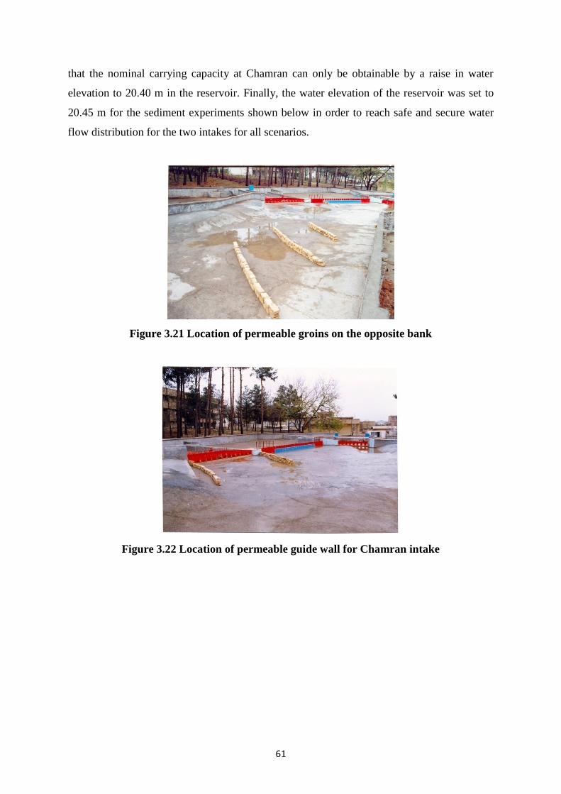
61
that the nominal carrying capacity at Chamran can only be obtainable by a raise in water
elevation to 20.40 m in the reservoir. Finally, the water elevation of the reservoir was set to
20.45 m for the sediment experiments shown below in order to reach safe and secure water
flow distribution for the two intakes for all scenarios.
Figure 3.21 Location of permeable groins on the opposite bank
Figure 3.22 Location of permeable guide wall for Chamran intake

62
Figure 3.23 Obstruction of reservoir width by a permeable wall
3.7.2 Sediment transport and morphodynamic section
In this research, different scenarios were considered in order to determine the amount of
sediments entering the intakes and investigating sediment grain size distribution in the
reservoir and through hydraulic structures. Besides, the role of sluice gates on the sediment
flashing in front of intakes was investigated in the physical model. Details are given below of
the physical model study of sediment transport process. For a better understanding of the
implication of the model results to the project, the results were transferred to the prototype
like flow and hydrodynamic section. This action would help us to get an overview about
engineering judgments. For brevity, the experimental results are presented as a graph and a
summarized table. The scenarios have been designed and carried out in the hydraulic
laboratory of Water Research Institute based on different operations for the intakes (in
percentage of opening of the gates), flow discharge and sediment concentrations put in the
reservoir by the author.
Previous studies in the field for existing condition of Hamidieh regulated reservoir have
showed that the suspended sediment transport is the dominant process and the majority of
sediment found in this region belongs to the non-cohesive type (WEOKP, 2001).
Sediment sampling was carried out in order to determine the sediment concentration and
particle size distributions in the physical model. The sampling of suspended sediment
concentration in the physical model was taken along the whole depth and calculated using a
depth integrated formula. Figure 3.24 presents the sites of the sediment samples at different
locations.
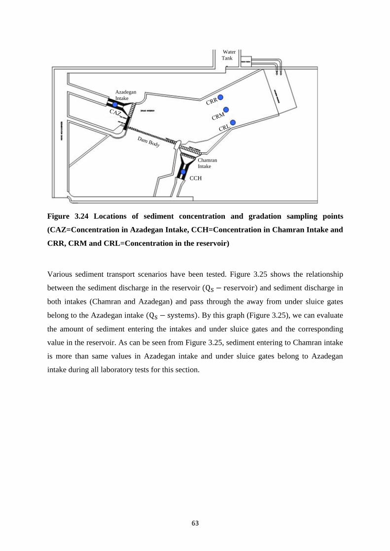
63
Figure 3.24 Locations of sediment concentration and gradation sampling points
(CAZ=Concentration in Azadegan Intake, CCH=Concentration in Chamran Intake and
CRR, CRM and CRL=Concentration in the reservoir)
Various sediment transport scenarios have been tested. Figure 3.25 shows the relationship
between the sediment discharge in the reservoir and sediment discharge in
both intakes (Chamran and Azadegan) and pass through the away from under sluice gates
belong to the Azadegan intake . By this graph (Figure 3.25), we can evaluate
the amount of sediment entering the intakes and under sluice gates and the corresponding
value in the reservoir. As can be seen from Figure 3.25, sediment entering to Chamran intake
is more than same values in Azadegan intake and under sluice gates belong to Azadegan
intake during all laboratory tests for this section.
Azadegan
Intake
Chamran
Intake
CCH
Water
Tank
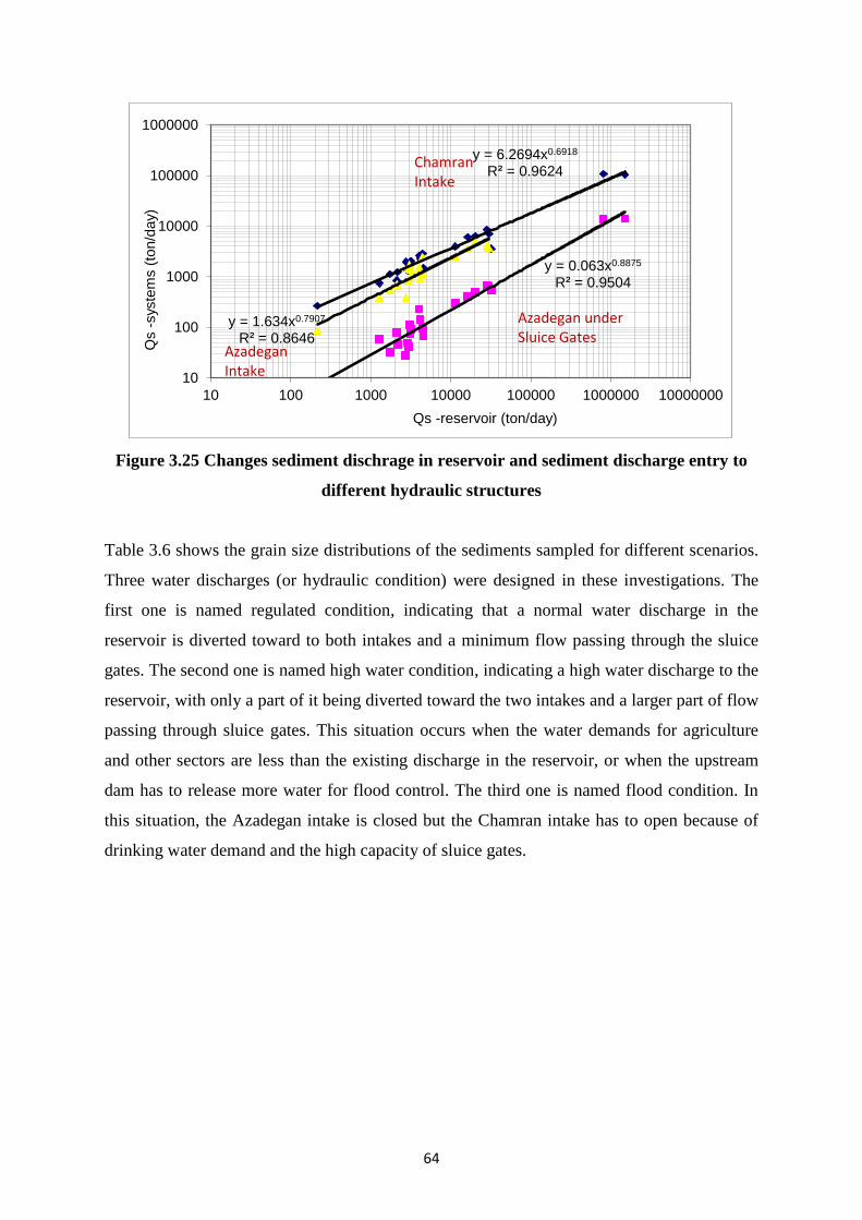
64
Figure 3.25 Changes sediment dischrage in reservoir and sediment discharge entry to
different hydraulic structures
Table 3.6 shows the grain size distributions of the sediments sampled for different scenarios.
Three water discharges (or hydraulic condition) were designed in these investigations. The
first one is named regulated condition, indicating that a normal water discharge in the
reservoir is diverted toward to both intakes and a minimum flow passing through the sluice
gates. The second one is named high water condition, indicating a high water discharge to the
reservoir, with only a part of it being diverted toward the two intakes and a larger part of flow
passing through sluice gates. This situation occurs when the water demands for agriculture
and other sectors are less than the existing discharge in the reservoir, or when the upstream
dam has to release more water for flood control. The third one is named flood condition. In
this situation, the Azadegan intake is closed but the Chamran intake has to open because of
drinking water demand and the high capacity of sluice gates.
y = 6.2694x0.6918 R² = 0.9624
y = 0.063x0.8875 R² = 0.9504
y = 1.634x0.7907 R² = 0.8646
10
100
1000
10000
100000
1000000
10 100 1000 10000 100000 1000000 10000000
Qs -
syste
ms (
ton/d
ay)
Qs -reservoir (ton/day)
Azadegan Intake
Chamran Intake
Azadegan under Sluice Gates

65
Table 3.6 Sediment grain size for different hydraulic and sediment transport scenarios
NO. Locations Sample
Code
mm
mm
mm
Discharge
Hydraulic
conditions
1
Aza
deg
an i
nta
ke
DAS3 0.011 0.09 0.36 75.73 Regulated
2 DAS14 0.005 0.081 0.34 41.77 - 42.61 Regulated
3 DAS2 0.0073 0.085 0.3 23.06 Regulated
4 DA13 0.005 0.12 0.6 54.3 High water
5 DA14 0.009 0.062 0.26 75.44 High water
6 DA15 0.009 0.075 0.18 46.4 High water
1
Cham
ran i
nta
ke
DGS3 0.0015 0.05 0.18 79.59 Regulated
2 DGS14 0.0035 0.05 0.2 77.45 - 69.39 Regulated
3 DGS2 0.01 0.05 0.18 43.88 Regulated
4 DG13 - 0.046 0.26 67.07 High water
5 DG14 0.006 0.08 0.18 84.5 High water
6 DG15 0.014 0.15 0.4 84.5 High water
7 DG16 0.017 0.13 0.43 47.45 Flood
1
Under
slu
ice
gat
es b
elon
g
to A
zadeg
an i
nta
ke
DTS3 0.01 0.046 0.2 3.1 Regulated
2 DTS14 0.0018 0.027 0.09 3.07 Regulated
3 DTS2 0.0013 0.04 0.12 2.87 Regulated
4 DT13 0.0016 0.039 0.17 8.25 High water
5 DT14 - 0.056 0.2 8.32 High water
6 DT15 0.0024 0.077 0.22 8.2 High water
7 DT16 0.0015 0.052 0.26 7.58 Flood
Note: The data have been converted are transferred to prototype
As can been seen from Table 3.6 that the sediment grain size distribution ( , and )
in Azadegan does not have any significant changes at the regulated condition. For high water
condition the sampling results for DA13 was considered wrong which is belong to the
sampling error, but for the two other samples (DA14 and DA15) reduces and
increases, with the mean sediment grain size ( ) decreasing for around 10%. This reduction
might be related to the flow carrying high concentration sediment passing through the sluice
gates at the high water condition.
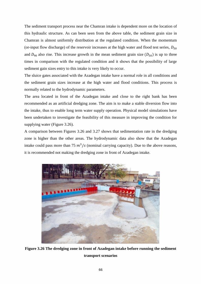
66
The sediment transport process near the Chamran intake is dependent more on the location of
this hydraulic structure. As can been seen from the above table, the sediment grain size in
Chamran is almost uniformly distribution at the regulated condition. When the momentum
(or-input flow discharge) of the reservoir increases at the high water and flood test series,
and also rise. This increase growth in the mean sediment grain size is up to three
times in comparison with the regulated condition and it shows that the possibility of large
sediment gain sizes entry to this intake is very likely to occur.
The sluice gates associated with the Azadegan intake have a normal role in all conditions and
the sediment grain sizes increase at the high water and flood conditions. This process is
normally related to the hydrodynamic parameters.
The area located in front of the Azadegan intake and close to the right bank has been
recommended as an artificial dredging zone. The aim is to make a stable diversion flow into
the intake, thus to enable long term water supply operation. Physical model simulations have
been undertaken to investigate the feasibility of this measure in improving the condition for
supplying water (Figure 3.26).
A comparison between Figures 3.26 and 3.27 shows that sedimentation rate in the dredging
zone is higher than the other areas. The hydrodynamic data also show that the Azadegan
intake could pass more than 75 (nominal carrying capacity). Due to the above reasons,
it is recommended not making the dredging zone in front of Azadegan intake.
Figure 3.26 The dredging zone in front of Azadegan intake before running the sediment
transport scenarios
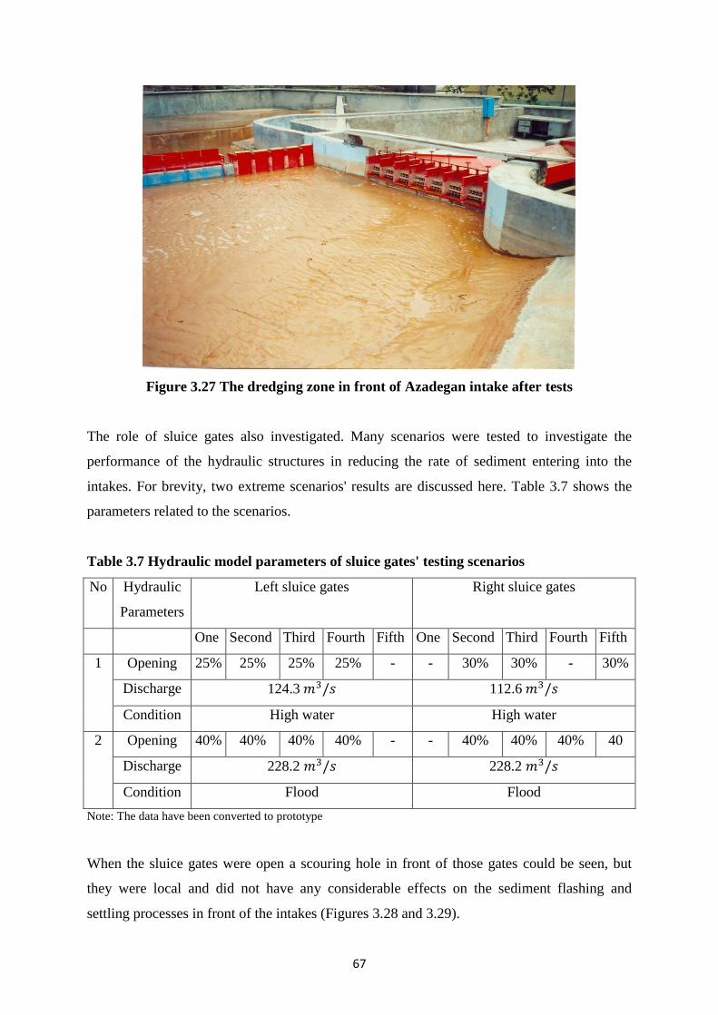
67
Figure 3.27 The dredging zone in front of Azadegan intake after tests
The role of sluice gates also investigated. Many scenarios were tested to investigate the
performance of the hydraulic structures in reducing the rate of sediment entering into the
intakes. For brevity, two extreme scenarios' results are discussed here. Table 3.7 shows the
parameters related to the scenarios.
Table 3.7 Hydraulic model parameters of sluice gates' testing scenarios
No Hydraulic
Parameters
Left sluice gates Right sluice gates
One Second Third Fourth Fifth One Second Third Fourth Fifth
1 Opening 25% 25% 25% 25% - - 30% 30% - 30%
Discharge 124.3 112.6
Condition High water High water
2 Opening 40% 40% 40% 40% - - 40% 40% 40% 40
Discharge 228.2 228.2
Condition Flood Flood
Note: The data have been converted to prototype
When the sluice gates were open a scouring hole in front of those gates could be seen, but
they were local and did not have any considerable effects on the sediment flashing and
settling processes in front of the intakes (Figures 3.28 and 3.29).
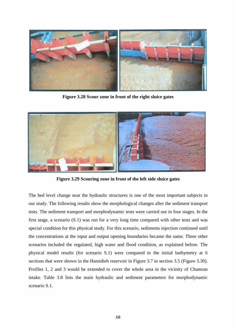
68
Figure 3.28 Scour zone in front of the right sluice gates
Figure 3.29 Scouring zone in front of the left side sluice gates
The bed level change near the hydraulic structures is one of the most important subjects in
our study. The following results show the morphological changes after the sediment transport
tests. The sediment transport and morphodynamic tests were carried out in four stages. In the
first stage, a scenario (S.1) was run for a very long time compared with other tests and was
special condition for this physical study. For this scenario, sediments injection continued until
the concentrations at the input and output opening boundaries became the same. Three other
scenarios included the regulated, high water and flood condition, as explained before. The
physical model results (for scenario S.1) were compared to the initial bathymetry at 6
sections that were shown in the Hamidieh reservoir in Figure 3.7 in section 3.5 (Figure 3.30).
Profiles 1, 2 and 3 would be extended to cover the whole area in the vicinity of Chamran
intake. Table 3.8 lists the main hydraulic and sediment parameters for morphodynamic
scenario S.1.

69
0.6
0.7
0.8
0.9
1
1.1
1.2
1.3
0 2 4 6 8 10 12 14 16
Hei
gh
t (m
)
Distance (m)
Profile L1-R1
0.6
0.7
0.8
0.9
1
1.1
1.2
0 2 4 6 8 10 12 14 16 18H
eigh
t (m
) Distance (m)
Profile L2-R2
0.6
0.7
0.8
0.9
1
1.1
1.2
1.3
0 2 4 6 8 10 12 14 16
Hei
gh
t (m
)
Distance (m)
Profile L3-R3
0.6
0.7
0.8
0.9
1
1.1
1.2
1.3
0 2 4 6 8
Hei
gh
t (m
)
Distance (m)
Profile L4-R4
Table 3.8 Main hydraulic and sediment parameters for morphodynamic scenario No
Operation Boundary Condition Concentration
(gr/liter) Time for simulation
(hour)
S.1
Reservoir Water level 20.45 m Discharge 126.8 /s 0.2321
48.5
Az Intake Opened Discharge 75 /s -
Ch Intake Opened Water level 20.45 m -
L S Closed - -
R S Closed - -
*Az Intake= Azadegan Intake, Ch Intake= Chamran Intake, L S= Left sluice gate and R S = Right sluice gate
**The whole data are transferred to prototype
Figure 3.30 Bed level changes after 48.5 hours in 6 section profiles (scenario S.1)
0.6
0.7
0.8
0.9
1
1.1
1.2
1.3
0 2 4 6 8
Hei
gh
t(m
)
Distance(m)
Profile L5-R5
0.6
0.7
0.8
0.9
1
1.1
1.2
0 2 4 6 8
Hei
gh
t(m
)
Distance(m)
Profile L6-R6
Initial bed
Physical simulation
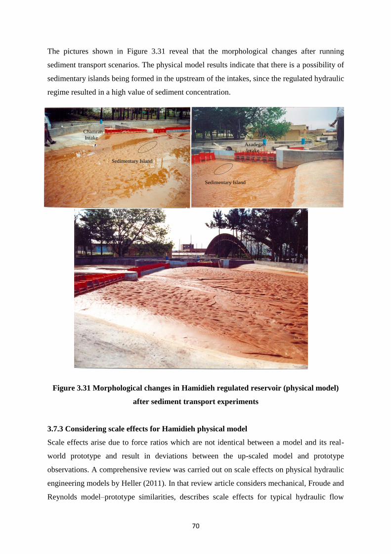
70
The pictures shown in Figure 3.31 reveal that the morphological changes after running
sediment transport scenarios. The physical model results indicate that there is a possibility of
sedimentary islands being formed in the upstream of the intakes, since the regulated hydraulic
regime resulted in a high value of sediment concentration.
Figure 3.31 Morphological changes in Hamidieh regulated reservoir (physical model)
after sediment transport experiments
3.7.3 Considering scale effects for Hamidieh physical model
Scale effects arise due to force ratios which are not identical between a model and its real-
world prototype and result in deviations between the up-scaled model and prototype
observations. A comprehensive review was carried out on scale effects on physical hydraulic
engineering models by Heller (2011). In that review article considers mechanical, Froude and
Reynolds model–prototype similarities, describes scale effects for typical hydraulic flow
Sedimentary Island
Sedimentary Island
Chamran
Intake
Azadegan
Intake

71
phenomena and discusses how scale effects are avoided, compensated or corrected. There are
some limiting conditions in the hydraulic model scale, which were also paid attention in our
physical model.
In hydraulic research the main criteria of similarity are the Froude and Reynolds laws. In
hydraulics the Mach or Weber laws are rarely decisive criteria. Problems with the decisive
effect of compressibility only occur at velocities greater than sound and are therefore
applicable, e.g., in water hammer problems and, above all, in aerodynamics. The forces
caused by surface tension are very important in hydraulic models, but in the solution of
practical engineering problems they are avoided by not reducing the model below a certain
dimension so that they are almost as insignificant on the model as in the majority of cases in
prototype. Separate research studies have shown that if the influence of surface tension and
capillarity is to be negligible, the following minimum limiting values must be observed on a
model operated according to the Froude law (Novak and Cabelka 1981):
- The velocity at the water surface on the model in order that gravity waves
might occur (this is important especially for experiments with the resistance of piers and head
losses for flow round various bodies), (Zegzhda 1938).
- The depth of flow on the model to eliminate the effect of capillary and surface
tension. This condition can lead to distorted models.
3.8 Conclusion
A series of physical model experiments have been undertaken to study the hydrodynamic,
sediment and morphological processes in the Hamidieh regulated reservoir. Laboratory tests
were designed based on three hydraulic conditions namely regulated, high water and flood
flows and sediment transport processes were investigated (see section 3.7.2). The physical
model results could, to a certain extent, reveal the governing processes in the system. It is
necessary to remember that the limitations and simplifications of the experiments may affect
the results. The capacity and operation time of the pumps, measurement tools, cost of
sediment material and construction and maintenance of reservoir bathymetry for running new
scenarios were all important aspects in this physical model study. The results obtained from
the hydraulic model experiments confirm the following technical features:
- The Chamran water intake could reach its nominal carrying capacity of 90 provided
that the water elevation is increased from 20.20m (proposed normal water level for regulatory
condition) to 20.45m in the reservoir.
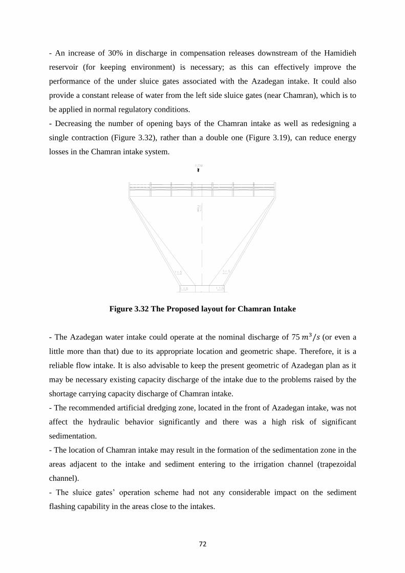
72
- An increase of 30% in discharge in compensation releases downstream of the Hamidieh
reservoir (for keeping environment) is necessary; as this can effectively improve the
performance of the under sluice gates associated with the Azadegan intake. It could also
provide a constant release of water from the left side sluice gates (near Chamran), which is to
be applied in normal regulatory conditions.
- Decreasing the number of opening bays of the Chamran intake as well as redesigning a
single contraction (Figure 3.32), rather than a double one (Figure 3.19), can reduce energy
losses in the Chamran intake system.
Figure 3.32 The Proposed layout for Chamran Intake
- The Azadegan water intake could operate at the nominal discharge of 75 (or even a
little more than that) due to its appropriate location and geometric shape. Therefore, it is a
reliable flow intake. It is also advisable to keep the present geometric of Azadegan plan as it
may be necessary existing capacity discharge of the intake due to the problems raised by the
shortage carrying capacity discharge of Chamran intake.
- The recommended artificial dredging zone, located in the front of Azadegan intake, was not
affect the hydraulic behavior significantly and there was a high risk of significant
sedimentation.
- The location of Chamran intake may result in the formation of the sedimentation zone in the
areas adjacent to the intake and sediment entering to the irrigation channel (trapezoidal
channel).
- The sluice gates’ operation scheme had not any considerable impact on the sediment
flashing capability in the areas close to the intakes.
73
- The movements of sediment in the reservoir were also observed at different scenarios
(regulated, high water and flood conditions). It means that the morphodynamic process
depends on sediment transport phenomena and hydrodynamic attitudes such as flow pattern,
speed and hydraulic operations.
- The dominant sediment transport process in the Hamidieh regulated reservoir was the
suspended sediment transport. The major reason for this process was related to existing
sediment grain size diameter in the water body.
- In the regulatory conditions the size of sediment entry moves to the Azadegan intake was
larger than Chamran intake.
From the analysis the results and methodology find following scientific features:
- The great flexibility of the undistorted physical model allowed easily designing different
scenarios without significant scale effects.
- Sediment material using in this physical model was obtained from broken pottery (baked
clay). This material is non-cohesive and has a similar specific gravity as that of the prototype
and for this reason the performance of sediment scenarios forms well. This material could be
proposed for similar studies better than lightweight material especially when the type of
model is undistorted and the scale is large.
- In the physical tests when high sediment concentrations were simulated by injecting dry
sediments method (existing sediment injection system, see Figure 3.15) observed some
problems in managing scenarios. This problem was related to low water depth in the physical
model (maximum water depth is around 21cm) and the injection method. In other word, when
the rate of injected sediment was increased part of those sediments could not mix well in the
water column and settle down near the sediment injection system. It would be suggested
making wet injection system for simulating high sediments concentrations. Also, the system
has to be installing enough far from the investigation area for getting best results.
- The physical model study reported herein presented that designing same scale for
investigation of hydrodynamic, sediment transport and morphodynamic processes in a
complicated water body system such as regulated dam raise accuracy of measurements. By
this method synchronization of these processes in the physical model keep such as prototype.
Besides the potential of using the physical model results in order to simulate, validate and
calibrate by the numerical model rises significantly.

74
3.9 Summary
In this chapter efforts were made to describe physical model theory and an experimental
study of a regulated reservoir. Selecting an appropriate scale is very important for a physical
model study. Model scale effects, the availability of material for constructing the physical
model and a good understanding of the physical processes are the key issues in any physical
model study. The result of this part of the research shows that an undistorted model is
preferred in the Hamidieh regulated reservoir study. This scheme prevents the significant
scale effects on hydrodynamic parameters, such as flow velocity, water depth and sediment
size and thus enhances the accuracy of the results. A comprehensive experimental study was
carried out to investigate hydrodynamic, sediment transport and morphological changes in
Hamidieh regulated reservoir. The results of the experimental study revealed many options
for better operation of the regulated reservoir and associated hydraulic structures, such as
intakes and sluice gates.
75
Chapter Four
Numerical Modelling (Governing Equations and Solutions)
4.1 Introduction
With the rapid increase in computer power in recent years, it is not surprising to note that
three-dimensional (3-D) numerical modelling of flow and sediment behavior near the
hydraulic structures has shifted from academic research to practical applications in order to
reduce the cost and time of design of hydraulic structures.
This chapter presents briefly the governing hydrodynamic, sediment transport and bed level
changes equations and solution methods. The emphasis of the study is on simulating the
three-dimensional hydrodynamic processes because of the complexity of the flow behavior
near the hydraulic structures. The main features of the turbulence model used in the current
study are discussed.
The numerical model contains three modules representing the hydrodynamic, sediment
transport and morphodynamic processes, in which the morphodynamic module is added the
first time to this numerical model by the author. Details are given herein of the development
and discretization of a three-dimensional layer integrated numerical model to predict
morphological changes in the vicinity of hydraulic structures. The effort is on presenting and
describing the computational scheme for solving the bed level change equation (in the
morphodynamic module) and coupling to other modules (hydrodynamic and sediment
transport).
4.2 Governing hydrodynamic equations
The governing equations used to describe flows in reservoirs are generally based on 3-D
Reynolds averaged Navier Stokes equations for incompressible and unsteady turbulent flows.
If the vertical acceleration of the flow is negligible in comparison with the gravity and the
vertical pressure gradient terms, then the hydrostatic pressure distribution assumption can be
made. Since the reservoir to be studied in the current study has a relatively shallow water, the
density of the water has also been assumed constant throughout the computational domain. In
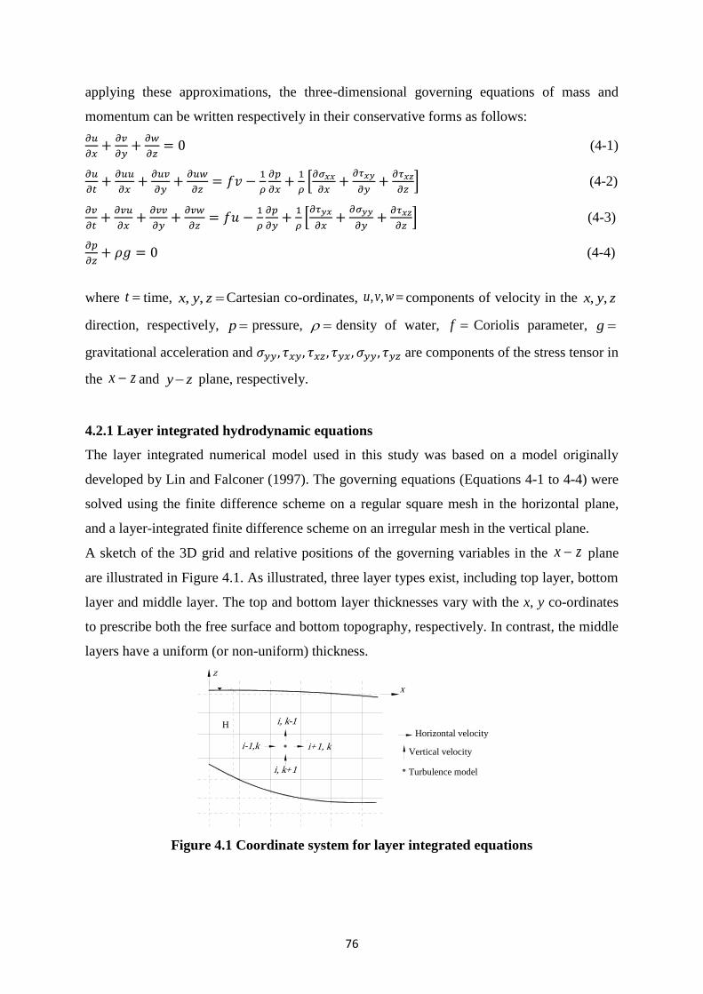
76
applying these approximations, the three-dimensional governing equations of mass and
momentum can be written respectively in their conservative forms as follows:
(4-1)
*
+ (4-2)
*
+ (4-3)
(4-4)
where t time, zyx ,, Cartesian co-ordinates, , ,u v w components of velocity in the zyx ,,
direction, respectively, p pressure, density of water, f Coriolis parameter, g
gravitational acceleration and are components of the stress tensor in
the zx and zy plane, respectively.
4.2.1 Layer integrated hydrodynamic equations
The layer integrated numerical model used in this study was based on a model originally
developed by Lin and Falconer (1997). The governing equations (Equations 4-1 to 4-4) were
solved using the finite difference scheme on a regular square mesh in the horizontal plane,
and a layer-integrated finite difference scheme on an irregular mesh in the vertical plane.
A sketch of the 3D grid and relative positions of the governing variables in the zx plane
are illustrated in Figure 4.1. As illustrated, three layer types exist, including top layer, bottom
layer and middle layer. The top and bottom layer thicknesses vary with the x, y co-ordinates
to prescribe both the free surface and bottom topography, respectively. In contrast, the middle
layers have a uniform (or non-uniform) thickness.
Figure 4.1 Coordinate system for layer integrated equations
Horizontal velocity
Vertical velocity
Turbulence model
H i, k-1
i, k+1
i-1,k i+1, k
z
x
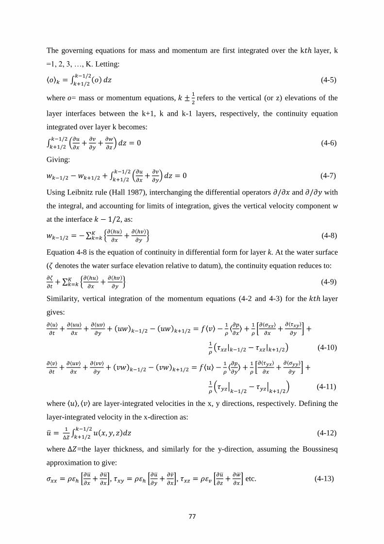
77
The governing equations for mass and momentum are first integrated over the k layer, k
=1, 2, 3, …, K. Letting:
⟨ ⟩ ∫
(4-5)
where = mass or momentum equations,
refers to the vertical (or z) elevations of the
layer interfaces between the k+1, k and k-1 layers, respectively, the continuity equation
integrated over layer k becomes:
∫ (
)
(4-6)
Giving:
∫ (
)
(4-7)
Using Leibnitz rule (Hall 1987), interchanging the differential operators and with
the integral, and accounting for limits of integration, gives the vertical velocity component w
at the interface , as:
∑ ,
-
(4-8)
Equation 4-8 is the equation of continuity in differential form for layer k. At the water surface
( denotes the water surface elevation relative to datum), the continuity equation reduces to:
∑ ,
-
(4-9)
Similarity, vertical integration of the momentum equations (4-2 and 4-3) for the layer
gives:
⟨ ⟩
⟨ ⟩
⟨ ⟩
⟨ ⟩
⟨
⟩
* ⟨ ⟩
⟨ ⟩
+
( | | ) (4-10)
⟨ ⟩
⟨ ⟩
⟨ ⟩
⟨ ⟩
⟨
⟩
* ⟨ ⟩
⟨ ⟩
+
( |
| ) (4-11)
where ⟨ ⟩ ⟨ ⟩ are layer-integrated velocities in the x, y directions, respectively. Defining the
layer-integrated velocity in the x-direction as:
∫
(4-12)
where =the layer thickness, and similarly for the y-direction, assuming the Boussinesq
approximation to give:
*
+, *
+, *
+ etc. (4-13)
78
where , = horizontal and vertical eddy viscosities, respectively, assuming a hydrostatic
pressure distribution given as:
(4-14)
and defining:
⟨ ⟩ ⟨ ⟩ (4-15)
Then Equations 4-10 and 4-11 can be rewritten as:
| *
+ |
| ,
*
+
*
+-
( | | )
(4-16)
| *
+ |
| ,
*
+
*
+-
( |
| )
(4-17)
At the free surface (where =1), the terms and can be eliminated using
the kinematic free surface condition and Leibnitz rule. At the bed, the terms and
become zero due to the no-slip boundary condition.
In applying these equations to large estuaries and reservoirs, the ratio of the vertical length
scale to the horizontal length scale is very small. The vertical eddy viscosity terms are
generally several orders of magnitude larger than the corresponding horizontal terms.
Therefore, it is important to prescribe the vertical eddy viscosity more accurately than for the
horizontal viscosity. In the original version of 3D layer-integrated model (TRIVAST), the
horizontal eddy viscosity was assumed to be constant in the vertical, and its value was
assumed to be equal to the depth-averaged eddy viscosity. The vertical eddy viscosity was
represented using a two-layer mixing length model (Rodi 1984) written in the following
form:
[(
)
(
)
]
(4-18)
where l is mixing length, defined as:
{
(4-19)
and is von Karman’s constant (0.41).
An enhanced version of 3D layer-integrated model is used in the current study; in which the
vertical eddy viscosity is calculated using the turbulence model. More details of the
turbulence model will be discussed in section 4.3.
79
4.2.2 Depth integrated hydrodynamic equations
Numerical modelling of fluid flow is based on the principles of continuity of mass and
conservation of momentum within the body of fluid to be modeled. In many cases, the flow is
defined by the Reynolds equations, which describe the three-dimensional turbulent motion of
the incompressible fluid. For flows which show little variation in the vertical direction, it is
appropriate to integrate these equations over the depth of water, resulting in simplified or
'two-dimensional' equations of motion. When integrated over the depth, the equations
governing fluid motion are as follows (Falconer and Lin 2001):
Conservation of mass:
mqy
q
x
p
t
(4-20)
Conservation of momentum:
22
2222
CH
qpgpWWWC
xgHfq
y
pV
x
pU
t
pyxxw
a
H
qppmDC
yx
q
y
p
x
pd
222
2
2
2
2
2
(4-21)
22
2222
CH
qpgqWWWC
ygHfp
y
qV
x
qU
t
qyxyw
a
H
qpqmDC
yx
p
y
q
x
qd
222
2
2
2
2
2
(4-22)
where:
- p (=UH), q (=VH) discharges per unit width in the x and y directions respectively (m 3
/s/m);
- mq source discharge per unit horizontal area (m 3 /s/m 2 );
- U,V depth averaged velocity components in the x and y directions respectively (m/s);
- momentum correction factor for a non-uniform vertical velocity profile;
- g gravitational acceleration (=9.806 m/s 2 );
- H total water depth = h ;
- water surface elevation above datum;
- h water depth below datum;
- a density of air ( 1.292 kg/m 3 );
- density of fluid (kg/m 3 );
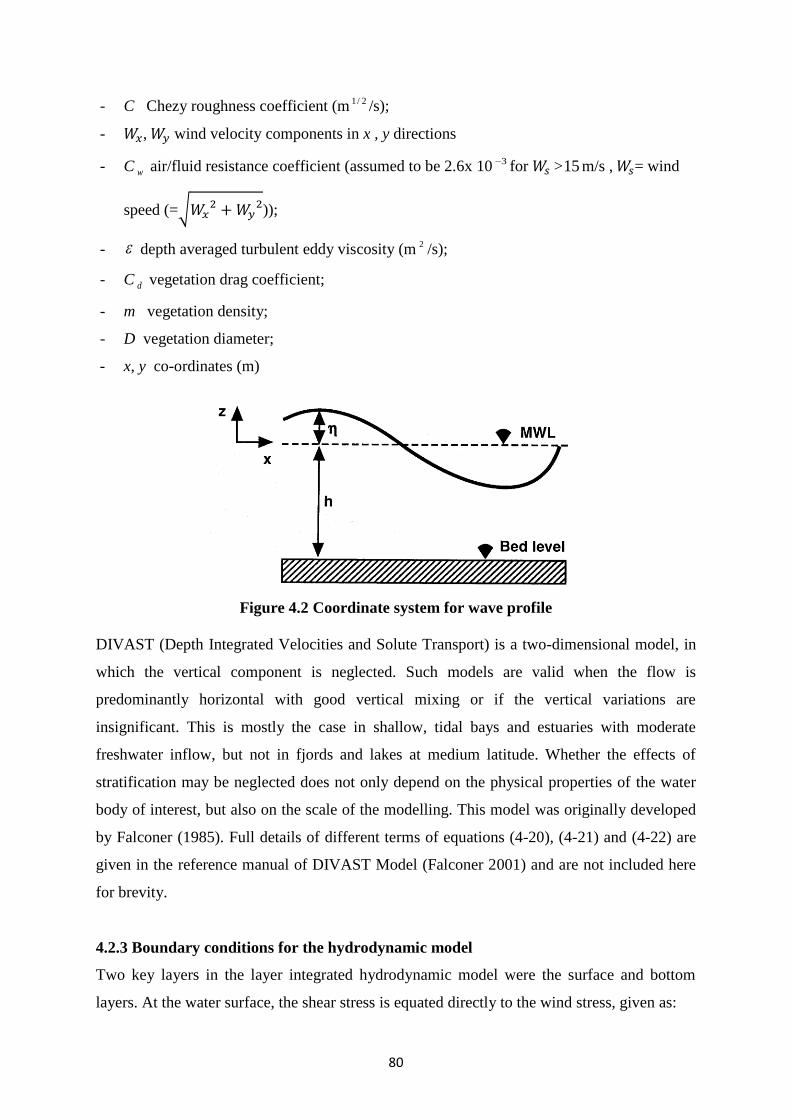
80
- C Chezy roughness coefficient (m 2/1 /s);
- , wind velocity components in x , y directions
- C w air/fluid resistance coefficient (assumed to be 2.6x 10 3 for >15 m/s , = wind
speed (=√
));
- depth averaged turbulent eddy viscosity (m 2 /s);
- C d vegetation drag coefficient;
- m vegetation density;
- D vegetation diameter;
- x, y co-ordinates (m)
Figure 4.2 Coordinate system for wave profile
DIVAST (Depth Integrated Velocities and Solute Transport) is a two-dimensional model, in
which the vertical component is neglected. Such models are valid when the flow is
predominantly horizontal with good vertical mixing or if the vertical variations are
insignificant. This is mostly the case in shallow, tidal bays and estuaries with moderate
freshwater inflow, but not in fjords and lakes at medium latitude. Whether the effects of
stratification may be neglected does not only depend on the physical properties of the water
body of interest, but also on the scale of the modelling. This model was originally developed
by Falconer (1985). Full details of different terms of equations (4-20), (4-21) and (4-22) are
given in the reference manual of DIVAST Model (Falconer 2001) and are not included here
for brevity.
4.2.3 Boundary conditions for the hydrodynamic model
Two key layers in the layer integrated hydrodynamic model were the surface and bottom
layers. At the water surface, the shear stress is equated directly to the wind stress, given as:
81
| (4-23)
| (4-24)
where = resistance coefficient; is air density; = wind speed; and , = wind
velocity components in the x, y directions, respectively.
At the bed:
(4-25)
where = bed shear stress; and = bed shear velocity. Assuming a logarithmic velocity
profile within the bottom layer (see French, 1986), the following equation can be obtained for
the bed shear stress:
|
⁄ ⁄
| ⁄ ⁄
* (
)+
(4-26)
where = thickness of the bottom layer; and = bed roughness length.
The bed stress obtained for the layer-integrated equations is also used in calculating the depth
integrated equations [see Lin and Falconer 1997]. In shallow regions where only one layer is
wet, the bed resistance stress is represented in the form of Darcy's equation, with the friction
factor being evaluated using the Colebrook-White equation (Falconer 1993).
4.2.4 Gates simulation
In this section details are given of the numerical technique added to the existing numerical
model (to the hydrodynamic model) for simulating flow through gates by the author. This
technique enhance existing numerical model in order to apply it for simulating flow through
hydraulic structures. Obstacles in the flow may generate sudden transitions from flow
contraction to expansion. The grid resolution is often low compared to the gradients of the
water level, the velocity and the bathymetry. The hydrostatic pressure assumption may
locally be invalid. Examples of these obstacles in civil engineering projects are: gates,
barriers, sluices, groins, weirs, bridge piers and porous plates. The obstacles generate energy
losses and may change the direction of the flow. Different methods suggested for simulation
the role of hydraulic structures in numerical models. This section has only explained a
technique for numerical simulation of gates. These steps are considered to represent the
technique in the numerical model:
- Determining the location of gates.
- Determining the head-discharge equation (non-linear) for vertical sluice gates with
regard to hydraulic conditions such as free surface, submerged and overtopping.
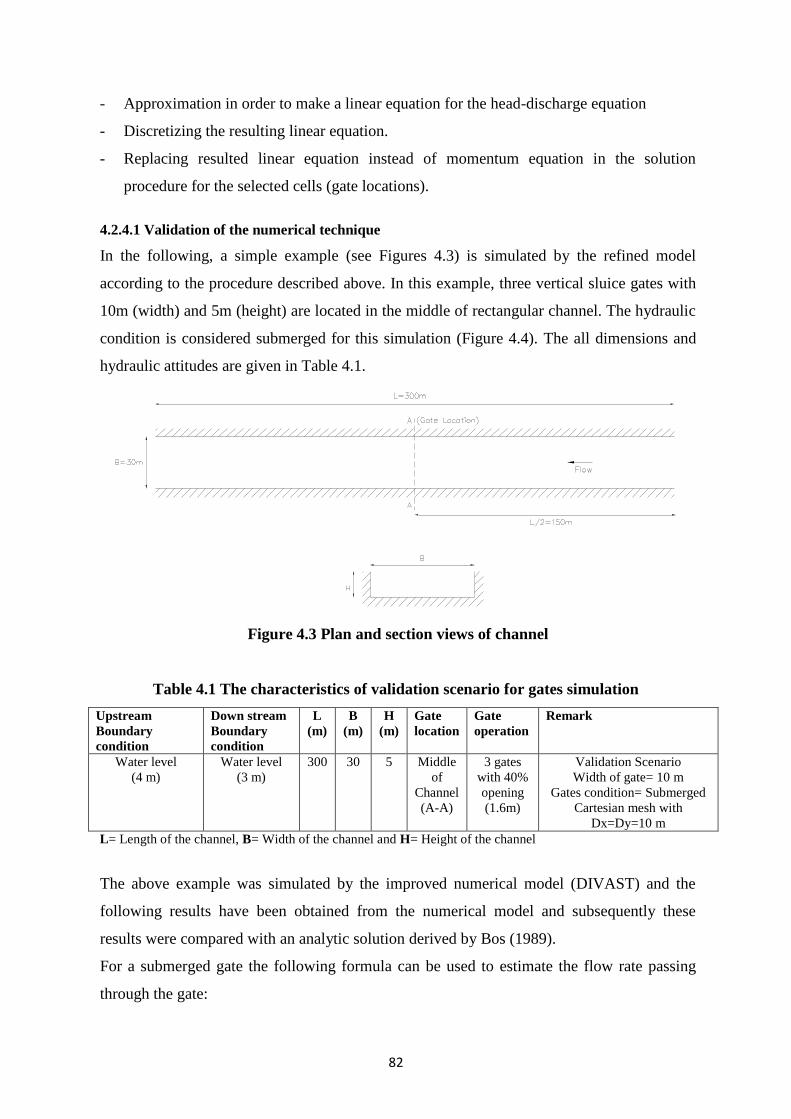
82
- Approximation in order to make a linear equation for the head-discharge equation
- Discretizing the resulting linear equation.
- Replacing resulted linear equation instead of momentum equation in the solution
procedure for the selected cells (gate locations).
4.2.4.1 Validation of the numerical technique
In the following, a simple example (see Figures 4.3) is simulated by the refined model
according to the procedure described above. In this example, three vertical sluice gates with
10m (width) and 5m (height) are located in the middle of rectangular channel. The hydraulic
condition is considered submerged for this simulation (Figure 4.4). The all dimensions and
hydraulic attitudes are given in Table 4.1.
Figure 4.3 Plan and section views of channel
Table 4.1 The characteristics of validation scenario for gates simulation
Upstream
Boundary
condition
Down stream
Boundary
condition
L
(m)
B
(m)
H
(m)
Gate
location
Gate
operation
Remark
Water level
(4 m)
Water level
(3 m)
300 30 5 Middle
of
Channel
(A-A)
3 gates
with 40%
opening
(1.6m)
Validation Scenario
Width of gate= 10 m
Gates condition= Submerged
Cartesian mesh with
Dx=Dy=10 m
L= Length of the channel, B= Width of the channel and H= Height of the channel
The above example was simulated by the improved numerical model (DIVAST) and the
following results have been obtained from the numerical model and subsequently these
results were compared with an analytic solution derived by Bos (1989).
For a submerged gate the following formula can be used to estimate the flow rate passing
through the gate:

83
Figure 4.4 Submerged gate flow
5.0
21 )(2 hhgbhCCQ ove (4-27)
provided that :
001.0oh ;
ohh 5.11 ; and
11161
2/ 1
02
oh
hhh
where:
)22/()2(15.0161.0 ooe hbhbC (4-28)
Contraction coefficient (see Bos 1989, Table 8.3)
vC Coefficient of approach velocity (see Bos 1989, Fig. 1.12.)
b Breadth of each vertical sluice gate at control section (m)
In the improved numerical model the above formula was used for simulating the role of
sluice gates with regard to the procedure described previously.
4.2.4.2 Results in the validated example
The following data explain the results calculated by the improved numerical model. Table
4.2 presents results obtained from the numerical model. Table 4.3 describes the analytic
solution based on formula (4-27).
Table 4.2 Results of the improved numerical model
Location Speed (m/s) Depth (m) Q/B (m3/s/m)
Gate 1 0.45 3.52 1.584
Gate 2 0.45 3.52 1.584
Gate 3 0.45 3.52 1.584
Total discharge per width unit (q) 4.752
Reference Numerical model Numerical model Numerical model
Flow
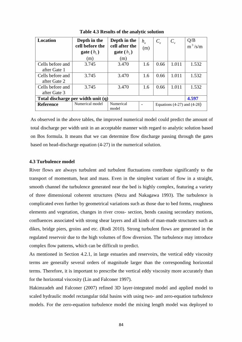
84
Table 4.3 Results of the analytic solution
Location Depth in the
cell before the
gate ( 1h )
(m)
Depth in the
cell after the
gate ( 2h )
(m)
oh
(m)
eC vC Q/B
m 3 /s/m
Cells before and
after Gate 1
3.745 3.470 1.6 0.66 1.011 1.532
Cells before and
after Gate 2
3.745 3.470 1.6 0.66 1.011 1.532
Cells before and
after Gate 3
3.745 3.470 1.6 0.66 1.011 1.532
Total discharge per width unit (q) 4.597
Reference Numerical model Numerical
model - Equations (4-27) and (4-28)
As observed in the above tables, the improved numerical model could predict the amount of
total discharge per width unit in an acceptable manner with regard to analytic solution based
on Bos formula. It means that we can determine flow discharge passing through the gates
based on head-discharge equation (4-27) in the numerical solution.
4.3 Turbulence model
River flows are always turbulent and turbulent fluctuations contribute significantly to the
transport of momentum, heat and mass. Even in the simplest variant of flow in a straight,
smooth channel the turbulence generated near the bed is highly complex, featuring a variety
of three dimensional coherent structures (Nezu and Nakagawa 1993). The turbulence is
complicated even further by geometrical variations such as those due to bed forms, roughness
elements and vegetation, changes in river cross- section, bends causing secondary motions,
confluences associated with strong shear layers and all kinds of man-made structures such as
dikes, bridge piers, groins and etc. (Rodi 2010). Strong turbulent flows are generated in the
regulated reservoir due to the high volumes of flow diversion. The turbulence may introduce
complex flow patterns, which can be difficult to predict.
As mentioned in Section 4.2.1, in large estuaries and reservoirs, the vertical eddy viscosity
terms are generally several orders of magnitude larger than the corresponding horizontal
terms. Therefore, it is important to prescribe the vertical eddy viscosity more accurately than
for the horizontal viscosity (Lin and Falconer 1997).
Hakimzadeh and Falconer (2007) refined 3D layer-integrated model and applied model to
scaled hydraulic model rectangular tidal basins with using two- and zero-equation turbulence
models. For the zero-equation turbulence model the mixing length model was deployed to
85
calculate the horizontal eddy viscosity coefficient, whereas for the two equation model, the
depth integrated turbulence model was used. Likewise, the layer integrated
turbulence model was used to determine the vertical eddy viscosity coefficient.
In current study, the horizontal eddy viscosity was calculated by zero- equation (mixing
length) and the vertical eddy viscosity was evaluated using the layer integrated form of the
equations based on Hakimzadeh and Falconer (2007).
In this section, the main features of the turbulence models which are used in the current
numerical model are discussed. The main efforts are focused on the turbulence model,
with the mixing length model being explained briefly.
4.3.1 Mixing length model
Based on dimensional analysis one can assume that the kinematic viscosity , which has
dimensions ⁄ , can be expressed as a product of a turbulent velocity and a
turbulent length scale . If one velocity scale and one length scale suffice to describe the
effects of turbulence, dimensional analysis yields (Versteeg and Malalasekera 2007):
(4-29)
where is a dimensionless constant of proportionality. The dynamic turbulent viscosity is
given by
(4-30)
Most of the kinetic energy of turbulence is contained in the largest eddies, and turbulence
length scale is therefore characteristic of these eddies which interact with the mean flow. If
we accept that there is a strong connection between the mean flow and the behavior of the
largest eddies we can attempt to link the characteristic velocity scale of eddies with the mean
flow properties. This has been found to work well in simple two-dimensional turbulent flows
where the only significant Reynolds stress is and the only significant
mean velocity gradient is
. For such flows it is at least dimensionally correct to state that,
if the eddy length scale is ,
|
| (4-31)
where is a dimensionless constant. The absolute value is taken to ensure that the velocity
scale is always a positive quantity irrespective of the sign of the velocity gradient.
Combing 4-29 and 4-31 and absorbing the two constants and into a new length scale
we obtain
86
|
| (4-32)
Referring to section 4.2.1 in solving for the Reynolds stresses; Boussinesq proposed that they
could be represented in a diffusive manner whereby:
*
+ , *
+ ,
*
+ (4-33)
To determine the Reynolds stresses given in equation 4-33, many different and varying
computed expressions exist for . The representation most widely used in coastal and
estuarine flows is to apply a zero-equation turbulence model similar to that prescribed by
Prandtl’s mixing length hypothesis (Goldstein 1938) where, for the x-direction:
(4-34)
where is some characteristic mixing length and
[ *
+
*
+
*
+
*
+
*
+
*
+
] ⁄
(4-35)
although this expression can usually be simplified due to the dominance of one or more
velocity gradients. In determining the mixing length Prandtl suggested:
(4-36)
near a wall, where = von Karman's constant (0.41) and y is the co-ordinate perpendicular to
the wall, with y = 0 at the wall. Other expressions are available for including, for example,
the von Karman representation given as
|
⁄ | (4-37)
For the zero-equation turbulence model, the horizontal eddy viscosity is evaluated using the
following equation outlined in Fischer (1973):
(4-38)
where = horizontal kinematic eddy viscosity; = eddy viscosity constant (typically 0.15
based upon laboratory data from Fischer. For real flows the value of is frequently much
larger and 1.0 is used in the current version of the model); = depth averaged shear
velocity; = total depth of flow.
In the current study, the horizontal eddy viscosity was assumed to be constant along the water
depth, with the depth-averaged eddy viscosity value being set in every layer. If the turbulent
shear stress is dominated by the bottom friction, a relationship between the Chezy coefficient
and the eddy viscosity exists. In the numerical model, the depth-integrated horizontal eddy
viscosity is calculated (after Fischer et. al 1979) using:
87
√ (4-39)
where = Chezy roughness coefficient: U,V=depth average velocity components in the x and
y directions respectively.
An overall assessment of the mixing length model can be found in Table 4.4 (Versteeg and
Malalasekera 2007):
Table 4.4 Mixing length model assessment
Advantages:
easy to implement and cheap in terms of computing resources
good predictions for thin shear layers: jets, mixing layers, wakes and boundary layers
well established
Disadvantages:
completely incapable of describing flows with separation and recirculation
only calculates mean flow properties and turbulent shear stress
4.3.2 model
In two-dimensional thin shear layers the changes in the flow direction are always so slow that
the turbulence can adjust itself to local conditions. In flows where convection and diffusion
cause significant differences between production and destruction of turbulence, e.g. in
recirculating flows, a compact algebraic prescription for the mixing length is no longer
feasible. Therefore it is necessary to consider the dynamics of turbulence. In two-equation
models, the turbulence velocity scale is computed from the turbulent kinetic energy, which is
provided from the solution of its transport equation. The turbulent length scale is estimated
from two properties of the turbulence field, usually the turbulent kinetic energy and its
dissipation rate. The dissipation rate of the turbulent kinetic energy is obtained from the
solution of its transport equation. The k- model focuses on the mechanisms that affect the
turbulence kinetic energy. k is the turbulence kinetic energy and is defined as the variance of
the fluctuations in velocity. It has dimensions of ( ); for example, ⁄ . is the
turbulence eddy dissipation (the rate at which the velocity fluctuations dissipate), and has
dimensions of k per unit time ( ); for example, ⁄ .The governing equations for the
turbulence kinetic energy and dissipation rate can be derived from Navier-Stokes equations
(Rodi 1984):
88
(
) (4-40)
(
)
(4-41)
Equations (4-40) and (4-41), together with the continuity equation can be rewritten as:
(
) (4-42)
(
)
(4-43)
where (
)
and , , , are empirical constants.
The eddy viscosity is derived from turbulence parameters and as
(4-44)
where is also an empirical constant. Eqs. (4-40) and (4-41) and the relationship by Eq. (4-
44) give the so-called turbulence model. Several carefully calibrated empirical
coefficients enter the k- turbulence model. The values of the constants suggested by the
ASCE (1988) can be summarized as follows:
, , , ,
4.3.2.1 Layer integrated model
In applying the model to the study, two approaches have been considered. In the first
approach equations (4-42) and (4-43) were solved directly to give the corresponding
homogenous eddy viscosity (i.e. similar velocity scales). In the second approach equations
(4-42) and (4-43) were selected in some way so that they gave horizontal and vertical eddy
viscosity values separately (i.e. different velocity scales) as proposed by Jin and Kranenburg
(1993). In the numerical model proposed by Falconer and Hakimzadeh (2007) the second
approach was used, i.e. for the vertical eddy viscosity, equations (4-42) and (4-43) were
written as proposed by Rodi (1993), to give:
(
) (4-45)
(
)
(4-46)
where [(
)
(
)
]
By assuming that ,(var)/1var2/1
2/1
m
mdzz where 2/1m refer to the vertical elevations of
the layer interface between the m+1 and m, and m and m-1 layers respectively such as
89
,/12/1
2/1
m
mkdzzk then the vertical eddy viscosity can be evaluated using the layer
integrated form of the k equations, as derived in Falconer and Hakimzadeh (2007),
giving
2/12/1
11
mm
m
yx
m
kwkwy
qk
x
qk
t
zk
zzpz
k
z
k
mk
tv
mk
tv
2/12/1
.. (4-47)
2/12/1
11
mm
m
yx
m
wwy
q
x
q
t
z
z
k
czp
k
czz
m
tv
m
tv
2
21
2/12/1
..
(4-48)
where 21 ,,,, ccck constant coefficient;
22
z
v
z
up tv (4-49)
2kctv (4-50)
and yx qq 11 , =layer integrated velocity components in the x, y directions. Full details of a range
of widely used formulas for the eddy viscosity representation have been outlined in Rodi
(1993) and Versteeg and Malalasekera (2007).
4.3.2.2 Boundary conditions for the turbulence model
For the turbulence equations the following boundary conditions were used:
(i) inlet: distribution of and were given.
Demuren and Rodi (1983) suggested two formulas for fully developed channel flows:
2004.0 dd uk (4-51)
b
kc d
d09.0
2/3
4/3
(4-52)
where du = inflow velocity, and b= inlet width
90
(ii) outlet: 0
n
k and 0
n
(iii) free surface: k and given
Krishnappan and Lau (1986) suggested for the following condition should be used:
f
f
f
fz
c
kc
2/3
(4-53)
where fz distance from the free surface to the centre of surface grid, and fk the
corresponding value for the turbulent energy. The value of fc used in equation (4-53) is
0.164, c 0.09 and 0.41 is the von Karman constant.
(iv) near wall regions and bottom layers:
With regards to the wall boundary conditions for k and , the hypothesis of equilibrium of
production and dissipation ( yields expressions for k and as follows (Rodi 1984):
√ (4-54)
(4-55)
where = shear velocity and = distance to the wall at the first grid point. The above
expressions for k and can be applied to both near wall regions and the bottom layer.
A summary of the performance assessment for the standard model is given in Table 4.5
(Versteeg and Malalasekera 2007).

91
Table 4.5 Standard model assessment
Advantages:
simplest turbulence model for which only initial and/or boundary conditions need to be supplied
excellent performance for many industrially relevant flows
well established, the most widely validated turbulence model
Disadvantages:
more expensive to implement than mixing length model
poor performance in a variety of important cases such as:
(i) some unconfined flows
(ii) flows with large extra strains (e.g. curved boundary layers, swirling flows)
(iii) rotating flows
(iv) flows driven by anisotropy of normal Reynolds stresses (e.g. fully developed flows in
non- circular ducts)
4.4 Sediment transport
One of the main factors responsible for erosion and deposition at the Earth’s surface is
sediment transport in flowing water. Water flow induces sediment transport and changes in
the surface morphology, which in turn modifies the flow. The study of natural river changes
and the interference of man in natural water bodies such as reservoirs is a difficult but
important activity, as increasing and shifting populations place more demands on the natural
sources of fresh water. The transport of sediment particles by a flow of water can be in the
form of bed-load and suspended load, depending on the size of the bed material particles and
the flow conditions. The suspended load may also contain some wash load, which is
governed by the upstream supply rate and not by the composition and properties of the bed
material. The next sections explain the mathematical scheme for suspended load and bed-load
sediment transport.
4.4.1 Suspended sediment transport model (3D)
In general, sediment is described as being cohesive if the particle (or grain) diameter is less
than about 60 m (0.06 mm), with the particles having cohesive properties due to
electrostatic forces comparable with gravity forces active between the particles (van Rijn
1993). The total load for non-cohesive sediment transport is subdivided into two different
modes of transport: bed load and suspended load. The bed load is defined as that part of the
92
total load where the sediment is almost continuously in contact with the bed, being carried by
rolling, sliding or hopping, whereas the suspended load is that part of the total load which is
maintained in suspension for considerable periods of time by the turbulence of the flow (van
Rijn 1993). These two components of total load transport are also represented by two
different formulations, since the transport mechanisms are different.
The transport of sediment particles in the water column can be expressed in the form of both
suspended and bed load transport. In formulating the fluxes of suspended and bed load
sediment transport, numerous theories and empirical equations have been postulated based on
both field and laboratory measured data. The formulations outlined by van Rijn (1984 a, b)
have been widely accepted for modelling both the suspended and bed load transport. From
the mathematical point of view, it is necessary to separate these two types of particle
transport, although in reality there is no sharp division between the bed load layer and the
suspended load layer.
Depending upon the size and density of the bed material and the flow conditions, sediment
particles can be transported by the flow in the form of bed load and suspended load. The 3-D
mass equation for sediment in suspension is written as (Lin and Falconer 1996):
x
S
xSww
zvS
yuS
xt
Sxs
z
S
zy
S
yzy (4-56)
where S sediment concentration, sw particle settling velocity, yx , and z sediment
mixing coefficient in x, y, z direction, respectively.
In a clear, still fluid the particle fall velocity ( sw ) of a solitary sand particle smaller than
about 100 m (Stokes-range) can be described by (van Rijn, 1984b):
18
)1(2
sss
gDSw
(4-57a)
For suspended sand particles in the range of 100-1000 ,m the following type of equation as
proposed by Zanke (1977) can be used:
1
101.0110
5.0
2
3
s
s
s
gDs
Dw (4-57b)
For particles larger than about 1000 m the following simple equation can be used (van
Rijn, 1984b):
5.0)1(1.1 sss gDSw (4-57c)
93
where kinematic viscosity for clear water, s specific density of suspended sediment,
and sD representative particle diameter of the suspended sediment particles which may be
smaller than of the bed material (for computing , see van Rijn 1984b)
The mixing coefficients were related to the turbulent eddy viscosity through the equations:
h
th
x
,
h
th
y
and
v
tv
z
(4-58)
where
vh , Schmidt numbers is the horizontal and vertical directions respectively, with
values ranging from 0.5 to 1.0.
In solving Eq. (4-56), four type of boundaries (open boundary, bank boundary, water surface
and sediment bed boundary) need to be specified. In the next section, more details will be
given of the specification of different boundary conditions.
Full details of the depth-integrated formation of Eq. 4-56 were given in Falconer and Chen
(1996) and are not included here for brevity.
4.4.1.1 Boundary conditions for suspended the sediment transport model
In solving the governing Equation 4-56, four types of boundary conditions needed to be
prescribed. These included:
a. Open boundary condition
In regulated reservoir with different hydraulic structures (intakes, sluice gates, etc.), flow
velocities may be directed inwards or outwards across the open boundaries of the
computational domain. For an inflow condition (inlet boundary) the concentration profiles are
specified using either field measurements that are available or using the equilibrium
concentration profiles corresponding to the local bed shear stresses. The general expression
for the equilibrium concentration is (van Rijn 1984):
(4-59)
The equilibrium sediment concentration profile follows from Eq. 4-59 by integration (van
Rijn 1984):
*(
) (
)+
for
(4-60a)
*(
)+
[ ] ⁄ for
(4-60b)
in which:
94
⁄ = dimensionless suspension parameter
equilibrium concentration at a reference level
The sediment concentration profile can be computed when the reference concentration is
known. The following expression has been proposed for this latter variable (van Rijn 1984):
(4-61)
where =sediment diameter of which 50% of the bed material is finer. = transport stage
parameter, and = dimensionless particle parameter. The reference concentration is a
function of the bed shear stress and the critical bed shear stress for the initiation of
sediment motion. If the bed shear stress exceeds the critical bed shear stress , then
particles settled on the bed will suspend into the flow and is therefore positive. If the bed
shear stress is less than , no erosion occurs and becomes zero. The definition of the
transport stage and dimensionless particle parameter can be found in van Rijn (1984).
Equation (4-61) specifies a dimensionless volume concentration; multiplying it by yields a
value in . Equation (4-61) is valid for particles in the range of 100 to 500 .
The reference level (z = a) is proposed to be equal to half the bed form height. The inlet
boundary should be selected at a location where no or only minor morphological changes are
expected.
For an outflow condition (outlet boundary) the concentration profiles are obtained by
extrapolation using a first – order upwinding scheme. The location of the outlet boundary
should be far away from the area of interest.
b. Bank boundary condition
At bank boundaries the sediment flux is set to zero, i.e., the normal derivatives of the
concentration are zero.
c. Water surface boundary condition
At the free surface, the net vertical sediment flux was assumed to be zero, giving:
*
+ (4-62)
where subscripts denotes the water surface elevation relative to datum.
95
d. Sediment bed boundary condition
The sediment bed boundary is usually given at a small height ''a'' (the reference level) above
the bed, and then the reference concentration or gradient of the concentration is prescribed by
its equilibrium value at this elevation. Both of these options are included in the present model
giving, respectively:
(i) or (4-63a)
(ii) (
)
(4-63b)
At the reference level ''a'' in which the subscript ae denotes the equilibrium value at the
reference level ''a''.
A wide variety of relationships exist in the literature for predicting the near-bed reference
concentration of suspended sediment, from which entertainment rate of bed sediment flux
into suspension can be obtained. Garcia and Parker (1991) carried out a detailed comparison
of seven relationships against a common set of experimental data, for which direct
measurements of the near-bed concentration were available. They found that relationship
given by van Rijn (1984) and Smith and Mclean (1977) performed best. The expression for
used in this study and described in Eq. (4-61) was given by van Rijn (1984).
The upward diffusive sediment flux is given by:
(4-64)
van Rijn (1984) proposed that if the bed-form dimensions are not know can be used form the
equivalent roughness height ( sk ), while a minimum value Ha 01.0 is used for reasons of
accuracy.
When the flow velocity is varying rapidly (steep bottom slope), the application of a bed-
concentration type of boundary condition may result in a positive concentration gradient near
the bed ( ⁄ ) at a certain location ( ). This is physically not realistic for a movable
bed situation. In that case the concentration at the location ( ) is recomputed using a zero-
bed concentration gradient ( ⁄ ) as bed-boundary condition (van Rijn, 1986).
Finally, it is noted that the bed-boundary condition is specified at small height (say half the
bed-form height) above the mean bed level. This approach is attractive because in that case
the bed concentration or sediment flux may be represented by its equilibrium value assuming
that there is an almost instantaneous adjustment to equilibrium conditions close to the bed.
Detailed experimental research has shown that these assumptions are reasonable (Delft
Hydraulics Laboratory, 1981 and 1983).
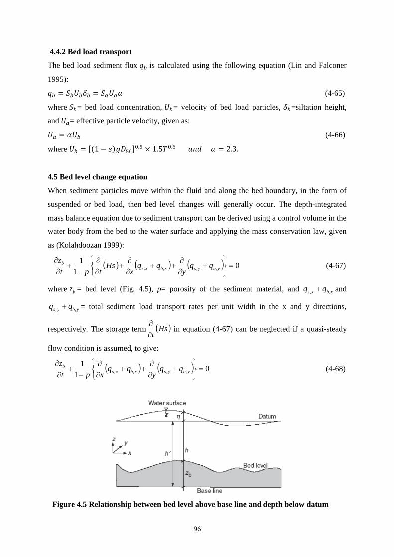
96
4.4.2 Bed load transport
The bed load sediment flux is calculated using the following equation (Lin and Falconer
1995):
(4-65)
where = bed load concentration, = velocity of bed load particles, =siltation height,
and = effective particle velocity, given as:
(4-66)
where [ ]
4.5 Bed level change equation
When sediment particles move within the fluid and along the bed boundary, in the form of
suspended or bed load, then bed level changes will generally occur. The depth-integrated
mass balance equation due to sediment transport can be derived using a control volume in the
water body from the bed to the water surface and applying the mass conservation law, given
as (Kolahdoozan 1999):
01
1,,,,
ybysxbxs
b qqy
qqx
sHtpt
z (4-67)
where bz = bed level (Fig. 4.5), p= porosity of the sediment material, and xbxs qq ,, and
ybys qq ,, = total sediment load transport rates per unit width in the x and y directions,
respectively. The storage term sHt
in equation (4-67) can be neglected if a quasi-steady
flow condition is assumed, to give:
01
1,,,,
ybysxbxs
b qqy
qqxpt
z (4-68)
Figure 4.5 Relationship between bed level above base line and depth below datum
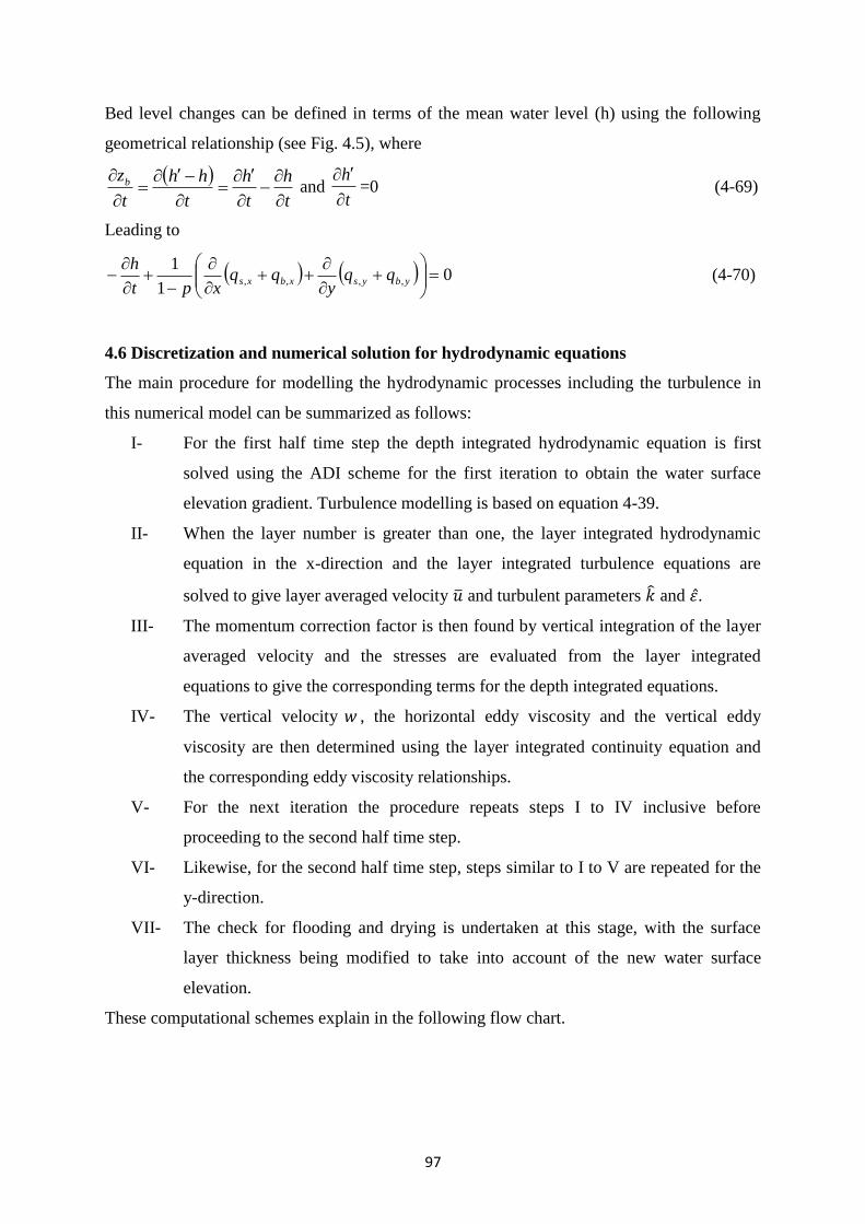
97
Bed level changes can be defined in terms of the mean water level (h) using the following
geometrical relationship (see Fig. 4.5), where
t
h
t
h
t
hh
t
zb
and
t
h
=0 (4-69)
Leading to
01
1,,,,
ybysxbxs qq
yqq
xpt
h (4-70)
4.6 Discretization and numerical solution for hydrodynamic equations
The main procedure for modelling the hydrodynamic processes including the turbulence in
this numerical model can be summarized as follows:
I- For the first half time step the depth integrated hydrodynamic equation is first
solved using the ADI scheme for the first iteration to obtain the water surface
elevation gradient. Turbulence modelling is based on equation 4-39.
II- When the layer number is greater than one, the layer integrated hydrodynamic
equation in the x-direction and the layer integrated turbulence equations are
solved to give layer averaged velocity and turbulent parameters and .
III- The momentum correction factor is then found by vertical integration of the layer
averaged velocity and the stresses are evaluated from the layer integrated
equations to give the corresponding terms for the depth integrated equations.
IV- The vertical velocity , the horizontal eddy viscosity and the vertical eddy
viscosity are then determined using the layer integrated continuity equation and
the corresponding eddy viscosity relationships.
V- For the next iteration the procedure repeats steps I to IV inclusive before
proceeding to the second half time step.
VI- Likewise, for the second half time step, steps similar to I to V are repeated for the
y-direction.
VII- The check for flooding and drying is undertaken at this stage, with the surface
layer thickness being modified to take into account of the new water surface
elevation.
These computational schemes explain in the following flow chart.
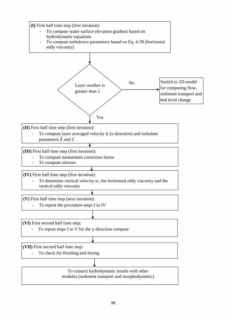
98
(II) First half time step (first iteration):
- To compute layer averaged velocity �� (x-direction) and turbulent
parameters �� and 𝜀 .
Layer number is
greater than 1
Yes
No Switch to 2D model
for computing flow,
sediment transport and
bed level change
(III) First half time step (first iteration):
- To compute momentum correction factor
- To compute stresses
(IV) First half time step (first iteration):
- To determine vertical velocity 𝑤, the horizontal eddy viscosity and the
vertical eddy viscosity
(I) First half time step (first iteration):
- To compute water surface elevation gradient based on
hydrodynamic equations
- To compute turbulence parameters based on Eq. 4-39 (horizontal
eddy viscosity)
(V) First half time step (next iteration):
- To repeat the procedure steps I to IV
(VI) First second half time step:
- To repeat steps I to V for the y-direction compute
(VII) First second half time step:
- To check for flooding and drying
To connect hydrodynamic results with other
modules (sediment transport and morphodynamic)
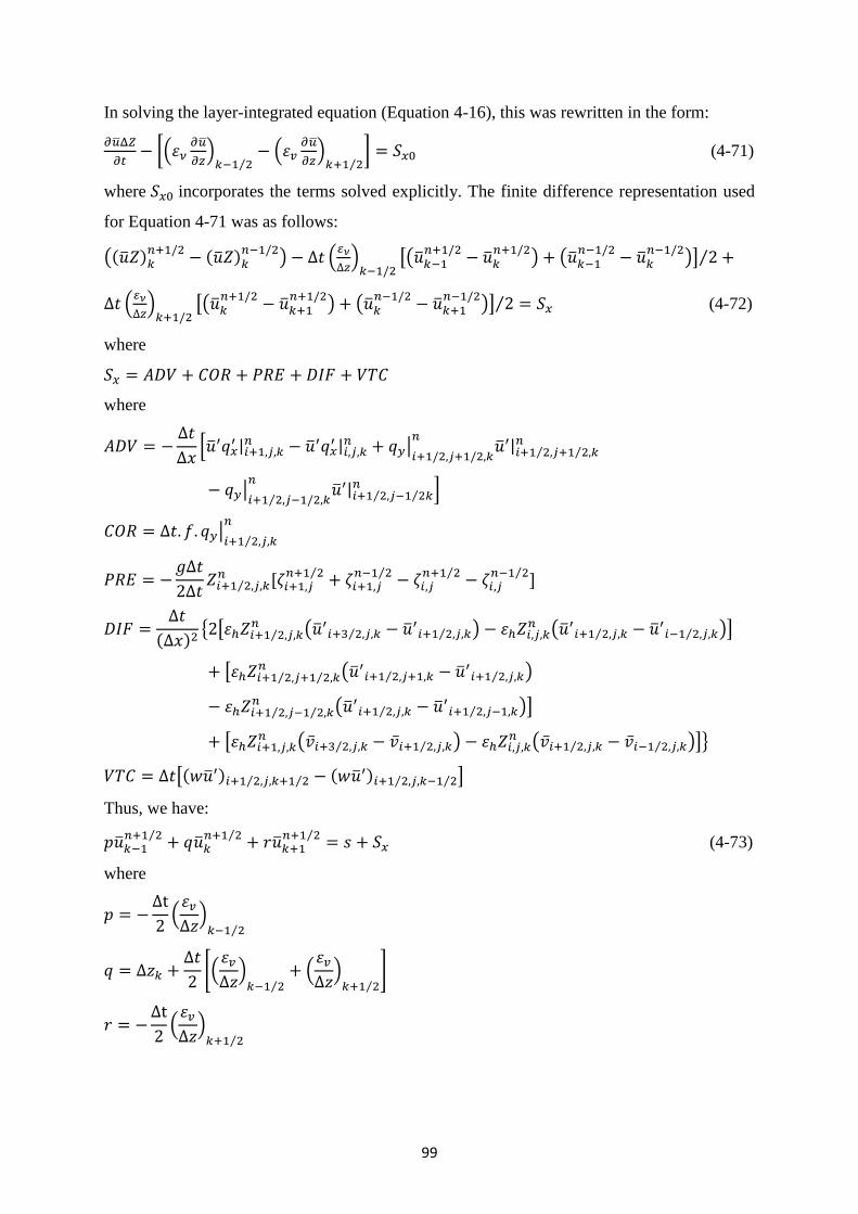
99
In solving the layer-integrated equation (Equation 4-16), this was rewritten in the form:
[(
) ⁄
(
) ⁄
] (4-71)
where incorporates the terms solved explicitly. The finite difference representation used
for Equation 4-71 was as follows:
(
) (
)
[(
) (
)] ⁄
(
)
[(
) (
)] ⁄ (4-72)
where
where
*
|
| |
| ⁄ ⁄
| ⁄
| ⁄ ⁄
+
| ⁄
⁄
[ ⁄
⁄ ⁄
⁄ ]
{ [ ⁄
( ⁄
⁄ ) (
⁄ ⁄ )]
[ ⁄ ⁄ (
⁄ ⁄ )
⁄ ⁄ (
⁄ ⁄ )]
[ ( ⁄ ⁄ )
( ⁄ ⁄ )]}
[ ⁄⁄ ⁄⁄ ]
Thus, we have:
⁄
⁄ ⁄ (4-73)
where
(
) ⁄
0(
) ⁄
(
) ⁄
1
(
) ⁄
100
⁄
2(
) ⁄
⁄ ⁄ 0(
) ⁄
(
) ⁄
1 ⁄
(
) ⁄
⁄ 3
Horizontally, a space-staggered grid representation was used, with the velocities and depths
being located at the centre of the sides of the grid cell, and with the other main variables
being located at the centre of the grid cell. For the horizontal differential terms, the same
basic finite difference scheme and grid representations were used both for the layer- and
depth integrated equations, thus the velocities obtained from these two set of equations were
consistent.
The discrete form of the layer integrated equations can be written in a similar manner
to the hydrodynamic equations. Therefore the layer integrated turbulent kinetic energy
equation can be written as (just for keeping the format of turbulence Equations 4-47 and 4-48
the notation of vertical eddy viscosity , is the same (Hamkinzadeh 1997)):
⁄
*
| ⁄
| ⁄ | ⁄
| ⁄
+
*( )
⁄ ( )
⁄+
⁄*
(
⁄
⁄ )+
⁄
⁄*
(
⁄ ⁄ )+
⁄
[( ⁄
⁄
⁄ ⁄ )
( ⁄ ⁄ ⁄
⁄ )
]
(4-74)
Similarly, the discrete form of the layer integrated equation for the dissipation rate of the
turbulent kinetic energy can be written as (Hakimzadeh 1997):
⁄
*
| ⁄
| ⁄ | ⁄
| ⁄
+
[ ⁄ ⁄ ]
⁄*
(
⁄
⁄ )+
⁄
⁄*
(
⁄ ⁄ )+
⁄
[( ⁄ ⁄
⁄ ⁄ )
( ⁄ ⁄ ⁄
⁄ )
]
(4-75)
For the layer integrated finite difference equations for the turbulence model, then these
equations can be solved by the Thomas Algorithm in a similar method in hydrodynamic
section. Hence, equation (4-73) can be written as (Hakimzadeh 1997):
101
⁄
⁄ ⁄ (4-76)
where
⁄.
/ ⁄
⁄.
/ ⁄
⁄.
/ ⁄
⁄.
/ ⁄
where
( )
*
| ⁄
| ⁄ | ⁄
| ⁄
+
[( ⁄
⁄ ⁄ ⁄ )
( ⁄ ⁄ ⁄
⁄ )
]
*( )
⁄ ( )
⁄+
Using the Thomas algorithm the unknown parameter can be calculated as outlined in
Hakimzadeh (1997). Likewise, the same procedure can be used for the equation for the
dissipation rate of the turbulence kinetic energy.
4.6.1 Representation of closed boundary conditions
Three closed boundary representations were considered to evaluate the second derivative for
the turbulent diffusion terms adjacent to solid boundaries and the advective acceleration
representations along the boundary.
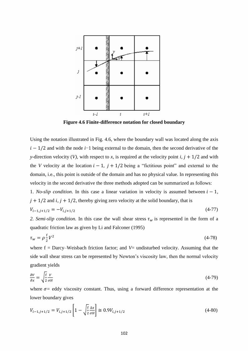
102
Figure 4.6 Finite-difference notation for closed boundary
Using the notation illustrated in Fig. 4.6, where the boundary wall was located along the axis
and with the node i−1 being external to the domain, then the second derivative of the
y-direction velocity (V), with respect to x, is required at the velocity point i, and with
the V velocity at the location being a ―fictitious point‖ and external to the
domain, i.e., this point is outside of the domain and has no physical value. In representing this
velocity in the second derivative the three methods adopted can be summarized as follows:
1. No-slip condition. In this case a linear variation in velocity is assumed between ,
and , , thereby giving zero velocity at the solid boundary, that is
⁄ ⁄ (4-77)
2. Semi-slip condition. In this case the wall shear stress is represented in the form of a
quadratic friction law as given by Li and Falconer (1995)
(4-78)
where f = Darcy–Weisbach friction factor; and V= undisturbed velocity. Assuming that the
side wall shear stress can be represented by Newton’s viscosity law, then the normal velocity
gradient yields
√
(4-79)
where = eddy viscosity constant. Thus, using a forward difference representation at the
lower boundary gives
⁄ ⁄ 0 √
1 ⁄ (4-80)
103
which is close to the free-slip boundary condition.
3. Partial-slip condition. In this case the velocity profile is assumed to follow a seventh
power law distribution between the free stream velocity, at some point and the wall [see
Alstead (1994)] giving
⁄ *
⁄+
(4-81)
Differentiating both for the first and second derivatives, this approach gives
⁄ ⁄ (4-82)
In section 4.6, discretization of the 3D hydrodynamic and turbulence equations of the
numerical model was explained. The 2D form of the numerical model can be found in the
reference manual of DIVAST model by Falconer and Lin (2001).
4.7 Discretization and numerical solution for sediment transport equations
An operator splitting was used to solve the suspended sediment transport equation 4-56. The
basic principle of this method is to split the advective –diffusion equation into several smaller
and simpler sub-equations, with each sub-equation being solved using the most efficient
numerical algorithm (Lin and Falconer 1997). For expressing the advective-diffusion
equation in the form of an initial value equation, with appropriate initial and boundary
conditions are referred to Lin and Falconer (1996) and are not included here for brevity
The main attraction of using this method is the flexibility in the choice of how to split the
original equation. Basically there are two ways of splitting an equation; one is to split the
governing equation according to the nature of physical processes of the terms, and the other is
to split the governing equation according to the direction of the partial differential terms.
Therefore a multi-dimensional sediment transport equation may be split into an advection
equation, a diffusion equation and a reaction equation (Ding and Liu, 1989) or into several
one-dimensional sub-equations for each direction. In an estuarine or reservoir study the
horizontal dimension is generally much larger than the vertical dimension, thus equation
4-56 could be rearranged into the following two equations:
(
) (4-83a)
*
+ at the water surface ,
and:
(
)
at the bed
104
where and other equation being:
(
)
(
) , (4-83b)
for and with the open
and closed boundary conditions being as highlighted previously.
Equation (4-83a) is a one dimensional equation and was discretized using an unequally
spaced grid in the vertical direction. Since the diffusion term is the most important term in
this equation, and some of the grid sizes may become very smaller near the bed and water
surface, the equation was solved an implicit finite volume method to avoid very small time
steps. In the study carried out by Lin and Falconer (1996), the total mass flux was
approximated by a power law scheme (Patankar 1988). This scheme used a combination of
an exponential function and a linear function to approximate the analytical solution of the
1-D advective-diffusion equation and only three vertical grid points are used in its differential
form. Since a sigma co-ordinate system was not used in this numerical model, the number of
vertical layers may be very small in the shallow part of an estuary or reservoir and thus the
power-law scheme is particularly attractive. The discretization equation for equation (4-83a)
is therefore:
(4-84)
where
| | [ ]
| | [ ]
where
| | [ | | ] (4-85)
The symbol [ ] is used to denote the greater of and , subscripts and denote the
control volume face, grid Peclet number, = diffusion coefficient and mass flow
rate, with full definitions being given in Patankar (1988).
Equation (4-84) has a tridiagonal matrix of coefficients and has therefore been solved using a
tridiagonal matrix algorithm. Equation (4-83b) has first integrated over the layer thickness
to give:
(
)
(
) (4-86)
105
for
Since a uniform grid square has been deployed horizontally and the grid size relatively large,
the advection terms (of order ) are likely to dominate over the diffusion terms (of
order ). Numerical experiments show that using traditional higher-order accurate finite
difference schemes, such as the QUICK scheme (Leonard 1991), pose difficulties in dealing
with advection dominated flows in that negative concentrations can arise as the result of
undershoot. Undershoot and overshoot usually occur in regions where the gradients of the
concentration are relatively large. One approach to overcome this problem is to introduce a
limiter function; such that undershoot and overshoot are first detected and then prevented.
There are a number of schemes documented for this purpose, with TVD (Total Variance
Diminishing) scheme being one of most popular for solving advective-diffusion problem.
Cahyono (1993) carried out a detailed study by comparing 36 finite difference schemes and
applying them to six numerical test cases for both one-dimensional and two-dimensional
flows. His comparisons showed that the ULTIMATE scheme, originally proposed by
Leonard (1991), was particularly attractive since it was more general than the other schemes
considered and was easier to apply. Lin and Falconer (1997), in their 2D depth integrated
estuarine model, used both splitting and non-splitting methods for third order QUIKEST
scheme combined with ULTIMATE limiter, to predict solute and sediment transport.
In the numerical reported herein, the ULTIMATE QUICKSET scheme has been used to
present the advective terms in equation (4-86), with the central difference scheme being used
to represent the diffusion terms and with the source term being represented by a first order
accurate difference approximation in time. For simplicity, only a brief discussion of
discretization of the advective terms will be given here.
For a typical cell i, j at layer k, the advection terms in equation (4-86) was expressed as the
sum of the four face values, i.e., west face, east face, south face and north face values. The
fluxes across these faces were then evaluated using the two-dimensional form of the third-
order QUIKSET scheme. These face values were then rewritten in the non-dimensional form
and a universal limiter was applied to check and eliminate any unphysical oscillations.
Further details of the scheme are given elsewhere (see Lin and Falconer 1996).
4.8 Discretization and numerical solution for bed level change equation
As the aim of this research was to model the morphodynamic processes, in this section
emphasis will be focused on the numerical solution method for predicting bed level changes.
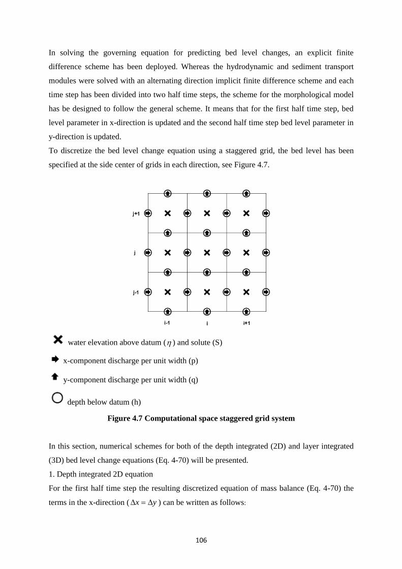
106
In solving the governing equation for predicting bed level changes, an explicit finite
difference scheme has been deployed. Whereas the hydrodynamic and sediment transport
modules were solved with an alternating direction implicit finite difference scheme and each
time step has been divided into two half time steps, the scheme for the morphological model
has be designed to follow the general scheme. It means that for the first half time step, bed
level parameter in x-direction is updated and the second half time step bed level parameter in
y-direction is updated.
To discretize the bed level change equation using a staggered grid, the bed level has been
specified at the side center of grids in each direction, see Figure 4.7.
water elevation above datum ( ) and solute (S)
x-component discharge per unit width (p)
y-component discharge per unit width (q)
depth below datum (h)
Figure 4.7 Computational space staggered grid system
In this section, numerical schemes for both of the depth integrated (2D) and layer integrated
(3D) bed level change equations (Eq. 4-70) will be presented.
1. Depth integrated 2D equation
For the first half time step the resulting discretized equation of mass balance (Eq. 4-70) the
terms in the x-direction ( yx ) can be written as follows:

107
t
hh
t
h
n
ji
n
ji
*5.0
,2
12
1
,2
1
(4-87)
n
ji
n
ji
n
ji
n
ji
xt
xbxs hsuxpx
q
pqq
xp2
1,
2
1
2
1,
2
1
2
1,
2
1
2
1,
2
1
,
,,*1
1
1
1
1
1
n
ji
n
ji
n
ji
n
jihsu
2
1,
2
1
2
1,
2
1
2
1,
2
1
2
1,
2
1 (4-88)
n
ji
n
ji
n
ji
n
ji
yt
ybys hsvypy
q
pqq
yp2
1,
2
1
2
1,
2
1
2
1,
2
1
2
1,
2
1
,
,,*1
1
1
1
1
1
n
ji
n
ji
n
ji
n
jihsv
2
1,
2
1
2
1,
2
1
2
1,
2
1
2
1,
2
1 (4-89)
Likewise for the second half time step (y-direction): ( yx )
t
hh
t
h
n
ji
n
ji
*5.0
2
1
2
1,
1
2
1,
(4-90)
2
1
2
1,
2
12
1
2
1,
2
12
1
2
1,
2
12
1
2
1,
2
1
,
,,*1
1
1
1
1
1 n
ji
n
ji
n
ji
n
ji
xt
xbxs hsuxpx
q
pqq
xp
2
1
2
1,
2
12
1
2
1,
2
12
1
2
1,
2
12
1
2
1,
2
1
n
ji
n
ji
n
ji
n
jihsu (4-91)
2
1
2
1,
2
12
1
2
1,
2
12
1
2
1,
2
12
1
2
1,
2
1
,
,,*1
1
1
1
1
1 n
ji
n
ji
n
ji
n
ji
yt
ybys hsvypy
q
pqq
yp
2
1
2
1,
2
12
1
2
1,
2
12
1
2
1,
2
12
1
2
1,
2
1
n
ji
n
ji
n
ji
n
jihsv (4-92)
2. Layer integrated 3D equation
For the first half time step the resulting discretized equation of mass balance (Eq. 4-70) the
terms in the x-direction ( yx ) can be written as follows:
t
lhlhlhlh
t
h
kk
k
kk
k
n
kji
n
kji
n
kji
n
kji
*5.0
)()()()(1max 1max
maxmax 1 1,,
2
12
1
,,2
1,,
2
12
1
,,2
1
(4-93)
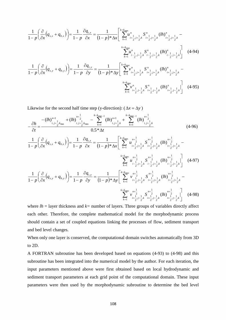
108
n
kji
n
kji
kk
k
n
kji
xt
xbxs lhSuxpx
q
pqq
xp ,2
1,
2
1,
2
1,
2
1
1,
2
1,
2
1
,
,, )(*1
1
1
1
1
1 max
n
kji
n
kji
kk
k
n
kjilhSu
,2
1,
2
1,
2
1,
2
1
1,
2
1,
2
1 )(max
(4-94)
n
kji
n
kji
kk
k
n
kji
yt
ybys lhSvypy
q
pqq
xp ,2
1,
2
1,
2
1,
2
1
1,
2
1,
2
1
,
,, )(*1
1
1
1
1
1 max
n
kji
n
kji
kk
k
n
kjilhSv
,2
1,
2
1,
2
1,
2
1
1,
2
1,
2
1 )(max
(4-95)
Likewise for the second half time step (y-direction): ( yx )
t
lhlhlhlh
t
h
kk
k
kk
k
n
kji
n
kji
n
kji
n
kji
*5.0
)()()()(1max 1max
maxmax 1 1
2
1
,2
1,
1
,2
1,
2
1
,2
1,
1
,2
1,
(4-96)
2
1
,2
1,
2
12
1
,2
1,
2
1
1
2
1
,2
1,
2
1
,
,, )(*1
1
1
1
1
1 max n
kji
n
kji
kk
k
n
kji
xt
xbxs lhSuxpx
q
pqq
xp
2
1
,2
1,
2
12
1
,2
1,
2
1
1
2
1
,2
1,
2
1 )(max n
kji
n
kji
kk
k
n
kjilhSu (4-97)
2
1
,2
1,
2
12
1
,2
1,
2
1
1
2
1
,2
1,
2
1
,
,, )(*1
1
1
1
1
1 max n
kji
n
kji
kk
k
n
kji
yt
ybys lhSvypy
q
pqq
xp
2
1
,2
1,
2
12
1
,2
1,
2
1
1
2
1
,2
1,
2
1 )(max n
kji
n
kji
kk
k
n
kjilhSv (4-98)
where lh = layer thickness and k= number of layers. Three groups of variables directly affect
each other. Therefore, the complete mathematical model for the morphodynamic process
should contain a set of coupled equations linking the processes of flow, sediment transport
and bed level changes.
When only one layer is conserved, the computational domain switches automatically from 3D
to 2D.
A FORTRAN subroutine has been developed based on equations (4-93) to (4-98) and this
subroutine has been integrated into the numerical model by the author. For each iteration, the
input parameters mentioned above were first obtained based on local hydrodynamic and
sediment transport parameters at each grid point of the computational domain. These input
parameters were then used by the morphodynamic subroutine to determine the bed level
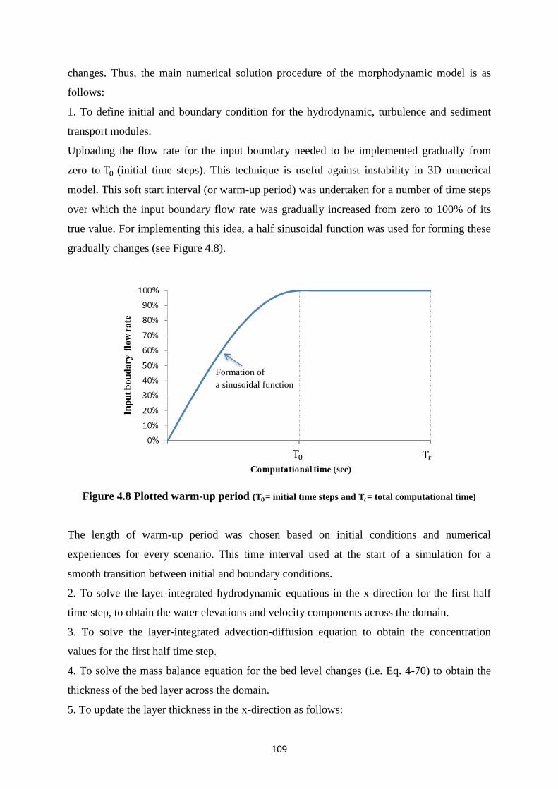
109
changes. Thus, the main numerical solution procedure of the morphodynamic model is as
follows:
1. To define initial and boundary condition for the hydrodynamic, turbulence and sediment
transport modules.
Uploading the flow rate for the input boundary needed to be implemented gradually from
zero to (initial time steps). This technique is useful against instability in 3D numerical
model. This soft start interval (or warm-up period) was undertaken for a number of time steps
over which the input boundary flow rate was gradually increased from zero to 100% of its
true value. For implementing this idea, a half sinusoidal function was used for forming these
gradually changes (see Figure 4.8).
Figure 4.8 Plotted warm-up period ( = initial time steps and = total computational time)
The length of warm-up period was chosen based on initial conditions and numerical
experiences for every scenario. This time interval used at the start of a simulation for a
smooth transition between initial and boundary conditions.
2. To solve the layer-integrated hydrodynamic equations in the x-direction for the first half
time step, to obtain the water elevations and velocity components across the domain.
3. To solve the layer-integrated advection-diffusion equation to obtain the concentration
values for the first half time step.
4. To solve the mass balance equation for the bed level changes (i.e. Eq. 4-70) to obtain the
thickness of the bed layer across the domain.
5. To update the layer thickness in the x-direction as follows:
𝑡
Formation of
a sinusoidal function
110
lhxulhxmlhxu )1( 11 (4-99)
where lhxulhxm, are layer thicknesses in the x-direction for pervious and current time step
respectively, ,1 is a relaxation coefficient,
Using equation 4-99 is a technique to avoid generating a ―chock‖ in the computational
scheme.
6. To update the values of the velocity components, sediment concentration and bed levels for
the next half time step.
7. To repeat steps 2-6 for the y-direction.
4.9 Summary
The hydrodynamic governing equations of flows in reservoirs have been reviewed in this
chapter. The original numerical model was designed for coastal and estuarine flows (see Lin
and Falconer 1997) and the mixing length model was used in the original version. Effort has
been made to enhance the ability of hydrodynamic model for using in the reservoir
environment. The depth integrated and layer integrated equations of water flow have been
reviewed and the scheme for simulating the role of the gates for the numerical model has
been introduced.
Also, the turbulence models, including the mixing length and models have been
reviewed briefly. The turbulence kinetic energy and dissipation rate of kinetic energy
equations have been explained. The constants and the boundary condition used in the above
turbulence models have been also outlined.
Besides, the governing sediment transport and bed level change equations have been
discussed. The morphodynamic process was the focus in this research and the governing
equation describing the bed level changes was derived by integrating the mass balance
equation over the full depth, including both the suspended and bed load layers
The layer integrated governing equations of the hydrodynamic (including the model),
sediment transport and morphodynamic processes were discretized in this chapter. This was
followed by the representation of suitable boundary conditions for both the open and closed
boundaries. Then the numerical solution of the layer integrated equations and solution
procedure for different modules (hydrodynamic, turbulence, sediment transport and
morphodynamic) were explained. The essence of this research lies in the three-dimensional
processes and for this reason the main emphasis has been placed on the 3D layer integrated
equations.
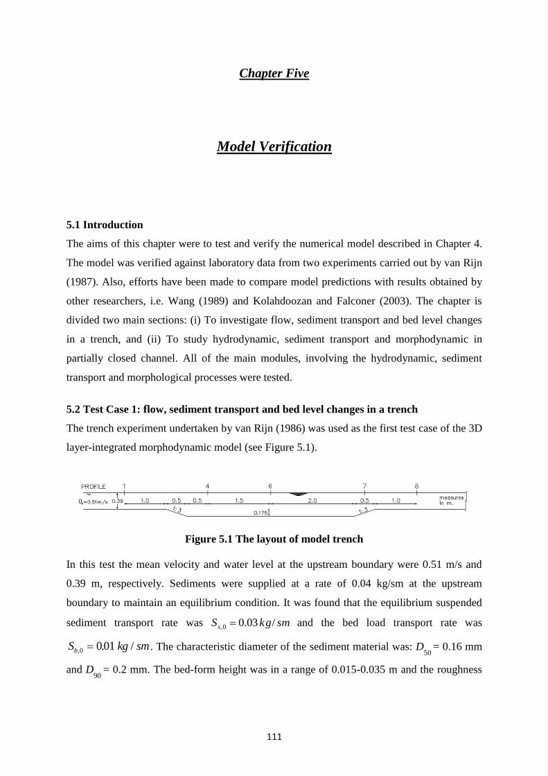
111
Chapter Five
Model Verification
5.1 Introduction
The aims of this chapter were to test and verify the numerical model described in Chapter 4.
The model was verified against laboratory data from two experiments carried out by van Rijn
(1987). Also, efforts have been made to compare model predictions with results obtained by
other researchers, i.e. Wang (1989) and Kolahdoozan and Falconer (2003). The chapter is
divided two main sections: (i) To investigate flow, sediment transport and bed level changes
in a trench, and (ii) To study hydrodynamic, sediment transport and morphodynamic in
partially closed channel. All of the main modules, involving the hydrodynamic, sediment
transport and morphological processes were tested.
5.2 Test Case 1: flow, sediment transport and bed level changes in a trench
The trench experiment undertaken by van Rijn (1986) was used as the first test case of the 3D
layer-integrated morphodynamic model (see Figure 5.1).
Figure 5.1 The layout of model trench
In this test the mean velocity and water level at the upstream boundary were 0.51 m/s and
0.39 m, respectively. Sediments were supplied at a rate of 0.04 kg/sm at the upstream
boundary to maintain an equilibrium condition. It was found that the equilibrium suspended
sediment transport rate was smkgSs /03.00, and the bed load transport rate was
S kg smb, . /0 001 . The characteristic diameter of the sediment material was: D50
= 0.16 mm
and D90
= 0.2 mm. The bed-form height was in a range of 0.015-0.035 m and the roughness
112
coefficient was sk = 0.025 m. More details of the model configuration and hydraulic
parameters can be found in van Rijn (1986).
In applying the 3D layer-integrated morphodynamic model to this case study the depth of the
(Equation 5-1) was used to compute the thickness of layers. The minimum thickness was
0.02 m near of the bed and the thickness of the upper layers was gradually changed to reach
0.078 m at the top (first layer).
(5-1)
(5-2)
where
= the vertical elevation of the th layer from the top surface (see Figure 5.1)
= the th layer thickness
= the number of layer
= coefficients
This method provides a greater resolution in the zone where large velocity and concentration
gradients exist (i.e. near the bed surface) and the sediment transport process can be simulated
more precisely. The most important point in this method is the consideration of a similar
bottom layer thickness for the upstream, excavation zone and downstream of the trench.
Comparisons between the model predicted and measured velocity profiles and sediment
concentration profiles at five cross sections shown in Figure 5.1 are given in Figures 5.2 and
5.3. It can be seen that the velocity profiles has been well predicted by the 3D layer-
integrated morphodynamic model, with the shape of the velocity curves following the
measured ones.
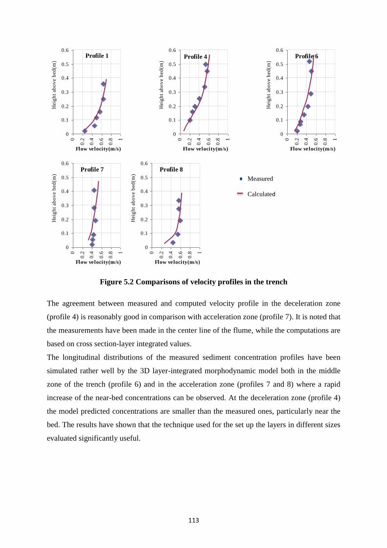
113
Figure 5.2 Comparisons of velocity profiles in the trench
The agreement between measured and computed velocity profile in the deceleration zone
(profile 4) is reasonably good in comparison with acceleration zone (profile 7). It is noted that
the measurements have been made in the center line of the flume, while the computations are
based on cross section-layer integrated values.
The longitudinal distributions of the measured sediment concentration profiles have been
simulated rather well by the 3D layer-integrated morphodynamic model both in the middle
zone of the trench (profile 6) and in the acceleration zone (profiles 7 and 8) where a rapid
increase of the near-bed concentrations can be observed. At the deceleration zone (profile 4)
the model predicted concentrations are smaller than the measured ones, particularly near the
bed. The results have shown that the technique used for the set up the layers in different sizes
evaluated significantly useful.
Profile 1
0
0.1
0.2
0.3
0.4
0.5
0.6
0
0.2
0.4
0.6
0.8 1
Flow velocity(m/s)
Heig
ht
ab
ov
e b
ed
(m)
Profile 4
0
0.1
0.2
0.3
0.4
0.5
0.6
0
0.2
0.4
0.6
0.8 1
Flow velocity(m/s)
Heig
ht
ab
ov
e b
ed
(m)
Profile 6
0
0.1
0.2
0.3
0.4
0.5
0.6
0
0.2
0.4
0.6
0.8 1
Flow velocity(m/s)
Heig
ht
ab
ov
e b
ed
(m)
Profile 7
0
0.1
0.2
0.3
0.4
0.5
0.6
0
0.2
0.4
0.6
0.8 1
Flow velocity(m/s)
Heig
ht
ab
ov
e b
ed
(m)
Profile 8
0
0.1
0.2
0.3
0.4
0.5
0.6
0
0.2
0.4
0.6
0.8 1
Flow velocity(m/s)
Heig
ht
ab
ov
e b
ed
(m)
♦ Measured
Calculated
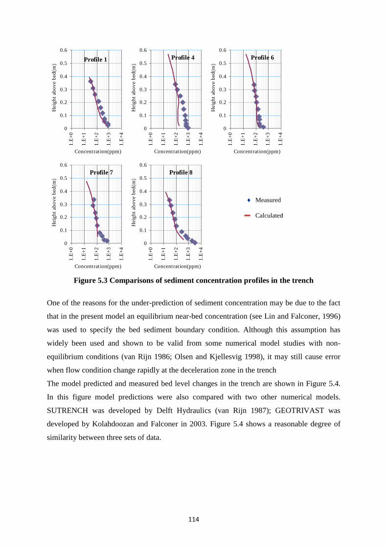
114
Figure 5.3 Comparisons of sediment concentration profiles in the trench
One of the reasons for the under-prediction of sediment concentration may be due to the fact
that in the present model an equilibrium near-bed concentration (see Lin and Falconer, 1996)
was used to specify the bed sediment boundary condition. Although this assumption has
widely been used and shown to be valid from some numerical model studies with non-
equilibrium conditions (van Rijn 1986; Olsen and Kjellesvig 1998), it may still cause error
when flow condition change rapidly at the deceleration zone in the trench
The model predicted and measured bed level changes in the trench are shown in Figure 5.4.
In this figure model predictions were also compared with two other numerical models.
SUTRENCH was developed by Delft Hydraulics (van Rijn 1987); GEOTRIVAST was
developed by Kolahdoozan and Falconer in 2003. Figure 5.4 shows a reasonable degree of
similarity between three sets of data.
Profile 1
0
0.1
0.2
0.3
0.4
0.5
0.6
1.E
+0
1.E
+1
1.E
+2
1.E
+3
1.E
+4
Concentration(ppm)
Heig
ht
ab
ov
e b
ed
(m)
Profile 4
0
0.1
0.2
0.3
0.4
0.5
0.6
1.E
+0
1.E
+1
1.E
+2
1.E
+3
1.E
+4
Concentration(ppm)
Heig
ht
ab
ov
e b
ed
(m)
Profile 6
0
0.1
0.2
0.3
0.4
0.5
0.6
1.E
+0
1.E
+1
1.E
+2
1.E
+3
1.E
+4
Concentration(ppm)
Heig
ht
ab
ov
e b
ed
(m)
Profile 7
0
0.1
0.2
0.3
0.4
0.5
0.6
1.E
+0
1.E
+1
1.E
+2
1.E
+3
1.E
+4
Concentration(ppm)
Heig
ht
ab
ov
e b
ed
(m)
Profile 8
0
0.1
0.2
0.3
0.4
0.5
0.6
1.E
+0
1.E
+1
1.E
+2
1.E
+3
1.E
+4
Concentration(ppm)
Heig
ht
ab
ov
e b
ed
(m)
♦ Measured
Calculated

115
Figure 5.4 Bed level profiles in the trench after 15 hours (Present N.M =Present Numerical
Model)
5.2.1 A sensitive analysis on vertical layers
The influence of the number (n) of vertical layers on the computed flow velocity and
sediment concentration has been investigated for this case study. The number (n) of vertical
layers is specified as an input parameter in this sensitive analysis. The model was run for 10
layers and explained in above section. For the second run, the depth of the channel is divided
into 20 layers with different thickness. The minimum thickness is 0.02 m near of the bed and
the thickness of the upper layers is gradually changed to reach 0.033 m at the top (first layer).
The computed velocity and sediment concentration profiles (for two runs, 10 layers and 20
layers) at five cross sections shown in Figure 5.1 are presented and compared with the
measured data in Figures 5.5 and 5.6.
0
0.04
0.08
0.12
0.16
0.2
0 1 2 3 4 5 6 7 8 9 10 11
Distance (m)
Bed
Level (m
)
Measured
SUTRENCH
GEOTRIVAST
Present N.M
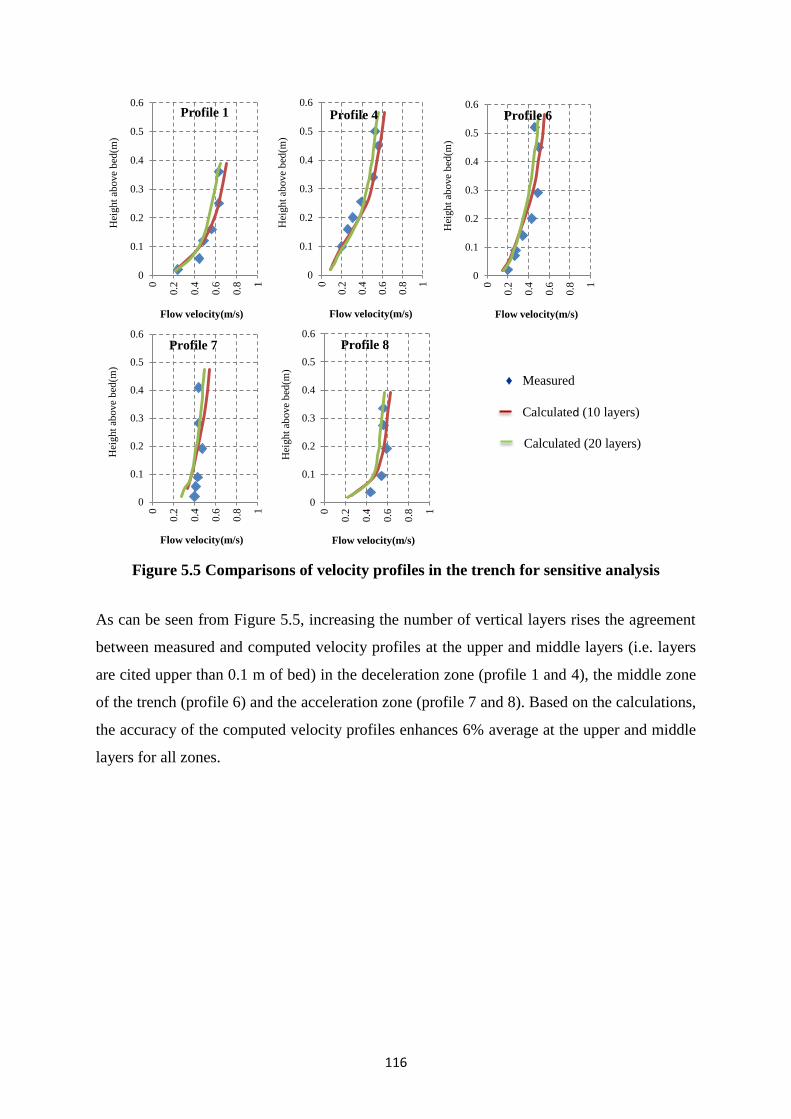
116
Figure 5.5 Comparisons of velocity profiles in the trench for sensitive analysis
As can be seen from Figure 5.5, increasing the number of vertical layers rises the agreement
between measured and computed velocity profiles at the upper and middle layers (i.e. layers
are cited upper than 0.1 m of bed) in the deceleration zone (profile 1 and 4), the middle zone
of the trench (profile 6) and the acceleration zone (profile 7 and 8). Based on the calculations,
the accuracy of the computed velocity profiles enhances 6% average at the upper and middle
layers for all zones.
0
0.1
0.2
0.3
0.4
0.5
0.6
0
0.2
0.4
0.6
0.8 1
Hei
gh
t ab
ove
bed
(m)
Flow velocity(m/s)
Profile 1
0
0.1
0.2
0.3
0.4
0.5
0.6
0
0.2
0.4
0.6
0.8 1
Hei
gh
t ab
ove
bed
(m)
Flow velocity(m/s)
Profile 4
0
0.1
0.2
0.3
0.4
0.5
0.6
0
0.2
0.4
0.6
0.8 1
Hei
gh
t ab
ove
bed
(m)
Flow velocity(m/s)
Profile 6
0
0.1
0.2
0.3
0.4
0.5
0.6
0
0.2
0.4
0.6
0.8 1
Hei
gh
t ab
ove
bed
(m)
Flow velocity(m/s)
Profile 7
0
0.1
0.2
0.3
0.4
0.5
0.60
0.2
0.4
0.6
0.8 1
Hei
gh
t ab
ove
bed
(m)
Flow velocity(m/s)
Profile 8
♦ Measured
Calculated (10 layers)
Calculated (20 layers)

117
Figure 5.6 Comparisons of sediment concentration profiles in the trench for sensitive
analysis
Figure 5.6 shows that comparison between measured and computed sediment concentration
profiles in different zones. By increasing the number of vertical layers, the errors between
measured and computed sediment concentration profiles at the upper and middle layers (i.e.
layers are cited upper than 0.1 m of bed) does not change considerably for all zones (profile
1, 4, 6, 7 and 8). The errors occur at the bottom layers (i.e. layers are cited lower than 0.1 m
of bed) of the acceleration zone (profile 7). This error might be related to an equilibrium
assumption in the numerical model near the bed that explained before in the end of section
5.2 (see Lin and Falconer 1996). For sediment concentration profiles, increasing the number
of vertical layers does not show any considerable influences on the results at the upper and
middle layers while the trend (vertical gradient) of the computed results is generally closer to
the trend of measured data at the bottom layers for profiles 1, 4, 6 and 8. Consequently, only
a greater resolution in vertical grid could not enhance the computed sediment concentration
0
0.1
0.2
0.3
0.4
0.5
0.6
1.E
+0
1.E
+1
1.E
+2
1.E
+3
1.E
+4
Hei
gh
t ab
ove
bed
(m)
Concentration(ppm)
Profile 1
0
0.1
0.2
0.3
0.4
0.5
0.6
1.E
+0
1.E
+1
1.E
+2
1.E
+3
1.E
+4
Hei
gh
t ab
ove
bed
(m)
Concentration(ppm)
Profile 4
0
0.1
0.2
0.3
0.4
0.5
0.6
1.E
+0
1.E
+1
1.E
+2
1.E
+3
1.E
+4
Hei
gh
t ab
ove
bed
(m)
Concentration(ppm)
Profile 6
0
0.1
0.2
0.3
0.4
0.5
0.6
1.E
+0
1.E
+1
1.E
+2
1.E
+3
1.E
+4
Hei
gh
t ab
ove
bed
(m)
Concentration(ppm)
Profile 7
0
0.1
0.2
0.3
0.4
0.5
0.6
1.E
+0
1.E
+1
1.E
+2
1.E
+3
1.E
+4
Hei
gh
t ab
ove
bed
(m)
Concentration(ppm)
Profile 8
♦ Measured
Calculated (10 layers)
Calculated (20 layers)
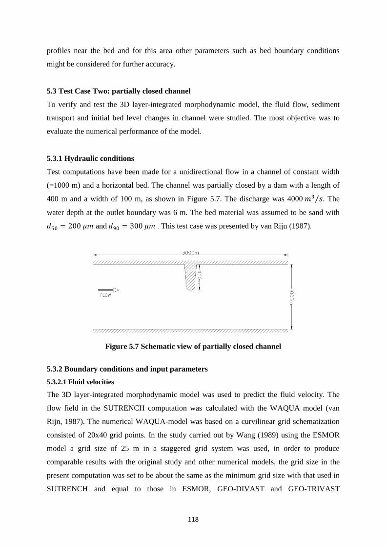
118
profiles near the bed and for this area other parameters such as bed boundary conditions
might be considered for further accuracy.
5.3 Test Case Two: partially closed channel
To verify and test the 3D layer-integrated morphodynamic model, the fluid flow, sediment
transport and initial bed level changes in channel were studied. The most objective was to
evaluate the numerical performance of the model.
5.3.1 Hydraulic conditions
Test computations have been made for a unidirectional flow in a channel of constant width
(=1000 m) and a horizontal bed. The channel was partially closed by a dam with a length of
400 m and a width of 100 m, as shown in Figure 5.7. The discharge was 4000 ⁄ . The
water depth at the outlet boundary was 6 m. The bed material was assumed to be sand with
and . This test case was presented by van Rijn (1987).
Figure 5.7 Schematic view of partially closed channel
5.3.2 Boundary conditions and input parameters
5.3.2.1 Fluid velocities
The 3D layer-integrated morphodynamic model was used to predict the fluid velocity. The
flow field in the SUTRENCH computation was calculated with the WAQUA model (van
Rijn, 1987). The numerical WAQUA-model was based on a curvilinear grid schematization
consisted of 20x40 grid points. In the study carried out by Wang (1989) using the ESMOR
model a grid size of 25 m in a staggered grid system was used, in order to produce
comparable results with the original study and other numerical models, the grid size in the
present computation was set to be about the same as the minimum grid size with that used in
SUTRENCH and equal to those in ESMOR, GEO-DIVAST and GEO-TRIVAST
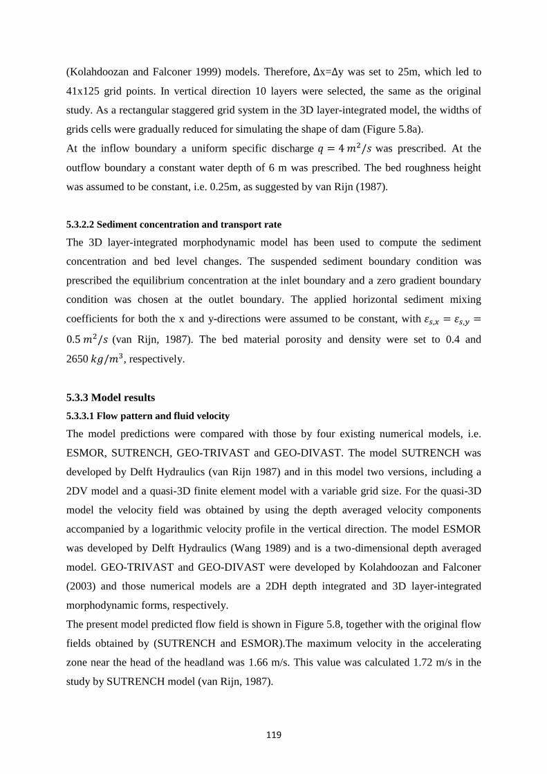
119
(Kolahdoozan and Falconer 1999) models. Therefore, x= y was set to 25m, which led to
41x125 grid points. In vertical direction 10 layers were selected, the same as the original
study. As a rectangular staggered grid system in the 3D layer-integrated model, the widths of
grids cells were gradually reduced for simulating the shape of dam (Figure 5.8a).
At the inflow boundary a uniform specific discharge was prescribed. At the
outflow boundary a constant water depth of 6 m was prescribed. The bed roughness height
was assumed to be constant, i.e. 0.25m, as suggested by van Rijn (1987).
5.3.2.2 Sediment concentration and transport rate
The 3D layer-integrated morphodynamic model has been used to compute the sediment
concentration and bed level changes. The suspended sediment boundary condition was
prescribed the equilibrium concentration at the inlet boundary and a zero gradient boundary
condition was chosen at the outlet boundary. The applied horizontal sediment mixing
coefficients for both the x and y-directions were assumed to be constant, with
(van Rijn, 1987). The bed material porosity and density were set to 0.4 and
2650 , respectively.
5.3.3 Model results
5.3.3.1 Flow pattern and fluid velocity
The model predictions were compared with those by four existing numerical models, i.e.
ESMOR, SUTRENCH, GEO-TRIVAST and GEO-DIVAST. The model SUTRENCH was
developed by Delft Hydraulics (van Rijn 1987) and in this model two versions, including a
2DV model and a quasi-3D finite element model with a variable grid size. For the quasi-3D
model the velocity field was obtained by using the depth averaged velocity components
accompanied by a logarithmic velocity profile in the vertical direction. The model ESMOR
was developed by Delft Hydraulics (Wang 1989) and is a two-dimensional depth averaged
model. GEO-TRIVAST and GEO-DIVAST were developed by Kolahdoozan and Falconer
(2003) and those numerical models are a 2DH depth integrated and 3D layer-integrated
morphodynamic forms, respectively.
The present model predicted flow field is shown in Figure 5.8, together with the original flow
fields obtained by (SUTRENCH and ESMOR).The maximum velocity in the accelerating
zone near the head of the headland was 1.66 m/s. This value was calculated 1.72 m/s in the
study by SUTRENCH model (van Rijn, 1987).

120
a) By the present model
b) By SUTRENCH
c) By ESMOR
Figure 5.8 The velocity field
Also, the streamline pattern in detail for the presented numerical model and SUTRENCH
model along the channel are shown in Figure 5.9. As can be seen from Figure 5.9, a high
agreement exists between both numerical results. Several nodes along the streamlines A and
B, and in the recirculating zone were chosen for comparing the results of present model with
those from the numerical models reported before. Due to high agreement between the
streamline patterns, the locations of these nodes are physically same (see Figure 5.9).
Besides, this arrangement of nodes (situated in a stream line) makes a platform for presenting
sediment transport results in a same stream tube of flow. Besides, the present model predicted
1.0 m/s
1.0
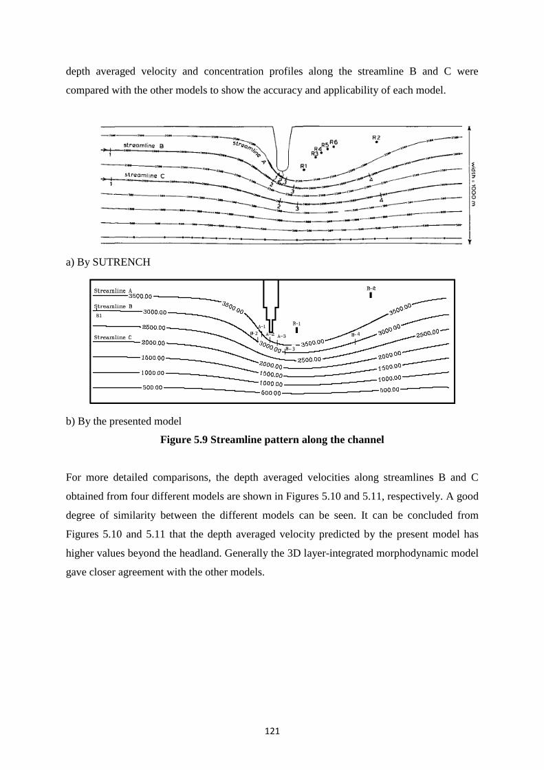
121
depth averaged velocity and concentration profiles along the streamline B and C were
compared with the other models to show the accuracy and applicability of each model.
a) By SUTRENCH
b) By the presented model
Figure 5.9 Streamline pattern along the channel
For more detailed comparisons, the depth averaged velocities along streamlines B and C
obtained from four different models are shown in Figures 5.10 and 5.11, respectively. A good
degree of similarity between the different models can be seen. It can be concluded from
Figures 5.10 and 5.11 that the depth averaged velocity predicted by the present model has
higher values beyond the headland. Generally the 3D layer-integrated morphodynamic model
gave closer agreement with the other models.
B1
2
3
4
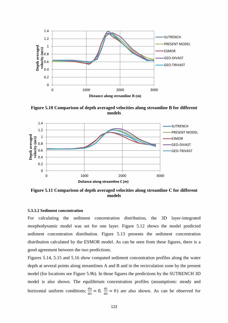
122
Figure 5.10 Comparison of depth averaged velocities along streamline B for different
models
Figure 5.11 Comparison of depth averaged velocities along streamline C for different
models
5.3.3.2 Sediment concentration
For calculating the sediment concentration distribution, the 3D layer-integrated
morphodynamic model was set for one layer. Figure 5.12 shows the model predicted
sediment concentration distribution. Figure 5.13 presents the sediment concentration
distribution calculated by the ESMOR model. As can be seen from these figures, there is a
good agreement between the two predictions.
Figures 5.14, 5.15 and 5.16 show computed sediment concentration profiles along the water
depth at several points along streamlines A and B and in the recirculation zone by the present
model (for locations see Figure 5.9b). In those figures the predictions by the SUTRENCH 3D
model is also shown. The equilibrium concentration profiles (assumptions: steady and
horizontal uniform conditions;
) are also shown. As can be observed for
0
0.2
0.4
0.6
0.8
1
1.2
1.4
0 1000 2000 3000
Dep
th a
ver
ag
ed
vel
oci
ty (
m/s
)
Distance along streamline B (m)
SUTRENCH
PRESENT MODEL
ESMOR
GEO-DIVAST
GEO-TRIVAST
0
0.2
0.4
0.6
0.8
1
1.2
1.4
0 1000 2000 3000
Dep
th a
ver
ag
ed
vel
oci
ty (
m/s
)
Dsitance along streamline C (m)
SUTRENCH
PRESENT MODEL
ESMOR
GEO-DIVAST
GEO-TRIVAST

123
streamlines A and B, the non-equilibrium concentrations are smaller than the equilibrium
values for increasing velocities (
acceleration zone) and larger for decreasing
velocities (
deceleration zone). van Rijn' studies in 1987 revealed that horizontal
distribution of the local equilibrium transport rates near the head of the dam are much larger
(up to a factor of 5!) than horizontal distribution of the depth-integrated suspension sediment
transport computed by the SUTRENCH-3D. Based on these results, he did not recommend to
apply an equilibrium transport formula to compute morphological variations in horizontal
directions in the case of fine sand conditions ( ) and large velocity gradients. It
is noted that the equilibrium concentrations in the recirculation zone are zero because the
velocities are below those for initiation of motion (Fig. 5.16).
Figure 5.12 Sediment concentration distribution obtained from the present model
Figure 5.13 Sediment concentration distribution obtained from ESMOR
As can be concluded from Figures 5.14, 5.15 and 5.16 the results obtained from the 3D layer-
integrated morphodynamic model are in most cases close to non-equilibrium scheme
(SUTRENCH). The results using the above two numerical models are much closer to each
other near the bed of the channel, but near of the water surface a major differences is
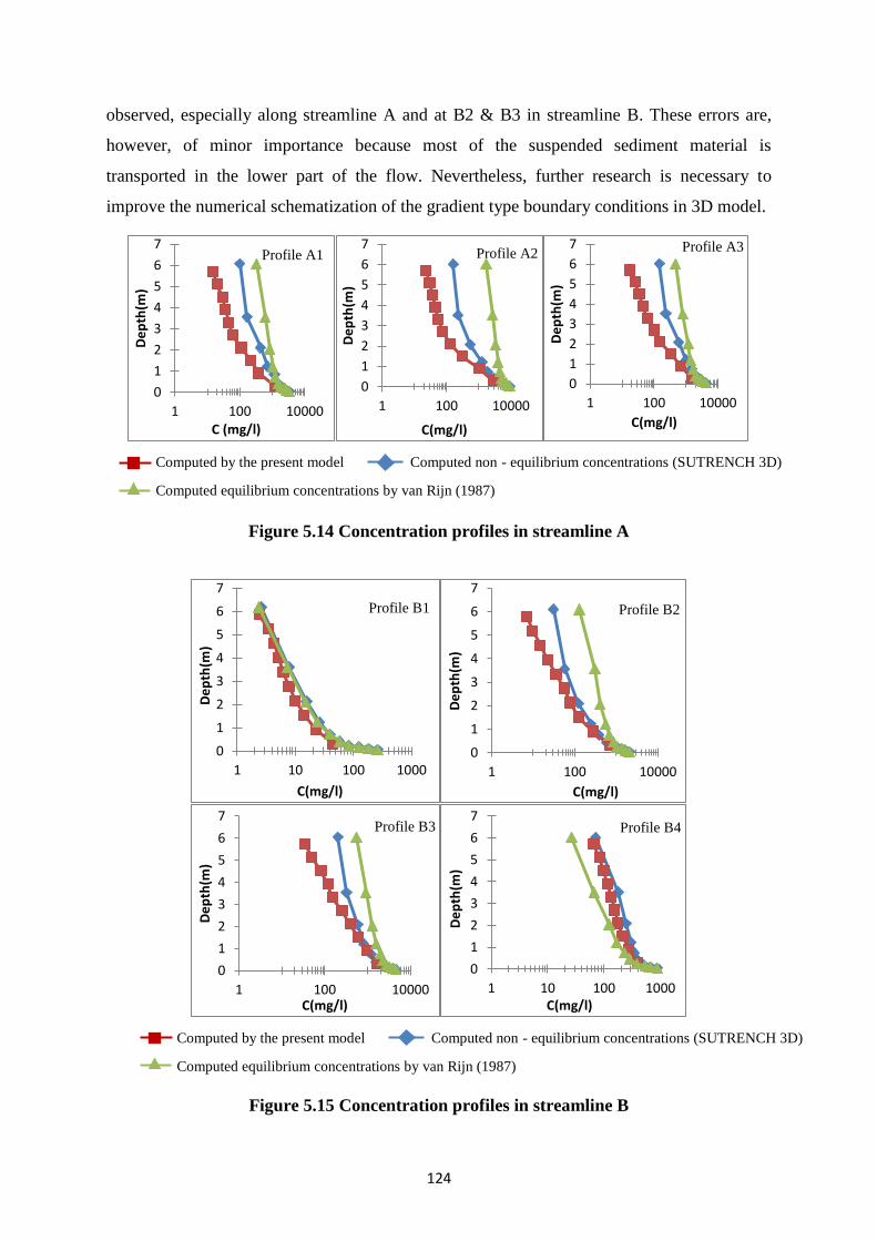
124
observed, especially along streamline A and at B2 & B3 in streamline B. These errors are,
however, of minor importance because most of the suspended sediment material is
transported in the lower part of the flow. Nevertheless, further research is necessary to
improve the numerical schematization of the gradient type boundary conditions in 3D model.
Figure 5.14 Concentration profiles in streamline A
Figure 5.15 Concentration profiles in streamline B
0
1
2
3
4
5
6
7
1 100 10000
De
pth
(m)
C (mg/l)
Profile A1
0
1
2
3
4
5
6
7
1 100 10000
De
pth
(m)
C(mg/l)
Profile A2
0
1
2
3
4
5
6
7
1 100 10000
De
pth
(m)
C(mg/l)
Profile A3
0
1
2
3
4
5
6
7
1 10 100 1000
De
pth
(m)
C(mg/l)
Profile B1
0
1
2
3
4
5
6
7
1 100 10000
De
pth
(m)
C(mg/l)
Profile B2
0
1
2
3
4
5
6
7
1 100 10000
De
pth
(m)
C(mg/l)
Profile B3
0
1
2
3
4
5
6
7
1 10 100 1000
De
pth
(m)
C(mg/l)
Profile B4
Computed by the present model Computed non - equilibrium concentrations (SUTRENCH 3D)
Computed equilibrium concentrations by van Rijn (1987)
Computed by the present model Computed non - equilibrium concentrations (SUTRENCH 3D)
Computed equilibrium concentrations by van Rijn (1987)

125
Figure 5.16 Concentration profile in recirculation zone
The present model and SUTRENCH 3D agreed well along whole depth at B1 and B4 in
streamline B and both nodes are located far from the headland (see Figure 5.9b). At R1 and
R4 in the recirculation zone, the present model shows reasonable agreement with
SUTRENCH 3D (Figure 5.16).
5.3.3.3 Sediment transport
Figures 5.17 and 5.18 show the depth-integrated suspended sediment transport rates
computed by the present model, the SUTRENCH-2D and 3D models for streamlines B and
C. One key difference between the two model results is that the concentration is lower than
those from other models in the vicinity of headland. Most of the differences are likely caused
by the numerical diffusion of the 3D-model (relatively large grid sizes). This could be
improved by reducing locally the model grid size in recirculation zones.
0
1
2
3
4
5
6
7
0.1 10 1000
De
pth
(m)
C(mg/l)
Profile R1
0
1
2
3
4
5
6
7
0.1 1 10 100
De
pth
(m)
C(mg/l)
Profile R2
Computed by the present model Computed non - equilibrium concentrations (SUTRENCH 3D)
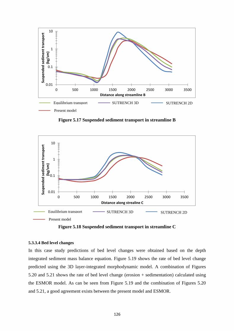
126
Figure 5.17 Suspended sediment transport in streamline B
Figure 5.18 Suspended sediment transport in streamline C
5.3.3.4 Bed level changes
In this case study predictions of bed level changes were obtained based on the depth
integrated sediment mass balance equation. Figure 5.19 shows the rate of bed level change
predicted using the 3D layer-integrated morphodynamic model. A combination of Figures
5.20 and 5.21 shows the rate of bed level change (erosion + sedimentation) calculated using
the ESMOR model. As can be seen from Figure 5.19 and the combination of Figures 5.20
and 5.21, a good agreement exists between the present model and ESMOR.
0.01
0.1
1
10
0 500 1000 1500 2000 2500 3000 3500
Susp
en
de
d s
ed
ime
nt
tran
spo
rt
(kg/
sm)
Distance along streamline B
0.01
0.1
1
10
0 500 1000 1500 2000 2500 3000 3500
Susp
en
de
d s
ed
ime
nt
tran
spo
rt
(kg/
sm)
Distance along strealine C
Equilibrium transport SUTRENCH 3D
Present model
SUTRENCH 2D
Equilibrium transport SUTRENCH 3D
Present model
SUTRENCH 2D

127
Figure 5.19 The rate of bed level change (mm/hr) obtained using the present model
Figure 5.20 Erosion (interval=4mm/hr) in ESMOR model
Figure 5.21 Sedimentation (interval=2mm/hr) in ESMOR model
The maximum erosion and deposition rates predicted in the headland vicinity using the
different models are presented in Table 5.1

128
Table 5.1 The maximum rates for erosion and deposition in different numerical models
Maximum Erosion
mm/hr
Deposition
mm/hr Models
ESMOR 43 10.5
SUTRENCH 100 25
GEODIVAST 40.7 3.9
GEOTRIVAST 45.5 12.8
Presented model 40 11
The differences among the results depend on different model grids and the essence of
different computational methods used in the model but generally the predictions are
acceptable. By applying the 3D layer-integrated morphodynamic model for this case study, it
was shown that the results obtained using the present model could reveal hydrodynamic,
sediment transport and morphological changes process with a reasonable agreement with
other numerical models.
5.4 Summary
This chapter presents two examples used to test the ability of the numerical model developed
to compute hydrodynamic behavior, sediment transport and morphological processes. The
numerical model has been set up based on geometry data and hydraulic parameters (boundary
conditions and initial conditions) for flow and sediment transport belong to two cases and the
model simulation involves all main modules (i.e. hydrodynamic, sediment transport and
morphodynamic processes). The model results have been compared with laboratory measured
data and other numerical model results and the present numerical model performed generally
well.
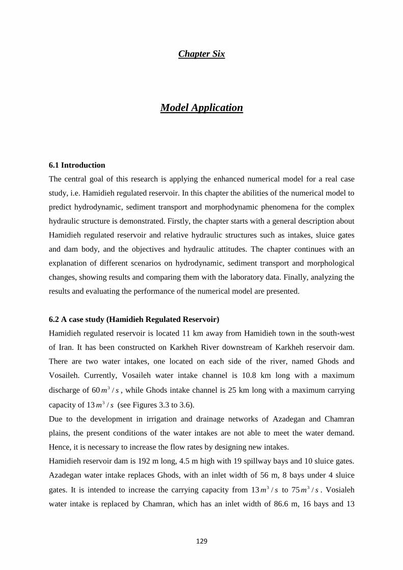
129
Chapter Six
Model Application
6.1 Introduction
The central goal of this research is applying the enhanced numerical model for a real case
study, i.e. Hamidieh regulated reservoir. In this chapter the abilities of the numerical model to
predict hydrodynamic, sediment transport and morphodynamic phenomena for the complex
hydraulic structure is demonstrated. Firstly, the chapter starts with a general description about
Hamidieh regulated reservoir and relative hydraulic structures such as intakes, sluice gates
and dam body, and the objectives and hydraulic attitudes. The chapter continues with an
explanation of different scenarios on hydrodynamic, sediment transport and morphological
changes, showing results and comparing them with the laboratory data. Finally, analyzing the
results and evaluating the performance of the numerical model are presented.
6.2 A case study (Hamidieh Regulated Reservoir)
Hamidieh regulated reservoir is located 11 km away from Hamidieh town in the south-west
of Iran. It has been constructed on Karkheh River downstream of Karkheh reservoir dam.
There are two water intakes, one located on each side of the river, named Ghods and
Vosaileh. Currently, Vosaileh water intake channel is 10.8 km long with a maximum
discharge of 60 sm /3 , while Ghods intake channel is 25 km long with a maximum carrying
capacity of 13 sm /3 (see Figures 3.3 to 3.6).
Due to the development in irrigation and drainage networks of Azadegan and Chamran
plains, the present conditions of the water intakes are not able to meet the water demand.
Hence, it is necessary to increase the flow rates by designing new intakes.
Hamidieh reservoir dam is 192 m long, 4.5 m high with 19 spillway bays and 10 sluice gates.
Azadegan water intake replaces Ghods, with an inlet width of 56 m, 8 bays under 4 sluice
gates. It is intended to increase the carrying capacity from 13 sm /3 to 75 sm /3 . Vosialeh
water intake is replaced by Chamran, which has an inlet width of 86.6 m, 16 bays and 13
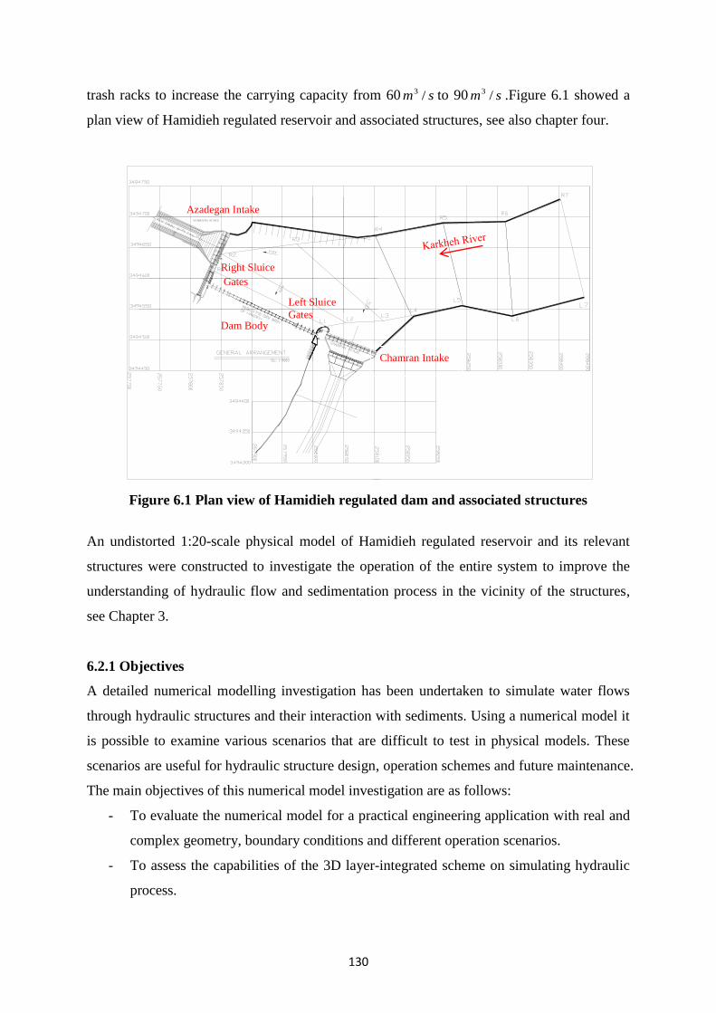
130
trash racks to increase the carrying capacity from 60 sm /3 to 90 sm /3 .Figure 6.1 showed a
plan view of Hamidieh regulated reservoir and associated structures, see also chapter four.
Figure 6.1 Plan view of Hamidieh regulated dam and associated structures
An undistorted 1:20-scale physical model of Hamidieh regulated reservoir and its relevant
structures were constructed to investigate the operation of the entire system to improve the
understanding of hydraulic flow and sedimentation process in the vicinity of the structures,
see Chapter 3.
6.2.1 Objectives
A detailed numerical modelling investigation has been undertaken to simulate water flows
through hydraulic structures and their interaction with sediments. Using a numerical model it
is possible to examine various scenarios that are difficult to test in physical models. These
scenarios are useful for hydraulic structure design, operation schemes and future maintenance.
The main objectives of this numerical model investigation are as follows:
- To evaluate the numerical model for a practical engineering application with real and
complex geometry, boundary conditions and different operation scenarios.
- To assess the capabilities of the 3D layer-integrated scheme on simulating hydraulic
process.
Chamran Intake
Azadegan Intake
Dam Body
Right Sluice
Gates
Left Sluice
Gates

131
- To reduce time and costs using numerical model to aid hydraulic structure designing
and to test for various scenarios that are generally more difficult to test with a
physical model.
6.3 Numerical model study
Physical and numerical models can be used jointly for designing hydraulic structures in order
to understand better natural processes. This approach makes a joint platform for solving
engineering problems and eliminates the cost. The numerical model has been set based on the
size of physical model to gain same simulation on hydraulic parameters (Reynolds number,
velocity and sediment sizes, grain Reynolds number and etc.) theoretically.
In recent years, several 3-D numerical models have been developed, for predicting
hydrodynamic, sediment transport and morphodynamic processes and applied in different
cases. Olsen and Kjellesvig (1999) undertook a 3-D numerical model study of bed changes in
a sand trap. The numerical model results compared well with the measurements obtained
from the physical model studies. Gessler et al (1999) developed a 3-D model of river
morphology, which included separate solvers for bed load transport and suspended sediment
transport. It considered several size fractions of sediment and recorded the bed composition
and evolution during each time step. Kolahdoozan and Falconer (2003) developed a three-
dimensional (3-D) layer-integrated morphological model for estuarine and coastal waters and
compared the numerical model predictions with experimental measurements in a laboratory
model harbour. They used the mixing length model for turbulence closure, and recommended
that a fine mesh should be used in areas of severe erosion or deposition. Olsen (2003) and
Rüther and Olsen (2003, 2005a, b) developed a fully 3-D model with an unstructured grid to
represent the domain. They showed results from a simulation of meander evolution. Their
work focused on the formation of alternate bars and the initiation of meandering starting from
a completely straight channel.
In many research projects physical and numerical model were used jointly to understand the
hydrodynamic and sediment transport behaviors. Stephan and Hengl (2010) used a physical
model test aimed at improving the sediment movement through the backwater of a
hydropower plant to reduce the flood risk of the town of Hallein. The 3D morphodynamic
model SSIIM was applied to this case in order to investigate if the 3D model could reproduce
the erosion and deposition pattern for such a complex situation. The numerical results agreed
with the measured erosion and deposition patterns but not the absolute bed levels.
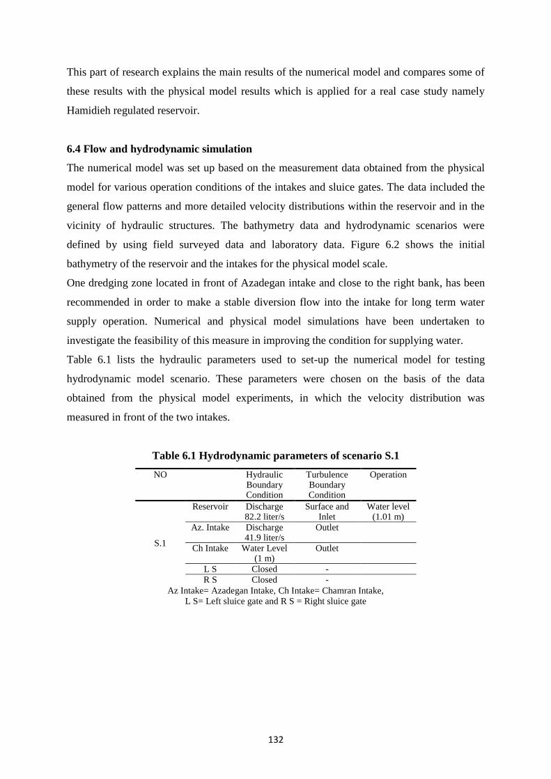
132
This part of research explains the main results of the numerical model and compares some of
these results with the physical model results which is applied for a real case study namely
Hamidieh regulated reservoir.
6.4 Flow and hydrodynamic simulation
The numerical model was set up based on the measurement data obtained from the physical
model for various operation conditions of the intakes and sluice gates. The data included the
general flow patterns and more detailed velocity distributions within the reservoir and in the
vicinity of hydraulic structures. The bathymetry data and hydrodynamic scenarios were
defined by using field surveyed data and laboratory data. Figure 6.2 shows the initial
bathymetry of the reservoir and the intakes for the physical model scale.
One dredging zone located in front of Azadegan intake and close to the right bank, has been
recommended in order to make a stable diversion flow into the intake for long term water
supply operation. Numerical and physical model simulations have been undertaken to
investigate the feasibility of this measure in improving the condition for supplying water.
Table 6.1 lists the hydraulic parameters used to set-up the numerical model for testing
hydrodynamic model scenario. These parameters were chosen on the basis of the data
obtained from the physical model experiments, in which the velocity distribution was
measured in front of the two intakes.
Table 6.1 Hydrodynamic parameters of scenario S.1
Az Intake= Azadegan Intake, Ch Intake= Chamran Intake,
L S= Left sluice gate and R S = Right sluice gate
NO Hydraulic Boundary Condition
Turbulence Boundary Condition
Operation
S.1
Reservoir Discharge 82.2 liter/s
Surface and Inlet
Water level (1.01 m)
Az. Intake Discharge 41.9 liter/s
Outlet
Ch Intake Water Level (1 m)
Outlet
L S Closed -
R S Closed -

133
Figure 6.2 The initial bathymetry of Hamidieh, physical model scale
In the physical model study the velocity was measured at several points in front of the intakes
by current-meters. The locations of these points were shown in the Figures 3.18 and 3.19. In
this study, the velocity measurements at these points, together with the observed water
surface levels were used for calibrating the hydrodynamic model.
In the physical model study, the velocity was measured by a current-meter at ( = water
depth) from the water surface and fitted to the physical scale. This depth had been chosen
based on velocity logarithmic profile assumption.
In applying the 3D layer integrated model to this case study the water depth was divided into
5 vertical layers. The thickness of the layers was all set to 0.057m except for the top layer,
which was set to 0.051m in the main channel. The grid size was set to 0.25m. The water
surface level was calibrated by comparing the water surface levels obtained from the physical
model and those predicted by the numerical model, with the difference being found to vary
between 0.0022m and 0.0055m. Roughness height was used as the calibration parameter.
Table 6.2 lists the velocity values for different locations shown in Figures 3.18 and 3.19 for
both the physical and the numerical models.
Efforts have been made to use the measured data for better calibration but it was not possible
to test and measure hydraulic parameters for more scenarios and locations. Despite these
limitations, the comparisons made using the available data in Table 6.2 shows that the trend
and quantities of velocity values obtained from the numerical and physical models are in an
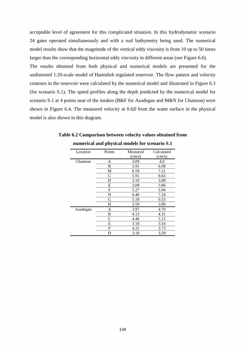
134
acceptable level of agreement for this complicated situation. In this hydrodynamic scenario
24 gates operated simultaneously and with a real bathymetry being used. The numerical
model results show that the magnitude of the vertical eddy viscosity is from 10 up to 50 times
larger than the corresponding horizontal eddy viscosity in different areas (see Figure 6.6).
The results obtained from both physical and numerical models are presented for the
undistorted 1:20-scale model of Hamidieh regulated reservoir. The flow pattern and velocity
contours in the reservoir were calculated by the numerical model and illustrated in Figure 6.3
(for scenario S.1). The speed profiles along the depth predicted by the numerical model for
scenario S.1 at 4 points near of the intakes (B&F for Azadegan and M&N for Chamran) were
shown in Figure 6.4. The measured velocity at 0.6 from the water surface in the physical
model is also shown in this diagram.
Table 6.2 Comparison between velocity values obtained from
numerical and physical models for scenario S.1
Location Points Measured (cm/s)
Calculated (cm/s)
Chamran A 3.09 4.0
B 5.91 6.08
M 6.59 7.21
C 5.91 6.63
D 3.10 3.89
E 3.08 3.86
F 5.27 5.94
N 6.40 7.24
G 5.18 6.53
H 3.59 3.89
Azadegan A 3.97 4.70
B 4.13 4.31
C 4.46 5.15
E 3.18 3.54
F 4.25 3.73
D 3.18 3.59

135
Figure 6.3 Numerical model predicted flow pattern and speed contours for scenario S.1
Figure 6.4 Model predicted velocity distributions and measured velocities at 0.6D from
water surface for scenario S.1 (Az=Azadegan Intake, Ch=Chamran Intake, Nu=Numerical,
Ph=Physical and TD=Total Depth (i.e. calculated by 3D layer-integrated numerical model along whole
depth))
From Figure 6.4 it can be seen that the mathematical model predicted velocity values agree
reasonably well with measured ones from the physical model although some variations can
be observed. The type of turbulence model has an important role in predicting the speed
parameters. For the model simulations reported herein, predictions were obtained using a
layer integrated three-dimensional hydrodynamic and sediment transport model and also
0
5
10
15
20
25
0 2 4 6 8 10
Velocity(cm/s)
Dep
th(c
m)
Az.Nu. Point B(TD)
Az.Ph. Point B(0.6D)
Az.Nu. Point F(TD)
Az.Ph. Point F(0.6D)
Ch.Nu. Point M(TD)
Ch.Ph. Point M(0.6D)
Ch.Nu. Point N(TD)
Ch.Ph. Point N(0.6D)
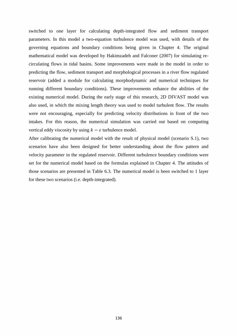
136
switched to one layer for calculating depth-integrated flow and sediment transport
parameters. In this model a two-equation turbulence model was used, with details of the
governing equations and boundary conditions being given in Chapter 4. The original
mathematical model was developed by Hakimzadeh and Falconer (2007) for simulating re-
circulating flows in tidal basins. Some improvements were made in the model in order to
predicting the flow, sediment transport and morphological processes in a river flow regulated
reservoir (added a module for calculating morphodynamic and numerical techniques for
running different boundary conditions). These improvements enhance the abilities of the
existing numerical model. During the early stage of this research, 2D DIVAST model was
also used, in which the mixing length theory was used to model turbulent flow. The results
were not encouraging, especially for predicting velocity distributions in front of the two
intakes. For this reason, the numerical simulation was carried out based on computing
vertical eddy viscosity by using turbulence model.
After calibrating the numerical model with the result of physical model (scenario S.1), two
scenarios have also been designed for better understanding about the flow pattern and
velocity parameter in the regulated reservoir. Different turbulence boundary conditions were
set for the numerical model based on the formulas explained in Chapter 4. The attitudes of
those scenarios are presented in Table 6.3. The numerical model is been switched to 1 layer
for these two scenarios (i.e. depth-integrated).
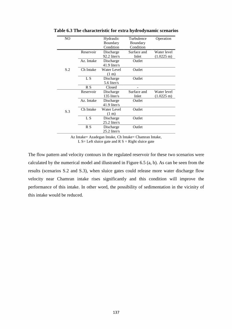
137
Table 6.3 The characteristic for extra hydrodynamic scenarios
Az Intake= Azadegan Intake, Ch Intake= Chamran Intake,
L S= Left sluice gate and R S = Right sluice gate
The flow pattern and velocity contours in the regulated reservoir for these two scenarios were
calculated by the numerical model and illustrated in Figure 6.5 (a, b). As can be seen from the
results (scenarios S.2 and S.3), when sluice gates could release more water discharge flow
velocity near Chamran intake rises significantly and this condition will improve the
performance of this intake. In other word, the possibility of sedimentation in the vicinity of
this intake would be reduced.
NO Hydraulic Boundary Condition
Turbulence Boundary Condition
Operation
S.2
Reservoir Discharge 92.2 liter/s
Surface and Inlet
Water level (1.0225 m)
Az. Intake Discharge 41.9 liter/s
Outlet
Ch Intake Water Level (1 m)
Outlet
L S Discharge 5.6 liter/s
Outlet
R S Closed -
S.3
Reservoir Discharge 135 liter/s
Surface and Inlet
Water level (1.0225 m)
Az. Intake Discharge 41.9 liter/s
Outlet
Ch Intake Water Level (1 m)
Outlet
L S Discharge 25.2 liter/s
Outlet
R S Discharge 25.2 liter/s
Outlet

138
(a)
(b)
Figure 6.5 Numerical model predicted flow pattern and speed contours
for (a) Scenario S.2 and (b) Scenario S.3
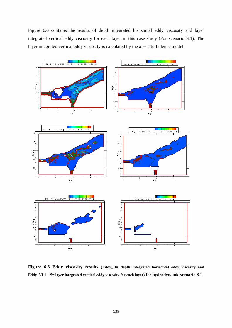
139
Figure 6.6 contains the results of depth integrated horizontal eddy viscosity and layer
integrated vertical eddy viscosity for each layer in this case study (For scenario S.1). The
layer integrated vertical eddy viscosity is calculated by the turbulence model.
Figure 6.6 Eddy viscosity results (Eddy_H= depth integrated horizontal eddy viscosity and
Eddy_VL1…5= layer integrated vertical eddy viscosity for each layer) for hydrodynamic scenario S.1

140
An analysis of the hydrodynamic results identifies two main issues:
-According to the observation of the flow direction, it is noticed that a non-uniform velocity
distribution zone exists upstream of Chamran intake on the left bank. This is thought to be
related to the location of the intake.
- The velocity pattern for the regulatory condition at the artificial dredging zone (in front of
Azadegan intake) indicates that this is a location for high potential sedimentation.
6.5 Sediment transport simulation
For simulating sediment transport in hydraulic systems information such as particle size
distribution, inflow discharge and associated sediment discharge, type of sediments (cohesive
or non-cohesive) and understanding the dominant process of sediment transport (suspended
load or bed load) in the nature are required. Previous studies have showed that the suspended
transport is the dominant process for existing situation in this case (WEOKP 2001). The
majority of sediment found in this region belongs to non-cohesive type. One of the most
important tasks is to prevent sediments from entering the intakes. Any sediment particles
deposited into the irrigation canals would cause a decrease in the flow rate. Currently, the
stakeholders of the irrigation network have to dredge the canals periodically. In designing the
new system of Hamidieh regulated reservoir a great effort has been made to mitigate the
sedimentation problem in canals.
In this research, various scenarios were considered in order to determine the amount of
sediments entering the intakes (see Table 6.4). Details are given below of the numerical
model study of the sediment transport process. The numerical model predictions were
compared with the physical model results at five sites. The plan of these sites was shown in
Chapter 3 at Figure 3.24.
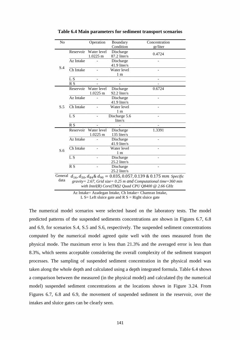
141
Table 6.4 Main parameters for sediment transport scenarios
No Operation Boundary Condition
Concentration gr/liter
S.4
Reservoir Water level 1.0225 m
Discharge 87.2 liter/s
0.4724
Az Intake - Discharge 41.9 liter/s
-
Ch Intake - Water level 1 m
-
L S - - -
R S - - -
S.5
Reservoir Water level 1.0225 m
Discharge 92.2 liter/s
0.6724
Az Intake - Discharge 41.9 liter/s
-
Ch Intake - Water level 1 m
-
L S - Discharge 5.6 liter/s
-
R S - - -
S.6
Reservoir Water level 1.0225 m
Discharge 135 liter/s
1.3391
Az Intake - Discharge 41.9 liter/s
-
Ch Intake - Water level 1 m
-
L S - Discharge 25.2 liter/s
-
R S - Discharge 25.2 liter/s
-
General data
Specific
gravity= 2.67, Grid size= 0.25 m and Computational time=360 min
with Intel(R) Core(TM)2 Quad CPU Q8400 @ 2.66 GHz
Az Intake= Azadegan Intake, Ch Intake= Chamran Intake, L S= Left sluice gate and R S = Right sluice gate
The numerical model scenarios were selected based on the laboratory tests. The model
predicted patterns of the suspended sediments concentrations are shown in Figures 6.7, 6.8
and 6.9, for scenarios S.4, S.5 and S.6, respectively. The suspended sediment concentrations
computed by the numerical model agreed quite well with the ones measured from the
physical mode. The maximum error is less than 21.3% and the averaged error is less than
8.3%, which seems acceptable considering the overall complexity of the sediment transport
processes. The sampling of suspended sediment concentration in the physical model was
taken along the whole depth and calculated using a depth integrated formula. Table 6.4 shows
a comparison between the measured (in the physical model) and calculated (by the numerical
model) suspended sediment concentrations at the locations shown in Figure 3.24. From
Figures 6.7, 6.8 and 6.9, the movement of suspended sediment in the reservoir, over the
intakes and sluice gates can be clearly seen.

142
Figure 6.7 Pattern of suspended sediments concentrations (SSC), scenario S.4
Figure 6.8 Pattern of suspended sediments concentrations (SSC), scenario S.5

143
Figure 6.9 Pattern of suspended sediments concentrations (SSC), scenario S.6
Table 6.5 SSC measured and predicted at sampling points
No Points SSC (Measured)
gr/liter
SSC (Calculated)
gr/liter
| |* %
S.4 CRL 0.401 0.452 12.72 CRM 0.423 0.456 7.8 CRR 0.417 0.452 8.39 CAZ 0.396 0.401 1.26 CCH 0.433 0.434 0.23
S.5 CRL 0.563 0.645 14.56 CRM 0.638 0.651 2.04 CRR 0.605 0.645 6.61 CAZ 0.618 0.589 4.69 CCH 0.681 0.619 9.10
S.6 CRL 1.18 1.3 10.17 CRM 1.38 1.31 5.07 CRR 1.12 1.3 16.07 CAZ 0.99 1.20 21.21 CCH 1.11 1.25 12.61
* | |=8.28%, SSC= sediment suspended sediment, Measured= measured in the physical model and Calculated= calculated by the numerical model
The scenarios are designed in three categories. The characteristics of these scenarios are:
- Low flow condition without sluice gates (scenario S.4).
- Low flow condition with one sluice gate (scenario S.5).
144
- High flow condition with sluice gates along both sides of the dam in operation (scenario
S.6).
The attributes of the scenarios are presented in Table 6.4. The results showed that the
suspended load has an important role in the sediment transport process and is closely related
to particle size. A good agreement has been observed between the SSCs obtained from
numerical and the physical models. The analysis of the sediment transport results identifies
that:
(i) The suspended sediment concentration in Chamran intake is higher than the one in
Azadegan intake. The main reason is thought to be the location of the intakes. Chamran
intake is located in the internal curve position when considering the layout of the system.
(ii) The pattern of the suspended sediment movement in the reservoir has showed that the
sediment entering rate to Chamran intake is affected very little by the sluice gate operation
schemes. It means that the sluice gates on the left side do not have a considerable effect on
reducing the suspended sediment concentration moving through Chamran intake.
(iii) It seems that the problem of sediment entering the intakes is remained. The layout of
these hydraulic structures is only part of the reason for this problem. The natural system of
sediment transport and the size of the sediments have an important role for this situation.
6.6 Morphodynamic
Details are first given below of the numerical model predictors of the morphological changes
in the Hamidieh regulated reservoir. The model simulation was based on field surveyed data
and laboratory data obtained from the physical model for various operation conditions of the
intakes and sluice gates. The hydrodynamic and sediment transport studies were presented in
the two above sections before. The bathymetry data and morphodynamic scenarios were
defined by using field surveyed data and laboratory measured data. The initial bathymetry of
the reservoir and the intakes in the physical model scale was plotted in Figure 6.2. Table 6.6
lists the hydraulic and sediments parameters used to set-up the numerical model for testing
the morphodynamic model scenarios. These parameters were chosen on the basis of the data
obtained from the physical model experiments.
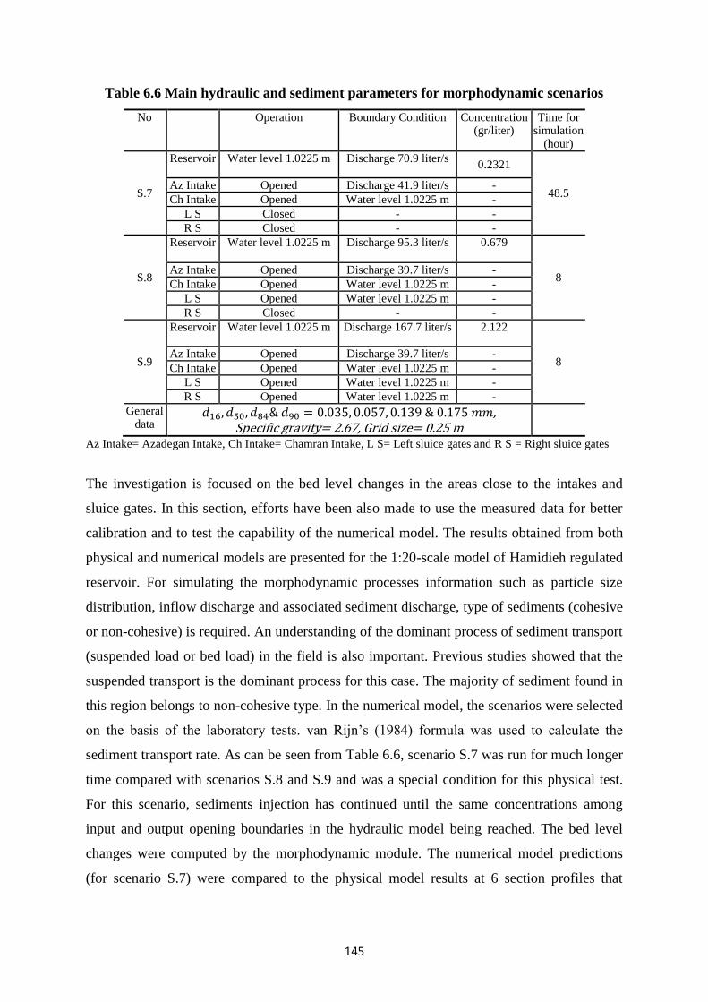
145
Table 6.6 Main hydraulic and sediment parameters for morphodynamic scenarios
No Operation Boundary Condition Concentration (gr/liter)
Time for simulation
(hour)
S.7
Reservoir Water level 1.0225 m Discharge 70.9 liter/s 0.2321
48.5 Az Intake Opened Discharge 41.9 liter/s -
Ch Intake Opened Water level 1.0225 m -
L S Closed - -
R S Closed - -
S.8
Reservoir Water level 1.0225 m Discharge 95.3 liter/s 0.679
8 Az Intake Opened Discharge 39.7 liter/s -
Ch Intake Opened Water level 1.0225 m -
L S Opened Water level 1.0225 m -
R S Closed - -
S.9
Reservoir Water level 1.0225 m Discharge 167.7 liter/s 2.122
8 Az Intake Opened Discharge 39.7 liter/s -
Ch Intake Opened Water level 1.0225 m -
L S Opened Water level 1.0225 m -
R S Opened Water level 1.0225 m -
General data
, Specific gravity= 2.67, Grid size= 0.25 m
Az Intake= Azadegan Intake, Ch Intake= Chamran Intake, L S= Left sluice gates and R S = Right sluice gates
The investigation is focused on the bed level changes in the areas close to the intakes and
sluice gates. In this section, efforts have been also made to use the measured data for better
calibration and to test the capability of the numerical model. The results obtained from both
physical and numerical models are presented for the 1:20-scale model of Hamidieh regulated
reservoir. For simulating the morphodynamic processes information such as particle size
distribution, inflow discharge and associated sediment discharge, type of sediments (cohesive
or non-cohesive) is required. An understanding of the dominant process of sediment transport
(suspended load or bed load) in the field is also important. Previous studies showed that the
suspended transport is the dominant process for this case. The majority of sediment found in
this region belongs to non-cohesive type. In the numerical model, the scenarios were selected
on the basis of the laboratory tests. van Rijn’s (1984) formula was used to calculate the
sediment transport rate. As can be seen from Table 6.6, scenario S.7 was run for much longer
time compared with scenarios S.8 and S.9 and was a special condition for this physical test.
For this scenario, sediments injection has continued until the same concentrations among
input and output opening boundaries in the hydraulic model being reached. The bed level
changes were computed by the morphodynamic module. The numerical model predictions
(for scenario S.7) were compared to the physical model results at 6 section profiles that

146
0.6
0.7
0.8
0.9
1
1.1
1.2
1.3
0 2 4 6 8
Hei
gh
t(m
)
Distance(m)
Profile L5-R5
0.6
0.7
0.8
0.9
1
1.1
1.2
0 2 4 6 8
Hei
gh
t(m
)
Distance(m)
Profile L6-R6
0.6
0.7
0.8
0.9
1
1.1
1.2
1.3
0 2 4 6 8 10 12 14 16
Hei
gh
t (m
)
Distance (m)
Profile L1-R1
0.6
0.7
0.8
0.9
1
1.1
1.2
0 2 4 6 8 10 12 14 16 18
Hei
gh
t (m
)
Distance (m)
Profile L2-R2
0.6
0.7
0.8
0.9
1
1.1
1.2
1.3
0 2 4 6 8 10 12 14 16
Hei
gh
t (m
)
Distance (m)
Profile L3-R3
0.6
0.7
0.8
0.9
1
1.1
1.2
1.3
0 2 4 6 8
Hei
gh
t (m
)
Distance (m)
Profile L4-R4
Azadegan
Intake
recognized in the Hamidieh reservoir in Figure 6.1 before. Profiles 1, 2 and 3 would be
extended for covering the whole area in the vicinity of Chamran intake.
From Figures 6.10 it can be seen that the mathematical model predicted bed level changes
agree reasonably well with the measured ones from the physical model, although some
differences can be observed. In most locations computational results of bed level changes are
less than the physical results. The predicted bed level change at L6-R6 is greater than the
measured one. This is thought to be due to a problem in the sediment injection system. It was
observed that some dry sediment injected into the reservoir from the river boundary (section
L7-R7) could not mix well initially and are settled and deposited near the injection system
(section L6-R6).
Figure 6.10 Bed level changes after 48.5 hours in 6 section profiles (scenario S.7)
Initial bed
Physical simulation
Numercial simulation
Dredging
zone
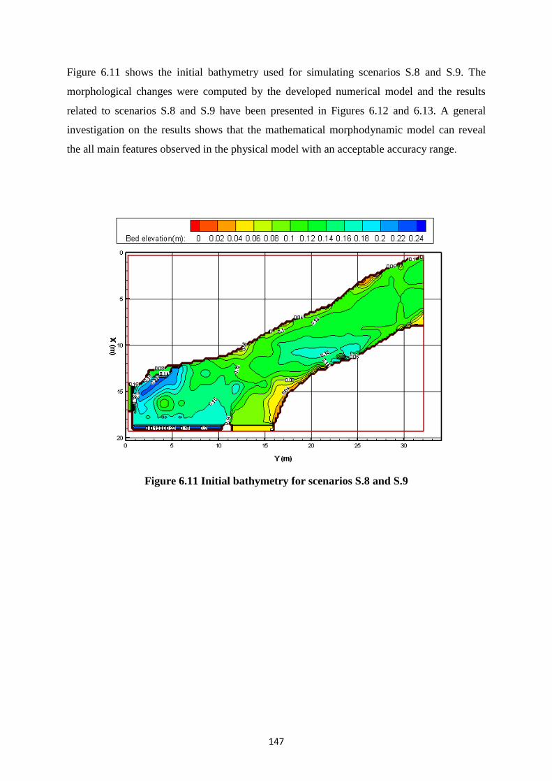
147
Figure 6.11 shows the initial bathymetry used for simulating scenarios S.8 and S.9. The
morphological changes were computed by the developed numerical model and the results
related to scenarios S.8 and S.9 have been presented in Figures 6.12 and 6.13. A general
investigation on the results shows that the mathematical morphodynamic model can reveal
the all main features observed in the physical model with an acceptable accuracy range.
Figure 6.11 Initial bathymetry for scenarios S.8 and S.9
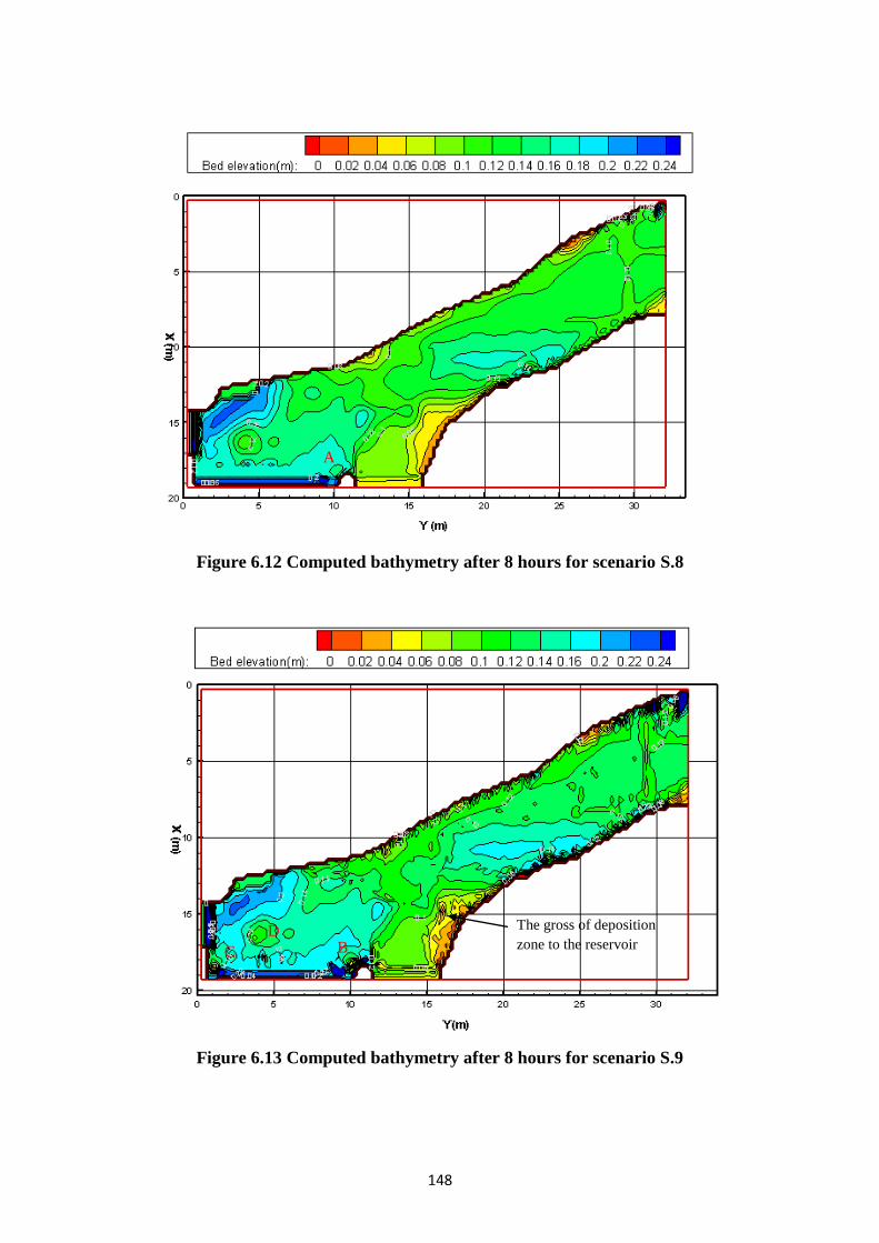
148
Figure 6.12 Computed bathymetry after 8 hours for scenario S.8
Figure 6.13 Computed bathymetry after 8 hours for scenario S.9
B D
C
The gross of deposition
zone to the reservoir
A
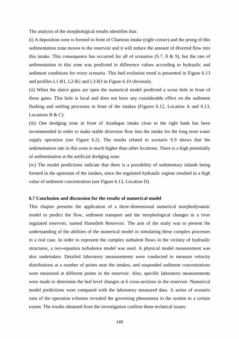
149
The analysis of the morphological results identifies that:
(i) A deposition zone is formed in front of Chamran intake (right corner) and the prong of this
sedimentation zone moves to the reservoir and it will reduce the amount of diverted flow into
this intake. This consequence has occurred for all of scenarios (S.7, 8 & 9), but the rate of
sedimentation in this zone was predicted in difference values according to hydraulic and
sediment conditions for every scenario. This bed evolution trend is presented in Figure 6.13
and profiles L1-R1, L2-R2 and L3-R3 in Figure 6.10 obviously.
(ii) When the sluice gates are open the numerical model predicted a scour hole in front of
those gates. This hole is local and does not have any considerable effect on the sediment
flashing and settling processes in front of the intakes (Figures 6.12, Location A and 6.13,
Locations B & C).
(iii) One dredging zone in front of Azadegan intake close to the right bank has been
recommended in order to make stable diversion flow into the intake for the long term water
supply operation (see Figure 6.2). The results related to scenario S.9 shows that the
sedimentation rate in this zone is much higher than other locations. There is a high potentially
of sedimentation at the artificial dredging zone.
(iv) The model predictions indicate that there is a possibility of sedimentary islands being
formed in the upstream of the intakes, since the regulated hydraulic regime resulted in a high
value of sediment concentration (see Figure 6.13, Location D).
6.7 Conclusion and discussion for the results of numerical model
This chapter presents the application of a three-dimensional numerical morphodynamic
model to predict the flow, sediment transport and the morphological changes in a river
regulated reservoir, named Hamidieh Reservoir. The aim of the study was to present the
understanding of the abilities of the numerical model in simulating these complex processes
in a real case. In order to represent the complex turbulent flows in the vicinity of hydraulic
structures, a two-equation turbulence model was used. A physical model measurement was
also undertaken. Detailed laboratory measurements were conducted to measure velocity
distributions at a number of points near the intakes, and suspended sediment concentrations
were measured at different points in the reservoir. Also, specific laboratory measurements
were made to determine the bed level changes at 6 cross-sections in the reservoir. Numerical
model predictions were compared with the laboratory measured data. A series of scenario
runs of the operation schemes revealed the governing phenomena in the system to a certain
extent. The results obtained from the investigation confirm these technical issues:
150
(i) A non-uniform velocity distribution zone exists upstream of Chamran intake on the left
bank side.
(ii) In the recommended dredging zone, located in front of Azadegan intake, there is a high
risk of significant sedimentation.
(iii) The location of Chamran intake has a considerable impact on the suspended sediment
moving through the intake and making the formation of the sedimentation zone in the areas
adjacent to the intake.
(iv) The sluice gates operation scheme did not have any considerable impact on the sediment
flushing capability in areas close to the intakes.
(v) The possibility of forming island in the reservoir is predicted by the numerical model.
(vi) The results of this research indicate that the calibrated numerical model could be used in
the hydraulic design. By this method, the laboratory tests are reduced and thus time and
budget are optimized.
It should be pointed out that simplifications and assumptions have been made in both the
physical and numerical models presented in this paper and they will have an impact on the
accuracy of the model results.
From the evaluation of the numerical results the following scientific features were found:
i) The 3D layer-integrated scheme used in the mathematical model revealed the main
hydrodynamic, solute transport and morphodynamic issues with a high degree of accuracy for
the cases considered and, in essence, the flow was basically fully three dimensional. By using
the layer integrated scheme the computational time reduces significantly in comparison with
fully 3-D scheme and the accuracy of the results are in an acceptable range. This is thought to
be the first time using this numerical model for simulating in regulated dam case study.
ii) The computed suspended sediment concentrations by the 3D layer-integrated model for
this case study agreed well with the ones measured from the physical model (see Table 6.5).
To acquire this level of accuracy, the hydrodynamic computational scheme and the selected
turbulence model play an important role. The results of this research showed that the
selection of the turbulence model in regulated reservoir where the Reynolds number is
high but without any significant local vortex near hydraulic structures (such as gates) was the
correct choice.
iii) An explicit method was used for discretizing the bed level change equation. This scheme
is compatible with the structure of mathematical solution for hydrodynamic and sediment
transport modules of the numerical model.
151
6.8 Summary
This chapter presents the application of the developed numerical model to compute the
hydrodynamic behavior, sediment transport and morphological changes for an engineering
case study. River regulated reservoirs are often constructed downstream of dams, with
relatively low elevations, thereby enabling the flow to be distributed for water supply
purposes. However, there are major differences between these regulatory reservoirs and those
associated with normal high head dams, in that strong turbulent flows are generated in the
regulated reservoir due to the high volumes of flow diversion. An enhanced turbulence model
( ) was used to represent the complex flow pattern in the vicinity of hydraulic structures.
In this research, the numerical model is developed and applied to a regulated reservoir dam,
associated with water intakes and sluice gates, and the model is used to investigate the flow
patterns, sediment transport processes and morphodynamic in the vicinity of the various
hydraulic structures. Calibration of the model was undertaken using previously made scaled
physical model measurements. In this context different scenarios were introduced to study the
effect of different intake and sluice gate configurations, as well as establishing how their
operation affected the flow, sediment transport processes and morphodynamic in Hamidieh
Reservoir. The results related to all modules (hydrodynamic, sediment transport and
morphodynamic) have been computed. The numerical results were agreed with laboratory
tests in a reasonable accuracy.

152
Chapter Seven
Conclusions and Recommendations
7.1 Summary of the research
In the thesis a 3D layer-integrated morphodynamic model has been presented. The governing
equations used to describe the morphodynamic processes include: the hydrodynamic,
sediment transport and bed-sediment mass balance equations, with the two-equation
model being used for turbulence closure. The hydrodynamic governing equations are
solved based on a combined layer-integrated and depth-integrated scheme, in which the finite
difference scheme for a regular square mesh is used in the horizontal plane, and a layer-
integrated finite difference scheme is used on an irregular mesh in the vertical. The operator
splitting technique and a highly accurate finite difference scheme have been used to solve the
suspended sediment transport equation. The depth-integrated mass balance equation for
sediment transport is derived using a control volume in the water body from the bed to the
water surface and applying the mass conservation law.
In this research study a new version of the TRIVAST model has been developed to predict
the hydrodynamic, sediment transport and morphological changes in a regulated reservoir.
This model was applied to a scaled hydraulic model using the two- and zero-equation
turbulence models as outlined by Hakimzadeh and Falconer (2007).
Some improvements, including numerical techniques for running different boundary
conditions and irregular mesh sizing in the vertical layer, were included in the model. These
improvements enhanced the ability of the existing numerical model and to the author’s
knowledge this is the first time a 3D layer-integrated model has been applied to a regulated
reservoir case study.
A numerical module including a proposed mathematical scheme has been developed and
added to the 3D layer-integrated model (TRIVAST) for solving the bed level change
equation. In solving the governing equations for predicting bed level changes, an explicit
finite difference scheme was deployed. In contrast the hydrodynamic and sediment transport
modules were solved with an alternating direction implicit finite difference scheme.
153
The verification of the numerical model has been done by applying the model to two widely
used test cases. The numerical model results were also compared with the results obtained
from other numerical models, such as by Wang (1989) and Kolahdoozan and Falconer
(1999). The model predictions agreed generally closely with the measured data and the other
numerical model results.
A physical model was constructed to represent the flow, sediment transport and
morphodynamic processes in Hamidieh regulated reservoir. The study procedures, including
the design scale, model construction and measurements, were carried out in the Water
Research Institute in Iran by the author. The physical model was designed based on the
Froude law of scaling and was undistorted. The model sediment size was determined in such
a manner that the same ratio of the particle’s fall velocity to shear velocity was maintained
for both the model and prototype reservoir. Stokes law was used in calculating the particle
fall velocity.
The enhanced numerical model was then applied to the scaled physical model of the
regulated reservoir. Regulated dams are often constructed downstream of large reservoirs,
with relatively low elevations, thereby enabling the flow to be distributed for water supply
purposes. There are major differences between these regulatory reservoirs and those
associated with normal high head dams, in that strong turbulent flows are generated in the
regulated reservoir due to high volumes of flow with low head differences.
A combined numerical and physical modelling approach has many benefits for designing a
hydraulic structure. In this thesis, especially in chapters 3, 5 and 6, these benefits are
discussed in detail. In the physical model study many techniques were designed for better
performance of the model. Sediment material used in this physical model was obtained from
broken pottery (baked clay). This material is non-cohesive and has a similar specific gravity
as that of the prototype and for this reason the performance of sediment scenario runs worked
well.
7.2 The main findings of the research
The main findings of this research study are:
I) The physical model study reported herein showed that designing with the same scales for
investigating the hydrodynamic, sediment transport and morphodynamic processes in a
complicated water system, such as a regulated dam, enhanced the accuracy. By this method,
synchronization of these processes in the physical model relates closely to conditions in the
154
prototype. The potential of using the physical model results in order to simulate, validate and
calibrate the numerical model is also significantly enhanced.
II) Physical model results of Hamidieh regulated dam confirm that Chamran Intake could
reach its nominal carrying capacity of 90 provided that the water elevation is increased
from 20.20m (i.e. the proposed normal water level for regulatory conditions) to 20.45m in the
reservoir. This is a key result of the physical model study on determining the normal water
elevation for diverting the flow into both intakes.
III) Based on the physical model results of Hamidieh regulated dam in the regulatory
conditions, the size of sediment entering the Azadegan intake is larger than that entering the
Chamran intake. This issue was obtained specifically from the physical model simulation
studies.
IV) The 3D layer-integrated scheme used in the mathematical model revealed the main
hydrodynamic, solute transport and morphodynamic issues with a high degree of accuracy for
the cases considered and, in essence, the flow was basically fully three dimensional. Due to
the important role of the near-bed layer (with high sediment concentration), for the processes
of sediment transport and morphological changes, the idea of a 3D layer-integrated
calculation was very close to the natural environment. By using this concept the
computational time was reduced significantly.
V) The calibrated numerical model of Hamidieh regulated dam revealed many hydraulic
aspects which were in reasonable agreement with the physical model study results. Some of
these important aspects are summarized below:
- The possibility of forming sedimentary islands in the reservoir;
- The sluice gates operation scheme did not have any considerable impact on the sediment
flushing capability in areas close to the intakes;
- To reveal deposition and erosion zones near the hydraulic structures and their impacts on
diverting flow into the intakes.
- There was no need to excavate the reservoir bed for making the proposed artificial dredging
zone, located in front of Azadegan intake, as there was a high risk of significant
sedimentation.
The whole aspects and points have been presented in the chapter 6 precisely.
VI) The results of this research have indicated that the calibrated numerical model could be
used in the hydraulic design and making decisions for management of the regulated reservoir,
with this being a real case study. By this method, the laboratory tests were reduced and thus
time and budget were optimized.
155
7.3 The novelties of the research
The research reveals many sound scientific points that would be so useful for considering in
similar studies.
The main novelty aspects of this research are summarized below:
I) Baked clay is a very useful material for non-cohesive sediment transport studies in the
physical model when the dominant process is suspended sediment transport. This material is
cheap and provided a desired grain distribution when a sieving technique is carried out. The
specific gravity for this material is around 2.67, the same as the sediment material in the
prototype. This means that by using this material scale effete could reduce significantly.
II) The computed suspended sediment concentration by the numerical model in Hamidieh
regulated reservoir case study agreed well with the measured results from the physical model
(averaged error is less than 8.3%, see Table 6.5). To acquire this level of accuracy, the
hydrodynamic computational scheme and the selected turbulence model play an important
role. The results of this research showed that the selection of the turbulence model in
regulated reservoirs where the Reynolds number is high, but without any significant local
vortex near hydraulic structures (such as gates) was the correct choice. An accurate
estimation of the eddy viscosity has a direct impact on the calculated flow velocity
distribution (both horizontally and vertically) and the mixing coefficient which is a key
parameter in calculating the sediment transport fluxes. This concept clearly showed the
capability of the refined numerical model.
III) A proposed algorithm has been implemented for 2D and 3D morphodynamic module. An
explicit method was used for discretizing the bed level change equation. The morphodynamic
model was validated across a range of processes and process interactions. The explicit
method reduced the computational time and enhanced the accuracy of the results
significantly.
IV) Experience showed that in order to prevent instability in the numerical model (especially
in the 3-D form), uploading the flow rate for the input boundary needed to be implemented
gradually from zero to (initial time steps). This soft start interval (or warm-up period) was
undertaken for a number of time steps over which the input boundary flow rate was gradually
increased from zero to 100% of its true value. For implementing this idea, a half sinusoidal
function was used for forming these gradually changes (see Figure 4.8). Also, it was
proposed to choose a water elevation for output boundaries. Both techniques were useful for
enhancing the stability of the numerical model

156
V) Using an irregular mesh sizing for the vertical direction in the computational domain
increased accuracy. This technique was used for investigating the flow, sediment transport
and bed level changes in a trench (see test case 1 in Chapter 5) and the results were
particularly encouraging. The first layer thickness (from the bed) was proposed to be set to
greater than the thickness of the reference level (a).
7.4 Recommendation for further study
In the integrated research study reported herein, efforts have been focused on presenting a
new way to apply numerical and physical modelling and combinations of these approaches
for solving engineering problems. A joint platform has been designed to obtain accurate
results from the numerical and physical model simulations. During the research programme,
many techniques and ideas have been reviewed and proposed in order to enhance the ability
of the numerical model and to run the physical model for a complicated and real case study
(Hamidieh regulated dam). In view of these findings, this research can be seen as a status
report of work in progress. This research will be continued with consideration of the
suggestions and recommendations that are presented in this section. In extending this
research study in the future, the following suggestions are proposed for further consideration:
I) To use large eddy simulation. The turbulent flow is complicated even further by
geometrical variations due to bed forms, roughness elements and vegetation changes in river
cross-section, bends causing secondary currents, confluences associated with strong shear
layers and all kinds of man-made structures such as dikes, bridge piers, groins etc. The Large-
Eddy Simulation (LES) technique is increasingly used in river flow calculations. Rodi (2010)
showed that LES can be applied to river flow problems and allows predicting and studying
situations with a particularly complex flow behavior. The method not only yields information
on complex mean-flow features but also in unsteady features by resolving the large scale
eddies of turbulent motion. The 3D time-dependent LES calculations are computationally
expensive, but they are affordable on modern high-performance computers and increasingly
on clusters of PCs. By using the LES technique, the velocities and suspended sediment
transport fluxes will be computed more accurately, especially in the vicinity of hydraulic
structures that engender highly three dimensional flow fields. Enhancing the ability of the
numerical model in simulating the level of turbulence is needed for further research.
II) To discretize the bed level change equations with other methods and make
comparisons among the numerical results. Existing morphological models use classical
lower order Lax–Wendroff or modified Lax–Wendroff schemes for morphology. These
157
schemes are not very stable for simulating long time sediment transport processes. Filtering
or artificial diffusion are often added to achieve stability. Long et al. (2008) addressed this
with the Euler-WENO scheme and showed it to have significant advantages over schemes
with artificial viscosity and filtering processes. Hence, this scheme is highly recommended,
especially for phase-resolving sediment transport models. They made their comparisons for a
number of numerical examples. The implementation of this idea in simulating morphological
changes for different real case studies will strengthen the capabilities of numerical schemes.
III) Making a new system to inject sediment input for the physical model. In the physical
tests when high sediment concentrations are simulated by injecting dry sediments the method
led to some problems in managing the scenarios. This problem was related to a low water
depth in the physical model (less than 20cm water depth) and the injection method. It is
suggested that a wet injection system be used for simulating high sediments concentrations.
Also, the system needs to be installed far enough upstream from the investigation area for
best results.
IV) Further application study of the numerical model. The 3D layer-integrated model
developed should be applied to more real case studies, such as: regulated dams, diversion
dams having field measurement data or laboratory data for further investigation of the flow
patterns, sediment transport and morphodynamic processes.
158
References
Abbott, M.B. 1978, Computational hydraulics. Elements of theory of free surface flows.
Pitman Publishing, London.
Alstead, R. D. 1994, Numerical modelling of tidal flow using nested and patched grid
schemes. Ph.D. thesis, Univ. of Bradford, Bradford, U.K.
Alvim, A.M. 1987, Modelo matemático bidimensionalde assoreamento em reservatórios. (2-
D mathematical model for reservoir sedimentation) M.Sc. dissertation, Engineering
School of Sao Carlos − University of Sao Paulo, Sao Carlos, Brazil (in Portuguese).
ASCE. 1982, Design of Water Intake Structures for Fish Protection. American Society of
Civil Engineers, New York, NY. pp. 69-73.
ASCE. 1988, Task Committee on Turbulence Models in Hydraulic Computations,
Turbulence modelling of surface water flow and transport, Parts I-III, Journal of Hydraulic
Engineering, ASCE, 114(9), 970-1051.
Atkinson, E. 1989, Predicting the performance predicting method for canal sediment
extractors. Hydraulic Research Wallingford, UK, Report no. OD/TN 41.
Atkinson, E., Lawson, JD. and Tosswell, P. 1993, Comparison of physical and computer
modelling of the Kapunga intake with performance of the prototype. Paper R 106, 15th
Congress of the Int. Comm. on Irrig. and Drain, The Hague.
Atkinson, E., Lawson, JD. and Tosswell, P. 1994, Comparison of physical and computer
modelling of the Kapunga intake with performance of the prototype. Hydraulic Research
Wallingford, UK, Report no. ODP121.
Atkinson, E. 1995, A numerical model for predicting sediment exclusion at intakes.
Hydraulic Research Wallingford, UK, Report no. OD130.
Avery, P. 1989, Sediment control at intakes. British Hydromechanics Research Association,
The Fluid Engineering Center, Cranfield, Bedford, England.
Boillat, J.-L. and De Cesare, G. 1994, Dichteströmungen im Bereich des Grundablasses des
Stausees Luzzone – Modellversuche. Tagungsband (proceedings) des Symposiums
―Betrieb, Erhaltung und Erneuerung von Talsperren und Hochdruckanlagen‖, pp. 183-192,
Graz, Austria.
Bos, M. G. 1989, Discharge Measurement Structures – ILRI Publication 20, Netherlands.
159
Buckingham, E. 1914, On physically similar systems – Illustrations of the use of dimensional
equations. Physical Review 4, 345–376.
Cahyono. 1993, Three-dimensional numerical modelling of sediment transport processes in
non-stratified estuarine and coastal waters, PhD. Thesis, Dept. of Civil Engineering,
University of Bradford, Bradford, January, pp.315.
Celic, I. and Rodi, W. 1988, Modelling suspended sediment transport in non-equilibrium
situation. J. Hydraul. Eng., ASCE, 114(10), 1157-1191.
Chadwick, A. J. and Morfett, J. C. 1986, Hydraulics in civil engineering. Allen & Unwin,
London, 492p.
Chang, H. H. 1982, Mathematical model for erodible channels. J. Hydraul. Div., Am. Soc.
Civ. Eng., 108(5), 678–689.
Chang, H.H., Harrison, L. L., Lee, W. and Tu, S. 1996, Numerical modeling for sediment-
pass-through reservoirs. Journal of Hydraulic Research 122(7).
Chanson, H. 1999, The Hydraulics of Open Channel Flow. Published by Arnold, 338 Euston
Road, London NW1 3BH, UK.
Chanson, H. and James, D.P. 1999, Siltation of Australian Reservoirs: some Observations
and Dam Safety Implications. Proc. 28th IAHR Congress, Graz, Austria, Session B5, 6
pages (CD-ROM).
Chapman, R. S. 1993, Modification of the momentum diffusion algorithm within CH3D.
Final Report to the Coastal Engineering Research Center. U.S. Army Corps of Engineers,
Waterways Experiment Station, Vicksburg, MS, USA.
Chien, N. and Wan, Z. 1998, Mechanics of Sediment Transport. ASCE Press, Reston, VA,
USA.
Chesher, T.J., Wallace, H.M., Meadowcroft, I.C., Southgate, H.N. 1993, PISCES. A
morphodynamic coastal area model, First annual report, Report SR 337. HR Wallingford.
Chow, V. T. 1959, Open Channel Hydraulics. McGraw-Hill New York.
Cogollo, P.R.J. and Villela, S.M. 1988, Mathematical model for reservoir silting. Proceedings
of the Porto Alegre Symposium of Sediment Budgets, IAHS Publication, Porto Alegre,
Brazil.
Cunge, J. A., Holly, F. M., Jr., and Verwey, A. 1980, Practical aspects of computational river
hydraulics, Pitman Publishing Inc., Boston.
Damgaard, J.S. and Chesher, T.J. 1997, Morphodynamic simulations of Helwick Bank,
Report TR 31. HR Wallingford.
160
Damgaard, J.S. 1998, Numerical schemes for morphodynamic simulations, Report IT 459.
HR Wallingford.
Delft Hydraulics Laboratory, 1981 and 1983, Development of sediment concentration
profiles in a steady uniform flow without initial sediment load, report M 1531 II and III,
Delft, The Netherland.
Demuren, A.O., Rodi, W. 1983, Side discharges into open channels: Mathematical Model.
Journal of Hydraulic Engineering, v 109, n 12, p 1707-1722.
Demuren, A.O. 1991, Development of a mathematical model for sediment transport in
meandering rivers. Report. no. 693, Institute for Hydromechanics, University of
Karlsruhe, Karlsruhe, Germany.
De Vriend, H.J. 1981, Steady flow in shallow channel bends. Communication on Hydraulics
81-3, Department of Civil Engineering, Delft University of Technology, Netherlands.
De Vriend, H.J., 1985, Flow formulation in mathematical models for 2DH morphological
changes, Report No. R1747-5, Delft Hydraulic Laboratory, Delft, The Netherlands.
De Vriend, H.J. 1986, Two- and three-dimensional mathematical modelling of coastal
morphology, Report No. H284-2, Delft Hydraulic Laboratory, Delft, The Netherlands.
De Vriend, H.J., Zyserman, J., Nicholson, J., Roelvink, J.A., Pechon, P. and Southgate, H.N.
1993, Medium-term 2DH coastal area modelling. Coastal Engineering 21 (1–3), 193–224.
De Vries, M. 1971, Solving river problems by hydraulic and mathematical models. Delft
Hydraulic Laboratory, Publ. No. 76 II, September.
De Vries, M. and Van Der Zwaard, J. J. 1975, Movable-bed river-models, ASCE Symp. On
Modelling, Pub. No. 156. San Francisco, pp.1-17.
De Vries, M. 1981, Morphological computations, Delft University of Technology, Dept. of
Civil Eng, Lecture notes f10a.
De Vries, M. 1993, Use of models for river problems, Int. Hydro. Prog. Studies and Reports
on Hydrology, 51, Paris, UNESCO Pub.
Dhamotharan, S., Gulliver, J.S. and Stefan, H.G. 1981, Unsteady One-Dimensional Settling
of Suspended Sediment. Water Resources Research 17(4), 1125-1132.
Dhondia, J. F. and Stelling, G. S. 2002, Application of one dimensional–two dimensional
integrated hydraulic model for flood simulation and damage. Proceedings of the
5th
International Conference on Hydroinformatics, Cardiff, 265–276.
Ding, D. and Liu, P. L. 1989, An operator-splitting algorithm for two-dimensional
convection-dispersion –reaction problems. International Journal for Numerical methods in
Engineering, Vol. 28, pp.1023-1040.
161
DUT. 1983, Flow user's guide, Delft University of technology, Dept. of civil Eng.
Faghihirad, S., Lin, B. and Falconer, R. A. 2010, 3D layer-integrated modelling of flow and
sediment transport through a river regulated reservoir. International Conference on Fluvial
Hydraulics, IAHR, Braunscheweig, Germany Volume 2, p1573-1580.
Faghihirad, S., Lin, B. and Falconer, R. A. 2011, 3D layer-integrated modelling
morphological changes in a river regulated reservoir. The 7th IAHR Symposium on River,
Coastal and Estuarine Morphodynamics (RCEM), Beijing, China.
Falconer, R. A. 1980, Numerical modelling of tidal circulation in harbours. Journal of the
Waterway, Port, Coastal and Ocean Division, ASCE 106, 31–48.
Falconer, R. A. 1986, A two-dimensional mathematical model study of the nitrate levels in an
inland natural basin. Proceedings of the International Conference on Water Quality
Modelling in the Inland Natural Environment, BHRA Fluid Engineering, Bournemouth,
England, Paper J1, June, pp. 325–344.
Falconer, R. A. and Owen, P. H. 1990, Numerical modelling of suspended sediment fluxes in
estuarine waters. Estuarine and Coastal and Shelf science, 31, 745-762.
Falconer, R. A., George, G.D. and Hall, P. 1991, Three-dimensional numerical modelling of
wind-driven circulation in a shallow homogeneous Lake. Journal of Hydrology, Elsevier
Science Publishers, Vol. 124, pp. 59-79.
Falconer, R. A. and Chen, Y. P. 1991, An improved representation of flooding and drying
and wind stress effects in a 2-D numerical model. Proceedings of the Institution of Civil
Engineers, Part 2, Research and Theory 91, 659–687.
Falconer, R. A. 1993, An introduction to nearly horizontal flows. In Coastal, Estuarial and
Harbour Engineers’ Reference Book (Abbott, M. B. & Price, W. A., eds). E & FN Spon
Ltd., London, 736 pp.
Falconer, R. A. and Chen, Y. 1996, Modelling Sediment Transport and Water Quality
Processes on Tidal Floodplains. In: Floodplain Processes, Malcom G. Anderson, Des E.
Walling and Paul D. Bates (editors), John Wiley & Sons Ltd.
Falconer, R. A. and Lin, B. 2001, DIVAST model Reference manual, Cardiff University.
Fang, H.W., Rodi, W. 2000, Three-Dimensional Calculation of Flow and Sediment Transport
in the Neighborhood of the Dam for the Three Gorges Project (TGP) reservoir in the
Yangtze River. Report of the Institute for Hydromechanics, No. 762, University of
Karlsruhe, Germany.
Fischer, H. B. 1973, Longitudinal dispersion and turbulent mixing in open channel flow.
Annu. Rev. Fluid Mech., 5, 59–78.
162
Fischer, H.B. 1976, Mixing and dispersion in estuaries. Annual Review of Fluid Mechanics,
8, 107-133.
Fischer, H.B. List, E. G., Koh, R. C. Y., Imberger, J. and Brooks, N. H. 1979, Mixing and
Dispersion in Inland and Coastal Waters. Academic Press, Inc., California.
French, R. H. 1986, Open channel hydraulics McGraw-Hill, New York.
Froehlich, D. C. 1989, Finite Element Surface Water Modeling System: Two dimensional
flow in a horizontal plane. User's Manual, U. S. Federal Highway Administration Report
No. FHWA-RD-88-177.
Gailani, J., Ziegler, C.K. and Lick, W. 1991. Transport of suspended solids in the Lower Fox
River. Journal of Great Lakes Reservoirs 17(4), 479-494.
Galppatti, G. and Vreugdenhil, C. B. 1985, A depth-integrated model for suspended sediment
transport. J. Hydraul. Eng., ASCE, 127, 30-37.
Garci, M. and Parker, G. 1991, Entrainment of bed sediment into suspension. Journal of
Hydraulic Engineering, ASCE, Vol. 117, No. 4, pp. 359-375.
Gessler, D., Hall, B., Spasojevic, M., Holly, F., Pourtaheri, H. and Raphelt, N. 1999,
Application of 3D mobile bed, hydrodynamic model. Journal of Hydraulic Engineering
125(7).
Goldstein, S. 1938, Modern developments in fluid dynamics. Vol 1, Oxford University Press,
Oxford.
Hakimzadeh, H. 1997, Turbulence modelling of tidal currents in rectangular harbors. Ph.D.
Thesis, Univ. of Bradford, Bradford, U.K.
Hakimzadeh, H., Falconer, R. A. 2007, Layer integrated modelling of three-dimensional
recirculating flows in model tidal basins. Journal of water, port, coastal and ocean
engineering; DOI: 10.1061/(ASCE)0733-950X.
Halcrow/HR Wallingford. 1999, ISIS Flow User Manual, Swindon, Wiltshire, SN4 OQD,
UK.
Hall, P. 1987, Numerical Modelling of Wind Induced Lake Circulation. Ph.D. Thesis,
University of Birmingham, 292 pp.
Han, Q. W. 1980, A study on the non-equilibrium transportation of suspended load. Proc., 1st
Int. Symp. on River Sedimentation, Beijing.
Heller, V. 2011, Scale effects in physical hydraulic engineering models. Journal of Hydraulic
Research, Vol. 49, No. 3 (2011), pp. 293–306. doi:10.1080/00221686.2011.578914.
Henderson, F.M. 1966, Open channel flow. Macmillan, NewYork.

163
Horritt, M.S. and Bates, P.D. 2001, Effects of special resolution on a raster based model of
flood flow, Journal of Hydrology, 253, 239-249.
Hudson, J., Damgaard, J., Dodd, N., Chesher, T., Cooper, A. 2005, Numerical approaches for
1D morphodynamic modelling. Coast. Eng. 52, 691–707.
Hughes, S.A. 1993, Advanced series on ocean engineering 7. Physical models and laboratory
techniques in coastal engineering, World Scientific, London.
Hydrological Engineering Center. 1997, UNET, One-dimensional unsteady flow through a
full network of open channels, User's Manual, U.S. Army Corps of Engineers, Davis, CA.
Hydrological Engineering Center. 2008, HEC-RAS River Analysis System, Hydraulic
Reference Manual, Version 4.0, U.S. Army Corps of Engineers, Davis, CA, Report
Number: CPD-69.
Interagency Committee on Water Resources, Subcommittee on Sedimentation. 1957,
Measurement and Analysis of Sediment Loads in Streams: Report No. 12, Some
Fundamentals of Particle Size Analysis. St. Anthony Falls Hydraulic Laboratory,
Minneapolis, MN.
Ivicsisc, L. 1975, Hydraulic models. VTTUKI, Budapest.
Jia, Y., and Wang, S. S.-Y. 1999, Numerical model for channel flow and morphological
change studies. Journal of Hydraulic Engineering, ASCE, Vol. 125, No. 9.
Jin, X., Kranenburg ,C. 1993, Quasi-3D Numerical modeling of shallow-water circulation.
ASCE J. Hydr. Eng. 119 (4) 458-472.
Johnson, H.K., Zyserman, J.A. 2002, Controlling spatial oscillations in bed level update
schemes. Coast. Eng. 46, 109–126.
Kamphuis, J. W. 1996, Physical Modeling of Coastal Processes In: LIU, P. L. (ed.), Advance
in Coastal and Ocean Engineering, World Scientific, pp.
Khan, A. A., Cadavid, R. and Wang, S. S.-Y. 2000, Simulation of channel confluence and
bifurcation using the CCHE2D model. Journal of Water and Maritime Engineering,
Proceeding Institution of Civil Engineers, Vol. 142, June.
Khosronejad, A., Salehi Neyshabouri, A. A. 2006, Numerical Simulation of Sediment
Release from Reservoirs. Internl. J. Sedim. Res. 21(1), 1-15.
Khosronejad, A., Rennie, C.D. and Salehi Neyshabouri, A. A. 2008, Three-dimensional
numerical modeling of reservoir sediment release. Journal of Hydraulic Research Vol. 46,
No. 2, pp. 209–223.
Knauss, J., Coordinating editor, IAHR, 1987, Swirling Flow Problems at Intakes.
164
Kobus, H., ed. 1980, Hydraulic modelling. German association for water resources and land
improvement, Bulletin 7. Parey, Hamburg.
Kocyigit, O., Lin, B. and Falconer, R. A. 2005, Modelling sediment transport using a
lightweight bed material. Proceeding of the institution of civil engineers, Maritime
engineering, p 3-14.
Kolahdoozan, M., 1999, Numerical Modelling of Geomorphological Processes in Estuarine
Waters. Ph.D Thesis, University of Bradford, Bradford, UK, pp. 288
Kolahdoozan, M. and Falconer, R. A. 2003, Three-dimensional geo-morphological modeling
of estuarine waters. International Journal of Sediment Research, Vol. 18, No. 1, pp. 1-16.
Krishnappan, B. G., Lau, Y. L. 1986, Turbulence modelling of flood plain flows. Journal of
hydraulic engineering, v 112, n 4, p 251-266.
Leendertse, J. J. 1967, Aspects of a computational model for long period water wave
propagation. Memorandum RM-5294-PR, RAND Corporation, Santa Monica, Calif.
Le Méhauté, B. 1990, Similitude. Ocean engineering science, the sea. B. Le Mehaute, D.M.
Hanes, eds. Wiley, New York, 955–980.
Leonard, B. P. 1991, The ULTIMATE conservative difference scheme applied to unsteady
one dimensional advection. Computer Methods in Applied Mechanics & Engineering,
Vol. 88, pp, 17-74.
Lesser, G.R., Roelvink, J.A., van Kester, J.A.T.M. and Stelling, G.S. 2004, Development and
validation of a three-dimensional morphological model. An International Journal for
coastal, Harbour and Offshore Engineers. Doi:10.1016/j.coastaleng.2004.07.014
Lick, W., Lick , J. and Ziegler , C.K. 1994, There-suspension and transport of fine-grained
sediments in Lake Irie. Journal of Great Lakes Reservoirs 20(4), 599-612.
Lin, B. and Falconer, R. A. 1995b, Three- dimensional layer integrated modelling of
estuarine flows with flooding and drying. Estuary and Coastal Shelf Science.
Lin, B. and Falconer, R. A. 1995, Modelling Sediment Fluxes in Estuarine Waters Using
Curvilinear Co-ordinate Grid System. Estuary, Coastal and Shelf Science, Vol. 14, pp.413-
428.
Lin, B. and Falconer, R. A. 1996, Numerical modelling of three dimensional suspended
sediment for estuarine and coastal waters. Journal of hydraulic research. 34(4), 435-456.
Lin, B. and Falconer, R. A. 1997, Tidal flow and transport modelling using ULTIMATE
QUICKSET scheme. Journal of Hydraulic Engineering, ASCE, Vol. 123, No. 4, 303-314.
Lin, B. and Falconer, R. A. 1997, Three-dimensional layer integrated modelling of estuarine
flows with flooding and drying. Estuarine, coastal and shelf science, 44, 737-751.
165
Lin, B., Wicks, J., Falconer, R. A. and Adams, K. 2006, Integrated 1D and 2D hydrodynamic
models for flood simulations. Proceedings of the Institution of Civil Engineers, Water
management 159, Issue WM1,Pages 19–25.
Li, C. W. and Falconer, R. A. 1995, Depth integrated modelling of tide induced circulation in
a Square Harbour. Journal of Hydraulic Research, Delft, the Netherlands, 33(3), 321–32.
Liu, X.-D., Osher, S. and Chan, T. 1994, Weighted essentially non-oscillatory schemes. J.
Comput. Phys. 115, 200.
Long, W., Kirby, J.T. and Shao, Z. 2008, A numerical scheme for morphological bed level
calculations. An International Journal for Coastal, Harbour and Offshore Engineers, 55
167-180. Doi:10.1016/j.coastaleng.2007.09.009
Lopez, S. J. L. 1978, Mathematical modeling of sediment deposition in reservoirs, In
Hydrology Papers, No. 95, Colorado State University, Fort Collins, Colorado, July.
Manson, JR. 1994, The development of a predictive procedure for localized three
dimensional river flows. PhD thesis, University of Glasgow.
Martin, H., Pohl, R., eds. 2000, Technische Hydromechanik 4 (Technical hydromechanics).
Verlag für Bauwesen, Berlin [in German].
Martinez, R. G., Saavedra, I. C., Power, B. F. D., Valera E. and Villoria, C. 1999, A two-
dimensional computational model to simulate suspended sediment transport and bed
changes. Journal of Hydraulic Research, 37, No. 3, 327–344.
Mefford, B., Stowell, H. and Heinje, C. 2008, Robles Diversion Dam High Flow and
Sediment Bypass Structure Ventura, California, Hydraulic Laboratory Report HL-2008-7,
Bureau of Reclamation’s Water Resources Research Laboratory, Colorado.
Moody, L. F. 1944, Friction factors for pipe flows, Trans. Am. Soc. Mech. Engrn. 66, pp.
671-684.
Nakato, T. and Ogden, F.L. 1998, Sediment control at water intakes along sand-bed rivers.
Journal of Hydraulic Engineering, Vol.124, No. 6, p.589-596.
Neary, V. S., Barkdoll, B., and Odgaard, A. J. 1994, Sandbar formation in side-diversion
channels. Proc., Nat. Conf., Hydraulics Division, American Society of Civil Engineers,
New York, 1171–1175.
Nezu, I., Nakagawa, A. 1993. Turbulence in open channel flows. IAHR Monograph Series,
Balkema, Rotterdam.
Nicholson, J., Broker, I., Roelvink, J.A., Price, D., Tanguy, J. M. and Moreno, L. 1997, Inter
comparison of coastal area morphodynamics models. Coastal Engineering 31, 97-123.
166
Nicklow, J.W. and Mays, L.W. 2000, Optimization of multiple reservoir networks for
sedimentation control. Journal of Hydraulic Engineering 126(4).
Noor Shahidan, N.F. and Abu Hasan, Z. 2010, Application of mathematical and physical
modeling to resolve sedimentation of Ijok intake. Proceeding of 3rd
International
Conference on Managing Rivers in 21st Century: Sustainable Solutions for Global Crisis
of Flooding, Pollution and Water Scarcity (Rivers 2011), Penang, Malaysia, pp. 784-790,
December 6-9, Penang, Malaysia. ISBN: 9789833067350
Norton, W. R., King, I. P. and Orlob, G. T. 1973, A finite element model for Lower Granite
Reservoir. Water Resources Engineers, Inc,. Walnut Creek, California.
Novak, P. and Cabelka, J. 1981, Models in hydraulic engineering. Pitman, Boston.
O’Connor, B.A. and Nicholson, J. 1988, A three-dimensional model of suspended particulate
sediment transport. Coast. Eng. 12,157-174.
O’Connor, B.A. and Nicholson, J. 1995, Suspended sediment transport equations, Report No.
CE/3/95. Department of Civil Engineering, University of Liverpool, p. 11.
Olesen, K.W. 1987, Bed topography in shallow river bends. Report 87-1, Faculty of Civil
Engineering, Delft University of Technology, Netherlands.
Olsen, N. R. B. and Skoglund, M. 1994, Three dimensional numerical modelling of water and
sediment flow un a sand trap. Journal of Hydraulic Research, IAHR, Vol. 32, pp. 833-844.
Olsen N. R. B. and Kjellesvig, H. M. 1998, A Three-dimensional numerical flow modelling
for estimation of maximum local scour depth. IAHR Journal of Hydraulic Research, 36,
579-590.
Olsen, N. R. B. 1999, Two-dimensional numerical modelling of reservoir flushing processes.
IAHR Journal of Hydraulic Research, 37, No. 1, 3–16.
Olsen, N. R. B. and Kjellesvig, H. M. 1999, Three-dimensional numerical modelling of bed
changes in a sand trap. IAHR Journal of Hydraulic Research, 37, No. 2, 189–197.
Olsen, N. R. B. 2000, CFD Modeling of Bed Change during Flushing of a Reservoir.
Hydroinformatic 2000, Iowa, USA.
Olsen N. R. B. 2002, A three dimensional numerical model for simulation of sediment
movements in water intakes with multi block option, User’s manual.
Olsen, N. R. B. 2003, Three dimensional CFD modelling of free-forming meander channel.
Journal of Hydraulic Engineering, 129 (5), 366–372.
Olsen N. R. B. 2011, A three dimensional numerical model for simulation of sediment
movements in water intakes with multi block option, Version 1 and 2, User’s manual.

167
Patankar, S. V. 1988, Elliptic Systems: Finite Difference Method I, Handbook of numerical
heat transfer, Eds. W. J. Minkowycz, E. M. Sparrow, et al., John Wiley & Sons, Inc., New
York.
Péchon, P., Teisson, C. 1996, Numerical modelling of bed evolution behind a detached
breakwater. Proceedings of the 25th
International Conference on Coastal Engineering,
ASCE, New York, pp. 2050–2057.
Pender, G., Keogh, D., Manson, JR. and Addison, P. 1995, Verification of a three-
dimensional river flow model with experimental data Hydra 2000, vol. 1: integration of
research approach sand applications, Pages: 290-295.
PIANC. 1991, Guidelines for the Design and Construction of Flexible Revetments
Incorporating Geotextiles in Marine Environment, Bulletin 7879.
Raghunath, H.M. 1967, Dimensional analysis and hydraulic model testing. Asia Publishing
House, London.
Rahuel, J. L., Holly, F. M., Chollet, J. P., Belleudy, P. J., and Yang, G.1989, Modelling of
riverbed evolution for bed load sediment mixtures. J. Hydraul. Eng., 115(11), 1521–1542.
Rodi, W. 1984, Turbulence Models and Their Application in Hydraulics. 2nd Edition. IAHR
Publication, Delft, 104 pp.
Rodi, W. 1993, Turbulence models and their application in hydraulics - a state of the art
review. International Association for Hydraulic Research, Delft, 3rd edition, Balkema.
Rodi, W. 2010, Large eddy simulation of river flows. Proc. International conference on
fluvial hydraulics. IAHR, Braunscheweig, Germany, Volume 1, p 23-32.
Roelvink, J. A., van Banning, G.K.F.M. 1994, Design and development of Delft3D and
application to coastal morphodynamics. In: Verwey, Minns, Babovic, Maksimovic (Eds.),
Hydroinformatics ’94. Balkema, Rotterdam, pp. 451–455.
Roelvink, J. A., Walstra, D.J.R., Chen, Z. 1994, Morphological modelling of Keta lagoon
case. Proc. 24th Int. Conf. on Coastal Engineering, ASCE, Kobe, Japan.
Roelvink, J.A. 2006, Coastal morphodynamic evolution techniques. Coast. Eng. 53, 277-287.
Russell, R. C. H. 1964, Methods of choosing scales for models in use at the Hydraulic
Research Station, Hydraulics Res. Stn, Wallingford, Report No. INT 40, November.
Rüther, N., Olsen, N. R. B. 2003, CFD modelling of alluvial channel instabilities. Proc. 3rd
IAHR Symposium on River, Coastal and Estuarine Morphodynamics. IAHR, Barcelona,
Spain.
168
Rüther, N., Olsen, N. R. B. 2005a, Advances in 3D Modelling of Free forming Meander
Formation from Initially Straight Alluvial Channels. 31st IAHR Congress, Seoul, South
Korea.
Rüther, N., Olsen, N. R. B. 2005b, Three dimensional modeling of sediment transport in a
narrow 90° channel bend. Journal of Hydraulic Engineering 131 (10), 917–920.
Ruether, N., Singh, J. M., Olsen, N. R. B. and Atkinson, E. 2005, 3D computation of
sediment transport at water intakes. Proceeding of the institution of civil engineering,
water management, Issue WMI, pages 1-8.
Schulz, E.F., Wilde, R. H. and Albertson, M. L. 1954, Influence of shape on the fall velocity
of sedimentary particles. MRD Sediment Series, no. 5.
Sharp, J. J. 1981, Hydraulic modeling. Butterworth & Co. (publisher) Ltd, London: 88
Kingsway, WC2B 6AB.
Shen, H. W. 1990, Introductory remarks. In NATO Workshop on Movable Bed Physical
Models (SHEN H. W. (ed.)). Kluwer Academic, Dordrecht, The Netherlands, pp. 1-12.
Sloff, C. J., Jagers, H.R.A. and Kitamura, Y.K. 2004, Study on the channel development in a
wide reservoir. Proceedings of the 2nd International Conference on Fluvial Hydraulics,
River Flow, Napels, Italy, 811-819.
Smith, J. D. and Mclean, S. R. 1977, Spatially averaged flow over a wavy surface. Journal of
Geophysical Research, Vol. 82, pp. 1725-1746.
Souza, L.B.S. 2006, Estudo experimental emodelagem numérica do escoamento e
doassoreamento em uma armadilha de sedimentos. (Experimental study and numerical
simulation of the flow and sedimentation in a sand trap), PhD thesis, Engineering School
of Sao Carlos - University of Sao Paulo, Sao Carlos, Brazil (in Portuguese).
Souza, L.B.S., Schulz, H.E., Villela, S.M., Gulliver, J.S. and Souza, L.B.S. 2010,
Experimental Study and Numerical Simulation of Sediment Transport in a Shallow
Reservoir. Journal of Applied Fluid Mechanics, Vol. 3, No. 2, pp. 9-21, 2010.
Spurk, J.H. 1992, Dimensions analyse in der Strömungslehre (Dimensional analysis in fluid
flow). Springer, Berlin [in German].
Steffler, P. and Blackburn, J. 2002, Introduction to depth averaged modelling and User's
Manual River 2D. University of Alberta.
Stephan, U. and Hengl, M. 2010, Physical and numerical modeling of sediment transport in
river Salzach. Proc. International conference on fluvial hydraulics. IAHR, Braunscheweig,
Germany, Volume 2, p 1259-1265.
169
Struiksma, N. 1985, Prediction of 2-D bed topography in rivers. ASCE Journal of Hydraulic
Engineering 111 (8), 1169-1182.
Talmon, A.M. 1992, Bed topography of river bends with suspended sediment transport.
Thesis, Delft University of Technology, Netherlands.
Tanguy, J.M., Zhang, B., Hamm, L. 1993, A new Lax–Wendroff algorithm to solve the bed
continuity equation with slope effect. Proc. 3rd Int. Conf. on Coastal Estuarine Modelling.
ASCE, pp. 134–148.
TELEMAC modeling system. 2007, 3D hydrodynamics, TELEMAC-3D code release 5.8,
Operating manual.
Thomas, W. A. 1982, Chapter 18: Mathematical modeling of sediment movement. Gravel-
bed rivers, R. D. Hey et al., eds., Wiley, New York.
Tsai, C. T., and Yen, C. L. 1982, Simulation of unsteady flow in movable bed channel. Proc.,
3rd
Congress of Asian and Pacific Regional Division, IAHR, Bandung, Indonesia.
van Niekerk, A., Vogel, K. R., Slingerland, R. L., and Bridge, J. S. 1992, Routing of
heterogeneous sediments over movable bed: Model development. J. Hydraul. Eng.,
118(2), 246–262.
van Rijn, L. C. 1984, Sediment transport, part I: bed load transport. J. Hydraulic Eng.
(ASCE), 110(10), 1431-1456.
van Rijn, L. C. 1984, Sediment transport, part II: suspended load transport. J. Hydraulic Eng.
(ASCE), 110(11), 1613-1641.
van Rijn, L. C. 1986, Mathematical modelling of suspended sediment in non-uniform flows.
J. Hydraulic Eng. (ASCE), 112(6), 433-455.
van Rijn, L. C. 1987, Mathematical Modelling of Morphological Processes in the Case of
Suspended Sediment Transport. PhD Thesis, Delft Technical University, Delft, The
Netherlands.
van Rijn, L. C., van Rossum, H. and Termes, P. 1990, Field verification of 2-D and 3-D
suspended sediment models. J. Hydraul. Eng., ASCE, 116(10), 1270-1278.
van Rijn, L. C. 1993, Principles of Sediment Transport in Rivers, Estuaries and Coastal Seas.
Aqua Publications, the Netherlands, 673 pp.
Vanoni, V.A., ed. 1975, Sedimentation Engineering: American Society of Civil Engineers,
Manuals and Reports on Engineering Practice, no. 54, 745 p.
Versteeg, H. K., Malalasekera, W. 2007, An introduction to computational fluid dynamics the
finite volume method. Second edition, Pearson education limited.
170
Verwey A. 2001, Latest development in floodplain modelling-1D/2D integration.
proceedings of the Australia Conference on Hydraulics in Civil Engineering, The Institute
of Engineers, Hobart.
Vreugdenhil, C. B., and Wijbenga, J. H. A. 1982, Computation of flow patterns in rivers. J.
Hydr. Div., ASCE, 108(11), 1296–1310.
Wang, S. S. Y. and Adeff, S. E. 1986, Three-dimensional modeling of river sedimentation
processes. Proceedings of the third international symposium on river sedimentation, The
University of Mississippi, Mississippi, USA.
Wang, Z.B. 1989, Mathematical modelling of morphological processes in estuaries. PhD
Thesis, Delft University of Technology, Delft, The Netherlands.
Wang, S. S. Y. and Hu, K. K. 1992, Improved methodology for formulating finite element
hydrodynamic models. Finite Element in Fluids, edited by T. J. Chung, Vol. 8,
Hemisphere Publishing Corp.
Water and Electricity Organization of Khuzestan Province (WEOKP). 2001, Karkhe
irrigation network operation company, Bulletin No. 31, p 23-31.
Whitham, G.B. 1974, Linear and Nonlinear Waves. John Wiley and Sons, Inc. Yu, J., Mei,
C.C., 2000. Formation of sand bars under surface waves. J. Fluid Mech. 416, 315–348.
Wicks, J., Syme, B., Hassan, M. A. A. M., Lin, B. and Tarrant, O. 2004, 2D modelling of
floodplains—is it worth the effort? Proceedings of the River and Coastal Flooding
Conference, Defra, UK, pp. 1–10.
Wu, W., Vieira, D.A. and Wang, S. S. Y. 2004, One-Dimensional Numerical Model for
Nonuniform Sediment Transport under Unsteady Flows in Channel Networks. J.
Hydraulic Eng., ASCE, 130(9), 914-923.
Yalin, M. S. 1971, Theory of hydraulic models. MacMillan, London.
Zanke, U. 1977, Berechnung der Sinkgeschwindigheiten von Sedimenten. Mitt des Franzius-
Institutes Fur Wassrbau, Heft 46, Seite 243, Technical University, Hannover, West
Deutcheland.
Zegzhda, A. P. 1938, Theory of similarity and method of computation hydraulic models, (in
Russian), Gosstrojizdat, Moscow.
Ziegler, C.K. and Nisbet, B.S. 1994, Fine-grained sediment transport in Pawtuxet River,
RhodeIsland. Journal of Hydraulic Engineering 120(5), 561-576.
Ziegler, C.K. and Nisbet, B.S. 1995, Long-term simulation of fine-grained sediment transport
in large reservoir. Journal of Hydraulic Engineering 121(11).

171
Zwamborn, J. A. 1966, Reproducibility in Hydraulic Models of Prototype River Morphology.
La Houille Blanche, no. 3, pp. 291-298.
Zwamborn, J. A. 1967, Solution of River Problems with Moveable-Bed Hydraulic Models.
MEG 597, Council for Scientific and Industrial Research, Pretoria, South Africa.
Zwamborn, J. A. 1969, Hydraulic Models, MEG 795, Council for Scientific and Industrial
Research, Stellenbosch, South Africa.