ARTICLE IN PRESS

0360-1323/$ - se

doi:10.1016/j.bu

�CorrespondE-mail addr

Building and Environment 43 (2008) 1361–1372

www.elsevier.com/locate/buildenv

Modelling of cowl performance in building simulation tools usingexperimental data and computational fluid dynamics

Andreas Pfeiffer, Viktor Dorer�, Andreas Weber

Empa, Swiss Federal Laboratories for Materials Testing and Research, Energy Systems and Building Equipment Laboratory,

Ueberlandstrasse 129, 8600 Duebendorf, Switzerland

Abstract

Exhaust cowls are used in conjunction with hybrid ventilation systems to efficiently convert wind energy into negative pressure and thus

minimize the electrical energy required by the extract fan. Yet the fact that cowl performance is largely dictated by operating conditions

imposes particularly stringent demands on modelling. This paper demonstrates, by way of a concrete example, the need for and potential

benefits of a new methodological approach to the modelling of cowls. The study focuses on a specific modelling strategy, applied within a

building simulation program, for a cowl used in a hybrid ventilation system. The method is progressively simplified to produce four

variants, which chiefly vary according to their level of detail and, hence, the associated modelling effort. Wind pressure coefficients at

facade, above roof and in the cowl are needed for all model variants. Some of the investigated variants rely on CFD computations of airflow

around the building to determine these values. This study uses the example of a single-family house (SFH) to identify those criteria requiring

particular attention in the performance of CFD numerical flow analyses. All four variants are examined on the basis of this example to

determine which simplifications to the model are appropriate and permissible without unduly compromising the accuracy of the results.

r 2007 Elsevier Ltd. All rights reserved.

Keywords: Hybrid ventilation; Exhaust cowls; Simulation; Computational fluid dynamics; CFD; Natural ventilation; Airflow around buildings

1. Introduction

Ventilation losses and fan operation account for almost10% of total energy use in the EU. Hybrid ventilationsystems are expected to yield significant energy savings inthe long term. A hybrid ventilation system is defined as atwo-mode system that is controlled to minimize energyconsumption while maintaining acceptable indoor airquality and thermal comfort. The two modes refer tonatural and mechanical driving forces.

In order to implement hybrid ventilation in the residentialsector, a fuller knowledge of the working principles andtechniques of these systems is vital. The RESHYVENT project[1], which ran from January 2002 to December 2004 as part ofthe EU Fifth Framework Programme, focused on theinvestigation and development of demand-controlled hybridventilation systems in residential buildings. The cluster project

e front matter r 2007 Elsevier Ltd. All rights reserved.

ildenv.2007.01.038

ing author. Tel.: +411 823 42 75; fax: +411 823 40 09.

ess: viktor.dorer@empa.ch (V. Dorer).

brought together four industrial consortia with a multi-disciplinary scientific group. Each of the industrial consortiahad developed, constructed and evaluated complete prototypesof a hybrid ventilation system for a specific climate. Amultidisciplinary group comprising 12 partners from researchinstitutes, consultancy companies and universities carried outthe scientific research for the development of these systems.Roof cowls are used to shelter the ventilation exhaust

duct from rain- and wind-induced flow reversal. Windacting on the end of a cylindrical duct produces a suctioneffect through the locally accelerated airflow around theduct. This effect can be more or less enhanced by the roofcowl, depending on its shape.One of the many technical issues warranting further

investigation and examined in this project was the suctionperformance of exhaust duct cowls for hybrid ventilationsystems. As hybrid ventilation systems operate with lowdriving pressures, the pressure augmentation and suctionperformance of the cowl must be determined more care-fully than for purely mechanical exhaust systems.

ARTICLE IN PRESS

Nomenclature

B building lengthCp;c cowl pressure coefficientCp;r wind pressure coefficient above roof (at cowl

position)Cp;f wind pressure coefficient at facade (at air

transfer device position)Cm empirically determined constant equal to 0.09F velocity ratio Ud=U loc

H building eave heightH thermally relevant stack heightI relative turbulencek turbulent kinetic energyps;f static air pressure on facade at air transfer

device positionps;r static air pressure above roof at cowl positionps;0 static air pressure in undisturbed flowpt;d total air pressure at end of exhaust ductR building ridge heightS building widthU10 wind velocity at 10m reference height

Ud exhaust duct air velocityU loc wind velocity at cowl locationU r wind velocity at ridge heightU� friction velocity_V exhaust volume airflow

Y 0 cowl position in y directionZ0 roughness heighta roof pitch angleb horizontal wind angleDpc cowl pressure difference (negative value means

pressure generation)Dpf fan pressure difference (positive value means

pressure generation)Dps pressure difference of ventilation system with-

out natural forces (positive value means pres-sure loss)

� rate of dissipation of turbulent energyk Karman constantj vertical wind incident angle at cowl positionmt turbulent viscosityr density of outdoor air

A. Pfeiffer et al. / Building and Environment 43 (2008) 1361–13721362

The ventilation system design tools presently developedby Standards Committee CEN/TC 156 WG7 consider thesuction effect of cowls in terms of their continuous andmonotonous pressure difference curves. This approach hasnot, however, been shown to be adequately sophisticatedfor the dimensioning and for performance assessments ofhybrid ventilation systems using transient building andventilation system computer simulations. This hasprompted the development of a more sophisticatedapproach, based on the following three elements: (a) cowlperformance data, determined in wind tunnel tests inaccordance with ventilation component test standards, (b)local data on wind airflow above the roof, determined byCFD, (c) an interface between CFD and the building andventilation simulation design tool.

This paper presents four methods for determining cowlperformance in function of the flow rates in the duct and thewind-induced flow field above the roof. It further describeshow these methods can be integrated and used in buildingsimulation tools. Typical airflow patterns over a pitchedroof, with the associated parameters air velocity (direction,speed) and pressure coefficient, are shown for several winddirections. The paper also examines the impact of simplifi-cations in cowl modelling on the results of hybrid ventilationsystem performance assessment studies.

2. Cowl modelling

2.1. Methodology

The suction effect of a cowl chiefly depends on theprevailing wind flow conditions, cowl characteristics and

exhaust mass flow rate. The value of some of theseparameters varies during the computation period. More-over, interdependencies exist in that the exhaust mass flowis itself influenced by the suction effect. A time-dependentcomputational method therefore needs to be adopted inmodelling such systems. As thermal conditions in thebuilding may also affect the air mass flow rate andadditional energy requirement, the incorporation of thecowl model within a thermal building simulation programsuch as TRNFLOW seems appropriate. TRNFLOWresulted from a wholesale integration of the multizoneairflow and pollutant transport model COMIS [2] in themultizone building module TRNSYS [3].This study outlines a possible approach to the modelling

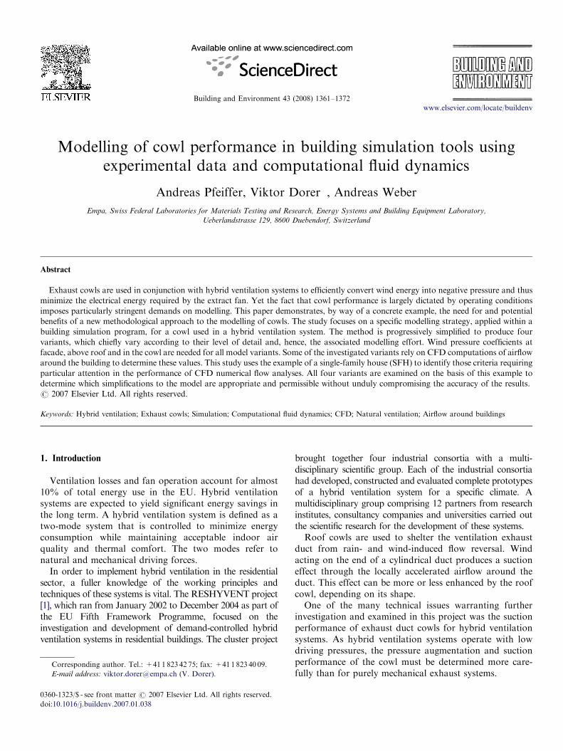
of cowls. Fig. 1 shows the dependencies governing ModelVariant D and its potential integration in a thermalmultizone flow program such as TRNFLOW. This model-ling approach was progressively simplified to produce threefurther variants (A–C) as set out in Table 1. All variantswere investigated and compared with the aid of an example.Variants A and B may be computed using the models

currently available in TRNFLOW. Variants C and D, onthe other hand, necessitate adjustments to the code as thecowl pressure coefficient Cp;c varies not only according towind direction but also in function of the velocity ratio atthe cowl.The required simulation input comprises both the

experimentally determined cowl characteristics and, fortheir application to the effective flow conditions above theroof, airflow data for various wind directions. Being largelydictated by the building geometry and cowl position, theseairflow data are scarcely amenable to generalization. It is,

ARTICLE IN PRESSA. Pfeiffer et al. / Building and Environment 43 (2008) 1361–1372 1363

however, possible to analyse the flow conditions in relationto a specific building for various wind directions by meansof CFD calculations. This is the approach adopted in thisstudy, the building type being a single-family house (SFH).

On the basis of the CFD calculation results (Section 5.1)and the cowl characteristics established by empiricalmeasurement (Section 2.2), the wind data and air velocityin the duct may be used to determine the pressure loss orgain of the cowl. As the exhaust mass flow rate is alsoinfluenced by other natural forces, an iterative solution isrequired. Except in Variant A, the wind pressure coefficientabove roof Cp;r used in the simulation is also derived fromthe CFD calculations. For Variant C, the schemeillustrated in Fig. 1 is simplified as follows:

1.

sim

w

Fig

pro

Tab

Co

Me

A

B

C

D

j ¼ 0.

2. U loc ¼ U r.

Consequently, no further CFD data are needed fortransposing the experimental cowl data.

ulation environment

cowl model

ind dataUr, β interpolation

Uloc = f (Ur, β)ϕ = f (β)

wind climate analysiscalculated CFD data(Section 2.3)

cowl characteristicswind tunnel test data(Section 2.2)

cowl pressureloss or gain

mass flowin the duct

buildingmodel

cowl

zone

m.

Δpc

Cp,r

interpolationCp,c = f (Ud /Uloc, ϕ)Δpc = f(Cp,r, ρ, Uloc)

ϕ Uloc

. 1. Proposed cowl model with integration in building simulation

gram (Model Variant D).

le 1

wl model variants A–D

thod Wind pressure coefficient above roof, Cp;r Cowl pressure

Four wind directions from [4] Constant aver

Sixteen wind directions from CFD calculations Constant aver

Sixteen wind directions from CFD calculations Pressure coeffi

Sixteen wind directions from CFD calculations Pressure coeffi

above roof. Lo

calculations.

2.2. Cowl characteristics

The aerodynamic characteristics of cowls and roofoutlets are determined by experimental measurements asspecified in [5]. The devices undergo a wind tunnel test,which makes additional allowance for an exhaust airflow.The pressure difference across the device is measured fordifferent wind and exhaust flow velocities. Both verticaland horizontal wind angles can be simulated by tilting androtating the duct in the wind tunnel as shown in Fig. 2.Using the total pressure in the duct pt;d and wind velocityU loc, the cowl pressure coefficient Cp;c can be calculatedfrom the static pressure measured in the wind tunnel ps;r infunction of wind angle and velocity ratio of wind andexhaust flow. The cowl pressure coefficient is defined as

Cp;c ¼2ðpt;d � ps;rÞ

r �U2loc

. (1)

The performance of standard and newly developed cowlshas been examined in several studies. De Gids and denOuden [6] investigated the behaviour of 13 different cowltypes in a wind tunnel and compared these with an openduct. The measured pressure coefficients are shown independency of the vertical wind incident angle j (fromperpendicular descending to perpendicular ascending) andof the airflow velocity ratio Ud=U loc, where Ud is theexhaust duct air velocity and U loc the local wind velocitynear the cowl. Comparison with an open duct arrangement

coefficient, Cp;c

age

age

cient in function of velocity ratio Ud to U r

cient in function of velocity ratio Ud to U loc and local wind direction jcal wind velocity and angle for 16 wind directions determined by CFD

Uloc

Ud

ps,r

pt,d

ϕ

Fig. 2. Experimental cowl pressure coefficient measurement set-up as

specified in [5].

ARTICLE IN PRESSA. Pfeiffer et al. / Building and Environment 43 (2008) 1361–13721364

allows the investigated cowls to be split into three groups:

1.

cowls which improve the pressure and flow stability inthe duct;

2.

cowls which adversely affect the pressure and flowstability in the duct;

3.

cowls which have a positive impact under certain circum-stances and a negative impact under others. These cowlsgenerally perform favourably in the presence of descendingwinds and unfavourably with rising winds.

In the example under study, the characteristics of cowltype no. 6 in [6]—a ‘‘Chinese hat’’—are digitized for use inthe calculation (Fig. 3). This cowl type is a typicalrepresentative of the third group.

2.3. Analysis of wind airflow patterns around buildings using

CFD

The results of CFD analyses may be used to factor in thelocal wind flow patterns that largely govern the suctioneffect of cowls. These calculations allow the transpositionof the experimentally determined cowl characteristics torealistic conditions. For Variants B–D, the wind pressurecoefficients above roof at the cowl position are derivedfrom the CFD results. Additional provision is made, in thecase of Variant D, for the local wind direction and windvelocity in transposing the cowl characteristics.

A flow field can be described by the conservation ofmass, momentum and energy. Given the boundary condi-tions, the resulting flow pattern is determined by solvingthe combined Navier–Stokes and energy or any otherscalar equations. CFD calculations of this kind are wellwithin the capacity of present-day computers. Wind flowpatterns around buildings or in built-up areas have oftenbeen computed in the past and investigated experimentally

-1.2

-1

-0.8

-0.6

-0.4

-0.2

0

0.2

0.4

0.6

0.8

1

0 15 30 45 60 75

co

wl

pre

ssu

re c

oeff

icie

nt Cp,c

[-

]

f=0

f=0.25

f=0.50

f=0.75

f=1

f = Ud/Uloc

vertical wind i

Fig. 3. Results from cowl performance measurements for d

using wind tunnels or full-scale structures. Key factors inCFD calculations include the effective discretization of thecalculation domain, choice of boundary conditions andmeshing. These work stages have a decisive impact on thequality of the computed results.

2.3.1. Dimensionality

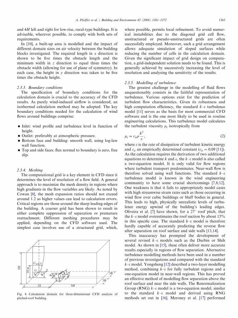
Oliveira et al. [7] demonstrated on a full-scale building thata two-dimensional flow field in the mid-span leads to seriousoverestimation of the suction pressure over the roof and onthe lee wall. Such differences between two- and three-dimensional modelling are largely attributable to thebuilding’s edge effects, with strong eddies and swirlingmotions occurring along the perimeter. Hence, if buildinglength B is limited, a three-dimensional calculation domain isneeded for the proper analysis of flow fields aroundbuildings, with two-dimensional simulations serving only toassist the design of grids suitable for three-dimensionalsimulations. Where the wind flow direction lies parallel to theplane of symmetry, computing effort may be substantiallycut by limiting the calculations to only one symmetrical half.

2.3.2. Domain size

In addition to the third dimension, the appropriatechoice of domain size is a further key prerequisite for theaccurate resolution of airflow patterns around buildings.The impact of calculation domain size has been evaluatedand documented by [7,8]. The higher blockage effect intwo-dimensional calculations necessitates a larger domainsize. For two-dimensional calculations performed on acubic building of height H, the upstream, downstream andcross-stream dimensions should be no less than 5H, 15H

and �4H. The domain height should be at least 10H.According to [7], the minimum domain size for three-dimensional calculations should be as shown in Fig. 4. Afurther source [9] recommends at least 4H to 5H upstream,

90 105 120 135 150 165 180

0°

90°

180°

vertical angle �

ncident angle � [°]

ifferent wind angles j and velocity ratios f (No. 6 [6]).

ARTICLE IN PRESSA. Pfeiffer et al. / Building and Environment 43 (2008) 1361–1372 1365

and 4H left and right for low-rise, rural-type buildings. It isadvisable, wherever possible, to comply with both sets ofrequirements.

In [10], a built-up area is modelled and the impact ofdifferent domain sizes on air velocity between the buildingblocks investigated. The required length in x direction isshown to be five times the obstacle length and theminimum width in z direction to equal three times theobstacle width (allowing for use of plane of symmetry). Ineach case, the height in y direction was taken to be fivetimes the obstacle height.

2.3.3. Boundary conditions

The specification of boundary conditions for thecalculation domain is crucial to the accuracy of the CFDresults. As purely wind-induced airflow is considered, anisothermal calculation method may be adopted. The keyboundary conditions needed for the calculation of windflows around buildings comprise:

�

5H

Fig

pitc

Inlet: wind profile and turbulence level in function ofheight.

� Outlet: preferably at atmospheric pressure. � Bottom face and building: smooth wall, using log-law

wall function.

� Top and side faces: flux normal to boundary is zero, free

slip.

2.3.4. Meshing

The computational grid is a key element in CFD since itdetermines the level of resolution of a flow field. A generalapproach is to maximize the mesh density in regions wherehigh gradients in the flow variables are likely. As noted byCowan [8], the mesh expansion ratios should not exceedaround 1.2 as higher values can lead to calculation errors.Critical regions are those around the sharp leading edges ofthe building. A coarser grid has been shown to result ineither complete suppression of separation or prematurereattachment. Different meshing procedures may beapplied, depending on the CFD software used. Thesimplest case involves use of a structured grid, which,

U10

10 m x

y

zB

S

H

5H 3S

3B

3B Ur

R R

α

. 4. Calculation domain for three-dimensional CFD analysis of

hed-roof building.

where possible, permits local refinement. To avoid numer-ical instabilities due to the diagonal grid cell flow,unstructured or pseudo-unstructured grids are oftensuccessfully employed. Moreover, such a grid arrangementallows adequate simulation of sloped surfaces whilereducing the number of cells in the calculation domain.Given the significant impact of grid design on computa-tion, a grid-independent solution needs to be found. This isgenerally achieved by successively increasing the level ofresolution and analysing the sensitivity of the results.

2.3.5. Modelling of turbulence

The greatest challenge in the modelling of fluid flowsunquestionably consists in the faithful representation ofturbulence. Various options exist for the prediction ofturbulent flow characteristics. Given its robustness andhigh computation efficiency, the standard k–� turbulencemodel [11] serves as the basis for most commercial CFDsoftware and is the one most likely to be used in routineengineering calculations. This turbulence model calculatesthe turbulent viscosity mt isotropically from

mt ¼ cmrk2

�, (2)

where � is the rate of dissipation of turbulent kinetic energyand cm an empirically determined constant (cm ¼ 0:09 [11]).As the calculation requires the derivation of two additionalequations to determine k and �, the k–� model is also calleda two-equation model. It is only valid for flow regionswhere turbulent transport predominates. Near-wall flow istherefore solved using wall functions. The standard k–�turbulence model is known in the wind engineeringcommunity to have some crucial shortcomings [7,8,12].One weakness is that it fails to appropriately model caseswith high streamwise strain rates such as those occurring inwind flow over cubic buildings or bluff bodies in general.This leads to high, physically unrealistic levels of turbu-lence energy upwind of the building’s leading edges.Oliveira et al. [7] have shown, for a 27� roof pitch, thatthe k–�model overestimates the roof suction by about 15%in this specific case. The standard k–� model is thereforehardly capable of accurately predicting the reverse flowafter separation on roof surface and side walls [13,14].This inaccuracy has prompted the development of

several revised k–� models such as the Durbin or Shihmodel. As shown in [15], these often deliver more accurateresults especially in regions of flow separation. Alternativeturbulence modelling methods have been used in a numberof previous investigations and compared with the standardk–�model. Yongsheng [12] described a two-layer modellingmethod, combining k–� for fully turbulent regions and aone-equation model in near-wall regions. This has provedan effective method of modelling flow separation above theroof surface and near the side walls. The RenormalizationGroup (RNG) k–� model is a two-equation model, similarto the standard k–� model and derived using RNGmethods set out in [16]. Meroney et al. [17] performed

ARTICLE IN PRESSA. Pfeiffer et al. / Building and Environment 43 (2008) 1361–13721366

calculations using the k–� RNG model to compare wind-tunnel measurements with computation results.

In analysing airflow patterns around buildings, theReynolds stress turbulence model (RSM) has beencompared with and found to be far more accurate thanthe standard k–� model [13]. Also large Eddy simulation(LES) is much more successful in predicting the flow fieldaround a bluff body. In recent LES computations, theconventional Smagorinsky SGS (subgrid scale) model hasbeen superseded by the dynamic SGS model, whichconstitutes one of the most significant advances in the fieldof CFD over the past few years. This has served to increasemodelling accuracy for velocities and pressure fieldsaround buildings.

3. Case study: analysis of wind-induced airflow above roof

The impact of the various model variants described inSection 2.1 was investigated using the example of a SFH.This necessitated the performance of a CFD analysis forthe specific building geometry to determine the airflowaround the building. The relevant literature gives theairflow patterns and associated wind pressure coefficientsonly for certain building configurations and seldomprovides details of local air velocity and flow directionabove the roof. A commercial CFD application wastherefore used to calculate the airflow pattern around apitched-roof SFH for various wind directions.

3.1. Method

The Flovent [18] CFD program used in this study adoptsthe widespread finite-volume method in conjunction withan orthogonal meshing system. This allows localized gridrefinement to increase resolution in regions with particu-larly high gradients and, accordingly, a rational use ofcomputing resources, particularly where substantial dis-crepancies in size arise in the geometrical configuration(e.g. between building and calculation domain). To over-come the difficulties in modelling near-wall grid cellsencountered with the standard k–� model [11], a revisedvariant—the so-called LVEL k–� model—was applied [19].Like a two-layer model, this permits accurate modelling ofnear-wall flows through variation of the turbulent viscosityaccording to the ‘‘law of the wall’’. The LVEL model canalso accommodate any desired number of grid cells in thewall boundary layer. The constants used with the standardk–�-model are set out in [18]. For the reasons stated inSection 2.3, the regions of flow separation warrantparticular attention when the standard k–� model isapplied. The results of cases presented in the existingliterature were therefore recomputed using Flovent and,among other things, the pressure coefficients above roof orat facade compared [20]. A relatively good concordancewas found with both experimental and computed resultsfor flat and gable roof constructions alike. Nonetheless,

greater accuracy is likely to be achieved using the RSMturbulence model or even LES.This study confined itself to the performance of three-

dimensional, steady-state calculations for a isothermalsituation. The wind profile was modelled using 12 inletspositioned at increasing heights, with the applied windvelocity averaged over the area. The impact of wind flowdirection, wind velocity, roughness parameter and gridresolution was investigated by means of a sensitivityanalysis using nine calculation models.

3.2. Boundary conditions

The approximate mean velocity profile of the approach-ing wind was derived from a logarithmic law model:

UðyÞ ¼ U10 lny

z0

� �ln

10

z0

� �� ��1. (3)

The roughness height z0 for flat or open terrain wastaken as 0.05 and the mean velocity U10 at the referenceheight as either 2 or 10m/s. As the k–� model was used, thevalues of k and � at the air inlet were required to takeaccount of turbulence in the approaching wind. It ispossible to determine turbulent kinetic energy k on thebasis of turbulence intensity. An average turbulenceintensity of 15% was assumed and the kinetic energycalculated using (4). This equation is based on theassumption that the fluctuation velocity components areequal.

k ¼ 32ðU � IÞ2. (4)

The other required value, dissipation rate �, may bedetermined on the basis of the assumption that the windis neutrally stratified and homogeneous in the surface layer.The dissipation rate may therefore be considered equal tothe rate of energy production as shown in (5), where k is0.41.

�ðyÞ ¼u3�

k � y. (5)

The friction velocity u� may be determined using Eq. (6)where cm is 0.09 [11] and k is calculated using (4):

k ¼u2�ffiffiffiffifficmp . (6)

A ‘‘smooth wall’’ was used to simulate the ground surfaceat the bottom of the calculation domain. The outflow faceswere set to open boundary, while symmetrical boundaryconditions were applied for the top face and sides ofthe domain. The boundary conditions are summarized inTable 2.

3.3. Geometry and calculation domain

The study used the example of a detached 12� 6m SFHwith a 30� roof pitch. The domain size—108� 60� 84m3,

ARTICLE IN PRESSA. Pfeiffer et al. / Building and Environment 43 (2008) 1361–1372 1367

see (Fig. 5)—was selected so as at least to meet therequirements specified in Section 2.3. For wind direction 0�

(parallel to x-axis), the 12 inlets were arranged at the y–z-low domain level. For wind directions 22:5�, 45� and 67:5�,both the y–z-low and the x–y-low domain levels wereprovided with inlets. These exhibit different flow anglesdepending on wind direction. Also, in these cases, the x–y-high domain level is left open to guarantee an outflow ofair. For wind direction 90�, only the x–y-low domain levelis provided with inlets and the x–y-high domain level leftopen.

3.4. Computational grid

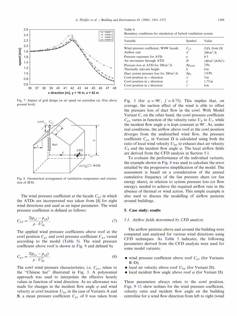
As mentioned in Section 2.3, one method for verifyingthe results consists in investigating the impact on these ofthe computational grid. This is why a solution withminimum dependency on the computational grid wassought for the present example. Four different gridstructures, as specified in Table 3, were investigated andthe air pressure, air velocity and flow angle at 10m heighton the building centreline were compared in each case.Moreover, with all variants, the grid was locally refined upto a distance of 6m in front of the building and 12m on theother faces (Fig. 6). Fig. 7 shows the air velocity above roofto depend on the choice of computational grid. Similar

Table 2

Boundary conditions used for calculation domain

Boundary Efficiency

Inlet Velocity profile applied to 12 separate inlets and derived

from log-law model in (3) where U10 ¼ 2 or 10m/s.

Turbulence parameters k and � using (4)–(6) where

I ¼ 15%

Outlet Open boundary face

Bottom Smooth wall, using log-law wall function

Top and sides Symmetrical boundary conditions applied, flux normal

to boundary ¼ 0, free slip

60 m

2 m/s

10 m x

y

z

12 m12 m

6 m

36 m

Ur

9.5

m

9.5

m

30

Fig. 5. Calculation domain and selecte

behaviour was observed in respect of static pressure andlocal incident flow angle, which were also investigated.Large error margins are inevitable with the coarse Mesh

1. Each grid refinement brings the results closer to thoseachieved by Mesh 4 (Fig. 7). Given the only minordifference in results between Meshes 3 and 4 and thedisproportionate rise in the computing effort needed forMesh 4, with double the grid cells, Mesh 3 was used for thefurther investigations.

4. Case study: multizone airflow modelling

To study the impact of Model Variants A–D, each wasapplied to a SFH with the geometry and size shown inFig. 5. As no integration in a thermal building simula-tion program is intended for the time being, a numberof simplifications were made to permit use of theEES (Engineering Equation Solver [21]) program forcomputation.First, a smart hybrid ventilation system was assumed,

which uses automatic control technology to limit themaximum airflow rate and sets the fan to the ideal speed inthe event of inadequate airflow. A steady airflow rate of200m3=h is thus maintained throughout the year. Theindoor air temperature was also assumed to remainconstant throughout the year. The air transfer devices(ATDs) are located within a single facade. Fig. 8 shows theflow model and arrangement of ventilation components.The characteristic values for the ventilation system,

presented in Table 4, are typical of a domestic hybridsystem. The applied external climatic conditions werebased on the Typical Metrological Year (TMY) atZurich-Kloten (Swiss Central Plateau). An average windvelocity for the year of 2.2m/s was thus assumed and west-south-west (WSW) taken as the prevailing wind direction.The impact of the model variants is largely dictated by thecowl position and building orientation. To maximize thedifferences between the variants, the building was posi-tioned so as to face the prevailing wind.

72 m

36 m

36 m˚

d geometry for pitched-roof SFH.

ARTICLE IN PRESS

Table 3

Grid design of test domains

Category Number of grid cells ðx; y; zÞ Total number of

grid cells

Grid distribution above roof

ðx; y; zÞBase grid Region grid

Mesh 1 26� 18� 21 31� 15� 25 20,283 1:0�1:0� 1:3m3

Mesh 2 52� 28� 41 61� 29� 49 137,877 0:5�0:5� 0:7m3

Mesh 3 78� 44� 61 91� 45� 73 487,197 0:35�0:3� 0:5m3

Mesh 4 104� 58� 79 121� 60� 99 1,140,388 0:25�0:2� 0:35m3

Fig. 6. Mesh structure for x–z (top) and x–y (bottom) plane of Mesh 3 with local grid refinement.

A. Pfeiffer et al. / Building and Environment 43 (2008) 1361–13721368

ARTICLE IN PRESS

0.6

0.8

1.0

1.2

1.4

1.6

1.8

2.0

2.2

2.4

2.6

36 37 38 39 40 41 42 43 44 45 46 47 48

sp

eed

[m

/s]

mesh 1mesh 2mesh 3mesh 4

x direction [m], y = 10 m, z = 42 m

Fig. 7. Impact of grid design on air speed on centreline (at 10m above

ground level).

duct

cowl

ATD

Cp,f

Cp,r

WSW

h

z'

x'

y'

V.

Fig. 8. Geometrical arrangement of ventilation components and orienta-

tion of SFH.

Table 4

Boundary conditions for simulation of hybrid ventilation system

Variable Symbol Value

Wind pressure coefficient, WSW facade Cp;f f ðbÞ, from [4]

Airflow rate _V 200m3=hPressure exponent for ATD n 0.5

Air movement through ATD D 140m3=ðhPanÞ

Pressure loss at ATD for 200m3=h DpATD 2Pa

Thermally relevant height h 6m

Duct system pressure loss for 200m3=h Dpd 2.6 Pa

Cowl position in x direction x0 3m

Cowl position in y direction y0 1.75m

Cowl position in z direction z0 6m

A. Pfeiffer et al. / Building and Environment 43 (2008) 1361–1372 1369

The wind pressure coefficient at the facade Cp;f in whichthe ATDs are incorporated was taken from [4] for eightwind directions and used as an input parameter. The windpressure coefficient is defined as follows:

Cp;f ¼2ðps;f � ps;0Þ

r �U210

. (7)

The applied wind pressure coefficients above roof at thecowl position Cp;r and cowl pressure coefficient Cp;c variedaccording to the model (Table 5). The wind pressurecoefficient above roof is shown in Fig. 9 and defined by

Cp;r ¼2ðps;r � ps;0Þ

r �U210

. (8)

The cowl wind pressure characteristics, i.e. Cp;c, relate tothe ‘‘Chinese hat’’ illustrated in Fig. 3. A polynomialapproach was used to interpolate the effective hourlyvalues in function of wind direction. As no allowance wasmade for changes in the incident flow angle j and windvelocity at cowl location U loc in the case of Variants A andB, a mean pressure coefficient Cp;c of 0 was taken from

Fig. 3 (for j ¼ 90�, f ¼ 0:75). This implies that, onaverage, the suction effect of the wind is able to offsetthe pressure loss of duct flow in the cowl. With ModelVariant C, on the other hand, the cowl pressure coefficientCp;c varies in function of the velocity ratio Ud to U r, whilethe incident flow angle j is kept constant at 90�. As, underreal conditions, the airflow above roof at the cowl positiondiverges from the undisturbed wind flow, the pressurecoefficient Cp;c in Variant D is calculated using both theratio of local wind velocity U loc to exhaust duct air velocityUd and the incident flow angle j. The local airflow fieldsare derived from the CFD analysis in Section 5.1.To evaluate the performance of the individual variants,

the example shown in Fig. 8 was used to calculate the errorentailed by the progressive simplification of the model. Theassessment is based on a consideration of the annualcumulative frequency of the fan pressure share (or fanenergy share), in relation to system pressure loss (or flowenergy), needed to achieve the required airflow rate in theabsence of thermal or wind action. This simple example isalso used to discuss the modelling of airflow patternsaround buildings.

5. Case study: results

5.1. Airflow fields determined by CFD analysis

The airflow patterns above and around the building werecomputed and analysed for various wind directions usingCFD techniques. As Table 5 indicates, the followingparameters derived from the CFD analysis were used forsome model variants:

�

wind pressure coefficient above roof Cp;r (for VariantsB–D); � local air velocity above roof U loc (for Variant D); � local incident flow angle above roof j (for Variant D).

These parameters always relate to the cowl position.Figs. 9–11 show isolines for the wind pressure coefficient,velocity ratio and incident flow angle on the buildingcentreline for a wind flow direction from left to right (wind

ARTICLE IN PRESSA. Pfeiffer et al. / Building and Environment 43 (2008) 1361–13721370

direction b ¼ 0�). Similar calculations and analyses wereperformed for other wind directions, e.g. 22:5�, 45�, 67:5�

and 90�. These results allow determination of the flowcharacteristics for any wind conditions.

These analyses may be used to define all threeparameters in function of wind direction b (Table 6) forthe cowl position shown in Fig. 8. These functions areneeded for the calculations in Section 5.2.

The results assume a wind velocity of 2m/s, approx-imating to the annual average in the Swiss Central Plateau.An additional CFD analysis for 10m/s showed a higherwind velocity to have relatively little effect on the results.The results set out in Figs. 9–11 are therefore deemed to beindependent of wind velocity.

Table 5

Variant-specific boundary conditions

Variable Symbol Variant A

Cowl pressure coefficient Cp;c 0

Wind pressure coefficient above roof Cp;r f ðbÞ, from [4]

Fig. 9. Isolines for wind pressure coefficient Cp;r on

Fig. 10. Isolines for air velocity ratio ðU loc=U rÞ on

The impact of the roughness parameter z0 was alsoinvestigated using the example. In place of 0.05, an inputvalue of 0.5 was applied to the simulation to represent asparsely developed area [20]. This change likewise had onlya minor impact on the results.

5.2. Comparison of Methods A–D

The results from Section 5.1 were used to perform a year-long simulation for a hybrid ventilation system based onModel Variants A–D. The SFH described in Section 4 wasmodelled and the additional fan pressure, in support of thenatural forces, needed to achieve an airflow rate of200m3=h was computed for every hour in the year. This

Variant B Variant C Variant D

0 f ðUd=U rÞ f ðUd=U loc; gjÞf ðbÞ, from CFD f ðbÞ, from CFD f ðbÞ, from CFD

building centreline for wind direction b ¼ 0�.

building centreline for wind direction b ¼ 0�.

ARTICLE IN PRESS

Fig. 11. Isolines for incident flow angle j on building centreline for wind direction b ¼ 0�.

Table 6

Wind pressure coefficient, velocity ratio and incident flow angle in

function of wind direction for cowl position shown in Fig. 8

Wind

direction bCp;r U loc=U r j (deg)

0 �0.34 0.22 120

22.5 �0.4 0.45 82

45 �0.45 1.1 75

67.5 �0.34 1.01 79.5

90 �0.22 0.93 89.5

112.5 �0.17 1.01 99

135 �0.18 1.04 104

157.5 0.05 0.95 108

180 0 0.9 109

202.5 0.05 0.95 108

225 �0.18 1.04 104

247.5 �0.17 1.01 99

270 �0.22 0.93 89.5

292.5 �0.34 1.01 79.5

315 �0.45 1.1 75

337.5 �0.4 0.45 82

360 �0.34 0.22 120

A. Pfeiffer et al. / Building and Environment 43 (2008) 1361–1372 1371

pressure difference may be expressed as a percentage of theoverall system pressure loss (4.6 Pa) and the resultant fanpressure share presented for each model variant in the formof a cumulative frequency curve (Fig. 12). As fan pressureis directly proportional to fan power, the terms ‘‘fanpressure share’’ and ‘‘fan power share’’ may be usedsynonymously.

As Fig. 12 shows, the fan remains switched off,depending on model variant, for between 2200 and3650 h in the year, during which time the natural forcessuffice to achieve the 200m3=h airflow rate. The graph alsoshows that Variant A records the lowest mean value andthus delivers the most optimistic results. The curves forVariants B and C progressively approach that of VariantD. The difference between Variants C and D is relativelysmall and chiefly depends on the vertical cowl position. Thesame calculation for a height y0 of 3.75m instead of 1.75mdelivered practically identical results for Variants C and D.Clearer differences between Variants C and D may beexpected for heights below 1.75m due to the lower wind

velocities. Given the substantial additional effort requiredfor the modelling and analysis of CFD results for VariantD and the only minor differences in results, Variant C maybe recommended for this example. However, as thesensitivity of Cp;c to the vertical incident flow angle jdepends on the cowl type and velocity ratio Ud=U loc

(Fig. 3), these findings cannot be generalized.

6. Conclusions

This study highlights the need for a new approach to themodelling of cowls incorporated in hybrid ventilationsystems. The aim of any such model is to achieve as faithfulas possible a representation of reality using the experimen-tally determined cowl characteristics and effectively pre-vailing wind conditions.Experiments show the suction effect of cowls to depend

on both local wind velocity and local wind direction.Ideally, therefore, the airflow fields around the buildingneed to be known for various wind directions and withregard to the specific structural geometry. The CFDmethod is particularly suitable for the analysis of airflowabove the roof, while a three-dimensional model is alwaysrequired for the computation of airflow around buildings.To avoid modelling errors, various criteria relating to thecalculation domain and computational grid need to beobserved in selecting the calculation domain. As theboundary conditions have a direct impact on the results,these require careful definition. Numerous investigationshave shown the k–� turbulence model to bring aboutcomputational errors in certain flow fields. More advancedmodels, e.g. the Reynolds stress model (RSM), shouldtherefore be preferred to the standard k–� model for thecalculation of airflow around buildings.A year-long simulation, which used a sample building to

examine the impact of Model Variants A–D, underlinedthe benefits of accurate modelling. A significant progressiveimprovement was observed in the calculation resultsbetween Variants A, B and C. The additional considerationof local wind conditions at the cowl position (Variant D) inthe investigated example was shown to have hardly any

ARTICLE IN PRESS

0%

20%

40%

60%

80%

100%

1460 2190 2920 3650 4380 5110 5840 6570 7300 8030 8760

fan

pre

ssu

re s

hare

, Δp

f /

Δps [

%] variant A

variant Bvariant Cvariant D

y' = 1.75 m

number of hours [-]

fan switched off (pure natural ventilation)

Fig. 12. Curves for model variants A–D showing fan pressure share for SFH in Zurich-Kloten.

A. Pfeiffer et al. / Building and Environment 43 (2008) 1361–13721372

impact on the results, the difference being largely dictatedby the vertical cowl position, cowl characteristics andvelocity ratio Ud=U loc. Where the cowl projects beyond theridge, practically identical results are likely for Variants Cand D in the investigated example. In view of these findingsand the higher computational effort required for VariantsD, C may be recommended in this case. Particularattention should be devoted to the calculation of the windpressure coefficient above roof Cp;r. A CFD analysis ofairflow based on the effective building geometry is there-fore indispensable.

Acknowledgements

This work has been partially funded by the Swiss StateSecretariat for Education and Research (contract BBW01.0046, EU project RESHYVENT) and by Empa.Contributions by the participants of the RESHYVENTproject and by our colleagues at Empa are gratefullyacknowledged.

References

[1] EU project report RESHYVENT, see hhttp://www.reshyvent.comi.

[2] Feustel H, et al. COMIS 3.1, Program for modelling of multizone

airflow and pollutant transport in buildings. Sophia–Antipolis,

France: CSTB; 2001.

[3] TRNSYS 15, Transient system simulation program. Madison, USA:

Solar energy laboratory (SEL), University of Wisconsin; 2000.

[4] Orme M, Liddament M, Wilson A. An analysis and data summary of

AIVC’s numerical database. IEA air infiltration and ventilation

centre. Technical Note 44, 1994.

[5] CEN EN Standard 13141-5. Ventilation for buildings—Performance

testing of components/products for residential ventilation—Part 5:

cowls and roof outlet terminal devices, 2004.

[6] De Gids W, den Ouden HPL. Three investigations of the behaviour

of ducts for natural ventilation in which an examination is made of

the influence of location and height of the outlet, of the built-up

nature of the surroundings and of the form of the outlet. TNO

Report, 1987. 42pp. [In Dutch with English translation available].

[7] Oliveira PJ, Younis BA. On the prediction of turbulent flows around

full-scale buildings. Journal of Wind Engineering and Industrial

Aerodynamics 2000;86:203–20.

[8] Cowan IR, Castro IP, Robins AG. Numerical considerations for

simulations of flow and dispersion around buildings. Journal of Wind

Engineering and Industrial Aerodynamics 1997;67&68:535–45.

[9] Hoxey RP, Richards PJ. Flow pattern and pressure field around a

full-scale building. Journal of Wind Engineering and Industrial

Aerodynamics 1993;50:203–12.

[10] Hu CH, Wang F. Using a CFD approach for the study of street-level

winds in a built-up area. Building and Environment 2005;40:617–31.

[11] Launder BE, Spalding DB. The numerical computation of turbulent

flows. Computer Methods in Applied Mechanics and Engineering

1974;3(2):269–89.

[12] Yongsheng Z, Stathopoulos T. A new technique for the numerical

simulation of wind flow around buildings. Journal of Wind

Engineering and Industrial Aerodynamics 1997;72:137–47.

[13] Murakami S. Current status and future trends in computational wind

engineering. Journal of Wind Engineering and Industrial Aerody-

namics 1997;67&68:3–34.

[14] Murakami S, Ooka R, Mochida A, Yoshida S, Kim S. CFD analysis

of wind climate from human scale to urban scale. Journal of Wind

Engineering and Industrial Aerodynamics 1999;81:57–81.

[15] Lun YF, Mochida A, Murakami S, Yoshino H, Shirasawa T.

Numerical simulation of flow over topographic features by revised

k—� models. Journal of Wind Engineering and Industrial Aero-

dynamics 2003;91:231–45.

[16] Yakhot V, Orszag SA. Renormalization group analysis of turbulence.

I. Basic theory. Journal of Scientific Computing 1986;1(1):3–51.

[17] Meroney RN, Leitl BM, Rafailidis S, Schatzmann M. Wind-tunnel

and numerical modelling of flow and dispersion about several

building shapes. Journal of Wind Engineering and Industrial

Aerodynamics 1999;81:333–45.

[18] FLOVENT Version 4.2 (Manual). Hampton Court UK: Flomerics

Ltd.; 2003.

[19] Agonafer D, Gan-Li L, Spalding DB. The LVEL turbulence model

for conjugate heat transfer at low Reynolds numbers. In: Application

of CAE/CAD Electronic Systems, EEP vol. 18. New York: ASME;

1996.

[20] Dorer V, Pfeiffer A, Weber A. Parameters for the design of demand

controlled hybrid ventilation systems for residential buildings. IEA

air infiltration and ventilation centre. Technical Note 59, 2005.

[21] Klein SA. Engineering equation solver (EES). Middleton, Wisconsin,

USA: f-chart software, 2003.