modelling of acoustic viscothermal losses using the
TRANSCRIPT
General rights Copyright and moral rights for the publications made accessible in the public portal are retained by the authors and/or other copyright owners and it is a condition of accessing publications that users recognise and abide by the legal requirements associated with these rights.
Users may download and print one copy of any publication from the public portal for the purpose of private study or research.
You may not further distribute the material or use it for any profit-making activity or commercial gain
You may freely distribute the URL identifying the publication in the public portal If you believe that this document breaches copyright please contact us providing details, and we will remove access to the work immediately and investigate your claim.
Downloaded from orbit.dtu.dk on: Feb 15, 2022
Modelling of acoustic viscothermal losses using the Boundary Element Method: Frommethod to optimization
Andersen, Peter Risby
Publication date:2018
Document VersionPublisher's PDF, also known as Version of record
Link back to DTU Orbit
Citation (APA):Andersen, P. R. (2018). Modelling of acoustic viscothermal losses using the Boundary Element Method: Frommethod to optimization. Technical University of Denmark.

From method to optimization
Modelling of acoustic viscothermal lossesusing the Boundary Element Method
Ph
DT
hes
is
Peter Risby AndersenCentre for Acoustic-MechanicalMicro Systems (CAMM)Acoustic TechnologyOctober 2018


This thesis was submitted to the Technical University of Denmark as partial fulfillmentof the requirements for the degree of Doctor of Philosophy (PhD). The studies wasfinanced by the Centre for Acoustic-Mechanical Micro Systems (CAMM), and com-pleted between October 1 2015 and September 30 2018 at the Department of ElectricalEngineering and the Acoustic Technology group under the supervision of AssociateProfessor Vicente Cutanda Henríquez and Associate Professor Niels Aage.
Title
Modelling of acoustic viscothermal losses using the Boundary Element Method: Frommethod to optimization
Author
Peter Risby Andersen
Supervisors
Assoc. Prof. Vicente Cutanda HenríquezAssoc. Prof. Niels Aage
Acoustic TechnologyDepartment of Electrical EngineeringTechnical University of DenmarkKgs. Lyngby, Denmark

ii

AbstractA range of acoustic engineering problems require the inclusion of viscous and thermaldissipation to be modelled accurately. The dissipative effects are especially relevantwhen the geometric dimensions of the acoustic domain become small which is thecase in acoustic transducers and hearing aids. Computer-based numerical tools suchas the Finite Element Method can be used to model and investigate the performance ofacoustic devices without expensive prototyping. Directly including acoustic dissipationinto the Finite Element Method comes at a significant computational cost, sometimesmaking simulations on modest hardware problematic. An interesting alternative to theFinite Element Method, is the Boundary Element Method that is capable of includingdissipation and at the same time avoid so-called boundary layer meshing. However,a potential shortcoming of the existing boundary element implementation is its use oftangential derivative finite difference coupling terms, that may lead to undesirable in-accuracies.
This work presents two new coupling strategies that avoid the use of finite differenceby either using boundary element itself or the shape functions to estimate the tangentialderivatives. Numerical experiments demonstrate increased stability and error reductionwhen using the new coupling strategies.
Furthermore, based on the improved viscothermal Boundary Element Method, agradient-based shape optimization technique is developed. The shape optimizationtechnique is used to optimize the absorption coefficient of two-dimensional quarte-wave and Helmholtz resonators located at an impedance tube termination. Shape opti-mization results show that high absorption coefficients are only obtained when viscousand thermal dissipation is modelled accurately. The shape optimization technique hasthe future potential of improving the design of acoustic devices which require the in-clusion of viscous and thermal dissipation.

iv

ResuméEn række ingeniørmæssige akustiske problemstillinger kræver præcis modellering afviskose og termiske tab. Tabseffekterne er specielt relevante når de geometriske di-mensioner af det akustiske domæne bliver små, hvilket ofte er tilfældet i akustisketransducere og høreapparater. Computerbaserede numeriske beregningsværktøjer, så-som finite element metoden, kan bruges til a modellere og undersøge kvaliteten af etakustiskapparat uden brugen af bekostelige prototyper. At inkludere de akustiske tabi finite element metoden gør beregningsarbejdet betydeligt tungere, hvilket kan gøredet svært at realisere simuleringer med normal computerhardware. Boundary elementmetoden udgør et interessant alternativ til finite element metoden. Med denne er detmuligt at inkludere tab og på samme tid undgå såkaldt grænselagsdiskretisering. Imple-menteringen af boundary element metoden gør på den anden side brug af tangentielleafledte koblingstermer beregnet med finit difference, hvilket kan føre til en uønsketberegningsunøjagtighed.
Dette ph.d. arbejde, præsenterer to nye koblingsstrategier som undgår brugen af fi-nite difference, ved enten at bruge boundary element metoden eller shape funktioner tilat estimere de tangentielle afledte. Med numeriske eksperimenter bliver det vist at deto nye koblingsstrategier giver øget stabilitet og kan minimere beregningsfejl.
Desuden bliver en gradientbaseret formoptimeringsteknik udviklet der er baseret påden forbedrede boundary element metode. Formoptimeringsteknikken er demonstreretved at optimere absorptionskoefficienten af henholdsvis kvartbølge- og helmholtzres-onatorer der er placeret i enden af et impedansrør. Formoptimeringsresultater viserat høje absorptionsværdier kan kun opnås når de viskose og termiske tab er mod-elleret præcist. Den udviklede formoptimeringsteknik har et fremtidigt potentiale tilat forbedre designet af akustiske apparater der kræver tabsmodellering.

vi
AcknowledgementsFirst of all, I am grateful for all the help and support that my supervisors Vicenteand Niels have given me, even in the darkest hour. Our many discussions and theirprofound knowledge in the areas of numerical methods, viscothermal losses and opti-mization have made this project possible.
I would like to thank everyone from CAMM for the many helpful discussions, com-ments and suggestions given during our meetings. Also, a big thanks to the AcousticTechnology group and fellow PhD students for making a pleasant and joyful researchenvironment.
During my stay in Munich at the Chair of Vibroacoustics of Vehicles and Machines, Ihad the pleasure of discussing Boundary Element Method with Steffen Marburg whichgreatly helped me progress with difficult parts of the work - for that I am grateful. Iwould also like to thank everyone at the chair for having me and discussing many dif-ferent aspects of acoustics.
Furthermore, I would like to thank José Sánchez-Dehesa for supplying interesting studycases and measurements, but also the discussions on viscothermal losses and their im-pact on novel acoustic devices have been valuable.
Also a big thanks to Peter Møller Juhl who was the first to introduce me to the ex-citing world of Boundary Element Method.
Last, but not least, the biggest thanks to family, friends and Elisabeth for always beingsupportive and being there, no matter what.

viii
PublicationsThe thesis is based on the following papers.
Paper APaper A V. Cutanda Henríquez, P. Risby Andersen, J. Søndergaard Jensen, P. Møller Juhl andJ. Sánchez-Desa, A Numerical Model of an Acoustic Metamaterial using the Boundary ElementMethod Including Viscous and Thermal Losses, Journal of Computational acoustics, (2016),doi.org/10.1142/S0218396X17500060doi.org/10.1142/S0218396X17500060
Paper BPaper B P. Risby Andersen, V. Cutanda Henríquez, N. Aage and J. Sánchez-Desa, Visco-thermaleffects on an acoustic cloak based on scattering cancellation, Proceedings from the 6th confer-ence on Noise and vibration emerging methods, 7-9 May (2018), Ibiza (Spain)
Paper CPaper C P. Risby Andersen, V. Cutanda Henríquez, N. Aage and S. Marburg A two dimen-sional acoustic tangential derivative boundary element method including viscous and thermallosses, Journal of Computational and Theoretical Acoustics, (2018),doi.org/10.1142/S2591728518500366doi.org/10.1142/S2591728518500366
Paper DPaper D V. Cutanda Henríquez and P. Risby Andersen, A three-dimensional acoustic BoundaryElement Method formulation with viscous and thermal losses based on shape function deriva-tives, Journal of Computational and Theoretical acoustics, (2018) ,doi.org/10.1142/S2591728518500391doi.org/10.1142/S2591728518500391
Paper EPaper E P. Risby Andersen, V. Cutanda Henríquez and N. Aage, Shape optimization of micro-acoustic devices including viscous and thermal losses, (2018)(Submitted to the Journal of Sound and Vibration)
A conference publication written during the course of the PhD, but not included inthe thesis:
Risby Andersen, P., Cutanda Henríquez, V., Aage, N. and Marburg, S., Numerical Acous-tic Models Including Viscous and Thermal losses: Review of Existing and New Methods,DAGA, 6-9 March (2017), Kiel (Germany)

x
ContentsAbstractAbstract . . . . . . . . . . . . . . . . . . . . . . . . . . . . . . . . . . . . iiiiiiResuméResumé . . . . . . . . . . . . . . . . . . . . . . . . . . . . . . . . . . . . vvAcknowledgementAcknowledgement . . . . . . . . . . . . . . . . . . . . . . . . . . . . . . viiviiPublicationsPublications . . . . . . . . . . . . . . . . . . . . . . . . . . . . . . . . . . ixix
1 Introduction1 Introduction 111.1 Motivation1.1 Motivation . . . . . . . . . . . . . . . . . . . . . . . . . . . . . . . . 111.2 Project goals1.2 Project goals . . . . . . . . . . . . . . . . . . . . . . . . . . . . . . . 221.3 Thesis structure1.3 Thesis structure . . . . . . . . . . . . . . . . . . . . . . . . . . . . . 33
2 Isentropic propagation of sound waves2 Isentropic propagation of sound waves 552.1 The wave equation2.1 The wave equation . . . . . . . . . . . . . . . . . . . . . . . . . . . 552.2 Finite Element Method2.2 Finite Element Method . . . . . . . . . . . . . . . . . . . . . . . . . 662.3 Boundary Element Method2.3 Boundary Element Method . . . . . . . . . . . . . . . . . . . . . . . 77
2.3.1 Non-uniqueness2.3.1 Non-uniqueness . . . . . . . . . . . . . . . . . . . . . . . . . 882.4 Boundary conditions2.4 Boundary conditions . . . . . . . . . . . . . . . . . . . . . . . . . . 99
3 Viscothermal losses in acoustics and its modelling3 Viscothermal losses in acoustics and its modelling 11113.1 State-of-the-art3.1 State-of-the-art . . . . . . . . . . . . . . . . . . . . . . . . . . . . . 11113.2 General assumptions3.2 General assumptions . . . . . . . . . . . . . . . . . . . . . . . . . . 15153.3 Viscothermal FEM3.3 Viscothermal FEM . . . . . . . . . . . . . . . . . . . . . . . . . . . 1616
3.3.1 Boundary conditions3.3.1 Boundary conditions . . . . . . . . . . . . . . . . . . . . . . 17173.4 Viscothermal BEM3.4 Viscothermal BEM . . . . . . . . . . . . . . . . . . . . . . . . . . . 1919
3.4.1 Boundary conditions3.4.1 Boundary conditions . . . . . . . . . . . . . . . . . . . . . . 20203.4.2 System of equations and coupling method3.4.2 System of equations and coupling method . . . . . . . . . . . 21213.4.3 Narrow gap and low frequency breakdown3.4.3 Narrow gap and low frequency breakdown . . . . . . . . . . 2222
3.5 Metamaterial (Paper APaper A)3.5 Metamaterial (Paper APaper A) . . . . . . . . . . . . . . . . . . . . . . . . . 23233.6 Cloak based on scattering cancellation (Paper BPaper B)3.6 Cloak based on scattering cancellation (Paper BPaper B) . . . . . . . . . . . 24243.7 Contribution3.7 Contribution . . . . . . . . . . . . . . . . . . . . . . . . . . . . . . . 2525
4 Improving the BEM implementation with losses4 Improving the BEM implementation with losses 27274.1 Tangential derivative BEM (Paper CPaper C)4.1 Tangential derivative BEM (Paper CPaper C) . . . . . . . . . . . . . . . . . . 2727
4.1.1 System of equations4.1.1 System of equations . . . . . . . . . . . . . . . . . . . . . . 2929
Contents xii
4.1.2 Unique normal and tangential vectors4.1.2 Unique normal and tangential vectors . . . . . . . . . . . . . 29294.1.3 Evaluation of the formulation4.1.3 Evaluation of the formulation . . . . . . . . . . . . . . . . . 3030
4.2 Shape function derivatives (Paper DPaper D)4.2 Shape function derivatives (Paper DPaper D) . . . . . . . . . . . . . . . . . . 30304.2.1 System of equations4.2.1 System of equations . . . . . . . . . . . . . . . . . . . . . . 31314.2.2 Evaluation of the formulation4.2.2 Evaluation of the formulation . . . . . . . . . . . . . . . . . 3232
4.3 Contribution4.3 Contribution . . . . . . . . . . . . . . . . . . . . . . . . . . . . . . . 3232
5 Acoustic shape optimization including losses5 Acoustic shape optimization including losses 35355.1 Optimization problem5.1 Optimization problem . . . . . . . . . . . . . . . . . . . . . . . . . . 36365.2 Gradient-based optimization5.2 Gradient-based optimization . . . . . . . . . . . . . . . . . . . . . . 36365.3 Shape optimization and parametrization5.3 Shape optimization and parametrization . . . . . . . . . . . . . . . . 37375.4 Sensitivity analysis5.4 Sensitivity analysis . . . . . . . . . . . . . . . . . . . . . . . . . . . 37375.5 Sparse assembly5.5 Sparse assembly . . . . . . . . . . . . . . . . . . . . . . . . . . . . . 38385.6 Constraints5.6 Constraints . . . . . . . . . . . . . . . . . . . . . . . . . . . . . . . 39395.7 Shape optimization including losses (Paper EPaper E)5.7 Shape optimization including losses (Paper EPaper E) . . . . . . . . . . . . . 4040
5.7.1 Optimization problem5.7.1 Optimization problem . . . . . . . . . . . . . . . . . . . . . 41415.7.2 Summery of shape optimization results5.7.2 Summery of shape optimization results . . . . . . . . . . . . 4242
5.8 Shape optimization of an acoustic cloak5.8 Shape optimization of an acoustic cloak . . . . . . . . . . . . . . . . 44445.9 Contribution5.9 Contribution . . . . . . . . . . . . . . . . . . . . . . . . . . . . . . . 4545
6 Discussion and conclusions6 Discussion and conclusions 47476.1 Conclusions6.1 Conclusions . . . . . . . . . . . . . . . . . . . . . . . . . . . . . . . 50506.2 Future research6.2 Future research . . . . . . . . . . . . . . . . . . . . . . . . . . . . . 5151
BibliographyBibliography 5353
Paper APaper A 6565
Paper BPaper B 7979
Paper CPaper C 8989
Paper DPaper D 105105
Paper EPaper E 121121

Chapter 1
Introduction
1.1 Motivation
The popularity of small electronic mobile devices, such as the smartphone, has createda need for acoustic transducers that maintain high performance when incorporated intoconfined spaces. In other acoustic devices, like hearing aids, the reduced device sizeis necessary to improve the usability for the end-user, yet at the same time achieveaccurate reproduction of acoustic signals. Common for these acoustic device types isthat their size is small, and that sound waves need to propagate in complicated narrowchannels and chambers. To accurately model and estimate the propagation of soundin such scenarios will require appropriate modelling methods that include the effectof viscosity and thermal conduction. Viscosity and thermal conduction will in narrowpassages act as a loss mechanism that attenuates and changes the phase of sound waves.Sometimes, the effect of losses is so significant that if neglected, results may becomeinaccurate [11, 22, 33, 44].
On the other hand, in many situations, sound waves are usually adequately modelledwithout directly accounting for viscous and thermal dissipation, and losses can typi-cally be included using simple impedance conditions. If possible, it is often attractiveto neglect, or model dissipation with simplified assumptions, since direct modelling andincorporation of the acoustic viscous and thermal effects into, e.g., numerical methodssuch as the Finite Element Method (FEM) or Boundary Element Method (BEM) comesat a significant computational cost. Additionally, it can be challenging to predict if theinclusion of viscous and thermal dissipation is necessary.
Besides the aforementioned mobile devices and hearing aids, it is well known thatlosses can significantly influence acoustic MEMS transducers [55, 66], condenser micro-phones [77, 88, 99], compression horn drivers [1010, 1111, 1212] and the importance of lossescan even be found in room acoustics, where the characterisation of micro-perforated

Chapter 1. Introduction 2
absorbers requires modelling of viscothermal effects [1313, 1414].
In recent years, acoustic metamaterials have been given much attention in the literature.Acoustic metamaterials are artificial structures created from scatters and resonators or-ganised in periodic patterns [1515]. If observed as a whole, metamaterials can showextraordinary properties, e.g. negative speed of sound and/or negative bulk modulus.The understanding of how viscous and thermal loss influences acoustic metamaterialsis only sparsely studied in the literature, but examples have been appearing during thisproject [1616, 1717, 1818, 1919] and Paper APaper A also studies the viscothermal effects on a metama-terial.
Computer-based numerical simulations tools, such as the FEM and the BEM, are valu-able when investigating and improving the broad range of acoustic devices discussedso far. Simulations allow engineers and researchers to predict the physical behaviourof such sophisticated devices, which can reduce the need for costly prototyping or givea more profound understanding of an acoustic phenomenon. Interpretation of simu-lations are often difficult, and ideas on how to improve a specific device design canbe even harder. In such cases, optimization based on numerical methods has provento be a helpful tool in discovering new high performing acoustic designs and creatingotherwise non-intuitive design choices [2020, 2121, 2222].
However, the acoustic devices discussed so far require modelling of viscous and ther-mal losses. In the literature, numerical acoustic optimization methods applicable tomore general acoustic problems that include accurate modelling of viscous and ther-mal losses are very scarce. To the best of this author’s knowledge, only one exampleexists of such optimization. In a very recent publication, Christensen [2323] showed thepossibility of performing topology optimization using FEM by applying the so-calledlow reduced frequency formulation, making it possible to topology optimize the cross-section of tubes and slits.
1.2 Project goals
In this project, methods for improving the reliability and stability of an existing BEMimplementation that incorporates viscous and thermal losses are sought. The currentBEM implementations are subject to certain shortcomings that can lead to undesiredinaccuracies in some situations.
Additionally, it is the desire to improve the understanding of how viscous and thermal

3 1.3. Thesis structure
losses impact novel acoustic devices such as metamaterials, but also use these oftencomplex acoustic devices to benchmark the viscothermal BEM.
Finally, it is the goal to develop a shape optimization technique that relies on the im-proved viscothermal BEM and is capable of including losses accurately. The shapeoptimization technique has the potential to advance the knowledge of how viscothemallosses affects acoustic optimization and improve the design of acoustic devices wherelosses are relevant.
1.3 Thesis structureThe thesis is organized as follows. In Chapter 22, the mathematical description of soundwaves in a lossless fluid is introduced, and the fundamentals of the corresponding FEMand BEM are explained. Chapter 33 gives an overview of the state-of-the-art meth-ods that incorporate viscous and thermal losses, with special attention to full FEMand BEM implementations. At the end of the chapter, two modelling examples fromPaper APaper A and Paper BPaper B, that investigate the effect of viscous and thermal losses on ametamaterial and an acoustic cloaking device, are summarised. Chapter 44 introducesPaper CPaper C and Paper DPaper D, where new ideas on how to improve the existing viscothermalBEM is given. Chapter 55 presents general acoustic shape optimization methods anddiscusses the viscothermal shape optimization technique developed in Paper EPaper E. Addi-tionally, the Chapter also includes unpublished shape optimization results of an acous-tic cloaking device. Finally, in Chapter 66, the included papers and the thesis are sum-marized with some general conclusions and suggestions for future research.

Chapter 1. Introduction 4
Chapter 2
Isentropic propagation of soundwaves2.1 The wave equation
The mathematical description of sound waves in an elastic medium can be deducedfrom the fundamental equations of fluid mechanics, i.e., the conservation of mass, en-ergy and momentum equations. The equations describe the motion of a fluid including,e.g. non-linearities, viscosity and thermal conduction [11]. Direct evaluation of acousticwave propagation from the fundamental equations is, in most cases, not feasible dueto their complexity. Therefore, assumptions simplifying the general problem are desir-able to make the computational effort reasonable.
In acoustics, the propagation of sound waves is usually based on the assumption that thefluctuations around the equilibrium are so small that linearity is a good approximation.Besides linearity, the thermodynamic process of sound waves can be approximated asadiabatic and reversible, i.e. an isentropic process - meaning that no acoustic energyis lost. As an addition, if air is approximated as an ideal gas, the result is the waveequation: [11]
∇2 p(x, t)− 1
c20
∂ p(x, t)∂ t
= 0 (2.1)
where p(x, t) is a pressure perturbation of the static pressure at the location x at time tand c0 is the speed of sound in air.
It is convenient to solve the wave equation in the frequency domain, which can beaccomplished by assuming a time-harmonic solution to Eq. (2.12.1), that is
p(x, t) = ℜ
p(x)eiωt (2.2)

Chapter 2. Isentropic propagation of sound waves 6
where i is the imaginary unit. Substitution of Eq. (2.22.2) into Eq. (2.12.1) and omitting thetime-dependency leads to
∇2 p(x)+ k2 p(x) = 0 (2.3)
which is commonly known as the Helmholtz equation. The wavenumber is k = ω
c0where ω is the angular frequency. The included papers only consider time-harmonicsolutions to the wave equation. For simplicity, we will in the following and in the in-cluded papers exclude the x dependency.
Modelling of isentropic acoustic wave problems, that extends beyond analytical so-lutions, can be accomplished with numerical methods. In this work, two methods areused, namely the FEM and the BEM.
2.2 Finite Element MethodThe FEM is a numerical domain method, first introduced for structural stiffness anddeflection analysis [2424], and now widely used to approximately solve physical phe-nomena.
Γ
Ω
Ωc
p≈ Np
Figure 2.1: On the left, a two-dimensional illustration of the domain Ω. On the right, FEMdiscretization in terms of triangles. Here, Γ represents the boundary and Ωc is the complementarydomain.
To apply the FEM to the Helmholtz equation, Eq. (2.32.3) is multiplied with a test functionφ and integration is carried out over the domain Ω (illustrated in Fig. 2.12.1). This yieldsthe expression ∫
Ω
φ[∆p+ k2 p
]dΩ = 0. (2.4)
By Green’s first identity the term containing the Laplace operator is transformed into adomain and a boundary integral, so that
−∫
Ω
∇φ ·∇pdΩ+∫
Γ
φ (∇p ·n) dΓ+∫
Ω
k2φ pdΩ = 0. (2.5)
7 2.3. Boundary Element Method
Eq. (2.52.5) is the weak form of Eq. (2.32.3). Assuming that the pressure can be approx-imated by p ≈ Np, where N is the interpolation functions (or shape functions), andapplying the Galerkin approach where the test function is assumed to be same as theinterpolation functions. The resulting expression is the FEM description applicable forestimation of acoustic isentropic wave propagation,
−∫
Ω
∇NT ·∇NdΩp+∫
Γ
NT (∇Np ·n) dΓ+∫
Ω
k2NT NdΩp = 0 (2.6)
where the terms, from the left to the right, are called the acoustic; stiffness, naturalboundary condition and mass matrices, respectively. The matrices are real, sparse andsymmetric. However, in the case of, e.g., damping, this might not always be true.
2.3 Boundary Element Method
Γ
p(Q)
R
p(P)
~n(Q)
Ω
Ωc
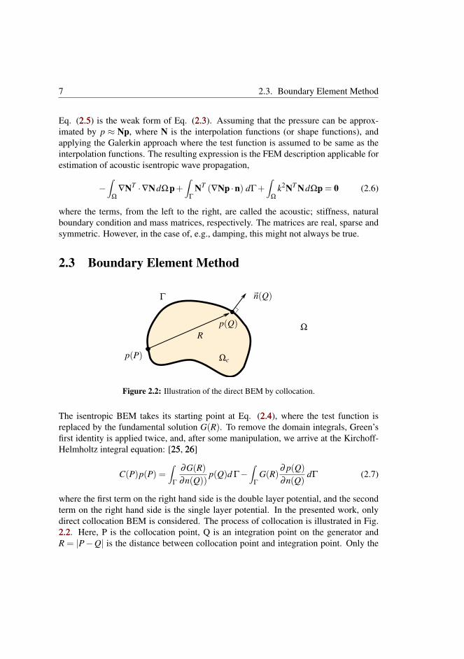
Figure 2.2: Illustration of the direct BEM by collocation.
The isentropic BEM takes its starting point at Eq. (2.42.4), where the test function isreplaced by the fundamental solution G(R). To remove the domain integrals, Green’sfirst identity is applied twice, and, after some manipulation, we arrive at the Kirchoff-Helmholtz integral equation: [2525, 2626]
C(P)p(P) =∫
Γ
∂G(R)∂n(Q))
p(Q)d Γ−∫
Γ
G(R)∂ p(Q)
∂n(Q)dΓ (2.7)
where the first term on the right hand side is the double layer potential, and the secondterm on the right hand side is the single layer potential. In the presented work, onlydirect collocation BEM is considered. The process of collocation is illustrated in Fig.2.22.2. Here, P is the collocation point, Q is an integration point on the generator andR = |P−Q| is the distance between collocation point and integration point. Only the
Chapter 2. Isentropic propagation of sound waves 8
most common form of collocation, where P is located at nodal points on the boundaryelement, is used. Additionally, C(P) is the geometric depended integral free term,which is 1
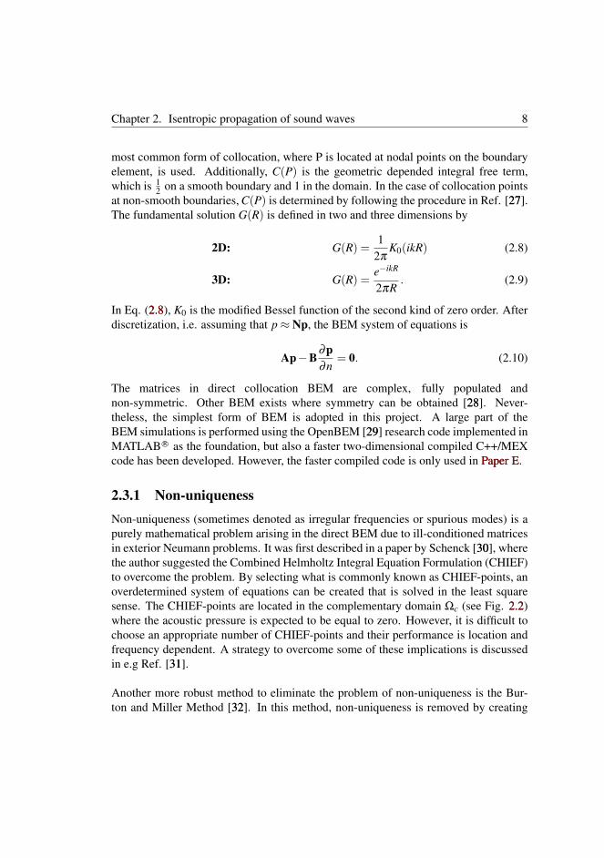
2 on a smooth boundary and 1 in the domain. In the case of collocation pointsat non-smooth boundaries, C(P) is determined by following the procedure in Ref. [2727].The fundamental solution G(R) is defined in two and three dimensions by
2D: G(R) =1
2πK0(ikR) (2.8)
3D: G(R) =e−ikR
2πR. (2.9)
In Eq. (2.82.8), K0 is the modified Bessel function of the second kind of zero order. Afterdiscretization, i.e. assuming that p≈ Np, the BEM system of equations is
Ap−B∂p∂n
= 0. (2.10)
The matrices in direct collocation BEM are complex, fully populated andnon-symmetric. Other BEM exists where symmetry can be obtained [2828]. Never-theless, the simplest form of BEM is adopted in this project. A large part of theBEM simulations is performed using the OpenBEM [2929] research code implemented inMATLAB R© as the foundation, but also a faster two-dimensional compiled C++/MEXcode has been developed. However, the faster compiled code is only used in Paper EPaper E.
2.3.1 Non-uniquenessNon-uniqueness (sometimes denoted as irregular frequencies or spurious modes) is apurely mathematical problem arising in the direct BEM due to ill-conditioned matricesin exterior Neumann problems. It was first described in a paper by Schenck [3030], wherethe author suggested the Combined Helmholtz Integral Equation Formulation (CHIEF)to overcome the problem. By selecting what is commonly known as CHIEF-points, anoverdetermined system of equations can be created that is solved in the least squaresense. The CHIEF-points are located in the complementary domain Ωc (see Fig. 2.22.2)where the acoustic pressure is expected to be equal to zero. However, it is difficult tochoose an appropriate number of CHIEF-points and their performance is location andfrequency dependent. A strategy to overcome some of these implications is discussedin e.g Ref. [3131].
Another more robust method to eliminate the problem of non-uniqueness is the Bur-ton and Miller Method [3232]. In this method, non-uniqueness is removed by creating
9 2.4. Boundary conditions
an additional boundary element equation derived from taking the normal derivative ofEq. (2.72.7). By combining the normal derivative equation with Eq. (2.72.7) as a linearcombination using a complex coupling parameter, the system becomes free of irregularfrequencies. The choice of coupling parameter was recently discussed in a publicationby Marburg [3333], where the author showed that a large part of the BEM community isutilizing an incorrect sign of the coupling parameter. Besides the coupling parameter,one of the implications of the Burton-Miller method is the requirement of a uniquenormal at the collocation point and the cumbersome evaluation of hypersingular inte-gration kernels that appear in the normal derivative equation.
In this project, the non-uniqueness problem is encountered in Paper BPaper B, where it issolved by utilizing the CHIEF.
2.4 Boundary conditionsIn the included papers, the boundary conditions encountered when solving the isen-tropic wave problems are pressure, normal velocity, normal impedance and unboundedconditions. The pressure condition is expressed as a superposition of an incident pres-sure pI and the scattered pressure pS, so the total pressure is
p = pI + pS on Γ. (2.11)
The relation between the normal fluid velocity vn and the normal pressure gradient isgiven by
∇p ·~n =∂ p∂~n
=−iωρ0vn on Γ (2.12)
where ρ0 is the static density of the fluid. Normal impedance conditions can be in-cluded by
vn− vs =1Zn
p on Γ (2.13)
with vs being the structural velocity and Zn being the normal impedance. In the case ofunbounded domains, the Sommerfeld radiation condition needs to be fulfilled, whichis
limr→∞
rn−1
2
[(∂ p∂ r
+ ikp)]
= 0 (2.14)
where r is the radial distance to a source and n is the spatial dimension. In the BEMthe Sommerfeld radiation condition is implicitly fulfilled; this is however not the casein FEM. Historically, the implicit fulfillment of the Sommerfeld radiation condition is

Chapter 2. Isentropic propagation of sound waves 10
one of the reasons why BEM has been a popular method in the field of acoustics andelectromagnetics. In the FEM, some truncation of the domain is necessary. The sim-plest way to approximate unbounded domains with the FEM is to use an appropriateimpedance boundary condition at the truncation. Unfortunately, in many cases this willlead to unwanted reflections. Other more elaborate methods exist, such as infinite ele-ments [3434, 3535, 3636] and perfectly matched layers (PML) [3737, 3838, 3939]. In these methods,an artificial region surrounding the computational domain is created where the wave ismore efficiently attenuated and reflections are limited.
In the papers AA, BB and DD, isentropic FEM simulations are performed using COMSOLMultiphysics R© [4040] and unbounded domains are handled with PML.

Chapter 3
Viscothermal losses in acousticsand its modellingIn this PhD project, the goal has been to explore when the assumptions of isentropicwave propagation are insufficient, meaning that viscous and thermal losses cannot beneglected, but also to improve the reliability of an existing BEM implementation thatincorporates such losses. Therefore, in this chapter, we will first introduce state-of-the-art modelling methods that can account for acoustic viscous and thermal dissipation.Special theoretical attention is given to the viscothermal BEM implementation sinceit is the foundation and starting point of the next chapter. Finally, at the end of thischapter, two modelling examples from Paper APaper A and Paper BPaper B are introduced where theeffects of viscous and thermal losses on a metamaterial and an acoustic cloaking deviceare investigated.
3.1 State-of-the-art
The interest in acoustic viscous and thermal losses dates back to at least Kirchhoff [4141]and Rayleigh [4242]. Kirchhoff studied the attenuation of sound waves in cylindricaltubes due to viscous and thermal effects, and showed that the full linearised Navier-Stokes equations, i.e. the linearised conservation of mass, energy and momentum, canbe decoupled into independent acoustic, entropic and vortical modes that are only cou-pled through boundary conditions. The entropic mode is described in terms of thermaldiffusion, and the vortical mode as momentum diffusion. Often, the entropic and vorti-cal modes are called the thermal pressure and viscous velocity, respectively. A namingconvention that is also adopted in the included papers. Additionally, the decoupling isreferred to as the Kirchhoff decomposition or Kirchhoff’s dispersion law. It is calledthe dispersion law because the decoupled modes have a corresponding wavenumberthat is dependent on the angular frequency. The decomposition allowed Kirchhoff toanalytically study the attenuation of sound waves in cylindrical tubes. Later, Rayleigh
Chapter 3. Viscothermal losses in acoustics and its modelling 12
revisited Kirchhoff’s work and included propagation of sound in very narrow tubes.In this case, the entire cross-section of the tube can be considered a thermodynamicisothermal process which simplifies the problem, so only viscosity needs to be con-sidered. In Rayleigh’s revisit, sound propagation in two-dimensional slits is also dis-cussed.
Zwikker and Kosten [4343] proposed an approximate evaluation of Kirchhoff’s origi-nal work, distinguishing between low (narrow tube) and high (wide tube) frequencies.Their approach was later named the low reduced frequency (LRF) method by Tijdeman[4444]. In the publication by Tijdeman, a range of approximate methods proposed by sev-eral authors on the propagation of sound waves in cylindrical tubes are discussed; thefinding is that the LRF approach is the best approximate solution over a broad rangeof frequencies. In the LRF method, it is assumed that the acoustic wavelength is muchlarger as compared to the cross-section of the tube, and that the sound pressure can beconsidered constant across the cross-section. With this, it is possible to split the equa-tions into a cross-sectional and propagational direction whereby propagation in thetube can be described by a propagation constant. The propagation constant is a mea-sure of how the amplitude and the phase changes in the propagation direction, makingit possible to describe sound propagation in tubes as a purely one-dimensional problem.Several authors have later extended the LRF model beyond circular tubes to include ar-bitrary cross-sectional shapes relying on some numerical calculations [4545, 4646]. A veryelaborate introduction to the LRF model can, for example, be found in Beltman’s PhDthesis [4747] and in the Refs. [4848] and [4949]. Beltman also shows the possibility of usingthe LRF model in combination with FEM [5050]. While the LRF method is an efficientway to include viscothermal losses into FEM, it is limited to the study of waveguidesand slits. Additionally, the LRF approach will fail to give accurate solutions in the caseof higher order acoustic modes where the pressure cannot be considered constant.
The approximate methods treating sound propagation in simple tubes can also be ex-tended into transmission line theory, where series impedances and shunt admittancescan be extracted to account for attenuation and phase shifts [5151, 5252, 5353]. With transmis-sion line theory more complex acoustic systems containing several tubes and cavitiescan be studied [5454].
The modelling approaches considered so far are somewhat limited in their applicationwith requirements to the specific geometry. It is possible to treat more general prob-lems using more elaborate numerical methods, such as the FEM and the BEM. FEMmodels that include viscothermal dissipation, and are suitable for simulations of arbi-trary geometries, can either be full models that solve the full linearised Navier-Stokes
13 3.1. State-of-the-art
(FLNS) equations without any simplification or methods where additional approximateassumptions are made to the governing equations. Among the authors who have dis-cussed full models are Malinen [5555], Nijhof [5656], Cheng [5757], Joly [5858] and Kampinga[5959].
Malinen [5555] uses a mixed formulation with an auxiliary unknown, the temperatureand the velocity as the dependent variables. However, it turns out that the auxiliaryunknown is just the density. In Malinen’s formulation the equations are discretizedusing MINI elements. Nijhof’s [5656] implementation is very similar to that of Malinen,but uses the pressure as the unknown variable instead of density. In the publication byNijhof, the two implementations are compared through convergence studies, showingvery similar results. It should be noted that using the pressure as the dependent vari-able should be considered the more appropriate choice since the density will in factform boundary layers, which is not the case for the pressure. Cheng [5757] also usesa mixed formulation with displacement and pressure as dependent variables, but theformulation completely neglects thermal conduction. In Joly’s work, the final systemof equations only depends on velocity and temperature.
Kampinga [5959] establishes a complex symmetric mixed formulation with temperature,pressure and velocity as the dependent variables. The complex symmetric formulationhas several advantages over the previous implementations since solvers like PARDISOand SPOOLS can take advantage of complex symmetry. As a result, the computationaltime is faster, and the method yields reduced memory requirements. The publicationby Kampinga includes convergence studies of several finite elements. From the conver-gence studies, it is shown that Crouzeix Raviat or Taylor Hood elements with velocityand temperature discretized by quadratic shape functions yields the best results. Ingeneral, the FLNS FEM publications considers mixed formulations to avoid so-calledlocking in the case of a nearly incompressible fluid; the same phenomenon is also en-countered in elastodynamics. One of the drawbacks of the FLNS implementations isthe increased system size due to the additional variables in the final system of equa-tions. This adds to the computational time and memory requirement. Additionally,the FLNS FEM requires careful meshing of the boundary layers to accurately resolveviscous an thermal effects in the vicinity of the boundaries. Martins [6060], for example,studies boundary layer meshing and its importance for the accuracy. An implemen-tation of the FLNS can be found in COMSOL R©. The COMSOL R© implementationis very comparable to the implementation discussed here by Kampinga, with the de-pended variables being pressure, temperature and velocity.
The computational complexity of the FLNS FEM implementations often makes three-

Chapter 3. Viscothermal losses in acoustics and its modelling 14
dimensional simulations with modest hardware problematic. Therefore, several authorshave investigated approximate methods which are still reliable but computationallycheaper. Here we will reproduce the classification of approximate methods given byKampinga [44]. Numerical approximate acoustic viscothermal models can be catego-rized as boundary layer impedance (BLI) models, the aforementioned LRF models orthe sequential linearised Navier-Stokes (SLNS) model.
In the BLI models, simplifying assumptions are used to create impedance-like con-ditions that account for the boundary layer effects. The requirement is that the ge-ometric dimensions are larger as compared to the boundary layer thickness. Bossart[6161] proposes an admittance-like condition solved in a three step procedure. First,an isentropic FEM or BEM pressure solution is calculated. The isentropic solution isthen used to approximate a tangential wavenumber which is applied in a final FEMor BEM calculation. In the work by Schmidt [6262] so-called Wentzell type boundaryconditions are used to include viscous losses through the normal pressure derivative,which can be substituted directly into the weak from of the Helmholtz equation. In avery recent publication by Berggren [1212], a similar Wentzell type boundary conditionis derived that also includes thermal losses. The BLI models proposed by Schmidt andBerggren are interesting because they are of the same complexity as the regular isen-tropic Helmholtz problem and therefore very efficient and do not require meshing ofboundary layers. On the other hand, one must be careful when using the method invery narrow regions where boundary layers can overlap.
The SLNS is an approximate FEM proposed by Kampinga [6363, 44]. It is deduced fromsimilar assumptions as the LRF model, but is not limited to simple tubes. In the SLNSmethod, two completely uncoupled viscous and thermal fields governed by inhomoge-neous wave equations are solved. The viscous and thermal fields are then used as inputto a homogeneous wave equation where the pressure is the only unknown variable.Several advantages can be identified in terms of computational speed and the abilityto accurately handle narrow gaps with overlapping boundary layers. Computationally,each equation reassembles similar complexity as the isentropic wave equation. How-ever, careful meshing of the boundary layers is necessary when computing the viscousand thermal fields.
Three authors have treated modelling of acoustic viscous and thermal losses using theBEM; namely Dokumaci [6464, 6565], Karra [6666, 6767], and Cutanda Henríquez [77, 6868, 6969,7070].
In the BEM formulation by Dokumaci [6464] viscosity is included through a boundary
15 3.2. General assumptions
layer approximation, assuming that the viscous velocity can be approximated purelythrough its boundary tangential component. The approach was later extended to alsoinclude thermal losses [6565]. Due to the way viscosity is included, the method can onlybe considered approximate.
Using a variational BEM formulation, Karra [6767], includes losses. However, the for-mulation completely neglects viscous effects and only considers thermal losses whichmakes the development much easier. The approach is a direct application of the gen-eralised version of Kirchhoff’s original dispersion relation developed by Bruneau [7171].Bruneau’s generalisation extents the dispersion relations to include both bulk viscosityand evanescent modes. Hereafter, the generalised approach by Bruneau is referred toas the Kirchhoff decomposition.
Cutanda Henríquez extended the idea of Karra using the Kirchhoff decomposition asa convenient starting point for a direct collocation BEM implementation. The Kirch-hoff decomposition consists of two scalar wave equations describing the acoustic andthermal pressures, and a vector wave equation with the viscous velocity as the variable.Each of the equations can be discretized separately with BEM and coupled throughboundary conditions. With Schur complement operations, it is possible to establisha system of equations relating the acoustic pressure to the boundary normal and tan-gential velocities. However, this requires the evaluation of coupling terms describedby both first and second order surface tangential derivatives of the acoustic pressure.In early implementations, the coupling terms were develop individually for specificgeometries [5454], but the model was later generalised to handle arbitrary geometries, fa-cilitating both axisymmetric and full three-dimensional simulations. Even though theimplementation can handle more general geometries, the coupling methodology in theRefs. [6868] and [7070] uses finite difference. The use of finite difference is known to besubject to several shortcomings and is cumbersome to implement in three dimensions.
3.2 General assumptionsIn the following as well as in the included papers, it is assumed that acoustic wave prop-agation in a viscous and thermally conductive fluid can be based on the assumptionsof:
• Linearity and time-harmonic wave behaviour.
• The medium is considered uniform, at its equilibrium and without flow.
Chapter 3. Viscothermal losses in acoustics and its modelling 16
• The material properties are based on a Newtonian fluid, follow Fouriers law ofheat conduction and the fluid (air) can be approximated as an ideal gas.
• The wavelength and the dimensions of the computational domain is larger thanthe molecular mean-free-path (approximately 10−7 m for air at ambient condi-tions).
3.3 Viscothermal FEMIn the papers AA, BB, CC and EE, COMSOL’s FEM implementation of the time-harmonicFLNS is mainly used as a comparative tool to validate the viscothermal BEM simula-tions. The time-harmonic FLNS is given by the linearised conservation of mass, energyand momentum equations, which are
iωρ +ρ0∇ ·~v = 0 (3.1)iωρ0CpT−λ∆T − iω p = 0 (3.2)
iωρ0~v =−∇p+(
µB +43
µ
)∇(∇ ·~v)−µ∇×∇×~v+~f (3.3)
where the properties of the medium are characterised by the static density ρ0, the spe-cific heat at constant pressure Cp, the thermal conductivity λ , the shear viscosity µ
and the bulk viscosity µB. It is possible to include volumetric body forces through thevector ~f (sometimes volumetric heat sources are also included into the energy equa-tion, but they are in this case not used and simply ignored). Only Paper APaper A makes useof the volumetric force term, where it is applied to artificially excite the waveguide inwhich the metamaterial is located. The volumetric force term is specific for the FEMsimulations and is not used when discussing the implementation of the viscothermalBEM.
Besides pressure fluctuations, the FLNS also includes small fluctuations in tempera-ture, density and velocity, given by the variables T , ρ and ~v, respectively. To solvethe Eqs. (3.13.1)-(3.33.3), it is necessary to eliminate one of the acoustic variables. This isaccomplished by substitution of the linearised ideal gas law into Eq. (3.13.1) which elim-inates the density, whereby only pressure, temperature and velocity are the dependedvariables.
The FLNS equations can be solved with the FEM by directly applying the Galerkinmethod as presented in Section 2.22.2. By multiplication of corresponding test functions,integration over the domain Ω and applying Green’s formula to eliminate the second

17 3.3. Viscothermal FEM
order derivatives, the weak form of Eqs. (3.13.1)-(3.33.3) can be established (assuming thatthe density is eliminated from Eq. (3.13.1)). The weak form and the coupled system is notpresented here, but can be found in e.g. Ref. [5959].
3.3.1 Boundary conditions
Thermal conduction and viscosity are the two primary mechanisms responsible forlosses in confined acoustic domains. Their effect is relevant in the vicinity of bound-aries where thermal and viscous boundary layers form as a consequence of boundaryconditions.
Temperature boundary condition
The heat capacity and thermal conductivity of the boundaries are usually much greateras compared to the fluid. Therefore, it is in most cases reasonable to consider theboundaries as isothermal, so that
T = 0 on Γ. (3.4)
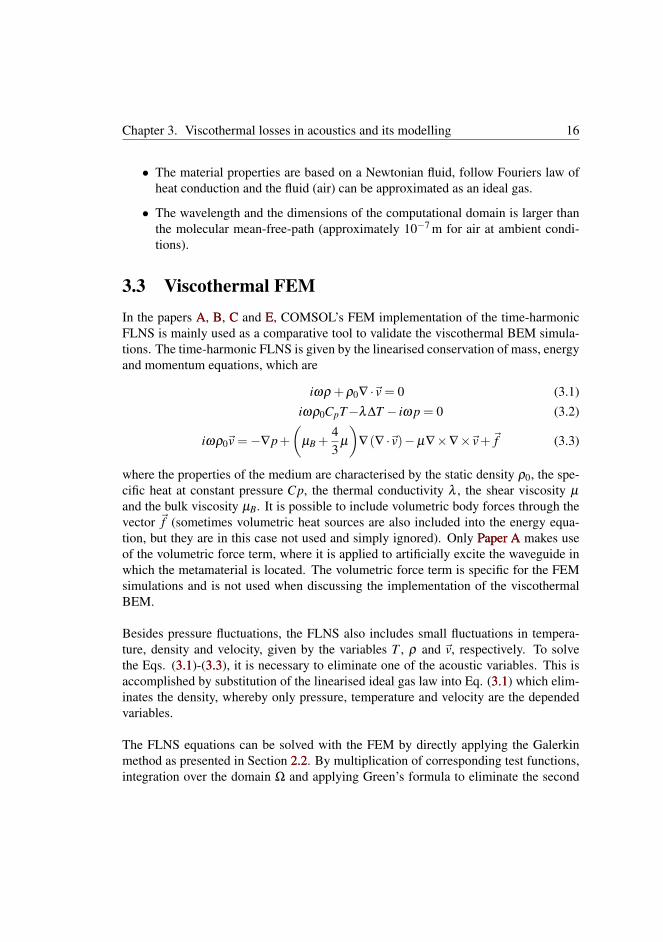
At the boundary, the acoustic temperature fluctuations are forced to zero, and as a re-sult, an exchange of heat between the boundary and the fluid will occur. This createsa transition region in the proximity of the boundary where the temperature behaviourchanges from isothermal into that of the bulk (the bulk is the region where wave prop-agation can be considered isentropic). The transition region is commonly known as athermal boundary layer. Fig. 3.13.1 illustrates the process and the formation of thermalboundary layers.
Chapter 3. Viscothermal losses in acoustics and its modelling 18
δh
T = 0
Flux of heat
Boundary
Boundary layer
Bulk
Figure 3.1: An illustration of the formation of a thermal boundary layer. An incoming planewave has associated pressure changes, but also changes in temperature. Since the boundary hasa higher heat capacity, the boundary temperature can be considered isothermal. Therefore, thetemperature fluctuations of the incident wave are forced to zero at the boundary. This creates thethermal boundary layer where the behaviour changes from isothermal into that of the bulk. Thethickness of the boundary layer is given by δh.
The thickness of the thermal boundary layer as a function of the frequency f is [11, p.286]
δh =
√2λ
ρ0ωCp
air≈ 2.51√
fmm (3.5)
which in the audible range, assuming the medium to be air, is approximately between550 µm to 20 µm.
Velocity boundary condition
Frictional forces between the boundary and the fluid will restrict movement of thefluid. It is usually said that the fluid particles closest to the boundary tend to stick tothe boundary, resulting in a no-slip boundary condition where
~v =~vb on Γ, (3.6)
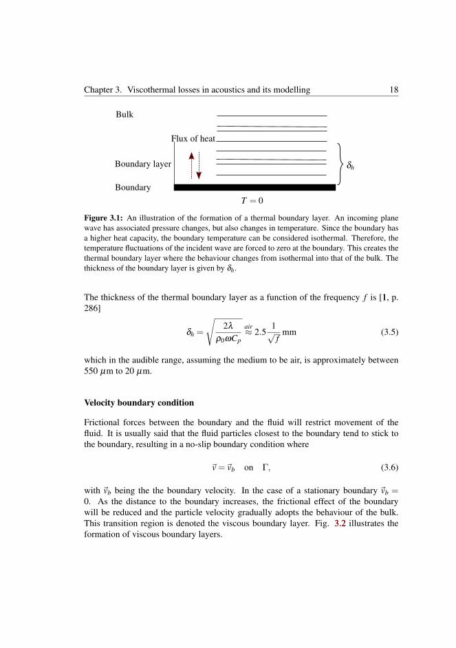
with ~vb being the the boundary velocity. In the case of a stationary boundary ~vb =0. As the distance to the boundary increases, the frictional effect of the boundarywill be reduced and the particle velocity gradually adopts the behaviour of the bulk.This transition region is denoted the viscous boundary layer. Fig. 3.23.2 illustrates theformation of viscous boundary layers.
19 3.4. Viscothermal BEM
δv
~v = 0
~v
Boundary
Boundary layer
Bulk
Figure 3.2: An illustration of the formation of viscous boundary layers. Due to frictional forcesbetween the boundary and the fluid, the particles closest to the boundary will tend to stick to theboundary forming what is commonly known as a viscous boundary layer. The thickness of theboundary layer is given by δv
The thickness of viscous boundary layers as a function of the frequency f is [11, p. 286]
δv =
√2µ
ρ0ω
air≈ 2.11√
fmm. (3.7)
In air, the thicknesses of the viscous and thermal boundary layers are very comparable,which yields a Prandtl number close to unity.
3.4 Viscothermal BEMWe will now review the BEM implementation including viscous and thermal losses aspresented by Cutanda Henríquez in the Refs. [7070] and [6868]. For simplicity only twodimensions are considered as opposed to the axissymmetric and three-dimensional im-plementations found in the references. The starting point for the BEM implementationis the Kirchhoff decomposition of the FLNS equations. The Kirchhoff decompositionis a convenient starting point, since regular acoustic BEM can be deployed directlywithout modification. The Kirchhoff decomposition of the FLNS leads to the equa-tions [7171]
∆pa + k2a pa = 0 (3.8)
∆ph + k2h ph = 0 (3.9)
∆~vv + k2v~vv =~0 (3.10)
Chapter 3. Viscothermal losses in acoustics and its modelling 20
where pa is the acoustic pressure, ph is the thermal pressure,~vv is the viscous velocity,ka is the acoustic wavenumber, kh is the thermal wavenumber and kv is the viscouswavenumber. The wavenumbers are in this case complex and depended on the fre-quency and the physical properties of the fluid (see e.g Appendix A in Ref. [7070] fortheir definition). While the Eqs. (3.83.8)-(3.103.10) are on the Helmholtz form, Eqs. (3.93.9) and(3.103.10) should rather be considered as diffusion-like equations, where the thermal pres-sure and the viscous velocity (entropic and vortical modes) only exist in the vicinity ofthe boundary.
As a consequence of the Kirchhoff decomposition, the total pressure is split into asuperposition of the acoustic and the thermal pressure so that
p = pa + ph. (3.11)
And in a similar way, the total velocity is split into
~v =~va +~vh +~vv (3.12)
where ~va and ~vh are the irrotional part of the velocity associated with pa and ph, re-spectively. The rotational part of the velocity is the viscous velocity. Therefore, therelations
∇× (~va +~vh) = 0 and ∇ ·~vv = 0 (3.13)
should be fulfilled. If each of the Eqs. (3.83.8)-(3.103.10) is discretized separately usingregular collocation BEM as presented in Section 2.32.3, the result is
Aapa−Ba∂pa
∂~n= 0 (3.14)
Ahph−Bh∂ph
∂~n= 0 (3.15)
Avvv,x−Bv∂vv,x
∂~n= 0 (3.16)
Avvv,y−Bv∂vv,y
∂~n= 0 (3.17)
where Eq. (3.103.10) has been split into its Cartesian components, and the subscripts a, hand v indicates the acoustic, thermal and viscous matrices, respectively.
3.4.1 Boundary conditionsThe next step is coupling of the discretized equations, i.e. Eqs (3.143.14) - (3.173.17), by as-suming isothermal and no-slip boundary conditions. Due to the nature of the Kirchhoff
21 3.4. Viscothermal BEM
decomposition, the form of the boundary conditions is slightly different as presented inthe FLNS FEM. In this case, the temperature is related to the acoustic and the thermalpressures through two complex constants, τa and τh, which are a function of frequencyand the fluid properties. The expression for the isothermal boundary condition is
T = τa pa + τh ph = 0 on Γ. (3.18)
In a similar way, the no-slip boundary condition can be described in terms of the acous-tic pressure, the thermal pressure and the viscous velocity. The boundary velocity is
~vb = φa∇pa +φh∇ph +~vv on Γ (3.19)
where φa and φh are complex constants. For the definition of τa, τh, φa and φh see e.g.Appendix A in Ref. [7070]. To make the boundary conditions suitable for the BEM theyare transformed into a local normal and tangential coordinate system, so
vb,n = φa∂ pa
∂~n+φh
∂ pa
∂~n+~vv,n on Γ (3.20)
and
vb,t = φa∂ pa
∂~t+φh
∂ pa
∂~t+~vv,t on Γ (3.21)
where the subscripts n and t denote the boundary normal and tangential component,respectively.
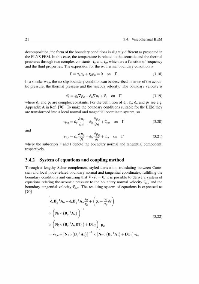
3.4.2 System of equations and coupling methodThrough a lengthy Schur complement styled derivation, translating between Carte-sian and local node-related boundary normal and tangential coordinates, fulfilling theboundary conditions and ensuring that ∇ ·~vv = 0, it is possible to derive a system ofequations relating the acoustic pressure to the boundary normal velocity ~vb,n and theboundary tangential velocity ~vb,t . The resulting system of equations is expressed as[7070]
[φaB−1
a Aa−φhB−1h Ah
τa
τh+
(φa−
τa
τhφh
)
×(
N1 (B−1
v Av))−1
×(
N2 (B−1
v AvDT1)+DT2
)]pa
= vb,n +[N1
(B−1
v Av)]−1×
[N2
(B−1
v Av)+DT1
]vb,t
(3.22)
Chapter 3. Viscothermal losses in acoustics and its modelling 22
where the operator is the so-called element-wise Hadamard product (see e.g. Ap-pendix A in Paper CPaper C for some properties of the Hadamard product) and the matrices,N1 and N2, contain the boundary normal and tangential components at the discretenodes. These matrices originate from a necessary translation between a Cartesian de-scription of the viscous velocity into the local boundary normal and tangential vectors.The translation is carried out on the discrete nodes located on the generator. In fact,this procedure requires that the normal and tangential components are uniquely definedat all nodes. In other words, the boundary elements need to be C1-continuous at collo-cation points. Unfortunately, this requirement is not fulfilled with regular continuousLagrange elements. However, the implementation do use such elements. Therefore, itis necessary to calculate the normal and tangential vectors as an average when nodesare shared by multiple elements. This is a possible shortcoming of the implementation.
Another concern regarding the formulation and implementation is the matrices DT1and DT2. These matrices contain first and second order tangential derivatives cre-ated with the use of centered finite difference schemes, and used to estimate tangentialderivatives of the acoustic pressure. The use of finite difference is known to be proneto errors and its implementation is problematic when the boundaries are curved and theelement size irregular. Additionally, the implementation into three-dimensions is evenmore cumbersome relying on Voronoi cells [6868, 7272, 7373]. Nevertheless, the implemen-tation as discussed here (and in other earlier versions) has been successfully applied tocalculate and analyse complex viscothermal problems [77, 33, 5454, 6969] and is also used inPaper APaper A and Paper BPaper B.
3.4.3 Narrow gap and low frequency breakdownBesides the aforementioned concerns regarding the implementation and couplingmethod, one should be careful when performing BEM calculations containing narrowgaps. The use of the BEM in domains with narrow regions requires certain treatment,where the so-called narrow gap breakdown (or thin-shape breakdown) can lead to un-wanted inaccuracies if integration is not treated correctly. The narrow gap breakdownproblem is for example discussed by Martinez [7474]. It is caused by the singular natureof the boundary element kernels. When boundaries are close in distance, the integra-tion becomes nearly singular which makes regular gauss integration insufficient. Toovercome the narrow gap breakdown, narrow passages encountered in the BEM im-plementation are treated with an adaptive recursive integration scheme [7575] which iscapable of treating the nearly singular integrals and accurately model narrow gaps.
Additionally, the BEM is subject to inaccuracies in low frequency interior problems due
23 3.5. Metamaterial (Paper APaper A)
to the absence of a quasi-static component [7676, 7777]. In certain viscothermal BEM prob-lems, more specifically the condenser microphone simulations presented in Paper DPaper D,the low frequency problem is known to exist. However, it is not observed in the othertest cases studied in this thesis.
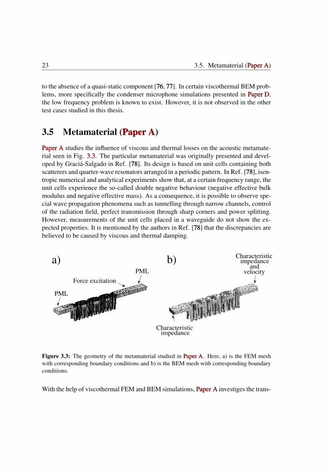
3.5 Metamaterial (Paper APaper A)
Paper APaper A studies the influence of viscous and thermal losses on the acoustic metamate-rial seen in Fig. 3.33.3. The particular metamaterial was originally presented and devel-oped by Graciá-Salgado in Ref. [7878]. Its design is based on unit cells containing bothscatterers and quarter-wave resonators arranged in a periodic pattern. In Ref. [7878], isen-tropic numerical and analytical experiments show that, at a certain frequency range, theunit cells experience the so-called double negative behaviour (negative effective bulkmodulus and negative effective mass). As a consequence, it is possible to observe spe-cial wave propagation phenomena such as tunnelling through narrow channels, controlof the radiation field, perfect transmission through sharp corners and power splitting.However, measurements of the unit cells placed in a waveguide do not show the ex-pected properties. It is mentioned by the authors in Ref. [7878] that the discrepancies arebelieved to be caused by viscous and thermal damping.
a) b)
PML
PMLForce excitation
Characteristicimpedance
Characteristicimpedance
andvelocity
Figure 3.3: The geometry of the metamaterial studied in Paper APaper A. Here, a) is the FEM meshwith corresponding boundary conditions and b) is the BEM mesh with corresponding boundaryconditions.
With the help of viscothermal FEM and BEM simulations, Paper APaper A investiges the trans-

Chapter 3. Viscothermal losses in acoustics and its modelling 24
mittance through the metamaterial. Fig. 3.33.3 shows the FEM and the BEM setup of themetamaterial including boundary conditions. Good agreement between lossy transmis-sion simulations and measurements are found, confirming the hypothesis that losses arein fact preventing the metamaterial from working as intended.
3.6 Cloak based on scattering cancellation (Paper BPaper B)
Paper BPaper B investigates the effect of losses on an existing acoustic cloak presented byGarcía-Chocano in Ref. [7979]. Acoustic cloaks are devices that can effectively hide anobject, so that sound waves in the neighbourhood of the object seem unaffected. In thiscase, the object is a large cylinder subject to an incoming plane propagating wave. InRef. [7979], a genetic optimization approach is used to locate 120 small cylinders aroundthe large cylinder in such a way that scattering is minimized. As a result, incident planewaves near 3kHz are not disturbed by the object. In Ref. [7979] some discrepancies be-tween isentropic FEM simulations and measurements are observed; therefore, it hasbeen of interest to investigate how much viscous and thermal losses influence this typeof cloak.
Acoustic cloakIncident plane wave
Object
Figure 3.4: The geometry of the acoustic cloak studied in Paper BPaper B and the incident plane wave.By proper distribution of 120 small cylinders the large cylindrical object is effectively hiddenand propagation of the plane wave appears unaffected.
The averaged visibility (a measure of how well the object is hidden) is used to validatethe performance of the cloak. In general, it is shown that losses have very little impacton the average visibility, but some attenuating effects can be observed both due to thecloak but also due to the finite hight of the waveguide in which the cloak is placed. It isnoted that discrepancies between simulations and measurements are mainly due to theexperimental setup, where it is difficult to achieve an ideal plane wave.

25 3.7. Contribution
3.7 ContributionIn Paper APaper A, losses are proven to have a significant influence on the performance of themetamaterial. The performance degradation ultimately leads to a metamaterial with-out the desired properties. Apart from the investigation of losses, the metamaterialhas served as a benchmark case to validate the three-dimensional viscothermal BEMimplementation. The benchmark is challenging, and while there is good agreementbetween simulations and measurements, it is far from an exact match, and deviationsbetween the FEM and BEM simulated transmittance are observed. However, it shouldbe noted that the FEM and the BEM simulations uses different boundary conditions,which might lead to some of the observed differences.
On the contrary, Paper BPaper B shows that the performance of the cloak is not influencedby losses. However, this is not too surprising since the cloak does not contain narrowgaps and resonators.
The intention is that Paper APaper A and Paper BPaper B can concribute to an increasing awareness ofacoustic viscothermal losses in novel acoustic devices and establish some basic guide-lines for when losses cannot be neglected.

Chapter 3. Viscothermal losses in acoustics and its modelling 26
Chapter 4
Improving the BEM implemen-tation with lossesIn the previous chapter, the BEM including viscothermal losses was presented, andpotential shortcomings of the current implementation were identified. In this chapter,two new approaches are introduced which improve the previous implementation. In-depth theoretical development and validation of the proposed improvements are foundin Paper CPaper C and Paper DPaper D. The focus of the papers is to find new solutions to the cou-pling of the discretized viscothermal BEM equations, and avoid the problematic finitedifference coupling terms.
4.1 Tangential derivative BEM (Paper CPaper C)
Paper CPaper C presents a two-dimensional implementation of the viscothermal BEM, wherethe finite difference derivative matrices, DT1 and DT2, are removed and replaced byan additional set of tangential derivative boundary element equations used to estimatethe derivatives of pa, ph, and~vv. Tangential derivatives of these quantities are obtainedby taking the tangential derivative of Eq. (2.72.7) at the collocation point, which leads tothe boundary integral
C(P)∂ p(P)∂~t(P)
=∫
Γ
∂ 2G(R)∂~t(P)∂~n(Q)
p(Q)dΓ(Q)−∫
Γ
∂G(R)∂~t(P)
∂ p(Q)
∂~n(Q)dΓ(Q) (4.1)
where~t is the tangential vector at the collocation point. Here,~t should not be confusedwith time. The tangential vector and its location on the generator are sketched in Fig.4.14.1. The tangential derivatives of the Greens functions are expressed as [8080]
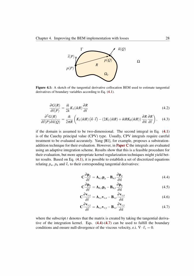
Chapter 4. Improving the BEM implementation with losses 28
Γ
p(Q)R
p(P)
~n(Q)
Ω
Ωc
~t(P)
Figure 4.1: A sketch of the tangential derivative collocation BEM used to estimate tangentialderivatives of boundary variables according to Eq. (4.14.1).
∂G(R)∂~t(P)
=ik2k
K1(ikR)∂R∂~t
(4.2)
∂ 2G(R)∂~t(P)∂~n(Q)
=ik
2πR
(K1(ikR)
(~n ·~t)− (2K1(ikR)+ ikRK0(ikR))
∂R∂~n
∂R∂~t
), (4.3)
if the domain is assumed to be two-dimensional. The second integral in Eq. (4.14.1)is of the Cauchy principal value (CPV) type. Usually, CPV integrals require carefultreatment to be evaluated accurately. Yang [8181], for example, proposes a substration-addition technique for their evaluation. However, in Paper CPaper C the integrals are evaluatedusing an adaptive integration scheme. Results show that this is a feasible procedure fortheir evaluation, but more appropriate kernel regularization techniques might yield bet-ter results. Based on Eq. (4.14.1), it is possible to establish a set of discretized equationsrelating pa, ph and~vv to their corresponding tangential derivatives:
C∂pa
∂~t= Aa,tpa−Ba,t
∂pa
∂~n(4.4)
C∂ph
∂~t= Ah,tph−Bh,t
∂ph
∂~n(4.5)
C∂vv,x
∂~t= Av,tvv,x−Bv,t
∂vv,x
∂~n(4.6)
C∂vv,y
∂~t= Av,tvv,y−Bv,t
∂vv,y
∂~n(4.7)
where the subscript t denotes that the matrix is created by taking the tangential deriva-tive of the integration kernel. Eqs. (4.44.4)-(4.74.7) can be used to fulfill the boundaryconditions and ensure null-divergence of the viscous velocity, e.i. ∇ ·~vv = 0.

29 4.1. Tangential derivative BEM (Paper CPaper C)
4.1.1 System of equations
The derivation and resulting system of equations in Paper CPaper C has many similarities tothe previous BEM formulation by Cutanda Henríquez. The system is derived throughSchur complement operations, and it only considers acoustic pressure and boundaryvelocity variables as unknowns. A limitation of this type of formulation is that tem-perature boundary conditions are not easily accessible. In other words, boundaries arealways assumed to be isothermal, which restricts the class of problems that the methodis directly capable of solving. On the other hand, it should be possible to develop otherconfigurations of the final system with access to the boundary temperature. Neverthe-less, the system of equations as presented in Paper CPaper C is applicable to a broad range ofacoustic problems where boundaries are assumed to be isothermal.
The main difference from the previous implementation is the way the BEM itself isused to estimate the tangential derivatives of pa, ph,~vv. As a result, the new implemen-tation completely avoids finite difference tangential derivatives, but also excludes theuse of second-order tangential derivatives. It should be noted that the proposed imple-mentation requires a full assembly of an additional set of matrices, making the methodless efficient.
4.1.2 Unique normal and tangential vectors
Eq. (4.14.1) requires that the tangential vector is uniquely defined at the collocation point,meaning that the collocation point needs to be C1-continuous. As previously discussedin Section 3.4.23.4.2, this requirement is not fulfilled with continuous Lagrange boundaryelements. To make the vectors at the collocation point unique, Paper CPaper C utilizes dis-continuous boundary elements. Discontinous boundary elements are elements that arenot continuous at element interfaces, but allows for any order of continuity at the col-location point (depending on the element order). Additionally, they are known to beadvantageous over continuous boundary elements [8282]. More specifically, Paper CPaper C usesquadratic discontinuous boundary elements with the shape functions defined as [8383]
N1 =1
2η2 ξ (ξ −η) (4.8)
N2 =1
η2 (η−ξ )(η +ξ ) (4.9)
N3 =1
2η2 ξ (ξ +η) . (4.10)
Chapter 4. Improving the BEM implementation with losses 30
In Eqs. (4.84.8)-(4.104.10), the local coordinate ξ is defined on a reference element with[−1≤ ξ ≤ 1] and η = 1−α , where α is a variable that determines the location of thenodes in the reference element. The use an equidistant distribution of nodes is sug-gested in Ref. [8383], meaning that α = 1
3 . Therefore, the equidistant distribution ofthe nodes is adopted in Paper CPaper C. When using discontinuous elements, the geometryis disctretized with regular quadratic continuous elements and only pa, ph and ~vv aredescribed through the discontinous shape functions.
Other examples exist of discretization methods that can achieve C1-continuity at thecollocation point, e.g cubic splines [8484] or Overhauser elements [8585, 8686, 8787]. How-ever, such elements are cumbersome to implement in comparison to the discontinuouselements.
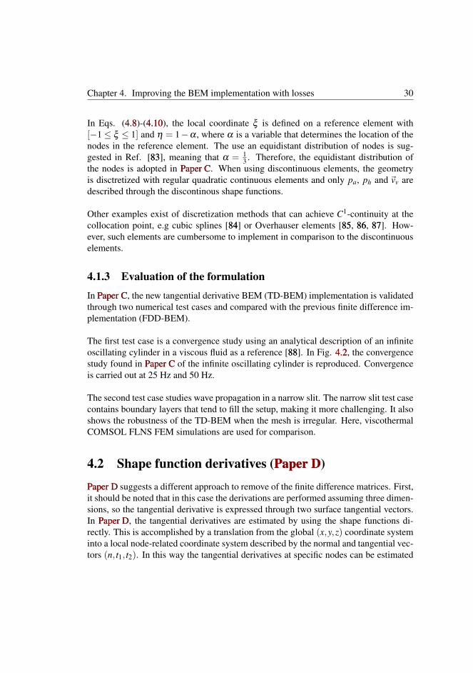
4.1.3 Evaluation of the formulationIn Paper CPaper C, the new tangential derivative BEM (TD-BEM) implementation is validatedthrough two numerical test cases and compared with the previous finite difference im-plementation (FDD-BEM).
The first test case is a convergence study using an analytical description of an infiniteoscillating cylinder in a viscous fluid as a reference [8888]. In Fig. 4.24.2, the convergencestudy found in Paper CPaper C of the infinite oscillating cylinder is reproduced. Convergenceis carried out at 25 Hz and 50 Hz.
The second test case studies wave propagation in a narrow slit. The narrow slit test casecontains boundary layers that tend to fill the setup, making it more challenging. It alsoshows the robustness of the TD-BEM when the mesh is irregular. Here, viscothermalCOMSOL FLNS FEM simulations are used for comparison.
4.2 Shape function derivatives (Paper DPaper D)
Paper DPaper D suggests a different approach to remove of the finite difference matrices. First,it should be noted that in this case the derivations are performed assuming three dimen-sions, so the tangential derivative is expressed through two surface tangential vectors.In Paper DPaper D, the tangential derivatives are estimated by using the shape functions di-rectly. This is accomplished by a translation from the global (x,y,z) coordinate systeminto a local node-related coordinate system described by the normal and tangential vec-tors (n, t1, t2). In this way the tangential derivatives at specific nodes can be estimated
31 4.2. Shape function derivatives (Paper DPaper D)
Figure 4.2: Convergence plots at 25 and 50 Hz of the BEM formulations with losses for the caseof an infinite oscillating cylinder. Both pressure and normal viscous velocity error are plotted forTD-BEM (solid) and FDD-BEM (dashed).
from the shape functions. Regular continuous elements are used in the implemen-tation, meaning that the tangential derivatives, the normal vector and the tangentialvectors need to be calculated as an average at element interfaces. As a benefit, thederivation only requires evaluation of the tangential derivative of the acoustic pressureand the viscous velocity. The formulation is named the shape function derivative BEM(SFD-BEM).
4.2.1 System of equations
As previously, the system of equations is derived by Schur complement operations,but in this case the viscous velocity is included as a depended variable in the resulting

Chapter 4. Improving the BEM implementation with losses 32
system of equations. The final form is given by
S
pavv,xvv,yvv,z
=
vb,n0
vb,t1vb,t2
(4.11)
where the matrix S is a combination of the acoustic, thermal and viscous matrices. InPaper DPaper D, this system type is referred to as an expanded system. To isolate and studythe effect of the expanded system, an alternative expanded version of the FDD-BEM isalso investigated. It is denoted as the FDD2-BEM.
4.2.2 Evaluation of the formulationIn Paper DPaper D, the new formulation is evaluated through two test cases. In the first testcase, an analytical solution of an oscillating sphere [8989, p. 435] is used to comparethe accuracy of SFD-BEM, FDD-BEM and FDD2-BEM. In the second test case, theresponse of a condenser microphone is calculated and the three different formulationsare compared with existing measurements.
4.3 ContributionIn Paper CPaper C, the main contribution is the way that tangential derivative BEM is used toavoid the finite difference coupling terms in the existing two-dimensional viscothermalBEM. The paper also suggests the use of discontinuous boundary elements to removethe unnecessary averaging of the normal and tangential vectors at element interfaces,which is new for the viscothermal BEM but not for BEM in general. Through twotest cases, it is demonstrated that the new implementation facilitates improved stabilityfor irregular meshes and reduced errors at high mesh densities. However, convergencestudies also reveal that low mesh densities might lead to larger errors in the viscous ve-locity computation. The low mesh density error and its impact on other computationalexamples will require more elaborate studies over what is presented in Paper CPaper C.
With a different approach, Paper DPaper D removes the finite difference matrices from thethree-dimensional viscothermal BEM implementation, by utilising the shape functionsto estimate the tangential derivatives of the acoustic pressure and viscous velocity. Incomparison to the two-dimensional implementation, the calculation of the tangentialpressure and viscous velocity derivatives with finite difference in three dimensions isvery cumbersome. Paper DPaper D demonstrates that the shape function approach leads to

33 4.3. Contribution
a significantly more accurate and stable solution. However, the implementation stillrelies on continuous Lagrange interpolated elements where the normal and tangentialvectors are averaged at element interfaces. Discontinuous elements are proposed as afuture improvement.

Chapter 4. Improving the BEM implementation with losses 34

Chapter 5
Acoustic shape optimization in-cluding losses
Optimization relying on numerical methods has gained an increasing interest due tothe possibility of improving the design, the performance or to find new solutions toproblems in engineering. This has become achievable through the evolution of morepowerful computers and the possibility of combining numerical computations with op-timization algorithms.
Optimization can be categorized by either parameter, shape or topology optimization.Topology optimization in particular, has gained much attention during the last decade,in part due to its ability to find completely new and surprising designs, but also be-cause additive manufacturing processes have made the realization of such complicateddesigns possible. However, from a viscothermal acoustic perspective, topology opti-mization has some disadvantages. The discretization in the entire design domain needsto resolve the boundary layers, thus making it very computationally demanding. Asan alternative, the focus of the presented work is showing the applicability of the vis-cothermal BEM in combination with shape optimization, and use it to optimize vis-cothermal acoustic problems.
We will now continue with an introduction to general optimization methods and shapeoptimization. This is followed by a section summarizing Paper EPaper E. In Paper EPaper E, the vis-cothermal BEM is combined with shape optimization to optimize the absorption ofan impedance termination. Additionally, some unpublished isentropic shape optimiza-tion results are shown utilizing the previous presented acoustic cloaking device as anexample.

Chapter 5. Acoustic shape optimization including losses 36
5.1 Optimization problemWhen performing optimization, an adequate measure of the performance of the spe-cific problem is necessary. In optimization, such measure is usually called an objectivefunction. The objective function is used by the optimization algorithm to determinehow a specific design variable needs to change to improve the design. In general, theway that a design change affects the objective function is described by the governingequations. In optimization, these equations are denoted as the state equations. In anacoustic context, the state equation would be the isentropic wave equation, or the FLNSequations if losses are to be considered.
A constrained shape optimization problem can be expressed as
minimize:v
φ(v)
subject to F(v) = 0a(v)≤ 0b(v) = 0
(5.1)
where φ(v) is the objective function, which depends on the design variables v. Inshape optimization, the vector v will determine the shape of the boundary and F(v) isthe state equation. Additionally, the optimization problem can be constrained by theequality constraint b(v) and the inequality constraint a(v).
5.2 Gradient-based optimizationPaper EPaper E performs shape optimization relying on an iterative gradient-based optimiza-tion approach. In gradient-based optimization, gradient information, and sometimesthe Hessian of the objective function, is used to search for minima of the objective func-tion. Usually, gradient-based optimization will lead to some local minimum, mean-ing that an optimal solution most often cannot be guaranteed. In most engineeringsituations, local minima are considered sufficient for improving and developing newdesigns. One of the simplest gradient-based optimization algorithms is the steep-est decent. However, other more elaborate and efficient gradient-based optimizationalgorithms exist such as the Method of Moving Asymptotes, Sequential Linear andQuadratic Programming, Interior Point Methods and Quasi-Newton Methods. In thefollowing shape optimization examples, the Sequential Quadratic Programming (SQP)method found in the MATLAB function fmincon is used [9090]. For an introduction tothe aforementioned methods consult, e.g. Ref. [9191].

37 5.3. Shape optimization and parametrization
Besides gradient-based optimization, other optimization methods exist such as evolu-tionary and genetic algorithms. For engineering purposes, they are usually consideredtoo inefficient, especially if the problem consists of a large amount of design vari-ables [9292]. Nevertheless, evolutionary and genetic algorithms have also been appliedto acoustic shape optimization problems [9393, 9494, 9595, 9696].
5.3 Shape optimization and parametrization
Shape optimization and its application in engineering can be found in a vast variety ofdisciplines, ranging from fluid mechanics [9797] to electromagnetics [9898], as well as inacoustics [9999].
In shape optimization, the choice of boundary parametrization is important, since it willrestrict the possible shapes of the boundary and limit the design freedom. In Paper EPaper E,cubic splines are used to represent the boundary shape. Cubic splines were chosenbecause it is a simple way of achieving some boundary regularization. Additionally, italso allows for the calculation of the boundary curvature, which is used as a constraint.On the other hand, the boundary is not able to form sharp features like corners andedges. Similarly, the boundary could also be represented with polynomials or othertypes of splines. During this project, Bézier curves, for example, have also been testedand used.
Another more direct approach is to manipulate the position of the nodes in the meshdirectly. This has some advantages in terms of the design freedom. However, it willrequire some sort of boundary regularization relying on, e.g. filtering techniques. Reg-ularization is necessary to avoid large numerical errors that can occur if the nodes aredistorted too much. Additionally, this approach will lead to more design variables com-pared to a parametrization utilizing splines or polynomials.
A survey including the parametrization approaches presented here and other methodsare given in the work by Samareh [100100].
5.4 Sensitivity analysis
Sensitivity analysis is the process of finding the gradients of the objective function withrespect to the design variables. In other words, it is a measure of how the objective

Chapter 5. Acoustic shape optimization including losses 38
function is influenced by a change in the boundary shape. The gradient information isthen used by the optimization algorithm to minimize or maximize the objective func-tion. This means that the gradients should be calculated as efficiently and accurately aspossible to improve the overall optimization time. In the BEM, the sensitivity analysisis usually carried out working on the continuous equations using direct differentiation[101101, 102102, 103103] or an adjoint method [104104, 105105, 106106].
However, no existing literature contains examples of direct differentiation or adjointmethods for the estimation of sensitivities in the case of the viscothermal BEM. Dur-ing the last part of this PhD project, a considerable amount of work has been put into thedevelopment of an adjoint method capable of calculating viscothermal BEM sensitives.Unfortunately, due to time limitations, no completely developed and tested formulationexists. Therefore, sensitivities in Paper EPaper E are obtained using the less efficient forwardfinite difference scheme
∂φ
∂vi=
φ(v+∆vi · ei)−φ(v)∆vi
, (5.2)
where vi is a single design variable, ei is a unit vector for the i-th variable and ∆vi isthe step length. To achieve some additional optimization speed, the sensitivities arecalculated in parallel using the UseParallel option in fmincon.
5.5 Sparse assembly
Additional computational speed of the viscothermal BEM simulations is achieved by aconcept here called sparse assembly. The BEM matrices are by default fully populatedand dense. However, in the assembly of the viscous and thermal matrices, most ofthe integrals do not contribute to the construction of the matrices. In fact, elementintegration only contributes to the viscous and thermal matrices when the distance tothe collocation point is comparable with the boundary layer thickness. Therefore, as acriterion in the assembly routine of the matrices, integration is only carried out whenthe distance between the element and the collocation point is below twenty times theboundary layer thickness. Fig. 5.15.1 depicts the concept of sparse assembly where δlim =20δv is the threshold that determines if integration is to be carried out. Therefore,integration is only performed if R< δlim or when the collocation point is on the element.Sparse assembly makes the assembly of the viscous and thermal matrices about anorder of magnitude faster.
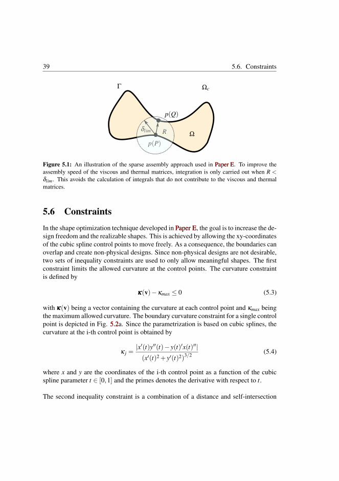
39 5.6. Constraints
Γ
p(Q)
p(P)Ω
δlim R
Ωc
Figure 5.1: An illustration of the sparse assembly approach used in Paper EPaper E. To improve theassembly speed of the viscous and thermal matrices, integration is only carried out when R <δlim. This avoids the calculation of integrals that do not contribute to the viscous and thermalmatrices.
5.6 Constraints
In the shape optimization technique developed in Paper EPaper E, the goal is to increase the de-sign freedom and the realizable shapes. This is achieved by allowing the xy-coordinatesof the cubic spline control points to move freely. As a consequence, the boundaries canoverlap and create non-physical designs. Since non-physical designs are not desirable,two sets of inequality constraints are used to only allow meaningful shapes. The firstconstraint limits the allowed curvature at the control points. The curvature constraintis defined by
κκκ(v)−κmax ≤ 0 (5.3)
with κκκ(v) being a vector containing the curvature at each control point and κmax beingthe maximum allowed curvature. The boundary curvature constraint for a single controlpoint is depicted in Fig. 5.25.2a. Since the parametrization is based on cubic splines, thecurvature at the i-th control point is obtained by
κ j =|x′(t)y′′(t)− y(t)′x(t)′′|(x′(t)2 + y′(t)2)3/2 (5.4)
where x and y are the coordinates of the i-th control point as a function of the cubicspline parameter t ∈ [0,1] and the primes denotes the derivative with respect to t.
The second inequality constraint is a combination of a distance and self-intersection
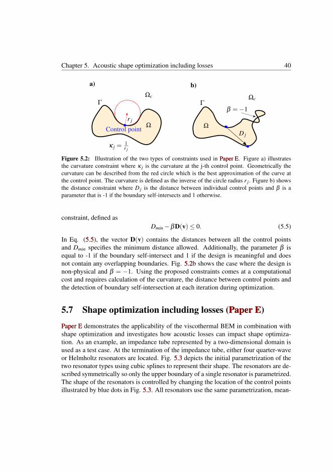
Chapter 5. Acoustic shape optimization including losses 40
Γ
Ω
Ωc
r j
Control point
a)
κ j =1r j
b)
D j
Γ
Ω
Ωc
β =−1
Figure 5.2: Illustration of the two types of constraints used in Paper EPaper E. Figure a) illustratesthe curvature constraint where κ j is the curvature at the j-th control point. Geometrically thecurvature can be described from the red circle which is the best approximation of the curve atthe control point. The curvature is defined as the inverse of the circle radius r j. Figure b) showsthe distance constraint where D j is the distance between individual control points and β is aparameter that is -1 if the boundary self-intersects and 1 otherwise.
constraint, defined asDmin−βD(v)≤ 0. (5.5)
In Eq. (5.55.5), the vector D(v) contains the distances between all the control pointsand Dmin specifies the minimum distance allowed. Additionally, the parameter β isequal to -1 if the boundary self-intersect and 1 if the design is meaningful and doesnot contain any overlapping boundaries. Fig. 5.25.2b shows the case where the design isnon-physical and β = −1. Using the proposed constraints comes at a computationalcost and requires calculation of the curvature, the distance between control points andthe detection of boundary self-intersection at each iteration during optimization.
5.7 Shape optimization including losses (Paper EPaper E)
Paper EPaper E demonstrates the applicability of the viscothermal BEM in combination withshape optimization and investigates how acoustic losses can impact shape optimiza-tion. As an example, an impedance tube represented by a two-dimensional domain isused as a test case. At the termination of the impedance tube, either four quarter-waveor Helmholtz resonators are located. Fig. 5.35.3 depicts the initial parametrization of thetwo resonator types using cubic splines to represent their shape. The resonators are de-scribed symmetrically so only the upper boundary of a single resonator is parametrized.The shape of the resonators is controlled by changing the location of the control pointsillustrated by blue dots in Fig. 5.35.3. All resonators use the same parametrization, mean-
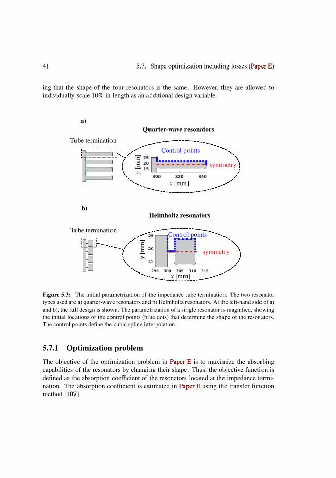
41 5.7. Shape optimization including losses (Paper EPaper E)
ing that the shape of the four resonators is the same. However, they are allowed toindividually scale 10% in length as an additional design variable.
a)
b)
Quarter-wave resonators
Helmholtz resonators
Control points
symmetry
Control points
symmetry
x [mm]
y[m
m]
y[m
m]
x [mm]
Tube termination
Tube termination
Figure 5.3: The initial parametrization of the impedance tube termination. The two resonatortypes used are a) quarter-wave resonators and b) Helmholtz resonators. At the left-hand side of a)and b), the full design is shown. The parametrization of a single resonator is magnified, showingthe initial locations of the control points (blue dots) that determine the shape of the resonators.The control points define the cubic spline interpolation.
5.7.1 Optimization problem
The objective of the optimization problem in Paper EPaper E is to maximize the absorbingcapabilities of the resonators by changing their shape. Thus, the objective function isdefined as the absorption coefficient of the resonators located at the impedance termi-nation. The absorption coefficient is estimated in Paper EPaper E using the transfer functionmethod [107107].
Chapter 5. Acoustic shape optimization including losses 42
Two different objective functions are defined to compare and investigate the effect oflosses. The first objective function is calculated using the viscothermal BEM and de-noted φV T . The second objective function is called φLL and is obtained using losslessBEM. Designs can hereby be optimized based on either a lossy or lossless assumption.In general, the absorption coefficient will range from 0 to 1, corresponding to null ormaximum absorption, respectively.
5.7.2 Summery of shape optimization resultsSeveral numerical optimization experiments are performed to evaluate the influence oflosses on the shape optimized quarter-wave and Helmholtz resonators. The optimiza-tion results and different studies are summarized in the following:
• The first study is a comparison of the quarter-wave resonators optimized at asingle-frequency either with or without losses. The study includes an investiga-tion of the absorption coefficient as a function of frequency for the optimizeddesigns. Here it is interesting to note that lossless optimization results in φLL= 1, thus full absorption is achieved using a formulation without losses. Thereason for this is a peculiar phenomenon in the BEM called numerical damping.Numerical damping acts as artificial losses, and is utilized by the optimizer toobtain a design that seemingly fully absorbs the sound wave. The discussed heredesigns are reproduced in Fig. 5.45.4. In the figure, it is observed that as soon aslosses are introduced, the performance of the lossless design is degraded.
• A second study performs multi-frequency optimization of the quarter-wave res-onators with the objective function defined as the sum of the absorption coeffi-cients at 3 frequencies. As a result, it is possible to broaden the frequency rangeand still achieve high absorption.
• In a third study, shape optimization of the quarter-wave resonators is performedassuming that losses can be described through a bulk loss. This method is oftenemployed in the literature [108108]. Losses are introduced into the isentropic BEMthrough a complex wave number defined as kB = kLL− iτs, with kLL being thelossless wavenumber and τs being a variable that determines the amount of bulkloss. Optimization experiments sweeping the value of τs show that it is difficultto choose an appropriate value of τs that yields a design with high absorption.
• The last study is single-frequency optimization of the Helmholtz resonators withand without losses. Here, it is found that the design of the Helmholtz resonators

43 5.7. Shape optimization including losses (Paper EPaper E)
based on lossy optimization yields the best performance, and the absorption ca-pabilities of the lossless optimized design is even worse when compared to theinitial design.
In all the numerical experiments presented in Paper EPaper E, it is found that for this particularoptimization problem, designs created including viscous and thermal losses yield thebest performance.
Lossless optimization Lossy optimization
Los
sles
san
alys
isL
ossy
anal
ysis
φV T = 0.49
φLL = 1 φLL = 0.05
φV T = 1x [mm] x [mm]
x [mm] x [mm]
Figure 5.4: Comparison (crosscheck) of the lossless and lossy optimized designs of theimpedance tube termination reproduced from Paper EPaper E. Here, φLL and φV T are the lossless andlossy objective functions calculated for the two designs. The initial design consists of simplequarter wave resonators controlled using a cubic spline representation of the boundary as de-picted in Fig. 5.35.3a. The plotted field variable is the real part of the pressure in Pascal.

Chapter 5. Acoustic shape optimization including losses 44
5.8 Shape optimization of an acoustic cloak
In Paper BPaper B, an existing acoustic cloaking design was investigated with the conclusionthat losses are negligible. The particular cloak used 120 small cylinders to achievehigh performance in terms of a low averaged visibility. We will demonstrate here howthe shape optimization technique proposed in this chapter can also be utilized in op-timizing devices like the acoustic cloak. Since losses are negligible, optimization iscarried out using isentropic BEM. In this case, 16 small cylinders are located aroundthe object. Four of the cylinders acts as reference cylinders parametrized using cubicsplines, and the remaining cylinders follow the shape of the reference cylinders sym-metrically. By minimizing the total scattered pressure field surrounding the cloak, adesign is created with similar properties as the design consisting of 120 cylinders. Fig.5.55.5 shows the initial design and the optimized design. The figure also includes fieldpressure calculations showing how the optimized cloaking design reconstructs the fieldinto an undisturbed plane propagating wave.
x [m] x [m]
y[m]
y[m]
Initial design Optimized design
Figure 5.5: Shape optimization of an acoustic cloaking device. On the left, the initial designconsisting of 16 small cylinder parametrized using cubic splines. On the right, the optimizedcloak. The colormap in both plots represents the real part of the pressure.
To validate the performance of the shape optimized cloak, the average visibility is com-pared with the existing cloak consisting of 120 cylinders. The average visibility for thetwo designs is plotted in Fig. 5.65.6. It is shown that the shape optimized cloak achievesalmost the same performance as the existing cloak. However, the shape optimizedcloak achieves the desirable low visibility with much fewer scatters.
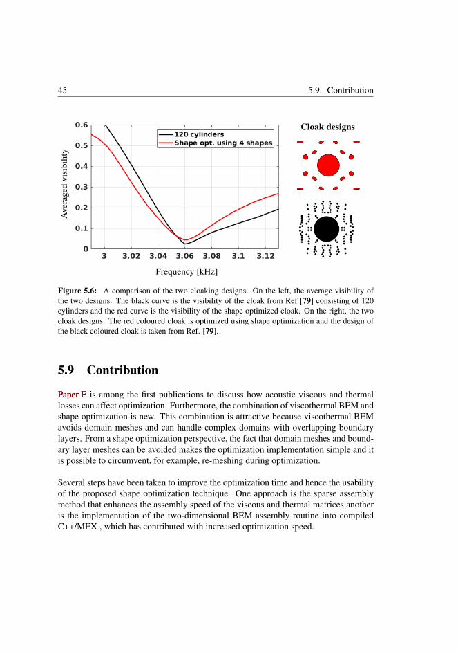
45 5.9. Contribution
Cloak designs
Frequency [kHz]
Ave
rage
dvi
sibi
lity
Figure 5.6: A comparison of the two cloaking designs. On the left, the average visibility ofthe two designs. The black curve is the visibility of the cloak from Ref [7979] consisting of 120cylinders and the red curve is the visibility of the shape optimized cloak. On the right, the twocloak designs. The red coloured cloak is optimized using shape optimization and the design ofthe black coloured cloak is taken from Ref. [7979].
5.9 Contribution
Paper EPaper E is among the first publications to discuss how acoustic viscous and thermallosses can affect optimization. Furthermore, the combination of viscothermal BEM andshape optimization is new. This combination is attractive because viscothermal BEMavoids domain meshes and can handle complex domains with overlapping boundarylayers. From a shape optimization perspective, the fact that domain meshes and bound-ary layer meshes can be avoided makes the optimization implementation simple and itis possible to circumvent, for example, re-meshing during optimization.
Several steps have been taken to improve the optimization time and hence the usabilityof the proposed shape optimization technique. One approach is the sparse assemblymethod that enhances the assembly speed of the viscous and thermal matrices anotheris the implementation of the two-dimensional BEM assembly routine into compiledC++/MEX , which has contributed with increased optimization speed.

Chapter 5. Acoustic shape optimization including losses 46
In Paper EPaper E, results show that viscous and thermal dissipation can have a significantimpact on the performance of the shape optimized resonators. However, the effect oflosses depends on the problem. In other cases, the extra effort of including losses mightnot be necessary. As an example, viscothermal losses have very little influence on theacoustic cloaking device and can be shape optimized with regular isentropic BEM asin Section 5.85.8.
Chapter 6
Discussion and conclusionsThe PhD thesis has treated three different subjects related to acoustic viscous and ther-mal dissipation; namely, an investigation of the effect of acoustic losses on two novelacoustic devices, improving an existing viscothermal BEM implementation and thedevelopment of a shape optimization technique based on the viscothermal BEM.
Modelling of two novel acoustic devices
Including viscous and thermal dissipation into numerical acoustic simulations based onthe FLNS equations comes at a significant computational cost. Therefore, if possible,it is desirable to simplify the problem using isentropic assumptions. In some cases,this requires a profound understanding of the given problem to decide on the suitablemodelling strategy. As an example, Paper APaper A presents a metamaterial developed un-der the assumptions that the acoustic wave behaviour can be considered lossless. Thisassumption leads to an analytically and numerically designed metamaterial that ex-hibits double negative behaviour using the combined effect of periodically distributedscatterers and quarter-wave resonators. Unfortunately, measurements in Ref. [7878] andlossy numerical FEM and BEM simulations in Paper APaper A reveal that viscothermal lossesnegatively impacts the performance of the metamaterial, making the initially proposeddesign lose its double-negative band. A similar comparison is made in Paper BPaper B wherenumerical experiments investigate the effect of losses on an acoustic cloaking devicebased on scattering cancellation. In this type of device, it is found that losses can beconsidered negligible, and the isentropic assumption is sufficient to give an accurateestimate of the cloaking performance. The main difference between the two types ofdevices is the fact that the metamaterial utilizes quarter-wave resonators to obtain thedesired effects. The quarter-wave resonators, and other resonators for that matter, willin most cases contribute with a considerable amount of loss.
The metamaterial simulations has served as a good benchmark to show the capabili-ties of the viscothermal BEM and its applicability to solve complicated large problems.

Chapter 6. Discussion and conclusions 48
While not used in this project, the SLNS FEM implementation is an alternative tothe FLNS FEM and could be used to more efficiently simulate the metamaterial in aFEM framework. In situations where it is not directly apparent that losses can playan important role, i.e. the geometry is far from having overlapping boundary layers,computationally cheaper methods like the BLI models are very interesting, since theywould allow for a cheap estimation of how losses influence a given problem. Addi-tionally, the BLI formulation should also be suitable for implementation into the BEMframework used here.
Improving the viscothermal BEM
A potential shortcoming of the previous viscothermal BEM is the use of first andsecond order finite difference coupling terms to estimate tangential derivatives of theacoustic pressure. The use of finite difference is prone to some error and is cumber-some to implement in three dimensions. This is addressed in Paper CPaper C and Paper DPaper D,where two new coupling strategies are discussed which improve on the existing imple-mentation by removing the use of finite difference.
The first approach is TD-BEM which uses the boundary element itself to estimatethe tangential derivatives by an additional set of two-dimensional tangential derivativeboundary element equations. As a result, only first order tangential derivative calcu-lations are necessary. Moreover, the previous implementation relies on an averagingof the normal and tangential vectors at the element interfaces. In the TD-BEM imple-mentation, the averaging is avoided by using discontinuous elements where the normaland tangential vectors are uniquely defined at the collocation points. The approachis evaluated and compared with the previous implementation through two simple testcases. The first test case is a convergence study using an analytical solution of an os-cillating cylinder as a reference (Fig. 4.24.2). It is found that higher mesh densities seemto favour the TD-BEM with slightly lower errors in the pressure and viscous velocitycalculation. On the other hand, the viscous velocity is found to have larger errors atlow mesh densities. It is not fully understood why this is the case, but it might be thatthe estimation of the tangential derivatives of the rapid decaying viscous velocity usingboundary element itself requires a better mesh resolution. A plausible solution wouldbe to use a coarse pressure mesh and a more refined mesh describing the viscous ve-locity. However, such implementation would come at an increased computational cost.Nevertheless, it should be noted that the lowest mesh densities corresponds to verycoarse meshes, considered insufficient in general. The second test case is a narrow

49
duct, which highlights some of the potential issues with the FDD-BEM and demon-strates the strength of TD-BEM. It is shown that the FDD-BEM is very sensitive toirregular element sizes which can lead to a larger error. The same instability issueis not observed when using TD-BEM. Computationally, the TD-BEM has some dis-advantages since the method requires an assembly of an additional set of tangentialderivative BEM matrices.
The second approach, SFD-BEM, directly uses the shape functions to estimate thetangential derivatives. The result is an expanded system of equations where both theacoustic pressure and viscous velocity becomes dependent variables. In Paper DPaper D, theSFD-BEM concept is implemented into a three-dimensional formulation and testedthrough two test cases: an oscillating sphere and a condenser microphone. It is shownthat the SFD-BEM is an improvement over the previous finite difference implementa-tion with better stability and reduced errors. Notably is the calculation of the viscousvelocity which is significantly better. It should be noted, that the use of finite differ-ence in three-dimensions is more problematic and prone to considerably larger errorsas compared to two dimensions. SFD-BEM, as presented in Paper DPaper D, relies on con-tinuous elements which require averaging of both the normal and tangential vectors atelement interfaces, but also the tangential derivatives. However, the averaging can beavoided by using the aforementioned discontinuous elements. Additionally, since theapproach relies on the shape functions to estimate the tangential derivatives, the tan-gential derivative will always become one order lower than the element order. There-fore, higher order elements are a requirement. In Paper DPaper D, isoparametric continuousquadratic elements are used, meaning that the description of the tangential derivativeis linear. As a benefit over the TD-BEM, the SFD-BEM only requires assembly ofthe acoustic, thermal and viscous matrices. In the BEM implementation, most of thetime is spent on the assembly of matrices, making the SFD-BEM faster as compared toTD-BEM.
In this project, much effort is given towards solutions that match the boundary con-ditions described in a local node-related coordinate system. In other words, the no-slipcondition is described in terms of its normal an tangential components using Eq (3.203.20)and Eq. (3.213.21). During this project another possibility was considered but not imple-mented due to time limitations: fulfilling the boundary conditions using a Cartesiandescription of the no-slip condition, i.e. Eq. (3.193.19). As an example, the gradients ofpa and ph can be found by taking the Cartesian derivative of the Kirchoff-Helmholtzintegral. This approach would in theory avoid the necessary translation using theHadamard product. On the other hand, such method would require integration of hy-persingular kernels. Another idea is to solve and fulfil the boundary conditions using
Chapter 6. Discussion and conclusions 50
some kind of iterative approach.
Acoustic shape optimization with losses
In Paper EPaper E, a two-dimensional shape optimization technique based on the SFD-BEMthat includes modelling of acoustic viscous and thermal dissipation is developed. Thetechnique is applied to maximize the absorption coefficient of quarter-wave andHelmholtz resonators located at an impedance tube termination. A series of numer-ical experiments investigate the role of losses when performing shape optimization.For the particular test cases, it is found that losses play a significant role and near per-fect absorption can only be obtained if losses are included.
During the development and testing of the shape optimization technique multiple testcases have been studied which are not included in this thesis. The primary goal hasbeen to establish an awareness that losses can play an important role when perform-ing optimization. The example chosen here, an impedance tube, is found to be a goodbenchmark for lossy optimization since it isolates the effect of losses. In fact, opti-mization can only be performed if the numerical model contains some loss, otherwisethe absorption coefficient will always be equal to zero. In isentropic BEM, intrin-sic numerical damping contributes with losses and makes shape optimization of thequarter-wave and Helmholtz resonators possible. It has been observed in some testcases that numerical damping contributes to the optimization by creating meaningfuldesigns that sometimes are similar to what is obtained with the viscothermal BEM. Asimilar situation is seen in the optimization of the quarter-wave resonators, where thefinal lossless optimized design has some absorbing capabilities.
Another observation worth noting is that visothermal dissipation stabilizes the opti-mization process, and lossy optimization usually requires less iterations.
6.1 Conclusions
The most important conclusions from the papers can be summarized as follows:
• It is numerically verified in Paper APaper A that acoustic dissipation is the reason whythe metamaterial is not behaving as intended when measured.
• Paper BPaper B shows that losses have very little influence on the averaged visibility andthe acoustic cloaking device performance in general.

51 6.2. Future research
• By utilizing either tangential derivative boundary element or the shape func-tions it is found possible in Paper CPaper C and Paper DPaper D to avoid the use of the tangen-tial derivative finite difference coupling terms used in the previous viscothermalBEM implementations. The two new approaches demonstrate increased stabilityand error reduction.
• Paper EPaper E sussesfully implements a two-dimensional gradient-based shape opti-mization technique that is capable of including acoustic viscous and thermaldissipation. The technique is demonstrated by maximizing the absorption co-efficient of quarter-wave and Helmholtz resonators. Shape optimization resultsconfirm that accurate modelling of acoustic losses is necessary to obtain designswith nearly perfect absorption.
6.2 Future researchIt is intended that the shape optimization technique developed in this thesis can be usedto design and improve the performance of acoustic transducers and hearing aids, butalso be applied to create new metamaterial designs where the effect of losses is in-cluded in the design process. The developed optimization technique seems promising;however, the thesis has only considered two-dimensional simple academic problems.Therefore, the extension into three dimensions is necessary to facilitate optimizationof real-world problems. Such an extension would require a more efficient sensitivityanalysis based on e.g. an adjoint method. Additionally, the work carried out here ispurely numerical, and experimental validation should be performed to verify the usabil-ity of the proposed shape optimization technique. The realization of optimized designswould require the inclusion of manufacturing constraints and robustness measures inthe optimization process. Another direction is to extend the shape optimization tech-nique to account for the mechanical coupling which is important in, e.g. hearing aids.
As already briefly discussed, other directions for the viscothermal BEM implemen-tation are possible, and methods to fulfil the boundary conditions differently or relyingon iterative methods could be subject for further research. Moreover, more direct stud-ies comparing viscothermal FEM and BEM models are necessary to give a better ideaof the computational benefits of the BEM in large-scale computations. To do this on anequal footing, implementation of the three dimensional viscothermal BEM into moreefficient languages like C++ or fortran is required.

Chapter 6. Discussion and conclusions 52
Bibliography[1] P. M. Morse and K. U. Ingard. Theoretical acoustics. McGraw-Hill, Inc, 1968.
[2] A. D Pierce. Acoustics: An Introduction to Its Physical Principles and Applica-tions. Acoustical Society of America, 1991 (second printing).
[3] R. Christensen. Acoustic Modeling of Hearing Aid Components. PhD thesis,University of Southern Denmark, 2010.
[4] W. R. Kampinga. Viscothermal acoustics using finite elements. Analysis tool forengineers. PhD thesis, University of Twente, Enschede, 2010.
[5] P. Honzik, C. Guianvarc’h, and M. Bruneau. Modeling of capacitive memsmicrophone with square membrane or plate using integral method. ELSEVIERSCIENCE BV, 120:418–421, 2015. doi: 10.1016/j.proeng.2015.08.656.
[6] D. Homentcovschi, R. N. Miles, P. V. Loeppert, and A. J. Zuckerwar. A microa-coustic analysis including viscosity and thermal conductivity to model the effectof the protective cap on the acoustic response of a mems microphone. Microsys-tem Technologies-micro-and Nanosystems-information Storage and ProcessingSystems, 20(2):265–272, 2014. doi: 10.1007/s00542-013-1800-5.
[7] V. Cutanda Henríquez. Numerical transducer Modeling. PhD thesis, TechnicalUniversity of Denmark, Lyngby, 2002.
[8] M. J. H. Jensen and E. S. Olsen. Virtual prototyping of condenser microphonesusing the finite element method for detailed electric, mechanic, and acousticcharacterization. volume 19, page 030039, 2013. doi: 10.1121/1.4799295.
[9] G. Plantier and M. Bruneau. Heat conduction effects on the acoustic response ofa membrane separated by a very thin air film from a backing electrode. JournalD’acoustique, 3(3):243–50, 243–250, 1990.
[10] R. Christensen and U. Skov. Compression driver simulation incl. vibroacoustic,viscothermal & porous acoustics. In Proceedings from the COMSOL conferencein Stuttgart (Germany), 2011.

Bibliography 54
[11] R. Christensen and U. Skov. Simulation of a 4" compression driver using afully coupled vibroacoustic finite element analysis including viscous and ther-mal losses. In Audio Engineering Society Convention 132, Apr 2012. URLhttp://www.aes.org/e-lib/browse.cfm?elib=16310http://www.aes.org/e-lib/browse.cfm?elib=16310.
[12] M. Berggren, A. Bernland, and D. Noreland. Acoustic boundary layers asboundary conditions. Journal of Computational Physics, 371:633–650, 2018.doi: 10.1016/j.jcp.2018.06.005.
[13] M. A. Temiz, I. L. Arteaga, and A. Hirschberg. Sound Absorption Measurementsfor Mirco-Perforated Plates: The Effect of Edge Profile. In Proceedings fromEURONOISE, 31 May - 3 June, Maarstrcih (Netherlands), 2015.
[14] J. Carbajo, J. Ramis, L. Godinho, P. Amado-Mendes, and J. Alba. A finite el-ement model of perforated panel absorbers including viscothermal effects. Ap-plied Acoustics, 90:1–8, 2015. doi: 10.1016/j.apacoust.2014.10.013.
[15] S. A. Cummer, J. Christensen, and A. Alù. Controlling sound with acousticmetamaterials. Nature reviews materials, 1:1–13, 2016. doi: doi:10.1038/natrevmats.2016.1.
[16] H. Ruiz, C. C. Claeys, E. Deckers, and W. Desmet. Numerical and experimentalstudy of the effect of microslits on the normal absorption of structual metama-terials. Mechanical Systems and Signal processing, 70-71:909–918, 2016. doi:doi:10.1016/j.ymssp.2015.09.028.
[17] H. Ryoo and W. Jeon. Dual-frequency sound-absorbing metasurface based onviscothermal effects with frequency dependence. Journal of Applied Physics,123:115110, 2018. doi: 10.1063/1.5017540.
[18] N. Jiménez, V. Romero-García, P. Pagneux, and J. Groby. Rainbow-trappingabsorbers: Broadband, perfect and asymmetric sound absorption by subwave-length panels for transmission problems. Scientific Reports, 7(1):13595, 2017.doi: 10.1038/s41598-017-13706-4.
[19] M. Molerón, M. Serra-Garcia, and C. Daraio. Visco-thermal effects in acousticmetamaterials: from total transmission to total reflection and high absorption.New J. Phys., 18:033003, 2016. doi: 10.1088/1367-2630/18/3/033003.
[20] E. Wadbro and M. Berggren. Topology optimization of an acoustic horn. Com-put. Methods Appl. Mech. Engrg., 196:420–436, 2006. doi: 10.1016/j.cma.2006.05.005.
55 Bibliography
[21] R. Udawalpola, E. Wasbro, and M. Berggren. Optimization of an acoustic hornwith respect to efficientcy and directivity. Int. J. Numer. Meth. Engng, 73:1571–1606, 2007. doi: 10.1002/nme.2132.
[22] R. Udawalpola, E. Wasbro, and M. Berggren. Optimization of a variable mouthhorn. Int. J. Numer. Meth. Engng, 85:591–606, 2010. doi: 10.1002/nme.2982.
[23] R. Christensen. Topology optimization of thermoviscous acoustics in tubes andslits with hearing aid applications. Proceedings of the COMSOL Conference inRotterdam, 2017.
[24] M. J. Turner, R. W. Clough, H. C. Martin, and L. J. Topp. Stiffness and deflectionanalysis of complex structual. Journal of the aeronautical sciences, 23(9):805–823, 1956. doi: 10.2514/8.3664.
[25] T. W. Wu. Boundary Element Acoustic. WIT press, 2000.
[26] P. M. Juhl. The Boundary Element Method for sound Field Calculations. PhDthesis, Department of Acoustic Technology, Technical Univarity of Denmark,1993.
[27] A. F. Seybert, B. Soenarko, F. J. Rizzo, and D. J. Shippy. An advanced computa-tional method for radiation and scattering of acoustic waves in three dimensions.Journal of the Acoustical Society of America, 77(2):362–8, 362–368, 1985. doi:10.1121/1.391908.
[28] A. Sutradhar, G. H. Paulino, and L. J. Gray. Symmetric galerkin boundary el-ement method. Symmetric Galerkin Boundary Element Method, pages 1–276,2008. doi: 10.1007/978-3-540-68772-6.
[29] V. Cutanda Henríquez and P. M. Juhl. OpenBEM - an open source BoundaryElement Method software in acoustics,. Proceedings of the 39th InternationalCongress on Noise Control Engineering, Inter-noise, Lisbon (Portugal), 2010.
[30] H. A. Schenck. Improved integral formulation for acoustic radiation problems.The Journal of the Acoustical Society of America, 44(1):44, 1968. doi: 10.1121/1.1911085.
[31] G. Bartolozzi, D’Amico R., A. Pratellesi, and Pierini M. An efficient methodfor selecting chief points. In Proceedings of the 8th International Conferenceon Structual Dynamics, 4-6 July, Leauven (Belgium), 2011.

Bibliography 56
[32] A. J. Burton and G. F. Miller. The application of integral equation methods tothe numerical solution of some exterior boundary-value problems. Proc. Roy.Soc. Lond. A., 323(1553):201–210, 1971. doi: 10.1098/rspa.1971.0097.
[33] S. Marburg. The Burton and Miller method: Unlocking another mystery of itscoupling parameter. Journal of Computational acoustics, 24(1):1550016, 2016.doi: 10.1142/S0218396X15500162.
[34] D. S. Burnett. A three-dimensional acoustic infinite element based on a pro-late spherodal multipole expansion. The Journal of the Acoustical Society ofAmerica, 96(5):2798, 1994. doi: doi.org/10.1121/1.411286.
[35] J. Autrique and F. Magoués. Studies of an infinite element method for acousticalradiation. Applied Mathematical Modelling, 30(7):641–655, 2005. doi: 10.1016/j.apm.2005.08.022.
[36] J. J. Shirron and S. Dey. Acoustic infinite elements for non-separable geome-tries. Comput. Methods Appl. Mech. Engrg., 191(37-38):4123–4139, 2002. doi:10.1016/S0045-7825(02)00355-9.
[37] J. Berenger. A perfectly matched layer for the absorption of electromagneticwaves. Journal of Computational Physics, 114(2):185–200, 1994. doi: 10.1006/jcph.1994.1159.
[38] Q. Liu and J. Tao. The perfectly matched layer for acoustic waves in absorptivemedia. J. Acoust. Soc. Am., 102(4):2072–2082, 1997. doi: 10.1121/1.419657.
[39] A. Bermúdez, L. Hervella-Nieto, A. Prieto, and Rodriguez R. An optimalperfectly matched layer with unbounded absorbing function for time-harmonicacoustic scattering problems. Journal of Computational Physics, 223(2):469–488, 2007. doi: 10.1016/j.jcp.2006.09.018.
[40] COMSOL Multiphysics Reference Manual, version 5.2. COMSOL Multi-physics Reference Manual, version 5.2. COMSOL, Inc, www.comsol.com.
[41] G. Kirchoff. Uber den Einfluss der Wärmeleitung in einem Gase auf due Schall-bewegung. Annalen Der Physik Und Chemie, 210(6):177–193, 1868. doi:10.1002/andp.18682100602and10.1002/(ISSN)1521-3889.
[42] Rayleigh. The theory of sound volume 2, 2nd edition. Dover publications, 1894.
[43] C. Zwikker and C. W. Kosten. Sound absorbing materials. Elsevier publisingcompany. inc, 1949.
57 Bibliography
[44] H. Tijdeman. On the propagation of sound waves in cylindrical tubes. Journal ofSound and Vibration, 39(1):1–33, 1975. doi: 10.1016/S0022-460X(75)80206-9.
[45] A. Cummings. Sound propagation in narrow tubes of arbitrary cross-section.Journal of Sound and Vibration, 162(1):27–42, 1991. doi: 10.1006/jsvi.1993.1100.
[46] A. Cummings. The propagation of plane sound waves in narrow and widecircular tubes, and generalization to uniform tubes of arbitary cross-sectionalshape. Journal of Acoustical Society of America, 89(2):550–558, 1991. doi:10.1121/1.400379.
[47] W. M. Beltman. Viscothermal wave propagation including acousto-elastic in-teraction. PhD thesis, University of Twente, Enschede, 1998.
[48] W. M. Beltman. Viscothermal wave propagation including acousto-elastic inter-action, part I: theory. Journal of Sound and Vibration, 227(3):555–586, 1999.doi: 10.1006/jsvi.1999.2355.
[49] W. M. Beltman. Viscothermal wave propagation including acousto-elastic inter-action, part II: applications. Journal of Sound and Vibration, 227(3):587–609,1999. doi: 10.1006/jsvi.1999.2356.
[50] W. M. Beltman, P. J. M. van der Hoogt, R. M. E. J. Spiering, and H. Tijdeman.Implementation and experimental validation of a new viscothermal acoustic fi-nite element for acousto-elastic problems. Journal of Sound and Vibration, 216(1):159–185, 1998. doi: 10.1121/1.400379.
[51] A. H. Benade. On the Propagation of Sound Waves in a Cylindrical Conduit.Journal of Acoustical Society of America, 44(2):616–623, 1968. doi: 10.1121/1.1911130.
[52] D. H. Keefe. Acoustical wave propagation in cylindrical ducts: Transmissionline parameter approximations for isothermal and nonisothermal boundary con-ditions. Journal of Acoustical Society of America, 75(1):58–62, 1984. doi:10.1121/1.390300.
[53] J. C. Zuercher, E. V. Carlson, and M. C. Killion. Small acoustic tubes: Newapproximations including isothermal and viscous effects. Journal of AcousticalSociety of America, 83(4):1653–1660, 1988. doi: 10.1121/1.395920.

Bibliography 58
[54] R. Christensen, P. Juhl, and Cutanda Henríquez V. Practical modeling of acousticlosses in air due to heat conduction and viscosity. In Proceedings from theEuropean Conference on Noise Control, June 29-July 4, Paris (France), 2008.
[55] M. Malinen, M. Lyly, P. Raback, A. Karkkainen, and L. Karkkainen. A finiteelement method for the modeling of termo-viscous effects in acoustics. In Pro-ceedings of the 4th European Congress on Computational Methods in Appliedand Engineering ECCOMAS, Jyvaskyla, Finland, 2004.
[56] M. J. J. Nijhof, Y. H. Wijant, and A. de Boer. An acoustic finite element includ-ing viscothermal effects. In Proceedings from the 14th International Congresson Sound and vibration, 9-12 july, Cairns (Australia), 2007.
[57] L. Cheng, R. D. White, and K. Grosh. Three-dimensional viscous finite ele-ment formulation for acoustic fluid-structure interaction. Computer Methodsin Applied Mechanics and Engineering, 197(49-50):4160–4172, 2008. doi:10.1121/1.395920.
[58] N. Joly. Finite element modeling of thermoviscous acoustics in closed cavities.In Proceeding from Acoustics’08, June 29-July 4, Paris (France), 2008.
[59] W. R. Kampinga, Y. H. Wijnant, and A. de Boer. Performance of Several Vis-cothermal Acoustic Finite Elements. Acta Acoustica United with Acustica, 96(1):115–124, 2010. doi: 10.3813/AAA.918262.
[60] G. C. Martins, J. A. Cordioli, and R. Jordan. An analysis of mesh parameters ofa viscothermal acoustic FE model. In Proceedings from the 18th InternationalCongress on Sound and vibration, 9-12 july, Rio de Janeiro (Brazil), 2011.
[61] R. Bossart, N. Joly, and M. Bruneau. Hybrid numerical and analytical solutionsfor acoustic boundary problems in thermo-viscous fluids. Journal of Sound andVibration, 263(1):69–84, 2002. doi: 10.1016/S0022-460X(02)01098-2.
[62] K. Schmidt and A Thöns-Zueva. Impedance boundary conditions for acoustictime harmonic wave propagation in viscous gases. 2014.
[63] R. Kampinga, Y. Wijnant, and A. de Boer. A two step viscothermal acousticFE method. In Proceedings from the 16th International Congress on Sound andvibration, 5-9 july, Kraków (Poland), 2009.
[64] E. Dokumaci. An integral equation formulation for boundary element analysisof acoustic radiation problems in viscous fluids. Journal of Sound and Vibration,147(2):335–348, 1991. doi: 10.1016/0022-460X(91)90720-5.

59 Bibliography
[65] E. Dokumaci. Prediction of the effects of entropy fluctuations on sound radiationfrom vibrating bodies using an integral equation approach. Journal of Sound andVibration, 186(5):805–819, 1995. doi: 10.1006/jsvi.1995.0489.
[66] C. Karra, M. Ben Tahar, G. Marquette, and Chau M. T. Boundary element anal-ysis of problems of acoustic propagation in viscothermal fluid. In Proceedingsof internose, 30 July - 2 August , Liverpool (UK), 1996.
[67] C. Karra and M. Ben Tahar. An integral equation formulation for boundaryelement analysis of propagation in viscothermal fluid. J. Acoust. Soc. Am., 102(3):1311–1318, 1997. doi: 10.1121/1.420050.
[68] V. Cutanda Henríquez and P. M. Juhl. Implementation of an acoustic 3d bemwith visco-thermal losses. In Proceedings of internose, 15-18 Sept , Insbruck(Austria), 2013.
[69] V. Cutanda Henríquez and P. M. Juhl. Verification of an acoustic 3d bem withvisco-thermal losses. In Proceedings of internose, 15-18 Sept , Insbruck (Aus-tria), 2013.
[70] V. Cutanda Henríquez and P. M. Juhl. An axisymmetric boundary element for-mulation of sound wave propagation in fluids including viscous and thermallosses. J. Acoust. Soc. Am., 134(5):3409–3418, 2013. doi: 10.1121/1.4823840.
[71] M. Bruneau, Ph. Herzog, J. Kergomard, and J. D. Polak. General formulation ofthe dispersion equation in bounded viso-thermal fluid, and application to somesimple geometries. Wave Motion 11, pages 441–451, 1988. doi: 10.1016/j.jcp.2006.09.018.
[72] C. Grossmann and H. G Roos. Numerical treatment of partial differential equa-tions. Springer, 2007.
[73] N. Sukumar and J. E. Bolander. Numerical computation of discrete differentialoperators on non-uniform grids. Cmes-computer Modeling in Engineering andSciences, 4(6):691–705, 2003.
[74] R. Martinez. The thin-shape breakdown (tsb) of the helmholtz integral equation.The Journal of the Acoustical Sociaty of America, 90(5):2728, 1991. doi: 10.1121/1.401868.
[75] V. Cutanda Henríquez, P. M. Juhl, and F. Jacobsen. On the modeling of nar-row gaps using the standard boundary element method. Journal of the AcousticSociety of America, 109(4):1296–1303, 2001. doi: 10.1121/1.1350399.
Bibliography 60
[76] S. Sorokin and S. T. Christensen. Low-frequency breakdown of bound-ary element formulation for closed cavities in excitation conditions with a’breathing’-type component. Communications in numerical methods in en-gineering, 16(5):325–334, 2000. doi: 10.1002/(SICI)1099-0887(200005)16:5<325::AID-CNM339>3.0.CO;2-G.
[77] K. A. Hussain and K. S. Peat. Boundary element analysis of low frequencycavity acoustical problems. Journal of Sound and Vibration, 169(2):197–209,1994. doi: 10.1006/jsvi.1994.1013.
[78] R. Garciía-Salgado, V. M. García-Chocano, D. Torrent, and J. Sánchez-Dehesa.Negative mass density and -near-zero quasi-two-dimensional metamaterial: De-sign and application. Phys. Rev. B, 88(22):224305, 2013. doi: 10.1103/PhysRevB.88.224305.
[79] V. M. Garcia-Chocano, L. Sanchis, A. Diaz-Rubio, J. Martinez-Pastor,F. Cervera, R. Llopis-Pontiveros, and J. Sanchez-Dehesa. Acoustic cloak forairborne sound by inverse design. Applied Physics Letters, 99(7):074102, 2011.doi: 10.1063/1.3623761.
[80] R. Gallego and A.E Martínez-Castro. Boundary integral equation for tangentialderivative of flux in laplace and helmholtz equations. Int. J. Numer. Meth. Engng,66(2):334–363, 2006. doi: 10.1002/nme.1563.
[81] S.A. Yang. Evaluation of the Helmholtz boundary integral equation and its nor-mal and tangential derivatives in two dimensions. Journal of Sound and Vibra-tions, 301(3-5):864–877, 2007. doi: 10.1016/j.jsv.2006.10.023.
[82] S. Marburg and S. Schneider. Influence of Element Types on Numeric errorfor Acoustic Boundary Elements. Journal of Computational Acoustics, 11(3):363–386, 2003. doi: 10.1142/S0218396X03001985.
[83] S. Marburg. Discretization Requirements: How many Elements per Wavelengthare Necessary?. In: Marburg S., Nolte B. (eds) Computational Acoustics ofNoise Propagation in Fluids - Finite and Boundary Element Methods. SpringerBerlin Heidelberg, 2008.
[84] J. A. Liggett and J. R. Salmon. Cubic spline boundary elements. Int. J. Numer.Meth. Engng, 17(4):543–556, 1980. doi: 10.1002/nme.1620170405and10.1002/(ISSN)1097-0207.
61 Bibliography
[85] A. W. Overhauser. Analytic definition of curves and surfaces by parabolic blend-ing. Technical Report SL 68-40, Mathematical and Theoretical Sciences Depart-ment, Scientific Laboratory, Ford Motor Company, Dearborn, Michigan, May1968.
[86] C. V. Camp and G. S. Gipson. Overhauser elements in boundary elementanalysis. Mathematical and Computer Modelling, 15(3-5):59–69, 1991. doi:10.1016/0895-7177(91)90053-A.
[87] H. Hadavinia, R. P. Travis, and R. T. Fenner. C1-continuous generalisedparabolic blending elements in the boundary element method. Mathematicaland Computer Modelling, 31(8-9):17–34, 2000. doi: 10.1016/S0895-7177(00)00057-1.
[88] L. P. Blinova and V. N. Kozhin. Radiation of a cylinder oscillating in a viscousmedium. Fluid Dynamics, 5(1):107–111, 1972. doi: 10.1007/BF01015007.
[89] S. Temkin. Elements of acoustics. Wiley New York, 1981.
[90] MATLAB Optimization Toolbox. MATLAB optimization toolbox, 2017b. TheMathWorks, Natick, MA, USA.
[91] J. Nocedal and S. J. Wright. Numerical Optimization, Second Edition. Springer,2006.
[92] O. Sigmund. On the usefulness of non-gradient approaches in topology opti-mization. Structural and Multidisciplinary Optimization, 43(5):589–596, 2011.doi: 10.1007/s00158-011-0638-7.
[93] D. Duhamel. Shape optimization of noise barriers using genetic algorithms,2006.
[94] E. A. Divo, A. J. Kassab, and M. S. Ingber. Shape optimization of acousticscattering bodies. Engineering Analysis With Boundary Elements, 27(7):695–703, 2003. doi: 10.1016/S0955-7997(03)00022-5.
[95] R. Toledo, J. J. Aznarez, D. Greiner, and O. Maeso. Shape design optimizationof road acoustic barriers featuring top-edge devices by using genetic algorithmsand boundary elements. Engineering Analysis With Boundary Elements, 63:49–60, 2016. ISSN 1873197x, 09557997. doi: 10.1016/j.enganabound.2015.10.011.
Bibliography 62
[96] T. Airaksinen and E. Heikkola. Multiobjective muffler shape optimization withhybrid acoustics modeling. Journal of the Acoustical Society of America, 130(3):1359–1369, 2011. ISSN 15208524, 00014966, 01630962. doi: 10.1121/1.3621119.
[97] B. Mohammadi and O. Pironneau. Applied Shape Optimization for Fluids, Sec-ond Edition. Oxford university press, 2010.
[98] J. Semmler, L. Pflug, M. Stingl, and G. Leugering. Shape Optimization in Elec-tromagnetic Applications, pages 251–269. Springer International Publishing,Cham, 2015. ISBN 978-3-319-17563-8. doi: 10.1007/978-3-319-17563-8_11.URL https://doi.org/10.1007/978-3-319-17563-8_11https://doi.org/10.1007/978-3-319-17563-8_11.
[99] R. Udawalpola. Shape Optimization for Acoustic Wave Propagation Problems.PhD thesis, University of uppsala, 2010.
[100] J. A. Samareh. A survey of shape parameterization techniques.CEAS/AIAA/ICASE/NSA Langley International Forum on Aeroelasticity andStructual Dynamics, pages 333–343, 1999.
[101] C. Liu, L. Chen, W. Zhao, and H. Chen. Shape optimization of sound barrier us-ing an isogeometric fast multipole boundary element method in two dimensions,2017.
[102] B. U. Koo, J. G. Ih, and B. C. Lee. Acoustic shape sensitivity analysis using theboundary integral equation. Journal of the Acoustical Society of America, 104(5):2851–2860, 1998. doi: 10.1121/1.423869.
[103] L. Chen, C. Zheng, and H. Chen. A wideband fmbem for 2d acoustic designsensitivity analysis based on direct differentiation method. Computational Me-chanics, 52(3):631–648, 2013. doi: 10.1007/s00466-013-0836-9.
[104] R. Udawalpola, E. Wadbro, and M. Berggren. Optimization of a variable mouthacoustic horn. International Journal for Numerical Methods in Engineering, 85(5):591–606, 2011. doi: 10.1002/nme.2982.
[105] L. Chen, L. Liu, W. Zhao, and H. Chen. 2d acoustic design sensitivity analysisbased on adjoint variable method using different types of boundary elements.Acoustics Australia, 44(2):343–357, 2016. doi: 10.1007/s40857-016-0065-4.
[106] T. Matsumoto, T. Yamada, T. Takahashi, C. J. Zheng, and S. Harada. Acousticdesign shape and topology sensitivity formulations based on adjoint method andbem, 2011.

[107] ISO 10534-2:1998. ISO 10534-2:1998, Acoustics – Determination of soundabsorption coefficient and impedance in impedance tubes – Part 2: Transfer-function method, 1998.
[108] R. E. Christensen and E. Fernandez-Grande. Experimental validation of a topol-ogy optimized acoustic cavity. J. Acoust. Soc. Am., 138:3470–3474, 2015. doi:10.1121/1.4936905.


Paper A
A Numerical Model of an Acous-tic Metamaterial using the Bound-ary Element Method Including Vis-cous and Thermal Losses(Including erratum)
October 26, 2017 15:31 WSPC/S0218-396X 130-JCA 1750006
Journal of Computational Acoustics, Vol. 25, No. 4 (2017) 1750006 (11 pages)c© IMACSDOI: 10.1142/S0218396X17500060
A Numerical Model of an Acoustic Metamaterial
Using the Boundary Element Method Including Viscousand Thermal Losses
V. Cutanda Henrıquez∗, P. Risby Andersen† and J. Søndergaard Jensen‡
Centre for Acoustic-Mechanical Micro SystemsTechnical University of Denmark, Ørsteds PladsBuilding 352, DK 2800, Kgs. Lyngby, Denmark
∗[email protected]†[email protected]‡[email protected]
P. Møller Juhl
Mærsk Mc-Kinney Møller InstituteUniversity of Southern Denmark
Campusvej 55, DK 5230 Odense M, [email protected]
J. Sanchez-Dehesa
Wave Phenomena Group, Department of Electronic EngineeringUniversitat Politecnica de Valencia
Camino de Vera s.n. building 7F, ES 46022 Valencia, [email protected]
Received 31 May 2016Accepted 3 October 2016
Published 13 December 2016
In recent years, boundary element method (BEM) and finite element method (FEM) implementa-tions of acoustics in fluids with viscous and thermal losses have been developed. They are based onthe linearized Navier–Stokes equations with no flow. In this paper, such models with acoustic lossesare applied to an acoustic metamaterial. Metamaterials are structures formed by smaller, usuallyperiodic, units showing remarkable physical properties when observed as a whole. Acoustic lossesare relevant in metamaterials in the millimeter scale. In addition, their geometry is intricate andchallenging for numerical implementation. The results are compared with existing measurements.
Keywords: Boundary element method; acoustic metamaterials; viscous and thermal acoustic losses.
1. Introduction
Acoustic metamaterials are artificial periodic structures with unit cells containing features
such as resonators or scatterers.1 The macroscopic acoustic properties may show values that
1750006-1
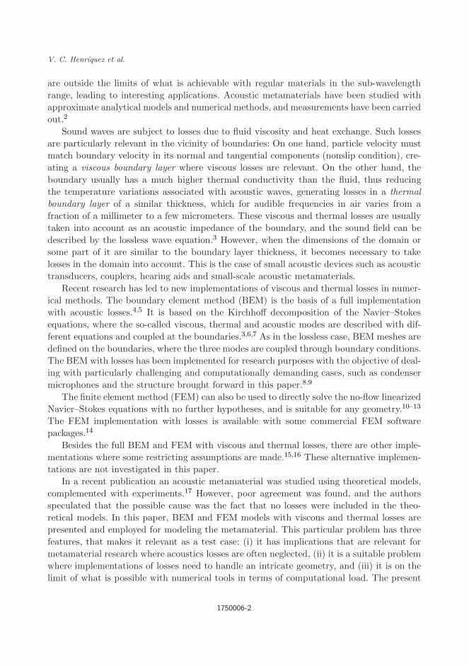
October 26, 2017 15:31 WSPC/S0218-396X 130-JCA 1750006
V. C. Henrıquez et al.
are outside the limits of what is achievable with regular materials in the sub-wavelength
range, leading to interesting applications. Acoustic metamaterials have been studied with
approximate analytical models and numerical methods, and measurements have been carried
out.2
Sound waves are subject to losses due to fluid viscosity and heat exchange. Such losses
are particularly relevant in the vicinity of boundaries: On one hand, particle velocity must
match boundary velocity in its normal and tangential components (nonslip condition), cre-
ating a viscous boundary layer where viscous losses are relevant. On the other hand, the
boundary usually has a much higher thermal conductivity than the fluid, thus reducing
the temperature variations associated with acoustic waves, generating losses in a thermal
boundary layer of a similar thickness, which for audible frequencies in air varies from a
fraction of a millimeter to a few micrometers. These viscous and thermal losses are usually
taken into account as an acoustic impedance of the boundary, and the sound field can be
described by the lossless wave equation.3 However, when the dimensions of the domain or
some part of it are similar to the boundary layer thickness, it becomes necessary to take
losses in the domain into account. This is the case of small acoustic devices such as acoustic
transducers, couplers, hearing aids and small-scale acoustic metamaterials.
Recent research has led to new implementations of viscous and thermal losses in numer-
ical methods. The boundary element method (BEM) is the basis of a full implementation
with acoustic losses.4,5 It is based on the Kirchhoff decomposition of the Navier–Stokes
equations, where the so-called viscous, thermal and acoustic modes are described with dif-
ferent equations and coupled at the boundaries.3,6,7 As in the lossless case, BEM meshes are
defined on the boundaries, where the three modes are coupled through boundary conditions.
The BEM with losses has been implemented for research purposes with the objective of deal-
ing with particularly challenging and computationally demanding cases, such as condenser
microphones and the structure brought forward in this paper.8,9
The finite element method (FEM) can also be used to directly solve the no-flow linearized
Navier–Stokes equations with no further hypotheses, and is suitable for any geometry.10–13
The FEM implementation with losses is available with some commercial FEM software
packages.14
Besides the full BEM and FEM with viscous and thermal losses, there are other imple-
mentations where some restricting assumptions are made.15,16 These alternative implemen-
tations are not investigated in this paper.
In a recent publication an acoustic metamaterial was studied using theoretical models,
complemented with experiments.17 However, poor agreement was found, and the authors
speculated that the possible cause was the fact that no losses were included in the theo-
retical models. In this paper, BEM and FEM models with viscous and thermal losses are
presented and employed for modeling the metamaterial. This particular problem has three
features, that makes it relevant as a test case: (i) it has implications that are relevant for
metamaterial research where acoustics losses are often neglected, (ii) it is a suitable problem
where implementations of losses need to handle an intricate geometry, and (iii) it is on the
limit of what is possible with numerical tools in terms of computational load. The present
1750006-2
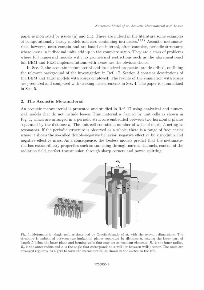
October 26, 2017 15:31 WSPC/S0218-396X 130-JCA 1750006
Numerical Model of an Acoustic Metamaterial with Losses
paper is motivated by issues (ii) and (iii). There are indeed in the literature some examples
of computationally heavy models and also containing intricacies.15,18 Acoustic metamate-
rials, however, must contain and are based on internal, often complex, periodic structures
where losses in individual units add up in the complete setup. They are a class of problems
where full numerical models with no geometrical restrictions such as the aforementioned
full BEM and FEM implementations with losses are the obvious choice.
In Sec. 2, the acoustic metamaterial and its desired properties are described, outlining
the relevant background of the investigation in Ref. 17. Section 3 contains descriptions of
the BEM and FEM models with losses employed. The results of the simulation with losses
are presented and compared with existing measurements in Sec. 4. The paper is summarized
in Sec. 5.
2. The Acoustic Metamaterial
An acoustic metamaterial is presented and studied in Ref. 17 using analytical and numer-
ical models that do not include losses. This material is formed by unit cells as shown in
Fig. 1, which are arranged in a periodic structure embedded between two horizontal planes
separated by the distance h. The unit cell contains a number of wells of depth L acting as
resonators. If the periodic structure is observed as a whole, there is a range of frequencies
where it shows the so-called double-negative behavior: negative effective bulk modulus and
negative effective mass. As a consequence, the lossless models predict that the metamate-
rial has extraordinary properties such as tunneling through narrow channels, control of the
radiation field, perfect transmission through sharp corners and power splitting.
Fig. 1. Metamaterial single unit as described by Gracia-Salgado et al. with the relevant dimensions. Thestructure is embedded between two horizontal planes separated by distance h, leaving the lower part oflength L below the lower plane and forming wells that may act as resonant elements. Ra is the inner radius,Rb is the outer radius and α is the angle that corresponds to a well (or between wells) sector. The units arearranged regularly as a grid to form the metamaterial, as shown in the sketch to the left.
1750006-3
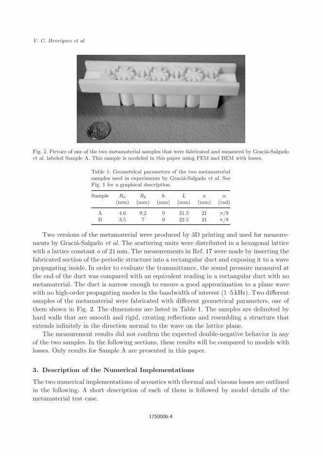
October 26, 2017 15:31 WSPC/S0218-396X 130-JCA 1750006
V. C. Henrıquez et al.
Fig. 2. Picture of one of the two metamaterial samples that were fabricated and measured by Gracia-Salgadoet al. labeled Sample A. This sample is modeled in this paper using FEM and BEM with losses.
Table 1. Geometrical parameters of the two metamaterialsamples used in experiments by Gracia-Salgado et al. SeeFig. 1 for a graphical description.
Sample Ra Rb h L a α(mm) (mm) (mm) (mm) (mm) (rad)
A 4.6 9.2 9 31.5 21 π/8B 3.5 7 9 22.5 21 π/8
Two versions of the metamaterial were produced by 3D printing and used for measure-
ments by Gracia-Salgado et al. The scattering units were distributed in a hexagonal lattice
with a lattice constant a of 21mm. The measurements in Ref. 17 were made by inserting the
fabricated section of the periodic structure into a rectangular duct and exposing it to a wave
propagating inside. In order to evaluate the transmittance, the sound pressure measured at
the end of the duct was compared with an equivalent reading in a rectangular duct with no
metamaterial. The duct is narrow enough to ensure a good approximation to a plane wave
with no high-order propagating modes in the bandwidth of interest (1–5 kHz). Two different
samples of the metamaterial were fabricated with different geometrical parameters, one of
them shown in Fig. 2. The dimensions are listed in Table 1. The samples are delimited by
hard walls that are smooth and rigid, creating reflections and resembling a structure that
extends infinitely in the direction normal to the wave on the lattice plane.
The measurement results did not confirm the expected double-negative behavior in any
of the two samples. In the following sections, these results will be compared to models with
losses. Only results for Sample A are presented in this paper.
3. Description of the Numerical Implementations
The two numerical implementations of acoustics with thermal and viscous losses are outlined
in the following. A short description of each of them is followed by model details of the
metamaterial test case.
1750006-4
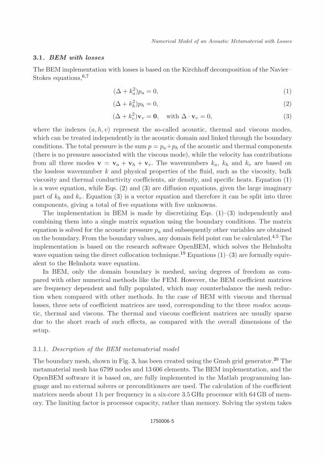
October 26, 2017 15:31 WSPC/S0218-396X 130-JCA 1750006
Numerical Model of an Acoustic Metamaterial with Losses
3.1. BEM with losses
The BEM implementation with losses is based on the Kirchhoff decomposition of the Navier–
Stokes equations,6,7
(∆ + k2a)pa = 0, (1)
(∆ + k2h)ph = 0, (2)
(∆ + k2v)vv = 0, with ∆ · vv = 0, (3)
where the indexes (a, h, v) represent the so-called acoustic, thermal and viscous modes,
which can be treated independently in the acoustic domain and linked through the boundary
conditions. The total pressure is the sum p = pa+ph of the acoustic and thermal components
(there is no pressure associated with the viscous mode), while the velocity has contributions
from all three modes v = va + vh + vv. The wavenumbers ka, kh and kv are based on
the lossless wavenumber k and physical properties of the fluid, such as the viscosity, bulk
viscosity and thermal conductivity coefficients, air density, and specific heats. Equation (1)
is a wave equation, while Eqs. (2) and (3) are diffusion equations, given the large imaginary
part of kh and kv . Equation (3) is a vector equation and therefore it can be split into three
components, giving a total of five equations with five unknowns.
The implementation in BEM is made by discretizing Eqs. (1)–(3) independently and
combining them into a single matrix equation using the boundary conditions. The matrix
equation is solved for the acoustic pressure pa and subsequently other variables are obtained
on the boundary. From the boundary values, any domain field point can be calculated.4,5 The
implementation is based on the research software OpenBEM, which solves the Helmholtz
wave equation using the direct collocation technique.19 Equations (1)–(3) are formally equiv-
alent to the Helmhotz wave equation.
In BEM, only the domain boundary is meshed, saving degrees of freedom as com-
pared with other numerical methods like the FEM. However, the BEM coefficient matrices
are frequency dependent and fully populated, which may counterbalance the mesh reduc-
tion when compared with other methods. In the case of BEM with viscous and thermal
losses, three sets of coefficient matrices are used, corresponding to the three modes: acous-
tic, thermal and viscous. The thermal and viscous coefficient matrices are usually sparse
due to the short reach of such effects, as compared with the overall dimensions of the
setup.
3.1.1. Description of the BEM metamaterial model
The boundary mesh, shown in Fig. 3, has been created using the Gmsh grid generator.20 The
metamaterial mesh has 6799 nodes and 13 606 elements. The BEM implementation, and the
OpenBEM software it is based on, are fully implemented in the Matlab programming lan-
guage and no external solvers or preconditioners are used. The calculation of the coefficient
matrices needs about 1 h per frequency in a six-core 3.5GHz processor with 64GB of mem-
ory. The limiting factor is processor capacity, rather than memory. Solving the system takes
1750006-5

October 26, 2017 15:31 WSPC/S0218-396X 130-JCA 1750006
V. C. Henrıquez et al.
Fig. 3. Boundary mesh employed in the BEM model with losses. Upper, metamaterial sample; lower, emptyduct. Linear three-node triangular elements are used.
6mins per frequency. The size of the system to be solved is the same as the number of
degrees of freedom of the boundary mesh. The calculated frequencies are spaced by 100Hz
from 1 kHz to 5 kHz, giving 41 frequencies. The sparsity of the thermal and viscous coeffi-
cient matrices is believed to enable some speed increase of the calculation, but it has not
been directly exploited.
In parallel, an empty rectangular duct of the same dimensions has been calculated. The
purpose of the empty duct is acting as a reference for the calculation of the metamaterial
transmittance and reflectance. This reference could also be calculated analytically, but the
numerical version serves as a test for the calculation issues described in the following.
The duct where the metamaterial is inserted and the empty duct used as a reference are
assumed sufficiently long so that no reflections are created on any of the two terminations,
emitting and receiving. In the FEM calculation described later, perfectly matched layers
are used for this purpose. In the BEM code, the emitter and receiving lids are given an
impedance of ρc instead, to make them anechoic to an incoming plane wave. One of the
terminations acts as a plane piston with a normal velocity of 1/ρcm/sec amplitude, so as
to normalize the resulting plane wave to an amplitude of one.
The boundary conditions are set so as the mesh nodes on the rim of the lids can represent
a sharp transition between the lid and the duct walls. This is done by splitting the columns
in the acoustic coefficient matrix corresponding to the normal derivative of the pressure in
the acoustic mode.21
In order to compare with the measurements in Ref. 17, transmitted power at the receiving
end needs to be calculated. Pressure and particle velocity in the propagation direction (X-
coordinate, duct length direction) are calculated on 10 field points situated on a plane that
is normal to the propagation direction, thus allowing an estimation of the acoustic intensity
and power. An equivalent calculation is made at the emitting side which is used to calculate
the reflectance of the metamaterial. Measurement results are not available for the latter
calculation, and it is not shown in this paper.
1750006-6
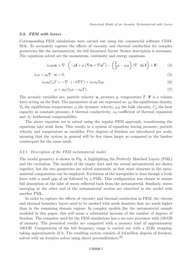
October 26, 2017 15:31 WSPC/S0218-396X 130-JCA 1750006
Numerical Model of an Acoustic Metamaterial with Losses
3.2. FEM with losses
Corresponding FEM simulations were carried out using the commercial software COM-
SOL. To accurately capture the effects of viscosity and thermal conduction for complex
geometries like the metamaterial, the full linearized Navier–Stokes description is necessary.
The equations solved are the momentum, continuity and energy equations,
iωρ0u = ∇ ·(−pI+ µ
(∇u+∇uT
)−
(2
3µ− µB
)(∇ · u) I
)+ F, (4)
iωρ+ ρ0∇ · u = 0, (5)
iωρ0CpT = −∇ · (−k∇T ) + iωα0T0p, (6)
ρ = ρ0(βT p− α0T ). (7)
The acoustic variables are; particle velocity u, pressure p, temperature T . F is a volume
force acting on the fluid. The parameters of air are expressed as: ρ0 the equilibrium density,
T0 the equilibrium temperature, µ the dynamic velocity, µB the bulk viscosity, Cp the heat
capacity at constant pressure, k thermal conductivity, α0 coefficient of thermal expansion
and βT isothermal compressibility.
The above equation set is solved using the regular FEM approach, transforming the
equations into weak form. This results in a system of equations having pressure, particle
velocity and temperature as variables. Five degrees of freedom are introduced per node,
meaning that the system in general will be five times larger as compared to the lossless
counterpart for the same mesh.
3.2.1. Description of the FEM metamaterial model
The model geometry is shown in Fig. 4, highlighting the Perfectly Matched Layers (PML)
and the excitation. The models of the empty duct and the actual metamaterial are shown
together, but the two geometries are solved separately, so that more elements in the meta-
material computation can be employed. Excitation of the waveguides is done though a body
force with a small gap of air followed by a PML. This configuration was chosen to ensure
full absorption at the inlet of waves reflected back from the metamaterial. Similarly, waves
emerging at the other end of the metamaterial section are absorbed in the model with
another PML.
In order to capture the effects of viscosity and thermal conduction in FEM, the viscous
and thermal boundary layers need to be meshed with mesh densities that are much higher
than in the remaining domain regions. In complex models like the metamaterial sample
modeled in this paper, this will mean a substantial increase of the number of degrees of
freedom. The computer used for the FEM simulations has a six-core processor with 128GB
of memory. The presented results are computed with a memory load of approximately
100GB. Computation of the full frequency range is carried out with a 25Hz stepping,
taking approximately 21 h. The resulting system consists of 3.6million degrees of freedom,
solved with an iterative solver using direct preconditioners.22
1750006-7
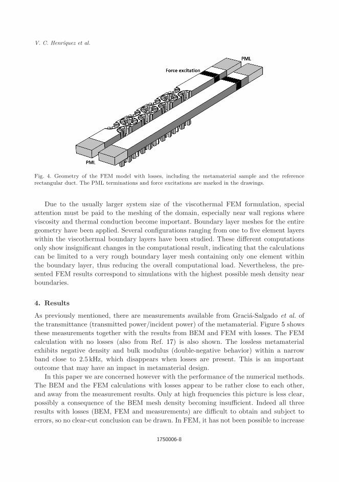
October 26, 2017 15:31 WSPC/S0218-396X 130-JCA 1750006
V. C. Henrıquez et al.
Fig. 4. Geometry of the FEM model with losses, including the metamaterial sample and the referencerectangular duct. The PML terminations and force excitations are marked in the drawings.
Due to the usually larger system size of the viscothermal FEM formulation, special
attention must be paid to the meshing of the domain, especially near wall regions where
viscosity and thermal conduction become important. Boundary layer meshes for the entire
geometry have been applied. Several configurations ranging from one to five element layers
within the viscothermal boundary layers have been studied. These different computations
only show insignificant changes in the computational result, indicating that the calculations
can be limited to a very rough boundary layer mesh containing only one element within
the boundary layer, thus reducing the overall computational load. Nevertheless, the pre-
sented FEM results correspond to simulations with the highest possible mesh density near
boundaries.
4. Results
As previously mentioned, there are measurements available from Gracia-Salgado et al. of
the transmittance (transmitted power/incident power) of the metamaterial. Figure 5 shows
these measurements together with the results from BEM and FEM with losses. The FEM
calculation with no losses (also from Ref. 17) is also shown. The lossless metamaterial
exhibits negative density and bulk modulus (double-negative behavior) within a narrow
band close to 2.5 kHz, which disappears when losses are present. This is an important
outcome that may have an impact in metamaterial design.
In this paper we are concerned however with the performance of the numerical methods.
The BEM and the FEM calculations with losses appear to be rather close to each other,
and away from the measurement results. Only at high frequencies this picture is less clear,
possibly a consequence of the BEM mesh density becoming insufficient. Indeed all three
results with losses (BEM, FEM and measurements) are difficult to obtain and subject to
errors, so no clear-cut conclusion can be drawn. In FEM, it has not been possible to increase
1750006-8

October 26, 2017 15:31 WSPC/S0218-396X 130-JCA 1750006
Numerical Model of an Acoustic Metamaterial with Losses
significantly the mesh at the boundary layers in order to study its effect. In BEM, a mesh
with less nodes than the one employed in this paper showed similar results. Also in BEM,
a drastic increase in mesh density would also make the calculation unaffordable. However,
to some extent the FEM and BEM results validate each other.
Using the numerical calculations, it is possible to examine the behavior of the structure
in a detail that is not reachable to measurements. As an example, Fig. 6 shows the pressures
along the propagation direction on the boundary of the metamaterial within the double-
negative band, calculated using BEM. Note that the BEM predicts the double-negative
behavior at a frequency of around 2600Hz, and this value is used in Fig. 6. The FEM
calculation with no losses in Fig. 5 shows a double negative band at 2400–2500 Hz.
If the duct was plain and empty, the boundary conditions would produce a plane pro-
gressive wave of amplitude 1, which is marked in Fig. 6 as thin solid lines. The amplitudes
Fig. 5. Transmittance, obtained at the receiving end of the setup. Solid line, FEM model without losses;dotted line, FEM model with losses; dash-dotted line, BEM model with losses; dashed line, measurementsby Gracia-Salgado et al.
Fig. 6. Sound pressure at a given instant of time on the surface mesh, calculated with BEM. The abscissasare the positions of the nodes in the propagation direction. The frequency is 2600Hz, which is within thedouble-negative band predicted by BEM. Left, calculation with no losses; right, calculation with viscous andthermal losses.
1750006-9
October 26, 2017 15:31 WSPC/S0218-396X 130-JCA 1750006
V. C. Henrıquez et al.
in the resonator units are much larger, and in the simulation with no losses they combine
in such a way as to produce the extraordinary behavior described by Gracia-Salgado et al.
The same figure shows the effect of losses, which prevent wave propagation to the receiving
end and destroy the interplay between metamaterial units.
5. Conclusions
A metamaterial test case from the literature has been modeled using BEM and FEM
with losses. The simulations confirm the conclusion from existing measurement results:
the double-negative behavior associated with the metamaterial’s extraordinary properties
is prevented by viscous and thermal losses. This conclusion applies in principle to this par-
ticular metamaterial, but may serve as a warning when estimating the behavior of similar
structures.
The test case is a challenging calculation both for BEM and FEM with losses. Numerical
transmittance results with losses using FEM and BEM are not far from each other, and both
predict less losses than the measurements. This can serve, to some extent, as a verification
of the numerical implementations with losses. However, it should be kept in mind that
measurements are also challenging and subject to deviations. Further refinement of the
numerical models would be necessary to obtain a better estimation, but this would lead to a
drastic increase of the computational burden, which is not bearable with the computers used
in this work. A possible way forward would be the creation of more efficient implementations
of acoustic losses.
Acknowledgments
The authors wish to thank Mads J. Herring Jensen, from the company COMSOL, for his
support in setting up the FEM model of the metamaterial. J. Sanchez-Dehesa acknowledges
the support by the Spanish Ministerio de Economıa y Competitividad, and the European
Union Fondo Europeo de Desarrollo Regional (FEDER) through Project No. TEC2014-
53088-C3-1-R.
References
1. R. V. Craster and S. Guenneau (eds.), Acoustic Metamaterials. Negative Refraction, Imaging,Lensing and Cloaking (Springer, London, 2013).
2. S. A. Cummer, J. Christensen and A. Alu, Controlling sound with acoustic metamaterials, Nat.Rev. Mat. 1(3) (2016) 16001.
3. P. M. Morse and K. U. Ingard, Theoretical Acoustics (McGraw-Hill, Princeton, 1968).4. V. Cutanda Henrıquez and P. M. Juhl, An axisymmetric boundary element formulation of
sound wave propagation in fluids including viscous and thermal losses, J. Acoust. Soc. Am.134(5) (2013) 3409–3418.
5. V. Cutanda Henrıquez and P. M. Juhl, Implementation of an acoustic 3D BEM with visco-thermal losses, in Proc. Internoise 2013, 15–18 September 2013, Innsbruck, Austria.
6. A. D. Pierce, Acoustics: An Introduction to Its Physical Principles and Applications, Chap. 10(McGraw Hill, New York, 1981).
1750006-10
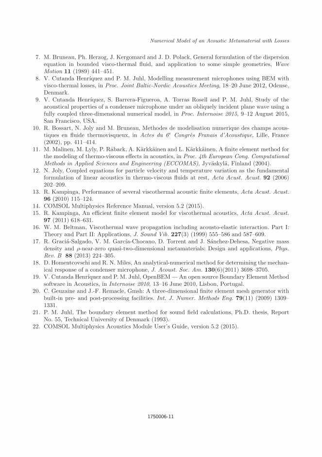
October 26, 2017 15:31 WSPC/S0218-396X 130-JCA 1750006
Numerical Model of an Acoustic Metamaterial with Losses
7. M. Bruneau, Ph. Herzog, J. Kergomard and J. D. Polack, General formulation of the dispersionequation in bounded visco-thermal fluid, and application to some simple geometries, WaveMotion 11 (1989) 441–451.
8. V. Cutanda Henrıquez and P. M. Juhl, Modelling measurement microphones using BEM withvisco-thermal losses, in Proc. Joint Baltic-Nordic Acoustics Meeting, 18–20 June 2012, Odense,Denmark.
9. V. Cutanda Henrıquez, S. Barrera-Figueroa, A. Torras Rosell and P. M. Juhl, Study of theacoustical properties of a condenser microphone under an obliquely incident plane wave using afully coupled three-dimensional numerical model, in Proc. Internoise 2015, 9–12 August 2015,San Francisco, USA.
10. R. Bossart, N. Joly and M. Bruneau, Methodes de modelisation numerique des champs acous-tiques en fluide thermovisqueux, in Actes du 6e Congres Franais d’Acoustique, Lille, France(2002), pp. 411–414.
11. M. Malinen, M. Lyly, P. Raback, A. Karkkainen and L. Karkkainen, A finite element method forthe modeling of thermo-viscous effects in acoustics, in Proc. 4th European Cong. ComputationalMethods in Applied Sciences and Engineering (ECCOMAS), Jyvaskyla, Finland (2004).
12. N. Joly, Coupled equations for particle velocity and temperature variation as the fundamentalformulation of linear acoustics in thermo-viscous fluids at rest, Acta Acust. Acust. 92 (2006)202–209.
13. R. Kampinga, Performance of several viscothermal acoustic finite elements, Acta Acust. Acust.96 (2010) 115–124.
14. COMSOL Multiphysics Reference Manual, version 5.2 (2015).15. R. Kampinga, An efficient finite element model for viscothermal acoustics, Acta Acust. Acust.
97 (2011) 618–631.16. W. M. Beltman, Viscothermal wave propagation including acousto-elastic interaction. Part I:
Theory and Part II: Applications, J. Sound Vib. 227(3) (1999) 555–586 and 587–609.17. R. Gracia-Salgado, V. M. Garcıa-Chocano, D. Torrent and J. Sanchez-Dehesa, Negative mass
density and ρ-near-zero quasi-two-dimensional metamaterials: Design and applications, Phys.Rev. B 88 (2013) 224–305.
18. D. Homentcovschi and R. N. Miles, An analytical-numerical method for determining the mechan-ical response of a condenser microphone, J. Acoust. Soc. Am. 130(6)(2011) 3698–3705.
19. V. Cutanda Henrıquez and P. M. Juhl, OpenBEM—An open source Boundary Element Methodsoftware in Acoustics, in Internoise 2010, 13–16 June 2010, Lisbon, Portugal.
20. C. Geuzaine and J.-F. Remacle, Gmsh: A three-dimensional finite element mesh generator withbuilt-in pre- and post-processing facilities. Int. J. Numer. Methods Eng. 79(11) (2009) 1309–1331.
21. P. M. Juhl, The boundary element method for sound field calculations, Ph.D. thesis, ReportNo. 55, Technical University of Denmark (1993).
22. COMSOL Multiphysics Acoustics Module User’s Guide, version 5.2 (2015).
1750006-11
March 13, 2017 13:42 WSPC/130-JCAJCA˙manuscript˙VCH-JSJ-PMJ-JSD˙2016˙ERRATUM
Journal of Computational Acousticsc© IMACS
Erratum to “A Numerical Model of an Acoustic Metamaterial using the
Boundary Element Method Including Viscous and Thermal Losses” (Journal
of Computational Acoustics, 2016, Volume 25, DOI:
10.1142/S0218396X17500060)
V. Cutanda Henrıquez*, P. Risby Andersen†, J. Søndergaard Jensen‡
Centre for Acoustic-Mechanical Micro Systems, Technical University of DenmarkØrsteds Plads, Building 352, DK-2800, Kgs. Lyngby, Denmark
*[email protected]†[email protected]‡[email protected]
P. Møller Juhl
Mærsk Mc-Kinney Møller Institute, University of Southern Denmark,Campusvej 55, DK-5230 Odense M, Denmark
J. Sanchez-Dehesa
Wave Phenomena Group, Department of Electronic Engineering, Universitat Politecnica de Valencia,Camino de Vera s.n. (building 7F), ES-46022 Valencia, Spain
Received (Day Month Year)Revised (Day Month Year)
One of the curves in Figure 5 of the published paper should be modified. It corresponds
to the transmittance measurement results. The results were obtained from a previous pub-
lication (reference [17] in the published paper), but the data was incorrectly squared.
Figure 1 below is a new version of Figure 5 in the original paper, where the measurement
curve has been plotted without squaring. The measurement plot is now closer to the trans-
mittance curves calculated using the Finite Element Method and the Boundary Element
Method with losses.
1
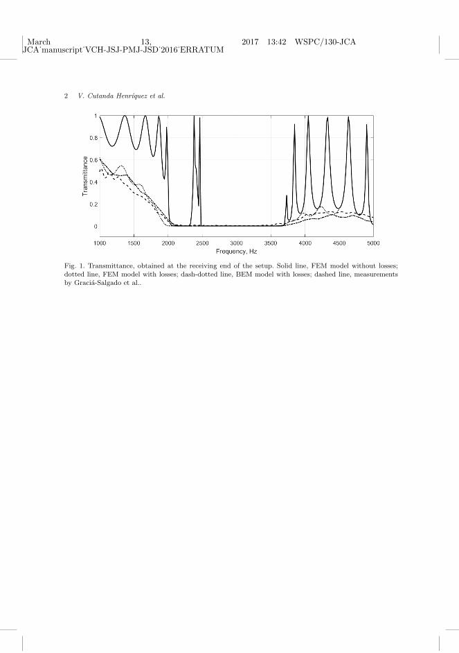
March 13, 2017 13:42 WSPC/130-JCAJCA˙manuscript˙VCH-JSJ-PMJ-JSD˙2016˙ERRATUM
2 V. Cutanda Henrıquez et al.
Fig. 1. Transmittance, obtained at the receiving end of the setup. Solid line, FEM model without losses;dotted line, FEM model with losses; dash-dotted line, BEM model with losses; dashed line, measurementsby Gracia-Salgado et al..

Paper B
Visco-thermal effects on an acous-tic cloak based on scattering can-cellation

VISCO-THERMAL EFFECTS ON AN ACOUSTIC CLOAKBASED ON SCATTERING CANCELLATION
Peter Risby Andersen1* , Vicente Cutanda Henrıquez1†, Niels Aage1‡ and Jose Sanchez-Dehesa 2
1Centre for Acoustic-Mechanical Micro Systems, Technical University of Denmark, ØrstedsPlads, Building 352, DK-2800, Kgs. Lyngby, Denmark
*Email: [email protected]†Email: [email protected]‡Email: [email protected]
2 Wave Phenomena Group, Universitat Politecnica de Valencia, Camino de Vera s.n. (Building4D), ES-46022 Valencia, Spain
Email: [email protected]
ABSTRACT
Recent research has shown that the performance of acoustic metamaterials can be greatly influ-enced by the effects of viscous and thermal dissipation. In the worst case, an isentropic assumptioncan lead to an undesired performance. To further investigate the impact of losses on novel acous-tic devices, an already known acoustic cloak is validated numerically, including the viscous andthermal dissipation effects. The specific cloaking device is realized using 120 small aluminiumcylinders distributed around a larger cylindrical object, in such a way, that plane waves incidentto the cloak will appear to be undisturbed, at the operational frequency of 3061 Hz. The initialoptimization procedure for determining the positions of the small cylinders assumes isentropicconditions neglecting dissipative effects, meaning that the actual realization of the cloak might be-have differently than intended. Through numerical simulations the acoustic cloak performance iscompared with and without dissipation, giving an estimate of the differences that can be expectedin similar cases. The results show that losses have very little impact on the key performance char-acteristic, the averaged visibility.
1 INTRODUCTION
The effect of viscous and thermal acoustic losses is often neglected when developing, for example,acoustic metamaterials or other type of acoustic devices, due to the assumption that viscous andthermal boundary layers are much smaller compared to the geometry under consideration. This
171971 - 1
sometimes overlooked effect was recently discussed in several papers, showing that losses can playa significant role for the behaviour of such devices, meaning that the usual isentropic assumptionmight not be sufficient.[1–3] To further investigate the effect of losses, this paper validates the dis-sipative impact on an already existing acoustic cloak found in a paper by Garcıa-Chocano.[4] Thespecific cloak was designed from an inverse design optimization procedure by distributing smallrigid cylinders around a larger cylindrical object a in way that effectively hides the larger cylinderdue to scattering cancellation. The general acoustic behaviour of the cylinders is described througha 2D multiple scattering method assuming isentropic conditions and an incident plane wave.[5] Thefinal optimized cloak design consists of 120 small cylinders distributed around the object, with anoperational frequency of 3061 Hz. Similar cloaking designs based on scattering cancellation de-veloped through topology optimization can be found in the literature of both acoustic and opticalcloaks.[6–8] In the paper by Garcıa-Chocano the design is validated both experimentally and nu-merically using a two-dimensional isentropic Finite Element Method (FEM) description of thecloak. One of the findings is that the experimental cloaking performance deviates from the FEMsimulations assuming an incident plane wave to the cloak. This difference is partly improved byfitting the actual, non-plane, shape of the experimental incident wave to the FEM calculations. Buteven with this improvement, experimental and numerical results still seem to deviate outside theoperational frequency. In the experimental work an attenuation of the pressure amplitude of 15 %as compared to simulations is also observed.
In the following, the cloak will be evaluated numerically using both FEM and Boundary ElementMethod (BEM) including the effects of acoustic viscous and thermal losses, to give an estimate ofhow the performance can be expected to change due to losses. Simulations will, for simplicity andclarity, restrict themselves to incident plane waves, since this is also the initial design assumption.
Firstly, the cloak geometry and performance parameter, the averaged visibility, are introduced.This is followed by sections on the numerical implementations including losses and simulationresults. Finally, conclusions are given on what to expect due to losses on this type of acousticdevice.
2 ACOUSTIC CLOAKING DEVICE
This section provides a brief introduction to the actual acoustic cloak under study here. For a morecomprehensive description, the reader is referred to the original paper by Garcıa-Chocano.[4] Thefinal optimized distribution of the 120 cylinders is seen in Figure 1. Each of the small cylindershas the same radius of 0.75 cm and the radius of the larger central cylindrical object is 11.25 cm.
The experiment was realized using aluminium cylinders placed in a two dimensional acousticwave guide with the dimensions 4.6×3.66×0.05 m3, ensuring that the chamber is well below thecut-off frequency of plausible modes in the z axis. This experimental setup is expected to be equiv-alent to simplified two-dimensional numerical simulations. While these two-dimensional type ofwave guide computations are simpler to conduct, they do lack the losses due to the upper and lowerwalls of the wave guide. In order to examine this, the results section also contains simulations ofan empty duct including losses, investigating the effect of not including the upper and lower wallsof the wave guide.
2.1 Visibility
The main validation of the performance and impact due to losses will be done in terms of the so-called averaged visibility, which is a measure of how well the cloak hides the larger cylinder. The
171971 - 2

averaged object visibility, γ, is defined as [4]
γ =1
N
∑
j
|Pmax,j| − |Pmin,j||Pmax,j|+ |Pmin,j|
(1)
with Pmax,j and Pmin,j being the maximum and minimum pressure amplitudes along the wavefront j in the measurement region shown in Figure 1, located behind the cloak. The measurementregion will contain around five wavelengths near the operational frequency.
-0.6 -0.4 -0.2 0 0.2 0.4 0.6 0.8 1x (m)
-0.5
-0.4
-0.3
-0.2
-0.1
0
0.1
0.2
0.3
0.4
0.5
y (m
)
Plane incident wave
Measurement region
Figure 1: The acoustic cloak geometry as proposed in [4]. The cloak consists of 120 cylinders,all with the same radius of 0.75 cm, distributed around a larger central cylindrical object with aradius of 11.25 cm. Evaluation of the visibility, γ, is done by observing the acoustic pressure inthe measurement region as seen in the figure.
3 NUMERICAL METHODS INCLUDING VISCOUS AND THERMAL LOSSES
The two main mechanisms accounting for the loss of energy in an acoustic wave are viscous andthermal effects. Fluid particles tend to stick to the surfaces (no-slip condition), forming the so-called viscous boundary layer. The viscous boundary layer thickness is frequency dependent. Forthe operational frequency of the cloak, the expected boundary layer thickness is approximately 38µm. [9] A similarly sized thermal boundary layer will also form near boundaries, due to the muchhigher heat capacity of the boundary material, essentially withholding an isothermal boundarycondition, forcing flux of heat between the boundary and the acoustic medium. To account for theeffects of both viscous and thermal losses in numerical acoustics simulations the full linearisedNavier-Stokes equations assuming no flow are utilized. Mainly two numerical acoustic methodsfor the full linearised Navier-Stokes equations exist, namely the BEM and the FEM. Both methodswill be used in the following sections to account for losses.
171971 - 3
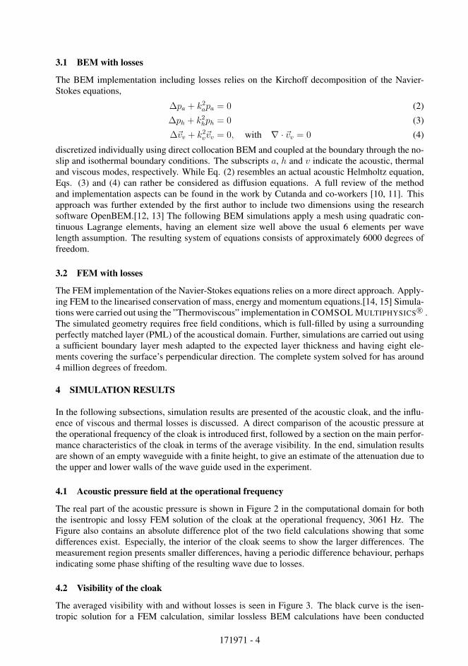
3.1 BEM with losses
The BEM implementation including losses relies on the Kirchoff decomposition of the Navier-Stokes equations,
∆pa + k2apa = 0 (2)
∆ph + k2hph = 0 (3)
∆~vv + k2v~vv = 0, with ∇ · ~vv = 0 (4)
discretized individually using direct collocation BEM and coupled at the boundary through the no-slip and isothermal boundary conditions. The subscripts a, h and v indicate the acoustic, thermaland viscous modes, respectively. While Eq. (2) resembles an actual acoustic Helmholtz equation,Eqs. (3) and (4) can rather be considered as diffusion equations. A full review of the methodand implementation aspects can be found in the work by Cutanda and co-workers [10, 11]. Thisapproach was further extended by the first author to include two dimensions using the researchsoftware OpenBEM.[12, 13] The following BEM simulations apply a mesh using quadratic con-tinuous Lagrange elements, having an element size well above the usual 6 elements per wavelength assumption. The resulting system of equations consists of approximately 6000 degrees offreedom.
3.2 FEM with losses
The FEM implementation of the Navier-Stokes equations relies on a more direct approach. Apply-ing FEM to the linearised conservation of mass, energy and momentum equations.[14, 15] Simula-tions were carried out using the ”Thermoviscous” implementation in COMSOL MULTIPHYSICS R© .The simulated geometry requires free field conditions, which is full-filled by using a surroundingperfectly matched layer (PML) of the acoustical domain. Further, simulations are carried out usinga sufficient boundary layer mesh adapted to the expected layer thickness and having eight ele-ments covering the surface’s perpendicular direction. The complete system solved for has around4 million degrees of freedom.
4 SIMULATION RESULTS
In the following subsections, simulation results are presented of the acoustic cloak, and the influ-ence of viscous and thermal losses is discussed. A direct comparison of the acoustic pressure atthe operational frequency of the cloak is introduced first, followed by a section on the main perfor-mance characteristics of the cloak in terms of the average visibility. In the end, simulation resultsare shown of an empty waveguide with a finite height, to give an estimate of the attenuation due tothe upper and lower walls of the wave guide used in the experiment.
4.1 Acoustic pressure field at the operational frequency
The real part of the acoustic pressure is shown in Figure 2 in the computational domain for boththe isentropic and lossy FEM solution of the cloak at the operational frequency, 3061 Hz. TheFigure also contains an absolute difference plot of the two field calculations showing that somedifferences exist. Especially, the interior of the cloak seems to show the larger differences. Themeasurement region presents smaller differences, having a periodic difference behaviour, perhapsindicating some phase shifting of the resulting wave due to losses.
4.2 Visibility of the cloak
The averaged visibility with and without losses is seen in Figure 3. The black curve is the isen-tropic solution for a FEM calculation, similar lossless BEM calculations have been conducted
171971 - 4

Figure 2: A comparison of the real part of the acoustic pressure for FEM simulations a) insentropiccaculation b) including viscous and thermal losses c) the absolute difference between the lossy andisentropic real part of the pressure. The frequency is 3061 Hz
showing identical visibility, but for brevity only the FEM solution is plotted. The average visibil-ity of the lossy FEM (green curve) and BEM (Red dots) simulations is also plotted, showing thatthe FEM solution is deviating more from the isentropic solution compared to BEM calulations.It is not fully understood why there is this difference between lossy FEM and BEM calculations.The BEM calculations are very similar to the isentropic calculation. Due to the difference in thesimulation parameters, speed of sound and temperature conditions of the experimental data, allsimulated data is shifted 26 Hz to match the operational frequency of the measurements, 3061Hz. For all the numerical results there is a large deviation in averaged visibility from the actualmeasurements, which is also the case for the plane incident wave calculations in the original paperby Garcıa-Chocano. The reason for this is assumed to be the non-plane incident wave front ofthe actual experiment. It should also be noted that comparing the original insentropic plane inci-dent wave averaged visibility calculations found in the work by Garcıa-Chocano, there is a slightdisagreement in the averaged visibility outside the operational frequency. It is unclear why thisdifference exists, but an explanation could perhaps be the different simulation boundary conditionsor parameters employed. The averaged visibility results presented in Figure 3 do in general have aslightly more broadband nature.
4.3 Empty waveguide
Since the simulations so far have shown that the losses seem to only have a minor impact on thesolution of the averaged visibility, it is interesting to investigate what amount of attenuation canbe expected from the finite height of the waveguide itself, since this effect is not included whenconsidering the cloak as a two-dimensional study case. Therefore, yet another FEM simulationhas been conducted representing an empty infinite slit in two dimensions, see Figure 4, containingthe height of the actual waveguide and using a perfectly matched layer to replicate an infinitetermination. In the numerical simulations, the duct is set with a pressure magnitude of 1 Pa atthe inlet. The acoustic pressure is then measured at the central part of duct, giving an averageestimate of what kind of attenuation is to be expected due to losses from the upper and lowerwalls of the waveguide. The average attenuation for different waveguide heights is seen in Figure5. In the experiment, the waveguide height is 5 cm, which simulations show corresponds to anaverage attenuation of 2.5 % in the measurement region. As it is observed, the average attenuationmagnitude is sensitive to the chosen height of the waveguide, so care must be taken when designingexperiments of this type to avoid the influence from losses.
171971 - 5
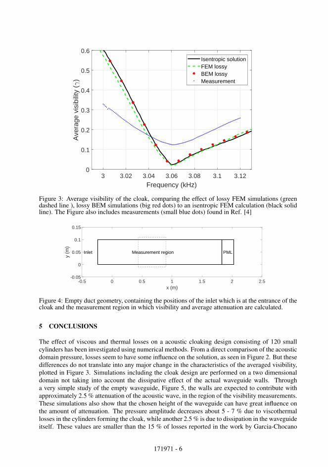
3 3.02 3.04 3.06 3.08 3.1 3.12
Frequency (kHz)
0
0.1
0.2
0.3
0.4
0.5
0.6
Ave
rage
vis
ibili
ty (
)
Isentropic solutionFEM lossyBEM lossyMeasurement
Figure 3: Average visibility of the cloak, comparing the effect of lossy FEM simulations (greendashed line ), lossy BEM simulations (big red dots) to an isentropic FEM calculation (black solidline). The Figure also includes measurements (small blue dots) found in Ref. [4]
-0.5 0 0.5 1 1.5 2 2.5x (m)
-0.05
0
0.05
0.1
0.15
y (m
)
Measurement regionInlet PML
Figure 4: Empty duct geometry, containing the positions of the inlet which is at the entrance of thecloak and the measurement region in which visibility and average attenuation are calculated.
5 CONCLUSIONS
The effect of viscous and thermal losses on a acoustic cloaking design consisting of 120 smallcylinders has been investigated using numerical methods. From a direct comparison of the acousticdomain pressure, losses seem to have some influence on the solution, as seen in Figure 2. But thesedifferences do not translate into any major change in the characteristics of the averaged visibility,plotted in Figure 3. Simulations including the cloak design are performed on a two dimensionaldomain not taking into account the dissipative effect of the actual waveguide walls. Througha very simple study of the empty waveguide, Figure 5, the walls are expected to contribute withapproximately 2.5 % attenuation of the acoustic wave, in the region of the visibility measurements.These simulations also show that the chosen height of the waveguide can have great influence onthe amount of attenuation. The pressure amplitude decreases about 5 - 7 % due to viscothermallosses in the cylinders forming the cloak, while another 2.5 % is due to dissipation in the waveguideitself. These values are smaller than the 15 % of losses reported in the work by Garcia-Chocano
171971 - 6

3 3.02 3.04 3.06 3.08 3.1 3.12
Frequency [kHz]
0
5
10
15
Ave
rage
atte
nuat
ion
in m
easu
rem
ent z
one
[%]
10 cm5 cm (used in experiment)2.5 cm1 cm
Figure 5: FEM simulations of the average attenuation in the measurement region of Figure 4, fordifferent waveguide heights: (blue dashed) 10 cm, (red dot dash) 5 cm, (yellow dotted) 2.5 cm and(blue dashed) 1 cm.
[4]. So, it can be concluded that the additional losses measured in the experiment might be due tothe setup employed. Future studies could cover full three-dimensional simulations including thewall effects, or the wall attenuation could simply be included in the incident wave to investigate itsimpact on the averaged visibility.
ACKNOWLEDGMENTS
J. Sanchez-Dehesa acknowledges the support by the Spanish Ministerio de Economıa y Competi-tividad, and the European Union Fondo Europeo de Desarrollo Regional (FEDER) through ProjectNo. TEC2014-53088-C3-1-R.
REFERENCES
[1] V. Cutanda Henrıquez, V. M. Garcıa-Chocano, and J. Sanchez-Dehesa. Viscothermal lossesin double-negative acoustic metamaterial. Physical Review Applied, 8(1):014029, 2017.
[2] V. Cutanda Henrıquez, P. Risby Andersen, J. S. Jensen, P. M. Juhl, and J. Sanchez-Dehesa. Anumerical model of an acoustic metamaterial using the Boundary Element Method includingviscous and thermal losses. Journal of Computational Acoustics, 25(4):1750006, 2017.
[3] R. E. Christensen and O. Sigmund. Experimental validation of systematically designedacoustc hyperbolic meta material slab exhibiting negative refraction. Applied Physics Let-ters, 109(10):101905, 2016.
[4] V. M. Garcıa-Chocano, Sanchis L., A Dıaz-Rubio, J. Martınez-Pastor, F. Cervena, R. Llopis-Pontiveros, and J. Sanchez-Dehesa. Acoustic cloak for airborne sound by inverse design.Applied Physics Letters, 99(7):074102, 2011.
171971 - 7
[5] L. Sanchis, A. Hakansson, F. Cervera, and J. Sanchez-Dehesa. Acoustic interferometersbased on two-dimensional arrays of ridgid cylinders in air. Physical Review B, 67(3):35422,2003.
[6] J. Andkjær and O. Sigmund. Topology optimized for airborne sound. ASME J. Vib. Acoust.,135:041011, 2013.
[7] J. Andkjær and O. Sigmund. Topology optimized low-contrast all-dielectric optical cloak.Applied Physics Letters., 98:021112, 2011.
[8] M. D. Guild, A. Alu, and M. R. Habermann. Cancellation of acoustic scattering from anelastic sphere. J. Acoust. Soc. Am., 129:1355, 2011.
[9] P. M. Morse and K. U. Ingard. Theoretical acoustics. McGraw-Hill, Inc, 1968.
[10] V. Cutanda Henrıquez and P. M. Juhl. An axisymmetric boundary element formulation ofsound wave propagation in fluids including viscous and thermal losses. Journal of the Acous-tical Society of America, 134(5):3409, 2013.
[11] V. Cutanda Henrıquez and P. M. Juhl. Implementaion of an acoustic 3D BEM with visco-thermal losses. Inter-noise, 15-18 sept, Insbruck (Austria), 2013.
[12] V. Cutanda Henrıquez and P. M. Juhl. OpenBEM - an open source Boundary Element Methodsoftware in acoustics,. Proceedings of the 39th International Congress on Noise ControlEngineering, Inter-noise, Lisbon (Portugal), 2010.
[13] P. Risby Andersen, V. Cutanda Henrıquez, N. Aage, and S. Marburg. Numerical acousticmodels including viscous and thermal losses: Review of exsisting and new methods. DAGA,6-9 March, Kiel (Germany), 2017.
[14] M. Malinen, M. Lyly, P. Raback, A. Karkainen, and L. Karkkainen. A Finite Element Methodfor the modeling of thermo-viscous effects in acoustics. Proceedings of the 4th EuropeanCongress on Computational Methods in Applied and Engineering ECCOMAS, Jyvaskyla(Finland), 2004.
[15] W. R. Kampinga. Viscothermal acoustics using Finite Elements. Analysis tool for engineers.PhD thesis, University of Twente, Enchede, 2010.
171971 - 8


Paper C
A two dimensional acoustic tan-gential derivative boundary ele-ment method including viscous andthermal losses

September 17, 2018 10:9 WSPC/S2591-7285 130-JTCA 1850036
Journal of Theoretical and Computational AcousticsVol. 26, No. 3 (2018) 1850036 (15 pages)c© The Author(s)DOI: 10.1142/S2591728518500366
A Two-Dimensional Acoustic Tangential Derivative Boundary
Element Method Including Viscous and Thermal Losses
P. Risby Andersen∗, V. Cutanda Henrıquez† and N. Aage‡
Centre for Acoustic-Mechanical Micro SystemsTechnical University of Denmark, Ørsteds Plads 352
DK-2800 Kgs. Lyngby, Denmark∗[email protected]†[email protected]‡[email protected]
S. Marburg
Institute of Vibroacoustics of Vehicles and MachinesFaculty of Mechanical Engineering, Technical University of Munich
Boltzmannstr. 15, 85748 Garching bei Munchen, [email protected]
Received 29 December 2017Accepted 26 April 2018
Published 5 September 2018
In recent years, the boundary element method has shown to be an interesting alternative to the finiteelement method for modeling of viscous and thermal acoustic losses. Current implementations relyon finite-difference tangential pressure derivatives for the coupling of the fundamental equations,which can be a shortcoming of the method. This finite-difference coupling method is removed hereand replaced by an extra set of tangential derivative boundary element equations. Increased stabilityand error reduction is demonstrated by numerical experiments.
Keywords: Boundary element method; viscous and thermal losses; acoustics.
1. Introduction
The isentropic acoustic wave equation is appropriate for modeling a vast variety of appli-
cations, but fails to give accurate solutions, especially if the acoustic domain is small and
contains narrow gaps. In such situations, the effects of viscous and thermal dissipations
must be considered. Two numerical approaches can be used for modeling of viscous and
thermal acoustic dissipations, namely the finite element method (FEM) and the boundary
∗Corresponding author.
This is an Open Access article published by World Scientific Publishing Company. It is distributed underthe terms of the Creative Commons Attribution 4.0 (CC-BY) License. Further distribution of this work ispermitted, provided the original work is properly cited.
1850036-1
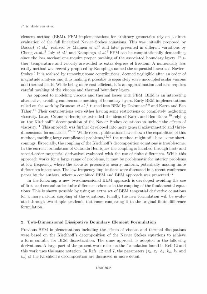
September 17, 2018 10:9 WSPC/S2591-7285 130-JTCA 1850036
P. R. Andersen et al.
element method (BEM). FEM implementations for arbitrary geometries rely on a direct
evaluation of the full linearized Navier–Stokes equations. This was initially proposed by
Bossart et al.,1 realized by Malinen et al.2 and later presented in different variations by
Cheng et al.,3 Joly et al.4 and Kampinga et al.5 FEM can be computationally demanding,
since the loss mechanisms require proper meshing of the associated boundary layers. Fur-
ther, temperature and velocity are added as extra degrees of freedom. A numerically less
costly method was recently proposed by Kampinga named the sequential linearized Navier–
Stokes.6 It is realized by removing some contributions, deemed negligible after an order of
magnitude analysis and thus making it possible to separately solve uncoupled scalar viscous
and thermal fields. While being more cost-efficient, it is an approximation and also requires
careful meshing of the viscous and thermal boundary layers.
As opposed to modeling viscous and thermal losses with FEM, BEM is an interesting
alternative, avoiding cumbersome meshing of boundary layers. Early BEM implementations
relied on the work by Bruneau et al.,7 turned into BEM by Dokumaci8,9 and Karra and Ben
Tahar.10 Their contributions were either having some restrictions or completely neglecting
viscosity. Later, Cutanda Henrıquez extended the ideas of Karra and Ben Tahar,10 relying
on the Kirchhoff’s decomposition of the Navier–Stokes equations to include the effects of
viscosity.11 This approach was further developed into more general axisymmetric and three-
dimensional formulations.12–14 While recent publications have shown the capabilities of this
method, tackling large complicated problems,15,16 the method might still have some short-
comings. Especially, the coupling of the Kirchhoff’s decomposition equations is troublesome.
In the current formulation of Cutanda Henrıquez the coupling is handled through first- and
second-order tangential derivatives evaluated with the use of finite differences. While this
approach works for a large range of problems, it may be problematic for interior problems
at low frequency, where the acoustic pressure is nearly uniform, potentially making finite
differences inaccurate. The low-frequency implications were discussed in a recent conference
paper by the authors, where a combined FEM and BEM approach was presented.17
In the following, a new two-dimensional BEM approach is developed avoiding the use
of first- and second-order finite-difference schemes in the coupling of the fundamental equa-
tions. This is shown possible by using an extra set of BEM tangential derivative equations
for a more natural coupling of the equations. Finally, the new formulation will be evalu-
ated through two simple academic test cases comparing it to the original finite-difference
formulation.
2. Two-Dimensional Dissipative Boundary Element Formulation
Previous BEM implementations including the effects of viscous and thermal dissipations
were based on the Kirchhoff’s decomposition of the Navier–Stokes equations to achieve
a form suitable for BEM discretization. The same approach is adopted in the following
derivations. A large part of the present work relies on the formulation found in Ref. 12 and
this work uses the same notation. In Refs. 12 and 7, the parameters (τa, τh, φa, ka, kh and
kv) of the Kirchhoff’s decomposition are discussed in more detail.
1850036-2
September 17, 2018 10:9 WSPC/S2591-7285 130-JTCA 1850036
A 2D Acoustic Tangential Derivative BEM Including Viscous and Thermal Losses
2.1. Kirchhoff ’s decomposition and boundary conditions
The final form of the decomposed Navier–Stokes equations is given in Eqs. (1)–(3), resulting
in three equations of the Helmholtz form, where pa and ph are the so-called acoustic and
thermal pressures, respectively.18,19 Their sum p = pa + ph represents the total pressure.
The vector vn is the rotational part of the velocity, also known as viscous velocity. In
this paper, magnitudes written with an arrow vector on top are vectorial fields, while bold
letters indicate matrices. While pa resembles an actual acoustic pressure wave, the equations
containing ph and vv can be considered as heavily damped wave equations. ka, kh and kvdenote the acoustic, thermal and viscous wavenumbers, respectively:
∆pa + k2apa = 0, (1)
∆ph + k2hph = 0, (2)
∆vv + k2vvv = 0 with ∇ · vv = 0. (3)
Equations (1)–(3) are coupled at the boundary through boundary conditions. It is reason-
able to assume isothermal boundary conditions. The heat capacity is very much higher
at the boundary than in the fluid that temperature variations at the boundary can be
neglected. An isothermal boundary condition can be expressed in terms of the acoustic
and thermal pressures and two frequency-dependent terms τa and τh relating the acous-
tic and thermal pressures to the temperature fluctuations T . This results in a frequency-
dependent thermal boundary layer forming at the boundary, with a thickness ranging from
micrometers to millimeters in the audible frequency range. Isolating ph in the isothermal
boundary condition, Eq. (4), is discretized as,
T = τapa + τhph = 0, (4)
which will be used as the first condition to couple the equations of Kirchhoff’s decomposition.
A second boundary condition states that the fluid will tend to stick to the boundaries (no-
slip condition). A viscous boundary layer will form, having similar thickness as the thermal
boundary layer. This boundary condition is expressed as
vb = φa∇pa + φh∇ph + vv, (5)
where vb is the boundary velocity and φa and φh are constants depending on physical
parameters and frequency. For the further development, it is convenient to describe the
no-slip conditions in a local boundary coordinate system:
vb,n = φa∂pa∂n
+ φh∂ph∂n
+ vv,n, (6)
vb,t = φa∂pa∂t
+ φh∂ph∂t
+ vv,t, (7)
with the subscripts n and t denoting the normal and tangential components to the
boundary.
1850036-3

September 17, 2018 10:9 WSPC/S2591-7285 130-JTCA 1850036
P. R. Andersen et al.
2.2. Boundary element discretization
The boundary element implementation for regular isentropic acoustic problems starts with
the integral form of the harmonic Helmholtz equation:
C(P )p(P ) =
∫
Γ
∂G(R)
∂n(Q)p(Q)dΓ(Q)−
∫
ΓG(R)
∂p(Q)
∂n(Q)dΓ(Q), (8)
where C(P ) is the integral-free term. The first term on the right-hand side is the double-
layer potential and the second term is the single-layer potential. P is a calculation point, Q
is an integration point on the generator, R = |Q − P | is the distance between calculation
and integration points and G(R) is the fundamental solution in free space. An eiωt time
convention is assumed. It should be noted that inclusion of a source term is omitted for
simplicity, but could be added as an extra term. Meshing and collocation of the Helmholtz
integral equation in matrix form is given by
Cp = Hp−B∂p
∂n, (9)
where C is a diagonal matrix containing the integral-free term, H and B are the discretized
double- and single-layer potential matrices, respectively, and p and ∂p∂n are vectors. A more
compact notation with A = H − C will be used in the following development. Since the
Kirchhoff’s decomposition produces equations formally equivalent to the Helmholtz wave
equation, it is straightforward to apply BEM to Eqs. (1)–(3) using collocation and replacing
the isentropic wavenumber k with ka, kh and kv:
Aapa −Ba∂pa
∂n= 0, (10)
Ahph −Bh∂ph
∂n= 0, (11)
Avvv,x −Bv∂vv,x
∂n= 0, (12)
Avvv,y −Bv∂vv,y
∂n= 0, (13)
where Eq. (3) is split into its Cartesian components forming Eqs. (12) and (13). Note that
we here and in the following limit the formulation to two dimensions (x, y) for simplicity. In
two dimensions, the fundamental solution is given by G(R) = 12πK0(ikR) where Kj(ikR) is
the modified Bessel function of the second kind of order j. The argument of the fundamental
solution is the imaginary unit i and the wavenumber k can be either acoustic, thermal or
viscous.
2.3. Coupling of equations
The previous boundary element implementations with losses make use of finite differences
to couple the fundamental equation set. The new approach presented here utilizes the
boundary element itself to estimate tangential derivatives. Taking the tangential derivative
1850036-4

September 17, 2018 10:9 WSPC/S2591-7285 130-JTCA 1850036
A 2D Acoustic Tangential Derivative BEM Including Viscous and Thermal Losses
of Eq. (8) with respect to the collocation point yields
C(P )∂p(P )
∂t(P )=
∫
Γ
∂2G(R)
∂t(P )∂n(Q)p(Q)dΓ(Q)−
∫
Γ
∂G(R)
∂t(P )
∂p(Q)
∂n(Q)dΓ(Q), (14)
thus allowing for the evaluation of the tangential derivative of the pressure on the collocation
points from boundary pressures p(Q) and their normal derivatives ∂p(Q)∂n . Equation (14) con-
tains second derivatives of the fundamental solution. A similar situation arises when dealing
with irregular frequencies for exterior problems using the Burton–Miller formulation, which
contains double normal derivative kernels that are said to be hypersingular and require spe-
cial treatment.20 However, the integrals arising from the tangential derivative equations are
Cauchy principal value (CPV) integrals. The kernel description can for example be found
in the work by Gallego and Martınez-Castro.21 The viscothermal implementation presented
here relies on an adaptive integration scheme for the evaluation of near-singular integrals
arising in the case of narrow gaps,22 but also for the evaluation of the CPV integrals. Ini-
tial convergence studies have shown that this approach is feasible for the evaluation of the
tangential kernels.
A second set of discretized equations can now be formed containing the tangential deriva-
tive kernels:
C∂pa
∂t= Aa,tpa −Ba,t
∂pa
∂n, (15)
C∂ph
∂t= Ah,tph −Bh,t
∂ph
∂n, (16)
C∂vv,x
∂t= Av,tvv,x −Bv,t
∂vv,x
∂n, (17)
C∂vv,y
∂t= Av,tvv,y −Bv,t
∂vv,y
∂n. (18)
It is possible to describe the no-slip condition in terms of the discretized equations by
isolating ∂pa∂n ,∂ph
∂n , ∂pa∂t and ∂ph
∂t in Eqs. (10), (11), (15) and (16), respectively. The boundary
condition equations, i.e. Eqs. (6) and (7), can then be described by
vb,n = φa(B−1a Aa)pa + φh(B
−1h Ah)ph + vv,n, (19)
vb,t = φaC−1(Aa,tpa −Ba,t((B
−1a Aa)pa)) + φhC
−1(Ah,tph −Bh,t((B−1h Ah)ph)) + vv,t.
(20)
Isolating ph in the isothermal boundary condition (4),
ph = − τaτh
pa, (21)
the thermal pressure can be eliminated from Eqs. (19) and (20). Finally, the boundary
conditions of the discretized equations can be stated as
vb,n = Enpa + vv,n, (22)
vb,t = Etpa + vv,t, (23)
1850036-5
September 17, 2018 10:9 WSPC/S2591-7285 130-JTCA 1850036
P. R. Andersen et al.
where
En = φa(B−1a Aa)− φh
τaτh
(B−1h Ah), (24)
Et = φa[C−1(Aa,t −Ba,t(B
−1a Aa))]− φh
τaτh
[C−1(Ah,t −Bh,t(B−1h Ah))]. (25)
2.4. Null-divergence of the viscous velocity
The viscous velocity forms a rotational vector field, meaning that∇ ·vv = 0 must be fulfilled.
This is ensured through the null-divergence in a normal and tangential coordinate system
(note that the tangential direction only has a single component in a 2D problem):
∂vv,n
∂n+
∂vv,t
∂t= 0, (26)
which will require a relation between local and global quantities on the boundary, achieved
in an all-geometry approach for the individual discrete nodes by
vv,n = nx vv,x + ny vv,y, (27)
vv,t = tx vv,x + ty vv,y, (28)
where is the element-wise Hadamard product (see Appendix A) and nx, ny, tx and ty are
the Cartesian components of the normal and tangential vectors at each node. The transform
of the viscous velocity back to the Cartesian coordinates is
vv,x = nx vv,n + tx vv,t, (29)
vv,y = ny vv,n + ty vv,t. (30)
The goal is now to establish an expression for each of the terms in Eq. (26) using the
discretized equations, containing only local normal and tangential components of the viscous
velocity. This requires taking the derivative of Eqs. (27) and (28) with respect to the normal
and tangential components, respectively. Doing so yields
∂vv,n
∂n= nx
∂vv,x
∂n+ nx
∂vv,y
∂n, (31)
∂vv,t
∂t= tx
∂vv,x
∂t+ ty
∂vv,y
∂t. (32)
By isolating∂vv,x
∂n and∂vv,y
∂n in Eqs. (12) and (13) and substituting into Eq. (31), we
obtain
∂vv,n
∂n= nx (B−1
v Avvv,x) + ny (B−1v Avvv,y). (33)
Using Eqs. (29) and (30) to describe the viscous velocity in terms of the normal and tan-
gential components, Eq. (33) becomes
∂vv,n
∂n= nx (B−1
v Av(nx vv,n + tx vv,t)) + ny (B−1v Av(ny vv,n + ty vv,t)). (34)
1850036-6
September 17, 2018 10:9 WSPC/S2591-7285 130-JTCA 1850036
A 2D Acoustic Tangential Derivative BEM Including Viscous and Thermal Losses
Applying the properties of the Hadamard product for diagonal terms, the terms in Eq. (34)
can be rearranged so that
∂vv,n
∂n= N1 (B−1
v Av)vv,n +N2 (B−1v Av)vv,t, (35)
where
N1 = nxnTx + nyn
Ty , (36)
N2 = nxtTx + nyt
Ty . (37)
The result of Eq. (35) will be used later to ensure that the null-divergence condition is
fulfilled. Proceeding with the second term in Eq. (26), a connection between the discretized
equations and∂vv,t
∂t is established. By isolating∂vv,x
∂t and∂vv,y
∂t in Eqs. (17) and (18) and
substituting the result into Eq. (28), an expression for the tangential derivative of the
tangential viscous velocity is found:
∂vv,t
∂t= tx
(C−1
(Av,tvv,x −Bv,t
∂vv,x
∂n
))+ ty
(C−1
(Av,tvv,y −Bv,t
∂vv,y
∂n
)). (38)
The Cartesian viscous quantities can be transformed into the local form by combining
Eqs. (29), (30), (12) and (13) into
∂vv,t
∂t= tx (C−1(Av,t(nx vv,n + tx vv,t)−Bv,t(B
−1v Av)(nx vv,n + tx vv,t)))
+ ty (C−1(Av,t(ny vv,n + ty vv,t)−Bv,t(B−1v Av)(ny vv,n + ty vv,t))).
(39)
Rearranging the terms and using the Hadamard product properties, the following equation
is obtained:
∂vv,t
∂t= N3 (C−1(Av,t −Bv,t(B
−1v Av)))vv,n +N4 (C−1(Avt −Bvt(B
−1v Av)))vv,t,
(40)
where
N3 = txnTx + tyn
Ty , (41)
N4 = txtTx + tyt
Ty . (42)
The result of the normal and tangential derivatives of the local viscous velocity components,
Eqs. (35) and (40), is substituted into the local form of the null-divergence, Eq. (26), forming
(N1 V)vv,n + (N2 V)vv,t + (N3 T)vv,n + (N4 T)vv,t = 0, (43)
where V and T are defined as
V = B−1v Av, (44)
T = C−1(Av,t −Bv,tV). (45)
1850036-7
September 17, 2018 10:9 WSPC/S2591-7285 130-JTCA 1850036
P. R. Andersen et al.
The result of Eq. (43) will be used in the following to ensure that the viscous velocity has
null-divergence.
2.5. System of equations and boundary quantities
It is now possible to establish a system of equations containing boundary normal and tan-
gential velocities and the acoustic pressure. Isolating vv,n and vv,t in Eqs. (43) and (23),
respectively, and substituting them into Eq. (22) yields the final system of equations:
[[(N1 V) + (N3 T)]En + [(N2 V) + (N4 T)]Et]pa
= [(N1 V) + (N3 T)]vb,n + [(N2 V) + (N4 T)]vb,t, (46)
which allows for applying boundary velocity conditions and solving for the nodal acoustic
pressures pa. The total pressure can be described as the sum of the acoustic and thermal
pressures, by assuming isothermal boundary conditions:
p = pa + ph = pa −τaτh
pa. (47)
The normal and tangential viscous velocities can be found by rearranging Eqs. (22) and (23),
so that
vv,n = Enpa − vb,n, (48)
vv,t = Etpa − vb,t. (49)
The evaluation of field points can be done by following the approach in Ref. 12. The expres-
sion using the finite-difference approach originally developed by Cutanda Henrıquez, is
reproduced here for comparison:[φaB
−1a Aa − φhB
−1h Ah
τaτh
+
(φa −
τaτh
φh
)× (N1 (B−1
v Av))−1
× (N2 (B−1v AvDT1) +DT2)
]pa
= vb,n + [N1 (B−1v Av)]
−1 × [N2 (B−1v Av) +DT1]vb,t, (50)
where DT1 and DT2 denote the first and second tangential surface finite-difference matri-
ces, respectively. Equation (50) is developed by taking the tangential derivative of the
boundary condition, Eq. (7), whereas the new approach presented in this paper achieves
this goal through a set of tangential boundary element matrices, Eq. (38). As a consequence,
the use of finite difference but also the evaluation of second tangential pressure derivatives
are avoided.
3. Test Cases
Only few analytical solutions are available for testing of acoustic viscothermal implementa-
tions. In the first example, the implementation will be compared with an analytical solution
1850036-8
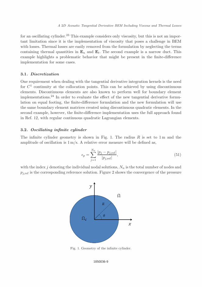
September 17, 2018 10:9 WSPC/S2591-7285 130-JTCA 1850036
A 2D Acoustic Tangential Derivative BEM Including Viscous and Thermal Losses
for an oscillating cylinder.23 This example considers only viscosity, but this is not an impor-
tant limitation since it is the implementation of viscosity that poses a challenge in BEM
with losses. Thermal losses are easily removed from the formulation by neglecting the terms
containing thermal quantities in En and Et. The second example is a narrow duct. This
example highlights a problematic behavior that might be present in the finite-difference
implementation for some cases.
3.1. Discretization
One requirement when dealing with the tangential derivative integration kernels is the need
for C1 continuity at the collocation points. This can be achieved by using discontinuous
elements. Discontinuous elements are also known to perform well for boundary element
implementations.24 In order to evaluate the effect of the new tangential derivative formu-
lation on equal footing, the finite-difference formulation and the new formulation will use
the same boundary element matrices created using discontinuous quadratic elements. In the
second example, however, the finite-difference implementation uses the full approach found
in Ref. 12, with regular continuous quadratic Lagrangian elements.
3.2. Oscillating infinite cylinder
The infinite cylinder geometry is shown in Fig. 1. The radius R is set to 1m and the
amplitude of oscillation is 1m/s. A relative error measure will be defined as,
εp =Nn∑
j=1
|pj − pj,ref ||pj,ref |
, (51)
with the index j denoting the individual nodal solutions,Nn is the total number of nodes and
pj,ref is the corresponding reference solution. Figure 2 shows the convergence of the pressure
Fig. 1. Geometry of the infinite cylinder.
1850036-9
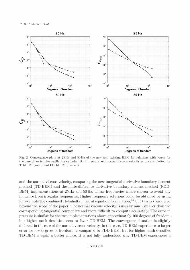
September 17, 2018 10:9 WSPC/S2591-7285 130-JTCA 1850036
P. R. Andersen et al.
Fig. 2. Convergence plots at 25Hz and 50Hz of the new and existing BEM formulations with losses forthe case of an infinite oscillating cylinder. Both pressure and normal viscous velocity errors are plotted forTD-BEM (solid) and FDD-BEM (dashed).
and the normal viscous velocity, comparing the new tangential derivative boundary element
method (TD-BEM) and the finite-difference derivative boundary element method (FDD-
BEM) implementations at 25Hz and 50Hz. These frequencies where chosen to avoid any
influence from irregular frequencies. Higher frequency solutions could be obtained by using
for example the combined Helmholtz integral equation formulation,25 but this is considered
beyond the scope of the paper. The normal viscous velocity is usually much smaller than the
corresponding tangential component and more difficult to compute accurately. The error in
pressure is similar for the two implementations above approximately 100 degrees of freedom,
but higher mesh densities seem to favor TD-BEM. The convergence situation is slightly
different in the case of the normal viscous velocity. In this case, TD-BEM experiences a larger
error for low degrees of freedom, as compared to FDD-BEM, but for higher mesh densities
TD-BEM is again a better choice. It is not fully understood why TD-BEM experiences a
1850036-10
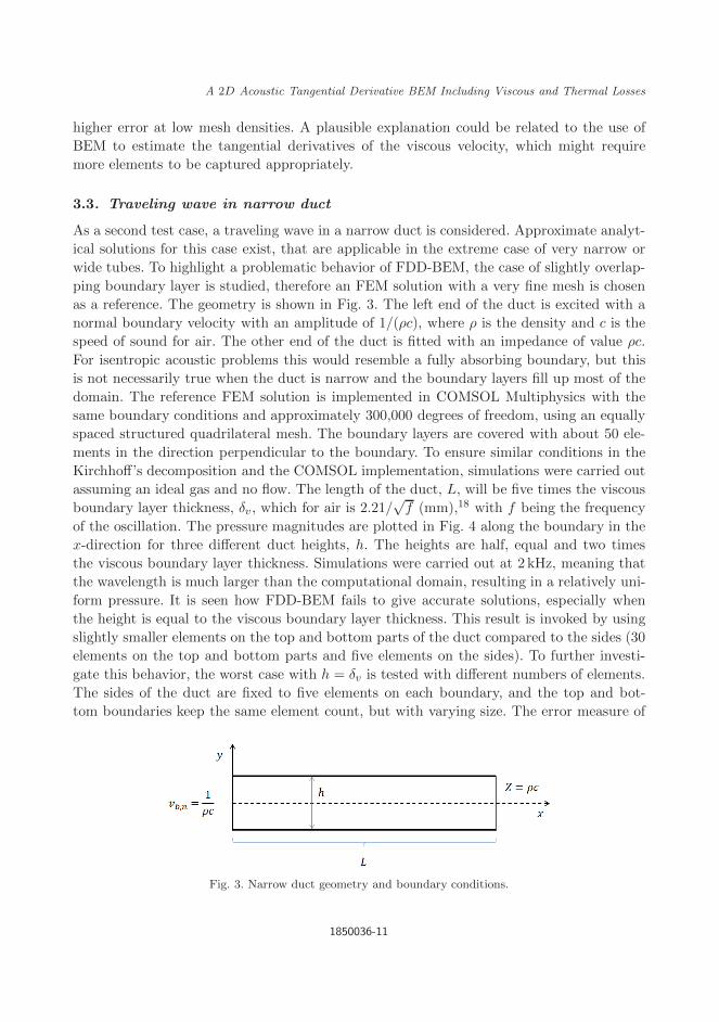
September 17, 2018 10:9 WSPC/S2591-7285 130-JTCA 1850036
A 2D Acoustic Tangential Derivative BEM Including Viscous and Thermal Losses
higher error at low mesh densities. A plausible explanation could be related to the use of
BEM to estimate the tangential derivatives of the viscous velocity, which might require
more elements to be captured appropriately.
3.3. Traveling wave in narrow duct
As a second test case, a traveling wave in a narrow duct is considered. Approximate analyt-
ical solutions for this case exist, that are applicable in the extreme case of very narrow or
wide tubes. To highlight a problematic behavior of FDD-BEM, the case of slightly overlap-
ping boundary layer is studied, therefore an FEM solution with a very fine mesh is chosen
as a reference. The geometry is shown in Fig. 3. The left end of the duct is excited with a
normal boundary velocity with an amplitude of 1/(ρc), where ρ is the density and c is the
speed of sound for air. The other end of the duct is fitted with an impedance of value ρc.
For isentropic acoustic problems this would resemble a fully absorbing boundary, but this
is not necessarily true when the duct is narrow and the boundary layers fill up most of the
domain. The reference FEM solution is implemented in COMSOL Multiphysics with the
same boundary conditions and approximately 300,000 degrees of freedom, using an equally
spaced structured quadrilateral mesh. The boundary layers are covered with about 50 ele-
ments in the direction perpendicular to the boundary. To ensure similar conditions in the
Kirchhoff’s decomposition and the COMSOL implementation, simulations were carried out
assuming an ideal gas and no flow. The length of the duct, L, will be five times the viscous
boundary layer thickness, δv , which for air is 2.21/√f (mm),18 with f being the frequency
of the oscillation. The pressure magnitudes are plotted in Fig. 4 along the boundary in the
x-direction for three different duct heights, h. The heights are half, equal and two times
the viscous boundary layer thickness. Simulations were carried out at 2 kHz, meaning that
the wavelength is much larger than the computational domain, resulting in a relatively uni-
form pressure. It is seen how FDD-BEM fails to give accurate solutions, especially when
the height is equal to the viscous boundary layer thickness. This result is invoked by using
slightly smaller elements on the top and bottom parts of the duct compared to the sides (30
elements on the top and bottom parts and five elements on the sides). To further investi-
gate this behavior, the worst case with h = δv is tested with different numbers of elements.
The sides of the duct are fixed to five elements on each boundary, and the top and bot-
tom boundaries keep the same element count, but with varying size. The error measure of
Fig. 3. Narrow duct geometry and boundary conditions.
1850036-11

September 17, 2018 10:9 WSPC/S2591-7285 130-JTCA 1850036
P. R. Andersen et al.
(a) (b) (c)
Fig. 4. Numerical solution at 2 kHz for narrow duct test case. The pressure magnitudes are plotted as afunction of the x-coordinate of the boundary for FDD-BEM (dashed), viscothermal FEM (dotted), isentropicBEM (crosses) and TD-BEM (solid) simulations. The boundary element formulations use a mesh consistingof five elements on the side and 30 elements on the top and bottom of the duct, while the reference FEMresult is calculated in the FEM software COMSOL Multiphysics using 300,000 degrees of freedom. The plotscorrespond to (a) h = δv/2, (b) h = δv and (c) h = 2δv .
Fig. 5. Comparison of TD-BEM and FDD-BEM in terms of pressure errors in the narrow duct for differentmesh configurations. Simulations are conducted at 2 kHz and the height of the duct is equal to the lengthof one viscous boundary layer.
Eq. (51) is used, but with the FEM solution as a reference. The results are shown in Fig. 5,
where the total number of elements in the geometry is ranging from 30 to 90. Surprisingly,
FDD-BEM shows an initial low error but a rapid error increase followed by a low error at 60
elements, recovering the high error at higher element counts. In the 60-element geometry,
1850036-12

September 17, 2018 10:9 WSPC/S2591-7285 130-JTCA 1850036
A 2D Acoustic Tangential Derivative BEM Including Viscous and Thermal Losses
all elements, including those on the lid, are of equal size. This means that FDD-FEM is
more likely to behave with low errors, for a controlled environment with elements of equal
size. This is also the case for the oscillating infinite cylinder. It appears that FDD-BEM
might result in instability problems if the element sizes are dissimilar and the pressure is
nearly uniform, as seen in the example. On the other hand, the new TD-BEM shows a much
more stable error response to the change in element size.
4. Conclusions
A new approach to the numerical implementation of the coupling of the Kirchhoff’s decom-
position describing the propagation of sound waves with viscous and thermal losses is shown
possible through development of an extra set of tangential boundary element equations. The
new formulation completely removes finite differences as a coupling method. This leads to an
improvement over the previous BEM implementation with losses. The method is compared
to an earlier implementation through a simple convergence study of an infinite cylinder,
showing that for higher element counts the new method can be expected to give slightly
lower errors. Coarser meshes might lead to a larger error in the viscous velocity computation.
In the second example, a narrow duct, the original finite-difference implementation presents
some instability issues, leading to an unwanted behavior when element sizes are different.
On the other hand, the presented new approach shows a much more stable error behavior.
There exists a hope that the new coupling concept can be extended to three dimensions,
where the use of tangential finite-difference derivatives is more cumbersome.
References
1. R. Bossart, N. Joly and M. Bruneau, Methods for numerical modeling of acoustic fields in athermoviscous fluid, in Proc. 6th French Congr. Acoustics (2002), pp. 411–414.
2. M. Malinen, M. Lyly, P. Raback, A. Karkkainen and L. Karkkainen, A finite element method forthe modeling of thermo-viscous effects in acoustics, in Proc. 4th European Congr. ComputationalMethods in Applied and Engineering (2004), pp. 1–12.
3. L. Cheng, R. D. White and K. Grosh, Three-dimensional viscous finite element formulation foracoustic fluid-structure interaction, Comput. Methods Appl. Mech. Eng. 197 (2008) 4160–4172.
4. N. Joly, M. Bruneau and R. Bossart, Coupled equations for particle velocity and temperaturevariation as the fundamental formulation of linear acoustics in thermo-viscous fluids at rest,Acta Acust. United With Acust. 92 (2006) 202–209.
5. W. R. Kampinga, Y. H. Wijnant and A. de Boer, Performance of several viscothermal acousticfinite elements, Acta Acust. United With Acust. 96 (2010) 115–124.
6. W. R. Kampinga, Viscothermal acoustics using finite elements: Analysis tool for engineers, PhDthesis, University of Twente, Enschede (2010).
7. M. Bruneau, Ph. Herzog, J. Kergomard and J. D. Polak, General formulation of the dispersionequation in bounded visco-thermal fluid, and application to some simple geometries, WaveMotion 11 (1988) 441–451.
8. E. Dokumaci, An integral equation formulation for boundary element analysis of acoustic radi-ation problems in viscous fluids, J. Sound Vib. 147 (1991) 335–348.
9. E. Dokumaci, Prediction of the effects of entropy fluctuations on sound radiation from vibratingbodies using an integral equation approach, J. Sound Vib. 186 (1995) 805–819.
1850036-13

September 17, 2018 10:9 WSPC/S2591-7285 130-JTCA 1850036
P. R. Andersen et al.
10. C. Karra and M. Ben Tahar, An integral equation formulation for boundary element analysisof propagation in viscothermal fluids, J. Acoust. Soc. Am. 102 (1997) 1311–1318.
11. V. Cutanda Henrıquez, Numerical transducer modeling, PhD thesis, Technical University ofDenmark, Lyngby (2002).
12. V. Cutanda Henrıquez and P. M. Juhl, An axisymmetric boundary element formulation of soundwave propagation in fluids including viscous and thermal losses, J. Acoust. Soc. Am. 134 (2013)3409–3418.
13. V. Cutanda Henrıquez and P. M. Juhl, Implementation of an acoustic 3D BEM with visco-thermal losses, in Proc. Internoise 2013 : Noise Control for Quality of Life (2013).
14. V. Cutanda Henrıquez and P. M. Juhl, Verification of an acoustic 3D BEM with visco-thermallosses, in Proc. Internoise 2013 : Noise Control for Quality of Life (2013).
15. V. Cutanda Henrıquez, P. R. Andersen, J. S. Jensen, P. M. Juhl and J. Sanchez-Dehesa, Anumerical model of an acoustic metamaterial using the boundary element method includingviscous and thermal losses, J. Comput. Acoust. 25 (2017) 1750006.
16. V. Cutanda Henrıquez, V. M. Garca-Chocano and J. Sanchez-Dehesa, Viscothermal losses indouble-negative acoustic metamaterials, Phys. Rev. Appl. 8 (2017) 014029.
17. P. R. Andersen, V. Cutanda Henrıquez, N. Aage and S. Marburg, Numerical acoustic modelsincluding viscous and thermal losses: Review of existing and new methods, in Proc. DAGA(2017).
18. P. M. Morse and K. U. Ingard, Theoretical Acoustics (McGraw-Hill, 1968).19. A. D. Pierce, Acoustics : An Introduction to Its Physical Principles and Applications (McGraw-
Hill, New York, 1981).20. A. J. Burton and G. F. Miller, The application of integral equation methods to the numerical
solution of some exterior boundary-value problems, Proc. R. Soc. Lond. A 323 (1971) 201–210.21. R. Gallego and A. E. Martınez-Castro, Boundary integral equation for tangential derivative of
flux in Laplace and Helmholtz equations, Int. J. Numer. Methods Eng. 66 (2006) 343–363.22. V. Cutanda Henrıquez, P. M. Juhl and F. Jacobsen, On the modeling of narrow gaps using the
standard boundary element method, J. Acoust. Soc. Am. 109 (2001) 1296–1303.23. L. P. Blinova and V. N. Kozhin, Radiation of a cylinder oscillating in a viscous medium, Izv.
Akad. Nauk SSSR, Mekh. Zirdk. Gaza 5(1) (1970) 121–126 [Fluid Dyn. 5(1) (1970) 107–111].24. S. Marburg and S. Schneider, Influence of element types on numerical error for acoustic boundary
elements, J. Comput. Acoust. 11(3) (2003) 363–386.25. H. A. Schenck, Improved integral formulation for acoustic radiation problems, J. Acoust. Soc.
Am. 44 (1971) 41–58.26. R. A. Beezer, in A First Course in Linear Algebra (Congruent Press, 2010), pp. 900–901.
Appendix A. The Hadamard Product
The Hadamard product (defined by ) is used extensively in the paper. This Appendix
briefly discusses its definition and properties for diagonal matrices. The Hadamard product
is defined as the entry-wise product of two equally sized matrices. If A and B are two m×n
matrices, the Hadamard product is given by
[A B]i,j = [A]i,j[B]i,j, (A.1)
where i and j are the row and column indices, respectively. If D and E are diagonal matrices,
having sizes m × m and n × n, respectively, then one of the properties of the Hadamard
1850036-14
September 17, 2018 10:9 WSPC/S2591-7285 130-JTCA 1850036
A 2D Acoustic Tangential Derivative BEM Including Viscous and Thermal Losses
product is26
D(A B)E = (DAE) B = (DA) (BE), (A.2)
from which it can be deduced that
D1FD2 = (d1dT2 ) F, (A.3)
where D1 and D2 are diagonal matrices of size m×m and F is a matrix of the same size.
In Eq. (A.3), d1 and d2 are m-sized column vectors, created from the diagonals of D1 and
D2, respectively. The relation (A.3) is used several times in the paper.
1850036-15
Paper D
A three-dimensional acoustic Bound-ary Element Method formulationwith viscous and thermal lossesbased on shape function deriva-tives
September 17, 2018 10:20 WSPC/S2591-7285 130-JTCA 1850039
Journal of Theoretical and Computational AcousticsVol. 26, No. 3 (2018) 1850039 (15 pages)c© IMACSDOI: 10.1142/S2591728518500391
A Three-Dimensional Acoustic Boundary ElementMethod Formulation with Viscous and Thermal
Losses Based on Shape Function Derivatives
V. Cutanda Henrıquez∗ and P. Risby Andersen†
Centre for Acoustic-Mechanical Micro SystemsTechnical University of Denmark, Ørsteds PladsBuilding 352, DK-2800, Kgs. Lyngby, Denmark
∗[email protected]†[email protected]
Received 8 January 2018Accepted 26 April 2018
Published 5 September 2018
Sound waves in fluids are subject to viscous and thermal losses, which are particularly relevant in theso-called viscous and thermal boundary layers at the boundaries, with thicknesses in the micrometerrange at audible frequencies. Small devices such as acoustic transducers or hearing aids must thenbe modeled with numerical methods that include losses. In recent years, versions of both the FiniteElement Method (FEM) and the Boundary Element Method (BEM) including viscous and thermallosses have been developed. This paper deals with an improved formulation in three dimensionsof the BEM with losses which avoids the calculation of tangential derivatives on the surface byfinite differences used in a previous BEM implementation. Instead, the tangential derivatives areobtained from the element shape functions. The improved implementation is demonstrated usingan oscillating sphere, where an analytical solution exists, and a condenser microphone as test cases.
Keywords: Boundary element method; viscous and thermal acoustic losses.
1. Introduction
The effect of viscous and thermal losses in sound waves has been described long ago and
is part of the general theory of physical acoustics.1–3 In free-field propagation in the audio
range, such effects are only important over long distances such as in large auditoria, or
outdoor sound propagation. However, they become very relevant at very close distance to
the domain boundaries because (i) air molecules cannot slide over the boundary so that
particle velocity must match boundary velocity in the normal and tangential directions,
and (ii) boundaries usually have such higher thermal conductivity than the fluid, that
temperature variation is negligible at the boundary. The viscous and thermal boundary
layers are generated by these effects, and are usually accounted for as boundary acous-
tic impedance. In the case of small setups with dimensions comparable to the boundary
layer thicknesses, which vary from a fraction of a millimeter to a few micrometers, such
1850039-1

September 17, 2018 10:20 WSPC/S2591-7285 130-JTCA 1850039
V. C. Henrıquez & P. R. Andersen
approximation is not possible, and some other analytical or numerical model is necessary.
Devices of this kind are acoustic transducers, couplers, hearing aids and small-scale acoustic
metamaterials.4–6
For intricate and highly coupled devices, approximate solutions taking limiting hypoth-
esis may not be sufficient for appropriate modeling. They must be tested or even replaced
by full numerical models of the sound field with viscous and thermal losses. On the one
hand, the Finite Element Method (FEM) can be employed for solving the no-flow linearized
Navier–Stokes equations with no further hypotheses.7–10 The FEM implementation with
losses is included in some commercial FEM software packages.11
On the other hand, an equally full implementation with losses uses the Boundary Ele-
ment Method (BEM).12,13 The BEM is applied to the so-called viscous, thermal and acous-
tic modes resulting from the Kirchhoff decomposition of the Navier–Stokes equations.2,3,14
These three modes are coupled at the boundary with extended boundary conditions. The
particle velocity boundary condition in the existing BEM with losses includes first and sec-
ond tangential derivatives of the pressure at the boundary, which use finite differences and,
as will be shown in this paper, can trigger numerical errors. The tangential derivative scheme
is particularly cumbersome in the three-dimensional BEM implementation with losses.13
It is therefore desirable that the BEM with losses can be reformulated in a way that
avoids finite difference intermediate calculations. One possibility is based on setting the
tangential derivative as an initial variable to be solved for and reformulating the integral
equations.15 In this paper, another alternative is presented, which preserves the integral
equations but replaces the finite differences by derivatives of the element shape functions.
The modified implementation is developed for three-dimensional domains and two examples
are used to test its performance.
After this introduction, Sec. 2 outlines the theoretical foundation on which the existing
BEM for acoustics with viscous and thermal losses is based. Section 3 explains the new
method for imposing the particle velocity boundary conditions. As a verification, Sec. 4
presents an oscillating sphere test case where the new formulation is compared with the
previous three-dimensional BEM implementation with losses and an analytical solution.
Section 5 examines the performance of the new and existing formulations with a model of a
condenser microphone. A discussion section comments the results of the tests, followed by
a final section with conclusions and future work.
2. BEM Formulation with Losses
The previously published three-dimensional BEM implementation with losses is described
in detail in Ref. 13. In this section, a short account of it is given with special focus on the
issues that motivate this paper. The physical framework is characterized by:
(∆ + k2a)pa = 0, (1)
(∆ + k2h)ph = 0, (2)
(∆ + k2v)vv = 0 with ∇ · vv = 0. (3)
1850039-2

September 17, 2018 10:20 WSPC/S2591-7285 130-JTCA 1850039
Shape-Function Derivative BEM with Losses
Equations (1)–(3) represent the three modes of the Kirchhoff decomposition of the
Navier–Stokes equations on which the BEM implementation is based.2,14 Harmonic time
dependence eiωt is omitted. The indexes (a, h, v) indicate the so-called acoustic, thermal
and viscous modes, respectively, which can be treated independently in the acoustic domain
and linked through the boundary conditions. The total pressure can be obtained as the
sum p = pa + ph of the acoustic and thermal components (there is not a viscous pv), while
the particle velocity has contributions from the three modes as v = va + vh + vv. In this
paper, magnitudes written with an arrow vector on top are vectorial fields, while bold let-
ters indicate matrices. The three wavenumbers ka, kh and kv are function of the lossless
wavenumber k and the physical properties of the fluid: viscosity, bulk viscosity and thermal
conductivity coefficients, air density, and specific heats.14 Equation (1) is a wave equation,
while Eqs. (2) and (3) are diffusion equations. There are five equations and five unknowns
because the viscous velocity vv is a three-component vector and therefore Eq. (3) is split
into three components. The boundary conditions are:
T = Ta + Th = τapa + τhph = 0, (4)
vboundary = va + vh + vv = φa∇pa + φh∇ph + vv. (5)
Equation (4) states that the temperature T , the sum of its acoustic and thermal compo-
nents Ta and Th, remains constant at the boundary, leading to a condition that links the ther-
mal and acoustic pressures pa and ph. Equation (5) ensures that the total particle velocity,
expressed as the sum of acoustic, thermal and viscous contributions, matches the boundary
velocity in any direction. The parameters τa, τh, φa and φh depend, like the wavenumbers in
Eqs. (1)–(3), on physical constants and the frequency. The velocity equation (5) is a vector
equation, which can be split for convenience into normal and tangential components:
vboundary,n = φa∂pa∂n
+ φh∂ph∂n
+ vv,n, (6)
vboundary,t = φa∇tpa + φh∇tph + vv,t. (7)
Note that Eqs. (1)–(3) are of the same form as the lossless harmonic Helmholtz equation.
The BEM implementation with losses starts by discretizing these three equations indepen-
dently, using the same procedure as in the lossless BEM, that is, converting the Helmholtz
equation into its integral form16,17
C(P )p(P ) =
∫
S
[∂G(Q)
∂np(Q)− ∂p(Q)
∂nG(Q)
]dS + pI(P ), (8)
where p is the sound pressure, G is the Green’s function and P and Q are points in the
domain and on the surface, respectively. C(P ) is a geometrical constant and pI(P ) is the
incident pressure, if present. The boundary is then divided into surface elements and Eq. (8)
is discretized as
Ap−B∂p
∂n+ pI = 0. (9)
1850039-3
September 17, 2018 10:20 WSPC/S2591-7285 130-JTCA 1850039
V. C. Henrıquez & P. R. Andersen
Equation (9) is defined over the boundary. Given a set of boundary conditions, it can
be solved for obtaining the boundary pressure and normal particle velocity. The acoustic
magnitudes in the domain are obtained from the surface solution by re-applying the dis-
cretized Helmholtz Integral Equation.
The harmonic Eqs. (1)–(3) of the Kirchhoff decomposition can be discretized as
Aapa −Ba∂pa
∂n+ pI = 0, (10)
Ahph −Bh∂ph
∂n= 0, (11)
Avvv −Bv∂vv
∂n= 0 with ∇ · vv = 0. (12)
The development in Ref. 13 makes use of coordinate transformations between the node-
based local reference system (normal and tangential vectors n, t1 and t2) and the global
Cartesian reference (x, y, z) to combine Eqs. (10)–(12). The coupling conditions in Eqs. (4)
and (5) and the null divergence of the viscous velocity in Eq. (12) are employed. The
resulting system of equations for obtaining the acoustic component of the pressure on the
boundary is[φaB
−1a Aa − φhB
−1h Ah
τaτh
+ [N11 (B−1v Av)]
−1
(φa −
τaτh
φh
)
×([N12 (B−1
v Av)]∂
∂t1+ [N13 (B−1
v Av)]∂
∂t2+∆t
)]pa
= vboundary,n + [N11 (B−1v Av)]
−1
[[N12 (B−1
v Av)]+
∂
∂t1
]vboundary,t1
+ [N11 (B−1v Av)]
−1
[[N13 (B−1
v Av)] +∂
∂t2
]vboundary,t2 − φaB
−1a pI . (13)
The “” operator in Eq. (13) is the Hadamard matrix product and the constant matrices
N11, N12 and N13 are obtained as
N11 = nxnTx + nyn
Ty + nzn
Tz ,
N12 = nxtT1,x + nyt
T1,y + nzt
T1,z,
N13 = nxtT2,x + nyt
T2,y + nzt
T2,z,
(14)
where the right-hand sides contain products of the (x, y, z) components of the node-based
normal and tangential vectors n, t1 and t2.
Equation (13) relates the prescribed normal and tangential velocities on the boundary
(vboundary,n, vboundary,t1 and vboundary,t2) and the incident pressure pI with the boundary
pressures associated with the acoustic mode pa. After solving this system, it is possible to
derive the remaining magnitudes on the boundary (ph, vv), and on the domain, as described
in Ref. 13.
1850039-4
September 17, 2018 10:20 WSPC/S2591-7285 130-JTCA 1850039
Shape-Function Derivative BEM with Losses
The ∂∂t1
, ∂∂t2
and ∆t operators in Eq. (13) are tangential derivatives and tangential
laplacian, respectively. They are implemented in Ref. 13 as matrices with a finite difference
scheme based on Voronoi cells over nonregular meshes.18,19 This method implies that the
finite difference step size is equivalent to the element dimensions of the boundary mesh. The
implementation described in this section will be termed Finite Difference Derivative BEM
(FDD-BEM).
3. BEM Implementation with Losses Using Shape Function Derivatives
It has been found that the finite difference scheme just described in the previous section
can be detrimental for the performance of the BEM with viscous and thermal losses, as will
be shown in the test case calculations further in this paper. In this section, we propose a
modified implementation that does not include finite differences. It is based on the same set
of equations and coupling conditions in the previous section, but in this case, the tangential
derivatives are adapted from the analytical derivatives of the element shape functions.
In this paper, a direct collocation implementation of the BEM is used.20 The boundary
surface is meshed with isoparametric quadratic triangular elements. Other elements could be
used, providing they are second-order (quadratic) or higher. This ensures that the tangential
derivative approximation is at least first-order (linear).
By using the chain rule derivation, the derivatives of the shape functions with respect to
the local element coordinates can be converted into derivatives with respect to the global
coordinates as21
∂Ni
∂x
∂Ni
∂y
∂Ni
∂z
=
∂x
∂ξ1
∂y
∂ξ1
∂z
∂ξ1
∂x
∂ξ2
∂y
∂ξ2
∂z
∂ξ2
∂x
∂ξ3
∂y
∂ξ3
∂z
∂ξ3
−1
∂Ni
∂ξ1
∂Ni
∂ξ2
∂Ni
∂ξ3
, (15)
where the inverted matrix in the right-hand side is the Jacobian and Ni is a shape function.
The derivatives (∂Ni∂ξ1
, ∂Ni∂ξ2
, ∂Ni∂ξ3
) are obtained analytically. Equation (15) is written for three-
dimensional elements, but it is possible to rewrite it for surface elements in three-dimensional
domains. Surface elements have only two independent local coordinates (ξ1, ξ2), so the last
row of the Jacobian matrix is obtained as the vector product of the first two rows.22 In
our case, the tangential derivatives ( ∂∂t1
, ∂∂t2
) at the nodal positions are needed. The global
(x, y, z) coordinate system is therefore replaced by the node-related local coordinate system
(n, t1, t2) using a linear coordinate change. This procedure is repeated for all shape functions
on every node. We calculate the two tangential derivatives of the viscous velocity vector as
∂vv,x
∂t1=
∑
i
(∂Ni
∂t1vv,x,i
),
∂vv,y
∂t1=
∑
i
(∂Ni
∂t1vv,y,i
),
∂vv,z
∂t1=
∑
i
(∂Ni
∂t1vv,z,i
),
1850039-5

September 17, 2018 10:20 WSPC/S2591-7285 130-JTCA 1850039
V. C. Henrıquez & P. R. Andersen
∂vv,x
∂t2=
∑
i
(∂Ni
∂t2vv,x,i
),
∂vv,y
∂t2=
∑
i
(∂Ni
∂t2vv,y,i
),
∂vv,z
∂t2=
∑
i
(∂Ni
∂t2vv,z,i
),
(16)
where vv,x, vv,y and vv,z are the Cartesian components of the viscous velocity vector. Their
tangential derivatives are expressed as a function of the nodal values vv,x,i, vv,y,i and vv,z,i.
Note that if the elements are continuous, nodes can be shared by several elements. In this
case, the contributions to the tangential derivatives from all elements the node belongs to
are averaged. The tangential derivatives of the acoustic pressure are obtained in the same
way,
∂pa∂t1
=∑
i
(∂Ni
∂t1pa,i
),
∂pa∂t2
=∑
i
(∂Ni
∂t2pa,i
). (17)
The viscous velocity is a rotational vector field; its divergence is zero (∂vv,n
∂n +∂vv,t1∂t1
+∂vv,t2∂t2
= 0). The three terms of this divergence can be expressed as
∂vv,n
∂n= nx (B−1
v Avvv,x) + ny (B−1v Avvv,y) + nz (B−1
v Avvv,z), (18)
∂vv,t1
∂t1= t1,x
∑
i
(∂Ni
∂t1vv,x,i
)+ t1,y
∑
i
(∂Ni
∂t1vv,y,i
)+ t1,z
∑
i
(∂Ni
∂t1vv,z,i
), (19)
∂vv,t2
∂t2= t2,x
∑
i
(∂Ni
∂t2vv,x,i
)+ t2,y
∑
i
(∂Ni
∂t2vv,y,i
)+ t2,z
∑
i
(∂Ni
∂t2vv,z,i
). (20)
Equation (18) is obtained by taking the normal derivative of the coordinate change
vv,n = nx vv,x + ny vv,y + nz vv,z and replacing the three Cartesian components of
Eq. (12). Equations. (19) and (20) are the result of replacing the relations of Eq. (16) in
the tangential derivatives of the remaining coordinate change equations vv,t1 = t1,x vv,x +
t1,y vv,y + t1,z vv,z and vv,t2 = t2,x vv,x + t2,y vv,y + t2,z vv,z.
Using the properties of the Hadamard operator “”, Eqs. (18)–(20) can be rearranged as
∂vv,n
∂n= [(nxI) (B−1
v Av)]vv,x + [(nyI) (B−1v Av)]vv,y + [(nzI) (B−1
v Av)]vv,z , (21)
∂vv,t1
∂t1= [(t1,xI) Dt1 ]vv,x + [(t1,yI) Dt1 ]vv,y + [(t1,zI) Dt1 ]vv,z , (22)
∂vv,t2
∂t2= [(t2,xI) Dt2 ]vv,x + [(t2,yI) Dt2 ]vv,y + [(t2,zI) Dt2 ]vv,z , (23)
whereDt1 andDt2 are matrices implementing the tangential derivatives and I is the identity
matrix. We may also impose the no-slip condition Eq. (7) by using Eq. (17). After some
1850039-6
September 17, 2018 10:20 WSPC/S2591-7285 130-JTCA 1850039
Shape-Function Derivative BEM with Losses
manipulation, it becomes
vboundary,t1 =
[(φa −
τaτh
φh
)Dt1
]pa + (t1,xI)vv,x + (t1,yI)vv,y + (t1,zI)vv,z, (24)
vboundary,t2 =
[(φa −
τaτh
φh
)Dt2
]pa + (t2,xI)vv,x + (t2,yI)vv,y + (t2,zI)vv,z. (25)
Finally, the normal velocity coupling condition Eq. (6) can be arranged as
vboundary,n =
[φaB
−1a Aa − φhB
−1h Ah
τaτh
]pa + (nxI)vv,x + (nyI)vv,y
+(nzI)vv,z + φaB−1a pI . (26)
The preceding equations are combined into a system of equations of the form
Normal velocity coupling, Eq. (26)
Null divergence of vv, Eqs. (21)–(23)
No-slip condition t1, Eq. (24)
No-slip condition t2, Eq. (25)
pa
vv,x
vv,y
vv,z
=
vboundary,n − φaB−1a pI
0
vboundary,t1
vboundary,t2
. (27)
Note that the system in Eq. (27) has four sets of unknowns, pa, vv,x, vv,y and vv,z,
while the original system in Eq. (13) is solved for pa alone. This means that a coefficient
matrix that is 4×4 times larger avoids the need of a second-order tangential derivative. The
system is solved, as for FDD-BEM, using the Matlab backslash operator. The expanded
coefficient matrix is not fully populated: in the sphere test case, only about 1/3 of the
matrix coefficients in Eq. (27) are nonzero. The solving could be made more efficient by
making use of sparsity, e.g. by using dedicated solvers.
From the solution of Eq. (27), it is possible to obtain all other magnitudes on the
boundary and the domain using the procedure described in Ref. 13. This new version of the
BEM with losses will be called Shape Function Derivative BEM (SFD-BEM).
In order to evaluate independently the effect of using shape function derivatives and the
expanded system of equations of Eq. (27), a combined version of the two methods is also
employed. It is named FDD2-BEM, and it uses the finite difference tangential derivatives
from Sec. 2 into Eq. (27).
4. Oscillating Sphere Test Case
The performance of the SFD-BEM against the FDD-BEM is studied using a test case con-
taining losses: a sphere with a radius of 1m that radiates sound by oscillating as a whole
with a velocity of 10−2 m/sec along the z-axis. Only the results at the boundary are calcu-
lated; domain results are possible, but less suitable for the purpose of this study. This test
case has an analytical solution and has been previously used for testing the axisymmetrical
1850039-7
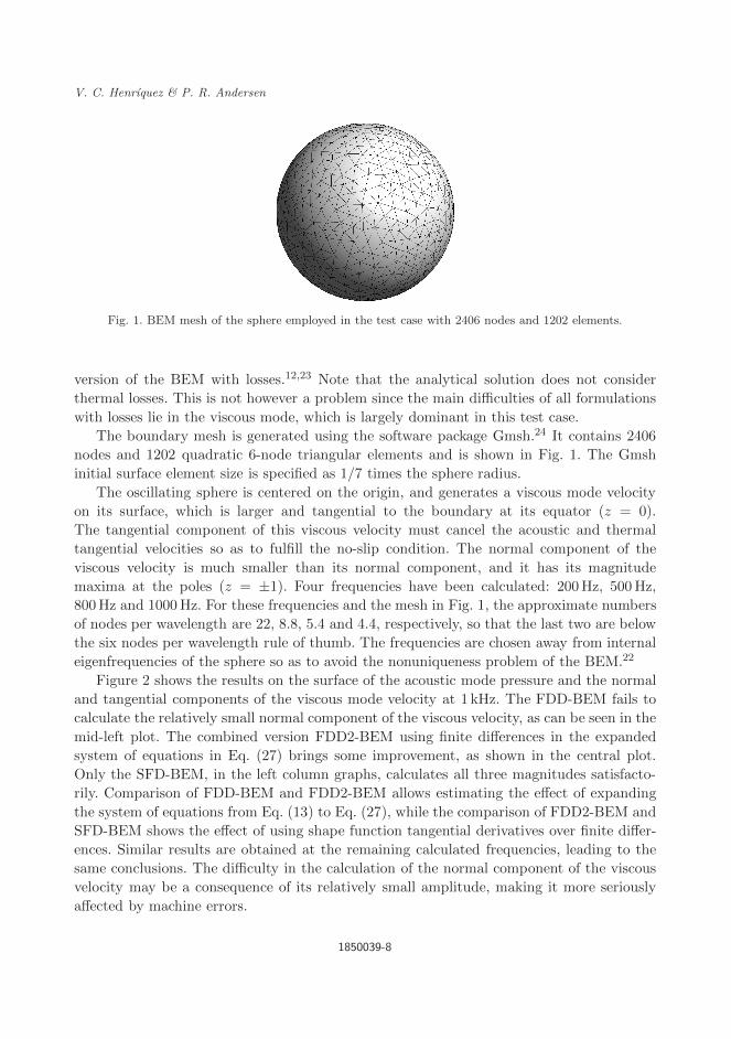
September 17, 2018 10:20 WSPC/S2591-7285 130-JTCA 1850039
V. C. Henrıquez & P. R. Andersen
Fig. 1. BEM mesh of the sphere employed in the test case with 2406 nodes and 1202 elements.
version of the BEM with losses.12,23 Note that the analytical solution does not consider
thermal losses. This is not however a problem since the main difficulties of all formulations
with losses lie in the viscous mode, which is largely dominant in this test case.
The boundary mesh is generated using the software package Gmsh.24 It contains 2406
nodes and 1202 quadratic 6-node triangular elements and is shown in Fig. 1. The Gmsh
initial surface element size is specified as 1/7 times the sphere radius.
The oscillating sphere is centered on the origin, and generates a viscous mode velocity
on its surface, which is larger and tangential to the boundary at its equator (z = 0).
The tangential component of this viscous velocity must cancel the acoustic and thermal
tangential velocities so as to fulfill the no-slip condition. The normal component of the
viscous velocity is much smaller than its normal component, and it has its magnitude
maxima at the poles (z = ±1). Four frequencies have been calculated: 200Hz, 500Hz,
800Hz and 1000Hz. For these frequencies and the mesh in Fig. 1, the approximate numbers
of nodes per wavelength are 22, 8.8, 5.4 and 4.4, respectively, so that the last two are below
the six nodes per wavelength rule of thumb. The frequencies are chosen away from internal
eigenfrequencies of the sphere so as to avoid the nonuniqueness problem of the BEM.22
Figure 2 shows the results on the surface of the acoustic mode pressure and the normal
and tangential components of the viscous mode velocity at 1 kHz. The FDD-BEM fails to
calculate the relatively small normal component of the viscous velocity, as can be seen in the
mid-left plot. The combined version FDD2-BEM using finite differences in the expanded
system of equations in Eq. (27) brings some improvement, as shown in the central plot.
Only the SFD-BEM, in the left column graphs, calculates all three magnitudes satisfacto-
rily. Comparison of FDD-BEM and FDD2-BEM allows estimating the effect of expanding
the system of equations from Eq. (13) to Eq. (27), while the comparison of FDD2-BEM and
SFD-BEM shows the effect of using shape function tangential derivatives over finite differ-
ences. Similar results are obtained at the remaining calculated frequencies, leading to the
same conclusions. The difficulty in the calculation of the normal component of the viscous
velocity may be a consequence of its relatively small amplitude, making it more seriously
affected by machine errors.
1850039-8

September 17, 2018 10:20 WSPC/S2591-7285 130-JTCA 1850039
Shape-Function Derivative BEM with Losses
Fig. 2. Solution on the surface over an arc from pole to pole (from z = 1 to z = −1) of an oscillating sphere,at 1 kHz. The plots on the left column are calculated using the existing FDD-BEM, the plots in the centralcolumn use the FDD2-BEM (finite differences combined with Eq. (27)), and the plots on the right columncome from the new SFD-BEM. The values are all real parts of the indicated magnitudes. The underlyingsolid line is the analytical solution, and the dots are BEM results on the mesh nodes. Note the differentscales on the normal viscous velocity plots.
Figure 3 examines the relative error for the three formulations (FDD-BEM, SFD-BEM
and the combined FDD2-BEM) at four different frequencies. In order to avoid difficulties
when the solution is close to zero, the error measure is made relative to the maximum
absolute value of the analytical solution over the geometry as
Error =∑
i
|Analyticali − Calculatedi||max(Analytical)| . (28)
The ideal expected behavior of the errors would be a steady increase as the frequency
grows and the mesh is kept constant.
1850039-9
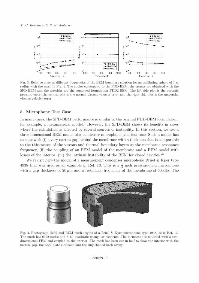
September 17, 2018 10:20 WSPC/S2591-7285 130-JTCA 1850039
V. C. Henrıquez & P. R. Andersen
Fig. 3. Relative error at different frequencies of the BEM boundary solution for an oscillating sphere of 1 mradius with the mesh in Fig. 1. The circles correspond to the FDD-BEM, the crosses are obtained with theSFD-BEM and the asterisks are the combined formulation FDD2-BEM. The left-side plot is the acousticpressure error, the central plot is the normal viscous velocity error and the right-side plot is the tangentialviscous velocity error.
5. Microphone Test Case
In many cases, the SFD-BEM performance is similar to the original FDD-BEM formulation,
for example, a metamaterial model.6 However, the SFD-BEM shows its benefits in cases
where the calculation is affected by several sources of instability. In this section, we use a
three-dimensional BEM model of a condenser microphone as a test case. Such a model has
to cope with (i) a very narrow gap behind the membrane with a thickness that is comparable
to the thicknesses of the viscous and thermal boundary layers at the membrane resonance
frequency, (ii) the coupling of an FEM model of the membrane and a BEM model with
losses of the interior, (iii) the intrinsic instability of the BEM for closed cavities.25
We revisit here the model of a measurement condenser microphone Bruel & Kjær type
4938 that was used as an example in Ref. 13. This is a 14 inch pressure-field microphone
with a gap thickness of 20µm and a resonance frequency of the membrane of 60 kHz. The
Fig. 4. Photograph (left) and BEM mesh (right) of a Bruel & Kjær microphone type 4938, as in Ref. 13.The mesh has 6322 nodes and 3160 quadratic triangular elements. The membrane is modeled with a two-dimensional FEM and coupled to the interior. The mesh has been cut in half to show the interior with thenarrow gap, the back plate electrode and the ring-shaped back cavity.
1850039-10

September 17, 2018 10:20 WSPC/S2591-7285 130-JTCA 1850039
Shape-Function Derivative BEM with Losses
Fig. 5. Normalized sensitivity response with actuator excitation of a Bruel & Kjær microphone type 4938.The dotted lines represent the upper and lower bounds of the measured sensitivities of 183 microphone units.The circles correspond to the FDD-BEM, the crosses are obtained with the SFD-BEM and the asterisks arethe combined formulation FDD2-BEM.
microphone and the corresponding BEM mesh are represented in Fig. 4. The interior of
the microphone is modeled using BEM with losses, and coupled to a membrane, which is
modeled with a two-dimensional FEM, also written for this purpose. The excitation is made
to resemble an electrostatic actuator measurement of the microphone sensitivity response by
setting a uniform sound pressure over the membrane. In Ref. 13, a node in the back cavity
(vent node) was given a finite impedance to stabilize the calculation. We have removed the
vent node and recalculated this microphone using SFD-BEM, FDD-BEM and FDD2-BEM
in the frequency range around the membrane resonance. The result is shown in Fig. 5. Note
that it is not possible to match the model with particular measurement results, given the
uncertainties in the model input parameters.
6. Discussion
The three formulations analyzed in this paper, the existing FDD-BEM, the new SFD-BEM
and the combined FDD2-BEM are studied through two test cases, an oscillating sphere
where an analytical solution exists and a measurement condenser microphone.
6.1. Oscillating sphere test case
In view of the results in Figs. 2 and 3, we can make the following observations:
(1) The SFD-BEM consistently produces smaller errors than the other two formulations
for the three magnitudes examined, as shown in Fig. 3.
1850039-11

September 17, 2018 10:20 WSPC/S2591-7285 130-JTCA 1850039
V. C. Henrıquez & P. R. Andersen
(2) As expected from the observation of Fig. 2, the errors in the calculation of the normal
component of the viscous velocity are greater in the case of FDD-BEM, followed by
FDD2-BEM and SFD-BEM.
(3) Again in Fig. 3 (right-side plot), the FDD-BEM and FDD2-BEM have errors of the tan-
gential component of the viscous velocity that actually decrease as frequency increases,
the reason probably being that finite differences have larger numerical errors as the
wavelength grows and the difference is closer to the machine precision, counterbalanc-
ing the error reduction due to a better discretization.
(4) In the calculation of the tangential component of the viscous velocity and the pres-
sure, FDD-BEM shows smaller errors than FDD2-BEM, indicating that the use of the
expanded system of equations in Eq. (27) comes with some cost.
(5) The SFD-BEM has a larger error (yet below 1%) for the normal component of the
viscous velocity than for the other two magnitudes. As pointed out in Sec. 4, its relatively
lower amplitude may be an explanation, together with the fact that the shape function
derivatives follow a linear approximation rather than quadratic.
The error behavior of the three shown magnitudes is different as a result of the involved
calculation process. Only the acoustic pressure, which is the first obtained result in all
formulations, has an error that grows with the frequency. All in all, the results shown in
Figs. 2 and 3 indicate that the expansion of the system of equations (Eq. (27)) and the
new strategy using shape functions for the tangential derivatives are advantageous over the
other strategies when combined into the SFD-BEM.
6.2. Condenser microphone test case
Condenser microphones rely on the viscous and thermal losses in the gap between membrane
and back electrode for the correct damping of the membrane resonance: a model with losses
is necessary. As mentioned in Sec. 5, the BEM, unlike FEM, becomes unstable for closed
interior domains, particularly at mid-low frequencies where the interior pressure tends to
be uniform.25 This problem affects the BEM with or without losses. We have experienced
this issue as a source of instability in all closed microphone models, and we have dealt
with it in previous publications by adding a finite impedance to one of the nodes in the
back cavity, resembling the vent all condenser measurement microphones have. We are
working on more fundamental solutions to this flaw of the BEM, since the vent node just
forces the pressure to vary in the back cavity without addressing the intrinsic instability of
the BEM.
The model should be able to run without a vent node, but the fact is that its removal
makes the BEM calculation more prone to instability, as the results presented here confirm.
The formulations that are based on finite differences have difficulties to overcome the insta-
bility, and this manifests as a system of equations that is close to being singular. In the
case of the FDD-BEM, the Matlab solver is just able to cope with the solution, however
issuing warnings on the unreliability of the solution. The expanded system, Eq. (27), in the
FDD2-BEM adds some extra difficulty that makes the solver fail; this is compatible with
1850039-12

September 17, 2018 10:20 WSPC/S2591-7285 130-JTCA 1850039
Shape-Function Derivative BEM with Losses
the observation made in item (4) in Sec. 6.1, about the oscillating sphere results. The solver
has no difficulty with the new SFD-BEM, which shows to be more stable and succeeds in
providing a solution despite using the expanded system of equations in Eq. (27).
7. Conclusions and Future Work
A modified implementation of the BEM for acoustic waves with viscous and thermal losses is
presented in this paper. The technique based in two-dimensional finite differences employed
in the previous version13 of BEM with losses is replaced by analytical derivatives of the
element shape functions, thus simplifying the implementation and making it less prone to
errors. This is demonstrated through two test cases: an oscillating sphere, which shows a
clear improvement for the same mesh density, and a condenser microphone model, where
the intrinsic instability of the setup threatens the solution when finite difference tangential
derivatives are used. The new shape function tangential derivatives perform well in both
test cases.
The benefits of the technique come with some drawbacks. The coefficient matrix of the
system of equations is 4 × 4 times larger, since it must be expanded from one to four sets
of unknowns. However, obtaining the six coefficient matrices for the three visco-thermal
modes in Eqs. (10)–(12) takes most of the calculation effort and this is the same for both
formulations. Another issue is the need for the order of the elements to be sufficient for a
good representation of the tangential derivatives, which are one order lower than the shape
functions. The quadratic elements employed lead to a linear representation of the derived
magnitudes.
The formulation presented here is defined in three dimensions. BEM formulations with
losses, based on finite differences, also exist for two-dimensional and axisymmetric prob-
lems.12,26 The shape function derivative technique has not been thoroughly tested in these
cases. However, considering that the one-dimensional finite difference scheme employed in
two-dimensional and axisymmetric implementations is much more straightforward and pre-
cise in these cases, less benefit is expected.
A possible future refinement of the technique is the use of discontinuous elements, where
element nodes are not shared.27–29 The shape function derivative formulation takes an
average of the contributions to normal vectors and tangential derivatives from all the ele-
ments a node belongs to; this would be avoided by using discontinuous elements, and may
lead to even better performance. Another possible improvement is the use of elements of
higher orders than quadratic, which would improve the representation of the tangential
derivative.
References
1. J. W. S. Rayleigh, The Theory of Sound, 2nd edn. (Dover, New York, 1945).2. A. D. Pierce, Acoustics : An Introduction to its Physical Principles and Applications, Chap. 10
(McGraw-Hill, New York, 1981).3. P. M. Morse and K. U. Ingard, Theoretical Acoustics (McGraw-Hill, Princeton, 1968).
1850039-13
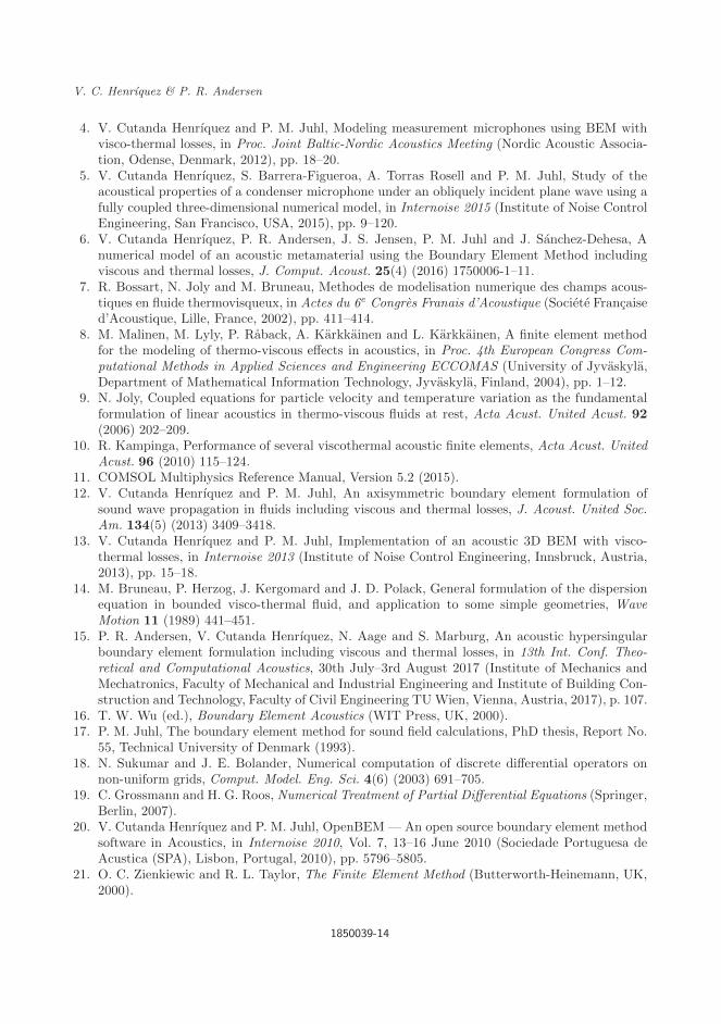
September 17, 2018 10:20 WSPC/S2591-7285 130-JTCA 1850039
V. C. Henrıquez & P. R. Andersen
4. V. Cutanda Henrıquez and P. M. Juhl, Modeling measurement microphones using BEM withvisco-thermal losses, in Proc. Joint Baltic-Nordic Acoustics Meeting (Nordic Acoustic Associa-tion, Odense, Denmark, 2012), pp. 18–20.
5. V. Cutanda Henrıquez, S. Barrera-Figueroa, A. Torras Rosell and P. M. Juhl, Study of theacoustical properties of a condenser microphone under an obliquely incident plane wave using afully coupled three-dimensional numerical model, in Internoise 2015 (Institute of Noise ControlEngineering, San Francisco, USA, 2015), pp. 9–120.
6. V. Cutanda Henrıquez, P. R. Andersen, J. S. Jensen, P. M. Juhl and J. Sanchez-Dehesa, Anumerical model of an acoustic metamaterial using the Boundary Element Method includingviscous and thermal losses, J. Comput. Acoust. 25(4) (2016) 1750006-1–11.
7. R. Bossart, N. Joly and M. Bruneau, Methodes de modelisation numerique des champs acous-tiques en fluide thermovisqueux, in Actes du 6e Congres Franais d’Acoustique (Societe Francaised’Acoustique, Lille, France, 2002), pp. 411–414.
8. M. Malinen, M. Lyly, P. Raback, A. Karkkainen and L. Karkkainen, A finite element methodfor the modeling of thermo-viscous effects in acoustics, in Proc. 4th European Congress Com-putational Methods in Applied Sciences and Engineering ECCOMAS (University of Jyvaskyla,Department of Mathematical Information Technology, Jyvaskyla, Finland, 2004), pp. 1–12.
9. N. Joly, Coupled equations for particle velocity and temperature variation as the fundamentalformulation of linear acoustics in thermo-viscous fluids at rest, Acta Acust. United Acust. 92(2006) 202–209.
10. R. Kampinga, Performance of several viscothermal acoustic finite elements, Acta Acust. UnitedAcust. 96 (2010) 115–124.
11. COMSOL Multiphysics Reference Manual, Version 5.2 (2015).12. V. Cutanda Henrıquez and P. M. Juhl, An axisymmetric boundary element formulation of
sound wave propagation in fluids including viscous and thermal losses, J. Acoust. United Soc.Am. 134(5) (2013) 3409–3418.
13. V. Cutanda Henrıquez and P. M. Juhl, Implementation of an acoustic 3D BEM with visco-thermal losses, in Internoise 2013 (Institute of Noise Control Engineering, Innsbruck, Austria,2013), pp. 15–18.
14. M. Bruneau, P. Herzog, J. Kergomard and J. D. Polack, General formulation of the dispersionequation in bounded visco-thermal fluid, and application to some simple geometries, WaveMotion 11 (1989) 441–451.
15. P. R. Andersen, V. Cutanda Henrıquez, N. Aage and S. Marburg, An acoustic hypersingularboundary element formulation including viscous and thermal losses, in 13th Int. Conf. Theo-retical and Computational Acoustics, 30th July–3rd August 2017 (Institute of Mechanics andMechatronics, Faculty of Mechanical and Industrial Engineering and Institute of Building Con-struction and Technology, Faculty of Civil Engineering TUWien, Vienna, Austria, 2017), p. 107.
16. T. W. Wu (ed.), Boundary Element Acoustics (WIT Press, UK, 2000).17. P. M. Juhl, The boundary element method for sound field calculations, PhD thesis, Report No.
55, Technical University of Denmark (1993).18. N. Sukumar and J. E. Bolander, Numerical computation of discrete differential operators on
non-uniform grids, Comput. Model. Eng. Sci. 4(6) (2003) 691–705.19. C. Grossmann and H. G. Roos, Numerical Treatment of Partial Differential Equations (Springer,
Berlin, 2007).20. V. Cutanda Henrıquez and P. M. Juhl, OpenBEM — An open source boundary element method
software in Acoustics, in Internoise 2010, Vol. 7, 13–16 June 2010 (Sociedade Portuguesa deAcustica (SPA), Lisbon, Portugal, 2010), pp. 5796–5805.
21. O. C. Zienkiewic and R. L. Taylor, The Finite Element Method (Butterworth-Heinemann, UK,2000).
1850039-14
September 17, 2018 10:20 WSPC/S2591-7285 130-JTCA 1850039
Shape-Function Derivative BEM with Losses
22. N. Atalla and F. Sgard, Finite Element and Boundary Methods in Structural Acoustics andVibration (CRC Press, Boca Raton, 2015).
23. S. Temkin, Elements of Acoustics (Wiley, New York, 1981).24. C. Geuzaine and J.-F. Remacle, Gmsh: A three-dimensional finite element mesh generator with
built-in pre- and post-processing facilities, Int. J. Numer. Methods Eng. 79(11) (2009) 1309–1331.
25. S. Sorokin and S. T. Christensen, Low-frequency breakdown of boundary element formulationfor closed cavities in excitation conditions with a ‘breathing’-type component, Commun. Numer.Methods Eng. 16 (2000) 325–334.
26. P. R. Andersen, V. Cutanda Henrıquez, N. Aage and S. Marburg, Numerical acoustic modelsincluding viscous and thermal losses: Review of existing and new methods, in Proc. DAGA 2017(Deutsche Gesellschaft fr Akustik e.V, Germany, 2017), pp. 1–4.
27. S. Marburg and S. Schneider, Influence of element types on numerical error for acoustic boundaryelements, J. Comput. Acoust. 11(3) (2003) 363–386.
28. L. Chen, H. Chen, C. Zheng and S. Marburg, Structural-acoustic sensitivity analysis of radiatedsound power using a finite element/discontinuous fast multipole boundary element scheme, Int.J. Numer. Methods Fluids 82(12) (2016) 858–878.
29. L. Chen, S. Marburg, H. Chen, H. Zhang and H. Gao, An adjoint operator approach for sensi-tivity analysis of radiated sound power in fully coupled structural-acoustic systems, J. Comput.Acoust. 25(1) (2017) 1750003.
1850039-15
Paper E
Shape optimization of micro-acousticdevices including viscous and ther-mal losses
Shape optimization of micro-acoustic devices includingviscous and thermal losses
Peter Risby Andersena,b,∗, Vicente Cutanda Henrıqueza,b, Niels Aagea,c
aCentre for Acoustic-Mechanical Micro Systems, Technical University of DenmarkØrsteds Plads, Building 352, DK-2800, Kgs. Lyngby, Denmark
bDepartment of Electrical EngineeringcDepartment of Mechanical Engineering
Abstract
Since the late 1980s, numerical acoustic shape optimization has been applied
successfully to improve the design and development of novel acoustic devices.
Most often, viscous and thermal dissipation effects are neglected in the opti-
mization process, as this is an acceptable assumption in e.g. room acoustics,
etc. However, in many acoustic devices, ranging from hearing aids to metamate-
rials, dissipation can significantly influence the acoustic wave behavior. In this
paper, we propose a numerical acoustic shape optimization technique and we
demonstrate it using two-dimensional quarter-wave and Helmholtz resonators
including accurate modelling of viscous and thermal dissipation. By combin-
ing a dissipative boundary element method with shape optimization, the sound
absorption capability of the resonators located at an impedance tube termi-
nation is maximized. Numerical experiments demonstrate the importance of
viscothermal dissipation and its impact on the optimization outcome. The re-
sulting resonator shapes, optimized using a lossy assumption, yield significantly
better performance compared to their lossless counterpart, with near perfect
absorption at the desired optimization frequencies.
Keywords: acoustics, shape optimization, viscothermal losses, boundary
element method
∗Corresponding authorEmail addresses: [email protected] (Peter Risby Andersen),
[email protected] (Vicente Cutanda Henrıquez), [email protected] (Niels Aage)
Preprint submitted to Journal of LATEX Templates August 28, 2018

1. Introduction
Accurate modelling of acoustic devices with small dimensions requires the
inclusion of viscous and thermal dissipative effects. The dissipative effects are
especially dominant near boundaries, within the viscous and thermal boundary
layers, which are in the order of 550-15 µm for air in the audible range. There-5
fore, as the size of the acoustic domain decreases, the portion of the domain
covered by the boundary layers increases, leading to changes in acoustic wave
propagation. This situation is very common in small acoustic devices, such as
hearing aids, acoustic MEMS devices and condenser microphones, where the di-
mensions are comparable to the thickness of the boundary layers. In such cases,10
correct modelling of acoustic dissipation is necessary, making the assumption
of isentropic wave propagation insufficient[1, 2, 3, 4, 5]. The same phenom-
ena is also observed in acoustic transducers such as compression drivers where
the response is influenced by dissipation, due to narrow channels and chambers
[6, 7, 8].15
Even within the field of room acoustics, micro structures have found their
everyday use. For example, the performance of absorbing panels, realized using
micro-perforated plates, quarter-wave or Helmholtz resonators, is often very
dependent on viscothermal dissipative effects[9, 10].
Another research field that has received attention in recent years is acoustic20
metamaterials, where unusual bulk behavior and extraordinary wave propaga-
tion effects can be achieved[11, 12]. Recent research has shown that ignoring
losses in the design of metamaterials may lead to a degraded behaviour[13, 14].
Other publications propose metamaterial designs which take advantage of vis-
cothermal dissipation[15, 16].25
Numerical shape and topology optimization have proven to be valuable tools
in the discovery of new and better acoustic designs. In the literature, several
numerical acoustic optimization approaches exist, making use of either the Fi-
nite Element Method (FEM) or the Boundary Element Method (BEM). Es-
2
pecially, optimization of acoustic horns is well studied [17, 18, 19]. Most of30
these acoustic optimization procedures are based on an isentropic assumption.
However, if the influence of viscous and thermal losses is significant, such op-
timizations might lead to poorly performing designs. In a recent publication,
Christensen [20] proposed a method for acoustic FEM topology optimization
including viscothermal losses. By applying the so-called low reduced frequency35
approximation, the author shows how to optimize the cross section of tubes
and slits. While topology optimization has certain advantages compared to,
e.g., shape optimization, sometimes yielding non-intuitive designs, viscothermal
topology optimization requires a mesh that can resolve the boundary layers in
the entire design region. This significantly increases the computational load and40
as a consequence heavily limits the application to full 3D models.
Efficient and reliable optimization tools that include viscothermal losses can
be very beneficial in the design of acoustic devices where losses are relevant,
such as those mentioned earlier in the introduction. In this work, we propose a
shape optimization technique based on BEM and demonstrate it by designing45
an anechoic termination of a two-dimensional wave-guide by using quarter-wave
and Helmholtz resonators. The absorbing properties of the resonators are op-
timized, showing how viscous and thermal dissipation alters the final layout
of the design. Shape optimization is conducted using a BEM implementation
incorporating both viscous and thermal dissipation without any simplification50
other than linearity and absence of flow. BEM with losses only requires dis-
cretization of the boundaries, thus avoiding the adaptation of the domain mesh
and boundary layer meshing, making it very suitable for shape optimization.
The proposed method has no restrictions to the geometry and can be applied
to any viscothermal acoustic problem. The paper is organized as follows; firstly,55
BEM with losses and the optimization approach are introduced. This is followed
by a series of simulations investigating shape optimization of quarter-wave and
Helmholtz resonators. Finally, the possibilities and limitations of the proposed
methodology are discussed.
3

2. Boundary Element Method with losses60
Numerical modelling of acoustic losses using e.g. FEM, the Finite Difference
Method or the Finite Volume Method, is usually realized by discretization of
the linearized time-harmonic Navier-Stokes equations [21]. BEM with losses
requires a further reformulation of linearized Navier-Stokes equations using the
Kirchhoff decomposition[1, 2], resulting in an equation-set given by [22]
∆pa + k2apa = 0 (1)
∆ph + k2hph = 0 (2)
∆~vv + k2v~vv = ~0 with ∇ · ~vv = 0 (3)
which consists of three separate equations with the unknown variables being the
acoustic pressure pa, the thermal pressure ph and the viscous velocity ~vv. Simi-
larly, ka, kh and kv are the acoustic, thermal and viscous complex wavenumbers,
respectively. Eqs. (1-3) are formally equal to the Helmholtz equation. The Kir-
choff decomposition is convenient because each of the equations can easily be
transformed into integral from, so that
C(P )pa(P ) =
∫
Γ
∂G(R)
∂n(Q)pa(Q)dΓ−
∫
Γ
G(R)∂pa(Q)
∂n(Q)dΓ (4)
C(P )ph(P ) =
∫
Γ
∂G(R)
∂n(Q)ph(Q)dΓ−
∫
Γ
G(R)∂ph(Q)
∂n(Q)dΓ (5)
C(P )vv,x(P ) =
∫
Γ
∂G(R)
∂n(Q)vv,x(Q)dΓ−
∫
Γ
G(R)∂vv,x(Q)
∂n(Q)dΓ (6)
C(P )vv,y(P ) =
∫
Γ
∂G(R)
∂n(Q)vv,y(Q)dΓ−
∫
Γ
G(R)∂vv,y(Q)
∂n(Q)dΓ (7)
with C(P ) being the integral-free term, P is the collocation point, Q is an
integration point on the generator, R = |Q − P | is the distance between P
and Q and G is the fundamental solution in two dimensions. In this case we
assume two-dimensional domain, and the viscous velocity ~vv is split into its
two Cartesian components vv,x and vv,y. Eqs. (4)-(7) can then be discretized
and coupled at the boundary by applying a no-slip and an isothermal boundary
4
condition[23]
~vb = φa∇pa + φh∇ph + ~vv (8)
T = τapa + τhph ' 0 (9)
where φa, φh, τa and τh are complex constants, derived from the physical quanti-
ties: the static density, the speed of sound, the ratio of specific heats at constant
pressure, the thermal conductivity, the coefficient of viscosity, the bulk viscosity
and the frequency. T is the temperature perturbation at the boundary and ~vb is
the boundary velocity. The total pressure perturbation is the sum of the acous-
tic and thermal pressures. After coupling and discretization, the final linear
system has the form
S
pa
vv,x
vv,y
=
vb,n
0
vb,t
. (10)
The small bold letters represent the discretized variables and the subindices n
and t indicate the boundary normal and tangential components. The matrix
S is the system matrix assembled according to the method found in Ref. [24],
with the assumption of two dimensions. Note that ph has been eliminated from
the final system by a Schur complement operation.65
Because the optimization approach introduced in the following sections re-
quires repeated function evaluations, code efficiency is important. Therefore, as-
sembly of the BEM matrix is carried out using a compiled MATLABR© MEX/C++
framework, inspired by the BEM software OpenBEM [25]. The C++ implemen-
tation has proven to be an order of magnitude faster as compared to the pure70
MATLABR© OpenBEM code, thus improving the efficiency and usability of the
proposed optimization approach.
Additionally, it is possible to take advantage of the sparse nature of the
viscous and thermal matrices (the matrices assembled by discretization of Eqs.
(5)-(7)). An increase of the computational speed is gained by only performing75
integration when the distance between P and Q is less than twenty times the
boundary layer thickness, or if P and Q are located on the same element. This
5
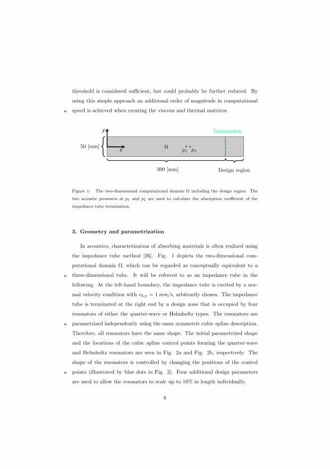
threshold is considered sufficient, but could probably be further reduced. By
using this simple approach an additional order of magnitude in computational
speed is achieved when creating the viscous and thermal matrices.80
Design regionDesign region
Termination
p2p1
300 [mm]
50 [mm]
Figure 1: The two-dimensional computational domain Ω including the design region. The
two acoustic pressures at p1 and p2 are used to calculate the absorption coefficient of the
impedance tube termination.
3. Geometry and parametrization
In acoustics, characterization of absorbing materials is often realized using
the impedance tube method [26]. Fig. 1 depicts the two-dimensional com-
putational domain Ω, which can be regarded as conceptually equivalent to a
three-dimensional tube. It will be referred to as an impedance tube in the85
following. At the left-hand boundary, the impedance tube is excited by a nor-
mal velocity condition with vb,n = 1mm/s, arbitrarily chosen. The impedance
tube is terminated at the right end by a design zone that is occupied by four
resonators of either the quarter-wave or Helmholtz types. The resonators are
parametrized independently using the same symmetric cubic spline description.90
Therefore, all resonators have the same shape. The initial parametrized shape
and the locations of the cubic spline control points forming the quarter-wave
and Helmholtz resonators are seen in Fig. 2a and Fig. 2b, respectively. The
shape of the resonators is controlled by changing the positions of the control
points (illustrated by blue dots in Fig. 2). Four additional design parameters95
are used to allow the resonators to scale up to 10% in length individually.
6
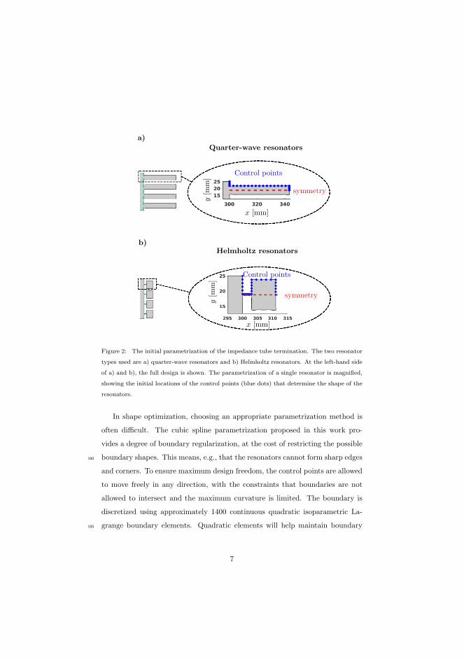
a)
b)
Quarter-wave resonators
Helmholtz resonators
Control points
symmetry
Control points
symmetry
x [mm]y
[mm
]y
[mm
]
x [mm]
Figure 2: The initial parametrization of the impedance tube termination. The two resonator
types used are a) quarter-wave resonators and b) Helmholtz resonators. At the left-hand side
of a) and b), the full design is shown. The parametrization of a single resonator is magnified,
showing the initial locations of the control points (blue dots) that determine the shape of the
resonators.
In shape optimization, choosing an appropriate parametrization method is
often difficult. The cubic spline parametrization proposed in this work pro-
vides a degree of boundary regularization, at the cost of restricting the possible
boundary shapes. This means, e.g., that the resonators cannot form sharp edges100
and corners. To ensure maximum design freedom, the control points are allowed
to move freely in any direction, with the constraints that boundaries are not
allowed to intersect and the maximum curvature is limited. The boundary is
discretized using approximately 1400 continuous quadratic isoparametric La-
grange boundary elements. Quadratic elements will help maintain boundary105
7
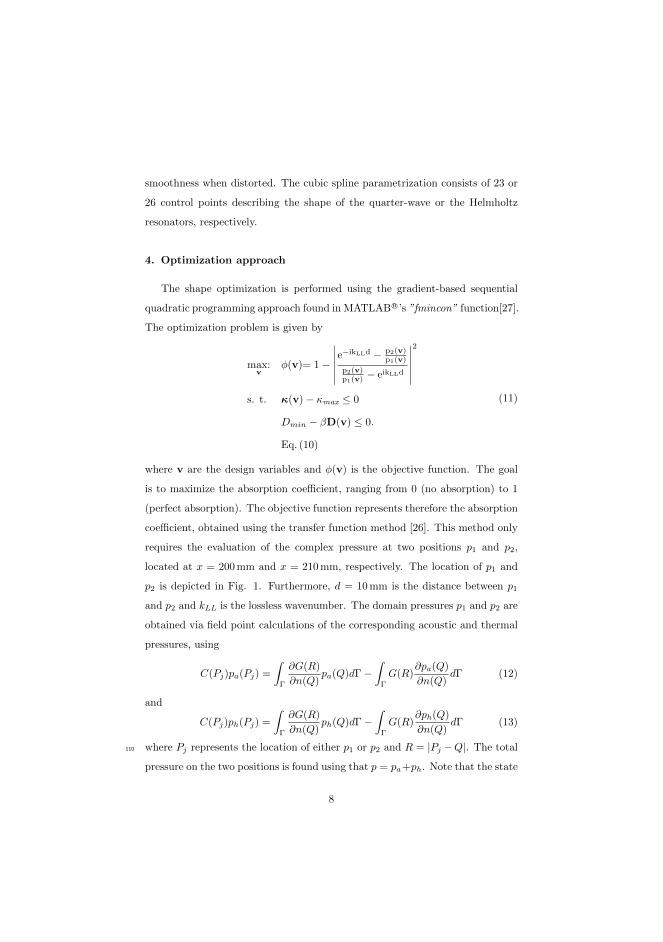
smoothness when distorted. The cubic spline parametrization consists of 23 or
26 control points describing the shape of the quarter-wave or the Helmholtz
resonators, respectively.
4. Optimization approach
The shape optimization is performed using the gradient-based sequential
quadratic programming approach found in MATLABR©’s ”fmincon” function[27].
The optimization problem is given by
max:v
φ(v)= 1−
∣∣∣∣∣∣e−ikLLd − p2(v)
p1(v)
p2(v)p1(v) − eikLLd
∣∣∣∣∣∣
2
s. t. κ(v)− κmax ≤ 0
Dmin − βD(v) ≤ 0.
Eq. (10)
(11)
where v are the design variables and φ(v) is the objective function. The goal
is to maximize the absorption coefficient, ranging from 0 (no absorption) to 1
(perfect absorption). The objective function represents therefore the absorption
coefficient, obtained using the transfer function method [26]. This method only
requires the evaluation of the complex pressure at two positions p1 and p2,
located at x = 200 mm and x = 210 mm, respectively. The location of p1 and
p2 is depicted in Fig. 1. Furthermore, d = 10 mm is the distance between p1
and p2 and kLL is the lossless wavenumber. The domain pressures p1 and p2 are
obtained via field point calculations of the corresponding acoustic and thermal
pressures, using
C(Pj)pa(Pj) =
∫
Γ
∂G(R)
∂n(Q)pa(Q)dΓ−
∫
Γ
G(R)∂pa(Q)
∂n(Q)dΓ (12)
and
C(Pj)ph(Pj) =
∫
Γ
∂G(R)
∂n(Q)ph(Q)dΓ−
∫
Γ
G(R)∂ph(Q)
∂n(Q)dΓ (13)
where Pj represents the location of either p1 or p2 and R = |Pj −Q|. The total110
pressure on the two positions is found using that p = pa+ph. Note that the state
8
problem is fullfilled at every cycle, i.e., following the so-called nested formulation
[28]. The absorption coefficient is a function of the boundary parametrization
v, which is a vector containing the coordinates of the control points as well as
the scaling factor for the resonator length.115
To avoid non-physical boundary behavior, the parametrized boundary is con-
strained using the curvature magnitude κ located at the control points and the
distance between control points D. Additionally, we introduce the parameter
β which equals -1 if the parametrized boundary self-intersects or 1 otherwise.
In this way, too sharp boundaries and self-intersection are avoided. The max-120
imum allowed curvature at the control points is κmax = 6.3 mm−1 and the
minimum distance between the individual control points is Dmin = 1µm, cf.
the dimensions given in Fig 1. Because the boundary is parametrized using C2
continuous cubic splines, the curvature at a control point is easily obtained in
a two-dimensional Cartesian coordinate system as125
κ =|x′(t)y′′(t)− y(t)′x(t)′′|
(x′(t)2 + y′(t)2)3/2
(14)
where x and y are the coordinates of a control point as a function of the cu-
bic spline parameter t ∈ [0, 1], with the primes denoting the derivative with
respect to t. The constraints require additional distance calculations between
control points, detection of boundary intersections and curvature calculations,
making optimization more computationally demanding. Constraints could be130
avoided by selecting a more restricted parametrization, that enforces a physical
behaviour. This would however limit the possible shapes and design freedom.
As a benefit, the constraints can also be used to specify and include manufac-
turing tolerances in the design process.
Gradient information is obtained using a simple forward finite difference135
(FD) scheme
∂φ
∂vi=φ(v + ∆vi · ei)− φ(v)
∆vi(15)
where vi is a single design variable, ei is a unit vector for the i-th variable
9

and ∆vi is the step length determined internally by fmincon. Efficient adjoint
methods can be found in the literature for lossless acoustic BEM shape optimiza-
tion [29, 17]. However, equivalent adjoint methods for lossy BEM are currently140
not available. To improve the speed of the FD gradient evaluation fmincon’s
UseParallel option is enabled, allowing the FD gradients to be calculated in
parallel. Optimization is performed on a desktop PC with six cores. The FD
gradient estimation used is computationally reasonable for the presented case.
However, performing optimization of larger problems including more design vari-145
ables would require an adjoint approach. This is, however, deemed outside the
scope of the presented work.
5. Results
In the following, we investigate how viscous and thermal damping affect
the design obtained by shape optimization for the impedance tube example.150
In Section 5.1, quarter-wave resonators are optimized using lossless and lossy
BEM formulations, including single- and multi-frequency optimization. As an
additional test, the quarter-wave resonators are optimized using a simple bulk
loss model. In the second example in Section 5.2, the impedance termination is
initialized as Helmholtz resonators which are then further optimized.155
5.1. Quarter-wave resonators
Fig. 3 shows the result of a single frequency shape optimization for the
quarter-wave resonators problem. The resonators are optimized for maximum
absorption at 2 kHz. The optimization was conducted using both lossless and
lossy BEM formulations, with φLL and φV T denoting the objective function of160
the final design, calculated either using a lossless or lossy assumption, respec-
tively. This makes it possible to analyze how the viscothermal losses will impact
the final resonator shape. As seen in Fig 3, the two designs deviate in shape
depending on whether losses are considered in the design (right side plots) or
not (left side plots). The lossless design forms narrower resonators and has165
10

Lossless optimization Lossy optimization
Lossless
analysis
Lossy
analysis
φV T = 0.49
φLL = 1 φLL = 0.05
φV T = 1
x [mm] x [mm]
x [mm] x [mm]
Figure 3: Comparison (crosscheck) of the lossless and lossy optimized designs of the impedance
tube termination. Here, φLL and φV T are the lossless and lossy objective functions calculated
for the two designs. The initial design consists, of simple quarter wave resonators controlled
using a cubic spline representation of the boundary as depicted in Fig. 2a. The plotted field
variable is the real part of the pressure in Pascal.
different features compared to that of the lossy design. This is an interesting
result because narrow domain parts should contribute to increased absorption,
and here, the narrowest design is achieved assuming no losses. It is worth not-
ing that both designs perform perfectly under the settings for which they are
optimized, i.e. φLL = 1 for the lossless design and φV T = 1 for the lossy design.170
The performance of the lossless model is a particularly surprising result, as the
lossless design is not expected to include any dissipation. Hence, it should not
be capable of absorbing any sound. The reason for this surprising result is due
11
to a peculiarity of numerical BEM: interior BEM problems are prone to nu-
merical damping as reported in [30, 31, 32]. This is most often not a problem175
when only performing standard analysis of acoustic devices. When optimization
is applied using lossless BEM, the optimizer makes use of numerical damping.
The design is therefore stable, but unphysical. Had the optimization been per-
formed using a standard FEM model for the analysis, this would no have been
the case. Lossless FEM does not introduce any additional phase with respect180
to the excitation, which translates into a purely imaginary complex pressure.
However, in BEM the complex pressure has a real part indicating an additional
phase shift due to numerical damping. The real part of the pressure is therefore
plotted in Fig 3 as a demonstration. Finally, it is worth noting that while the
lossless design does in fact have an absorption coefficient of 0.49 when analysed185
using the lossy model, the lossy design has almost no absorption capabilities
when modelled using the lossless model. This makes it interesting to investigate
the influence of the damping mechanism on the optimized designs and also, how
much can be achieved using the simple ”lossless” BEM model.
First, we examine how the numerical damping performs as compared to190
the true physical viscothermal model. We start by noting that for the lossless
BEM design, convergence can only be achieved when the tubes are allowed to
scale in length individually. This allows the quarter-wave resonators to become
slightly de-tuned, making it possible for the acoustic energy to be exchanged
between the resonators rather than being reflected. This effect is often used in195
recent publications on metamaterial absorbing surfaces, such as [33, 34]. The
resonators in the example form two de-tuned pairs, upper and lower, with the
same properties. Combining the phenomena of de-tuned resonators with the
inherent numerical damping, consequently gives a lossless design that appears
to be a perfect absorber.200
On the other hand, the lossy design perfectly absorbs sound at the optimiza-
tion frequency. Here, the thickness of the resonators is larger compared to the
lossless design and the entrance of the resonators has a rippled funnel-shape.
The entrance presumably acts as an impedance match, so the acoustic wave can
12

propagate easier into the narrow region where losses are more significant. At205
the end of the quarter wave resonators, the boundary is slightly expanded, a
possible attempt to maximize boundary length in the region where the pressure
magnitude is larger, contributing with additional losses. The lengths of the
resonators are organized in a similar pattern as the lossless design, seemingly
taking advantage of the de-tuned resonator phenomena. However, the length210
difference between the de-tuned resonators is slightly larger, and the pressure
in the tubes is significantly reduced as compared to that of the lossless design.
Iteration number
φ
Figure 4: The evolution of the objective function for lossless (blue curve) and lossy (red
curve) quarter-wave resonator shape optimization. Selected design shapes obtained at specific
iterations are included.
Fig. 4 shows the evolution of the objective function during the optimization
process for both lossless and lossy models, with blue and red curves correspond-
ing to φLL or φV T , respectively. In this example, optimization with losses215
requires less iterations to achieve perfect absorption as compared to lossless op-
timization. In the lossless case, there is a large change in the objective function
between iteration 5 and 6, which is most likely due to the unstable nature of
13

resonances. Such behaviour is not observed when losses are included. Viscother-
mal losses stabilize and reduce high-pressure amplitudes near resonance. The220
total optimization time is 194 min for the lossless design and 135 min for the
lossy design. More importantly, we note that the chosen optimizer solves the
chosen problem in Eqs. (11) to stationarity, i.e., to an actual KKT point. This
is clearly seen in Fig. 4 where the change in objective, as well as the change
in layout, is negligible after reaching half of the used iterations. Hence, from225
an engineering perspective, one could with confidence apply a stopping criteria
based on the objective function and the change in layout, and thus save 50% of
the computational time.
φVT
Frequency [Hz]
Figure 5: Absorption coefficients, calculated including losses, as a function of frequency for
the initial, lossless and lossy designs. The solutions for the lossless and lossy designs are
compared with corresponding lossy FEM simulations.
The absorption coefficient as a function of frequency, calculated including
losses, is plotted in Fig. 5 for both initial, lossless, and lossy design. As expected,230
14

the lossy design outperforms the lossless design, yielding perfect absorption at
the optimization frequency. However, it is worth noting that the lossless design
provides an improvement as compared to the initial design. For comparison, Fig
5 includes lossy FEM calculations (red curves) of the corresponding lossless and
lossy design. BEM and FEM simulations show almost the same frequency ab-235
sorption response; however, a 5 Hz frequency shift is observed between the two
methods. It is not uncommon to register differences between BEM and FEM
models near resonances [35, 36, 37]. Additionally, the FEM geometry might be
slightly altered when compared to that of the BEM. The FEM simulations were
performed in COMSOL MultiphysicsR©[38], with a geometry made up of very240
fine polygons, obtained from an interpolation that uses the BEM shape func-
tions to create additional points along the boundary. This strategy destroys the
quadratic geometry discretization in the FEM simulations and most likely con-
tributes to some discrepancies. On the other hand, the FEM simulations were
discretized using significantly more elements (approximately 8 million degrees245
of freedom).
5.1.1. Multi-frequency optimization of quarter-wave resonators
Single frequency optimization limits absorption of the quarter-wave res-
onators to a narrow band, and in acoustic applications broadband absorption is
often desired. A broader absorption response is obtained by including additional
optimization frequencies as a part of the objective function. The multi-frequency
objective function is defined as the sum of individual objective functions calcu-
lated at different frequencies,
φ =∑
i
φi (16)
where index i denotes the specific optimization frequency and φ is the objec-
tive function evaluated at a single frequency. Fig. 6 presents multi-frequency
optimization results of the quarter-wave resonators. In this case, the setup is250
optimized at 1950 Hz, 2000 Hz, and 2050 Hz. The additional optimization fre-
quencies increase the frequency range at which sound waves are absorbed, with
15

φVT
Frequency [Hz]
Figure 6: Multi-frequency optimization results, using the sum of the objective functions
at 1950, 2000 and 2050 Hz. Field pressure magnitudes are plotted for each optimization
frequency. The solid blue and dashed red lines are BEM and FEM simulations, respectively.
Both BEM and FEM simulations are calculated including viscothermal losses.
almost full absorption from 1900 to 2100 Hz. The figure also includes insets
with the optimized design and the corresponding pressure field magnitudes at
the three optimization frequencies. Compared to the previous single frequency255
designs, the resonators have slightly narrower passages and increased variation
along the quarter-wave resonator boundaries. Note also, that the behaviour of
the individual quarter-wave resonators changes with frequency. At 2050 Hz, the
highest pressure magnitude is observed in the shortest resonator, whereas lower
frequencies tend to excite the longer resonators. The length of the quarter-wave260
resonators is seen to be the primary factor that determines the operational fre-
quency. By having different quarter-wave resonator lengths, the frequency span
with high absorption is therefore increased.
16

φVT
τs
Figure 7: A series of shape optimization results of quarter-wave resonators at 2 kHz with the
acoustic losses modeled using a complex wavenumber with a tunable imaginary part. Here, τs
is the value of the imaginary part of a complex wavenumber and α is the absorption coefficient
calculated including viscothermal losses for a given design. The figure includes selected designs
obtained with τs equal to 10−6, 10−4, 0.05, 1.6 and 32.
5.1.2. Bulk loss description
A common practice when comparing experimental work with lossless simula-265
tions is to correct the simulations with an added bulk loss, e.g., using a complex
wavenumber with a controllable imaginary part. However, no general proce-
dure exists to estimate the magnitude of the imaginary part, and it is typically
problem dependent [39]. It is therefore interesting to investigate how varying
the imaginary part of the wavenumber affects the optimization of the quarter-270
wave resonators. This is accomplished by defining the complex wavenumber
as kB = kLL − iτs, where τs is the tunable parameter. In Fig. 7, optimized
designs are presented using different values of τs and compared to the actual
absorption coefficient, calculated including viscothermal losses. It is seen how
certain values of τs result in high absorption coefficients above 80 %. However,275
none of the used values for τs results in a design with perfect absorption. It
should also be noted that only a limited amount of simulations with different
17

Lossless optimization Lossy optimization
Lossless
analysis
Lossy
analysis
φV T = 0.58
φLL = 1 φLL = 0.09
φV T = 1
x [mm] x [mm]
x [mm] x [mm]
Figure 8: Optimization results of Helmholtz resonators located at the impedance tube termi-
nation. The designs are based on either a lossless or a lossy assumption. The field variables
are the pressure magnitudes in Pascal
values of τs were performed and that there might exist values of τs resulting
in higher absorption coefficients. In the range τs ∈ 0.01, 3, the absorption
coefficients are very sensitive to the choice of τs, making it difficult to choose280
an appropriate value for this particular example. Fig. 7 also depicts inserts
with selected designs. It is noteworthy to highlight the design corresponding to
τs = 0.05 because it is very similar to the single frequency lossy quarter-wave
resonator design, although its performance is inferior.
18

5.2. Helmholtz resonators285
In this section, the impedance tube termination is initially parametrized
forming four equally sized Helmholtz resonators as described in Fig 2b. The neck
and cavity dimensions of the initial shape of the resonators yields an operational
frequency near 2 kHz. The Helmholtz resonators are, as in the case of the
quarter-wave resonators, optimized under both lossless and lossy conditions.290
The optimization is carried out at 2 kHz. Fig. 8 contains the resulting lossless
and lossy designs which are overlaid with acoustic pressure magnitude field
calculations of both the lossless and lossy solutions. Similar to the quarter-
wave optimization results, the performance of the lossless design is degraded
when introducing losses. When calculated without losses, the lossless design295
contains varying high pressure amplitudes between the individual cavities of
the Helmholtz resonators, which are de-tuned in a similar way to the quarter-
wave resonators. However, the pressure differences and de-tuning disappears
when calculated with losses.
In the case of optimization including losses, the design outcome deviates far300
from the classical Helmholtz resonator shape, with the cavity best described
as a four-leaf clover. Usually, the neck of Helmholtz resonators is the primary
source of viscothermal dissipation. In this case, however, it is believed that the
clover shape contributes to increased damping, with closer boundaries. Whether
the lossy design can still be considered a Helmholtz resonator is unclear, but it305
does include a neck and a slightly unconventionally shaped cavity. While the
overall shape between the lossless and lossy design deviates, the neck shape at
the entrance of the Helmholtz resonators is very similar.
The absorption coefficient as a function of frequency is plotted in Fig. 9.
Interestingly, optimized designs based on a lossless assumption produce poorer310
designs when compared to the initial guess, indicating that numerical damping
alone is not sufficient in this case. On the other hand, including viscothermal
losses during optimization results in an improved design, with perfect absorption
at the optimization frequency. The figure includes viscothermal FEM calcula-
tions, with conclusions similar to those in Section 5.1.315
19
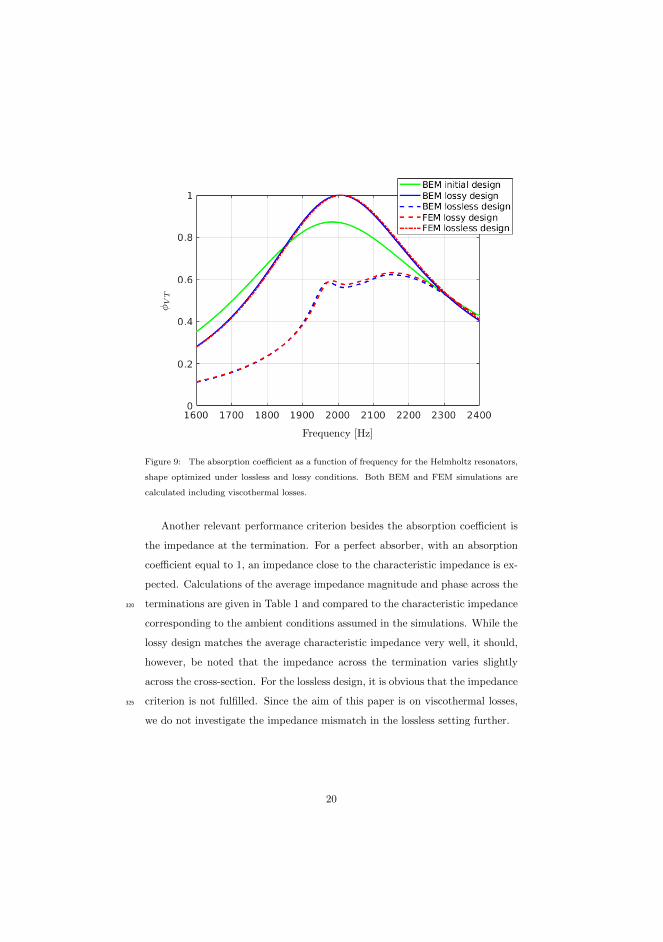
Frequency [Hz]
φVT
Figure 9: The absorption coefficient as a function of frequency for the Helmholtz resonators,
shape optimized under lossless and lossy conditions. Both BEM and FEM simulations are
calculated including viscothermal losses.
Another relevant performance criterion besides the absorption coefficient is
the impedance at the termination. For a perfect absorber, with an absorption
coefficient equal to 1, an impedance close to the characteristic impedance is ex-
pected. Calculations of the average impedance magnitude and phase across the
terminations are given in Table 1 and compared to the characteristic impedance320
corresponding to the ambient conditions assumed in the simulations. While the
lossy design matches the average characteristic impedance very well, it should,
however, be noted that the impedance across the termination varies slightly
across the cross-section. For the lossless design, it is obvious that the impedance
criterion is not fulfilled. Since the aim of this paper is on viscothermal losses,325
we do not investigate the impedance mismatch in the lossless setting further.
20
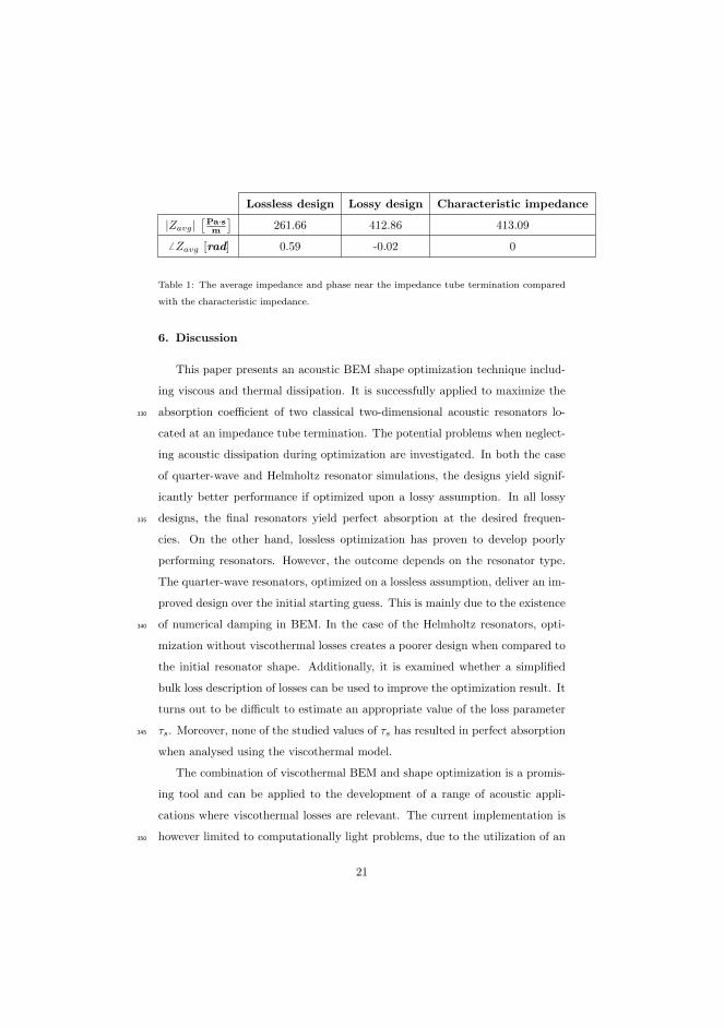
Lossless design Lossy design Characteristic impedance
|Zavg|[Pa·sm
]261.66 412.86 413.09
6 Zavg [rad] 0.59 -0.02 0
Table 1: The average impedance and phase near the impedance tube termination compared
with the characteristic impedance.
6. Discussion
This paper presents an acoustic BEM shape optimization technique includ-
ing viscous and thermal dissipation. It is successfully applied to maximize the
absorption coefficient of two classical two-dimensional acoustic resonators lo-330
cated at an impedance tube termination. The potential problems when neglect-
ing acoustic dissipation during optimization are investigated. In both the case
of quarter-wave and Helmholtz resonator simulations, the designs yield signif-
icantly better performance if optimized upon a lossy assumption. In all lossy
designs, the final resonators yield perfect absorption at the desired frequen-335
cies. On the other hand, lossless optimization has proven to develop poorly
performing resonators. However, the outcome depends on the resonator type.
The quarter-wave resonators, optimized on a lossless assumption, deliver an im-
proved design over the initial starting guess. This is mainly due to the existence
of numerical damping in BEM. In the case of the Helmholtz resonators, opti-340
mization without viscothermal losses creates a poorer design when compared to
the initial resonator shape. Additionally, it is examined whether a simplified
bulk loss description of losses can be used to improve the optimization result. It
turns out to be difficult to estimate an appropriate value of the loss parameter
τs. Moreover, none of the studied values of τs has resulted in perfect absorption345
when analysed using the viscothermal model.
The combination of viscothermal BEM and shape optimization is a promis-
ing tool and can be applied to the development of a range of acoustic appli-
cations where viscothermal losses are relevant. The current implementation is
however limited to computationally light problems, due to the utilization of an350
21

inefficient FD sensitivity estimation. Future work should therefore investigate
methods for obtaining more accurate and efficient sensitivities, i.e., development
and implementation of an adjoint method. This would allow for the study of
three-dimensional test cases suitable for experimental validation. In general,
experimental realization of optimized acoustic designs will require the inclusion355
of manufacturing constraints and robustness measures. The proposed technique
includes constraints that might be applicable, but not necessarily sufficient for
this purpose, i.e., the curvature and distance constraints. Additionally, the pro-
posed shape optimization technique can be extended to account for mechanical
coupling which often plays an important role in small micro-acoustic devices. Fi-360
nally, it would be interesting to pursue alternative objectives or multi-objectives
such as impedance and total energy loss.
References
[1] P. M. Morse, Theoretical Acoustics, McGraw-Hill, Princeton, 1968.
[2] A. D. Pierce, Acoustics. An introduction to its principles and applications365
(Ch. 10), McGraw Hill, New York, 1981.
[3] R. Kampinga, Viscothermal acoustics using finite elements analysis tools
for engineers, Ph.D. thesis, University of Twente, Enschede (2010).
[4] R. Christensen, Acoustic modeling of hearing aid components, Ph.D. thesis,
University of Southern Denmark (2010).370
[5] D. Homentcovschi, R. N. Miles, P. Loeppert, A. J. Zuckerwar, A microa-
coustic analysis including viscosity and thermal conductivity to model
the effect of the protective cap on the acoustic response of mems mi-
crophone, Microsyst Technol. 20 (2) (2014) 265–275. doi:10.1007/
s00542-013-1800-5.375
[6] R. Christensen, U. Skov, Compression driver simulation incl. vibroacous-
tic, viscothermal & porous acoustics, in: Proceedings from the COMSOL
conference in Stuttgart (Germany), 2011.
22
[7] R. Christensen, U. Skov, Simulation of a 4” compression driver using a fully
coupled vibroacoustic finite element analysis including viscous and thermal380
losses, in: Audio Engineering Society Convention 132, 2012.
URL http://www.aes.org/e-lib/browse.cfm?elib=16310
[8] M. Berggren, A. Bernland, D. Noreland, Acoustic boundary layers as
boundary conditions, Journal of Computational Physics 371 (2018) 633–
650. doi:10.1016/j.jcp.2018.06.005.385
[9] J. Carbajo, J. Ramis, Godinho, J. Amado-Mendes, P., J. Alba, A finite
element model of perforated panel absorber including viscothermal effects,
Journal of Applied Acoustics 90 (2014) 1–8. doi:10.1016/j.apacoust.
2014.10.013.
[10] A. I. Komkin, M. A. Mirov, A. I. Bykov, Sound absorption by a helmholtz390
resonator, Acoustical Physics 63 (4) (2017) 385–392. doi:10.1134/
S1063771017030071.
[11] S. A. Cummer, J. Christensen, A. Alu, Controlling sound with acoustic
metamaterials, Nature reviews materials 1 (2016) 1–13. doi:doi:10.1038/
natrevmats.2016.1.395
[12] R. E. Christensen, O. Sigmund, Exprimental validation of systematically
designed acoustic hyperbolic meta material slab exibiting refraction, Appl.
Phys. Lett. 109 (2016) 101905. doi:10.1063/1.4962441.
[13] V. C. Henrıquez, V. Garcıa-Chocano, J. Sanchez-Dehesa, Viscothermal
losses in double-negative acoustic metamaterial, Physical Review Applied400
8 (12) (2017) 014029. doi:10.1103/PhysRevApplied.8.014029.
[14] V. C. Henrıquez, P. Andersen, J. S. Jensen, P. M. Juhl, J. Sanchez-Dehesa,
A numerical model of an acoustic metamaterial using the Boundary Ele-
ment Method including viscous and thermal losses, Journal of Computa-
tional Acoustics 25 (4) (2017) 1750006. doi:10.1142/S0218396X17500060.405
23

[15] M. Moleron, M. Serra-Garcia, C. Daraio, Visco-thermal effects in acoustic
metamaterials: from total transmission to total reflection and high absorp-
tion, New J. Phys. 18 (2016) 033003. doi:10.1088/1367-2630/18/3/
033003.
[16] N. Jimenez, V. Romero-Garcıa, P. Pagneux, J. Groby, Rainbow-trapping410
absorbers: Broadband, perfect and asymmetric sound absorption by sub-
wavelength panels for transmission problems, Scientific Reports 7 (1) (2017)
13595. doi:10.1038/s41598-017-13706-4.
[17] R. Udawalpola, E. Wasbro, M. Berggren, Optimization of a variable mouth
horn, Int. J. Numer. Meth. Engng 85 (2010) 591–606. doi:10.1002/nme.415
2982.
[18] E. Wadbro, M. Berggren, Topology optimization of an acoustic horn, Com-
put. Methods Appl. Mech. Engrg. 196 (2006) 420–436. doi:10.1016/j.
cma.2006.05.005.
[19] R. Udawalpola, E. Wasbro, M. Berggren, Optimization of an acoustic horn420
with respect to efficientcy and directivity, Int. J. Numer. Meth. Engng 73
(2007) 1571–1606. doi:10.1002/nme.2132.
[20] R. Christensen, Topology optimization of thermoviscous acoustics in tubes
and slits with hearing aid applications, Proceedings of the COMSOL Con-
ference in Rotterdam.425
[21] M. Malinen, M. Lyly, P. Raback, A. Karkainen, L. Karkkainen, A Finite
Element Method for the modeling of thermo-viscous effects in acoustics,
Proceedings of the 4th European Congress on Computational Methods in
Applied and Engineering ECCOMAS, Jyvaskyla (Finland).
[22] M. Bruneau, P. Herzog, J. Kergomard, J. D. Polack, General formulation430
of the dispersion equation in bounded visco-thermal fluid, and application
to some simple geometries, Wave Motion 11 (1989) 441451doi:10.1016/
0165-2125(89)90018-8.
24
[23] V. Cutanda Henrıquez, P. M. Juhl, An axisymmetric boundary element for-
mulation of sound wave propagation in fluids including viscous and thermal435
losses, Journal of the Acoustical Society of America 134 (5) (2013) 3409.
doi:10.1121/1.4823840.
[24] V. Cutanda Henrıquez, P. Risby Andersen, A three-dimensional acous-
tic boundary element method formulation with viscous and thermal losses
based on shape function derivatives, Journal of Computational and Theo-440
retical Acoustics (Accepted 2018).
[25] V. Cutanda Henrıquez, P. M. Juhl, OpenBEM - an open source Boundary
Element Method software in acoustics,, Proceedings of the 39th Interna-
tional Congress on Noise Control Engineering, Inter-noise, Lisbon (Portu-
gal).445
[26] ISO 10534-2:1998, Acoustics – Determination of sound absorption coef-
ficient and impedance in impedance tubes – Part 2: Transfer-function
method, Standard, International Organization for Standardization (1998).
[27] MATLAB optimization toolbox, the MathWorks, Natick, MA, USA
(2017b).450
[28] Topology Optimization Theory, Methods, and Applications, author =
Bendœ, M. P. and Sigmund, O., YEAR = 2004, PUBLISHER = Springer,.
[29] L. Chen, L. Liu, W. Zhao, H. Chen, 2D acoustic design sensitiv-
ity analysis based on adjoint variable method using different types of
boundary elements, Acoust. Aust. 44 (2016) 343–357. doi:10.1007/455
s40857-016-0065-4.
[30] J. Fahnline, Numerical difficulties with boundary element solutions of inte-
rior acoustic problems, Journal of Sound and Vibration 319 (2008) 1083–
1096. doi:10.1016/j.jsv.2008.06.040.
25

[31] S. Marburg, Numerical damping in the acoustic boundary element method,460
Acta Acustica United with Acustica 102 (2018) 1550016. doi:10.3813/
AAA.918958.
[32] S. Marburg, A pollution effect in the boundary element mmethod for acous-
tic problems, Journal of Computaional Acoustics 26 (18) (2018) 1850018.
doi:10.1142/S0218396X18500182.465
[33] H. Ryoo, W. Jeon, Dual-frequency sound-absorbing metasurface based on
viscothermal effects with frequency dependence, Journal of Applied Physics
123 (2018) 115110. doi:10.1063/1.5017540.
[34] J. Li, W. Wang, Y. Xie, B. Popa, S. A. Cummer, A sound absorbing
metasurface with coupled resonators, Appl. Phys. Lett. 109 (2016) 091908.470
doi:10.1063/1.4961671.
[35] N. Aage, V. Egede Johansen, Topology optimization of microwave waveg-
uide filters, International Journal for Numerical Methods in Engineering
112 (3) (2017) 283–300. doi:10.1002/nme.5551.
[36] N. Aage, Mortensen, N. A., O. Sigmund, Topology optimization of metallic475
devices for microwave applications, International Journal for Numerical
Methods in Engineering 83 (2) (2010) 228–248. doi:10.1002/nme.2837.
[37] A. R. Diaz, O. Sigmund, A topology optimization method for design
of negative permeability metamaterials, International Journal for Nu-
merical Methods in Engineering 41 (2) (2010) 163–177. doi:10.1007/480
s00158-009-0416-y.
[38] COMSOL Multiphysics Reference Manual, version 5.2, COMSOL, Inc,
www.comsol.com.
[39] R. E. Christensen, E. Fernandez-Grande, Experimental validation of a
topology optimized acoustic cavity, J. Acoust. Soc. Am. 138 (2015) 3470–485
3474. doi:10.1121/1.4936905.
26

DTU Electrical Engineering
Department of Electrical Engineering
Technical University of Denmark
Ørsteds Pl. 352
2800 Kgs. Lyngby
www.elektro.dtu.dk