modelling mean annual rainfall for zimbabwe
TRANSCRIPT

Modelling Mean AnnualRainfall for Zimbabwe
Retius Chifurira
January 2018
Modelling Mean Annual Rainfall for Zimbabwe
by
RETIUS CHIFURIRA
(2009057023)
THESIS
Submitted in fulfilment of the requirements for the degree of
PHILOSOPHIAE DOCTOR
in
STATISTICS
(APPLIED)
in the
FACULTY OF NATURAL AND AGRICULTURAL SCIENCES
DEPARTMENT OF MATHEMATICAL SCIENCES AND ACTUARIAL SCIENCE
at the
UNIVERSITY OF THE FREE STATE
BLOEMFONTEIN: JANUARY 2018
Thesis promoter: Dr Delson Chikobvu
UNIVERSITY OF THE FREE STATE
FACULTY OF NATURAL AND AGRICULTURAL SCIENCES
DEPARTMENT OF MATHEMATICAL STATISTICS AND ACTUARIAL SCIENCE
BLOEMFONTEIN, SOUTH AFRICA

Declaration
I, Retius Chifurira, declare that
1. The thesis is hereby submitted for the qualification of Doctor of Philosophy in
Statistics at the University of the Free State.
2. The research reported in this thesis, except where otherwise indicated, is my
original research.
3. This thesis has not been submitted for any degree or examination at any other
University/Faculty.
4. This thesis does not contain other persons’ writing, unless specifically acknowl-
edged as being sourced from other researchers. Where other written sources
have been quoted, then
(a) their words have been re-written but the general information attributed
to them has been referenced, or
(b) where their exact words have been used, then their writing has been
placed in italics and referenced.
5. I cede copyright of the thesis to the University of the Free State.
Retius Chifurira Date
Copyright c© University of the Free State
All right reserved

Disclaimer
This document describes work undertaken as a PhD programme of study at the Uni-
versity of the Free State. All views and opinions expressed therein remain the sole
responsibility of the author, and do not necessarily represent those of the institution.

A man’s mind, stretched by new ideas, may never return to its original dimensions.
Oliver Wendell Holmes Jr.

Abstract
Rainfall has a substantial influence on agriculture, food security, infrastructure de-
velopment, water quality and the economy. Zimbabwe, like most other Southern
African countries, has distinctive meteorological features which are characterized
by a high variability of temporal and spatial rainfall distributions, flash floods and
prolonged drought periods. Because people struggle to adapt to these diverse rain-
fall patterns, a better understanding of rainfall characteristics, its distribution and
potential predictors will help mitigate the effects of these adverse weather condi-
tions. The aim of this thesis is to develop an early warning tool that can help predict
a drought and/or flash flood in Zimbabwe, and to estimate the amount of rainfall
during the year. In this thesis, mean annual rainfall figures from 1901 to 2015 ob-
tained from 40 rainfall stations scattered throughout Zimbabwe were used.
The thesis consists of three sections. In the first section, appropriate statistical mod-
els are applied to a set of annual rainfall figures that have been divided by 12 to
produce a mean annual rainfall figure for the year with a view towards finding po-
tential predictors for rainfall in Zimbabwe. Monthly-based indicator variables asso-
ciated with the Southern Oscillation Index (SOI) and the standardised Darwin sea
level pressure readings (SDSLP) were considered as predictor variables with the SOI
and SDSLP readings for August (two months before the onset of the rainfall season)
producing the most important predictor variables for future rainfall in Zimbabwe.
In the second part of the thesis, several characteristics associated with the mean
ii

Abstract
annual rainfall for Zimbabwe are studied using an appropriately fitted theoretical
probability distribution. More specifically, the annual rainfall figures from 1901 to
2009 were used to fit a gamma, lognormal and log-logistic distribution to the an-
nual rainfall data. The relative performance of the fitted distributions were then
assessed using the following goodness-of-fit tests, namely; the relative root mean
square error (RRMSE), relative mean absolute error (RMAE) and the probability plot
correlation coefficient (PPCC). All the fitted distributions, however, were not able to
adequately predict periods of extreme rainfall. Extreme value distributions such as
generalised extreme value and generalised Pareto distributions were then fitted to
the mean annual rainfall data. The possibility that periods of extreme rainfall may
be time-dependent and be influenced by weather/climate change drivers was then
considered. This study shows that, although rainfall extremes for Zimbabwe are not
time-dependent, they are highly influenced SDSLP anomalies for April.
In the third and last part of this thesis, we categorized rainfall data using a drought
threshold value of 570 mm. We compared the relative performance of the logis-
tic regression model in estimating drought probabilities for Zimbabwe with that of
a generalised extreme value regression model for binary data. The department of
meteorological services in Zimbabwe uses 75% of normal annual rainfall (usually
a 30-year time series data) to declare a drought year. Results show that the GEVD
regression model with SDSLP anomaly for April is the best performing model and
can be used to predict drought probabilities for Zimbabwe.
Key words: Drought, early warning system, extreme value theory, floods, mean
annual rainfall, southern oscillation index, standardized Darwin sea level pressure,
Zimbabwe.
iii

Acknowledgements
I gratefully acknowledge my supervisor Dr. D. Chikobvu for his inspiration, com-
petent guidance, patience and encouragement through all the different stages of this
research. I thank him for guiding me in conducting my PhD research in a chal-
lenging area of meteorological modelling application which can be used to benefit a
drought-prone country such as Zimbabwe.
I would like to thank everyone in the School of Mathematics, Statistics and Com-
puter Science at University of KwaZulu-Natal. In particular, a special thanks to
Prof. Henry Mwambi for reading my draft thesis and to my best friend Knowledge
Chinhamu for discussing statistics questions.
I would also like to thank Danielle Roberts for IT support and Jahvaid Hummura-
judy for proof reading papers submitted for publication.
Finally, I would like to thank my wife Cornelia, my son Tinashe, my daughter Tiri-
vashe and members of my family for their unwavering support and encouragement
throughout my study.
iv
Contents
Abstract ii
Page
List of Figures xiv
List of Tables xvii
Abbreviations xviii
Research Output xix
Conference Presentations xx
Chapter 1: Introduction 1
1.1 Background . . . . . . . . . . . . . . . . . . . . . . . . . . . . . . . . . . . . . 1
1.2 Statement of the problem . . . . . . . . . . . . . . . . . . . . . . . . . . . . . 3
1.3 Aim and objectives of the thesis . . . . . . . . . . . . . . . . . . . . . . . . . 3
1.4 Literature review . . . . . . . . . . . . . . . . . . . . . . . . . . . . . . . . . . 4
1.4.1 Introduction to literature review . . . . . . . . . . . . . . . . . . . . . . 4
1.4.2 Modelling rainfall for Zimbabwe . . . . . . . . . . . . . . . . . . . . . 5
1.5 Significance of the study . . . . . . . . . . . . . . . . . . . . . . . . . . . . . . 8
1.6 Contributions . . . . . . . . . . . . . . . . . . . . . . . . . . . . . . . . . . . . 9
1.7 Thesis layout . . . . . . . . . . . . . . . . . . . . . . . . . . . . . . . . . . . . 10
Chapter 2: Methodology 12
v

CONTENTS
2.1 Introduction . . . . . . . . . . . . . . . . . . . . . . . . . . . . . . . . . . . . . 12
2.2 Tests for stationarity . . . . . . . . . . . . . . . . . . . . . . . . . . . . . . . . 12
2.2.1 Augmented-Dickey Fuller (ADF) test . . . . . . . . . . . . . . . . . . . 13
2.2.2 Phillips-Perron (PP) test . . . . . . . . . . . . . . . . . . . . . . . . . . 14
2.2.3 Kwiatkowski-Phillips-Schmidt-Shin (KPSS) test . . . . . . . . . . . . . 15
2.3 Tests for randomness and serial correlation . . . . . . . . . . . . . . . . . . . 16
2.3.1 Bartels rank test . . . . . . . . . . . . . . . . . . . . . . . . . . . . . . . 16
2.3.2 Ljung-Box test . . . . . . . . . . . . . . . . . . . . . . . . . . . . . . . . 16
2.3.3 Brock-Dechert-Scheinkman (BDS) test . . . . . . . . . . . . . . . . . . 17
2.4 Test for heteroscedasticity . . . . . . . . . . . . . . . . . . . . . . . . . . . . . 19
2.4.1 ARCH-LM test . . . . . . . . . . . . . . . . . . . . . . . . . . . . . . . . 19
2.5 Tests for normality . . . . . . . . . . . . . . . . . . . . . . . . . . . . . . . . . 20
2.5.1 Jarque-Bera test . . . . . . . . . . . . . . . . . . . . . . . . . . . . . . . 20
2.5.2 Shapiro-Wilk test . . . . . . . . . . . . . . . . . . . . . . . . . . . . . . 21
2.6 Model adequacy and goodness-of-fit tests . . . . . . . . . . . . . . . . . . . . 22
2.6.1 Probability-Probability plot . . . . . . . . . . . . . . . . . . . . . . . . 22
2.6.2 Quantile-Quantile plot . . . . . . . . . . . . . . . . . . . . . . . . . . . 22
2.6.3 Kolmogorov-Smirnov test . . . . . . . . . . . . . . . . . . . . . . . . . 23
2.6.4 Anderson-Darling test . . . . . . . . . . . . . . . . . . . . . . . . . . . 23
2.7 Model selection . . . . . . . . . . . . . . . . . . . . . . . . . . . . . . . . . . . 24
2.7.1 Akaike information criterion . . . . . . . . . . . . . . . . . . . . . . . . 24
2.7.2 Assessing model performance . . . . . . . . . . . . . . . . . . . . . . . 25
2.7.3 Forecast statistics . . . . . . . . . . . . . . . . . . . . . . . . . . . . . . 26
Chapter 3: Rainfall data 27
3.1 Introduction . . . . . . . . . . . . . . . . . . . . . . . . . . . . . . . . . . . . . 27
3.2 Mean annual rainfall data . . . . . . . . . . . . . . . . . . . . . . . . . . . . . 27
3.3 Weather/climate change determinants . . . . . . . . . . . . . . . . . . . . . 32
vi
CONTENTS
3.3.1 Southern oscillation index and standardised Darwin sea level pressure32
3.4 Concluding remarks . . . . . . . . . . . . . . . . . . . . . . . . . . . . . . . . 35
Chapter 4: Modelling mean annual rainfall using weather/climate change determi-
nants: Weighted regression models 37
4.1 Introduction . . . . . . . . . . . . . . . . . . . . . . . . . . . . . . . . . . . . . 37
4.2 Research methodology . . . . . . . . . . . . . . . . . . . . . . . . . . . . . . . 41
4.2.1 General linear model . . . . . . . . . . . . . . . . . . . . . . . . . . . . 42
4.2.2 Principal component analysis . . . . . . . . . . . . . . . . . . . . . . . 44
4.2.3 Weighted least squares model . . . . . . . . . . . . . . . . . . . . . . . 45
4.3 The models . . . . . . . . . . . . . . . . . . . . . . . . . . . . . . . . . . . . . 46
4.3.1 Assessing model performance . . . . . . . . . . . . . . . . . . . . . . . 47
4.3.2 Model selection criterion . . . . . . . . . . . . . . . . . . . . . . . . . . 47
4.4 Empirical results . . . . . . . . . . . . . . . . . . . . . . . . . . . . . . . . . . 47
4.5 Concluding remarks . . . . . . . . . . . . . . . . . . . . . . . . . . . . . . . . 51
4.6 Appendix . . . . . . . . . . . . . . . . . . . . . . . . . . . . . . . . . . . . . . 53
Chapter 5: Extreme rainfall: Candidature probability distributions for mean annual
rainfall data: An application to Zimbabwean data 55
5.1 Introduction . . . . . . . . . . . . . . . . . . . . . . . . . . . . . . . . . . . . . 55
5.2 Research methodology . . . . . . . . . . . . . . . . . . . . . . . . . . . . . . . 58
5.2.1 Two-parameter gamma distribution . . . . . . . . . . . . . . . . . . . 58
5.2.2 Two-parameter lognormal distribution . . . . . . . . . . . . . . . . . . 59
5.2.3 Two-parameter log-logistic distribution . . . . . . . . . . . . . . . . . 60
5.2.4 Two-parameter exponential distribution derived from extreme value
theory . . . . . . . . . . . . . . . . . . . . . . . . . . . . . . . . . . . . . 62
5.3 Empirical results . . . . . . . . . . . . . . . . . . . . . . . . . . . . . . . . . . 63
5.3.1 Selecting the best fitting parent distribution . . . . . . . . . . . . . . . 67
5.4 Concluding remarks . . . . . . . . . . . . . . . . . . . . . . . . . . . . . . . . 71
vii

CONTENTS
Chapter 6: Modelling of extreme maximum rainfall using generalised extreme value
distribution for Zimbabwe 73
6.1 Introduction . . . . . . . . . . . . . . . . . . . . . . . . . . . . . . . . . . . . . 73
6.2 Research methodology . . . . . . . . . . . . . . . . . . . . . . . . . . . . . . . 76
6.2.1 Extreme value theory for block maxima . . . . . . . . . . . . . . . . . 76
6.2.2 Generalised extreme value distribution (GEVD) for block maxima
and minima . . . . . . . . . . . . . . . . . . . . . . . . . . . . . . . . . 80
6.2.3 Estimation procedure of parameters for the GEVD . . . . . . . . . . . 86
6.2.4 Properties of the GEVD log-likelihood . . . . . . . . . . . . . . . . . . 87
6.2.5 Non-stationary GEVD model . . . . . . . . . . . . . . . . . . . . . . . 92
6.2.6 Modelling minima random variables . . . . . . . . . . . . . . . . . . . 95
6.2.7 The models . . . . . . . . . . . . . . . . . . . . . . . . . . . . . . . . . . 96
6.2.8 Return level estimates . . . . . . . . . . . . . . . . . . . . . . . . . . . . 97
6.2.9 Model diagnostics . . . . . . . . . . . . . . . . . . . . . . . . . . . . . . 98
6.2.10 Model selection . . . . . . . . . . . . . . . . . . . . . . . . . . . . . . . 100
6.3 Empirical results . . . . . . . . . . . . . . . . . . . . . . . . . . . . . . . . . . 100
6.3.1 The Maximum likelihood estimation of the annual maxima rainfall
data . . . . . . . . . . . . . . . . . . . . . . . . . . . . . . . . . . . . . . 101
6.4 Concluding remarks . . . . . . . . . . . . . . . . . . . . . . . . . . . . . . . . 109
6.5 Appendix . . . . . . . . . . . . . . . . . . . . . . . . . . . . . . . . . . . . . . 112
Chapter 7: Modelling of extreme minimum rainfall using generalised extreme value
distribution for Zimbabwe 121
7.1 Introduction . . . . . . . . . . . . . . . . . . . . . . . . . . . . . . . . . . . . . 121
7.2 Research methodology . . . . . . . . . . . . . . . . . . . . . . . . . . . . . . . 124
7.2.1 Normal distribution . . . . . . . . . . . . . . . . . . . . . . . . . . . . . 124
7.2.2 Generalised extreme value distribution (GEVD) . . . . . . . . . . . . . 124
7.2.3 Bayesian analysis of extreme values for GEVD . . . . . . . . . . . . . 129
7.3 Empirical results . . . . . . . . . . . . . . . . . . . . . . . . . . . . . . . . . . 130
viii

CONTENTS
7.4 Concluding remarks . . . . . . . . . . . . . . . . . . . . . . . . . . . . . . . . 142
7.5 Appendix . . . . . . . . . . . . . . . . . . . . . . . . . . . . . . . . . . . . . . 144
Chapter 8: Modelling mean annual rainfall extremes using a generalised Pareto dis-
tribution model 147
8.1 Introduction . . . . . . . . . . . . . . . . . . . . . . . . . . . . . . . . . . . . . 147
8.2 Research methodology . . . . . . . . . . . . . . . . . . . . . . . . . . . . . . . 149
8.2.1 Pitfalls of the GEVD . . . . . . . . . . . . . . . . . . . . . . . . . . . . . 150
8.2.2 r largest order statistics model . . . . . . . . . . . . . . . . . . . . . . . 150
8.2.3 Peaks-over threshold models . . . . . . . . . . . . . . . . . . . . . . . . 151
8.2.4 Generalised Pareto distribution (GPD) . . . . . . . . . . . . . . . . . . 152
8.2.5 Threshold selection . . . . . . . . . . . . . . . . . . . . . . . . . . . . . 153
8.2.6 Declustering . . . . . . . . . . . . . . . . . . . . . . . . . . . . . . . . . 157
8.2.7 Estimation procedure of parameters for the Generalised Pareto Dis-
tribution . . . . . . . . . . . . . . . . . . . . . . . . . . . . . . . . . . . 158
8.2.8 Time-heterogenous GPD model . . . . . . . . . . . . . . . . . . . . . . 160
8.2.9 Model diagnostics and goodness-of-fit . . . . . . . . . . . . . . . . . . 160
8.3 Empirical Results . . . . . . . . . . . . . . . . . . . . . . . . . . . . . . . . . . 161
8.3.1 Fitting time-homogeneous generalised Pareto distribution . . . . . . 161
8.4 Concluding remarks . . . . . . . . . . . . . . . . . . . . . . . . . . . . . . . . 167
Chapter 9: Generalised extreme value regressions with binary dependent variable:
An application to predicting meteorological drought probabilities 168
9.1 Introduction . . . . . . . . . . . . . . . . . . . . . . . . . . . . . . . . . . . . . 168
9.2 Research methodology . . . . . . . . . . . . . . . . . . . . . . . . . . . . . . . 171
9.2.1 The logistic regression model . . . . . . . . . . . . . . . . . . . . . . . 171
9.2.2 The Generalised extreme value distribution (GEVD) regression model172
9.3 The data . . . . . . . . . . . . . . . . . . . . . . . . . . . . . . . . . . . . . . . 174
9.4 The models . . . . . . . . . . . . . . . . . . . . . . . . . . . . . . . . . . . . . 176
ix

CONTENTS
9.5 Empirical results . . . . . . . . . . . . . . . . . . . . . . . . . . . . . . . . . . 177
9.5.1 Estimation results using the logistic regression model . . . . . . . . . 177
9.6 Concluding remarks . . . . . . . . . . . . . . . . . . . . . . . . . . . . . . . . 182
9.7 Appendix . . . . . . . . . . . . . . . . . . . . . . . . . . . . . . . . . . . . . . 183
Chapter 10: Conclusion 185
10.1 Introduction . . . . . . . . . . . . . . . . . . . . . . . . . . . . . . . . . . . . . 185
10.2 Thesis summary . . . . . . . . . . . . . . . . . . . . . . . . . . . . . . . . . . 186
10.3 Summary of the key findings . . . . . . . . . . . . . . . . . . . . . . . . . . . 190
10.4 Limitations of the thesis . . . . . . . . . . . . . . . . . . . . . . . . . . . . . . 191
10.5 Ideas for further research . . . . . . . . . . . . . . . . . . . . . . . . . . . . . 191
References 193
x

List of Figures
Figure 3.1 Location of the rainfall stations in Zimbabwe (selected for this study) . . . . 28
Figure 3.2 Time series plot of mean annual rainfall for Zimbabwe for the period 1901-
2009 . . . . . . . . . . . . . . . . . . . . . . . . . . . . . . . . . . . . . . . . . . . . . . 29
Figure 3.3 ACF plot of mean annual rainfall for Zimbabwe for the period 1901-2009 . . 31
Figure 4.1 Box and QQ-plots of residuals of the selected model (Model 1) . . . . . . . . 50
Figure 4.2 Mean annual rainfall versus predicted rainfall . . . . . . . . . . . . . . . . . 51
Figure 4.3 ACF and PACF correlogram of residuals from the best fitting Model 1 . . . 53
Figure 4.4 ACF and PACF correlogram of squared residuals from the best fitting
Model 1 . . . . . . . . . . . . . . . . . . . . . . . . . . . . . . . . . . . . . . . . . . . . 54
Figure 5.1 The c.d.f. of three theoretical parent distributions and mean annual rainfall
for Zimbabwe . . . . . . . . . . . . . . . . . . . . . . . . . . . . . . . . . . . . . . . . 64
Figure 5.2 Diagnostic plots illustrating the fit of the mean annual rainfall data for
Zimbabwe to the gamma distribution, (a) Empirical and gamma densities plot
(top left panel), (b) QQ-plot (top right panel), (c) Empirical and gamma’s c.d.f.
plot (Bottom left panel) and (d) PP-plot (Bottom right panel) . . . . . . . . . . . . . 65
Figure 5.3 Diagnostic plots illustrating the fit of the mean annual rainfall data for
Zimbabwe to the lognormal distribution, (a) Empirical and gamma densities plot
(top left panel), (b) QQ-plot (top right panel), (c) Empirical and lognormal’s c.d.f.
plot (Bottom left panel) and (d) PP-plot (Bottom right panel) . . . . . . . . . . . . . 65
xi

LIST OF FIGURES
Figure 5.4 Diagnostic plots illustrating the fit of the mean annual rainfall data for
Zimbabwe to the log-logistic distribution, (a) Empirical and gamma densities plot
(top left panel), (b) QQ-plot (top right panel), (c) Empirical and log-logistic’s c.d.f.
plot (Bottom left panel) and (d) PP-plot (Bottom right panel) . . . . . . . . . . . . . 66
Figure 5.5 The fitted theoretical line of variate and mean annual rainfall above the
selected threshold of 473 mm by the two-parameter exponential distribution . . . . 69
Figure 6.1 Illustration of selecting variables for block maxima approach . . . . . . . . . 77
Figure 6.2 Diagnostic plots illustrating the fit of the mean annual rainfall data for
Zimbabwe to the GEVD for Model 1, (a) Probability plot (top left panel), (b) Quan-
tile plot (top right panel), (c) Return level plot (bottom left panel) and (d) Density
plot (Bottom right panel) . . . . . . . . . . . . . . . . . . . . . . . . . . . . . . . . . . 102
Figure 6.3 Profile likelihood for the generalised parameter shape for Model 1 . . . . . 103
Figure 6.4 Trace plots of the GEVD parameters using non-informative priors for max-
ima annual rainfall. . . . . . . . . . . . . . . . . . . . . . . . . . . . . . . . . . . . . . 104
Figure 6.5 Posterior densities of the GEVD parameters using non-informative priors
for maximum annual rainfall for Zimbabwe for the period 1901-2009. . . . . . . . . 105
Figure 6.6 Posterior return level plot in a Bayesian analysis of the Zimbabwean rain-
fall data. The curves represent means (solid line) and intervals containing 95% of
the posterior probability (dashed lines). . . . . . . . . . . . . . . . . . . . . . . . . . 107
Figure 6.7 Diagnostic plot for GEVD Model 2 . . . . . . . . . . . . . . . . . . . . . . . . 118
Figure 6.8 Diagnostic plot for GEVD Model 3 . . . . . . . . . . . . . . . . . . . . . . . . 118
Figure 6.9 Diagnostic plot for GEVD Model 4 . . . . . . . . . . . . . . . . . . . . . . . . 119
Figure 6.10 Diagnostic plot for GEVD Model 5 . . . . . . . . . . . . . . . . . . . . . . . . 119
Figure 6.11 Diagnostic plot for GEVD Model 6 . . . . . . . . . . . . . . . . . . . . . . . . 120
Figure 7.1 Time series plot of the −xi annual rainfall for Zimbabwe for the period
1901 to 2009. . . . . . . . . . . . . . . . . . . . . . . . . . . . . . . . . . . . . . . . . . 131
Figure 7.2 Diagnostic plots illustrating the fit of the minimum mean annual rainfall
data for Zimbabwe to the normal distribution model, (a) Probability plot (top left
panel), (b) Quantile plot (top right panel), (c) Return level plot (bottom left panel)
and (d) Density plot (Bottom right panel) . . . . . . . . . . . . . . . . . . . . . . . . 133
xii

LIST OF FIGURES
Figure 7.3 Diagnostic plots illustrating the fit of the minimum mean annual rainfall
data for Zimbabwe for the period 1901-2009 to the GEVD model, (a) Probabil-
ity plot (top left panel), (b) Quantile plot (top right panel), (c) Return level plot
(bottom left panel) and (d) Density plot (Bottom right panel) . . . . . . . . . . . . . 135
Figure 7.4 Profile likelihood for the GEVD parameter shape, for minimum annual
rainfall for Zimbabwe for the period 1901-2009. . . . . . . . . . . . . . . . . . . . . . 136
Figure 7.5 Trace plots of the GEVD parameters using non-informative priors for min-
imum annual rainfall for Zimbabwe for the period 1901-2009. . . . . . . . . . . . . 138
Figure 7.6 Trace plots of the GEVD parameters using non-informative priors for min-
imum annual rainfall for Zimbabwe for the period 1901-2009. . . . . . . . . . . . . 138
Figure 7.7 Diagnostic plot for GEVD Model 2 . . . . . . . . . . . . . . . . . . . . . . . . 144
Figure 7.8 Diagnostic plot for GEVD Model 3 . . . . . . . . . . . . . . . . . . . . . . . . 145
Figure 7.9 Diagnostic plot for GEVD Model 4 . . . . . . . . . . . . . . . . . . . . . . . . 145
Figure 7.10 Diagnostic plot for GEVD Model 5 . . . . . . . . . . . . . . . . . . . . . . . . 146
Figure 7.11 Diagnostic plot for GEVD Model 6 . . . . . . . . . . . . . . . . . . . . . . . . 146
Figure 8.1 Pareto quantile plot for mean annual rainfall for Zimbabwe for the period
1901-2009. . . . . . . . . . . . . . . . . . . . . . . . . . . . . . . . . . . . . . . . . . . 161
Figure 8.2 Mean excess plot for mean annual rainfall for Zimbabwe for the period
1901-2009. . . . . . . . . . . . . . . . . . . . . . . . . . . . . . . . . . . . . . . . . . . 162
Figure 8.3 Parameter stability plot for mean annual rainfall for Zimbabwe for the
period 1901-2009. . . . . . . . . . . . . . . . . . . . . . . . . . . . . . . . . . . . . . . 163
Figure 8.4 Plot of declustered exceedances for mean annual rainfall for Zimbabwe for
the period 1901-2009. . . . . . . . . . . . . . . . . . . . . . . . . . . . . . . . . . . . . 164
Figure 8.5 Diagnostic plots illustrating the fit of the mean annual rainfall data for
Zimbabwe for the period 1901-2009 to the GPD Model 1, (a) Probability plot (top
left panel), (b) Quantile plot (top right panel), (c) Return level plot (bottom left
panel) and (d) Density plot (Bottom right panel) . . . . . . . . . . . . . . . . . . . . 164
Figure 8.6 Diagnostic plots illustrating the fit of the mean annual rainfall data for
Zimbabwe for the period 1901-2009 to the GPD Model 2, (a) Residual probability
plot (left panel), (b) Residual quantile plot (right panel). . . . . . . . . . . . . . . . . 165
xiii
LIST OF FIGURES
Figure 9.1 Plot of mean annual rainfall and predicted drought years from selected
logistic regression model (in-sample data). . . . . . . . . . . . . . . . . . . . . . . . 179
Figure 9.2 Plot of mean annual rainfall and predicted drought years from the selected
GEVD regression model (in-sample data). . . . . . . . . . . . . . . . . . . . . . . . . 180
Figure 9.3 ACF and PACF correlogram of residuals from the best fitting Model 3 . . . 183
Figure 9.4 ACF and PACF correlogram of squared residuals from the best fitting
Model 3 . . . . . . . . . . . . . . . . . . . . . . . . . . . . . . . . . . . . . . . . . . . . 184
xiv
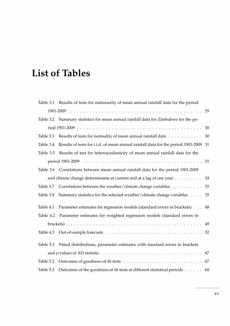
List of Tables
Table 3.1 Results of tests for stationarity of mean annual rainfall data for the period
1901-2009 . . . . . . . . . . . . . . . . . . . . . . . . . . . . . . . . . . . . . . . . . . . 29
Table 3.2 Summary statistics for mean annual rainfall data for Zimbabwe for the pe-
riod 1901-2009 . . . . . . . . . . . . . . . . . . . . . . . . . . . . . . . . . . . . . . . . 30
Table 3.3 Results of tests for normality of mean annual rainfall data . . . . . . . . . . . 30
Table 3.4 Results of tests for i.i.d. of mean annual rainfall data for the period 1901-2009 31
Table 3.5 Results of test for heteroscedasticity of mean annual rainfall data for the
period 1901-2009 . . . . . . . . . . . . . . . . . . . . . . . . . . . . . . . . . . . . . . 31
Table 3.6 Correlations between mean annual rainfall data for the period 1901-2009
and climate change determinants at current and at a lag of one year . . . . . . . . . 34
Table 3.7 Correlations between the weather/climate change variables . . . . . . . . . . 35
Table 3.8 Summary statistics for the selected weather/climate change variables . . . . 35
Table 4.1 Parameter estimates for regression models (standard errors in brackets) . . . 48
Table 4.2 Parameter estimates for weighted regression models (standard errors in
brackets) . . . . . . . . . . . . . . . . . . . . . . . . . . . . . . . . . . . . . . . . . . . 49
Table 4.3 Out-of-sample forecasts . . . . . . . . . . . . . . . . . . . . . . . . . . . . . . . 52
Table 5.1 Fitted distributions, parameter estimates with standard errors in brackets
and p-values of AD statistic . . . . . . . . . . . . . . . . . . . . . . . . . . . . . . . . 67
Table 5.2 Outcomes of goodness-of-fit tests . . . . . . . . . . . . . . . . . . . . . . . . . 67
Table 5.3 Outcomes of the goodness-of-fit tests at different statistical periods . . . . . . 68
xv
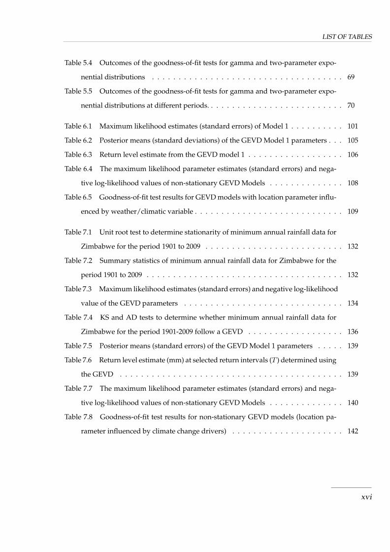
LIST OF TABLES
Table 5.4 Outcomes of the goodness-of-fit tests for gamma and two-parameter expo-
nential distributions . . . . . . . . . . . . . . . . . . . . . . . . . . . . . . . . . . . . 69
Table 5.5 Outcomes of the goodness-of-fit tests for gamma and two-parameter expo-
nential distributions at different periods. . . . . . . . . . . . . . . . . . . . . . . . . . 70
Table 6.1 Maximum likelihood estimates (standard errors) of Model 1 . . . . . . . . . . 101
Table 6.2 Posterior means (standard deviations) of the GEVD Model 1 parameters . . . 105
Table 6.3 Return level estimate from the GEVD model 1 . . . . . . . . . . . . . . . . . . 106
Table 6.4 The maximum likelihood parameter estimates (standard errors) and nega-
tive log-likelihood values of non-stationary GEVD Models . . . . . . . . . . . . . . 108
Table 6.5 Goodness-of-fit test results for GEVD models with location parameter influ-
enced by weather/climatic variable . . . . . . . . . . . . . . . . . . . . . . . . . . . . 109
Table 7.1 Unit root test to determine stationarity of minimum annual rainfall data for
Zimbabwe for the period 1901 to 2009 . . . . . . . . . . . . . . . . . . . . . . . . . . 132
Table 7.2 Summary statistics of minimum annual rainfall data for Zimbabwe for the
period 1901 to 2009 . . . . . . . . . . . . . . . . . . . . . . . . . . . . . . . . . . . . . 132
Table 7.3 Maximum likelihood estimates (standard errors) and negative log-likelihood
value of the GEVD parameters . . . . . . . . . . . . . . . . . . . . . . . . . . . . . . 134
Table 7.4 KS and AD tests to determine whether minimum annual rainfall data for
Zimbabwe for the period 1901-2009 follow a GEVD . . . . . . . . . . . . . . . . . . 136
Table 7.5 Posterior means (standard errors) of the GEVD Model 1 parameters . . . . . 139
Table 7.6 Return level estimate (mm) at selected return intervals (T ) determined using
the GEVD . . . . . . . . . . . . . . . . . . . . . . . . . . . . . . . . . . . . . . . . . . 139
Table 7.7 The maximum likelihood parameter estimates (standard errors) and nega-
tive log-likelihood values of non-stationary GEVD Models . . . . . . . . . . . . . . 140
Table 7.8 Goodness-of-fit test results for non-stationary GEVD models (location pa-
rameter influenced by climate change drivers) . . . . . . . . . . . . . . . . . . . . . 142
xvi

LIST OF TABLES
Table 8.1 Maximum likelihood parameter estimates and negative log-likelihood of
the time-homogenous and non-stationary GPD models for mean annual rainfall
data for Zimbabwe . . . . . . . . . . . . . . . . . . . . . . . . . . . . . . . . . . . . . 165
Table 8.2 Return level estimate (mm) at selected return intervals (T ) determined using
the GPD Model 1 . . . . . . . . . . . . . . . . . . . . . . . . . . . . . . . . . . . . . . 166
Table 9.1 Parameter estimates, deviance statistic and p-value of C statistic for logistic
regression models . . . . . . . . . . . . . . . . . . . . . . . . . . . . . . . . . . . . . . 178
Table 9.2 Parameter estimates, deviance statistic and p-value of C statistic for GEVD
regression models . . . . . . . . . . . . . . . . . . . . . . . . . . . . . . . . . . . . . . 180
Table 9.3 The in-sample and out-of-sample sizes . . . . . . . . . . . . . . . . . . . . . . 181
Table 9.4 The in-sample and out-of-sample sizes . . . . . . . . . . . . . . . . . . . . . . 182
xvii

Abbreviations
ACF Autocorrelation Function
AD Anderson-Darling
ADF Augmented Dickey-Fuller
EVT Extreme Value Theory
FAO Food and Agriculture Organisation of the United Nations
GEVD Generalised Extreme Value Distribution
GLM Generalised Linear Model
GPD Generalised Pareto Distribution
JB Jacque Bera
KPSS Kwiatkowski-Phillips-Schmidt Shin
LM Lagrange Multiplier
MCMC Markov Chain Monte Carlo
MLE Maximum Likelihood Estimation
NLL Negative Log-Likelihood
PACF Partial Autocorrelation Function
PP Phillips Perron
PPCC Probability Plot Correlation Coefficient
Q-Q Quantile to Quantile
RRMSE Relative Root Mean Square Error
RMAE Relative Mean Absolute Error
SDSLP Standardised Darwin Sea Level Pressure
SOI Southern Oscillation Index
SPEI Standardised Precipitation Evapotranspiration Index
xviii

Research Output
A list of publication from this thesis is given below.
Peer-reviewed Journal Publications
1. R. Chifurira, D. Chikobvu, and D. Dubihlela (2016). Rainfall prediction for
sustainable economic growth. Environmental Economics , 7(4), 120-129.
2. D. Chikobvu and R. Chifurira (2015). Modelling extreme minimum rainfall
using the generalised extreme value distribution for Zimbabwe. South African
Journal of Science, 111(9/10):1-8.
3. R. Chifurira and D. Chikobvu (2014). Modelling extreme maximum rainfall
for Zimbabwe. South African Statistical Journal Proceedings: Proceedings of
the 56th Annual Conference of the South African Statistical Association, 9-16.
4. D. Chikobvu and R. Chifurira (2012). Predicting Zimbabwe’s annual rainfall
using the Southern Oscillation Index: Weighted regression approach. African
Statistical Journal, 15, 97-107.
5. R. Chifurira and D. Chikobvu (2017) Extreme Rainfall: Candidature probabil-
ity distributions for mean annual rainfall data. Under Review. Submitted to
Journal of Disaster Risk Studies.
xix

Conference Presentations
1. R. Chifurira and D. Chikobvu. Modelling extreme minimum annual rainfall
for Zimbabwe. 33rd Southern Africa Mathematical Sciences Association An-
nual Conference, 24-28 November 2014, Victoria Falls, Zimbabwe.
2. R. Chifurira and D. Chikobvu. Modelling extreme maximum annual rainfall
for Zimbabwe. 56th Annual Conference of the South African Statistical Asso-
ciation, 28 - 30 October 2014, Rhodes University, Grahamstown, South Africa.
3. R. Chifurira and D. Chikobvu. Predicting Zimbabwe’s Annual Rainfall us-
ing Darwin Sea Level Pressure Index . 54th Annual Conference of the South
African Statistical Association,5-9 November 2012, Nelson Mandela Metropoli-
tan University, Port Elizabeth, South Africa.
4. D. Chikobvu and R. Chifurira. Predicting Rainfall and drought using the
Southern Oscillation Index in drought-prone Zimbabwe. 53th Annual Confer-
ence of the South African Statistical Association,31 October-4 November 2011,
Council for Scientific and Industrial Research and Statistics South Africa, Pre-
toria, South Africa.
xx
Chapter 1
Introduction
This chapter outlines the background of the study, statement of the problem, re-
search aim, objectives, and the significance of the study. The chapter also summa-
rizes related literature on modelling rainfall, contributions of the study and con-
cludes with the thesis layout.
1.1 Background
There is an increasing concern in Southern Africa about the declining rainfall pat-
terns as a result of global warming (Rurinda et al., 2014; Mushore, 2013; Mazvimavi,
2010). According to Muchunu at al. (2014) Southern Africa is a region of significant
rainfall variability and is prone to serious drought and flood events. This raises seri-
ous concern, if proved correct, because rainfall has a substantial influence over agri-
culture, food security, infrastructure development and the economy. Zimbabwe’s
rain-fed agriculture production is the main driver of the economy (Mamombe at al.,
2017) and any effort to revive the country’s economy can be hampered by erratic
rains. Although knowledge of rainfall patterns over an area may be used for strate-
gic economic planning, it is one of the most difficult meteorological parameters to
study because of a lack of reliable data and large variations of rainfall in space, and
time. Therefore, developing methods that can suitably predict meteorological events
is extremely valuable for both meteorologists and statisticians in light of global cli-
1

1.1. Background
mate change. Zimbabwe’s developmental goals and drought/floods mitigation ef-
forts depend on long-lead time and accurate prediction of rainfall in a challenging
global climate change environment. The upsurge of extreme weather events and
global weather/climate change call for extensive research. Timely and accurate pre-
diction of the amounts of rainfall in Zimbabwe is important not only in developing
the economy, but also for assisting in decision-making on planning disaster risk re-
duction strategies by government agencies and citizens.
Zimbabwe is situated in Southern Africa between latitudes 15030′′and 22030
′′south
of the equator, and between longitudes 250 and 33010′′
east of the Greenwich Merid-
ian. It is a land locked country that shares its border with Mozambique to the east,
South Africa to the south, Botswana to the west and Zambia to the north. It has a
land area of approximately 390 757 square kilometers. Zimbabwe has, in previous
years, been severely affected by erratic rainfall patterns and sometimes droughts.
According to Rurinda et al. (2013), Zimbabwe is one of the ’hotspots’ for climate
change with predicted increases in rainfall variability and increased probability of
extreme events such as droughts and flash floods. During the 1991 to 1992 rainy
season, Zimbabwe and some Southern Africa Development Community (SADC)
countries experienced the worst drought period (Zimbabwe Central Statistical Of-
fice Handbook, 1994). In the year 2000, Zimbabwe was ravaged by cyclone Eline.
Between 2001 to 2003, Zimbabwe only experienced rainfall in the first half of the
rainfall season and a dry spell in the second half, resulting in severe droughts in
some parts of the country. Between 2004 to 2008, Zimbabwe received an average
amount of rainfall in the northern parts of the country while other parts received
very little to no rainfall. During the 2009 to 2010 rainfall seasons, Zimbabwe re-
ceived below average rainfall in the first half of the rainfall season and above aver-
age rainfall in the second half of the rainfall season (Zimbabwe Central Statistical
Office Handbook, 2010). Due to these changes in rainfall patterns in Zimbabwe, re-
search in predicting the amount of rainfall in the country is crucial.
2

1.2. Statement of the problem
1.2 Statement of the problem
Zimbabwe’s economy is mainly agro-based and is thus vulnerable to the effects of
weather and climatic change. The severe impact of weather and climatic change is
due to the fact that the country does not have adequate resources or technology to
deal with the conditions that accompany weather and climatic change. Challenges
include droughts, floods, cyclones and more recently high variability in seasonal
rainfall (Dodman and Mitlin, 2015; Washington and Preston, 2006). Therefore, there
is a need to model annual rainfall patterns for Zimbabwe with the aim of predicting
extreme annual rainfall trends. Such an analysis will be used to compute the return
period, which is the mean period of time in years for a rare event such as droughts
or floods of a given magnitude to be equaled or exceeded once.
1.3 Aim and objectives of the thesis
The main aim is to develop a modelling framework which can be used in the mete-
orological sector for carrying out accurate assessments of the frequency and level of
occurrence of extreme mean annual rainfall.
The objectives are to:
(a) Propose predicting models for mean annual rainfall for Zimbabwe.
(b) Fit parent theoretical distributions to mean annual rainfall and select the best
fitting distribution. Distributions considered include the gamma, normal, log-
normal and log-logistic. Parent distributions concentrate on the location of the
main body of the data.
(c) Fit extreme value distributions namely; two-parameter exponential, Gener-
alised Extreme Value and Generalised Pareto Distributions to mean annual
3

1.4. Literature review
rainfall and select the best fitting distribution. Extreme value distributions
concentrate on what happens at the extremes, away from the main body of
the data i.e. at the tails of the data.
(d) Identify the main weather/climatic change drivers of extreme mean rainfall
for Zimbabwe.
(e) Propose prediction models for meteorological drought probabilities for Zim-
babwe.
1.4 Literature review
This section reviews relevant studies in the modelling of rainfall that have been pre-
viously conducted.
1.4.1 Introduction to literature review
Natural disasters such as floods, droughts, earthquakes and other natural disasters
are established in the literature as destructive to humans and their environment.
The impacts of these natural disasters may be severe. Therefore, careful planning
and mitigating efforts are required to reduce the risks associated with these natu-
ral disasters. This thesis focuses on reducing the risk of disasters that occur as a
result of extreme rainfall such as floods and droughts. Modelling mean annual rain-
fall for a drought-prone country, such as Zimbabwe, is very important for decision-
making in the agricultural sector and sectors involved in disaster risk reduction.
Decision-making in the agricultural sector involves strategic planning with regard
to water resource management and the selection of types of crops, and animals to
raise. Whereas, in the disaster risk reduction sector, decision-making involves strate-
gic planning on coping mechanisms for the country using information on the sever-
ity and occurrence (return period) of drought/flash flood. It is, therefore, important
to produce very reliable predictions as the consequences of underestimation or over-
4

1.4. Literature review
estimation can be extremely costly. Failure to accurately predict annual rainfall can
result in loss of lives and low agriculture production. It can also result in economic
challenges since the country’s economy is agro-based.
1.4.2 Modelling rainfall for Zimbabwe
Previous studies on modelling rainfall in Zimbabwe mainly used correlation anal-
ysis. Unganai (1996) fitted a linear regression model to mean annual rainfall for
Zimbabwe using the national data set for the period 1901-1994. Using tempera-
ture as a covariate, the study established that mean annual rainfall for Zimbabwe
had declined by 10% during the period under investigation. Makarau (1995) also
made a similar conclusion. Mason and Jury (1997) investigated quasi-periodicities
in annual rainfall totals over Southern Africa. The study established that an El Nino
Southern Oscillation event and sea surface temperature anomalies in the Indian and
South Atlantic Oceans influence rainfall variability in Southern Africa. Chikodzi et
al. (2013) used time series analysis to investigate trends in national rainfall data and
Zaka rainfall station data. The study used data for the years 1930-2010 and showed
a significant decline in rainfall amounts during this period.
Mazvimavi (2008) departed from the use of correlation analysis and employed non-
parametric tests to investigate possible changes in extreme annual rainfall in Zim-
babwe. The study used the Mann-Kendal test to investigate whether rainfall data
from 40 rainfall stations in Zimbabwe vary with time. The main finding was that
there was no evidence that annual rainfall data for the years 1892-2000 for each rain-
fall station had changed over time i.e. the Mann-Kendal test showed no significant
trend with time for the data.
Mazvimavi (2010) investigated changes over time of annual rainfall for the same 40
rainfall stations using quantile regression technique. The total rainfall data set for
5

1.4. Literature review
the period 1892-2000 was divided as follows (a) the early part of the rainfall sea-
son (October-November-December), (b) middle to end of the rainy season (January-
February-March) and (c) the whole year. The study established that the annual rain-
fall at the 40 rainfall stations did not demonstrate evidence of changes with time in
all the three time periods. The researcher noted that the absence of trends with time
did not imply that global warming will not cause changes in rainfall in Zimbabwe,
but the effects did not result in significant statistical changes in the historical rainfall
record.
Shoko and Shoko (2014) analysed the relationship between mean annual rainfall
amounts for Zimbabwe and the El Nino Southern Oscillation phases. The study
used mean annual rainfall data for the period 1901-1997. The data set was divided
into three categories, namely: drought (rainfall less than 488.4 mm), normal (rain-
fall between 489 mm and 839 mm) and wet (rainfall equal to 840 mm and more).
Correlation analysis was used to find relationships between mean annual rainfall
amounts in different categories and the El Nino Southern Oscillation phases. The
results indicated a positive relationship between rainfall and the El Nino Southern
Oscillation phases in all the categories.
Manatsa et al. (2008), using averaged seasonal rainfall for the period 1901-2000
showed the superiority of the Darwin sea level pressure anomalies over the Southern
Oscillation Index (SOI) as a simple drought predictor for Southern Africa. Using cor-
relation analysis, the study established that the averaged Darwin sea level pressure
anomalies for the months March, April, May and June were the earliest and sim-
plest predictor of drought in Zimbabwe. Hoell et al. (2017) using southern Africa’s
precipitation data of the months December to March for the period 1979 to 2014
showed that opposing El Nino Southern Oscillation and Subtropical Indian Ocean
Dipole result in strong southern Africa climate impacts during December to March
period. Manatsa et al. (2017) using correlation analysis investigated the relationship
6

1.4. Literature review
between Nino 3.4 index an El Nino Southern Oscillation index and the standard-
ised precipitation evapotranspiration index (SPEI) for Southern Africa. The study
showed that Nino 3.4 values for the month of May are correlated to SPEI. Research
on the influence of weather/climate drivers such as El Nino Southern Oscillation is
not limited to Southern Africa’s climate only, Roghani et al. (2016) using monthly
rainfall data for the period 1951 to 2011 investigated the relationship between SOI
and October to December rainfall in Iran. The study showed that average SOI and
SOI phases during July to September were related with October to December rain-
fall.
However, in this thesis, we used a longer data set, i.e. data set for the period 1901-
2009 as the in-sample data set and 2010-2015 as the out-of-sample data set. Secondly,
we employed the use of extensive statistical models to (i) identify the simplest and
earliest warning meteorological indicators that influence mean annual rainfall for
Zimbabwe, (ii) identify the best suitable probability distribution of mean annual
rainfall, (iii) describe extreme maxima and minima annual rainfall for Zimbabwe
using extreme value theory and (iv) predict drought probabilities for Zimbabwe us-
ing extreme value theory. This was a clear departure from available literature on
Zimbabwe and to our knowledge, there is no work which uses extreme value theory
on Zimbabwean mean annual rainfall.
Much research has been conducted to study the physical and statistical properties of
rainfall using observational data. Research has been done on finding the probability
distributions of rainfall amount (Deka et al., 2009; Cho et al., 2004). It is gener-
ally assumed that a hydrological variable follows a certain probability distribution.
Many probability distributions, in many different situations have been considered.
Stagge et al. (2015), Husak et al. (2007),Cho et al. (2004), Aksoy (2000), Adiku et
al. (1997),and McKee et al. (1993) modelled daily rainfall data using the gamma
distribution. Suhaila et al. (2011), Deka et al. (2009), and Cho et al. (2004) inves-
7

1.5. Significance of the study
tigated the performance of the lognormal distribution in fitting daily and monthly
rainfall data. Fitzgerald (2005) and Ahmad et al. (1988) fitted the log-logistic dis-
tribution to daily rainfall data. Sakulski et al. (2014) fitted the log-logistic, Singh-
Maddala, lognormal, generalised extreme value, Frechet and Rayleigh distributions
to spring, autumn and winter rainfall data from the Eastern Cape province, South
Africa. The researchers found the Singh-Maddala distribution to be the best fitting
distribution to all four seasons rainfall data. Stagge et al. (2015) fitted seven can-
didate distributions to standardised precipitation index (SPI) for Europe and rec-
ommended the two-parameter gamma distribution for modelling SPI. Suhaila and
Jemain (2007) found that the mixed Weibull distribution was the better fitting dis-
tribution when compared to single distributions in modelling rainfall amounts in
Peninsular Malaysia. Zin et al. (2009) also found that the generalised lambda dis-
tribution was the best fitting distribution for Peninsular Malaysia. However, the
results obtained by Suhaila and Jemain (2007) differ from the results obtained by
Zin et al. (2009). Each kind of probability distribution has its own applications and
limitations. A regionalised study on the statistical modelling of annual rainfall is,
therefore, very essential as statistical models may vary according to geographical
location of the area and the length of the data series used.
1.5 Significance of the study
Understanding the processes governing rainfall is important for a wide range of hu-
man activities. This study provides the first application of statistical analysis of mean
annual rainfall for Zimbabwe using parent and extreme value distributions. Thus,
this study aims to enhance our understanding of rainfall patterns in order to develop
tools that reduce the negative impact of extreme rainfall events in the agricultural
and other rain-dependent sectors. The amount of rainfall is a key determinant of the
success of the agriculture sector. Knowledge of rainfall behaviour at a lead-time be-
fore the onset of the rainfall season plays a pivotal role in guiding farmers and agri-
culture experts on the type of crops that are viable in the following rainfall season.
8

1.6. Contributions
Knowledge of rainfall behaviour is also important in defining appropriate water
harvesting and distribution plans for industrial and domestic use. Finally, knowl-
edge of rainfall behaviour is essential as an early drought/flood monitoring tool for
citizens, government agencies and non-governmental organizations involved in dis-
aster management associated with drought and flood risk assessment. By estimating
return periods of high rainfall amounts or extremely low rainfall amounts that can
lead to floods or droughts, respectively, the management of the disaster risk that
occurs as a result of extreme mean annual rainfall is supported.
1.6 Contributions
The main contribution of this thesis is to apply statistical techniques in modelling
mean and extreme annual rainfall for Zimbabwe.
The specific contributions are to:
1. Propose a suitable model to explain the influence of Southern Oscillation Index
(SOI) and standardised Darwin Sea level Pressure anomalies on mean annual
rainfall for Zimbabwe.
2. Investigate the best theoretical parent distributions for mean annual rainfall
for Zimbabwe.
3. Propose a suitable Generalised Extreme Value Distribution model for extreme
maximum annual rainfall for Zimbabwe.
4. Propose a suitable Generalised Extreme Value Distribution model for extreme
minimum annual rainfall for Zimbabwe
5. Propose a suitable Generalised Pareto Distribution model for extreme maxi-
mum annual rainfall for Zimbabwe.
6. Propose a Generalised Extreme Value Distribution binary regression model for
predicting drought probabilities for Zimbabwe
9

1.7. Thesis layout
1.7 Thesis layout
The thesis is organized as follows: Chapter 2 reviews statistical tests and graph-
ical methods used to analyse the data. Chapter 3 describes the data used in this
thesis. Chapter 41 deals with modelling mean annual rainfall using the Southern
Oscillation index and standardised Darwin sea level pressure anomalies using the
weighted regression approach. The best fitting candidate probability distribution
for mean annual rainfall is selected in Chapter 5.2 Goodness-of-fit tests, namely:
RRMSE, RMAE and PPCC are used to select the best fitting distribution. The first
part of the thesis shows that modelling mean annual rainfall using the ’averaging
thinking’ only is not enough. Therefore, in the second part of the thesis, extreme
mean annual rainfall for Zimbabwe is modelled using different approaches.
In Chapters 6 to 83, modelling of the tail behaviour of the mean annual rainfall
through the Extreme Value Theory (EVT) is discussed. The theory behind estima-
tion of the parameters of the extreme value distributions are also discussed in the
Chapter 6. In Chapters 6 and 7, it is revealed that extreme maxima and minima an-
nual rainfall for Zimbabwe does not trend with time. It is also shown in the same
chapters that incorporating meteorological climate change indicators improves the
generalised extreme value distribution model for the data. Chapter 84 deals with
modelling extreme maxima annual rainfall data using the peak-over-threshold ap-
proach. The chapter also confirms that extreme mean annual rainfall for Zimbabwe
does not trend with time. In Chapter 95, we propose a binary model to predict
1 Rainfall prediction for sustainable economic growth. Environmental Economics, Vol. 7(4), 2016,pp. 120-129; Predicting Zimbabwe’s annual rainfall using the Southern Oscillation Index: Weightedregression approach. The African Statistical Journal, Vol. 15, 2012, pp. 87-107.
2 Extreme Rainfall: Selecting the best probability distribution for mean annual rainfall: An applica-tion to Zimbabwean data
3 Modelling extreme maximum annual rainfall for Zimbabwe. South African Statistical Journal:Peer-reviewed Proceedings of the 56th Annual Conference of the South African Statistical Association,2014, pp. 9-16; Modelling of extreme minimum rainfall using generalised extreme value distributionfor Zimbabwe, South African Journal of Science, 2015, pp. 1-8.
4 Modelling mean annual rainfall extremes using a Generalised Pareto Distribution Model5 Generalised Extreme Value Regression with Binary Dependent variable: An application to pre-
dicting meteorological drought probabilities. Submitted to Journal of disaster risk studies, 2017
10

1.7. Thesis layout
drought probabilities when the binary dependent variable is extreme. In order to ad-
equately predict drought probabilities, we used the generalised linear model (GLM)
with the quantile function of the generalised extreme value distribution (GEVD) as
the link function. Chapter 9 shows that the GEVD regression model performs better
than the logistic model, thereby providing a good alternative candidate for predict-
ing drought probabilities for Zimbabwe. The chapter also establishes that standard-
ised Darwin sea level pressure anomalies for April of the same year is an earlier and
skillful predictor of meteorological droughts in Zimbabwe.
The following statistical packages were used in this thesis: R, Eviews and SAS.
11

Chapter 2
Methodology
2.1 Introduction
This chapter mainly presents statistical tests and graphical methods used to analyse
the mean annual rainfall data in Zimbabwe.
2.2 Tests for stationarity
A common assumption in many time series techniques is that the data is stationary.
There are two types of stationarity, namely weakly stationary (usually referred to as
stationary) and strongly stationary (usually referred to as strictly stationary). A time
series {xt, t ∈ Z} (where Z is the integer set) is said to be weakly stationary or just
stationary if
(i) E(x2t ) <∞ ∀ t ∈ Z.
(ii) E(xt) = µ ∀ t ∈ Z.
(iii) Cov(xs, xt) = Cov(xs+h, xt+h) ∀ s, t, h ∈ Z.
Thus, a stationary time series has the property that the mean, variance and autocor-
relation structure is time invariant i.e. depends only on (t− s) and not on s or t.
12

2.2. Tests for stationarity
A time series {xt, t ∈ Z} is said to be strongly or strictly stationary if the joint distri-
butions
(xt1 , ..., xtk) D= (xt1+h, ..., xtk+h
)
for all sets of time points t1, ..., tk ∈ Z and integer h.
In this study, the augmented-Dickey Fuller (ADF), Phillips-Perron(PP) and Kwiatkowski-
Phillips-Schmidt-Shin (KPSS) tests are used to formally test for stationarity in data.
The null hypothesis for the ADF and PP tests is that the mean annual rainfall series
is non-stationary while for the KPSS test is that the mean annual rainfall series is
stationary.
2.2.1 Augmented-Dickey Fuller (ADF) test
The ADF test is one of the most commonly used tests for stationarity of time series.
The test is also known as the unit root (non-stationary) test. There are three cases of
the ADF test equation depending on the nature of the time series data being tested.
a) When the time series is flat (no trend) and potentially slow-turning to zero
value. The test equation is:
∆xt = φxt−1 + θ1∆xt−1 + θ2∆xt−2 + ...+ θk∆xt−k + εt
The equation has no intercept and no time trend.
b) When the time series is flat (no trend) and potentially slow-turning to non-zero
value. The test equation is:
∆xt = α0 + φxt−1 + θ1∆xt−1 + θ2∆xt−2 + ...+ θk∆xt−k + εt
The equation has an intercept (α0) but no time trend.
c) When the time series has trend in it (either up or down) and is potentially
slowly turning around a trend line you would draw through the data. The test
13

2.2. Tests for stationarity
equation is:
∆xt = α0 + φxt−1 + γt+ θ1∆xt−1 + θ2∆xt−2 + ...+ θk∆xt−k + εt
The equation has an intercept (α0) and time trend γt. In all cases εt is a white
noise error.
where εt ∼ i.i.d.(0, σ2) and the number of augmenting lags (k) is determined by
minimising the Schwartz Bayesian information criterion or lags are dropped until
the last lag is statistically significant. According to Niyimbanira (2013) the ADF test
relies on rejecting the null hypothesis of the data need to be differenced to make
it stationary (the series is non-stationary) in favour of the alternative hypothesis of
the data is stationary and does not need to be differenced. Once a value for the test
statistic:
ADF =φ
σwhere φ = ρ− 1,
is computed it can be compared to the relevant critical value for the Dickey-Fuller
test. σ is the OLS standard error of φ. If the test statistic is less than the critical value,
then the null hypothesis of φ = 0 is rejected and no unit root is present.
2.2.2 Phillips-Perron (PP) test
The PP stationarity test and the ADF test differ mainly on how they deal with serial
correlation and heteroscedasticity in the errors. The ADF test uses a parametric auto-
regression to approximate the auto-regressive moving average structure of the errors
in the regression while the PP test ignore any serial correlation in the test regression.
For the model
xt = α0 + φxt−1 + εt,
the test regression for the PP test is:
∆xt = α0 + δxt−1 + εt
14
2.2. Tests for stationarity
where we may exclude the constant (α0) or include a trend term γt and
εt = δεt + ut, ut ∼ i.i.d(0, σ2),
where i.i.d stand for independent and identically distributed. The null hypothesis
to be tested is H0 : δ = 0. The PP test correct for any serial correlation and het-
eroscedasticity in the errors εt of the test regression by directly modifying the ADF
test statistic. There are two statistics, Zδ and Zt, calculated as:
Zδ = nδ − 12n2(s.e(δ))
σ2(λ2
n − σ2) (2.1)
Zt =
√σ2
λ2n
δn − 1
s.e(δ)− 1
2(λ2
n − σ2)1
λ2n
n(s.e(δ))σ2
(2.2)
where σ2 and λ2n are the consistent estimates of the variance parameters
λ2n = lim
n→∞E
[1nε2t
](2.3)
σ2 =1
n− plim
n←∞
n∑t=1
E(ε2t ) (2.4)
where εt is the OLS residual, p is the number of covariates in the regression. Un-
der the null hypothesis that δ = 0, Zt and Zδ statistics have the same asymptotic
distributions as the ADF statistic.
2.2.3 Kwiatkowski-Phillips-Schmidt-Shin (KPSS) test
The KPSS test has been developed to complement tests for non-stationarity as the
ADF and PP tests have low power with respect to near non-stationary and long-run
trend processes. KPSS has stationary as the null hypothesis. Assuming there is no
trend, then it follows that:
xt = β′Dt + µt + ut (2.5)
µt = µt−1 + εt, εt ∼ N(0, σ2ε ),
15

2.3. Tests for randomness and serial correlation
where Dt contains deterministic components (constant or constant plus time trend).
The null hypothesis that xt is stationary, I(0), is formulated as H0 : σ2ε = 0, which
implies that µt is a constant. The KPSS test statistic is the Langrange multiplier (LM)
or score statistic for testing σ2ε = 0 against the alternative that σ2
ε > 0 and is given by
KPSS =
(n−2
n∑t=1
S2t
)/λ2 (2.6)
where St =∑t
j=1 uj , ut is the residual of a regression of yt and Dt. λ2 is a consistent
estimate of the long-run variance of ut using ut.
2.3 Tests for randomness and serial correlation
2.3.1 Bartels rank test
This is the rank version of von Neumann’s Ratio test for randomness. The test statis-
tic is:
RV N =∑n−1
i=1 (Ri −Ri+1)2∑ni=1(Ri − (n+ 1)/2)2
(2.7)
where Ri = rank(yi), i = 1, ...., n. It is known that (RV N − 2)/σ is asymptotically
standard normal, where σ2 = 4(n−2)(5n2−2n−9)5n(n+1)(n−1) . The possible alternatives are ”two
sided”, ”left sided” and ”right sided”. By using the alternative ”two sided” the null
hypothesis of randomness is tested against non-randomness. By using the alterna-
tive ”left sided” the null hypothesis of randomness is tested against a trend. By using
the alternative ”right sided” the null hypothesis of randomness is tested against a
systematic oscillation. In this thesis we use the ”two sided” alternative.
2.3.2 Ljung-Box test
The Ljung-Box test is widely applied in econometrics and other applications of time
series analysis. Ljung-Box (1978) is a modification of the Box and Pierce (1970)’s
16
2.3. Tests for randomness and serial correlation
Portmanteau Statistic for auto-correlation
Q∗(m) = n
m∑l=1
ρ2l (2.8)
a test statistic for the null hypothesis H0 : ρ1 = ... = ρm = 0, that is the data are
independently distributed. The Ljung-Box statistic is
Q(m) = n(n+ 2)m∑
l=1
ρ2l
n− l. (2.9)
The null hypothesis of independence and identically distributed is rejected if Qm >
χ2α, where χ2
α denotes the 100(1−α)th percentile of the chi-squared distribution with
m degrees of freedom. The Ljung-Box test has more power in finite samples than the
Box and Pierce (1970) test.
2.3.3 Brock-Dechert-Scheinkman (BDS) test
The BDS test is a portmanteau test time based dependence in a series and can be
used for testing against a variety of possible deviations from independence includ-
ing linear dependence, non-linear dependence, or chaos. This test can be applied
to a data series to check for independence and identically distribution (i.i.d.). The
null hypothesis is the data series is i.i.d. against an unspecified alternative (Dutta et
al., 2015; Kuan, 2008). The BDS test takes its root from the concept of a correlation
integral, a measure of spatial correlation in m-dimensional space originally devel-
oped by Grassberger and Procaccia (1983). The correlation integral at embedding
dimension m can be estimated by
Cm,ε =2
Tm(Tm − 1)
∑m≤s≤t≤T
I(xmt , x
ms ; ε) (2.10)
where Tm = n−m+1 and I(xmt , x
ms ; ε) is an indicator function which is equal to one
if | xt−i − xs−i |< ε for i = 0, 1, ...,m− 1, and zero otherwise.
The correlation integral estimates the probability that any twom-dimensional points
17

2.3. Tests for randomness and serial correlation
are within a distance ε of each other. That is, it estimates the joint probability:
Pr(| xt − xs |< ε, | xt−i − xs−i |< ε, ..., | xt−m+i − xs−m+i |< ε).
If xt are i.i.d. this probability should be equal to the following in the limiting case:
Cm1,ε = Pr(| xt − xs |< ε)m.
Brook et al. (1996) define the BDS statistic as follows:
Vm,ε =√nCm,ε − Cm
1,ε
sm,ε, (2.11)
where sm,ε is the standard of√n(Cm,ε−Cm
1,ε) and can be estimated consistently. Un-
der moderate regularity conditions, the BDS statistic converges in distribution to the
standard normal distribution so that the null hypothesis of i.i.d. is rejected at the 5%
significance level whenever | Vm,ε |> 1.96 (Brook et al., 1996).
Alternatively, we establish if the data series {x1, x2, ..., xn} are a realization of an
i.i.d. process:
xt ∼ i.i.d.(µ, σ2)
using a correlogram. If the data {x1, x2, ..., xn} were really generated by an i.i.d.
process, then about 95% of the autocorrelations ρ1, ρ2, ....., ρn should fall between
the bounds ±1.96√n
, i.e. if the process is i.i.d. we would expect 95% of the sample au-
tocorrelations to lie within the dashed lines of the Auto-Correlation Function (ACF)
plot (Maddala and Kim, 1998).
In this thesis, the ACF plot and the theoretical tests for randomness and serial corre-
lation will be used.
18

2.4. Test for heteroscedasticity
2.4 Test for heteroscedasticity
2.4.1 ARCH-LM test
An uncorrelated time series can still be serially dependent due to a dynamic con-
ditional variance process. A time series exhibiting conditional heteroscedasticity or
autocorrelation in the squared series is said to have autoregressive conditional het-
eroscedastic (ARCH) effects. The ARCH is a Lagrange Multiplier (LM) test of Engle
(1982) to assess the significance of ARCH effects. The test is usually referred to as
the ARCH-LM test.
Consider a time series
xt = µt + εt
where µt is the conditional mean of the process, and εt is an innovation with mean
zero.
Suppose the innovations are generated as εt = σtεt where εt is an independent and
identically distributed process with mean 0 and variance 1. Thus, E(εtεt+h) = 0 for
all lags h 6= 0 and the innovations are uncorrelated.
Let Ht denote the history of the process available at time t. The conditional variance
of xt is:
var(xt | Ht−1) = var(εt | Ht−1) = E(ε2t | Ht−1) = σ2t .
Thus, conditional heteroscedasticity in the variance process is equivalent to autocor-
relation in the squared innovation process.
Now we define the innovation (residual) series as:
19

2.5. Tests for normality
εt = xt − µt
and the squared series ε2t , is then used to check for conditional heteroscedasticity,
which is also known as the ARCH effects. The presence of the ARCH effect is based
on the linear regression
ε2t = α0 + α1ε2t−1 + ...+ αmε
2t−m + εt, for t = m+ 1, ....., n,
where εt denote the error term, m is a pre-specified positive integer, and n is the
sample size. The null hypothesis corresponding to homoscedasticity is:
H0 : α1 = ... = αm = 0
The test statistic for Engle’s ARCH-LM test is the usual F statistic for regression on
the squared residuals. Under the null hypothesis, the F statistic follows a χ2 distri-
bution with m degrees of freedom. A large critical value indicates rejection of the
null hypothesis in favour of the alternative.
2.5 Tests for normality
2.5.1 Jarque-Bera test
In statistical analysis the assumption of data coming from a normal distribution is
often made, however, most informed opinion have accepted that populations might
be non-normal. The Jarque-Bera (JB) test is a goodness-of-fit test of departure from
normality based on the sample skewness and kurtosis. The JB statistic is:
JB = n
[s2
6+
(k − 3)2
24
](2.12)
20

2.5. Tests for normality
where s is the skewness and k is the kurtosis statistics. The skewness estimate statis-
tic is defined as:
s =1n
∑nt=1(xt − x)3
(σ2)32
where xt is each observation and
σ2 =1n
n∑t=1
(xt − x)2.
The skewness gives a measure of how symmetric the observations are about the
mean.
The kurtosis estimate is defined as:
k =1n
∑nt=1(xt − x)4
(σ2)2
The kurtosis gives a measure of the thickness in the tails of a probability density
function.
The JB statistic follows a χ2 distribution with two degrees of freedom. For large sam-
ple sizes, the null hypothesis of normality is rejected if the JB statistic is greater than
the critical value from the χ2 distribution with 2 degrees of freedom.
2.5.2 Shapiro-Wilk test
The Shapiro-Wilk test calculates a W statistic that tests whether a random sample
x1, x2, ..., xn comes from a normal distribution. The W statistic is:
W =(∑n
i=1 aixi)2∑n
i=1 (xi − x)2(2.13)
21

2.6. Model adequacy and goodness-of-fit tests
where xi are the ordered sample values and ai are constants generated from the
means, variances and covariances of the order statistics of a sample of size n from a
normal distribution.
The W statistics is obtained as an F -ratio. The null hypothesis of normality is re-
jected if the calculated p-value is less than α the level of significance.
2.6 Model adequacy and goodness-of-fit tests
2.6.1 Probability-Probability plot
The probability-probability (PP) plot is a graphical technique for determining if the
percentiles of the data and the fitted theoretical distribution come from the same
underlying distribution. If the percentiles are identically distributed variables, then
the PP plot will be a straight line configuration oriented from (0,0) to (1,1). The PP
plot is usually sensitive to discrepancies in the middle of a distribution rather in the
tails. Therefore, the PP plot is not desirable for model adequacy using heavy-tailed
data.
2.6.2 Quantile-Quantile plot
The quantile-quantile (QQ) plot is a graphical technique for determining if the quan-
tiles of the data and the fitted theoretical distribution come from the same distribu-
tion. If the two sets (quantiles of data and fitted theoretical distribution) come from
a population with the same distribution, the points should fall approximately along
the 45-degree reference line. Any significant departure from the reference line indi-
cates that the quantiles of the data and the fitted theoretical distribution have come
from populations with different distributions. The QQ plot tends to emphasise the
comparative structure in the tails and to blur the distinctions in the middle of the
distribution. For this reason, the QQ plot is a better graphical technique when fitting
heavy-tailed distributions.
22

2.6. Model adequacy and goodness-of-fit tests
2.6.3 Kolmogorov-Smirnov test
The Kolmogorov-Smirnov (KS) test is used to decide if a sample comes from a pop-
ulation with a specific distribution. The KS test belongs to the supremum class of
empirical distribution function statistics and is based on the largest vertical differ-
ence between the hypothesized and empirical distribution (Razali and Wah, 2011).
Given that x1, x2, ..., xn are n ordered data points, Conover (1999) defined the test
statistic proposed by Kolmogorov (1933) as
T = supx | F ∗(x)− Fn(x) | (2.14)
where ”sup” stands for supremum which means the greatest. F ∗(x) is the hypothe-
sized distribution function whereas Fn(x) is the empirical distribution function. If T
exceeds the 1 − α quantile as given by the table of quantiles for the KS test statistic,
then we reject the null hypothesis that the data follows a specified distribution at the
level of significance, α. The main disadvantage of the KS test statistic is that it places
more weight at the center of the distribution than on the tails and therefore cannot
adequately check goodness-of-fit of heavy tailed distribution.
2.6.4 Anderson-Darling test
The Anderson-Darling (AD) test is an improvement of the Kolmogorov-Smirnov
(KS) test. It gives more weight to the tails of the distribution than the KS test does
(Farrel and Rogers-Stewart, 2006). The AD statistic is defined as:
W 2n = n
∫ ∞−∞
[Fn(x)− F ∗(x)]2ψ(F ∗(x))dF ∗(x) (2.15)
where ψ is a non-negative weight function which can be computed from
ψ = [F ∗(x)(1− F ∗(x))]−1.
23

2.7. Model selection
In order to make the computation of the statistic easier, Arshad et al. (2003) redefined
the AD statistic as
W 2n = −n− 1
2
n∑t=1
(2t− 1)[lnF ∗(xt) + ln(1− F ∗(xn−t+1))] (2.16)
where F ∗(xt) is the cumulative distribution function of the specified distribution, yt
is ordered data and n is the sample size.The null hypothesis of the AD test is that
the data follows a specified distribution at the level of significance, α. According to
Arshad et al. (2003), the AD test is the most powerful empirical distribution func-
tion test. Since the AD statistic is a measure of the distance between the empirical
and hypothesized distribution functions, the fitted distribution with the smallest AD
statistic value will be selected as the best fitting model.
In this thesis the QQ plot and AD test are used to check for model adequacy of the
fitted models.
2.7 Model selection
In this thesis the Akaike information criterion (AIC) and natural forecast statistic
namely; the relative root mean square error (RRMSE) and relative mean absolute
error (RMAE) and probability plot correlation coefficient (PPCC) are used to select
the best fitting model against competing models.
2.7.1 Akaike information criterion
AIC is a measure of how well the fitted model fits with the data in respect to candi-
date models. AIC estimates the quality of each model relative to the other models.
The AIC is given by:
AIC = −2ln
+2kn
where l is the log likelihood, k is the number of parameters in the model and n is the
sample size. The model with the smallest AIC value is usually regarded as the best
24

2.7. Model selection
model for the data (Tsay, 2013).
2.7.2 Assessing model performance
In this thesis the measures of average error namely, mean absolute percentage error
(MAPE) and root mean square error (RMSE) are applied to evaluate model perfor-
mance. These measures are based on statistical summaries of εt(t = 1, 2, .., n). The
average model-estimation error can be written generically as:
εt =[∑n
t=1 vt | εt |ω∑nt=1 vt
] 1ω
(2.17)
where ω ≥ 1 and vt is a scaling assigned to each | εt |ω according to its hypothesized
influence on the total error (Willmott and Matsuura, 2005). For the calculation of
RMSE, ω = 2 and vt = 1. RMSE is measured in the same unit as the forecast and is
given by:
RMSE =
[n−1
n∑t=1
| εt |2] 1
2
(2.18)
The MAPE is also measured in the same unit as the forecast, but gives less weight
to large forecast errors than the RMSE. To obtain the MAPE we set ω = 1 and vt = 1
and is given by:
MAPE =
[n−1
n∑t=1
| 100εi |
](2.19)
According to Willmott and Matsuura (2005) and Truck and Liang (2012), MAPE is
the most natural measure of average error magnitude and it is an unambiguous
measure of the average error magnitude. The MAPE and RSME values can range
from 0 to infinity and smaller values indicate a better model.
25

2.7. Model selection
2.7.3 Forecast statistics
The relative root mean square error (RRMSE) and relative mean absolute error (RMAE)
assesses the difference between the observed values and the expected values of the
assumed distributions. The probability plot correlation coefficient (PPCC) measures
the correlation between ordered values and the corresponding expected values of
the assumed distribution. The formulae for the tests are
RRMSE =
√√√√ 1n
n∑i=1
(xi:n − Q(Fi)
xi:n
)2
(2.20)
RMAE =1n
n∑i=1
∣∣∣∣∣xi:n − Q(Fi)xi:n
∣∣∣∣∣ (2.21)
PPCC =∑n
i=1(xi:n − x)(Q(Fi)−Q(Fi))√∑ni=1(xi:n − x)2
√∑ni=1(Q(Fi)−Q(F ))2
(2.22)
where xi:n is the observed values of the ith order statistics of a random sample of
size n. Q(Fi) is the estimated quantile value of the assumed distribution associated
with the ith Landwehr plotting position, Fi = i−0.35n . Q(Fi) and x are the averages of
Q(Fi) and xi:n respectively. Heo et al. (2008) investigated the performance of differ-
ent probability plotting positions for extreme value distribution and recommended
the Landwehr plotting position for medium sample sizes. In this thesis we use the
Landwehr plotting position to estimate quantiles of the fitted distributions. The fit-
ted distribution with the smallest values of the RRMSE and RMAE is selected as the
best fitting distribution while the distribution with the computed PPCC closest to 1
indicates the best fitting distribution.
26

Chapter 3
Rainfall data
3.1 Introduction
In this chapter we described the data used in this thesis. Rainfall data series from
Zimbabwe, the Southern Oscillation Index (SOI) and standardised Darwin sea level
pressure (SDSLP) anomalies were used in this study. The SOI and SDSLP were used
to investigate their influence on the amount of rainfall in Zimbabwe. The descriptive
statistics and properties, such as stationarity and distribution of the rainfall data set,
are discussed. Lastly, we used data correlation techniques to select the SOI and
SDSLP for a particular month at a lag which can significantly influence rainfall in
Zimbabwe.
3.2 Mean annual rainfall data
We used the mean annual rainfall data series for the period 1901-2015 obtained from
the Department of Meteorological Services in Zimbabwe. In this study, mean an-
nual rainfall data was chosen over using monthly or daily rainfall data because (i) at
monthly and daily time-lines, rainfall amount records for rainfall stations contains
many zeros (no rainfall amount recorded), (ii) the focus of the thesis was to develop
a national drought/flash floods early warning system. The data set was divided
into the in-sample data set (1901-2009) and the out-of-sample data set (2010-2015).
27

3.2. Mean annual rainfall data
The rainfall amounts were from 40 rainfall stations located across the country. The
rainfall stations had monthly rainfall recordings for more than 100 years. Figure 3.1
shows the map and locations of these rainfall stations.
Figure 3.1: Location of the rainfall stations in Zimbabwe (selected for this study)
The mean annual rainfall for Zimbabwe was calculated. The mean annual rainfall
were considered to improve the signal to noise ratio compared to the use of indi-
vidual station data. The rainfall season in Zimbabwe stretches from mid November
to mid-March of the following year (Mamombe, 2017). Thus, an average annual
rainfall for example 2000 means the average rainfall recorded from October 2000 to
April 2001. Figure 3.2 shows the time series plot of mean annual rainfall for the pe-
riod 1901-2009.
The time series plot in Figure 3.2 shows that the mean annual rainfall appears to be
28

3.2. Mean annual rainfall data
Figure 3.2: Time series plot of mean annual rainfall for Zimbabwe for the period 1901-2009
stationary. We formally tested for stationarity of mean annual rainfall data using the
augmented Dickey-Fuller (ADF), Phillips-Perron (PP) and Kwiatkowski-Phillips-
Schmidt-Shin (KPSS) tests. The results of testing for stationary of mean annual rain-
fall are reported in Table 3.1.
Table 3.1: Results of tests for stationarity of mean annual rainfall data for the period 1901-2009
Test ADF PP KPSSp-value < 0.01 < 0.01 > 0.10
The null hypothesis for the ADF and PP statistic is that the data series is not sta-
tionary. Both the ADF and PP statistics with p-values < 0.01 < 0.05, reject that the
null hypothesis at 5% significance level implying that the mean annual rainfall data
are stationary. This is confirmed by the KPSS statistic with p-value > 0.05 which
fails to reject the null hypothesis for stationarity at 5% level of significance. Table 3.2
presents the summary statistics for the mean annual rainfall data.
The small positive skewness and excess kurtosis clearly illustrates the normality of
29
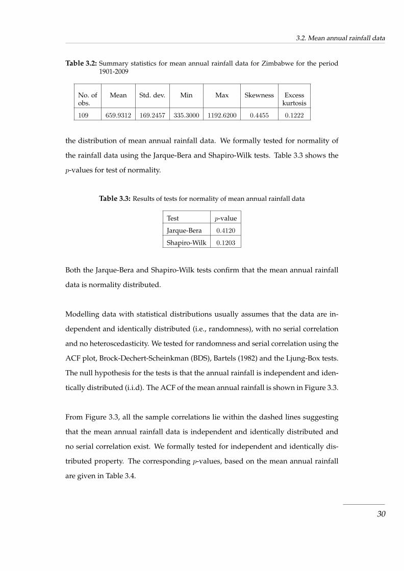
3.2. Mean annual rainfall data
Table 3.2: Summary statistics for mean annual rainfall data for Zimbabwe for the period1901-2009
No. of Mean Std. dev. Min Max Skewness Excessobs. kurtosis
109 659.9312 169.2457 335.3000 1192.6200 0.4455 0.1222
the distribution of mean annual rainfall data. We formally tested for normality of
the rainfall data using the Jarque-Bera and Shapiro-Wilk tests. Table 3.3 shows the
p-values for test of normality.
Table 3.3: Results of tests for normality of mean annual rainfall data
Test p-value
Jarque-Bera 0.4120
Shapiro-Wilk 0.1203
Both the Jarque-Bera and Shapiro-Wilk tests confirm that the mean annual rainfall
data is normality distributed.
Modelling data with statistical distributions usually assumes that the data are in-
dependent and identically distributed (i.e., randomness), with no serial correlation
and no heteroscedasticity. We tested for randomness and serial correlation using the
ACF plot, Brock-Dechert-Scheinkman (BDS), Bartels (1982) and the Ljung-Box tests.
The null hypothesis for the tests is that the annual rainfall is independent and iden-
tically distributed (i.i.d). The ACF of the mean annual rainfall is shown in Figure 3.3.
From Figure 3.3, all the sample correlations lie within the dashed lines suggesting
that the mean annual rainfall data is independent and identically distributed and
no serial correlation exist. We formally tested for independent and identically dis-
tributed property. The corresponding p-values, based on the mean annual rainfall
are given in Table 3.4.
30

3.2. Mean annual rainfall data
Figure 3.3: ACF plot of mean annual rainfall for Zimbabwe for the period 1901-2009
Table 3.4: Results of tests for i.i.d. of mean annual rainfall data for the period 1901-2009
Test p-value
BDS 0.3970
Bartels (1982) 0.7570
Ljung-Box 0.1270
We tested for no heteroscedasticity using the ARCH LM test. The null hypothesis
for the test is that the annual rainfall data has no presence of heteroscedasticity. The
corresponding p-values based on the annual rainfall are given in Table 3.5.
Table 3.5: Results of test for heteroscedasticity of mean annual rainfall data for the period1901-2009
Test p-value
ARCH-LM 0.2790
The tests reported in Tables 3.4 and 3.5 are semi-parametric in nature, i.e., no strict
distributional assumptions are made about the data. The tests confirm that the mean
annual rainfall data are independent and identically distributed, with no serial cor-
31
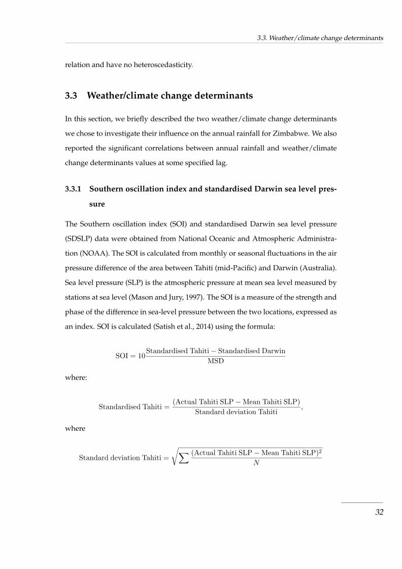
3.3. Weather/climate change determinants
relation and have no heteroscedasticity.
3.3 Weather/climate change determinants
In this section, we briefly described the two weather/climate change determinants
we chose to investigate their influence on the annual rainfall for Zimbabwe. We also
reported the significant correlations between annual rainfall and weather/climate
change determinants values at some specified lag.
3.3.1 Southern oscillation index and standardised Darwin sea level pres-
sure
The Southern oscillation index (SOI) and standardised Darwin sea level pressure
(SDSLP) data were obtained from National Oceanic and Atmospheric Administra-
tion (NOAA). The SOI is calculated from monthly or seasonal fluctuations in the air
pressure difference of the area between Tahiti (mid-Pacific) and Darwin (Australia).
Sea level pressure (SLP) is the atmospheric pressure at mean sea level measured by
stations at sea level (Mason and Jury, 1997). The SOI is a measure of the strength and
phase of the difference in sea-level pressure between the two locations, expressed as
an index. SOI is calculated (Satish et al., 2014) using the formula:
SOI = 10Standardised Tahiti− Standardised Darwin
MSD
where:
Standardised Tahiti =(Actual Tahiti SLP−Mean Tahiti SLP)
Standard deviation Tahiti,
where
Standard deviation Tahiti =
√∑ (Actual Tahiti SLP−Mean Tahiti SLP)2
N
32

3.3. Weather/climate change determinants
where N = number of months
and
Standardized Darwin =(Actual Darwin SLP−Mean Darwin SLP)
Standard deviation Darwin,
where
Standard deviation Darwin =
√∑ (Actual Darwin SLP−Mean Darwin SLP)2
N
where N = number of months
and
MSD =
√∑ (Standardised Tahiti− Standardised Darwin)2
N
where N = number of months
Comparing lead times of SOI and SDSLP values
Monthly SOI and SDSLP values were matched to mean annual rainfall. Table 3.6
shows the correlations between mean annual rainfall and monthly weather/climatic
determinants at current and at a lag of one year.
The focus of this thesis is developing an early warning system for disaster manage-
ment for Zimbabwe. In order to inform government departments and other stake-
holders involved in disaster risk reduction, a timeous prediction of extreme rainfall
for the country is important. Predicting mean annual rainfall at a longer lead-time
before the onset of rainfall season guards against the risk of disaster and can help
the country prepare for extreme rainfall. Thus, we aim to determine a particular
month’s weather/climatic determinant which has a high correlation with mean an-
nual rainfall at a longer lead-time. From Table 3.6, the highest correlation between
the mean annual rainfall for Zimbabwe and monthly SOI values is 0.4289 (SOI value
for August of the current year), which gave a lead-time of 2 months before the onset
33

3.3. Weather/climate change determinants
Table 3.6: Correlations between mean annual rainfall data for the period 1901-2009 and
climate change determinants at current and at a lag of one year
Month SOI SDSLP
current lag of a year current lag of a year
January 0.0468 0.0792 0.0002 0.0780
February 0.1349 0.0120 -0.0784 0.0120
March 0.1748 0.0183 -0.2068 0.0181
April 0.1684 -0.0526 -0.2479 -0.0523
May 0.2570 -0.0429 -0.2000 -0.0424
June 0.2346 0.1118 -0.2022 0.1115
July 0.3027 -0.0484 -0.2166 -0.0482
August 0.4289 -0.0572 -0.3359 -0.0572
September 0.3866 -0.0666 -0.2586 -0.0664
October 0.3189 0.0679 -0.2669 -0.0465
November 0.3465 0.0754 -0.3357 -0.0368
December 0.3322 0.1055 -0.2754 -0.0622
of the rainfall season. The correlation of the SOI value for May of the current year
and mean annual rainfall is 0.2570, which gave a lead-time of 5 months before the
onset of the rainfall season. We also noticed that the highest correlation of mean
annual rainfall and SDSLP values is -0.3359 (SDSLP value for August of the current
year), which also gave a lead-time of 2 months before the onset of rainfall season.
At a lead-time of at least six months before the onset of the rainfall season, the high-
est correlation is -0.2479 (SDSLP value for April of the current year), which gave a
lead-time of 6 months before the onset of the rainfall season. At more than 6 months
lead-time, there are no significant correlations between mean annual rainfall and the
weather/climatic determinants.
Therefore, we selected the SOI values for August and May and SDSLP anomalies
for August and April to be the weather/climate change determinants in this thesis.
Since, we aimed to use both SOI and SDSLP values as input variables in our models,
we checked for correlation between the input variables. Table 3.7 shows the correla-
34
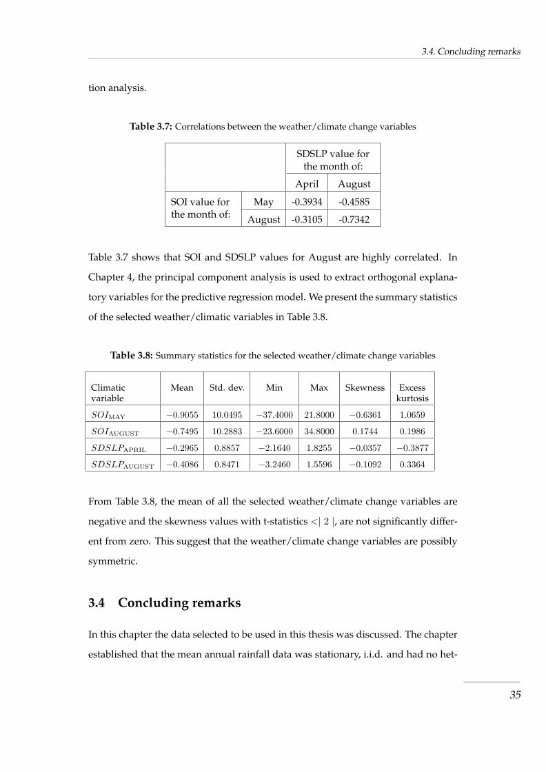
3.4. Concluding remarks
tion analysis.
Table 3.7: Correlations between the weather/climate change variables
SDSLP value forthe month of:
April August
SOI value forthe month of:
May -0.3934 -0.4585
August -0.3105 -0.7342
Table 3.7 shows that SOI and SDSLP values for August are highly correlated. In
Chapter 4, the principal component analysis is used to extract orthogonal explana-
tory variables for the predictive regression model. We present the summary statistics
of the selected weather/climatic variables in Table 3.8.
Table 3.8: Summary statistics for the selected weather/climate change variables
Climatic Mean Std. dev. Min Max Skewness Excessvariable kurtosis
SOIMAY −0.9055 10.0495 −37.4000 21.8000 −0.6361 1.0659
SOIAUGUST −0.7495 10.2883 −23.6000 34.8000 0.1744 0.1986
SDSLPAPRIL −0.2965 0.8857 −2.1640 1.8255 −0.0357 −0.3877
SDSLPAUGUST −0.4086 0.8471 −3.2460 1.5596 −0.1092 0.3364
From Table 3.8, the mean of all the selected weather/climate change variables are
negative and the skewness values with t-statistics <| 2 |, are not significantly differ-
ent from zero. This suggest that the weather/climate change variables are possibly
symmetric.
3.4 Concluding remarks
In this chapter the data selected to be used in this thesis was discussed. The chapter
established that the mean annual rainfall data was stationary, i.i.d. and had no het-
35

3.4. Concluding remarks
eroscedasticity. The chapter also established that mean annual rainfall for Zimbabwe
was correlated with SOI values for May and August of the current year. At a lead
time of more than 6 months before the onset of summer rainfall season, there was no
significant correlations between mean annual rainfall and SOI values for a particu-
lar month. The chapter also established that mean annual rainfall was correlated to
SDSLP values of April and August of the current year. Using these weather/climate
change variables, we aim to develop simple but reliable models that can be used as
an early warning tool for floods or droughts in Zimbabwe. In the following chapter,
we develop a simple rainfall predictive model using the selected weather/climate
change variables discussed in this chapter.
36

Chapter 4
Modelling mean annual rainfall
using weather/climate change
determinants: Weighted regression
models
4.1 Introduction
Southern Africa’s economic performance in the last decade was disappointing, with
much of the region unable to break away from the paths of low or negative per capita
income growth and balance of payments difficulties. In economic literature, one of
the suggested cause of poor economic growth is persistent droughts that has been
experienced in the region considering that southern Africa’s economy is highly de-
pendent on agriculture (Jayne et al., 2007). Agriculture is the backbone of the econ-
omy in Zimbabwe. It provides employment and income for 60 to 70 percent of the
population, supplies 60 percent of the raw materials required by the industrial sector
and contributes 40 percent of the total export earnings (Mazvimavi, 2010). Despite
agriculture offering high level employment opportunities, it only contributes 20% to
the annual Gross Domestic Product (GDP) of the country depending on the rainfall
37

4.1. Introduction
patterns (Government of Zimbabwe, 2001; Jury, 1996). The contribution of this sector
to the economy has not been fully realised. Concerns over economic growth, envi-
ronmental issues and sustainable development is relatively recent and has captured
the attention of researchers, aid agencies and development and environmental plan-
ners. This is because sustainable development may equate to sustainable economic
growth (Lele, 1991). Economic sustainability seeks to avoid extreme future imbal-
ances in production (Harris, 2003). With long run economic sustainability, welfare is
maximised over time. The interest rests in the need for development programmes to
eradicate poverty and food insecurity in most economies (Perman et al., 2003).
Ample theories have been proposed to explain the relatively poor economic growth
of Zimbabwe and other sub-Saharan countries (Manatsa et al., 2008; Jury, 1996). In
essence the theories can be divided into those arising from politics and those due
to exogenous factors. Political explanations usually refer to poor and inconsistent
policies that are argued to have impacted negatively on economic growth in Zim-
babwe and other sub-Saharan African countries (FAO, 2001; Mangoyana and Meda,
2001; UNECA, 2000). These include poor fiscal and trade policies, lack of good gov-
ernance, corruption and ill functional financial and labour markets. Exogenous ex-
planations include external aid allocation (Burnside and Dollar, 2004) and a lack of
diversification of exports tropical climates including a lack of early drought warning
tools (Sachs and Warner, 1997). Given the importance of agriculture to a developing
country such as Zimbabwe and the dependence of this sector on rainfall as suggested
by Manatsa et al., (2008) and Mangonyana and Meda, (2001), a decline in rainfall and
lack of prediction tools can have severe consequences for sustainable growth. Addi-
tionally, this decline and lack of prediction tools may have a detrimental impact on
the energy supply in Zimbabwe which heavily relies on hydro-power for electricity
generation (Kaunda et al., 2012).
Rainfall patterns are affected by various natural phenomena. Firstly, large scale
38

4.1. Introduction
weather/climatic variation that occur from one year to year (Panu and Sharma,
2002). This is the Southern Oscillation climatic condition, which manifests itself in
the differential oceanic temperature phenomenon across the tropical Pacific Ocean.
The Southern Oscillation Index (SOI) as defined is the difference between season-
ally normalised sea level pressures of Darwin (in Australia) and Tahiti (in the Mid
Pacific). Secondly, Darwin Sea Level Pressures (Darwin SLP) have been found to
influence seasonal rainfall patterns in Zimbabwe (Manatsa et al, 2008).
Evidence of relationships among meteorological variables is well documented (Rocha,
1992; Ropelewski and Halpert, 1987; Webster, 1981). Most research on rainfall pat-
terns for Zimbabwe have focused on correlations between phases of SOI and rainfall
(Torrance, 1990; Matarira and Unganai, 1994; Waylen and Henworth, 1996; Richard
et al., 2000). Rocha (1992) found that southeast Zimbabwean rainfall correlated sig-
nificantly with the SOI (+0.4), with a lead time of four to five months. Using precip-
itation data from 68 meteorological sites with at least 20 years of complete records,
Waylen and Henworth (1996) investigated the association between monthly precip-
itation totals and the SOI throughout Zimbabwe. Simple lag cross-correlations be-
tween the SOI and annual precipitation totals, both annual and monthly, were used
to determine significant associations. The researchers revealed positive correlations,
with almost 30% of the stations at lag zero. They found a negative correlation at lag
-1 (month). The periods with the strongest positive association were the months of
the rainy season from October to April, which were correlated to synchronous values
of the SOI and those in the preceding June-to-September period. March precipita-
tion was found to be positively correlated with the SOI value for the same month.
More than 70% of the stations in the study reported significant correlations between
March precipitation and the SOI in the preceding July and at least 25% of the sta-
tions reported similar associations with monthly SOI in the preceding May (lag -10)
to February (lag -1). The correlation was found to extend through the end of the
rainy season into April and May. November and December precipitation were less
39

4.1. Introduction
strongly correlated with the SOI values in the same period. January and February
precipitation were not correlated with monthly SOI values.
Matarira (1990) found that during the warm phase of ENSO, rainfall tends to be low
across much of the country, whereas the converse is true for the cold phase. Us-
ing an average of the SOI during the preceding 12 months (January to December),
Matarira (1990) found a positive correlation of +0.42 with total rainfall for the wet
season (November to April). Matarira and Unganai (1994) reported a peak corre-
lation of +0.56 with November to January rainfall in the south eastern part of the
country, using the SOI one to two months earlier. They concluded that the SOI can
explain up to 30% of the annual variance in summer rainfall in some parts of the
country.
In a comparison of SOI anomalies with Zimbabwean seasonal rainfall, Torrance
(1990) found that the positive values of the SOI coincided with amounts that were
101% to 125 % of normal. Negative SOI values were generally associated with below-
normal rainfall. Torrance’s study focused on correlations between SOI values and
rainfall. He grouped positive SOI levels into a positive phase, and negative SOI
levels into a negative phase. By contrast, this research aims to identify a particular
month and lag whose SOI value explains total annual rainfall in Zimbabwe; that is, it
seeks to identify the explanatory variable at a time lag of about one year in advance.
Makarau and Jury (1997) used a host of meteorological variables to predict summer
rainfall in Zimbabwe. Makarau and Jury (1997) found an association between ENSO
phases and extreme rainfall. Specifically, when the SOI is within one standard devi-
ation of the long-term mean, the probability is high that rainfall in Zimbabwe will
be within 10% of the mean. Based on a 41-year time series and using the average
of August to October SOI values, the correlation between the SOI and Zimbabwean
summer rainfall was +0.44. Ismail (1987) proposed an empirical rule from which
40

4.2. Research methodology
the mean seasonal rainfall over Zimbabwe can be predicted three months before the
start of the rainy season and ten months before its end using SOI. Ismail (1987) con-
cluded that SOI has an influence on the seasonal rainfall over Zimbabwe. Manatsa et
al. (2008) used correlation analysis to identify the lag periods for which SOI and Dar-
win pressure anomalies are significantly correlated with the Zimbabwean Summer
Precipitation Index. They concluded that progressive lagged four months averaged
Darwin sea level pressure anomalies were correlated with the Zimbabwean precipi-
tation index. Our work advances the work of Manatsa et al. (2008) by trying to pro-
pose a simple early warning rainfall predictive model using climatic determinants
such as SOI value and SDSLP anomalies for Zimbabwe, at a longer lead time before
the onset of the rainfall season. Annual rainfall patterns are crucial for agriculture,
water management, hydro-power electricity generation and infrastructure design.
Any meaningful planning requires information based on the rainfall patterns of the
crucial months of the rainfall season. We are not aware of any literature relating to
modelling mean annual rainfall for Zimbabwe using SDSLP and SOI values.
The rest of the chapter is organised as follows: Section 4.2 presents the research
methodology. Section 4.3 presents the empirical results and discussion of the find-
ings. Section 4.4 provides the concluding remarks. Finally, Section 4.5 and Section
4.6 (Appendix) presents the concluding remarks and the correlograms for residual
analysis respectively.
4.2 Research methodology
In this chapter, dependent mean annual rainfall variable is expressed in terms of
independent explanatory variables; SDSLP anomalies and SOI. Multiple linear re-
gression can be used to model a relationship between the dependent variable and
the explanatory variables. It allows for investigating the effect of changes in the var-
ious factors on the dependent variable. If the observations are measured over time,
the model becomes a time series regression model. The resulting statistical relation-
41

4.2. Research methodology
ship can be used to predict values of rainfall. To ascertain the predictive power of
the model, all assumptions of multiple linear regressions must be met.
4.2.1 General linear model
Probabilistic models that include more than one independent variables are called
multiple regression. The model can be written as:
yt = β0 + β1x1,t + β2,tx2,t + ...+ βpxp,t + εt, t = 1, 2, ..., n (4.1)
where yt is the tth dependent variable and xj,t is the corresponding observation of
the explanatory variable whose predictive influence is of interest i.e. SOI and SD-
SLP values. Parameters βt are unknown and the probabilistic component of the
model εt is the unknown error term. The value of the coefficient βt determines the
contribution of the independent variable xj,t given that the other independent vari-
ables are held constant. Using classical estimation techniques estimates for the un-
known parameters are obtained. If the estimated values for β0, β1, ..., βp are given
by β0, β1, ..., βp then the dependent variable is estimated as:
yt = β0 + β1x1,t + β2,tx2,t + ...+ βpxp,t, t = 1, 2, ..., n (4.2)
and the estimate εt for the error term εt is determined as the difference between the
observed and the predicted dependent variable; εt = yt − yt.
The model (4.1) can be rewritten as:
y = Xβ + ε (4.3)
where
42
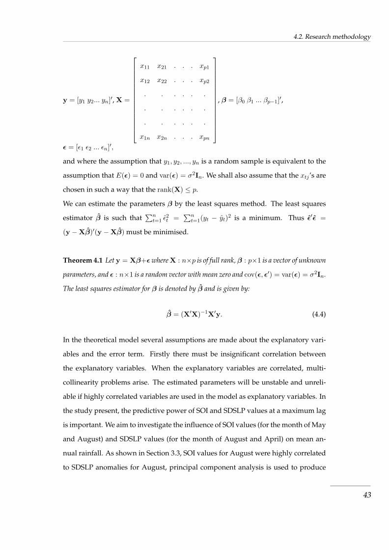
4.2. Research methodology
y = [y1 y2... yn]′, X =
x11 x21 . . . xp1
x12 x22 . . . xp2
. . . . . .
. . . . . .
. . . . . .
x1n x2n . . . xpn
, β = [β0 β1 ... βp−1]′,
ε = [ε1 ε2 ... εn]′,
and where the assumption that y1, y2, ..., yn is a random sample is equivalent to the
assumption that E(ε) = 0 and var(ε) = σ2In. We shall also assume that the xtj ’s are
chosen in such a way that the rank(X) ≤ p.
We can estimate the parameters β by the least squares method. The least squares
estimator β is such that∑n
t=1 ε2t =
∑nt=1(yt − yt)2 is a minimum. Thus ε′ε =
(y −Xβ)′(y −Xβ) must be minimised.
Theorem 4.1 Let y = Xβ+ε where X : n×p is of full rank, β : p×1 is a vector of unknown
parameters, and ε : n×1 is a random vector with mean zero and cov(ε, ε′) = var(ε) = σ2In.
The least squares estimator for β is denoted by β and is given by:
β = (X′X)−1X′y. (4.4)
In the theoretical model several assumptions are made about the explanatory vari-
ables and the error term. Firstly there must be insignificant correlation between
the explanatory variables. When the explanatory variables are correlated, multi-
collinearity problems arise. The estimated parameters will be unstable and unreli-
able if highly correlated variables are used in the model as explanatory variables. In
the study present, the predictive power of SOI and SDSLP values at a maximum lag
is important. We aim to investigate the influence of SOI values (for the month of May
and August) and SDSLP values (for the month of August and April) on mean an-
nual rainfall. As shown in Section 3.3, SOI values for August were highly correlated
to SDSLP anomalies for August, principal component analysis is used to produce
43

4.2. Research methodology
orthogonal explanatory variables that can be used in a general linear model.
4.2.2 Principal component analysis
Principal component analysis (PCA) also known as empirical orthogonal function
has been used in many different disciplines including finance, agriculture, biology,
chemistry, climatology, demography, ecology, psychology and meteorology. PCA
is a technique used to combine highly correlated factors into principal components
that are much less highly correlated with each other. This improves the efficiency of
the model.
In this chapter, the predictive power of SOI values (I1) and SDSLP values (I2) is ex-
plored. Two new, uncorrelated factors, I(I∗1 )and (I∗2 ), can be constructed as follows:
Let I∗1 = I1
Then, we carry out a linear regression analysis to determine the parameters γ1 and
γ2 in the equation:
I2 = γ1 + γ2I∗1 + ε∗i (4.5)
γ1 and γ2 are the intercept and slope parameters of the regression model respectively
and ε∗i is the ’error’ term, which by definition is independent of I∗1 = I1.
We then set:
I∗2 = ε∗i = I2 − (γ1 + γ2I∗1 ) (4.6)
By construction I∗2 is uncorrelated with SOI values (I1) since I∗2 = ε∗i , the residual
term in the equation. Changes in I∗2 is interpreted as the change in the observed val-
ues of SDSLP (I2) that cannot be explained by the observed change in SOI (I1). I∗2 in
the rainfall model (4.1) explains the component of rainfall that cannot be explained
by the SOI.
44
4.2. Research methodology
The other assumptions of the rainfall model (4.1) are that there is no serial correla-
tion and heteroscedasticity of error terms. These assumptions are likely to be vio-
lated in regression models with time series data. Autocorrelation (the error terms
being correlated among themselves through time) leads to regression coefficients
which are biased, inefficient and the standard errors are probably wrong making t
and F tests unreliable. In a regression with auto-correlated errors, the errors will
probably contain information that is not captured by the explanatory variables. The
Durbin-Watson test is used to assess whether the residuals are significantly corre-
lated. A Durbin-Watson statistic of 2 indicates the absence of autocorrelation. The
autocorrelation function and partial autocorrelation function can also be used to de-
tect autocorrelation among the residuals.
4.2.3 Weighted least squares model
The least squares method assumes that each data point provides equally precise
information about the deterministic part of the total process variation i.e. the stan-
dard deviation of the error term is constant over all values of the explanatory vari-
ables. This assumption, however, clearly does not hold in all instances, even ap-
proximately, in every modelling application. In situations when it may not be rea-
sonable to assume that every observation should be treated equally, weighed least
squares weighs some observations more heavily than others, giving each data point
its proper amount of influence over the parameter estimates. This maximises the
efficiency of parameter estimation. Weighted least square reflects the behaviour of
the random errors in the model.
To find the weighted least square parameters of the weighted model, we minimise
the weighted sum of squared errors (WSSE):
n∑t=1
wtε2t =
n∑t=1
wt(yt − yt)2
45

4.3. The models
where wt > 0 is the weight assigned to the tth observation. The weight wt can be the
reciprocal of the variance of that observation’s error term, σ2t , i.e.,
wt =1σ2
t
Observations with larger error variances will receive less weight (and hence have
less influence on the analysis) than observations with smaller error variances. The
estimates are:
β∗
= (X′WX)−1X′Wy. (4.7)
where W = [w1, w2, ..., wn] is the weight vector.
The biggest disadvantage of weighted least squares is the fact that the theory behind
this method is based on the assumption that the exact weights are known. This is
almost never the case in real applications where estimated weights are used (Carrol
and Ruppert, 1988). In this chapter, we aim to estimate reliable weights for mod-
elling mean annual rainfall using SOI and SDSLP values.
4.3 The models
The data for this chapter is the mean annual rainfall data and selected SOIMay,
SOIAugust, SDSLPApril and SDSLPAugust discussed in Chapter 3. It was shown in
Chapter 3 that SOIAugust was highly correlated to SDSLPAugust. We set SOIAugust =
I1 = I∗1 and SDSLPAugust = I2 and ran a regression I2 = γ1 + γ2I∗1 + ε∗i . We extracted
the residuals ε∗i and standardised them. The extracted standardised residuals de-
noted by I∗2 are orthogonal (not correlated to SOIAugust = I∗1 . Therefore, we propose
the following rainfall predictive models.
(i) yt = β0 + β1SOIAugust + β2I∗2 (to be referred to as Model 1)
(ii) yt = β0 + β1SOIAugust + β2SDSLPApril (to be referred to as Model 2)
46

4.4. Empirical results
(iii) yt = β0 + β1SOIMay + β2SDSLPApril (to be referred to as Model 3)
where yt is the estimated rainfall amount at time period t.
4.3.1 Assessing model performance
To evaluate the performance of the considered models, we applied the measures of
average error namely, mean absolute percentage error (MAPE) and root mean square
error (RMSE) discussed in Chapter 2.
4.3.2 Model selection criterion
The scope of model selection is to identify the model that is better suited to predict
mean annual rainfall using SOI and SDSLP values. The AIC discussed in Chapter 2
is used for model selection.
4.4 Empirical results
In this section, results from general regression and weighted regression models are
also presented.
We investigate the influence of the climatic variables using multiple regression ap-
proach. The SOIAugust = I∗1 and SDSLPAugust = I2 are highly correlated as shown
in Chapter 3. We extract the residuals I∗2 of the simple regression of SOIAugust as
the dependent variable and SDSLPAugust as the explanatory variable. The estimated
simple regression model is:
ˆSOIAugust = −4.3896− 8.9086SDSLPAugust,
with R2 = 0.5337. The simple model is significant. The extracted residuals I∗2 are
then used as one of the explanatory variables in multiple regression model. Table
4.1 shows the results of the multiple regression approach for Models 1, 2 and 3.
From Table 4.1, the models parameter estimates are significant at 10% level of sig-
47

4.4. Empirical results
Table 4.1: Parameter estimates for regression models (standard errors in brackets)
Modelβ0
AIC Adjusted R2β1
β2
1 664.9689∗∗(14.8507)
6.7211∗∗(1.9672) 12.9426 0.1690
0.7234∗∗(2.8943)
2 657.5519∗∗(15.6949)
6.4106∗∗(1.5041) 12.9252 0.1834
−24.2283∗(17.4727)
3 653.0067∗∗(16.8821)
3.1855∗∗(1.6948) 13.0506 0.0741
−33.0797(19.2309)
Note: ** and * indicates significant at 5% and 10% level of significance
nificance except β2 in Model 3. Based on the AIC values, the best model is Model
2. Adjusted R2 = 0.1834 which indicates that the model only explains 18.34% of
the variations in mean annual rainfall. The Durbin-Watson statistic for Model 2 is
2.3173. This indicate that the model does not violate the assumption of serial corre-
lation of the residuals. However, the selected model has low forecasting power, thus
we can improve the models by using different weights in the regression model. Var-
ious weights are considered in arriving at estimates using the weighted regression.
A bigger class of models was however considered and the better models are listed
in Table 4.2. The parameter estimates, AIC values and statistics for checking model
adequacy for some of the weighted regression models are reported in Table 4.2.
We use the MAPE and RMSE measures to assess the forecasting performance of the
models and the AIC to select the best fitting model. The weights are assumed to be
proportional to the inverse standard deviation. Model 1 with (I∗2 )2 as the weight is
selected to be the best predictive model, since it has the least AIC value. The model
has the least MAPE and RMSE values indicating that it performs better than the
other models in forecasting mean annual rainfall. The model is also significant at
48

4.4. Empirical results
Table 4.2: Parameter estimates for weighted regression models (standard errors in brackets)
Model Weightβ0
AIC Adjusted R2 MAPE RMSEβ1
with a time lag β2
1 I∗2 519.1459(67.3999)
6.8718(3.2014) 16.9549 0.3786 28.6553 236.0212
15.87054(7.7761)
1∗ (I∗2 )2 716.5207(14.8638)
5.3913(1.0445) 12.3958 0.6629 22.9341 162.9557
5.4111(0.9335)
2 (SDSLPAPRIL)2 660.1174(18.0899)
6.0862(1.1068) 13.6137 0.2665 29.6337 163.4481
−7.5155(10.6878)
3 (SDSLPAPRIL)3 838.5388(89.1952)
−0.6079(2.6977) 12.4650 0.1734 50.2127 346.2853
−239.6288(72.1891)
Note: All the parameters are significant at 5% level of significance
5% significance level. The multiple adjusted R2 = 0.6629, indicates that the model
explains 66.3% of the variations in mean annual rainfall from just two variables. SOI
explains only approximately 30% of the rainfall variability, which means that other
factors should also be taken into account when predicting rainfall. Figure 4.1 shows
the box plot and QQ-plot of selected model’s residuals.
From Figure 4.1 it appears that the residuals do not violate the assumption of nor-
mality. The box plot seems to be symmetric and there is no serious departure from
the reference line of the QQ-plot. The ACF and PACF correlogram (see Section 4.6)
shows that the residuals are independent. This is confirmed by the Durbin-Watson
statistic value equal to 2.1616, indicating that the residuals are approximately inde-
pendent. The correlogram of squared residuals (see Appendix 4.1) shows that the
model does not violate the assumption of homoscedasticity. This is confirmed by the
White test, which produce an F -statistic of 19.7600 (p-value= 0.0000 < 0.05). It is
49

4.4. Empirical results
Figure 4.1: Box and QQ-plots of residuals of the selected model (Model 1)
important to check the in-sample forecasting power of the model. Figure 4.2 shows
the plot of observed mean annual rainfall against predicted rainfall from the selected
model.
From Figure 4.2 the model seems to be able to predict in-sample mean annual rain-
fall. The model seems to show little variability between predicted and actual rainfall.
The model can be used to predict mean annual rainfall for Zimbabwe. The out-of-
sample forecasts for the years 2010 to 2015 are shown in Table 4.3.
The out-of-sample forecasts seem to be reasonable. The MAPE value of 0.2018 and
RMSE value of 141.65 are not so large considering that only two climatic explana-
tory variables have been used in the model. The model however seems to slightly
over-forecast the mean rainfall. This suggests that the proposed model is reasonable
and can be used as an early warning tool to inform the government, farmers and
other stake-holders about the upcoming rainfall season. The model may still need
improvement and can be complimented by other models.
50

4.5. Concluding remarks
Figure 4.2: Mean annual rainfall versus predicted rainfall
4.5 Concluding remarks
We proposed a simple annual rainfall predicting tool for Zimbabwe using SOI and
SDSLP values. The simple model can be used as part of a drought early warning
system. This chapter’s main finding is that annual rainfall for Zimbabwe correlates
with SOI and SDSLP values of the month of August. We employed principal compo-
nent analysis to construct orthogonal factors (non collinear variables) since SOI and
SDSLP values are highly correlated. The combination of regression and time series
analysis offers a powerful tool for predicting annual rainfall using SOI and SDSLP
values of a particular month with a lag of at least 2 months. Developing a simple
model for annual rainfall prediction provides important drought forecasts so that
precautionary measures can be taken. These measures may involve an adjustment
in the national budget expenditure in order to carter for the forthcoming drought,
deciding on the type of seeds to plant and other possible measures of saving water
as a scarce resource. The following measures may be taken based on the research
results: (a) adaptive measures, thus create standby measures to deal with climate
51

4.5. Concluding remarks
Table 4.3: Out-of-sample forecasts
Year Actual Mean annual Predicted annualrainfall (mm) rainfall (mm)
2010 681.6 874.5316
2011 676.5 765.9985
2012 601.7 709.5376
2013 618.3 717.7716
2014 554.0 664.5861
2015 421.4 590.4050
related disasters, (b) shifting agricultural activities to be in line with the amount of
anticipated rain. With regard to the data, it is clear that the explanatory variables
incorporated in the model are limited. It would be interesting to include other cli-
matic determinants such as Sea Surface Temperatures at Darwin and wind speed.
However, the use of weighted regression gives an acceptable fit in the absence of
these other factors. Extending the model with more factors may provide a better un-
derstanding of the rainfall patterns in Zimbabwe and is an area for further research.
52

4.6. Appendix
4.6 Appendix
Diagnostic plots of Model 1
Figure 4.3: ACF and PACF correlogram of residuals from the best fitting Model 153

4.6. Appendix
Figure 4.4: ACF and PACF correlogram of squared residuals from the best fitting Model 1
54

Chapter 5
Extreme rainfall: Candidature
probability distributions for mean
annual rainfall data: An
application to Zimbabwean data
5.1 Introduction
Dry spells, of varying severities, are regular occurrences in Zimbabwe usually result-
ing in drought. Drought is a calamity with severe impacts on society. It contributes
to the loss of crops, animals and valuable property. Although knowledge of rainfall
patterns over an area may be used for such disaster prevention purposes, it is one
of the most difficult meteorological parameters to study because of lack of reliable
data and large variations of rainfall in space and time. Developing methods that can
provide a suitable prediction of meteorological events is always interesting for both
meteorologists and statisticians, because of its role in infrastructure development,
water resource management and agriculture. Knowledge of rainfall characteristics,
its temporal and spatial distribution plays a major role in drought-prone southern
Africa, where economies are mainly driven by rain-fed agriculture (Jury, 1996). To
55

5.1. Introduction
improve on modelling rainfall processes, many researches have been searching for
physical and statistical properties of rainfall using observational data. One area of
interest is the parent probability distribution of rainfall amount ( Deka et al., 2009;
Cho et al., 2004). Dan’azumi et al. (2010), Husak et al. (2007), Suhaila and Jemain
(2007) and Martins and Stedinger (2000) provide the most recent research on math-
ematical modelling of rainfall patterns. It is generally assumed that a meteorolog-
ical variable follows a certain probability distribution. Many probability distribu-
tions have been considered, in many different situations. These distributions are
gamma distribution (Stagge et al., 2015; Husak et al., 2007; Cho et al., 2004; Aksoy,
2000; Adiku et al., 1997; McKee at al., 1993), lognormal distribution (Suhaila et al.,
2011; Deka et al., 2009; Cho et al., 2004), the generalised extreme value distribution
(GEVD) (Roth et al., 2014; Coles et al., 2001; Aksoy, 2000; Martins and Stedinger,
2000; Bulu and Aksoy, 1998; Madsen et al., 1997; ) and the log-logistic distribution
(Fitzgerald, 2005; Ahmad et al., 1988).
Rainfall data have been modelled by several researchers from different regions of
the world. Koutsoyiannis and Baloutsos (2000) analysed rainfall data from Greece.
Sakulski et al. (2014) fitted the six probability distributions, namely; the log-logistic,
Singh-Maddala, lognormal, generalised extreme value, Frechet and Rayleigh distri-
butions to spring, summer, autumn and winter rainfall data from the Eastern Cape
province, South Africa. They found that the Singh-Maddala distribution was the
best fitting distribution for all seasons’ rainfall data. Rakhecha and Soman (1994)
analysed the annual rainfall series from India covering over 80-years of rainfall data.
Stagge et al. (2015) fitted seven candidate distributions to the standardised precipi-
tation index (SPI) and the standardized evapo-transpiration index (SPEI) for Europe
and recommended the two-parameter gamma distribution for modelling SPI and
GEVD for modelling SPEI. Suhaila and Jemain (2007) found the mixed Weibull dis-
tribution to be the best fitting distribution over single distributions in modelling
rainfall amounts in Peninsular Malaysia. Suhaila and Jemain (2007) found the gen-
56

5.1. Introduction
eralised lambda distribution as the best fitting distribution for rainfall amounts in
Peninsular Malaysia as well. These results differ from the results obtained by Zin et
al. (2009). Therefore, each kind of probability distribution has its own applicability
and limitations. A regionalised study on statistical modelling of annual rainfall is
very essential as the statistical properties may vary according to the geographical
location of the area considered and the length of the rainfall data series. In this chap-
ter, an attempt is made to fit the gamma, lognormal and log-logistic distributions
to mean annual rainfall data series for Zimbabwe. These distributions are referred
to as parent distributions since they fit the main body of data. However, the tail
of the theoretical parent distributions sometimes diverges in the extreme minima
or maxima rainfall data region. Extreme value theory is an alternative to fit min-
ima and maxima mean annual rainfall (Chikobvu and Chifurira, 2015). Berger et al.,
(1982) and Surman et al., (1987) showed that the two-parameter exponential distri-
bution fits extreme weather and atmospheric data well. Therefore, the purpose of
this Chapter is to: (i) compare the relative performance of the gamma, lognormal,
log-logistic distributions and the two-parameter exponential distributions in fitting
the mean annual rainfall for Zimbabwe, (ii) investigate the performance of the can-
didate distributions at 25, 50 and 75-year periods, (iii) select the most robust model
using goodness-of-fit tests namely relative root mean square error (RRMSE), relative
mean absolute error (RMAE) and probability plot correlation coefficient (PPCC) as
discussed in Chapter 2 and (iv) estimate the mean return period for specific return
levels. It should be noted that the normal distribution was considered/assumed in
chapters 2, 3 and 4.
The rest of the chapter is organized as follows: Section 5.2 presents the research
methodology. Section 5.3 presents the empirical results and discussion of the find-
ings. Finally, Section 5.4 provides the concluding remarks.
57

5.2. Research methodology
5.2 Research methodology
In this section, we present some background theory on theoretical distributions namely;
the two-parameter gamma, two-parameter lognormal, the two-parameter log-logistic
and the two-parameter exponential distribution fitted to the mean annual rainfall
data described in Chapter 2. The parameters are estimated by method of maximum
likelihood. The procedure always gives the minimum variance estimate of parame-
ters.
5.2.1 Two-parameter gamma distribution
The two-parameter gamma distribution is recommended for hydrological/meteorological
frequency analysis (McKee et al., 1993; Hosking, 1990). The two-parameter gamma
distribution is defined by the density function:
fg(x) =xξg−1
σξgg Γ(ξg)
exp(− x
σg
), x ≥ 0 (5.1)
where σg, ξg > 0 and x represent mean annual rainfall. σg is the scale parameter and
ξg is the shape parameter of the gamma distribution. The quantile function of the
gamma distribution has no explicit form. In this thesis, we estimate the quantiles for
the gamma distribution using R package ”fitdistrplus”.
Parameter estimation of the two-parameter gamma distribution
Under the assumption that the observed n independent data points X1, ..., Xn have
a gamma distribution, the log-likelihood for the two-parameter gamma distribution
is
l(σg, ξg) = (ξg − 1)n∑
i=1
ln(xi)− nlnΓ(ξg)− nξgln(σg)−1σg
n∑i=1
xi (5.2)
58

5.2. Research methodology
The estimate of σg is found to be
σg =x
ξg(5.3)
and substituting (5.3) into the log-likelihood gives
l(ξg) = n(ξg − 1)n∑
i=1
ln(xi)− nlnΓ(ξg)− nξgln(x) + nξgln(ξg)− nξg (5.4)
which is maximised via the generalised Newton algorithm to obtain the estimate of
ξg. For details of the algorithm see Minka (2002). The estimate of ξg is given by
ξg ≈0.5
lnx− lnx(5.5)
where lnx > lnx.
5.2.2 Two-parameter lognormal distribution
Another distribution that is commonly used to model rainfall amounts is the two-
parameter lognormal distribution (Cho et al., 2004). The two-parameter lognormal
distribution is similar in appearance to the gamma distribution. An assumption of
the lognormal distribution is that the logarithms of the data are normally distributed.
The two-parameter lognormal distribution is defined by the density function
fl(x) =1
xξl√
2πexp
[−(ln(x)− σl)2
2ξ2l
], x > 0 (5.6)
where −∞ < σl <∞ and ξl > 0. σl and ξl are the scale and shape parameters of the
lognormal density function respectively. Due to a close relationship with the normal
distribution, the scale parameter σl, may be interpreted as the mean of the logarithm
of the random variable, while the shape parameter ξl, maybe interpreted as the stan-
dard deviation of the logarithmically transformed variables. Modelling with the log-
normal distribution allows the use of normal-theory statistics on a logarithmic scale,
and parameter estimation is then straightforward (Manning and Mullahy, 2001).
59

5.2. Research methodology
The quantile function of the lognormal distribution is given by
Q(p) = exp(σl + ξlΦ−1(p)) (5.7)
where Φ−1(.) has a standard normal distribution and 0 < p < 1.
Parameter estimation of the two-parameter lognormal distribution
Under the assumption that the observed n independent data points X1, ..., Xn have
a lognormal distribution, the log-likelihood for the two-parameter lognormal distri-
bution is derived by taking the product of the probability densities of the individual
Xis:
l(σl, ξl) = ln
((2πξ2l )
−n2
n∏i=1
X−1i exp
[(ln(xi)− σl)2
ξl
])(5.8)
By maximising the log-likelihood the estimates of σl and ξl are obtained. The maxi-
mum likelihood parameter estimates are:
σl =∑n
i=1 ln(xi)n
(5.9)
and
ξl =
∑ni=1
(ln(xi)−
Pni=1 ln(xi)
n
)2
n(5.10)
5.2.3 Two-parameter log-logistic distribution
The log-logistic distribution is related to the logistic distribution in the same manner
as the lognormal distribution is related to the normal distribution. A logarithmic
transformation of the logistic distribution generates the log-logistic distribution. The
60

5.2. Research methodology
log-logistic distribution is defined by the density function:
fll(x) =1[
1 +(
xσll
)ξll]2
(ξllσll
)(x
σll
)ξll−1
, x > 0 (5.11)
where σll > 0 and ξll > 0. σll and ξll are the scale parameter and shape parameter of
the log-logistic distribution respectively. The log-logistic distribution has different
shapes, it can be strictly decreasing, right skewed, or unimodal. This property of
flexibility enables the log-logistic distribution to fit data from many different fields,
including engineering, economics, hydrology/meteorology and survival analysis.
The quantile function of the log-logistic distribution is given by:
Q(Fll) = σll
(p
1− p
) 1ξll
(5.12)
Parameter estimation of the log-logistic distribution
Under the assumption that n observations, denoted by X1, ..., Xn are from a log-
logistic distribution, the log-likelihood function is:
l(σll, ξll) = nln(ξll)− nξllln(σll) + (ξll − 1)n∑
i=1
ln(xi)− 2n∑
i=1
ln[1 +
(xi
σll
)σll]
(5.13)
The parameter estimates are obtained by differentiating the log-likelihood function
with respect to σll and ξll, and equating to zero.
In this thesis, we use the R package ”fitdistrplus” to obtain the maximum likelihood
parameter estimates of the gamma, lognormal and log-logistic distributions.
61

5.2. Research methodology
5.2.4 Two-parameter exponential distribution derived from extreme value
theory
Extreme value theory has emerged as one of the most important statistical disci-
plines for meteorological sciences over the last 50 years (Li et al., 2015). The two-
parameter exponential distribution is recommended to model extreme events or
heavy tailed data (Lu, 2004). A random variable X is said to have a two-parameter
exponential distribution (Exp(µe, σe)) if its probability density function is of the form
frme(x) =1σe
exp[−(x− µe
σe
)], −∞ < x <∞, σe > 0, (5.14)
where µe is the location parameter and σe is the scale parameter. Berger et al. (1982)
derived the two-parameter exponential distribution, Fe, from extreme value theory
to represent the cumulative frequency distribution of maxima random variable over
a specific percentile,
Fe = 1− exp[−y] (5.15)
where y = x−µe
σe. The mean annual rainfall below a specific drought threshold was
chosen from the complete set of mean annual rainfall to fit the two-parameter ex-
ponential distribution. The estimated cumulative probability Fe can be calculated
using
Fe =N − r + 1N + 1
= Pi (5.16)
where N is the size of the chosen maxima mean annual rainfall. Pi is the probability
of a value that is ranked i out of N values. Therefore, the relationship between the
variate y and Pi is given by
y(i) = ln(1− Pi). (5.17)
62

5.3. Empirical results
The estimates of µe and σe can be estimated by the least-squares method since y
and x are linearly related. The quantile function of the two-parameter exponential
distribution is given by
Q(Fe) = µe − σeln(1− Fi) (5.18)
Return period
In order to develop an effective early warning drought monitoring strategy, we can
estimate how often the extreme quantiles occur with a certain return level. The cu-
mulative two-parameter exponential distribution is used to calculate return period
as suggested by Berger et al. (1982). The return period is given by
R(x) =1
(1− f)(1− Fe(x))(5.19)
where R(x) is the return period in years of the mean annual rainfall, x and f is the
chosen specific percentile.
5.3 Empirical results
The three parent distributions were fitted to the data described in Chapter 2. The
performance of the best fitting parent distribution was compared to the performance
of the two-parameter exponential distribution derived from extreme value theory.
Figure 5.2 shows the c.d.f. of the three theoretical parent distributions and mean an-
nual rainfall for Zimbabwe.
From Figure 5.1, the c.d.f. of the three fitted theoretical distributions seems simi-
lar to the frequency distribution of the data. The distribution parameters i.e. scale
and shape parameters can be estimated by the maximum likelihood procedure. Fig-
ure 5.2 to Figure 5.4 (a) (Top right panel) the empirical and theoretical densities, (b)
63

5.3. Empirical results
Figure 5.1: The c.d.f. of three theoretical parent distributions and mean annual rainfall forZimbabwe
(top right panel) shows the QQ-plot, (c) (bottom left panel) shows the empirical and
theoretical c.d.fs and (d) (bottom right panel) the empirical and theoretical c.d.f.s
and (iv) the PP -plot of the fitted gamma, lognormal and log-logistic distributions
respectively.
From Figure 5.2 (a) (Top right panel), it seems the empirical and theoretical densi-
ties are similar. The QQ-plot shown in Figure 5.2 (b) (top right panel) suggests that
quantiles of the gamma distribution seems to match the quantile of the data (there is
no serious divergence from the reference line), indicating that the gamma distribu-
tion may fit the data well.
From Figure 5.3 (a) (Top right panel), it seems the empirical and theoretical densities
are similar. TheQQ-plot shown in Figure 5.3(b) (top right panel) suggests that quan-
64

5.3. Empirical results
Figure 5.2: Diagnostic plots illustrating the fit of the mean annual rainfall data for Zim-babwe to the gamma distribution, (a) Empirical and gamma densities plot (topleft panel), (b) QQ-plot (top right panel), (c) Empirical and gamma’s c.d.f. plot(Bottom left panel) and (d) PP-plot (Bottom right panel)
Figure 5.3: Diagnostic plots illustrating the fit of the mean annual rainfall data for Zimbabweto the lognormal distribution, (a) Empirical and gamma densities plot (top leftpanel), (b) QQ-plot (top right panel), (c) Empirical and lognormal’s c.d.f. plot(Bottom left panel) and (d) PP-plot (Bottom right panel)
65

5.3. Empirical results
tiles of the lognormal distribution seems to match the quantile of the data (there is
no serious divergence from the reference), indicating that the lognormal distribution
may fit well the data well.
Figure 5.4: Diagnostic plots illustrating the fit of the mean annual rainfall data for Zimbabweto the log-logistic distribution, (a) Empirical and gamma densities plot (top leftpanel), (b) QQ-plot (top right panel), (c) Empirical and log-logistic’s c.d.f. plot(Bottom left panel) and (d) PP-plot (Bottom right panel)
From Figure 5.4 (a) (Top right panel), it seems the empirical and theoretical densities
are similar. TheQQ-plot shown in Figure 5.4(b) (top right panel) suggests that quan-
tiles of the log-logistic distribution seems to match the quantile of the data (there is
no serious divergence from the reference except at the upper tail of the distribution),
indicating that the log-logistic distribution may fit the data well.
The maximum likelihood parameter estimates with their standard errors and p-
values of the AD statistic for the fitted distributions are shown in Table 5.1.
66
5.3. Empirical results
Table 5.1: Fitted distributions, parameter estimates with standard errors in brackets andp-values of AD statistic
Distribution σ ξ p-valuefor AD statistic
Gamma 0.0232 15.2801 0.2835
(0.0030) (1.9752)
Lognormal 6.4591 0.2598 0.4637
(0.0249) (0.0176)
Log-logistic 644.0337 6.6773 0.5125
(16.1974) (0.5288)
The p-values of the AD statistics are all greater than 0.05 as reported in Table 5.1,
confirming that the three theoretical distributions fits the data well. Overall, the
log-logistic distribution gives the best fit by having the largest p-value for the AD
statistic.
5.3.1 Selecting the best fitting parent distribution
Subsequent analysis involves selection of the best fitting distribution out of the three
candidate distributions using the goodness-of-fit tests discussed in Chapter 2. Re-
sults of the goodness-of-fit tests are presented in Table 5.2.
Table 5.2: Outcomes of goodness-of-fit tests
Distribution RRMSE RMAE PPCC
Gamma 0.0218 0.0156 0.9970
Lognormal 0.0260 0.0200 0.9950
Log-logistic 0.0318 0.0266 0.9879
The distribution that is best at least twice out of the three goodness-of-fit tests was
selected as the best fitting distribution. Results indicated that the gamma distribu-
tion was the best fitting parent distribution since it had the least RRMSE and RMAE
67

5.3. Empirical results
and the highest PPCC values. We compared the relative performance of the fitted
distributions at 25, 50 and 75 year periods. Table 5.3 shows the goodness-of-fit test
results at different periods.
Table 5.3: Outcomes of the goodness-of-fit tests at different statistical periods
PeriodDistribution
Gamma Lognormal Log-logistic
RRMSE RMAE PPCC RRMSE RMAE PPCC RRMSE RMAE PPCC
25 0.5821 0.5147 0.2359 0.5864 0.5135 0.2317 0.6141 0.5311 0.2260
50 0.3061 0.2718 0.9559 0.3089 0.2713 0.9389 0.3168 0.2739 0.9191
75 0.1774 0.1545 0.9657 0.1825 0.1537 0.9500 0.1998 0.1627 0.9257
From Table 5.3, the gamma distribution was found to be the best fitting period be-
cause it had the lowest RRMSE values and had the highest PPCC value which is
closer to one. The results also showed that by increasing the period (hence data size)
the performance of the fitted distribution improved. The PPCC value was greater
than 0.9 for all the distributions when the period is 50 years or more. This suggests
that analysing mean annual rainfall data using parent distributions, requires data of
length at least 50 or longer.
Parent distributions are known to diverge in predicting high or low rainfall amounts.
We fitted a two-parameter exponential distribution and compared their relative per-
formance against the best fitting gamma distribution. To fit a two-parameter expo-
nential distribution to extreme maxima rainfall, we selected the 90th percentile which
corresponds to 473 mm. Rainfall amounts above 473 mm were selected. We fitted the
two-parameter exponential distributions to the selected data using the least-squares
method since y(i) and x are linearly related. Figure 5.5 shows the theoretical line of
the variate, y(i), and mean annual rainfall over the selected threshold of 473 mm.
68

5.3. Empirical results
Figure 5.5: The fitted theoretical line of variate and mean annual rainfall above the selectedthreshold of 473 mm by the two-parameter exponential distribution
The regression model result showed that the coefficient of determination was greater
than 0.95 which indicates that the two-parameter exponential distribution can fit
maxima mean annual rainfall well. The Fe can be calculated from (5.15). The fitted
two-parameter exponential distribution is Fe(x) = 1 − exp[−0.0062(x − 538.3710)].
The goodness-of-fit tests are used to compare the relative performance of the two-
parameter distribution against the best fitting parent distribution. Table 5.4 shows
the goodness-of-fit tests for the gamma and two-parameter exponential distribu-
tions.
Table 5.4: Outcomes of the goodness-of-fit tests for gamma and two-parameter exponentialdistributions
Distribution RRMSE RMAE PPCC
Gamma 0.0323 0.0220 0.9887
Exponential 0.0136 0.0012 0.9998
From Table 5.4, the goodness-of-fit results shows that the two-parameter exponential
distribution fits the data better at the tail than the best fitting parent distribution, the
gamma distribution. We also compared the two distributions at different periods.
69

5.3. Empirical results
Table 5.5 shows the goodness-of-fit tests results at different periods.
Table 5.5: Outcomes of the goodness-of-fit tests for gamma and two-parameter exponentialdistributions at different periods.
PeriodDistribution
Gamma Exponential
RRMSE RMAE PPCC RRMSE RMAE PPCC
25 0.5821 0.5147 0.2359 0.0230 0.0136 0.9892
50 0.3061 0.2718 0.9559 0.0254 0.0124 0.9887
75 0.1774 0.1545 0.9657 0.0262 0.0117 0.9900
From Table 5.5, the two-parameter exponential distribution was found to be the best
performing distribution in fitting mean annual rainfall data series at all given pe-
riods. It can also be seen that the PPCC value for the two-parameter exponential
distribution was closer to one at all periods. This indicates that the two-parameter
exponential distribution fits the data well with even small data length. Thus, the
distribution is a good candidate distribution for fitting and modelling extreme mean
annual rainfall data regardless of the sample size of the data.
The Fe and return period of mean annual rainfall is calculated from (5.15) and (5.20).
For example, Fe(473mm) = 1−exp)[−0.0062(473−538.3701)] = −0.4997. The chosen
data above the drought threshold value of 473 mm corresponds to 90th percentile,
i.e. f = 0.90. Then the return period of 473 mm isR(xc) = 1/[(1−0.9)(1+0.4997)] =
7 years, so a mean annual rainfall amount of 473 mm is expected to return in ev-
ery 7 years’ time. The maximum mean annual rainfall for Zimbabwe is 1192.6 mm
recorded the in 1923/24 rainfall season. The mean return period associated with a
return level estimate of 1193 mm is approximately 579 years. This suggests that an
extreme flood of this magnitude is likely to return in every 579 years on average.
This return period is very high, thus we explored analysis of extreme annual rainfall
using the generalised extreme value and the generalised Pareto distributions in the
70

5.4. Concluding remarks
chapters that follow.
5.4 Concluding remarks
This chapter mainly investigated the relative performance of three commonly used
probability distributions for mean annual rainfall, with the purpose of providing
recommendation in the selection of suitable distribution for frequency analysis of
mean annual rainfall. The results showed that the gamma distribution was the most
suitable parent distribution. The worst performing was the log-logistic distribution.
These results are consistent with the findings of Stagge et al. (2015), Cho et al. (2004)
and Husak et al. (2007). This suggests that the statistical properties of daily rainfall
may be similar to mean annual rainfall. Thus, in the absence of daily rainfall data
set, the Department of Meteorological Services in Zimbabwe can use mean annual
rainfall data to calculate drought indicators such as SPI. In addition, this study also
established that when the length of the data is 50 or more, the gamma, lognormal
and the logistic distributions fits well to the mean annual rainfall data. The perfor-
mance of the best fitting parent distribution was compared to the performance of
the two-parameter exponential distribution in fitting high rainfall extremes. This
study established that the fitted two-parameter exponential agrees better with the
actual data than the best fitting parent distribution at all different lengths of data
outperforming the gamma distribution. This leads to the recommendation that the
two-parameter exponential distribution is best suited to model mean annual rain-
fall. The return level estimates, which is the return level expected to be exceeded
in a certain period of time T in years are calculated for Zimbabwe rainfall using the
two-parameter exponential distributions. The highest mean annual rainfall amount
recorded for the country was 1192.6 mm. A return level of 1193 mm is associated
with a mean return period of 579 years, on average. This is too high and calls for
further analysis of extreme rainfall for Zimbabwe using other extreme value dis-
tributions. Although, national data are analysed, the results of this study can be
extended to station data in Zimbabwe. The findings of this study provided useful
71

5.4. Concluding remarks
information for early extreme rainfall monitoring management and provide a good
alternative candidate for modelling mean annual rainfall extremes.
72

Chapter 6
Modelling of extreme maximum
rainfall using generalised extreme
value distribution for Zimbabwe
6.1 Introduction
Floods, although rare, present a problem in many parts of Southern Africa. The im-
pact of such floods is felt on social and economic scales. The extent and severity
of the damage resulting from such floods has been measured in many ways includ-
ing loss of property, loss of lives, an agricultural crisis and high insurance claims
(Gaioni et al., 2009). There are structural and non-structural flood mitigation mea-
sures in place in Zimbabwe. In Zimbabwe, dams were put in place to improve water
security, they also serve as flood mitigation structures. Apart from the Kariba dam,
Zimbabwe being in a semi-arid region, has 12 dams that play a part in flood miti-
gation. With regard to the non-structural flood mitigation measures, these include
from early warning flood forecasting by the Department of Meteorological Services
of Zimbabwe to rescue operations of the Civil Protection Organization of Zimbabwe.
However, developing methods that can give an accurate prediction of meteorolog-
ical events such as floods, is always a challenge to meteorologist and statisticians.
73

6.1. Introduction
The use of standard statistical techniques which model average rainfall in forecast-
ing and prediction of extreme events is less prudent due to gross under estimation
(Schmidli et al., 2007). At the most extreme levels, data is scarce, whereas for struc-
tural design purposes, it is the behavior at these levels which is of greatest interest.
The use of Extreme Value Theory (EVT) which deals with the stochastic behavior of
extreme values in a process, has a long history (Nadarajah and Choi, 2007).
Recent research provides evidence of the importance of classical methods of mod-
elling extreme rainfall amounts from different regions of the world; see Nadarajah
and Choi (2007) for an application to a rainfall data set from South Korea. Kout-
soyiannis (2004) applied extreme value theory to a rainfall data set from Europe and
the USA. Koutsoyiannis and Baloutsous (2000) applied the theory to Greece’s rainfall
data. Coles and Tawn (2005) argues that classical methods are not efficient in terms
of data usage since typically only the most extreme observation per year is modelled.
Research has also focused on the development of inferential procedures that max-
imise the use of available data. To improve efficiency in the modelling of extreme
values, it is important to include other sources of knowledge in the analysis. This
may be information from known physical constraints on the data or derived from an
understanding of related processes at different locations. This leads to the Bayesian
inferential framework as a basis for undertaking extreme value analysis. Research on
modelling extreme rainfall amounts incorporating Bayesian methodology is limited.
Notable ones are Gaioni et al. (2009) who modelled flash floods with prior elicita-
tion using one historic US river data while Coles and Tawn (2005) analysed extreme
rainfall in South-West England using expert prior information. Smith and Naylor
(1987) examined the effect of different prior assumptions on the distributions of the
parameters of a Weibull distribution. There is no work known to us on extremes
of Zimbabwean rainfall using the Bayesian framework. The aim of this study is to
propose an early warning system to predict the frequency of floods in Zimbabwe. In
this study, we provide an application of extreme value distribution to model rainfall
74

6.1. Introduction
data from Zimbabwe using the Bayesian statistics approach. In March 1996, Febru-
ary 2000 and March 2003, cyclones hit Zimbabwe bringing with it intense storms
which caused flooding in many parts of the country (Gwimbi, 2009; Madamombe,
2004). In February 2005 and December 2007, the Department of Meteorological Ser-
vices in Zimbabwe warned of flooding in the Muzarabani and Chadereka districts
(Chingombe et al., 2015). The mean annual rainfall for the years 1996, 2000, 2003,
2005 and 2007 for which recent flooding in many parts of the country was reported
was 801.6 mm, 728.6 mm, 712.3 mm, 835.7 mm and 796.2 mm respectively. It is our
assumption that a higher mean annual rainfall (above 775 mm) may lead to flood-
ing. In this chapter, we model maxima annual rainfall assuming that it may lead to
floods. Knowledge of floods, especially their return periods, will assist in develop-
ing flooding preparedness and coping strategies for the people of Zimbabwe. There
is no known work to us on rainfall extremes in Zimbabwe. In this chapter, we pro-
vide the first application of extreme value distributions to model maxima annual
rainfall in Zimbabwe.
In Chapter 4 we discussed the modelling of mean annual rainfall using parent dis-
tributions. Parent distributions covers the main body of the data. At times there is
need to depart from focusing on the main body and exploit information provided by
the extremes (tails of distribution). Parent distributions are known to diverge in pre-
dicting extreme rainfall amounts. In order to fully capture the statistical properties
of mean annual rainfall, it is important to model the tail distribution of the rainfall
data. The objective of this Chapter is to quantify and describe the behaviour of ex-
treme high rainfall in Zimbabwe. In particular, the aim is to model (i) extreme high
rainfall using GEVD by using the maximum likelihood estimation method and the
Bayesian statistics approach. (ii) calculate the mean return period of high rainfall i.e.
the number of years on average before another flood of equal or greater intensity.
(iii) investigate the influence of time and weather/climate change drivers, namely;
SOI and SDSLP anomalies on extreme maxima rainfall.
75

6.2. Research methodology
The rest of the chapter is organized as follows: Section 6.2 presents the research
methodology. Section 6.3 presents the empirical results and discussion of the find-
ings. Section 6.4 gives the general remarks of the results. Section 6.5 provides the
concluding remarks. Finally, derivations of important results and diagnostic plots
for the fitted non-stationary models are shown in the Section 6.6.
6.2 Research methodology
In this section we discuss the background theory on stationary and non-stationary
GEVD models. The data used in this chapter was described in Chapter 3. The pa-
rameters of the fitted models are estimated by the method of maximum likelihood
and method of Bayesian statistics.
6.2.1 Extreme value theory for block maxima
Suppose X1, ..., Xn is a sequence of independent and identically distributed (i.i.d.)
mean annual rainfall amounts with distribution function G. Then, the behaviour of
Mn = max{X1, ..., Xn} (6.1)
where Mn is the maximum mean annual rainfall amounts over an n-observation
period. If the exact statistical behaviour of the Xi were known, the corresponding
behaviour of Mn could also be calculated exactly. But, in practice, the behaviour of
Xi is unknown, making it difficulty to determine the behaviour of Mn. However,
under suitable assumptions, for large n the approximate behaviour of Mn can be
determined. Thus, properties of Mn as n → ∞ are of particular importance. The
behaviour of selected Mn values in every consecutive period is of great interest. The
selected observations are named block maxima. Figure 6.1 illustrates how 4 maxima
were selected over a period covering 4 blocks. Each block has 5 observations.
76

6.2. Research methodology
Figure 6.1: Illustration of selecting variables for block maxima approach
The block maxima approach in EVT, consists of dividing the observation period into
non-overlapping periods of equal size (blocks) and restricts attention to the maxi-
mum observation in each period. The new observations (maxima from each block)
under extreme value conditions, follows approximately an extreme value distribu-
tion (Ferreira and de Haan, 2015). Parametric statistical methods for the extreme
value distributions (EVD) are then applied to these new observations. In theory the
distribution of Mn in the case of a maxima can be derived exactly for all values of n
as:
Pr{Mn ≤ x} = Pr{X1 ≤ x, ...,Xn ≤ x} (6.2)
= Pr{X1 ≤ x} × ...× Pr{Xn ≤ x}
=n∏
i=1
Pr{X ≤ x}
= [Pr(X ≤ x)]n
= Gn(x)
77
6.2. Research methodology
Mn converges almost surely to ω(G) whether it is finite or infinite. To estimate the
value of Gn from observed data, one possibility is to use standard statistical tech-
niques. However, For any x < x+ where x+ is the upper point of G, two problems
can be encountered from using standard statistical techniques. The first problem is
that, G is not the exact distribution for these new observations, a bias may appear.
The second one, FGn → 0 as n → ∞ since G(x) < 1 (Pocernich, 2002). The first
problem is avoided by accepting that F is unknown and to look for appropriate
families of models for Gn which can be estimated on the basis of extreme data only.
The second problem is avoided by allowing a linear renormalization of the variable
Mn. The limit theory in univariate extremes seeks normalising constants an > 0 and
bn and a nondegenerate function F such that the c.d.f. of a normalized version of
Mn converges to G, i.e.
Pr
(Mn − bn
an≤ x
)= Gn(anx+ bn) → F (x) (6.3)
as n → ∞. If this holds for suitable choices of {an} and {bn}, then we say that
F is an extreme value c.d.f. and G is in the domain attraction of F , written as
G ∈ D(F ). We say further that two extreme value cdfs F and F ∗ are of the same
type if F ∗(x) = F (ax + b) for some a > 0, b and all x (Fisher and Tippet, 1928 and
Gnedenko, 1943).
Theorem 6.1 (Extremal types theorem)
If there exist sequences of constants {an > 0} and {bn} such that
Pr{(Mn − bn)/an ≤ x} → F (x), as n→∞ (6.4)
where F is a non-degenerate distribution function, then F belongs to one of the following
families:
I : F (x) = exp{−exp
[−(x− b
a
)]}, if −∞ < x <∞; (6.5)
78

6.2. Research methodology
II : F (x) =
0, if x ≤ b,
exp{−(
x−ba
)−α}, if x > b;
(6.6)
III : F (x) =
exp
{−[−(
x−ba
)α]}, if x < b;
1, if x ≥ b,
(6.7)
For parameters a > 0, b, and α > 0.
The theorem says if there are suitable sequences {an} and {bn} to stabilize Mn, then
F has a limiting distribution which is one of the types I, II and III . These three
families of distributions are known as the Gumbel, Frechet and Weibull distribu-
tions respectively and are collectively known as the extreme value distributions.
The family of EVDs can be equivalently characterised via the class of max-stable
distributions. Two distributions F ∗ and F are equivalent if F ∗(ax+b) = F (x). While
a distribution is max-stable if for n = 2, 3, .... there are constants σn and ξn such that
Fn(σnx+ ξn) = F (x) (de Haan and Lin, 2001; Leadbetter et al., 2012). Leadbetter et
al. (2012) gave a comprehensive account of necessary and sufficient conditions for
G ∈ D(F ) and characterizations of an and bn, when F is one of the three extreme
value cdfs. The necessary and sufficient conditions for the three cdfs in (6.5), (6.6)
and (6.7) are:
I : ∃γ(t) > 0 s.t. limt↑ω(G)
1−G(t+ xγ(t)1−G(t)
= exp(−x), x ∈ <, (6.8)
II : ω(G) = ∞ and limt↑∞
1−G(tx)1−G(t)
= x−ξ, x > 0, (6.9)
III : ω(G) <∞ and limt↓0
1−G(ω(G)− tx)1−G(ω(G)− t)
= xξ, x > 0. (6.10)
79

6.2. Research methodology
The corresponding characterizations of an and bn are:
I : an = γ(G←(1− n−1)) and bn = G←(1− n−1),
II : an = G←(1− n−1) and bn = 0,
III : an = ω(G)−G←(1− n−1) and bn = ω(G),
where G← denotes the inverse function of G.
An equivalent characterization of F is by means of the definition of max-stability:
Theorem 6.2 (Max-stable distributions) A distribution F is max-stable if and only if, it
is of the same type as an extreme value distribution.
From Theorem 6.2, it implies that the distribution of maxima of independent sam-
ples is of the same type as that of the underlying population if and only if, the un-
derlying population itself has a distribution of extreme value type.
Leadbetter et al. (2012) showed that the class of extreme value distributions are pre-
cisely the class of nondegenerate max-stable distributions. Resnick (2013) showed
that the αn and bn for the distributions in (6.5), (6.6) and (6.7) are:
I : σn = 1 and ξn = −logn,
II : σn = n−1/σ and σn = 0,
III : σn = n1/σ and ξn = 0.
6.2.2 Generalised extreme value distribution (GEVD) for block maxima
and minima
An approach to unify the three families of extreme value distributions was proposed
by von Mises (1954) and Jenkinson (1955), into a single family to allow a continu-
80
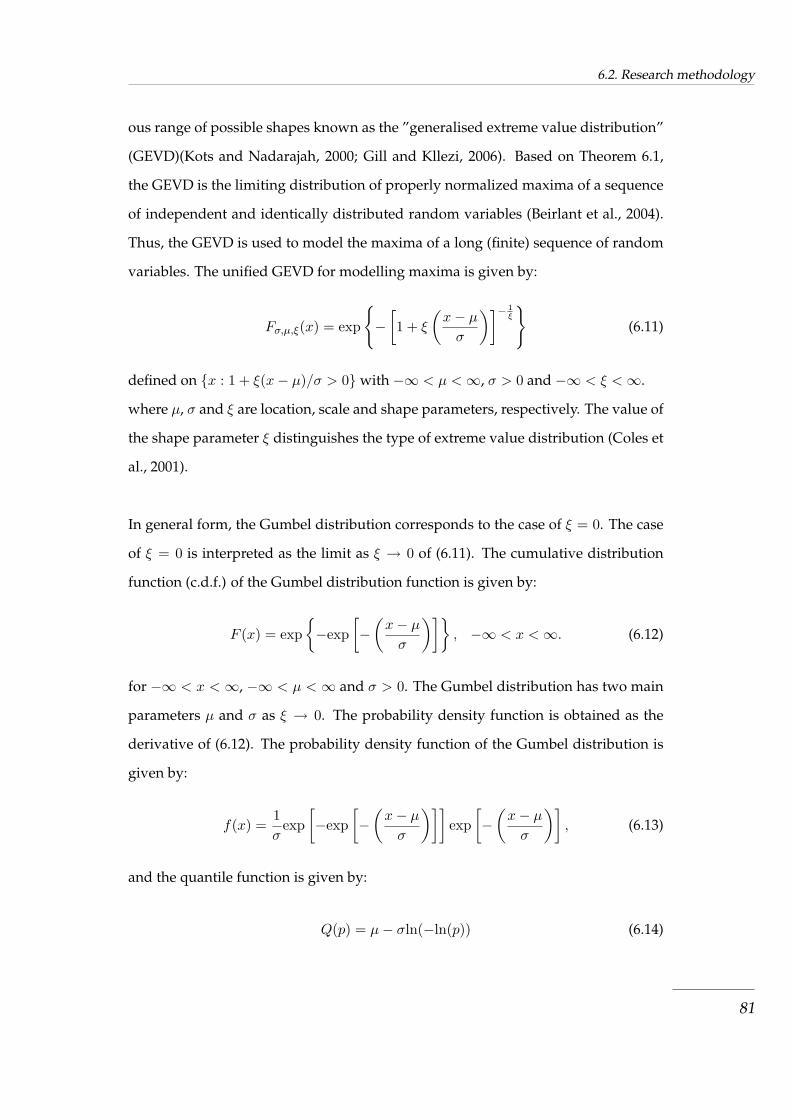
6.2. Research methodology
ous range of possible shapes known as the ”generalised extreme value distribution”
(GEVD)(Kots and Nadarajah, 2000; Gill and Kllezi, 2006). Based on Theorem 6.1,
the GEVD is the limiting distribution of properly normalized maxima of a sequence
of independent and identically distributed random variables (Beirlant et al., 2004).
Thus, the GEVD is used to model the maxima of a long (finite) sequence of random
variables. The unified GEVD for modelling maxima is given by:
Fσ,µ,ξ(x) = exp
{−[1 + ξ
(x− µ
σ
)]− 1ξ
}(6.11)
defined on {x : 1 + ξ(x− µ)/σ > 0} with −∞ < µ <∞, σ > 0 and −∞ < ξ <∞.
where µ, σ and ξ are location, scale and shape parameters, respectively. The value of
the shape parameter ξ distinguishes the type of extreme value distribution (Coles et
al., 2001).
In general form, the Gumbel distribution corresponds to the case of ξ = 0. The case
of ξ = 0 is interpreted as the limit as ξ → 0 of (6.11). The cumulative distribution
function (c.d.f.) of the Gumbel distribution function is given by:
F (x) = exp{−exp
[−(x− µ
σ
)]}, −∞ < x <∞. (6.12)
for −∞ < x < ∞, −∞ < µ < ∞ and σ > 0. The Gumbel distribution has two main
parameters µ and σ as ξ → 0. The probability density function is obtained as the
derivative of (6.12). The probability density function of the Gumbel distribution is
given by:
f(x) =1σ
exp[−exp
[−(x− µ
σ
)]]exp
[−(x− µ
σ
)], (6.13)
and the quantile function is given by:
Q(p) = µ− σln(−ln(p)) (6.14)
81

6.2. Research methodology
The Gumbel distribution comprises distributions such as:
(i) Exponential distribution: F (x) =[1− e−x
n
]n→ exp(−e−x), which is the Gum-
bel distribution with µ = 0 and σ = 1.
(ii) Normal, logistic and gamma distributions.
These distributions are identified as light-tailed distributions, thus ξ → 0 is related
to the light-tailed Gumbel order of distribution. The Gumbel distribution is also
called the double exponential distribution and is bounded, which means every mo-
ment exists.
The characteristic function of the Gumbel distribution is obtained by first transform-
ing the Gumbel random variableX into a standard random variable using Z = X−µα .
The density of Z is then given by:
f(z) = e−e−ze−z, for−∞ < z <∞. (6.15)
The characteristic function of Z is determined to be:
E(eitZ) =∫ ∞−∞
eitze−e−ze−zdz
This solves to give:
E(eitZ) = Γ(1− it)
where i =√−1. Then the characteristic function of Gumbel distribution is therefore
given by:
E(eitX) = eitµΓ(1− itσ). (6.16)
The first and second derivative of (6.16) at the interval t = 0, gives the first and
82

6.2. Research methodology
second moments of X . These moments are:
E(X) = µ− σΓ(1) = µ+ σγ (6.17)
E(X2) = µ2 − 2σµΓ(1) + σ2Γ(2)(1) = (µ+ σγ)2 + σ2π2
6(6.18)
and the constant γ which is referred as the Euler-Mascheroni’s constant and γ ≈
0.577215664901532. Thus the mean and variance of the Gumbel distribution are
µ+ σγ and σ2 π2
6 (Feng et al., 2007).
For the case ξ 6= 0 in (6.11), we have the type II when ξ > 0 and type III when ξ < 0.
The type II EVD also known as the Frechet distribution. The Frechet distribution
has heavy upper tails for all ξ > 0. Its upper tails become heavier with smaller values
of ξ. The heavy tail distribution of the Frechet family of distributions includes the
Pareto, log-gamma, Student t and the Cauchy distributions. The Frechet type of
distribution is described by a polynomial tail decay, having moments only up to γ.
The Frechet distribution has a c.d.f. given by:
F (x) = exp
{−(x− µ
σ
)−α}
(6.19)
for x > µ, α > 0, −∞ < µ < ∞ and σ > 0. The type III EVD is equivalent to the
Weibull distribution. The Weibull distribution has heavy tails for 0 < α < 1. Its up-
per tails become heavier with smaller values of α ∈ (0, 1). The Weibull distribution
has exponentially decaying light upper tails for all α ≥ 1. Its upper tails become
lighter with larger values of α ∈ [1,∞). The Weibull family of distributions includes
the Uniform and Beta distributions. The Weibull type of distribution is characterized
by a bounded tail with a finite endpoint, although not all of its moments are finite.
The Weibull distribution has the cdf:
F (x) = 1− exp{−(x− µ
σ
)α}(6.20)
83
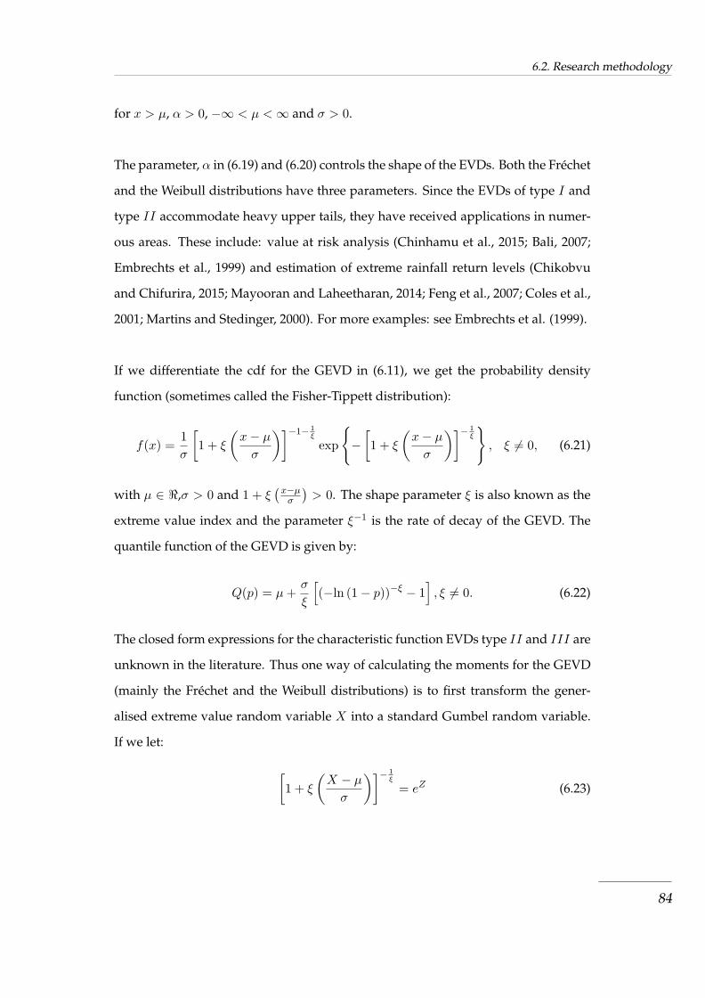
6.2. Research methodology
for x > µ, α > 0, −∞ < µ <∞ and σ > 0.
The parameter, α in (6.19) and (6.20) controls the shape of the EVDs. Both the Frechet
and the Weibull distributions have three parameters. Since the EVDs of type I and
type II accommodate heavy upper tails, they have received applications in numer-
ous areas. These include: value at risk analysis (Chinhamu et al., 2015; Bali, 2007;
Embrechts et al., 1999) and estimation of extreme rainfall return levels (Chikobvu
and Chifurira, 2015; Mayooran and Laheetharan, 2014; Feng et al., 2007; Coles et al.,
2001; Martins and Stedinger, 2000). For more examples: see Embrechts et al. (1999).
If we differentiate the cdf for the GEVD in (6.11), we get the probability density
function (sometimes called the Fisher-Tippett distribution):
f(x) =1σ
[1 + ξ
(x− µ
σ
)]−1− 1ξ
exp
{−[1 + ξ
(x− µ
σ
)]− 1ξ
}, ξ 6= 0, (6.21)
with µ ∈ <,σ > 0 and 1 + ξ(x−µ
σ
)> 0. The shape parameter ξ is also known as the
extreme value index and the parameter ξ−1 is the rate of decay of the GEVD. The
quantile function of the GEVD is given by:
Q(p) = µ+σ
ξ
[(−ln (1− p))−ξ − 1
], ξ 6= 0. (6.22)
The closed form expressions for the characteristic function EVDs type II and III are
unknown in the literature. Thus one way of calculating the moments for the GEVD
(mainly the Frechet and the Weibull distributions) is to first transform the gener-
alised extreme value random variable X into a standard Gumbel random variable.
If we let:
[1 + ξ
(X − µ
σ
)]− 1ξ
= eZ (6.23)
84
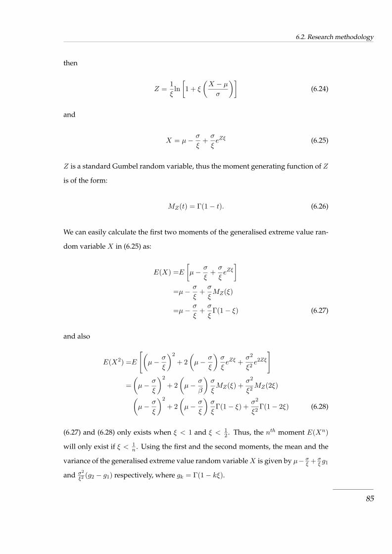
6.2. Research methodology
then
Z =1ξln[1 + ξ
(X − µ
σ
)](6.24)
and
X = µ− σ
ξ+σ
ξeZξ (6.25)
Z is a standard Gumbel random variable, thus the moment generating function of Z
is of the form:
MZ(t) = Γ(1− t). (6.26)
We can easily calculate the first two moments of the generalised extreme value ran-
dom variable X in (6.25) as:
E(X) =E[µ− σ
ξ+σ
ξeZξ
]=µ− σ
ξ+σ
ξMZ(ξ)
=µ− σ
ξ+σ
ξΓ(1− ξ) (6.27)
and also
E(X2) =E
[(µ− σ
ξ
)2
+ 2(µ− σ
ξ
)σ
ξeZξ +
σ2
ξ2e2Zξ
]
=(µ− σ
ξ
)2
+ 2(µ− σ
β
)σ
ξMZ(ξ) +
σ2
ξ2MZ(2ξ)(
µ− σ
ξ
)2
+ 2(µ− σ
ξ
)σ
ξΓ(1− ξ) +
σ2
ξ2Γ(1− 2ξ) (6.28)
(6.27) and (6.28) only exists when ξ < 1 and ξ < 12 . Thus, the nth moment E(Xn)
will only exist if ξ < 1n . Using the first and the second moments, the mean and the
variance of the generalised extreme value random variableX is given by µ− σξ + σ
ξ g1
and σ2
ξ2 (g2 − g1) respectively, where gk = Γ(1− kξ).
85
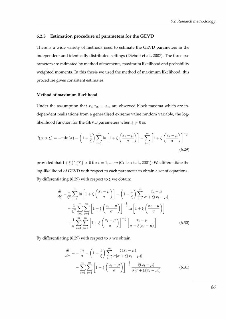
6.2. Research methodology
6.2.3 Estimation procedure of parameters for the GEVD
There is a wide variety of methods used to estimate the GEVD parameters in the
independent and identically distributed settings (Diebolt et al., 2007). The three pa-
rameters are estimated by method of moments, maximum likelihood and probability
weighted moments. In this thesis we used the method of maximum likelihood, this
procedure gives consistent estimates.
Method of maximum likelihood
Under the assumption that xi, x2, ..., xm are observed block maxima which are in-
dependent realizations from a generalised extreme value random variable, the log-
likelihood function for the GEVD parameters when ξ 6= 0 is:
l(µ, σ, ξ) = −mln(σ)−(
1 +1ξ
) m∑i=1
ln[1 + ξ
(xi − µ
σ
)]−
m∑i=1
[1 + ξ
(xi − µ
σ
)]− 1ξ
(6.29)
provided that 1+ξ(xi−µ
σ
)> 0 for i = 1, ...,m (Coles et al., 2001). We differentiate the
log-likelihood of GEVD with respect to each parameter to obtain a set of equations.
By differentiating (6.29) with respect to ξ we obtain:
dl
dξ=
1ξ2
m∑i=1
ln[1 + ξ
(xi − µ
σ
)]−(
1 +1ξ
) m∑i=1
xi − µ
σ + ξ(xi − µ)
− 1ξ2
m∑i=1
m∑i=1
[1 + ξ
(xi − µ
σ
)]− 1ξ
ln[1 + ξ
(xi − µ
σ
)]
+1σ
m∑i=1
m∑i=1
[1 + ξ
(xi − µ
σ
)]− 1ξ[
xi − µ
σ + ξ(xi − µ)
](6.30)
By differentiating (6.29) with respect to σ we obtain:
dl
dσ=− m
σ−(
1 +1ξ
) m∑i=1
ξ(xi − µ)σ[σ + ξ(xi − µ)]
−m∑
i=1
m∑i=1
[1 + ξ
(xi − µ
σ
)]− 1ξ ξ(xi − µ)σ[σ + ξ(xi − µ)]
(6.31)
86

6.2. Research methodology
By differentiating 6.29 with respect to µ we obtain:
dl
dµ=(
1 +1ξ
) m∑i=1
ξ
σ + ξ(xi − µ)−[1 + ξ
(xi − µ
σ
)]− 1ξ[
1σ + ξ(xi − µ)
](6.32)
Note: see Section 6.6 for the derivation of the (6.30) to (6.32).
(6.30), (6.31) and (6.32) have no analytical solutions. To obtain the maximum like-
lihood estimates of ξ, σ and µ (6.30), (6.31) and (6.32) are set to zero and standard
numerical optimization algorithms such as Quasi-Newton numerical maximization
are applied.
6.2.4 Properties of the GEVD log-likelihood
The following proposition gives us some basic properties of the GEVD log-likelihood.
We note x− and x+ the left and right end point of the domain l, i.e.
(x−, x+) = {x ∈ <; 1 + ξx > 0}.
Clearly, it is equal to (−∞,−1ξ ), < and (−1
ξ ,+∞) when ξ < 0, ξ = 0 and ξ > 0 re-
spectively.
Proposition 6.1 The function l is smooth on its domain.
1. If ξ ≤ −1, l is strictly increasing on its domain and
limx→x−
l(x) = −∞ limx→x+
l(x) =
+∞ if ξ < −1
0 if ξ = −1(6.33)
2. If ξ > −1, l is increasing on (x−, x+] and decreasing on [x−, x+), where
x∗ =(1 + ξ)−ξ − 1
ξ(6.34)
87

6.2. Research methodology
Furthermore
limx→x−
l(x) = limx→x+
l(x) = −∞
and l reaches its maximum l(x∗) = (1 + ξ)(ln(1 + ξ)− 1) uniquely.
This entails that the log-likelihood (6.29) has no local maxima in (−∞,−1] × < ×
(0,+∞) and that any maximum likelihood estimate (µ, σ, ξ) satisfies ξ > −1. Hence,
no consistent maximum likelihood estimate does exist if ξ < −1 (Smith, 1985b).
Estimating the parameters of GEVD using the Bayesian approach
Estimating parameters of extreme value distributions using the method of maxi-
mum likelihood may produce some irregularities as outlined by Smith (1985). Ac-
cording to Smith and Naylor (1987), the problem of regularity assumptions in the
limiting behaviour of the maximum likelihood estimation method is encountered
if the estimated shape parameter, ξ < −12 . The Bayesian estimation method is in-
dependent of any regularity conditions (Beirlant et al., 2004). Bayesian inference
allows additional information about the processes to be incorporated as prior in-
formation. This additional information is modelled through the introduction of the
prior distribution π(θ), where θ is a vector of parameters with no reference to the
data, i.e. θ = {σ, µ, ξ} in this thesis. For specification of the prior, the parameteri-
sation φ = log(σ) is easier to work with since σ is constrained to be positive. The
parameters φ, µ and ξ are treated as random variables for which we specify prior
distributions. Therefore, prior density is
π(φ, µ, ξ) = πφ(φ)πµ(µ)πξ(ξ), (6.35)
where each marginal prior is normally distributed with large variances. The vari-
ances are chosen to be large enough to make the distributions almost flat, corre-
sponding to prior ignorance. The benefits of using any information available are
likely to be great, however not all available information can be formulated into prior
88

6.2. Research methodology
information. Coles and Powell (1996) acknowledges that scarce extreme data may
pose a challenge to experts to formulate prior beliefs about the process. There are
two types of priors that are commonly used namely; informative and non-informative
priors. Priors based on expert information are called informative priors, while the
priors formulated without the expert information are known as non-informative pri-
ors.
After formulating the prior distribution, the second step involves collecting data to
form the likelihood function denoted by L(θ | x), where x = {xi, ..., xm} is the
vector of realizations of a random variable with density from the parametric family
z = {f(x; θ) : θ ∈ Θ}. The likelihood for θ is
L(θ | x) = f(x | θ)
=m∏
i=1
1σ
[1 + ξ
(xi − µ
σ
)]− 1ξ−1
exp
{−[1 + ξ
(xi − µ
σ
)]− 1ξ
}
=1σm
exp
{−
m∑i=1
[1 + ξ
(xi − µ
σ
)]− 1ξ
}m∏
i=1
[1 + ξ
(xi − µ
σ
)]− 1ξ−1
(6.36)
The likelihood describes how vector x depends on θ (Renard et al., 2006). The last
step is combining the prior distribution with the likelihood to form the posterior
distribution. The posterior distribution is computed using Bayes’ Theorem
π(θ | x) =π(x | θ)π(θ)∫
Θ π(x | θ)π(θ)dθ(6.37)
where Θ is the space parameter and the posterior distribution is usually written as:
π(θ | x) ∝ π(θ)× L(θ | x) (6.38)
The Markov chain Monte Carlo (MCMC) technique is used to simulate realisations
of the posterior distribution. Estimates of the posterior distribution could then be
obtained from the simulated sample.
89

6.2. Research methodology
MCMC techniques
The MCMC technique provides a way of simulating from complex distributions by
simulating Markov chains which have the target distributions as their stationary
distributions. There are many MCMC techniques available (see Gilks et al., 1996;
Gamerman, 1997; Besag, 2001), however, in this thesis we discuss the Gibbs sampler
and Metropolis-Hastings sampling.
The Gibbs sampler
The Gibbs sampler was used by Geman and Geman (1984) for models with Gibbs
distribution and was extended to the general form by Gelfand and Smith (1990).
Suppose the density of interest is π(θ), where θ = (θ1, ..., θd)′ and the full condition-
als are given by
π(θi | θ1, ..., θi−1, θi+1, ..., θd) = π(θi | θ−i), i = 1, ..., d. (6.39)
If it is possible to simulate from the full conditionals then the Gibbs sampler can be
obtained using the following algorithm:
(i) Initialize the counter to k = 1 and the state of the chain to θ(0) = (θ(0)1 , ..., θ
(0)d )′.
(ii) Obtain a new value θ(k) from θ(k−1) by successive simulation from the full
conditionals
θ(k)1 ∼ π
(θ1 | θ(k−1)
2 , ...θ(k−1)d
)θ(k)2 ∼ π
(θ2 | θ(k)
1 θ(k−1)3 , ...θ
(k−1)d
).
.
.
90
6.2. Research methodology
θ(k)d ∼ π
(θd | θ
(k)1 θ
(k−1)3 , ...θ
(k−1)d−1
)(iii) Increase counter from k to k + 1 and return to step (ii).
The Gibbs sampler should be run after initialising the sampler somewhere in the
support of θ. The resulting chain will converge, after an initial ”burn-in” period, to
the posterior distribution (Tosh and Dasgupta, 2014).
Metropolis-Hastings sampling
The Gibbs sampler simulate from multivariate distributions provided that the full
conditionals can be simulated. In many cases it is not straightforward to simulate
from full conditionals. The Metropolis-Hastings sampling techniques provides a
straightforward way of simulating from full conditionals (Korattikara et al., 2014;
Hastings, 1970; Metropolis et al., 1953). Given a distribution of interest, π, a re-
versible Markov chain, which has this distribution as its stationary distribution, can
be constructed.
The procedure is to construct a transition kernel p(θ, φ) such that the equilibrium
distribution of the chain is π. The transition kernel is made up of two elements
namely the arbitrary transition kernel q(θ, φ) and the acceptance probability a(θ, φ).
The Metropolis-hastings algorithm is
(i) Initialize the counter to k = 1 and the state of the chain to θ(0).
(ii) Simulate a proposed value φ using the kernel q(θ, φ) .
(iii) Find the acceptance probability of proposed value a(θ(k−1), φ).
(iv) Accept θ(k) = φ with probability a(θ(k−1), φ) and take θ(k) = θ(k−1) otherwise.
(v) Increase the counter from k to k + 1 and return to step (ii).
91

6.2. Research methodology
MCMC algorithm
In this thesis, the density of interest is the posterior
π(σ, µ, ξ | x) ∝ πφ(φ)πµ(µ)πξ(ξ)L(θ | x) (6.40)
with σ replaced by eφ. So the full conditionals are of the form:
π(φ | µ, ξ) = πφ(φ)L(θ | x)
π(µ | φ, ξ) = πµ(µ)L(θ | x)
π(ξ | µ, σ) = πξ(ξ)L(θ | x)
The three transition densities are denoted by qφ, qµ and qξ, and the proposed values
for each variable are given by
φ∗ = φ+ ωφ,
µ∗ = µ+ ωµ,
ξ∗ = µ+ ωξ,
where ωφ, ωµ and ωξ are normally distributed with mean zero and high variances.
The variances are high to make the distributions almost flat, corresponding to prior
ignorance. For more details of the MCMC algorithm refer to R package: evdbayes
version1.1-1.
6.2.5 Non-stationary GEVD model
Since the original work of Dalrymple (1960), almost all regional extreme rainfall
analysis assumed that observations are independent, homogeneous and stationary
(Nguyen et al., 2014). In the context of meteorological processes, non-stationarity
is often apparent because of seasonal effects, perhaps due to long-changing climatic
conditions. The models that were introduced in Section 6.2 and 6.3 assumed that
92

6.2. Research methodology
the observations used were independent and identically distributed. In Chapter
3, we found out that the mean annual rainfall for Zimbabwe is influenced by SOI
values for September of the previous year and a component of SDSLP values for
March which are not explained by SOI values. In this section we discuss the the-
ory of non-stationary GEVD models. In the non-stationary case, the parameters
are expressed as a function of covariates such as time: GEVD(µt, σt, ξt) (Coles et
al., 2001). To ensure a positive value for the scale parameter σ, a transformation
such that ϕt = log(σt) is used when estimating the parameters. Using the notation
GEVD(µ, σ, ξ) to denote the GEVD with parameters µ,σ and ξ, it follows that a suit-
able model forXt, maxima mean annual rainfall where the location parameter µ and
σ are allowed to vary linearly with time t is given by:
X(t) ∼ GEVD(µt, σt, ξ) (6.41)
where
µt = θ0 + θ1t, (6.42)
with σt = exp(σ01 + σ01t), and ξ = constant
The log-likelihood of the non-stationary GEVD is:
lns(µt, σt, ξ) =−mln(σt)−(
1 +1ξ
) m∑i=1
ln[1 + ξ
(xi − µt
σt
)]
−m∑
i=1
[1 + ξ
(xi − µt
σt
)]− 1ξ
(6.43)
The maximum likelihood estimators are the solution of an equation system formed
by setting the derivatives of lns with respect to each parameter to zero. For the non-
stationary GEVD with only the location parameter µ allowed to vary linearly with
time and σt = σ (constant), the derivative of the log-likelihood with respect to each
93

6.2. Research methodology
parameter ξ, σ, θ0, θ1 are:
dlns
dξ=
1ξ2
m∑i=1
ln[1 + ξ
(xi − µt
σ
)]−(
1 +1ξ
) m∑i=1
xi − µt
σ + ξ(xi − µt)
− 1ξ2
m∑i=1
m∑i=1
[1 + ξ
(xi − µt
σ
)]− 1ξ
ln[1 + ξ
(xi − µt
σ
)]
+1ξ
m∑i=1
m∑i=1
[1 + ξ
(xi − µt
σ
)]− 1ξ[
xi − µt
σ + ξ(xi − µt)
](6.44)
dlns
dσ= − m
σ−(
1 +1ξ
) m∑i=1
ξ(xi − µt)σ[σ + ξ(xi − µt)]
−m∑
i=1
m∑i=1
[1 + ξ
(xi − µt
σ
)]− 1ξ ξ(xi − µt)σ[σ + ξ(xi − µt)]
(6.45)
dlns
dθ0=ξ + 1σ
m∑i=1
[1 + ξ
(xi − µt
σ
)]−1
− 1σ
m∑i=1
[1 + ξ
(xi − µt
σ
)]−1− 1ξ
(6.46)
dlns
dθ1=ξ + 1σ
m∑i=1
t
[1 + ξ
(xi − µt
σ
)]−1
− 1σ
m∑i=1
t
[1 + ξ
(xi − µt
σ
)]−1− 1ξ
(6.47)
respectively (see Section 6.6 for the derivations). By setting the system of equations
i.e. (6.44) to (6.47) to zero and applying the numerical optimization algorithms such
as Quasi-Newton numerical maximization, the maximum likelihood estimates are
obtained for ξ, σ, θ0, θ1.
If we allow the location parameter to vary with different climatic change drivers
such as SOI and SDSLP values (6.41) becomes
X(k) ∼ GEVD(µk, σ, ξ) (6.48)
where
µk = θ0 + θ1k, (6.49)
and k is the climatic change driver value i.e. SOIMAY, SOIAUGUST, SDSLPAPRIL or
SDSLPAUGUST (see Chapter 3 for details of correlation between the weather/climatic
94

6.2. Research methodology
change drivers and annual rainfall for Zimbabwe).
6.2.6 Modelling minima random variables
The classical GEVD for extremes is based on asymptotic approximations to the sam-
pling behaviour of block maxima. If Mn = min{X1, ..., Xn}, where Xi denote the
independent and identically distributed random variable and if Yi = −Xi for i =
1, ...,m,
Mn = max{Y1, ..., Yn} (6.50)
then Mn = −Mn. Hence, for large n,
Pr
{Mn ≤ x
}= Pr {−Mn ≤ x}
= Pr{Mn ≥ −x}
= 1− Pr{Mn ≤ −x}
≈ 1− exp
{−[1 + ξ
(−x− µ
σ
)]− 1ξ
}
= 1− exp
{−[1− ξ
(x− µ
σ
)]− 1ξ
}(6.51)
defined on {x : 1 − ξ(x − µ)/σ > 0}, where µ = −µ. This result is a GEVD for min-
ima. Which we can state as a theorem (Extremal types theorem for block minima).
Theorem 6.3 If there exist sequences of constants {an > 0} and {bn} such that
Pr
{(Mn − bn
an
)≤ x
}→ F (x) as n→∞ (6.52)
for a nondegenerate distribution function F , then F is a member of the generalised extreme
95

6.2. Research methodology
value family of distributions for minima:
F = 1− exp
{−[1− ξ
(x− µ
σ
)]− 1ξ
}(6.53)
defined on {x : 1− ξ(x− µ)/σ > 0}, where µ ∈ <, σ > 0 and −∞ < ξ <∞.
The maximum likelihood estimates can then be obtained. An alternative method to
model minima random variables is to use the duality between the distributions for
maxima and minima. If Mn = min{X1, ..., Xn} and if Yi = −Xi for i = 1, ...,m, then
the change of sign means the small values ofXi corresponds to large values of Yi. So
if
Mn = min{X1, ..., Xn}, (6.54)
and
Mn = max{Y1, ..., Yn} (6.55)
then Mn = −Mn. The minima becomes:
Mn = max{−X1, ...,−Xn} (6.56)
Extreme maxima theory and methods discussed in Section 6.2 are then used to model
extreme minima (Coles et al., 2001; Gomes and Guillou, 2015).
6.2.7 The models
In this chapter, we model maxima mean annual rainfall. We fit the basic model (6.2.8)
with µ, σ and ξ constant (to be referred to as Model 1). To investigate the existence
of a trend in the extreme rainfall with respect to time, we fit a four-parameter GEVD
model, which is the variation of Model 1 where the location parameter µ is allowed
96

6.2. Research methodology
to vary linearly with time (to be referred to as Model 2).
Model 2 : µt = θ0 + θ1t with σ = constant, and ξ = constant, (6.57)
where t is the year i.e. t = 1, 2, ..., 109.
In Chapter 3, we observed that mean annual rainfall for Zimbabwe correlates with
SOIMay,SOIAugust,SDSLPApril and SDSLPAugust. To investigate the influence of SOI
and SDSLP on extreme rainfall, we fit a non-stationary GEVD model, which is the
variation of Model 1 where the location parameter µ is allowed to vary linearly
with SOIMay (to be referred to as Model 3), SOIAugust (to be referred to as Model
4), SDSLPApril (to be referred to as Model 5) and SDSLPAugust (to be referred to as
Model 6) respectively. That is:
Model i : µi = θ0 + θ1k with σ = constant, and ξ = constant, (6.58)
where k is the weather/climatic change variable i.e. SOIMay,SOIAugust,SDSLPApril
and SDSLPAugust and i = 3, 4, 5 and 6.
6.2.8 Return level estimates
Estimates of extreme quantiles of the annual maxima or minima are of particular
interest in meteorological extremes, as they give an estimate of the level the pro-
cess is expected to exceed once, on average, in a given number of years (T ) with a
probability of p. The quantiles are obtained by inverting (6.11) and (6.12):
Qp =
µ+ σ
ξ
[[−ln (1− p)]−ξ − 1
], ξ 6= 0,
µ− σln [−ln(1− p)] , ξ = 0,(6.59)
The quantity Qp is known as the return level associated with the T year return pe-
riod (note that p = 1/T ). To obtain estimates of return levels beyond the range of
the data used, the relationships given in (6.59) is extrapolated. One way of checking
97

6.2. Research methodology
whether the extrapolated return levels are significant is to use the return level plots.
A return level plot is a plot of the estimated quantiles (Qp) against return period,
usually shown on a logarithmic scale.
The confidence intervals for the return level estimates are obtained by employing
the profile likelihood method. The 100(1 − α)% confidence interval for Qp is given
by the set:
{θ : 2log
(L(µ, σ, ξ)Lm(θ)
)< χ2
1,1−α
}, (6.60)
where χ21,1−α denotes 100(1 − α)% quantile of the chi-square distribution with one
degree of freedom. Lm(θ) is obtained by re-parameterizing the likelihood (6.29) in
terms of (Qp, σ, ξ) and by calculating the profile likelihood Lm(Qp) given by:
Lm(Qp) = maxσ,ξL(Qp, σ, ξ). (6.61)
6.2.9 Model diagnostics
After estimating the parameters of GEVD, we checked for model adequacy using
the AD test statistic, the PP plots and the QQ plots. In Chapter 2 we discussed the
AD test, PP and QQ plots for model adequacy checking. We now describe the PP
and QQ-plots in more detail for checking the model validity of a GEVD model.
The PP plot is a comparison of the empirical and fitted distribution functions. With
ordered block maxima data x1 ≤ x2 ≤ ... ≤ xm, the empirical function evaluated at
xi is
F (xi) = i/(m+ 1). (6.62)
If we substitute parameter estimates into (6.29), the corresponding model is
98

6.2. Research methodology
F (xi) = exp
{−[1 + ξ
(xi − µ
σ
)]− 1
ξ
},
and if the GEVD model is working well, then
F (xi) ≈ F (xi)
for each i. Therefore, a probability plot, consisting of the points
{(F (xi), F (xi)
), i = 1, ...,m
}, (6.63)
should lie close to the unit diagonal. Any significant departures from linearity are
indicative of the GEVD model not fitting well to the data.
The major weakness of the probability plot for extreme value models is that both
F (xi) and F (xi) are bound to approach 1 as xi increases, while it is usually the accu-
racy of the model for large values of x that is of greatest concern (Coles et al., 2001).
The weakness of the probability plot is avoided by the quantile plot, consisting of
the points
{(F−1(i/(m+ 1)), xi)
)i = 1, ...,m
},
where from (6.59),
F−1
(i
m+ 1
)= µ+
σ
ξ
[[−ln
(i
m+ 1
)]−ξ
− 1
]. (6.64)
Any significant departures from linearity in the quantile plot also indicates model
inadequacy.
99

6.3. Empirical results
6.2.10 Model selection
The deviance (D) statistic will be used to select the best model. With models M1 ⊂
M2, then we will define the D statistic as:
D = 2[l2(M2)− l1(M1)] (6.65)
where l2(M2) and l1(M1) are the maximised log-likelihood under models M2 and
M1 respectively. The D statistic follows a chi-square distribution with k degrees of
freedom, χ2k. k is the difference in dimensionality of models M2 and M1. Thus, the
calculated values of the D statistic are compared to critical values from χ2k at 5% level
of significance. Large values of the D statistic suggest that model M2 explains more
variation in the data than M1.
Goodness-of-fit tests namely; RRMSE, RMAE and PPCC will also be used to check
for goodness-of-fit and model selection. In (6.22), we substitute p with Fi, where
Landwehr plotting position Fi = i−0.35n , to calculate (2.21), (2.22) and (2.23) for the
GEVD models.
In this chapter we use the AD statistic and the quantile plot to check for model
adequacy. The D statistic, RRMSE, RMAE and PPCC statistics are used to check for
goodness-of-fit and model selection.
6.3 Empirical results
In this section, the results of modelling maximum annual rainfall using the maxi-
mum likelihood method and Bayesian framework are discussed. To fit models 1 to
6, we need to test whether mean annual rainfall data is independent and identically
distributed (i.i.d.). In Chapter 3 we described the source and the properties of the
data set used in this chapter. In Chapter 3, it was also shown that the mean annual
rainfall data are i.i.d., thus we can fit the data to the GEVD.
100

6.3. Empirical results
6.3.1 The Maximum likelihood estimation of the annual maxima rainfall
data
Table 6.1 shows the maximum likelihood estimates of the GEVD with their corre-
sponding standard errors in brackets and negative log-likelihood (NLL) value for
Model 1.
Table 6.1: Maximum likelihood estimates (standard errors) of Model 1
µ σ ξ NLL value
590.3810 152.8543 −0.1407 711.3708
(16.2924) (11.4984) (0.0630)
The results show that data can be modelled using a Weibull class of distribution
because ξ = −0.1407 < 0 (bounded tail). Combining estimates and their correspond-
ing standard errors, the 95% confidence intervals for µ, σ and ξ are [558.4401; 606.0255],
[130.3174; 175.3912] and [−0.2642;−0.0172] respectively.
It is important to confirm that the data adequately fits the stationary GEVD. Figure
6.2 shows the diagnostic plots for the goodness of fit of the GEVD fitted using max-
imum likelihood method to mean annual rainfall for Model 1.
The quantiles of maxima rainfall regressed against the quantiles of GEVD shows a
straight line. The diagnostic plots show each set of plotted points to be near linear,
validating use of the GEVD. Also plotted is a 95% confidence interval of the return
level estimates, which are wider for long return periods. This finding suggests that
the data does not deviate significantly from the assumption that they follow a GEVD.
This is confirmed by the Anderson-Darling statistic (p-value= 0.8725 > 0.05) which
fails to reject the null hypothesis. We therefore conclude that the maximum annual
rainfall for Zimbabwe follows the specified GEVD (Model 1).
101

6.3. Empirical results
Figure 6.2: Diagnostic plots illustrating the fit of the mean annual rainfall data for Zimbabweto the GEVD for Model 1, (a) Probability plot (top left panel), (b) Quantile plot(top right panel), (c) Return level plot (bottom left panel) and (d) Density plot(Bottom right panel)
The maximum likelihood for ξ is significantly different from zero because zero is not
contained in the 95% confidence interval. Greater accuracy of the confidence interval
is achieved by the use of the profile likelihood. Figure 6.3 shows the profile likeli-
hood of the generalised extreme value parameter ξ, from which a 95% confidence
interval for ξ is obtained as approximately [−0.2400; 0] which is almost the same as
the calculated 95% confidence interval. This suggests that the GEVD model 1 of the
Weibull class of distribution is a good fit to the maxima mean annual rainfall.
102

6.3. Empirical results
Figure 6.3: Profile likelihood for the generalised parameter shape for Model 1
Bayesian analysis of maxima annual rainfall data
We now seek more informative estimates of the GEVD model 1 based on the prior
information. The Markov Chain Monte Carlo (MCMC) method is applied to the an-
nual maxima rainfall data. In the absence of any expert information on the rainfall
pattern for Zimbabwe, the only genuine prior information available in the GEVD
parameters will be non-informative distributions with large variances. The GEVD
scale parameter was re-parameterised as φ = log(σ) to retain the positivity of this
parameter. The prior density was chosen to be
π(µ, φ, ξ) = πµ(µ)πφ(φ)πξ(ξ),
where the marginal priors, πµ(.), πφ(.) and πξ(.) are
µ ∼ N(0, 400000)
φ ∼ N(0, 400000)
ξ ∼ N(0, 10000)
103

6.3. Empirical results
for the three parameters of the GEVD, where, for example, N(0, 400000) denotes
a Gaussian distribution with mean 0 and variance, 400000. These are indepen-
dent normal priors with large variances. The variances are chosen large enough
to make the distributions almost flat, corresponding to prior ignorance. Initializing
the MCMC algorithm with maximum likelihood estimates as our initial vector θ0 =
(590, 152,−0.14), should produce a chain with small burn-in period. After some
pilot runs, the proposed standard deviations were taken to be s = (0.25, 0.1, 0.1)
and a Markov chain of 30000 iterations were carried out, of which the first 1000
were discarded. The remaining simulations were then regarded as realizations of
the marginal distributions of the posterior. Figure 6.4 shows the MCMC trace plots.
Figure 6.4: Trace plots of the GEVD parameters using non-informative priors for maximaannual rainfall.
To check that the chains had converged to the correct place, different starting points
were used. The chains all converged. The estimated posterior densities for the
GEVD parameters for Zimbabwe are given in Figure 6.5.
The posterior means and standard deviations for the GEVD parameters are given in
104

6.3. Empirical results
Figure 6.5: Posterior densities of the GEVD parameters using non-informative priors formaximum annual rainfall for Zimbabwe for the period 1901-2009.
Table 6.2. Using non-informative priors which are almost flat and add very little in-
formation to the likelihood, the posterior means are close to the maximum likelihood
estimates of the GEVD parameters given in Table 6.1 but with smaller standard de-
viations. The frequentist properties are preserved by using non-informative priors
in the Bayesian statistics approach.
Table 6.2: Posterior means (standard deviations) of the GEVD Model 1 parameters
µ σ ξ
588.3402 155.3500 −0.1213
(2.0100) (12.8300) (0.0621)
Return level estimates
The return levels/periods are estimated using the GEVD Model 1 parameters esti-
mated by maximum likelihood estimation (ML) method and the Bayesian approach.
In Table 6.3 we show the return level estimates (in mm of rainfall) at selected return
105

6.3. Empirical results
intervals T in years.
Table 6.3: Return level estimate from the GEVD model 1
Method T = 5 T = 10 T = 15 T = 20 T = 25 T = 30 T = 50 T = 100
ML 797.0761 885.2228 930.9982 961.4641 984.0796 1001.9494 1049.3508 1108.0562
Bayesian 801.3873 894.2811 943.0781 975.7832 1000.1849 1019.5439 1071.2444 1136.0306
We observe that the return level estimates based on the Bayesian approach are slightly
higher than their corresponding return level estimates based on the maximum like-
lihood estimation method. Using the parameter estimates based on the Bayesian
approach, the return level of 1193 mm is associated with a mean return period of
around 190 years. The maximum mean annual rainfall for Zimbabwe is 1192.6 mm
recorded in 1923/24 rainfall season. This suggests that an extreme flood of this mag-
nitude is likely to return once in every 190 years. Recent floods in many parts of
Zimbabwe, as reported by Chingombe et al. (2015), Gwindi (2009) and Madamombe
(2004), occurred when the annual rainfall are around 775 mm or above. The return
level of 775 mm is associated with a mean return period of around 4 years. This also
suggests that floods of this magnitude is expected once in every 4 years. The poste-
rior return level plot in Figure 6.6 shows the upper 95% limit to be further from the
mean than the lower limit. This is because of the heavier upper tail of the posterior
distribution.
We explore the possibility of time (Model 2) and different natural drivers of cli-
matic change (Models 3, 4, 5 and 6) influencing extreme rainfall for Zimbabwe. We
fit Model 2, Model 3, Model 4, Model 5 and Model 6 to mean annual rainfall. Ta-
ble 6.3 shows the maximum likelihood parameter estimates with standard errors in
brackets and negative log-likelihood (NLL) values for the fitted models.
The residual probability plot of Model 2 presented in Figure 6.6 (left panel) (Ap-
pendix 6.2) shows some slight departure from the straight line. This suggests that
the extreme annual rainfall for Zimbabwe does not trend with time. We use the
106

6.3. Empirical results
Figure 6.6: Posterior return level plot in a Bayesian analysis of the Zimbabwean rainfall data.The curves represent means (solid line) and intervals containing 95% of the pos-terior probability (dashed lines).
D statistic to check whether allowing the location parameter to trend with time is
worthwhile. The model pair (M1,M2) had a D statistic of 2[−711.1775 + 711.3708] =
0.3866 < χ21,0.05 = 3.841, we conclude that there is no evidence of significant trends
with respect to time. The residual probability and residual quantile plots for model
3 to Model 6, shown in Figure 6.7 to Figure 6.9 respectively (Appendix 6.2), shows
no significant departure from the straight line. This suggests that climatic variables
appear to influence the extreme annual rainfall for Zimbabwe. We check whether
there is significant improvement to the stationary model (Model 1) if we allow the
location parameter to trend with climatic variables using the D statistic. The model
pair (M1,M3) had a D statistic of 2[−707.4624+711.3708] = 7.8168 > χ21,0.05 = 3.841,
we conclude that there is a significant influence of SOI value for May on the ex-
treme annual rainfall for Zimbabwe. The model pair (M1,M4) had a D statistic of
2[−701.1743 + 711.3708] = 20.3930 > χ21,0.05 = 3.841, we conclude that there is a
significant influence of the SOI value for August on the extreme annual rainfall for
Zimbabwe. The model pair (M1,M5) had a D statistic of 2[−707.9489 + 711.3708] =
6.8438 > χ21,0.05 = 3.841, we conclude that there is a significant influence of SDSLP
107

6.3. Empirical results
Table 6.4: The maximum likelihood parameter estimates (standard errors) and negativelog-likelihood values of non-stationary GEVD Models
Model θ0 θ1 σ ξ NLL value
2 607.7044 −0.3055 152.9264 −0.1455 711.1775
(32.1209) (0.4916) (11.5560) (0.0645)
3 596.4754 4.2380 146.9625 −0.1433 707.4624
(16.0620) (1.5073) (11.5544) (0.0749)
4 603.9008 6.6728 141.8688 −0.1681 701.1743
(15.0597) (1.4221) (10.3929) (0.0575)
5 579.7127 −43.7269 148.3106 −0.1421 707.9489
(16.3725) (16.5153) (11.1393) 0.0627
6 570.4727 −55.6099 144.8190 −0.1330 705.9603
(16.61930) (16.3992) (10.8993) 0.0632
anomalies for April on the extreme annual rainfall for Zimbabwe. The model pair
(M1,M6) had a D statistic of 2[−705.9603+711.3708] = 10.9603 > χ21,0.05 = 3.841, we
conclude that there is a significant influence of SDSLP anomalies for August on the
extreme annual rainfall for Zimbabwe.
It is important to select a robust model for modelling extreme maximum annual
rainfall for Zimbabwe. The goodness-of-fit tests namely; RRMSE, RMAE and PPCC
values are used to select the most robust model. We use the ith Landwehr plotting
position Fi = i−0.35n , in place of p in (6.2.18) and
µ = θ0 + θ1×value of the weather/climatic variable
to estimate Q(Fi) for the models. Table 6.6 shows the goodness-of-fit values of the
non-stationary models.
The best model at least twice out of the three goodness-of-fit tests is selected as the
best performing model. Results indicate that Model 5 is the best performing GEVD
108

6.4. Concluding remarks
Table 6.5: Goodness-of-fit test results for GEVD models with location parameter influencedby weather/climatic variable
Model RRMSE RMAE PPCC
3 0.0325 0.0543 0.9077
4 0.1019 0.0758 0.9335
5 0.0662 0.0503 0.9758
6 0.0828 0.0622 0.9712
model since it has the least RMAE and the highest PPCC values. Thus, this study
proposes that the best performing GEVD model for mean annual rainfall for Zim-
babwe is:
F (x) = exp
{−[1− 0.1421
(x− (579.7127 + 43.7269SDSLPAPRIL)
148.3106
)] 10.1421
}where x is the mean annual rainfall for Zimbabwe. According to Cheng et al. (2014)
estimating of return levels using non-stationary GEVD models is challenging since
the behaviour of physically-based covariates is not constant. In the presence of
SDSLPAPRIL values of the next 100 or more years, the return level estimates of max-
ima mean annual rainfall for Zimbabwe can be calculated.
6.4 Concluding remarks
The purpose of this chapter was to fit the stationary generalised extreme value dis-
tributions using the maximum likelihood estimation method and Bayesian statistics
approach to mean annual rainfall using annual rainfall data from year 1901 to 2009.
Results obtained using the maximum likelihood estimation method were compared
with those obtained using non-informative priors Bayesian approach. The distribu-
tion of the block maxima was explored by fitting the GEVD. The GEVD model with
shape and scale parameters constant, but allowing the location parameter to vary
with time, was found to be inadequate to model extreme maximum rainfall in Zim-
babwe. Model diagnostics which include the probability plot, quantile plot and AD
109

6.4. Concluding remarks
tests show that the simple GEVD model (Model 1) fits the data well. The confidence
interval of the shape parameter ξ using the profile likelihood contains a zero. This
suggests that the GEVD of the Weibull class of distributions fits the maxima mean
annual rainfall well. Return level estimates, which is the return level expected to
be exceeded in a certain period of time T in years were calculated for Zimbabwe
rainfall. The highest mean annual rainfall amount recorded for the country is 1192.6
mm. A return level of 1193 mm is associated with a mean return period of 190 years
while a return level of 775 mm is associated with a mean return period of around 4
years using the Bayesian approach. Recent flooding has occurred in many parts of
the country with a mean annual rainfall of 775 mm and above. The GEVD param-
eter estimates using the Bayesian approach, are close to the maximum likelihood
estimates with smaller standard deviations. This improves the precision of the es-
timates. Thus, using non-informative priors, the expected benefit of the Bayesian
analysis is the improvement in the precision of parameter estimates over maximum
likelihood estimates is realised.
However, substantial evidence shows that climate is non-stationary, possibly due to
anthropogenic climate change (Cheng, et al., 2014). We explored the possibility of
extreme annual rainfall for Zimbabwe influenced by different natural and anthro-
pogenic drivers. We allowed the location parameter to be influenced by SOI and
SDSLP values. The GEVD models which allow the location parameter to be influ-
enced by natural drivers perform better than the stationary GEVD model. Thus,
this study proposes the GEVD model with location parameter influenced by SDSLP
anomalies of April as the best performing model for mean annual rainfall for Zim-
babwe. This proposed model should be used only as a early warning tool for floods
in Zimbabwe. For climate change drivers-varying GEVD models to be accepted as a
simple extrapolation of results from historical trends, one has to rely on the inertia of
the climate system. In order to understand when the inertia stops, one has to rely on
other tools such as dynamic models. Therefore, extrapolating into the future using
110

6.4. Concluding remarks
historical trends is risky. Furthermore, we have incorporated one natural driver as
a covariate in our proposed model, but many different natural and anthropogenic
weather/climate change drivers can be added as covariates to improve the model.
Therefore, an area of further research is modelling maximum annual rainfall in Zim-
babwe using many weather/climate change drivers.
111

6.5. Appendix
6.5 Appendix
Proof of maximum likelihood estimates for stationary GEVD model parameters
fµ,σ,ξ(x) =1σ
[1 + ξ
(x− µ
σ
)]−1− 1ξ
exp
{−[1 + ξ
(x− µ
σ
)]− 1ξ
}the log-likelihood of the GEVD when ξ 6= 0 is:
l(µ, σ, ξ) = −mlnσ −(
1 +1ξ
) m∑i=1
ln[1 + ξ
(xi − µ
σ
)]−
m∑i=1
[1 + ξ
(xi − µ
σ
)]− 1ξ
Differentiating l with respect to ξ
To differentiate∑m
i=1
[1 + ξ
(xi−µσ
)]− 1ξ we let
y =m∑
i=1
[1 + ξ
(xi − µ
σ
)]− 1ξ
taking natural logarithm on both sides
lny = lnm∑
i=1
[1 + ξ
(xi − µ
σ
)]− 1ξ
=m∑
i=1
ln[1 + ξ
(xi − µ
σ
)]− 1ξ
= −1ξ
m∑i=1
ln[1 + ξ
(xi − µ
σ
)]
Now we differentiate implicitly
1y
dy
dξ=
1ξ2
m∑i=1
ln[1 + ξ
(xi − µ
σ
)]− 1ξ
m∑i=1
xi − µ
σ.
11 + ξ
(xi−µσ
)=
1ξ2
m∑i=1
ln[1 + ξ
(xi − µ
σ
)]− 1ξ
m∑i=1
xi − µ
σ + ξ(xi − µ)
112

6.5. Appendix
Therefore
dy
dξ=y
[1ξ2
m∑i=1
ln[1 + ξ
(xi − µ
σ
)]− 1ξ
m∑i=1
xi − µ
σ + ξ(xi − µ)
]
=m∑
i=1
[1 + ξ
(xi − µ
σ
)]− 1ξ
[1ξ2
m∑i=1
ln[1 + ξ
(xi − µ
σ
)]− 1ξ
m∑i=1
xi − µ
σ + ξ(xi − µ)
]
Now
dl
dξ=
1ξ2
m∑i=1
ln[1 + ξ
(xi − µ
σ
)]−(
1 +1ξ
) m∑i=1
xi − µ
σ.
11 + ξ
(xi−µσ
)−
m∑i=1
[1 + ξ
(xi − µ
σ
)]− 1ξ
[1ξ2
m∑i=1
ln[1 + ξ
(xi − µ
σ
)]− 1ξ
m∑i=1
xi − µ
σ.
11 + ξ
(xi−µσ
)]
dl
dξ=
1ξ2
m∑i=1
ln[1 + ξ
(xi − µ
σ
)]−(
1 +1ξ
) m∑i=1
xi − µ
σ + ξ(xi − µ)
− 1ξ2
m∑i=1
m∑i=1
[1 + ξ
(xi − µ
σ
)]− 1ξ
ln[1 + ξ
(xi − µ
σ
)]
+1σ
m∑i=1
m∑i=1
[1 + ξ
(xi − µ
σ
)]− 1ξ[
xi − µ
σ + ξ(xi − µ)
](6.66)
Differentiating l with respect to σ
dl
dσ=− m
σ−(
1 +1ξ
) m∑i=1
11 + ξ
(xi−µσ
) .(−ξ)(xi − µ
σ2
)
−m∑
i=1
[1 + ξ
(xi − µ
σ
)]− 1ξ
[−1ξ
m∑i=1
11 + ξ
(xi−µσ
) .(−ξ)(xi − µ
σ2
)]dl
dσ=− m
σ−(
1 +1ξ
) m∑i=1
ξ(xi − µ)σ[σ + ξ(xi − µ)]
−m∑
i=1
[1 + ξ
(xi − µ
σ
)]− 1ξ
.m∑
i=1
ξ(xi − µ)σ[σ + ξ(xi − µ)]
dl
dσ=− m
σ−(
1 +1ξ
) m∑i=1
ξ(xi − µ)σ[σ + ξ(xi − µ)]
−m∑
i=1
m∑i=1
[1 + ξ
(xi − µ
σ
)]− 1ξ ξ(xi − µ)σ[σ + ξ(xi − µ)]
(6.67)
113

6.5. Appendix
Differentiating l with respect to µ
dl
dµ=−
(1 +
1ξ
) m∑i=1
11 + ξ
(xi−µσ
) .(− ξσ
)
−[1 + ξ
(xi − µ
σ
)]− 1ξ
[−1ξ
11 + ξ
(xi−µσ
) .(− ξσ
)]dl
dµ=(
1 +1ξ
) m∑i=1
ξ
σ + ξ(xi − µ)−[1 + ξ
(xi − µ
σ
)]− 1ξ[
1σ + ξ(xi − µ)
](6.68)
To obtain maximum likelihood estimates of ξ, σ and µ (6.66), (6.67) and (6.68) are set
to zero and standard numerical optimization algorithms are applied.
114

6.5. Appendix
Proof of maximum likelihood estimates for non-stationary GEVD model parame-
ters
fµt,σ,ξ(x) =1σ
[1 + ξ
(x− µt
σ
)]−1− 1ξ
exp
{−[1 + ξ
(x− µt
σ
)]− 1ξ
}
the log-likelihood of the GEVD when ξ 6= 0 is:
l(µt, σ, ξ) = −mlnσ −(
1 +1ξ
) m∑i=1
ln[1 + ξ
(xi − µt
σ
)]−
m∑i=1
[1 + ξ
(xi − µt
σ
)]− 1ξ
where µt = θ0 + θ1t. It implies that
l(θ0 + θ1t, σ, ξ) =−mlnσ −(
1 +1ξ
) m∑i=1
ln[1 + ξ
(xi − (θ0 + θ1t)
σ
)]
−m∑
i=1
[1 + ξ
(xi − (θ0 + θ1t)
σ
)]− 1ξ
set
h =−(
1 +1ξ
) m∑i=1
ln[1 + ξ
(xi − (θ0 + θ1t)
σ
)]
and
g =−m∑
i=1
[1 + ξ
(xi − (θ0 + θ1t)
σ
)]− 1ξ
so that
l(µt, σ, ξ) = −mlnσ + h+ g
115

6.5. Appendix
so
dh
dθ0= −
(1 +
1ξ
) m∑i=1
1
1 + ξ(
xi−(θ0+θ1t)σ
) d
dθ0
[1 + ξ
(xi − (θ0 + θ1t)
σ
)]
= −(
1 +1ξ
) m∑i=1
σ
σ[1 + ξ
(xi−(θ0+θ1t)
σ
)] .(− ξσ
)
=(ξ + 1σ
) m∑i=1
1
1 + ξ(
xi−(θ0+θ1t)σ
)for g and taking natural logarithm both sides we obtain
lng =1ξ
m∑i=1
ln[1 + ξ
(xi − (θ0 + θ1t)
σ
)]
Differentiating implicitly
1g
dg
dθ0=
1ξ
m∑i=1
1
1 + ξ(
xi−(θ0+θ1t)σ
) . ddθ0
[1 + ξ
(xi − (θ0 + θ1t)
σ
)]
=1ξ
m∑i=1
σ
σ + ξ(xi − θ0 − θ1t).ξ
σ
1g
dg
dθ0=
1σ
m∑i=1
1
1 + ξ(
xi−(θ0+θ1t)σ
)Therefore
dg
dθ0=
1σ
m∑i=1
1
1 + ξ(
xi−(θ0+θ1t)σ
) .[ m∑i=1
[1 + ξ
(xi − (θ0 + θ1t)
σ
)]− 1ξ
]
= − 1σ
m∑i=1
[1 + ξ
(xi − θ0 − θ1t
σ
)]−1− 1ξ
Thus
dl
dθ0=ξ + 1σ
m∑i=1
[1 + ξ
(xi − θ0 − θ1t
σ
)]−1
− 1σ
m∑i=1
[1 + ξ
(xi − θ0 − θ1t
σ
)]−1− 1ξ
(6.69)
116

6.5. Appendix
and for dldθ1
:
dh
dθ1= −
(1 +
1ξ
) m∑i=1
1
1 + ξ(
xi−(θ0+θ1t)σ
) d
dθ1
[1 + ξ
(xi − (θ0 + θ1t)
σ
)]dh
dθ1= −
(1 +
1ξ
) m∑i=1
σ
σ + ξ(xi − θ0 − θ1t).
(−ξtσ
)
=(ξ + 1σ
) m∑i=1
t
[1 + ξ
(xi − (θ0 + θ1t)
σ
)]−1
and
dg
dθ1=
1σ
m∑i=1
t
[1 +
ξ(xi − θ0 − θ1t)σ
]−1[−[1 +
ξ(xi − θ0 − θ1t)σ
]− 1ξ
]dg
dθ1= − 1
σ
m∑i=1
t
[1 + ξ
(xi − θ0 − θ1t
σ
)]−1− 1ξ
hence
dl
dθ1=ξ + 1σ
m∑i=1
t
[1 + ξ
(xi − θ0 − θ1t
σ
)]−1
− 1σ
m∑i=1
t
[1 + ξ
(xi − θ0 − θ1t
σ
)]−1− 1ξ
(6.70)
dl
dσ=− m
σ−(
1 +1ξ
) m∑i=1
ξ(xi − µt)σ[σ + ξ(xi − µt)]
−m∑
i=1
m∑i=1
[1 + ξ
(xi − µt
σ
)]− 1ξ ξ(xi − µt)σ[σ + ξ(xi − µt)]
(6.71)
dl
dξ=
1ξ2
m∑i=1
ln[1 + ξ
(xi − µt
σ
)]−(
1 +1ξ
) m∑i=1
xi − µt
σ + ξ(xi − µt)
− 1ξ2
m∑i=1
m∑i=1
[1 + ξ
(xi − µt
σ
)]− 1ξ
ln[1 + ξ
(xi − µt
σ
)]
+1σ
m∑i=1
m∑i=1
[1 + ξ
(xi − µt
σ
)]− 1ξ[
xi − µt
σ + ξ(xi − µt)
](6.72)
To obtain maximum likelihood estimates of θ0, θ1, σ and ξ (6.69), (6.70), (6.71) and
(6.72) are set to zero and standard numerical optimization algorithms are applied.
117

6.5. Appendix
Diagnostic plots for non-stationary GEVD models of mean annual rainfall for
Zimbabwe
Figure 6.7: Diagnostic plot for GEVD Model 2
Figure 6.8: Diagnostic plot for GEVD Model 3
118

6.5. Appendix
Figure 6.9: Diagnostic plot for GEVD Model 4
Figure 6.10: Diagnostic plot for GEVD Model 5
119

6.5. Appendix
Figure 6.11: Diagnostic plot for GEVD Model 6
120

Chapter 7
Modelling of extreme minimum
rainfall using generalised extreme
value distribution for Zimbabwe
7.1 Introduction
Extreme low rainfall attributed to global warming, although rare, is a natural phe-
nomenon that affects people’s socio-economic activities worldwide. Extreme droughts
occur from time to time in Zimbabwe and impact negatively on the country’s eco-
nomic performance. The drought of rainfall season year 1991/1992 was one of the
worst in the recorded history of Zimbabwe. Its impact was felt even in the in-
surance industry which received high claims for crop failure (Makarau and Jury,
1997). Droughts can be viewed as extreme events outside of the normal rainfall oc-
currences, such as exceptionally lower amounts of mean annual rainfall (Panu and
Sharma, 2002). In Zimbabwe, at least 50% of the gross domestic product is derived
from rain-fed agriculture (Jury, 1996). With more low technology indigenous farmers
entering commercial agriculture through the accelerated land-reform programme,
modelling and prediction of extremely low annual rainfall and the associated prob-
abilities of drought become more relevant.
121

7.1. Introduction
Developing methods that can give a suitable prediction of meteorological events is
always interesting for both meteorologists and statisticians. The use of standard sta-
tistical techniques in modelling, forecasting and prediction of extremes in average
rainfall and rare events is less prudent because of gross under-estimation (Hasan et
al., 2012). Extreme value theory is an alternative and superior approach to quantify
the stochastic behaviour of a process at unusually large or small levels (Hasan et al.,
2012). Extreme value theory provides the statistical framework to make inferences
about the probability of very rare and extreme events. It is based on the analysis of
the maximum (or minimum) value in a selected time period.
Recently there has been growing interest in modelling extreme events, especially
in situations in which scientists underestimated the probabilities of extreme events
that subsequently occurred and caused catastrophic damage (Coles et al., 2001). Re-
search conducted provides evidence of the importance of modelling rainfall from
different regions of the world: Nadarajah and Choi (2007) used extreme value the-
ory for rainfall data from South Korea while Koutsoyiannis (2004) applied extreme
value theory to rainfall data from Europe and the USA. Koutsoyiannis and Balout-
sos (2000) applied extreme value theory to Greece’s rainfall data; and Crisci et al.
(2002) applied extreme value distributions to rainfall data from Italy. The use of
extreme value distributions is not restricted to meteorological events and research
occurs in such fields such as energy (Chikobvu and Sigauke, 2013); insurance (Smith
and Goodman, 2000); fish management (Hilborn and Mangel, 1997) and ecology
(Ludwig, 1996). There is no work known to us on rainfall extremes in Zimbabwe.
In this research, we provide the first application of extreme value distributions to
model minimum annual rainfall in Zimbabwe.
Rainfall in Zimbabwe is associated with the behaviour of the inter-tropical conver-
gence zones whose oscillations are influenced by changing pressure patterns to the
122

7.1. Introduction
north and south of the country (Makarau and Jury, 1997). Zimbabwe lies in the
Southwest Indian Ocean zone, which is often affected by tropical cyclones. Tropical
cyclones are low pressure systems that have well-defined clockwise (in the south-
ern hemisphere) wind circulations which spiral toward the centre where the winds
are strongest and rains are heaviest. Cyclones that develop over the western side of
the Indian Ocean occasionally affect the rainy season. The amount and intensity of
rainfall during a given wet spell is enhanced by the passage of upper westerly wind
waves of mid-latitude origin (Buckle, 1996; Smith, 1985a).
Studies of extreme low rainfall are beneficial to decision-makers in government and
non-governmental organisations involved in early warning systems and food secu-
rity, poverty alleviation and disaster management and risk management. This study
will also inform climatologists about the behaviour of extreme low rainfall. Appro-
priate decisions and plans can be made based on the results of this study to prepare
the general public for changes brought on by extremely low rainfall. The objective of
this chapter was to quantify and describe the behaviour of extreme minimum rain-
fall in Zimbabwe. The aim was to model (i) extreme minimum rainfall using GEVD
by using the maximum likelihood estimation method and the Bayesian statistics ap-
proach, (ii) calculate the mean return period of low rainfall i.e. the number of years
on average before another drought of equal or greater intensity occurs, (iii) inves-
tigate the influence of time and climatic change drivers, namely; SOI and SDSLP
values on extreme minimum annual rainfall.
The rest of the chapter is organised as follows: Section 7.2 presents the research
methodology. Section 7.3 presents the empirical results and discussion of the find-
ings. Section 7.4 provides the concluding remarks. Finally, Section 7.6 (Appendix)
presents some diagnostic plots of the fitted models.
123

7.2. Research methodology
7.2 Research methodology
In this section we discuss the background theory on the GEVD model. The data used
in this chapter is described in Chapter 3. The parameters of the fitted models are
estimated by the method of maximum likelihood and method of Bayesian statistics.
7.2.1 Normal distribution
A normal distribution is symmetrical and has a bell-shaped density curve with a
single peak. The normal density function, which gives the height of the density at
any value x is given by:
f(x) =1√
2πσ2exp
{− 1
2σ2(xi − µ)2
}, with σ > 0, (7.1)
where µ is the mean (where the peak of the density occurs) and σ is the standard
deviation (which indicates the spread or girth of the bell curve).
7.2.2 Generalised extreme value distribution (GEVD)
In climatology, meteorology and hydrology, maxima of temperatures, precipitation
and river discharges have been recorded for many decades (Hosking and Wallis,
1987). The extreme value theorem provides a theoretical framework to model the
distribution of extreme events and the three-parameter GEVD was recommended
for meteorology frequency analysis (Bunya et al., 2007). The three parameters are:
location, scale and shape. The GEVD is a family of continuous probability distri-
butions developed within extreme value theorem. The GEVD unites the Gumbel,
Frechet and Weibull family of distributions into a single family to allow for a contin-
uous range of possible shapes. Based on the extreme value theorem, the GEVD is the
limiting distribution of properly normalised maxima of a sequence of independent
and identically distributed random variables (Beirlant et al., 2004). Thus, the GEVD
is used to model the maxima of a long (finite) sequence of random variables. The
124

7.2. Research methodology
unified GEVD for modelling maxima is given by:
Fξ,µ,σ(x) = exp
{−[1 + ξ
(x− µ
σ
)]− 1ξ
}, with ξ 6= 0, (7.2)
with µ ∈ <, σ > 0 and 1 + ξ(x−µ
σ
)> 0.
Where µ, σ and ξ are the location, scale and shape parameters, respectively. The
probability density function is sometimes called the Fisher-Tippett distribution and
is obtained as the derivative of the distribution function:
fξ,µ,σ(x) =1σ
[1 + ξ
(x− µ
σ
)]−1− 1ξ
exp
{−[1 + ξ
(x− µ
σ
)]− 1ξ
}, ξ 6= 0 (7.3)
The shape parameter ξ is also known as the extreme value index. The parameter
ξ−1 is the rate of tail decay of the GEVD. If ξ > 0, F belongs to the heavy-tailed
Frechet class of distributions such as Pareto, Cauchy, student-t and mixture distri-
butions. If ξ < 0, F belongs to the short-tailed with finite lower bounds Weibull
class of distributions which includes distributions such as uniform and beta distri-
butions. If ξ = 0, F then belongs to the light-tailed Gumbell class of distributions
which includes distributions such as normal, exponential, gamma and log-normal
distributions (Bali, 2003).
Modelling minima random variables
The classical GEVD for extremes is based on asymptotic approximations to the sam-
pling behaviour of block maxima (discussed in Chapter 6). The block maxima size
(hourly, daily, weekly, monthly or yearly) varies according to instrument constraints,
seasonality and the application at hand. The only possible limiting form of a nor-
malised maximum of a random sample (when a non-degenerate limit exists) is cap-
tured by the GEVD. The data set is partitioned into blocks of equal length and distri-
bution and GEVD is fitted to the set of block maxima. In this study, minima rainfall
was modelled using GEVD. In order to model minima random variables we use
125

7.2. Research methodology
the duality between the distributions for maxima and minima (see Chapter 6 for
details). If MN = min{X1, X2, ..., XN} where X1, X2, ..., XN is a sequence of inde-
pendent random variables having a common distribution function and Yi = −Xi for
i = 1, 2, ..., N , the change of sign means that small values of Xi correspond to large
values of Yi . So if MN = min{X1, X2, ..., XN} and MN = max{Y1, Y2, ..., YN} , then
MN = −MN . The minima becomes:
Mn = max{−X1, ...,−Xn}
Extreme maxima theory and methods discussed in Section 6.2 are then used to model
extreme minima −X1, ...,−Xn where Xi represents mean annual rainfall in period
i (Coles et al., 2001). Extreme maxima theory and methods are then used to model
extreme minima (Coles et al., 2001; Hosking, 1984). Based on the extreme value
theorem that derives the GEVD, we can fit a sample of extremes to the GEVD to
obtain the parameters that best explain the probability distribution of the extremes.
Parameter estimation
There is a wide variety of methods to estimate the GEVD parameters in the indepen-
dent and identically distributed settings (Diebolt et al., 2007). The three parameters
are estimated using methods of moments, maximum likelihood method and prob-
ability weighted moments or equivalent L-moments (Bunya et al., 2007). Hosking
(1985) showed that the probability weighted moments quantile estimators for the
GEVD are better than the maximum likelihood method for small samples (n < 50).
Madsen et al. (1997), also showed that method of moments quantile estimators per-
form well when the sample size is modest. In this study, the maximum likelihood
method was exploited because n > 50.
126

7.2. Research methodology
Maximum likelihood method
Under the assumption that X1, X2, ..., Xm are independent random samples having
a GEVD, the log-likelihood for the GEVD parameters when ξ 6= 0 is:
l(µ, σ, ξ) = −mln(σ)−(
1 +1ξ
) m∑i=1
ln[1 + ξ
(xi − µ
σ
)]−
m∑i=1
[1 + ξ
(xi − µ
σ
)]− 1ξ
(7.4)
provided that 1 + ξ(xi−µ
σ
)> 0 for i = 1, ...,m (Coles et al., 2001). We differenti-
ated the log-likelihood of GEVD to find a set of equations which we solved using
numerical optimization algorithms. For computational details, we refer to Chapter
6 and previous studies ( Macleod, 1989; Hosking, 1985; Prescott and Walden, 1980).
The support of F depends on the unknown parameter values therefore, the usual
regularity conditions underlying the asymptotic properties of maximum likelihood
estimators are not satisfied. This problem is studied in depth by Smith (1985b). In
the case ξ > −0.5 , the usual properties of consistency, asymptotic efficiency and
asymptotic normality hold.
Test for stationarity
The augmented Dickey Fuller (ADF) stationarity test is performed on the data to test
for stationarity. The null hypothesis of the ADF test is that there is no trend while
the alternative hypothesis is that there is a trend in the data.
Goodness of fit
To access the quality of convergence of the GEVD, the Kolmogorov-Smirnov (KS)
and Anderson-Darling (AD) goodness-of-fit tests were used. The KS test, based on
the empirical cumulative distribution function, is used to decide if a sample comes
from the hypothesized continuous distribution. The K-S test is less sensitive at the
tails than at the centre of the distribution. The AD test, which is an improvement
of the KS test, compares the fit of an observed cumulative distribution function to
127

7.2. Research methodology
an expected cumulative distribution function. The AD test gives more weight to the
tails of a distribution than does the KS test (Stephens, 1974).
Return period or level estimates
We can estimate how often the extreme quantiles occur with a certain return level.
The return level is defined as a level that is expected to be equalled or exceeded on
average once every interval of time (T ) with a probability of p . For the normal
distribution we set:
Fµ,σx =∫ xp
−∞
1√2πσ2
exp{− 1
2σ2(xp − µ)2
}dx = 1− p (7.5)
where xp the return level. By setting the return period and solving the equation
(Section 7.5) the return level, xp , can be calculated:
xp = σφ−1(1− p) + µ (7.6)
which can be re-written as:
xp = σZ1−p + µ (7.7)
Similarly, for the GEVD we set:
Fξ,µ,σ(x) = exp
{−[1 + ξ
(x− µ
σ
)]− 1ξ
}= 1− p, (7.8)
The return level (see Chapter 6) is given by:
µ+σ
ξ
[[−ln
(1− 1
T
)]−ξ
− 1
](7.9)
Return levels are important for prediction purposes and can be estimated from sta-
tionary models. The mean return period is the number of years we expect to wait
on average before we observe another drought of equal or greater intensity. If the
128
7.2. Research methodology
exceedance probability of observing a drought of a given severity in any given year
is p then the mean return period T is such that T = 1p .
7.2.3 Bayesian analysis of extreme values for GEVD
Inference on the extremes of environmental processes is important to meteorologists,
civil engineers, agriculturalists and statisticians. Naturally, data at extreme levels are
scarce. Bayesian inference allows any additional information about the processes to
be incorporated as prior information. The basic theory of Bayesian analysis of ex-
treme values is well documented (see Gamerman, 1997, Coles et al., 2001 and Coles
and Tawn, 2005 for more information). The Markov Chain Monte Carlo techniques
are applied in this research to give Bayesian analysis of the annual minima rainfall
data for Zimbabwe. In this chapter, the prior is constructed by assuming there is no
information available about the process (rainfall) apart from the data. The annual
rainfall data have a GEVD, i.e. Xi ∼ GEVD(µ, σ, ξ) , and the parameters µ, σ and ξ
are treated as random variables for which we specify prior distributions. For speci-
fication of the prior, the parameterisation φ = log(σ) is easier to work with because
it is constrained to be positive. The specification of priors enables us to supplement
the information provided by the data. The prior density is:
π(µ, φ, ξ) = πµ(µ)πφ(φ)πξ(ξ) (7.10)
where each marginal prior is normally distributed with large variances. The vari-
ances are chosen to be large enough to make the distributions almost flat, corre-
sponding to prior ignorance. The joint posterior density is the product of the prior
and the likelihood and is given as:
π(σ, µ, ξ | x) ∝ πφ(φ)πµ(µ)πξ(ξ)L(µ, φ, ξ | x) (7.11)
129

7.3. Empirical results
where
L(σ, µ, ξ | x) =1σm
exp
{−
m∑i=1
[1 + ξ
(xi − µ
σ
)]− 1ξ
}m∏
i=1
[1 + ξ
(xi − µ
σ
)]− 1ξ−1
(7.12)
is the likelihood with σ replaced by eφ. The Gibbs sampler is used to simulate from
each of the full conditionals. The posterior is of the form:
π(σ, µ, ξ | x)L(µ, φ, ξ | x) ∝ πµ(µ)πφ(φ)πξ(ξ)L(µ, φ, ξ | x) (7.13)
So the full conditionals are of the form:
π(φ | µ, ξ) = πφ(φ)L(µ, φ, ξ | x)
π(µ | φ, ξ) = πµ(µ)L(µ, φ, ξ | x)
π(ξ | µ, σ) = πξ(ξ)L(µ, φ, ξ | x)
For details of the Markov Chain Monte Carlo algorithm refer to R package (evdbayes
version1.1-1).
7.3 Empirical results
In this section, the results of modelling minimum annual rainfall using the max-
imum likelihood method and Bayesian framework are discussed. We also briefly
discuss the description of the rainfall data (Note: a full description of the data set is
given in Chapter 3).
Description of data
The analyses was based on the historical mean annual rainfall data recorded from
all 40 weather stations in Zimbabwe, dating from as far back as year 1901 to year
2009. A mean annual rainfall figure for the country was calculated. The mean data
130

7.3. Empirical results
were obtained from the Zimbabwe Department of Meteorological Services. For the
description of the mean annual data set see Chapter 3. In fitting a 109-year data set
to a GEVD, a block size had to be chosen so that individual block minima had a
common distribution; yearly blocks were therefore used in this study. The duality
principle between the distribution of minima and maxima to fit the distribution of
minimal rainfall for Zimbabwe was employed. Maximum likelihood estimates of
parameters were estimated. Figure 7.1 shows the graph of −xi annual rainfall for
Zimbabwe.
Figure 7.1: Time series plot of the −xi annual rainfall for Zimbabwe for the period 1901 to2009.
Unit root test for stationarity
The augmented Dickey Fuller (ADF) test was used to check for stationarity of −xi
annual rainfall for Zimbabwe. Table 7.1 shows the results of the ADF test.
131

7.3. Empirical results
Table 7.1: Unit root test to determine stationarity of minimum annual rainfall data for Zim-babwe for the period 1901 to 2009
TestTest’s critical values
Test statistic1% 5% 10%
Augmented Dickey Fuller −4.05 −3.45 −3.15 −4.26
The ADF test statistic = −4.26 is significant at 1%, 5% and 10% level of significance;
we therefore reject the null hypothesis of no stationary at 1%, 5% and 10% levels
of significance and conclude that the rainfall data are stationary. The ADF test also
indicates that the data does not follow any trend. Therefore, we can determine the
return levels of minima annual rainfall.
Descriptive statistics
Table 7.2 shows the descriptive statistics - specifically the coefficient of skewness and
Jarque-Bera normality test - of the 109 years of annual rainfall data. The coefficient
of skewness of minima annual rainfall (−xi) is negative. This observation suggests
that the rainfall data fits a distribution which is relatively long left tailed.
Table 7.2: Summary statistics of minimum annual rainfall data for Zimbabwe for the period1901 to 2009
No. of Mean Std. dev. Min Max Skewness Jarque-Beraobs. statistic
109 −659.9300 169.2500 −1192.6000 −335.3000 −0.4501 3.850(0.15)
Fitting distributions to minimum mean annual rainfall
Normal distribution
Figure 7.2 shows the diagnostic plots illustrating the fit of minima mean annual rain-
fall data for the period 1901 to 2009 to the normal distribution.
132

7.3. Empirical results
Figure 7.2: Diagnostic plots illustrating the fit of the minimum mean annual rainfall data forZimbabwe to the normal distribution model, (a) Probability plot (top left panel),(b) Quantile plot (top right panel), (c) Return level plot (bottom left panel) and(d) Density plot (Bottom right panel)
The parameter estimates and their corresponding standard errors in brackets are:
µ = −659.9312(16.1362)
σ = 168.4675(11.4101)
Figure 7.2 shows the minima mean annual rainfall data normal QQ-plot of min-
ima annual rainfall for Zimbabwe. The normal QQ-plot of minima annual rainfall
shows deviation from a normal distribution at both lower and upper tails of the
133

7.3. Empirical results
data. However, based on the p-value of the Jarque-Bera test, we fail to reject the null
hypothesis of normality. The question is: If annual rainfall is normally distributed,
then how do we account for extremely low rainfall (severe droughts) or extremely
high rainfall (severe floods) events that have been recorded? The normal distribu-
tion approximates these events as negligible or close to zero. If the distribution of
minima annual rainfall is heavy-tailed or skewed, the normal distribution may be
misleading. Thus, the normal distribution is not a good fit for this rainfall data. The
further one gets into the tails of the distribution, the rarer the event, but the event
will be catastrophic if it happens. It is important to fit a distribution that is able to
capture the probability of extreme minimum annual rainfall.
Generalised extreme value distribution
Figure 7.3 shows the diagnostic plots for the goodness of fit of the minima annual
rainfall for Zimbabwe for the period 1901 to 2009.
Table 7.3 shows the maximum likelihood estimates of the GEVD model with their
corresponding standard errors in brackets and negative log-likelihood (NLL) value.
Table 7.3: Maximum likelihood estimates (standard errors) and negative log-likelihoodvalue of the GEVD parameters
ξ σ µ NLL value
−0.4410 179.2709 −707.6685 710.3372
(0.0587) (13.6584) (18.7453)
These results show that the data can be modelled using a Weibull class of distribu-
tion because ξ < 0 (bounded tail). Combining estimates and standard errors, the
95% confidence intervals for ξ, σ and µ are [−0.5561;−0.3259] ,[154.8222; 203.7196]
and [−744.4090;−670.9278], respectively. ξ is significantly different from zero be-
cause zero is not contained in the interval.
134

7.3. Empirical results
Figure 7.3: Diagnostic plots illustrating the fit of the minimum mean annual rainfall data forZimbabwe for the period 1901-2009 to the GEVD model, (a) Probability plot (topleft panel), (b) Quantile plot (top right panel), (c) Return level plot (bottom leftpanel) and (d) Density plot (Bottom right panel)
Model diagnostic
It is important to confirm that the data adequately fits the GEVD. Figure 7.3 shows
the diagnostic plots of the GEVD. The quantiles of minima rainfall regressed against
the quantiles of GEVD shows a straight line. This finding suggests that the data does
not deviate from the assumption that they follow a GEVD. Table 7.4 shows the KS
and AD statistics for checking adequacy of GEVD model.
The AD test statistic is less than its 5% critical value and the KS test statistic test leads
135

7.3. Empirical results
Table 7.4: KS and AD tests to determine whether minimum annual rainfall data for Zim-babwe for the period 1901-2009 follow a GEVD
Kolmogorov-Smirnov test Anderson-Darling test
statistic critical statistic criticalvalue value
0.058 0.130 0.241 2.50
to a decision of non-rejection of the null hypothesis. We conclude that the minimum
annual rainfall for Zimbabwe follows the specified GEVD.
The maximum likelihood estimate for ξ is negative, corresponding to a bounded
distribution, in which the 95% confidence interval does not contain zero. Greater
accuracy of the confidence interval is achieved by the use of the profile likelihood.
Figure 7.4 shows the profile likelihood of the generalised extreme value parame-
ter ξ, from which a 95% confidence interval for ξ was obtained as approximately
[−0.55;−0.45], which is almost the same as the calculated 95% confidence interval.
Figure 7.4: Profile likelihood for the GEVD parameter shape, for minimum annual rainfallfor Zimbabwe for the period 1901-2009.
136

7.3. Empirical results
Bayesian analysis of minima annual rainfall data
The Markov Chain Monte Carlo method was applied to the annual minimum rain-
fall data. The GEVD scale parameter was re-parameterized as φ = log(σ) to retain
the positivity of this parameter. The prior density was chosen to be
π(µ, φ, ξ) = πµ(µ)πφ(φ)πξ(ξ),
where the marginal priors, πµ(.)πφ(.)πξ(.) are
µ ∼ N(0, 400000),
φ ∼ N(0, 400000),
ξ ∼ N(0, 10000),
for the three parameters of the GEVD, where, for example, denotes a Gaussian dis-
tribution with mean 0 and variance 400 000. These are independent normal priors
with large variances. The variances were chosen to be large enough to make the
distributions almost flat, corresponding to prior ignorance. In this chapter, 30 000 it-
erations of the algorithm were carried out. Figure 7.5 shows the MCMC trace plots.
To check that the chains had converged to the correct place, different starting points
were used. All the chains converged. The estimated posterior densities for the
GEVD parameters for Zimbabwe are given in Figure 7.6.
The posterior means and standard deviations for the GEVD parameters are given in
Table 7.5.
Using non-informative priors, which are almost flat and add very little information
to the likelihood, the posterior means were close to the maximum likelihood esti-
mates of the GEVD parameters given in Table 7.3. The frequentist properties are
preserved by using non-informative priors in the Bayesian statistics approach.
137

7.3. Empirical results
Figure 7.5: Trace plots of the GEVD parameters using non-informative priors for minimumannual rainfall for Zimbabwe for the period 1901-2009.
Figure 7.6: Trace plots of the GEVD parameters using non-informative priors for minimumannual rainfall for Zimbabwe for the period 1901-2009.
Return level estimate
The return levels or periods are estimated using the GEVD Model 1 based on the
maximum likelihood (ML) estimates and Bayseian MCMC estimates. Rainfall less
138

7.3. Empirical results
Table 7.5: Posterior means (standard errors) of the GEVD Model 1 parameters
ξ σ µ
−0.4318 182.2600 −705.6514
(0.1501) (38.0311) (55.6321)
than 473 mm per annum is categorised by the Department of Meteorological Ser-
vices in Zimbabwe as a meteorological drought. Table 7.6 shows the return level
estimates at selected return intervals T using the GEVD. Mean annual rainfall is ex-
pected to be below the drought threshold value of 473 mm in every return period of
about T = 8 years.
Table 7.6: Return level estimate (mm) at selected return intervals (T ) determined using theGEVD
Method T = 5 T = 10 T = 15 T = 20 T = 25 T = 30 T = 50 T = 100
ML 510.8254 451.6059 425.8784 410.5143 399.9734 392.1458 373.4254 354.6190
Bayesian 504.4229 443.2929 416.6044 400.6187 389.6276 381.4519 361.8436 341.4674
We observed that the estimated return levels based on the Bayesian MCMC param-
eters were significantly smaller than their corresponding estimates based on maxi-
mum likelihood estimation method. We accept the Bayesian approach based return
level estimates as they are more realistic. The minimum mean annual rainfall for
Zimbabwe was 335.3 mm, recorded in the 1991/1992 rainfall season. This is the
worst drought in the recorded history of the country. The return level estimate of
335.2 mm is associated with a mean return period of about 100 years. That is, we
expect a severe drought of similar magnitude or worse in every 100 years’ time.
There is substantial evidence in the literature about weather/climate change, due
to different natural drivers and human activity. It is worthwhile to investigate the
influence of time trend and climatic drivers on extreme minimum rainfall. Thus
139

7.3. Empirical results
we also modelled a non-stationary GEVD model, allowing the location parameter
to vary with (i) time (to be referred to as Model 2), (ii) SOIMAY (to be referred to
as Model 3), (iii) SOIAUGUST (to be referred to as Model 4), (iv) SDSLPAPRIL (to be
referred to as Model 5) and (v) SDSLPAUGUST (to be referred to as Model 6). Table
7.6 shows the parameter estimates with standard errors in brackets and negative
log-likelihood (NLL) values for the fitted non-stationary GEVD models.
Table 7.7: The maximum likelihood parameter estimates (standard errors) and negativelog-likelihood values of non-stationary GEVD Models
Model θ0 θ1 σ ξ NLL value
2 −725.0418 0.3684 180.0839 −4555 709.9620
(29.7976) (0.4254) (14.0893) (0.0649)
3 −703.3994 −4.2782 176.4838 −0.5028 705.1606
(18.5678) (1.3612) (14.4330) (0.0684)
4 −710.0861 −6.3409 161.1798 −0.3952 700.9601
(16.9167) (1.4513) (12.0135) (0.0584)
5 −693.3414 39.4236 174.5347 −0.4398 707.1581
(18.4444) (15.1030) (13.3703) 0.0599
6 −679.7833 52.6916 173.5585 −0.4746 704.7572
(18.9762) (14.4412) (13.7558) 0.0683
The residual probability (left panel) and residual quantile plots (right panel) of Model
2 presented in Figure 7.7 (Section 7.6) shows no significant departure from the straight
line. This seems to suggest that the extreme minimum annual rainfall for Zimbabwe
varies with time. We use the D statistic to check whether allowing the location pa-
rameter to trend with time is worthwhile. The model pair (M1,M2) had a D statis-
tic of 2[−709.9620 + 710.3372] = 0.7504 < χ21,0.05 = 3.841, we conclude that there
is no evidence of significant trends with respect to time. The residual probability
and residual quantile plots for Model 3 to Model 6 shown in Figure 7.8 to Figure
7.11 (Section 7.6) show no significant departure from the straight line. This suggest
140

7.3. Empirical results
that the natural weather/climatic change drivers seem to influence extreme mini-
mum annual rainfall for Zimbabwe. We checked whether there is significant im-
provement to the stationary model (Model 1) if we allow the location parameter to
trend with weather/climatic change drivers using the D statistic. The model pair
(M1,M3) had a D statistic of 2[−705.1606 + 710.3372] = 10.3532 > χ21,0.05 = 3.841,
we conclude that there is a significant influence of the SOI value for May on ex-
treme minimum annual rainfall for Zimbabwe. The model pair (M1,M4) had a
D statistic of 2[−700.9601 + 710.3372] = 18.7542 > χ21,0.05 = 3.841, we conclude
that there is a significant influence of the SOI value for August on extreme min-
imum annual rainfall for Zimbabwe. The model pair (M1,M5) had a D statistic of
2[−707.1581+710.3372] = 6.3582 > χ21,0.05 = 3.841, we conclude that there is a signif-
icant influence of the SDSLP value for April on extreme minimum annual rainfall for
Zimbabwe. The model pair (M1,M6) had a D statistic of 2[−704.7572 + 710.3372] =
11.1600 > χ21,0.05 = 3.841, we conclude that there is a significant influence of the
SDSLP value for August on extreme minimum annual rainfall for Zimbabwe.
It is important to select the best performing non-stationary GEVD model for mod-
elling extreme minimum annual rainfall for Zimbabwe. The goodness-of-fit tests
namely; RRMSE, RMAE and PPCC values were used to select the most robust model.
We use the ith Landwehr plotting position, Fi = 1−0.35n in place of p in (6.22) and
µ = θ0 + θ1×value of the climatic change driver
to estimate Q(Fi) for the models. Table 7.8 shows the goodness-of-fit values of the
non-stationary models.
The best model at least twice out of the three goodness-of-fit tests is selected as the
best performing model. Results indicate that Model 5 is the best performing GEVD
model since it has the least RRMSE and RMAE values. Thus, this study proposes
141

7.4. Concluding remarks
Table 7.8: Goodness-of-fit test results for non-stationary GEVD models (location parameterinfluenced by climate change drivers)
Model RRMSE RMAE PPCC
3 0.0512 0.0325 0.9916
4 0.0560 0.0446 0.9945
5 0.0319 0.0238 0.9940
6 0.0396 0.0304 0.9934
that the best performing GEVD model for mean annual rainfall for Zimbabwe is:
F (y) = exp
{−[1− 0.4398
(y − (−693.3414 + 39.4236SDSLPAPRIL)
174.5347
)] 10.4398
}(7.14)
where y is the minima mean annual rainfall i.e. y = −x where x is the observed
mean annual rainfall for Zimbabwe. According to Cheng et al. (2014) estimating of
return levels using non-stationary GEVD models is challenging since the behaviour
of physically-based covariates is not constant. In the presence of SDSLPAPRIL values
of the next 100 or more years, the return level estimates of maxima mean annual
rainfall for Zimbabwe can be calculated.
7.4 Concluding remarks
We modelled extreme minimum annual rainfall in Zimbabwe using the GEVD. Ex-
ploring the duality of maxima and minima, annual rainfall data from 1901 to 2009
were fitted to the stationary GEVD. The maximum likelihood estimation and Bayesian
methods were used to obtain the estimates of the parameters. The stationary GEVD
parameter estimates using the Bayesian approach were close to the maximum like-
lihood estimates with smaller standard deviations. Using non-informative priors,
the frequentist properties of the model were preserved. This confirmed that using
classical statistics is akin to using Bayesian statistics with non-informative priors.
Expert opinion, when available in future, can be used to improve the model further.
142

7.4. Concluding remarks
Model diagnostics, which included the quantile plot, the K-S and AD tests, showed
that the minimum annual rainfall follows a Weibull class of distribution. Return
level estimates, which are the return levels expected to be exceeded in a certain pe-
riod, were calculated for Zimbabwe. The 1992 record drought is likely to return in
a mean return period of T = 100 years. The Department of Meteorological Services
in Zimbabwe categorises a year with mean annual rainfall below 473 mm as a me-
teorological drought year. The mean annual rainfall is expected to be less than the
drought threshold value of 473 mm in a mean return period of T = 8 years.
The ADF test showed that the minima annual rainfall data were stationary and had
no trend. The non-stationary GEVD which allows the location parameter to trend
with time was found not to perform better than the stationary GEVD. We also ex-
plored the possibility of the location parameter varying with climate change drivers.
The main finding of this chapter was that the non-stationary GEVD model that
allows the location parameter to vary with SDSLPAPRIL out performs other com-
peting models. This proposed model should be used only as a early warning tool
for drought in Zimbabwe. Care should be taken, however, in using the proposed
model in extrapolating into the future using historical trends, since the behaviour of
SDSLPAPRIL into the future has not been investigated in this study. Furthermore,
we have incorporated one natural driver as a covariate in our proposed model, but
many different natural and anthropogenic climate change drivers can be added as
covariates to improve the model. An area of further research can be forecasting of
SDSLPAPRIL.
143

7.5. Appendix
7.5 Appendix
Diagnostic plots of non-stationary GEVD models of minimum mean annual rain-
fall for Zimbabwe
Figure 7.7: Diagnostic plot for GEVD Model 2
144
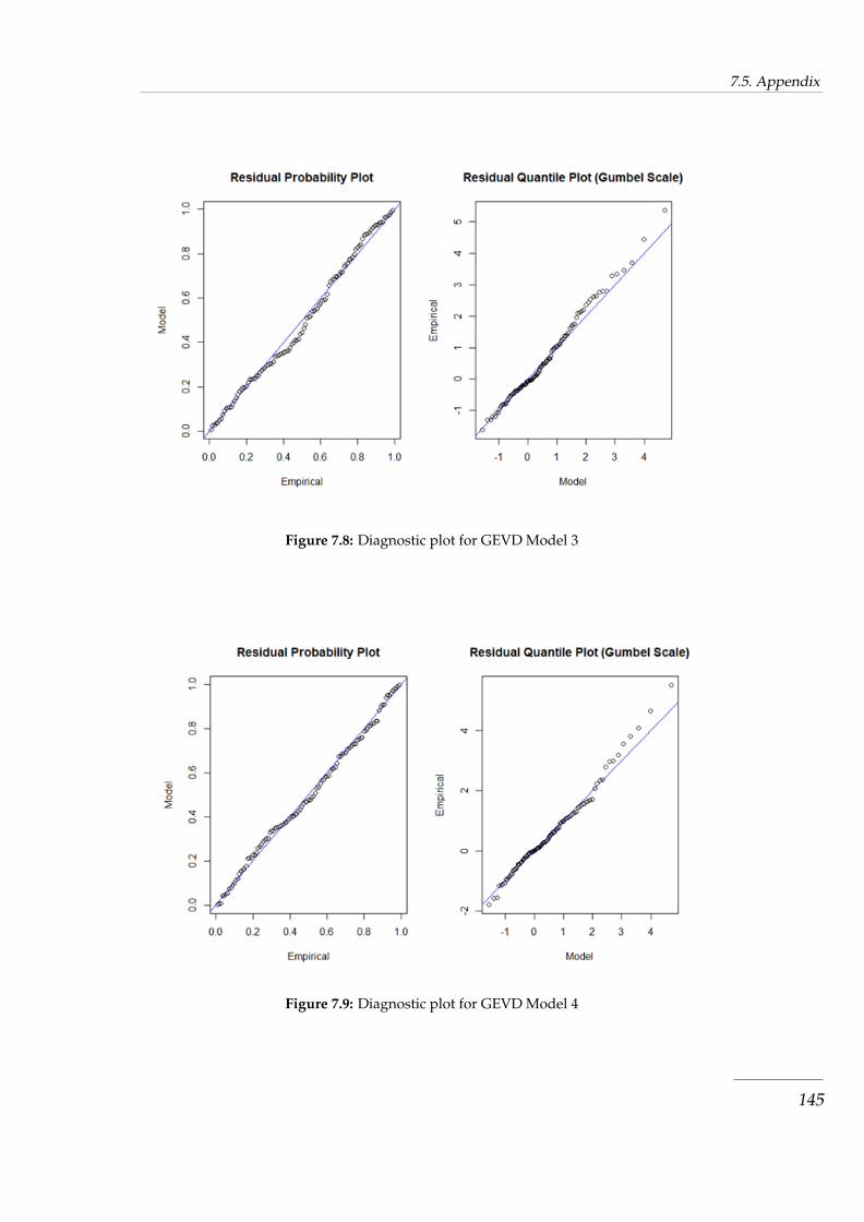
7.5. Appendix
Figure 7.8: Diagnostic plot for GEVD Model 3
Figure 7.9: Diagnostic plot for GEVD Model 4
145

7.5. Appendix
Figure 7.10: Diagnostic plot for GEVD Model 5
Figure 7.11: Diagnostic plot for GEVD Model 6
146

Chapter 8
Modelling mean annual rainfall
extremes using a generalised Pareto
distribution model
8.1 Introduction
Frequency analysis of extreme values of meteorological quantities have been widely
used for problems related to agriculture, engineering design and risk management
of buildings, roads and bridges. The information on extreme rainfall events is of
obvious importance to society, especially to populations living in drought or flood
risk areas (Sugahara et al., 2009). In recent years, Zimbabwe has been regularly af-
fected by extreme rainfall that has an enormous influence on social development and
threatens the country’s efforts to revive its failing economy. Zimbabwe’s economy
is hugely dependent on rain-fed agriculture (Jury, 1996). Consequently, estimations
of extreme rainfall events in Zimbabwe play a significant role in efficient risk ap-
praisal and for the reduction of losses of the economy. Knowledge of the statistics
pertaining to the occurrence of floods or droughts allows decision makers to de-
sign efficient mitigating measures. It helps in planning and constructing of water
management and sewage systems. It also helps in supporting decisions regarding
147
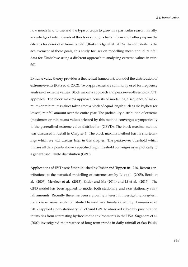
8.1. Introduction
how much land to use and the type of crops to grow in a particular season. Finally,
knowledge of return levels of floods or droughts help inform and better prepare the
citizens for cases of extreme rainfall (Brakenridge et al. 2016). To contribute to the
achievement of these goals, this study focuses on modelling mean annual rainfall
data for Zimbabwe using a different approach to analysing extreme values in rain-
fall.
Extreme value theory provides a theoretical framework to model the distribution of
extreme events (Katz et al. 2002). Two approaches are commonly used for frequency
analysis of extreme values: Block maxima approach and peaks-over-threshold (POT)
approach. The block maxima approach consists of modelling a sequence of maxi-
mum (or minimum) values taken from a block of equal length such as the highest (or
lowest) rainfall amount over the entire year. The probability distribution of extreme
(maximum or minimum) values selected by this method converges asymptotically
to the generalised extreme value distribution (GEVD). The block maxima method
was discussed in detail in Chapter 6. The block maxima method has its shortcom-
ings which we will discuss later in this chapter. The peaks-over threshold which
utilises all data points above a specified high threshold converges asymptotically to
a generalised Pareto distribution (GPD).
Applications of EVT were first published by Fisher and Tippett in 1928. Recent con-
tributions to the statistical modelling of extremes are by Li et al. (2005), Bordi et
al. (2007), McAleer et al. (2013), Ender and Ma (2014) and Li et al. (2015). The
GPD model has been applied to model both stationary and non stationary rain-
fall amounts. Recently there has been a growing interest in investigating long-term
trends in extreme rainfall attributed to weather/climate variability. Demaria et al.
(2017) applied a non-stationary GEVD and GPD to observed sub-daily precipitation
intensities from contrasting hydroclimatic environments in the USA. Sugahara et al.
(2009) investigated the presence of long-term trends in daily rainfall of Sao Paulo,
148
8.2. Research methodology
Brazil. While Tan and Gan (2016) investigated the non stationarity of heavy precipi-
tation over Canada using the GEVD, GPD and the Poisson distribution.
The main objective of this chapter is to perform frequency analysis of annual rainfall
for Zimbabwe using GPD modelling particularly investigating whether the intensity
of annual rainfall has changed over the years. Thus, frequency analysis of extreme
rainfall in this study is carried out in a non-stationary context. There are at least two
reasons for non-stationary modelling of extreme values of annual rainfall in Zim-
babwe. The first is that over the years Zimbabwe has received a declining pattern of
rainfall each year (Manatsa et al. 2008). This is attributed to global climate change
which is a potential driver of extreme hydro-meteorological events (Trenberth, 1999;
Felici et al., 2007; Parey et al., 2007). The second reason is related to the results ob-
tained from some studies evidencing statistically significant positive trends in the
extreme rainfall time series in other parts of the world. There is no work known to
us on trend analysis of extreme rainfall in Zimbabwe.
The rest of the chapter is organised as follows: In Section 8.2 we discuss common pit-
falls of the block maxima approach in modelling extreme values. We also present the
research methodology in the same chapter. Section 8.3 presents the empirical results
and discussion of the findings. Finally, Section 8.4 gives the concluding remarks.
8.2 Research methodology
In this section we discuss the background theory on stationary and non-stationary
generalised Pareto distribution models. The data used in this chapter were described
in Chapter 3. The parameters of the fitted models are estimated by the method of
maximum likelihood. We first look at the pitfalls of the GEVD discussed in Chapter
6 and justify the application of GPD in modelling extreme rainfall for Zimbabwe.
149

8.2. Research methodology
8.2.1 Pitfalls of the GEVD
The block maxima approach, which is the basis for the GEVD is considered wasteful
of data if more data on the extremes are available (Zhang et al., 2014). For example, if
daily rainfall data is available and we use a month as the block size, then the maxima
rainfall for the month is selected for modelling under this approach. Two methods
have been developed to overcome this problem namely; the r largest order statistics
method and the peaks-over threshold method.
8.2.2 r largest order statistics model
In Section 6.2 we supposed that X1, ..., Xn is a sequence of independent and identi-
cally distributed random variables and aimed to model the extreme behaviour of the
Xi. For the r largest order statistics, we extend the limiting distribution by defining
Mkn = kth largest of {X1, ..., Xn}, (8.1)
and identifying the limiting behaviour of this variable, for fixed k, as n → ∞. The
extremal types theorem (Theorem 8.1) is generalised by Theorem 6.4.
Theorem 8.1 If there exist sequences of constants {an > 0} and {bn} such that
Pr
{(Mn − bn)
an≤ x
}→ F (x) as n→∞ (8.2)
for some nondegenerate distribution function, F , so that F is the GEVD function given by
(6.11), then, for fixed k,
Pr
{(Mk
n − bn)an
≤ x
}→ Fk(x) (8.3)
on {x : 1 + ξ(x− µ)/σ > 0}, where
Fk(x) = exp{−τ(x)}k−1∑s=0
τ(x)s
s(8.4)
150

8.2. Research methodology
with
τ(x) =[1 + ξ
(x− µ
σ
)]− 1ξ
(8.5)
The theorem implies that, if the kth largest statistic in a block is normalized in exactly
the same way as the maximum, then the parameters correspond to the parameters
of limiting GEVD of the block maxima. Model (8.4) is, however, difficult to use as a
model. The problem is having each value of the largest r order statistic within each
of several blocks, for some value of r (Smith, 1986). Therefore, in this thesis the r
largest order statistic method is not used to model extreme rainfall for Zimbabwe.
8.2.3 Peaks-over threshold models
If the GEVD is considered wasteful, the r largest order statistics method is also re-
garded as wasteful of data as well. For example; if one block of data has a lot of ex-
treme observations relative to other blocks, many of these may not be used as only
the r largest are modelled. Modelling all observations exceeding a specified high
threshold value, usually known as the peaks over threshold (POT) approach can be
regarded as not wasteful of extreme data. The model of all observations exceeding
a specified high threshold was first proposed by Pickands (1975) and a detailed dis-
cussion of the model was given by Davison and Smith (1990).
Suppose X1, ..., Xn is a sequence of independent and identically distributed ran-
dom variables, having a common distribution G. Then, the Xi exceeding some high
threshold u (usually known as threshold exceedances) can be regarded as extreme
events. Let X denote an arbitrary term in the Xi sequence, then a description of the
stochastic behavior of extreme events is given by the conditional probability:
Pr {X > u+ y | X > u} =1−G(u+ y)
1−G(u), y > 0. (8.6)
The distribution of threshold exceedances would therefore be known ifGwas known.
151

8.2. Research methodology
In practice G is unknown, so the distribution is approximated.
8.2.4 Generalised Pareto distribution (GPD)
Theorem 8.2 Let X1, ...., Xn be a sequence of independent and identically distributed ran-
dom variables with common distribution function G, and let
Mn = max{X1, ..., Xn}.
Let X denote an arbitrary term in the Xi sequence and suppose that G satisfies Theorem 6.1,
so that for large n and a nondegenerate distribution function, F ,
Pr{Mn ≤ x} ≈ F (x),
where
F (x) = exp
{−[1 + ξ
(x− µ
σ
)]− 1ξ
}(8.7)
for some µ, σ > 0 and ξ. Then for a specific threshold u, the distribution function of X − u,
conditional on X > u, is approximately
Fu(y) = 1−(
1 +ξy
σ
)− 1ξ
(8.8)
defined on {y : y > 0 and (1 + ξy/σ) > 0} , where
σ = σ + ξ(u− µ). (8.9)
For large u, if ξ = 0, then
limu→∞
Pr(X − u ≤ y | X > u) = Fu(y) ={
1− exp( yσ
)− 1ξ
}, y > 0 (8.10)
which corresponds to an exponential distribution with parameter 1eσ . The generalised
Pareto distribution is the name given to the distributions defined in (8.7) and (8.8)
152

8.2. Research methodology
(Scarrott and MacDonald, 2012; Magadia, 2010;). From Theorem 6.5, we can deduce
that the shape parameter ξ of the GPD is in fact equal to the corresponding shape
parameter of the GEVD while the scale parameter σ is equal to σ+ξ(u−µ). Thus, the
GPD has two parameters namely; the scale parameter σ and the shape parameter ξ.
The distribution function is given by:
Fu(y) =
1−
(1 + ξyeσ
)− 1ξ, if ξ 6= 0,
1− exp( yeσ)− 1
ξ , if ξ = 0,(8.11)
where y > 0 when ξ ≥ 0, 0 ≤ y ≤ −σ/ξ when ξ < 0, and the scale parameter σ > 0
(Tsay, 2013).
The quantile function of the GPD is given by:
QN =
u+ eσ
ξ
[( ny
Nup)−ξ − 1
], ξ 6= 0,
u− σlog( ny
Nu(1− p)), ξ = 0
(8.12)
Where ny is the number of observations per year, N is the number of exceedances
above threshold u in a given sample. p, the probability of an individual observation
exceeding the threshold u and
p =k
n
where kn is the sample proportion of points exceeding u. To obtain estimates of the
quantiles (return levels), the estimate of ζu and the maximum likelihood estimates
of σ and ξ can be substituted into (8.12). Standard errors or confidence intervals of
QN can be derived by the delta method (Rao, 1973). The mean and the variance of
the GPD are eσ1−ξ and eσ2
(1−ξ)2(1−2ξ)respectively.
8.2.5 Threshold selection
Before modelling data using the GPD, it is important to choose an appropriate thresh-
old u. The choice of threshold is a matter of balancing bias and variance. Coles et
al. (2001) pointed out that if the threshold is too low, it is more likely to violate
153

8.2. Research methodology
the asymptotic property of the model and cause bias; if the threshold is too high, it
will generate few exceedances for estimation and results in high variances. A basic
strategy is to select a threshold as low as possible such that the limiting approxima-
tion of the model can provide a reasonable result (Giles et al., 2016). The classical
fixed threshold selection approach uses graphical diagnostics, essentially assessing
aspects of the model fit, to make an a priori threshold choice. Some of the graphical
diagnostics are Pareto quantile plot, mean excess plot and the parameter stability
plot ( Berning, 2010; Gomes and Gullou., 2015; de Haan and Lin, 2001;).
Pareto Quantile Plots
Beirlant et al. (1996) considered choosing the tail fraction to provide an optimal lin-
ear fit to the Pareto quantile plot. The Pareto quantile plot is a graphical method for
inspecting the parameters of a Pareto distribution (Beirlant et al., 1996). If the Pareto
distribution holds, there is a linear relationship between the logarithms of the ob-
served values and the quantiles of the standard exponential distribution, since the
logarithm of a Pareto distributed random variable follows an exponential distribu-
tion. The observations on the y-axis where the plot starts to follow a straight line
is taken as the optimal threshold. The tail of the data follows a Pareto distribution
if the logarithms of the observed values form almost a straight line. The left most
point of the straight line (tail of the data) is the estimate of the optimal threshold
u. The main drawback of this threshold selection procedure is after selection of the
appropriate threshold there is no formal assessment of the certainty associated with
the threshold choice.
Mean excess plot
Beirlant et al. (2004) defines the mean excess function with the finite expectation
E(Y ) <∞ as:
e(u) = E(Y − u | Y > u),
154

8.2. Research methodology
i.e., the mean of exceedances over a threshold u. If the underlying distribution of
Y − u | Y > u follows a GPD, then the corresponding mean excess function is
e(u) =σ + ξu
1− ξ, (8.13)
provided that σ + ξu > 0 and ξ < 1. From (8.13), we can clearly see that the mean
excess function must be linear in u. More precisely, Y > u follows a GPD if, and only
if, the mean excess function is linear in u (Coles et al., 2001). This provides us a way
of selecting an appropriate threshold. Given the data set, we define the empirical
mean excess function as:
en(u) =
∑ni=1(Yi − u)I{Yi>u}∑n
i=1 I{Yi>u}, (8.14)
where n is the sample size. In this case the indicator function I{Yi>u} is defined such
that:
I{Yi>u} =
1 if Yi > u,
0 Otherwise(8.15)
The empirical excess plot is a graphical representation of the locus of (u, en(u)) and
we can examine this plot to choose the threshold u such that en(u) is the lowest
level where all the higher threshold based sample mean excesses are approximately
linear for Y > u. Coles et al. (2001) acknowledged that the interpretation of the
mean excess plots can be challenging.
The parameter stability plots
We exploit another useful property of the extremal index estimator to derive a fur-
ther tool for threshold selection. The threshold stability of the extremal index esti-
mator refers to its invariance to change in threshold above a suitably high thresh-
old. That is, once a threshold is high enough, raising the threshold further should
not dramatically change the estimated value of ξ. The parameter stability plot in-
volves plotting the parameter estimates from the GPD against u, for a range values
155

8.2. Research methodology
of u. The parameter estimates should be stable (i.e. constant) above the threshold at
which the GPD model becomes valid. Scarrot and MacDonald (2012) acknowledged
that parameter stability plots do not provide firm conclusions, since inconsistencies
are observed between the estimated shape parameter at the chosen threshold and
higher thresholds.
Extremal mixture models
The drawback with fixed threshold approaches is that once the threshold has been
chosen it is treated as fixed, so the associated subjectivity or uncertainty is ignored in
subsequent inferences. (Scarrot and MacDonald, 2012). Extreme mixture models, in
the last decade have been proposed which encapsulate the usual threshold model in
combination with a component intended to capture all of the non-extreme distribu-
tion (bulk distribution) i.e. the procedure considers both the distribution of excesses
(exceedances) and non-exceedances. The two distributions share information about
the location of the threshold and the threshold in mixture models is defined as the
parameter to be estimated. The mixture model accounts for uncertainty associated
in threshold choice in subsequent inferences (Scarrot and MacDonald, 2012). The
major drawbacks of the mixture models are that the asymptotic properties of their
impromptu heuristics are not yet well understood and their behaviour at the thresh-
old point is still unclear (Bernadara et al., 2014).
In this thesis, the commonly used Pareto quantile plot, mean excess plot and the pa-
rameter stability plot will be applied concurrently to select an appropriate threshold
since recently developed mixture models still have challenges in their computational
abilities. The subsection that follows reviews the declustering techniques associated
with the POT approach and GPD distribution.
156
8.2. Research methodology
8.2.6 Declustering
The theory of extreme value distribution establishes a limiting distribution of series
of random variables which are independent and identically distributed. Extreme
events usually take place in clusters as a result of dependency in data (Beirlant et
al., 2006; Bernadara et al., 2014). Time series data are known to be auto-correlated
thus a naive selection of exceedances above a given threshold may lead to events
that are no longer considered independent, but dependent. In order to reduce the
dependencies of time series data, a technique called declustering is used (Coles et
al., 2001; Ferro and Segers, 2003; Ribatet, 2006; Yilmaz and Perera, 2013). The R sta-
tistical package ”clust” tries to identify peaks over a threshold while meeting the
independence criteria. According to Ribatet (2006), clusters are identified as follows:
(i) The first exceedance initiates the first cluster;
(ii) The first observation under the threshold u ”ends” the cluster unless tim.cond
(time condition for independence) does not hold;
(iii) The next exceedance which hold tim.cond initiates a new cluster;
(iv) The process is iterated as needed.
The declustering approach has been criticized in the literature for being sensitive to
the run length, r, that is chosen arbitrarily in cluster determination and discards of
all data to leave out cluster maxima only (Coles et al., 2001).
Ferro and Segers (2003) proposed a declustering technique which involves the es-
timation of the extremal index, ξ and the method proposes an automatic selection
of the run-length auxiliary parameter, r, used to identify independent clusters. The
extremal index is given by:
ξu =2[∑N−1
i=1 (Ti − 1)]2
(N − 1)∑N−1
i=1 (Ti − 1)(Ti − 1)(8.16)
157

8.2. Research methodology
where Ti denote the exceedance times andN is the number of threshold exceedances.
In this case, u is a sufficiently high threshold. According to Coles et al. (2001), the
extremal index measures the amount of clustering and 0 < ξu < 1, and 1ξu
is the
limiting mean cluster size. The exceedance times consist of two groups: one corre-
sponding to inter-cluster times and the other corresponding to intra-cluster times.
Under Ferro and Segers (2003) model, the extremal index ξu arises as the propor-
tion of interdependence times which are also inter-cluster times. Assuming that we
have observed N threshold exceedances, then the ξuN largest interexceedance times
are assumed to be approximately independent inter-cluster times. The value of ξu is
used to identify the critical cut off interexceedance time that distinguishes inter from
intra-cluster times. Once clusters have been identified, the cluster characteristics can
be examined. Inference on these cluster maxima can be carried out and such infer-
ence is much more straight forward than the inference on the original dependent
sequence.
In this thesis, we use the declustering approach as proposed by Ferro and Segers
(2003). To check for goodness of fit of the Ferro and Segers (2003) model for esti-
mated ξu, we use a QQ-plot of interexceedance times against standard exponential
quantiles.
8.2.7 Estimation procedure of parameters for the Generalised Pareto Dis-
tribution
After determining an appropriate threshold, the parameters of a GPD can be esti-
mated by method of maximum likelihood. Suppose we have a a sufficiently high
threshold u and assume we have yi, ..., ym exceedances over a sufficiently hight
threshold from the original random variable x1, ..., xn where m < n i.e. m obser-
vations with Yi − u ≥ 0, the subsample {y1 − u, ..., ym − u} has an underlying GPD
distribution, where Yi−u ≥ 0 for ξ ≥ 0, 0 ≤ Yi−u ≤ −eσξ for ξ < 0, then the logarithm
158

8.2. Research methodology
of the probability density function of yi can be derived as:
lnfu(yi − u) =
−ln(σ)− 1+ξ
ξ ln[1 + ξ
(yi−ueσ )]for ξ 6= 0,
−ln(σ)− 1eσ (yi − u) for ξ = 0.(8.17)
Hence, the log-likelihood function l(ξ, σ | yi − u) for the GPD is the logarithm of the
joint density of the m observations, i.e.
l(ξ, σ | yi − u) =
−mln(σ)− 1+ξ
ξ
∑mi=1 ln
[1 + ξ
(yi−ueσ )]for ξ 6= 0,
−mln(σ)− 1eσ ∑mi=1(yi − u) for ξ = 0.
(8.18)
By differentiating (8.18) with respect to ξ we obtain:
dl
dξ=
1ξ2
∑mi=1 ln
[1 + ξ
(yi−ueσ )]− 1+ξeσξ
∑mi=1
yi−u
1+ξ“
yi−ueσ” , for ξ 6= 0
0, for ξ = 0(8.19)
By differentiating (8.18) with respect to σ we obtain:
dl
dσ=
−meσ + 1+ξeσξ
∑mi=1
ξ(yi−u)eσ+ξ(yi−u) , for ξ 6= 0
−meσ + 1eσ2
∑mi=1(yi − u), for ξ = 0
(8.20)
The equations (8.19) and (8.20) have no analytical solutions. To obtain the estimates
of ξ and σ we set the (8.19) and (8.20) to zero and solve using numerical techniques.
According to de Zea Bermudez and Turkman (2003) maximum likelihood estima-
tors for GPD only exist for ξ ≤ 1. In fact, if ξ > 1, the log-likelihood tends to infin-
ity as σ/ξ approaches yn:n. McNeil and Frey (2000) comment that consistency and
asymptotic properties of the maximum likelihood estimators such as normality and
efficiency hold uniquely if ξ < 0.5. According to Hosking and Wallis (1987), estimat-
ing the parameters of the GPD, algorithms used to compute maximum likelihood
estimates may experience convergence problems.
159

8.2. Research methodology
8.2.8 Time-heterogenous GPD model
If we consider the stationary GPD model in (8.11) for ξ 6= 0, that is
Fu(y) = 1−(
1 +ξy
σ
)− 1ξ
(8.21)
and let (8.21) be M0. We propose another GPD model, M1 with scale parameter
which trend with time i.e. lnσ(t) = σ0 + σ1t and ξ(t) = ξ = constant. Thus, the
general form for non-stationary GPD model, M1, is given by
Fu(σ(t), ξ, t) = 1−(
1 +ξy
exp(σ0 + σ1t)
)− 1ξ
, for ξ 6= 0, (8.22)
where 0 ≤ y ≤ x− u.
8.2.9 Model diagnostics and goodness-of-fit
Before estimating return levels (8.12), we checked for model adequacy and goodness-
of-fit. PP plots, QQ plots and return level plots are useful for assessing the adequacy
of a fitted generalised Pareto model. Assuming a threshold u, threshold excesses
y1 ≤ ... ≤ ym and an estimated model Fu, the probability plot consists of pairs
{(i/(m+ 1), Fu(yi)); i = 1, ...,m} (8.23)
where
Fu(y) = 1−
(1 +
ξy
σ
)− 1
ξ
,provided ξ 6= 0. (8.24)
If the generalised Pareto model is adequate for modelling excesses of u, both the
probability and quantile plots should consist of points that are approximately linear.
160

8.3. Empirical Results
8.3 Empirical Results
In this section, the results of modelling mean annual rainfall for Zimbabwe using
the GPD are presented. Results for the time-homogeneous GPD model (Model 1)
and time-dependent GPD model (Model 2) are also presented. To fit Model 1 and
Model 2, we need to check whether the mean annual rainfall data is independent
and identically distributed (i.i.d.). In Chapter 3, the source and the properties of the
rainfall data set was described and shown to be i.i.d., thus, we can fit the data to the
generalised Pareto distribution.
8.3.1 Fitting time-homogeneous generalised Pareto distribution
To fit a GPD model, we check whether the tail of the mean annual rainfall data fol-
lows a Pareto distribution. Figure 8.1 shows the Pareto quantile plot for mean annual
rainfall for Zimbabwe.
Figure 8.1: Pareto quantile plot for mean annual rainfall for Zimbabwe for the period 1901-2009.
From Figure 8.1, the tail of the data is almost a line confirming that the data may
161

8.3. Empirical Results
follow a generalised Pareto distribution. To determine, the high threshold, u, the
mean excess (mean residual life) and parameter stability plots were used to come up
with a reasonable high threshold u. Figure 8.2 shows the mean excess plot of mean
annual rainfall data for the period 1901-2009.
Figure 8.2: Mean excess plot for mean annual rainfall for Zimbabwe for the period 1901-2009.
The suitable threshold must lie where there is a positive gradient change in the mean
excess. From Figure 8.2, the optimal threshold seems to lie around 725 mm. The se-
lection of a suitable threshold is empirically done. To validate the threshold value,
we used the parameter stability plot, shown in Figure 8.3.
Figure 8.3 shows that the estimated parameters are stable when u ≥ 725. The Pareto
quantile plot is then used to come up with the optimal threshold u of 727.9 mm. The
threshold of 727.9 mm was chosen in order to meet the requirements of the bias-
variance threshold trade-off, such as, it is high enough for asymptotic theorem to
be considered accurate and low enough to have sufficient data to estimate the GPD
162

8.3. Empirical Results
Figure 8.3: Parameter stability plot for mean annual rainfall for Zimbabwe for the period1901-2009.
parameters. There are 38 observations above the threshold. Since the exceedances
above the optimal threshold can not be assumed to be independent and identically
distributed, declustering was performed and the results are shown in Figure 8.4.
We fit Model 1 (time homogenous GPD) and Model 2 (time-heterogenous GPD) to
the declustered exceedances. Table 8.1 reports the maximum likelihood (ML) esti-
mates with standard errors in the parentheses of the Model 1 and Model 2, namely;
shape (ξ) and scale (σ) fitted to the mean annual rainfall data.
The shape parameter for Model 1 and Model 2 were significantly different from zero
(p-values< 0.05). Figure 8.5 and Figure 8.6 shows the diagnostic plots of Model 1
and Model 2 respectively.
From Figure 8.5, the probability plot (top left panel) and the quantile plot (top right
panel) suggest that the exceedances seems to follow the time-homogenous GPD
163

8.3. Empirical Results
Figure 8.4: Plot of declustered exceedances for mean annual rainfall for Zimbabwe for theperiod 1901-2009.
Figure 8.5: Diagnostic plots illustrating the fit of the mean annual rainfall data for Zimbabwefor the period 1901-2009 to the GPD Model 1, (a) Probability plot (top left panel),(b) Quantile plot (top right panel), (c) Return level plot (bottom left panel) and(d) Density plot (Bottom right panel)
164

8.3. Empirical Results
Table 8.1: Maximum likelihood parameter estimates and negative log-likelihood of thetime-homogenous and non-stationary GPD models for mean annual rainfall datafor Zimbabwe
Model σ0 σ1 ξ NLL value
M1 166.4076 0.0000 −0.2242 159.0276
(45.0578) (0.1953)
M2 5.8406 −0.0101 −0.5145 157.2157
(0.2947) (0.0015) (0.2361)
model. The return level plot (bottom left panel) confirms that the time-homogenous
GPD model is adequate to estimate return levels of the exceedances. Finally, the
density plot seems consistent with the histogram of the data. Thus, all the diagnos-
tic plots suggest that the exceedances follows the time-homogenous GPD model.
Figure 8.6: Diagnostic plots illustrating the fit of the mean annual rainfall data for Zimbabwefor the period 1901-2009 to the GPD Model 2, (a) Residual probability plot (leftpanel), (b) Residual quantile plot (right panel).
From Figure 8.6, the residual probability plot (left panel) shows no significant de-
165
8.3. Empirical Results
parture from the straight line suggesting that the exceedances above the threshold
follows a time-dependent GPD model. However, the residual quantile plot (left
panel) seem to suggest that time-dependent GPD model may be adequate to esti-
mate return levels at smaller return periods. At higher return periods the model is
inadequate. The residual quantile plot departs from the straight line at the tail of the
data.
In order to check whether allowing the scale parameter to trend with time is worth-
while, we use the D statistic discussed in Chapter 6. The model pair (M1,M2)
had a D statistic value of 2(−157.2157 + 159.0276) = 3.6238 and a critical value
of χ21,0.05 = 3.841. Since D statistic= 3.6238 < χ2
1,0.05 = 3.841, this indicates that
the time-dependent GPD model is not worthwhile over the time-homogenous GPD
model. Thus the proposed model based on the findings of this study is the time-
homogenous GPD model (Model 1). The time-homogenous GPD model for mean
annual rainfall for Zimbabwe is given in (8.25)
Fu=727.9(σ, ξ) = 1−(
1 +−0.2242yi
166.4076
) 10.2242
(8.25)
where yi = xi − 727.9 are the exceedances over the optimal threshold of 727.9 mm.
We estimate return levels at selected time (T ) intervals. Table 8.2 shows the return
levels of mean annual rainfall for Zimbabwe at selected time (T ) intervals.
Table 8.2: Return level estimate (mm) at selected return intervals (T ) determined using theGPD Model 1
T = 5 T = 10 T = 15 T = 20 T = 25 T = 30 T = 50 T = 100
1061.5974 1120.3975 1150.7876 1170.7344 1185.3442 1196.7505 1226.3333 1531.2136
The highest mean annual rainfall of 1192.6 mm was recorded during 1924/25 rainfall
season. Using the proposed GPD model, a high mean annual rainfall of this mag-
nitude is likely to return once in every 30 year period. The return levels estimated
166

8.4. Concluding remarks
using the stationary GPD model (see Table 8.2) are slightly higher than the return
level estimates using GEVD as reported in Chapter 6 (see Table 6.3). The reason for
the slightly higher return levels using the GPD model is still unknown. One reason
might be the high optimal threshold used, since the return level estimates should
always greater than the threshold.
8.4 Concluding remarks
We extended the works of Li et al. (2004), Sugahara (2009) and Demaria et al. (2017)
who fitted daily rainfall data to stationary and time-dependent GPD models using
maximum likelihood estimation. In this chapter, we have shown that the meth-
ods can be applied to averaged annual rainfall data. We are the first to model
mean annual rainfall data for a drought-prone country such as Zimbabwe using
the GPD model. We modelled mean annual rainfall data for Zimbabwe using time-
homogenous GPD, with a high threshold value of u = 727.9 mm. The study has
shown that exceedances above the 727.9 mm threshold do not vary with time. Us-
ing the proposed model, the estimates of return levels at selected time intervals are
slightly higher than those obtained using the stationary GEVD. According to Fer-
reira and de Haan (2015), the POT method is most efficient if the number of ex-
ceedances is much larger than the number of blocks. In Chapter 6, we used yearly
blocks for GEVD, i.e. 109 blocks and the number of exceedance is 38 which is less
than the number of blocks. However, this study has revealed that the shape param-
eter, ξ is less than zero and results obtained from the data and findings in this study
suggest that the proposed model is reliable. Therefore, in the case where the number
of observations is equal to the number of blocks, the POT method seems to produce
reliable results.
167
Chapter 9
Generalised extreme value
regressions with binary dependent
variable: An application to
predicting meteorological drought
probabilities
9.1 Introduction
Meteorological drought although rare, impacts severely on the environment and
economy of a country. Many significant events across several disciplines such as
hydrology, meteorology, medicine, epidemiology and finance are rare. In hydrol-
ogy and meteorology, extreme value theory is applied to model temperature, floods,
minima rainfall and wind speed. The methodology for modelling occurrence of rare
events are well established. The two-parameter exponential distribution derived
from extreme value theory is generally used to model extreme data (see Lu, 2004).
The Generalised Pareto and Generalised Extreme Value Distributions are also com-
monly used to model rare and extreme events in finance and hydrology (see Em-
168

9.1. Introduction
brechts et al., 1997, Coles et al., 2001, Koutsoyiannis, 2004; Nadarajah and Choi, 2007
and Bhunya et al., 2007;). Meteorological drought is the occurrence of below normal
rainfall. A rainfall season or a calendar year can be declared as a drought period
if the average seasonal/annual rainfall received in that particular rainfall season or
year is below the average normal rainfall. Thus, a rainfall season/year can be cate-
gorised as experiencing a drought or no drought (binary).
Droughts affect a large number of people worldwide and causes tremendous eco-
nomic losses, environmental damage, social hardships, yet droughts are the least
understood of all weather phenomena (Obasi, 1994). In Zimbabwe, droughts occur
frequently and are often severe and impacting negatively on the country’s economic
performance. At least 50% of the Gross Domestic Product (GDP) in Zimbabwe is de-
rived from rain-fed agriculture production (Jury, 1996). Thus, apart from immediate
food shortages, droughts have a significant impact on the overall performance of the
Zimbabwe agriculturally based economy. Over the past three decades, Zimbabwe
has been ravaged by erratic rainfall patterns which has sometimes led to droughts.
Since independence in 1980, Zimbabwe recorded the lowest average rainfall in the
1991/1992 rainfall season and the highest average rainfall in the 1999/2000 rainfall
season (Zimbabwe Central Statistical Report, 2014). The 1991/1992 rainfall season,
was influenced by an El Nino year whilst for the 1999/2000 season was affected by a
La Nina year. Cyclone Eline accounted for most of the abnormal rainfall experience
in the 1999/2000 rainfall season.
From year 2001 to 2003, Zimbabwe had rainfall in the first half of the rainfall season
only and a dry spell in the second half, resulting in severe drought in some parts
of the country. From year 2004 to 2008, Zimbabwe received an average rainfall in
the northern parts of the country whilst other parts received very little rainfall or no
rainfall at all. In the 2009/2010 rainfall season, Zimbabwe received below average
rainfall in the first half of the rainfall season and above average rainfall in the second
169
9.1. Introduction
half of the rainfall season. Generally, the rainfall patterns are becoming more and
more erratic making it difficult to plan. For the 2015/2016 rainfall season, the South-
ern African Regional Climate Outlook Forum (SARCOF) predicted a 90% chance
that an El Nino will develop during the period October-December 2015 for coun-
tries in southern Africa. The occurrence of an El Nino is likely to result in poor rains
in Zimbabwe. Given this background on the rainfall and droughts patterns in Zim-
babwe, research on predicting drought for the country, in any given year, becomes
of paramount importance. Timely predictions will assist farmers with planning for
each rainfall season, for instance; using drought resistant crops or varieties given
the expected drought probability. It is imperative that a simple and accurate tool be
proposed to predict the occurrence of drought at a reasonable time lag. This study
argues, since droughts are rare and extreme, using the GEVD regression model can
add value in the prediction of drought probabilities.
In this study we modelled binary rare events data, i.e. drought as the dependent
variable. Several models of binary dependent variables have been suggested in lit-
erature by considering different link functions: logit, probit, log-log and contem-
porary log-log models. The logistic regression model is the most commonly used
model. However, the logistic regression has been shown to underestimate the prob-
ability of rare events and the logit link function is a symmetric function, thus the
response curve approaches zero as the same rate approaches one (King and Zeng,
2001). Calabrese and Osmetti (2013) proposed the Generalised Extreme Value Distri-
bution (GEVD) regression model for modelling rare binary responses. The proposed
model, however, has not been previously used to model extreme rainfall patterns.
In this study, our aim are to (i) propose a model to predict meteorological drought
probabilities for Zimbabwe that can be used as a drought early warning system, (ii)
compare the relative performance of the logistic regression model and the GEVD re-
gression model in predicting drought probabilities for Zimbabwe.
170

9.2. Research methodology
This chapter is organized as follows. In Section 9.2 we present the research method-
ology. The description of the data set for the chapter is given in Section 9.3. In Section
9.4, the proposed models are outlined. In Section 9.5, the results of the fitted models
and their implications are discussed. Finally, the concluding remarks and appendix
are provided in Section 9.6 and Section 9.7 respectively.
9.2 Research methodology
In this section the logistic regression model and its drawbacks in modelling rare
events data are discussed. The GEVD regression model is also discussed.
9.2.1 The logistic regression model
Suppose y1, ..., yn be realizations of Bernoulli independent random variables Y1, ..., Yn
that can take the value one and zero with probabilities πt and 1− πt for t = 1, 2, ..., n
respectively. A generalised linear model (GLM) considers a link function and co-
variate vector xt such that
g(π) = β′xt (9.1)
The probability πt is obtained by applying the inverse function of g(.) i.e.
πt = g−1(β′xt). (9.2)
In the logistic model, the probability πt is a logistic cumulative distribution function
π(xt) =exp(β′xt)
1 + exp(β′xt)(9.3)
with
β′ = [β0, β1, ..., βk] x′ = [1, x1, ..., xn].
171

9.2. Research methodology
Thus the logit link function is
logit(π(xt)) = ln(
π(xt)1− π(xt)
)= β′xt. (9.4)
If we set
yt = ln(
π(xt)1− π(xt)
)(9.5)
The transformed logistic regression model is
yt = β′xt. (9.6)
Because logistic regression predicts probabilities, rather than classes, we estimate the
parameter vector β′ using the method of maximum likelihood. The log-likelihood
function of the logistic regression model is
l(β) =n∑
t=1
yt(xtkβk)− ntlog
(1− exp
{K∑
k=0
xtkβk
}). (9.7)
The estimates of the parameters are obtained by setting the first derivative of the
log-likelihood function with respect to each β to zero and solving the systems of
equations. The resultant system of equations have no closed form solutions, we
however approximately solve then numerically using the Newton’s method for nu-
merical optimization.
9.2.2 The Generalised extreme value distribution (GEVD) regression model
The logistic regression model underestimates the probability of a rare event (Cal-
abrese and Osmetti, 2011). In meteorology and hydrology maxima of temperatures,
precipitation and river discharges have been recorded for many decades (Hosking
and Wallis, 1987). The Extreme Value Theorem (EVT) provides a robust theoreti-
cal frame work to model the distribution of rare events. The Generalised Extreme
Value Distribution (GEVD) was recommended for hydrological frequency analysis
172
9.2. Research methodology
(Bunya et al., 2007). There are three parameters that describe the GEVD and these
are: location (µ), scale (σ) and shape (ξ). The GEVD is a family of continuous proba-
bility distributions developed within extreme value theorem. The GEVD unites the
Gumbel, Frechet and Weibull class of distributions into a single family to allow for a
continuous range of possible shapes. Based on the extreme value theorem the GEVD
is the limiting distribution of properly normalized maxima of a sequence of indepen-
dent and identically distributed random variables (Beirlant et al., 2004). Thus, the
GEVD is used to model the maxima of long (finite) sequence random variables. The
detailed description of the GEVD was given in Chapter 6 pages 80-84.
The quantiles of the GEVD are given in terms of parameters and the cumulative
probability p by
Q(p) = µ+σ
ξ
[(−ln (1− p))−ξ − 1
], ξ 6= 0. (9.8)
In this study we used the quantile function of the GEVD as the link function of the
GLM as proposed by Calabrese and Osmetti (2013). The GLM with the quantile
function as the link function is referred to as a GEVD regression model. The link
function of the GEVD regression model is given by
[−lnπ(xt)]−ξ − 1
ξ= β′xt (9.9)
For the interpretation of the parameters β and ξ, we suppose that the value of the j-th
regressor (with j = 1, 2, ..., k) is increased by one unit and all the other independent
variables remain unchanged. Let x∗ be the new covariate values, whereas x denotes
the original covariate values. From (9.11), we deduce that βj = g(π(x∗)) − g(π(x))
with j = 1, 2, ..., k. This means that if the parameter βj (with j = 1, 2, ..., k) is positive
and all the other parameters are fixed, by increasing the j-th regressor the estimate
π(x) decreases. Otherwise, if βj is negative, by increasing the j-th regressor the esti-
mate π(x) of the GEVD model also increases.
173
9.3. The data
Again, we analyse the parameter β0: for all fixed values of ξ and for a null indepen-
dent variable, β0 has a positive monotonic relationship with the estimate of π(x).
Finally, we analyse the influence of the ξ parameter on π(x). We find that for β0 = 0
and by considering null values for all the covariates, from GEVD model we obtain
an estimate π(x) that is almost equal to e−1 for all the values of ξ. This means that
π(x) variations depend on the covariate variations and not on ξ variations. The
maximum likelihood method is used to estimate the parameters of the GEVD re-
gression model. Let Y = (Y1, Y2, ..., Yn) be a simple random sample of size n, the
log-likelihood function of the GEVD regression model is
l(β, ξ) =n∑
t=1
{−yt
[1 + ξ(β′xt)
]− 1ξ + (1− yt)ln
[1− exp
{−[1 + ξ(β′xt)
]− 1ξ
}]}(9.10)
The first derivative of the log-likelihood function with respect to each parameter are
dl(β, ξ)dβj
= −n∑
t=1
xtjln[π(xt)]1 + ξβ′xt
yt − π(xt)1− π(xt)
, j = 0, 1, ..., k, (9.11)
dl(β, ξ)dξ
= −n∑
i=1
[1ξ2
ln(1 + ξβ′xt)−β′xt
ξ(1 + ξβ′xt)
]yt − π(xt)1− π(xt)
ln[π(xt)]. (9.12)
which are set to zero and we solve the system of equations using a constrained opti-
mization method with {xt : 1 + ξβ′xt > 0} (Calabrese and Osmetti, 2013).
9.3 The data
Average annual rainfall data for Zimbabwe over the period 1901-2015 (115 years)
were obtained from Department of Meteorological Services in Zimbabwe. Mete-
orological drought, which is the scarcity of rainfall, is caused by various natural
phenomena such as El Nina, global warming and sea level pressures. The depart-
ment of Meteorological Services in Zimbabwe uses a threshold of 75% of normal
174

9.3. The data
average annual rainfall to declare a year as a drought year. The average annual
precipitation claims for Zimbabwe range from 663 mm (Shoko, 2014) to 867 mm
(http://www.climatetemp.info/zimbabwe). This gives a range average of 760 mm.
We use 570 mm (75% of 760 mm) as the drought threshold in this study. Mean annual
rainfall of less than 570 mm is categorized as drought indexed 1, otherwise mean an-
nual rainfall is categorized as no drought indexed 0. Thus, the drought index can be
treated as binary data
Yt =
1, If mean annual rainfall < 570mm
0, Otherwise(9.13)
We aim to propose a simple early warning drought predictive model using weather/climate
change drivers such as the Southern Oscillation Index (SOI) and the standardised
Darwin sea level pressure (SDSLP) anomalies. The Southern Oscillation is the most
notable large scale climatic variation that occurs from year to year (Panu and Sharma,
2002). This is measured using the Southern Oscillation Index (SOI) which is the dif-
ference in sea level air pressure between Tahiti (in Mid Pacific) and Darwin (in Aus-
tralia) (Mason and Jury, 1997). The SOI values range from about -35 to +35. A strong
and consistent negative SOI pattern is related to El Nino, the abnormal warming
of ocean surface temperatures in the eastern tropical Pacific that recurs every few
years. The El Nino phenomena is usually (but not always) associated with below
normal rainfall. On the other hand, a strong and consistent positive SOI pattern is
related to La Nina, the cooling of surface ocean waters in the eastern tropical Pa-
cific ocean. La Nina usually precedes above normal rainfall. The monthly SOI and
the SDSLP values are obtained from National Weather Service Climate Prediction
Centre (http://www.longpaddock.qld.gov.au.). The drought index for each year is
matched to average monthly SOI values and SDSLP anomalies observed in the same
year and the previous year. Thus the data set is of the form:
S = {xt1,xt2, Yt}, for t = 1, 2, ..., 115,
175

9.4. The models
where xt1 and xt2 are dimensional vectors containing average monthly SOI and SD-
SLP values respectively that have been matched to mean annual rainfall recorded in
year t and Yt is the drought index for year t.
9.4 The models
In this chapter, we estimate drought probabilities using natural weather/climatic
drivers discussed in Chapter 3. We apply the logistic and GEVD regression model
with
(i) SOIMAY (to be referred to as Model 1),
(ii) SOIAUGUST (to be referred to as Model 2),
(iii) SDSLPAPRIL (to be referred to as Model 3) and
(iv) SDSLPAUGUST (to be referred to as Model 4)
as covariates to obtain drought probabilities for Zimbabwe. The Deviance (D) statis-
tic is used to check for goodness-of-fit and selection of the best performing model.
The D statistic is defined as:
D = −2n∑
t=1
[ytln
(πi
yt
)+ (1− ytln
(1− πt
1− yt
)](9.14)
where πt = πxt . Smaller values of the D-statistic indicate that the data fits the model
better. The rule of thumb for goodness-of-fit of the model is that the D statistic must
be less than the degrees of freedom, which are equal to n − p, where n is the num-
ber of observations and p is the number of parameters estimated. A model with
with D statistic which is 1.5 times the degrees of freedom is acceptable (Hosmer and
Lemeshow, 2000). The model with the smallest D statistic is selected as the best lo-
gistic model. For continuous predictor variable, Hosmer and Lemeshow (2000) criti-
cised the use of the D statistic as a model selection criterion urging that the statistics
are still valid but their values become unreliable. Hosmer and Lemeshow (2000)
176

9.5. Empirical results
proposed grouping based on the values of the estimated probabilities. The Hosmer
and Lemeshow, C statistics is given by
C =n∑
t=1
(yt − πt)2
πt(1− πt)(9.15)
where πt is the estimated probabilities. The statistic follows a chi-square distribution
with n− p− 1 degrees of freedom and p is the number of parameters. p-value of the
C statistic greater than 0.05 indicates good fit. The advantage of the C is it provides
a single, easily interpretable value that can be used to assess fit. The main disadvan-
tage of the C statistic is that in the process of grouping we may miss an important
deviation from fit due to a small number of individual data points. Therefore, before
finally accepting that the model fits the data well, the usual residual analysis must
be checked i.e. residuals are uncorrelated and have constant variance.
9.5 Empirical results
In this section, the results of modelling drought probabilities using the logistic and
GEVD regression models with SOI and SDSLP values (discussed in Chapter 3) as
covariates were presented. In order to avoid over-fitting of the proposed models,
resulting in over-optimistic estimates of the predictive accuracy, we divide our data
into in-sample data set (1901-1980) and out-of-sample data set (1981-2015).
9.5.1 Estimation results using the logistic regression model
Table 9.1 reports the parameter estimates with standard errors in brackets, deviance
statistic and p-value of C statistic obtained by applying the logistic regression model
using different climatic variables to the in-sample data set.
From Table 9.1, all the models are significant at 5% level of significance (p-values<
0.05). Using the D statistic, Model 3 has the lowest D statistic and is selected as the
best performing model. The selected model seems to fit the data quite well since
177
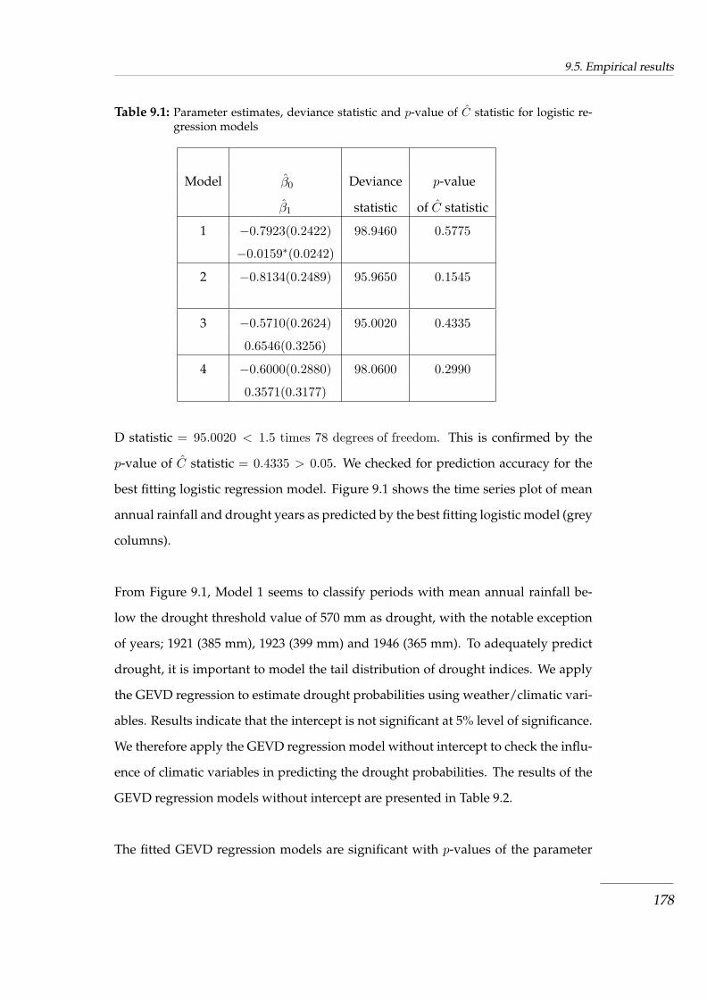
9.5. Empirical results
Table 9.1: Parameter estimates, deviance statistic and p-value of C statistic for logistic re-gression models
Model β0 Deviance p-value
β1 statistic of C statistic
1 −0.7923(0.2422) 98.9460 0.5775
−0.0159∗(0.0242)
2 −0.8134(0.2489) 95.9650 0.1545
3 −0.5710(0.2624) 95.0020 0.4335
0.6546(0.3256)
4 −0.6000(0.2880) 98.0600 0.2990
0.3571(0.3177)
D statistic = 95.0020 < 1.5 times 78 degrees of freedom. This is confirmed by the
p-value of C statistic = 0.4335 > 0.05. We checked for prediction accuracy for the
best fitting logistic regression model. Figure 9.1 shows the time series plot of mean
annual rainfall and drought years as predicted by the best fitting logistic model (grey
columns).
From Figure 9.1, Model 1 seems to classify periods with mean annual rainfall be-
low the drought threshold value of 570 mm as drought, with the notable exception
of years; 1921 (385 mm), 1923 (399 mm) and 1946 (365 mm). To adequately predict
drought, it is important to model the tail distribution of drought indices. We apply
the GEVD regression to estimate drought probabilities using weather/climatic vari-
ables. Results indicate that the intercept is not significant at 5% level of significance.
We therefore apply the GEVD regression model without intercept to check the influ-
ence of climatic variables in predicting the drought probabilities. The results of the
GEVD regression models without intercept are presented in Table 9.2.
The fitted GEVD regression models are significant with p-values of the parameter
178

9.5. Empirical results
Figure 9.1: Plot of mean annual rainfall and predicted drought years from selected logisticregression model (in-sample data).
estimates < 0.05 except Model 1. The best performing model is Model 3 which has
the lowest D statistic. Model 3, i.e. g(π) = 0.3455SDSLPAPRIL with the link func-
tion g(π) = [−lnπ(xi)]ξ−1
ξ , seems to fit the data well since D statistic = 95.5419 <
1.5 times 79 degrees of freedom. This is confirmed by the p-value of C statistic =
0.3941 > 0.05. The residuals from Model 3 are uncorrelated and do not show signif-
icant heteroscedasticity (see ACF and PACF correlogram of residuals and squared
residuals in Section 9.7). In order to access the predictive accuracy of the best GEVD
regression model, we plot the time series of mean annual rainfall and check if the
model would pick mean annual rainfall below the drought threshold value of 570
mm. Figure 9.2 shows the time series plot of mean annual rainfall and drought years
as predicted by the best fitting GEVD regression model (grey columns).
The selected GEVD regression model seems to classify drought years better than
the best fitting logistic model. From Figure 9.2 the selected GEVD regression model
seems able to classify drought periods as drought except for years 1923 (399 mm)
and 1946 (365 mm). This shows an improvement from the predictive accuracy of the
selected logistic model. Thus, we formally compare the predictive accuracy of the
179

9.5. Empirical results
Table 9.2: Parameter estimates, deviance statistic and p-value of C statistic for GEVD re-gression models
Model β1 Deviance p-valuestatistics of C statistic
1 −0.0121 99.9430 0.5295
2 −0.0296 96.7919 0.2274
3 0.3455 95.5419 0.3941
4 0.2088 98.2806 0.2870
Figure 9.2: Plot of mean annual rainfall and predicted drought years from the selectedGEVD regression model (in-sample data).
best performing GEVD regression here proposed with the best fitting logistic regres-
sion model. We assess the predictive accuracy of the two best fitting models using
performance measures namely; the Mean Square Error (MSE) and Mean Absolute
Error (MAE). The MSE and MAE are defined as
MSE =1n
n∑t=1
(yt − yt)2 MAE =1n
n∑t=1
| yt − yt | (9.16)
where yt and yt are the actual and the predicted drought indices respectively. The
180

9.5. Empirical results
model with a lower MSE and MAE better forecast the dependent variable.
The classification of a rainfall season as a drought (mean annual rainfall below the
drought threshold) before the onset of the rainfall season is important because it is
very costly to classify a rainfall season as a good rainfall season when it turns out
to be a drought. Inaccurate classification of the rainfall season will lead farmers to
choose the wrong type of crop for the season. For example, if the rainfall season is
classified as no drought, farmers will choose crop varieties which are not drought
resistant. This will lead to food shortages and non-performance of agriculture de-
pendent industries. For this reason, we focus our attention on the tail of the response
curve for values of the dependent variable equal to one that represent drought. We
compare the two models by computing MSE and MAE only for drought years i.e.we
consider only the positive errors yi− yt > 0 and n = 13 is the number of years classi-
fied as drought. In order to avoid the problem of over-fitting the data, we calculate
MSE and MAE using the out-of-sample data set (1981-2015). The in-sample and out-
of-sample sizes are reported in Table 9.3.
Table 9.3: The in-sample and out-of-sample sizes
Classification In-sample Out-of-sample
Drought 25 13
No drought 55 22
Table 9.4 reports the MSE and MAE for the selected logistic and GEVD regression
models.
From the results reported in Table 9.4, the proposed GEVD regression model per-
forms better than the logistic regression model having the least MSE and MAE val-
ues. Therefore, the proposed model for predicting drought probabilities for Zim-
babwe is yi = 0.3455SDSLPAPRIL, where yi = [−lnπ(x)]−ξ−1
ξ. Since variations of π(x)
do not depend on variations of ξ, if we use the value of ξ = −0.4398 for the best fit-
181

9.6. Concluding remarks
Table 9.4: The in-sample and out-of-sample sizes
Goodness-of-fit testModels
Logistic regression GEVD regression
MSE 0.3751 0.3608
MAE 0.5898 0.5839
ting minima annual rainfall for Zimbabwe (see Chapter 7), then any SDSLPAPRIL ≥
0.9797 will indicate the possibility of drought in the coming raining season.
9.6 Concluding remarks
In this study, we extended the work of Shoko and Shoko (2014) and Manatsa et al.
(2008) by proposing a GLM regression model with the quantile of GEVD distribu-
tion as the link function for predicting drought probabilities for Zimbabwe. Manatsa
et. al. (2008) found the MAMJ Darwin anomalies (average of March to June Darwin
sea level pressure anomalies) as an earlier and more skilful predictor of Zimbab-
wean droughts. The main findings of this study is that the SDSLP anomaly for April
alone is a skillful predictor of droughts in Zimbabwe. We have also proposed that
any SDSLP anomaly greater than or equal to 0.9797 is an indicator of meteorological
drought in Zimbabwe. This is a distinct departure from earlier related research cited
in literature. The proposed model can be used as an early drought warning tool that
reduces the risk of drought by farmers, government agencies, non-governmental or-
ganizations and citizens.
182

9.7. Appendix
9.7 Appendix
Diagnostic plots for Model 3
Figure 9.3: ACF and PACF correlogram of residuals from the best fitting Model 3183

9.7. Appendix
Figure 9.4: ACF and PACF correlogram of squared residuals from the best fitting Model 3
184

Chapter 10
Conclusion
10.1 Introduction
In this thesis a simple but skillful early warning tool for disaster risk reduction as-
sociated with extreme rainfall was presented. Frequency analysis of mean annual
rainfall data was presented and discussed using various statistical methods. The
main focus of the thesis was on the extensive application of methods based on the
statistics of extremes of mean annual rainfall data series and the identification of an
earlier and more skillful predictor of extreme annual rainfall for Zimbabwe.
Modelling mean annual rainfall for a drought-prone country such as Zimbabwe has
potential use in disaster-risk reduction, meteorology, agriculture and in water har-
vesting planning and management. Zimbabwe’s agro-based economy relies heavily
on rain-fed agriculture, thus timely and reliable prediction of mean annual rainfall
before the onset of the rainfall season can play a pivotal role in enhancing disaster
preparedness and adaptation to the impacts of extreme rainfall. This thesis there-
fore, presented models that can be used to predict extreme mean annual rainfall at
least 5 months before the onset of a rainfall season. The thesis was organised into
various chapters each addressing research objectives stated in Chapter 1. The main
findings of the various chapters of the thesis are presented in this chapter.
185
10.2. Thesis summary
10.2 Thesis summary
Mean annual rainfall data for the period 1901-2015 obtained from the Department
of Meteorological services in Zimbabwe was used as the main data set. The data
set was divided into two; mean annual rainfall for the period 1901-2009 (in-sample
data set for Chapters 4-7) and mean annual rainfall for the period 2010-2015 (out-of-
sample data set used in Chapter 4). In Chapter 9 the data set was divided into two
parts as follows: in-sample data set (1901-1980) and out-of-sample (1981-2015). The
monthly Southern Oscillation Index and standardized Darwin Sea Level Pressure
anomalies data set for the period 1901-2015 was obtained from NOAA. Correlation
analysis was used to find correlations between mean annual rainfall and natural cli-
matic change variables. At a longer period before the onset of the rainfall season
in mid-November, SOI for May and SOI for August were found to be highly corre-
lated with mean annual rainfall. SDSLP anomalies for April and August were also
found to be highly correlated with mean annual rainfall for Zimbabwe. Correlations
of SOI and SDSLP anomalies with mean annual rainfall at a lead time of more than
one year were found to be statistically insignificant. This finding is not in agreement
with the findings of Shoko and Shoko (2014), who found that SOI values for April
and May of the previous year were correlated with the amount of rainfall. Therefore,
SOI for May, SOI for August, SDSLP for April and SDSLP for August were selected
as predictors of mean annual rainfall for Zimbabwe.
In order to use the selected rainfall predictors in a linear regression model, corre-
lation analysis between the predictors was performed. SOI values for August was
found to be highly correlated to the SDSLP annomalies for August. Principal com-
ponent analysis was applied to extract a component of SDSLP anomaly for Au-
gust which is orthogonal to the SOI value for August. Goodness-of-fit tests namely
MAPE and RMSE were used to select the best regression model for predicting mean
annual rainfall. Weighted regression model using the the SOI value for August and
a component of SDSLP anomaly for August which is not explained by SOI as pre-
186
10.2. Thesis summary
dictors was found to be the best fitting model. The proposed model has three main
drawbacks. Firstly, predictions of mean annual rainfall can only be done at least two
months before the onset of the rainfall season. This provides a short space of time for
farmers to select the type of crop for the next rainfall season and other stakeholders
in government and non-governmental organisations involved in disaster risk reduc-
tion. Secondly, the proposed model seems to slightly over-forecast the mean annual
rainfall, therefore it was concluded that the predictive model still need to be im-
proved. Finally, the linear regression model assumes that the dependent variable in
this case mean annual rainfall is normal but in the literature rainfall amounts have
been shown to be non linear. Therefore, in order to fully understand the mean an-
nual rainfall patterns, the distribution analysis of mean annual rainfall was explored.
In the literature, the two-parameter gamma, two-parameter lognormal and the two-
parameter log-logistics distributions are some of the distributions which usually fit
to rainfall amounts well. The performance of the three candidature distributions in
fitting to mean annual rainfall for Zimbabwe was assessed using RRMSE, RMAE
and PPCC goodness-of-fit tests. The two-parameter gamma distribution was es-
tablished at the best fitting parent distribution. This finding is consistent with the
findings of Cho et al. (2004), Husak et al. (2007) and Stagge et al. (2015). This the-
sis noted that the tail of the parent distributions sometimes diverges in the extreme
region, thus, the performance of extreme value distributions in fitting to the mean
annual rainfall data were explored.
The characteristics of extreme mean annual rainfall for Zimbabwe was explored in
three parts. Firstly, extreme maxima annual rainfall analysis was explored using the
block maxima approach. A yearly block was used to fit the stationary GEVD model
to maxima annual rainfall data using both the maximum likelihood method and
Bayesian MCMC approach. In the absence of expert knowledge, non-informative
prior was used. Using the Anderson-Darling test, the thesis established that the
187

10.2. Thesis summary
stationary GEVD model adequately fitted the maxima mean annual rainfall for Zim-
babwe. The maximum likelihood parameter estimates were found to be close to their
Bayesian counter parts, but the latter produced parameter estimates with smaller
standard deviations. Thus, the inclusion of the prior distribution improves the preci-
sion of tail quantile estimates. Furthermore, it was established that the return levels
based on the Bayesian approach are substantially higher than their corresponding
maximum likelihood based return levels. The possibility of statistics of extremes in
changing climate was explored using the maximum likelihood estimation method.
The GEVD model which allows the location parameter to vary with time and se-
lected climate change drivers was fitted to maxima annual rainfall data. The thesis
revealed that the extreme maxima rainfall for Zimbabwe does not vary with time.
The GEVD model which incorporate SDSLP anomalies for April as a covariate of
the location parameter was established to perform better than the stationary GEVD
model for maxima annual rainfall for Zimbabwe. This improvement in fit estab-
lishes the indicator of meteorological volatility known as SDSLP anomalies for April
as a single predictor of extreme maxima annual rainfall for Zimbabwe. This finding
is very important for planning and policy-making by the government and the peo-
ple of Zimbabwe.
Secondly, statistics of extreme minima annual rainfall was explored using the block
maxima method. The duality of maxima and minima distributions was explored to
fit GEVD to minima annual rainfall. The maximum likelihood estimation method
and the Bayesian MCMC approach were used to estimate parameters of stationary
the GEVD model. As noted earlier, the inclusion of the prior distribution although it
was non-informative improved the estimation of return level estimates. The return
level estimates, based on the Bayesian approach are significantly smaller than their
corresponding return level estimates based on the maximum likelihood estimation
method. Using lower expected return levels in drought risk reduction is more im-
portant, than preparing for a higher return level. Then the actual rainfall amount
188

10.2. Thesis summary
received is less than expected. The possibility of statistics of extremes in changing
climate was also explored using the maximum likelihood estimation method. The
GEVD model which allows the location parameter to vary with time and meteoro-
logical indicators was fitted to minima annual rainfall data. The thesis revealed that
extreme minima rainfall for Zimbabwe does not vary with time. The GEVD model
which incorporate SDSLP anomalies for April as a covariate of the location param-
eter was established to perform better than the stationary GEVD model for minima
annual rainfall for Zimbabwe. This improvement in fit establishes the indicator of
meteorological volatility known as SDSLP anomalies for April as a single predictor
of extreme minima annual rainfall for Zimbabwe. This is consistent with the find-
ings of Manatsa et al. (2008) that the Darwin sea level pressure anomalies are a more
superior predictor of Zimbabwean droughts than SOI values. Findings in this study
improves on the work of Manatsa et al. (2008) and is very important for planning
and policy-making by the government and the people of Zimbabwe.
Thirdly, extreme maxima annual rainfall was modelled using the POT approach of
EVT. The thesis established that the time-homogenous GPD model fitted the data
well. This thesis revealed that return levels, estimated using parameters of the time-
homogenous GPD model were significantly higher than their corresponding esti-
mates generated using the stationary GEVD model. The reasons for this significant
difference is unknown.
Finally, this research attempted to propose an early warning drought monitoring
tool for rare events. Mean annual rainfall data were categorised into drought, in-
dexed 1 and no drought, indexed 0, thus, a binary dependent variable was gener-
ated. In order to propose a good and reliable drought monitoring tool for the coun-
try, the predictive accuracy of a logistic regression model and a GLM model, using
the quantile function of GEVD as the link function were compared. The signifi-
cant meteorological indicators were used as explanatory variables. This thesis estab-
189
10.3. Summary of the key findings
lished that the GEVD regression model performed better than the logistic regression
model in predicting drought probabilities. Furthermore, this thesis revealed that
SDSLP anomalies for April is associated with drought probabilities. This is not sur-
prising since this research had established SDSLP anomalies for April as a skillful
predictor of mean annual rainfall for Zimbabwe. It is hoped that these findings will
contribute towards decision making in Zimbabwe and help reduce the impacts of
drought on people and wildlife.
10.3 Summary of the key findings
We provide a summary of key findings of this thesis, which are as follows:
1. The meteorological indicator known as the Standardized Darwin Sea Level
Pressure anomalies for April is an earlier (6 months before the onset of rainfall
season) and more skillful predictor of mean annual rainfall for Zimbabwe and
any SDSLP anomaly of April greater than 0.9797 is an indicator of drought in
the forthcoming rainfall season.
2. The gamma distribution is the most suitable parent distribution to model mean
annual rainfall for Zimbabwe, however, it fails to describe the tail distribution
of mean annual rainfall.
3. The non-stationary GEVD model with SDSLP anomalies of April as a covariate
is the most suitable model for both maxima and minima annual rainfall for
Zimbabwe.
4. Extreme annual rainfall for Zimbabwe does not change with time.
5. For suitably declustered exceedances, time-homogenous GPD models provide
appropriate models for mean annual rainfall for Zimbabwe.
6. The GEVD regression model for binary rare events performs better than the
logistic regression model in modelling drought probabilities for Zimbabwe.
190

10.4. Limitations of the thesis
The key objective of this thesis was to provide an early warning system for floods
and droughts in Zimbabwe using extensive statistical methods. Overall, our find-
ings appear adequate to answer the key objective. Our findings are important and
contribute to decision making, enhancing knowledge about extreme annual rainfall
and in developing strategies to reduce the impacts of disasters associated with ex-
treme annual rainfall.
10.4 Limitations of the thesis
This thesis adds value to the growing body of theoretical and empirical research
mainly on application of EVT methodology in meteorology. We have given a brief
yet arduous treatment of EVT, providing the academic and researcher with a quick
and handy overview of the main theories and models. One theoretical limitation of
this thesis is some topics and details which others may have found important have
been left out. However, we have striven to include the results that we consider the
most important to the application of EVT in meteorology.
On the empirical front, one of the limitations of this thesis is that we only used
aggregated national annual rainfall data to develop models that can be used for
drought/flash floods early warning systems in Zimbabwe. It would have been inter-
esting to develop models for drought/flash floods early warning systems for each
agro-ecological region in Zimbabwe. Another limitation is that we only used SOI
and SDSLP values as weather/climate predictors. Other weather/climate predictors
such as wind speed, temperature etc would have been used to improve the models.
10.5 Ideas for further research
This thesis focussed on developing tools that can be used as an early warning system
for drought/flash floods in Zimbabwe. However, there is still potential and need for
further development and refinement, both theoretically and empirically. We there-
191

10.5. Ideas for further research
fore, propose possible ideas for further research.
• In this thesis aggregated national annual rainfall data is used. Further research
should look at modelling mean annual rainfall for each of the natural regions
in Zimbabwe. Zimbabwe is divided into 5 agro-ecological regions, known as
natural regions, on the basis of the rainfall regime, soil quality and vegetation.
Therefore, developing early warning systems for each natural region will as-
sist in predicting the occurrence of drought/flash floods for a specific natural
region. It will also assist in developing drought/flash floods coping mecha-
nism for a specific region.
• One area which needs further research is investigating the applicability of
spatial-zero-inflated models in modelling the daily summer rainfall count data
with extra zeros in Zimbabwe.
• Modelling daily summer rainfall with weather/climate-change predictors us-
ing a Poisson-EVT generalised linear modelling approach.
192

References
ADIKU, S.G.K., DAYANANDA, P.W.A., ROSE, C.W. and DOWUONA, G.N.N., (1997).
An analysis of the within-season rainfall characteristics and simulation of the daily
rainfall in two savanna zones in Ghana. Agricultural and Forest Meteorology, 86(1-2),
pp.51-62.
AHMAD, M.I., SINCLAIR, C.D. and WERRITTY, A., (1988). Log-logistic flood fre-
quency analysis. Journal of Hydrology, 98(3-4), pp.205-224.
AKSOY, H., (2000). Use of gamma distribution in hydrological analysis. Turkish Jour-
nal of Engineering and Environmental Sciences, 24(6), pp.419-428.
ARSHAD, M., RASOOL, M.T. and AHMAD, M.I., (2003). Anderson Darling and
modified Anderson Darling tests for generalised Pareto distribution. Pakistan Jour-
nal of Applied Sciences, 3(2), pp.85-88.
BALI, T.G., (2003). The generalised extreme value distribution. Economic Letters,79:423-
427.
BALI, T.G., (2007). A generalised extreme value approach to financial risk measure-
ment. Journal of Money, Credit and Banking, 39(7), pp.1613-1649.
BARTELS, R. (1982). The rank version of von Neumann’s ratio test for randomness,
193

References
Journal of the American Statistical Association, 77(377), pp. 40-46.
BEIRLANT, J., TEUGELS, J.L. and VYNCKIER, P., (1996). Practical analysis of extreme
values. Leuven University Press.
BEIRLANT, J., GOEGEBEUR, Y., SEGERS, J., de WALL, D. and FERRO, C. (2004).
Statistics of extremes: theory and applications. John Wiley & Sons Ltd, West Sussex.
BEIRLANT, J., GOEGEBEUR, Y., SEGERS, J. and TEUGELS, J., (2006). Statistics of
extremes: theory and applications. John Wiley & Sons Ltd, West Sussex.
BERGER, A., MELICE, J.L. and DEMUTH, C.L., (1982). Statistical distributions of
daily and high atmospheric SO2-concentrations. Atmospheric Environment (1967),
16(12), pp.2863-2877.
BERNARDARA, P., MAZAS, F., KERGADALLAN, X. and HAMM, L., (2014). A
two-step framework for over-threshold modelling of environmental extremes. Nat-
ural Hazards and Earth System Sciences, 14(3), p.635.
BERNING, T.L., (2010). Improved estimation procedures for a positive extreme value index
(Doctoral dissertation, Stellenbosch: University of Stellenbosch).
BESAG, J.,(2001). Markov chain Monte Carlo for statistical inference. Center for
Statistics and the Social Sciences, 9, pp.24-25.
BHUNYA, P.K., JAIN, S.K., OJHA, C.S. and AGARWAL, A., (2007). Simple parame-
ter estimation technique for three-parameter generalised extreme value distribution.
Journal of Hydrologic Engineering, 12(6), pp.682-689.
194
References
BORDI, I., FRAEDRICH, K., PETITTA, M. and SUTERA, A., (2007). Extreme value
analysis of wet and dry periods in Sicily. Theoretical and Applied Climatology, 87(1),
pp.61-71.
BOX, G.E.P. and PIERCE, D.A., (1970). Distribution of the autocorrelations in auto-
regressive moving average time series models. Journal of American Statistical Associa-
tion, 65, pp. 1509-1526.
BUCKLE, C., (1996). Weather and climate in Africa. Longman.
BULU, A. and AKSOY, H., (1998), June. Low flow and drought studies in Turkey. In
Low Flows Expert Meeting pp. 133-141.
BURNSIDE, C. and DOLLAR, D. (2004). Aid, Policies and Growth, World Bank Re-
search, Working Papers on International Economics, Trade and Capital Flows, No.
1777.
BRAKENRIDGE, G.R., SYVITSKI, J.P., NIEBUHR, E., OVEREEM, I., HIGGINS, S.A.,
KETTNER, A. and PRADES, L., (2016). Design with nature: Causation and avoidance of
catastrophic flooding, Myanmar. Earth-Science Reviews.
BROOCK, W.A., SCHEINKMAN, J.A., DECHERT, W.D. and LEBARON, B., (1996).
A test for independence based on the correlation dimension. Econometric reviews,
15(3), pp.197-235.
CALABRESE, R. and OSMETTI, S.A., (2011). Generalised extreme value regression
for binary rare events data: an application to credit defaults. Bulletin of the Inter-
national Statistical Institute LXII, 58th Session of the International Statistical Institute,
pp.5631-5634.
195
References
CARROLL, R. J., and RUPPERT, D. (1988). Transformation and Weighting in Regres-
sion, New York: Chapman and Hall.
CHENG, L., AGHAKOUCHAK, A., GILLELAND, E. and KATZ, R.W., (2014). Non-
stationary extreme value analysis in a changing climate. Climatic Change, 127(2),
pp.353-369.
CHIKOBVU, D. and CHIFURIRA, R., (2015). Modelling of extreme minimum rain-
fall using generalised extreme value distribution for Zimbabwe. South African Jour-
nal of Science, 111(9-10), pp.01-08.
CHIKOBVU, D. and SIGAUKE, C., 2013. Modelling influence of temperature on
daily peak electricity demand in South Africa. Journal of Energy in Southern Africa,
24(4), pp.63-70.
CHIKODZI, D., ZINHIVA, H., SIMBA, F.M. and MURWENDO, T., (2013). Reclassi-
fication of agroecological zones in Zimbabwe-the rationale, methods and expected
benefits: the case of Masvingo Province. Journal of Sustainable Development in Africa,
15(1), pp.104-116.
CHINGOMBE, W., PEDZISAI, E., MANATSA, D., MUKWADA, G. and TARU, P.,
(2015). A participatory approach in GIS data collection for flood risk management,
Muzarabani district, Zimbabwe. Arabian Journal of Geosciences, 8(2), pp.1029-1040.
CHINHAMU, K. HUANG, C.K., HUANG, C.S. and HAMMUJUDDY, J., (2015). Em-
pirical analyses of extreme value models for the South African Mining Index. South
African Journal of Economics, 83(1), pp.41-55.
196

References
CHO, H.K., BOWMAN, K.P. and NORTH, G.R., (2004). A comparison of gamma
and lognormal distributions for characterizing satellite rain rates from the tropical
rainfall measuring mission. Journal of Applied Meteorology, 43(11), pp.1586-1597.
COLES, S., BAWA, J., TRENNER, L. and DORAZIO, P., (2001). An introduction to
statistical modeling of extreme values (Vol. 208). London: Springer.
COLES, S. and POWELL, E.A., (1996). Bayesian methods in extreme value mod-
elling: a review and new developments. International Statistics Review/Revue Inter-
natinale de Statistique, pp. 119-136.
COLES, S. and TAWN, J., (2005). Bayesian modelling of extreme surges on the UK
east coast. Philosophical Transactions of the Royal Society of London A: Mathematical,
Physical and Engineering Sciences, 363(1831), pp.1387-1406.
COLLIER, P. and GUNNING, J.W., (1999). Why has Africa grown slowly? The Jour-
nal of Economic Perspectives, 13(3), pp.3-22.
CONOVER, W.J., (1999). Practical Nonparametric Statistics. Third Edition, New York:
John Wiley & Sons, Inc.
CRISCI, A., GOZZINI, B., MENEGUZZO, F., PAGLIARA, S. and MARACCHI, G.,
(2002). Extreme rainfall in a changing climate: regional analysis and hydrological
implications in Tuscany. Hydrological Processes, 16(6), pp.1261-1274.
DALRYMPLE, T., (1960). Flood frequency analyses. Water Supply: Geological Survey,
Reston, Virginia, USA , 1543-A.
DAN’AZUMI, S., SHAMSUDIN, S. and ARIS, A., (2010). Modelling the distribution
197

References
of rainfall intensity using hourly data. Stochastic Environmental Research and Risk As-
sessment, pp. 1-15.
DAVISON, A.C. and SMITH, R.L., (1990). Models for exceedances over high thresh-
olds. Journal of the Royal Statistical Society. Series B (Methodological), pp.393-442.
de HAAN, L. and LIN, T., (2001). On convergence toward an extreme value distri-
bution in C [0, 1]. Annals of probability, pp.467-483.
DEKA, S., BORAH, M. and KAKATY, S.C., (2009). Distributions of annual maximum
rainfall series of north-east India. European Water, 27(28), pp.3-14.
DEMARIA, E.M., GOODRICH, D. and KEEFER, T., (2017). Frequency Analysis of
Extreme Sub-Daily Precipitation under Stationary and Non-Stationary Conditions
across Two Contrasting Hydroclimatic Environments. Hydrology and Earth System
Sciences, pp. 1-28.
de ZEA BERMUDEZ, P. and TURKMAN, M.A.A., (2003). Bayesian approach to pa-
rameter estimation of the generalised Pareto distribution. Test, 12(1), pp.259-277.
DIEBOLT, J., GUILLOU, A. and RACHED, I., (2007). Approximation of the distri-
bution of excesses through a generalised probability-weighted moments method.
Journal of Statistical Planning and Inference, 137(3), pp.841-857.
DODMAN, D. and MITLIN, D., (2015). The national and local politics of climate
change adaptation in Zimbabwe. Climate and Development, 7(3), pp.223-234.
DUTTA, S., ESSADDAM, N., KUMAR, V. and SAADI, S., (2015). How does elec-
tronic trading affect efficiency of stock market and conditional volatility? Evidence
198

References
from Toronto Stock Exchange. Research in International Business and Finance, 39(B),
pp. 867-877.
EMBRECHTS, P., RESNICK, S.I. and SAMORODNITSKY, G., (1999). Extreme value
theory as a risk management tool. North American Actuarial Journal, 3(2), pp.30-41.
ENDER, M. and MA, T., (2014). Extreme value modeling of precipitation in case
studies for China. International Journal of Scientific and Innovative Mathematical Re-
search (IJSIMR), 2(1), pp.23-36.
ENGLE, R.F., (1982). Autoregressive conditional heteroscedasticity with estimates
of the variance of United Kingdom inflation. Econometrica: Journal of the Econometric
Society, pp.987-1007.
FAO. (2001). Global Watch Report. United Nations, Rome.
FARRELL, P.J. and ROGERS-STEWART, K., (2006). Comprehensive study of tests
for normality and symmetry: extending the Spiegelhalter test. Journal of Statistical
Computation and Simulation, 76(9), pp.803-816.
FELICI, M., LUCARINI, V., SPERANZA, A. and VITOLO, R., (2007). Extreme value
statistics of the total energy in an intermediate-complexity model of the midlatitude
atmospheric jet. Part II: trend detection and assessment. Journal of the atmospheric
sciences, 64(7), pp.2159-2175.
FENG, S., NADARAJAH, S. and HU, Q.,(2007). Modeling annual extreme precipita-
tion in China using the generalised extreme value distribution. Journal of the Meteo-
rological Society of Japan. Series. II, 85(5), pp.599-613.
199

References
FERREIRA, A. and de HAAN, L., (2015). On the block maxima method in extreme
value theory: PWM estimators. The Annals of statistics, 43(1), pp.276-298.
FERRO, C.A. and SEGERS, J., (2003). Inference for clusters of extreme values. Journal
of the Royal Statistical Society: Series B (Statistical Methodology), 65(2), pp.545-556.
FISHER, R.A. and TIPPETT, L.H.C., (1928). Limiting forms of the frequency distribution
of the largest or smallest member of a sample. In Mathematical Proceedings of the Cam-
bridge Philosophical Society,(Vol. 24, No. 2, pp. 180-190). Cambridge University
Press.
FITZGERALD, D.L., (2005). Analysis of extreme rainfall using the log logistic distri-
bution. Stochastic Environmental Research and Risk Assessment, 19(4), pp.249-257.
GAMERMAN, D., (1997). Sampling from the posterior distribution in generalised
linear mixed models. Statistics and Computing, 7(1), pp.57-68.
GAOINI, E., DEY, D. and RUGGERI, F., (2009). Bayesian modeling of flash floods using
generalised extreme value distribution with prior elicitation. University of Connecticut,
Department of Statistics.
GELFAND, A.E. and SMITH, A.F., (1990). Sampling-based approaches to calculating
marginal densities. Journal of the American statistical association, 85(410), pp.398-409.
GEMAN, S. and GEMAN, D., (1984). Stochastic relaxation, Gibbs distributions, and
the Bayesian restoration of images. IEEE Transactions on pattern analysis and machine
intelligence, (6), pp.721-741.
GILES, D.E., FENG, H. and GODWIN, R.T., (2016). Bias-corrected maximum likeli-
200

References
hood estimation of the parameters of the generalised Pareto distribution. Communi-
cations in Statistics-Theory and Methods, 45(8), pp.2465-2483.
GILKS, W.R., RICHARDSON, S. and SPIEGELHALTER, D.J., (1996). Introducing
markov chain monte carlo. Markov chain Monte Carlo in practice, 1, p.19.
GILLI, M. and KLLEZI, E., (2006). An application of extreme value theory for mea-
suring financial risk. Computational Economics, 27(2), pp.207-228.
GNEDENKO, B., (1943). Sur la distribution limite du terme maximum d’une serie
aleatoire. Annals of mathematics, pp.423-453.
GOMES, M.I. and GUILLOU, A., (2015). Extreme value theory and statistics of uni-
variate extremes: a review. International Statistical Review, 83(2), pp.263-292.
GOVERNMENT OF ZIMBABWE. (2001). The agricultural sector of Zimbabwe. Statis-
tical Bulletin, Harare.
GRASSBERGER, P. and PROCACCIA, I., (1983). Measuring the strangeness of strange
attractors. Physical Review ,9D, pp. 189-208.
GWIMBI, P., (2009). Linking rural community livelihoods to resilience building in
flood risk reduction in Zimbabwe. Jamba: Journal of Disaster Risk Studies, 2(1), pp.71-
79.
HASAN, H., AHMAD RADI, N.F. and KASSIM, S., (2012), Modeling of extreme
temperature using generalised extreme value (GEV) distribution: a case study of
Penang. In World Congress on Engineering, 1(2012), pp. 181-186.
201

References
HARRIS, J.M., (2003). Sustainability and sustainable development. International So-
ciety for Ecological Economics, 1(1), pp.1-12.
HASTINGS, W. K. , (1970). Monte Carlo sampling methods using Markov chains
and their applications. Biometrika, 57(1), 97-109.
HEO, J.H., KHO, Y.W., SHIN, H., KIM, S. and KIM, T., (2008). Regression equations
of probability plot correlation coefficient test statistics from several probability dis-
tributions. Journal of Hydrology, 355(1-4), pp. 1-15.
HILBORN, R. and MANGEL, M., (1997). The ecological detective: confronting models
with data (Vol. 28). Princeton University Press.
HOELL, A., FUNK, C., ZINKE, J., and HARRISON, L., (2017). Modulation of the
Southern Africa precipitation response to the El Nino Southern Oscillation by the
subtropical Indian Ocean Dipole. Climate Dynamics, 48, pp.2529-2540.
HOSKING, J.R., (1984). Testing whether the shape parameter is zero in the gener-
alised extreme-value distribution. Biometrika, 71(2), pp.367-374.
HOSKING, J.R., (1985). Algorithm as 215: Maximum-likelihood estimation of the
parameters of the generalised extreme-value distribution. Journal of the Royal Statis-
tical Society. Series C (Applied Statistics), 34(3), pp.301-310.
HOSKING, J.R. and WALLIS, J.R., (1987). Parameter and quantile estimation for the
generalised Pareto distribution. Technometrics, 29(3), pp.339-349.
HOSMER, D.W. and LEMESHOW, S., (2000). Interpretation of the fitted logistic regres-
sion model. Applied Logistic Regression, 2rd edition, pp.47-90.
202

References
HUSAK, G.J., MICHAELSEN, J. and FUNK, C., (2007). Use of the gamma distri-
bution to represent monthly rainfall in Africa for drought monitoring applications.
International Journal of Climatology, 27(7), pp.935-944.
ISMAIL, S.A., (1987). Long-range seasonal rainfall forecast for Zimbabwe and its re-
lation with El-Nio/Southern Oscillation (ENSO). Theoretical and applied climatology,
38(2), pp.93-102.
JAYNE, T.S., GOVEREH, J., CHILONDA, P., MASON, N., CHAPOTO, A. and HAAN-
TUBA, H., (2007). Trends in agricultural and rural development indicators in Zambia.
Lusaka: Food Security Research Project.
JENKINSON, A. F., (1955). The frequency distribution of the annual maximum (or
minimum) values of meteorological elements. Quarterly Journal of the Royal Meteoro-
logical Society, 81(348), pp. 158-171.
JURY, M.R., (1996). Regional teleconnection patterns associated with summer rain-
fall over South Africa, Namibia and Zimbabwe. International Journal of Climatology,
16(2), pp.135-153.
KATZ, R.W., PARLANGE, M.B. and NAVEAU, P., (2002). Statistics of extremes in
hydrology. Advances in water resources, 25(8), pp.1287-1304.
KAUNDA, C.S., KIMAMBO, C.Z. and NIELSEN, T.K., (2012). Hydropower in the con-
text of sustainable energy supply: a review of technologies and challenges. ISRN Renewable
Energy.
KING, G. and ZENG, L., (2001). Logistic regression in rare events data. Political anal-
203

References
ysis, 9(2), pp.137-163.
KOLMOGOROV, A.N., (1933). Sulla determinazione empirica delle leggi di proba-
bilita. Giorn. Ist. Ital. Attuari, 4, pp.1-11.
KORATTIKARA, A., CHEN, Y. and WELLING, M., (2014). Austerity in MCMC land:
Cutting the Metropolis-Hastings budget. In Proceedings of the 31st International Con-
ference on Machine Learning (ICML-14), pp. 181-189.
KOTZ, S. and NADARAJAH, S., (2000). Extreme value distributions: theory and ap-
plications. World Scientific.
KOUTSOYIANNIS, D., (2004). Statistics of extremes and estimation of extreme rain-
fall: II. Empirical investigation of long rainfall records/Statistiques de valeurs ex-
trmes et estimation de prcipitations extrmes: II. Recherche empirique sur de longues
sries de prcipitations.Hydrological Sciences Journal, 49(4).
KOUTSOYIANNIS, D. AND BALOUTSOS, G., (2000). Analysis of a long record of
annual maximum rainfall in Athens, Greece, and design rainfall inferences. Natural
Hazards, 22(1), pp.29-48.
KUAN, C.M., (2008). Lecture on time series diagnostic tests. Institute of Economics
Academia.
LEADBETTER, M.R., LINDGREN, G. and ROOTZN, H., (2012). Extremes and related
properties of random sequences and processes. Springer Science & Business Media.
LELE, S.M., (1991). Sustainable development: a critical review. World development,
19(6), pp.607-621.
204

References
LI, Z., LI, Z., ZHAO, W. and WANG, Y., (2015). Probability modeling of precipitation
extremes over two river basins in northwest of China. Advances in Meteorology,
LI, Z., BRISSETTE, F. and CHEN, J., (2013). Finding the most appropriate precip-
itation probability distribution for stochastic weather generation and hydrological
modelling in Nordic watersheds. Hydrological Processes, 27(25), pp.3718-3729.
LI, Y., CAI, W. and CAMPBELL, E.P., (2005). Statistical modeling of extreme rainfall
in southwest Western Australia. Journal of climate, 18(6), pp.852-863.
LU, H.C., (2004). Estimating the emission source reduction of PM 10 in central Tai-
wan. Chemosphere, 54(7), pp.805-814.
LUDWIG, D., (1996). Uncertainty and the assessment of extinction probabilities.
Ecological Applications, 6(4), pp.1067-1076.
LJUNG, G.M. and BOX, G.E.P., (1978). On measure of lack of fit in time series model.
Biometrika, 65, pp. 297-303.
MACLEOD, A.J., (1989). A remark on algorithm AS 215: Maximum-likelihood es-
timation of the parameters of the generalised extreme-value distribution. Applied
Statistics, 38(1), pp.198-199.
MADAMOMBE, E.K., (2004). Zimbabwe: Flood management practices-Selected flood
prone areas Zambezi Basin. Unpublished Paper, Wmo/Gwp Associated Programme
on Flood Management.
MADDALA, G.S. and KIM, I.M., (1998). Unit roots, cointegration, and structural change
205
References
(No. 4). Cambridge University Press.
MADSEN, H., RASMUSSEN, P.F. and ROSBJERG, D., (1997). Comparison of annual
maximum series and partial duration series methods for modeling extreme hydro-
logic events: 1. At-site modeling. Water Resources Research, 33(4), pp.747-757.
MAGADIA, J., (2010). Value-at-risk modeling via the peaks-over-threshold approach.
Annual Bangko Sentral ng Pilipinas-University of the Philippines Professional Chair Lec-
tures.
MAKARAU, A. (1995). Intra-seasonal oscillatory models of the Southern Africa
summer circulation, Unpublished PhD Thesis, University of Cape Town.
MAMOMBE, V., KIM, W. and CHOI, Y.S., (2017). Rainfall variability over Zimbabwe
and its relation to large-scale atmosphere-ocean process. International Journal of Cli-
matology, 37, pp. 963-971.
MANATSA, D., CHINGOMBE, W., MATSIKWA, H. and MATARIRA, C.H., (2008).
The superior influence of Darwin Sea level pressure anomalies over ENSO as a sim-
ple drought predictor for Southern Africa. Theoretical and Applied Climatology, 92(1),
pp.1-14.
MANATSA, D., MUSHORE, T. and LENOUO, A. , (2017). Improved predictability
of drought over southern Africa using the standardized precipitation evapotranspi-
ration index and ENSO. Theoretical and Applied Climatology, 127, pp.259-274.
MANGOYANA, S. and MEDA, T., (2001). Food Security and Sustainability in Zim-
babwe. University of Zimbabwe Publications, Harare.
206

References
MANNING, W.G. and MULLAHY, J., (2001). Estimating log models: to transform
or not to transform?. Journal of health economics, 20(4), pp.461-494.
MARTINS, E.S. and STEDINGER, J.R., (2000). Generalised maximum likelihood
generalised extreme value quantile estimators for hydrologic data. Water Resources
Research, 36(3), pp.737-744.
MASON, S.J., and JURY, M.R., (1997). Climatic variability and change over Southern
Africa: A reflection on underlying process. Progress in Physical Geography, 21(1), pp.
23-50.
MATARIRA, C.H., (1990). Drought over Zimbabwe in a regional and global context.
International Journal of Climatology, 10(6), pp.609-625.
MATARIRA, C.H. and UNGANAI, L.S., (1994).A rainfall prediction scheme for southern
Africa based on the southern oscillation. Technical report, SADC-REWU, Harare.
MAYOORAN, T. and LAHEETHARAN, A., (2014). The Statistical Distribution of
Annual Maximum Rainfall in Colombo District. Sri Lankan Journal of Applied Statis-
tics, 15(2).
MAZVIMAVI, D., (2008). Investigating possible changes of extreme annual rainfall
in Zimbabwe. em Hydrology & Earth System Sciences Discussions, 5(4), pp.1765-
1784.
MAZVIMAVI, D., (2010). Investigating changes over time of annual rainfall in Zim-
babwe. Hydrology and Earth System Sciences, 14(12), pp.2671-2679.
McALEER, M., JIMENEZ-MARTIN, J.A. and PEREZ-AMARAL, T., (2013). Has the
Basel Accord improved risk management during the global financial crisis? The
207
References
North American Journal of Economics and Finance, 26, pp.250-265.
McKEE, T.B., DOESKEN, N.J., and KLEIST, J., (1993). The relationship of drought
frequency and duration to time scales. In Proceedings of the 8th Conference on Applied
Climatology, 17(22), 179-183.
McNEIL, A.J. and FREY, R., (2000). Estimation of tail-related risk measures for het-
eroscedastic financial time series: an extreme value approach. Journal of empirical
finance, 7(3), pp.271-300.
METROPOLIS, N., ROSENBLUTH, A.W., ROSENBLUTH, M.N., TELLER, A.H., and
TELLER, E., (1953). Equation of state calculations by fast computing machine. Jour-
nal of Chemical Physics, 21, 1087-1091.
MINKA, T.P., (2002). Estimating a Gamma distribution. Microsoft Research, Cam-
bridge, UK, Technical. Report.
MUCHURU, S., LANDMAN, W,A., De WITT, D. and LOTTER, D., (2014). Seasonal
rainfall predicability over the Lake Kariba catchment area. Water SA, 40, pp. 461-470.
MUSHORE, T.D., (2013). Climatic changes, erratic rains and the necessity of con-
structing water infrastructure: Post 2000 land reform in Zimbabwe. International
Journal of Scientific & Technology Research, 2(8), pp. 304-310.
NADARAJAH, S. and CHOI, D., (2007). Maximum daily rainfall in South Korea.
Journal of Earth System Science, 116(4), pp.311-320.
NATIONAL ENVIRONMENTAL RESEARCH COUNCIL (NERC). (1975). Flood stud-
ies report. Wallingford: Institute of Hydrology.
208

References
NGUYEN, C.C., GAUME, E. and PAYRASTRE, O., (2014). Regional flood frequency
analyses involving extraordinary flood events at ungauged sites: further develop-
ments and validations. Journal of Hydrology, 508, pp.385-396.
NIYIMBANIRA, F., (2013). An Econometric Evidence of the Interactions between
Inflation and Economic Growth in South Africa. Mediterranean Journal of Social Sci-
ences, 4(13), p.219.
OBASI, G.O.P., (1994). WMO’s role in the international decade for natural disaster
reduction. Bulletin of the American Meteorological Society, 75(9), pp.1655-1661.
PANU, U.S. and SHARMA, T.C., (2002). Challenges in drought research: some per-
spectives and future directions. Hydrological Sciences Journal, 47(S1), pp.S19-S30.
PAREY, S., MALEK, F., LAURENT, C. and DACUNHA-CASTELLE, D., (2007). Trends
and climate evolution: Statistical approach for very high temperatures in France. Cli-
matic Change, 81(3), pp.331-352.
PERMAN, R., MA, Y., McGILVRAY, J. and COMMON, M., (2003). Natural Resource
and Environmental Economics 3rd edition, New York: Pearson Addison Wesley.
PICKANDS III, J., (1975). Statistical inference using extreme order statistics. The An-
nals of Statistics, pp.119-131.
POCERNICH, M.J. (2002). Application of Extreme Value Theory and Threshold models to
hydrological event, (Master’s thesis, University of Colorado).
PRESCOTT, P. and WALDEN, A.T., (1983). Maximum likelihood estimation of the
209

References
parameters of the three-parameter generalised extreme-value distribution from cen-
sored samples. Journal of Statistical Computation and Simulation, 16(3-4), pp.241-250.
RAKHECHA, P.R. and SOMAN, M.K., (1994). Trends in the annual extreme rainfall
events of 1 to 3 days duration over India. Theoretical and Applied Climatology, 48(4),
pp.227-237.
RAO, C.R. (1973). Linear Statistical Inference and its Applications, 2rd edition. Wiley,
New York.
RAZALI, N.M. and WAH, Y.B., (2011). Power comparisons of Shapiro-Wilk, Kolmogorov-
Smirnov, Lilliefors and Anderson-Darling tests. Journal of statistical modeling and an-
alytics, 2(1), pp.21-33.
RENARD, B., LANG, M. and BOIS, P., (2006). Statistical analysis of extreme events
in a non-stationary context via a Bayesian framework: case study with peak-over-
threshold data. Stochastic environmental research and risk assessment, 21(2), pp.97-112.
RESNICK, S.I., (2013). Extreme values, regular variation and point processes. Springer.
RICHARD, Y., TRZASKA, S., ROUCOU, P. and ROUAULT, M., (2000). Modification
of the southern African rainfall variability/ENSO relationship since the late 1960s.
Climate Dynamics, 16(12), pp.883-895.
RIBATET, M., (2006). A user’s guide to the POT package (version 1.4). month. ROCHA,
A.M.C., (1992). The influence of global sea surface temperatures on southern African sum-
mer climate (Doctoral dissertation, University of Melbourne).
ROCHA, A.M.C., (1992). The influence of global sea surface temperatures on Southern
210

References
African summer climate, PhD Thesis, University of Melbourne.
ROGHANI, R., SOLTANI, S. and BASHARI, H., (2016). Influence of Southern Os-
cillation on autumn rainfall in Iran (1951-2011). Theoretical and Applied Climatology,
124(2), pp.411-423.
ROPELEWSKI, C.F. and HALPERT, M.S., (1987). Global and regional scale precip-
itation patterns associated with the El Nio/Southern Oscillation. Monthly weather
review, 115(8), pp.1606-1626.
ROTH, M., BUISHAND, T.A., JONGBLOED, G., TANK, A.K. and VAN ZANTEN,
J.H., (2014). Projections of precipitation extremes based on a regional, non-stationary
peaks-over-threshold approach: A case study for the Netherlands and north-western
Germany. Weather and Climate Extremes, 4, pp.1-10.
RURINDA, J., MAPFUMO, P., van WIJK, M.T., MTAMBANENGWE, F., RUFINO,
M.C., CHIKOWO, R. and GILLER, K.E., (2014). Sources of vulnerability to a variable
and changing climate among smallholder households in Zimbabwe: A participatory
analysis. Climate Risk Management, 3, pp. 65-78.
RURINDA, J., MAPFUMO, P., van WIJK, M.T., MTAMBANENGWE, F., RUFINO,
M.C., CHIKOWO, R. and GILLER, K.E., (2013) Managing soil fertility to adapt to
rainfall variability in smallholder cropping systems in Zimbabwe. Field Crops Re-
search, 154, pp. 211-225.
SACHS, J.D. and WARNER, A.M., (1997). Sources of slow growth in African economies.
Journal of African economies, 6(3), pp.335-376.
SAKULSKI, D., JORDAAN, A., TIN, L. and GREYLING, C., (2014). Fitting theoretical
211

References
distributions to Rainy Days for Eastern Cape Drought Risk assessment. In Proceedings of
Daily Meteo. org/2014 Conference (p. 48).
SATISH, P., GIRI, R.K. and SATISH, C., (2014). Environmental hazard-landslides
and avalances (Kasmir region). International Journal of Physics and Mathematical Sci-
ences, 4(3), pp. 87-99.
SCARROTT, C. and MACDONALD, A., (2012). A review of extreme value threshold
estimation and uncertainty quantification. REVSTAT-Statistical Journal, 10(1), pp.33-
60.
SCHMIDLI, J., GOODESS, C.M. FREI, C., HAYLOCK, M.R., HUNDECHA, Y., RIB-
ALAYGUA, J. and SCHMITH, T., (2007). Statistical and dynamic downscaling of
precipitation: An evaluation and comparison of scenarios for the European Alps.
Journal of Geophysical Research Atmospheres, 112(D4).
SHOKO, K. and SHOKO, N., (2014). Drought and El nino phases in Zimbabwe. The
Dyke, 17(8.3), pp. 1-18.
SMITH, S.V., (1985a). Studies of the effects of cold fronts during the rainy season in
Zimbabwe. Weather, 40(7), pp.198-203.
SMITH, E., (2005). Bayesian modelling of extreme rainfall data (Doctoral dissertation,
University of Newcastle upon Tyne).
SMITH, R.L., (1985b). Maximum likelihood estimation in a class of nonregular cases.
Biometrika, 72(1), pp.67-90.
SMITH, R.L., 1986. Extreme value theory based on the r largest annual events. Jour-
212

References
nal of Hydrology, 86(1-2), pp.27-43.
SMITH, R.L. and GOODMAN, D.J., (2000). Bayesian risk analysis. Extremes and In-
tegrated Risk Management, pp.235-251.
SMITH, R.L. and NAYLOR, J.C., (1987). A comparison of maximum likelihood and
Bayesian estimators for the three-parameter Weibull distribution. Applied Statistics,
pp.358-369.
STAGGE, J.H., TALLAKSEN, L.M., GUDMUNDSSON, L., VAN LOON, A.F. and
STAHL, K., (2015). Candidate distributions for climatological drought indices (SPI
and SPEI). International Journal of Climatology, 35(13), pp.4027-4040.
STEPHENS, M.A., (1974). EDF statistics for goodness of fit and some comparisons.
Journal of the American statistical Association, 69(347), pp.730-737.
SUGAHARA, S., DA ROCHA, R.P. and SILVEIRA, R., (2009). Non stationary fre-
quency analysis of extreme daily rainfall in Sao Paulo, Brazil. International Journal
of Climatology, 29(9), pp.1339-1349.
SUHAILA, J., CHING-YEE, K., FADHILAH, Y. and HUI-MEAN, F., (2011). Introduc-
ing the mixed distribution in fitting rainfall data. Open Journal of Modern Hydrology,
1(2), pp. 11.
SUHAILA, J. and JEMAIN, A.A., (2007). Fitting daily rainfall amount in Peninsular
Malaysia using several types of exponential distributions. Journal of applied sciences
research, 3(10), pp.1027-1036.
SURMAN, P.G., BODERO, J. and SIMPSON, R.W., (1987). The prediction of the num-
213

References
bers of violations of standards and the frequency of air pollution episodes using ex-
treme value theory. Atmospheric Environment (1967), 21(8), pp.1843-1848.
TAN, X. and GAN, T.Y., (2017). Non-stationary analysis of the frequency and in-
tensity of heavy precipitation over Canada and their relations to large-scale climate
patterns. Climate Dynamics, 48(9-10), pp.2983-3001.
TRENBERTH, K.E., (1999). Conceptual framework for changes of extremes of the hydro-
logical cycle with climate change. In Weather and Climate Extremes (pp. 327-339).
Springer Netherlands.
TRUCK, S. and LIANG, K., (2012). Modelling and forecasting volatility in the gold
market. International Journal of Banking and Finance, 9(1), pp. 48-80.
TORRANCE, J.D., (1990). The Southern Oscillation and the rainy season in Zim-
babwe. Zimbabwe Science News, 24, pp.4-6.
TOSH, C. and DASGUPTA, S., (2014). Lower bounds for the gibbs sampler over
mixtures of Gaussians. In Proceedings of the 31st International Conference on Machine
Learning (ICML-14), pp. 1467-1475.
TSAY, R.S., (2013). Multivariate Time Series Analysis: with R and financial applications.
John Wiley & Sons.
UNECA. (2000). HIV/AIDS and education in Eastern and Southern Africa: Leadership
challenge and the way forward. Addis Ababa, UNECA.
UNGANAI, L.S., (1996). Historic and future climatic change in Zimbabwe. Climate
research, pp.137-145.
214

References
von MISES, R. (1954). La distribution de la plus grande de n valeurs. American Math-
ematical Society, Providence, RI, Selected Papers, 2, pp. 271-294.
WASHINGTON, R. and PRESTON, A., (2006). Extreme wet years over Southern
Africa: Role of Indian Ocean sea surface temperatures. Journal of Geophysical Re-
search: Atmospheres, 111(D15).
WAYLEN, P.E.T.E.R. and HENWORTH, S., (1996). A note on the timing of precip-
itation variability in Zimbabwe as related to the Southern Oscillation. International
journal of climatology, 16(10), pp.1137-1148.
WEBSTER, P.J., (1981). Mechanisms determining the atmospheric response to sea
surface temperature anomalies. Journal of the Atmospheric Sciences, 38(3), pp.554-571.
WILLMOTT, C.J. and MATSUURA, K.,( 2005). Advantages of the mean absolute
error (MAE) over the root mean square error (RMSE) in assessing average model
performance. Climate research, 30(1), pp.79-82.
YILMAZ, A.G. AND PERERA, B.J.C., (2013). Extreme rainfall non-stationarity in-
vestigation and intensity-frequency-duration relationship. Journal of Hydrologic En-
gineering, 19(6), pp.1160-1172.
ZHANG, T., GEORGIOPOULOS, M. and ANAGNOSTOPOULOS, G.C., (2014). On-
line model racing based on extreme performance. In Proceedings of the 2014 Annual
Conference on Genetic and Evolutionary Computation (pp. 1351-1358). ACM.
ZIMBABWE CENTRAL STATISTICAL OFFICE HANDBOOK (2014). October-Environmental
Statistics Report.
215

References
ZIMBABWE CENTRAL STATISTICAL OFFICE HANDBOOK (2010). October-Environmental
Statistics Report.
ZIMBABWE CENTRAL STATISTICAL OFFICE HANDBOOK (1994). October-Environmental
Statistics Report.
ZIN, W.Z.W., JEMAIN, A.A. and IBRAHIM, K., (2009). The best fitting distribution
of annual maximum rainfall in Peninsular Malaysia based on methods of L-moment
and LQ-moment. Theoretical and applied climatology, 96(3-4), pp.337-344.
216