modelling manufacturing export volumes equations … · eco/wkp(2000)8 2 abstract/rÉsumÉ...

Unclassified ECO/WKP(2000)8

Organisation de Coopération et de Développement Economiques OLIS : 06-Apr-2000Organisation for Economic Co-operation and Development Dist. : 14-Apr-2000__________________________________________________________________________________________

English text onlyECONOMICS DEPARTMENT

MODELLING MANUFACTURING EXPORT VOLUMES EQUATIONSA SYSTEM ESTIMATION APPROACH

ECONOMICS DEPARTMENT WORKING PAPERS N0. 235

byKeiko Murata, Dave Turner, Dave Rae and Laurence Le Fouler

Unclassified

EC

O/W

KP

(2000)8E

nglish text only

Most Economics Department Working Papers beginning with No. 144 are now available throughOECD’s Internet Web site at http://www.oecd.org/eco/eco.

89705

Document complet disponible sur OLIS dans son format d’origine

Complete document available on OLIS in its original format

ECO/WKP(2000)8

2

ABSTRACT/RÉSUMÉ

International trade is a principle transmission mechanism by which developments in one countrycan have repercussions in others and how it is modelled is an important part of any multi-country model.This paper describes recent estimation work carried out by the OECD, which respecifies and updates theequations which determine manufactures export volumes in the OECD INTERLINK model. An importantfeature of this estimation work is that the relevant equations are estimated as a consistent system, allowingdata acceptable parameter restrictions to be imposed across countries. For a number of countries andregions allowance is also made for the possible influence of supply-side factors on market shareperformance over and above that explained by changes in price competitiveness, using non-linear trendvariables. The paper reports both estimation results and the simulation properties of the equations both inisolation and as part of corresponding country models and the fully linked world model.

JEL Code: C20,C22,C23,F17,F47Keywords: Exports, Trade, Forecasting & Simulation

*****

Le commerce international est un mécanisme de transmission essentiel par lequel l'évolution dela situation dans un pays peut avoir des répercussions sur les autres pays, et la façon dont il est modéliséjoue un rôle important dans tout modèle multinational. Ce document décrit le travail d'estimationrécemment entrepris par l'OCDE qui modifie les specifications et met à jour les équations qui déterminentles volumes d'exportation de produits manufacturés dans le modèle INTERLINK de l'OCDE. Unecaractéristique importante de ce travail est que les équations concernées sont estimées de façon à former unsystème cohérent, permettant de contraindre les coefficients à être identiques entre pays, lorsque les testséconométriques le justifient. Pour un certain nombre de pays et de régions, l'utilisation d'une tendance nonlinéaire permet aussi d'expliquer l'évolution de leurs parts de marchés par l'influence possible de facteursd'offre, outre les effets dûs à l'évolution de leur compétitivité prix. Ce document présente à la fois lesrésultats de l'estimation et les propriétés dynamiques des équations individuelles, integrées dans lesmodèles des pays concernés, puis dans le modèle mondial.

Copyright: OECD, 2000Applications for permission to reproduce or translate all, or part of, this material should be made to:Head of Publications Service, OECD, 2 rue André-Pascal, 75775 PARIS CEDEX 16, France

ECO/WKP(2000)8

3

TABLE OF CONTENTS

MODELLING MANUFACTURING EXPORT VOLUMES: A SYSTEM ESTIMATION APPROACH .. 4

Introduction and Summary.......................................................................................................................... 4

1. Modelling export volumes ................................................................................................................... 4

1.1 Specification of the export equations ........................................................................................... 41.2 General estimation procedure....................................................................................................... 61.3 OLS estimation results ................................................................................................................. 81.4 Japan: a special case ..................................................................................................................... 91.5 System estimation results ........................................................................................................... 101.6 Estimating equations for countries for which system estimation is not feasible ........................ 11

2. Simulation properties ......................................................................................................................... 12

2.1 Single-country properties ........................................................................................................... 122.2 Full model properties.................................................................................................................. 14

BIBLIOGRAPHY......................................................................................................................................... 16

Tables ………………………………………………………………………………………………………16

Figures ……………………………………………………………………………………………………..24

ECO/WKP(2000)8

4

MODELLING MANUFACTURING EXPORT VOLUMES: A SYSTEM ESTIMATIONAPPROACH

by Keiko Murata, Dave Turner, Dave Rae and Laurence Le Fouler1

Introduction and Summary

1. Trade is a principle transmission mechanism by which developments in one country can haverepercussions in others and so how it is modelled is an important part of any multi-country model, both forforecasting and simulation analysis. This paper describes recent estimation work to respecify and updatethe equations determining manufacturing export volumes which play a major role in the internationallinkage mechanisms of the OECD Secretariat’s Interlink model.2 Two distinctive features of this estimationare that: the relevant equations are mainly estimated as a system, which allows common parameters to beimposed across countries where such restrictions are data-acceptable; and for a number of countries anon-linear trend is included to capture the effect of supply side factors which influence changes in exportmarket shares which cannot be explained by changes in price competitiveness.

2. Overall, the results support the use of this general approach for estimating equations in a multi-country model and allow greater confidence to be placed on evidence of significant cross-countrydifferences, where relevant. Simulations tests confirm the broad acceptability of the estimated equationswhich are now embodied in the current version of the OECD Interlink model.

1. Modelling export volumes

1.1 Specification of the export equations

3. There are a number of strong prior reasons for thinking that export trade relationships need to beconsidered in the context of a system estimation approach. Firstly, by their very nature, exportrelationships (which are predominantly demand-based) represent the behaviour of a common set of agentsin world markets rather than specifically those uniquely of the country in question. Thus it is often thetastes and preferences of this common set of agents which are being modelled and hence a degree ofregularity in parameters might be expected across exporting countries.3 Secondly, since within the overallmodel exports are typically modelled for a given level of world demand or world trade, a high degree of

1. The authors are all members of the Macroeconomic Analysis and Systems Management Division of the

OECD Economics Department. They are grateful to Pete Richardson and Ignazio Visco for comments andideas based on previous drafts; and to Rosemary Chahed and Jan-Cathryn Davies for technical preparation.

2. See Richardson (1988) and Richardson et. al (2000) for general background on the structure and propertiesof the OECD Interlink model.

3. These may, of course, differ at the aggregate level across countries according to market and productstructure.

ECO/WKP(2000)8

5

consistency in responsiveness to some shocks is required to ensure that exports “add-up” across countries.In the absence of any “residually-determined” trade, this necessarily implies coefficient restrictions acrosscountry equations.

4. The basis for the specification of the estimated equations considered here, broadly consistent witha range of other studies, is the inverse relationship between manufacturing export performance and ameasure of international competitiveness. Such a relationship is apparent for many, but not all, countries(see Figure 1).4 Export performance here (and throughout this paper) is taken to be a measure of exportmarket share, defined as export volumes divided by export market demand, where the latter is a weightedaverage of world manufacturing imports (with weights reflecting the importance of each export market toeach individual exporting country in a common base year, 1995). Price competitiveness is defined in termsof relative export prices, where the prices of all competitors across all “third” markets are weightedtogether.5,6

5. Changes in relative competitiveness do not, of course, provide a complete explanation of changesin export performance but other factors, notably those associated with supply conditions or changes in thequality of products, are typically more difficult to model quantitatively. Two alternative approachesconsidered in earlier work capture trend movements in export performance, not explained by changes inprice competitiveness involve the inclusion of a linear time trend or by allowing the long-run elasticity ofexports with respect to market demand to differ from unity. Neither of these approaches consistentlydominates the other in terms of their explanatory power across all OECD countries. However, a difficultywith both of them is that it is unreasonable to assume that a country’s propensity to gain or lose marketshare remains fixed over time. In order to allow for such possibilities, a non-linear function of time hasbeen included in the estimated equation, of the following form:

( )( )2exp)( ttf −= [1]

where α < 0 and t is a linear time trend. Note that this function tends to zero over time, which has thedesirable property that at some point (possibly in the distant future) its effect on export performance iseventually eliminated. On the other hand, the functional form is sufficiently flexible to accommodateconsiderable variation in export performance over any estimation period.

6. Changes in a country’s export performance may also be related to its stage of development. Forexample changes in industrial structure involving a switch of resources from primary production tomanufacturing may involve rapid gains in market share, although such gains are likely to eventuallymoderate as the economy matures and specialises more in the provision of services. Such a profile may bere-enforced by foreign direct investment: inward foreign direct investment that facilitates catch-up intechnical progress and product quality, and for a developed economy outward foreign direct investmentmay be a means of shifting manufacturing production offshore perhaps to be closer to markets or a cheapersource of labour7. More generally, the inclusion of the non-linear time trend represents an attempt to

4. The measure of relative export prices in Figure 1 has been inverted so that the postulated relationship

between export performance and relative prices should produce a positive correlation between the twoplotted series.

5. A measure of price competitiveness was used in preference to relative labour costs following work whichfound that it had greater explanatory power for most countries.

6. For further details of the relevant measures see Durand, et al., (1992 and 1998).

7. See for example Pain and Wakelin (1998) who find that inward foreign direct investment generally has apositive effect on the trade performance of the eleven OECD countries which they examine.

ECO/WKP(2000)8

6

capture the effect of supply-side factors in what otherwise might be classified as a standard demand drivenmodel of exports.

7. There has been much recent discussion on the importance of supply-side factors in trade models,much of it relating to the observed relationship between estimated elasticities on foreign activity in exportequations and the rate of growth of domestic output referred to as the “45-degree rule” (see Krugman[1989]). It has been argued that this empirical regularity suggests the need for the inclusion of a termmeasuring domestic supply in export equations. Such a term can be justified on the basis of new tradetheories of trade which emphasise the importance of increasing returns to scale in production and the desireof consumers for greater variety (see Krugman [1989]). The non-linear trend variable included in thecurrent specification may, therefore, capture such effects as an alternative to more direct proxies, such asreal GDP or the capital stock of the exporting country.

8. The overall equation is specified in the following logarithmic dynamic error correction form:

).(loglog

logloglog

logloglog

81716

15423

2110

tfRPXMXMPERF

RPXMRPXMXMVMKT

XMVMKTXMPERFXMPERF

+++∆+∆+∆+

∆+∆+=∆

−−

−−

−

[2]

where ∆ denotes the first difference operator and:

XMPERF = XMV/XMVMKT = Manufacturing export performance,

XMV = Manufacturing export volume,

XMVMKT = Manufacturing export market demand,

RPXM = Relative manufacturing export prices,

f(t) = Non-linear time trend, as described in equation [1].

9. The dynamic form is specified in terms of changes in export performance so that even in theshort-run the effect of a change in demand on export volumes is being implicitly evaluated against a nullhypothesis of a unit elasticity. This specification is favoured over an alternative whereby the dependentvariable is taken to be proportionate changes in export volumes [∆ ln XMV], because once statisticallyinsignificant variables are dropped it is likely to imply less short-run variation in export marketperformance following a change in export market demand. It is, therefore, likely to reduce inconsistenciesbetween changes in exports and imports at a global level.

1.2 General estimation procedure

10. The general approach adopted is to estimate equations for each country separately by OLS andsubject them to a range of mis-specification tests. Only those equations which produce satisfactory resultsin terms of these tests, as well as plausible coefficient estimates, are included in the system estimationexercise (described below). Equations for those countries which are not suitable for inclusion in the systemestimation are constructed through a combination of single equation estimation and judgement.

11. Thus, equation [1] was initially estimated separately for each country/region by OLS for24 OECD countries and all non-OECD regions using semi-annual data, which for most OECD countries

ECO/WKP(2000)8

7

covered the period 1975 to 1997.8 Five OECD countries were excluded: Turkey and Iceland, because of theabsence of any recent data on relative export prices; and Poland, Hungary and the Czech Republic due tothe lack of sufficient historical data.

12. The non-linear time trend was included in the equation for any country for which a linear timetrend was previously found to have been significant or for which the long-run demand elasticity was foundto have been significantly different from unity. The parameters of the non-linear function were identifiedby conducting a grid search.

13. After dropping insignificant explanatory variables the equation was then subject to a series ofmisspecification tests. These include tests for autocorrelation (an LM-test for up to second orderautocorrelation), normality in the residuals, functional form (the RESET test), Chow’s predictive failuretest (over the last three years of the sample) and Chow’s structural stability test (dividing the estimationperiod in two). The outcome of the test results are used to try to improve the equations: for example, wherethe Chow test rejects the null of structural stability, the sample period is shortened; or the outcome of thenormality or functional form tests may suggest the need to include dummy variables for particular outliers.

14. Having obtained a satisfactory set of individual OLS equations they are then estimated within asystem so as to allow for the possibility of imposing common parameters across equations and to test forcommon residual influences. The non-OECD regions were not included in pooled estimation on thegrounds that the data for these are less reliable. For the purpose of system estimation the equations are,however, re-specified in the following non-linear form to facilitate the testing of a common long-runresponse to competitiveness:

( ) ).(loglog

logloglog

logloglog

81716

15423

2110

tfRPXMXMPERF

RPXMRPXMXMVMKT

XMVMKTXMPERFXMPERF

+++∆+∆+∆+

∆+∆+=∆

−−

−−

−

[3]

where the “α” coefficients are consistent with equation [2] and β7 = α7/α6. This re-specification means thatthe long-run price elasticity is a directly estimated parameter (β7) that is clearly distinct from thecoefficient which determines the speed of adjustment to equilibrium (α6)

9. The (country-specific)parameters defining the non-linear trend variable [α and β in equation [1]], remain fixed at the valuesobtained in the single equation estimation, although the parameter α8 is allowed to vary.

15. Tests on the initial system regression results revealed a strong correlation of contemporaneousresiduals across countries suggesting the need to use the method of Seemingly Unrelated RegressionEstimation (SURE) rather than OLS.10,11

Such a finding might be expected from at least two sources in this

8. Belgium and Luxembourg are combined.

9. This follows a similar approach to that adopted by Pain and Holland, (1998).

10. The test for contemporaneous correlation of residuals across system members is that proposed by Breuschand Pagan and is based on the sum of sample correlation coefficients of residuals across system members,see Breusch and Pagan (1980).

11. The SURE method estimates the system of equation exploiting any information on the correlation betweencontemporaneous errors across countries. Typically in system estimation of dynamic models with fixedeffects, where the number of system members is large relative to the number of time periods, there is aneed to instrument the lagged dependent variable to avoid estimation bias. However, in the presentapplication where the number of time periods is relatively large (usually greater than 40) the potential biasis reduced (see Nickell, 1981) and so instrumental variables have not been used.

ECO/WKP(2000)8

8

application: firstly, an (unexplained) increase in the export share for a major country is likely to beassociated with an (unexplained) decline in the share of others. Secondly, there may be commonregion-specific omitted variables underlying export performance. Thus, all subsequent regressions werecarried out using SURE methods.

16. In order to test for a common long-run price relative price elasticity, the restriction that thecoefficient β7 is the same across countries is tested. This test is initially carried out on the two countrieswhich have a long-run competitiveness response which is closest to the average across all countries(excluding outliers) based on the single equation results. When this restriction was found to be valid (at the5 per cent significance level) it was imposed and the next country with the coefficient closest to thiscommon coefficient is tested. This process is repeated until all countries have been tested.

17. Further tests were then carried out, in the same manner, to establish whether the process ofdynamic adjustment is similar across countries. Thus, subsequent tests examined whether the coefficientson variables on the error-correction terms (α6) and the first difference of relative prices (α4 and α5) can beimposed at the same values across countries.

18. Although, as previously explained, most diagnostic checks were carried out at the stage ofsingle-equation estimation, a final test for autocorrelation (of up to second order) is also carried out on theresiduals of the final preferred set of system equations.

1.3 OLS estimation results

19. The single equation estimation results for OECD countries are summarised in Table 1. For thosecountries where a trend variable is statistically significant the results of using the non-linear trend variableare compared alongside those obtained from using a linear time trend. For most countries there is acorrectly-signed long-run effect from relative prices, although the magnitude of this effect variesconsiderably across countries (among the G7 from -0.55 for the United States to more than –2 for Japanwhen linear trend is included).

20. A test of the alternative trend variables, whereby both the non-linear and linear time trend areincluded in the same regression, suggests that for five OECD countries (Austria, Mexico, Norway, Spainand Sweden) the non-linear trend is clearly preferred, although for the others it is difficult to distinguishbetween them on strictly statistical criteria (there are no equations for which the linear trend is clearlypreferred to the non-linear trend). The contribution which the trend variable makes to export growth overthe estimation period and which it would make over any projection period (to the year 2010) is shown incomparison with the estimated effect of the linear time trend in Figure 2.

21. In a number of cases the contribution of the non-linear trend to export growth varies considerablyover the estimation and projection periods, particularly as might be expected in those countries which haveundergone major changes in structure. An extreme case is Mexico (although Ireland is a similar example)where the contribution of the non-linear trend to export growth rises from nothing in the mid-1970s to peakin the early-1990s, when it is adding more than 6 per cent per annum to export growth, after which thecontribution declines, but remains strongly positive. The positive contribution from the non-linear trendadds 4½ per cent to Mexican export growth in 1999H1 (which, coincidentally, is similar to that impliedfrom the linear trend equation), but over a medium-term projection this contribution would steadily declineso that by 2010 it would be only 1 per cent per annum. Such behaviour is entirely consistent with the rapidindustrialisation and integration of Mexico within the world trading system since the late 1980s. For mostcountries (Spain is an exception) the non-linear trend variable has the attractive feature that the magnitude

ECO/WKP(2000)8

9

of its contribution to export growth over any projection horizon is smaller than that which would beimplied by using a linear-time trend.

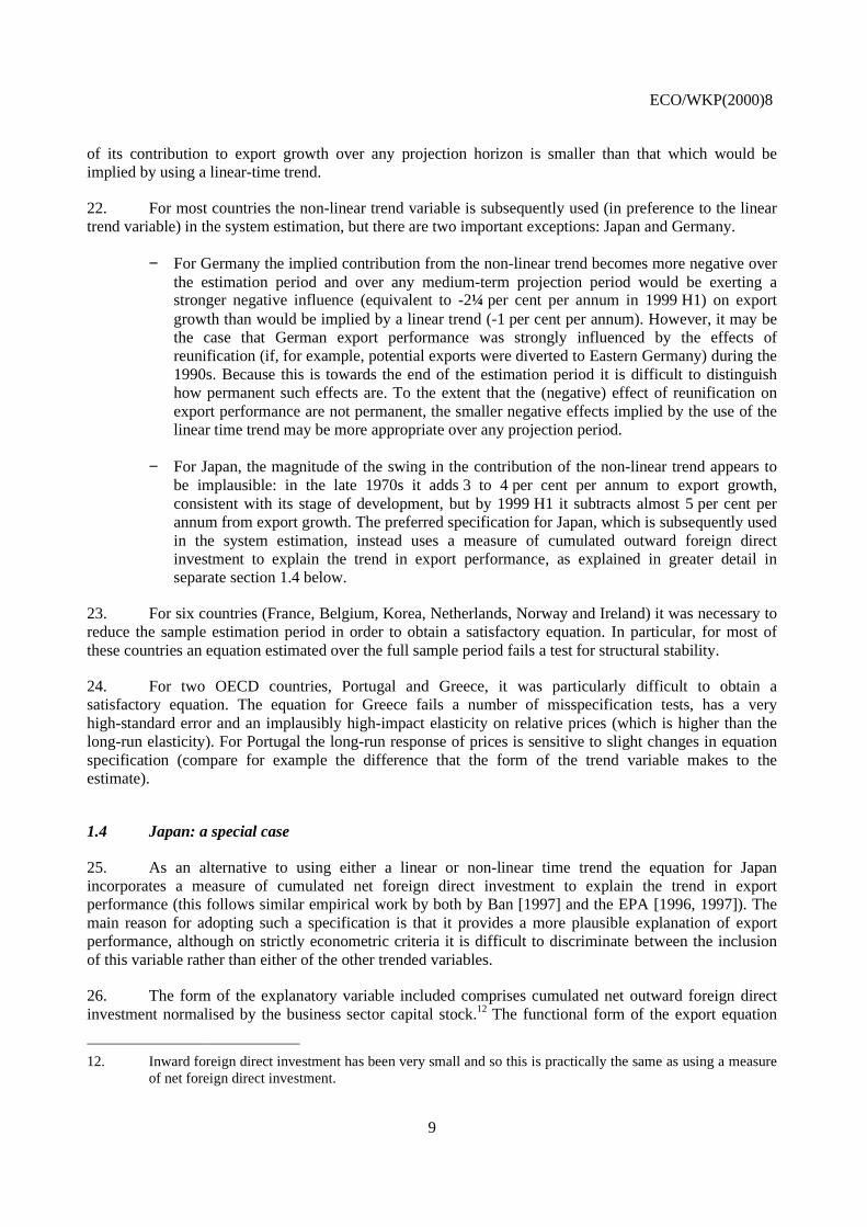
22. For most countries the non-linear trend variable is subsequently used (in preference to the lineartrend variable) in the system estimation, but there are two important exceptions: Japan and Germany.

− For Germany the implied contribution from the non-linear trend becomes more negative overthe estimation period and over any medium-term projection period would be exerting astronger negative influence (equivalent to -2¼ per cent per annum in 1999 H1) on exportgrowth than would be implied by a linear trend (-1 per cent per annum). However, it may bethe case that German export performance was strongly influenced by the effects ofreunification (if, for example, potential exports were diverted to Eastern Germany) during the1990s. Because this is towards the end of the estimation period it is difficult to distinguishhow permanent such effects are. To the extent that the (negative) effect of reunification onexport performance are not permanent, the smaller negative effects implied by the use of thelinear time trend may be more appropriate over any projection period.

− For Japan, the magnitude of the swing in the contribution of the non-linear trend appears tobe implausible: in the late 1970s it adds 3 to 4 per cent per annum to export growth,consistent with its stage of development, but by 1999 H1 it subtracts almost 5 per cent perannum from export growth. The preferred specification for Japan, which is subsequently usedin the system estimation, instead uses a measure of cumulated outward foreign directinvestment to explain the trend in export performance, as explained in greater detail inseparate section 1.4 below.

23. For six countries (France, Belgium, Korea, Netherlands, Norway and Ireland) it was necessary toreduce the sample estimation period in order to obtain a satisfactory equation. In particular, for most ofthese countries an equation estimated over the full sample period fails a test for structural stability.

24. For two OECD countries, Portugal and Greece, it was particularly difficult to obtain asatisfactory equation. The equation for Greece fails a number of misspecification tests, has a veryhigh-standard error and an implausibly high-impact elasticity on relative prices (which is higher than thelong-run elasticity). For Portugal the long-run response of prices is sensitive to slight changes in equationspecification (compare for example the difference that the form of the trend variable makes to theestimate).

1.4 Japan: a special case

25. As an alternative to using either a linear or non-linear time trend the equation for Japanincorporates a measure of cumulated net foreign direct investment to explain the trend in exportperformance (this follows similar empirical work by both by Ban [1997] and the EPA [1996, 1997]). Themain reason for adopting such a specification is that it provides a more plausible explanation of exportperformance, although on strictly econometric criteria it is difficult to discriminate between the inclusionof this variable rather than either of the other trended variables.

26. The form of the explanatory variable included comprises cumulated net outward foreign directinvestment normalised by the business sector capital stock.12

The functional form of the export equation

12. Inward foreign direct investment has been very small and so this is practically the same as using a measure

of net foreign direct investment.

ECO/WKP(2000)8

10

implies that a once-for-all permanent increase in this ratio will have a permanent negative effect on thelevel of export performance as export production is relocated abroad. The estimated effects imply that thestrong outward foreign direct investment which took place in the early 1990s in response to theappreciation of the yen substantially reduced Japanese export performance in this period reducing exportgrowth by more than 5 per cent per annum at its peak effect. However, more recently the rise in the FDIratio has been more modest implying a negative contribution to export growth less than 1 per cent perannum.

27. The inclusion of the FDI ratio reduces the long-run price elasticity obtained from previousestimates, in the range of 2.5 to 3, to a value closer to 2, which is still high but nearer to the average forother countries. Moreover the speed of response of export volumes to a change in relative prices becomesmuch quicker with the median lag falling from about 4-5 semesters to 2-3 semesters, which is again ismore in line with the results for other countries. This finding is explained by the fact that FDI is itself inpart, responsive to changes in competitiveness, albeit with a longer lag. This result is confirmed by asimple dynamic regression explaining the FDI ratio in terms of movements in the real exchange rate.Indeed allowing for an endogenous response of both FDI and price competitiveness to a change in theexchange rate implies an overall response of export volumes which is similar to the larger (and slower)response implied by specifications which do not explicitly incorporate the FDI ratio.

1.5 System estimation results

28. A summary of the SURE estimation results for the preferred set of equations under eachspecification is provided in Table 2 and Figure 3, and the residuals are plotted in Figure 4. All equationspass a test for up to second order serial correlation of residuals. The average standard error across allsystem equations is about 3 per cent, although it is much higher for Spain, Korea, Australia and Mexico.The final preferred set of 21 equations have 24 freely-estimated coefficients (excluding intercepts anddummy variables) compared to the unrestricted system that has 63 coefficients. Thus, the final set ofequations impose a total of 39 restrictions: 15 restrictions with respect to the long-run price elasticity,9 with respect to the error correction coefficient and 15 with respect to the short-run price dynamics.

29. Fourteen countries accept a common long-run price elasticity of about (minus) unity. Among theG7, five countries accept this common long-run price elasticity, with Japan having a higher long-run priceelasticity of -1.7, and the United States a lower elasticity of0.6.

30. The speeds of adjustment of export volumes to a change in relative export prices, illustrated inFigure 5 are relatively quick. Eleven countries complete at least 50 per cent of the long-run adjustmentwithin the first two semesters and for sixteen countries 80 per cent of the adjustment is completed withinsix semesters. The adjustment is slowest for Korea: the median is 4-5 semesters with 80 per cent of theadjustment to a relative export price shock taking eleven to twelve semesters.

31. Differences between estimates of the relative price elasticities from the two alternativespecifications including linear and non-linear time trend are relatively small for most countries comparedto the difference between all of the above and the elasticities of previous Interlink equations, see Figure 6.For a majority of OECD countries the long-run price elasticity in the previous version of Interlink is set at-1.20 (with no countries having an elasticity smaller than unity), which might be compared to the commonsystem elasticity of -0.99.13

There are more marked differences among individual countries. Particularly

13. Direct comparisons with estimates from other studies are difficult because the explanatory variables used

often differ in important respects. For example, the “income” variable is sometimes weighted foreign GDP(rather than imports) and consequently estimated income elasticities are typically much higher.

ECO/WKP(2000)8

11

noteworthy are differences for the United States for which the previous Interlink elasticity is -1.4 comparedto current estimates of around –0.6, and Japan for which the existing elasticity is -1.3 compared to currentestimates of between -1.7 and -2.5 (depending on what allowance is made for the endogeneity of foreigndirect investment). Other countries for which there is a particularly large difference between currentestimates and Interlink are France, Netherlands, Norway and Ireland (in all cases the revised estimates arelower).

32. Some form of time-trend variable is present in the equations for thirteen countries. Evaluating thecontribution which this makes to export growth in 1999 H1, the largest positive effect is for Mexico(adding 4.3 per cent per annum to export volume growth) and the largest negative effect is for Canada(equivalent to -1.9 per cent per annum). Of the G7 countries, three have negative time trend effects(Germany, France and Canada), the negative contribution from the rising foreign direct investment ratioreduces export growth in Japan in 1999, whilst for the other three countries a trend effect is absent.

33. The equations imply that for most countries export volumes adjust almost immediately to anychange in export market demand. For only seven countries is there any temporary change in exportperformance following a shock to export market demand. Among the G7, Japan initially gains marketshare, whilst Italy and Canada temporarily lose market share following an increase in export marketdemand.

1.6 Estimating equations for countries for which system estimation is not feasible

34. For those OECD countries (Iceland, Turkey, Hungary, Czech Republic and Poland) for whichinsufficient data are available to estimate an equation, the response of export performance to relative pricesobtained in the system estimation is assumed. The non-linear time trend effect is then estimated by lookingat recent trends (and in the case of the Eastern European countries, looking at recent Economic Outlookprojections) of export performance. For Greece and Portugal, the results obtained using single OLSequations are used which include the non-linear time trend.

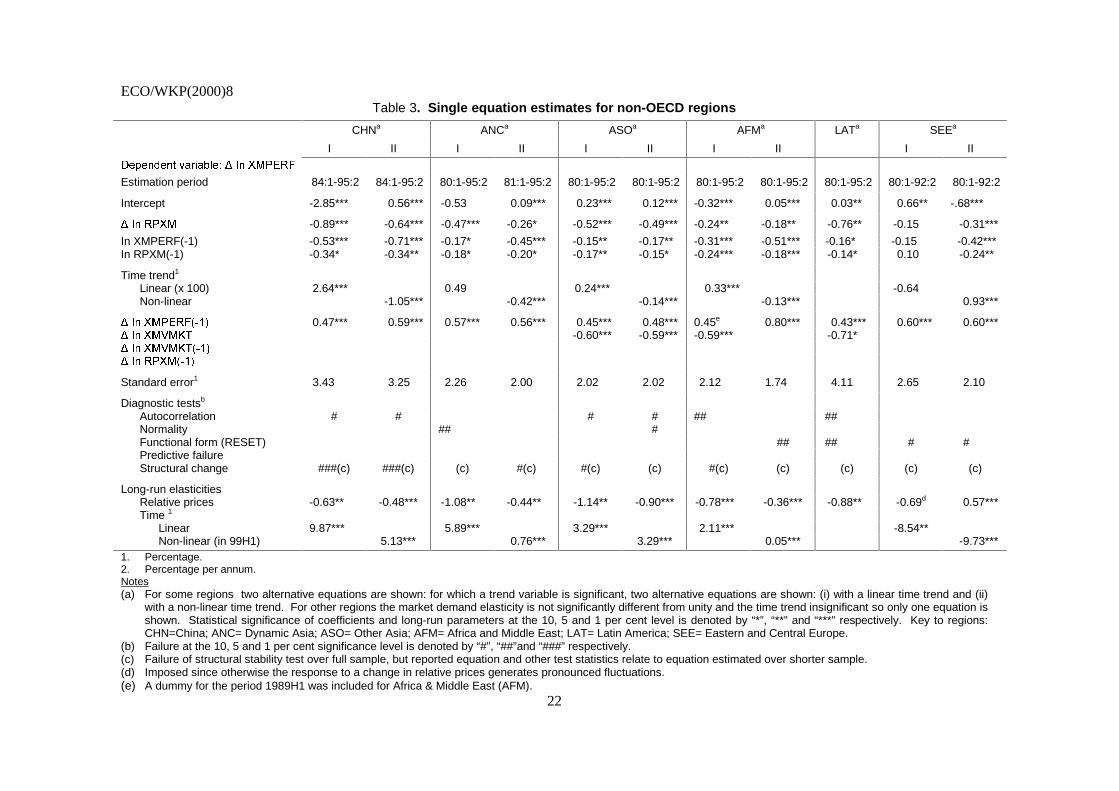
35. For the non-OECD, equation [1] is estimated separately for each region by OLS, and the resultspresented in Table 3, alongside those obtained when a linear time trend is used instead of the non-lineartrend. Overall the equations for the non-OECD perform less well in terms of the diagnostic tests than theequations estimated for the OECD countries. In particular, all equations are estimated over shortenedsamples (usually beginning in 1980) in order to obtain sensible parameter estimates and/or avoid failingtests for structural stability. The equation for Latin America has a particularly high standard error and failsa test for serial correlation of residuals at the 5 per cent significance level. The equation for China also hasa high standard error and fails a Chow test for structural stability even over a shortened estimation period.

36. The use of the non-linear time trend is econometrically preferred over the linear time trend in theequations for Dynamic Asia, Africa and Middle East, and non-OECD Europe (in the equations for OtherAsia and China this choice is not clear cut on purely econometric criteria). More importantly, thecontribution of the non-linear trend to export performance appears to be more plausible than that of thelinear trend (with the possible exception of non-OECD Europe where the magnitude of the negativecontribution of the trend variable is very large in both cases). For example, for China and Dynamic Asiathe linear trend would contribute nearly 10 and 6 per cent per annum, respectively, to export volumegrowth, whereas the contribution from the non-linear trend peaks in the late-1980s or early-1990s and by1999 H1 would only add 5 and 0.7 per cent per annum, respectively, to export growth (see Figure 2).

37. The estimated long-run price elasticity is correctly signed and statistically significant for allnon-OECD regions. In the case of both Latin America and Other Asia the estimate is about -0.9 and can

ECO/WKP(2000)8

12

readily be imposed at the common long-run elasticity (of minus unity) obtained in the system estimation ofOECD countries. For the other non-OECD regions the long-run elasticity is closer to -0.5 and therestriction that this is the same as the common long-run elasticity obtained in the system estimation ofOECD countries is rejected.

2. Simulation properties

38. While single-equation diagnostics are important, it is often more informative to look at how theequations affect the properties of single-country or multi-country models. In this section the new equationsare embedded and tested in the OECD’s Interlink model for a number of standard simulation shocks.14 Theimpact of an appreciation of the exchange rate is considered first by looking at each country on its own andthen taking account of international spillovers. Further simulations look at the impact of a rise ingovernment spending and in particular whether a fiscal expansion crowds out exports - the so-called “twindeficits” phenomenon.

2.1 Single-country properties

2.1.1 An appreciation of the exchange rate

39. The first set of simulations is run on an individual country basis. Each country’s exchange rate israised (appreciated) by 10 per cent and the model then simulates the impact using the equations for thatcountry only. This approach contrasts with multi-country simulation, described in a following section,which takes account of international linkages. For example, a slow-down in the US economy wouldnormally cause a slow-down in the rest of the world, which would then feed back on US exports and theUS economy in general. For initial diagnostic purposes, these international linkages have beenswitched-off in the individual country simulations.

40. In addition both fiscal and monetary policies are assumed not to change, in the sense that realinterest rates and real government spending and investment are held at their baseline levels.15 Note that thenature of the shock is different for Euro members. For these, it is assumed that the Euro appreciates by10 per cent, but the international linkages are still switched off. As an example, the French simulationshows the impact, using the French model, of a 10 per cent rise in the Euro while holding imports intoGermany, Italy, etc, at their baseline levels. By shifting the Euro, the effective size of the shock to eachEuro member is less than 10 per cent. In the case of France, a 10 per cent rise in the Euro is equivalent to afall in French competitiveness of only 5.7 per cent because a significant proportion of France’s exports goto other Euro members.

41. The results of the above exercise are summarised in Table 4 and Figure 7. The initial impact ofthe appreciation is a relatively sharp drop in manufactured exports for most countries. The average OECD

country has exports 1½ per cent lower after one year and 2 per cent lower after two years. The US impactis similar to the OECD average while the impact on Japan is noticeably larger, reflecting Japan’s higherrelative price elasticity (Japan’s exports are 2 per cent and 5 per cent lower in the first two years). Theimpacts on the major European economies are much smaller, which partly reflects the nature of the shock:

14 . A more comprehensive analysis of the simulation properties of the most recent version of the INTERLINK

model is given by Richardson et al. (2000).

15 . A variety of alternative assumptions could be made based on alternative policy rules, but for diagnosticpurposes those considered here are sufficient.

ECO/WKP(2000)8

13

a 10 per cent appreciation of the Euro does not represent a 10 per cent drop in competitiveness for the Eurocountries relative to their trading partners. OECD GDP is approximately ½ per cent lower after one yearand ¾ per cent lower after two years.

42. Recall from Figure 3 that the long-run single-equation response to an exchange rate shock isapproximately one-for-one for most OECD economies, which corresponds to a 10 per cent decline inexports for this shock. In contrast, the ultimate decline in exports is, however, clearly less severe when thewhole country model is run; in fact, exports return to baseline in all countries in the long run.

43. There are several reasons for this recovery and the most important is that export prices (indomestic currency terms) also adjust to changes in competitiveness. Export prices are determined bydomestic costs and by competitors’ export prices, with competitors’ prices having the most weight. Usingthe United States as an example, export prices in dollar terms fall by 2.7 per cent in the year following theappreciation - offsetting a sizeable proportion of the original exchange rate appreciation. Looking furtherahead, prices are 5 per cent lower after five years and 10 per cent lower after ten years. In other words, theappreciation is effectively reversed within a decade. In Japan the adjustment to prices is much quicker:5 per cent in the first year - wiping out half the effect of the appreciation - and 7.5 per cent after five years.The different adjustment speeds across countries reflect the differing degrees of pricing to market. Forexample, previous OECD empirical work (see for example Herd, 1987) suggests that Japan has a greaterdegree of pricing to market than does the United States or Europe, and so a change in the exchange rate isabsorbed in domestic profit margins to a significantly greater extent. Even so, in real terms, thecompetitiveness positions of most economies are back where they started after five to ten years.

44. There is also a secondary channel operating in these simulations, although this is much lessimportant. This works through a terms-of-trade or price-wedge effect. Real unit-labour costs from aproducer’s point of view (i.e. calculated using the GDP deflator) are approximately unchanged for mostcountries but real consumption wages (using the private consumption deflator) are higher. The wedgebetween production and consumption real wages is driven by a change in the terms of trade, which in turnis driven by different adjustment speeds for export and import prices. In the case of the United States, theterms of trade improve by 4 per cent in the first year; Japan’s rise by 3.5 per cent; and the OECD average is2.8 per cent. This causes a temporary increase in domestic consumption that partially offsets the fall inexports.

45. A further channel for the erosion of exchange rate effects is that by which higher exports raiseGDP relative to potential, closing the “output gap”. Such an effect would be expected to influence inflationin general and raise domestic costs entering the export price decision. Thus the stimulus to demand wouldalso be expected to act as a force which returns export competitiveness towards baseline in the longer run.

2.1.2 Government spending shock

46. Next the impact of fiscal policy is considered, and the extent to which a rise in governmentspending crowds out exports. The impact of a rise in government spending will clearly depend on whichparts of the budget are changed. For example, a rise in wage consumption is likely to bid up economy-widewages by more than would an equivalent rise in non-wage consumption, and a rise in governmentinvestment may have a smaller impact than other parts of the budget if investment goods have a highimport component. In this simulation, government real non-wage consumption is raised by 1 per cent ofbaseline GDP in each country. The nominal exchange rate and real interest rates are held at their baselinelevels, and real government investment is assumed to be unchanged.

ECO/WKP(2000)8

14

47. The results are broadly as expected and are summarised in Table 5. A rise in spending raisesGDP by 1–1½ per cent after one year in the major economies, although this effect dies off relativelyquickly. The United States has the strongest short-term government spending multiplier. The rise indomestic demand pushes up prices and wages in every country, leading to an appreciation of the realeffective exchange rate (recall that the nominal exchange rate is fixed). This, in turn, crowds out exports.After three years, manufacturing exports are 0.6 per cent lower on average for OECD economies, althoughthe impact is more severe in Japan. A direct consequence is a “worsening” of the trade account. After fiveyears, the current-account balance as a proportion of GDP is 0.3 per cent lower. On average OECD

economies see a worsening of two-thirds of a per cent of GDP, but the impact is noticeably more severe inEurope.

48. Comparing the United States and Europe, and ignoring the first-year impact effect, theUnited States experiences a significantly smaller impact on its current account despite a sharper decline inexport volumes and, in fact, a more aggressive expansion of imports. The reason is that it has more pricingpower on world markets. It is able to pass on a larger fraction of its domestic cost pressures. Its exportprices are 5 per cent higher after five years, while its import prices are only 2 per cent higher. In contrast,the Euro area the corresponding Figures are 1.5 and 0.5 per cent. By expanding the domestic economy, theUnited States’ terms of trade moves in its favour. However, there is no free lunch. US firms are not able topass on all their cost increases: and corporate profits are permanently lower.

49. These results suggest a clear link between fiscal policy and the current account, despite keyinternational transmission channels being switched off. In particular, additional and potentially largeeffects may occur if real interest rates and the nominal exchange rate are allowed to increase in response tothe rise in spending. An endogenous monetary policy response is also likely to increase the degree ofcrowding out as that would lead to a further rise in interest and exchange rates in response to theinflationary pressure generated by the fiscal expansion.

2.2 Full model properties

2.2.1 Exchange rate shock

50. Exchange rate shocks for the United States, Japan, and the Euro area were also run using thewhole model with all international linkages switched on. As before, real government consumption andinvestment are held at their baseline levels, as are real interest rates. However, this time there is a smalldifference for the Euro countries. For these countries it is assumed that the area’s real interest rate remainsat its baseline level (i.e., the Euro short-term rate minus the Euro average inflation rate). Euro memberswill have their own inflation rate, so their individual real interest rates will also differ slightly. The mainresults are summarised by the dashed lines in Figure 7.16

51. Three features stand out when comparing the full model with the single-country results. First,impact effects on exports are generally stronger. For example, US exports fall by approximately twice asmuch in the first year when international feedbacks are accounted for. This is not a surprise. As anexample, consider what happens in Germany when the US dollar appreciates. In the single-countrysimulation, it is assumed that all other countries (e.g. Germany) buy the same volume of imports.US exports drop because the higher exchange rate leads to a loss of market share. In other words, Germanbuyers substitute away from US goods and towards, say, Japanese products. Second, not only does the

16. The dashed lines represent different simulations. In the US panel it represents the impact on US exports of

a US dollar appreciation; the Japanese panel shows the impact of a yen shock, and so on.

ECO/WKP(2000)8

15

United States lose market share, but the size of its market also falls. An appreciation of the US dollarmakes domestic (German) goods more attractive, so in Germany there is a further substitution away fromUS exports and towards locally-made goods.

52. There is a third, simpler channel operating in these simulations. Weaker US exports lead to aneconomic slowdown in the United States, which then affects demand in the rest of the world. That is whythe increase in US imports is not as large using the full model as it is looking at the single-country results.The same phenomenon is seen for Japanese exports following a yen appreciation. However, the differencebetween the single-country and full-model simulations is very small. This reflects the small impact thatJapan has on the rest of the model. The spillovers from Europe are greater, reflecting the comparative sizeand openness of the Euro Area compared to Japan.

ECO/WKP(2000)8

16

BIBLIOGRAPHY

BAN, K. ed. (1997), “Research on Japan’s balance of payment and capital and financial account,” Institutefor Economic and Financial Research (Zaisei Keizai kyokai), Tokyo (in Japanese).

BREUSCH, T.S. and A.R. PAGAN (1980), “The Lagrange Multiplier Test and its Application to ModelSpecifications in Econometrics”, Review of Economic Studies, 44, pp. 149-192.

DURAND M., J. SIMON and C. WEBB (1992), “OECD’s Indicators of International Trade andCompetitiveness”, Economics Department Working Paper No. 120.

DURAND, M., C. MADASCHI, and G. TERRIBLE (1998), “Trends in OECD Countries InternationalCompetitiveness: the Influence of Emerging Market Economies”, Economics Department WorkingPaper No. 195.

ECONOMIC PLANNING AGENCY (1996), Economic Survey of Japan 1995-1996, Tokyo.

ECONOMIC PLANNING AGENCY (1997), Economic Survey of Japan 1996-1997, Tokyo.

HERD R. (1987), “Import and export prices for manufactures”, OECD Economics Department, WorkingPaper No. 43.

KRUGMAN P. (1989), “ Differences in Income Elasticities and Trends in Real Exchange Rates”,European-Economic-Review; 33(5), pp. 1031-1046.

NICKELL S. (1981), “Biases in Dynamic Models with Fixed Effects”, Econometrica, 49, pp. 1399-1416.

PAIN N. and K. WAKELIN (1998), “Export Performance and the Role of Foreign Direct Investment”,Manchester-School, 66(0), Supplement 1998, pp. 62-88.

PAIN, N. and D. HOLLAND (1998), “International Trade in Services: Putting UK Export Performance inPerspective”, NIESR mimeo.

RICHARDSON, P. (1988), “The Structure and Simulation Properties of OECD’s INTERLINK Model”,OECD Economic Studies No. 10, Spring 1988.

RICHARDSON, P., C. GIORNO, D. TURNER and D. RAE (2000), “The structure and properties of theOECD INTERLINK model”, OECD Economics Department Working Papers (forthcoming).

ECO/WKP(2000)8

17

Table 1. Summary of single equation OLS results for manufacturing exports volumesa

United States Japan Germany France Italy UnitedKingdom

Canada

I II III I II I II I II

Estimation period 76:2-97:1e 78:2-97:1 78:2-97:1 78:2-97:1d 76:2-97:1e 76:2-97:1e 83:1-97:1 83:1-97:1 76:2-97:1 76:2-97:2 76:2-97:1 76:2-97:1

Elasticity wrt relative prices: impact -0.09 -0.47** -0.18* -0.32*** -0.21* -0.23** -0.32*** -0.17 -0.24 -0.22** -0.49*** -0.47***: long-run -0.56*** -2.67*** -0.75*** -2.15*** -1.44** -1.05** -0.81*** -0.60*** -0.98*** -1.58*** -0.90*** -0.74***

Time trend1

Linear -1.13** -1.04** -0.75*** -2.86***Non-linear ( in 99H1)f -4.76*** -2.27*** -0.16*** -1.61**

Elasticity wrt market demand: Impact 1.00*** 1.45*** 1.21*** 1.30*** 1.00*** 1.00*** 1.00*** 1.00*** 0.60 1.00*** 0.80*** 0.74***: Long-run 1.00*** 1.00*** 1.00*** 1.00** 1.00*** 1.00*** 1.00*** 1.00*** 1.00*** 1.00*** 1.00*** 1.00***

Standard error2 2.04 1.42 1.60 1.79 1.73 1.72 1.16 1.25 3.19 1.82 2.70 2.75

Diagnostic testsb

Autocorrelation # # #NormalityFunctional form (RESET) # ## # # # #Predictive failureStructural change # (c) (c)

ECO/WKP(2000)8

18

Table 1 (contd.). Summary of single equation OLS results for manufacturing exports volumesa

Australia Austria Belgium Denmark Finland Greece Ireland Korea Mexico

I II I II I II I II I II

Estimation period 76:1-97:1 76:2-94:2 80:1:94:2 81:1-96:1 76:2-96:2 76:2-96:2 76:2-96:2e 76:2-94:2 76:2-94:2 81:2-92:2 81:2-92:2 81:1-97:1 76:2-96:2 76:2-97:1

Elasticity wrt relative prices: Impact -0.44*** -0.30*** -0.44*** -0.22 -0.14 -0.09 -0.28** -1.38*** -1.38*** -0.81** -0.80** -0.33** -0.56*** -0.48***: Long-run -1.12* -0.82*** -0.94*** -1.13 -0.78** -0.64** -1.34*** -1.25*** -1.25*** -1.23 -1.15 -1.74*** -1.84*** -1.24***

Time trend1

Linear 0.77*** 0.94*** -1.36** 2.27 3.89**Non-linear ( in 99H1)f 0.01*** 0.02*** -1.13* 1.80 3.93***

Elasticity wrt market demand: Impact 0.59 (d) 1.00*** 1.00*** 0.57** 0.55*** 0.55*** 0.42** 1.00*** 1.00*** 1.00* 1.00*** 1.00** 1.00*** 1.00***: Long-run 1.00*** 1.00*** 1.00*** 1.00*** 1.00*** 1.00*** 1.00*** 1.00*** 1.00*** 1.00* 1.00 1.00** 1.00*** 1.00***

Standard error2 4.27 2.00 1.50 2.34 2.68 2.73 3.25 9.57 9.57 3.10 3.08 4.90 5.65 5.33

Diagnostic testsb

Autocorrelation ### # #NormalityFunctional form (RESET) ## ## # # ##Predictive failureStructural stability # (c) # (c)

ECO/WKP(2000)8

19

Table 1 (contd.). Summary of single equation OLS results for manufacturing exports volumesa

Netherlands e New Zealand Norway Portugal d Spain Sweden e Switzerland

I II I II I II I II I II I II

Estimation period 84:1-96:2 76:2-97:1 76:2-97:2 81:1-97:2 81:1-97:2 76:2-97:1 76:2-97:1 76:2-97:1 76:2-97:1 76:2-97:1 76:2-97:1 76:2-97:1 76:2-97:1

Elasticity wrt relative prices: Impact -0.47** -0.38** -0.40** -0.39*** -0.32** -0.60*** -0.56*** -0.79*** -0.68*** -0.30*** -0.26*** -0.20* -0.23*: Long-run -0.39** -0.86 -0.96 -0.57** -0.42*** -5.29*** -1.73*** -1.41*** -1.40*** -1.28*** -1.20*** -0.23 -0.17

Time trend1

Linear -1.66*** -1.66*** - 2.94*** -1.17*** -2.34***Non-linear ( in 99H1)f -0.00*** -0.14*** 0.17*** 4.61*** -0.14*** 2.63***

Elasticity wrt market demand: Impact 1.00*** 0.82*** 0.80*** 1.00*** 1.00*** 1.00*** 1.00*** 1.00*** 1.00*** 1.00*** 1.00*** 1.00*** 1.00***: Long-run 1.00*** 1.00*** 1.00*** 1.00*** 1.00*** 1.00*** 1.00*** 1.00*** 1.00*** 1.00*** 1.00*** 1.00** 1.00**

Standard error2 2.29 4.09 4.02 3.12 2.88 4.20 3.79 5.31 4.97 1.76 1.70 2.40 2.48

Diagnostic testsb

Autocorrelation #NormalityFunctional form (RESET) ##Predictive failureStructural stability ##(c) (c) (c)

1. Percentage per annum.2. Percentage.Notes:(a) For those countries for which a trend variable is significant, two alternative equations are shown: (i) with a linear time trend and (ii) with a non-linear time trend.

Statistical significance of the impact and long-run responses at the 10, 5 and 1 per cent significance levels are denoted by “*”, “**” and “***”, respectively;(b) Failure of the tests at the 10, 5 and 1 per cent significance level is denoted by “#”, “##”, “###”, respectively;(c) Failure of structural stability test at the 5 per cent level over the full sample, but the reported equation relates to one estimated over a shorter sample;(d) For Portugal, a non-linear trend is included although a linear trend is not significant. This is because the long-run price elasticity obtained in the model excluding a linear

trend is high and seems to be correlated with a linear time trend;(e) A seasonal dummy was included for Netherlands while a dummy for the period 1980H1 was included for Sweden;(f) The contribution of the non-linear trend to export growth varies over the sample estimation period, but for purposes of comparison is evaluated here at 1999H1.

ECO/WKP(2000)8

20

Table 2. Summary of system estimation results

United States Japan Germany France Italy UnitedKingdom

Canada Australia Austria Belgium Denmark

'HSHQGHQW�YDULDEOH�� ,Q�;03(5)

Estimation period 76:2-97:1 78:1-97:1 76:2-97:1 83:1-97:1 76:2-97:1 76:2-97:1 76:2-97:1 76:2-97:1 76:2-94:2 81:1-96:1 76:2-97:1

Intercept 0.00 0.08*** -0.01** -0.01*** 0.02** 0.00 -0.14*** 0.00 0.02*** 0.02** 0.01

�,Q�53;0 -0.08 -0.35*** -0.35*** -0.35*** -0.35*** -0.22*** -0.35*** -0.35*** -0.35*** -0.35*** -0.13

Error correction termγ*[ln XMPERF(-1) + θ*lnRPXM(-1)]

γ -0.33*** -0.18*** -0.11*** -0.33*** -0.33*** -0.16*** -0.33*** -0.16*** -0.61*** -0.15*** -0.33***θ -0.63*** -1.69*** -0.99*** -0.99*** -0.99*** -0.99*** 0.99*** -0.99*** -0.99*** -0.99*** -0.62***

Time trendLinear (x 100) -0.08***Non-linear 0.11*** 0.54*** -0.06*** -0.05***

�,Q�;03(5)�� 0.39*** 0.33***�,Q�;090.7 -0.61*** -0.26*** -0.39*** -0.54***�,Q�;090.7��,Q�;090.7 -0.75***

�,Q�53;0�� -0.18** 0.31***

Other explanatory variables (b) (c) (d)

Standard error1 2.10 1.95 1.59 1.48 3.38 2.01 2.88 4.14 1.90 2.36 2.76

Time Trend2

Linear -0.76***Non-Linear (in 99H1) -0.16*** -1.89*** 0.01*** 0.02***

ECO/WKP(2000)8

21

Table 2 (contd.). Summary of system estimation results

Finland Ireland Korea Mexico Netherlands New Zealand Norway Spain Sweden Switzerland


Estimation period 76:2-97:1 81:1-92:2 81:1-97:1 76:2-97:1 84:1-96:2 76:2-97:1 81:-97:1 76:2-97:1 76:1-97:1 76:2-97:1

Intercept 0.06*** 0.15*** 0.01 0.37 0.00 0.03*** -0.02** 0.91*** 0.00 0.34***

�,Q�53;0 -0.35*** -0.17 -0.35*** -0.35*** -0.35*** -0.35*** -0.35*** -0.35*** -0.18*** -0.31***

Error correction termγ*[ln XMPERF(-1) + θ*lnRPXM(-1)]

γ -0.33*** -0.17*** -0.12*** -0.55*** -0.73*** -0.22*** -0.66*** -0.33*** -0.33*** -0.33***θ -0.99*** -0.99*** -1.69*** -0.99*** -0.54*** -0.99*** -0.42** -0.99*** -0.99*** -0.48e

Time trendLinear (x 100) -0.30***Non-linear -0.21*** -0.74*** 0.05*** 0.21*** 0.11***

�,Q�;03(5)�� -0.24*** 0.37*** 0.36***�,Q�;090.7 -0.38** -0.31***�,Q�;090.7�� -0.34***�,Q�;090.7

�,Q�53;0�� -0.17 -0.44**

Other explanatory variables (f) (g) (h) (i)

Standard error1 3.37 3.77 4.96 5.45 2.01 4.12 2.94 5.52 1.79 2.40

Time Trend2

LinearNon-linear (in 99H1) 2.18*** 4.27*** -0.00*** -0.15*** 3.89*** -0.13*** -1.90***

1. Percentage.2. Percentage per annum.Notes:(e) Imposed (freely estimated coefficient implausibly small).(f) A dummy for the period 1991H1 was included.(g) A seasonal dummy was included.(h) A dummy for the period 1989H2 was included.(i) A dummy for the period 1980H1 was included.

ECO/WKP(2000)8

22

Table 3. Single equation estimates for non-OECD regions

CHNa ANCa ASOa AFMa LATa SEEa

I II I II I II I II I II


Estimation period 84:1-95:2 84:1-95:2 80:1-95:2 81:1-95:2 80:1-95:2 80:1-95:2 80:1-95:2 80:1-95:2 80:1-95:2 80:1-92:2 80:1-92:2

Intercept -2.85*** 0.56*** -0.53 0.09*** 0.23*** 0.12*** -0.32*** 0.05*** 0.03** 0.66** -.68***

�,Q�53;0 -0.89*** -0.64*** -0.47*** -0.26* -0.52*** -0.49*** -0.24** -0.18** -0.76** -0.15 -0.31***

In XMPERF(-1) -0.53*** -0.71*** -0.17* -0.45*** -0.15** -0.17** -0.31*** -0.51*** -0.16* -0.15 -0.42***In RPXM(-1) -0.34* -0.34** -0.18* -0.20* -0.17** -0.15* -0.24*** -0.18*** -0.14* 0.10 -0.24**

Time trend1

Linear (x 100) 2.64*** 0.49 0.24*** 0.33*** -0.64Non-linear -1.05*** -0.42*** -0.14*** -0.13*** 0.93***

�,Q�;03(5)�� 0.47*** 0.59*** 0.57*** 0.56*** 0.45*** 0.48*** 0.45e 0.80*** 0.43*** 0.60*** 0.60***�,Q�;090.7 -0.60*** -0.59*** -0.59*** -0.71*�,Q�;090.7��,Q�53;0��

Standard error1 3.43 3.25 2.26 2.00 2.02 2.02 2.12 1.74 4.11 2.65 2.10

Diagnostic testsb

Autocorrelation # # # # ## ##Normality ## #Functional form (RESET) ## ## # #Predictive failureStructural change ###(c) ###(c) (c) #(c) #(c) (c) #(c) (c) (c) (c) (c)

Long-run elasticitiesRelative prices -0.63** -0.48*** -1.08** -0.44** -1.14** -0.90*** -0.78*** -0.36*** -0.88** -0.69d 0.57***Time 1

Linear 9.87*** 5.89*** 3.29*** 2.11*** -8.54**Non-linear (in 99H1) 5.13*** 0.76*** 3.29*** 0.05*** -9.73***

1. Percentage.2. Percentage per annum.Notes(a) For some regions two alternative equations are shown: for which a trend variable is significant, two alternative equations are shown: (i) with a linear time trend and (ii)

with a non-linear time trend. For other regions the market demand elasticity is not significantly different from unity and the time trend insignificant so only one equation isshown. Statistical significance of coefficients and long-run parameters at the 10, 5 and 1 per cent level is denoted by “*”, “**” and “***” respectively. Key to regions:CHN=China; ANC= Dynamic Asia; ASO= Other Asia; AFM= Africa and Middle East; LAT= Latin America; SEE= Eastern and Central Europe.

(b) Failure at the 10, 5 and 1 per cent significance level is denoted by “#”, “##”and “###” respectively.(c) Failure of structural stability test over full sample, but reported equation and other test statistics relate to equation estimated over shorter sample.(d) Imposed since otherwise the response to a change in relative prices generates pronounced fluctuations.(e) A dummy for the period 1989H1 was included for Africa & Middle East (AFM).

ECO/WKP(2000)8

23

Table 4. Impact of an exchange rate shock

(10 per cent appreciation of exchange rate, on a country-by-country basis)

Deviations from baseline, in per cent

Years after shock

1 2 3 4 5

United StatesGDP level -0.2 -0.7 -0.3 -0.1 0.1Consumer price inflation -0.7 -0.5 -0.8 -1.0 -1.2Current account1 0.0 -0.1 -0.2 -0.3 -0.3Manufactured exports -1.3 -3.0 -3.5 -3.5 -3.1

Euro areaGDP level -0.6 -0.6 -0.4 -0.1 0.1Consumer price inflation -0.9 -0.8 -0.9 -0.9 -1.0Current account1 -0.2 -0.4 -0.5 -0.5 -0.5Manufactured exports -1.2 -1.7 -1.5 -1.3 -0.9

JapanGDP level -0.4 -1.0 -1.1 -1.0 -0.9Consumer price inflation -0.4 -0.7 -1.3 -1.5 -1.7Current account1 -0.2 -0.4 -0.6 -0.7 -0.9Manufactured exports -2.0 -4.5 -5.9 -6.4 -6.6

OECD average2

GDP level -0.5 -0.8 -0.6 -0.3 -0.1Consumer price inflation -0.9 -0.8 -1.1 -1.2 -1.2Current account1 -0.2 -0.4 -0.5 -0.6 -0.6Manufactured exports -1.4 -1.7 -3.1 -3.0 -2.7

1. Percentage of GDP.2. Single country responses, averaged across OECD countries.Note: Real government consumption and investment held at their baseline levels. Real interest rates areheld at their baseline level.

ECO/WKP(2000)8

24

Table 5. Government spending shock

(1 per cent rise in government non-wage consumption: country-by-country basis)

Deviations from baseline, in per cent

Years after shock

1 2 3 4 5

United StatesGDP level 1.7 1.3 0.5 0.2 0.1Consumer price inflation 0.2 0.9 1.4 1.5 1.5Current account1 -0.5 -0.4 -0.2 -0.3 -0.4Manufactured exports 0.0 -0.2 -0.7 -1.3 -2.0

Euro areaGDP level 0.9 0.8 0.7 0.5 0.4Consumer price inflation 0.2 0.4 0.5 0.6 0.6Current account1 -0.5 -0.6 -0.7 -0.7 -0.9Manufactured exports 0.0 -0.1 -0.3 -0.6 -0.8

JapanGDP level 1.4 1.1 0.7 0.5 0.4Consumer price inflation 0.5 1.6 1.3 1.4 1.7Current account1 -0.3 -0.2 -0.2 -0.2 -0.3Manufactured exports -0.1 -0.6 -1.5 -2.5 -3.8

OECD average2

GDP level 1.2 1.0 0.6 0.4 0.2Consumer price inflation 0.3 0.8 1.0 1.0 1.0Current account1 -0.5 -0.4 -0.4 -0.5 -0.6Manufactured exports 0.0 -0.2 -0.6 -1.0 -1.6

3. Per cent of GDP.4. Single country responses, averaged across OECD countries.Note: Real government investment held at its baseline level. Real interest rates are held at theirbaseline level.

ECO/WKP(2000)8

25

Figure 1. Export performance and competitivenessIndex 1991 = 100, competitiveness as inverse of relative export prices

1976 1978 1980 1982 1984 1986 1988 1990 1992 1994 199670

75

80

85

90

95

100

105

110

115

50

60

70

80

90

100

110

120

130

140performance competitiveness

United States

1976 1978 1980 1982 1984 1986 1988 1990 1992 1994 199650

60

70

80

90

100

110

120

130

140

75

80

85

90

95

100

105

110

115


Japan

1976 1978 1980 1982 1984 1986 1988 1990 1992 1994 199675

80

85

90

95

100

105

110

115

120

125

80

85

90

95

100

105

110

115

120

125


Germany

1976 1978 1980 1982 1984 1986 1988 1990 1992 1994 199685

90

95

100

105

110

115

120

125

130

135

92

94

96

98

100

102

104

106

108

110


France

1976 1978 1980 1982 1984 1986 1988 1990 1992 1994 199695

100

105

110

115

120

125

95

100

105

110

115

120


Italy

1976 1978 1980 1982 1984 1986 1988 1990 1992 1994 199695

100

105

110

115

120

125

130

135

140

85

90

95

100

105

110

115

120

125


United Kingdom

ECO/WKP(2000)8

26

Figure 1. (Continued)Index 1991 = 100, competitiveness as inverse of relative export prices

1976 1978 1980 1982 1984 1986 1988 1990 1992 1994 199680

90

100

110

120

130

140

60

70

80

90

100

110


Canada

1976 1978 1980 1982 1984 1986 1988 1990 1992 1994 199670

80

90

100

110

120

130

140

60

70

80

90

100

110

120


Australia

1976 1978 1980 1982 1984 1986 1988 1990 1992 1994 199670

75

80

85

90

95

100

105

110

75

80

85

90

95

100

105

110


Austria

1976 1978 1980 1982 1984 1986 1988 1990 1992 1994 199695

100

105

110

115

120

125

130

135

80

85

90

95

100

105

110

115


Belgium

1976 1978 1980 1982 1984 1986 1988 1990 1992 1994 1996126

128

130

132

134

136

138

140

142

88.5

89.0

89.5

90.0

90.5

91.0

91.5

92.0

92.5performance competitiveness

Czech Republic

1976 1978 1980 1982 1984 1986 1988 1990 1992 1994 199675

80

85

90

95

100

105

110

90

95

100

105

110

115

120


Denmark

1976 1978 1980 1982 1984 1986 1988 1990 1992 1994 199680

90

100

110

120

130

140

150

95

100

105

110

115

120

125


Finland

1976 1978 1980 1982 1984 1986 1988 1990 1992 1994 199670

80

90

100

110

120

130

140

150

60

70

80

90

100

110

120

130


Greece

ECO/WKP(2000)8

27


1976 1978 1980 1982 1984 1986 1988 1990 1992 1994 199690

95

100

105

110

115

120

125

130

97

98

99

100

101

102

103

104


Hungary

1976 1978 1980 1982 1984 1986 1988 1990 1992 1994 199620

40

60

80

100

120

140

160

0

20

40

60

80

100

120


Iceland

1976 1978 1980 1982 1984 1986 1988 1990 1992 1994 19960

20

40

60

80

100

120

80

85

90

95

100

105


Ireland

1976 1978 1980 1982 1984 1986 1988 1990 1992 1994 1996-50

0

50

100

150

200

40

60

80

100

120


Korea

1976 1978 1980 1982 1984 1986 1988 1990 1992 1994 1996-20

0

20

40

60

80

100

120

140

50

60

70

80

90

100

110

120


Mexico

1976 1978 1980 1982 1984 1986 1988 1990 1992 1994 199690

95

100

105

110

115

120

80

85

90

95

100

105


Netherlands

1976 1978 1980 1982 1984 1986 1988 1990 1992 1994 199670

80

90

100

110

120

130

80

85

90

95

100

105


New Zealand

1976 1978 1980 1982 1984 1986 1988 1990 1992 1994 199690

100

110

120

130

140

150

160

170

80

85

90

95

100

105

110

115


Norway

ECO/WKP(2000)8

28


1976 1978 1980 1982 1984 1986 1988 1990 1992 1994 1996110

115

120

125

130

135

140

145

100

101

102

103

104

105

106


Poland

1976 1978 1980 1982 1984 1986 1988 1990 1992 1994 19960

20

40

60

80

100

120

140

60

70

80

90

100

110

120


Portugal

1976 1978 1980 1982 1984 1986 1988 1990 1992 1994 199670

80

90

100

110

120

130

140

150

95

100

105

110

115

120

125

130


Spain

1976 1978 1980 1982 1984 1986 1988 1990 1992 1994 199690

95

100

105

110

115

120

125

130

85

90

95

100

105

110

115

120


Sweden

1976 1978 1980 1982 1984 1986 1988 1990 1992 1994 199680

90

100

110

120

130

140

150

80

90

100

110

120

130

140


Switzerland

1976 1978 1980 1982 1984 1986 1988 1990 1992 1994 1996-200

-150

-100

-50

0

50

100

150

200

92

94

96

98

100

102

104

106


Turkey

1976 1978 1980 1982 1984 1986 1988 1990 1992 1994 19960

20

40

60

80

100

120

140

90

100

110

120

130

140

150


China

1976 1978 1980 1982 1984 1986 1988 1990 1992 1994 1996-20

0

20

40

60

80

100

120

140

80

85

90

95

100

105

110

115


ANIEs

ECO/WKP(2000)8

29


1976 1978 1980 1982 1984 1986 1988 1990 1992 1994 199650

60

70

80

90

100

110

120

130

50

60

70

80

90

100

110

120


Other Asia

1976 1978 1980 1982 1984 1986 1988 1990 1992 1994 199660

70

80

90

100

110

120

130

85

90

95

100

105

110

115


African and Middle East

1976 1978 1980 1982 1984 1986 1988 1990 1992 1994 199660

70

80

90

100

110

120

130

50

60

70

80

90

100

110


Central and South America

1976 1978 1980 1982 1984 1986 1988 1990 1992 1994 199660

80

100

120

140

160

180

200

60

70

80

90

100

110

120


Central and Eastern Europe

ECO/WKP(2000)8

30

a. OECD countries where a non-linear time trend is preferredNon-linear trend Linear trend

b. OECD countries where a linear time trend is preferred in system equation c. Japan

The thin solid line for Japan shows the effect of FDI variable.

Figure 2. Effects of time trend variable on manufacturing exports 1,2

(Contribution to export volume growth, per cent per annum.)

France

-2

0

2

1975

1980

1990

2000

2010

forecasts

Canada

-4

-2

0

1975

1980

1990

2000

2010

Austria

-2

0

2

1975

1980

1990

2000

2010

Denmark

-2

0

2

1975

1980

1990

2000

2010

Ireland

0

2

4

1975

1980

1990

2000

2010

Mexico

-4

0

4

8

1975

1980

1990

2000

2010

New Zealand

-4

0

419

75

1980

1990

2000

2010

Norway

-4

-2

0

1975

1980

1990

2000

2010

Spain

0

4

8

1975

1980

1990

2000

2010

Sweden

-2

0

2

1975

1980

1990

2000

2010

Germany

-4

-2

0

1975

1980

1990

2000

2010

Switzerland

-4

-2

0

1975

1980

1990

2000

2010

Japan

-8

-4

0

4

8

1975

1980

1990

2000

2010

ECO/WKP(2000)8

31

d . OECD countries where a non-linear trend is preferred and not in a system estimation

e. Non-OECD area and regions with a non-linear time trend

1. Non-linear time trend effect is from the system of equations while the linear time trend effect is based on the single equation results.2. Scales differ for different countries.

Figure 2 (continued). Effects of time trend variable on manufacturing exports

Greece

-2

0

2

1975

1980

1990

2000

2010

Portugal

0

4

8

1975

1980

1990

2000

2010

China

0

4

8

12

1975

1980

1990

2000

2010

Dynamic Asia

0

4

8

12

1975

1980

1990

2000

2010

Other Asia

0

4

8

12

1975

1980

1990

2000

2010

Africa and Middle east

0

4

8

12

1975

1980

1990

2000

2010

Eastern and Central Europe

-16

-8

0

8

1975

1980

1990

2000

2010

Hungary

0

8

16

1975

1980

1990

2000

2010

Poland

0

8

1975

1980

1990

2000

2010

Czech Republic

0

4

8

1975

1980

1990

2000

2010

Turkey

0

8

16

24

1975

1980

1990

2000

2010

ECO/WKP(2000)8

32

Figure 3. Long run relative price elasticities

-0.0 -0.2 -0.4 -0.6 -0.8 -1.0 -1.2 -1.4 -1.6 -1.8

Japan

Korea

Germany

France

Italy

UK

Canada

Australia

Austria

Belgium

Finland

Ireland

Mexico

Netherlands

Norway

Sweden

OECD Ave

Europe Ave

Denmark

United States

New Zealand

Switzerland

Spain

Common system elasticity

ECO/WKP(2000)8

33

Figure 4. Residuals from the system estimation

-0.20

-0.15

-0.10

-0.05

0.00

0.05

0.10

0.15

78 80 82 84 86 88 90 92 94 96

USA

-0.20

-0.15

-0.10

-0.05

0.00

0.05

0.10

0.15

78 80 82 84 86 88 90 92 94 96

JPN

-0.20

-0.15

-0.10

-0.05

0.00

0.05

0.10

0.15

78 80 82 84 86 88 90 92 94 96

DEU

-0.20

-0.15

-0.10

-0.05

0.00

0.05

0.10

0.15

78 80 82 84 86 88 90 92 94 96

FRA

-0.20

-0.15

-0.10

-0.05

0.00

0.05

0.10

0.15

78 80 82 84 86 88 90 92 94 96

ITA

-0.20

-0.15

-0.10

-0.05

0.00

0.05

0.10

0.15

78 80 82 84 86 88 90 92 94 96

GBR

-0.20

-0.15

-0.10

-0.05

0.00

0.05

0.10

0.15

78 80 82 84 86 88 90 92 94 96

CAN

-0.20

-0.15

-0.10

-0.05

0.00

0.05

0.10

0.15

78 80 82 84 86 88 90 92 94 96

AUS

-0.20

-0.15

-0.10

-0.05

0.00

0.05

0.10

0.15

78 80 82 84 86 88 90 92 94 96

AUT

-0.20

-0.15

-0.10

-0.05

0.00

0.05

0.10

0.15

78 80 82 84 86 88 90 92 94 96

BEL

-0.20

-0.15

-0.10

-0.05

0.00

0.05

0.10

0.15

78 80 82 84 86 88 90 92 94 96

DNK

-0.20

-0.15

-0.10

-0.05

0.00

0.05

0.10

0.15

78 80 82 84 86 88 90 92 94 96

FIN

-0.20

-0.15

-0.10

-0.05

0.00

0.05

0.10

0.15

78 80 82 84 86 88 90 92 94 96

IRE

-0.20

-0.15

-0.10

-0.05

0.00

0.05

0.10

0.15

78 80 82 84 86 88 90 92 94 96

KOR

-0.20

-0.15

-0.10

-0.05

0.00

0.05

0.10

0.15

78 80 82 84 86 88 90 92 94 96

MEX

-0.20

-0.15

-0.10

-0.05

0.00

0.05

0.10

0.15

78 80 82 84 86 88 90 92 94 96

NLD

-0.20

-0.15

-0.10

-0.05

0.00

0.05

0.10

0.15

78 80 82 84 86 88 90 92 94 96

NZL

-0.20

-0.15

-0.10

-0.05

0.00

0.05

0.10

0.15

78 80 82 84 86 88 90 92 94 96

NOR

-0.20

-0.15

-0.10

-0.05

0.00

0.05

0.10

0.15

78 80 82 84 86 88 90 92 94 96

ESP

-0.20

-0.15

-0.10

-0.05

0.00

0.05

0.10

0.15

78 80 82 84 86 88 90 92 94 96

SWE

-0.20

-0.15

-0.10

-0.05

0.00

0.05

0.10

0.15

78 80 82 84 86 88 90 92 94 96

CHE

ECO/WKP(2000)8

34

Figure 5. The response of export volumes to a one percent fall in relative export prices

a. G7 countries

0.0

0.5

1.0

1.5

2.0

1 2 3 4 5 6 Years

United States

Japan

Germany

France and Italy

United Kingdom

Canada

b. Nordic countries in the system estimation

0.0

0.5

1.0

1.5

2.0

1 2 3 4 5 6 Years

Denmark

Finland

Norway

Sweden

c. Other smaller European countries in the system estimation

0.0

0.5

1.0

1.5

2.0

1 2 3 4 5 6Years

Belgium

Ireland

Netherlands

Austria

Spain

Switzerland

d. Other OECD countries in the system estimation

0.0

0.5

1.0

1.5

2.0

1 2 3 4 5 6Years

Australia

Korea

Mexico

New Zealand

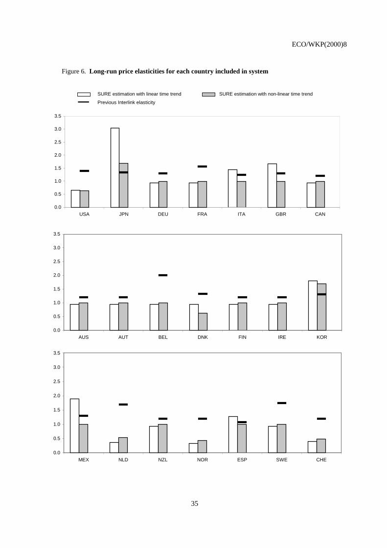
ECO/WKP(2000)8

35

Figure 6. Long-run price elasticities for each country included in system

SURE estimation with linear time trend SURE estimation with non-linear time trend

Previous Interlink elasticity

0.0

0.5

1.0

1.5

2.0

2.5

3.0

3.5

USA JPN DEU FRA ITA GBR CAN

0.0

0.5

1.0

1.5

2.0

2.5

3.0

3.5

AUS AUT BEL DNK FIN IRE KOR

0.0

0.5

1.0

1.5

2.0

2.5

3.0

3.5

MEX NLD NZL NOR ESP SWE CHE

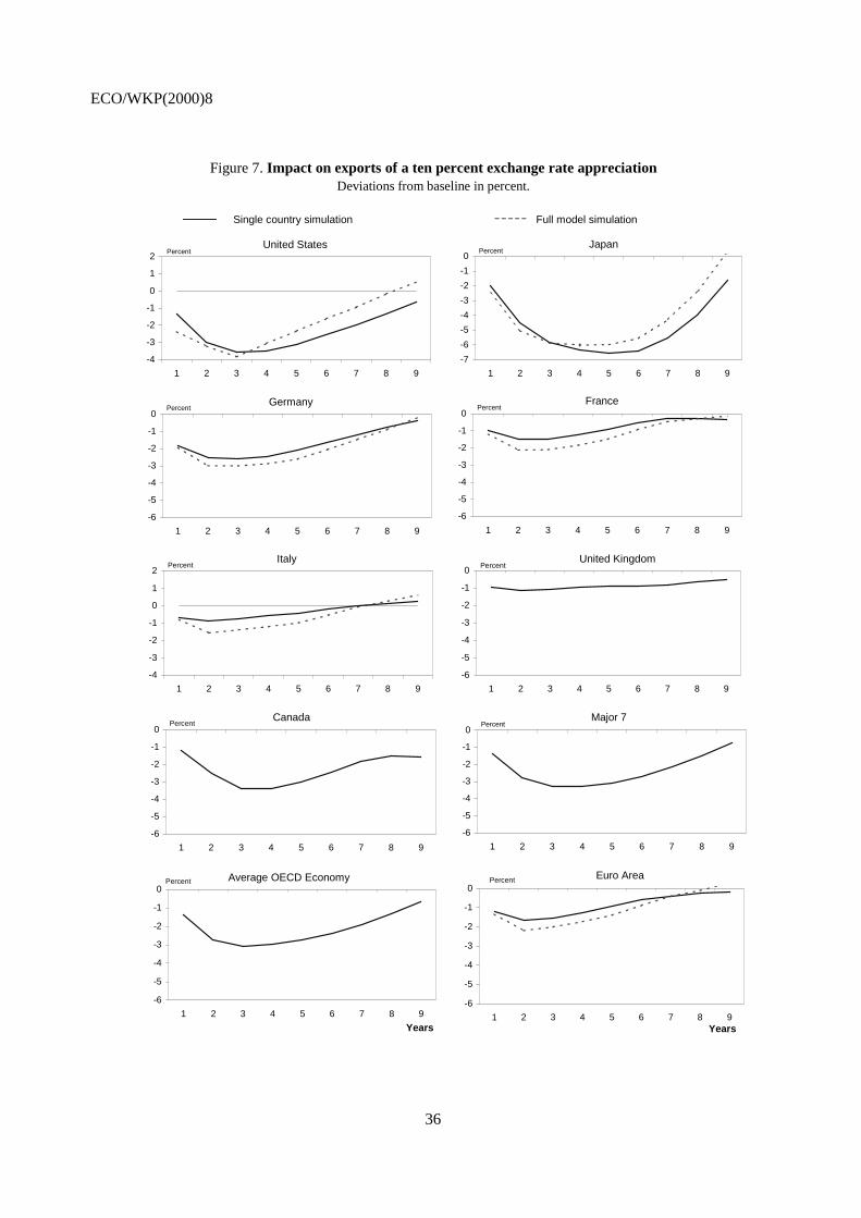
ECO/WKP(2000)8

36

Single country simulation Full model simulation

Figure 7. Impact on exports of a ten percent exchange rate appreciationDeviations from baseline in percent.

-4

-3

-2

-1

0

1

2

1 2 3 4 5 6 7 8 9

United StatesPercent

-7

-6

-5

-4

-3

-2

-1

0

1 2 3 4 5 6 7 8 9

JapanPercent

-6

-5

-4

-3

-2

-1

0

1 2 3 4 5 6 7 8 9

GermanyPercent

-6

-5

-4

-3

-2

-1

0

1 2 3 4 5 6 7 8 9

FrancePercent

-4

-3

-2

-1

0

1

2

1 2 3 4 5 6 7 8 9

ItalyPercent

-6

-5

-4

-3

-2

-1

0

1 2 3 4 5 6 7 8 9

United KingdomPercent

-6

-5

-4

-3

-2

-1

0

1 2 3 4 5 6 7 8 9

CanadaPercent

-6

-5

-4

-3

-2

-1

0

1 2 3 4 5 6 7 8 9

Major 7Percent

-6

-5

-4

-3

-2

-1

0

1 2 3 4 5 6 7 8 9

Years

Average OECD EconomyPercent

-6

-5

-4

-3

-2

-1

0

1 2 3 4 5 6 7 8 9Years

Euro AreaPercent

ECO/WKP(2000)8

37

ECONOMICS DEPARTMENTWORKING PAPERS

234. The Polish Tax Reform(March 2000) Patrick Lenain and Leszek Bartoszuk

233. The tax system in Mexico : a need for strengthening the revenue raising capacity(March 2000) Thomas Dalsgaard

232. EMU, the Euro and the European policy mix(February 2000) Jonathan Coppel, Martine Durand and Ignazio Visco

231. The tax system in Japan: a need for comprehensive reform(February 2000) Thomas Dalsgaard and Masaaki Kawagoe

230. The size and role of automatic fiscal stabilisers in the 1990s and beyond(January 2000) Paul van den Noord

229. Enhancing environmentally sustainable growth in Finland(January 2000) Ann Vourc’h and Miguel Jimenez

228. Finance and growth: Some theoretical considerations, and a review of the empirical literature(January 2000) Kotaro Tsuru

227. What the yield curves say about inflation: Does it change over time?(December 1999) Sebastian T. Schich

226. Summary Indicators of Product Market Regulation with an Extension to Employment Protection Legislation(December 1999) Giuseppe Nicoletti, Stefano Scarpetta and Olivier Boylaud

225. Some Issues Related to the Equity-Efficiency Trade-Off in the Swedish Tax and Transfer System(November 1999) Henning Strand

224. The Economic Effects of Employment-Conditional Income Support Schemes for the Low-Paid : An Illustrationfrom a CGE Model Applied to Four OECD Countries(October 1999) Andrea Bassanini, Jørn Henrik Rasmussen and Stefano Scarpetta

223. The Use of Financial Market Indicators by Monetary Authorities(September 1999) Paul Mylonas and Sebasian Schich

222. Tax Reform in Switzerland(August 1999) David Carey, Kathryn Gordon and Philippe Thalman

221. Trends in Market Openness(August 1999) Jonathan Coppel and Martine Durand

220. Technology Upgrading with Learning Cost : A Solution for Two “Productivity Puzzles”(July 1999) Sanghoon Ahn

ECO/WKP(2000)8

38

219. Testing for a Common OECD Phillips Curve(July 1999) Dave Turner and Elena Seghezza

218. Sustainable Economic Growth: Natural Resources and the Environment(July 1999) Paul van den Noord and Ann Vourc’h

217. Coping with Population Ageing in Australia(July 1999) David Carey

216. Estimating Prudent Budgetary Margins for 11 EU Countries : A Simulated SVAR Model Approach(July 1999) Thomas Dalsgaard and Alain de Serres

215. The Problems and Prospects Faced by Pay-As-You-Go Pension Systems : A Case Study of Greece(June 1999) Paul Mylonas and Christine de la Maisonneuve

214. Greek Public Enterprises : Challenges for Reform(May 1999) Paul Mylonas and Isabelle Joumard

213. The Levels and Cyclical Behaviour of Mark-Ups Across Countries and Market Structures(May 1999) Joaquim Oliveira Martins and Stefano Scarpetta

212. Poverty Dynamics in Four OECD Countries(April 1999) Pablo Antolín, Thai-Thanh Dang and Howard OxleyAssisted by Ross Finnie and Roger Sceviour

211. The Recent Experience with Capital Flows to Emerging Market Economies(February 1999) Sveinbjörn Blöndal and Hans Christiansen

210. Foreign Portfolio Investors Before and During a Crisis(February 1999) Woochan Kim and Shang-Jin Wei

209. Towards More Efficient Government : Reforming Federal Fiscal Relations in Germany(February 1999) Eckhard Wurzel

208. Stock Market Fluctuations and Consumption Behaviour : Some Recent Evidence(December 1998) Laurence Boone, Claude Giorno and Pete Richardson

207. Microeconometric analysis of the retirement decision: The Netherlands(June 1998) Maarten Lindeboom

206. Microeconometric analysis of the retirement decision: United Kingdom(June 1998) Raffaele Miniaci and Elena Stancanelli

205. Microeconometric analysis of the retirement decision: Italy(June 1998) Raffaele Miniaci

204. Microeconometric analysis of the retirement decision: Germany(June 1998) Pablo Antolin and Stefano Scarpetta

203. Microeconometric analysis of the retirement decision: United States(June 1998) Joseph Quinn, Richard Burkhauser, Kevin Cahill and Robert Weathers

modelling manufacturing export volumes equations … · eco/wkp(2000)8 2 abstract/rÉsumÉ...

Documents