modelling consumer type specific electricity load in iceland · contents acknowledgements viii...
TRANSCRIPT

Modelling Consumer Type Specific Electricity Load inIceland
by
Berit Hanna Czock
Dissertation submitted to the School of Science and Engineeringat Reykjavík University in partial fulfillment
of the requirements for the degree ofMaster of Science
May 2018
Thesis Committee:
Ewa L. Carlson, SupervisorAssistant Professor, Reykjavík University, Iceland
Samuel Perkin, Co-SupervisorSpecialist, Landsnet, Iceland
Tryggvi Jónsson, ExaminerTeam Lead, Arion Banki, Iceland
i

CopyrightBerit Hanna Czock
May 2018
ii

The undersigned hereby certify that they recommend to the School of Science andEngineering at Reykjavík University for acceptance this Dissertation entitled Mod-elling Consumer Type Specific Electricity Load in Iceland submitted by BeritHanna Czock in partial fulfillment of the requirements for the degree of Master ofScience (MSc.) in Sustainable Energy Science
date
Ewa L. Carlson, SupervisorAssistant Professor, Reykjavík University, Iceland
Samuel Perkin, Co-SupervisorSpecialist, Landsnet, Iceland
Tryggvi Jónsson, ExaminerTeam Lead, Arion Banki, Iceland
iii

The undersigned hereby grants permission to the Reykjavík University Library toreproduce single copies of this Dissertation entitled Modelling Consumer TypeSpecific Electricity Load in Iceland and to lend or sell such copies for private,scholarly or scientific research purposes only.The author reserves all other publication and other rights in association with thecopyright in the Dissertation, and except as herein before provided, neither the Dis-sertation nor any substantial portion thereof may be printed or otherwise reproducedin any material form whatsoever without the author’s prior written permission.
date
Berit Hanna CzockMaster of Science
iv

Modelling Consumer Type Specific Electricity Load inIceland
Berit Hanna Czock
May 2018
Abstract
Accurate modelling and forecasting of electricity load is important for many aspectsin managing and maintaining a power system. Methods for short-term, medium-term and long-term forecasting include conventional time series approaches as wellas machine learning techniques and powerful hybrid models. Next to projections ofload aggregates, different stakeholders in the power market are interested in user typespecific data and forecasts. Detailed consumer related data sets can be created usingbottom-up or top-down methods, which require the input of behavioural and socio-demographic data or measured user type specific loads respectively. Data of this type isnot available in Iceland, however, user type specific loads can roughly be approximatedusing a Monte Carlo simulation approach which samples values from seasonal ARIMAmodels. Those are based on representative user type curves extracted from a data setof hourly total load observations at 44 substations in the Icelandic system and theircorresponding end user divisions (average load for the year 2015). This approach hasseveral advantages over the benchmark method, user type specific curves based on theaverage end user divisions. It however fails to model higher resolution patterns so thatthe potential for better output quality lies in improvements of the sampling method.
v

Modelling Consumer Type Specific Electricity Load inIceland
Berit Hanna Czock
maí 2018
Útdráttur
Nákvæmt líkan og spá rafmagnsvinnslu eru mikilvæg fyrir mörg sjónarhorn stjórn-unar og viðhalds raforkukerfa. Aðferðir fyrir skammtíma, miðlungstíma og langtímaspár eru bæði hefðbundnar tímarunur, vélaþjálfunartækni og öflugar blandaðar aðferð-ir. Fyrir utan heildræna spá um rafmagnsvinnslu hafa mismunandi hagsmunaaðilar áorkumarkaðnum áhuga á notendabundnum gögnum og spám. Nákvæm neytendatengdgagnasöfn geta verið búin til með því að nota bottom-up eða top-down aðferðir, semkrefjast hegðunar- og félagsfræðilegra gagna eða mældra neytendategundar rafmagns-vinnslu. Gögn af þessu tagi eru ekki til á Íslandi, en hægt er að áætla neytendategundarrafmagnsvinnslu með því að nota Monte Carlo aðferð sem tekur mið af gildum frá árs-tíðabundnum ARIMA líkönum. Þau eru byggð á dæmigerðum notendagerðarferlumsem fengnir eru úr gagnasafni heildarmagns á 44 tengivirkjum á klukkustundar fresti ííslenska kerfinu og samsvarandi enda notendasviðum (meðaltal rafmagnsvinnslu fyrirárið 2015). Þessi aðferð hefur nokkra kosti yfir benchmark aðferð, neytendatengdarlínur sem byggjast á meðaltali deildar endanotenda. Hún tekst hins vegar ekki aðmóta lægri upplausnarmynstur þannig að möguleikinn á betri framleiðslugetu liggur íendurbót sýnatökuaðferðarinnar.
vi

I dedicate this to my parents and my sisters.
vii

Acknowledgements
The data used in this thesis was kindly provided by Samuel Perkin, Specialist at Land-snet, Reykjavik. I would like to thank him and Ewa Lazarczyk Carlson for taking onthe role as my supervisors and supporting me during this project. I would furthermorelike to mention my fellow students and classmates at Iceland School of Energy and theenvironment of support and scientific debate that we created for ourselves.
viii

Contents
Acknowledgements viii
Contents ix
List of Figures x
List of Tables xii
List of Abbreviations xiii
List of Symbols xiv
1 Introduction 1
2 Literature Review 32.1 Energy Demand Modelling . . . . . . . . . . . . . . . . . . . . . . . . . . . . 3
2.1.1 Load Forecasting . . . . . . . . . . . . . . . . . . . . . . . . . . . . . 32.1.2 Load Profiling . . . . . . . . . . . . . . . . . . . . . . . . . . . . . . . 14
2.2 The Icelandic Electricity Sector . . . . . . . . . . . . . . . . . . . . . . . . . 20
3 Methods 233.1 Data . . . . . . . . . . . . . . . . . . . . . . . . . . . . . . . . . . . . . . . . 233.2 Method Identification . . . . . . . . . . . . . . . . . . . . . . . . . . . . . . . 27
3.2.1 Monte Carlo Simulation . . . . . . . . . . . . . . . . . . . . . . . . . 283.2.2 Representative User Curves . . . . . . . . . . . . . . . . . . . . . . . 31
4 Results 334.1 Preliminary Modelling . . . . . . . . . . . . . . . . . . . . . . . . . . . . . . . 33
4.1.1 Representative Load Curves . . . . . . . . . . . . . . . . . . . . . . . 334.1.2 ARIMA modelling . . . . . . . . . . . . . . . . . . . . . . . . . . . . 36
4.2 Example Simulation . . . . . . . . . . . . . . . . . . . . . . . . . . . . . . . . 384.3 General Results . . . . . . . . . . . . . . . . . . . . . . . . . . . . . . . . . . 434.4 Benchmark Testing . . . . . . . . . . . . . . . . . . . . . . . . . . . . . . . . 47
5 Discussion 505.1 Conclusion . . . . . . . . . . . . . . . . . . . . . . . . . . . . . . . . . . . . . 505.2 Further Research . . . . . . . . . . . . . . . . . . . . . . . . . . . . . . . . . 52
Bibliography 54
A Appendix 61
ix

List of Figures
2.1 Breakdown of Icelandic electricity consumption in 2016 according to [89] . 212.2 Landsnet’s transmission system in 2016 [90] . . . . . . . . . . . . . . . . . 22
3.1 Residential node 1 . . . . . . . . . . . . . . . . . . . . . . . . . . . . . . . 243.2 Light industry node 1 . . . . . . . . . . . . . . . . . . . . . . . . . . . . . 243.3 Agriculture node 1 . . . . . . . . . . . . . . . . . . . . . . . . . . . . . . . 243.4 Mixed node 1 . . . . . . . . . . . . . . . . . . . . . . . . . . . . . . . . . . 243.5 Residential node 2 . . . . . . . . . . . . . . . . . . . . . . . . . . . . . . . 253.6 Light industry node 2 . . . . . . . . . . . . . . . . . . . . . . . . . . . . . 253.7 Agriculture node 2 . . . . . . . . . . . . . . . . . . . . . . . . . . . . . . . 253.8 Mixed node 2 . . . . . . . . . . . . . . . . . . . . . . . . . . . . . . . . . . 253.9 Two weeks zoom-in, Residential node 1 . . . . . . . . . . . . . . . . . . . . 253.10 Two weeks zoom-in, Light industry node 1 . . . . . . . . . . . . . . . . . . 253.11 Two weeks zoom-in, Agriculture node 1 . . . . . . . . . . . . . . . . . . . . 263.12 Two weeks zoom-in, Mixed node 1 . . . . . . . . . . . . . . . . . . . . . . 263.13 Node types, example 1, histograms . . . . . . . . . . . . . . . . . . . . . . 263.14 Algorithm flow chart . . . . . . . . . . . . . . . . . . . . . . . . . . . . . . 29
4.1 Residential pattern . . . . . . . . . . . . . . . . . . . . . . . . . . . . . . . 344.2 Light industry pattern . . . . . . . . . . . . . . . . . . . . . . . . . . . . . 344.3 Agriculture pattern . . . . . . . . . . . . . . . . . . . . . . . . . . . . . . . 344.4 Utilities pattern . . . . . . . . . . . . . . . . . . . . . . . . . . . . . . . . . 344.5 Representative patterns, histograms . . . . . . . . . . . . . . . . . . . . . . 344.6 Reconstruction tests 1, real vs. reconstructed . . . . . . . . . . . . . . . . 354.7 Reconstruction tests 2, real vs. reconstructed . . . . . . . . . . . . . . . . 354.8 Reconstruction tests 3, real vs. reconstructed . . . . . . . . . . . . . . . . 354.9 Autocorrelation functions RPP time series . . . . . . . . . . . . . . . . . . 374.10 Error ARIMA RPP model . . . . . . . . . . . . . . . . . . . . . . . . . . . 374.11 Example ARIMA (1,1,1) fit . . . . . . . . . . . . . . . . . . . . . . . . . . 384.12 50 Simulations from RPP ARIMA model . . . . . . . . . . . . . . . . . . . 384.13 Random initialization MC - Output from simulation with lowest error, Res-
idential node 1 . . . . . . . . . . . . . . . . . . . . . . . . . . . . . . . . . 394.14 Normal distribution initialization MC - Output from simulation with lowest
error, Residential node 1 . . . . . . . . . . . . . . . . . . . . . . . . . . . . 394.15 ARIMA initialization MC - Output from simulation with lowest error, Res-
idential node 1 . . . . . . . . . . . . . . . . . . . . . . . . . . . . . . . . . 394.16 Error development over 10,000 simulations, Residential node 1 . . . . . . . 404.17 Random initialization MC - Output errors for simulation with lowest error,
Residential node 1 . . . . . . . . . . . . . . . . . . . . . . . . . . . . . . . 41
x

4.18 Normal distribution initialization MC - Output errors for simulation withlowest error, Residential node 1 . . . . . . . . . . . . . . . . . . . . . . . . 41
4.19 ARIMA initialization MC - Output errors for simulation with lowest error,Residential node 1 . . . . . . . . . . . . . . . . . . . . . . . . . . . . . . . 41
4.20 Random initialization MC - Output errors for simulation with lowest errorzoom-in, Residential node 1 . . . . . . . . . . . . . . . . . . . . . . . . . . 42
4.21 Normal distribution initialization MC - Output errors for simulation withlowest error zoom-in, Residential node 1 . . . . . . . . . . . . . . . . . . . 42
4.22 ARIMA initialization MC - Output errors for simulation with lowest errorzoom-in, Residential node 1 . . . . . . . . . . . . . . . . . . . . . . . . . . 42
4.23 End user divisions from simulation output, best ARIMA simulation, Resi-dential node 1 . . . . . . . . . . . . . . . . . . . . . . . . . . . . . . . . . . 48
4.24 Average curves vs. simulated curves zoom-in: Residential node 1 . . . . . . 484.25 Average curves vs. simulated curves zoom-in: Light Industry node 1 . . . . 494.26 Average curves vs. simulated curves zoom-in: Agriculture node 1 . . . . . 494.27 Average curves vs. simulated curves zoom-in: Mixed node 1 . . . . . . . . 49
xi

List of Tables
4.1 Results Residential node 1 . . . . . . . . . . . . . . . . . . . . . . . . . . . 444.2 Results Light Industry node 1 . . . . . . . . . . . . . . . . . . . . . . . . . 444.3 Results Agriculture node 1 . . . . . . . . . . . . . . . . . . . . . . . . . . . 444.4 Results Mixed node 1 . . . . . . . . . . . . . . . . . . . . . . . . . . . . . 444.5 Results Residential node 2 . . . . . . . . . . . . . . . . . . . . . . . . . . . 454.6 Results Light Industry node 2 . . . . . . . . . . . . . . . . . . . . . . . . . 454.7 Results Agriculture node 2 . . . . . . . . . . . . . . . . . . . . . . . . . . . 454.8 Results Mixed node 2 . . . . . . . . . . . . . . . . . . . . . . . . . . . . . 45
xii

List of Abbreviations
AI Artificial IntelligenceANN Artificial Neural Network(s)ARIMA Autoregressive Integrated Moving AverageBVAR Bayesian Vector AutoregressiveCF Coincidence FactorDSM Demand Side ManagementFNN Feed Forward Neural Network(s)GA Genetic AlgorithmGARPUR Generally Accepted Reliability Principle with Uncertainty Modelling
and through Probabilistic Risk AssessmentGDP Gross Domestic ProductGWh Gigawatt-hourHVAC Heating, ventilation, and air conditioningIEEE The Institute of Electrical and Electronics EngineerskWh Kilowatt-hourLEAP Long-range Energy Alternatives PlanningMA Moving AverageMARKAL Market AllocationMAPE Mean Absolute Percentage ErrorMC Monte CarloMTLF Medium-term load forecastingMW MegawattNGO Non-Governmental OrganizationNN Neural Network(s)RNN Recurrent Neural NetworksRPP Residential, private services and public servicesSARIMAX Seasonal Autoregressive Integrated Moving Average with
external variablesSVM Support Vector MachineTIMES The Integrated MARKAL-EFOM SystemTSO Transmission System OperatorVAR Vector Autoregressive
xiii

List of Symbols
Symbol Descriptiona Node specification indexd Order of differencingϵ Errorϵt Error at hour tI Number of simulation iterationsi Simulation iterationN Number of user typesn User typep Order of AR processϕp AR coefficientq Order of MA processRn Representative pattern of user type nsn End user division of user type n at a nodeT Number of simulated time stepst Time stepθq MA coefficientU Simulated load matrix at a nodeun,t Estimation for load of user type n at hour t at a nodeX Vector of original load data at a nodeXa Vector of original load data at a specified node axt Load at hour t at a nodeyt Observation at hour tyt Estimate for yt
xiv

Chapter 1
Introduction
David Bowie once said that "tomorrow belongs to those who can hear it coming" [1].Even though he was most likely not referring to power systems, in fact, accurately mod-elling and forecasting electricity consumption is an important instrument for planningand operation in the power sector. Being able to realistically project energy relatedvariables, such as demand or prices, can be important for stakeholders in all parts of apower system: Policy makers, producers and operators equally benefit from accuratepredictions and can use them as a basis for optimal decision-making.
Background
Energy demand forecasting and particularly electricity load forecasting uses a great va-riety of methods and modelling techniques. Load is predicted on a long-term, medium-term and short-term time scale. Forecasting methods are often classified into conven-tional models (linear ARIMA models, Exponential Smoothing methods, econometricmethods), machine learning techniques (Artificial Neural Networks, Support VectorMachines and Fuzzy Logic etc.) and hybrid methods that combine approaches intopowerful forecasting tools [2][3]. The great number of papers and projects that re-search this task were used as inspiration for the present project, which explores thepotential of modelling electricity load in Iceland.
Load modelling and forecasting can be implemented on a total load level, howeverdifferent stakeholders in the market might be interested in a more detailed represen-tation in terms of user type specific load data (consumer load profiles). Informationabout consumption patterns of specific consumer types can be important for all powersystem planning tasks that were mentioned before. As such, user type specific loaddata can help to make more optimal decisions when it comes to grid planning and main-tenance, short- and long-term load scheduling and last but not least in making ad-hoccontrol room decisions. Again, methods for this level of load modelling, consumer loadprofiling, are very diverse and range from bottom-up approaches using behaviouraland demographic input to top-down methods that are based on smart-meter data [4].
Research Task
In Iceland, electricity load is characterized by different consumer groups with varyingpredictability. While electricity load is measured as an aggregate at the connectionpoints in the system, user type specific load curves are not metered. Given the sig-nificance of detailed information about electricity consumption, this thesis seeks to

2 CHAPTER 1. INTRODUCTION
explore the possibility of modelling user type specific electricity load curves based onthe load data that is available. This research project uses seven years of hourly reso-lution data from 44 nodes in the Icelandic system, which was kindly provided by theIcelandic transmission system operator (TSO). Additionally, data about the averageconsumption for eight pre-defined user types at most of the nodes is available for theyear 2015. Those consumer groups include private households as well as agriculture,public and private services, light industry, utilities, unspecified and other load. Heavyindustry consumption is not modelled in this thesis, because loads of this kind repre-sent entire substations in the system (i.e. the aggregate load curves only contain oneuser type) so that measurements are available at a sufficiently high resolution.
Methodology
This thesis is an explorative study which approaches the task of modelling consumertype specific load data for the case of Iceland. In order to make optimal use of theavailable input data, this project follows a two-fold approach that combines a review ofexisting methods and the development and implementation of a case specific modellingand validation method. Doing so, this thesis is structured as follows: In chapter 2,a literature review investigates the background and relevance of load modelling andload profiling specifically. In the literature review, different methods that are appliedin the field of load modelling are presented and discussed with a focus on the methodsused in the modelling part of this thesis. Secondly, the specifics of the Icelandic case,namely the power sector are introduced. This gives background on the relevance offorecasting electricity load and modelling consumer type specific data in Iceland. Inchapter 3, the data and methods of this thesis are presented. It is explored how thedata that is available for this project fits into the context of the methods that areapplied in the field of load modelling. Based on this, suitable models are identifiedand their implementation is described. Furthermore, a validation method suitable tothe input data is developed. Chapter 4 then presents the modelling results and reviewsthe models’ performance. Finally, chapter 5 concludes on the suitability of the methoddeveloped in this thesis and critically discusses other methods and models that couldbe implemented in further research.

Chapter 2
Literature Review
This chapter introduces different modelling methods that are used for both, load fore-casting and load profiling and thereby points out the background and relevance ofmodelling electricity load. Here, the approaches relevant for the modelling parts ofthis thesis, namely ARIMA and Monte Carlo methods, are described in more detail.Additionally, to add context to the research task of this thesis, a short overview of theIcelandic electricity sector is given.
2.1 Energy Demand ModellingWith the rise of globalization and industrialization, the role of energy for industrial,business and private life is only increasing. At the same time the world’s growingdemand for fuel and electricity causes ecological effects with fatal consequences [5].The management of energy demand is therefore important on different levels: Firstly,energy demand must be satisfied so that all consumers can carry out and developtheir activities. Secondly, consumption in all segments of the energy sector (transport,electricity, heating) could and should be optimized so that limited resources are notwasted. Both of these tasks involve different players in energy markets, such as policymakers and administration, energy providers, transmission system operators, as wellas NGOs and civil society. All of these stakeholders are thus potentially interestedin information related to the future of the energy sector. Given the significance ofthe topic for our every day life and future, it is therefore no surprise that all kinds ofenergy related modelling methods have emerged in the past 50 years and are utilizedas a tool of energy demand management on different levels.
2.1.1 Load ForecastingDisciplines such as energy demand or energy price modelling have produced a greatnumber of approaches applying all kinds of mathematical methods to accurately predictdevelopments on the energy markets. Especially methods for modelling and forecastingelectricity demand (or load) receive a lot of attention, which is mirrored by the numberof papers and projects that seek to create accurate models and predictions. In thissense, electricity load means the aggregated consumption plus distribution losses ata defined connection point in an electricity grid. Therefore it is often referred to as"consumption" or "demand". Electricity demand or load forecasts can serve differentpurposes depending on their resolution and range:

4 CHAPTER 2. LITERATURE REVIEW
1. Long-term forecasts: Long-term load forecasts estimate the level of consumptionfrom days to years ahead. Hence, they are interesting to policy makers and gridoperators, because they give an account of future power demand. Generally, long-term forecasts are an important tool in strategic decision-making, for examplewhen it comes to generation or transmission capacity build-up e.g. constructionof facilities and new transmission lines [6]. Long-term forecasts are subject togreat uncertainty as the future of demand increasingly depends on factors likepopulation, economy and climate, the further the predictions go [7].
2. Medium-term forecasts: Medium-term load forecasting (MTLF) predicts elec-tricity load from a week to a year ahead and is used in generation planning andmaintenance scheduling as well as in negotiating forward contracts. MTLF canalso play a role in developing power system infrastructure when projects requirea shorter time frame for completion [8]. Other sources mention the importanceof medium-term load forecasting in the context of growing cities where electricitysupply might not be able to keep up with the increasing demand. Forecastingmonths ahead can be vital for strategy development when it comes to avoid-ing and mitigating supply shortages. According to [9], some of the fast-growingcommunities in Asia are suffering from blackouts as a result of short-comings inmedium-term load forecasting.
3. Short-term forecasts: Short-term forecasts predict electricity load minutes, hoursand days ahead. Accurate short-term load predictions are important for the day-to-day operations of power systems as they enable the operators to ensure thatsupply matches demand [10]. Short-term predictions also play a significant rolefor electricity price forecasting, a task that is especially important in competitivemarkets where prices are difficult to predict. According to [11], market playersuse price forecasts for decision-making in terms of buying and selling electricity.
Different purposes and time horizons require different modelling approaches. In [2],Suganthi et al. provide a review of the variety of techniques for forecasting energydemand. Even though this includes heating and fuel demand next to electricity, thepaper provides a good overview of the most popular modelling methods. In the fol-lowing sub-sections, they are summarized and examined for relevance with regards tolong-term, medium-term and short-term electricity load/ demand forecasting.
Literature often classifies approaches into two groups: Classical methods that arebased on time series, regression or econometric methods and then so called ArtificialIntelligence (AI) or machine learning techniques [12][13]. In [2], Suganthi and hercolleagues further sort the modelling methods into the following 12 categories:
Time series models
Time series models seek to extract information, namely patterns and trends fromhistoric data. Different methods fall under this category: Exponential smoothing usespast values (lags) of the time series to explain future values. The weights of pastdata decrease exponentially so that newer data points play a bigger role in prediction.Exponential smoothing is a very basic and widely used time series analysis methodand has been applied for short-term load forecasting as early as 1971 [14]. However,simple exponential smoothing cannot deal with data that exhibits a trend which is

2.1. ENERGY DEMAND MODELLING 5
why double and triple exponential smoothing was introduced. In the so called Holt-Winter’s method, the trend (double) and a seasonal component (triple) are estimatedand smoothing parameters are applied to them as well. In [15], the authors employdifferent exponential smoothing approaches for very short-term load forecasting andfind that they perform better than regression models that use weather data as aninput.
Regression models
Regression models employ external variables like weather, electricity prices and con-sumer income to explain electricity demand or load. Both, linear and non-linear re-lationships between electricity consumption as the dependent variable and differentindependent or explanatory variables can be captured. A lot of energy demand mod-elling projects use regression for long-term energy demand forecasts that are based onpopulation and economic data (such as electricity prices), but in [16], a paper from1990, weather and calendar data are incorporated into a model for short-term loadwhich uses weighted least squares for parameter optimization. [17] describes a non-parametric approach which is implemented in order to be able to capture the complexand non-linear relationship between temperature and daily peak demand. The methodoutperforms the paper’s benchmark model, a multivariate linear regression model. To-day regression techniques are also often paired with more powerful methods in hybridmodels which will be discussed in a later section.
Econometric models
According to [2], econometric methods are based on assumptions about the correlationof energy demand and macro-economic variables like GDP and population develop-ment. They are therefore often used to determine very long-term demand projectionsrather than short- or medium-term load predictions. Several papers also focus onestimating price and income elasticities of electricity consumption based on the de-mand functions that were obtained using econometric methods. In [2], [18] and [19]are cited as examples. Econometric models use all kinds of methods to determinethe relationship between variables, it however seems that often regression methods areapplied.
Decomposition models
Decomposition methods can be used for different levels of energy demand forecastingas well. Long-term demand oriented approaches seek to identify underlying factorsfor changes in historic energy demand time series. [2] refers to [20] which gives anoverview of time series approaches that are used to decompose changes in industrialload into causal effects.
Decomposition methods furthermore refer to methods like spectral analysis which issuccessfully applied for short-term load forecasting for the Iranian market in [21]. Theauthors of the paper decomposed a non-stationary hourly load time series into a trend,an oscillation component and random noise. For prediction the time series is then re-constructed using those components. The method was found to be suitable for thedata set that exhibits a trend. Predictions were implemented based on real data toavoid cumulative error that occurs when forecasts are based on earlier predictions. A

6 CHAPTER 2. LITERATURE REVIEW
method that was only briefly mentioned in [2] but is nevertheless relevant for energydemand forecasting, is Fourier and Wavelet Transform based decomposition. Both ap-proaches decompose signals into underlying mathematical processes which is useful inorder to extract the regular patterns that load time series often show. The transformedtime series are often used as input for different forecasting methods.
A Fourier analysis transforms a signal from time into frequency domain by decompos-ing it into cos() and sin() waves and thus provides information about the frequenciespresent in the data. This can be used for filtering, for example to remove spikes whichis a property useful in load forecasting [22]. Wavelet Transforms deconstruct the timeseries into a number of small wavelets. Those can be scaled differently whereas infinitecos() and sin() waves always remain at the same scale. Using the Wavelet Transform,the data can be represented in time-frequency domain [23]. In [24] Wavelet Transformis used to break down load time series into "subseries". A neural network with anevolutionary algorithm is then implemented to predict an hour and a day ahead basedon this input. In [25] an extensive study on Wavelet based forecasting methods isconducted. It is concluded that models trained on decomposed data outperform theones based on original load data.
Unit root test and cointegration models
Unit root tests are performed to determine whether a time series or process is stationaryand exhibits a stochastic trend. This is useful because a lot of forecasting methods relyon the input to be stationary, i.e. without a trend. [2] discusses a number of paperswhere unit root tests and cointegration models are used for examining the (causal)relationship between different factors relevant to energy demand. Cointegration modelslook at whether variables share a long-term trend and non-stationarity which haveto be eliminated before their relationship can be modelled [26]. In load forecastingspecifically, unit root tests are mostly employed for stationarity and trend analysis(see [27], [28]).
ARIMA models
So called ARIMA (Autoregressive Integrated Moving Average) methods are one ofthe most popular choices when it comes to modelling seasonal and periodic time se-ries. In fact, energy demand and especially electricity load time series often exhibitre-occurring patterns so that a great number of research projects have implementedvariations of this flexible and relatively simple modelling method. ARIMA methodsare often associated with other time series modelling techniques (for example in [29],[30], [31]) even though in [2] they are given an extra section. They do fall into theoverall category of classical or statistical modelling approaches [13].
ARIMA models are a regression method where the value of a time series at pointt, denoted as yt, is explained by its own past values or lags yt−1...p (for the autoregres-sive part). In the moving average part of the ARIMA model, yt is explained by pastvalues of the modelling error, ϵt−1...q, which is assumed to be white noise (random andnormally distributed around zero mean). The full ARIMA model for yt, the estimatefor yt, can be formulated as
yt = ϕ1yt−1 + ...ϕpyt−p + θ1ϵt−1 + ...θqϵt−q + ϵt (2.1)

2.1. ENERGY DEMAND MODELLING 7
where ϕ1...ϕp and θ1...θq are the coefficients estimated in the modelling process and ϵtis the residual value for time step t. In an ARIMA model of order (p, d, q) p and qrepresent the number of lags used for the time series values yt−p and the error termsϵt−p that explain yt (or estimate yt), respectively. d refers to the order of differencingthat is performed to make the time series stationary, a requirement for ARIMA mod-elling. This is referred to as the "Integrated" part of the model and explains the "I" inARIMA [13].
In order to determine p and q for a specific model, the autocorrelation (acf) andthe partial autocorrelation (pacf) functions of the time series to be modelled are as-sessed. The acf is a measure of how correlated a time series is with its own lags (pastvalues). It can be used to identify q, the order for the MA part of the model. TheAR order, p, can be determined by looking at the partial autocorrelation which givesan account of how a time series is partially correlated with its own lags, meaning thatfor each lag the partial correlation coefficient that ignores correlation explained by amutual correlation with other variables, is computed. It therefore helps identifying thecorrelation of a time series with itself and only with itself.
For most ARIMA approaches the order of differencing d is set to 1. Thus, a time seriesis transformed into a time series of changes between yt and yt−1, so that trends areeliminated. This makes modelling and prediction more simple. After the model fitting,the resulting values are transformed back into the original trends. Again, pacf and acfare are useful indicator to determine the order. If they show large and slowly decaying(partial) autocorrelations for all lags, it can be assumed that a trend is present in thedata and other effects are overpowered. Differencing should then be applied to removethe trend so that relevant lags can be identified and the time series becomes stationary.
Extensions of the theory allow to model seasonal patterns by using AR and MA termswith seasonal lags such as days, weeks, years etc.. Model coefficients are then addition-ally estimated for lags of yt and ϵt that represent a season (24 for a day in the case ofan hourly resolution data set, or 8,760 for a year etc.). Similarly, seasonal differencescan be useful in order to make a time series more stationary.
The models are able to incorporate external variables (or their lags), however fore-casts then need external input data with a corresponding time stamp. With thoseextensions, the models are also referred to as SARIMAX methods, "S" for seasonaland "X" for external variables. Load forecasting often includes weather and calendarvariables that might explain consumption patterns [13].
ARIMA models can be additive or multiplicative, additive models as explained inequation 2.1 are however more common. The choice depends on whether trend, sea-sonalities and errors should be added or multiplied to reconstruct a time series. Forexample, multiplicative models are used when the seasonalities of the time series in-crease/ decrease with the trend, e.g. become wider with an increasing trend. TheARIMA model coefficients can be obtained using different optimization algorithms,which allows for variation in the approaches.

8 CHAPTER 2. LITERATURE REVIEW
Most papers that employ a "simple" ARIMA approach are older, such as [32], or use itas a method to benchmark other models (see [33] and [3]), because it is relatively easyto implement. However, recently ARIMA models have risen to popularity for hybridapproaches and are often coupled with neural networks. This will be discussed in alater section.
Artificial Systems - Experts systems and ANN models
In [2] it is mentioned that artificial systems, such as neural networks (NN) and expertsystems have become increasingly popular in energy demand forecasting. The twomodelling approaches are often regarded as two different categories of methods (see[34], [11]).
Neural networks are artificial systems that are able to capture complex relationshipsbetween input variables and produce accurate forecasts. [30] provides a good overviewof different NN implementations for electricity load forecasting. A neural network com-putes its outputs as "some linear or non-linear mathematical function of its inputs"[30]. The input can consist of data such as historic load, weather data, calendar vari-ables etc. or the output of other models. Neural networks consist of different layers,each of which are made up of a number of neurons. Between the input and the outputlayers, the neurons of the hidden layers transform the information from the previouslayer according to a predefined activation function. For the most simple set-up, datais only fed from the input layer in direction of the output layer (feed-forward neuralnetwork/ FNN) but other structures are possible. The neurons of each layer are, inmost models, all interconnected with the next layer neurons and the magnitude ofinfluence between all of them is determined by weights that are learnt in the trainingprocess. A popular method for the case of supervised learning is the back propagationalgorithm where the output from the network is compared to real values from a testdata set and the error is used as a basis to alter the weights in reverse [30].
Due to their flexibility with regards to set-up and input, neural networks are usedfor all kinds of research projects in energy demand forecasting. With regards to loadforecasting, neural networks have been implemented as early as the 1990s. In 1992[35] discussed a NN based on temperature and load data for 24 hours ahead forecast-ing. The paper states that the average error decreased by roughly 3 % compared tothe then state of the art. NN forecasting techniques have been and are still beingdeveloped frequently. Already in 1993 [36] introduced a more sophisticated NN ap-proach, namely an adaptive neural network for week long forecasting that was basedon decomposed load data. Model performance was competitive even though the NNwas trained on five months of load data only and had no additional explanatory in-put. Since then, countless research projects have implemented neural networks usingdifferent architectures and optimization algorithms (for example [37], [38]). In [39],five different network structures were tested. Specifically, the authors implementedrecurrent neural networks (RNN), which can capture "temporal dependency" withinthe data. As opposed to feed forward neural networks where all inputs are assumed tobe independent, RNN have a memory of previous inputs and outputs. The networkswere tested on different synthetic and real world data sets. The paper came to theconclusion that no single architecture outperforms the others for all data sets.

2.1. ENERGY DEMAND MODELLING 9
Expert systems, which are often regarded a separate class of methods, are a differentAI approach on load forecasting. Expert systems are trained on data that representshuman decisions and infer rules, such as "if-then" relationships. If used for forecasting,the expert system bases its predictions on those rules [30]. An early example for theuse of expert systems in load forecasting is [40], in which a system trained on systemoperator experience was implemented. The knowledge-based system performed betterthan the benchmark Box-Jenkins model. A newer example is [41] which discusses anexpert system that chooses the optimal input variables and forecasting method basedon rules that are learnt from system planner experience. The authors state that theforecast error has improved significantly and that their expert system can provide valu-able input for control room decisions because it was programmed with a user interface.Like neural networks, expert systems have evolved over the years and are often coupledwith other methods, especially fuzzy logic which will be discussed later.
Grey prediction models
Grey models were initially proposed to analyse grey systems, systems characterizedby "partial information". Grey models base their predictions on a defined window ofhistoric data from which they extract "governing laws" such as general increasing ordecreasing trends [42]. They are applicable when only a limited amount of discretedata is available [43]. In the context of load modelling, this is a useful propertywhen only non-continuous load representation data is available. [2] briefly discussgrey prediction models under time series methods but also dedicate a full section tothem. In their summary the authors present a number of papers that combine greymodels with ARIMA or Holt-Winter’s models. When it comes to load forecasting[44] concludes that simple grey models can perform long-term prediction, but unlessimproved with Markov and Moving Average models, exhibit high errors. In [43] animproved dynamic grey model for load forecasting is developed and found to be verysuitable for prediction in the short-term. It is stated that generally, grey models can bean accurate representation of electric systems, because the variety of partially unknowninfluencing factors in fact makes them grey systems. In [45] a grey Markov model anda spectral analysis approach are compared. The paper finds that grey models performwell for time series that exhibit an exponential trend (applied for long-term forecastingof electricity consumption in India) while spectral decomposition is more suitable topredict time series with fluctuating patterns like natural gas consumption.
Input-output models
Input-output models, a method very popular in economic research, also belong tothose categories of methods that are mostly applied for long-term energy demandanalysis and causal research. This modelling approach uses tables to represent theflow of resources between economic sectors [46] and was regarded as ground-breakingwhen first published by Wassily Leontief in 1976. Input-output models often lookat the impact of changes in one or multiple variable(s) on another variable. Theyare frequently applied in analysing the environmental impact of energy consumption.For example in [47] the authors analyse the relationship between household electricityconsumption and CO2 emissions in China. They find that households in fact have abigger impact on CO2 emissions than previously acknowledged and derive hands-onpolicy recommendations from their causal analysis. In [48] developments and changes

10 CHAPTER 2. LITERATURE REVIEW
in sector specific energy demand, namely China’s construction industry, are modelled.Input-output models are however not a forecasting approach per se because the focuslies more on examining the relationship between variables rather than mathematicallyobtaining the most accurate forecast.
Fuzzy logic/ Genetic algorithm models
Fuzzy logic is an extension of Boolean logic where the truth value of a variable caneither be 0 or 1. In fuzzy logic the truth value can be any real number between 0 and1 which corresponds to "fuzzy" or "linguistic" values for the variables, such as "veryhigh", "very low", "high". Fuzzy models map a combination of input variables to achosen combination of output values, often using "if-then" relationships or rules [49].The main advantage of fuzzy models is that they can handle numerical inputs as wellas expert knowledge, which is why they have found wide application in load forecasting.
Next to providing a very good overview of fuzzy logic theory, in [49] a fuzzy logicmodel for short-term load forecasting is developed. The authors conclude that themodel is able to forecast with satisfying accuracy and is well suited to incorporateoperator knowledge which presents a great advantage over NN methods in terms ofreal world usability. In [50] a fuzzy model based on load, temperature and humiditydata is successfully implemented for long-term load forecasting. The model is ableto capture the non-linear relationships between the input and output variables andpredict a year ahead with a mean absolute percentage error (MAPE) of 6.9 % basedon the rules it learnt. [2] mentions a number of load forecasting projects that employfuzzy logic within neural networks or expert systems. In fact, fuzzy logic is a popularforecasting method and is often used in expert systems or even coupled with ARIMAmodels as well. For example in [51] it is concluded that this approach does not onlyproduce accurate mid-term forecasts but also provides a flexible model that can easilybe applied for different load forecasting problems.
Genetic algorithms (GA) belong to a class of methods for optimization or searchingthat are inspired by biological and specifically evolutionary processes such as naturalselection, mutation and chromosome cross-over. Genetic algorithms go through mul-tiple generations of populations of solutions that are altered (cross-over, mutation) ordiscarded (selection) based on their value for an objective function in each iteration[52]. Genetic algorithms were introduced by John Henry Holland [53] in 1975 and canbe used for solving a great variety of problems. [2] cites several papers that employgenetic algorithms for energy demand forecasting in Turkey. In [54] fossil fuel demandis modelled using a non-linear method based on GDP, population, import and exportdata. The parameters are obtained using a GA, the authors remark that this methodis powerful as well as simple in implementation. In [55] a full energy demand projec-tion for the year 2025 in Turkey is implemented using the same variables. The authorsfind that their GA optimized model tends to underestimate demand but still performsbetter than official predictions based on an unspecified model.
In load forecasting, genetic and other bio-inspired algorithms are often used for opti-mizing weights or parameters of models like NN and ARIMA with regards to an errorfunction. The authors of [56] remark that because of the way they mimic evolution,genetic algorithms can find robust solutions to load forecasting problems. In [57] a

2.1. ENERGY DEMAND MODELLING 11
genetic algorithm is used to optimize both, architecture of the neural network andthe parameters. It is found that the method predicts with a higher accuracy thanthe benchmark linear model and simple neural network. Generally, genetic algorithmsclassify as an optimization algorithm rather than a modelling method and thus usuallyare combined with other methods for load forecasting.
Integrated models - Bayesian Vector Autoregressive models, SupportVector Regression, Particle Swarm Optimization models
The approaches discussed in [2] under this category all have in common that they haveevolved or become popular in energy demand forecasting fairly recently. Furthermore,more sophisticated hybrid approaches are mentioned in this section as well.
Bayesian Vector Autoregressive (BVAR) models are an extension of simple VectorAutoregressive (VAR) models which perform AR analysis on multiple time series. Fu-ture values are then explained not only by past values of a time series itself but also bythose of one or more other time series. In BVAR an a-priori distribution of the VARmodel parameters is inferred from the data [58]. This method is popular in economicforecasting, [2] mentions two papers that use BVAR to relate energy demand and eco-nomic development.
A modelling approach even more relevant to load forecasting are support vector ma-chines (SVM). SVM, which can be used for classification or regression, map inputdata into a higher dimensional space using non-linear kernel functions that have tobe chosen in the modelling process. In the new space, linear functions are used tocreate "decision boundaries" (during training). Those are computed based on an errorfunction that represents the distance from the real value, errors that lie above a certainerror threshold are ignored [30]. A great number of papers have used support vectormachines for load forecasting, most prominently [59] which won the load forecastingcompetition that was organised by EUNITE (European Network on Intelligent Tech-nologies for smart adaptive Systems). Training on half a year of load data, the modelforecasted 30 days ahead. As opposed to most other competitors who used methodsranging from NN to ARIMA to hybrid approaches, the authors did not use temper-ature data as an input. They concluded that support vector regression is a flexibleload forecasting method that avoids over- and underfitting. However, the choice of themodel parameters (error-cost function, width of the decision boundary space, kernelfunction) is crucial to the model performance [59]. This presents a problem compara-ble to choosing the architecture for a neural network [30].
In this section, [2] also mentions multiple papers that use bio-inspired solvers. Forexample in [60] an ant colonization algorithm is used to optimize the parameters fora quadratic energy demand model that includes GDP, population, import and exportin Turkey. Using the same variables, in [61] Turkey’s 2025 energy demand is projectedusing particle swarm optimization for parameter determination. Both of those papersapproach the same problem as [55] with the GA application. Again, both approachesyielded more realistic results than the models used for the official predictions, the par-ticle swarm method however seems to underestimate the demand.
As mentioned before, different forecasting models can be fused into hybrid approaches

12 CHAPTER 2. LITERATURE REVIEW
that often predict with a higher accuracy because they combine the advantages ofdifferent methods [11]. An example is provided by [62] where an ARIMA model iscombined with seasonal exponential smoothing and a SVM for regression. The finalforecast is a weighted combination of the three models, weights are determined byparticle swarm optimization.
A model is often referred to as a hybrid either when the output of one model isused as input for the next or when a sophisticated optimization algorithm is used toobtain model parameters. The number of possible combinations makes it difficult tocategorize hybrid approaches. Judging from the research papers available, it howeverseems that in load forecasting the following four are most popular:
• ARIMA based methods: Because load time series often exhibit re-occurringpatterns which can be represented very well by ARIMA models, those are oftencombined with other approaches like neural networks. As one of many examples,in [63] an ARIMA approach is used to model the linear part of the load forecastingproblem and then a NN is fitted to the residuals in order to capture remainingnon-linearities. This reduced the error by 16.13 % compared to a simple ARIMAand by 9.89 % compared to a benchmark NN.
• SVM based methods: Support vector regression models are often combined withpowerful optimization algorithms such as the aforementioned bio-inspired ones.For example in [64] a hybrid modified firefly algorithm for finding optimal SVMmodel parameters is proposed. The model outperforms ARIMA and NN meth-ods as well as SVM with different optimization algorithms for short-term loadforecasting for all of the paper’s five data sets.
• Fuzzy logic based methods: In [65] a neural network fuzzy logic expert systemhybrid was presented as early as 1995. The model starts with a preliminary NNforecast which is then improved by an expert system that was trained using fuzzylogic. The system outperformed the benchmark exponential smoothing model.A newer example of a fuzzy logic based hybrid is provided by [66] in whicha self-adaptive evolutionary fuzzy model is implemented with an evolutionaryalgorithm that optimizes both the model parameters and the selection of input.Not only did the model predict short-term load on a micro-grid more accuratelythan the research projects it was compared to, the approach also is "a stepforward in determining a general procedure for input variable selection" [66].
• Decomposition based methods: In [67] Wavelet decomposition is performed onthe input load and temperature data before modelling with a neural network andan SVM. Dissecting the time series allows to eliminate redundant componentsfrom the input which are identified using Graham-Schmidt feature selection. Theshort-term load forecasting hybrid in fact predicts with higher accuracy thanthe plain NN and SVM that were used for comparison. Because they can helpto extract extra information, decomposition methods are often applied to timeseries data before modelling is done on the new decomposed input (for anotherexample see [68]).

2.1. ENERGY DEMAND MODELLING 13
Bottom-up models - MARKAL/ TIMES/ LEAP
Under the category discussed in this section, [2] mentions several systemic approachesfor long-term energy demand scenario projections. Those models are often appliedin the context of policy making, for example with regards to supply security and en-vironmental impact mitigation. The MARKAL (MARKet ALlocation) model thatwas developed by the International Energy Agency computes energy market scenariosbased on input like demand for a certain technology and technology price projection.It integrates both, a supply and demand side which react to changes of the other.MARKAL models can be used for analysis of tax effects, identification of the low-est cost technology and projection of economic effects of environmental policy [69].TIMES (The Integrated MARKAL-EFOM System) is an extension of the MARKALmodel family that also includes a technological side next to the economic approachand, like MARKAL, is based on linear programming [70].
Long-range Energy Alternatives Planning (LEAP) modelling is used to develop scenar-ios of energy use and greenhouse gas emissions. The method, that was developed bythe Stockholm Environment Institute at Boston, is capable of performing "bottom-updemand modelling", "end-use accounting" and "top-down macro-economic modelling"specific to an energy system. LEAP incorporates methods such as econometric analy-sis, simulation and optimization (e.g. with regards to costs) [71].
As such, those models are less relevant to load forecasting but nevertheless repre-sent an interesting and holistic approach to energy demand modelling that is capableof predicting long-term impacts of new technologies or policies.
Discussion
Generally, [2] provides a good overview of methods available for energy demand fore-casting. It can be concluded that not all of the model categories are equally importantfor the specific sub-task of electricity load forecasting. Specifically those models thatincorporate a lot of external factors (economics, environment etc.) seem to be moresuitable for long-term demand scenario modelling. Methods for short-, medium- andlong-term electricity load forecasting usually are based on historic load time series butoften include weather variables as well. The focus lies on mathematically extractingas much information as possible from training time series and different methods areflexibly combined and developed further in order to reach this goal.
The categorization of models used by Suganthi et al. in [2] slightly differs from othermodel reviews. Especially with regards to their discussion of AI methods, it couldbe argued that there is no clear distinction between actual modelling methods andalgorithms that are used to optimize parameters or input selection etc. within othermodels.
A family of methods that is very specific to electricity load modelling and was notdiscussed in detail in [2], is probabilistic load forecasting. Decision-making in powersystems is often based on uncertainty that stems from load forecasting errors andoutages etc.. It is thus important to quantify this uncertainty. Probabilistic load mod-elling methods include simulation approaches, Bayesian methods that treat load as a

14 CHAPTER 2. LITERATURE REVIEW
random variable with a certain distribution, stochastic models that include a certainpercentage of uncertainty as a random variable and many more. [72] provides an exten-sive review of probabilistic load forecasting methods. Because probabilistic forecastingis not applied in this thesis, please refer to the literature for more information on thiscomplex family of methods.
2.1.2 Load ProfilingNext to obtaining high accuracy forecasts of aggregated load, consumer type specificmodelling, or load profiling, has become more and more relevant. Scientific publi-cations on this topic generally mention several driving factors that have lead to anincrease in interest in this research field. New technologies that generate electricityusing intermittent renewable resources, such as wind and solar on one hand, and in-novations in the field of electricity storage on the other, introduce new challenges andpossibilities into the operation and balancing of power systems [4]. More informationabout the consumption behaviour of different consumer types (such as residential, agri-cultural, etc.) can help to manage grid operation on a local level and optimize capacitywith regards to specific consumer requirements [73]. Furthermore, the liberalizationof electricity markets has lead to more competition with users being able to chosebetween different suppliers. This is reflected by new business models and strategies sothat precise information about consumer behaviour has become a valuable instrumentfor all market players [74]. [75] discusses the importance of consumer type specificload forecasting for optimal socio-economic risk assessment in power systems, i.e. theoptimization of infrastructure related decision-making with regards to consumer typespecific interruption costs. Generally, also the availability of smart-metering technol-ogy has increased the amount of consumer type specific data, which has sparked a newwave of interest in modelling [76].
The term "load profile" usually refers to a load curve that is specific to a certain con-sumer type, here residential consumption is the one that has received the most atten-tion. Those curves can represent different time frames, such as hours, days and years.Some studies estimate season-specific load profiles and distinguish between weekdaysand holidays/ weekends (see [77]) or summer and winter profiles (for example in [78])in order to provide a more accurate representation of consumption. However, loadprofiles are also computed for buildings or specific electricity appliances. As this thesisseeks to model load for different consumer types in Iceland, the focus of this literaturereview lies on consumer load curves.
Different modelling methods can be applied to obtain consumer type specific loadprofiles. They are often categorized into bottom-up versus top-down approaches andtheir application mostly depends on the data that is available. In order to give anoverview of the methods, in the following, a variety of papers that fall under each ofthe categories are discussed.
Bottom-up approaches
When small scale consumption data is used to construct the load profile for an entity(such as a household, building, area etc.) the load profiling method is referred to asa "bottom-up" approach. The data used in research projects that employ a bottom-

2.1. ENERGY DEMAND MODELLING 15
up approach usually consists of information about electric appliances and their users.The need for detailed data about consumers and their behaviour is one of the maindisadvantages of this method [4].
[79] was the first publication that approached load modelling in terms of combin-ing appliance load data and information about consumer behaviour in 1985. Themodel that was proposed, computes daily "residential load shapes" using "availabilityfunctions" which represent the probability of household members being at home and"proclivity functions" which model them using electricity based appliances with pa-rameters obtained from empirical data. The load curve for a four person householdsimulated based on this model is in accordance with measurements from a load surveythat was conducted in the same region. The deviation from empirical data is withinday-to-day variations. The authors propose to empirically verify the functions for con-sumer behaviour and then use the simulations in power generation planning. Becausethe model is based on socio-demographic and behavioural variables, the authors statethat it could be used for assessing the impact of socio-economic changes on electricityconsumption.
Another early example for a bottom-up load profiling research project was provided by[80] in 1994. In order to reduce "load investigations" that utility providers had to carryout for proper load modelling, the authors proposed a construction of load curves basedon socio-demographic data similar to [79]. Instead of two, they use eight functions thatrepresent residential behaviour and technological aspects (such as contractually fixedload limit and technology penetration) of household load, the two elements that aremodelled are "appliances" and "household members". The method requires an inputof demographic and social surveys as well as studies on appliance time-use. Basedon the chosen functions, individual appliance load is modelled. More precisely, thefunctions are combined into a household specific time allocation profile that reflectsthe probability of household members using appliances. "Definite time allocation" issampled from this probability representation so that a household load profile can beaggregated. To represent residential load in a specific area, sample households are thencombined into an aggregated load curve.
The authors conclude that their model is sufficiently capable of modelling residen-tial electricity load and point out that it allows for flexible input in terms of consumerbehaviour probability functions so that it can easily be applied for different researchquestions and environments. They remark that weather related input data couldbecome useful once weather dependent appliances like HVAC systems become morecommon in the area they modelled.
A newer approach that is often cited with regards to load profiling, was providedby Paatero et al. in 2006 [73]. The authors describe previous load profile modellingapproaches and their need for fine grained socio-demographic and technological data.Consequently they propose a less data intensive method. The model consists of twoparts: The first part models daily fluctuations of household load based on a probabilityPsocial that is obtained from load data where seasonal fluctuations were removed. Thefirst part also picks a sample of appliances present for each of the households that aremodeled. This is simply based on the average saturation of a type of technology inFinnish households. The second model part generates a consumption time profile for

16 CHAPTER 2. LITERATURE REVIEW
each appliance that is present, those are based on a seasonal factor which incorporatesyearly fluctuations, an hourly probability function that relates the probability of use tothe time of day and a factor that checks whether the appliance is already in use. Theappliance load curves are aggregated into a household profile. The set-up of the modelallows to obtain specific load profiles for weekdays or weekends and different seasons.The authors test their model against real household consumption data but also putit to use in the context of Demand Side Management (DSM). They use their residen-tial household profiles to evaluate three different scenarios where load is shifted frompeak into off-peak periods and are able to calculate the effects on residential consumers.
In 2009 Armstrong et al. conducted an extensive study on synthetically generat-ing household load curves in Canada [77]. They specifically concentrate on deriving 5minute resolution load curves for single family detached houses. The analysis excludesHVAC loads and focuses on resident-driven consumption from electronic appliancesand lightning. In order to holistically model housing in Canada, the authors generateload profiles for three different types of households: High, average and low consump-tion.
In the process of constructing load profiles, educated assumptions about the averagesaturation of different technologies (every house was assumed to have a refrigeratoretc.) were made. The authors also made assumptions about how a "use factor" foreach of the appliances in a detached house differs from the Canadian average whichwas available as input data. They came up with use factors for each appliance foreach of the housing types. Doing so they were able to obtain a level of "annual con-sumption" that is related to each of the appliances in each of the household types.To model the household consumption, the set of appliances (and their specific loadcurves), use factors, annual consumption and "time of use probabilities" were com-bined into a household profile. The time-use probabilities were taken from an earliersurvey for most appliances, lighting was modelled using seasonal variations (summer/winter/ rest). The model incorporates intra-day variation using a "chance factor" thatcontrols the time of day a specific appliance is started. The chance factors for eachappliance were computed so that for each technology the annual consumption targetis met. For each of the household types the authors generated 365 days of 5 minuteresolution load data and compared it to measured data, which was available in 15minutes resolution.
The paper concludes that in terms of peaks and yearly averages, the proposed mod-elling method produces realistic results. The modelled load exhibits greater varietythan the test data which only represents a very small sample of households, whilethe synthetic profiles incorporate a lot of variations in the underlying factors. Aftertesting for accuracy, the profiles were used as input for a simulation of a residentialcogeneration scenario and were found to be valuable because they express a realisticdiversity of household load. Similar to [79] and [80] the Canadian approach requires alot of empirical data which was, according to the authors, one of the main difficultiesin modelling. At the same time, Armstrong and her colleagues seem to make good useof the data that is available and constructed a model around it. The authors claimthat their model could be improved by including seasonal variations for some of theelectrical appliances other than lightning.

2.1. ENERGY DEMAND MODELLING 17
[81] provides another example for bottom-up residential load profile modelling. Theproposed simulation based approach included electricity use as well as space heatingand hot water use for detached houses in Sweden, where electric heating is commonand thus plays a major role in residential load. The three components of the methodare modelled individually: Appliance use and water use are incorporated based on res-ident behaviour which is represented by household members moving between differentstates. This is modelled using non-homogenous Markov chains which stochasticallyrepresent a process as a sequence of different states. Each of the states is reachedwith a certain probability so that the probability of being in one state depends onthe previous states and their probabilities. For non-homogeneous Markov chains, theprobabilities specific to each state are given as functions. For this study, those are ob-tained from survey data which was collected from 179 households and contains activitylogs with 5 minute resolution. The space heating component of the model is based ona thermodynamic approach where weather data and a certain reference temperatureas well as building specifics are used to compute energy use.
The load data is then simulated using a Monte Carlo (MC) approach. The MonteCarlo method is generally used to numerically approach stochastic problems by sam-pling a high number of solutions from a distribution that represents the problem.Following the law of large numbers which states that if an experiment is repeated ahigh number of times, the results should meet the underlying probabilities of an eventoccuring, MC methods employ pseudo-experiments for all kinds of problem solving [82].
Simulations are either completely random ("natural") or artificial, which is the casewhen the distribution from which values are sampled, is defined. Monte Carlo methodsare flexible to all kinds of input and relatively easy to implement [82]. They are beingused for different kinds of tasks in problem solving, such as sampling, estimation andoptimization. In this sense, sampling refers to the generation of a number of sampleswhich represent realizations of a process, random or defined by a certain distribution.The most popular example for Monte Carlo based estimation is probably the approx-imation of π by simulating picking random points of a square of size 1, please see [95]for further information. In optimization, Monte Carlo methods are applied in order tointroduce a random component into the search of an optimal outcome for an objectivefunction in a solution space.
In [81] values are sampled from the probabilistic part of the model a chosen num-ber of times, additionally the size of a household is picked as a random number froma representative interval. By sampling from two distributions at the same time, andwithout further consideration of a correlation between the two, the authors assumethat the consumption probabilities are not correlated with the household size. This ishowever not expanded on in the paper. Combining the sampled data and the heatingdata specific to each household size and weather scenario, the load profiles are gener-ated as the average from all simulations. The authors state that because the MonteCarlo approach samples from representative probabilities, it should be able to "capturethe mean behaviour of the population" [81].
The authors conclude that generally, their method is able to produce realistic loadprofiles for detached houses in Sweden, when validating the model results againstmeasured data. They note that the model was not able to capture a sudden drop in

18 CHAPTER 2. LITERATURE REVIEW
consumption that resulted from a media outrage about high electricity prices and men-tion that model performance was better for the summer than for the winter months.They relate those inaccuracies to lack of information about the behaviour of peopleand the specific architecture (insulation etc.) of houses respectively. The authors alsohighlight the importance of consumer type specific load modelling for both, the opti-mization of electricity consumption and supply security in general. They argue thatwell-informed providers could shift loads away from peak times and thus reduce thestress on the system and production in general.
In [83], Nijhuis et al. follow a similar approach to bottom-up load profiling in terms ofMarkov chain based Monte Carlo modelling, however they criticize that the approachproposed in [81] relies on very detailed data that is not available for most regions.They make an effort to construct a model based on publicly available data and cameup with an approach that can be transfered to any region where averages of appliancesaturation and time-use surveys are obtainable. The model is also flexible with regardsto other input such as weather data or population specifics like wealth distribution etc..
Top-down approaches
When consumer type specific load is modelled "top-down", load profiles are synthe-sized from measured data. The data used in top-down approaches is often obtainedusing smart-meters that provide real time measurements of electricity use. Those arehowever not common in most power systems and costly to install. Therefore, just likewith bottom-up approaches, the reliance on very fine grained data is a drawback of themethod. Top-down load profiling, as opposed to the bottom-up approach, focuses onrealistically re-generating aggregated load profiles for an entity (such as a household)instead of synthesizing from single appliances. The difficulty lies in generating realistic(household) load profiles without using additional information about the underlyingfactors and processes. Most residential load profiling projects are in fact bottom-upapproaches, be it because of the availability of suitable input data or the fact that theoutput is more informative in terms of factors that generate the aggregated householdload [4].
[4] however is an example for statistical top-down load profiling in which a method thatcan easily be transferred to other research projects is developed. The proposed modelis based on extracting distribution parameters from a data set of household loads. Thepaper actually uses data that was synthesized using a bottom-up approach, howeverthe same method could be applied to load profiles measured from a sufficient numberof households. In order to set up a model that is able to create a large number ofrepresentative household load profiles, the paper makes use of the statistical prop-erties of several load related inputs: The actual domestic load pattern and the loadduration curve. The domestic load pattern, acquired from averaging measurementsor bottom-up modelled load profiles, is analyzed with regards to its distribution. Itwas found that no single density function (like the Gauss or Weibull distribution) isuseful to approximate the histogram of the pattern. Inspired by several examples fromthe literature, the authors therefore utilize a Beta distribution for synthesizing theirload profiles. Similarly, the load duration curve (a curve that represents the averageduration of any load level at any time of the day) from the input data is examinedstatistically and found to be roughly exponentially distributed.

2.1. ENERGY DEMAND MODELLING 19
Because top-down approaches do not look at single appliances, an alternative ap-proach for incorporating appliance dependent load was found. Instead of using "powerfactors" specific to appliance types the authors assumed that different levels of loadhave different distributions of those power factors. Those are inverted from data andincluded in the model in order to not neglect appliance dependent load and its influ-ence on household load profiles. The algorithm generates 24 hour long load profiles bysampling from the defined underlying distributions. The results are concluded to bein line with real data. This was quantified in terms of a Coincidence Factor (CF) i.e."the ratio of the maximum coincident total demand of a group of consumers to thesum of the maximum power demands of individual consumers", a validation conceptintroduced in the IEEE Standard Dictionary of Electrical and Electronic Terms [84].
The authors however state that the synthesized household load profiles have difficul-ties to represent appliance loads that follow distinctive consumption patterns (such aswashing machines etc.) or autocorrelated loads with repetitive switching patterns suchas freezers and fridges. Those appliances require relatively big amounts of electricityand therefore have a significant impact on the generated load profiles. If those loadscannot be modelled accurately, the individual load profiles might not represent realisticconsumption. Over the entirety of the generated load profiles this effect is most likelysmoothed out. Improving the individual load profiles would require more informationon consumer behaviour and appliance specific load curves so that a bottom-up methodwould be more suitable for modelling.
A second and quite different top-down modelling approach for residential load is pro-vided by [85]. The authors recognize the lack of consumer behaviour representationin top-down load profile models and propose a multi-stage model that is based on ca.1,300 measured load profiles and is able to bypass this problem. As the first step ofthe model, the input is clustered into groups using a k-means method which groupsdata by minimizing the distance between single data points and a cluster center. Theclusters are assumed to reflect different kind of household types and thus artificiallyrepresent variations in behaviour. For each of the clusters the model estimates a cu-mulative probability density function (cpdf) which is used to create a Markov chainmodel of the cluster-specific behaviour. In order to do so, cpdfs are discretized so thata number of equally likely states represents the behaviour of households in a cluster.This first Markov chain model is coupled with another one which represents differenttypes of days in order to introduce weekly variations.
The authors find that the load profiles generated with this method are a good simu-lation for a standard neighbourhood which is verified by comparing average load andthe distribution of the synthesized data to those of the measured household loads. Itis stated that the load profile generation generally worked well for those clusters thatcontained a lot of households. Two clusters were classified as outliers and very fewprofiles were sorted into them, so that there was not enough data to derive valuableinformation from. Hence, the profiles generated based on those distributions were notas valuable. The paper generally concludes that top-down approaches can generatefeasible results because the modelling intensity is a lot lower than with bottom-upmodels.

20 CHAPTER 2. LITERATURE REVIEW
Discussion
All of the papers mentioned in this section were published with the goal of modellinghousehold/ residential load. Even though this consumer group is the one most targetedin the field of load profiling, other consumer groups such as industry or agriculture arebeing looked at as well. In [73], the authors however remark that the fine grained dataneeded for bottom-up modelling is even harder to obtain for those other consumertypes. Bottom-up load profiling seems to be the more popular approach. Some ofthe papers that have successfully implemented top-down modelling mimic bottom-upmethods by extracting information on user behaviour from measured load profiles.
2.2 The Icelandic Electricity SectorIceland is an island state with a population of ca. 350,000 and is located in the NorthAtlantic. Icelandic climate is classified as sub-arctic and characterized by wind andprecipitation. Icelandic average temperatures with -2◦ C to 2◦ C in the winter and 7◦
C to 13◦ C in the summer lie above the averages from regions of similar latitude. Thisis attributed to the warmth of the North Atlantic Current [86].
Almost all of Iceland’s electricity and energy used for heating is generated from re-newable resources. Even though the country was fully dependent on imported coaland peat until the middle of the 20th century, today’s technology makes it possibleto utilize the abundant energy resources on the island itself. Due to its location onthe meeting point of two tectonic plates, the American and the European one, Icelandsits on "hot rock" and has a large volcanic system. The Earth’s heat can be extractedthrough wells drilled up to 4.5 km into the crust and is used for generating electricityor heating water which is in turn used directly or for space heating. Additionally,Icelandic landscape is characterized by the abundance of water in the form of glaciersand hundreds of rivers and waterfalls. The potential energy of the water is utilizedand converted into electricity at more than 14 hydro power stations. Recently, effortsto make use of the ever blowing Icelandic winds have been made and a test site withtwo wind turbines was set up.
73 % of Iceland’s electricity is generated as hydro power. Geothermal energy accountsfor 27 % of electricity generation but is also used for space heating/ warm water fordirect use, fish farming and snow melting so that it makes up 66 % of primary energyuse in Iceland. In total, renewables generate 81 % of primary energy used in Iceland,oil is however still relevant for the transport sector [87].
The three main producers in the Icelandic electricity market are Landsvirkjun, astate-owned company which provides around 75 % of all electricity [88], OrkuveitaReykjavíkur (mainly owned by municipalities) and HS Orka which is owned by Al-terra, a Canadian company and the Icelandic pension funds.
The graphs in Figure ??, based on numbers published by the National Energy Author-ity in Iceland, break down electricity consumption, which amounts to 18,060 GWh peryear, into different user types.

2.2. THE ICELANDIC ELECTRICITY SECTOR 21
Figure 2.1: Breakdown of Icelandic electricity consumption in 2016 according to [89]
Only 21 % of electricity consumption in Iceland is related to public use, which isfurther explained in the right hand figure. Heavy industry accounts for a 79 % sharein electricity consumption [89]. Electricity generation in Iceland does not require thefrequent input of expensive resources such as coal or oil, therefore electricity pricesare competitive compared to other countries. The guarantee of stable supply and rela-tively low prices fixed in long-term contracts have attracted energy intensive industriessuch as aluminium and silicon processors. Consequently, Iceland has the highest con-sumption of electricity per capita in the world with just below 53,400 kWh per capitain 2016 [89].
Iceland’s electricity grid is owned and operated by the transmission system opera-tor (TSO) Landsnet, a public company. Landsnet itself is owned by Landsvirkjun,Orkuveita Reykjavíkur and other electricity market players and it is overseen by theNational Energy Authority.
Grid operation in Iceland is characterized by several difficulties that stem from thegeographic/ climate conditions in Iceland and the composition of users. As can beseen in Figure 2.2, Iceland has one single grid which spans the country and spreadsout into regional networks in some places. The grid is isolated, meaning it is not con-nected to other countries [90].
Power stations with a capacity of more than 10 MW are connected to the trans-mission system, so that the electricity can be transmitted to the distributors or heavyindustry directly. The promise of reliable supply for (industrial) consumers on the onehand and some of the planet’s most unfriendly weather (with wind speeds up to 60m/s) and frequent snow fall/ icing endangering transmission lines on the other hand,make grid operation difficult [91]. Additionally, Landsnet has to perform regular TSOtasks i.e. the balancing of supply and demand and developing grid infrastructure toensure long-term reliability [90].
Landsnet participated in GARPUR (Generally Accepted Reliability Principle withUncertainty Modelling and through Probabilistic Risk Assessment), a research projectthat was funded by the European Union. The project’s objective was to develop anew "methodology in grid reliability calculations". Landsnet specifically focused onmethods for assessing real time system operation decisions in terms of socio-economiccosts. This refers to decisions that are made in the TSO’s control room where elec-tricity input and consumption are balanced in real time and in reaction to events and

22 CHAPTER 2. LITERATURE REVIEW
Figure 2.2: Landsnet’s transmission system in 2016 [90]
disturbances. The aim was to ensure system performance while minimizing the socio-economic costs of control room decisions (such as taking regions or specific consumersoff the grid) [90]. In order to compute the costs corresponding to different controlroom options, it is crucial to have detailed information on the consumption patternsof different consumer types, all of which are impacted by power outages in differentways at different times, i.e. have individual cost functions. Accurate consumer typespecific load data is therefore a valuable input for the models developed within theGARPUR project at Landsnet.

Chapter 3
Methods
The first section of this chapter introduces and explains the data that is available forthis project. In section 2, the modelling and validation methods used in this thesis aredeveloped based on the available input.
3.1 DataAs mentioned in the introduction part, the main input to this project is load data,measured at 44 substations, or nodes, in the Icelandic system. The data was kindlyprovided by Landsnet, the Icelandic TSO, and includes the years 2010-2016 at anhourly resolution, given in kWh. The load data represents the total consumptionplus distribution losses at those 44 locations and thus aggregates all user types thatmight be present and active at a node. Nodes can represent different kinds of entities,such as city districts, municipalities, regions or villages or single heavy industry con-sumers. The latter will however be excluded because they often represent 100 % of theload at a substation, thus hourly resolution load data is automatically measured forthem. The load data is confidential, so that in this thesis no locations will be disclosed.
Because the number and composition of users present at different nodes vary andare dependent on the population at the specific location, the level of load differs fromnode to node. Information about the user types and their consumption at the nodes inthe Icelandic system is provided in the form of average consumption for a year, brokendown into the following eight consumer types: Agriculture, light industry, residential,private services, public services, utilities, other and unspecified. Those end user di-visions represent average consumption shares in the year 2015 and were provided byEFLA, an Icelandic consultancy company. They have been utilized to estimate the"interruption cost", the cost of power outages, across Iceland. The calculations arebased on value generated by each of the user types and their average electricity con-sumption and compute the interruption cost for different time frames (working hours,non-working hours) and interruption lengths [92].
Figures 3.1 - 3.4 visualize the load data and show nodes with very different end userdivisions in the following order: Nodes that are dominated by residential, light indus-try or agriculture consumption are compared to a rather mixed node where no groupis dominant. Even though the data set is very diverse, most nodes can more or less be

24 CHAPTER 3. METHODS
sorted into one of those categories 1.
Figure 3.1: Residential node 1 Figure 3.2: Light industry node 1
Figure 3.3: Agriculture node 1 Figure 3.4: Mixed node 1
None of the nodes are dominated by private or public services, utilities, unspecified orother load. For the first three types, this might be due to the fact that those mostlikely correlate with the amount of residents at a location. These plots provide an ex-ample of how the load curves of nodes with different end user divisions exhibit differentpatterns which seem to repeat over the course of a year (8,760 data points). In thefollowing, those four will be used as example time series to derive further conclusionsabout the data. However, to depict the diversity of the data set, Figures 3.5 - 3.8 shownodes that have similar end user divisions for comparison.
It can be concluded that for the residential and the agricultural nodes, the patternslook quite similar across the nodes even though the level of load might be different.For the nodes that are dominated by light industry, the curves are very different. Thiscould be due to the fact that light industry includes different types of industries. Simi-larly, the nodes where all user groups are present and none is dominant (mixed nodes)exhibit patterns that are quite different.
In section 2.1.2 demonstrated that electricity consumption is influenced by consumer1For the purpose of categorization, a node is assumed to be dominated by a user type, if 30 % or
more of the load were consumed by this type and no other user group has a share higher than 30 %.Nodes where no or multiple user types are dominant are regarded as mixed nodes.

3.1. DATA 25
Figure 3.5: Residential node 2 Figure 3.6: Light industry node 2
Figure 3.7: Agriculture node 2 Figure 3.8: Mixed node 2
behaviour which results in the repetition of patterns throughout a load data set. Thiscan refer to daily routines such as leaving the house and going to work, or the type ofthe day (weekday/ weekend) which influences the consumers’ schedules and the use ofappliances. Other re-occuring fluctuations could be caused by changes in the amount oflight per day or outside temperatures (in the summer, people might dry their clothesoutside but use a dryer in the colder months). All of the example load time seriesshown in the previous plots exhibit yearly seasonalities (patterns that repeat everyyear) with the load being higher in the winter for all examples. The following fourgraphs (Figures 3.9 - 3.12) show two weeks for each of the time series from example 1:
Figure 3.9: Two weeks zoom-in, Residentialnode 1
Figure 3.10: Two weeks zoom-in, Light indus-try node 1

26 CHAPTER 3. METHODS
Figure 3.11: Two weeks zoom-in, Agriculturenode 1
Figure 3.12: Two weeks zoom-in, Mixed node1
Those examples are taken from the first two weeks of a January and clearly illus-trate that all of the example time series show patterns that repeat through every dayand then also over the course of a week. The same is true for most nodes in the dataset, please refer to Appendix A for similar plots that represent the nodes from example2. Any modelling approach should therefore include the analysis of daily, weekly andyearly seasonalities.
To extract as much information as possible from the data set, the following givesan account of how the data is distributed. Figure 3.13 displays the histograms forthe aggregated load data from the four example nodes. Normal distributions basedon the data sets’ means and standard deviations are plotted over them in order toillustrate the deviation from a normal distribution. According to the histogram, theresidential example load loosely resembles a normal distribution. The same is true forthe agricultural and mixed node examples, even though the histograms are quite wideand show several peaks. The light industry dominated node’s histogram has severalpeaks and might contain several normal distributions. Even though this analysis ne-glects seasonalities and repeating patterns in the data, the information is useful forthe modelling process.
Figure 3.13: Node types, example 1, histograms
With regards to the quality of measurements it can be concluded from the previ-ous examples that the nodal load data sets show outliers, meaning both, extremelylow and extremely high values for hourly aggregated load. A load value of zero in-dicates that a blackout occurred at the corresponding hour(s) or that all users weredisconnected from one substation and switched to another, e.g. for balancing. If theload drops significantly, but not all the way to zero, different reasons are thinkable:For instance, the TSO might have had to disconnect a large portion of the load for

3.2. METHOD IDENTIFICATION 27
balancing or an industry user that makes up a big share of the aggregated load turnsoff their appliances, e.g. if a factory is not in use. A drop to a number close to zerocould also indicate a blackout on the distribution level. Upward spikes in the data,as can be seen for Residential node 1 (Figure 3.1), can occur if large industry userssuddenly connect or if load is transferred from one substation to another [93]. Thespecific nature of the outliers cannot be determined from the given data which meansthat they have to be treated carefully in order to not jeopardize the goal of modellinguser type specific consumption. Many modelling techniques are not suited to handleoutliers in the input data set, much less predict them. Periods of zero-loads weretherefore removed from the data set using a function that fills missing values/ zeroswith the last positive value. This method is not suitable for long blackouts or switchedloads. However, for the present data set, where zero-loads did not last for more than acouple of hours, it was sufficient. All other outliers in the data set were not treated, asthey mostly reflect the consumer behaviour to be modelled in this thesis, even thoughthis might have an impact on modelling quality.
Some of the nodes will be excluded from the data set because of a large amountof missing values and/ or significant shifts in the load level. Furthermore, the loaddata is provided by the TSO and looks at substations in the system, while the enduser divisions are compiled at a distribution level and one substation might be cateredby multiple distributors. The nodes where the two do not correspond were not usedin the modelling part of this thesis.
3.2 Method IdentificationIt is the goal of this research project to explore the possibility of obtaining load curvesspecific to consumer types at different nodes in the Icelandic system. Since the dataaggregates all of those types at a nodal level and consumer type specific data is onlyavailable in the form of yearly average consumption, so far, the best approximation areaverage load curves. Those are generated by applying the average end user divisionsto every time step in the data set. Naturally, all curves synthesized in this way willreflect the general load level of the respective consumer type but will also show a pat-tern that is a skewed version of the full nodal pattern. This approach cannot possiblyyield an accurate solution, because it is unlikely that all user types at a node followthe same pattern. This would also imply that consumers of one type do not share acommon pattern across nodes, which is assumed to be unrealistic, at least for some ofthe user types. For example, residential load can be expected to look similar at dif-ferent locations in the same country, because the residents’ schedules which determinethe load are most likely comparable. However, the average load curves do provide thebenchmark for this thesis, because any model can be compared to them in terms ofinformative value.
Based on the data that is available, none of the bottom-up and top-down methodspresented in the literature review are applicable. A bottom-up model would requireat least detailed information about the composition of population and the types ofeconomic activities at the nodes to be modelled. Additionally, time-use surveys of theconsumer types and the appliances they use would be needed to construct load profiles.Data of this kind is not yet available for Iceland.

28 CHAPTER 3. METHODS
It would also be difficult to use data from other countries in a bottom-up approach.As pointed out in section 2.2, Icelandic climate is characterized by dark and mild win-ters and bright but relatively cold summers so that it can be assumed that weatherrelated loads reflect this singularity. Additionally, factors like the abundance of energyresources and the resulting low electricity prices might influence electricity consump-tion, not just for industry and services but also for households. Similarly, top-downapproaches would require data that is not (yet) available for the Icelandic electric-ity sector. In order to derive representative load profiles for one or more user types,measured data, preferably a large sample, would be needed. At this point in time,no smart-meters, devices that measure load at a high time resolution, are installed tomeasure individual consumer type load in Iceland.
Other approaches that were discarded for this research project include so called signaldecomposition approaches. Methods such as Independent Component Analysis, whichdecomposes data into maximally independent components, are used for load profiling(see [94]), however not on a consumer type level, but rather in identifying load profilesfor appliances. This method requires the assumption that the signals or componentspresent in the data are statistically independent, a property not given for consumertype load profiles. All of the loads to be modelled are generated by the same peopleliving and working at a certain location so that the different types of load at one nodecan not be regarded as independent signals.
Inspired by the literature on both, bottom-up and top-down approaches, a simula-tion approach was found to be suitable for approximating user type specific load whilemaking use of the input data that is available in Iceland. This method allows forflexible inclusion of data and introduces a random component to it, so that a solutioncan be approached by generating a high number of potential load curves and testingthem for validity.
3.2.1 Monte Carlo SimulationAs explained in section 2.1.2, the basic idea of a Monte Carlo simulation is to performrandom experiments in order to find a solution to a quantitative problem. To synthesizeconsumer type specific load data, this thesis employs a Monte Carlo method thatgenerates a chosen number of simulations for the consumer type specific load curves ata node. For each of those simulation results, a number that represents the estimationerror is computed and compared to the error values from all other simulations withinthe same trial. The algorithm was implemented in python, using both numpy andpandas data types.
Algorithm
The algorithm developed in this thesis computes solutions with regards to specificnodes and takes the aggregated load data from the node to be modelled as input.Additionally, the end user divisions at the chosen node are used during the simulation.Because the end user divisions are only available for 2015, the simulations are limitedto generating one year of data. For some nodes, a trend was observed over the courseof the whole data set so that the 2015 end user divisions cannot be assumed to be

3.2. METHOD IDENTIFICATION 29
valid for all years.
Figure 3.14 further explains the algorithm and can be summarized as follows: Foreach simulation iteration i, all 1 ≤ n ≤ N user curves with the user type specificdata points 1 ≤ t ≤ T are generated at the same time. After the initial sampling,each value is divided by the sum of all data points in its curve and multiplied withthe respective yearly load computed with the end user divisions. Doing so, the initialvalues in each curve are represented as portions of the sum of the simulated curve,which are then multiplied with the target sum (total consumption of a user type overa year). This forces the simulated load values to the correct load level for the chosennode and ensures that the correct average end user divisions are met.
Figure 3.14: Algorithm flow chart
In a matrix based representation of the algorithm applied at an arbitrary node,
X =[x1 x2 x3 x4 x5 x6 x7 x8 x9 x10 · · · xT
]is the vector that contains all xt, which are the T = 8, 760 data points in the original,aggregated load curve of the node in one year. The following matrix U contains theN curves sampled in every simulation iteration i. un,t represents a data point specificto a user type and a time point, i.e. the simulated user type specific load at hour t atthe node.

30 CHAPTER 3. METHODS
U =
u1,1 u1,2 u1,3 u1,4 u1,5 u1,6 u1,7 u1,8 u1,9 · · · u1,T
u2,1 u2,2 u2,3 u2,4 u2,5 u2,6 u2,7 u2,8 u2,9 · · · u2,T... · · · · · · · · · · · · · · · · · · · · · · · · . . . ...
uN,1 uN,2 uN,3 uN,4 uN,5 uN,6 uN,7 uN,8 uN,9 · · · uN,T
For the case studied in this thesis, N denotes as the number of end user types, whichis fixed as N = 8. After sampling the initial values for the user type specific curves,all un,t are manipulated so that:
T∑t=1
u1,t
T∑t=1
u2,t
...T∑t=1
uN,t
=
s1 ·T∑t=1
xt
s2 ·T∑t=1
xt
...
sN ·T∑t=1
xt
(3.1)
sn refers to the end user division value (share) for the user type with the index n.
Validation
Because individual consumer type load data is not available, the modelling error cannot be computed for each of the synthesized curves. However, a measurement of errorcan be approximated as the difference between the real load at a node and the aggregateof the simulated curves. The quality of the resulting matrix from a simulation i is thuscharacterized by the following sum of errors:
ϵ =T∑t=1
(∣∣∣xt −N∑
n=1
un,t
∣∣∣xt
)(3.2)
The sum of the generated data points un,t over all n is computed for each of the hourst. This sum is compared to the actual data point xt. Because xt is the real aggregatedload of the N consumer types, a low value for the difference between xt and the sumof un,t is desirable. Note that this error is computed as a number relative to the actualdata point xt in order to be able to compare simulations at different load levels/ nodes.To obtain a measurement of quality for a full N -curve simulation, the errors for eachhour t are summed up as well. As explained in Figure 3.14, every time a simulation atiteration i is better than the best one yet (the lowest relative error sum from iterations1...i − 1), the output matrix is stored so that it can be evaluated further. The bestoutput matrix with regards to the sum of relative errors is then regarded as the finaloutput of the simulation.
However, it has to be noted that this error measurement is limited. Even thoughit gives an account of how well a simulation output mathematically meets the realload, it allows little conclusion on the quality of the individual curves. For instance,one curve might be overestimating the real consumer type specific load, while anotherunderestimates. By summing the values, this is neglected. However, without test data,this error gives the best possible numerical validation of the simulation output.

3.2. METHOD IDENTIFICATION 31
Sampling Distribution Variations
The algorithm was implemented with three variations regarding the distribution fromwhich the initial values for each iteration are sampled. This refers to the step beforethe values are manipulated so that the condition of matching the end user divisionsis fulfilled. The most simple method draws T random numbers for each of the Ncurves. Using python’s built-in function random.sample, the curves are filled withvalues picked as a random sample from a uniform distribution.
The other two variations of the Monte Carlo algorithm represent artificial samplingmethods which fill the curves with values from a pre-defined distribution. This methodallows for the inclusion of more information specific to a user type than simply theend user divisions. As suggested by the histograms of the original load data, the dis-tributions of some of the loads roughly resemble a normal distribution. It is thereforeuseful to test whether initial values that are sampled from a normal distribution mightproduce a better result than those sampled randomly from a uniform distribution.
However, as was shown in section 3.1, loads are characterized by temporal depen-dencies and follow repetitive patterns. Naturally, those cannot be approximated bysimply sampling from a normal distribution so that a more sophisticated method isneeded. As discussed in the literature review, ARIMA methods are suitable to modelseasonal patterns and are therefore often applied in load forecasting. Next to predic-tions, it is possible to obtain simulations based on a defined ARIMA model. New timeseries are then generated based on model coefficients and input of random numbers. Inthis thesis, a built-in function from python’s statsmodels package is used to generatesaid ARIMA based curves. Specifically, the function picks random values and thenuses lags of those values as well as the ARIMA model coefficients to compute datapoints for every time step in a specified range.
Both of the artificial sampling methods require the input of additional parameters.In the case of the normal distribution those are a mean and a standard deviation. Forthe ARIMA based simulation, fully trained ARIMA models and their coefficients arerequired as input into the sampling function. In order to make educated guesses aboutthose parameters specific to each of the user types, the following section discusses thepossibility of obtaining representative load curves for each of them. Said distributionparameters can then be based on those curves and thus are specific to each of the usertypes.
Conclusively, three different variations of the Monte Carlo algorithm are implementedin this research project. For cross-validation, the relative error sums, which identifythe best simulation of one approach, are then also used to compare the best outputsfrom the three MC approaches and identify a best best solution for a node.
3.2.2 Representative User CurvesBecause no fine grained data is available, curves that are assumed to be representativefor the N user types were approximated. Even though not all user types might havea representative pattern valid for all nodes, this approach allows to extract extrainformation from the given data set, so that it can be used in the modelling approach.

32 CHAPTER 3. METHODS
Generating the curves is based on the assumption that the load at nodes, where one ofthe user groups is dominant, is representative for the patterns specific to a particularend user type. Because not all user groups actually dominated one or more nodes(this is the case for utilities, private services, public services, unspecified and other),a method of manual deduction seems most suitable for obtaining approximations forthose types. This approach requires all nodal data sets to be normalized to an intervalbetween [0, 1], so that differences in the level of load are removed. As a first step,a node where one of the user types consumes a large share is chosen and the firstrepresentative pattern is computed using
R1 = s1,a ·Xa (3.3)
where R1 is a vector of the representative pattern for user type n = 1, s1,a is the(dominant) user type’s end user division at the chosen node a and Xa contains thedata points of the original aggregated load at said node. Once the first pattern isobtained, the node with the next largest share of a (different) user type can be usedto approximate the next pattern.
R2 = s1,b ·R1 + s2,b ·Xb (3.4)
This manual deduction approach can be used until a representative curve is approx-imated for every user type. It can be assumed that the more a pattern is based onother approximated representative patterns, the less accurate it can be.
It is useful to compute more than one pattern for a user type and compare whetherthey are of similar nature. If they are, the assumption of one pattern being valid forusers of a type at all nodes, seems more feasible. To test the quality of the represen-tative curves, it is useful to examine whether they are capable of reconstructing loadsthat were not part of the deduction process. This is done by multiplying original enduser divisions with the representative patterns for the user types.
Xz = s1,z ·R1 + s2,z ·R2...+ sN,z ·RN (3.5)
Xz denotes the estimate for load Xz, the original time series at a node z that wasnot used to compute the representative patterns. In order to assess the quality of thepattern, Xz can then be compared to Xz.

Chapter 4
Results
This chapter gives an overview of the results from the model implementation. Thefirst section concentrates on presenting the preliminary modelling that is necessaryfor two of the three MC approaches. The second and third section summarize theoutput from the actual Monte Carlo simulations. This includes error and performancemeasurements for simulations from different nodes, which are compared in order toenable a holistic conclusion on the feasibility of the proposed modelling approach.Finally, the method will be tested against the benchmark method.
4.1 Preliminary Modelling
4.1.1 Representative Load CurvesAs an initial point for the generation of representative patterns, a node where com-bined residential, public services and private services consumption represented about70 % of the load, was chosen. The normalized curve was multiplied by 0.7 and thenutilized as the curve representative for residential, public services and private services(RPP)1. In order to obtain a curve for agricultural load, agriculture dominated loadcurves were identified. Because the highest end user division for agriculture is 50 %and other end users were significant as well, a fraction corresponding to the combinedRPP end user division times the RPP curve was subtracted. This was done for threedifferent curves in order to see if the resulting curves followed a similar pattern, whichwas the case.
A similar approach was used in order to deduct a light industry curve, this timeboth, the RPP curve and the agriculture curves times their respective end user divi-sions were subtracted. Because light industry contains different types of businesses,the three example curves that were generated using this approach look very different.In order to obtain a representative curve, they were averaged. The curve for utilityload was deducted using only one node, where utility load equaled 20 %. Utility loaddoes not dominate a single node, which is due to the nature of utility load and how itis generated. Because other and unspecified load represent less than 3 % at most of thenodes, those two load types are not modelled in this sense and assumed to be constant
1Looking at the end user divisions, it became clear that residential and private and public servicesload shares are highly correlated, so that is was not possible to separate the three based on this dataset. Consequently, the simulations based on the representative curves only model N = 6 consumertypes.

34 CHAPTER 4. RESULTS
at their yearly averages in all simulations. Figures 4.1 - 4.4 show the representativecurves that were generated using this manual deduction approach.
Figure 4.1: Residential pattern Figure 4.2: Light industry pattern
Figure 4.3: Agriculture pattern Figure 4.4: Utilities pattern
The histograms of the representative curves (RPP, light industry, agriculture, utili-ties respectively) show that normal distributions can be used to roughly approximatethe distributions of most of the curves. The light industry pattern seems to contain amixture of Gaussians similar to the light industry dominated example node presentedin section 3.1. Again, this only refers to the distribution of the data and does notcapture temporal dependencies.
Figure 4.5: Representative patterns, histograms
Generally, all representative curves are only approximations of the patterns that un-derlie the consumption of each end user type and the method used to generate themis based on assumptions. In order to test the quality of the representative curves, theywere used to reconstruct the aggregated load of nodes that not part of the deduction

4.1. PRELIMINARY MODELLING 35
process. For reconstruction, the representative curves were multiplied by their cor-responding end user divisions at the chosen node and added. Figures 4.6 - 4.8 showa graphic comparison of constructed and real aggregated load, which illustrates thatthe explanatory power of the approximated representative curves varies from node tonode. The curves are compared to normalized load curves from the original data set,as all their values lie in the [0,1] interval.
Figure 4.6: Reconstruction tests 1, real vs. reconstructed
Figure 4.7: Reconstruction tests 2, real vs. reconstructed
Figure 4.8: Reconstruction tests 3, real vs. reconstructed
While in reconstruction test 1 and 2, the artificial time series match the patternsof the original load quite well, for the third test case this is not as successful. This

36 CHAPTER 4. RESULTS
might be due to the fact that the node from test 3 is quite dominated by light in-dustry which can refer to different business types and is thus hard to represent withone curve. The value of the representative curves will further be demonstrated, whenthe simulation results from the simple random uniform method will be compared toapproaches where values are sampled from models based on them.
4.1.2 ARIMA modellingIn 3.1 it was demonstrated that aggregated load curves exhibit seasonal patterns, suchas daily, weekly and yearly repetitions. This is backed by common sense, on a workingday when residents leave the house in the morning and go to work, load will shift fromhousehold to industry or service consumption. Similarly, load can be expected to behigher in the winter, when it is dark outside and more lighting is needed. The sameis true for the approximated representative user curves as they are built on real loaddata. In section 2.1.1 it was mentioned that Autoregressive Integrated moving Average(ARIMA) methods are suitable to flexibly model re-occuring patterns in input dataand can thus incorporate seasonalities. Once an ARIMA model is fitted to a data set,it is possible to simulate from it, i.e. produce new time series based on the modelcoefficients and a random component. This is used to initialize the Monte Carlo algo-rithm, so that the consumer type specific curves are based on seasonal models of therepresentative user patterns.
Before the model can be fitted and coefficients are estimated, the model order spe-cific to the input time series has to be defined. This process is explained using theRPP time series as an example. A similar analysis was carried out for the light indus-try, agriculture and utility time series and resulted in model orders of (1,1,1), (3,1,2)and (1,1,1) respectively. All models were chosen as additive models. For all models,daily, weekly and yearly seasonalities were incorporated, using the lags t− 24, t− 168and t − 8, 760 for yt and ϵt. Specifics of the model fitting process for the other threetime series can be found in Appendix A.
The following two plots show the acf and pacf for 50 lags of the RPP time series. Theseplots were obtained after taking the first difference of the data. As mentioned before,ARIMA models require stationary input, which is achieved by computing yt − yt−1
for every time step t. Instead of the full time series, then acf and pacf are looked atfor a time series of changes between t and t− 1 so that long-term trends are factoredout. For both, pacf and acf, it is clear that the first lag has significant correlationcoefficients, the second lag should be evaluated as well. Consequently, a (1,1,1) anda (2,1,2) model were fit to the data. Additionally, the autocorrelation plots show apattern that repeats over 24 hours. It seems that lag 24 is significant for both modelparts as well. This is backed by the observations on daily re-occuring patterns made insection 3.1. Additionally a weekly (t− 168) and a yearly lag (t− 8, 760) was includedfor the AR and MA terms as well, in order to model weekly and yearly load variation.
The model was fitted to data from the approximated representative user curves equiva-lent to three years, using python’s SARIMAX() function from the statsmodels package.The model statistics for the (2,1,2) model were only slightly better than for the (1,1,1)so that is was decided to discard the higher order model, because a higher number ofcoefficients requires significantly more computational power when simulating new time

4.1. PRELIMINARY MODELLING 37
Figure 4.9: Autocorrelation functions RPP time series
series from the model. Figure 4.11 shows the model fit for 500 data points. It can beconcluded that the patterns are captured quite well, while the model has difficultiesto fully meet upwards and downwards movements. However, with a mean error of 2% the model fit can be regarded as sufficient.
Figure 4.10 shows the residuals from the chosen model. They look sufficiently ran-dom and are almost normally distributed around zero mean, with the exception of apeak in the histogram. The occasionally high errors indicate that some part of thedata cannot be recreated with the chosen model. This could be due to the outliers inthe data set or the model overlooking certain trends and seasonalities. For the purposeof developing and testing the feasibility of an ARIMA based Monte Carlo approach,the models are regarded as sufficient2.
Figure 4.10: Error ARIMA RPP model
To illustrate the output of an ARIMA based simulation, Figure 4.12 shows 50 ex-ample time series simulated based on the ARIMA model for the RPP time series.Some of the simulated curves show upwards or downwards trends while others remain
2Residuals for the light industry and utilities pattern models look quite similar. The modelresiduals for the agriculture time series exhibit a triannual seasonality which indicates that the modelignores a pattern present in the data. Different model orders and lags were tried to improve themodel, however none of the set-ups was able to overcome this problem. Please refer to Appendix Afor a graphical representation.

38 CHAPTER 4. RESULTS
Figure 4.11: Example ARIMA (1,1,1) fit Figure 4.12: 50 Simulations from RPPARIMA model
on a constant level. Because four of the N = 6 curves are simulated using this kind ofrandom component, the relative error sum of a simulation output matrix of iteration iultimately depends on whether the combination of trends that are sampled meets thetrue trend of the simulated node’s load.
4.2 Example SimulationAll three variations of the Monte Carlo simulation - random uniform initialization,normal distribution initialization and ARIMA based sampling - were implemented foreight nodes in the Icelandic system. For each node, each of the simulation types wascomputed I = 10, 000 times. In order to achieve maximum validity regarding thequality of the proposed MC approach it is crucial that the choice of nodes reflects thevariety of the data set.3 Therefore the simulations were carried out for the examplenodes from section 3.1 and include two nodes of each type; dominated by residential,light industry or agriculture consumption and mixed nodes.
The following figures illustrate the modelling process and explain the simulation outputfor the three MC variations based on a node dominated by residential load (Residentialnode 1 ). Similar simulation output plots and error representations for the other nodesfrom example 1 can be found in Appendix A. Please refer to Figure 3.1 which showsthe original load and end user divisions at the node examined in this section.
Figures 4.13 - 4.15 display the curves from the best simulation (with regards to thesum of relative errors computed using equation 3.2) for each of the MC variations, i.e.the final simulation output. On the left hand side, the full best simulation that equals8,760 data points (a year) is shown.
It can be concluded that neither, the data generated with the random uniform ornormal distribution initialization of the MC approach, exhibit seasonal variations over
3To properly test those approaches that are based on the representative user curves from section3.2.2, it is important that the test nodes are not the ones used to create said curves. However, becauseonly two suitable test nodes that are dominated by agriculture exist in the data set, Agriculture node1 is an exception from this rule. It was included nonetheless to fully represent the diversity of thedata set.

4.2. EXAMPLE SIMULATION 39
Figure 4.13: Random initialization MC - Output from simulation with lowest error, Resi-dential node 1
Figure 4.14: Normal distribution initialization MC - Output from simulation with lowesterror, Residential node 1
Figure 4.15: ARIMA initialization MC - Output from simulation with lowest error, Residen-tial node 1
the full year. The ARIMA approach generates curves with a yearly trend. However,like the normal distribution method, it synthesizes load values below zero, which bydefinition cannot be correct.
The right hand side contains a zoom-in that includes 400 data points, starting att = 3, 000, which is the beginning of April. Looking at the 400 hour zoom-in of the

40 CHAPTER 4. RESULTS
ARIMA approach, at least for the RPP curve, a slight pattern that re-occurs every 24hours can be observed in the synthesized data and a weekly pattern is indicated bythe change in trend around t = 150. For the other two approaches, it is difficult todetermine, whether a daily or weekly pattern exists. The noisiness of the simulatedvalues however suggests that even if a re-occuring pattern is generated, it might notrepresent realistic consumption patterns. For further investigation of higher resolutionpatterns, the relative error for each of the simulated time steps will be examined moreclosely at a later point.
As can be seen in Figure 4.16, the approach that samples its initial values from theARIMA model, yields the lowest sum of relative errors for a best output matrix at thisnode. The left hand side of this figures only displays the "lowest error yet" over 10,000simulations for each of the MC variations. It can be concluded that after startingwith a high error sum in the first iteration, the ARIMA method quickly undercuts theothers. It is remarkable that the best solution is already reached before the 2,000thsimulation. The next section, which compares simulation results from different nodes,will discuss whether a lower number of simulations would be feasible by looking atsimilar measurements from other nodes. The right hand side picture displays the ac-tual error sum for the output matrix from every simulation iteration. The ARIMAbased method’s error shows a great range with extremely high values. The other twoapproaches have a more constant output error that only varies by roughly 6 % aroundthe mean error sum4.
Figure 4.16: Error development over 10,000 simulations, Residential node 1
Figures 4.17 - 4.19 give a graphic error representation for the best output matrixof each of the MC variations. The left side shows the N curves from the best simu-lation matrix for each approach added together versus the actual load curve from thesimulated year, to illustrate the deviation. The right side shows the relative error ateach simulated hour t. Instead of an error sum for the full best output matrix, thisrelative error is computed for every time step using
ϵt =
(∣∣∣xt −N∑
n=1
un,t
∣∣∣xt
)(4.1)
4The mean error was computed as the sum of all error sums within I iterations divided by thenumber of iterations for one simulation type at one node.
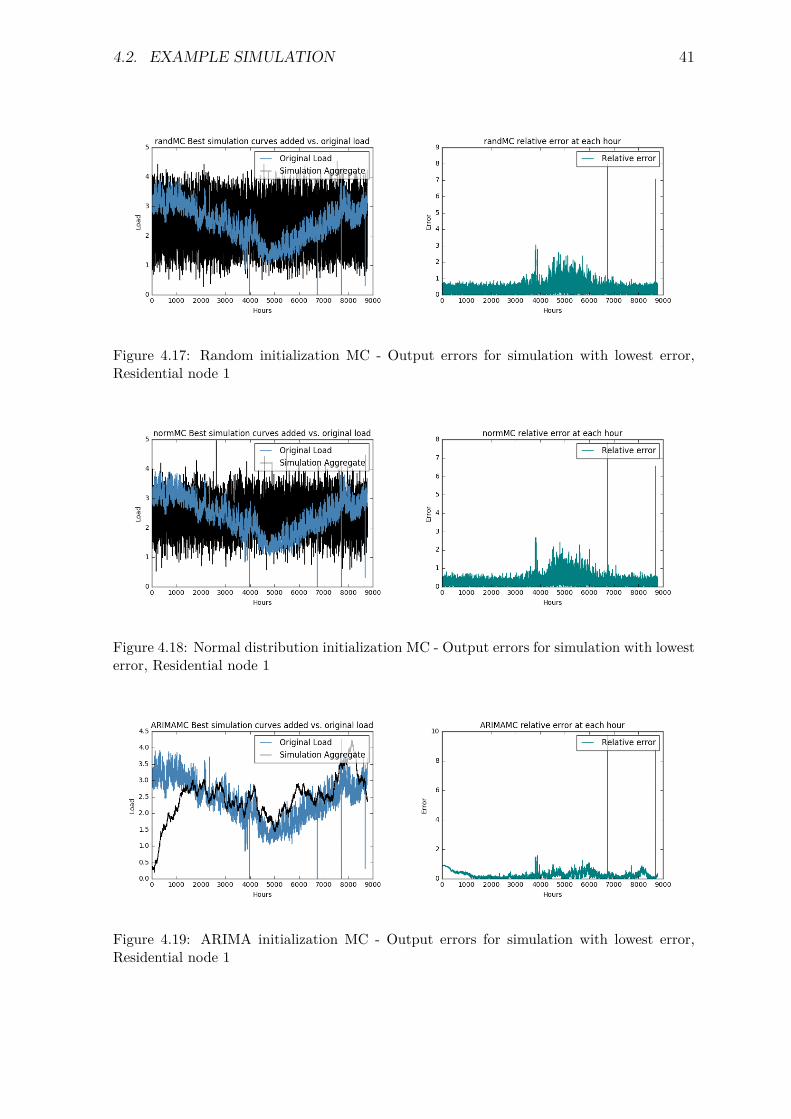
4.2. EXAMPLE SIMULATION 41
Figure 4.17: Random initialization MC - Output errors for simulation with lowest error,Residential node 1
Figure 4.18: Normal distribution initialization MC - Output errors for simulation with lowesterror, Residential node 1
Figure 4.19: ARIMA initialization MC - Output errors for simulation with lowest error,Residential node 1

42 CHAPTER 4. RESULTS
Figures 4.20 - 4.22 provide a zoom-in into the simulation error of the best outputmatrix at each hour. The left hand side depicts three weeks (504 hours), the right sideillustrates the hourly error for one week (168 hours), all starting at t = 3, 000.
Figure 4.20: Random initialization MC - Output errors for simulation with lowest errorzoom-in, Residential node 1
Figure 4.21: Normal distribution initialization MC - Output errors for simulation with lowesterror zoom-in, Residential node 1
Figure 4.22: ARIMA initialization MC - Output errors for simulation with lowest errorzoom-in, Residential node 1

4.3. GENERAL RESULTS 43
The error analysis allows the following conclusion on the performance of all three sim-ulation types for this example node: The ARIMA based Monte Carlo simulation wasthe only method to capture the nodal load pattern over the full year. It also yieldedthe lowest sum of relative errors for the best matrix. For the random uniform andnormal distribution simulations, no yearly variation was modelled. Instead the curvethat displays the relative error at each hour t exhibits a seasonal pattern over thesimulated year. It seems that errors are significantly higher for the summer months,which indicates a systematic neglect of the yearly seasonality from the data set.
The modelling of higher resolution patterns can be analyzed further by looking atthe zoom into the relative error curves. For the ARIMA simulation, the error curveexhibits a clear daily and weekly seasonality which indicates that a rather big portionof those patterns was missed in the simulation. It was already stated that for the othertwo MC approaches, the noisiness of the simulated data prevents a clear conclusionon daily or weekly patterns. However, the hourly simulation error looks quite randomas well, only a slight weekly pattern (three peaks in the three weeks excerpt) can beidentified. This does not necessarily mean that those two approaches were able tosimulate the daily pattern present in the original data. Instead, for both of them theerror level is significantly higher than for the ARIMA based simulation so that theirgeneral quality has to be questioned.
Even though it overall seems to perform best at this node, the simulated ARIMAcurves start out at a value of zero and take about 2,000 hours, which equals 25 % ofthe simulated values, to converge to the correct load level. Looking back at Figure4.12 this property was expected and could most possibly be avoided by simulating alonger period of time.
4.3 General ResultsThe following tables compare the simulation results from all eight nodes. For eachnode, all three MC approaches were implemented over 10,000 iterations. Several indi-cators and measurements will be used for a holistic quality assessment of the algorithmand its variations and their performance at different nodes. Firstly, error measure-ments regarding the best simulation output matrix from the random uniform, normaldistribution and ARIMA MC will be looked at:
• Index of the simulation iteration where the best simulation output matrix wasachieved
• Sum of relative errors from the best simulation output matrix
• Average relative error over all time steps t from the best simulation output matrix
Then, indicators that represent all simulation iterations will be analyzed to get anoverview of general performance of the algorithms:
• Runtime over all 10,000 simulations
• Mean output error sum for outputs from all simulation iterations
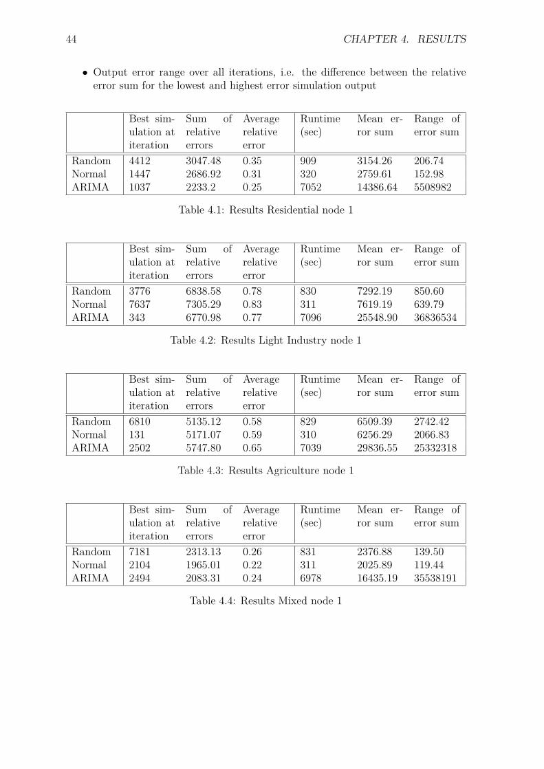
44 CHAPTER 4. RESULTS
• Output error range over all iterations, i.e. the difference between the relativeerror sum for the lowest and highest error simulation output
Best sim-ulation atiteration
Sum ofrelativeerrors
Averagerelativeerror
Runtime(sec)
Mean er-ror sum
Range oferror sum
Random 4412 3047.48 0.35 909 3154.26 206.74Normal 1447 2686.92 0.31 320 2759.61 152.98ARIMA 1037 2233.2 0.25 7052 14386.64 5508982
Table 4.1: Results Residential node 1
Best sim-ulation atiteration
Sum ofrelativeerrors
Averagerelativeerror
Runtime(sec)
Mean er-ror sum
Range oferror sum
Random 3776 6838.58 0.78 830 7292.19 850.60Normal 7637 7305.29 0.83 311 7619.19 639.79ARIMA 343 6770.98 0.77 7096 25548.90 36836534
Table 4.2: Results Light Industry node 1
Best sim-ulation atiteration
Sum ofrelativeerrors
Averagerelativeerror
Runtime(sec)
Mean er-ror sum
Range oferror sum
Random 6810 5135.12 0.58 829 6509.39 2742.42Normal 131 5171.07 0.59 310 6256.29 2066.83ARIMA 2502 5747.80 0.65 7039 29836.55 25332318
Table 4.3: Results Agriculture node 1
Best sim-ulation atiteration
Sum ofrelativeerrors
Averagerelativeerror
Runtime(sec)
Mean er-ror sum
Range oferror sum
Random 7181 2313.13 0.26 831 2376.88 139.50Normal 2104 1965.01 0.22 311 2025.89 119.44ARIMA 2494 2083.31 0.24 6978 16435.19 35538191
Table 4.4: Results Mixed node 1

4.3. GENERAL RESULTS 45
Best sim-ulation atiteration
Sum ofrelativeerrors
Averagerelativeerror
Runtime(sec)
Mean er-ror sum
Range oferror sum
Random 7934 3207.37 0.37 824 3304.69 189.69Normal 7235 3125.96 0.36 311 3208.34 173.10ARIMA 5316 2520.48 0.29 7173 18764.44 20971042
Table 4.5: Results Residential node 2
Best sim-ulation atiteration
Sum ofrelativeerrors
Averagerelativeerror
Runtime(sec)
Mean er-ror sum
Range oferror sum
Random 2335 276161.52 31.44 831 302321.66 54407.91Normal 8072 310695.97 35.37 307 330893.47 40258.72ARIMA 2290 33226.27 3.78 7225 557004.79 87253942
Table 4.6: Results Light Industry node 2
Best sim-ulation atiteration
Sum ofrelativeerrors
Averagerelativeerror
Runtime(sec)
Mean er-ror sum
Range oferror sum
Random 1174 3011.91 0.34 827 3138.60 248.10Normal 9370 2486.07 0.28 306 2588.53 190.30ARIMA 437 3210.84 0.37 7193 22746.89 36330647
Table 4.7: Results Agriculture node 2
Best sim-ulation atiteration
Sum ofrelativeerrors
Averagerelativeerror
Runtime(sec)
Mean er-ror sum
Range oferror sum
Random 8914 4643.01 0.53 828 4848.67 412.50Normal 5097 4748.82 0.54 309 4916.67 343.01ARIMA 4672 4470.34 0.51 7125 29258.70 92879491
Table 4.8: Results Mixed node 2

46 CHAPTER 4. RESULTS
Regarding the measurements that concern the best simulation outputs of each of theMC approaches, the following conclusions can be drawn: Firstly, it seems that the in-dex of the simulation iteration where a best matrix is reached is completely arbitraryfor all approaches and nodes. Secondly, when comparing the sum of relative errorsfor the best matrices of each approach and at every node, several things are notable.The ARIMA solution generates the best best5 simulation five out of eight times. Thenormal distribution approach provides the best best simulation two times, the randomMC only undercuts the others at one of the nodes. Amongst the nodes where theARIMA simulation performed best is Agriculture node 1, where the original data ispart of the pattern that underlies the ARIMA model for agricultural load. At thisnode, the ARIMA simulation undercuts the random uniform solution by only 0.01 andgenerally the average relative error is very high with 0.58 for the ARIMA simulation.It seems that, for this example, the relation to the real nodal pattern did not have apositive impact on the error. In fact, the ARIMA simulation performed significantlybetter at the other agriculture node.
The magnitude of the error and therefore the quality of the estimation however variesover all eight nodes. The lowest sum of relative errors, 1, 965, and an average rela-tive error of 0.22 over every simulated time step t is achieved for Mixed node 1 andgenerated using the normal distribution approach. The highest error sum for a bestmatrix is 310, 695 with an average relative error of 35.37 per time step. This extremelyhigh error represents the best solution from the normal distribution approach for LightIndustry node 2. The average relative error for the ARIMA MC at this node is 3.78,which is ten times lower. Generally, simulations at this node produce very high errorscompared to the other nodes, where most average relative errors lie between 0.22 and0.60.
Errors for the ARIMA simulation include the time steps where the model needs timeto converge. If the first 2,000 time steps are ignored, ARIMA simulations generate thebest best simulation at six of the nodes. This is backed by graphic analysis. Pleaserefer to Appendix A for plots that illustrate the aggregated simulated loads versus theoriginal load, similar to Figures 4.17, 4.18 and 4.19 in the previous section. It becomesclear that, like at the residential example node from the previous section, the ARIMAsimulation output is the only one to generate a yearly pattern which resembles theoriginal load’s yearly fluctuation. The nodes where random uniform and normal dis-tribution samples generate a better best output are often nodes with a very stationaryload which do not exhibit an overall yearly trend. In those cases the rather constantrandom uniform/ normally distributed simulations seem to coincidentally meet theoverall load pattern.
Examining the performance of all three MC approaches over all iterations and notjust the one that yielded a best simulation, it can be concluded that again randomuniform and normal distribution behave quite similarly while the ARIMA MC pro-vides some very different measurements. Especially looking at the runtime, it standsout with over 7,000 seconds (or almost two hours) per 10,000 iterations. With around
5As explained in Figure 3.14, the simulation output from the Monte Carlo method proposed inthis thesis is the best solution in terms of error. To determine which of the MC variations performswith the lowest error, their best solutions are compared and a best best solution specific to a node isidentified.

4.4. BENCHMARK TESTING 47
15 and 5 minutes per 10,000 iterations, the random uniform and normal distributionsimulations seem to be a lot less computationally expensive. This is no surprise as theARIMA MC method samples four curves with 8,760 data points from four seasonalARIMA models with at least 10 coefficients each. Looking at the mean relative er-ror sum, computed based on the output matrices from every iteration, an observationmade in the previous section is reinforced: The range and thus the mean of outputmatrix error sums is extremely high for the ARIMA model. In this context, it becomesclear that a high number of simulation iterations is more important for the ARIMAMC than for the other two methods where the output error is more constant. Thisshows that while it produces the best simulations for a majority of the test nodes,the ARIMA method also generates simulations that have very high errors. Those arehowever discarded in the MC algorithm, so that ultimately the ARIMA approach hasthe best performance out of the three methods proposed in this thesis.
Judging from the present example simulations it is difficult to derive a connectionbetween the performance of the approaches and the node type. Generally, it can benoted that all approaches perform relatively well for the residential nodes. Especiallythe ARIMA approach stands out with average relative errors of 0.25 and 0.29. Thiscould indicate that the representative pattern for RPP load is especially informativeand valid for both nodes. The opposite is true for light industry dominated loads: Herethe average relative errors lie between 0.77 and the extremely high 35.37. For bothlight industry nodes the ARIMA model performed best. However, comparing to theerror rates achieved by ARIMA simulations for other nodes, the light industry nodesyield significantly higher simulation errors. This allows the conclusion that the repre-sentative pattern that was used to train the ARIMA model from which light industrycurves are sampled, is not viable, as has been suspected before. For the other nodetypes no such general relationship can be determined.
4.4 Benchmark TestingIn the previous section it was concluded that out of the three approaches proposedin this thesis, the simulations which sample from ARIMA models trained on repre-sentative user curves, perform with the lowest error. Nonetheless, it has already beenconcluded that the ARIMA method has several flaws; Higher resolution patterns arenot modelled, the curves take about 2, 000 time steps to converge and negative loadvalues are sampled. To ultimately conclude on the viability of the proposed modellingapproach, it is important to test its output against the benchmark method, curvescomputed based on the average end user divisions. This stage of testing has to becarried out in a qualitative manner, because again, the error for the individual usercurves is not quantifiable. If the average curves were to be tested with regards tothe relative error sum as computed with equation 3.2, the observations would haveno value, since the error sum must logically be zero. This measurement is thereforenot suitable to compare the simulation output to the benchmark method. A graphicrepresentation will be used instead.
Figure 4.23 depicts the hourly end user divisions computed from the ARIMA sim-ulation output for the residential node that was previously used as an example. Thegraphs, which show the full year and a 72 hour zoom-in at t = 3, 000, illustrate how

48 CHAPTER 4. RESULTS
Figure 4.23: End user divisions from simulation output, best ARIMA simulation, Residentialnode 1
the (simulated) end user divisions are stable over the course of the year and seemto vary around the average. Even though no final conclusion can be drawn withoutinformation about the real distribution, this seems potentially realistic and might be abetter approximation than assuming the average end user divisions are valid for everytime step (i.e. a straight line over the course of the full data set). However, sincesome of the patterns are absent in the underlying simulation output, those end userdivisions are to be treated with some reservation.
More about the quality of the simulation output can be learnt when directly compar-ing it to the benchmark curves, obtained by multiplying the average end user divisionswith every time step of a node’s load.
Figure 4.24: Average curves vs. simulated curves zoom-in: Residential node 1
Figures 4.24 - 4.27 compare zoom-ins of 72 data points for both set-ups at the fourexample nodes from section 3.1. They allow several conclusions: As mentioned before,the patterns generated in the ARIMA simulation lack detail in the higher resolutionand contain values below zero. In comparison, the benchmark method provides moredistinctive patterns. However, those patterns simply follow the nodal load so that eachcurve is a skewed version of the original aggregate. Especially looking at figure 4.25,it is unrealistic that residential load follows this kind of (industrial) pattern, when atthe other nodes it looks quite different. Looking at the outputs from the ARIMA sim-

4.4. BENCHMARK TESTING 49
Figure 4.25: Average curves vs. simulated curves zoom-in: Light Industry node 1
Figure 4.26: Average curves vs. simulated curves zoom-in: Agriculture node 1
Figure 4.27: Average curves vs. simulated curves zoom-in: Mixed node 1
ulations, it seems that they come closer to distinctive patterns for each user type thatare valid across nodes, which is assumed to be true at least for some of the user types.Unlike the benchmark curves, they do not simply follow the overall nodal pattern asthe average curves do by default.

Chapter 5
Discussion
This chapter draws a conclusion about the suitability of the approach for synthesizinguser type specific load curves, that was presented in this thesis. The first section dis-cusses the variations of the Monte Carlo method and concludes on their performance.Drawbacks of the method and potential improvements are listed. The second sectionproposes different methods that could potentially be viable to approach the presentproblem and thus gives an account of further research that could be done in this field.
5.1 ConclusionIt was the aim of this research project to explore the possibility of modelling consumertype specific electricity load for the case of Iceland. The task was carried out by de-veloping and testing a method that synthesizes the desired curves for different nodesin the Icelandic system. No original user curves were available as input data, howeverthe aggregated load from 44 nodes and their corresponding average end user divisionswere given. The main difficulty was therefore to infer the hourly resolution patternsthat characterize consumer behaviour at the different nodes without knowing anythingabout their nature other than averages.
Inspired by the literature, a Monte Carlo approach that simulates the curves, wasdeveloped, implemented and tested. Here, the conditions defined by the data set (theend user divisions and therefore yearly targets for each curve) were used to force thesimulations to the correct load level. Another piece of information from the data set,the hourly values for the original load and thus the target for the aggregate of thesynthesized curves, was used to compute or approximate a quality measurement forthe simulation output because detailed test data was unavailable.
Each of the three Monte Carlo variations that were tested, was equipped with a dif-ferent distribution to sample its values from. While the approach that picked randomnumbers from a defined interval includes no additional information, the other two ap-proaches are based on representative load curves for each of the user types. Those wereextracted using a manual deduction approach based on load curves of nodes where auser type was dominant. This approach is based on the assumption that a representa-tive pattern, that is valid at all nodes, exists for each user type. Three reconstructiontests showed that this assumption loosely holds and the patterns have some merit eventhough they are only rough approximations.

5.1. CONCLUSION 51
Generally, all Monte Carlo approaches examined in this thesis generate solutions witha relatively high error with average relative factors of 0.22 to 35.37. It can howeverbe concluded that the approaches which simulate based on the information extractedfrom the representative user type curves, performed best in terms of error. Lookingback at the plots and histograms of the original data in section 3.1, this is not a sur-prising outcome. The simulation that picks from a random uniform distribution shouldby default have difficulties to match the distribution of real loads which mostly canbe approximated by normal distributions. The normal distribution approach, whichwas in fact the second best with regards to the eight test nodes, thus samples froma distribution that loosely matches the distributions underlying the aggregated loadsbut naturally misses time-dependency of the processes. ARIMA models, which predicta time series’ future values based on its past values, are a viable method to includesuch seasonal patterns. The ARIMA based simulation samples its values based on sea-sonal ARIMA models and thus incorporates the seasonalities of the training data sets,i.e. the representative user curves. The curves generated by the ARIMA MC roughlyfollow the original load if aggregated. This is best illustrated in Figure 4.19 where theerror at each simulated hour t appears to be without a clear yearly seasonality. Afterextensive error analysis it can however be concluded that the higher resolution patterns(weekly, daily) were not fully simulated even though re-occuring patterns were presentin the simulated data. However, the hourly simulation error showed clear seasonalitiesas well. Generally, with average relative errors between 0.25 and 0.77 (excluding thenode where errors are above 300 %) for the simulated curves it becomes clear that eventhis method is unable to simulate the full patterns for every user type. This resultis reinforced by the closer look at the simulated patterns (see section 4.4). However,compared to the benchmark curves based on average end user divisions, the simulationoutput seems to have the potential for a more realistic approximation. Unlike for theaverage curves, end user divisions are not constant and user type specific curves arenot mere skewed copies of the aggregated load.
The high errors and lack of detailed modelling even for the best MC method couldhave several reasons, all of which provide opportunities for improvement or furtherinquiry. Firstly, the Monte Carlo algorithm could be improved in terms of efficiency.This refers to both, reduction of the runtime, but also a pre-selection of simulationoutputs which discards high error solutions before the full curves are sampled. Definedattributes such as a threshold number of negative values or measures that control therelationships between curves could help to further describe the quality of the outputmatrix and help eliminating undesirable solutions early, thus improving efficiency andquality. However, those require assumptions with regards to the defined thresholds.
Secondly, the explanatory power of the approximated representative user curves mightbe limited. This was already observed in section 3.2.2, where it was concluded that itis difficult to find a pattern for light industry consumption that is valid for all nodes.The same could be true for agriculture (for example different kinds of farming mightrequire different energy inputs). The representative curves obtained using the man-ual deduction approach thus might not be an accurate representation, so that furtherwork could include finding better representative curves. Additionally it is questionablewhether the key assumption of a single representative pattern for every user type validat every node actually holds.

52 CHAPTER 5. DISCUSSION
Thirdly, the ARIMA models, which provide the basis for simulation, have potentialfor improvement. Different approaches are conceivable, amongst them the extensionof the models using weather input, calendar variables etc. or a re-fitting of the mod-els. Also the possibility of fitting multiplicative models should be investigated further.Additionally the sampling method itself could be improved, for example with the sam-pling of a longer time period so that the time the model needs to converge is excludedfrom the result. If the ARIMA simulations sampled positive values only, the problemof negative simulated load values would be eliminated. Since the sampling is carriedout using a built-in function where those attributes cannot be tuned, the developmentof a different method could yield potential for improvement of the simulation results.
Finally, other modelling methods which rely on representative patterns and introducea random component to them could be implemented. As an example and a methodthat can be used within the MC approach, Markov chains based on the representativepatterns come to mind.
As a general conclusion it can be stated that the simulation results improve withthe amount of information included through the sampling method. The ARIMA MCmethod’s performance could likely be enhanced with the inclusion of more and possi-bly node-specific data. This refers to the aforementioned weather and calendar databut also demographic and population data or behavioural variables such as workingschedules etc.. Necessary improvements have to be made with regards to the samplingmethod which at this point seems to neglect higher resolution patterns and producesnegative values. This thesis therefore comes to the conclusion that while it is notfeasible at this point, a Monte Carlo approach based on ARIMA models could be de-veloped further and have the potential to estimate user type specific curves for thecase of Iceland.
5.2 Further ResearchThe previous section already discussed possible improvements to the method presentedin this thesis. Further research on the subject could additionally include the followingtwo things: Further analysis of the data generated with the Monte Carlo approach andentirely different modelling methods.
Regarding the first point, it is important to state that this research project only rep-resents the first step in load profiling in Iceland. The simulated data could be treatedas samples and utilized in a top-down approach in order to generate load profiles forthe user types. Further analysis could also include the breakdown of the simulatedcurves into working days versus weekend/ holidays or winter versus summer loads.Additionally, the simulated data could be used as input into a forecasting model thatpredicts end user divisions on an hourly basis. Due to the high error present evenin the best simulations, all of those efforts should be seen as a further contributionto testing rather than an application of the simulated data. However, if the data isput to use, the results could yield further insights on the performance of the proposedapproach and highlight its flaws and qualities.

5.2. FURTHER RESEARCH 53
The majority of modelling methods that are imaginable to solve the present researchproblem involve detailed data on consumer behaviour such as load measurements ortime-use surveys. Conducting and including such measurements or surveys could ei-ther improve the presented approach or allow for the implementation of the top-downor bottom-up methods discussed in the literature review. A method that does notrequire further input but again assumes that user types have a specific pattern validat every node, is the formulation of the problem in terms of a matrix based linearequation system. Based on the available seven years of load data at 44 nodes and theircorresponding end user divisions, an optimization approach (e.g. least squares) couldbe used to solve for eight curves that fulfill this system of equations best. Generally,since no true data that can serve as a target is available, any models that requiretraining and rely on an error function to be optimized are difficult to implement.

Bibliography
[1] R. Griffin, David Bowie: The Golden Years. Omnibus Press, 2016.[2] L. Suganthi and A. A. Samuel, “Energy models for demand forecasting - A
review”, Renewable and sustainable energy reviews, vol. 16, no. 2, pp. 1223–1240, 2012.
[3] A. Veit, C. Goebel, R. Tidke, C. Doblander, and H.-A. Jacobsen, “Householdelectricity demand forecasting: benchmarking state-of-the-art methods”, in Pro-ceedings of the 5th international conference on Future energy systems, ACM,2014, pp. 233–234.
[4] C. Bucher and G. Andersson, “Generation of domestic load profiles-an adaptivetop-down approach”, in Proceedings of PMAPS, 2012, pp. 10–14.
[5] S. J. Davis, K. Caldeira, and H. D. Matthews, “Future CO2 emissions and climatechange from existing energy infrastructure”, Science, vol. 329, no. 5997, pp. 1330–1333, 2010.
[6] G. R. Esteves, B. Q. Bastos, F. L. Cyrino, R. F. Calili, and R. C. Souza,“Long term electricity forecast: a systematic review”, Procedia Computer Sci-ence, vol. 55, pp. 549–558, 2015.
[7] L. Ekonomou, “Greek long-term energy consumption prediction using artificialneural networks”, Energy, vol. 35, no. 2, pp. 512–517, 2010, ECOS 2008, issn:0360-5442. doi: https://doi.org/10.1016/j.energy.2009.10.018. [On-line]. Available: http://www.sciencedirect.com/science/article/pii/S0360544209004514.
[8] M. Ghiassi, D. K. Zimbra, and H. Saidane, “Medium term system load fore-casting with a dynamic artificial neural network model", journal = "ElectricPower Systems Research”, vol. 76, no. 5, pp. 302–316, 2006, issn: 0378-7796. doi:https://doi.org/10.1016/j.epsr.2005.06.010. [Online]. Available: http://www.sciencedirect.com/science/article/pii/S0378779605001951.
[9] W.-J. Lee and J. Hong, “A hybrid dynamic and fuzzy time series model formid-term power load forecasting”, International Journal of Electrical Power &Energy Systems, vol. 64, pp. 1057–1062, 2015, issn: 0142-0615. doi: https ://doi.org/10.1016/j.ijepes.2014.08.006. [Online]. Available: http://www.sciencedirect.com/science/article/pii/S0142061514005328.
[10] M. El-Telbany and F. El-Karmi, “Short-term forecasting of Jordanian electricitydemand using particle swarm optimization”, Electric Power Systems Research,vol. 78, no. 3, pp. 425–433, 2008, issn: 0378-7796. doi: https://doi.org/10.1016/j.epsr.2007.03.011. [Online]. Available: http://www.sciencedirect.com/science/article/pii/S0378779607000673.

BIBLIOGRAPHY 55
[11] A. Srivastava, A. S. Pandey, and D. Singh, “Short-term load forecasting methods:A review”, in Emerging Trends in Electrical Electronics & Sustainable EnergySystems (ICETEESES), International Conference on, IEEE, 2016, pp. 130–138.
[12] H. Hahn, S. Meyer-Nieberg, and S. Pickl, “Electric load forecasting methods:Tools for decision making”, European Journal of Operational Research, vol. 199,no. 3, pp. 902–907, 2009, issn: 0377-2217. doi: https://doi.org/10.1016/j.ejor.2009.01.062. [Online]. Available: http://www.sciencedirect.com/science/article/pii/S0377221709002094.
[13] R. Weron, Modeling and forecasting electricity loads and prices: A statisticalapproach. John Wiley & Sons, 2007, vol. 403.
[14] W. R. Christiaanse, “Short-Term Load Forecasting Using General ExponentialSmoothing”, IEEE Transactions on Power Apparatus and Systems, vol. PAS-90,no. 2, pp. 900–911, Mar. 1971, issn: 0018-9510. doi: 10.1109/TPAS.1971.293123.
[15] J. W. Taylor, “An evaluation of methods for very short-term load forecasting us-ing minute-by-minute British data”, International Journal of Forecasting, vol. 24,no. 4, pp. 645–658, 2008, Energy Forecasting, issn: 0169-2070. doi: https ://doi.org/10.1016/j.ijforecast.2008.07.007. [Online]. Available: http://www.sciencedirect.com/science/article/pii/S0169207008000708.
[16] A. D. Papalexopoulos and T. C. Hesterberg, “A regression-based approach toshort-term system load forecasting”, IEEE Transactions on Power Systems,vol. 5, no. 4, pp. 1535–1547, 1990.
[17] C. Sigauke and D. Chikobvu, “Daily peak electricity load forecasting in SouthAfrica using a multivariate non-parametric regression approach”, ORiON, vol. 26,no. 2, 2010.
[18] L. C. Hunt and Y. Ninomiya, “Primary energy demand in Japan: an empiricalanalysis of long-term trends and future CO2 emissions”, Energy Policy, vol. 33,no. 11, pp. 1409–1424, 2005.
[19] R. Haas and L. Schipper, “Residential energy demand in OECD-countries andthe role of irreversible efficiency improvements”, Energy economics, vol. 20, no. 4,pp. 421–442, 1998.
[20] B. Ang, “Decomposition methodology in industrial energy demand analysis”,Energy, vol. 20, no. 11, pp. 1081–1095, 1995, issn: 0360-5442. doi: https://doi.org/10.1016/0360-5442(95)00068-R. [Online]. Available: http://www.sciencedirect.com/science/article/pii/036054429500068R.
[21] K. Afshar and N. Bigdeli, “Data analysis and short term load forecasting in Iranelectricity market using singular spectral analysis (SSA)”, Energy, vol. 36, no. 5,pp. 2620–2627, 2011, issn: 0360-5442. doi: https://doi.org/10.1016/j.energy.2011.02.003. [Online]. Available: http://www.sciencedirect.com/science/article/pii/S0360544211000806.
[22] C. Guan, P. B. Luh, L. D. Michel, Y. Wang, and P. B. Friedland, “Very short-term load forecasting: wavelet neural networks with data pre-filtering”, IEEETransactions on Power Systems, vol. 28, no. 1, pp. 30–41, 2013.

56 BIBLIOGRAPHY
[23] S. G. Mallat, “A theory for multiresolution signal decomposition: the waveletrepresentation”, IEEE transactions on pattern analysis and machine intelligence,vol. 11, no. 7, pp. 674–693, 1989.
[24] N. Amjady and F. Keynia, “Short-term load forecasting of power systems bycombination of wavelet transform and neuro-evolutionary algorithm”, Energy,vol. 34, no. 1, pp. 46–57, 2009, issn: 0360-5442. doi: https://doi.org/10.1016/j.energy.2008.09.020. [Online]. Available: http://www.sciencedirect.com/science/article/pii/S0360544208002454.
[25] D. Benaouda, F. Murtagh, J.-L. Starck, and O. Renaud, “Wavelet-based nonlin-ear multiscale decomposition model for electricity load forecasting”, Neurocom-puting, vol. 70, no. 1, pp. 139–154, 2006, Neural Networks, issn: 0925-2312. doi:https://doi.org/10.1016/j.neucom.2006.04.005. [Online]. Available: http://www.sciencedirect.com/science/article/pii/S0925231206001172.
[26] C. W. Granger, “Developments in the study of cointegrated economic variables”,Oxford Bulletin of economics and statistics, vol. 48, no. 3, pp. 213–228, 1986.
[27] J. W. Taylor, “Short-term load forecasting with exponentially weighted meth-ods”, IEEE Transactions on Power Systems, vol. 27, no. 1, pp. 458–464, 2012.
[28] L. J. Soares and M. C. Medeiros, “Modeling and forecasting short-term elec-tricity load: A comparison of methods with an application to Brazilian data”,International Journal of Forecasting, vol. 24, no. 4, pp. 630–644, 2008.
[29] M. T. Hagan and S. M. Behr, “The time series approach to short term loadforecasting”, IEEE Transactions on Power Systems, vol. 2, no. 3, pp. 785–791,1987.
[30] E. A. Feinberg and D. Genethliou, “Load forecasting”, in Applied mathematicsfor restructured electric power systems, Springer, 2005, pp. 269–285.
[31] H. Hahn, S. Meyer-Nieberg, and S. Pickl, “Electric load forecasting methods:Tools for decision making”, European journal of operational research, vol. 199,no. 3, pp. 902–907, 2009.
[32] G. Juberias, R. Yunta, J. G. Moreno, and C. Mendivil, “A new ARIMA modelfor hourly load forecasting”, in Transmission and Distribution Conference, 1999IEEE, IEEE, vol. 1, 1999, pp. 314–319.
[33] N. H. Miswan, N. H. Hussin, R. M. Said, K. Hamzah, and E. Z. Ahmad, “ARARAlgorithm in Forecasting Electricity Load Demand in Malaysia”, Global Journalof Pure and Applied Mathematics, vol. 12, no. 1, pp. 361–367, 2016.
[34] H. K. Alfares and M. Nazeeruddin, “Electric load forecasting: literature surveyand classification of methods”, International journal of systems science, vol. 33,no. 1, pp. 23–34, 2002.
[35] D. C. Park, M. El-Sharkawi, R. Marks, L. Atlas, and M. Damborg, “Electricload forecasting using an artificial neural network”, IEEE transactions on PowerSystems, vol. 6, no. 2, pp. 442–449, 1991.
[36] T. Peng, N. Hubele, and G. G. Karady, “An adaptive neural network approach toone-week ahead load forecasting”, IEEE Transactions on Power Systems, vol. 8,no. 3, pp. 1195–1203, 1993.

BIBLIOGRAPHY 57
[37] L. Wang, Y. Zeng, and T. Chen, “Back propagation neural network with adaptivedifferential evolution algorithm for time series forecasting”, Expert Systems withApplications, vol. 42, no. 2, pp. 855–863, 2015.
[38] R. Hu, S. Wen, Z. Zeng, and T. Huang, “A short-term power load forecastingmodel based on the generalized regression neural network with decreasing stepfruit fly optimization algorithm”, Neurocomputing, vol. 221, pp. 24–31, 2017.
[39] F. M. Bianchi, E. Maiorino, M. C. Kampffmeyer, A. Rizzi, and R. Jenssen, “Anoverview and comparative analysis of recurrent neural networks for short termload forecasting”, arXiv preprint arXiv:1705.04378, 2017.
[40] K.-L. Ho, Y.-Y. Hsu, C.-F. Chen, T.-E. Lee, C.-C. Liang, T.-S. Lai, and K.-K.Chen, “Short term load forecasting of Taiwan power system using a knowledge-based expert system”, IEEE Transactions on Power Systems, vol. 5, no. 4,pp. 1214–1221, 1990.
[41] M. Kandil, S. M. El-Debeiky, and N. Hasanien, “Long-term load forecasting forfast developing utility using a knowledge-based expert system”, IEEE transac-tions on Power Systems, vol. 17, no. 2, pp. 491–496, 2002.
[42] E. Kayacan, B. Ulutas, and O. Kaynak, “Grey system theory-based models intime series prediction”, Expert systems with applications, vol. 37, no. 2, pp. 1784–1789, 2010.
[43] G.-D. Li, C.-H. Wang, S. Masuda, and M. Nagai, “A research on short termload forecasting problem applying improved grey dynamic model”, InternationalJournal of Electrical Power & Energy Systems, vol. 33, no. 4, pp. 809–816, 2011.
[44] J. Kang and H. Zhao, “Application of improved grey model in long-term loadforecasting of power engineering”, Systems engineering procedia, vol. 3, pp. 85–91, 2012.
[45] U. Kumar and V. Jain, “Time series models (Grey-Markov, Grey Model withrolling mechanism and singular spectrum analysis) to forecast energy consump-tion in India”, Energy, vol. 35, no. 4, pp. 1709–1716, 2010, Demand ResponseResources: the US and International Experience, issn: 0360-5442. doi: https://doi.org/10.1016/j.energy.2009.12.021. [Online]. Available: http://www.sciencedirect.com/science/article/pii/S0360544209005416.
[46] W. Leontief, “Sructure of the world economy: outline of a simple input-outputformulation”, The American Economic Review, pp. 823–834, 1974.
[47] Y.-J. Zhang, X.-J. Bian, W. Tan, and J. Song, “The indirect energy consumptionand CO2 emission caused by household consumption in China: an analysis basedon the input–output method”, Journal of Cleaner Production, vol. 163, pp. 69–83, 2017.
[48] J. Hong, G. Q. Shen, S. Guo, F. Xue, and W. Zheng, “Energy use embodied inChina’s construction industry: A multi-regional input–output analysis”, Renew-able and Sustainable Energy Reviews, vol. 53, pp. 1303–1312, 2016.
[49] D. Ranaweera, N. Hubele, and G. Karady, “Fuzzy logic for short term loadforecasting”, International journal of electrical power & energy systems, vol. 18,no. 4, pp. 215–222, 1996.

58 BIBLIOGRAPHY
[50] D. Ali, M. Yohanna, M. Puwu, and B. Garkida, “Long-term load forecast mod-elling using a fuzzy logic approach”, Pacific Science Review A: Natural Scienceand Engineering, vol. 18, no. 2, pp. 123–127, 2016.
[51] W.-J. Lee and J. Hong, “A hybrid dynamic and fuzzy time series model formid-term power load forecasting”, International Journal of Electrical Power &Energy Systems, vol. 64, pp. 1057–1062, 2015.
[52] D. Whitley, “A genetic algorithm tutorial”, Statistics and computing, vol. 4,no. 2, pp. 65–85, 1994.
[53] J. H. Holland, “Adaptation in natural and artificial systems. An introductoryanalysis with application to biology, control, and artificial intelligence”, AnnArbor, MI: University of Michigan Press, pp. 439–444, 1975.
[54] O. E. Canyurt and H. K. Ozturk, “Application of genetic algorithm (GA) tech-nique on demand estimation of fossil fuels in Turkey”, Energy Policy, vol. 36,no. 7, pp. 2562–2569, 2008.
[55] H. Ceylan and H. K. Ozturk, “Estimating energy demand of Turkey based oneconomic indicators using genetic algorithm approach”, Energy Conversion andManagement, vol. 45, no. 15-16, pp. 2525–2537, 2004.
[56] K. Metaxiotis, A. Kagiannas, D. Askounis, and J. Psarras, “Artificial intelli-gence in short term electric load forecasting: a state-of-the-art survey for theresearcher”, Energy Conversion and Management, vol. 44, no. 9, pp. 1525–1534,2003, issn: 0196-8904. doi: https://doi.org/10.1016/S0196- 8904(02)00148 - 6. [Online]. Available: http : / / www . sciencedirect . com / science /article/pii/S0196890402001486.
[57] S. B. Defilippo, G. G. Neto, and H. S. Hippert, “Short-term load forecastingby artificial neural networks specified by genetic algorithms–a simulation studyover a Brazilian dataset”, in XIII Simposio Argentino de Investigación Operativa(SIO)-JAIIO 44 (Rosario, 2015), 2015.
[58] T. Woniak, “Bayesian Vector Autoregressions”, Australian Economic Review,vol. 49, no. 3, pp. 365–380, 2016.
[59] B.-J. Chen, M.-W. Chang, et al., “Load forecasting using support vector ma-chines: A study on EUNITE competition 2001”, IEEE transactions on powersystems, vol. 19, no. 4, pp. 1821–1830, 2004.
[60] M. D. Toksar, “Ant colony optimization approach to estimate energy demand ofTurkey”, Energy Policy, vol. 35, no. 8, pp. 3984–3990, 2007.
[61] A. Ünler, “Improvement of energy demand forecasts using swarm intelligence:The case of Turkey with projections to 2025”, Energy Policy, vol. 36, no. 6,pp. 1937–1944, 2008.
[62] J. Wang, S. Zhu, W. Zhang, and H. Lu, “Combined modeling for electric loadforecasting with adaptive particle swarm optimization”, Energy, vol. 35, no. 4,pp. 1671–1678, 2010.
[63] G. P. Zhang, “Time series forecasting using a hybrid ARIMA and neural networkmodel”, Neurocomputing, vol. 50, pp. 159–175, 2003.

BIBLIOGRAPHY 59
[64] A. Kavousi-Fard, H. Samet, and F. Marzbani, “A new hybrid modified fire-fly algorithm and support vector regression model for accurate short term loadforecasting”, Expert systems with applications, vol. 41, no. 13, pp. 6047–6056,2014.
[65] K.-H. Kim, J.-K. Park, K.-J. Hwang, and S.-H. Kim, “Implementation of hybridshort-term load forecasting system using artificial neural networks and fuzzyexpert systems”, IEEE Transactions on Power Systems, vol. 10, no. 3, pp. 1534–1539, 1995.
[66] V. N. Coelho, I. M. Coelho, B. N. Coelho, A. J. Reis, R. Enayatifar, M. J. Souza,and F. G. Guimarães, “A self-adaptive evolutionary fuzzy model for load fore-casting problems on smart grid environment”, Applied Energy, vol. 169, pp. 567–584, 2016.
[67] A. Abdoos, M. Hemmati, and A. A. Abdoos, “Short term load forecasting usinga hybrid intelligent method”, Knowledge-Based Systems, vol. 76, pp. 139–147,2015.
[68] S. Li, P. Wang, and L. Goel, “A novel wavelet-based ensemble method for short-term load forecasting with hybrid neural networks and feature selection”, IEEETransactions on power systems, vol. 31, no. 3, pp. 1788–1798, 2016.
[69] R. Loulou, G. Goldstein, K. Noble, et al., “Documentation for the MARKALFamily of Models”, Energy Technology Systems Analysis Programme, pp. 65–73,2004.
[70] A. J. Seebregts, G. A. Goldstein, and K. Smekens, “Energy/environmental mod-eling with the MARKAL family of models”, in Operations research proceedings2001, Springer, 2002, pp. 75–82.
[71] C. Heaps, “An introduction to LEAP”, Stockholm Environment Institute, pp. 1–16, 2008.
[72] T. Hong and S. Fan, “Probabilistic electric load forecasting: A tutorial review”,International Journal of Forecasting, vol. 32, no. 3, pp. 914–938, 2016.
[73] J. V. Paatero and P. D. Lund, “A model for generating household electricity loadprofiles”, International journal of energy research, vol. 30, no. 5, pp. 273–290,2006.
[74] N. Anuar and Z. Zakaria, “Electricity load profile determination by using fuzzycmeans and probability neural network”, Energy Procedia, vol. 14, pp. 1861–1869, 2012.
[75] K. Alvehag, “Impact of dependencies in risk assessments of power distributionsystems”, PhD thesis, KTH, 2008.
[76] F. M. Andersen, H. V. Larsen, and T. K. Boomsma, “Long-term forecasting ofhourly electricity load: Identification of consumption profiles and segmentationof customers”, Energy conversion and Management, vol. 68, pp. 244–252, 2013.
[77] M. M. Armstrong, M. C. Swinton, H. Ribberink, I. Beausoleil-Morrison, and J.Millette, “Synthetically derived profiles for representing occupant-driven electricloads in Canadian housing”, Journal of Building Performance Simulation, vol. 2,no. 1, pp. 15–30, 2009.
60 BIBLIOGRAPHY
[78] D. Shiming and J. Burnett, “Energy use and management in hotels in HongKong”, International Journal of Hospitality Management, vol. 21, no. 4, pp. 371–380, 2002.
[79] C. F. Walker and J. L. Pokoski, “Residential load shape modelling based oncustomer behavior”, IEEE Transactions on Power Apparatus and Systems, no. 7,pp. 1703–1711, 1985.
[80] A. Capasso, W. Grattieri, R. Lamedica, and A. Prudenzi, “A bottom-up ap-proach to residential load modeling”, IEEE Transactions on Power Systems,vol. 9, no. 2, pp. 957–964, 1994.
[81] C. Sandels, J. Widén, and L. Nordström, “Forecasting household consumer elec-tricity load profiles with a combined physical and behavioral approach”, Appliedenergy, vol. 131, pp. 267–278, 2014.
[82] D. P. Kroese, T. Brereton, T. Taimre, and Z. I. Botev, “Why the Monte Carlomethod is so important today”, Wiley Interdisciplinary Reviews: ComputationalStatistics, vol. 6, no. 6, pp. 386–392, 2014.
[83] M. Nijhuis, M. Gibescu, and J. Cobben, “Bottom-up markov chain monte carloapproach for scenario based residential load modelling with publicly availabledata”, Energy and Buildings, vol. 112, pp. 121–129, 2016.
[84] F. Jay and J. Goetz, “IEEE standard dictionary of electrical and electronicsterms”, Institute of Electrical and Electronics Engineers, 1988.
[85] W. Labeeuw and G. Deconinck, “Residential electrical load model based on mix-ture model clustering and Markov models”, IEEE Transactions on IndustrialInformatics, vol. 9, no. 3, pp. 1561–1569, 2013.
[86] H. Ólafsson, M. Furger, and B. Brummer, “The weather and climate of Iceland”,Meteorologische Zeitschrift, vol. 16, no. 1, pp. 5–8, 2007.
[87] Orkustofnun, “Energy Statistics in Iceland in 2016”, (2017).[88] Landsvirkjun, “Annual Report 2016”, (2017).[89] Orkustofnun, “OS-2017-T016-01: Development of electricity consumption in Ice-
land (2016)”, (2017).[90] Landsnet, “Annual Report - Landsnet 2016”, (2017).[91] ——, “Annual Report - Landsnet 2015”, (2016).[92] EFLA Verkfræðistofa, “KOSTNAÐUR VEGNA RAFORKUSKORTS Tölur til
notkunar árin 2016 og 2017”, (2016).[93] S. Perkin, personal communication, 2018.[94] H. Liao and D. Niebur, “Load profile estimation in electric transmission networks
using independent component analysis”, IEEE Transactions on Power Systems,vol. 18, no. 2, pp. 707–715, 2003.
[95] D. D. McCracken, “The monte carlo method”, Scientific American, vol. 192,no. 5, pp. 90–97, 1955.

Appendix A
Appendix
Figure A.1: Node types example 2, two weeks zoom-in

62 APPENDIX A. APPENDIX
Figure A.2: Autocorrelation functions Light Industry time series
Figure A.3: Autocorrelation functions Agriculture time series
Figure A.4: Autocorrelation functions Utilities time series

63
Figure A.5: Residuals Light Industry ARIMA
Figure A.6: Residuals Agriculture ARIMA

64 APPENDIX A. APPENDIX
Figure A.7: Residuals Utilities ARIMA
Figure A.8: Random initialization MC - Output from simulation with lowest error, LightIndustry node 1
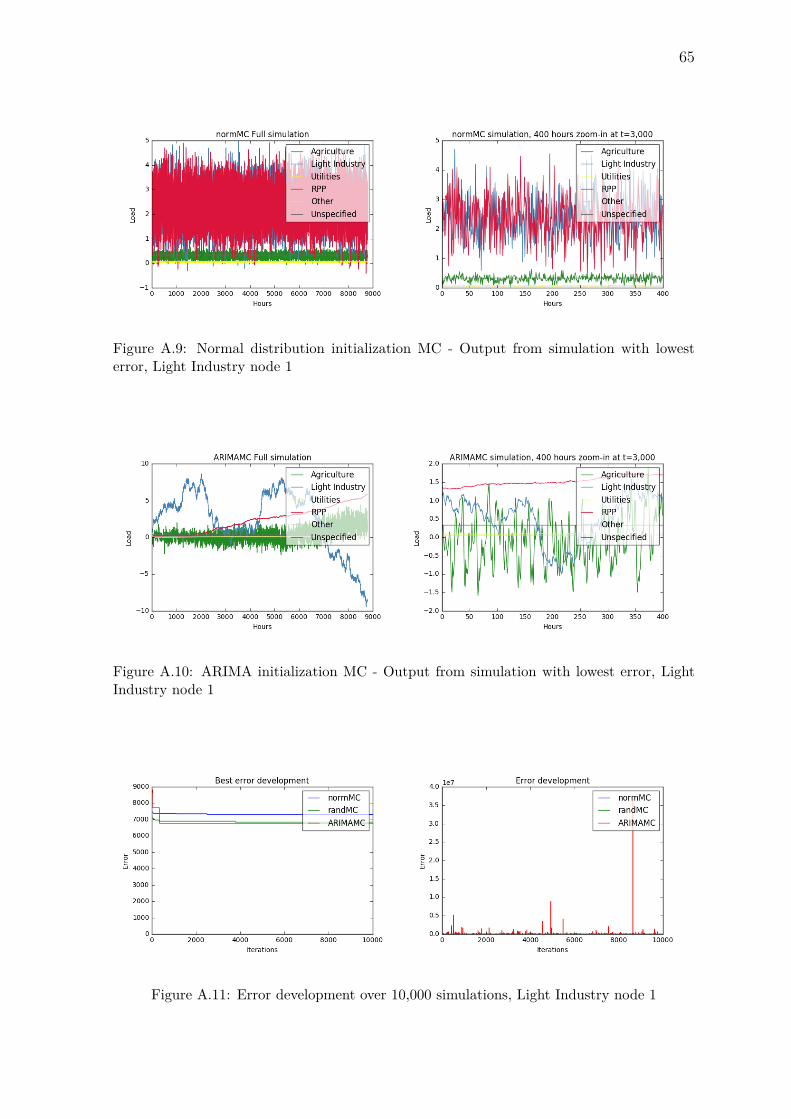
65
Figure A.9: Normal distribution initialization MC - Output from simulation with lowesterror, Light Industry node 1
Figure A.10: ARIMA initialization MC - Output from simulation with lowest error, LightIndustry node 1
Figure A.11: Error development over 10,000 simulations, Light Industry node 1

66 APPENDIX A. APPENDIX
Figure A.12: Random initialization MC - Output errors for simulation with lowest error,Light Industry node 1
Figure A.13: Normal distribution initialization MC - Output errors for simulation with lowesterror, Light Industry node 1
Figure A.14: ARIMA initialization MC - Output errors for simulation with lowest error,Light Industry node 1

67
Figure A.15: Random initialization MC - Output from simulation with lowest error, Agri-culture node 1
Figure A.16: Normal distribution initialization MC - Output from simulation with lowesterror, Agriculture node 1
Figure A.17: ARIMA initialization MC - Output from simulation with lowest error, Agricul-ture node 1

68 APPENDIX A. APPENDIX
Figure A.18: Error development over 10,000 simulations - Agriculture node 1
Figure A.19: Random initialization MC - Output errors for simulation with lowest error,Agriculture node 1
Figure A.20: Normal distribution initialization MC - Output errors for simulation with lowesterror, Agriculture node 1

69
Figure A.21: ARIMA initialization MC - Output errors for simulation with lowest error,Agriculture node 1
Figure A.22: Random initialization MC - Output from simulation with lowest error, Mixednode 1
Figure A.23: Random initialization MC - Output from simulation with lowest error, Mixednode 1

70 APPENDIX A. APPENDIX
Figure A.24: ARIMA initialization MC - Output from simulation with lowest error, Mixednode 1
Figure A.25: Error development over 10,000 simulations - Mixed node 1
Figure A.26: Random initialization MC - Output errors for simulation with lowest error,Mixed node 1

71
Figure A.27: Normal distribution initialization MC - Output errors for simulation with lowesterror, Mixed node 1
Figure A.28: ARIMA initialization errors - Mixed node 1

72