Modelling and simulation of reinforced concretebeamsCoupled analysis of imperfectly bonded reinforcement in fracturing

concreteMaster’s thesis in Solid and Structural Mechanics

DIMOSTHENIS FLOROS

OLAFUR AGUST INGASON

Department of Applied MechanicsDivision of Solid MechanicsCHALMERS UNIVERSITY OF TECHNOLOGYGoteborg, Sweden 2013Master’s thesis 2013:42

MASTER’S THESIS IN SOLID AND STRUCTURAL MECHANICS

Modelling and simulation of reinforced concrete beams

Coupled analysis of imperfectly bonded reinforcement in fracturing concrete

DIMOSTHENIS FLOROSOLAFUR AGUST INGASON

Department of Applied MechanicsDivision of Solid Mechanics

CHALMERS UNIVERSITY OF TECHNOLOGY

Goteborg, Sweden 2013

Modelling and simulation of reinforced concrete beamsCoupled analysis of imperfectly bonded reinforcement in fracturing concreteDIMOSTHENIS FLOROSOLAFUR AGUST INGASON

© DIMOSTHENIS FLOROS , OLAFUR AGUST INGASON, 2013

Master’s thesis 2013:42ISSN 1652-8557Department of Applied MechanicsDivision of Solid MechanicsChalmers University of TechnologySE-412 96 GoteborgSwedenTelephone: +46 (0)31-772 1000

Cover:Results from the developed program not accounting for tension softening. The graphs showfrom the top, steel stress ,bond-slip and crack pattern

Chalmers ReproserviceGoteborg, Sweden 2013

Modelling and simulation of reinforced concrete beamsCoupled analysis of imperfectly bonded reinforcement in fracturing concreteMaster’s thesis in Solid and Structural MechanicsDIMOSTHENIS FLOROSOLAFUR AGUST INGASONDepartment of Applied MechanicsDivision of Solid MechanicsChalmers University of Technology

Abstract

Cracking in reinforced concrete beams is a normal process. It occurs for a small portion of theultimate load, already in the service state. This kind of local failure in concrete is quantifiedmainly via crack widths and crack spacing in the tensile zone. Durability, functionality andaesthetics are the main reasons why the aforementioned characteristics should be limited topredefined values. Due to cracking, stiffness redistribution takes place in the flexural memberand the reinforced concrete section can no longer be considered to act as a linear elastic,homogeneous material. In addition, the connection between the reinforcement bars and thesurrounding concrete is not perfect. A certain slip in the interface between the two materialsneeds to be considered. Thus, the non-linear constitutive response of concrete and the bond-sliprelation need to be incorporated in an accurate model of a reinforced concrete beam underfracture.

This thesis aims to develop a finite element model of a beam that is able to describe theinteraction between the reinforcement bars and the cracked concrete. Emphasis is given to theparameter of the two predominant length scales in reinforced concrete structures: the localdamage in concrete, which comprises the small scale, and the finite length of the reinforcementbars, which accounts for the large scale. For the development of such a 1D model, advancedbeam elements were employed, where the effects of the reinforcement bars were homogenizedover the concrete cross-section. The implementation and a non-linear FE analysis of themodel were performed in a Matlab code. Outputs from that analysis were compared to (i)experimental results from literature, (ii) analytical calculations of a reinforced concrete beamaccounting for tension stiffening, (iii) a 1D beam-type model where fracture of concrete wastaken into consideration by the stiffness adaptation method, and, (iv) a FE beam-type modelconsidering perfect bond between the constitutive materials developed in the Diana software.The results from the developed model were found to correspond well to the aforementionedmethods and the experimental curves. However, further parametric studies are proposed inorder to improve the performance of the model.

Keywords: reinforced concrete beam; cracking; bond-slip; length scales

i

ii

Contents

Abstract i

Contents iii

1 Introduction 1

2 Modelling techniques 32.1 Modelling of the behaviour of reinforced concrete beams . . . . . . . . . . . . . . 32.1.1 3D modelling . . . . . . . . . . . . . . . . . . . . . . . . . . . . . . . . . . . . . 42.1.2 2D modelling . . . . . . . . . . . . . . . . . . . . . . . . . . . . . . . . . . . . . 52.2 Beam models . . . . . . . . . . . . . . . . . . . . . . . . . . . . . . . . . . . . . . 62.2.1 Multi-fibre beam model . . . . . . . . . . . . . . . . . . . . . . . . . . . . . . . 82.2.2 Applications accounting for the damaged concrete . . . . . . . . . . . . . . . . . 92.2.3 Applications accounting for cracking and bond-slip . . . . . . . . . . . . . . . . 10

3 A model for reinforced concrete beams 113.1 Derivation of the non-linear continuous formulation . . . . . . . . . . . . . . . . . 123.1.1 Cross sectional forces . . . . . . . . . . . . . . . . . . . . . . . . . . . . . . . . . 123.1.2 Equilibrium conditions . . . . . . . . . . . . . . . . . . . . . . . . . . . . . . . . 123.1.3 Kinematic relations . . . . . . . . . . . . . . . . . . . . . . . . . . . . . . . . . . 143.2 FE formulation . . . . . . . . . . . . . . . . . . . . . . . . . . . . . . . . . . . . . 163.2.1 Differential equations and boundary conditions . . . . . . . . . . . . . . . . . . 163.2.2 Weak form . . . . . . . . . . . . . . . . . . . . . . . . . . . . . . . . . . . . . . 163.2.3 Boundary conditions . . . . . . . . . . . . . . . . . . . . . . . . . . . . . . . . . 173.2.4 Constitutive equations . . . . . . . . . . . . . . . . . . . . . . . . . . . . . . . . 183.2.5 Introduce the constitutive relations into the weak form . . . . . . . . . . . . . . 183.2.6 Discretization of the continuous displacements field . . . . . . . . . . . . . . . . 193.2.7 Galerkin’s method . . . . . . . . . . . . . . . . . . . . . . . . . . . . . . . . . . 203.2.8 Formulation of the internal force vector . . . . . . . . . . . . . . . . . . . . . . . 213.2.9 Involve essential boundary conditions . . . . . . . . . . . . . . . . . . . . . . . . 223.3 Linearization of the non-linear problem . . . . . . . . . . . . . . . . . . . . . . . . 243.3.1 Linearization of the FE-equations . . . . . . . . . . . . . . . . . . . . . . . . . . 243.4 Constitutive models . . . . . . . . . . . . . . . . . . . . . . . . . . . . . . . . . . 303.4.1 Concrete . . . . . . . . . . . . . . . . . . . . . . . . . . . . . . . . . . . . . . . . 303.4.2 Reinforcement steel . . . . . . . . . . . . . . . . . . . . . . . . . . . . . . . . . . 343.4.3 Bond-slip . . . . . . . . . . . . . . . . . . . . . . . . . . . . . . . . . . . . . . . 343.5 Numerical schemes . . . . . . . . . . . . . . . . . . . . . . . . . . . . . . . . . . . 363.5.1 Newton’s method . . . . . . . . . . . . . . . . . . . . . . . . . . . . . . . . . . . 363.5.2 Incremental methods . . . . . . . . . . . . . . . . . . . . . . . . . . . . . . . . . 373.5.3 Numerical integration . . . . . . . . . . . . . . . . . . . . . . . . . . . . . . . . 393.5.4 Step control . . . . . . . . . . . . . . . . . . . . . . . . . . . . . . . . . . . . . . 413.6 Strain localization and mesh dependency . . . . . . . . . . . . . . . . . . . . . . . 423.7 Description and flowchart of the program . . . . . . . . . . . . . . . . . . . . . . . 45

iii

4 Evaluation and comparison with experiments and Eurocode 474.1 Experiments from literature . . . . . . . . . . . . . . . . . . . . . . . . . . . . . . 474.2 Analytical calculations . . . . . . . . . . . . . . . . . . . . . . . . . . . . . . . . . 484.2.1 Mid span deflection . . . . . . . . . . . . . . . . . . . . . . . . . . . . . . . . . . 484.2.2 Tensile strength . . . . . . . . . . . . . . . . . . . . . . . . . . . . . . . . . . . . 494.2.3 Steel stress . . . . . . . . . . . . . . . . . . . . . . . . . . . . . . . . . . . . . . 494.2.4 Crack widths . . . . . . . . . . . . . . . . . . . . . . . . . . . . . . . . . . . . . 504.3 Analysis with the developed beam model . . . . . . . . . . . . . . . . . . . . . . . 514.4 Comparison of results . . . . . . . . . . . . . . . . . . . . . . . . . . . . . . . . . 534.4.1 Stiffness adaptation method . . . . . . . . . . . . . . . . . . . . . . . . . . . . . 534.4.2 Diana analysis . . . . . . . . . . . . . . . . . . . . . . . . . . . . . . . . . . . . 534.4.3 Global deflection and crack widths . . . . . . . . . . . . . . . . . . . . . . . . . 544.4.4 Crack pattern . . . . . . . . . . . . . . . . . . . . . . . . . . . . . . . . . . . . . 55

5 Conclusions and suggestions for further work 56

References 58

iv

1 Introduction

Reinforced concrete beams are flexural members which, in the ultimate limit state, are designedallowing for a certain local damage to take place, assuming all tensile forces to be carriedby the steel bars. The limit of that damage in a cross-sectional design process is governedby the ultimate compressive strain of concrete so as to avoid crushing when yielding of thereinforcement bars occurs. Hence, the occurrence of cracking in concrete is a rather expectedphenomenon for relatively high loads. It should be noted however, that cracks, in cases whereno prestressing is applied, are expected to form even for a small portion of the ultimate load,i.e. already in the service state. In addition to the ultimate limit considerations, flexural cracksin reinforced concrete beams, according to a sound design, should be controlled with respect towidth and well distributed over the length of the member.

Cracking in concrete is accompanied by overall stiffness reduction, larger deflections, lackof homogeneity of the cross-section, and it is also aesthetically undesired. Furthermore, widecracks contribute to an increased permeability of the structural member, which under severeenvironmental conditions could enhance corrosion in the reinforcement, spalling of the concretecover and local bond deterioration at the interface between the constitutive materials.

Thus, fracture in reinforced concrete beams might be harmful, but on the other hand in moststructural engineering applications it cannot be avoided. These considerations highlight theimportance for an accurate estimation of the crack widths and the crack pattern in structuralengineering.

During the present thesis, a one-dimensional finite element model of a reinforced concretebeam was developed, that is able to describe the interaction between the cracked concreteand the reinforcement bars, while accounting also for the relative slip between the constitutivematerials and the different length scales involved in the model. Namely, the microscopic scaleinduced by fracture of concrete and the finite length of the reinforcement bars. Crack widthsand crack pattern were the outputs that the thesis focused mostly on.

After a short literature survey on the existing techniques to model fracture in reinforcedconcrete beams in Chapter 2, the ’construction’ of the model is outlined in Chapter 3. For thatpurpose, an advanced beam element was applied as it is shown in Section 3.1, accompaniedby the derivation of the governing equations of the continuous, as well as, the discrete systemin Section 3.2. The concluding FE formulation was a non-linear system of equations, wherethe factors of non-linearity were induced by the non-linear constitutive models that wereemployed, so as to account for cracking in concrete, yielding in the steel bars and the bond-slipat the steel/concrete interface. A detailed discussion on the specific constitutive materiallaws that were used is presented in Section 3.4. The linearization of the non-linear system ofequations is described in Section 3.3. The iterative/incremental methods that were used tosolve the non-linear system of equations for each load or displacements increment are outlinedin Section 3.5, followed by the numerical integration schemes that were employed in order toobtain solutions for the integrals involved in the FE equations. Then, a remedy to the issue ofmesh-dependency that sourced from the use of a softening law to take cracking of concrete intoconsideration is given in Section 3.6. The FE formulation derived in Section 3.2, was appliedin a computer program in Matlab environment. The flowchart and a description of the basicsteps that were followed in the developed program is presented in Section 3.7.

In Chapter 4, the specific application of a reinforced concrete beam subjected to ’four-point bending’ is examined. A comparison is provided in Section 4.4 on the load-displacement

1

diagrams, the maximum crack-widths and the crack-pattern obtained from the developed modeland from (i) experimental results from literature, (ii) analytical calculations of a reinforcedconcrete beam accounting for tension stiffening, (iii) a 1D beam-type model where fractureof concrete was taken into consideration by the stiffness adaptation method, and, (iv) a FEbeam-type model considering perfect bond between the constitutive materials developed in theDiana software. The general conclusion that was drawn was that the curves obtained from thedeveloped model fitted well with the ones obtained from the other methods. Details on theexperimental set up are given in Section 4.1. The beam theory that was used for the analyticalsolution of a reinforced concrete beam is outlined in Section 4.2, while the in-data that wereprovided in the developed model are given in Section 4.3. The present thesis sums up with adiscussion on the conclusions from the modelling process in Chapter 5. At the end of the samechapter, proposals for future work are also given.

2

2 Modelling techniques

2.1 Modelling of the behaviour of reinforced concrete

beams

Reinforced concrete beams are flexural members employed in a vast majority of civil engi-neering applications. For the prediction of their response, various methods are being used,either analytical or numerical. Analytical calculations of an externally statically determinatehomogeneous beam with a rather simple geometry may be considered as a very familiar andeasy-to-implement process, especially, as long as the concrete remains uncracked. However, ifthe ’problem’ is to be fully defined, sources of heterogeneity in the cross-section, such as theeffect of the reinforcement, material non-linearities induced by cracking of concrete and therelative slip between the constitutive materials need to be accounted for. In such cases, theproblem is no longer statically determinate, nor linear elastic, thus equilibrium and compatibil-ity conditions, as well as constitutive material laws need to occupied in a non-linear analysisfor the determination of the beam characteristic figures. It can be understood that facingsituations as the aforementioned analytically is restricted to very fundamental applications,due to the complexity of the nature of the problem, usually for verification of other solutionstrategies chosen at beforehand.

On the other hand, the difficulties in obtaining a predictive solution for cumbersome struc-tural cases like the one just described, together with the development of very powerful computersand sophisticated non-linear numerical analysis software have promoted the implementation ofnumerical methods for most of the engineering applications. Among others, the finite elementmethod is, nowadays, the most widely used numerical procedure. If it is applied correctly, itprovides fast, efficient solution schemes, of accuracy specified by the user, depending on thespecific case.

The finite element method that needs to be employed in a specific investigation depends onseveral factors, namely:

1. The scale of the structure (single member or entire structure)

2. The complexity of the problem (1D, 2D or 3D)

3. The outputs sought for (features on the global or local scale)

4. The level of accuracy

5. The limitations of the model (material or geometric non-linearities, computational toolsavailable)

In general, when a finite element analysis is to be performed, the main issue the analyst hasto face is that of the balance between the accuracy and the computational cost. For the globalanalysis of a relatively large structure, a detailed model would probably be computationally’expensive’ or even unnecessary. On the other hand, in the examination of structural membersor simple geometries, the development of a refined model that is able to describe more complexphenomena is, often, feasible and essential. Such complex phenomena may include various

3

kinds of non-linearities, arising either from the material behaviour or the specimen’s geometry,as well as local scale effects.

As regards to cracking in reinforced concrete structures, it belongs to local damage effects.Together with another phenomenon, that of the relative slip between concrete and reinforcingsteel, they form two main sources of non-linearity in the composite material. For the aforemen-tioned characteristics to be captured, advanced computational methods need to be developed.The term, advanced, may stand for more sophisticated constitutive models for the materials,or for special elements that need to be implemented apart from the structural elements out ofwhich the main part of the model is comprised of.

2.1.1 3D modelling

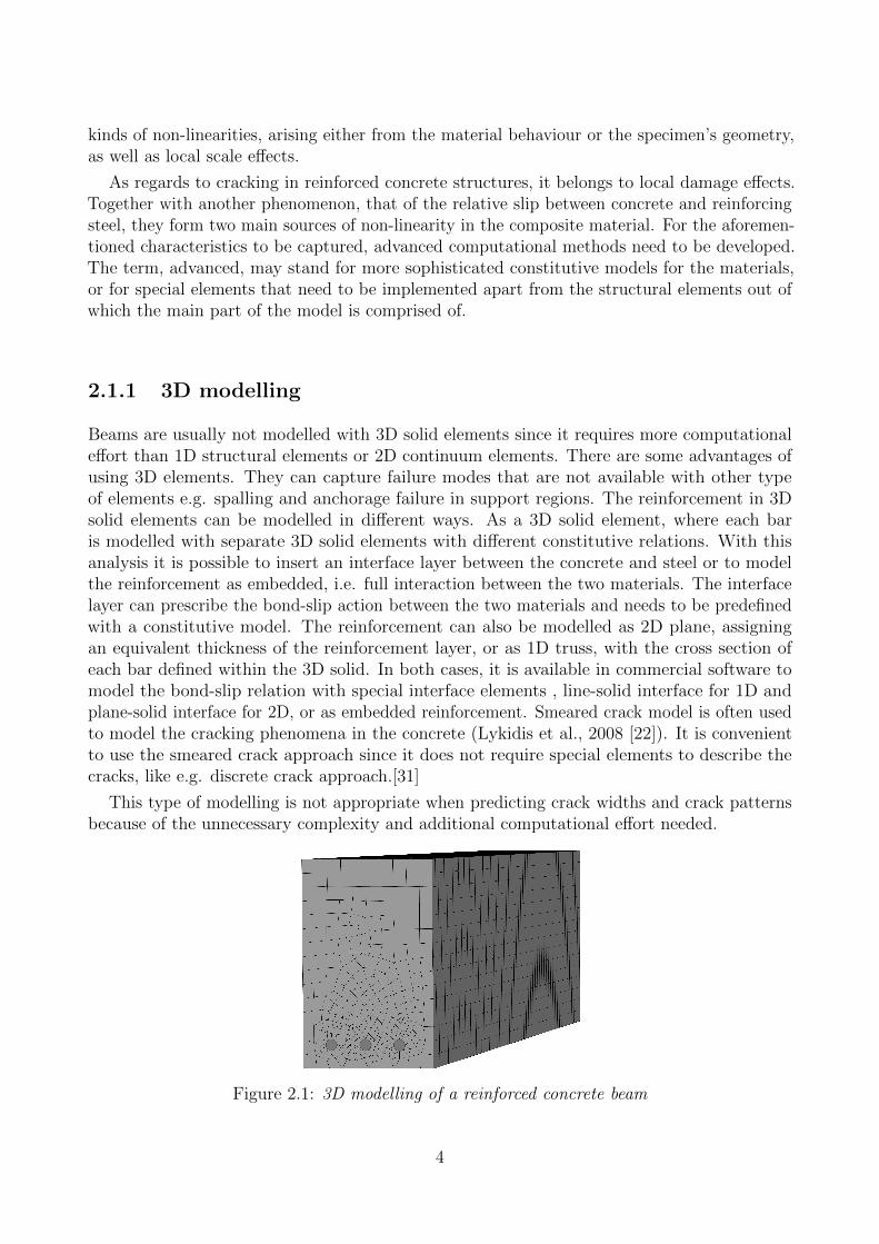
Beams are usually not modelled with 3D solid elements since it requires more computationaleffort than 1D structural elements or 2D continuum elements. There are some advantages ofusing 3D elements. They can capture failure modes that are not available with other typeof elements e.g. spalling and anchorage failure in support regions. The reinforcement in 3Dsolid elements can be modelled in different ways. As a 3D solid element, where each baris modelled with separate 3D solid elements with different constitutive relations. With thisanalysis it is possible to insert an interface layer between the concrete and steel or to modelthe reinforcement as embedded, i.e. full interaction between the two materials. The interfacelayer can prescribe the bond-slip action between the two materials and needs to be predefinedwith a constitutive model. The reinforcement can also be modelled as 2D plane, assigningan equivalent thickness of the reinforcement layer, or as 1D truss, with the cross section ofeach bar defined within the 3D solid. In both cases, it is available in commercial software tomodel the bond-slip relation with special interface elements , line-solid interface for 1D andplane-solid interface for 2D, or as embedded reinforcement. Smeared crack model is often usedto model the cracking phenomena in the concrete (Lykidis et al., 2008 [22]). It is convenientto use the smeared crack approach since it does not require special elements to describe thecracks, like e.g. discrete crack approach.[31]

This type of modelling is not appropriate when predicting crack widths and crack patternsbecause of the unnecessary complexity and additional computational effort needed.

Figure 2.1: 3D modelling of a reinforced concrete beam

4

2.1.2 2D modelling

Like with 3D modelling, 2D modelling of beams is usually not carried out when looking ata global behavior of a beam. However when looking at cracking, i.e. crack widths and crackpatterns, the 2D analysis can be feasible.

Since the beam is relatively long compared to its width plane stress elements are commonlyused to model beams in 2D analysis. The reinforcement can be modelled with 2D and 1Delements as embedded reinforcement or with slip, with line-plane interface for 2D reinforcementand line for bar reinforcement [5]. Like with 3D models, the smeared crack approach is oftenused to account for cracking.

5

2.2 Beam models

In general, an one-dimensional element is represented by a line, in which a certain cross-sectional area is assigned. It can be comprised either of only one material, a fact that wouldcharacterize it as homogeneous, or of many additional ones, which are then homogenized overthe cross-section. The simplest FE model that can be implemented is made of two-node bar,or else, truss elements, having one or two translational degrees of freedom per node (Figure2.2). Higher order 1D elements are used as well when more complicate phenomena are to becaptured, which then contain more than two nodes and approximating functions of higherorder. A special place in the ’family’ of 1D elements is held by the so-called beam or structuralelements.

Figure 2.2: Simplest possible finite elements

In their simplest form, as shown in Figure 2.3, they are met as two-node elements, witha vertical translational and a rotational degree of freedom per node. It is probably the mostwidely known and used finite element, mainly due to the simplifications that usually liebehind its constitutive theories and the low computational cost, factors that are making itvery user-friendly. Substantial realm of such theories is covered by the principle that ’planesections remain plane and perpendicular to the reference axis of the beam’, known also asthe Euler-Bernoulli beam theory (Ottosen and Petersson, 1992 [29]). Examples of their useare when the global response of a whole structure is sought for, or, when structural cases ofprofound bending are examined.

Figure 2.3: Euler-Bernoulli beam theory

6

Another popular theory, that ’plane sections remain plane but not necessarily perpendicularto the reference axis’, or else, the Timoshenko beam theory is often employed (Hjelmstad, 2005[14]). Models comprised of Timoshenko beam elements are also used for the global structuralanalysis, they have similar advantages as the Euler-Bernoulli elements, but their main use isin cases where shear action is considered to be important for the prediction of the response ofthe member under consideration (Figure 2.4).

Figure 2.4: Timoshenko beam theory

The next one-dimensional element to be described is also known as plane-frame element.It can be combined with both beam theories mentioned before, while it also accounts for theaxial displacement of the reference axis of the element (Figure 2.5). The pertinent element isused in simulations of plane frame structures and, in general, in applications where the axialmotion of the system is of importance. As it will be shown in Section 2.2.1, the considerationof the axial displacement degree of freedom is very useful for modelling effects and geometriesthat take place and exist, respectively, in the axial direction of the model, as is the effect ofthe reinforcement and the bold-slip in reinforced concrete members.

Figure 2.5: Plane-frame element

Furthermore, apart from the aforementioned fundamental structural elements, more advanced1D beam-type models have been developed. These are usually comprised of more than onematerial, homogenized over the cross-section and they employ more specialized modellingtechniques. The construction of such models was motivated from the need to cover in asimplified, but nevertheless, representative manner more complicated tasks, which may involveseveral localized phenomena that would not be feasible to capture by using the Euler-Bernoullior the Timoshenko beam theory alone. Examples of such elements are outlined in Section2.2.1.

7

2.2.1 Multi-fibre beam model

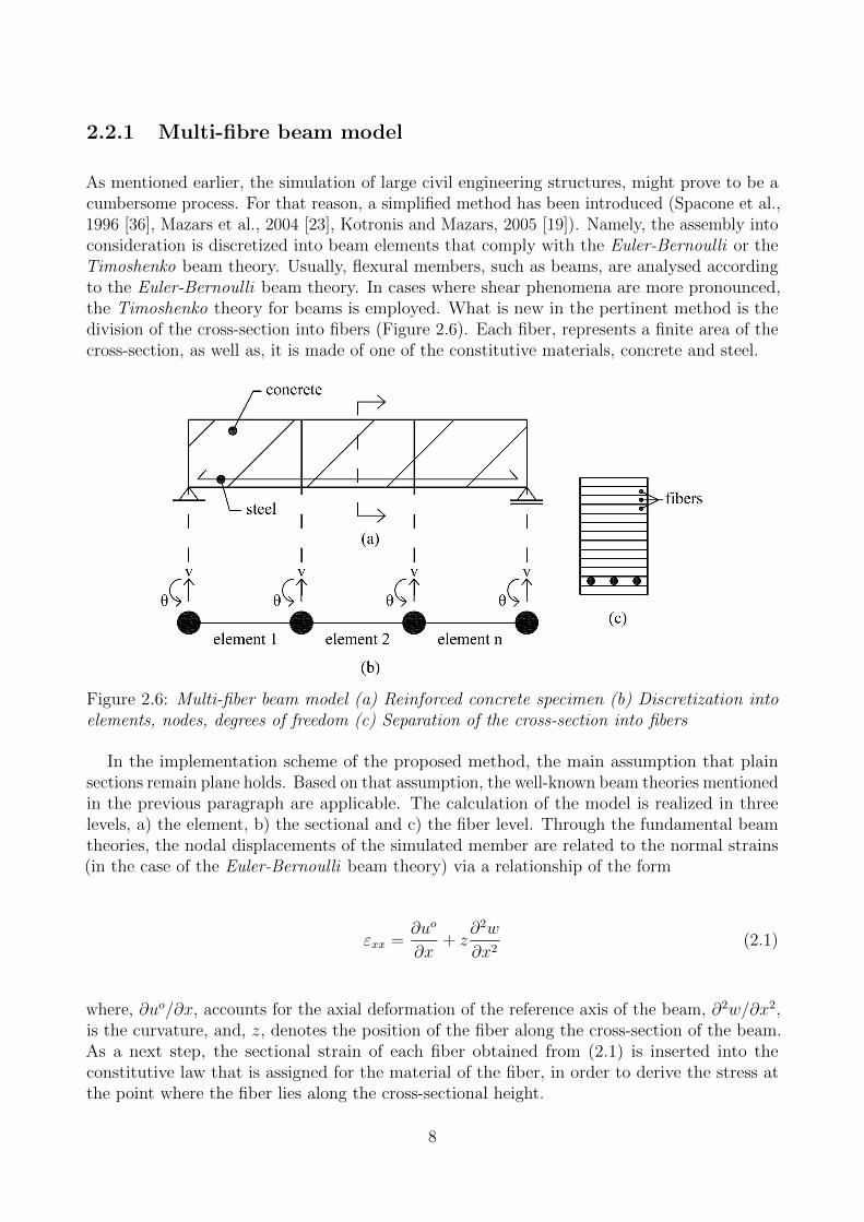
As mentioned earlier, the simulation of large civil engineering structures, might prove to be acumbersome process. For that reason, a simplified method has been introduced (Spacone et al.,1996 [36], Mazars et al., 2004 [23], Kotronis and Mazars, 2005 [19]). Namely, the assembly intoconsideration is discretized into beam elements that comply with the Euler-Bernoulli or theTimoshenko beam theory. Usually, flexural members, such as beams, are analysed accordingto the Euler-Bernoulli beam theory. In cases where shear phenomena are more pronounced,the Timoshenko theory for beams is employed. What is new in the pertinent method is thedivision of the cross-section into fibers (Figure 2.6). Each fiber, represents a finite area of thecross-section, as well as, it is made of one of the constitutive materials, concrete and steel.

Figure 2.6: Multi-fiber beam model (a) Reinforced concrete specimen (b) Discretization intoelements, nodes, degrees of freedom (c) Separation of the cross-section into fibers

In the implementation scheme of the proposed method, the main assumption that plainsections remain plane holds. Based on that assumption, the well-known beam theories mentionedin the previous paragraph are applicable. The calculation of the model is realized in threelevels, a) the element, b) the sectional and c) the fiber level. Through the fundamental beamtheories, the nodal displacements of the simulated member are related to the normal strains(in the case of the Euler-Bernoulli beam theory) via a relationship of the form

εxx =∂uo

∂x+ z

∂2w

∂x2(2.1)

where, ∂uo/∂x, accounts for the axial deformation of the reference axis of the beam, ∂2w/∂x2,is the curvature, and, z, denotes the position of the fiber along the cross-section of the beam.As a next step, the sectional strain of each fiber obtained from (2.1) is inserted into theconstitutive law that is assigned for the material of the fiber, in order to derive the stress atthe point where the fiber lies along the cross-sectional height.

8

2.2.2 Applications accounting for the damaged concrete

Early stage applications of the simplified method are attributed to Spacone et al., 1996 [36],Mazars et al., 2004 [23], Kotronis and Mazars, 2005 [19]. Common characteristic of the citedworks is that they do not include any relevant slip between the steel and the concrete fibers.Thus, full bond conditions are considered between the constitutive materials. The fibers in thiscase, depending on their position along the cross-sectional height, represent either concrete intension/compression or the steel bars. In that sense, two material laws are implemented.

In their article on simplified dynamic analysis of reinforced concrete walls, Kotronis andMazars [19] depict two examples of the multi-fiber approach on reinforced concrete walls. Inthese applications, beam elements complying with either the Euler-Bernoulli or the Timoshenkobeam theory were used for the discretization of the member in the global scale. Non-linearitiesresulting from fracture and cyclic loading were inserted into the analysis via the materialconstitutive models in the fibers scale. Uni-axial continuum damage mechanics stress-strainrelation was employed for concrete. Two damage variables, one for tension and one forcompression (dynamic loading conditions are accompanied by sign reversal of the load) wereintroduced in the concrete material law, ranging from one to zero. By means of these twovariables, the stiffness properties of concrete, namely Young’s modulus, E, and Poisson’s ratio,ν, were degrading through each load cycle. As regards to steel, a uni-axial plasticity lawincluding non-linear kinematic hardening was applied (Armstrong and Frederick, 1966 [10]).

A general conclusion that was drawn by the use of the aforementioned model for concreteis the difficulty to obtain results in extensively damaged regions, for instance crack spacingand crack-widths, outputs that were of major interest in the present thesis. It would takean advanced 3D constitutive law to capture localized fracture more accurately. Anotherdisadvantage that should be noted is the mesh-dependency of the results due to the strainsoftening law in tension that was used in the concrete model. One solution to that problemis obtained by the use of non-local constitutive models, as described by Pijaudier-Cabot andBazant, 1987 [30]. The theory recommends to separate the total strain into an elastic part,which would follow a local material law, and an inelastic part, that would be attributed tocracking and the variables associated to that part of the strain, they would be treated bynon-local damage model. Another way to get rid of the obstacle of mesh-dependency is providedin Kotronis et al., 2005 [20] by local second gradient theory. However, as it was also appliedby the authors in the present thesis, an efficient way to ’tackle’ mesh-dependency upon meshrefinement is to scale the stress-strain softening law expressed in terms of the crack width, w,with the area where each crack is expected to localize, as explained in Section 3.6.

In Mazars et al., 2004 [23] the benefits of using two simplified approaches are exposed ontwo reinforced concrete wall specimens under seismic excitation. The first model is comprisedof Euler-Bernoulli beam elements on the global scale and each cross-section is divided intofibers. La Borderie uni-axial model [21] is employed for concrete, so as to account for all thenon-linear effects arising from dynamic loading such as earthquake. The same plasticity law asin Kotronis and Mazars, 2005 [19] is used for steel (Armstrong and Frederick, 1966 [10]). Next,the second model is realized via Timoshenko beam elements. The Pontiroli-Rouquand-Mazars(PRM [34]) constitutive relation is applied for concrete, whereas the elasto-plastic material lawavailable in Abaqus CAE is implemented for steel.

9

The two simplified models presented in the latter article are computationally efficient andthey are able to represent global phenomena, as well as some fundamental local ones, in asatisfactory way. However, more advanced 3D modelling, as stated by the authors, would benecessary in order to describe localized fracture in more accurate manner.

2.2.3 Applications accounting for cracking and bond-slip

As it has already been outlined, the inclusion of the properties of the steel/concrete interfaceis important for an appropriate description of the response of reinforced concrete structures,together with the consideration of local scale effects, like fracture of concrete. Towards thisnecessity, significant contribution has been the work by Monti and Spacone, 2000 [26]. Thebasic formulation at the element and the sectional scale is similar to the one described inSection 2.2.1.

However, in Monti and Spacone, 2000 [26], in order to account for the relative slip, theperfect bond assumption is no longer valid. Instead, in the fibers scale, the total strain ofthe steel fiber is divided into a part which accounts for the deformation of the reinforcing barand a second part that considers the relative slip between the constitutive materials. So, thedeformations compatibility condition is stated this time between the surrounding concretestrain and the total steel fiber strain.

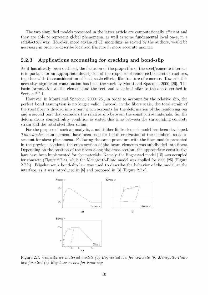
For the purpose of such an analysis, a multi-fiber finite element model has been developed.Timoshenko beam elements have been used for the discretization of the members, so as toaccount for shear phenomena. Following the same procedure with the fiber-models presentedin the previous sections, the cross-section of the beam elements was subdivided into fibers.Depending on the position of the fibers along the cross-section, the appropriate constitutivelaws have been implemented for the materials. Namely, the Hognestad model [15] was occupiedfor concrete (Figure 2.7.a), while the Menegotto-Pinto model was applied for steel [25] (Figure2.7.b). Eligehausen’s bond-slip law was used to describe the behavior of the model at theinterface, as it was introduced in [6] and proposed in [3] (Figure 2.7.c).

Figure 2.7: Constitutive material models (a) Hognestad law for concrete (b) Menegotto-Pintolaw for steel (c) Eligehausen law for bond-slip

10

3 A model for reinforced concrete beams

To develop a simplified one-dimensional reinforced concrete beam model, that should be able todescribe the interaction between the cracked concrete and the rebars, a standard procedure wasfollowed regarding the establishment of the finite element model. According to that process, aderivation took place first, which started from stating the strong form for the ’problem’ of areinforced concrete beam subjected to transverse and longitudinal distributed loading. Then,the weak form of the differential equations that cover the pertinent problem was obtained.Later on, the finite element formulation of the non-linear problem was derived, together withthe linearization of the non-linear relationships. Finally, appropriate iterative/incrementalprocedures and integration schemes were employed for the numerical solution of the non-linearfinite element form.

The theoretical foundations of the derivation mentioned in the previous paragraph was thebasis for the finite element code constructed at the next step. The outputs from the developedcomputer program were then used for comparison with relevant tests from literature, figuresobtained from analytical calculations, the finite element stiffness adaptation method, as well aswith a ’perfect bond’ model performed using the Diana software.

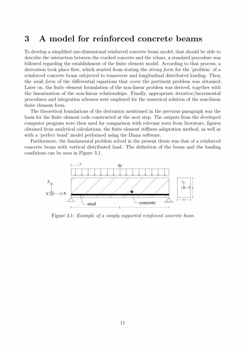
Furthermore, the fundamental problem solved in the present thesis was that of a reinforcedconcrete beam with vertical distributed load. The definition of the beam and the loadingconditions can be seen in Figure 3.1.

Figure 3.1: Example of a simply supported reinforced concrete beam

11

3.1 Derivation of the non-linear continuous formulation

3.1.1 Cross sectional forces

At the cross-section scale, by definition, the following equations hold for the internal forces M ,V , N and N i, whereas, the contribution of the steel bars is taken into account in (3.1) and(3.3), apart from the concrete contribution for a typical homogeneous cross-section.

The axial force N is defined by

N =

∫A

σconcxx dA+∑i

Aiσsi (3.1)

where σconcxx , is the axial concrete stress across the cross-section A. The shear force V is givenby

V =

∫A

σxz dA (3.2)

where, σxz, is the shear stress across the concrete cross-section. The bending moment M iscalculated as

M =

∫A

z · σconcxx dA+∑i

Ai · ziσsi (3.3)

and, for each layer of n-reinforcement bars, the axial force of each layer is returned by

N i = Ai · σsi (3.4)

where, Ai, denotes the total area of the nbars within the i-st layer of reinforcement, nbarsaccounts for the number of bars contained in the i-st layer, and, σsi, is the axial steel stress ofthe i-st layer. Finally, the definition of the bond force between the i-st layer of reinforcementand the surrounding concrete is introduced here, according to the relationship

fi = τ bondxx · si (3.5)

where, τ bondxx , is the longitudinal bond stress between the constitutive materials and, si, is thesum of the circumference of the nbars that comprise the i-st steel layer.

3.1.2 Equilibrium conditions

As a next step, the equilibrium conditions that are applicable for the beam under considerationare outlined. First, consider an infinitesimal part of the beam, as shown in Figure 3.2.

From equilibrium in the vertical direction (over the height of the cross-section), it can bestated ∑

Fz = 0⇒ −V + V + ∂V + qz · ∂x = 0

⇒ −∂V∂x

= qz (3.6)

A bending moment equation around the left-most point of the reference axis of the beamcan be written as

12

Figure 3.2: Internal forces of an infinitely small part of a reinforced concrete beam

∑Mleft = 0⇒ (M + ∂M)− (V + ∂V )∂x+ qz · ∂x ·

∂x

2−M = 0

⇒ ∂M

∂x− V − ∂V + qz ·

∂x

2︸ ︷︷ ︸infinitesimal

= 0

⇒ ∂M

∂x− V = 0 (3.7)

Equilibrium between the forces in the horizontal (longitudinal) direction requires∑Fx = 0⇒ N + ∂N −N = 0

⇒ ∂N

∂x= 0 (3.8)

Now, from equilibrium between the longitudinal stress of the i-st layer of reinforcement andthe relevant bond stress coming from the surrounding concrete, it can be derived (lower partof Figure 3.2) ∑

F barx = 0⇒ N i + ∂N i −N i − fi · ∂x = 0

⇒ −∂N i

∂x+ fi = 0 (3.9)

Next, inserting (3.6) into (3.7) it is obtained

−∂2M

∂x2= qz (3.10)

13

3.1.3 Kinematic relations

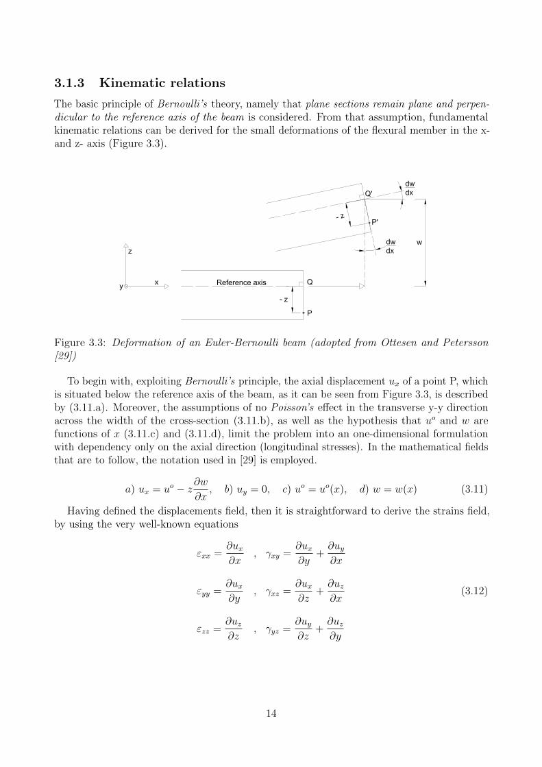
The basic principle of Bernoulli’s theory, namely that plane sections remain plane and perpen-dicular to the reference axis of the beam is considered. From that assumption, fundamentalkinematic relations can be derived for the small deformations of the flexural member in the x-and z- axis (Figure 3.3).

Figure 3.3: Deformation of an Euler-Bernoulli beam (adopted from Ottesen and Petersson[29])

To begin with, exploiting Bernoulli’s principle, the axial displacement ux of a point P, whichis situated below the reference axis of the beam, as it can be seen from Figure 3.3, is describedby (3.11.a). Moreover, the assumptions of no Poisson’s effect in the transverse y-y directionacross the width of the cross-section (3.11.b), as well as the hypothesis that uo and w arefunctions of x (3.11.c) and (3.11.d), limit the problem into an one-dimensional formulationwith dependency only on the axial direction (longitudinal stresses). In the mathematical fieldsthat are to follow, the notation used in [29] is employed.

a) ux = uo − z∂w∂x

, b) uy = 0, c) uo = uo(x), d) w = w(x) (3.11)

Having defined the displacements field, then it is straightforward to derive the strains field,by using the very well-known equations

εxx =∂ux∂x

, γxy =∂ux∂y

+∂uy∂x

εyy =∂ux∂y

, γxz =∂ux∂z

+∂uz∂x

εzz =∂uz∂z

, γyz =∂uy∂z

+∂uz∂y

(3.12)

14

Combining (3.11) and (3.12), the normal strain of the concrete beam and the i-st layer ofsteel can be determined, as

εconcxx (x, z) =∂uo

∂x− z∂

2w

∂x2(3.13)

εbarxx,i(x) =∂uo

∂x− zi

∂2w

dx2+∂∆i

∂x(3.14)

where uo is the axial displacement at the reference axis∆i is the bond-slip between the i-st layer of reinforcement and

the surrounding concrete

As it can be seen from (3.13), the axial strain of any point at the concrete beam is a functionof the horizontal translation, uo(x), of the reference axis at the section where the point belongs,and the curvature, κ = ∂2w/∂x2. As for the axial strain of the i-st layer of reinforcement (3.14),the deformation of the steel layer equals to the deformation of concrete at the height of thereinforcement layer, plus the contribution from the relative slip, ∆i, between the constitutivematerials.

In other words, the compatibility condition that holds between the i-st layer of reinforce-ment and the surrounding concrete can be expressed in a more appropriate manner, in thedisplacements field, as

∆i(x) = ui(x)− uo(x) + zi∂w(x)

∂x(3.15)

where, ui(x), denotes the axial displacement of the i-st steel layer.

15

3.2 FE formulation

3.2.1 Differential equations and boundary conditions

Equations (3.8), (3.9) and (3.10) are the equilibrium equations which along with the boundaryconditions (Table 3.1) make up the strong form of the problem. In these equations, there are(2n + 2) unknown sectional forces (N,M,Nn, fn), while only (n + 2) equilibrium equationsexist. Thus, compatibility conditions and constitutive relations are needed for the solution ofsuch an internally statically indeterminate member.

∂N

∂x= 0 , 0 ≤ x ≤ L (3.16)

−∂2M

∂x2= qz , 0 ≤ x ≤ L (3.17)

−∂N i

∂x+ fi = 0 , ai ≤ x ≤ bi (3.18)

where, L, is the length of the beam, and, ai, bi, are the starting and the ending points,respectively, of the i-st layer of reinforcement in the longitudinal direction of the beam.

3.2.2 Weak form

After ’constructing’ the strong form of the problem (Section 3.2.1), and, in order to ’get rid’of the derivatives accompanying the internal variables, the weak, or variational, form of theequations needs to be employed.

The first step on the way to extract the weak form is to multiply (3.16), (3.17) and (3.18)by arbitrary test-functions δu0, δw and δ∆i, respectively, and integrate over the appropriatefor each variable domain ∫

L

δuo∂N

∂xdx = 0 (3.19)

−∫L

δw∂2M

∂x2dx =

∫L

δw · qz dx (3.20)

−∫ bi

ai

δ∆i∂N i

∂xdx+

∫ bi

ai

δ∆i · fi dx = 0 (3.21)

and, secondly, to perform integration by parts once for (3.19) and (3.21), and twice for (3.20).In that sense, (3.19) becomes ∫

L

∂δuo

∂xN dx =

[δuoN

]L0

(3.22)

while, (3.20) takes the form

−∫L

∂2δw

∂x2M dx =

∫L

δw · qz dx−[∂δw

∂xM

]L0

+[δw · V

]L0

(3.23)

16

and, similarly, (3.21) reforms to∫ bi

ai

(∂δ∆i

∂xN i + δ∆i · fi) dx =

[δ∆i ·N i

]biai

(3.24)

At this point, as a by-product of the integration by parts, the boundary terms of the loadvector have appeared at the RHS of (3.22), (3.23) and (3.24). These terms lie upon thepoints of the domain, where either the forces and the moments are prescribed as ’natural’boundary conditions or the displacements are prescribed as ’essential’ boundary conditions.Thus, where the ’natural’ boundary vector is known, the relevant boundary terms can bedetermined, while at the points where the essential boundary conditions are defined, therespective boundary terms vanish simply by setting the pertinent test-function to zero. Theequations (3.22), (3.23) and (3.24) along with the boundary conditions comprise the weak formof the differential equations. Examples of possible boundary conditions, as well as, the specificboundary conditions that need to applied in order to avoid rigid body motion of the reinforcedconcrete beam under consideration are given in Section 3.2.3.

3.2.3 Boundary conditions

A beam element accounting for bond-slip has 4 degrees of freedom in each node, horizontaltranslation (x-direction), vertical translation (z-direction), rotation around y-axis and slip inthe interface between concrete and steel. That means for the simplest case a straight beamsupported in two nodes at the ends needs 8 boundary conditions essential, natural or convective.Convective boundary conditions are a combination of essential and natural.

Table 3.1: Possible essential (Dirichlet) and natural (Neumann) boundary conditions for thereinforced beam element accounting for bond-slip

Degree of freedom Essential Natural

Horizontal translation uo Normal force NVertical translation w Shear force VRotation θy Moment MSlip ∆i Normal (anchoring) force N i

In Table 3.1 the possible boundary conditions are listed. However there are certain limitationsto what boundary conditions combinations give unique solutions. To avoid rigid body motionboth the criteria below need to be fulfilled:

� at least one degree of freedom in the horizontal direction has to be prescribed.

� one vertical translational degree of freedom and one rotational or two vertical translationaldegrees of freedom need to be prescribed

17

3.2.4 Constitutive equations

So far, the internal variables (N,M,Nn, fn) in the strong form were inserted in the relevantequations as forces. In the subsequent chapters, the pertinent forces are restated, using thedefinitions of (3.1), (3.3), (3.4) and (3.5), thus introducing the relevant constitutive operators,that represent the constitutive models of the materials. Symbolically, the substitutions justdescribed take the form

σconcxx = σconcxx (εconcxx (x, z))

σbarxx = σbarxx (εbarxx (x))

τ bondxx = τ bondxx (∆i(x))

In that manner, the force-displacement relations of the strong form of (3.16), (3.17) and(3.18) are to be turned into stress-deformation relations in the sections that come next. As itwill be shown, with the strains already defined in a typical step of the chosen solution scheme,the stresses are then obtained through the constitutive law set for each material. The materiallaws just mentioned, can be chosen, so far, arbitrarily by the programmer, due to the generalform that is kept for the derivation of the finite element equations outlined in the presentchapter.

3.2.5 Introduce the constitutive relations into the weak form

At the current section, the semi-linear a(u; v) form and the load vector L(v) of the problem areto be defined, a notation that is adopted here in order to facilitate the rest of the derivationprocess. For that purpose, the equations of the weak form, (3.22), (3.23) and (3.24) can berestated as

au0(uo, w,∆i; δuo) = Luo(δu

o) (3.25)

aw(uo, w,∆i; δw) = Lw(δw) (3.26)

a∆i(uo, w,∆i; δ∆i) = L∆i

(δ∆i) (3.27)

respectively, where, auo , Luo are defined as

auo(uo, w,∆i; δu

o) =

∫L

∂δuo

∂x

[∫A

σconcxx (εconcxx ) dA+∑i

Ai · σsi(εbarxx )

]dx =

=

∫L

∂δuo

∂x

[∫A

σconcxx

(∂uo

∂x− z∂

2w

∂x2

)dA+

∑i

Ai · σsi(∂uo

∂x− zi

∂2w

∂x2+∂∆i

δx

)]dx (3.28)

and,

Luo(δuo) =

[δuoN

]L0

(3.29)

18

while, aw, Lw stand for

aw(uo, w,∆i; δw) =

∫L

∂2δw

∂x2

{−

[∫A

z · σconcxx (εconcxx ) dA+∑i

Ai · zi · σsi(εbarxx)]}

dx =

=

∫L

∂2δw

∂x2

{−[∫

A

z · σconcxx

(∂uo

∂x− z∂

2w

∂x2

)dA+

+∑i

Ai · zi · σs(∂uo

∂x− zi

∂2w

∂x2+∂∆i

δx

)]}dx (3.30)

and,

Lw(δw) =

∫L

δw · qz dx−[∂δw

∂xM

]L0

+[δw · V

]L0

(3.31)

whereas, a∆i, L∆i

account for

a∆i(uo, w,∆i; δ∆i) =

∫ bi

ai

[∂δ∆i

∂xAi · σsi

(εbarxx)− δ∆i · si · τ bondxx (∆i(x))

]dx (3.32)

and,

L∆i(δ∆i) =

[δ∆i ·N i

]biai

(3.33)

where, si, is the sum of the circumference of the reinforcement bars used at the i-st steel layer.

3.2.6 Discretization of the continuous displacements field

Until this point, the equations used in the strong form (3.16), (3.17) and (3.18), as well as,in the weak form of the problem (3.22), (3.23) and (3.24), are continuous over the respectivedomain of each internal variable. In order to transmit the aforementioned relations into finiteelement equations, they need to be discretized. For that purpose, the approximations on uo, wand ∆i have to be introduced, according to

uo ≈ uoh(x) = Nuo(x) · auo

w ≈ wh(x) = Nw(x) · aw

∆i ≈ ∆i,h(x) = N∆i(x) · a∆i

where, Nuo , Nw and N∆iare shape functions, while auo ,aw and a∆i

contain the nodal valuesof uo, w and ∆i.

Then, the axial displacement of the reference axis of the beam can be written as

uo(x) ≈Nuo(x)auo ⇒ ∂uo

∂x≈ ∂Nuo(x)

∂xauo = Buo(x)auo (3.34)

In a finite element, the shape functions that are to be used for the approximation of theexpected deformed shape of the beam in the longitudinal direction take the form

Neuo(x) = [N e

1 , Ne2 ] =

[− 1

Le(x− x2) ,

1

Le(x− x1)

]19

Similarly, the continuous field of the deflections of the beam after discretization becomes

w ≈Nw(x)aw ⇒∂2w

∂x2≈ ∂2Nw(x)

∂x2aw = Bwaw (3.35)

The approximating functions that describe the deflected form of the beam in the i-st finiteelement are given by

New(x) = [N e

1 , Ne2 , N

e3 , N

e4 ] =

=

[1− 3x2

Le2 +2x3

Le3 , x

(1− 2x

Le+

x2

Le2

),x2

Le2

(3− 2x

Le

),x2

Le

( xLe− 1)]

Finally, for the the field of the relative slip between the constitutive materials it is deduced

∆i ≈N∆i(x)a∆i

⇒ ∂∆i(x)

∂x≈ ∂N∆i

(x)

∂xa∆i

= B∆ia∆i

(3.36)

The shape functions that are to be occupied to describe the anticipated slip relation betweenthe concrete and the rebars in the finite element have the form

Ne∆i

(x) = [N e1 , N

e2 ] =

[− 1

Le(x− x2) ,

1

Le(x− x1)

]

3.2.7 Galerkin’s method

Referring back at Section 3.2.2, the term test-functions was mentioned. This term, or elsethe weight-functions, symbolically stated as δuo, δw and δ∆i is used to denote the virtualdisplacements of the system in the directions of uo, w and ∆i, respectively. As it has already beenstated, the pertinent functions can be chosen arbitrarily. However, there have been developeddifferent methods for the choice of the test-functions, and one which is very functional isGalerkin’s method. It belongs to the ’family’ of weighted residual methods, together with otherones, as the Point collocation method, the Subdomain collocation method and the Least-squaresmethod, as described in [29].

In the present thesis, Galerkin’s method is followed for the appropriate choice of the test-functions. The basic idea behind it is to choose the weight-functions the same as the shapefunctions. For instance, the first weight-function δuo is taken as

δuo ≈Nuo(x)cuo = cTuoNTuo(x) (δuo is scalar)

⇒ ∂δuo

∂x≈ ∂Nuo(x)

∂xcuo = Buocuo = cTuoB

Tuo (3.37)

whereas, δw, is chosen as

δw ≈Nw(x)cw = cTwNTw (x) (δw is scalar)

⇒ ∂2δw

∂x2≈ ∂2Nw(x)

∂x2cw = Bwcw = cTwB

Tw (3.38)

and, in the same manner, δ∆i is replaced by

δ∆i ≈N∆i(x)c∆i

= cT∆iNT

∆i(x) (δ∆i is scalar)

20

⇒ ∂δ∆i

∂x≈ ∂N∆i

(x)

∂xc∆i

= B∆ic∆i

= cT∆iBT

∆i(3.39)

In the equations above, cuo , cw and c∆iare column matrices of arbitrary coefficients.

3.2.8 Formulation of the internal force vector

After defining the approximations on uo, w, ∆i in (3.34), (3.35) and (3.36) at Section 3.2, andthe weight-functions δuo, δw, δ∆i in (3.37), (3.38) and (3.39) at Section 3.2.7, the internal forcevector, fint, can be deduced, by introducing them into the variational form of the problemstated in (3.28) to (3.33).

Replacing, first, the approximated displacement fields and test-functions into (3.25), (3.28)and (3.29), it is derived

cTuo

{∫L

BTuo

[∫A

σconxx (Buoauo − zBwaw)dA+

+∑i

Ai · σsi(Buoauo − ziBwaw +B∆ia∆i

)

]dx

}= cTuo

{[NT

uoN]L

0

}⇒ cTuofint,uo(auo, aw, a∆i

) = cTuofuo (3.40)

Similarly, upon introduction of the discretized displacements and weight-functions into (3.26),(3.30) and (3.31), it is obtained

cTw

∫L

BTw

{−[∫

A

z · σconxx (Buoauo − zBwaw)dA+

+∑i

Ai · zi · σsi(Buoauo − ziBwaw +B∆ia∆i

)

]}dx =

cTw

{∫L

NTwqzdx−

[∂NT

w

∂xM

]L0

+[NT

wV]L

0

}

⇒ cTwfint,w(auo, aw, a∆i) = cTwfw (3.41)

Following the same procedure for (3.27), (3.32) and (3.33), results in

cT∆i

∫ bi

ai

[BT

∆i· Ai · σsi (Buoauo − ziBwaw +B∆i

a∆i) +

+NT∆i· si · τ bondxx (N∆i

a∆i)]dx = cT∆i

[NT

∆iNi

]biai

⇒ cT∆ifint,∆i

(auo, aw, a∆i) = cT∆i

f∆i(3.42)

Assembling the components fint,uo , fint,w, and fint,∆idetermined in (3.40), (3.41) and (3.42),

respectively, into the total internal force vector fint, it can be written

cTfint(a) = cTf (3.43)

21

where

fint(a) =

fint,uo(a)fint,w(a)fint,∆i

(a)

, a =

auo

aw

a∆i

, f =

fuo

fwf∆i

, c =

cuo

cwc∆i

3.2.9 Involve essential boundary conditions

In order to obtain a solution for the displacements, a, that satisfies (3.43), it is convenient todiscretize the full vector, a, into free and constrained degrees of freedom, according to

a =

[aF

aC

], where aF =

a1

a2...

aNfree

, aC =

aNfree+1

aNfree+2...

aNdof

(3.44)

where, aC , is a vector containing the prescribed degrees of freedom, while, aF , are theunknown ones.

Similarly, the same categorization can be done for the shape functions, as well

N =[NF NC

](3.45)

The approximated non-linear system is fully defined at this stage, and, it can be stated asthe problem of finding uoh ∈ Vh, wh ∈Wh and ∆i,h ∈ Dh such that

a(uoh; δuoh) = L(δuoh) (3.46)

a(wh; δwh) = L(δwh) (3.47)

a(∆i,h; δ∆i,h) = L(δ∆i,h) (3.48)

where, the trial spaces are set as follows

Vh ={uoh : uo = Nuo,Fauo,F +Nuo,Cauo,C for any auo,F ∈ RNuo,free

}Wh =

{wh : w = Nw,Faw,F +Nw,Caw,C for any aw,F ∈ RNw,free

}Dh =

{∆i,h : ∆i = N∆i,Fa∆i,F +N∆i,Ca∆i,C for any a∆i,F ∈ RN∆i,free

}while, the FE test spaces are defined as

Voh =

{uoh : uo = Nuo,F cuo,F for any cuo,F ∈ RNuo,free

}Wo

h ={wh : w = Nw,F cw,F for any cw,F ∈ RNw,free

}Doh =

{∆i,h : ∆i = N∆i,F c∆i,F for any c∆i,F ∈ RN∆i,free

}22

Referring back to the non-linear system of equations in (3.43), after the separation accom-plished in (3.44) and (3.45), the unknown displacements aF can be determined via the solutionof a reduced system of equations, which takes into account only the free degrees of freedom.The pertinent approach is realized by setting all the arbitrary coefficients contained in cTCequal to zero in (3.43). Thus, the system takes the form

[cTF 0

] [ fint,F

fint,C

]=[cTF 0

] [ fFfC

](3.49)

while,fC = fl,C + fb,C = fint,C(a) (3.50)

In (3.50), fl,C , denotes the external force vector and, fb,C , accounts for the boundary loadvector. The reduced system of equations becomes

fint,F (a) = fF

⇒ g(aF ) = 0 (3.51)

where, g, is known as the out-of-balance force vector, numerically defines the residual of thefinite element equations and is given by

g(aF ) = fint,F

([aF

aC

])− fF (3.52)

After solving (3.51) for a, it is possible to define fint,C in (3.50) and, thereafter, to solve(3.50) for the boundary vector fb,C . The latter column matrix represents the ’reaction forces’that arise from the application of the constraints at the relevant degrees of freedom.

23

3.3 Linearization of the non-linear problem

The system of equations (3.51) is a system of Nfree non-linear equations. The factor of non-linearity originates directly from the constitutive laws that are to be implemented for thematerials. Thus, in order to obtain a solution for the unknown displacements in the iterativesolution scheme that is to be used later on, a linearization of the system should be performedfirst, as described in the following derivation.

For that purpose, the residuals of the continuous system in question, namely (3.25), (3.26)and (3.27) are defined, as

Ruo = Luo(δuo)− auo(uo, w,∆i; δu

o) (3.53)

Rw = Lw(δw)− aw(uo, w,∆i; δw) (3.54)

R∆i= L∆i

(δ∆i)− a∆i(uo, w,∆i; δ∆i) (3.55)

At this point, a function a∗ reasonably close to the true solution of the system of (3.53),(3.54) and (3.55) is assumed. Then, for the latter equations it can be written

R(a∗; v) = L(v)− a(a∗, v) (3.56)

Employing the linearization of (3.25), (3.26) and (3.27), which comprise the semi-linearform, the residual in (3.56) is linearized according to

R(a∗ + ∆a; v) ≈ R(a∗; v)− a′(a∗; v,∆a) (3.57)

where, R(a∗; v), is given by (3.56) and, a′(a∗; v,∆a), is the directional derivative of a(a∗; v) inthe direction of ∆a.

3.3.1 Linearization of the FE-equations

As it was described for the continuous system in the previous section, a similar linearizationscheme is performed for the discrete equations (3.51). Namely, a ’good’ guess a∗ of theapproximate solution a is assumed. In matrix form it can be stated as

a∗ ≈ a⇒ a∗ =

uo∗

w∗

∆∗i

≈ a =

uo

w∆i

In (3.52), the out-of-balance force vector was defined as

g(a) = fint(a)− f

Considering then a small change ∆aF in a∗, then, expanding g(a∗F + ∆aF ) in Taylor series, itis obtained

g(a∗F + ∆aF ) ≈ g(a∗F ) +dg

da∗F(a∗F )∆aF (3.58)

24

where, g(a∗F ), is the value of function g evaluated at a∗F and dg/da∗F is the derivative of g interms of a∗F , or else, the tangent stiffness matrix.

Finally, comparing the linearized residual of the continuous equations (3.57) and thelinearized out-of-balance force vector in (3.58), it can be observed by term-wise identificationthe correspondence between R(a∗; v) and g(a∗F ), as well as, between, −a′(a∗; v,∆a), anddg/da∗F (a∗F )∆aF . Next, the directional derivatives of the semi-linear form of (3.25), (3.26) and(3.27) in the direction of ∆uo, ∆w and ∆∆i are to be derived. Thus, having three equationsand three directions each, results in nine equations for the derivatives, which after introducingthe approximations on uo, w and ∆i, the nine components-submatrices of the tangent stiffnessmatrix will be defined.

To begin with, the directional derivative of (3.25) in the direction of ∆uo is given by

a′uouo(uo∗, w∗,∆∗i ; δu

o,∆uo) =∂

∂εauo(u

o∗ + ε∆uo, w∗,∆∗i ; δuo)

∣∣∣∣ε=0

=

=∂

∂ε

{∫L

∂δuo

∂x

[∫A

σconxx

(∂(uo∗ + ε∆uo)

∂x− z∂

2w∗

∂x2

)dA+

+∑i

Aiσsi

(∂(uo∗ + ε∆uo)

∂x− zi

∂2w∗

∂x2+∂∆∗i∂x

)]dx

}∣∣∣∣∣ε=0

=

=

∫L

∂δuo

∂x

[∫A

∂σconxx∂ε

dA+∑i

Ai∂σsi∂ε

]∂∆uo

∂xdx (3.59)

Introducing the approximations on uo∗, w∗,∆∗i and δuo,∆uo into (3.59) leads to

a′uouo(Na∗;Nuocuo ,Nuo∆auo) = cTuo

∫L

BTuo

[∫A

∂σconxx∂ε

dA+∑i

Ai∂σsi∂ε

]Buodx∆auo =

= cTuoKuouo∆auo (3.60)

where

Kuouo =

∫L

BTuo

[∫A

∂σconxx∂ε

dA+∑i

Ai∂σsi∂ε

]Buodx (3.61)

Similarly, the derivative of (3.25) in the direction of ∆w becomes

a′uow(uo∗, w∗,∆∗i ; δuo,∆w) =

∂

∂εauo(u

o∗, w∗ + ε∆w,∆∗i ; δuo)

∣∣∣∣ε=0

=

=∂

∂ε

{∫L

∂δuo

∂x

[∫A

σconxx

(∂uo∗

∂x− z∂

2(w∗ + ε∆w)

∂x2

)dA+

+∑i

Aiσsi

(∂uo∗

∂x− zi

∂2 (w∗ + ε∆w)

∂x2+∂∆∗i∂x

)]dx

}∣∣∣∣∣ε=0

=

=

∫L

∂δuo

∂x

{−

[∫A

z∂σconxx∂ε

dA+∑i

Aizi∂σsi∂ε

]}∂2∆w

∂x2dx (3.62)

25

Introducing the approximations on uo∗, w∗,∆∗i and δuo,∆w into (3.62) results in

a′uow(Na∗;Nuocuo ,Nw∆aw) = cTuo

∫L

BTuo

{−

[∫A

z∂σconxx∂ε

dA+∑i

Aizi∂σsi∂ε

]}Bwdx∆aw =

= cTuoKuow∆aw (3.63)

where

Kuow =

∫L

BTuo

{−

[∫A

z∂σconxx∂ε

dA+∑i

Aizi∂σsi∂ε

]}Bwdx (3.64)

Furthermore, the derivative of (3.25) in the direction of ∆∆i is determined by

a′uo∆i(uo∗, w∗,∆∗i ; δu

o,∆∆i) =∂

∂εauo(u

o∗, w∗,∆∗i + ε∆∆i; δuo)

∣∣∣∣ε=0

=

=∂

∂ε

{∫L

∂δuo

∂x

[∫A

σconxx

(∂uo∗

∂x− z∂

2w∗

∂x2

)dA+

+∑i

Aiσsi

(∂uo∗

∂x− zi

∂2w∗

∂x2+∂ (∆∗i + ε∆∆i)

∂x

)]dx

}∣∣∣∣∣ε=0

=

=

∫L

∂δuo

∂x

[∑i

Ai∂σsi∂ε

]∂∆∆i

∂xdx (3.65)

Introducing the approximations on uo∗, w∗,∆∗i and δuo,∆∆i gives

a′uo∆i(Na∗;Nuocuo ,N∆i

∆a∆i) = cTuo

∫L

BTuo

[∑i

Ai∂σsi∂ε

]B∆i

dx∆a∆i=

= cTuoKuo∆i∆a∆i

(3.66)

where

Kuo∆i=

∫L

BTuo

[∑i

Ai∂σsi∂ε

]B∆i

dx (3.67)

To continue with the derivation process, for the derivative of (3.26) in the direction of ∆uo,it can written

a′wuo(uo∗, w∗,∆∗i ; δw,∆u

o) =∂

∂εaw(uo∗ + ε∆uo, w∗,∆∗i ; δw)

∣∣∣∣ε=0

=

=∂

∂ε

{∫L

∂2δw

∂x2

{−[∫

A

z · σconxx(∂(uo∗ + ε∆uo)

∂x− z∂

2w∗

∂x2

)dA+

+∑i

Aiziσsi

(∂(uo∗ + ε∆uo)

∂x− zi

∂2w∗

∂x2+∂∆∗i∂x

)]}dx

}∣∣∣∣∣ε=0

=

=

∫L

∂2δw

∂x2

{−

[∫A

z∂σconxx∂ε

dA+∑i

Aizi∂σsi∂ε

]}∂∆uo

∂xdx (3.68)

26

Replacing the approximations on uo∗, w∗,∆∗i and δw,∆uo into (3.68) gives

a′wuo(Na∗;Nwcw,Nuo∆auo) = cTw

∫L

BTw

{−

[∫A

z∂σconxx∂ε

dA+∑i

Aizi∂σsi∂ε

]}Buodx∆auo =

= cTwKwuo∆auo (3.69)

where

Kwuo =

∫L

BTw

{−

[∫A

z∂σconxx∂ε

dA+∑i

Aizi∂σsi∂ε

]}Buodx (3.70)

At this point, it is useful to observe the symmetry that holds between the relevant componentsof the tangent stiffness matrix. For instance, from (3.64) and (3.70) it is straightforward toobserve that

Kuow = K′wuo (3.71)

In the same manner, the concept of symmetry can be exploited in the derivation process of therest components of the stiffness matrix K.

Likewise, the derivative of (3.26) in the direction of ∆w is determined by

a′ww(uo∗, w∗,∆∗i ; δw,∆w) =∂

∂εaw(uo∗, w∗ + ε∆w,∆∗i ; δw)

∣∣∣∣ε=0

=

=∂

∂ε

{∫L

∂2δw

∂x2

{−[∫

A

zσconxx

(∂uo∗

∂x− z∂

2(w∗ + ε∆w)

∂x2

)dA+

+∑i

Aiziσsi

(∂uo∗

∂x− zi

∂2 (w∗ + ε∆w)

∂x2+∂∆∗i∂x

)]}dx

}∣∣∣∣∣ε=0

=

=

∫L

∂2δw

∂x2

[∫A

z2∂σconxx

∂εdA+

∑i

Aiz2i

∂σsi∂ε

]∂2∆w

∂x2dx (3.72)

Introducing the approximations on uo∗, w∗,∆∗i and δw,∆w into (3.72) results in

a′ww(Na∗;Nwcw,Nw∆aw) = cTw

∫L

BTw

[∫A

z2∂σconxx

∂εdA+

∑i

Aiz2i

∂σsi∂ε

]Bwdx∆aw =

= cTwKww∆aw (3.73)

where

Kww =

∫L

BTw

[∫A

z2∂σconxx

∂εdA+

∑i

Aiz2i

∂σsi∂ε

]Bwdx (3.74)

27

To continue with the derivative of (3.26) in the direction of ∆∆i, it can be stated

a′w∆i(uo∗, w∗,∆∗i ; δw,∆∆i) =

∂

∂εaw(uo∗, w∗,∆∗i + ε∆∆i; δw)

∣∣∣∣ε=0

=

=∂

∂ε

{∫L

∂2δw

∂x2

{−[∫

A

zσconxx

(∂uo∗

∂x− z∂

2w∗

∂x2

)dA+

+∑i

Aiziσsi

(∂uo∗

∂x− zi

∂2w∗

∂x2+∂ (∆∗i + ε∆∆i)

∂x

)]}dx

}∣∣∣∣∣ε=0

=

=

∫L

∂2δw

∂x2

[−∑i

Aizi∂σsi∂ε

]∂∆∆i

∂xdx (3.75)

Introducing the approximations on uo∗, w∗,∆∗i and δw,∆∆i into (3.75), it is obtained

a′w∆i(Na∗;Nwcw,N∆i

∆a∆i) = cTw

∫L

BTw

[−∑i

Aizi∂σsi∂ε

]B∆i

dx∆a∆i=

= cTwKw∆i∆a∆i

(3.76)

where,

Kw∆i=

∫L

BTw

[−∑i

Aizi∂σsi∂ε

]B∆i

dx (3.77)

As it was the case for the previous relevant components of the stiffness matrix, accountingfor symmetry, the following hold

K∆iuo = K′uo∆i(3.78)

and,K∆iw = K′w∆i

(3.79)

where, Kuo∆iand Kw∆i

are determined in (3.67) and (3.77), respectively.The last component to be calculated is K∆i∆i

, according to

a′∆i∆i(uo∗, w∗,∆∗i ; δ∆i,∆∆i) =

∂

∂εa∆i

(uo∗, w∗,∆∗i + ε∆∆i; δ∆i)

∣∣∣∣ε=0

=

=∂

∂ε

[∫ bi

ai

∂δ∆i

∂xAiσsi

(∂uo∗

∂x− zi

∂2w∗

∂x2+∂ (∆∗i + ε∆∆i)

∂x

)dx+

+

∫ bi

ai

δ∆i · si · τ bondxx (∆∗i + ε∆∆i) dx

]∣∣∣∣ε=0

=

∫ bi

ai

∂δ∆i

∂x

[∑i

Ai∂σsi∂ε

]∂∆∆i

∂xdx+

∫ bi

ai

δ∆i

[∑i

si∂τ bondxx

∂ε

]∆∆idx =

∫ bi

ai

{∂δ∆i

∂x

[∑i

Ai∂σsi∂ε

]∂∆∆i

∂x+ δ∆i

[∑i

si∂τ bondxx

∂ε

]∆∆i

}dx (3.80)

28

Introducing the approximations on uo∗, w∗,∆∗i and δ∆i,∆∆i into (3.80) gives

a′∆i∆i(Na∗;N∆i

c∆i,N∆i

∆a∆i) = cT∆i

∫ bi

ai

{BT

∆i

[∑i

Ai∂σsi∂ε

]B∆i

+

+NT∆i

[∑i

si∂τ bondxx

∂ε

]N∆i

}dx∆a∆i

= cT∆iK∆i∆i

∆a∆i(3.81)

where

K∆i∆i=

∫ bi

ai

{BT

∆i

[∑i

Ai∂σsi∂ε

]B∆i

+NT∆i

[∑i

si∂τ bondxx

∂ε

]N∆i

}dx (3.82)

In conclusion, the resulting linearized equation (3.58) can be written

cTfint(a∗ + ∆a) ≈ cTfint(a

∗) + cTK(a∗)∆a (3.83)

or, in terms of the reduced out-of-balance force vector

cTFg(a∗F + ∆aF ) ≈ cTFg(a∗F ) + cTFK(a∗F )∆aF (3.84)

In the latter equations, the internal and external force vectors, fint and f , are defined by (3.40),(3.41) and (3.42), while the tangent stiffness matrix, denoted as K is assembled employing(3.61)-(3.82), into the global stiffness matrix, schematically shown as

K =

Kuouo Kuow Kuo∆i

Kwuo Kww Kw∆i

K∆iuo K∆iw K∆i∆i

(3.85)

29

3.4 Constitutive models

The aim of the project, as it has already been described in the introduction of Chapter 3, wasto develop a simplified FE model that should be able to describe the interaction between thecracked concrete and the reinforcement bars, accounting for the relative slip at the steel/concreteinterface, as well as, the different length scales involved in the model. Significant contributioninto the accomplishment of the goals just outlined was the implementation of the appropriatenon-linear material laws.

3.4.1 Concrete

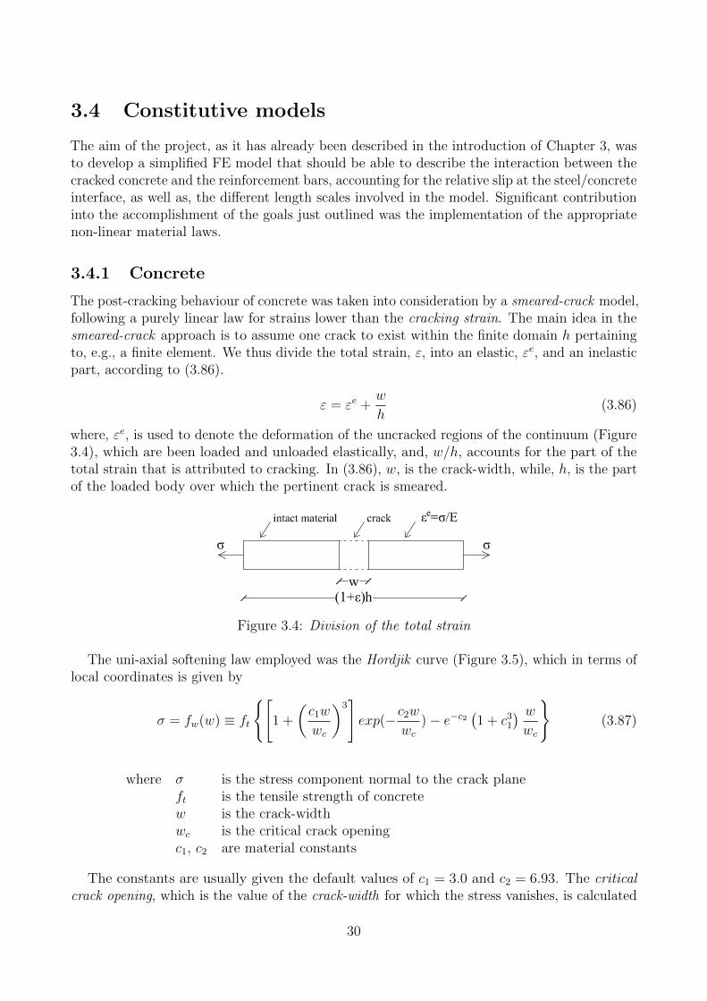
The post-cracking behaviour of concrete was taken into consideration by a smeared-crack model,following a purely linear law for strains lower than the cracking strain. The main idea in thesmeared-crack approach is to assume one crack to exist within the finite domain h pertainingto, e.g., a finite element. We thus divide the total strain, ε, into an elastic, εe, and an inelasticpart, according to (3.86).

ε = εe +w

h(3.86)

where, εe, is used to denote the deformation of the uncracked regions of the continuum (Figure3.4), which are been loaded and unloaded elastically, and, w/h, accounts for the part of thetotal strain that is attributed to cracking. In (3.86), w, is the crack-width, while, h, is the partof the loaded body over which the pertinent crack is smeared.

Figure 3.4: Division of the total strain

The uni-axial softening law employed was the Hordjik curve (Figure 3.5), which in terms oflocal coordinates is given by

σ = fw(w) ≡ ft

{[1 +

(c1w

wc

)3]exp(−c2w

wc)− e−c2

(1 + c3

1

) wwc

}(3.87)

where σ is the stress component normal to the crack planeft is the tensile strength of concretew is the crack-widthwc is the critical crack openingc1, c2 are material constants

The constants are usually given the default values of c1 = 3.0 and c2 = 6.93. The criticalcrack opening, which is the value of the crack-width for which the stress vanishes, is calculated

30

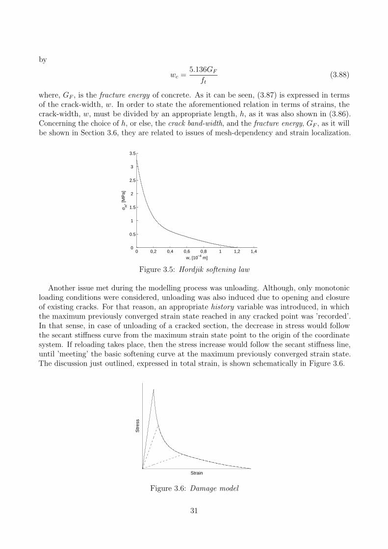
by

wc =5.136GF

ft(3.88)

where, GF , is the fracture energy of concrete. As it can be seen, (3.87) is expressed in termsof the crack-width, w. In order to state the aforementioned relation in terms of strains, thecrack-width, w, must be divided by an appropriate length, h, as it was also shown in (3.86).Concerning the choice of h, or else, the crack band-width, and the fracture energy, GF , as it willbe shown in Section 3.6, they are related to issues of mesh-dependency and strain localization.

0 0,2 0,4 0,6 0,8 1 1,2 1,40

0.5

1

1.5

2

2.5

3

3.5

σ H, [

MP

a]

w, [10−4 m]

Figure 3.5: Hordjik softening law

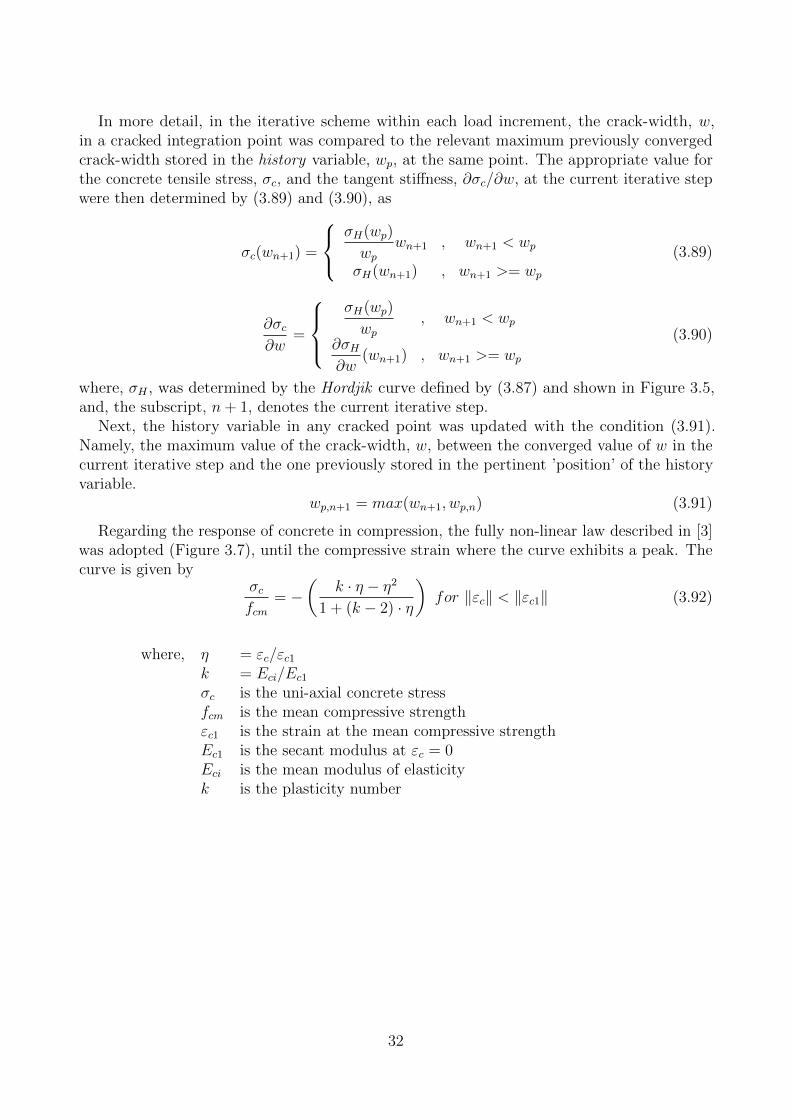
Another issue met during the modelling process was unloading. Although, only monotonicloading conditions were considered, unloading was also induced due to opening and closureof existing cracks. For that reason, an appropriate history variable was introduced, in whichthe maximum previously converged strain state reached in any cracked point was ’recorded’.In that sense, in case of unloading of a cracked section, the decrease in stress would followthe secant stiffness curve from the maximum strain state point to the origin of the coordinatesystem. If reloading takes place, then the stress increase would follow the secant stiffness line,until ’meeting’ the basic softening curve at the maximum previously converged strain state.The discussion just outlined, expressed in total strain, is shown schematically in Figure 3.6.

Strain

Str

ess

Figure 3.6: Damage model

31

In more detail, in the iterative scheme within each load increment, the crack-width, w,in a cracked integration point was compared to the relevant maximum previously convergedcrack-width stored in the history variable, wp, at the same point. The appropriate value forthe concrete tensile stress, σc, and the tangent stiffness, ∂σc/∂w, at the current iterative stepwere then determined by (3.89) and (3.90), as

σc(wn+1) =

σH(wp)

wpwn+1 , wn+1 < wp

σH(wn+1) , wn+1 >= wp

(3.89)

∂σc∂w

=

σH(wp)

wp, wn+1 < wp

∂σH∂w

(wn+1) , wn+1 >= wp

(3.90)

where, σH , was determined by the Hordjik curve defined by (3.87) and shown in Figure 3.5,and, the subscript, n+ 1, denotes the current iterative step.

Next, the history variable in any cracked point was updated with the condition (3.91).Namely, the maximum value of the crack-width, w, between the converged value of w in thecurrent iterative step and the one previously stored in the pertinent ’position’ of the historyvariable.

wp,n+1 = max(wn+1, wp,n) (3.91)

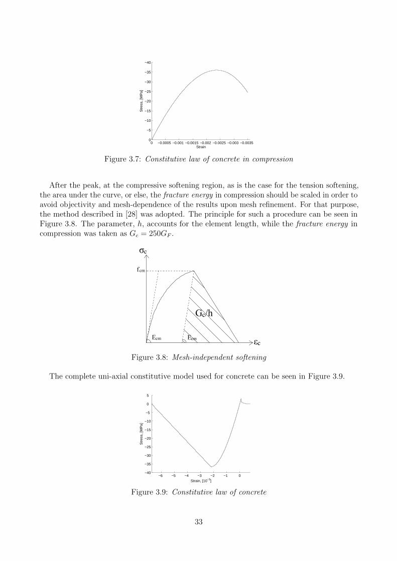
Regarding the response of concrete in compression, the fully non-linear law described in [3]was adopted (Figure 3.7), until the compressive strain where the curve exhibits a peak. Thecurve is given by

σcfcm

= −(

k · η − η2

1 + (k − 2) · η

)for ‖εc‖ < ‖εc1‖ (3.92)

where, η = εc/εc1k = Eci/Ec1σc is the uni-axial concrete stressfcm is the mean compressive strengthεc1 is the strain at the mean compressive strengthEc1 is the secant modulus at εc = 0Eci is the mean modulus of elasticityk is the plasticity number

32

−0.0035−0.003−0.0025−0.002−0.0015−0.001−0.00050

−40

−35

−30

−25

−20

−15

−10

−5

0S

tres

s, [M

Pa]

Strain

Figure 3.7: Constitutive law of concrete in compression

After the peak, at the compressive softening region, as is the case for the tension softening,the area under the curve, or else, the fracture energy in compression should be scaled in order toavoid objectivity and mesh-dependence of the results upon mesh refinement. For that purpose,the method described in [28] was adopted. The principle for such a procedure can be seen inFigure 3.8. The parameter, h, accounts for the element length, while the fracture energy incompression was taken as Gc = 250GF .

Figure 3.8: Mesh-independent softening

The complete uni-axial constitutive model used for concrete can be seen in Figure 3.9.

−6 −5 −4 −3 −2 −1 0−40

−35

−30

−25

−20

−15

−10

−5

0

5

Str

ess,

[MP

a]

Strain, [10−3]

Figure 3.9: Constitutive law of concrete

33

3.4.2 Reinforcement steel

As regards the steel bars, a ’simple’ elasto-plastic law was occupied, as shown in Figure 3.10.The curve is fully defined by the Young’s modulus Es = 200GPa, which is a rather standardvalue for reinforcement steel, and the tensile yield strength of fy = 500GPa .

0 0.001 0.002 0.003 0.004 0.005 0.006 0.0070

50

100

150

200

250

300

350

400

450

500

550

Str

ess,

[MP

a]

Strain

Figure 3.10: Elasto-plastic constitutive law of reinforcement steel

3.4.3 Bond-slip

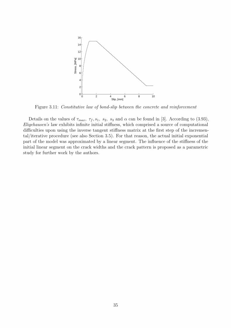
Much discussion took place during the modelling phase regarding the bond-slip law that shouldbe inserted in the analysis. The ’classic’ Eligehausen’s law was considered to be the mostsuitable, as it is also recommended in [3]. The graph of the model is drawn in Figure 3.11.

Four distinct regions can be recognized in the graph, which are described by (3.93).

τ(s) =

τmax

(s

s1

)α, 0 ≤ s ≤ s1

τmax , s1 < s ≤ s2

τf − τmaxs3 − s2

s+

[τf −

τf − τmaxs3 − s2

], s2 < s ≤ s3

τf , s ≥ s3

(3.93)

where, τmax = 2.5√fcm [MPa] (fcm in MPa)

τf = 0.4τmaxs1 = 0.001ms2 = 0.005ms3 = 0.009mα = 0.4

34

0 2 4 6 8 100

2

4

6

8

10

12

14

16

Str

ess,

[MP

a]

Slip, [mm]

Figure 3.11: Constitutive law of bond-slip between the concrete and reinforcement

Details on the values of τmax, τf , s1, s2, s3 and α can be found in [3]. According to (3.93),Eligehausen’s law exhibits infinite initial stiffness, which comprised a source of computationaldifficulties upon using the inverse tangent stiffness matrix at the first step of the incremen-tal/iterative procedure (see also Section 3.5). For that reason, the actual initial exponentialpart of the model was approximated by a linear segment. The influence of the stiffness of theinitial linear segment on the crack widths and the crack pattern is proposed as a parametricstudy for further work by the authors.

35

3.5 Numerical schemes

3.5.1 Newton’s method

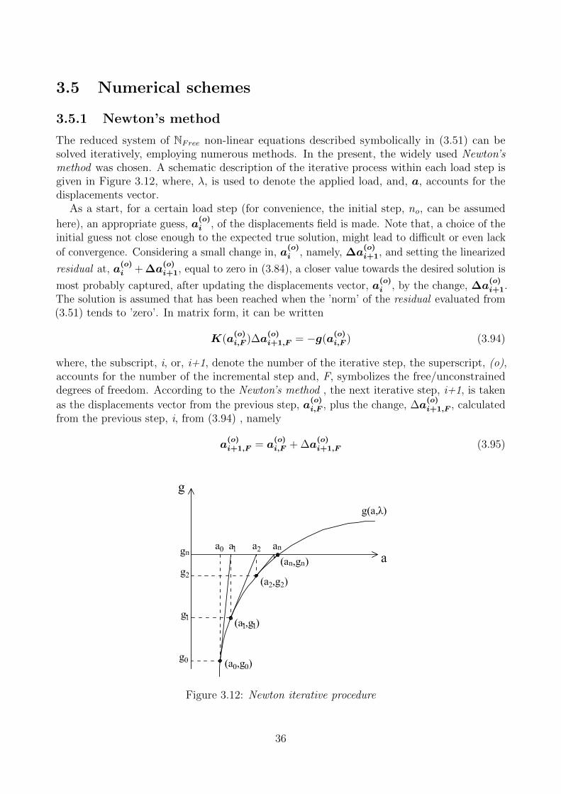
The reduced system of NFree non-linear equations described symbolically in (3.51) can besolved iteratively, employing numerous methods. In the present, the widely used Newton’smethod was chosen. A schematic description of the iterative process within each load step isgiven in Figure 3.12, where, λ, is used to denote the applied load, and, a, accounts for thedisplacements vector.

As a start, for a certain load step (for convenience, the initial step, no, can be assumed

here), an appropriate guess, a(o)i , of the displacements field is made. Note that, a choice of the

initial guess not close enough to the expected true solution, might lead to difficult or even lack

of convergence. Considering a small change in, a(o)i , namely, ∆a

(o)i+1, and setting the linearized

residual at, a(o)i + ∆a

(o)i+1, equal to zero in (3.84), a closer value towards the desired solution is

most probably captured, after updating the displacements vector, a(o)i , by the change, ∆a

(o)i+1.

The solution is assumed that has been reached when the ’norm’ of the residual evaluated from(3.51) tends to ’zero’. In matrix form, it can be written

K(a(o)i,F )∆a

(o)i+1,F = −g(a

(o)i,F ) (3.94)

where, the subscript, i, or, i+1, denote the number of the iterative step, the superscript, (o),accounts for the number of the incremental step and, F, symbolizes the free/unconstraineddegrees of freedom. According to the Newton’s method , the next iterative step, i+1, is taken

as the displacements vector from the previous step, a(o)i,F , plus the change, ∆a

(o)i+1,F , calculated

from the previous step, i, from (3.94) , namely

a(o)i+1,F = a

(o)i,F + ∆a

(o)i+1,F (3.95)

Figure 3.12: Newton iterative procedure

36

3.5.2 Incremental methods

The iterative procedure described at Section 3.5.1 is repeated until convergence at the currentiterative step is reached. The convergence criterion used was that ‖g‖ should be less thana predefined tolerance. So, for a certain load step, the solution vector has been obtainedfollowing Newton’s method. What comes next, is the incremental process. In other words,to calculate the new displacements vector when adding one load step, n1, to the previous

converged load step, no. For that purpose, the starting ’guessed’ displacements vector, a(1)1,F ,

would be the converged solution of the previous step, a(o)n,F , where, n, denotes the number of

iterations needed for the desired tolerance to be met in the previous step, no.It can be stated that three major categories of incremental methods exist, the load-control,

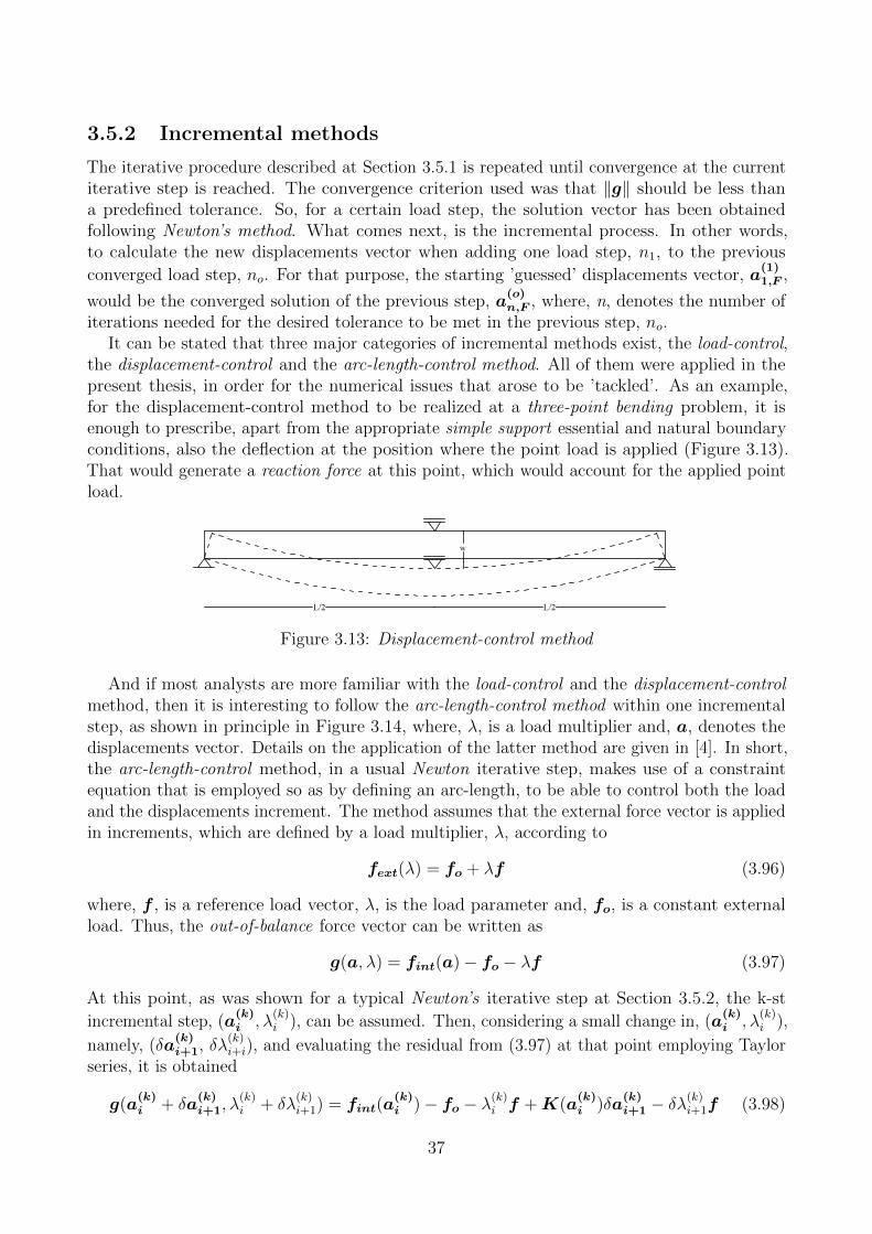
the displacement-control and the arc-length-control method. All of them were applied in thepresent thesis, in order for the numerical issues that arose to be ’tackled’. As an example,for the displacement-control method to be realized at a three-point bending problem, it isenough to prescribe, apart from the appropriate simple support essential and natural boundaryconditions, also the deflection at the position where the point load is applied (Figure 3.13).That would generate a reaction force at this point, which would account for the applied pointload.

Figure 3.13: Displacement-control method

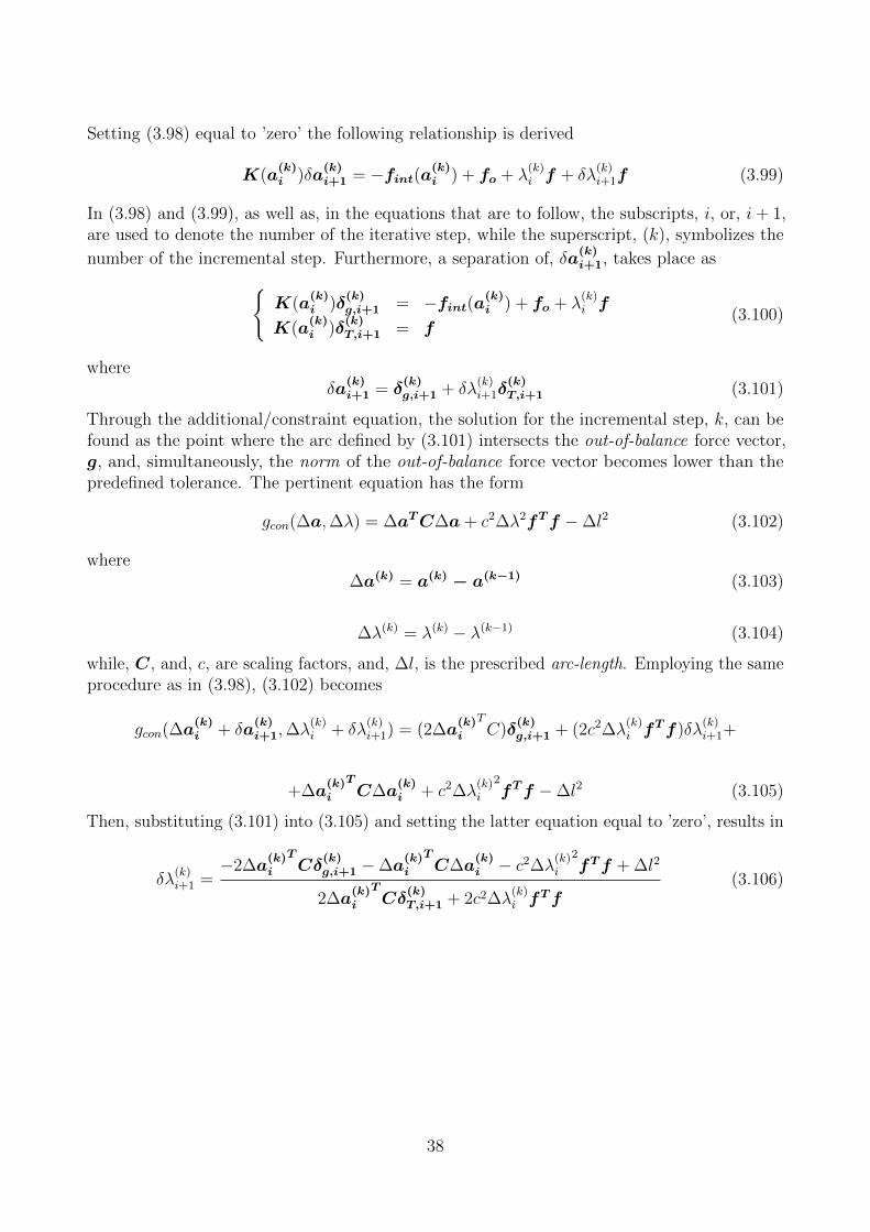
And if most analysts are more familiar with the load-control and the displacement-controlmethod, then it is interesting to follow the arc-length-control method within one incrementalstep, as shown in principle in Figure 3.14, where, λ, is a load multiplier and, a, denotes thedisplacements vector. Details on the application of the latter method are given in [4]. In short,the arc-length-control method, in a usual Newton iterative step, makes use of a constraintequation that is employed so as by defining an arc-length, to be able to control both the loadand the displacements increment. The method assumes that the external force vector is appliedin increments, which are defined by a load multiplier, λ, according to

fext(λ) = fo + λf (3.96)

where, f , is a reference load vector, λ, is the load parameter and, fo, is a constant externalload. Thus, the out-of-balance force vector can be written as

g(a, λ) = fint(a)− fo − λf (3.97)

At this point, as was shown for a typical Newton’s iterative step at Section 3.5.2, the k-st

incremental step, (a(k)i , λ

(k)i ), can be assumed. Then, considering a small change in, (a

(k)i , λ

(k)i ),

namely, (δa(k)i+1, δλ

(k)i+i), and evaluating the residual from (3.97) at that point employing Taylor

series, it is obtained

g(a(k)i + δa

(k)i+1, λ

(k)i + δλ

(k)i+1) = fint(a

(k)i )− fo − λ(k)

i f +K(a(k)i )δa

(k)i+1 − δλ

(k)i+1f (3.98)

37

Setting (3.98) equal to ’zero’ the following relationship is derived

K(a(k)i )δa

(k)i+1 = −fint(a

(k)i ) + fo + λ

(k)i f + δλ

(k)i+1f (3.99)

In (3.98) and (3.99), as well as, in the equations that are to follow, the subscripts, i, or, i+ 1,are used to denote the number of the iterative step, while the superscript, (k), symbolizes the

number of the incremental step. Furthermore, a separation of, δa(k)i+1, takes place as{

K(a(k)i )δ

(k)g,i+1 = −fint(a

(k)i ) + fo + λ

(k)i f

K(a(k)i )δ

(k)T,i+1 = f

(3.100)

whereδa

(k)i+1 = δ

(k)g,i+1 + δλ

(k)i+1δ

(k)T,i+1 (3.101)

Through the additional/constraint equation, the solution for the incremental step, k, can befound as the point where the arc defined by (3.101) intersects the out-of-balance force vector,g, and, simultaneously, the norm of the out-of-balance force vector becomes lower than thepredefined tolerance. The pertinent equation has the form

gcon(∆a,∆λ) = ∆aTC∆a+ c2∆λ2fTf −∆l2 (3.102)

where∆a(k) = a(k) − a(k−1) (3.103)

∆λ(k) = λ(k) − λ(k−1) (3.104)

while, C, and, c, are scaling factors, and, ∆l, is the prescribed arc-length. Employing the sameprocedure as in (3.98), (3.102) becomes

gcon(∆a(k)i + δa

(k)i+1,∆λ

(k)i + δλ

(k)i+1) = (2∆a

(k)i

TC)δ

(k)g,i+1 + (2c2∆λ

(k)i f

Tf)δλ(k)i+1+

+∆a(k)i

TC∆a

(k)i + c2∆λ

(k)i

2fTf −∆l2 (3.105)

Then, substituting (3.101) into (3.105) and setting the latter equation equal to ’zero’, results in

δλ(k)i+1 =

−2∆a(k)i

TCδ

(k)g,i+1 −∆a

(k)i

TC∆a

(k)i − c2∆λ

(k)i

2fTf + ∆l2

2∆a(k)i

TCδ

(k)T,i+1 + 2c2∆λ

(k)i f

Tf(3.106)

38

Figure 3.14: Arc-length-control method

3.5.3 Numerical integration

From (3.40), (3.41) and (3.42), it can be observed that evaluation of integrals of the form

Iz,σ =

∫A

f(z)σ(x, z)dA = b

∫ h/2

−h/2f(z)σ(x, z)dz (3.107)

Iz,dσ =

∫A

f(z)∂σ

∂ε(x, z)dA = b

∫ h/2

−h/2f(z)

∂σ

∂ε(x, z)dz (3.108)

is needed along the height, where, h, is the height, and, b, is the width of the cross-section, zand x, are the axes along the height and the length of the elements, respectively. Also, from(3.61)-(3.82) it can be observed that evaluation of integrals of the form

Ix,σ =

∫L

BT (x)σ(x, z)B(x)dx (3.109)

Ix,dσ =

∫L

BT (x)∂σ

∂ε(x, z)B(x)dx (3.110)

is needed over the length of the finite elements, where the B-matrices were defined in the FE-formulation of the problem, and, ε, denotes the normal strains of the beam. For the evaluationof the pertinent integrals, where, usually, it is difficult to obtain closed-form analytical solutions,suitable numerical methods need to be employed. After performing the transformation fromz ∈ [−h/2, h/2] to ξ ∈ [−1, 1], (3.107) and (3.108) reform to

Iz =bh

2

∫ 1

−1

g(x,h

2ξ)dξ =

bh

2

n∑i=1

wz,ig(x,h

2ξi) (3.111)

39

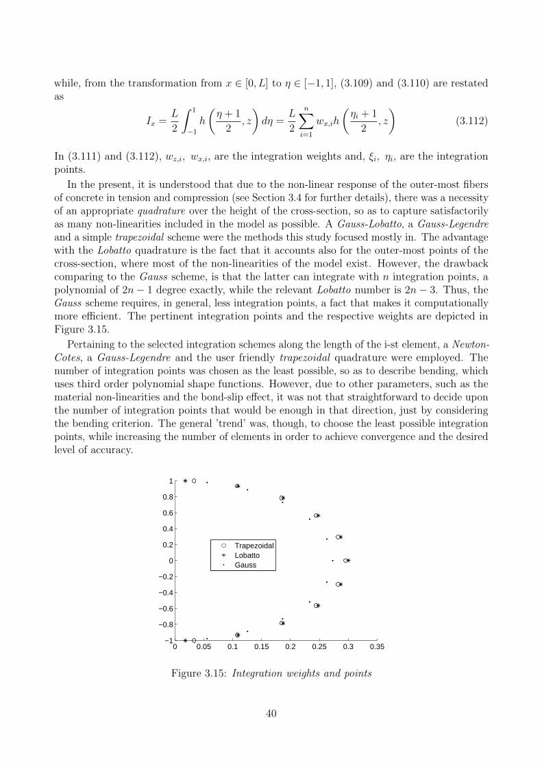
while, from the transformation from x ∈ [0, L] to η ∈ [−1, 1], (3.109) and (3.110) are restatedas

Ix =L

2

∫ 1

−1

h

(η + 1

2, z

)dη =

L

2

n∑i=1

wx,ih

(ηi + 1

2, z

)(3.112)

In (3.111) and (3.112), wz,i, wx,i, are the integration weights and, ξi, ηi, are the integrationpoints.

In the present, it is understood that due to the non-linear response of the outer-most fibersof concrete in tension and compression (see Section 3.4 for further details), there was a necessityof an appropriate quadrature over the height of the cross-section, so as to capture satisfactorilyas many non-linearities included in the model as possible. A Gauss-Lobatto, a Gauss-Legendreand a simple trapezoidal scheme were the methods this study focused mostly in. The advantagewith the Lobatto quadrature is the fact that it accounts also for the outer-most points of thecross-section, where most of the non-linearities of the model exist. However, the drawbackcomparing to the Gauss scheme, is that the latter can integrate with n integration points, apolynomial of 2n− 1 degree exactly, while the relevant Lobatto number is 2n− 3. Thus, theGauss scheme requires, in general, less integration points, a fact that makes it computationallymore efficient. The pertinent integration points and the respective weights are depicted inFigure 3.15.

Pertaining to the selected integration schemes along the length of the i-st element, a Newton-Cotes, a Gauss-Legendre and the user friendly trapezoidal quadrature were employed. Thenumber of integration points was chosen as the least possible, so as to describe bending, whichuses third order polynomial shape functions. However, due to other parameters, such as thematerial non-linearities and the bond-slip effect, it was not that straightforward to decide uponthe number of integration points that would be enough in that direction, just by consideringthe bending criterion. The general ’trend’ was, though, to choose the least possible integrationpoints, while increasing the number of elements in order to achieve convergence and the desiredlevel of accuracy.

0 0.05 0.1 0.15 0.2 0.25 0.3 0.35−1

−0.8

−0.6

−0.4

−0.2

0

0.2

0.4

0.6

0.8

1

TrapezoidalLobattoGauss

Figure 3.15: Integration weights and points

40

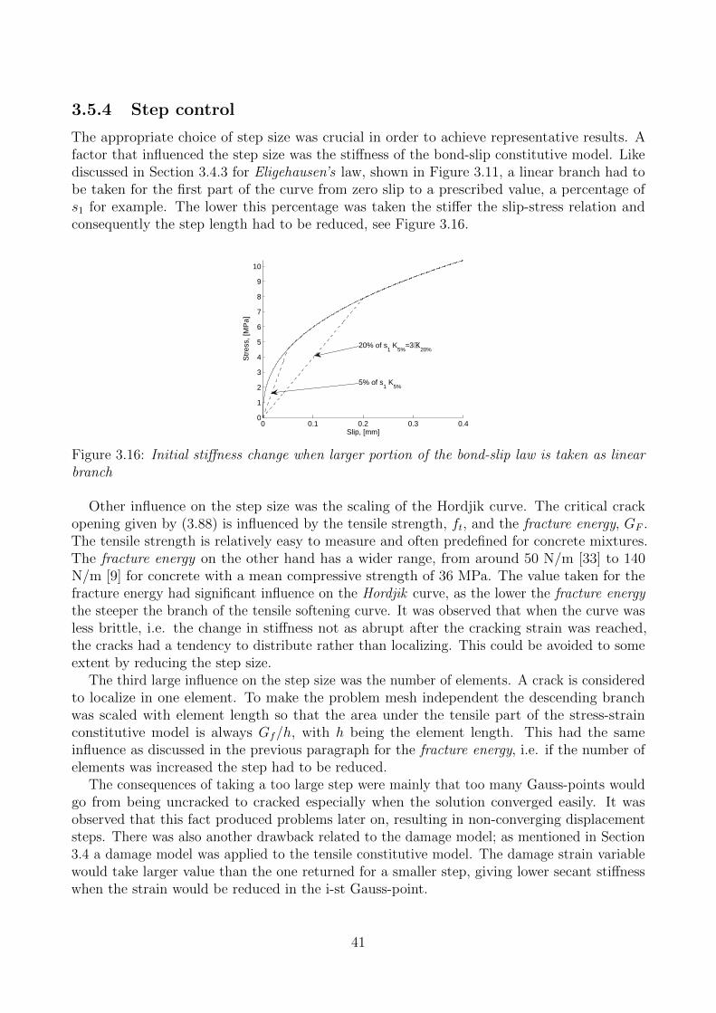
3.5.4 Step control

The appropriate choice of step size was crucial in order to achieve representative results. Afactor that influenced the step size was the stiffness of the bond-slip constitutive model. Likediscussed in Section 3.4.3 for Eligehausen’s law, shown in Figure 3.11, a linear branch had tobe taken for the first part of the curve from zero slip to a prescribed value, a percentage ofs1 for example. The lower this percentage was taken the stiffer the slip-stress relation andconsequently the step length had to be reduced, see Figure 3.16.

0 0.1 0.2 0.3 0.40

1

2

3

4

5

6

7

8

9

10

Str

ess,

[MP

a]

Slip, [mm]

5% of s1 K

5%

20% of s1 K

5%≈3⋅K

20%

Figure 3.16: Initial stiffness change when larger portion of the bond-slip law is taken as linearbranch

Other influence on the step size was the scaling of the Hordjik curve. The critical crackopening given by (3.88) is influenced by the tensile strength, ft, and the fracture energy, GF .The tensile strength is relatively easy to measure and often predefined for concrete mixtures.The fracture energy on the other hand has a wider range, from around 50 N/m [33] to 140N/m [9] for concrete with a mean compressive strength of 36 MPa. The value taken for thefracture energy had significant influence on the Hordjik curve, as the lower the fracture energythe steeper the branch of the tensile softening curve. It was observed that when the curve wasless brittle, i.e. the change in stiffness not as abrupt after the cracking strain was reached,the cracks had a tendency to distribute rather than localizing. This could be avoided to someextent by reducing the step size.

The third large influence on the step size was the number of elements. A crack is consideredto localize in one element. To make the problem mesh independent the descending branchwas scaled with element length so that the area under the tensile part of the stress-strainconstitutive model is always Gf/h, with h being the element length. This had the sameinfluence as discussed in the previous paragraph for the fracture energy, i.e. if the number ofelements was increased the step had to be reduced.

The consequences of taking a too large step were mainly that too many Gauss-points wouldgo from being uncracked to cracked especially when the solution converged easily. It wasobserved that this fact produced problems later on, resulting in non-converging displacementsteps. There was also another drawback related to the damage model; as mentioned in Section3.4 a damage model was applied to the tensile constitutive model. The damage strain variablewould take larger value than the one returned for a smaller step, giving lower secant stiffnesswhen the strain would be reduced in the i-st Gauss-point.

41

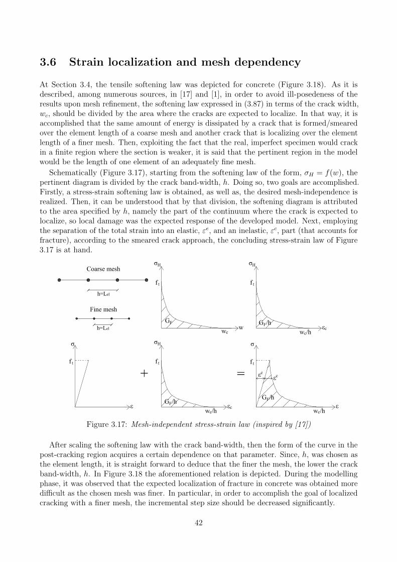
3.6 Strain localization and mesh dependency

At Section 3.4, the tensile softening law was depicted for concrete (Figure 3.18). As it isdescribed, among numerous sources, in [17] and [1], in order to avoid ill-posedeness of theresults upon mesh refinement, the softening law expressed in (3.87) in terms of the crack width,wc, should be divided by the area where the cracks are expected to localize. In that way, it isaccomplished that the same amount of energy is dissipated by a crack that is formed/smearedover the element length of a coarse mesh and another crack that is localizing over the elementlength of a finer mesh. Then, exploiting the fact that the real, imperfect specimen would crackin a finite region where the section is weaker, it is said that the pertinent region in the modelwould be the length of one element of an adequately fine mesh.

Schematically (Figure 3.17), starting from the softening law of the form, σH = f(w), thepertinent diagram is divided by the crack band-width, h. Doing so, two goals are accomplished.Firstly, a stress-strain softening law is obtained, as well as, the desired mesh-independence isrealized. Then, it can be understood that by that division, the softening diagram is attributedto the area specified by h, namely the part of the continuum where the crack is expected tolocalize, so local damage was the expected response of the developed model. Next, employingthe separation of the total strain into an elastic, εe, and an inelastic, εc, part (that accounts forfracture), according to the smeared crack approach, the concluding stress-strain law of Figure3.17 is at hand.

Figure 3.17: Mesh-independent stress-strain law (inspired by [17])

After scaling the softening law with the crack band-width, then the form of the curve in thepost-cracking region acquires a certain dependence on that parameter. Since, h, was chosen asthe element length, it is straight forward to deduce that the finer the mesh, the lower the crackband-width, h. In Figure 3.18 the aforementioned relation is depicted. During the modellingphase, it was observed that the expected localization of fracture in concrete was obtained moredifficult as the chosen mesh was finer. In particular, in order to accomplish the goal of localizedcracking with a finer mesh, the incremental step size should be decreased significantly.

42

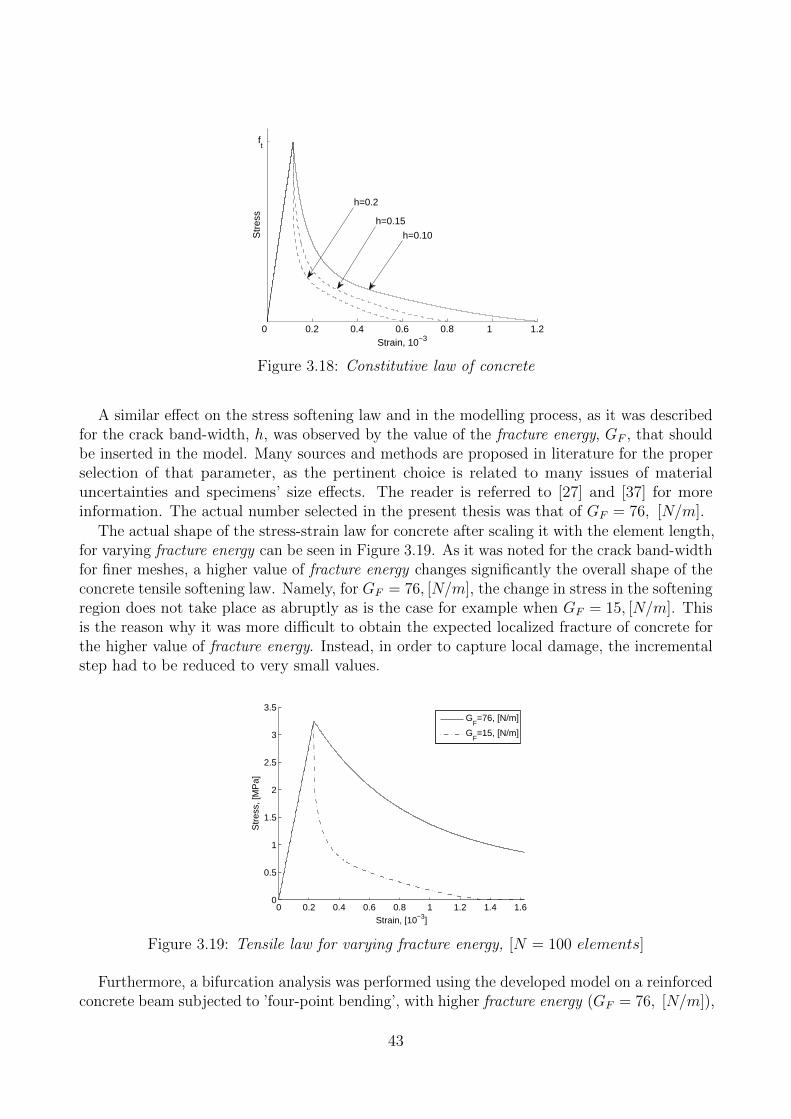
0 0.2 0.4 0.6 0.8 1 1.2

ft

Strain, 10−3

Str

ess

h=0.10

h=0.2

h=0.15

Figure 3.18: Constitutive law of concrete

A similar effect on the stress softening law and in the modelling process, as it was describedfor the crack band-width, h, was observed by the value of the fracture energy, GF , that shouldbe inserted in the model. Many sources and methods are proposed in literature for the properselection of that parameter, as the pertinent choice is related to many issues of materialuncertainties and specimens’ size effects. The reader is referred to [27] and [37] for moreinformation. The actual number selected in the present thesis was that of GF = 76, [N/m].

The actual shape of the stress-strain law for concrete after scaling it with the element length,for varying fracture energy can be seen in Figure 3.19. As it was noted for the crack band-widthfor finer meshes, a higher value of fracture energy changes significantly the overall shape of theconcrete tensile softening law. Namely, for GF = 76, [N/m], the change in stress in the softeningregion does not take place as abruptly as is the case for example when GF = 15, [N/m]. Thisis the reason why it was more difficult to obtain the expected localized fracture of concrete forthe higher value of fracture energy. Instead, in order to capture local damage, the incrementalstep had to be reduced to very small values.

0 0.2 0.4 0.6 0.8 1 1.2 1.4 1.60

0.5

1

1.5

2

2.5

3

3.5

Str

ess,

[MP

a]

Strain, [10−3]

GF=76, [N/m]

GF=15, [N/m]

Figure 3.19: Tensile law for varying fracture energy, [N = 100 elements]

Furthermore, a bifurcation analysis was performed using the developed model on a reinforcedconcrete beam subjected to ’four-point bending’, with higher fracture energy (GF = 76, [N/m]),

43

which if an adequately small incremental step was not chosen, the resulting load-deflectioncurve would exhibit distributed, rather than localized cracking. If a bifurcation point wouldexist at the point on the load-deflection diagram where the first localized crack should appear,then one could conclude that the system is following an unstable equilibrium path, sincefrom ’reality’ it is known for the specific ’four-point bending’ problem that the path whichresults in localization is the one which releases more energy, the stable one. Then, via thearc-length-control method and an appropriate guess, it would be possible to enforce the solutiontowards the ’real’ response which involves localization. However, after checking the lowesteigenvalues of the tangent stiffness matrix right before the possible critical points and afterthose, no change of sign was observed. Thus, the existence of bifurcation points was excluded,a fact that led to the conclusion that it was most probably the value of the fracture energyand the crack band-width, which governed the difficulty of localized cracking to take place.

The aforementioned difficulties in obtaining the expected localized fracture in concrete wereovercome, mainly, by using a weaker middle element (i.e. the most stressed one upon addingthe self-weight in the applications examined in Chapter 4). That was accomplished by insertinglower tensile strength and fracture energy for the middle element, which was the one where thefirst localized crack was expected to form. Another way to ’trigger’ localization was by updatingthe history variable (see also Section 3.4.1 for more details on the history variable) using valuesfor the crack width that resulted from ’controlled’ non-converged Newton’s iterative steps, onlyin critical points, i.e. when cracks were about to form. The term ’controlled’ refers to thefact that out of all the non-converged Newton’s iterative steps that appeared within a criticalincremental step, only the values for the crack width from the iterative step with the leastdivergence were stored in the history variable. That measure had a perturbation effect on thestiffness of the most stressed part of the beam, where the first crack was to form, contributingin obtaining the first localized crack, using less integration points than it would be necessaryto use if the history variable was updated only by converged Newton’s iterative steps.

44

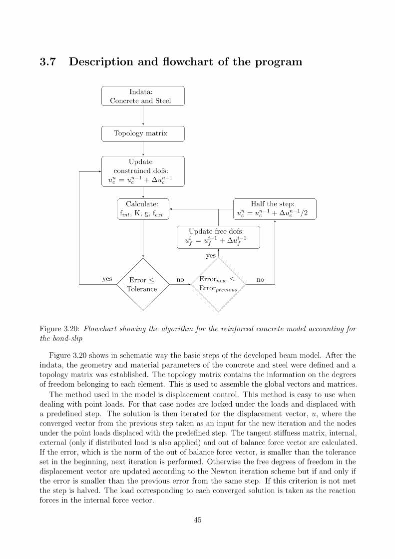
3.7 Description and flowchart of the program

Indata:Concrete and Steel

Topology matrix

Updateconstrained dofs:

unc = un−1c + ∆un−1

c

Calculate:fint, K, g, fext

Error ≤Tolerance

Half the step:unc = un−1

c + ∆un−1c /2

Errornew ≤Errorprevious

Update free dofs:uif = ui−1

f + ∆ui−1f

yes no no

yes

Figure 3.20: Flowchart showing the algorithm for the reinforced concrete model accounting forthe bond-slip

Figure 3.20 shows in schematic way the basic steps of the developed beam model. After theindata, the geometry and material parameters of the concrete and steel were defined and atopology matrix was established. The topology matrix contains the information on the degreesof freedom belonging to each element. This is used to assemble the global vectors and matrices.

The method used in the model is displacement control. This method is easy to use whendealing with point loads. For that case nodes are locked under the loads and displaced witha predefined step. The solution is then iterated for the displacement vector, u, where theconverged vector from the previous step taken as an input for the new iteration and the nodesunder the point loads displaced with the predefined step. The tangent stiffness matrix, internal,external (only if distributed load is also applied) and out of balance force vector are calculated.If the error, which is the norm of the out of balance force vector, is smaller than the toleranceset in the beginning, next iteration is performed. Otherwise the free degrees of freedom in thedisplacement vector are updated according to the Newton iteration scheme but if and only ifthe error is smaller than the previous error from the same step. If this criterion is not metthe step is halved. The load corresponding to each converged solution is taken as the reactionforces in the internal force vector.

45

The program has also a feature, in which if convergence is not obtained after halving thestep for a predefined number of times the program is forced to try the next step with the latestconverged displacement vector.

46

4 Evaluation and comparison with experimentsand Eurocode

4.1 Experiments from literature

In the present chapter, methods that will be presented in Section 4.2 are used to calculate beamsof the same length, cross-section and material properties as beams tested in the laboratoryby Gilbert et al. [12]. In the pertinent study, twelve specimens were cast (six beams and sixslabs). With regard to the beams, three different cross-sections were used.

For each cross-section, two identical specimens were made and tested at different concreteages. The dimensions and the cross-sections of the beams are given in Figure 4.1 and Table4.1. The material data for the three different configurations of the beams are shown in Table4.2. Since the values for the steel properties were not given in the experimental results, theywere assumed; the characteristic tensile strength, fyk = 500 MPa, and the elastic modulus,Es = 200 GPa. The concrete properties were interpolated from measured values for appropriateages. This is reasonable since the change in properties is small. The uniaxial tensile strengthwas obtained from tensile splitting tests, the used relation is given in Section 4.2.2.

Figure 4.1: Beams test configuration with dimensions, varying parameters and cross sectionlayout. Test setup from Gilbert et al. [12]

Table 4.1: Values of varying parameters of the beams

h [mm] c [mm] n [bars]B1 348 40 2B2 333 25 2

Table 4.2: Material properties of the tested beams, the numbers in bold represent measuredvalues, the other are interpolated values.

Age [days] 27 28 42 45 48 53 54 55 63 68

fcm [MPa] 36.0 36.3 36.5 36.6 36.6 37.1 37.2 37.3 39.1 40.1fctm [MPa] 3.05 3.06 3.19 3.22 3.25 3.30 3.31 3.31 3.39 3.44Ecm [GPa] 26.9 27.0 27.7 27.8 28.0 28.2 28.2 28.3 28.7 28.9

47

4.2 Analytical calculations

To verify the developed FEM beam model simple analytical calculations were conducted. Theywere then compared to experimental results. Furthermore experimental results were used forcomparison.

4.2.1 Mid span deflection

Euler-Bernoulli beam theory was used to calculate the moment and deflection resulting frombending.

d2w

dx2= −M

EI(4.1)

The beams were all statically determinate and symmetric, see Figure 4.1. Therefore thesectional forces can be determined by equilibrium equations. This means that globally there isonly one solution that fulfills equilibrium, so when the beam cracks there will only be forceredistribution locally within the beam cross section. When the beam cracks it looses stiffnessgradually until fully cracked[7].

ζ(x) =

(1−

(Mcr

M(x)

))(4.2)

EI(x) = ζ(x)EII + (1− ζ(x))EIII (4.3)

where ζ is a distribution coefficientEII is stiffness of the uncracked sectionEIII is stiffness of the fully cracked section

The mid point deflection is given by the following equation [7].

f(l/2) = l/2

∫ l/2

0

κ(x)dx−∫ l/2

0

κ(x)(l/2− x)dx (4.4)

where κ is the curvature given by Equation (4.1)

48

4.2.2 Tensile strength

When calculating the crack widths the uniaxial tensile strength, fctm is needed. In Section4.1 test results are compared to the EC2 model for crack widths. In the experimental resultspresented in Gilbert et al.[12] the concrete has been tested by using tensile splitting test. TheFIB model code from 2010 [9] recommends that the uniaxial tensile strength is determinedfrom splitting test as

fctm = Asp · fct,sp (4.5)

where Asp is a conversion factor, FIB Model code suggests 1.0fct,sp is the mean splitting tensile strength

4.2.3 Steel stress

The steel stress σs in a beam in state II, fully cracked was calculated using Naviers formula forbending stress

σs =M

III(d− xII) · αc (4.6)

where M is the moment in the sectiond is the distance from the top edge down to the gravity center

of reinforcementxII is the depth of compressive zone in the reinforced concrete

beam in state IIIII is the second moment of area of the fully cracked cross section

in state IIαe is the ratio Es/Ec

The second moment of area was calculated as

III =bx3

II

3+ Asαc (d− xII)2

and the depth of the concrete compressive zone in state II, xII , without compressivereinforcement and linear stress-strain relation can be solved from the following second orderpolynomial

bx2II

2− As · αc(d− xII) = 0

49

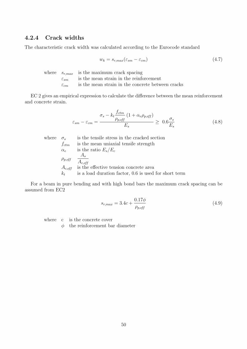
4.2.4 Crack widths

The characteristic crack width was calculated according to the Eurocode standard

wk = sr,max(εsm − εcm) (4.7)

where sr,max is the maximum crack spacingεsm is the mean strain in the reinforcementεcm is the mean strain in the concrete between cracks

EC 2 gives an empirical expression to calculate the difference between the mean reinforcementand concrete strain.

εsm − εcm =

σs − ktfctmρp,eff

(1 + αeρp,eff )

Es≥ 0.6

σsEs

(4.8)

where σs is the tensile stress in the cracked sectionfctm is the mean uniaxial tensile strengthαe is the ratio Es/Ec

ρp,effAsAc,eff

Ac,eff is the effective tension concrete areakt is a load duration factor, 0.6 is used for short term

For a beam in pure bending and with high bond bars the maximum crack spacing can beassumed from EC2

sr,max = 3.4c+0.17φ

ρp,eff(4.9)

where c is the concrete coverφ the reinforcement bar diameter

50

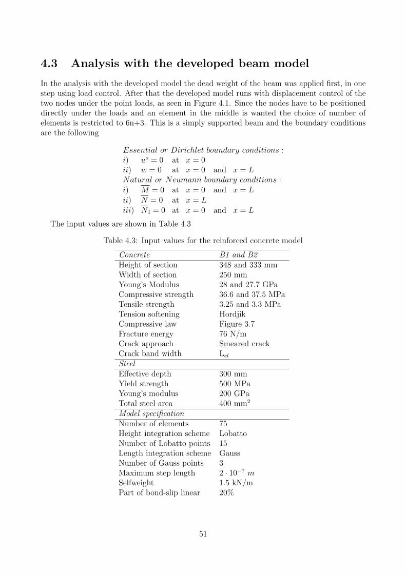
4.3 Analysis with the developed beam model

In the analysis with the developed model the dead weight of the beam was applied first, in onestep using load control. After that the developed model runs with displacement control of thetwo nodes under the point loads, as seen in Figure 4.1. Since the nodes have to be positioneddirectly under the loads and an element in the middle is wanted the choice of number ofelements is restricted to 6n+3. This is a simply supported beam and the boundary conditionsare the following

Essential or Dirichlet boundary conditions :i) uo = 0 at x = 0ii) w = 0 at x = 0 and x = LNatural or Neumann boundary conditions :i) M = 0 at x = 0 and x = Lii) N = 0 at x = Liii) N i = 0 at x = 0 and x = L

The input values are shown in Table 4.3

Table 4.3: Input values for the reinforced concrete model

Concrete B1 and B2Height of section 348 and 333 mmWidth of section 250 mmYoung’s Modulus 28 and 27.7 GPaCompressive strength 36.6 and 37.5 MPaTensile strength 3.25 and 3.3 MPaTension softening HordjikCompressive law Figure 3.7Fracture energy 76 N/mCrack approach Smeared crackCrack band width LelSteelEffective depth 300 mmYield strength 500 MPaYoung’s modulus 200 GPaTotal steel area 400 mm2

Model specificationNumber of elements 75Height integration scheme LobattoNumber of Lobatto points 15Length integration scheme GaussNumber of Gauss points 3Maximum step length 2 · 10−7 mSelfweight 1.5 kN/mPart of bond-slip linear 20%

51

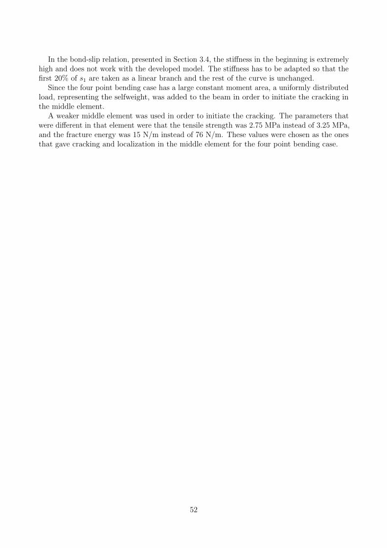
In the bond-slip relation, presented in Section 3.4, the stiffness in the beginning is extremelyhigh and does not work with the developed model. The stiffness has to be adapted so that thefirst 20% of s1 are taken as a linear branch and the rest of the curve is unchanged.

Since the four point bending case has a large constant moment area, a uniformly distributedload, representing the selfweight, was added to the beam in order to initiate the cracking inthe middle element.

A weaker middle element was used in order to initiate the cracking. The parameters thatwere different in that element were that the tensile strength was 2.75 MPa instead of 3.25 MPa,and the fracture energy was 15 N/m instead of 76 N/m. These values were chosen as the onesthat gave cracking and localization in the middle element for the four point bending case.

52

4.4 Comparison of results

In section 4.2.4 the Eurocode method for calculating crack widths was presented. Equation(4.7) gives the upper characteristic crack width that means that 95% of cracks should besmaller than the values given by the equation. In the experiments, Gilbert et al. [12], all thecracks were measured. The maximum crack opening was compared to the Eurocode model, seeFigures 4.2 and 4.4.

4.4.1 Stiffness adaptation method

The stiffness adaptation method was adopted to compare with the load-deflection diagramretrieved from the developed model. Stiffness adaptation is a Finite Element method where thestiffness is changed if a element cracks, i.e. when a element cracks it goes from being uncracked,in state I, to being fully cracked, in state II. The element is determined to be cracked or notfrom the average moment in each element and if that is higher than the cracking moment. Itis obvious that when using this method, the tension stiffening or the influence of the bond slipare not considered in the development of crack and crack positions.

4.4.2 Diana analysis

Models of the beams were set up using the commercial FE program Diana, where all thenon-linearities of the material were considered. Classic beam elements, L7BEN, were usedwhere both translational degrees of freedom were locked at the left boundary and on the rightside the vertical translation was locked. The beam consisted of 11 nodes and 10 elements.Other input values and parameters are specified in Table 4.4. No bond slip was considered, i.e.the reinforcement was embedded with full interaction between concrete and steel. Thereforethe crack band width was choosen as the expected crack spacing calculated from (4.9).

Table 4.4: Diana input for the non-linear FE-analysis

Concrete B1 and B2Height of section 348 and 333 mmWidth of section 250 mmYoung’s Modulus 28 and 27.7 GPaCompressive strength 36.6 and 37.5 MPaTensile strength 3.25 and 3.3 MPaTension softening HordjikCompressive law ThorenFracture energy 76 N/mCrack approach Smeared crackCrack band width 0.176 mSteelEffective depth 300 mmYield strength 500 MPaYoung’s modulus 200 GPaYield criterion Von MisesTotal steel area 400 mm2

53

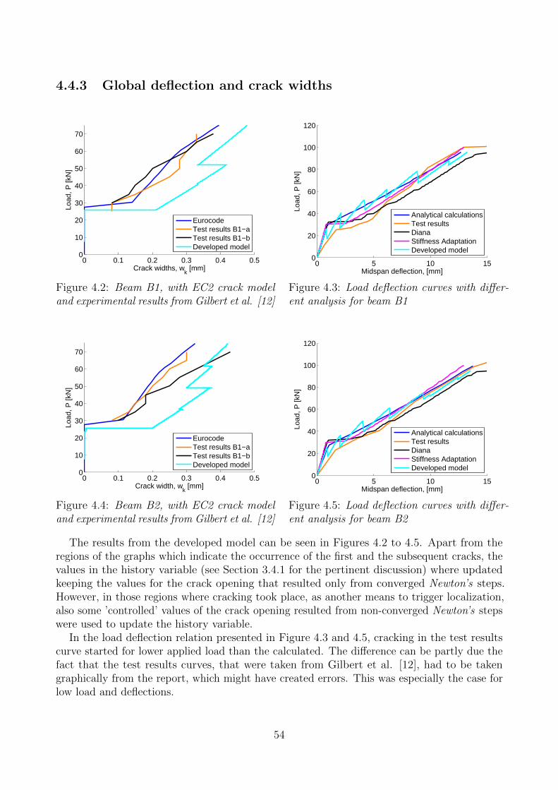
4.4.3 Global deflection and crack widths

0 0.1 0.2 0.3 0.4 0.50

10

20

30

40

50

60

70

Crack widths, wk [mm]

Load

, P [k

N]

EurocodeTest results B1−aTest results B1−bDeveloped model

Figure 4.2: Beam B1, with EC2 crack modeland experimental results from Gilbert et al. [12]

0 5 10 150

20

40

60

80

100

120

Midspan deflection, [mm]

Load

, P [k

N]

Analytical calculationsTest resultsDianaStiffness AdaptationDeveloped model

Figure 4.3: Load deflection curves with differ-ent analysis for beam B1

0 0.1 0.2 0.3 0.4 0.50

10

20

30

40

50

60

70

Crack width, wk [mm]

Load

, P [k

N]

EurocodeTest results B1−aTest results B1−bDeveloped model

Figure 4.4: Beam B2, with EC2 crack modeland experimental results from Gilbert et al. [12]

0 5 10 150

20

40

60

80

100

120

Midspan deflection, [mm]

Load

, P [k

N]

Analytical calculationsTest resultsDianaStiffness AdaptationDeveloped model

Figure 4.5: Load deflection curves with differ-ent analysis for beam B2

The results from the developed model can be seen in Figures 4.2 to 4.5. Apart from theregions of the graphs which indicate the occurrence of the first and the subsequent cracks, thevalues in the history variable (see Section 3.4.1 for the pertinent discussion) where updatedkeeping the values for the crack opening that resulted only from converged Newton’s steps.However, in those regions where cracking took place, as another means to trigger localization,also some ’controlled’ values of the crack opening resulted from non-converged Newton’s stepswere used to update the history variable.

In the load deflection relation presented in Figure 4.3 and 4.5, cracking in the test resultscurve started for lower applied load than the calculated. The difference can be partly due thefact that the test results curves, that were taken from Gilbert et al. [12], had to be takengraphically from the report, which might have created errors. This was especially the case forlow load and deflections.

54

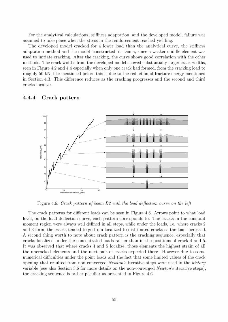
For the analytical calculations, stiffness adaptation, and the developed model, failure wasassumed to take place when the stress in the reinforcement reached yielding.

The developed model cracked for a lower load than the analytical curve, the stiffnessadaptation method and the model ’constructed’ in Diana, since a weaker middle element wasused to initiate cracking. After the cracking, the curve shows good correlation with the othermethods. The crack widths from the developed model showed substantially larger crack widths,seen in Figure 4.2 and 4.4 especially when only one crack had formed, from the cracking load toroughly 50 kN, like mentioned before this is due to the reduction of fracture energy mentionedin Section 4.3. This difference reduces as the cracking progresses and the second and thirdcracks localize.

4.4.4 Crack pattern

0 5 10 150

10

20

30

40

50

60

70

80

90

100

Maximum deflection, [mm]

Tot

al lo

ad, [

kN]

Figure 4.6: Crack pattern of beam B2 with the load deflection curve on the left

The crack patterns for different loads can be seen in Figure 4.6. Arrows point to what loadlevel, on the load-deflection curve, each pattern corresponds to. The cracks in the constantmoment region were always well defined in all steps, while under the loads, i.e. where cracks 2and 3 form, the cracks tended to go from localized to distributed cracks as the load increased.A second thing worth to note about crack pattern is the cracking sequence, especially thatcracks localized under the concentrated loads rather than in the positions of crack 4 and 5.It was observed that where cracks 4 and 5 localize, those elements the highest strain of allthe uncracked elements and the next pair of cracks expected there. However due to somenumerical difficulties under the point loads and the fact that some limited values of the crackopening that resulted from non-converged Newton’s iterative steps were used in the historyvariable (see also Section 3.6 for more details on the non-converged Newton’s iterative steps),the cracking sequence is rather peculiar as presented in Figure 4.6.

55

5 Conclusions and suggestions for further work

In the present thesis, a 1D finite element model was developed, that is able to describe theresponse of a reinforced concrete beam that undergoes local damage, while accounting alsofor the relative slip at the steel/concrete interface. Three non-linear constitutive laws wereimplemented for the materials. A softening law was used to account for fracture in concrete; toobtain objectivity of the results upon mesh refinement, it was scaled with the element length. Asimple elasto-plastic law was inserted for steel and Eligehausen’s law was used for the bond-slip.Newton’s iterative scheme was chosen for the solution of the non-linear system of equationsobtained from the FE-formulation of the problem. The pertinent equations were developed forthe case of a reinforced concrete beam subjected to transverse distributed loading. Pertainingto the incremental procedures, load-control, displacement-control, arc-length-control, as wellas combinations between the aforementioned methods were applied in order to obtain resultsovercoming numerical problems of various kinds.

The developed model was used in non-linear FE analysis of reinforced concrete beamssubjected to ’four-point bending’. Several observations were made: First, initiation of crackingwas a crucial parameter in the model. It was found that the combination of a higher value offracture energy, together with the scaling of the stress softening diagram of concrete with theelement length resulted in a less steep softening curve. Secondly, it was observed that the lesssteep the softening curve, the more difficult was for the first localized crack to appear. Onlyby ’triggering’ localization, the first concentrated crack would form. Ways for such ’triggering’were to reduce the tensile strength and the fracture energy of the middle element. In that way,a more brittle behaviour in that element was forced.

Furthermore, a certain dependence of the results obtained from the developed model on thechosen incremental step size was observed. This effect was attributed to the influence of thehistory variable introduced in order to account for the unloading of the beam upon openingand closure of existing cracks. A larger step size would lead more integration points to passbeyond the cracking strain. These points would, then, upon unloading, instead of following thelinear branch of the stress-strain law, unload with the secant stiffness from the point reachedin the softening law towards the origin of the coordinate system.

A rather unexpected phenomenon was captured during the analysis for the ’four-pointbending’ problem. Namely, the first cracking would always tend to appear under the pointloads, instead of forming at the middle element, which was the most stressed one, as theself-weight was included. Then, depending on where the first crack/cracks would appear, thesequence of appearance of the next cracks was also affected.

Some comments could also be stated upon the stiffness of the implemented bond-sliprelation, Eligehausen’s law in particular. The first one is related to the initial infinite stiffnessof the pertinent exponential law. Upon using the inverse of the tangent stiffness matrix inthe Newton’s iterative scheme, the infinite stiffness of the initial branch of Eligehausen’s lawresulted in an non-invertible matrix. Even when trespassing the stiffness value evaluated for’zero’ slip, the stiffness of the constitutive model is so high, that in order to be implemented, avery low step for the slip should be inserted in the displacements field so as to avoid divergenceof the iterative procedure. In order to overcome these objective obstacles pertaining to thebond-slip law, it was decided to use a linear approximation of the initial part of the exponentialcurve, stiff enough to allow for the expected number of cracks to appear for each specific modelapplication. However, the extent of such an initial branch has a significant influence on the

56

crack widths and the crack spacing.As exposed in the previous discussion, many parameters affected the resulting scheme,

whether it is the load-deflection response, or the crack widths and crack patterns, as a resultof the material non-linearities considered in the developed model. Therefore further work isneeded in order to improve the performance of the model, as well as, to broaden its applicability,if possible. A suggestion of profound importance for future work is regarded to be the studyon ’triggering’ cracking consistently, i.e. updating the history variable keeping the values ofthe crack width that result only from converged Newton’s iterative steps. Furthermore, aparametric study on the effect of the value of the fracture energy on the overall response of thesystem is considered to be essential.

Also, the influence of the stiffness of the initial linear approximation of the Eligehausen’slaw is a parameter that is worth investigating further, especially the effect that it has on thecrack widths and crack pattern. Referring to Eligehausen’s law, it should be noted that besidesthe difficulties in its numerical application, there is very limited guidance in the literature toovercome the obstacles just described.

Another interesting investigation is regarded the study upon the phenomenon describedearlier regarding the occurrence of the first crack/s under the point loads at the ’four-pointbending’ problem. It is still not clear why the first crack in the pertinent problem wouldalways tend to form under the point loads instead of appearing in the middle element wherethe stress had a maximum provided that the self-weight was included. The pertinent obstaclein the analyses performed in the present study was attributed mainly to ’numerical issues’.Possible ways to ’tackle’ them, as a proposed future work, are considered to be the studyof half the beam, exploiting symmetry appropriately, as well as, increasing the integrationpoints especially over the cross-sectional height and, finally, to perform the analyses with anadequately reduced step size.

Finally, it was observed that the number of integration points along the height of the cross-section, as well as, over the element length had significant influence on whether convergencewould be achieved and on the overall performance of the model. Therefore, a study on thenumber of integration points in both directions is considered of great importance for futurework.

57

References

[1] Z. P. Baiant. “Mechanics of distributed cracking”. In: Appl. Mech. Rev 39.5 (1986),pp. 675–705.

[2] CEB-FIB. Model Code 1990. Vol. 1. Thomas Telford Services Ltd, 1993.[3] CEN. Eurocode 2: Design of concrete structures - Part 1-1. European Commitee for

Standardization, 2004.[4] M. A. Crisfield. “A fast incremental/iterative solution procedure that handles “snap-

through””. In: Computers & Structures 13.1 (1981), pp. 55–62.[5] T. Diana. “TNO Diana manual release 9.4.4”. 2012.[6] R. Eligehausen, E. P. Popov, and V. V. Bertero. “Local bond stress-slip relationships of

deformed bars under generalized excitations”. In: (2012).[7] B. Engstrom. Design and analysis of continuous beams and columns. Chalmers University

of Technology, 2011.[8] B. Engstrom. Restraint cracking of reinforced concrete structures. Chalmers University

of Technology, 2011.[9] FIB. Model Code 2010, Draft model code, Bulletin 55. International Federation for

Structural Concrete, 2010.[10] C. Frederick and P. Armstrong. “A mathematical representation of the multiaxial

Bauschinger effect”. In: Materials at High Temperatures 24.1 (2007), pp. 1–26.[11] C. F. Gerd Jan Schreppers and Hee-Jeong. “Prediction of Crack-width and Crack-pattern”.

2011.[12] R. Gilbert et al. An Experimental Study of Flexural Cracking in Reinforced Concrete

Members Under Short Term Loads. UNICIV report. University of New South Wales,2004.

[13] L. G.R and Q. S.S. The finite element method, a practical course. Butterworth Heinemann,2003.

[14] K. D. Hjelmstad. Fundamentals of structural mechanics. Springer, 2005.[15] E. Hognestad et al. A study of combined bending and axial load in reinforced concrete

members / [A report of an investigation conducted by the Engineering Experiment Station,University of Illinois, under the auspices of the Engineering Foundation, through theReinforced Concrete Research Council. English. University of Illinois, Urbana : 1951, 128p. :

[16] B. C. Jensen. Teknisk Stabi. Vol. 21. Nyt Teknisk Forlag, 2011.[17] M. Jirasek. “Damage and smeared crack models”. In: Numerical modeling of concrete

cracking. Springer, 2011, pp. 1–49.[18] M. Jirasek. “Numerical modeling of deformation and failure of materials”. In: Lecture

notes (1999).[19] P. Kotronis and J. Mazars. “Simplified modelling strategies to simulate the dynamic

behaviour of R/C walls”. In: Journal of earthquake engineering 9.02 (2005), pp. 285–306.[20] P. Kotronis et al. “Local second gradient models and damage mechanics: application

to concrete”. In: 11th international conference on fracture, Turin, Italy, Org. ICF, cd,paper. 5712. 2005, pp. 20–25.

[21] C. La Borderie. “Phenomenes unilateraux dans un materiau endommageable: modelisationet application a l’analyse de structures en beton”. PhD thesis. 1991.

58

[22] G. C. Lykidis and K. Spiliopoulos. “3D Solid Finite-Element Analysis of CyclicallyLoaded RC Structures Allowing Embedded Reinforcement Slippage”. In: Journal ofstructural engineering 134.4 (2008), pp. 629–638.

[23] J. Mazars et al. “Numerical modelling for earthquake engineering: the case of lightlyRC structural walls”. In: International journal for numerical and analytical methods ingeomechanics 28.7-8 (2004), pp. 857–874.

[24] J. Mazars. “A description of micro-and macroscale damage of concrete structures”. In:Engineering Fracture Mechanics 25.5 (1986), pp. 729–737.

[25] M. Menegotto. Method of analysis for cyclically loaded RC plane frames including changesin geometry and non-elastic behaviour of elements under combined normal force andbending. IABSE, 1973.

[26] G. Monti and E. Spacone. “Reinforced concrete fiber beam element with bond-slip”. In:Journal of Structural Engineering 126.6 (2000), pp. 654–661.

[27] S Muralidhara et al. “Fracture process zone size and true fracture energy of concrete usingacoustic emission”. In: Construction and Building Materials 24.4 (2010), pp. 479–486.

[28] H. Nakamura and T. Higai. “Compressive fracture energy and fracture zone length ofconcrete”. In: Modeling of inelastic behavior of RC structures under seismic loads (2001),pp. 471–487.

[29] N. Ottesen and H. Pettersson. Introduction to the finite element method. Pearson Educa-tion Limited, 1992.

[30] G. Pijaudier-Cabot and Z. P. Bazant. “Nonlocal damage theory”. In: Journal of Engi-neering Mechanics 113.10 (1987), pp. 1512–1533.

[31] M. Plos. Finite element analyses of reinforced concrete structures. Chalmers Universityof Technology, 2000.

[32] B. Richard et al. “A multi-fiber approach for modeling corroded reinforced concretestructures”. In: European Journal of Mechanics-A/Solids 30.6 (2011), pp. 950–961.

[33] C Rossello, M Elices, and G. Guinea. “Fracture of model concrete: 2. Fracture energyand characteristic length”. In: Cement and concrete research 36.7 (2006), pp. 1345–1353.

[34] A. Rouquand and C. Pontiroli. “Some Considerations on Implicit Damage ModelsIncluding Crack Closure Effects and Anisotropic Behaviour”. In: Proc. FRAMCOS-2,Ed. FH Wittmann, AEDIFICATIO Publisher, Freiburg, Germany (1995).

[35] G. J. Schreppers. “Embedded Reinforcement”. 2011.[36] E. Spacone, F. Filippou, and F. Taucer. “Fibre beam-column model for non-linear

analysis of R/C frames: Part I. Formulation”. In: Earthquake Engineering and StructuralDynamics 25.7 (1996), pp. 711–726.

[37] V. Vydra, K. Trtık, and F. Vodak. “Size independent fracture energy of concrete”. In:Construction and Building Materials 26.1 (2012), pp. 357–361.

[38] F. Wang et al. “Simulation analysis of static and shaking table tests on rc columns withinsufficient lap splices”. In: SMIRT 19th Conference. 2007.

59

Appendix

%%Main file for the solution of the four−point%bending problem employing linear constitutive%models for the materials with displacement control%%Created by: Dimosthenis Floros% Olafur Agust Ingason%

clear allclose allclc

%Concrete cross−section definition

h=0.333; %Cross−sectional height [m]b=0.25; %Cross−sectional width [m]d=0.3; %Distance from top to reinforcement [m]c=0.04; %Concrete cover of reinforcement [m]

%Steel bar cross−section definition

phi=0.016; %Diameter of the i−st layer of reinforcement [m]n bars=2; %Number of rebars at i−st layer [#]As i=pi*phiˆ2/4; %Area of one bar [mˆ2]z i=h/2−d; %Distance of the G.C of the i−st layer of rein−

%forcement from reference axis of the beam [m]s i=pi*phi; %Circuference of one rebar [m]

%Concrete material parameters

f t=3.3e6; %Tensile strength of concrete [Pa]f c=36.6e6; %Compressive strength of concrete [Pa]Ec=27.7e9; %Elastic modulus of concrete [Pa]e t=f t/Ec; %Cracking strain [−]G f=76; %Fracture energy [N/m]

%Steel material parameters

Es=200e9; %Steel Youngs modulus [Pa]fy=500e6; %Yield stress [Pa]

%Discretization

num el=33; %Number of elementsL=3.5; %Length of the beamL el=L/num el; %Length of the element

% Topology matrix

Edof=zeros(num el,9);

60

Edof(1,2:end)=1:8;Edof(2,2:end)=[2 9 5 6 10 11 8 12];Edof(3,2:end)=[9 13 10 11 14 15 12 16];

Ex=zeros(num el,2);

for i=0:(num el−1)

Edof(i+1,1)=i+1;

Ex(i+1,1)=L el*i;Ex(i+1,2)=L el*(i+1);

end

for i=4:num el

Edof(i,2:end)=Edof(i−1,2:end)+4*ones(1,8);

end

%Number of int points, guessed displacements

ne x=3; %Number of integration points along the element lengthu=zeros(max(max(Edof)),1); %Initial guess for the iterations' schemene z=15; %Number of integration points over height of cross sec[z,w]=lglnodes(ne z−1); %Possitions and weights of Lobatto integrationz=−z'*h/2;

%Calculate the external force vectorF ext=f external(−1.5e3,Edof,L el,num el);

%Properties for the f internal.mep inter=[z i,Es,fy,Ec,e t,f t,b,As i,f c,s i,n bars,G f];

dw=−10e−7;steel yield=0;p=0;e cr old=zeros(length(z),ne x*num el);

while steel yield==0disp(p)p=p+1;u previous=u;

%Update the constrained degrees of freedombc=[1 0; 3 0; Edof(end,6) 0;....

Edof(num el/3,6) u(Edof(num el/3,6))+dw; ...Edof(2*num el/3,6) u(Edof(2*num el/3,6))+dw];

bc total=(1:max(max(Edof)))';Constr=bc(:,1);Free=setdiff(bc total,Constr);

u(Constr)=bc(:,2);

61

Error=100; TOL=1e−4; counter=0; old Error=1e100; upp=1; temp=0;

while Error>TOL | | rcond(K FF)<1e−14

counter=counter+1;

[F int,K,ec,x el out,es,t di,delta i,M,N,slip,steel,...e cr new,s concrete]=f internal(num el,ne x,ne z,z,L el,...

u,Edof,Ex,ep inter,e cr old,w);

g F=F int(Free)−F ext(Free); %Calculate the new out−of−balanceError=norm(g F); %Calculate the errorK FF=K(Free,Free); %Extract the Free dofs of the

%This loop halfs the step if the criteria is metwhile old Error<=Error | | counter==30

counter=1;u=u previous;

bc=[1 0; 3 0; Edof(end,6) 0;....Edof(num el/3,6) u(Edof(num el/3,6))+dw/upp*2; ...Edof(2*num el/3,6) u(Edof(2*num el/3,6))+dw/upp*2];

u(Constr)=bc(:,2);

upp=upp+1;

[F int,K]=f internal(num el,ne x,ne z,z,L el,u,Edof,Ex,...ep inter,e cr old,w);

g F=F int(Free)−F ext(Free); %Calculate the new out−of−balance

old Error=norm(g F); %Calculate the errorK FF=K(Free,Free); %Extract the Free dofs of the

Da F=−K FF\g F;

u(Free)=u(Free)+Da F;

[F int,K,ec out,x el out,es,t di,delta i,M,N,...slip,steel,e cr new,s concrete]=f internal(num el,ne x,ne z,z,L el,...u,Edof,Ex,ep inter,e cr old,w);

g F=F int(Free)−F ext(Free);

Error=norm(g F);

if old Error>=Error | | upp==5break

end

end

old Error=Error;

62

Da F=−sparse(K FF)\g F; %Solve g(a+Da)=0 for the update Da F

if Error>TOLu(Free)=u(Free)+Da F; %Update the displacements vector

elseif Error<TOL

breakend

if upp==5u=u previous;u(Edof(num el/3,6))=u(Edof(num el/3,6))+dw;u(Edof(2*num el/3,6))=u(Edof(2*num el/3,6))+dw;disp('break')

breakend

end

for col=1:ne x*num elfor row=1:length(z)

if e cr old(row,col)<e cr new(row,col)e cr old(row,col)=e cr new(row,col);

endend

end

steel yield=sum(steel>fy);

end

63

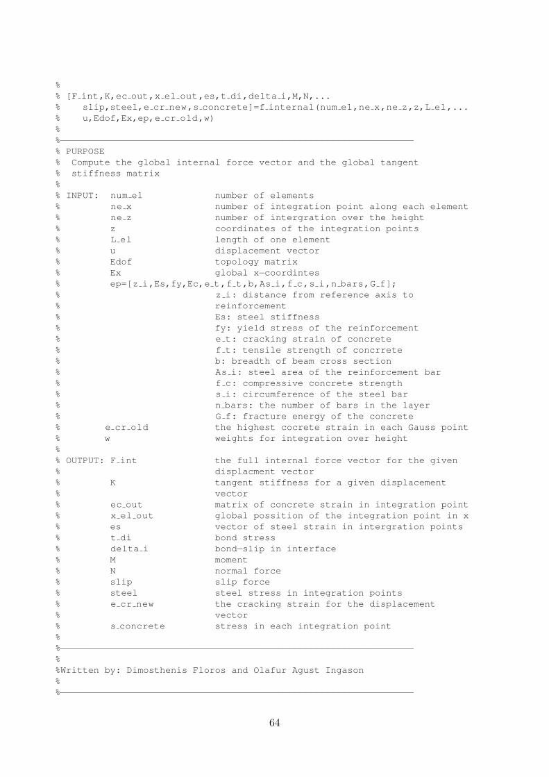
%% [F int,K,ec out,x el out,es,t di,delta i,M,N,...% slip,steel,e cr new,s concrete]=f internal(num el,ne x,ne z,z,L el,...% u,Edof,Ex,ep,e cr old,w)%%−−−−−−−−−−−−−−−−−−−−−−−−−−−−−−−−−−−−−−−−−−−−−−−−−−−−−−−−−−−−−−−−% PURPOSE% Compute the global internal force vector and the global tangent% stiffness matrix%% INPUT: num el number of elements% ne x number of integration point along each element% ne z number of intergration over the height% z coordinates of the integration points% L el length of one element% u displacement vector% Edof topology matrix% Ex global x−coordintes% ep=[z i,Es,fy,Ec,e t,f t,b,As i,f c,s i,n bars,G f];% z i: distance from reference axis to% reinforcement% Es: steel stiffness% fy: yield stress of the reinforcement% e t: cracking strain of concrete% f t: tensile strength of concrrete% b: breadth of beam cross section% As i: steel area of the reinforcement bar% f c: compressive concrete strength% s i: circumference of the steel bar% n bars: the number of bars in the layer% G f: fracture energy of the concrete% e cr old the highest cocrete strain in each Gauss point% w weights for integration over height%% OUTPUT: F int the full internal force vector for the given% displacment vector% K tangent stiffness for a given displacement% vector% ec out matrix of concrete strain in integration point% x el out global possition of the integration point in x% es vector of steel strain in intergration points% t di bond stress% delta i bond−slip in interface% M moment% N normal force% slip slip force% steel steel stress in integration points% e cr new the cracking strain for the displacement% vector% s concrete stress in each integration point%%−−−−−−−−−−−−−−−−−−−−−−−−−−−−−−−−−−−−−−−−−−−−−−−−−−−−−−−−−−−−−−−−%%Written by: Dimosthenis Floros and Olafur Agust Ingason%%−−−−−−−−−−−−−−−−−−−−−−−−−−−−−−−−−−−−−−−−−−−−−−−−−−−−−−−−−−−−−−−−

64

function [F int,K,ec out,x el out,es,t di,delta i,M,N,...slip,steel,e cr new,s concrete]=f internal(num el,ne x,ne z,z,L el,...u,Edof,Ex,ep,e cr old,w)

z i=ep(1);Es=ep(2);fy=ep(3);Ec=ep(4);e t=ep(5);f t=ep(6);b=ep(7);As i=ep(8);f c=ep(9);s i=ep(10);n bars=ep(11);G f=ep(12);

%Internal vectors and matrices definition%

x el=[−sqrt(3/5) 0 sqrt(3/5)]*L el/2+L el/2; %Gauss pointsw gauss=[5/9 8/9 5/9]; %Gauss weights

a=extract(Edof,u); %Arrangement of displacement to%the pertinent dofs

f int=zeros(8,1); %Internal force vector

ec=zeros(ne z,ne x); %Concrete strain

es=zeros(1,ne x); %Steel strain

delta i=zeros(1,ne x); %Slip between concrete and rebars

K u0w=zeros(2,4); %Block matricies for the tangent stiffnessK ww=zeros(4,4);K diw=zeros(2,4);K didi=zeros(2,2);

K=zeros(max(max(Edof)),max(max(Edof))); %Global tangent stiffness matrix

F int=zeros(max(max(Edof)),1); %Internal force vector

ec out=[];x el out=[];M=[];N=[];slip=[];steel=[];e cr new=[];s concrete=[];

%

for i=1:num el

%Coordinates of int points along the length of element i%

ex=Ex(i,:);x(i,:)=linspace(ex(1,1),ex(1,2),ne x);

65

%

%Arrange the pertinent displacements of element i%

a u0=[a(i,1);a(i,2)]; %Nodal axial displacement at the reference axis

a w=[a(i,3);a(i,4);a(i,5);a(i,6)]; %Nodal deflections and rotations%at the nodes

a di=[a(i,7);a(i,8)]; %Nodal relative slip

%

%Shape functions for the approximation of the slip%

N di 1=−1/L el*(x(i,:)−ex(2));N di 2=1/L el*(x(i,:)−ex(1));

%

%B matrices (Derivative of the shape functions)%

B u0=1/L el*[−1 1];

B w 1=−6/L elˆ2+12*x el/L elˆ3;B w 2=−4/L el+6*x el/L elˆ2;B w 3=6/L elˆ2−12*x el/L elˆ3;B w 4=6*x el/L elˆ2−2/L el;

B di=1/L el*[−1 1];

%

%Concrete and steel strains at the network of int points%(ne x: Integration points along the length of the element)%(ne z: Integration points along the cross−section height)%

for j=1:ne x

B w(1,1:4)=[B w 1(1,j) B w 2(1,j) B w 3(1,j) B w 4(1,j)];

N delta i(1,1:2)=[N di 1(1,j) N di 2(1,j)];

ec(:,j)=B u0*a u0−z'*B w*a w;

es(1,j)=B u0*a u0−z i*B w*a w+B di*a di;

delta i(1,j)=N delta i*a di;

end

66

%

%Concrete and steel stresses at the network of int points%

[s si,D si]=sigma si(es,Es,fy,ne x);

%Make the middle element weaker and with lower fracture energyif i==ceil(num el/2)

f t new=f t−0.5e6;[s xx con,D con,e cr nytt]=sigma xx con(ne x,ne z,ec,Ec,f t new/Ec,...f t new,f c,L el,15,e cr old(:,3*i−2:3*i));else[s xx con,D con,e cr nytt]=sigma xx con(ne x,ne z,ec,Ec,e t,f t...,f c,L el,G f,e cr old(:,3*i−2:3*i));end

%

%f int u0%

%Numerical integration along the height of the cross−section

N con=b*lobatto(z,s xx con,w);

N=[N N con+n bars*As i*s si];

%Numerical ingration across the length of the element

f int(1:2,1)=B u0'*gaussi(L el,(N con+n bars*As i*s si),w gauss');

%

%f int w%

%Numerical integration along the height of the cross−section

M con=zeros(1,ne x); dM con=zeros(1,ne x); z dM con=zeros(1,ne x);

for i m=1:ne x

M con(1,i m)=b*lobatto(z,s xx con(:,i m).*z',w);dM con(1,i m)=b*lobatto(z,D con(:,i m).*z',w);z dM con(1,i m)=b*lobatto(z,D con(:,i m).*z'.ˆ2,w);

end

%Numerical ingration across the length of the element

f int(3:6,1)=[gaussi(L el,B w 1.*(−(M con+n bars*As i*z i*s si)),...w gauss');

gaussi(L el,B w 2.*(−(M con+n bars*As i*z i*s si)),...w gauss');

67

gaussi(L el,B w 3.*(−(M con+n bars*As i*z i*s si)),...w gauss');

gaussi(L el,B w 4.*(−(M con+n bars*As i*z i*s si)),...w gauss')];

%

%f int di%

[t di,D ti]=b slip(delta i,ne x,f c);

%Numerical ingration across the length of the element

f int(7:8,1)=[gaussi(L el,B di(1,1)*n bars*As i*s si+N di 1.*t di*...s i*n bars,w gauss');

gaussi(L el,B di(1,2)*n bars*As i*s si+N di 2.*t di*...s i*n bars,w gauss')];

%

%Tangent stiffness matrix%

%Numerical integration along the height of the cross−section

dN con=b*trapz(z,D con);

%Numerical ingration across the length of the element

K u0u0=B u0'*gaussi(L el,(dN con+n bars*As i*D si),w gauss')*B u0;

%Numerical ingration across the length of the element

K u0w(1,1)=gaussi(L el,B u0(1,1)*(−(dM con+n bars*As i*z i*D si))...

*B w 1,w gauss');K u0w(1,2)=gaussi(L el,B u0(1,1)*(−(dM con+n bars*As i*z i*D si))....*B w 2,w gauss');K u0w(2,1)=gaussi(L el,B u0(1,2)*(−(dM con+n bars*As i*z i*D si))...

.*B w 1,w gauss');K u0w(2,2)=gaussi(L el,B u0(1,2)*(−(dM con+n bars*As i*z i*D si))...

.*B w 2,w gauss');K u0w(1,3)=gaussi(L el,B u0(1,1)*(−(dM con+n bars*As i*z i*D si))...

.*B w 3,w gauss');K u0w(2,3)=gaussi(L el,B u0(1,2)*(−(dM con+n bars*As i*z i*D si))...

.*B w 3,w gauss');K u0w(1,4)=gaussi(L el,B u0(1,1)*(−(dM con+n bars*As i*z i*D si))...

.*B w 4,w gauss');K u0w(2,4)=gaussi(L el,B u0(1,2)*(−(dM con+n bars*As i*z i*D si))...

.*B w 4,w gauss');

%Numerical ingration across the length of the element

K u0di=B u0'*gaussi(L el,n bars*As i*D si,w gauss')*B di;

K wu0=K u0w'; %Exploit symmetry of the tangent stiffness matrix

68

%Numerical ingration across the length of the element

K ww(1,1)=gaussi(L el,B w 1.*(z dM con+n bars*As i*z iˆ2*D si)....*B w 1,w gauss');

K ww(1,2)=gaussi(L el,B w 1.*(z dM con+n bars*As i*z iˆ2*D si)....*B w 2,w gauss');

K ww(1,3)=gaussi(L el,B w 1.*(z dM con+n bars*As i*z iˆ2*D si)....*B w 3,w gauss');

K ww(1,4)=gaussi(L el,B w 1.*(z dM con+n bars*As i*z iˆ2*D si)....*B w 4,w gauss');

K ww(2,1)=K ww(1,2);K ww(2,2)=gaussi(L el,B w 2.*(z dM con+n bars*As i*z iˆ2*D si)...

.*B w 2,w gauss');K ww(2,3)=gaussi(L el,B w 2.*(z dM con+n bars*As i*z iˆ2*D si)...

.*B w 3,w gauss');K ww(2,4)=gaussi(L el,B w 2.*(z dM con+n bars*As i*z iˆ2*D si)...

.*B w 4,w gauss');K ww(3,1)=K ww(1,3);K ww(3,2)=K ww(2,3);K ww(3,3)=gaussi(L el,B w 3.*(z dM con+n bars*As i*z iˆ2*D si)...

.*B w 3,w gauss');K ww(3,4)=gaussi(L el,B w 3.*(z dM con+n bars*As i*z iˆ2*D si)...

.*B w 4,w gauss');K ww(4,1)=K ww(1,4);K ww(4,2)=K ww(2,4);K ww(4,3)=K ww(3,4);K ww(4,4)=gaussi(L el,B w 4.*(z dM con+n bars*As i*z iˆ2*D si)...

.*B w 4,w gauss');

%Numerical integration across the length of the element

K diw(1,1)=gaussi(L el,B di(1,1)*(−z i*n bars*As i*D si)....*B w 1,w gauss');

K diw(1,2)=gaussi(L el,B di(1,1)*(−z i*n bars*As i*D si)....*B w 2,w gauss');

K diw(1,3)=gaussi(L el,B di(1,1)*(−z i*n bars*As i*D si)....*B w 3,w gauss');

K diw(1,4)=gaussi(L el,B di(1,1)*(−z i*n bars*As i*D si)....*B w 4,w gauss');

K diw(2,1)=gaussi(L el,B di(1,2)*(−z i*n bars*As i*D si)....*B w 1,w gauss');

K diw(2,2)=gaussi(L el,B di(1,2)*(−z i*n bars*As i*D si)....*B w 2,w gauss');

K diw(2,3)=gaussi(L el,B di(1,2)*(−z i*n bars*As i*D si)....*B w 3,w gauss');

K diw(2,4)=gaussi(L el,B di(1,2)*(−z i*n bars*As i*D si)....*B w 4,w gauss');

%Numerical integration across the length of the element

K wdi=K diw';

%Numerical integration across the length of the element

K diu0=K u0di';

69

%Numerical integration across the length of the element

K didi(1,1)=gaussi(L el,B di(1,1)*n bars*As i*D si*B di(1,1)...+N di 1.*D ti.*N di 1*s i*n bars,w gauss');

K didi(1,2)=gaussi(L el,B di(1,1)*n bars*As i*D si*B di(1,2)...+N di 1.*D ti.*N di 2*s i*n bars,w gauss');

K didi(2,1)=gaussi(L el,B di(1,2)*n bars*As i*D si*B di(1,1)...+N di 2.*D ti.*N di 1*s i*n bars,w gauss');

K didi(2,2)=gaussi(L el,B di(1,2)*n bars*As i*D si*B di(1,2)...+N di 2.*D ti.*N di 2*s i*n bars,w gauss');

%Assemble the element tangent stiffness matrix

Ke=[K u0u0 K u0w K u0di;K wu0 K ww K wdi;K diu0 K diw K didi];

%Assemble the element matrices into the global one

[K,F int]=assem(Edof(i,:),K,Ke,F int,f int);

ec out=[ec out ec]; x el out=[x el out x(i,:)]; slip=[slip delta i];steel=[steel s si]; e cr new=[e cr new e cr nytt];s concrete=[s concrete s xx con]; M=[M M con+n bars*As i*z i*s si];

endend

70

%% [F ext]=f external(q,Edof,L el,num el)%%%−−−−−−−−−−−−−−−−−−−−−−−−−−−−−−−−−−−−−−−−−−−−−−−−−−−−−−−−−−−−−−−−% PURPOSE% Compute the effect on the degrees of freedom in a beam element from a% uniformly distributed load%% INPUT: q uniformly distributed load% Edof topology matrix% L el length of the element% num el number of elements%% OUTPUT: F ext the full external force vector from the load%−−−−−−−−−−−−−−−−−−−−−−−−−−−−−−−−−−−−−−−−−−−−−−−−−−−−−−−−−−−−−−−−%%Written by: Dimosthenis Floros and Olafur Agust Ingason%%−−−−−−−−−−−−−−−−−−−−−−−−−−−−−−−−−−−−−−−−−−−−−−−−−−−−−−−−−−−−−−−−

function [F ext]=f external(q,Edof,L el,num el)

F ext=zeros(max(max(Edof)),1);f ext=zeros(8,1);

for k=1:num el

f ext(3,1)=1/2*q*L el;f ext(4,1)=1/12*q*L elˆ2;f ext(5,1)=1/2*q*L el;f ext(6,1)=−1/12*q*L elˆ2;

F ext(Edof(k,2:end))=F ext(Edof(k,2:end))+f ext;end

end

71

%% [t di,D ti]=b slip(delta i,ne x,f c)%%−−−−−−−−−−−−−−−−−−−−−−−−−−−−−−−−−−−−−−−−−−−−−−−−−−−−−−−−−−−−−−−−% PURPOSE% Compute the shear stress and stiffness in the interface between concrete% and reinforcement steel. This model is adopted from FIB model code from% 2010%% INPUT: delta i the slip in the integration points% ne x number of integration points along the beam% f c characteristic compressive strength%% OUTPUT: t di shear stress in interface% D ti tangent stiffness in interface%−−−−−−−−−−−−−−−−−−−−−−−−−−−−−−−−−−−−−−−−−−−−−−−−−−−−−−−−−−−−−−−−%%Written by: Dimosthenis Floros and Olafur Agust Ingason%%−−−−−−−−−−−−−−−−−−−−−−−−−−−−−−−−−−−−−−−−−−−−−−−−−−−−−−−−−−−−−−−−

function [t di,D ti]=b slip(delta i,ne x,f c)

%Model constants for the definition of the curve%

s0=20e−5; %To this point the constituitive is linears1=0.001; %Constants from FIB model code for good bonds2=0.002;s3=0.009;a=0.4;t max=2.5*sqrt(f c/1e6)*1e6; %Maximum shear stress in interfacet f=0.4*sqrt(f c/1e6)*1e6; %Final shear stress in interface

%

t di=zeros(1,ne x);D ti=zeros(1,ne x);

K fake=(t max*abs(s0)ˆa/s1ˆa)/s0;

for j=1:ne x

%Linear branch of the curveif abs(delta i(1,j))>=0 && abs(delta i(1,j))<=s0

t di(1,j)=K fake*delta i(j);D ti(1,j)=K fake;

%Non−linear part of the curve%

elseif abs(delta i(1,j))>s0 && abs(delta i(1,j))<=s1

t di(1,j)=delta i(j)/abs(delta i(j))*(t max*abs(delta i(1,j))...ˆa/s1ˆa);

72

D ti(1,j)=delta i(j)/abs(delta i(j))*(a*t max/s1ˆa*...abs(delta i(1,j))ˆ(a−1));

%

%Higher plateau of the curve%

elseif abs(delta i(1,j))>s1 && abs(delta i(1,j))<=s2

t di(1,j)=delta i(j)/abs(delta i(j))*t max;D ti(1,j)=0;

%

%Linear degrading part of the curve%

elseif abs(delta i(1,j))>s2 && abs(delta i(1,j))<=s3

t di(1,j)=delta i(j)/abs(delta i(j))*(t max−(t max−t f)...

*(abs(delta i(1,j))−s2)/(s3−s2));D ti(1,j)=(t max−t f)/(s2−s3);

%

%Lower plateau of the curve%

elseif abs(delta i(1,j))>s3

t di(1,j)=delta i(j)/abs(delta i(j))*t f;D ti(1,j)=0;

end

end

73

%% [s si,D si]=sigma si(es,Es,fy,ne x)%%−−−−−−−−−−−−−−−−−−−−−−−−−−−−−−−−−−−−−−−−−−−−−−−−−−−−−−−−−−−−−−−−% PURPOSE% Compute the steel stress and tangent stiffness from steel strains% 2010%% INPUT: es steel strains in an element% ne x number of integration points along the beam% fy characteristic yield strength% Es Youngs modulus%% OUTPUT: s si steel stress% D si tangent stiffness for the steel%−−−−−−−−−−−−−−−−−−−−−−−−−−−−−−−−−−−−−−−−−−−−−−−−−−−−−−−−−−−−−−−−%%Written by: Dimosthenis Floros and Olafur Agust Ingason%%−−−−−−−−−−−−−−−−−−−−−−−−−−−−−−−−−−−−−−−−−−−−−−−−−−−−−−−−−−−−−−−−

function [s si,D si]=sigma si(es,Es,fy,ne x)

s si=zeros(1,ne x);D si=zeros(1,ne x);

for j=1:ne x

%Elastic part of the curve%

if es(1,j)>=0 && es(1,j)<=fy/Es

s si(1,j)=Es*es(1,j);D si(1,j)=Es;

%

%Plastic part of the curve%

elseif es(1,j)>fy/Es

s si(1,j)=fy;D si(1,j)=0;

%

endend

74

%% [s xx con,D con,e cr new]=sigma xx con(ne x,ne z,ec,Ec,e t...% ,f t,f c,L el,G f,e cr old)%%−−−−−−−−−−−−−−−−−−−−−−−−−−−−−−−−−−−−−−−−−−−−−−−−−−−−−−−−−−−−−−−−% PURPOSE% Compute element stress and tangent stiffness from a given total strain% values%% INPUT: ne x number of integration point along length% ne z number of integration points over height% ec total strain% Es concrete stiffness% e t cracking strain% f t tensile strength% f c compressive strength% L el length of the element% G f fracture energy% e cr old highest cracking strain in each Gauss point%% OUTPUT: s xx con concrete stress% D con Tangent stiffness% e cr new new cracking strain%%−−−−−−−−−−−−−−−−−−−−−−−−−−−−−−−−−−−−−−−−−−−−−−−−−−−−−−−−−−−−−−−−%%Written by: Dimosthenis Floros and Olafur Agust Ingason%%−−−−−−−−−−−−−−−−−−−−−−−−−−−−−−−−−−−−−−−−−−−−−−−−−−−−−−−−−−−−−−−−function [s xx con,D con,e cr new]=sigma xx con(ne x,ne z,ec,Ec,e t...,f t,f c,L el,G f,e cr old)

%Material constants for concrete%

e f=5.136*G f/(L el*f t);

k=1.81;ec1=−2.366*10ˆ(−3);ec lim=−3.5*10ˆ(−3);

e cr new=zeros(size(e cr old));

%

s xx con=zeros(ne z,ne x);D con=zeros(ne z,ne x);

for j=1:ne x %Loop for i.p. along the length of the i−st element

for i z=1:ne z %Loop for i.p. along the height of the cross−section

e cr=0;

%Linear tensile part of the curve%

75

if ec(i z,j)>=0 && ec(i z,j)<=e t && e cr old(i z,j)==0

s xx con(i z,j)=Ec*ec(i z,j);D con(i z,j)=Ec;

%

%Tension softening part of the curve%

elseif (ec(i z,j)>e t && ec(i z,j)<=e f) | | (ec(i z,j)>=0 ...&& ec(i z,j)<=e t && e cr old(i z,j)>0)

e cr=1e−2; %initial guess

%'Hordjik' curve in local coordinates

[f cr,D c]=hordjik(e cr,e cr old(i z,j),e f,f t);

%Out−of−balance force function

g c=Ec*ec(i z,j)−Ec*e cr−f cr;

Error cr=norm(g c); %Evaluate the error

n cr=0; %Counter of iterations

while Error cr>10ˆ(−8) %Iterations' loop

J cr=−Ec−D c; %Tangent stiffness function

De cr=−J cr\g c; %Solve g(e cr+De cr) for e cr

e cr=e cr+De cr; %Update the cracking strain e cr

[f cr,D c]=hordjik(e cr,e cr old(i z,j),e f,f t);

g c=Ec*(ec(i z,j)−e cr)−f cr; %Calculate the new%o−o−b force function

Error cr=norm(g c); %Evaluate the error

n cr=n cr+1; %Add one step

end%Material tangent stiffness in Global coordinatesD=Ec−Ec*(Ec+D c)ˆ(−1)*Ec;

%Cracked concrete stress in total deformations xx con(i z,j)=Ec*(ec(i z,j)−e cr);

D con(i z,j)=D;

%

76

%Stress for strains over the ultimate strain e f%

elseif ec(i z,j)>e f

s xx con(i z,j)=0;D con(i z,j)=0;

e cr=e f;

%

%Compressive part of the curve%

elseif ec(i z,j)<0 && abs(ec(i z,j))<=abs(ec lim)

s xx con(i z,j)=−f c*(k*ec(i z,j)/ec1−ec(i z,j)ˆ2/ec1ˆ2).../(1+(k−2)*ec(i z,j)/ec1);D con(i z,j)=f c*((k/abs(ec1)−2*abs(ec(i z,j))/ec1ˆ2)...

*(1+(k−2)*ec(i z,j)/ec1)−(k*ec(i z,j)/ec1−ec(i z,j)ˆ2/ec1ˆ2)...

*(k−2)/abs(ec1))/(1+(k−2)*ec(i z,j)/ec1)ˆ2;

elseif ec(i z,j)<0 && abs(ec(i z,j))>abs(ec lim)

s xx con(i z,j)=0;D con(i z,j)=0;

end

e cr new(i z,j)=e cr;

end

endend

77

%% [f cr,D c]=hordjik(e cr,e cr old,e f,f t)%%−−−−−−−−−−−−−−−−−−−−−−−−−−−−−−−−−−−−−−−−−−−−−−−−−−−−−−−−−−−−−−−−% PURPOSE% Compute element post cracking stress, from a Hordjik tension softening,% from a given cracking strain. Has a damage history variable for a secant% damage model from the highest provious converged strain.%%% INPUT: e cr cracking strain% e cr old highest previously converged strain% e f minimum strain to give tensile stress% f t tensile strength%% OUTPUT: f cr stress% D c Tangent stiffness%−−−−−−−−−−−−−−−−−−−−−−−−−−−−−−−−−−−−−−−−−−−−−−−−−−−−−−−−−−−−−−−−%%Written by: Dimosthenis Floros and Olafur Agust Ingason%%−−−−−−−−−−−−−−−−−−−−−−−−−−−−−−−−−−−−−−−−−−−−−−−−−−−−−−−−−−−−−−−−

function [f cr,D c]=hordjik(e cr,e cr old,e f,f t)

c1=3; %Constants of the Hordjik curvec2=6.93;

%Checks if cracking strain is larger then previous valueif e cr<e cr old

f cr=e cr/e cr old*(f t*((1+(c1*e cr old/e f)ˆ3)*exp(−c2*e cr old/e f)−...exp(−c2)*(1+c1ˆ3)*e cr old/e f));

D c=1/e cr old*(f t*((1+(c1*e cr old/e f)ˆ3)*exp(−c2*e cr old/e f)−...exp(−c2)*(1+c1ˆ3)*e cr old/e f));

elseif e cr>=e cr oldf cr=f t*((1+(c1*e cr/e f)ˆ3)*exp(−c2*e cr/e f)−...

exp(−c2)*(1+c1ˆ3)*e cr/e f);D c=f t*((3*c1ˆ3*exp(−c2*e cr/e f)*e crˆ2/e fˆ3)−...

((1+c1ˆ3)*exp(−c2)/e f)−(c2*exp(−c2*e cr/e f)*...(1+c1ˆ3*e crˆ3/e fˆ3)/e f));

end

end

78