modelling and simulation of environmental disturbances · modelling and simulation of environmental...
TRANSCRIPT

18/09/2007 One-day Tutorial, CAMS'07, Bol, Croatia 1
Modelling and Simulation of Environmental Disturbances
(Module 5)Dr Tristan Perez Centre for Complex Dynamic Systems and Control (CDSC)
Prof. Thor I FossenDepartment of Engineering Cybernetics
18/09/2007 One-day Tutorial, CAMS'07, Bol, Croatia 2
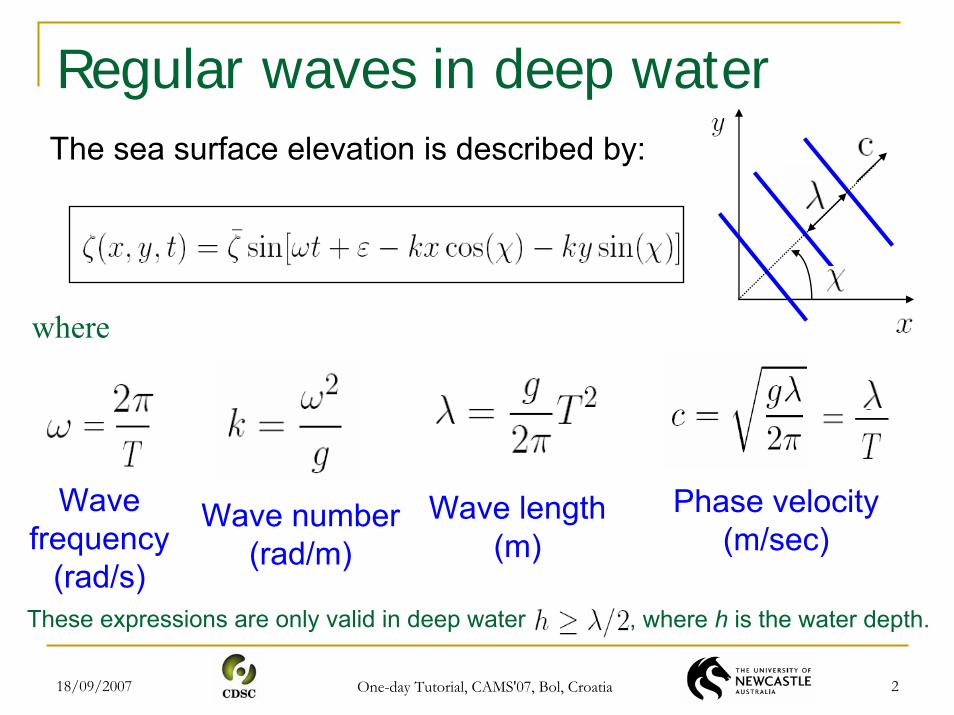
Regular waves in deep waterThe sea surface elevation is described by:
where
Wave number(rad/m)
Wave length(m)
Phase velocity(m/sec)
These expressions are only valid in deep water , where h is the water depth.
Wave frequency
(rad/s)

18/09/2007 One-day Tutorial, CAMS'07, Bol, Croatia 3
Sailing conditionThe sailing condition of a vessel is given by its forward speed U and its encounter angle, i.e., the heading angle relative to the waves.
Encounter angle
18/09/2007 One-day Tutorial, CAMS'07, Bol, Croatia 4
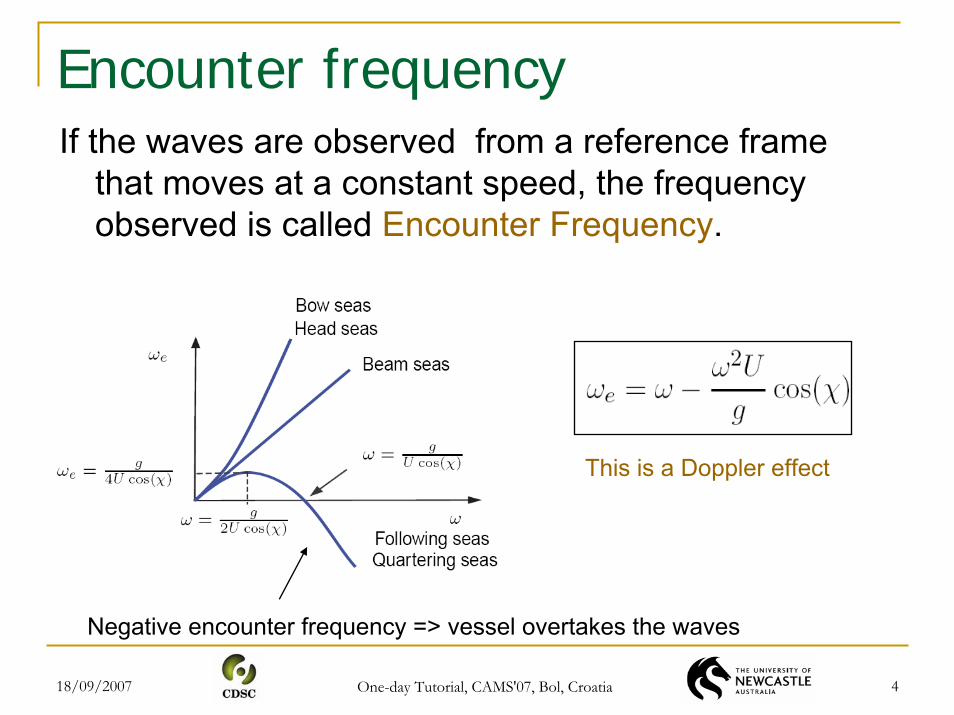
Encounter frequencyIf the waves are observed from a reference frame
that moves at a constant speed, the frequency observed is called Encounter Frequency.
This is a Doppler effect
Negative encounter frequency => vessel overtakes the waves

18/09/2007 One-day Tutorial, CAMS'07, Bol, Croatia 5
Ocean waves
Ocean waves present, in general, irregularity in time and space and cannot be predicted exactly: Stochastic Process.
t
ζ(0,0,t)
ζ(x,y,0)

18/09/2007 One-day Tutorial, CAMS'07, Bol, Croatia 6
Gaussian waves
The elevation of the sea surface can be thought as being generated as the sum of many sinusoidal waves with different amplitudes, frequencies, and phases.
ζ(x,y,0)
t
ζ
p(ζ)
ζ(xo
,yo,
t)(xo,yo)

18/09/2007 One-day Tutorial, CAMS'07, Bol, Croatia 7
How good are these hypotheses?From data collected at sea (Haverre & Moan, 1985), it can be stated that
For low and moderate seas (< 4m), the sea can be considered stationary for periods over 20 min. For more severe sea states, stationarity can be questioned even for periods of 20 min.
For medium seas (4m to 8m), Gaussian models are still accurate,but deviations from Gaussianity slightly increase with the increasing severity of the sea state.
If the water is sufficiently deep, wave elevation can be consider Gaussian regardless of the sea state.
18/09/2007 One-day Tutorial, CAMS'07, Bol, Croatia 8
Random sea characterizationUnder the Gaussianity assumption, the process is
completely described by
MeanVariance
The sea surface elevation is described relative to the mean free surface; therefore, the mean of the SP is zero.
The variance is described in terms of a sea power spectral density or sea spectrum.

18/09/2007 One-day Tutorial, CAMS'07, Bol, Croatia 9
Power spectral density definitionIf we use the frequency in Hz to define the FT, then
∫∫
∞+
∞−
+∞
∞−
−
=
=
dfefSR
deRfS
fjxxxx
fjxxxx
τπ
τπ
τ
ττ
2
2
)()(
)()(
[ ] ∫+∞
∞−== dffSRx xxxx )()0(var
and
from which the name power spectral density follows.
This definition is common in the literature of electrical communications and signal processing.

18/09/2007 One-day Tutorial, CAMS'07, Bol, Croatia 10
PSD alternative definitionWhen we use the circular frequency (rad/s) to define
the FT,
π
ωωτ
ττω
ωτ
ωτ
21
)()(
)()(
=
=
=
∫∫
∞+
∞−
+∞
∞−
−
ba
deSbR
deRaS
jxxxx
jxxxx
We need to be careful on how we compute power!!!

18/09/2007 One-day Tutorial, CAMS'07, Bol, Croatia 11
Random sea characterization
The spectral moments of order n are defined as:
Then the variance and standard deviation (RMS value) are
σ =
18/09/2007 One-day Tutorial, CAMS'07, Bol, Croatia 12
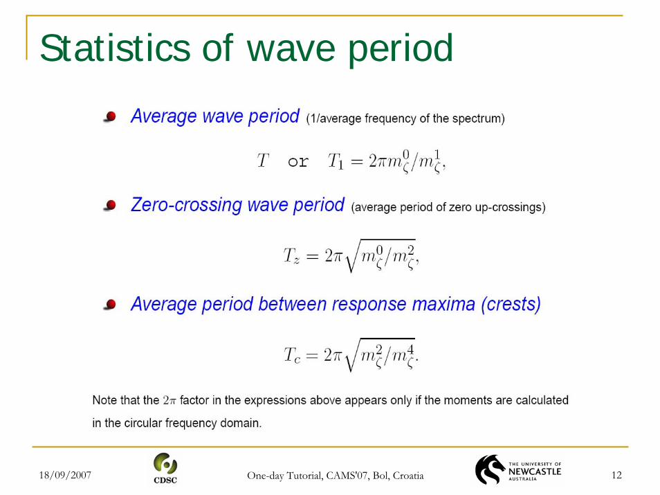
Statistics of wave period

18/09/2007 One-day Tutorial, CAMS'07, Bol, Croatia 13
Statistics of wave height
18/09/2007 One-day Tutorial, CAMS'07, Bol, Croatia 14
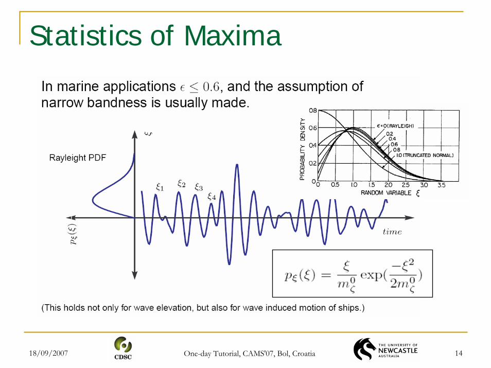
Statistics of Maxima

18/09/2007 One-day Tutorial, CAMS'07, Bol, Croatia 15
Long- and short-crested Seas
After the wind has blown constantly for a certain period of time, the sea elevation can be assumed statistically stable. In this case, the sea is referred to as fully-developed.
If the irregularity of the observed waves are only in the dominant wind direction, so that there are mainly uni-directional wave crests with varying separation but remaining parallel to each other, the sea is referred to as a long-crested irregular sea.
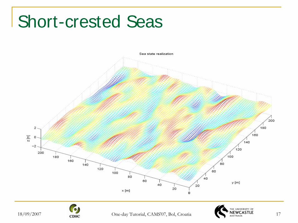
When irregularities are apparent along the wave crests at right angles to the direction of the wind, the sea is referred to as short crested or confused sea.

18/09/2007 One-day Tutorial, CAMS'07, Bol, Croatia 16
Long-crested Seas
18/09/2007 One-day Tutorial, CAMS'07, Bol, Croatia 17
Short-crested Seas
18/09/2007 One-day Tutorial, CAMS'07, Bol, Croatia 18
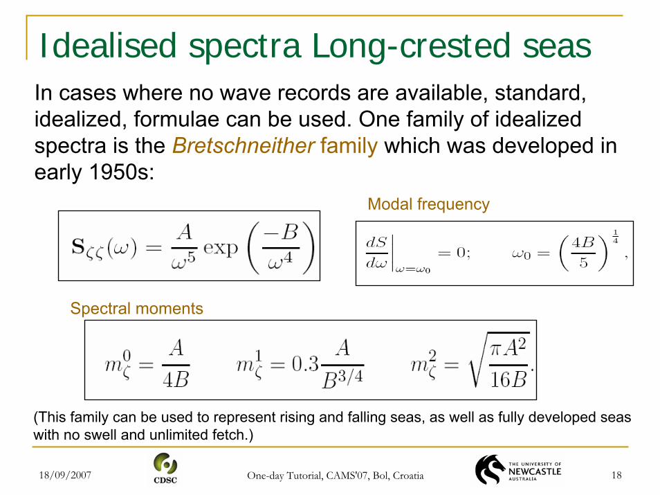
Idealised spectra Long-crested seasIn cases where no wave records are available, standard, idealized, formulae can be used. One family of idealized spectra is the Bretschneither family which was developed in early 1950s:
(This family can be used to represent rising and falling seas, as well as fully developed seas with no swell and unlimited fetch.)
Spectral moments
Modal frequency
18/09/2007 One-day Tutorial, CAMS'07, Bol, Croatia 19
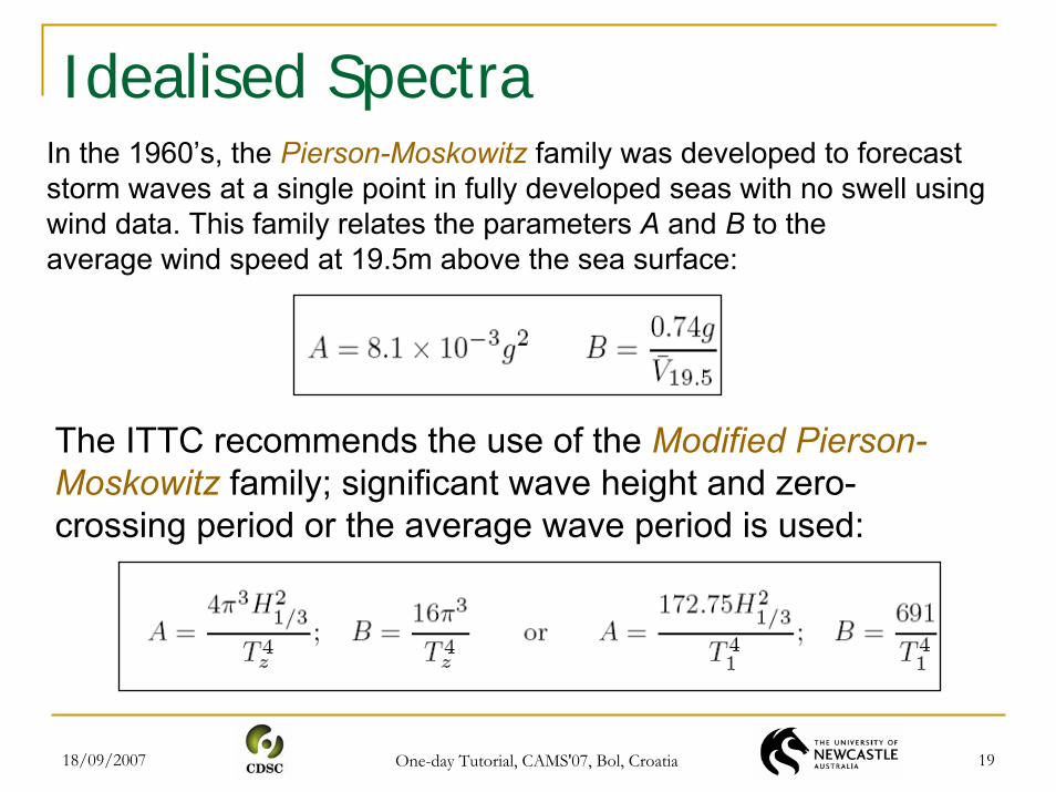
Idealised SpectraIn the 1960’s, the Pierson-Moskowitz family was developed to forecast storm waves at a single point in fully developed seas with no swell using wind data. This family relates the parameters A and B to theaverage wind speed at 19.5m above the sea surface:
The ITTC recommends the use of the Modified Pierson-Moskowitz family; significant wave height and zero-crossing period or the average wave period is used:

18/09/2007 One-day Tutorial, CAMS'07, Bol, Croatia 20
Example ITTC spectra

18/09/2007 One-day Tutorial, CAMS'07, Bol, Croatia 21
Other SpectraOther families:
The JONSWAP spectral family accounts for the case of limited fetch wind waves
The TMA spectral family is an extension of the JONSWAP for finite water depth,
The double-peak Torsethaugen spectral family accounts for both swell and wind waves,
The Ochi six-parameter spectral family can be fitted to almost any wave record (it could account for swell and wind waves.)
For further details see Ochi, K. (1998) Ocean Waves: The Stochastic Approach, Cambridge University Press. Ocean Tech. Series.
18/09/2007 One-day Tutorial, CAMS'07, Bol, Croatia 22
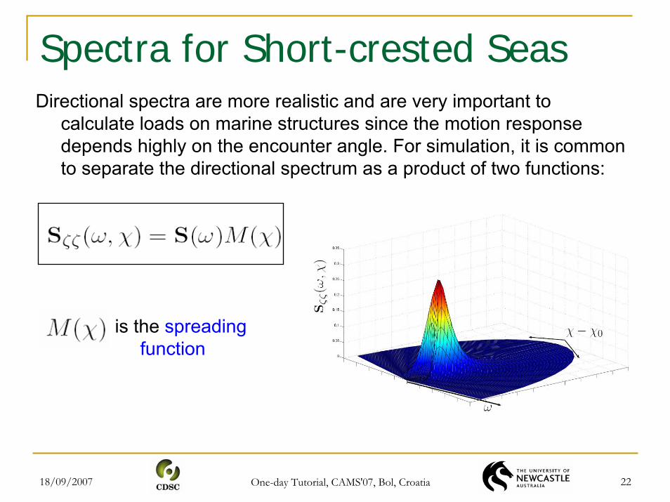
Spectra for Short-crested SeasDirectional spectra are more realistic and are very important to
calculate loads on marine structures since the motion response depends highly on the encounter angle. For simulation, it is common to separate the directional spectrum as a product of two functions:
is the spreading function
18/09/2007 One-day Tutorial, CAMS'07, Bol, Croatia 23
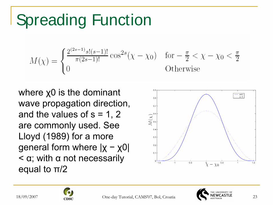
Spreading Function
where χ0 is the dominant wave propagation direction, and the values of s = 1, 2 are commonly used. See Lloyd (1989) for a more general form where |χ − χ0| < α; with α not necessarily equal to π/2

18/09/2007 One-day Tutorial, CAMS'07, Bol, Croatia 24
Time-domain SimulationsIf ζ(t) is stationary and Gaussian on time interval [0, T], its realizations can be approximated to any degree of accuracy by
with N sufficiently large; where σn are constants and the phases εn are independent identically distributed random variables with uniform distribution in [0, 2π].
The autocorrelation is given by
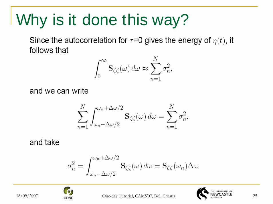
18/09/2007 One-day Tutorial, CAMS'07, Bol, Croatia 25
Why is it done this way?

18/09/2007 One-day Tutorial, CAMS'07, Bol, Croatia 26
Time-domain Simulations

18/09/2007 One-day Tutorial, CAMS'07, Bol, Croatia 27
Formulae for Time-daminSimulations

18/09/2007 One-day Tutorial, CAMS'07, Bol, Croatia 28
Spectral Factorization ApproachThe realizations of a sea surface elevation are modelled by filtered
white noise:
wwjH SS 2|)(|)( ωωζζ ≈A typical model is a 2nd-order system :
22 2)(
nnssssH
ωξω ++=
The parameters can be adjusted as follows (Perez, 2005):Sww = max Sζζ
ωn chosen to be the modal frequency.ξ is chose to the variance is the same; and thus the RMS value.

18/09/2007 One-day Tutorial, CAMS'07, Bol, Croatia 29
WindWind is commonly divided in two components; a mean value and a
fluctuating component, or gust.
It is a 3D phenomenon, but in marine applications we restrict it to 2D, and velocities are considered only in the horizontal plane.
Wind is parameterized by the velocity U and the direction ψ. The direction is taken with respect to the North-East.
Note that, in general, the direction of the wind is the direction from where the wind is coming from, e.g., a SE wind blows from the SE towards NW.

18/09/2007 One-day Tutorial, CAMS'07, Bol, Croatia 30
Wind Mean-velocity ComponentSlowly-varying fluctuations in the mean wind velocity can be
modeled by a 1st order Gauss-Markov Process:
where w is Gaussian white noise and μ ≥ 0 is a constant.
The magnitude of the velocity should be restricted by saturation elements

18/09/2007 One-day Tutorial, CAMS'07, Bol, Croatia 31
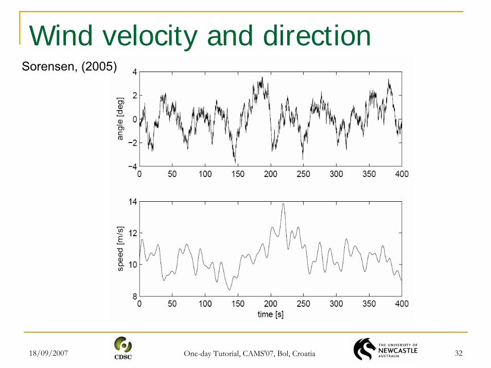
Wind Mean-direction componentSlowly-varying fluctuations in the mean wind direction can
also be implemented by a 1st order Gauss-Markov Process (Sorensen, 2005):
The direction is taken with respect to the (n-frame).
NOTE: This direction is often the direction from where the windis blowing: North-East (NE) wind blows from the NE
18/09/2007 One-day Tutorial, CAMS'07, Bol, Croatia 32
Wind velocity and directionSorensen, (2005)

18/09/2007 One-day Tutorial, CAMS'07, Bol, Croatia 33
Wind GustThe wind gust is model as a realization of a stochastic process
with a particular spectrum (Sorensen, 2005).

18/09/2007 One-day Tutorial, CAMS'07, Bol, Croatia 34
Current
Current velocity magnitude:
Current direction:
The direction is taken with respect to the (n-frame). NOTE: This direction is the directionto where the current flows : North-East (NE) current flow towards the NE. (This is different from the convention for wind)
Surface Current
18/09/2007 One-day Tutorial, CAMS'07, Bol, Croatia 35
References
Perez, T. (2005) Ship Motion Control. Springer.
Ochi, M. (2005) Ocean Waves: the stochastic approach. Cambridge University Press.
Sorensen, A.J. (2005) “Marine Cybernetics.”Lecture notes, Dept. of Marine Technology NTNU, NORWAY.