Modelling and detecting tumour oxygenation levels

A.C. Skeldon1,†, G. Chaffey1, D.J.B. Lloyd1, V. Mohan1,∗, D. Bradley2 and A. Nisbet2,3

1 Department of Mathematics, University of Surrey, GU2 7XH2 Department of Physics, University of Surrey, GU2 7XH

3 Department of Medical Physics, Royal Surrey County Hospital, GU2 7XX∗ Current address: Department of Mathematics, ETH Zurich, CH-8092

† Communicating author

April 3, 2012

Abstract

Tumours that are low in oxygen (hypoxic) tend to be more aggressive and respond less well

to treatment. Knowing the spatial distribution of oxygen within a tumour could therefore play

an important role in treatment planning, enabling treatment to be targeted in such a way that

higher doses of radiation are given to the more radioresistant tissue.

Mapping the spatial distribution of oxygen in vivo is difficult. Radioactive tracers that

are sensitive to different levels of oxygen are under development and in the early stages of

clinical use. The concentration of these tracer chemicals can be detected via positron emission

tomography resulting in a time dependent concentration profile known as a tissue activity curve

(TAC). Pharmaco-kinetic models have then been used to deduce oxygen concentration from

TACs. Some such models have included the fact that the spatial distribution of oxygen is often

highly inhomogeneous and some have not. We show that the oxygen distribution has little

impact on the form of a TAC; it is only the mean oxygen concentration that matters. This has

significant consequences both in terms of the computational power needed, and in the amount

of information that can be deduced from, TACs.

1 Introduction

The rapid growth that is frequently associated with malignant tumours results in regions of the

tumour becoming low in oxygen, in other words, hypoxic. Understanding tumour hypoxia is im-

portant because hypoxic cells are both more aggressive and harder to treat [1, 2]. Furthermore, low

oxygenation promotes the growth of blood vessels within the tumour (angiogenesis) contributing

to the transition from avascular to vascular tumour growth [3]. Yet tissue hypoxia is diffficult

to identify in vivo. Invasive techniques, such as the use of an Eppendorf probe, only give local

information and can seed cancerous cells along the line of entry.

Non-invasive techniques for the detection of oxygen using positron emission tomography (PET)

scans are in the early stages of clinical practice. With PET scanners, a patient is first injected

with a radioactive isotope of a molecule that takes a prominent part in whatever process is of

interest; most radioactive tracers that are in clinical use focus on the metabolisation of glucose but

there are some new tracers, such as [F-18]-flouromisonidazole (Fmiso) and Cu64 diacetyl-bis(N4-

methylthiosemicarbazone) (Cu64-ATSM), that are being developed to detect regions of low oxygen

concentration. The tracer is distributed around the body by the blood. In the case of glucose

detecting tracers, the highest concentrations of the tracer will occur in very active areas, such as

1

tumours. Similarly with Fmiso or Cu64-ATSM the tracer will accumulate in areas of hypoxic tissue.

The PET scanner detects the radiation that is emitted from the tracer as it undergoes radioactive

decay, and an image of the concentration of the tracer at different parts of the body can then

be re-constructed. This re-construction process is difficult resulting in images of relatively poor

resolution, typically 2− 3mm3. The time dependent decay signal from the PET scanner is known

as the tissue activity curve (TAC).

The concentration of the tracer at any location gives a qualitative picture of the degree of tumour

hypoxia. Padhani [1] notes that in clinical settings, such qualitative imaging can work well enough,

but does introduce a level of subjectivity and that there is a need for greater quantitative under-

standing. In fact, the concentration of the tracer at any given location is not related to the oxygen

concentration of the tissue in a trivial manner and knowing the quantitative relationship between

the tracer concentration and tissue oxygenation levels is of great importance if accurate deductions

as to the radio-resistance of the tissue are to be made [4]. Indeed, an image created by a snapshot

at a single point in time can give a misleading impression because, while for normal tissue the TAC

drops after an initial peak, for hypoxic tissue there tends to be a gradual increase in the TAC.

This can result in a cross-over point where TACs from both normal and hypoxic tissue give the

same result [5] and it is therefore important to consider the TAC at multiple time points. Methods

that fit TACs to a nonlinear mathematical model that includes the pharmaco-kinetic behaviour

of the tracer and thereby translate the concentration of the tracer to the oxygenation level of the

tissue have been developed. The most widely tested of these mathematical models have been com-

partment models [5–8]. These divide the tracer into, typically, three compartments: tracer in the

blood plasma; tracer that diffuses freely in the tissue, and tracer that is bound to the tissue via a

reaction that is dependent on the concentration of oxygen. The resulting pharmaco-kinetic (PK)

models have defined rates of transfer between the different compartments and results in a set of

ordinary differential equations that can be solved analytically. The total TAC is a weighted sum

of the signal from each of the compartments. The weights and some of the transfer coefficients

are calculated by fitting the experimentally determined TACs to the TACs produced by the PK

model. The values of the weights and the transfer coefficients are then used to deduce whether the

tissue is hypoxic and what kind of hypoxia occurs. Proof of concept experiments have been carried

out which demonstrate that PK models have the ability to qualitatively reproduce the features of

TACs and distinguish between different types of hypoxia. However, compartment models take no

account of the spatial distribution of oxygen. So for PET scan data, the fitting can be done for

each individual 2mm3 voxel but there is an inherent assumption that the tissue within that voxel

is homogeneous and can be represented by an average value. This is not necessarily the case—in

vascular tumours, the vessels that deliver oxygen tend to be irregular and tortuous making it likely

that the distribution of oxygen within a voxel is highly inhomogeneous. There has been some

initial work that includes space explicitly by including tracer diffusion in the tissue and allowing

the concentration of oxygen to vary from one point to the next, initially by Kelly and Brady [9]

and subsequently by Monnich et al [10]. These studies replace the ordinary differential equation

compartment model with partial differential equations. Our original interest was in comparing a

partial differential equation model for tracer reactions and diffusion with the analogous compart-

ment model to investigate whether the inhomogeneity of the distribution of blood vessels actually

matters on the scale of a voxel. However, this comparison is dependent on first establishing the

oxygen distribution within the tissue and that has led to a number of other considerations. In

general, if more than a qualitative understanding is to be developed, then one needs to be able

to quantify the uncertainties/errors that occur, be they uncertainty that is introduced because of

modelling assumptions (for example, whether the tissue can be treated as homogeneous or not), un-

certainty due to the difficulty of experimentally measuring parameters that are critical to the model

2

behaviour and finally, computational errors that are introduced due to numerical inaccuracies.

Consequently, the aim of this paper is three-fold. Our first aim is to understand the impact of two

particular modelling assumptions. The first relates to the way that oxygen is delivered to tissue.

This is a subject that many authors have focussed on and a review article on this subject is given by

Goldman [11], yet in even the simplest models of oxygen diffusion and consumption different authors

have used different methods and, as we will see, these different assumptions can give quantitatively

quite different results. In particular we find that modelling the discrete blood vessels by a ‘source’

term gives a good approximation to the, more realistic, mixed boundary conditions between the

vessel walls and the tissue and suggests that efficient algorithms in three-space dimensions could

be developed using a source method. The second modelling assumption that we examine is to

what extent, on the scale of a voxel, it is important to take account of the spatial distribution of

the oxygen in deducing information from TACs, by comparing the results of a partial differential

equation model that accounts for oxygen and tracer diffusion with the analogous compartment

model.

Our second aim is to examine the sensitivity of the computed oxygenation level of tissue to the

various parameters in the model. Measuring physical parameters such as consumption rate of

oxygen, diffusivity of oxygen and permeability of blood vessels and the distribution of oxygen is

challenging, making it hard to validate any particular mathematical model. However, by under-

standing the mathematical models one can examine which parameters have a significant effect on

predictions that are made by a model and, therefore, which parameters one needs to find for an

accurate prediction or, equivalently, to what extent the uncertainty in a particular parameter leads

to an uncertainty in the results.

Our final aim is to demonstrate the impact of numerical error that results in the solution of the

partial differential equations on too coarse a mesh. We provide computational parameters where the

discrete approximations can confidently be considered to be close to the continuous PDE solution.

The paper is outlined as follows. In §2 the simplest models for the diffusion and consumption of

oxygen in tissue are re-visited. The different approaches to the different ways of modelling the

boundary between the vascular structures that deliver the oxygen and the tissue are examined and

a limit is derived in §2.1 where one expects the mixed boundary conditions used by some authors

[12] and the Dirichlet boundary conditions of others [13] to give similar results. In order to separate

out the effects of the parameters on the oxygen distribution as compared with how multiple vessels

modify the final oxygen distribution we consider a sequence of problems. In §2.3 we look at just

a single vessel and then, we consider a pair of vessels at different distances apart in §2.4. In §2.5

we consider multiple vessels and examine to what extent the multivessel results can be understood

as a superposition of the single vessel results. In §3 we introduce the particular model of tracer

reaction and diffusion that we have studied and examine first the tracer dynamics around a single

vessel in §3.2 and then for multiple vessels in §3.3, comparing the TACs that results from both

random and regular arrangements of vessels. In §3.4 we fit the TACs produced by the partial

differential equation model with a compartment model. In spite of the heterogeneity of the oxygen

model we find that the compartment model can distinguish between different levels of oxygen. Our

conclusions are summarised in §4.

3

2 Oxygen distribution

Many mathematical models of oxygen transport are built on the Krogh-Erlang cylinder model [14]

that models oxygen transport by a diffusive process through a homogeneous medium governed by

the equation∂P

∂t= D∇2P −K, (2.1)

for the oxygen partial pressure P within the tissue, where D is the diffusivity of oxygen in tissue

and K describes oxygen consumption by the tissue. In the original Krogh-Erlang model [14], the

oxygen partial pressure was fixed at the vessel wall (a Dirichlet boundary condition) with the

consumption rate K set to be constant. This latter assumption means that equation (2.1) has to

be supplemented with a requirement that the consumption rate is zero when P is zero to prevent

the equations from giving solutions with regions of negative partial pressures. A more realistic form

for the oxygen consumption term in equation (2.1) is the Michaelis-Menten form,

K =KmaxP

P + P50. (2.2)

With this nonlinear consumption rate, as P →∞ the consumption asymptotes to the constant value

K = Kmax, so that when oxygen is abundant, consumption is approximately constant. However,

when oxygen is scarce, oxygen consumption is proportional to the amount of oxygen available. This

choice for K means that the oxygen partial pressure remains positive (or zero) at all times.

In Goldman [11] all the underlying assumptions of the Krogh-Erlang cylinder model are listed and

a thorough review of current work that relaxes these assumptions is given. Of particular relevance

here is the intravascular O2 resistance (IVR); in the original Krogh-Erlang model the use of Dirichlet

boundary conditions at the vessel wall excluded the possibility that the oxygen delivery to the tissue

may be dependent on the partial pressure difference across the vessel wall. As discussed further

below, this is only valid if the vessel wall is sufficiently permeable to oxygen.

One way of including IVR is to ignore intravascular processes but to model the flux of oxygen as it

diffuses across the vessel wall, and then on into tissue explicitly via a mixed boundary condition,

sometimes known as a Robbins boundary condition. This mixed boundary condition arises as

follows: assuming that a blood vessel wall consists of two concentric cylinders of outer radius R

with width w between the two cylinders, as shown in cross-section in figure 1, and that there is

just diffusion and no consumption by the wall tissue, then the flux at r = R, FR is given by

FR = −Dw∂P

∂n

∣∣∣∣R

= −Dw

R

P0 − Pln(1− w

R

) (2.3)

where Dw is the diffusivity in the wall and P0 is the partial pressure of oxygen inside the vessel.

For capillaries w � R, (typical vessel radii are 7µm [12] and vessel walls are 0.2 − 1 µm [9]) and

equation (2.3) becomes

FR ≈Dw

w(P0 − P ) = Pm (P0 − P ) , (2.4)

where Pm = Dw/w is the permeability of the vessel. The inclusion of IVR can therefore be modelled

by using the boundary condition (2.4) at the vessel wall.

An alternative model that includes IVR is to model the vessels by a so-called distributed source

where instead of modelling the vessels as discrete entities leading to the solution of the diffusion

equation on a punctured domain, the source is represented by a function which has localised spikes

at the vessel positions [9]. With such a source term, the diffusion model becomes

∂P

∂t= D∇2P −K +

2PmR

(P0 − P ) · S, (2.5)

4

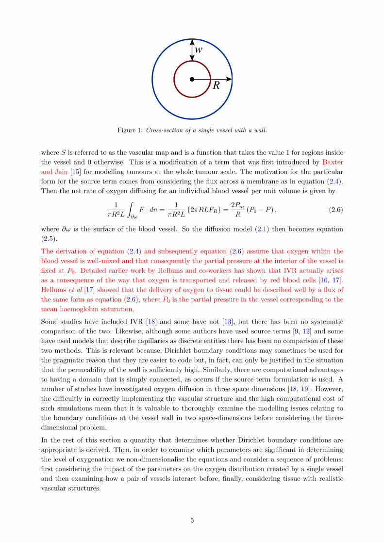
w

R

Figure 1: Cross-section of a single vessel with a wall.

where S is referred to as the vascular map and is a function that takes the value 1 for regions inside

the vessel and 0 otherwise. This is a modification of a term that was first introduced by Baxter

and Jain [15] for modelling tumours at the whole tumour scale. The motivation for the particular

form for the source term comes from considering the flux across a membrane as in equation (2.4).

Then the net rate of oxygen diffusing for an individual blood vessel per unit volume is given by

1

πR2L

∫∂ωF · dn =

1

πR2L{2πRLFR} =

2PmR

(P0 − P ) , (2.6)

where ∂ω is the surface of the blood vessel. So the diffusion model (2.1) then becomes equation

(2.5).

The derivation of equation (2.4) and subsequently equation (2.6) assume that oxygen within the

blood vessel is well-mixed and that consequently the partial pressure at the interior of the vessel is

fixed at P0. Detailed earlier work by Hellums and co-workers has shown that IVR actually arises

as a consequence of the way that oxygen is transported and released by red blood cells [16, 17].

Hellums et al [17] showed that the delivery of oxygen to tissue could be described well by a flux of

the same form as equation (2.6), where P0 is the partial pressure in the vessel corresponding to the

mean haemoglobin saturation.

Some studies have included IVR [18] and some have not [13], but there has been no systematic

comparison of the two. Likewise, although some authors have used source terms [9, 12] and some

have used models that describe capillaries as discrete entities there has been no comparison of these

two methods. This is relevant because, Dirichlet boundary conditions may sometimes be used for

the pragmatic reason that they are easier to code but, in fact, can only be justified in the situation

that the permeability of the wall is sufficiently high. Similarly, there are computational advantages

to having a domain that is simply connected, as occurs if the source term formulation is used. A

number of studies have investigated oxygen diffusion in three space dimensions [18, 19]. However,

the difficultly in correctly implementing the vascular structure and the high computational cost of

such simulations mean that it is valuable to thoroughly examine the modelling issues relating to

the boundary conditions at the vessel wall in two space-dimensions before considering the three-

dimensional problem.

In the rest of this section a quantity that determines whether Dirichlet boundary conditions are

appropriate is derived. Then, in order to examine which parameters are significant in determining

the level of oxygenation we non-dimensionalise the equations and consider a sequence of problems:

first considering the impact of the parameters on the oxygen distribution created by a single vessel

and then examining how a pair of vessels interact before, finally, considering tissue with realistic

vascular structures.

5

2.1 Mixed versus Dirichlet boundary conditions

If a boundary is sufficiently “leaky”, one would expect mixed and Dirichlet boundary conditions

to give the same results. An idea for what is “sufficiently leaky” can be obtained by considering

steady-states of equation (2.1) for a single vessel which satisfy

D∇2P = K. (2.7)

For a cylindrical vessel with no axial dependence, this reduces to

1

r

d

dr

(rd

dr

)P =

K

D. (2.8)

In case that K is constant, equation (2.8) is exactly soluble and gives

P =1

4

K

Dr2 +A ln r +B,

where A and B are integration constants. At some radius r = rm the oxygen partial pressure will

drop to zero and there will be no flux of oxygen. Applying the boundary conditions P = dP/dr = 0

at r = rm gives

P =1

4

K

D

(r2 − r2m

)− 1

2

Kr2mD

lnr

rm.

The maximum oxygen diffusion distance, rm, is determined by the boundary condition at r = R.

Using P = P0 at r = R leads to the equation(r2m −R2

)+ 2r2m ln

R

rm+

4DP0

K= 0. (2.9)

Using the mixed boundary condition gives

(r2m −R2

)(1− 2D

PmR

)+ 2r2m ln

R

rm+

4DP0

K= 0. (2.10)

As 2DPmR

→ 0 equations (2.9) and (2.10) for rm become identical, suggesting that provided 2DPmR

� 1

both mixed and Dirichlet boundary conditions will give similar results. Typical values for D,Pm and

R for tumour blood vessels (see appendix A, table 2) result in a value for 2D/PmR > 1, suggesting

that Dirichlet boundary conditions are unlikely to give similar results to mixed boundary conditions.

2.2 Non-dimensionalisation

The original problem has six parameters describing tissue and vessel properties, namely, the tissue

consumption parameters P50 and Kmax, the oxygen diffusivity D, the permeability of the blood

vessel to oxygen Pm, the partial pressure of the oxygen within the blood vessel P0 and the vessel

radius, R. The process of non-dimensionalisation shows that the six tissue and vessel parameters are

not truly independent, and the problem can be reduced to just three non-dimensional parameters

namely, the scaled partial pressure inside the vessel u0; the scaled permeability Pm and the scaled

vessel radius, R. The advantage of studying the non-dimensionalised equations is that one has a

much reduced parameter space to investigate.

The equations are rescaled by defining P = P50u and scaling the length by√DP50/Kmax. Conse-

quently, for the steady-state solution of the reaction-diffusion equation with rate given by equation

(2.2) three different problems are considered: (i) Dirichlet boundary conditions, (ii) mixed boundary

conditions, (iii) distributed source term. These are listed below.

6

Dirichlet

∇2u =u

u+ 1for (x, y) ∈ (Lx, Ly), (x, y) 6∈ vessel, (2.11)

u(vessel wall) = u0.

Mixed

∇2u =u

u+ 1for (x, y) ∈ (Lx, Ly) 6∈ vessel (2.12)

∇u|vessel wall = −Pm (u0 − u) ,

where Pm = Pm√P50/KmaxD.

Source

∇2u =u

u+ 1− 2Pm

R(u0 − u) · S for(x, y) ∈ (Lx, Ly), (2.13)

where

S =

{1 for (x, y) ∈ vessel interior

0 for (x, y) 6∈ vessel

Typical values for the measured physical parameters are listed in appendix A table 2 and the

corresponding ranges of values for the non-dimensional parameters are given in appendix A table

3.

2.3 Computations for a single vessel

With a single vessel the diffusion problem is axi-symmetric and the diffusion problem in two-space

dimensions can be reduced to a diffusion problem in one, radial, direction. For example, equation

(2.12) becomes1

r

d

dr

(rdu

dr

)=

u

u+ 1for r ∈ (R, L), r(R) = u0. (2.14)

and the source case becomes

1

r

d

dr

(rdu

dr

)=

u

u+ 1− 2Pm

R(u0 − u) · S for r ∈ (0, L), (2.15)

where

S =

{1 r < R

0 r ≥ R.

Each case leads to a boundary-value problem. For the flux and Dirichlet cases this problem was

solved on the large but finite domain, r ∈ (R, L), corresponding to the region outside a vessel of

radius R. The value for L was chosen sufficiently large (typically L = 20) that the results were

independent of whether Dirichlet or Neumann boundary conditions were chosen at r = L. In the

cases of the source term, r ∈ (0, L) with ∂u/∂r = 0 at the lefthand boundary. Each one-dimensional

problem was solved using the matlab boundary value problem solver bvp4c; typical solutions are

shown in figure 2. All boundary conditions lead to a simlar, monotonically decreasing, profile:

in fact the maximum principle can be used to show that the maximum value of the oxygen has

to occur on the boundary. The difference between the various boundary conditions is that with

Dirichlet boundary conditions, this maximum value is pinned to the value of u0, the scaled partial

pressure in the blood vessel, but in all other cases the maximum value is at some value that is

lower than this. The consequence of this pinning of the partial pressure to the value of u0 at the

7

0 2 4 6 8 100

4

8

12

16

20

r

u(r)

DirichletFluxSource

Figure 2: Typical solution of oxygen profiles of a single vessel for Dirichlet and flux boundary conditions and

for oxygen delivery via a source term. Parameter values are R = 0.55, u0 = 16, Pm = 2.75.

vessel boundary is that the Dirichlet boundary conditions tend to give higher levels of oxygenation

than mixed boundary conditions or the source term. On figure 2 the vertical dashed line represents

the boundary of the vessel. The ‘maximum diffusion distance’ for oxygen in tissue is often quoted

as 70 microns, equating to approximately 4 units in the non-dimensional units used in figure 2.

Considering just a single vessel with a Michelis-Menten consumption term, there is no maximum

diffusion distance for oxygen in that the oxygen decreases monotonically with distance from the

vessel, with u(r) → 0 only as r → ∞. The ‘maximum diffusion distance’ can therefore only be

specified in terms of a distance below which the level of oxygen is too small to be detected.

In order to compare the different solutions systematically as the parameters are varied, we have

considered two different measures. Firstly the the L1 norm, ‖u‖1, where

‖u‖1 =

∫ ∫|u|dx dy. (2.16)

The L1 norm is related to the average level of oxygenation, u, of a piece of tissue of area A by

u =‖u‖1A

.

Oxygenation of tissue samples on the microscale are often examined using tissue staining where a

dye that is oxygen sensitive is applied to a tissue slice. This tends to lead to a binary measure:

either oxygen is present or not (or only at a concentration below a threshold value). Results are

often quoted as a hypoxic fraction, that is the fraction of the tissue that is hypoxic. In order to

mimic this kind of measure we have also calculated the ‘oxygenated area’, Aox, which is the area

for which the oxygen partial pressure is greater than a threshold value uh.

Aox =

∫ ∫dx dy, and u > uh, (2.17)

For a given area of tissue A the hypoxic fraction Ah could then be calculated from

Ah =A−Aox

A.

As can be seen from figure 2, the calculated value for the oxygenated area will depend strongly on

the particular value of the threshold uh that is chosen: for the Dirichlet boundary case depicted in

figure 2, threshold values uh = 4 and uh = 2 lead to oxygenated radii of 2.28 and 3.15 respectively.

In turn, these values lead to oxygenated areas of 16.3 for uh = 4 and nearly double that value, 31.2

8

for uh = 2. Different threshold values are important for different aspects of a cell function, but

broadly oxygen levels below 5-15mmHg (uh = 2−6, for typical parameter values) have a significant

impact on the outcome of cancer therapies [1]. In the case of radiation treatment, half-maximal

sensitivity to radiation therapy occurs at oxygen levels of 2-5mmHg (uh = 0.8− 2). Typical tissue

staining techniques stain tissue at threshold values of between 5 mmHg and 10 mmHg (uh = 2 and

4). Given the sensitivity of the results to the value of the threshold, if comparison is to be made

with experimental data, it is particularly important that an accurate value for this threshold is

known and this in itself can be difficult. In Pogue et al [12] a careful study fitting a diffusion model

for oxygen with vascular maps derived from real tissue samples was performed. They found their

results were very sensitive to the threshold that was chosen and that their model fitted the data

best for a value for the threshold that was much lower than the conventionally accepted value. For

many of the results that are presented in this paper, we have selected the value uh = 2.

0

50

100

Aox

DirichletFluxSource

10 20 30 40u0

(a)

0

50

100

Aox

0 20 40Pm

(c)

~

0

50

100

Aox

10 20 30 40u0

(b)

0

50

100

Aox

0 20 40Pm

(d)

~

Figure 3: Oxygenated area using uh = 2 for a single vessel with non-dimensional radius R = 0.55. (a) Fixed

permeability, Pm = 2 and varying vessel partial pressure, u0. (b) Fixed permeability, Pm = 50 and varying

vessel partial pressure, u0. (c) Fixed vessel partial pressure, u0 = 8 and varying permeability, Pm. (d) Fixed

vessel partial pressure, u0 = 40 and varying permeability, Pm.

Results for the oxygenated area for fixed radius but varying vessel partial pressure u0 and perme-

ability Pm are shown in figure 3. As is to be expected, these show that at high permeability, all three

sets of boundary conditions give similar results. At low permeability, the source term representation

gives a reasonable approximation to the mixed boundary conditions. Note that the condition found

in §2.1 for the Dirichlet and flux boundary conditions to coincide translates to PmR � 2 or, for

R = 0.55, Pm � 3.6. For the experimentally measured range of values of Pm = 0.55− 2.75, figure

3(c) and (d) show that modelling oxygenation using Dirichlet rather than flux boundary conditions

9

will result in an over estimate for the oxygenated area and that this is more significant the lower

the vessel partial pressure. So, for example, for the low scaled vessel partial pressure of u0 = 8

(equivalent to 20mmHg), mixed boundary conditions give an oxygenated area of 4.9 and Dirichlet

boundary conditions give a value that is more than two and a half times bigger of 12.7. Even

at the highest scaled vessel partial pressures, u0 = 40 (equivalent to 100mmHg), mixed boundary

conditions give an oxygenated area of 57.0 and Dirichlet boundary conditions give a 50% larger

value of 86.1.

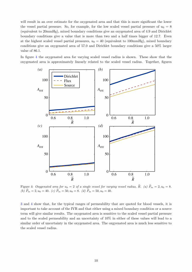
In figure 4 the oxygenated area for varying scaled vessel radius is shown. These show that the

oxygenated area is approximately linearly related to the scaled vessel radius. Together, figures

0

50

100

Aox

0.6 0.8 1.0

(a)

DirichletFluxSource

R~

0

50

100

Aox

0.6 0.8 1.0

(c)

R~

0

50

100

Aox

0.6 0.8 1.0

(b)

R~

0

50

100

Aox

0.6 0.8 1.0

(d)

R~

Figure 4: Oxygenated area for uh = 2 of a single vessel for varying vessel radius, R. (a) Pm = 2, u0 = 8.

(b) Pm = 2, u0 = 40. (c) Pm = 50, u0 = 8. (d) Pm = 50, u0 = 40.

3 and 4 show that, for the typical ranges of permeability that are quoted for blood vessels, it is

important to take account of the IVR and that either using a mixed boundary condition or a source

term will give similar results. The oxygenated area is sensitive to the scaled vessel partial pressure

and to the scaled permeability and an uncertainty of 10% in either of these values will lead to a

similar order of uncertainty in the oxygenated area. The oxgyenated area is much less sensitive to

the scaled vessel radius.

10

2.4 Two vessels

In a piece of tissue there is typically many vessels, not just a single isolated one. If two vessels are

sufficiently far apart, then each will be unaffected by the presence of the other, as illustrated in

figure 5(a) and (c). As they become closer and closer, the oxygen distribution around each vessel

will become more and more affected by its neighbour, see figure 5(b) and (d). The computations

0

-10

10

y

-20 0 20x

(a)

0

-10

10

y

-20 0 20x

(b)

10

0

20

u

-20 0 20x

(c)

10

0

20

u

-20 0 20x

(d)

Figure 5: Contour plots and solution profiles for two vessels placed at different separations. In all cases,

u0 = 16, Pm = 2.75, R = 0.55 and the source model for the delivery of oxygen to the tissue was used. (a)

Contour plot for two widely separated vessels, seperation s = 15. (b) Contour plot for two vessels that are

close enough to interact, separation s = 5. (c) Oxygen concentration profile along the line y = 0 for s = 15.

(d) Oxygen concentration profile along the line y = 0 for s = 5.

shown in figure 5 were carried out on a two-dimensional domain with a grid of 401×201 grid points

using a square mesh of grid size 0.1. Grid refinement checks were carried out to check that this was

sufficiently fine (see table 1). The grid refinement checks suggest that, for results that are accurate

Grid spacing grid/vessel ratio Dirichlet ||u||1 Source ||u||11.0000 1 1089.671 818.8468

0.5000 2 1716.200 1270.952

0.2500 4 1641.403 1036.248

0.1250 8 1774.854 1146.761

0.0625 16 1808.991 1141.513

0.0400 25 1831.189 1147.694

Table 1: Grid refinement check: the L1 norm as a function of grid size for two vessels separated by 5 units

with u0 = 40 and Pm = 2.75

to 10%, a grid of between two and four grid points per vessel should be used. We note that in

order to minimize computational cost, previous studies have frequently used a grid of spacing of

the same size as the vessel and that this will introduce an error of 30−40%, depending on the type

of boundary conditions used.

We have systematically examined how the L1 norm and the oxygenated area vary as the separation

between the vessels is changed and the results are summarised in figure 6 as a function of the

11

separation. Only the oxygenated area is shown as the results for the L1 norm are qualitatively

similar. For vessels sufficiently far apart, the L1 norm and the oxygenated area are twice the values

calculated in §2.3 for one vessel. This corresponds to the flat section to the far right of figure 6 and

shows that for a separation s greater than about ten the vessels interact only minimally. Note that

in these non-dimensional units, this represents a separation of approximately nine vessel diameters.

As the vessels get closer, the oxygenation of the tissue initially increases but then decreases ap-

proaching the value of the oxygenation produced by a single vessel as s→ 0. The increase is much

more prominent in the L1 norm than in the oxygenated area, reflecting the fact that the dominant

effect of two vessels close together is that the level of oxygenation of the oxygenated tissue increases,

rather than that more tissue reaches the oxygen threshold value of uh.

0

300

||u||1

0 10 20Separation

(a)

200

100

uh = 0.004

uh = 0.04uh = 0.08uh = 2.0uh = 4.0

0

300

0 10 20Separation

(b)

200

100

Aox

Figure 6: (a) ||u||1 norm and (b) oxygenated area as a function of separation for for uh = 0.04, 0.4, 0.8, 2 and

4 (typically corresponding to Ph = 0.1, 1, 2, 5 and 10 mmHg). The source term model for oxygen delivery has

been used; the behaviour for Dirichlet or flux boundary conditions is qualitatively similar. Each vessel has

a scaled radius R = 0.55 and scaled permeability Pm = 2.75. The scaled vessel partial pressure is u0 = 16

(typically corresponding to P0 = 40 mmHg).

2.5 Multi-vessel

In normal tissue, blood vessels are regularly spaced in order to deliver oxygen to tissue in an

optimal manner. In tumour tissue, this is not the case and the position of blood vessels is much

more closely represented by a random distribution, resulting in a log-normal distribution for the

distance between blood vessels.

First we outline how we distribute vessels on the plane while still being able to carry out computa-

tional grid refinements. In order to randomly place the vessels without overlap we first construct a

‘vascular grid’ that has a grid length of 2R. Vessels are placed so that their centres are at random

points of the vascular grid. The choice of grid length means that no vessels can overlap each other.

A computational mesh is then constructed that forms a sub-grid of the larger vascular grid, one

example is shown in figure 7. This computational mesh can be refined to give adequate numeri-

cal resolution. Computations were carried out on a domain of 55 × 55 in non-dimensional units,

equating to 1 mm2 of tissue for typical values of the parameters. As for the two vessel case, a

grid spacing of 0.1 gave good resolution. The effect of varying microvessel density (MVD), was

considered by solving equations (2.13) for a sequence of different MVDs. For each value of the

MVD, ten different random vascular maps were created and the L1 norm and the oxygenated area

calculated. The random selection of points on the vascular grid results in vascular maps which have

a log normal distribution of nearest neighbour distances. As the MVD increases, both the mean

and the variance of this distribution decreases (mean ∝ 1/√

MVD, variance ∝ 1/MVD). We have

12

Figure 7: Vascular grid versus computational grid. Blood vessels are located randomly on a fixed coarse

vascular grid (solid black lines) allowing a refined computational grid (light grey lines).

considered MVDs in the range 0− 200 per mm2, which includes the values used in previous studies

of tumour oxygenation [9, 13].

Commonly quoted values for vessel partial pressures range from 20mmHg to 100mmHg where,

100mmHg is typical of arterioles and 40mmHg typical of venules. Often tumour supply is from the

venule side, and although some of the results that are presented below are for the full range from

20mmHg to 100mmHg (8 to 40 in nondimensional units), more detailed results are shown for the

case of vessel partial pressure 40mmHg (16 in nondimensional units). The results for the fraction

of the area of the tissue that is oxygenated for three different values of the vessel partial pressure

u0 and varying hypoxic levels uh are shown in figure 8. The general trends are not surprising: more

vessels are needed to oxygenate more tissue up to some cut-off number beyond which all the tissue

is oxygenated; the vessel density that is needed for the tissue to be oxygenated depends on the

value that is used to specify oxygenation (uh), with more vessels needed the higher the value of

uh. Typically, tissue is considered to be hypoxic if it has partial pressures in the range 1-10mmHg

and necrotic for partial pressures less than 1mmHg. So, for example, in figure 8(b) corresponding

to vessel partial pressures of u0 = 16 (40mmHg) and for a micro-vessel density of 50 vessels/mm2,

typically 90% of the tissue receives some level of oxygen, but for most of the tissue this is at too

low a level to be significant resulting in the fact that only approximately 15% is oxygenated, 35%

is hypoxic and the remaining 50% is necrotic.

0

1

0 100 200MVD

(a)

0.5

Aox/A

uh = 0.04uh = 0.4

uh = 2.0uh = 4.0

uh = 0.8

0

1

0 100 200MVD

(b)

0.5

Aox/A

0

1

0 100 200MVD

(c)

0.5

Aox/A

Figure 8: Mean of ten realisations of the oxygenated area versus vessel density (MVD) (a) u0 = 8 (b) u0 = 16

c) u0 = 40. In all cases, Pm = 2.75 and the source model for oxygen entry from the blood vessels is used.

The different lines on each plot represent different values of the threshold, uh used to measure the level of

oxygenation.

The computational cost of simulating multi-vessel distributions to attain average quantities leads

one to ask whether one could predict the multi-vessel results just from the one-vessel results. In

13

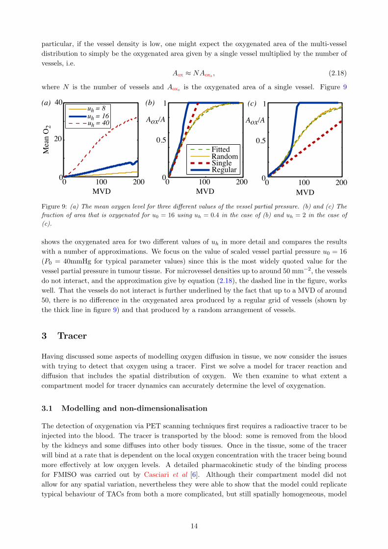
particular, if the vessel density is low, one might expect the oxygenated area of the multi-vessel

distribution to simply be the oxygenated area given by a single vessel multiplied by the number of

vessels, i.e.

Aox ≈ NAoxs , (2.18)

where N is the number of vessels and Aoxs is the oxygenated area of a single vessel. Figure 9

uh = 16uh = 8

uh = 40

FittedRandomSingleRegular

0

1

0 100 200MVD

(b)

0.5

Aox/A

0

1

0 100 200MVD

(c)

0.5

Aox/A

0

40

0 100 200MVD

(a)

20

Mea

n O

2

Figure 9: (a) The mean oxygen level for three different values of the vessel partial pressure. (b) and (c) The

fraction of area that is oxygenated for u0 = 16 using uh = 0.4 in the case of (b) and uh = 2 in the case of

(c).

shows the oxygenated area for two different values of uh in more detail and compares the results

with a number of approximations. We focus on the value of scaled vessel partial pressure u0 = 16

(P0 = 40mmHg for typical parameter values) since this is the most widely quoted value for the

vessel partial pressure in tumour tissue. For microvessel densities up to around 50 mm−2, the vessels

do not interact, and the approximation give by equation (2.18), the dashed line in the figure, works

well. That the vessels do not interact is further underlined by the fact that up to a MVD of around

50, there is no difference in the oxygenated area produced by a regular grid of vessels (shown by

the thick line in figure 9) and that produced by a random arrangement of vessels.

3 Tracer

Having discussed some aspects of modelling oxygen diffusion in tissue, we now consider the issues

with trying to detect that oxygen using a tracer. First we solve a model for tracer reaction and

diffusion that includes the spatial distribution of oxygen. We then examine to what extent a

compartment model for tracer dynamics can accurately determine the level of oxygenation.

3.1 Modelling and non-dimensionalisation

The detection of oxygenation via PET scanning techniques first requires a radioactive tracer to be

injected into the blood. The tracer is transported by the blood: some is removed from the blood

by the kidneys and some diffuses into other body tissues. Once in the tissue, some of the tracer

will bind at a rate that is dependent on the local oxygen concentration with the tracer being bound

more effectively at low oxygen levels. A detailed pharmacokinetic study of the binding process

for FMISO was carried out by Casciari et al [6]. Although their compartment model did not

allow for any spatial variation, nevertheless they were able to show that the model could replicate

typical behaviour of TACs from both a more complicated, but still spatially homogeneous, model

14

and clinically extracted TACs. They did find that including some transport limitations into the

compartments representing tracer in the tissue was important.

In order to take account of the diffusion of tracer and the spatial distribution of oxgyen, Kelly and

Brady [9] suggest taking the model for the partial pressure of oxgyen, equation (2.5) and coupling

it to a partial differential equation for the tracer,

∂Tf∂t

= DT∇2Tf −KtracerTf +2PTR

(Tblood − Tf ) · S,

∂Tb∂t

= KtracerTf , (3.1)

where Tf is tracer that is free to diffuse and Tb is bound tracer. The parameter Ktracer is the rate

at which the free tracer is bound and is dependent on the oxygen partial pressure P ,

Ktracer =

(kmaxP1

P + P1

)(P

P + P2

).

The second term in brackets acts as a switch to turn off the binding if tissue is necrotic. The

concentration of tracer in the blood, also known as the plasma input function, Tblood, is modelled

as the sum of two exponential decays,

Tblood = A(

e−k0t + be−kkt). (3.2)

The first term represents the dispersal of the tracer around the body, the second the renal term

representing the removal of tracer by the kidneys. Typically, kk � k0. Implicit in modelling the

tracer in the blood in this way is that the tumour is a small volume compared with the volume of

the rest of the body. Consequently the fact that some tracer flows into the tumour has a negligible

impact on Tblood.

Monnich et al use a similar model [10], but instead of using a source term to model the entry

of tracer from the blood they use mixed boundary conditions. In §2 we found that for oxygen

diffusion using a source term gave comparable results to the use of mixed boundary conditions,

and we would expect this to be the same for the tracer. Kelly and Brady [9] show that this

model can reproduce typical TACs by considering random distributions of vessels. Monnich et al

do a similar comparison, but this time using vascular maps that are obtained from tissue staining.

Comparing with experimentally determined TACs shows that the partial differential equation model

does mimic the behaviour that is seen in practice. Our aim here is to examine to what extent the

partial differential equation (3.1) model is needed in order to accurately model the behaviour that

is seen and to what extent a compartment model is adequate.

As for the oxygen problem, we first non-dimensionalise by rescaling space by√DP50/Kmax and

the oxygen partial pressure P = P 50u and introducing Tf = Avf , Tb = Avb, Tblood = Avblood, t =DP50

DTKmaxτ . This results in the model for the oxygen and tracer as :

∇2u =u

u+ 1− 2Pm

R(u0 − u) · S for (x, y) ∈ (Lx, Ly), (3.3)

and for free and bound tracer,

∂vf∂τ

= ∇2vf −

(kP1

u+ P1

)(u

u+ P2

)vf +

2PT

R(vblood − vf ) · S,

∂vb∂τ

=

(k

u+ P1

)(u

u+ P2

)vf , (3.4)

15

where the scaled plasma input function is

vblood =(

e−k0τ + be−kkτ), (3.5)

and

S =

{1 for (x, y) ∈ vessel interior

0 for (x, y) 6∈ vessel.

Since at the start there is no tracer in the tissue, only in the blood plasma, both vf and vb are set

to zero initially.

The scaled parameters for the tracer dynamics are PT = PT√

P50DKmaxD2

T, kmax = kmaxDP50

DTKmax, P1 =

P1P50

, P2 = P2P50

, k0 = DP50DTKmax

k0, kk = DP50DTKmax

kk. The process of non-dimensionalisation reduces the

original 17 parameters to 10.

3.2 Single vessel

Before considering how randomly distributed vessels within a piece of tissue behave, we first examine

a single vessel. Equations (3.3) are solved to find the steady-state oxygen distribution as shown in

figure 10(a). Then, equations (3.4) are solved to give the concentrations of free and bound tracer

as a function of time and space. For these computations and for those in the following sections

we have chosen representative values from the literature for the various parameter values. The

parameter ranges are given in Appendix A in table 2 for the dimensioned parameters and in table

3 for the corresponding non-dimensional parameters.

Typical concentrations of the free and bound tracer as are shown in 10(b) and (c) respectively for

three different points in time. These show how, initially, the dominant effect is the diffusion of

the tracer into the tissue—at τ = 10 there is essentially no bound tracer but tracer has diffused

a considerable distance from the vessel (note the vessel radius is 0.55 in these non-dimensional

units). However, as time goes on the binding process becomes important—by τ = 500 the way

that the binding is dependent on the oxygen level is apparent, with both the low binding rate at

high oxygen concentrations and the effect of the necrotic term resulting in the shape of the bound

oxygen profile in 10(c). In fact, the maximal binding rate occurs when u =√P1P2 which, for the

parameters we have used is u = 0.38.

In order to further illustrate the behaviour, in figure 11(a) the decay of the plasma input function,

equation (3.5), as a function of time is shown and, in figure 11(b) and (c), the concentration of free

and bound tracer respectively are shown for three different points in space. For the parameters we

have chosen the initial concentration of the plasma in the blood vessel is 1.5. However as k0 � kkthis value rapidly drops, so fast that on the timescale shown this is not visible, and in fact the

blood plasma term is dominated by the second term in equation (3.5). As time continues, the free

tracer diffuses from the blood vessels into the tissue, so that at any particular location the free

tracer concentration initially increases with time, as seen in figure 11(b). The further from the

blood vessel, the longer it takes the tracer to diffuse, so the slower this increase. At the same time

as diffusing in space, the free tracer binds at a rate dependent on the oxygen, and this ultimately

leads to the decay of the free tracer over time. In figure 11 (c) the growth of the bound tracer as a

function of time for three different points are shown. At r = 10, the bound tracer is zero because

the oxygen concentration is so low that the tissue is necrotic.

A TAC consists of the sum of signals from the plasma, free and bound tracer,

TAC =

∫ ∫(vblood.S + (vf + vb) .(1− S)) dxdy. (3.6)

16

𝝉 = 50𝝉= 10

𝝉 = 500

0

15

0 5 10r

(a)

10

Oxy

gen,

u

5 Free

trac

er, v

f

Boun

d tra

cer,

v b

00 5 10r

(b)

0.4

0.2

00 5 10r

(c)

0.4

0.2

𝝉 = 50𝝉= 10

𝝉 = 500

Figure 10: (a) Oxygen partial pressure against r. (b) Free tracer against r for three different times. (c)

Bound tracer against r for three different times. The parameters are: u0 = 16, R = 0.55, Pm = 2.75, PT =

4, P1 = 0.6, P2 = 0.24, kmax = 0.01, k0 = 5, kk = 0.01, b = 0.5.

The general characteristics of TACs from normoxic, hypoxic and necrotic tissue can be seen by

considering the three points r = 1, r = 5 and r = 10 respectively, as shown in figure 11. For r = 1,

the sum of the free and bound tracer will show a very rapid increase from zero initially to a high

level and then a slower but still fairly rapid decline. Whereas, for r = 10, the tissue is necrotic and

there is effectively no bound tracer. The only tracer contribution to the TAC then comes from the

free component, which because of the distance of this point from the blood vessel, shows only a

gradual increase that is diffusion limited. The point r = 5 sits between these two extremes. That

there is a cross-over point, as mentioned by Wang et al [5], where both oxygenated and hypoxic

tissue would give the same image is clearly seen.

3.3 Multi-vessels

In §2 it was seen that the distribution of oxygen can be considered as a superposition of the

oxygen distribution from single vessels for low enough vessel densities, or equivalently that the

oxygen distribution from a regular grid of vessels and that for a random arrangement of vessels

give similar oxygenation levels below a vessel density of about 50 for a scaled partial pressure

of u0 = 16 (equating to a partial pressure of 40mmHg if typical parameter values are used).

Below, the analogous behaviour is considered for the TAC that results from different microvessel

density distributions. For each microvessel density both random and regular vessel distributions

are considered. Having specified an arrangement of vessels, the oxygen map is first calculated by

solving equations (3.3). One example of the resulting oxygen map is shown in figure 12 (a). The

tracer equations (3.4) are then solved as a function of time with the plasma input function shown

in figure 12(b). The resulting maps for the free and bound tracer at a sequence of points in time

are shown in figure 12 (c),(e),(g) and (d),(f),(h) respectively. In figure 12(b) and (c) it is seen how

the initial phase is diffusion dominated, with tracer only occuring close to the blood vessels and

the bound tracer at a rather lower level than the free tracer. Over time, as seen in (d) and (e) and

then in (f) and (g) the free tracer continues to diffuse and is also gradually converted to bound

tracer, with highest levels of bound tracer occuring in the hypoxic ‘rings’ that form around blood

vessels. These rings have a maximum value at a distance of around five non-dimensional units and

are the two-dimensional manifestation of the maximum seen in the tracer profile in figure 10(c).

The corresponding TAC for this square of tissue was then calculated by combining the plasma

input function, and the free and bound tracer using equation 3.6. The resulting TACs for different

vessel densities are shown in figure 13. At the lowest vessel density of five vessels per mm2, as

17

Plas

ma

inpu

t, v i

n

Free

trac

er, v

f

Boun

d tra

cer,

v b

TAC

Time, 𝝉

0

1.5

0 100 200

1

0.5

300 400 500

(a)

Time, 𝝉

0

0.5

0 100 200 300 400 500

(b)

0.4

0.3

0.2

0.1

Time, 𝝉

0

200

0 100 200 300 400 500

(d)

150

100

50

Time, 𝝉

0

0.5

0 100 200 300 400 500

(c)

0.4

0.3

0.2

0.1

r=1 r=5 r=10

r=1 r=5 r=10

Figure 11: (a) Plasma input function. (b) Free tracer against time for three different points in space. (c)

Bound tracer against time for three different points in space. (d) Tissue activity curve.

shown in the top row, a regular arrangement of vessels would be indistinguishable from a random

arrangement of vessels. More surprisingly, even at high vessel densities, the differences between the

random arrangement of vessels and the regular arrangements are rather subtle. This suggests that

it is in fact not the random nature of the vessel distribution that is most critical, on the scale of a

millimetre.

18

0

50

y

0 50x

(a)

0

10

0

50

y

0 50x

(c)

0

0.5

0

50

y

0 50x

(e)

0

0.5

0

50

y

0 50x

(g)

0

0.5

0

50

y

0 50x

(h)

0

0.1

0.05

0

50

y

0 50x

(f)

0

0.1

0.05

0

50

y

0 50x

(d)

0

0.1

0.05Bo

und

trace

r, v b

Time, 𝝉0 200 400

2

1

0

(b)

Figure 12: Oxygen map and contours of vf and vb at various times for a microvessel density of 100 mm−2.

(a) Oxygen concentration. (b) Plasma input function as a function of time. (c) vf at τ = 10. (d) vb at

τ = 10. (e) vf at τ = 50. (f) vb at τ = 50. (g) vf at τ = 500. (h) vb at τ = 500.

19

RandomRegular

TAC

Time, 𝝉00 500

(b)1500

1000

500

TAC

Time, 𝝉00 500

(e)1500

1000

500

TAC

Time, 𝝉00 500

(h)1500

1000

500

TAC

Time, 𝝉00 500

(k)1500

1000

500

Time, 𝝉00 500

(j)1500

1000

500

Time, 𝝉00 500

(g)1500

1000

500

Time, 𝝉00 500

(d)1500

1000

500

Time, 𝝉00 500

(a)1500

1000

500

Hyp

oxic

frac

tion

Realisation00 10

(c)1

0.5

5

Hyp

oxic

frac

tion

Realisation00 10

(f)1

0.5

5

Hyp

oxic

frac

tion

Realisation00 10

(i)1

0.5

5

Hyp

oxic

frac

tion

Realisation00 10

(l)1

0.5

5

PlasmaFreeBound

Figure 13: Each row corresponds to a different microvessel density (5, 50, 100 and 150 per mm2 respectively).

The first column shows the contribution to the TAC from the tracer in the blood plasma and the free and

bound tracer in the tissue. Ten different random vessel distributions were considered, so ten different sets of

curves are shown for each contribution. The central column shows the TACs that result from the ten different

random vessel arrangements (solid line) and the TAC as computed from a regular arrangement of vessels

(dashed line). The final column shows the hypoxic fraction for each of the different random realisations.

20

3.4 Comparison with compartment models

Having computed the oxygen map and the resulting TAC, one can ask to what extent a compart-

ment model can extract parameters such as the mean level of oxygenation. Previous authors have

compared both compartment models and partial differential equation models with real experimen-

tal data. The advantage of trying to fit a compartment model with ‘experimental data’ generated

from a partial differential equation is that one has much greater knowledge and control over the

the exact parameter values that are used. If fitting cannot work in this idealised scenario, then it

has little hope in the real world.

In order to compare the behaviour of compartment models with a model that includes diffusion of

the tracer and the spatial dependence of the oxygen within the tissue we consider the compartment

model constructed by Thorwarth et al [7] and used in [5, 8, 10]. This model considers three

compartments, one for the tracer in the blood, one for the free tracer and one for the bound

tracer. The tracer in the blood is modelled by equation (3.2), the remaining two compartments are

modelled by the coupled ordinary differential equations,

dCfdt

= k1Cblood − (k2 + k3)Cf ,

dCbdt

= k3Cf . (3.7)

Here, Cf represents the free tracer, Cb represents the bound tracer. The constants k1 and k2 repre-

sent the rate at which tracer enters/leaves the free compartment and is related to the permeability

of the vessels to the tracer. The constant k3 is the net binding rate of the tracer in the tissue and is

related to the level of oxygenation of the tissue. Non-dimensionalising by letting vblood = ATblood,

wf = ACf , wb = ACb and t = DHDtq

τ leads to the equations

vblood =(e−k0τ + be−kkτ

), (3.8)

dwfdτ

= k1vblood −(k2 + k3

)wf ,

dwbdτ

= k3wf . (3.9)

Initially there is no free or bound tracer so that wf (0) = wb(0) = 0, leading to the analytical

solution to equations (3.9)

wf =k1

k2 + k3 − k0e−k0τ +

k1b

k2 + k3 − kk

e−kkτ (3.10)

−k1(

1

k2 + k3 − k0+

b

k2 + k3 − kk

)e−(k2+k3)τ , (3.11)

wb = − k1k3

k0

(k2 + k3 − k0

)e−k0τ − k1k3b

kk

(k2 + k3 − kk

)e−kkτ (3.12)

+k1k3

k2 + k3

(1

k2 + k3 − k0+

b

k2 + k3 − kk

)e−(k2+k3)τ (3.13)

+k1k3

k2 + k3

(1

k0+

b

kk

). (3.14)

Typical time tracers of vblood, wf and wb are shown in figure 14. There are three time scales that

are important here corresponding to the three different rates that appear in the exponential terms.

Typically kk � k0 and kk < k2 + k3, but k2 + k3 can be either greater or less than k0 depending on

21

the oxygenation level of the tissue. It is the two timescales kk and k0 that are relevant for vblood,

and the fact that kk � k0 is seen by the very rapid decline in vblood in the first few time units

followed by a much slower decline thereafter. For the free tracer, although all three timescales

appear in the solution, it is the influence of kk and k2 + k3 that are most clearly seen in figure

14. The concentration of free tracer first increases then decreases over time as tracer first diffuses

from the blood into the free compartment and then leaves to become bound. However, the position

and height of the consequent maximum in the free tracer depends on how fast the free tracer is

converted to bound tracer relative to the dispersal of tracer around the body as is shown by the

two cases in figure 14. In 14(b) k2 + k3 > k0, and as soon as the tracer enters the free compartment

it is converted to bound tracer so the amount of free tracer remains low.

vbloodwfwb

Time, 𝝉00 400

(a)15

10

5

200Time, 𝝉

00 400

(b)15

10

5

200

Figure 14: vblood, wf and wb using k0 = 5, kk = 0.01, k1 = 0.5, k2 = k3, b = 0.5 (a) k2 + k3 = 0.1 (b)

k2 + k3 = 4.

The TAC consists of a signal with different weightings of the three components, vblood, wb and

wf . Fitting of the weights along with the rate constant k3 are used to give some idea if tissue is

hypoxic or not: hypoxic tissue should have a relatively high value for k3 and more bound tracer

than normal tissue.

TAC = αvblood + β (wf + wb) ,

= α(e−k0τ + be−kkτ

)+ β

{k1

k2 + k3 − k0

(1− k3

k0

)e−k0τ

+bk1

k2 + k3 − kk

(1− bk3

kk

)e−kkτ . (3.15)

In each case, we first compute a TAC by solving the partial differential equation model for a

particular microvessel density. This computed TAC is then fitted to the formula for the TAC given

by (3.15). We assume that the plasma input parameters, k0, kk and b, are known and fit for k1, k2, k3and the weights α and β. A sequence of calculations for increasing microvessel density was carried

out, for each of three vessel partial pressures—u0 = 8, u0 = 16 and u0 = 40 respectively. The

results are summarised in figure 15 and figure 16. The parameters k1 and k2 in the compartment

model are the rates at which tracer enters and leaves the free tracer compartment. As can be seen

from figure 15, the values of this parameter are dependent on both the vessel partial pressure and

the mean oxygenation level—or equivalently the microvessel density. The parameter k3, as shown

22

in figure 15(c) is the rate at which oxygen binds to the tissue, and here the nonlinear relationship

between the amount of oxygen and the mean value of oxygen is apparent with a binding rate that is

highest for hypoxic tissue and low both for very low levels of oxygen, where tissue is predominantly

necrotic, and low for high values of oxygen. The parameters k1, k2 and β are strongly correlated

with each other, as demonstrated in figure 16. Consequently, without knowing the vessel partial

pressure it is not possible to deduce information about the mean oxygen levels or, equivalently,

the microvessel density from these parameters alone. Values for the parameter k3 do give a clear

indication of hypoxia, with the maximum value of k3 occuring for a non-dimensional mean oxygen

level of around 1 (corresponding to 2.5 mmHg). Low values of k3 can occur for one of two reasons,

either because tissue is necrotic or because tissue is normoxic. The difference between these two

cases can be deduced by considering both k3 and k1: normoxic tissue would have a low value of k3and a high value of k1 wherease necrotic tissue would have a low value of k3 and a low value of k1.

0

1

0 5 10

(a)

0.5

Mean O2

15

1.5

1

k1

0

0.1

0 5 10

(b)

0.05

Mean O2

15

0.15

0.2

k2

0

2

0 5 10

(c)

1

Mean O2

15

3

k3

x10-3

0

100

0 5 10

(d)

50

Mean O2

15

150𝜷

200

250

~ ~

~

u0=8 u0=16 u0=40

Figure 15: The fitted values of (a) k1, (b) k2, (c) k3 and (d) β as a function of the mean oxygen level of the

tissue. For the computation of each point, first the MVD is fixed. The oxygen map is then computed from

equation (3.3) and the mean oxygen level of the tissue determined. The TAC from the PDE is then constructed

by solving equations (3.4) and computing the expression given in (3.6). Finally, values of k1, k2, k3 and β are

determined by fitting the TAC from the PDE to the compartment model TAC, equation (3.15). The circles,

points and crosses are calculations for different vessel partial pressures: circles represent calculations with

u0 = 8; points represent calculations with u0 = 16, and crosses represent calculations with u0 = 40.

The parameter k3 in the compartment model represents the binding rate. This rate is dependent

23

0

0.2

0 1 2

(a)

0.1

k1

k2

x10-3

0

3

0 1 2

(b)

2

k1

k3

1

0

200

0 1 2

(c)

100

k1

𝜷~ ~

~ ~ ~

Figure 16: Correlation of k1 with (a) k2, (b) k3 and (c) β. The circles are computations with a vessel partial

pressure u0 = 8; the points are for u0 = 16, and the crosses are for u0 = 40.

on the mean oxygenation level in the free tracer compartment and should be directly related to the

binding rate in the partial differential equation model given in equation (3.4),

k3 =

(k

u+ P1

)(u

u+ P2

).

By assuming that the parameters k, P1 and P2 are known, one can invert this relationship and

examine to what extent the value of k3 given by fitting the compartment model correlates to the

actual mean value of oxygen given by the partial differential equation calculation, see figure 17.

00 5 10

(a)

Actual Mean O2

15

Pred

icte

d M

ean

O2

5

10

15

00 5 10

(b)

Actual 𝜷15

50

100

150

200

250

𝜷

Figure 17: (a) The value of the mean oxygen level as predicted by fitting the compartment model to the TAC

that is computed from the partial differential equation versus the actual mean oxygen level. (b) The predicted

value of the parameter β versus the actual value. The circles represent computations with a vessel partial

pressure of u0 = 8; the dots represent computations with u0 = 16 and the crosses represent computations

with u0 = 40.

24

4 Discussion

Modelling the distribution of tracer in the body is a difficult task. There are a number of different

levels of uncertainty and inaccuracy. Firstly, in writing down a mathematical model various mod-

elling assumptions are made as to which processes may be neglected and which cannot. Secondly,

in most models there are parameters which have to be determined. The value of these parameters

can affect both the qualitative and quantitative behaviour of the model. Finally, there are com-

putational errors that are introduced when numerical methods are used to solve equations. If a

mathematical model is to be of use, these different types of error need to be quantified and, ideally,

an estimate of the uncertainty of any result made.

In this paper we have sought to quantify the effect of some of these sorts of error for the partic-

ular problem of oxygen diffusing in a (two-dimensional) piece of tissue and the consequent tracer

dynamics. We have addressed two particular modelling issues: firstly the consequence of using

different kinds of boundary condition to describe the flow of oxygen from blood vessel to tissue and

secondly the extent to which compartment models can be used to describe tracer concentration

in tissue where the oxygen distribution is inhomogeneous. For typical vessel permeabilities and

partial pressures for tumour tissue, we have found that using a Dirichlet type boundary would

typically result in an overestimate of the amount of oxygen by a factor of two, suggesting that

either mixed, or the source method should be used. The fact that the source method gives good

results, is significant as this is a method that is likely to be easier to implement in three space

dimensions than modelling blood vessels as discrete entities with flux boundary conditions. The

second modelling assumption that we have investigated is to what extent the heterogeneous nature

of the vascular supply is important/detectable by a TAC that averages over a region of a square

millimetre. In fact, the actual distribution of the vessels does not significantly affect the form of the

TAC: TACs from both regular and randomly arranged blood vessels were strikingly similar with

the qualitative and quantitative features much more strongly dependent on the partial pressure of

the vessels and their number. In part, this is because after the first few minutes, although one can

still see the after-effects of the position of the blood vessels in the spatial distribution of the tracer,

as shown in figure 12, the actual magnitude of the variation at any point in time is relatively small.

This is because typical diffusion times for tracers, x2/2DT , are an order of magnitude shorter than

typical times associated with the binding for tracers, as given by 1/kmax. In real tissue, the vessels

are not only highly heterogeneous in their position, but also in their size, vessel partial pressure

and vessel blood flow rates. However, the difference in timescales between the diffusion and the

chemical kinetics suggests that this heterogeneity is averaged out by the diffusion process and is

not detectable on the timescale of the chemical kinetics. The consequence is that fitting a TAC

to a partial differential equation model including the full heterogeneity in the distribution and the

characteristics of the vessels will result in essentially the same prediction for mean oxygen partial

pressure as fitting to a compartment model. While the partial differential equation models that

include vascular structures are valuable for allowing the investigation of how changes to the un-

derlying physiological parameters affect the results, this suggests that compartment models will be

sufficient in a clinical setting.

One of the difficulties in comparing with experiment is that some of the parameters are hard to

measure. The sensitivity results of section §2.3 showed that a 10% error in the scaled permeability

Pm or the scaled partial pressure u0 will result in a similar error in the oxygenated area. Similarly

the value of the oxygen threshold used to define the oxygenated area, uh, has a significant effect on

the results.

Finally we note that one source of error is the computational error: for the sake of computational

25

time, many authors have used a single point to represent a vessel. As we have seen, this in itself

can introduce an error of approximately 30%.

26

A Appendix

Parameter Value Source

Radius, R 6µm [13]

7µm [12]

Diffusivity of oxygen in tissue, 0.002mm2s−1 [12]

D 4.2× 10−10cm3O2/cm/s/mmHg. [20]

Kmax 15mmHg s−1 [13]

2− 16mmHg s−1 [12]

P50 2.5mmHg [13]

Partial pressure in vessel, Pv 20− 100mmHg

40mmHg [9]

30− 80mmHg [20]

Permeability of capillaries to oxygen, 0.3 mm s−1

Pm 0.06 mm s−1 [9]

Vessel density ≈ 60 mm−2 [9, 13]

Hypoxic level, Ph 5 mmHg [9]

1− 14 µM [12]

2.5, 5 mmHg [13]

Diffusivity of tracer in tissue,

DT 5.5× 10−5 mm2 s−1 [10]

Permeability of capillaries to tracer,

PT 0.024− 0.094 mm s−1 [9]

kmax 1.7× 10−4 s−1 [10]

2.4× 10−3 s−1 [6]

Tracer 8.0× 10−4 s−1 [21]

binding P1 0.8− 1.5 mmHg [10]

constants 2710 ppm [6]

1.8 mmHg [21]

P2 0.6 mmHg [21]

Blood A 8000− 12000 [21]

input k0 0.13− 0.22 [21]

parameters kk 0.001− 0.002 [21]

b 0.1− 1.67 [21]

Table 2: Measured values for the physical parameters

Acknowledgements

GC is funded by an EPSRC supported Doctoral Training Centre, funded through EP/P505755/1.

References

[1] A.R Padhani, K.A. Krohn, J.S. Lewis, and M. Alber. Imaging oxygenation of human tumours.

Eur. Radiol., 17:861–872, 2007.

[2] E.J. Hall. Radiobiology for the radiologist. Lippincott Williams and Wilkins, 2000.

27

Parameter Range

R =√

qDhR 0.55

Pm =√

hDqPm 0.55− 2.75

u0 = 1hPv 8− 40

PT =√

DhD2

T qPT 2− 60

kmax = DhDT q

kmax 0.001− 0.1

P1 = 1hP1 0.6

P2 = 1hP2 0.24

k0 = DhDT q

k0 0.7− 10

kk = DhDT q

kk 0.006− 0.09

Table 3: Parameter ranges for non-dimensional quantities

[3] M.R. Owen, T. Alarcon, P.K. Maini, and J.M. Byrne. Angiogenesis and vascular remodelling

in normal and cancerous tissues. Journal of Mathematical Biology, 58:689–721, 2009.

[4] B. Titz and R Jeraj. An imaging-based tumour growth and treatment response model: inves-

tigating the effect of tumour oxygenation on radiation therapy response. Physics in Medicine

and Biology, 53:4471–4488, 2008.

[5] W. Wang, N.Y. Lee, J-C Georgi, M. Narayanan, J. Guillem, H. Schoder, and J.L. Humm.

Pharmacokinetic analysis of hypoxia 18F-fluoromisonidazole dynamic PET in head and neck

cancer. Journal of Nuclear Medicine, 51:37–45, 2010.

[6] J.J. Casciari, M.M. Graham, and J.S. Rasey. A modeling approach for quantifying tumor

hypoxia with [F-18]fluoromisonidazole PET time-activity data. Medical Physics, 22:1127–1139,

1995.

[7] D. Thorwarth, S.M. Eschmann, F. Paulsen, and M. Alber. A kinetic model for dynamic [F18]-

FMISO PET data to analyse tumour hypoxia. Physics in Medicine and Biology, 50:2209–2224,

2005.

[8] W. Wang, J-C Georgi, S.A. Hehmeh, M. Narayanan, T. Paulus, M. Bal, J. O’Donoghue, P.B.

Zanzonico, C.R. Schmidtlein, N.Y. Lee, and J.L. Humm. Evaluation of a compartmental

model for estimating tumor hypozia via FMISO dynamic PET imaging. Physics in Medicine

and Biology, 54:3083–3099, 2009.

[9] C.J. Kelly and M. Brady. A model to simulate tumour oxygenation and dynamic [18F]-FMISO

PET data. Physics in Medicine and Biology, 51:5859–5873, 2006.

[10] D. Monnich, E.G.C. Troost, J.H.A.M. Kaanders, W.J.G. Oyen, M. Alber, and D. Thorwarth.

Modelling and simulation of [18F]fluoromisonidazole dynamics based on histology-derived mi-

crovessel maps. Physics in Medicine and Biology, 56:2045–2057, 2011.

[11] D. Goldman. Theoretical models of microvascular oxygen transport to tissue. Microcirculation,

15:795–811, 2008.

[12] B.W. Pogue, J. O’Hara, C.M. Wilmot, K.D. Paulsen, and H.M. Swartz. Estimation of oxygen

distribution in RIF-1 tumours by diffusion model-based interpretation of pimonidazole hypozia

and Eppendorf measurements. Radiation Research, 155:15–25, 2001.

28

[13] A. Dasu, I Toma-Dasu, and M. Karlsson. Theoretical simulation of tumour oxygenation and

results from acute and chronic hypoxia. Physics in Medicine and Biology, 48:2829–2842, 2003.

[14] A. Krogh. The number and distribution of capillaries in muscles with calculations of the oxygen

pressure head necessary for supplying the tissue. Journal of Physiology, 52:409–415, 1919.

[15] L.T. Baxter and R.K. Jain. Transport of fluid and macromolecules in tumors. iii role of binding

and metabolism. Microvascular Research, 41:5–23, 1991.

[16] J.D. Hellums. The resistance to oxygen transport in the capillaries relative to that in the

surrounding tissue. Microvascular Research, 13:131–136, 1977.

[17] J.D. Hellums, P.K. Nair, N.S. Huang, and N. Ohshima. Simulation of intraluminal gas trans-

port processes in the microcirculation. Annals of Biomedical Engineering, 24:1–24, 1996.

[18] T.W. Secomb, R. Hsu, E.Y.H. Park, and M.W. Dewhirst. Green’s function methods for analysis

of oxygen delivery to tissue by microvascular networks. Annals of Biomedical Engineering,

32:1519–1529, 2004.

[19] D.A. Beard and J.B. Bassingthwaighte. Modeling advection and diffusion of oxygen in complex

vascular networks. Annals of Biomedical Engineering, 29:298–310, 2001.

[20] M.W. Dewhirst, T.W. Secomb, E.T. Ong, R. Hsu, and J.F. Gross. Determination of local

oxygen consumption rates in tumours. Cancer Research, 54:3333–3336, 1994.

[21] C.J. Kelly. Quantitative modelling of positron emission tomography tracer kinetics in hypoxia.

PhD thesis, Oxford University, 2007.

29