modelling and design of a low-cost autonomous sailboat for
TRANSCRIPT

Univers
ity of
Cap
e Tow
n
Modelling and Design of an AutonomousSailboat for Ocean Observation
Geoffrey Kilpin
Department of Electrical Engineering,University of Cape Town, Cape Town, South Africa
Submitted to the Faculty of Engineering & the Built Environment at the University of Cape Town inpartial fulfilment of the academic requirements for a Master of Science degree in Engineering in Electrical
Engineering.
The financial assistance of the National Research Foundation (NRF) and the University of Cape Town(UCT) towards this research is hereby acknowledged. Opinions expressed and conclusions arrived at, are
those of the author and are not necessarily to be attributed to the NRF or UCT.
November 20, 2014
Keywords: autonomous sailboat, autonomous yacht, robotic sailing, sailboat modelling

Univers
ity of
Cap
e Tow
nThe copyright of this thesis vests in the author. No quotation from it or information derived from it is to be published without full acknowledgement of the source. The thesis is to be used for private study or non-commercial research purposes only.
Published by the University of Cape Town (UCT) in terms of the non-exclusive license granted to UCT by the author.


Declaration
I know the meaning of plagiarism and declare that all the work in the document, save for that which is
properly acknowledged, is my own.
Signature of the author:. . . . . . . . . . . . . . . . . . . . . . . . . . .
G. F. Kilpin
Date:. . . . . . . . . . . . . . . . . . . . . . . . . . . . . . .
i

Acknowledgements
The author wishes to acknowledge the following individuals for their assistance over the course of this work:
Ms. Robyn Verrinder, my MSc. supervisor, for her support and advice.
Staff in the Department of Electrical Engineering at the University of Cape Town, including Mr.
Dominic De Maar, Mr. Justin Pead, Mr. Chris Wozniak, and Mr. Phillip Titus, for their advice and
loan of equipment.
Bruce Johnson for his advice regarding the purchase of a RC controller.
Dr. Stewart Bernard and Mr. Nicholas Weggelaar of the Natural Resources Group at the Council for
Scientific and Industrial Research for making the initial hull used in this project available and support
of the study.
Paul Amayo, Arnold Pretorius, Baden Morgan, Callum Kilpin, Matthew Burke, and Thomas van der
Ploeg for their assistance during testing.
My fellow students and other staff in the Robotics and Mechatronics Research Group for the sharing
of ideas, feedback, and support.
My mother, Julie Kilpin, for her support and assistance with proof reading.
Kira Dusterwald, for putting up with technical discussions, providing inspiration and support, and
assistance with proof reading.
The financial assistance of the National Research Foundation (NRF) and the University of Cape Town (UCT)
towards this research is hereby acknowledged. Opinions expressed and conclusions arrived at, are those of
the author and are not necessarily to be attributed to the NRF or UCT.
The author further wishes to acknowledge open source software that proved important in this study, in
particular the Marine Systems Simulator1 and the APM Autopilot Suite2.
1MSS. Marine Systems Simulator (2010). Viewed 2013-2014, http://www.marinecontrol.org.2http://ardupilot.com/
ii

Abstract
This study presents various aspects of the development of an autonomous sailboat for ocean observation, with
specific focus on modelling and simulation. The potential value of such platforms for ocean observation is
well established, with there being a number of expected advantages over existing solutions. A comprehensive
literature review is presented, revealing that the modelling of sailboats is an existing field but that the
modelling of small autonomous platforms appears to have been limited. This study develops three and four
degree of freedom models of a small autonomous J-Class style sailboat. The sailboat is a prototype platform
which is developed from its existing state as part of the study. Both models are validated against data logged
during field tests, showing broad agreement with some limitations being noted. Results of simulations of
the models are used to draw a number of conclusions regarding the appropriate design of the platform’s
wing-sail, the wing-sail’s control requirements in different wind conditions, potential modifications of the
platform’s design, and the control of its heading while sailing. Results are also used to inform the proposal
of a novel ‘variable draft sailing spar’ as an alternative autonomous sailboat design.
iii
Table of Contents
Declaration i
Abstract iii
Table of Contents iv
List of Figures x
List of Tables xiv
1 Introduction 1
1.1 Brief Background to the Study . . . . . . . . . . . . . . . . . . . . . . . . . . . . . . . . . . . 1
1.2 Research Questions and Hypothesis . . . . . . . . . . . . . . . . . . . . . . . . . . . . . . . . . 1
1.3 Research Methodology . . . . . . . . . . . . . . . . . . . . . . . . . . . . . . . . . . . . . . . . 2
1.4 Significance of the Study . . . . . . . . . . . . . . . . . . . . . . . . . . . . . . . . . . . . . . . 3
1.5 Other Applications of the Study . . . . . . . . . . . . . . . . . . . . . . . . . . . . . . . . . . 4
1.6 Scope and Limitations . . . . . . . . . . . . . . . . . . . . . . . . . . . . . . . . . . . . . . . . 4
2 Literature Review 5
iv

2.1 Theoretical Basis . . . . . . . . . . . . . . . . . . . . . . . . . . . . . . . . . . . . . . . . . . . 5
2.1.1 Physics of Sailing . . . . . . . . . . . . . . . . . . . . . . . . . . . . . . . . . . . . . . . 5
2.1.2 Stability . . . . . . . . . . . . . . . . . . . . . . . . . . . . . . . . . . . . . . . . . . . . 8
2.1.3 Balance . . . . . . . . . . . . . . . . . . . . . . . . . . . . . . . . . . . . . . . . . . . . 9
2.2 Related work . . . . . . . . . . . . . . . . . . . . . . . . . . . . . . . . . . . . . . . . . . . . . 10
2.3 Hardware . . . . . . . . . . . . . . . . . . . . . . . . . . . . . . . . . . . . . . . . . . . . . . . 15
2.3.1 Hull Design . . . . . . . . . . . . . . . . . . . . . . . . . . . . . . . . . . . . . . . . . . 15
2.3.2 Sail Design . . . . . . . . . . . . . . . . . . . . . . . . . . . . . . . . . . . . . . . . . . 15
2.3.3 Electronics and Communication . . . . . . . . . . . . . . . . . . . . . . . . . . . . . . . 17
2.4 Simulation and Modelling . . . . . . . . . . . . . . . . . . . . . . . . . . . . . . . . . . . . . . 19
2.5 Control and Navigation . . . . . . . . . . . . . . . . . . . . . . . . . . . . . . . . . . . . . . . 21
2.5.1 Low-level Control . . . . . . . . . . . . . . . . . . . . . . . . . . . . . . . . . . . . . . . 21
2.5.2 Navigation and Obstacle Avoidance . . . . . . . . . . . . . . . . . . . . . . . . . . . . 23
2.5.3 Software Architecture . . . . . . . . . . . . . . . . . . . . . . . . . . . . . . . . . . . . 25
3 System Modelling 26
3.1 Approach to Modelling . . . . . . . . . . . . . . . . . . . . . . . . . . . . . . . . . . . . . . . . 28
3.1.1 Mathematical Model . . . . . . . . . . . . . . . . . . . . . . . . . . . . . . . . . . . . . 29
3.1.2 Damping Forces . . . . . . . . . . . . . . . . . . . . . . . . . . . . . . . . . . . . . . . 31
3.2 Surge, Sway, and Roll - the Three Degree of Freedom Model . . . . . . . . . . . . . . . . . . . 31
3.2.1 Forces Generated by the Sail . . . . . . . . . . . . . . . . . . . . . . . . . . . . . . . . 32
v

3.2.2 Hydrodynamic Resistance . . . . . . . . . . . . . . . . . . . . . . . . . . . . . . . . . . 38
3.2.3 Restoring Forces and Moments . . . . . . . . . . . . . . . . . . . . . . . . . . . . . . . 45
3.3 Yaw - the Four Degree of Freedom Model . . . . . . . . . . . . . . . . . . . . . . . . . . . . . 47
3.3.1 Adaptation of Three Degree of Freedom Model . . . . . . . . . . . . . . . . . . . . . . 47
3.3.2 Additional Hydrodynamic Resistance Forces . . . . . . . . . . . . . . . . . . . . . . . . 50
3.3.3 Modelling of the Rudder . . . . . . . . . . . . . . . . . . . . . . . . . . . . . . . . . . . 52
3.3.4 Modelling of Actuators . . . . . . . . . . . . . . . . . . . . . . . . . . . . . . . . . . . 55
3.3.5 Environmental Disturbances . . . . . . . . . . . . . . . . . . . . . . . . . . . . . . . . . 56
3.4 Parameter Determination . . . . . . . . . . . . . . . . . . . . . . . . . . . . . . . . . . . . . . 57
3.4.1 Development of the CAD Model . . . . . . . . . . . . . . . . . . . . . . . . . . . . . . 58
3.4.2 Added Mass . . . . . . . . . . . . . . . . . . . . . . . . . . . . . . . . . . . . . . . . . . 65
3.4.3 Determined Parameters . . . . . . . . . . . . . . . . . . . . . . . . . . . . . . . . . . . 67
3.5 Model Implementation . . . . . . . . . . . . . . . . . . . . . . . . . . . . . . . . . . . . . . . . 67
3.5.1 Adaptation of the MSS . . . . . . . . . . . . . . . . . . . . . . . . . . . . . . . . . . . 67
3.5.2 Forces Implementation . . . . . . . . . . . . . . . . . . . . . . . . . . . . . . . . . . . . 69
3.5.3 GUI and Interfacing . . . . . . . . . . . . . . . . . . . . . . . . . . . . . . . . . . . . . 70
3.5.4 Demonstration of Operation . . . . . . . . . . . . . . . . . . . . . . . . . . . . . . . . . 70
4 Platform Development 73
4.1 Mechanical Platform . . . . . . . . . . . . . . . . . . . . . . . . . . . . . . . . . . . . . . . . . 73
4.1.1 Sail Actuation . . . . . . . . . . . . . . . . . . . . . . . . . . . . . . . . . . . . . . . . 74
vi
4.1.2 Rudder Actuation . . . . . . . . . . . . . . . . . . . . . . . . . . . . . . . . . . . . . . 76
4.1.3 General Assembly . . . . . . . . . . . . . . . . . . . . . . . . . . . . . . . . . . . . . . 78
4.2 Electronic Platform . . . . . . . . . . . . . . . . . . . . . . . . . . . . . . . . . . . . . . . . . . 78
4.2.1 System Overview . . . . . . . . . . . . . . . . . . . . . . . . . . . . . . . . . . . . . . . 79
4.2.2 Power and Actuator Control . . . . . . . . . . . . . . . . . . . . . . . . . . . . . . . . 82
4.2.3 Sensor Interfacing and Selection . . . . . . . . . . . . . . . . . . . . . . . . . . . . . . 83
4.2.4 Logging and Remote Access . . . . . . . . . . . . . . . . . . . . . . . . . . . . . . . . . 88
4.2.5 Sailing Controllers . . . . . . . . . . . . . . . . . . . . . . . . . . . . . . . . . . . . . . 91
5 Results 94
5.1 Platform Testing Details . . . . . . . . . . . . . . . . . . . . . . . . . . . . . . . . . . . . . . . 94
5.2 Performance Prediction and Validation . . . . . . . . . . . . . . . . . . . . . . . . . . . . . . . 96
5.2.1 Speed Prediction and Validation . . . . . . . . . . . . . . . . . . . . . . . . . . . . . . 97
5.2.2 Upwind Performance Prediction . . . . . . . . . . . . . . . . . . . . . . . . . . . . . . 106
5.2.3 Yaw Prediction Validation . . . . . . . . . . . . . . . . . . . . . . . . . . . . . . . . . . 107
5.2.4 Effect of Varying Sail Parameters . . . . . . . . . . . . . . . . . . . . . . . . . . . . . . 108
5.3 Sail Control Requirement Analysis . . . . . . . . . . . . . . . . . . . . . . . . . . . . . . . . . 112
5.3.1 Wing-sail Analysis . . . . . . . . . . . . . . . . . . . . . . . . . . . . . . . . . . . . . . 112
5.3.2 Three Degree of Freedom Model Sail Analysis . . . . . . . . . . . . . . . . . . . . . . . 114
5.4 Steering Control Analysis . . . . . . . . . . . . . . . . . . . . . . . . . . . . . . . . . . . . . . 116
5.4.1 Results of Simulations . . . . . . . . . . . . . . . . . . . . . . . . . . . . . . . . . . . . 116
vii

5.4.2 Results of Prototype Controller Tests . . . . . . . . . . . . . . . . . . . . . . . . . . . 116
5.5 Alternative Designs and Configurations . . . . . . . . . . . . . . . . . . . . . . . . . . . . . . 118
5.5.1 Fully Rotating Wing-Sail . . . . . . . . . . . . . . . . . . . . . . . . . . . . . . . . . . 120
5.5.2 Wing-sail Angles Beyond the Centreline . . . . . . . . . . . . . . . . . . . . . . . . . . 120
5.5.3 Variable Draft Sailing Spar Concept . . . . . . . . . . . . . . . . . . . . . . . . . . . . 121
6 Conclusions and Recommendations 124
6.1 Conclusions . . . . . . . . . . . . . . . . . . . . . . . . . . . . . . . . . . . . . . . . . . . . . . 124
6.2 Recommendations . . . . . . . . . . . . . . . . . . . . . . . . . . . . . . . . . . . . . . . . . . 127
Appendices 128
A Ethics Form 129
B Technical Drawings 131
B.1 H-Bridge Circuit . . . . . . . . . . . . . . . . . . . . . . . . . . . . . . . . . . . . . . . . . . . 131
B.2 System Circuit Diagram . . . . . . . . . . . . . . . . . . . . . . . . . . . . . . . . . . . . . . . 132
B.3 Laser Cut Aluminium Parts . . . . . . . . . . . . . . . . . . . . . . . . . . . . . . . . . . . . . 133
C Model Parameters and Coefficients 135
C.1 Determined Platform Parameters . . . . . . . . . . . . . . . . . . . . . . . . . . . . . . . . . . 135
C.2 Parameters that vary with Heel . . . . . . . . . . . . . . . . . . . . . . . . . . . . . . . . . . . 145
C.3 Residuary Resistance (Hull) . . . . . . . . . . . . . . . . . . . . . . . . . . . . . . . . . . . . . 146
C.4 Change in Residuary Resistance (Hull) due to 20°Heel . . . . . . . . . . . . . . . . . . . . . . 146
viii

C.5 Residuary Resistance Keel . . . . . . . . . . . . . . . . . . . . . . . . . . . . . . . . . . . . . . 147
C.6 Change in Residuary Resistance Keel due to Heel . . . . . . . . . . . . . . . . . . . . . . . . . 147
C.7 Side Force . . . . . . . . . . . . . . . . . . . . . . . . . . . . . . . . . . . . . . . . . . . . . . . 147
C.8 Effective Span Coefficients . . . . . . . . . . . . . . . . . . . . . . . . . . . . . . . . . . . . . . 147
C.9 Wingsail Lift and Drag Coefficients . . . . . . . . . . . . . . . . . . . . . . . . . . . . . . . . . 148
D Component Comparisons 151
D.1 Wind Sensor . . . . . . . . . . . . . . . . . . . . . . . . . . . . . . . . . . . . . . . . . . . . . 151
E Source Code 153
E.1 Added Mass Calculation . . . . . . . . . . . . . . . . . . . . . . . . . . . . . . . . . . . . . . . 153
E.2 CAD Model Buoyancy Script . . . . . . . . . . . . . . . . . . . . . . . . . . . . . . . . . . . . 155
E.3 Platform Test Polar Diagram Script . . . . . . . . . . . . . . . . . . . . . . . . . . . . . . . . 158
Bibliography 161
ix

List of Figures
2.1 Diagram showing the forces produced by a sail, the resultant force, and decomposition of the
resultant force into the driving force and side force. . . . . . . . . . . . . . . . . . . . . . . . . 6
2.2 Diagram showing the balancing of forces on a yacht. . . . . . . . . . . . . . . . . . . . . . . . 7
2.3 Diagram showing how the heel of the boat shifts the centre of buoyancy, creating a righting
moment. . . . . . . . . . . . . . . . . . . . . . . . . . . . . . . . . . . . . . . . . . . . . . . . . 8
2.4 The USNA boats. . . . . . . . . . . . . . . . . . . . . . . . . . . . . . . . . . . . . . . . . . . . 11
2.5 The Avalon boat, IBOAT, and Florida Atlantic University boat. . . . . . . . . . . . . . . . . 12
2.6 The second University of Wales/Aberystwyth University boat, BeagleB, and Pinta. . . . . . . 13
2.7 The engineering model of the Atlantis and the ASV Roboat. . . . . . . . . . . . . . . . . . . . 14
2.8 The ‘wind-propelled small water-plane area spar’ proposed by Rynne and von Ellenrieder.
Source: [1] . . . . . . . . . . . . . . . . . . . . . . . . . . . . . . . . . . . . . . . . . . . . . . 14
3.1 Diagrams showing the coordinate systems used by the model. . . . . . . . . . . . . . . . . . . 29
3.2 Variation of aerofoil parameters with angle of attack - (a) shows the coefficients of lift while
(b) shows the coefficients of drag and total drag (including induced drag). . . . . . . . . . . . 34
3.3 The lift to drag ratios of the NACA0018 aerofoil for for various Reynolds numbers and angles
of attack showing the small range of angles of attack for which the lift to drag ratio is optimal. 35
3.4 Diagram showing the determination of the transverse metacentre. . . . . . . . . . . . . . . . . 47
x

3.5 Plot of the NACA0013 representation of the keel with the rudder set to 45 generated using
XFOIL. . . . . . . . . . . . . . . . . . . . . . . . . . . . . . . . . . . . . . . . . . . . . . . . . 54
3.6 Results of a simulation of the Marine Systems Simulator Wind block compared with data
logged during a test of the platform showing the larger variations in wind direction seen by
the platform’s wind sensor. . . . . . . . . . . . . . . . . . . . . . . . . . . . . . . . . . . . . . 57
3.7 View of the bulkheads generated for the CAD model. . . . . . . . . . . . . . . . . . . . . . . . 58
3.8 View of the hull created as part of the CAD model. . . . . . . . . . . . . . . . . . . . . . . . . 59
3.9 The final assembly of the CAD model. . . . . . . . . . . . . . . . . . . . . . . . . . . . . . . . 61
3.10 The waterline model. . . . . . . . . . . . . . . . . . . . . . . . . . . . . . . . . . . . . . . . . . 62
3.11 View of the buoyancy model created by the SolidWorks macro at 60 of heel. . . . . . . . . . 63
3.12 The section of the hull model considered as the keel where separation of the keel and canoe
body proved necessary. . . . . . . . . . . . . . . . . . . . . . . . . . . . . . . . . . . . . . . . . 65
3.13 Results of the iterations test. . . . . . . . . . . . . . . . . . . . . . . . . . . . . . . . . . . . . 71
3.14 The model’s graphical user interface. . . . . . . . . . . . . . . . . . . . . . . . . . . . . . . . . 72
3.15 Demonstrations of operation of the models. . . . . . . . . . . . . . . . . . . . . . . . . . . . . 72
4.1 Perpendicular force produced by the wing-sail as the angle of attack varies for different wind
speeds. . . . . . . . . . . . . . . . . . . . . . . . . . . . . . . . . . . . . . . . . . . . . . . . . . 75
4.2 Assembly of the mast step - (a) shows the placement of the lower bracket, while (b) shows
the complete assembly including waterproofing. . . . . . . . . . . . . . . . . . . . . . . . . . . 76
4.3 The rudder assembly. . . . . . . . . . . . . . . . . . . . . . . . . . . . . . . . . . . . . . . . . . 77
4.4 Images showing general aspects of the assembly of the platform. . . . . . . . . . . . . . . . . 79
4.5 The electronic platform system configuration. . . . . . . . . . . . . . . . . . . . . . . . . . . . 81
4.6 Demonstration of the application of the ‘compassmot’ offsets in the magnetomter x axis show-
ing the effectiveness of compensation for disturbances due to the linear actuator. . . . . . . . 85
xi
4.7 The temperature recorded inside the electronics box during the third sailing test, showing
how temperature increased over the course of the test. . . . . . . . . . . . . . . . . . . . . . . 86
4.8 The wind sensor attached to the boat. . . . . . . . . . . . . . . . . . . . . . . . . . . . . . . . 87
4.9 The Mavelous GUI. . . . . . . . . . . . . . . . . . . . . . . . . . . . . . . . . . . . . . . . . . . 89
5.1 Photographs of the platform during testing. . . . . . . . . . . . . . . . . . . . . . . . . . . . . 95
5.2 GPS tracks of the second Zeekoevlei test plotted on a satelite image of Zeekoevlei. Plotted
using and adapted from Google Earth - image and data ©2014 AfriGIS (Pty) Ltd and ©2014
DigitalGlobe. . . . . . . . . . . . . . . . . . . . . . . . . . . . . . . . . . . . . . . . . . . . . . 97
5.3 Polar diagram showing maximum predicted forward speeds of the platform for different wind
speeds and directions. . . . . . . . . . . . . . . . . . . . . . . . . . . . . . . . . . . . . . . . . 99
5.4 Optimal sail settings for different sailing conditions. . . . . . . . . . . . . . . . . . . . . . . . 101
5.5 Specific results of testing of the model. . . . . . . . . . . . . . . . . . . . . . . . . . . . . . . . 102
5.6 Comparison of the speed of the platform during the second Zeekoevlei test, subject to various
forms of data processing, with forward speeds predicted by the model. . . . . . . . . . . . . . 104
5.7 The number of data-points for each wind direction during the second Zeekoevlei test. . . . . . 105
5.8 Sideways velocity and leeway angles when forward velocity is at its maximum for a wind speed
of 10m/s, showing the large sideways velocity predicted for some sailing conditions. . . . . . . 105
5.9 Comparison of forward and sideways velocities for a range of sail positions in 10m/s of wind
at 300, showing that an increase in sail angle results in a small decrease in forward velocity
and larger decrease in sideways velocity. . . . . . . . . . . . . . . . . . . . . . . . . . . . . . . 106
5.10 The maximum velocity made good values for the platform for a range of wind speeds deter-
mined from the model. . . . . . . . . . . . . . . . . . . . . . . . . . . . . . . . . . . . . . . . . 107
5.11 The wind directions for which the boat’s velocity made good is a maximum for given wind
speeds determined from the model. . . . . . . . . . . . . . . . . . . . . . . . . . . . . . . . . . 108
5.12 Results of the platform test and model simulation of the gybe of the boat, showing that while
there is broad agreement between the results, the model predicts slower yaw speeds than were
experienced in reality. . . . . . . . . . . . . . . . . . . . . . . . . . . . . . . . . . . . . . . . . 109
xii
5.13 Plots of the position during the gybe test of the platform and the simulated model, showing
broad agreement between the two but making the effect of faster turn of the platform clear. . 110
5.14 Maximum velocity made good as a function of wind speed for different sail areas, showing
that smaller wing-sails peform better at low wind speeds than larger wig-sails but that the
opposite is the case for high speeds. . . . . . . . . . . . . . . . . . . . . . . . . . . . . . . . . 111
5.15 Maximum velocity made good as a function of wind speed for different wing-sail aspect ratios,
showing that a smaller aspect ratio results in degraded performance while a larger aspect ratio
results in similar performance with some degradation at higher wind speeds. . . . . . . . . . . 111
5.16 Driving and side forces produced by the wing-sail for various wind directions and wing-sail
angles of attack at a wind speed of 7.17m/s. . . . . . . . . . . . . . . . . . . . . . . . . . . . . 113
5.17 Results of the sensitivity analysis on the three degree of freedom model. . . . . . . . . . . . . 115
5.18 Results of a simulation of the platform’s controller with (b) and without (a) disturbances due
to variations in the wind. The results show that the variations in wind have little effect on
the heading of the simulated boat. . . . . . . . . . . . . . . . . . . . . . . . . . . . . . . . . . 117
5.19 Data logged during three periods of steering mode operation of the platform showing large
variations in heading and rapid actuation of the rudder between its limits. . . . . . . . . . . . 119
5.20 Result of the simulation of the model with a fully-rotating wing-sail, showing that there is
little benefit to such a modification to the platform. . . . . . . . . . . . . . . . . . . . . . . . 120
5.21 Result of the test of the model with angles of attack across the full 0 and 90 angle of attack
range at a 6m/s wind speed, showing that there is limited benefit to actuating the wing-sail
to these positions. . . . . . . . . . . . . . . . . . . . . . . . . . . . . . . . . . . . . . . . . . . 121
5.22 Diagram showing an overview of the variable draft sailing spar. . . . . . . . . . . . . . . . . . 122
5.23 Diagrams showing the variable draft sailing spar’s ability to adjust its effective sail area by
sinking into the water. . . . . . . . . . . . . . . . . . . . . . . . . . . . . . . . . . . . . . . . . 123
C.1 A demonstration of the areas used to determine the rudder φ value. The grey area is the keel
while the black is the rudder. . . . . . . . . . . . . . . . . . . . . . . . . . . . . . . . . . . . . 146
xiii

List of Tables
3.1 Definitions of variables referred to in Chapter 3. . . . . . . . . . . . . . . . . . . . . . . . . . 28
C.1 Summary of determined parameters, their methods of determination, and values. . . . . . . . 144
C.2 Distance between the boat’s centre of mass and centre of buoyancy in the x, y, and z axes and
moment arm lengths in mm for various angles of heel. . . . . . . . . . . . . . . . . . . . . . . 145
C.3 Canoe body and keel surface areas for various angles of heel. . . . . . . . . . . . . . . . . . . 145
C.4 Residuary resistance coefficients as determined by Keuning and Katgert [2] . . . . . . . . . . 146
C.5 Change in Residuary Resistance due to 20°Heel coefficients as determined by Keuning and
Sonnenberg [3] . . . . . . . . . . . . . . . . . . . . . . . . . . . . . . . . . . . . . . . . . . . . 146
C.6 Residuary Resistance of the Keel coefficients as determined by Keuning and Sonnenberg [3] . 147
C.7 Change in Residuary Resistance of the Keel coefficients as determined by Keuning and Son-
nenberg [3] . . . . . . . . . . . . . . . . . . . . . . . . . . . . . . . . . . . . . . . . . . . . . . 147
C.8 Side force coefficients as determined by Keuning and Sonnenberg [3] . . . . . . . . . . . . . . 147
C.9 Effective span coefficients as determined by Keuning and Sonnenberg [3] . . . . . . . . . . . . 148
C.10 Coefficients of lift of the NACA0018 as presented by Sheldahl and Klimas [4]. . . . . . . . . . 149
C.11 Coefficients of drag of the NACA0018 as presented by Sheldahl and Klimas [4]. . . . . . . . . 150
D.1 Comparison of wind sensors considered for use on the platform. . . . . . . . . . . . . . . . . . 152
xiv

Chapter 1
Introduction
1.1 Brief Background to the Study
This study presents the results of work that examines various aspects of the development of an autonomous
sailboat suitable for use as a platform for ocean observation. As it is not possible or necessary to examine
every aspect of this broad topic, the study specifically focusses on the development of a model of a small
autonomous sailboat.
The study follows the researcher’s previous limited work in the field [5], which dealt primarily with practical
aspects of the development of a hardware platform. This platform is developed further for use in this study
and as a foundation for further research in the field.
Following development of the model and hardware platform, the results of sailing tests are used to validate
the model and insight into the dynamics and control requirements of the platform are found through various
simulations of the model.
It is hoped that aside from addressing the specific research questions presented below, that the study will
further the field of autonomous sailing and assist in the development of institutional knowledge at the
University of Cape Town, allowing for further work in the field.
1.2 Research Questions and Hypothesis
The overarching hypothesis of this work is that the development of a dynamic model of a small autonomous
boat is possible and that insight into its behaviour can be drawn.
1

Specifically, the following research questions are addressed:
What is necessary to develop a dynamic model of a yacht? Approaches described in the literature are
assessed and adapted for use here for both three and four degree of freedom models.
What improvements must be made to the existing hardware platform in order to ensure a robust
platform suitable for use in autonomous sailboat research? While the study does not involve the
development of a comprehensive or optimal platform design, the physical platform should be suitable
for use in various weather conditions and should inform the development of future platforms.
What is the best approach to the development of the electronics for the hardware platform? The study
describes the construction of an electronics platform capable of facilitating testing of the sailboat and
includes the development of simple sail and rudder controllers to facilitate testing.
Does the model accurately predict the performance of the hardware platform? Results of sailing tests
of the sailboat are compared to those generated by the model.
What are the sail control requirements imposed by the physical platform? Results of simulations of
the model are used to provide insight into the operating range of the platform’s sail, outside of which
performance is significantly degraded.
How does the simple controller developed for the platform perform? While good performance is not
expected given the nature of the developed controller, results of its performance highlight considerations
regarding rudder control.
Are other approaches to sailboat design preferable? Results of simulations of the model are used to
consider potential changes to the hardware platform, while a novel autonomous sailboat concept is
presented.
Asides from these specific research questions, the study shows that the hardware platform performed well
during tests - validating the concept of a small autonomous sailboat for ocean observation and providing
motivation for the additional work necessary to adapt the platform so that it is suitable for extended ocean
voyages.
1.3 Research Methodology
As much of the detail of the methodology of this study is contained in the chapters that follow the literature
review presented in Chapter 2, this section shall provide an overview of the structure of the study - which
has been divided into three principle parts.
First, Chapter 3 develops the two models used in the study. The first is a three degree of freedom model that
considers the surge, sway, and heel of the the sailboat, while a four degree of freedom model additionally
2

considers yaw. The approach to this chapter involves determining a modelling methodology based on the
most appropriate approaches described in the literature. The chapter proceeds to determine the parameters
of the prototype platform, a detailed process that requires some explanation. Finally, the method used to
implement the model is presented.
Second, Chapter 4 details the work conducted on the prototype hardware platform. The necessary mechanical
improvements are described, which together resulted in a robust construction (subject to some limitations)
that worked well during field tests. It is noted that this work is based on the author’s previous work on the
same platform [5], and that the wing-sail used was developed as part of a separate study [54] and selected
due to its convenient availability. The chapter further discusses the development of the electronic platform
implemented on the sailboat, which was new work that does not draw on the pre-existing system - and which
includes the design of a simple set of controllers used to facilitate testing.
Third, Chapter 5 presents the results of the study, which are based on four field tests of the prototype
platform and a series of simulations of the model. In particular, results of field tests and simulations are
compared and it is shown that while some limitations exist, the results are in broad agreement. Other results
establish the effect of varying wing-sail design parameters and the requirements imposed by the system on
the control of the wing-sail. Results of tests of the rudder controller are presented, as well as results which
consider potential modifications to the prototype platform. Finally, a novel design proposal that draws on
the presented results is described.
Finally, Chapter 6 discusses the study’s conclusions and recommendations for future work. While substantial
progress has been made in the development of a sailboat suitable for ocean observation, further work that
is outside the scope of this study is required to achieve this objective.
1.4 Significance of the Study
The potential benefits of low-cost autonomous sailboats suitable for ocean observation are well established,
particularly when compared with alternative ocean observation technologies. Ships present high costs and
cover limited areas, both tethered and untethered buoys cannot navigate to locations determined by re-
searchers and are either expensive to deploy (tethered buoys) or are often lost (untethered buoys), satellites
are expensive and lack resolution, and submersible gliders, while offering unique advantages, suffer from slow
speeds and energy restrictions [6–8]. For these reasons, low-cost autonomous platforms have been proposed
as an alternative observation tool. It has also been suggested that the first few centimetres of the surface of
the ocean are worthy of separate analysis and that large ships, not suitable due to the surface disturbances
they introduce, should be replaced by autonomous sailboats for such measurements [9].
3

1.5 Other Applications of the Study
While the focus of this study shall be on the development of a platform suitable for ocean observation, it
has been proposed that autonomous yachts are suitable for tasks such as oil spill recovery, plastic garbage
collection, radioactivity monitoring, and ocean monitoring in piracy prone and other unstable areas [10].
Although adaptation of platforms for such applications may be necessary, many of the underlying principles
addressed in this study will continue to apply.
1.6 Scope and Limitations
While the study involves the development of a robust sailboat platform suitable for testing on inland bodies
of water (and almost certainly ocean testing), it cannot be considered a final, robust, or replicable hardware
design as its intended use is as a prototype.
The models developed are limited to three and four degree of freedom models and explicitly exclude consid-
eration of certain components and sailing conditions - including the effects of waves, interaction between the
sail and water, and sailing backwards. While some of these limitations can be considered potential avenues
of future work, it is shown that valid results are still achieved. Furthermore, insights gained from the model
are not affected (expect where noted) by these limitations.
4
Chapter 2
Literature Review
This section describes work previously completed by others in the development of autonomous yachts, as
well as other developments relevant to the field.
2.1 Theoretical Basis
The theoretical basis underpinning autonomous yachts is, at a conceptual level, relatively simple and, in terms
of mechanical systems, very similar to that of larger (non-autonomous) yachts. This section will therefore
address some key principles of sailing - including how yachts sail upwind and hull design considerations.
Unless otherwise noted, much of the material covered here is a review of that presented by Larsson and
Eliasson [11]. The section is limited to discussion of static forces, as this is sufficient for development of the
theoretical basis of sailing, leaving a discussion of dynamic forces for Chapter 3.
2.1.1 Physics of Sailing
The means by which a yacht is propelled by sailing can be explained by considering the forces on the yacht,
both those resulting from the wind and those from interaction between the boat’s hull and the water. Key
to all yachts is the force generated by the sail or sails, providing propulsion for the boat. A sail, as an
aerofoil, produces both lift (at right angles to the wind) and drag (parallel to the wind) when operating [12].
Together, the lift and drag form a resultant force, which can be decomposed into a driving force and side
force - the driving force providing the force necessary for the boat to move forward [11]. Figure 2.1 illustrates
this arrangement.
The side force resulting from the sails acts so as to cause the boat to slide sideways. As this takes place,
5

Driving force
Side force
Lift
Drag
Resultant force
Direction of motion
Apparent winddirection
βAW
Figure 2.1: Diagram showing the forces produced by a sail, the resultant force, and decomposition of theresultant force into the driving force and side force. Reproduced with minor adaptations from [11]
a hydrodynamic side force acts to balance the side force generated by the sails - however this only occurs
as the boat moves slightly sideways - meaning that the boat does not move in the direction in which it is
headed [11]. Similarly, hydrodynamic forces exist that cancel out the sails’ driving force. The combined
effect of the hydrodynamic and aerodynamic forces can be seen in Figure 2.2.
While the hydrodynamic side force is primarily the result of the keel and rudder [11], the hydrodynamic
resistance force is the result of a number of components. While these will not be presented in detail here, a
brief discussion of each follows:
Frictional resistance
This is the result of the direct friction between the hull of a boat and the water, and is dependant
on the wetted surface area of the hull. The resistance can be calculated using software programs,
however it is possible to estimate the value using a formula that accounts for the wetted surface area
and a friction coefficient, which in turn is determined by considering the Reynolds number (which is
determined by considering velocity, length, and the water kinematic viscosity).
Surface roughness
Surface roughness is an important component of the total resistance: if the hull is not smooth then a
resistance is created. A hull may be considered ‘hydraulically smooth’ if the roughness is sufficiently
small. While it appears that it is not possible to estimate resistance resulting from surface roughness
using any formula, the literature notes tests using flat plates covered with sand have found that
roughness height of 500µm results in a 30% increase in viscous resistance (that which includes frictional
resistance, roughness, and viscous pressure) at 2 knots, and by almost 80% at 7 knots - a substantial
amount, given that viscous resistance can account for over 40% of the total resistance. The literature
also notes that barnacle growth could result in greater resistance forces - indicating a need to avoid
such growth during long missions.
Residuary resistance
6

heading
directionof motion
Hydrodynamic side force
Aerodynamic side force Hydrodynamic resistance force
Aerodynamic driving force
apparent wind directionleeway angle
β B
Figure 2.2: Diagram showing the balancing of forces on a yacht. Based on diagrams from [11] and [13].
This resistance component accounts for two components of resistance: viscous pressure and added
wave resistance. Viscous pressure resistance results from the unbalanced pressure resistance along
the hull (which in turn is caused by the changing thickness of the flow boundary layer), while added
wave resistance results from waves generated by the boat as it moves through the water. An important
consideration regarding wave resistance is interference - which occurs when the wave systems generated
by the bow and stern interact. Depending on the boat’s speed, these waves can either attenuate or
amplify each other. Amplified waves cause additional resistance, and when the wavelength of the
combined waves is equal to the waterline length of the boat this is particularly large - to such an extent
that many boats cannot overcome the resistance, limiting their speed. The speed at which this occurs
can be predicted [11] - and in the case of the 1.75m boat that is used for this project, it is 3.6 knots.
Boats that can overcome this additional resistance enter the semi-planing speed range.
As both resistance due to viscous pressure and wave resistance depend on the shape of the hull and are
cause by pressure imbalances, general practice involves developing a formula for residuary resistance
(which accounts for both). Formulae developed by testing various models and presented as part of the
Delft Systematic Yacht Hull Series allow for calculation of the residuary resistance.
Heel resistance
The heel resistance is one of two components developed when the hull heels (the other being induced
resistance), representing the added resistance of previously mentioned components due to the heel
angle. As with residuary resistance, the Delft Systematic Yacht Hull Series allows determination of a
simple formula that calculates the heel resistance.
Induced resistance
This is the result of leeway (the sideways movement of the boat) and the vortices caused by pressure
differences. Again, estimations of this component are possible using results derived from the Delft
Systematic Yacht Hull Series.
Added resistance in waves
7

centre of gravity
centre of buoyancy
centre of gravity centre of buoyancy
Figure 2.3: Diagram showing how the heel of the boat shifts the centre of buoyancy, creating a rightingmoment. Based on Figure 4.9 in [11].
External waves also add to resistance on the yacht. This occurs when waves cause the boat to heave,
pitch and roll - especially at the boat’s resonant frequency. While some formulae based on the Delft
Systematic Yacht Hull Series have been presented, this has not been comprehensively reviewed for this
work.
As noted above, it is possible to predict the forces generated by certain components using regression based
formulae derived from the Delft Systematic Yacht Hull Series. A complete discussion of the literature
discussing these formulae is presented in Section 3.2.2.
2.1.2 Stability
Consideration of the stability of a boat, in particular rolling, is important in terms of its ability to recover
from a capsize and its performance. When a yacht heels (perhaps as a result of waves or the force of the
wind on the sail), a righting moment is developed. Figure 2.3 shows hows this occurs.
Based on the above principle, it is possible to determine the curve of static stability for a boat. This is a
plot of the righting moment generated for different angles of heel of the boat, from zero to 180. Such a
plot will indicate the maximum possible righting moment (above which the boat will capsize), as well as the
stability range of the boat - which is the range of angles of heel for which the boat has a positive righting
moment. In the stable upside-down range, the boat will not self right - indicating a safety consideration.
An important consideration, introduced above in terms of added hydrodynamic resistance in waves, is the
effect of waves on stability. Should waves cause a boat to roll at its natural frequency, resonance occurs -
and there is a risk of capsize. Such a risk can be addressed by changing the course of the boat while sailing,
8
while the design of the boat’s hull can effect the natural frequency and damping, the latter determining the
effect of resonance. Furthermore, waves result in a changing waterline - which can effect stability, and under
certain conditions waves can break into droplets - reducing the righting moment of a hull substantially.
As a means to consider the above factors (and others not noted here), the STIX ‘stability index’ can be
used to provide a rating of the seaworthiness of a boat, although it is not apparent whether the measure will
prove useful for small autonomous yachts.
2.1.3 Balance
Balance refers to the problem of determining the position of the sails of a boat. Proper positioning of the
sails relative to the underwater part of the hull ensures that the rudder does not have to be set too far off
centre for the boat to sail in a straight line. In general zero helm (a rudder with no actuation) for straight
line sailing is not desired, as a certain amount of helm can have a positive effect on resistance and it is
considered advantageous for a boat to tend to head into the wind in a gust. For these reasons a small
amount of weather helm is often preferred.
The centre of effort of the underwater part of the hull, known as the Centre of Lateral Resistance (CLR),
is an important part of determining balance. The hydrodynamic CLR is generally not in the same position
as the geometric centre of gravity of the underwater part of the hull, this being a result of the underwater
section being considered a wing while the boat is moving.
Methods to determine the centre of effort (CE) on the sails are discussed in the literature but are not
presented here, as the type of sail used will affect the method.
In order to achieve weather helm, which as noted above is preferable, the CE should be placed in front of
the CLR. The precise amount generally is based on experience, however guidelines exist that suggest ‘leads’
of between 3% and 16% of the waterline length, depending on hull and sail types.
It is important to note that both the CE and CLR change as the boat heels. While the effect can be
insignificant, this is not always the case. This suggests that a control consideration may arise should the
effective zero position of the rudder change as the boat heels.
The treatment of forces relevant to balance in terms of the approaches presented in the literature is examined
further in Section 3.3.
9

2.2 Related work
In order to provide a general overview of the field, a number of previous autonomous systems developed
by others are described below. Later parts of this review will reference some of these systems. It is worth
noting the observation [14] that prior to 2005 work in the field was limited, and that many of the projects
developed since then appear to have been driven by competitions (a number of the projects noted below
have competed in such events). Projects have been presented in no particular order.
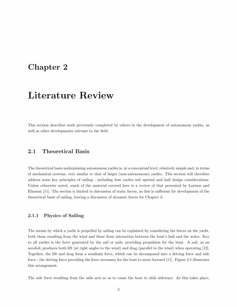
United States Naval Academy (USNA) (Figure 2.4)
The USNA has developed four 2m boats (USNA Sailbots 1-4) for entry into the SailBot competition as part
of an undergraduate academic programme [15–17]. While the first three boats were developed for light wind
conditions, the fourth was intended for longer term voyages and accounted for stronger winds.
All four USNA boats utilised cloth sails, some designed using the SMSW6 sail design software program, and
notably one rig design included a flexible mast that de-powered in strong wind. Likewise, all four hulls were
developed using the PCSail velocity prediction program before being constructed from a milled foam core.
In some variations, swept keel designs were developed to minimise weed capture.
The boats appear to have made use of relatively simple control strategies - employing a proportional controller
for rudder control and velocity made good (VMG) calculations for upwind direction control (by determining
the sailing direction that maximises the component of the boat’s velocity in the direction of the wind). Plans
for a configurable mechanical self-steering system (linked to a wind vane) are noted but not implemented,
presenting a potential area of research. It appears that minimal results of autonomous operation have been
published, but it has been noted that low freeboard in the second boat resulted in bow submersion in strong
wind and that waves resulted in limited communications (suggesting a need for a radio mast).
AVALON (Figure 2.5a)
The AVALON project [18] presents one of the most promising mechanical designs discussed in the literature.
Based at the Federal Institute of Technology, Zurich, the 3.95m boat was custom built and includes two
rudders, a balanced rig, a 160kg keel, solar and fuel cell power supplies and other notable features. While
the design appears to hold great potential, its high development cost (reportedly 209 000 Swiss francs as
of 2009 [18]), together with its large size renders it relatively incomparable with lower cost systems such as
that developed in this study. Despite this, the project includes notable approaches that may prove useful:
including (unexplained) algorithmic optimisation of the hull design, the use of a balanced rig (reducing power
consumption), and use of a route planner making use of a grid-based A* algorithm.
IBOAT (Figure 2.5b)
The IBOAT project [19] involved the construction of a 2.4m boat with a balanced rig with cloth sails. It is
notable for its good simulation results (discussed in section 2.4), as well as its state machine based approach
10
(a) (b) (c)
Figure 2.4: The USNA boats - (a) shows boat 1, while (b) and (c) show boat 4 (source: [15, 17]).
to control of the boat.
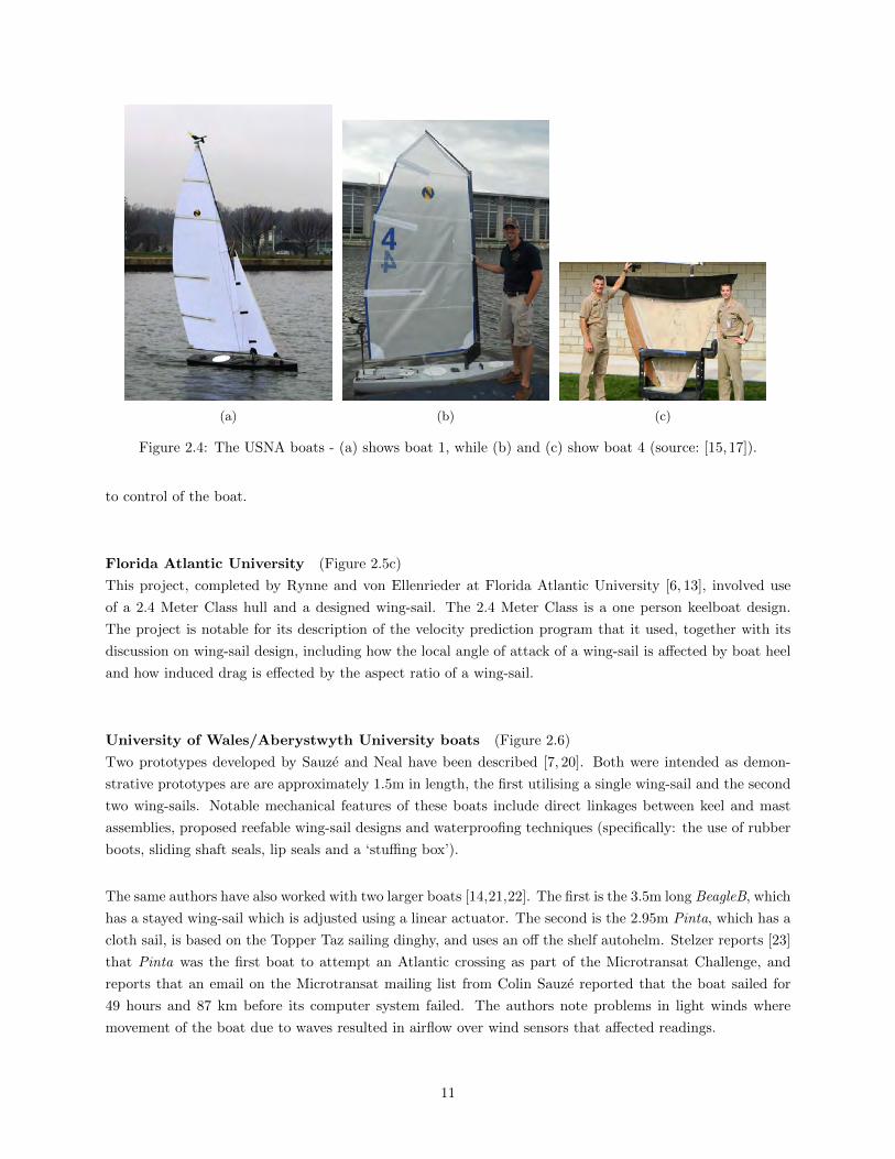
Florida Atlantic University (Figure 2.5c)
This project, completed by Rynne and von Ellenrieder at Florida Atlantic University [6, 13], involved use
of a 2.4 Meter Class hull and a designed wing-sail. The 2.4 Meter Class is a one person keelboat design.
The project is notable for its description of the velocity prediction program that it used, together with its
discussion on wing-sail design, including how the local angle of attack of a wing-sail is affected by boat heel
and how induced drag is effected by the aspect ratio of a wing-sail.
University of Wales/Aberystwyth University boats (Figure 2.6)
Two prototypes developed by Sauze and Neal have been described [7, 20]. Both were intended as demon-
strative prototypes are are approximately 1.5m in length, the first utilising a single wing-sail and the second
two wing-sails. Notable mechanical features of these boats include direct linkages between keel and mast
assemblies, proposed reefable wing-sail designs and waterproofing techniques (specifically: the use of rubber
boots, sliding shaft seals, lip seals and a ‘stuffing box’).
The same authors have also worked with two larger boats [14,21,22]. The first is the 3.5m long BeagleB, which
has a stayed wing-sail which is adjusted using a linear actuator. The second is the 2.95m Pinta, which has a
cloth sail, is based on the Topper Taz sailing dinghy, and uses an off the shelf autohelm. Stelzer reports [23]
that Pinta was the first boat to attempt an Atlantic crossing as part of the Microtransat Challenge, and
reports that an email on the Microtransat mailing list from Colin Sauze reported that the boat sailed for
49 hours and 87 km before its computer system failed. The authors note problems in light winds where
movement of the boat due to waves resulted in airflow over wind sensors that affected readings.
11

(a) (b) (c)
Figure 2.5: a: The Avalon boat (source: [18]) b: IBOAT (source: [19]) c: Florida Atlantic University boat(source: [13])
Later work by Sauze and Neal covered the construction of the ‘MOOP’ boats [21, 24] - 72cm long boats
with a mass of 4kg that aimed to be affordable and manageable platforms. Various aspects of this work are
notable - including the use of magnetic rudder linkages, tests using dual-wing-sail configurations, an attempt
to construct an ultra-sonic wind sensor, the use of lead shot embedded in resin for keel construction, and
use of a similar method of wing-sail construction to that used in the author of this study’s previous work [5].
Cited related work that used the boats to test “power management algorithms based upon an abstraction
of the mammalian endocrine system” offers a potential area of further review.
The Atlantis Project (Figure 2.7a)
This project [25] saw the development of an autonomous 7.2m long catamaran that demonstrated sub-metre
control accuracy. Notably, the project utilised a self-trimming wing-sail - a concept that is described in
detail later in this review, but which importantly is capable of automatically setting itself to an angle to the
wind determined by its tail. The importance of mechanical automatic sail trimming is noted by the project’s
author with the observation that wind direction during one test varied by up to 20 degrees from its nominal
direction. The project’s approach to system identification and control is discussed (and is examined below),
however its applicability to small autonomous boats is at this stage unclear.
The Roboat Boats (Figure 2.7b)
Work by Stelzer towards his 2012 thesis [23] saw the development of two boats, Roboat I - a 1.73m, 17.5kg
boat based on an off-the-shelf model yacht with cloth sails with an area of 0.855m2 - and ASV Roboat - a
3.72m, 300kg boat based on the Laerling class boat with 4.5m2 of cloth sail area and a 60kg keel. Stelzer
reports that the former (smaller) boat suffered from extreme sensitivity to gusts and small waves, leading to
12

(a) (b) (c)
Figure 2.6: a: The second University of Wales/Aberystwyth University boat (source: [7]) b: BeagleB (source:[21]) c: Pinta (source: [22])
the development of the second boat - however it is unclear whether problems with the first boat were due
to its size or relatively large sail area. Notable features of the second boat include its use of a self-tacking
jib and its inclusion of a solar panel and fuel cell. Stelzer’s work on a communication strategy, navigation,
and fuzzy logic control has been noted elsewhere in this review.
Protei
Protei is an effort to develop an autonomous yacht with a strong emphasis on open source (both hardware and
software) principles [26], which collaborates with academia, but is not itself an academic project. Although
its envisioned use includes a number of possible missions, its focus is on collection of oil during oil spills by
means of oil absorbent booms dragged behind boats. The project has involved the construction of a number
of boats, the sixth iteration being comprehensively discussed in the project handbook [10], and current
designs involve shape-shifting hulls that act as the boat’s rudder, a design that followed from placing the
rudder at the front of a boat. While the Protei design presents a novel and promising alternative to standard
rigid hulls, public test results appear to be limited and suggest that further development is required.
Other Projects
Other projects not noted above have taken various approaches. One novel proposal was a ‘wind-propelled
small water-plane area spar’ [1], based on known benefits of reduced waterplane area (including damped
response to waves). Figure 2.8 shows the conceptual diagram proposed for this concept. The investigation
into the concept concluded that it offered little benefit in terms of boat velocity, but that, as it might present
other benefits, it was a concept worthy of further analysis.
Other practical decisions and considerations worth noting from projects not discussed above include:
13

(a) (b)
Figure 2.7: a: The engineering model of the Atlantis (source: [27]) b: ASV Roboat (source: [23])
Figure 2.8: The ‘wind-propelled small water-plane area spar’ proposed by Rynne and von Ellenrieder. Source:[1]
14

The ENSIETA yacht’s use of waterproof connectors and a waterproof electronics box [28]. Later work
by some of the same authors, on the Breizh Spirit project [29], advocated use of a foam hull to assist
with buoyancy - arguing that proper waterproofing of a hull is difficult (it should be noted that the
latter project achieved some promising results, but that it presented little that is noteworthy here).
The FASt platform’s hull construction method and its use of wiper motors (which despite their low
efficiency, are robust and include naturally locking gearboxes - saving energy), boom position, moisture,
ambient light, and interior temperature sensors, and a Field-Programmable Gate Array (FPGA) based
computer system [30,31].
It is noted that commercial autonomous sailboats, such as that which is under development by Autonomous
Marine Systems1, have not been reviewed here.
2.3 Hardware
2.3.1 Hull Design
Hull design and selection appears to have received relatively little attention in the literature specific to small
autonomous sailboats. The UNSA boats were developed by making use of the ‘PCSAIL’ velocity prediction
program, which appears to be spreadsheet-based - allowing variation of design parameters, and analysis of
the effect of varying different parameters [16]. While a number of other considerations have been noted in
the above review of previous work, this is not examined in further detail here as hull design is not considered
to be a major aspect of this study.
2.3.2 Sail Design
Four key variations in sail configuration for autonomous yachts have been utilised by other projects, each of
which is detailed below. Much of this analysis, except where otherwise noted, is based on the work of Neal,
Sauze, and Thomas [21].
Flexible Sails
Similar to the traditional cloth sails used on many yachts, these sails have been used by a number
of projects. Their advantages include easy handling by a human, simple reefing (reduction in area),
easy repair, and the flexibility offered in terms of ability to change shape. These benefits, however,
appear to apply principally to manned yachts, and - as noted by Neal et al. [21] - they are prone to
wear and tear, luffing (loss of shape if sailed at too small an angle of attack), twist (change in shape
1http://www.automarinesys.com/
15
and and angle of attack along length), and require rigging that can add to a boat’s aerodynamic drag.
An important variation to the standard flexible sail configuration is use of a balanced rig [14], which
reduces actuator load.
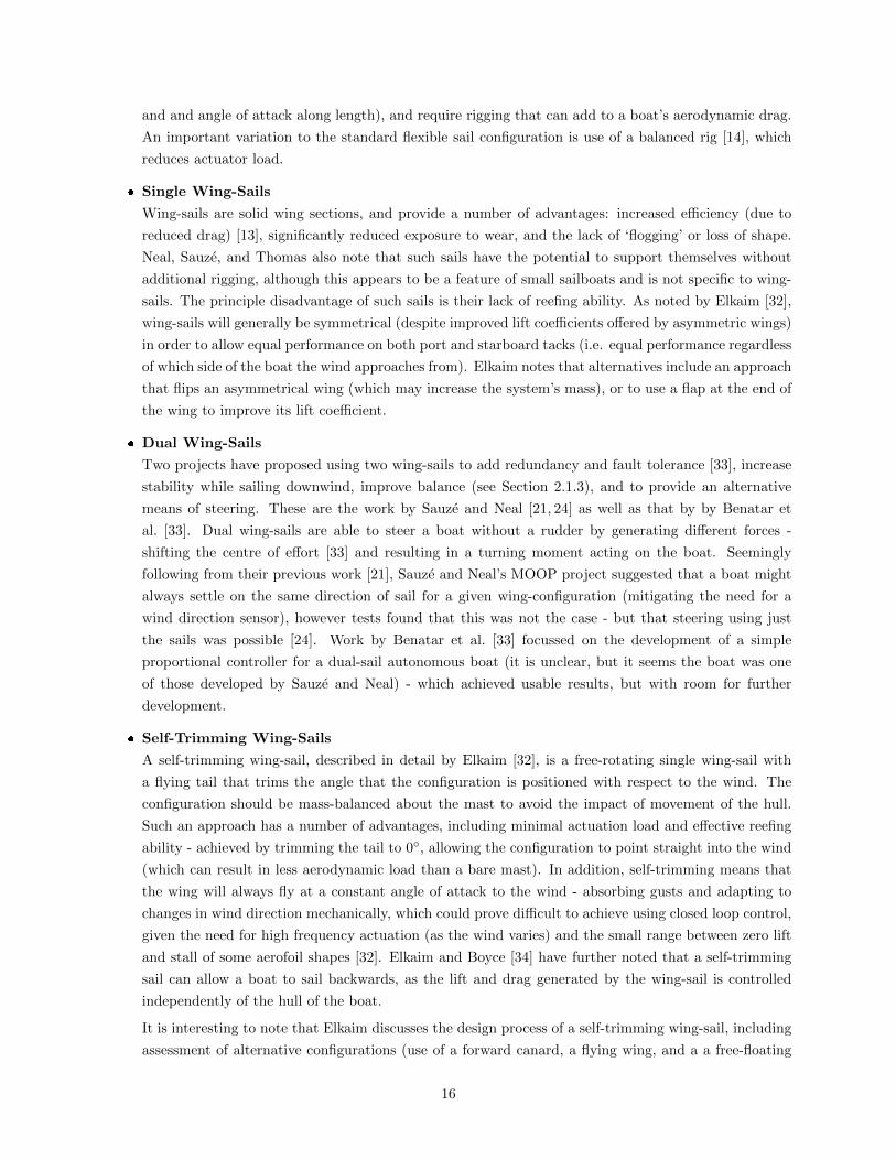
Single Wing-Sails
Wing-sails are solid wing sections, and provide a number of advantages: increased efficiency (due to
reduced drag) [13], significantly reduced exposure to wear, and the lack of ‘flogging’ or loss of shape.
Neal, Sauze, and Thomas also note that such sails have the potential to support themselves without
additional rigging, although this appears to be a feature of small sailboats and is not specific to wing-
sails. The principle disadvantage of such sails is their lack of reefing ability. As noted by Elkaim [32],
wing-sails will generally be symmetrical (despite improved lift coefficients offered by asymmetric wings)
in order to allow equal performance on both port and starboard tacks (i.e. equal performance regardless
of which side of the boat the wind approaches from). Elkaim notes that alternatives include an approach
that flips an asymmetrical wing (which may increase the system’s mass), or to use a flap at the end of
the wing to improve its lift coefficient.
Dual Wing-Sails
Two projects have proposed using two wing-sails to add redundancy and fault tolerance [33], increase
stability while sailing downwind, improve balance (see Section 2.1.3), and to provide an alternative
means of steering. These are the work by Sauze and Neal [21, 24] as well as that by by Benatar et
al. [33]. Dual wing-sails are able to steer a boat without a rudder by generating different forces -
shifting the centre of effort [33] and resulting in a turning moment acting on the boat. Seemingly
following from their previous work [21], Sauze and Neal’s MOOP project suggested that a boat might
always settle on the same direction of sail for a given wing-configuration (mitigating the need for a
wind direction sensor), however tests found that this was not the case - but that steering using just
the sails was possible [24]. Work by Benatar et al. [33] focussed on the development of a simple
proportional controller for a dual-sail autonomous boat (it is unclear, but it seems the boat was one
of those developed by Sauze and Neal) - which achieved usable results, but with room for further
development.
Self-Trimming Wing-Sails
A self-trimming wing-sail, described in detail by Elkaim [32], is a free-rotating single wing-sail with
a flying tail that trims the angle that the configuration is positioned with respect to the wind. The
configuration should be mass-balanced about the mast to avoid the impact of movement of the hull.
Such an approach has a number of advantages, including minimal actuation load and effective reefing
ability - achieved by trimming the tail to 0, allowing the configuration to point straight into the wind
(which can result in less aerodynamic load than a bare mast). In addition, self-trimming means that
the wing will always fly at a constant angle of attack to the wind - absorbing gusts and adapting to
changes in wind direction mechanically, which could prove difficult to achieve using closed loop control,
given the need for high frequency actuation (as the wind varies) and the small range between zero lift
and stall of some aerofoil shapes [32]. Elkaim and Boyce [34] have further noted that a self-trimming
sail can allow a boat to sail backwards, as the lift and drag generated by the wing-sail is controlled
independently of the hull of the boat.
It is interesting to note that Elkaim discusses the design process of a self-trimming wing-sail, including
assessment of alternative configurations (use of a forward canard, a flying wing, and a a free-floating
16
canard).
It is noted that this section has not considered many of the design decisions necessary for the implementation
of the above sail designs. These include construction techniques, the use of position feedback, and types of
actuators - although it is worth noting Neal et al’s use of a floating wing-sail [21] to mitigate the effect of
capsize as well as the Atlantis Project’s use of lead-screws for actuator control [25], which presumably results
in reduced power consumption - potentially useful given noted concerns regarding the power continuously
drawn by servomotors [22].
2.3.3 Electronics and Communication
Various electronics systems have been described in the literature. While a detailed review will not take
place here (as choice appears to be affected by available technology, specific project requirements, and
other factors), the overview of options presented by Sauze and Neal [22] is notable. This covers traditional
microcontrollers, so-called ‘easy to use’ microcontrollers, single-board computers or PDAs, embedded PCs,
or combinations of these options. It is noted that the use of an operating system can allow remote login.
The FPGA utilised by the FASt project [30,31] also presents an alternative approach.
Other important sub-systems that must be considered are sensors and the communication system.
Sensors
A number of sensors, some less critical than others, have been used as part of previous projects. This section,
while noting important sensors and related considerations, is not intended as a comprehensive review of each
type of sensor.
Wind Direction
Required by the vast majority of control strategies, wind direction sensing allows a boat to determine
wind direction relative to itself. There are three major types of wind-sensors [21]: mechanical sensors,
contactless mechanical sensors, and ultrasonic sensors. Mechanical sensors generally involve a wind
vane directly connected to a potentiometer (contact mechanical sensor) or to a magnet, the position of
which is detected with a Hall effect sensor (contactless mechanical sensor). Both types of mechanical
sensor suffer from wear and tear and poor performance in light winds, while contact mechanical sensors
are much more difficult to waterproof than contactless sensors, which can be embedded in Epoxy or
a similar material. Ultrasonic sensors transmit ultrasonic signals, which are affected by wind speed -
meaning that measurement of the signals in two axes allow determination of wind direction. With no
moving parts, ultrasonic sensors offer minimal wear and tear and easy waterproofing.
The literature notes that commercial ultrasonic wind sensors are very expensive, and an attempt to
17

develop a simple ultrasonic sensor has produced limited results [21] (the same authors’ techniques to
deal with wind direction value discontinuities around 360/0 are also notable).
Wind Speed
Less common than wind direction sensors, wind speed sensors nevertheless have been included in
some projects. It appears that such sensors are subject to similar considerations regarding contact
mechanical and contactless mechanical anemometers as wind direction sensors, and that ultrasonic
sensors described above can output wind speed in addition to wind direction [21].
Global Positioning
Many projects have utilised GPS, and in two cases differential GPS [15,32], in order to determine the
position of the boat. It has also been noted [23] that the Iridum satellite communication system can
provide rough positioning information.
Compass
A digital compass provides information about the boat’s heading, which can be used for navigation
purposes. When making use of a compass it is necessary to compensate for tilt of the boat and to
consider its calibration. Tilt can be addressed by using swinging arms to keep the compass level or
tilt-compensated compasses [22]. The researcher’s previous work [5] demonstrated the need for tilt-
compensation of a compass and noted a method to do so using attitude data from other sensors. This
previous work also found that calibration of a digital magnetometer used as a compass must frequently
take place, which may be difficult at sea. Approaches to calibration of a digital magnetometer are
discussed in more detail in Section 4.2.3.
Attitude Detection
A number of projects have included sensors to assist with attitude detection. The Atlantis Project
utilised knowledge of the heel of the boat to detect imminent capsize, allowing the boat to react [27],
while Elkaim and Boyce have further noted that it is possible to estimate the force on the sail of a boat
using knowledge of its roll [34]. While most projects appear to have just used an accelerometer for
attitude detection (Elkaim notes that an attitude system based on an accelerometer and magnetometer
data was used for the Atlantis Project [25]), this is likely to lead to inaccuracies due to acceleration of
the platform in non-static operation. The researcher’s previous work [5] made simple use of a gyroscope
to minimise the effect of dynamic motion.
Communication
While different projects have utilised various technologies for the communication system of an autonomous
sailboat, the three part approach described by Stelzer and Jafarmadar [35] appears to formalise aspects
of what others have described while presenting a useful architecture from which to work. Two use cases
for a communications system are described: manual control of the boat and real-time monitoring and
instruction, while three components are considered: the boat, visualisation software (to receive data or
transmit instructions), and a remote controller (particularly important during testing). It is worth noting
that some projects, including Stelzer and Jafarmadar’s, planned their systems to allow remote reprogramming
of the boat.
18
The three parts to Stelzer and Jafarmadar’s communications system are wireless LAN (affordable with high
bandwidth but requiring special infrastructure and offering very limited range), cellular network (offering
existing infrastructure and high bandwidth but potentially presenting high costs and limited range), and
satellite communication (covering the entire Earth and offering a rough GPS backup but operating with
limited bandwidth, high latency, and high costs). Parts are considered preferable in the order presented,
but as wireless LAN and mobile networks are not always available, the boat should be capable of switching
dynamically between communication methods depending on what is available. Variance of communication
strategy (whether primarily to utilise a push or pull system and what data to transmit automatically) can
occur based on the communication system being utilised.
2.4 Simulation and Modelling
Obtaining a system model for an autonomous yacht for use in simulations has not been pursued by many
previous projects that have focussed on small systems, however it is an important part of this study.
It appears that one of the most common forms of modelling in yacht design is the use of velocity prediction
programmes (VPPs), which predict a boat’s performance in different wind conditions for different angles of
sail - providing useful analysis of hull performance during the design stage. Larsson and Eliasson [11] have
described the principles behind a VPP that uses an iterative process to determine the boat state parameters,
such as heel angle and velocity, for a given wind speed and direction. This is done by solving equations for
equilibrium, such as that the driving force of the sail is equal to the hydrodynamic resistance - as described
in Section 2.1.1. Larsson and Eliasson report that most VPPs do not consider vertical forces or pitching
moments (assuming that these are always balanced), and that only advanced VPPs consider yaw moments
arising from non-zero rudder angles.
The Florida Atlantic University project [13] made use of a VPP based on that described by Larsson and
Eliasson. Results of on-the-water tests resulted in velocities less than those predicted by the VPP, its authors
suggesting that this could be attributed to the system not reaching steady state - it needing a larger testing
area to do so. It is also possible that the model predicted high velocities because of the omission of some
aspects of the hydrodynamic model. Of note are the project’s consideration of wind gradient and the effect
of heel on the sail’s angle of attack, as well as its use of the International Towing Tank Conference Line to
determine frictional resistance.
While VPPs of the sort described above are useful, they are generally limited to consideration of the boat’s
speed. As this study includes consideration of dynamic modelling of the boat, a number of other approaches
have been reviewed:
The IBOAT project [19] proposed a model based on assumptions about boat dynamics. Beginning by
determining forces generated by the sail and hull, a relationship was proposed relating the resultant
force to velocity. Similarly, the project proposed a simplified heading model (based on rudder angle
19

and other parameters) which assumed that the boat was properly balanced. Sea trials allowed the
determination of model parameters using closed loop identification. Estimation of sea current velocity
is performed for this model, as the project had no means of measuring current directly.
Results of simulated control of the boat appear to be remarkably good when compared with real world
tests. It should be noted that reported results do not include trials in waves and that the results are
for simulation of the boat’s position, a comparison of velocity prediction results not being reported.
Importantly, this model appears to account for hydrodynamic resistance in the model parameters,
meaning that factors such as resistance from waves are not accounted for.
The Avalon project proposed [36] a six degree of freedom model that considered forces on the sail and
rudder while estimating resistance and damping forces using a simple relationship with parameters
determined experimentally. Actual performance of the boat is reported to have been “quite different”
from the proposal.
As part of the Atlantis Project, Elkaim [37] describes a simplified state space approach that imposes
a constraint on the system by assuming that the boat’s rudders cannot move sideways through the
water. This resulted, in transfer function form, in a triple integrator with respect to distanced travelled.
A controller was designed for this model, but it was shown that the system would become unstable
when the design velocity was exceeded. The model was then extended to create a velocity invariant
model, which addressed increased speed challenges. However it was found that both these models did
not address issues of mismodelling or sensor noise (the effect of which would get worse with speed,
despite being addressed by the controller as a disturbance), and tests of the velocity invariant model
showed that oscillations occurred in waves. It was also noted that the models do not account for
vehicle dynamics because of the assumption regarding the effect of the rudder. The project went on
to utilise a method of system identification, Observer Kalman Identification, from which a controller
that demonstrated excellent results was designed and from which it was assumed that the boat was
assumed to be a fourth order system, in contrast to the third order triple integrator noted above. It
should be noted that the project utilised a much larger boat than that which is being considered for
this proposal, that a lower bound of 1m/s was used for velocity measurements (due to the presence of
noise), and that one of the parameters being considered was the boat’s cross-track error - indicating
that the same considerations may not apply to all autonomous yachts.
It is interesting to note the merits of a system identification approach, as discussed by Elkaim. While
system identification approaches do not require often-inaccurate and slow physical modelling (which
may be based on assumptions to reduce complexity), they generally do not provide physical intuition
about the system being modelled.
A particularly interesting approach to modelling is that described by Xiao and Jouffroy [38], where
a four degree of freedom (covering forward and sideways velocity, roll, and yaw) state-space model is
considered in order to allow the design and simulation of a heading controller. The model is based
on work by Fossen [39], and considers added mass, Coriolis, and centripetal effects. Importantly, the
model is defined in terms of specific forces acting on the boat - meaning that it can be adapted and
combined with some other models, including the VPP described above. As the model assumes calm
waters and appears to assume constant centre of mass, it is thought that there is room to expand the
model to consider the effect of waves (possibly resulting in an extension of the model into six degrees
20

of freedom), as well as the effect of the movement of actuators. Also of note is Xiao and Jouffroy’s
proposal to use an internal moving mass system for steering of the boat, as well as the non-linear
controller that they developed using the model.
Review of the approach to modelling presented by Fossen [39] revealed a useful framework which was
adopted in this study. A comprehensive overview of the approach is discussed in Section 3.1.
Roncin and Kobus [40] developed a 6 degree of freedom model of a sailboat for use in simulation of a
match race between two boats that appears to be similar to Xiao and Jouffroy’s. Notably the model
considers aerodynamic interaction between the boats, as well as a simple wave model. Importantly,
results suggest that considering the pitch of the boat in the model is important.
Legursky [41] presents a six degree of freedom model of a 23 foot yacht based on Fossen’s [39] approach
and using hydrodynamic forces predicted by the Delft Systematic Yacht Hull Series results and sail
coefficients determined from results of a series of sailing tests.
de Ridder et. al. [42] present a four degree of freedom model of a yacht that is notable for its detailed
application of the results of the Delft Systematic Yacht Hull Series.
While it appears it has not been considered by any of the above methods, the concept of speed made good to
windward (or VMG), which is the the distance a boat has travelled directly to windward in a given time [43],
must be noted. This concept highlights the fact that going faster or being able to sail close to the wind are
not sufficient measures of performance in isolation, as sailing close to the wind can result in a loss of speed
and sailing fast but not close to the wind (if that is the desired direction) is not useful. The concept thus
presents a potential useful measure of performance.
2.5 Control and Navigation
While there has been no single approach to control of autonomous sailboats, many have separated functions
into low level and high level control considerations - an approach which is described in more detail in Section
2.5.3. This approach has been used as a framework for this section.
2.5.1 Low-level Control
It appears that the general approach in the literature has been to consider sail and rudder control as
separate independent single-input single-output systems, an approach that was noted by Erckens et al. [36]
as appearing to be reasonable - and one that has been adopted elsewhere, such as in the work of Stelzer et.
al. [44].
21
Rudder Control
A number of projects, such as the USNA Boats [15] and the IBOAT project [19], report reasonable results
when utilising simple proportional controllers configured to minimise error between the boat’s heading and
the desired heading determined by the navigation algorithm - although it is unclear under what conditions
these were achieved. Stelzer and Karim, in their review of robotic sailing [14] note that the majority
of self-steering systems use PID controllers, although these appear to have been less common amongst
small autonomous sail boats. One exception is the Avalon project, which reported use of a Matlab-tuned
PID controller that appears to have lead to reasonable results (including in strong winds) with minimal
overshoot [36]
There are a number of cases in the literature of fuzzy logic controllers being used to control small boats.
Vaneck describes a strategy of controlling a small motor-powered boat [45] - noting that work was required to
avoid oscillations, while Abril et al. describe a method of controlling a small sail boat with a fuzzy controller
which appears to result in a differing proportional-derivative output [46]. More recently, Stelzer et. al. [44]
have reported on their development of a fuzzy logic controller which notably includes the boat’s angular
velocity as an input and provides an output of rudder change (as opposed to rudder position). In his 2012
thesis [23] , Stelzer reports on processing speed modifications required for different boats for this controller,
and on promising results from real world tests - although it is unclear whether these hold for rough weather
conditions.
Other controllers noted in the literature include the nonlinear controller presented by Xiao and Jouffroy [38]
and Elkaim’s linear quadratic Gaussian controller [37].
As noted in Section 2.1.1, a yacht does not sail directly in the direction in which it is headed - which should
be considered for control. Erckens et al. [36] note that the Avalon project’s approach was to measure the
boat’s drift velocity and to adapt the desired heading accordingly.
Another approach to rudder control is the use of a weather vane, which does not appear to have been
implemented by any autonomous sailing projects. Such an approach would mitigate the need for a wind
direction sensor and potentially minimises energy consumption. Both Stelzer and Blevens et al. (of the
UNASA project) describe [17, 23] how such a device ensures that a boat maintains a constant angle to the
wind, while an approach using this method has been proposed by Sliwka et al. [47] which places the weather
vane at the front of the boat (as opposed to the back, where inversion of the steering would be necessary).
Simulations have confirmed that the boat is able to sail to a predefined angle to the wind from all starting
angles of sail. It has been noted that a weather vane can suffer from stability problems due the impact
of waves on apparent wind direction, particularly while sailing downwind and boat speed varies [30]. It is
assumed that for boats that use this approach, whether or not a wind sensor is necessary for other purposes
would further depend on the choice of sail and navigation algorithm.
22

Sail Control
Specific approaches to sail control appear to have received little attention in the literature. Stelzer and
Karim [14], in their review of robotic sailing note that most strategies rely on wind data measured by the
boat. In contrast, Stelzer et. al’s [44] fuzzy logic controller (developed alongside that noted above) separately
considered sail control - ensuring air flow over the sail and avoiding capsize of the boat by controlling the
heel of the boat according to the wind conditions (an equation to determine desired heel was proposed). It
is unclear whether controlling boat heel is an optimal approach.
Also notable is the observation of Miller et al. that the USNA project encountered steering problems while
the sail was trimmed, requiring it to be eased in strong winds to allow steering away from the wind [15].
This highlights the effect of the sail on steering.
2.5.2 Navigation and Obstacle Avoidance
Autonomous sailboat navigation can be considered at two levels: navigation to account for the limitations of
a sailing vessel, such as its inability to sail into the wind, and navigation undertaken to reach a destination
by avoiding obstacles. While distinct concepts, often both are considered together as part of a single strategy
- and so this section will present a number of different approaches and note their respective capabilities. In
some cases disctictions can be made between static obstacles, like jetties, and moving obstacles. It is also
worth noting the distinction between deliberative (involving in-advance planning) and reactive (connecting
sensor data to actuators) approaches to navigation, as described by Stelzer [23].
The literature notes some simplistic approaches to navigation - such as Sauze and Neal’s [22] method
of offsetting the desired heading (the bearing to a manually determined waypoint) if the heading falls
within the boat’s no sail zone, such as within 45 of the wind direction. Such approaches direct the
boat towards the next waypoint while ensuring that it does not attempt to sail into the wind, and do
not consider obstacles.
Stelzer’s [23] approach is similar to the above simplistic approaches, providing formality by seeking to
optimise the boat’s speed made good by using its polar diagram (indicating speed for different directions
of sail) as well as a hysteresis condition to ensure consistent tacking when heading upwind. Results of
simulations revealed sub-optimal routes for some courses, requiring use of a simplified polar diagram -
which (the author of this review assumes) could be sub-optimal in other respects, potentially indicating
an area requiring further investigation. The approach was later extended to account for obstacles by
modifying the boat’s polar diagram.
A strategy proposed by Xiao et al. [48] suggests that it is possible to achieve navigation of a sailboat
without knowledge of the wind direction by using the ‘no-go zone’ (the sailing direction relative to the
wind direction in which the boat cannot sail, i.e. into the wind) as a reference point. This involves
devising a navigation strategy using Voronoi diagrams, which indicates a desired heading that the boat
23
attempts to sail, failing which an alternative heading that is guaranteed to lie outside of the ‘no-go
zone’ is sailed. While the strategy is a novel technique that could be used should a wind-sensor fail,
it seems that it it would be relatively inefficient when compared with other techniques as it does not
find the optimal sailing direction.
Sliwka et al. [47] have proposed a navigation strategy that sets rudder angle based on angle to a target
and the distance between the boat and the desired path to the target (using the sum of two proportional
controllers) in order to track direction and line following as a means to compensate for drift of a boat.
Benjamin et al. [49] have described a method of avoiding another vessel that complies with the Interna-
tion Regulations for Prevention of Collision at Sea by utilising a method of multi-objective optimisation,
known as interval programming, to find the best possible action when considering both ordinary navi-
gation objectives (such as the heading determined by Sauze and Neal’s method) and collision avoidance.
The method requires information about other vessels’ location, speed and heading. Candidate actions
are rated based on their fulfilment of the ordinary navigation objectives, and based on their compliance
with regulations to avoid other vessels and the two measures are combined, allowing for the optimal
solution to be selection. Evaluation takes place continuously, meaning that should the other vessel
change course then the boat can adapt to the changing situation.
As part of the Avalon project, Erckens et al. [36] have proposed a modified version of the A* grid-based
algorithm. The technique divides the area under consideration into a two dimensional grid - which
together with the boat’s heading forms a three dimensional grid, allowing each block on the three
dimensional grid to be assigned a cost value as they are considered in the determination of the optimal
route. Sailing restrictions are considered by use of a polar diagram (which provides boat speeds at
different wind velocities for different angles of sail), which also contributes to the cost factors considered
by the algorithm.
Work by Langbein et al. [50] developed a strategy for long term routing for the ASV Roboat, also based
on the A* algorithm, which accounted for weather forecasts. The approach is intended to work alongside
a short term routing algorithm to navigate between waypoints, and so does not consider when the boat
will tack and similar manoeuvres. Notably, the authors describe potential future work as including
consideration of ensemble forecasts (which consider different scenarios with different probabilities) as
well as the consideration of currents.
Aside from the above obstacle avoidance techniques, the simple approach adopted as part of the USNA
project [17] is noted - which involved mounting two ultrasonic range sensors on either side of the front of the
boat, allowing it to turn appropriately if any obstacle is detected. Assuming that such sensors perform well
in an ocean environment (results are not reported), this provides a promising alternative, or compliment, to
the above techniques.
Obstacle Detection
Naturally knowledge of obstacles is a fundamental aspect of obstacle avoidance. Generally speaking, ap-
proaches to this problem have relied either on on-board sensors or data about obstacles from other sources.
24
On-board sensors described in the literature have included laser scanners [51] (although poor performance
in rough conditions has been noted) and the ultra-sonic sensors employed by the USNA project [17].
While it has been noted that the Automatic Identification System, which broadcasts ship positions, courses
and speeds along with other information [52], could potentially provide information about moving obstacles
- others have noted [51] that smaller vessels may not use the system.
In some cases, the method used to detect obstacles does not affect the avoidance strategy - suggesting that
it may be worth considering utilisation of multiple methods.
2.5.3 Software Architecture
While the software architecture implemented is implied by the approaches described above, some further
points and general approaches are worth noting:
Some projects have implemented a state machine based approach to control. For example, the IBOAT
project [19] utilised three states: one for normal sailing, the second for tacking, and the third for jibing
when tacking failed. Similarly, the Avalon project [36] switched between standard navigation, goal
approach and new calculation states. It appears that dividing control tasks by ‘states’ has provided a
helpful level of abstraction.
In their system designed to assist human sailors on large yachts, the architecture implemented by van
Aartrijk et al. [53] (who described their approach as utilising ‘jargon’) involved a number of ‘agents’
that were responsible for relevant concepts in sailing. The agents would monitor the boat, determining
(for example) whether it was close hauled or planing, and feeding the resulting information into the
command hierarchy. The command hierarchy implemented the various tasks of individuals aboard
a yacht (such as the helmsman or watchman), relying on information from the agents and giving
precedence to different aspects of the hierarchy when necessary - for example by allowing the watchman
to instruct the helmsman to steer into the wind during a gust. This approach appears to match the
subsumption architecture approach described and referenced by Stelzer [23].
25
Chapter 3
System Modelling
This chapter outlines the development of the model of the sailboat. Two primary models were developed -
a three degree of freedom model which predicted movement in the x and y planes as well as roll, and a four
degree of freedom model which additionally considered yaw (steering).
In order to facilitate reading, Table 3.1 presents the definitions of key variables referred to in this chapter.
the sources of definitions are those referred to in this chapter.
η Vehicle position and orientation with respect to the Earth-fixed frame m, radians
υ Linear and angular velocity with respect to the body-fixed reference frame m/s, rad/s
τRB Forces and moments acting on the vehicle in the body-fixed reference frame N, Nm
J Transformation between υ and η
MRB Rigid-body inertia matrix
CRB Rigid-body Coriolis and centripetal matrix
τH Hydrodynamic forces and moments in the body-fixed reference frame N, Nm
τE Environmental forces and moments in the body-fixed reference frame N, Nm
τ Propulsion forces and moments in the body-fixed reference frame N, Nm
g(η) Restoring forces and moments in the body-fixed reference frame N, Nm
τD Damping forces and moments in the body-fixed reference frame N, Nm
MA Added mass inertia matrix
CA Added mass Coriolis and centripetal matrix
Re Reynolds number
V Wind speed m/s
l Aerofoil length m
ν Kinematic viscosity m2s−1
CL Lift coefficient
CL Drag coefficient
CM Moment coefficient
26
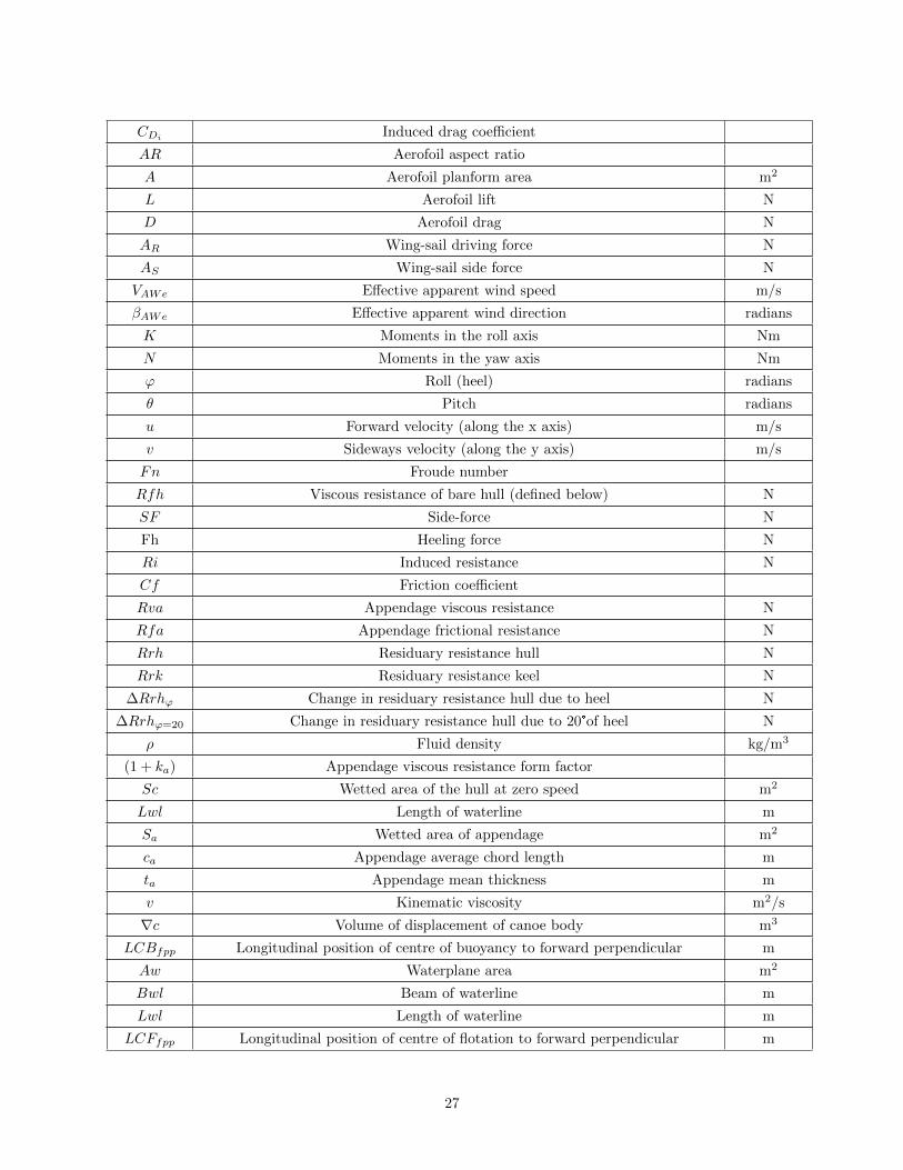
CDi Induced drag coefficient
AR Aerofoil aspect ratio
A Aerofoil planform area m2
L Aerofoil lift N
D Aerofoil drag N
AR Wing-sail driving force N
AS Wing-sail side force N
VAWe Effective apparent wind speed m/s
βAWe Effective apparent wind direction radians
K Moments in the roll axis Nm
N Moments in the yaw axis Nm
ϕ Roll (heel) radians
θ Pitch radians
u Forward velocity (along the x axis) m/s
v Sideways velocity (along the y axis) m/s
Fn Froude number
Rfh Viscous resistance of bare hull (defined below) N
SF Side-force N
Fh Heeling force N
Ri Induced resistance N
Cf Friction coefficient
Rva Appendage viscous resistance N
Rfa Appendage frictional resistance N
Rrh Residuary resistance hull N
Rrk Residuary resistance keel N
∆Rrhϕ Change in residuary resistance hull due to heel N
∆Rrhϕ=20 Change in residuary resistance hull due to 20°of heel N
ρ Fluid density kg/m3
(1 + ka) Appendage viscous resistance form factor
Sc Wetted area of the hull at zero speed m2
Lwl Length of waterline m
Sa Wetted area of appendage m2
ca Appendage average chord length m
ta Appendage mean thickness m
v Kinematic viscosity m2/s
∇c Volume of displacement of canoe body m3
LCBfpp Longitudinal position of centre of buoyancy to forward perpendicular m
Aw Waterplane area m2
Bwl Beam of waterline m
Lwl Length of waterline m
LCFfpp Longitudinal position of centre of flotation to forward perpendicular m
27

Tc Draft of canoe body m
T Draft m
Cm Midship section coefficient
Cp Prismatic coefficient
Zcbk Vertical position of centre of buoyancy of keel m
∇k Volume of displacement of keel m3
TR Taper ratio
βB Leeway angle in the body-fixed reference frame radians
βE Leeway angle in the Earth-fixed reference frame radians
ψ Yaw radians
N Yaw moment Nm
Xmast Longitudinal position of centre of mast m
Zce Vertical position of centre of effort m
cs The wing-sail chord length m
cmast Distance between wing-sail leading edge and centre of the mast along the chord m
bk Span of keel m
BGi Distance between the centre of mass and centre of buoyancy in the i axis m
δs Sail angle radians
δr Rudder angle radians
α Aerofoil angle of attack radians
hc Distance between aerofoil leading edge and centre of mass where c is the chord m
shull−keel Area of the combined hull and keel m2
chull−keel Chord of the combined hull and keel m
Table 3.1: Definitions of variables referred to in this chapter.
3.1 Approach to Modelling
This work utilises the approach to modelling of a marine vehicle presented by Fossen [39]. This approach has
been utilised elsewhere - such as Xiao and Jouffroy’s model [38]. As an approach to dynamic (as opposed to
static) modelling, it provides a simple framework from which to extend the approach to velocity prediction
programmes discussed in Section 2.4, which only predict static states.
The following subsection describes the details of the model, and is largely derived from Fossen’s own expla-
nation [39]. The resulting model, which considers the vehicle to be a rigid body, is defined in terms of forces
acting on the vehicle and vehicle’s own properties. The rest of this section discusses the approach taken
towards damping forces in terms of those described by Fossen.
28

x
x
y
y
z
z
φψ
θ
(a)
δs
δr(b)
Figure 3.1: Diagrams showing the coordinate systems used by the model. (a) shows the axes coordinatesystem (origin at the centre of mass), and is reproduced with minor adaptations from [42] and is consistentwith [55], while (b) shows the coordinate system for the sail and rudder angles (origins at the pivot points).
3.1.1 Mathematical Model
The complete model describes the motion of a vehicle in six degrees of freedom with position and translational
motion in the x (surge), y (sway), and z (heave) axes and orientation and rotational motion about these
axes as roll (ϕ), pitch (θ), and yaw (ψ). The position of these axes with respect to a boat, together with the
appropriate symbols, are visible in Figure 3.1a.
Two coordinate frames are considered as part of the model - a moving frame attached to the vehicle referred
to as the body-fixed reference frame, and an inertial reference frame relative to which its motion is described
- known as the Earth-fixed reference frame (the model assumes that the motion of Earth can be neglected).
Velocities of the vehicle are described relative to the body-fixed reference frame while position and orientation
are described relative to the Earth-fixed reference frame.
This approach results in three vectors which describe the motion of the vehicle: η, which describes position
and orientation with respect to the Earth-fixed frame, υ, which describes linear and angular velocity with
respect to the body-fixed frame, and τRB , which describes the forces and moments acting on the vehicle in
the body-fixed reference frame. The relationship between υ and η is described by the transformation J, as
seen in Equation 3.1.
η = J(η)υ (3.1)
29

While Fossen derives the relationships between the various vectors for both Euler angles and quaternions,
this detail is not considered relevant here as the principles of the model hold for both approaches.
Fossen proceeds to show that the six degree of freedom nonlinear dynamic equations of motion can be
expressed in a compact form by Equation 3.2, where MRB is the rigid-body inertia matrix and CRB is the
rigid-body Coriolis and centripetal matrix..
MRBυ + CRB(υ)υ = τRB (3.2)
In considering hydrodynamic forces and moments, Fossen considers two sub-problems: radiation-induced
forces (also referred to here as hydrodynamic forces, and comprising of three components present when “the
body is forced to oscillate with the wave excitation frequency and there are no incident waves” - added
mass, radiation-induced potential damping, and restoring forces) and Froude-Kriloff and diffraction forces
(considered as environmental forces - which arise when “the body is restrained from oscillating and there are
incident regular waves”). These sub-problems, together with propulsion forces, allow τRB to be considered
in terms of hyrodynamic forces and moments τH , environmental forces and moments τE , and propulsion
forces and moments τ - as seen in Equation 3.3.
τRB = τH + τE + τ (3.3)
In the presentation of his model, Fossen considers the radiation-induced potential damping component of
the hydrodynamic forces as a damping matrix that includes other damping effects and which is proportional
to υ as a D(υ)υ component. In this work, this has been replaced with τD as a general expression of the
damping forces. Other contributions to τH include restoring forces, g(η), and added mass MAυ + CA(υ)υ.
This results in a the final definition of τH seen in Equation 3.4.
τH = −MAυ −CA(υ)υ − τD − g(η) (3.4)
Finally, these definitions are substituted into Equation 3.2 and the rigid-body and added mass interia and
Coriolis and centripetal matrices are considered together to determine Equation 3.5 - which represents the
system’s equations of motion.
Mυ + C(υ)υ + τD + g(η) = τE + τ (3.5)
30
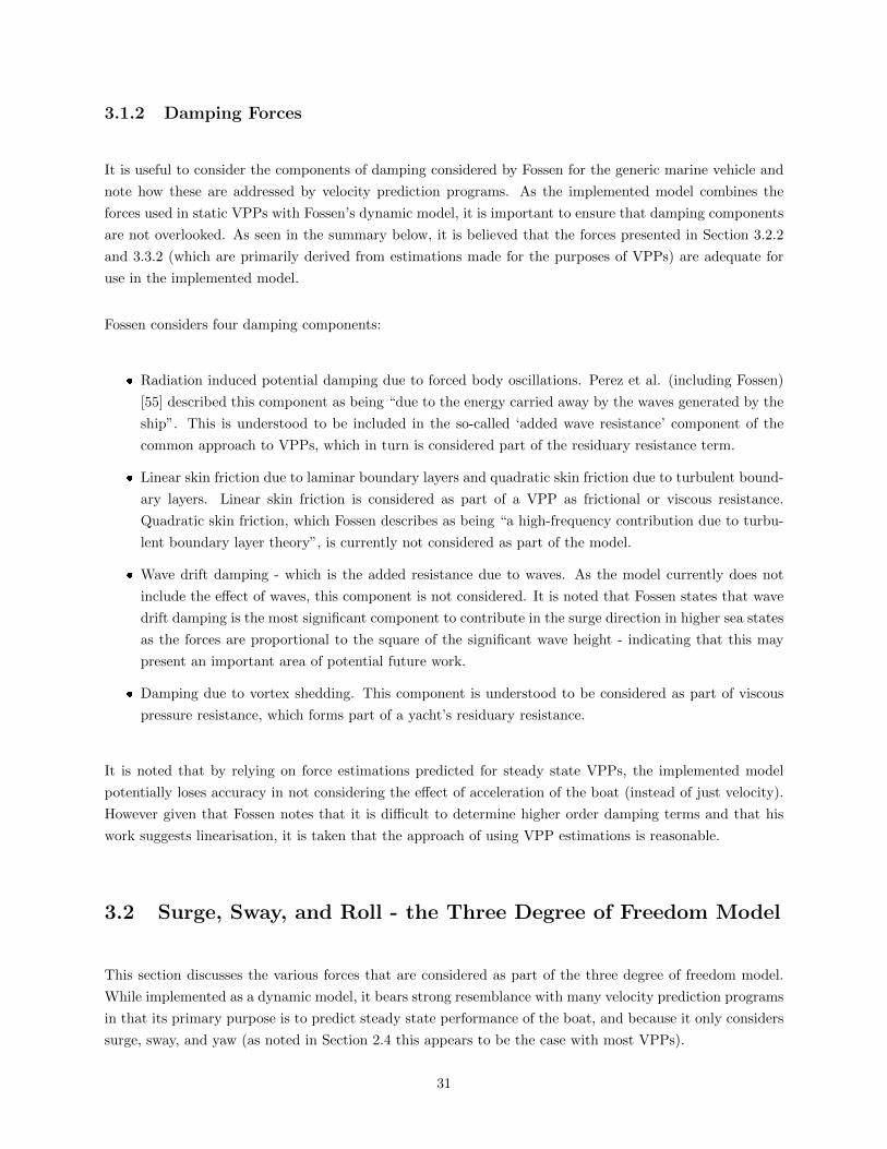
3.1.2 Damping Forces
It is useful to consider the components of damping considered by Fossen for the generic marine vehicle and
note how these are addressed by velocity prediction programs. As the implemented model combines the
forces used in static VPPs with Fossen’s dynamic model, it is important to ensure that damping components
are not overlooked. As seen in the summary below, it is believed that the forces presented in Section 3.2.2
and 3.3.2 (which are primarily derived from estimations made for the purposes of VPPs) are adequate for
use in the implemented model.
Fossen considers four damping components:
Radiation induced potential damping due to forced body oscillations. Perez et al. (including Fossen)
[55] described this component as being “due to the energy carried away by the waves generated by the
ship”. This is understood to be included in the so-called ‘added wave resistance’ component of the
common approach to VPPs, which in turn is considered part of the residuary resistance term.
Linear skin friction due to laminar boundary layers and quadratic skin friction due to turbulent bound-
ary layers. Linear skin friction is considered as part of a VPP as frictional or viscous resistance.
Quadratic skin friction, which Fossen describes as being “a high-frequency contribution due to turbu-
lent boundary layer theory”, is currently not considered as part of the model.
Wave drift damping - which is the added resistance due to waves. As the model currently does not
include the effect of waves, this component is not considered. It is noted that Fossen states that wave
drift damping is the most significant component to contribute in the surge direction in higher sea states
as the forces are proportional to the square of the significant wave height - indicating that this may
present an important area of potential future work.
Damping due to vortex shedding. This component is understood to be considered as part of viscous
pressure resistance, which forms part of a yacht’s residuary resistance.
It is noted that by relying on force estimations predicted for steady state VPPs, the implemented model
potentially loses accuracy in not considering the effect of acceleration of the boat (instead of just velocity).
However given that Fossen notes that it is difficult to determine higher order damping terms and that his
work suggests linearisation, it is taken that the approach of using VPP estimations is reasonable.
3.2 Surge, Sway, and Roll - the Three Degree of Freedom Model
This section discusses the various forces that are considered as part of the three degree of freedom model.
While implemented as a dynamic model, it bears strong resemblance with many velocity prediction programs
in that its primary purpose is to predict steady state performance of the boat, and because it only considers
surge, sway, and yaw (as noted in Section 2.4 this appears to be the case with most VPPs).
31
3.2.1 Forces Generated by the Sail
As previously noted, a single wing-sail constructed as part of another project at the University of Cape Town
was used for this work. The wing-sail is a 1 meter tall NACA0018 aerofoil with a 30cm chord length, and
includes an approximately 18cm long 22mm diameter shaft that serves as its connection to the boat.
As part of his motivation for using a self-trimming wing-sail, Elkaim notes [32] that the aerofoil selected for
the Atlantis Project has an angle of attack range of between zero lift and wing-sail stall of less than 12, and
that wind variation results in high speed actuation requirements - together presenting challenging control
requirements should the project have utilised a simple actuated wing-sail. Based on this observation, this
section will make some observations regarding the expected control requirements of this wing-sail while a
comprehensive examination of this question is discussed in Section 5.3.1.
It is necessary to note that this work, consistent with others in the literature, only includes consideration of
dynamic movement of the sailboat to a limited extent. The speed of the platform in the x and y axes, as
well as the heel velocity, is considered to determine the relative velocity of the wind, while other components
such as the speed at which the sail is actuated and the yaw velocity of the platform (in the four degree of
freedom model) are omitted as the forces arising from these are expected to be negligible due to the small
speeds involved.
Determination of Sail Coefficients
A fundamental aspect of the calculation of forces generated by the wing-sail is the determination of its lift
and drag coefficients. Other projects [13, 32] have made use of XFOIL1, a software program that is able
to analyse the performance of aerofoils, to determine these coefficients (principally for design, but it would
appear also for modelling). This approach was initially used here, however as convergence errors occurred
for angles of attack above 30, it was ultimately considered unsuitable as the wing-sail is expected to operate
at higher angles of attack.
As an alternative measure, results of tests of NACA aerofoils for use with vertical axis wind turbines,
including the NACA0018, presented by Sheldahl and Klimas [4] were utilised. Sheldahl and Klimas’ report
presents coefficients for lift and drag for the NACA0018 aerofoil (amongst others) for a range of Reynolds
numbers determined by use of computer predictions and measurements of similar aerofoil shapes. The
Reynolds number is a representation of the airspeed, and is defined by Equation 3.6 (where V is the wind
speed, l the length, and ν the kinematic viscosity - which is 1.46x10⁻⁵m2s−1 in air) [12]. At present, the
model makes use of coefficients presented for Reynolds numbers between 10000 and 2000000, while analysis
here only considers Reynolds numbers between 10000 and 700000 (the later corresponding to a wind speed
of 34.1806m/s) as operation at higher speeds is not expected2. These coefficients can be seen in Appendix
1http://web.mit.edu/drela/Public/web/xfoil/2The model allows for larger Reynolds numbers so that it is able to simulate wing-sails with longer chord than that present
on the current platform.
32
C.9. In order to determine coefficients between values defined by Sheldahl and Klimas, the model makes use
of linear interpolation.
Re =V l
ν(3.6)
As it is assumed that Sheldahl and Klimas’ coefficients are defined for a two dimension aerofoil, the induced
drag of the wing-sail was calculated using Equation 3.7 (where CL is the coefficient of lift and AR is the
aerofoil’s aspect ratio - defined as the span divided by the chord3) - which accounts for the effects of flow of
air from the underside of the wing to the upper side [12]. The sum of the induced drag and the drag defined
by Sheldahl and Klimas is the total drag on the aerofoil. For simplicity, three dimensional effects on lift were
not considered - primarily because it appeared that the standard method to do so, using lifting line theory,
was not directly compatible with the results such as those presented by Sheldahl and Klimas or XFOIL.
CDi =CL(α)2
πAR(3.7)
Figure 3.2 shows plots of the wing-sail’s coefficients of lift, drag, and total drag (including induced drag) as a
function of angle of attack as presented by Sheldahl and Klimas and (in the case of induced drag) calculated
here. Figure 3.3 shows the lift to drag ratios of the wing-sail, calculated using the drag coefficient and the
total drag (including induced drag). Of note is the sharp increase and then decrease in lift of the aerofoil
between 0-20 (in Figure 3.2a), as well as the very notable impact of the induced drag on the lift-to-drag
ratio. As in the results described by Elkaim, it is seen that the optimal angle of attack range (in this case
considered in terms of the lift-to-drag ratio) is very small - suggesting the existence of a difficult control
problem (a consideration which is examined further in Section 5.3).
Driving and Side Forces
Once information about the lift and drag of the aerofoil is known, it is necessary to determine the lift and
drag forces. These are calculated using Equations 3.8 and 3.9 (where L is the lift force, D the drag force, A
is the planform area4 and V is the wind speed) [11,12].
3For a rectangular aerofoil this is consistent with Houghton and Carpenter’s definition [56] of(span)2
area4While there is some ambiguity amongst some sources regarding the correct definition of A, Houghton and Carpenter [56]
clarify that generally in the case of a wing the planform area is used, but that for other bodies the projected frontal area,maximum cross-sectional area, or (volume)2/3 is usually used. This means that it is necessary to state the definition used ineach case. It has been assumed here that Sheldahl and Klimas make use of the planform definition.
33

-1,5
-1
-0,5
0
0,5
1
1,5
-20 30 80 130 180
Coe
ffici
ent o
f lift
Angle of attack in degrees
Cl Re=0
Cl Re=10000
Cl Re=20000
Cl Re=40000
Cl Re=80000
Cl Re=160000
Cl Re=360000
Cl Re=700000
(a)
0
0,2
0,4
0,6
0,8
1
1,2
1,4
1,6
1,8
2
-20 30 80 130 180Coe
ffici
ent o
f dra
g an
d to
tal d
rag
(incl
udin
g in
duce
d dr
ag)
Angle of attack in degrees
Cd Re=0
Cd Re=10000
Cd Re=20000
Cd Re=40000
Cd Re=80000
Cd Re=160000
Cd Re=360000
Cd Re=700000
Cdt Re=0
Cdt Re=10000
Cdt Re=20000
Cdt Re=40000
Cdt Re=80000
Cdt Re=160000
Cdt Re=360000
Cdt Re=700000
(b)
Figure 3.2: Variation of aerofoil parameters with angle of attack - (a) shows the coefficients of lift while (b)shows the coefficients of drag and total drag (including induced drag).
34
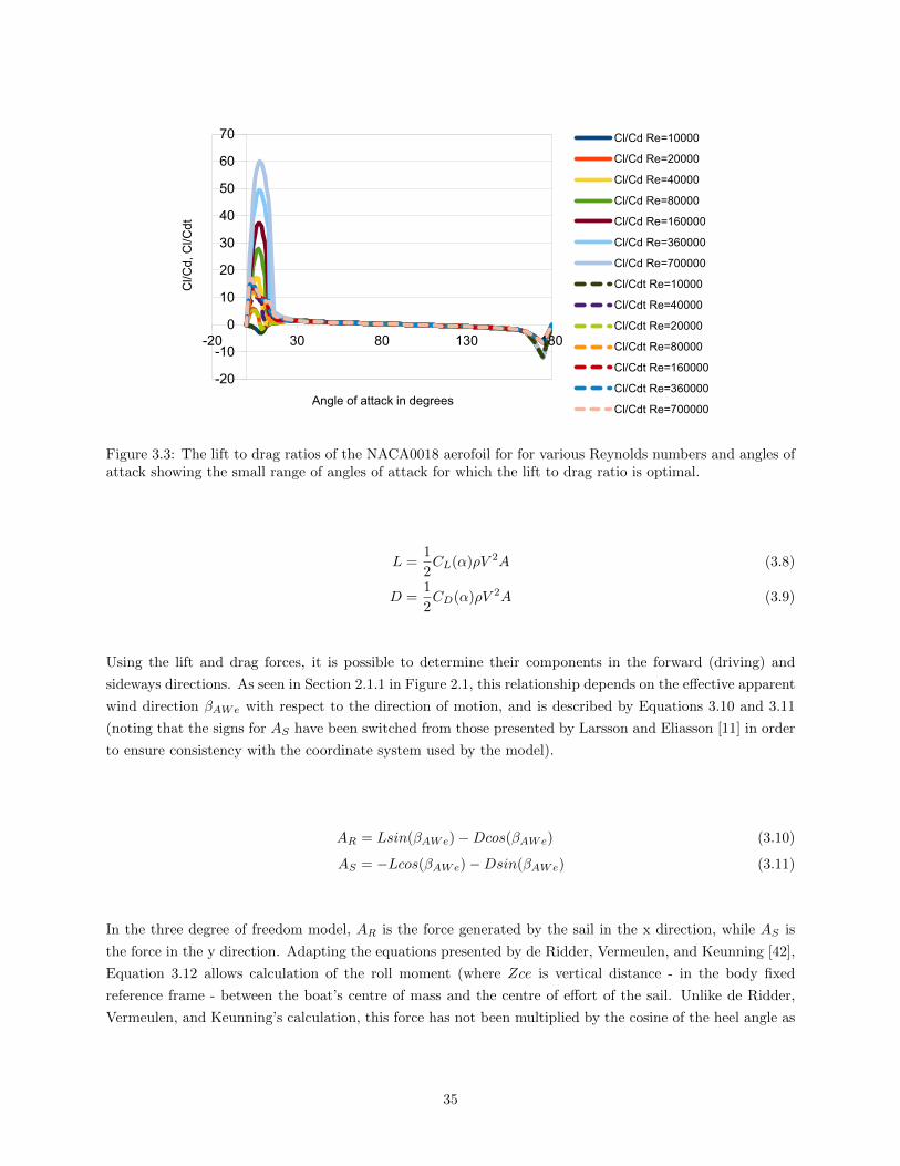
-20
-10
0
10
20
30
40
50
60
70
-20 30 80 130 180
Cl/C
d, C
l/Cdt
Angle of attack in degrees
Cl/Cd Re=10000
Cl/Cd Re=20000
Cl/Cd Re=40000
Cl/Cd Re=80000
Cl/Cd Re=160000
Cl/Cd Re=360000
Cl/Cd Re=700000
Cl/Cdt Re=10000
Cl/Cdt Re=40000
Cl/Cdt Re=20000
Cl/Cdt Re=80000
Cl/Cdt Re=160000
Cl/Cdt Re=360000
Cl/Cdt Re=700000
Figure 3.3: The lift to drag ratios of the NACA0018 aerofoil for for various Reynolds numbers and angles ofattack showing the small range of angles of attack for which the lift to drag ratio is optimal.
L =1
2CL(α)ρV 2A (3.8)
D =1
2CD(α)ρV 2A (3.9)
Using the lift and drag forces, it is possible to determine their components in the forward (driving) and
sideways directions. As seen in Section 2.1.1 in Figure 2.1, this relationship depends on the effective apparent
wind direction βAWe with respect to the direction of motion, and is described by Equations 3.10 and 3.11
(noting that the signs for AS have been switched from those presented by Larsson and Eliasson [11] in order
to ensure consistency with the coordinate system used by the model).
AR = Lsin(βAWe)−Dcos(βAWe) (3.10)
AS = −Lcos(βAWe)−Dsin(βAWe) (3.11)
In the three degree of freedom model, AR is the force generated by the sail in the x direction, while AS is
the force in the y direction. Adapting the equations presented by de Ridder, Vermeulen, and Keunning [42],
Equation 3.12 allows calculation of the roll moment (where Zce is vertical distance - in the body fixed
reference frame - between the boat’s centre of mass and the centre of effort of the sail. Unlike de Ridder,
Vermeulen, and Keunning’s calculation, this force has not been multiplied by the cosine of the heel angle as
35

the force is that in the body-fixed reference frame5 .
Ksail = AS ·Zce (3.12)
Effect of Heel, Wind Gradient, and Roll Velocity
Three important considerations that must also be included in a model of the forces generated by the sail
are the effects of heel of the boat, roll velocity, and the wind gradient. Rynne and von Ellenrieder [13] note
their use of the open-ocean wind model in their VPP, which provides an estimate of the wind velocity for
heights between 0 and 10 metres above the still water line - indicating that the wind velocity varies with
height. Larsson and Eliasson’s [11] description of how to correct angle of attack and wind velocity to account
for heel means that the angle attack of the sail varies along its length - and so Rynne and von Ellenrieder’s
approach of integrating lift and drag along the length of the wing-sail is utilised. Finally, it is necessary to
consider the effect of roll velocity on the apparent wind.
Wind Gradient
According to Rynne and von Ellenrieder [13], the open-ocean wind model allows estimation of the wind
speed gradient using Equation 3.13 where z is the height in metres above the still waterline and U10 is the
1 hour averaged wind speed at 10 metres.
U
U10= (
z
10)1/7 (3.13)
It should be noted that where relevant, u10 has been considered the instantaneous wind speed at 10 metres
given the need for instantaneous values for the wind gradient when comparing simulations to field tests
and because, where relevant, wind speed is recorded by a sensor on the boat or using a hand-held sensor -
suggesting that estimations for using these readings taken over a shorter period will be reasonably accurate,
if not more so.
Roll Velocity
The effect of roll velocity on the apparent wind is taken into account in the manner presented by De Ridder,
Vermeulen, and Keunning [42] whereby the apparent wind caused by the velocity of the boat in the x and y
axes is decomposed into those axes, the effect of the roll is added to the y axis, and the new apparent wind
is determined. These calculations can be seen in Equations 3.14 and 3.15, where the speed and direction of
5It was concluded that de Ridder, Vermeulen, and Keunning’s equation erroneously assumed that the side force acts parallelto the water surface instead of perpendicular to the wing-sail.
36

the apparent wind is determined (the component which considers yaw velocity has been omitted here as this
is discussed as part of the four degree of freedom model).
VAWϕ=√
(ϕZce+ VAW sin(βAW ))2 + (VAW cos(βAW ))2 (3.14)
βAWϕ= tan−1(
ϕZce+ VAW sin(βAW )
VAW cos(βAW )) (3.15)
Effect of Heel
As explained by Larsson and Eliasson [11], the heel of the boat needs to be taken into account as this affects
the effective velocity and angle wind angle seen by the sail. Larsson and Eliasson achieve this by calculating
values in a plane that heels with the boat - as seen in Equations 3.16, 3.17, 3.18, and 3.19 where V1 is the
apparent wind velocity along the direction of motion, V2 is the apparent wind velocity at right angles to the
mast and direction of motion, VAWe is the effective apparent wind velocity, βAWe is the effective apparent
wind angle, Vs is the boat velocity, VTW is the true wind velocity, βTW is the true wind angle, and ϕ is the
heel angle.
V1 = Vs + VTW ·cos(βTW ) (3.16)
V2 ≈ VTW ·sin(βTW )·cos(ϕ) (3.17)
VAWe =
√V1
2 + V22 (3.18)
βAWe = artan(V2V1
) (3.19)
As the above equations ignore leeway, Equations 3.16 and 3.17 have been adapted in order to take this into
account by considering the boat’s forward and sideways velocities. In addition, the new versions of these
equations make use of the components of Equation 3.14 so that the effect of the roll velocity is taken into
account at this point. The adapted equations, seen below as Equations 3.20 and 3.21, continue to be used
as part of Equations 3.18 and 3.19.
V1 = u+ VTW ·cos(βTW ) (3.20)
37

V2 = VTW ·sin(βTW )·cos(ϕ) + ϕZce+ v (3.21)
Given that the apparent wind due to the velocity of the boat does not have a wind gradient, while the true
wind does, it is clear that this method will result in different effective apparent wind velocities and angles
depending on the height above the water for which they are calculated. Rynne and von Ellenrieder address
this problem by integrating along the length of the sail. In the implementation of this model this has been
done by dividing the sail into segments and considering each in turn - an approach which is discussed further
in Section 3.5.
3.2.2 Hydrodynamic Resistance
Having determined forces from the sail, it is necessary to determine the forces acting on the underwater part
of the boat as it reaches steady state. This section will present the methods used to determine hydrodynamic
forces based on those described in the literature.
As discussed in Section 2.1.1, the hydrodynamic resistance of the hull of a yacht can be considered in terms
of a number of components - such as frictional and residuary resistance. Larsson and Eliasson describe [11]
three principle approaches to determining these forces: use of formulas derived from tests conducted at the
Delft University of Technology, towing tank tests, and computational fluid dynamics.
While calculating forces using computational fluid dynamics is an attractive option, it was not used in this
case as an accurate computer model of the hull of the boat used was not available and the potential additional
accuracy over the formulaic approach was not considered necessary.
Larsson and Eliasson appear to consider a towing tank test of a model of a yacht to be the most accurate
approach, and in the case of this project it would be particularly suitable as it might be possible to test the
actual boat instead of a model of it - however this approach was not considered feasible due to the lack of
immediate availability of a testing tank and the associated cost.
The Delft Systematic Yacht Hull Series (DSYHS) consists, as of 2008 [2], of 70 different models tested using
the same procedures. Data from these tests has been used to derive regression formulations of the forces
on the hull of a yacht - allowing for prediction of these forces using measurable parameters of the hull. In
2008 Keuning and Katgert [2] provided an overview of the formulations derived from the DSYHS, which over
time were improved as new models were added to the series. Based on this overview, and the author’s own
assessment of the literature, three sources of formulations have been used in the development of this model:
Work from 1998 [3] by Keuning and Sonnenberg where the presented formula break from previous
approaches by considering the keel and rudder of the boat separately and which appears to be the
most recent comprehensive presentation of upright and heeled formula.
38
The 2004 report [42] of De Ridder, Vermeulen, and Keunning which, building on previous work,
focussed on the tacking manoeuvre of a yacht and presented revised formulae that took account of
additional considerations, such as the rolling motion of a boat.
The new upright residuary resistance formulation presented by Keuning and Katgert in 2008 [2],
which takes into account new hulls that have been included in the DSYHS. The authors also present
preliminary work that shows that the overhang aft affects the residuary resistance, however no generally
applicable correction was made available.
It is important to note that while use of the DSYHS provides the benefit of easy modification of the model
to provide results for other boat designs, accurate speed estimations for the boat used for this project were
not considered likely given its design - which is unlike most in the DSYHS. This is seen in results reported
by Oliver and Robinson [57], where it was found that their approach to separating the keel and hull of a
J-Class yacht had limitations when used for race handicapping purposes. A sensitivity analysis of the point
chosen to separate the hull and keel showed that results varied substantially for different boats. Oliver and
Robinson go on to develop a VPP for specific use by the J-Class of boats, and while its considerations may
prove useful in analysing successes of this model, insufficient information has been made available to make
use of it here.
Despite the above concerns of the approach to estimating hydrodynamic resistance forces, it is nevertheless
considered appropriate given the unsuitability of alternative approaches and because accurate speed pre-
diction is not considered the primary objective of the system model. It is expected that use of DSYHS
force estimations should capture the dynamics of the boat fairly well, making the model useful for various
applications that require a dynamic model instead of a simple velocity prediction program.
The remainder of this section shall present the various components considered, the formulae used, their
sources, and any modifications that were made. It should be noted that descriptions of these components
was presented in Section 2.1.1, however where necessary further explanation has been given.
The definitions of two variables are provided here as they are relevant to a number of components. These
are the Reynolds number in Equation 3.22 [3] - where it should be noted that 70% of the waterline length
of the boat is used (when calculating the Reynolds number of an appendage, such as the keel, the average
chord length is used [3] and the Froude Number - defined in Equation 3.23 6 [42].
Re =u·0.7·Lwl
v(3.22)
Fn =u√g·Lwl
(3.23)
6There is some ambiguity in the literature as to whether the Froude number calculation should make use of the boat’s velocityor forward velocity. Larsson and Eliasson specify “the velocity” [11], de Ridder, Vermeulen, and Keuning the longitudinalvelocity [42], and Roncin and Kobus the velocity of the gravity centre in the Earth reference frame [40]. In this work, theforward (longitudinal) velocity has been used.
39

Viscous Resistance (Hull)
Also referred to as frictional resistance, the viscous resistance of bare hull of the boat is defined by Keuning
and Sonnenberg [3] in Equation 3.24, while the friction coefficient is defined in Equation 3.25 using the ITTC-
57 extrapolation line. It should be noted that De Ridder, Vermeulen, and Keunning’s [42] interpretation of
the “forward velocity of the yacht” being the velocity along the x axis has been adopted here.
Rfh =1
2ρ·u2·Sc·Cf (3.24)
Cf =0.075
(log(Re)− 2)2(3.25)
It should be noted that while Keuning and Sonnenberg present formulae for the estimation of the wetted
area of the hull (Sc) for both the upright and heeled conditions, these were not used as estimated surface
areas calculated in Section 3.4 were considered more accurate. It is also noted that this calculation method
accounts for the change in surface area due to heel - avoiding the need for separate ‘upright’ and ‘heeled’
calculations as with other components.
Viscous Resistance (Keel and Rudder)
According to Keuning and Sonnenberg [3], the DSYHS considers viscous resistance of appendages to be
a summation of frictional resistance and “other” viscous effects. The “other” effects are accounted for by
introducing a form factor, seen in Equation 3.26.
Rva = Rfa·(1 + ka) (3.26)
Frictional resistance of the appendage Rfa is calculated using the same formula as the hull frictional resis-
tance - seen in Equation 3.27 with the correct parameters, while the friction coefficient is also calculated
in the same way, using Equation 3.25, however with the Reynolds number Rn calculated using the average
chord length of the appendage instead of 70% of the hull waterline length. This adapted calculation for Rn
is seen in Equation 3.28. Finally, the form factor (1 + k) seen in Equation 3.26 is calculated using Equation
3.29.
Rfa =1
2ρ·u2·Sa·Cf (3.27)
Re =u·cav
(3.28)
40

(1 + ka) = (1 + 2· taca
+ 60·( taca
)4) (3.29)
As the platform used for this project has a J-Class hull where the rudder is an extension of the keel, the
model currently considers the keel and the rudder as the same appendage for the purposes of calculating
viscous resistance. As a result, the reduction in water velocity over the rudder suggested by Keuning and
Sonnenberg to account for the wake effect of the keel is not implemented in the model - which nevertheless
is the correct approach here as no wake effects from the keel on the rudder are expected for the J-Class hull.
While it appears that the DSYHS generally assumes that the keel and rudder surface areas remain constant,
when implementing this model the surface areas of appendages are determined as a function of the boat’s
heel using the same methods used for the canoe body (described in Section 3.4).
Residuary Resistance (Hull)
The formula used to calculate residuary resistance is the revised version presented by Keuning and Katgert
in 2008 [2] as is seen in Equation 3.30. The formula is defined in terms of a number of coefficients which
vary depending on Froude number (defined above in Equation 3.23) - which are reproduced from the original
source in Table C.4. It should be noted that in addition to the coefficient values defined by Keuning and
Katgert, all coefficients have been defined as zero for a Froude number of zero in order to ensure that the
resistance when the boat is not moving is calculated as zero.
Rrh
∇c·ρ·g= a0 + (a1·
LCBfppLwl
+ a2·Cp+ a3·∇c 2
3
Aw+ a4·
Bwl
Lwl+ a5·
LCBfppLCFfpp
+ a6·Bwl
Tc+ a7·Cm)·∇c
13
Lwl(3.30)
Change in Residuary Resistance (Hull) due to Heel
Keuning and Sonnenberg’s approach [3] to accounting for the effect of heel on the hull residuary resistance
is to consider an additional component - the change in residuary resistance due to heel. The expression for
this change is based on measured data for 20°of heel - seen in Equation 3.31. This value is then used to
calculate the change for an arbitrary in Equation 3.32. While this approach appears to be limited - they
report that “[i]n general a good fit was obtained”. Coefficients can be seen in Table C.5, and the explanation
in Appendix C.4 regarding the interpretation of the source of the coefficients should be noted. As above,
the coefficients have been set to zero when the boat is stationary.
∆Rrhϕ=20
∇c·ρ·g= u0 + u1·
Lwl
Bwl+ u2·
Bwl
Tc+ u3·(
Bwl
Tc)2 + u4·LCBfpp + u5·LCB2
fpp (3.31)
41

∆Rrhϕ = ∆Rrhϕ=20·6.0·ϕ1.7 (3.32)
Residuary Resistance (Keel and Rudder)
One again Keuning and Sonnenberg’s work [3] provides the source of this component. The formula derived,
seen in Equation 3.33, makes use of data from the DSYHS as well as certain results from the separate Delf
Systematic Keel Series and Delft Various Keel Series. It should be noted that it appears no results for the
residuary resistance of the rudder have been presented - however for the purposes of calculating the residuary
resistance the rudder has been considered part of the keel due to their continuous nature when the rudder
is in its neutral position.
The coefficients used in Equation 3.33 are presented in Table C.6. As with other coefficient tables, coefficients
have been set to zero at a Froude number of zero to ensure that there is zero resistance when the boat is
stationary.
Rrk
∇k·ρ·g= A0 +A1·
T
Bwl+A2·
(Tc+ Zcbk)3
∇k+A3·
∇c∇k
(3.33)
Change in Residuary Resistance (Keel) due to Heel
The change in residuary resistance of appendages is a result of the volume of the appendages being brought
closer to the water surface [3]. Keuning and Sonnenberg [3] present Equations 3.34 and 3.35 as a means to
calculate this change in resistance. Coefficients referred to in Equation 3.35 are noted in Table C.7.
Rrkϕ
∇k·ρ·g= Ch·Fn2·ϕ (3.34)
Ch = H1·Tc
T+H2·
Bwl
Tc+H3·
Tc
T·BwlTc
+H4·Lwl
∇c 13
(3.35)
Side-force and Induced Resistance
The induced resistance on the hull is the result of side-force production - effectively the result of the sideways
movement of the boat. Formulae describing these resistances was presented by Keuning and Sonnenberg [3]
and was expanded upon in further detail in 2004 by De Ridder, Vermeulen, and Keunning [42] (providing
certain clarifications - such as the direction in which some forces are applied).
42
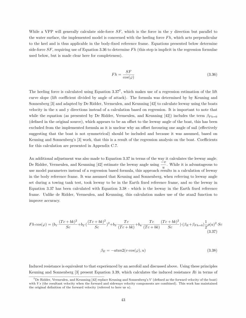
While a VPP will generally calculate side-force SF , which is the force in the y direction but parallel to
the water surface, the implemented model is concerned with the heeling force Fh, which acts perpendicular
to the keel and is thus applicable in the body-fixed reference frame. Equations presented below determine
side-force SF , requiring use of Equation 3.36 to determine Fh (this step is implicit in the regression formulae
used below, but is made clear here for completeness).
Fh =SF
cos(ϕ)(3.36)
The heeling force is calculated using Equation 3.377, which makes use of a regression estimation of the lift
curve slope (lift coefficient divided by angle of attack). The formula was determined by by Keuning and
Sonnenberg [3] and adapted by De Ridder, Vermeulen, and Keunning [42] to calculate leeway using the boats
velocity in the x and y directions instead of a calculation based on regression. It is important to note that
while the equation (as presented by De Ridder, Vermeulen, and Keunning [42]) includes the term βFh=0
(defined in the original source), which appears to be an offset to the leeway angle of the boat, this has been
excluded from the implemented formula as it is unclear why an offset favouring one angle of sail (effectively
suggesting that the boat is not symmetrical) should be included and because it was assumed, based on
Keuning and Sonnenberg’s [3] work, that this is a result of the regression analysis on the boat. Coefficients
for this calculation are presented in Appendix C.7.
An additional adjustment was also made to Equation 3.37 in terms of the way it calculates the leeway angle.
De Ridder, Vermeulen, and Keunning [42] estimate the leeway angle using−vu
. While it is advantageous to
use model parameters instead of a regression based formula, this approach results in a calculation of leeway
in the body reference frame. It was assumed that Keuning and Sonnenberg, when referring to leeway angle
set during a towing tank test, took leeway to be in the Earth fixed reference frame, and so the leeway in
Equation 3.37 has been calculated with Equation 3.38 - which is the leeway in the Earth fixed reference
frame. Unlike de Ridder, Vermeulen, and Keunning, this calculation makes use of the atan2 function to
improve accuracy.
Fh·cos(ϕ) = (b1·(Tc+ bk)2
Sc+b2·(
(Tc+ bk)2
Sc)2+b3·
Tc
(Tc+ bk)+b4·
Tc
(Tc+ bk)
(Tc+ bk)2
Sc)·(βE+βFh=0)
1
2ρ(u)2·Sc
(3.37)
βE = −atan2(v·cos(ϕ), u) (3.38)
Induced resistance is equivalent to that experienced by an aerofoil and discussed above. Using these principles
Keuning and Sonnenberg [3] present Equation 3.39, which calculates the induced resistance Ri in terms of
7De Ridder, Vermeulen, and Keunning [42] replace Keuning and Sonnenberg’s V (defined as the forward velocity of the boat)with V s (the resultant velocity when the forward and sideways velocity components are combined). This work has maintainedthe original definition of the forward velocity (referred to here us u).
43
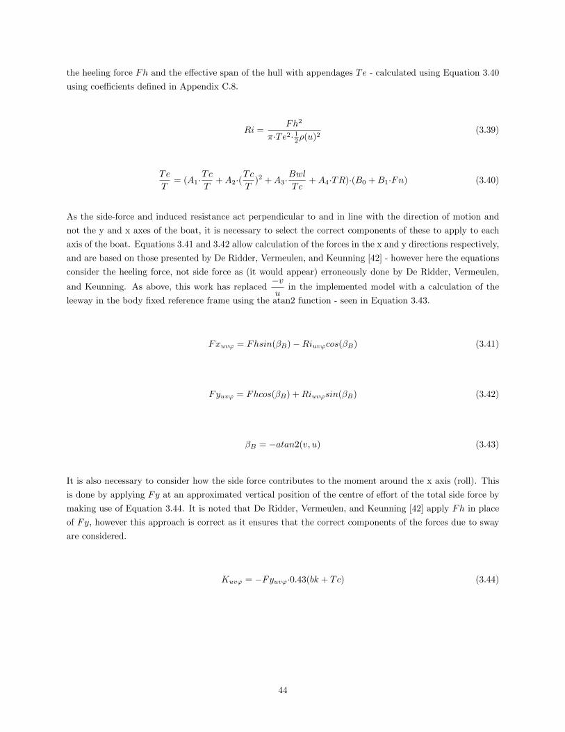
the heeling force Fh and the effective span of the hull with appendages Te - calculated using Equation 3.40
using coefficients defined in Appendix C.8.
Ri =Fh2
π·Te2· 12ρ(u)2(3.39)
Te
T= (A1·
Tc
T+A2·(
Tc
T)2 +A3·
Bwl
Tc+A4·TR)·(B0 +B1·Fn) (3.40)
As the side-force and induced resistance act perpendicular to and in line with the direction of motion and
not the y and x axes of the boat, it is necessary to select the correct components of these to apply to each
axis of the boat. Equations 3.41 and 3.42 allow calculation of the forces in the x and y directions respectively,
and are based on those presented by De Ridder, Vermeulen, and Keunning [42] - however here the equations
consider the heeling force, not side force as (it would appear) erroneously done by De Ridder, Vermeulen,
and Keunning. As above, this work has replaced−vu
in the implemented model with a calculation of the
leeway in the body fixed reference frame using the atan2 function - seen in Equation 3.43.
Fxuvϕ = Fhsin(βB)−Riuvϕcos(βB) (3.41)
Fyuvϕ = Fhcos(βB) +Riuvϕsin(βB) (3.42)
βB = −atan2(v, u) (3.43)
It is also necessary to consider how the side force contributes to the moment around the x axis (roll). This
is done by applying Fy at an approximated vertical position of the centre of effort of the total side force by
making use of Equation 3.44. It is noted that De Ridder, Vermeulen, and Keunning [42] apply Fh in place
of Fy, however this approach is correct as it ensures that the correct components of the forces due to sway
are considered.
Kuvϕ = −Fyuvϕ·0.43(bk + Tc) (3.44)
44

Roll Damping
Introduced by De Ridder, Vermeulen, and Keunning [42], the roll damping component is the additional
resistance as a result of the roll action of the boat and is calculated by considering the additional angle of
attack of the hull introduced by the rolling motion. It is described by Equation 3.45. The original equation
has been modified here to determine the additional angle of attack using the atan2 function, seen in Equation
3.46, contrast with De Ridder, Vermeulen, and Keunning’s estimation of0.43(bk + Tc)ϕ
u. As with the side-
force in the previous section, the βFh=0 component has been ignored in order to ensure that the boat is
considered symmetrical from the perspective of the model.
Fhcos(ϕ)uvϕ = (b1(Tc+ bk)2
Sc+b2(
(Tc+ bk)2
Sc)2+b3
Tc
Tc+ bk+b4
Tc
(Tc+ bk)
(Tc+ bk)2
Sc)·(βϕ+βFh=0)
1
2ρ(u)2Sc
(3.45)
βϕ = atan2(0.43(bk + Tc)ϕ, u) (3.46)
As a further adaptation, this component has been implemented by considering it part of the leeway calculation
for the determination of the side force - thus replacing Equation 3.38 with Equation 3.47.
βEϕ = atan2((−v + 0.43(bk + Tc)ϕ)·cos(ϕ), u) (3.47)
3.2.3 Restoring Forces and Moments
In his model, Fossen [39] refers to gravitational and buoyant forces as restoring forces (g(η) in Section 3.1.1).
Taking the weight of the vehicle W = mg through the centre of mass and buoyancy B = ρg∇ (consistent
with Archimedes’ principle [12]) through the centre of buoyancy, both acting in the z axis of the Earth
reference plane, Fossen derives Equation 3.48.
g(η) =
(W −B)sin(θ)
−(W −B)cos(θ)sin(ϕ)
−(W −B)cos(θ)cos(ϕ)
−(yGW − yBB)cos(θ)cos(ϕ) + (zGW − zBB)cos(θ)sin(ϕ)
(zGW − zBB)sin(θ) + (xGW − xBB)cos(θ)cos(ϕ)
−(xGW − xBB)cos(θ)sin(ϕ)− (yGW − yBB)sin(θ)
(3.48)
45

In the case of a neutrally buoyant vehicle, W = B, resulting in a simplification to Equation 3.49 where BGx,
BGy, and BGz are distances between the centres of mass and buoyancy in the x, y, and z axes. For the
three degree of freedom model a further simplification is achieved by deriving Equation 3.50 by setting the
pitch angle to zero and omitting the z, pitch, and yaw axes.
g(η) =
0
0
0
−BGyWcos(θ)cos(ϕ) +BGxWcos(θ)sin(ϕ)
BGzWsin(θ) +BGxWcos(θ)cos(ϕ)
−BGxWcos(θ)sin(ϕ)−BGyWsin(θ)
(3.49)
g(η) =
0
0
−BGyWcos(ϕ) +BGzWsin(ϕ)
(3.50)
Having examined this generic approach, it is relevant to consider the way in which most models of sailing
boats account for restoring forces, as described by Larsson and Eliasson [11]. As seen in Figure 2.3, when
considering heel both gravity and the buoyancy force act to create a righting moment. This allows calculation
of the righting moment using Equation 3.51, where GZ is the lever arm (distance between the centres of
gravity and buoyancy in the plane parallel to the water surface).
RM = m·g·GZ (3.51)
Larsson and Eliasson proceed to explain how the transverse metacentre, which is the intersection of the
vertical line through the centre of buoyancy and boat’s symmetry plane, is considered fixed for small angles.
This allows the calculation GZ = GM ·sin(ϕ) where GM is the distance between the centre of gravity and
the transverse metacentre. The position of these points can be seen in Figure 3.4.
While this approach is a useful generalisation, it was not used here given the necessary assumption that
the transverse metacentre remains fixed and because this relies on further assuming that heel angles remain
small, which seems unlikely for the implemented platform.
As an alternative, values for BGy, BGz, and (in the four degree of freedom model) BGx were determined
from calculated positions of the boat’s center of mass and centre of buoyancy for various angles of heel -
with the process of determining the coordinates of these positions being described in Section 3.4.1.
46

centre of gravity G
centre of buoyancy
transverse metacentre
Z
GZ
GM
φ
Figure 3.4: Diagram showing the determination of the transverse metacentre. Adapted from Larsson andEliasson’s [11] Figure 4.9.
3.3 Yaw - the Four Degree of Freedom Model
The extension of the three degree of freedom model to include consideration of yaw is an important step
that takes the model beyond the results obtained from traditional VPPs (as noted in Section 2.4, Larsson
and Eliasson [11] report that only advanced VPPs consider yaw). This section begins by describing the
additions that are necessary in order to apply forces already discussed to the yaw movement of the boat,
before considering distinct hydrodynamic forces that arise when considering yaw. In addition, the section
also describes the limited consideration of environmental disturbances in this study as this has been done as
part of this model. The section relies principally on De Ridder, Vermeulen, and Keunning’s 2004 report [42],
which focussed on the taking movement of a yacht through the development of a four degree of freedom
model.
3.3.1 Adaptation of Three Degree of Freedom Model
The primary adaptations to the three degree of freedom model involve applying forces already considered
about the z axis so that their contribution to the resultant yaw moment are included in the model. For most
components this is relatively simple as the point at which these forces act is known - however in the case of
the side force additional considerations are noted, and the effect of yaw velocity on the apparent wind must
also be accounted for.
47
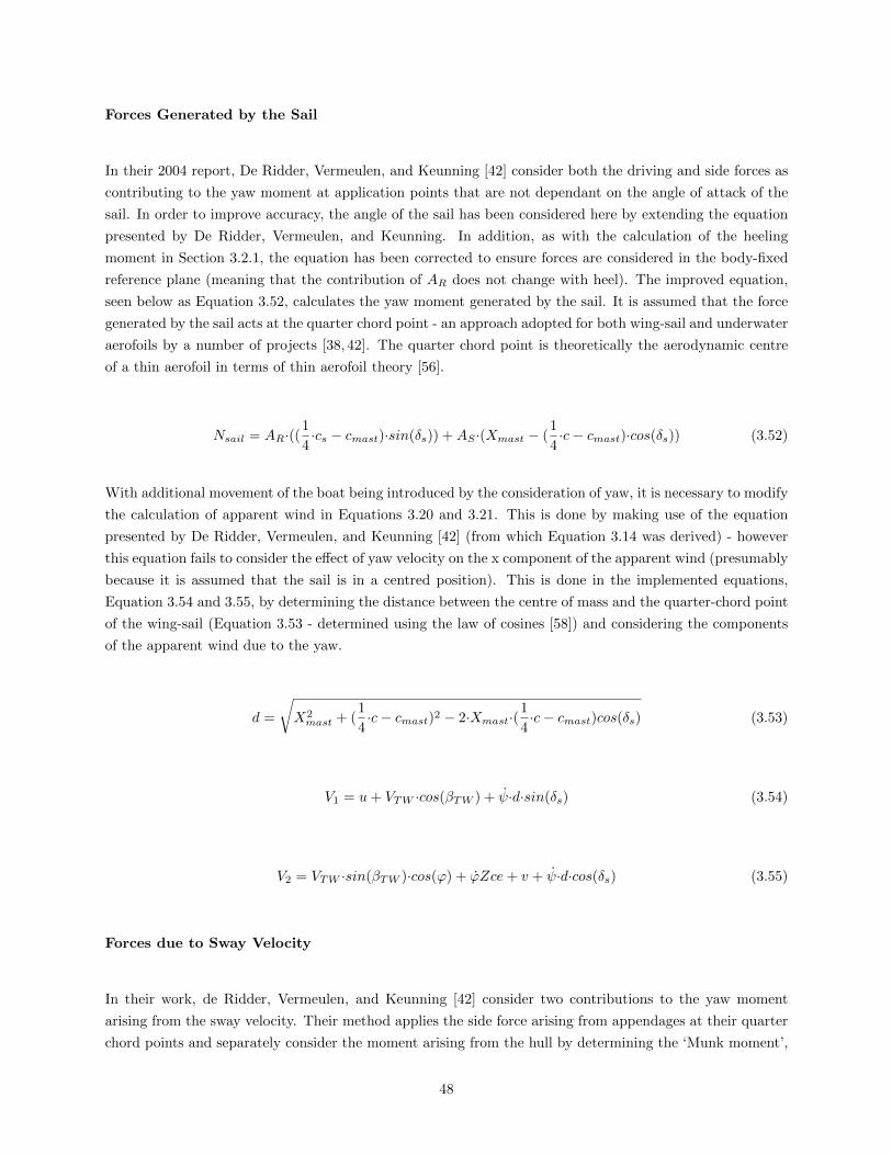
Forces Generated by the Sail
In their 2004 report, De Ridder, Vermeulen, and Keunning [42] consider both the driving and side forces as
contributing to the yaw moment at application points that are not dependant on the angle of attack of the
sail. In order to improve accuracy, the angle of the sail has been considered here by extending the equation
presented by De Ridder, Vermeulen, and Keunning. In addition, as with the calculation of the heeling
moment in Section 3.2.1, the equation has been corrected to ensure forces are considered in the body-fixed
reference plane (meaning that the contribution of AR does not change with heel). The improved equation,
seen below as Equation 3.52, calculates the yaw moment generated by the sail. It is assumed that the force
generated by the sail acts at the quarter chord point - an approach adopted for both wing-sail and underwater
aerofoils by a number of projects [38, 42]. The quarter chord point is theoretically the aerodynamic centre
of a thin aerofoil in terms of thin aerofoil theory [56].
Nsail = AR·((1
4·cs − cmast)·sin(δs)) +AS ·(Xmast − (
1
4·c− cmast)·cos(δs)) (3.52)
With additional movement of the boat being introduced by the consideration of yaw, it is necessary to modify
the calculation of apparent wind in Equations 3.20 and 3.21. This is done by making use of the equation
presented by De Ridder, Vermeulen, and Keunning [42] (from which Equation 3.14 was derived) - however
this equation fails to consider the effect of yaw velocity on the x component of the apparent wind (presumably
because it is assumed that the sail is in a centred position). This is done in the implemented equations,
Equation 3.54 and 3.55, by determining the distance between the centre of mass and the quarter-chord point
of the wing-sail (Equation 3.53 - determined using the law of cosines [58]) and considering the components
of the apparent wind due to the yaw.
d =
√X2mast + (
1
4·c− cmast)2 − 2·Xmast·(
1
4·c− cmast)cos(δs) (3.53)
V1 = u+ VTW ·cos(βTW ) + ψ·d·sin(δs) (3.54)
V2 = VTW ·sin(βTW )·cos(ϕ) + ϕZce+ v + ψ·d·cos(δs) (3.55)
Forces due to Sway Velocity
In their work, de Ridder, Vermeulen, and Keunning [42] consider two contributions to the yaw moment
arising from the sway velocity. Their method applies the side force arising from appendages at their quarter
chord points and separately consider the moment arising from the hull by determining the ‘Munk moment’,
48

which appears to be the result of a method of determining the side-force (and moment) on the hull by
considering pressure along its length. However as de Ridder, Vermeulen, and Keunning do not separate
the side-forces produced by the hull from the hull and keel combination (and thus presumably apply the
combined side-force arising from the hull and keel at the quarter chord point), their method appears to result
in applying the hull’s contribution to the moment twice.
Due to this apparent flaw in this approach, the implemented model has not determined the Munk moment.
This, as discussed below, results in the calculation not considering the layout of the hull. While it may be
possible to separate the contributions of the hull and keel using the Munk moment calculation and thus
improve the determination of the yaw moment, for simplicity this has not been attempted here. Clearly this
presents an avenue of potential further work.
Moment due to the Side-Force
In the three degree of freedom model, the hydrodynamic side force is calculated with Equation 3.37. In
determining the point of application of this force, Keuning and Vermeulen [59] (presenting the method
adopted by de Ridder, Vermeulen, and Keunning [42]) make use of an approach they attribute to Prof J.
Gerritsma referred to as the Extended Keel Method. This method estimates the proportion of the side force
(which is the force resulting from the hull, keel, and rudder) that can be attributed to the hull and keel and
the proportion that can be attributed to the rudder and applies the former as acting on the keel and the
latter as acting on the rudder.
As the model presented here has considered the keel and rudder together due to their continuous nature on
the boat being modelled, the separation of forces using the Extended Keel Method is unnecessary. Instead,
the model applies the entire side force (resulting from the hull, keel, and rudder) on the quarter chord line of
the keel at 43% of the total draft (which is the point at which the Extended Keel Method applies each of the
forces on the keel and rudder). While this approach results in an application point that does not account for
the layout of the hull of the boat, it is consistent with the approach described above which has been utilised
with apparent success by others.
Restoring Forces and Moments
Making use of the method used to derive Equation 3.50 in Section 3.2.3, Equation 3.56 was derived to include
the yaw moment arising from the restoring forces. As previously noted, values for BGx are determined using
the method described in Section 3.4.1.
g(η) =
0
0
−BGyWcos(ϕ) +BGzWsin(ϕ)
−BGxsin(ϕ)
(3.56)
49

3.3.2 Additional Hydrodynamic Resistance Forces
Additional hydrodynamic forces in the four degree of freedom model arise due to the yaw moment of the
boat. In modelling these forces, De Ridder, Vermeulen, and Keunning [42] assume a “normal” layout of
boat appendages and assume that forces resulting from the keel can be neglected due to its proximity to
the centre of mass, and thus only consider forces arising from the movement of the rudder. This approach
was considered inappropriate for this work for three reasons. First, the long keel present on this work’s
boat suggests that its forces arising from yaw are more substantial than keels on other boats. Second, only
considering the rudder when it is attached to the keel suggests a contradiction. Third, the approach does
not consider the effect of the hull - which may be appropriate for boats with a shallow canoe draft, but is
unlikely to be accurate in the case of the displacement hull considered here.
De Ridder, Vermeulen, and Keunning’s [42] method for considering the rudder forces arising from yaw
should also be noted: their work considers the rudder to be an aerofoil subject to an angle attack which
is calculated based on the forward velocity of the boat and the sideways velocity of the rudder resulting
from the yaw velocity. While this approach may be valid for a rudder with a small chord, it is unlikely to
be valid for the long keel used here as the calculated angle of attack along the length of the keel will vary
significantly depending on each point’s distance from the boat’s centre of mass (indeed, the sign of the angle
of attack may vary over its length), making the assumption of a single angle of attack for the whole keel
inappropriate. Additionally, it is unclear how such an approach interacts with the calculation of the forward
and side resistance forces based on the DSYHS.
Given the above conclusions regarding De Ridder, Vermeulen, and Keunning’s [42] approach, it was necessary
to determine a new approach to estimating hydrodynamic resistance forces arising from yaw. To this end,
thin aerofoil theory as presented by Houghton and Carpenter [56] in the estimation of the normal force
and pitching moment derivatives of an aeroplane due to pitching was adapted for use here. The following
description of this approach is based on the content presented by Houghton and Carpenter.
The rate of change of aerodynamic forces and moments on an aeroplane with respect to pitch velocity, which
are “two of the aerodynamic quasi-static derivatives” (referred to as derivatives), occur as the aeroplane
moves forward through the air. This is equivalent to a boat moving forward in the water and being subject
to a change in yaw. The approach replaces the wing (here taken as the keel and hull) with the equivalent
thin aerofoil of chord c and distance hc between its leading edge and the centre of mass. This allows (using
thin aerofoil theory) the derivation of the coefficient of lift of the aerofoil as seen in Equation 3.57 where α
is the angle of attack, h is hc/c, ψ is the yaw (previously pitching) velocity, Vs is the flow stream velocity,
and A0 and A1 are the first two terms of the Fourier series of the function describing the camber line of the
aerofoil. The term a accounts for the aspect ratio change of the aerofoil in three dimensions (noting that
equations were derived for two dimensions) - ideally 2π.
CL = a[α−A0 +A1
2+ (
3
4− h)
ψc
Vs] (3.57)
50

In this work, as the boat and keel are symmetrical, both A0 and A1 are set to zero. A further change is made
by excluding the lift of a non-pitching aerofoil (as this had already been determined in Section 3.2.2), which
in the case of a non-cambered foil analysed using thin aerofoil theory is 2πα - resulting in the removal of the
α term and a determination of the change in the coefficient of lift seen in Equation 3.58. As per Houghton
and Carpenter - the same result can be achieved by differentiating Equation 3.57 with respect to ψ in order
to find the rate of change the coefficient of lift with respect to ψ.
∆CL = a(3
4− h)
ψc
Vs(3.58)
Finally, Houghton and Carpenter present the pitching moment coefficient about the leading edge of the
aerofoil - seen in Equation 3.59 - which, accounting for the constant component of the coefficient of lift and
the zero values of A1 and A2, is adapted to find the change in moment ∆CMLEin Equation 3.60 (which, as
above, can also be found by differentiating with respect to ψ). Given Equation 3.61 (which Houghton and
Carpenter use to shift the moment so that it is about the centre of gravity), the change in moment about the
centre of gravity CMCGis determined using Equation 3.62 (which makes use of the simplification presented
by Houghton and Carpenter).
CMLE=π
4(A2 −A1)− π
8
ψc
V− 1
4CL (3.59)
∆CMLE= −π
8
ψc
V− 1
4∆CL = −π
8
qc
V− 1
4
(a
(3
4− h)ψc
V
)(3.60)
CMCG= CMLE
+ hCL (3.61)
∆CMCG= −π
8
qc
V+
(h− 1
4
)(a
(3
4− h)qc
V
)= −
(a
4(1− 2h)2 +
2π − a16
)ψc
V(3.62)
It is important to note that aside from consideration of the induced drag (accounted for using Equation
3.7), this approach does not estimate the drag due to the yaw movement of the boat - presenting a potential
limitation. In addition, for simplicity it has been assumed that the hull and its keel can be considered as a
rectangular wing, avoiding the need for integration when determining coefficients.
51

Surge, Sway, and Heeling Forces due to Yaw Velocity
Using the above results, and specifically Equation 3.58, it is simple to calculate forces on the boat in the
x and y axes. First, lift and drag forces are calculated by making use of Equations 3.63 (which is adapted
from Houghton and Carpenter [56]) and 3.64 and the coefficients determined using Equations 3.58 and 3.7.
Due to leeway, which can be expected to be relatively large while a boat is turning, the lift and drag forces
must be decomposed into the x and y axes. This is achieved by making use of Equations 3.65 and 3.66 -
which are largely based on those presented by De Ridder, Vermeulen, and Keunning [42].
Lψ =1
2ρV 2
s shull−keel∆CL (3.63)
Dψ =1
2ρV 2
s shull−keel∆CDi (3.64)
Fxψ = Lψ·sin(βB)−Dψ·cos(βB) (3.65)
Fyψ = Lψcos(ϕ)·cos(βB) +Dψ·sin(βB) (3.66)
Finally, the side force’s contribution to the heeling moment of the boat was calculated using Equation 3.44.
Yaw Forces due to Yaw Velocity
As with the surge, sway, and heeling forces, calculation of the additional yaw moment using the above results
is relatively simple. The moment is calculated by making use of Equation 3.67 and the coefficient determined
using Equation 3.62.
Nψ =1
2ρV 2
s shull−keelchull−keel∆CMCG(3.67)
3.3.3 Modelling of the Rudder
As in the previous section, De Ridder, Vermeulen, and Keunning’s [42] approach to modelling the rudder
was considered inappropriate for the J-Class hull. De Ridder, Vermeulen, and Keunning model the rudder as
52

a simple aerofoil subject to a reduction in velocity due to the wake of the keel and hull. Given the rudder’s
attachment to the keel, both aspects of this approach appear to be inapplicable. The approach utilised here
is to consider the rudder a flap on the aerofoil that is the keel.
Initial Approach - Thin Aerofoil Theory
As an initial method to determine the effect of the flap, Houghton and Carpenter’s [56] explanation of thin
aerofoil theory and (in this case) its application to a flapped aerofoil to model the rudder was considered.
In their work, Houghton and Carpenter derive Equations 3.68 and 3.69 - the coefficient of lift and moment
coefficient of a flapped aerofoil where α is the angle of attack and φ is the hinge point in a mapping from x
to θ with the leading edge of the aerofoil being 0 and the trailing edge π by use of x = (c/2)(1 − cosθ). In
the approach it is stated that the influence of the flap can be considered as an addition to the lift due to the
angle of incidence and camber of the aerofoil. Relying on this consideration, both equations are modified
to exclude the components present in the non-flapped aerofoil coefficient calculations and these are seen in
Equations 3.70 and 3.71 (noting that the derivatives of the equations with respect to the flap angle would
reveal the same remaining components).
CL = 2πα+ 2(π − φ+ sin(φ))η (3.68)
CMLE= −π
2α− 1
2[π − φ+ sin(φ)(2− cos(φ))]η (3.69)
∆CL = 2(π − φ+ sin(φ))η (3.70)
∆CMLE= −1
2[π − φ+ sin(φ)(2− cos(φ))]η (3.71)
Equations of the same form as Equations 3.63, 3.64, 3.65, 3.66, and 3.67 are used to determine the forces
and moments caused by the deflection of the rudder.
While this approach presented reasonable results for some sailing conditions, it was found that under some
circumstances unreasonably large forces are calculated - presumably because Houghton and Carpenter’s
derivation assumes angles are small and because of the equation’s linearity, which is unlikely to match
reality. Thus it was considered necessary to determine an alternative approach.
53

Figure 3.5: Plot of the NACA0013 representation of the keel with the rudder set to 45 generated usingXFOIL.
Second Approach - Aerofoil with Flap Simulation
The method ultimately adopted involved modelling the boat’s hull and keel as an aerofoil with a flap and
simulating it using XFOIL (which, as noted in Section 3.2.1, has been used by other projects [13, 32] to
predict the lift and drag coefficients of a wing-sail). Unlike the above approach using thin aerofoil theory,
this method has the advantage of predicting drag - making it more likely that its results will be accurate.
First, it is necessary to determine an aerofoil with which to model the hull and heel. While it would be
possible to extract an outline of a cross section of the hull using the CAD model developed in Section 3.4.1,
it is unclear at what height this should be taken. Instead, the average thickness of the keel tk as a percentage
of keel mean chord length ck was calculated to be 13%. As noted by Houghton and Carpenter [56], NACA
aerofoils are defined by their four digit number where the first two digits define the define the camber and
the second two equal the maximum thickness as a fraction of the chord multiplied by 100 - making selection
of a NACA0013 aerofoil a natural choice.
In order to determine an appropriate hinge point, the ratio of the area of the keel to the sum of the areas
of the rudder and keel, rudder ratio, was determined and set as the hinge point along the chord (where 0 is
the leading edge and 1 the trailing edge). Using XFOIL, this results in a a NACA0013 aerofoil with a flap
set to a determined angle - as seen in Figure 3.5.
Assuming an average speed through the water of 1m/s, XFOIL was set to viscous mode with a Reynolds
number (calculated using Equation 3.22) of 657640, mach number of 0.002939 (determined for 1m/s using
the Wolfram Alpha engine), and kinematic viscosity8 of 8.9x10⁻⁷ m2/s. Simulations of the aerofoil through
angles of attack between 0 and 10 for rudder angle settings ranging between -45 and 45 (the expected
operating range of the rudder) every 5 were run, resulting in the determination of lift, drag, and moment
coefficients each condition. Due to the large amount of data produced, coefficients have not been reproduced
here.
As a means to compare the results predicted by XFOIL, the equivalent coefficient of lift that would produce
the side force predicted by the method described in Section 3.2.2 was calculated using Equation 3.8 for a
test of the model under arbitrary conditions. This resulted in the prediction of a coefficient of lift of 0.0029
with a leeway angle of 0.0745. The NACA0013 was simulated with flap angle of zero and the same angle
8Wolfram—Alpha knowledgebase, 2014 - accessed via Wolfram Alpha.
54

of attack, predicting a coefficient of lift of 0.0078. While differing by a magnitude of approximately 2.6, this
suggests that XFOIL predicts coefficients in approximately the correct range.
By subtracting the zero rudder angle values of the lift, drag, and moment coefficients from their values
determined with a rudder angle, the additional lift, drag, and moment caused by the rudder was determined
using Equations 3.8, 3.9, and 3.72 [56].
Nδr =1
2ρV 2Sc·CM (3.72)
As before, calculated lift and drag are then decomposed into the x and y axes using Equations 3.41 and 3.42.
Determination of the heeling force is achieved using Equation 3.44.
When implemented, it was found that this alternative method also predicts unreasonably large lift coeffi-
cients, and so the side-force, heeling moment, and contribution of lift to drag has been disregarded. This
clearly requires further investigation, however it should be noted that it is believed that the XFOIL approach
is still preferable to lifting line theory given the determination of drag coefficients.
3.3.4 Modelling of Actuators
Given the 4 degree of freedom model’s intended use as a dynamic model, modelling of the boat’s actuators
is introduced at this point. This ensures that when simulating control of the boat the model accounts for
any delay or dynamics present when operating the actuators.
Rudder Servomotor
Modelling of the servomotor which drives the rudder is a two step process. First, the servomotor’s specifica-
tions (as recorded on its packaging) were considered - resulting in a rated speed of 0.14sec/60 being noted,
with no stated time constant. While the lack of knowledge of a timing constant will result in a less accurate
model of the servomotor, it was assumed that an assumption of an infinitely small constant (zero) would be
appropriate given the additional restrictions discussed below.
Thus, the speed rating of the servomotor was accounted for by limiting its rate of change of position to
428.57/s (implemented in the model using a Simulink Rate Limiter block).
A second speed limitation is introduced by the microcontroller controlling the servomotor. As discussed in
Section 4.2.2, testing showed that the servomotor behaved unpredictably if commanded to large differences in
position, and thus the change in position was limited in code. The same algorithm used on the microcontroller
was implemented in the model - ensuring that the servomotor does not change position by more than 3.375
55

every 20ms. As this prevents the servomotor from operating at its rated speed, this restriction will dominate
- limiting inaccuracies due to the lack of knowledge of the correct time constant.
Sail Linear Actuator
In order to determine the dynamics of the linear-actuator, data logged during a lab test of the actuator
was inspected. By calculating the speed of the actuator between sample points during actuation, a mean
speed of 36.34/second was determined. Due to the low sampling rate and noise present in the data it
would be difficult to determine an accurate time constant or more accurate transfer function representing
the actuator, however given the apparent constant operating speed it as been assumed that modelling the
actuator as operating at a constant speed is reasonable.
Therefore, as with the servomotor, the rate of change of actuator position in the model was limited - in this
case to 36.34/second.
3.3.5 Environmental Disturbances
Consideration of environmental disturbances by the model has been limited to variations in wind conditions,
given the simple application to the developed model and relevance to the tests conducted using the model.
Disturbances arising from waves have not been considered, in part because it is expected that interaction of
a small platform with waves should make use of a six degree of freedom model given the relative size of the
platform to the waves it is likely to encounter. This has been done despite Keuning and Sonnenberg’s [3]
presentation of a method of estimating resistance in the x axis arising from waves (which would be relatively
straightforward to apply to both the three and four degree of freedom models) as full consideration of the
effect of waves is considered important and because the method appears to determine average resistance
in a form suitable for use in a VPP but not in a dynamic model. While not relevant to environmental
disturbances, it is also noted that Keuning and Sonnenberg’s [3] description of the consideration of the
additional resistance due to change in trim angle might be considered if a model that considered pitch were
developed.
While simple to apply to the model (given that it is an input to the Marine Systems Simulator Simulink
equations of motion blocks discussed in Section 3.5), current has also not been explicitly considered in this
work as it is not considered relevant to the tests conducted.
56

Figure 3.6: Results of a simulation of the Marine Systems Simulator Wind block compared with data loggedduring a test of the platform showing the larger variations in wind direction seen by the platform’s windsensor.
Disturbances due to Wind
In order to estimate variations of wind conditions, use was made of the Marine Systems Simulator’s Wind
block (the simulator is discussed further in Section 3.5) - which generates wind speed and direction using
specified parameters including average speed and direction. The model provides an option between gust
models based on measurements over land and the North Sea, the former being selected due to tests being
conducted on an inland body of water. The model’s various other parameters were left at their defaults.
Figure 3.6 provides an example of the wind speed and direction output by the wind block over 30 seconds,
compared with the wind directions logged by the platform during the first Zeekoevlei test (test 3) and
corrected for changes in the boat’s heading. While it is clear that the platform appears to experience greater
variations in wind direction, it is unclear whether this is a result of actual variations of the wind or the
design of the wind sensor and any natural oscillation in the wind. Due to this lack of clarity it was assumed
that the default settings of the wind block would suffice for use in the test conducted in Section 5.4.1.
3.4 Parameter Determination
Thus far the presented model has defined all forces in terms of parameters of the physical boat. This section
describes some of the methods used to determine these parameters, and records their values.
Given the difficulty in measuring some of these parameters on the boat itself (such as surface area), and
the lack of availability of this information, an approach to quickly determine these values with reasonable
57

Figure 3.7: View of the bulkheads generated for the CAD model.
accuracy was considered important. To this end, a Computer-aided Design (CAD) model of the boat and its
components was developed. It was also believed that an available model would be useful for design purposes
- although for the current work this proved unnecessary. The SolidWorks CAD package was selected for this
task due to its immediate availability and familiarity to the author.
It should be noted that consistent with the priorities of this work, a high degree of accuracy and detail in
the model was not considered entirely necessary given the need to save time and achieve usable results for
other aspects of the work.
This section discusses the development of the CAD model, the approach taken to the determination of the
added mass matrix, and presents a summary of the determined parameters along with the methods used to
determine them.
3.4.1 Development of the CAD Model
The most complicated aspect of the development of the CAD model was the need to represent the hull -
an irregular and complicated three-dimensional shape. In order to achieve this, a method inspired by, but
different to, a SolidWorks tutorial [60] was utilised. The author’s previous work [5] included the creation of
electronic templates of cross sections of the boat’s hull to allow for bulkheads to be laser-cut for use in the
boat. While these templates were not particularly accurate (considering that once cut they required manual
adjustment in order to ensure a good fit), they were considered of sufficient accuracy to provide a skeleton
of a model of the boat.
58
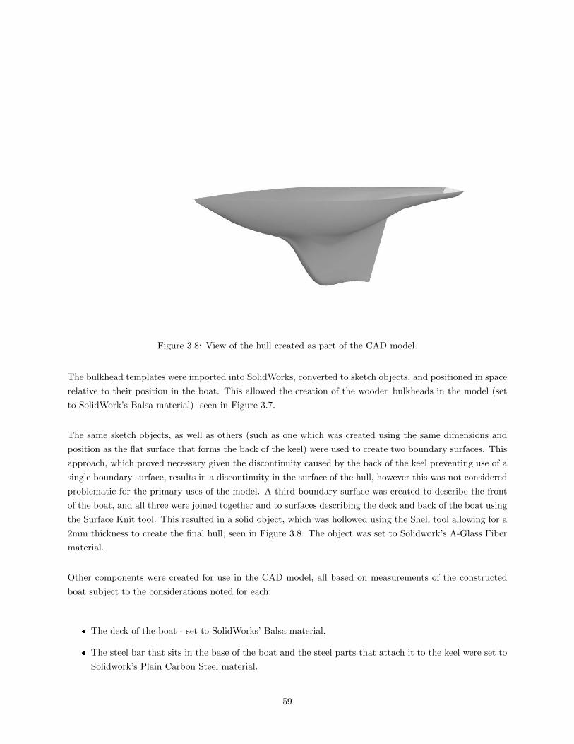
Figure 3.8: View of the hull created as part of the CAD model.
The bulkhead templates were imported into SolidWorks, converted to sketch objects, and positioned in space
relative to their position in the boat. This allowed the creation of the wooden bulkheads in the model (set
to SolidWork’s Balsa material)- seen in Figure 3.7.
The same sketch objects, as well as others (such as one which was created using the same dimensions and
position as the flat surface that forms the back of the keel) were used to create two boundary surfaces. This
approach, which proved necessary given the discontinuity caused by the back of the keel preventing use of a
single boundary surface, results in a discontinuity in the surface of the hull, however this was not considered
problematic for the primary uses of the model. A third boundary surface was created to describe the front
of the boat, and all three were joined together and to surfaces describing the deck and back of the boat using
the Surface Knit tool. This resulted in a solid object, which was hollowed using the Shell tool allowing for a
2mm thickness to create the final hull, seen in Figure 3.8. The object was set to Solidwork’s A-Glass Fiber
material.
Other components were created for use in the CAD model, all based on measurements of the constructed
boat subject to the considerations noted for each:
The deck of the boat - set to SolidWorks’ Balsa material.
The steel bar that sits in the base of the boat and the steel parts that attach it to the keel were set to
Solidwork’s Plain Carbon Steel material.
59
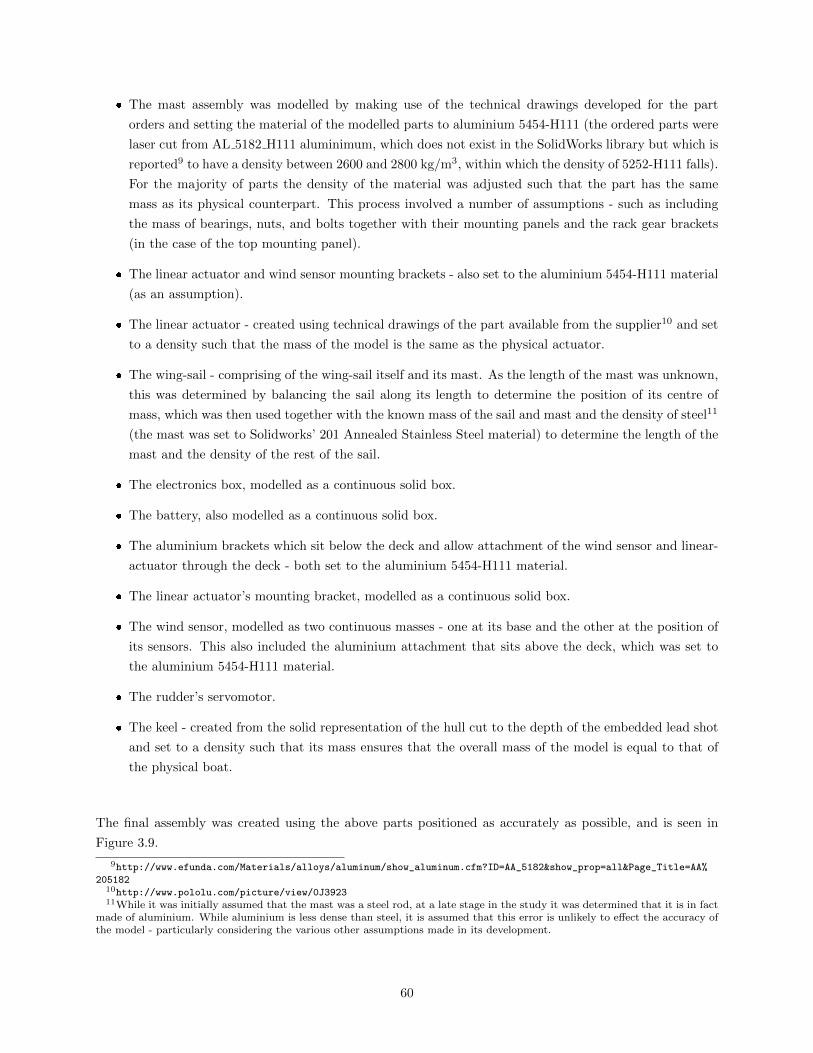
The mast assembly was modelled by making use of the technical drawings developed for the part
orders and setting the material of the modelled parts to aluminium 5454-H111 (the ordered parts were
laser cut from AL 5182 H111 aluminimum, which does not exist in the SolidWorks library but which is
reported9 to have a density between 2600 and 2800 kg/m3, within which the density of 5252-H111 falls).
For the majority of parts the density of the material was adjusted such that the part has the same
mass as its physical counterpart. This process involved a number of assumptions - such as including
the mass of bearings, nuts, and bolts together with their mounting panels and the rack gear brackets
(in the case of the top mounting panel).
The linear actuator and wind sensor mounting brackets - also set to the aluminium 5454-H111 material
(as an assumption).
The linear actuator - created using technical drawings of the part available from the supplier10 and set
to a density such that the mass of the model is the same as the physical actuator.
The wing-sail - comprising of the wing-sail itself and its mast. As the length of the mast was unknown,
this was determined by balancing the sail along its length to determine the position of its centre of
mass, which was then used together with the known mass of the sail and mast and the density of steel11
(the mast was set to Solidworks’ 201 Annealed Stainless Steel material) to determine the length of the
mast and the density of the rest of the sail.
The electronics box, modelled as a continuous solid box.
The battery, also modelled as a continuous solid box.
The aluminium brackets which sit below the deck and allow attachment of the wind sensor and linear-
actuator through the deck - both set to the aluminium 5454-H111 material.
The linear actuator’s mounting bracket, modelled as a continuous solid box.
The wind sensor, modelled as two continuous masses - one at its base and the other at the position of
its sensors. This also included the aluminium attachment that sits above the deck, which was set to
the aluminium 5454-H111 material.
The rudder’s servomotor.
The keel - created from the solid representation of the hull cut to the depth of the embedded lead shot
and set to a density such that its mass ensures that the overall mass of the model is equal to that of
the physical boat.
The final assembly was created using the above parts positioned as accurately as possible, and is seen in
Figure 3.9.
9http://www.efunda.com/Materials/alloys/aluminum/show_aluminum.cfm?ID=AA_5182&show_prop=all&Page_Title=AA%
20518210http://www.pololu.com/picture/view/0J392311While it was initially assumed that the mast was a steel rod, at a late stage in the study it was determined that it is in fact
made of aluminium. While aluminium is less dense than steel, it is assumed that this error is unlikely to effect the accuracy ofthe model - particularly considering the various other assumptions made in its development.
60

Figure 3.9: The final assembly of the CAD model.
61

(a) (b)
Figure 3.10: The waterline model - (a) shows the 3 dimensional CAD model (although faint, the second partof the hull can be observed to the left of the figure) while (b) shows the corrected outline generated with theInkscape vector graphics editor.
Waterline Model
One of the various sets of measurements required of the CAD model was the determination of parameters of
what shall be referred to here as the ‘waterline’ model - that is the model used to determine parameters of
the boat at its waterline. Given that the full CAD model, because of the method by which it was assembled,
was not considered accurate as a buoyancy model (in that direct observations of the boat were preferred
where possible), the assembled platform was observed in a tank of water and the approximate distances
between the deck of the boat and the waterline were recorded - a process which revealed that the boat
pitched slightly up in the water with the front being 10.5cm above the waterline and the back 5cm and the
waterline intersecting the hull approximately 18cm from the front of the boat and 7.5cm from the back.
These measurements were used to place a reference plane in the hull model which, using the Surface Cut
tool, allowed the section of the hull beneath the water to be isolated. Following this step it became clear
that the backward part of the CAD model of the hull was slightly concave (a property which the prototype
itself clearly did not share), resulting in two separate sections of the hull remaining. As the only property
of the waterline model that was of interest was the section at which the waterline intersects the hull, this
inaccuracy was mitigated by manually adding lines between the two sections to estimate the actual waterline.
This adjustment, as well as changes which removed necessary features and duplicate lines, was completed
using the Inkscape vector graphics editor. The 3 dimensional CAD waterline model is seen in Figure 3.10a,
while the corrected outline of the waterline is seen in Figure 3.10b.
62

Figure 3.11: View of the buoyancy model created by the SolidWorks macro at 60 of heel.
Buoyancy Model
Despite, as noted above, the CAD model not being considered particularly accurate as a buoyancy model,
it was nevertheless used to study the location of the centre of buoyancy as the boat heels, primarily in order
to calculate the contribution of buoyancy to the roll moment of the boat (as discussed in Section 3.2.3). The
method described here was inspired by, but is different to, online sources including a Solidworks tutorial [61].
In assembling the buoyancy model, first the hull model developed above without the application of the Shell
tool was set to SolidWorks’ water material - resulting in a continuous object the shape of the boat’s hull
with the density of water. A reference plane at the same angle to the boat’s deck as that inserted for the
waterline model was inserted - representing the pitch of the boat observed when it was placed in a water
tank. The creation of a second reference plane, parallel to and at the correct distance from the first, followed
by the application of the Surface Cut tool would result in a model of the water displaced by the hull when it
is buoyant - allowing for determination of its centroid (by finding its centre of mass), which would coincide
with the boat’s centre of buoyancy [12].
In order to determine the correct offset for the second reference plane, a SolidWorks macro was developed
which ran an iterative process to determine the correct offset. The macro, which was developed by first
recording the manual process using SolidWorks’ Record tool before manually editing the produced Visual
Basic code to add the iterative steps, determines success of the process when the mass of the buoyancy model
is equal to that of the assembled boat. The script, which is seen in Appendix E.2, is capable of creating the
second reference plane at a predetermined roll angle - allowing for the recording of the centre of buoyancy
at multiple angles of heel. Figure 3.11 shows the buoyancy model produced by the macro at 60 of heel.
Following each generation of the buoyancy model for an angle of heel, the centre of mass (centre of buoyancy),
canoe body surface area, and keel surface area were all recorded. The centre of mass of the assembled model
was also recorded using the same coordinate system as that used for the buoyancy models. For each model,
63

the distance in each axis, BGi, between the boat’s centre of mass and centre of buoyancy was determined -
allowing use in Equations 3.50 and 3.56 to determine the restoring force and moment arm (restoring force
divided by the boat’s weight). As the hull shape is considered symmetrical, surface area data for the same
positive and negative angles of heel were averaged to determine the surface area for each angle of heel.
Regression formulae were determined to represent the values of the moment arms calculated from the values
of BGi over the full range of expected heel values - this being determined using Microsoft Excel’s trend-line
tool. It is noted that initially linear interpolation of the tabulated values was used by the model, but that
this approach resulted in the prediction of unstable oscillatory behaviour (presumably a result of errors
introduced by interpolation) - leading to the adoption of the method used here, which did not exhibit this
behaviour.
The final determined parameters are presented in Section 3.4.3 and can be seen in Tables C.2 and C.3,
together with the regression formulations of the moment arms in Equations C.1 and C.2.
Definition of the Canoe Body
It is convenient to clarify here how the canoe body has been defined in the development of this model. As
noted by Larsson, Eliasson, and Orych [62], the canoe body is the hull without its keel. In the case of the
boat developed for this project this presents a complication in that it is not clear where the canoe body ends
and the keel begins, given the continuous nature of the J-Class style hull. In their development of a VPP
for J-Class yachts, Oliver and Robinson [57] note how when the separation line, initially set at the point of
inflection of the midship section (defined by Larsson, Eliasson, and Orych [62] as the point midway between
the fore and aft ends of the waterline), was varied the expected performance of different hulls diverged
dramatically. This resulted in their VPP making use of towing tank test data from J-Class models and
various adaptations (including coefficients which appear not to have been published). With this option not
possible here, and in order to maintain the use of a general approach which can be reused for other boat
designs, this model continues to separate the canoe body and keel - necessitating the determination of a
separation point.
As an initial approximation, the approach of choosing the inflection point of hull outline described by
Oliver and Robinson was considered appropriate for use here. In order to simplify the determination of
parameters a further approximation is made: as the Solidworks CAD model of the boat includes distinct
surfaces (separated by discontinuities in the model), the sections most clearly approximating the keel were
considered as such - thus simplifying determination of parameters such as surface areas. Figure 3.12 shows
the ‘keel’ section of the hull highlighted in blue. Revision of this simplification presents a potential avenue
of future work.
While this approach works well for the determination of surface areas, it is unclear how parameters such as
canoe body draft or volume of displacement should be handled. In these cases, again as an approximation,
the model has assumed that the division between the sections occurs at the lowest point of the canoe body
64
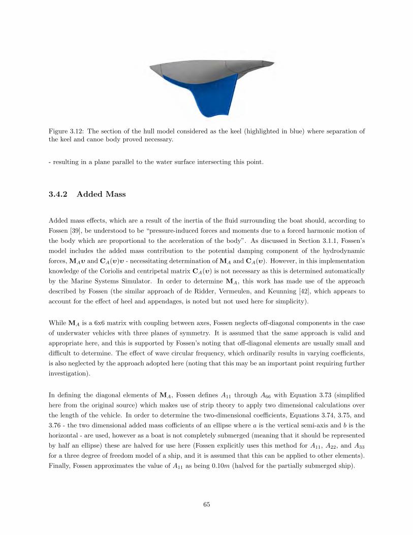
Figure 3.12: The section of the hull model considered as the keel (highlighted in blue) where separation ofthe keel and canoe body proved necessary.
- resulting in a plane parallel to the water surface intersecting this point.
3.4.2 Added Mass
Added mass effects, which are a result of the inertia of the fluid surrounding the boat should, according to
Fossen [39], be understood to be “pressure-induced forces and moments due to a forced harmonic motion of
the body which are proportional to the acceleration of the body”. As discussed in Section 3.1.1, Fossen’s
model includes the added mass contribution to the potential damping component of the hydrodynamic
forces, MAυ and CA(υ)υ - necessitating determination of MA and CA(υ). However, in this implementation
knowledge of the Coriolis and centripetal matrix CA(υ) is not necessary as this is determined automatically
by the Marine Systems Simulator. In order to determine MA, this work has made use of the approach
described by Fossen (the similar approach of de Ridder, Vermeulen, and Keunning [42], which appears to
account for the effect of heel and appendages, is noted but not used here for simplicity).
While MA is a 6x6 matrix with coupling between axes, Fossen neglects off-diagonal components in the case
of underwater vehicles with three planes of symmetry. It is assumed that the same approach is valid and
appropriate here, and this is supported by Fossen’s noting that off-diagonal elements are usually small and
difficult to determine. The effect of wave circular frequency, which ordinarily results in varying coefficients,
is also neglected by the approach adopted here (noting that this may be an important point requiring further
investigation).
In defining the diagonal elements of MA, Fossen defines A11 through A66 with Equation 3.73 (simplified
here from the original source) which makes use of strip theory to apply two dimensional calculations over
the length of the vehicle. In order to determine the two-dimensional coefficients, Equations 3.74, 3.75, and
3.76 - the two dimensional added mass cofficients of an ellipse where a is the vertical semi-axis and b is the
horizontal - are used, however as a boat is not completely submerged (meaning that it should be represented
by half an ellipse) these are halved for use here (Fossen explicitly uses this method for A11, A22, and A33
for a three degree of freedom model of a ship, and it is assumed that this can be applied to other elements).
Finally, Fossen approximates the value of A11 as being 0.10m (halved for the partially submerged ship).
65

Aii =
∫ L/2
−L/2A
(2D)ii (y, z)dx (3.73)
A(2D)22 = πρa2 (3.74)
A(2D)33 = πρb2 (3.75)
A(2D)44 =
1
8πρ(b2 − a2
)2(3.76)
Having determined the components of MA in surge, sway, and heave using the terms defined for an ellipse,
Fossen defines Equations 3.77 and 3.78 (where L, B, and H are the main dimensions of the vehicle), allowing
the determination of A55 and A66 (it is noted that de Ridder, Vermeulen, and Keunning [42] consider x in
their calculation of A66 - using an equation similar but different to Equation 3.78 - to be relative to the
centre of gravity, however the implicit definition to the contrary in Fossen’s presentation has been utilised
here). In these equations, terms including A11 have been considered in the same manner as Fossen does for
the calculation of Equation 3.78 for a ship - by dividing A11 = 0.10m over the integration, resulting in (for
example)∫ B/2−B/2 y
2A(2D)11 (y, z)dy =
∫ B/2−B/2 y
2 0.1mB dy = 1
24 (0.1mB2).
∫ L/2
−L/2A
(2D)55 (y, z)dx ,
∫ L/2
−L/2x2A
(2D)33 (y, z)dx+
∫ H/2
−H/2z2A
(2D)11 (y, z)dz (3.77)
∫ L/2
−L/2A
(2D)66 (y, z)dx ,
∫ B/2
−B/2y2A
(2D)11 (y, z)dy +
∫ L/2
−L/2x2A
(2D)22 (y, z)dx (3.78)
In order to calculate the final values of the MA matrix, use was made of the CAD model developed as part
of Section 3.4.1. The port (left) half of the waterline outline seen in Figure 3.10b was used together with the
outline of the side view of the completed model shortened to the waterline length of the boat (accounting for
the approximate positions of waterline start and end points) before being rotated such that the waterline in
the diagram (if it were included) is horizontal. A simple Python program, seen in Appendix E.1, was written
to extract the coordinates of the outline of the hull from the variable describing the vector path (using the
svg.path package12 - the path variables were obtained by opening the outline’s svg files in a text editor) and
to calculate the added mass coefficients over the length of the boat. The final values are noted in Section
3.4.3.
12https://pypi.python.org/pypi/svg.path
66
3.4.3 Determined Parameters
As is apparent from the previous sections in this chapter, it is necessary to determine a number of parameters
of the platform being modelled - both from measurements of the platform itself and the CAD model. Table
C.1 in Appendix C.1 describes these parameters, while Tables C.2 and C.3 record the buoyancy and surface
area values recorded for the heeling buoyancy model. As CAD measurements often involve measures of
high precision (which do not necessarily correlate to the actual boat), for consistency 5 significant figures
have been used where possible. Equations C.1 and C.2 presents the formulae derived using regression that
describes the moment arms presented in Table C.2 (noting that for the purposes of these equations roll is
defined in degrees).
3.5 Model Implementation
In implementing the model use was made of the Marine Systems Simulator [55, 63] (MSS), an open source
Simulink library intended to assist with modelling of marine systems with a focus on controller design. The
MSS provides various tools including equations of motion based on Fossen’s approach to modelling, Simulink
blocks predicting environmental conditions, and tools to assist with controller design. Of note is the MSS
Marine Hydro add-in, which appears to be capable of assisting in the generation of a model using other
commercial software tools. The add-in has not been used for this work as the required software tools were
not available and it is not clear whether they are suitable for a small platform, however this may present a
useful avenue of future development.
In this work, the MSS equations of motion block has been used as the central component of the model. It is
important to note that this block calculates the Coriolis and centripetal matrix automatically in the manner
described in other work by Fossen13. While there has not been an opportunity to review this reference, it
has been assumed that it is appropriate for use here.
3.5.1 Adaptation of the MSS
As the MSS only makes six degree of freedom and three degree of freedom (in surge, sway, and yaw) equations
of motion Simulink blocks available, it was necessary to modify the six degree of freedom block in order to
implement the three degree of freedom (in surge, sway, and heel) and four degree of freedom (in surge, sway,
heel, and yaw) models implemented here. Aspects of Fossen’s [39] derivations are therefore considered here.
The three and four degree of freedom models of this work assume that there is no motion in the excluded
axes (the z axis, pitch axis, and - in the three degree of freedom model - yaw axis). This assumption is
13Referenced by the block description as: T. I. Fossen (2002). Marine Control Systems: Guidance, Navigation and Controlof Ships, Rigs and Underwater Vehicles, Marine Cybernetics AS, ISBN 82-92356-00-2.
67

considered reasonable - a boat’s heave and pitch movement is small compared to that in other axes, while
for the three degree of freedom model it is assumed that the boat does not turn.
First, it is noted that Fossen’s Equation 3.79 continues to hold for the different models (providing that 03×3
scales accordingly). This equation is the definition of the transformation matrix in Equation 3.1 (where η2
is the vehicle’s orientation vector).
J =
[J1(η2) 03×3
03×3 J2(η2)
](3.79)
Fossen proceeds to derive J1 and J2 in Equations 3.80 and 3.81.
J1(η2) =
cos(ψ)cos(θ) −sin(ψ)cos(ϕ) + cos(ψ)sin(θ)sin(ϕ) sin(ψ)sin(ϕ) + cos(ψ)cos(ϕ)sin(θ)
sin(ψ)cos(θ) cos(ψ)cos(ϕ) + sin(φ)sin(θ)sin(ψ) −cos(ψ)sin(ϕ) + sin(θ)sin(ψ)cos(ϕ)
−sin(θ) cos(θ)sin(ϕ) cos(θ)cos(ϕ)
(3.80)
J1(η2) =
1 sin(ϕ)tan(θ) cos(ϕ)tan(θ)
0 cos(ϕ) −sin(ϕ)
0 sin(ϕ)/cos(θ) cos(ϕ)/cos(θ)
(3.81)
Corrected transformation matrices were found by setting unused angles (yaw and pitch in the three degree
of freedom model and pitch in the four degree of freedom model) to zero and disregarding components that
would be multiplied by an angle set to zero when applying the transformation. This process resulted in new
definitions for J1 and J2 for both the three and four degree of freedom models - seen in Equations 3.82 and
3.83 for the three degree of freedom model and in Equations 3.84 and 3.85 for the four degree of freedom
model. It is noted that it was confirmed that the four degree of freedom derivations matched those presented
by Xiao and Jouffroy [38], who used the same approach in the development of their model.
J1(η2) =
[1 0
0 cos(ϕ)
](3.82)
J2(η2) =[1]
(3.83)
68
J1(η2) =
[cos(ψ) −sin(ψ)cos(ϕ)
sin(ψ) cos(ψ)cos(ϕ)
](3.84)
J2(η2) =
[1 0
0 cos(ϕ)
](3.85)
The adapted transformation matrix was implemented in Simulink by modifying the MSS six degree of freedom
equations of motion block. The block was also adapted to ensure that no forces in the omitted axes are
considered, in a manner that is consistent with the differences between the six and three degree of freedom
blocks in the MSS.
It is also noted that an inconsistency exists in the MSS in the manner in which the three and six degree
of freedom models enable calculation of Coriolis forces. While the three degree of freedom model simply
provides an input of the vehicle’s speed multiplied by the enable variable (effectively providing no input if
the Coriolis forces are disabled in the block parameters), the six degree of freedom model multiplies by a gain
of the parameter minus 1. As no input should be provided if the forces are disabled, it has been assumed
that the six degree of freedom implementation is a bug and the three degree of freedom model’s approach
has been implemented.
3.5.2 Forces Implementation
Implementation of the forces described in the previous sections in the model is relatively straightforward.
The MSS equations of motion blocks accept four inputs: the rigid body mass matrix, the added mass matrix,
a vector describing the current, and a single τ input - representing the sum of all forces acting on the body.
The various components acting on the boat were implemented separately in different sub-systems or Matlab
functions.
It is not considered necessary to describe the implementation of each component in detail as this process
effectively involved the simple task of implementing the formulae already described - however a number of
notable aspects of the implementation are listed below.
The forces generated by the sail are implemented using a Simulink Embedded Matlab Function block.
As noted in Section 3.2.1, the model integrates the forces along the length of the wing-sail in order
to account for the varying angle of attack - achieved by dividing the wing-sail into a predetermined
number of parts, considered in turn to calculate their contribution to the forces generated by the
windsail.
A simple study was conducted to determine the number of parts into which the wing-sail should be
divided. Three arbitrarily selected sailing conditions were considered and the outputs were tested for
69

a number of divisions between 1 and 500. For the first and second test the value at 300 iterations was
the same as the value at 500, while for the third the value at 300 was within 2% of the value at 500 -
and so the number of iterations was set to 300 for the final implementation. This result can be seen in
Figure 3.13.
It is further noted that the implemented model assumes that the wind speed for a simulation is that
at the height of the boat’s wind sensor.
Various sanity checks are included to avoid the model attempting estimation of forces in ranges for
which it does not hold. These include stopping the simulation if the boat begins to move backwards
or heels by more than 89, and using saturation blocks to prevent resistance forces and the calculated
value for Rn (in the hull frictional resistance and appendage viscous resistance calculations) from being
below zero.
In the four degree of freedom model the rudder was modelled in a separate Matlab m file in order to
allow use of Matlab cell arrays, which were used as a means to implement a custom two-dimension
interpolation function (Matlab’s built in function requiring vectors of the same length, which were not
available as the number of coefficients generated by XFOIL for different rudder angles varied depending
on when XFOIL was able to converge).
3.5.3 GUI and Interfacing
In considering how the implemented model is used, it is necessary to note both how the model accepts
parameters and returns its data. All parameters used by the model are defined in variables in the Matlab
workspace, allowing for simple testing of alternative designs or different environmental conditions. The
model outputs key parameters including speed, position, forces, rudder angle, and others used for debugging
using output ports - allowing for easy interfacing with returned data using Matlab tools or scripts used to
run tests.
Key amongst the uses of the returned data is the model’s graphical user interface (GUI). While not necessary
for the model to be run (the Matlab command line or a script being two alternatives), the GUI allows for
quick evaluation of a test by presenting plots of important parameters (while allowing the user to selected
alternative data to display) and allows the user to enter test parameters before running a simulation. The
GUI was constructed using Matlab’s GUIDE tool, while its logic is scripted in the GUI’s m file. A screenshot
of the GUI can be seen in Figure 3.14.
3.5.4 Demonstration of Operation
In order to demonstrate simulations of the three and four degree of freedom models and verify that their
behaviour is expected, two simple simulations are presented.
70

(a) Driving-force. Wind speed = 5m/s. Wind direction = 50.Sail angle = -40.
(b) Side-force. Wind speed = 10m/s. Wind direction = 330.Sail angle = 20.
(c) Roll moment. Wind speed = 20m/s. Wind direction = 180. Sailangle = -90.
Figure 3.13: Results of the iterations test.
71

Figure 3.14: The model’s graphical user interface.
The first, seen in Figure 3.15a, shows the forward velocity of the three degree of freedom model reaching
steady state with a wind speed of 5m/s, direction of 70, and sail angle of -60. The second, seen in Figure
3.15b, shows the yaw angle of the four degree of freedom model steering itself to a heading of 20 from an
initial heading of with a wind speed of 7m/s and direction of 160.
These results demonstrate that the model is able to reach steady state and that it is capable of steering to a
heading. While further demonstrations of its operation are not shown here for brevity, the results generated
from the models in Chapter 5 further show its capabilities.
(a) Forward velocity of the three degree of freedom modelfrom an initial velocity of zero with a wind speed of 5m/s,direction of 70, and sail angle of -60.
(b) Yaw angle of the four degree of freedom model whensteering between 0 and 20 with a wind direction of 160
and speed of 7m/s.
Figure 3.15: Demonstrations of operation of the models.
72
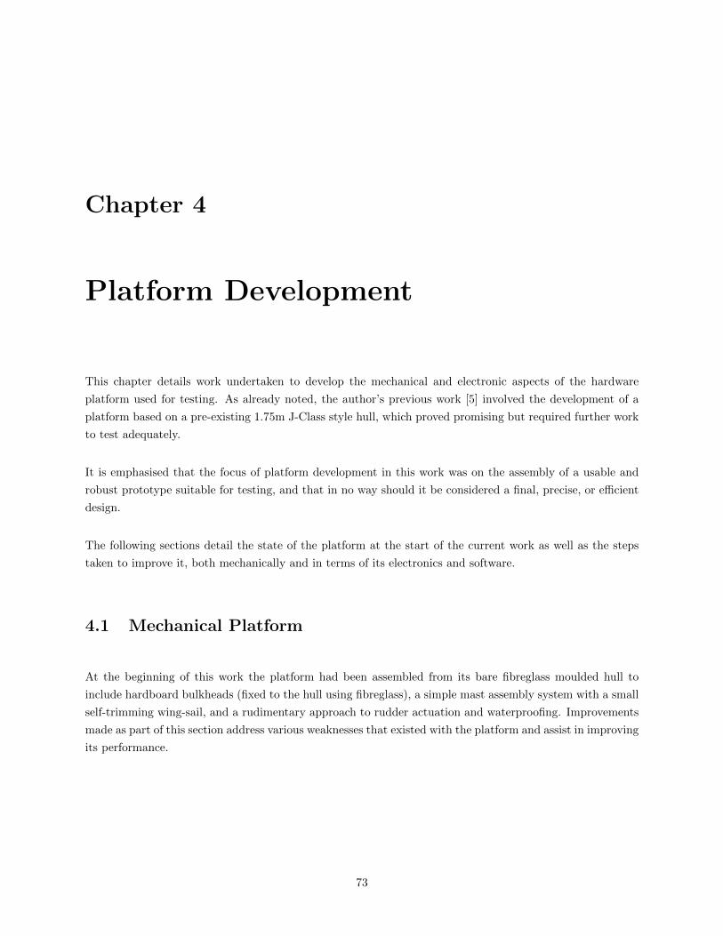
Chapter 4
Platform Development
This chapter details work undertaken to develop the mechanical and electronic aspects of the hardware
platform used for testing. As already noted, the author’s previous work [5] involved the development of a
platform based on a pre-existing 1.75m J-Class style hull, which proved promising but required further work
to test adequately.
It is emphasised that the focus of platform development in this work was on the assembly of a usable and
robust prototype suitable for testing, and that in no way should it be considered a final, precise, or efficient
design.
The following sections detail the state of the platform at the start of the current work as well as the steps
taken to improve it, both mechanically and in terms of its electronics and software.
4.1 Mechanical Platform
At the beginning of this work the platform had been assembled from its bare fibreglass moulded hull to
include hardboard bulkheads (fixed to the hull using fibreglass), a simple mast assembly system with a small
self-trimming wing-sail, and a rudimentary approach to rudder actuation and waterproofing. Improvements
made as part of this section address various weaknesses that existed with the platform and assist in improving
its performance.
73

4.1.1 Sail Actuation
One of the primary changes made to the platform involved the selection of a new sail. The self-trimming
wing-sail used previously was too small to be effective, construction of a new self-trimming wing-sail would
have been time consuming, and it was thought that a directly actuated sail would add simplicity to the
platform. Therefore, an alternative NACA0018 wing-sail with a span of 1m and chord of 30cm developed as
part of a separate project [54] was selected for use on the platform. This wing-sail included an integrated
mast positioned in front of the quarter-chord point, resulting in a greater load on the wing-sail’s actuator
that might be the case otherwise - but the difference was considered small enough to be negligible. It is
noted that assessment of approaches to sail design for autonomous sailboats, as seen in Section 2.3.2, reveals
that a self-trimming sail has various advantages over the directly actuated variety, and that for this reason
separate consideration of a self-trimming sail is considered an avenue of potential future work.
Having selected a wing-sail for use with the platform, it was necessary to determine an approach to its
actuation.
Actuator Specification Determination
In order to estimate the required specifications of the motor to be used for control of the wing-sail, an
assessment of the expected forces on the sail was conducted. By considering the lift and drag forces on the
sail (as discussed in Section 3.2.1), the force perpendicular to the wing-sail was found by deriving Equation
4.1. This allowed, by making use of lift and drag data calculated using XFOIL1, Figure 4.1 to be plotted
- showing the perpendicular force generated by the wing-sail for angles of attack between 0 and 30. The
graph indicates that while there is a local maximum, it appears that the perpendicular force increases with
angle of attack (the dip around 30 in the 30 knot plot was assumed to be a simulation error).
F⊥ = Lcos(α) +Dsin(α) (4.1)
Given this trend, drag of the wing-sail at 90 was calculated (using a drag coefficient of 1.8 - the maximum
expected value based on the results presented by Sheldahl and Klimas [4] - and Equation 3.9) to find a force
of 79.1N in 30 knots of wind - which is greater than the forces predicted in Figure 4.1, and thus the maximum
expected force.
Finally, calculation of the required motor torque required knowledge of the position of the centre of effort
of the wing-sail. Larsson and Eliasson’s [11] note that a sail at 90 angle of attack has its centre of effort at
its geometric centre of gravity - indicating a centre of effort half way between the leading and trailing edges
1As noted in Section 3.2.1, XFOIL was initially used to determine the lift and drag coefficients on the wing-sail - and thuswere the values used when this calculation was performed.
74

0
10
20
30
40
50
60
0 5 10 15 20 25 30 35
Perp
en
dic
ula
r F
orc
e i
n N
ew
ton
s
Angle of attack in degrees
30 knots15 knots10 knots
Figure 4.1: Perpendicular force produced by the wing-sail as the angle of attack varies for different windspeeds.
of the wing-sail. Accounting for the location of the wing-sail shaft, this results in a distance from shaft to
centre of effort of 0.08m - and a maximum expected moment of 6.33Nm.
Actuator Selection and Assembly Design
As with other projects (such as the USNA Sailbots [15]), the use of an actuator which does not require
continuous actuation in order to hold its position was considered necessary in order to conserve power. Two
approaches were thus considered: the mounting of a motor driving a worm gear next to the shaft, and
the use of a linear actuator driving a rack and pinion gear - as in the approach of the BeagleB boat [21].
Despite the second approach being less efficient (in that rotational motion is translated into linear motion
using a worm gear inside the linear actuator before being translated back into rotational motion), it was
considered mechanically simpler and easier to construct. Consideration of linear actuators from an online
supplier resulted in the selection of Pololu’s Generic Linear Actuator with Feedback2 - a device with a load
rating of 51kg (which was determined to be sufficient for the torque requirement calculated above) and a
built in potentiometer for position feedback, which again simplified construction and control.
The gearing system designed for the actuator was inevitably similar to that which appears to have been
used for the BeagleB platform. Both the rack and pinion gears were developed using the rack and spur gear
generators in the Solidworks Toolbox.
Finally, it was necessary to design an approach to assembly of the gearing and mast-mounting system (the
latter being referred to here as the mast step). The author’s previous work mounted the small self-trimming
wing-sail to the boat using bearings attached to two aluminium plates mounted above the deck and attached
to a steel bar in the centre of the boat using threaded aluminium dowel. A similar design was utilised for
2http://www.pololu.com/product/2337
75

(a) (b)
Figure 4.2: Assembly of the mast step - (a) shows the placement of the lower bracket, while (b) shows thecomplete assembly including waterproofing.
the mounting of the new wing-sail, however the aluminium plates were mounted lower in the boat (the lower
one immediately above the steel bar that runs down the boat’s centre, and the upper immediately above the
deck) and new bearings were purchased in order to accommodate the shaft of the new wing-sail. In addition,
the new design differed from the old in that the upper plate was made larger on one side to allow the
mounting of brackets to support the linear actuator and was also separated into two parts to accommodate
a waterproofing system.
Waterproofing of the assembly is achieved by sandwiching a rubber mat between the two upper plates and
between the deck of the boat and an aluminium bracket that surrounds the mast assembly - allowing for
small movements of the mast relative to the deck while maintaining waterproofing. When assembled, marine
silicone was also applied in order to further assist with waterproofing in case the ‘sandwiching’ should prove
insufficient. Waterproofing of the upper bearing is achieved using petroleum jelly, in lieu of a grease.
The assembly is seen in Figure 5.4, while technical drawings of its laser cut parts as provided to the supplier
can be seen in Appendix B.3.
4.1.2 Rudder Actuation
As with the author’s previous work, use of a servomotor for control of the rudder has been adopted, however
the 5.2kg.cm device used previously was replaced with a Power HD High-Torque Servo 1501MG3, rated at
17kg.cm. The author’s previous work [5] included a rough estimate of a worst case torque requirement of
18.11kg.cm. Given that the assumptions for this estimate included the rudder acting at a 90 angle of attack,
which is not expected of the platform, the rating of the new servomotor was considered adequate.
3http://www.pololu.com/product/1057/specs
76
(a) (b)
7.5mm
4.5mm3mm 12mm3mm 3mm
(c)
Figure 4.3: The rudder assembly. (a) shows the attachment of the servomotor inside the hull, (b) shows therudder stuffing box (with a servo arm that was later replaced) prior to its installation in the boat, and (c)shows a drawing of the stuffing box design with approximate dimensions.
The previous method of attachment of the servomotor (which was a temporary measure involving duct
tape to secure the bracket that held the servomotor) was considered inadequate for reliable operation of
the platform, and so the new servomotor was mounted in the boat using a perspex bracket secured to
two additional bulkheads installed in the boat for this purpose (and attached using fibreglass between the
bulkheads and hull). This assembly can be seen in Figure 4.3a.
The author’s previous work had also made use of a temporary measure to waterproof the rudder’s entry
into the boat - a process made particularly difficult by the short shaft attached to the rudder. The previous
approach of creating a tight rubber seal was considered and tested in a water tank, but was ultimately found
to be unreliable and prone to leaking when the rudder was actuated.
In order to address this problem, a small stuffing box was constructed. Inspection of remote control boat
hobby websites and Internet forum [64–66] pages about the use of stuffing boxes for use primarily for propeller
shafts allowed the design of a simple box for use with the platform’s rudder, seen in Figures 4.3b and 4.3c.
The box was constructed from two sections of a plastic dowel machined using a lathe to an appropriate
diameter. Holes drilled in each section allow room for bolts to secure the assembly and for the shaft and
stuffing area. The box was filled with Vaseline, a form of cosmetic petroleum jelly, which was noted as a
suitable material for hobby use by one source [64].
As seen in Figure 4.3a, the final assembly made use of a different servo arm attached to the rudder shaft to
that seen in Figure 4.3b (a metal rod, bent to allow attachment, connects the servo arms on the servomotor
77

and rudder shaft to facilitate actuation). This replacement was made following a loss of thread on the shaft
- preventing tightening of the nuts securing the arm. The second arm is secured with a small bolt acting
as a grub screw as well as Spabond 420LW epoxy adhesive set in the well formed by the arm. While this
assembly worked well, slipping of the rudder occasionally occurs (possibly because the flat section on the
shaft to which the grub screw makes contact is not large enough) - highlighting one of the limitations of
this arrangement. While it might be possible to reduce the torque on actuator connections by replacing the
rudder with one with its shaft positioned so as to balance the torque acting on it, this is likely to require
substantial reconfiguration of the hull.
Finally, the stuffing box was secured in the hull of the boat using the same Spabond 420LW epoxy adhesive.
Testing of the assembly in a water tank while the rudder underwent actuation resulted in no water leaking
into the boat. It is important to note that while this assembly was sufficient for the purposes required of the
platform, it is sub-optimal and further improvements are necessary to improve reliability. It is likely that
the most suitable improvement would be to lengthen the rudder shaft, allowing for it to enter the hull above
the waterline (an approach discussed in the author’s previous work [5]).
4.1.3 General Assembly
Having made the improvements to specific parts of the platform described above, other more general changes
were made. First, scrap lead previously used to weigh down the keel was replaced with 10kg of lead shot
set in resin (an approach used by a number of other projects [15–17,24]). Mounting brackets were installed
immediately beneath the deck of the boat where the linear actuator and wind sensor were to be installed, as
seen in Figures 4.4a and 4.4b, ensuring that the deck would not be required to support these and minimising
the movement of the bolts through the holes in the deck (which risks compromising waterproofing). Metal
brackets were installed to support the electronics box, as seen in Figure 4.4c, and an additional hatch cover
was installed to allow access to this area of the boat. Finally, as with the author’s previous work, the deck
was attached to the boat using marine silicon with care being taken to apply silicon at potential leak points
(such as the wind sensor attachment point and points at which cables exit the hull).
4.2 Electronic Platform
Unlike in the case of the mechanical platform, the basic electronic platform developed as part of the author’s
previous work was not considered suitable for use here - and so a new platform was developed. This process
included an assessment of the requirements of the platform, taking potential future work into account, and
the writing of software to support the platform.
78

(a) (b)
(c)
Figure 4.4: Images showing general aspects of the assembly of the platform. (a) shows the wind sensormounting bracket, (b) shows the equivalent bracket for the linear actuator, and (c) shows the electronics boxbracket and the layout of components in the boat.
4.2.1 System Overview
In developing the electronics platform, a number of considerations and requirements were noted - including:
Modularity and the ability to interface with various external sensors, actuators, and communication
platforms
The inclusion of various basic sensors including a GPS, inertial measurement unit, compass, and wind
sensor (all generally used on autonomous sailboats, as discussed in Section 2.3.3)
The potential to use the platform on another sailboat for use in other research
The ability to facilitate future work, such as the running of navigation algorithms
79

Early in the development of the platform the APM Autopilot Suite (also known as Ardupilot) was considered
for use as the starting point for the electronics platform, and assessment quickly revealed its potential. The
platform comprises of a number of components: a set of hardware devices, firmware that runs on the
hardware, and ground-station computer software for mission planning and analysis. The hardware platforms
were of particular interest given that the APM devices generally include relevant sensors. The APM 2.5, was
immediately available and thus considered. It includes a ATMEGA2560 microprocessor, a MPU-6000 6DOF
Accelerometer and Gyroscope, a 3-axis magnetometer, a MS5611-01BA03 barometer [67], and the ability
to easily interface with an external GPS. Other APM hardware platforms include the APM 2.6, which is
similar to the APM 2.5 but makes use of an external compass [68], and the 3DR Pixhawk which includes a
32 bit processor [69]. It is notable that, at least in the case of the APM 2.5, the platform works well with
existing remote controllers used for hobby purposes - allowing normal manual control when the correct mode
is enabled.
Preliminary assessment of the open-source APM firmware [70] revealed that it includes libraries for interfacing
with the platform’s sensors, control, and navigation. Of note is the platform’s Plane, Copter, and Rover
divisions.
Given the apparent suitability of the APM platform for use in controlling an autonomous sailboat, the APM
2.5’s immediate availability, and the expected time-saving benefits of using the existing platform, it was
selected for use with the project. While at times development using the platform proved difficult (primarily
due to a lack of documentation and at times confusing code - although this appears to be improving to a
certain degree), ultimately the platform worked well.
So as to make use of the APM platform’s ability to operate together with a traditional hobby remote
control (hereafter referred to as the RC controller), a Spektrum DX5e 2.4GHz 5-channel remote control,
which includes a AR600 6-channel receiver, was purchased on the advice of Mr. Bruce Johnson, who has
experience with RC devices (and who also advised the author regarding previous work).
As noted in Section 2.3.3, some other autonomous sailboats have made use of both a low-level micro-controller
and a device with more processing power for high-level operations. In order to expand logging capabilities
of the platform, allow more flexible communication with the boat than provided by the RC system, and
facilitate future development which might require additional processing power it was decided to place an
on-board computer on the boat in addition to the APM 2.5. Both the BeagleBone Black and Raspberry
Pi were immediately available for use, and the BeagleBone Black was selected for its faster processor. As
discussed in a Section 4.2.4, the BeagleBone Black was configured to operate with a D-Link Wireless N 150
USB Adapter to provide access to the device via a laptop or mobile device.
Figure 4.5 provides an overview of the system configuration, while the following sections will describe each
sub-system in detail.
80

APM 2.5(including internal sensors)
BeagleBoneBlack
USB
D-Link Wireless
N 150 USB Adapter
USB
H-Bridge
Digital I/O
LinearActuator
Analogue Feedback
WindSensor
AnalogueFeedback(direction)
Digital Interrupt(wind speed)
RudderServomotor
RCReceiver
Digital I/O
GPS
Serial
Figure 4.5: The electronic platform system configuration.
81
4.2.2 Power and Actuator Control
While power management on an autonomous sailboat used for long missions is naturally important, at this
stage the prototype platform does not focus on this requirement as tests were expected to be relatively short
and include opportunities to change batteries. The platform currently makes use of a 2.3Ah 12V lead acid
battery to power its electrical systems.
As the APM 2.5, BeagleBone Black, servomotor, and h-bridge all require 5V power, three voltage regulators
are used to enable this. Two LM2576T-5 switched mode regulators each supply the servomotor and Bea-
gleBone Black as it was found that a single regulator would result in the BeagleBone Black resetting when
the servomotor drew too much current. A third LM7805CT linear regulator powers the APM 2.5 - it being
found that if a switched mode regulator was used the APM 2.5’s analogue to digital converter would pick up
too much noise on the linear actuator position potentiometer for smooth control to be achieved. The APM
2.5’s regulator also powers the GPS and RC receiver, as these receive their power from that board, while
the wireless adapter is powered via the BeagleBone Black’s USB port. In order to ensure that differences
in operating voltage between the BeagleBone Black and the APM 2.5 does not cause any faults, the power
cable of the USB connection between the two (which ordinarily provides power to USB devises, which is not
required here) was cut - an approach discussed in the DIY Drones forums [71].
Control of the servomotor is not discussed here as this is handled by the APM platform. However it is noted
that as it was found that rapid changes in the commands sent to the servomotor resulted in unpredictable
behaviour different to that commanded, and so a rate limiter was implemented which ensures that the rudder
does not move more than 3.375 every 20 milliseconds.
A circuit diagram showing the configuration of major components and their power supplies can be seen in
Appendix B.2.
Linear Actuator Control
As a means to control the linear actuator the STK681-332-E Forward/Reverse Motor Driver [72] was selected,
primarily due to it being the only through-hole h-bridge integrated circuit available from a local supplier
capable of driving the linear actuator at its rated 12 volts and maximum (stall) current of 7 amperes (a
through-hole integrated circuit being preferred in order to avoid the need for surface mounting components).
As the SIP-19 package used by the device has 1mm gaps between its pins and compatible strip-board could
not be sourced, a printed circuit board was designed and ordered that implemented its sample application
circuit [72]. The circuit, indicating the inputs and outputs of the printed circuit board and omitting the
current sensing resistor (it was found that the h-bridge’s current limiting function was unreliable and resulted
in the entering of fault mode during normal operation), can be seen in Appendix B.1.
Following completion of the circuit it became apparent that the actuator’s speed and mechanical dampening
82

is such that it can be operated by a simple bang-bang controller, making the speed control functionality
of the h-bridge circuit unnecessary (and meaning that mechanical relay switches could conceivably be used
instead). As a result, control of the linear actuator proved simple to achieve.
The simple bang-bang controller was implemented on the APM 2.5 by creating a new SailLinearActuator
library and adding the relevant function calls to the APM scheduler. The library, based on the AP BattSensor
library, has four implemented modes: disabled, stop, forward, and reverse (fault detection is envisioned, which
would result in use of a fifth fault mode, however this is not used - primarily due to the effective disabling of
the h-bridge circuit’s current limiting function). When not disabled, the APM calls a read() method every
20ms which records the position of the linear actuator by using the APM’s analogue to digital converter,
converting it to an equivalent sail angle, and subjecting it to a 160ms sliding filter. The filtered position is
compared to the set-point (allowing for a 3 hysteresis), and if necessary the library switches to forward or
reverse mode to reposition the actuator.
The read() method also monitors the current drawn by the linear actuator as it operates, disabling it should
it exceed 1.8 amperes. This is done in order to avoid the actuator damaging the boat should an obstacle
prevent the sail or rack or pinion gears from moving separate to the actuator. Current monitoring is achieved
by monitoring a separate analogue pin on the APM 2.5 - which is connected to the output of an operational
amplified configured as a differential amplifier that monitors the current drawn by the h-bridge circuit using
a 0.1Ω resistor, two resistor divider circuits, and operational amplifiers configured as buffer circuits (the
complete circuit can be seen in Appendix B.2).
Separately, the APM’s steering set servos () function, when the APM is in manual mode, receives the throttle
value on the RC controller and converts it to its equivalent value on the -90 to 90 operating range of the
wing-sail and sets the set-point via the SailLinearActuator library’s set () method. Separate methods in the
library allow for the setting of the mode (allowing for disabling of the actuator outside of the library) and
for the retrieval of operating parameters such as current position, set-point, current usage, and maximum
current usage.
4.2.3 Sensor Interfacing and Selection
Much of the necessary interfacing with sensors, such as the accelerometer and gyroscope, is automatically
handled by the APM and so need not be discussed here. Therefore this section will focus on where changes
have been made to the default behaviour of the APM and on the wind sensor, which is not ordinarily
interfaced with the APM platform.
83

Magnetometer
Given that navigation approaches for the boat will almost certainly rely on its heading, proper calibration of
the magnetometer is an important aspect of the electronic platform’s operation. APM documentation [73]
describes approaches to this. By default the APM platform makes use of a live calibration procedure that
requires the user to rotate the vehicle around all axes to determine appropriate offsets. It was immediately
apparent that this approach would not be possible with the platform used here - it being unclear whether
the lead keel would remain in place should the boat be turned completely upside down.
Fortunately the APM platform includes a procedure to learn offsets during operation, and so this mode was
enabled for use here. The procedure used [74, 75], which essentially relies on the fact that the length of the
vector returned by the magnetometer should have a constant length to estimate offsets over time (noting
that this is a simplified interpretation of the proof provided by the original source), compares subsequent
magnetometer readings and updates offsets if there is a sufficiently large change. As operation of the linear
actuator results in additional offsets to the magnetic field seen by the magnetometer (a problem discussed
further below), the potential exists for the algorithm to learn the incorrect offsets. For this reason, the APM
firmware was modified to disable learning when the linear actuator library was in forward or reverse mode.
Inspection of data logged during the first sailing test of the platform revealed that the learning of offsets took
an extended period of time, possibly because periods when the boat’s heading changed (when the learning
algorithm determines new offsets) coincided with actuation of the sail - reducing learning opportunities. In
order to mitigate this problem, a calibration procedure was added to operation of the platform whereby it
would be rotated and heeled while the sail was stationary in order to speed the learning of correct offsets
for the location of the test. During field tests the magnetometer offsets did not settle to constant values -
it being assumed that this is a result of noise and environmental variations in the magnetic field seen by
the platform. Assessment of the effects of this may be possible by comparing headings determined using the
compass and the GPS during an extended test.
A further challenge was presented by the effect on heading readings caused by interference from the linear
actuator. The simplest solution to this would be to install an external compass and place it as far from
the actuator on the boat as possible, however given that this would have required sourcing a magnetometer
suitable for use with the APM platform as well as determining an approach to its waterproofing in the
limited available time, it was decided to rather implement compensation based on measurements of the
current drawn by the linear actuator.
The APM Copter firmware includes a ‘compassmot’ procedure to compensate for interference from motors
by applying an additional offset in each axis to compass readings that is proportional to current drawn by
the vehicle’s motors - the compensation necessary being determined during the ‘compassmot’ calibration
procedure which is run while the vehicle is held stationary. As this form of compensation is the same as
that required for this platform, the ‘compassmot’ code was transferred to the APMRover2 firmware and
modified to be compatible with the linear actuator. In addition, the procedure was modified to actuate the
linear actuator during testing automatically (as opposed to manually) - resulting in reliable running of the
84
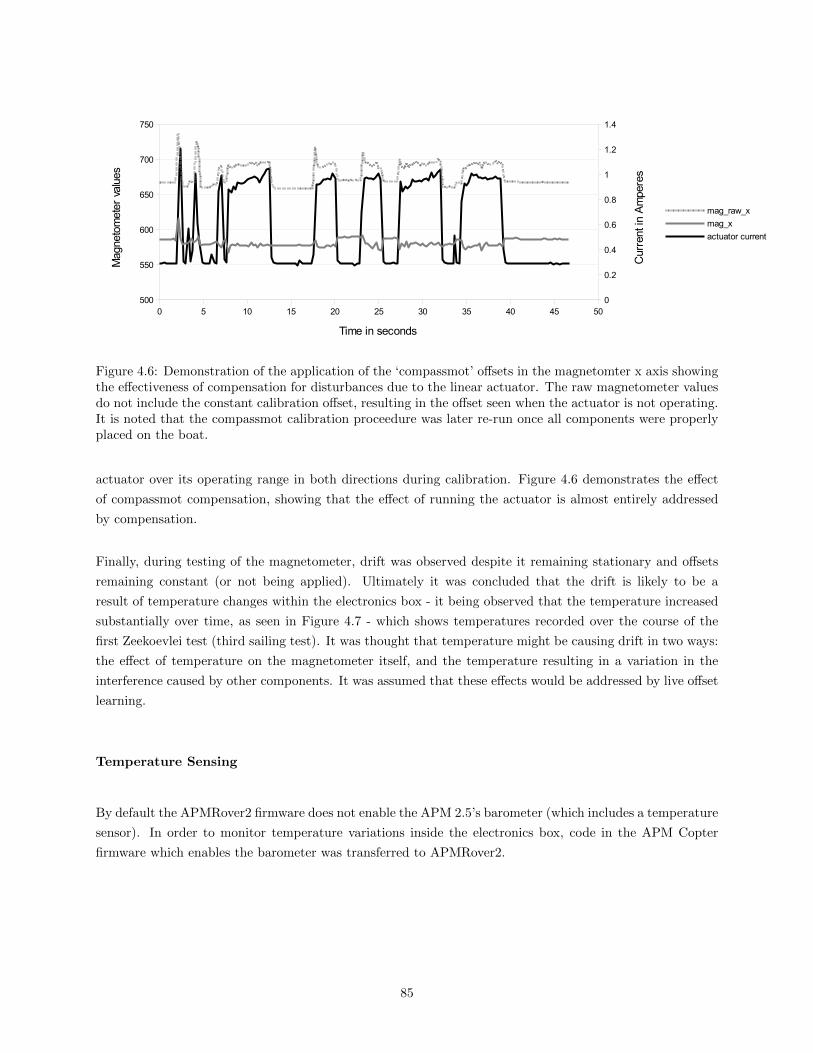
0 5 10 15 20 25 30 35 40 45 50500
550
600
650
700
750
0
0.2
0.4
0.6
0.8
1
1.2
1.4
mag_raw_x
mag_x
actuator current
Time in seconds
Mag
neto
met
er v
alue
s
Cur
rent
in A
mpe
res
Figure 4.6: Demonstration of the application of the ‘compassmot’ offsets in the magnetomter x axis showingthe effectiveness of compensation for disturbances due to the linear actuator. The raw magnetometer valuesdo not include the constant calibration offset, resulting in the offset seen when the actuator is not operating.It is noted that the compassmot calibration proceedure was later re-run once all components were properlyplaced on the boat.
actuator over its operating range in both directions during calibration. Figure 4.6 demonstrates the effect
of compassmot compensation, showing that the effect of running the actuator is almost entirely addressed
by compensation.
Finally, during testing of the magnetometer, drift was observed despite it remaining stationary and offsets
remaining constant (or not being applied). Ultimately it was concluded that the drift is likely to be a
result of temperature changes within the electronics box - it being observed that the temperature increased
substantially over time, as seen in Figure 4.7 - which shows temperatures recorded over the course of the
first Zeekoevlei test (third sailing test). It was thought that temperature might be causing drift in two ways:
the effect of temperature on the magnetometer itself, and the temperature resulting in a variation in the
interference caused by other components. It was assumed that these effects would be addressed by live offset
learning.
Temperature Sensing
By default the APMRover2 firmware does not enable the APM 2.5’s barometer (which includes a temperature
sensor). In order to monitor temperature variations inside the electronics box, code in the APM Copter
firmware which enables the barometer was transferred to APMRover2.
85
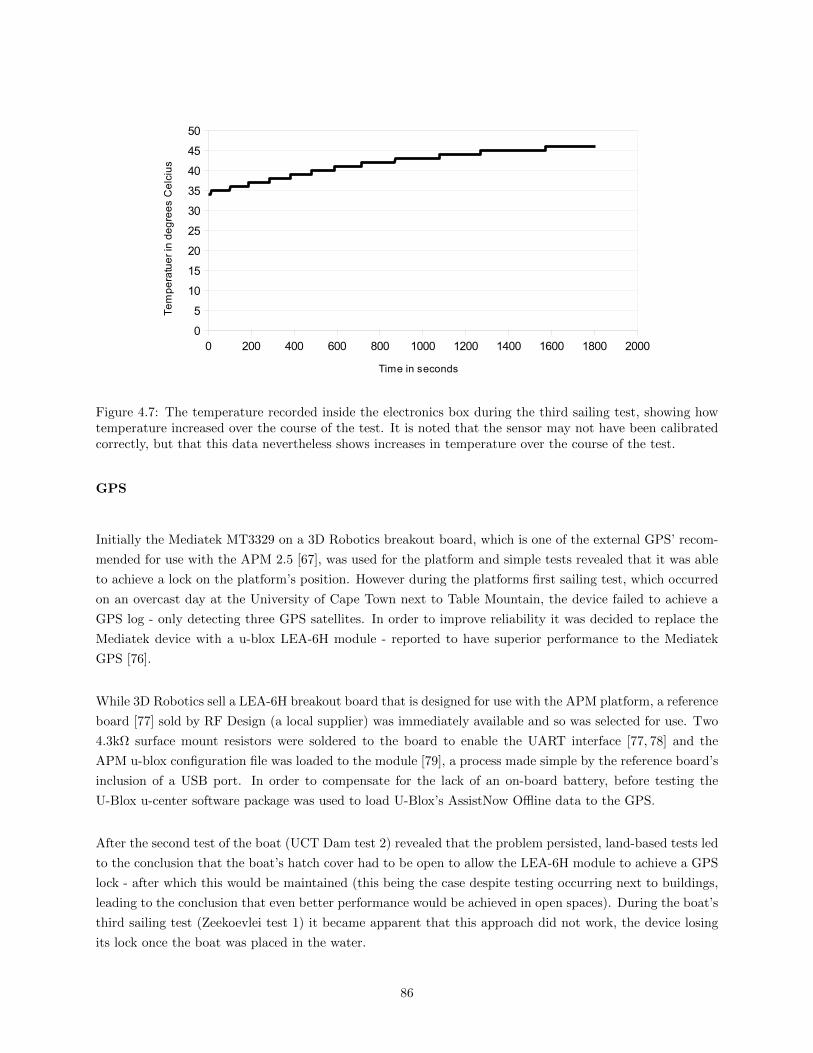
Figure 4.7: The temperature recorded inside the electronics box during the third sailing test, showing howtemperature increased over the course of the test. It is noted that the sensor may not have been calibratedcorrectly, but that this data nevertheless shows increases in temperature over the course of the test.
GPS
Initially the Mediatek MT3329 on a 3D Robotics breakout board, which is one of the external GPS’ recom-
mended for use with the APM 2.5 [67], was used for the platform and simple tests revealed that it was able
to achieve a lock on the platform’s position. However during the platforms first sailing test, which occurred
on an overcast day at the University of Cape Town next to Table Mountain, the device failed to achieve a
GPS log - only detecting three GPS satellites. In order to improve reliability it was decided to replace the
Mediatek device with a u-blox LEA-6H module - reported to have superior performance to the Mediatek
GPS [76].
While 3D Robotics sell a LEA-6H breakout board that is designed for use with the APM platform, a reference
board [77] sold by RF Design (a local supplier) was immediately available and so was selected for use. Two
4.3kΩ surface mount resistors were soldered to the board to enable the UART interface [77, 78] and the
APM u-blox configuration file was loaded to the module [79], a process made simple by the reference board’s
inclusion of a USB port. In order to compensate for the lack of an on-board battery, before testing the
U-Blox u-center software package was used to load U-Blox’s AssistNow Offline data to the GPS.
After the second test of the boat (UCT Dam test 2) revealed that the problem persisted, land-based tests led
to the conclusion that the boat’s hatch cover had to be open to allow the LEA-6H module to achieve a GPS
lock - after which this would be maintained (this being the case despite testing occurring next to buildings,
leading to the conclusion that even better performance would be achieved in open spaces). During the boat’s
third sailing test (Zeekoevlei test 1) it became apparent that this approach did not work, the device losing
its lock once the boat was placed in the water.
86

Figure 4.8: The wind sensor attached to the boat.
As a final modification, the GPS was moved from the electronics box to a separate watertight box on the deck
of the boat (an approach which had previously been avoided so as not to risk compromising waterproofing).
This worked well, allowing the logging of GPS data during the fourth sailing test (Zeekoevlei test 2).
Wind Sensor
While approaches to control of an autonomous sailboat without a wind sensor are noted in Section 2.3.3,
the inclusion of a wind sensor was considered important so as not to rely on such approaches, to ensure that
the platform is flexible and can be used for various tests, and because local wind data would be necessary
for comparison of the boat’s performance with that predicted by its model. Both wind direction and speed
information were considered requirements. While noting the merits of the various wind sensor technologies
discussed in Section 2.3.3, cost was also considered an important factor informing the selection of a sensor.
Taking note of these requirements, a comparison of wind sensors available for purchase was conducted - the
results of which can be seen in Table D.1 in Appendix D.1.
Having completed this comparison, the Davis Anemometer 6140 was selected - primarily due to its low cost
and ability to measure both speed and direction. While it is a mechanical sensor and cannot be considered
entirely waterproof, this was considered acceptable given the expected testing conditions. The sensor was
mounted at the front of the platform (seen in Figure 4.8) - and while this location does result in interference
from the sail while travelling downwind, this was considered acceptable given the expected difficulty of
mounting the sensor on the top of the sail and because it is believed the necessity for accurate measurements
is greatest when travelling at angles to the wind other than 180.
Interfacing between the wind sensor and APM 2.5 is relatively simple. The wind direction sensor is connected
to a potentiometer, allowing its position to be determined by measuring an analogue signal. The wind speed
87

sensor pulls its signal to ground once per rotation - resulting in the use of a pull up resistor which ensures
that the signal seen by the APM 2.5 is high unless the wind sensor pulls it low, allowing for the use of an
interrupt to track its rotations.
Reading of the values generated by the wind sensor is achieved with a WindSensor library (again based on
the AP BattSensor library) written for the APM firmware for this purpose. The library includes a read()
method which is called every 20 milliseconds by the APM scheduler. This method records the position of the
wind direction sensor by using the APM 2.5’s analogue to digital converter with a sliding filter that operates
over 2 seconds (a time period determined by inspection of the oscillation period of the data logged during
the first sailing test, where the window used was smaller). The direction () method returns the direction in
degrees.
In the case of wind speed, the library attaches an interrupt to the pin connected to the wind speed sensor
and records the time it was triggered. When called, the speed() function determines the speed by applying
Equation 4.2 (based on the wind sensor’s datasheet [80] - where T is the sample period and P the number
pulses during that period). This was adjusted to the form of Equation 4.3 (where timecurrent is the current
time and timeoldest is the oldest time in the sampling window) which calculates the speed based on the
time taken for the last 50 rotations to take place and converts4 it to m/s. It is notable that this method of
calculating the speed results in a variable sliding window (in that the sample time is not fixed), an approach
which was chosen to simplify implementation of the algorithm. A window of 50 samples was selected based
on testing of the sensor with a desk fan.
Vmph = P ·2.25
T(4.2)
Vm/s =50·0.447·2.25
timecurrent − timeoldest(4.3)
While the wind direction sensor performed well during testing, logs reveal that wind speed data is exception-
ally noisy and unusable. It is assumed that this is a result of the motion of the boat, given that bench tests
revealed that manual turning of the wind speed sensor shaft led to noise and because the sensor is designed
for mounting in a fixed location. In order for wind speed data to be used, further work is required to address
this issue - possibly by implementing a filter on the wind speed interrupt pin.
4.2.4 Logging and Remote Access
This section primarily addresses the role of the BeagleBone Black on the platform, which primarily had the
role of logging test data and facilitating remote access to the boat via a wireless access point. This section
will also discuss changes that were made to the APM firmware to allow logging of linear actuator, wind, and
4Wolfram—Alpha knowledgebase, 2014 - accessed via Wolfram Alpha.
88

Figure 4.9: The Mavelous GUI.
barometer data.
Wireless Access Point Configuration
Configuration of the wireless access point on the BeagleBone Black was achieved based on a number of online
tutorials [81–83] - with some difficulty being experienced in ensuring the final configuration worked correctly.
Notably, it was necessary to set the subnet mask to avoid conflicts with the BeagleBone Black’s Ethernet
and USB network connections.
The final configuration ensures that the access point is started automatically (using the systemd system
manager) and creates a secure access point that allows access to the web server running on the BeagleBone
Black and maintenance via SSH.
Remote Interface and Logging
In order to interface with the APM platform remotely, use was made of the Mavelous [84] computer program
- which is an open-source ground control station written in Python capable of communicating with any
device using the MAVLink protocol (which is used by the APM platform). Mavelous provides its graphical
user interface (GUI) via a web browser - meaning that once it was installed on the BeagleBone Black, its
interface was easily accessible via any device with a web browser connected to the platform’s wireless access
point. A screenshot of the GUI can be seen in Figure 4.9.
Mavelous’ functionality includes the plotting of the vehicle on a map, an artificial horizon indicating the
vehicle’s orientation, the display of various information such as GPS and battery status, and the ability for
a user to send commands to the vehicle (such as to enter loiter mode or to navigate to a location indicated
on the map). The software also has a page, ordinarily used by the Javascript GUI to retrieve the latest flight
information, which lists all data received from the vehicle via MAVLink - which proved particularly useful
for debugging. At present, Mavelous’ control functionality is not used - however it is likely to prove useful
for future work.
89

In order to adapt Mavelous for use here, two major changes were made. First, display of the vehicle’s heading
was added to the GUI (allowing for an automatically updating indicator of whether the compass is working).
Second, logging functionality was added. This functionality allows the user to start and end logging via the
GUI, and ensure that when enabled, relevant data is logged to a file on the BeagleBone Black as it is received
from the vehicle. While it would be possible to log all data, this is not done in order to save storage space on
the BeagleBone Black and because much of the data received is not needed for analysis of the performance
of the platform.
Logged data includes:
The platform’s orientation and rate of change of orientation
All GPS-related data, including current latitude and longitude, number of visible satellites, ground
speed, and lock type
Raw accelerometer, gyroscope, magnetometer, and barometer sensor data
Sensor calibration values
All wind-related data
Data describing the state of the linear actuator and servomotor
The boat’s mode of operation (manual or steering)
When installing Mavelous on the BeagleBone Black, it was configured to run automatically on boot after a
delay (which was determined by manual testing in order to allow other functionality, such as the wireless
access point, to be enabled). This was achieved using the systemd system manager, which was used to set
automatic configuration of the wireless access point. In addition, it proved necessary to modify the version of
MAVProxy used by the installation (MAVProxy providing the interface between Mavelous and the MAVLink
messages received from the platform) to disable user input via the command line as such input is not possible
when run via systemd and results in the program crashing. This adaptation was made on the basis of a
discussion of a Mavelous bug report [85].
Finally, it is noted that while the APM 2.5 includes its own logging functionality [86], the above approach of
implementing logging functionality on the BeagleBone Black was adopted in order to allow simpler control
of when to start and end logs, and to allow greater amounts of data to be logged (the APM reportedly [86]
including 16Mb of memory for logs versus the BeagleBone Black’s 4GB of on-board storage [87]). While
this results in the BeagleBone Black logging data slower than the APM 2.5, this was considered acceptable
for the study’s purposes. In addition, APM logging continues to function - allowing it to be used if faster
logging is required.
90

APM Data Transmission
In order to transmit additional data (beyond that transmitted by default) from the APM 2.5 to the Beagle-
Bone Black, it was necessary to modify the APM firmware. The firmware, in the case of the APM Rover,
specifies data to be sent in the GCS Mavlink.pde file by calling appropriate Mavlink protocol functions, such
as mavlink msg attitude send(). Many messages are already defined, meaning that in the case of wind data
the WIND packet defined for APM platform could be used by simply calling the appropriate function.
As no suitable function was available to transmit linear actuator information, a new LINEAR ACTUATOR
packet was defined in the Ardupilot Mavlink xml definitions file. Relying on the instructions provided by
the QGroundControl guidelines [88], the Python Mavlink Generator program5 was used to generate the
appropriate functions that would be called to transmit the data. This step was performed for both the APM
firmware and the Mavelous ground station software.
4.2.5 Sailing Controllers
While the control of an autonomous sailboat is not a research question in this study, a simple control strategy
was implemented on the platform in order to act as a proof of concept and allow preliminary conclusions
to be drawn to inform later work. A rudder controller was also necessary for inclusion in the four degree of
freedom model in order to ensure yaw stability when running simulations. To this end, two simple controllers
were developed to control the rudder and sail.
In the implementation on the platform, the RC controller’s mode switch was used to switch the APM
firmware’s mode between manual and steering. Manual mode corresponds to direct control of the rudder
and sail using the RC controller, while in steering mode the sail is set to the appropriate angle of attack
to the wind using data from the wind sensor, while the rudder is controlled so as to maintain the boat’s
heading as recorded at the point the mode was switched to steering.
Sail Control
As discussed in Section 5.2.1, results of tests of the platform model allow determination of the optimal
angle of attack of the wing-sail for different sailing conditions. The controller implemented on the platform
therefore uses an early set of results from these tests to set the correct sail-angle (implementation of the final
results being left for future work). It is important to note that the controller does not take into account
wind speed - but that this would be possible once remaining issues with the wind speed sensor noted above
are addressed.
Using this approach, the implemented controller determines the wind speed by querying the wind sensor
5https://github.com/mavlink/mavlink
91
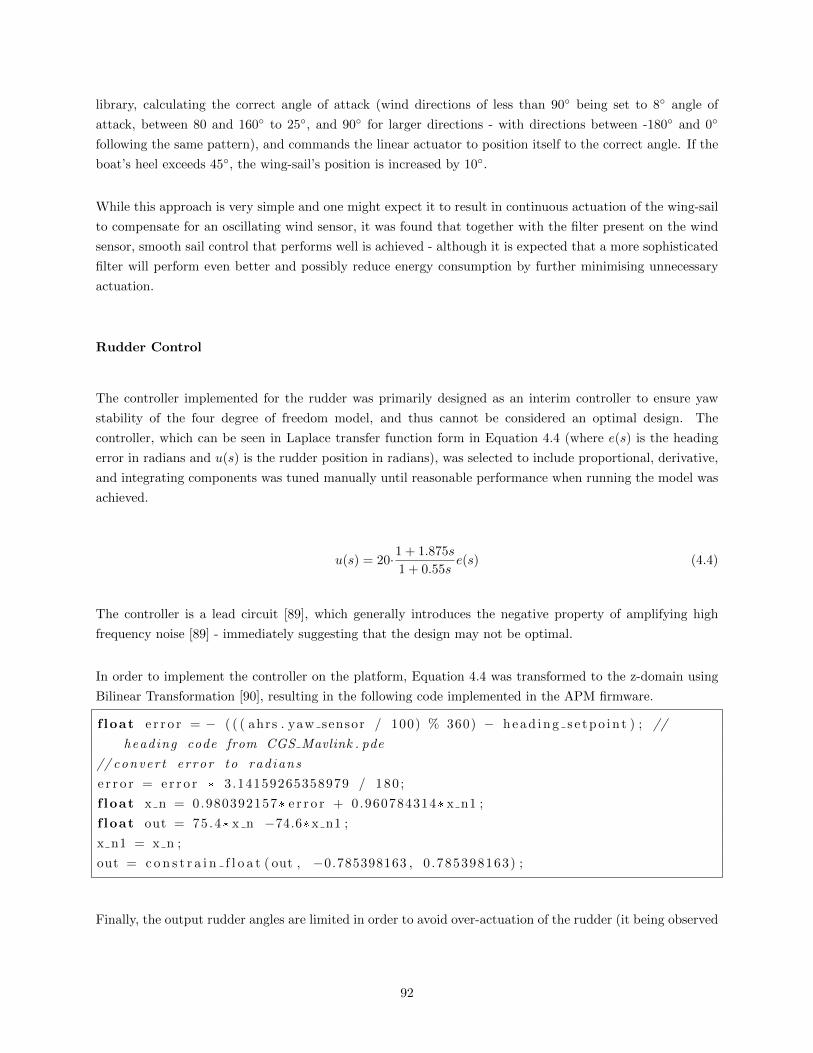
library, calculating the correct angle of attack (wind directions of less than 90 being set to 8 angle of
attack, between 80 and 160 to 25, and 90 for larger directions - with directions between -180 and 0
following the same pattern), and commands the linear actuator to position itself to the correct angle. If the
boat’s heel exceeds 45, the wing-sail’s position is increased by 10.
While this approach is very simple and one might expect it to result in continuous actuation of the wing-sail
to compensate for an oscillating wind sensor, it was found that together with the filter present on the wind
sensor, smooth sail control that performs well is achieved - although it is expected that a more sophisticated
filter will perform even better and possibly reduce energy consumption by further minimising unnecessary
actuation.
Rudder Control
The controller implemented for the rudder was primarily designed as an interim controller to ensure yaw
stability of the four degree of freedom model, and thus cannot be considered an optimal design. The
controller, which can be seen in Laplace transfer function form in Equation 4.4 (where e(s) is the heading
error in radians and u(s) is the rudder position in radians), was selected to include proportional, derivative,
and integrating components was tuned manually until reasonable performance when running the model was
achieved.
u(s) = 20·1 + 1.875s
1 + 0.55se(s) (4.4)
The controller is a lead circuit [89], which generally introduces the negative property of amplifying high
frequency noise [89] - immediately suggesting that the design may not be optimal.
In order to implement the controller on the platform, Equation 4.4 was transformed to the z-domain using
Bilinear Transformation [90], resulting in the following code implemented in the APM firmware.
f loat e r r o r = − ( ( ( ahrs . yaw sensor / 100) % 360) − head ing s e tpo in t ) ; //
heading code from CGS Mavlink . pde
// conver t er r or to rad ians
e r r o r = e r r o r * 3.14159265358979 / 180 ;
f loat x n = 0.980392157* e r r o r + 0.960784314* x n1 ;
f loat out = 75.4* x n −74.6* x n1 ;
x n1 = x n ;
out = c o n s t r a i n f l o a t ( out , −0.785398163 , 0 .785398163) ;
Finally, the output rudder angles are limited in order to avoid over-actuation of the rudder (it being observed
92

that a greater range resulted in potential damage to the platform)6 , while the manual rudder control
command is observed and allowed to override the controller if a large command is received. This was done
in order to facilitate sailing in a straight line before stepping this system, and provides the added advantage
of allowing emergency changes in direction without requiring a change in mode.
6It is further noted that an error in the implementation results in the limited range not being symmetrical, which is apparentin the results presented in Chapter 5. It is also noted that the current implementation does not account for variances in theneutral position of the rudder - which occurred during test due to slipping of the connection to the actuator.
93

Chapter 5
Results
This chapter details the results of tests that inform the conclusions of this study. Performance of the model
is established and validated against tests of the boat, while the effect of varying certain design parameters
is also explored. Results of the platform and model in their controlled modes are also presented.
While simulation results presented in this chapter have been generated using the model described in Chapter
3, a minor implementation error in the correct use of leeway angle and platform velocity when calculating
the side force was present when three degree of freedom model results were generated. While time did not
allow for correction of this error, its effect is considered negligible.
5.1 Platform Testing Details
Throughout this chapter, reference is made to tests of the hardware platform described in Chapter 4. Four
major tests constitute the sailing tests of the platform, with the final two providing the majority of the data
presented here. This section briefly describes each test. While some hardware development issues relevant
to the tests are noted, these are described more fully in Section 4.
1. First UCT Dam Test - 16 July 2014
An initial test was conducted in the dam adjacent to the University of Cape Town Upper Campus (referred
to as the UCT Dam). While the dam is relatively small and sheltered from the wind by its banks and
nearby trees (as seen in Figure 5.1a and 5.1b - noting that the bank not seen is much less of an obstruction),
which results in inconsistent and changing wind conditions, it provided a convenient means to ensure that
the platform operated correctly before major tests.
94

(a) (b)
(c)
Figure 5.1: Photographs of the platform during testing. (a) and (b) are of the platform at the UCT Dam(and are courtesy of Ms. Robyn Verrinder), showing the trees and banks surrounding the dam that obstructthe wind, while (c) is of the platform during the first Zeekoevlei test.
95
This test revealed challenges that existed with rudder actuation, communication using the RC controller,
and the GPS and provided data used to adjust the filters used on the wind sensor. The test was considered a
success for its confirmation that the platform operates as expected and it easily controlled in manual mode.
2. Second UCT Dam Test - 2 August 2014
A follow-up test was conducted in the UCT Dam, which confirmed that improvements to rudder actuation
were effective and allowed testing of the basic controller implemented on the boat. The test further revealed
that despite changing the GPS used on the platform, challenges still existed in obtaining a fix.
3. First Zeekoevlei Test - 15 August 2014
This was the first major test conducted at Zeekoevlei, a body of water in Grassy Park, Cape Town. Running
of the test was based at the UCT Yacht Club using a rigid-inflatable boat to follow the platform during the
test. Measurements using a hand-held anemometer revealed wind speeds of between 7.3 and 8.5 m/s.
This test revealed that the platform performed exceptionally well in the conditions present, but that GPS
challenges continued to exist.
4. Second Zeekoevlei Test - 17 August 2014
A final test was conducted at Zeekoevlei, during which the GPS performed well. Wind speeds between 4.3
and 6.6 m/s were noted. During the test it became apparent that the platform’s rudder occasionally slipped
- preventing accurate steering. Despite this, the platform was tested for an extended period - allowing the
logging of speed data.
A GPS track of the platform during this test is plotted in Figure 5.2 - where it can be seen that the test was
conducted over a relatively small area. This was a result of difficulties experienced with the rigid-inflatable
boat used to follow the platform, necessitating anchoring and sailing the platform around the larger boat.
5.2 Performance Prediction and Validation
This section presents the model’s predicted performance of the boat and validates it against test data. Two
system outputs are considered: the boat’s speed, and the model’s accuracy in predicting the yaw dynamics
of the boat. For the former output, use is made of the three degree of freedom model, while the four degree
of freedom model allows consideration of yaw.
96
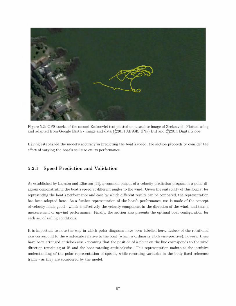
Figure 5.2: GPS tracks of the second Zeekoevlei test plotted on a satelite image of Zeekoevlei. Plotted usingand adapted from Google Earth - image and data ©2014 AfriGIS (Pty) Ltd and ©2014 DigitalGlobe.
Having established the model’s accuracy in predicting the boat’s speed, the section proceeds to consider the
effect of varying the boat’s sail size on its performance.
5.2.1 Speed Prediction and Validation
As established by Larsson and Eliasson [11], a common output of a velocity prediction program is a polar di-
agram demonstrating the boat’s speed at different angles to the wind. Given the suitability of this format for
representing the boat’s performance and ease by which different results can be compared, the representation
has been adopted here. As a further representation of the boat’s performance, use is made of the concept
of velocity made good - which is effectively the velocity component in the direction of the wind, and thus a
measurement of upwind performance. Finally, the section also presents the optimal boat configuration for
each set of sailing conditions.
It is important to note the way in which polar diagrams have been labelled here. Labels of the rotational
axis correspond to the wind-angle relative to the boat (which is ordinarily clockwise-positive), however these
have been arranged anticlockwise - meaning that the position of a point on the line corresponds to the wind
direction remaining at 0 and the boat rotating anticlockwise. This representation maintains the intuitive
understanding of the polar representation of speeds, while recording variables in the body-fixed reference
frame - as they are considered by the model.
97

Model Test Procedure
In order to determine the boat’s speed using the three degree of freedom model, it is necessary to determine
a wind speed, wind direction, and sail angle - together representing the sailing conditions for the test.
Generation of a polar diagram for a particular wind speed thus requires consideration of a range of wind
directions and the setting of the sail angle. As the optimal sail angle for each wind speed and direction
combination is not known, the test procedure requires considering possible sail angles and determining
which predicts the maximum forward speed. As running the test was a time consuming process, only sail
angles between 0 and the angle corresponding to 0 angle of attack were tested for each wind direction as
this the range in which a sail is usually operated.
Having established this approach to the test, data was determined using a Matlab script and analysis in a
spreadsheet. The Matlab script considers all wind speeds between 0 and 10 m/s, wind directions between
-180 and 180 every 10, and for each case evaluates a sail angle between 0 and 90 for wind directions
less than 0 and between 0 and -90 for wind directions greater than 0 but limited to a minimum angle of
attack of 0. The forward velocity for each case is logged for evaluation (the test currently not considering
leeway).
In order to evaluate these results, analysis was performed using a spreadsheet program. For each wind speed
and direction combination, the maximum forward speed was determined together with the sail angle at which
the maximum occurred.
Model Test Results
Results of the speed estimation aspect of this test are present in Figure 5.3 - which plots predicted forward
speeds for wind speeds between 1 and 10m/s on a single polar diagram.
This simple figure has a number of notable features:
In general, greater speeds are predicted for greater wind speeds while the speeds appear to be ap-
proaching the boat’s maximum speed as the wind speed increases.
The polar diagram is not perfectly symmetrical about the 0/180 axis, which is contrary to what one
would ordinarily expect.
This is attributed to the fact that the model considers the restoring heeling moment of the boat across
the full -89 to 89 range of heel angles (as opposed to simply taking the absolute value of the heel).
As the boat’s weight distribution in the y axis is not equal (the boat tending to heel slightly when no
wind is present) - primarily due to the heavy linear actuator being placed on the starboard side of the
deck - it will tend to heel more when the wind angle is negative (larger than 180) than when under
equivalent conditions with a positive wind angle.
98

Figure 5.3: Polar diagram showing maximum predicted forward speeds of the platform for different windspeeds and directions.
99

For lower wind speeds straight downwind performance (wind directions in the region of 180) appears
to be worse than that when reaching (downwind directions closer to 90 or 270), which is consistent
with the example result of a VPP presented by Larsson and Eliasson [11] with their note that a
VPP can assist a sailor determine the optimal downwind direction to sail (downwind velocity made
good). However the plot further reveals that at higher wind speeds the downwind speed appears
to be independent of wind direction (which is a result closer to that presented by Rynne and von
Ellenrieder [13], where straight downwind performance exceeded certain other downwind directions).
This indicates that for this platform it may be necessary to optimise navigation strategies for downwind
directions in low wind speeds, but that as the wind speed increases this is not necessary.
Having considered speed results, it is useful to consider the sail angles at which the predicted maximum
speeds occur. Such information is useful in the design of control algorithms, as discussed in Section 4.2.5.
Figure 5.4a shows the absolute value (in order to allow comparison of symmetries) of the optimal sail angle
for each angle of sail, while Figure 5.4b shows the optimal angle of attack.
A number of observations from this result are made:
While results for different wind speeds roughly correlate, differences in the optimal sail angle exist
- suggesting that the sail controller should take into account wind speed in order to ensure optimal
performance.
As with the polar diagram, and therefore as expected, the results are not symmetrical about the
0/180 centreline.
For some larger wind speeds the optimal sail angle for a wind direction of 180 is not the expected 90.
Inspection of a plot of the simulated speeds of the platform for a wind direction of 180 and wind
speed of 9m/s, seen in Figure 5.5a, shows that the predicted speed is approximately constant around
a sail-angle 90 - suggesting that this result can be attributed to modelling errors.
The increase in angle of attack at approximately 50 wind direction is very large for a wind speed of
6m/s (and to a lesser extent 7m/s).
Plots of the angle of attack of the sail against the predicted speed for various wind directions with a
wind speed of 6m/s, seen in Figure 5.5b provide some insight regarding this result. The plot shows
how the two local maximums of predicted speed result in the sharp increase in optimal angle of attack,
while showing how at larger angles of attack the predicted speed is approximately constant. Based
on this observation, the unexpected increase in optimal angle of attack is also attributed to modelling
errors.
Ultimately it is concluded that variations in the predicted optimal sail angles necessitate the sensitivity
analysis in Section 5.3.1 in order to determine to what extent wind speed should be considered by the sail’s
controller.
100

(a)
(b)
Figure 5.4: Optimal sail settings as wind direction varies for different wind speeds. (a) shows the optimalsail angle (relative to the boat), while (b) shows the optimal angle of attack (relative to the wind).
101

(a) Simulated forward speed with a wind direction of180. Zero speeds seen for the 9m/s result are a result ofthe model predicting a capsize under these conditions.
(b) Forward speed for various wind directions and windspeed of 6m/s.
Figure 5.5: Specific results of testing of the model. (a) shows how predicted forward speeds for wind with aspeed of 9m/s and direction of 180 are approximately constant for sail angles around 90, suggesting thatthe prediction of an optimal sail angle of less than 90 may be a simulation error. (b) shows how two localmaximums in the predicted forward speed of the platform suggest that an unexpected increase in optimalangle of attack at 6m/s as wind direction varies can be attributed to a simulation error.
It is also useful to note two further observations regarding the results in Figure 5.5 (which is presented
primarily as a means to explain the above observations). First, one can see in Figure 5.5a that for certain
sail angles when sailing downwind in 9m/s of wind platform speeds of zero are predicted, while this is not
the case for a wind speed of 6m/s. This is attributed to the large side-forces produced by the wing-sail for
certain sail angles, resulting in the boat capsizing (the model stops a simulation if a capsize is predicted).
This indicates that control of the platform becomes more difficult as the wind speed increases.
Secondly, it is seen in Figure 5.5b that for smaller wind directions (specifically 50), the forecast speed
increases with angle of attack before dropping to zero. The zero speed is attributed to the test not considering
sail angles past the 0 point, meaning that in reality the platform is not expected to have zero speed for larger
angles of attack. In the case of larger wind directions it is seen that consistent performance is simulated for
a wide range of angles of attack (contrast with the narrow range in which the optimal speed is observed for
a direction of 50). Together, these observations suggest that considering sail angles past the 0 point may
result in simpler control of the platform - a hypothesis which informs the study of this point in Section 5.5.2.
Model Validation
In order to validate these results, the results of the second Zeekoevlei test (test 4) of the boat were considered
as this test included GPS data. Before processing, the two log files that made up the test were combined
after sections at the beginning and end of each (which did not correlate to the actual sailing of the boat) were
removed. In addition, it is important to note that all results have been presented alongside model results for
wind speeds of 4, 5, 6, and 7m/s as these speeds cover the range of the majority of wind speeds noted by a
hand-held anemometer during the test (the minimum recorded speed was 4.3m/s and the maximum 6.6m/s
102

however the majority of readings fell between 4 and 5 m/s)1.
As an initial approach, the logged data from the test was assessed and each ground speed data-point was
allocated to one of 36 groups of data correlating to the wind direction relative to the boat at that time. In
each group, the maximum speed was found and the results were plotted in Figure 5.6a. While this approach
seems reasonable, one can see that it results in substantial ground speeds being recorded for the boat when
sailing directly into the wind - assumed to be a result of the boat’s velocity as it tacked across the wind.
In order to confirm this hypothesis, the work of Rynne and von Ellenrieder [13] was considered. In their
comparison of results measured using their platform with performance predicted with their VPP, Rynne and
von Ellenrieder plot their platform’s speed against its angle to the wind across their entire 7.5 minute test -
while applying “some data processing” including the removal of data correlating to the tacking manoeuvre.
This approach was considered, however simply disregarding the data from tacking was considered inappro-
priate as it is unclear at what point data should be excluded and because during the test the boat completed
turns that did not necessarily involve tacking. For these reasons the change in heading was considered (by
finding the difference between logged heading values) and speed data logged while the change in heading
was greater than 0.01745 rad/s (determined by manual inspection of the data) was disregarded.
The results of this approach are seen in Figure 5.6b, where it is apparent that the problem persists -
presumably because the boat decelerates during a turn slower than it turns. While it might be possible
to only consider data during periods of extended constant heading, this process would require filtering of
heading data (due to the presence of noise) and the definition of criteria for the consideration of data.
Furthermore, the limited data logged during the test is likely to result in an incomplete polar diagram. As
an alternative, periods during which the boat was in steering mode were considered as these correlate to
periods of constant heading (despite the challenges experienced with the rudder during the test).
The result of limiting consideration to the steering mode is seen in Figure 5.6c. Due to the limited number of
periods during which this mode was enabled during the test, and thus the limited wind directions for which
there is data, the plot is clearly incomplete.
Given that inspection of the speeds for a wind direction of 0 revealed that the large maximum speed was the
result of a small number of data points, as a final approach the data points for each point were considered
and the 75th percentile (upper quartile) was set as the speed for that direction. The result of this approach
is seen in Figure 5.6d, and while certainly still subject to inaccuracies due to turning, can be considered to
show that test results are in broad agreement with those obtained from the model. It is important to note
that the speed predicted in the 0 wind direction can be attributed to both inaccuracies due to turning and
the size of the wind direction groups, as a speed logged at (for example) 4 will be considered as part of the
0 group.
It is useful to note Figure 5.7, which plots the number of speed data-points logged for each wind direction.
The limited number of data-points for some wind directions indicates that a longer test may result in better
1Ideally these speeds would be corrected for the height at which they were noted in terms of the wind gradient discussed inSection 3.2.1, however given the range of wind speeds noted during the test this was not considered necessary.
103

(a) Maximum logged speed. (b) Maximum speed subject to a yaw rate limit.
(c) Maximum speed while in steering mode. (d) Speed at the 75th percentile.
Figure 5.6: Comparison of the speed of the platform during the second Zeekoevlei test, subject to variousforms of data processing, with forward speeds predicted by the model.
104
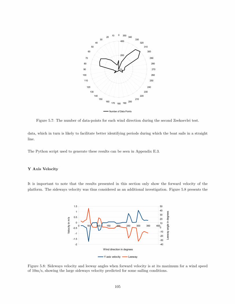
01020
30
40
50
60
70
80
90
100
110
120
130
140
150160
170 180 190200
210
220
230
240
250
260
270
280
290
300
310
320
330340
350
0
200
400
Number of Data Points
Figure 5.7: The number of data-points for each wind direction during the second Zeekoevlei test.
data, which in turn is likely to facilitate better identifying periods during which the boat sails in a straight
line.
The Python script used to generate these results can be seen in Appendix E.3.
Y Axis Velocity
It is important to note that the results presented in this section only show the forward velocity of the
platform. The sideways velocity was thus considered as an additional investigation. Figure 5.8 presents the
Figure 5.8: Sideways velocity and leeway angles when forward velocity is at its maximum for a wind speedof 10m/s, showing the large sideways velocity predicted for some sailing conditions.
105
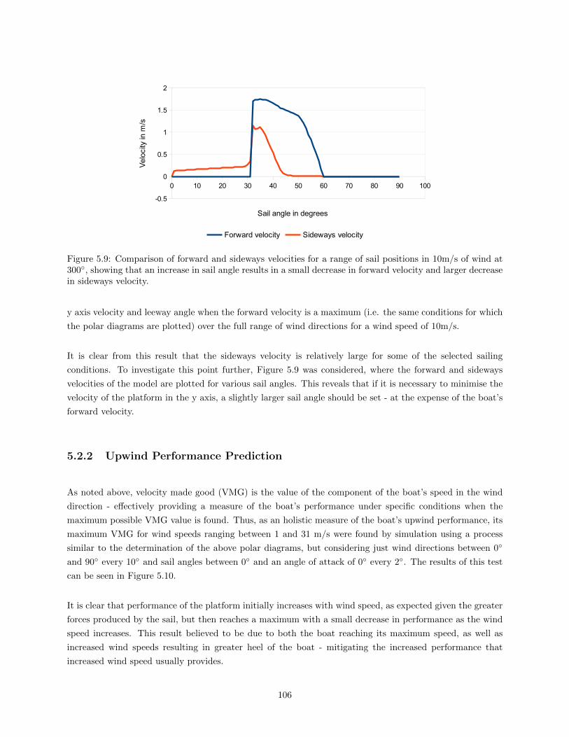
Figure 5.9: Comparison of forward and sideways velocities for a range of sail positions in 10m/s of wind at300, showing that an increase in sail angle results in a small decrease in forward velocity and larger decreasein sideways velocity.
y axis velocity and leeway angle when the forward velocity is a maximum (i.e. the same conditions for which
the polar diagrams are plotted) over the full range of wind directions for a wind speed of 10m/s.
It is clear from this result that the sideways velocity is relatively large for some of the selected sailing
conditions. To investigate this point further, Figure 5.9 was considered, where the forward and sideways
velocities of the model are plotted for various sail angles. This reveals that if it is necessary to minimise the
velocity of the platform in the y axis, a slightly larger sail angle should be set - at the expense of the boat’s
forward velocity.
5.2.2 Upwind Performance Prediction
As noted above, velocity made good (VMG) is the value of the component of the boat’s speed in the wind
direction - effectively providing a measure of the boat’s performance under specific conditions when the
maximum possible VMG value is found. Thus, as an holistic measure of the boat’s upwind performance, its
maximum VMG for wind speeds ranging between 1 and 31 m/s were found by simulation using a process
similar to the determination of the above polar diagrams, but considering just wind directions between 0
and 90 every 10 and sail angles between 0 and an angle of attack of 0 every 2. The results of this test
can be seen in Figure 5.10.
It is clear that performance of the platform initially increases with wind speed, as expected given the greater
forces produced by the sail, but then reaches a maximum with a small decrease in performance as the wind
speed increases. This result believed to be due to both the boat reaching its maximum speed, as well as
increased wind speeds resulting in greater heel of the boat - mitigating the increased performance that
increased wind speed usually provides.
106

Figure 5.10: The maximum velocity made good values for the platform for a range of wind speeds determinedfrom the model.
As a further assessment, the wind directions for which the VMG for a given wind speed is at its maximum
are plotted in Figure 5.11. This reveals that for low wind speeds it is more efficient to sail at greater angles
to the wind than at speeds above 5m/s, after which further increases in wind speed do not effect the optimal
wind direction.
5.2.3 Yaw Prediction Validation
In order to validate the predictions of the four degree of freedom model, a comparison between the a gybe
(turning away from the wind) logged during the second Zeekoevlei test (test 4) and the results of the
equivalent action in the model was made.
Given that the sail and rudder angles sent to the boat during the test (the boat being in manual mode) are
highly dependent on situational conditions (specifically the state of the boat at that point, which in turn is
a result of changes in the wind and other environmental factors), direct application of the logged commands
to the four degree of freedom model was considered inappropriate. For this reason this comparison compares
the logged data with the path taken by the model to pass through the same initial and final positions as
determined by the heading of the boat. During the simulation, the model was allowed 80 seconds to reach a
steady state that matches the initial heading of the logged data before the final heading was set as the new
heading set-point.
The results of this test, seen in Figures 5.12 and 5.13, demonstrate approximate agreement between the
results from the platform and those from the model, however it is noted that the model takes approximately
20 seconds longer than the platform to complete the turn - despite maintaining a higher speed. This suggests
107

Figure 5.11: The wind directions for which the boat’s velocity made good is a maximum for given windspeeds determined from the model.
that the model currently under-predicts the yaw moment due to the rudder. It is also notable that both
ground-speed results see the speed decrease as the turn begins before increasing again - presumably a result
of the sail producing more force as the boat heads downwind in the middle of the turn.
It is noted that the rudder angles of the platform presented in these results cannot be considered to be
accurate due to implementation errors and because of use of the RC controller’s offset function to adjust
the centre position, a setting that is not logged as it occurs separate from the electronic platform. This
means that while Figure 5.12b shows platform angles between -45 and 45, actual angles are unlikely to
have occurred over this range. Slippage of the rudder during the test also contributes to this limitation of
the logged data.
5.2.4 Effect of Varying Sail Parameters
Sail design is naturally an important design parameter of a sailboat - and so here the effect of varying the
size of the wing-sail is considered by using maximum velocity made good as a measure of performance. It
has been assumed that a rectangular NACA0018 wing-sail will continue to be used, and thus the effects of
using alternative aerofoils, wing shapes, or configurations (such as self-trimming wing-sails or dual wing-sail
designs) have not been evaluated. This results in the assessment of two parameters: the span and chord of
the wing-sail.
Together, these parameters determine the area and aspect ratio of the wing-sail - and thus variation of both
were considered. First, alternative areas were simulated by halving and doubling the areas (by multiplying
the span and chord by√
0.5 and√
2 respectively) and running the VMG test procedure discussed previously.
108
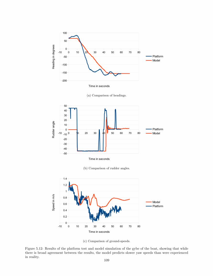
(a) Comparison of headings.
(b) Comparison of rudder angles.
(c) Comparison of ground-speeds.
Figure 5.12: Results of the platform test and model simulation of the gybe of the boat, showing that whilethere is broad agreement between the results, the model predicts slower yaw speeds than were experiencedin reality.
109
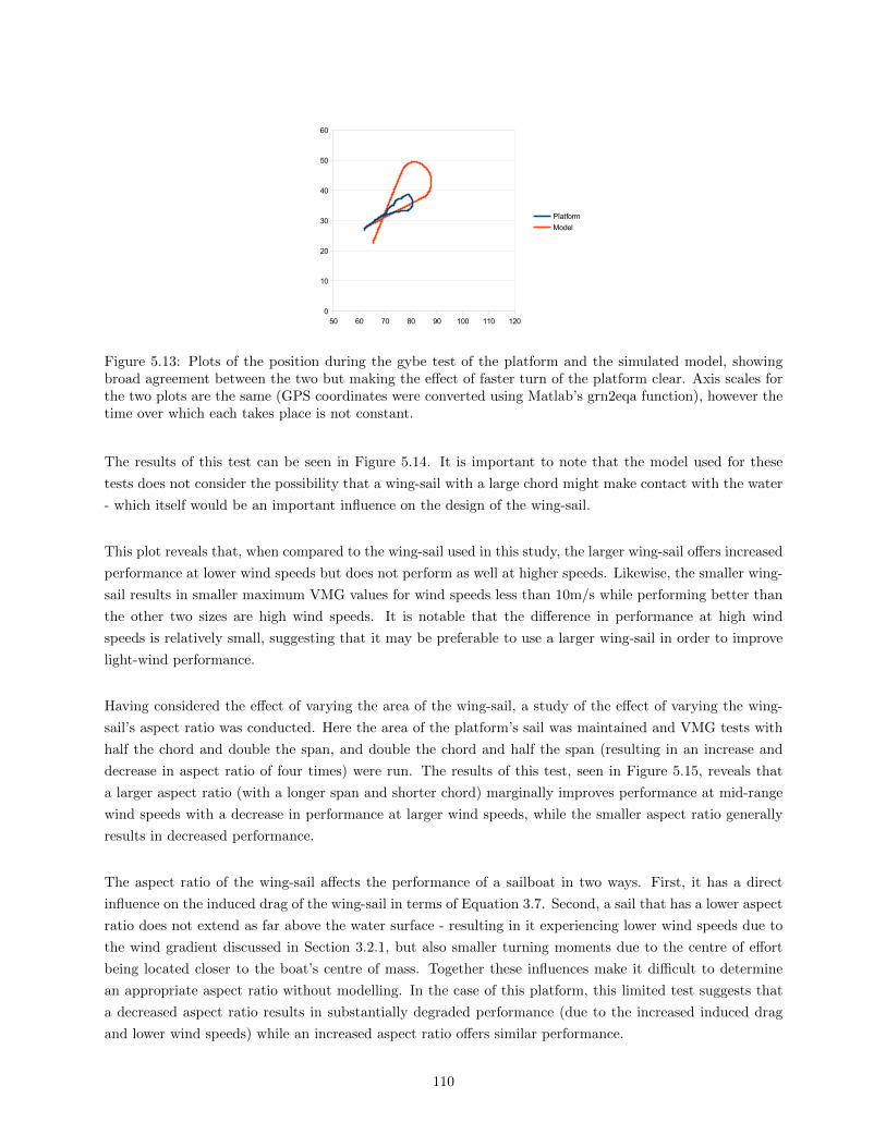
Figure 5.13: Plots of the position during the gybe test of the platform and the simulated model, showingbroad agreement between the two but making the effect of faster turn of the platform clear. Axis scales forthe two plots are the same (GPS coordinates were converted using Matlab’s grn2eqa function), however thetime over which each takes place is not constant.
The results of this test can be seen in Figure 5.14. It is important to note that the model used for these
tests does not consider the possibility that a wing-sail with a large chord might make contact with the water
- which itself would be an important influence on the design of the wing-sail.
This plot reveals that, when compared to the wing-sail used in this study, the larger wing-sail offers increased
performance at lower wind speeds but does not perform as well at higher speeds. Likewise, the smaller wing-
sail results in smaller maximum VMG values for wind speeds less than 10m/s while performing better than
the other two sizes are high wind speeds. It is notable that the difference in performance at high wind
speeds is relatively small, suggesting that it may be preferable to use a larger wing-sail in order to improve
light-wind performance.
Having considered the effect of varying the area of the wing-sail, a study of the effect of varying the wing-
sail’s aspect ratio was conducted. Here the area of the platform’s sail was maintained and VMG tests with
half the chord and double the span, and double the chord and half the span (resulting in an increase and
decrease in aspect ratio of four times) were run. The results of this test, seen in Figure 5.15, reveals that
a larger aspect ratio (with a longer span and shorter chord) marginally improves performance at mid-range
wind speeds with a decrease in performance at larger wind speeds, while the smaller aspect ratio generally
results in decreased performance.
The aspect ratio of the wing-sail affects the performance of a sailboat in two ways. First, it has a direct
influence on the induced drag of the wing-sail in terms of Equation 3.7. Second, a sail that has a lower aspect
ratio does not extend as far above the water surface - resulting in it experiencing lower wind speeds due to
the wind gradient discussed in Section 3.2.1, but also smaller turning moments due to the centre of effort
being located closer to the boat’s centre of mass. Together these influences make it difficult to determine
an appropriate aspect ratio without modelling. In the case of this platform, this limited test suggests that
a decreased aspect ratio results in substantially degraded performance (due to the increased induced drag
and lower wind speeds) while an increased aspect ratio offers similar performance.
110

Figure 5.14: Maximum velocity made good as a function of wind speed for different sail areas, showing thatsmaller wing-sails peform better at low wind speeds than larger wig-sails but that the opposite is the casefor high speeds.
Figure 5.15: Maximum velocity made good as a function of wind speed for different wing-sail aspect ratios,showing that a smaller aspect ratio results in degraded performance while a larger aspect ratio results insimilar performance with some degradation at higher wind speeds.
111

This result demonstrates that a correctly designed wing-sail is important for optimal performance of a
sailboat, and shows that there is some benefit to being able to adjust the sail’s size for different conditions
(which is common on large yachts) - but that this is less than expected. It is noted that this study has not
considered the effect of varying sail parameters on the sensitivity results in Section 5.3.2 below - which may
provide further insight into the value of the ability to vary sail area.
5.3 Sail Control Requirement Analysis
An important aspect of control of an autonomous sailboat is control of its sail. For this reason investigations
were undertaken to determine the expected amount of actuation necessary to control the sail of the boat.
The small range of optimal lift-to-drag ratio observed in Figure 3.3 in Section 3.2.1 suggests that it may be
important to accurately maintain the wing-sail’s angle of attack, however further analysis is necessary to
determine the effect on the entire system.
5.3.1 Wing-sail Analysis
As an initial approach, the driving and side forces of the wing-sail, which are a result of both lift and drag,
were considered in order to establish the effect of varying the angle of attack of the sail. The method of
calculating these forces described in Section 3.2.1 (but implemented using the sail forces block in the Simulink
model) was used to plot the driving force, side force, and driving to side force ratio as the angle of attack
of the wing-sail (with respect to the wind direction) is varied for different directions of sail. The results of
this are seen in Figure 5.16. It is noted that a wind-speed of 7.17m/s, approximately equal to 15 knots, was
arbitrarily selected for consideration here and that it is not expected that variation of this parameter will
affect the conclusions drawn from these initial results.
A number of important preliminary conclusions regarding this can be drawn. The first is that as the wind
direction increases, the predicted driving force tends to have two local maxima, and that for wind directions
greater than 90 the maxima at the larger angle of attack results in a greater driving force. This is a result
of both lift and drag contributing to the driving force for wind directions greater than 90 (for small wind
directions drag acts to cancel out lift, which results in negative driving forces for large angles of attack). The
second is that for wind directions less than 90 the optimal angle of attack is approximately constant, while
for larger wind directions the optimal value increases. Finally, for wind directions less than 90 the control
requirement for the wing-sail appears to be very small (Figure 5.16c presents the same data in that region,
making this more apparent), while larger wind directions appear to be more tolerant.
These conclusions suggest that when sailing upwind accurate control of the wing-sail is important, but from
these results it is unclear what this requirement is in a quantified form. For downwind sailing the control
requirement appears to be less strict, but again this needs to be quantified and - as seen below - other
considerations are not taken into account here.
112

(a) Driving force produced by the wing-sail for different wind directions (in degrees) as angle of attack varies.
(b) Side force produced by the wing-sail for different wind directions (in degrees) as angle of attack varies.
(c) Figure 5.16a limited to angles of attack between 0 and 30.
Figure 5.16: Driving and side forces produced by the wing-sail for various wind directions and wing-sailangles of attack at a wind speed of 7.17m/s.
113
5.3.2 Three Degree of Freedom Model Sail Analysis
While the above results allow preliminary conclusions regarding wing-sail control requirements to be drawn,
it is necessary to consider the effect of changing the wing-sail angle on the whole system so that hydrodynamic
and other forces are taken into account.
To this end, data recorded during the model tests conducted to determine the polar diagrams in Section 5.2.1
(which is a record of the predicted speed of the platform for each sail angle, wind direction, and wind speed
combination) was assessed using the Python script seen in Appendix E.3. The script allows, for each of the
available wind speeds, for consideration of each wind direction and its maximum predicted speed and in each
case the determination of the minimum2 amount of change in sail position required for a 30% reduction in
speed (other percentages naturally being possible) and the range of sail angles over which the platform is
predicted to perform within 30% of its maximum speed. The former result is seen in Figure 5.17a and the
later in Figure 5.17b.
These results reveal important considerations in the control of the wing-sail. First, in general the minimum
change from the optimal position seen in Figure 5.17a shows that in general for wind directions less than
90 the tolerance for a variation in sail angle is very small - in many cases one, or even zero, degrees. This
is almost certainly a result of the small angle of attack required for maximising speed seen in Figure 5.16a -
a small adjustment in sail angle results in a near-zero angle of attack, which results in the sail producing no
lift.
The second important consideration is that there is a clear decrease in the minimum change in sail position
as the wind speed increases - which indicates that the control requirement of the wing-sail becomes stricter
as the wind speed increases. One might not expect there to be a strict control requirement when sailing
downwind (as is the case with smaller wind speeds), however as previously noted this effect is attributed to
large side-forces resulting in the boat capsizing under these conditions
The third important consideration lies in the result seen in Figure 5.17b, where greater tolerances can be
seen in the range of wing-sail angles over which performance within 30% of the maximum is achieved. This
leads to the conclusion that greater performance requires stricter control requirements for the wing-sail, and
that (particularly for higher wind speeds) it may be necessary to avoid attempting to achieve optimal speed.
As with other results, those seen in Figure 5.19 are not smooth (as might be expected) and behaviour as
wind speed and direction are varied is not consistent. This is attributed to the various non-linearities in the
model, including the data generated from the CAD model and the use of linear-interpolation to determine
regression parameters.
2If the minimum change should arise due to the wing-sail being actuated to its +/-90 position this value is disregarded -however it is considered for the range of sail angles test.
114

(a) The minimum change in sail angle required for a 30% reduction in boat speed for various wind speeds anddirections.
(b) The range of sail angles that result in the platform performing within 30% of its maximum speed for variouswind speeds and directions.
Figure 5.17: Results of the sensitivity analysis on the three degree of freedom model, showing the change ofsail position required for a 30% decrease in forward speed. The results show that as wind speed increasesthe amount of change in position required decreases - reflecting a stricter control requirement.
115
5.4 Steering Control Analysis
This section presents the results of tests of the prototype controller described in Section 4.2.5, implemented
on both the model and the prototype platform. An overview of the controller’s performance is presented
together with conclusions regarding how it might be improved.
5.4.1 Results of Simulations
First, it is useful to consider the results of simulations of the controller’s performance. It is noted that the
preliminary sail controller (which was based on preliminary modelling results) is used as that is what was
implemented on the platform. Tests of the model make use of a wind speed of 8m/s in order to approximately
match the conditions during the first Zeekoevlei test (test 3), while the heading set-point is set arbitrarily
as -15 with a wind direction of 70.
Figure 5.18a presents the results of this test without environmental disturbances arising from the wind,
showing that while the model takes some time to reach the set-point (in part a result of its initial velocity
being zero, requiring it to gain speed before the rudder becomes effective), once the set-point is reached it is
maintained with no actuation of the rudder. This result is expected given the lack of disturbances.
The test was repeated with environmental disturbances enabled, the result being seen in Figure 5.18b. Here it
can be seen that the boat does entirely maintain its heading and that rudder actuation is necessary - however
both the heading error and amount of actuation required are very small, indicating that the disturbances
are small.
5.4.2 Results of Prototype Controller Tests
This section presents the results of tests of the prototype controller described in Section 4.2.5. During tests
2-4 (the second UCT Dam test and the two Zeekoevlei tests) the APM platform’s steering mode was enabled
a number of times. Preliminary inspection of the logged data during these tests reveal promising results
from the second UCT Dam test and first Zeekoevlei test, however due to the difficulties experienced with
the platform’s rudder during the second Zeekoevlei test its results have not been considered here.
Three periods during which steering mode was enabled are presented here - selected as periods during which
the mode was enabled for an extended period and for notable features discussed below. It is noted that the
set-point for each set of results is the heading of the boat at the time the test begins, and that due to the
way in which data is logged it is possible that the first heading shown does not match the set-point recorded
by the boat.
116

(a) Model heading without wind variation.
(b) Model heading with wind variation.
Figure 5.18: Results of a simulation of the platform’s controller with (b) and without (a) disturbances dueto variations in the wind. The results show that the variations in wind have little effect on the heading ofthe simulated boat.
117
The three results are as follows:
The result seen in Figure 5.19a, a period during the second UCT Dam test (test 2). This result, which
was achieved during very low wind speeds, suggests that the controller is able to maintain the boat’s
heading but that the rudder cycles between its limits. Video footage of the second UCT Dam test
confirms that the large variations in heading seen at the end of the logged period are a result of a
sudden gust of wind, effectively a disturbance on the system.
Figure 5.19b shows a period during the first Zeekoevlei test (test 3), where the boat appears to take
some time to return to its set-point once the steering mode was enabled before maintaining its heading
(after approximately the 660 seconds point) while exhibiting the same rudder behaviour observed
above.
Figure 5.19c, which shows a second period during the first Zeekoevlei test. Here it can be seen that
the boat drifts beyond its set-point (confirmed by the rudder being set to its maximum angle). While
it appears that the boat may be beginning to return to its set-point toward the end of the test period,
this may simply be the result of environmental disturbances.
The long periods during the first Zeekoevlei test (seen in the later two results) where the controller does
not maintain the boat’s heading are surprising given the ease of control experienced when manual mode
was engaged. It is assumed that this may be a result of the setting of the sail, however further testing and
analysis is necessary to confirm this. It is also noted that this may be the result of the controller assuming
a different neutral position to that on the platform, an error which may have arisen when the rudder lost its
alignment.
These results demonstrate that while the controller appears to be capable of maintaining the boat’s heading,
it is clearly sub-optimal due to the observed cycling of the rudder between its limits and lack of performance
during the second Zeekoevlei test. It is also notable that there are substantial disturbances present in the
platform test data that are not predicted by the model, suggesting that sources of disturbances other than
wind - such as waves - should be accounted for.
5.5 Alternative Designs and Configurations
Drawing on the above results, this section presents an alternative configuration and approach to the existing
platform, and briefly discusses an alternative sailboat design.
118
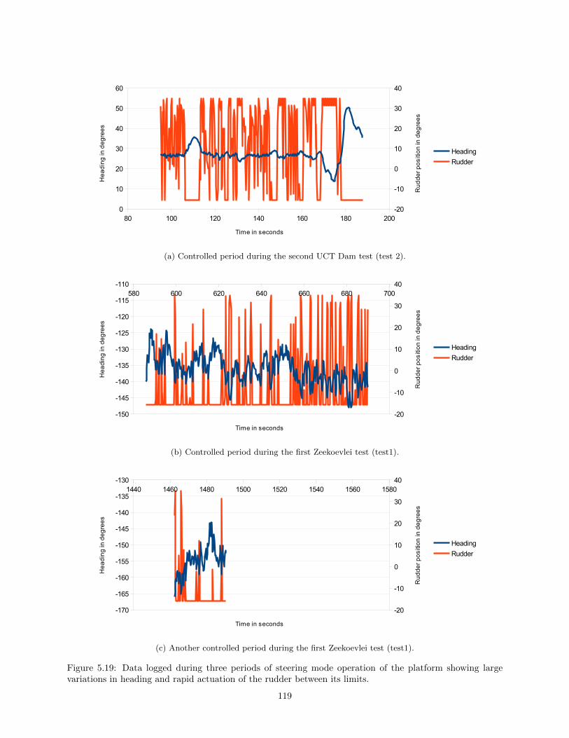
(a) Controlled period during the second UCT Dam test (test 2).
(b) Controlled period during the first Zeekoevlei test (test1).
(c) Another controlled period during the first Zeekoevlei test (test1).
Figure 5.19: Data logged during three periods of steering mode operation of the platform showing largevariations in heading and rapid actuation of the rudder between its limits.
119

Figure 5.20: Result of the simulation of the model with a fully-rotating wing-sail, showing that there is littlebenefit to such a modification to the platform.
5.5.1 Fully Rotating Wing-Sail
The platform developed in this study limits the rotation of the wind-sail to a range of -90 to 90, not unlike
a traditional sailboat where supports for the mast prevent the sail from rotating further. Given the result
presented in Figure 5.5a, which suggests that sail angels greater than 90 might continue the wide range
of consistent performance across sail angles, the boat’s performance with greater sail angles is investigated.
The script used to generate the polar diagrams in Section 5.2.1 was adapted to consider wind directions
between 90 and 180 and for each sail angles between 0 and -180 for the single wind speed of 10m/s. The
result of this test is seen in Figure 5.20.
This result indicates that constant behaviour is observed for greater sail angles, but that there is little (or
negligible) increase in performance. This leads to the simple conclusion that there is no benefit to adapting
the platform to allow the wing-sail to fully rotate.
5.5.2 Wing-sail Angles Beyond the Centreline
Based on the results seen in Figure 5.5b, a hypothesis was made in Section 5.2.1 that increasing the wing-
sail angle beyond the centre-line may result in increased performance of the boat. To test this, the polar
diagram script in Section 5.2.1 was adapted to consider wind directions 0 and 90 and for each angles of
attack between 0 and 90 (which all, except in the case of the 90 wind direction, cross the centreline). The
script was run for a wind speed of 6m/s, and the results are seen in Figure 5.21.
This result reveals that there is only a small benefit to performance if the wing-sail is set across the centreline,
and then only for a small range of angles before zero speed is predicted. Despite the results that led to the
120
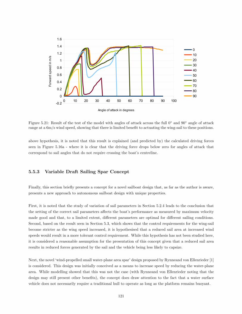
Figure 5.21: Result of the test of the model with angles of attack across the full 0 and 90 angle of attackrange at a 6m/s wind speed, showing that there is limited benefit to actuating the wing-sail to these positions.
above hypothesis, it is noted that this result is explained (and predicted by) the calculated driving forces
seen in Figure 5.16a - where it is clear that the driving force drops below zero for angles of attack that
correspond to sail angles that do not require crossing the boat’s centreline.
5.5.3 Variable Draft Sailing Spar Concept
Finally, this section briefly presents a concept for a novel sailboat design that, as far as the author is aware,
presents a new approach to autonomous sailboat design with unique properties.
First, it is noted that the study of variation of sail parameters in Section 5.2.4 leads to the conclusion that
the setting of the correct sail parameters affects the boat’s performance as measured by maximum velocity
made good and that, to a limited extent, different parameters are optimal for different sailing conditions.
Second, based on the result seen in Section 5.3, which shows that the control requirements for the wing-sail
become stricter as the wing speed increased, it is hypothesised that a reduced sail area at increased wind
speeds would result in a more tolerant control requirement. While this hypothesis has not been studied here,
it is considered a reasonable assumption for the presentation of this concept given that a reduced sail area
results in reduced forces generated by the sail and the vehicle being less likely to capsize.
Next, the novel ‘wind-propelled small water-plane area spar’ design proposed by Rynneand von Ellenrieder [1]
is considered. This design was initially conceived as a means to increase speed by reducing the water-plane
area. While modelling showed that this was not the case (with Rynneand von Ellenrieder noting that the
design may still present other benefits), the concept does draw attention to the fact that a water surface
vehicle does not necessarily require a traditional hull to operate as long as the platform remains buoyant.
121

flaps to act as rudderand add camber towing-sail
Lower sectioncontaining lead (the keel) and electronics
Water tanks andwater pumps
Independentlyactuated rotationpoints
Figure 5.22: Diagram showing an overview of the variable draft sailing spar.
This leads to the proposal presented here: a spar divided into multiple sections, each capable of orientating
themselves at different angles relative to each other and having the same cross section. Sections above the
water surface act as the sail, while sections below act as the keel. Sections in the middle are capable of filling
and emptying water tanks to increase and decrease their density, leading to the platform sinking or floating
deeper or out of the water and changing the volume of the underwater section and area of the sail. Such an
approach allows the sail area to be reduced, reducing forces generated by the sail. It is noted that the design
does result in the centre of mass moving closer to the water surface, which reduces the moment arm to the
restoring force resulting from buoyancy - however as the centre of effort also moves closer to the centre of
mass due to the decreased sail span it is assumed that this is not problematic, but modelling would confirm
this.
Figure 5.22 presents a visualisation of this concept, where it can be seen that trailing edge flaps are envisioned
to act as rudders and adjust the camber of the wing-sail (potentially assisting with performance). Figure
5.23 further demonstrates the concept, showing how the platform would vary its draft.
Clearly this proposal is conceptual and requires further analysis to conclude whether the envisioned benefits
hold. This process should include design of the platform to ensure that it is possible to construct while
maintaining the ability to vary draft and appropriate modelling to validate the expected performance and
verify that the platform can be controlled.
122

(a) (b)
Figure 5.23: Diagrams showing the variable draft sailing spar’s ability to adjust its effective sail area bysinking into the water.
123

Chapter 6
Conclusions and Recommendations
Conclusions of and recommendations arising from the study are presented in this chapter.
6.1 Conclusions
This study has involved the successful development of two important aspects of the development of an
autonomous sailboat: modelling of the dynamics of a small sailboat and the assembly of a prototype platform
suitable for the validation of the model, testing of control strategies, and facilitation of other work in the
field. A comprehensive review of the field of autonomous sailing has also been presented.
Conclusions regarding the prototype platform will be presented first, followed by those based on modelling
and simulation.
Platform Development
While being an anecdotal conclusion, it is first noted that observations of the prototype platform sailing
suggest that its construction can be considered a success. The platform sails well, is manoeuvrable under
manual control, and is operational in light to medium wind speeds - as well as in the presence of small waves.
More specifically, the platform did not leak during field tests (with the exception of the ingress of a small
amount of water when towed at speed with part of the deck underwater), was capable of sailing both upwind
and downwind, and the electronic platform performed without incident.
124

Despite this success, two principle limitations exist with the platform. First, difficulties experienced with the
rudder during the final test indicate that the current design is too easily damaged. Second, the data received
from the wind speed sensor is currently unusable. However these issues can easily be addressed and do not
limit the full potential of the platform. Other limitations, such as battery life, are design compromises and
are thus considered acceptable.
System Modelling
This study has presented a comprehensive overview of its approach to modelling by drawing on methods
described in the literature and making appropriate improvements. These have included correcting errors
and devising an approach to modelling of aspects of the J-Class style hull of the prototype platform where
the methods described in the literature do not apply. This process has also involved a detailed examination
of the process of determining the parameters of the prototype platform in order to inform the model.
The model has been validated by comparing the maximum simulated forward speeds for various sailing
conditions with the ground-speed of the prototype platform during the final field test, as determined by its
GPS module. This has revealed broad agreement between the model and the field test results, although
comparison is made difficult by the range of wind speeds observed during the field test - meaning that
it is unclear whether results are accurate for their corresponding wind speed. Despite this limitation, it
is clear that the model predicts speeds that are consistent with those experienced by the platform over a
corresponding range of wind speeds.
Further validation of the dynamic behaviour of the model has been performed by comparing a gybe of
the prototype platform with the equivalent action modelled using the four degree of freedom model. This
test has again revealed broad agreement between results, but shows that the model currently appears to
under-estimate the turning moment generated by the boat’s rudder as the model turns more slowly than the
prototype platform. It is assumed that this may be a result of the method used to determine the size of the
rudder (when modelled as a flap) relative to the hull and keel. The limited quantity of field test data means
that a full study of this limitation is difficult, but given that aside from the turning speed the behaviour of
the model and platform are consistent (including in the form of increases and decreases of speed during the
gybe), it is concluded that this is not a fundamental flaw.
The results of simulations provide results that can inform control of the sailboat. First, the optimal sail-angle
for different wind directions and speeds was determined - showing that wind speed does affect control of
the wing-sail. However, results of a sensitivity analysis of the the wing-sail suggest that to a certain extent
this is mitigated by tolerances in the system. The sensitivity analysis, which established to what extent
not setting the wing-sail to its optimal position affects performance, revealed that the control requirement
on the wing-sail becomes stricter as wind speed increases and that it may be preferable to set the sail to a
sub-optimal position in order to maximise tolerances in either direction.
A further set of simulations established the upwind performance of the sailboat - showing that its maximum
125
velocity made good (the component of its velocity vector in the direction from which the wind comes)
increases with wind speed to a maximum before decreasing slightly as wind speed increases. While the
decrease with increased wind speed - which is the result of the wind causing the boat to heel too much - is
less than expected, there is no reason to doubt its veracity. It is thought that the result shows the value in
modelling by demonstrating that behaviour may be different from that which is expected.
Finally, the results of simulations of the simple controller implemented on the platform were presented,
showing good results even in the presence of simulated wind speed and direction disturbances. These results
were compared with data logged during the field tests, in which far greater disturbances were experienced
- presumably due to waves. It was also observed that the platform experienced the rudder moving rapidly
between its limits, which is inefficient behaviour that can likely be addressed by the development of an
improved rudder controller.
Insight Gained from Simulations
A number of other simulation were conducted that provide insight into the platform and sailboats in general.
A study of the effect of varying the area and aspect ratio of the wing-sail was conducted. This showed
that a larger wing-sail would result in improved upwind performance at lower wind speeds but degraded
performance at higher wind speeds - a result which was expected. It was also found that the current wing-
sail area appears to be fairly optimal, with reasonable light-wind performance and limited degradation at
higher wind speeds when compared with a smaller wing-sail.
The study of the effect of varying the aspect ratio also suggests that the current design is optimal compared
to other ratios that were considered - it being seen that an increased aspect ratio would be of limited benefit,
while a decreased aspect ratio would lower upwind performance.
Two other studies were conducted to determine whether actuation of the wing-sail beyond the centreline
of the boat should be considered and whether the platform should be adapted to allow full rotation of the
wing-sail. In both cases it was found that change is unnecessary or of marginal benefit: a fully rotating
wing-sail providing no improvement in performance, and the wing-sail being actuated beyond the centreline
only increasing performance for some wind directions and even in these cases by a very small amount for a
small amount of additional actuation.
Finally, drawing on the above conclusions regarding the wing-sail size and increased sensitivity of the wing-
sail as wind speed increases, a novel sailboat design - the ‘variable draft sailing spar’ - was presented. This
concept, which allows the vehicle to sink into the water to reduce its sail size, may conceivably result in
improved performance and simpler control over a greater range of wind speeds, although the design requires
further development and modelling in order to validate these expectations.
126

6.2 Recommendations
As a broad and young field, there is a wide range of potential further work that might be recommended. This
section will therefore be limited to specific recommendations related to the current study with the eventual
objective of the development of a robust platform suitable for long ocean voyages.
First, it is recommended that the immediate shortcomings of the current study be addressed. Specifically,
the prototype platform’s rudder should be replaced with one that is easier to actuate reliably and unusable
data received from the wind speed sensor should be investigated. Further testing should be conducted to
determine the extent of the observed slow turning speed of the model and if necessary the model should
be adapted to consider a larger flap when modelling the keel and rudder as an aerofoil with a flap. These
simple improvements, which address relatively minor shortcomings of the current work, will ensure that the
current prototype platform and model are suitable for further development.
Second, it is recommended that the current model be extended to six degrees of freedom and the effect of
waves be modelled. This is based both on the possibility of considering additional resistance due to pitch
as noted in Section 3.3.5, as well as the large disturbances observed during field tests that are attributed to
waves and discussed in Section 5.4.2. It is believed that this further development of make the model more
suitable for use as a tool for the testing of control algorithms.
Third, steps to further develop the platform toward the objective of an extended ocean voyage are recom-
mended. These include hardware improvements (including the incorporation of sustainable power manage-
ment and long range communication) as well as work to improve low-level control and to develop an approach
to navigation and obstacle avoidance.
Finally, it is recommended that the novel ‘variable draft sailing spar’ proposed here be considered further.
This should be done by developing a simple design and modelling its performance to determine whether
the concept is feasible and envisioned advantages are achieved. If this is successful, a prototype should be
constructed for testing.
127

Appendices
128

Appendix A
Ethics Form
129

130
EBE Faculty: Assessment of Ethics in Research Projects (Rev2)
Any person planning to undertake research in the Faculty of Engineering and the Built Environment at the University of Cape Town is required to complete this form before collecting or analysing data. When completed it should be submitted to the supervisor (where applicable) and from there to the Head of Department. If any of the questions below have been answered YES, and the applicant is NOT a fourth year student, the Head should forward this form for approval by the Faculty EIR committee: submit to Ms Zulpha Geyer ([email protected]; Chem Eng Building, Ph 021 650 4791). NB: A copy of this signed fonn must be included with the thesis/dissertation/report when it is submitted for examination
This form must only be completed once the most recent revision EBE EiR Handbook has been read.
Name of Principal Researcher/Student: Geoffrey Kilpin Department: Electrical Engineering
Preferred email address of the applicant: [email protected]
If a Student: Degree: MSc (Eng) Supervisor: R.A. Verrinder
If a Research Contract indicate source of funding/sponsorship: n/a
Research Project Title: Development of an autonomous sailboat
Overview of ethics issues in vour research project: Question 1: Is there a possibility that your research could cause harm to a third party (i.e. a oerson not Involved in vour oroiect? ¥eS NO
Question 2: Is your research making use of human subjects as sources of data? ¥eS NO If vour answer is YES, olease comolete Addendum 2.
Question 3: Does your research involve the participation of or provision of services to communities? ¥68 NO If vour answer is YES, olease comolete Addendum 3. Question 4: If your research is sponsored, is there any potential for conflicts of interest?
¥eS NO If vour answer is YES, olease comolete Addendum 4. If you have answered YES to any of the above questions, please append a copy of your research proposal, as well as any interview schedules or questionnaires (Addendum 1) and please complete further addenda as appropriate. Ensure that you refer to the EiR Handbook to assist you in completing the documentation requirements for this form.
I hereby undertake to carry out my research in such a way that there is no apparent legal objection to the nature or the method of research; and
• the research will not compromise staff or students or the other responsibilities of the University; the stated objective will be achieved, and the findings will have a high degree of validity; limitations and alternative interpretations will be considered;
• the findings could be subject to peer review and publicly available; and I will comply with the conventions of copyright and avoid any practice that would constitute plagiarism.
Si ned b :
Date Principal Researcher/Student:
24/05/2013
This aoolication is aooroved bv: Supervisor (if applicable): #"J"" HOD (or delegated nominee): Final authority for all assessments with NO to
R.A. Verrinder 24/05/2014 all questions and for all undergraduate research. Chair : Faculty EIR Committee For applicants other than undergraduate students who have answered YES to any of the above auestions.

Appendix B
Technical Drawings
B.1 H-Bridge Circuit
1 kW
1 kW
1 kW
1 kW
C3
C1R1
C2
R2
OUT2
OUT1
GND
VCC
FAULT
S.GND
ENABLE
IN2
IN1
VDD
VREF
ENABLE
IN2
IN1
VDD
S.GND
FAULT
N.C.
N.C.
GND
GND
GND
OUT2
N.C.
OUT2
VCC
OUT1
VCC
OUT1
STK681-332-E
131

B.2 System Circuit Diagram
This diagram provides an overview of the circuit diagram of the electronic platform. It excludes the wind sensor, BeagleBone Black, wireless module,and GPS.
0.1W
8.2 kW
2.2 kW
8.2 kW
2.2 kW100W
0.33uF 0.1uF100 µF
100µH
1000µF
100 µF
100µH
1000µF
TO BEAGLEBONE BLACK
100W10 kW
10 kW
IN1
IN2
ENABLE
VDD
VCC
OUT1
OUT2
GND
S.GND
FAULT
THRO
RUDD
GEAR
Vcc
GN
D
IN3
IN1
IN8
GN
DV
cc
A1
A2
D1
D4
D6
D5
N.C.
1 2 3 4
8 7 6 5
LM358N
1 2 3 4
8 7 6 5
LM358N
LM7805CT1
2
3
LM2576T-51
2
4
3 5
LM2576T-51
2
4
3 5
SERVO
+12V
H-Bridge
LinearActuator
APM 2.5RC Receiver
132
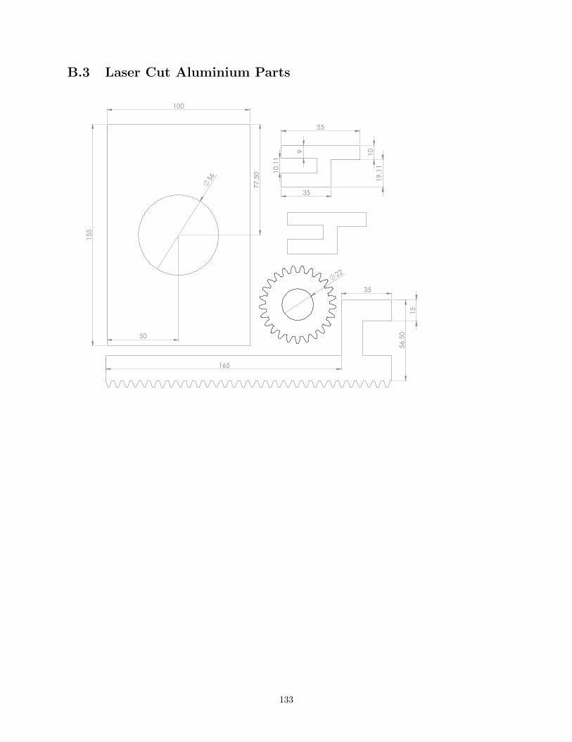
B.3 Laser Cut Aluminium Parts 1
55
100
56
77.
50
50
56.
50
15
35
165
22
55
10
19.
11
35
9
10.
11
133

230
210
165
145
155
125
56
77.50
50
134
Appendix C
Model Parameters and Coefficients
C.1 Determined Platform Parameters
135

Parameter Method Value
Mass (m, M) The assembled platform was weighed and the mass of its
stand and objects used to support it on the scale were sub-
tracted from the total.
27.9kg
Rigid Body Inertia Matrix
(MRB , MRB)
The definition of the matrix as presented by Fossen [39] was
used and the mass and inertia values determined using the
Solidworks’s Mass Properties tool were used to determine
the final parameters.
MRB =
(mI3x3 −mS(rG)
mS(rG) I0
)= 27.9 0 0 0 0 0
0 27.9 0 0 0 00 0 27.9 0 0 00 0 0 1.1607 0.0231 0.30980 0 0 0.0231 2.6022 0.01860 0 0 0.3098 −0.0186 1.5241
where I3x3 is the identity matrix,
I0 =
(Ix −Ixy −Ixz−Iyx Iy −Iyz−Izx −Izy Iz
)is the inertia
tensor, and S(λ) =
(0 −λ3 λ2
λ3 0 −λ1
−λ2 λ1 0
)is a
skew-symmetric matrix equal to 0 as the
centre of gravity rG is equal to 0.
Added Inertia Matrix (MA, MA) As described in Section 3.4.2. MA =
1.3950 0 0 0 0 00 101.0051 0 0 0 00 0 24.2096 0 0 00 0 0 0.7623 0 00 0 0 0 18.5168 00 0 0 0 0 77.2074
Waterline length (Lwl, LWL) Length of forward and backward overhanging lengths of
boat in tank test subtracted from length of boat along deck.
1.505m
Beam of waterline (Bwl, BWL) The maximum beam (width [30]) at the waterline [62]. De-
termined by adapting the Python script used to calculate
added mass in Section 3.4.2.
0.3007m
136

Parameter Method Value
Longitudinal position of centre of
buoyancy to forward perpendicu-
lar (LCBfpp, LCBfpp)
Where the forward perpendicular is the forward end of the
waterline [62]. The 0 buoyancy model was evaluated: the
forward point was found by creating a reference point at the
intersection of the curve describing the hull and the sketch
line down the centreline of the boat (which was created
as part of the buoyancy script), while a line between this
point and the centre of mass in a 3D sketch (created using
3D sketch points at the correct coordinates1 ) was projected
onto the top surface of the buoyancy model using the Con-
vert Entities tool. The distance was then determined by
finding the length in the line’s properties.
0.6995487m
Longitudinal position of centre of
flotation to forward perpendicu-
lar (LCFfpp, LCFfpp)
Where the centre of flotation is the centre of gravity of the
water-plane area [62]. A reference point was created at the
centroid of the top surface of the 0 buoyancy model and
the distance between this and the forward reference point
found for the determination of the LCBfpp was measured
using Solidworks’ Measure tool.
0.761707m
1The approach of using a 3D sketch point at the correct coordinates for the centre of mass was described in the SolidWorks forums(https://forum.solidworks.com/message/210863), and this approach was developed from that point.
137
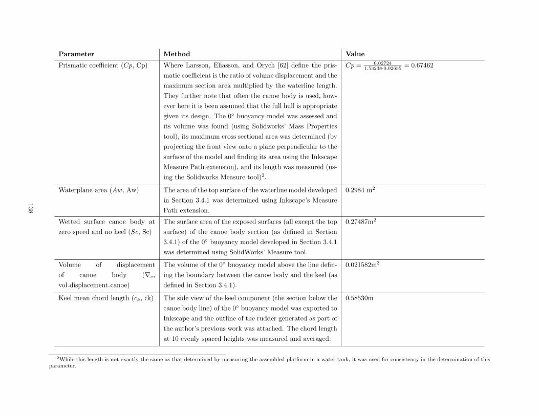
Parameter Method Value
Prismatic coefficient (Cp, Cp) Where Larsson, Eliasson, and Orych [62] define the pris-
matic coefficient is the ratio of volume displacement and the
maximum section area multiplied by the waterline length.
They further note that often the canoe body is used, how-
ever here it is been assumed that the full hull is appropriate
given its design. The 0 buoyancy model was assessed and
its volume was found (using Solidworks’ Mass Properties
tool), its maximum cross sectional area was determined (by
projecting the front view onto a plane perpendicular to the
surface of the model and finding its area using the Inkscape
Measure Path extension), and its length was measured (us-
ing the Solidworks Measure tool)2.
Cp = 0.027241.53238·0.02635 = 0.67462
Waterplane area (Aw, Aw) The area of the top surface of the waterline model developed
in Section 3.4.1 was determined using Inkscape’s Measure
Path extension.
0.2984 m2
Wetted surface canoe body at
zero speed and no heel (Sc, Sc)
The surface area of the exposed surfaces (all except the top
surface) of the canoe body section (as defined in Section
3.4.1) of the 0 buoyancy model developed in Section 3.4.1
was determined using SolidWorks’ Measure tool.
0.27487m2
Volume of displacement
of canoe body (∇c,vol displacement canoe)
The volume of the 0 buoyancy model above the line defin-
ing the boundary between the canoe body and the keel (as
defined in Section 3.4.1).
0.021582m3
Keel mean chord length (ck, ck) The side view of the keel component (the section below the
canoe body line) of the 0 buoyancy model was exported to
Inkscape and the outline of the rudder generated as part of
the author’s previous work was attached. The chord length
at 10 evenly spaced heights was measured and averaged.
0.58530m
2While this length is not exactly the same as that determined by measuring the assembled platform in a water tank, it was used for consistency in the determination of thisparameter.
138
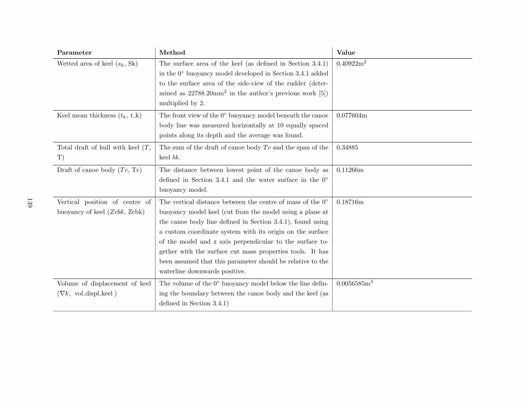
Parameter Method Value
Wetted area of keel (sk, Sk) The surface area of the keel (as defined in Section 3.4.1)
in the 0 buoyancy model developed in Section 3.4.1 added
to the surface area of the side-view of the rudder (deter-
mined as 22788.20mm2 in the author’s previous work [5])
multiplied by 2.
0.40922m2
Keel mean thickness (tk, t k) The front view of the 0 buoyancy model beneath the canoe
body line was measured horizontally at 10 equally spaced
points along its depth and the average was found.
0.077604m
Total draft of hull with keel (T ,
T)
The sum of the draft of canoe body Tc and the span of the
keel bk.
0.34885
Draft of canoe body (Tc, Tc) The distance between lowest point of the canoe body as
defined in Section 3.4.1 and the water surface in the 0
buoyancy model.
0.11266m
Vertical position of centre of
buoyancy of keel (Zcbk, Zcbk)
The vertical distance between the centre of mass of the 0
buoyancy model keel (cut from the model using a plane at
the canoe body line defined in Section 3.4.1), found using
a custom coordinate system with its origin on the surface
of the model and z axis perpendicular to the surface to-
gether with the surface cut mass properties tools. It has
been assumed that this parameter should be relative to the
waterline downwards positive.
0.18716m
Volume of displacement of keel
(∇k, vol displ keel )
The volume of the 0 buoyancy model below the line defin-
ing the boundary between the canoe body and the keel (as
defined in Section 3.4.1)
0.0056585m3
139
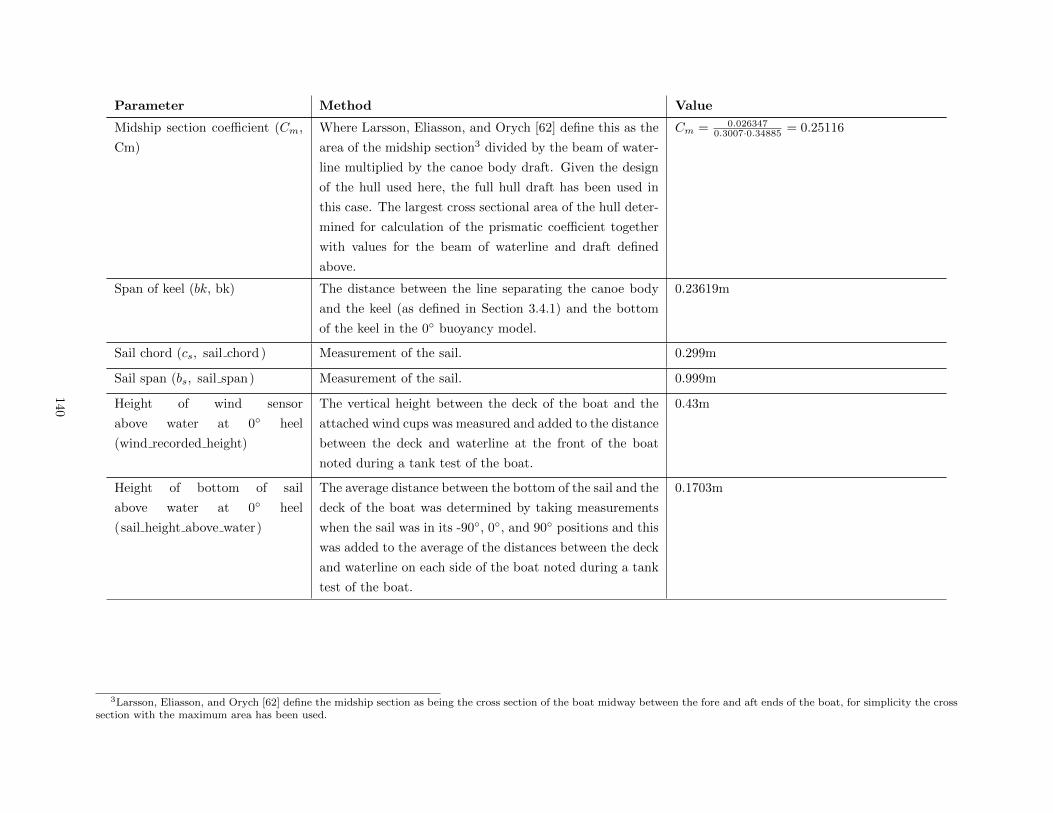
Parameter Method Value
Midship section coefficient (Cm,
Cm)
Where Larsson, Eliasson, and Orych [62] define this as the
area of the midship section3 divided by the beam of water-
line multiplied by the canoe body draft. Given the design
of the hull used here, the full hull draft has been used in
this case. The largest cross sectional area of the hull deter-
mined for calculation of the prismatic coefficient together
with values for the beam of waterline and draft defined
above.
Cm = 0.0263470.3007·0.34885 = 0.25116
Span of keel (bk, bk) The distance between the line separating the canoe body
and the keel (as defined in Section 3.4.1) and the bottom
of the keel in the 0 buoyancy model.
0.23619m
Sail chord (cs, sail chord ) Measurement of the sail. 0.299m
Sail span (bs, sail span) Measurement of the sail. 0.999m
Height of wind sensor
above water at 0 heel
(wind recorded height)
The vertical height between the deck of the boat and the
attached wind cups was measured and added to the distance
between the deck and waterline at the front of the boat
noted during a tank test of the boat.
0.43m
Height of bottom of sail
above water at 0 heel
(sail height above water)
The average distance between the bottom of the sail and the
deck of the boat was determined by taking measurements
when the sail was in its -90, 0, and 90 positions and this
was added to the average of the distances between the deck
and waterline on each side of the boat noted during a tank
test of the boat.
0.1703m
3Larsson, Eliasson, and Orych [62] define the midship section as being the cross section of the boat midway between the fore and aft ends of the boat, for simplicity the crosssection with the maximum area has been used.
140

Parameter Method Value
Vertical distance between bot-
tom of sail and centre of mass
(sail height above com)
A pitched reference plane parallel to the waterline (as dis-
cussed in the development of the waterline model in Section
3.4.1) was inserted into the CAD model and a coordinate
system parallel to it was created with the z-axis normal to
the plane. The distance in the z-axis between the origin
and the centre of mass was added to the average of the dis-
tance in the z axis between the origin and the leading and
trailing edges of the bottom of the sail.
0.26756m
Longitudinal position of centre of
mast (Xmast, Xce)
This variable (which replaces part of the longitudinal posi-
tion of centre of effort Xce due to the model’s consideration
of the sail angle) is the longitudinal distance between the
centre of the mast and centre of mass. This has been deter-
mined using the pitched coordinate system discussed above
and by finding the length between the centre of mass and
the centre of the mast at the base of the sail in the longi-
tudinal direction (forward positive).
0.0805m
Position of mast along sail chord
(cmast, chord mast)
The length between the centre of the mast and the leading
edge of the wingsail along the chord line measured on the
wingsail.
0.07m
Longitudinal position of centre of
lateral resistance (Xclr, Xclrd)
As discussed in Section 3.3.1, the centre of lateral resistance
has been taken as the point along the quarter chord line of
the keel at 43% of the total draft of the side-view. This
has been found by exporting a side-view of the waterline
model to the Inkscape vector graphics editor, appropriately
scaling and attaching an outline of the rudder to the view,
finding the 43% draft line, and finding the quarter chord
point along it.
0.059137m
141

Parameter Method Value
Combined hull/keel chord
(chull−keel, hull keel chord )
As previously noted, this work has (for simplicity) assumed
that the hull and keel can be considered as a single rectan-
gular wing - requiring estimation of the equivalent aspect
ratio. It has been assumed that the equivalent wing should
have the same draft as the boat, resulting in a chord deter-
mined such that the area remains constant.
0.252270.34885 = 0.72315m
Combined hull/keel h value (h,
hull keel h )
Determination of h requires knowledge of the distance be-
tween the leading edge of the aerofoil and centre of mass hc.
The leading edge has been assumed to be approximately at
the location of the inflection point of the leading edge of
the keel and hull. Positive forward direction.
0.26565m
Combined hull/keel area
(shull−keel, S hull keel )
Given that this parameter is used for the determination of
forces due to yaw velocity, which is based on thin aerofoil
theory, it has been determined by finding (using Inkscape’s
Measure Path extension) the projected area of the side-view
of the waterline model which was used for determination of
added mass parameters added to the area of the side-view
of the rudder noted above.
0.25227m2
Combined hull/keel aspect ratio
( hull keel ar )
Taken as the ratio of the draft of the boat to the effective
chord of the keel and hull determined above.
0.348850.72315 = 0.4824
Rudder to Hull and Keel Ratio
(rudder ratio)
The ratio of the area of hull and keel to the area of the hull,
keel, and rudder.
0.186420.18642+0.022788 = 0.89107
142

Parameter Method Value
Rudder φ (φ, rudder phi) As noted in Section 3.3.3, φ is the hinge point in a mapping
of the leading edge of the aerofoil being 0 and the trailing
edge π by use of x = (c/2)(1 − cosθ). As this point is not
constant on the model, it has been estimated by ensuring
that the ratio between x and c is the same as that between
the area of the keel and the keel and rudder together - tak-
ing the keel here to be the section of the boat beneath the
waterline that falls below the horizontal line that intersects
the top of the rudder (Figure C.1 shows these points).
ratio = 0.186420.18642+0.022788 = 0.89107 θ =
arcos(1− 2xc ) = arcos(1− 2·ratio) = 2.46891
Rudder area (Sr, rudder s) As determined in the author’s previous work [5]. This pa-
rameter is the area of the side-view of the rudder.
0.022788m2
Rudder chord (cr, rudder chord) Given its irregular shape, it is unclear how the chord should
be defined for rudder force calculations - however for sim-
plicity this has been assumed to be the maximum chord
(measured on the rudder itself).
0.101m
Rudder aspect ratio (rudder ar) Determined using Houghton and Carpenter’s definition [56]
of aspect ratio of(span)2
area.
0.44765
Taper Ratio of keel (TR) Defined by Larsson, Eliasson, and Orych [62] as the ratio of
the tip of the chord to the root chord and calculated using
values determined from the model where the root of the
keel was considered to be in line with the top of the rudder.
0.33671.056 = 0.31885
Gravitational acceleration (g, g) Taken as the gravitational acceleration value in Cape Town,
South Africa4.
9.79621m/s2
Density of water (p, p) As the platform is tested in fresh water, its density5 is used. 1000kg/m3
Density of air (pair, p) The density of air at sea level6. 1.225 kg/m3
4Wolfram—Alpha knowledgebase, 2014 - accessed via Wolfram Alpha.5Wolfram—Alpha knowledgebase, 2014 - accessed via Wolfram Alpha.6Wolfram—Alpha knowledgebase, 2014 - accessed via Wolfram Alpha.
143

Parameter Method Value
Table C.1: Summary of determined parameters, their methods of determination, and values.
144

C.2 Parameters that vary with Heel
Angle BGx BGy BGz 1000·g(η)3W 1000·g(η)4W-51.32569 -35.53634 47.65569 62.65437 -63.47653391 -35.53092764-50.31685 -28.67019 46.64685 53.84215 -64.0806164 -27.69327697-48.12945 -24.37764 44.45945 48.50573 -64.23691941 -21.11165552-44.36293 -21.39587 40.69293 43.70543 -59.67865268 -15.12916477-37.45906 -19.70912 33.78906 38.49307 -48.50871933 -9.85456-29.39367 -21.33702 25.72367 34.80517 -36.07641211 -7.297690639-23.98256 -23.08986 20.31256 33.10871 -28.18959101 -5.976095517-18.40358 -24.61407 14.73358 31.86318 -20.04272696 -4.2741884-12.75717 -25.63966 9.08717 31.11615 -11.76454174 -2.234643611-7.17661 -26.50318 3.50661 30.82898 -3.50661 0-1.36588 -25.81127 -2.30412 31.11558 5.007253614 2.2496004084.33814 -24.96082 -8.00814 31.86992 13.42063189 4.3344009069.95393 -23.61983 -13.62393 33.09748 21.72596401 6.113261846
15.39336 -21.90573 -19.06336 34.83894 29.82931797 7.49220091423.43455 -20.58096 -27.10455 38.52881 42.73763386 10.2904830.33075 -22.54091 -34.00075 43.72719 54.96195346 15.9388303234.12756 -25.82187 -37.79756 48.57882 60.96927221 22.3623953936.34431 -30.31191 -40.01431 53.94091 62.45938357 29.2790567137.35996 -37.46547 -41.02996 62.84416 63.55066007 37.45976383
Table C.2: Distance between the boat’s centre of mass and centre of buoyancy in the x, y, and z axes andmoment arm lengths in mm for various angles of heel.
Angle Canoe Body Surface Area (m2) Keel Surface Area (m2)0 0.27487263 0.363643995 0.27450409 0.36360167
10 0.27423715 0.3633958815 0.27374821 0.3630647620 0.27769772 0.3625258830 0.30471758 0.36087645 0.33753117 0.3552200260 0.37217133 0.3381783475 0.41050717 0.3126037389 0.45495718 0.25244739
Table C.3: Canoe body and keel surface areas for various angles of heel.
1000·g(η)3W
= 10−12ϕ6 + 10−8ϕ5 − 3·10−8ϕ4 − 0.0002ϕ3 + 0.0006ϕ2 + 1.7008ϕ− 3.3848 (C.1)
1000·g(η)4W
= 10−12ϕ6 + 10−9ϕ5 − 3·10−8ϕ4 − 5·10−6ϕ3 + 0.0003ϕ2 + 0.3603ϕ+ 0.0046 (C.2)
145

Figure C.1: A demonstration of the areas used to determine the rudder φ value. The grey area is the keelwhile the black is the rudder.
Fn a0 a1 a2 a3 a4 a5 a6 a70 0 0 0 0 0 0 0 0
0.15 -0.0005 0.0023 -0.0086 -0.0015 0.0061 0.001 0.0001 0.00520.2 -0.0003 0.0059 -0.0064 0.007 0.0014 0.0013 0.0005 -0.002
0.25 -0.0002 -0.0156 0.0031 -0.0021 -0.007 0.0148 0.001 -0.00430.3 -0.0009 0.0016 0.0337 -0.0285 -0.0367 0.0218 0.0015 -0.0172
0.35 -0.0026 -0.0567 0.0446 -0.1091 -0.0707 0.0914 0.0021 -0.00780.4 -0.0064 -0.4034 -0.125 0.0273 -0.1341 0.3578 0.0045 0.1115
0.45 -0.0218 -0.5261 -0.2945 0.2485 -0.2428 0.6293 0.0081 0.20860.5 -0.0388 -0.5986 -0.3038 0.6033 -0.043 0.8332 0.0106 0.1336
0.55 -0.0347 -0.4764 -0.2361 0.8726 0.4219 0.899 0.0096 -0.22720.6 -0.0361 0.0037 -0.296 0.9661 0.6123 0.7534 0.01 -0.3352
0.65 0.0008 0.3728 -0.3667 1.3957 1.0343 0.323 0.0072 -0.46320.7 0.0108 -0.1238 -0.2026 1.1282 1.1836 0.4973 0.0038 -0.4477
0.75 0.1023 0.7726 0.504 1.7867 2.1934 -1.5479 -0.0115 -0.0977
Table C.4: Residuary resistance coefficients as determined by Keuning and Katgert [2]
C.3 Residuary Resistance (Hull)
C.4 Change in Residuary Resistance (Hull) due to 20°Heel
It should be noted that Keuning and Katgert [2] state that these ”[c]oefficients are multiplied by 1000”. Thisstatement was considered ambiguous - however it was interpreted to mean that when used the coefficientsshould be divided by 1000. This approach produced reasonable results of a scale similar to that of the zeroheel residuary resistance calculation.
Fn u0 u1 u2 u3 u4 u50 0 0 0 0 0 0
0.25 -26.8 -1.4 -5.7 1.6 -7 -1.70.3 662.8 -63.2 -69.9 6.9 45.9 -0.4
0.35 1643.3 -214.4 -164 19.9 -54 -26.80.4 -865.9 -35.4 222.6 18.8 -580 -113.3
0.45 -3271.5 137.2 554.7 26.8 -1006.4 -202.60.5 -197.6 -148 -659.3 186.2 -748.9 -164.8
0.55 1587.3 -374.9 -710.5 214.6 -481.8 -117.4
Table C.5: Change in Residuary Resistance due to 20°Heel coefficients as determined by Keuning andSonnenberg [3]
146

C.5 Residuary Resistance Keel
Fn A0 A1 A2 A30 0 0 0 0
0.2 -0.00104 0.00172 0.00117 -0.000080.25 -0.0055 0.00597 0.0039 -0.000090.3 -0.0111 0.01421 0.00069 0.00021
0.35 -0.00713 0.02632 -0.00232 0.000390.4 -0.03581 0.08649 0.00999 0.00017
0.45 -0.0047 0.11592 -0.00064 0.000350.5 0.00553 0.07371 0.05991 -0.00114
0.55 0.04822 0.0066 0.07048 -0.000350.6 0.01021 0.14173 0.06409 -0.00192
Table C.6: Residuary Resistance of the Keel coefficients as determined by Keuning and Sonnenberg [3]
C.6 Change in Residuary Resistance Keel due to Heel
H1 -3.5837H2 -0.0518H3 0.5958H4 0.2055
Table C.7: Change in Residuary Resistance of the Keel coefficients as determined by Keuning and Sonnenberg[3]
C.7 Side Force
Heel angle (degrees) b1 b2 b3 b40 2.025 9.551 0.631 -6.575
10 1.989 6.729 0.494 -4.74520 1.98 0.633 0.194 -0.79230 1.762 -4.957 -0.087 2.766
Table C.8: Side force coefficients as determined by Keuning and Sonnenberg [3]
C.8 Effective Span Coefficients
147

heel angle (degrees) A1 A2 A3 A4 B0 B10 3.7455 -3.6246 0.0589 -0.0296 1.2306 -0.7256
10 4.4892 -4.8454 0.0294 -0.0176 1.4231 -1.297120 3.9592 -3.9804 0.0283 -0.0075 1.545 -1.562230 3.4891 -2.9577 0.025 -0.0272 1.4744 -1.3499
Table C.9: Effective span coefficients as determined by Keuning and Sonnenberg [3]
C.9 Wingsail Lift and Drag Coefficients
148

An
gle
of
Att
ack
Cl
Re=
0
Cl
Re=
10000
Cl
Re=
20000
Cl
Re=
40000
Cl
Re=
80000
Cl
Re=
160000
Cl
Re=
360000
Cl
Re=
700000
Cl
Re=
1000000
Cl
Re=
2000000
0 0 0 0 0 0 0 0 0 0 01 0 -0.0045 0.0607 0.0936 0.0889 0.11 0.11 0.11 0.11 0.112 0 -0.0154 0.1135 0.1833 0.1935 0.22 0.22 0.22 0.22 0.223 0 -0.0233 0.155 0.2688 0.2924 0.3088 0.33 0.33 0.33 0.334 0 -0.0368 0.1788 0.3495 0.388 0.4114 0.44 0.44 0.44 0.445 0 -0.0577 0.1788 0.4117 0.4753 0.5068 0.524 0.55 0.55 0.556 0 -0.0839 0.1582 0.4573 0.56115 0.596 0.6228 0.6328 0.66 0.667 0 -0.1182 0.1161 0.4758 0.6224 0.6724 0.71 0.7291 0.7362 0.74498 0 -0.1501 0.0214 0.4428 0.6589 0.7373 0.7879 0.8156 0.8256 0.84399 0 -0.1584 -0.0682 0.3544 0.6606 0.7781 0.8526 0.8904 0.9067 0.9314
10 0 -0.1423 -0.1003 0.2108 0.6248 0.7949 0.8983 0.9541 0.9751 1.011111 0 -0.1125 -0.08025 0.11235 0.5531 0.7852 0.9249 0.9973 1.0284 1.077212 0 -0.0767 -0.0602 0.0139 0.4408 0.7488 0.9279 1.0245 1.0664 1.129613 0 -0.0341 -0.0215 0.0314 0.3332 0.6923 0.9104 1.0289 1.0304 1.166214 0 0.0085 0.0172 0.0489 0.2256 0.6237 0.8803 1.0175 1.0793 1.181316 0 0.1051 0.1114 0.1287 0.2027 0.4896 0.8007 0.9648 1.0402 1.169518 0 0.207 0.212 0.2228 0.2603 0.4202 0.7319 0.915 0.9959 1.138320 0 0.3111 0.3151 0.3236 0.3472 0.4382 0.6997 0.8877 0.9707 1.117222 0 0.4172 0.4198 0.4265 0.443 0.5026 0.705 0.8867 0.9696 1.112725 0 0.5775 0.5798 0.584 0.5963 0.6321 0.7724 0.9326 1.0107 1.146830 0 0.855 0.855 0.855 0.855 0.855 0.855 0.855 0.855 0.85535 0 0.98 0.98 0.98 0.98 0.98 0.98 0.98 0.98 0.9840 0 1.035 1.035 1.035 1.035 1.035 1.035 1.035 1.035 1.03545 0 1.05 1.05 1.05 1.05 1.05 1.05 1.05 1.05 1.0550 0 1.02 1.02 1.02 1.02 1.02 1.02 1.02 1.02 1.0255 0 0.955 0.955 0.955 0.955 0.955 0.955 0.955 0.955 0.95560 0 0.875 0.875 0.875 0.875 0.875 0.875 0.875 0.875 0.87565 0 0.76 0.76 0.76 0.76 0.76 0.76 0.76 0.76 0.7670 0 0.63 0.63 0.63 0.63 0.63 0.63 0.63 0.63 0.6375 0 0.5 0.5 0.5 0.5 0.5 0.5 0.5 0.5 0.580 0 0.365 0.365 0.365 0.365 0.365 0.365 0.365 0.365 0.36585 0 0.23 0.23 0.23 0.23 0.23 0.23 0.23 0.23 0.2390 0 0.09 0.09 0.09 0.09 0.09 0.09 0.09 0.09 0.0995 0 -0.05 -0.05 -0.05 -0.05 -0.05 -0.05 -0.05 -0.05 -0.05
100 0 -0.185 -0.185 -0.185 -0.185 -0.185 -0.185 -0.185 -0.185 -0.185105 0 -0.32 -0.32 -0.32 -0.32 -0.32 -0.32 -0.32 -0.32 -0.32110 0 -0.45 -0.45 -0.45 -0.45 -0.45 -0.45 -0.45 -0.45 -0.45115 0 -0.575 -0.575 -0.575 -0.575 -0.575 -0.575 -0.575 -0.575 -0.575120 0 -0.67 -0.67 -0.67 -0.67 -0.67 -0.67 -0.67 -0.67 -0.67125 0 -0.76 -0.76 -0.76 -0.76 -0.76 -0.76 -0.76 -0.76 -0.76130 0 -0.85 -0.85 -0.85 -0.85 -0.85 -0.85 -0.85 -0.85 -0.85135 0 -0.93 -0.93 -0.93 -0.93 -0.93 -0.93 -0.93 -0.93 -0.93140 0 -0.98 -0.98 -0.98 -0.98 -0.98 -0.98 -0.98 -0.98 -0.98145 0 -0.9 -0.9 -0.9 -0.9 -0.9 -0.9 -0.9 -0.9 -0.9150 0 -0.77 -0.77 -0.77 -0.77 -0.77 -0.77 -0.77 -0.77 -0.77155 0 -0.67 -0.67 -0.67 -0.67 -0.67 -0.67 -0.67 -0.67 -0.67160 0 -0.635 -0.635 -0.635 -0.635 -0.635 -0.635 -0.635 -0.635 -0.635165 0 -0.68 -0.68 -0.68 -0.68 -0.68 -0.68 -0.68 -0.68 -0.68170 0 -0.85 -0.85 -0.85 -0.85 -0.85 -0.85 -0.85 -0.85 -0.85175 0 -0.66 -0.66 -0.66 -0.66 -0.66 -0.66 -0.66 -0.66 -0.66180 0 0 0 0 0 0 0 0 0 0
Table C.10: Coefficients of lift of the NACA0018 as presented by Sheldahl and Klimas [4].
149
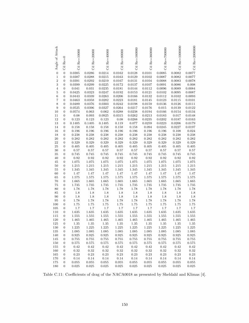
An
gle
of
Att
ack
Cd
Re=
0
Cd
Re=
10000
Cd
Re=
20000
Cd
Re=
40000
Cd
Re=
80000
Cd
Re=
160000
Cd
Re=
360000
Cd
Re=
700000
Cd
Re=
1000000
Cd
Re=
2000000
0 0 0.0385 0.0286 0.0214 0.0162 0.0128 0.0101 0.0085 0.0082 0.00771 0 0.0387 0.0288 0.0215 0.0163 0.0129 0.0102 0.0087 0.0082 0.00772 0 0.0391 0.0292 0.0219 0.0167 0.0131 0.0104 0.0088 0.0083 0.00783 0 0.0399 0.0299 0.0225 0.0172 0.0137 0.0107 0.0091 0.0086 0.0084 0 0.041 0.031 0.0235 0.0181 0.0144 0.0112 0.0096 0.0089 0.00845 0 0.0425 0.0323 0.0247 0.0192 0.0153 0.0121 0.0102 0.0095 0.00876 0 0.0443 0.0339 0.0263 0.0206 0.0166 0.0132 0.0112 0.0102 0.00937 0 0.0463 0.0358 0.0282 0.0223 0.0181 0.0145 0.0123 0.0115 0.01018 0 0.0489 0.0376 0.0303 0.0242 0.0198 0.0159 0.0136 0.0126 0.01119 0 0.0525 0.0396 0.0327 0.0264 0.0217 0.0176 0.015 0.0139 0.0122
10 0 0.0574 0.063 0.062 0.0288 0.0238 0.0194 0.0166 0.0154 0.013411 0 0.08 0.093 0.0925 0.0315 0.0262 0.0213 0.0183 0.017 0.014812 0 0.123 0.123 0.123 0.08 0.0288 0.0235 0.0202 0.0187 0.016313 0 0.1405 0.1405 0.1405 0.119 0.077 0.0259 0.0223 0.0206 0.017914 0 0.158 0.158 0.158 0.158 0.158 0.094 0.0245 0.0227 0.019716 0 0.196 0.196 0.196 0.196 0.196 0.196 0.196 0.108 0.02418 0 0.238 0.238 0.238 0.238 0.238 0.238 0.238 0.238 0.23820 0 0.282 0.282 0.282 0.282 0.282 0.282 0.282 0.282 0.28222 0 0.329 0.329 0.329 0.329 0.329 0.329 0.329 0.329 0.32925 0 0.405 0.405 0.405 0.405 0.405 0.405 0.405 0.405 0.40530 0 0.57 0.57 0.57 0.57 0.57 0.57 0.57 0.57 0.5735 0 0.745 0.745 0.745 0.745 0.745 0.745 0.745 0.745 0.74540 0 0.92 0.92 0.92 0.92 0.92 0.92 0.92 0.92 0.9245 0 1.075 1.075 1.075 1.075 1.075 1.075 1.075 1.075 1.07550 0 1.215 1.215 1.215 1.215 1.215 1.215 1.215 1.215 1.21555 0 1.345 1.345 1.345 1.345 1.345 1.345 1.345 1.345 1.34560 0 1.47 1.47 1.47 1.47 1.47 1.47 1.47 1.47 1.4765 0 1.575 1.575 1.575 1.575 1.575 1.575 1.575 1.575 1.57570 0 1.665 1.665 1.665 1.665 1.665 1.665 1.665 1.665 1.66575 0 1.735 1.735 1.735 1.735 1.735 1.735 1.735 1.735 1.73580 0 1.78 1.78 1.78 1.78 1.78 1.78 1.78 1.78 1.7885 0 1.8 1.8 1.8 1.8 1.8 1.8 1.8 1.8 1.890 0 1.8 1.8 1.8 1.8 1.8 1.8 1.8 1.8 1.895 0 1.78 1.78 1.78 1.78 1.78 1.78 1.78 1.78 1.78
100 0 1.75 1.75 1.75 1.75 1.75 1.75 1.75 1.75 1.75105 0 1.7 1.7 1.7 1.7 1.7 1.7 1.7 1.7 1.7110 0 1.635 1.635 1.635 1.635 1.635 1.635 1.635 1.635 1.635115 0 1.555 1.555 1.555 1.555 1.555 1.555 1.555 1.555 1.555120 0 1.465 1.465 1.465 1.465 1.465 1.465 1.465 1.465 1.465125 0 1.35 1.35 1.35 1.35 1.35 1.35 1.35 1.35 1.35130 0 1.225 1.225 1.225 1.225 1.225 1.225 1.225 1.225 1.225135 0 1.085 1.085 1.085 1.085 1.085 1.085 1.085 1.085 1.085140 0 0.925 0.925 0.925 0.925 0.925 0.925 0.925 0.925 0.925145 0 0.755 0.755 0.755 0.755 0.755 0.755 0.755 0.755 0.755150 0 0.575 0.575 0.575 0.575 0.575 0.575 0.575 0.575 0.575155 0 0.42 0.42 0.42 0.42 0.42 0.42 0.42 0.42 0.42160 0 0.32 0.32 0.32 0.32 0.32 0.32 0.32 0.32 0.32165 0 0.23 0.23 0.23 0.23 0.23 0.23 0.23 0.23 0.23170 0 0.14 0.14 0.14 0.14 0.14 0.14 0.14 0.14 0.14175 0 0.055 0.055 0.055 0.055 0.055 0.055 0.055 0.055 0.055180 0 0.025 0.025 0.025 0.025 0.025 0.025 0.025 0.025 0.025
Table C.11: Coefficients of drag of the NACA0018 as presented by Sheldahl and Klimas [4].
150

Appendix D
Component Comparisons
D.1 Wind Sensor
Image Device Description Price
Young Wind Monitor JR
(model 04101)1Potentiometer wind vane and
brushless wind speed sensor.
Compact design (0.5kg) intended
for marine use (marine model).
R13 965.00
MCS 176 Wind Direction
Sensor2Weather vane coupled to poten-
tiometer.
R2 958.303
MCS 177 Wind Speed
Sensor43 cup anemometer. R2 793.005
Davis Anemometer 64106 Weather vane coupled to poten-
tiometer and wind cups coupled
to a magnetic switch.
R2 394.007
1http://inteltronics.co.za/products/windsensors/windsensors.htm2http://www.mcsystems.co.za/html/mcs_176.html3http://www.enviromon.co.za/em-01c.htm4http://www.mcsystems.co.za/html/mcs_177.html5http://www.enviromon.co.za/em-01c.htm6http://www.davisnet.com/weather/products/weather_product.asp?pnum=079117http://www.meacon.co.za/
151

Image Device Description Price
Gill Windsonic Wind
Speed & Direction Sen-
sor8
2 axis ultrasonic wind sensor. R14 000.009
EVANE - Electronic Wind
Direction Sensor10Sealed hall effect sensor. Direc-
tion only.
£109.00 excl.
VAT
Vaisala Wind Sensor
WM3011Direction (potentiometer) and
speed (dual reed switch).
£98012
Vaisala WINDCAP Ul-
trasonic Wind Sensor
WMT5213
Ultrasonic sensor that measures
horizontal wind speed and direc-
tion.
£961.9614
Table D.1: Comparison of wind sensors considered for use on the platform. It is noted that in a numberof cases prices are estimates provided by suppliers by telephone in March 2014. Images are sourced fromwebsites referenced by footnotes to illustrate the range of designs available.
8http://www.gillinstruments.com/products/anemometer/windsonic.htm9http://www.meacon.co.za/
10http://www.audon.co.uk/weather_sensors/evane.html11http://www.vaisala.com/en/products/windsensors/Pages/WM30.aspx12http://www.kompartpomiar.pl/zdjecia/File/cennik_pogodowe_en_2.pdf13http://www.vaisala.com/en/products/windsensors/Pages/WMT52.aspx14http://www.omniinstruments.co.uk/products/product/moredetails/display.php?product_id=201&producttitle=
Vaisala%20WINDCAP%20Ultrasonic%20Wind%20Sensor%20WMT52
152
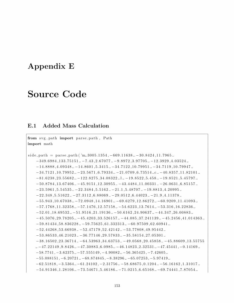
Appendix E
Source Code
E.1 Added Mass Calculation
from svg . path import parse path , Path
import math
s ide pa th = parse path ( ’m 3005.1354 ,−669.11638 −30.8424 ,11.7965
−349.6984 ,133.75151 −7.43 ,2.67077 −9.8972 ,3.97705 −12.3929 ,4.03524
−14.8888 ,4.09348 −14.8601 ,5.3415 −34.7122 ,10.79951 −34.7119 ,10.79947
−34.7121 ,10.79952 −23.5671 ,6.79334 −21.0709 ,6.73514 c −40.8357 ,11.82101
−81.6238 ,23.55682 −122.8275 ,34.08322 l −19.8522 ,5.458 −19.8521 ,5.45797
−50.8784 ,13.67406 −45.9151 ,12.30955 −43.4484 ,11.00331 −26.0631 ,6.85157
−23.5961 ,5.54535 −22.3484 ,5.5162 −21.1 ,5.48707 −19.8813 ,4.20995
−22.348 ,5.51622 −27.3112 ,6.88069 −29.0512 ,6.44023 −21.9 ,4.11378
−55.943 ,10.67038 −72.0948 ,14.16901 −69.6279 ,12.86272 −60.9209 ,11.41093
−57.1768 ,11.32358 −57.1476 ,12.57158 −54.6223 ,13.7614 −53.316 ,16.22836
−52.01 ,18.69532 −51.9516 ,21.19136 −50.6162 ,24.90637 −44.347 ,26.00883
−45.5076 ,29.78205 −45.4203 ,33.526157 −44.085 ,37.241139 −45.2456 ,41.014363
−59.81434 ,58.836228 −59.75625 ,61.332313 −60.97509 ,62.60941
−52.44268 ,53.66938 −52.47179 ,52.42142 −53.77808 ,49.95442
−53.86533 ,46.21023 −36.77146 ,29.57833 −35.58154 ,27.05301
−38.16502 ,23.36714 −64.53963 ,34.63753 −49.0568 ,20.45858 −45.88609 ,13.55755
−47.22149 ,9.8426 −47.30883 ,6.0985 −46.14823 ,2.32531 −47.45441 ,−0.14169
−58.7741 ,−3.62375 −57.555149 ,−4.90082 −56.365425 ,−7.42605
−55.088151 ,−6.20721 −68.874845 ,−8.38296 −65.07253 ,−5.97419
−62.51818 ,−3.5364 −61.24102 ,−2.31756 −58.68675 ,0.1204 −56.16162 ,1.31017
−54.91346 ,1.28106 −73.54671 ,5.46186 −71.0215 ,6.65168 −69.74441 ,7.87054
153
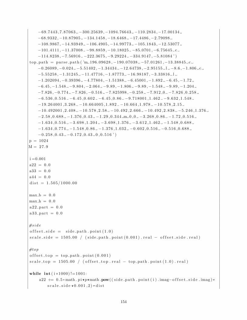
−69.7443 ,7.87063 −300.25639 ,−1094.76643 −110.2834 ,−17.00134
−68.9332 ,−10.87905 −134.1458 ,−18.6468 −17.4486 ,−2.79098
−108.9867 ,−14.93949 −106.4905 ,−14.99773 −105.1843 ,−12.53077
−101.4111 ,−11.37008 −98.8859 ,−10.18025 −85.0701 ,−6.75645 c
−114.8238 ,−7.56916 −222.3675 ,−9.29224 −334.9147 ,−5.81084 ’ )
top path = parse path ( ’m 196.09628 ,−190.07038 −57.01261 ,−13.38845 c
−0.26089 ,−0.024 −5.51402 ,−1.34434 −12.64738 ,−2.95155 l −8.6 ,−1.806 c
−5.55258 ,−1.31245 −11.47716 ,−1.87773 −16.98187 ,−3.33816 l
−1.202094 ,−0.39396 −4.77804 ,−1.51388 −6.45001 ,−1.892 −6.45 ,−1.72
−6.45 ,−1.548 −9.804 ,−2.064 −9.89 ,−1.806 −9.89 ,−1.548 −9.89 ,−1.204
−7.826 ,−0.774 −7.826 ,−0.516 −7.825998 ,−0.258 −7.912 ,0 −7.826 ,0.258
−6.536 ,0.516 −6.45 ,0.602 −6.45 ,0.86 −9.718001 ,1.462 −9.632 ,1.548
−19.264001 ,3.268 −10.664005 ,1.892 −10.664 ,1.978 −10.578 ,2.15
−10.492001 ,2.408 −10.578 ,2.58 −10.492 ,2.666 −10.492 ,2.838 −5.246 ,1.376
−2.58 ,0.688 −1.376 ,0.43 −1.29 ,0.344 m 0 ,0 −3.268 ,0.86 −1.72 ,0.516
−1.634 ,0.516 −3.698 ,1.204 −3.698 ,1.376 −3.612 ,1.462 −1.548 ,0.688
−1.634 ,0.774 −1.548 ,0.86 −1.376 ,1.032 −0.602 ,0.516 −0.516 ,0.688
−0.258 ,0.43 −0.172 ,0.43 0 ,0 .516 ’ )
p = 1024
M = 27.9
i =0.001
a22 = 0 .0
a33 = 0 .0
a44 = 0 .0
d i s t = 1 .505/1000 .00
max b = 0 .0
max h = 0 .0
a22 part = 0 .0
a33 part = 0 .0
#s i d e
o f f s e t s i d e = s ide pa th . po int ( 1 . 0 )
s c a l e s i d e = 1505.00 / ( s i d e pa th . po int ( 0 . 0 0 1 ) . r e a l − o f f s e t s i d e . r e a l )
#top
o f f s e t t o p = top path . po int ( 0 . 0 0 1 )
s c a l e t o p = 1505.00 / ( o f f s e t t o p . r e a l − top path . po int ( 1 . 0 ) . r e a l )
while int ( i *1000) !=1001:
a22 += 0.5*math . p i *p*math .pow( ( s i d e pa th . po int ( i ) . imag−o f f s e t s i d e . imag ) *
s c a l e s i d e *0 .001 ,2 ) * d i s t
154
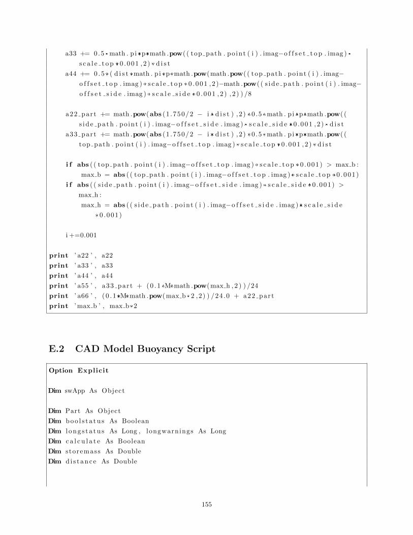
a33 += 0.5*math . p i *p*math .pow( ( top path . po int ( i ) . imag−o f f s e t t o p . imag ) *
s c a l e t o p *0 .001 ,2 ) * d i s t
a44 += 0 . 5* ( d i s t *math . p i *p*math .pow(math .pow( ( top path . po int ( i ) . imag−o f f s e t t o p . imag ) * s c a l e t o p *0 .001 ,2 )−math .pow( ( s i d e pa th . po int ( i ) . imag−o f f s e t s i d e . imag ) * s c a l e s i d e *0 .001 ,2 ) , 2 ) ) /8
a22 part += math .pow(abs (1 .750/2 − i * d i s t ) , 2 ) *0 .5*math . p i *p*math .pow( (
s i d e pa th . po int ( i ) . imag−o f f s e t s i d e . imag ) * s c a l e s i d e *0 .001 ,2 ) * d i s t
a33 part += math .pow(abs (1 .750/2 − i * d i s t ) , 2 ) *0 .5*math . p i *p*math .pow( (
top path . po int ( i ) . imag−o f f s e t t o p . imag ) * s c a l e t o p *0 .001 ,2 ) * d i s t
i f abs ( ( top path . po int ( i ) . imag−o f f s e t t o p . imag ) * s c a l e t o p *0 .001) > max b :
max b = abs ( ( top path . po int ( i ) . imag−o f f s e t t o p . imag ) * s c a l e t o p *0 .001)
i f abs ( ( s i d e pa th . po int ( i ) . imag−o f f s e t s i d e . imag ) * s c a l e s i d e *0 .001) >
max h :
max h = abs ( ( s i d e pa th . po int ( i ) . imag−o f f s e t s i d e . imag ) * s c a l e s i d e
*0 .001)
i +=0.001
print ’ a22 ’ , a22
print ’ a33 ’ , a33
print ’ a44 ’ , a44
print ’ a55 ’ , a33 part + ( 0 . 1*M*math .pow(max h , 2 ) ) /24
print ’ a66 ’ , ( 0 . 1*M*math .pow( max b *2 ,2) ) /24 .0 + a22 part
print ’ max b ’ , max b*2
E.2 CAD Model Buoyancy Script
Option Explicit
Dim swApp As Object
Dim Part As Object
Dim b o o l s t a t u s As Boolean
Dim l o n g s t a t u s As Long , longwarnings As Long
Dim c a l c u l a t e As Boolean
Dim storemass As Double
Dim d i s t anc e As Double
155

’ Based on recorded macros and r e f e r e n c e to So l idworks API documentation and
examples
Sub main ( )
Set swApp =
Appl i ca t ion . SldWorks
Set Part = swApp . ActiveDoc
’ run the macro at an ang le o f 271 de gre es − v a r i e d manually
i t e r a t e (271)
End Sub
Function i t e r a t e ( ang le As Double ) As Double ( )
c a l c u l a t e = True
d i s t anc e = 0 ’ s t a r t i n g d i s t a n c e . v a r i e d manually to speed t e s t i n g .
Debug . Pr int ”START NEW”
While c a l c u l a t e = True
Part . Extension . StartRecordingUndoObject
Dim boatmass As SldWorks . MassProperty
’ check the current mass
Set boatmass = Part . Extension . CreateMassProperty
storemass = boatmass . Mass
Debug . Pr int boatmass . Mass
’ i n s e r t a new plane at the t e s t i n g d i s t a n c e to the r e f e r e n c e p lane
Dim myModelView As Object
Set myModelView = Part . ActiveView
myModelView . FrameState = swWindowState e . swWindowMaximized
b o o l s t a t u s = Part . Extension . SelectByID2 ( ” p i t c h e d r e f e r e n c e ” , ”PLANE” ,
0 , 0 , 0 , True , 0 , Nothing , 0)
Dim myRefPlane As Object
Set myRefPlane = Part . FeatureManager . In se r tRe fP lane (264 , d i s t anc e /
1000 , 0 , 0 , 0 , 0)
Part . C l e a r S e l e c t i o n 2 True
’ rename the new plane
156
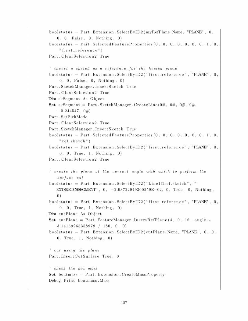
b o o l s t a t u s = Part . Extension . SelectByID2 ( myRefPlane . Name, ”PLANE” , 0 ,
0 , 0 , False , 0 , Nothing , 0)
b o o l s t a t u s = Part . S e l e c t ed Fea tu r ePr ope r t i e s (0 , 0 , 0 , 0 , 0 , 0 , 0 , 1 , 0 ,
” f i r s t r e f e r e n c e ” )
Part . C l e a r S e l e c t i o n 2 True
’ i n s e r t a s k e t c h as a r e f e r e n c e f o r the h e e l e d p lane
b o o l s t a t u s = Part . Extension . SelectByID2 ( ” f i r s t r e f e r e n c e ” , ”PLANE” , 0 ,
0 , 0 , False , 0 , Nothing , 0)
Part . SketchManager . In s e r tSke t ch True
Part . C l e a r S e l e c t i o n 2 True
Dim skSegment As Object
Set skSegment = Part . SketchManager . CreateLine (0#, 0#, 0#, 0#,
−0.244547 , 0#)
Part . SetPickMode
Part . C l e a r S e l e c t i o n 2 True
Part . SketchManager . In s e r tSke t ch True
b o o l s t a t u s = Part . S e l e c t ed Fea tu r ePr ope r t i e s (0 , 0 , 0 , 0 , 0 , 0 , 0 , 1 , 0 ,
” r e f s k e t c h ” )
b o o l s t a t u s = Part . Extension . SelectByID2 ( ” f i r s t r e f e r e n c e ” , ”PLANE” , 0 ,
0 , 0 , True , 1 , Nothing , 0)
Part . C l e a r S e l e c t i o n 2 True
’ c r e a t e the p lane at the c o r r e c t ang l e wi th which to perform the
s u r f a c e cut
b o o l s t a t u s = Part . Extension . SelectByID2 ( ” L ine1@re f ske tch ” , ”
EXTSKETCHSEGMENT” , 0 , −2.93722949300559E−02, 0 , True , 0 , Nothing ,
0)
b o o l s t a t u s = Part . Extension . SelectByID2 ( ” f i r s t r e f e r e n c e ” , ”PLANE” , 0 ,
0 , 0 , True , 1 , Nothing , 0)
Dim cutPlane As Object
Set cutPlane = Part . FeatureManager . In se r tRe fP lane (4 , 0 , 16 , ang le *
3.14159265358979 / 180 , 0 , 0)
b o o l s t a t u s = Part . Extension . SelectByID2 ( cutPlane . Name, ”PLANE” , 0 , 0 ,
0 , True , 1 , Nothing , 0)
’ cut us ing the p lane
Part . In se r tCutSur face True , 0
’ check the new mass
Set boatmass = Part . Extension . CreateMassProperty
Debug . Pr int boatmass . Mass
157

’ undo s t e p s to a l l o w the next i t e r a t i o n to t ake p l a c e
Part . Extension . FinishRecordingUndoObject ( ”API Undo” )
’ check whether the o b j e c t has the c o r r e c t mass or whether i t e r a t i n g
must cont inue
I f boatmass . Mass < 27 .91 And boatmass . Mass > 27 .89 Then
c a l c u l a t e = False
E l s e I f boatmass . Mass >= 27.9 Then
c a l c u l a t e = True
d i s t anc e = d i s t anc e + 0.05
Part . EditUndo2 1
Debug . Pr int ”DISTANCE ” & d i s t ance
E l s e I f boatmass . Mass <= 27.9 Then
c a l c u l a t e = True
d i s t anc e = d i s t anc e − 0 .1
Part . EditUndo2 1
Debug . Pr int ”DISTANCE ” & d i s t ance
Else
c a l c u l a t e = False
Debug . Pr int ” Error ”
End I f
Wend
Debug . Pr int ”END”
End Function
E.3 Platform Test Polar Diagram Script
import csv
from s c ipy . i n t e r p o l a t e import i n te rp1d
import numpy
step=10
headings = range (0 , 360− step , s tep )
#f i r s t c r e a t e wind d i r e c t i o n and yaw r a t e i n t e r p o l a t i o n c l a s s e s
t imes wind =[ ]
t i m e s a t t i t u d e =[ ]
winddirs =[ ]
158
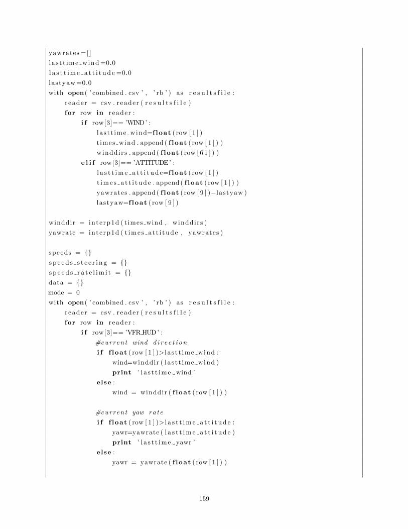
yawrates =[ ]
l a s t t ime wind =0.0
l a s t t i m e a t t i t u d e =0.0
lastyaw =0.0
with open( ’ combined . csv ’ , ’ rb ’ ) as r e s u l t s f i l e :
r eader = csv . r eader ( r e s u l t s f i l e )
for row in reader :
i f row[3]== ’WIND’ :
l a s t t ime wind=f loat ( row [ 1 ] )
t imes wind . append ( f loat ( row [ 1 ] ) )
winddirs . append ( f loat ( row [ 6 1 ] ) )
e l i f row[3]== ’ATTITUDE ’ :
l a s t t i m e a t t i t u d e=f loat ( row [ 1 ] )
t i m e s a t t i t u d e . append ( f loat ( row [ 1 ] ) )
yawrates . append ( f loat ( row [ 9 ] )−lastyaw )
lastyaw=f loat ( row [ 9 ] )
winddir = inte rp1d ( times wind , winddirs )
yawrate = inte rp1d ( t ime s a t t i tude , yawrates )
speeds = s p e e d s s t e e r i n g = s p e e d s r a t e l i m i t = data = mode = 0
with open( ’ combined . csv ’ , ’ rb ’ ) as r e s u l t s f i l e :
r eader = csv . r eader ( r e s u l t s f i l e )
for row in reader :
i f row[3]== ’VFR HUD ’ :
#current wind d i r e c t i o n
i f f loat ( row [ 1 ] )>l a s t t ime wind :
wind=winddir ( l a s t t ime wind )
print ’ l a s t t i m e wind ’
else :
wind = winddir ( f loat ( row [ 1 ] ) )
#current yaw r a t e
i f f loat ( row [ 1 ] )> l a s t t i m e a t t i t u d e :
yawr=yawrate ( l a s t t i m e a t t i t u d e )
print ’ l a s t t i m e yawr ’
else :
yawr = yawrate ( f loat ( row [ 1 ] ) )
159

#check the heading
for heading in headings :
#ensure no wrap around problems
i f wind>=(360− s tep /2) :
wind=360−wind
i f ( ( heading−s tep /2)<=wind ) and ( ( heading+step /2)>wind ) :
#data f o r p e r c e n t i l e a n a l y s i s
i f not heading in data :
data [ heading ] = [ ]
data [ heading ] . append ( f loat ( row [ 3 2 ] ) )
#max speed
i f (not heading in speeds ) or ( speeds [ heading ]<row [ 3 2 ] ) :
speeds [ heading ]=row [ 3 2 ]
#r a t e l i m i t max speed
i f abs ( yawr ) <0.01745:
i f (not heading in s p e e d s r a t e l i m i t ) or (
s p e e d s r a t e l i m i t [ heading ]<row [ 3 2 ] ) :
s p e e d s r a t e l i m i t [ heading ]=row [ 3 2 ]
#s t e e r i n g mode max speed
i f mode==3:
i f (not heading in s p e e d s s t e e r i n g ) or (
s p e e d s s t e e r i n g [ heading ]<row [ 3 2 ] ) :
s p e e d s s t e e r i n g [ heading ]=row [ 3 2 ]
e l i f row[3]== ’HEARTBEAT’ :
#note the curren t mode . i n t e r p o l a t i o n not used as t h i s i s b inary
mode = int ( row [ 6 6 ] )
#output the r e s u l t s
print ’Max ’
for speed in speeds :
print speed , speeds [ speed ]
print ’−−− ’
print ’ Rate l i m i t max ’
for speed in s p e e d s r a t e l i m i t :
print speed , s p e e d s r a t e l i m i t [ speed ]
print ’−−− ’
160

print ’ S t e e r i ng mode max ’
for speed in s p e e d s s t e e r i n g :
print speed , s p e e d s s t e e r i n g [ speed ]
print ’−−− ’
print ’Max upper q u a r t i l e ’
for speed in data :
print speed , numpy . p e r c e n t i l e (numpy . array ( data [ speed ] ) ,75) , len ( data [ speed
] )
161

Bibliography
[1] P. Rynne and K. von Ellenrieder, “A wind-propelled small waterplane area spar,” OCEANS 2009,
MTS/IEEE Biloxi-Marine Technology for Our Future: Global and Local Challenges, 2009. [Online].
Available: http://ieeexplore.ieee.org/xpls/abs all.jsp?arnumber=5422480
[2] J. A. Keuning and M. Katgert, “A Bare Hull resistance Prediction Method Derived from the Results
of the Delft Systematic Yacht Hull Series Extended to Higher Speeds,” in International Conference on
Innovation in High Performance Sailing Yachts, 2008.
[3] J. A. Keuning and U. B. Sonnenberg, “Approximation of the Hydrodynamic Forces on a Sailing Yacht
based on the ’Delft Systematic Yacht Hull Series’,” Proceedings of the 15th International HISWA Sym-
posium on ”Yacht Design and Yacht Construction”, 1998.
[4] R. Sheldahl and P. Klimas, “Aerodynamic characteristics of seven symmetrical airfoil sections
through 180-degree angle of attack for use in aerodynamic analysis of vertical axis wind
turbines,” Sandia National Labs., Albuquerque, NM (USA), Tech. Rep., 1981. [Online]. Available:
http://mac6.ma.psu.edu/VAWT/Sand80-2114.pdf
[5] G. Kilpin, “Autonomous sail boat for ocean observation (Rig construction and sensor interfacing),”
undergraduate final year project, 2012.
[6] P. F. Rynne and K. D. von Ellenrieder, “A wind and Solar-Powered Autonomous Surface
Vehicle for sea surface measurements,” Oceans 2008, pp. 1–6, 2008. [Online]. Available:
http://ieeexplore.ieee.org/lpdocs/epic03/wrapper.htm?arnumber=5152116
[7] C. Sauz and M. Neal, “An Autonomous Sailing Robot for Ocean Observation,” proceedings of TAROS,
2006.
[8] H. Klinck, R. Stelzer, K. Jafarmadar, and D. K. Mellinger, “AAS Endurance: An autonomous acoustic
sailboat for marine mammal research,” 2nd International Robotic Sailing Conference, 2009.
[9] T. Gorgues and O. Menage, “An innovative approach of the surface layer sampling,”
Journal des Sciences Halieutique et Aquatique, vol. 2, pp. 105–109, 2011. [Online]. Available:
http://hal.archives-ouvertes.fr/hal-00690782/
[10] C. M. Harada, Q. Zhou, S. Mullauer, F. de la Taste, L. Williams, G. Levine, P. Wirtz, R. J. Melendez,
P. Keen, E. Gernez, F. Crabbie, and S. Selbe, “Protei Open Source Sailing Drone (handbook),” 2011.
[Online]. Available: http://protei.org/download/20110831press-kit/handbook/Protei-Handbook-web.
162
[11] L. Larsson and R. E. Eliasson, Principles of Yacht Design, 2nd ed. International Marine, 2000.
[12] J. F. Douglas, J. M. Gasiorek, J. A. Swaffield, and L. B. Jack, Fluid Mechanics, 5th ed. Pearson/Prentice
Hall, 2005.
[13] P. F. Rynne and K. D. von Ellenrieder, “Development and Preliminary Experimental
Validation of a Wind- and Solar-Powered Autonomous Surface Vehicle,” IEEE Journal of
Oceanic Engineering, vol. 35, no. 4, pp. 971–983, Oct. 2010. [Online]. Available: http:
//ieeexplore.ieee.org/lpdocs/epic03/wrapper.htm?arnumber=5634056
[14] R. Stelzer and K. Jafarmadar, “History and Recent Developments in Robotic Sailing,” Proceedings of
the 4th International Robotic Sailing Conference, 2011.
[15] P. Miller, O. Brooks, and M. Hamlet, “Development of the USNA SailBots (ASV),” 2009. [Online].
Available: http://oai.dtic.mil/oai/oai?verb=getRecord&metadataPrefix=html&identifier=ADA534672
[16] P. Miller, B. Beal, C. Capron, R. Gawboy, P. Mallory, C. Ness, R. Petrosik, C. Pryne, T. Murphy,
H. Spears, and M. Hamlet, “Increasing Performance and Added Capabilities of USNA Sail-Powered
Autonomous Surface Vessels (ASV),” pp. 1–6, 2009.
[17] C. Blevens, M. Debbink, T. Deeter, M. Ham, M. Harmon, C. Keef, P. Miller, M. Nicholson, S. Rohrs,
N. Tashner, U. States, and N. Academy, “Development of a Sail-Powered Autonomous Surface Vessel
(ASV) for Trans-Atlantic Voyaging,” vol. 4, no. August, pp. 16–17, 2011.
[18] L. Giger, S. Wismer, S. Boehl, G. A. Busser, H. Erckens, J. Weber, P. Moser, P. Schwizer, C. Pradalier,
and R. Siegwart, “Design and Construction of the Autonomous Sailing Vessel AVALON,” Proceedings
of the 2nd International Robotic Sailing Conference, pp. 17–22, 2009.
[19] Y. Briere, “IBOAT: An autonomous robot for long-term offshore operation,” MELECON 2008 - The
14th IEEE Mediterranean Electrotechnical Conference, pp. 323–329, May 2008. [Online]. Available:
http://ieeexplore.ieee.org/lpdocs/epic03/wrapper.htm?arnumber=4618455
[20] M. Neal, “A Hardware Proof of Concept of a Sailing Robot for Ocean Observation,” IEEE Journal of
Oceanic Engineering, vol. 31, no. 2, pp. 462–469, 2006.
[21] M. Neal, C. Sauze, and B. Thomas, “Technologies for Autonomous Sailing : Wings and Wind Sensors,”
Proceedings of International Robotic Sailing Conference, 2009.
[22] C. Sauz and M. Neal, “Design Considerations for Sailing Robots Performing Long Term Autonomous
Oceanography,” International Robotic Sailing Conference, 2008.
[23] R. Stelzer, “Autonomous Sailboat Navigation,” PhD Thesis, De Montfort University, 2012. [Online].
Available: https://www.dora.dmu.ac.uk/handle/2086/7364
[24] C. Sauze and M. Neal, “MOOP : A Miniature Sailing Robot Platform,” Proceedings of the 4th Interna-
tional Robotic Sailing Conference, 2011.
[25] G. H. Elkaim, “The Atlantis Project : A GPS-Guided Wing-Sailed Autonomous Catamaran,” Journal
of the Institute of Navigation, vol. 53, no. 4, pp. 237–247, 2006.
163

[26] E. Gernez, C. M. Harada, R. Bootsman, Z. Chaczko, G. Levine, and P. Keen, “Protei open source
sailing drones: A platform for education in ocean exploration and conservation,” 2012 International
Conference on Information Technology Based Higher Education and Training (ITHET), pp. 1–7, Jun.
2012. [Online]. Available: http://ieeexplore.ieee.org/lpdocs/epic03/wrapper.htm?arnumber=6246036
[27] G. H. Elkaim, “System Identification for Precision Control of a Wingsail GPS-Guided Catamaran,”
Ph.D. Thesis, 2001.
[28] J. Sliwka, P.-h. Reilhac, R. Leloup, P. Crepier, and H. De, “Autonomous Robotic Boat of ENSIETA,”
International Robotic Sailing Conference, pp. 1–7, 2009.
[29] R. Leloup, F. L. Pivert, S. Thomas, G. Bouvart, H. D. Malet, L. Vienney, Y. Gallou, and K. Roncin,
“Breizh Spirit, a Reliable Boat for Crossing the Atlantic Ocean,” Proceedings of the 4th International
Robotic Sailing Conference, 2011.
[30] J. Alves and N. Cruz, “FASt - an autonomous sailing platform for oceanographic missions,”
OCEANS 2008, pp. 1–7, 2008. [Online]. Available: http://ieeexplore.ieee.org/lpdocs/epic03/wrapper.
htm?arnumber=5152114http://ieeexplore.ieee.org/xpls/abs all.jsp?arnumber=5152114
[31] J. C. Alves, T. M. Ramos, and N. A. Cruz, “A reconfigurable computing system for an autonomous
sailboat,” International Robotic Sailing Conference, pp. 13–20, 2008.
[32] G. H. Elkaim, “Autonomous Surface Vehicle Free-Rotating Wingsail Section Design and Configuration
Analysis,” Journal of Aircraft, vol. 45, no. 6, pp. 1835–1852, Nov. 2008. [Online]. Available:
http://doi.aiaa.org/10.2514/1.27284
[33] N. Benatar, O. Qadir, J. Owen, and P. Baxter, “P-Controller as an Expert System for Manoeuvring
Rudderless Sail Boats,” UK Workshop on Computational Intelligence, 2009.
[34] G. H. Elkaim and C. O. L. J. Boyce, “Experimental Aerodynamic Performance of a Self-Trimming Wing-
Sail for Autonomous Surface Vehicles,” IFAC Conference on Control Applications in Marine Systems,
2007.
[35] R. Stelzer and K. Jafarmadar, “Communication architecture for autonomous sailboats,” Proceedings of
International Robotic Sailing Conference, pp. 31–36, 2009.
[36] H. Erckens, G.-a. Busser, C. Pradalier, and R. Y. Siegwart, “Navigation Strategy and Trajectory Follow-
ing Controller for an Autonomous Sailing Vessel,” IEEE Robotics & Automation Magazine, no. March,
pp. 45–54, 2010.
[37] G. H. Elkaim, “System identification-based control of an unmanned autonomous wind-propelled
catamaran,” Control Engineering Practice, vol. 17, no. 1, pp. 158–169, Jan. 2009. [Online]. Available:
http://linkinghub.elsevier.com/retrieve/pii/S0967066108001081
[38] L. Xiao and J. Jouffroy, “Modeling and Nonlinear Heading Control of Sailing Yachts,” IEEE Journal
of Oceanic Engineering, pp. 1–13, 2013. [Online]. Available: http://ieeexplore.ieee.org/lpdocs/epic03/
wrapper.htm?arnumber=6484198
[39] T. I. Fossen, Guidance and Control of Ocean Vehicles. Wiley, 1994.
164
[40] K. Roncin and J. M. Kobus, “Dynamic simulation of two sailing boats in match racing,”
Sports Engineering, vol. 7, no. 3, pp. 139–152, Sep. 2004. [Online]. Available: http:
//link.springer.com/10.1007/BF02844052
[41] K. Legursky, “A modified model, simulation, and tests of a full-scale sailing yacht,” 2012 Oceans, pp.
1–7, Oct. 2012. [Online]. Available: http://ieeexplore.ieee.org/lpdocs/epic03/wrapper.htm?arnumber=
6404952
[42] E. J. de Ridder, K. J. Vermeulen, and J. A. Keuning, “A mathematical model for the tacking
maneuver of a sailing yacht,” The International HISWA Symposium on Yacht Design and Yacht
Construction, pp. 1–34, 2004. [Online]. Available: http://www.hiswasymposium.com/assets/files/pdf/
2004/[email protected]
[43] C. A. Marchaj, Aero-Hydrodynamics of Sailing. Granada Publishing, 1979.
[44] R. Stelzer, T. Proll, and R. John, “Fuzzy logic control system for autonomous sailboats,”
Proceedings of IEEE International Conference on Fuzzy Systems, pp. 6–11, 2007. [Online]. Available:
http://ieeexplore.ieee.org/xpls/abs all.jsp?arnumber=4295347
[45] T. W. Vaneck, “Fuzzy guidance controller for an autonomous boat,” Control Systems, IEEE,
vol. 17, no. 2, pp. 43–51, 1997. [Online]. Available: http://xplorebcpaz.ieee.org/stamp/stamp.jsp?tp=
&arnumber=581294&isnumber=12604
[46] J. Abril, J. Salom, and O. Calvo, “Fuzzy control of a sailboat,” International Journal
of Approximate Reasoning, vol. 16, no. 3-4, pp. 359–375, Apr. 1997. [Online]. Available:
http://linkinghub.elsevier.com/retrieve/pii/S0888613X96001326
[47] J. Sliwka, J. Nicola, R. Coquelin, F. B. D. Megille, B. Clement, and L. Jaulin, “Sailing without Wind
Sensor and Other Hardware and Software Innovations,” Proceedings of the 4th International Robotic
Sailing Conference, 2011.
[48] K. Xiao, J. Sliwka, and L. Jaulin, “A wind-independent control strategy for autonomous sailboats based
on Voronoi diagram,” Proceedings of CLAWAR 2011: the 14th International Conference on Climbing
and Walking Robots and the Support Technologies for Mobile Machines, pp. 1–15, 2011.
[49] M. Benjamin, J. Curcio, J. Leonard, and P. Newman, “Navigation of unmanned marine vehicles
in accordance with the rules of the road,” Proceedings 2006 IEEE International Conference on
Robotics and Automation, 2006. ICRA 2006., no. May, pp. 3581–3587, 2006. [Online]. Available:
http://ieeexplore.ieee.org/lpdocs/epic03/wrapper.htm?arnumber=1642249
[50] J. Langbein, R. Stelzer, and T. Fruhwirth, “A Rule-Based Approach to Long-Term Routing for
Autonomous Sailboats,” in Proceedings of International Robotic Sailing Conference, Lubeck, Germany,
2011, pp. pp. 195–204. [Online]. Available: http://www.cci.dmu.ac.uk/administrator/components/
com jresearch/assets/publications/1314175597.pdf
[51] T. Bandyophadyay, L. Sarcione, and F. Hover, “A simple reactive obstacle avoidance algorithm
and its application in singapore harbor,” Field and Service Robotics, 2010. [Online]. Available:
http://www.springerlink.com/index/324JW323K6360G8J.pdf
165

[52] U.S. Coast Guard Navigation Center, “Automatic Identification System Overview.” [Online]. Available:
http://www.navcen.uscg.gov/?pageName=AISmain
[53] M. V. Aartrijk, C. Tagliola, and P. Adriaans, “AI on the Ocean: the RoboSail Project,” ECAI,
2002. [Online]. Available: http://citeseerx.ist.psu.edu/viewdoc/download?doi=10.1.1.84.8172&rep=
rep1&type=pdf
[54] S. Pritzen, “Autonomous Sailboat for Ocean Observation,” undergraduate final year project, 2012.
[55] T. Perez, O. y. N. Smogeli, T. I. Fossen, and A. J. Sø rensen, “An Overview of the Marine
Systems Simulator (MSS): A Simulink Toolbox for Marine Control Systems,” Modeling, Identification
and Control: A Norwegian Research Bulletin, vol. 27, no. 4, pp. 259–275, 2006. [Online]. Available:
http://www.mic-journal.no/ABS/MIC-2006-4-4.asp
[56] E. L. Houghton and P. W. Carpenter, Aerodynamics for Engineering Students, 4th ed. Edward Arnold,
1993.
[57] C. Oliver and J. Robinson, “Development of a Vpp based rating for J-Class Yachts,” 20th International
HISWA Symposium on Yacht Design and Yacht Construction, 2008.
[58] J. Stewart, Calculus Concepts and Contexts, 3rd ed. Thomson Brooks/Cole, 2006.
[59] J. A. Keuning and K. J. Vermeulen, “On the balance of large sailing yachts,” in 17th International
Symposium on Yacht Design & Yacht Construction, HISWA, 2002.
[60] SolidWorks, “How to Design a Boat Hull in SolidWorks Free Form Demo,” 2009. [Online]. Available:
https://www.youtube.com/watch?v=I00QBv9khMA
[61] Javelin Technologies, “Calculating Centre of Buoyancy in SolidWorks,” 2011. [Online]. Available:
https://www.youtube.com/watch?v=HRJY-0Ryw6I
[62] L. Larsson, R. Eliasson, and M. Orych, Principles of Yacht Design, 4th ed. A&C Black, 2014.
[63] T. I. Fossen and T. Pere, “MSS. Marine Systems Simulator,” 2010. [Online]. Available:
http://www.marinecontrol.org/
[64] P. Blix, “Model Boat Propeller Shaft.” [Online]. Available: http://www.building-model-boats.com/
model-boat-propeller-shaft.html
[65] Warship Models Underway, “Making and Installing propeller shafts.” [Online]. Available:
http://wmunderway.8m.com/cont/shaft/shaft.htm
[66] “newbie question - shaft seal (RCGroups.com Forums),” 2007. [Online]. Available: http:
//www.rcgroups.com/forums/showthread.php?t=721067
[67] 3D Robotics, “APM 2.5 + Set.” [Online]. Available: https://store.3drobotics.com/products/
apm-2-5-kit
[68] ——, “APM 2.6 Set.” [Online]. Available: https://store.3drobotics.com/products/apm-2-6-kit-1
[69] ——, “3DR Pixhawk.” [Online]. Available: https://store.3drobotics.com/products/3dr-pixhawk
166
[70] DIY Drones, “APM Plane, APM Copter, APM Rover source.” [Online]. Available: https:
//github.com/diydrones/ardupilot
[71] J. Mallett, “Connect USB and power module at the same time?” 2014. [Online].
Available: http://diydrones.com/forum/topics/connect-usb-and-power-module-at-the-same-time?
commentId=705844:Comment:1586069
[72] ON Semiconductor, “STK681-332-E Forward/Reverse Motor Driver,” pp. 1–14, 2013.
[73] APM Copter, “Advanced Compass Setup.” [Online]. Available: http://copter.ardupilot.com/wiki/
ac compasssetupupadvanced/
[74] DIY Drones, “Compass learn.cpp,” 2014. [Online]. Available: https://github.com/diydrones/ardupilot/
blob/df4bc3d617a98bf574c669e06983c284604d0fc2/libraries/AP Compass/Compass learn.cpp
[75] W. Premerlani, “Magnetometer Offset Cancellation: Theory and Implementation, revisited,” pp. 1–4,
2011. [Online]. Available: http://gentlenav.googlecode.com/files/MagnetometerOffsetNullingRevisited.
[76] 3D Robotics, “3DR uBlox GPS with Compass Kit.” [Online]. Available: http://store.3drobotics.com/
products/3dr-gps-ublox-with-compass
[77] RF Design, “LEA-6H Reference Board and Ceramic Patch (12 April 2013 Archive).” [Online].
Available: https://web.archive.org/web/20130412040147/http://www.rfdesign.co.za/pages/5645456/
Products/GPS-Products/Receiver-Boards.asp
[78] The Paparazzi Project, “3rd Party u-blox Reference Design Boards.” [Online]. Available:
http://wiki.paparazziuav.org/wiki/Sensors/GPS#3rd Party u-blox Reference Design Boards
[79] APM Copter, “UBlox GPS Module configuration.” [Online]. Available: http://copter.ardupilot.com/
wiki/common-ublox-gps/
[80] Davis Instruments, “Anemometer 6410 Specification Sheet,” 2013. [Online]. Available: http:
//www.davisnet.com/product documents/weather/spec sheets/6410 SS.pdf
[81] N. Dumont, “WiFi hotspot and DHCP from a BeagleBone,” 2012. [Online]. Available:
http://www.nathandumont.com/blog/wifi-hotspot-and-dhcp-from-a-beaglebone
[82] Adafruit, “Setting up a Raspberry Pi as a WiFi access point,” 2013. [Online]. Available:
https://learn.adafruit.com/setting-up-a-raspberry-pi-as-a-wifi-access-point
[83] Embedded Linux Wiki, “RPI-Wireless-Hotspot,” 2014. [Online]. Available: http://elinux.org/
RPI-Wireless-Hotspot
[84] J. Wiseman, “Mavelous.” [Online]. Available: https://github.com/wiseman/mavelous/
[85] P. Hickey, “Unable to run mavproxy in the background,” 2013. [Online]. Available: https:
//github.com/wiseman/mavelous/issues/51#issuecomment-14001777
[86] APM Copter, “Datalogging.” [Online]. Available: http://copter.ardupilot.com/wiki/datalogging/
[87] BeagleBoard.org, “BeagleBone Black.” [Online]. Available: http://beagleboard.org/black
167

[88] QGroundControl, “Create a new MAVLink Message.” [Online]. Available: http://qgroundcontrol.org/
mavlink/create new mavlink message
[89] M. Braae, Control Engineering - 1, 2nd ed., 2001.
[90] ——, Control Engineering - 2, 2nd ed., 2001.
168