modelling and control of railway vehicle suspensions · modelling and control of railway vehicle...

Loughborough UniversityInstitutional Repository

Modelling and control ofrailway vehicle suspensions

This item was submitted to Loughborough University's Institutional Repositoryby the/an author.

Citation: ZOLOTAS, A.G. and GOODALL, R.M., 2007. Modelling and con-trol of railway vehicle suspensions. IN: Turner, M.C. and Bates, D.G. (eds.),Lecture Notes in Control and Information Sciences, Mathematical Methods forRobust and Nonlinear Control. New York : Springer, pp. 373-412.

Additional Information:

• This book chapter was published in the book, Lecture Notes in Controland Information Sciences, Mathematical Methods for Robust and Non-linear Control [ c© Springer] and the definitive version is available from:http://www.springer.com/series/642

Metadata Record: https://dspace.lboro.ac.uk/2134/4336

Version: Accepted for publication

Publisher: c© Springer

Please cite the published version.

https://dspace.lboro.ac.uk/2134/4336

This item was submitted to Loughborough’s Institutional Repository (https://dspace.lboro.ac.uk/) by the author and is made available under the

following Creative Commons Licence conditions.

For the full text of this licence, please go to: http://creativecommons.org/licenses/by-nc-nd/2.5/

Modelling and Control of Railway Vehicle

Suspensions

Argyrios C. Zolotas and Roger M. Goodall

Control Systems Group, Department of Electronic and Electrical Engineering,Loughborough University, Loughborough, Leicestershire, LE11 2TJ, [email protected]

[email protected]

This chapter uses a railway vehicle as an example of a mechanical dynamicsystem to which control can be applied in a manner that yields significantbenefits from an engineering and operational viewpoint. The first part de-scribes the fundamentals of railway vehicles and their dynamics: the normalconfiguration, the suspension requirements, how they are modelled and anoverview of the types of control concept that are currently applied or un-der consideration. The second part provides a case study of controller designissues.

1 Overview of Railway Vehicle Dynamics and Control

1.1 Railway vehicles – conventional configuration

Railway vehicles employ steel wheels running on tracks with steel rails, whichprovide the support and guidance functions. The interface between the two isestablished at contact point(s) between the wheels and rail surface, and boththe vehicle configuration and the track greatly influence how vehicles behave[1].

Most modern passenger-carrying railway vehicles have the configurationshown schematically in Fig. 1, which gives simplified side-view and end-viewdiagrams. The vehicle body is supported by two bogies using relatively softsecondary suspensions to provide isolation from the track-induced vibrations,i.e. to provide a good ride quality. Each bogie has four wheels arranged in twopairs, where each pair is rigidly connected via a common axle (known as thesolid-axle wheelset) such that the two wheels have to rotate at the same speed.The wheelsets are connected to the bogie via primary suspension elements:these are much stiffer than in the secondary suspension and are designed tosatisfy the vehicle’s stability and guidance requirements.

2 Argyrios C. Zolotas and Roger M. Goodall

Fig. 1. Simplified side-view and end-view diagrams of a bogie vehicle

Both primary and secondary suspensions are provided in the vertical, lat-eral and longitudinal directions, and extra stiffness is often added in the sec-ondary roll suspension. These suspensions mainly comprise passive springsand dampers connected in parallel and/or series, but airbags providing bet-ter performance are commonly used for the secondary suspension on modernpassenger vehicles.

1.2 Suspension design requirements

Fundamentally there are three things that a suspension needs to do:

• support the (changing) weight of the vehicle• provide guidance so that the vehicle follows the intended path• provide isolation to give a satisfactory ride quality

The first two requirements are satisfied by a suspension that is relativelystiff, although in both cases this is a characteristic that is only really requiredat low frequencies, significantly less than 1 Hz. The third requirement calls fora suspension that is soft, but the track irregularities that cause vibrations ofthe vehicle body don’t become significant until around 1 Hz and higher. Hencethere is clearly a design trade-off to be achieved in the suspension design. Thistrade-off is clarified by further consideration of the inputs.

The main dynamic excitations, in addition to the weight which changesrather slowly and is therefore essentially a quasi-static problem, are the trackinputs, which can be divided into two types:

• Deterministic inputs– Isolated features – steps, dips, short ramps, etc– Intended inputs – gradients, curves, etc. having well-defined character-

isticsDesign requirement: constraint on suspension deflection

• Random inputs

Modelling and Control of Railway Vehicle Suspensions 3

– Irregularities and imperfections (roughness of track)– Characterised by a power spectrum (track velocity spectrum approxi-

mates to white noise)Design requirement: satisfactory ride quality

In fact, designing any suspension is a non-trivial, multi-objective problem,particularly when combined with the dynamic complexity mentioned in thenext subsection, and an active suspension brings additional issues. The overallprocess is summarised by Fig. 2. The inputs mentioned above are shown onthe left, all of which occur in the vertical, lateral and roll direction.

Act

ua

tors

Se

nso

rs

Controller

Track features(deterministic)

Track irregularities(stochastic)

Load changes

Body acceleration(minimise)

Suspension deflection(constrain)

Stability(constrain)

Curving performance(optimise)

Vehicle system

Fig. 2. Design requirements

The outputs are shown on the right, and four items are shown. The accel-eration levels on the vehicle body, which represents the quality of ride, are tobe minimised, and as mentioned the suspension movements must not becometoo large, i.e. they must be constrained. It is also necessary to ensure thatthere is a minimum margin of stability, a constraint which applies mainly tothe wheelset dynamics determined by the primary suspension. The other pri-mary suspension characteristic is its curving performance: essentially this isconcerned with the guidance function, and is mainly about minimising anywear of the wheels and the rails, so an optimisation is needed. There are there-fore three input types to consider, two output measures to minimise and twodesign constraints to meet, and as indicated for an active system it is neces-sary to choose a set of actuators , identify what measurements can practicallybe made to choose the set of sensors , then design a controller to satisfy themultiple objectives.

1.3 Modelling of suspensions (for applying control)

Railway vehicles are dynamically-complex multi-body systems. Each masswithin the system has six dynamic degrees of freedom corresponding to threedisplacements (longitudinal, lateral and vertical) and three rotations (roll,pitch and yaw). Each degree of freedom results in a second-order differential


equation and hence 6×N differential equations will be necessary to representthe system mathematically, where N is the number of masses. For a con-ventional bogie vehicle, there are seven main masses (one vehicle body, twobogies and four wheelsets) and therefore a total of 42 second-order differen-tial equations will be required if no constraints are considered. In addition,wheel-rail contact presents a highly non-linear dynamic/kinematic problemadding extra complexity to the already complex system.

In the modelling, Newton’s law is applied to every degree of freedom ofvehicle body and bogies, and external forces/torques are applied throughsuspension components. For design purposes, the suspensions can be largelyconsidered as linear components, and can readily be generated using controldesign software such as Matlab. More thorough modelling for simulation willrequire the inclusion of non-linearities due to factors such as dead-band, hard-ening/softening and Coulomb friction elements, and nowadays will normallybe undertaken using one of a number of 3D modelling packages which will in-corporate the full complexity and non-linearity, including effects such as bodyflexibility that are essential for properly assessing ride quality, for example. Itis of course essential that such modelling software can support the integrationof the controller into the mechanical system.

The forces on the wheelset arise from so-called “creepages” between thewheel and rail, small relative velocities which arise because of elastic deforma-tion of the steel at the point of contact and which apply in both the longitudi-nal and the lateral directions. Modelling of these effects is rather complex andnon-linear [2], but it is a useful simplification to consider the effects separatelyfor the two translational directions with linearized creep coefficients. Using thisassumption, dynamic responses can be adequately described by deriving thecreepages and using these coefficients to determine the corresponding creepforces generated at the contact interface.

For applying control to complex systems such as these, it is important todistinguish between the design model and the simulation model. The designmodel is a simplified version used for synthesis of the control strategy andalgorithm, whereas the simulation model is a more complex version used totest fully the system performance. For example, there is a relatively weakcoupling between the vertical and lateral motions of a vehicle and, dependingon the objectives, only selected degrees of freedom need to be included in thedesign model. To study the vertical response, it would be adequate to includethe bounce, pitch and sometimes roll degrees of freedom of the components.For the lateral response, the lateral, yaw and sometimes roll degrees of freedomare sufficient. In studies of the longitudinal dynamics, the longitudinal, pitchand roll degrees of freedom may be included in the model. As a commonpractice, the vehicle model is partitioned into side-view, plan-view and end-view models. The side-view model is concerned with the bounce, pitch andlongitudinal degrees of freedom; the plan-view model deals with the lateraland yaw motions and the end-view model covers the bounce and roll motions.


The complete vehicle model can be assembled by determining which massesand directions of motion are to be included, and then creating a correspondingset of simultaneous differential equations that can be represented in matrixform.

m

ck

z

m

c'k'

z'

zt

fa

Primarysuspension

Secondarysuspension

Vehiclebody

Track/roadinput

Actuator

Fig. 3. Two-mass suspension example

1/s2 1/mk+sck+sc+ 1/m 1/s2+ + +-

--

fa

zt

z' z

Primary suspension displacement

Secondary suspension displacement

Secondary suspension force

Fig. 4. Block diagram representation of two-mass suspension

As an example, the two-mass vertical model shown in Fig. 3 can eitherbe represented in block diagram form as shown by Fig. 4, or by the followingequations:

mz + c(z − z′) + k(z − z′) = fa (1)

m′ z′ + c(z′ − z) + c′(z′ − zt) + k(z′ − z) + k′(z′ − zt) = −fa (2)

which can in turn be written using a matrix equation


Mz + Cz + Kz = Ctzt + Ktzt + Bafa (3)

z =[

z z′]

T (4)

M =

[

m 00 m′

]

; C =

[

c −c−c (c + c′)

]

; K =

[

k −k−k (k + k′)

]

(5)

This can subsequently be converted into state-space form as follows:

zz′

zz′

zt

=

−M−1C −M−1K −M−1Kt

1 0 0 0 00 1 0 0 00 1 0 0 −10−6

zz′

zz′

zt

+

M−1Ba

000

fa+

M−1Ct

001

w

(6)As observed in the previous subsection, there is a design trade-off betweenthe suspension deflection and the ride quality, the latter being quantified by afrequency-weighted r.m.s. acceleration, and so it is primarily these two quanti-ties that are required as outputs. Accordingly the corresponding output equa-tion to give the secondary suspension deflection and the acceleration of thesecondary mass is

[

zz − z′

]

=

[

A1j

0 0 1 −1 0

]

zz′

zz′

zt

+

[

B1

0

]

fa +

[

G1

0

]

w (7)

Here the track input is a scalar, i.e.w = [zt], and the actuator (control) in-put is also a scalar u = [fa], but in general it is obvious that this kind ofrepresentation can be extended to accommodate multiple inputs.

The example doesn’t include the more complicated modelling of thewheelset dynamics [2], i.e. it doesn’t include creep forces etc., but the generalprinciple can readily include these aspects.

1.4 Control Concepts

Active control can be applied to both secondary and primary suspensions. Thecontrol can be directed towards the response to the deterministic (intended)inputs such as curves or gradients, or towards the response to irregularities,or to a combination of the two. Although in principle this offers a very broadrange of possibilities, in practice it’s possible to provide more focussed cate-gorisation of the major opportunities as follows:

• Secondary suspension control(a) Tilting trains – enables higher speeds through curves via improved

response to deterministic track features.


(b) Active secondary suspensions – provides better ride quality, i.e. animproved response to track irregularities.

• Primary suspension (control of wheels and wheelsets)(a) Active steering – gives improved curving leading to reduced wheel and

rail wear (improved response to deterministic track features).(b) Active stability/guidance – provides improved stability and/or higher

speed (improved response to track irregularities).

In practice tilting and active secondary suspensions are sufficiently distinctin an operational sense that separate descriptions are appropriate, whereasthe technology required to achieve the two primary suspension options is verysimilar and so they are described together, even though the control strategieswill be very different.

Tilting trains

The basic idea is to lean the vehicles inwards on curves to reduce the acceler-ation felt by the passengers [3]. However this acceleration as a vehicle passesonto a railway curve does not rise suddenly: there is a transition from thestraight to the curve, usually lasting around 2 seconds, which is a deliberatedesign feature so that passengers are not made uncomfortable by too suddenan application of sideways acceleration. Normally the track is leaned inwardor “canted” to reduce the lateral acceleration experienced by the passengers,and this also increases steadily through the transition - Fig. 5.

Time

Acceleration

TransitionStraight Curve

Tilt

Perceived acceleration

Cant

Fig. 5. Tilting concept

At higher speeds the curving acceleration rises, and the transition will alsobe more severe because the duration of the transition will reduce, that is unlessthe track is changed. This is where tilt comes in, to bring the acceleration backto the level it was before. However, it is not only what happens in the steadycurve that is important, but also the dynamic response during the transition.


Ideally the tilt angle of the body should rise progressively, perfectly alignedboth with the onset of curving acceleration and the rising cant angle.

Some means of providing tilt of the vehicle body relative to the bogie isachieved using a combination of a tilting mechanism and a set of actuators.Essentially this achieves active control of the secondary roll suspension, butfor tilting the aim is only to respond to curve inputs so as to reduce thelateral acceleration perceived by the passengers; the response to lateral trackirregularities is largely unaffected and characterised by the components inthe secondary suspension. To avoid motion sickness it is now normal not tocompensate fully for the curving acceleration, with typically around 60-70%compensation being used. It is particularly important to respond quickly incurve transitions, i.e. as well as providing appropriate steady-state curvingperformance, and achieving this without degrading the straight track ridequality is a non-trivial issue. Control can either use a feed-forward systemwhere the track features are determined and used to provide an appropri-ate command input for the tilt actuation system, or a feedback approach inwhich lateral accelerations on the vehicle body or bogie are measured, or acombination of the two.

Active secondary suspensions

The essential theoretical concepts involved were identified back in the 1970s,and are largely based upon the use of so-called “skyhook” damping in whichthe actuators are made to appear like “virtual dampers” connected to an ab-solute datum (see Fig. 6), which enables significantly higher levels of dampingto be introduced into the suspension dynamic modes without compromis-ing the performance at higher frequencies [4]. Active control also means thatcharacteristics of the different modes (vertical, pitch, lateral, yaw, roll) can beinfluenced in a much more flexible manner, for example the rotational modescan be made significantly softer than the translational modes, which furtherimproves the suspension performance. The improvements can be used eitherto provide a better ride quality, or to achieve higher speed of operation, or toenable the use of a lower track quality.

Active primary suspensions

Before discussing the use of active elements, it’s necessary to understand howthe conventional railway wheelset works. It consists of two coned or otherwiseprofiled wheels rigidly connected by an axle. On straight track the wheelsetruns in a centralised position, but when a curve is encountered the wheelsetnaturally moves outwards; this causes the outer wheel to run on a larger radiusand the inner on a smaller radius. Being connected by the axle the wheels muststill rotate at the same rotational speed, so the outer wheel moves faster alongthe track, and the effect is to make the wheelset go around the curve, i.e. anatural mechanical steering action.


ActuatorSensor

Controller

damper"Skyhook"

Fig. 6. Active secondary suspension concept

However there is a problem, which arises when the dynamics of thewheelset are assessed. The combination of the profiled wheels and the creepforces mentioned previously is to create an oscillatory system, a combinedlateral and yaw motion known as “hunting”. Adding mechanical dampersdoesn’t provide stability, and the normal solution is to have two wheelsetsconnected to a bogie frame by means of longitudinal springs. These springscreate non-conservative creep forces at the wheel-rail contact point and sta-bilise the hunting motion.

However, on a curve these stabilising longitudinal springs produce forceswhich interfere with the natural curving action of the wheelset. The resultis that on the tighter curves the wheel flange will be in contact with theside of the rail, causing wear of the wheels, wear of the rails and often sig-nificant amounts of noise. There is therefore a difficult design trade-off: stiffsprings give stable high-speed running, but poor curving; soft springs meanthat the curving performance is better, but stable running is only possible atlow speeds.

+-

+ -

Fig. 7. Active primary suspension concept

The variety of possibilities for controlling the wheels and wheelsets isvery large, and based upon an analysis of possible configurations (mechanical


scheme, axle type, control objective and actuation technology) [5]. Howeverthe most basic scheme is shown in Fig. 7, in which longitudinal actuatorsbetween the bogie frame and the ends of the wheelsets are controlled in adifferential sense to apply a yaw torque to each wheelset. This torque caneither be used to provide a steering action on curves, or it can be used toprovide stability to the wheelset without affecting the natural curving, or acombination of the two.

2 Case Study: Control of Secondary Suspensions -

Tilting Trains

The concept of tilting trains and associated general control concepts havealready been discussed in section 1.4. In this case study we will encounterspecific issues on the modelling, control objectives, assessment and controldesign of a tilting train.

2.1 Historical facts on tilt control

Vehicle Dynamics(plant model)

yacc

+-

1g

curvature,cant,

lateral trackirregularities (measured lateral

acceleration)

(effective cantdeficiency angle)

(suspension roll)θs

Controller-

disturbances:

(equivalent cantdeficiency angle)

0 (zero)

(a) Intuitive partial nullingcontrol (early-type)

(b) Command driven withprecedence control(commercial)

k/g LPF +- Tilt

angle 1

Bogieaccel.

1

+- Tilt

angle 2

actuatordemand

actuatordemand

previeweffect

K(s) Vehicle2

k/g LPF

K(s) Vehicle1

+- Tilt

angle 3

actuatordemand

... to vehicle 4, etc

K(s) Vehicle3

k/g LPF

Digitallytransmitted

scaling

Fig. 8. Tilt control schemes

Early tilt control systems were based solely upon local-per vehicle measure-ments (Fig.8a), however it proved impossible at the time to get an appropriatecombination of straight track and curve transition performance. Interactionsbetween suspension and controller dynamics (with the sensors being withinthe control loop) led to control limitations and stability problems. Since then,tilt controllers have evolved in an incremental sense, the end result of whichis a control structure which is not optimised from a system point of view. The


industrial norm nowadays is to utilise precedence control devised in the early1980s as part of the UK’s Advanced Passenger Train development [4]. In thisscheme a bogie-mounted accelerometer from the vehicle in front is used to pro-vide “precedence” (a priori track information) (via appropriate inter-vehiclecable/signalling connections), carefully designed so that the delay introducedby the filter compensates for the preview time corresponding to approximatelya vehicle length (Fig.8b). Normally nowadays a single command signal wouldbe generated from the first vehicle and transmitted digitally with appropriatetime delays down the train. Consequently the velocity and the direction oftravel are important factors for the correct operation of the tilt system.

The command-driven with precedence strategy proved to be successfuland it is nowadays used by most tilting train manufacturers. However it isa complex scheme, direction-sensitive, signal connections between trains arerequired, while the tilt system performance can be optimised for a specificroute operation. Moreover, leading vehicles have inferior performance due tolack of precedence.

Nevertheless achieving a satisfactory local tilt control strategy remains animportant issue because of the system simplifications and more straightfor-ward failure detection.

2.2 Tilting Vehicle Modelling

The modelling of the baseline railway vehicle is based upon a linearised end-view model version (Fig.9). It includes the lateral and roll dynamics of boththe body and the bogie plus a state from the airspring dynamics, resulting toa 9th order model.

Vehicle body

Vehicle bogie

Wheelset

c.o.g

c.o.g

kaz

yv

θv

hg1

hg2

krz crz

ksz

csy

ksy

d1

cpzkpz

kpy

kvr

h1

h2

h3θb

yb

δa

+

+

+

+

yo

θo+ +

d2cpy

(a) End-view model

T

θο

F

F

Fz

FF'

F"

F

GP

dd'

hy

y

R

g

1

1hg1

T"

1

2

2

d1

TF

FFz2

F

F"-

y

R

gT"-

1

Gb

v

Fy2

Fz1

Fz1

Fy3

Fy4Fz4

Fz3hg2

d1

d2

h2h3

d1

d2

-

-

(b) Free body diagram

Fig. 9. Tilting vehicle end-view diagram with actuation system


A pair of linear airsprings represents the vertical suspensions, which onlycontribute to the roll motion of the vehicle (the vertical degrees of freedom areignored). The model also contains the stiffness of an anti-roll bar connectedbetween the body and the bogie frame. Detailed wheelset dynamics were notincluded for simplicity.

To provide active tilt a rotational displacement ideal actuator, is includedin series with the roll stiffness (‘active anti-roll bar (ARB)’ [6]). The ARB-system is assumed to provide up to a maximum tilt angle of 10 degrees. Theadvantages of active ARBs results from their relative simplicity, i.e. smallweight increase, low cost, easily fitted as an optional extra to build or as aretro-fit.

The mathematical models of increasing complexity, via Newton’s laws,were developed to encapsulate the lateral and roll dynamics of the tiltingvehicle system. The equations of motion are given below with all variablesand parameter values provided in Appendix A. For the vehicle body:

mvyv = −2ksy(yv − h1θv − yb − h2θb) − 2csy(yv − h1θv − yb − h2θb)

−mvv

2

R+ mvgθo − hg1mvθo (8)

ivrθv = −kvr(θv − θb − δa) + 2h1ksy(yv − h1θv − yb − h2θb)

+csy(yv − h1θv − yb − h2θb)

+mvg(yv − yb) + 2d1−kaz(d1θv − d1θb)

−ksz(d1θv − d1θr) − ivrθo (9)

For the vehicle bogie:

mbyb = 2ksy(yv − h1θv − yb − h2θb) + 2csy(yv − h1θv − yb − h2θb)

−2kpy(yb − h3θb − yo) − 2cpy(yb − h3θb − yo)

−mbv2

R+ mbgθo − hg2mbθo (10)

ibrθb = kvr(θv − θb − δa) + 2h2ksy(yv − h1θv − yb − h2θb)

+csy(yv − h1θv − yb − h2θb)

−2d1−kaz(d1θv − d1θb) − ksz(d1θv − d1θr)

+2d2(−d2kpzθb − d2cpzθb)

+2h3kpy(yb − h3θb − yo) + cpy(yb − h3θb − yo) − ibrθo (11)

for the (additional) airspring state:

θr = −(ksz + krz)

crzθr +

ksz

crzθv +

krz

crzθb + θb (12)


Local track references were used, and both the translation and rotationof these reference axes associated with curves were allowed for in the equa-tions (F ′′, F ′′ and T ′′, T ′′. Moreover, (9) includes an end moment effect,F ′ = mvg(yv − yb), modelling the roll effect of the body weight due to thelateral displacement of its centre of gravity on the curve. However, this effectwas neglected in the case of the bogie mass owing to the high stiffness of theprimary suspensions. The complexity of the system is clearly shown by theset of equations of motion.

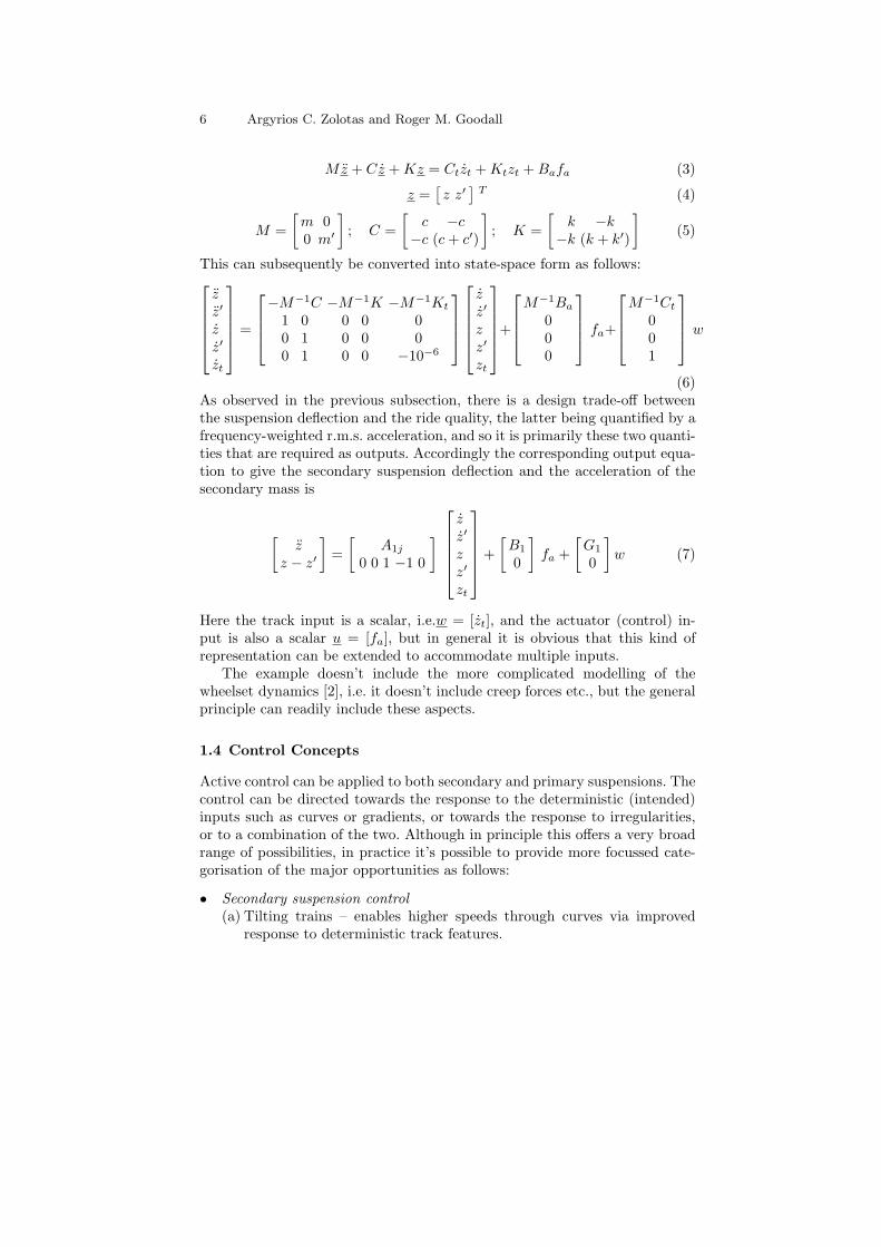
Note also that substantial coupling exists between the lateral and roll mo-tions which result in two sway modes combining both lateral and roll move-ment, and their centres located at points other than the vehicle centre ofgravity. An ‘upper sway’ mode, its node appears above the body c.o.g., withpredominantly roll movement; and a ‘lower sway’ mode, its node located belowthe body c.o.g., characterised predominantly by a lateral motion. The modalanalysis of the vehicle is shown in Table 1, with the modes being close to theindustrial-norm.

Table 1. ARB vehicle model dynamic modes

Mode Damping (%) Frequency (Hz)

Body lower sway 16.5 0.67Body upper sway 27.2 1.50Bogie lateral 12.4 26.80Bogie roll 20.8 11.10Airspring mode 100.0 3.70

For system analysis and control design, the system is written in the statespace form

x = Ax + Bu + Bww (13)

y = Cx + Hw (14)

where,

x =[

yv θv yb θb yv θv yb θb θr

]T, u = [δa], . . . (15)

w =[

R−1 θo θo θo yo yo

]T(16)

For simulation purposes only, disturbance signals θo, θo, yo should be in-corporated into the A matrix (in this case the stochastic track includes thefiltering effects of the wheelset). It should be noted, that the necessary C andD output matrices, for control design, can be formed from the relevant rows(depending on the required outputs) of the given A and B matrices. A num-ber of outputs is available such as displacements, velocities, accelerations of


the vehicle body and bogies and also displacements, velocities of the activeelements.

A series of transient tests ensure that the vehicle behaves in a similarmanner to its full scale equivalent (real) vehicle (for the passive model, withactuator inactive). The track profiles, both deterministic and stochastic, usedfor this purpose can be seen in Section 2.3.

0 200 400 600 800 1000 1200−1.5

−1

−0.5

0

0.5

track (m)

angl

e (d

egre

es)

Roll angle

0 200 400 600 800 1000 1200−0.5

0

0.5

1

1.5Lateral acceleration

track (m)

acce

l. (m

s−2 )

(a) Vehicle body

0 200 400 600 800 1000 1200−0.6

−0.4

−0.2

0

0.2

track (m)an

gle

(deg

rees

)

Roll angle

0 200 400 600 800 1000 1200−0.5

0

0.5

1

1.5Lateral acceleration

track (m)

acce

l. (m

s−2 )

(b) Vehicle bogie

0 200 400 600 800 1000 1200−0.04

−0.03

−0.02

−0.01

0

0.01

track (m)

defle

ctio

n (m

)

Secondary suspension

0 200 400 600 800 1000 1200−4

−2

0

2x 10

−4

track (m)

defle

ctio

n (m

)

Primary suspension

(c) Suspension deflections on det. track

0 200 400 600 800 1000 1200−1.5

−1

−0.5

0

0.5

1

track (m)

acce

l. (m

s−2 )

Body Lateral Acceleration

0 200 400 600 800 1000 1200−5

−2.5

0

2.5

5Bogie Lateral Acceleration

track (m)

acce

l. (m

s−2 )

(d) Lateral acceleration on stochastictrack @ 45(m/s)

Fig. 10. Vehicle body/bogie time histories @ 45(m/s)

In this passive (non-tilting) case, a nominal vehicle speed of vo = 45ms

(162kmh ) is assumed, and the designed cant deficiency at this speed is

v2o

R −gθo = 5.83o or 1.0( m

s2 ). Fig. 10(a) shows the lateral acceleration and corre-sponding roll angle for the body mass. The lateral acceleration level is whatthe passengers would experience on the curve transition, and it is providedby a lateral accelerometer placed on the vehicle body c.o.g. The peak value is13.0%g, while the steady-state value is around 11.93%g at a forward vehiclespeed of 45(m/s). The increase in lateral acceleration is because the lateral


suspension acts significantly lower than the body centre of gravity, and as aconsequence the body roll-outwards on curves (steady-state 1.0o).

In the case of the bogie mass, Fig. 10(b), the roll-out is less (steady statevalue of 0.43o) due to the stiffer primary suspensions. The steady-state levelof the bogie lateral acceleration of 10.7%g is closer to the cant deficiency forwhich the track was designed by the civil engineers. Note that more highfrequency components are now present due to the harsh environment of thebogie system.

Fig. 10(c) shows a comparison between the lateral displacements of thevehicle body and bogie. The effect of the two different sets of suspensionsis clearly evident. The soft secondary suspensions cause a displacement of36.5(mm) in steady-state, while the primary suspensions owing to the highstiffness have hardly been displaced by 0.3(mm) in steady-state.

It is also important to test the behaviour of the vehicle model on thestraight track irregularities, which are the primary cause of ride quality degra-dation. Fig. 10(d) presents the time histories for the lateral acceleration ofboth the body and the bogie travelling on straight track. The nominal vehiclespeed is assumed 45(m/s). The bogie due to its harsh environment has anR.M.S. value of lateral acceleration equal to 16.4%g, while the soft secondarysuspensions filter out a large amount of high frequencies and leave the bodywith an R.M.S. lateral acceleration of 2.932%g.

2.3 Tilt Control Requirements and Assessment Approach

Requirements

The performance of tilt control systems on the curve transitions is critical;most importantly the passenger ride comfort provided by the tilting vehicleshould not be (significantly) degraded compared to the non-tilting vehiclespeeds. The main objectives of any tilt control system are:

1. to provide an acceptably fast response to changes in track cant and cur-vature (deterministic track features)

2. not to react significantly to track irregularities (stochastic track features)

However, any tilt control system directly controls the secondary suspensionroll angle (i.e. the inclination of the body) and not the vehicle lateral ac-celeration. Hence, there is a fundamental trade-off between the vehicle curvetransition response and straight track performance. Moreover, for reasons ofhuman perception, designers utilise partial tilt compensation. In such a casethe passenger will still experience a small amount of acceleration on steadycurve, in order to minimise motion sickness phenomena.

From a control design point of view the objectives of the tilt system canbe translated (in terms of shaping the loop) as: increasing the response of thesystem at low frequencies (deterministic track features), while reducing the


high frequency system response (stochastic track features) and maintainingstability.

Note that in this study the tilt controllers should provide 60% tilt com-pensation on steady curve at high speed (for reasons of passenger motionsickness as discussed earlier in the chapter), i.e. the curving acceleration atthe increased speed is reduced to 40% of the non-tilting case (at the samespeed) rather than to zero. Although this strictly is known as partial-nullingtilt, for simplicity we will refer to it as nulling tilt.

Tilt Control Assessment

As mentioned previously, the performance of the tilt controller on the curvetransition is critical, and their assessment is based upon a combination of twoapproaches, i.e. the ‘PCT factors’ and the ‘ideal tilting ’ assessment.

The former is based upon a comprehensive experimental/empirical studywhich provides the percentage of (both standing and seated) passengers whofeel uncomfortable during the curve transition. The latter method emphasisesthe assessment of the control system performance by determining the devia-tions from the concept of “ideal tilting”, i.e. the tilt action follows the specifiedtilt compensation in an ideal manner, defined on the basis of the maximumtilt angle and cant deficiency compensation factor. This combination of para-meters is optimised via the PCT factors approach to choose a basic operatingcondition. The procedure follows a minimisation approach of dynamic effectsrelative to tilt angles, roll velocities and lateral accelerations (Fig.11); moredetails can be found in [7].

•|ym − ymi|, the deviation of the actual lateral acceleration ym from the

ideal lateral acceleration ymi, in the time interval between 1s before the start

of the curve transition and 3.6s after the end of the transition.•∣

∣

∣θm − θmi

∣

∣

∣, the deviation of the actual absolute roll velocity θm from the

ideal absolute roll velocity θmi, in the time interval between 1s before the

start of the curve transition and 3.6s after the end of the transition.Regarding the straight track case the ‘rule-of-thumb’ currently followed

by designers is to allow a lateral ride quality degradation of the tilting trainby no more than a specified margin of between 7.5%− 10% compared with thenon-tilting vehicle.

Track inputs

The deterministic track input employed for simulation purposes consists of acurved section with a radius of 1000m superimposed by a maximum track cantangle of 155mm(i.e. 6o), with a tilting speed of 209km/h over a track lengthof 1200m. The stochastic track inputs represent the irregularities in the trackalignment on both straight track and curves, and these were characterised by

an approximate spatial spectrum equal to Ωlv2

f3s

( m2

cycle/m ) with a lateral track

roughness Ωl of 0.33·10−8m [12].


Fig. 11. “Ideal Tilting”- Calculation of deviation of actual from ideal responses foracceleration and roll velocity[7]

2.4 Conventional Tilt Control

This section deals with the early-type conventional nulling control scheme andthe current practice followed by industry i.e. command-driven with precedenceapproach.

Classical nulling control strategy

In this intuitively formulated control strategy (as seen from Figure 8a), whichis a classical application of SISO feedback control, the signal from a body-mounted lateral accelerometer provides a measurement of the curving accel-eration experienced by the passengers. The controller would drive the feedbacksignal to zero and therefore give 100% compensation, so a portion of the sus-pension roll angle (actual tilt angle) is included in the feedback path, chosento provide the required 60% compensation.

The control input comprises an angular displacement (δa) provided bya rotary actuator in series with the anti-roll bar, which in turn provides atorque to the vehicle body. Note that the reference signal is ‘zero’, i.e. thesystem is subject to track disturbances only. The feedback signal for partialtilt compensation is the effective cant deficiency angle θ′dm which is given by

θ′dm =

(

−λ1yvm

g− λ2θ2sr

)

(17)


where yvm is the lateral acceleration felt by the passengers as measured froman accelerometer on the body c.o.g (18), and θ2sr is the secondary suspensionroll angle (19).

yvm =v2

R− g (θo + θv) + yv (18)

θ2sr = θv − θb (19)

Note the effect of the deterministic track included in (18). Factors λ1, λ2

ensure partial tilt and for 60% compensation need to be set to 0.615 and0.385 respectively, taking in account bogie roll-out in (19).

Remark: The sign of the feedback signal is inverted for correct ap-plication of negative feedback based upon the chosen axes system. Alllateral motions (y) are positive inwards to the curve center and all rollmotions (θ) are positive clockwise. However, the lateral accelerometer(a mass on a spring) measures positive acceleration outwards (18).Hence, the acceleration is translated into a positive cant deficiencyangle1 , combined with a portion of the suspension roll, and is thenfed back (note that λ1

yvm

g ≥ λ2θ2sr). The combined signal will thus

be a positive (w.r.t. the choice of directions) angle, which if fed backusing negative feedback will cause the controller to provide a negativetilt angle (i.e. anti-clockwise rotation), consequently destabilising thesystem. Thus inversion of the sign of the feedback signal is necessaryto guarantee proper body rotation for correct compensation.

Conclusions about the stability of the closed-loop may be drawn by investi-gating the open-loop frequency response of the system. The nominal open-loopfrequency responses from u := δa to y1 := θ′dm, and y2 := θ2sr can be seen inFig. 12. Note that, while gain reduction is required to stabilise the closed-loopsystem, the opposite applies in the case of fast tilt response. Hence, there mustbe a compromise between the tilt response and the ride quality.

A closer investigation of the open-loop poles and zeros of the transfer func-

tion Gy1u(s) =θ′

dm(s)δa(s) reveals that, while the system is open-loop stable, is also

non-minimum phase due to the existence of two RHP zeros at (s− 29.4) and(s− 6.02), Table 2. The pole-zero map of the uncompensated system Gy1u(s)can be seen in Fig. 13. The presence of RHP-zeros imposes a fundamentallimitation on control, and high controller gains induce closed-loop instability.

Integral action is necessary to guarantee zero effective cant deficiency angle

on steady curve. We design a classical PI controller Kpi(s) = kg

(

1 + 1sτi

)

,

with the proportional term limiting the extra phase-lag at increasing fre-quency. The settings for kg and τi were adjusted to suffice both the determin-istic and stochastic criteria, i.e. kg = 0.225, τi = 0.4 s (these can be slightly

1 Cant deficiency defines the difference between the existing degree of cant andthe degree required to fully eliminate the effect of centrifugal force at maximumallowable speed


Actuator input to inferred tilt (effective cant deficiency)

Open−Loop Phase (deg)

Ope

n−Lo

op G

ain

(dB

)

−540 −495 −450 −405 −360 −315 −270 −225 −180 −135 −90 −45 0−60

−50

−40

−30

−20

−10

0

10

20

30

40

6 dB

3 dB

1 dB

0.5 dB

0.25 dB

0 dB

−1 dB

−3 dB

−6 dB

−12 dB

−20 dB

−40 dB

−60 dB

(a) Tilt model open-loop responses(Nichols)

Actuator input to actual tilt (secondary suspension roll)


Ope

n−Lo

op G

ain

(dB

)

−360 −315 −270 −225 −180 −135 −90 −45 0−60

−50

−40

−30

−20

−10

0

10

20

30

40

6 dB

3 dB

1 dB

0.5 dB

0.25 dB

0 dB

−1 dB

−3 dB

−6 dB

−12 dB

−20 dB

−40 dB

−60 dB

(b) Effective cant deficiency open-loop

Fig. 12. Tilt angle open-loop

Table 2. Open-loop poles and zeros of Gy1u(jω)

OL poles OL zeros

-20.87 ± 167.34j -2.41 ± 125.94j-14.57 ± 68.38j 29.36 ± 0.00j

-2.56 ± 9.03j -40.73± 0.00j-0.69 ± 4.12j -26.18± 0.00j-23.22± 0.00j 6.02± 0.00j

- -3.83 ± 3.13j

further tuned via optimization). Table 3 presents the overall controller assess-

−50 −40 −30 −20 −10 0 10 20 30−200

−150

−100

−50

0

50

100

150

200

non−minimumphase

Pole-Zero map of Gy1u(jω)

Imag

Axis

Real Axis

Fig. 13. Pole-zero map of uncompensated OL


Table 3. Early-type nulling PI control assessment @ 58(m/s)

Deterministic

Lateral accel. - steady-state n/a (%g)(actual vs ideal) - R.M.S. deviation error 5.555 (%g)

- peak value 19.510 (%g)Roll gyroscope - R.M.S. deviation 0.032 (rad/s)

- peak value 0.086 (rad/s)(PCT-factor) - peak jerk level 10.286 (%g/s)

- standing 71.411 (% of passng)

- seated 22.640 (% of passng)

Stochastic

Passenger comfort - R.M.S. passive (equiv.) 3.778 (%g)- R.M.S. active 3.998 (%g)- degradation 5.802 (%)

ment, while Fig. 14 and Fig. 15 present the simulation results on curved trackand the corresponding frequency responses respectively. Clearly the responseis very slow with the steady-state values for acceleration, roll angle and rollrate profiles not met. Note that, due to the vehicle body inertia at the startand the end of curve, the body roll angle initially has an inverse response andthen rises slowly up to the required steady-state value. The difference betweenthe control input δa and the body roll θv is due to the torque imposed by thesecondary suspension subject to the curving forces on the vehicle body. Thus,additional control effort is demanded to overcome this extra torque and regu-late the body roll (via the suspension roll portion) to the desired value. Thereis also great difficulty in controlling the roll rates appropriately, which has adetrimental effect on the overall system performance. Note that the secondarysuspension deflection is given by x2dfl = yv − h1θv − (yb + h2θb).

Moreover, the complementary sensitivity T , in Fig. 15(b), shows that thecontrol action in the frequency range

[

0.4( radss ), 4( rads

s )]

does not affect thesystem, which causes a slow response (i.e. insufficient bandwidth). Moreover,higher frequency components enter owing to the sway mode resonances in theinterval

[

4( radss ), 10( rads

s )]

, with the control action incapable of improvingthe performance due to |S| > 1. The uncompensated and compensated open-loop responses are presented in Fig. 15(a), with the latter emphasising theOL integral action at low frequencies.

The difficulties in the early-type classical nulling strategy are the following:(i) the sensor exists within the control loop resulting in interactions betweencontroller and suspension dynamics, and (ii) the system is also non-minimumphase and there is a stability threshold point set by the non-minimum phasezero, which result in major limitations in the controller design.

Later on in the section we will see how we can improve the performanceof nulling-type schemes with the use of modern control methods.


0 200 400 600 800 1000 1200−1

−0.5

0

0.5

1

1.5

2actual"ideal"

Body lateral acceleration @ 58 ms

accel.

(m s2

)

track (m)

(a) Passenger acceleration

0 200 400 600 800 1000 1200−6

−4

−2

0

2

4

6passiveactive actualactive "ideal"

Body roll gyroscope (abs roll rates) @ 58 ms

rate

(d

eg

s)

track (m)

(b) Roll rate

0 200 400 600 800 1000 1200−2

0

2

4

6

8

10

12activecommand (u)

activeactual (θ

2sr)

passive (θ2sr

)

activeideal

profile

Tilt angles @ 58 ms

angle

(d

eg

re

es)

track (m)

(c) Tilt angles

0 200 400 600 800 1000 1200−0.1

−0.08

−0.06

−0.04

−0.02

0

0.02

active @ 58m/spassive @ 45m/s

Secondary lateral suspension deflection

deflectio

n(m

)

track (m)

(d) Suspension Deflection

Fig. 14. Early-type nulling PI scheme for deterministic track

Command-driven with precedence control

The problems with the early-type nulling schemes and also with heavy lowpass filtering in attempting local command-driven strategies (to reduce theeffect of bogie high frequency components in the feedback signal used), led tothe currently used by industry command-driven with precedence scheme (theconcept can be seen in Fig. 8(b)).

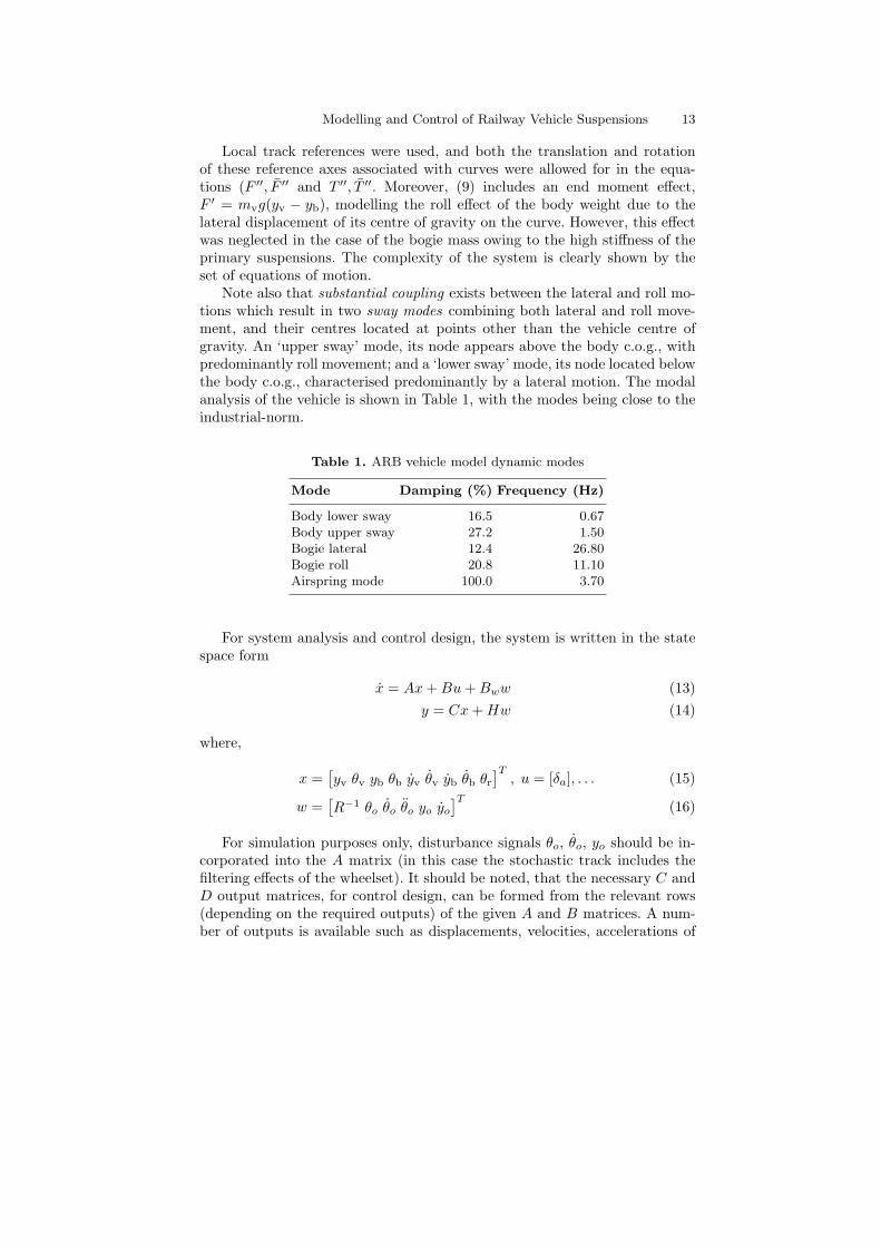
For illustrative purposes we consider the command-driven with precedencescheme in Fig. 16. It employs an accelerometer on the leading bogie of theleading vehicle (a preview of 29m was assumed) provided the curving acceler-ation signal, passed via a 0.45Hz low pass filter. The signal is then processedto provide 60% compensation for the lateral acceleration (K is set to 0.6).The actuator is controlled using an additional feedback of tilt angle (i.e. thesuspension roll).

For appropriate comparison to the local tilt strategies, the filter delaywas chosen to match the precedence time, however this can be changed toemphasise precedence information if necessary. The transfer function of the


Nichols Chart


Ope

n−Lo

op G

ain

(dB

)

−540 −495 −450 −405 −360 −315 −270 −225 −180 −135 −90 −45 0−60

−50

−40

−30

−20

−10

0

10

20

30

40

6 dB

3 dB

1 dB

0.5 dB

0.25 dB

0 dB

−1 dB

−3 dB

−6 dB

−12 dB

−20 dB

−40 dB

−60 dB

uncompensatedcompensated

uncompensatedGM = −9.6 at 8.64 (rad/s)PM = −86o at 16.9 (rads/s)

compensatedGM = 3.15 at 7.84 (rad/s)PM = 40.58o at 4.95 (rad/s)

(a) Uncompensated and compensatedOL

−60

−50

−40

−30

−20

−10

0

10

20

10−2

10−1

100

101

102

103

−450

−360

−270

−180

−90

0

90

S T K⋅S

S

K⋅S

T

Bode Diagrams T , S, KS

Frequency ( radssec

)

Phase

(d

eg)

Mag.(d

B)

(b) Complementary Sensitivity, Sensi-tivity and Control Sensitivity

Fig. 15. Early-type nulling PI system frequency responses

LP filter is given by

HLP2(s) =w2

c2

s2 + 2ζ2wc2+ w2

c2

, wc2= 2π × 0.45, ζ2 = 0.707 (20)

and the time delay introduced is tdLP=

2ζ2wc2

w2c2

, which for the current case is

0.5s. Thus for the precedence to match the filter delay, it takes l = 58(ms ) ×

0.5s = 29m precedence, i.e. approximately 1.5 vehicle length. Note that thetilting response for the leading vehicle will unavoidably be too late.

The leading vehicle controller was chosen as Kpi(s) =(

1 + 1s0.5

)

. For thetrailing vehicle, the controller designed to actively tilt the body is a PI com-pensator in series with a low-pass filter (LPF)2, in order to remove high fre-quencies from the secondary suspension roll (those are introduced due to thebogie roll contribution). The overall controller transfer function is

Ktotal(s) =

(

1.5 + s0.75

s0.5

)

×400

s2 + 28.28s + 400

The compensated and uncompensated open loop together with the overallcompensator frequency response can be viewed in Fig. 17(a). The correspond-ing sensitivity and complementary sensitivity of the closed loop system arepresented in Fig. 17(b), where it is evident that the control action influencesthe system over a wider range of frequencies compared to the classical nullingcase.

A set of time-domain results for the deterministic track case is shownin Fig. 18, where it is obvious that the precedence scheme is superior tothe classical nulling approach. The tilt controller performance is presented in

2 the LP filter will be redundant in the case of actuator dynamics, i.e. actuator willhave limited bandwidth by default.


yvm

..

suspensionroll

θ2sr

Track

+

-

ControllerK2(s)

δae

u

r Vehicle DynamicsLocal Vehicle

yvm

..

suspensionroll

θ2sr

Track

+

-

ControllerK1(s)

δae

u

K/g

ybm

..

r

tilt command

Vehicle DynamicsPrecedent

Vehicle

LPF0.45HzK/g

precedenceeffect

Precedent Vehicle

Local Vehicle (current)

tilt command

29.0m

LPF0.45Hz

(a) Block Diagram

LeadingTrailing

1.5 Vehicle length preview (~29m)

xxxxxxxxxxxxxxxxxxxxxxxx

xxxxxxxxxxxxxxxxxxxxxxxxxxxxxxxxxxxx



xxxx

Low-Pass

0.45Hz

bg

accel

Tilt

comm.

K/g

Track

Datae-s0.5

for simulation

speed=58(m/s)

bogie

vehicle body

tilt

mechanism

direction of travel

(b) Interpretation for simulation purposes

Fig. 16. Command-driven with precedence approach

Table 4, and it is closer to the ideal performance as expected in all cases.In the stochastic case there is an improvement in ride quality by the activesystem, because the precedence time matches the filter delay meaning thatthe reference and track input are uncorrelated, thus the tilt command willcompensate for long wavelengths.

Emphasising more precedence information improves the deterministic per-formance, subject of course to the amount of precedence used, i.e. too muchprecedence (over-precedence) can be disastrous for the normal operation ofthe train (tilt action will apply on straight track segments much sooner thanthe intended start of the curve!). In addition, the amount of precedence usedwill influence the stochastic ride quality either in a positive or negative waydepending upon the correlation of the signals (in the case where the prece-dence time differs from the filter delay, the reference and track input signalsare no longer uncorrelated). It should be noted that, even in the precedence


10−1

100

101

102

−360

−270

−180

−90

0

−150

−100

−50

0

50uncompenscompensatorcompensated

Bode Diagrams OL (δa) to θ2sr

Frequency ( radssec

)

Phase

(d

eg)

Mag.(d

B)

(a) Compensated and uncompensatedOL

10−2

10−1

100

101

102

103

−150

−100

−50

0

50

10−2

10−1

100

101

102

103

−400

−300

−200

−100

0

100

S T

S

T

Bode Diagrams T , S

Frequency ( radssec

)

Phase

(d

eg)

Mag.(d

B)

(b) Complementary Sensitivity, Sensi-tivity

Fig. 17. Command-driven with precedence system frequency responses

Table 4. Command-driven with precedence - assessment @ 58(m/s)

Deterministic

Lateral accel. - steady-state 9.53 (%g)(actual vs ideal) - R.M.S. deviation error 1.54 (%g)


- peak value 0.104 (rad/s)(P-factor) - peak jerk level 6.80 (%g/s)



Stochastic

Passenger comfort - R.M.S. passive (equiv.) 3.78 (%g)- R.M.S. active 3.31 (%g)- degradation -12.12 (%)

schemes, sensors located on each vehicle (i.e. local sensors) are used to en-sure the correct operation of the overall tilting system (the sensors are alwayspresent for safety purposes).

2.5 Nulling-type tilt via robust control techniques

In this section we will see how to improve the performance nulling-typeschemes by employing robust control methods, in order to achieve compa-rable results to the command-driven with precedence scheme. In particularthe case study involves an LQG/LTR approach [11] and a multiple objectiveH∞/H2 scheme [12].


0 200 400 600 800 1000 1200−0.4

−0.2

0

0.2

0.4

0.6

0.8

1

1.2actual"ideal"


accel.

(m s2

)

track (m)


0 200 400 600 800 1000 1200−6

−4

−2

0

2

4

6active actualactive "ideal" profpassive actual


rate

(d

eg

s)

track (m)

(b) Roll rate

0 200 400 600 800 1000 1200−4

−2

0

2

4

6

8

10

12

14θ

v passive actual

θv

active actual

u command"ideal" profile

Tilt angles @ 58 ms

angle

(d

eg

re

es)

track (m)

(c) Tilt angles

0 200 400 600 800 1000 1200−0.09

−0.08

−0.07

−0.06

−0.05

−0.04

−0.03

−0.02

−0.01

0

0.01

active @ 58m/spassive @ 45m/s

Secondary lateral suspension deflection

deflectio

n(m

)

track (m)

(d) Suspension Deflection

Fig. 18. Command-driven with precedence on deterministic track

LQG/LTR nulling-type tilt control

Linear Quadratic Gaussian control is well documented in [8],[10], defining thefollowing state-space plant model

x = Ax + Bu + Γw (21)

y = Cx + v, (22)

where w, v are (ideally) white uncorrelated process and measurement noiseswhich excite the system, and are characterised by covariance matrices W,Vrespectively. The separation principle can be applied to first find the optimalcontrol u = −Krx which minimises (23)

J = limT→∞

1

TE

∫ T

0

[xT Qx + uT Ru]dτ

, (23)

where Kr = R−1BT X and X is the positive semi-definite solution of thefollowing Algebraic Riccati Equation (ARE)


[

X −I]

[

A −BR−1BT

−Q −AT

] [

IX

]

= 0 (24)

Next find the optimal state estimate x of x where

x = Ax + Bu + Kf (y − Cx) (25)

to minimise E

[x − x]T

[x − x]

. The optimal Kalman gain is given by Kf =

Y CT V −1 and Y is the positive semi-definite solution of the following ARE

[

Y −I]

[

AT −CT V −1C−ΓWΓT −A

] [

IY

]

= 0 (26)

Weighting matrices Q (pos. semidefn.), R (pos. defn.) for control, and W (pos.semidefn.), V (pos. defn.) for estimation, can be tuned to provide the desiredresult. Note that it is also possible to follow the dual procedure, i.e. solve forthe state estimate sub-problem and next for the optimal gain sub-problem(although this is not considered in our study).

For synthesizing the tilt controller we consider a simple extension to theclassical nulling approach in an optimal control framework by deriving theSISO model, from δa to θ′dm, with all disturbance signals set to zero. Thus,on measurement is effectively use for the Kalman filter.

We will synthesize the controller using the weighting matrices Q,R,W, Vpurely as tuning parameters until an appropriate design is obtained. In par-ticular, the structure of the LQG tilt compensator is found by shaping theprincipal gains of the system, i.e. return ratios. First the LQR is synthesizedvia Q,R to obtain a satisfactory a satisfactory return ratio −Kr (sI − A)

−1B,

with the Kalman Filter designed via W,V such that the return ratio at the in-put of the compensated plant converges sufficiently close to −Kr (sI − A)

−1B

over the frequency range of interest (Loop Transfer Recovery to recover asmuch as possible of the robust properties of LQR).

For disturbance rejection and/or reference tracking (which is zero in thiscase), the system should be augmented using an extra state, the integral of theeffective cant deficiency θ′dm. This approach will produce an optimal controllerwith integral action [8]. Hence, the system is becomes

(

xx′

)

=

(

A 0C ′ 0

)(

xx′

)

+

(

B0

)

u (27)

where x′ =∫

θ′dm and C ′ is the selector matrix for integral action and is foundfrom θ′dm = C ′x. The control signal has the form

u = −(

Kp Ki

)

(

xx′

)

(28)

We start with the simplest possible choices for Q,R


Q =

(

09×9 09×1

01×9 qi

)

, R = 1 (29)

thus adjusting only the weight of the integral state, and imposing no con-straints on the remaining states. Fig.19 illustrates the return ratio−Kr (sI − A)

−1B for various qi. We choose the return ratio for qi = 100

with a crossover of approx 20rad/s, to recover for in the next steps. Howevera simple calculation of the transmission zeros for the design plant reveals anon-minimum phase zeros at approximately 6.0rad/s (this is characteristic forsuch a setup in tilting trains [12]), thus making full recovery cumbersome. Forillustration, the usual LTR procedure is followed up to the limit of recoveryallowed from the non-minimum phase zero (usually the achievable bandwidthof the system is less than half of the RHP zero frequency [10]).

10−1

100

101

102

103

−80

−60

−40

−20

0

20

40

60

Kr(sI−A)−1B; q

i=[.1 1 5 10 100 500 1e3]

Frequency (rad/sec)

Sin

gula

r V

alue

s (d

B)

increasing qi

Fig. 19. Return ration −Kr (sI − A)−1 B for various qi

Moreover, for the design of the Kalman Filter, the zero eigenvalue of theaugmented A matrix needs to be placed just to the left of the origin forthe solution to exist. For controller implementation this should move back tothe origin for proper integration. equal to B, 1 respectively (still for the SISOmodel). Setting Γ = B refers to any (virtual) disturbances on the plant actingvia the input, rather than the actual track disturbances from the track.

The sensor noise covariance matrices is set to V = 1 (can be reduced tocharacterise better quality measurements), while the process noise covariancematrix is set to W = Wo + wI (Wo = 0). Fig.20 illustrates the amount of


recovery at plant output for increasing values of w. It is seen that there isno point in recovering after w = 500 as appropriate integral action is alreadyrecovered and the actual crossover limit is placed by the non-minimum phasezero.

10−5

100

105

−200

−150

−100

−50

0

50

100

150

200

LQG/LTR @ input for w=[.1 1 5 10 100 500 1e3]

Frequency (rad/sec)

Sin

gula

r V

alue

s (d

B)

Kr(sI−A)−1B

Klqg

(s)G(s)

increasing

increasing

Fig. 20. LTR at plant output for increasing w

Fig. 21 presents the principal gains of the designed closed loop systemw.r.t. sensitivity S and complementary sensitivity T . The bandwidth of thesystem is rather low (approx. 1rad/s due to the NMP zero) however thereis some compensation at higher frequencies which cater for few stochasticcomponents (on straight track ride).

The synthesized LQG controller realization is given by

Klqgs=

[

A − BKr − KfC Kf

−Kr 0

]

(30)

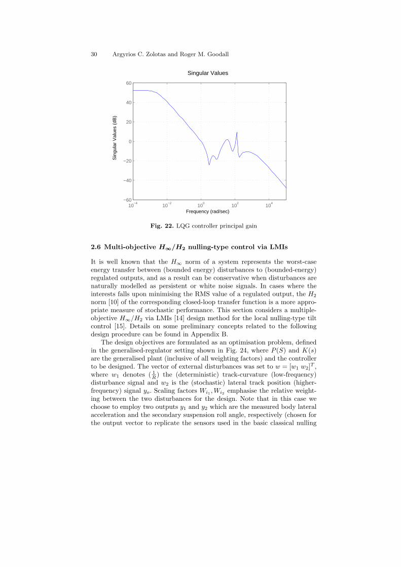
and is 10th order and its frequency response can be seen in Fig. 22. This canbe further reduced either in an open loop or closed sense [10], however at theexpense of performance quality.

The time domain results for the lateral acceleration felt by the passengersand the related body tilt angle can be seen in Fig. 23, while the performanceassessment of the controller is presented in Table 5. It is seen that althoughthe LQG-based is a simple straightforward optimal extension of the classical


Principal Gains

Frequency (rad/sec)

Sin

gula

r V

alue

s (d

B)

10−3

10−2

10−1

100

101

102

103

−60

−50

−40

−30

−20

−10

0

10

compl.sensitivity

sensitivity

Fig. 21. Designed system Sensitivity and Compl. Sensitivity with LQG controller

Table 5. LQG nulling-type control assessment @ 58(m/s)

Deterministic






Stochastic


nulling scheme, the performance is much improved (emphasizing robustnesswith the additional damping injected).

It is worth mentioning that the performance of the controller can be furtherimproved by using extra sensor information, i.e. passenger acceleration, bodyroll rate, vehicle yaw rate [13]. The design system in this case will be non-square with more outputs than inputs, as a result the LQG controller will benon-square (more inputs than outputs). However, we can still synthesize viathe separation principle, but make the system square for LTR [8].


10−4

10−2

100

102

104

−60

−40

−20

0

20

40

60

Singular Values

Frequency (rad/sec)

Sin

gula

r V

alue

s (d

B)

Fig. 22. LQG controller principal gain

2.6 Multi-objective H∞/H2 nulling-type control via LMIs

It is well known that the H∞ norm of a system represents the worst-caseenergy transfer between (bounded energy) disturbances to (bounded-energy)regulated outputs, and as a result can be conservative when disturbances arenaturally modelled as persistent or white noise signals. In cases where theinterests falls upon minimising the RMS value of a regulated output, the H2

norm [10] of the corresponding closed-loop transfer function is a more appro-priate measure of stochastic performance. This section considers a multiple-objective H∞/H2 via LMIs [14] design method for the local nulling-type tiltcontrol [15]. Details on some preliminary concepts related to the followingdesign procedure can be found in Appendix B.

The design objectives are formulated as an optimisation problem, definedin the generalised-regulator setting shown in Fig. 24, where P (S) and K(s)are the generalised plant (inclusive of all weighting factors) and the controllerto be designed. The vector of external disturbances was set to w = [w1 w2]

T ,where w1 denotes ( 1

R ) the (deterministic) track-curvature (low-frequency)disturbance signal and w2 is the (stochastic) lateral track position (higher-frequency) signal yo. Scaling factors Wi1 ,Wi2 emphasise the relative weight-ing between the two disturbances for the design. Note that in this case wechoose to employ two outputs y1 and y2 which are the measured body lateralacceleration and the secondary suspension roll angle, respectively (chosen forthe output vector to replicate the sensors used in the basic classical nulling


0 200 400 600 800 1000 1200−1

−0.5

0

0.5

1

1.5

2Body acceleration

track (m)

acce

lera

tion

(m/s

2 )

actualideal

(a) Lateral acceleration

0 200 400 600 800 1000 1200−1

0

1

2

3

4

5

6

7

8

9Body roll (tilt)

track (m)

tilt (

deg)

actualideal

(b) Tilt angle

Fig. 23. Lateral acceleration and tilt profile on curved track with LQG

control). It is worth noting that the system transfer function with the twoaforementioned measurements is not NMP.

It is very important to meet both deterministic (curve track) and stochastic(straight track) requirements, thus the following multi-objective optimisationproblem was formulated


P

K

z1

y=[y 1 y 2] T

w1

u

Wi 1

Wi 2

W1

W2z2 w2

Fig. 24. Generalised Regulator configuration for multi-objective control

minK∈S

α ‖W1Tz1w‖2∞

+ β ‖W2Tz2w‖22 (31)

in which S denotes the set of all internally stabilising controllers. The firstregulated output z1 for infinity-norm minimisation, was chosen as the effectivecant deficiency z1 = θ′dm. For the minimisation of the 2-norm, z2 was chosen asthe control input u denoting the actuator roll angle δa. Regulating z1 to zerocorresponds to 60% tilt compensation and thus attains the desired (steady-state) level of acceleration on steady state curve. Tziw (i = 1, 2) denotes the(closed-loop) transfer functions between signals w and z1, z2 respectively.

Multi-objective optimisation typically refers to the joint optimisationof a vector consisting of two or more functions, typically representingconflicting objectives. Common types of multi-objective optimisationproblems include “Pareto-optimal” (non-inferior) optimality criteria,minimax optimality criteria, etc. In the context of this exercise, theterm “multi-objective” refers simply to the fact that the cost functionof the optimisation problem involves two different types of norms,capturing the deterministic and stochastic objectives of the design.The two different norms that are used here are the 2-norm and theinfinity-norm. Thus, typical examples of multi-objective problems inour context include:

1. Constrained minimisation:Minimise ‖W1Txy‖2 subject to ‖W2Tzw‖∞ < γ,

2. Unconstrained minimisation:Minimise β ‖W1Txy‖2 + α ‖W2Tzw‖∞, and

3. Feasibility problem:Find a stabilising K(s) (if one exists) such that‖W1Txy‖2 ≤ γ1 and ‖W2Tzw‖∞ ≤ γ2


Txy and Tzw represent two general closed-loop transfer functions,weighted via W1 and W2.

Scalars α and β, in (31), are positive definite design parameters whichmay be used to shift the emphasis of the optimisation problem between theminimisation of the ‖Tz1w‖∞ term (deterministic objective) and the ‖Tz2w‖2

term (stochastic objective). The frequency-domain weights W1 and W2 havebeen chosen as:

W1(s) = 104s

200 + 1s

0.0001 + 1(32)

W2(s) = 0.5s3 + 1.59s2 + 0.58s + 0.06

s3 + 13.81s2 + 38.4s + 2.98(33)

W1 is essentially a low-pass filter with a very low pole cut-off frequency(10−4 rads

s ) and high gain at low frequencies, Fig. 25(a). Thus W1 emphasisesminimisation of the ‖Tz1w‖∞ term in the low frequency range and effectivelyenforces integral control on the regulated output (z1). W2 is a high-pass filterwith pole (10 rads

s ) and zero (0.2 radss ) cut-off frequencies. A lead/lag network

is also included in W2, in the range of [.1 radss , 6 rads

s ], which found to have apositive effect on controller design (by enhancing the cross-over frequency ofW1,W2), Fig. 25(a). By limiting the high-frequency components of the con-trol input (z2), effectively places a limit on the closed-loop bandwidth of thesystem, which in turn limits the RMS acceleration on straight track (stochas-tic case). Additional benefits include a smoother control signal and improvedrobustness properties of the controller when the effects of uncertainty in P (s)and in the actuator dynamics are taken into account. Moreover, the relativeweighting between w1 and w2 were simply set to unity, i.e.

Wi =

[

Wi1 00 Wi2

]

=

[

1 00 1

]

(34)

Thus the energy of either of the signals is equally incorporated in the costfunction. Increasing either Wi1 or Wi2 with respect to the other will put moreemphasis on the deterministic or the stochastic track respectively. However,the current choice of Wi provides the best results.

The minimisation problem in (31) was solved in Matlab using the LMItoolbox [14], i.e. representing the problem in a set of Linear Matrix Inequalitiesand follow a convex optimisation approach. This technique has very attractivecomputational properties and is widely used in systems and control theory.

For controller design, the generalised plant was formulated as follows

x = Ax + B1w + B2u

z∞ = C∞x + D∞1w + D∞2u (35)

z2 = C2x + D21w + D22u (36)

y = Cyx + Dy1w (37)


10−3

10−2

10−1

100

101

102

103

−60

−40

−20

0

20

40

60Bode diagram

mag

(dB

)

Frequency (rads/s)

W1(s)

W2(s)

(a) Weighting filters

10−3

10−2

10−1

100

101

102

103

−50

−40

−30

−20

−10

0

10Singular values

mag

(dB

)

Frequency (rads/s)(b) Controller principal gains

Fig. 25. Multi-objective H∞/H2 LMI approach scheme

where all matrices can be formed based upon the state space model of the sys-tem and the specifications in the generalised plant discusses earlier in this sec-tion. The controller can be then found by using matlab function hinfmix().The optimisation problem was solved for a few combinations of the α and β

Table 6. α-β combinations for the H∞/H2 problem

α β Ride Quality-Degrad.(%) Deviations-Determ.(%g)

1 1 21.7 1.951 2.5 10 2.151 5 4.95 2.371 10 3.4 2.621 20 2.1 2.9

Ride Quality-Degrad.: ride-quality degradation @58m/s of activesystem compared to passive @58m/s (straight track)Deviations-Determ.: RMS acceleration deviation from the ideal responseof an ideal tilting controller @58m/s (curved track)

parameters and the results can be seen in Table 6. The results shown in thetable clearly illustrate the fundamental trade-off between the deterministicand the stochastic objectives of the design.

As expected, increasing the value of β relative to α places more emphasison the stochastic aspects of the design, and as a result the RMS accelerationon straight track is further reduced. This is at the expense of deterministicperformance and, therefore, the curved track response becomes slower (largerdeviations from the ideal tilt response). Since it is required that stochasticperformance deteriorates by no more than 7.5% compared to the passive sys-tem, the “best” design was obtained for α = 1 and β = 5. The result returnedin Matlab for the “best” configuration is shown below (summary)


Optimization of 1.000 * G^2 + 5.000 * H^2 :

----------------------------------------------

Solver for linear objective minimization under LMI constraints

Iterations : Best objective value so far

1

.

.

.

16

* switching to QR

17

.

.

.

.

35

36 1.018621e+005

37 1.018621e+005

38 6.830550e+004

39 6.830550e+004

40 5.029532e+004

41 5.029532e+004

42 4.475980e+004

43 4.226245e+004

*** new lower bound: 3159.072336

44 4.067042e+004

45 3.932891e+004

.

.

.

62 3.493807e+004

*** new lower bound: 3.437031e+004

63 3.488358e+004


64 3.483742e+004


Result: feasible solution of required accuracy

best objective value: 3.483742e+004

guaranteed relative accuracy: 9.50e-003

f-radius saturation: 88.219\% of R = 1.00e+008

Guaranteed Hinf performance: 1.54e+002

Guaranteed H2 performance: 4.68e+001

Note that, in the first few iterations, the algorithm does not find any solutions,however the solution converges soon after. The resulting controller is of 2-input/1-output dimension due to the two measurements used in the formulation. The singularvalue plot is shown in Fig. 25(b), by definition depicting the largest singular of thetwo output/one input system transfer function. Note that the controller order isequal to 13, i.e. 9 states from the train model + 4 states from the weights. However,


it can be easily reduced down to a 7th order equivalent, e.g. via balanced truncation[10], with minimal degradation in performance.

The performance of the designed system is assessed in Table 7, where it can beseen that it is significantly improved compared to the classical nulling and LQGnulling-type control schemes. This exercises illustrate the usability of employingtwo measurements (compared to only one in the LQG scheme) and the effectivenessof distinguishing the design objectives in the cost function. For completeness theassociated time history analysis for the design track is presented in Fig. 26.

Table 7. H∞/H2 multi-objective LMI approach @ 58(m/s)

Deterministic






Stochastic


2.7 Case Study Remarks

This exercise has considered the design of local tilt controllers (a form of secondaryrailway suspension control) based upon advanced control concepts. The problemswith early-type classical nulling approaches has been presented, and briefly discussedthe currently-used precedence strategy. It has been shown that by using moderncontrol methods, i.e. LQG and H∞ based schemes, the performance of nulling-type controllers can be significantly improved. Problems with the two model-basedschemes include high-order controller size and the choice of weighting functions.Controller reduction can be employed for the former, while the latter requires arealistic setup of the design problem (to reduce the complexity of choosing thestructure of the weights) and usually designer experience (this being the case forthe majority of engineering applications).


0 200 400 600 800 1000 1200−0.6

−0.4

−0.2

0

0.2

0.4

0.6

0.8

1

1.2

1.4


accel.

(m s2

)

track (m)

actual

ideal


0 200 400 600 800 1000 1200−0.2

−0.15

−0.1

−0.05

0

0.05

0.1

0.15


rate

(r

ad

ss

)

track (m)

actual

ideal

(b) Body Roll rate

0 200 400 600 800 1000 1200−0.02

0

0.02

0.04

0.06

0.08

0.1

0.12

0.14

0.16

Tilt angles @ 58 ms

angle

(r

ad

s)

track (m)

actual

ideal

(c) Tilt angles

Fig. 26. Design track time history results for H∞/H2 design

References

1. Iwnicki S (Ed.) (2006) Handbook of Railway Vehicle Dynamics. Taylor andFrancis

2. Wickens A (2003) Fundamentals of Rail Vehicle Dynamics. Swets and Zeitlinger3. Goodall RM, Brown S (2001) Tilt technology still evolving as the cost falls.

Railway Gazette International. 521–5254. Goodall, RM (1999) Tilting Trains and Beyond – the Future for Active Railway

Suspensions: Part 1 Improving Passenger Comfort. Computing and ControlEngineering Journal. August 153–159

5. Goodall RM, Bruni S, Mei TX (2005) Concepts and prospects for actively-controlled railway running gear. Procs 19th IAVSD Symposium. Milano

6. Pearson JT , Goodall RM, Pratt I (1998) Control System Studies of an ActiveAnti-Roll Bar Tilt System for Railway Vehicles. Proceedings of the Institutionof Mechanical Engineers Part F. 212(F1):43–60

7. Goodall RM, Zolotas AC, Evans J (2000) Assessment of the Performance ofTilt System Controllers. Proceedings of the Railway Technology ConferenceIMechE. C580/028/2000. Birmingham UK. November 231–239


8. Maciejowski JM (1989) Multivariable Feedback Design. Addison-Wesley9. Zhou K, Doyle JC (1998) Essentials of Robust Control. Prentice-Hall

10. Skogestad S, Postlethwaite I (2000) Multivariable Feedback Control: Analysisand Desgn. Wiley and Sons

11. Zolotas AC, Halikias GD, Goodall RM and Wang J (2006) Model ReductionStudies in LQG Optimal Control Design for High-Speed Tilting Railway Car-riages. Proceedings of the 2006 American Control Conference. Minneapolis MNUSA. June 1796–1801

12. Zolotas A C (2002) Advanced Control Strategies for Tilting Trains. PhD Thesis,Loughborough University, UK

13. Zolotas AC, Goodall RM (2005) Improving the tilt control performance of high-speed railway vehicles: an LQG approach. Proceedings of the 16th IFAC WorldCongress. Prague

14. Gahinet P, Nemirovski A, Laub A, Chilali M (1994) LMI Control Toolbox.Natick, MA, The MathWorks.

15. Zolotas AC, Halikias GD, Goodall RM (2000) A Comparison of Tilt ControlApproaches for High Speed Railway Vehicles. Proceedings of the 14th Interna-tional Conference on Systems Engineering ICSE 2000, Coventry UK. 2:632–636


Appendix A- Tilting Train Parameter values and

notation

yv, yb, yo Lateral displacem. of body, bogie, trackθv, θb, θr Roll displacement of body, bogie, airspring reservoirδa ARB applied tiltθo, R Track cant, curve radiusv Vehicle forward speedmv Half body mass, 19,000(kg)ivr Half body roll inertia, 25,000(kgm2)mb Bogie mass, 2,500(kg)ibr Bogie roll inertia, 1,500(kgm2)g gravitational acceleration, 9.81(ms−2)

— Values per bogie side —kaz Airspring area stiffness, 210,000( N

m)

ksz Airspring series stiffness, 620,000( Nm

)krz Airspring reservoir stiffness, 244,000( N

m)

crz Airspring reservoir damping, 33,000(Ns

m)

ksy Secondary lateral stiffness, 260,000( Nm

)csy Secondary lateral damping, 33,000(Ns

m)

kvr Anti-roll bar stiffness/bogie, 2,000,000(Nm

rad)

kpz Primary vertical stiffness, 2,000,000( Nm

)cpz Primary vertical damping, 20,000(Ns

m)

kpy Primary lateral stiffness, 35,000,000( N

m)

cpy Primary lateral damping, 16,000(Nsm

)d1 Airspring semi-spacing, 0.90(m)d2 Primary vertical suspension semi-spacing, 1.00(m)h1 2ndary lateral susp. height(body cog), 0.9(m)h2 2ndary lateral susp. height(bogie cog), 0.25(m)h3 Primary lateral susp. height(bogie cog), -0.09(m)hg2 Bogie cog height(rail level), 0.37(m)hg1 Body cog height(rail level), 1.52(m)

Appendix B- H∞ based controllers: Preliminaries

Basic Notation

A continuous time, linear time invariant, state space system is given by

x(t) = Ax(t) + Bu(t) (38)

y(t) = Cx(t) + Du(t) (39)

where A ∈ ℜn×n, B ∈ ℜn×m, C ∈ ℜp×n and D ∈ ℜp×m. The above state spacesystem is characterised by the following transfer function with dimension p × n


G(s) = C(sI − A)−1B + D (40)

This thesis adopts the following conventional state-space representation to representG(s)

G(s)s=

A B

C D

(41)

Note also that the complex conjugate of G(s) is given by

G∗(s) = GT (−s)s=

−AT −BT

CT DT

(42)

and if G(s)G∗(s) = I = G∗(s)G(s) for all s ∈ jℜ, then G(s) is said to be all-pass.

Finally if matrix D is invertible, then G−1(s) is given by3

G−1(s)s=

A − BD−1C BD−1

−D−1C D−1

(43)

• Frequency Domain Spaces and Norms

This part introduces the meaning of frequency domain spaces and norms of realrational, matrix valued, transfer functions. For a more comprehensive study thereader is referred to Zhou and Doyle [9].

Let R denote the space of all real rational transfer function matrices. The L2/H2

norm of G(s) is given by

‖G‖2

,

s1

2π

Z∞

−∞

tr (G∗(jω)G(jω)) dω (44)

which is used to define the following spaces

(i). RL2 refers to the space of all real rational transfer function matrices with nopoles on the imaginary axis and is characterised by a finite L2 norm.

(ii). RH2 defines the space of all transfer function matrices in RL2 with no poles inRe(s) > 0.

The L∞/H∞ norm of G(s) is given by

‖G‖∞

, supω∈ℜ

σ [G(jω)] (45)

and

(i). RL∞ refers to the space of all real rational transfer function matrices with nopoles on the imaginary axis (with finite L∞ norm).

(ii). RH∞ defines the space of all transfer function matrices in RL∞ with no polesin Re(s) > 0.

3 Using the matrix inversion lemma:(A1 + A2A3A4)

−1 = A−11 − A−1

1 A2(A4A−11 A2 + A−1

3 )−1A4A−11 .


Also, the H∞ norm of a stable transfer function G(s) is its largest input/outputRMS gain

‖G‖∞

, supu∈L2u6=0

‖y‖L2

‖u‖L2

(46)

where L2 is the space of signals having finite energy and y is the output of the systemG for a given input u. Thus, for any input u of unit energy, the output energy in yis bounded by the H∞ norm of G(s).

• Linear Fractional Transformations

The basic concept of Linear Fractional Transformations is outlined in this section.Linear Fractional Transformations (LFT) are frequently used in the area of H∞

optimisation as well as in other areas of control theory. They do represent a meansof standardising a wide variety of feedback arrangements [10].

Let P (s) define a transfer function matrix with the following state-space repre-sentation

P (s)s=

24A B1 B2

C1 D11 D12

C2 D21 D22

35 (47)

which can be also partitioned as

P (s)s=

P11 P12

P21 P22

(48)

wherePij(s) = Ci(sI − A)−1Bj + Dij (49)

P (S)

K(S)

¾

¾

- -

¾

¾w(s)z(s)

u(s)y(s)

Fig. 27. The Generalised Regulator Configuration

Referring to Fig. 27, which presents the generalised regulator configuration, the(lower) linear fractional transformation4 of P and K is given by

FL(P, K) , P11 + P12K(I − P22K)−1P21 (50)

4 There is also the concept of the upper LFT which is employed in representinguncertainties in a system [10].


for det(I − P22K) 6= 0. P (s) represents the “generalised plant”, consisting of thenominal model G(s) combined with all frequency weightings appropriately chosento shift the emphasis with frequency between different design objectives. In addition,the signals are: u the control variables, w the exogenous inputs such as disturbanceswd and commands r, y the measured variables and z the regulated outputs, i.e. thesignals need to minimise to meet the design objectives. In fact FL(P, K) representsthe transfer function between w and z in Fig. 27, i.e.

z(s) =P11 + P12K(I − P22K)−1P21

w(s) (51)

H∞ and H2 control implies the minimisation of the H∞-norm and the H2-normof FL(P, K) respectively.

modelling and control of railway vehicle suspensions · modelling and control of railway vehicle...

Documents