modelling and control of ball-plate...
TRANSCRIPT

Modelling and Control of Ball-Plate System
Final Project ReportMohammad Nokhbeh and Daniel KhashabiUnder the supervision of Dr.H.A.Talebi
Amirkabir University of Technology, 2011
Abstract
Abstract–In this report we will have a detailed look into controlling aBall-on-Plate system apparatus. We will first derive the exact non-lineardifferential equations of Ball-on-Plate apparatus by the use of Lagrange-Euler equations. At the rest we derive several useful linearised model forour system. We use the linearised model to design compensator for thesystem. We simulate the results using non-linear model of system andevaluate the results by step responses and trajectory tracking.
Contents
1 Introduction 2
2 Review on Previous Works 2
3 Mathematical Modelling 33.1 Plant Values: . . . . . . . . . . . . . . . . . . . . . . . . . . . . . 63.2 Motor Model . . . . . . . . . . . . . . . . . . . . . . . . . . . . . 63.3 Model Linearisation . . . . . . . . . . . . . . . . . . . . . . . . . 7
3.3.1 Linearised Model of a Ball-on-Plate . . . . . . . . . . . . 73.3.2 State-space Model of System . . . . . . . . . . . . . . . . 83.3.3 Complete Linearisation of Ball-on-Plate and DC Motor . 9
4 Controller Design 104.1 Single Compensator in Open-Loop . . . . . . . . . . . . . . . . . 104.2 Compensator With Prefilter . . . . . . . . . . . . . . . . . . . . . 11
4.2.1 Multi-loop controller 1 . . . . . . . . . . . . . . . . . . . . 124.2.2 Multi-loop controller 2 . . . . . . . . . . . . . . . . . . . . 12
5 Result Evaluation 135.1 Non-linear Simulation . . . . . . . . . . . . . . . . . . . . . . . . 15
5.1.1 Trajectory Tracking Using Non-linear Simulator . . . . . 16
1

5.1.2 Coulomb Friction . . . . . . . . . . . . . . . . . . . . . . . 165.2 Two-Dimensional Overshoot . . . . . . . . . . . . . . . . . . . . . 17
6 Conclusions 18
7 Acknowledgement 18
1 Introduction
Balancing systems are one of most challenging problems in Control field. Thereare lots of platforms for this sake like cart-pole system(inverted pendulum),ball-beam system, double and multiple inverted pendulums[1].The ball-on-plate system is a promoted version of the traditional ball-on-beamcontrol problem. The problem consists of a plate which its deviation can bemanipulated in two perpendicular directions. The goal is to carry the ballmoving on the plate to a desired position, that is to control a freely rolling ballon a specific position or moving on a trajectory on the plate. In more preciseway, one can do stabilization control in which the goal is to carry the ball fromone specific position and hold it in the desired position or do trajectory trackingcontrol in which the goal is to make the ball follow a predefined trajectory withthe least error and in a the minimum time.
2 Review on Previous Works
We can classify the previous works on ball-on-plate system into to general cate-gories. Those based in mathematical modelling and those proposing model-freecontrollers.The [2] is devoted to a mechatronic design of the system which benefits a touchsensor feedback. In [1] a Fuzzy Reinforcement Learning method is proposed.The previous paper benefits a high accuracy stepping motor with 0.9 degreesize of steps which is reducible by the drivers down to 1/200 of step size, i.e.4.5 ∗ 10−3. It uses precise incremental encoder (3600 ppr) which is coupled tomotor’s shaft. Altogether by taking the mechanical limitations, it benefits thesmallest measurable and applicable amount of rotation 0.1 degrees. It uses a 15inches touch sensor that its output is a message packet being sent through RS-232 serial communication with 19200 bps. Thus the fastest sampling rate of thewhole sensor block is 384 samples per second. This implies that the maximumavailable time for decision making is 1/384 ∼= 2.6∗10−3 seconds. The area of thesurface of the touch sensor on which pressure can be sensed 30.41 × 22.81cm.Sensor resolution is 1900*1900 pixels so if the sensor sensitivity is uniformlydistributed on its sensitive area, then each pixel is assigned to an area approxi-mately equals to 1.8*1.2 mm2 of the surface of the sensor.In [3] a PID neural network controller(PIDNN) based on genetic algorithm(GA)is used for control. In this approach GA is a applied in training weighting factorof multilayer feed-forward neural network in order to overcome the disadvantage
2
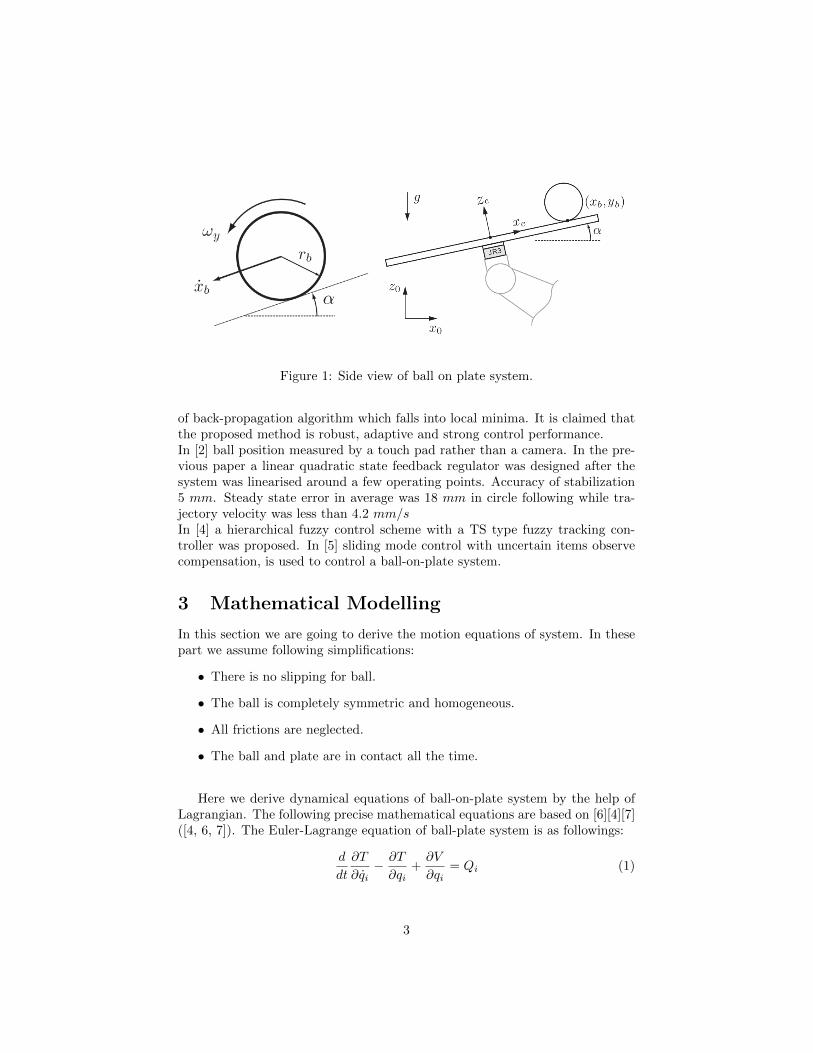
Figure 1: Side view of ball on plate system.
of back-propagation algorithm which falls into local minima. It is claimed thatthe proposed method is robust, adaptive and strong control performance.In [2] ball position measured by a touch pad rather than a camera. In the pre-vious paper a linear quadratic state feedback regulator was designed after thesystem was linearised around a few operating points. Accuracy of stabilization5 mm. Steady state error in average was 18 mm in circle following while tra-jectory velocity was less than 4.2 mm/sIn [4] a hierarchical fuzzy control scheme with a TS type fuzzy tracking con-troller was proposed. In [5] sliding mode control with uncertain items observecompensation, is used to control a ball-on-plate system.
3 Mathematical Modelling
In this section we are going to derive the motion equations of system. In thesepart we assume following simplifications:
• There is no slipping for ball.
• The ball is completely symmetric and homogeneous.
• All frictions are neglected.
• The ball and plate are in contact all the time.
Here we derive dynamical equations of ball-on-plate system by the help ofLagrangian. The following precise mathematical equations are based on [6][4][7]([4, 6, 7]). The Euler-Lagrange equation of ball-plate system is as followings:
d
dt
∂T
∂qi− ∂T
∂qi+∂V
∂qi= Qi (1)
3

Where qi stands for i-direction coordinate, T is kinetic energy of the system, Vis potential energy of system and Q is composite force.The system has 4 degree of freedom; two in ball motion and two in inclinationof plate. Here we assume the generalized coordinates of system to be (is) xband yb ball’s position on plate and α and β the inclination of the plate. It isimportant to note that we assume the center of x− y coordinates be at centerof plate. The kinetic energy of ball consists of its both rotational with respectto its center of mass and translational energy:
Tb =1
2mb
(x2b + y2b
)+
1
2Ib(ωx
2 + ωy2)
(2)
Where mb is mass of the ball and Ib is moment of inertia of the ball; xb andxb are ball’s translational velocities along x-axis and y-axis; ωx and ωy are ball’srotational velocities along x-axis and y-axis. The following relations betweentranslational velocities and rotational velocities:
xb = rbωy , yb = rbωx (3)
In which rb denotes ball’s radius. By substituting equations 3 into equations4 we will have:
Tb =1
2
[mb
(x2b + y2b
)+Ibr2b
(x2b + y2b
) ]=
1
2
(mb +
Ibrb2
)(x2b + y2b
)(4)
The kinetic energy of the plate, by considering ball as a point mass which isplaced in (xb, yb), , consists of the (ezafi) its rotational energy with respect toits center of mass:
Tp = 12 (Ip + Ib)
(α2 + β2
)+ 1
2mb
(xbα+ ybβ
)2
= 12 (Ip + Ib)
(α2 + β2
)+ 1
2mb
(x2b α
2 + 2xbαybβ + y2b β2) (5)
Where α and β are plate’s angle of inclination along x-axis and y-axis, re-spectively. Therefore α and β are plate’s rotational velocity. Here we cancalculate the kinetic energy of system as followings:
Where α and β are plate’s angle of inclination along x-axis and y-axis, re-spectively. Therefore α and β are plate’s rotational velocity. Here we cancalculate the kinetic energy of system as followings: (paragraf tekrari)
T = Tb + Tp
= 12
(mb + Ib
rb2
) (x2b + y2b
)+ 1
2 (Ip + Ib)(α2 + β2
)+ 1
2mb
(x2b α
2 + 2xbαybβ + y2b β2) (6)
The potential energy of the ball relative (the relative potential) to horizontalplane in the center of the inclined plate can be calculated as:
4

Vb = mbgh = mbg (xb sinα+ yb sinβ) (7)
Here we can derive the system’s equation by Lagrangian and equations 4-7:
L = Tb + Tp − Vb (8)
We use L to derive system’s equations:
∂T
∂α= (Ip + Ia)αx +mbxb
(xbα+ ybβ
),
∂L
∂α= mg cosα (9)
∂T
∂β= (Ip + Ia)βx +mbyb
(ybβ + xbα
),
∂L
∂β= mg cosβ (10)
∂T
∂xb=
(mb +
Ibr2b
)xb ,
∂L
∂xb= mb
(xbα+ ybβ
)α (11)
∂T
∂yb=
(mb +
Ibr2b
)yb ,
∂L
∂yb= mb
(xbα+ ybβ
)β (12)
We assume generalized toques as τx and τy which are exerted torques on theplate. From Lagrange-Euler equation we can write:
ddt∂T∂α −
∂L∂α = (Ip + Ib) α+mbx
2α+ 2mbxbxbα+mbxbybα
+ mbxbybβ +mbxbyβ −mbg cosα = τx(13)
ddt∂T∂β− ∂L
∂β = (Ip + Ib) β +mby2b β + 2mbybybβ +mbxbybβ
+ mbybxbα+mbybxbα−mbg cosβ = τy(14)
ddt
∂T∂xb− ∂L
∂xb=(mb + Ib
r2b
)xb −mb
(xbα+ ybβ
)α+mbg sinα = 0 (15)
ddt∂T∂yb− ∂L
∂yb=(mb + Ib
r2b
)yb −mb
(ybβ + xbα
)α+mbg sinβ = 0 (16)
So the non-linear differential equations for the ball-plate-system as follow-ings: (
mb +Ibr2b
)xb −mb
(xbα
2 + ybαβ)
+mbg sinα = 0 (17)
(mb +
Ibr2b
)yb −mb
(ybβ
2 + xbαβ)
+mbg sinβ = 0 (18)
τx =(Ip + Ib +mbx
2b
)α+ 2mbxbxbα+mbxbybβ
+mxbybβ +mbxbybβ +mbgxb cosα(19)
τy =(Ip + Ib +mby
2b
)β + 2mbybybβ +mbybxbα
+mbxbybα+mbxbybα+mbgyb cosβ(20)
5

The equations (18)-(17) shows the relation between ball’s state and plate’sstate that is plate’s inclination. The equations (19)-(20) shows the effect ofexternal torque on the ball-on-plate system. It is obvious that working with suchcomplex equations is too hard. So in order to do Laplace analysis on system’stransfer function, we derive the linearised model of system in neighbourhood ofworking state.
3.1 Plant Values:
In this report we use the values that are shown in following table that are basedon [4]:
Parameter Description Value
mb Mass of the ball 0.11kgrb Radius of the ball 0.02mSp Dimension of the plate 1.0× 1.0m2
vmax Maximum velocity of the ball 4mm/smp Mass of the plate 0.1kgIp Mass moment of inertia of the plate 0.5kg.m2
Ib Mass moment of inertia of the ball 1.76× 10⁻⁵kg.m2
g Gravitational acceleration 9.81
3.2 Motor Model
Here we assume (use or consider) an Armature-Controlled DC motor which it’sblock diagram is shown in figure 2. The motor uses armature current ia as thecontrol variable. The stator field can be established by a field coil current. Thedetailed description of equations can be found in [8] and [9]. When we have aconstant current in the field coil, we have the following postulates:
Tm(s) = KmIa(s)V (s) = (Ra + Las)Ia(s) + Ea(s)
V (s) = Kbω(s)=⇒ Ia(s) = [V (s)−Kbω (s)] / [Ra + Las]
The absolute torque exerted on the load can be found by:
TL(s) = Tm(s)− Td(s)
By letting Td(s) = 0 and considering GL(s) = ωL(s)TL(s) to the load torque-
velocity characteristic, one can find the input-output transfer function:
G(s) = θL(s)V (s) = KmGL(s)
s[(Ra+sLa)+KmKbGL(s)]
6

Figure 2: Block diagram for an armature-controlled DC motor.
We can assume an approximate function for load characteristic as following :TL(s) = 1
Js+B Where J stands for load inertia and B for load damping. Werewrite the motors transfer function in this way:
G(s) = θL(s)V (s) = Km
s[(Ra+sLa)(Js+B)+KmKb]
We assume following typical values for DC motor[10]:
Parameter Description Value
Km Toque constant 6.876× 10⁻⁴N.m/AKb Back-emf constant 7.2× 10⁻⁵V/rpm or 1.9099× 10⁻⁷V.s/radJm Rotor inertia 1× 10⁻³N.m.s2/radB Rotor damping 10−8N.m/(rad/s)τf Field time constant 1msτ Rotor time constant 100msR Armature resistance 3.9ΩL Armature inductance 12× 10−6H
Pmax Maximum output power 0.25hpTs Stall torque 2.4−4N ×mVfl Rated DC supply voltage 1.5V
3.3 Model Linearisation
In this part we will derive several linearised model of system that we will usethem in next sections.
3.3.1 Linearised Model of a Ball-on-Plate
The approximate value for a solid ball’s moment of inertia is Iball = 25mbr
2b .
Therefore equations (17) and (18) can be written as:
7

mb
[5
7xb −
(xbα
2 + ybαβ)
+ g sinα
]= 0 (21)
mb
[5
7yb −
(ybβ
2+ xbαβ
)+ g sinβ
]= 0 (22)
We can linearise above equation by assuming:
• Small angle of inclination for the plate(up to ± 5): α 1 and β 1=⇒ sinα ' α, sinβ ' β
• Slow rate of change for the plate: α 0 and β 0 =⇒ αβ ' 0 , α2 ' 0,
β2' 0.
5
7xb + gα = 0 (23)
5
7yb + gβ = 0 (24)
By linearising the above equations, we find two separate differential equationsfor each of x and y axis. Note that we can use above linear differential equationsto estimate the ball-on-plate system’s states xb, yb, xb, yb. By assuming α(s)and β(s) as inputs to ball-on-plate system, we find the transfer functions:
Px(s) =Xb(s)
α(s)=
g57s
2(25)
Py(s) =Yb(s)
β(s)=
g57s
2(26)
3.3.2 State-space Model of System
One can write state equations of ball-on-plate system by considering Equa-tions (17)-(20)[3]. As mentioned τx and τy are toques exerted on the plane(oron the ball from the earth) in y-axis and x-axis direction respectively. Bydefining state variables X = [x1, x2, x3, x4, x5, x6]T = [xb, xb, α, α, yb, yb, β, β]T ,
U = [ux, uy]T
= [α, β]T
and constant value B = m/(m+ Ib/r
2b
)we write the
non-linear state equation x = f(x,u):
x1x2x3x4x5x6x7x8
=
x2B(x1x
24 + x4x5x8 − g sinx3)
x40x6
B(x5x28 + x1x4x8 − g sinx7)
x80
+
0 00 00 01 00 00 00 00 1
[uxuy
]
8
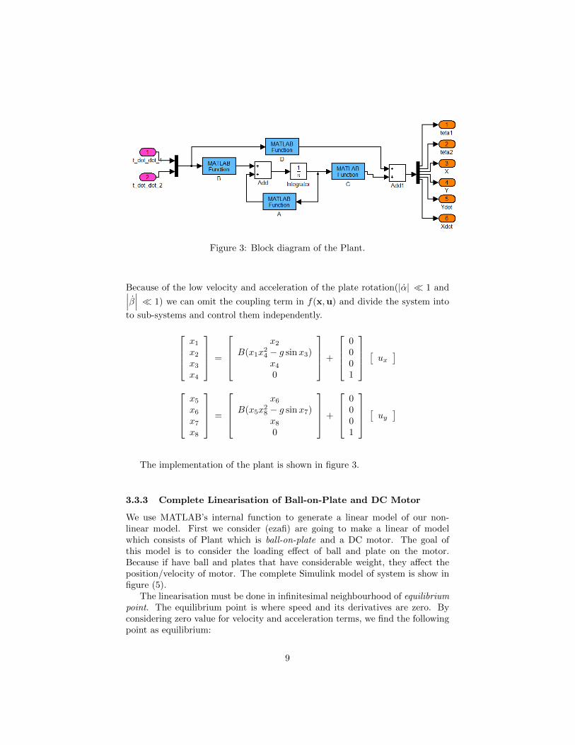
Figure 3: Block diagram of the Plant.
Because of the low velocity and acceleration of the plate rotation(|α| 1 and∣∣∣β∣∣∣ 1) we can omit the coupling term in f(x,u) and divide the system into
to sub-systems and control them independently.
x1x2x3x4
=
x2
B(x1x24 − g sinx3)x40
+
0001
[ ux ]x5x6x7x8
=
x6
B(x5x28 − g sinx7)x80
+
0001
[ uy ]
The implementation of the plant is shown in figure 3.
3.3.3 Complete Linearisation of Ball-on-Plate and DC Motor
We use MATLAB’s internal function to generate a linear model of our non-linear model. First we consider (ezafi) are going to make a linear of modelwhich consists of Plant which is ball-on-plate and a DC motor. The goal ofthis model is to consider the loading effect of ball and plate on the motor.Because if have ball and plates that have considerable weight, they affect theposition/velocity of motor. The complete Simulink model of system is show infigure (5).
The linearisation must be done in infinitesimal neighbourhood of equilibriumpoint. The equilibrium point is where speed and its derivatives are zero. Byconsidering zero value for velocity and acceleration terms, we find the followingpoint as equilibrium:
9
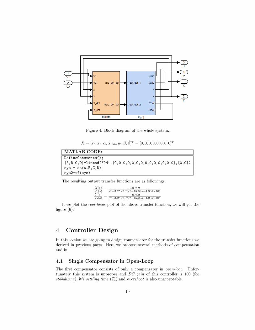
Figure 4: Block diagram of the whole system.
X = [xb, xb, α, α, yb, yb, β, β]T = [0, 0, 0, 0, 0, 0, 0, 0]T
MATLAB CODE:
DefineConstants();
[A,B,C,D]=linmod(’PM’,[0,0,0,0,0,0,0,0,0,0,0,0,0,0],[0,0])
sys = ss(A,B,C,D)
sys2=tf(sys)
The resulting output transfer functions are as followings:
X(s)V1(s)
= −802.2s5+3.25×10⁵s4−15.09s−4.905×10⁶
Y (s)V2(s)
= −802.2s5+3.25×10⁵s4−15.09s−4.905×10⁶
If we plot the root-locus plot of the above transfer function, we will get thefigure (6).
4 Controller Design
In this section we are going to design compensator for the transfer functions wederived in previous parts. Here we propose several methods of compensationand in
4.1 Single Compensator in Open-Loop
The first compensator consists of only a compensator in open-loop. Unfor-tunately this system is unproper and DC gain of this controller is 100 (forstabalizing), it’s settling time (Ts) and overshoot is also unacceptable.
10

Figure 5: Block diagram of the motors with non-linear load characteristics.
C(s) = −3461538.4615(s+0.01)2(s+2)(s2+10s+26)(s−1.8)(s+100)
Gain Poles Zeros
100 2 5
Root-locus and step response of the first compensator are shown in figure (7).
4.2 Compensator With Prefilter
The second compensator consists of a compensator and a prefilter. Unlike firstcompensator this system is proper and DC gain and percent overshoot of thiscontroller is acceptable but this compensator have a Ts = 15s settling time.
C(s) = −0.4294s5−139600s4−323700s3−705500s2−1.202×10⁶s−798.5s5+9.971s4+43.77s3+111.2s2+195.5s
F (s) = 798.50.4294s5+139600s4+323700s3+705500s2+1.202×10⁶s+798.5
Gain Poles Zeros Prefilter poles
4.08 5 5 5
In order to find better compensator, we change the architecture add followingadd a new controlling loop. The compensator at the rest of report are designedto control plant and previous controller.
11

Figure 6: Pole-zero map of system’s transfer function.
4.2.1 Multi-loop controller 1
the following system is designed to make the settling time of second compensatorappropriate. this compensator’s aim is to get have overshoot but rapid timerise.
Gain Poles Zeros Prefilter poles
1.6 8 8 1
F (s) = 16.12s+10
C(s) =7.296×10¹³s8+5.597×10¹⁴s7+1.906×10¹⁵s6+3.729×10¹⁵s5+4.586×10¹⁵s4+3.613×10¹⁵s3+1.788×10¹⁵s2+4.917×10¹⁴s+6.251×10¹³
s8+400s7+7×10⁴s6+7×10⁶s5+4.375×10⁸s4+1.75×10¹⁰s3+4.375×10¹¹s2+6.251×10¹²s+3.907×10¹³
4.2.2 Multi-loop controller 2
the following compensator is desinged to make the settling time of second com-pensator appropriate. this compensator’s aim is to critical damp mode.
Gain Poles Zeros Prefilter poles
.6 8 8 1
F (s) = 26.66s+10
C(s) =2.736×10¹³s8+2.099×10¹⁴s7+7.148×10¹⁴s6+1.398×10¹⁵s5+1.72×10¹⁵s4+1.355×10¹⁵s3+6.706×10¹⁴s2+1.844×10¹⁴s+2.344×10¹³
s8+400s7+7×10⁴s6+7×10⁶s5+4.375×10⁸s4+1.75×10¹⁰s3+4.375×10¹¹s2+6.251×10¹²s+3.907×10¹³
12

Figure 7: Root-locus and step response of the first compensator.
5 Result Evaluation
In this part we are going to evaluate the results we got from previous parts.The main goal of this part part is to check the validity of the previous resultsand whether they are valid for the case of main non-linear equations. For thisgoal, we designed the comprehensive non-linear simulator to check the validityof results.
13

Figure 8: Root-locus and step response of the second compensator.
Figure 9: Architecture of added controlling loop.
14

Figure 10: Root-locus and step response of the third compensator.
5.1 Non-linear Simulation
In order to have a realistic evaluation of the designed compensator and itsoperation we need to design a non-linear simulator by the use of primary non-linear equations (17)-(20).
15

Figure 11: Root-locus and step response of the forth compensator.
5.1.1 Trajectory Tracking Using Non-linear Simulator
The task of tracking a trajectory is one of important tasks that one controllermust be able to accomplish. In figure (14) the results of several tracking exper-iments are shown.
5.1.2 Coulomb Friction
Despite the complex microscopic origins of Coulomb friction, we can model itby simple models. One popular model for formulating the Coulomb friction isas following[11] [12] :
16
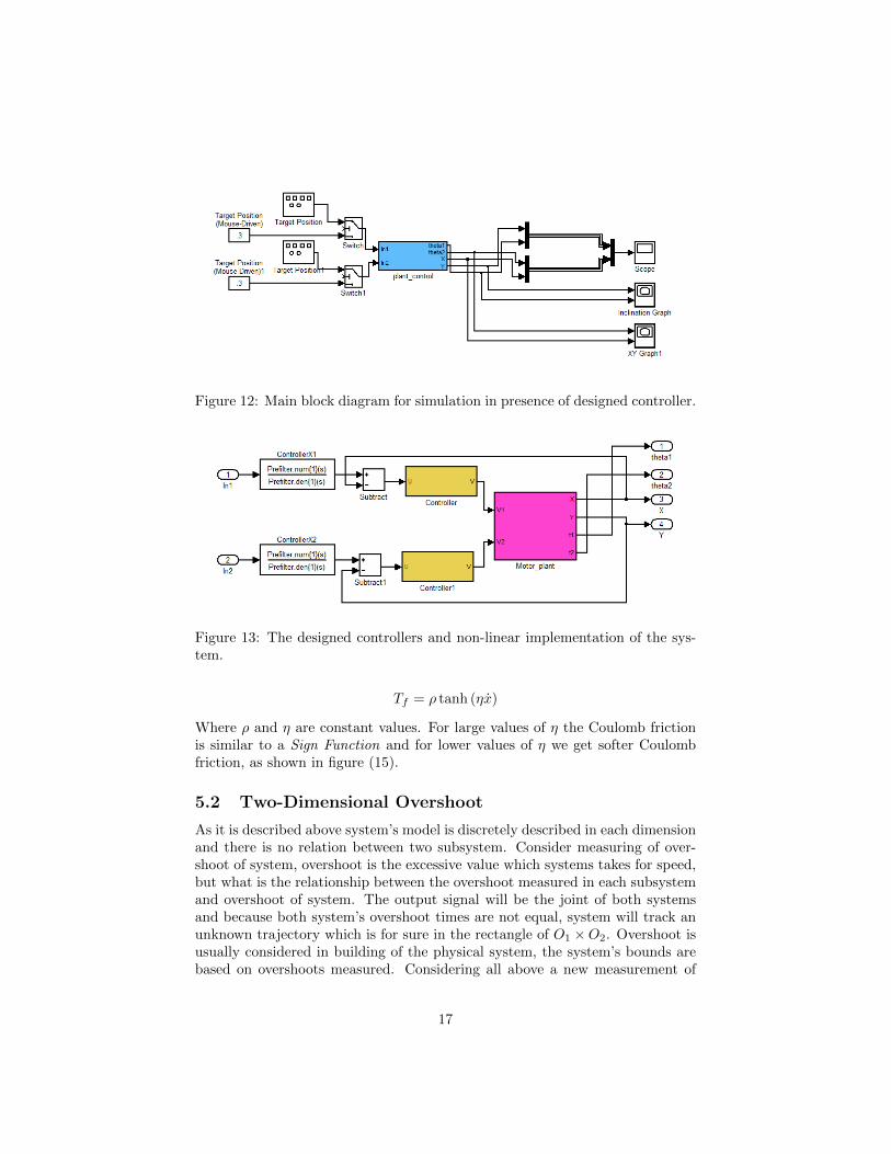
Figure 12: Main block diagram for simulation in presence of designed controller.
Figure 13: The designed controllers and non-linear implementation of the sys-tem.
Tf = ρ tanh (ηx)
Where ρ and η are constant values. For large values of η the Coulomb frictionis similar to a Sign Function and for lower values of η we get softer Coulombfriction, as shown in figure (15).
5.2 Two-Dimensional Overshoot
As it is described above system’s model is discretely described in each dimensionand there is no relation between two subsystem. Consider measuring of over-shoot of system, overshoot is the excessive value which systems takes for speed,but what is the relationship between the overshoot measured in each subsystemand overshoot of system. The output signal will be the joint of both systemsand because both system’s overshoot times are not equal, system will track anunknown trajectory which is for sure in the rectangle of O1 ×O2. Overshoot isusually considered in building of the physical system, the system’s bounds arebased on overshoots measured. Considering all above a new measurement of
17

overshoot can be considered which is maximum distance from the zero point inthe 2D path. Figure 16 2d-overshoot point (the point with maximum distanceof zero) of a joint system consisting of two standard 2nd order linear subsystemsare drawn. Assuming ωn1 = ωn2 this will be just in the corner of rectangle, butwhen ωn1 6= ωn2 this point will be on one of the sides.
H1(s) =ω2
n1
s2+2ζ1ωn1+ω2n1
H2(s) =ω2
n2
s2+2ζ2ωn2+ω2n2
In figure 17 the 2d-overshoot of different systems with different ζ1 = ζ2 isshown.It shows that systems which their natural frequencies of their subsystemsare equal have the worse 2d-overshoot:
√2(O1d) (It is also proven with some
other experiments). For example when ωn1 = 1, ωn2 = 1, ζ1 = ζ1 = .6, O2d =1.5482, but for ωn1 = 1, ωn2 = .5, ζ1 = ζ1 = .6, O2d = 1.4767.
6 Conclusions
In this report we derived complete equations of ball-on-plate system. We didlinearisation analysis to find the transfer function of the system. We designedseveral compensator and at the rest made some analysis on the results. We triedseveral trajectory tracking tasks. The final results showed that the designedcontrollers had almost acceptable performances.
7 Acknowledgement
The authors would like to thank all their classmates, friends and masters thathelped on this project. They would like to thank Ehsan Omidi and FarokhAtashzar for their illuminating discussion and ideas. They also knowledgeDr.H.A.Talebi for his comprehensive and off course perfect instructions.
References
[1] N. Mohajerin, M. B. Menhaj, and A. Doustmohammadi, “A reinforcementlearning fuzzy controller for the ball and plate system,” in Proc. IEEE IntFuzzy Systems Conference, 2010, pp. 1–8.
[2] S. Awtar, C. Bernard, N. Boklund, A. Master, D. Ueda, and K. Craig,“Mechatronic design of a ball-on-plate balancing system,” Mechatronics,vol. 12, no. 2, pp. 217–228, 2002.
[3] X. Dong, Z. Zhang, and C. Chen, “Applying genetic algorithm to on-lineupdated pid neural network controllers for ball and plate system,” in Proc.
18
Fourth Int Innovative Computing, Information and Control (ICICIC) Conf,2009, pp. 751–755.
[4] X. Fan, N. Zhang, and S. Teng, “Trajectory planning and tracking of balland plate system using hierarchical fuzzy control scheme,” Fuzzy Sets andSystems, vol. 144, no. 2, pp. 297–312, 2004.
[5] D. Liu, Y. Tian, and H. Duan, “Ball and plate control system based onsliding mode control with uncertain items observe compensation,” in IEEEInternational Conference on Intelligent Computing and Intelligent Systems,ICIS09, vol. 2. IEEE, 2009, pp. 216–221.
[6] K. kyu Lee, G. Btz, and D. Wollherr, “Basketball robot: Ball-on-plate withpure haptic information,” in IEEE International Conference on Roboticsand Automation, May 2008.
[7] D. Yuan and Z. Zhang, “Modelling and control scheme of the ball-platetrajectory-tracking pneumatic system with a touch screen and a rotarycylinder,” Control Theory & Applications, IET, vol. 4, no. 4, pp. 573–589,2010.
[8] F. Golnaraghi and B. Kuo, Automatic control systems, vol. 2.
[9] R. Dorf and R. Bishop, Modern control systems, 11th ed. Pearson PrinticeHall, 2008.
[10] W. Bolton, Mechatronics: electronic control systems in mechanical andelectrical engineering. Prentice Hall, 2004.
[11] D. Haessig and B. Friedland, “On the modeling and simulation of friction,”in American Control Conference. IEEE, 2009, pp. 1256–1261.
[12] C. S.J. and T. R.W., “On the modeling of coulomb friction,” UNKNOWNJOURNAL OR CONFERENCE, 1998.
19

Figure 14: Results of trajectory tracking.
20

Figure 15: Coulomb Friction Models.
Figure 16: 2-D overshoot place. This figure shows the point which has themaximum distance from zero for different parameters of ζ1 and ζ2. Each curveis a class of systems which have one subsystem and the other subsystem differs.
21

Figure 17: 2-D overshoot. This figure shows the the maximum distance fromzero for different systems with ζ1 = ζ2 according to their subsystems naturalfrequencies ratios.
22