modelling and analysis of a logic reactor for the

MODELLING AND ANALYSIS OF A LOGIC REACTOR FOR THE SYNTHESIS OF METHANOL VIA CO2 HYDROGENATION

FRANCISCA ISABEL SANTOS VALENTE LEAL DISSERTAÇÃO DE MESTRADO APRESENTADA À FACULDADE DE ENGENHARIA DA UNIVERSIDADE DO PORTO EM CHEMICAL ENGINEERING

M 2020

Master in Chemical Engineering

Modelling and Analysis of a LOGIC Reactor for the Synthesis of Methanol via CO2 Hydrogenation

Master dissertation

of

Francisca Leal

Developed within the course of dissertation

held in

DMT Environmental Technology

Supervisor at FEUP: Prof. Alexandre Ferreira

Joint supervisor at FEUP: Prof. Ricardo Santos

Coordinator at DMT Environmental Technology: Eng. Benny Bakker

October 2021


Acknowledgment

I would like to start by thanking every one of my colleagues at DMT Environmental Technologies

for welcoming me so well into the company. In particular, I thank my supervisors, Maria Marcela

and Benny Bakker, who guided me through every step of the way.

I also have to give my thanks to my FEUP supervisors, Professor Ricardo Santos and, especially,

Professor Alexandre Ferreira, without whom I would not have ever been able to complete this

work.

I thank my housemates at De Flecke, with whom I shared this journey, and all my friends, who

have made these last five years possible.

Thank you, Tiago, for always helping me stay sane throughout it all.

Lastly, I thank my family: my mom and dad, and my biggest role models, my sisters, Raquel

and Zé. Thank you for always being my biggest supporters and for always helping me take those

difficult steps. I will do my best to make you proud in the future.


Abstract

Methanol seems to be an ideal candidate in light of the current demand for new sustainable

alternatives to fossil fuels. This versatile product can be produced sustainably by recycling

captured CO2 and used as a gasoline substitute or upgraded to a diesel substitute. It may also

be used in fuel cells for the production of electrical energy.

The liquid-out gas-in concept (LOGIC) reactor was designed to efficiently produce methanol

from CO2, achieving conversion rates of nearly 100 %. The innovative nature of this reactor

design lies in the fact that it can operate with internal gas recycle, driven by natural convection

inside the reactor.

The main objective of this thesis work was to build a mathematical model of the LOGIC reactor

and simulate its behavior while operating under different conditions to achieve a better

understanding of the catalytic synthesis of methanol in this type of reactor.

Simulations varying the reactor feed composition and reactor dimensions were performed, and

the changes in reactor behavior according to these variations were discussed. After studying

five different fresh feed compositions, it was seen that a slight excess of H2 seems to improve

the methanol yield when compared to the case where CO2 and H2 are fed to the reactor in

stoichiometric proportions.

Simulations where the reactor dimensions were varied were also performed. The results of

these simulations indicated that the improvement in methanol yield is more significant when

the reactor's length is increased compared to when the diameter is increased.

Keywords: Methanol synthesis, LOGIC reactor, reactor modelling, recycling of CO2.


Resumo

Diante da atual necessidade de encontrar alternativas sustentáveis para os combustíveis fósseis,

o metanol parece ser um candidato perfeito. Este versátil produto pode ser produzido de

maneira sustentável através da reciclagem de CO2 e utilizado como substituto da gasolina ou

transformado num substituto do gasóleo. Também pode ser utilizado em células de combustível

para produção de energia elétrica.

O reator LOGIC (liquid-out gas-in concept) foi concebido para produzir metanol através de CO2

de maneira eficiente, atingindo conversões de aproximadamente 100 %. A natureza inovadora

deste reator provém do facto de este operar com reciclagem de gás interna, impulsionada pela

convecção natural dentro do reator.

O principal objetivo desta dissertação foi construir um modelo matemático para o reator LOGIC

e simular o seu comportamento ao operar sobre diferentes condições, de maneira aprofundar

o conhecimento já adquirido sobre a síntese de metanol neste tipo de reator.

Várias simulações foram feitas onde a composição da alimentação ao reator foi sendo variada.

As mudanças verificadas no comportamento do reator face a estas variações foram depois

discutidas. Depois de serem estudadas cinco diferentes composições de alimentação, foi

verificado, em comparação com o caso estequiométrico, que um pequeno excesso de H2 parece

melhorar a produção de metanol.

Simulações onde as dimensões do reator foram sendo variadas também foram feitas. Os

resultados destas simulações indicaram que, ao aumentar o comprimento do reator, o aumento

na produção de metanol é mais significativo do que quando o diâmetro do reator é aumentado.


Declaration

I hereby declare, under word of honour, that this work is original and that all non-original

contributions are indicated, and due reference is given to the author and source.

20/09/2021


i

Index

1 Introduction ........................................................................................... 1

1.1 Framing and presentation of the work .................................................... 1

1.2 Presentation of the company ................................................................ 1

1.3 Contribution of the author to the work ................................................... 1

1.4 Organization of the dissertation ............................................................ 2

2 Context and State of the art ....................................................................... 3

2.1 Methanol Synthesis ............................................................................ 3

2.2 Methanol reactors .............................................................................. 3

2.2.1 Isothermal reactors .................................................................................... 4

2.2.2 Adiabatic reactors ..................................................................................... 5

2.3 The LOGIC reactor ............................................................................. 6

3 Materials and Methods .............................................................................. 9

3.1 Reactor model ................................................................................ 10

3.1.1 Overall heat transfer coefficients ................................................................. 10

3.1.2 Reaction kinetics ..................................................................................... 11

3.2 Economizer .................................................................................... 13

3.3 Thermodynamic properties of the gas mixture ........................................ 14

3.4 Recycle stream calculations ............................................................... 17

3.5 Simulation process ........................................................................... 17

4 Results and discussion ............................................................................ 19

4.1 Fresh feed composition variation ......................................................... 19

4.2 Variation of the reactor dimensions ...................................................... 24

5 Conclusion ........................................................................................... 27

6 Assessment of the work done ................................................................... 29

6.1 Objectives Achieved ......................................................................... 29

6.2 Final Assessment ............................................................................. 29

7 References .......................................................................................... 31


ii

Annex A - Supporting information .................................................................... 35

Annex B - MATLAB code ................................................................................ 37


iii

List of Figures

Figure 1: (a) Lurgi reactor; (b) Linde Isothermal reactor; (c) Mitsubishi Superconverter (Dieterich et

al., 2020). ............................................................................................................... 4

Figure 2: a) Quench reactor; b) Indirect cooling reactor (Palma et al., 2018). .............................. 5

Figure 3: Schematic representation of the LOGIC reactor (provided by DMT Environmental

Technology). ............................................................................................................ 6

Figure 4: Representation of the reactor geometry adopted. ................................................... 9

Figure 5: Inner tube side temperature profile through the catalyst section for each pass through the

reactor (case 1). ..................................................................................................... 20


reactor (case 2). ..................................................................................................... 20


reactor (case 3). ..................................................................................................... 21


reactor (case 4). ..................................................................................................... 21


reactor (case 5). ..................................................................................................... 21

Figure 10: Per pass conversion for each case. ................................................................... 22

Figure 11: Methanol selectivity in each pass for each case. .................................................. 22

Figure 12: Methanol yield per pass for each case. .............................................................. 23

Figure 13: Average Reynolds number per pass for each case. ................................................ 23

Figure 14: Pressure drop per pass for each case. ............................................................... 24

Figure 15: Inner tube side temperature profile through the catalyst section for each case. ............ 25


v

List of Tables

Table 1: Parameters used in the calculation of the kinetic constants (Vanden Bussche & Froment,

1996). .................................................................................................................. 12

Table 2: Parameters used in the calculation of the equilibrium constants (Graaf & Winkelman, 2016).

......................................................................................................................... 13

Table 3: Parameters used in the calculation of the heat capacity of each component (Yaws, 1999). .. 14

Table 4: Parameters used in the calculation of the viscosity of each component (Yaws, 1999). ........ 14

Table 5: Parameters used in the calculation of the thermal conductivity of each component (Yaws,

1999). .................................................................................................................. 15

Table 6: Percentage of each of the components’ reactor outlet molar flowrate that will be recycled. 17

Table 7: Fixed parameters. ........................................................................................ 19

Table 8: Reactor dimensions. ...................................................................................... 19

Table 9: Molar composition of the fresh feed for each case. ................................................. 20

Table 10: Reactor dimensions for cases A and B. ............................................................... 25

Table 11: Amount of catalyst inside the inner tube for each case. .......................................... 25

Table 12: Reactor performance parameters for each case. ................................................... 26

Table A.1: Catalyst bed information. ............................................................................. 35

Table A.2: Fluid properties (Bos et al., 2019). .................................................................. 35


vii

Notation and Glossary

�� Transversal area of the inner tube m2 �� Specific heat capacity of the gas mixture J·kg-1·K-1 �� Specific heat capacity of component i J·mol-1·K-1 �� Particle diameter m �� Equivalent diameter of the annulus m ��,� Inside diameter of the inner tube m ��, Outside diameter of the inner tube m �,� Inside diameter of the outer tube m �� Fugacity of component i bar �� Friction factor on the inner tube side ��, � Molar flow rate of component i at the outlet of the reactor mol·s-1 � Friction factor on the outer tube side ℎ� Heat transfer coefficient on the inner tube side W·m-2·K-1 ℎ Heat transfer coefficient on the outer tube side W·m-2·K-1 �� Equilibrium constant i �� Kinetic constant i �� Binary interaction parameter between components i and j �� Thermal conductivity of the tube wall W·m-1·K-1 �� Tube length on the catalyst section m �� Tube length on the economizer section m �� Mass flow rate on the inner tube side kg·s-1 �� Molar mass of component i kg·mol-1 Nu� Nusselt number on the inner tube side Nu Nusselt number on the outer tube side �� Mass flow rate on the outer tube side kg·s-1 � Pressure Pa, bar �� Critical pressure of component i Pa �� Reactor inlet pressure Pa !"� Polarity correction parameter of component i # Ideal gas constant J·K-1·mol-1 Re Reynolds number on the inner tube side of the catalyst section &�� Critical temperature of component i K '� Reaction rate of reaction j mol·kgcat-1·s-1 & Temperature K &� Temperature on the inner tube side K &��()*+ Inner tube side inlet temperature K & Temperature on the outer tube side K &�()*+ Outer tube side inlet temperature K &� Inner tube wall temperature K , Superficial velocity m·s-1 -� Overall heat transfer coefficient for the inner tube side W·m-2·K-1 - Overall heat transfer coefficient for the outer tube side W·m-2·K-1 .� Mass fraction of component i /� Mole fraction of component i 0 Axial coordinate m 1 Compressibility factor


viii

Greek Letters ∆34 Reaction enthalpy kJ·mol-1 56 Voidage of the packed bed 7 Thermal conductivity of the gas mixture W·m-1·K-1 7� Thermal conductivity of component i W·m-1·K-1 8 Viscosity of the gas mixture kg·m−1·s−1 8� Viscosity of component i kg·m−1·s−1 89 Viscosity of the gas mixture at the inner tube wall temperature kg·m−1·s−1 :6 Density of the catalyst bed kgcat·m-3 :" Density of the fluid mixture kg·m-3 ;< Molar volume m3·mol-1 =� Stoichiometric coefficient of component i >� Fugacity coefficient of component i ?� Acentric factor of component i

List of Acronyms

CH3OH Methanol CO Carbon monoxide CO2 Carbon dioxide EoS Equation of State H2 Hydrogen ICI Imperial Chemical Industries LOGIC Liquid-Out Gas-In Concept NC Number of components NR Number of reactions RWGS Reverse water-gas shift SRK Soave-Redlich-Kwong


Introduction 1

1 Introduction

1.1 Framing and presentation of the work

For many decades now, modern societies have been dependent on fossil-based energy sources.

And, as the global energy demand continues to increase, so does the pace at which these limited

resources are depleted, creating concern for what might happen when they run out. Moreover,

as more fossil fuel is consumed, more CO2 is released into the atmosphere, aggravating global

warming and climate change. For these reasons, it is imperative that new sustainable energy

sources are adopted to mitigate CO2 emissions and society’s dangerous fossil fuel dependency.

One way to tackle both of these concerns simultaneously is chemical recycling of CO2 to

methanol. This incredibly versatile product can be used in fuel cells for electric energy

production, as a gasoline substitute or additive, and as feedstock for several chemical products,

including dimethyl ether, a diesel substitute (Goeppert et al., 2014).

Methanol can be obtained from carbon dioxide via direct hydrogenation. However, the CO2

hydrogenation reaction is generally characterized by low carbon conversion. Therefore,

appropriate reactor design is important to have an efficient methanol production process.

The liquid-out gas-in concept (LOGIC) leads to a novel reactor, designed to operate with

internal gas recycling. This allows it to efficiently convert CO2 to methanol, achieving a carbon

conversion of nearly 100 %.

1.2 Presentation of the company

DMT Environmental Technology is a Dutch engineering company, founded in 1987 with the goal

of creating a more sustainable world. For the last 30 years, DMT has been at the forefront of

green technology, bringing to market several innovative solutions in the fields of biogas

upgrading, gas desulfurization and wastewater treatment.

By investing in the development of the LOGIC reactor, DMT aims to, once again, contribute to

a greener future. With this technology, the company would be able to give purpose to the CO2

left at the end of their biogas upgrading processes by using it to produce methanol, a

sustainable fuel option.

1.3 Contribution of the author to the work

My work consisted of building a mathematical model of the LOGIC reactor and simulating its

behaviour under different operating conditions to achieve a higher understanding of the


Introduction 2

catalytic conversion of CO2 to methanol in this type of reactor. Hopefully, an effort that will

contribute to the process of scaling up a LOGIC reactor in the future.

1.4 Organization of the dissertation

This dissertation consists of five main sections: the context and state of the art, the materials

and methods, the results and discussion, the conclusion, and, finally, the assessment of the

work done.

The first section describes the general methanol synthesis process, and a review of the most

common industrial reactor designs used for methanol production is given.

Next, in the materials and methods section, a description of the developed mathematical model

and the simulation process is detailed.

In the following section, the results obtained in each of the simulations performed are analysed.

The discussion is divided into two sections: in the first, the influence that the changes in feed

composition have on the reactor behaviour is discussed, while, in the second, the result of

altering the reactor dimensions is analysed.

As the name suggests, the conclusion section states the conclusions reached at the end of the

analysis, highlighting the most relevant results obtained.

In the final section, a brief evaluation of the work conducted is given.


Context and State of the art 3

2 Context and State of the art

Methanol, the simplest alcohol, is one of the most important commodities in the chemical

industry. The global demand for this organic compound has been continuously rising since the

1990’s, reaching 70 Mt in 2015, which signifies a 500% increase over the last 15 years (Olah et

al., 2018; Palma et al., 2018). This is in great part due to its emerging potential as an energy

carrier. Methanol can be used efficiently in fuel cells to produce electricity; it is an additive or

substitute for gasoline and it may be upgraded to dimethyl ether, an efficient diesel substitute.

Apart from energy applications, methanol is also commonly used as feedstock to produce a

variety of chemicals such as formaldehyde and acetic acid, as well as ethylene and propylene,

through the methanol-to-olefins (MTO) process (Goeppert et al., 2014).

2.1 Methanol Synthesis

Methanol is commonly obtained from the catalytic conversion of synthesis gas, a mixture of

carbon monoxide (CO), hydrogen (H2), and some carbon dioxide (CO2), also referred to as

syngas. Three main reactions translate the synthesis of methanol from syngas: the

hydrogenation of CO (Equation 1), the hydrogenation of CO2 (Equation 2), and the reverse

water-gas shift reaction (Equation 3) (Olah et al., 2009).

CO + 2HE ⇌ CHGOH ∆3EHI K4 = −90.8 kJ ∙ molXY (1)

COE + 3HE ⇌ CHGOH + HEO ∆3EHI K4 = −49.2 kJ ∙ molXY (2)

COE + HE ⇌ CO + HEO ∆3EHI K4 = 41.6 kJ ∙ molXY (3)

Since both of the hydrogenation reactions are exothermic, methanol formation is favoured by

low temperatures. However, temperatures above 200 °C are required in order to achieve

satisfactory reaction rates. At the same time, temperatures above 300 °C will induce fast

catalyst deactivation. Therefore, methanol synthesis processes generally operate within a

restricted temperature range of 200 to 300 °C. Also, because methanol formation results in an

overall reduction of the number of moles, according to Le Chatelier’s principle, it is favoured

by high pressures. Thus, typical operating pressures range from 50 to 100 bar (Bozzano &

Manenti, 2016; Nestler et al., 2020).

2.2 Methanol reactors

Current industrial methanol synthesis processes do not differ much from each other. All utilize

a copper-based catalyst, CuO/ZnO/Al2O3 being the most widely used, all typically operate at



temperatures of 200-300 °C and pressures of 50-100 bar, as previously mentioned, and most

are carried out in the gas phase. The most relevant differences between processes are related

to reactor design and catalyst arrangement. Two main types of reactors are typically used:

isothermal and adiabatic (Bozzano & Manenti, 2016; Palma et al., 2018).

2.2.1 Isothermal reactors

An isothermal reactor works, essentially, as a heat exchanger, where a cooling fluid constantly

removes the heat released in the course of the reactions. This reactor concept has been widely

adopted within the industry, and many companies have developed their customized version of

this type of converter. Some notable examples include the Lurgi reactor, the Linde isothermal

reactor, and the Mitsubishi Superconverter (Palma et al., 2018).

In the 1970s, Lurgi (now belonging to Air Liquid) was the first to introduce this reactor concept

for methanol synthesis. The Lurgi reactor (Figure 1a) functions as a shell and tube heat

exchanger, operated in the vertical position, in which the tubes are filled with the catalyst and

boiling water circulates on the shell-side, acting as a coolant.

In the case of the Linde isothermal reactor (Figure 1b), the catalyst is placed on the shell-side,

and helically coiled tubes, where boiling water circulates, are embedded in the catalyst bed.

When compared with reactors where the catalyst is placed on the tube-side, this design allows

for an increased heat transfer efficiency, reducing the required cooling area and, therefore,

reducing material costs.

Figure 1: (a) Lurgi reactor; (b) Linde Isothermal reactor; (c) Mitsubishi Superconverter

(Dieterich et al., 2020).

The Mitsubishi Superconverter (Figure 1c) also operates as a vertical shell and tube heat

exchanger, with the particularity of having double-pipe tubes. In this reactor, the catalyst is

placed in the space between the inner and outer tubes, and boiling water runs on the shell-



side. The gas is fed to the inner tubes at the bottom of the reactor and is heated up as it flows

upwards. After it reaches the top, the gas enters the annular space and flows downwards

through the catalyst bed, exiting at the bottom. Such a configuration creates a temperature

profile in the catalyst bed characterized by a high temperature near the inlet, which decreases

towards the outlet. This keeps the reaction rate close to its maximum, increasing the

conversion per pass (Bozzano & Manenti, 2016; Dieterich et al., 2020; Palma et al., 2018).

2.2.2 Adiabatic reactors

Adiabatic reactors may yet be divided into two main types: the quench reactor and the indirect

cooling reactor.

The quench reactor (Figure 2a) was first introduced by ICI (now Johnson Matthey) in 1966 and

is perhaps the most common type of reactor used in methanol synthesis. It is composed of a

series of up to five adiabatic packed beds placed inside a pressurized shell. In this type of

reactor, the feed gas stream is split into a main stream, which is preheated and fed at the top

of the reactor, and a few quench gas streams, which are fed cold and stepwise along the

reactor, cooling the gas coming from the previous bed and, therefore, increasing the conversion

of syngas.

The indirect cooling reactor (Figure 2b) is made up of multiple adiabatic fixed bed reactors

separated by external heat exchangers, which are used to cool down the outlet stream of the

previous reactor before it is fed to the next. This type of reactor is quite simple in its design

but very effective when it comes to ensuring high productivity.

Figure 2: a) Quench reactor; b) Indirect cooling reactor (Palma et al., 2018).



2.3 The LOGIC reactor

The liquid-out gas-in concept (LOGIC) reactor, first introduced by Bos & Brilman (2015), is a

novel reactor, designed for the production of methanol via CO2 hydrogenation. This reactor is

characterized by two temperature zones: a hot zone at the bottom and a cold zone at the top.

The hot zone, where the catalyst is placed, operates at reaction conditions, while the cold zone

operates at a temperature low enough to condensate the methanol and water products in situ.

This is the origin of the LOGIC designation: the reactants are fed as gases at the bottom of the

reactor, and the products are collected as liquids at the top. The unreacted gas is then

internally recycled, thanks to natural convection. This is made possible by the density gradient

created by the two zones' difference in composition and temperature (Bos et al., 2019).

Figure 3: Schematic representation of the LOGIC reactor (provided by DMT Environmental

Technology).



Now, a new section has been added to the design of the LOGIC reactor: the economizer section.

The current design consists of a vertical shell and tube reactor, where the catalyst is placed in

the first section of the tubes, making up the catalyst section. The remaining length of the pipes

makes up the economizer section. The area at the stop corresponds to the condenser section.

Figure 3 displays a schematic representation of the reactor. This new section aims to promote

heat exchange between the stream circulating on the tube side and the recycle stream,

circulating on the shell side.

Since 2020, the University of Twente, ISPT, Shell, and DMT Environmental Technology have

joined resources, in an effort to scale up the LOGIC reactor, having now reached a point where

a 15 kg·day-1 pilot unit has been fully designed and is in the midst of being built.


Materials and Methods 9

3 Materials and Methods

A mathematical model for the LOGIC reactor was developed and implemented in MATLAB to

study the changes in the behaviour inside the reactor when varying the fresh feed composition

and the reactor dimensions. The resulting MATLAB code may be found in Annex B.

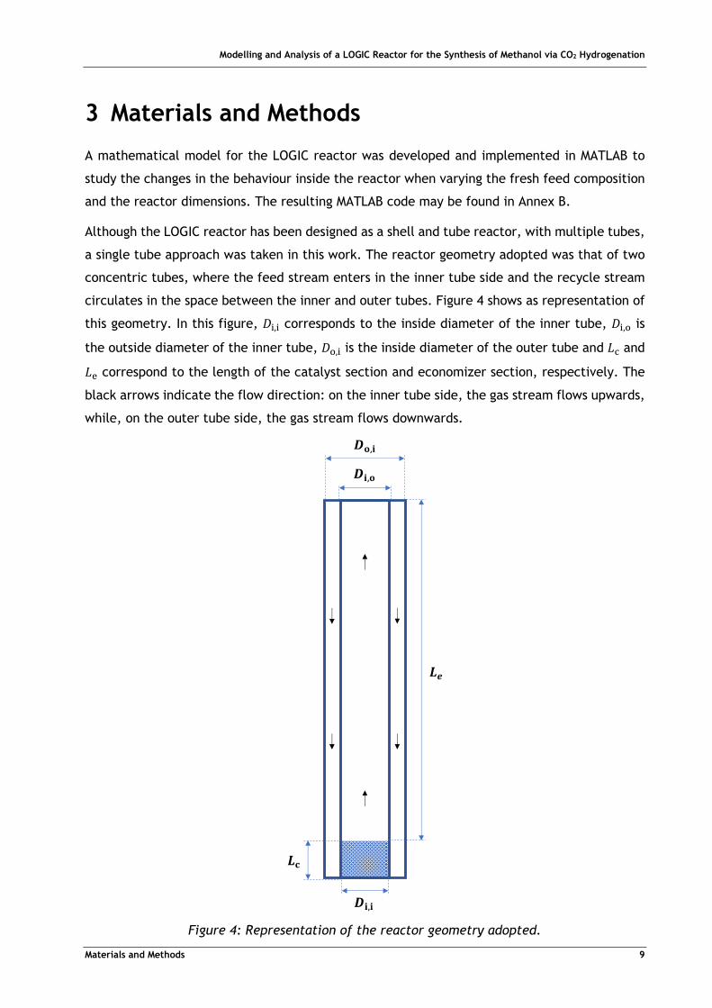
Although the LOGIC reactor has been designed as a shell and tube reactor, with multiple tubes,

a single tube approach was taken in this work. The reactor geometry adopted was that of two

concentric tubes, where the feed stream enters in the inner tube side and the recycle stream

circulates in the space between the inner and outer tubes. Figure 4 shows as representation of

this geometry. In this figure, ��,� corresponds to the inside diameter of the inner tube, ��, is

the outside diameter of the inner tube, �,� is the inside diameter of the outer tube and �� and �� correspond to the length of the catalyst section and economizer section, respectively. The

black arrows indicate the flow direction: on the inner tube side, the gas stream flows upwards,

while, on the outer tube side, the gas stream flows downwards.

Figure 4: Representation of the reactor geometry adopted.



3.1 Reactor model

A one-dimensional pseudo-homogeneous model was applied to describe the catalyst section of

the LOGIC reactor, as this is the most common approach to steady-state modelling of fixed-bed

reactors for methanol synthesis. Based on this model, the reactor behaviour can be predicted

by solving a system of eight ordinary differential equations given by Equations 4-7 (Manenti et

al., 2011). The first corresponds to the mass balance equation. Since there are five different

chemical components inside the reactor, five mass balances need to be solved. Equations 5 and

6 express the energy balance on the inner and outer tube sides, respectively. Equation 7

corresponds to the Ergun equation (1952), which translates the pressure drop through the

catalyst packed bed, i.e., momentum balance.

�.��0 = �� :6 ^ =�'�_`

� (4)

�&��0 = �� ab ��,�� -�c& − &�d + :6 ^e−∆3�fg'�_`

� h (5)

�&�0 = −b ��,�� -c&� − &d (6)

��0 = − i150 c1 − 56dE56G 8,��E + 1.75 c1 − 56d56G :",E�� l (7)

In these expressions, the values for the molar mass of each component, ��, the packed bed

density, :6, and porosity, 56, as well as the particle diameter, ��, are listed in Annex A. The

calculation of the reaction enthalpy, ∆3�f, and the Reynolds number on the inner tube side of

the catalyst section, Re, are also described in Annex A.

3.1.1 Overall heat transfer coefficients

The overall heat transfer coefficients for the tube side, -�, and shell side, -, are given by

Equations 8 and 9, respectively (Flynn et al., 2019).

-� = 11ℎ� + ��,� lne��,/��,�g2�� + ��,�ℎ��,

(8)

- = 11ℎ + ��, lne��,/��,�g2�� + ��,ℎ��,�

(9)



The thermal conductivity of the tube wall, ��, at a given wall temperature, &�, is calculated

through Equation 10, derived from data available in Mills (2002). The wall temperature was

estimated through the logarithmic mean of &� and &.

�� = c3.81 × 10XHd&9G − c1.80 × 10Xpd&�E + c3.60 × 10XEd&� + 4.22 (10)

The inner tube side heat transfer coefficient is calculated through Leva’s correlation (1949) for

a tube packed with pellets (Equation 11), while the outer tube side heat transfer coefficient

was obtained through Equation 12 (Flynn et al., 2019),

ℎ� = 7��,� 3.50 i�� 8 lq.r sXt.uvw/x�,� (11)

ℎ = 7Nu�� (12)

where the equivalent diameter, De, is given by Equation 13 and the Nusselt number, Nu, for

laminar flow, is determined by the Sieder-Tate correlation for Re<2100 (Equation 14) (Flynn et

al., 2019) and, for transient and turbulent flow, by the correlation proposed by Gnielinski (1976)

(Equation 15). The friction factor on the outer tube side, �, is obtained though Equation 16,

developed by Petukhov (1970).

�� = �,�E − ��,E��, (13)

Nu = 1.86 i 4�� b��,8 ��87 �� lY/G y 889zq.Yt (14)

Nu = c�/8d y 4�� b��,8 − 1000z ��871 + 12.7c�/8dY/E {|��87 }E/G − 1~ (15)

� = i0.790 ln i 4�� b��,8l − 1.64lXE (16)

3.1.2 Reaction kinetics

Despite many years of research, there is still no consensus regarding the reaction mechanism

behind methanol synthesis. Many authors have proposed different kinetic models; however,

only two are widely used in methanol reactor modelling (Bozzano & Manenti, 2016). These are

the models proposed by Graaf et al. (1988) and Vanden Bussche & Froment (1996), the latter

used in this work.



The model proposed by Bussche and Froment is based on the reactions given by Equations 2 and

3, as CO2 is assumed to be the primary source of carbon. The rate expressions for these reactions

are given by Equations 17 and 18. To account for the non-ideal behaviour of the gas, the partial

pressure of each component is substituted by its fugacity.

'�� = �Y �� − 1��!�� E �

y1 + �E �� + �G�� + �t��zG (17)

r`�� = �p {�� − 1�� ~

1 + �E �� + �G�� + �t�� (18)

The kinetic constants, �Y to �p, are calculated by the Arrhenius equation (Equation 19), and

the equilibrium constants �� and �� are obtained through Equations 20 and 21, respectively,

given by Graaf & Winkelman (2016). The parameters �� and ��, needed for the calculation of

the kinetic constants, can be found in Table 1, while the parameters �Y to �r and �Y to �r, need

to calculate the equilibrium constants, are listed in Table 2.

�� = ��s 6�� (19)

ln �� = 1#& �cY + cE& + cG&E + ct&G + cp&t + cu&p + cr& ln &� (20)

ln �� = 1#& �dY + dE& + dG&E + dt&G + dp&t + du&p + dr& ln &� (21)

Table 1: Parameters used in the calculation of the kinetic constants (Vanden Bussche &

Froment, 1996).

�� 0.499 17 197

�� 6.62×10-11 124 119

�� 3 453.38 —

�� 1.07 36 696

�� 1.22×1010 -94 765



Table 2: Parameters used in the calculation of the equilibrium constants (Graaf &

Winkelman, 2016).

�� 3.50019×104 �� -3.94121×104

�� 1.351084×102 �� -54.1516

�� -2.3199×10-2 �� -5.5642×10-2

�� 3.28032×10-5 �� 2.576×10-5

�� -1.32647×10-8 �� -7.6594×10-9

� 2.0505×10-12 � 1.0161×10-12

�¡ -45.935 �¡ 18.429

3.2 Economizer

Only the energy balances on the inner and outer tube sides need to be solved for the economizer

section. The expressions that make up the energy balances in this section are almost exactly

the same as the ones used for the catalyst section, with just a few differences. On the

economizer section, there is no catalyst or heat generation on the inner tube side. Therefore,

in this case, &� and ℎ� are given by Equations 22 and 23, respectively, where Nu� is given by

either Equation 24 or 25, in the same way as explained previously.

�&��0 = b ��,�� -�c& − &�d (22)

ℎ� = 7Nu��,� (23)

Nu� = 1.86 i 4�� b��,�8 ��87 ��,�� lY/G y 889zq.Yt (24)

Nu� = c�/8d y 4�� b��,�8 − 1000z ��871 + 12.7c��/8dY/E {|��87 }E/G − 1~ (25)

�� = i0.790 ln i 4�� b��,�8l − 1.64lXE (26)



3.3 Thermodynamic properties of the gas mixture

The specific heat capacity of each component, ��, is given by Equation 27 (Yaws, 1999), while

the specific heat capacity of the gas mixture, ��, is calculated according to Equation 28.

Parameters A, B, C, D and E are listed for each component in Table 3.

�� = A� + B�& + C�&E + D�&G + E�&t (27)

�� = ^ ��.��¦§�¨Y (28)

Table 3: Parameters used in the calculation of the heat capacity of each component (Yaws,

1999).

A B C D E

CO2 27.437 4.2315×10-2 -1.9555×10-5 3.9968×10-9 -2.9872×10-13

H2 25.399 2.0178×10-2 -3.8549×10-5 3.188×10-8 -8.7585×10-12

CH3OH 40.046 -3.8287×10-2 2.4529×10-4 -2.1679×10-7 5.9909×10-11

H2O 33.933 -8.4186×10-3 2.9906×10-5 -1.7825×10-8 3.6934×10-12

CO 29.556 -6.5807×10-3 2.013×10-5 -1.2227×10-8 2.2617×10-12

The viscosity, 8�, and the thermal conductivity, 7�, of each component are given by Equations

29 and 30, respectively (Yaws, 1999). Parameters F, G and H are listed in Table 4, while Table

5 lists parameters I, J and K.

8� = F� + G�& + H�&E (29)

7� = I� + J�& + K�&E (30)

Table 4: Parameters used in the calculation of the viscosity of each component (Yaws, 1999).

F G H

CO2 11.336×10-7 4.9918×10-8 -1.0876×10-11

H2 27.758×10-7 2.12×10-8 -3.28×10-12

CH3OH -14.236×10-7 3.8935×10-8 -6.2762×10-12

H2O -36.826×10-7 4.29×10-8 -1.62×10-12

CO 35.086×10-7 5.0651×10-8 -1.3314×10-11



Table 5: Parameters used in the calculation of the thermal conductivity of each component

(Yaws, 1999).

I J K

CO2 -1.183×10-2 1.0174×10-4 -2.2242×10-8

H2 3.951×10-2 4.5918×10-4 -6.4933×10-8

CH3OH 2.34×10-3 5.434×10-6 1.3154×10-7

H2O 5.3×10-4 4.7093×10-5 4.9551×10-8

CO 1.5×10-3 8.2713×10-5 -1.9171×10-8

The mixed viscosity, 8, and mixed thermal conductivity, 7, are obtained through Equations 31

and 32, respectively, where �� is given by Equation 33 for both cases (Bird et al., 2007; Wilke,

1950).

8 = ^ /�8�∑ /��p�Ÿp

�Ÿ (31)

7 = ^ /�7�∑ /��p�Ÿp

�Ÿ (32)

�� = �1 + y8�8�zY/E + y��zY/t�E

{8 y1 + ��z~Y/E (33)

The original Soave-Redlich-Kwong (SRK) equation of state (EoS) for a pure substance, proposed

by Soave (1972), is given by Equation 34.

� = #&;< − � − �;<c;< + �d (34)

Equation 35 corresponds to the SRK EoS written in its cubic form. Its largest solution gives the

value of the compressibility factor, 1. In this expression, A and B are defined by Equations 36

and 37, respectively.

1G − 1E + 1c� − ¯ − ¯Ed − �¯ = 0 (35)

� = ��#E&E (36)

¯ = ��#& (37)



For a mixture, � and � become dependent on the composition according to Equations 38 and

39, where �� and �� are given by Equations 40 and 41 and the binary interaction parameters, ��, are listed in Annex A.

� = ^ ^ /�/��e1 − ��g¦§�Ÿ

¦§�Ÿ (38)

� = ^ /��¦§�Ÿ (39)

�� = 0.42747 #E&��E�� °� (40)

�� = 0.08664 #&�� (41)

The temperature dependent parameter °� is obtained through Equation 42, where a polarity

correction parameter, !"�, is included (Mathias, 2002).

°�q.p = 1 + �� a1 − ± &&��h − !"� i1 − &&��l i0.7 − &&��l (42)

The parameter �� is calculated by Equation 43 (Graboski & Daubert, 2002).

�� = 0.48508 + 1.55171?� − 0.15613?�E (43)

The critical properties, &�� and ��, as well as the acentric factor, ?�, and the polarity correction

parameter, !"�, are listed in Annex A for each component.

The fugacity coefficients, >�, are then given by Equation 44 (Meyer et al., 2016) and the

fugacity of each component, ��, is calculated according to Equation 45.

ln >� = �� c1 − 1d − lnc1 − ¯d − �̄ ²2 ∑ /�e1 − ��g��_��¨� � − �� ³ ln y1 + ¯1 z (44)

�� = >�� (45)

Finally, the density of the gas mixture, :", is given by Equation 46.

:" = �#&1 ^ /��_��Ÿ (46)



3.4 Recycle stream calculations

The condenser section of the LOGIC reactor was not modelled, as this was outside of the work

objectives. However, a method to estimate the recycle stream composition was still necessary.

Equilibrium data provided by DMT was used to calculate what percentage of each of the

components’ reactor outlet molar flowrate would be collected in the condenser’s gas outlet

stream and, thus, be recycled. The results obtained are summarized Table 6.

Table 6: Percentage of each of the components’ reactor outlet molar flowrate that will be

recycled.

i ´�,µ¶· recycled / %

CO2 99.85

H2 99.98

CH3OH 30.95

H2O 10.86

CO 99.94

3.5 Simulation process

Having implemented the mathematical model of the catalyst and economizer sections in

MATLAB, the simulations followed the procedure below.

The first step consists in running the catalyst section code, which will calculate the mass

fraction of each component along the reactor, the temperature profile in the inner and outer

tubes, and the pressure drop across the packed bed. To run the simulation, the following inputs

are needed: the inner tube inlet composition (input 1), the outer tube inlet composition (input

2), and mass flow rate (input 3).

For the first pass simulation, input 1 corresponds to the fresh feed composition. Inputs 2 and 3

are estimated by first performing an adiabatic simulation and calculating the recycle stream

composition and mass flow rate through the process described in section 3.3.

After running the catalyst section simulation, the economizer section simulation can be run.

The inputs needed in this case are the economizer’s inner tube inlet composition (input 4) and

temperature (input 5), as well as inputs 2 and 3, which are the same as in the catalyst section

simulation. Inputs 4 and 5 are given by the output of the catalyst section simulation.

After running the economizer section code, the first pass simulation is complete. In each

subsequent pass, inputs 1, 2 and 3 are given by the output of the previous simulation.


Results and discussion 19

4 Results and discussion

In the simulations performed, three parameters were varied: the composition of the fresh feed

and the radius and length of the reactor. The influence of the variation of these parameters on

the temperature profiles, conversion, methanol selectivity and yield, pressure drop and flow

regime on the inner tube side of the catalyst section was at the centre of this work’s studies.

Some parameters were kept constants for all the simulations. These are reported in Table 7.

Table 7: Fixed parameters.

�̧ ¹ / kg·s-1 0.0004

º¹¹»¼½· / K 513.15

ºµ¹»¼½· / K 342.05

¾�¿ÀÁÂ / Pa 75×105

4.1 Fresh feed composition variation

In this first section, the influence of the fresh feed composition on the reactor behaviour will

be discussed. The reactor dimensions were kept constant at the values reported in Table 8.

Table 8: Reactor dimensions.

Ã¹,¹ / m 0.0254

Ã¹,µ / m 0.0287

Ãµ,¹ / m 0.0381

Ä� / m 0.127

Ä½ / m 1

Five distinct cases with different fresh feed compositions were defined. The compositions for

each case are listed in Table 9. For each case, 14 passes through the reactor were simulated to

verify the changes in the reactor behaviour as the composition approaches the thermodynamic

equilibrium limitation.



Table 9: Molar composition of the fresh feed for each case.

CO2 H2 CH3OH H2O CO

Å�

Case 1 0.25 0.75 0 0 0

Case 2 0.30 0.70 0 0 0

Case 3 0.20 0.80 0 0 0

Case 4 0.35 0.65 0 0 0

Case 5 0.15 0.85 0 0 0

Figures 5 through 9 show, for each case, the inner tube side temperature profile through the

catalyst section for each pass in the reactor.

Figure 5: Inner tube side temperature profile through the catalyst section for each pass

through the reactor (case 1).



480

490

500

510

520

530

540

550

560

570

0 0.02 0.04 0.06 0.08 0.1 0.12 0.14

Ti/

K

z /m

1st pass

3rd pass

5th pass

7th pass

9th pass

11th pass

14th pass

480

490

500

510

520

530

540

550

560

570

0 0.02 0.04 0.06 0.08 0.1 0.12 0.14

Ti/

K

z /m

1st pass

3rd pass

5th pass

7th pass

9th pass

11th pass

14th pass









490

500

510

520

530

540

550

560

0 0.02 0.04 0.06 0.08 0.1 0.12 0.14

Ti/

K

z /m

1st pass

3rd pass

5th pass

7th pass

9th pass

11th pass

14th pass

480

490

500

510

520

530

540

550

560

570

0 0.02 0.04 0.06 0.08 0.1 0.12 0.14

Ti/

K

z /m

1st pass

3rd pass

5th pass

7th pass

9th pass

11th pass

14th pass

495

500

505

510

515

520

525

530

535

540

0 0.02 0.04 0.06 0.08 0.1 0.12 0.14

Ti/

K

z /m

1st pass

3rd pass

5th pass

7th pass

10th pass

14th pass



After analysing these figures, it can be seen that, for all cases, with every subsequent pass, the

temperature inside the reactor reaches increasingly higher temperatures. As the

thermodynamic equilibrium is approached, the temperature rise inside de inner tube reaches

a maximum level. For cases 1, 2 and 4, this level seems to sit at around 560 K. In cases 3 and

5, 14 passes through the reactor appear to have not been enough for it to be possible to identify

the maximum temperature.

In Figures 10, 11 and 12, the conversion, the methanol selectivity and the methanol yield are

represented for each of the 14 passes of cases 1 to 5.

Figure 10: Per pass conversion for each case.

As seen in Figure 10, the two cases with the lowest CO2 percentage at the inlet, cases 5 and 3,

present the highest conversion per pass. In case 5, a conversion as high as 23.7 % was reached.

While, for case 3, the maximum conversion observed was 21.2 %.

Figure 11: Methanol selectivity in each pass for each case.

5.0

7.0

9.0

11.0

13.0

15.0

17.0

19.0

21.0

23.0

25.0

0 5 10 15

Co

nv

ers

ion

/ %

pass

Case 1 Case 2 Case 3 Case 4 Case 5

5.0

15.0

25.0

35.0

45.0

55.0

65.0

75.0

85.0

95.0

105.0

0 5 10 15

Me

tha

no

l S

ele

ctiv

ity

pass




Figure 11 shows the methanol selectivity in each of the 14 passes simulated for each case. It

can be seen that, in all cases, the selectivity towards methanol generally increases after each

pass. This is due to the accumulation of CO in the reactor.

In the first few passes, the reverse water-gas shift reaction dominates, leading to the formation

CO. As indicated in section 3.4, most of the CO at the outlet of the reactor (99.94 %) will be

recycled, which eventually causes the equilibrium of the RWGS reaction to shift towards the

opposite direction. As a result, the methanol selectivity increases and, by the 14th pass, values

of over 95 % are observed in all cases.

Figure 12: Methanol yield per pass for each case.

The methanol yield per pass for each of the 5 cases is shown in Figure 12. Case 3 presents the

highest values, with a methanol yield of 1.17×10-3 mol·s-1 on the 14th pass. This suggests that a

slight excess of H2 improves the reactor performance.

Figure 13: Average Reynolds number per pass for each case.

0.0E+00

2.0E-04

4.0E-04

6.0E-04

8.0E-04

1.0E-03

1.2E-03

1.4E-03

0 5 10 15

Me

tha

no

l y

ield

/

mo

le·s

-1

pass


800

850

900

950

1000

1050

0 5 10 15

Re

pass




Figure 13 shows, for every case, the average Reynolds number on the inner tube side of the

catalyst section. The highest values correspond to case 5, where Re takes values of over 1000.

However, in all cases, the Reynolds number stays within the laminar flow range.

Figure 14: Pressure drop per pass for each case.

The pressure drop through the packed bed in every pass of each case is represented in Figure

14. In this figure, it is possible to see that the pressure drop increases as the CO2 content in the

fresh feed decreases, with case 5 showing the highest values. Nevertheless, the pressure drop

is negligible in all cases, which would be expected since the flow through the reactor is laminar,

with small values of Re for all cases.

4.2 Variation of the reactor dimensions

In this section, the influence of the reactor dimensions on reactor behaviour will be discussed.

Two cases were analysed: for case A, the length of the catalyst section was doubled, while, for

case B, the diameter of the inner tube was doubled.

In case B, the values of the diameter of the outer tube and the inner tube thickness were also

doubled so that their proportion to the inner tube diameter stayed the same as in the original

case. For the purpose of consistency, the length of the economizer section for case B was

changed as well, in order to maintain the same heat transfer area as in the original case. The

reactor dimensions for cases A and B are listed in Table 10.

In the simulations performed, the inner tube side inlet composition and the outer tube side

mass flow rate and composition, were kept constant at the values listed in Table 10. These

correspond to the input values for the simulation of case 1’s 14th pass through the reactor,

which is referred to here as the base case.

0.0

5.0

10.0

15.0

20.0

25.0

30.0

35.0

40.0

45.0

0 5 10 15

Pre

ssu

re d

rop

/ P

a

pass




Table 10: Reactor dimensions for cases A and B.

Case A Case B

Ã¹,¹ / m 0.0254 0.0508

Ã¹,µ / m 0.0287 0.0574

Ãµ,¹ / m 0.0381 0.0762

Ä� / m 0.254 0.127

Ä½ / m 1 0.5

Figure 15: Inner tube side temperature profile through the catalyst section for each case.

Figure 15 illustrates the inner tube side temperature profile across the catalyst section for

cases A and B, as well as for the base case. Case A shows a very similar behaviour to the base

case, with a more extended temperature profile. In case B, the temperature rise is sharper and

higher.

Since the reactor dimensions were altered, while :6 was kept constant, the mass of catalyst

needed inside the inner tube is different for each case. Table 11 lists the required amount of

catalyst for the three cases.

Table 11: Amount of catalyst inside the inner tube for each case.

Base case Case A Case B

Catalyst amount / kg 0.05 0.1 0.2

510

520

530

540

550

560

570

580

0 0.05 0.1 0.15 0.2 0.25 0.3

Ti/

K

z / m

Base Case Case A Case B



Table 12 gives an overview of some reactor performance parameters for cases A and B, as well

as for the base case.

Table 12: Reactor performance parameters for each case.

Base case Case A Case B

CO2 conversion / % 17.22 17.84 18.07

H2 conversion / % 13.87 15.17 14.70

CH3OH selectivity / % 97.51 100 99.01

CH3OH yield / mol·s-1 1.06×10-3 1.20×10-3 1.13×10-3

Pressure drop / Pa 21 43 2.5

Re 878 866 428

Although case B shows the highest CO2 conversion, the selectivity is highest for case A, resulting

in higher methanol yield.

Even though case B utilizes a larger amount of catalyst, the yield is still higher for case A. This

may be due to the more abrupt temperature profile observed for case B. Since low

temperatures favour methanol formation, a more significant methanol yield is achieved for

case A.

Because the length of the tube is bigger, the pressure drop observed is higher for case A.

Although the Reynolds number observed is higher for case A than for case B, the flow profile

can be considered laminar for both cases.


Conclusion 27

5 Conclusion

A complete mathematical model of the LOGIC reactor was developed in this thesis work. This

model was then used to predict the reactor behavior as the fresh feed composition, and reactor

dimensions were varied.

Five different fresh feed compositions were simulated: one with CO2 and H2 fed to the reactor

in stoichiometric proportions (case 1), two where CO2 was fed in excess (cases 2 and 4), and

two others where H2 was fed in excess (cases 3 and 5). High methanol selectivity (over 95 %)

was observed for all cases. In terms of methanol yield, it was seen that a slight excess of H2 in

the feed stream seems to improve it. Laminar flow was observed for all the simulated cases

and, although the pressure drop was observed to increase as the amount of CO2 in the fresh

feed decreased, the values obtained were still small for all cases.

Cases where the catalyst section’s length or diameter were doubled were also simulated. The

results of these simulations showed that increasing the length gives a better outcome than

increasing the diameter in the same proportion. Even though less catalyst is used, methanol

yield was still higher in the case where the length was doubled, as the temperature rise in the

reactor was shown to be much more abrupt in the case where the diameter was doubled.


Assessment of the work done 29

6 Assessment of the work done

6.1 Objectives Achieved

A mathematical model of the LOGIC reactor was successfully developed and implemented in

MATLAB.

Although many simulations were performed in regard to the influence of the fresh feed

composition on reactor behaviour, due to the inefficiency of the simulation process, it was not

possible to obtain the thermodynamic equilibrium composition for all of the cases studied,

which could have affected the results.

Regarding the simulations where the reactor dimensions were varied, it was only possible to

study two cases. To achieve a better understanding of the influence of these parameters on

the reactor behaviour, it would have been beneficial if more cases could have been analysed.

6.2 Final Assessment

When using the mathematical model developed, many iterations were needed in order to reach

the thermodynamic equilibrium, making the simulation process very long and not very efficient.

Therefore, it would have been advantageous if a convergence loop could have been

implemented, so that the results for the thermodynamic equilibrium composition could have

been achieved with a single simulation. Although this possibility was not explored in this thesis

work, if the mathematical model developed is used in the future to perform further studies,

the implementation of a convergence loop would most likely be very helpful.


References 31

7 References

Bird, R. B., Stewart, W. E., & Lightfoot, E. N. (2007). Thermal Conductivity and the Mechanisms

of Energy Transport. In Transport Phenomena (pp. 265–289). John Wiley & Sons, Inc.

Bos, M. J., & Brilman, D. W. F. (2015). A novel condensation reactor for efficient CO2 to

methanol conversion for storage of renewable electric energy. Chemical Engineering

Journal, 278, 527–532. https://doi.org/10.1016/J.CEJ.2014.10.059

Bos, Martin J, Slotboom, Y., Kersten, S. R. A., & Brilman, D. W. F. (2019). 110th Anniversary:

Characterization of a Condensing CO2 to Methanol Reactor. Industrial & Engineering

Chemistry Research, 58(31), 13987–13999. https://doi.org/10.1021/ACS.IECR.9B02576

Bozzano, G., & Manenti, F. (2016). Efficient methanol synthesis: Perspectives, technologies and

optimization strategies. Progress in Energy and Combustion Science, 56, 71–105.

https://doi.org/10.1016/J.PECS.2016.06.001

Dieterich, V., Buttler, A., Hanel, A., Spliethoff, H., & Fendt, S. (2020). Power-to-liquid via

synthesis of methanol, DME or Fischer–Tropsch-fuels: a review. Energy & Environmental

Science, 13(10), 3207–3252. https://doi.org/10.1039/D0EE01187H

Ergun, S. (1952). Fluid flow through packed columns. Chemical Engineering Progress, 48(2), 89.

Flynn, A. M., Akashige, T., & Theodore, L. (2019). Kern’s Process Heat Transfer (2nd Edition).

Wiley. https://doi.org/10.1002/9781119364825

Gnielinski, V. (1976). New equations for heat and mass transfer in turbulent pipe and channel

flow. International Chemical Engineering, 16(2), 359–368.

Goeppert, A., Czaun, M., Jones, J.-P., Prakash, G. K. S., & Olah, G. A. (2014). Recycling of

carbon dioxide to methanol and derived products – closing the loop. Chemical Society

Reviews, 43(23), 7995–8048. https://doi.org/10.1039/C4CS00122B

Graaf, G. H., Stamhuis, E. J., & Beenackers, A. A. C. M. (1988). Kinetics of low-pressure

methanol synthesis. Chemical Engineering Science, 43(12), 3185–3195.

https://doi.org/10.1016/0009-2509(88)85127-3

Graaf, Geert H., & Winkelman, J. G. M. (2016). Chemical Equilibria in Methanol Synthesis

Including the Water–Gas Shift Reaction: A Critical Reassessment. Industrial and

Engineering Chemistry Research, 55(20), 5854–5864.

https://doi.org/10.1021/ACS.IECR.6B00815

Graboski, M. S., & Daubert, T. E. (2002). A Modified Soave Equation of State for Phase

Equilibrium Calculations. 1. Hydrocarbon Systems. Industrial and Engineering Chemistry


References 32

Process Design and Development, 17(4), 443–448. https://doi.org/10.1021/I260068A009

Leva, M. (1949). Fluid flow through packed beds. Chemical Engineering, 56(5), 115.

Manenti, F., Cieri, S., & Restelli, M. (2011). Considerations on the steady-state modeling of

methanol synthesis fixed-bed reactor. Chemical Engineering Science, 66(2), 152–162.

https://doi.org/10.1016/J.CES.2010.09.036

Mathias, P. M. (2002). A versatile phase equilibrium equation of state. Industrial and

Engineering Chemistry Process Design and Development, 22(3), 385–391.

https://doi.org/10.1021/I200022A008

Meyer, J. J., Tan, P., Apfelbacher, A., Daschner, R., & Hornung, A. (2016). Modeling of a

Methanol Synthesis Reactor for Storage of Renewable Energy and Conversion of CO2 –

Comparison of Two Kinetic Models. Chemical Engineering & Technology, 39(2), 233–245.

https://doi.org/10.1002/CEAT.201500084

Mills, K. C. (2002). Fe - 316 Stainless Steel. In Recommended Values of Thermophysical

Properties for Selected Commercial Alloys. Elsevier.

https://doi.org/10.1533/9781845690144.135

Nestler, F., Schütze, A. R., Ouda, M., Hadrich, M. J., Schaadt, A., Bajohr, S., & Kolb, T. (2020).

Kinetic modelling of methanol synthesis over commercial catalysts: A critical assessment.

Chemical Engineering Journal, 394, 124881. https://doi.org/10.1016/J.CEJ.2020.124881

Olah, G. A., Goeppert, A., & Prakash, S. G. K. (2018). Beyond Oil and Gas: The Methanol

Economy, 3rd Edition | Wiley. https://www.wiley.com/en-

us/Beyond+Oil+and+Gas%3A+The+Methanol+Economy%2C+3rd+Edition-p-9783527338030

Olah, G. A., Goeppert, A., & Surya Prakash, G. K. (2009). Production of Methanol: From Fossil

Fuels and Bio-Sources to Chemical Carbon Dioxide Recycling. In Beyond Oil and Gas: The

Methanol Economy (Second Edition). Wiley-VCH Verlag GmbH & Co. KGaA.

https://doi.org/10.1002/9783527627806.ch12

Palma, V., Meloni, E., Ruocco, C., Martino, M., & Ricca, A. (2018). State of the Art of

Conventional Reactors for Methanol Production. Methanol: Science and Engineering, 29–

51. https://doi.org/10.1016/B978-0-444-63903-5.00002-9

Petukhov, B. S. (1970). Advances in heat transfer (J. P. Harnett & T. F. Irvine (eds.); Vol. 6).

Academic Press.

Soave, G. (1972). Equilibrium constants from a modified Redlich-Kwong equation of state.

Chemical Engineering Science, 27(6), 1197–1203. https://doi.org/10.1016/0009-

2509(72)80096-4


References 33

Vanden Bussche, K. M., & Froment, G. F. (1996). A Steady-State Kinetic Model for Methanol

Synthesis and the Water Gas Shift Reaction on a Commercial Cu/ZnO/Al2O3Catalyst.

Journal of Catalysis, 161(1), 1–10. https://doi.org/10.1006/JCAT.1996.0156

Wilke, C. R. (1950). A Viscosity Equation for Gas Mixtures. The Journal of Chemical Physics,

18(4). https://doi.org/10.1063/1.1747673

Yaws, C. L. (1999). Chemical Properties Handbook. In Chemical engineering books. McGraw-

Hill.


Annex A - Supporting information 35

Annex A - Supporting information

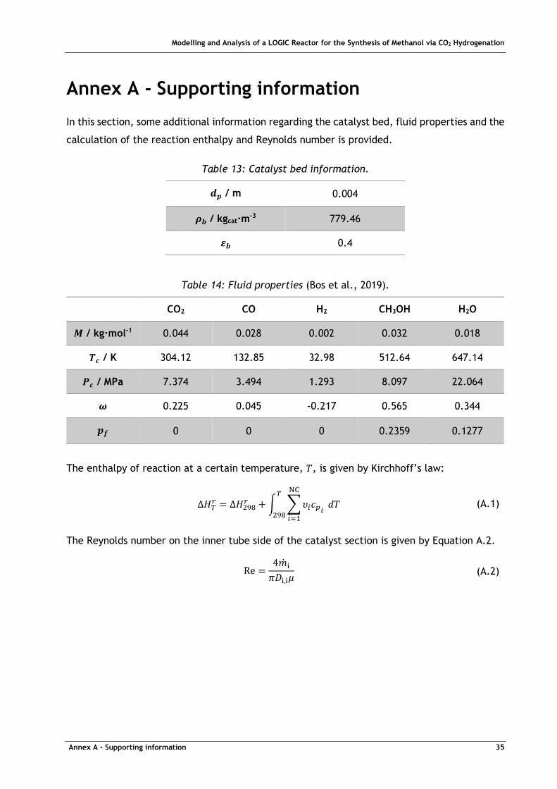
In this section, some additional information regarding the catalyst bed, fluid properties and the

calculation of the reaction enthalpy and Reynolds number is provided.

Table 13: Catalyst bed information.

ÆÇ / m 0.004

ÈÉ / kgcat·m-3 779.46

ÊÉ 0.4

Table 14: Fluid properties (Bos et al., 2019).

CO2 CO H2 CH3OH H2O

Ë / kg·mol-1 0.044 0.028 0.002 0.032 0.018

ºÌ / K 304.12 132.85 32.98 512.64 647.14

¾Ì / MPa 7.374 3.494 1.293 8.097 22.064

Í 0.225 0.045 -0.217 0.565 0.344

ÇÎ 0 0 0 0.2359 0.1277

The enthalpy of reaction at a certain temperature, &, is given by Kirchhoff’s law:

∆3�4 = ∆3EHI4 + Ï ^ =�� &_��¨Y

�EHI (A.1)

The Reynolds number on the inner tube side of the catalyst section is given by Equation A.2.

Re = 4�� b��,�8 (A.2)


Annex B – MATLAB code 37

Annex B - MATLAB code

1. Catalyst section script

close all clear

L=0.127; %Tube length [m]

range_z=[0 L];

IC=[0.697886802912880,0.117086721836820,3.76965017785287E-

02,6.03819019524899E-03,0.141291783276522,513.15,75e05,397.35]; %Initial

conditions

[zsol,varsol]=ode45(@odess,range_z,IC); %Integrates the system of odes from 0

to L with IC as initial conditions

1.1. ODE system

function balances=odess(z,var) %Constants D=0.0508; %Internal diameter of the tube [m] Dio=D+(0.003302*2); %outside diameter of the tube [m] Doi=0.0762; %inside diameter of the shell [m] L=0.127; %tube lenght [m] Ar=pi*((D/2)^2); %Tube cross-section area [m2] m=0.0004; %mass flow rate on the tube side [kg/s] rho_bed=779.46; %Effective catalyst bed density [kg/m3] M=[0.044009 0.002016 0.032042 0.018015 0.02801]; %molar mass of each

component [kg/mol] eb=0.4; %bed porosity; dp=0.004; %particle diameter [m] R=8.314; %[J/mol/K] w_shell=[0.669857531005802,0.116512860303489,4.35171495365750E-

02,6.98170567410152E-03,0.163130753480033]; m_shell=3.46162361367433E-04; %mass flow rate on the shell side [kg/s]

w(1)=var(1); %mass fraction of CO2 w(2)=var(2); %mass fraction of H2 w(3)=var(3); %mass fraction of MeOH w(4)=var(4); %mass fraction of H2O w(5)=var(5); %mass fraction of CO T=var(6); %Temperature on the tube side [K] P=var(7); %Pressure on the tube side [Pa]=[kg/s^2/m] T_shell=var(8); %Temperature on the shell side [K]

[r_MeOH,r_rwgs]=rrates(P,T,w); %reaction rates [mol/kgcat/s]

[visc_tube,~,integ_Cp,Cp_mix]=properties_tube(T,w);

[~,~,Cp_shell]=properties_shell(T_shell,w_shell);

[dH1,dH2]=dH(integ_Cp);

[U_tube,U_shell]=global_htc(T,w,T_shell,w_shell,m_shell,D,Dio,Doi,L);

y=(w./M)/(sum(w./M)); %mole fraction



Z=compr_factor(w,T,P); rho_tube=P*sum(y.*M)/(Z*R*T); %[kg/m^3]

u0=m/rho_tube/Ar; %superficial velocity on the tube side [m/s]

balances(1,1)=(Ar/m)*M(1)*rho_bed*(-r_MeOH-r_rwgs); %dwCO2/dz balances(2,1)=(Ar/m)*M(2)*rho_bed*(-3*r_MeOH-r_rwgs); %dwH2/dz balances(3,1)=(Ar/m)*M(3)*rho_bed*(r_MeOH); %dwMeOH/dz balances(4,1)=(Ar/m)*M(4)*rho_bed*(r_MeOH+r_rwgs); %dwH2O/dz balances(5,1)=(Ar/m)*M(5)*rho_bed*(r_rwgs); %dwCO/dz balances(6,1)=(Ar/(m*Cp_mix))*(pi*D*U_tube*(T_shell-T)/Ar+rho_bed*(-

dH1*r_MeOH-dH2*r_rwgs)); %dT/dz on the tube side balances(7,1)=-(150*((1-eb)^2)*visc_tube*u0/(dp^2)/(eb^3)+1.75*(1-

eb)*rho_tube*(u0^2)/dp/(eb^3)); %dP/dz on the tube side balances(8,1)=-pi*Dio*U_shell*(T-T_shell)/(m_shell*Cp_shell); %dT/dz on the

shell side end

1.1.1. Reaction rates

function [r_MeOH,r_rwgs] = rrates(P,T,w) %Constants: R=8.314; %[J/mol/K] M=[0.044009 0.002016 0.032042 0.018015 0.02801]; %molar mass of each

component [kg/mol] c=[3.50019e+04 1.351084e+02 -2.3199e-02 3.28032e-05 -1.32647e-08 2.0505e-12 -

4.5935e+01]; %parameters for the calculation of Keq1 from (Graaf 2016) b=[-3.94121e+04 -5.41516e+01 -5.5642e-02 2.576e-05 -7.6594e-09 1.0161e-12

1.8429e+01]; %parameters for the calculation of Keq2 from (Graaf 2016) A=[1.07 3453.38 0.499 6.62e-11 1.22e10]; %A values for the calculation of the

rate constants using the Arrhenius equation B=[36696 0 17197 124119 -94765]; %B values for the calculation of the rate

constants using the Arrhenius equation


[~,fug_coef]=compr_factor(w,T,P); %fugacity coefficients

Keq1=exp((1/(R*T))*(c(1)+c(2)*T+c(3)*T^2+c(4)*T^3+c(5)*T^4+c(6)*T^5+c(7)*T*lo

g(T))); Keq2=exp((1/(R*T))*(b(1)+b(2)*T+b(3)*T^2+b(4)*T^3+b(5)*T^4+b(6)*T^5+b(7)*T*lo

g(T)));

k = [1 1 1 1 1]; for n=1:5 k(n)=A(n)*exp(B(n)/(R*T)); end

p=y.*(P*1.0e-5); %partial pressure [bar]

f=fug_coef.*p; %fugacity [bar]

r_MeOH=(k(1)*f(1)*f(2)*(1-

(f(4)*f(3)/Keq1/(f(2)^3)/f(1))))/((1+k(2)*f(4)/f(2)+k(3)*sqrt(f(2))+k(4)*f(4)

)^3); %mol/kgcat/s r_rwgs=(k(5)*f(1)*(1-

(f(4)*f(5)/Keq2/f(2)/f(1))))/(1+k(2)*f(4)/f(2)+k(3)*sqrt(f(2))+k(4)*f(4));

%mol/kgcat/s end



1.1.2. Reaction enthalpy

function [dH1,dH2]=dH(integ_Cp)

h0=[-393500 0 -201160 -241820 -110540]; %Standard enthalpy of formation

(298K) [J/mol}

h=[1 1 1 1 1]; for i=1:5 h(i)=h0(i)+integ_Cp(i); end

dH1=h(3)+h(4)-h(1)-3*h(2); dH2=h(5)+h(4)-h(1)-h(2); end

1.1.3. Overall heat transfer coefficients

function [U_tube,U_shell] =

global_htc(T,w,T_shell,w_shell,m_shell,D,Dio,Doi,L) %constants De=(Doi^2-Dio^2)/(Dio^2); %equivalent diameter [m] S=(pi/4)*(Doi^2-Dio^2); %cross-sectional annular area [m2] Ar=pi*((D/2)^2); %Tube cross-section area [m2] m=0.0004; %mass flow rate (tube) [kg/s] dp=0.004; %particle diameter [m]

Tw=(T-T_shell)/(log(T/T_shell)); visc_shell_w=visc_wall_shell_side(Tw,w_shell); k_wall=(3.81e-09)*(Tw^3)-(1.80e-05)*(Tw^2)+(3.60e-02)*Tw+4.22; %thermal

conductivity of the tube wall [W/(m·K)]

[visc_tube,lambda_tube]=properties_tube(T,w);

[visc_shell,lambda_shell,Cp_shell]=properties_shell(T_shell,w_shell);

hi=(lambda_tube/D)*3.50*((m*dp/Ar/visc_tube)^0.7)*exp(-4.6*dp/D); %

[W/(m^2·K)}

Re_shell=De*m_shell/S/visc_shell;

Pr_shell=Cp_shell*visc_shell/lambda_shell;

f_shell=(0.790*log(Re_shell)-1.64)^(-2);

if Re_shell<2100

Nu_shell=1.86*((Re_shell)^(1/3))*((Pr_shell)^(1/3))*((De/L)^(1/3))*((visc_she

ll/visc_shell_w)^0.14); else Nu_shell=(f_shell/8)*(Re_shell-

1000)*Pr_shell/(1+12.7*((f_shell/8)^0.5)*((Pr_shell^(2/3))-1)); end

ho=Nu_shell*lambda_shell/De; %[W/(m^2·K)}

U_tube=1/(1/hi+D*log(Dio/D)/2/k_wall+D/ho/Dio); %U_tube [W/(m^2·K)} U_shell=1/(1/ho+Dio*log(Dio/D)/2/k_wall+Dio/hi/D); %U_shell [W/(m^2·K)} end



2. Economizer section script

close all clear

L=0.5; %Tube length [m]

range_z=[0 L];

IC=[567.333486667165,385.342679240598]; %Initial conditions

[zsol,varsol]=ode45(@economizer,range_z,IC); %Integrates the system of odes

from 0 to L with IC as initial conditions

2.1. ODE system

function econ_balances = economizer(z,var) %Constants D=0.0508; %Internal diameter of the tube [m] Dio=D+(0.003302*2); %outside diameter of the tube [m] Doi=0.0762; %inside diameter of the shell [m] L=0.5; %tube lenght [m] m=0.0004; %mass flow rate on the tube side [kg/s] M=[0.044009 0.002016 0.032042 0.018015 0.02801]; %molar mass of each

component [kg/mol]

w=[0.571768698304980,0.0998693569073272,0.128609672135193,0.0576643951649444,

0.142087877487556]; %mass fraction composition of the fluid on the tube side w_shell=[0.669857531005802,0.116512860303489,4.35171495365750E-

02,6.98170567410152E-03,0.163130753480033]; m_shell=3.46162361367433E-04; %mass flow rate on the shell side [kg/s]

T=var(1); %Temperature on the tube side [K] T_shell=var(2); %Temperature on the shell side [K]

%Constants used for the calculation of the heat capacity AA=[27.437 25.399 40.046 33.933 29.556]; BB=[0.042315 0.020178 -0.038287 -0.0084186 -0.0065807]; CC=[-1.9555e-05 -3.8549e-05 0.00024529 2.9906e-05 2.013e-05]; DD=[3.9968e-09 3.188e-08 -2.1679e-07 -1.7825e-08 -1.2227e-08]; EE=[-2.9872e-13 -8.7585e-12 5.9909e-11 3.6934e-12 2.2617e-12];

Cp=zeros(1,5); Cp_s=zeros(1,5); for i=1:5 Cp(i)=AA(i)+BB(i)*T+CC(i)*T^2+DD(i)*T^3+EE(i)*T^4; %Heat Capacity of each

component (tube side) [J/mol/K]

Cp_s(i)=AA(i)+BB(i)*T_shell+CC(i)*T_shell^2+DD(i)*T_shell^3+EE(i)*T_shell^4;

%Heat Capacity of each component (shell side) [J/mol/K] end

Cp_mass=Cp./M; %heat capacity of each component (tube side) [J/kg/K] Cp_mix=sum(w.*Cp_mass); %Heat Capacity of the mixture(tube side) [J/kg/K]

Cp_s_mass=Cp_s./M; %heat capacity of each component (shell side) [J/kg/K] Cp_shell=sum(w_shell.*Cp_s_mass); %heat capacity of the fluid mix (shell

side)[J/kg/K]

[U_tube,U_shell]=U_econom(T,w,T_shell,w_shell,m_shell,D,Dio,Doi,L);



econ_balances(1,1)=pi*D*U_tube*(T_shell-T)/(m*Cp_mix); %dT/dz on the tube

side econ_balances(2,1)=-pi*Dio*U_shell*(T-T_shell)/(m_shell*Cp_shell); %dT/dz on

the shell side end

2.1.1. Overall heat transfer coefficients

function [U_tube,U_shell] = U_econom(T,w,T_shell,w_shell,m_shell,D,Dio,Doi,L) %constants De=(Doi^2-Dio^2)/(Dio^2); %equivalent diameter [m] S=(pi/4)*(Doi^2-Dio^2); %cross-sectional annular area [m2]

Tw=(T-T_shell)/(log(T/T_shell)); %Temperature on the tube wall [K]

[visc_tube,lambda_tube,~,Cp_mix]=properties_tube(T,w); Re_tube=reynolds(T,w,D); [visc_shell,lambda_shell,Cp_shell]=properties_shell(T_shell,w_shell); visc_tube_w=visc_wall_tube_side(Tw,w); visc_shell_w=visc_wall_shell_side(Tw,w_shell);

Re_shell=De*m_shell/S/visc_shell;

Pr_tube=Cp_mix*visc_tube/lambda_tube; Pr_shell=Cp_shell*visc_shell/lambda_shell;

f_tube=(0.790*log(Re_tube)-1.64)^(-2); f_shell=(0.790*log(Re_shell)-1.64)^(-2);

if Re_shell<2100

Nu_shell=1.86*((Re_shell)^(1/3))*((Pr_shell)^(1/3))*((De/L)^(1/3))*((visc_she

ll/visc_shell_w)^0.14); else Nu_shell=(f_shell/8)*(Re_shell-

1000)*Pr_shell/(1+12.7*((f_shell/8)^0.5)*((Pr_shell^(2/3))-1)); end

if Re_tube<2100

Nu_tube=1.86*((Re_tube)^(1/3))*((Pr_tube)^(1/3))*((D/L)^(1/3))*((visc_tube/vi

sc_tube_w)^0.14); else Nu_tube=(f_tube/8)*(Re_tube-

1000)*Pr_tube/(1+12.7*((f_tube/8)^0.5)*((Pr_tube^(2/3))-1)); end

ho=Nu_shell*lambda_shell/De; %[W/(m^2·K)] hi=Nu_tube*lambda_tube/D; %[W/(m^2·K)] k_wall=(3.81e-09)*(Tw^3)-(1.80e-05)*(Tw^2)+(3.60e-02)*Tw+4.22; %thermal

conductivity of the tube wall [W/(m·K)]

U_tube=1/(1/hi+D*log(Dio/D)/2/k_wall+D/ho/Dio); %U_tube [W/(m^2·K)} U_shell=1/(1/ho+Dio*log(Dio/D)/2/k_wall+Dio/hi/D); %U_shell [W/(m^2·K)} end



3. Fluid properties (inner tube side)

function [visc_tube,lambda_tube,integ_Cp,Cp_mix]=properties_tube(T,w) M=[0.044009 0.002016 0.032042 0.018015 0.02801]; %molar mass of each

component [kg/mol] %Constants used for the calculation of the viscosity A1=[11.336 27.758 -14.236 -36.826 35.086]; B1=[4.9918e-01 2.12e-01 3.8935e-01 4.29e-01 5.0651e-01]; C1=[-1.0876e-04 -3.28e-05 -6.2762e-05 -1.62e-05 -1.3314e-04]; %Constants used for the calculation of the thermal conductivity A2=[-0.01183 0.03951 0.00234 0.00053 0.0015]; B2=[1.0174e-04 4.5918e-04 5.434e-06 4.7093e-05 8.2713e-05]; C2=[-2.2242e-08 -6.4933e-08 1.3154e-07 4.9551e-08 -1.9171e-08]; %Constants used for the calculation of the heat capacity AA=[27.437 25.399 40.046 33.933 29.556]; BB=[0.042315 0.020178 -0.038287 -0.0084186 -0.0065807]; CC=[-1.9555e-05 -3.8549e-05 0.00024529 2.9906e-05 2.013e-05]; DD=[3.9968e-09 3.188e-08 -2.1679e-07 -1.7825e-08 -1.2227e-08]; EE=[-2.9872e-13 -8.7585e-12 5.9909e-11 3.6934e-12 2.2617e-12];


for i=1:5 visc(i)=(A1(i)+B1(i)*T+C1(i)*T^2)*1.0e-07; %viscosity of each component

(tube side) [Pa·s or kg/m/s] lambda(i)=A2(i)+B2(i)*T+C2(i)*T^2; %thermal conductivity of each

component (tube side) [W/m/K] Cp(i)=AA(i)+BB(i)*T+CC(i)*T^2+DD(i)*T^3+EE(i)*T^4; %heat capacity of each

component (tube side) [J/mol/K] integ_Cp(i)=AA(i)*(T-298)+BB(i)*(T^2-298^2)/2+CC(i)*(T^3-

298^3)/3+DD(i)*(T^4-298^4)/4+EE(i)*(T^5-298^5)/5; %Integral of the Cp of

each component (tube side) [J/mol] end

Cp_mass=Cp./M; %heat capacity of each component (tube side) [J/kg/K]

for i=1:5 for j=1:5

fi(i,j)=((1+((visc(i)/visc(j))^0.5)*((M(j)/M(i))^0.25))^2)/((4/sqrt(2))*(1+M(

i)/M(j))^0.5); end end

for i=1:5 for j=1:5 denominator(i,j)=(y(j)/y(i))*fi(i,j); end end

denom=sum(denominator,2);

visc_tube=visc(1)/denom(1)+visc(2)/denom(2)+visc(3)/denom(3)+visc(4)/denom(4)

+visc(5)/denom(5); %viscosity of the fluid mix [Pa·s or kg/m/s] lambda_tube=lambda(1)/denom(1)+lambda(2)/denom(2)+lambda(3)/denom(3)+lambda(4

)/denom(4)+lambda(5)/denom(5); %thermal conductivity of the fluid mix [W/m/K] Cp_mix=sum(w.*Cp_mass); %Heat Capacity of the mixture [J/kg/K] end



4. Fluid properties (outer tube side)

function [visc_shell,lambda_shell,Cp_shell] =

properties_shell(T_shell,w_shell) M=[0.044009 0.002016 0.032042 0.018015 0.02801]; %molar mass of each

component [kg/mol] %Constants used for the calculation of the viscosity B1=[4.9918e-01 2.12e-01 3.8935e-01 4.29e-01 5.0651e-01]; C1=[-1.0876e-04 -3.28e-05 -6.2762e-05 -1.62e-05 -1.3314e-04]; A1=[11.336 27.758 -14.236 -36.826 35.086]; %Constants used for the calculation of the thermal conductivity A2=[-0.01183 0.03951 0.00234 0.00053 0.0015]; B2=[1.0174e-04 4.5918e-04 5.434e-06 4.7093e-05 8.2713e-05]; C2=[-2.2242e-08 -6.4933e-08 1.3154e-07 4.9551e-08 -1.9171e-08]; %Constants used for the calculation of the heat capacity AA=[27.437 25.399 40.046 33.933 29.556]; BB=[0.042315 0.02017 -0.038287 -0.0084186 -0.0065807]; CC=[-1.9555e-05 -3.8549e-05 0.00024529 2.9906e-05 2.013e-05]; DD=[3.9968e-09 3.188e-08 -2.1679e-07 -1.7825e-08 -1.2227e-08]; EE=[-2.9872e-13 -8.7585e-12 5.9909e-11 3.6934e-12 2.2617e-12];

y_shell=(w_shell./M)/(sum(w_shell./M)); %mole fraction

for i=1:5 visc_s(i)=(A1(i)+B1(i)*T_shell+C1(i)*T_shell^2)*1.0e-07; %viscosity of

each component (shell side) [Pa·s or kg/m/s] lambda_s(i)=A2(i)+B2(i)*T_shell+C2(i)*T_shell^2; %thermal conductivity of

each component (shell side) [W/m/K]

Cp_s(i)=AA(i)+BB(i)*T_shell+CC(i)*T_shell^2+DD(i)*T_shell^3+EE(i)*T_shell^4;

%Heat Capacity of each component (shell side) [J/mol/K] end

Cp_s_mass=Cp_s./M; %heat capacity of each component (shell side) [J/kg/K]

for i=1:5 for j=1:5

fi_shell(i,j)=((1+((visc_s(i)/visc_s(j))^0.5)*((M(j)/M(i))^0.25))^2)/((4/sqrt

(2))*(1+M(i)/M(j))^0.5); end end

for i=1:5 for j=1:5 denominator_shell(i,j)=(y_shell(j)/y_shell(i))*fi_shell(i,j); end end

denom_s=sum(denominator_shell,2);

visc_shell=visc_s(1)/denom_s(1)+visc_s(2)/denom_s(2)+visc_s(3)/denom_s(3)+vis

c_s(4)/denom_s(4)+visc_s(5)/denom_s(5); %viscosity of the fluid mix [Pa·s or

kg/m/s] lambda_shell=lambda_s(1)/denom_s(1)+lambda_s(2)/denom_s(2)+lambda_s(3)/denom_

s(3)+lambda_s(4)/denom_s(4)+lambda_s(5)/denom_s(5); %thermal conductivity of

the fluid mix [W/m/K] Cp_shell=sum(w_shell.*Cp_s_mass); %heat capacity of the fluid mix [J/kg/K] end



5. Viscosity of the fluid at inner tube wall temperature (inner tube side)

function visc_tube_w=visc_wall_tube_side(Tw,w)

M=[0.044009 0.002016 0.032042 0.018015 0.02801]; %molar mass of each

component [kg/mol] %Constants used for the calculation of the viscosity A1=[11.336 27.758 -14.236 -36.826 35.086]; B1=[4.9918e-01 2.12e-01 3.8935e-01 4.29e-01 5.0651e-01]; C1=[-1.0876e-04 -3.28e-05 -6.2762e-05 -1.62e-05 -1.3314e-04];

y=(w./M)/(sum(w./M)); %mole fraction of each component in the mix (tube side)

visc_wall=zeros(1,5); for i=1:5 visc_wall(i)=(A1(i)+B1(i)*Tw+C1(i)*Tw^2)*1.0e-07; %viscosity of each

component (shell side) at wall temperature [Pa·s or kg/m/s] end

fi_w=zeros(1,5); for i=1:5 for j=1:5

fi_w(i,j)=((1+((visc_wall(i)/visc_wall(j))^0.5)*((M(j)/M(i))^0.25))^2)/((4/sq

rt(2))*(1+M(i)/M(j))^0.5); end end

denominator_w=zeros(1,5); for i=1:5 for j=1:5 denominator_w(i,j)=(y(j)/y(i))*fi_w(i,j); end end

denom_w=sum(denominator_w,2);

visc_tube_w=visc_wall(1)/denom_w(1)+visc_wall(2)/denom_w(2)+visc_wall(3)/deno

m_w(3)+visc_wall(4)/denom_w(4)+visc_wall(5)/denom_w(5); %viscosity of the

fluid mix at wall temperature [Pa·s or kg/m/s] end

6. Viscosity of the fluid at inner tube wall temperature (outer tube side)

function visc_shell_w=visc_wall_shell_side(Tw,w_shell)

M=[0.044009 0.002016 0.032042 0.018015 0.02801]; %molar mass of each

component [kg/mol] %Constants used for the calculation of the viscosity A1=[11.336 27.758 -14.236 -36.826 35.086]; B1=[4.9918e-01 2.12e-01 3.8935e-01 4.29e-01 5.0651e-01]; C1=[-1.0876e-04 -3.28e-05 -6.2762e-05 -1.62e-05 -1.3314e-04];

y_shell=(w_shell./M)/(sum(w_shell./M)); %mole fraction of each component in

the mix (shell side)

visc_s_wall=zeros(1,5); for i=1:5 visc_s_wall(i)=(A1(i)+B1(i)*Tw+C1(i)*Tw^2)*1.0e-07; %viscosity of each

component (shell side) at wall temperature [Pa·s or kg/m/s]



end

fi_shell_w=zeros(1,5); for i=1:5 for j=1:5

fi_shell_w(i,j)=((1+((visc_s_wall(i)/visc_s_wall(j))^0.5)*((M(j)/M(i))^0.25))

^2)/((4/sqrt(2))*(1+M(i)/M(j))^0.5); end end

denominator_shell_w=zeros(1,5); for i=1:5 for j=1:5 denominator_shell_w(i,j)=(y_shell(j)/y_shell(i))*fi_shell_w(i,j); end end

denom_s_w=sum(denominator_shell_w,2);

visc_shell_w=visc_s_wall(1)/denom_s_w(1)+visc_s_wall(2)/denom_s_w(2)+visc_s_w

all(3)/denom_s_w(3)+visc_s_wall(4)/denom_s_w(4)+visc_s_wall(5)/denom_s_w(5);

%viscosity of the fluid mix at wall temperature [Pa·s or kg/m/s] end

7. Compressibility factor

function [Z,fug_coef]=compr_factor(w,T,P) Tc=[304.12 32.98 512.64 647.14 132.85]; %Critical temperature [K] Tr=T./Tc; Pc=[7.374e06 1.293e06 8.097e06 22.064e06 3.494e06]; %Critical pressure [Pa] wi=[0.225 -0.217 0.565 0.344 0.045]; %acentric factor pf=[0 0 0.2359 0.1277 0]; %polarity factor kij=[0 0.1164 0.10 0.30 0.1164; 0.1164 0 -0.125 -0.745 -0.0007; 0.10 -0.125 0

-0.075 -0.37; 0.30 -0.745 -0.075 0 -0.474; 0.1164 -0.0007 -0.3700 -0.474 0]; R=8.314; %[J/mol/K] M=[0.044009 0.002016 0.032042 0.018015 0.02801]; %molar mass of each

component [kg/mol]


mi=0.48508+1.55171.*wi-0.15613.*wi.^2; alpha=(1+mi.*(1-sqrt(Tr))-pf.*(1-Tr).*(0.7-Tr)).^2; ai=(0.42747.*alpha.*(R^2).*(Tc.^2))./Pc; bi=0.08664.*R.*Tc./Pc;

aZ=0; for i=1:5 for j=1:5 aZ=aZ+y(i)*y(j)*sqrt(ai(i)*ai(j))*(1-kij(i,j)); end end

bZ=sum(y.*bi);

AZ=aZ*P/(R^2*T^2); BZ=bZ*P/(R*T);

coeff1=AZ-BZ-BZ^2; coeff2=-AZ*BZ;



polinom=[1 -1 coeff1 coeff2]; ZRoots=roots(polinom);

Z=max(ZRoots);

v=R*T*Z/P; %[m^3/mol]

for i=1:5 for j=1:5 param(i,j)=y(i)*sqrt(ai(i)*ai(j))*(1-kij(i,j)); end end

param_1=sum(param);

for i=1:5 fug_coef(i)=exp(log(v/(v-bZ))-

(2*param_1(i)/(R*T*bZ))*log((v+bZ)/v)+(bi(i)/(v-bZ))-

log(Z)+(aZ*bi(i)/(R*T*(bZ^2)))*(log((v+bZ)/v)-bZ/(v+bZ))); end end

8. Reynolds number (inner tube side)

function Re_tube=reynolds(T,w,D) Ar=pi*((D/2)^2); %Tube cross-section area [m^2] m=0.0004; %mass flow rate on the tube side [kg/s]

visc_tube=properties_tube(T,w);

Re_tube=(m/Ar)*D/visc_tube; %Reynolds number (tube side) end

modelling and analysis of a logic reactor for the

Documents