modeling volatility of financial time series using arc length
TRANSCRIPT

Georgia Southern University
Digital Commons@Georgia Southern
Electronic Theses and Dissertations Graduate Studies, Jack N. Averitt College of
Fall 2017
Modeling Volatility of Financial Time Series Using Arc Length Benjamin H. Hoerlein
Follow this and additional works at: https://digitalcommons.georgiasouthern.edu/etd
Part of the Longitudinal Data Analysis and Time Series Commons, Numerical Analysis and Scientific Computing Commons, and the Statistical Models Commons
Recommended Citation Hoerlein, Benjamin H., "Modeling Volatility of Financial Time Series Using Arc Length" (2017). Electronic Theses and Dissertations. 1671. https://digitalcommons.georgiasouthern.edu/etd/1671
This thesis (open access) is brought to you for free and open access by the Graduate Studies, Jack N. Averitt College of at Digital Commons@Georgia Southern. It has been accepted for inclusion in Electronic Theses and Dissertations by an authorized administrator of Digital Commons@Georgia Southern. For more information, please contact [email protected].

MODELING VOLATILITY OF FINANCIAL TIME SERIES USING ARC LENGTH
by
BENJAMIN HANS HOERLEIN
(Under the Direction of Tharanga Wickramarachchi)
ABSTRACT
This thesis explores how arc length can be modeled and used to measure the risk involved
with a financial time series. Having arc length as a measure of volatility can help an in-
vestor in sorting which stocks are safer/riskier to invest in. A Gamma autoregressive model
of order one(GAR(1)) is proposed to model arc length series. Kernel regression based
bias correction is studied when model parameters are estimated using method of moment
procedure. As an application, a model-based clustering involving thirty different stocks is
presented using k-means++ and hierarchical clustering techniques.
INDEX WORDS: Time Series, Arc length, Gamma distribution, Clustering analysis
2009 Mathematics Subject Classification: Statistics

MODELING VOLATILITY OF FINANCIAL TIME SERIES USING ARC LENGTH
by
BENJAMIN HANS HOERLEIN
B.S., Florida Institute of Technology, 2016
A Thesis Submitted to the Graduate Faculty of Georgia Southern University in Partial
Fulfillment of the Requirements for the Degree
MASTER OF SCIENCE
STATESBORO, GEORGIA

c©2017
BENJAMIN HANS HOERLEIN
All Rights Reserved

1
MODELING VOLATILITY OF FINANCIAL TIME SERIES USING ARC LENGTH
by
BENJAMIN HANS HOERLEIN
Major Professor: Tharanga WickramarachchiCommittee: Stephen Carden
Arpita Chatterjee
Electronic Version Approved:December 2017

2
DEDICATION
This thesis is dedicated to my family who has always supported me in my endeavors, as
well as my fiance. Without the support of my family and loved ones, I would not be in the
position I am in today. So, for that, I am very thankful and I dedicate this thesis to them.

3
ACKNOWLEDGMENTS
I would like to thank, Dr. Wickramarachchi, for all of the work and guidance he has put
into my thesis as well as my development in understanding upper level statistics. Also, I
would like to thank Dr. Carden and Dr. Chatterjee for kindly accepting to be apart of my
Thesis Committee. Finally, I would like the thank the Mathematics/Statistics Department
at Georgia Southern University for allowing me to grow my understanding of statistics by
completing my Master’s Degree here.

4
TABLE OF CONTENTS
Page
ACKNOWLEDGMENTS . . . . . . . . . . . . . . . . . . . . . . . . . . . . . . 3
LIST OF FIGURES . . . . . . . . . . . . . . . . . . . . . . . . . . . . . . . . . 6
CHAPTER
1 Introduction . . . . . . . . . . . . . . . . . . . . . . . . . . . . . . . 8
1.1 An Overview of Financial Time Series Analysis . . . . . . . . 8
1.2 Prices vs. Log-Returns . . . . . . . . . . . . . . . . . . . . . 9
1.3 Arc length . . . . . . . . . . . . . . . . . . . . . . . . . . . 12
1.4 Motivation . . . . . . . . . . . . . . . . . . . . . . . . . . . 13
2 Theory and Methods . . . . . . . . . . . . . . . . . . . . . . . . . . 14
2.1 Introduction . . . . . . . . . . . . . . . . . . . . . . . . . . 14
2.2 AR Models . . . . . . . . . . . . . . . . . . . . . . . . . . . 14
2.3 The Shifted Gamma Distribution . . . . . . . . . . . . . . . . 15
2.4 Method of Moments Estimation . . . . . . . . . . . . . . . . 16
2.5 Fernandez and Salas Suggested bias correction for γ . . . . . . 20
2.6 Kernel Regression . . . . . . . . . . . . . . . . . . . . . . . 22
2.7 Clustering Algorithms . . . . . . . . . . . . . . . . . . . . . 24
2.7.1 K-means and K-means++ . . . . . . . . . . . . . . . . . . 24
2.7.2 Hierarchical Clustering Algorithms . . . . . . . . . . . . . 26
2.7.3 Clustering Linkage Functions . . . . . . . . . . . . . . . . 26
3 Results . . . . . . . . . . . . . . . . . . . . . . . . . . . . . . . . . 29

5
3.1 Bias Correction of Kurtosis Estimator . . . . . . . . . . . . . 29
3.2 An Application . . . . . . . . . . . . . . . . . . . . . . . . . 35
3.3 Cluster Analysis . . . . . . . . . . . . . . . . . . . . . . . . 37
3.4 Feature-Based Clustering vs Model-Based Clustering . . . . . 38
4 Conclusion . . . . . . . . . . . . . . . . . . . . . . . . . . . . . . . 43
A R Code . . . . . . . . . . . . . . . . . . . . . . . . . . . . . . . . . 46

6
LIST OF FIGURES
Figure Page
1.1 Time series plot for raw prices for KO(left) and time series plot oflog-returns for KO(right) . . . . . . . . . . . . . . . . . . . . . . . 10
1.2 Kernel density plot of log-return daily closing prices of KO . . . . . . 11
1.3 ACF graph for log returns prices for KO(left) and ACF graph for rawprices for KO(right) . . . . . . . . . . . . . . . . . . . . . . . . . . 11
1.4 Time series plot of arc length for KO(left) and time series plot of arclength for GOOGL(right) . . . . . . . . . . . . . . . . . . . . . . . 12
2.1 Arc length density plot for general electric company . . . . . . . . . . 15
2.2 Arc length empirical density plot for general electric company(left)and a randomly generated density plot for a shifted gammadistribution(right) . . . . . . . . . . . . . . . . . . . . . . . . . . . 16
3.1 Simulation study estimated values(left) of ¯φ , ¯g1, and γ , kernel regression
of the estimated values(right) of ¯φ , ¯g1, and γbc) . . . . . . . . . . . . 32
3.2 Lattice plot of validation data(left) and bias corrected for the validationdata set(right) . . . . . . . . . . . . . . . . . . . . . . . . . . . . . 33
3.3 Residual plot for bias correction from literature(left) and residual plotfor bias correction using kernel regression(right) . . . . . . . . . . . 34
3.4 Unbiased parameter estimates for thirty stocks . . . . . . . . . . . . . 36
3.5 The hierarchical dendogram for the complete linkage(left) and a clusterplot based on k-means clustering(right) . . . . . . . . . . . . . . . . 37
3.6 Cluster placement for each stock for hierarchical clustering(top) andk-means clustering(bottom). . . . . . . . . . . . . . . . . . . . . . 38
3.7 Cluster placement for K-means++ based on feature/model-basedclustering . . . . . . . . . . . . . . . . . . . . . . . . . . . . . . . 39

7
3.8 Log-returns for cluster 1(row 1), cluster 2(row 2), and cluster 3(row 3) . 40
3.9 Log-returns for CVX(left), BP(middle), and CAT(right) . . . . . . . . 41
3.10 Log-returns for UTX(left) and CAT(right) . . . . . . . . . . . . . . . 42
8
CHAPTER 1
INTRODUCTION
1.1 AN OVERVIEW OF FINANCIAL TIME SERIES ANALYSIS
In financial time series, a variety of models have been proposed to model time depen-
dent data. The autoregressive moving average model(ARMA), posed by Peter Wittle[18]
is one of the famous time series models. One main assumption in ARMA models is the
constant variance. In financial time series, this assumption becomes unrealistic. The first
big stride in measuring financial volatility would come from Fisher Black, Robert Mer-
ton, and Myron Scholes [1] in 1973 when they created the Black-Scholes Model. This
model is used for modeling price variation over time of different financial instruments. The
Black-Scholes model has a non-constant variance due to the geometric Brownian motion
used in the model. The second stride for nonlinear modeling for time series came from
Engle[6]. Engle won a Nobel prize in economics for his work developing the autoregres-
sive conditional heteroskedastic(ARCH) time series model. The biggest stride in capturing
non-constant variance came from Bollersley[3] who generalized the ARCH model and pro-
posed the generalized autoregressive conditional heteroskedastic (GARCH) model. While
the ARCH model assumes that the conditional variance depends only on past variance, the
GARCH model assumes that conditional variance depends on both past variance and past
observations.
As described by Wickramarachchi et al. [20]: Arc length is a natural measure of
the fluctuations in a data series and can be used to quantify volatility. They proved the
asymptotic distribution of sample arc length and used it to detect change points in terms of
volatility. Wickramarachchi and Tunno [19], discusses how sample arc length can be used
to classify financial time series into highly volatile and less volatile series. This method is
a feature-based clustering technique. In this thesis, we try to model the arc length series

9
of a financial time series and use a model-based technique to cluster them according to
volatility(risk).
1.2 PRICES VS. LOG-RETURNS
It is a common practice that log returns of a financial time series is taken into consideration
rather than raw prices. Let Pt be the raw prices of a discrete financial time series and is
observed at equally spaced out times t. Mikosch and Starica [16] have shown the usefulness
of a log-transformation in the financial time series process. This log-transformation, called
Log-Returns is mathematically defined as
xt = logPt− logPt−1 (1.1)
where t = 2,3, · · · . Figure 1.1 shows time series plot of the Coca-Cola Company(KO) from
December 2005 to March 2007, just before the recession hit. The plot on the left is the
raw prices for KO and the plot on the right is the log-returns for KO. The log-return plot
exposes that the Coca-Cola Company was most volatile around October 2006 and shows
the non-constant volatility over time.

10
Figure 1.1: Time series plot for raw prices for KO(left) and time series plot of log-returnsfor KO(right)
Mikosch and Starica [16] state the following three properties of log-returns of financial
time series data that can not be observed in raw prices:
1. The distribution of log-returns is not normal, but rather with a high peak at zero and
heavy-tailed. This comes from most days having little change, i.e. a “flat” day.
2. There is dependence in the tails of the distribution. These tails represent major
changes in returns, which do not happen often, but tend to trend together.
3. The sample auto-covariance function(ACF) in the log return process is negligible at
all lags, expect possibly the first lag.
To help understand some of the properties visually, lets consider the first property. Figure
1.2 is the empirical density of the log-return daily closing prices for the Coca-Cola Com-
pany. As one can see, this density has a very high peak with heavy tails. This follows what
was stated in property one.

11
Figure 1.2: Kernel density plot of log-return daily closing prices of KO
Figure 1.3: ACF graph for log returns prices for KO(left) and ACF graph for raw prices forKO(right)
The sample ACF of log-return prices for KO in figure 1.3 shows that all lags are
negligible expect for the first lag. This supports the third claim of log-returns of financial
time series data stated by Mikosch and Starica [16].

12
1.3 ARC LENGTH
As described by Wickramarchchi et al. [20]: arc length is a natural measure of the fluctu-
ations in a data series and can be used to quantify volatility. Also, Wickramarchchi et al,
[20] proved that the difference between two sample arc lengths has an asymptotic normal
distribution, see Corollary 1 from [20] for the detailed proof. The sample arc length is
defined as follows: Let Pt be the raw prices observed at t = 2,3,· · · ,n. Then the sample arc
length at lag 1 is defined as:
xt =n
∑t=2
√1+(logPt− logPt−1)2 (1.2)
In this study, we focus on the series of arc length pieces of the log transformed series,√1+(logPt− logPt−1)2. Figure 1.4 shows the calculated arc length returns for the Coca-
Cola Company and for Google. As one can see by looking at the y-scale, the arc length
values for KO(left) have a low variation through 2005 to 2007 compared to Google(right).
Figure 1.4: Time series plot of arc length for KO(left) and time series plot of arc length forGOOGL(right)

13
1.4 MOTIVATION
In investment decision making, clustering stocks based on risk they carry can be very useful
for reducing losses one may incur. The idea of clustering stocks based on arc length(as a
measure of risk) was first proposed by Wickramarachchi et al[19]. This paper grouped
financial time series into different clusters using sample arc length. Since this has been
done observing one attribute of a series, it is called feature-based clustering.
In this thesis, we propose to fit an appropriate model to series of arc length pieces
and apply a model based clustering technique to group time series based on the risk they
carry. The rationale behind the idea is that a model for arc length series represents how its
volatility changes over time. We expect it to represent a different aspect of time series in
terms of volatility than the sample arc length.
This is how the thesis will proceed. In chapter 2, the properties of autoregressive
processes are presented. In addition, method of moments estimation, kernel regression,
and clustering techniques will be presented. Chapter 3 will contain results based on the
methods and theory in chapter 2. Chapter 4 will contain the conclusion of this thesis as
well as potential future studies.

14
CHAPTER 2
THEORY AND METHODS
2.1 INTRODUCTION
In this chapter, we will discuss the autoregression model for modeling arc length data.
Furthermore, we present the shifted gamma distribution and discuss method of moments
estimators of an AR(1) process that follows a shifted gamma distribution, proposed by
Fernandez and Salas [7]. This section also discusses concepts behind kernel regression that
is proposed as a bias correction technique for kurtosis estimator. Finally, a discussion on
different types of clustering techniques is presented.
2.2 AR MODELS
First, we define an AR process of order p, since the AR(1) model has been used to describe
the autocorrelation structure in arc length series. Note that white noise is defined as (WN).
Definition 2.1. (Brockwell and Davis[4])
The time series {Xt} is an AR(p) process if it is stationary and satisfies (for every t)
Xt = φ1Xt−1 + · · ·+φpXt−p +Zt (2.1)
where Zt ∼WN(0,σ2).
In this thesis, we will be focusing on the AR(1) process:
Definition 2.2. (Brockwell and Davis[4])
The time series {Xt} is an AR(1) process if it is stationary and satisfies (for every t)
Xt = φXt−1 +Zt (2.2)

15
where Zt ∼WN(0,σ2) and |φ |< 1.
Note that |φ |< 1 guarantees that AR(1) process has an unique stationary solution.
2.3 THE SHIFTED GAMMA DISTRIBUTION
It is apparent that arc length sequences of a financial time series follows a heavily right
skewed distribution. It is also shifted to the right since one step ahead arc length is bounded
by 1 from the left. The empirical density plot for General Electric’s(GE) arc length, shown
below, confirms these attributes discussed above.
Figure 2.1: Arc length density plot for general electric company
As one can see, it is justifiable to suggest that the marginal distribution of arc length
sequences follow a shifted gamma distribution. A randomly generated shifted gamma dis-
tribution with parameters (α = 1, β = 1, λ = 1) was created in R using the rgamma3 function
[15] and the empirical density is shown below being compared to the Arc length Density
plot for GE.

16
Figure 2.2: Arc length empirical density plot for general electric company(left) and a ran-domly generated density plot for a shifted gamma distribution(right)
The narrow peak in empirical density of GE above on the left in Figure 2.2 suggests
an extremely large scale parameter.
Definition 2.3. (Fernandez and Salas [7])
Let X be a RV that follows a shifted gamma distribution, then the probability density func-
tion of X is given by:
f (x) =αβ (x−λ )β−1e−α(x−λ )
Γ(β )(2.3)
where α > 0 is the scale parameter, β > 0 is the shape parameter, and λ > 0 is the shift
parameter.
2.4 METHOD OF MOMENTS ESTIMATION
Method of moments and maximum likelihood estimation are two highly popular procedures
discussed in inferential statistics. Method of moments estimation has been used in many
studies [5] in the past due to its simplicity. In fact, Yule Walker estimation in time series
setting is a method of moment estimation. The following is the definition used in Casella

17
and Berger Statistical Inference textbook on page 312 for method of moments estimation
[5]:
Let X1, · · · ,Xn be a sample from a population with pdf or pmf f (x|θ1, · · · ,θk). Method
of moments estimators are found by equating the first k sample moments to the correspond-
ing k population moments, and solving the resulting system of simultaneous equations.
More precisely, define
m1 =1n
n
∑i=1
X1i , µ1 = EX1
m2 =1n
n
∑i=1
X2i , µ2 = EX2
...
mk =1n
n
∑i=1
Xki , µk = EXk
The population moment µ j will typically be a function of (θ1, · · · ,θk), say µ j(θ1, · · · ,θk).
The method of moments estimator (θ1, · · · , θk) of (θ1, · · · ,θk) is obtained by solving the
following system of equations for (θ1, · · · ,θk) in terms of (m1, · · · ,mk):
m1 = µ1(θ1, · · · ,θk)
m2 = µ2(θ1, · · · ,θk)
...
mk = µk(θ1, · · · ,θk)
As one can see, method of moments estimation can be a very quick method for estimating
parameter of a given distribution. These estimators are often improved in order to reduce
18
the bias in them. In this thesis, method of moments estimation will be implemented using
techniques given by Fernandez and Salas [7].
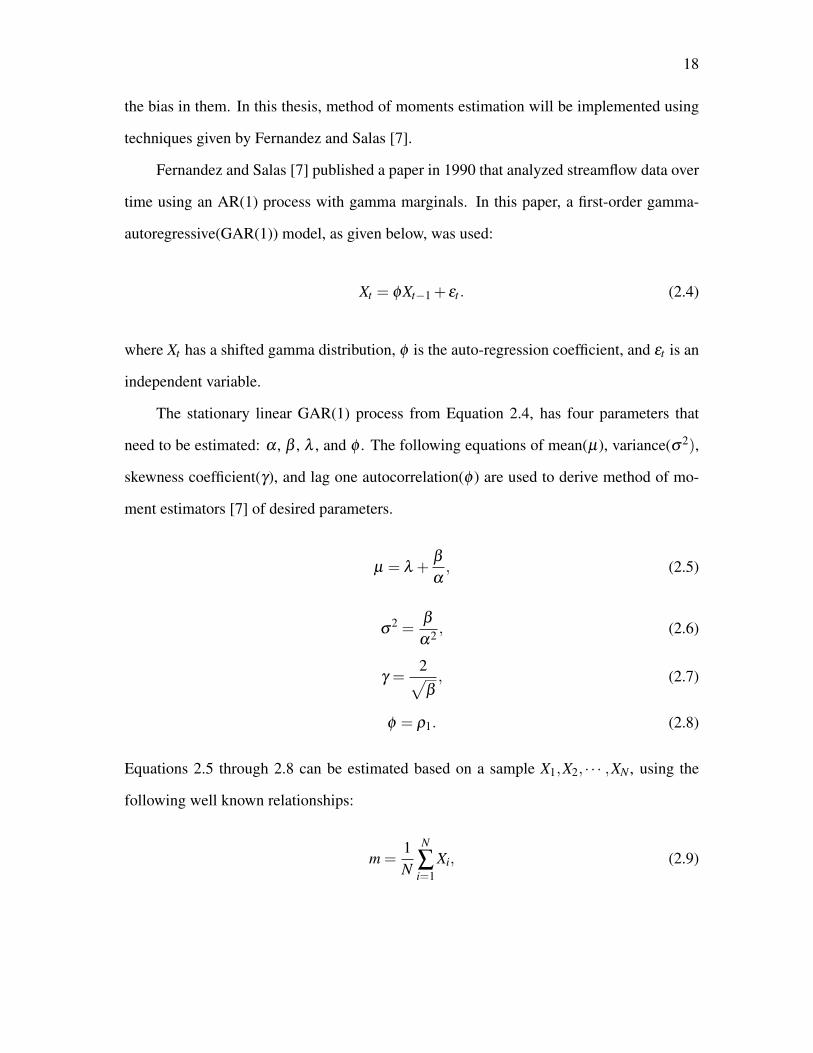
Fernandez and Salas [7] published a paper in 1990 that analyzed streamflow data over
time using an AR(1) process with gamma marginals. In this paper, a first-order gamma-
autoregressive(GAR(1)) model, as given below, was used:
Xt = φXt−1 + εt . (2.4)
where Xt has a shifted gamma distribution, φ is the auto-regression coefficient, and εt is an
independent variable.
The stationary linear GAR(1) process from Equation 2.4, has four parameters that
need to be estimated: α , β , λ , and φ . The following equations of mean(µ), variance(σ2),
skewness coefficient(γ), and lag one autocorrelation(φ ) are used to derive method of mo-
ment estimators [7] of desired parameters.
µ = λ +β
α, (2.5)
σ2 =
β
α2 , (2.6)
γ =2√β, (2.7)
φ = ρ1. (2.8)
Equations 2.5 through 2.8 can be estimated based on a sample X1,X2, · · · ,XN , using the
following well known relationships:
m =1N
N
∑i=1
Xi, (2.9)

19
s2 =1
N−1
N
∑i=1
(Xi−m)2, (2.10)
g1 =N
(N−1)(N−2)s3
N
∑i=1
(Xi−m)3, (2.11)
r1 =1
(N−1)s2
N
∑i=1
(Xi−m)(Xi+1−m). (2.12)
where m is the estimator of µ , s2 is the estimator for σ2, g1 is the estimator for γ ,
r1 is the estimator of ρ1, and N is the sample size. Unfortunately, the estimator of σ2,γ ,
and φ are biased. But Fernandez and Salas [7] have suggested a bias correction for φ and
σ2. These bias corrections are presented in Equations 2.13 through 2.15. A bias correction
must be done before using m,s2,g1, and r1 into the Equations 2.5 through 2.8 to estimate
the GAR(1) model parameters. The following equations shows the bias corrected estimator
ρ1 and σ2:
ρ1 =r1N +1N−4
, (2.13)
where r1 was calculated from equation (2.12)
σ2 =
N−1N−K
s2, (2.14)
where
K =[N(1− ρ1)−2ρ1(1− ρN
1 )]
[N(1− ρ1)2]. (2.15)
Fernandez and Salas [7] has suggested a bias correction for γ given in Equation 2.11. The
method Fernandez and Salas proposed does not work in our particular problem, and will
be discussed in the next section.

20
2.5 FERNANDEZ AND SALAS SUGGESTED BIAS CORRECTION FOR γ
It has been noticed that the estimation of γ , given in Equation 2.11, yields a negative bias
[7]. In 1974, Wallis et al [17] used a simulation study and suggested a bias correction for
iid random variables of gamma, lognormal, and weibull distributions. Then, Bobee and
Robiataille [2] proposed a correction factor to adjust the estimator of γ . The corresponding
bias corrected sample skewness coefficient(g) is defined as:
g =
1N
N∑
i=1(Xi−m)3
(1N
N∑
i=1(Xi−m)2)3/2
. (2.16)
As described in Fernandez and Salas [7], Kirby [10], showed that Equation 2.16 is bounded
by ±L given as:
L =(N−2)√
N−1. (2.17)
Similarly,±√
N equals the bounds of g1 given in Equation 2.11. Bobee and Robitatille(1975)
[2] gave a bias corrected estimator of γ for iid gamma variables with 0.25 ≤ γ ≤ 5 and
20≤ N ≤ 90, as follows:
γ0 =Lg1[A+B(
L2
N)g2
1]√
N, (2.18)
where A and B are defined as:
A = 1+6.51N−1 +20.2N−2, (2.19)
B = 1.48N−1 +6.77N−2. (2.20)
None of the stated Equations in 2.17 through 2.20 can be used in time series setting because
of the independence assumption. Fernandez and Salas conducted a Monte Carlo simulation

21
study, discussed later in the chapter, for GAR(1) model in equation (2.4) with the goal of in-
troducing a bias correction for the skewness coefficient. The following are the summarized
results from the study:
1. The bias of the estimator for γ decreases as N increases.
2. As L increases, ρ1 increases as well.
3. If ρ1 = 0, then the estimated skewness values are very similar to Equation 2.18.
4. When the values are not linearly correlated, then equation 2.18 does not hold.
5. Results from the Monto Carlo Simulation indicate that the only factors that are af-
fecting the skewness are the auto-correlation coefficient and the sample size
From these notes above. Fernandez and Salas [7] proposed the following unbiased estima-
tor of γ:
γ =γ0
f(2.21)
where f is an additional factor to be used when the values are auto-correlated when 0.25≤
γ ≤ 2 and 0≤ ρ1 ≤ 0.8. Using a non-linear least-squares equation scheme the coefficients
of the following regression equation were obtained:
f = (1−3.12p3.71 N−0.49) (2.22)
A few big takeways from this Monto Carlo simulation study and bias correction for γ are
the followings:
1. Bobee and Robiataille [2] proposed bias correction can not be applied for correlated
data.
2. Fernandez and Salas [7] bias correction is not appropriate in our application due to
higher kurtosis and large sample size.

22
As a result, a different method needs to be proposed in order to estimate the skewness with
a large sample size. Before we discuss a different estimation technique, we will present
how the innovation sequence of GAR(1) can be generated. This idea has been used in
subsequent simulation studies.
Fernandez and Salas [7] gave two alternative approaches to calculate ε . The first
approach was found by Gaver and Lewis [8] and will be used for integer values of β of
equation 2.4 is given by:
ε =λ (1−φ)
β+
β
∑j=1
η j. (2.23)
where η j = 0, with probability φ . η j = exp(α), with probability (1−φ) and exp(α) is an
exponentially distributed random variable with the mean equal to1α
. The second approach,
proposed by Lawrance [11], found a solution for non-integer β values. In this case, ε can
be obtained by the following:
ε = λ (1−φ)+η . (2.24)
where η = 0 if M = 0, or η =M∑j=1
Y j(φ)U j if M > 0,
where M is an integer random variable that follows a Poisson distribution with mean value
equal to −β ln(φ). The set U j is an iid random variable with an uniform distribution in
(0,1). Also, Yj is an iid random variable with an exponential distribution with mean (1α).
The next section will introduce the non-parametric regression technique of kernel re-
gression.
2.6 KERNEL REGRESSION
Kernel regression is a non-parametric regression technique. This method is different from
linear and polynomial regression since it does not assume a particular form for the condi-
tional expectation.
Let E(Y |X = xi) = g(xi) and

23
yi = g(xi)+ εi
where ε is the random error that has mean zero. Then the predicted y is given by y = g(x).
In simple linear regression the function g takes the form of g(X) = β0+β1X . But in kernel
regression, as stated above, we do not assume any particular form.
A reasonable approximation to the regression curve g(x0) will be the weighted mean
of response variable near a point x0. This local averaging procedure can be defined as
g(x0) =N
∑i=1
wN,h,i(x0)yi (2.25)
The average will smooth the data. The weights depend on the value of x0 and on h, where
h is called the bandwidth or the smoothing parameter. As h gets smaller, (that is, the size of
the neighborhood gets smaller) g(x0) becomes less biased but also has a greater variance.
In kernel regression, weights are constructed from a kernel function. A kernel func-
tion, K(z) satisfies following conditions.
1. K(z)> 0
2.∫
K(z)dz = 1
3. K(z) = K(−z)
4.∫
z2K(z)dz < ∞
Then weights are defines as
wN,h,i(x0) =K(xi−x0
h
)∑
Ni=i K
(xi−x0h
) .The bandwidth h determines the degree of smoothing. As mentioned above, a large h in-
creases the width of the bins, increasing the smoothness of g(x0). The famous Nadaraya−
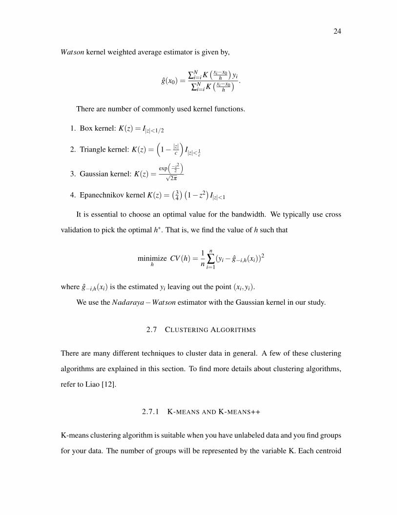
24
Watson kernel weighted average estimator is given by,
g(x0) =∑
Ni=i K
(xi−x0h
)yi
∑Ni=i K
(xi−x0h
) .
There are number of commonly used kernel functions.
1. Box kernel: K(z) = I|z|<1/2
2. Triangle kernel: K(z) =(
1− |z|c)
I|z|< 1c
3. Gaussian kernel: K(z) =exp(−z2
2
)√
2π
4. Epanechnikov kernel K(z) =(3
4
)(1− z2) I|z|<1
It is essential to choose an optimal value for the bandwidth. We typically use cross
validation to pick the optimal h∗. That is, we find the value of h such that
minimizeh
CV (h) =1n
n
∑i=1
(yi− g−i,h(xi))2
where g−i,h(xi) is the estimated yi leaving out the point (xi,yi).
We use the Nadaraya−Watson estimator with the Gaussian kernel in our study.
2.7 CLUSTERING ALGORITHMS
There are many different techniques to cluster data in general. A few of these clustering
algorithms are explained in this section. To find more details about clustering algorithms,
refer to Liao [12].
2.7.1 K-MEANS AND K-MEANS++
K-means clustering algorithm is suitable when you have unlabeled data and you find groups
for your data. The number of groups will be represented by the variable K. Each centroid

25
of a cluster is based on different features which will define the resulting group. Examining
the feature weight of each centriod can show someone what kind of group each cluster
represents. The pseudo-code for the K-Means algorithm was first created by MacQueen
[13] and goes as follow:
1. Choose the number of clusters k for your set S.
2. Randomly partition S into k clusters and determine their centers (averages) or directly
generate k random points as cluster centers.
3. Assign each member from S to the nearest cluster, using some pre-chosen norm.
4. Recompute the new cluster centers.
5. Repeat steps 3 and 4 until clusters stabilize.
The K-means++ clustering algorithm was proposed by Ostrovsky et al [14]. The K-means++
algorithm is an improvement from the k-means algorithm since the K-means++ clustering
algorithm is more carefully selecting the initial centers. This will create a more optimal
method of clustering. The following is the algorithm of K-means++ clustering:
1. Choose one center uniformly at random from the data points.
2. For each data point x, compute the distance D(x) between x and the nearest center
that has already been chosen.
3. Add one new data point at random as a new center, using a weighted probability
distribution where point x is chosen with probability proportional to (D(x))2.
4. Repeat Steps 2 and 3 until k distinct centers have been chosen.

26
2.7.2 HIERARCHICAL CLUSTERING ALGORITHMS
Hierarchical Clustering Algorithms work by grouping data on a one-by-one basis of the
nearest distance measure between each data points. For this thesis, the Euclidean distance
is used as the measure of distance, the definition follows:
Definition 2.4. For two points #»x ∈ Rn and #»y ∈ Rn the euclidean distance (d) is:
d =
√n
∑i=1
(xi− yi)2 (2.26)
Given a set of N items to be clustered, and an N ∗N distance matrix, the basic process
of hierarchical clustering defined by Johnson [9] is as follows:
1. Start by assigning each item to a cluster, so that if you have N items, you now have
N clusters, each containing just one item. Let the distances between the clusters be
the same as the distances between the items they contain.
2. Find the closest pair of clusters and merge them into a single cluster, so that now you
one cluster less.
3. Compute distances between the new cluster and each of the old clusters.
4. Repeat steps 2 and 3 until all items are clustered into a single cluster of size N.
Step 3 of this algorithm can be completed in different ways, which would be the single-
linkage, complete-linkage, and average-linkage.
2.7.3 CLUSTERING LINKAGE FUNCTIONS
We will briefly introduce each clustering linkage functions. First, the single-linkage al-
gorithm will be presented. For single-linkage clustering, which can also be referred as

27
the minimum method, considers the shortest distances between any members of two clus-
ters while calculating the distance. Complete-linkage clustering, which is also called the
maximum method, considers the maximum distances between any members of two clusters
while calculating the distance. Average-linkage clustering considers the average distances
between any members of two clusters while calculating the distance. The following is the
single-linkage clustering algorithm that was introduced by Johnson [9]:
Let D = [d(i, j)] be an N ∗N proximity matrix. The clusterings are assigned sequence
numbers 0,1, · · · ,(n− 1) and L(k) is the level of the kth clustering. A cluster with se-
quence number m is denoted (m) and the proximity between clusters (r) and (s) is denoted
d[(r),(s)]. The single-linkage clustering algorithm follows these steps:
1. Begin with the disjoint clustering having level L(0) = 0 and sequence number m = 0.
2. Find the least dissimilar pair of clusters in the current clustering, say pair (r), (s),
according to d[(r),(s)] = min(d[(i),( j)]) where the minimum is over all pairs of
clusters in the current clustering.
3. Increment the sequence number : m = m + 1. Merge clusters (r) and (s) into a
single cluster to form the next clustering m. Set the level of this clustering to L(m) =
d[(r),(s)].
4. Update the proximity matrix, D, by deleting the rows and columns corresponding to
clusters (r) and (s) and adding a row and column corresponding to the newly formed
cluster. The proximity between the new cluster, denoted (r,s) and old cluster (k) is
defined: d[(k),(r,s)] = min(d[(k),(r)],d[(k),(s)]).
5. If all objects are in one cluster, stop. Else, go to step 2.
Average-linkage and complete-linkage have similar algorithms to the single-linkage, expect

28
one would consider the maximum or average instead of the minimum for all the pairs in
each cluster.

29
CHAPTER 3
RESULTS
Chapter 3 of the thesis presents the results of the research question. We first present the
kernel regression based bias correction technique for the skewness parameter and its mer-
its compared to techniques proposed in literature. Proceeding sub-sections discuss model
based clustering proposed on arc length series of stocks found in the Dow Jones Index
(DWJ).
3.1 BIAS CORRECTION OF KURTOSIS ESTIMATOR
For a fixed sample size, simulation can be used to bias correct using kernel regression. For
each value of λ ,α,β , and φ in the range of values given below, we simulate 100 samples of
size 753 each from different shifted gamma distribution that has a lag-one autocorrelation
structure. The fixed sample size has been chosen as 753 since it represents three years
worth of stock returns. We choose values of each parameter from a limited range so that it
works for our application. We were unable to cover the complete range, since the running
time of the simulation part was too long. These bounds are chosen based on a preliminary
study carried out on those thirty stocks without considering any bias correction. Following
this argument, we fix the value of λ at 1.000164, which is the average of sample means
of thirty arc length series from DWJ index. The value of λ can be easily picked from a
range of values in the future when the method is expanded. Other parameters are chosen as
follows:
10 ≤ α ≤ 108 with increments of 10n(where n has the values of 1 ≤ n ≤ 8 with in-
crements of 1), 0.004≤ β ≤ 1 with increments of 0.002, (this guarantees that the kurtosis
parameter falls between 2 and 31.63), and 0≤ φ ≤ 0.21 with increments of 0.01.
Based on these chosen values we generate 100 samples of size 753 from each of 21×
499× 8 = 83,832 shifted gamma distributions with AR(1) autocorrelation structure. For

30
each generated sample its sample kurtosis using Equation 2.11 and bias corrected sample
autocorrelation at lag-one are computed. Then, for each combination of parameter values,
100 values of g1 and φ are averaged. At the same time, the true kurtosis has been computed
using Equation 2.7. This simulation creates a database of γ, g1, and ¯φ . These data are used
to fit a kernel regression model for true γ against ˆg1 and ¯φ using Gaussian kernel. In
this process we use the Nadaraya-Watson estimator discussed in section 2.6. The optimal
bandwidth of the corresponding model is 0.000218 for ¯φ and 0.0788 for ˆg1. Note that
we considered a burn period of the first five observations in the random generation. The
pseudocode corresponding to the data generation is provided in Algorithm 1 and Algorithm
2.
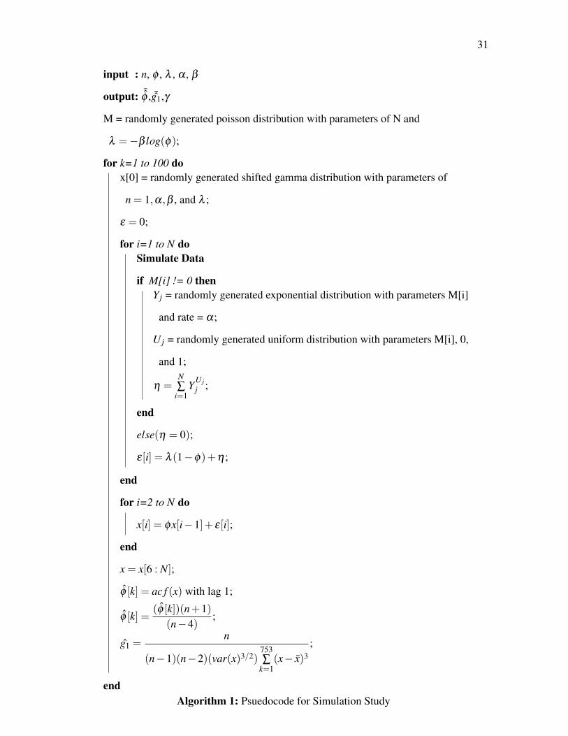
31
input : n, φ , λ , α , β
output: ¯φ , ¯g1,γ
M = randomly generated poisson distribution with parameters of N and
λ =−β log(φ);
for k=1 to 100 dox[0] = randomly generated shifted gamma distribution with parameters of
n = 1,α,β , and λ ;
ε = 0;
for i=1 to N doSimulate Data
if M[i] != 0 thenYj = randomly generated exponential distribution with parameters M[i]
and rate = α;
U j = randomly generated uniform distribution with parameters M[i], 0,
and 1;
η =N∑
i=1YU j
j ;
end
else(η = 0);
ε[i] = λ (1−φ)+η ;
end
for i=2 to N do
x[i] = φx[i−1]+ ε[i];
end
x = x[6 : N];
φ [k] = ac f (x) with lag 1;
φ [k] =(φ [k])(n+1)
(n−4);
g1 =n
(n−1)(n−2)(var(x)3/2)753∑
k=1(x− x)3
;
endAlgorithm 1: Psuedocode for Simulation Study

32
Parameter Estimation¯φ = mean(φ);
¯g1 = mean(g1);
γ =2√β
;
Algorithm 2: Psuedocode for Parameter Estimation
The fitted kernel regression model is presented in figure 3.1. Raw data are not shown
on the same plot since it becomes too messy. The fitted value of γ is taken as the new bias
corrected kurtosis estimate denoted by γbc of each combination of ¯g1 and ¯φ .
Figure 3.1: Simulation study estimated values(left) of ¯φ , ¯g1, and γ , kernel regression of the
estimated values(right) of ¯φ , ¯g1, and γbc)
We carry out a second kernel regression analysis to see how well this idea works. In
this study, we partition our 83,832 data values into a training data set, consisting of 99% of
the data, and a validation data set, consisting of 1% of the data.
The following is the algorithm that was implemented in R to validate the data:
1. Create a data frame that contains ¯φ , ¯g1, and γ as vectors.
2. Create the training data set where 99% of the data frame created in step 1 was chosen.
3. Create two vectors containing the training set and the validation set(1% of data).
33
4. Run the kernel regression function and then observe the results.
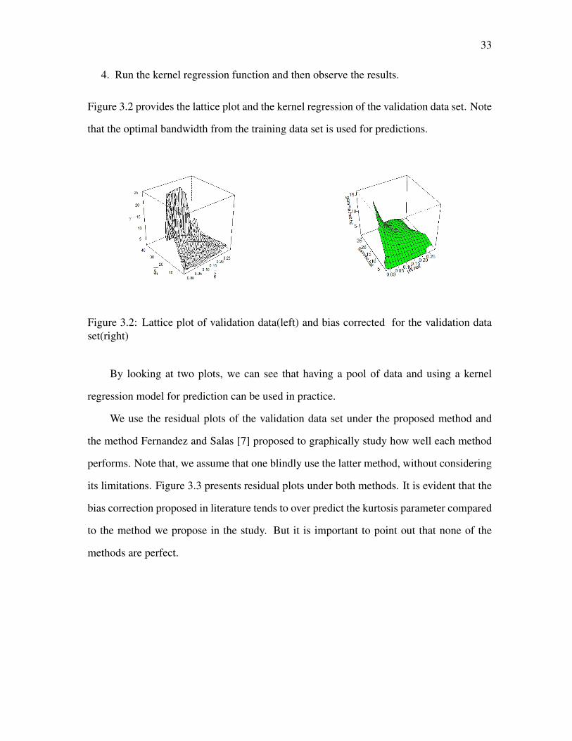
Figure 3.2 provides the lattice plot and the kernel regression of the validation data set. Note
that the optimal bandwidth from the training data set is used for predictions.
Figure 3.2: Lattice plot of validation data(left) and bias corrected for the validation dataset(right)
By looking at two plots, we can see that having a pool of data and using a kernel
regression model for prediction can be used in practice.
We use the residual plots of the validation data set under the proposed method and
the method Fernandez and Salas [7] proposed to graphically study how well each method
performs. Note that, we assume that one blindly use the latter method, without considering
its limitations. Figure 3.3 presents residual plots under both methods. It is evident that the
bias correction proposed in literature tends to over predict the kurtosis parameter compared
to the method we propose in the study. But it is important to point out that none of the
methods are perfect.

34
Figure 3.3: Residual plot for bias correction from literature(left) and residual plot for biascorrection using kernel regression(right)
Both plots have a fanning pattern from the smallest residuals to the maximum residu-
als. The following are a few key observations from Figure 3.3:
1. The range of the residuals clearly favors our proposes bias correction.
2. The bias correction generated by kernel regression has a more constant funnel com-
pared to the Fernenadez and Salas [7] proposed bias correction.
3. We tried different transformations since the plot shows an increasing variance. But
none of them worked well. There is some room for improvements.
From the notes above, it is clear that the kernel regression method works better compared
to the bias correction offered by the Fernandez and Salas [7].
Furthermore, we computed the mean sum of squares of errors (MSSE) under method
proposed by Fernandez and Salas [7] and kernel regression method and found out those to
be 512.54 and 5.09, respectively. As a results, we can clearly see that the MSSE under our
method is significantly smaller compared to the method we found in literature.

35
3.2 AN APPLICATION
As mentioned before, we fit GAR(1) models for arc length series of thirty stocks in DWJ
index. We used method of moments estimation with kernel regression based bias correction
for kurtosis parameter when parameters are estimated. Simulated pool of data and the opti-
mal bandwidth obtained using kernel regression are used to bias correct kurtosis estimates.
Bias corrected parameter estimates of the thirty stocks are given in Figure 3.4:

36
Stock α β φ λ γbcKO 2.32E7 0.0826 0.1050 1.00003 6.961JNJ 2.65E7 0.1268 0.0537 1.00003 5.617PG 6.74E6 0.0557 0.1669 1.00004 8.472GE 1.86E7 0.1339 0.1141 1.00005 5.466
WMT 4.43E6 0.0747 0.0551 1.00006 7.318UTX 8.75E1 0.0053 −0.0003 1.00029 27.43IBM 2.39E7 0.7828 0.0908 1.00006 2.261
T 5.04E6 0.0811 0.1152 1.00007 7.021DD 2.24E6 0.0543 0.0253 1.00007 8.584DIS 4.58E6 0.1051 0.0739 1.00007 6.168
MSFT 5.69E4 0.0060 0.0111 1.00008 25.820BP 5.96E6 0.0944 0.0170 1.00008 6.511
JPM 4.44E6 0.1553 0.1099 1.00008 5.075C 2.32E6 0.1392 0.1 1.00008 5.361
MCD 6.75E6 0.1719 0.1656 1.00008 4.824HON 9.83E6 0.1983 0.0364 1.00008 4.492BA 2.13E7 0.6769 0.0968 1.00009 2.431
AXP 1.00E5 0.0120 0.0301 1.00010 18.257HD 6.25E6 0.1945 0.1140 1.00010 4.535IP 1.18E7 0.2664 0.0458 1.00010 3.875
CVX 1.88E7 0.3512 0.0411 1.00010 3.375XOM 1.09E7 0.1339 0.1141 1.00010 3.776MRK 8.07E4 0.0140 0.0438 1.00010 16.901INTC 1.64E5 0.0186 −0.0038 1.00012 14.683HPQ 1.21E5 0.0180 0.0015 1.00012 14.907CAT 9.65E1 0.0054 −0.0009 1.00035 27.255AA 1.98E6 0.1725 0.0414 1.00135 4.816
EKDAQ 5.60E4 0.0160 0.0345 1.00017 15.811GOOGL 3.52E5 0.0656 0.1070 1.00018 7.806AAPL 9.01E1 0.0054 −0.0020 1.00051 27.223
Figure 3.4: Unbiased parameter estimates for thirty stocks
Note that there are four stocks (UTX, INTC, CAT, AAPL) that indicate a negative first
order auto-correlation. No literature is available about bias correction of kurtosis parameter
when negative autocorrelation is present. Furthermore, no research has been carried out
about generating gamma marginal AR(1) processes with negative autocorrelation. It sill
remains as an open question. As a result, we were unable to carry out a bias correction for
kurtosis in that case. Thus the γbc listed in Figure 3.4 for those corresponding stocks UTX,
INTC, CAT, and AAPL are the kurtosis parameter estimates without a bias correction. The
matter will be discussed more in the conclusion.

37
3.3 CLUSTER ANALYSIS
In this thesis, Model based clustering is applied to identify stocks with similar volatility.
The Euclidean distance between models, i.e, the distance between parameter estimates, is
computed to measure the similarity between two stocks. The Figure 3.5 shows the den-
dogram created based on the complete linkage function(left) and a cluster plot based on
k-means clustering(right) when k = 5. The dendogram appears to be the same under all
other linkage methods.
Figure 3.5: The hierarchical dendogram for the complete linkage(left) and a cluster plotbased on k-means clustering(right)
The horizontal line drew above creates five cluster of stocks for the dendogram. On the
right plot, we can see where each stock is clustered when we chose our k = 5 for k-means
clustering. Figure 3.6 shows where each stock were grouped according to hierarchical
clustering and k-means clustering. Depending on the position one places the partition line,
the number of clusters you get might change. But having a higher number of clusters may
not be practically important. As one can see from Figure 3.6, hierarchical clustering and
k-means clustering grouped each stock in the same cluster, with the exception of stock
17(BA).
Here are a few notes to take away from Figure 3.6:

38
1. Notice that the stocks(UTX, CAT, AAPL, and INTC) who had negative correlation
coefficient are grouped in cluster 5.
2. The majority of big tech companies such as Apple, Google, Untied Technologies,
Microsoft,..etc are grouped in cluster 5.
Cluster Number StocksCluster 1 GE CVXCluster 2 KO JNJ BACluster 3 IP XOM HONCluster 4 PG WMT T DIS BP JPM MCD HDCluster 5 UTX DD MSFT C AXP MRK INTC HPQ CAT AA EKDAQ GOOGL AAPL
Cluster Number StocksCluster 1 GE CVX BACluster 2 KO JNJCluster 3 IP XOM HONCluster 4 PG WMT T DIS BP JPM MCD HDCluster 5 UTX DD MSFT C AXP MRK INTC HPQ CAT AA EKDAQ GOOGL AAPL
Figure 3.6: Cluster placement for each stock for hierarchical clustering(top) and k-meansclustering(bottom).
3.4 FEATURE-BASED CLUSTERING VS MODEL-BASED CLUSTERING
The paper published by Wickramarachchi et al [19] in 2015 used the exact same thirty
stocks as an application. The paper [19] used the sample arc lengths as a feature of volatil-
ity and carried out a feature-based clustering of stocks in terms of volatility. K-mean++
algorithm with three cluster has been used in the application. Feature-based clustering re-
duces large amount of data into one feature that carries an attribute of a series and takes it
into account when clustering is performed. One draw back of this method is that it fails to
take any correlation structure or the behavior of data when they are grouped. This method
fails to take any correlation structure or the behavior of data over time, when they are
grouped.

39
Figure 3.8 compares results of the current study to the results of Wickramarchchi et al
[19]. The figure shows how each stock has been grouped under each respective method.
Stock Company Name K−means++ Model−Based K−means++ Feature−BasedKO Coca−Cola 1 1JNJ Johnson & Johnson 1 1PG The Procter and Gamble 2 1GE General Electric 1 1
WMT Wal−mart 2 1UTX United Technologies 3 1IBM IBM 1 2
T AT& T 2 1DD E.I du Pont de Nemours 3 1DIS WaltDisney 1 1
MSFT Microsoft 3 1BP BP 2 2
JPM JPMorgan and Chase 2 1C Citigroup 3 1
MCD McDonald′s 2 1HON Honeywell 2 2BA Boeing 1 2
AXP American Express 3 1HD Home Depot 2 2IP International Paper Company 2 2
CVX Chervon 1 2XOM Exxon Mobil 2 2MRK Merck 3 1INTC Intel 3 2HPQ HP 3 2CAT Caterpillar 3 2AA Alcoa 3 2
EKDAQ EKDAQ 3 3GOOGL Google 3 3AAPL Apple 3 3
Figure 3.7: Cluster placement for K-means++ based on feature/model-based clustering
Following are the key points we observed.
1. As one can see feature-based clustering method, has sixteen stocks in cluster 1,
eleven in cluster 2, and three in cluster 3.
2. Under Model-based clustering, there are six stocks in cluster 1, eleven stocks in
cluster 2, and thirteen stocks in cluster 3.
3. As stated above, our model-based clustering method is more focused on the dis-
tribution and the correlation structure of arc length series, while the feature-based
technique is more focused on the overall behavior.
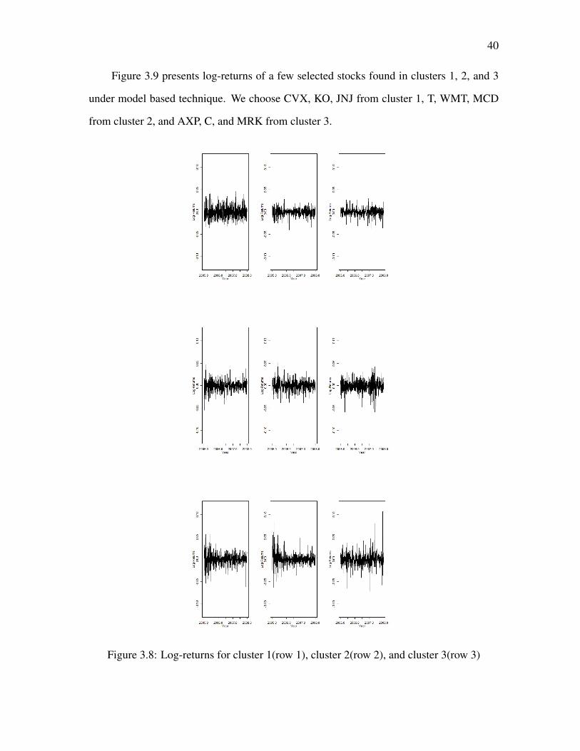
40
Figure 3.9 presents log-returns of a few selected stocks found in clusters 1, 2, and 3
under model based technique. We choose CVX, KO, JNJ from cluster 1, T, WMT, MCD
from cluster 2, and AXP, C, and MRK from cluster 3.
Figure 3.8: Log-returns for cluster 1(row 1), cluster 2(row 2), and cluster 3(row 3)

41
Below are some key take away from Figure 3.9:
1. Those three stocks in high volatile cluster 3 under model-based clustering appears in
low volatile cluster 1 under feature-based clustering.
2. Stock CVX is grouped in less volatile cluster 1 under model-based clustering while
it has been placed in mid-volatile cluster 2 by feature-based clustering.
3. Those three mid-volatile stocks under model based clustering has been categorized
as less volatile stocks by feature-based clustering.
Figure 3.10 presents log-returns of CVX, BP, and CAT. An interesting feature we
observed in figure 3.10 is that all three stocks, CVX, BP, and CAT, have been grouped in
the mid-volatile cluster 2 by feature-based clustering. But the visual inspection of three
plots of log returns does not support this result. The model-based technique we propose,
place them in less, mid, and high volatile groups respectively.
Figure 3.9: Log-returns for CVX(left), BP(middle), and CAT(right)
In addition, the Figure 3.11 shows log-returns of UTX and CAT. Visually both stocks
have to be in same cluster. As expected the method we propose places them in high volatile
cluster 3. But the feature-based clustering technique failed to place them in the same cluster.

42
Figure 3.10: Log-returns for UTX(left) and CAT(right)
We can suggest that model-based clustering provides sensible results compared to
feature-based clustering presented in Wickramarachchi et al [19].
It is important to note that the estimated scale parameter(α) has a significant role in
determining where each stock is placed. When looking at all estimated scale parameters,
most of the values are over one million expect for a few. Those stocks that have a very
low α value are all grouped in the same cluster, which would be the third. It makes perfect
sense since α represents the scale parameter. Therefore those stocks with a low α value are
considered as highly volatile. The converse can be confirmed as well since the stocks with
the highest α value, are all grouped in the first cluster.

43
CHAPTER 4
CONCLUSION
In this study, we explored the possibility of fitting a time series model for the arc length
series of a financial time series. We proposed a GAR(1) type model. One of the main
outcomes of the study is that the kernel regression based bias correction is significantly
better compared to the bias correction proposed by Fernandez and Salas [7] for the kurtosis
estimator. We successfully carried out a model-based clustering on thirty stocks in DWJ
as an application. We were able to identify low volatile and less volatile stocks better
compared to feature-based clustering proposed by Wickramarchchi et al [19].
There is a lot of room to improve our study. First, we have to generalize our simulation
study as it covers a full range of parameter values. We can also consider ways of improving
the fit of the model. We can explore the suitability of other types of kernel functions and
some additional predictors for the model.
One other unexplored area in the bias correction of kurtosis estimator is the case where
negative lag-one autocorrelation is present. Generating gamma marginals with negative
lag-one autocorrelation structure also remains as an open problem.

Bibliography
[1] Black, F., Merton, R., and Scholes, M. (1973). The pricing of options and corporate
liabilities. Journal of Political Economy, 81(3):637–654.
[2] Bobee, B. and Robitatille, R. (1975). Correction of bias in the estimation of the coeffi-
cient of skewness. Water Resour, 11:851–854.
[3] Bollerslev, T. (1986). Generalized autoregressive conditional heteroskedasticity. Jour-
nal of Econometrics, 31(3):307 – 327.
[4] Brockwell, P. J. and Davis, R. A. (2002). Introduction to time series and forecasting.
Springer texts in statistics. Springer, New York, Berlin, Heidelberg.
[5] Casella, G. and Berger, R, L. (2002). Statisical Inference. Duxbury Press.
[6] Engle, R. (1982). Autoregressive conditional heteroscedasticity with estimates of the
variance of united kingdom inflation. Econometrica, 50(4):987–1007.
[7] Fernandez, B. and J.D, S. (1990). Gamma autoregressive models for stream-flow sim-
ulation. Journal of Hydraulic Engineering, 116:1403–1414.
[8] Gaver, D. and Lewis.P.A.W (1980). First order autoregressive gamma sequences and
point process. Adv. Applied Probability, 12:727–745.
[9] Johnson, S. (1967). Hierarchical clustering schemes. Psychometrika, 2:241–254.
[10] Kirby, W. (1974). Algebraic boundness of sample statistics. Water Resour, 10:220–
222.
[11] Lawrance, A. J. (1982). The innovation distribution of a gamma distributed auto-
regressive process. Scandinavian J. Statistics, 9:234–236.
44

45
[12] Liao, T. (2005). Clustering of time series data-a survey. Pattern Recognition,
38:1857–1874.
[13] MacQueen, J. (1967). Some methods for classification and analysis of multivariate
observations. Proceedings of the 5th Berkeley Symposium on Mathematical Statistics
and Probability, 1:281–297.
[14] Ostrovsky, R., Rabani, T., Schilman, L., and Swamy, C. (2012). The effectiveness of
lloyd-type methods for the k-means problem. Journal of ACM, 59:article 28.
[15] R Core Team (2014). R: A Language and Environment for Statisti-
cal Computing. R Foundation for Statistical Computing, Vienna, Austria.
http://www.R-project.org/.
[16] Thomas Mikosch, C. S. (2000). Limit theory for the sample autocorrelations and
extremes of a garch (1, 1) process. The Annals of Statistics, 28(5):1427–1451.
[17] Wallis, J. R., Matalas, N. C., and Slack, J. R. (1974). Just a moment! Water Resour,
10:211–219.
[18] Whittle, P. and Sargent, T. J. (1983). Prediction and Regulation by Linear Least-
Square Methods. University of Minnesota Press, ned - new edition edition.
[19] Wickramarachchi, T. and Tunno, F. (2015). Using arc length to cluster financial time
series according to risk. Communications in Statistics: Case Studies, Data Analysis and
Applications, 1(4):217–225.
[20] Wickramarachchi, T. D., Gallagher, C., and Lund, R. (2015). Arc length asymp-
totics for multivariate time series. Applied Stochastic Models in Business and Industry,
31(2):264–281.

46
Appendix A
R CODE
Appendix A contains R code for the simulation study, as well as code for the graphics
generated in Chapters 1, 2, and 3.
## Calculating Arc Length ##
install.packages("readxl")
library(readxl) ## To read Excel Files ##
data<-read_excel("data.xlsx")
x<-data[,30]
x
n=length(x)
yt1 = 0
yt =0
## Used to plot the Arc length of a specific stock out of the group of thirty chosen ##
for(k in 10)
{
for(i in 1:753)
{
yt[i] = sqrt(1+((log(data[,k][i+1]))-log(data[,k][i]))ˆ2) #arclength
}
arclength = ts(yt,start=c(2005, 1), frequency=252)
plot(arclength,ylim = c(1,1.0025),xlab="Year", main = "Arclength for CAT")
47
}
## Calculating and plot Log-Returns ##
for(j in 1:753)
{
yt1[j] = log(x[j+1]/x[j])
}
plot(ts((yt1)),main = "Log Return Prices for Coca-Cola Company",xlab = "Data", ylab = "Closing Price")
## Plotting the Empirical Density for a certain stock ##
plot(density(yt1),main = "Kernel Density Plot of Log-Returns for Coca-Cola Comapany ")
#####Simulation Study######
###Create Function to Simulate Data###
##N - Number of Repetitions Desired##
##n - Size of Simulated Data Sets##
##lambda,alpha,beta - Gamma Parameters##
##phi - GAR(1) Parameters##
install.packages("FAdist")
library(FAdist)## used to create a shifted gamma distribution

48
#Initialization#
phi = seq(-0.05,0.21,0.01)
phi = 0.05
power = c(1:8)
alpha = 10ˆpower
beta = seq(0.004,1,0.002)
beta = 0.1
n = 754
N=n+5
#Create Function for Simulation study as suggested by Fernandez and Salas#
simu = function(n, phi, lamada, alpha, beta){
M = rpois(N,lambda= -beta*log(phi))
g1=0
phihat=0
for(k in 1:100){
x0 = rgamma3(n=1, shape=alpha, scale=beta, thres=lamada) ##X0 term for the first observation
epsil = 0
for(i in 1:N){
if(M[i]!=0){
Yj = rexp(M[i],rate=alpha)

49
Uj = runif(M[i], 0, 1)
eta = sum(YjˆUj)
} else{eta=0}
epsil[i] = lamada*(1-phi)+eta
}
x=0
x[1] = phi*x0+epsil[1] #first observation
for(i in 2:N){
x[i] = phi*x[i-1]+epsil[i]
}
x= x[6:N]
phihat[k] = acf(x)$acf[2]
phihat[k] = (phihat[k]*n+1)/(n-4)
g1[k] = (n/((n-1)*(n-2)*var(x)ˆ(3/2)))*sum((x-mean(x))ˆ3)
}
phihatbar = mean(phihat)
g1bar = mean(g1)
gamma = 2/sqrt(beta)
true_phi=phi
newlist = list("phihatbar"= phihatbar, "g1bar"=g1bar, "gamma"=gamma, "true_phi"=true_phi)
return(newlist)
}

50
#Creating the Training data set for the simulation study#
v1 = sapply(beta, function(beta) sapply(phi, function(phi) sapply(alpha, simu, beta=beta, n=n, phi=phi, lamada = lamada)))
## Used to get estimated values for our simulation ##
k=seq(1,672,4)
s=seq(2,672,4)
t=seq(3,672,4)
j=1:499
phihatbarout = v1[k,j]
g1barout = v1[s,j]
gammaout = v1[t,j]
phihatvec=as.numeric(phihatbarout)
g1barvec=as.numeric(g1barout)
gammavec=as.numeric(gammaout)
d3 = data.frame(phihatvec,g1barvec,gammavec)
train1 = sample(nrow(d3),0.99*nrow(d3))
d4 <- d3[train1,] ## Training data set
d4.validate<-d3[-train1,] ## Validation data set
## Graphing the Training data set vs Full data set ##

51
install.packages("sm")
library(sm)
k1=sm.regression(cbind(d4[,1], d4[,2]), d4[,3],xlab="Phihatbar",ylab="G1bar",zlab="Gamma") ## Training Data Set
k=sm.regression(cbind(phihatvec, g1barvec), gammavec) ## Full Data Set
## Creating the bandwidth for the Predicted $\gamma$ values ##
install.packages("np")
library(np)
bw <- npregbw(xdat=data.frame(d4[,1:2]), ydat=d4[,3], regtype="lc", bwmethod="cv.aic", tol=.01, ftol=.01)
predict.out<-fitted(npreg(exdat=data.frame(d4[,1:2]), bws=bw1)) ## Predicted Gamma Values
## Calculating MSE, Bias, and Plot Residual Plots for Predicted $\gamma$ ##
gamma_obs = d4.validate[,3]
gamma_estimate = predict.out
variance = var(gamma_estimate)
bias = gamma_estimate - d4.validate[,3]
MSE = variance + biasˆ2
res = d4.validate[,3] - gamma_estimate
plot(gamma_obs,res, xlab = "gamma observed", ylab ="Residual", main = "Residual plot for Bias Correction from Kernel Regression")
## Calculating the MSE, Bias, and Plot Residual Plots for $\gamma$ from suggestion by Fernandez and Salas ##
52
## Method Suggested by Fernandez and Salas ##
n = 754
L = (n-2)/sqrt(n-1)
A = 1+6.51*nˆ(-1)+20.2*nˆ(-2)
B = 1.48*nˆ(-1)+6.77*nˆ(-2)
gamma0 = (L*g1.validate*(A+B*((Lˆ2)/n)*g1.validateˆ2))/sqrt(n)
f = (1 - 3.12*(phi.validateˆ(3.7))*nˆ(-.49))
gamma = gamma0/f
gamma
## Calculating the MSE and ploting the Residual Plot ##
gamma_obs = d4.validate[,3]
gamma_estiamate = gamma
variance = var(gamma)
bias = gamma - d4.validate[,3]
MSE = variance + biasˆ2
res3 = d4.validate[,3]-gamma
plot(gamma_obs,res3,xlab = "gamma observed",ylab="Residual",main = "Residual Plot Bias Correction From Paper")
## Method of Moments Calculation using the unbias $\gamma$ estimation ##

53
### Same method but with the yt
n = length(yt)
m=mean(yt)
s2 = var(yt)
g1 = (n/((n-1)*(n-2)*s2ˆ(3/2)))*sum((yt-m)ˆ3)
r1 = (1/((n-1)*s2))*sum((yt[1:n-1]-m)*(yt[2:n]-m));
## Correction for r1
p1 = (r1*n+1)/(n-4)
## correction for s2
K = ((n*(1-p1ˆ2))-2*p1*(1-p1ˆn))/(n*(1-p1)ˆ2)
sigma2 = s2*(n-1)/(n-K)
## Fitting with Unbias Gamma ##
54
d3 = data.frame(abs(phi),g1)
Unbias_Gamma<-fitted(npreg(exdat=data.frame(d3), bws=bw))
## Estimating Shifted Gamma parameters with unbias Gamma ##
Unbias_beta = (2/Unbias_Gamma)ˆ2
Unbias_beta
phi = p1
p1
Unbias_alpha = Unbias_beta/sigma2
Unbias_alpha
Unbias_lamada = m - Unbias_beta/Unbias_alpha
Unbias_lamada
Unbias_alpha
Unbias_beta
p1
Unbias_lamada
Unbias_Gamma
55
## Model-based clustering for unbias esitimates ##
alpha = c(23159914,26522442,6739005,18617797,4433520,87.45,23927783,5043800,2242692,4579838,56932.73,5958331,4440553,2318633,6749583,9833621,21311974,100285.6,6254844,11788494,18841939,10902528,80718.61,163887.5,120624.7,96.46775,1980827,56041.58,351527,90.107)
beta = c(0.08255588,0.1267607,0.05573179,0.1338863,0.07468809,0.005316261,0.7827966,0.08114764,0.05429077,0.1051352,0.006,0.09435821,0.1552851,0.1391698,0.1719227,0.1982691,0.6768846,0.012,0.1944895,0.26635321,0.3512395,0.2805609,0.01400348,0.01855432,0.018,0.005384881,0.1724826,0.01600091,0.06563742,0.005397311)
phi = c(0.10497,0.053684,0.166852,0.114144,0.055074,-0.000301,0.090807,0.115215,0.0253051,0.07393236,0.0111105,0.0169825,0.1099256,0.1000062,0.1655639,0.03639002,0.09683009,0.03009054,0.1139784,0.04578822,0.04107013,0.07463203,0.04379598,-0.003812698,0.001506284,-0.00093941,0.04141586,0.03454594,0.1070449,-0.001963859)
lamada = c(1.00003,1.00003,1.00004,1.000045,1.000061,1.000285,1.000062,1.000065,1.000072,1.000073,1.000077,1.000078,1.000078,1.000081,1.00008,1.00008,1.000092,1.000102,1.000095,1.000096,1.000098,1.000098,1.000104,1.000121,1.000124,1.000349,1.00153,1.000174,1.000184,1.000513)
gamma = c(6.960749,5.617431,8.471855,5.465903,7.318201,27.43007,2.260544,7.020888,8.583551,6.168165,25.81989,6.510887,5.07534,5.361144,4.823513,4.491615,2.430931,18.25742,4.535049,3.87527,3.374647,3.775865,16.90098,14.68275,14.90712,27.25473,4.815677,15.81094,7.806462,27.22333)
m = matrix(c(alpha,beta,phi,lamada,gamma),ncol =5, nrow =30)
## Creating a function for the euclidian distance calculation ##
distfunc <- function(x) {
d <- dist(m, method = "euclidian")
#d <- as.dist((1-cor(t(x))))
return (d)
}
d <- distfunc(m)
#1. Hierarchical
#run hierarchical clustering using single, average, and complete methods#
groups <- hclust(d,method="single")
plot(groups, hang=-1)
#2. K-means, k = 3 for three clusters#
56
### k-means (this uses euclidean distance)
clusters <- kmeans(as.matrix(d), 3, nstart = 30)
plot(as.matrix(d), col = clusters$cluster)
points(clusters$centers, col = 1:10, pch = 8)
install.packages(’cluster’)
#better way to visualize clusters
library(cluster)
clusplot(as.matrix(d), clusters$cluster, color=T, shade=T, labels=2, lines=0)
## K-means++ clustering ##
alpha = c(23159914,26522442,6739005,18617797,4433520,87.45,23927783,5043800,2242692,4579838,56932.73,5958331,4440553,2318633,6749583,9833621,21311974,100285.6,6254844,11788494,18841939,10902528,80718.61,163887.5,120624.7,96.46775,1980827,56041.58,351527,90.107)
beta = c(0.08255588,0.1267607,0.05573179,0.1338863,0.07468809,0.005316261,0.7827966,0.08114764,0.05429077,0.1051352,0.006,0.09435821,0.1552851,0.1391698,0.1719227,0.1982691,0.6768846,0.012,0.1944895,0.26635321,0.3512395,0.2805609,0.01400348,0.01855432,0.018,0.005384881,0.1724826,0.01600091,0.06563742,0.005397311)
phi = c(0.10497,0.053684,0.166852,0.114144,0.055074,-0.000301,0.090807,0.115215,0.0253051,0.07393236,0.0111105,0.0169825,0.1099256,0.1000062,0.1655639,0.03639002,0.09683009,0.03009054,0.1139784,0.04578822,0.04107013,0.07463203,0.04379598,-0.003812698,0.001506284,-0.00093941,0.04141586,0.03454594,0.1070449,-0.001963859)
lamada = c(1.00003,1.00003,1.00004,1.000045,1.000061,1.000285,1.000062,1.000065,1.000072,1.000073,1.000077,1.000078,1.000078,1.000081,1.00008,1.00008,1.000092,1.000102,1.000095,1.000096,1.000098,1.000098,1.000104,1.000121,1.000124,1.000349,1.00153,1.000174,1.000184,1.000513)
gamma = c(6.960749,5.617431,8.471855,5.465903,7.318201,27.43007,2.260544,7.020888,8.583551,6.168165,25.81989,6.510887,5.07534,5.361144,4.823513,4.491615,2.430931,18.25742,4.535049,3.87527,3.374647,3.775865,16.90098,14.68275,14.90712,27.25473,4.815677,15.81094,7.806462,27.22333)
m = matrix(c(alpha,beta,phi,lamada),ncol =4, nrow =30)
k=3
s=vector()
s[1]=sample(1:30,1)
57
c=matrix(,ncol=4)
c[1,] = m[s[1],]
d1=1:30
for(i in 1:30){
d1[i]=sum((c[1,]-m[i,])ˆ2) ##computeD(x)ˆ2
}
prob=d1/sum(d1)
s[2]=sample(1:30,1,prob=prob)
c = rbind(c,m[s[2],])
for(i in 1:30){
d1[i] = min(sum((c[1,]-m[i,])ˆ2), sum((c[2,]-m[i,])ˆ2)) ## Compute min(D1ˆ2, D2ˆ2)
}
prob=d1/sum(d1)
s[3]=sample(1:30, 1, prob=prob)
c = rbind(c,m[s[3],])
kmeans(m, c)