modeling visual problem-solving as analogical reasoning ... · modeling visual problem-solving as...
TRANSCRIPT
Visual Problem-Solving 1
Running Head: MODELING VISUAL PROBLEM-SOLVING
Modeling Visual Problem-Solving as Analogical Reasoning
Andrew Lovett and Kenneth Forbus
Northwestern University
Manuscript
Visual Problem-Solving 2
Abstract
We present a computational model of visual problem-solving, designed to solve problems
from the Raven’s Progressive Matrices intelligence test. The model builds on the claim that
analogical reasoning lies at the heart of visual problem-solving, and intelligence more broadly.
Images are compared via structure-mapping, aligning the common relational structure in two
images to identify commonalities and differences. These commonalities or differences can
themselves be reified and used as the input for future comparisons. When images fail to align,
the model dynamically re-represents them to facilitate the comparison. In our analysis, we find
that the model matches adult human performance on the Standard Progressive Matrices test, and
that problems which are difficult for the model are also difficult for people. Furthermore, we
show that model operations involving abstraction and re-representation are particularly difficult
for people, suggesting that these operations may be critical for performing visual problem-
solving, and reasoning more generally, at the highest level.
Keywords: Visual comparison, analogy, problem-solving, cognitive modeling.
Visual Problem-Solving 3
Modeling Visual Problem-Solving as Analogical Reasoning
Analogy is perhaps the cornerstone of human intelligence (Gentner, 2003, 2010; Penn,
Holyoak, & Povinelli, 2008; Hofstadter & Sander, 2013). By comparing two domains and
identifying commonalities in their structure, we can derive useful inferences and develop novel
abstractions. Analogy can drive scientific discovery, as when Rutherford famously suggested
that electrons orbiting a nucleus were like planets orbiting a sun. But it also plays a role in our
everyday lives, allowing us to apply what we’ve learned in past experiences to the present, as
when a person solves a physics problem, chooses a movie to watch, or considers buying a new
car.
Analogy’s power lies in its abstract nature. We can compare two wildly different
scenarios, applying what we’ve learned in one scenario to the other, based on commonalities in
their relational structure. Given this highly abstract mode of thought, and its importance in
human reasoning, it may be surprising that when researchers want to test an individual’s
reasoning ability, they often rely on concrete, visual tasks.
Figure 1 depicts an example problem from Raven’s Progressive Matrices (RPM), an
intelligence test (Raven, Raven, & Court, 1998). This test requires that participants compare
images in a (usually) 3x3 matrix, identify a pattern across the matrix, and solve for the missing
image. RPM was designed to measure a subject’s eductive ability (the ability to discover patterns
in confusing stimuli), a term that has now been mostly replaced by fluid intelligence (Cattell,
1963). It has remained popular for decades because it is highly successful at predicting a
subject’s performance on other ability tests—not just visual tests, but verbal and mathematical as
well (Burke & Bingham, 1969; Zagar, Arbit, & Friedland, 1980; Snow, Kyllonen, & Marshalek,
Visual Problem-Solving 4
1984). A classic scaling analysis which positioned ability tests based on their intercorrelations
placed RPM in the center, indicating it was the single most predictive test (Figure 2).
How is a visual test so effective at measuring general problem-solving ability? We
believe that despite its concrete nature, RPM tests individuals’ abilities to make effective
analogies. The connection between RPM and analogy is well-supported by the analysis in Figure
2. In that analysis, visual (or geometric), verbal, and mathematical analogy problems were
clustered around RPM, suggesting that they correlate highly with it and that they are also strong
general measures. Indeed, RPM can be seen as a complex geometric analogy problem, where
subjects must determine the relation between the first two images and the last image in the top
row and then compute an image that produces an analogous relation in the bottom row.
Consistent with this claim, Holyoak and colleagues showed that high RPM performers required
less assistance when performing analogical mappings (Vendetti, Wu, & Holyoak, 2014) and
retrievals (Kubricht et al., 2015). Furthermore, a meta-analysis of brain imaging studies found
that verbal analogies, geometric analogies, and matrix problems engage a common brain region,
the left rostrolateral prefrontal cortex, which may be associated with relational reasoning
(Hobeika et al., 2016)1.
Here we argue that the mechanisms and strategies that support effective analogizing are
also those that support visual problem-solving. To test this claim, we model human performance
on RPM using a well-established computational model of analogy, the Structure-Mapping
Engine (SME) (Falkenhainer, Forbus, & Gentner, 1989). While SME was originally developed
to model abstract analogies, there is increasing evidence that its underlying principles also apply
1 Matrix problems, specifically, engage several additional areas, perhaps due to their greater complexity and the
requirement that test-takers select from a set of possible answers, both of which may increase working memory
demands.
Visual Problem-Solving 5
to concrete visual comparisons (Markman & Gentner, 1996; Sagi, Gentner, & Lovett, 2012).
RPM provides the opportunity to test the role of analogy in visual thinking on a large scale, and
to determine what components are needed to perform this task outside of the analogical mapping
that SME provides. In particular, we consider the dual challenges of perception and re-
representation: How do you represent concrete visual information in a manner that supports
abstract analogical thought, and how do you change your representation when images fail to
align?
This approach also allows us to gain new insights about RPM and what it evaluates in
humans. By ablating the model’s ability to perform certain operations and comparing the
resulting errors to human performance, we can identify factors that make a problem easier or
more difficult for people. As we show below, problems tend to be more difficult when they a)
must be represented more abstractly, or b) require complex re-representation operations. We
close by considering whether abstract thinking and re-representation in RPM might generalize to
other analogical tasks and thus be central to human intelligence.
We next describe RPM in greater detail, including a well-established previous
computational model. Afterwards, we present our theoretical framework, showing how
analogical reasoning maps onto RPM and visual problem-solving more broadly. We then
describe our computational model, which builds on this framework and follows previous models
of other visual problem-solving tasks. We present a simulation of the Standard Progressive
Matrices, a 60-item intelligence test. The model’s overall performance matches average
American adults. We finish with our ablation analysis.
Visual Problem-Solving 6
Raven’s Progressive Matrices
On a typical RPM problem, test-takers are shown a 3x3 matrix of images, with the lower
right image missing. By comparing the images and identifying patterns across each row and
column, they determine the answer that best completes the matrix, choosing from eight possible
answers. Figures 3-5 show several example problems, which will be used as references
throughout the paper and referred to by their respective letters. Note that no actual test problems
are shown, but these example problems are analogous to real test problems.
RPM has been a popular intelligence test for decades. It is successful because it does not
rely on domain-specific knowledge or verbal ability. Thus, it can be used across cultures and
ages to assess fluid intelligence, the ability to reason flexibly while solving problems (Cattell,
1963). RPM is one of the best single-test predictors of problem-solving ability: participants who
do well on RPM do well on other intelligence tests (e.g., Burke & Bingham, 1969; Zagar, Arbit,
& Friedland, 1980; see Raven, Raven, & Court, 2000b, for a review) and do well on other verbal,
mathematical, and visual ability tests (Snow, Kyllonen, & Marshalek, 1984; Snow & Lohman,
1989). Thus, RPM appears to tap into core, general-purpose cognitive abilities. However, it
remains unclear what exactly those abilities are.
Carpenter, Just, and Shell (1990) conducted an influential study of the Advanced
Progressive Matrices (APM), the hardest version of the test. They ran test-takers with an eye
tracker, analyzed the problems, and built two computational models.
Carpenter et al. found that participants generally solved problems by looking across a row
and determining how each object varied between images. Their analysis produced five rules to
explain how objects could vary: 1) constant in a row: the object stays the same; 2) quantitative
pairwise progression: the object changes in some way (e.g., rotating or increasing in size)
Visual Problem-Solving 7
between images (problem A, Figure 3); 3) distribution of three: there are three different objects
in the three images; those objects will be in every row, but their order will vary (problem B); 4)
figure subtraction or addition: add or subtract the objects in the first two images to produce the
objects in the last (problem E); and 5) distribution of two: each object is in only two of the three
images (problems F, H). While the final rule sounds simple, it is actually quite complex. It
requires recognizing that there is no corresponding object in one of the three images.
Carpenter et al.’s FAIRAVEN model implements these rules. Given hand-coded,
symbolic image representations as input, it analyzes each row via the following steps:
1. Identify corresponding objects. The model uses simple heuristics, such as matching
same-shaped objects, or matching leftover objects.
2. For each set of corresponding objects, determine which of the five rules (see above) it
instantiates. FAIRAVEN can recognize every rule type except distribution of two.
The model performs these steps on each of the first two rows and then compares the two
rows’ rules, generalizing over them. Finally, it applies the rules to the bottom row to compute
the answer.
The BETTERAVEN model improves on FAIRAVEN in a few ways. Firstly, during
correspondence-finding, it can recognize cases where an object is only in two of the three
images. Secondly, it checks for the distribution of two rule. Thirdly, it has a more developed
goal management system. It compares the rules identified in the top two rows, and if they are
dissimilar, it backtracks and looks for alternate rules.
Carpenter et al. argued that this last improvement, better goal management, was what
truly set BETTERAVEN apart. They believed that skilled RPM test-takers are adept at goal
management, primarily due to their superior work memory capacity. This could explain RPM’s
Visual Problem-Solving 8
strong predictive power: it may accurately measure working memory capacity, a key asset in
other ability tests. In support of this hypothesis, other researchers (Vodegel-Matzen, van der
Molen, & Dudink, 1994; Embretson, 1998) have found that as the number and complexity of
Carpenter rules in a problem increases, the problem becomes harder. Presumably, a greater
number of rules places more load on working memory.
We believe Carpenter et al.’s models are limited in that they fail to capture perception,
analogical mapping, and re-representation. As we have suggested above and argue below, these
processes are critical in both analogical thought and visual problem-solving. Because they do not
analyze these or other general processes, Carpenter et al. can derive only limited connections
between RPM and other problem-solving tasks. The primary connection they derive is that RPM
requires a high working memory capacity. Below, we briefly describe each of the model’s
limitations.
1. Perception. The Carpenter models take symbolic representations as input. These
representations are hand-coded, based upon descriptions given by participants. While we agree
on the use of symbolic representations, this approach is limited in two respects: a) it ignores the
challenge of generating symbolic representations from visual input, and b) it makes no
theoretical claims about what information should or should not be captured in the symbolic
representations. In fact, problem-solving depends critically on what information is captured in
the initial representations, and the ability to identify and represent the correct information might
well be a skill underlying effective problem-solving.
2. Analogical mapping. When the BETTERAVEN model compares images, it identifies
corresponding objects using three simple heuristics: a) match up identical shapes, b) match up
leftover shapes, c) allow a shape to match with nothing. In contrast, we believe visual
Visual Problem-Solving 9
comparison can use the same rich relational alignment process used in abstract analogies
(Markman & Gentner, 1996; Sagi, Gentner, & Lovett, 2012).
In addition, we believe one challenge in RPM may be determining which images to
compare. For example, in RPM it is typically enough to compare the adjacent images in each
row, but for some problems one must also compare the first and last images in the row (e.g.,
problem E). In our analysis below, we test whether problems requiring this additional image
comparison are more difficult to solve.
3. Re-representation. Carpenter et al. mention that in some cases their model is given a
second representation to try if the first one fails to produce a satisfying answer. This is an
example of re-representation: changing an image representation to facilitate a comparison.
However, it appears that re-representation is not performed or analyzed in any systematic way. In
fact it is likely not needed in most cases because the initial representations are hand-coded—if
the initial representations are constructed to facilitate the comparison, then no re-representation
will be required.
We believe re-representation can play a critical role in visual problem-solving, as well as
in analogy more broadly. In this paper we show how re-representation is used to solve problems
such as G, and we analyze the difficulty of these problems for human test-takers.
Theoretical Framework
We argue that visual thinking often involves analogical processing of the same form that
is used elsewhere in cognition (e.g. Gentner & Smith, 2013; Kokinov & French 2003). That is, a
problem is encoded (perception) and analyzed to ascertain what comparison(s) are needed to be
done. The comparisons are carried out via structure-mapping (Gentner, 1983). The results are
analyzed and evaluated by task-specific processes, which include methods for re-representation
Visual Problem-Solving 10
(Yan et al. 2003), often leading to further comparisons. This is an example of a map/analyze
cycle (Falkenhainer, 1990; Forbus, 2001; Gentner et al., 1997), a higher-level pattern of
analogical processing which has been used in modeling learning from observation and
conceptual change. The same overall structure, albeit with vision-specific encoding and analysis
processes, appears to be operating in solving some kinds of visual problems, and specifically
RPM problems. This provides a straightforward explanation as to why RPM is so predictive of
performance on so many non-visual problems: The same processes are being used.
One key claim which should be emphasized is: Re-representation is driven by
comparison. Rather than a top-down search process that explores different possible
representations for each image, we are suggesting that initial, bottom-up representations are
changed only when necessary to facilitate a comparison.
Below we provide background on analogical mapping. We then describe five steps for
visual problem-solving:
1. Perception: Generate symbolic representations from images.
2. Visual Comparison: Align the relational structure in two images, identify commonalities
and differences.
3. Perceptual Reorganization: Re-represent the images, if necessary, to facilitate a
comparison.
4. Difference Identification: Symbolically represent the differences between images.
5. Visual Inference: Apply a set of differences to one image to infer a new image.
We have previously modeled two other visual problem-solving tasks using analogy: a
visual oddity task (Lovett & Forbus, 2011a) and geometric analogy (Lovett et al., 2009b) (Figure
Visual Problem-Solving 11
6). In what follows, we speak generally of visual problem-solving when possible, and focus on
RPM specifics only when necessary.
Analogical Mapping
Cases are represented symbolically, as entities, attributes, and relations. Two
representations, a base and a target, are aligned based on their common relational structure
(Gentner, 1983; Hummel & Holyoak, 1997; Larkey & Love, 2003; Doumas & Hummel, 2013).
Based on the corresponding attributes and relations, corresponding entities can be identified. The
result of a mapping is a set of correspondences between the base and target, and a similarity
score based on the depth and breadth of aligned structure (Falkenhainer, Forbus, & Gentner,
1989). According to structure-mapping theory (Gentner, 1983, 2010), mappings are constrained
to allow each base item to map to just one target item. Mappings also include candidate
inferences, where structure in one description is projected to the other. The results of a mapping
can be represented symbolically, so that they themselves can play a role in future reasoning
(even in future analogies). We use two types of reification that have been used elsewhere in the
literature for non-visual comparisons:
1. Generalization. Here one constructs an abstraction, sometimes called a schema,
describing the commonalities in the base and target (Glick & Holyoak, 1983; Kuehne et
al., 2000).
2. Difference Identification. Here one explicitly represents the differences between the base
and target. The most interesting differences are alignable differences, where there is some
expression in the base and some corresponding but different expression in the target
(Gentner & Markman, 1994).
Visual Problem-Solving 12
Visual Perception
To perform analogy between two stimuli, one must first generate symbolic
representations to describe them (Gentner, 2003, 2010; Penn, Holyoak, & Povinelli, 2008). Here
we are interested not in low-level visual processing, but rather in the resulting representations
and the ways they can support problem-solving. Visual representations can be characterized as
hierarchical hybrid representations (HHRs). They are hierarchical (Palmer, 1977; Marr &
Nishihara, 1978; Hummel & Stankiewicz, 1996) in that a given image can be represented at
multiple levels of abstraction in a spatial hierarchy; for example, a rectangle could be seen as a
single object or as a set of four edges. They are hybrid in that there are separate qualitative and
quantitative components at each level in the hierarchy (Kosslyn et al., 1989). The qualitative, or
categorical component symbolically describes relations between elements; for example, one
object contains another, or two edges are parallel (Biederman, 1987; Hummel & Biederman,
2002; Forbus, Nielsen, & Faltings, 1991). The quantitative component describes concrete
quantitative values for each element, e.g., its location, size, and orientation (Forbus, 1983;
Kosslyn, 1996).
Qualitative representations are critical for helping us remember, reproduce, and compare
spatial information (e.g., quadrants of a circle: Huttenlocher, Hedes, & Duncan: 1991; angles
between object parts: Rosielle & Cooper, 2001; locations: Maki, 1982). We believe that these
representations capture structural information about a visual scene, and that they can be
compared via the same alignment processes used in analogy (Markman & Gentner, 1996; Sagi,
Gentner, & Lovett, 2012). However, as in any analogy, the outcome of the comparison depends
heavily on the representations used. In particular, one must select the appropriate level in the
spatial hierarchy.
Visual Problem-Solving 13
How many hierarchical levels are used in the human visual system is still an open
question. Here we assume three levels for two-dimensional perception: groups, objects, and
edges. Groups are sets of objects grouped together based on similarity. Objects are individual
objects. Edges are the edges that make up each object. We further propose that when an
individual views a scene, the highest level is available first—for example, Figure 7A contains no
obvious groups, so one would initially perceive this as a row of three objects, including
qualitative relations between these objects. This follows reverse hierarchy theory (Hochstein &
Ahissar, 2002; see also: Love, Rouder, & Wisniewski, 1999), which claims that visual perception
is a bottom-up process, beginning with low-level features, but that large-scale, high-level
features are the ones initially available for conscious access; deliberate effort is required to move
down the hierarchy and think about the smaller-scale details (e.g., the relations among the edges
of each shape in Figure 7A).
Two clarifying points must be made about the spatial hierarchy. Firstly, it is distinct from
a relational hierarchy, i.e., describing attributes, lower-order relations, and higher-order
relations. The level in the spatial hierarchy determines the entities—edges, objects, or groups—
but it does not determine whether lower-order or higher-order relations may be applied to these
entities. For example, Kroger, Holyoak, and Hummel (2004) found that when comparing images
of four colored squares, it was easier to compare the squares’ colors directly, and more difficult
to compare higher-order relations between the squares (e.g., “The top two squares are the same
color, and the bottom two squares are a different color, so the relations describing the top two
vs. the bottom two squares are different”). Here, both the attributes and the higher-order
relations described the squares’ colors, and thus they existed at the same level in the spatial
hierarchy.
Visual Problem-Solving 14
Secondly, the high-level advantage in the spatial hierarchy is not absolute. For example,
Navon (1977) showed that when large letters were made up of arrangements of smaller letters, it
was easier to perceive the large letter than to perceive the smaller letters. But follow-up studies
showed there were many ways to disrupt this advantage (e.g., varying the absolute size of the
letters: Kinchla & Wolfe, 1979; the density of the letters: LaGrasse, 1993; or the spatial
frequency components of the letters: Hughes, Norzawa, & Kitterlie, 1996).
Qualitative Vocabulary. We propose that there are qualitative relations and attributes at
the level of groups, objects, and edges. One key question is: What are those relations and
attributes? That is, what are the visual properties that are important enough to be captured
qualitatively? Some qualitative relations are obvious (e.g., one object is right of another, or one
object contains another), while others are strongly supported by psychological evidence (e.g.,
concave angles between edges are highly salient: Hulleman, te Winkel, & Bosiele, 2000;
Ferguson, Aminoff, & Gentner, 1996). However, there is no straightforward way to produce a
complete qualitative vocabulary. Thus, our approach has been to consider the constraints of the
tasks we are modeling. We have developed a qualitative vocabulary that can be used across three
different tasks: geometric analogy (Lovett et al., 2009b), the visual oddity task (Lovett et al.,
2011a), and RPM. It can be viewed in its entirety at (Lovett et al., 2011b). We see this
vocabulary as one important outcome of the modeling work, as it provides a set of predictions
about human visual cognition. At the paper’s conclusion, we consider how these predictions can
be further tested.
Visual Comparison
If visual perception produces a range of representations—qualitative and quantitative
components at different hierarchical levels—then visual problem solving consists of a strategic
Visual Problem-Solving 15
search through these representations, using comparison in order to find the key similarities and
differences between two images. We view this search as proceeding top-down and from
qualitative to quantitative, though again we do not claim that high-level representations are
universally accessed first. At each step, the search is guided by analogical mapping, which
identifies corresponding elements in the two images. Next, we summarize top-down comparison
and qualitative/quantitative comparison.
Top-down comparison. Oftentimes, comparisons at a high level in the spatial hierarchy
can guide comparisons at a lower level. Consider Figure 7. Each image contains three objects,
and each object contains four edges. Thus, an object-level representation would consist of three
entities, while an edge-level representation would consist of 12 entities. It is much simpler to
compare the objects than to compare the individual edges. However, once the corresponding
objects are known, the individual edges may be compared more easily.
A comparison between object-level representations, using analogical mapping, can
identify the corresponding objects in the two images. In Figure 7, the leftmost trapezoid in image
A goes with the leftmost trapezoid in image B because they occupy the same spot in the
relational structure. Once the corresponding objects are identified, one can compare the edge-
level representations for each object pair. Thus, instead of comparing two images with 12 edges
each, one is comparing two objects with four edges each. These objects may be compared using
the shape comparison strategy below.
Qualitative/Quantitative comparison of shapes. This strategy identifies transformations
between shapes, e.g., the rotation between trapezoids in Figure 7. It is inspired by research on
mental rotation, in which participants are shown two shapes and asked whether a rotation of one
would produce the other (Shepard & Metzler, 1971; Shepard & Cooper, 1982). A popular
Visual Problem-Solving 16
hypothesis is that people perform an analog rotation in their minds, transforming one object’s
representation to align it with the other. Our approach assumes the existence of two
representations: a qualitative, orientation-invariant representation that describes the edges’
locations and orientations relative to each other; and a quantitative, orientation-specific
representation that describes the absolute location, orientation, size, and curvature of each edge.
It works as follows (Lovett et al., 2009b):
1. Using structure-mapping, compare qualitative, orientation-invariant representations for
the two shapes. This will identify corresponding parts in the shapes. For example,
comparing the two leftmost shapes, the lower edge in Figure 7A goes with the leftmost
edge in 7B.
2. Take one pair of corresponding parts. Compute a quantitative transformation between
them. Here, there is a 90° clockwise rotation between the two edges.
3. Apply the quantitative transformation to the first shape. Here, we rotate the shape 90°.
After the rotation is complete, compare the aligned quantitative representations to see if
the locations, sizes, orientations, and curvatures of the corresponding edges match.
Perceptual Reorganization
One limitation of top-down comparison is that it is constrained by the initial bottom-up
perception. If one perceives two edges A and B as being part of one object and some other edge
C as being part of another, one will never consider how edge C relates to edges A and B. This is a
problem because for some comparisons, those extra relations may be critical. For example,
consider Figures 8A and 8B. Seeing the similarity between the objects inside the rectangles
requires leaving the object level, decomposing them into edge-level representations, and re-
grouping the edges differently. We term this process perceptual reorganization, as it is a
Visual Problem-Solving 17
reevaluation of the perceptual organization that initially groups elements of a scene together
(Palmer & Rock, 1994). It comes in two forms.
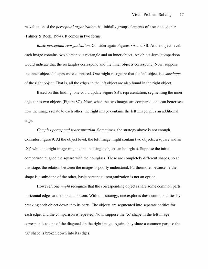
Basic perceptual reorganization. Consider again Figures 8A and 8B. At the object level,
each image contains two elements: a rectangle and an inner object. An object-level comparison
would indicate that the rectangles correspond and the inner objects correspond. Now, suppose
the inner objects’ shapes were compared. One might recognize that the left object is a subshape
of the right object. That is, all the edges in the left object are also found in the right object.
Based on this finding, one could update Figure 8B’s representation, segmenting the inner
object into two objects (Figure 8C). Now, when the two images are compared, one can better see
how the images relate to each other: the right image contains the left image, plus an additional
edge.
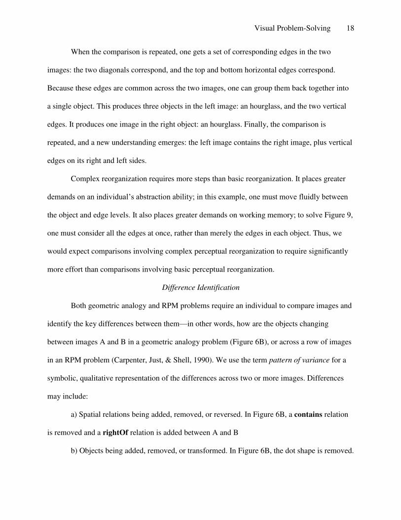
Complex perceptual reorganization. Sometimes, the strategy above is not enough.
Consider Figure 9. At the object level, the left image might contain two objects: a square and an
‘X;’ while the right image might contain a single object: an hourglass. Suppose the initial
comparison aligned the square with the hourglass. These are completely different shapes, so at
this stage, the relation between the images is poorly understood. Furthermore, because neither
shape is a subshape of the other, basic perceptual reorganization is not an option.
However, one might recognize that the corresponding objects share some common parts:
horizontal edges at the top and bottom. With this strategy, one explores these commonalities by
breaking each object down into its parts. The objects are segmented into separate entities for
each edge, and the comparison is repeated. Now, suppose the ‘X’ shape in the left image
corresponds to one of the diagonals in the right image. Again, they share a common part, so the
‘X’ shape is broken down into its edges.
Visual Problem-Solving 18
When the comparison is repeated, one gets a set of corresponding edges in the two
images: the two diagonals correspond, and the top and bottom horizontal edges correspond.
Because these edges are common across the two images, one can group them back together into
a single object. This produces three objects in the left image: an hourglass, and the two vertical
edges. It produces one image in the right object: an hourglass. Finally, the comparison is
repeated, and a new understanding emerges: the left image contains the right image, plus vertical
edges on its right and left sides.
Complex reorganization requires more steps than basic reorganization. It places greater
demands on an individual’s abstraction ability; in this example, one must move fluidly between
the object and edge levels. It also places greater demands on working memory; to solve Figure 9,
one must consider all the edges at once, rather than merely the edges in each object. Thus, we
would expect comparisons involving complex perceptual reorganization to require significantly
more effort than comparisons involving basic perceptual reorganization.
Difference Identification
Both geometric analogy and RPM problems require an individual to compare images and
identify the key differences between them—in other words, how are the objects changing
between images A and B in a geometric analogy problem (Figure 6B), or across a row of images
in an RPM problem (Carpenter, Just, & Shell, 1990). We use the term pattern of variance for a
symbolic, qualitative representation of the differences across two or more images. Differences
may include:
a) Spatial relations being added, removed, or reversed. In Figure 6B, a contains relation
is removed and a rightOf relation is added between A and B
b) Objects being added, removed, or transformed. In Figure 6B, the dot shape is removed.
Visual Problem-Solving 19
Top-down comparison provides an effective means for computing patterns of variance.
Analogical mapping identifies changes in the relational structure, or objects in one image that
have no corresponding object in another image. Shape comparison identifies transformations,
such as when an object rotates.
Patterns of variance may be reminiscent of transformational distance models of
similarity, where two stimuli are compared by computing the transformations between them
(e.g., Hahn, Chatter, & Richardson, 2003). However, they are distinct in that patterns of variance
are the result of the comparison, and not the actual mechanism of comparison.
Patterns of variance in RPM
RPM is unique among the tasks we’ve considered in that it requires computing patterns
of variance across rows of three objects. These patterns can be complex, and identifying the
correct pattern type is critical to solving the problems (Carpenter, Just, & Shell, 1990). We
propose that the patterns may be characterized via two binary parameters, resulting in four
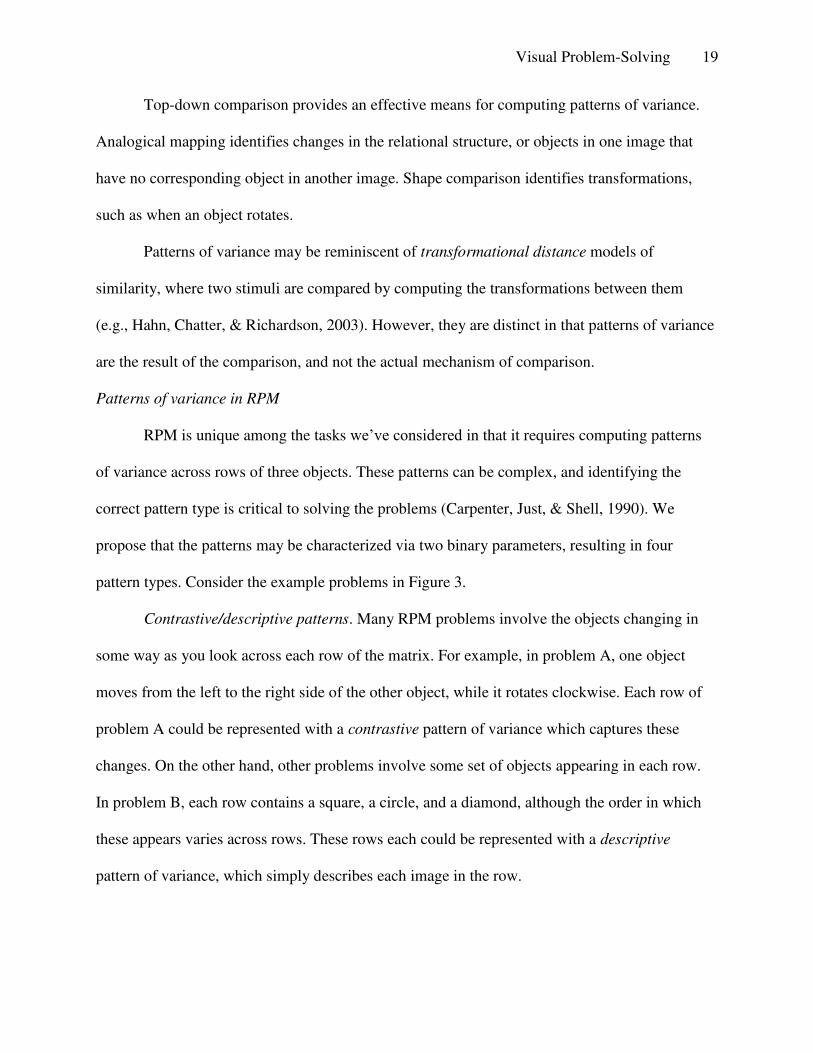
pattern types. Consider the example problems in Figure 3.
Contrastive/descriptive patterns. Many RPM problems involve the objects changing in
some way as you look across each row of the matrix. For example, in problem A, one object
moves from the left to the right side of the other object, while it rotates clockwise. Each row of
problem A could be represented with a contrastive pattern of variance which captures these
changes. On the other hand, other problems involve some set of objects appearing in each row.
In problem B, each row contains a square, a circle, and a diamond, although the order in which
these appears varies across rows. These rows each could be represented with a descriptive
pattern of variance, which simply describes each image in the row.
Visual Problem-Solving 20
While a descriptive pattern doesn’t explicitly describes differences, it is sensitive to them.
In the top row of problem B, there is an inner circle in each image. Because this circle does not
change across the images of the row, it is not included in the pattern of variance. Thus, the
pattern only describes the square, circle, and diamond shapes, which are the key information
needed to solve the problem.
Holistic/component patterns. Patterns may also be classified as holistic or component.
The examples given above are holistic patterns, where differences between entire images are
represented. In component patterns, images must be broken down into their component elements,
which are represented independently. For example, problem D requires a component descriptive
pattern which essentially says: “Each row contains a circle, a square, and a diamond.
Independently, each row also contains a group of squares, a horizontal line, and an ellipse.”
Which objects are paired together in the images will vary across rows, and so it can’t be a part of
the pattern.
A given matrix row can be represented using any of the four pattern types. Thus, to
determine if one has chosen the correct type, one must compare the patterns for the top and
middle rows. This can be done using the same analogical mapping process. If the patterns align,
this confirms that the rows are being represented correctly. If not, it will be necessary to
backtrack and represent the rows differently.
One open question is whether some pattern types are more difficult to represent than
others. In particular, as the patterns become more abstract and farther from the initial concrete
images, will they be processed less fluently (Kroger et al.)? Comparing contrastive and
descriptive patterns, contrastive patterns appear more abstract, as they describe the differences
between images, rather than the contents of each image. Comparing holistic and component
Visual Problem-Solving 21
patterns, component patterns appear more abstract, as they isolate each object from the image in
which it appeared. The simulation below presents an opportunities to compare these pattern types
and determine their relative difficulty.
Visual Inference
Finally, a set of differences can be applied to one image to infer a new image. Consider
our geometric analogy example (Figure 6B). First, images A and B are compared to compute a
pattern of variance between them, as described above. Next, images A and C are compared to
identify the corresponding objects. Finally, the A/B differences are applied to image C to infer
D’, a representation of the answer image. In this case, the dot is removed and the ‘Z’ shape is
moved to the left of the pie shape. Note that because this inference is performed on qualitative,
symbolic representations, the resulting D’ is another representation, not a concrete image. Thus,
the problem-solver can infer that the ‘Z’ shape should be on the left, but they may not know the
exact, quantitative locations of the objects.
Visual inference can also be performed on the patterns of variance in RPM. Consider
problem A (Figure 3). The pattern of variance for the top row indicates that one object moves to
the right while rotating clockwise. By comparing the images in the top and bottom rows, one can
determine that the arrow maps to the rectangle, while the circle maps to the trapezoid. Thus, one
infers that in the answer image, the rectangle should move to the right of the trapezoid and rotate
clockwise.
Note that the above strategy is not the only way to solve problem A. Alternatively, one
might use a second-order comparison strategy: 1) Compare images in the top row, compute a
pattern of variance. 2) For each possible answer, insert it into the bottom row and compute a
pattern of variance. 3) Compare the top row pattern to each bottom row pattern, and pick the
Visual Problem-Solving 22
answer that produces the closest fit. Later, we will use the model to explain why people might
use a visual inference strategy or a second-order comparison strategy.
Model
Our computational model builds on the above claims, in particular: 1) analogy drives
visual problem-solving, 2) hierarchical hybrid representations (HHRs) capture visual
information, and 3) problem-solving is a strategic search through the representation space. If
interested, the reader may download the computational model and run it on example problems A-
K2. The model possesses two key strengths:
1) The model is not strongly tied to Raven’s Matrices. It uses the Structure-Mapping
Engine, a general computational model of analogy, and it incorporates operations that have been
used to model other visual problem-solving tasks, including geometric analogy (Lovett &
Forbus, 2012) and the visual oddity task (Lovett & Forbus, 2011). Furthermore, the visual
representations used here are identical to those used in the geometric analogy model, and nearly
identical to those used in the oddity task model.3 Thus, this model allows us to test the generality
of our claims.
2) The model possesses multiple strategies for solving a problem. One strategy solves
the simpler, more visual problems found in the first section of the Standard Progressive Matrices
(SPM) test (e.g., problem I). The other two strategies, described in the next section, capture
alternative approaches for solving typical 3x3 problems. While including both strategies is not
necessary for solving the problems, it allows us to more fully model the range of human
problem-solving behavior.
2 http://www.qrg.northwestern.edu/software/cogsketch/CogSketch-v2023-ravens-64bit.zip
(Windows only) 3 The only difference from the oddity task model is the inclusion of an attribute describing the relative size of an
object. This attribute has been included in later versions of the oddity task model.
Visual Problem-Solving 23
This section is divided up as follows: 1) We provide an overview of how the model
solves problems, walking through several examples and covering the special cases where a 3x3
matrix is not used (example problems I, J, and K). 2) We summarize the existing systems on
which the model is built. 3) We describe the basic operations used to model RPM and other
visual problem-solving tasks. 4) We cover the strategic decisions the model must make during
problem-solving. As we shall see, the difficulty of a problem depends greatly on the outcome of
the strategic decisions, and thus they allow us to explore what makes a problem difficult and
what makes an individual an effective problem-solver.
Figure 10 illustrates the steps the model takes to solve 3x3 matrix problems. Each
problem is solved through a series of comparisons, first comparing the images in a row to
generate a pattern of variance that describes how the images are changing, then comparing the
patterns in the top two rows. Each of these comparisons requires a strategic search for the
representation that best facilitates the comparison. Finally, the model solves a problem using one
of two strategies: visual inference (step 5) or second-order comparison (step 6). Below, we walk
through the steps using problems A, D, and G as examples.
Step 1. The model automatically generates a representation for each image in the problem
(i.e., each cell of the matrix). The model generates the highest-level representation possible,
focusing on the big picture (e.g., groupings of objects), rather than the small details (edges within
each object). Each representation includes a list of objects and set of qualitative relations
between the objects, as well as qualitative features for each object. The set of qualitative
relations and features is known as a structural representation, and it allows two images to be
compared via structure-mapping.
Visual Problem-Solving 24
In problem A, the upper leftmost image representation would indicate that they are two
objects, one open and one closed. The closed object is rightOf the open object. The closed
object is curved and symmetrical (this is just a sampling of the representation). In problem D,
the three squares in the upper leftmost image would be grouped together based on similarity. The
representation would describe a group which is located above an object. In the problem G, the
representation would include two objects: an ellipse and an ‘X’ shape inside the ellipse.
Step 2. The adjacent images in the top row are compared via top-down comparison: first
the images are compared to identify corresponding objects, and then the corresponding objects
are compared to identify shape changes and transformations. The full set of differences is
encoded as a pattern of variance: a qualitative, symbolic representation of what is changing
between the images.
In problem A, the pattern indicates that an object moves from left of to within to right of
another object while rotating. In problem D, the pattern indicates that the objects are entirely
changing their shapes between each image. In problem G, the pattern, which matches the ellipse
shape to an hourglass shape to a simpler, squared-off hourglass shape, is largely unsatisfying.
However, the comparison indicates that corresponding objects have some parts in common (the
vertical and diagonal edges). Therefore, the model initiates complex perceptual reorganization,
breaking the objects down into their component edges. Grouping the corresponding edges back
up, it determines that each image contains the squared-off hourglass shape found in the rightmost
image. Thus, the change is that there are first two horizontal curves, then two vertical curves,
then neither, while the squared-off hourglass remains the same.
Step 3. The same steps are performed for the middle row.
Visual Problem-Solving 25
Step 4. The patterns of variance for the top two rows are compared via structure-mapping.
A generalized pattern consisting of the common elements to both rows is generated.
In problem A, the rows are a perfect match: they both contain an object moving to the
right and rotating. Similarly, in problem G they both contain two horizontal curves, then two
vertical curves, then neither. In problem D, however, there is a bad match: in the top row, there
is a change from circle to square, whereas in the middle row there is a change from diamond to
circle (as described below, the model does not know terms like “square,” but it is able to
distinguish different shapes). Thus, the model must search through the range of possible
representations for a pattern of variance.
The typical representation is a holistic contrastive representation, which represents the
changes between each image. Here, the model gets better results with a component descriptive
representation. It is descriptive in that it describes what it sees, rather than describing changes.
For example, in the top row, it sees a circle, so it expects to find a circle somewhere in the
middle row. It is component in that it does not group objects together in images. The circle and
the group of square are in the same image in the top row, but it does not expect to find them in
the same image in the next row. Essentially, the representation says that in each row there is a
circle, a square, and a diamond; and also a group, a horizontal edge, and an ellipse. Using this
representation, the model finds a perfect fit between the rows.
Step 5. When possible, the model attempts to solve problems via visual inference. It
projects the differences to the bottom row and infers the answer image. This first requires
finding correspondences between the bottom row objects and objects in a row above, again using
structure-mapping.
Visual Problem-Solving 26
In problem A, the trapezoid and rectangle in the bottom row correspond to the circle and
arrow in the top row4 (based on corresponding relational structure). The model infers that in the
missing image, the rectangle should be to the right of the trapezoid, and it should be rotated 90°
from its orientation in the middle image. In problem B, the objects in the bottom row correspond
to the objects in the top row. The missing objects are a circle and a horizontal edge, so the model
infers that the answer should contain these objects.
In problem G, the inference fails. The model required all three images to perform
complex perceptual reorganization on the above rows, suggesting that all three images will be
needed for a similar perceptual reorganization on the bottom row. Without knowing the third
image in the bottom row, the model abandons the visual inference strategy. Another approach
must be used to solve for the answer.
Step 6. When visual inference fails, the model falls back on a simpler strategy: second-
order comparison. It iterates over the list of answers and plugs each answer into the bottom row,
computing the bottom row’s pattern of variance. It selects the answer whose associated pattern
best matches the generalized pattern for the above rows.
In problem G, the model selects answer 4 because when the ‘X’ is plugged into the
bottom row, it produces a similar pattern of two horizontal curves, then two vertical curves, then
neither.
The visual inference and second-order comparison approaches map onto classic strategies
for analogical problem-solving. Psychologists and modelers studying geometric analogy (“A is
to B as C is to…?”) have argued over whether people solve directly for the answer (Sternberg,
1977; Schwering et al., 2009) or evaluate each possible answer (Evans, 1968; Mulholland,
4 Either the top or middle row can be compared to the incomplete bottom row. The model actually uses
whichever is closest to the bottom row, in terms of number of elements per image.
Visual Problem-Solving 27
Pellegrino, & Glaser, 1980), with some (Bethell-Fox, Lohman, & Snow, 1984) suggesting that
we adjust our strategy depending on the problem. We previously showed how a geometric
analogy model incorporating both strategies could better explain human response times (Lovett
& Forbus, 2012).
Here, we model both strategies not because both are required—the Carpenter model used
visual inference exclusively, while our own model could use second-order comparison
exclusively without a drop in performance. Rather, we hope to better explain human
performance by incorporating a greater range of behavior. Following our geometric analogy
model, this model attempts to solve for answers directly via visual inference. When this fails, it
reverts to second-order comparison. In our analysis, we consider whether people have greater
difficulty on the problems where this happens.
Solving 2x2 Matrices
The Standard Progressive Matrices (SPM) includes simpler 2x2 matrices (e.g., problem
K) which lack a middle row. Because there is no way to evaluate the top row representation, the
model simply assumes that a contrastive representation is appropriate, skipping steps 2 and 3
above. Problem-solving is otherwise the same.
Solving Non-Matrix Problems
In addition to visual inference and second-order comparison, the model utilizes a texture
completion strategy for solving more basic problems which are not framed in a matrix (e.g.,
problem I). Because texture detection is a low-level perceptual operation that does not
distinguish objects and their relations (Julesz, 1984; Nothdurft, 1991), this strategy does not rely
on qualitative structure. Instead, it operates directly on the concrete image, in the form of a
bitmap. It scans across the top half of the image, looking for a repeating pattern (Figure 11A). It
Visual Problem-Solving 28
then scans across the bottom half, inserting each possible answer into the missing portion of the
image. If one answer produces a pattern that repeats at a similar frequency, that answer is
selected.
Some section A problems are more complex (problem J). If texture completion fails, the
model turns the image into a 2x2 matrix. It does this by carving out three other pieces of the
image (Figure 11B), such that the missing piece will be the bottom right cell in the matrix. Now,
the problem can be solved in the way other 2x2 and 3x3 matrices are solved.
Existing Systems
The model builds on two pre-existing systems: the CogSketch sketch understanding
system (Forbus et al., 2011), and the Structure-Mapping Engine (SME) (Falkenhainer, Forbus, &
Gentner, 1989). CogSketch is used to process the input stimuli, generating visual representations
for problem-solving. SME plays a ubiquitous role in the model, performing comparisons
between shapes, images, and patterns of variance. The systems are briefly described below.
CogSketch
CogSketch is an open-domain sketch understanding system. It automatically encodes the
qualitative spatial relations between objects in a 2-D sketch. To produce a sketch, a user can
either a) draw the objects by hand; or b) import 2-D shapes from PowerPoint. Importing from
PowerPoint is useful for cognitive modeling because psychological stimuli can be recreated as
PowerPoint slides, if they are not in that form already.
CogSketch does not fully model visual perception. It depends on the user to manually
segment a sketch into separate objects, essentially telling the system where one object stops and
the next begins (as described below, the model can automatically make changes to the user’s
segmentation when necessary). Given this information, CogSketch computes several qualitative
Visual Problem-Solving 29
spatial relations, including topology (e.g., one object contains another, or two objects intersect)
and relative position. The relations are a basic model of the features a person might perceive in
the sketch. In this work, we use CogSketch to simplify perception and problem-solving in three
ways:
1. Each RPM problem is initially manually segmented into separate objects. Problems are
recreated in PowerPoint, drawing one PowerPoint shape for each object5, and then imported into
CogSketch. The experimenters attempt to segment each image into objects consistently, based on
the Gestalt grouping rules of closure and good continuation (Wertheimer, 1938), i.e., preferring
closed shapes and longer straight lines. We note that the system may revise this segmentation
based on its automatic grouping processes, and based upon perceptual reorganization.
2. For non-matrix problems (e.g., problems I-J), the large, upper rectangle is given the
label “Problem” within CogSketch. The smaller shape within this rectangle that surrounds the
missing piece is given the label “Answer.” The model uses this information to locate these
objects during problem-solving.
3. Each RPM problem is segmented into separate images (i.e., the cells of the matrix and
the list of possible answers) using sketch-lattices. A sketch-lattice is an NxN grid that can be
overlaid on a sketch. Each cell of the grid is treated as a separate image, for the purposes of
computing image representations. Sketch-lattices can be used to locate particular images (e.g.,
the upper leftmost image in the top sketch-lattice). RPM problems require two sketch-lattices:
one for the problem matrix, and one for the list of possible answers.
CogSketch’s objects are the starting point for our model’s perceptual processing. The
model automatically forms higher-level representations by grouping objects together and lower-
5 Some objects cannot be drawn as a single shape, due to PowerPoint’s limitations. These are drawn as multiple
shapes, imported into CogSketch, and then joined together using CogSketch’s merge function.
Visual Problem-Solving 30
level representations by segmenting objects into their edges. It supplements CogSketch’s initial
spatial relations to form a complete HHR for each image.
Structure-Mapping Engine (SME)
SME is a computational model of comparison based on structure-mapping theory. It
operates on structured representations organized as predicate calculus statements (e.g., (rightOf
Object-A Object-B)). Given two representations, it aligns their common structure to compute a
mapping between them. A mapping consists of: 1) a set of correspondences, 2) a similarity
score, and 3) candidate inferences based on carrying over unmatched structure. For this work, we
used a normalized similarity score, ranging from 0 to 1. Note that SME is domain-general—it
operates on visual representations as easily as more abstract conceptual representations.
One important feature in SME is the ability to specify match constraints, rules that affect
what can be matched with what. For example, a user may specify that entities with a particular
attribute can only match with other entities that share that attribute. In the visual domain, one can
imagine a variety of possible match constraints (only allow objects with the same color, or size,
or shape to match, etc). To support creative reasoning and comparison, our model uses no match
constraints in its initial comparisons. As described below, it dynamically adds constraints when
necessary as part of the problem-solving process.
Model Operations
The RPM model builds on a set of operations which have previously been used to solve
other visual problem-solving tasks. Figure 12 illustrates the operations used at each step in the
process (compare with Figure 10). Below, we describe each operation, including its input, its
output, and any additional options available when performing the operation (e.g., the option of
Visual Problem-Solving 31
representing either a contrastive or descriptive pattern of variance). In the following section, we
will discuss the key strategic decisions made regarding these options at each step.
See the Appendix for additional details on how each operation is implemented.
Encode
Given an image, this produces a qualitative, structural representation at a particular level
in the spatial hierarchy (Edges, Objects, or Groups). The representation contains a list of
elements and a list of symbolic expressions. For example, an object-level representation would
list the objects in an image and include relations like (rightOf Object-A Object-B). An edge-
level representation would list the edges in an object and include relations like (parallel Edge-A
Edge-B). A group-level representation would include any groups that could be formed (e.g., a
row of identical shapes could be grouped together) but otherwise be identical to the object level.
Note that objects may include closed shapes (e.g., a circle), open shapes (e.g., an ‘X’), texture
patches (a grouping of parallel edges), and negative space. See the Appendix for more details.
Additional Options. The level of the desired representation (Edges, Objects, or Groups)
can be specified. Note that the RPM model, in keeping with HHRs, begins by representing at the
highest level, Groups, because representations are sparser and easier to compare at this level.
Compare Shapes
This operation takes two elements and computes a transformation between them by
comparing their parts—that is, it compares the edges in two objects or the objects in two groups.
Like the other comparison operations (see below), it compares qualitative, structural
representations using SME.
Compare Shapes can produce shape transformations, shape deformations, and group
transformations. The shape transformations are rotations, reflections, and changes in scale. The
Visual Problem-Solving 32
shape deformations are lengthening, where two edges along a central axis grow longer (Figure
13A); part-lengthening, where two edges along a part of the object grow longer (13B); part-
addition, where a new part is added to the object (13C), and the subshape deformation, where
two objects are identical, except that one has extra edges (used to trigger basic perceptual
reorganization, as in Figure 8).
The group transformations are identical groups, larger group (similar to subshape where
two groups are identical except that one has more objects), different groups (where groups have
different arrangements of the same objects), and object to group (where a single object maps to a
group of similar objects). As with subshape, the larger group and object to group
transformations may serve as triggers for basic perceptual reorganization.
Recognize Shape
This operation assigns a shape category label to an object. While the model has no pre-
existing knowledge of shape types (e.g., “square”), it can learn categories for the shapes found
within a particular problem. Shapes are grouped into the same category if there is a valid
transformation between them (scaling + rotation or reflection). When a new element is
encountered, it is recognized by comparing it to an exemplar from each shape category. If it does
not match any category, a new category is created.
Objects may be assigned arbitrary labels for their shape categories, which apply only in a
particular problem context (e.g., all squares might be assigned the category “Type-1” within the
context of solving a problem).
Compare Images
Given two image representations, Compare Images performs top-down comparison.
First, it compares the image representations with SME to find the corresponding groups or
Visual Problem-Solving 33
objects. Then, it calls Compare Shapes on those corresponding elements, in order to compute
any shape transformations. It returns: a) a similarity score for the two images, computed by
SME but modified based on whether corresponding elements are the same shape; b) a set of
corresponding elements; c) a set of commonalities, based on those parts of the representations
that aligned during the SME mapping; d) a set of differences.
There are three types of differences: 1) changes in the relational structure, found by SME,
e.g., a change from (above Object-A Object-B) to (rightOf Object-A Object-B); 2) additions or
removals of elements between the images (i.e., when an object is present in one image but absent
in the next); 3) shape transformations between the images (see Compare Shapes above for a list
of possible shape transformations). In some cases, an object may change shape entirely, as when
a square maps to a circle. In this case, the transformation is encoded as a change between the two
shapes’ category labels.
Find Differences
This operation compares a sequence of images, using Compare Images, and produces a
pattern of variance, a structural representation of the differences between them (see the previous
section for a list of possible difference types). For example, suppose Find Differences was called
on the top row in problem A. It would compare adjacent images (the left and middle images, and
the middle and right images), identifying the corresponding objects. Here, the circle shapes
correspond and the arrow shapes correspond. It would then encode the changes between
adjacent images, using the differences from Compare Images. Between the first two images, the
circle shape changes from being right of the arrow to containing the arrow. Also, the arrow
rotates 90°. Between the next two images, the arrow moves to the right of the circle and rotates
again.
Visual Problem-Solving 34
Additional Options. As discussed above, much of the strategy in RPM relates to rows of
images: how they should be compared, and how their differences should be represented. Find
Differences supports several strategic choices regarding how images are compared:
1) Basic perceptual reorganization can be triggered, based on one object (or group) being
a subshape of another. For the top row of problem E, the middle object is a subshape of the right
object, so the right object can be segmented into objects, one identical to the middle object and
one identical to the left object.
2) Complex perceptual reorganization can be triggered, based on two objects (or groups)
sharing common parts. This is used in problem G.
3) First-to-last comparison can be performed. That is, the first and last images can be
compared, even though they are not adjacent. For the top row in problem H, this allows one to
see that the curved edge in the left image matches the curved edge in the right image.
4) Strict shape matching can be enforced for some or all shape categories. This means the
SME mapping is constrained to only allow identically-shaped objects to match each other. This
is paired with first-to-last comparison. In problem H, it would ensure that the curved edge in the
left image doesn’t map to anything in the middle image. Thus, Find Differences would determine
that there is an object present in the first and last image, but not the middle image.
Find Differences also supports two strategic decisions for how a row’s pattern of variance
is represented, once it has been computed.
1) A pattern can be contrastive or descriptive. A contrastive pattern represents the
differences between each adjacent pair of images, while a description pattern describes each
image, abstracting out features that are common across the images. Shape labels from Recognize
Visual Problem-Solving 35
Shape are used to capture information such as “This row contains a square, a circle, and a
diamond.”
2) A pattern can be holistic or component. A holistic pattern represents the row in terms
of images, including what changes between images (contrastive) or what is present in each image
(descriptive). Alternatively, a component pattern ignores the overall images and represents how
each individual object changes (contrastive) or what objects are present in the row (descriptive).
If every image contains only a single object, then a component descriptive pattern breaks
the objects down into their features and represents those separately. In problem C, each row
contains a parallelogram, a circle, and a triangle; and a black object, a white object, and a gray
object.
A component pattern of variance is the most abstract kind, since it abstracts out the image
itself. Two things necessarily following from this: 1) ordering is not constrained, as there are no
images to order; 2) spatial relations are not represented, as objects are no longer tied together in
an image.
Generalize
Like Find Differences, this operation compares two or more items via SME. However,
instead of encoding the differences, it encodes the commonalities, i.e., the attributes and relations
that successfully align. It returns: a) a similarity score, computed by SME, and b) a new
representation, containing the commonalities in the compared representation, i.e., the expressions
that successfully aligned.
Infer Shape
This operation applies a shape transformation to an object to produce a novel object. It
provides a way of solving geometric analogy problems (“A is to B as C is to…?”) wherein we
Visual Problem-Solving 36
have a transformation between A and B, and we want to apply it to C to infer D. For example, in
Figure 14A we have a reflection over the x-axis between shapes A and B. Applying this to shape
C produces D. Suppose instead we have Figure 14B, where this is no transformation between A
and B. Normally, if there is no transformation, the operation cannot complete. However, in this
case the operation exploits a feature of analogy problems: “A is to B as C is to D” is equivalent
to “A is to C as B is to D” (Grudin, 1980). If there is no valid transformation between A and B,
the operation checks for a transformation between A and C.
Infer Shape also makes changes to an object’s color or texture. For example, suppose
that in the A->B comparison, the fill color is changed, or a texture gets added or removed. The
operation will similarly change the fill or texture of C to produce D.
Infer Shape also works on shape deformations (see the Appendix).
Infer Image
This operation applies a complete row’s pattern of variance to an incomplete row to infer
the missing image. It produces a qualitative, structural image representation, along with a list of
the elements (objects and groups) in the image. This information is sufficient to support top-
down comparison between the inferred image and existing images to select the best answer.
Infer Image works in two steps: 1) Compare the complete row to the incomplete row,
identifying the corresponding elements. 2) Apply the differences from the complete row to the
corresponding elements in the incomplete row, inferring the missing image. For example,
consider problem A. The operation compares the top row to the bottom row (after computing a
pattern of variance for each). The circle maps to the trapezoid and the arrow maps to the
rectangle because in each case the smaller shape rotates and moves inside the larger shape. The
Visual Problem-Solving 37
model takes the differences between the top row’s second and third images and applies them to
the bottom row, inferring that the rectangle should rotate and be to the right of the trapezoid.
There are two ways that Infer Image can fail. Firstly, it may be unable to apply a shape
transformation. For example, there might be a part removal deformation, but the target object
might lack extra parts to be removed. Secondly, the operation may find that there is insufficient
information to compute the incomplete bottom row’s pattern of variance. This happens on
problems involving perceptual reorganization (e.g., problem G). Here, the model sees that in the
top row, the first and second images were both reorganized, suggesting that information from the
third image was necessary to reorganize them. Because there is no third image in the bottom
row, the model does not attempt to complete the operation.
Detect Texture
This operation implements the texture completion strategy for non-matrix problems (e.g.,
problem I). Unlike the other operations, it does not use HHRs—instead, it prints every object in
an image to a bitmap and operates directly on that bitmap. Given an image, and the location of a
corridor along that image (e.g., the gray rectangles in Figure 11A), it scans along the corridor,
looking for a repeating pattern.
Additional Options.
1) Detect Texture can be directed to insert a second image into the first image at a certain
point. For example, it can insert one of the answer images into the hole (the object labeled
“Answer”) and evaluate how well that completes the texture.
2) Detect Textures can be directed to only consider textures at a particular frequency.
After finding a repeating texture at a particular frequency on the top part of Figure 11A, it can be
directed to seek out an answer that produces a texture at the same frequency in the bottom part.
Visual Problem-Solving 38
Strategic Decisions
We now consider the strategic decisions made at each step in the problem-solving
process.
1. Encoding each image
As described above, images are always encoded at the highest level possible, Groups,
meaning similar objects are grouped together. This ensures a sparse, simple representation for
problem-solving.
2, 3. Computing a pattern of variance for each row
If there are fewer differences between images, then patterns of variance will be more
concise, and thus easier to store in memory. Thus, when computing a row’s pattern of variance,
the model tries to minimize differences between corresponding objects. It attempts to meet the
following constraints:
A) Identicality: It’s always best if corresponding objects are identical.
B) Relatability: If corresponding objects aren’t identical, there should be at least some
valid transformation or deformation between them.
C) Correspondence: Whenever possible, an object in one image should at least
correspond to something in another.
If relatability is violated, the pattern of variance must describe a total shape change. If
correspondence is violated, the pattern must describe an object addition. It is assumed that either
of these makes the pattern more complex and more difficult to store in memory. Below, we refer
to violations of relatability or correspondence as bad shape matches.
Figure 15 describes how the model pursues the above constraints. Essentially, the model
calls the Find Differences operation repeatedly. Each call produces a pattern of variance for the
Visual Problem-Solving 39
row. The model evaluates the results, and if certain conditions (specified in the figure) are met, it
calls an updated Find Differences operation, specifying changes to the way images are
represented or compared.
Step I (in Figure 15) is the initial call to Find Differences. Steps II and III support basic
and complex perceptual reorganization. Basic perceptual reorganization is helpful for problem
E, a figure addition problem. Because the second image in each row is a subshape of the third
image, the third image is segmented into two objects. These objects are identical to the first and
second image, allowing the model to detect figure addition.
Complex perceptual reorganization is helpful for problem G. Consider the top row. In
the initial pattern of variance (step I), the corresponding objects are all different shapes. Because
they contain similar edges, they are broken down into their edges (step III), with each edge
treated as a separate object.
Step IV checks whether there are matching objects in the first and last images of a row.
Note that Find Differences only performs this check when there are bad object matches in the
first or last image. If there are, it compares the first and last images and checks whether this
places any such bad objects into correspondence with identical objects.
In the second row of problem H, the curved edges are bad object matches—neither aligns
with a similar shape in the middle image. Therefore, the first and last images are compared, and
the model discovers that the curved edges match perfectly. This triggers step IV, in which the
first and last images in the row are compared as part of the pattern of variance. At this step, the
model further requires that curved edges can only match to other objects with identical shapes.
This can be specified via an SME matching constraint. It ensures that the circle in the second
Visual Problem-Solving 40
image won’t match the curved edge in the first image. Thus, in the resulting pattern of variance,
we find that the curved edge is present in only the first and last images.
Note that step IV also applies to problem E. Here, each row’s third image contains a
leftover object. When the third and first images are compared, the model discovers a perfect
match to this leftover object. Thus, it finds that the third image contains both the objects found
in the previous two images.
Step V implements the second half of complex perceptual reorganization: objects with
the same correspondence pattern are grouped back together. In the top row of problem G, the
edges forming the squared-off horizontal hourglass shape are found in all three images. Thus,
these are grouped together to form a single object in each image. Similarly, in the second row,
the edges forming the squared-off vertical hourglass are grouped together. Now each row
contains one object that stays the same, along with the following changes: the first image has two
vertical edges, the second image has two horizontal edges, and the third image has neither.
Step VI contains an additional heuristic for improving patterns of variance. If there are
mismatched objects (violating relatability) and SME has found a lower-scoring, alternative
image mapping that places better-matched objects into correspondence, the model switches to
the alternative mapping.
Step VII finalizes the first-to-last comparison strategy. If this strategy was previously
implemented in step IV, the model now requires that every object only match to other identical
objects (i.e., objects with the same shape type). This makes the conservative assumption that if
we are dealing with complex correspondences (between the first and last images), we will not
also be dealing with shape transformations (where non-identical shapes correspond). While this
Visual Problem-Solving 41
is the correct approach for the Standard Progressive Matrices test, future tests may challenge this
assumption.
4. Comparing the patterns of variance for the top two rows
There are multiple ways to represent variance across a row of images. Carpenter et al.’s
model has five rule types for describing variation. In contrast, the present model makes two
strategic decisions when representing each row’s pattern of variance. It evaluates these decisions
by comparing the top two rows’ patterns. If the patterns are highly similar, this indicates that the
same differences have been detected in each row. If the patterns are not similar, this suggests
that the rows are being represented incorrectly.
Recall that the decisions are descriptive/contrastive and holistic/component. A
contrastive type represents the differences between images, while a descriptive type describes
what is found in each image. A holistic type represents how images vary, while a component
type represents how objects vary, independent of the image in which they are found.
The model iterates over the strategies in the following order: holistic contrastive, holistic
descriptive, component descriptive, component contrastive. It evaluates each strategy by
building a pattern of variance for the two rows and comparing them. It stops once a strategy is
sufficient. If no strategy is sufficient, it picks the highest-scoring valid strategy. The criteria for
sufficiency and validity depend on the strategy:
Holistic Contrastive: This default strategy is always valid. It is sufficient if the
similarity of the two rows, as computed by SME, is above a threshold. For our simulation, we
use a threshold of 0.80, where 1.0 would indicate a perfect match. However, a sensitivity
analysis found that this threshold could vary from .67 to .87 and the results would be the same,
Visual Problem-Solving 42
both for the simulation reported here and for our geometric analogy simulation (Lovett &
Forbus, 2012).
Holistic Descriptive: This is the most concrete approach, since it represents what holds
in each image, rather than differences between images. No leeway is allowed in the comparison.
The strategy is valid and sufficient only if there are no differences detected between the rows.
Component: It is easy for component patterns of variance to appear similar—because
spatial relations are abstracted out, only object attributes and transformations must align to
produce a perfect match. Further restrictions must be applied, or component patterns will often
override other, more informative patterns. Thus, they are restricted to only being valid when
they produce an otherwise impossible mapping, e.g., one where two top-row objects in the same
image map to two middle-row objects in different images.
5/6. Solving via visual inference or second-order comparison
After computing a generalized pattern of variance from the top two rows, the model
applies the pattern to the bottom row to infer an answer image representation. First, the model
builds a pattern of variance for the first two images in the bottom row. It applies any strategic
shifts made on the first two rows, e.g., component vs. descriptive patterns, holistic vs. component
patterns, or constraining matches to only be between identical shapes. Next, it generates the
answer representation using the Infer Image operation (described above). Infer Image may fail
if:
1. A shape transformation cannot be applied.
2) There is insufficient information for perceptual reorganization.
Visual Problem-Solving 43
If visual inference succeeds, the model takes the inferred image representation and finds
the best match among the answers. When the model compares the inferred image to a possible
answer image, it can again use perceptual reorganization to improve the match.
If visual inference fails, the model reverts to second-order comparison. It iterates over
the answers. For each answer, it inserts it into the bottom row and computes a pattern of
variance, again using the strategic decisions from the top two rows. It compares each answer’s
pattern of variance to the generalized pattern from the above rows. The answer producing the
most similar pattern is chosen.
Evaluation
The model was evaluated on the 60-item Standard Progressive Matrices (SPM) test. The
test problems were recreated in PowerPoint and imported into the CogSketch sketch
understanding system, as described above.
We also gathered human performance data, for comparison. SPM has been studied
extensively in the past. However, we built a computerized version of the test, allowing access to
data not typically available from paper versions, such as response times and answers test-takers
considered before making their final answer.
In conducting this evaluation, our goal was to explore the representations, processes, and
strategic shifts made by the model—to what extent are they sufficient for performing at a human
level, and to what extent are they useful in explaining why a problem is easy or difficult for
humans. For example, is a problem more difficult if it requires complex perceptual
reorganization? Our goal was not to test the particular order in which the model performs
operations and makes strategic decisions. We suspect humans vary a great deal in the order in
which they perform operations.
Visual Problem-Solving 44
For example, in studying a related geometric analogy task, Bethell-Fox, Lohman, and
Snow (1984) found that higher-performing individuals preferred to solve directly for the answer
(similar to our model’s visual inference strategy), while others were more likely to try out each
possible answer (similar to our model’s second-order comparison strategy). In contrast, our
model always attempts visual inference first. While our approach offers the possibility of
explaining individual differences through separate models that match different population groups
(Lovett & Forbus, 2011a), we view this as future work for the present domain.
Below, we describe the behavioral study. We then present the model simulation.
Behavioral Study
The SPM consists of five 12-problem sections. Section A uses 1x1 matrices, section B
uses 2x2 matrices, and the remaining sections use 3x3 matrices. Only the 3x3 matrices were
used in the behavioral study, as our emphasis is on explaining how people solve these more
difficult problems. It is possible that participants would do worse on these problems without
having first solved the easier 2x2 matrices. Therefore, participants were given two 2x2 matrices
for practice.
Methods
Participants. The test was administered to 42 Northwestern University students. There
were 16 males and 26 females. All students ranged from 18 to 22 years old, with a mean age of
18.8 and a median age of 18.
Materials. The experiment was run in CogSketch. CogSketch has a built-in harness to
support behavioral experiments. Within CogSketch, participants viewed scanned-in images of
each SPM problem, including the list of possible answers. When they clicked on an answer, a
Visual Problem-Solving 45
square appeared around that answer. However, participants were still free to consider the chosen
answer and potentially change their mind.6
Overall, the test used the 36 3x3 problems from SPM sections C-E, as well as two 2x2
problems from SPM section B: B3 and B9. The problems from section B were used for practice.
We included an early B section problem and a later B section problem to provide greater range,
as problems are designed to get progressively more difficult within each section.
Procedure. Participants began with a brief training period. Instructions within
CogSketch described how matrix problems work and told participants that they had up to an hour
to finish the problems, but that they might finish in less time. Participants solved two 2x2
matrices from section B of the SPM (B3 and B9). Participants were given feedback after each
response.
Participants then answered 36 problems, sections C-E of the test, in order. Participants
answered each problem by clicking on their chosen answer, causing a square to appear around it,
and then hitting the “Next” button. CogSketch recorded their final answer for each question, as
well as any previously selected answers. Timing information was also recorded. After each
question, participants were given the option of taking a break and told to hit “Next” when they
were ready to continue.
Results
Two participants were removed from the analysis because they fell more than two
standard deviations below the mean. Among the remaining 40 participants, the mean
performance was 30.0/36. Splitting by sections, the mean scores were:
Section C: 10.9/12
6 This addresses a request by Raven, Raven, and Court (2000b), who asked that any computerized version of the
test allow participants to view their chosen answer before committing to it.
Visual Problem-Solving 46
Section D: 10.7/12
Section E: 8.5/12
An individual with these scores would typically score a perfect 12/12 on the two easier
sections (Raven, Raven, & Court, 2000b, Table SPM2), resulting in an overall 54/60. This score
is in the 61st percentile for American adults, according to the 1993 norms (Table SPM13).
The mean response time (considering only correct responses) was 21.1 s, and the median
(by item) was 15.9 s. Across the 36 problems, there was a remarkably high correlation between
mean accuracy and mean response time (r = -.89). Thus, participants were more likely to fail on
problems that took longer to solve.
Discussion
The participants performed above average, according to the 1993 US norms. However,
these norms are fairly old, and RPM scores are known to increase in a population over time
(Raven, Raven, & Court, 2000b). Thus it may be helpful to consider more recent data. In 2000,
a large-scale examination of Estonians found that 18-year-olds averaged 29.6/36 on the same
sections (Lynn, Allik, & Irwing, 2000). In addition to achieving the same mean score, the
Estonians showed similar error rates across the 36 problems (r = .96, comparing the percentage
of correct responses on each problem).
It may be surprising that students at a major university would perform the same as
average 18-year-olds. However, there are at least two reasons the Northwestern students’ scores
might be deflated: 1) They were taking a computerized version of the test, or 2) They were
taking the test as a psychological experiment, rather than as an intelligence test. Previous studies
(Williams & McCord, 2006; Arce-Ferrer & Guzmán, 2009) have suggested that results are
comparable on computerized and paper versions of RPM. Therefore, we suspect the students
Visual Problem-Solving 47
were less motivated because they saw the test as a psychological experiment rather than an
intelligence test. The data on each problem’s relative difficulty should still be valid, given the
high correlation between Northwestern and Estonian error rates.
Simulation
We ran the computational model on the full, 60-problem SPM test. Each problem was
recreated as accurately as possible, with two exceptions: 1) On one problem dashed lines were
replaced with gray-colored lines. Presently, CogSketch lacks the perceptual ability to recognize
dashed lines. 2) The final problem (E12) proved difficult to reconstruct, and it requires a strategy
outside the bounds of this model (or any other model we know of): computing an arithmetic
equation to relate the number of object parts in each image. Thus, it was counted as an incorrect
response and left out of further testing. As described above, CogSketch requires that the user
manually segment each image into separate objects, although the model can then perform
grouping and segmentation operations.
Given the problems, the model automatically constructed image representations using the
Encode operation. Encode generated the exact same representations as in our geometric analogy
model (Lovett & Forbus, 2012) and nearly the same as in our oddity task model7 (Lovett &
Forbus, 2011a). Thus, we can evaluate the generality of our encoding scheme. Note that the
initial representations produced by Encode were updated and modified during perceptual
reorganization.
7 As previously mentioned, the published oddity task model contained one change to its representations: it did
not represent object size attributes. However, we have developed an unpublished version of the model that includes
the size attributes and produces comparable results.
Visual Problem-Solving 48
Results & Analysis
In analyzing the model’s performance, three questions were asked: 1) How many
problems can the model solve on each test section? If the model performs as well as human
adults, this indicates the model’s representations and processes are sufficient for the task. 2) Are
the problems that are hard for the model also difficult for humans? If the model’s error patterns
match human patterns, this further suggests that the model’s representations and processes are
similar to those of humans. 3) Can the model help explain what determines a problem’s
difficulty? To evaluate the model’s explanation ability, each problem was coded for whether it
required certain model operations, and for its working memory load. A multiple linear
regression determined whether these factors explained human performance.
Sufficiency. The model solved 56/60 problems, placing it in the 75th percentile for
American adults, by the 1993 norms. This also placed it above the college-age participants,
whose performance translated to a 54/60. Thus, the model appears at least as effective as the
average adult.
Among the 56 solved problems, the strategy breakdown is as follows:
Texture Completion: 4
Visual Inference: 43
Second-Order Comparison: 9
The model solved most problems using visual inference. Only nine problems required
reverting to second-order comparison. Note that four of these are from section A, the 1x1
matrices. Section A problems are conceptually easy, but they sometimes present perceptual
problems for the model. In most cases, the model fell back on second-order comparison because
of an error in its shape or image representations.
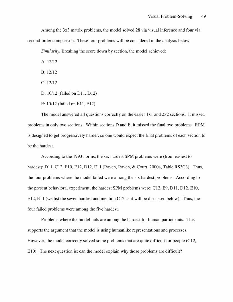
Visual Problem-Solving 49
Among the 3x3 matrix problems, the model solved 28 via visual inference and four via
second-order comparison. These four problems will be considered in the analysis below.
Similarity. Breaking the score down by section, the model achieved:
A: 12/12
B: 12/12
C: 12/12
D: 10/12 (failed on D11, D12)
E: 10/12 (failed on E11, E12)
The model answered all questions correctly on the easier 1x1 and 2x2 sections. It missed
problems in only two sections. Within sections D and E, it missed the final two problems. RPM
is designed to get progressively harder, so one would expect the final problems of each section to
be the hardest.
According to the 1993 norms, the six hardest SPM problems were (from easiest to
hardest): D11, C12, E10, E12, D12, E11 (Raven, Raven, & Court, 2000a, Table RS3C3). Thus,
the four problems where the model failed were among the six hardest problems. According to
the present behavioral experiment, the hardest SPM problems were: C12, E9, D11, D12, E10,
E12, E11 (we list the seven hardest and mention C12 as it will be discussed below). Thus, the
four failed problems were among the five hardest.
Problems where the model fails are among the hardest for human participants. This
supports the argument that the model is using humanlike representations and processes.
However, the model correctly solved some problems that are quite difficult for people (C12,
E10). The next question is: can the model explain why those problems are difficult?
Visual Problem-Solving 50
Explanation. We begin by discussing C12, an anomalous problem that is surprisingly
difficult for people. We then present a series of linear models that converge on an explanation
for problem difficulty in RPM.
Problem C12 (see Figure 16 for an analogous problem) is one of the most difficult for
human test-takers. This is surprising because it is in one of the easier sections (C is the first to
use 3x3 matrices), and there is nothing obviously difficult about it. The model solves it using the
default strategy (a holistic contrastive pattern of variance, without comparing the first and last
images). What makes this problem so challenging for humans?
van der Ven and Ellis (2000) have suggested some C problems are difficult due to a
conflict between the perceptual appearance of the problem images and the answer images. For
example, in C12, the first two rows show an object becoming longer. In the bottom row, and
only in the bottom row, becoming longer causes the object to overlap another object. Thus, the
answer contains a unique perceptual feature: overlapping objects (Figure 16, answer 5).
The model confirms this conflict in perceptual appearance for C12. Overall, the model
solves 28 of the 3x3 matrices via visual inference. For 24 problems, the model infers an answer
identical to the answer image. For the other four, the inferred answer is non-identical. On C12,
the model fails to infer an overlapping relation between the two texture patches, so when it
compares its inferred answer to the correct answer, it doesn’t get a perfect match.
But one question remains. The model also fails to get a perfect match on three other
problems (all from section E), all of which are much easier for humans. Why is C12 specifically
so hard? Perhaps it is because there is no example of overlapping textures anywhere in the
problem matrix. Unlike the three other problems, here the missing overlapping relation is
Visual Problem-Solving 51
unique to the answer image. This may particularly cause confusion for human participants, as
van der Ven and Ellis supposed.
In the further analysis, we focus on the 3x3 matrix problems. We exclude problems the
model failed to solve, as well as C12 (discussed above). This leaves 31 problems: C1-C11, D1-
D10, and E1-E10. Our analysis focuses on explaining two values for each problem: its difficulty,
and the average response time to solve it. For difficulty, we use estimates (in logits) for each
problem based on the 1993 norms. We use these values rather than difficulty estimates from our
own data because it is difficult to produce reliable difficulty estimates from a sample size of 40
participants. Note, however, that the important results reported below come out the same when
the difficulty measure is instead the percentage of participants in our study who correctly solved
the problem.
For response time, we use the natural log of the average time required by our participants
to solve each problem. Only response times for correct responses are included.
We have suggested that problem difficulty relates to correspondence-finding and
representation. Problems may be more difficult if they require comparing the first and last
images in a row, performing perceptual reorganization, or representing patterns of variance in a
particular way. The 31 problems were coded for these factors by ablating the model: removing
the model’s ability to perform an operation and noting which problems it now failed to solve. In
total, five factors were evaluated:
First-to-Last: Comparing the first and last images in the row.
Basic-Reorg: Basic perceptual reorganization.
Complex-Reorg: Complex perceptual reorganization.
Descriptive: Using a descriptive pattern of variance.
Visual Problem-Solving 52
Component: Using a component pattern of variance.
Each factor could be 1 (indicating that a problem required this operation) or 0. The final
two factors determine which pattern of variance types can be encoded. We presupposed that
holistic contrastive pattern might be the most natural (e.g., example problem A), and thus tested
whether problems requiring component patterns or descriptive patterns were more difficult. Note
that the descriptive pattern of variance is actually more concrete than the contrastive pattern, as it
simply describes what is true in each image. In contrast, the component pattern of variance is
more abstract, as it breaks an image down into its individual objects.
Participant accuracy was modeled via a multiple linear regression on these factors. Table
1 shows the linear model. For each factor, this table indicates the factor’s predicted contribution
to item difficulty (B), the factor’s unique contribution to the model’s predictive power (ΔR), and
the statistical significance of the factor’s contribution. Overall, the model explains .48 of the
variance in human performance. Two factors contribute significantly to the model: First-to-Last
and Complex-Reorg. Thus, it appears that problems were more difficult when participants had to
compare the first and last images in a row or perform complex perceptual reorganization.
This analysis found a far greater cost for complex reorganization than for basic
reorganization. This confirms the model’s prediction that complex reorganization is more
cognitively demanding. Consider problems E and G, which require basic and complex perceptual
reorganization, respectively. The finding that problems like G are far more difficult suggests that
comparison is indeed tied to our initial division of a scene into objects, and that real effort is
required to reorganize the objects in one’s representation.
The analysis did not find any significant costs based on the pattern of variance type.
However, there was a trend towards component patterns being more difficult. This may indicate
Visual Problem-Solving 53
there is a cost for using more abstract patterns. On the other hand, descriptive patterns were
easier, although this was far from significant.
Descriptive patterns of variance are required for most of section D, the section involving
Carpenter’s distribution-of-three rule. Overall, these problems are quite easy: participants
averaged over .90 on all but the last two problems (D11, D12), the ones where the model failed.
In contrast, problems involving contrastive patterns of variance (sections C and E) vary far more
in their difficulty.
One possible reason for the increased variability is working memory load. Perhaps
representing abstract differences is more cognitively demanding than representing what is true in
each image, and thus working memory load is more of a factor for contrastive patterns than for
descriptive patterns. This would match the results in geometric analogy (Lovett & Forbus,
2012), where working memory load mattered for the abstract differences more than for the
individual images.
To test this hypothesis, Descriptive was replaced with a new factor: Diff-Elements. This
factor describes the number of elements (objects or groups) in the model’s generalized pattern of
variance for the top two rows of a problem. Because working memory effects can be non-linear
(Mulholland, Pellegrino, & Glaser, 1980), we follow our geometric analogy analysis in
discounting the first two elements and only counting the number of elements beyond two.
Furthermore, the number is set to zero any time a descriptive pattern of variance is used. Thus,
this is working memory load for contrastive patterns of variance only.
Table 2 shows the resulting linear model. This is a much stronger model: it accounts for
.63 of the variance in human performance. Furthermore, all factors except Basic-Reorg now
contribute significantly. This suggests that working memory is a factor when one considers
Visual Problem-Solving 54
abstract differences between images. It also indicates that there is indeed a cost for using a more
abstract component pattern of variance.
We now consider the model’s final strategic shift: reverting from visual inference to
second-order comparison. Recall that the model makes this shift on four of the 31 problems. In
one case (C6), it is unable to apply a shape deformation during visual inference. The other three
cases involve perceptual reorganization, either basic (C11) or complex (E8, E9). In each case,
the model cannot infer the answer because it is unsure how to organize the objects in the bottom
row’s first two images. Interestingly, while C11 requires only basic reorganization, the accuracy
on this problem was lower than on other problems requiring basic reorganization.
A third linear model was built, replacing Basic-Reorg and Complex-Reorg with
Disruptive-Reorg. This refers to any reorganization that disrupts visual inference, forcing one to
revert to second-order comparison. Table 3 shows the results. This model accounts for .67 of
the variance in human performance. Thus, it performs better than the above model with one less
factor.
Response Times. It is important to ask whether the present model can also explain human
response times on the SPM. As explained above, it is not our goal to capture the exact sequence
of operations performed by problem-solvers. However, given the high correlation between mean
accuracy and mean response time on the SPM problems (r = -.89), we would expect the above
factors to explain much of the variance in response times as well.
Table 4 lists two linear models built to explain response times on the problems (compare
to Tables 2 and 3 for problem difficulty). The results were quite similar to the difficulty results.
There was only one notable difference: Complex-Reorg, despite having a high cost to response
time, was only a marginally significant contributor. This may be due to the fact that only a small
Visual Problem-Solving 55
number (2/31) of the problems required complex reorganization. Note that Disruptive-Reorg,
which refers to any reorganization that results in a strategy shift to second-order comparison, was
a significant contributor in the right table.
Failures. It is also useful to consider the four problems on which the model failed: D11,
D12, E11, and E12. Problems D11 and D12 can be solved using a descriptive pattern of variance
if one represents the appropriate features for each image. However, they depend on complex,
often quantitative features such as the number of edges in an object, the number of objects in a
group, and whether the objects in a group contain straight or curved edges. Figure 17 displays an
analog for problem D12. Here, each row contains a group of squares, a group of triangles, and a
group of “L” shapes; and each row has a group of two, a group of three, and a group of four. The
correct answer is 8, a group of four curved triangles.
According to hierarchical hybrid representations, people rely on abstract qualitative
features when possible. These problems require abandoning the default representation and
performing an exhaustive search through the range of possible features in an image. This feature
search can be seen as another form of re-representation. However, it is outside the bounds of the
model and also quite difficult for the human test-takers.
Problem E11 can be solved via complex perceptual reorganization. However, the model
fails to recognize the clues that perceptual reorganization is an option. Thus, it correctly predicts
that this will be an especially difficult problem for human participants. On the other hand,
problem E12 cannot be solved via any strategy used by the model (nor can other computational
models solve it, to our knowledge). It requires counting the number of external loops in each
shape, and subtracting the number of internal loops. This bizarrely unique strategy explains why
E12 is so difficult for human participants.
Visual Problem-Solving 56
While the model effectively predicts the problems on which participants will fail, it does
not predict the incorrect answers participants give on these problems. To do so, the model would
need to incorporate the guessing strategies employed by participants when they simply don’t
know what’s going on, e.g., copying over an adjacent cell of the matrix (Vodegel Matzen, van
der Molen, & Dudink, 1994). In many cases, these guessing strategies may give rise to a
divergence of responses. For example, on problems D11 and D12, there were four different
answers that were each selected by at least 10% of participants in our study. On problem E11,
there were five.
Discussion
We may draw several conclusions from the analysis above. Firstly, there is a cost for
abstract representations. When participants had to represent differences between images, rather
than what held true in each image, they became slower and less accurate as the number of objects
increased. Participants were also less effective when they had to represent objects separately
from their images (component patterns of variance). This cost might also involve working
memory load, as it may be more difficult to remember each object when they aren’t tied together
in images.
Secondly, perceptual reorganization presents a significant challenge. Problems are harder
when participants must reorganize the objects in each image, particularly when complex
reorganization is required. Given the current results, there are at least two points when a cost
may be incurred: a) When participants compare the images in each of the top two rows, they
must reorganize their representations to determine what is changing between the images. b)
When participants attempt to solve for the answer in the bottom row, they may have difficulty
performing a reorganization without knowing the final image, forcing them instead to consider
Visual Problem-Solving 57
each possible answer. We suspect that both of these are sources of difficulty. Note that in the
analysis, Disruptive-Reorg, which referred to a basic or complex reorganization that forced the
model to consider each possible answer, was a particularly effective predictor of problem
difficulty and response time.
Finally, the analysis shows a consistent cost for the first-to-last image comparison
strategy shift. Recall that this involves: a) comparing the first and last images in the row, and b)
constraining mappings to only align identically-shaped objects. This result suggests there is a
cost when object correspondences become more complex.
Related Work
Re-Representation
Hofstadter’s Fluid Analogies Research Group shares our interest in perception and re-
representation, and their critical roles in analogical reasoning (Hofstadter, 1995). However,
whereas we see these as separate processes that can occur in sequence, FARG models interleave
perception and mapping by stochastically choosing at each timestep from a wide range of
possible micro-operations. For example, Copycat (Mitchell, 1993) solves letter string analogies
such as “abc is to abd as iijjkk is to…?”. In solving this problem, Copycat would tend to group
the i’s, j’s, and k’s together based on similarity, at the same time as it was computing a mapping
between abc and iijjkk. The answer chosen would vary depending on the timing and success of
the grouping operations.
The research at FARG was pioneering in its focus on perception and re-representation.
However, the work is limited due to 1) the focus on microdomains like letter string analogies; 2)
the highly stochastic nature of the models, with some of the most interesting solutions being
reached only rarely; 3) the lack of psychological support for the models. Though the group
Visual Problem-Solving 58
argued that perception and analogical mapping are necessarily interleaved, we believe the
present work shows that perception, mapping, and re-representation can work in sequence to
solve large-scale problems.
Raven’s Matrices
Hunt (1974) proposed two models for solving a subset of the Advanced Progressive
Matrices (APM). While the first was a concrete Gestalt model, the second was an abstract
analytic model. The analytic model had a pre-existing set of operations (e.g., constancy,
expansion, addition, composition). Given a row or column (and assuming it knew the
representations and correspondences), it would check whether each operation described the
changes between images. While Hunt’s model was never fully implemented, the model’s
operations and strategies match several of the rules Carpenter et al. would later define.
Carpenter, Just, and Shell (1990) presented the first automated computational models. As
described above, their models incrementally identified instances of five hard-coded rule
categories. Their FAIRAVEN model performed as well as typical college student on the APM,
while their BETTERAVEN model performed as well as the best students. Their models were
limited in that they used hand-coded input representations, they possessed a simplified
correspondence-finding strategy, and they did not perform re-representation.
Note that the Carpenter models tested for five types of rules (e.g., Quantitative Pairwise
Progression), whereas the present model uses four types of patterns of variance (e.g., holistic
contrastive). Nonetheless, the present model can solve problems involving all five Carpenter
rules, as well as some problems (e.g., problem G) that don’t appear to match any Carpenter rule.
Rasmussen and Eliasmith (2011) presented a spiking neuron model designed to solve the
APM. The model relied on the user to hand-code both the symbolic image representations and
Visual Problem-Solving 59
the object correspondences between images. Given the appropriate representations, it learned
rules describing how objects vary. No results were presented for the model, and it was unclear
how it would handle problems like problem B (where the present model uses descriptive patterns
of variance, and Carpenter et al.’s model uses a distribution of three rule).
Cirillo and Ström’s (2010) model for solving SPM shared several features with the
present model. Representations were automatically generated from vector graphical descriptions
(similar to sketches, but more abstract) and organized hierarchically. The model moved down
the hierarchy, going from the most concrete to the most abstract as needed during problem-
solving. However, the model had two limitations: 1) It did not perform shape comparison;
rather, it recognized five shape types (e.g., ellipse, rectangle) and encoded each object’s rotation
from the upright position. Thus, it could not handle complex shapes and shape deformations. 2)
Rather than building up differences from image comparisons, the model was entirely top-down:
it possessed seven pattern-matching strategies, each with its own rules about correspondence-
finding (most searched exhaustively over all combinations). Overall, the model solved 28/36
problems from SPM sections C, D, and E, suffering particularly in section C, which has more
perceptual shape-based problems.
Kunda and colleagues (Kunda, McGreggor, & Goel, 2013; McGreggor, Kunda, & Goel,
2014) have developed two related models that operate directly on scanned images of the
problems, requiring no symbolic representations. These models compare images by computing
mathematical transformations between their pixels. The affine model computes a single
transformation between images, composing operations such rotation and scaling. It is effective
for problems involve shape transformations or figure additions, but it fails on descriptive pattern
Visual Problem-Solving 60
of variance problems (e.g., example problem B), a problem type that is relatively easy for human
test-takers.
In contrast, the fractal model computes many transformations between partitions of each
image. Using a second-order comparison approach, it performs impressively well on the APM,
matching the 75th percentile for American adults. Surprisingly, it performs less well on the SPM,
achieving 50/60 (compared to the present model’s 56/60), which is the 41st percentile. It is
unclear what the model’s performance can tell us about visual comparison and problem-solving
in humans. Its approach of representing images at the pixel level and performing exhaustive
searches for optimal transformations does not appear to be consistent with what we know about
human perception and reasoning.
Kunda and colleagues view their approach as complementary to the more symbolic,
propositional approaches described above. This distinction is similar to the
qualitative/quantitative distinction that motivated the present model, with the Kunda models
falling on the quantitative side. We believe our approach is important in that it uses both
qualitative representations for comparison and reasoning and quantitative information for
computing shape transformations.
Future Work
There are several important directions for future work on modeling visual problem-
solving.
Solving the Advanced Progressing Matrices
The present model solves problems from the Standard Progressive Matrices test (SPM),
whereas some previous models have been built for the Advanced Progressive Matrices test
(APM) (Carpenter, Just, & Shell, 1990; Kunda, McGreggor, & Goel, 2012). We chose to focus
Visual Problem-Solving 61
on the SPM for two reasons: 1) The SPM has a good difficulty level for capturing typical human
intelligence, as the average adult can solve most SPM problems (Raven, Raven, & Court,
2000b). 2) The APM presents challenges not addressed by the current theory and model.
In particular, many APM problems require performing a search through a space of non-
obvious visual features—in contrast, only a few SPM problems require such a feature search
(e.g., problem D12, see Figure 17 for an analog). Feature search is a form of re-representation,
but it is less straightforward than the perceptual reorganization performed by the present model.
To model it effectively, we believe it is necessary to build a visual routines system in which
basic operations like curve-tracing, scanning, and counting can be flexibly combined to encode
different visual features (Ullman, 1984). Notably, none of the current models which solve APM
problems possess such a system—either they use hand-coded inputs (Carpenter, Just, & Shell,
1990), or they use no symbolic representations at all (Kunda, McGreggor, & Goel, 2012).
Learning Patterns of Variance
The present model has four pattern of variance types built into it, based on the
contrastive/descriptive and holistic/component distinctions. In contrast, humans may learn ways
to represent differences as they are taking the test. We believe it would be immensely valuable to
model this learning process. However, the great majority of psychological studies have focused
on individual problem difficulties, and not how problem-solving strategies are progressively
learned across problems. We believe more human data is required before a learning process may
be captured effectively in a computational model.
Modeling Working Memory Limitations
The present work indicates that working memory may be an important factor in
determining problem difficulty, but the model has no built-in working memory limitations.
Visual Problem-Solving 62
Currently, we believe it is an open question how working memory interacts with analogical
thinking. For example, must relational structure be stored entirely in working memory during
mapping? According to the long-term working memory theory (Ericsson & Kintsch, 1995),
structured information may be offloaded to long-term memory and called up only as needed
during reasoning. Note that other analogical reasoning models have addressed the memory issue
directly by incorporating working memory constraints (Hummel & Holyoak, 1997; Doumas,
Hummel, & Sandhofer, 2008).
Modeling Individual Differences
This work aims to model a typical problem-solving strategy, used by the average test-
taker. However, individuals will vary in the strategies they employ. In a previous study (Lovett
& Forbus, 2011a), we modeled cultural differences by showing that ablating certain operations in
the model caused it to behave more like one group or the other. With RPM, we would like to
study individual differences in problem-solving strategy. We have already mentioned that test-
takers might vary in using visual inference or second-order comparison, but they might also vary
in focusing on rows or columns, in their ability to perform shape transformations (Janssen &
Geiser, 2010), or in their ability to use small-scale vs. large-scale representations in the spatial
hierarchy (Lovett & Forbus, 2011a).
Unlike the case of cultural differences, with individual differences there are no a priori
groups into which to divide participants. Therefore, the limited set of problems in the SPM may
not provide sufficient statistical power for this analysis. By designing new problems which,
according to the model, require particular operations and giving these to test-takers, we may gain
new insights into how people vary in their visual problem-solving abilities.
Visual Problem-Solving 63
Evaluating the Qualitative Vocabulary
This and other modeling work has led to the development of a qualitative vocabulary, a
list of qualitative attributes and relations which capture the 2D visual features we claim are most
salient to people (Forbus & Lovett, 2011b). It is important that this vocabulary be tested on
humans. We propose to do so using a same/different paradigm, where participants compare two
images and respond “same” if they are identical, or “different” if they spot any difference (Farell,
1985). A common finding with this paradigm is that participants spot differences more easily if
they cross a qualitative or categorical boundary—e.g., it is easier to distinguish blue from green
than to distinguish two shades of blue (Bornstein & Korda, 1984). While this effect, termed
categorical perception has been demonstrated extensively for object features like color, there is
far less evidence regarding qualitative relations between objects (but see Kim & Biederman,
2012). We are currently testing for categorical perception of topological relations: touching,
overlapping, and contains.
Conclusion
We have argued that visual problem-solving requires analogical thinking. Visual scenes
are represented symbolically and compared via structural alignment. Representations are
iteratively updated and refined, as one searches through the space of hierarchical hybrid
representations (HHRs) for the key commonalities and differences. Importantly, re-
representation is directly driven by the comparison process, rather than any top-down search
through a space of possible representations. The commonalities or differences identified during
comparison can be reified and used in further reasoning, including future comparisons.
These claims are supported by our computational model. The model, which implements
HHRs and structure-mapping, meets three criteria: 1) Sufficiency: The model performs as well as
Visual Problem-Solving 64
American adults. 2) Similarity: Problems that are difficult for the model are also difficult for
people. 3) Explanation: The model can help explain what makes one problem harder than
another.
Overall, the computational model stands out above previous problem-solving models for
several reasons: 1) It uses the Structure-Mapping Engine, an existing model of analogy, to
perform all comparisons. Thus, it demonstrates that structure-mapping can play a ubiquitous role
in the problem-solving process, not only for identifying commonalities and differences, but also
for computing shape transformations and determining when re-representation is necessary. 2) It
builds on a set of representations and processes that have been used to model several other
problem-solving tasks. Thus, it allows us to test the generality of the problem-solving approach,
rather than tying our claims purely to Raven’s Matrices. 3) It supports ablation analysis, in which
components of the model are broken and the resulting error patterns are examined. Thus, beyond
supporting the initial claims, the model can generate hypotheses about visual problem-solving in
humans.
The ablation analysis suggests three key factors underlying effective performance on
difficult RPM problems:
1. One needs a high working memory capacity. Problems were more difficult when the
model represented contrastive differences across more objects.
2. One must be able to think abstractly about concrete stimuli. Problems were more
difficult when they required a component pattern of variance, where one abstracts
away the images and thinks about each object in isolation.
3. One must be able to flexibly re-represent stimuli to support comparisons. Problems
were more difficult when they required complex perceptual reorganization.
Visual Problem-Solving 65
Because we have linked visual problem-solving to analogical reasoning, we can
generalize these factors to intelligent thought more broadly. Working memory is already a well-
established factor which affects problem-solving performance on Raven’s (Carpenter, Just, &
Shell, 1990; Unsworth & Engle, 2005) and in other tasks (e.g., Johnstone & El-Banna, 1986;
Andersson, 2007; Engle, 1994).
Abstraction plays an important role in analogical retrieval and inference—when we view
a new problem or scenario, we can retrieve an analogous example more effectively if the
example was represented and stored in a more abstract way. Education researchers often find
that when students are taught an abstract version of a concept, they are better able to transfer it to
new stimuli, or even to a new domain (e.g., Kaminski, Sloutsky, & Heckler, 2008; Goldstone &
Son, 2005). If a student can form her own abstractions from concrete examples, she should be
better able to learn and apply new concepts.
Re-representation is critical because analogies are slaves to their symbolic
representations. If two cases happen to be represented with different relational structure, they
will fail to align, and the only way to complete the analogy will be to change the structure.
Importantly, re-representation depends on the other two factors because a) working memory is
needed to keep multiple representations in mind, and b) abstraction is an effective form of re-
representation. However, it may also depends on a certain fluidity—a willingness to abandon
one’s particular point of view and search for a new perspective.
Interestingly, one can turn the above claims around and say that effective re-
representation strategies increase one’s apparent working memory capacity. This is because if
one can discover more concise ways to represent a problem, an image, or even a single shape,
one frees up cognitive resources. Taking an anecdote from the Carpenter, Just, & Shell (1990)
Visual Problem-Solving 66
Raven’s paper, participants who saw a row as containing an upward-facing arrow, then a
rightward-facing arrow, then a downward facing arrow tended to be less effective problem-
solvers than participants who saw a row as containing an arrow that was rotating clockwise.
Participants with the second, more concise representation would need to remember fewer details
while solving a problem. Similarly, Taatgen (2014) has argued that effective representational
strategies could allow participants to perform better even on tests designed specifically to test
working memory capacity.
We began this paper with the claim that analogy is the cornerstone of human intelligence.
Perhaps representational flexibility is a shining tower, a key feature separating great thinkers
from good thinkers, allowing them to draw insightful connections, solve complex problems, and
make significant discoveries.
References
Andersson, U. (2007). The contribution of working memory to children’s mathematical word
problem solving. Applied Cognitive Psychology, 21(9), 1201-1216.
Arce-Ferrer, A. J., & Guzmán E. M. (2009). Studying the equivalence of computer-delivered and
paper-based administrations of the Raven Standard Progressive Matrices Test.
Educational and Psychological Measurement, 69, 855-867.
Bethell-Fox, C. E., Lohman, D. F., & Snow, R. E. (1984). Adaptive reasoning: Componential
and eye movement analysis of geometric analogy performance. Intelligence, 8, 205-238.
Biederman, I. (1987). Recognition-by-components: A theory of human image understanding.
Psychological Review, 94, 115-147.
Visual Problem-Solving 67
Bornstein, M. H., & Korda, N. O. (1984). Discrimination and matching within and between hues
measured by reaction times: Some implications for categorical perception and levels of
information processing. Psychological Research, 46, 207-222.
Burke, H. R., & Bingham, W. C. (1969). Raven’s Progressive Matrices: More on construct
validity. Journal of Psychology: Interdisciplinary and Applied, 72(2), 247-251.
Carpenter, P. A., Just, M. A., & Shell, P. (1990). What one intelligence test measures: A
theoretical account of the processing in the Raven Progressive Matrices test.
Psychological Review, 97(3), 404-431.
Cattell, R. B. (1963). Theory of fluid and crystallized intelligence: A critical experiment. Journal
of Educational Psychology, 54, 1-22.
Cirillo, S., & Ström, V. (2010). An anthropomorphic solver for Raven’s Progressive Matrices
(No. 2010:096). Goteborg, Sweden: Chalmers University of Technology.
Dehaene, S., Izard, V., Pica, P., & Spelke, E. (2006). Core knowledge of geometry in an
Amazonian indigene group. Science, 311, 381-384.
Doumas, L. A. A. & Hummel, J. E. (2013). Comparison and mapping facilitate relation
discovery and predication. PLOS One, 8 (6), e63889. doi:10.1371/ journal.pone.0063889.
Doumas, L. A. A., Hummel, J. E., & Sandhofer, C. M. (2008). A theory of the discovery and
predication of relational concepts. Psychological Review, 115, 1-43.
Engle, R. W. (1994). Memory. In R. Sternberg (Ed.), Encyclopedia of Intelligence (pp. 700-704).
New York: MacMillan.
Ericsson, K. A., & Kintsch, W. (1995). Long-term working memory. Psychological Review,
102(2), 211-245.
Visual Problem-Solving 68
Falkenhainer, B., Forbus, K., & Gentner, D. (1989). The structure mapping engine: Algorithm
and examples. Artificial Intelligence, 41, 1-63.
Farell, B. (1985). “Same”-“different” judgments: A review of current controversies in perceptual
comparisons. Psychological Bulletin, 98(3), 419-456.
Ferguson, R. W., Aminoff, A., & Gentner, D. (1996). Modeling qualitative differences in
symmetry judgments. Proceedings of the 18th Annual Meeting of the Cognitive Science
Society.
Forbus, K. (2001). Exploring analogy in the large. In D. Gentner, K. Holyoak, & B. Kokinov,
(Eds.) Analogy: Perspectives from Cognitive Science. Cambridge, MA: MIT Press.
Forbus, K. (1983). Qualitative reasoning about space and motion. In D. Gentner & A. Stevens
(Eds.), Mental Models. West Orange, NJ: LEA Associates, Inc.
Forbus, K., Nielsen, P., & Faltings, B. (1991). Qualitative spatial reasoning: The CLOCK
project. Artificial Intelligence, 51(1-3), 417-471.
Forbus, K., Usher, J., Lovett, A., Lockwood, K., & Wetzel, J. (2011). CogSketch: Sketch
understanding for cognitive science research and for education. Topics in Cognitive
Science, 3(4), 648-666.
Gentner, D. (2010). Bootstrapping the mind: Analogical processes and symbol systems.
Cognitive Science, 34(5), 752-775.
Gentner, D. (2003). Why we're so smart. In D. Gentner and S. Goldin-Meadow (Eds.), Language
in Mind: Advances in the Study of Language and Thought (pp.195-235). Cambridge, MA:
MIT Press.
Gentner, D. (1983). Structure-mapping: A theoretical framework for analogy. Cognitive Science,
7, 155-170.
Visual Problem-Solving 69
Gentner, D., Brem, S., Ferguson, R. W., Markman, A. B., Levidow, B. B., Wolff, P., & Forbus,
K. (1997). Analogical reasoning and conceptual change: A case study of Johannes
Kepler. The Journal of the Learning Sciences, 6(1), 3-40.
Gentner, D., & Markman, A. B. (1994). Structural alignment in comparison: No difference
without similarity. Psychological Science, 5(3), 152-158.
Gentner, D., & Markman, A. B. (1997). Structure mapping in analogy and similarity. American
Psychologist, 52, 45-56.
Gentner, D., & Smith, L. A. (2013). Analogical learning and reasoning. In D. Reisberg (Ed.), The
Oxford Handbook of Cognitive Psychology (pp. 668-681). New York, NY: Oxford
University Press.
Glick, M. L., & Holyoak, K. J. (1983). Schema induction and analogical transfer. Cognitive
Psychology, 15, 1-38.
Goldstone, R. L., & Medin, D. L. (1994). Time course of comparison. Journal of Experimental
Psychology: Learning, Memory and Cognition, 20(1), 29-50.
Goldstone, R. L., Medin, D. L., & Gentner, D. (1991). Relational similarity and the non-
independence of features in similarity judgments. Cognitive Psychology, 23, 222-264.
Goldstone, R.L., & Son, J.Y. (2005). The transfer of scientific principles using concrete and
idealized simulations. Journal of the Learning Sciences, 14, 69-114.
Grudin, J. (1980). Processes in verbal analogy solution. Journal of Experimental Psychology:
Human Perception and Performance, 6(1), 67-74.
Hahn, U., Chater, N., & Richardson, L. B. (2003). Similarity as transformation. Cognition, 87, 1-
32.
Visual Problem-Solving 70
Hobeika, L., Diard-Detoeuf, C., Garcin, B., Levy, R., & Volle, E. (2016). General and
specialized brain correlates for analogical reasoning: A meta-analysis of functional
imaging studies. Human Brain Mapping, 37(5), 1953-1969.
Hochstein, S., & Ahissar, M. (2002). View from the top: Hierarchies and reverse hierarchies in
the visual system. Neuron, 36, 791-804.
Hoffman, D. D., & Richards, W. A. (1984). Parts of recognition. Cognition, 8(1–3), 65–96.
Hofstadter, D., & Sander, E. (2013). Surfaces and Essences: Analogy as the Fuel and Fire of
Thinking. New York, NY: Basic Books.
Hughes, H. C., Norzawa, G., & Kitterle, F. (1996). Global precedence, spatial frequency
channels, and the statistics of natural images. Journal of Cognitive Neuroscience, 8, 187-
230.
Hulleman, J., te Winkel, W., & Boselie, F. (2000). Concavities as basic features in visual search:
Evidence from search asymmetries. Perception & Psychophysics, 62(1), 162-174.
Hummel, J. E., & Biederman, I. (1992). Dynamic binding in a neural network for shape
recognition. Psychological Review, 99, 480-517.
Hummel, J. E., & Holyoak, K. J. (1997). Distributed representations of structure: A theory of
analogical access and mapping. Psychological Review, 104, 427-466.
Hummel, J. E., & Stankiewicz, B. J. (1996). An architecture for rapid, hierarchical structural
description. In T. Inui and J. McClelland (Eds.), Attention and Performance XVI:
Information Integration in Perception and Communication (pp. 93-121). Cambridge,
MA: MIT Press.
Huttenlocher, J., Hedges, L. V., & Duncan, S. (1991). Categories and particulars: Prototype
effects in estimating spatial location. Psychological Review, 98(3), 352-376.
Visual Problem-Solving 71
Janssen, A. B., & Geiser, C. (2010). On the relationship between solution strategies in two
mental rotation tasks. Learning and Individual Differences, 20(5), 473-478.
Johnstone, A. H., & El-Banna, H. (1986). Capacities, demands and processes – A predictive
model for science education. Education in Chemistry, 23, 80-84.
Julesz, B. (1984). A brief outline of the texton theory of human vision. Trends in Neurosciences,
7(2), 41-45.
Kaminski, J. A., Sloutsky, V. M., & Heckler, A. F. (2008). The advantage of abstract examples
in learning math. Science, 320(5875), 454.
Kim, J. G., & Biederman, I. (2012). Greater sensitivity to nonaccidental than metric changes in
the relations between simple shapes in the lateral occipital cortex. NeuroImage, 63, 1818-
1826.
Kinchla, R. A., & Wolfe, J. M. (1979). The order of visual processing: “Top-down,” “bottom-
up,” or “middle-out.” Perception and Psychophysics, 25, 225-231.
Kokinov, B., & French, R. M. (2003). Computational models of analogy-making. In L. Nadel
(Ed.), Encyclopedia of Cognitive Science, Vol. 1 (pp.113 - 118). London: Nature
Publishing Group.
Kosslyn, S. M. (1996). Image and Brain: The Resolution of the Imagery Debate. Cambridge,
MA: MIT Press.
Kosslyn, S. M., Koenig, O., Barrett, A., Cave, C. B., Tang, J., & Gabrieli, J. D. E. (1989).
Evidence for two types of spatial representations: hemispheric specialization for
categorical and coordinate relations. Journal of Experimental Psychology: Human
Perception and Performance, 15, 723-735.
Visual Problem-Solving 72
Kroger, J. K., Holyoak, K. J., & Hummel, J. E. (2004). Varieties of sameness: The impact of
relational complexity on perceptual comparisons. Cognitive Science, 28, 335-358.
Kubricht, J., Lu, H., & Holyoak, K. J. (2015). Animation facilitates source understanding and
spontaneous analogical transfer. Proceedings of the 37th Annual Conference of the
Cognitive Science Society.
Kuehne, S., Forbus, K., Gentner, D. and Quinn, B. (2000). SEQL: Category learning as
progressive abstraction using structure mapping. Proceedings of the 22nd Annual
Meeting of the Cognitive Science Society.
Kunda, M., McGreggor, K., & Goel, A. K. (2013). A computational model for solving problems
from the Raven’s Progressive Matrices intelligence test using iconic visual
representations. Cognitive Systems Research, 22-23, 47-66.
LaGasse, L. (1993). Effects of good form and spatial frequency on global precedence.
Perception and Psychophysics, 53, 89-105.
Larkey, L., & Love, B. (2003). CAB: Connectionist Analogy Builder. Cognitive Science, 27,
781-794.
Love, B. C., Rouder, J. N., Wisniewski, E. J. (1999). A structural account of global and local
processing. Cognitive Psychology, 38, 291-316.
Lovett, A., & Forbus, K. (2012). Modeling multiple strategies for solving geometric analogy
problems. Proceedings of the 33rd Annual Meeting of the Cognitive Science Society.
Lovett, A., & Forbus, K. (2011a). Cultural commonalities and differences in spatial problem-
solving: A computational analysis. Cognition, 121(2), 281-287.
Lovett, A. & Forbus, K. (2011b). Organizing and representing space for visual problem-
solving. Proceedings of the 25th International Workshop on Qualitative Reasoning.
Visual Problem-Solving 73
Lovett, A., Gentner, D., Forbus, K., & Sagi, E. (2009a). Using analogical mapping to simulate
time-course phenomena in perceptual similarity. Cognitive Systems Research 10(3):
Special Issue on Analogies - Integrating Cognitive Abilities, 216-228.
Lovett, A., Tomai, E., Forbus, K., & Usher, J. (2009b). Solving geometric analogy problems
through two-stage analogical mapping. Cognitive Science 33(7), 1192-1231.
Lynn, R., Allik, J., & Irwing, P. (2004). Sex differences on three factors identified in Raven’s
Standard Progressive Matrices. Intelligence, 32, 411-424.
Maki, R. H. (1982). Why do categorization effects occur in comparative judgment tasks?
Memory & Cognition, 10(3), 252-264.
Markman, A. B., & Gentner, D. (1993). Structural alignment during similarity
comparisons. Cognitive Psychology, 25, 431-467.
Markman, A. B., & Gentner, D. (1996). Commonalities and differences in similarity
comparisons. Memory & Cognition, 24(2), 235-249.
Marr, D., & Nishihara, H. K. (1978). Representation and recognition of the spatial organization
of three-dimensional shapes. Philosophical Transactions of the Royal Society of London,
Series B, Biological Science, 200(1140), 269-294.
McGreggor, K., Kunda, M., & Goel, A. K. (2014). Fractals and Ravens. Artificial Intelligence,
215, 1-23.
McLure, M. D., Friedman, S. E., Lovett, A., & Forbus, K. D. (2011). Edge-cycles: A qualitative
sketch representation to support recognition. Proceedings of the 25th International
Workshop on Qualitative Reasoning.
Medin, D. L., Goldstone, R. L., & Gentner, D. (1993). Respects for similarity. Psychology
Review, 100(2), 254-178.
Visual Problem-Solving 74
Mulholland, T. M., Pellegrino, J. W., & Glaser, R. (1980). Components of geometric analogy
solution. Cognitive Psychology, 12, 252-284.
Navon, D. (1977). Forest before trees: The precedence of global features in visual perception.
Cognitive Psychology, 9(3), 353–383.
Nothdurft, H. C. (1991). Texture segmentation and pop-out from orientation contrast. Vision
Research, 31(6), 1073-1078.
Oppenheim, A. V., & Schafer, R. W. (2009). Discrete-Time Signal Processing, Third Edition.
Upper Saddle River, NJ: Prentice Hall.
Palmer, S. E. (1977). Hierarchical structure in perceptual representation. Cognitive Psychology,
9, 441-474.
Palmer, S., & Rock, I. (1994). Rethinking perceptual organization: The role of uniform
connectedness. Psychonomic Bulletin & Review, 1(1), 29-55.
Penn, D. C., Holyoak, K. J., & Povinelli, D. J. (2008). Darwin’s mistake: Explaining the
discontinuity between human and nonhuman minds. Behavioral and Brain Sciences,
31(2): 109-130.
Primi, R. (2001). Complexity of geometric inductive reasoning tasks: Contribution to the
understanding of fluid intelligence. Intelligence, 30, 41-70.
Rasmussen, D., & Eliasmith, C. (2011). A neural model of rule generation in inductive
reasoning. Topics in Cognitive Science, 3(1), 140-153.
Raven, J., Raven, J. C., & Court, J. H. (2000a). Manual for Raven’s Progressive Matrices and
Vocabulary Scales: Research Supplement 3. Neuropsychological Applications. Oxford:
Oxford Psychologists Press.
Visual Problem-Solving 75
Raven, J., Raven, J. C., & Court, J. H. (2000b). Manual for Raven’s Progressive Matrices and
Vocabulary Scales: Section 3. Standard Progressive Matrices. Oxford: Oxford
Psychologists Press.
Raven, J., Raven, J. C., & Court, J. H. (1998). Manual for Raven’s Progressive Matrices and
Vocabulary Scales: Section 1. General Overview. Oxford: Oxford Psychologists Press.
Rosielle, L. J., & Cooper, E. E. (2001). Categorical perception of relative orientation in visual
object recognition. Memory & Cognition, 29(1), 68-82.
Sagi, E., Gentner, D., & Lovett, A. (2012). What difference reveals about similarity. Cognitive
Science, 36(6), 1019-1050.
Schwering, A., Gust, H., Kühnberger, K., & Krumnack, U. (2009). Solving geometric
proportional analogies with the analogy model HDTP. Proceedings of the 31st Annual
Meeting of the Cognitive Science Society.
Shepard, R. N., & Cooper, L. A. (1982). Mental Images and Their Transformations. Cambridge,
MA: MIT Press.
Shepard, R. N., & Metzler, J. (1971). Mental rotation of three-dimensional objects. Science, 171,
701-703.
Snow, R. E., Kyllonen, P. C., & Marshalek, B. (1984). The topography of learning and ability
correlations. In R. J. Sternberg (Ed.), Advances in the Psychology of Human Intelligence
(vol. 2, pp. 47–103). Hillsdale, NJ: Lawrence Erlbaum Associates.
Snow, R.E., & Lohman, D.F. (1989). Implications of cognitive psychology for educational
measurement. In R. Linn (Ed.), Educational Measurement, 3rd ed. (pp. 263–331). New
York, NY: Macmillan.
Visual Problem-Solving 76
Sternberg, R. J. (1977). Intelligence, Information Processing, and Analogical Reasoning.
Hillsdale, NJ: Erlbaum.
Stevens, K. A. (1981). The information content of texture gradients. Biological Cybernetics, 42,
95-105.
Taatgen, N. (2014). Between architecture and model: Strategies for cognitive control.
Biologically Inspired Cognitive Architectures, 8, 132-139.
Ullman, S. (1984). Visual routines. Cognition, 18, 97-159.
Unsworth, N., & Engle, R. W. (2005). Working memory capacity and fluid abilities: Examining
the correlation between operation span and Raven. Intelligence, 33(1), 67-81.
van der Ven, A. H. G. S., Ellis, J. L. (2000). A Rasch analysis of Raven’s standard progressive
matrices. Peronsality and Individual Differences, 29, 45-64.
Vendetti, M., Wu, A., & Holyoak, K. J. (2014). Far out thinking: Generating solutions to distant
analogies promotes relational thinking. Psychological Science, 25, 928-933.
Vodegel Matzen, L. B. L., van der Molen, M. W., & Dudink, A. C. M. (1994). Error analysis of
Raven test performance. Personality and Individual Differences, 16(3), 433-445.
Wertheimer, M. (1938). Laws of organization in perceptual forms. In W. D. Ellis (Ed.), A Source
Book of Gestalt Psychology. London: Kegan Paul, Trench, Trubner & Co.
Williams, J. E., & McCord, D. M. (2006). Equivalence of standard and computerized versions of
the Raven Progressive Matrices Test. Computers in Human Behavior, 22, 791-800.
Yan, J., Forbus, K., & Gentner, D. (2003). A theory of rerepresentation in analogical matching.
Proceedings of the 25th Annual Meeting of the Cognitive Science Society.
Zagar, R., Arbit, J. & Friedland, J. (1980). Structure of a psychodiagnostic test battery for
children. Journal of Clinical Psychology, 36, 313 - 318.
Visual Problem-Solving 77
Appendix A
Model Operations
Encode
Encode supports representations at three levels: Edges, Objects, and Groups. Encode
begins with the objects, since these are provided by CogSketch. It can segment one object into
edges, or join several objects into a group. At each level, a set of qualitative attributes and
relations describe the elements.
Note that our goal is not to model the details of how the encoding process works;
encoding likely does not begin at the object level (but see Palmer & Rock, 1994). Our goal is to
model the resulting representation. The qualitative attributes and relations in our representations
were selected based on a) psychological evidence; and b) the constraints imposed by RPM and
other problem-solving tasks. Encode produces representations that work consistently across
tasks. Our geometric analogy model (Lovett & Forbus, 2012) uses identical representations to
the present model, while the oddity task model’s (Lovett & Forbus, 2011a) representations differ
in one minor respect—they lack attributes for an object’s relative size.
Below, we describe representations at the Edge, Object, and Group levels. We briefly
summarize the qualitative features encoded at each level. For the full set of qualitative terms,
and more details on interactions between the levels, see Lovett and Forbus (2011b).
Edges
Given an object made of one or more ink strokes, Encode identifies an object’s
meaningful edges by joining together ink strokes with common endpoints and segmenting ink
strokes at corners. Corners are detected as discontinuities in curvature, or locations where three
or more edges meet. See (Lovett et al., 2009b) for details on the edge-segmentation algorithm.
Visual Problem-Solving 78
This produces a list of edges, and a list of junctions where the edges meet. For example, a square
would have four edges with junctions between them.
Encode’s edge-level representation describes the edges along an object’s contour
(Hoffman & Richards, 1984), i.e., the object’s shape. Internal edges are not represented at this
level. For example, the house in Figure 18 would be represented as five edges. This
representation scheme is effective for comparing two-dimensional shapes, but further detail is
required to represent three-dimensional objects (Biederman, 1987; McLure et al., 2011).
If an object is a closed shape, the representation describes the cycle of edges going
around that shape. It indicates adjacent corners along that cycle and classifies them as convex or
concave. It also describes parallel and perpendicular edges. Note that because these features
are orientation-invariant, two shapes at different orientations will have essentially the same
representation. Thus, the model can determine that Figures 18B and 18C are the same shape,
and it can compute transformations between them (see below). (Representations for open shapes
are similar but contain fewer details.)
Optionally, Encode can produce an orientation-specific representation, describing the
relative locations of an object’s edges. This more concrete representation is less useful for
computing shape transformations, but it does provide greater detail. It is used by the model
when computing shape deformations (see Shape Comparison below).
Objects
Objects are provided directly by CogSketch, so Encode does not need to identify them.
However, it does possess some basic grouping abilities. If several parallel lines have been drawn
as separate objects, it will group them together to form a texture patch (Figure 19A). This
texture patch can be associated with some other object that forms its contour, e.g., the square in
Visual Problem-Solving 79
Figure 19B. The square in Figure 19C contains two overlapping texture patches. In addition, if
an object contains one or more other objects such that they create a single, convex piece of
negative space, this negative space will represented as a separate object, e.g., a square containing
a black triangle creates the perception of a complementary white triangle in Figure 19D.
The object-level representation includes attributes for color, texture, closure, curvedness,
symmetry, and size (based on the overall distribution of sizes in the problem). There are
relations for relative position, topology, and shape transformations (i.e., rotations, reflections,
and changes in scale between objects in an image—see the next section on Compare Shapes).
Groups
Encode groups objects together based on the Gestalt grouping rules of similarity,
proximity, and good continuation (Wertheimer, 1938). For several objects to be grouped
together, they must be of similar size and shape (based on their object-level attributes); they must
be equidistant from each other; and they must be aligned with the grouping’s orientation. In
Figures 20A and 20C, the circles would be joined into a single group. In 20B there would be
two groups, based on proximity. In 20D the triangles would be grouped, but in 20E they would
not because they don’t align with the grouping’s orientation. In 20F, the image’s topology
breaks the circles into two groups.
The group-level representation describes any groups, as well as any individual objects
that failed to group. For example, Figure 20F would contain two groups and one individual
object: the rectangle. In many cases a group-level representation will contain no groups at all,
and so it will be identical to the object level. The qualitative relations at the group level are
similar to those at the object level.
Visual Problem-Solving 80
Compare Shapes
Shape transformations are computed using the shape comparison strategy described
previously: 1) Compare edge-level representations with SME, get corresponding edges. 2) Take
one pair of corresponding edges and compute a quantitative transformation between them,
consisting of a rotation or reflection, a size change, and a translation. 3) Apply this
transformation to the quantitative edges in the first object, checking whether the transformed
edges match those in the second object, in terms of their orientation, length, location, and
curvedness. Note that a rotation of approximately 0°, combined with a scaling factor of about
1.0, indicates that the objects are identical.
For shape transformations, there is a single quantitative transformation that transforms all
edges in the first shape into their corresponding edges in the second shape. For shape
deformations, however, the model computes separate transformations for each pair of
corresponding edges, as follows: For lengthening (Figure 13A), two edges about a central axis
become longer. Other edges change (translating or becoming longer or shorter) to accommodate
the changes in the lengths of the two central edges. For part-lengthening (Figure 13B), two edges
along the bounds of one part become longer (parts are defined by concave corners, Hoffman &
Richards, 1984). Again, other edges change to accommodate. For part-addition (Figure 13C),
new edges are added to the shape to produce an additional part (again, defined by concave
corners), and other edges change to accommodate. Finally, for subshape (Figure 8), there is a
perfect identity match between the corresponding edges in two shapes, but one shape has
additional edges.
Visual Problem-Solving 81
Within the current model, the subshape deformation is never encoded as a difference
between two images (e.g., when representing a row of differences with Find Differences). It is
only used to guide basic perceptual reorganization.
For group transformations, the two groups’ object-level representations are compared to
identity corresponding objects. Then, one pair of corresponding objects are compared to check if
they are the same shape. Group transformations are only encoded for groups whose objects are
the same shape (e.g., two groups of circles).
For groups, rotations, reflections, and deformations are not considered. The only
possibilities are: 1) There is a perfect identity match between corresponding objects within the
groups (indicates identical groups, a larger group, or object to group, depending on the number
of objects in each group. 2) There is not an identity match between corresponding objects
(indicates a different groups transformation).
Recognize Shape
Shape categories are stored in a shape registry. Each category is stored as an arbitrary
label (e.g., Type-1), a prototype (simply the first example encountered), and a list of all known
exemplars. When a new object is encountered, it is compared to the most similarly-sized
exemplar in each category. If a valid shape transformations is found, the object is added to that
category. If no match is found, a new shape category is created.
An object’s shape may be referenced in either of two ways: 1) Using the shape’s category
label, or 2) Using the category label and the transformation from the prototype. For an example
of this, see the next section.
Visual Problem-Solving 82
Compare Images
This operation compares two images using SME to find the corresponding objects or
groups. Then it compares these using Compare Shapes. It returns: a) a similarity score for the
two images; b) a set of corresponding elements; c) a set of commonalities; and d) a set of
differences.
For example, suppose the images in Figure 21 were compared (the letters are included as
object labels, and are not part of the images). The initial SME mapping would align A with D, B
with E, and C with F, based on each object’s shape attributes, and on the spatial relations
between objects. The model would call Compare Shapes on each pair, determining that there is
a 90° rotation between A and D, that B and E are identical, and that E and F are entirely different
shapes. It computes its output as follows:
Similarity score. The similarity score is computed by SME. The initial mapping’s score
is likely to be heavily influenced by attributes, since Encode produces a large set of shape
attributes. To simplify the score, the model updates the image representations, removing all
shape attributes and replacing them with a single attribute for each object, referring to its exact
shape (this is distinct from the category labels described above, as here the two shapes must be
identical to share the same attribute). In Figure 21, B and E will share the same shape attribute,
while other pairs will have different attributes. The model then reruns SME and takes SME’s
similarity score. Thus, the similarity score describes whether the spatial relations and the shapes
are the same in the two images.
Corresponding elements. This is the list of corresponding elements in the images.
Commonalities. This is a list of symbolic expressions which SME aligned during the
mapping. In Figure 21, one commonality is that C/F is right of B/E.
Visual Problem-Solving 83
Differences. The differences consist of: 1) Changes in the spatial relations, found by
SME. In Figure 21A, B is right of A, but in 21B, E is below D. 2) Additions or removals of
elements between images. 3) Transformations and shape changes. Transformations are
represented qualitatively. For example, rotations are rounded to the nearest 90°, so there is a
qualitative RotatatedShape-90 attribute for the A/D pair.
Shape changes (such as the C/F pair) are trickier to represent. Ideally, one would
represent “a square changes to a circle.” However, the model has no foreknowledge of the
shapes it will encounter, so it cannot have names for them all. Instead, it uses the category labels
computed by Recognize Shape. The model can account for transformations from the category
prototypes. For example, suppose the category prototypes for square and circle shapes were
established based on the shapes in Figure 21. The square and circle shapes in Figure 22 are
smaller instances of those categories. Because they are both smaller instances, there is no
perceived change in size from 22A to 22B, and the model would represent the shape change as
merely a change between the two shape categories.
Note that the model similarly recognizes textures so that it can encode changes to an
object’s texture. Because texture patches are groupings of parallel lines, a change in texture
means the orientation or thickness of the lines has changed.
Resolving ambiguity. Sometimes the initial comparison finds multiple equally good
mappings between two images. The model employs two strategies for resolving ambiguity to
pick the preferred mapping. Firstly, consider Figures 23A and 23B. Based purely on object-
level shape features, the object in 23A maps equally well to either object in 23B. In this case, the
model performs shape comparisons between the 23A object and the two 23B objects, selecting
the mapping that produces the best shape match.
Visual Problem-Solving 84
Secondly, consider Figures 23C and 23D. Here, all shapes match equally well, and the
mapping truly is ambiguous. The model imposes a left->right and top->bottom ordering in such
cases. Here, the circle in 23C maps to the leftmost circle in 23D. We do not claim this is a
better mapping than the alternative. It simply ensures the model is consistent.
Find Differences
The details on this operation are fully given in the main text.
Generalize
This operation computes a generalization over two or more representations. This works
as follows (Kuehne et al., 2000): 1) Compare the first two items with SME. Abstract out any
expressions that don’t align, building a new structural representation with the commonalities in
these two items. 2) For each additional item, compare it to the generalization, pruning off any
expressions that don’t match this item. This produces a single structural representation
describing what is common to all the items.
The operation also returns a similarity score, based on the similarity SME finds between
the items. If more than two items were compared, it returns the lowest similarity score from
among the comparisons.
Infer Shape
Given a shape transformation between two object (‘A’ and ‘B’), this operation applies
that transformation to another object (‘C’) to generate a novel object (‘D’). Recall that shape
transformations include rotation, reflections, and changes and scale. These transformations can
be easily applied to the edges in object C to produce the edges for the new object D
(transforming the location, orientation, length, and curvedness of the edges).
Visual Problem-Solving 85
Inferring shape deformations is more difficult because there is a separate quantitative
transformation between each pair of edges in the A/B deformation. Thus, the corresponding
edges must be identified in object C because the transformations can be applied to them. For
example, Figure 24A shows a deformation in which a part is added between A and B. Here, the
leftmost edge in shape A grows twice as long, becoming an edge of the newly added part. To
infer a deformation, Infer-Shapes first compares shape A to shape C. It finds a reflection over
the x-axis between them. It then applies the appropriate quantitative transformation to each
edge; here, again, the leftmost edge grows to twice as long. It adds the new part after applying
any appropriate A->C transformations; in this case, it reflects the part over the x-axis before
adding it. The resulting shape is D, which has a part added at the top, instead of a part added at
the bottom.
Sometimes, there is no valid mapping between the edges of A and C. For example, in
Figure 24B, there is no mapping between the rectangle (A), and the double-headed arrow (C). In
this case, the operation must make its best guess at the appropriate edges for the deformation. In
Figure 24B, the operation lengthens the horizontal edges, while in Figure 24C, the operation
lengthens the left part.
Infer Image
This operation applies a complete row’s pattern of variance to an incomplete row, to infer
what the final image in the row should be. For a contrastive pattern of variance, the differences
come in three forms: additions/removals of spatial relations, shape transformations, and
additions/removals of objects. The operation uses all of these to infer the missing image. It adds
or removes relations to the corresponding elements in the incomplete bottom row. For example,
on the bottom row of problem A, it removes a contains relation and adds a rightOf relation,
Visual Problem-Solving 86
inferring that the rectangle should now be right of the trapezoid. Next, it takes the shape
transformations and applies them to the corresponding elements in the bottom row, using Infer
Shape. Finally, it removes any objects that should be removed. The operation can also handle
additions of new objects. However, in RPM, it is never necessary to infer the shape of an object
that exists only in the missing image.
For a descriptive pattern of variance, the differences are not explicitly encoded. Instead,
the pattern encodes what is found in each image or for each object. For example, problem D is
solved using a component descriptive pattern of variance, where each image has been broken up
into objects. In this case, the operation can simply compare the top and bottom rows, identify
which top-image elements were not found in the bottom row, and place them in the final, missing
image. Here, the bottom row lacks a horizontal line and a circle, so these are selected for the
missing image. Note that because component patterns do not encode spatial relations between
objects, the operation will not generate the spatial relationship between the line and the circle.
Essentially, it determines only, “There should be a line and a circle in the missing image.”
Detect Texture
This operation detects textures using a simplified representation. Given an image, it prints
all the objects in the image to a bitmap—a 2x2 array of points which makes no distinction
between one object and another. It then scans along a corridor of the bitmap (Figure 11) to see if
there is a repeating texture.
Detect-Texture uses autocorrelation (Oppenheim & Schafer, 2009), a common approach
from signal processing, to detect repeating patterns in a corridor. The idea is to divide the signal
into windows and check whether consecutive windows correlate with each other. One varies the
Visual Problem-Solving 87
window length to find the best correlation. Here, each window is a portion of the corridor’s total
length.
Detect Texture computes two signals from a window: rows and columns. For rows, it
takes each row of the window and adds up the pixels that are “on,” i.e., those that are not empty
space. Similarly, it takes each column of the window and adds up the pixels that are “on.” In
computing the correlation between two windows, Detect Texture takes the lower of the
correlation between rows and the correlation between columns.
A row’s overall score is the minimum correlation value for all adjacent windows. If this
score exceeds a threshold (0.85), the operation is a success. It returns the score and the window
size that produced this score.
Autocorrelation is a useful tool for detecting repeating patterns in an image. However, we
view this as only an approximation of human texture detection—accurately modeling low-level
texture detection is not a priority for this work. For a more in-depth model of texture processing,
see (Stevens, 1981).
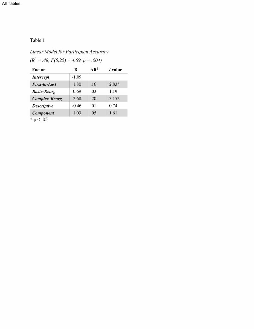
Table 1
Linear Model for Participant Accuracy
(R2 = .48, F(5,25) = 4.69, p = .004)
Factor B ΔR2 t value
Intercept -1.09
First-to-Last 1.80 .16 2.83*
Basic-Reorg 0.69 .03 1.19
Complex-Reorg 2.68 .20 3.15*
Descriptive -0.46 .01 0.74
Component 1.03 .05 1.61
* p < .05
All Tables
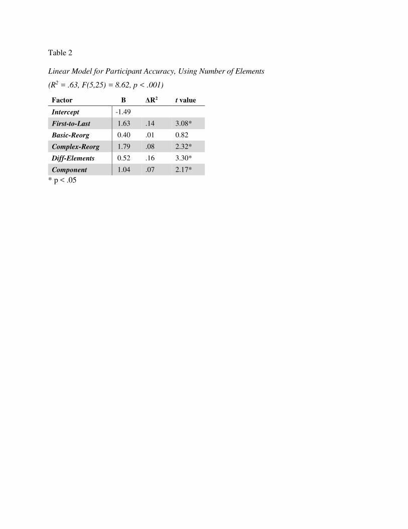
Table 2
Linear Model for Participant Accuracy, Using Number of Elements
(R2 = .63, F(5,25) = 8.62, p < .001)
Factor B ΔR2 t value
Intercept -1.49
First-to-Last 1.63 .14 3.08*
Basic-Reorg 0.40 .01 0.82
Complex-Reorg 1.79 .08 2.32*
Diff-Elements 0.52 .16 3.30*
Component 1.04 .07 2.17*
* p < .05
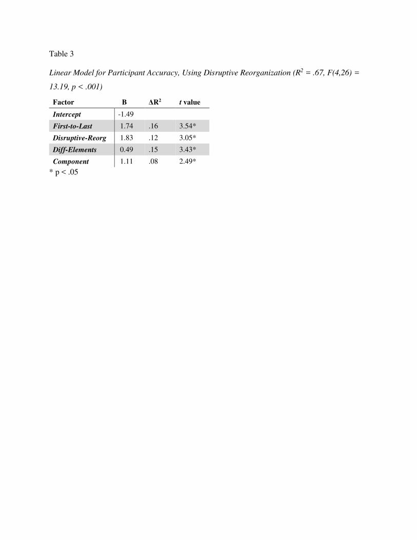
Table 3
Linear Model for Participant Accuracy, Using Disruptive Reorganization (R2 = .67, F(4,26) =
13.19, p < .001)
Factor B ΔR2 t value
Intercept -1.49
First-to-Last 1.74 .16 3.54*
Disruptive-Reorg 1.83 .12 3.05*
Diff-Elements 0.49 .15 3.43*
Component 1.11 .08 2.49*
* p < .05
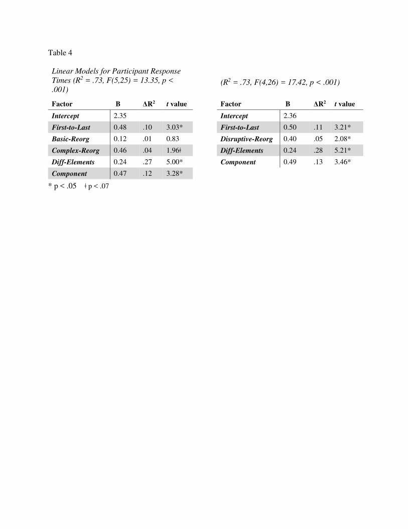
Table 4
Linear Models for Participant Response
Times (R2 = .73, F(5,25) = 13.35, p <
.001)
(R2 = .73, F(4,26) = 17.42, p < .001)
Factor B ΔR2 t value Factor B ΔR2 t value
Intercept 2.35 Intercept 2.36
First-to-Last 0.48 .10 3.03* First-to-Last 0.50 .11 3.21*
Basic-Reorg 0.12 .01 0.83 Disruptive-Reorg 0.40 .05 2.08*
Complex-Reorg 0.46 .04 1.96ǂ Diff-Elements 0.24 .28 5.21*
Diff-Elements 0.24 .27 5.00* Component 0.49 .13 3.46*
Component 0.47 .12 3.28*
* p < .05 ǂ p < .07

Figure 1. Raven’s Matrix problem. To protect the security of the test, all the problems
presented here were constructed by the authors. Many are analogous to actual problems.
All Figures
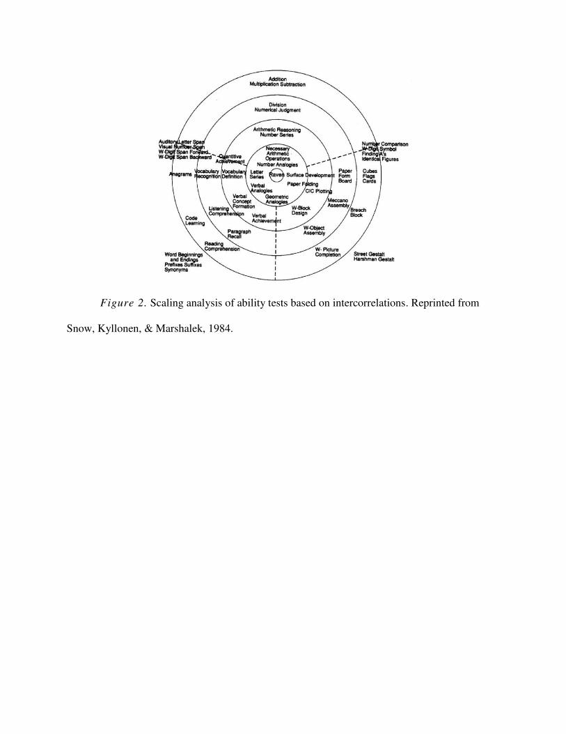
Figure 2. Scaling analysis of ability tests based on intercorrelations. Reprinted from
Snow, Kyllonen, & Marshalek, 1984.
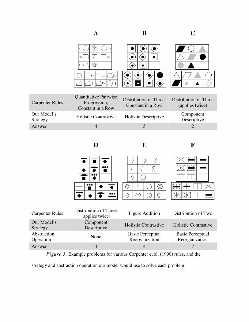
A
B
C
Carpenter Rules
Quantitative Pairwise
Progression,
Constant in a Row
Distribution of Three,
Constant in a Row
Distribution of Three
(applies twice)
Our Model’s
Strategy Holistic Contrastive Holistic Descriptive
Component
Descriptive
Answer 4 5 2
D
E
F
Carpenter Rules Distribution of Three
(applies twice) Figure Addition Distribution of Two
Our Model’s
Strategy
Component
Descriptive Holistic Contrastive Holistic Contrastive
Abstraction
Operation None
Basic Perceptual
Reorganization
Basic Perceptual
Reorganization
Answer 4 4 7
Figure 3. Example problems for various Carpenter et al. (1990) rules, and the
strategy and abstraction operation our model would use to solve each problem.
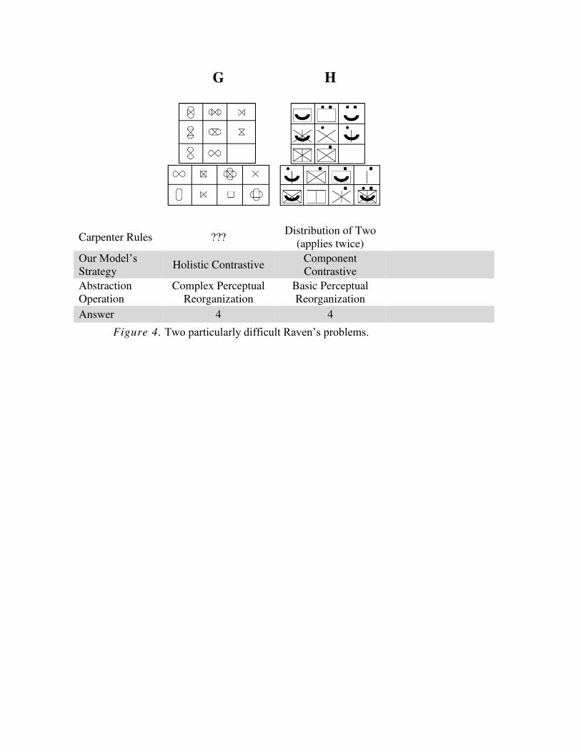
G
H
Carpenter Rules ??? Distribution of Two
(applies twice)
Our Model’s Strategy
Holistic Contrastive Component
Contrastive
Abstraction
Operation
Complex Perceptual
Reorganization
Basic Perceptual
Reorganization
Answer 4 4
Figure 4. Two particularly difficult Raven’s problems.
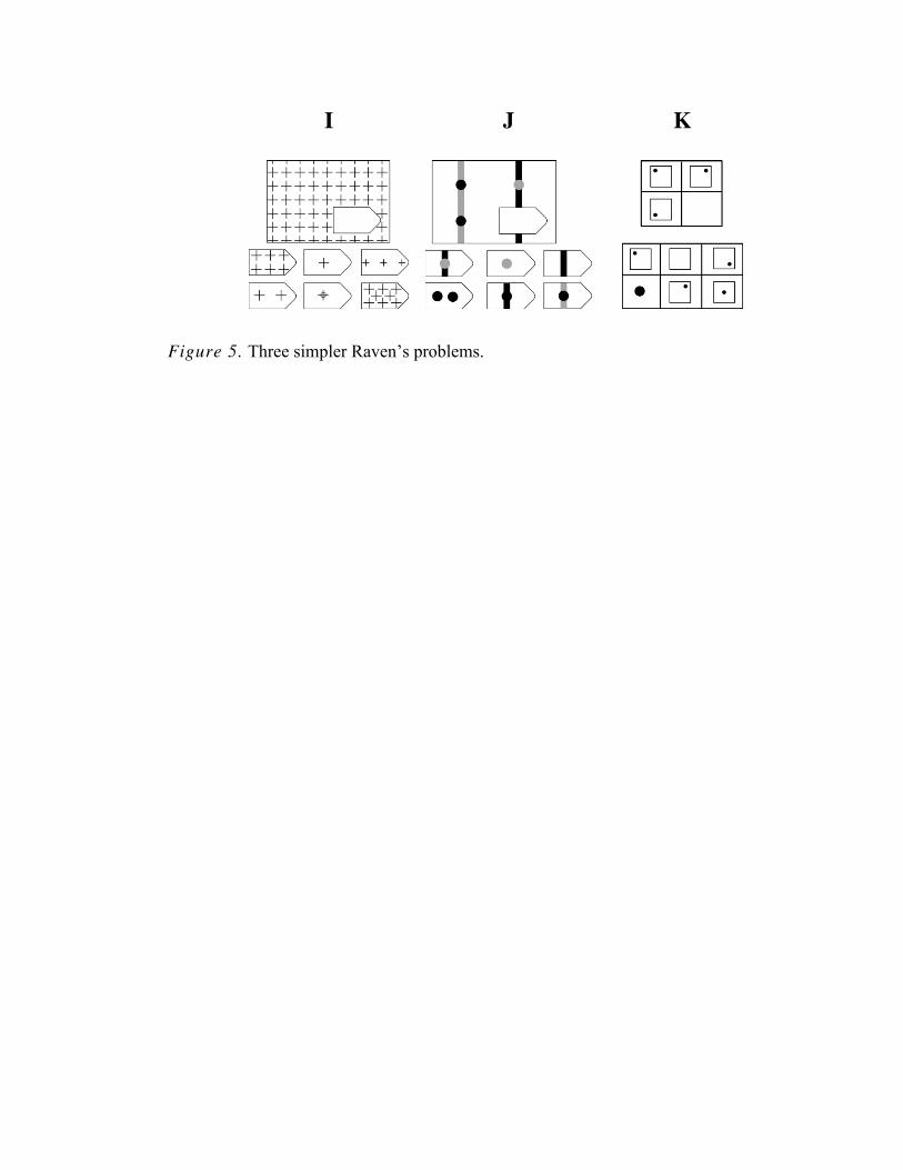
I
J
K
Figure 5. Three simpler Raven’s problems.
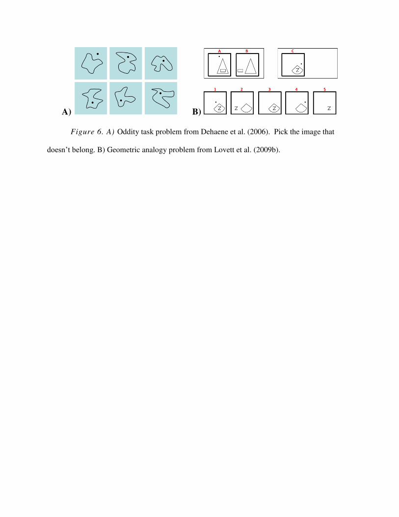
A) B)
Figure 6. A) Oddity task problem from Dehaene et al. (2006). Pick the image that
doesn’t belong. B) Geometric analogy problem from Lovett et al. (2009b).

A) B)
Figure 7. Images that might be compared structurally.

A) B) C)
Figure 8. Basic perceptual reorganization facilitates this comparison.

A) B)
Figure 9. Complex perceptual reorganization facilitates this comparison.
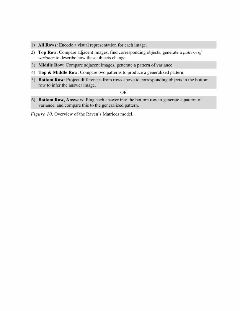
1) All Rows: Encode a visual representation for each image.
2) Top Row: Compare adjacent images, find corresponding objects, generate a pattern of
variance to describe how these objects change.
3) Middle Row: Compare adjacent images, generate a pattern of variance.
4) Top & Middle Row: Compare two patterns to produce a generalized pattern.
5) Bottom Row: Project differences from rows above to corresponding objects in the bottom
row to infer the answer image.
OR
6) Bottom Row, Answers: Plug each answer into the bottom row to generate a pattern of
variance, and compare this to the generalized pattern.
Figure 10. Overview of the Raven’s Matrices model.

A) B)
Figure 11. Strategies for solving problems I and J.
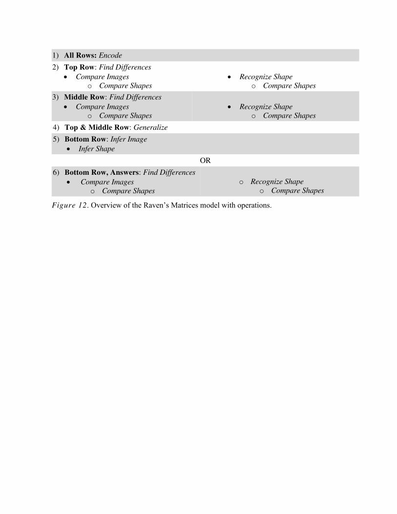
1) All Rows: Encode
2) Top Row: Find Differences
Compare Images
o Compare Shapes
Recognize Shape
o Compare Shapes
3) Middle Row: Find Differences
Compare Images
o Compare Shapes
Recognize Shape
o Compare Shapes
4) Top & Middle Row: Generalize
5) Bottom Row: Infer Image
Infer Shape
OR
6) Bottom Row, Answers: Find Differences
Compare Images
o Compare Shapes
o Recognize Shape
o Compare Shapes
Figure 12. Overview of the Raven’s Matrices model with operations.

A) B) C)
Figure 13. Examples of shape deformations.
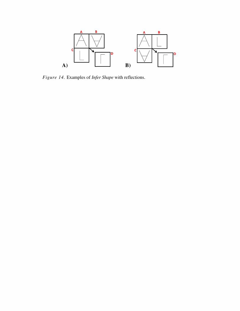
A) B)
Figure 14. Examples of Infer Shape with reflections.
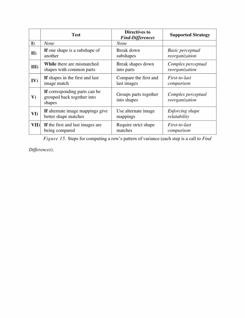
Test
Directives to
Find-Differences Supported Strategy
I) None None
II) If one shape is a subshape of
another
Break down
subshapes
Basic perceptual
reorganization
III) While there are mismatched
shapes with common parts
Break shapes down
into parts
Complex perceptual
reorganization
IV) If shapes in the first and last
image match
Compare the first and
last images
First-to-last
comparison
V)
If corresponding parts can be
grouped back together into
shapes
Groups parts together
into shapes
Complex perceptual
reorganization
VI) If alternate image mappings give
better shape matches
Use alternate image
mappings
Enforcing shape
relatability
VII) If the first and last images are
being compared
Require strict shape
matches
First-to-last
comparison
Figure 15. Steps for computing a row’s pattern of variance (each step is a call to Find
Differences).
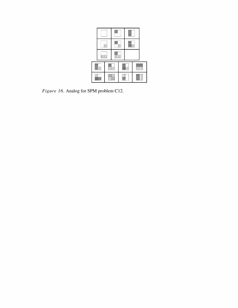
Figure 16. Analog for SPM problem C12.
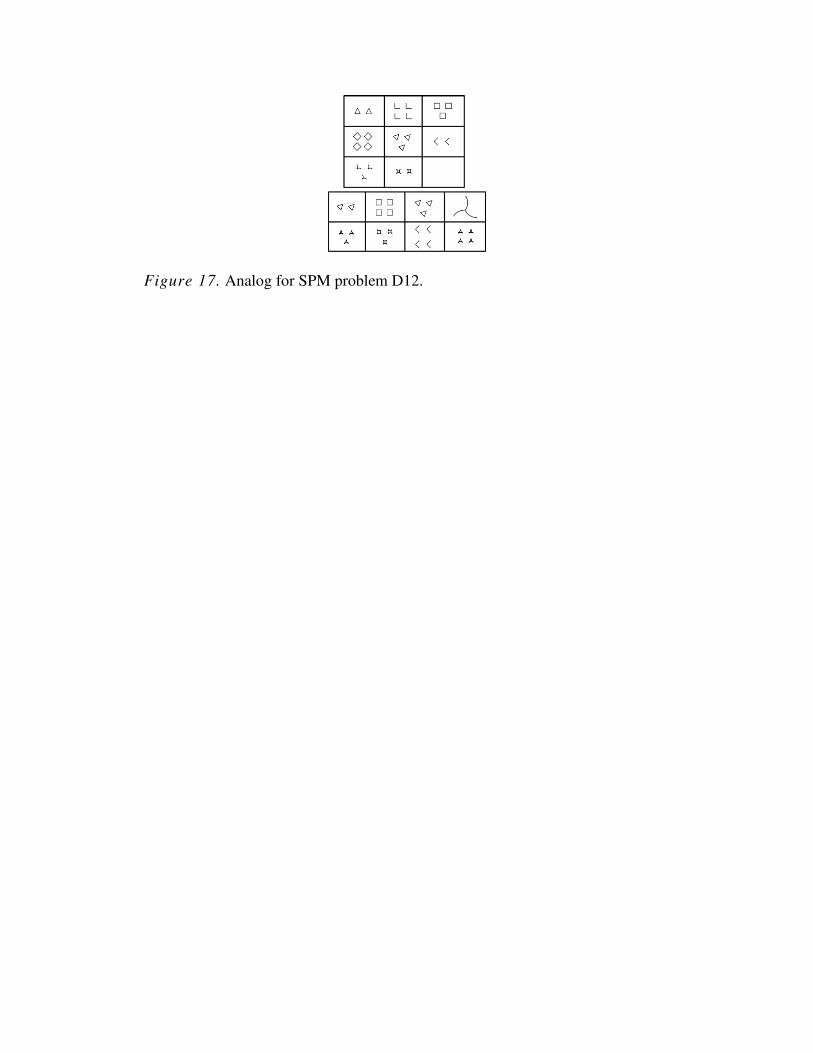
Figure 17. Analog for SPM problem D12.

A) B) C)
Figure 18. A: A house. B: The house’s contour. C: The contour, rotated.

A) B) C) D)
Figure 19. Examples of texture patches and negative space.

A) B) C) D) E) F)
Figure 20. Grouping examples.

A) B)
Figure 21. Two images with differences in their shapes and spatial relations.

A) B)
Figure 22. Smaller versions of the C/F pair from Figure 21.

A) B) C) D)
Figure 23. Two ambiguous mappings.
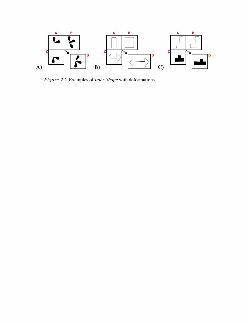
A) B) C)
Figure 24. Examples of Infer-Shape with deformations.