modeling the revolving revolution: the debt collection channel
TRANSCRIPT

February 12, 2016
Modeling the Revolving Revolution:The Debt Collection Channel
Lukasz A. Drozd and Ricardo Serrano-Padial∗
Abstract
We investigate the role of information technology (IT) in the collection of delinquent con-sumer debt. We argue that the widespread adoption of IT by the debt collection industryin the 1990s contributed to the observed expansion of risky lending to consumers, such asunsecured credit card lending. Our model stresses the role of private information about adelinquent borrower’s solvency. The presence of private information implies that the costs ofdebt collection must be borne by lenders to sustain incentives to repay debt. IT is used toconcentrate collection efforts on those delinquent borrowers who are more likely to repay.
Keywords: debt collection, credit cards, consumer credit, unsecured credit, revolving credit,moral hazard, costly state verification, informal bankruptcy, information technology
JEL codes: E21, D91, G20.
∗Drozd: Federal Reserve Bank of Philadelphia and the Wharton School of the University of Pennsylvania.Serrano-Padial: School of Economics, Drexel University. The previous version of this paper circulated underthe title: “Modeling the Revolving Revolution: The Role of IT Reconsidered.” This research has beensupported by the following grants: Vanguard Research Fellowship from Rodney L. White Center for FinancialResearch (Drozd), Cynthia and Bennet Golub Endowed Faculty Scholar Award (Drozd), and Universityof Wisconsin-Madison Graduate School Research Committee Award (Serrano-Padial). We thank SatyajitChatterjee, Joao Gomes, Urban Jermann, Wenli Li, Scott Richard, and Amir Yaron for insightful comments.We are especially grateful to Robert Hunt for his support and expert guidance. All remaining errors are ours.The views expressed here are those of the authors and do not necessarily represent the views of the FederalReserve Bank of Philadelphia or the Federal Reserve System.

1 Introduction
The consumer credit industry is one of the most information technology-intensive (Triplett
and Bosworth, 2002). In fact, today there are hardly any aspects of consumer lending that
would not involve the use of IT (Berger, 2003). Yet, however apparent the use of IT might be,
its transformative effect on consumer credit markets is difficult to gauge and requires careful
modeling. Our paper investigates the effect of IT adoption by the very industry that sustains
consumer lending—the debt collection industry.1
Our focus on debt collection stems from the fact that the adoption of IT by the lending
industry has been mirrored by similar developments in the debt collection industry. Chief
among them was the emergence of IT-enabled statistical modeling of the evolution of delinquent
debt, resulting in an extensive use of large databases to automate the collection process and
improve collection efficiency. The new technology diffused throughout the 1990s and has been
associated with major efficiency gains by the collection industry.2 Other notable improvements
include internet-based skiptracing, predictive dialers, and the provision of collection scores by
the credit bureaus. These new tools have improved tracking of delinquent borrowers, allowed for
real-time estimation of their ability to repay debt, and made economies of scale readily accessible
to the industry.
To explore the idea that improvements in debt collection might have affected consumer
lending during this period, we develop a new model of consumer default in which both debt
collection and IT play a role consistent with micro-level evidence (Makuch et al., 1992; Chin
and Kotak, 2006). We embed this model in an otherwise standard theory of consumer borrowing
(Chatterjee et al., 2007; Livshits et al., 2007) and calibrate it to the data.
1Depending on industry definition, the debt collection industry employs at least 150,000 and up to 430,000according to the Bureau of Labor Statistics. About two-thirds of debt collected is consumer debt accordingto ACA International (2007). To put these numbers in perspective, total number of officers across all lawenforcement agencies is about 700,000. See Section 3 (fact 2) for a more detailed discussion.
2Section 3 (fact 3) and the online Appendix review the evidence.
1
The central element of our approach is modeling consumer default as persistent delinquency.
This contrasts with the conventional view of consumer default as filing for bankruptcy protection,
which by definition abstracts from debt collection. As we show in this paper (Section 3) and
as has already been documented by Dawsey and Ausubel (2004) and Agarwal et al. (2003),
persistent delinquency rather than formal bankruptcy is the prevalent form of consumer default
in the data. Delinquency rationalizes the existence of the debt collection industry and justifies
the use of IT to mitigate informational asymmetries about borrowers’ ability to repay debt.
The formal setup builds on the theory of costly state verification (Townsend, 1979). Default
involves private information about financial distress experienced by delinquent borrowers and
IT provides lenders with a noisy signal of the hidden state. Since debt collection is costly and
ineffective against distressed borrowers, signals can be used to improve collection efficiency. This
is achieved by concentrating debt collection efforts on those borrowers who are most likely to
repay (i.e., those with signals of no distress). Since such a strategy also entails a cost associated
with strategic default by borrowers who no longer face debt collection, the adoption of IT is
endogenous and takes place above a certain level of signal precision.
The main prediction of our model is that improvements in signal precision drive up the
riskiness of consumer debt. Intuitively, the use of IT to collect debt reduces the price of contracts
exposed to default risk (risky contracts) and makes them more attractive to consumers, and
hence more prevalent. As risky contracts become relatively more prevalent—compared to riskless
contracts characterized by tight credit limits—the average riskiness of outstanding debt goes up.
Moreover, this effect can be substantial even if post-adoption collection costs are modest.
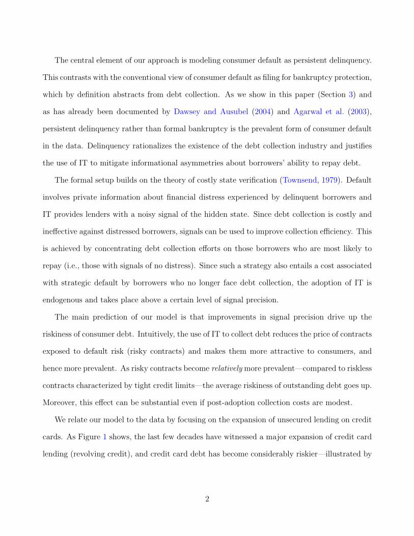
We relate our model to the data by focusing on the expansion of unsecured lending on credit
cards. As Figure 1 shows, the last few decades have witnessed a major expansion of credit card
lending (revolving credit), and credit card debt has become considerably riskier—illustrated by
2

the upward trend in the charge-off rate on credit card loans.3 A natural question is whether our
framework can speak to these trends.
0%
15%
30%
45%
1968 1980 1992 2004Year
Consumer credit / median income
Unsecured credit / median income
Revolving credit / median income
1%
3%
5%
7%
1985 1990 1995 2000Year
Net charge‐off rate on revolving credit
Figure 1: Expansion of risky credit card lending in the U.S.
We calibrate the model to data prior to the 2005 bankruptcy reform and the 2008 financial
crisis. We match the 2004 trend values of credit card debt to (median) income of 15.1% and
charge-off rate of 5.2%. We set debt collection parameters to account for the estimated aggregate
costs of collecting delinquent credit card debt in 2004 (about 4% of charge-offs in 2004). We
also assume that signal precision is sufficiently high to ensure that IT had already been adopted
by 2004. Finally, to quantify the effect of IT adoption and its subsequent progress, we recreate
the credit card market prior to the adoption by reducing signal precision.
We find that a reduction in signal precision that undoes the use of IT in collections has a
significant effect on the equilibrium charge-off rate, which falls from the calibrated value of 5.2%
3 With the exception of total unsecured lending, all series come from the G.19 Statistical Release by the FederalReserve Board of Governors (FRB). Approximate total unsecured lending comes from Livshits et al. (2010).The FRB defines consumer credit as outstanding credit extended to individuals for household, family, and otherpersonal expenditures, excluding loans secured by real estate. Credit card loans comprise most of revolvingconsumer credit. Charge-offs are loans removed from the books and charged against loss reserves. The charge-off rate is measured net of recoveries, and as a percentage of outstanding loans. Federal regulations requirecreditors to charge off revolving credit accounts after 180 days of payment delinquency. See Uniform RetailCredit Classification and Account Management Policy, 65 FR 36903-01 (June 12, 2000).
3
to at least 3.3%. In the context of the data presented in Figure 1 (right panel), we interpret this
result as suggesting that improvements in debt collection might have contributed to the rising
default losses on credit card loans. In this context, its effects can be seen as complementary
to the IT-driven adoption of credit scoring by the lending industry—which has similarly been
linked to the expansion of the credit card market (see literature review in Section 2).
Importantly, the effect of IT adoption predicted by our model is broadly consistent with
the available industry evidence from the 1990s. Makuch et al. (1992) describe the adoption
of one of the industry’s first IT-based statistical platforms to collect unpaid credit card debt.
Prior to its adoption in 1990, GE capital (the credit card servicer under study) faced an annual
flow of $1 billion in delinquent credit card debt and $400 million in annual charge-offs on a
$12 billion portfolio. Pre-adoption collection costs represented 1.25% of outstanding debt and
37% of charge-offs. Moreover, the new IT-based collection platform saved the company 31 basis
points relative to outstanding debt and about 9% relative to pre-adoption charge-offs (estimated
using a controlled trial). Our model is consistent with these efficiency gains.
Finally, our analysis implies that post-adoption debt collection should rely less on legal
collections—such as judgments and wage garnishments filed in court—while it should use “sig-
nals” more extensively. We find confirmation of these predictions in the data. Specifically,
we show that in the credit bureau data the average number of legal collections per delinquent
borrower decreased by 16% from 2000 to 2006. At the same time, the use of credit bureau
information on delinquent borrowers by debt collectors went up by 30%. While our data does
not go back to the 1990s, using court data on wage garnishments from Virginia, Hynes (2006)
documents that the growth of debt-related garnishments was similarly negative in the 1990s.
The rest of this paper is organized as follows. Section 2 reviews the related literature. Section
3 discusses key motivating facts. Section 4 presents our theoretical framework and our results.
Section 5 describes our quantitative model and discusses the findings. Section 6 concludes.
4
2 Related literature
Our paper falls into the broader body of research investigating the link between IT progress
and the observed rise in risky consumer lending, such as unsecured credit card lending. Nara-
jabad (2012), Athreya et al. (2012), Sanchez (2012) and Livshits et al. (forthcoming) analyze
the effect of improvements in information available to lenders about a borrower’s default risk.
Livshits et al. (forthcoming) additionally explore the effect of declining costs of creating (risky)
credit contracts under asymmetric information. In this context, Livshits et al. (2010) show that
under perfect information declining costs of intermediation cannot explain the rise in consumer
bankruptcies, justifying the focus of the aforementioned literature on micro-founded models of
IT. In addition, our focus on persistent delinquency is related to the literature studying the
connection between delinquency and formal bankruptcy, such as Chatterjee (2010), Athreya et
al. (2015) Benjamin and Mateos-Planas (2013), and White (1998). Finally, our paper is also re-
lated to the literature that studies the debt collection industry. For instance, Fedaseyeu (2015)
investigates how regulation of the debt collection industry might have affected the supply of
consumer credit. Fedaseyeu and Hunt (2014) provide a model that justifies outsourcing of debt
collection to third-party agencies.
3 Basic facts about debt collection
Fact 1: Persistent delinquency is a prevalent form of consumer default.
We analyze a representative panel of over 150,000 individuals provided by Experian—one of the
three major credit bureaus in the U.S. We identify delinquent consumers on bank cards in 2001,
2003 and 2005. We then follow them for four years.4
4Delinquent borrowers are those who have at least one bank card opened within the last two years that is 90+days overdue. This definition is similar to the one used by Agarwal et al. (2003).
5

As is clear from Table 1, out of 31 delinquencies per 1000 individuals, we find that as many
as 20 remain delinquent after two years and only 6 file for bankruptcy by that time.5 This result
is in line with earlier studies using account-level data (Dawsey and Ausubel, 2004; Agarwal et
al., 2003) and shows that persistent delinquency is a prevalent form of consumer default.
Table 1: Persistent delinquency in the U.S. data.
31 per 1000 newly delinquent borrowers in 2001, 2003, 2005a
show no sign of improvementb files for bankruptcy
2 years after 66% (20 per 1000) 17% (5.5 per 1000)4 years after 52% (16 per 1000) 20% (6.3 per 1000)
aHas at least one bank card opened within last two years that is 90 days+ overdue, charged off or in collection.bPaid in full or settled on any previously delinquent account, regardless of type (credit card, auto loan, . . . ).
While it is difficult to say why so many borrowers do not file for bankruptcy, our findings
are consistent with the hypothesis that the costs associated with filing may preclude borrowers
from seeking bankruptcy protection. Hynes (2008) reports a filing fee of $299 plus $1000-2000
in lawyer fees in 2007. These costs are comparable to the debt relief borrowers may get by filing
formally, as the average credit card debt in collection in 2007 is only $2,500 per account according
to the Association of Credit and Collection Professionals (ACA International, 2007), with the
median being less than $1,000. While consumers may have multiple accounts in collection, the
Consumer Protection Bureau reports that in 2014 the average non-mortgage debt in collection
per borrower was only $5,178. At the same time, as many as 35% of adults with credit files had
some non-mortgage debt in collection.6 The evidence reported by Makuch et al. (1992) suggests
that delinquency was an important concern for credit card lenders in the early 1990s.
5These statistics are similar if we restrict our sample to delinquent borrowers with no prior history of bankruptcy.While a fraction of delinquent borrowers show improvement, this by no means implies full repayment. Thisis because our definition of ‘improvement,’ due to the lack of account level information, is fairly broad andindicates repayment of any credit account in the portfolio of a delinquent borrower. Hence it is plausible thatmany borrowers that we flag as non-delinquent are still delinquent two years later.
6For more details, see CFPB (2015) and Ratcliffe et al. (2014), and the earlier study by Avery et al. (2003).
6

Fact 2: The collection of consumer debt is costly.
There is a large industry devoted to the collection of unpaid consumer debt in the U.S. The
Department of Labor reports employment of 157,000 workers in the debt collection industry
(NAICS 56144) prior to the financial crisis (data for 2006). This, however, excludes in-house
collection departments. Taken together, bill and account collectors as a profession held about
434,000 jobs according to the Bureau of Labour Statistics (2006). Consumer debt accounts for
about two-thirds of debt placed in collection and credit card debt accounts for about a quarter
according to the annual surveys of debt collection industry (ACA International, 2007).
But what is the cost of collecting delinquent credit card debt in particular? According to
ACA International (2007), revenues from commissions on collection of credit card debt are the
highest among major debt categories.7 If we assume equal marginal product from collection
resources across different debt categories, we can use the share of credit card debt placed in
collection as a proxy to measure its contribution to costs. Gross output in the debt collection
industry before the crisis was about 6.2 billion in 2004 dollars (IBISWorld, 2013b)—which
excludes in-house collection departments and hence is a lower bound on total costs. Assuming
that collection of credit card debt represents about a quarter of total collected debt by the
industry, this implies a cost of about $1.5 billion in 2004, or 4% of the annual charge-offs.8
Fact 3: The use of IT to collect consumer debt improved collection efficiency.
According to most studies, before the 1990s, the debt collection industry relied on labor-intensive
methods of collecting debt (Makuch et al., 1992; Hunt, 2007). Under this traditional approach,
debt collectors looked into each case and decided what action to take, often analyzing data them-
7For instance, the median commission rate on hospital and healthcare debt was 24% in 2006, while in the samesurvey it was 31.3% for credit cards (see page 25). The mean values were about 40% for hospital and health-caredebt and about 60% for credit card debt (see page 13, 15, and 16 of the report).
8To calculate charge-offs, we multiply the charge-off rate on credit card debt by the total revolving debt outstand-ing. Note that the charge-off rate is measured net of recoveries. We consider 2004 the most recent representativeyear because of a major bankruptcy law reform in 2005 and the 2008 financial crisis.
7

selves. Occasionally, ad hoc in-house solutions would be deployed to aid this heuristic approach
(Rosenberg and Gleit, 1994). In the late 1980s and especially in the 1990s, the approach to debt
collection changed dramatically with the growing availability of payment history databases and
higher computing power.
The defining feature of the modern IT-based approach to debt collection is the use of au-
tomated statistical cost-benefit analysis to allocate collection resources. For instance, the core
idea behind PAYMENT—one of the first large-scale collection systems adopted by GE Capital
in 1990 (Makuch et al., 1992)—was to model the portfolio of delinquent accounts as a Markov
matrix summarizing the transition probability from X to X + y days of delinquency, with the
probability being a function of a set of collection actions that can be undertaken in a given
state. A computer algorithm would use this matrix to perform cost-benefit analysis and choose
the best action for each delinquent account based on borrower and account characteristics.9
The use of such systems is associated with considerable savings. For example, using a
randomized controlled trial on a subset of accounts, Makuch et al. (1992) estimate that the
adoption of PAYMENT saved GE Capital $37 million annually on a $150 million collection
budget, which amounts to 31 basis points in relation to its portfolio of $12 billion in credit
card debt or about 9% of $400 million in annual write-offs. One of the key changes introduced
by PAYMENT was a sharp reduction in the frequency of costly collection attempts, to which
Makuch et al. (1992) attribute the bulk of savings. Today, most IT companies that offer solutions
to the collection industry advertise efficiency gains that are at least as high. For example,
FICO—the provider of credit scores—reports several testimonials of its clients who purchased its
system. Most of them claim gains of 50% or more.10 Similarly, First Data claims efficiency gains
of 48%, while attributing them to improved precision of information (Davey, 2009). Portfolio
9See Chin and Kotak (2006); Hopper and Lewis (1992); Till and Hand (2003) for an additional description of thisapproach and Rosenberg and Gleit (1994) for a survey of the different methods such as decision trees, neuralnetworks and Markov chains.
10See Fair Isaac Corporation (2006) and also http://www.fico.com/en/node/8140?file=5656
8

Recovery Associates, one of the largest debt collection agencies that primarily deals with credit
card debt (about 60% share), reports in its 2005 annual SEC filling that its debt collection
efficiency per resource spent increased by 120% from 1998 to 2005. The company explicitly
attributes these gains to its proprietary IT infrastructure.
In addition, since mid 1990s, all three credit bureaus offer collection scores alongside other
products, such as skiptracing or real-time monitoring of unpaid debt. These offerings make
economies of scale readily accessible to the industry.11 IBISWorld (2013a) reports that the
share in revenue of credit bureaus and rating agencies accounted for by debt collection and risk
management services was 7.5% in 2013. To put this number in perspective, about 37% of the to-
tal revenue came from banks and other financial institutions (excluding mortgage originators).12
For more details on the debt collection industry and its evolution see the online Appendix
and the overview by Hunt (2007).
4 Theory
We consider a two-period model economy populated by a large number of lenders and a contin-
uum of consumers. Lenders have deep pockets and extend competitively priced credit lines to
consumers. They fully commit to contracts.
Consumers borrow from lenders to smooth consumption. They face an exogenous income
stream Y and start in period one with a stock of pre-existing debt B that they wish to roll over.
With probability p < 1/2, they suffer from an idiosyncratic financial distress shock that reduces
11Experian introduced RecoveryScore for charged-off accounts in 1995 (personal communication), while Tran-sUnion have been offering collection scores since at least 1996 (Pincetich and Rubadue, 1997). As an exampleof collection scores, Section 2 Table 4 in the online Appendix shows that Experian’s Bankcard RecoveryScoreis correlated with future repayment by currently delinquent consumers.
12The success of segmentation and prioritization in the collection of credit card debt has led other industriesto adopt a similar approach. Examples include Fannie May and Freddie Mac in 1997 to manage delinquentmortgages (Cordell et al., 1998); and New York State in 2009 to collect unpaid taxes (Miller, 2012). Afteradoption, New York State increased its collections from delinquent taxpayers by $83 million (an 8% increase)using the same amount of collection resources.
9

their second period income by a fixed amount E > 0 (e.g., job loss, divorce, or medical bills).
The random variable denoting this shock is d = 0, 1.
Credit is unsecured and consumers can renege on repayment at a pecuniary dead-weight cost
0 < θY < 1. Lenders can resort to costly debt collection to recover unpaid debt. Collection cost
is sunk and equal to λ > 0. It is effective in the case of non-distressed consumers and ineffective
in the case of distressed consumers.
The realization of the financial distress shock d is private information. However, lenders
(and consumers) observe a noisy signal of the shock before they engage in debt collection (state
verification). The realization of this signal is denoted by d and its precision is denoted by π ∈
[0, 1]. Specifically, the signal reveals d with probability π and is uninformative with probability
1− π. Signal precision represents the state of IT in the economy.
The timing of events is as follows: 1) credit market opens and lenders extend credit to
consumers; 2) consumers privately observe the shock and the signal is revealed; 3) consumers
choose consumption and decide whether to repay or default; and 4) debt collection takes place.
4.1 Lender problem
Credit contracts are exogenously restricted to credit lines.13 Credit lines are characterized by a
credit limit L that restricts borrowing, a fixed finance charge I paid for the line, and a state veri-
fication or monitoring strategy P (d) which represents the probability of debt collection in case of
default. There is Bertrand competition in the lending market, implying that lenders maximize
consumer’s indirect utility subject to a resource constraint. The resource constraint requires
that lenders’ revenue stream, net of collection costs, must be non-negative in expectation.
13Our model is best interpreted as a positive theory of consumer lending. It nonetheless is possible to outline aset of assumptions under which this restriction decentralizes an optimal mechanism. However, the conditionsare quite restrictive and involve such features as non commitment of the principal and hidden borrowing andlending against promised consumption by the principal. We thus do not discuss it here. Having a fixed financefee eliminates the intertemporal distortion associated with interest rates and simplifies the proofs.
10

We denote the revenue stream from a given contract by Π(·). It depends on consumers’
default decision and the outcome of debt collection. Specifically, let δ(S, I, L, P ) describe the
consumer’s default decision as a function of her exogenous state S := (d, d) and her contract
(I, L, P ). If the consumer does not default (δ = 0), the revenue stream is I. If, on the other hand,
the consumer defaults (δ = 1) and she is distressed (d = 1), the lender suffers a loss equal to
L. Finally, if the consumer is non-distressed (d = 0), and debt collection takes place, the lender
recovers the principal L and additionally collects an exogenous penalty I > 0. In summary,
Π(S, I, L, P ) :=
I if δ(S, I, L, P ) = 0
−L+ (1− d)P (d)(L+ I) if δ(S, I, L, P ) = 1.
(1)
The expected costs of collections on a portfolio of accounts of measure one, which we denote
by Λ, are determined by the unit cost λ of each collection, and the measure of consumers who
default and are subjected to debt collection, δ(S, I, L, P )P (d). Hence,
Λ(S, I, L, P ) := λδ(S, I, L, P )P (d). (2)
Finally, let V (I, L, P ) be the ex ante indirect utility function of consumers from contract
(I, L, P ). Given these definitions, lenders in our model choose contracts to solve
maxI,L,P
V (I, L, P ) (3)
subject to ∑S
[Π(S, I, L, P )− Λ(S, I, L, P )]Pr(S) ≥ 0,
where Pr(S) is the probability distribution of the exogenous state S = (d, d).14
14 Pr(S) := Pr(d, d) is given by Pr(0, 0) = (π + (1 − π)(1 − p))(1 − p), Pr(1, 0) = Pr(0, 1) = (1 − π)(1 − p)2,
11

4.2 Consumer problem
Consumers borrow from lenders to maximize utility. The utility function is given by U(c, c′),
where c and c′ denote consumption in periods 1 and 2, respectively. We assume that U is strictly
concave, differentiable and symmetric with respect to c and c′.
Consumers choose consumption c, c′ contingent on their default decision δ. To simplify the
analysis, we assume that consumers make these choices after observing the exogenous state S.15
Hence,
δ(S, I, L, P ) :=
1 if D(S, I, L, P ) > N(S, I, L, P )
0 otherwise
(4)
where N(·) is the indirect utility function associated with repayment and D(·) is the indirect
utility associated with default.
The indirect utility function associated with repayment is straightforward and given by the
intertemporal optimization problem
N(S, I, L, P ) := maxb≤L
U(c, c′) (5)
subject to
c = Y −B + b
c′ = Y − b− I − dE.
To define the indirect utility from defaulting we must introduce some notation. To this
end, let m = 0, 1 be the random variable indicating debt collection. Recall that its probability
and Pr(1, 1) = (π + (1− π)p)p.15Since in realistic applications p would be small, this assumption is innocuous.
12

distribution is determined by P, which is part of the contract. Then, D(S, I, L, P ) is16
D(S, I, L, P ) := maxb≤L
∑m
U(c, c′)Pr(m) (6)
subject to
c = Y −B + b
c′ = (1− θ)Y − b+ L− dE −m(1− d)(L+ I).
The ex ante indirect utility that consumers use to evaluate contracts is
V (I, L, P ) :=∑S
(δ(S, I, L, P )D(S, I, L, P ) + (1− δ(S, I, L, P ))N(S, I, L, P ))Pr(S). (7)
Finally, equilibrium is comprised of indirect utility functions V , N , D and decision rules δ,
b, I, L, and P. Neither existence nor uniqueness of equilibrium poses a problem. While we do
not discuss it explicitly, these properties indirectly follow from the analysis below.
4.3 Equilibrium effect of IT progress
We begin with a characterization of consumer’s default decision. We then describe lenders’
strategies to collect debt in equilibrium. We conclude this discussion by showing how IT adoption
in debt collection and its subsequent progress affects the riskiness of debt.
Proposition 1 characterizes the consumer’s default decisions. It is governed by two cutoffs,
denoted by Lmin(I) and P (I, L). The first cutoff identifies the maximum credit limit L that
can be sustained as default free. The second cutoff characterizes default decision of a non-
16We assume that the lender’s information set is summarized by the signal. In particular, no additional informa-tion can be extracted by observing how much the consumer borrows. This could be justified by the presenceof a savings technology that allows consumers to initially borrow L and allocate resources across periods as afunction of the shock.
13

distressed consumer for L > Lmin(I). While a distressed consumer defaults in such a case,
a non-distressed consumer may choose to repay depending on the probability of facing debt
collection. Accordingly, we refer to P (I, L) as the default prevention threshold.
The intuition behind this result is straightforward. Since the consumer faces a pecuniary
cost of defaulting, she does not default on small credit lines regardless of her state. On the
other hand, since debt collection is effective against non-distressed consumers, a sufficiently
high probability of debt collection deters them from defaulting.
Proposition 1. Consider any contract (I, L, P ). Then, i) if L ≤ Lmin(I) := θY − I, consumers
never default for all S; ii) if L > Lmin then distressed consumers always default and, if for
some P ′ ∈ (0, 1] a non-distressed consumer chooses to repay when P (d) = P ′, then there ex-
ists P (I, L) ∈ (0, 1] such that non-distressed consumers repay if and only if P (d) ≥ P (I, L).
Furthermore, P (I, L) ∈ (0, 1] is continuous, increasing in I and independent from π.
Proposition 1 implies that in equilibrium credit lines up to Lmin(0) = θY are default free. This
is because such credit lines break even at I = 0, maximizing borrower utility (N is decreasing
in I). Conversely, any equilibrium credit lines with L > Lmin are risky, i.e., they are exposed to
a positive risk of default.
Corollary 1. Equilibrium credit lines with L ≤ Lmin := θY are risk-free; credit lines with
L > Lmin are risky.
The next result derives a sufficient condition ensuring that, 1) the set of zero-profit risky con-
tracts L > Lmin is non-empty and, 2) that if a risky contract arises in equilibrium, it necessarily
involves some default prevention.
Proposition 2. If the following condition holds,
pλ < (1− p)θY, (8)
14

then 1) the set of L > Lmin such that for some P ∈ (0, 1] non-distressed consumers choose to
repay is non-empty, and 2) default prevention is optimal under at least one signal realization.
Condition (8) ensures that risky contracts can actually arise in equilibrium and, if that’s the
case, that not all agents default on such contracts.17 Since this is the only relevant case, in what
follows we assume that this condition is satisfied.
The next result states that lenders rely on only two collection strategies to sustain risky
contracts. Importantly, one of them uses IT and the other does not. To see why this is the case,
note that the signal segments the population of delinquent borrowers into two groups: those
who are less likely to be distressed and those who are more likely to be so. Recall that lenders
can prevent default of non-distressed consumers in a segment d by setting P (d) ≥ P . Hence,
they choose prevention for each segment separately. Furthermore, if P (d) ≥ P for one signal
realization, it must be when d = 0 because default prevention is more effective in this case.
Proposition 3. Risky contracts are supported by two collection strategies: 1) full monitoring,
P (d) = P (I, L) for d = 0, 1; and 2) selective monitoring, P (0) = P (I, L) and P (1) < P (I, L).
Furthermore, if π > π∗ := 1− λ(L+I)(1−p) then P (1) = 0.
Although selective monitoring (as defined in Proposition 3) can save on collection costs,
relative to full monitoring, it can also be more costly because of strategic default by non-
distressed agents whose signal incorrectly indicates distress.
Corollary 2. In equilibrium there is no strategic default under full monitoring, while there is
strategic default by non-distressed borrowers with d = 1 under selective monitoring.
17The following example is helpful to illustrate why for some parameter values it may be sometimes feasible andeven optimal to extend contracts such that all agents default. To this end, suppose both I and λ are sufficientlyhigh relative to the pecuniary cost of defaulting θY. Furthermore, suppose risk aversion is low. In such a case,since collecting from consumers up to the prevention point P is costly due to high λ—and defaulting is not—itmay be better to extend a contract on which all consumers default and instead collect from only a small massof them to ensure resource feasibility. Sufficiently high I ensures that such a “collection cost saving scheme”may be feasible. If risk aversion is sufficiently low, it may also be optimal. Numerical examples we constructedrequire exotic parameter values for this to be the case.
15

Having identified equilibrium collection strategies, we next characterize the way in which
risky contracts are priced in equilibrium. In describing pricing, we distinguish pure default
risk premium (henceforth default premium) from total default risk premium, which additionally
includes collection costs. We refer to the latter component of total default premium as the
collection premium.
Consider first the zero profit condition on risky contracts under full monitoring:
(1− p)I − p(L+ P (I, L)λ) = 0, (9)
where the first term is expected revenue, and the remaining terms capture expected default
losses and collection costs. The zero profit finance charge can be expressed as follows: I =(DF +MF
)L, whereDF = p/(1−p) corresponds to the default premium andMF = p
1−p P (I, L) λL
corresponds to the collection premium. Proposition 4 extends this result to include selectively
monitored contracts. Let Pπ(1) denote P (1) under selective monitoring to make explicit its
potential dependence on signal precision.
Proposition 4. If L is sustained using full monitoring then I = IF (L) :=(DF +MF
)L, where
DF =p
1− p and MF =p
1− pP (I, L)λ
L.
If L is sustained using selective monitoring, then I = IS(L) :=(DS +MS
)L, where
DS =p
Pr(0, 0)+
Pr(1, 0)
Pr(0, 0)︸ ︷︷ ︸“strategic” default
and
MS =Pr(0, 1)P (I, L) + pPπ(1)
Pr(0, 0)
λ
L− Pr(1, 0)
Pr(0, 0)Pπ(1)
(1 +
I
L
).
Furthermore, as π → 1, DS and MS converge to DF and 0, respectively.
16

Proposition 4 allows us to make the following key observations about pricing of risky credit
contracts. First, under full monitoring, pricing is independent from signal precision. It is only
under selective monitoring that the signals matter. Second, selectively monitored contracts are
inherently riskier than fully monitored contracts due the presence of strategic default by non-
distressed borrowers whose signal (incorrectly) indicates distress. Hence, the choice of equilib-
rium collection strategy generally involves a trade-off between the dead-weight loss associated
with strategic default and lower collection costs. Finally, selectively monitored contracts are
strictly preferred by consumers when similarly priced. This result is quite intuitive and follows
from the fact that consumers internalize the benefit from strategic default. The proof is trivial
and therefore omitted.
Proposition 5. For any two equally priced risky credit lines with the same credit, selective
monitoring is strictly preferred by consumers.
The next result characterizes the effect of IT progress on pricing. Specifically, it establishes
that Pπ(1) under selective monitoring, if positive, it is strictly decreasing in signal precision π
and vanishes at π∗ < 1, as defined in Proposition 3. This implies that, under a slack restriction
on penalty charge I, IS is strictly decreasing in π. Hence, it must be eventually lower than IF .
Proposition 6. If I ≤ λ and Pπ(1) > 0 then Pπ(1) and IS(L) are strictly decreasing in π and
limπ↑π∗ Pπ(1) = 0. In addition, IS(L) < IF (L) for sufficiently high π.
With these results in hand, we are ready to characterize the impact information technology
has on lending. To this end, consider Figure 6. The figure illustrates the contract selection
problem described in (3). The two panels show price schedules for selectively and fully monitored
contracts under two precision levels: high precision (left panel) and low precision (right panel).
The indifference curve corresponds to the indirect utility derived from selectively monitored
contracts for risky L > Lmin and risk-free contracts below Lmin. Lower indifference curves are
17

associated with a higher utility. Finally, signal precision on the left panel is assumed to be high
enough so that IS(L) < IF (L), implying that a selectively monitored contract is chosen.
L
I High π
risk-free risky
0
selectivemonitoring
fullmonitoring
IC
L∗ L
I Low π
risk-free risky
0
selectivemonitoring
fullmonitoring
IC
L∗ = Lmin
Figure 2: Effect of IT on credit risk.
When signal precision is lower—as is the case on the right panel of the figure—the key differ-
ence is that the price of a selectively monitored contract is higher than that of the corresponding
fully monitored contract. By Proposition 5, we know that the indifference curve associated with
a fully monitored contract with limit L and finance charge I involves lower utility than a selec-
tively monitored contract with the same L and I. Hence, the risk-free contract with L = Lmin
is strictly preferred. Depending on the initial position of the fully monitored price schedule,
a switch from a fully monitored contract to a selectively monitored contract is also possible.
However, this is not the case when λ is sufficiently high.
The switch from risk-free to selectively monitored contracts drives up the average riskiness
of debt (discharged debt relative to total debt). Crucially, such a switch is compatible with even
low aggregate collection costs in the post-adoption equilibrium. What is important is that λ is
not too low so that the price of fully monitored risky contracts is sufficiently high.
While in the illustrated case it is the size of the credit line that leads to variation in default
exposure, it is important to stress that an analogous effect would arise if instead the risk of
18

distress p differed among agents. For example, consider a two-type consumer population: low
risk consumers with p = p1 and high-risk consumers with p = p2 > p1. In such a case, the
impact of IT progress on the price schedule of selectively monitored contracts would be higher
in the p2 segment. This follows directly from the inspection of formulas listed in Proposition 4.
As a result, the effect of IT leading to a switch from risk-free to risky contracts would be more
pronounced in the high-risk segments of the market.
5 Quantitative analysis
While our model can apply to all risky categories of consumer credit, we relate it to the observed
expansion of risky credit card lending illustrated in Figure 1 (Section 1). As is clear from the
figure, credit card lending not only expanded in the 1990s, but it has also become considerably
more risky. Here we ask whether our model can speak to these trends.
5.1 Extended life-cycle setup
We begin by embedding our framework in a more standard life-cycle environment (Livshits et
al., 2010; Chatterjee et al., 2007). This extension generalizes our setup so that it is amenable
to quantitative analysis.
5.1.1 Consumer problem
Consumers live for T periods. In each period their state is summarized by age t = 1, ..., T ,
income realization z = 1, ..., n, distress shock d = 0, 1, signal of distress d = 0, 1, and debt they
carry into the period B (savings if negative). Let S = (t, z, d, d) be period t exogenous state
and S ′ = (t + 1, z′, d′, d′) the state at t + 1. Finally, let (I, L, P ) be the equilibrium contract
extended to a consumer in state (B, S) and (I ′, L′, P ′) be the equilibrium contract in (B′, S ′).
19

Consumer’s default decision δ solves
V (B, S; I, L, P ) := maxδ∈{0,1}
{(1− δ)N(B, S; I, L, P ) + δD(B, S; I, L, P )},
where N(·) and D(·) are the value function associated with repayment and default, respectively.
The value function associated with repayment is dynamic and it is described by the following
Bellman equation
N(B, S; I, L, P ) := maxC,B′≤L
{U(C) + βESV (B′, S ′; I ′, L′, P ′)} ,
subject to
C ≤ Y (z, t)−B +B′ − I − dE(z). (10)
(We allow the size of the shocks E(z) to depend on the income state z. ES denotes the expec-
tation operator conditional on state S.)
The value function associated with default is given by
D(B, S; I, L, P ) := maxC,B′≤L
ES {U(C) + βESV (0, S ′; 0, 0, 0)} ,
which reflects the fact that consumers who default are exogenously excluded from credit markets
in the next period. In addition, we allow defaulting consumers to discharge a fraction (1−φ(z))
of the distress shock (e.g., medical bills) in addition to B′. Accordingly, if debt collection does
not take place (m = 0), the budget constraint is
C ≤ (1− θ)Y (z, t)−B +B′ − φ(z)dE(z), (11)
20

and when debt collection does take place, it is
C ≤ (1− θ)Y (z, t)−B +B′ − φ(z)dE(z)−X. (12)
where X = B′ + I as long as the following minimum consumption requirement holds
C ≥ Cmin − θY (z, t), (13)
and otherwise X < B′ + I ensures the condition holds with equality or X = 0. The minimum
consumption constraint generalizes our earlier assumption that no debt can be collected from
distressed consumers to an environment with multiple income states.
5.1.2 Lender problem
Lenders extend competitively priced one-period credit lines after observing z, d and B (they also
know consumer’s age). They additionally face a positive cost of funds τ that reduces their profit
by τEzB′ and debt collection is limited by the minimum consumption constraint (13). Apart
from these modifications, their problem is analogous to (3).
5.2 Parameterization
Consumers live for 31 two-year periods. During the first 24 periods their income is stochastic
(ages 18-65). The last 6 periods correspond to retirement. The total number of periods corre-
sponds to conditional life expectancy. The utility function is of constant relative risk aversion
with risk aversion parameter equal to 2. Consumption is age adjusted as in Livshits et al. (2007)
to reflect varying household size over the life cycle.18
18Consumption that enters the utility function is Ct/νt, where νt is extrapolated from the values assumed byLivshits et al. (2007) due to different period length in our model.
21

5.2.1 Independently selected parameters
Income during working age is given by Y (z, t) = A(t)Z(z), where z = 1, 2, ..., 6 follows a Markov
switching process and A(t) is an age-dependent deterministic trend. The initial value of income
is drawn from the ergodic distribution of this process. The transition matrix P (z|z−1) of the
Markov process is age-invariant until retirement.
To estimate the income process during the working age and the distress shock process, we use
the same process for log earnings as Livshits et al. (2010) and their estimates of major life-cycle
shocks (expense shocks in their paper). Shocks include costs of divorce, unwanted pregnancy,
and medical bills. We estimate (A(t), Z(z), P (z|z−1)) and (E(z), p(z), φ(z)) jointly by assuming
that the distress shock process in the model absorbs all life-cycle shocks as well as any drops of
earnings below 50% of mean earnings.19 We assume that only medical bills can be discharged
by defaulting and set φ accordingly. The obtained distress shock is (E, p, φ) = (.24, .15, .9) for
the lowest realization of z and (E, p, φ) = (.33, .05, .5) otherwise. The transition matrix and
income brackets are reported in the online Appendix.
We assume that during retirement income is constant and equal to the average of the con-
sumer’s realized income in the period prior to retirement and the average income in the economy,
appropriately scaled down to imply a 70% median replacement rate (Munnell and Soto, 2005).
To account for the difference between interest earned on savings (normalized to zero) and
19More specifically, since Livshits et al. (2010) use a triennial model, we scale the probability of the life-cycleshocks accordingly. Hence, the small expense shock −.26 arrives with probability .071× (2/3) (per our modelperiod) and the large expense shock −0.264 arrives with probability 0.0046×(2/3). The continuous state annualprocess of earnings is taken from Livshits et al. (2010) and given by y = atηtζt, where at is a deterministic timetrend, ζ is the persistent component and η is the transitory component. The persistent component follows anAR(1) process in logs, log(ζ) = .95 log(ζ−1) + ε, where ε ∼ N(µ = 0, σ2 = 0.025). The transitory componentis log-normally distributed, log(η) ∼ N(µ = 0, σ2 = 0.05). We then turn the joint stationary process ηζ to abiannual process by averaging two consecutive annual realizations. We assume that the single distress shock inour model absorbs all expense shocks as well as any realizations of the stationary component that falls belowthe cutoff value of 0.5. We use the remaining portion to estimate the Markov process (Z,P ). Y (z, t) is theproduct of the Markov process and the deterministic trend A(t) (where A(t) has been interpolated from apolynomial approximation of at’s to adjust for period length differences.)
22

interest paid on debt, we assume lenders’ cost of funds is τ = 0.0816 (4% per annum).20
To calibrate the value of Cmin we recover the minimum consumption requirement implicit in
Title 3 of the Consumer Credit Protection Act (CCPA, hereafter) using equations (10) and (11).
Title 3 bans wage garnishments when disposable weekly income falls below 30 times the federal
hourly minimum wage. We interpret this clause as an intended legislative target to preserve
minimum consumption of a median debtor in the economy.21
5.2.2 Jointly selected parameters
We choose the value of β, λ, θ and π jointly by targeting the following moments in the U.S.
data: 1) the 2004 trend value of debt to (median) income ratio of 15.1%, 2) the 2004 trend value
of net charge-off rate on credit card debt of 5.2%, and 3) the 2004 estimated aggregate costs
of collecting credit card debt of 4% relative to charge-offs as reported at the end of Section 3
(fact 2). In addition, consistent with the mentioned evidence of the widespread adoption of IT
by 2000s, we restrict attention to parameter values such that at least 90% of risky monitored
contracts are sustained using selective monitoring.
Given signal precision π, the first three moment conditions do not always uniquely identify
parameters β, θ and λ. Specifically, it is possible that there are two sets of parameters consistent
with these targets. The first set always features partial adoption of IT to collect debt (prevalence
20To set the value of τ we calculate the annual interest rate on credit card debt reported by Federal Reserve Boardof Governors, net of the charge off rate on credit card debt and the yield on 5 years to maturity governmentbonds. Consistent with the way we treat other credit market related calibration targets, we estimate a trendline between 1993 and 2004 and target the trend value rather than the actual value of the series in 2004.
21We calculate Cmin as follows. We note that by (11) and (13) we can rewrite the budget constraint when (13)binds as follows Cmin+B = DI−R, whereR = L−X ≥ is debt recovered when (13) binds and DI is disposableincome, given by DI = Y − φdE. Let DI0 denote the highest disposable income such that R = 0 and notethat, since nothing is recovered, DI corresponds to the minimum wage restriction in Title 3 of CCPA. Hence,we assume DI0
Y= 30×5.3×52
23355 , where Y is the median income in the model, while 30× 5.3× 52 is the restrictionon garnishment imposed by Title 3 of CCPA, given the average 5.3 minimum hourly wage across U.S. states in2004, and 23,355 is the median annual net compensation according to the Social Security Administration (seehttps://www.ssa.gov/oact/cola/central.html). To obtain Cmin, we assume that the legislator’s intention is for
the minimum consumption restriction to apply to the median debtor. Hence, we use BY
= .152 (the targeteddebt to median income of 15.2% in our calibration).
23

Table 2: Calibration of jointly selected parameters.
ModelData∗ π = 0.76 π = 0.78 π = 0.80
Targeted moments (all in %)
Debt / income 15.1 15.1 15.1 15.1
Charge-off rate 5.2 5.2 5.2 5.2
Costs of collections / debt 0.21 0.21 0.21 0.21
Costs of collections / charge-offs 4.0 4.0 4.0 4.0
Use of selective monitoring in collections > 90% 100 100 100
Calibrated parameter values
Discount factor β 0.7296 0.7306 0.7339
Cost of defaulting 1− θ 0.0774 0.0777 0.079
Collection cost λ 0.0930 0.1015 0.1090
∗Reported data values for debt to income ratio and charge-off rate pertain to trend values for 2004 and 1990,respectively. These estimates have been obtained using 1985-2004 fitted trend line. Section 3 describes how weestimate costs of collecting credit card debt.
of full monitoring relative to selective monitoring) and the other set features full or almost full
adoption of IT (prevalence of selective monitoring relative to full monitoring). It is the last
parameter restriction that pins down the exact value of β, θ, λ. It also places a lower bound on
the admissible values of signal precision.
Using a global search over the entire parameter space, we determine that signal precision
must be at least π = 0.76 given the values of independently calibrated parameters. To cover
a range of possible cases, we report our results for three distinct calibrations assuming three
distinct levels of signal precision (π = .76, π = .78 and , π = .8). The values of the calibrated
parameters are reported in Table 2.
To get a better sense of how our calibration works, consider Figure 3. The parameter λ is
on the horizontal axis and costs of collections over discharged debt is on the vertical axis, while
β, θ are set to match the first two moment conditions. The three lines pertain to three different
24

levels of signal precision chosen for illustrative purposes. As is clear from the figure, it is possible
that our moment conditions give rise to two sets of parameters for the intermediate value of π.
However, only one of these parameterizations is consistent with our last restriction (90% percent
adoption rate). In addition, it is not possible to satisfy all the targets when precision is low.
The figure also shows that higher precision levels are associated with higher values of λ.
0
2
4
6
8
10
12
0 0.05 0.1 0.15 0.2 0.25 0.3
costs o
f collections/disc
harged
deb
t
λ
.70
.80
.90
IT adoption<90%
Figure 3: Joint calibration of β, θ and λ.
5.2.3 Interpretation of the calibrated value of λ
While it is difficult to identify an exact counterpart of λ in the data, it should be related to
the costs of legal enforcement of credit contracts borne by the private sector. Given the median
biannual compensation of $46,710 in 2004 according to the Social Security Administration, the
implied value of λ in the calibration with π = .78 would be $5,091 in 2004 dollars.
Although this may seem like a high number, since lenders use stochastic debt collection, costs
per distressed borrower are less than 10% of the calibrated value of λ. Hence, if we interpret
stochastic debt collection as intensity of collection, the cost of an average collection is only a few
hundred dollars. In addition, in the data consumers often default on several accounts, implying
that collection costs may be borne by multiple lenders at the same time. Finally, λ reflects
25

collection costs in the span of two years, rather than the cost of a single legal collection.
5.3 Findings
Table 3 reports the results of reducing signal precision to recreate the credit market before the
adoption of IT in debt collection. Accordingly, each row of the table contains two numbers:
the top one pertains to the calibrated precision level and the bottom one corresponds to zero
precision. The first three columns contain three admissible calibrations of our model listed in
Table 2 and the last column contains data values. Recall that the first case, π = .76, is the
lowest precision level consistent with our calibration targets.
5.3.1 Effect of IT progress on credit markets
In panel A of the table we report the effect of IT improvements in debt collection on credit
markets. First, in terms of the growth of credit card debt, our model accounts for only a small
fraction of the observed change in the data. In each of the three cases reducing signal precision
has a significant impact on the equilibrium charge-off rate, implying that the adoption of IT in
debt collection is associated with a substantial increase in the average riskiness of credit card
debt. Quantitatively, our model predicts a fall in the charge-off rate from the calibrated value
of 5.2% to less than 3.3%. This is more than the (trend) change in the data.
To get some intuition, it is instructive to consider a simulation of a low-income consumer
who faces the same sample path of income and signals in the pre- and post-adoption economies.
The sample path of this consumer has been selected to highlight the key mechanism, and it is
not necessarily representative. The top panel of Figure 4 illustrates her income and the bottom
panels present her credit market performance in each respective economy until retirement.
The key difference is that the consumer receives risky contracts more often in the π = .78 than
26

Table 3: Effect of reducing signal precision below the adoption point.
Statistics Model Data
.76 .78 .80Signal precision π
0 0 0
100 100 100Use of selective monitoring in collections (in %)
0 0 0
A. Implications of IT adoption for credit markets (in % unless noted)
15.1 15.1 15.1 15.1aDebt / income
14.7 14.6 14.2 8.5a
5.2 5.2 5.2 5.2bCharge-off rate
3.3 3.2 2.9 3.4b
18 18 17 19cDelinquencies per 1000
13 13 12
2.1 1.9 1.8Strategic delinquencies per 1000
0 0 0
63 63 62 47dUtilization rate
65 65 65 46
B. Implications of IT adoption for debt collection industry (in %)
Efficiency gains from IT / debt .11 .23 .37 .31e
Efficiency gains from IT / charge-offs 3.4 7.3 12.9 9e
Efficiency gains from IT / charge-offs (myopic) 31 33 35
10 9 9 9.2fFrequency of collections per delinquency
47 43 40
.21 .21 .21 .21Costs of collections / debt
.71 .71 .67 1.25g
4 4 4 4hCosts of collections/ charge-offs
22 22 23 37g
a,bTrend values for 2004 and 1989. Linear trends estimated using time series from 1985 to 2004.cSee Section 3 (fact 1), Table 1.dPulled from the 1989 and 2004 waves of the Survey of Consumer Finance.eBased on results reported by Makuch et al. (1992). See Section 3.fAverage number of lawsuits, judgments or wage garnishments filed per delinquent borrower. Computed using ourExperian dataset described in Section 3 (fact 1).gAs reported by Makuch et al. (1992). Should not be compared to lowest bound estimate for 2004 above.hLowest bound calibration target for 2004. See Section 3 (fact 2).
27

0
1
2
1 6 11 16 21Age
Income
Financial distress
‐1
0
1
1 6 11 16 21Age
Borrowing DefaultCredit limit Risky contractFully monitored contract Selectively monitored contract
.78
L=.25 L=.28
‐1
0
1
1 6 11 16 21Age
Borrowing DefaultCredit limit Risky contractFully monitored contract Selectively monitored contract
borrows exclusively on risk‐free contracts
0
L=.15
Figure 4: Simulation of a sample consumer in the benchmark model (π = .78 calibration).
in the π = 0 economy. As a result, she defaults once in the former and not at all in the latter. The
figure implicitly shows the presence of a third type of risky contract in the quantitative model,
non-monitored risky contracts, characterized by tight credit limits to ensure that non-distressed
agents do not default when P = 0. Such contracts do not arise in our theoretical model, but
our quantitative model gives rise to them mainly because distress shocks are partly defaultable
φ > 0.22 The presence of these contracts makes little quantitative difference. Similarly to our
theoretical model, it is the replacement of risk-free contracts by selectively monitored contracts
that drives the results. This is shown in Figure 5, which compares the contribution of each type
22Distressed agents discharge L + (1 − φ(z))E(z) while non-distressed agents discharge L. This gives rise to arange of L in which distressed consumers default while non-distressed agents repay even if P = 0.
28

of risky contract to the flow of credit in the two economies.
0%
20%
40%
60%
80%
Risk‐freecontracts
Risky non‐monitoredcontracts
Risky fullymonitoredcontracts
Risky selectivelymonitoredcontracts
0.78
0
π
π
Figure 5: Credit lines by contract type.
Finally, consider the following decomposition of the charge-off rate
charge-off rate = delinquency rate︸ ︷︷ ︸extensive margin=72%
× average discharge per delinquency
average debt per consumer︸ ︷︷ ︸intensive margin=28%
This decomposition breaks up the charge-off rate into the contribution of the extensive margin
(delinquency rate) and the contribution of the intensive margin (amount discharged per default
relative to average debt per consumer). We find that, while the extensive margin generally
dominates, the intensive margin also plays a role and accounts for 28% of the observe change in
the charge-off rate. This is mainly driven by the replacement of risky non-monitored contracts
by risky selectively monitored contracts. The contribution of strategic default to the overall
effect is about a third.
29

5.3.2 Effect of IT progress on debt collection industry
Panel B of the table focuses on debt collection. The reported numbers in the first three rows
focus on efficiency gains from IT adoption and their calculation mimics the methodology in
Makuch et al. (1992). Specifically, we consider a hypothetical lender who holds a large portfolio
of equilibrium accounts in the π = 0 economy and assume that, after extending the loans,
she receives a signal of the calibrated precision. We then allow her to adjust the collection
strategy so as to maximize profits. We report gains in profitability relative to total debt on
these accounts and also to charge-offs prior to the observation of the signal. Finally, we consider
two sets of measures. The first set, labeled rational expectations and shown in the first two
rows of the panel, assumes that consumers decide to default after they become aware of the the
new signal. The second set, labeled myopic, considers the case of borrowers who are unaware
of the new signal. Since borrowers over a longer period of time likely become aware of any new
technology, and delinquency additionally allows them to ‘test the waters,’ we expect the data
to fall somewhere in between these two measures.
We find that our model does fall within a plausible range of the estimated gains from IT
adoption reported by Makuch et al. (1992), which, recall from Section 3, are modest relative
to the advertised effect of IT-based debt collection by the industry today. In particular, under
rational expectations the model is consistent with even lower gains. Under myopic expectations
it implies gains that are about three times higher than the ones reported by this study.23
The next two items in Panel B compare total collection costs to those reported by Makuch et
al. (1992). In this regard we find that our model underpredicts the costs of collecting delinquent
debt back in the 1990s. Given our conservative approach of calibrating the model to the lower
bound of the overall costs of collecting credit card debt, our model should undershoot the effect
23The gains from IT adoption are lower under rational expectations because consumers default strategically inthis case. In the myopic case there is no strategic default.
30

10
15
20
2
3
4
5
6
7
8
0.2 0.3 0.4 0.5 0.5 0.6 0.7 0.8 0.9 1.0
π
charge‐off rate(left axis, in %)
debt / income(right axis, in %)
IT adoption > 95%
0
0.1
0.2
0.3
0.4
0.5
0.6
0.7
0.8
0
5
10
15
20
25
0.2 0.3 0.4 0.5 0.5 0.6 0.7 0.8 0.9 1.0
π
costs of collections / debt(right axis, in %)
costs of collections / charge‐offs(left axis, in %)
IT adoption > 95%
Figure 6: Effect improved signal precision in the benchmark model (π = .78 calibration).
of IT on collection costs and this is indeed the case. As we show in the online Appendix (Section
1.3), it is also possible to calibrate the model to these higher collection costs. The effect of IT
adoption on the charge-off rate is similar (if not stronger).
Finally, Figure 1 considers our comparative statics exercise over the entire range of signal
precision levels (for π = .78 calibration). The figure highlights the non-linear nature of the effect
and also shows how little impact IT has until it reaches the critical level that spurs adoption.
This my explain why the adoption of IT in debt collection lagged behind its use in lending, as
is pointed out in the literature.24
5.4 Sensitivity analysis
We finish our analysis by looking at some natural variations of the model to gauge the robustness
of our results. We report the details in the online Appendix and only summarize them here.
24For instance, in their survey paper Rosenberg and Gleit (1994) report that, while the 1980s witnessed thespread of credit scoring, as well as an increase automation of credit card account management, the use ofsegmentation and prioritization in collections was still rare.
31

1. Credit lines with interest rates: We studied a version of our model in which the finance
charge I is assessed in proportion to borrowing. Results are essentially identical.
2. IT modeled as a drop in transaction or intermediation wedges: We analyzed the effect of
a drop in transaction costs τ while keeping π constant. We found that while a decline in
transaction costs increases debt-to-income, it leads to a counterfactually lower charge-off
rate. We also analyzed the effect of a decline in fixed contract origination or intermedi-
ation costs and found a similar result. These findings do not depend on the presence of
asymmetric information and are consistent with results reported by Livshits et al. (2010).
3. Alternative calibration: We looked at a calibration in which we targeted the collection costs
reported by Makuch et al. (1992). Specifically, we calibrated λ, β, θ to target a charge off
rate of 3.3%, costs of collections/debt of 1.25%, and costs of collections/discharged debt
of 37%. We dropped debt-to-income as a calibration target. Since this study pertains to
the pre-IT adoption period, we assumed π = 0. We found that the model can match all
these targets. We also found that comparative statics results are similar.
4. No debt collection: Finally, we studied the effect of removing debt collection technology
from our model. We found that without debt collection we cannot match the targeted
value of debt-to-income ratio and the charge-off rate by varying β and θ. The presence of
debt collection technology in our model is thus necessary to match these targets.
6 Model limitations and concluding remarks
We conclude the paper by discussing some of the limitations of our model.
1. Formal bankruptcy. Modeling the choice between bankruptcy and delinquency is beyond
32

the scope of this paper.25 Despite this limitation, our approach is supported by the fact
that delinquency is what gives rise to debt collection costs. In Section 3 we show that
delinquency is the prevalent form of consumer default. In addition, by calibrating our
model to aggregate collection costs we take into account the reduction in collection costs
implied by bankruptcy filings. One may nonetheless be concerned that the absence of a
formal bankruptcy option may interfere with our comparative statics exercise. For this
to happen, however, the nature of consumer default must have qualitative changed over
the 1990s. Available evidence suggests this was not the case (Dawsey and Ausubel, 2004;
Makuch et al., 1992).
2. Screening. Our model does not allow for ex-post renegotiation. Both debt forgiveness or
the option of filing for bankruptcy can serve as a tool for screening consumers and thus save
on enforcement costs.26 For instance, Kovrijnykh and Livshits (2013) show how the use of
partial debt forgiveness can help lenders separate consumers by propensity/ability to repay
their debts. Nonetheless, renegotiation and screening are still costly for lenders. Hence,
as signals become more precise, the use of of these tools becomes less attractive than
preventing agents with non-distress signals from defaulting through the use of selective
monitoring with little or no debt forgiveness. Accordingly, the effect of IT progress would
be qualitatively similar in a model with these additional features.
Likewise, lenders may use the choice between formal and informal default to identify
distressed borrowers. Specifically, lenders may offer to subsidize defaulting borrowers’
costs of filing for bankruptcy, this way separating distressed from non-distressed delinquent
borrowers who may not be eligible for bankruptcy protection. Such a possibility would
invalidate our channel if collection costs were substantially higher than formal bankruptcy
25For some recent work in this area, see Athreya et al. (2015).26We thank an anonymous referee for point this out.
33

costs. However, to implement such a strategy all delinquent borrowers would have to
be offered such a deal. Since average costs of collections per delinquent borrower in our
calibrated model amount to a few several hundred dollars, lenders would be on very a
tight budget to implement such a strategy.27
3. Other manifestations of IT progress. We do not consider here improvements in debt
collection that imply lower unit collection cost λ, even though such a change would have
a similar effect on credit markets in our model. The reason why we focus on precision
of information is twofold. First, while other costs might have decreased, legal collection
costs have actually increased. Consumer protection from debt collectors was also on the
rise in the 1990s. We thus do not know in which direction this parameter might have
changed. Second, a fall in λ produces a counterfactual prediction of a more intensive use
of debt collection. Using our credit bureau dataset, we find that the average number of
legal collections per delinquent borrower—such as judgments and wage garnishments filed
in court—decreased by about 16% relative to debt from 2000 to 2006. At the same time,
the use of credit bureau information on delinquent borrowers by debt collectors—a close
counterpart to the notion of signals in our model—went up by 30%.28
4. Other credit instruments. Our model restricts attention to a single credit instrument.
Although this is a standard practice in this literature, this is a potential limitation of our
analysis. In our context, the presence of other credit instruments could result in credit
substitution and potentially affect our results. Nonetheless, our mechanism would still
apply to defaultable debt altogether.
27Hynes (2008) reports filing fee of $299 plus $1,000-2,000 in lawyer fees in 2007.28While our data do not go back to the 1990s, using court data on wage garnishments from Virginia, Hynes
(2006) documents that the growth of debt-related garnishment orders was also negative.
34

In summary, we have explored the impact of improvements in debt collection technology
on consumer lending. We found that IT adoption in debt collection can significantly drive up
default risk in consumer credit markets. A question we leave unanswered is about the relative
contribution of the debt collection channel compared to other channels. Answering such a
question would call for a more complex model and richer data.
A Omitted Proofs
Proof of Proposition 1 and Corollary 1. We begin by noting several properties of indirect utility
functions N and D, defined in (5) and (6): i) N is constant in P and D is decreasing in P ; ii)
N is strictly decreasing in I and D is constant in I; iii) they are both continuous in I and P. In
what follows, we conveniently denote consumption in each respective period by cδ(P, d), c′δ(P, d),
where δ = 0, 1 denotes default decision of the consumer. We often use notation P := P (d), unless
it is necessary to emphasize the dependence of debt collection strategy P on a particular signal.
i) We compare (5) and (6) for d = 1 and any P , and then for d = 0 and P = 0. It is clear that
D > N in these cases iff c′1(P, d) − c′0(P, d) > 0, as the first period budget constraint and the
objective functions are identical. In both cases D > N iff L > Lmin(I) := θY − I. Since D is
decreasing in P , consumers never default when L ≤ Lmin(I) ≡ θY − I for all d and P .
ii) D being independent of P when d = 1 implies that distressed consumers always default when
L > Lmin(I). For d = 0, we note from i) that the default decision of a non-distressed consumer
must be decreasing in the underlying collection probability; that is, if a non-distressed consumer
decides not to default for P (d) = P , she will not default for any P (d) > P . Accordingly, there
must exist some P ≤ 1, contingent on contract terms (I, L), such that a non-distressed consumer
defaults if P (d) < P and does not default when P (d) ≥ P . Continuity w.r.t. I, as well as iii),
both trivially follow from the Maximum Theorem. N is strictly decreasing in I because I shrinks
35

the budget set of the consumer and the objective function is strictly increasing in consumption
in both periods. P (I, L) is independent of π since expressions for (5) and (6) are independent
of signal precision.
To prove the corollary, note that I = 0 and L < Lmin(0) = θY is a break-even contract.
Since lower interest is preferred, I = 0 is the optimal contract such credit limits.
Proof of Proposition 2. Consider a non-distressed consumer who expects debt collection with
probability P = 1. Similarly as in the proof of Proposition 1, observe that such a consumer
defaults iff c′1(1, 1) > c′0(1, 1), which boils down to I > Imax := θY + I . Hence, if a risky contract
can be sustained through default prevention, it must be that L > Lmin := θY breaks even at an
interest rate that does not exceed Imax defined above. We first derive a sufficient condition that
guarantees this is the case.
Assuming default prevention is successful by setting P = 1, the costs of collecting debt are pλ
and lender losses associated with consumers defaulting are pL. Hence, the break-even interest
rate is I0(L) = pL + pλ, and to ensure I0(L) < Imax it must be the case that L < Lmax :=
(θY + I−pλ)/p. Accordingly, the set of risky contracts is non-empty if Lmax > Lmin, which boils
down to pλ < (1− p)θY + I (∗).
We next derive a condition that L > Lmax does not satisfy resource feasibility. To this end,
we note that default losses on such a line are at least pLmax, while in the best case scenario of the
lender being able to collect from all non-distressed consumers total interest (penalty) revenue is
(1− p)I . Hence, L > Lmax is not feasible as long as pLmax > (1− p)I . Plugging in for Lmax, we
obtain pλ < θY + pI (∗∗).
It now remains to be shown that for any L such that Lmin < L ≤ Lmax default prevention is
optimal following at least one signal realization. To this end, we compare a break-even contract
(I, L, P ) that features default prevention following both signals d, i.e. P = P for both signal
realizations, to a contract (I ′, L, P ′) that features no default prevention, i.e. P < P in the case
36

of both signals. We show that (I, L, P ) attains a higher value in lender’s program (3).
To see this, note that distressed consumers are irrelevant here. First, their utility is the
same because credit limits are identical. Second, nothing is collected from them. Hence, it is
non-distressed consumers who determine any utility and resource differences.
The above observation implies that a sufficient condition can be obtained by simply showing
that the dead-weight costs of collections associated with contract (I, L, P )—which are pλP <
pλ—are smaller than the dead-weight pecuniary costs of defaulting suffered by defaulting non-
distressed consumers in the case of contract (I ′, L, P ′)—and who would otherwise be prevented
from defaulting in the case of contract (I, L, P ). Note that the mass of such consumers is (1−p),
and the total dead-weight costs in question are (1− p)θY.
To see why this condition is sufficient, note that the dead-weight costs from defaulting θY
are incurred by consumers in the second period, and so are all interest payments I and collected
penalty payments I . Note that all these payments must, by the zero profit condition, add up
to pL plus the total costs of collecting debt from consumers. In addition, we know that in the
case of (I ′, L, P ′) non-distressed agents face random consumption in the second period—which
given they are risk averse must result in lower utility.
Accordingly, default prevention is optimal whenever pλ < (1− p)θY. Since this condition is
tighter than both (∗) and (∗∗) above for any I ≥ 0, it is sufficient to guarantee all of them.
Proof of Proposition 3. This proof builds on the proof of Proposition 2. Proposition 2 shows
that prevention of default is always optimal. We first show that, while a deviation from a fully
monitored contract P ≥ P to a contract featuring P < P for both signal realizations is not
possible under condition (8), it may nonetheless be optimal to set P (1) < P .
To see why, consider the argument underlying Proposition 2. There we show that fully
37

monitored contract is better under (8) because this assumption implies
(1− p)θY − pλP > 0. (14)
Given that lenders may use signals to discriminate among the two groups, it is instructive to
rewrite the above condition as follows:
(1− p)(Pr(0|0)θY − Pr(1|0)λP )+
p(Pr(0|1)θY − Pr(1|1)λP ) > 0. (15)
where Pr(x|z) denotes Pr(d = x|d = z).
Hence, (14) implies that either both terms in (15) are positive or at least one of them is.
This is the key distinction that may lead to the use of selective monitoring even if (14) holds.
The key observation to be made, however, is that because Pr(0|0) > Pr(0|1) and Pr(1|0) <
Pr(1|1), if only one of these two terms is positive it must be the first one. Accordingly, by an
argument analogous to the one made in Proposition 2 but applied to a given signal, we note
that Pr(0|0)θY − Pr(1|0)λP > 0 implies P (0) = P , while Pr(0|1)θY − Pr(1|1)λP < 0 may
still imply P (1) < P . If both expressions are positive, it is optimal to set P ≥ P regardless of
the signal (i.e. the deviation considered in Proposition 2 applies).
Next, note that it is suboptimal to set P > P since collections are costly and doing so does
not increase collection revenue.
We finish the proof by showing that if P (1) < P (I, L) and π ≥ π∗ then P (1) = 0. Note
that, since all agents default under d = 1, if P (1) < P (I, L), for any fixed contract the marginal
38

increase in profits due to a infinitesimal increase in P (1) satisfies
∂EΠ(S, I, L, P )
∂P (1)= Pr(1, 0)(L+ I)− Pr(d = 1)λ = p
((1− p)(1− π)(L+ I)− λ
)
for all P (1) < P (I, L). It is easy to check that∂EI,L,P Π(S,I,L,P )
∂P (1)≤ 0 when π ≥ π∗. As a result,
lowering monitoring probabilities all the way down to P (1) = 0 with (I, L) unchanged is profit
feasible and increases utility, since consumers prefer lower P. Furthermore, lenders can (weakly)
lower I, which also increases utility.
Proof of Proposition 4. We complete the proof by considering selectively monitored contracts.
Fully monitored contracts are considered in text. Since all agents with d = 1 default, and a
fraction Pπ(1) of non-distressed agents are collected upon under d = 1, zero profit implies
Pr(0, 0)I = [p+ Pr(1, 0)]L+[Pr(0, 1)P (I, L) + Pr(d = 1)Pπ(1)
]λ− Pr(1, 0)(L+ I)Pπ(1).
To derive expressions for DS and MS we just solve for I and rearrange terms. The last part
follows form the fact that, as π increases, Pr(1, 0) and Pr(0, 1) monotonically decrease to zero,
and Pπ(1) = 0 for all π > π∗ by Proposition 3.
Proof of Proposition 6. We show that Pπ(1) is strictly decreasing in π whenever it is positive.
The second part directly follows from Pπ(1) being decreasing and Proposition 3. Fix credit
limit L and signal precision πL, and let P ∗(0) = P (I, L) and 0 ≤ P ∗(1) < P (I, L) be the
collection probabilities under the preferred selective monitoring contract with credit limit L.
Also, let I(πL, L, P∗) denote the associated zero profit interest rate. Suppose the precision of
information improves to πH = πL + ε, for some infinitesimal ε and let P ∗∗ denote the collection
probabilities of the best selective monitoring contract with L under πH . We need to prove that
P ∗∗(1) ≤ P ∗(1), with strict inequality if P ∗(1) > 0.
39

By contradiction, suppose that P ∗∗(1) > P ∗(1) and for now assume P remains constant (we
later show this indeed will loss of generality). Let Vπ denote consumers’ ex ante utility under π.
Our goal is to show that
VπH (I(πH , P∗∗), L, P ∗∗) ≥ VπH (I(πH , L, P
∗), L, P ∗)
implies
VπL(I(πL, L, P∗∗), L, P ∗∗) > VπL(I(πL, L, P
∗), L, P ∗).
Recall that, by Corollary 2, that non-distressed consumers repay under d = 0 and default
under d = 1. Let x denote the additional revenue collected by lenders under πH by going from
P ∗ to P ∗∗. By assumption, the collected revenue must be strictly higher than the additional
collection costs implied by the deviation, as otherwise consumers’ ex-ante utility would be lower
under P ∗∗ than under P ∗. Note that, while the additional collection costs associated with going
from P ∗ to P ∗∗ are independent of π (the mass of defaulting agents with d = 1 is equal to
Pr(d = 1) = p), the increase in revenue is strictly higher under πL than under πH . This is
because the mass of non-distressed agents with d = 1 is higher when π is lower. Specifically, the
extra revenue collected under πL is fx, where f = Pr(0|1;πL)Pr(0|1;πH)
> 1 and Pr(y|z; π) is the probability
that d = y conditional on signal d = z when precision is π.29
Next, suppose the collected resources under πH are used to lower I so that the zero profit
condition holds. Our goal is to show that, if such drop in I justifies the increase in collection
probability under πH relative to P ∗, it must justify a similar increase under πL. To this end,
note that the utility of distressed agents is independent of P and I, and so the change in ex-ante
29The extra (gross) revenue collected due to an increase ∆P (1) is given by Pr(d = 1)Pr(0|1, π)(L+ I)∆P (1).
40

utility under π is determined by:
∆Vπ = Vπ(I(π, L, P ∗∗), L, P ∗∗)− Vπ(I(π, L, P ∗), L, P ∗)
= pPr(0|1;π)∆Dπ + (1− p)Pr(0|0;π)∆Nπ,
where ∆Dπ and ∆Nπ denote the change in the indirect utility of non-distressed consumers under
signals d = 1 and d = 0, respectively. Importantly, ∆Dπ is the same under πL and πH . This
follows from the fact that for a non-distressed defaulting consumer the only relevant variables
are L and P , and these probabilities are identical in both cases. Hence, we can express the
change in the ex-ante utility under πL as follows
∆VπL = pPr(0|1;πL)∆DπL + (1− p)Pr(0|0;πL)∆NπL
= f
(pPr(0|1; πH)∆DπH + (1− p)Pr(0|0; πH)
g
f∆NπL
),
where g = Pr(0|0;πL)Pr(0|0;πH)
< 1 since πH > πL. This implies that, if we establish
g
f∆NπL > ∆NπH , (16)
we would have shown that ∆VπL > f∆VπH . This is enough to establish the contradiction since
∆VπH ≥ 0 would imply ∆VπL > 0. To see why (16) holds, note the following. Under πL, all non-
distressed consumers with d = 0 receive a transfer of resources equal to fx. However, compared
to πH , their mass is lower by a factor g < 1. Hence, the transfer of resources from d = 1 to d = 1
under πH caused by the increase in monitoring probability, which in per capita terms is x, is
lower than fgx, which is the per capita transfer under πL. Furthermore, as we show in Lemma 1
below, the zero profit condition implies that I(πL, L, P∗∗) > I(πH , L, P
∗∗) when I < λ. But then
41

the marginal utility from an identical transfer is higher under πL than under πH . Specifically,
by the symmetry of U ,
N(S, I, L, P ) =
U(Y −B + L, Y − L− I) L < B+I
2
U(Y − B+I2, Y − B+I
2) L ≥ B+I
2.
Accordingly, if Ui denotes the marginal utility of consumption in sub-period i = 1, 2, we have
that
∂N(S, I, L, P )
∂I=
−U2(Y −B + L, Y − L− I) L < B+I
2
−U2(Y − B+I2, Y − B+I
2) L ≥ B+I
2,
where the last term comes from the FOC for borrowing (U1(C,C ′) = U2(C,C ′)). Hence, by the
concavity of U , the higher I the higher the increase in N following a decrease in I.
This finishes the proof that (16) holds, as the increase in utility more than compensates the
differences in masses. In addition, the drop in P (I, L) is (weakly) higher under πL due a larger
impact on N (and no impact on D). This implies a (weakly) larger reduction in collection costs
due to a change P (I, L), as there are more defaulting consumers with d = 1 at lower precision.
Hence, our initial assumption of fixing P (I, L) in the above argument was without loss. Finally,
the continuity of Vπ w.r.t. P yields the strict inequality P ∗∗(1) < P ∗(1).
The last part of the proposition follows directly from the last part of Proposition 4.
Lemma 1. Fix L > Lmin and P (·) with P (1) < P (I, L) ≤ P (0). If I < λ then the zero profit I
is strictly decreasing in π.
Proof. We need to show that DS +MS in Proposition 4 goes down with π when we replace
P (I, L) and Pπ(1) with P (0) and P (1), respectively. That is, we need to show that
p
Pr(0, 0)+Pr(1, 0)
Pr(0, 0)+Pr(0, 1)P (0) + pP (1)
Pr(0, 0)
λ
L− Pr(1, 0)
Pr(0, 0)P (1)
(1 +
I
L
)42

is decreasing in π if I ≤ λ. Since Pr(1, 0) = Pr(0, 1), the above expression yields
Pr(1, 0)
Pr(0, 0)
(1 + P (0)
λ
L− P (1)
(1 +
I
L
))+
p
Pr(0, 0)
(1 + P (1)
λ
L
).
The last term is clearly decreasing in π. The first term is decreasing in π if the expression in
brackets is positive. But this is the case whenever I ≤ λ, given that P (0) > P (1).
References
ACA International, “Top Collection Markets Survey,” 2007.
Agarwal, Sumit, Chunlin Liu, and Lawrence Mielnicki, “Exemption Laws and Consumer
Delinquency and Bankruptcy Behavior: An Empirical Analysis of Credit Card Data,” The
Quarterly Review of Economics and Finance, 2003, 43 (2), 273–289.
Athreya, Kartik, Xuan S. Tam, and Eric R. Young, “A Quantitative Theory of Infor-
mation and Unsecured Credit,” American Economic Journal: Macroeconomics, July 2012, 4
(3), 153–83.
, , Juan M. Sanchez, and Eric R. Young, “Bankruptcy and Delinquency in a Model
of Unsecured Debt,” 2015. Federal Reserve of St. Louis Working Paper 042B.
Avery, Robert B., Paul S. Calem, and Glenn B. Canner, “An Overview of Consumer
Data and Credit Reporting,” Federal Reserve Bulletin, February 2003, 2, 47–73.
Benjamin, David and Xavier Mateos-Planas, “Formal versus Informal Default in Con-
sumer Credit,” 2013. unpublished manuscript.
Berger, Allen N., “The Economic Effects of Technological Progress: Evidence from the Bank-
ing Industry,” Journal of Money, Credit, and Banking, 2003, 35 (2), pp. 141–176.
43

Bureau of Labour Statistics, “Occupational Outlook Handbook,” Technical Report 2006.
CFPB, “Fair Debt Collection Practices Act,” 2015. Consumer Financial Protection Bureau
Annual Report.
Chatterjee, Satyajit, “An Equilibrium Model of the Timing of Bankruptcy Filings,” 2010.
2010 Meeting Paper 1282, Society for Economic Dynamics.
, Dean Corbae, Makoto Nakajima, and Jose-Victor Rios-Rull, “A Quantitative The-
ory of Unsecured Credit with Risk of Default,” Econometrica, 2007, 75 (6), 1525–1589.
Chin, Amita Goyal and Hiren Kotak, “Improving Debt Collection Processes Using Rule-
Based Decision Engines: A Case Study of Capital One,” International Journal of Information
Management, 2006, 26 (1), 81–88.
Cordell, Larry, Matthew Klena, Timothy Malamphy, and Wan-Qi Ting,
“EarlyIndicatorSM : Design and Validation of a Comprehensive Behavior Scoring System for
Delinquent Mortgages,” in Elizabeth Mays, ed., Credit Risk Modeling: Design and Applica-
tion, Glenlake Chicago, IL, 1998, chapter 7, pp. 113–128.
Davey, Don, “Collect More for Less: Strategic Predictive Analytics Is Key to Growing Collec-
tions and Reducing Costs,” A First Data White Paper, 2009.
Dawsey, Amanda E. and Lawrence M. Ausubel, “Informal Bankruptcy,” 2004. unpub-
lished manuscript.
Fair Isaac Corporation, “Pumping Up Recoveries: US Bank Relies on RMS Muscle,” View-
Points, 2006, 30 (2), 19–20.
Fedaseyeu, Viktar, “Debt Collection Agencies and the Supply of Consumer Credit,” 2015.
Federal Reserve Bank of Philadelphia Working Paper 15-23.
44

and Rober Hunt, “The Economics of Debt Collection: Enforcement of Consumer Credit
Contract,” 2014. Federal Reserve Bank of Philadelphia Working Paper 14-7.
Hopper, Mary A and Edward M Lewis, “Behaviour Scoring and Adaptive Control Sys-
tems,” in DB Edelman LC Thomas, JN Crook, ed., Credit Scoring and Credit Control, 1992,
pp. 257–276.
Hunt, Robert M., “Collecting Consumer Debt in America,” Business Review, 2007, Q2, 11–
24.
Hynes, Richard M, “Bankruptcy and State Collections: The Case of the Missing Garnish-
ments,” Cornell Law Review, 2006, 91, 603–652.
, “Broke But Not Bankrupt: Consumer Debt Collection In State Courts,” Florida Law Review,
2008, 60, 1.
IBISWorld, “Credit Bureaus & Rating Credit Bureaus & Rating Agencies in the US,” Septem-
ber 2013. IBISWorld Industry Report 56145.
, “Debt Collection Agencies in the US,” November 2013. IBISWorld Industry Report 56144.
Kovrijnykh, Natalia and Igor Livshits, “Screening as a Unified Theory of Delinquency,
Renegotiation, and Bankruptcy,” 2013. unpublished manuscript.
Livshits, Igor, James MacGee, and Michele Tertilt, “Consumer Bankruptcy: A Fresh
Start,” American Economic Review, 2007, 97 (1), 402–418.
, , and , “Accounting for the Rise in Consumer Bankruptcies,” American Economic
Journal: Macroeconomics, 2010, 2 (2), 165–193.
, , and , “The Democratization of Credit and the Rise of Consumer Bankruptcies,”
Review of Economic Studies, forthcoming.
45
Makuch, William M, Jeffrey L Dodge, Joseph G Ecker, Donna C Granfors, and
Gerald J Hahn, “Managing Consumer Credit Delinquency in The US Economy: A Multi-
Billion Dollar Management Science Application,” Interfaces, 1992, 22 (1), 90–109.
Miller, Gerard, “Tax Collections Optimization for New York State,” Interfaces, 2012, 42 (1),
74–84.
Munnell, Alicia H and Mauricio Soto, “What Replacement Rates Do Households Actually
Experience in Retirement?,” 2005. Center for Retirement Research Working Paper 10.
Narajabad, Borghan N., “Information Technology and the Rise of Household Bankruptcy,”
Review of Economic Dynamics, 2012, 15, 526–550.
Pincetich, Maria and Tom Rubadue, “Creditors Explore New Skip-Tracing Strategies as
Delinquencies Reach Record Highs,” Credit World, 1997, 85, 35–36.
Ratcliffe, Caroline, Signe-Mary Mckernan, Brett Theodos, Emma Kalish, John
Chalekian, Peifang Guo, and Christopher Trepel, “Delinquent Debt in America,” 2014.
Urban Institute Report.
Rosenberg, Eric and Alan Gleit, “Quantitative Methods in Credit Management: A Survey,”
Operations Research, 1994, 42 (4), 589–613.
Sanchez, Juan M., “The IT Revolution and the Unsecured Credit Market,” 2012. Federal
Reserve of St. Louis Working Paper 022B.
Till, Robert and David Hand, “Behavioural models of credit card usage,” Journal of Applied
Statistics, 2003, 30 (10), 1201–1220.
Townsend, Robert, “Optimal Contracts and Competitive Markets with Costly State Verifi-
cation,” Journal of Economic Theory, 1979, 21 (2), 265–293.
46

Triplett, Jack E. and Barry P. Bosworth, “‘Baumol’s Disease’ Has Been Cured: IT and
Multifactor Productivity in U.S. Services Industries,” 2002. Brookings Institution Working
Paper.
White, Michelle J., “Why Don’t More Households File for Bankruptcy?,” Journal of Law,
Economics, and Organization, 1998, 14 (2), pp. 205–231.
47