modeling the relaxation dynamics of fluids in nanoporous

University of Massachusetts Amherst University of Massachusetts Amherst

ScholarWorks@UMass Amherst ScholarWorks@UMass Amherst

Open Access Dissertations

9-2012

Modeling the Relaxation Dynamics of Fluids in Nanoporous Modeling the Relaxation Dynamics of Fluids in Nanoporous

Materials Materials

John R. Edison University of Massachusetts Amherst

Follow this and additional works at: https://scholarworks.umass.edu/open_access_dissertations

Part of the Chemical Engineering Commons

Recommended Citation Recommended Citation Edison, John R., "Modeling the Relaxation Dynamics of Fluids in Nanoporous Materials" (2012). Open Access Dissertations. 638. https://doi.org/10.7275/8eq9-4264 https://scholarworks.umass.edu/open_access_dissertations/638

This Open Access Dissertation is brought to you for free and open access by ScholarWorks@UMass Amherst. It has been accepted for inclusion in Open Access Dissertations by an authorized administrator of ScholarWorks@UMass Amherst. For more information, please contact [email protected].

https://scholarworks.umass.edu/

https://scholarworks.umass.edu/open_access_dissertations

https://scholarworks.umass.edu/open_access_dissertations?utm_source=scholarworks.umass.edu%2Fopen_access_dissertations%2F638&utm_medium=PDF&utm_campaign=PDFCoverPages

http://network.bepress.com/hgg/discipline/240?utm_source=scholarworks.umass.edu%2Fopen_access_dissertations%2F638&utm_medium=PDF&utm_campaign=PDFCoverPages

https://doi.org/10.7275/8eq9-4264

https://scholarworks.umass.edu/open_access_dissertations/638?utm_source=scholarworks.umass.edu%2Fopen_access_dissertations%2F638&utm_medium=PDF&utm_campaign=PDFCoverPages

mailto:[email protected]

MODELING THE RELAXATION DYNAMICS OFFLUIDS IN NANOPOROUS MATERIALS

A Dissertation Presented

by

JOHN R EDISON

Submitted to the Graduate School of theUniversity of Massachusetts Amherst in partial fulfillment

of the requirements for the degree of

DOCTOR OF PHILOSOPHY

September 2012

Department of Chemical Engineering

c© Copyright by John R Edison 2012

All Rights Reserved


A Dissertation Presented

by

JOHN R EDISON

Approved as to style and content by:

Peter A. Monson, Chair

Scott M. Auerbach, Member

David M. Ford, Member

Jonathan Machta, Member

Dimitrios Maroudas, Member

T. J. Mountziaris, Department ChairDepartment of Chemical Engineering

To my parents and teachers

ACKNOWLEDGEMENTS

This past five years I have lived in a beautiful place and have had a job which

I enjoyed doing. I feel blessed and thank God for it. I d like to thank my advisor

Prof Monson. He is a great teacher and he has spent a lot of time working together

and teaching me how to think about my research problems. His willingness to share

his experiences in research has been hugely beneficial. He is highly professional and

most importantly very kind and cares deeply about the careers of his students. I have

truly enjoyed my time working in his lab and I would like to express my most sincere

gratitude to him for everything.

I would like to thank Prof Auerbach, Prof Ford, Prof Machta and Prof. Maroudas

for serving in my thesis committee and their helpful comments on my proposal. I

would also like to thank past and current members of my research group and the under

graduate students who worked with me. Special thanks to Eric for all the techniques

that he taught me and to Lin for her constant reminders about any deadline I was

supposed to meet, abstract submissions, tax returns and travel reimbursements and

so on. I would also like to thank Dr Rustem Valiullin and members of his research

group at Leipzig for their hospitality during my stay there.

I thank the department and the then graduate program director when I entered

UMass, Prof Maroudas for giving me the opportunity to work here. I thank my stu-

dent colleagues and the staff in the department office who are always very helpful,

especially Vivek Tomar for his constant support and encouragement during the initial

phase of my Ph. D. I have attended some very interesting courses as a graduate stu-

dent here in this department which are made possible by faculty who enjoy teaching

the most. They set very high standards for us students who might someday like to

v

teach too. I have been blessed with very good teachers from an early age. My mother

was a high school biology teacher. My higher secondary Mathematics and Physics

teachers Mr Shanmugaraj and Mr Manivannan, and my undergraduate Process Mod-

elling and Process Calculations teachers Dr T R and Dr Arunagiri are a big reason

for whatever I have been able to do so far with my career.

Thanks to my family for all their love and support and prayers. When you stay far

from your family, friends are not just friends, but they are more like family. Thanks

to all my friends in Amherst and my heartfelt thanks to my undergraduate friends

for being so kind to me especially Suresh and Srivathsan.

vi

ABSTRACT


SEPTEMBER 2012

JOHN R EDISON

B. Tech., ANNA UNIVERSITY

Ph.D., UNIVERSITY OF MASSACHUSETTS AMHERST

Directed by: Professor Peter A. Monson

Mesoporous materials are being widely used in the chemical industry in various

environmentally friendly separation processes and as catalysts. Our research can be

broadly described as an effort to understand the behavior of fluids confined in such

materials. More specifically we try to understand the influence of state variables like

temperature and pore variables like size, shape, connectivity and structural hetero-

geneity on both the dynamic and equilibrium behavior of confined fluids. The dy-

namic processes associated with the approach to equilibrium are largely unexplored.

It is important to look into the dynamic behavior for two reasons. First, confined

fluids experience enhanced metastabilities and large equilibration times in certain

classes of mesoporous materials, and the approach to the metastable/stable equilib-

rium is of tremendous interest. Secondly, understanding the transport resistances in

a microscopic scale will help better engineer heterogeneous catalysts and separation

processes. Here we present some of our preliminary studies on dynamics of fluids in

ideal pore geometries.

vii

The tool that we have used extensively to investigate the relaxation dynamics of

fluids in pores is the dynamic mean field theory (DMFT) as developed by Monson[P.

A. Monson, J. Chem. Phys., 128, 084701 (2008) ]. The theory is based on a lattice

gas model of the system and can be viewed as a highly computationally efficient

approximation to the dynamics averaged over an ensemble of Kawasaki dynamics

Monte Carlo trajectories of the system. It provides a theory of the dynamics of the

system consistent with the thermodynamics in mean field theory. The nucleation

mechanisms associated with confined fluid phase transitions are emergent features in

the calculations.

We begin by describing the details of the theory and then present several appli-

cations of DMFT. First we present applications to three model pore networks (a) a

network of slit pores with a single pore width; (b) a network of slit pores with two pore

widths arranged in intersecting channels with a single pore width in each channel;

(c) a network of slit pores with two pore widths forming an array of ink-bottles. The

results illustrate the effects of pore connectivity upon the dynamics of vapor liquid

phase transformations as well as on the mass transfer resistances to equilibration. We

then present an application to a case where the solid-fluid interactions lead to partial

wetting on a planar surface. The pore filling process in such systems features an

asymmetric density distribution where a liquid droplet appears on one of the walls.

We also present studies on systems where there is partial drying or drying associated

with weakly attractive or repulsive interactions between the fluid and the pore walls.

We describe the symmetries exhibited by the lattice model between pore filling for

wetting states and pore emptying for drying states, for both the thermodynamics

and dynamics. We then present an extension of DMFT to mixtures and present some

examples that illustrate the utility of the approach. Finally we present an assessment

the accuracy of the DMFT through comparisons with a higher order approximation

based on the path probability method as well as Kawasaki dynamics.

viii

TABLE OF CONTENTS

Page

ACKNOWLEDGEMENTS v

ABSTRACT vii

List of Tables xiii

List of Figures xiv

1 INTRODUCTION 1

1.1 Illustrative example . . . . . . . . . . . . . . . . . . . . . . . . . . . . . . . . . . . . . . . . . . . . . . . 51.2 Outline of thesis . . . . . . . . . . . . . . . . . . . . . . . . . . . . . . . . . . . . . . . . . . . . . . . . . . 8

2 MODELS AND METHODS 112.1 Symmetry in the lattice model . . . . . . . . . . . . . . . . . . . . . . . . . . . . . . . . . . . . 112.2 Static Behavior . . . . . . . . . . . . . . . . . . . . . . . . . . . . . . . . . . . . . . . . . . . . . . . . . . 12

2.2.1 Mean field theory (MFT) . . . . . . . . . . . . . . . . . . . . . . . . . . . . . . . . . . 122.2.2 Grand Canonical Monte Carlo Simulations . . . . . . . . . . . . . . . . . . . . 14

2.3 Dynamic Behavior . . . . . . . . . . . . . . . . . . . . . . . . . . . . . . . . . . . . . . . . . . . . . . . 15

2.3.1 Dynamic Mean Field Theory . . . . . . . . . . . . . . . . . . . . . . . . . . . . . . . . 162.3.2 Dynamic Mean Field Theory: Implementation . . . . . . . . . . . . . . . . 172.3.3 Kawasaki Dynamics Monte Carlo Simulations . . . . . . . . . . . . . . . . . 18

3 HIGHER ORDER APPROXIMATIONS BEYOND DMFT: PATHPROBABILITY METHOD 19

3.1 Introduction . . . . . . . . . . . . . . . . . . . . . . . . . . . . . . . . . . . . . . . . . . . . . . . . . . . . 193.2 Bethe Peierls Approximation . . . . . . . . . . . . . . . . . . . . . . . . . . . . . . . . . . . . . . 193.3 Path Probability Method . . . . . . . . . . . . . . . . . . . . . . . . . . . . . . . . . . . . . . . . . 213.4 Long time behavior . . . . . . . . . . . . . . . . . . . . . . . . . . . . . . . . . . . . . . . . . . . . . . 243.5 Results and Discussion . . . . . . . . . . . . . . . . . . . . . . . . . . . . . . . . . . . . . . . . . . . 25

3.5.1 Bulk Phase behavior . . . . . . . . . . . . . . . . . . . . . . . . . . . . . . . . . . . . . . . 253.5.2 Static Behavior . . . . . . . . . . . . . . . . . . . . . . . . . . . . . . . . . . . . . . . . . . . 25

ix

3.5.3 Dynamic Behavior . . . . . . . . . . . . . . . . . . . . . . . . . . . . . . . . . . . . . . . . . 26

3.6 Conclusion . . . . . . . . . . . . . . . . . . . . . . . . . . . . . . . . . . . . . . . . . . . . . . . . . . . . . 28

4 DMFT : APPLICATION TO PORE NETWORKS 294.1 Results . . . . . . . . . . . . . . . . . . . . . . . . . . . . . . . . . . . . . . . . . . . . . . . . . . . . . . . . . 32

4.1.1 Static Behavior : Network with a single pore size . . . . . . . . . . . . . . 324.1.2 Dynamic Behavior : Network with a single pore size . . . . . . . . . . . 344.1.3 Static Behavior : Network of slit pores with two pore widths

arranged in intersecting channels with a single pore widthin each channel . . . . . . . . . . . . . . . . . . . . . . . . . . . . . . . . . . . . . . . . 37

4.1.4 Network of slit pores with two pore widths forming an arrayof ink-bottles . . . . . . . . . . . . . . . . . . . . . . . . . . . . . . . . . . . . . . . . . . 41

4.2 Summary and Conclusions . . . . . . . . . . . . . . . . . . . . . . . . . . . . . . . . . . . . . . . . 45

5 DMFT : APPLICATION TO PARTIAL WETTING SYSTEMS 475.1 Introduction . . . . . . . . . . . . . . . . . . . . . . . . . . . . . . . . . . . . . . . . . . . . . . . . . . . . 475.2 Results . . . . . . . . . . . . . . . . . . . . . . . . . . . . . . . . . . . . . . . . . . . . . . . . . . . . . . . . . 47

5.2.1 Static behavior . . . . . . . . . . . . . . . . . . . . . . . . . . . . . . . . . . . . . . . . . . . 485.2.2 Dynamics behavior . . . . . . . . . . . . . . . . . . . . . . . . . . . . . . . . . . . . . . . . 545.2.3 Static Behavior of a 12-4 Ink Bottle pore . . . . . . . . . . . . . . . . . . . . . 59


6 DMFT : APPLICATION TO COMPLETE AND PARTIALDRYING SYSTEMS 636.1 Results . . . . . . . . . . . . . . . . . . . . . . . . . . . . . . . . . . . . . . . . . . . . . . . . . . . . . . . . . 65

6.1.1 Static properties . . . . . . . . . . . . . . . . . . . . . . . . . . . . . . . . . . . . . . . . . . 65

6.1.1.1 Contact angles versus surface field . . . . . . . . . . . . . . . . . . . 656.1.1.2 Density versus chemical potential isotherms . . . . . . . . . . . 67

6.1.2 Dynamics of evaporation from pores . . . . . . . . . . . . . . . . . . . . . . . . . 71

6.1.2.1 Two-dimensional slit pore . . . . . . . . . . . . . . . . . . . . . . . . . . 716.1.2.2 Three-dimensional slit pore . . . . . . . . . . . . . . . . . . . . . . . . . 756.1.2.3 Patterned surfaces . . . . . . . . . . . . . . . . . . . . . . . . . . . . . . . . 76


7 DMFT: APPLICATION TO BINARY MIXTURES CONFINED INPOROUS MATERIALS 847.1 Introduction . . . . . . . . . . . . . . . . . . . . . . . . . . . . . . . . . . . . . . . . . . . . . . . . . . . . 84

x

7.2 Theory . . . . . . . . . . . . . . . . . . . . . . . . . . . . . . . . . . . . . . . . . . . . . . . . . . . . . . . . . 85

7.2.1 Static Behavior . . . . . . . . . . . . . . . . . . . . . . . . . . . . . . . . . . . . . . . . . . . 857.2.2 Dynamic Behavior . . . . . . . . . . . . . . . . . . . . . . . . . . . . . . . . . . . . . . . . . 87

7.3 Systems Studied . . . . . . . . . . . . . . . . . . . . . . . . . . . . . . . . . . . . . . . . . . . . . . . . . 887.4 Results and Discussion . . . . . . . . . . . . . . . . . . . . . . . . . . . . . . . . . . . . . . . . . . . 89

7.4.1 Mixture I : Static Behavior . . . . . . . . . . . . . . . . . . . . . . . . . . . . . . . . . 89

7.4.1.1 Mixture I : Static Behavior in a slit pore . . . . . . . . . . . . . 907.4.1.2 Mixture I : Static Behavior in an Ink Bottle pore . . . . . . 92

7.4.2 Mixture I : Dynamic Behavior in a slit pore . . . . . . . . . . . . . . . . . . . 94

7.4.2.1 Pore filling at fixed bulk composition . . . . . . . . . . . . . . . . 947.4.2.2 Pore filling at fixed bulk pressure . . . . . . . . . . . . . . . . . . . . 977.4.2.3 Pore emptying at fixed bulk composition . . . . . . . . . . . . . 997.4.2.4 Pore emptying at fixed bulk pressure . . . . . . . . . . . . . . . 100

7.4.3 Mixture II : Static Behavior . . . . . . . . . . . . . . . . . . . . . . . . . . . . . . . 102

7.4.3.1 Static Behavior in a 12-4 Ink Bottle pore . . . . . . . . . . . . 104

7.4.4 Mixture II : Dynamic Behavior . . . . . . . . . . . . . . . . . . . . . . . . . . . . . 106

7.4.4.1 Pore filling in 12-4 ink bottles . . . . . . . . . . . . . . . . . . . . . . 1067.4.4.2 Cavitation in 12-4 ink bottles . . . . . . . . . . . . . . . . . . . . . . 106

7.5 Conclusions . . . . . . . . . . . . . . . . . . . . . . . . . . . . . . . . . . . . . . . . . . . . . . . . . . . . 108

8 COMPARISON OF DMFT WITH DYNAMIC MONTE CARLOSIMULATIONS 1108.1 Implementation . . . . . . . . . . . . . . . . . . . . . . . . . . . . . . . . . . . . . . . . . . . . . . . . 111

8.1.1 Systems Studied . . . . . . . . . . . . . . . . . . . . . . . . . . . . . . . . . . . . . . . . . 1118.1.2 Problem : Dynamics of Capillary condensation . . . . . . . . . . . . . . . 1128.1.3 Studying the formation of liquid bridges in DMC

simulations . . . . . . . . . . . . . . . . . . . . . . . . . . . . . . . . . . . . . . . . . . . 1138.1.4 Relating timescales in DMFT and DMC . . . . . . . . . . . . . . . . . . . . . 1148.1.5 High temperature behavior . . . . . . . . . . . . . . . . . . . . . . . . . . . . . . . . 115

8.2 Results and Discussion . . . . . . . . . . . . . . . . . . . . . . . . . . . . . . . . . . . . . . . . . . 116

8.2.1 Static behavior . . . . . . . . . . . . . . . . . . . . . . . . . . . . . . . . . . . . . . . . . . 1168.2.2 Dynamics of filling of slit pores of length L = 20 . . . . . . . . . . . . . 1178.2.3 Dynamics of filling of slit pores of length : L = 40 . . . . . . . . . . . 125

xi

8.2.4 Dynamics of filling of slit pores of length : L > 40 . . . . . . . . . . . 1298.2.5 Dynamics of desorption . . . . . . . . . . . . . . . . . . . . . . . . . . . . . . . . . . . 1318.2.6 Glauber Dynamics vs Kawasaki Dynamics . . . . . . . . . . . . . . . . . . . 131

8.3 Conclusion . . . . . . . . . . . . . . . . . . . . . . . . . . . . . . . . . . . . . . . . . . . . . . . . . . . . 133

9 CONCLUSIONS AND SUGGESTIONS FOR FUTURE WORK 135

APPENDIX: GRAND CANONICAL TRANSITION MATRIXMONTE CARLO SIMULATIONS . . . . . . . . . . . . . . . . . . . . . . . . . . . . 142

BIBLIOGRAPHY . . . . . . . . . . . . . . . . . . . . . . . . . . . . . . . . . . . . . . . . . . . . . . . . . . 147

xii

LIST OF TABLES

Table Page

7.1 Interaction parameters of the two different binary mixturesstudied . . . . . . . . . . . . . . . . . . . . . . . . . . . . . . . . . . . . . . . . . . . . . . . . . . . . . . 89

8.1 Activities of the initial and final states of the step changes studied inthis chapter . . . . . . . . . . . . . . . . . . . . . . . . . . . . . . . . . . . . . . . . . . . . . . . . . 113

xiii

LIST OF FIGURES

Figure Page

1.1 Schematic illustrations of a pore blocking mass transfer resistance inan ink-bottle pore. . . . . . . . . . . . . . . . . . . . . . . . . . . . . . . . . . . . . . . . . . . . . . 3

1.2 From the work of Monson [74]. a) Isotherms of the density (averagefractional occupancy), ρ, and grand potential, Ω, versus relativeactivity, λ/λ0 for a slit pore with H = 6 kept in contact with thebulk fluid. The curve above the zero line is the density isothermand the curve below the zero line is the grand potential isotherm.b) Density of the slit pore versus time for L = 40 during a stepchange of the relative activity from λ/λ0 = 0.00674 toλ/λ0 = 0.951. The initial and final points of the step change aredenoted by black dots in the isotherm. The full line gives theaverage density throughout the pore and the dashed line gives theaverage density of two planes present mid-way between the endsof the pore. . . . . . . . . . . . . . . . . . . . . . . . . . . . . . . . . . . . . . . . . . . . . . . . . . . . 5

1.3 From the work of Monson [74]. Visualizations of the densitydistribution in a slit pore of length 40 lattice units showing theprocess of pore filling during a step change of the relative activityfrom λ/λ0 = 0.00674 to λ/λ0 = 0.951. a)w0t = 0; b) w0t = 400; c)w0t = 2000; d) w0t = 6000; e) w0t = 8000; f) w0t = 16000; g)w0t = 16400; h) w0t = 18400; i) w0t = 24000. A darker shade ofgray indicates a higher density. . . . . . . . . . . . . . . . . . . . . . . . . . . . . . . . . . . 7

3.1 Phase coexistence diagram of the bulk lattice gas a) T vs ρ and b) Tr

vs ρ, computed the MFT, BPA methods and compared with theseries approximation results of Essam and Fisher [27]. . . . . . . . . . . . . . 25

3.2 Isotherms of a slit pore of width H = 6 and length L = 40 computedwith MFT (black) BPA (blue) and GCMC (red) simulations. Thefull lines are for a pore in contact with bulk fluid, and the dashedlines are for a slit pore placed in periodic boundaries. The curvesare shifted along the y-axis by 1 unit each for clarity . . . . . . . . . . . . . . 26

xiv

3.3 Density evolution curves for a step change in relative activity fromλ/λ0 = 0.001 to λ/λ0 = 0.95 a) DMFT b) PPM. Density of thepore : solid line. Density of a layer of sites in the middle of thepore : Dashed Line . . . . . . . . . . . . . . . . . . . . . . . . . . . . . . . . . . . . . . . . . . . 27

3.4 Visualizations of states emergent in the dynamics during a step inchange in relative activity from λ/λ0 = 0.001 to λ/λ0 = 0.95 for aL = 40 slit pore predicted by the DMFT (left panel) and thePPM (right panel) methods . . . . . . . . . . . . . . . . . . . . . . . . . . . . . . . . . . . . 28

4.1 Pore geometries considered in this work. a) a single pore b) a slitnetwork; c) Network of slit pores with two pore widths arrangedin intersecting channels with a single pore width in each channel;d) Network of slit pores with two pore widths forming an array ofink-bottles. . . . . . . . . . . . . . . . . . . . . . . . . . . . . . . . . . . . . . . . . . . . . . . . . . . 31

4.2 a) Adsorption isotherm and b) Grand potential, for the 2D Network(dashed line) vs. the slit pore (full line) c) Adsorption isothermand b) Grand potential of slit pore networks with segment lengthsof L = 8/12/24 compared with a single slit pore. All theisotherms are computed at T ∗ = 1.0. . . . . . . . . . . . . . . . . . . . . . . . . . . . 33

4.3 Visualizations of the density distribution for fluid uptake in a 2D slitnetwork, during a step change of the relative activity fromλ/λ0 = 0.005 to λ/λ0 = 0.95 : (a) w0t = 0, (b) w0t = 10000, (c)w0t = 20000, (d) w0t = 45000, (e) w0t = 50000, (f) w0t = 70000,(g) w0t = 120000, (h) w0t = 140000. . . . . . . . . . . . . . . . . . . . . . . . . . . . . . 34

4.4 a) Density vs time for the 2D slit network during a step change of therelative activity from λ/λ0 = 0.005 to λ/λ0 = 0.95. b) Density vstime for the 2D slit network (full line) compared with a 2D inkbottle network pore (dashed line). . . . . . . . . . . . . . . . . . . . . . . . . . . . . . . 35

4.5 Visualizations of the density distribution for fluid uptake in a 2D inkbottle network, during a step change of the relative activity fromλ/λ0 = 0.005 to λ/λ0 = 0.95 : (a) w0t = 0, (b) w0t = 15000, (c)w0t = 40000, (d) w0t = 60000, (e) w0t = 100000, (f)w0t = 120000, (g) w0t = 200000, (c) w0t = 300000. . . . . . . . . . . . . . . . . 36

4.6 Dynamic uptake curves for L=12 showing 2 different step changes ofequal magnitude for the 2D slit network. Dashed curve : stepchange from λ/λ0 = 0.91 to λ/λ0 = 0.93. Solid Curve : stepchange from λ/λ0 = 0.9 to λ/λ0 = 0.92. . . . . . . . . . . . . . . . . . . . . . . . . . . 37

xv

4.7 a) Adsorption isotherm and b) Grand potential for slit network withtwo different sizes, compared with the single slit pore atT ∗ = 1.0. . . . . . . . . . . . . . . . . . . . . . . . . . . . . . . . . . . . . . . . . . . . . . . . . . . . . 38

4.8 Density evolution curves for a step change across the capillarycondensation transition for (λ/λ0 = 0.913 to λ/λ0 = 0.918) a 2-6slit network with segment length L=12. . . . . . . . . . . . . . . . . . . . . . . . . . . 39

4.9 Visualizations of the density distribution for dynamics of pore fillingin a 2D 2-6 slit network with segment length L = 12, during astep change of the relative activity from λ/λ0 = 0.913 toλ/λ0 = 0.918 : (a) w0t = 80, (b) w0t = 80000 (c) w0t = 100000,(d) w0t = 110000, (e) w0t = 220000, (f) w0t = 240000. . . . . . . . . . . . . . 40

4.10 a) Adsorption/Desorption isotherm and b) Grand Potential forink-bottle network at T ∗ = 1.0. . . . . . . . . . . . . . . . . . . . . . . . . . . . . . . . . . 41

4.11 Density vs. time for a capillary condensation process in a 2-6 inkbottle network during a step change of the relative activity fromλ/λ0 = 0.752 to λ/λ0 = 0.772. . . . . . . . . . . . . . . . . . . . . . . . . . . . . . . . . . . 42

4.12 Visualizations of the density distribution for condensation in the largepores in a 2D 2-6 ink-bottle network, during a step change of therelative activity from λ/λ0 = 0.752 to λ/λ0 = 0.772 : (a) w0t = 0,(b) w0t = 80000 (c) w0t = 166000, (d) w0t = 170000, (e)w0t = 280000, (f) w0t = 340000. . . . . . . . . . . . . . . . . . . . . . . . . . . . . . . . . 42

4.13 Density vs. time for a cavitation process in a 2-6 ink bottle networkduring a step change of the relative activity from λ/λ0 = 0.616 toλ/λ0 = 0.596. . . . . . . . . . . . . . . . . . . . . . . . . . . . . . . . . . . . . . . . . . . . . . . . . 44

4.14 Visualizations of the density distribution for cavitation in a 2D 2-6ink-bottle network, during a step change of the relative activityfrom λ/λ0 = 0.616 to λ/λ0 = 0.596 : (a) w0t = 0, (b) w0t = 9000(c) w0t = 20000, (d) w0t = 27000, (e) w0t = 80000, (f)w0t = 180000. . . . . . . . . . . . . . . . . . . . . . . . . . . . . . . . . . . . . . . . . . . . . . . . . 45

5.1 Isotherms of (a) density and (b) grand free energy for the latticemodel of a fluid in a slit pore of length L = 40 from static MFT inthe grand ensemble. Full line - finite length pore in contact withthe bulk; dashed line - infinite length pore . . . . . . . . . . . . . . . . . . . . . . . 48

xvi

5.2 Isotherms of (a) density and (b) grand free energy for the latticemodel of a fluid in a slit pore of length L = 40 with repulsivewalls placed on either side of the slit, from static MFT in thegrand ensemble. Full line - finite length pore in contact with thebulk; dashed line - infinite length pore . . . . . . . . . . . . . . . . . . . . . . . . . . . 50

5.3 Visualizations of the density distributions for states on adsorption forthe finite length pore from the isotherm in figure 5.2. The valuesof activity λ/λ0 are a) 0.02 b) 1.24 c) 1.26. Visualizations of thedensity distributions for states on desorption for the finite lengthpore from the isotherm in figure 5.2. The values of activity λ/λ0

are d) 1.19 e) 0.89 f) 0.87. Repulsive walls of strength α = −2.0and length 5 lattice sites are placed on either side of the slit. . . . . . . 51

5.4 Isotherms of (a) density and (b) grand free energy (b) for the latticemodel of a fluid in a slit pore from static MFT in the canonicalensemble. The results are for the infinite length pore. . . . . . . . . . . . . . . 52

5.5 Visualizations of the density distributions for states on pore filling forthe infinite length pore from the isotherm in figure 5.4. Thevalues of density ρ are a) 0.1000 b) 0.1080 c) 0.1155 d) 0.1175 e)0.1702 f) 0.2680. . . . . . . . . . . . . . . . . . . . . . . . . . . . . . . . . . . . . . . . . . . . . . 53

5.6 Visualizations of the density distributions for states on pore emptyingfor the infinite length pore from the isotherm in figure 5.4. Thevalues of density ρ are a) 0.28 b) 0.23 c) 0.14 d) 0.11 e) 0.09 f0.08) . . . . . . . . . . . . . . . . . . . . . . . . . . . . . . . . . . . . . . . . . . . . . . . . . . . . . . . 54

5.7 Density versus time for L = 20 during a step change in relativeactivity from λ/λ0 = 1.245 for λ/λ0 = 1.2550. Full line - averagedensity throughout the pore; dashed line - average density of twoplanes equidistant from the pore ends. . . . . . . . . . . . . . . . . . . . . . . . . . . . 55

5.8 Visualizations of the density distribution during pore filling forL = 20 during a step change in relative activity from λ/λ0 = 1.245for λ/λ0 = 1.255. The values of time w0t are a) 0 b) 2000 c) 8000d) 12400 e) 13000 f) 15000 g) 17400 h) 17600 i) 17800 j) 18000 j)21000 l) 26000. Repulsive walls of strength α = −2.0 and length 5lattice sites are placed on either side of the slit. . . . . . . . . . . . . . . . . . . 56

5.9 Density versus time for L = 40 during a step change in relativeactivity from λ/λ0 = 1.242 to λ/λ0 = 1.2470. Full line - averagedensity throughout the pore; dashed line - average density of twoplanes equidistant from the pore ends. . . . . . . . . . . . . . . . . . . . . . . . . . . . 57

xvii

5.10 Visualizations of the density distribution during pore filling forL = 40 during a step change in relative activity fromλ/λ0 = 1.242 to λ/λ0 = 1.247. The values of time w0t are a) 0 b)57000 c) 58000 d) 68000 e) 78400 f) 78600 g) 79200 h) 79400 i)89000 j) 92000. Repulsive walls of strength α = −2.0 and length 5lattice sites are placed on either side of the slit. . . . . . . . . . . . . . . . . . . . 58

5.11 Isotherms of (a) density and (b) grand free energy (b) for the latticemodel of a fluid in a 12 -4 ink bottle pore at three different valuesof wettabililty α. The isotherms are shifted up by 1 unit each andthe grand potential curves are shifted by 0.25 units each forclarity. . . . . . . . . . . . . . . . . . . . . . . . . . . . . . . . . . . . . . . . . . . . . . . . . . . . . . . 59

5.12 Visualizations of the density distributions for states on desorption forthe 12-4 ink bottle pore with partially wetting pore walls ofwettability α = 0.6, from the isotherm in figure 5.11. The valuesof activity λ/λ0 are a) 0.98 e) 0.94 f) 0.88 d) 0.80. Repulsive wallsof strength α = −2.0 and length 5 lattice sites are placed oneither side of the pore. . . . . . . . . . . . . . . . . . . . . . . . . . . . . . . . . . . . . . . . 60

5.13 Isotherms of density for the lattice model of a fluid in slit pores ofdifferent pore width for a) completely wetting pore walls withα = 3.0 and b) partially wetting pore walls with α = 0.6. Thevertical line in both graphs is the mean field stability limit of thebulk fluid. . . . . . . . . . . . . . . . . . . . . . . . . . . . . . . . . . . . . . . . . . . . . . . . . . . . 61

6.1 The two slit pore geometries considered in this chapter. In the firstmodel the pore is infinite in the y - direction. Periodic boundariesare used in the x - direction with the pore in contact with thebulk fluid. In the second model the pore is in contact with thebulk in both the x - and y - directions. . . . . . . . . . . . . . . . . . . . . . . . . . . 65

6.2 Isotherm of cos(θ) versus α for T/Tc = 0.667, computed via the Meanfield (MFT) (full line) and the Bethe-Peierls Approximation (BP)(dashed line) . . . . . . . . . . . . . . . . . . . . . . . . . . . . . . . . . . . . . . . . . . . . . . . . . 66

6.3 Adsorption/Desorption isotherms of density vs. the chemicalpotential µ for (a) a completely wetting [α = 2] and (b) acompletely drying [α = −1] slit pore at T/Tc = 0.667 computedwith the Mean Field (full line) and the Bethe-PeierlsApproximations (dashed line) . . . . . . . . . . . . . . . . . . . . . . . . . . . . . . . . . . 67

xviii

6.4 Adsorption/Desorption isotherms of density vs. the relative activityλ/λ0 for (a) a completely wetting [α = 2] and (b) a completelydrying [α = −1] slit pore at T/Tc = 0.667 computed with theMean Field (full line) and the Bethe-Peierls Approximations(dashed line) . . . . . . . . . . . . . . . . . . . . . . . . . . . . . . . . . . . . . . . . . . . . . . . . . 67

6.5 Visualizations of the density distribution for intrusion (a-d) andextrusion (e-h) states on the isotherm (completely drying slit pore[α = −1]) shown in Fig. 6.3 : a) λ/λ0 = 1.041 b) λ/λ0 = 1.241 c)λ/λ0 = 1.291 d) λ/λ0 = 4.0 e) λ/λ0 = 4.0 f) λ/λ0 = 3.0 g)λ/λ0 = 1.075 h) λ/λ0 = 1.065 . . . . . . . . . . . . . . . . . . . . . . . . . . . . . . . . . . 69

6.6 Adsorption/Desorption isotherms of density vs. the chemicalpotential µ for (a) a partially wetting [θ = 60] and (b) a partiallydrying [θ = 120] slit pore with H = 6 at T/Tc = 0.667 computedwith the Mean Field (full line)and the Bethe PeierlsApproximations (dashed line) . . . . . . . . . . . . . . . . . . . . . . . . . . . . . . . . . . 70

6.7 Visualizations of the density distribution for intrusion (a-c) andextrusion (d-f) states on the isotherm (partially drying caseθ = 120) shown in Fig. 6.6: a) µ = −2.941 b) µ = −2.904 c)µ = −1.128 d) µ = −1.908 e) µ = −3.1278 f) µ = −3.186 . . . . . . . . . . 70

6.8 Symmetry preserved in dynamics of pore filling/emptying(dashed/full lines) for completely wetting/drying slit pores. . . . . . . . . 71

6.9 Density vs. time during a pore emptying process for a step change ofmagnitude ∆µ = 0.03 across the capillary evaporation transitionfor a completely drying slit pore. Black curves are from DMFTand gray (blue online) curves are from the PPM approximation.For each case we show both the density averaged over the entirepore (full line) and the density averaged over z at a value of xequidistant from the pore ends (dashed line). . . . . . . . . . . . . . . . . . . . . . 72

6.10 Visualizations showing a sequence of states along an evaporationprocess for a completely drying slit pore computed via the DMFT(left side) and PPM (right side). . . . . . . . . . . . . . . . . . . . . . . . . . . . . . . . 73

6.11 Density vs. time for a pore emptying process for a step change ofmagnitude ∆µ = 0.005 across the capillary evaporation transitionfor a partially drying slit pore. We show both the density averagedover the entire pore (full line) and the density averaged over z ata value of x equidistant from the pore ends (dashed line). . . . . . . . . . . 74

xix

6.12 Visualizations showing a sequence of states along an evaporationprocess for a partially drying slit pore from DMFT. . . . . . . . . . . . . . . . 75

6.13 Density vs. time for a step change across the capillary evaporationtransition with ∆µ = 0.01 for a completely dryingthree-dimensional slit pore. We show both the density averagedover the entire pore (full line) and the density averaged over z ata point equidistant from the pore sides (dashed line). . . . . . . . . . . . . . . 76

6.14 Visualizations showing a sequence of states along an evaporationprocess for a complete drying three-dimensional slit pore. Eachpanel shows at the top a visualization from a two-dimensionalslice into the distribution half way across the pore and parallel toone of the pore sides, and below that the density in the x− yplane in the third layer. . . . . . . . . . . . . . . . . . . . . . . . . . . . . . . . . . . . . . . . 77

6.15 Density vs. time for a step change across the capillary evaporationtransition ∆µ = 0.0001 for a partially drying three-dimensionalslit pore. We show both the density averaged over the entire pore(full line) and the density averaged over z at a point equidistantfrom the pore sides (dashed line). . . . . . . . . . . . . . . . . . . . . . . . . . . . . . . . 78

6.16 Visualizations showing a sequence of states along an evaporationprocess for a partially drying three-dimensional slit pore. Eachpanel shows at the top a visualization from a two-dimensionalslice into the distribution half way across the pore and parallel toone of the pore sides, and below that the density in the x− yplane in the third layer. . . . . . . . . . . . . . . . . . . . . . . . . . . . . . . . . . . . . . . . 79

6.17 Visualizations showing a sequence of states along an evaporationprocess for the Janus pore. Each panel shows at the top avisualization from a two-dimensional slice into the distributionhalf way across the pore and parallel to one of the pore sides, andbelow that the density in the x− y plane in the third layer. . . . . . . . . 80

6.18 Visualizations showing a sequence of states along an evaporationprocess for the checkerboard pore. The first panel shows thepatterning with hydrophobic in light gray (red online) andhydrophilic in dark gray (blue online). Each of the other panelsshow at the top a visualization from a two-dimensional slice intothe distribution half way across the pore and parallel to one of thepore sides, and below that the density in the x− y plane in thethird layer. . . . . . . . . . . . . . . . . . . . . . . . . . . . . . . . . . . . . . . . . . . . . . . . . . . 82

7.1 Bulk phase diagram (P-x-y) of binary mixture I at T = 0.8. . . . . . . . . . . 90

xx

7.2 a) The path in the bulk phase diagram along which the isotherm infigure (b) is computed. b) Isotherms of total density (ρA + ρB)versus relative pressure for mixture I, at fixed values of bulkcomposition at T ∗ = 0.8. . . . . . . . . . . . . . . . . . . . . . . . . . . . . . . . . . . . . . . 90

7.3 The path in the bulk phase diagram along which the isotherm infigure (b) is computed. b) Isotherms of total density (ρA + ρB)versus composition for system I at fixed bulk pressure ofP = 0.036.b) . . . . . . . . . . . . . . . . . . . . . . . . . . . . . . . . . . . . . . . . . . . . . . . . 91

7.4 The path in the bulk phase diagram along which the isotherm infigure (b) is computed. b) Isotherms of total density (ρA + ρB)versus relative pressure in a 12/4 ink bottle pore for mixture I, atfixed values of bulk composition at a temperature of T ∗ = 0.8. . . . . . . 92

7.5 a)The path in the bulk phase diagram along which the isotherms arecomputed. b) Isotherms of total density (ρA + ρB) versuscomposition for mixture I in a 12-4 ink bottle pore at pressures ofi) P = 0.02 (black), ii) P = 0.036 (blue), iii) P = 0.05 (red) andiv) P = 0.08 (green). . . . . . . . . . . . . . . . . . . . . . . . . . . . . . . . . . . . . . . . . . . 93

7.6 a) Evolution of the total density (black), density of species A (blue)and density of species B (red) in a L = 40, H = 6 slit pore causedby a step change in bulk pressure from P = 0.0001 to P = 0.036at a temperature of T ∗ = 0.8. Shown in the inset is the section ofthe uptake curve between w0t = 45000 to w0t = 80000. b)Evolution of the density (blue full) and composition (blue dashed)of species A in the pore. . . . . . . . . . . . . . . . . . . . . . . . . . . . . . . . . . . . . . . . 94

7.7 Visualizations of the density distribution of species A (top) andspecies B (bottom) in a L = 40, H = 6 slit pore caused by a stepchange in bulk pressure from P = 0.0001 to P = 0.036 at atemperature of T ∗ = 0.8, at a) w0t = 0; b) w0t = 14000; c)w0t = 28000; d) w0t = 32000; e) w0t = 44000; f) w0t = 60000. Weuse ten shades of gray to represent the density at a given latticesite, and the density of species A is visualized at the top and B atthe bottom. . . . . . . . . . . . . . . . . . . . . . . . . . . . . . . . . . . . . . . . . . . . . . . . . . . 95

7.8 a) Evolution of the density (blue full) and composition (blue dashed)of species A in the pore at a fixed pressure of P = 0.036 caused bya step change in bulk composition from yA = 0.01 to yA = 0.515in a L = 40, H = 6 slit pore at a temperature of T ∗ = 0.8 . b)Evolution of the density (blue full) and composition (blue dashed)of species A in the pore. . . . . . . . . . . . . . . . . . . . . . . . . . . . . . . . . . . . . . . . 97

xxi

7.9 Visualizations of the density distribution of species A (top) andspecies B (bottom) in a in a L = 40, H = 6 slit pore at pressureP = 0.036, with initial bulk composition yA = 0.01, final bulkcomposition yA = 0.515 at a temperature of T ∗ = 0.8 at a)w0t = 0; b) w0t = 2000; c) w0t = 8000; d) w0t = 20000 e)w0t = 28000 f) w0t = 44000. . . . . . . . . . . . . . . . . . . . . . . . . . . . . . . . . . . . 98

7.10 a) Evolution of the total density (black), density of species A (blue)and density of species B (red) in a L = 40, H = 6 slit pore causedby a step change in bulk pressure from P = 0.036 to P = 0.0001in a L = 40, H = 6 slit pore at a temperature of T ∗ = 0.8. b)Evolution of the density (blue full) and composition (blue dashed)of species A in the pore. . . . . . . . . . . . . . . . . . . . . . . . . . . . . . . . . . . . . . . . 99

7.11 Visualizations of the density distribution of species A (top) andspecies B (bottom) in a L = 40, H = 6 slit pore caused by a stepchange in bulk pressure from P = 0.036 to P = 0.0001 at atemperature of T ∗ = 0.8 , at a) w0t = 0; b) w0t = 1200; c)w0t = 2800; d) w0t = 8000; e) w0t = 20000; f) w0t = 36000 . . . . . . . . 100

7.12 a) Evolution of the density (blue full) and composition (blue dashed)of species A in a L = 40, H = 6 slit pore at a fixed pressure ofP = 0.036, for a step change in bulk composition from yA = 0.515and yA = 0.01 at a temperature of T ∗ = 0.8 . b) Evolution of thedensity (blue full) and composition (blue dashed) of species A inthe pore. . . . . . . . . . . . . . . . . . . . . . . . . . . . . . . . . . . . . . . . . . . . . . . . . . . . 101

7.13 Visualizations of the density distribution of species A (top) andspecies B (bottom) in a L = 40, H = 6 slit pore at pressureP = 0.036, with initial bulk composition yA = 0.515, final bulkcomposition yA = 0.01 at a temperature of T ∗ = 0.8 at a) w0t = 0;b) w0t = 2000; c) w0t = 5200; d) w0t = 10000; e) w0t = 12000; f)w0t = 32000. . . . . . . . . . . . . . . . . . . . . . . . . . . . . . . . . . . . . . . . . . . . . . . . . 101

7.14 a) Density profile of the vapor liquid interface at a liquid compositionof xA = 0.82 at T ∗ = 1.0. b) Surface tension of the vapor liquidinterface versus composition of species A in the liquid phase formixtures I and II. . . . . . . . . . . . . . . . . . . . . . . . . . . . . . . . . . . . . . . . . . . . 103

7.15 a) Bulk phase diagram diagram of mixture II at T ∗ = 1.0. b)Isotherm of mixture II in a 12-4 ink bottle at a temperatureT ∗ = 1.0 and at a bulk composition of yA = 0.5. . . . . . . . . . . . . . . . . . 104

xxii

7.16 Visualizations of the density distribution of species A (top) andspecies B (bottom) showing the dynamics of pore filling in a12− 4 for a step change in bulk pressure from P = 0.001 toP = 0.14 in a 12-4 ink bottle pore at a temperature of T ∗ = 1.0 ata) w0t = 0; b) w0t = 5000; c) w0t = 60000; d) w0t = 12000; e)w0t = 135000; f) w0t = 160000. . . . . . . . . . . . . . . . . . . . . . . . . . . . . . . . . 105

7.17 Visualizations of the density distribution of species A (top) andspecies B (bottom) showing the dynamics of cavitation caused bya step change in bulk pressure from P = 0.1 to P = 0.095 in a12− 4 ink bottle pore at a temperature of T ∗ = 1.0 at a) w0t = 0;b) w0t = 7000; c) w0t = 9000; d) w0t = 9200; e) w0t = 13000; f)w0t = 26000. . . . . . . . . . . . . . . . . . . . . . . . . . . . . . . . . . . . . . . . . . . . . . . . . 107

8.1 Schematic representation of a slit pore of length L and height H.Periodic boundaries are applied in the y-direction. The twopartitions seen at the two edges of the system separate the systemfrom the control volumes or particle reservoirs. . . . . . . . . . . . . . . . . . . 111

8.2 Comparison of DMFT (full black line) and DMC (dashed black line)for fluid uptake between a dilute state and dense state in a L = 40slit pore at a) T ∗ = 2 and b) T ∗ = 10. . . . . . . . . . . . . . . . . . . . . . . . . . 115

8.3 Adsorption / Desorption isotherms for a slit pore of width H = 6computed with a) MFT and b) GCMC simulations (the linesconnecting the points are a guide to the eye) at T/Tc = 0.66. . . . . . . 116

8.4 Visualizations of the sequence of states encountered in the filling ofL=20 pore for step change I a) as predicted by the DMFT and b)computed as an average of 1536 statistically independent DMCtrajectories. Density evolution maps ρ(x) vs t for step change Icomputed with c) DMFT and d) DMC simulations. . . . . . . . . . . . . . . 118

8.5 Density evolution of the L = 20 slit pore averaged over 15360 DMCtrajectories (full black line) together with the DMFT (dashedblack line) prediction for step change I. . . . . . . . . . . . . . . . . . . . . . . . . . 120

8.6 a) Density of pore vs. time of the L = 20 slit pore for step change Itogether with the histogram of liquid bridge formation times fromDMC simulations. b) Histograms of liquid bridge formationlocations. ( 11 ≤ x ≤ 30 is the region where the slit pore ispresent.) . . . . . . . . . . . . . . . . . . . . . . . . . . . . . . . . . . . . . . . . . . . . . . . . . . . 120

xxiii

8.7 a) Density evolution of the L = 20 slit pore averaged over 1536 DMCtrajectories (full black line) together with the DMFT (dashedblack line) prediction for step change II. b) Density evolutioncurve plotted together with the histogram of bridge formationtimes computed from DMC simulations for step change II. Figuresc) and d) are density evolution maps computed with DMFT andDMC simulations respectively. . . . . . . . . . . . . . . . . . . . . . . . . . . . . . . . . . 121

8.8 Density evolution of the L = 20 slit pore averaged over 1536 DMCtrajectories (full black line) together with the DMFT prediction(dashed black line) and DMC for step changes III and IV areshown in figures a) and c) respectively. The correspondinghistograms of bridge formation times plotted with the densityevolution curves computed from DMC simulations are shown infigures b) and d). . . . . . . . . . . . . . . . . . . . . . . . . . . . . . . . . . . . . . . . . . . . . 123

8.9 a) Density evolution curves computed with DMC simulations for fourdifferent step changes where the relative activity of the initialstate is fixed at λ/λ0 = 0.001, and the relative activity of the finalstates varies as 0.85, 0.89, 0.93 and 0.97. The initial part of eachdensity evolution curve is shown in the inset. Figure b) showsequilibration times vs activity of the final state of the step change.The dashed dashed line is the capillary condensation transitionpoint in the isotherm of the H = 6 slit pore, and the dotted line isthe stability limit of the adsorbed vapor phase. . . . . . . . . . . . . . . . . . . 124

8.10 Density evolution maps of the L = 40 slit pore predicted by the a)DMFT and b) computed by averaging over 1536 statisticallyindependent DMC trajectories for step change V respectively. . . . . . 125

8.11 Distributions of liquid bridge formation locations observed for stepchange V in a L = 40 slit pore a) for trajectories where a singleliquid bridge was observed and b) for trajectories where twobridges were observed. . . . . . . . . . . . . . . . . . . . . . . . . . . . . . . . . . . . . . . . . 126

8.12 a) Density evolution of the L = 40 slit pore averaged over 1536 DMCtrajectories (full black line) together with the DMFT (dashedblack line) prediction for step change II. b) Density evolutioncurve plotted together with the histogram of bridge formationtimes computed from DMC simulations for step change II. Figuresc) and d) are density evolution maps computed with DMFT andDMC simulations respectively. . . . . . . . . . . . . . . . . . . . . . . . . . . . . . . . . . 127

xxiv

8.13 Density evolution maps of the L = 60 slit pore a) predicted byDMFTand b) computed by averaging over 1536 statistically independentDMC trajectories for step change VII. . . . . . . . . . . . . . . . . . . . . . . . . . . 128

8.14 Density evolution maps of the L = 120 slit pore a) predicted byDMFT and b) computed by averaging over 1536 statisticallyindependent DMC trajectories for step change VIII. . . . . . . . . . . . . . . 129

8.15 Density evolution maps of two DMC trajectories of the L = 120 porefor step change VIII, where three liquid bridges wereobserved. . . . . . . . . . . . . . . . . . . . . . . . . . . . . . . . . . . . . . . . . . . . . . . . . . . . 130

8.16 Density evolution maps computed with a) DMFT and b) DMCsimulations respectively for a pore emptying step change fromλ/λ0 = 0.95 to λ/λ0 = 0.001. . . . . . . . . . . . . . . . . . . . . . . . . . . . . . . . . . . 131

8.17 Density evolution maps of two Glauber dynamics trajectories of theL = 120 pore for step change VIII. . . . . . . . . . . . . . . . . . . . . . . . . . . . . . 132

9.1 a - e. ) Snapshots of a capillary condensation in a completely wettingslit pore simulation using Grand Canonical Molecular Dynamics(GCMD). f - j) Snapshots of capillary evaporation in a completelydrying slit pore simulated using the GCMD technique. . . . . . . . . . . . . 138

A.1 a) Probability distribution of a bulk lattice gas at saturation chemicalpotential. The vertical lines are the densities of the two coexistingphases estimated by series approximation of Essam and Fisher[27]. b) Grand potential vs relative activity of the bulk latticegas. . . . . . . . . . . . . . . . . . . . . . . . . . . . . . . . . . . . . . . . . . . . . . . . . . . . . . . . . 144

A.2 a) Probability distribution of a H = 6, L = 20 slit pore with periodicboundaries at a temperature of T/Tc = 0.66 at relative activitiesof λ/λ0 = 0.72.The inset shows the two peaks of the probabilitydistribution. b) Grand potential vs relative activity of a L = 20slit pore placed in periodic boundaries plotted together with theisotherm of a L = 60 slit pore placed in contact with the bulkfluid. . . . . . . . . . . . . . . . . . . . . . . . . . . . . . . . . . . . . . . . . . . . . . . . . . . . . . . 145

A.3 Probability distribution of a H = 6, L = 20 slit pore placed incontact with the bulk at a temperature of T/Tc = 0.66 at relativeactivities of λ/λ0 = 0.72.The inset shows the two peaks of theprobability distribution. Grand potential vs relative activity of aL = 20 slit pore kept in contact with the bulk plotted togetherwith the isotherm of a L = 60 slit pore placed in contact with thebulk fluid. . . . . . . . . . . . . . . . . . . . . . . . . . . . . . . . . . . . . . . . . . . . . . . . . . . 146

xxv

CHAPTER 1

INTRODUCTION

Fluids confined between solid surfaces exhibit rich and interesting behavior[28, 35].

In systems where the characteristic size of the confinement is in the range of tens of

molecular diameters of the confined fluid, the fluid solid (surface) interactions com-

pete with the fluid fluid interactions. This results in new phase transitions unseen in

bulk fluids like layering, wetting and prewetting. It can also shift bulk phase tran-

sitions, one example being capillary condensation, which is similar to a bulk vapor

liquid transition, but is shifted to pressures below bulk saturation. The strength of

the surface field (relative to the strength of the fluid-fluid interactions) determines the

relative stability of the solid-vapor and solid liquid interfaces and hence the wetting

characteristics and this in turn determines the location of phase transitions relative

to those in the bulk. Confinement can also enhance metastability which can play an

important role in the phase behavior when there is no means of nucleating phase tran-

sitions other than through rare event fluctuations. The occurrence of metastability as

well as the potential for mass transfer limitations to equilibration make studies of the

dynamics also of substantial importance. Apart from the curiosity in understanding

the fundamentals and the rich variety of challenges it provides to theory, the study

of confined fluids carries significant technological and commercial implications.

In the early nineties researchers at Mobil corporation synthesized MCM 41 [3]

an ordered mesoporous material where the individual pores are cylindrical channels

with a well defined pore diameter. They also demonstrated that synthesis conditions

can be tuned to control the size of the channels. Further advancements in chemistry

1

and material science over the last two decades, have enabled the ability to better

engineer the synthesis of nanoporous materials[40, 16]. Such materials have wide

ranging applications in fields ranging from heterogeneous catalysis to gas storage to

energy efficient separation processes to microelectronics to drug delivery. Realizing

the potential of such materials requires a thorough understanding of the behavior of

fluids confined in them.

The effect of confinement in pores upon fluid properties is also of significant inter-

est in the field of biology. Water bound between surfaces of protein molecules mediate

several bio chemical process and understanding the process of dewetting of confined

water is a crucial step in understanding protein folding[2, 4].

The equilibrium behavior for pure fluids in pores has been extensively studied in

the past [28, 35], yet very few studies have focused on understanding the associated

dynamic processes at a microscopic scale (relaxation mechanisms). The objective of

this thesis is to focus on the relaxation dynamics of confined fluids. One motivation

for this study is to better understand the phenomena of adsorption/desorption hys-

teresis for fluids in mesoporous materials. The fact that sorption isotherms are not

reversible over a range of pressure is an indication that the fluid confined inside the

porous material has not reached equilibrium for a range of states. Another motivation

is to develop a more sophisticated understanding of the transport resistances to equi-

libration in adsorption isotherms and how these depend on the structure of the porous

materials. This could then be an aid in materials characterization. The transport of

fluids in mesoporous materials may involve some very interesting phenomena.

• Phase Transitions : Dynamics associated with pore filling or pore emptying

transitions may involve phase transitions. The birth of a new phase, involves

creation of nuclei of the new phase which is separated from the exciting phase

by an interface. The formation of such states are activated processes, with an

associated free energy barrier determined by the thermodynamics of the system.

2

Figure 1.1: Schematic illustrations of a pore blocking mass transfer resistance in anink-bottle pore.

• Transport resistances : Mass transfer resistances might be present in a sys-

tem, or might emerge as it approaches equilibrium. Figure 1.1 illustrates a

simple case of transport resistance where we show a system filled with liquid.

Here the emptying of fluid from region 2, cannot happen before region 1 has

emptied and this is a pore blocking mass transfer resistance.

• Network effects : In materials with an ordered or disordered network of pores

the confined fluid can cooperatively redistribute itself between different regions

of the pore to facilitate the evolution to an equilibrium (stable / metastable)

state.

Relaxation dynamics of fluids in pores is thus a rich and complex problem, and

we have investigated the above phenomena both individually and when coupled with

each other. The natural candidate to investigate such problems is grand canonical

molecular dynamics as done by Sarkisov and Monson [97]. However the system sizes

and length scales involved in such problem make an extensive study with molecular

dynamics unfeasible. A natural alternative would be to look at coarse grained models

which retain only the minimum and essential details. One such model is the lattice gas

model of fluids. Monte Carlo simulations and theories of such models have been widely

used in recent years [20, 22, 80, 28, 44, 119] because they are simple to implement

and computationally efficient yet qualitatively realistic. Applications have included

wetting transitions [22, 79] as well as the properties of fluids in porous materials

3

[64, 63, 44, 119, 117]. The dynamic behavior for such models can be studied in

dynamic Monte Carlo simulations and one approach is to use Kawasaki dynamics,

which generates dynamics via nearest neighbor hopping processes [57, 85, 117, 115].

Though Kawasaki Dynamics Monte Carlo simulations provide an excellent description

of adsorption dynamics, they are computationally expensive. An alternative approach

would be to look for theoretical approaches that describe dynamics at the microscopic

scale.

The idea of building dynamical theories of systems with phase transitions based

upon free energy functionals that give a physically realistic picture of the equilibrium

behavior is an old one and goes back to the work of Cahn [10] who incorporated

the Cahn-Hilliard square gradient free energy functional[12, 9, 11] into a diffusion

equation and used the resulting equation to describe the early stages of spinodal

decomposition. This idea has had enormous impact in many fields, ranging from

polymer phase separation dynamics[33] to colloidal dynamics [1, 62]. We have used

one such approach called the mean field kinetic theory (MFKT) or dynamic mean field

theory (DMFT) as developed by Monson [74]. It is a theory of the time dependent

molecular density distribution in a lattice gas model of a system. The evolution of

molecular density distribution is described in terms of the probabilities of transitions

between states of the system governed by a master equation that describes Kawasaki

Dynamics. It is thus an approximation to the average of the time dependent density

distribution resulting from an ensemble of Kawasaki dynamics Monte Carlo trajecto-

ries. The theory has its origin in the dynamic mean field theories of the Ising[82] and

binary alloy[65] models first developed almost 20 years ago and reviewed by Gouyet

et al.[37]. It has also been used to model diffusion in membranes and bulk fluids by

Matuszak et al.[69, 70, 71].

The result of the analysis in this theory is a differential equation for the local

density in the system based on a mean field approximation for the transition prob-

4

-1

-0.5

0

0.5

1

0 0.25 0.5 0.75 1

ρ,Ω

λ/λ0

(a)

0

0.25

0.5

0.75

1

0 20000 40000

ρ

w0 t

(b)

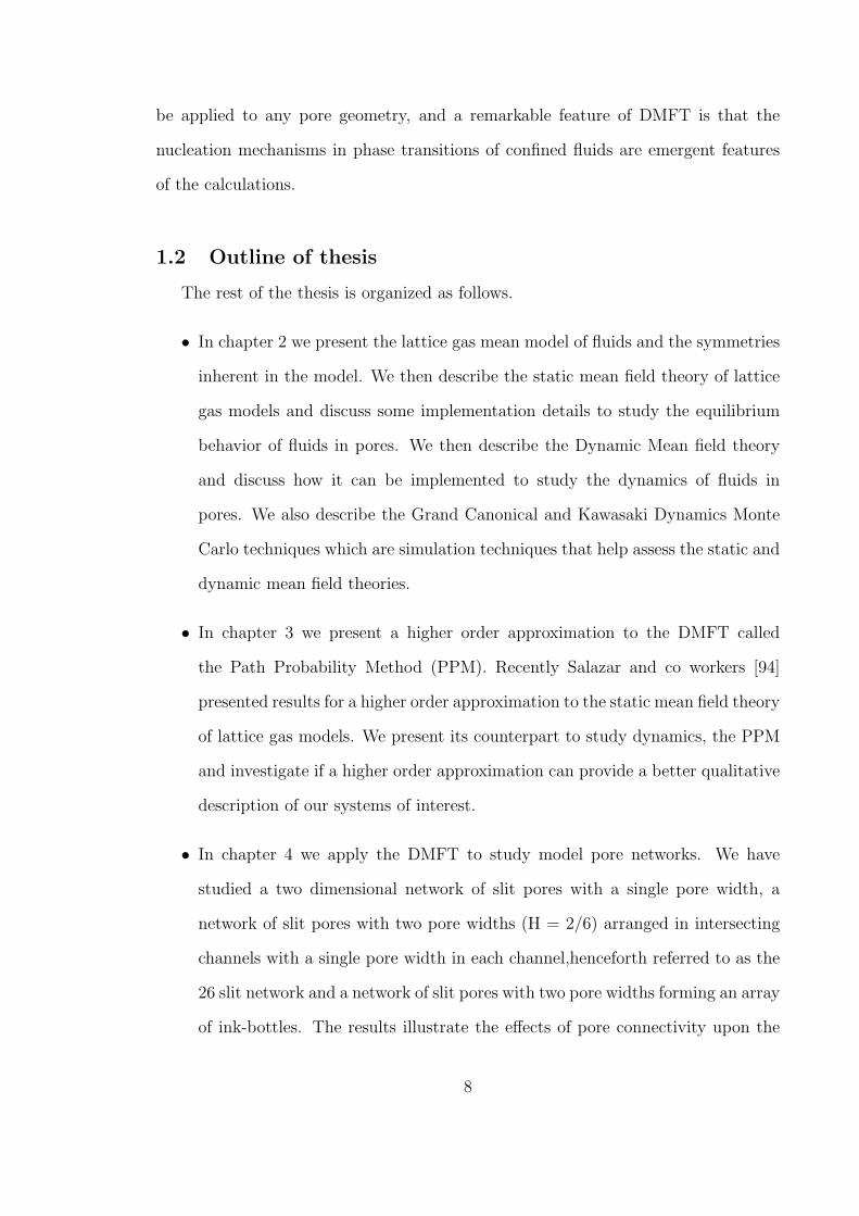
Figure 1.2: From the work of Monson [74]. a) Isotherms of the density (averagefractional occupancy), ρ, and grand potential, Ω, versus relative activity, λ/λ0 for aslit pore with H = 6 kept in contact with the bulk fluid. The curve above the zeroline is the density isotherm and the curve below the zero line is the grand potentialisotherm. b) Density of the slit pore versus time for L = 40 during a step changeof the relative activity from λ/λ0 = 0.00674 to λ/λ0 = 0.951. The initial and finalpoints of the step change are denoted by black dots in the isotherm. The full linegives the average density throughout the pore and the dashed line gives the averagedensity of two planes present mid-way between the ends of the pore.

abilities. The transition probabilities can be related to the chemical potential from

mean field density functional theory (DFT) of the lattice gas model and the density

distribution predicted by the DMFT approaches the distribution from DFT for long

times. As we shall we be seeing later in this thesis one of the significant advantages of

this theory is its ability to describe the thermodynamic (static) and dynamic behavior

of the system within the same framework.

1.1 Illustrative example

We first present a calculation done by Monson [74] to illustrate the utility of the

dynamic mean field theory and provide a flavour of the wide variety of problems that

can be investigated with this approach. The system is a slit pore geometry which is

two solid walls kept parallel to each other. The walls of this system strongly attract

5

the fluid under study. The equilibrium behavior of fluid in a pore is given by its

adsorption isotherm which gives the pore fluid density at a fixed relative activity. The

adsorption isotherm of a slit pore of height H = 6, together with its grand potential

is shown in figure 1.2a. The step in the isotherm at lower activity is associated with

the formation of a monolayer, and the step closer to the bulk saturation (λ/λ0 = 1.0)

is associated with a capillary condensation transition. The grand potential isotherm

shows two branches, the intersection of which denotes the equilibrium vapor liquid

transition. Monson studied the dynamics associated with pore filling. The slit pore

is initialized at an initial state (black dot in figure 1.2a at λ/λ0 = 0.00674) where it

is almost empty. The activity of the bulk fluid is then changed to a state where fluid

is present in a condensed state in the pore (black dot in figure 1.2a at high relative

activity λ/λ0 = 0.95). DMFT can predict the evolution of the density distribution of

the system which we have visualized using the graphics package RASMOL.

Figure 1.2b shows the density evolution curves of the total density of the pore

and the density in two layers of sites at the middle of the slit pore in the y-z plane.

Figure 1.3 shows some snapshots of the slit pore during the evolution process. The

uptake in the initial phase is associated with formation of adsorbed monolayers on

the pore walls and this is associated with the steep rise in density seen in figure 1.2b.

Then undulates form near the two ends of the pore which lead to the formation of

liquid bridges between the pore walls. This is associated with the cusp in the density

evolution curve of the pore. The formation of liquid bridges at the pore ends is also

associated with some depletion in density in the middle of pore and it is clear from

the dashed line in figure 1.2b. Thereafter the uptake slows down due to an internal

mass transfer resistance associated with transfer of fluid across the liquid bridges into

the pore. The example illustrates the level of information provided by this theory.

Moreover the DMFT has the ability to access length and time scales which are almost

impossible with a grand canonical molecular dynamics simulations. The theory can

6

(a)

(b)

(c)

(d)

(e)

(f)

(g)

(h)

(i)

Figure 1.3: From the work of Monson [74]. Visualizations of the density distributionin a slit pore of length 40 lattice units showing the process of pore filling during astep change of the relative activity from λ/λ0 = 0.00674 to λ/λ0 = 0.951. a)w0t = 0;b) w0t = 400; c) w0t = 2000; d) w0t = 6000; e) w0t = 8000; f) w0t = 16000; g)w0t = 16400; h) w0t = 18400; i) w0t = 24000. A darker shade of gray indicates ahigher density.

7

be applied to any pore geometry, and a remarkable feature of DMFT is that the

nucleation mechanisms in phase transitions of confined fluids are emergent features

of the calculations.

1.2 Outline of thesis

The rest of the thesis is organized as follows.

• In chapter 2 we present the lattice gas mean model of fluids and the symmetries

inherent in the model. We then describe the static mean field theory of lattice

gas models and discuss some implementation details to study the equilibrium

behavior of fluids in pores. We then describe the Dynamic Mean field theory

and discuss how it can be implemented to study the dynamics of fluids in

pores. We also describe the Grand Canonical and Kawasaki Dynamics Monte

Carlo techniques which are simulation techniques that help assess the static and

dynamic mean field theories.

• In chapter 3 we present a higher order approximation to the DMFT called

the Path Probability Method (PPM). Recently Salazar and co workers [94]

presented results for a higher order approximation to the static mean field theory

of lattice gas models. We present its counterpart to study dynamics, the PPM

and investigate if a higher order approximation can provide a better qualitative

description of our systems of interest.

• In chapter 4 we apply the DMFT to study model pore networks. We have

studied a two dimensional network of slit pores with a single pore width, a

network of slit pores with two pore widths (H = 2/6) arranged in intersecting

channels with a single pore width in each channel,henceforth referred to as the

26 slit network and a network of slit pores with two pore widths forming an array

of ink-bottles. The results illustrate the effects of pore connectivity upon the

8

dynamics of vapor liquid phase transformations as well as on the mass transfer

resistances to equilibration.

• In chapter 5 we apply the DMFT to study systems with partially wetting pore

walls. In these systems a capillary condensation transition is only observed

at pressures higher than the bulk saturation pressure though the equilibrium

transition lies below the saturation pressure. We have studied the dynamics

of capillary condensation in a slit pore geometry and present cases where the

pore filling process features an asymmetric density distribution where a liquid

droplet appears on one of the walls.

• In chapter 6 we apply the DMFT to study systems with completely drying

and partially drying pore walls. The motivation behind this study was to

understand intrusion/extrusion of non-wetting liquids into pores[86, 85, 13],

such as in mercury porosimetry [86, 85]. It is also of wider interest in con-

nection with the general problem of dewetting processes between hydrophobic

surfaces[4, 51, 52, 56, 57, 58]. We present some results on the dynamics of cap-

illary evaporation in slit pores and in a slab geometry with homogeneous and

patterned walls.

• In chapter 7 we present an extension of the DMFT framework to study confined

fluid mixtures. While the theory can be applied to mixtures with any number

of components we restrict our numerical investigations to just binary mixtures.

We have chosen two different mixtures and studied the dynamics of capillary

condensation and cavitation in slits and ink bottle pores respectively.

• In chapter 8 we present comparisons of the DMFT with Kawasaki Dynamics

Monte Carlo simulations. The problem we chose to make the comparisons is

the dynamics of capillary condensation in slit pores. Our primary objective

of this study was to assess if the predictions of the DMFT were qualitatively

9

consistent with the simulations. We have also presented some analysts of the

simulation results that provide more information on the dynamics of capillary

condensation in slits.

• Finally we present a summary of our work and possible future directions in

chapter 9.

10

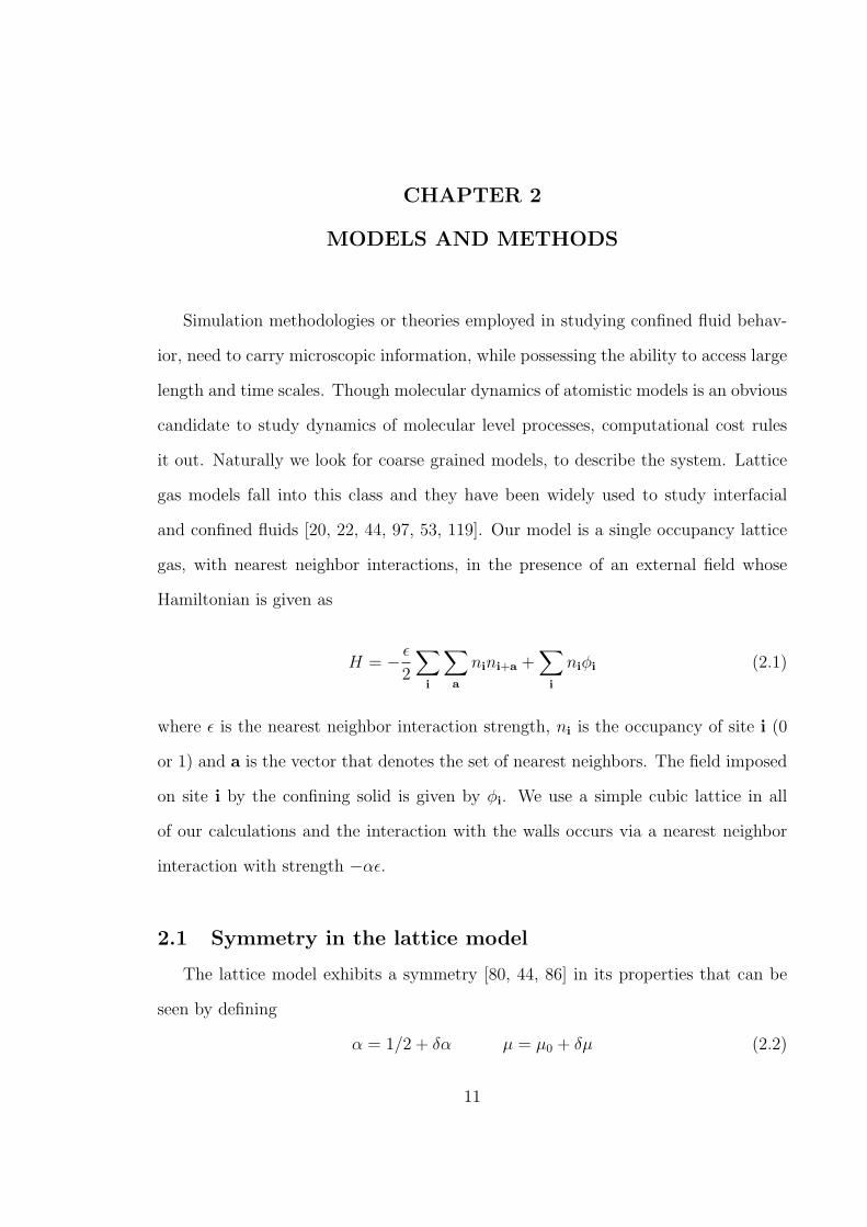
CHAPTER 2

MODELS AND METHODS

Simulation methodologies or theories employed in studying confined fluid behav-

ior, need to carry microscopic information, while possessing the ability to access large

length and time scales. Though molecular dynamics of atomistic models is an obvious

candidate to study dynamics of molecular level processes, computational cost rules

it out. Naturally we look for coarse grained models, to describe the system. Lattice

gas models fall into this class and they have been widely used to study interfacial

and confined fluids [20, 22, 44, 97, 53, 119]. Our model is a single occupancy lattice

gas, with nearest neighbor interactions, in the presence of an external field whose

Hamiltonian is given as

H = − ε

2

∑

i

∑a

nini+a +∑

i

niφi (2.1)

where ε is the nearest neighbor interaction strength, ni is the occupancy of site i (0

or 1) and a is the vector that denotes the set of nearest neighbors. The field imposed

on site i by the confining solid is given by φi. We use a simple cubic lattice in all

of our calculations and the interaction with the walls occurs via a nearest neighbor

interaction with strength −αε.

2.1 Symmetry in the lattice model

The lattice model exhibits a symmetry [80, 44, 86] in its properties that can be

seen by defining

α = 1/2 + δα µ = µ0 + δµ (2.2)

11

where µ0 is the chemical potential at bulk saturation (µ0 = −zε/2 for the lattice

gas model with coordination number z). Positive values of δα are associated with

the situation where the fluid wets or partially wets the solid and negative values

are associated with a drying (non wetting) or partially drying situation. Positive

values of δµ correspond to the stable liquid state of the bulk fluid and negative values

to the stable vapor state of the bulk fluid. The state of a fluid with positive δα

and negative δµ (corresponding to gas adsorption/desorption in the wetting case)

is isomorphic with that of a fluid with negative δα and positive δµ of the same

magnitudes as in the wetting case and with all the fluid site occupancies reversed

(corresponding to intrusion/extrusion in the drying case). This symmetry is only

very roughly followed in off-lattice models or in nature. Nevertheless it is a useful

line of thinking and has helped researchers understand, for instance, the relationship

between pore characterization methods based on gas adsorption to those based on

mercury porosimetry[86].

2.2 Static Behavior

2.2.1 Mean field theory (MFT)

We start by describing the lattice density functional theories that we use to study

the equilibrium behavior of confined fluids. The mean field (MFT) Helmholtz energy

is written

F = kT∑

i

[ρi ln ρi + (1− ρi) ln(1− ρi)]− ε

2

∑

i

∑a

ρiρi+a +∑

i

ρiφi (2.3)

where ρi is the mean density at site i. Similarly the grand free energy is given by

Ω = kT∑

i

[ρi ln ρi + (1− ρi) ln(1− ρi)]− ε

2

∑

i

∑a

ρiρi+a +∑

i

ρi (φi − µ) (2.4)

12

where µ is the chemical potential. By minimizing Ω at fixed chemical potential or F

at fixed overall density we can obtain solutions of the mean field equations for the

grand canonical and canonical ensembles, respectively. These yield the free energy

and density distributions in these ensembles. In both cases the necessary condition

for equilibrium leads to the following equations relating the chemical potential to the

local density at site i.The necessary condition for a Helmholtz energy minimum, at

fixed temperature and overall density is

∂F

∂ρi

− µ = 0 ∀ i (2.5)

where the chemical potential, appears as a Lagrange multiplier associated with the

constraint of fixed overall density. Using equations 2.5 with eqn. 2.3 it is readily

shown that

ρi =λci

1 + λci∀ i (2.6)

where λ = exp (µ/kT ) is the activity and ci = exp [− (φi − ε∑

a ρi+a) /kT ]. This set

of equations can be solved together with the density constraint expressed as

∑

i

λci1 + λci

−N = 0 (2.7)

to give the equilibrium density distribution and the chemical potential in the canonical

ensemble. We iterate through equations 2.6 and 2.7 by writing

ρ(n+1)i =

λ(n)c(n)i

1 + λ(n)c(n)i

∀ i (2.8)

and

λ(n+1) = λ(n)N

(∑

i

λ(n)c(n)i

1 + λ(n)c(n)i

)−1

(2.9)

13

The results for the grand ensemble (fixed µ, V, T ) are obtained by solving equations

2.6 without the density constraint, equation 2.7. Equation 2.6 can be rearranged to

give an expression for the chemical potential at site i

µi = kT ln

[ρi

1− ρi

]− ε

∑a

ρi+a + φi (2.10)

Solutions of the static MFT equations lead to the µi being uniform throughout the

system. This equation also helps establish the limiting behavior of the dynamic mean

field theory for long times.

2.2.2 Grand Canonical Monte Carlo Simulations

A direct assessment of the validity of the mean field approximation can be done

by performing Grand Canonical Monte Carlo (GCMC) simulations. We also use this

technique to understand phenomena were fluctuations might play a significant role.

The GCMC technique on lattices is well established [78] and involves moves where

a particle is either created on a random site, or removed from the system. The

acceptance criteria are given by

acc(N → N + 1) = min [1, expβ[µ− U(N + 1) + U(N)]] (2.11)

acc(N → N − 1) = min [1, exp−β[µ + U(N − 1)− U(N)]] (2.12)

where µ is the chemical potential at which we want the system to equilibrate at

and β is inverse temperature. An isotherm is typically computed by carrying out

simulations for a sequence of states with increasing / decreasing chemical potential

with the run at each new state initiated from the configuration at the end of the run

at the previous state.

14

2.3 Dynamic Behavior

Before we present theories that describe dynamics we brief state the phenomenol-

ogy we employ to describe diffusion in a lattice gas - Kawasaki Dynamics. It is a very

basic model in which particles move to neighboring sites via vacancy hopping. In the

past our group has used Kawasaki Dynamics Monte Carlo simulations on a lattice

gas, to study the dynamic behavior of fluids [85, 117, 115]. As we shall see below this

phenomenology was retained, to describe diffusion, in our dynamic field theories. We

start by briefly describing the Dynamic Mean Field Theory (DMFT).

As seen in section 2.2 density functional theories allow us to calculate the free

energy and density distribution for fluids inside porous materials for equilibrium states

of the system. In building theories to describe relaxation dynamics under confinement,

it is advantageous to focus on approaches that have built into them a description

of the thermodynamics from DFT. This idea dates back to the work of Cahn [10]

who incorporated the Cahn-Hilliard square gradient free energy functional[9] into a

diffusion equation and used the resulting equation to describe the early stages of

spinodal decomposition.

Following this approach Monson [74] developed the dynamic mean field theory

(DMFT). DMFT [74, 37, 69] gives an approximation to the time evolution of the

density distribution averaged over an ensemble of kinetic Monte Carlo simulations of

the lattice gas model using Kawasaki dynamics. It provides a theory of the dynam-

ics of the system consistent with the thermodynamics in mean field theory [74] as

described in section 2.2.1. The DMFT approach of Monson closely follows the work

of Gouyet and coworkers [37] which in-turn is based on the seminal contributions of

Martin[65] and Penrose[82], but yields equations identical to those of Matuszak et

al.[69].

15

2.3.1 Dynamic Mean Field Theory

In DMFT the evolution of the ensemble average density at site i can be expressed

exactly in terms of the net fluxes from site i to its nearest neighbor sites i + a via

∂ρi

∂t= −

∑a

< wi,i+a(n)ni(1− ni+a)− wi+a,i(n)ni+a(1− ni) >t (2.13)

where wi,i+a(n) is the transition probability for transitions from site i to site

i + a for a configuration n. The occupancy factors ni(1 − ni+a) and ni+a(1 − ni)

impose the requirement that in a hopping move from site i to site j, site i must be

occupied and site j unoccupied, and vice versa.

In the mean field approximation we obtain

∂ρi

∂t= −

∑a

[wi,i+a(ρ)ρi(1− ρi+a)− wi+a,i(ρ)ρi+a(1− ρi)] (2.14)

Given expressions for the transition probabilities, eqn. 2.14 can be solved to obtain

ρi as a function of t. The mean field approximation for the Metropolis transition

probabilities in Kawasaki dynamics yields

wij(ρ) = wo exp(−Eij/kT ) (2.15)

where

Eij =

0 Ej < Ei

Ej − Ei Ej > Ei

(2.16)

and

Ei = −ε∑a

ρi+a + φi (2.17)

Using equations 2.10 and 2.15 we obtain

16

∂ρi

∂t= −

∑a

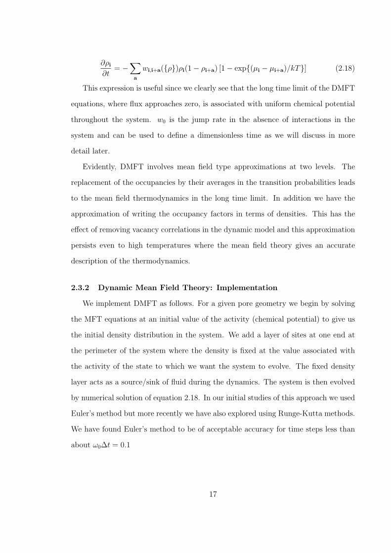
wi,i+a(ρ)ρi(1− ρi+a) [1− exp(µi − µi+a)/kT] (2.18)

This expression is useful since we clearly see that the long time limit of the DMFT

equations, where flux approaches zero, is associated with uniform chemical potential

throughout the system. w0 is the jump rate in the absence of interactions in the

system and can be used to define a dimensionless time as we will discuss in more

detail later.

Evidently, DMFT involves mean field type approximations at two levels. The

replacement of the occupancies by their averages in the transition probabilities leads

to the mean field thermodynamics in the long time limit. In addition we have the

approximation of writing the occupancy factors in terms of densities. This has the

effect of removing vacancy correlations in the dynamic model and this approximation

persists even to high temperatures where the mean field theory gives an accurate

description of the thermodynamics.

2.3.2 Dynamic Mean Field Theory: Implementation

We implement DMFT as follows. For a given pore geometry we begin by solving

the MFT equations at an initial value of the activity (chemical potential) to give us

the initial density distribution in the system. We add a layer of sites at one end at

the perimeter of the system where the density is fixed at the value associated with

the activity of the state to which we want the system to evolve. The fixed density

layer acts as a source/sink of fluid during the dynamics. The system is then evolved

by numerical solution of equation 2.18. In our initial studies of this approach we used

Euler’s method but more recently we have also explored using Runge-Kutta methods.

We have found Euler’s method to be of acceptable accuracy for time steps less than

about ω0∆t = 0.1

17

2.3.3 Kawasaki Dynamics Monte Carlo Simulations

We implement Kawasaki Dynamics Monte Carlo simulations via a control volume

simulation technique developed by Frank van Swol and coworkers [81]. We will refer to

our dynamics simulation with the acronym DMC. We divide our simulation volume,

into two regions, the system and the control volume. The system and control volume

are first equilibrated by GCMC moves at an initial activity (chemical potential). A

step change is then made to the activity of the control volume to a state where we

want the system to evolve to. At every Monte Carlo sweep we perform two steps.

First we update all the sites in the control volume via Glauber moves k times(i.e

create a particle / destroy a particle). Then we attempt to move all the particles,

in the simulation box to the nearest neighbor site via a Kawasaki move (vacancy

hopping). The move is accepted based on a Metropolis criterion. In short we make

unphysical particle creations and deletions in the control volume, however the system

is accessible only via diffusive moves. In calculations shown in this paper the value of

k = 1 seems sufficient to maintain the control volume at a fixed chemical potential.

The initial / final state of a given step change in DMC can be a stable or metastable

state. If we begin with a metastable state, and we simulate the system in this state

without making a step change in the bulk reservoir, fluctuations would enable the

system to move to the stable equilibrium state eventually at long times. However

this process of spontaneous transition to a stable equilibrium cannot be studied with

the DMFT. Here if the initial state is metastable it is still a solution of the MFT

equations, and hence would not evolve to another equilibrium state.

In principle we can use this technique to study the system’s response to any other

kind of external stimuli. However in this thesis we have only considered step changes

to the bulk activity.

18

CHAPTER 3

HIGHER ORDER APPROXIMATIONS BEYOND DMFT:PATH PROBABILITY METHOD

3.1 Introduction

In this chapter the question we try to assess the validity of the Mean Field approx-

imation by comparing it with a higher order approximation. We start by comparing

the static behavior predicted by the MFT with an higher order approximation called

the Bethe Peierls approximation (BPA). The Bethe Peierls approximation (BPA), is

also a mean field approximation in spirit. It is better than the MFT in that, we

treat first nearest neighbor interactions via absolute occupancies, and the rest via

an effective field. Recently Salazar and Gelb [94] have implemented this method, to

study fluids in disordered porous materials. Detailed derivations of the BPA can be

found in Appendix B of their paper[94]. We briefly explain the theory in this chap-

ter. We then compare the DMFT with an higher order approximation called the Path

Probability method (PPM). The path probability method was introduced by Kikuchi

and co workers [47, 41] to study relaxation dynamics in binary alloys. This method

was developed to treat the lattice model at a desired level of approximation (pair,

triangle, square), but in this work we restrict ourselves to the pair approximation.

3.2 Bethe Peierls Approximation

The Bethe Peierls approximation (BPA), is also a mean field approximation in

spirit. It is better that the point approximation in that, we treat first nearest neighbor

interactions via absolute occupancies, and the rest via an effective field. We briefly

19

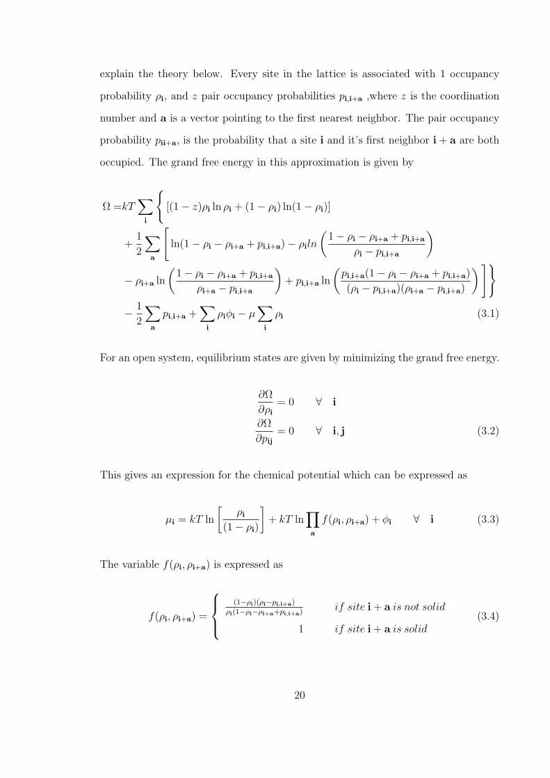
explain the theory below. Every site in the lattice is associated with 1 occupancy

probability ρi, and z pair occupancy probabilities pi,i+a ,where z is the coordination

number and a is a vector pointing to the first nearest neighbor. The pair occupancy

probability pii+a, is the probability that a site i and it’s first neighbor i + a are both

occupied. The grand free energy in this approximation is given by

Ω =kT∑

i

[(1− z)ρi ln ρi + (1− ρi) ln(1− ρi)]

+1

2

∑a

[ln(1− ρi − ρi+a + pi,i+a)− ρiln

(1− ρi − ρi+a + pi,i+a

ρi − pi,i+a

)

− ρi+a ln

(1− ρi − ρi+a + pi,i+a

ρi+a − pi,i+a

)+ pi,i+a ln

(pi,i+a(1− ρi − ρi+a + pi,i+a)

(ρi − pi,i+a)(ρi+a − pi,i+a)

) ]

− 1

2

∑a

pi,i+a +∑

i

ρiφi − µ∑

i

ρi (3.1)

For an open system, equilibrium states are given by minimizing the grand free energy.

∂Ω

∂ρi

= 0 ∀ i

∂Ω

∂pij

= 0 ∀ i, j (3.2)

This gives an expression for the chemical potential which can be expressed as

µi = kT ln

[ρi

(1− ρi)

]+ kT ln

∏a

f(ρi, ρi+a) + φi ∀ i (3.3)

The variable f(ρi, ρi+a) is expressed as

f(ρi, ρi+a) =

(1−ρi)(ρi−pi,i+a)

ρi(1−ρi−ρi+a+pi,i+a)if site i + a is not solid

1 if site i + a is solid(3.4)

20

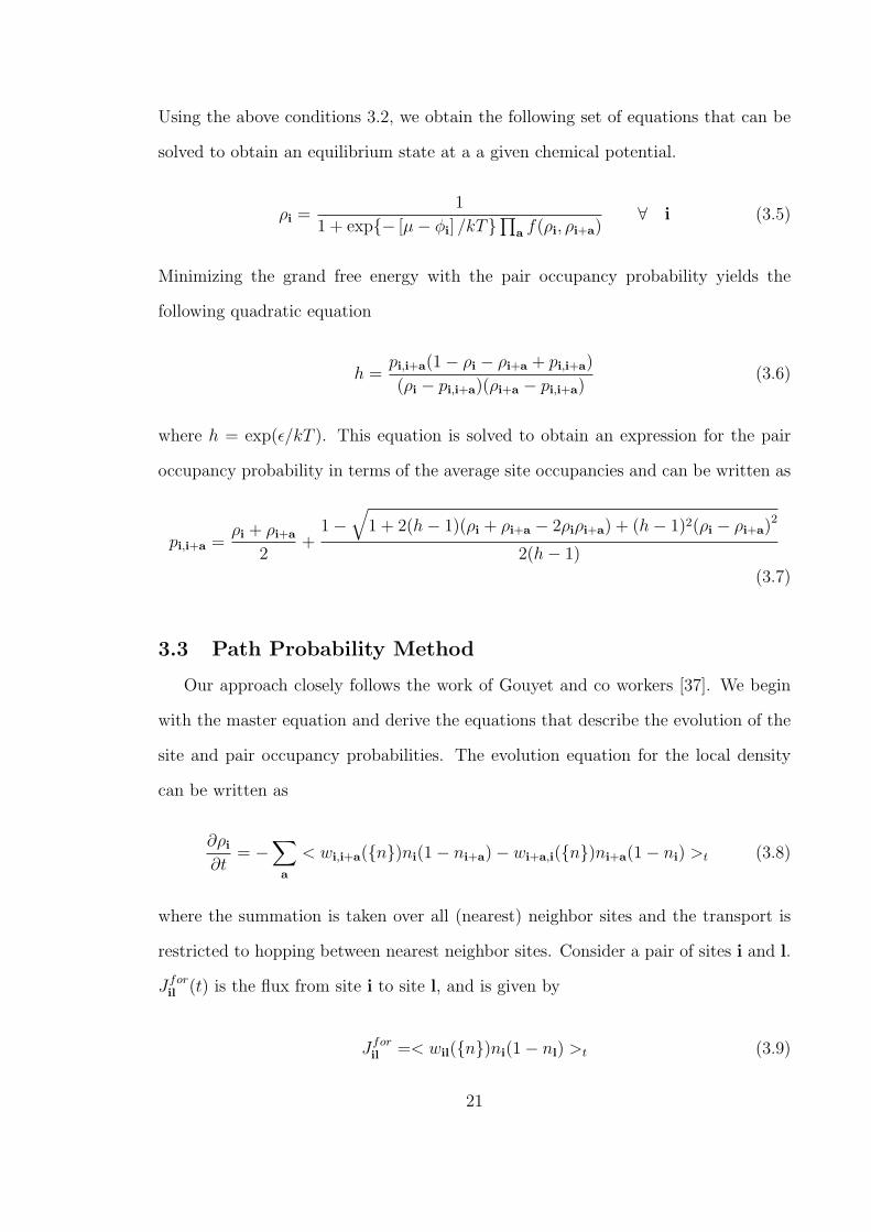
Using the above conditions 3.2, we obtain the following set of equations that can be

solved to obtain an equilibrium state at a a given chemical potential.

ρi =1

1 + exp− [µ− φi] /kT∏a f(ρi, ρi+a)∀ i (3.5)

Minimizing the grand free energy with the pair occupancy probability yields the

following quadratic equation

h =pi,i+a(1− ρi − ρi+a + pi,i+a)

(ρi − pi,i+a)(ρi+a − pi,i+a)(3.6)

where h = exp(ε/kT ). This equation is solved to obtain an expression for the pair

occupancy probability in terms of the average site occupancies and can be written as

pi,i+a =ρi + ρi+a

2+

1−√

1 + 2(h− 1)(ρi + ρi+a − 2ρiρi+a) + (h− 1)2(ρi − ρi+a)2

2(h− 1)

(3.7)

3.3 Path Probability Method

Our approach closely follows the work of Gouyet and co workers [37]. We begin

with the master equation and derive the equations that describe the evolution of the

site and pair occupancy probabilities. The evolution equation for the local density

can be written as

∂ρi

∂t= −

∑a

< wi,i+a(n)ni(1− ni+a)− wi+a,i(n)ni+a(1− ni) >t (3.8)

where the summation is taken over all (nearest) neighbor sites and the transport is

restricted to hopping between nearest neighbor sites. Consider a pair of sites i and l.

Jforil (t) is the flux from site i to site l, and is given by

Jforil =< wil(n)ni(1− nl) >t (3.9)

21

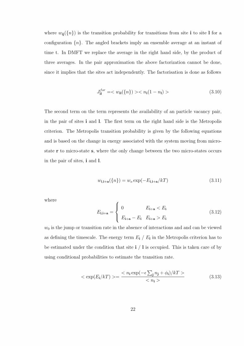
where wij(n) is the transition probability for transitions from site i to site l for a

configuration n. The angled brackets imply an ensemble average at an instant of

time t. In DMFT we replace the average in the right hand side, by the product of

three averages. In the pair approximation the above factorization cannot be done,

since it implies that the sites act independently. The factorisation is done as follows

Jforil =< wil(n) >< ni(1− nl) > (3.10)

The second term on the term represents the availability of an particle vacancy pair,

in the pair of sites i and l. The first term on the right hand side is the Metropolis

criterion. The Metropolis transition probability is given by the following equations

and is based on the change in energy associated with the system moving from micro-

state r to micro-state s, where the only change between the two micro-states occurs

in the pair of sites, i and l.

wi,i+a(n) = wo exp(−Ei,i+a/kT ) (3.11)

where

Ei,i+a =

0 Ei+a < Ei

Ei+a − Ei Ei+a > Ei

(3.12)

w0 is the jump or transition rate in the absence of interactions and and can be viewed

as defining the timescale. The energy term Ei / El in the Metropolis criterion has to

be estimated under the condition that site i / l is occupied. This is taken care of by

using conditional probabilities to estimate the transition rate.

< exp(Ei/kT ) >=< ni exp(−ε

∑j nj + φi)/kT >

< ni >(3.13)

22

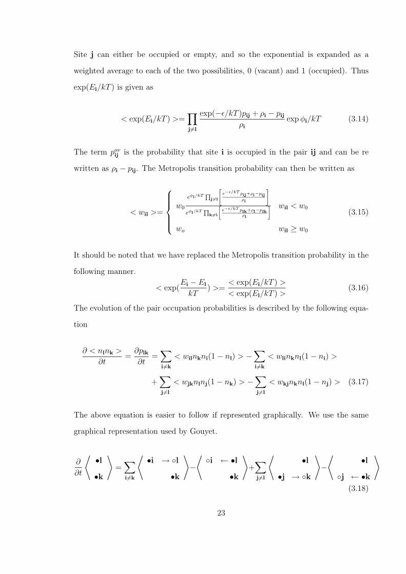
Site j can either be occupied or empty, and so the exponential is expanded as a

weighted average to each of the two possibilities, 0 (vacant) and 1 (occupied). Thus

exp(Ei/kT ) is given as

< exp(Ei/kT ) >=∏

j6=l

exp(−ε/kT )pij + ρi − pij

ρi

exp φi/kT (3.14)

The term povij is the probability that site i is occupied in the pair ij and can be re

written as ρi − pij. The Metropolis transition probability can then be written as

< wil >=

w0

eφi/kTQ

j6=l

"e−ε/kT pij+ρi−pij

ρi

#

eφl/kTQ

k6=i

»e−ε/kT plk+ρl−plk

ρl

– wil < w0

wo wil ≥ w0

(3.15)

It should be noted that we have replaced the Metropolis transition probability in the

following manner.

< exp(Ei − El

kT) >=

< exp(Ei/kT ) >

< exp(El/kT ) >(3.16)

The evolution of the pair occupation probabilities is described by the following equa-

tion

∂ < nlnk >

∂t=

∂plk

∂t=

∑

i6=k

< wilnkni(1− nl) > −∑

i 6=k

< wlinknl(1− ni) >

+∑

j 6=l

< wjknlnj(1− nk) > −∑

j 6=l

< wkjnknl(1− nj) > (3.17)

The above equation is easier to follow if represented graphically. We use the same

graphical representation used by Gouyet.

∂

∂t

⟨•l•k

⟩=

∑

i 6=k

⟨•i → l

•k

⟩−

⟨i ← •l

•k

⟩+

∑

j6=l

⟨•l

•j → k

⟩−

⟨•l

j ← •k

⟩

(3.18)

23

Terms 1 and 3 in the above equation 3.16 are pair creation terms, and terms 2 and

4 are pair annihilation terms. We factorize the above equation, in terms to pair and

point occupation probabilities, as follows. Consider term 1 on the right hand side.

< wilnkni(1− nl) >=< nk(1− nl) >

< (1− nl) >< Jil(n) >t (3.19)

In other words term 1 is nothing but the flux from site i to site l having site k

occupied.

< wilnkni(1− nl) >=ρk − plk

(1− ρl)< Jil(n) >t (3.20)

Similarly term 2 is flux from l to site i given that, site k is occupied. The presence of

a particle in site k is accounted for by carefully evaluating the Metropolis criterion.

The term e−βplk + ρl − plk which is the contribution to energy El is replaced with

e−βplk since site k is occupied.

3.4 Long time behavior

At the final equilibrium state we have from equation 3.8

< wil >

< wli >=

(ρi − pil)

(ρl − pil)= w0

eβφi∏

j6=l

[e−βpij+ρi−pij

ρi

]

eβφl∏

k6=i

[e−βplk+ρl−plk

ρl

] (3.21)

By using the equation 3.6 it can be shown the above equation reduces to

exp(µi − µl) = 1 (3.22)

which results in uniform chemical potential throughout the system. Also at the steady

state the first two terms in equation 3.18 can be equated to zero. Using equations

3.21 we can show that the first two terms at the steady state reduce to equation 3.6.

Thus the states predicted by the PPM in the long time limit are consistent with the

states predicted by the BPA.

24

0

0.25

0.5

0.75

1

1.25

1.5

0 0.2 0.4 0.6 0.8 1

T

ρ

MFTBPA

Series approx.

(a)

0

0.25

0.5

0.75

1

0 0.2 0.4 0.6 0.8 1

Tr

ρ

MFTBPA

Series approx.

(b)

Figure 3.1: Phase coexistence diagram of the bulk lattice gas a) T vs ρ and b) Tr vsρ, computed the MFT, BPA methods and compared with the series approximationresults of Essam and Fisher [27].

3.5 Results and Discussion

3.5.1 Bulk Phase behavior

In figure the bulk phase diagram of the lattice gas computed with the MFT and

BPA is compared with the Pade series approximation of Essam and Fisher [27]. As

shown in figure 3.1 inclusion of correlations at just the pair level, decreases the critical

temperature of the system from T ∗C = 1.5 (MFT) to T ∗

C = 1.233 (BPA), much closer

to the critical temperature of the lattice gas which is T ∗C = 1.128. Figure 3.1b shows

the three binodals scaled with their respective critical temperatures. We compare the

results of the DMFT and the PPM methods at the same relative temperature T/Tc,

in order to make the comparison more relevant.

3.5.2 Static Behavior

The system we consider is an ideal slit pore with wettability y = 3.0, the schematic

of which is shown in chapter 7 (refer figure 8.1). The comparison is done at a fixed

reduced temperature T/Tc = 0.66. In figure 3.2 we plot isotherms of a slit pore of

width H = 6 computed by the MFT, BPA methods and GCMC simulations. Each

25

0

1

2

3

0 0.25 0.5 0.75 1ρ

λ/λ0

Figure 3.2: Isotherms of a slit pore of width H = 6 and length L = 40 computed withMFT (black) BPA (blue) and GCMC (red) simulations. The full lines are for a porein contact with bulk fluid, and the dashed lines are for a slit pore placed in periodicboundaries. The curves are shifted along the y-axis by 1 unit each for clarity

curve is shifted along the y - axis by 1.0 for clarity. For each method we plot the

isotherm of a pore of finite length L = 40 (full line) and an infinite pore (dashed line).

The finite length pore desorbs at a higher activity than the infinite pore since it is

directly in contact with the bulk reservoir, an observation first made by Marconi and

van Swol [64, 63]. At a given reduced temperature confinement effects are felt least

in MFT with the hysteresis loop being the widest in the mean field approximation

and narrowest when computed with GCMC simulations.

3.5.3 Dynamic Behavior

The case we pick to compare the dynamics predicted by the DMFT and PPM is

the filling of a slit pore of length L = 40 from a dilute state to a completely filled state.

The comparison with the DMC simulations is shown in chapter 8 (Step change V).

The density evolution curves predicted by the DMFT and PPM are shown in figure

3.3. The visualizations of the states encountered in the dynamics in shown in figure

3.4. Dynamics at short times is associated with the formation of a liquid like mono-

26

0

0.25

0.5

0.75

1

0 15000 30000 45000

ρ

w0 t

(a)

0

0.25

0.5

0.75

1

0 15000 30000 45000

ρ

w0t

(b)

Figure 3.3: Density evolution curves for a step change in relative activity from λ/λ0 =0.001 to λ/λ0 = 0.95 a) DMFT b) PPM. Density of the pore : solid line. Density ofa layer of sites in the middle of the pore : Dashed Line

layer at the pore walls. It is then followed by the appearance of two liquid bridges at

the ends of the pore which then proceed to fill the pore. The visualizations clearly

indicate the predictions of the DMFT qualitatively agree with the PPM technique.

The density evolution curve also agree qualitatively with each other. There are subtle

differences however when we compare the density evolution of the middle of the pore

(dashed curves) shown in figure 3.3. In case of the DMFT this curve separates from

the overall density curve right before the cusp corresponding to the formation of the

liquid bridge. This indicates that the undulates that precede the liquid bridges are

formed by temporary redistribution of density from the middle of the pore to the

ends of the pore. This is not predicted by the PPM. However the fall in density in

the middle of the pore during the instant the bridge is formed (cusp of the overall

pore density curve) is predicted by both the methods. This may be a consequence

of the difference in temperatures used in the two methods in order to use the same

value of T/Tc. Here we restrict the comparisons to just one case. Later in chapter

6 we present more comparisons of the DMFT with the PPM for partial drying and

complete drying situations.

27

Figure 3.4: Visualizations of states emergent in the dynamics during a step in changein relative activity from λ/λ0 = 0.001 to λ/λ0 = 0.95 for a L = 40 slit pore predictedby the DMFT (left panel) and the PPM (right panel) methods

3.6 Conclusion

We began with the Bethe Peierls Approximation which is a higher order approx-

imation to the MFT or the lattice gas mean field theory. We then presented the

dynamic counterpart of the BPA or the higher order approximation to the DMFT

namely the Path Probability Method. We chose to compare the DMFT with the

PPM at the same reduced temperature since the bulk and confined phase behavior

are more comparable in this way.We have demonstrated with a test case that for com-

pletely wetting systems in sub critical conditions the predictions of the DMFT show

good qualitative agreement with the PPM. The dis advantage of the PPM lies in the

fact that for every lattice site z + 1 equations have to be integrated in comparison to

just one for the DMFT. Also the equations are stiffer in comparison to the DMFT,

thus requiring finer time steps while using explicit integrators. This results in about

an order of magnitude increase in computation time. Given that our model is a lat-

tice gas and our objective is to study relaxation mechanisms of confined fluids under

sub-critical conditions in a qualitative fashion we do not find a compelling reason to

use the PPM over the DMFT.

28

CHAPTER 4

DMFT : APPLICATION TO PORE NETWORKS

The void space in many porous materials consist of networks of interconnected

pores and an important question from the point of view of characterization by gas ad-

sorption and mercury porosimetry is the extent to which such systems can be viewed

as collections of independent pores with a distribution in pore size. The indepen-

dent pore concept underlies most standard characterization procedures based on gas

adsorption measurements[93, 103]. Yet as has been known for many years there are

good reasons to question the applicability of those concepts[29]. For instance des-

orption can be strongly influenced by void space connectivity through pore blocking

and cavitation[67, 66, 68, 44, 45, 117, 118, 119]. For disordered materials very slow

adsorption dynamics may make the concept of equilibrium essentially irrelevant in

understanding the isotherm in the region where there is hysteresis[44, 45, 115, 117].

The ability to model the thermodynamics of fluids confined in model network struc-

tures with classical density functional theory represents an important step forward in

our understanding of these systems as has been shown in a number of recent studies

[28, 61, 60, 44, 98, 45, 117, 34, 36, 94, 95, 102], especially with lattice gas models

where 2-D and 3-D calculations are especially feasible.

Here we take this a step further by considering the dynamic behavior of adsorption

and desorption in pore network systems. Some of the interesting questions that we

try to understand are a) What are the transport resistances that affect fluid uptake

? b) Does pore connectivity affect the nucleation mechanisms of an associated phase

29

transition (capillary condensation / cavitation) ? c) Can data obtained from dynamic

uptake experiments help characterize porous materials ?

We apply DMFT to three model pore networks:

• A network of slit pores with a single pore width (H=6)

• A network of slit pores with two pore widths (H=2 / 6) arranged in intersecting

channels with a single pore width in each channel, henceforth referred to as the

2-6 slit network

• A network of slit pores with two pore widths forming an array of ink-bottles

The pore geometries are illustrated in figure 4.1. These examples were chosen to

illustrate key concepts in the thermodynamics and dynamics of fluids confined in pore

networks. For the single pore width we compare the thermodynamics and dynamics

with that of a single slit pore and study the effect of the junctions in the network

upon the observed behavior. For the system with two pore widths we are interested

in studying the effects of microporous connectivity upon the thermodynamics and

dynamic uptake mechanisms and whether this leads to any cooperative behavior. We

also consider the nature of the mass transfer resistances in the system. We chose the

ink-bottle network with a narrow neck diameter to match the situation encountered in

experiments on hierarchically ordered mesoporous silicas[114, 48, 87] where desorption

from the larger pores occurs by cavitation rather than pore blocking. We also look

at the dynamics of cavitation and pore filling in these systems. All of these systems

are uniform and infinite in the plane normal to the paper. All calculations presented

in this chapter are for nearest neighbor walls with a ratio of solid-fluid to fluid-fluid

interaction strengths of εsf/εff = α = 3.0 and at a temperature T ∗ = kT/ε = 1.0.

30

(a) (b)

(c) (d)

Figure 4.1: Pore geometries considered in this work. a) a single pore b) a slit network;c) Network of slit pores with two pore widths arranged in intersecting channels witha single pore width in each channel; d) Network of slit pores with two pore widthsforming an array of ink-bottles.

31

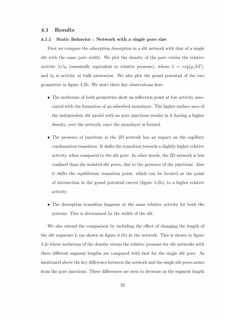
4.1 Results

4.1.1 Static Behavior : Network with a single pore size

First we compare the adsorption desorption in a slit network with that of a single

slit with the same pore width. We plot the density of the pore versus the relative

activity λ/λ0 (essentially equivalent to relative pressure), where λ = exp(µ/kT ),

and λ0 is activity at bulk saturation. We also plot the grand potential of the two

geometries in figure 4.2b. We state three key observations here.

• The isotherms of both geometries show an inflection point at low activity asso-

ciated with the formation of an adsorbed monolayer. The higher surface area of

the independent slit model with no pore junctions results in it having a higher

density, over the network, once the monolayer is formed.

• The presence of junctions in the 2D network has an impact on the capillary

condensation transition. It shifts the transition towards a slightly higher relative

activity, when compared to the slit pore. In other words, the 2D network is less

confined than the isolated slit pores, due to the presence of the junctions. Also

it shifts the equilibrium transition point, which can be located as the point

of intersection in the grand potential curves (figure 4.2b), to a higher relative

activity.

• The desorption transition happens at the same relative activity for both the

systems. This is determined by the width of the slit.

We also extend the comparison by including the effect of changing the length of

the slit segments L (as shown in figure 4.1b) in the network. This is shown in figure

4.2c where isotherms of the density versus the relative pressure for slit networks with

three different segment lengths are compared with that for the single slit pore. As

mentioned above the key difference between the network and the single slit pores arises

from the pore junctions. These differences are seen to decrease as the segment length

32

0

0.25

0.5

0.75

1

0 0.25 0.5 0.75 1

ρ

λ/λ0

SlitNetwork

(a)

-1

-0.75

-0.5

-0.25

0

0 0.25 0.5 0.75 1

Ω

λ/λ0

SlitNetwork

(b)

0

0.25

0.5

0.75

1

0 0.25 0.5 0.75 1

ρ

λ/λ0

SlitL=8

L=12L=24

(c)

-1

-0.75

-0.5

-0.25

0

0 0.25 0.5 0.75 1

Ω

λ/λ0

SlitL=8

L=12L=24

(d)

Figure 4.2: a) Adsorption isotherm and b) Grand potential, for the 2D Network(dashed line) vs. the slit pore (full line) c) Adsorption isotherm and b) Grand po-tential of slit pore networks with segment lengths of L = 8/12/24 compared with asingle slit pore. All the isotherms are computed at T ∗ = 1.0.

33

(a) (b) (c) (d)

(e) (f) (g) (h)

Figure 4.3: Visualizations of the density distribution for fluid uptake in a 2D slitnetwork, during a step change of the relative activity from λ/λ0 = 0.005 to λ/λ0 =0.95 : (a) w0t = 0, (b) w0t = 10000, (c) w0t = 20000, (d) w0t = 45000, (e) w0t =50000, (f) w0t = 70000, (g) w0t = 120000, (h) w0t = 140000.

increases and the condensation step in the network moves toward that for the single

slit. Indeed for a segment length of 24 sites the condensation steps for the network

and single pore are very close. This reflects the fact that as the segment length is

increasing the fraction of the pore volume occupied by the junctions is decreasing.

The grand free energy isotherm for the three different segment lengths shown in figure

4.2d add support to the arguments presented above. In essence, the independent pore

model would tend to overestimate the pore size distribution of a system where the

junctions occupy a significant pore volume.

4.1.2 Dynamic Behavior : Network with a single pore size

Here we consider the dynamics associated with a step change in relative activity

of λ/λ0 = 0.005 to λ/λ0 = 0.95. The initial state of the system corresponds to an

almost empty pore, and the final state corresponds to a completely filled pore. The

uptake behavior of the 2D network is richer as seen from the visualizations in 4.3.

34

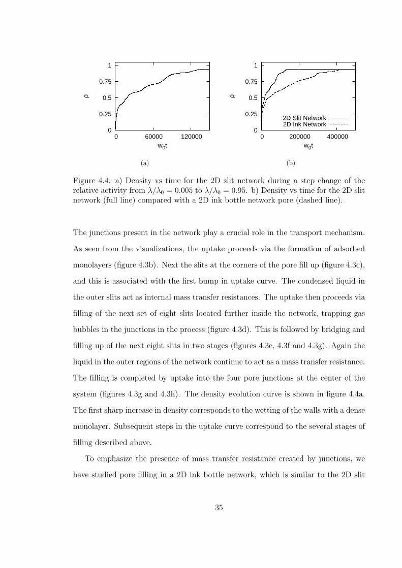
0

0.25

0.5

0.75

1

0 60000 120000

ρ

w0t

(a)

0

0.25

0.5

0.75

1

0 200000 400000

ρ

w0t

2D Slit Network2D Ink Network

(b)

Figure 4.4: a) Density vs time for the 2D slit network during a step change of therelative activity from λ/λ0 = 0.005 to λ/λ0 = 0.95. b) Density vs time for the 2D slitnetwork (full line) compared with a 2D ink bottle network pore (dashed line).

The junctions present in the network play a crucial role in the transport mechanism.

As seen from the visualizations, the uptake proceeds via the formation of adsorbed

monolayers (figure 4.3b). Next the slits at the corners of the pore fill up (figure 4.3c),

and this is associated with the first bump in uptake curve. The condensed liquid in

the outer slits act as internal mass transfer resistances. The uptake then proceeds via

filling of the next set of eight slits located further inside the network, trapping gas

bubbles in the junctions in the process (figure 4.3d). This is followed by bridging and

filling up of the next eight slits in two stages (figures 4.3e, 4.3f and 4.3g). Again the

liquid in the outer regions of the network continue to act as a mass transfer resistance.

The filling is completed by uptake into the four pore junctions at the center of the

system (figures 4.3g and 4.3h). The density evolution curve is shown in figure 4.4a.

The first sharp increase in density corresponds to the wetting of the walls with a dense

monolayer. Subsequent steps in the uptake curve correspond to the several stages of

filling described above.

To emphasize the presence of mass transfer resistance created by junctions, we

have studied pore filling in a 2D ink bottle network, which is similar to the 2D slit

35

(a) (b) (c) (d)

(e) (f) (g) (h)

Figure 4.5: Visualizations of the density distribution for fluid uptake in a 2D inkbottle network, during a step change of the relative activity from λ/λ0 = 0.005 toλ/λ0 = 0.95 : (a) w0t = 0, (b) w0t = 15000, (c) w0t = 40000, (d) w0t = 60000, (e)w0t = 100000, (f) w0t = 120000, (g) w0t = 200000, (c) w0t = 300000.

pore network, except that the junctions are wider (12 x 12 lattice units as compared

to 6 x 6 lattice units). In figure 4.4b, we compare the average density of the pore

versus time for the 2D ink bottle network and the 2D slit network. The equilibration

times are approximately τslitnetwork = 150000 and τinknetwork = 400000 for the 2D

network and 2D ink bottle network respectively. We can see that once the monolayer

is formed the subsequent steps in the uptake curve of the 2D ink bottle network are

stretched in time, indicating the time elapsed in the filling of the pore junctions.

Visualizations of the pore filling process in the 2D ink bottle network are shown in

figure 4.5. The time elapsed in filling the pore junctions at the corners (seen in 4.5f

and 4.5g) is ∼ w0t = 80000.

We have observed that for a step change in the bulk state of a given magnitude the

mechanism of uptake is sensitive to the initial and final relative activities. We took

the slit network with segment length L = 12 and studied two capillary condensation

36

0.25

0.5

0.75

1

0 250000 500000

ρ

w0t

Figure 4.6: Dynamic uptake curves for L=12 showing 2 different step changes of equalmagnitude for the 2D slit network. Dashed curve : step change from λ/λ0 = 0.91 toλ/λ0 = 0.93. Solid Curve : step change from λ/λ0 = 0.9 to λ/λ0 = 0.92.

step changes of equal magnitude ∆λ/λ0 = 0.02. In the first case the final state is

taken just across the capillary condensation transition. In the second case the initial

and final activity points are equidistant from the capillary condensation transition in

the isotherm. From the uptake curves shown in figure 4.6 we see that the dynamics

is much slower for the first case. This may be due to a large fraction of the driving

force being used up in the formation of undulates in the individual segments and the

driving force to take the system from this state to the condensed state is small. The

sequence in which the individual pore segments fill is also sensitive to the activity of

the final state.

4.1.3 Static Behavior : Network of slit pores with two pore widths ar-

ranged in intersecting channels with a single pore width in each

channel

We have also studied a network of two pore-sizes as shown in figure 4.1 c where the

pore segments are of width 6 site and width 2 sites, with segment length L = 12. In

37

0

0.25

0.5

0.75

1

0 0.25 0.5 0.75 1

ρ

λ/λ0

Slit2-6 Slit network

(a)

-1

-0.5

0

0 0.25 0.5 0.75 1

Ω

λ/λ0

Slit2-6 Slit network

(b)

Figure 4.7: a) Adsorption isotherm and b) Grand potential for slit network with twodifferent sizes, compared with the single slit pore at T ∗ = 1.0.

the latter case we have essentially micropores and the pore filling is primarily a simul-

taneous two-dimensional condensation on the pore walls. The adsorption/desorption

isotherm is shown in figure 4.7 together with that of the single slit of width 6 sites.

The condensation and evaporation steps for the wider slit in the network occur for

states very close to those for the single slit. Thus the two sets of pores in this

network operate independently from each other with respect to their thermodynam-

ics.The low pressure behavior for the slit network shows features associated with both

two-dimensional condensation on the walls of the wider pores and filling of the mi-

cropores. The former feature coincides with that for the single slit pore (see figure

4.7). The latter feature is the filling of the micropores and can be viewed as a simul-

taneous two-dimensional condensation on the pore walls. The cooperativity between

the condensation transitions on the two walls leads to this occurring at lower pressure

relative to the two-dimensional condensation on the walls of the wider pores. The

condensation and evaporation steps for the wider slit in the network occur for states

very close to those for the single slit. Thus the two sets of pores in this network

operate independently from each other with respect to their thermodynamics.

38

0.4

0.6

0.8

1

0 80000 160000 240000

ρ

w0t

Figure 4.8: Density evolution curves for a step change across the capillary condensa-tion transition for (λ/λ0 = 0.913 to λ/λ0 = 0.918) a 2-6 slit network with segmentlength L=12.

To understand if the microporous connectivity influences the uptake mechanisms

we studied three cases: a) where we begin with an empty pore and make a step change

in the activity to a state where the pore is completely filled, b) where we begin with a

filled pore and make a step change in the activity to a state where the pore is almost

empty and c) a step change across the capillary condensation transition. The uptake

behavior for the first two cases are very similar to the filling of an isolated slit pore,

shown in chapter 8. The results of the first two cases are reported in one of our papers

[25]. Here we present only the third case.

In the third case we looked at a capillary condensation transition where the final

activity point was placed just to the right of the transition and the initial driving

force was fixed at ∆λ/λ0 = 0.005. The dynamic uptake curve for this case is shown

in figure 4.8. The uptake mechanism is very different and occurs in two broad stages.

This is related to the geometry of the network where two of the wide pores have access

to the bulk via one layer of micropores in addition to their pore openings. The other

39

(a) (b) (c)

(d) (e) (f)

Figure 4.9: Visualizations of the density distribution for dynamics of pore filling in a2D 2-6 slit network with segment length L = 12, during a step change of the relativeactivity from λ/λ0 = 0.913 to λ/λ0 = 0.918 : (a) w0t = 80, (b) w0t = 80000 (c)w0t = 100000, (d) w0t = 110000, (e) w0t = 220000, (f) w0t = 240000.

two wider pores are connected to the bulk via their pore ends as well as via two layers

of micropores to the wider pores at the top and the bottom of the network. The

initial flat part of the uptake curve in figure 4.8 is associated with the formation of

undulates in the slit segments of the wider pores. This can be seen from figure 4.9b.

Then the upper and lower wide pores fill first via formation of liquid bridges 4.9c.

The driving force to proceed to completion is very low resulting in low influx of fluid

into these pores from the bulk reservoir. This is where pore connectivity seems to

play a crucial role. To compensate for the low influx, fluid is being transferred from

the two middle wider pores to the wider pores at the top and bottom of the network.

Even the undulates formed initially in these middle pores disappear as can been from

figure 4.9d. This delays the formation of bridges in these two inner pores. They

are delayed up to a point where the pores at the top and bottom are almost filled

completely.

40

0

0.25

0.5

0.75

1

0 0.25 0.5 0.75 1

ρ

λ/λ0

(a)

-2

-1.5

-1

-0.5

0

0 0.25 0.5 0.75 1

Ω

λ/λ0

(b)

Figure 4.10: a) Adsorption/Desorption isotherm and b) Grand Potential for ink-bottlenetwork at T ∗ = 1.0.

4.1.4 Network of slit pores with two pore widths forming an array of

ink-bottles

The ink-bottle pore geometry has been the subject of renewed interest in recent

years following the discovery using non-equilibrium molecular dynamics simulations

that on desorption the large cavity or bottle could empty while the neck remained

filled [97]. The traditional picture of this this system is one where on desorption the

emptying of the bottle is delayed until the pressure is reached where the neck empties.

Subsequently this cavitation behavior has been studied in other simulations[116], DFT

calculations[53] and also in an application of DMFT[75] (refer chapter 3). Recent

experiments on hierarchically ordered mesoporous silica systems[114, 87] provide the

clearest evidence for this phenomenon in real systems. For the largest pore sizes

studied in these experiments ( ∼ 50 nm) the liquid at the pore center is bulk-like

so it is possible to achieve, prior to cavitation, a very high degree of metastability

of the liquid state. These systems provide a new experimental approach to studying

metastable states of liquids [87], in addition to its importance in the understanding

the fundamentals of adsorption/desorption hysteresis

41

0.7

0.8

0.9

1

0 150000 300000

ρ

w0t

Figure 4.11: Density vs. time for a capillary condensation process in a 2-6 ink bottlenetwork during a step change of the relative activity from λ/λ0 = 0.752 to λ/λ0 =0.772.

(a) (b) (c)

(d) (e) (f)

Figure 4.12: Visualizations of the density distribution for condensation in the largepores in a 2D 2-6 ink-bottle network, during a step change of the relative activityfrom λ/λ0 = 0.752 to λ/λ0 = 0.772 : (a) w0t = 0, (b) w0t = 80000 (c) w0t = 166000,(d) w0t = 170000, (e) w0t = 280000, (f) w0t = 340000.

42

In the hierarchical mesoporous silica materials the necks are micropores and we

capture that in the model ink-bottle networks considered here by using a slit width

of 2 sites for the necks as shown in figure 4.1d. Figure 4.10a shows the adsorp-

tion/desorption isotherm for the system. The two steps in the isotherm correspond

to the filling of the necks and the bottles. These two steps are well separated in relative

pressure. Figure 4.10b shows the grand potential isotherms and we see two crossings

associated with the two transitions apparent in the isotherm. The micropore filling

and emptying process is essentially the same as that for the network discussed in the

previous section. At the lowest pressures the curvature in the isotherm is associated

with the build up of density at the corners of the bottles. Notice that the desorption

step for the large pores does not occur at the equilibrium point between vapor and

liquid in the pore. The liquid in the large pores is metastable when desorption occurs,

consistent with cavitation close to the stability limit.

We have studied the dynamics of both capillary condensation and cavitation in

this system. For the condensation process that fills the large pores the density versus

time for the entire system and for a section in the middle of the system, denoted

by dashed lines in figure 4.1d is shown in figure 4.11 . Visualizations of the states

during the dynamics are shown in figure 4.12. We see from figure 4.12b that initially

the bottles in the corners fill up. The filling of these pores is a slow process. This is

in part due to the mass transfer resistance created by the liquid filled necks in the

system. Next the rest of the bottles on the periphery of the network start to fill up.

During the later stages of this process a temporary loss of density from the rest of

the system to these bottles are observed. Since the bottles are connected to the bulk

only via filled microporous channels, the mass transfer rates are slow, causing the rest

of the system to act as local reservoirs redistributing density. This can also be seen

by looking at the uptake curves in figure 4.11. The steps seen in the curve for the

whole network (full line) are associated with the filling up the bottles. Notice that

43

0.7

0.8

0.9

1

0 75000 150000 225000

ρ

w0t

Figure 4.13: Density vs. time for a cavitation process in a 2-6 ink bottle networkduring a step change of the relative activity from λ/λ0 = 0.616 to λ/λ0 = 0.596.

the density in the middle of the system (dashed line) drops for the first two steps,

which are associated with the filling of the bottles in the corners, followed by the rest

of the bottles in the periphery.

We have also studied the dynamics of the cavitation process using a step change

between states either side of the desorption step in the isotherm for the large pores.

The density versus time is shown in figure 4.13. Once the step change is made in

the reservoir, the fluid in the large pores starts diffusing out causing the liquid to be

more and more stretched as time progresses. The liquid stretches up to its stability

limit and then cavitates. This can seen by the sharp vertical drops in the density

versus time plot in figure 4.13 and from the visualizations in figures 4.14c, 4.14d

and 4.14e. The cavitation of the liquid in a bottle is associated with a significant

loss of density, which has to transported to the bulk reservoir via the microporous

channels. As seen in the previous case, as the mass transport rates are small, this

density is redistributed among the bottles in the interior. The dashed line in figure

44

(a) (b) (c)

(d) (e) (f)

Figure 4.14: Visualizations of the density distribution for cavitation in a 2D 2-6 ink-bottle network, during a step change of the relative activity from λ/λ0 = 0.616 toλ/λ0 = 0.596 : (a) w0t = 0, (b) w0t = 9000 (c) w0t = 20000, (d) w0t = 27000, (e)w0t = 80000, (f) w0t = 180000.

4.13 shows two stages of influx of fluid to the middle of the system, when the bottles

in the corners and the rest in the periphery cavitate in succession.

4.2 Summary and Conclusions

In this chapter we have discussed the application of DMFT to the dynamics of

capillary condensation and evaporation in model pore networks. The results show

the benefits of having a theory of the dynamics that is consistent with a realistic de-

scription of the thermodynamics via DFT. The applications presented here illustrate

the possibility for the coupled effects on the dynamics arising from the geometry of

the pore network, phase transition dynamics and mass transfer resistances.

For the 2D slit pore network with a single pore size we have seen the impact of the

pore junctions on the thermodynamics and how this changes with the segment length.

The desorption branch in the slit pore network is more metastable in comparison

45

to the single slit pore. As the segment length is increased, or as the fraction of

pore volume in the junctions is considerably reduced, the thermodynamics of a slit

pore network behaves similar to a single slit pore. We have also seen the effect of

segment length upon the dynamics. An interesting feature is the sensitivity of the

results for the dynamics of capillary condensation, to the positioning of the final

state of the step change relative to the condensation pressure. If positioned just

higher than the condensation pressure, the equilibration times are found to be much

larger, than positioning the initial and final states of the step change equidistant from

the condensation pressure. For any kind of phase transition (desorption / cavitation

/condensation) within a porous material, we have observed that when the final point

of the step change is positioned right next to the transition pressure, the dynamics is

much slower in comparison to a step change of equal magnitude with the initial and

final points being placed equidistant across the transition pressure.

For the 2D slit network with microporous connectivity the thermodynamics re-

flected the independence of the type of pore segments. We also found that the uptake

mechanism for the wider pores were very similar to that a single slit pore with the

same length. However, for the dynamics of capillary condensation, the microporous

connectivity more dramatically affects the nucleation mechanisms. When the influx

of fluid from the bulk reservoirs is less, the system relies on the micropores which are

filled with a condensed liquid like phase, to enable the redistribution of fluid within

the system to regions where condensation has begun. This delays the condensation

in certain regions of the system, while aiding the growth of the condensed phase in

other parts of the system.

For the ink-bottle network our principle observation was that in the dynamics of

both pore filling and cavitation cooperative transfer of fluid between the bottles is an

important component of equilibration. The bottles communicate with each other via

the microporous connectivity to facilitate equilibration

46

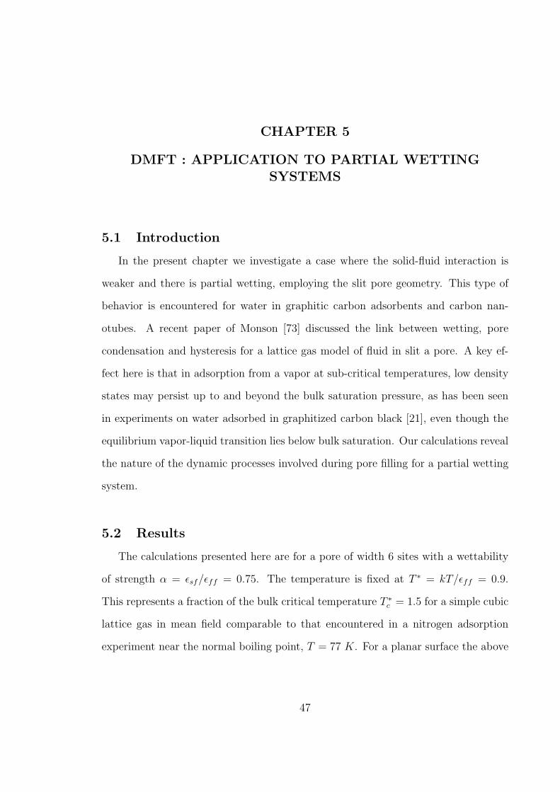
CHAPTER 5

DMFT : APPLICATION TO PARTIAL WETTINGSYSTEMS

5.1 Introduction

In the present chapter we investigate a case where the solid-fluid interaction is

weaker and there is partial wetting, employing the slit pore geometry. This type of

behavior is encountered for water in graphitic carbon adsorbents and carbon nan-

otubes. A recent paper of Monson [73] discussed the link between wetting, pore

condensation and hysteresis for a lattice gas model of fluid in slit a pore. A key ef-

fect here is that in adsorption from a vapor at sub-critical temperatures, low density

states may persist up to and beyond the bulk saturation pressure, as has been seen

in experiments on water adsorbed in graphitized carbon black [21], even though the

equilibrium vapor-liquid transition lies below bulk saturation. Our calculations reveal

the nature of the dynamic processes involved during pore filling for a partial wetting

system.

5.2 Results

The calculations presented here are for a pore of width 6 sites with a wettability

of strength α = εsf/εff = 0.75. The temperature is fixed at T ∗ = kT/εff = 0.9.

This represents a fraction of the bulk critical temperature T ∗c = 1.5 for a simple cubic

lattice gas in mean field comparable to that encountered in a nitrogen adsorption

experiment near the normal boiling point, T = 77 K. For a planar surface the above

47

0

0.25

0.5

0.75

1

0 0.5 1 1.5

ρ

λ/λ0

(a)

-0.5

-0.25

0

0.25

0.5

0 0.5 1 1.5

Ω

λ/λ0

(b)

Figure 5.1: Isotherms of (a) density and (b) grand free energy for the lattice modelof a fluid in a slit pore of length L = 40 from static MFT in the grand ensemble. Fullline - finite length pore in contact with the bulk; dashed line - infinite length pore

stated value for wettability, gives rise to partial wetting with a contact angle of about

60o[73].

5.2.1 Static behavior

We have calculated the static behavior using MFT in both the grand canonical

and canonical ensembles. The grand canonical ensemble results give us the behavior

encountered by the DMFT in the long time limit and correspond to the results ob-

tained in adsorption experiments. On the other hand the canonical ensemble results

give some insight into the nature of the density distributions encountered during the

dynamics.

Figure 5.1 shows isotherms of the density and grand free energy for the slit pore

system we have studied that were obtained in the grand ensemble. The average

density at the center of the pore is shown versus the relative activity, λ/λ0 with the

bulk saturation associated with λ/λ0 = 1. Results for adsorption and desorption

are shown for the open slit pore as well as for an infinite pore (closed pore) with

no bulk contact, modeled by a pore of finite length with periodic boundaries in the

48

x−direction. We note that the isotherm for the open and closed pore are exactly the

same. While on adsorption it is not unusual that the open and isotherm coincide, the

desorption branch should be different for the open pore because of it’s contact with

the bulk fluid. Below, we explain why this happens, but first we explain the behavior

along the adsorption branch.

We see that there is a hysteresis loop with the adsorption branch continuing be-

yond bulk saturation. Usually such states are not accessible in experiments because

bulk condensation occurs without any metastability. A notable exception is work by

Easton and Machin[21] for water in graphitized carbon black where special precau-

tions were taken to delay water condensation in the sample cell. In our system the

bulk region is comparable in size to the pore space and bulk condensation is nucle-

ated as soon as the pore is filled with liquid. Presumably this did not happen in the

Easton and Machin[21] experiment because of the small size of the porous material

sample relative to the bulk region of the sample cell. Also the bulk persists in the

liquid state until the stability limit of the liquid in the pore is reached. So desorp-

tion occurs at the same activity for both the open and closed pore. The vertical line

shown in figure 5.1 correspond to the stability limit of the bulk liquid, and in partially

wetting situations the mean field stability limit of the pore lies at or higher than the

bulk stability limit. Observing liquid phases in the bulk phases for pressures below

saturation requires very careful experimental conditions and it highly unlikely. One

way to relate our isotherms to experiments is during desorption bulk can be switched

over to vapor once the bulk saturation state is reached. We employed this trick to

obtain isotherms in one of our papers [24].

Here in this chapter we present another method inspired by the experiments of

Easton and Machin [21]. We add a layer of solid sites with repulsive interactions on

either side of the pore walls. We will be using this pore model to present results

on the dynamic studies as well. This ensures that the bulk does not condense with

49

0

0.25

0.5

0.75

1

0 0.5 1 1.5

ρ

λ/λ0

(a)

-0.5

-0.25

0

0.25

0.5

0 0.5 1 1.5

Ω

λ/λ0

(b)

Figure 5.2: Isotherms of (a) density and (b) grand free energy for the lattice modelof a fluid in a slit pore of length L = 40 with repulsive walls placed on either sideof the slit, from static MFT in the grand ensemble. Full line - finite length pore incontact with the bulk; dashed line - infinite length pore

pore. The isotherm obtained in this fashion is shown in figure 5.2 and as expected

the open pore desorbs at a higher activity because of it’s contact with bulk vapor.

The grand free energy isotherm in figure 5.2 shows a phase transition between vapor

and liquid states in the pore. Notice that this transition is close to the desorption

step in the isotherm for the open pore system. This is a key feature of desorption

from simple pores that are in contact with the bulk vapor and has been discussed

in detail elsewhere [64, 64, 74, 73]. The fact that desorption occurs for λ/λ0 slightly

lower than the equilibrium vapor to liquid transition is related to the formation of

the meniscus at the pore ends during desorption for the open pore. For the infinite

pore we see no change in the adsorption branch but the desorption branch extends

to lower pressure relative to that for the finite length pore, with the desorption step

occurring at the stability limit of the pore liquid [64, 63, 73, 74].

The density distributions associated with points on the isotherms in figure 5.2 are

shown in figures 5.3. We see that adsorption proceeds by the formation of relatively

low density layers on the pore surfaces followed by filling of the pore in a single sharp

50

(a)

(b)

(c)

(d)

(e)

(f)

Figure 5.3: Visualizations of the density distributions for states on adsorption forthe finite length pore from the isotherm in figure 5.2. The values of activity λ/λ0

are a) 0.02 b) 1.24 c) 1.26. Visualizations of the density distributions for states ondesorption for the finite length pore from the isotherm in figure 5.2. The values ofactivity λ/λ0 are d) 1.19 e) 0.89 f) 0.87. Repulsive walls of strength α = −2.0 andlength 5 lattice sites are placed on either side of the slit.

step. Desorption occurs first with the appearance of a meniscus at the pore entrance

which retreats into the pore until the equilibrium value of λ/λ0 associated with the

vapor-liquid transition is reached when desorption occurs in a single step leaving

medium to low density adsorbed layers on the pore walls.

Figure 5.4 shows the density and grand free energy isotherms obtained from static

MFT in the canonical ensemble, with visualizations of the density distributions ob-

tained shown in figure 5.5. For this case we consider the pore of infinite length as

described above. The solution space of the MFT in the canonical ensemble is much

more complex as was demonstrated by Maier and Stadherr[59]. We have found that

for this partial wetting case the complexity is greater than that encountered for a

complete wetting case in our earlier work [73] and solutions obtained sensitive to

the initialization procedure. For instance, for average densities of about 0.5 we have

encountered solutions where the density on one side of the pore is vapor-like and on

the other side liquid-like with a vapor-liquid interface in the x−direction, as well as

solutions corresponding to a liquid bridge between the two pore walls. This extra

51

0

0.5

1

0 0.5 1 1.5

ρ

λ/λ0

(a)

-0.5

-0.25

0

0.25

0 0.5 1 1.5

Ω

λ/λ0

(b)

Figure 5.4: Isotherms of (a) density and (b) grand free energy (b) for the latticemodel of a fluid in a slit pore from static MFT in the canonical ensemble. The resultsare for the infinite length pore.

complexity occurs because for partial wetting situations low density adsorbed layers

on the pore walls have comparable stability to high density adsorbed layers.

We present results for two solution sequences chosen because of their interest in

relation to the dynamics and generated in the following way. One sequence starts

with an empty pore and gradually increases the average density. At each step we

initialize the density a high value for pairs of sites in four layers on one side and at

the center of the pore, equidistant from the pore ends. This procedure allows us to

search for undulate and bridge states, which we have found in previous work [73]

feature prominently in the dynamics. The other sequence starts with a filled pore

and gradually decreases the density. In this case at each step we set the density to a

very low value for a layer of sites at each end of the system. This allows us to search

for bubble states on desorption. As noted in our previous work the bubble and bridge

states are indistinguishable due to the periodic boundaries in the x−direction.

The behavior we see here is somewhat different to that described in our work

for a complete wetting situation[73]. In that case pore filling proceeded via the

formation of undulates on both walls followed by the formation of a liquid bridge

52

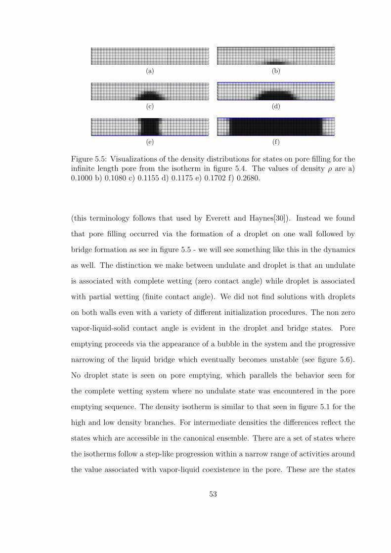
(a) (b)

(c) (d)

(e) (f)

Figure 5.5: Visualizations of the density distributions for states on pore filling for theinfinite length pore from the isotherm in figure 5.4. The values of density ρ are a)0.1000 b) 0.1080 c) 0.1155 d) 0.1175 e) 0.1702 f) 0.2680.

(this terminology follows that used by Everett and Haynes[30]). Instead we found

that pore filling occurred via the formation of a droplet on one wall followed by

bridge formation as see in figure 5.5 - we will see something like this in the dynamics

as well. The distinction we make between undulate and droplet is that an undulate

is associated with complete wetting (zero contact angle) while droplet is associated

with partial wetting (finite contact angle). We did not find solutions with droplets

on both walls even with a variety of different initialization procedures. The non zero

vapor-liquid-solid contact angle is evident in the droplet and bridge states. Pore

emptying proceeds via the appearance of a bubble in the system and the progressive

narrowing of the liquid bridge which eventually becomes unstable (see figure 5.6).

No droplet state is seen on pore emptying, which parallels the behavior seen for

the complete wetting system where no undulate state was encountered in the pore

emptying sequence. The density isotherm is similar to that seen in figure 5.1 for the

high and low density branches. For intermediate densities the differences reflect the

states which are accessible in the canonical ensemble. There are a set of states where

the isotherms follow a step-like progression within a narrow range of activities around

the value associated with vapor-liquid coexistence in the pore. These are the states

53

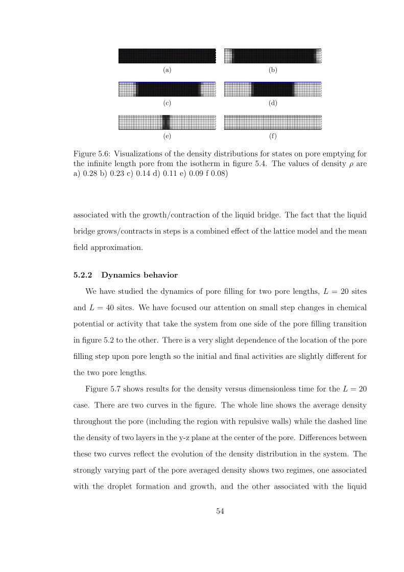
(a) (b)

(c) (d)

(e) (f)

Figure 5.6: Visualizations of the density distributions for states on pore emptying forthe infinite length pore from the isotherm in figure 5.4. The values of density ρ area) 0.28 b) 0.23 c) 0.14 d) 0.11 e) 0.09 f 0.08)

associated with the growth/contraction of the liquid bridge. The fact that the liquid

bridge grows/contracts in steps is a combined effect of the lattice model and the mean

field approximation.

5.2.2 Dynamics behavior

We have studied the dynamics of pore filling for two pore lengths, L = 20 sites

and L = 40 sites. We have focused our attention on small step changes in chemical

potential or activity that take the system from one side of the pore filling transition

in figure 5.2 to the other. There is a very slight dependence of the location of the pore

filling step upon pore length so the initial and final activities are slightly different for

the two pore lengths.

Figure 5.7 shows results for the density versus dimensionless time for the L = 20

case. There are two curves in the figure. The whole line shows the average density

throughout the pore (including the region with repulsive walls) while the dashed line

the density of two layers in the y-z plane at the center of the pore. Differences between

these two curves reflect the evolution of the density distribution in the system. The

strongly varying part of the pore averaged density shows two regimes, one associated

with the droplet formation and growth, and the other associated with the liquid

54

0

0.25

0.5

0.75

1

0 20000 40000

ρ

w0t

Figure 5.7: Density versus time for L = 20 during a step change in relative activityfrom λ/λ0 = 1.245 for λ/λ0 = 1.2550. Full line - average density throughout the pore;dashed line - average density of two planes equidistant from the pore ends.

bridge formation and growth, as can be seen by matching the density distributions

visualized in figure 5.8 with points on the isotherm in figure 5.7. The visualizations

reveal that the density distribution is initially symmetric about the center of the pore

but as time progresses the density builds up on one wall. This symmetry breaking

is quite striking and we believe that it is a consequence of the partial wetting nature

of the solid fluid interaction in this case, where as mentioned earlier, low density

adsorbed layers on the pore walls have comparable stability to high density adsorbed

layers. Once a droplet forms on one wall it grows and spreads towards the ends

of the pore. After this a quite sharp transition occurs where a liquid bridge forms

in the system. The density distribution now regains symmetry, and pore filling is

completed by the growth of the liquid bridge. Notice that there is some resemblance

between the density distributions encountered in the dynamics in figure 5.8 and those

seen in our canonical MFT calculations in figure 5.5, especially between the short

time states in figure 5.8 and the low density states in figure 5.5. We do not yet

completely understand the origin of the symmetry breaking in the dynamics. Tests

55

(a) (b)

(c) (d)

(e) (f)

(g) (h)

(i) (j)

(k) (l)

Figure 5.8: Visualizations of the density distribution during pore filling for L = 20during a step change in relative activity from λ/λ0 = 1.245 for λ/λ0 = 1.255. Thevalues of time w0t are a) 0 b) 2000 c) 8000 d) 12400 e) 13000 f) 15000 g) 17400 h)17600 i) 17800 j) 18000 j) 21000 l) 26000. Repulsive walls of strength α = −2.0 andlength 5 lattice sites are placed on either side of the slit.

thus far carried out suggest that it is not due to round-off error or the accuracy of

the integration scheme.

The uptake curve for the center of the pore indicates that there are stepwise

changes in the local density and these appear to be associated with changes in the

morphology of the droplet. The large step is associated with the transition from the

droplet to bridge morphology. Notice from figure 5.8) that once the pore is filled with

liquid the liquid-vapor interface is denied from moving into the bulk region by the

repulsive walls on either side.

56

0

0.25

0.5

0.75

1

0 30000 60000 90000

ρ

w0t

Figure 5.9: Density versus time for L = 40 during a step change in relative activityfrom λ/λ0 = 1.242 to λ/λ0 = 1.2470. Full line - average density throughout the pore;dashed line - average density of two planes equidistant from the pore ends.

The behavior observed for L = 40 is substantially different. The visualizations

of the states observed in the dynamics are shown in figure5.10. For short times the

behavior is similar to the L = 20 case with the formation of a droplet that then

spreads along the length of the pore. However, instead of a single bridge we see two

bridges form with a large transfer of fluid from the center of the pore as is seen in

the uptake curve for the center of the pore in figure 5.9. Another interesting feature

here is that after the double bridge formation the pore filling is not complete until

there has been significant condensation in the bulk region. If we use a larger bulk

region this does not happen. The mechanism of uptake is sensitive to the final point

of the step change. If the final point is placed away from the capillary condensation

transition point we observe the formation of a symmetric liquid bridge rather than a

asymmetric droplet.

57

(a) (b)

(c) (d)

(e) (f)

(g) (h)

(i) (j)

Figure 5.10: Visualizations of the density distribution during pore filling for L = 40during a step change in relative activity from λ/λ0 = 1.242 to λ/λ0 = 1.247. Thevalues of time w0t are a) 0 b) 57000 c) 58000 d) 68000 e) 78400 f) 78600 g) 79200 h)79400 i) 89000 j) 92000. Repulsive walls of strength α = −2.0 and length 5 latticesites are placed on either side of the slit.

58

0

1

2

3

0 0.25 0.5 0.75 1 1.25

ρ

λ/λ0

α=3.0α=1.0α=0.6

(a)

-0.8

-0.4

0

0.4

0.8

0 0.25 0.5 0.75 1 1.25

Ω

λ/λ0

(b)

Figure 5.11: Isotherms of (a) density and (b) grand free energy (b) for the latticemodel of a fluid in a 12 -4 ink bottle pore at three different values of wettabililtyα. The isotherms are shifted up by 1 unit each and the grand potential curves areshifted by 0.25 units each for clarity.

5.2.3 Static Behavior of a 12-4 Ink Bottle pore

It is also of interest to study ink bottle pores with partially wetting pore walls.

Here we present one such interesting calculation on the static behavior of fluids in

partially wetting ink bottles. The ink bottle geometry is the simplest model of a pore

network, where a central pore called the bottle is connected to the bulk via constric-

tions called necks. Let us consider an ink bottle pore with completely wetting pore

walls filled with liquid. Now on desorption the larger section of the pore, the bottle

has to empty. However it is surrounded by necks filled with liquid. Now desorption

from the bottle can occur via two mechanisms namely pore blocking and cavitation

[97, 88]. Pore blocking is a scenario in which the desorption of the condensed phase

in the bottle is delayed until the fluid in the necks evaporates. Cavitation is a phe-

nomena in which the bottle can desorb independently while the neck remains filled,

and this happens when the fluid in the bottle approaches its stability limit. Given

59

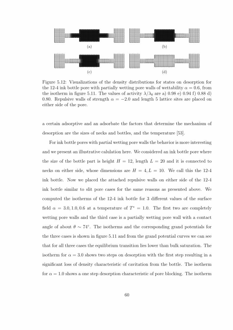
(a) (b)

(c) (d)

Figure 5.12: Visualizations of the density distributions for states on desorption forthe 12-4 ink bottle pore with partially wetting pore walls of wettability α = 0.6, fromthe isotherm in figure 5.11. The values of activity λ/λ0 are a) 0.98 e) 0.94 f) 0.88 d)0.80. Repulsive walls of strength α = −2.0 and length 5 lattice sites are placed oneither side of the pore.

a certain adsorptive and an adsorbate the factors that determine the mechanism of

desorption are the sizes of necks and bottles, and the temperature [53].

For ink bottle pores with partial wetting pore walls the behavior is more interesting

and we present an illustrative calulation here. We considered an ink bottle pore where

the size of the bottle part is height H = 12, length L = 20 and it is connected to

necks on either side, whose dimensions are H = 4, L = 10. We call this the 12-4

ink bottle. Now we placed the attached repulsive walls on either side of the 12-4

ink bottle similar to slit pore cases for the same reasons as presented above. We

computed the isotherms of the 12-4 ink bottle for 3 different values of the surface

field α = 3.0, 1.0, 0.6 at a temperature of T ∗ = 1.0. The first two are completely

wetting pore walls and the third case is a partially wetting pore wall with a contact

angle of about θ ∼ 74. The isotherms and the corresponding grand potentials for

the three cases is shown in figure 5.11 and from the grand potential curves we can see

that for all three cases the equilibrium transition lies lower than bulk saturation. The

isotherm for α = 3.0 shows two steps on desorption with the first step resulting in a

significant loss of density characteristic of cavitation from the bottle. The isotherm

for α = 1.0 shows a one step desorption characteristic of pore blocking. The isotherm

60

0

0.25

0.5

0.75

1

0 0.25 0.5 0.75 1

ρ

λ/λ0

H=4H=6H=8

(a)

0

0.25

0.5

0.75

1

0 0.5 1 1.5

ρ

λ/λ0

H=4H=8

H=12

(b)

Figure 5.13: Isotherms of density for the lattice model of a fluid in slit pores of differentpore width for a) completely wetting pore walls with α = 3.0 and b) partially wettingpore walls with α = 0.6. The vertical line in both graphs is the mean field stabilitylimit of the bulk fluid.

for the partial wetting case α = 0.65 shows two steps, however the size of the step

indicating the necks emptying ahead of the bottle. Inspection of the visualizations of

states along the desorption isotherm indicate this to be the case and they are shown

in figure 5.12.

This behavior can be explained simply based on the dependence of pore size vs

desorption activity or pressure. In figure 5.13a we plot the isotherms of slits of

three different sizes H = 4, 6, 8 at T ∗ = 1.0 for a completely wetting case. The full

curves correspond to open slits, in other words slits in contact with the bulk and the

dashed curve corresponds to slits in periodic boundaries. For the slits with completely

wetting pore walls the desorption activity or pressure increases with pore size, and

stability limit of the confined liquid phase is at or lower than the stability limit of

the bulk liquid. In figure 5.13b we plot the isotherms of slits of three different sizes

H = 4, 8, 12 at T ∗ = 1.0 for a partial wetting case. For the partial wetting case the

open slits have repulsive walls at the ends of the pore to prevent bulk condensation. In

the partial wetting case the dependence of pore size vs desorption pressure is opposite

61

with the smaller pores desorbing at the higher activity or pressure as seen in figure

5.13b. Also the stability limit of the confined liquid phase lies at or above than the

stability limit of the bulk liquid. This explains the desorption behavior seen in the

12-4 ink bottle with partial wetting pore walls.


We have described an application to the dynamics of pore filling in a slit pore where

there is partial wetting of the pore walls. This situation is relevant to systems such

as water in graphitized carbon black or carbon nanotubes. For partial wetting the

adsorption branch of the isotherm extends beyond the bulk-vapor liquid transition

even though the equilibrium transition lies below this transition. In experiments

studying adsorption from supersaturated states requires that special steps be taken

to prevent condensation of the bulk liquid. We have taken care of this in our model

by adding a strip of sites with repulsive walls at the ends of the pore.

The most striking feature of the results is the asymmetry of the density distri-

butions that appear during the dynamics. In particular we note the formation of

droplet on one of the walls. While we do not fully understand why this symmetry

breaking occurs it is related to the special nature of the solid-fluid interface when

there is partial wetting. With partial wetting both low density vapor-like states and

dense liquid-like states can be stable near the pore wall. This makes it possible to

have asymmetric density distributions, with low density states on one pore wall and

high density states on the other. Such states do not appear in the static MFT in the

grand ensemble but are readily found in the canonical ensemble MFT. Moreover such

asymmetry has also been observed in the literature [99, 72].

We also studied the static behavior of fluids in ink bottle pores with partial wetting

pore walls, and observed that the pore can desorb in two steps with the fluid in the

necks evaporating at a higher pressure than the fluid in the bottle.

62

CHAPTER 6

DMFT : APPLICATION TO COMPLETE AND PARTIALDRYING SYSTEMS

In this chapter we focus on pore/fluid systems when the solid-fluid interaction is

weakly attractive or even repulsive, giving rise to partial drying or complete drying.

This was of interest to us in the first instance in connection with intrusion/extrusion

of non-wetting liquids into pores[86, 85, 13], such as in mercury porosimetry [86, 85]

as noted above. It is also of wider interest in connection with the general problem

of dewetting processes between hydrophobic surfaces[4, 51, 52, 56, 57, 58]. Several

studies of lattice models of dewetting have been made [51, 52, 56, 57, 58]. The DMFT

method presented here provides an approximate description of the dynamics of these

systems also. We illustrate this with the example of dewetting of a pair of hydrophobic

plates immersed in a liquid as we change the bulk chemical potential towards bulk

saturation. We focus on the differences in the nucleation mechanism for dewetting

for surface fields yielding partial drying versus surface fields yielding complete drying.

Our DMFT results show that for partial drying cases nucleation can occur by bubble

formation at one of the surfaces, analogous to what is seen in the partial wetting case

and consistent with Monte Carlo simulations of nucleation by Barrat and coworkers

[99]. We also consider the case of the Janus pore where one wall is hydrophobic and

the other hydrophilic [123]as well as the effect of surface patterning on the pore wall

[51, 57, 39].

We consider two slit pore geometries where in both cases the pores are open to

the bulk fluid as shown in figure 6.1. In one case we have a slit pore that is of

finite length in the x-direction and in contact with the bulk in that direction while

63

infinite in the y-direction. The density distribution in this system is two-dimensional

and this greatly reduces the computer time for the MFT and DMFT. In the other

case we have a square slit pore finite in both x- and y-directions so that the density

distribution is fully three-dimensional. This latter geometry allows the observation of

two-dimensional patterning parallel to the pore walls in condensation and evaporation

processes and is a more direct model of the surface forces apparatus where capillary

evaporation of water from hydrophobic pores has been studied experimentally [17,

18]. As discussed above for partial wetting capillary condensation may occur for

metastable vapor states. Similarly, capillary evaporation for a partial drying system

may occur for metastable liquid states. A difficulty with studying the dynamics of

capillary condensation/evaporation for metastable bulk states is that the liquid/vapor

in the pore can act to nucleate bulk condensation/evaporation. In experiments on

water condensation in graphitized carbon black, Easton and Machin [21] were able

to suppress condensation of the bulk gas by silanizing the walls of the sample tube

before adding the adsorbent material. This made it possible for them to observe

condensation in the pores at metastable bulk vapor states. In this chapter we adjust

the surface field at the ends of the pore to suppress this nucleation process. For

partial wetting we would make the surface field at the pore edges strongly repulsive

and for partial drying we make the surface field at the pore edges strongly attractive.

In addition to results from DMFT we will also present some results from a higher

order dynamic theory based on the path probability method of Kikuchi [47, 37] that

yields the Bethe-Peierls or quasi-chemical approximation [94] at equilibrium. The

lattice model exhibits a symmetry between pore filling for wetting states and pore

emptying for drying states, for both the thermodynamics and dynamics, and we will

take advantage of this in the presentation of our results.

64

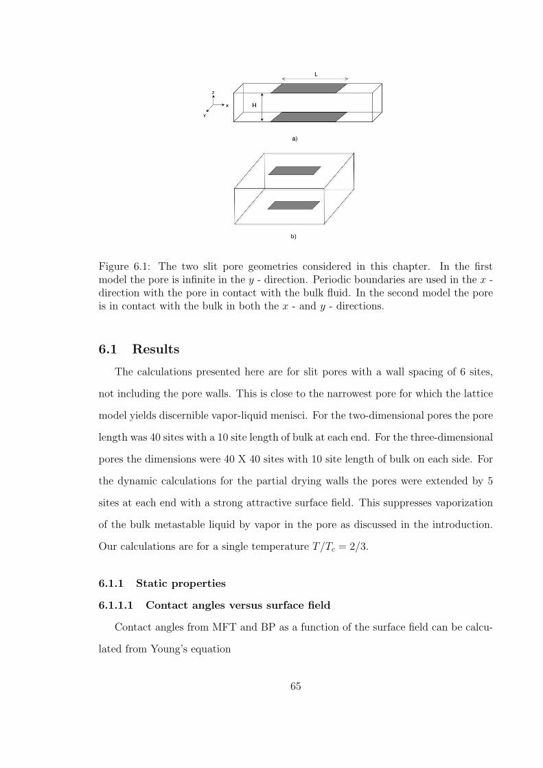
Figure 6.1: The two slit pore geometries considered in this chapter. In the firstmodel the pore is infinite in the y - direction. Periodic boundaries are used in the x -direction with the pore in contact with the bulk fluid. In the second model the poreis in contact with the bulk in both the x - and y - directions.

6.1 Results

The calculations presented here are for slit pores with a wall spacing of 6 sites,

not including the pore walls. This is close to the narrowest pore for which the lattice

model yields discernible vapor-liquid menisci. For the two-dimensional pores the pore

length was 40 sites with a 10 site length of bulk at each end. For the three-dimensional

pores the dimensions were 40 X 40 sites with 10 site length of bulk on each side. For

the dynamic calculations for the partial drying walls the pores were extended by 5

sites at each end with a strong attractive surface field. This suppresses vaporization

of the bulk metastable liquid by vapor in the pore as discussed in the introduction.

Our calculations are for a single temperature T/Tc = 2/3.

6.1.1 Static properties

6.1.1.1 Contact angles versus surface field

Contact angles from MFT and BP as a function of the surface field can be calcu-

lated from Young’s equation

65

cos θ =σSV − σSL

σV L

(6.1)

where θ is the contact angle and σIJ gives the interfacial tension for the IJ interface.

The latter are determined from the excess grand free energies from the MFT or BP

approximations for the IJ interface via

σIJ = ΩIJ + φP M (6.2)

0 0.2 0.4 0.6 0.8 1α

-1

0

1

cos(

θ)

Figure 6.2: Isotherm of cos(θ) versus α for T/Tc = 0.667, computed via the Meanfield (MFT) (full line) and the Bethe-Peierls Approximation (BP) (dashed line)

For lattice models these calculations should strictly include the effect of the orien-

tation of the interfaces with respect to the lattice planes. However, these effects are

expected to be small at the temperature at which our calculations were performed[99].

Figure 6.2 shows a plot of cos θ versus α = εsf/εff from the MFT and BP approxima-

tions. The results indicate first order wetting and drying transitions for this model

at this temperature although we have not studied these transitions in detail. Both

lines exhibit the symmetry cos θ(α) = − cos θ(1− α) which follows from a symmetry

inherent in the lattice gas model [80, 44, 86] as discussed earlier. The slope of cos(θ)

is much steeper in the BP approximation than in the DMFT. This suggested to us

that in order to compare the theories for partial wetting systems we should compare

them at fixed contact angle rather than surface field and this is what we have done.

66

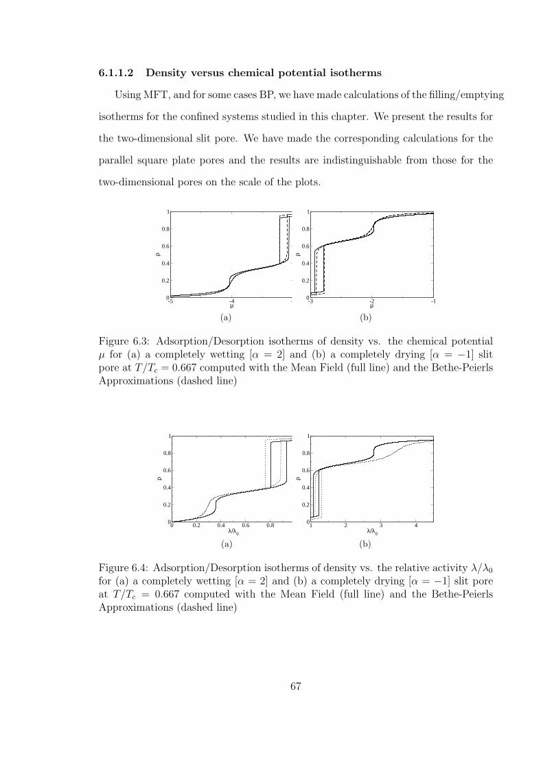
6.1.1.2 Density versus chemical potential isotherms

Using MFT, and for some cases BP, we have made calculations of the filling/emptying

isotherms for the confined systems studied in this chapter. We present the results for

the two-dimensional slit pore. We have made the corresponding calculations for the

parallel square plate pores and the results are indistinguishable from those for the

two-dimensional pores on the scale of the plots.

-5 -4 -3µ

0

0.2

0.4

0.6

0.8

1

ρ

(a)

-3 -2 -1µ

0

0.2

0.4

0.6

0.8

1

ρ

(b)

Figure 6.3: Adsorption/Desorption isotherms of density vs. the chemical potentialµ for (a) a completely wetting [α = 2] and (b) a completely drying [α = −1] slitpore at T/Tc = 0.667 computed with the Mean Field (full line) and the Bethe-PeierlsApproximations (dashed line)

0 0.2 0.4 0.6 0.8 1λ/λ0

0

0.2

0.4

0.6

0.8

1

ρ

(a)

1 2 3 4λ/λ0

0

0.2

0.4

0.6

0.8

1

ρ

(b)

Figure 6.4: Adsorption/Desorption isotherms of density vs. the relative activity λ/λ0

for (a) a completely wetting [α = 2] and (b) a completely drying [α = −1] slit poreat T/Tc = 0.667 computed with the Mean Field (full line) and the Bethe-PeierlsApproximations (dashed line)

67

Figure 6.3 shows isotherms of the density versus chemical potential for complete

wetting (α = 2) and complete drying (α = −1) systems from MFT and the BP

approximations. In these and all other results, we are presenting the density at the

center of the pore. This reduces the pore end effects upon the density and the results

are then quite insensitive to pore length. For complete wetting the pore fills at a

chemical potential less than the bulk saturation chemical potential, −3ε, while for

complete drying the pore fills at a chemical potential above bulk saturation and there

is hysteresis in both cases. In the hysteresis region for the complete wetting case

the states on the adsorption branch are metastable while those on desorption are

essentially at equilibrium since there is contact with the bulk vapor on desorption

eliminating any nucleation barrier. This was shown in our earlier work [74] for a

complete wetting case using plot of the grand free energy. Conversely in the hysteresis

region for the complete drying case the states on the emptying or evaporation branch

are metastable while those on filling are essentially at equilibrium since there is contact

with the bulk liquid. The step-like features in the isotherms at very low or very

high chemical potentials are associated with the formation of a dense monolayer

(wetting case) and dilute monolayer or vapor layer (drying case). The symmetry in

the isotherms is evident. The comparison between MFT and BP is done at the same

value of T/Tc which reduces the effect of the differences in the critical temperatures

(kT(MFT )c /ε = 1.5 vs. kT

(BP )c /ε = 1.233) in comparing the results. The qualitative

agreement is very good when the results are plotted in this way. Figure 3.4 presents

the same results but with the density versus the relative activity, λ/λ0 where λ =

eµ/kT . In this case the symmetry is no longer evident. The relative activity is of the

same order of magnitude as the relative bulk pressure and the plot shows the large

values of bulk pressure required to bring about intrusion of the non wetting liquid

into the pores for the complete drying case.

68

(a)

(b)

(c)

(d)

(e)

(f)

(g)

(h)

Figure 6.5: Visualizations of the density distribution for intrusion (a-d) and extrusion(e-h) states on the isotherm (completely drying slit pore [α = −1]) shown in Fig. 6.3: a) λ/λ0 = 1.041 b) λ/λ0 = 1.241 c) λ/λ0 = 1.291 d) λ/λ0 = 4.0 e) λ/λ0 = 4.0 f)λ/λ0 = 3.0 g) λ/λ0 = 1.075 h) λ/λ0 = 1.065

Figure 6.5 shows a series of visualizations of the density distribution from MFT

in the complete drying case during filling and emptying. We note that the intrusion

of the liquid into the pore begins with the formation of a meniscus near the pore

entrance. Figures 6.5g and 6.5h show the states either side of the drying or dewetting

transition. Our DMFT calculations will reveal the nature of the states encountered

during the dynamics of this transition.

Isotherms of density versus chemical potential for the partial wetting and partial

drying cases are shown in figure 6.6. The partial wetting case corresponds to a

contact angle of 60 while the partial drying case corresponds to 120. Notice that

the hysteresis loops associated with capillary condensation extend beyond µ/ε =

−3. Thus for partial wetting condensation occurs for metastable bulk vapor states

even though the equilibrium transition between vapor and liquid in the pore occurs

for µ/ε < −3 as discussed recently[74, 54, 55]. The experiments of Easton and

Machin[21] on water condensation in carbon also show this behavior. Similarly for

69

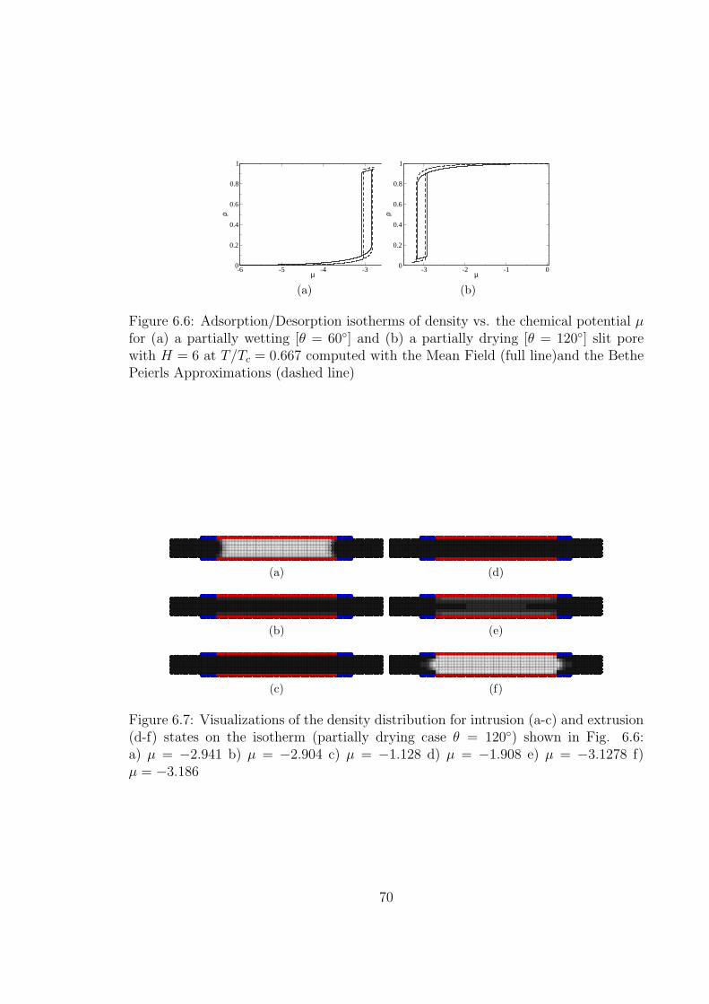
-6 -5 -4 -3µ

0

0.2

0.4

0.6

0.8

1

ρ

(a)

-3 -2 -1 0µ

0

0.2

0.4

0.6

0.8

1

ρ

(b)

Figure 6.6: Adsorption/Desorption isotherms of density vs. the chemical potential µfor (a) a partially wetting [θ = 60] and (b) a partially drying [θ = 120] slit porewith H = 6 at T/Tc = 0.667 computed with the Mean Field (full line)and the BethePeierls Approximations (dashed line)

(a)

(b)

(c)

(d)

(e)

(f)

Figure 6.7: Visualizations of the density distribution for intrusion (a-c) and extrusion(d-f) states on the isotherm (partially drying case θ = 120) shown in Fig. 6.6:a) µ = −2.941 b) µ = −2.904 c) µ = −1.128 d) µ = −1.908 e) µ = −3.1278 f)µ = −3.186

70

partial drying capillary evaporation occurs for µ/ε < −3 even though the equilibrium

transition between vapor and liquid in the pore occurs for µ/ε > −3. Figure 6.7 shows

visualizations of the density distribution in the partial drying case during filling and

emptying.

6.1.2 Dynamics of evaporation from pores

6.1.2.1 Two-dimensional slit pore

Figure 6.8: Symmetry preserved in dynamics of pore filling/emptying (dashed/fulllines) for completely wetting/drying slit pores.

We now consider the dynamics associated with changes of state between closely

spaced states either side of the filling/emptying transitions shown in figure 6.3. Fig-

ure 6.8 shows the average density over the pore versus time from DMFT for the

dynamics of filling of the complete wetting pore together with that for the dynamics

of emptying of the complete drying pore. We see that the symmetry of the lattice

model is preserved in the dynamics - the uptake dynamics for complete wetting is

the same as the emptying dynamics for the complete drying pore. We return to this

point later. In the filling dynamics for the complete wetting pore the dominant event

is the formation of a liquid bridge between the walls of the pore, which is associated

with the cusp in the uptake curve, as is evident in the visualizations shown in our

earlier work[74]. Once the nucleation process of bridge formation has occurred the

71

dynamics of pore filling proceeds quite quickly. Conversely, in the emptying dynamics

the dominant event is the appearance of a vapor bridge.

0 15000 30000 45000w

0t

0

0.15

0.3

0.45

0.6

ρ

Figure 6.9: Density vs. time during a pore emptying process for a step change ofmagnitude ∆µ = 0.03 across the capillary evaporation transition for a completelydrying slit pore. Black curves are from DMFT and gray (blue online) curves are fromthe PPM approximation. For each case we show both the density averaged over theentire pore (full line) and the density averaged over z at a value of x equidistant fromthe pore ends (dashed line).

A comparison of the dynamics of emptying from the DMFT with the higher order

PPM are shown in figure 6.9 and the agreement is qualitatively good. For each case

we show both the density averaged over the entire pore and the density averaged over

z at a value of x equidistant from the pore ends. The density decreases more rapidly

at the center of the pore since this is where vaporization is nucleated. Visualizations

of the states appearing in the dynamics of emptying from DMFT in the complete

drying case are shown in figure 6.10, where the nucleation via the formation of a

vapor bridge is evident. We note that the dynamics for the PPM is a little different

from that in DMFT in that we do not see well defined vapor undulates near the pore

walls prior to the bridge formation. This may be a consequence of the difference in

temperatures used in the two methods in order to use the same value of T/Tc.

A brief comment about the influence of the model pore geometry is in order here.

We are considering a pore with periodic boundaries in the y−direction so that in our

72

Figure 6.10: Visualizations showing a sequence of states along an evaporation processfor a completely drying slit pore computed via the DMFT (left side) and PPM (rightside).

system there are no density variations in that direction. This means that condensation

and evaporation nuclei will have the form of bridges or cylindrical droplets with axes

in the y−direction. Later when we consider slit pores that are finite in both the x−and y− directions we will see droplets with circular symmetry and bridges which are

cylinders with axes normal to the pore walls.

At first glance the symmetry in the dynamics for the system may seem non-

physical. One would expect perhaps that vapor bridge formation in a liquid would

be slower than liquid bridge formation in a vapor, given the greater potential for

hydrodynamic effects in the latter. Nevertheless the symmetry will likely occur for

Kawasaki dynamics without the DMFT or PPM approximations and we are currently

checking this with dynamic Monte Carlo simulations. We also plan to investigate the

relative timescales for condensation and evaporation processes using grand canonical

molecular dynamics calculations such as those of Sarkisov and Monson[96, 97].

We now turn to the case of partial wetting and partial drying systems. Having

shown the symmetry of the lattice model for both thermodynamics and dynamics at

73

0 25000 50000w

0t

0

0.3

0.6

0.9

ρ

Figure 6.11: Density vs. time for a pore emptying process for a step change ofmagnitude ∆µ = 0.005 across the capillary evaporation transition for a partiallydrying slit pore. We show both the density averaged over the entire pore (full line)and the density averaged over z at a value of x equidistant from the pore ends (dashedline).

this point we simply focus on the partial drying case. Our results for pore emptying

for the partial drying case with surface field strength αε can be interpreted as also

applying to pore filling for the partial wetting case with surface field strength (1−α)ε.

In figure 6.11 we show the average density in the pore during evaporation from a filled

pore in the partial drying case from DMFT. We see that initially there is only a slow

change in the density with time until a point is reached where the density starts to

fall rapidly.

As shown in the visualizations presented in figure 6.12 this point is associated

with the appearance of a vapor bubble that is attached to one of the surfaces. This

behavior contrasts with the complete drying case where the vapor bubble bridges the

two surfaces and it is consistent with the results obtained in Monte Carlo simula-

tions of nucleation in a lattice model of a fluid in a cylindrical pore by Barrat and

coworkers[99]. The breaking of the symmetry of the density distribution during the

74

Figure 6.12: Visualizations showing a sequence of states along an evaporation processfor a partially drying slit pore from DMFT.

DMFT dynamics is a quite remarkable result and is observed in the PPM approxima-

tion also. We previously observed the analogous behavior for the partial wetting case

where a liquid droplet is formed on one of the walls in the condensation process[23]

and this has also been seen in density functional studies of nucleation for an off-lattice

model of a fluid a slit pore [110].

6.1.2.2 Three-dimensional slit pore

We now consider the dynamics of emptying from the three-dimensional slit pore

for complete drying (α = −1) and partial drying (α = 0.3165) cases calculated

from DMFT. Figure 6.13 shows the density versus time for a change in the chemical

potential between two neighboring states either side of the emptying transition for

the complete drying case. The shape of the curve is similar to that seen in figure 6.9.

Visualizations of the behavior are shown in figure 6.14 for each point in time we show

a two-dimensional slice through the density distribution half way across the pore.

In addition we show the density in the third layer in the x − y plane. Evaporation

proceeds via the formation of a vapor cylinder at the center of the pore, analogous to

the vapor bridge seen in the two-dimensional case.

75

0 10000 20000 30000w

0t

0

0.2

0.4

ρ

Figure 6.13: Density vs. time for a step change across the capillary evaporationtransition with ∆µ = 0.01 for a completely drying three-dimensional slit pore. Weshow both the density averaged over the entire pore (full line) and the density averagedover z at a point equidistant from the pore sides (dashed line).

Figure 6.15 shows the corresponding behavior for the partial drying case with

visualizations in figure 6.16. In this case evaporation proceeds via the formation of

a vapor bubble attached to one of the pore walls in the center of the square. This is

analogous to the cylindrical bubble seen in the two-dimensional case.

6.1.2.3 Patterned surfaces

As an illustration of the wider utility of the approach presented here we consider

some cases where the surface is patterned with both wetting and drying regions.

We consider two cases. The first is a so-called Janus pore[123] where one pore wall

has a partial drying (hydrophobic) surface field and the other a complete wetting

(hydrophilic) surface field. We implement this by having a surface field with α =

0.3165 on one wall and a surface field α = 3 on the other. The second case is a

patterned surface in which the pore walls have both hydrophilic and hydrophobic

regions. In the present case we consider a checkerboard pattern on each wall similar

76

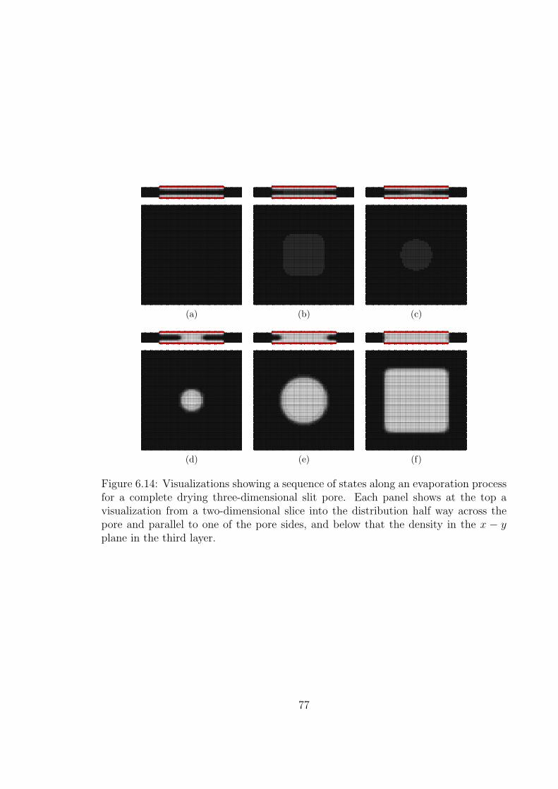
(a) (b) (c)

(d) (e) (f)

Figure 6.14: Visualizations showing a sequence of states along an evaporation processfor a complete drying three-dimensional slit pore. Each panel shows at the top avisualization from a two-dimensional slice into the distribution half way across thepore and parallel to one of the pore sides, and below that the density in the x − yplane in the third layer.

77

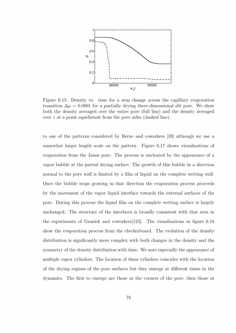
80000 90000w

0t

0

0.2

0.4

0.6

0.8

1

ρ

Figure 6.15: Density vs. time for a step change across the capillary evaporationtransition ∆µ = 0.0001 for a partially drying three-dimensional slit pore. We showboth the density averaged over the entire pore (full line) and the density averagedover z at a point equidistant from the pore sides (dashed line).

to one of the patterns considered by Berne and coworkers [39] although we use a

somewhat larger length scale on the pattern. Figure 6.17 shows visualizations of

evaporation from the Janus pore. The process is nucleated by the appearance of a

vapor bubble at the partial drying surface. The growth of this bubble in a direction

normal to the pore wall is limited by a film of liquid on the complete wetting wall.

Once the bubble stops growing in that direction the evaporation process proceeds

by the movement of the vapor liquid interface towards the external surfaces of the

pore. During this process the liquid film on the complete wetting surface is largely

unchanged. The structure of the interfaces is broadly consistent with that seen in

the experiments of Granick and coworkers[123]. The visualizations in figure 6.18

show the evaporation process from the checkerboard. The evolution of the density

distribution is significantly more complex with both changes in the density and the

symmetry of the density distribution with time. We note especially the appearance of

multiple vapor cylinders. The location of these cylinders coincides with the location

of the drying regions of the pore surfaces but they emerge at different times in the

dynamics. The first to emerge are those at the corners of the pore, then those at

78

(a) (b) (c)

(d) (e) (f)

Figure 6.16: Visualizations showing a sequence of states along an evaporation processfor a partially drying three-dimensional slit pore. Each panel shows at the top avisualization from a two-dimensional slice into the distribution half way across thepore and parallel to one of the pore sides, and below that the density in the x − yplane in the third layer.

79

(a) (b) (c)

(d) (e) (f)

Figure 6.17: Visualizations showing a sequence of states along an evaporation processfor the Janus pore. Each panel shows at the top a visualization from a two-dimensionalslice into the distribution half way across the pore and parallel to one of the pore sides,and below that the density in the x− y plane in the third layer.

80

the sides of the pore with those at the interior the pore appearing later. Also note

that at the center of the pore there is liquid maintained between two drying regions

until the very last stage of the emptying process. Clearly we are seeing the role of

the mass transfer limitations on the development of the density distribution in the

system during the dynamics.


We have presented results for dynamics of evaporation for a lattice model of fluids

confined in slit pores with a focus on partial drying and complete drying cases. As

explained in chapter 2 the dynamics is calculated via a DMFT which is consistent

with the thermodynamics from mean field for equilibrium or metastable equilibrium

states. The lattice model exhibits a symmetry between pore filling for a wetting

(hydrophilic) pore and emptying for a drying (hydrophobic) pore and vice versa.

This symmetry also carries over to the dynamics in DMFT and PPM and likely to

Kawasaki dynamics as well.

We have presented results for two slit pore geometries (two-dimensional and three-

dimensional) where the pore is in contact with the bulk liquid. In each geometry

we compared the evaporation processes for partial drying pore walls with those for

complete drying case. In the former the evaporation process studied proceeds by

the formation of a vapor bubble attached to one of the pore walls, representing a

symmetry breaking in the density distribution during the dynamics. This has also

been seen in the complementary case of condensation in pore with partial wetting

walls[24] and observed in nucleation calculations for fluids in pores via density func-

tional theory[110] and Monte Carlo simulations[99]. For the complete drying case the

evaporation proceeds via the formation of a vapor bridge (two-dimensional pore) or

vapor cylinder (three-dimensional pore). These observations are for processes with

small changes in chemical potential. For larger step changes in chemical potential we

81

(a) (b) (c)

(d) (e) (f)

(g) (h) (i)

Figure 6.18: Visualizations showing a sequence of states along an evaporation processfor the checkerboard pore. The first panel shows the patterning with hydrophobicin light gray (red online) and hydrophilic in dark gray (blue online). Each of theother panels show at the top a visualization from a two-dimensional slice into thedistribution half way across the pore and parallel to one of the pore sides, and belowthat the density in the x− y plane in the third layer.

82

may encounter multiple vapor bridges during the dynamics analogous to the multiple

liquid bridges formed during condensation in a wetting pore[74].

Our results for patterned surfaces (Janus pore and checkerboard pore) illustrate

the potential wider utility of the DMFT method. The Janus pore shows an evap-

oration process that proceeds via the motion of the vapor liquid interface with a

fairly stable liquid film on the hydrophilic surface. For the checkerboard pattern a

quite complex evolution of the density distribution takes place during the evapora-

tion with multiple vapor cylinders developing and growing at different times due to

mass transfer limitations upon the dynamics. It will likely be fruitful to relate the

phenomena seen here to those encountered in other studies of fluids confined between

patterned surfaces via density functional theory[6]. Also the effect of patterning in

these systems is somewhat analogous to the effects of pore structure in complex porous

materials[44, 117, 115] and in particular it will be interesting to look at the effects of

disorder on the dynamics[57, 117, 115].

83

CHAPTER 7

DMFT: APPLICATION TO BINARY MIXTURESCONFINED IN POROUS MATERIALS

7.1 Introduction

In this chapter we describe the formulation and application of DMFT to the case

of fluid mixtures. For mixtures the range of phenomena is greatly expanded by the

competitive interactions of the components with the pore walls and the fact that

equilibration of the composition distribution will be an important component of the

relaxation dynamics.

Our work can viewed as building on previous studies of mixture adsorption using

classical density functional theory (DFT) [38, 46, 111, 105, 43, 106, 121, 7, 8, 92,

107, 108, 120, 83, 91]. Several issues have been explored in these works. One focus

has been on understanding the solution thermodynamics for adsorbed mixtures and,

in particular, departures from the ideal adsorbed solution theory [46, 106]. Another

emphasis has been on the effect of confinement upon the composition relative to

the bulk phase (selective adsorption) due to confinement[111, 105, 92, 108, 83, 91].

There has also been a significant effort in understanding how confinement influences

vapor-liquid [111, 7, 8] and liquid-liquid [43, 121, 120] equilibrium.

The two model mixtures we consider in this chapter have parameters appropriate

to simple n-alkane mixtures in carbon slit pores. One is a close to ideal mixture mod-

eling ethane and methane while the other, modeling butane and methane is somewhat

more non ideal. We calculation the bulk vapor-liquid phase diagrams for the models

and study the static and dynamic behavior of the mixtures confined in two pore ge-

ometries, a slit pore and an ink bottle pore. We look at the behavior of the system as

84

the bulk vapor state approaches saturation by isothermal, isobaric changes in com-

position or by changes isothermal changes in bulk pressure at fixed bulk composition.

We pay particular attention to the evolution of the species density distributions in the

system and especially at vapor-liquid interfaces inside the pores. For the ink bottle

pore we pay special attention to the cavitation process on desorption[97, 88, 53, 75].

In section 7.2 we present the mean field theory for binary mixture lattice gases,

and the extension of DMFT to binary mixtures. In section 7.4 we then present our

studies on two different binary fluid mixtures, including the bulk phase diagram, the

static behavior of the confined mixtures and the relaxation dynamics predicted by

DMFT. Section 7.5 gives a summary of our results and conclusions.

7.2 Theory

7.2.1 Static Behavior

Our model is a single occupancy lattice gas with nearest neighbor interactions

in the presence of an external field. Any site i on the lattice can be occupied by a

molecule of species α or remain vacant, and the Hamiltonian for this model is given

by

H = −1

2

∑

i

∑a

∑α

∑γ

εαγnαi nγ

i+a +∑

i

∑α

nαi φα

i (7.1)

where nαi is the occupancy of site i (0 or 1) by species α, and a is a vector pointing

to the nearest neighbors of site i. The second term in the Hamiltonian describes the

external field created by the solid surface, acting on the fluid species α. The grand

free energy of the system within the mean field approximation can be written as

Ω = kT∑

i

[∑α

ραi log ρα

i + (1−∑

α

ραi ) log(1−

∑α

ραi )

]− 1

2

∑

i

∑a

∑α

∑γ

εαγραi ργ

i+a

+∑

i

∑α

ραi (φα

i − µα) (7.2)

85

Minimizing the free energy functional with respect to density of species α yields an

expression for the the chemical potential of species α.

µα = kT∑

i

[ln ρα

i − ln(1−∑

α

ραi )

]−

∑a

∑γ

εαγργi+a + φα ∀ i (7.3)

For a given pore geometry, the above set of coupled non linear equations are solved

at fixed chemical potentials of the individual species and at a fixed temperature to

yield the the density distribution of the system at equilibrium. Equation 7.3 can be

rewritten for a bulk fluid mixture as follows.

µα = kT

[ln ρα

b − ln(1−∑

α

ραb )

]− z

∑γ

εαγργb (7.4)

where z is the coordination number of the lattice and ραb , is the density of species α in

the bulk fluid mixture. Our interest lies primarily in studying states of the confined

fluid at conditions where the bulk fluid mixture is in vapor phase. This makes it

essential to know the phase diagram of the bulk fluid mixture. In order to compute

the bulk phase diagram or the vapor-liquid -equilibrium (VLE) diagram of a binary

mixture we solve the following set of coupled equations.

ω(ρAI , ρB

I ) = ω(ρAII , ρ

BII) (7.5)

µA(ρAI , ρB

I ) = µA(ρAII , ρ

BII)

µB(ρAI , ρB

I ) = µB(ρAII , ρ

BII)

ω is the grand potential density, and µA and µB are chemical potentials of species

A and B. The Roman numeral subscripts stand for the two different phases in

equilibrium. We rewrite the above equations in terms of the total density ρtb = ρA

b +ρBb ,

and composition yA = ρAb /ρt

b, for convenience and solve them using Newton’s method.

86

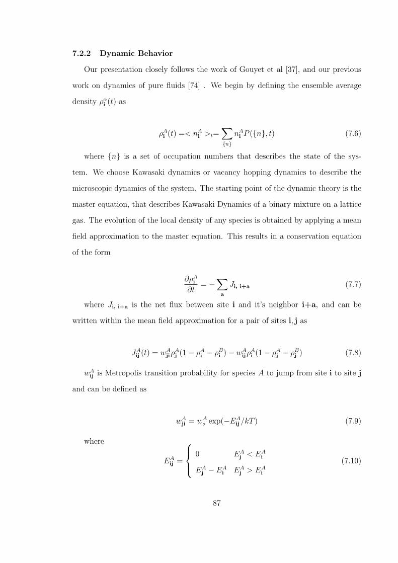
7.2.2 Dynamic Behavior

Our presentation closely follows the work of Gouyet et al [37], and our previous

work on dynamics of pure fluids [74] . We begin by defining the ensemble average

density ραi (t) as

ρAi (t) =< nA

i >t=∑

nnA

i P (n, t) (7.6)

where n is a set of occupation numbers that describes the state of the sys-

tem. We choose Kawasaki dynamics or vacancy hopping dynamics to describe the

microscopic dynamics of the system. The starting point of the dynamic theory is the

master equation, that describes Kawasaki Dynamics of a binary mixture on a lattice

gas. The evolution of the local density of any species is obtained by applying a mean

field approximation to the master equation. This results in a conservation equation

of the form

∂ρAi

∂t= −

∑a

Ji, i+a (7.7)

where Ji, i+a is the net flux between site i and it’s neighbor i+a, and can be

written within the mean field approximation for a pair of sites i, j as

JAij (t) = wA

jiρAj (1− ρA

i − ρBi )− wA

ijρAi (1− ρA

j − ρBj ) (7.8)

wAij is Metropolis transition probability for species A to jump from site i to site j

and can be defined as

wAji = wA

o exp(−EAij /kT ) (7.9)

where

EAij =

0 EAj < EA

i

EAj − EA

i EAj > EA

i

(7.10)

87

and

EAi = −εAA

∑a

ρAi − εAB

∑a

ρBi+a + φA

i (7.11)

wA0 is the ratio of the hopping frequency of species A and the coordination number

of the lattice. Putting together equations 7.7 - 7.11 results in the following expression

for flux of species A.

JAij (t) = −wA

ijρAi (1− ρA

j − ρBj )

[1− exp

(µA

j − µAi

kT

)](7.12)

Here µAj is an expression given by 7.3 and is defined as the chemical potential at

equilibrium. Looking at above equation it is straightforward to realize that at the

long time limit where system approaches equilibrium, or when flux between the sites

vanish, the chemical potential at every site in the system is uniform.

The factors wA0 and wB

0 have to be different, However for the sake of simplicity we

have considered them to be the same in this chapter wA0 = wB

0 = w0. We repeated the

dynamics calculations repeated in this chapter, with a ratio of wA0 /wB

0 , other than

1 and found no difference in the qualitative behavior. The implementation of the

DMFT for binary mixtures is very similar to that of the pure fluid case described in

section 2.3.2. For a given pore geometry we begin by solving the static mean field

(MFT) equations at a certain initial state given by chemical potentials of species

A and B. This gives the initial density distribution of the system. Next we fix the

density and chemical potentials of the individual species to a value associated with

the final state of the system, at the boundaries of the pore geometry. The system is

then evolved by numerical solution of equation 7.7. We have found Euler’s method

to be of acceptable accuracy for time steps less than about ω0∆t = 0.2.

7.3 Systems Studied

In this chapter we consider only binary mixtures. The set of interaction parameters

for the bulk fluid are εAA, εBB, εAB. The interaction between unlike species is defined

88

as εAB = (1 − kAB)√

εAAεBB, where kAB is the non-ideality parameter. Here we

present a few studies on a mixture whose interaction parameters qualitatively resemble

ethane methane. The mixtures is confined in pores with completely wetting pore

walls with wettability yA = εAS/εAA = 3.0. We fix εBS based on the relationship

εAS/εBS =√

εAA/εBB. The set of interaction parameters used are shown in table 7.1.

All quantities with dimensions of energy are made dimensionless with the interaction

energy εAA. The objective of this chapter is to merely illustrate the usefulness of this

framework to study sub critical mixtures in porous materials. Hence we consider two

ideal pore geometries, the slit pore and the ink bottle pore. The slit pore that we

consider has a height of H = 6 lattice units and a length L = 40 lattice units. The

ink bottle pore that we consider has a bottle part with height H = 12, length L = 20

and it is connected to necks on either side, whose dimensions are H = 4, L = 10. We

call this system the 12-4 ink bottle pore. Both the pores that we consider are placed

in contact with bulk fluid.

Table 7.1: Interaction parameters of the two different binary mixtures studied

System εBB/εAA kAB εAS/εAA εBS/εAA

Mixture I 0.6 0.0 3.0 2.32Mixture II 0.25 0.0 3.0 1.5


7.4.1 Mixture I : Static Behavior

Figure 7.1 we show the bulk VLE diagrams of mixture I at T ∗ = kT/εAA = 0.8.

The bulk phase behavior resembles an ideal mixture that can be described by Raoult’s

law. Both the pure fluids of components A and B are at a subcritical state with the

P − x or the bubble point curve almost linearly connecting the vapor pressure of

pure fluid A and pure fluid B. As mentioned earlier we are interested in states of the

confined fluid which lie below the P − y or the dew point curve in the phase diagram.

89

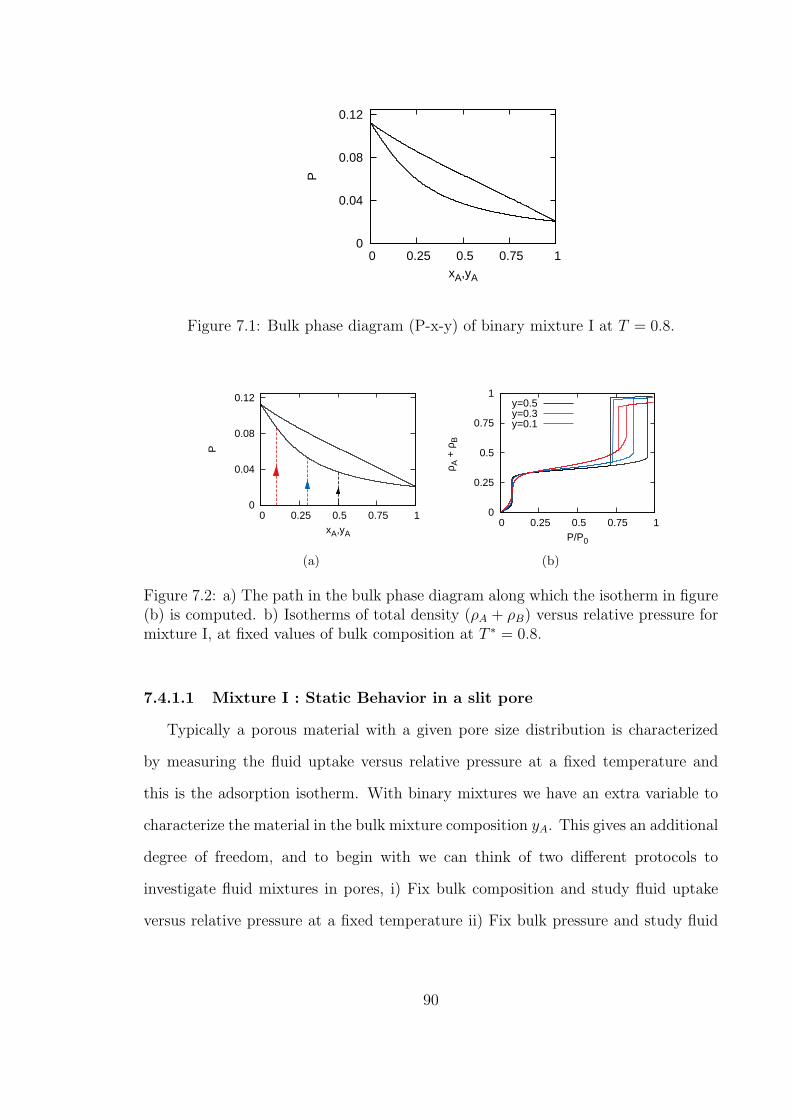
0

0.04

0.08

0.12

0 0.25 0.5 0.75 1

P

xA,yA

Figure 7.1: Bulk phase diagram (P-x-y) of binary mixture I at T = 0.8.

0

0.04

0.08

0.12

0 0.25 0.5 0.75 1

P

xA,yA

(a)

0

0.25

0.5

0.75

1

0 0.25 0.5 0.75 1

ρ A +

ρB

P/P0

y=0.5y=0.3y=0.1

(b)

Figure 7.2: a) The path in the bulk phase diagram along which the isotherm in figure(b) is computed. b) Isotherms of total density (ρA + ρB) versus relative pressure formixture I, at fixed values of bulk composition at T ∗ = 0.8.

7.4.1.1 Mixture I : Static Behavior in a slit pore

Typically a porous material with a given pore size distribution is characterized

by measuring the fluid uptake versus relative pressure at a fixed temperature and

this is the adsorption isotherm. With binary mixtures we have an extra variable to

characterize the material in the bulk mixture composition yA. This gives an additional

degree of freedom, and to begin with we can think of two different protocols to

investigate fluid mixtures in pores, i) Fix bulk composition and study fluid uptake

versus relative pressure at a fixed temperature ii) Fix bulk pressure and study fluid

90

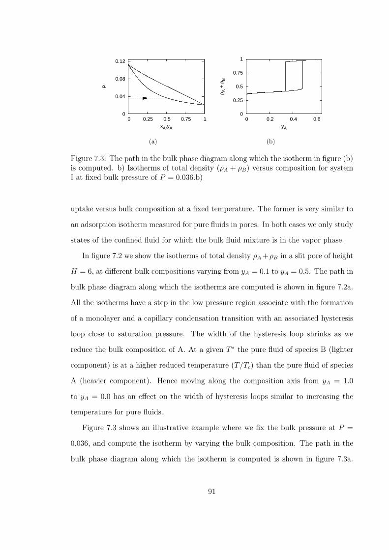
0

0.04

0.08

0.12

0 0.25 0.5 0.75 1

P

xA,yA

(a)

0

0.25

0.5

0.75

1

0 0.2 0.4 0.6

ρ A +

ρB

yA

(b)

Figure 7.3: The path in the bulk phase diagram along which the isotherm in figure (b)is computed. b) Isotherms of total density (ρA + ρB) versus composition for systemI at fixed bulk pressure of P = 0.036.b)

uptake versus bulk composition at a fixed temperature. The former is very similar to

an adsorption isotherm measured for pure fluids in pores. In both cases we only study

states of the confined fluid for which the bulk fluid mixture is in the vapor phase.

In figure 7.2 we show the isotherms of total density ρA +ρB in a slit pore of height

H = 6, at different bulk compositions varying from yA = 0.1 to yA = 0.5. The path in

bulk phase diagram along which the isotherms are computed is shown in figure 7.2a.

All the isotherms have a step in the low pressure region associate with the formation

of a monolayer and a capillary condensation transition with an associated hysteresis

loop close to saturation pressure. The width of the hysteresis loop shrinks as we

reduce the bulk composition of A. At a given T ∗ the pure fluid of species B (lighter

component) is at a higher reduced temperature (T/Tc) than the pure fluid of species

A (heavier component). Hence moving along the composition axis from yA = 1.0

to yA = 0.0 has an effect on the width of hysteresis loops similar to increasing the

temperature for pure fluids.

Figure 7.3 shows an illustrative example where we fix the bulk pressure at P =

0.036, and compute the isotherm by varying the bulk composition. The path in the

bulk phase diagram along which the isotherm is computed is shown in figure 7.3a.

91

0

0.04

0.08

0.12

0 0.25 0.5 0.75 1

P

xA,yA

(a)

0

0.25

0.5

0.75

1

0 0.25 0.5 0.75 1

ρ A +

ρB

P/P0

y=0.5y=0.3y=0.1

(b)

Figure 7.4: The path in the bulk phase diagram along which the isotherm in figure (b)is computed. b) Isotherms of total density (ρA +ρB) versus relative pressure in a 12/4ink bottle pore for mixture I, at fixed values of bulk composition at a temperature ofT ∗ = 0.8.

For the entire range of composition considered above the bulk fluid is in vapor phase.

A capillary transition occurs at the composition for which P = 0.036, is the stability

limit of the adsorbed monolayer. We also observe hysteresis associated with this

capillary transition.

7.4.1.2 Mixture I : Static Behavior in an Ink Bottle pore

The ink bottle pore is the simplest model of a pore network, where the middle

section called the bottle, can access the bulk fluid only via narrow constrictions placed

on either side called necks. This geometry has been used to illustrate the different

mechanisms of desorption in pore networks namely pore blocking and cavitation [97,

88]. Pore blocking is a scenario in which the desorption of the condensed phase in

the bottle is delayed until the necks empty. Cavitation is a phenomena in which the

bottle can desorb independently while the neck remains filled, and this happens when

the fluid in the bottle approaches its stability limit. Given a certain adsorptive and

an adsorbate the factors that determine the mechanism of desorption are the sizes of

necks and bottles, and the temperature. With increasing temperature the stability

limits of the liquid in the bottle and equilibrium pressure (desorption pressure) of the

92

0

0.04

0.08

0.12

0 0.25 0.5 0.75 1

P

xA,yA

(a)

0

0.25

0.5

0.75

1

0 0.25 0.5 0.75 1

ρ A +

ρB

yA

(b)

Figure 7.5: a)The path in the bulk phase diagram along which the isotherms arecomputed. b) Isotherms of total density (ρA + ρB) versus composition for mixture Iin a 12-4 ink bottle pore at pressures of i) P = 0.02 (black), ii) P = 0.036 (blue), iii)P = 0.05 (red) and iv) P = 0.08 (green).

necks change. At a given temperature along the desorption branch of the isotherm

if the stability limit of the liquid in the bottle is reached ahead of the equilibrium

pressure of the necks, cavitation is observed.

It was shown by Ravikovitch and Neimark [88] and by Libby and Monson [53],

that for a pure fluid, increasing temperature the desorption mechanism changes from

pore blocking to cavitation. As described in section 7.4.1.1 for mixture I, varying the

composition has similar effects as varying the temperature of a pure fluid. Hence if

we study adsorption isotherms of mixture I at various bulk compositions we expect to

see a transition in the desorption mechanism from pore blocking to cavitation. This

is indeed the case for mixture I and we show in figure 7.4 adsorption isotherms at

different bulk compositions for the 12-4 ink bottle pore. For compositions yA = 0.5

and yA = 0.3 the isotherms show a single step desorption, where the necks and bottle

empty in one step characteristic of pore blocking. The isotherm for composition

yA = 0.1 shows a two step desorption or a cavitation transition in which the bottle

empties independent of the necks.

93

0

0.25

0.5

0.75

1

0 30000 60000

ρ

w0 t

(a)

0

0.25

0.5

0.75

1

0 30000 60000

ρ A, x

A

w0 t

(b)

Figure 7.6: a) Evolution of the total density (black), density of species A (blue) anddensity of species B (red) in a L = 40, H = 6 slit pore caused by a step change inbulk pressure from P = 0.0001 to P = 0.036 at a temperature of T ∗ = 0.8. Shownin the inset is the section of the uptake curve between w0t = 45000 to w0t = 80000.b) Evolution of the density (blue full) and composition (blue dashed) of species A inthe pore.

In figure 7.5 we show fluid uptake vs composition for the 12-4 ink bottle pore. At

the lowest pressure considered (P = 0.02) we see a two step adsorption and a single

step desorption characteristic of pore blocking. At the highest pressures considered

P = 0.05 we see a two step desorption transition in the isobar which is characteristic

of cavitation. On desorption as we make decrements of the independent variable, (

yA / P ) we will observe cavitation, if the the stability limit of the liquid in the bottle

is reached before the equilibrium pressure of the neck.

7.4.2 Mixture I : Dynamic Behavior in a slit pore

7.4.2.1 Pore filling at fixed bulk composition

We now present the dynamic behavior associated with pore filling in a slit pore

of height H = 6 and length L = 40. The bulk composition of the mixture is fixed

at yA = 0.5 and the temperature is fixed at T ∗ = 0.80 (for bulk phase diagram refer

figure 7.1). The slit pore is initialized at a dilute state (P = 0.0001) and then a step

change is made to the bulk pressure to a value of P = 0.036. We can see from the

isotherm shown in figure 7.2b that at P = 0.036 the fluid in the pore is in a condensed

94

(a) (b)

(c) (d)

(e) (f)

Figure 7.7: Visualizations of the density distribution of species A (top) and speciesB (bottom) in a L = 40, H = 6 slit pore caused by a step change in bulk pressurefrom P = 0.0001 to P = 0.036 at a temperature of T ∗ = 0.8, at a) w0t = 0; b)w0t = 14000; c) w0t = 28000; d) w0t = 32000; e) w0t = 44000; f) w0t = 60000. Weuse ten shades of gray to represent the density at a given lattice site, and the densityof species A is visualized at the top and B at the bottom.

95

state. We integrate the DMFT equations to follow the relaxation of the system to

this final equilibrium state. The visualizations of the density distributions of species

A (top) and species B (bottom), at different stages of evolution are shown in figure

7.7. The visualizations are made with RASMOL [100, 5], and the density of a certain

species in a lattice site is represented by ten shades of gray. The visualizations show

the formation of a monolayer filled mostly with species A during the initial stages, fig

: 7.7b . Later undulates appear near the ends of the system fig :7.7c, followed by the

formation of two liquid bridges close to both ends of the pore fig : 7.7d. The liquid

bridges widen to fill the pore completely. The pore filling behavior of this mixture

appears similar to the filling by a pure fluid which is reported in the work of Monson

[74].

In figure 7.6a we plot the evolution of the total density and density of the individual

species. The first cusp in the total density curve is associated with the formation of

undulates in the pore, and the second cusp is associated with the formation of liquid

bridges. We describe two interesting observations in the uptake behavior. At short

times during the formation of the monolayer on the surface of the pore we can observe

a peak in the density of the lighter component B in the pore. The lighter component

is then displaced from the surface of the pore by species A. Also interesting is the

long time behavior. In the inset of 7.6a we plot the final stages of the uptake between

w0t = 45000 to w0t = 80000. The total density (black line) saturates or reaches

an equilibrium at about w0t = 45000. However the component densities continue

to vary significantly indicating that the last phase of the uptake process involves

compositional equilibration, where relative amounts of the species change until the

chemical potentials of the species in the bulk match with the pore. We also show the

evolution of the density (full line) and the composition of A (dashed line) in figure

7.6b. The composition of A shows an initial increase until the monolayer forms and

96

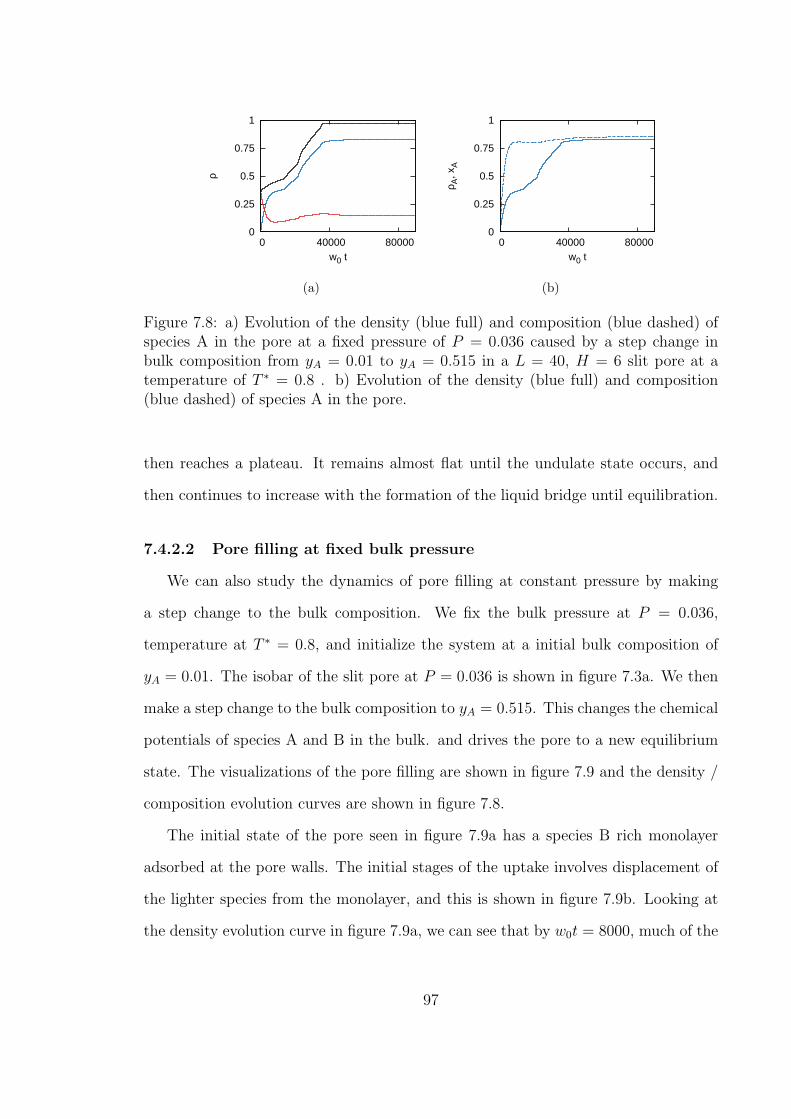
0

0.25

0.5

0.75

1

0 40000 80000

ρ

w0 t

(a)

0

0.25

0.5

0.75

1

0 40000 80000

ρ A, x

A

w0 t

(b)

Figure 7.8: a) Evolution of the density (blue full) and composition (blue dashed) ofspecies A in the pore at a fixed pressure of P = 0.036 caused by a step change inbulk composition from yA = 0.01 to yA = 0.515 in a L = 40, H = 6 slit pore at atemperature of T ∗ = 0.8 . b) Evolution of the density (blue full) and composition(blue dashed) of species A in the pore.

then reaches a plateau. It remains almost flat until the undulate state occurs, and

then continues to increase with the formation of the liquid bridge until equilibration.

7.4.2.2 Pore filling at fixed bulk pressure

We can also study the dynamics of pore filling at constant pressure by making

a step change to the bulk composition. We fix the bulk pressure at P = 0.036,

temperature at T ∗ = 0.8, and initialize the system at a initial bulk composition of

yA = 0.01. The isobar of the slit pore at P = 0.036 is shown in figure 7.3a. We then

make a step change to the bulk composition to yA = 0.515. This changes the chemical

potentials of species A and B in the bulk. and drives the pore to a new equilibrium

state. The visualizations of the pore filling are shown in figure 7.9 and the density /

composition evolution curves are shown in figure 7.8.

The initial state of the pore seen in figure 7.9a has a species B rich monolayer

adsorbed at the pore walls. The initial stages of the uptake involves displacement of

the lighter species from the monolayer, and this is shown in figure 7.9b. Looking at

the density evolution curve in figure 7.9a, we can see that by w0t = 8000, much of the

97

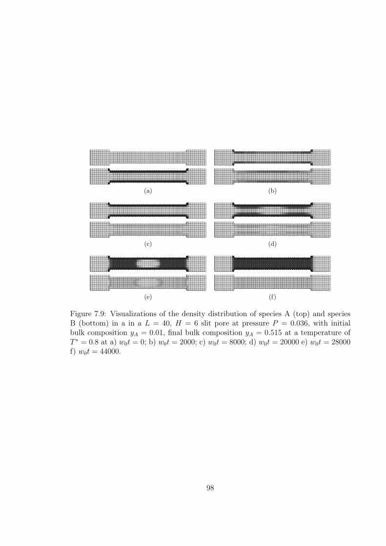
(a) (b)

(c) (d)

(e) (f)

Figure 7.9: Visualizations of the density distribution of species A (top) and speciesB (bottom) in a in a L = 40, H = 6 slit pore at pressure P = 0.036, with initialbulk composition yA = 0.01, final bulk composition yA = 0.515 at a temperature ofT ∗ = 0.8 at a) w0t = 0; b) w0t = 2000; c) w0t = 8000; d) w0t = 20000 e) w0t = 28000f) w0t = 44000.

98

0

0.25

0.5

0.75

1

0 25000 50000

ρ A, ρ

B

w0 t

(a)

0

0.25

0.5

0.75

1

0 25000 50000

ρ A, x

A

w0 t

(b)

Figure 7.10: a) Evolution of the total density (black), density of species A (blue) anddensity of species B (red) in a L = 40, H = 6 slit pore caused by a step change in bulkpressure from P = 0.036 to P = 0.0001 in a L = 40, H = 6 slit pore at a temperatureof T ∗ = 0.8. b) Evolution of the density (blue full) and composition (blue dashed) ofspecies A in the pore.

displacement has occurred. The composition evolution curve shown in figure 7.9b,

suggests that the composition of the pore reaches much closer to its final value, once

the displacement is complete. The mechanism of filling after this point resembles the

previous case. Two liquid bridges are observed close to the ends of the pore, and they

proceed to fill the pore, as shown in figures 7.9c , 7.9d. Also in figure 7.9e we can

observe an enrichment of species B at the interface between the liquid bridge and the

trapped vapor bubble. We shall revisit this later in this chapter.

7.4.2.3 Pore emptying at fixed bulk composition

Next we present the dynamics of pore emptying where we initialize the system

at a condensed state P = 0.036 and make a step change in the bulk pressure to

P = 0.0001, at fixed bulk composition of yA = 0.5. The density / composition

evolution curves and the visualizations of this process are shown in figures 7.10 and

7.11. As shown in the visualizations the emptying process occurs via the meniscus

receding into the pore. The meniscus recedes until it reaches the middle of the pore,

99

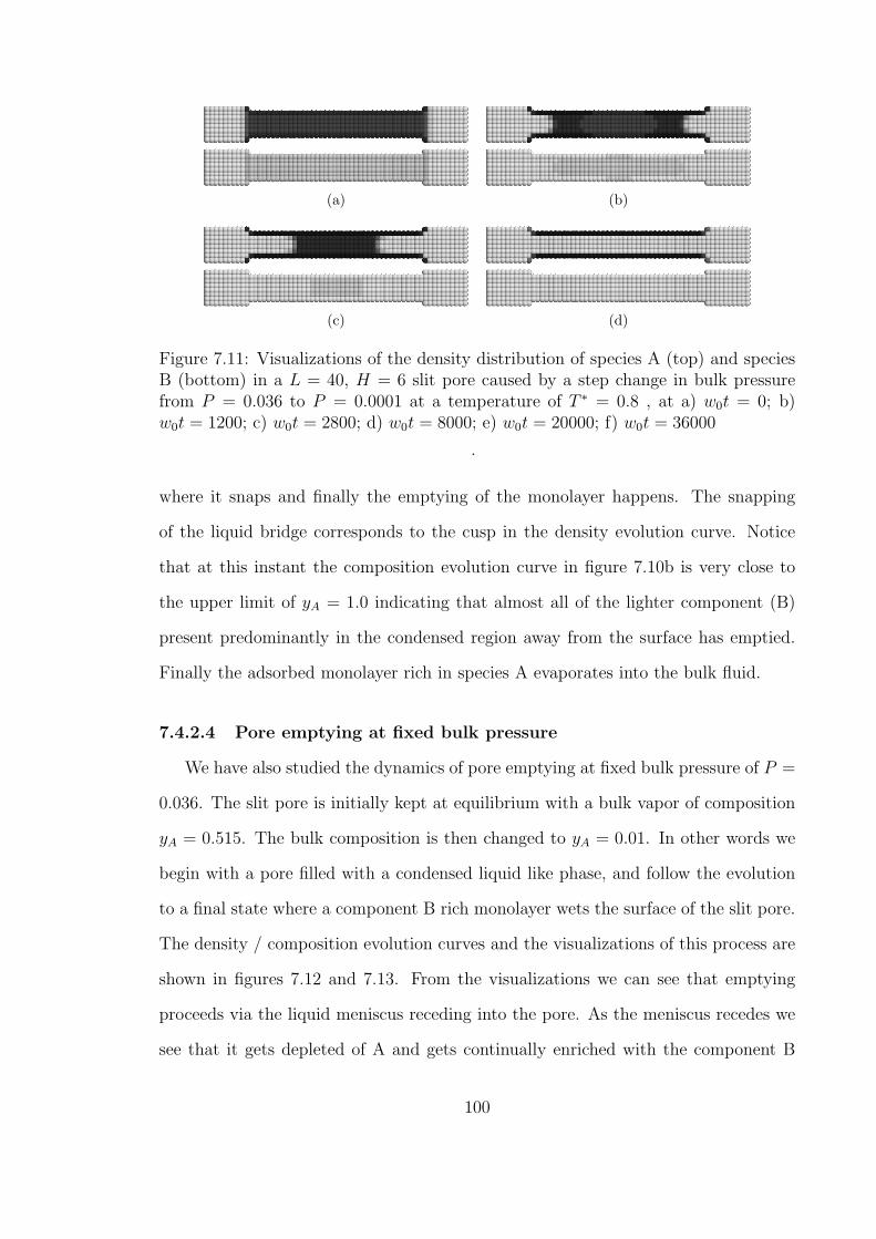
(a) (b)

(c) (d)

Figure 7.11: Visualizations of the density distribution of species A (top) and speciesB (bottom) in a L = 40, H = 6 slit pore caused by a step change in bulk pressurefrom P = 0.036 to P = 0.0001 at a temperature of T ∗ = 0.8 , at a) w0t = 0; b)w0t = 1200; c) w0t = 2800; d) w0t = 8000; e) w0t = 20000; f) w0t = 36000

.

where it snaps and finally the emptying of the monolayer happens. The snapping

of the liquid bridge corresponds to the cusp in the density evolution curve. Notice

that at this instant the composition evolution curve in figure 7.10b is very close to

the upper limit of yA = 1.0 indicating that almost all of the lighter component (B)

present predominantly in the condensed region away from the surface has emptied.

Finally the adsorbed monolayer rich in species A evaporates into the bulk fluid.

7.4.2.4 Pore emptying at fixed bulk pressure

We have also studied the dynamics of pore emptying at fixed bulk pressure of P =

0.036. The slit pore is initially kept at equilibrium with a bulk vapor of composition

yA = 0.515. The bulk composition is then changed to yA = 0.01. In other words we

begin with a pore filled with a condensed liquid like phase, and follow the evolution

to a final state where a component B rich monolayer wets the surface of the slit pore.

The density / composition evolution curves and the visualizations of this process are

shown in figures 7.12 and 7.13. From the visualizations we can see that emptying

proceeds via the liquid meniscus receding into the pore. As the meniscus recedes we

see that it gets depleted of A and gets continually enriched with the component B

100

0

0.25

0.5

0.75

1

0 15000 30000

ρ

w0 t

(a)

0

0.25

0.5

0.75

1

0 15000 30000

ρ A, x

A

w0 t

(b)

Figure 7.12: a) Evolution of the density (blue full) and composition (blue dashed)of species A in a L = 40, H = 6 slit pore at a fixed pressure of P = 0.036, for astep change in bulk composition from yA = 0.515 and yA = 0.01 at a temperature ofT ∗ = 0.8 . b) Evolution of the density (blue full) and composition (blue dashed) ofspecies A in the pore.

(a) (b)

(c) (d)

(e) (f)

Figure 7.13: Visualizations of the density distribution of species A (top) and speciesB (bottom) in a L = 40, H = 6 slit pore at pressure P = 0.036, with initial bulkcomposition yA = 0.515, final bulk composition yA = 0.01 at a temperature of T ∗ =0.8 at a) w0t = 0; b) w0t = 2000; c) w0t = 5200; d) w0t = 10000; e) w0t = 12000; f)w0t = 32000.

101

near the interface. This continues until about w0t ∼ 7500 following which the density

of both components continue to decrease until the liquid bridge snaps . Once the

bridge snaps completely the liquid monolayer in the wall continually gets richer with

component B until equilibrium is reached.

7.4.3 Mixture II : Static Behavior

We present briefly the thermodynamics and dynamics of one other mixture in

order to give a flavour of the different types of problems that can be studied with

this framework. In mixture II the pure fluid interaction strengths of species A and

B are fixed such that component B is highly volatile(refer table 7.1). Naturally the

critical temperatures of the two pure fluids are very different and so are the saturation

pressures of the two pure fluids at any fixed sub critical temperature. Figure 7.15a

shows the P-x-y diagram of mixture II at T ∗ = 1.0. At this temperature the lighter

component (species B) is above it s critical temperature and is non condensable in

it s pure fluid form and therefore the P-x-y diagram is a loop detached from the

y axis. At the vapor liquid interface of such binary mixtures an enrichment of the

lighter component is observed. This was first observed years ago by Plesner et al

[84], and studied extensively by simulations and classical density functional theories

most notably by Rowlinson and co workers [15], Gubbins and co workers [50] , Evans

and co workers [19, 112, 113], and Davis and co workers [14]. Later Oxtoby and

co workers studied nucleation of bubbles in liquid mixtures [122, 109] and noted

that surface enrichment will be observed in the density profiles of the critical nuclei.

Mixture I also exhibits surface enrichment under certain conditions as shown in the

visualizations of figure 7.9. However the effect is much more pronounced in mixture

II due to the vast difference in interaction strengths of the two species.

The phenomenon of surface enrichment is built into the lattice model considered

and in figure 7.14a we plot the vapor liquid interface of mixture II at a bulk liquid

102

0

0.25

0.5

0.75

0 50 100 150 200

ρ A,ρ

B

z

ρAρB

(a)

0

0.1

0.2

0.3

0 0.25 0.5 0.75 1

γ vl

xA

Mixture IIMixture I

(b)

Figure 7.14: a) Density profile of the vapor liquid interface at a liquid compositionof xA = 0.82 at T ∗ = 1.0. b) Surface tension of the vapor liquid interface versuscomposition of species A in the liquid phase for mixtures I and II.

composition of xA = 0.82. We can clearly see the enrichment of the lighter component

at the interface. This lowers the surface tension of the liquid mixture. The surface

tension of the vapor liquid interface γvl can be computed from the excess grand

potential as follows.

γvl = Ωvl − Ωb (7.13)

Here Ωvl, is the grand free energy of the system with a vapor liquid interface and

Ωb is the grand free energy of the homogeneous bulk fluid at the same state conditions.

Details on implementation of the mean field theory to compute surface tensions of

pure fluids can be found in the work of Monson [73]. We have used the same approach

here to estimate interfacial tensions of binary fluid mixtures. In figure 7.14b we plot

the surface tensions of mixtures I and II versus liquid phase composition. We can see

that for mixture II the surface tension drops sharply as the composition of the lighter

component increases in the liquid phase. Next we present some results an illustrative

calculation on the dynamics of pore filling and cavitation in an ink bottle pore, and

103

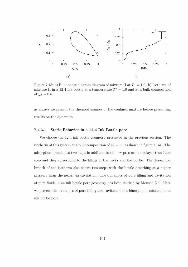
0

0.1

0.2

0.3

0 0.25 0.5 0.75 1

P

xA,yA

(a)

0

0.25

0.5

0.75

1

0 0.25 0.5 0.75 1

ρ A +

ρB

P/P0

(b)

Figure 7.15: a) Bulk phase diagram diagram of mixture II at T ∗ = 1.0. b) Isotherm ofmixture II in a 12-4 ink bottle at a temperature T ∗ = 1.0 and at a bulk compositionof yA = 0.5.

as always we present the thermodynamics of the confined mixture before presenting

results on the dynamics.

7.4.3.1 Static Behavior in a 12-4 Ink Bottle pore

We choose the 12-4 ink bottle geometry presented in the previous section. The

isotherm of this system at a bulk composition of yA = 0.5 is shown in figure 7.15a. The

adsorption branch has two steps in addition to the low pressure monolayer transition

step and they correspond to the filling of the necks and the bottle. The desorption

branch of the isotherm also shows two steps with the bottle desorbing at a higher

pressure than the necks via cavitation. The dynamics of pore filling and cavitation

of pure fluids in an ink bottle pore geometry has been studied by Monson [75]. Here

we present the dynamics of pore filling and cavitation of a binary fluid mixture in an

ink bottle pore.

104

(a) (b)

(c) (d)

(e) (f)

Figure 7.16: Visualizations of the density distribution of species A (top) and speciesB (bottom) showing the dynamics of pore filling in a 12− 4 for a step change in bulkpressure from P = 0.001 to P = 0.14 in a 12-4 ink bottle pore at a temperatureof T ∗ = 1.0 at a) w0t = 0; b) w0t = 5000; c) w0t = 60000; d) w0t = 12000; e)w0t = 135000; f) w0t = 160000.

105

7.4.4 Mixture II : Dynamic Behavior

7.4.4.1 Pore filling in 12-4 ink bottles

We first present the dynamic behavior associated with pore filling in a 12-4 ink

bottle. In the bulk we have an equimolar quantity of mixture II at T ∗ = 1.0 (for

bulk phase diagram refer figure 7.15a). The pore is initialized at a state (P = 0.001)

and then a step change is made in the bulk pressure (P = 0.14) to a state where the

bottle is filled with a liquid like state, (refer figure 7.15b). The visualizations of the

states encountered in the dynamics is shown in figure 7.16. We can see from figure

7.16a that initially the pore is empty. First a monolayer is formed in the necks and

the bottle (figure 7.16b), and necks fill up.This traps a bubble in the bottle. The

bottle fills up by squeezing the bubble out. As the bubble shrinks we observe surface

enrichment of species B at the vapor liquid interface of the bubble (figure 7.16c,figure

7.16d). Finally pore is filled with a liquid like state 7.16e) and then compositional

equilibration takes place.

7.4.4.2 Cavitation in 12-4 ink bottles

We now present the dynamic behavior associated with cavitation in a 12-4 ink

bottle. In the bulk we have an equimolar quantity of mixture II at T ∗ = 1.0 (for

bulk phase diagram refer figure 7.15a). The pore is initialized at a condensed state

(P = 0.1) and then a step change is made in the bulk pressure (P = 0.095) to a

state where the bottle is empty but the necks remain filled (refer figure 7.17a) . The

visualizations of the states encountered in the dynamics are shown in figure 7.17.

We can see from figure 7.17a that initially the density of fluid in the bottle is less

dense than the neck part and is more stretched. As time progresses the fluid becomes

more stretched (figure 7.17b), and at w0t = 9400, (figure 7.17d) a bubble forms in the

middle of the pore. The bubble expands until the bottle is empty. Note that as soon as

the bubble forms fluid B adsorbs at the vapor liquid interface. Oxtoby and co workers

106

(a) (b)

(c) (d)

(e) (f)

Figure 7.17: Visualizations of the density distribution of species A (top) and species B(bottom) showing the dynamics of cavitation caused by a step change in bulk pressurefrom P = 0.1 to P = 0.095 in a 12− 4 ink bottle pore at a temperature of T ∗ = 1.0at a) w0t = 0; b) w0t = 7000; c) w0t = 9000; d) w0t = 9200; e) w0t = 13000; f)w0t = 26000.

107

[109] the studied the rates of bubble formation in liquid mixtures at conditions where

both the species were subcritical in their pure form. They speculated the possibility

of cavitation being a two step process with a liquid liquid phase separation preceding

the bubble formation. It would be interesting to see if such behavior can be observed

in the DMFT, and we reserve this for future work.

7.5 Conclusions

We have presented studies of two different mixtures in this chapter. The bulk

phase behavior of mixture I resembles an ideal mixture, that can be described by

Raoult’s law. For such a mixture we observe that the trend in behavior of the mixture

in a slit pore as we increase the fraction of the lighter component in the bulk fluid,

is equivalent to the trend in behavior of a pure fluid upon increasing temperatures.

For slit pores we observe shrinking hysteresis loops, and for a 12-6 ink bottle pore we

observe a change in the desorption mechanism from pore blocking to cavitation as we

increase the fraction of the lighter component in the bulk fluid. We also presented

the dynamics of pore filling (capillary condensation) and (pore emptying) of mixtures

in a slit pore. Next we briefly presented the thermodynamics and dynamics of a

mixture with very different pure fluid interaction energies. In such mixtures the

lighter component has to tendency to aggregate at the vapor liquid interface. We

presented the dynamics of a cavitation process of this mixture in a 12-4 ink bottle

and observed surface aggregation to be present along the different states encountered

in the dynamics.

We have presented a framework to study the thermodynamics and dynamics of

mixtures confined in porous materials. It is clear from the calculations presented

above that the mean field lattice gas approach can qualitatively capture different

types of bulk phase diagrams of binary mixtures. Surface tensions of interfaces can

be computed, and thermodynamics and dynamics of confined binary mixtures can

108

be studied in any pore geometry. Moreover nucleation behavior are emergent feature

of the DMFT. The level of detail that we obtain given the modest computational

resources we invest is one of the most significant advantages of the DMFT. This

framework could very well be used to understand the dynamics of separation processes

at a microscopic scale in a wide variety of systems.

109

CHAPTER 8

COMPARISON OF DMFT WITH DYNAMIC MONTECARLO SIMULATIONS

In this chapter we assess the impact of the approximations in DMFT as a descrip-

tion of the lattice model dynamics. Mean field theory in thermodynamics replaces the

instantaneous local density by its ensemble average, thus neglecting the effect of fluc-

tuations on the equilibrium properties. For a lattice gas model with nearest neighbor

interactions this approximation is accurate for very dense or very dilute states but is

less accurate for medium density states and is in greatest error in the critical region.

Yet researchers continue to rely on mean field theory as a qualitative tool in mapping

the phase behavior of systems, such as fluids confined in porous materials, because it

so often yields a qualitatively correct description of the thermodynamics that can be

refined by further studies with Monte Carlo simulations or perhaps with higher order

theories. As we will discuss in more detail later, within the context of the lattice gas

model dynamics the mean field approximation enters by replacing instantaneous site

occupancies in the master equation for the system with their average values from an

ensemble of trajectories. The success of the theory depends in part on the width of

the distribution of fluctuations in space and time relative to the mean values. For

instance for a slit pore we will consider in detail the condensation transition from

vapor to liquid driven by a step change in the bulk chemical potential. DMFT pre-

dicts this as a process whereby a liquid bridge or bridges form in the pore. In DMFT

the nucleation occurs at a given time and the density distribution is symmetric with

respect to the pore geometry. This can be compared with the results from an en-

semble of trajectories generated via dynamic Monte Carlo simulations.[117, 57, 51] In

110

xy

zH

Figure 8.1: Schematic representation of a slit pore of length L and height H. Periodicboundaries are applied in the y-direction. The two partitions seen at the two edgesof the system separate the system from the control volumes or particle reservoirs.

dynamic Monte Carlo the ensemble of trajectories yields a distribution of nucleation

times and locations, and while the ensemble average density distribution is symmetric

with respect to the pore geometry, that in the individual trajectories is not.

The organization of this chapter is as follows. In section 8.1 we describe how the

theory and the simulation are implemented to study capillary condensation in slit

pores, and we present the system which we use to make the comparisons. In section

8.2 we present our results and provide a summary of our results and conclusions in

section 8.3.

8.1 Implementation

8.1.1 Systems Studied

Our focus in this work is on the pore geometry in figure 8.1 where we have a

finite length slit pore in contact with the bulk. All the calculations are performed

for nearest neighbor pore walls of α = 3.0 at a pore width H = 6 and at a reduced

temperature of T/Tc = 0.66, which is T ∗ = 1.0 for the DMFT/MFT and T ∗ = 0.741

for the DMC/GCMC. This choice of different temperatures for the two methods was

made to reduce the effects differences in the bulk thermodynamics and phase diagram

upon the comparison between theory and simulations. We describe the equilibrium

state of the system in terms of relative activity λ/λ0 = exp[(µ− µ0)/kT ], where µ is

the chemical potential of the system and µ0 the chemical potential at saturation.

111

The dimensions of the system are as follows. The wall spacing in the slit is H = 6

in lattice constants and the length of the slit varies from L=20 to L=60. The slit pore

has periodic boundary conditions in the y-direction. This makes the MFT and DMFT

calculations two-dimensional. The simulations are done in a three-dimensional system

with the pore width in the y-direction fixed at 12 lattice constants. The dimensions of

the bulk region on each side of the slit are 20 (length) ×12× 12 lattice constants. In

the DMC simulations the bulk regions are divided into two regions of length 10 lattice

units, with the region furthest from the pore being the control volume. By increasing

or decreasing the chemical potential in this region we can bring about net mass

transfer to or from the rest of the system including the pore. The implementation of

the DMFT and DMC simulations with the control volume technique is explained in

sections 2.3.2 and 2.3.3 respectively.

8.1.2 Problem : Dynamics of Capillary condensation

As stated in the introduction the objective of our present work is make compar-

isons between the DMFT and DMC. The processes we consider to make the compar-

isons are the dynamics associated with a change of state along an adsorption isotherm

that crosses the capillary condensation transition (see figures 8.3 a) and b)). The na-

ture of this process depends upon the size of the step in relative activity (chemical

potential) used as well as the location of the starting and ending states. We consider

various examples of such step changes of state and look at the dynamics of the nucle-

ation processes involved. Table 8.1 shows the list of activity step changes studied in

this work. As seen in section 2.3.1 the density evolution predicted by the DMFT can

be considered an approximation to an ensemble average of dynamic MC trajectories.

Hence for most of the simulation results presented in this work we have averaged

the DMC data from 1536 statistically independent runs, although we have some re-

sults with up to 15360 trajectories. The availability of high performance computing

112

Table 8.1: Activities of the initial and final states of the step changes studied in thischapter

Pore length Step change No.DMFT DMC

Start End Start End

L = 20

I 0.001 0.95 0.001 0.95II 0.77 0.92 0.71 0.86III 0.001 0.92 0.001 0.86IV 0.031 0.95 0.091 0.95

L = 40V 0.001 0.95 0.001 0.95VI 0.77 0.92 0.71 0.86

L = 60 VII 0.001 0.95 0.001 0.95

L = 120 VIII 0.001 0.95 0.001 0.95

clusters with multicore processors facilitates the simultaneous study of such a large

number of trajectories. In the next section 8.1.3 we describe the algorithm used to

observe the nucleation process in each of 1536 statistically independent trajectories.

8.1.3 Studying the formation of liquid bridges in DMC simulations

Capillary condensation in slit pores with completely wetting pore walls is a first

order phase transition and the critical nucleus is a liquid bridge [90, 110, 74]. In this

work we use the following algorithm to analyze the formation of liquid bridges in

the DMC simulations. Every 200 MC sweeps, we compute the x-directional density

profile ρ(xi). Since the slit pore is semi-infinite in the y-direction, ρ(xi) or the density

averaged over a given y-z plane is sufficient to identify a liquid bridge. A consecutive

number w of such planes with density ρ(xi) exceeding a specified value ρBridge is

identified as a liquid bridge. The starting and ending x-coordinates of all liquid

113

bridges are stored in data files. Once the simulations are done we post process this

data to identify the critical nucleus. The value of w, which sets the minimum width

of the liquid bridge and τs, which is the survival time, or the duration over which

an observed liquid bridge has to remain stable or grow in order to be identified as a

critical nucleus. If the width of an observed liquid bridge is equal to or exceeds w, and

is observed to remain stable or grow for a duration exceeding the survival time τs ,

we classify the liquid bridge as a post critical nucleus and store the x-coordinates and

the time at which it was first observed. For the results presented here we use w = 4,

ρliq = 0.85 and τs to be at least 60000 MCS. We have observed that all liquid bridges

identified in this way proceed to grow and fill the pore with liquid. These parameters

and definitions are somewhat arbitrary but serve the objective of our present work,

which is to make qualitative comparisons of the mechanism of capillary condensation

in slit pores between the DMFT and the DMC simulations.

8.1.4 Relating timescales in DMFT and DMC

The DMFT is derived from the master equation that describes the evolution of a

DMC trajectory. Hence we should be able to compare the results of both the methods

with the same time scale. The factor w0 in the Metropolis criterion sets the time scale

for the DMFT. As shown by Matuszak et al. w0 can be written as [69]

w0 =ν

z(8.1)

where ν is the frequency at which every particle in the lattice has attempted

one hopping event and z is the coordination number of the lattice. The DMFT

conservation equation eqn. 2.14 considers flux between all the nearest neighbors of

a given lattice site and the factor 1/z accounts for the fact that at any given time a

hopping attempt can be made to only one of the z nearest neighbors. In the DMC

simulations every particle makes one hopping attempt to its nearest neighbor per

114

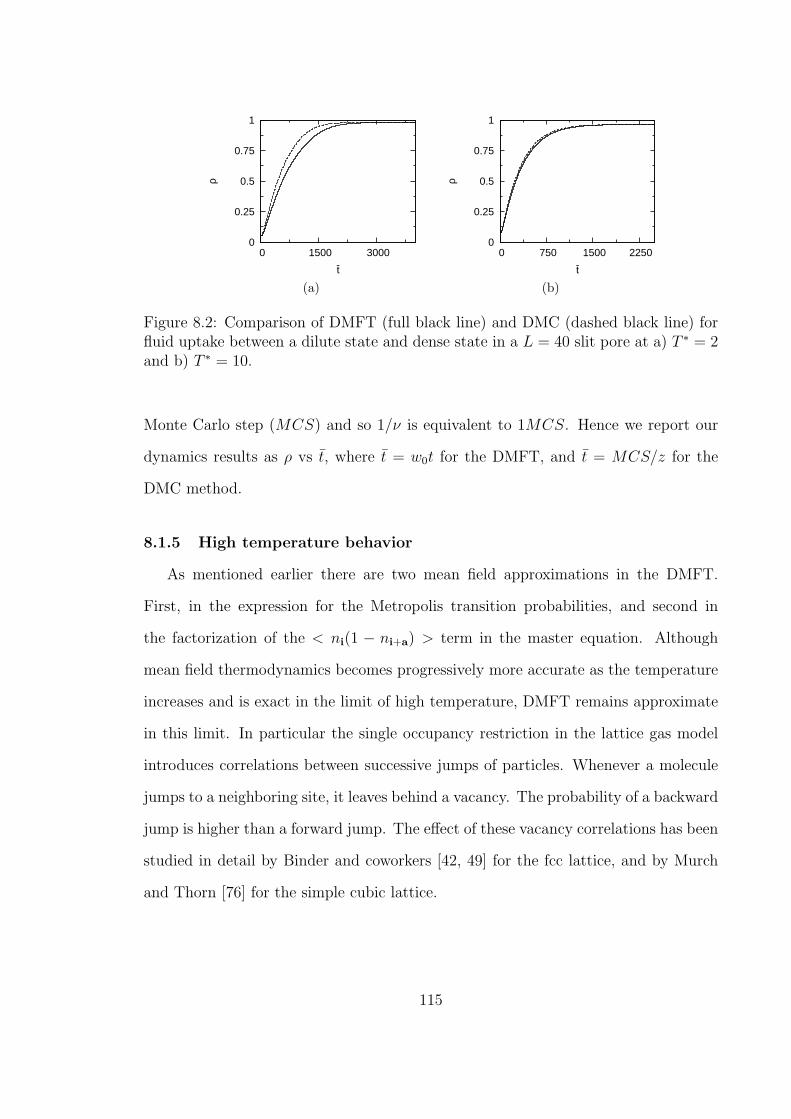
0

0.25

0.5

0.75

1

0 1500 3000

ρ

t-

(a)

0

0.25

0.5

0.75

1

0 750 1500 2250

ρ

t-

(b)

Figure 8.2: Comparison of DMFT (full black line) and DMC (dashed black line) forfluid uptake between a dilute state and dense state in a L = 40 slit pore at a) T ∗ = 2and b) T ∗ = 10.

Monte Carlo step (MCS) and so 1/ν is equivalent to 1MCS. Hence we report our

dynamics results as ρ vs t, where t = w0t for the DMFT, and t = MCS/z for the

DMC method.

8.1.5 High temperature behavior

As mentioned earlier there are two mean field approximations in the DMFT.

First, in the expression for the Metropolis transition probabilities, and second in

the factorization of the < ni(1 − ni+a) > term in the master equation. Although

mean field thermodynamics becomes progressively more accurate as the temperature

increases and is exact in the limit of high temperature, DMFT remains approximate

in this limit. In particular the single occupancy restriction in the lattice gas model

introduces correlations between successive jumps of particles. Whenever a molecule

jumps to a neighboring site, it leaves behind a vacancy. The probability of a backward

jump is higher than a forward jump. The effect of these vacancy correlations has been

studied in detail by Binder and coworkers [42, 49] for the fcc lattice, and by Murch

and Thorn [76] for the simple cubic lattice.

115

In figure 8.2, we compare the results of fluid uptake in a L = 40 slit pore at high

temperature. We initialize the system at a dilute state and increase to activity to

drive the system to a high density state. We repeat this calculation at four different

temperatures all of which are above the bulk critical temperature. Unlike the sub-

critical cases presented in this paper the comparison with the DMFT is done at the

same temperature and not the same reduced temperature. At the temperatures con-

sidered the mean field approximation will be accurate for the thermodynamics and

we can assess the impact of the neglect of vacancy correlations separately. As can

be seen in figure 8.2 the agreement between DMC and DMFT is very good improves

as temperature increases, although even at the highest temperature considered the

DMFT does not become exact. Evidently the neglect of vacancy correlations is not

substantial under these conditions.


8.2.1 Static behavior

0

0.25

0.5

0.75

1

0 0.25 0.5 0.75 1

ρ

λ/λ0

(a)

0

0.25

0.5

0.75

1

0 0.25 0.5 0.75 1

ρ

λ/λ0

(b)

Figure 8.3: Adsorption / Desorption isotherms for a slit pore of width H = 6 com-puted with a) MFT and b) GCMC simulations (the lines connecting the points are aguide to the eye) at T/Tc = 0.66.

We first present the static (equilibrium or metastable equilibrium) behavior of the

fluid in the slit pore. The adsorption/desorption isotherm for the L = 60 slit pore in

116

contact with the bulk from GCMC simulations and MFT are shown in figures 8.3 a)

and b). Both the isotherms exhibit two transitions. The step at low relative activity

corresponds to a monolayer formation or two dimensional condensation on the walls

for the pore. The second transition region at higher relative activity is a capillary

condensation transition exhibiting hysteresis. As shown in previous work on a slit pore

model of a lattice gas [74], the metastable states in the hysteresis loop are all on the

adsorption branch and are associated with the free energy barrier to nucleation of the

liquid phase in the pore via the formation of a liquid bridge. This is now generally

believed to be the correct interpretation of hysteresis for fluids in simple uniform

pores like slits and cylinders and in real systems such as nitrogen in MCM-41 which

can be accurately represented by such models [89, 74]. The width of the hysteresis

loop is narrower in the GCMC isotherm as compared to the MFT isotherm. This

reflects the fact that in MFT nucleation does not occur until the low density (vapor)

phase reaches a stability limit, while in the GCMC simulations fluctuations can cause

nucleation for lower degrees of supersaturation of the low density phase (with respect

to the equilibrium capillary transition. The results in figure 8.3 show that although

there is not close quantitative agreement between the GCMC simulation results and

MFT, the qualitative agreement is very good. We now turn to comparisons of DMFT

with DMC simulations.

8.2.2 Dynamics of filling of slit pores of length L = 20

We begin by discussing the dynamics of pore filling for four different step changes

in a L = 20 slit pore. The starting and ending points of the four activity changes

are given in table 8.1. We have chosen these processes to illustrate the effect of i)

magnitude of the step change ii) positions of the initial and final states of the step

change on the phase diagram on equilibration times and mechanisms of nucleation.

117

ρ

t-

0 10 20 30 40

x

0

7500

15000

0

0.25

0.5

0.75

1ρ

t-

0 10 20 30 40

x

0

20000

40000

0

0.25

0.5

0.75

1

Figure 8.4: Visualizations of the sequence of states encountered in the filling of L=20pore for step change I a) as predicted by the DMFT and b) computed as an averageof 1536 statistically independent DMC trajectories. Density evolution maps ρ(x) vst for step change I computed with c) DMFT and d) DMC simulations.

118

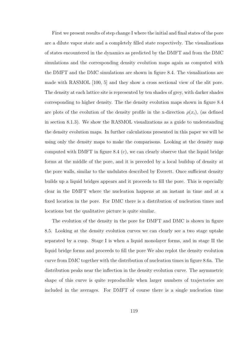
First we present results of step change I where the initial and final states of the pore

are a dilute vapor state and a completely filled state respectively. The visualizations

of states encountered in the dynamics as predicted by the DMFT and from the DMC

simulations and the corresponding density evolution maps again as computed with

the DMFT and the DMC simulations are shown in figure 8.4. The visualizations are

made with RASMOL [100, 5] and they show a cross sectional view of the slit pore.

The density at each lattice site is represented by ten shades of grey, with darker shades

corresponding to higher density. The the density evolution maps shown in figure 8.4

are plots of the evolution of the density profile in the x-direction ρ(xi), (as defined

in section 8.1.3). We show the RASMOL visualizations as a guide to understanding

the density evolution maps. In further calculations presented in this paper we will be

using only the density maps to make the comparisons. Looking at the density map

computed with DMFT in figure 8.4 (c), we can clearly observe that the liquid bridge

forms at the middle of the pore, and it is preceded by a local buildup of density at

the pore walls, similar to the undulates described by Everett. Once sufficient density

builds up a liquid bridges appears and it proceeds to fill the pore. This is especially

clear in the DMFT where the nucleation happens at an instant in time and at a

fixed location in the pore. For DMC there is a distribution of nucleation times and

locations but the qualitative picture is quite similar.

The evolution of the density in the pore for DMFT and DMC is shown in figure

8.5. Looking at the density evolution curves we can clearly see a two stage uptake

separated by a cusp. Stage I is when a liquid monolayer forms, and in stage II the

liquid bridge forms and proceeds to fill the pore We also replot the density evolution

curve from DMC together with the distribution of nucleation times in figure 8.6a. The

distribution peaks near the inflection in the density evolution curve. The asymmetric

shape of this curve is quite reproducible when larger numbers of trajectories are

included in the averages. For DMFT of course there is a single nucleation time

119

0

0.25

0.5

0.75

1

0 15000 30000ρ

t-

Figure 8.5: Density evolution of the L = 20 slit pore averaged over 15360 DMCtrajectories (full black line) together with the DMFT (dashed black line) predictionfor step change I.

0

0.25

0.5

0.75

1

0 20000 40000 0

0.05

0.1

0.15

0.2

t-, τ

ρ P(τ)

(a)

0

0.05

0.1

0 20 40

P(x

)

x

(b)

Figure 8.6: a) Density of pore vs. time of the L = 20 slit pore for step change Itogether with the histogram of liquid bridge formation times from DMC simulations.b) Histograms of liquid bridge formation locations. ( 11 ≤ x ≤ 30 is the region wherethe slit pore is present.)

120

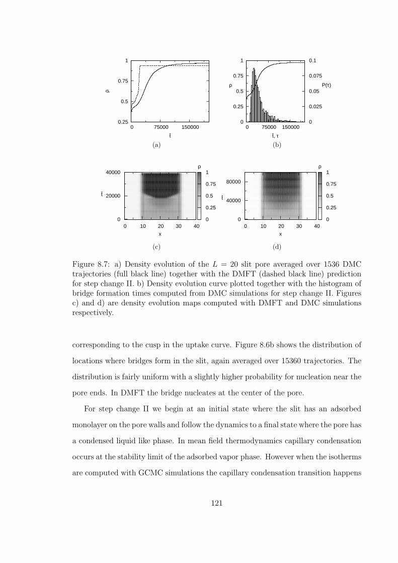
0.25

0.5

0.75

1

0 75000 150000

ρ

t-

(a)

0

0.25

0.5

0.75

1

0 75000 150000 0

0.025

0.05

0.075

0.1

t-, τ

ρ P(τ)

(b)

ρ

t-

0 10 20 30 40

x

0

20000

40000

0

0.25

0.5

0.75

1

(c)

ρ

t-

0 10 20 30 40

x

0

40000

80000

0

0.25

0.5

0.75

1

(d)

Figure 8.7: a) Density evolution of the L = 20 slit pore averaged over 1536 DMCtrajectories (full black line) together with the DMFT (dashed black line) predictionfor step change II. b) Density evolution curve plotted together with the histogram ofbridge formation times computed from DMC simulations for step change II. Figuresc) and d) are density evolution maps computed with DMFT and DMC simulationsrespectively.

corresponding to the cusp in the uptake curve. Figure 8.6b shows the distribution of

locations where bridges form in the slit, again averaged over 15360 trajectories. The

distribution is fairly uniform with a slightly higher probability for nucleation near the

pore ends. In DMFT the bridge nucleates at the center of the pore.

For step change II we begin at an initial state where the slit has an adsorbed

monolayer on the pore walls and follow the dynamics to a final state where the pore has

a condensed liquid like phase. In mean field thermodynamics capillary condensation

occurs at the stability limit of the adsorbed vapor phase. However when the isotherms

are computed with GCMC simulations the capillary condensation transition happens

121

at an activity where the nucleation barrier for capillary condensation is sufficiently

small to be overcome within the fixed run length of the simulation. Hence to fix the

final state for the DMC simulations we compute the system size dependent stability

limit (see appendix) of the monolayer in the pore via GC TMMC simulations and fix

the activity of the final state og the step change beyond this point. The initial and

final activities for step change II for the DMFT and DMC are given in table 8.1.

The density evolution curves and maps for step change II computed with the

DMFT and DMC are shown in figure 8.7. The density evolution curve computed

with the DMC qualitatively agrees with the DMFT. However the equilibration time

however is almost five times higher. A smaller driving force results in a much smaller

flux into the pore and a much broader distribution of nucleation times. as shown in

figure 8.7b. The density evolution map computed with from the DMC simulations is

shown in 8.7d reflects the much broader distribution of nucleation times and locations.

It is also interesting to investigate the effect of changing the activity of the final

state of the step change . We present results of step changes III and IV together

in figure 8.8.The magnitude of the step change is equal in both, however the end

point of the step change III is closer to the capillary condensation transition in the

phase diagram (isotherm) than step change IV. This has a significant effect on the

relaxation behavior. The density evolution curves computed with the DMFT and

DMC simulations for step changes III and IV are shown in figure 8.8. The response

of the system to step change III, is almost identical to the response to step change II,

and this can be clearly seen by comparing figures 8.8a / 8.8b and 8.5 / 8.6a . Step

change IV has the same magnitude as step change III, however the final state of the

step change is shifted away from the capillary condensation transition towards bulk

saturation. The density evolution curves shown in figure 8.8c / 8.8d show that the

response of the system to step change IV, is identical to the response to step change

122

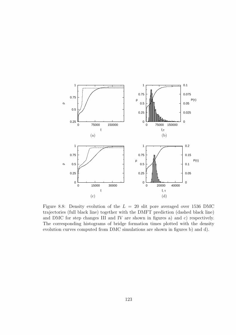
0.25

0.5

0.75

1

0 75000 150000

ρ

t-

(a)

0

0.25

0.5

0.75

1

0 75000 150000 0

0.025

0.05

0.075

0.1

t-,τ

ρ P(τ)

(b)

0

0.25

0.5

0.75

1

0 15000 30000

ρ

t-

(c)

0

0.25

0.5

0.75

1

0 20000 40000 0

0.05

0.1

0.15

0.2

t-, τ

ρ P(τ)

(d)

Figure 8.8: Density evolution of the L = 20 slit pore averaged over 1536 DMCtrajectories (full black line) together with the DMFT prediction (dashed black line)and DMC for step changes III and IV are shown in figures a) and c) respectively.The corresponding histograms of bridge formation times plotted with the densityevolution curves computed from DMC simulations are shown in figures b) and d).

123

0

0.25

0.5

0.75

1

0 120000 240000

ρ

t-

0.850.890.930.97

0

0.25

0.5

0 4000

(a)

0

600000

1.2e+06

0.7 0.8 0.9 1

τ eq

λf

(b)

Figure 8.9: a) Density evolution curves computed with DMC simulations for fourdifferent step changes where the relative activity of the initial state is fixed at λ/λ0 =0.001, and the relative activity of the final states varies as 0.85, 0.89, 0.93 and 0.97.The initial part of each density evolution curve is shown in the inset. Figure b) showsequilibration times vs activity of the final state of the step change. The dashed dashedline is the capillary condensation transition point in the isotherm of the H = 6 slitpore, and the dotted line is the stability limit of the adsorbed vapor phase.

I shown in figures 8.7a / 8.7b. This makes it clear that the equilibration times are

largely dependent on the final state of the step change.

In order to substantiate the arguments stated above, we show uptake curves of

four different step changes (not given in table 8.1), where we fix the activity of the

initial state to be the same for all cases at λ/λ0 = 0.001, and vary the activity of the

final state of the step change from λ/λ0 = 0.83 to 0.97. The density evolution curves

of the pore for the different step changes are shown in figure 8.9a. The inset of figure

8.9a shows the initial part of the uptake process, corresponding to the formation of

the monolayer. We can clearly see that the initial phase is very similar for the four

different step changes. However once it reaches a state where a monolayer is filled the

rate of the fluid uptake uptake process varies significantly. In figure 8.9b we report

the equilibration times as τeq vs λf , where λf is the activity of final state of the step

change. The vertical blue dashed line in figure 8.9b is the point where the isotherm

of the H = 6, L = 20 slit pore shows a step corresponding to a capillary condensation

transition. The red dashed line represents the system size dependent stability limit

124

ρ

t-

0 10 20 30 40 50 60

x

0

15000

30000

0

0.25

0.5

0.75

1

(a)

ρ

t-

0 10 20 30 40 50 60

x

0

40000

80000

0

0.25

0.5

0.75

1

(b)

Figure 8.10: Density evolution maps of the L = 40 slit pore predicted by the a) DMFTand b) computed by averaging over 1536 statistically independent DMC trajectoriesfor step change V respectively.

of the adsorbed vapor phase in the slit pore. For states to the right of the red line,

the condensed state is the only equilibrium state of the pore. For states lying to the

left of the red line, the monolayer state is a metastable state and it is separated from

the stable condensed state by a finite free energy barrier. Hence if the final point

of the step change is between the two vertical lines the dynamics involves a finite

nucleation barrier crossing in addition to diffusion limitations, thus resulting in very

large equilibration times. Also as the final state of the step change approaches the

capillary condensation transition, the distribution of nucleation times becomes much

wider which explains the trend in equilibration times.

8.2.3 Dynamics of filling of slit pores of length : L = 40

For the L = 40 pore we first present the results of step change V, where we begin

with an almost empty state and follow the evolution of the pore to a condensed state.

The density evolution maps computed with the DMFT and DMC are shown in figure

8.10. Looking at the DMFT density evolution map in figure 8.10a it is clear that

the pore fills via the formation of two liquid bridges, near the ends of the pore. The

DMC density evolution map is more diffuse. Though it appears to show two bridges

125

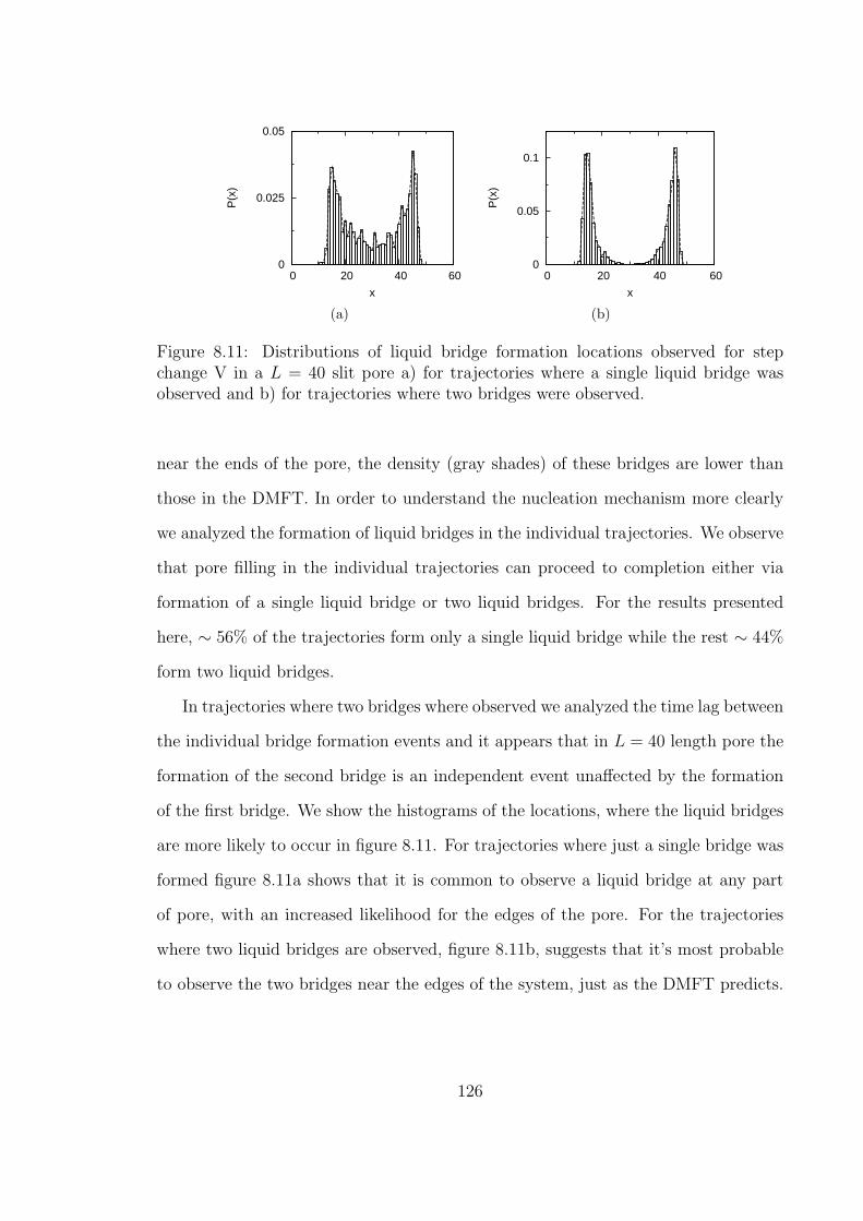
0

0.025

0.05

0 20 40 60

P(x

)

x

(a)

0

0.05

0.1

0 20 40 60

P(x

)

x

(b)

Figure 8.11: Distributions of liquid bridge formation locations observed for stepchange V in a L = 40 slit pore a) for trajectories where a single liquid bridge wasobserved and b) for trajectories where two bridges were observed.

near the ends of the pore, the density (gray shades) of these bridges are lower than

those in the DMFT. In order to understand the nucleation mechanism more clearly

we analyzed the formation of liquid bridges in the individual trajectories. We observe

that pore filling in the individual trajectories can proceed to completion either via

formation of a single liquid bridge or two liquid bridges. For the results presented

here, ∼ 56% of the trajectories form only a single liquid bridge while the rest ∼ 44%

form two liquid bridges.

In trajectories where two bridges where observed we analyzed the time lag between

the individual bridge formation events and it appears that in L = 40 length pore the

formation of the second bridge is an independent event unaffected by the formation

of the first bridge. We show the histograms of the locations, where the liquid bridges

are more likely to occur in figure 8.11. For trajectories where just a single bridge was

formed figure 8.11a shows that it is common to observe a liquid bridge at any part

of pore, with an increased likelihood for the edges of the pore. For the trajectories

where two liquid bridges are observed, figure 8.11b, suggests that it’s most probable

to observe the two bridges near the edges of the system, just as the DMFT predicts.

126

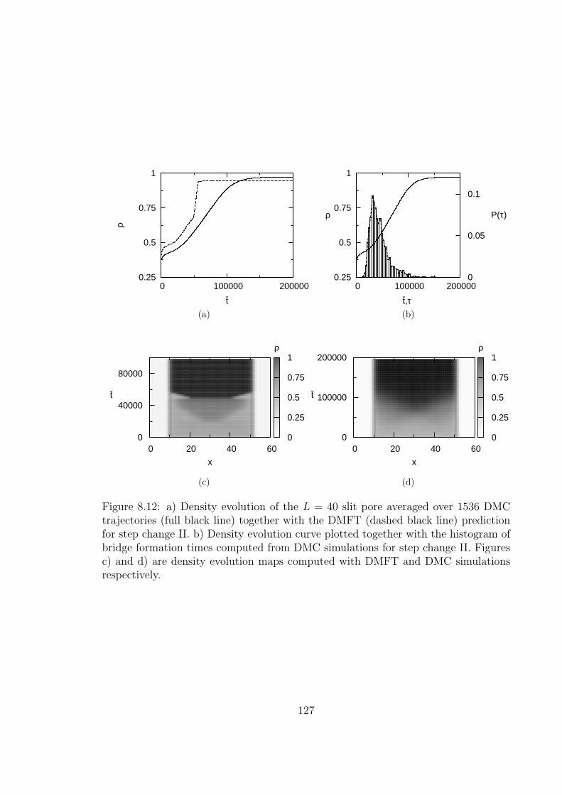
0.25

0.5

0.75

1

0 100000 200000

ρ

t-

(a)

0.25

0.5

0.75

1

0 100000 200000 0

0.05

0.1

t-,τ

ρ P(τ)

(b)

ρ

t-

0 20 40 60

x

0

40000

80000

0

0.25

0.5

0.75

1

(c)

ρ

t-

0 20 40 60

x

0

100000

200000

0

0.25

0.5

0.75

1

(d)

Figure 8.12: a) Density evolution of the L = 40 slit pore averaged over 1536 DMCtrajectories (full black line) together with the DMFT (dashed black line) predictionfor step change II. b) Density evolution curve plotted together with the histogram ofbridge formation times computed from DMC simulations for step change II. Figuresc) and d) are density evolution maps computed with DMFT and DMC simulationsrespectively.

127

ρ

t-

0 20 40 60 80

x

0

30000

60000

0

0.25

0.5

0.75

1

(a)

ρ

t-

0 20 40 60 80

x

0

75000

150000

0

0.25

0.5

0.75

1

(b)

Figure 8.13: Density evolution maps of the L = 60 slit pore a) predicted byDMFTand b) computed by averaging over 1536 statistically independent DMC trajectoriesfor step change VII.

In step change VI the activity of the final state is fixed close to the capillary

condensation transition and the magnitude of the step change is kept small. The

uptake curves and density evolution maps computed with the DMFT and DMC are

shown in figure 8.12. DMFT predicts that the pore filling in such situations occurs

with the formation of just one liquid bridge at the middle of the pore and this has been

shown in earlier work [74]. This is clear from the density evolution map shown in figure

8.12c. Similar to cases presented above the density evolution maps computed from

the DMC fail to provide a clear explanation of the relaxation mechanism. Analysis of

the trajectories reveal that ( 99%) of the DMC trajectories formed only a single liquid

bridge. Only 13 of the 1536 trajectories < 1% formed two liquid bridges. The low

driving force, results in a low influx of fluid making it harder for nucleation events to

occur. The relaxation mechanism observed in the DMC results is thus qualitatively

consistent with the DMFT predictions.

128

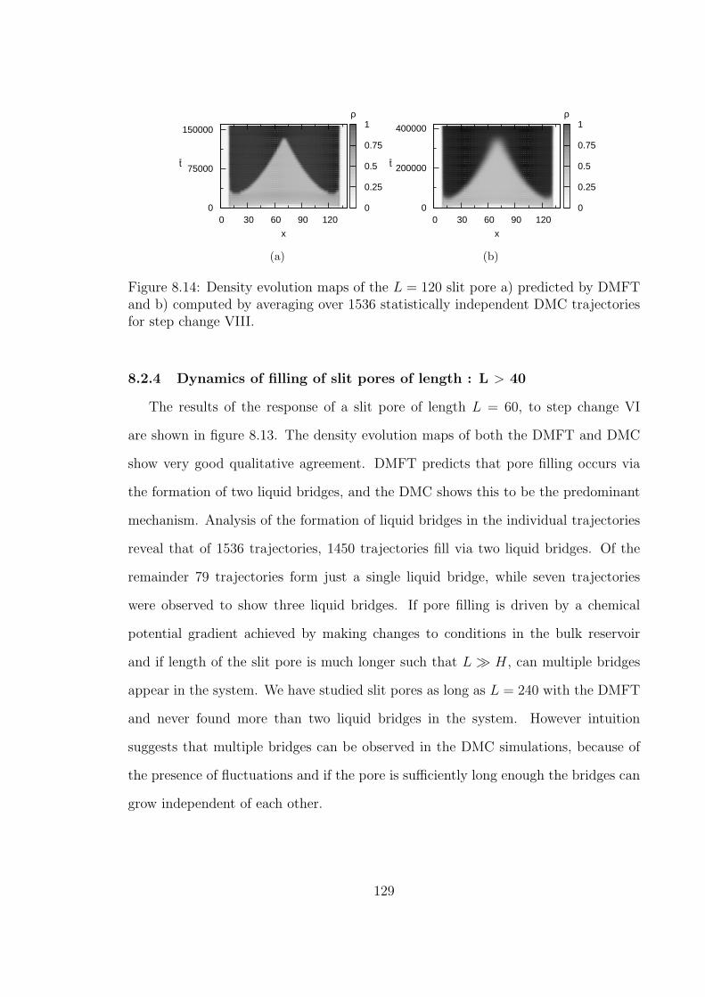
ρ

t-

0 30 60 90 120

x

0

75000

150000

0

0.25

0.5

0.75

1

(a)

ρ

t-

0 30 60 90 120

x

0

200000

400000

0

0.25

0.5

0.75

1

(b)

Figure 8.14: Density evolution maps of the L = 120 slit pore a) predicted by DMFTand b) computed by averaging over 1536 statistically independent DMC trajectoriesfor step change VIII.

8.2.4 Dynamics of filling of slit pores of length : L > 40

The results of the response of a slit pore of length L = 60, to step change VI

are shown in figure 8.13. The density evolution maps of both the DMFT and DMC

show very good qualitative agreement. DMFT predicts that pore filling occurs via

the formation of two liquid bridges, and the DMC shows this to be the predominant

mechanism. Analysis of the formation of liquid bridges in the individual trajectories

reveal that of 1536 trajectories, 1450 trajectories fill via two liquid bridges. Of the

remainder 79 trajectories form just a single liquid bridge, while seven trajectories

were observed to show three liquid bridges. If pore filling is driven by a chemical

potential gradient achieved by making changes to conditions in the bulk reservoir

and if length of the slit pore is much longer such that L À H, can multiple bridges

appear in the system. We have studied slit pores as long as L = 240 with the DMFT

and never found more than two liquid bridges in the system. However intuition

suggests that multiple bridges can be observed in the DMC simulations, because of

the presence of fluctuations and if the pore is sufficiently long enough the bridges can

grow independent of each other.

129

ρ

t-

0 30 60 90 120

x

0

200000

400000

0

0.25

0.5

0.75

1

(a)

ρ

t-

0 30 60 90 120

x

0

200000

400000

0

0.25

0.5

0.75

1

(b)

Figure 8.15: Density evolution maps of two DMC trajectories of the L = 120 porefor step change VIII, where three liquid bridges were observed.

To answer such questions we studied the response of a L = 120 slit pore to step

change VIII. Analysis of the DMC trajectories reveals that of the 1536 trajectories

analyzed 1533 showed two liquid bridges, and the only 3 trajectories had three liq-

uid bridges. None of the trajectories filled with just a single bridge. Though these

numbers vary from run to run, it is clear that the pore fills predominantly via the

formation of two liquid bridges. In figure 8.14 we show the density evolution maps

computed with the DMFT and the DMC simulations, and we can observe good qual-

itative agreement between the two methods. We also present density evolution maps

of two trajectories where three bridges were observed in figure 8.15. In figure 8.15a

the third bridge forms close to an existing liquid bridge, eventually merging into it.

Figure 8.15b shows an example of a situation where additional liquid bridges can-

not survive to proceed to completion since the filling proceeds via the two dominant

bridges at the corners and there is very low influx of fluid to sustain the middle bridge.

This can be thought of as an Ostwald ripening situation where smaller nuclei decay

to aid the growth of the dominant nuclei. We have also studied a L = 240 length

pore, and observed just 3 out of 1536 trajectories with three bridges. Although this

does not rule out the possibility of multiple bridging the formation of more than two

bridges appears to be a relatively rare event.

130

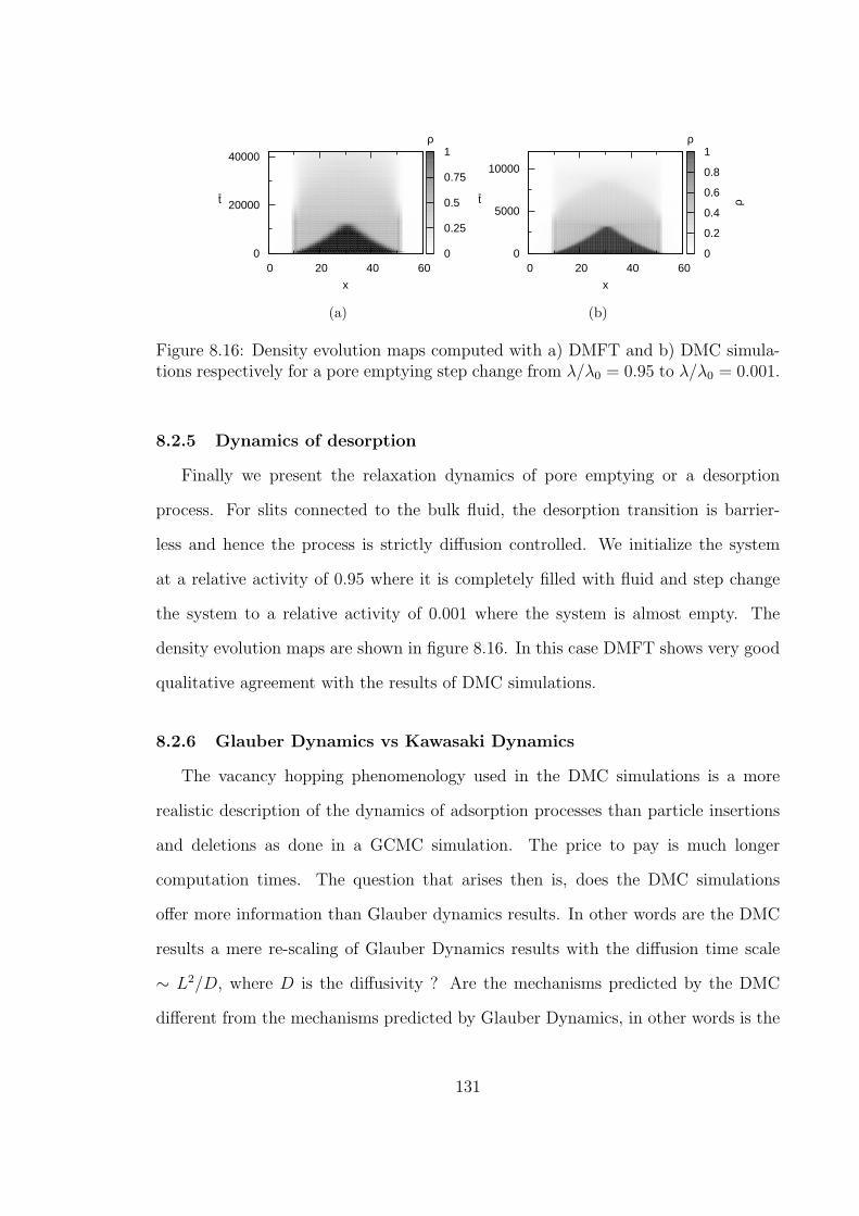
ρ

t-

0 20 40 60

x

0

20000

40000

0

0.25

0.5

0.75

1

(a)

t-

ρ

0 20 40 60

x

0

5000

10000

0

0.2

0.4

0.6

0.8

1

ρ

(b)

Figure 8.16: Density evolution maps computed with a) DMFT and b) DMC simula-tions respectively for a pore emptying step change from λ/λ0 = 0.95 to λ/λ0 = 0.001.

8.2.5 Dynamics of desorption

Finally we present the relaxation dynamics of pore emptying or a desorption

process. For slits connected to the bulk fluid, the desorption transition is barrier-

less and hence the process is strictly diffusion controlled. We initialize the system

at a relative activity of 0.95 where it is completely filled with fluid and step change

the system to a relative activity of 0.001 where the system is almost empty. The

density evolution maps are shown in figure 8.16. In this case DMFT shows very good

qualitative agreement with the results of DMC simulations.

8.2.6 Glauber Dynamics vs Kawasaki Dynamics

The vacancy hopping phenomenology used in the DMC simulations is a more

realistic description of the dynamics of adsorption processes than particle insertions

and deletions as done in a GCMC simulation. The price to pay is much longer

computation times. The question that arises then is, does the DMC simulations

offer more information than Glauber dynamics results. In other words are the DMC

results a mere re-scaling of Glauber Dynamics results with the diffusion time scale

∼ L2/D, where D is the diffusivity ? Are the mechanisms predicted by the DMC

different from the mechanisms predicted by Glauber Dynamics, in other words is the

131

ρ

MCS

0 30 60 90 120

x

0

50

100

0

0.25

0.5

0.75

1

(a)

ρ

MCS

0 30 60 90 120

x

0

50

100

0

0.25

0.5

0.75

1

(b)

Figure 8.17: Density evolution maps of two Glauber dynamics trajectories of theL = 120 pore for step change VIII.

path taken by the system in phase space the same in both cases. To understand this

better we repeated step change VIII, i.e pore filling in L = 120 slit pore with Glauber

Dynamics. The system is equilibrated at the initial value of the chemical potential

(activity) where the only stable phase is a dilute phase. A step change is made to the

activity of the control volume to a state where the only stable phase is a condensed

phase. According to the DMC results shown in figure 8.14, the dynamics proceeds

predominantly via the formation of two liquid bridges at the two ends of the pore.

In figure 8.17 we show two trajectories computed with Glauber Dynamics. We see

that multiple liquid bridges, or many post critical nuclei appear and proceed to fill

the pore. This is very much unlike the DMC predictions, where the incoming flux

restricts the number of liquid bridges to two and making it more probable to appear

at the ends. If at the activity of the final state of the step change, both a metastable

and stable state separated by a finite free energy barrier exist, then we expect the

mechanisms predicted by both methods would be same, since the process is limited

by the formation of the critical nucleus and not by mass transfer resistances. It is

also interesting to look at step changes to states with a single equilibrium state in

systems with heterogeneities as studied by Luzar co workers [57]. We reserve this for

future work.

132

8.3 Conclusion

We have presented a comparison of DMC simulations with the predictions DMFT

for the relaxation dynamics of a fluid in a slit pore in contact with bulk gas. We

first presented results of the dynamics of pore filling in L = 20 slit pore starting

from a low activity state with only vapor in the pore. Since fluctuations are not

included in the DMFT, the nucleation event occurs at a specific time, at a specific

location for a certain step change. The presence of fluctuations in the simulations

results in a distribution of nucleation times and locations. Otherwise for step change

I DMFT qualitatively agrees with the simulation results. In step change II we studied

the dynamics between states just either side of the capillary condensation transition.

The equilibration times predicted by the DMFT are very different from the simulation

results and this can be explained by the wide distribution of nucleation times. We

showed that the location of the activity of the final state of the step change affects the

uptake behavior significantly. The farther the end point of the step change is placed

from the capillary condensation transition, the shorter the equilibration times get. We

repeated simulations of step change I with five and ten times as many trajectories.

We observed that the shape and width of the histogram of nucleation times remains

unchanged.

We also studied longer pores. L = 20, 40, 120. For the L = 40 case DMFT

predicts that for step change V the pore fills via the formation of two liquid bridges

at the edges of the system. The DMC simulation results show some variations, in

that about 56% trajectories fill only with a single bridge, while the rest form two

bridges. However whenever two bridges were observed as predicted by the DMFT

they were more likely to be observed in the edges of the system. We studied the

L = 60 and L = 120 length pore to see if more than two bridges could form in the

pore. DMFT predicts that for large driving forces, two bridges appear near the ends

of the pore, and system fills only with the growth of these two dominant bridges. In

133

the simulations only a very small fraction of trajectories < 1% with three bridges were

observed. Although the possibility of multiple bridges cannot be ruled out, that large

influx of fluids forms bridges near the edges, and these are the dominant nuclei via

which the system proceeds to equilibration. Overall the DMFT qualitatively captures

the uptake mechanisms in the slit pore. It is computationally efficienct and provides

the ability to study any pore morphology of interest. This is a significant advantage

over the simulations.

We expect that some improvement in the predictions from the theory as compared

with DMC can be achieved in two ways. First of all we could add noise to the

evolution equation for the density in a similar way to that shown by Biben and

coworkers [90]. The difficulty with that approach is that one needs to study a large

number of trajectories to obtain a good sample of the ensemble, just as we have

done here for DMC. This somewhat compromises the efficiency of the approach with

respect to DMC. Second we can study higher order approximations based on the path

probability method. We will report on such calculations in a subsequent paper.

Finally we note important earlier work on nucleation down with DFT in which

studies of critical nuclei and nucleation barriers were made for fluids in slit pores

and cylinders. In these studies the form of the critical nucleus has to be assumed at

the outset [110, 99, 90]. These studies focus on identifying the nature of the critical

nuclei and estimating the respective nucleation barriers and rates of formation during

a spontaneous transition from a metastable state to a condensed stable state with

the same activity. In DMFT the nature of nucleation processes is emergent in the

dynamics.

134

CHAPTER 9

CONCLUSIONS AND SUGGESTIONS FOR FUTUREWORK

The objective of this research was to study the relaxation dynamics of fluids in

model pore geometries. Our principal focus was on systems where the characteris-

tic pore dimension is in the mesopore range. The tool which we have extensively

used in our study is the Dynamic Mean Field Theory or DMFT, as developed by

Monson[74]. In chapter 2 we presented the DMFT and our way of implementation to

study relaxation dynamics in pores.

In chapter 3 we presented a higher order approximation to the DMFT called the

Path Probability Method (PPM). We presented a few calculations comparing the

DMFT and the PPM and observed the DMFT to be qualitatively consistent with

the predictions of the PPM for those cases. In the DMFT we integrate one partial

different equation per site, whereas for PPM we have to integrate z+1 partial different

equations where z is the co ordination number of the lattice. The PPM equations

are much stiffer than the DMFT equations and requires finer time steps for explicit

integrators. We concluded that for studying relaxation dynamics in pores at sub

critical conditions the PPM does not offer any significant advantage over the DMFT

is computationally intensive by an order of magnitude.

In chapter 4 we applied the DMFT to three different model pore networks. The

three applications presented illustrate the possibility for the coupled effects on the

dynamics arising from the geometry of the pore network, phase transition dynamics

and mass transfer resistances. For the 2D slit pore network with a single pore size we

135

studied the impact of the pore junctions on the thermodynamics and how this changes

with the segment length. We also showed the slow down in dynamics caused by the

presence of the junctions. For the 2D slit network with microporous connectivity

the thermodynamics reflected the independence of the microporous and mesoporous

segments. However, for the dynamics of capillary condensation where the fluid influx

is very low the microporous connectivity enabled the redistribution of fluid within the

system thus delaying the condensation in certain regions of the system, while aiding

the growth of the condensed phase in other parts of the system. For the ink bottle

network we observed similar behavior where cooperative transfer of fluid between

the bottles facilitated by microporous connectivity is an important component of

equilibration. In future DMFT can be applied to study networks with 3D connectivity.

In addition to studying model networks of the type considered here, we may also

consider systems designed to mimic real materials more explicitly, including ordered

mesoporous structures such as MCM-48 as well as disordered ones such as Vycor glass

and porous silicon. We have only considered system with completely wetting pore

walls. It might be interesting to look at systems partial wetting pore walls and study

the nucleation mechanisms. We can also investigate systems where different regions

of the network have different wettabilities.

In chapter 5 we applied to DMFT to study pores with partially wetting pore

walls. In such systems the capillary condensation transition occurs at states higher

than the bulk saturation pressure even though the equilibrium transition lies below

saturation. We studied the mechanism of capillary condensation in slit pores with

partially wetting pore walls, and depending on the final point of the step change we

observed either an asymmetric droplet on one surface or a symmetric liquid bridge

to be the critical nucleus. The observation of spontaneous symmetry breaking as

shown in figure 5.7 of chapter 5 during the dynamics of capillary condensation is very

puzzling. The observed asymmetric configuration defies logical understanding. It is

136

important to investigate and understand when and how the system evolves via an

asymmetric nuclei.

In situations where the dynamics of a system can be described by a diffusion equa-

tion, with flux given by Fick’s law, as the system approaches equilibrium the driving

force asymptotically reaches zero, or the density decays exponentially to the final

equilibrium value. In case of relaxation processes coupled with phase transitions such

as the cases that we have presented in this thesis, this is not the case. The potential

driving the change varies non monotonically with time. This is due to the nature of

the free energy landscape and we need to better understand its relationship to the

trajectory along which the system evolves. For closed systems (canonical ensemble)

it can be shown in the DMFT the mean field Helmholtz free energy functional acts

as the Lyapunov functional. It is not clear if we can identify a Lyapunov functional

for the dual control volume implementation. In chapter 6 we presented results for

dynamics of capillary evaporation for fluids confined in partial drying and complete

drying cases. We described the symmetries exhibited by the lattice models under

the transformation ρi → 1 − ρi and α → 0.5 − α. The thermodynamics of the lat-

tice gas model exhibits the following symmetries a.) Bulk phase diagram T vs ρ b.)

Wetting diagram cosθ vs α. Given the nature of the master equation that governs

the Kawasaki Dynamics Monte Carlo trajectory the symmetry carries over to the

dynamics in DMFT and the DMC simulations i.e. the uptake dynamics for complete

wetting is the same as the emptying dynamics for the complete drying pore. Some

questions that arise out of this observation are

• How does this picture change when one looks at an off lattice model like the

square well fluid ? The square well fluid does possess a symmetric phase dia-

gram, and a symmetric wetting line. Is this symmetry carried in the dynamics

mechanistically ? Does an underlying symmetric phase diagram imply mecha-

nistic symmetry in dynamics ?

137

(a)

(b)

(c)

(d)

(e)

(f)

(g)

(h)

(i)

(j)

Figure 9.1: a - e. ) Snapshots of a capillary condensation in a completely wetting slitpore simulation using Grand Canonical Molecular Dynamics (GCMD). f - j) Snapshotsof capillary evaporation in a completely drying slit pore simulated using the GCMDtechnique.

• How does the picture change when looks an off lattice fluid like LJ or WCA fluid,

whose bulk phase diagrams are themselves asymmetric ? We have performed

a few calculations of the dynamics of a pore filling in a completely wetting slit

pore and dynamics of capillary evaporation in a completely drying slit pore.

Figure 9.1 shows snapshots of the slit pore during the evolution process. Pre-

liminary results seem to suggest a qualitative mechanistic symmetry. A detailed

investigation has to be carried out to understand if such a symmetry truly exists

and if not what breaks the symmetry.

We could also treat the above case (say capillary condensation in a slit pore )

as a rigorous transport problem, by ensuring proper mechanisms of momentum and

138

heat transfer. The usual way of maintaining the right temperature in Molecular

Dynamics simulations is via an nonphysical re-scaling of the particle velocities. Re-

scaling particle velocities, destroys the velocity correlations in the system, and hence

does not ensure proper momentum and heat transfer. One way of avoiding these

artifacts is to implement the Dissipative Particle Dynamics thermostat as done by

Soddemann and co workers [104]. The motivation behind this is to understand if the

vacancy hopping phenomenology used by us is a faithful representation of transport

in nature.

In chapter 7 we presented an extension of the DMFT mixtures to study mixtures

in confinement. In case of pure fluids the fluid solid interaction strength and the size

of the confinement determines the phase behavior at a given temperature. Even for

the simplest case of binary mixtures we have three different fluid fluid interaction

strengths (AA, AB, BB) and two different fluid surface interaction strengths. The

increased dimensionality of the parameter space makes an extensive investigation

unfeasible. We chose two different mixtures and studied their relaxation dynamics in

slits and ink bottle pores. The objective was to merely illustrate the utility of the

DMFT framework where one can investigate the bulk phase diagram, the interfacial

behavior and the static and dynamic behavior under confinement for a given mixture

with very little computational effort. There lie a wide variety of problems that can

be studied with this methodology, particularly in the field of separations. To begin

with we can simple mixtures in more complex pore geometries and later move on to

investigate non ideal cases like mixtures which exhibit azeotropic phase diagrams. The

phenomena of cavitation of mixtures is also very interesting. Talanquer and Oxtoby

[109] studied nucleation of bubbles in binary mixtures, where one of the components

has a high volatility. The predict a local liquid liquid phase separation to occur just

before the critical nucleus is formed and this can certainly be investigated by the

DMFT.

139

In chapter 8 we presented predictions of the DMFT for capillary condensation in

slit pores and compared it with Kawasaki Dynamics Monte Carlo simulations. We

found that overall the predictions of the DMFT are qualitatively consistent with the

DMC simulation results. We followed the formation of liquid bridges in the individual

simulation trajectories and presented an analysis of the formation times and locations.

We found that the equilibration time was highly sensitive to the proximity of the

final state to the capillary condensation transition rather than the initial magnitude

of the imposed step change in the bulk reservoir. We also presented a comparison

of the density evolution of the pore simulated via Glauber dynamics (GDMC) and

Kawasaki Dynamics. Glauber Dynamics involves nonphysical particle insertion and

deletion moves, whereas in the dual control volume Kawasaki Dynamics technique

the fluid particles can access the pore only via diffusion. Are the results of the

DMC simulations, a mere re-scaling in time of the GDMC results, in other words is

the relaxation mechanism predicted by Glauber Dynamics consistent with the DMC

simulations. We have learnt that for step changes that involve a phase transition

with the final state being the only stable state of the new phase the GDMC and DMC

results were inconsistent. If however the dynamics was limited by an activated barrier

crossing then the DMC and GDMC mechanisms are consistent. It is then of interest

to extend this comparison to the systems as studied by Luzar and co workers [51, 52].

They looked at pores with energetic heterogeneities or slit pores with patches in the

pore walls having different wettabilities. Now if one were to study the dynamics of

pore filling in such a system with GDMC, nucleation would occur at a location where

it is energetically the most favourable. However if one were to study the dynamics

of this system connected to an external reservoir with the DMC technique a different

picture might emerge.

The DMFT does not describe the fluctuation events associated with individual

Kawasaki dynamics (or molecular dynamics) trajectories since the theories are built

140

by averaging over an ensemble of trajectories. For this reason the nucleation processes

studied here are limited to those where the final state lies beyond the stability limit

of the confined liquid (confined vapor for wetting and partial wetting systems). One

can add fluctuations to the DMFT evolution equation in an ad hoc manner, and

this might be useful for studying nucleation from metastable states closer to the

equilibrium transition[90]. This might also be useful in studying systems which have

a rough free energy landscape like Vycor or porous silicon [115, 77]. On the other

hand the theoretical status of the resulting calculations is questionable[1].

141

APPENDIX

GRAND CANONICAL TRANSITION MATRIX MONTECARLO SIMULATIONS

Here we briefly present the algorithm used for the grand canonical transition ma-

trix Monte Carlo simulations (GC-TMMC). The algorithm involves a few bookkeeping

steps in a routine lattice GCMC simulation. A detailed presentation can be found in

the work of Errington [26, 101], which was in turn based on earlier work by Fitzgerald

and co workers [31, 32]. The objective of the GC TMMC simulation is to estimate

the probability that the system exists in a certain macrostate characterized by one or

more variables. For the present case we estimate Π(N), probability that the system

contains N particles. The simulation involves the following steps. We begin by fixing

µ, V, T , as in a standard GCMC simulation.

• A random site is the system is picked, and a particle is inserted / deleted, if the

site is vacant / occupied.

• The acceptance probability of an insertion move is given by

pa(N → N + 1) = min1, exp [β(µ− E(N + 1) + E(N)] (A.1)

• The acceptance probability of a deletion move is given by

pa(N → N − 1) = min1, exp [−β(µ + E(N − 1)− E(N)] (A.2)

142

• Regardless of whether a move is accepted or not, a collection matrix is updated

after every move in the following fashion

C(N,N ′) = C(N, N ′) + pa(N → N ′)

C(N, N) = C(N, N) + 1− pa(N → N ′) (A.3)

where N ′ can be N + 1 or N − 1. The size of the collection matrix is M x M ,

where M is the total number of sites in the lattice.

• Periodically during the simulation the macrostate transition probability P (N →N ′) is estimated as follows

P (N → N ′) =C(N,N ′)

C(N, N − 1) + C(N, N) + C(N,N + 1)(A.4)

• Once the macrostate transition probabilities are estimated the macrostate prob-

abilities Π(N) are estimated using the detailed balance condition

Π(N)P (N → N + 1) = Π(N + 1)P (N + 1→ N) (A.5)

∑N

Π(N) = 1

Since the unbiased GCMC simulation cannot sample the entire range of particle

numbers in a system, the trial moves are biased in the following fashion

pbias(N → N ′) = min1, exp[η(N ′)]exp[η(N)]

pa (A.6)

where η(N) = − ln[Π(N)]. We initially begin with a flat distribution for η(N).

Then routinely as Π(N) is estimated, we update the biasing function and the

simulations are continued until the distribution Π(N), converges within a certain

143

specified tolerance. Also several copies of the system can be simulated in parallel

to collect data for the collection matrix. A sample output of a TMMC simulation

for a lattice gas of dimension 12 x 12 x 12 at saturation chemical potential

µ = −3.0 is shown in figure A.1a.

-100

-50

0

0 0.25 0.5 0.75 1

ln (

Π [ρ

])

ρ

-0.3

0

0.3

0.8 1 1.2

Ω

λ/λ0

Figure A.1: a) Probability distribution of a bulk lattice gas at saturation chemicalpotential. The vertical lines are the densities of the two coexisting phases estimatedby series approximation of Essam and Fisher [27]. b) Grand potential vs relativeactivity of the bulk lattice gas.

Once we obtain the probability distribution for the entire range of occupancies for

any chemical potential µ0, we can use histogram reweighting technique to obtain the

distribution to any other chemical potential µ as follows,

ln Π(N ; µ, V, T ) = ln Π(N ; µ0, V, T ) + [β(µ− µ0)N ] (A.7)

We can also compute the grand free energies of the co existing phase from Π(N),

using the following equation

Ωl = −kT

ln

Nvspin∑0

Π(N)

− ln Π(0)

Ωv = −kT

ln

M∑

N lspin

Π(N)

− ln Π(0)

(A.8)

144

and N vspin, N

lspin are system size dependent spinodal points where the second derivative

of Π(N) crosses zero. For the bulk lattice gas we have used equation A.8 computed

the grand potential and this is shown in figure A.1b.

-1200

-800

-400

0

0 0.25 0.5 0.75 1

ln (

Π [ρ

])

ρ

-100

-50

0

0.3 0.6 0.9

-1

-0.5

0

0.5

1

0 0.25 0.5 0.75 1

ρ, Ω

λ/λ0

Figure A.2: a) Probability distribution of a H = 6, L = 20 slit pore with periodicboundaries at a temperature of T/Tc = 0.66 at relative activities of λ/λ0 = 0.72.Theinset shows the two peaks of the probability distribution. b) Grand potential vsrelative activity of a L = 20 slit pore placed in periodic boundaries plotted togetherwith the isotherm of a L = 60 slit pore placed in contact with the bulk fluid.

The probability distribution Π(N) for the H = 6, L = 20 slit pore placed in

periodic boundaries estimated using this technique is shown in figure A.2a. Also

shown is the grand potential of the infinite slit pore together with the isotherm of an

L = 60 pore kept in contact with the bulk. A slit pore kept in contact with the bulk

should desorb at its equilibrium activity and this is evident from figure A.2b. The

reason we use the isotherm of the L = 60 slit pore is that L = 20 slit pore is too short

and the bulk fluid in contact with the pore affects the pore fluid equilibrium. We

can also conduct a TMMC simulation for a pore in contact with the bulk. However

the resulting Π(N) is for the composite system, and does not gives estimates for

free energy or system size dependent stability limits for the pore. So for the pore in

contact with bulk we estimated Π(Npore) i.e probability that the slit pore in contact

with the bulk has Npore particles. We used this data to compute the grand potential

of the L = 20 slit pore and compared with it’s isotherm.

145

-1200

-800

-400

0

0 0.25 0.5 0.75 1

ln (

Π [ρ

pore

])

ρpore

-100

-50

0

0.3 0.6 0.9

-1

-0.5

0

0.5

1

0 0.25 0.5 0.75 1

ρ por

e, Ω

λ/λ0

Figure A.3: Probability distribution of a H = 6, L = 20 slit pore placed in contactwith the bulk at a temperature of T/Tc = 0.66 at relative activities of λ/λ0 = 0.72.Theinset shows the two peaks of the probability distribution. Grand potential vs relativeactivity of a L = 20 slit pore kept in contact with the bulk plotted together with theisotherm of a L = 60 slit pore placed in contact with the bulk fluid.

The results are shown in figure A.3 and we can see that the isotherm is consistent

with the free energy calculation. We then computed the system size dependent kinetic

stability limit, i.e the chemical potential at with the barrier between the liquid like

phase and the monolayer phase disappears and used this data for figure 8.9.

146

BIBLIOGRAPHY

[1] Archer, A. J., and Rauscher, M. Dynamical density functional theory for inter-acting brownian particles: stochastic or deterministic? J. Phys. A: Math. Gen.37, 40 (2004), 9325–9333.

[2] Ball, Philip. Water as an active constituent in cell biology. Chem. Rev. 108, 1(2008), 74–108. PMID: 18095715.

[3] Beck, J., Vartuli, J., W., Roth, and Leonowicz, M. A new family of mesoporousmolecular sieves prepared with liquid crystal templates. J. Am. Chem. Soc. 114(1992), 10834–10843.

[4] Berne, Bruce J, Weeks, John D, and Zhou, Ruhong. Dewetting and hydrophobicinteraction in physical and biological systems. Annu. Rev. Phys. Chem. 60, 1(May 2009), 85–103.

[5] Bernstein, Herbert J. Recent changes to rasmol, recombining the variants.Trends Biochem. Sci. 25, 9 (2000), 453–455.

[6] Bock, H, Diestler, DJ, and Schoen, M. Role of nanoscopic liquid bridges instatic friction. Phys. Rev. E 64, 4 (Jan 2001), 046124.

[7] Bucior, Katarzyna. Capillary condensation of a model binary mixture in slit-like pores. Colloids and Surfaces A: Physicochemical and Engineering Aspects219, 1-3 (2003), 113 – 124.

[8] Bucior, Katarzyna. Capillary condensation of a model binary mixture in slit-likepores with differently adsorbing walls. Colloids and Surfaces A: Physicochemicaland Engineering Aspects 243, 13 (2004), 105 – 115.

[9] Cahn, J. W. Free energy of a nonuniform system .2. thermodynamic basis. J.Chem. Phys. 30, 5 (1959), 1121–1124.

[10] Cahn, J. W. Phase separation by spinodal decomposition in isotropic systems.J. Chem. Phys. 42, 1 (1965), 93–99.

[11] Cahn, J. W., and Hilliard, J. E. Free energy of a nonuniform system .1. inter-facial free energy. J. Chem. Phys. 28, 2 (1958), 258–267.

[12] Cahn, J. W., and Hilliard, J. E. Free energy of a nonuniform system .3. nu-cleation in a 2-component incompressible fluid. J. Chem. Phys. 31, 3 (1959),688–699.

147

[13] Cailliez, Fabien, Stirnemann, Guillaume, Boutin, Anne, Demachy, Isabelle, andFuchs, Alain H. Does water condense in hydrophobic cavities? a molecularsimulation study of hydration in heterogeneous nanopores. J Phys Chem C112, 28 (Jan 2008), 10435–10445.

[14] Carey, B. S., Scriven, L. E., and Davis, H. T. Semiempirical theory of surfacetension of binary systems. AIChE J. 26, 5 (1980), 705–711.

[15] Chapela, Gustavo A., Saville, Graham, Thompson, Stephen M., and Rowlinson,John S. Computer simulation of a gas-liquid surface. part 1. J. Chem. Soc.,Faraday Trans. 2 73 (1977), 1133–1144.

[16] Choi, Minkee, Cho, Hae Sung, Srivastava, Rajendra, Venkatesan, Chithravel,Choi, Dae-Heung, and Ryoo, Ryong. Amphiphilic organosilane-directed syn-thesis of crystalline zeolite with tunable mesoporosity. Nat. Mater. 5, 9 (SEP2006), 718–723.

[17] Christenson, HK, and Claesson, PM. Cavitation and the interaction betweenmacroscopic hydrophobic surfaces. Science 239, 4838 (Jan 1988), 390–392.

[18] Claesson, PM, and Christenson, HK. Very long-range attractive forces betweenuncharged hydrocarbon and fluorocarbon surfaces in water. J. Phys. Chem. 92,6 (Jan 1988), 1650–1655.

[19] Dagama, MMT, and Evans, R. Theory of the liquid-vapor interface of a binarymixure of lennard-jones fluids. Mol. Phys. 41, 5 (1980), 1091–1112.

[20] DeOliveira, M. J., and Griffiths, R. B. Lattice-gas model of multiple layeradsorption. Surf. Sci. 71, 3 (1978), 687–694.

[21] Easton, E. B., and Machin, W. D. Adsorption of water vapor on a graphitizedcarbon black. J. Colloid Interface Sci. 231, 1 (2000), 204–206.

[22] Ebner, C. Evidence for the roughening and wetting transitions in the lattice-gasmodel of adsorption from monte-carlo simulations. Phys. Rev. A 23, 4 (1981),1925–1930.

[23] Edison, J., and Monson, P. A. Edison, j. r., and monson, p. a., dynamics ofcapillary transitions in slit pores : Comparison of dynamic mean field theorywith kawsaki dynamics monte carlo simulations. In preparation (2012).

[24] Edison, John R, and Monson, Peter A. Modeling relaxation processes for fluidsin porous materials using dynamic mean field theory: An application to partialwetting. J. Low Temp. Phys. 157, 3-4 (Jan 2009), 395–409.

[25] Edison, J.R., and Monson, P.A. Dynamic mean field theory of condensation andevaporation in model pore networks with variations in pore size. MicroporousMesoporous Mater. 154, 0 (2012), 7 – 15.

148

[26] Errington, Jeffrey R. Evaluating surface tension using grand canonical tran-sition matrix monte carlo simulation and finite size scaling. Phys. Rev. E 67(Jan 2003), 012102.

[27] Essam, John W., and Fisher, Michael E. Pad[e-acute] approximant studies ofthe lattice gas and ising ferromagnet below the critical point. The Journal ofChemical Physics 38, 4 (1963), 802–812.

[28] Evans, R. Fluids adsorbed in narrow pores - phase-equilibria and structure. J.Phys. : Condens. Matter 2, 46 (1990), 8989–9007.

[29] Everett, D. H. Adsorption hysteresis. In The Solid-Gas Interface, E. A. Flood,Ed., vol. 2. Dekker, 1967, ch. 36.

[30] Everett, D. H., and Haynes, J. M. Model studies of capillary condensation .1.cylindrical pore model with zero contact angle. J. Colloid Interface Sci. 38, 1(1972), 125–137.

[31] Fitzgerald, M., Picard, R. R., and Silver, R. N. Canonical transition proba-bilities for adaptive metropolis simulation. EPL (Europhysics Letters) 46, 3(1999), 282.

[32] Fitzgerald, M, Picard, RR, and Silver, RN. Monte carlo transition dynamics andvariance reduction. Journal of Statistical Physics 98, 1-2 (Jan 2000), 321–345.

[33] Fraaije, J.G.E.M. Dynamic density-functional theory for microphase separationkinetics of block-copolymer melts. J. Chem. Phys. 99, 11 (1993), 9202–9212.

[34] Frink, LJD, and Salinger, AG. Rapid analysis of phase behavior with densityfunctional theory. ii. capillary condensation in disordered porous media. J.Chem. Phys. 118, 16 (Jan 2003), 7466–7476.

[35] Gelb, L. D., Gubbins, K. E., Radhakrishnan, R., and Sliwinska-Bartkowiak,M. Phase separation in confined systems. Rep. Prog. Phys. 62, 12 (1999),1573–1659.

[36] Gelb, LD, and Salazar, R. Adsorption in controlled-pore glasses: Comparisonof molecular simulations with a mean-field lattice gas model. Adsorption 11(2005), 283–288.

[37] Gouyet, J. F., Plapp, M., Dieterich, W., and Maass, P. Description of far-from-equilibrium processes by mean-field lattice gas models. Advances in Physics 52,6 (2003), 523–638.

[38] Hadjiagapiou, I., and Evans, R. Adsorption from a binary fluid mixture. Mol.Phys. 54, 2 (1985), 383–406.

[39] Hua, Lan, Zangi, Ronen, and Berne, B. J. Hydrophobic interactions and dewet-ting between plates with hydrophobic and hydrophilic domains. J Phys ChemC 113, 13 (Jan 2009), 5244–5253.

149

[40] HUO, QS, MARGOLESE, DI, CIESLA, U, FENG, PY, GIER, TE, SIEGER,P, LEON, R, PETROFF, PM, SCHUTH, F, and STUCKY, GD. Generalizedsynthesis of periodic surfactant inorganic composite-materials. NATURE 368,6469 (MAR 24 1994), 317–321.

[41] Ishii, Tadao, Sato, Hiroshi, and Kikuchi, Ryoichi. Theory of hopping conductionby the path-probability method. Phys. Rev. B 34 (Dec 1986), 8335–8344.

[42] Kehr, K. W., Kutner, R., and Binder, K. Diffusion in concentrated lattice gases.self-diffusion of noninteracting particles in three-dimensional lattices. Phys RevB 23 (May 1981), 4931–4945.

[43] Kierlik, E., Fan, Y., Monson, P. A., and Rosinberg, M. L. Liquid-liquid equi-librium in a slit pore: Monte carlo simulation and mean field density functionaltheory. J. Chem. Phys. 102 (Mar. 1995), 3712–3719.

[44] Kierlik, E., Monson, P. A., Rosinberg, M. L., Sarkisov, L., and Tarjus, G. Capil-lary condensation in disordered porous materials: Hysteresis versus equilibriumbehavior. Phys. Rev. Lett. 8705, 5 (2001), 055701.

[45] Kierlik, E., Monson, P. A., Rosinberg, M. L., and Tarjus, G. Adsorption hystere-sis and capillary condensation in disordered porous solids: a density functionalstudy. J. Phys.: Condens. Matter 14, 40 (2002), 9295–9315. 612AX TimesCited:12 Cited References Count:53.

[46] Kierlik, E., Rosinberg, M., Finn, J.E., and Monson, P.A. Binary vapour mix-tures adsorbed on a graphite surface: A comparison of mean field density func-tional theory with results from monte carlo simulations. Mol. Phys. 75, 6 (1992),1435–1454.

[47] Kikuchi, R. Path probability method. Sup Prog Theor Phys, 35 (Jan 1966), 1.

[48] Kleitz, Freddy, Berube, Francois, Guillet-Nicolas, Remy, Yang, Chia-Min, andThommes, Matthias. Probing adsorption, pore condensation, and hysteresisbehavior of pure fluids in three-dimensional cubic mesoporous kit-6 silica. TheJournal of Physical Chemistry C 114, 20 (2010), 9344–9355.

[49] Kutner, R., Binder, K., and Kehr, K. W. Diffusion in concentrated lattice gases.ii. particles with attractive nearest-neighbor interaction on three-dimensionallattices. Phys. Rev. B 26 (Sept. 1982), 2967–2980.

[50] Lee, D. J., Telo da Gama, M. M., and Gubbins, Keith E. Adsorption andsurface tension reduction at the vapor-liquid interface. The Journal of PhysicalChemistry 89, 8 (1985), 1514–1519.

[51] Leung, K, and Luzar, A. Dynamics of capillary evaporation. ii. free energybarriers. J. Chem. Phys. 113, 14 (Jan 2000), 5845–5852.

150

[52] Leung, K, Luzar, A, and Bratko, D. Dynamics of capillary drying in water.Phys. Rev. Lett. (Jan 2003), 065502.

[53] Libby, B., and Monson, P. A. Adsorption/desorption hysteresis in inkbottlepores: A density functional theory and monte carlo simulation study. Langmuir20, 10 (2004), 4289–4294.

[54] Liu, J. C., and Monson, P. A. Does water condense in carbon pores? Langmuir21 (2005), 10219–10225.

[55] Liu, J.C., Monson, P.A., and van Swol, F. Studies of a lattice model of waterconfined in a slit pore. J. of Phys. Chem. C 111, 43 (2007), 15976–15981.

[56] Lum, K, and Chandler, D. Phase diagram and free energies of vapor films andtubes for a confined fluid. Int. J. Thermophys. 19, 3 (Jan 1998), 845–855.

[57] Luzar, A, and Leung, K. Dynamics of capillary evaporation. i. effect of mor-phology of hydrophobic surfaces. J. Chem. Phys. 113, 14 (2000), 5836–5844.

[58] Maibaum, L, and Chandler, D. A coarse-grained model of water confined in ahydrophobic tube. J. Phys. Chem. B 107 (Nov 2003), 1189–1193.

[59] Maier, R. W., and Stadtherr, M. A. Reliable density-functional-theory cal-culations of adsorption in nanoscale pores. A.I.Ch.E Journal 47, 8 (2001),1874–1884.

[60] Malanoski, A. P., and van Swol, F. Lattice density functional theory investi-gation of pore shape effects. i. adsorption in single nonperiodic pores. Phys.Rev. E 66, 4 (2002), 041602. Part 1 614EV Times Cited:3 Cited ReferencesCount:16.

[61] Malanoski, A. P., and van Swol, F. Lattice density functional theory investi-gation of pore shape effects. ii. adsorption in collections of noninterconnectedpores. Phys. Rev. E 66, 4 (2002), 041603. Part 1 614EV Times Cited:4 CitedReferences Count:4.

[62] Marconi, U. M. B., and Tarazona, P. Nonequilibrium inertial dynamics ofcolloidal systems. J. Chem. Phys. 124, 16 (2006). 164901.

[63] Marconi, U. M. B., and van Swol, F. Microscopic model for hysteresis andphase-equilibria of fluids confined between parallel plates. Phys. Rev. A 39, 8(1989), 4109–4116.

[64] Marconi, U. M. B., and van Swol, F. A model of hysteresis in narrow pores.Europhys. Lett. 8, 6 (1989), 531–535.

[65] Martin, G. Atomic mobility in cahn’s diffusion-model. Phys. Rev. B 41, 4(1990), 2279–2283.

151

[66] Mason, G. The effect of pore-space connectivity on the hysteresis of capillarycondensation in adsorption desorption isotherms. J. Colloid Interface Sci. 88,1 (Jan 1982), 36–46.

[67] Mason, G. A model of adsorption desorption hysteresis in which hysteresis isprimarily developed by the interconnections in a network of pores. Proc RoySoc Lond A Mat 390, 1798 (Jan 1983), 47–72.

[68] Mason, G. Determination of the pore-size distributions and pore-space intercon-nectivity of vycor porous-glass from adsorption desorption hysteresis capillarycondensation isotherms. P Roy Soc Lond A Mat 415, 1849 (Jan 1988), 453–486.

[69] Matuszak, D., Aranovich, G. L., and Donohue, M. D. Lattice density functionaltheory of molecular diffusion. J. Chem. Phys. 121, 1 (2004), 426–435.

[70] Matuszak, D., Aranovich, G. L., and Donohue, M. D. Modeling fluid diffusionusing the lattice density functional theory approach: counterdiffusion in anexternal field. Phys. Chem. Chem. Phys. 8, 14 (2006), 1663–1674.

[71] Matuszak, D., Aranovich, G. L., and Donohue, M. D. Single-component per-meation maximum with respect to temperature: A lattice density functionaltheory study. Industrial and Engineering Chemistry Research 45, 16 (2006),5501–5511.

[72] Mayol, R., Ancilotto, F., Barranco, M., Hernandez, E. S., and Pi, M. Novelaspects of wedge filling by liquid helium. J. Low Temp. Phys. 148, 5-6 (SEP2007), 851–855.

[73] Monson, P. A. Contact angles, pore condensation and hysteresis: Insights froma simple molecular model. Langmuir 24, 21 (2008), 12295–12302.

[74] Monson, P. A. Mean field kinetic theory for a lattice gas model of fluids confinedin porous materials. J. Chem. Phys. 128, 8 (2008), 084701.

[75] Monson, P. A. Dynamic mean field theory for fluids confined in porous ma-terials: Application to an ink bottle pore geometry. In Characterization ofPorous Solids VIII (2009), S Kaskel, P Llewellyn, F Rodriguez Reinoso, andNA Seaton, Eds., no. 318 in ROYAL SOCIETY OF CHEMISTRY SPECIALPUBLICATIONS, pp. 103–110.

[76] Murch, G. E., and Thorn, R. J. Interstitial solute diffusion in metals. J. Phys.Chem. Solids 38 (1977), 789–793.

[77] Naumov, Sergej, Khokhlov, Alexey, Valiullin, Rustem, Karger, Jorg, and Mon-son, Peter A. Understanding capillary condensation and hysteresis in poroussilicon: Network effects within independent pores. Phys. Rev. E 78, 6 (Dec2008), 060601.

152

[78] Newman, M. E. J., and T., Barkema G. Monte Carlo Methods in StatisticalPhysics. Oxford University Press, 1999.

[79] Nicolaides, D., and Evans, R. Monte-carlo study of phase-transitions in a con-fined lattice gas. Phys. Rev. B 39, 13 (1989), 9336–9342.

[80] Pandit, R., Schick, M., and Wortis, M. Systematics of multilayer adsorptionphenomena on attractive substrates. Phys. Rev. B 26, 9 (1982), 5112–5140.

[81] Papadopoulou, Aphrodite, Becker, Ezra D., Lupkowski, Mark, and van Swol,Frank. Molecular dynamics and monte carlo simulations in the grand canonicalensemble: Local versus global control. The Journal of Chemical Physics 98, 6(1993), 4897–4908.

[82] Penrose, O. A mean-field equation of motion for the dynamic ising-model.Journal of Statistical Physics 63, 5-6 (1991), 975–986.

[83] Pini, Ronny, Ottiger, Stefan, Storti, Giuseppe, and Mazzotti, Marco. Predictionof competitive adsorption on coal by a lattice dft model. Adsorption 16 (2010),37–46.

[84] Plesner, I. W., Platz, O., and Christiansen, S. E. Statistical-mechanical calcu-lation of surface properties of simple liquids and liquid mixtures. ii. mixtures.J. Chem. Phys. 48 (June 1968), 5364–5370.

[85] Porcheron, F., and Monson, P. A. Dynamic aspects of mercury porosimetry: Alattice model study. Langmuir 21, 7 (2005), 3179–3186.

[86] Porcheron, F., Monson, P. A., and Thommes, M. Modeling mercury porosime-try using statistical mechanics. Langmuir 20, 15 (2004), 6482–6489.

[87] Rasmussen, Christopher J., Vishnyakov, Aleksey, Thommes, Matthias, Smarsly,Bernd M., Kleitz, Freddy, and Neimark, Alexander V. Cavitation in metastableliquid nitrogen confined to nanoscale pores. Langmuir 26, 12 (2010), 10147–10157. PMID: 20210340.

[88] Ravikovitch, P.I., and Neimark, A.V. Experimental confirmation of differentmechanisms of evaporation from ink-bottle type pores: Equilibrium, pore block-ing, and cavitation. Langmuir 18, 25 (2002), 9830–9837.

[89] Ravikovitch, PI, ODomhnaill, SC, Neimark, AV, Schuth, F, and Unger, KK.Capillary hysteresis in nanopores: Theoretical and experimental studies of ni-trogen adsorption on mcm-41. Langmuir 11, 12 (Jan 1995), 4765–4772.

[90] Restagno, F, Bocquet, L, and Biben, T. Metastability and nucleation in capil-lary condensation. Phys. Rev. Lett. 84, 11 (Jan 2000), 2433–2436.

153

[91] Ritter, James A., Pan, Huanhua, and Balbuena, Perla B. Adsorption of binarygas mixtures in heterogeneous carbon predicted by density functional theory:On the formation of adsorption azeotropes. Langmuir 26, 17 (2010), 13968–13975.

[92] Rother, G., Woywod, D., Schoen, M., and Findenegg, G. H. Confinementeffect on the adsorption from a binary liquid system near liquid/liquid phaseseparation. J. Chem. Phys. 120, 24 (June 2004), 11864–11873.

[93] Rouquerol, F., J., Rouquerol, and Sing, K. S. W. Adsorption by powders andporous solids : principles, methodology, and applications. Academic Press, 1999.

[94] Salazar, R, and Gelb, LD. Application of the bethe-peierls approximation to alattice-gas model of adsorption on mesoporous materials. Phys. Rev. E 71, 4(Jan 2005), 041502.

[95] Salazar, Rafael, and Gelb, Lev D. A computational study of the reconstruc-tion of amorphous mesoporous materials from gas adsorption isotherms andstructure factors via evolutionary optimization. Langmuir 23, 2 (Jan 2007),530–541.

[96] Sarkisov, L., and Monson, P. A. Hysteresis in monte carlo and molecular dy-namics simulations of adsorption in porous materials. Langmuir 16, 25 (2000),9857–9860.

[97] Sarkisov, L., and Monson, P. A. Modeling of adsorption and desorption inpores of simple geometry using molecular dynamics. Langmuir 17, 24 (2001),7600–7604.

[98] Sarkisov, L, and Monson, Peter A. Lattice model of adsorption in disorderedporous materials: Mean-field density functional theory and monte carlo simu-lations. Phys Rev E 65, 1 (2002), 011202.

[99] Saugey, A, Bocquet, L, and Barrat, JL. Nucleation in hydrophobic cylindricalpores: A lattice model. J. Phys. Chem. B 109, 14 (Jan 2005), 6520–6526.

[100] Sayle, Roger, and Milner-White, E. James. Rasmol: Biomolecular graphics forall. Trends Biochem. Sci. 20, 9 (1995), 374.

[101] Shen, Vincent K., and Errington, Jeffrey R. Metastability and instability inthe lennard-jones fluid investigated by transition-matrix monte carlo?,? TheJournal of Physical Chemistry B 108, 51 (2004), 19595–19606.

[102] Siderius, Daniel W, and Gelb, Lev D. Predicting gas adsorption in complexmicroporous and mesoporous materials using a new density functional theoryof finely discretized lattice fluids. Langmuir 25, 3 (2009), 1296–1299.

154

[103] Sing, K S W, Everett, D H, Haul, R A W, L, L Moscou, Pierotti, R A, Rouqerol,J, and Siemieniewska, T. Reporting physisorption data for gas/solid systemswith special reference to the determination of surface area and porosity (rec-ommendations 1984). Pure Appl. Chem. 57, 4 (1985), 603–619.

[104] Soddemann, Thomas, Dunweg, Burkhard, and Kremer, Kurt. Dissipative par-ticle dynamics: A useful thermostat for equilibrium and nonequilibrium molec-ular dynamics simulations. Phys. Rev. E 68, 4 (Oct 2003), 046702.

[105] Sowers, Susanne L., and Gubbins, Keith E. Optimizing removal of trace com-ponents from nitrogen/x mixtures using adsorption: Theory and simulation.Langmuir 11, 12 (1995), 4758–4764.

[106] Sweatman, MB, and Quirke, N. Predicting the adsorption of gas mixtures:Adsorbed solution theory versus classical density functional theory. Langmuir18, 26 (2002), 10443–10454.

[107] Sweatman, MB, and Quirke, N. Gas adsorption in active carbons and theslit-pore model 1: Pure gas adsorption. J. Phys. Chem. B 109, 20 (2005),10381–10388.

[108] Sweatman, MB, and Quirke, N. Gas adsorption in active carbons and the slit-pore model 2: Mixture adsorption prediction with dft and iast. J. Phys. Chem.B 109, 20 (2005), 10389–10394.

[109] Talanquer, V., and Oxtoby, D. W. Nucleation of bubbles in binary fluids. J.Chem. Phys. 102 (Feb. 1995), 2156–2164.

[110] Talanquer, V, and Oxtoby, DW. Nucleation in a slit pore. J. Chem. Phys. 114,6 (Jan 2001), 2793–2801.

[111] Tan, Ziming, and Gubbins, Keith E. Selective adsorption of simple mixturesin slit pores: a model of methane-ethane mixtures in carbon. The Journal ofPhysical Chemistry 96, 2 (1992), 845–854.

[112] Telo da Gama, M.M., and Evans, R. The structure and surface tension of theliquid-vapour interface near the upper critical end point of a binary mixture oflennard-jones fluids. Mol. Phys. 48, 2 (1983), 229–250.

[113] Telo da Gama, M.M., and Evans, R. The structure and surface tension of theliquid-vapour interface near the upper critical end point of a binary mixture oflennard-jones fluids. Mol. Phys. 48, 2 (1983), 251–266.

[114] Thommes, Matthias, Smarsly, Bernd, Groenewolt, Matthijs, Ravikovitch, Pe-ter I., and Neimark, Alexander V. Adsorption hysteresis of nitrogen and argonin pore networks and characterization of novel micro- and mesoporous silicas.Langmuir 22, 2 (2006), 756–764.

155

[115] Valiullin, R., Naumov, S., Galvosas, P., Karger, J., Woo, H. J., Porcheron, F.,and Monson, P. A. Exploration of molecular dynamics during transient sorptionof fluids in mesoporous materials. Nature 443 (2006), 965–968.

[116] Vishnyakov, A, and Neimark, AV. Monte carlo simulation test of pore blockingeffects. Langmuir 19, 8 (2003), 3240–3247.

[117] Woo, H. J., and Monson, P. A. Phase behavior and dynamics of fluids inmesoporous glasses. Phys. Rev. E 67, 4 (2003), 041207.

[118] Woo, H. J., Porcheron, F., and Monson, P. A. Modeling desorption of fluidsfrom disordered mesoporous materials. Langmuir 20, 11 (2004), 4743–4747.822KE Times Cited:1 Cited References Count:21.

[119] Woo, H. J., Sarkisov, L., and Monson, P. A. Mean-field theory of fluid adsorp-tion in a porous glass. Langmuir 17, 24 (2001), 7472–7475.

[120] Woywod, D., Schemmel, S., Rother, G., Findenegg, G. H., and Schoen, M.Phase behavior and local structure of a binary mixture in pores: Mean-fieldlattice model calculations for analyzing neutron scattering data. J. Chem. Phys.122, 12 (Mar. 2005), 124510.

[121] Woywod, Dirk, and Schoen, Martin. Phase behavior of confined symmetricbinary mixtures. Phys. Rev. E 67, 2 (Feb 2003), 026122.

[122] Zeng, X. C., and Oxtoby, D. W. Binary homogeneous nucleation theory forthe gas–liquid transition: A nonclassical approach. The Journal of ChemicalPhysics 95, 8 (1991), 5940–5947.

[123] Zhang, XY, Zhu, YX, and Granick, S. Hydrophobicity at a janus interface.Science 295, 5555 (Jan 2002), 663–666.

156

modeling the relaxation dynamics of fluids in nanoporous

Documents