1

Modeling the Impact of Drought on Groundwater and Crops

• Larry L. Dale, Norman L. Miller, Sebastian D. Vicuna– LBNL, UC Berkeley

• Charles F. Brush, Tariq N. Kadir, EminC. Dogrul, and Francis I. Chung– California Department of Water Resources

2

Overview of Project1. Modeling project covering the joint optimization of

groundwater levels and cropping in the Central Valley

2. Steps include a drought, a groundwater model and a cropping model.

• The drought is imposed with impacts on surface water supply

• Groundwater model determines groundwater level, subject to crop water demand.

• Crop model uses groundwater level, to determine crop acres and crop water demand.

• The linked model determines joint groundwater levels and crop water demands over a multi-period drought.

3

1. There are three ways to measure groundwater impacts in droughts.The easy way is to hold crop water demand constant.

– Define drought– Estimate decline in groundwater using standard model (C2VSIM).

2. A better approach is to allow crop fallowing as groundwater levels fall.

– Estimate rise in pump costs as groundwater levels fall.– Estimate farmer’s willingness to irrigate marginal crops with groundwater.– When pump costs exceed farmer willingness to pay, crops are fallowed.

3. The best approach is to permit crop switching– Estimate crop switching and other water saving practices, across range

of groundwater levels, using crop production model (CVPM).– Summarize crop switching (etc.) into crop response functions. – Integrate crop response functions into the groundwater model (C2VSIM)– Estimate changes in groundwater jointly with changes in cropping.

Three ways to measure impact drought on groundwater and cropping

4

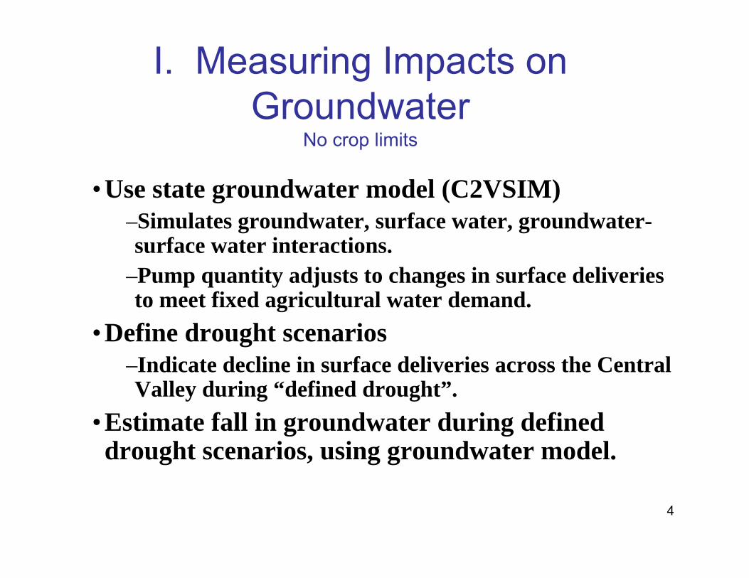
I. Measuring Impacts on Groundwater

No crop limits

•Use state groundwater model (C2VSIM)–Simulates groundwater, surface water, groundwater-surface water interactions.

–Pump quantity adjusts to changes in surface deliveries to meet fixed agricultural water demand.

•Define drought scenarios–Indicate decline in surface deliveries across the Central Valley during “defined drought”.

•Estimate fall in groundwater during defined drought scenarios, using groundwater model.

5

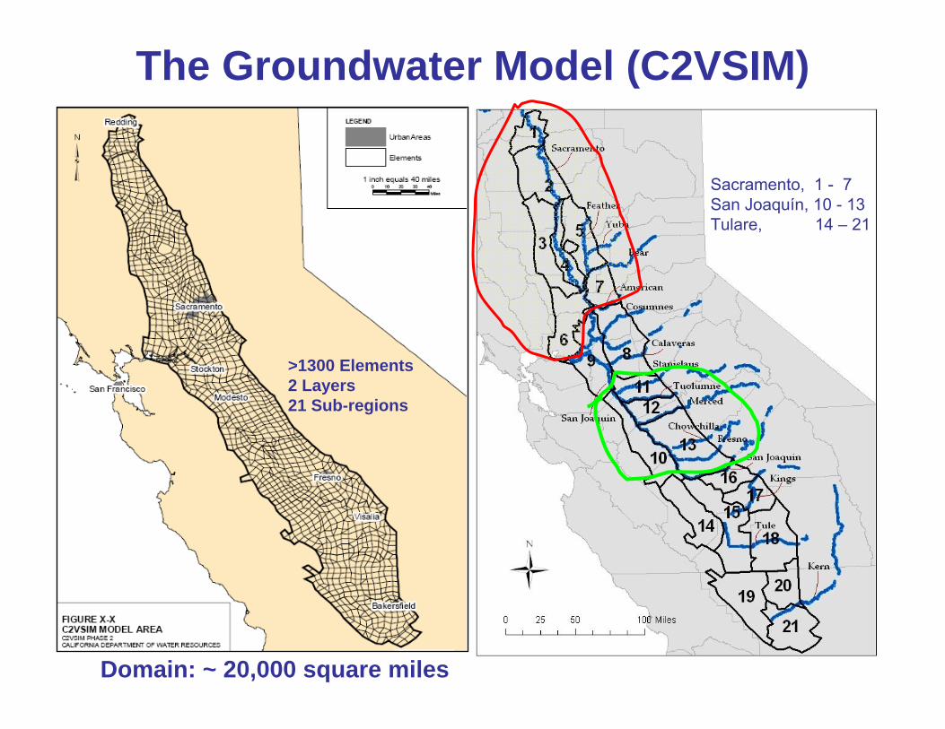
The Groundwater Model (C2VSIM)

�Domain: ~ 20,000 square miles

>1300 Elements2 Layers21 Sub-regions

Sacramento, 1 - 7 San Joaquín, 10 - 13 Tulare, 14 – 21

6

Define the Drought Scenarios

• We divided 1922 - 2002 into normal, dry, and critically dry years.

• Severe drought is 60 years of repeating critically dry years. – Average of 36% decline deliveries, “severe drought”

• The light drought is 60 years of repeating dry years– Average 10% decline deliveries in “light drought”

7

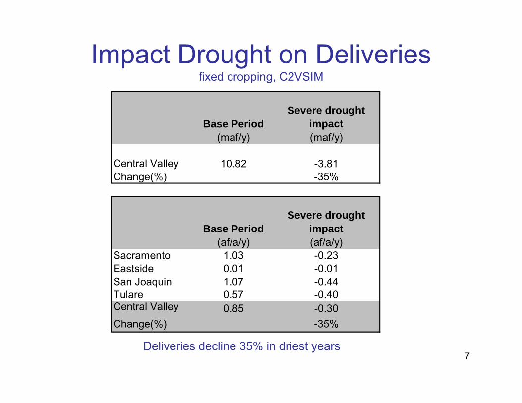
Impact Drought on Deliveries fixed cropping, C2VSIM

Deliveries decline 35% in driest years

Base PeriodSevere drought

impact(maf/y) (maf/y)

Central Valley 10.82 -3.81Change(%) -35%

Base PeriodSevere drought

impact(af/a/y) (af/a/y)

Sacramento 1.03 -0.23Eastside 0.01 -0.01San Joaquin 1.07 -0.44Tulare 0.57 -0.40Central Valley 0.85 -0.30Change(%) -35%

8

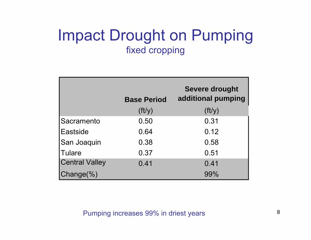
Impact Drought on Pumpingfixed cropping

Pumping increases 99% in driest years

Base PeriodSevere drought

additional pumping(ft/y) (ft/y)

Sacramento 0.50 0.31Eastside 0.64 0.12San Joaquin 0.38 0.58Tulare 0.37 0.51Central Valley 0.41 0.41Change(%) 99%

9

I. Impact Drought on Groundwaterfixed cropping, C2VSIM

Groundwater declines almost 3.8 feet per year across San Joaquin Basin

Base PeriodSevere drought

impact(af/a/y) (af/a/y)

Sacramento -0.07 -0.92Eastside -1.67 -1.73San Joaquin -1.60 -3.81Tulare 1.35 -2.99Central Valley 0.18 -2.26

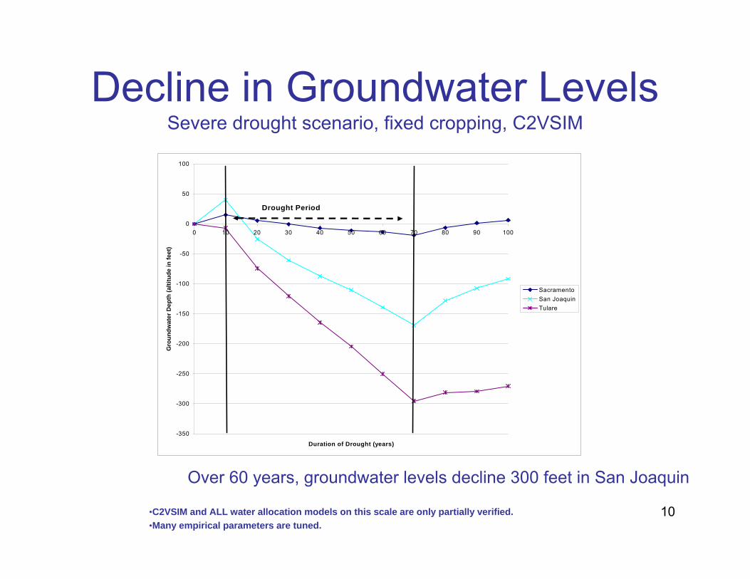
10

-350

-300

-250

-200

-150

-100

-50

0

50

100

0 10 20 30 40 50 60 70 80 90 100

Duration of Drought (years)

Gro

undw

ater

Dep

th (a

ltitu

de in

feet

)

SacramentoSan JoaquinTulare

Drought Period

Decline in Groundwater LevelsSevere drought scenario, fixed cropping, C2VSIM

•C2VSIM and ALL water allocation models on this scale are only partially verified. •Many empirical parameters are tuned.

Over 60 years, groundwater levels decline 300 feet in San Joaquin

11

II. Measuring Climate Impacts on GroundwaterCrop fallowing

• Net crop value – Crop value determines farmer willingness to

pump groundwater• Depth to groundwater

– Groundwater depth indicates pump cost.• Crop groundwater diagram, no crop

switching – When pump costs exceed willingness to

pump, crops are fallowed.

12

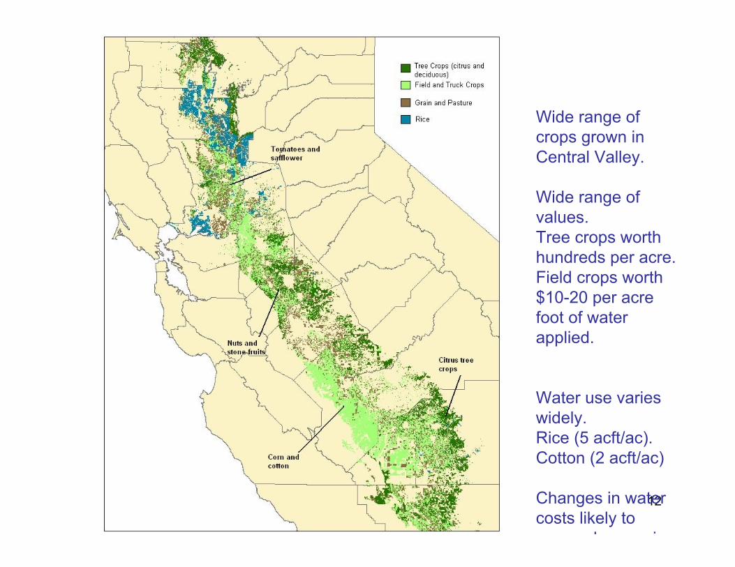
San Joaquin Valley Cropping

Wide range of crops grown in Central Valley.

Wide range of values.Tree crops worth hundreds per acre.Field crops worth $10-20 per acre foot of water applied.

Water use varies widely. Rice (5 acft/ac).Cotton (2 acft/ac)

Changes in water costs likely to

h i

13

Net Crop Value Tulare Basin, CVPM crop budgets

14

Willingness to Pay for Groundwater

Crop limits to groundwater depth.Maximum depth willing to pump, inferred @ .08/kWh

15

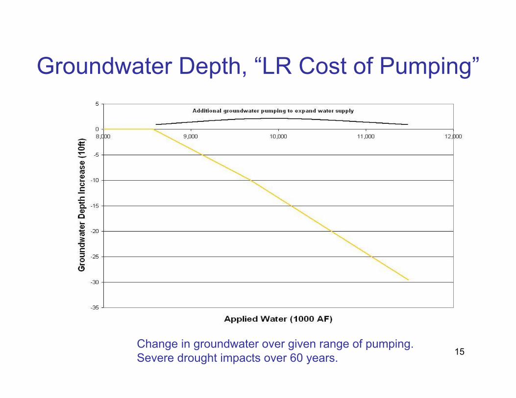
Groundwater Depth, “LR Cost of Pumping”

Change in groundwater over given range of pumping.Severe drought impacts over 60 years.

16

Equilibrium GroundwaterWhere LR cost pumping equals WTP

17

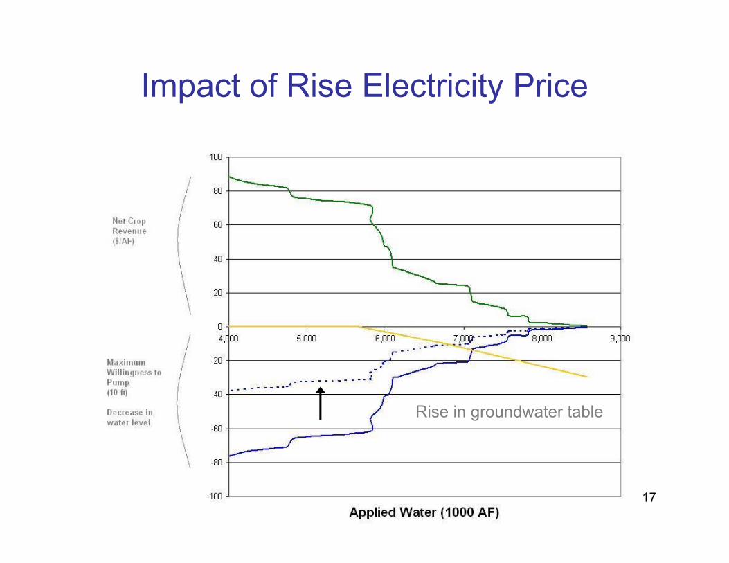
Impact of Rise Electricity Price

Rise in groundwater table

18

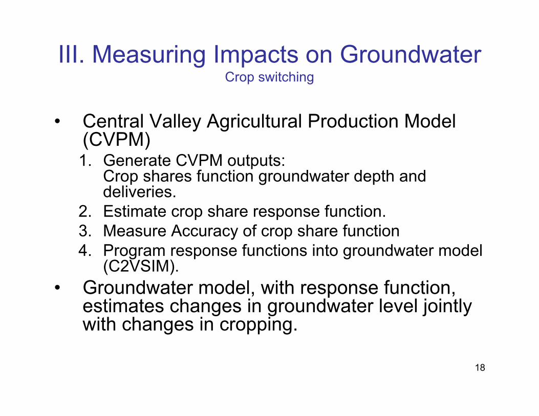
III. Measuring Impacts on GroundwaterCrop switching

• Central Valley Agricultural Production Model (CVPM)1. Generate CVPM outputs:

Crop shares function groundwater depth and deliveries.

2. Estimate crop share response function.3. Measure Accuracy of crop share function4. Program response functions into groundwater model

(C2VSIM). • Groundwater model, with response function,

estimates changes in groundwater level jointly with changes in cropping.

19

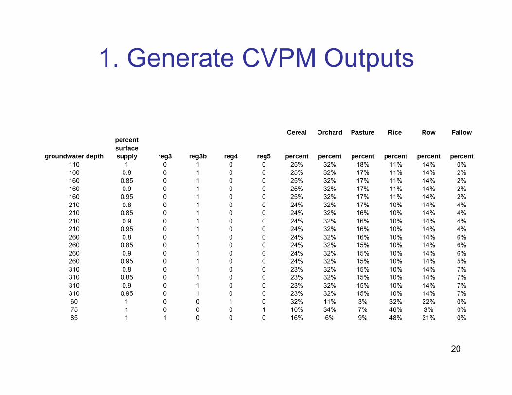
1. Generate CVPM outputs (long run and short run mode)

Generate multiple CVPM model outputs:• base water supply and groundwater depth, • 10% -20% decrease from base water

supply• 100 –200 foot drop in the groundwater

depth • Model runs provide multiple estimates of

crop shares across a range of regional, water supply and groundwater depth inputs.

20

1. Generate CVPM Outputs

Cereal Orchard Pasture Rice Row Fallow

groundwater depth

percent surface supply reg3 reg3b reg4 reg5 percent percent percent percent percent percent

110 1 0 1 0 0 25% 32% 18% 11% 14% 0%160 0.8 0 1 0 0 25% 32% 17% 11% 14% 2%160 0.85 0 1 0 0 25% 32% 17% 11% 14% 2%160 0.9 0 1 0 0 25% 32% 17% 11% 14% 2%160 0.95 0 1 0 0 25% 32% 17% 11% 14% 2%210 0.8 0 1 0 0 24% 32% 17% 10% 14% 4%210 0.85 0 1 0 0 24% 32% 16% 10% 14% 4%210 0.9 0 1 0 0 24% 32% 16% 10% 14% 4%210 0.95 0 1 0 0 24% 32% 16% 10% 14% 4%260 0.8 0 1 0 0 24% 32% 16% 10% 14% 6%260 0.85 0 1 0 0 24% 32% 15% 10% 14% 6%260 0.9 0 1 0 0 24% 32% 15% 10% 14% 6%260 0.95 0 1 0 0 24% 32% 15% 10% 14% 5%310 0.8 0 1 0 0 23% 32% 15% 10% 14% 7%310 0.85 0 1 0 0 23% 32% 15% 10% 14% 7%310 0.9 0 1 0 0 23% 32% 15% 10% 14% 7%310 0.95 0 1 0 0 23% 32% 15% 10% 14% 7%60 1 0 0 1 0 32% 11% 3% 32% 22% 0%75 1 0 0 0 1 10% 34% 7% 46% 3% 0%85 1 1 0 0 0 16% 6% 9% 48% 21% 0%

21

2. Estimate Crop Share response function(regional dummy variables, long run mode)

Cereal Orchard Pasture Row RiceB1 B2 B3 B4 B5

Depth (ft) -0.004 -0.004 -0.005 -0.005 -0.004Percent supply 6.225 5.992 6.799 6.568 5.999region 3 -1.287 -2.473 -1.569 0.609 -0.414region 4 -0.130 -1.412 -2.201 0.681 0.111region 5 -1.361 -0.405 -1.518 0.931 -2.074constant -2.683 -2.235 -3.481 -3.817 -3.074

Obs. 173597Log Likelihood -2.592Outcome Fallow is the comparison crop.

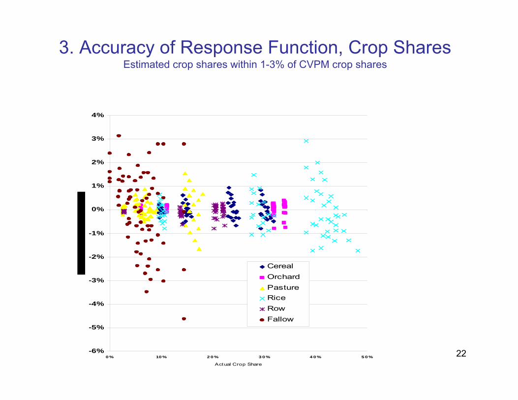
22

3. Accuracy of Response Function, Crop SharesEstimated crop shares within 1-3% of CVPM crop shares

-6%

-5%

-4%

-3%

-2%

-1%

0%

1%

2%

3%

4%

0 % 10 % 2 0 % 3 0 % 4 0 % 5 0 %

Actual Crop Share

CerealOrchardPastureRiceRowFallow

23

3. Accuracy of Response Function: Impact Depth on Crop AcresLogit vs CVPM acreage change estimates

CVPM vs Logit (groundwater depth change)

0

50

100

150

200

250

300

350

400

450

1500 1700 1900 2100 2300 2500 2700 2900 3100

Cropped Acres

GW

dep

th c

hang

e

CVPMPooled Logit

24

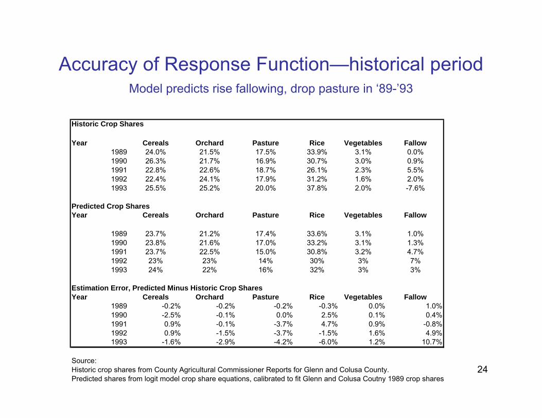
Accuracy of Response Function—historical periodModel predicts rise fallowing, drop pasture in ‘89-’93

Historic Crop Shares

Year Cereals Orchard Pasture Rice Vegetables Fallow1989 24.0% 21.5% 17.5% 33.9% 3.1% 0.0%1990 26.3% 21.7% 16.9% 30.7% 3.0% 0.9%1991 22.8% 22.6% 18.7% 26.1% 2.3% 5.5%1992 22.4% 24.1% 17.9% 31.2% 1.6% 2.0%1993 25.5% 25.2% 20.0% 37.8% 2.0% -7.6%

Predicted Crop SharesYear Cereals Orchard Pasture Rice Vegetables Fallow

1989 23.7% 21.2% 17.4% 33.6% 3.1% 1.0%1990 23.8% 21.6% 17.0% 33.2% 3.1% 1.3%1991 23.7% 22.5% 15.0% 30.8% 3.2% 4.7%1992 23% 23% 14% 30% 3% 7%1993 24% 22% 16% 32% 3% 3%

Estimation Error, Predicted Minus Historic Crop SharesYear Cereals Orchard Pasture Rice Vegetables Fallow

1989 -0.2% -0.2% -0.2% -0.3% 0.0% 1.0%1990 -2.5% -0.1% 0.0% 2.5% 0.1% 0.4%1991 0.9% -0.1% -3.7% 4.7% 0.9% -0.8%1992 0.9% -1.5% -3.7% -1.5% 1.6% 4.9%1993 -1.6% -2.9% -4.2% -6.0% 1.2% 10.7%

Source: Historic crop shares from County Agricultural Commissioner Reports for Glenn and Colusa County.Predicted shares from logit model crop share equations, calibrated to fit Glenn and Colusa Coutny 1989 crop shares

25

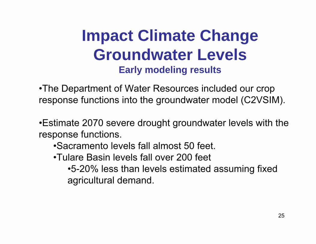
Impact Climate Change Groundwater Levels

Early modeling results

•The Department of Water Resources included our crop response functions into the groundwater model (C2VSIM).

•Estimate 2070 severe drought groundwater levels with the response functions.

•Sacramento levels fall almost 50 feet.•Tulare Basin levels fall over 200 feet

•5-20% less than levels estimated assuming fixed agricultural demand.

26

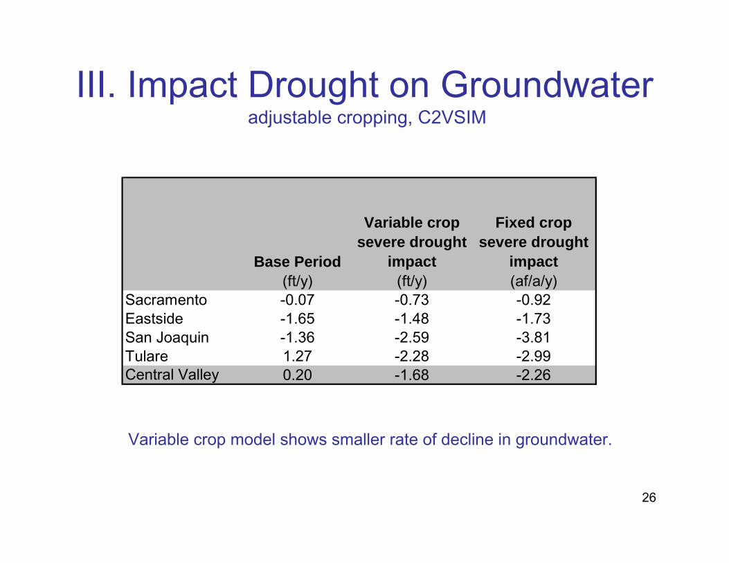
III. Impact Drought on Groundwateradjustable cropping, C2VSIM

Variable crop model shows smaller rate of decline in groundwater.

Base Period

Variable crop severe drought

impact

Fixed crop severe drought

impact(ft/y) (ft/y) (af/a/y)

Sacramento -0.07 -0.73 -0.92Eastside -1.65 -1.48 -1.73San Joaquin -1.36 -2.59 -3.81Tulare 1.27 -2.28 -2.99Central Valley 0.20 -1.68 -2.26

27

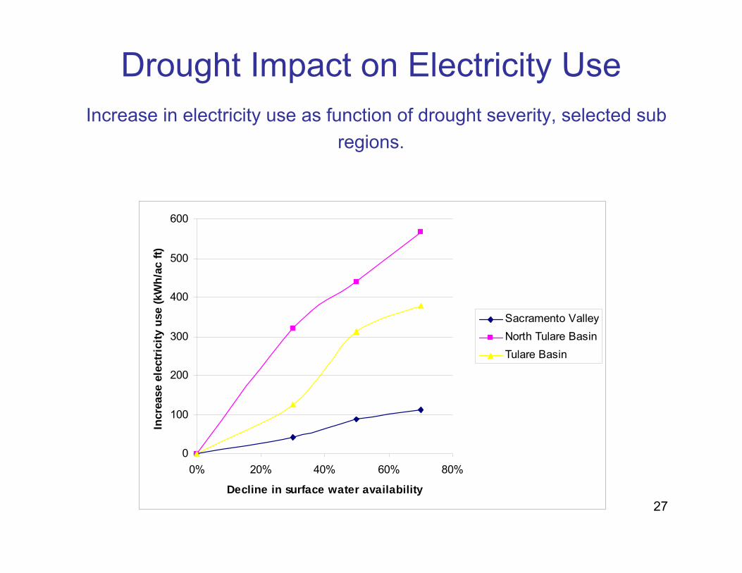
Drought Impact on Electricity UseIncrease in electricity use as function of drought severity, selected sub

regions.

0

100

200

300

400

500

600

0% 20% 40% 60% 80%

Decline in surface water availability

Incr

ease

ele

ctri

city

use

(kW

h/ac

ft)

Sacramento ValleyNorth Tulare BasinTulare Basin

28

Conclusion and Future Work• Two stage logit modeling of CVPM• Estimate long run crop shares using the long run

logit (stage one equation) • Estimate short run crop shares with a second

stage equation, where the the RHS explanatory variables include long run crop shares.

• To estimate impacts with this logit equation, need four water supply inputs--base case long run and short run supply--to estimate long and short run base crop shares; and long and short run impact supply--to estimate impacts.

29

Formulation of the logit equation

∑+=

j

x

x

ir jrr

irr

ee

β

β

α1

irβ

irrir xa γ=

Let i and j index crops and let r and s index regions. A multinomial logit model predicts the share of acreage in each region planted with a given crop. The share of land planted in crop i and region r is given by:

where xr is a vector of regional explanatory variables and is a vector of estimated coefficients. The summation in the denominator includes a term for each of the crops (except the reference crop), including crop i. Applied water per acre for crop i and region r is given by:

where xr is again a vector of explanatory variables which may vary by region and is a vector of estimated coefficients which may vary by region and crop.

irγ

30

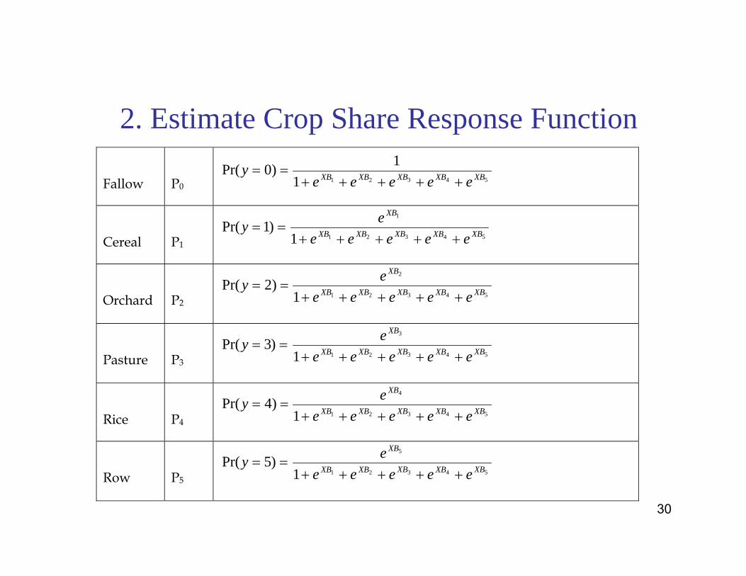
Fallow

P0

== )0Pr(y543211

1XBXBXBXBXB eeeee +++++

Cereal

P1 == )1Pr(y

54321

1

1 XBXBXBXBXB

XB

eeeeee

+++++

Orchard

P2 == )2Pr(y

54321

2

1 XBXBXBXBXB

XB

eeeeee

+++++

Pasture

P3 == )3Pr(y

54321

3

1 XBXBXBXBXB

XB

eeeeee

+++++

Rice

P4 == )4Pr(y

54321

4

1 XBXBXBXBXB

XB

eeeeee

+++++

Row

P5 == )5Pr(y

54321

5

1 XBXBXBXBXB

XB

eeeeee

+++++

2. Estimate Crop Share Response Function