modeling the effect of flow and sediment transport on ... · modeling the effect of flow and...

Modeling the Effect of Flow and Sediment Transporton White Sturgeon Spawning Habitat in the Kootenai

River, IdahoRichard McDonald1; Jonathan Nelson, M.ASCE2; Vaughn Paragamian3; and Gary Barton4

Abstract: Kootenai River white sturgeon spawn in an 18-km reach of the Kootenai River, Id. Since completion of Libby Dam upstreamfrom the spawning reach in 1972, 1974 is the only year with documented significant recruitment of juvenile fish. Where successful inother rivers, white sturgeon spawn over clean coarse material of gravel size or larger. The channel substrate in the current �2008� 18-kmspawning reach is composed primarily of sand and some buried gravel; within a few kilometers upstream there is an extended reach ofclean gravel, cobble, and bedrock. We used a quasi-three-dimensional flow and sediment-transport model along with the locations ofcollected sturgeon eggs as a proxy for spawning location from 1994 to 2002 to gain insight into spawning-habitat selection in a reachwhich is currently unsuitable due to the lack of coarse substrate. Spatial correlations between spawning locations and simulated velocityand depth indicate fish select regions of higher velocity and greater depth within any river cross section to spawn. These regions of highvelocity and depth occur in the same locations regardless of the discharge magnitude as modeled over a range of pre- and postdam flowconditions. A flow and sediment-transport simulation shows high discharge, and relatively long-duration flow associated with predam flowevents is sufficient to scour the fine sediment overburden, periodically exposing existing lenses of gravel and cobble as lag deposits in thecurrent spawning reach. This is corroborated by video observations of bed surface material following a significant flood event in 2006,which show gravel and cobble present in many locations in the current spawning reach. Thus, both modeling and observations suggest thatthe relative rarity of extremely high flows in the current regulated flow regime is at least partly responsible for the lack of successfulspawning; in the predam flow regime, frequent high flows removed the fine sediment overburden, unveiling coarse material and providingsuitable substrate in the current spawning reach.

DOI: 10.1061/�ASCE�HY.1943-7900.0000283

CE Database subject headings: River systems; Velocity; Depth; Shear stress; Sediment transport; Sand, hydraulic; Gravel; Scour;Dams; Ecosystems; Idaho.

Author keywords: River systems; Velocity; Depth; Shear stress; Sediment transport; Sand; Gravel; Scour; Dams; Ecology.

Introduction

The Kootenai River white sturgeon population is physically iso-lated and genetically distinct from other white sturgeon popula-tions in the Columbia River basin �Setter and Brannon 1990�.Following the completion of Libby Dam by the U.S. Army Corpsof Engineers in Montana during 1972, the only year of relevantrecruitment to the population occurred in 1974 �Paragamian et al.2005�. During subsequent years, a small number of naturally pro-

1Hydrologist, Geomorphology and Sediment Transport Laboratory,USGS, 4620 Technology Dr., Suite 400, Golden, CO 80403 �correspond-ing author�. E-mail: [email protected]

2Hydrologist, Geomorphology and Sediment Transport Laboratory,USGS, 4620 Technology Dr., Suite 400, Golden, CO 80403. E-mail:[email protected]

3Biologist, Idaho Dept. of Fish and Game, Coeur D’Alene, ID 83815.E-mail: [email protected]

4Hydrogeologist, Idaho Water Science Center, USGS, Boise, ID83702. E-mail: [email protected]

Note. This manuscript was submitted on February 4, 2009; approvedon May 18, 2010; published online on May 19, 2010. Discussion periodopen until May 1, 2011; separate discussions must be submitted for indi-vidual papers. This paper is part of the Journal of Hydraulic Engineer-ing, Vol. 136, No. 12, December 1, 2010. ©ASCE, ISSN 0733-9429/
2010/12-1077–1092/$25.00.
JOURNAL

Downloaded 22 Nov 2010 to 136.177.114.114. Redistrib

duced juvenile fish have been found but their abundance is toolow to sustain the population �Paragamian et al. 2005; Parag-amian and Hansen 2008�. In 1994 the Kootenai River white stur-geon population was listed as endangered �U.S. Fish and WildlifeService �USFWS� 1994�. Further protection was obtained in 2001through the designation of 18 river kilometers �rkm� downstreamfrom Bonners Ferry, Id., as critical habitat �U.S. Fish and WildlifeService �USFWS� 2001�. Increased spring flows from Libby Damfor spawning in recent years appear to have resulted in increasedspawning as evidenced by the collection of more sturgeon eggs�Paragamian et al. 2002�. Monitoring locations of adult whitesturgeon through telemetry studies and inferring general spawn-ing locations from egg collections has consistently shown thecritical habitat reach to be the main region of spawning �Parag-amian et al. 2001�.

White sturgeon are broadcast spawners with eggs that becomeadhesive shortly after exposure to water �Scott and Crossman1973; Conte et al. 1988�. Where successful spawning occurs inother river systems, eggs are assumed to settle into interstitialspaces provided by coarse substrates such as gravels and cobbles�Parsley et al. 1993; 2002�. Successful spawning of KootenaiRiver white sturgeon occurs annually from approximately mid-May to June within the critical habitat reach, confirmed by theannual presence of viable eggs and developing embryos �Parag-
amian et al. 2001�. However, the river substrate under most flow
OF HYDRAULIC ENGINEERING © ASCE / DECEMBER 2010 / 1077

ution subject to ASCE license or copyright. Visithttp://www.ascelibrary.org

conditions in the critical habitat reach is predominantly composedof fine sand with large migrating dunes �Barton 2004�. Spawnedeggs are presumed to settle onto the bed and may become coveredin fine sand or buried in the trough of migrating dunes resulting insuffocation and/or predation. As little as 5 mm of fine sedimentcover can cause up to 100% mortality to incubating white stur-geon embryos �Kock et al. 2006�. Interestingly, a few kilometersupstream from the spawning locations, the river has suitable sub-strate composed mostly of gravel and cobble; however, the chan-nel changes from a meandering form to a braided form that isrelatively shallow and fast compared to the meandering reach.

Successful spawning and recruitment of Kootenai River whitesturgeon involve complicated biological and ecological processesthat may be affected by hydraulic and sediment-transport charac-teristics. The reason that Kootenai River white sturgeon selecttheir current spawning grounds is not known. It may be an evo-lutionary artifact from over 10,000 years of spawning in thepresent reach of river. Alternatively, they may be compelled tospawn there because preferred habitat is unavailable or false en-vironmental cues are present. Several hypotheses relating to thehydraulic and sediment-transport characteristics of the KootenaiRiver have been put forth as possible explanations for the declineof successful recruitment in this system. Duke et al. �1999� out-lined how Libby Dam may have affected successful sturgeonspawning. First, prior to Libby Dam, higher lake stage inKootenay Lake resulted in greater backwater extent, increasingriver stage, which may have encouraged the fish to spawn furtherupstream in the braided reach. Second, in the postdam period, theloss of naturally occurring high spring flow in addition to lowerKootenay Lake stages may have shifted the spawning furtherdownstream into the current spawning reach. Third, the higherpredam discharge may have mobilized and scoured the bed suffi-ciently in the current spawning reach to expose coarse-grainedsubstrate suitable for egg hatching.

The goal of this paper is to examine the hydraulic andsediment-transport hypothesis presented by Duke et al. �1999�using field observations and the results of a coupled flow andsediment-transport model encompassing the 18-km critical habitatreach to �1� gain insight into the hydraulic conditions in thespawning reach; �2� assess whether these hydraulic conditionsserve as spawning cues; �3� assess the effects of flow management�Kootenay Lake Stage and Libby Dam discharge� on those cues;and �4� gain insight into the role of pre- and postdam flows inregulating the sediment substrate characteristics in the spawningreach.

Background

Natural climate variability in the Pacific Northwest during thePleistoscene and Holocene produced a diverse landscape shapedto a large degree by the advance and retreat of the continental icecap. Glacial land forms, including lacustrine, fluvial, and morainedeposits, influence the local hydraulic conditions and nature ofthe bed material in the study area. More recently, the KootenaiRiver basin has undergone dramatic changes in land use and man-agement of the river for flood control and hydroelectric genera-tion; these actions also have a substantive effect on the hydraulicsof the river. Natural recruitment of juvenile sturgeon has been indecline since the 1950s �Paragamian et al. 2005� with inconsistentrecruitment of sturgeon during the 1960s, followed by an almosttotal lack of natural recruitment during the period of flow man-
agement through Libby Dam from 1975 to the present. For these
1078 / JOURNAL OF HYDRAULIC ENGINEERING © ASCE / DECEMBER 20


reasons, a brief overview of the geomorphology, hydrology, andwhite sturgeon biology is given to provide the proper context forthe study presented here.

Geomorphology

The Kootenai River is 721 km long and a major tributary to theColumbia River �Fig. 1�. The Kootenai River originates inKootenay National Park �spelled Kootenay for Canadian waters�,B.C., Canada, and flows south into Montana and Koocanusa Res-ervoir formed by Libby Dam. Below Libby Dam the river flowsgenerally to the west through bedrock canyons and into northernIdaho near the town of Bonners Ferry. For the 11-km reach up-stream from Bonners Ferry, the channel is unconfined and weaklybraided as it exits the bedrock canyon reach. Downstream fromBonners Ferry the river meanders north for 85 km back into Brit-ish Columbia and the south arm of Kootenay Lake.

Three geomorphic reaches have been identified in the studyreach—a canyon reach, a braided reach, and a meander reach�Snyder and Minshall 1996�. The canyon reach extends fromLibby Dam to the Moyie River confluence �Figs. 1 and 2� wherethe valley begins to widen �rkm 365.7–256.6�. The braided reachextends to the bedrock constriction at Ambush Rock near BonnersFerry �rkm 256.6–245.9�. The braided reach has since been sub-divided by breaking out the short straight reach between rkm245.9 and 244.5 and identifying a transition zone between themeandering reach and the braided reach �Barton 2004� hereafterreferred to as the transition reach. The meander reach extendsdownstream from the bedrock constriction �rkm 244.5� near Bon-ners Ferry for approximately 100 km to Lake Kootenay. The18-km �rkm 228–246� reach of critical habitat �hereafter referredto as the critical habitat reach� extends downstream from BonnersFerry and includes the transition reach and the top 16.5 rkm of themeandering reach

The braided reach has a slope of approximately 0.00046 andlies in a wide and flat valley bounded by thick glaciolacustrineand glaciofluvial terraces �Weisel 1980�. The reach consists ofmultiple channels that are actively migrating. At the transitionreach �near Bonners Ferry� the width of the valley floor narrowsagain and contains numerous bedrock outcroppings. Depths in thebraided and transition reach are approximately 1–3 m and the bed

MontanaIdaho

British Columbia

Washington

North

Arm

West Arm

Koo

tenay

Lake

South

Arm

Goat River

Moyie River Yaak River

LakeK

oo

canu

sa

Libby DamDeep Creek

N

Study Area

Corra LinnDam

Kootenai River

Columbi a

River

Kootenai R iver

Boundary Creek

Boundary Creek, near Porthill, Id(12321500)

Kootenai River at Tribal Hatchery, Id (rkm 241)(12310100)

Kootenai River at Klockman Ranch, Id (rkm 225)(12314000) Kootenai River at Leonia, Id (rkm 270)

(12305000)

Kootenai River at Porthill, Id (rkm 170)(12322000)

Kootenai River at Bonners Ferry, Id (rkm 246)(12309500)

USGS Gage Name, State (location in River Kilometers (rkm))(Gage Number)

(rkm 352)

(rkm 120)

Kilometers0 50

Explanation

Fig. 1. Location of study area near Bonners Ferry, Id.

material is generally gravel and cobbles with some sand in the

10


transition reach. The meander reach has a gentle slope of 0.000 02and meanders across lacustrine deposits filling the wide valleybottom in the Kootenai Flats floodplain. The Boundary CountySoil Survey �USDA 2007� maps the soils on the valley bottom asprimarily glacially derived lacustrine with some interbedded flu-vial deposits. The bed material consists of predominantly sanddeposits and discrete interbedded gravels and cobbles with somelacustrine clay steps, particularly in the lower part of the reachnear Shorty Island. Large dunes migrate along the bottom duringlow flow and are washed out at higher flows.

Hydrology

The present flow regime as managed by releases from Libby Damis quite different from the natural flow regime. Libby Dam wascompleted in 1972 and became fully operational in 1974. Averageannual Kootenai River discharge is shown in Fig. 3�a� during

Shorty Island

Kootenai River

USGS gaging station

Ball Creek

BurtonCreek

LostCreek

MyrtleCreek

Deep Creek

x

x

xx

x

x

x

x

x

x

x

xx

x

x

x

xx

x

x

x

x

x

x

x

x

Kilometer 245

Kilometer 240

Kilometer 235

Kilometer 230

Kilometer 225

95

1000 meters

Explanation

Kootenai River

Kootenai Flats Floodplain

River Kilometer

2000 Vibra-core

2004 Vibra-core

2006 Video Survey

N

x

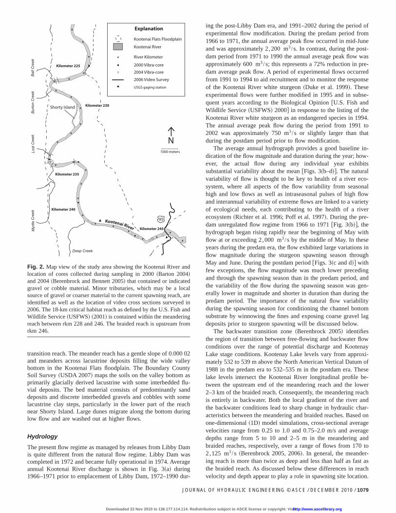
Fig. 2. Map view of the study area showing the Kootenai River andlocation of cores collected during sampling in 2000 �Barton 2004�and 2004 �Berenbrock and Bennett 2005� that contained or indicatedgravel or cobble material. Minor tributaries, which may be a localsource of gravel or coarser material to the current spawning reach, areidentified as well as the location of video cross sections surveyed in2006. The 18-km critical habitat reach as defined by the U.S. Fish andWildlife Service �USFWS� �2001� is contained within the meanderingreach between rkm 228 and 246. The braided reach is upstream fromrkm 246.

1966–1971 prior to emplacement of Libby Dam, 1972–1990 dur-

JOURNAL


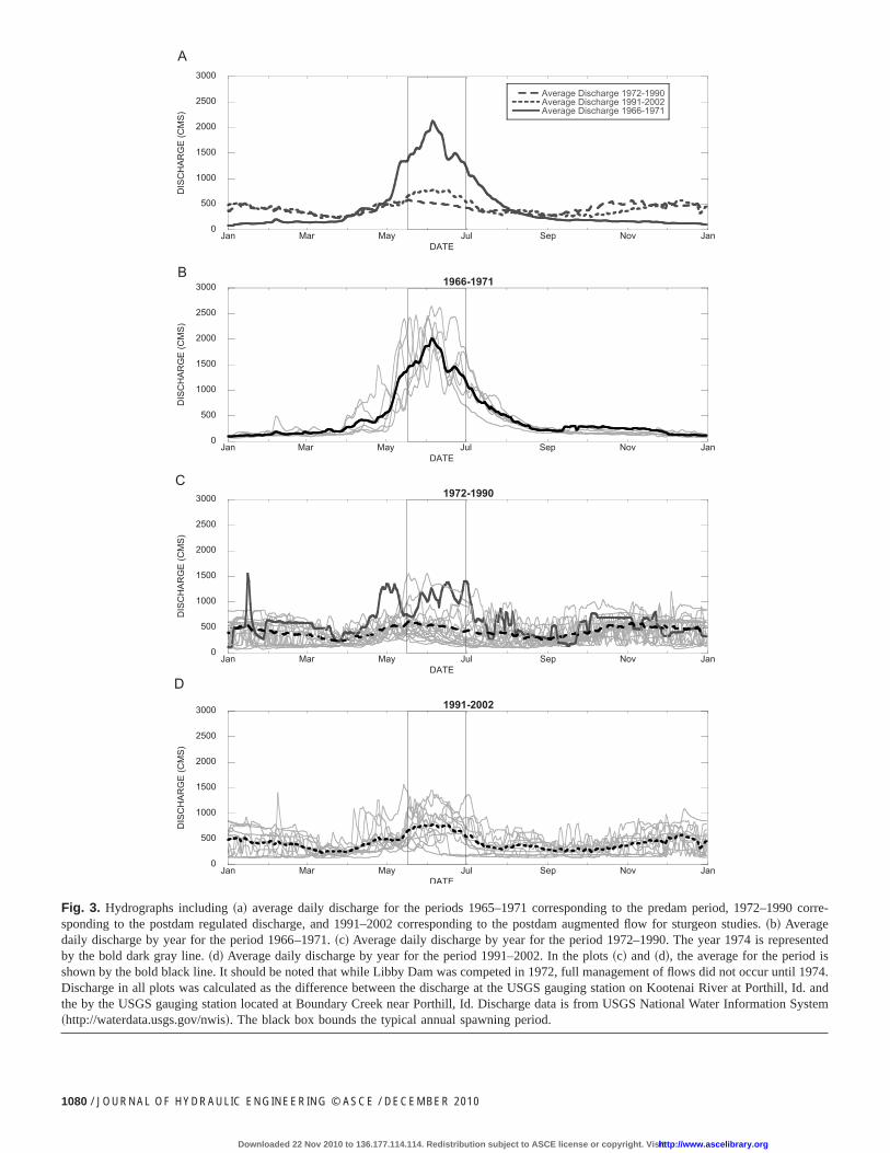
ing the post-Libby Dam era, and 1991–2002 during the period ofexperimental flow modification. During the predam period from1966 to 1971, the annual average peak flow occurred in mid-Juneand was approximately 2 ,200 m3 /s. In contrast, during the post-dam period from 1971 to 1990 the annual average peak flow wasapproximately 600 m3 /s; this represents a 72% reduction in pre-dam average peak flow. A period of experimental flows occurredfrom 1991 to 1994 to aid recruitment and to monitor the responseof the Kootenai River white sturgeon �Duke et al. 1999�. Theseexperimental flows were further modified in 1995 and in subse-quent years according to the Biological Opinion �U.S. Fish andWildlife Service �USFWS� 2000� in response to the listing of theKootenai River white sturgeon as an endangered species in 1994.The annual average peak flow during the period from 1991 to2002 was approximately 750 m3 /s or slightly larger than thatduring the postdam period prior to flow modification.

The average annual hydrograph provides a good baseline in-dication of the flow magnitude and duration during the year; how-ever, the actual flow during any individual year exhibitssubstantial variability about the mean �Figs. 3�b–d��. The naturalvariability of flow is thought to be key to health of a river eco-system, where all aspects of the flow variability from seasonalhigh and low flows as well as intraseasonal pulses of high flowand interannual variability of extreme flows are linked to a varietyof ecological needs, each contributing to the health of a riverecosystem �Richter et al. 1996; Poff et al. 1997�. During the pre-dam unregulated flow regime from 1966 to 1971 �Fig. 3�b��, thehydrograph began rising rapidly near the beginning of May withflow at or exceeding 2,000 m3 /s by the middle of May. In theseyears during the predam era, the flow exhibited large variations inflow magnitude during the sturgeon spawning season throughMay and June. During the postdam period �Figs. 3�c and d�� withfew exceptions, the flow magnitude was much lower precedingand through the spawning season than in the predam period, andthe variability of the flow during the spawning season was gen-erally lower in magnitude and shorter in duration than during thepredam period. The importance of the natural flow variabilityduring the spawning season for conditioning the channel bottomsubstrate by winnowing the fines and exposing coarse gravel lagdeposits prior to sturgeon spawning will be discussed below.

The backwater transition zone �Berenbrock 2005� identifiesthe region of transition between free-flowing and backwater flowconditions over the range of potential discharge and KootenayLake stage conditions. Kootenay Lake levels vary from approxi-mately 532 to 539 m above the North American Vertical Datum of1988 in the predam era to 532–535 m in the postdam era. Theselake levels intersect the Kootenai River longitudinal profile be-tween the upstream end of the meandering reach and the lower2–3 km of the braided reach. Consequently, the meandering reachis entirely in backwater. Both the local gradient of the river andthe backwater conditions lead to sharp change in hydraulic char-acteristics between the meandering and braided reaches. Based onone-dimensional �1D� model simulations, cross-sectional averagevelocities range from 0.25 to 1.0 and 0.75–2.0 m/s and averagedepths range from 5 to 10 and 2–5 m in the meandering andbraided reaches, respectively, over a range of flows from 170 to2 ,125 m3 /s �Berenbrock 2005, 2006�. In general, the meander-ing reach is more than twice as deep and less than half as fast asthe braided reach. As discussed below these differences in reach
velocity and depth appear to play a role in spawning site location.


0

500

1000

1500

2000

2500

3000

Jan Mar May Jul Sep Nov Jan

Average Discharge 1972-1990Average Discharge 1991-2002Average Discharge 1966-1971

DISCHARGE(CMS)

DATE

0

500

1000

1500

2000

2500

3000


1966-1971

DISCHARGE(CMS)

DATE

0

500

1000

1500

2000

2500

3000


1972-1990

DISCHARGE(CMS)

DATE

0

500

1000

1500

2000

2500

3000


1991-2002

DISCHARGE(CMS)

DATE

A

B

C

D

Fig. 3. Hydrographs including �a� average daily discharge for the periods 1965–1971 corresponding to the predam period, 1972–1990 corre-sponding to the postdam regulated discharge, and 1991–2002 corresponding to the postdam augmented flow for sturgeon studies. �b� Averagedaily discharge by year for the period 1966–1971. �c� Average daily discharge by year for the period 1972–1990. The year 1974 is representedby the bold dark gray line. �d� Average daily discharge by year for the period 1991–2002. In the plots �c� and �d�, the average for the period isshown by the bold black line. It should be noted that while Libby Dam was competed in 1972, full management of flows did not occur until 1974.Discharge in all plots was calculated as the difference between the discharge at the USGS gauging station on Kootenai River at Porthill, Id. andthe by the USGS gauging station located at Boundary Creek near Porthill, Id. Discharge data is from USGS National Water Information System�http://waterdata.usgs.gov/nwis�. The black box bounds the typical annual spawning period.


Downloaded 22 Nov 2010 to 136.177.114.114. Redistribution subject to ASCE license or copyright. Visithttp://www.ascelibrary.org

White Sturgeon Biology

Studies of white sturgeon spawning habitat in other river basins inthe western United States where spawning and rearing are suc-cessful, such as the Sacramento, the Columbia, and the Fraserrivers, generally describe the location of spawning sites as occur-ring in river reaches with relatively high velocity and a substratethat is composed of gravel and larger-sized material �Paragamianet al. 2001; Perrin et al. 2000, 2003; Parsley et al. 1993; Parsleyand Beckman 1994; Coutant 2004; Golder Associates 2005�.However, there are some site-specific differences from these ide-alized habitat values. Known spawning reaches on both the Sac-ramento and Fraser rivers are associated with some sand as wellas coarser material and on the Fraser River generally are locatedin shallower water �Kohlhorst 1976; Schaffter 1997; Perrin et al.2000, 2003�. Conversely, known spawning sites within the criticalhabitat reach of the Kootenai River are located in lower velocityareas compared to other rivers and are dominated by sand-sizedmaterial during the current regulated flow conditions.

Kootenai River white sturgeons have reached critically lowpopulation sizes where genetic and demographic risks are signifi-cant. No relevant recruitment of juvenile sturgeon has occurredsince possibly 1974 and consistent recruitment has not occurredsince at least 1965. A few wild juveniles are periodically cap-tured, but although recent managed flows �1991–present� havestimulated spawning, they have not apparently encouraged thesurvival of eggs and larva as hoped �Paragamian et al. 2001�.Flow augmentation during spring may have stimulated sturgeonspawning behavior as eggs are collected in most years, but habitatchanges and spawning locations are still unfavorable to egg sur-vival �Paragamian et al. 2001; Anders et al. 2002�. Consistenthistoric recruitment coincided with wet years and high runoffconditions that have been precluded by hydropower operationssince completion of Libby Dam in 1972 �Paragamian et al. 2005�.However, recruitment failures prior to Libby Dam constructionsuggest that early life history/recruitment has also been impactedby other habitat changes such as levee construction and discon-nection from the river floodplain in the 1920s to the 1950s �Daleyet al. 1981�, Kootenay Lake regulation following the completionof Corra Linn Dam in 1932 �Duke et al. 1999�, and changes insystem productivity �Anders et al. 2002; Paragamian 2002�.

Flow augmentation implemented to date has not increased thesurvival of eggs although measures have fallen short of targetsdesired by some fish managers �B. Hallock, U.S. Fish and Wild-life Service, personal communication�. The key to designing sucha restoration is how the fish select spawning sites and how thephysical characteristics of those sites may be prohibiting the suc-cessful recruitment of juvenile fish from naturally spawned eggs.In the work described here, these issues are investigated usingobserved spawning sites along with the physical characteristics ofthe sites and computational flow modeling.

Field Data Collection

The channel topography, channel substrate, and white sturgeonegg-collection data used in this study were collected from severalprevious and ongoing studies as described below. The modeledreach of river extends from the upstream end of the critical habitatreach at Bonners Ferry �rkm 245.9� to 5.5 rkm downsteam fromthe critical habitat reach at rkm 222.5 �Fig. 2�. The extent of themodeled reach was selected to provide insight to the hydraulic
conditions of the critical habitat reach and conditions just down-
JOURNAL


stream from the critical habitat reach to see what if anything ishydraulically unique about the reach.

Topography

Collecting channel bathymetry and bank and floodplain topogra-phy is the first step in characterizing the physical habitat and isrequired for computational models of flow and sediment trans-port. Bathymetry for the modeling reach is based on mappingconducted during 2002–2005. Details on the collection of bathy-metric data are provided in Barton and Moran �2004� and Bartonet al. �2005� and briefly summarized here.

Bathymetry was collected with real-time global positioningsystem �GPS� equipment interfaced with survey-grade single andmultibeam echo sounders with a horizontal accuracy of�0.051 m and a vertical accuracy of �0.041 m �Barton andMoran 2004; Barton et al. 2005�. During 2002 and 2003, 260cross sections and two to seven longitudinal lines were surveyedin the modeling reach. Spacing between the cross sections rangedfrom less than 10 to about 50 m. During 2004 and 2005, topog-raphy was measured with a multibeam echo sounder. The spacingbetween each of the four sounding transducers was 2.8 m. Lon-gitudinal lines were collected so they were roughly parallel andspaced relatively close to one another. The bank and floodplaintopography was obtained from a light detection and ranging dataset �Richard Duncan, GeoEngineers, personal communication,2005� collected in 2005.

Channel Substrate

Several studies have been conducted to characterize the channelsubstrate in the Kootenai River in the existing spawning reach.Barton �2004� used vibracores and piston cores at various loca-tions through the 18-km length of the critical habitat reach. Basedon the grain size and stratigraphy of these cores, the river wasclassified into three broad zones: a sand-gravel-cobble zone in thetransition reach downstream from Bonners Ferry �245.9–244.5rkm�, a buried gravel-cobble zone �244.5–241 rkm�, and a sandzone with isolated lenses of buried cobble �241–228 rkm� �Fig.2�. A subsequent vibracore study in 2004 to better characterize thestratigraphy of the buried gravel-cobble zone for 1D sediment-transport modeling �Berenbrock 2005� found that this zone ischaracterized by discontinuous lenses of buried coarse material.Fig. 2 shows the locations of cores containing gravel or cobblesized material for the two studies above.

In addition to the coring studies, informal field observationshave identified that gravel-cobble sized material occurs at theconfluence of three small tributaries with the Kootenai River inthe meandering reach: Lost Creek, Burton Creek, and Ball Creek�Fig. 2�. Periodic large floods from these small tributaries providea limited supply of coarse material to the river. Two larger tribu-taries, Deep Creek and Myrtle Creek �Fig. 2�, have gravel-cobblesize material in their upper reaches. However, their potential fordelivering coarse material to the river is uncertain, particularly asboth must travel significant distances over the broad and rela-tively flat floodplain and are backwatered by the river itself up-stream from their confluence with the Kootenai River. Withoutmajor tributary supplies, the gravel-cobble substrate within thetransition and braided reaches may have historically providedcoarse material to the meandering reach. Determining the locationand extent of gravels in the current spawning reach is criticallyimportant for evaluating the role of higher flows in uncovering
areas of sufficient spatial extent for successful spawning habitat.


Egg Mat Studies

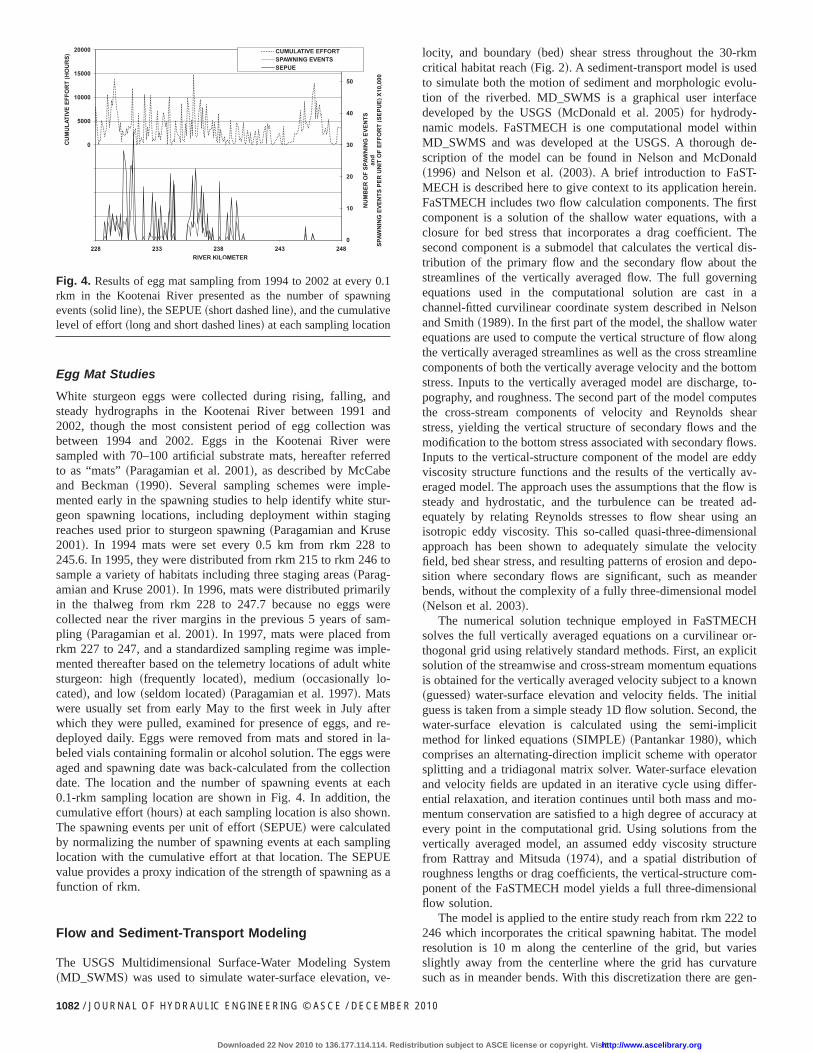
White sturgeon eggs were collected during rising, falling, andsteady hydrographs in the Kootenai River between 1991 and2002, though the most consistent period of egg collection wasbetween 1994 and 2002. Eggs in the Kootenai River weresampled with 70–100 artificial substrate mats, hereafter referredto as “mats” �Paragamian et al. 2001�, as described by McCabeand Beckman �1990�. Several sampling schemes were imple-mented early in the spawning studies to help identify white stur-geon spawning locations, including deployment within stagingreaches used prior to sturgeon spawning �Paragamian and Kruse2001�. In 1994 mats were set every 0.5 km from rkm 228 to245.6. In 1995, they were distributed from rkm 215 to rkm 246 tosample a variety of habitats including three staging areas �Parag-amian and Kruse 2001�. In 1996, mats were distributed primarilyin the thalweg from rkm 228 to 247.7 because no eggs werecollected near the river margins in the previous 5 years of sam-pling �Paragamian et al. 2001�. In 1997, mats were placed fromrkm 227 to 247, and a standardized sampling regime was imple-mented thereafter based on the telemetry locations of adult whitesturgeon: high �frequently located�, medium �occasionally lo-cated�, and low �seldom located� �Paragamian et al. 1997�. Matswere usually set from early May to the first week in July afterwhich they were pulled, examined for presence of eggs, and re-deployed daily. Eggs were removed from mats and stored in la-beled vials containing formalin or alcohol solution. The eggs wereaged and spawning date was back-calculated from the collectiondate. The location and the number of spawning events at each0.1-rkm sampling location are shown in Fig. 4. In addition, thecumulative effort �hours� at each sampling location is also shown.The spawning events per unit of effort �SEPUE� were calculatedby normalizing the number of spawning events at each samplinglocation with the cumulative effort at that location. The SEPUEvalue provides a proxy indication of the strength of spawning as afunction of rkm.

Flow and Sediment-Transport Modeling

The USGS Multidimensional Surface-Water Modeling System

0

10

20

30

40

50

60

-20000

-15000

-10000

-5000

0

5000

10000

15000

20000

228 233 238 243 248

NUMBER

OFSPAW

NINGEVENTS

and

SPAW

NINGEVENTS

PERUNITOFEFFORT(SEPUE )X10,000

CUMULATIVE

EFFORT(HOURS)

RIVER KILOMETER

CUMULATIVE EFFORTSPAWNING EVENTSSEPUE

Fig. 4. Results of egg mat sampling from 1994 to 2002 at every 0.1rkm in the Kootenai River presented as the number of spawningevents �solid line�, the SEPUE �short dashed line�, and the cumulativelevel of effort �long and short dashed lines� at each sampling location

�MD_SWMS� was used to simulate water-surface elevation, ve-



locity, and boundary �bed� shear stress throughout the 30-rkmcritical habitat reach �Fig. 2�. A sediment-transport model is usedto simulate both the motion of sediment and morphologic evolu-tion of the riverbed. MD_SWMS is a graphical user interfacedeveloped by the USGS �McDonald et al. 2005� for hydrody-namic models. FaSTMECH is one computational model withinMD_SWMS and was developed at the USGS. A thorough de-scription of the model can be found in Nelson and McDonald�1996� and Nelson et al. �2003�. A brief introduction to FaST-MECH is described here to give context to its application herein.FaSTMECH includes two flow calculation components. The firstcomponent is a solution of the shallow water equations, with aclosure for bed stress that incorporates a drag coefficient. Thesecond component is a submodel that calculates the vertical dis-tribution of the primary flow and the secondary flow about thestreamlines of the vertically averaged flow. The full governingequations used in the computational solution are cast in achannel-fitted curvilinear coordinate system described in Nelsonand Smith �1989�. In the first part of the model, the shallow waterequations are used to compute the vertical structure of flow alongthe vertically averaged streamlines as well as the cross streamlinecomponents of both the vertically average velocity and the bottomstress. Inputs to the vertically averaged model are discharge, to-pography, and roughness. The second part of the model computesthe cross-stream components of velocity and Reynolds shearstress, yielding the vertical structure of secondary flows and themodification to the bottom stress associated with secondary flows.Inputs to the vertical-structure component of the model are eddyviscosity structure functions and the results of the vertically av-eraged model. The approach uses the assumptions that the flow issteady and hydrostatic, and the turbulence can be treated ad-equately by relating Reynolds stresses to flow shear using anisotropic eddy viscosity. This so-called quasi-three-dimensionalapproach has been shown to adequately simulate the velocityfield, bed shear stress, and resulting patterns of erosion and depo-sition where secondary flows are significant, such as meanderbends, without the complexity of a fully three-dimensional model�Nelson et al. 2003�.

The numerical solution technique employed in FaSTMECHsolves the full vertically averaged equations on a curvilinear or-thogonal grid using relatively standard methods. First, an explicitsolution of the streamwise and cross-stream momentum equationsis obtained for the vertically averaged velocity subject to a known�guessed� water-surface elevation and velocity fields. The initialguess is taken from a simple steady 1D flow solution. Second, thewater-surface elevation is calculated using the semi-implicitmethod for linked equations �SIMPLE� �Pantankar 1980�, whichcomprises an alternating-direction implicit scheme with operatorsplitting and a tridiagonal matrix solver. Water-surface elevationand velocity fields are updated in an iterative cycle using differ-ential relaxation, and iteration continues until both mass and mo-mentum conservation are satisfied to a high degree of accuracy atevery point in the computational grid. Using solutions from thevertically averaged model, an assumed eddy viscosity structurefrom Rattray and Mitsuda �1974�, and a spatial distribution ofroughness lengths or drag coefficients, the vertical-structure com-ponent of the FaSTMECH model yields a full three-dimensionalflow solution.

The model is applied to the entire study reach from rkm 222 to246 which incorporates the critical spawning habitat. The modelresolution is 10 m along the centerline of the grid, but variesslightly away from the centerline where the grid has curvature
such as in meander bends. With this discretization there are gen-
10


erally 15–25 active computational grid nodes in the cross-streamdirection. The model was calibrated to computed water-surfaceelevations, from a 1D model �Berenbrock 2005, 2006� that spansthe study reach from rkm 170 to 276, from a wide selection ofdischarge magnitudes �170–2,120 m3 /s� up to and exceedingthe predam mean annual peak discharge. Complete details of themodel calibration and verification for the Kootenai River can befound in Barton et al. �2005, 2009�. A brief description of thecalibration procedure and of the simulation verification as pro-vided by a comparison between the simulated and measured ve-locities is provided here for completeness.

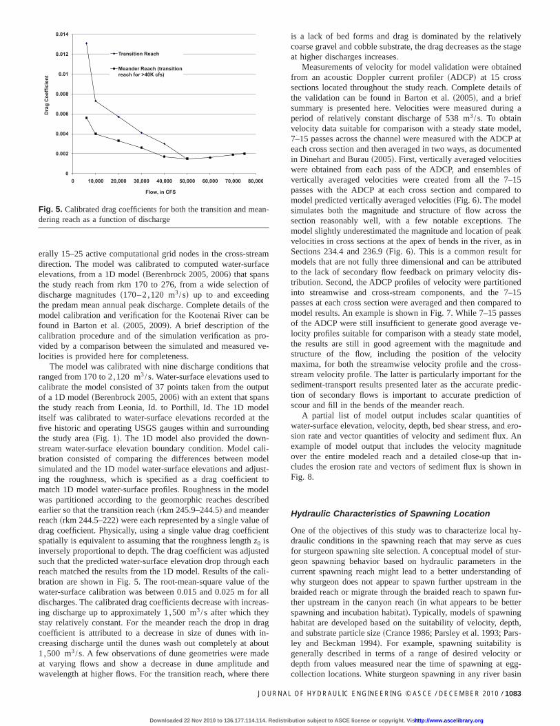
The model was calibrated with nine discharge conditions thatranged from 170 to 2 ,120 m3 /s. Water-surface elevations used tocalibrate the model consisted of 37 points taken from the outputof a 1D model �Berenbrock 2005, 2006� with an extent that spansthe study reach from Leonia, Id. to Porthill, Id. The 1D modelitself was calibrated to water-surface elevations recorded at thefive historic and operating USGS gauges within and surroundingthe study area �Fig. 1�. The 1D model also provided the down-stream water-surface elevation boundary condition. Model cali-bration consisted of comparing the differences between modelsimulated and the 1D model water-surface elevations and adjust-ing the roughness, which is specified as a drag coefficient tomatch 1D model water-surface profiles. Roughness in the modelwas partitioned according to the geomorphic reaches describedearlier so that the transition reach �rkm 245.9–244.5� and meanderreach �rkm 244.5–222� were each represented by a single value ofdrag coefficient. Physically, using a single value drag coefficientspatially is equivalent to assuming that the roughness length z0 isinversely proportional to depth. The drag coefficient was adjustedsuch that the predicted water-surface elevation drop through eachreach matched the results from the 1D model. Results of the cali-bration are shown in Fig. 5. The root-mean-square value of thewater-surface calibration was between 0.015 and 0.025 m for alldischarges. The calibrated drag coefficients decrease with increas-ing discharge up to approximately 1 ,500 m3 /s after which theystay relatively constant. For the meander reach the drop in dragcoefficient is attributed to a decrease in size of dunes with in-creasing discharge until the dunes wash out completely at about1 ,500 m3 /s. A few observations of dune geometries were madeat varying flows and show a decrease in dune amplitude and

0

0.002

0.004

0.006

0.008

0.01

0.012

0.014

0 10,000 20,000 30,000 40,000 50,000 60,000 70,000 80,000

DragCoefficient

Flow, in CFS

Transition Reach

Meander Reach (transitionreach for >40K cfs)

Fig. 5. Calibrated drag coefficients for both the transition and mean-dering reach as a function of discharge

wavelength at higher flows. For the transition reach, where there

JOURNAL


is a lack of bed forms and drag is dominated by the relativelycoarse gravel and cobble substrate, the drag decreases as the stageat higher discharges increases.

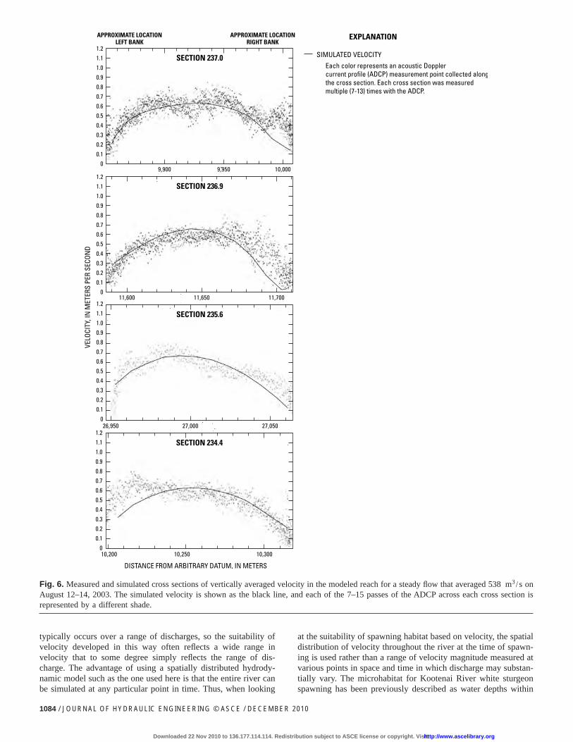
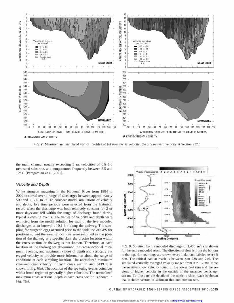
Measurements of velocity for model validation were obtainedfrom an acoustic Doppler current profiler �ADCP� at 15 crosssections located throughout the study reach. Complete details ofthe validation can be found in Barton et al. �2005�, and a briefsummary is presented here. Velocities were measured during aperiod of relatively constant discharge of 538 m3 /s. To obtainvelocity data suitable for comparison with a steady state model,7–15 passes across the channel were measured with the ADCP ateach cross section and then averaged in two ways, as documentedin Dinehart and Burau �2005�. First, vertically averaged velocitieswere obtained from each pass of the ADCP, and ensembles ofvertically averaged velocities were created from all the 7–15passes with the ADCP at each cross section and compared tomodel predicted vertically averaged velocities �Fig. 6�. The modelsimulates both the magnitude and structure of flow across thesection reasonably well, with a few notable exceptions. Themodel slightly underestimated the magnitude and location of peakvelocities in cross sections at the apex of bends in the river, as inSections 234.4 and 236.9 �Fig. 6�. This is a common result formodels that are not fully three dimensional and can be attributedto the lack of secondary flow feedback on primary velocity dis-tribution. Second, the ADCP profiles of velocity were partitionedinto streamwise and cross-stream components, and the 7–15passes at each cross section were averaged and then compared tomodel results. An example is shown in Fig. 7. While 7–15 passesof the ADCP were still insufficient to generate good average ve-locity profiles suitable for comparison with a steady state model,the results are still in good agreement with the magnitude andstructure of the flow, including the position of the velocitymaxima, for both the streamwise velocity profile and the cross-stream velocity profile. The latter is particularly important for thesediment-transport results presented later as the accurate predic-tion of secondary flows is important to accurate prediction ofscour and fill in the bends of the meander reach.

A partial list of model output includes scalar quantities ofwater-surface elevation, velocity, depth, bed shear stress, and ero-sion rate and vector quantities of velocity and sediment flux. Anexample of model output that includes the velocity magnitudeover the entire modeled reach and a detailed close-up that in-cludes the erosion rate and vectors of sediment flux is shown inFig. 8.

Hydraulic Characteristics of Spawning Location

One of the objectives of this study was to characterize local hy-draulic conditions in the spawning reach that may serve as cuesfor sturgeon spawning site selection. A conceptual model of stur-geon spawning behavior based on hydraulic parameters in thecurrent spawning reach might lead to a better understanding ofwhy sturgeon does not appear to spawn further upstream in thebraided reach or migrate through the braided reach to spawn fur-ther upstream in the canyon reach �in what appears to be betterspawning and incubation habitat�. Typically, models of spawninghabitat are developed based on the suitability of velocity, depth,and substrate particle size �Crance 1986; Parsley et al. 1993; Pars-ley and Beckman 1994�. For example, spawning suitability isgenerally described in terms of a range of desired velocity ordepth from values measured near the time of spawning at egg-
collection locations. White sturgeon spawning in any river basin


typically occurs over a range of discharges, so the suitability ofvelocity developed in this way often reflects a wide range invelocity that to some degree simply reflects the range of dis-charge. The advantage of using a spatially distributed hydrody-namic model such as the one used here is that the entire river can

SECTION 237.0

SECTION 236.9

SECTION 235.6

SECTION 234.4

VELO

CITY

,IN

MET

ERS

PER

SECO

ND

DISTANCE FROM ARBITRARY DATUM, IN METERS

1.2

1.1

1.0

0.9

0.8

0.7

0.6

0.5

0.4

0.3

0.2

0.1

0

10,200 10,250 10,300

9,900 9,950 1

11,600 11,650 11,

1.2

1.1

1.0

0.9

0.8

0.7

0.6

0.5

0.4

0.3

0.2

0.1

0

26,950 27,000 27,050

1.2

1.1

1.0

0.9

0.8

0.7

0.6

0.5

0.4

0.3

0.2

0.1

0

1.2

1.1

1.0

0.9

0.8

0.7

0.6

0.5

0.4

0.3

0.2

0.1

0

APPROXIMATE LORIGHT BANK

APPROXIMATE LOCATIONLEFT BANK

Fig. 6. Measured and simulated cross sections of vertically averagedAugust 12–14, 2003. The simulated velocity is shown as the black lirepresented by a different shade.

be simulated at any particular point in time. Thus, when looking



at the suitability of spawning habitat based on velocity, the spatialdistribution of velocity throughout the river at the time of spawn-ing is used rather than a range of velocity magnitude measured atvarious points in space and time in which discharge may substan-tially vary. The microhabitat for Kootenai River white sturgeon

EXPLANATION

SIMULATED VELOCITY

Each color represents an acoustic Dopplercurrent profile (ADCP) measurement point collected alongthe cross section. Each cross section was measuredmultiple (7-13) times with the ADCP.

ty in the modeled reach for a steady flow that averaged 538 m3 /s ond each of the 7–15 passes of the ADCP across each cross section is

0,000

700

CATION

velocine, an

spawning has been previously described as water depths within

10


the main channel usually exceeding 5 m, velocities of 0.5–1.0m/s, sand substrate, and temperatures frequently between 8.5 and12°C �Paragamian et al. 2001�.

Velocity and Depth

White sturgeon spawning in the Kootenai River from 1994 to2002 occurred over a range of discharges between approximately500 and 1,500 m3 /s. To compare model simulations of velocityand depth, five time periods were selected from the historicalrecord when the discharge was both relatively constant for 2 ormore days and fell within the range of discharge found duringtypical spawning events. The values of velocity and depth wereextracted from the model solution for each of the five modeleddischarges at an interval of 0.1 km along the thalweg. The sam-pling for sturgeon eggs occurred prior to the wide use of GPS forpositioning, and the sample locations were recorded as the posi-tion of the thalweg at a specific rkm; the precise location withinthe cross section or thalweg is not known. Therefore, at eachlocation in the thalweg we determined the cross-sectional mini-mum, average, and maximum values of depth and vertically av-eraged velocity to provide more information about the range ofconditions at each sampling location. The normalized maximumcross-sectional velocity in each cross section and SEPUE isshown in Fig. 6�a�. The location of the spawning events coincideswith a broad region of generally higher velocities. The normalizedmaximum cross-sectional depth in each cross section is shown in

ARBI

TRAR

YEL

EVAT

ION

,IN

MET

ERS

ARBITRARY DISTANCE FROM FROM LEFT BANK, IN METERS

ELEV

ATIO

N,I

NM

ETER

S

1514131211109876543210

-10 0 10 30 40 50 60 7020 80 90 100 110 120 130 140 1

537536535534533532531530529528527526525524523522

MEASURED

SIMULATED

A. DOWNSTREAM VELOCITY

0 to 0.20.2 to 0.40.4 to 0.60.6 to 0.8Greater than

0.8

Velocity, in metersper second

Fig. 7. Measured and simulated vertical profiles of �a� s

ARBI

TRAR

YEL

EVAT

ION

,IN

MET

ERS

ARBITRARY DISTANCE FROM FROM LEFT BANK, IN METERS

ELEV

ATIO

N,I

NM

ETER

S

1514131211109876543210

-10 0 10 30 40 50 60 7020 80 90 100 110 120 130 140 150

537536535534533532531530529528527526525524523522

50

MEASURED

SIMULATED

B. CROSS-STREAM VELOCITY

Greater than0.3

Velocity, in metersper second

-0.3-2.0-1.00.0.10.2

-2.0-1.000.10.20.3

totototototo

treamwise velocity; �b� cross-stream velocity at Section 237.0

Fig. 7�a�.

JOURNAL


Fig. 8. Solution from a modeled discharge of 1,400 m3 /s is shownfor the entire modeled reach. The direction of flow is from the bottomto the top. rkm markings are shown every 1 rkm and labeled every 5rkm. The critical habitat reach is between rkm 228 and 246. Thesimulated vertically averaged velocity ranged from 0 to 1.7 m/s. Notethe relatively low velocity found in the lower 3–4 rkm and the re-gions of higher velocity in the outside of the meander bends up-stream. To illustrate the details of the model a short reach is shownthat includes vectors of sediment flux and erosion rate.



Correlation with Sturgeon Spawning Locations

Qualitatively �Figs. 9�a� and 10�a�� there appears to be a positivecorrelation between spawning location, as identified by the proxyof egg locations, and both high maximum velocity and high maxi-mum depth. To test this observation, a spatial correlation wascomputed between spawning location and maximum velocity andmaximum depth by shifting the spawning location over a 1.0-kmrange both downstream �positive lag� and upstream �negative lag�by 0.1-km increments �Figs. 9�b� and 10�b��. The resulting corre-lations, reported as R values and with significance at the 99th

A

B

-0.002

0

0.002

0.004

0.006

0.008

0.01

0.012

-4

-2

0

2

4

6

221 226 231 236 241 246

SpawningEvents

perUnitofEffort(SEPUE)

NormalizedMaximum

Velocity(U-Umean/std.

deviationU)

River Kilometer (Kilometers)

NormalizedMaximum Velocity

535 cms

770 cms

1050 cms

1400 cms

1600 cms

MC DCLCBC

MeanderingReach

BraidedReach

-0.1

0

0.1

0.2

0.3

0.4

0.5

CorrelationCoefficient

Lag in SEPUE Data Series

550 cms

770 cms

1050 cms

1400 cms

1600 cms

Shift eggs downstreamShift eggs upstream

Fig. 9. �a� Normalized maximum vertically averaged velocity �U−Umean�/�standard deviation U�, where U=maximum vertically aver-aged velocity; Umean=mean of U at all extracted cross sections of themodeled reach; and the standard deviation U=standard deviation ofU at all cross sections in the modeled reach, and SEPUE as a functionof rkm. Following the thalweg of the flow solution, the maximumvertically averaged cross-sectional velocity is extracted from themodel results at cross sections located every 0.1 km along. The re-sults are shown for five modeled discharges ranging from 535 to1,600 m3 /s. These discharges span the range of discharges that oc-curred during the spawning seasons from 1992 to 2002. The upwardpointing arrows indicate the location of tributaries �Fig. 2� whereDC=Deep Creek; MC=Myrtle Creek; LC=Lost Creek; and BC=Ball Creek. The horizontal black arrow indicates the span of thecritical habitat reach. �b� The correlation between maximum verti-cally averaged velocity at each modeled discharge and the SEPUE. Apositive lag of 1 corresponds to shifting SEPUE downstream by 0.1rkm and a negative lag corresponds to shifting SEPUE upstream by0.1 rkm.

percentile, while not particularly robust, revealed a broad region



of positive correlation. The maximum correlation occurs betweena lag of −1 and a lag of 6; in other words, shifting the egglocations upstream by 0.1 km or downstream by 0.6 km results innearly the same correlation value. There is also a slight asymme-try in the correlations which is expressed in the correlation valuesdecreasing faster with negative lags than with positive lags. Bothpatterns are consistent with the assumption that the eggs are re-leased somewhere in the water column near the upstream end ofhigh velocity zones and as they settle to the bottom of the river, orroll along the bottom of the river, they move in the streamwisedirection. Correlations calculated between the average velocityand average depth but not reported here were not as conclusive.The correlation results support the results of previous studies thatfound sturgeon tends to select regions of higher velocity andgreater depth �McCabe and Tracy 1994; Parsley et al. 1993; Pars-ley and Beckman 1994�. However, these results do not provideevidence for a particular threshold velocity or even a specificrange of velocity sturgeon select, rather, all other things consid-ered �such as sufficient discharge and temperature�, they appear toselect higher velocity and greater depth within the spawning re-

B

A

0

0.002

0.004

0.006

0.008

0.01

0.012

0.014-2

-1

0

1

2

3

4

5221 226 231 236 241 246

SpawningEventsperUnitEffort(SEPUE)

NormalizedThalwegDepth(H-Hmean)/std.dev.H

RiverKilometer (kilometers)

NormalizedMaximum Depth550 cms

770 cms

1050 cms

1400 cms

1600 cms

SEPUE

BraidedReach

MeanderingReach

-0.2

-0.1

0

0.1

0.2

0.3

0.4

0.5

CorrelationCoefficient

Lag in SEPUE Data Series

550 cms

770 cms

1050 cms

1400 cms

1600 cms

Shift eggs downstreamShift eggs upstream

Fig. 10. �a� Normalized maximum depth �H−Hmean�/�standard de-viation H�, where H=maximum cross-sectional depth; Hmean=meanof H in the modeled reach; and the standard deviation H=standarddeviation of H in the modeled reach, and SEPUE as a function ofrkm. Following the thalweg of the flow solution, the maximum ver-tically averaged cross-sectional velocity is extracted from the modelresults at cross sections located every 0.1 km along. The results areshown for five modeled discharges ranging from 535 to 1,600 m3 /s.These discharges span the range of discharges that occurred duringthe spawning seasons from 1992 to 2002. �b� The correlation betweenmaximum depth and SEPUE �see Fig. 5 for the definition of the lag�.

gion for the given discharge when the fish are physiologically

10


ready to spawn. This interpretation suggests that spawning fishwill seek out the best perceived location to deposit eggs given thecurrent environmental conditions.

Effect of Backwater on Spawning Site Selection

Normalized maximum cross-sectional velocity, in each cross sec-tion, was extracted from four model simulations with a range ofdischarges close to the predam mean annual peak flow�2,200 m3 /s� with both predam high and low Kootenay Lakestages �Fig. 11�. Kootenay Lake stage is varied to account for itseffect on the upstream extent of backwater for a given discharge.Duke et al. �1999� hypothesized that higher predam KootenayLake stage reduced velocities in the meandering reach and en-couraged sturgeon to move into the braided reach where the ve-locities would be higher. The limited number of simulationsperformed in this study indicated that the velocity may be slightlyreduced in the meandering reach under higher lake stages com-pared to lower lake stages. However, the decrease in simulatedvelocity using the highest lake stages relative to that found usingthe lowest lake stages is relatively small, and the spatial variabil-ity in the simulated velocity pattern remains relatively unchanged.Thus, it seems unlikely that high lake levels could significantlyalter the selection of spawning areas within the critical habitatreach.

Sediment-Transport Modeling

The only year with natural reproduction measured by catch of 20or more Kootenai River white sturgeons during the postdam pe-riod was 1974. Uniquely this year had both high discharge��1,300 m3 /s� and relatively long flow period �14 days� in earlyMay, prior to the spawning season, compared to any other year inthe postdam record �Fig. 3�. Flow regulation has long been pos-tulated as a factor limiting natural recruitment for various reasons,including diminished migration cues and reduced transport offine-grained sand in the system, leaving potential coarse materialburied where sturgeon currently spawn. As noted previously, there

0

0.002

0.004

0.006

0.008

0.01

0.2

0.4

0.6

0.8

1

1.2

1.4

1.6

1.8

221 226 231 236 241 246

SpawningEventsperUnitEffort(SEPUE)

Maximum

Velocity(meters/second)

River Kilometer (kilometers)

1920 Maximum High Stage1660 Maximum2540 Maximum High Stage2540 MaximumSpawning Events

Fig. 11. To illustrate the effect of backwater on the pattern of maxi-mum velocities in the Kootenai River, two pairs of discharges aresimulated: �1� 1,920 m3 /s with predam high lake stage and1,660 m3 /s with postdam lake stage and �2� 2,540 m3 /s with highpredam lake stage and 2,540 with low predam lake stage. Each dis-charge magnitude is close to the predam annual peak discharge of2 ,200 m3 /s.

is suitable substrate identified in the critical habitat reach but

JOURNAL


most, if not all, is buried to some degree by sand. To explore thepotential of high flows to periodically remove the sand and ex-pose coarse gravel or a suitable substrate for egg adhesion weused the 1974 hydrograph as a test case in a sediment-transportsimulation. The hydrograph was idealized to a steady-flow periodof 14 days at a constant discharge of 1 ,300 m3 /s, correspondingto the high-flow period prior to the usual spawning season, toevaluate the spatial pattern and magnitude of erosion and deposi-tion in the critical habitat reach.

Several specific assumptions were used in the model: �1� theupstream sediment supply boundary condition of the modelingreach was set such that the upstream transport of sediment intothe modeling reach was equal to the hydraulically determinedcapacity at the upstream boundary �i.e., the sediment-transportcapacity was set equal to that calculated from the grain size andpredicted bed shear stress at the upstream boundary�; �2� a meangrain size �0.2 mm� equivalent to the existing bed material wasused; �3� only a single grain size was considered; and �4� we usedthe Engelund-Hansen total load equation �Engelund and Hansen1967� to determine the transport rate. Details of the sediment-transport model can be found in Nelson et al. �2003�.

Fig. 12 shows the initial and ending topographies for a smallportion of the meandering reach of river at 234–235 rkm. Thisreach lies within the current spawning reach. Note that there isgeneralized scour of approximately 1 m, as shown by the negativechange in elevation in Fig. 12�d� throughout the outside of themeander bend and more locally intensive scour of up to approxi-mately 3 m near the apex of the meander bend. Based on the corerecords from this location, as shown in Fig. 2, the scour would besufficient to at least partially expose some buried gravel andcobble. This suggests that the flow in 1974 may have uncoveredgravel in the current reach, thereby explaining the successful re-cruitment in that year.

However, these results should be viewed with some degree ofcaution. Although there is relatively high confidence in the patternof scour and deposition, as shown in Figs. 12�c and d�, the mag-nitude of the change is much less certain for several reasons. Asstated earlier, sediment transport is assumed to be in equilibriumwith the bed shear stress at the upstream cross section of themodel reach. However, the scour could be greater or less depend-ing on the distance from the upstream end of the reach and thequantitative disparity between the assumed and the actual supply.Furthermore, the elevation of the topography at any point in timedepends on the actual morphology of the bed, and the computa-tions were started with the current topography, not the topographythat existed on the bed prior to the high-flow event in 1974. Theresults clearly indicate the potential for flow with magnitude andduration similar to that in 1974 to scour the bed and expose lim-ited patches of suitable substrate. However, it should also benoted that many biotic and abiotic conditions experienced by stur-geon embryos in the Kootenai River today vary considerablyfrom those of 1974, including increased water clarity, alteredpredator/prey ratios, and severely reduced population fecundity�Paragamian 2002; Paragamian et al. 2005�. In other words, cur-rently providing a 1974 hydrograph might not produce a yearclass similar to that of 1974 due to limiting factors in addition tothose of the postdevelopment physical environment.

2006 High Discharge Event and Model Validation

During the 2006 runoff season Libby Dam released a 40-day sus-3
tained discharge above 1,000 m /s between May 17th and June


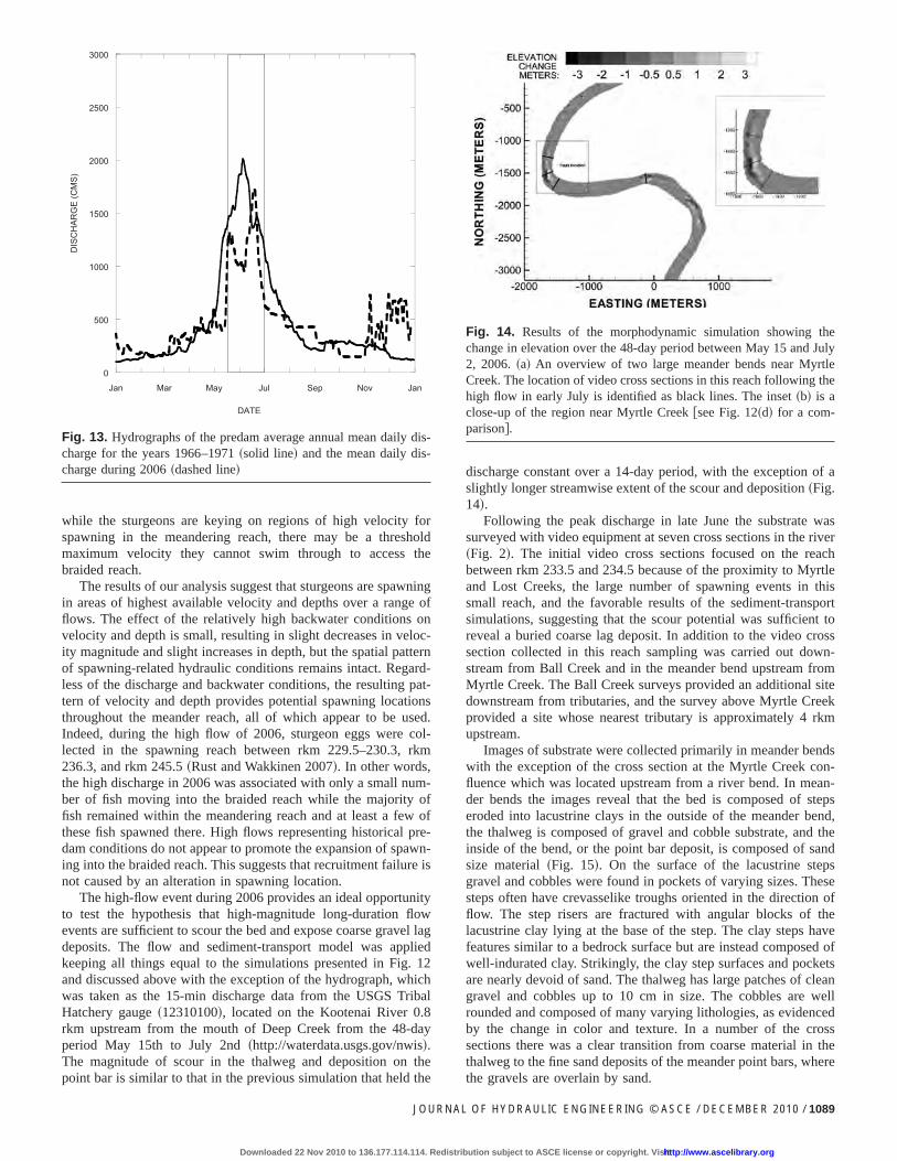
25th. The flow reached a mean daily discharge of 1 ,730 m3 /s onJune 18th and spent 12 days above 1,300 m3 /s during the periodof June 11th–22th. While the discharge was the largest in thepostdam period it did not quite approach the magnitude and du-ration of flows recorded in the predam period �Fig. 13�. As statedin the original recovery plan for Kootenai River white sturgeon�Duke et al. 1999�, significant changes in the natural flow regimesince operation of Libby Dam are considered to be the primaryreason for the decline of white sturgeon. However, since publica-tion of the recovery plan uncertainty has arisen over the connec-tion between natural flows and successful recruitment of whitesturgeon. On one hand there is the idea that prior to managedflows out of Libby Dam the sturgeon must have used the reach ofriver above Bonners Ferry where there is suitable substrate. Highdischarge in combination with high predam Kootenay Lake stagesis presumed to have increased the upstream extent of backwatersuch that the transition between the relatively fast, shallow, andfree-flowing water and the relatively slow, deep, and backwaterconditions occurred above Bonners Ferry in the braided reach,where there is suitable coarse substrate. On the other hand is theidea that the sturgeons are spawning where they have alwaysspawned and the current lack of high flows during the spawningseason limits the transport potential, leaving the bed composed of

-1800 -1600 -1400 -1200-1800

-1600

-1400

-1200

Depth Time =0

-1500 -1000 -500 0 500-3000

-2500

-2000

-1500

-1000

-500

Change in Elevation

238

233

235

234

236

237

Northing(meters)

Eas

A)

C)

Fig. 12. Results of the morphodynamic simulation for a 14-day peritime=14 days. The change in elevation over the 14-day period at theand �d� delineated in �c�. The dashed lines adjacent to the channel shalso Fig. 4�. The solid black lines across the channel indicate the appof the meander bends with scour in the thalweg and adjacent depositioCreek bend is shown in �d�.

fine-grained sand rather than scouring the bed and exposing



gravel lag deposits. The high discharge event in 2006 occurredafter the original analysis of both the spawning site selection andthe potential for high 1974-like discharge event to sufficientlyscour the bed in the existing spawning reach provides an oppor-tunity to validate our understanding of the effect of a near predamhigh flow on sturgeon spawning behavior and the effect of highflows on substrate composition.

During the high-flow event in 2006, of the 29 tagged adultwhite sturgeons that were in spawning condition, 27 moved as farupstream as rkm 235.2 �above Myrtle Creek�, 23 moved as farupstream as rkm 239 �just below Deep Creek�, 12 went as farupstream as rkm 243.5 �Ambush Rock�, 9 went as far as rkm 245�bottom of the braided reach�, 5 went as far as rkm 246.8, and 2went as far as rkm 248.6. These last two fish moved well into thebraided reach where the channel becomes much shallower andmultithreaded. Results of a 1D model of flow in this reach �Ber-enbrock 2005� show almost a doubling of average velocity at rkm249 compared to most of the reach downstream from rkm 249.The other region of relatively high velocity is that found in thetransition reach, near Bonners Ferry. Here there are consistentlyhigher velocities than in the meandering reach downstream. Priorto the 2006 high-flow event, no sturgeon had been tracked abovethis region of higher-flow velocities �Paragamian et al. 2002; Rust

-1800 -1600 -1400 -1200-1800

-1600

-1400

-1200

Depth222018161412108642

Depth Time = 14 days

-1800 -1600 -1400 -1200

-1600

-1400

-1200

Change inElevation

3210.5-0.5-1-2-3

Change in Elevation

eters)

B)

D)

h a constant discharge of 1 ,300 m3 /s. �a� The depth at time=0; �b�ge meander bends near Myrtle Creek, with the area shown in �a�, �b�,approximate locations of spawning activity from 1994 to 2002 �seete rkm location. The greatest change in elevation occurs in the apexhe point bars. A close-up of the scour and deposition near the Myrtle

ting (m

od wittwo larow theroximan on t

and Wakkinen 2005, 2007; Rust et al. 2007�. Thus it appears that

10


while the sturgeons are keying on regions of high velocity forspawning in the meandering reach, there may be a thresholdmaximum velocity they cannot swim through to access thebraided reach.

The results of our analysis suggest that sturgeons are spawningin areas of highest available velocity and depths over a range offlows. The effect of the relatively high backwater conditions onvelocity and depth is small, resulting in slight decreases in veloc-ity magnitude and slight increases in depth, but the spatial patternof spawning-related hydraulic conditions remains intact. Regard-less of the discharge and backwater conditions, the resulting pat-tern of velocity and depth provides potential spawning locationsthroughout the meander reach, all of which appear to be used.Indeed, during the high flow of 2006, sturgeon eggs were col-lected in the spawning reach between rkm 229.5–230.3, rkm236.3, and rkm 245.5 �Rust and Wakkinen 2007�. In other words,the high discharge in 2006 was associated with only a small num-ber of fish moving into the braided reach while the majority offish remained within the meandering reach and at least a few ofthese fish spawned there. High flows representing historical pre-dam conditions do not appear to promote the expansion of spawn-ing into the braided reach. This suggests that recruitment failure isnot caused by an alteration in spawning location.

The high-flow event during 2006 provides an ideal opportunityto test the hypothesis that high-magnitude long-duration flowevents are sufficient to scour the bed and expose coarse gravel lagdeposits. The flow and sediment-transport model was appliedkeeping all things equal to the simulations presented in Fig. 12and discussed above with the exception of the hydrograph, whichwas taken as the 15-min discharge data from the USGS TribalHatchery gauge �12310100�, located on the Kootenai River 0.8rkm upstream from the mouth of Deep Creek from the 48-dayperiod May 15th to July 2nd �http://waterdata.usgs.gov/nwis�.The magnitude of scour in the thalweg and deposition on the

0

500

1000

1500

2000

2500

3000


DISCHARGE(CMS)

DATE

Fig. 13. Hydrographs of the predam average annual mean daily dis-charge for the years 1966–1971 �solid line� and the mean daily dis-charge during 2006 �dashed line�

point bar is similar to that in the previous simulation that held the

JOURNAL


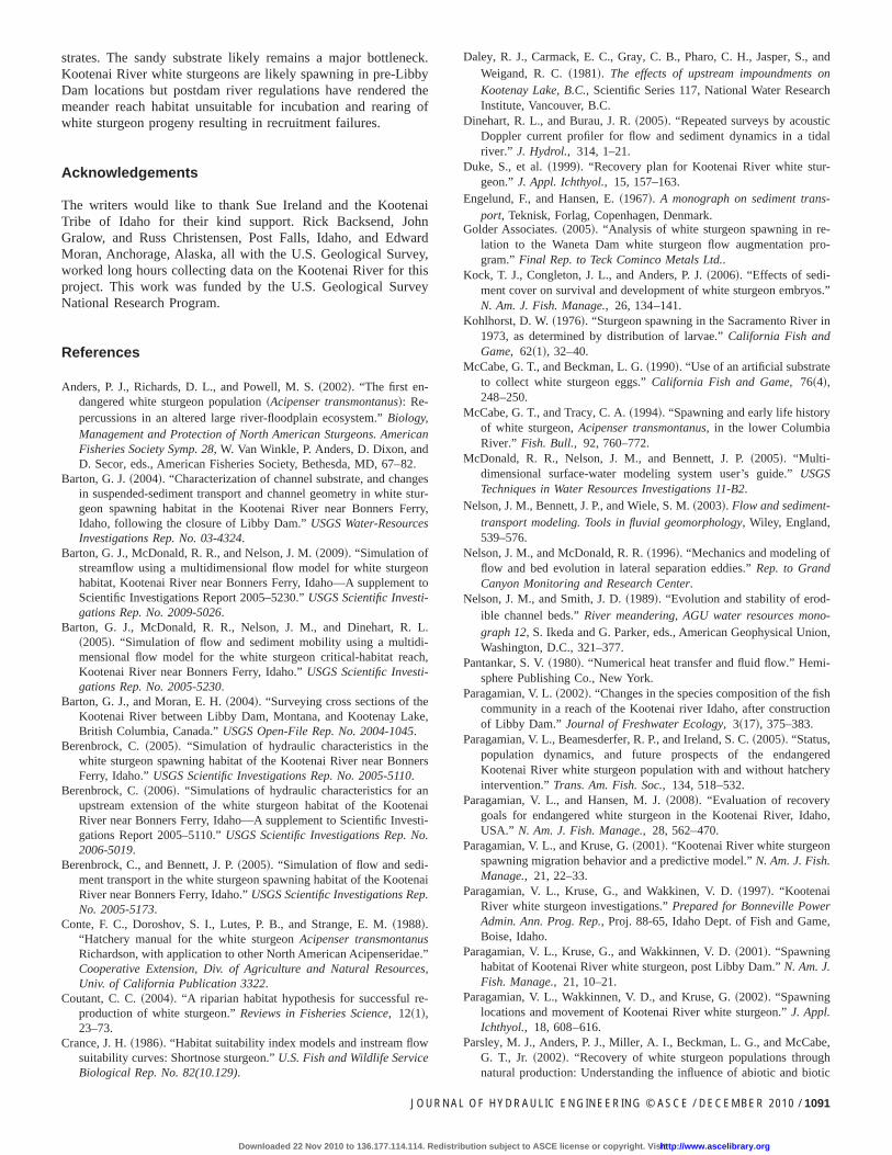
discharge constant over a 14-day period, with the exception of aslightly longer streamwise extent of the scour and deposition �Fig.14�.

Following the peak discharge in late June the substrate wassurveyed with video equipment at seven cross sections in the river�Fig. 2�. The initial video cross sections focused on the reachbetween rkm 233.5 and 234.5 because of the proximity to Myrtleand Lost Creeks, the large number of spawning events in thissmall reach, and the favorable results of the sediment-transportsimulations, suggesting that the scour potential was sufficient toreveal a buried coarse lag deposit. In addition to the video crosssection collected in this reach sampling was carried out down-stream from Ball Creek and in the meander bend upstream fromMyrtle Creek. The Ball Creek surveys provided an additional sitedownstream from tributaries, and the survey above Myrtle Creekprovided a site whose nearest tributary is approximately 4 rkmupstream.

Images of substrate were collected primarily in meander bendswith the exception of the cross section at the Myrtle Creek con-fluence which was located upstream from a river bend. In mean-der bends the images reveal that the bed is composed of stepseroded into lacustrine clays in the outside of the meander bend,the thalweg is composed of gravel and cobble substrate, and theinside of the bend, or the point bar deposit, is composed of sandsize material �Fig. 15�. On the surface of the lacustrine stepsgravel and cobbles were found in pockets of varying sizes. Thesesteps often have crevasselike troughs oriented in the direction offlow. The step risers are fractured with angular blocks of thelacustrine clay lying at the base of the step. The clay steps havefeatures similar to a bedrock surface but are instead composed ofwell-indurated clay. Strikingly, the clay step surfaces and pocketsare nearly devoid of sand. The thalweg has large patches of cleangravel and cobbles up to 10 cm in size. The cobbles are wellrounded and composed of many varying lithologies, as evidencedby the change in color and texture. In a number of the crosssections there was a clear transition from coarse material in thethalweg to the fine sand deposits of the meander point bars, where

Fig. 14. Results of the morphodynamic simulation showing thechange in elevation over the 48-day period between May 15 and July2, 2006. �a� An overview of two large meander bends near MyrtleCreek. The location of video cross sections in this reach following thehigh flow in early July is identified as black lines. The inset �b� is aclose-up of the region near Myrtle Creek �see Fig. 12�d� for a com-parison�.

the gravels are overlain by sand.



The cross section at the Myrtle Creek confluence showed moreangular substrate on the right bank downstream from the conflu-ence with Myrtle Creek where there was also substantial woodydebris; however, most of the cross section consisted of a sandysurface that was interspersed by a few clean lacustrine clay sur-faces and one small patch of coarse material with grain sizeslarger than 10 cm. The presence of more sand and less lacustrinesurfaces suggests that there is less scour in this cross section thanthe others, which is consistent with the modeling results.

The pattern of substrate composition at each of the video crosssections surveyed within meander bends �Fig. 15� qualitativelycorroborates the patterns of scour in the model simulations of thehigh-flow events in 1974 and 2006 and the existence of graveland cobble lag deposits where the vibracore studies previouslyfound gravel and cobble substrate covered by sand. The consistentpresence of gravel and cobble located in the thalweg suggests thatfollowing a period of significant high flow such as that experi-enced in 2006, gravel and cobble lag deposits are likely to beunveiled throughout much of the thalweg in the meander bends ofthe Kootenai River. Perhaps more revealing is the complexity ofthe channel bottom in the meander bends. Where surveyed therewere extensive portions of the bed composed of lacustrine stepsthat were nearly sand free. These lacustrine steps, unveiled ofsand, may provide a viable spawning substrate, not yet consid-ered, in addition to gravel and cobble substrates. Hard clay hasbeen identified as spawning substrate for other sturgeon speciessuch as the Gulf sturgeon �U.S. Fish and Wildlife Service�USFWS� 2003� and Atlantic sturgeon �Wilson and McKinley2004�.

Paragamian et al. �2001� noted that the Kootenai River whitesturgeon uses a longer reach of river to spawn than white sturgeonelsewhere. Perhaps this is an adaptation to Kootenai River wherethe natural variability in flow magnitude and duration from 1 yearto another created variability in the distribution of exposed,coarse substrate depending on the downstream transport of coarsematerial from the locations upstream and local inputs of coarsematerial from tributaries; therefore, the location of suitable sub-strate varied from 1 year to another. Metapopulation theory sug-

Nearly Devoid of Sand

Eroded Clay Steps

Gravel Lag andWoody Debris

Sandy Substrate

Eroded Clay stepsand pocketscontaining gravel

Gravel lag Deposit Gravel and SandTransition

Gravel andWoodyDebris

Fig. 15. Idealized cross section of the channel substrate, in a mean-der bend, following a high-flow scouring event. The outside of thebend through the thalweg is nearly devoid of sand and composed oflacustrine clay steps, and gravel/cobble lag deposits occur in the thal-weg. Patches of new and old woody debris are often found in thethalweg. The inside of the bed is composed of fine sandy materialforming the point bar deposit.

gests that dispersal of progeny over large areas has adaptive value



to long-term persistence of populations. It is possible that theKootenai River population of white sturgeon, once they becamegeographically isolated, adapted a strategy of spawning widelyover marginally suitable habitats. However, human developmentwithin the Kootenai River basin has degraded these habitats. Al-though historically these areas may have been marginally suitablefor spawning and egg incubation, they no longer are capable ofproviding all the requirements, leading to successful hatching andproduction of enough free-swimming embryos to sustain thepopulation.

Conclusions

The goal of this investigation was to integrate a detailed data setof white sturgeon spawning locations during 1994–2002, as rep-resented by egg-collection locations and the spatially distributedresults from a multidimensional model of flow and sedimenttransport to gain insight to the following questions about whitesturgeon spawning in the Kootenai River. Are white sturgeon re-sponding to false environmental cues created by flow regulationand spawning outside the historic spawning reach? Or are whitesturgeon spawning in the historic spawning reach, but in thepresent managed flow regime, this reach lacks the energy neces-sary to scour the bed and expose coarse-grained substrate suitablefor egg incubation?

The analysis of the model simulations demonstrates that thewhite sturgeon spawning locations in the meander reach coincidewith a broad region of high velocity which is higher than thatfound downstream; thus the sturgeon appears to migrate to areach with higher velocities. Within this broad region of highvelocity the white sturgeon spawn in the meander bends wherethe velocities and depths are locally higher, as indicated by themodel results and the spatial correlation analysis. The locations ofhigh velocity and depth in the meander bends are consistent atboth pre- and postdam discharge magnitudes. Thus, the hydrauliccues currently used for spawning existed prior to flow manage-ment and suggest that the current and historical spawning reachesare the same. This assertion is supported by the migration patternsof 29 radio-tagged white sturgeon during the 2006 high-flowevent which had discharge magnitude and duration near thatfound in the predam period. A large number �24� of these stur-geons migrated into the current spawning reach where spawningwas recorded by egg mats at three locations. Only five sturgeonswere recorded in the lower 2.5 km of the braided reach. Highpredam flows do not appear to promote the expansion of spawn-ing into the braided reach. This suggests that recruitment failure isnot caused by an alteration in spawning location.

Prior coring studies identified the existence of buried graveland cobble lenses under one to several meters of sand in thecurrent spawning reach. A flow and sediment-transport modelsimulation of the high discharge prior to the spawning seasonduring 1974, the only year in the postdam period with significantrecruitment of juvenal white sturgeon, indicated the potential ofhigh discharge to scour the sand and expose these regions ofburied gravel and cobble. Model simulations of scour during the2006 high-flow event predicted sufficient scour to uncover theburied gravel and cobble. A video survey of the channel substratefollowing the high-flow event in 2006 revealed the existence ofgravel and cobble in the thalweg of the channel where corerecords indicated the presence of these coarser substrates buriedby sand. Most Libby Dam era discharges have been incapable of
scouring and exposing areas that have suitable incubation sub-
10


strates. The sandy substrate likely remains a major bottleneck.Kootenai River white sturgeons are likely spawning in pre-LibbyDam locations but postdam river regulations have rendered themeander reach habitat unsuitable for incubation and rearing ofwhite sturgeon progeny resulting in recruitment failures.

Acknowledgements

The writers would like to thank Sue Ireland and the KootenaiTribe of Idaho for their kind support. Rick Backsend, JohnGralow, and Russ Christensen, Post Falls, Idaho, and EdwardMoran, Anchorage, Alaska, all with the U.S. Geological Survey,worked long hours collecting data on the Kootenai River for thisproject. This work was funded by the U.S. Geological SurveyNational Research Program.

References

Anders, P. J., Richards, D. L., and Powell, M. S. �2002�. “The first en-dangered white sturgeon population �Acipenser transmontanus�: Re-percussions in an altered large river-floodplain ecosystem.” Biology,Management and Protection of North American Sturgeons. AmericanFisheries Society Symp. 28, W. Van Winkle, P. Anders, D. Dixon, andD. Secor, eds., American Fisheries Society, Bethesda, MD, 67–82.

Barton, G. J. �2004�. “Characterization of channel substrate, and changesin suspended-sediment transport and channel geometry in white stur-geon spawning habitat in the Kootenai River near Bonners Ferry,Idaho, following the closure of Libby Dam.” USGS Water-ResourcesInvestigations Rep. No. 03-4324.

Barton, G. J., McDonald, R. R., and Nelson, J. M. �2009�. “Simulation ofstreamflow using a multidimensional flow model for white sturgeonhabitat, Kootenai River near Bonners Ferry, Idaho—A supplement toScientific Investigations Report 2005–5230.” USGS Scientific Investi-gations Rep. No. 2009-5026.

Barton, G. J., McDonald, R. R., Nelson, J. M., and Dinehart, R. L.�2005�. “Simulation of flow and sediment mobility using a multidi-mensional flow model for the white sturgeon critical-habitat reach,Kootenai River near Bonners Ferry, Idaho.” USGS Scientific Investi-gations Rep. No. 2005-5230.

Barton, G. J., and Moran, E. H. �2004�. “Surveying cross sections of theKootenai River between Libby Dam, Montana, and Kootenay Lake,British Columbia, Canada.” USGS Open-File Rep. No. 2004-1045.

Berenbrock, C. �2005�. “Simulation of hydraulic characteristics in thewhite sturgeon spawning habitat of the Kootenai River near BonnersFerry, Idaho.” USGS Scientific Investigations Rep. No. 2005-5110.

Berenbrock, C. �2006�. “Simulations of hydraulic characteristics for anupstream extension of the white sturgeon habitat of the KootenaiRiver near Bonners Ferry, Idaho—A supplement to Scientific Investi-gations Report 2005–5110.” USGS Scientific Investigations Rep. No.2006-5019.

Berenbrock, C., and Bennett, J. P. �2005�. “Simulation of flow and sedi-ment transport in the white sturgeon spawning habitat of the KootenaiRiver near Bonners Ferry, Idaho.” USGS Scientific Investigations Rep.No. 2005-5173.

Conte, F. C., Doroshov, S. I., Lutes, P. B., and Strange, E. M. �1988�.“Hatchery manual for the white sturgeon Acipenser transmontanusRichardson, with application to other North American Acipenseridae.”Cooperative Extension, Div. of Agriculture and Natural Resources,Univ. of California Publication 3322.

Coutant, C. C. �2004�. “A riparian habitat hypothesis for successful re-production of white sturgeon.” Reviews in Fisheries Science, 12�1�,23–73.

Crance, J. H. �1986�. “Habitat suitability index models and instream flowsuitability curves: Shortnose sturgeon.” U.S. Fish and Wildlife Service
Biological Rep. No. 82(10.129).
JOURNAL


Daley, R. J., Carmack, E. C., Gray, C. B., Pharo, C. H., Jasper, S., andWeigand, R. C. �1981�. The effects of upstream impoundments onKootenay Lake, B.C., Scientific Series 117, National Water ResearchInstitute, Vancouver, B.C.

Dinehart, R. L., and Burau, J. R. �2005�. “Repeated surveys by acousticDoppler current profiler for flow and sediment dynamics in a tidalriver.” J. Hydrol., 314, 1–21.

Duke, S., et al. �1999�. “Recovery plan for Kootenai River white stur-geon.” J. Appl. Ichthyol., 15, 157–163.

Engelund, F., and Hansen, E. �1967�. A monograph on sediment trans-port, Teknisk, Forlag, Copenhagen, Denmark.

Golder Associates. �2005�. “Analysis of white sturgeon spawning in re-lation to the Waneta Dam white sturgeon flow augmentation pro-gram.” Final Rep. to Teck Cominco Metals Ltd..

Kock, T. J., Congleton, J. L., and Anders, P. J. �2006�. “Effects of sedi-ment cover on survival and development of white sturgeon embryos.”N. Am. J. Fish. Manage., 26, 134–141.

Kohlhorst, D. W. �1976�. “Sturgeon spawning in the Sacramento River in1973, as determined by distribution of larvae.” California Fish andGame, 62�1�, 32–40.

McCabe, G. T., and Beckman, L. G. �1990�. “Use of an artificial substrateto collect white sturgeon eggs.” California Fish and Game, 76�4�,248–250.

McCabe, G. T., and Tracy, C. A. �1994�. “Spawning and early life historyof white sturgeon, Acipenser transmontanus, in the lower ColumbiaRiver.” Fish. Bull., 92, 760–772.

McDonald, R. R., Nelson, J. M., and Bennett, J. P. �2005�. “Multi-dimensional surface-water modeling system user’s guide.” USGSTechniques in Water Resources Investigations 11-B2.

Nelson, J. M., Bennett, J. P., and Wiele, S. M. �2003�. Flow and sediment-transport modeling. Tools in fluvial geomorphology, Wiley, England,539–576.

Nelson, J. M., and McDonald, R. R. �1996�. “Mechanics and modeling offlow and bed evolution in lateral separation eddies.” Rep. to GrandCanyon Monitoring and Research Center.

Nelson, J. M., and Smith, J. D. �1989�. “Evolution and stability of erod-ible channel beds.” River meandering, AGU water resources mono-graph 12, S. Ikeda and G. Parker, eds., American Geophysical Union,Washington, D.C., 321–377.

Pantankar, S. V. �1980�. “Numerical heat transfer and fluid flow.” Hemi-sphere Publishing Co., New York.

Paragamian, V. L. �2002�. “Changes in the species composition of the fishcommunity in a reach of the Kootenai river Idaho, after constructionof Libby Dam.” Journal of Freshwater Ecology, 3�17�, 375–383.

Paragamian, V. L., Beamesderfer, R. P., and Ireland, S. C. �2005�. “Status,population dynamics, and future prospects of the endangeredKootenai River white sturgeon population with and without hatcheryintervention.” Trans. Am. Fish. Soc., 134, 518–532.

Paragamian, V. L., and Hansen, M. J. �2008�. “Evaluation of recoverygoals for endangered white sturgeon in the Kootenai River, Idaho,USA.” N. Am. J. Fish. Manage., 28, 562–470.

Paragamian, V. L., and Kruse, G. �2001�. “Kootenai River white sturgeonspawning migration behavior and a predictive model.” N. Am. J. Fish.Manage., 21, 22–33.

Paragamian, V. L., Kruse, G., and Wakkinen, V. D. �1997�. “KootenaiRiver white sturgeon investigations.” Prepared for Bonneville PowerAdmin. Ann. Prog. Rep., Proj. 88-65, Idaho Dept. of Fish and Game,Boise, Idaho.

Paragamian, V. L., Kruse, G., and Wakkinnen, V. D. �2001�. “Spawninghabitat of Kootenai River white sturgeon, post Libby Dam.” N. Am. J.Fish. Manage., 21, 10–21.

Paragamian, V. L., Wakkinnen, V. D., and Kruse, G. �2002�. “Spawninglocations and movement of Kootenai River white sturgeon.” J. Appl.Ichthyol., 18, 608–616.

Parsley, M. J., Anders, P. J., Miller, A. I., Beckman, L. G., and McCabe,G. T., Jr. �2002�. “Recovery of white sturgeon populations through
natural production: Understanding the influence of abiotic and biotic


factors on spawning and subsequent recruitment.” Biology, Manage-ment, and Protection on North American Sturgeon. American Fisher-ies Society, Symposium 28, W. Van Winkle, P. J. Anders, D. H. Secor,and D. A. Dixon, eds., 55–66.

Parsley, M. J., and Beckman, L. G. �1994�. “White sturgeon spawningand rearing habitat in the lower Columbia River.” N. Am. J. Fish.Manage., 14, 812–827.

Parsley, M. J., Beckman, L. G., and McCabe, G. T., Jr. �1993�. “Spawn-ing and rearing habitat used by white sturgeon in the Columbia Riverdownstream of McNary Dam.” Trans. Am Fish. Soc., 122, 217–227.

Perrin, C. J., Heaton, A., and Laynes, M. A. �2000�. “White sturgeon�Acipenser transmontanus� spawning habitat in the lower FraserRiver.” Rep. prepared by Limnotek Research and Development Inc.for BC Fisheries.

Perrin, C. J., Rempel, L. L., and Rosenau, M. L. �2003�. “White sturgeonspawning habitat in an unregulated river: Fraser River, Canada.”Trans. Am. Fish. Soc., 132, 154–165.

Poff, N. L., et al. �1997�. “The natural flow regime.” BioScience, 47,769–784.

Rattray, M., Jr., and Mitsuda, E. �1974�. “Theoretical analysis of condi-tions in a sale wedge.” Estuarine Coastal Mar. Sci., 2, 373–394.

Richter, B. D., Boumgartner, J. V., Powell, J., and Braun, D. P. �1996�. “Amethod for assessing hydrological alteration within ecosystems.”Conserv. Biol., 10�4�, 1163–1174.

Rust, P. J., and Wakkinen, V. �2005�. “Kootenai River white sturgeonspawning and recruitment evaluation.” Prepared for Bonneville PowerAdministration, IDFG Rep. No. 05-37, Idaho Dept. of Fish and Game,Boise, Idaho.

Rust, P. J., and Wakkinen, V. �2007�. “Kootenai River white sturgeonspawning and recruitment evaluation.” Prepared for Bonneville PowerAdministration, IDFG Rep. No. 07-54, Idaho Dept. of Fish and Game,Boise, Idaho.

Rust, P. J., Wakkinen, V., and Kiser, T. �2007�. “Kootenai River whitesturgeon spawning and recruitment evaluation.” Prepared for Bonnev-ille Power Administration, IDFG Rep. No. 07-23, Idaho Dept. of Fishand Game, Boise, Idaho.

Schaffter, R. G. �1997�. “White sturgeon spawning migrations and loca-tion of spawning habitat in the Sacramento River, California.” Cali-fornia Fish and Game, 83�1�, 1–20.

Scott, W. B., and Crossman, E. J. �1973�. “Freshwater fishes of Canada.”



Fisheries Research Board of Canada, Bulletin 184.Setter, A., and Brannon, E. �1990�. “Report on Kootenai River white

sturgeon electrophoretic studies—1989, Report for the Idaho Depart-ment of Fish and Game. Aquaculture Extension, Univ. of Idaho. Pp30–50.” Kootenai River White Sturgeon Investigations and Experi-mental Culture. Annual Progress Rep. No. FY 1989, K. A. Apperson,ed., Idaho Dept. of Fish and Game and Bonneville Power Adminis-tration, Portland, Ore., Contract No. DE-A179-88BP3497, Project No.88-65.

Snyder, E. B., and Minshall, G. W. �1996�. Ecosystem metabolism andnutrient dynamics in the Kootenai River in relation to impoundmentand flow enhancement of fisheries management, Stream Ecology Cen-ter, Idaho State Univ., Boise, Idaho, variously paged.

U.S. Fish and Wildlife Service �USFWS�. �1994�. “Endangered andthreatened wildlife and plants; determination of endangered status forthe Kootenai River population of white sturgeon—Final rule.” Fed-eral Register, 59�171�, 45989–46002.

U.S. Fish and Wildlife Service �USFWS�. �2000�. “Final biologicalopinion—Effects to listed species from operations of the Federal Co-lumbia River Power System.” Consultation performed for US ArmyCorps of Engineers, Bonneville Power Administration, and US Bu-reau of Reclamation, USFWS, Region 1, Portland, Ore., �http://www.fws.gov/pacific/finalbiop/BiOp.pdf� �2008�.

U.S. Fish and Wildlife Service �USFWS�. �2001�. “Endangered andthreatened wildlife and plants; final designation of critical habitat forthe Kootenai River population of white sturgeon.” Federal Register,66�173�, 46548–46561.

U.S. Fish and Wildlife Service �USFWS�. �2003�. “Critical habitat forGulf sturgeon.” Federal Register, 68�53�, 13454.

USDA. �2007�. “National resources conservation service.” ID601—Soilsurvey of Boundary County Area, Idaho, web soil survey, availableonline at �http://websoilsurvey.nrcs.usda.gov/� �Jul. 18, 2007�.

Weisel, C. �1980�. “Soil survey of Boundary County area, Idaho.” U.S.Dept. of Agriculture, Natural Resources Conservation Service, onlineat �http://soils.usda.gov/survey/online_surveys/idaho/� �2008�.

Wilson, J. A., and McKinley, S. R. �2004�. “Chapter 2: Distribution,habitat and movements.” Sturgeons and paddlefish of North America,G. T. O. Lebreton, F. W. H. Beamish, and R. S. McKinley, eds.,Kluwer Academic, The Netherlands, 40–72.

10


modeling the effect of flow and sediment transport on ... · modeling the effect of flow and...

Documents