modeling streamflow and water temperature in...

WQPBIMTSTD-003

MODELING STREAMFLOW AND

WATER TEMPERATURE IN THE

BEAVERHEAD RIVER

November 2011 (Revised in March 2014)

Prepared by: Water Quality Planning Bureau Montana Department of Environmental Quality Water Quality Planning Bureau 1520 E. Sixth Avenue P.O. Box 200901 Helena, MT 59620-0901

ABSTRACT

The enhanced river water quality model QUAL2K was applied to the Beaverhead River in southwestern Montana by the Montana Department of Environmental Quality (DEQ) to evaluate stream temperature improvement scenarios for a 66 mile reach extending from Barretts to Twin Bridges, MT as part of the temperature Total Maximum Daily Load (TMDL) investigation for the river. Heat transfer principles were used to evaluate a number of scenarios and their effect on diurnal water temperature. A companion model, Shadev3.0.xls was used to evaluate shade. Existing data were used for model development including climatic information from the National Weather Service (NWS) and Bureau of Reclamation AgriMet program, streamflow and temperature data from Montana State University (collected for the Bureau of Reclamation), data from the U.S. Geological Survey, and associated field measurements made by DEQ during 2009. Models were calibrated relatively successfully with mean relative error of 0.01% and root mean squared error of 0.9°F. Following calibration we employed scenario analysis to determine feasible management strategies for the river. We evaluated the following: (1) the effect of riparian vegetation and shading improvement along the stream corridor, (2) morphological changes to the river’s width depth ratio, (3) irrigation efficiency improvement and maintenance projects, and (4) natural and naturally occurring conditions. Based on our evaluation, we determined that the Beaverhead River is impaired for water temperature due to a number of reasons, most notably, the cumulative effect of irrigation dewatering and shade removal. Overall, the river is 3.7°F warmer than naturally occurring with the most significant effect being irrigation. Consequently, we recommend that irrigation efficiency be considered as the highest priority for any management plan to meet the state water temperature standard. Other best management practices that should be considered in conjunction with these activities include riparian enhancement (tree planting). The study was commissioned by DEQ as part of our statewide watershed planning work.

Suggested citation: Flynn, K.F. Regensburger, E., and K. Fortman. 2011. Modeling streamflow and water temperature in the Beaverhead River. Helena, MT: Montana Dept. of Environmental Quality. Photos: (Top panel) Beaverhead River upstream of Poindexter Slough. (Bottom panel) Beaverhead River at Barretts Diversion Dam. Photos from www.bigskyfishing.com.

Modeling Streamflow and Water Temperature in the Beaverhead River –Table of Contents

11/3/11 Final i

TABLE OF CONTENTS

Acronyms ...................................................................................................................................................... v

1.0 Background ............................................................................................................................................. 1

1.1 Prior Studies ........................................................................................................................................ 1

1.2 Montana’s Temperature Standard (ARM 17.30.623) ......................................................................... 1

1.3 The Effects of Management on Water Temperature ......................................................................... 1

1.4 Reservoir Influence ............................................................................................................................. 2

2.0 Study Area Description ........................................................................................................................... 2

2.1 Climate ................................................................................................................................................ 4

2.2 Streamflow .......................................................................................................................................... 5

2.3 Groundwater ....................................................................................................................................... 5

2.4 Irrigation and Land Use ....................................................................................................................... 6

2.5 Fish and Aquatic Life ........................................................................................................................... 6

3.0 Data Summary ......................................................................................................................................... 7

3.1 Overview ............................................................................................................................................. 7

3.2 Quality Assessment of Previously Collected Data............................................................................... 7

3.3 Summary ........................................................................................................................................... 11

4.0 Modeling Approach............................................................................................................................... 11

4.1 QUAL2K Description .......................................................................................................................... 11

4.2 Conceptual Representation .............................................................................................................. 12

4.3 Heat Balance ..................................................................................................................................... 12

4.4 Assumptions and Limitations ............................................................................................................ 14

4.5 Shade Model (Shadev3.0.xls) ............................................................................................................ 14

5.0 Model Setup and Development ............................................................................................................ 15

5.1 Modeling Analysis Period Selection .................................................................................................. 15

5.2 Comparison With Historical Conditions ............................................................................................ 16

5.3 Model Physical Description and Segmentation ................................................................................ 18

5.4 Meteorological Data ......................................................................................................................... 20

5.5 Hydrology .......................................................................................................................................... 22

5.6 Hydraulics .......................................................................................................................................... 24

5.7 Shade ................................................................................................................................................. 27

5.8 Boundary Conditions ......................................................................................................................... 29

5.9 Groundwater Temperature............................................................................................................... 30

5.10 Wastewater Treatment Facility Influent ......................................................................................... 31

Modeling Streamflow and Water Temperature in the Beaverhead River –Table of Contents

11/3/11 Final ii

6.0 Model Calibration ................................................................................................................................. 31

6.1 Evaluation Criterion .......................................................................................................................... 32

6.2 Results and Discussion ...................................................................................................................... 32

6.2.1 Hydrology ................................................................................................................................... 32

6.2.2 Hydraulics ................................................................................................................................... 33

6.2.3 Water Temperature ................................................................................................................... 34

7.0 Watershed Management Scenarios ...................................................................................................... 35

7.1 Baseline ............................................................................................................................................. 36

7.2 Improved Riparian Habitat Scenario ................................................................................................. 36

7.3 Channel Morphology Scenario ............................................................. Error! Bookmark not defined.

7.4 Irrigation Efficiency Improvement Scenario ..................................................................................... 37

7.5 Naturally Occurring Condition Scenario ........................................................................................... 38

7.6 Natural Condition Scenario ............................................................................................................... 39

7.7 Scenario Summary ............................................................................................................................ 41

8.0 Conclusion ............................................................................................................................................. 42

9.0 References ............................................................................................................................................ 43

Modeling Streamflow and Water Temperature in the Beaverhead River –List of Tables

11/3/11 Final iii

LIST OF TABLES

Table 1-1. General trout temperature tolerances. ....................................................................................... 2

Table 3-1. Overview of the monitoring locations on Beaverhead River in 2005. ......................................... 8

Table 4-1. QUAL2K input requirements ...................................................................................................... 11

Table 4-2. ShadeV3.0.xls model input requirements. ................................................................................. 15

Table 5-1. Beaverhead River steady-state water balance. ......................................................................... 22

Table 5-2. Beaverhead River rating curve coefficients and exponents. ..................................................... 24

Table 5-3. Beaverhead River Q2K reach properties. ................................................................................... 25

Table 5-4. Shade and morphological data for the Beaverhead River. ........................................................ 27

Table 5-5. Beaverhead River riparian shade conditions from aerial assessment and 2009 field data. ...... 27

Table 5-6. Shadev3.0.xls input parameters. ............................................................................................... 28

Table 5-7. Beaverhead River boundary conditions. .................................................................................... 29

Table 5-8. Groundwater data used in accretion flow determination. ........................................................ 31

Table 6-1. Calibration statistics for each calibration node. ........................................................................ 35

Table 7-1. Summary of the management scenario analysis for the Beaverhead River. ............................. 42

Modeling Streamflow and Water Temperature in the Beaverhead River –List of Figures

11/3/11 Final iv

LIST OF FIGURES

Figure 2-1. Beaverhead River vicinity map showing TPA boundary and associated features. ..................... 3

Figure 2-2. Beaverhead River detailed study reach. ..................................................................................... 4

Figure 2-3. Beaverhead River climate and streamflow summary. ................................................................ 5

Figure 3-1. Temperature QA comparisons for the Beaverhead River .......................................................... 9

Figure 3-2. Correction of Co-op canal data for influence of hot spring. ....................................................... 9

Figure 3-3. Quality assessments between USGS, BOR, and MSU discharge measurements. .................... 10

Figure 4-1. Conceptual representation of a river reach within QUAL2K. ................................................... 12

Figure 4-2. Graphical representation of the heat balance within a Q2K model element. ......................... 13

Figure 4-3. Surface heat exchange in Q2K model. ...................................................................................... 14

Figure 4-4. Conceptual representation of Shadev3.0.xls. ........................................................................... 15

Figure 5-1. Water temperature data used to determine the model analysis period. ................................ 16

Figure 5-2. Conditions encountered during 2005 compared to historical data. ........................................ 17

Figure 5-3. Longitudinal discharge and water temperature relationships for the Beaverhead River. ....... 18

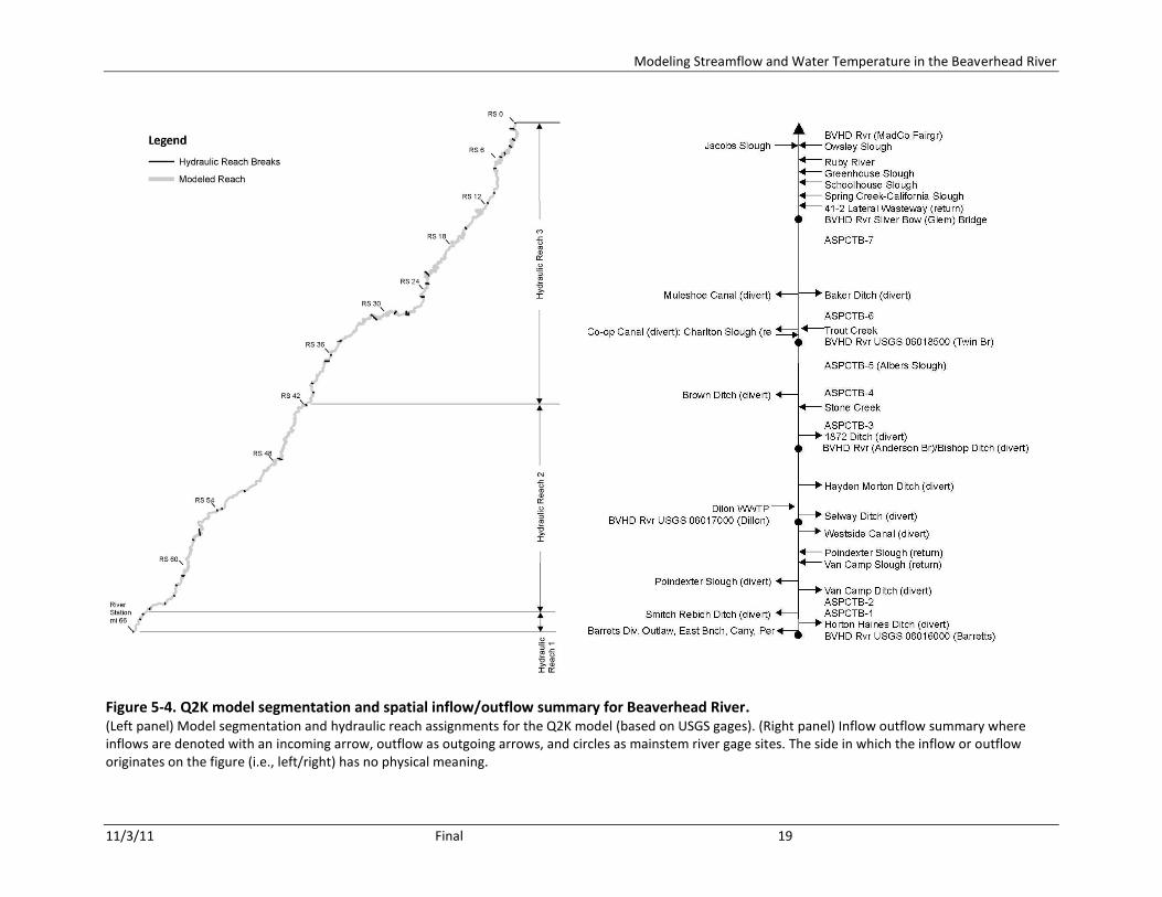
Figure 5-4. Q2K model segmentation and spatial inflow/outflow summary for Beaverhead River. ......... 19

Figure 5-5. Hourly meteorological data summary for August 4-7th, 2005 summer period. ....................... 20

Figure 5-6. Mean repeating day meteorological data summary for August 4-7th, 2005 summer period. . 21

Figure 5-7. QUAL2K steady-state water balance for a given element. ....................................................... 22

Figure 5-8. Rating curve compilation for gages on the Beaverhead River. ................................................ 26

Figure 5-9. Simulated and observed longitudinal shade on the Beaverhead River. ................................... 28

Figure 5-10. Comparison of diurnal sinusoid with respect to field data .................................................... 29

Figure 6-1. Streamflow calibration for the Beaverhead River. ................................................................... 33

Figure 6-2. Simulated Beaverhead River hydraulics. .................................................................................. 34

Figure 6-3. Simulated and observed water temperatures for the Beaverhead River during 2005. ........... 35

Figure 7-1. Simulated reference shade conditions for the Beaverhead River. ........................................... 37

Figure 7-2. Simulated reference channel morphology for the Beaverhead River. ....... Error! Bookmark not defined.

Figure 7-3. Irrigation improvement scenario on the Beaverhead River. .................................................... 38

Figure 7-4. Simulated naturally occurring condition scenario for the Beaverhead River. .......................... 39

Figure 7-5. Median discharge rates corrected for dam influences. ............................................................ 40

Figure 7-6. Simulated natural conditions on the Beaverhead River. .......................................................... 41

Figure 7-7. Comparison of management scenarios on the Beaverhead River. .......................................... 42

Modeling Streamflow and Water Temperature in the Beaverhead River –Acronyms

11/3/11 Final v

ACRONYMS

Acronym Definition ARM Administrative Rules of Montana ASOS Automated surface observing Station BLM Bureau of Land Management (federal) BOR Bureau of Reclamation CC Clark Canyon Dam CCWC Canyon Canal Water Company DEQ Department of Environmental Quality (Montana) DNRC Department of Natural Resources & Conservation EBID East Bench Irrigation District EPA Environmental Protection Agency (US) FWP Fish, Wildlife, and Parks FWS Fish & Wildlife Service (US) GWIC Groundwater Information Center HUC Hydrologic Unit Code MBMG Montana Bureau of Mines and Geology MCA Montana Codes Annotated MPDES Montana Pollutant Discharge Elimination System MSU Montana State University NAIP National Agriculture Imagery Program NOAA National Oceanic and Atmospheric Administration NSDZ Near Stream Disturbance Zone NWS National Weather Service QA Quality Assurance RE Relative Error RMSE Root Mean Squared Error TMDL Total Maximum Daily Load TPA TMDL Planning Area USGS United States Geological Survey WWTP Wastewater Treatment Plant

Modeling Streamflow and Water Temperature in the Beaverhead River –Acronyms

11/3/11 Final vi

Modeling Streamflow and Water Temperature in the Beaverhead River

11/3/11 Final 1

1.0 BACKGROUND

The river water quality model QUAL2K was applied to the Beaverhead River in southwestern Montana to evaluate stream temperature improvement scenarios for a 66.3 mile reach between Barretts and Twin Bridges, MT. Models were constructed to ascertain the relationship between flow, riparian conditions, river management, and in-stream water temperature as part of the TMDL. Information on the project background, modeling results, and scenario analyses are contained within the rest of the document.

1.1 PRIOR STUDIES

Prior investigations into water temperature on the Beaverhead River have suggested that it is impaired for a number of reasons. For example numerous times the river has been greater than 21.1°C (70°F), and twice it has exceeded 25°C (78 and 79°F) (CDM, et al., 2003). Such values are near the upper limit for most salmonid species and are of concern. To compound the issue, the river is dewatered (Montana Fish, Wildlife, and Parks, 2003). Sections with problems include:

The upper Beaverhead River, which is periodically dewatered from the Clark Canyon Dam to the West Side Canal (21 miles).

The lower Beaverhead River, which is chronically dewatered from the West Side Canal to the Big Hole River (39 miles).

In addition to the previous assertions, vegetation losses from the riparian corridor and dam operation have all been speculated as other possible causes of impairment (CDM, et al., 2003). None have ever been validated quantifiably however. As a result, modeling was commissioned by DEQ to identify whether feasible irrigation efficiency improvement or maintenance projects or riparian vegetation or channel morphology improvements as part of the TMDL would have a significant influence on water temperature. We subsequently will use that information to identify management practices, if any, are of merit in meeting the Montana stream temperature standard (ARM 17.30.623(2)(e) (2006)).

1.2 MONTANA’S TEMPERATURE STANDARD (ARM 17.30.623)

Water quality impairment in Montana is currently arbitrated according to the state water temperature standard (ARM 17.30.623(2)(e) (2006)). For B-1 waters (which the Beaverhead River is) a maximum allowable increase of 1°F over “naturally occurring” is acceptable when natural temperatures are within the range of 32°F to 66°F. If temperatures are 66.5°F or greater, a 0.5°F increase is allowed (ARM 17.30.623(2)(e) (2006)). Hence certain increases are allowed, but with limitations. The standard was originally developed to address point source discharges therefore it is difficult to interpret for nonpoint sources. To fully evaluate its requirements, DEQ must first characterize the departure from “naturally occurring” (which reflects the implementation of “all reasonable soil and water conservation practices”) (per ARM 17.30.602) and then recommend best management practices (BMPs) to mitigate the impairment. Modeling is one of the most effective ways to make this determination. Consequently, this document and project were conceptualized to link water temperature with reasonable management conditions along the river corridor).

1.3 THE EFFECTS OF MANAGEMENT ON WATER TEMPERATURE

It has been well established that river management has an effect on water temperature (LeBlanc, et al., 1997; Meier, et al., 2003; Poole and Berman, 2001; Rutherford, et al., 1997). For example, healthy


11/3/11 Final 2

riparian areas absorb incoming solar shortwave radiation, reflect longwave radiation, and influence microclimate (i.e., air temperature, humidity, and wind speed). Added streamflow volume (i.e., flow rate) increases the temperature buffering capacity of a waterbody via thermal inertia or assimilative heat capacity. Channel morphology is critical for maintenance of hyporheic flow and minimizes solar gain. These variables that are influenced by river management are important in assessing stream health and associated effects on fish and aquatic life. Critical limits and temperature tolerances for fluvial inhabitants are an effective way to characterize waterbody condition. Temperature tolerances for fish species present in the Beaverhead River are summarized in Table 1-1. Temperatures slightly over 70°F are lethal for 10 percent of the salmonid population (LC10) in an exposure lasting 24 hours1. Optimum ranges are nearer 60°. Thus given our knowledge about the Beaverhead River, there are potentially impacts to most of the trout species. Table 1-1. General trout temperature tolerances. From DEQ 2011 (R. McNeil, personal communication).

Species Optimum Range (°F) LC10 for 24 hours (°F)

Brown trout (adult) 57 75

Rainbow trout (adult) 57 80

Brook trout (adult) 60 77

Cutthroat trout (adult) 56 71

1.4 RESERVOIR INFLUENCE

The Beaverhead River is also reservoir regulated therefore the operation of upstream storage facilities is a consideration. Clark Canyon Reservoir is at the uppermost end of the project reach and provides nearly all flow in the river. According to Smith (1973), this is a net benefit as the reservoir buffers diurnal temperatures and provides stable cool hypolimnetic water. It also provides flow beyond what may naturally be available. As a result, temperature downstream of the reservoir is significantly better (i.e., cooler and less diurnal flux) than a non-regulated system of similar size. A second consideration is Lima Reservoir (much further upstream) which also partially regulates flow in the Red Rock River, a tributary to Clark Canyon Reservoir. It is less important given its storage volume and proximity to the study area. Consequently, there are further considerations in regard to water temperature management in the Beaverhead River than those stated in previous sections.

2.0 STUDY AREA DESCRIPTION

The Beaverhead River is located in Beaverhead and Madison counties in southwestern Montana (Figure 2-1). The river flows out of Clark Canyon Dam northeasterly for approximately 80 miles past the towns of Dillon and Twin Bridges, MT until ultimately confluencing with the Big Hole River near Twin Bridges. The temperature impairment extends from Grasshopper Creek to the Big Hole River (segment ID MT41B001_020) and is 62.7 miles long (DEQ, 2011). The entire area is part of United States Geological

1 It should be noted that coldwater fish species have varied temperature requirements that are dependent on life stage. Table 1-1 should only be used as a rough guide.


11/3/11 Final 3

Survey (USGS) Hydrologic Unit Code (HUC) 10020002. Note: the 62.7 miles referenced above is a different length than used in model development (as detailed in later sections).

Figure 2-1. Beaverhead River vicinity map showing TPA boundary and associated features. The area being modeled extends from the USGS gage at Barretts (USGS 06016000) to the Highway 41 Bridge near Twin Bridges (Madison County Fairgrounds). This encompasses the available field data. The impairment actually extends slightly upstream to Grasshopper Creek. The study area is most easily accessed via Interstate-15 between Idaho Falls, ID and Dillon, MT, and on Montana Highway 41 between Dillon and Twin Bridges (Figure 2-2). Monitoring sites and USGS gages are also shown and are referenced in future sections.


11/3/11 Final 4

Figure 2-2. Beaverhead River detailed study reach.

2.1 CLIMATE

Climate of the Beaverhead River is inter-continental. Located on the eastern side of the continental divide, it is influenced by relatively dry cells pushed inland by prevailing westerly to northwesterly winds. Systems of low-pressure are most prevalent during the winter months and produce both rain and snow. Pacific highs influence the summer climate and cause long periods of warm and dry weather.


11/3/11 Final 5

Automated surface observing Station (ASOS) number 242404 is most proximal to the project reach and provides a suitable characterization of long-term climate (Dillon Airport, period of record of 1948-2005). According to site records (Western Regional Climate Center, 2006), July and early August are the most probable time-period when river impairment would occur. Air temperatures approach 80-85°F and coincide with a relatively dry period in the basin (Figure 2-3, left).

Figure 2-3. Beaverhead River climate and streamflow summary. (Left panel). Monthly temperature and precipitation for the Dillon airport. (Right panel) Mean monthly discharge for gages in the project site. Both climate station and gage locations are shown in Figure 2-2.

2.2 STREAMFLOW

Streamflow in the watershed originates primarily from snowmelt out of the Tendoy and Centennial mountain ranges to the south and east and from the Beaverhead Mountains to west. Precipitation concentrates in these locations to form both major inflows to Clark Canyon Reservoir (Red Rock River and Horse Prairie Creek). Hydrology downstream of the reservoir is entirely regulated. From October to March, water is stored for the upcoming irrigation season. Conservation pool releases then occur from April through September to meet irrigation demands. The U.S. Geological Survey (USGS) operates three gages on Beaverhead River (Figure 2-3, right panel). These include: (1) USGS 06016000 Beaverhead River at Barretts MT (upstream of all major diversions), (2) USGS 06017000 Beaverhead River at Dillon MT, and (3) USGS 06018500 Beaverhead River near Twin Bridges MT. The hydrograph at all locations is influenced by irrigation. Annual streamflow in the upper watershed has a pronounced yet shifted hydrograph peak of about 800 ft3/s in July (during the irrigation season due to storage releases) whereas streamflow in the lower river shows an inverted hydrograph from cumulative diversions (flows between 200 and 500 ft3/s). Minimum discharges usually occur during late summer months and often result in late-season shortages of irrigation water.

2.3 GROUNDWATER

Groundwater is abundant in the project area and potentiometric surface maps indicate the flow path is generally from the uplands towards the floodplains, and then northeast along the Beaverhead River

0.0

0.5

1.0

1.5

2.0

0

20

40

60

80

100

Jan

Feb

Mar

Ap

r

May Jun

Jul

Au

g

Sep

Oct

Nov

Dec

Pre

cip

itat

ion

(in

)

Tem

pe

ratu

re (°

F)

Month

Maximum Temperature

Minimum Temperature

Precipitation

0

200

400

600

800

1000

Jan

Feb

Mar

Ap

r

Ma

y

Jun

Jul

Au

g

Sep

Oct

Nov

Dec

Me

an M

on

thly

Dis

char

ge (f

t3 /s)

Month

USGS 06016000 Barretts (1965-2004)

USGS 06017000 Dillon (1965-1983)

USGS 06018500 Twin (1965-2004)


11/3/11 Final 6

(Uthman and Beck, 1998). The uppermost tertiary aquifer is believed to have the most interaction with the river resulting in both gaining and losing reaches. Near Dillon, the river is thought to be gaining. Groundwater accretion comprises a large part of this baseflow. The upper reaches are characterized as losing (Uthman and Beck, 1998). Historical hydrogeologic data suggest groundwater resources in the basin are stable. The construction of Clark Canyon Dam (CC) caused the water table in the vicinity of the East Bench irrigation canal to rise as much as 100 feet [Botz 1967 as cited in Uthman and Beck (1998)], however, groundwater elevations are now seasonally stable. In some places, drain tiles have been installed to help route groundwater. Changes are related to artificial recharge from the dam and leakage through the canals, and further detail on the hydrogeology of the project site is found in Uthman and Beck (1998).

2.4 IRRIGATION AND LAND USE

Land use in the Beaverhead River valley is primarily irrigated agriculture. Crops consist of alfalfa and grass hay (U.S. Department of Agriculture, 2011) and production consists of 2 or 3 cuttings per year which are then either sold as hay or are used to winter cattle. Water for irrigation is provided by two main companies; the East Bench Irrigation District (EBID) whose major diversion is located approximately three miles below Grasshopper Creek at Barretts (eleven miles below Clark Canyon Reservoir), and the Clark Canyon Water Supply Company which is on the west side of the river and consists of a number of smaller ditch companies or private irrigation shareholders. In total, each unit provides full irrigation service to 28,055 and 33,706 acres respectively (Bureau of Reclamation, 2006a). About 46 percent of the watershed is under private ownership. Another 39 percent is under federal management, and 15 percent is stewarded by the state (including FWP managed lands and surface waters) (CDM, et al., 2003). Most of the federal lands are in the higher elevations whereas the lower elevations are mostly private (with some BLM and State Trust Lands). The condition of these areas is highly variable. Riparian corridors vary from healthy native vegetation stands in some instances to severely impacted locations elsewhere. In most places, willow and aspen communities were historically present, but have been removed through human activity [BLM, 2003 as cited in CDM et al., (2003)].

2.5 FISH AND AQUATIC LIFE

Despite being one of the better fisheries in the state, the Beaverhead River has declined over the years. The upper and mid-river has suffered from reductions in fish populations for nearly a decade as a result of persistent drought [R. Oswald, personal communication as cited in CDM et al., (2003)]. Conditions have not improved much until recently. Limited releases from Clark Canyon Reservoir during the winters of 2002-2003 (<27 ft3/s) were mostly to blame. These depressed trout populations through reductions in wetted stream perimeter, feeding habitat, macroinvertebrate prey food, spawning sites, and protective woody debris [R. Oswald, personal communication as cited in CDM et al., (2003)]. The size, health, and vigor of the trout population in the Beaverhead River was cumulatively affected. The lower river (Anderson Lane, Mule Shoe, and Twin Bridges sections, downstream of Dillon) has suffered from low fish densities for a long time (since the 1970s). This is believed to be related to a variety of habitat problems including altered flow regimes, heavy bedload transport, channel atrophy, excessively high summer temperatures, and bank instability from a lack of woody riparian vegetation [Oswald (2000) and Oswald and Brammer (1993) as cited in CDM et al., (2003)]. The lower river is in poor condition subsequently, and will likely benefit from a temperature TMDL.


11/3/11 Final 7

3.0 DATA SUMMARY

A data summary has been prepared to overview some of the information collected by other agencies in support of the modeling. Most of the review is focused on the data collected by Montana State University (MSU) (Sessoms and Bauder, 2005) for Bureau of Reclamation (BOR) water contract renegotiations. These were the primary data used in the model development. Since some of this data happened to be an indirect measure (i.e., the dataloggers just happened to record temperature), a short section is provided here to ensure that the data is valid for TMDL planning purposes.

3.1 OVERVIEW

Thirty-four discharge and temperature monitoring stations were established in 2005 as part of the Bureau of Reclamation (BOR) water balance effort (Sessoms and Bauder, 2005). Monitoring instrumentation was Tru-track WT-VO capacitance meters which are voltage output water height probes that log both water height and temperature. Stage is measured with a temperature corrected accuracy of ±1%, and water temperatures are measured within ±0.5°F. Thus the absolute accuracy of these instruments is 2% and 1.0°F respectively. Each logger was housed in a stilling well and logged at one-hour intervals. Flow measurements were made with Marsh-McBirney Model 2000 Flo-Mate portable flow meters to rate the gaging sites. Discharges were correlated with Tru-track stage heights to establish site rating curves and were visited approximately once per month from April 4 to October 24. Standard operating procedures were used in the collection of the data as outlined in the “Water Measurement Manual” (Bureau of Reclamation, 2001) or USGS Water Supply Paper 2175 Measurement and Computation of Streamflow (Rantz, 1982)2. EBID uses flumes for their discharge measurements, which according to Sessoms and Bauder (2005) are sufficiently accurate for use as well. The flow measurement and temperature monitoring locations used in this study are identified in Table 3-1. From Figure 2-2 it is apparent that many sites are not located directly on the main river, but are on its periphery (i.e., the easiest locations to measure). From a water temperature perspective this is not ideal as the potential arises (however unlikely that it is) that changes could occur between the diversion point and the logger location. This concern is further compounded by the fact that there was no formal quality documentation for the work (personal communication, H. Sessoms, 2006). Hence a quality assurance (QA) assessment was completed to ensure this data met our requirements.

3.2 QUALITY ASSESSMENT OF PREVIOUSLY COLLECTED DATA

The first phase of QA consisted of completing spot checks of temperature at several locations during the fall of 2005. A Horiba Water Quality Checker U-10 (accuracy ±0.5°F) was used. Field measured temperatures were correlated with the date and time of the datalogger recording for comparison. Results are shown in Figure 3-1 (Left panel). As evidenced by the good correlation between field temperature and recorded temperature at the logger, the MSU data appears to have good accuracy and precision over the study reach. Sites that received field QA included: (1) Beaverhead River at Madison

2 These are the two primary sources for such flow measurement activities.


11/3/11 Final 8

County Fairgrounds, (2) Jacobs Slough, (3) Ruby River, (4) Greenhouse Slough, (5) East Bench 41-2 Lateral Wasteaway, (6) Beaverhead River at Giem Bride, (7) Spring Creek, (8) California Slough, (9) Schoolhouse Slough, (10) Owsley Slough, (11) Coop Ditch, and (12) Beaverhead River at Anderson Lane Bridge. Table 3-1. Overview of the monitoring locations on Beaverhead River in 2005. Site Type Agency Locations

Mainstem River USGS USGS MSU USGS MSU/BOR MSU

Beaverhead River at Barretts MT Beaverhead River at Dillon MT Beaverhead River at Anderson Lane Bridge Beaverhead River near Twin Bridges MT Beaverhead River at Giem (Silverbow Lane) Bridge Beaverhead River at Twin Bridges (Madison County Fairgrounds)

Tributaries MSU MSU MSU MSU MSU MSU MSU MSU MSU MSU MSU MSU

Poindexter Slough Stone Creek near Highway 41 bridge Trout Creek near Point of Rocks California Slough near Silverbow Lane Spring Creek near Silverbow Lane East Bench 41-2 lateral waste way Baker Ditch waste way/Redfield Lane Ditch Schoolhouse Slough at Highway 41 crossing Owsley Slough at Highway 41 crossing Greenhouse Slough at East Bench Road Ruby River at East Bench Road bridge Jacob’s Slough at East Bench Road

Diversions EBID CCWC MSU MSU MSU MSU MSU MSU MSU MSU MSU MSU MSU MSU MSU MSU MSU

East Bench Canal Canyon Canal Smith-Rebich Canal below Barrett’s gauging station Outlaw Ditch at Barrett’s Diversion Dam Perkins Ditch at Barrett’s Diversion Dam Horton Haines Ditch Van Camp Ditch Poindexter Slough Diversion Westside Canal Selway Slough/Ditch Horton Haines Ditch Bishop Ditch 1872 Ditch Brown Ditch Co-op Ditch near Point of Rocks Muleshoe Canal Baker Ditch

BOR = Bureau of Reclamation CCWC = Canyon Canal Water Company EBID = East Bench Irrigation District MSU = Montana State University USGS = U.S. Geological Survey

A similar correlation was made between the USGS temperature monitor on the mainstem river and the Co-op ditch Tru-track (very close proximity to the USGS gage) in order to verify that the logger


11/3/11 Final 9

temperature (even though some distance from the river) is similar to that of the mainstem river (Figure 3-1, Right panel). In this instance, there seems to be a potential issue due to a consistent positive bias.

Figure 3-1. Temperature QA comparisons for the Beaverhead River (Left panel). MSU Tru-track vs. DEQ Horiba at multiple sites. (Right panel) MSU Tru-track vs. USGS gage.

After further review of the data supporting Figure 3-1 (Right panel), it was identified that the MSU comparison site (Co-op canal) had a hot spring in it (i.e., 80°F in October noted by field personnel). It therefore is a poor comparison site. Consequently we cannot verify our assumption whether outgoing ditch temperatures truly reflect the mainstem river. We will address this concern later through the use of the model. To correct the Co-op Tru-track site, we did a simple adjustment as shown in Figure 3-2 which required a constant shift of -2°F.

Figure 3-2. Correction of Co-op canal data for influence of hot spring. (Left panel). Uncorrected Co-op canal data. (Right panel). Corrected data.

32

36

40

44

48

52

56

60

32 36 40 44 48 52 56 60

Ho

rib

a Te

mp

erat

ure

(°F

)

Tru-track Temperature (°F)

Tru-track vs Horiba (Instantaneous Temp)

Line of Equal Value

32

40

48

56

64

72

80

32 40 48 56 64 72 80

MSU

Me

asu

red

Tem

p (°

F)

USGS Measured Temp (°F)

USGS vs MSU (Mean Daily Temp)

Line of Equal Value

50

54

58

62

66

70

74

78

8/2 8/3 8/4 8/5 8/6 8/7 8/8

MSU

Me

asu

red

Tem

p (

oF)

USGS Measured Temp (oF)

USGS min MSU min

USGS mean MSU mean

USGS max MSU max

50

54

58

62

66

70

74

78

8/2 8/3 8/4 8/5 8/6 8/7 8/8

MSU

Me

asu

red

Tem

p (

oF)

USGS Measured Temp (oF)

USGS min MSU corr min

USGS mean MSU corr mean

USGS max MSU corr max


11/3/11 Final 10

QA of the flow data is shown in Figure 3-3. We compared daily USGS, BOR, and MSU flow measurements. Most discharge measurements appear to be reasonable according to the line of equal value as only minor deviations occur between USGS and BOR observations3. For example, residuals were not greater than 15% at any time which indicate a suitable fit (Sauer and Meyer, 1992). Deviation between the MSU and BOR data, however, is more concerning. MSU discharge estimates at Anderson Bridge are nearly 40% different than the BOR data4. Giem Bridge provided much better results (approximately 15% low) somewhat affirming the quality of the data.

Figure 3-3. Quality assessments between USGS, BOR, and MSU discharge measurements. (Top left and right panels). Comparisons between Barretts and Twin Bridges for USGS and BOR sites. (Bottom left and right panels). Same but between MSU and BOR for Anderson and Giem Bridge.

3 Mean daily discharge for these locations were obtained electronically via the National Water Information System (NWIS) and BOR Hydromet websites (Bureau of Reclamation, 2006b; U.S. Geological Survey, 2006). 4 This site had nuisance weeds/algae which apparently interfered with the flow measurement.

500

520

540

560

580

600

620

640

500 520 540 560 580 600 620 640

BO

R M

eas

ure

d F

low

(cfs

)

USGS Measured Flow (cfs)

USGS vs BOR (Mean Daily Flow)

Line of Equal Value

0

20

40

60

80

100

120

140

0 20 40 60 80 100 120 140

BO

R M

eas

ure

d F

low

(cfs

)

USGS Measured Flow (cfs)

USGS vs BOR (Mean Daily Flow)

Line of Equal Value

0

20

40

60

80

100

120

140

0 20 40 60 80 100 120 140

MSU

Me

asu

red

Flo

w (c

fs)

BOR Measured Flow (cfs)

BOR vs MSU (Mean Daily Flow)

Line of Equal Value

0

20

40

60

80

100

120

140

0 20 40 60 80 100 120 140

MS

U M

eas

ure

d F

low

(cf

s)

BOR Measured Flow (cfs)

BOR vs MSU (Mean Daily Flow)

Line of Equal Value


11/3/11 Final 11

3.3 SUMMARY

Based on the data in this section (in regard to both temperature and flow), DEQ feels comfortable in proceeding with the modeling assuming that the concerns and limitation of the data are adequately addressed in their use. As such, any questionable information will be scrutinized and validated prior to use. In cases of unexplainable or grossly erroneous data, these will be removed from the analysis entirely. Any data concerns from this point on will be noted in the text.

4.0 MODELING APPROACH

DEQ selected a mechanistic modeling approach to evaluate the relationship between management activities and water temperature on the Beaverhead River. The enhanced river quality model QUAL2K (Q2K) was selected for analysis due to a number of reasons including its frequency in application for TMDL planning, fairly standardized heat flux algorithms, and endorsement by EPA (Rauch, et al., 1998; Wool, 2009). Shadev3.0 was used as a companion model to identify hourly changes in shade from topographic and riparian shade. Each tool is briefly described in this section.

4.1 QUAL2K DESCRIPTION

Q2K is a steady-state one-dimensional river model that simulates the movement of water and heat flux in completely mixed systems. It is applicable to rivers where the major transport mechanisms of advection and dispersion are significant along the longitudinal direction of flow, with the assumption that lateral and vertical water temperature gradients are negligible. By operating the model in a quasi-dynamic mode, the user has the ability to study the diurnal variation of temperature on an hourly or sub-hourly time scale. Q2K allows multiple waste discharges, withdrawals, tributary flows, and incremental inflow and outflow to be positioned anywhere along the channel, and includes sediment heat flux routines and reach variable meteorology. Consequently it is a significant improvement over the original QUAL2E model (Brown and Barnwell, 1987). Q2K is limited to periods where both streamflow and input heat loads are steady-state and input data requirements are shown in Table 4-1. Table 4-1. QUAL2K input requirements Data Type Input Requirement

1

Meteorology 1. Hourly air temperature 2. Hourly dew point temperature 3. Hourly wind speed 4. Hourly percent cloud cover 5. Atmospheric turbidity coefficient 6. Reach latitudes and longitudes

Hydrology 1. Discharge data for headwaters, and point and nonpoint sources 2. Temperature data for headwaters, and point and nonpoint sources

Hydraulics 1. Stream network configuration 2. Reach lengths and elevations 3. Transport function (rating curves, etc.)

Shade 1. Hourly percent shade for each reach 1Most of the input variables in Table 4-1 can readily be acquired through existing field measurement programs.

Their use in development of the model are described in Section 5.0.


11/3/11 Final 12

4.2 CONCEPTUAL REPRESENTATION

A river in Q2K is represented as a series of reaches and elements where point sources (e.g., tributaries) and nonpoint source inflows (e.g., groundwater) or withdrawals are present (Figure 4-1). Reaches are homogeneous stretches of river that have similar aspect, shading, or hydraulic characteristics, whereas the element is the fundamental computational unit of the model. Reach stationing determines the placement of the point and nonpoint source inflows. Additional information regarding Q2K can be found in Chapra, et al., (2008).

Figure 4-1. Conceptual representation of a river reach within QUAL2K. Taken from Chapra, et al., (2008). Please refer to the modeling documentation for further discussion.

4.3 HEAT BALANCE

The heat balance in Q2K is written as Equation 4-1, where for each control volume i (an element) the change in temperature Ti [

oC] is computed according to t = time [d], E’i = the bulk dispersion coefficient between reaches i and i + 1 [m3/d], Wh,i = the net heat load from point and nonpoint sources into reach i

[cal/d], w = the density of water [g/cm3], Cpw = the specific heat of water [cal/(g oC)], Jh,i = the air-water heat flux [cal/(cm2 d)], and Js,i = the sediment-water heat flux [cal/(cm2 d)] (Chapra, et al., 2008). This is shown graphically in Figure 4-2.

1

2

3

4

5

6

8

7

Non-point

abstraction

Non-point

source

Point source

Point source

Point abstraction

Point abstraction

Headwater boundary

Downstream boundary

Point sourcen = 4n = 4

ReachReach ElementsElements


11/3/11 Final 13

(Equation 4-1)

cm 100

m

cm 100

m

cm 10

m

,,

36

3,

1

'

1

'1,

11

ipww

is

ipww

ih

ipww

ih

iii

iii

i

ii

i

iabi

i

ii

i

ii

HC

J

HC

J

VC

W

TTV

ETT

V

ET

V

QT

V

QT

V

Q

dt

dT

Figure 4-2. Graphical representation of the heat balance within a Q2K model element. Reproduced from Chapra, et al., (2008).

The surface heat exchange is modeled as a combination of five processes including solar shortwave radiation, atmospheric longwave radiation, conduction from air and sediments, and advective heat input from water inflows. This is shown in Equation 4-2, where I(0) = net solar shortwave radiation at the water surface, Jan = net atmospheric longwave radiation, Jbr = longwave back radiation from the water, Jc = conduction, and Je = evaporation. All fluxes are expressed as cal/cm2/d.

(Equation 4-2) 5 ecbranh JJJJIJ )0(

A graphical rendition of surface heat exchage is also shown in Figure 4-3. Heat losses include longwave radiation, conduction to air and bed sediments, and evaporation and outflow from the river. Heat gains include both radiation and non-radiation terms.

5 Shortwave radiation within the model is determined as a function of latitude and longitude of the modeled reach. It is attenuated by atmospheric transmission, cloud cover, reflection, and topographic and vegetative shading. Water and atmospheric longwave radiation are calculated according to the Stefan-Boltzmann law and conduction and evaporation are calculated using the Brady, Graves, and Geyer method and Dalton’s Law (Chapra, et al., 2008). Air and water temperature, wind speed, and the saturation vapor pressure (relative humidity) are all required as well.

iinflow outflow

dispersion dispersion

heat load heat abstraction

atmospheric

transfer

sediment-water

transfer

sediment


11/3/11 Final 14

Figure 4-3. Surface heat exchange in Q2K model. Reproduced from Chapra, et al., (2008)

4.4 ASSUMPTIONS AND LIMITATIONS

Q2K has a number of assumptions and limitations. Those critical to temperature assessment such as in the Beaverhead River include the following:

Negligible water temperature gradients (i.e., the channel is assumed to be well-mixed both vertically and laterally).

Steady flow and heat load conditions (i.e., river hydrology, hydraulics, and boundary conditions are assumed to be steady state).

Diurnally uniform meteorological forcings (i.e., climatic conditions are assumed uniform over the project reach both spatially and temporally).

A final assumption implicit in the model is that diversion water temperatures measured by MSU are representative of the temperature of the Beaverhead River (in order to calibrate the model). We were unable to prove this in Section 3.2. However the assumption is valid given the relative proximity of these sites to the diversion point from the river. We provide further justification in Section 6.0.

4.5 SHADE MODEL (SHADEV3.0.XLS)

Shade for Q2K was simulated in Shadev3.0.xls. This software is a visual basic for applications package developed by the Oregon Department of Environmental Quality and adapted by Washington Ecology (Pelletier, 2007) to determine shade from both topography and vegetation using solar time and position, aspect, position, and vegetation characteristics of a channel (Figure 4-4). Required field data for the shading calculation include: (1) tree canopy height, (2) density, (3) overhang, (4) stream reach aspect, (5) wetted channel width, (6) near stream disturbance zone (NSDZ) width, (7) channel incision, and (8) topographic shading (Table 4-2). These values were collected by a DEQ contractor in 2009. Similar to Q2K, Shadev3.0.xls has a number of assumptions. These include: (1) that vegetative parameters (tree height, density, and overhang) are considered uniform over the project reach for a particular species type and age class (2) that calculation of solar position (e.g. azimuth and altitude) is accurate for each Julian day at the respective modeling latitude and longitude, and (3) that topographic

air-water

interface

solar

shortwave

radiation

atmospheric

longwave

radiation

water

longwave

radiation

conduction

and

convection

evaporation

and

condensation

radiation terms non-radiation terms

net absorbed radiation water-dependent terms


11/3/11 Final 15

angle can accurately be estimated using ArcGIS viewshed. Further information regarding Shadev3.0.xls can be found in Boyd and Kasper (2003) and Pelletier (2007).

Figure 4-4. Conceptual representation of Shadev3.0.xls. Diagram taken from Boyd and Kasper (2003).

5.0 MODEL SETUP AND DEVELOPMENT

The Q2K model setup and development is described in this section. Included is a brief summary of the analysis period, details on the physical model construction, and other information related to model development.

5.1 MODELING ANALYSIS PERIOD SELECTION

The analysis period was based on critical limiting conditions (i.e., the time of year when temperature impairment is most likely to occur). Review of 5 years of temperature data at USGS 06018500 Beaverhead River near Twin Bridges gage (2000-2004) suggests this period occurs somewhere between July and August (Figure 5-1, left panel). Temperature data collected during 2005 (the year the model will be developed) corroborate these findings (Figure 5-1, right panel). Accordingly, the period of August 4-7, 2005 was used for Q2K development, at or when conditions are likely to impair water temperature.

Table 4-2. ShadeV3.0.xls model input requirements. Data Type Specific Input Requirement

Solar Position 1. Latitude and longitude of reach 2. Date and time

Stream Morphology

1. Aspect 2. Channel width 3. Near stream disturbance zone (NSDZ) width 4. Incision

Vegetation 1. Canopy height 2. Canopy density 3. Overhang

Geographic 1. Topographic angle


11/3/11 Final 16

Figure 5-1. Water temperature data used to determine the model analysis period. (Left panel). USGS temperature data from 1999-2004. (Right panel) Data from 2005 at Anderson Bridge. The most critical limiting period occurs sometime in July or August.

Data were then compiled over the period of interest. MSU discharge data were readily available in MS Excel spreadsheets and required very little reduction. USGS, BOR, and NOAA data were downloaded from each agency’s web site and assembled into individual data files. All units were converted to standard international (S.I.) and were aggregated into a format for modeling (i.e., mean repeating day time-series which are consistent with the requirements of Q2K). In other words, input data were averaged over the study period into a single daily time-series of climate, discharge, and temperature.

5.2 COMPARISON WITH HISTORICAL CONDITIONS

A comparison of the analysis period with historical conditions is shown in Figure 5-2. Both climate (as represented by mean daily air temperature and precipitation) and streamflow (as annual hydrograph) were evaluated. The meteorological conditions during August were very similar to that of the climatic normals (1970-2001)(National Oceanic and Atmospheric Administration, 2011) (Figure 5-2, left) and streamflow was below average, between the 5th and 25th percentile. Thus the conditions are very close to those that would be expected during critical low flow conditions.

32

37

42

47

52

57

62

67

72A

ug-

99

Feb

-00

Au

g-00

Feb

-01

Au

g-01

Feb

-02

Au

g-02

Feb

-03

Au

g-03

Feb

-04

Au

g-04

Me

asu

red

Te

mp

(oF)

Date

Water Temperature

32

40

48

56

64

72

80

May

-05

Jun

-05

Jul-

05

Au

g-05

Au

g-05

Sep

-05

Me

asu

red

Tem

p (

oF

Date

Water Temperature


11/3/11 Final 17

Figure 5-2. Conditions encountered during 2005 compared to historical data. (Left panel) Climatological data. (Right panel) Streamflow hydrology. For flow, only March through October is shown as the gage was not operated during the winter months for most of the period of record.

Water temperature data for this period is shown in Figure 5-3. Upon examination, a number of general interpretations can be made. First, temperatures are fairly similar in the main-stem river, but show a slight increase from approximately 65°F at Barretts to 68°F near Twin Bridges (mean daily temperatures are reported in the figure). On the whole, incoming tributaries tend to be cooler than the river, whereas the sloughs and Ruby River (in the lower watershed) are nearly the same temperature or perhaps slightly cooler. Probably the biggest difference in the figure is flow. Mean daily discharges ranges from over 550 ft3/s in the upper river to nearly 50 ft3/s in the lower reaches. From up- to down-stream, the profile is characteristic of heavy irrigation depletion followed by a number of irrigation returns. Slough inflow from Spring Creek, California Slough, Schoolhouse Slough, Charlton Slough, Greenhouse Slough, etc. (most of these are from the Big Hole River) and the Ruby River nearly quadruple the flow over a very short extent. This perhaps somewhat attenuates the temperature effect. Additionally from Figure 5-3 it should be apparent that ascertaining the relationship between river management and water temperature from simply looking at data is difficult. While a 3°F increase in water temperature does occur (in combination with flow depletion), we have no way of knowing whether the increase is natural or human-caused, or the extent thereof. Water quality models will therefore be used to: (1) better formalize the mechanistic relationship between variables such as flow, water temperature, and others, (2) determine whether this increase in temperature is natural or anthropogenic, (3) understand the cause-effect relationships of management activities and observed stream temperature, and (4) provide recommendations, if any, that can be implemented to meet the temperature standard in the river.

0

5

10

15

20

250

10

20

30

40

50

60

70

80

90

100

Jan Feb Mar Apr May Jun Jul Aug Sep Oct Nov Dec

Pre

cip

itat

ion

(hu

nd

reth

s)

Air

Te

mp

era

ture

(°F)

Date

Dillon Airport Precipitation Normal (1971-2000)

Dillon Airport Precipitation (2005)

Dillon Airport Temperature Normal (1971-2000)

Dillon Airport Temperature (2005)

0

100

200

300

400

500

600

700

800

900

1000

Jan Feb Mar Apr May Jun Jul Aug Sep Oct Nov Dec

Stre

amfl

ow

(ft3 /

s)

Date

5th percentile (47 years)

25th percentile (47 years)

Mean daily statistic (47 years)

Mean daily discharge - 2005


11/3/11 Final 18

Figure 5-3. Longitudinal discharge and water temperature relationships for the Beaverhead River. Water temperature data are reflective of the mean daily temperature.

5.3 MODEL PHYSICAL DESCRIPTION AND SEGMENTATION

The Beaverhead River Q2K model reflects the physical mechanics of advection and dispersive heat transport for the river. The model was segmented to describe: (1) major inflows and outflows identified by Sessoms and Bauder (2005), (2) the USGS and BOR gage sites, (3) aspect and vegetation breaks, and (4) other important features identified by DEQ. In total, 36 reaches were discretized with an average approximate reach length of three miles. These are shown in Figure 5-4 (Left panel). They also coincide with the Q2K reaches shown in Figure 5-3. Although 36 different reaches were identified (as indicated by the dark black lines on the river plan drawing) there was insufficient information to describe all of these hydraulically. The paucity of river width and depth data necessitated a much simpler hydraulic representation. As a result only 3 generalized hydraulic regions were used which correspond to the USGS gaging sites (also shown in Figure 5-4, Left panel). The stationing of tributaries, other inflows, and outflows is shown in Figure 5-4 (Right panel). These are more directly addressed in Section 5.5. More information on the model hydraulics is contained within Section 5.6.

50

55

60

65

70

75

0

100

200

300

400

500

600

BV

HD

Rvr U

SGS 0

60

16

00

0 (B

arretts)

Smitch

Re

bich

Ditch

(dive

rt)

Barre

ts Div. O

utlaw

, East Bn

ch, C

any, …

Ho

rton

Hain

es D

itch (d

ivert)

ASP

CTB

-1

ASP

CTB

-2

Van

Cam

p D

itch (d

ivert)

Po

ind

exte

r Slou

gh (d

ivert)

Van

Cam

p Slo

ugh

(retu

rn)

Po

ind

exte

r Slou

gh (re

turn

)

We

stside

Can

al (dive

rt)

BV

HD

Rvr U

SGS 0

60

17

00

0 (D

illon

)

Selw

ay Ditch

(dive

rt)

Hayd

en

Mo

rton

Ditch

(dive

rt)

BV

HD

Rvr (A

nd

erso

n B

r)/Bish

op

Ditch

…

18

72

Ditch

(dive

rt)

ASP

CTB

-3

Ston

e C

ree

k

Bro

wn

Ditch

(dive

rt)

ASP

CTB

-4

ASP

CTB

-5 (A

lbe

rs Slou

gh)

Co

-op

Can

al (dive

rt): Ch

arlton

Slou

gh …

BV

HD

Rvr U

SGS 0

60

18

50

0 (Tw

in B

r)

Trou

t Cre

ek

ASP

CTB

-6

Mu

lesh

oe

Can

al (dive

rt)

Bake

r Ditch

(dive

rt)

ASP

CTB

-7

BV

HD

Rvr Silve

r Bo

w (G

iem

) Brid

ge

41

-2 Late

ral Waste

way (re

turn

)

Sprin

g Cre

ek-C

aliforn

ia Slou

gh

Scho

olh

ou

se Slo

ugh

Gre

en

ho

use

Slou

gh

Ru

by R

iver

Jacob

s Slou

gh

Ow

sley Slo

ugh

BV

HD

Rvr (M

adC

o Fairgr)

Tem

per

atu

re (°F

)

Stre

amfl

ow

(cfs

)

Q2K Reach

Streamflow Mainstem Temperature Tributary Temperature

Data not consistent withrest of profile


11/3/11 Final 19

Figure 5-4. Q2K model segmentation and spatial inflow/outflow summary for Beaverhead River. (Left panel) Model segmentation and hydraulic reach assignments for the Q2K model (based on USGS gages). (Right panel) Inflow outflow summary where inflows are denoted with an incoming arrow, outflow as outgoing arrows, and circles as mainstem river gage sites. The side in which the inflow or outflow originates on the figure (i.e., left/right) has no physical meaning.


11/3/11 Final 20

5.4 METEOROLOGICAL DATA

Q2K requires hourly meteorological data to calculate diurnal heat flux within the model. Four sites have requisite data. These are: (1) ASOS 242404 Dillon, MT, (2) Dillon Valley Agrimet, (3) Ruby Valley Agrimet, and (4) Jefferson Valley Agrimet. Hourly observations of temperature, wind speed, and dew point were available from each location and are shown in Figure 5-5. They were averaged1 to provide mean repeating day input for Q2K (Figure 5-6).

Figure 5-5. Hourly meteorological data summary for August 4-7th, 2005 summer period. (Top left/right panel). Air and dew point temperature [°F]. (Bottom left/right panel). Wind speed [mi/hr] and cloud cover [%]. It should be noted that the model actually requires input in SI units.

1 All sites were within close proximity to the watershed, therefore the average of the four sites were used. Only one site, (Dillon ASOS) had information regarding cloud cover.

30

40

50

60

70

80

90

100

Air

Te

mp

era

ture

(°F)

Date

Data Range Mean

2025303540455055606570

De

wp

oin

t Te

mp

era

ture

(°F)

Date

Data Range Mean

0

5

10

15

20

25

30

Win

d S

pe

ed

(mi/

hr)

Date

Data Range Mean

0102030405060708090

100

Clo

ud

Co

ver(

%)

Date

Dillon Airport


11/3/11 Final 21

Figure 5-6. Mean repeating day meteorological data summary for August 4-7th, 2005 summer period. These data reflect the aggregation of the time-series in Figure 5-5. In other words, values at 6:00 a.m., 7:00 a.m., and so on were averaged to provide a single day’s time-series.

Wind speed data were corrected to an appropriate height using the power-law profile (Lindsey, et al., 1982) (Equation 5-1), where: v = mean wind speed at conversion height, v1= measured wind speed at some standard height, z = conversion height, z1 = standard measurement height, and k = exponent.

(Equation 5-1)

k

z

z

v

v

11 The height of the anemometer at Dillon is 33 ft (10 m) (personnel communication, National Weather Service, Great Falls, 2006). Agrimet sensor heights are approximately 6.5 ft (2 m) (personal communication T. Grove, BOR, 2006). A value of k= 0.18 was used for the Dillon ASOS (airport) and 0.25 for the AgriMet sites (grass field) to make the adjustment to the 7 meter height required by Q2K.

30

40

50

60

70

80

90

100A

ir T

em

pe

ratu

re (°

F)

Date

4-day Mean

303540455055606570

De

wp

oin

t Te

mp

era

ture

(°F)

Date

4-day Mean

0123456789

10

Win

d S

pe

ed

(mi/

hr)

Date

4-day Mean

0102030405060708090

100

Clo

ud

Co

ver (

%)

Date

4-day Mean


11/3/11 Final 22

5.5 HYDROLOGY

A steady-state flow balance was used to define the hydrology in the model (Equation 5-2), where Qi = outflow from reach i into reach i + 1 [m3/d], Qi–1 = inflow from the upstream reach i – 1 [m3/d], Qin,j= total inflow into the reach from point and nonpoint sources [m3/d], and Qab,i= total outflow from the reach due to point and nonpoint abstractions [m3/d]. All major inflow and outflow components were field measured. A graphical version of this balance is shown in Figure 5-7.

(Equation 5-2) iabiinii QQQQ ,,1 Inflow and outflow locations in the water balance were based on the channel centerline digitized by DEQ using aerial photography from 2005 National Agriculture Imagery Program (NAIP) while nonpoint sources and abstractions were modeled as line sources. A tabular version of the water balance for the model analysis period is shown in Table 5-1.

Figure 5-7. QUAL2K steady-state water balance for a given element. Reproduced from Chapra, et al., (2008).

Table 5-1. Beaverhead River steady-state water balance. Data for the period of August 4-7th, 2005.

Location Description Surface Water (m

3/s)

1

Groundwater (m

3/s)

BVHD00 Observed - BVHD Rvr USGS 06016000 (Barretts) 564.6

17.8

BVHD01 Smith Rebich Ditch (divert) -27.7

BVHD02 Barretts Diversions (divert) -285.4

BVHD03 Horton Haines Ditch (divert) -25.7

BVHD04 ASPCTB-1 0

BVHD05 ASPCTB-2 0

BVHD06 Van Camp Ditch (divert) -13.2

BVHD07 Poindexter Slough (divert) -33.1

BVHD08 Van Camp Slough (return) 6.9

BVHD09 Poindexter Slough (return) 36.2

BVHD10 Westside Canal (divert) -72

TOTAL 150.6

1 Recall that all flow estimates were based on the MSU water balance during 2005 (Sessoms and Bauder, 2005).

i i + 1i 1

Qi1 Qi

Qin,i Qab,i


11/3/11 Final 23

Table 5-1. Beaverhead River steady-state water balance. Data for the period of August 4-7th, 2005.

Location Description Surface Water (m

3/s)

1

Groundwater (m

3/s)

BVHD11 Observed - BVHD Rvr USGS 06017000 (Dillon) 168.4

*Includes Outlaw, East Bench, Canyon Canal, and Perkins Diversions

BVHD12 Selway Ditch (divert) -5.4

-15.7

BVHD13 Hayden Morton Ditch (divert) -16.5

++++++ Bishop Ditch (divert) -11.1

TOTAL 135.4

BVHD14 Observed - BVHD Rvr (Anderson Br) 119.7

*Bishop ditch diversion occurs directly upstream of Anderson Bridge

BVHD15 1872 Ditch (divert) -10.5

5.5

BVHD16 ASPCTB-3 0

BVHD17 Stone Creek 1.7

BVHD18 Brown Ditch (divert) -19.1

BVHD19 ASPCTB-4 0

BVHD20 ASPCTB-5 (Albers Slough) 13.5

BVHD21 Co-op Canal (divert) -23.6

++++++ Charlton Slough (return) 11.6

TOTAL 93.4

BVHD22 Observed - BVHD Rvr USGS 06018500 (Twin Br) 98.9

*Charlton Slough Return occurs directly downstream of the Co-op Canal

BVHD23 Spring-Trout Creek 0.4

-10.9

BVHD24 ASPCTB-6 0

BVHD25 Muleshoe Canal (divert) -26.5

BVHD26 Baker Ditch (divert) -14.8

BVHD27 ASPCTB-7 0

TOTAL 58.0

BVHD28 Observed - BVHD Rvr Silver Bow (Giem) Bridge 47.0

BVHD29 41-2 Lateral Wasteway (return) 1.5

18.2

BVHD30 Spring Creek-California Slough-Redfield Ditch 36.7

BVHD31 Schoolhouse Slough 16.9

BVHD32 Greenhouse Slough 20.5

BVHD33 Ruby River 64.4

BVHD34 Jacobs Slough 5.3

BVHD35 Owsley Slough 38.2

TOTAL 230.6

BVHD36 Observed - BVHD Rvr (MadCo Fairgr) 248.9

BVHDij is the Beaverhead reach number in the Q2K model ASPCTB denotes reach break due to aspect change


11/3/11 Final 24

5.6 HYDRAULICS

The movement of water through the model was represented using rating curves1. These relate mean velocity and depth to discharge in the form of a power equation (Equation 5-3 and Equation 5-4), where H=depth [m] and U=velocity [m/s] are related to discharge (Q)[m/s] through the empirical coefficients

and exponents a and b and , and [all unitless].

Equation 5-3. baQU

Equation 5-4. QH

Computed U and H are then used to determine the cross-sectional area (Ac) and average reach top width (B) which are the primary attributes of interest for temperature modeling (Equation 5-5 and Equation 5-6) [Chapra, et al., (2008)].

Equation 5-5. U

QAc

Equation 5-6. H

AB c

Data to determine the coefficients and exponents described previously are available from the USGS

gages (i.e., Barretts [upper], Dillon [middle], and Twin Bridge [lower]). The values a and b and , and were determined through least-square regression and were assigned the hydraulic regions identified previously in Figure 5-4. Estimates were found to be consistent with the literature (Barnwell, et al.,

1989; Flynn and Suplee, 2010; Leopold and Maddock, 1953) (Table 5-2) and the sum of b and was less than or equal to 1. Table 5-2. Beaverhead River rating curve coefficients and exponents.

Equation Exponent Typical value Range1 Beaverhead Values

baQU b 0.43 0.4-0.6 Upper=0.43, Middle=0.46, Lower=0.37

H Q

0.45 0.3-0.5 Upper=0.43, Middle=0.35, Lower=0.41

1From the following: (Barnwell, et al., 1989; Flynn and Suplee, 2010; Leopold and Maddock, 1953).

We also measured bankfull width and wetted width properties during 2009 (4 sites) to benefit the model calibration. A summary of reach properties determined through this work are shown in Table 5-3. Rating curves for the sites are in Figure 5-82.

1 The rating curve approach was selected for the hydraulic parameterization due the paucity of hydraulic data (cross-sectional geometry, top width, etc.). We regressed discharge with mean channel velocity and width to come up with coefficient and exponent estimates for the river. 2 It should be noted that additional data became available on the river after the initial modeling. This came in the form of a HEC-RAS model developed by the Bureau of Reclamation (BOR) for the purpose of sediment flushing flow analysis. The analysis extent was from Clark Canyon Dam to Barretts (Klumpp, 2010), however the model had insufficient cross-sectional geometry (only three surveyed sections) which were actually provided by DEQ. Since this did not provide any additional information beyond what DEQ had already obtained, we did not use the HEC-RAS information.


11/3/11 Final 25

Table 5-3. Beaverhead River Q2K reach properties. Reach ID Reach Label Reach

Length (mi)

River Station

(mi)

Latitude Longitude Upstream Elevation

(ft)

Downstream Elevation

(ft)

Rating Curve Info.

U coef

Exp H coef

Exp

BVHD01 Smith Rebich Ditch 1.0 65.3 45.13 112.74 5269 5249 0.18 0.43 0.34 0.43

BVHD02 Barretts, East Bnch, Cany, etc. 0.0 64.9 45.13 112.74 5249 5246 0.18 0.43 0.34 0.43

BVHD03 Horton Haines Ditch 1.0 64.3 45.14 112.73 5246 5243 0.20 0.46 0.46 0.35

BVHD04 ASPCTB-1 1.0 63.3 45.14 112.71 5243 5220 0.20 0.46 0.46 0.35

BVHD05 ASPCTB-2 1.0 62.3 45.15 112.70 5220 5207 0.20 0.46 0.46 0.35

BVHD06 Van Camp Ditch 1.0 61.6 45.15 112.70 5207 5197 0.20 0.46 0.46 0.35

BVHD07 Poindexter Slough 1.0 60.8 45.16 112.70 5197 5184 0.20 0.46 0.46 0.35

BVHD08 Van Camp Slough 4.0 57.2 45.18 112.69 5184 5144 0.20 0.46 0.46 0.35

BVHD09 Poindexter Slough 1.0 56.3 45.20 112.68 5144 5141 0.20 0.46 0.46 0.35

BVHD10 Westside Canal 3.0 53.0 45.21 112.67 5141 5108 0.20 0.46 0.46 0.35

BVHD11 USGS 06017000 (Dillon) 0.0 52.7 45.22 112.66 5108 5098 0.20 0.46 0.46 0.35

BVHD12 Selway Ditch 2.0 50.7 45.50 112.35 5098 5069 0.20 0.46 0.46 0.35

BVHD13 Hayden Morton Ditch 4.0 46.6 45.25 112.61 5069 5020 0.20 0.46 0.46 0.35

BVHD14 Anderson Br/Bishop Ditch 6.0 40.2 45.30 112.58 5020 4954 0.20 0.46 0.46 0.35

BVHD15 1872 Ditch 1.0 39.0 45.31 112.56 4954 4941 0.19 0.37 0.37 0.41

BVHD16 ASPCTB-3 1.0 38.3 45.32 112.56 4941 4928 0.19 0.37 0.37 0.41

BVHD17 Stone Creek 2.0 35.9 45.33 112.55 4928 4905 0.19 0.37 0.37 0.41

BVHD18 Brown Ditch 0.0 35.5 45.34 112.54 4905 4902 0.19 0.37 0.37 0.41

BVHD19 ASPCTB-4 2.0 33.9 45.35 112.53 4902 4882 0.19 0.37 0.37 0.41

BVHD20 ASPCTB-5 (Albers Slough) 4.0 30.2 45.37 112.51 4882 4852 0.19 0.37 0.37 0.41

BVHD21 Co-op Canal: Charlton Slough 3.0 26.9 45.38 112.48 4852 4829 0.19 0.37 0.37 0.41

BVHD22 USGS 06018500 (Twin Br) 1.0 25.9 45.38 112.46 4829 4823 0.19 0.37 0.37 0.41

BVHD23 Trout Creek 0.0 25.5 45.38 112.45 4823 4821 0.19 0.37 0.37 0.41

BVHD24 ASPCTB-6 2.0 23.5 45.39 112.44 4821 4803 0.19 0.37 0.37 0.41

BVHD25 Muleshoe Canal 2.0 22.0 45.40 112.43 4803 4797 0.19 0.37 0.37 0.41

BVHD26 Baker Ditch 1.0 20.7 45.41 112.43 4797 4783 0.19 0.37 0.37 0.41

BVHD27 ASPCTB-7 7.0 13.2 45.44 112.41 4783 4724 0.19 0.37 0.37 0.41

BVHD28 Silver Bow (Giem) Bridge 4.0 9.6 45.46 112.38 4724 4708 0.19 0.37 0.37 0.41

BVHD29 41-2 Lateral Wasteway 1.0 8.9 45.48 112.36 4708 4706 0.19 0.37 0.37 0.41

BVHD30 Spring Creek-California Slough 2.0 6.6 45.49 112.35 4706 4678 0.19 0.37 0.37 0.41

BVHD31 Schoolhouse Slough 2.0 4.7 45.51 112.35 4678 4655 0.19 0.37 0.37 0.41

BVHD32 Greenhouse Slough 1.0 4.0 45.51 112.35 4655 4642 0.19 0.37 0.37 0.41


11/3/11 Final 26

Table 5-3. Beaverhead River Q2K reach properties. Reach ID Reach Label Reach

Length (mi)

River Station

(mi)

Latitude Longitude Upstream Elevation

(ft)

Downstream Elevation

(ft)

Rating Curve Info.

U coef

Exp H coef

Exp

BVHD33 Ruby River 1.0 2.7 45.52 112.34 4642 4641 0.19 0.37 0.37 0.41

BVHD34 Jacobs Slough 1.0 1.7 45.52 112.34 4641 4639 0.19 0.37 0.37 0.41

BVHD35 Owsley Slough 1.0 0.5 45.53 112.33 4639 4637 0.19 0.37 0.37 0.41

BVHD36 BVHD Rvr (MadCo Fairgr) 1.0 0.0 45.54 112.34 4637 4636 0.19 0.37 0.37 0.41

Reach lengths based on digitized centerline 2005 NAIP Imagery (Montana DEQ, 2006) Up- and down-stream elevations taken from USGS DEM U = Velocity H = Depth

Figure 5-8. Rating curve compilation for gages on the Beaverhead River. Data from USGS 06016000 Beaverhead River at Barretts MT, USGS 06017000 Beaverhead River at Dillon MT, and USGS 06018500 Beaverhead River near Twin Bridges MT.

0.00

1.00

2.00

3.00

4.00

5.00

6.00

7.00

0 500 1000 1500 2000

Ch

ann

el D

ep

th (

ft)

Streamflow (ft3/s)

Twin Barretts Dillon

0

0.5

1

1.5

2

2.5

3

3.5

4

4.5

5

0 500 1000 1500 2000

Ch

ann

el V

elo

city

(ft

/s)

Streamflow (ft3/s)

Twin Barretts Dillon


11/3/11 Final 27

5.7 SHADE

Shade was estimated using Shadev3.0.xls. Segmentation identical to the Q2K model was used (i.e., 36 reaches) and average conditions for each species type, condition, and age class determined during 2009 (Water & Environment Technologies, 2009) were used in the analysis (Table 5-4). Shade was also measured along with dominant vegetation type, height, offset/overhang, canopy density, and channel dimensions to validate the model. Table 5-4. Shade and morphological data for the Beaverhead River.

Location Dominant Veg. Type

Topo. + Veg. Shade (%)

Overhang (ft)

Veg. Height

(ft)

Density (%)

Wetted Width

(ft)

Upstream of Grasshopper Creek (BHS-6)

Willow 2.4 0 7 77 69

Barrett’s campground (BHS-5)

Cottonwood 8.3 0 66 68 49

Anderson Lane (BHS-4) Grass-sedge 0.9 0 3 18 42

Highway 41 (BHS-3)

Willow 0.3 0 13 12 43

Silverbow Lane (BHS-2) Grass-sedge 0.6 0 3 53 64

DS confluence with Ruby (BHS-1)

Grass-sedge 0.1 0 2 65 75

Note: only the dominant vegetation at each site shown.

Values from Table 5-4 were averaged to provide reach-wide estimates for the modeling (Table 5-5). Simulated shade results are shown in Figure 5-9 (against observed data) and mean daily values are quite low, less than 10%. Subsequently shade is not of great importance to the heat balance on the Beaverhead River. This will be reiterated in later sections. Table 5-6 identifies the input parameters used in the calculation. Table 5-5. Beaverhead River riparian shade conditions from aerial assessment and 2009 field data.

Code Source Description Height (m)

Density %

OH (m)

700 DEQ willow complex - sparse 2.5 63 0.1

701 DEQ willow complex - dense 2.7 73 0.4

702 DEQ dmd (cottonwood) - medium, sparse 15.0 68 0.0

703 DEQ grass/rush/sedge riparian 0.6 61 0.0

704 DEQ 50% willow 50%grass-sedge 1.6 62 0.0

705 DEQ css - conifer, small, sparse 15.0 68 0.0


11/3/11 Final 28

Figure 5-9. Simulated and observed longitudinal shade on the Beaverhead River. (Left panel) Simulated and observed longitudinal shade from the Shadev3.0.xls model. Note that the simulated values pattern the field measurements well. (Right panel). Diurnal shade for one of the reaches. Shade from both vegetation and topography was considered.

Table 5-6. Shadev3.0.xls input parameters.

Reach ID Aspect from N

NSDZ (bfull)

B (est)

NSDZ θ W

θ S

θ E

LB RB

BVHD01 Smitch Rebich Ditch (divert) 25 25.0 19.0 3.0 10 6 6 701 701

BVHD02 Barretts, East Bnch, Cany, etc. 30 18.5 14.0 2.0 9 5 5 701 700

BVHD03 Horton Haines Ditch (divert) 40 16.5 12.0 2.0 10 2 5 700 702

BVHD04 ASPCTB-1 75 15.5 12.0 2.0 3 1 3 700 703

BVHD05 ASPCTB-2 50 15.0 11.0 2.0 2 2 4 700 703

BVHD06 Van Camp Ditch (divert) 10 16.5 12.0 2.0 2 2 3 700 700

BVHD07 Poindexter Slough (divert) 30 18.5 14.0 2.0 2 2 3 700 700

BVHD08 Van Camp Slough (return) 15 19.5 15.0 2.0 2 2 3 700 700

BVHD09 Poindexter Slough (return) 50 20.0 15.0 3.0 2 1 3 700 700

BVHD10 Westside Canal (divert) 40 18.5 14.0 2.0 4 2 3 700 700

BVHD11 USGS 06017000 (Dillon) 70 19.5 15.0 2.0 11 2 2 702 700

BVHD12 Selway Ditch (divert) 60 17.0 13.0 2.0 5 2 2 700 701

BVHD13 Hayden Morton Ditch (divert) 40 15.5 12.0 2.0 2 2 3 700 700

BVHD14 (Anderson Br)/Bishop Ditch 25 17.5 13.0 2.0 1 2 2 704 704

BVHD15 1872 Ditch (divert) 30 16.0 12.0 2.0 1 3 1 703 703

BVHD16 ASPCTB-3 350 15.0 11.0 2.0 2 1 1 703 703

BVHD17 Stone Creek 35 17.5 13.0 2.0 2 3 1 703 703

BVHD18 Brown Ditch (divert) 25 17.5 13.0 2.0 2 3 1 703 703

BVHD19 ASPCTB-4 35 20.5 15.0 3.0 2 2 2 703 703

BVHD20 ASPCTB-5 (Albers Slough) 50 21.0 16.0 3.0 2 2 2 703 703

BVHD21 Co-op Canal: Charlton Slough 80 22.0 17.0 3.0 2 2 2 703 703

BVHD22 USGS 06018500 (Twin Br) 90 21.0 16.0 3.0 2 2 2 700 700

BVHD23 Trout Creek 110 20.0 15.0 3.0 4 1 2 701 704

BVHD24 ASPCTB-6 40 19.5 15.0 2.0 2 1 2 700 704

BVHD25 Muleshoe Canal (divert) 30 17.5 13.0 2.0 1 1 1 703 703

BVHD26 Baker Ditch (divert) 355 20.5 15.0 3.0 2 1 1 703 704

BVHD27 ASPCTB-7 35 18.0 14.0 2.0 1 1 2 703 703

0%

5%

10%

15%

20%

0 4 8 12 16 20 24 28 32 36

Sola

r rad

iati

on

blo

cke

db

y to

po

grap

hy

& v

ege

tati

on

(%)

Q2K Reach

Simulated Shade (Shadev3.0.xls)

Observed Data

0%

25%

50%

75%

100%

12:00 AM 12:00 PM 12:00 AM

Sola

r rad

iati

on

blo

cke

db

y to

po

grap

hy

& v

ege

tati

on

(%)

Time (hours)

BVHD Upper Reaches

BVHD Middle Reaches

BVHD Lower Reaches


11/3/11 Final 29

Table 5-6. Shadev3.0.xls input parameters. Reach ID Aspect

from N NSDZ (bfull)

B (est)

NSDZ θ W

θ S

θ E

LB RB

BVHD28 Silver Bow (Giem) Bridge 30 17.0 13.0 2.0 3 1 2 703 703

BVHD29 41-2 Lateral Wasteway (return) 30 21.0 16.0 3.0 3 2 1 703 705

BVHD30 Spring Creek-California Slough 355 20.0 15.0 3.0 1 3 1 703 703

BVHD31 Schoolhouse Slough 30 18.0 14.0 2.0 2 3 1 703 703

BVHD32 Greenhouse Slough 65 19.5 15.0 2.0 3 2 1 703 703

BVHD33 Ruby River 40 20.5 15.0 3.0 2 3 1 703 703

BVHD34 Jacobs Slough 0 23.0 17.0 3.0 2 3 1 703 703

BVHD35 Owsley Slough 330 25.0 19.0 3.0 3 2 2 703 703

BVHD36 BVHD Rvr (MadCo Fairgr) 20 25.0 19.0 3.0 2 3 2 701 703

θ = Degrees, N = North, E = East, W = West NSDZ = Near Stream Disturbance Zone

5.8 BOUNDARY CONDITIONS

Surface water boundary conditions were specified for remaining tributary and point source inputs using field data. They were averaged over the analysis period similar to other data. Temperature at each location was varied as a sinusoid per the Q2K documentation (Chapra, et al., 2008) which necessitated specification of mean daily temperature, time of maximum, and range (Figure 5-10, left panel). A comparison of how the approximation correlated with measured data is shown in Figure 5-10 (right panel). A summary of all tributary boundary conditions are shown in Table 5-7.

Figure 5-10. Comparison of diurnal sinusoid with respect to field data (Left panel). Methodology used to approximate diurnal conditions. (Right panel) Sinusoid approximation at one location in the model network. Note that the estimates are very close to the observed diel cycle in the river.

Table 5-7. Beaverhead River boundary conditions. Name Location

(mi) Abstraction

(ft3/s)

Inflow (ft

3/s)

mean (°F)

range/2 (°F)

Time of max

USGS 06016000 (Barretts) 66.3 Headwater boundary condition

Smith Rebich Diversion 65.3 27.7 n/a n/a n/a n/a

Barretts Diversion Dam 64.9 285.4 n/a n/a n/a n/a

Horton Haines Diversion 64.4 25.7 n/a n/a n/a n/a

10.0

15.0

20.0

25.0

0.00 0.25 0.50 0.75 1.00

He

adw

ate

r Te

mp

(o C)

Time (days)

Measured Sine Approximation


11/3/11 Final 30

Table 5-7. Beaverhead River boundary conditions. Name Location

(mi) Abstraction

(ft3/s)

Inflow (ft

3/s)

mean (°F)

range/2 (°F)

Time of max

Van Camp Diversion 61.8 13.2 n/a n/a n/a n/a

Poindexter Slough (divert) 60.8 33.1 n/a n/a n/a n/a

Van Camp Slough (return) 57.2 n/a 6.9 67 36 5:30 PM

Poindexter Slough (return) 56.3 n/a 36.2 63 37 4:00 PM

Westside Canal Diversion 53.0 72 n/a n/a n/a n/a

USGS 06017000 (Dillon) 52.7 0 n/a n/a n/a n/a

Selway Ditch (divert) 50.6 5.4 n/a n/a n/a n/a

Hayden Morton Ditch (divert) 46.6 16.5 n/a n/a n/a n/a

BVHD Rvr Anderson/Bishop Ditch 40.2 11.1 n/a n/a n/a n/a

1872 Ditch (divert) 39.0 10.5 n/a n/a n/a n/a

Stone Creek 35.9 n/a 1.7 55 38 4:30 PM

Brown Ditch (divert) 35.5 19.1 n/a n/a n/a n/a

ASPCTB-5 (Albers Slough) 30.2 n/a 13.5 66 40 5:30 PM

Co-op Canal (divert) 26.9 23.6 n/a n/a n/a n/a

Charlton Slough (return) 26.9 n/a 11.6 60 41 5:00 PM

BVHD Rvr USGS 06018500 (Twin Br) 25.8 0 n/a n/a n/a n/a

Trout Creek 25.5 n/a 0.4 64 41 5:00 PM

ASPCTB-6 23.5 0 n/a n/a n/a n/a

Muleshoe Canal (divert) 21.9 26.5 n/a n/a n/a n/a

Baker Ditch (divert) 20.7 14.8 n/a n/a n/a n/a

ASPCTB-7 13.2 n/a n/a n/a n/a n/a

BVHD Rvr Silver Bow (Giem) Bridge 9.6 n/a n/a n/a n/a n/a

41-2 Lateral Wasteway (return) 8.9 n/a 1.5 69 36 5:00 PM

Spring Creek-California Slough 6.5 n/a 36.7 67 41 5:30 PM

Schoolhouse Slough 4.7 n/a 16.9 68 39 6:00 PM

Greenhouse Slough 3.9 n/a 20.5 68 38 5:30 PM

Ruby River 2.6 n/a 64.4 67 38 6:00 PM

Jacobs Slough 1.7 n/a 5.3 69 40 4:00 PM

Owsley Slough 0.5 n/a 38.2 69 38 6:00 PM

BVHD Rvr (MadCo Fairgr) 0.0 n/a 0 32 32 n/a

5.9 GROUNDWATER TEMPERATURE

The last consideration in model development is groundwater temperature, which according to Smith

and Lavis (1975) can account for large temperature changes in smaller streams (7-9 F). Uthman and Beck (1998) previously demonstrated localized areas of groundwater influx occur in the Beaverhead River and we wished to reflect these appropriately in the model. Therefore the groundwater temperature for the Beaverhead River was calculated using two approaches: (1) from mean annual air temperature as recommended by Theurer, et al., (1984) and (2) through evaluation of the Montana Ground Water Information Center (GWIC) database records. From the first method, mean annual

temperature at Dillon ASOS 242404 was 43F (6C). The GWIC database indicates a slightly warmer

estimate; 51F based on examination of wells within one mile laterally of the river (Table 5-8). We use the GWIC data due to its applicability to the project site and similarity with other locations in the state.


11/3/11 Final 31

Table 5-8. Groundwater data used in accretion flow determination. Data from Montana Bureau of Mines and Geology (MBMG) GWIC database

10.

Sample GWIC ID

Latitude Longitude Aquifer Depth (ft)

Agency Sample Date Water Temp.

(°F)

1996Q0408 151328 45.234 -112.599 110ALVM 41 MBMG 9/21/1995 46

1996Q0375 109401 45.232 -112.606 111ALVM 29 MBMG 9/14/1995 54

1996Q0379 109402 45.233 -112.617 111ALVM 30 MBMG 9/14/1995 52

1996Q0378 109436 45.228 -112.627 111ALVM 55 MBMG 9/14/1995 54

1994Q5009 145389 45.228 -112.634 110ALVM 0 DNRC 11/14/1993 45

1991Q5000 109444 45.219 -112.636 111ALVM 60 USGS 8/21/1991 48

1996Q0410 109444 45.219 -112.636 111ALVM 60 MBMG 9/21/1995 51

1996Q0409 151329 45.214 -112.673 110ALVM 84 MBMG 9/21/1995 51

1991Q5001 149185 45.214 -112.672 110ALVM 124 USGS 8/22/1991 49

1994Q0353 133400 45.208 -112.674 110ALVM 85 USGS 8/27/1993 50

1994Q0357 133402 45.208 -112.674 110ALVM 20 USGS 8/27/1993 50

1994Q0503 133403 45.218 -112.654 110ALVM 31 USGS 9/15/1993 53

2004Q0138 133390 45.191 -112.673 110ALVM 18 MBMG 9/17/2003 52

1994Q0505 133398 45.181 -112.702 110ALVM 92 USGS 9/14/1993 51

1994Q0522 133394 45.164 -112.686 110ALVM 49 USGS 9/2/1993 52

1994Q0355 133396 45.153 -112.704 110ALVM 51 USGS 8/28/1993 49

1994Q0515 133409 45.140 -112.714 110ALVM 53 USGS 9/1/1993 57

1994Q0502 133397 45.134 -112.730 110ALVM 51 USGS 9/14/1993 49

2004Q0176 133397 45.134 -112.730 110ALVM 51 MBMG 10/1/2003 51

5.10 WASTEWATER TREATMENT FACILITY INFLUENT

The last input consideration was the Dillon, MT wastewater treatment plant (WWTP). Inflow was determined from MPDES permit records for the month of August 2005 and consisted of a flow rate of 450,000 gallons per day and a temperature of 67.3 oF. There was insufficient data to prescribe temperature from the Dillon WWTP in the model, so data from Darby, MT (a similar lagoon system) was used instead.

6.0 MODEL CALIBRATION

The calibration involved adjustment of the model representation to reflect the observed data from Sessoms and Bauder (2005). Fourteen locations were used for the calibration. These were: (1) Barrets Diversion Dam, (2) Van Camp Ditch, (3) Poindexter Slough (diversion), (4) Westside Canal, (5) Selway Ditch, (6) Hayden Morton Ditch, (7) Beaverhead River at Anderson Bridge, (8) 1872 Ditch, (9) Brown Ditch, (10) Co-op Canal, (11) Muleshoe Canal, (12) Bishop Canal, (13) Silver Bow (Giem) Bridge, and (14)

10

A screening procedure was used to filter un-representative wells out of the GWIC database. This included the following:

1. Sorting on geologic code - keeping only ALVM 2. Sorting on date - removing data that is not +/- 2 months of study date 3. Removing data older than 20 years 4. Removing data with null temperature values (0.0 degrees)

5. Removing data greater than 2 standard deviations from the mean.


11/3/11 Final 32

Madison County Fairgrounds. Model calibration procedures are described in detail elsewhere (ASTM, 1984; Reckhow and Chapra, 1983; Thomann, 1982). Details specific to the Beaverhead River are described in the following sections.

6.1 EVALUATION CRITERION

Two statistical methods were selected to evaluate the sufficiency of the Beaverhead River model. These were relative error (RE) and root mean squared error (RMSE). RE is a measure of the percent difference between observed and predicted ordinates. It was calculated as shown in Equation 6-1, where RE = relative simulation error, To = observed temperature, and Ts = simulated temperature. RE should be less than ±5.0% at all locations (or ±1°F respectively). Overall system RE should approach 0%.

(Equation 6-1)

o

os

T

TTRE

Root mean squared error (RMSE) was also used which is a common objective function for water quality model calibration (Chapra, 1997; Little and Williams, 1992). It compares the difference between the modeled and observed ordinates and uses the squared difference as the measure of fit. Thus a difference of 10 units between the predicted and observed values is one hundred times worse than a difference of 1 unit. Squaring the differences also treats both overestimates and underestimates by the model as undesirable. The root of the average difference is then taken. Calculation of RMSE is shown in Equation 6-2 (Diskin and Simon, 1977), where n=the number of observations being evaluated.

(Equation 6-2)

2

1

)]()([1

ni

iso iTiT

nRMSE

6.2 RESULTS AND DISCUSSION

The results and discussion regarding the Beaverhead River Q2K model calibration are presented below.

6.2.1 Hydrology Simulated and observed hydrology are shown in Figure 6-1. There was no model error (RE and RMSE were 0% and 0°F) because we directly implemented the steady-state water balance outlined in Section 5. Features of significance were the diversion at Barretts which withdrew approximately half of the flow in the river and then numerous smaller diversions that incrementally deplete flow until it a minimum is reached near Silver Bow (Giem) Bridge. Gains occur thereafter from sloughs out of the Big Hole River and the Ruby River. The lowest flow was approximately 50 ft3/s.


11/3/11 Final 33

Figure 6-1. Streamflow calibration for the Beaverhead River. Longitudinal plot of streamflow over the August 4-7, 2005 calibration period.

6.2.2 Hydraulics A plot of simulated channel wetted width is shown in Figure 6-2. RE and RMSE for the simulation were 4.5% and 12.7 ft respectively, which is adequate for our purposes. Hydraulic calibration involved adjustment of both depth and velocity coefficients until the observed and simulated indicators of (1) observed diel maximum and minimum peaks at each calibration node and (2) simulated wetted widths were in agreement. From examination of our results, it appears as if the model represents channel attributes reasonably. Observed values in the figure were taken from field data as well as analysis of rating curves for each of the USGS gage sites11. Only a very basic summary of hydraulics is presented here given the limited data in the watershed.

11 Channel wetted widths were determined from the rating curves described in Section 5.5 which were then applied to the flow conditions during 2005 to estimate velocity, depth, and wetted width using a wide rectangular channel approximation.

0

100

200

300

400

500

600

010203040506070

Stre

amfl

ow

(ft3

/s)

River Station (mi)

Measured Flow Simulated Flow

Bar

rett

s U

SGS

0601

6000

Dil

lon

USG

S 06

0170

00

An

de

rso

n

Bri

dge

Twin

Bri

dge

s U

SGS

0601

8500

Ru

by

Riv

er

Silv

erB

ow

Bri

dge

(G

iem

)

Fair

gro

un

ds

Twin

Bri

dge

s

Sloughs from Big Hole River

Bar

rett

sD

ive

rsio

n

Po

ind

ext

er S

lou

gh

We

stsi

de

Can

al


11/3/11 Final 34

Figure 6-2. Simulated Beaverhead River hydraulics. Longitudinal plot of over the August 4-7, 2005 calibration period.

6.2.3 Water Temperature Simulated minimum, mean, and maximum daily water temperatures are shown in Figure 6-3. RE and RMSE were quite good at 0.01% and 0.91°F, which included the exclusion of one data point which was clearly in error12 (mile 46.6). Overall, the river generally increases in temperature (and diurnal flux) from the headwater boundary to mile 12, and then has a short region of cooling coincident with increased flow volume. The addition of the WWTP discharge was found to have a small effect in the middle river and actually caused a decrease in maximum temperatures of less than 0.05oF for several miles downstream (i.e., the WWTP effluent is cooler than the river). In summary, very little calibration was needed to accurately simulate water temperature after physical constraints in the previous sections were addressed (i.e., hydrology and hydraulics). The calibration mainly involved adjustment of influent nonpoint source water temperature by attributing it to either groundwater (cold water) or unaccounted return flow (warm water). The procedure for ascribing the relative relationship was determined by modifying the percentage of each component until temperature simulations were within the desired criterion. Composite statistics for the temperature simulation are provided in Table 6-1.

12 According to several authors (Barnwell, et al., 1989; Theurer, et al., 1984) temperature loggers are easily affected by local environmental conditions and model users should be skeptical of observed data when major unexplained differences between observed and simulated values occur. Selway ditch (mi 50.6) and Hayden Morton ditch (mi 46.6) and are two such examples.

0

10

20

30

40

50

60

70

80

90

100

010203040506070

We

tte

d W

idth

(ft)

River Station (mi)

Top width from USGS gage regression (2005 flow conditions)

2009 Field Data

Simulated Top Width

Bar

rett

s U

SGS

0601

6000

Dil

lon

USG

S 06

0170

00

An

de

rso

n

Bri

dge

Twin

Bri

dge

s U

SGS

0601

8500

Ru

by

Riv

er

Silv

erB

ow

Bri

dge

(G

iem

)

Fair

gro

un

ds

Twin

Bri

dge

s


Bar

rett

sD

ive

rsio

n

Shif

t in

hyd

rau

lic

par

ame

ters

We

stsi

de

Can

al


11/3/11 Final 35

Figure 6-3. Simulated and observed water temperatures for the Beaverhead River during 2005. Table 6-1. Calibration statistics for each calibration node. Calibration Node Distance

x(mi) Mean Temp

(°F)

Min Temp

(°F)

Max Temp

(°F)

RE Error

Mean Min Max Max Min Max

Barretts 64.9 66.1 61.7 71.0 0.00 0.00 0.00 0.02 0.02 0.02

Van Camp 61.8 66.3 61.7 70.4 0.00 -0.01 0.00 0.00 0.27 0.03

Poindexter 60.8 66.4 61.8 70.2 0.00 0.00 -0.02 0.00 0.05 1.41

Westside Canal 53.0 66.4 62.8 69.9 -0.01 0.00 -0.01 0.50 0.07 0.97

Selway Ditch 50.6 66.8 63.0 70.5 0.02 0.03 0.00 1.17 4.49 0.03

Hayden Morton 46.6 67.3 63.3 71.4 0.01 -0.01 0.04 0.87 0.62 8.03

Anderson Bridge 40.2 68.3 63.7 72.8 0.01 0.02 0.00 0.72 1.08 0.01

1872 ditch 39.0 68.4 63.7 73.0 0.01 0.02 -0.01 0.56 0.92 0.21

Brown ditch 35.5 68.7 63.4 74.2 Data excluded from analysis

Co-op canal 26.9 68.6 62.8 74.2 0.00 -0.01 0.00 0.05 0.76 0.01

Muleshoe canal 21.9 69.3 63.9 74.6 0.00 0.01 -0.01 0.06 0.39 0.16

Baker Ditch 20.7 69.5 63.8 75.4 0.01 0.00 0.01 0.42 0.10 0.15

Giem Bridge 9.6 70.4 63.7 77.1 0.02 0.03 0.01 2.63 3.23 1.20

Madison Co. Fair. 0.0 68.1 62.6 73.0 0.00 -0.01 -0.01 0.09 0.61 0.20

Averages RE = 0.01 RMSE = 0.91

7.0 WATERSHED MANAGEMENT SCENARIOS

The calibrated Q2K model was subsequently used to determine the impact of potential watershed management alternatives on the flow and temperature regime of the Beaverhead River. Six different management scenarios were evaluated: (1) baseline conditions; (2) two improved riparian habitat scenarios, (3) an increased flow scenario, (4) a naturally occurring condition scenario, and (5) an unmodified hydrology scenario. Results of the model simulations are described below and will be used

50

55

60

65

70

75

80

85

90

010203040506070

Wat

er

Tem

pe

ratu

re (

°F)

River Station (mi)

Measured Temp

Simulated Temp Avg

Observed Min/Max

Simulated Min/Max

Bar

rett

s U

SGS

0601

6000

Dil

lon

USG

S 06

0170

00

An

de

rso

n

Bri

dge

Twin

Bri

dge

s U

SGS

0601

8500

Ru

by

Riv

er

Silv

erB

ow

Bri

dge

(G

iem

)

Fair

gro

un

ds

Twin

Bri

dge

s


Bar

rett

sD

ive

rsio

n

Po

ind

ext

er S

lou

gh

We

stsi

de

Can

al

Data excluded


11/3/11 Final 36

to determine the amount of stream temperature impairment, and the relative effectiveness of management changes on the warm weather temperatures in the river.

7.1 BASELINE

The baseline scenario describes existing conditions in the watershed and is merely a reflection of the calibration. In review, baseline modeling was completed during drought and in low flow conditions. The simulation results have been documented in prior sections and indicate reasonable good water temperature calibration based on performance statistics of RE and RMSE. Water temperature was shown to increase from the upstream boundary near Barretts until Silver Bow (Giem) Bridge and then decrease thereafter. Simulated values from the baseline form the basis for which all other scenarios will be compared.

7.2 IMPROVED RIPARIAN HABITAT SCENARIO

Enhanced riparian conditions were simulated on the Beaverhead River to evaluate the influence of shade along the river corridor. Previous work suggests shade could be a possible contributor to river impairment and could potentially be improved. Consequently, two different shade conditions were evaluated: (1) where reference willow canopy was present along the entire reach (which is likely the best possible condition under reservoir hydrology) and (2) where vigorous cottonwood stands were present due to natural conditions (i.e. no human impacts or native hydrology). Simulations were implemented by simply changing riparian cover conditions in the model. For example in the first scenario, shade was changed to “dense willow complex” which effectively provided more shade for the river. The second scenario was done identically, but with cottonwoods. The results of these scenarios are shown in Figure 7-1. Relative to baseline conditions, the temperature effect of both scenarios decreases the maximum and minimum temperatures over the entire modeling reach. The cottonwood shade scenario resulted in a significant decrease of river temperatures of 5.2 oF compared to the willow shade scenario which decreased temperatures less than 1oF. This shows that under the current reservoir regulated hydrology, riparian enhancements will provide limited temperature improvement to the river if implemented (unless continuous tree-planting programs are instated). Tabular results for this scenario (and all others) are shown in Table 7-1 at the end of this section.


11/3/11 Final 37

Figure 7-1. Simulated reference shade conditions for the Beaverhead River.

7.3 INCREASED FLOW SCENARIO

The effect of water use on instream flow and water temperature was considered. Although Montana standards do not necessarily apply to existing water rights, it is important to assess the cumulative effect of these practices on the overall thermal regime of the river. The simple relationship presented by Brown (1969) suggests that large volume streams are less responsive to temperature changes than low flow streams and will also exhibit smaller diel fluctuations. The scenario consisted of keeping the 20% water savings gained through improved irrigation delivery and allowing that water savings to flow down the lower Beaverhead River (any voluntary water savings and subsequent in-stream flow augmentation must be done in a way that protects water rights). The 20% water savings was based on three grant proposals submitted to the state of Montana by the East Bench Irrigation District (EBID). Two of the grants were for lining 2,000 (Department of Natural Resources and Conservation and Resource Development Division, 2007) and 1,175 (Department of Natural Resources and Conservation and Resource Development Division, 2009) feet of main canal respectively which were estimated by EBID to reduce annual leakage by 3,600 and 2,585 acre-feet. The third grant was to replace slide gates at three existing check structures (Department of Natural Resources and Conservation and Resource Development Division, 2011) which was expected to conserve another 7,855 acre-feet. Hence the total annual water savings by the three proposals was 14,040 acre-feet or 20.8% of the 67,260 acre-feet diverted annually between 1996 and 2005 (except for 2004 when no water was diverted) was. This value was rounded to 20% for the scenario and reflects the potential improvement through implementing reasonable BMPs. Additional reductions may be feasible through other canal improvements or improvement in irrigation delivery and efficiency in other areas of the watershed, but it is unknown whether these are reasonable or feasible at this time. Results of the increased flow scenario are shown in Figure 7-2. Based on model simulations, the 20% savings would result in an additional 117 ft3/s of water in the river and would lead to maximum

50

55

60

65

70

75

80

85

90

010203040506070

Tem

pe

ratu

re (o F

)

River Station (mi)

Baseline (min) Baseline (mean) Baseline (max)

Willlow Shade (min) Willow Shade (mean) Willow Shade (max)

Cottonwood Shade (min) Cottonwood Shade (mean) Cottonwood Shade (max)B

arre

tts

USG

S 06

0160

00

Dil

lon

USG

S 06

0170

00

An

de

rson

B

rid

ge

Twin

Bri

dge

s U

SGS

0601

8500

Silv

erB

ow

B

rid

ge (G

iem

)

Fair

gro

un

ds

Twin

Bri

dge

s


11/3/11 Final 38

reductions of 3oF between miles 10 and 20. Minimum temperatures actually increased nearly the same (2.6oF) due to added thermal inertia. This scenario indicates that reasonable irrigation delivery improvements can have a significant effect on the overall temperature regime in the river.

Figure 7-2. Increased flow (water use) scenario on the lower Beaverhead River

7.4 NATURALLY OCCURRING CONDITION SCENARIO

The naturally occurring scenario represents lower Beaverhead River water temperatures when all reasonable land, soil, and water conservation practices are implemented (ARM 17.30.602). Pursuant to 75-5-306, Montana Code Annotated (MCA) “Conditions resulting from the reasonable operation of dams at July 1, 1971” are also considered natural. Thus, this scenario establishes the bar for which the allowable 0.5°F temperature increase is compared (refer to Section 1.2). Assumptions used in the development of the naturally occurring scenario include the following: (1) shade conditions as described in the shade scenario (willow complex) and (2) a 20% reduction in the rate of diverted flow as described in the water use scenario. Results of the naturally occurring scenario are shown in Figure 7-3. The scenario indicates the river is impaired extending from approximately mile 56 downstream to the confluence with the Big Hole River (mile 0). The largest temperature increase over baseline condition is 3.7oF at mile 11.4. The impairment is believed to be primarily related to irrigation based on evaluation of the previous scenarios.


11/3/11 Final 39

Figure 7-3. The maximum naturally occurring temperature relative to the existing condition (baseline scenario) and the allowed temperature

7.6 UNMODIFIED HYDROLOGY SCENARIO

The unmodified hydrology scenario reflects the temperature regime that would be expected absent of the influence of humans. While this scenario is clearly not realistic from a socio-economic implementation standpoint, it does allow us to characterize the extent of departure from original hydrologic conditions and evaluate the maximum potential improvement in the watershed. It also may be helpful in future resource conservation efforts. For the purpose of this study, unmodified hydrology was defined as the removal of all human influences that affect the river. Unmodified hydrology scenario assumptions included the following: (1) reference shade conditions by incorporating 50% willows and 50% cottonwoods along the river, (2) decreased width to depth ratios (3) no irrigation or consumptive water use, (4) removal of CC and Lima dam, and (5) removal of the Dillon WWTP discharge. Evaluation of unmodified hydrology first required estimation of original flows within the river. The CC dam began altering the flow regime in the study area in 1964. Prior to 1964 the river was still modified to a lesser extent by the Lima dam upstream. The annual median hydrograph from the USGS Beaverhead at Barretts gage (#06016000) both pre- and post-construction of the CC dam is shown in Figure 7-4. Several other unregulated streams/rivers in the project vicinity are also shown (Grasshopper Creek, USGS 06015500 and the Big Hole River near Melrose, USGS 06025500) for comparative


11/3/11 Final 40

purposes13. The dam extends the period of high flow into the latter parts of the summer months to supply irrigation water which subsequently provides additional flow that would otherwise not be present. To estimate this increase, the influence of storage in the Lima Reservoir14 (which was constructed in 1902) was removed from the pre-Clark Canyon dam hydrograph at Barrets. The result was that the original flow during the modeling period (August 5th) is likely around 180 ft3/s, or about 32% of the existing flow (564.4 cfs).

Figure 7-4. Median discharge rates corrected for dam influences. Results of the unmodified hydrology scenario are shown in Figure 7-5. Clearly the river’s thermal regime has been significantly altered and the cumulative effect is very apparent. The results show a significant improvement (decrease) of the maximum temperatures throughout most of the modeling reach, with a maximum temperature decrease of 6.4oF at mile 11.4. If the unmodified hydrology scenario only accounted for dam removal, the results would show temperature increases as compared to baseline.

13 Each gage station has irrigation diversions above them, so the hydrographs are not considered unaltered, but are applicable to comparison to the Beaverhead River. 14 The Lima reservoir storage was based on monthly average values of inflow versus outflow from 1989-2011 as recorded by the BOR. The BOR records are only monthly averages and these were interpolated linearly to provide an estimated daily corrections for storage in this analysis.

10

100

1000

Jan Feb Mar Apr May Jun Jul Aug Sept Oct Nov Dec

Dis

char

ge R

ate

(cf

s)

Beaverhead @ Barretts (pre CC dam) Beaverhead @ Barretts (post CC dam)Beaverhead @ Barretts (corrected) Grasshopper CrBelow Lima Res (corrected) Big Hole River


11/3/11 Final 41

Figure 7-5. Simulated unmodified hydrology conditions on the Beaverhead River.

7.7 SCENARIO SUMMARY

All of the scenarios detailed in this section are summarized below (Figure 7-6). In every situation, water temperature improvements were gained, the most significant being those related to the water volume (i.e., flow). Future conservation efforts should therefore focus on prioritizing restoration efforts with these in mind. A tabular summary of the findings are shown in Table 7-1.

50

55

60

65

70

75

80

85

90

010203040506070

Tem

pe

ratu

re (o

F)

River Station (mi)

Baseline (min) Baseline (mean) Baseline (max)

Natural Conditions (min) Natural Conditions (mean) Natural Conditions (max)B

arre

tts

USG

S 06

0160

00

Dil

lon

USG

S 06

0170

00

An

de

rson

B

rid

ge

Twin

B

rid

ges

USG

S06

0185

00

Silv

er

Bo

wB

rid

ge(G

iem

)

Fair

gro

un

ds

Twin

Bri

dge

s


11/3/11 Final 42

Figure 7-6. Comparison of management scenarios on the Beaverhead River. Table 7-1. Summary of the management scenario analysis for the Beaverhead River.

Scenario Mean Temp (°F)

Min Temp (°F)

Max Temp (°F)

Mean ΔT decrease

(°F)

Min ΔT decrease

(°F)1

Max ΔT decrease

(°F)

Baseline 67.9 61.6 77.5 NA NA NA

Willow Shade 67.6 61.3 76.5 0.4 0 1.0

Cottonwood Shade 66.1 60.0 72.5 2.4 0 5.2

Increased Flow (Water Use) 67.9 61.6 74.5 0.9 0 3.0

Naturally Occurring 67.6 61.6 73.8 1.3 0 3.7

Unmodified Hydrology 67.1 61.3 71.5 2.2 -0.1 6.4 1Negative values indicate an increase of temperature compared to baseline.

8.0 CONCLUSION

Water temperature modeling was completed on the lower Beaverhead River such that the mechanistic relationship between in-stream water temperature, riparian conditions, and water management practices could be established for the summer critical low-flow period. Through scenario analysis, it was shown that flow alteration was the most crucial management component influencing water temperature in the basin. Existing water temperatures are up to 3.7°F warmer than naturally occurring conditions, and are up to 6.4°F higher than the unmodified hydrological condition. Thus the key management recommendation originating from this study is to protect and reestablish instream flows to the extent possible. Other management scenarios were evaluated to identify the most effective means of the improving water temperature in the river. Decreasing irrigation diversions through better delivery efficiency appears to be the most effective method available. However, riparian improvement could also


11/3/11 Final 43

be used in conjunction with improved irrigation delivery and efficiency to a greater benefit. If riparian improvements were realized, it would reduce the amount of water savings needed from irrigation delivery and efficiency to fully mitigate the current temperature impairment.

9.0 REFERENCES

American Society for Testing and Materials. 1984. Standard Practice for Evaluating Environmental Fate Models of Chemicals. Philadephia, PA. Report Designation E978-84.

Barnwell, T. O., L. C. Brown, and W. Mareck. 1989. Application of Expert Systems Technology in Water Quality Modeling. Water Science and Technology. 21(8-9): 1045-1056.

Boyd, M. and B. Kasper. 2003. Analytical Methods for Dynamic Open Channel Heat and Mass Trasfer: Methodology for the Heat Source Model Version 7.0. http://www.deq.state.or.us/wq/TMDLs/tools.htm.

Brown, G. W. 1969. Predicting Temperatures of Small Streams. Water Resources Research. 5(1): 68-75.

Brown, L. C. and T. O. Barnwell. 1987. The Enhanced Stream Water Quality Models QUAL2E and QUAL2E-UNCAS: Documentation and User Manual. Athens, GA: U.S. EPA Environmental Research Laboratory. Report EPA/600/3-87/007.

Bureau of Reclamation. 2001. Water Measurement Manul. Water Resources Research Laboratory. Washington, DC:

U.S. Government Printing Office. http://www.usbr.gov/pmts/hydraulics_lab/pubs/manuals/WMM_3rd_2001.pdf.

-----. 2006a. Final Environmental Assessment and Finding of No Signficant Impact. Great Plains Region Montana Area Office: U.S. Department of the Interior. http://www.usbr.gov/gp/mtao/clarkcanyon/fea/ea_fonsi_entire.pdf.

-----. 2006b. HYDROMET Data System. http://www.usbr.gov/gp/hydromet/. Accessed 6/2/06b.

CDM, Kirk Environmental, and C. Kruer. 2003. Beaverhead Watershed TMDL Phase 1 Assessment. Report to Beaverhead Watershed Committee and Montana Department of Environmental Quality.

Chapra, S. C. 1997. Surface Water-Quality Modeling, Boston, MA: McGraw-Hill.

Chapra, S. C., G. J. Pelletier, and H. Tao. 2008. A Modeling Framework for Simulating River and Stream Water Quality, Version 2.1: Documentaion and Users Manual. Medford, MA: Civil and Environmental Engineering Department, Tufts University.

http://www.deq.state.or.us/wq/TMDLs/tools.htm

http://www.usbr.gov/pmts/hydraulics_lab/pubs/manuals/WMM_3rd_2001.pdf

http://www.usbr.gov/gp/mtao/clarkcanyon/fea/ea_fonsi_entire.pdf

http://www.usbr.gov/gp/hydromet/


11/3/11 Final 44

Department of Natural Resources and Conservation and Resource Development Division. 2007. Governor's Executive Budget Fiscal Years 2008-2009: Renewable Resource Grant and Loan Program. Helena, MT: State of Montana.

-----. 2009. Governor's Executive Budget Fiscal Years 2010-2011: Renewable Resource Grant and Loan Program. Helena, MT: State of Montana.

-----. 2011. Governor's Executive Budget Fiscal Years 2012-2013: Renewable Resource Grant and Loan Program. Helena, MT: State of Montana.

Diskin, M. H. and E. Simon. 1977. A Procedure for the Selection of Objective Functions for Hydrologic Simulation Models. Journal of Hydrology. 34(1977): 129-149.

Flynn, K. and M. Suplee. 2010. Defining Large Rivers in Montana Using a Wadeability Index. Helena, MT. Report Montana DEQ Agency White Paper.

Klumpp, C. C. 2010. Beaverhead River Flushing Flow Study. Denver, CO: U.S. Department of the Interior Bureau of Reclamation.

LeBlanc, R. T., R. D. Brown, and J. E. FitzGibbon. 1997. Modeling the Effects of Land Use Change on the Water Temperature in Unregulated Urban Streams. Journal of Environmental Management. 49: 445-469.

Leopold, L. B. and T. Maddock. 1953. The Hydraulic Geometry of Stream Channels and Some Physiographic Implications. Report USGS Professional Paper 252. http://eps.berkeley.edu/people/lunaleopold/(040)%20The%20Hydraulic%20Geometry%20of%20Stream%20Channels%20and%20Some%20Physiographic%20Implications.pdf.

Little, K. W. and R. E. Williams. 1992. Least-Squares Calibration of QUAL2E. Water Environment Research. 64(2): 179-185.

Meier, W., C. Bonjour, A. Wuest, and P. Reichert. 2003. Modeling the Effect of Water Diversion on the Temperature of Mountain Streams. Journal of Environmental Engineering. 129(8): 755-764.

Montana Department of Environmental Quality. 2011. Clean Water Act Information Center. http://cwaic.mt.gov. Accessed 6/17/11.

Montana Fish, Wildlife, and Parks. 2003. Dewatered Streams List. Bozeman, MT: Fisheries Division. ftp://ftp-fc.sc.egov.usda.gov/MT/www/programs/eqip/DewateredStreams.pdf.

National Oceanic and Atmospheric Administration. 2011. National Climatic Data Center (NCDC). http://www.ncdc.noaa.gov/oa/ncdc.html. Accessed 7/24/11.

http://eps.berkeley.edu/people/lunaleopold/(040)%20The%20Hydraulic%20Geometry%20of%20Stream%20Channels%20and%20Some%20Physiographic%20Implications.pdf

http://eps.berkeley.edu/people/lunaleopold/(040)%20The%20Hydraulic%20Geometry%20of%20Stream%20Channels%20and%20Some%20Physiographic%20Implications.pdf

http://cwaic.mt.gov/

ftp://ftp-fc.sc.egov.usda.gov/MT/www/programs/eqip/DewateredStreams.pdf

http://www.ncdc.noaa.gov/oa/ncdc.html


11/3/11 Final 45

Shade.Xls: a Tool for Estimating Shade From Riparian Vegetation. Ver. 2. Washington State Department of Ecology. 2007.

Poole, G. C. and C. H. Berman. 2001. An Ecological Perspective on in-Stream Temperature: Natural Heat Dynamics and Mechanisms of Human-Caused Thermal Degradation. Environmental Management. 27(6): 787-802.

Rantz, S. E. 1982. Measurement and Computation of Streamflow: Volume 1. Measurement of Stage and Discharge. Washington, DC: United State Government Printing Office. Report USGS Water Supply Paper 2174.

Rauch, W., M. Henze, L. Koncsos, P. Reichert, P. Shanahan, L. Somlyody, and P. Vanrolleghem. 1998. River Water Quality Modelling: I. State of the Art. In: IAWQ Biennial International Conference; June 21, 1998; Vancouver, British Columbia, Canada.

Reckhow, K. H. and S. C. Chapra. 1983. Confirmation of Water Quality Models. Ecological Modelling. 20(1983): 113-133.

Rutherford, J. C., S. Blackett, C. Blackett, L. Saito, and R. J. Davies-Colley. 1997. Predicting the Effects of Shade on Water Temperature in Small Streams. New Zealand Journal of Marine and Freshwater Research. 31: 707-721.

Sauer, V. B. and R. W. Meyer. 1992. Determination of Error in Individual Discharge Measurements. Norcross, GA: U.S. Geological Survey. Report Open-File Report 92-144.

Sessoms, H and J. Bauder. 2005. Beaverhead River, East Bench Unit Water Budget 2005. Bozeman, MT: Montana State University. Report Progress Report - USBR Cooperative Agreement No. 99FC6011440.

Smith, K. 1973. Some Effects of Clark Canyon Reservoir on the Limnology of the Beaverhead River in Montana. Bozeman, MT: Montana State University.

Smith, K. and M. E. Lavis. 1975. Environmental Influences on the Temprature of a Small Upland Stream. OIKOS. 26(2): 228-236.

State of Montana. 2006. Adminstrative Rules of Montana. Report ARM 17.30.623(2)(e).

Theurer, F. D., K. A. Voos, and W. J. Miller. 1984. Instream Flow Information Paper: No. 16. U.S. Fish and Wildlife Service. Report FWS/OBS-85/15.

Thomann, R. V. 1982. Verification of Water Quality Models. Journal of Environmental Engineering. 108(5): 923-940.


11/3/11 Final 46

U.S. Department of Agriculture. 2011. National Agricultural Statistics Service. http://www.agcensus.usda.gov/Publications/2007/Full_Report/Volume_1,_Chapter_2_County_Level/Montana/st30_2_025_025.pdf. Accessed 7/18/11.

U.S. Geological Survey. 2006. National Water Information System (NWISWeb) Data Avaialble on the World Wide Web. http://waterdata.usgs.gov/nwis/. Accessed 6/7/06.

Uthman, W. and J. Beck. 1998. Hydrogeology of the Upper Beaverhead Basin Near Dillon, MT. Helena, MT: Montana Department of Natural Resources and Conservation. Report Montana Bureau of Mines and Geology Open-File Report 384.

Water & Environment Technologies. 2009. Beaverhead River Temperature Impairment Shade and Vegetation Monitoring. Butte, MT.

Western Regional Climate Center. 2006. Western U.S. Climate Historical Summaries. http://www.wrcc.dri.edu/Climsum.html. Accessed 6/1/06.

Wool, T. A. 2009. TMDL Modeling Toolbox. http://www.epa.gov/athens/wwqtsc/Toolbox-overview.pdf. Accessed 5/1/07.

http://www.agcensus.usda.gov/Publications/2007/Full_Report/Volume_1,_Chapter_2_County_Level/Montana/st30_2_025_025.pdf

http://www.agcensus.usda.gov/Publications/2007/Full_Report/Volume_1,_Chapter_2_County_Level/Montana/st30_2_025_025.pdf

http://waterdata.usgs.gov/nwis/

http://www.wrcc.dri.edu/Climsum.html

http://www.epa.gov/athens/wwqtsc/Toolbox-overview.pdf

modeling streamflow and water temperature in...

Documents