Modeling Steady-State Irrigated Production

Richard Howitt1, Duncan MacEwan

2, and Siwa Msangi

3

Abstract

In this paper we evaluate the intensive, extensive, and dynamic margin response to sustainable

agricultural practices. We define sustainable agriculture as a system in which the resource and

pollution stocks associated with production have a steady-state solution consistent with a

resource-use path resulting in long run utility maximization. As an empirical application we

consider two state variables, fertility levels and groundwater stocks, and a two-crop rotation

system, alfalfa-cotton. Agricultural production leads to a fundamental tradeoff represented by the

rotation between net-nitrogen using crops and net-nitrogen fixing crops. In addition, nitrogen

using crops generally have higher net returns than nitrogen fixing crops, but nitrogen fixing

crops have a higher water use per unit revenue. It follows that rotation shifts that favor nitrogen

fixing crops result in greater groundwater depletion. To achieve sustainability in this context, one

must simultaneously strike a steady-state balance, or at least a repeated cycle, between the rates

of fertility change and changes in stocks of groundwater. We estimate the sustainability problem

in three stages. First we estimate the rotation dynamic first order conditions. Next we incorporate

the estimated rotation parameters into a calibrated economic production model that reflects the

implicit crop production costs and calibrates to the base observed solution. Finally, we use the

outputs from the calibrated production model to drive the equations of motion for groundwater

use and fertility changes. We estimate the model with 13 years of geo-referenced field data in

California's Central Valley and simulate the effect of changing rotations on the ability to achieve

sustainable groundwater and nitrogen use, and the implicit social costs of achieving

sustainability.

1 Professor Emeritus, Department of Agricultural and Resource Economics at UC Davis; Principal, ERA Economics

2 Principal, ERA Economics

3 Senior Research Fellow, International Food Policy Research Institute

2

Introduction

Agriculture by its very nature seeks to increase the productivity of specific species by

reducing the ecological entropy of the natural ecosystem. This reduction in entropy can be

measured in terms of biodiversity or energy flows which are changed by the process of

agriculture, a process that can be viewed as the addition of both energy and information to

change an ecosystem. Early agriculture was initiated by crop selection, cultivation, irrigation,

and rotation. Over the past 80 years the first three agricultural practices have bloomed and

developed beyond all recognition, while the final aspect of rotations, traditionally used to

maintain fertility and control weeds and diseases, has been steadily reduced in its importance to

highly productive irrigated agriculture by the substitution of energy, chemicals and information.

The remarkable productivity that this process has engendered is well known.

However, there is a growing concern over the depletion of natural resources and

contamination of the environment by external effects of conventional high-input agriculture. The

question arises as to whether the current system is sustainable. It is our view that the question of

sustainability rests on whether an equilibrium steady-state natural resource use and economic

feasibility exists. If such feasibility does not exist with the current technology, what

technological shifts would enable an irrigated agricultural system to move towards the steady-

state of water use, water and land quality maintenance, and economic viability? The central

tenant of this paper and the resulting model is that sustainable irrigation systems can only be

achieved by substituting rotational fertility and pest controls for some of the current level of

applied chemical technology. In simple economic terms we propose that sustainability in

irrigated agricultural systems can only be achieved by moving back around the isoqant

production curve towards a greater reliance on crop and probably livestock rotations.

For purposes of simplicity and empirical convenience, we locate our empirical example in an

agricultural region of Southern California called Kern County, and identify fields rotated with

two major crops, namely, alfalfa and cotton. Similarly we characterize the effect on the

agricultural resource base in terms of water quantity, measured in this case by depth to

groundwater, and water quality measured by the principal pollution in the region, namely the

concentration of nitrates in the groundwater. We focus on these two effects because we feel that

they dominate the resource base used in irrigated agriculture in many parts of the world.

3

The contributions of this paper are three-fold, (i) quantify the dynamics of agricultural

rotations, (ii) incorporate the dynamics of agricultural production into a calibrated optimization

model, and (iii) use the model to estimate the dynamic steady-state and implicit costs of

sustainability. We consequently offer contributions in applied modeling, estimation and

calibration methods, and policy application. The paper is structured as follows. First, we discuss

and define sustainability to put the policy application in this paper into context. Next, we present

our three-step modeling and estimation framework. We conclude with a policy example for the

study region of Kern County and discuss application to other regions and externalities.

Global Costs of Unsustainable Production

Sustainable practices require that resource use follows a steady-state dynamic solution which

results in long run utility maximization. In the absence of this sustainable path, we expect to

deplete or degrade the available resource. We see this trend in a number of areas and

applications.

In many regions of the world with irrigated agriculture current levels of water use are

unsustainable. We can measure sustainability by the current rate of overdrafting of groundwater

supplies. A recent study Gleeson et al.(2012) used a worldwide hydrologic model to estimate that

almost a quarter of the world's population, 1.7 billion people, live in regions where groundwater

is being overdrafted and used in an unsustainable manner. They also show that many of the

overdrafted regions are those in which water supplies are most critical and urban and agricultural

water stress is the highest. In California, the United States Geological Survey has recently

released a study using satellite images that shows the rate of subsidence in California’s Central

Valley is greater than previously estimated (Sneed et al, 2013). The USGS estimates subsidence

at more than 1 foot per year in some areas, creating substantial strain on California’s state and

federal water conveyance infrastructure.

In addition to overuse, surface and groundwater global supplies are threatened by quality

degradation due to unintended salinity or chemical pollution. In the Central Valley of California

Harter et al. (2012) show that nitrate pollution of groundwater stocks has risen to the level where

it poses a severe health hazard to several agricultural communities. Salinization is the oldest

water quality problem facing irrigated agriculture and has been responsible for removing several

established irrigation systems and civilizations. A recent study by Schoups et al. (2005) estimates

4

the scope of the global problem salinity affects between 20 and 30 million hectares. They show

that salinity is a growing concern for irrigated agriculture along the Westside of California’s

Central Valley.

Groundwater overdraft and water quality degradation are difficult to quantify on a broad

scale. Pitman and Lauchli (2002) estimate that at least 20% of the 227 million hectares of world-

wide irrigated land suffers from reduced yields due to secondary salinization. Ghassemi et al.

(1995) estimate the cost, in constant 1995 dollars, to be at least $12 billion. In addition to the

costs of salinization, contamination by heavy metals and pesticides may be a more serious long-

term threat to groundwater. These contaminants move slowly through the aquifer and are

essentially irreversible once established. Other pollutants such as nitrogen and salinity can be

treated if groundwater is pumped and used on crops which are tolerant to salts and heavy metals

and enable some removal of these contaminants by the crop harvest.

We think the contribution of irrigated agriculture towards world food production and the

threat of unsustainable production on the long-term prospects for irrigated agriculture warrant a

formal and empirically-based modeling approach. Such an approach will help encourage future

research on what the process of achieving sustainable irrigated agriculture involves, and may

show what technological shifts would be needed to achieve sustainability in both water quantity

and quality while maintaining viable economic production.

Defining and Modeling Sustainable Irrigated Production

The lack of importance of rotations to most agricultural economists is shown by the standard

microeconomic analyses of agricultural production that define their classification of response in

terms of the intensive and extensive margins production. MacEwan and Howitt (2013) argue that

there is a third margin of adjustment in agriculture that reflects the positive or negative

intertemporal effects of continuous or rotational cropping. They term this dynamic effect on

agricultural productivity the “dynamic margin”, and propose that a full intertemporal

microeconomic analysis should include both the intensive and extensive static margins, in

addition to the dynamic margin. They argue that only in the context of all three dimensions can

one correctly reflect productivity and the user cost of the resources used in agriculture.

To evaluate the intensive, extensive, and dynamic margin response to sustainable agricultural

practices, we define sustainable irrigated agriculture as a system in which the resource and

5

pollution stocks associated with production have a steady-state solution that is consistent with a

resource-use path that results in long run utility maximization. There is a substantial body of

literature which defines sustainable systems in a more general economic equilibrium. Our

approach defines sustainability as only depending on the sustainability of the utility of the

consumers. This definition of sustainability has several attractive features, most notably it is

consistent with patterns of resource use that may be systematically depleting the natural resource

stock, as long as it is invested sufficiently well in alternative capital assets that maintain or grow

the utility of consumers. Essentially, the utility approach treats renewable resources as extractive

resources with finite horizons if their productivity, compared with alternative uses of the capital,

is low. A classic paper showing the logical conclusion of this approach is by Spence (1974) who

long ago noted that the reproductive rate of Blue Whales is below the rate of return of treasury

bills, and thus the optimal long-term equilibrium is to drive Blue Whales into extinction and turn

them all into treasury bills. We refine the strict utility-maximization approach and take a more

ecological viewpoint of sustainability and define it in terms of a path that results in steady-state

of water quantity and quality, while maximizing net returns and presumably long run utility from

an irrigated agriculture system.

Agricultural production leads to a fundamental tradeoff which, since the advent of the Norfolk

Four Course rotation in the 18th

century, is represented by a rotation between net-nitrogen using

crops and net-nitrogen fixing crops. In addition, nitrogen using crops generally have higher net

returns than nitrogen fixing crops, but nitrogen fixing crops have a higher water use per unit

revenue. It follows that rotation shifts that favor lower applied nitrogen requirements will result

in reduced leaching of nitrates but greater groundwater depletion. In most cases, the adoption of

crop intensification technologies results in greater use of both nitrogen and water. Sustainable

intensification recognizes that, to offset these, we must have a change in the rotation to preserve

the physical steady-state between groundwater and nitrogen use. The sustainability problem is, in

this context, one of simultaneously striking a steady-state balance, or at least a repeated cycle,

between the rates of nitrogen pollution and changes in stocks of groundwater.

We can think of this problem in several dimensions. The existence of steady-state equilibrium

of groundwater and nitrate levels can be visualized using a phase diagram. The existence of

steady-state depends on the starting levels of nitrates and groundwater and in the, yet unknown,

rates-of-change and use of these resources in production. The problem is further complicated by

6

the static intensive and extensive margin, which means the grower has the ability to shift land

use and input use intensity. Shifts around the farm-level production surface, even along the same

isoquant, presumably lead to a different dynamic system and steady-state equilibrium.

As an empirical application we consider two state variables, water quality in terms of nitrate

levels in the groundwater, and groundwater stocks measured by the depth of groundwater in the

aquifer. We model a two crop rotation system, alfalfa and cotton, observed over a set of fields on

a single farm where fields are assumed to have a uniform physical capital endowment. While

fallow is often included in the rotation for short periods, it is excluded in this example for

empirical simplicity. We use this framework to simulate the effect of changing rotations on the

ability to achieve sustainable groundwater and nitrogen use, and the implicit social costs of

achieving sustainability. In addition, we conjecture that different intensification technologies will

notably change the ability to achieve steady-state resource use.

We develop a sequential-estimation framework for the agriculture sustainability problem that

includes three stages. First, we estimate the rotation dynamic first-order conditions using geo-

referenced field-level data in Kern County and the method developed by MacEwan and Howitt

(2013). Their approach uses the dynamic first order conditions to infer the expected yield change

above or below the expected average, adjusted for soil type salinity and water availability, which

explains the observed actions of the farmer and switching crops. Next, we incorporate the

estimated rotation parameters into a farm-level calibrated economic production model that

reflects the implicit crop production costs and calibrates to the rotational path that is observed in

the base data. This stage uses standard calibration methods such as in Howitt et al (2012) that

utilize prior econometric estimates of the elasticities of supply, elasticities of substitution and

elasticities of the demand. In the last stage, we use the outputs from the calibrated production

model to drive the equations of motion for groundwater use and fertility changes.

Dynamic Switching Crop Rotation Problem

To quantify the dynamic margin of adjustment we need to first understand the inter-temporal

effects of crop rotation. We apply a method proposed by MacEwan and Howitt (2013) that

imposes the dynamic first-order conditions of the observed rotation in order to estimate the

dynamic switching costs. Their approach uses a three-step procedure where rotation systems are

first identified using a sequence identification algorithm, the corresponding dynamic first-order

7

conditions are derived, and then they estimate the corresponding rotation parameters. We are

able to leverage our empirical framework and identify fields in an alfalfa-cotton based rotation,

thereby circumventing the first step. Alfalfa is treated as a fixed four-year perennial crop.

We specify the rotation estimation problem as follows. Consider alfalfa as a four year crop,

and define crops alfalfa and cotton as and ,i k a c . We denote the crop-specific prices as ip ,

yield as iy , and variable costs of production as iF . Equation (1) defines the profits generated from

the field planted in crop i for year t, in the absence of rotation effects. Average yields and

production costs are assumed constant over time.

, ,t i t i i ip y F (1)

Annual crop yields vary due to a range of stochastic factors including weather shocks and

management effects. We estimate the average yield variance from a time-series of county-

specific average yields, 2

i , and allow stochastic yield shocks to follow a stationary normal

distribution, 2~ (0, )i iN . Equation (2) represents field profits with stochastic average yields.

, ,t i t i i i ip y F (2)

In practice, crop rotation affects both crop yield and production costs. For empirical simplicity

we allow for inter-temporal crop yield effects and fix average production costs. We allow for a

one-period rotation effect lag in the model. In other words, the previous crop is the only factor

that affects today’s crop yield. We introduce the parameter |i k for the yield carry-over effect and

we measure the rotation effects as deviation from the mean, iy . The i, k entry of the matrix

represents the yield adjustment from planting crop i today given that the farmer planted crop k in

the previous year. We allow the parameters to represent both positive and negative agronomic

effects from rotating crops. We can now define the current period profits,

, , |t i t i i i i k ip y F (3)

Rotation effects may be positive or negative, depending on the relationship between the crop

planted in the current and previous period. In our example, cotton extracts a relatively large

amount of nutrients from the soil, whereas alfalfa replaces soil nutrients. Cotton-cotton rotation

decreases average yields and requires additional nitrogen application, whereas alfalfa-cotton

requires lower nitrogen application. We assume that soil quality and salinity are constant across

8

all fields in our dataset. As we discuss below, we estimate our model using data from a subset of

fields on a single farm and consequently feel that this assumption is a reasonable empirical

simplification.

We can derive the corresponding set of Euler conditions that must hold for the observed base

alfalfa-cotton rotation. Variations on the base rotation system result from economic factors

including changes in relative prices, costs, resource constraints, or changes in field-specific

physical capital. We consider the effect of changes in some of these factors in the policy

simulations in the following sections of this paper. Given n fields we can write the corresponding

set of Euler equations which must hold at any time t, where we have suppressed the time-

subscript.

, | , |n a c n a c (4)

, | , |n c a n a a (5)

Equations (4) and (5) describe the first-order switching conditions of the field-level crop

rotation problem. We discuss estimation of these conditions in a subsequent section.

Dynamic Calibrated Optimization Model

The rotation model tells us the dynamic switching cost of the cotton-alfalfa rotation. To

estimate sustainability and grower response to policies, we require a framework that allows for

simulation of policy alternatives. We specify a calibrated optimization model of the alfalfa-

cotton farm-wide operation.

We specify the calibrated optimization farm model using the method of Positive

Mathematical Programming (PMP), after the procedure in Howitt et al (2012). We make a

modification to the calibration procedure to account for the dynamics of crop rotation. Standard

PMP uses available data in the form of supply elasticities, average production costs, and

observed land use in order to calibrate model parameters. The calibrated model reproduces the

observed base year solution in inputs and outputs. This procedure works as expected so long as

the observed production process is in steady-state equilibrium. We argue that the standard PMP

procedure omits the dynamic effects of crop rotations. We consequently adjust the calibration

process.

9

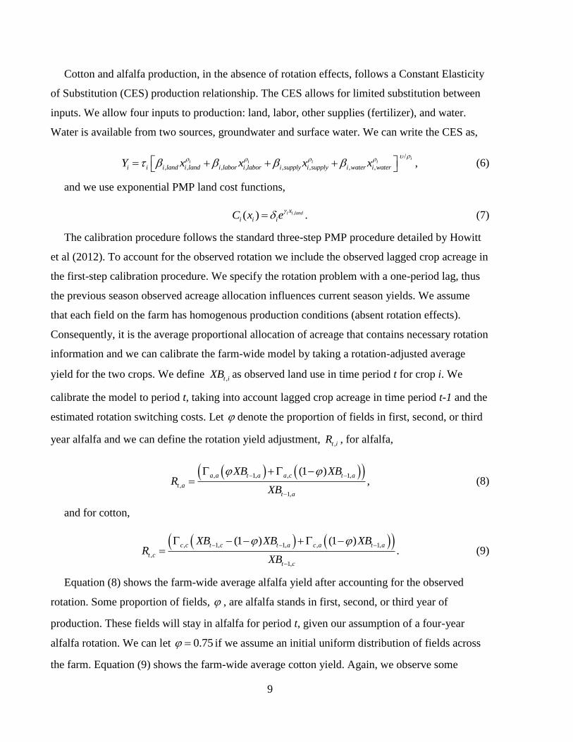
Cotton and alfalfa production, in the absence of rotation effects, follows a Constant Elasticity

of Substitution (CES) production relationship. The CES allows for limited substitution between

inputs. We allow four inputs to production: land, labor, other supplies (fertilizer), and water.

Water is available from two sources, groundwater and surface water. We can write the CES as,

/

, , , , , , , , ,i

i i i i

i i i land i land i labor i labor i supply i supply i water i waterY x x x x (6)

and we use exponential PMP land cost functions,

,( ) .i i landx

i i iC x e

(7)

The calibration procedure follows the standard three-step PMP procedure detailed by Howitt

et al (2012). To account for the observed rotation we include the observed lagged crop acreage in

the first-step calibration procedure. We specify the rotation problem with a one-period lag, thus

the previous season observed acreage allocation influences current season yields. We assume

that each field on the farm has homogenous production conditions (absent rotation effects).

Consequently, it is the average proportional allocation of acreage that contains necessary rotation

information and we can calibrate the farm-wide model by taking a rotation-adjusted average

yield for the two crops. We define ,t iXB as observed land use in time period t for crop i. We

calibrate the model to period t, taking into account lagged crop acreage in time period t-1 and the

estimated rotation switching costs. Let denote the proportion of fields in first, second, or third

year alfalfa and we can define the rotation yield adjustment, ,t iR , for alfalfa,

, 1, , 1,

,

1,

(1 ),

a a t a a c t a

t a

t a

XB XBR

XB

(8)

and for cotton,

, 1, 1, , 1,

,

1,

(1 ) (1 ).

c c t c t a c a t a

t c

t c

XB XB XBR

XB

(9)

Equation (8) shows the farm-wide average alfalfa yield after accounting for the observed

rotation. Some proportion of fields, , are alfalfa stands in first, second, or third year of

production. These fields will stay in alfalfa for period t, given our assumption of a four-year

alfalfa rotation. We can let 0.75 if we assume an initial uniform distribution of fields across

the farm. Equation (9) shows the farm-wide average cotton yield. Again, we observe some

10

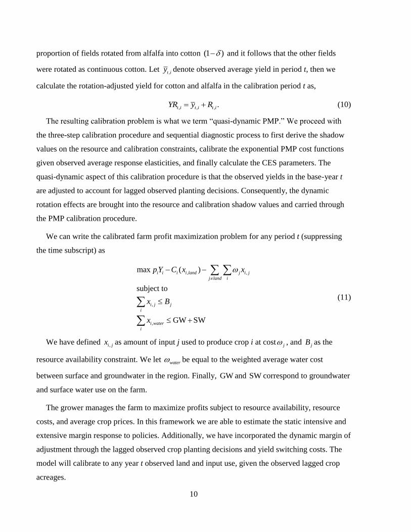
proportion of fields rotated from alfalfa into cotton (1 ) and it follows that the other fields

were rotated as continuous cotton. Let ,t iy denote observed average yield in period t, then we

calculate the rotation-adjusted yield for cotton and alfalfa in the calibration period t as,

, , , .t i t i t iYR y R (10)

The resulting calibration problem is what we term “quasi-dynamic PMP.” We proceed with

the three-step calibration procedure and sequential diagnostic process to first derive the shadow

values on the resource and calibration constraints, calibrate the exponential PMP cost functions

given observed average response elasticities, and finally calculate the CES parameters. The

quasi-dynamic aspect of this calibration procedure is that the observed yields in the base-year t

are adjusted to account for lagged observed planting decisions. Consequently, the dynamic

rotation effects are brought into the resource and calibration shadow values and carried through

the PMP calibration procedure.

We can write the calibrated farm profit maximization problem for any period t (suppressing

the time subscript) as

, ,

,

,

max ( )

subject to

GW SW

i i i i land j i j

j land i

i j j

i

i water

i

p Y C x x

x B

x

(11)

We have defined ,i jx as amount of input j used to produce crop i at cost j , and jB as the

resource availability constraint. We let water be equal to the weighted average water cost

between surface and groundwater in the region. Finally, GW and SW correspond to groundwater

and surface water use on the farm.

The grower manages the farm to maximize profits subject to resource availability, resource

costs, and average crop prices. In this framework we are able to estimate the static intensive and

extensive margin response to policies. Additionally, we have incorporated the dynamic margin of

adjustment through the lagged observed crop planting decisions and yield switching costs. The

model will calibrate to any year t observed land and input use, given the observed lagged crop

acreages.

11

Dynamic Nitrate and Groundwater Model

Finally we link the calibrated farm profit maximization model, with rotation switching costs,

to a dynamic framework for nitrates and groundwater. Nitrogen-based fertilizers are essential for

modern cropping rotation systems and help ensure that we are able to meet global food demand.

However, when fertilizer application exceeds plant demand and denitrification capacity of the

soil this can lead to leaching into the groundwater. Point and non-point sources of nitrate

contamination include fertilizer and manure, dissolved nitrogen in irrigation and septic tanks and

dairy lagoons. In this paper we model a simplified dynamic framework for nitrate concentrations

in groundwater and isolate the effect of fertilizer application on the Kern County farm over an

assumed closed groundwater basin.

We model a system where nitrogen is applied as fertilizer to the crops in the rotation as a

fixed average requirement in pounds per acre. We assume zero runoff and a fixed proportion for

plant uptake, leaving the remaining proportion available for leaching. Denitrification,

immobilization, and mineralization are modeled as a function of applied water and depth to

groundwater. Increased irrigation water application increases leaching, and increased depth to

groundwater leads to greater denitirfication.

Alfalfa increases and cotton decreases available soil nitrogen and thus potential nitrate

leaching. As the ratio of alfalfa to cotton changes across the farm there will be a corresponding

shift in the total amount of nitrates leached into the groundwater. The rate of change depends on

the alfalfa-cotton ratio and relative differences in applied nitrogen and applied water. Define

,t iAN as applied nitrogen to crop i in period t, and nf and nl as the crop use adjustment and

leaching factors specific to the farm. Recall that ,i jx is amount of input j used for crop i and we

can define the nitrate dynamic equation as:

, , , ,

1

t i i land t t i water

i it t

t t

nf AN x N x

N Nnl TDL RC

(12)

Alfalfa has higher evapotranspiration than cotton and thus requires more irrigation water.

We include a dynamic feedback between depth to groundwater and pumping cost. We calculate

the change in depth to groundwater as,

12

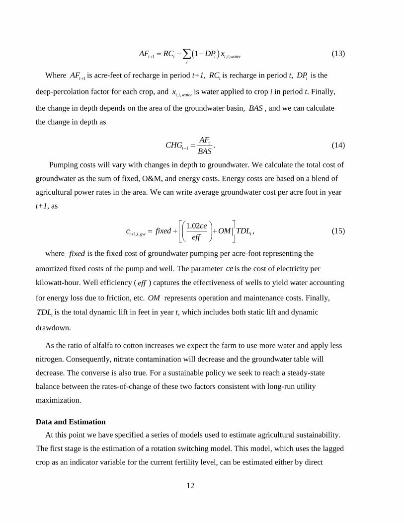
1 , ,1t t i t i water

i

AF RC DP x (13)

Where 1tAF is acre-feet of recharge in period t+1, tRC is recharge in period t, iDP is the

deep-percolation factor for each crop, and , ,t i waterx is water applied to crop i in period t. Finally,

the change in depth depends on the area of the groundwater basin, BAS , and we can calculate

the change in depth as

1 .tt

AFCHG

BAS (14)

Pumping costs will vary with changes in depth to groundwater. We calculate the total cost of

groundwater as the sum of fixed, O&M, and energy costs. Energy costs are based on a blend of

agricultural power rates in the area. We can write average groundwater cost per acre foot in year

t+1, as

1, ,

1.02,t i gw t

cec fixed OM TDL

eff

(15)

where fixed is the fixed cost of groundwater pumping per acre-foot representing the

amortized fixed costs of the pump and well. The parameter ce is the cost of electricity per

kilowatt-hour. Well efficiency ( eff ) captures the effectiveness of wells to yield water accounting

for energy loss due to friction, etc. OM represents operation and maintenance costs. Finally,

tTDL is the total dynamic lift in feet in year t, which includes both static lift and dynamic

drawdown.

As the ratio of alfalfa to cotton increases we expect the farm to use more water and apply less

nitrogen. Consequently, nitrate contamination will decrease and the groundwater table will

decrease. The converse is also true. For a sustainable policy we seek to reach a steady-state

balance between the rates-of-change of these two factors consistent with long-run utility

maximization.

Data and Estimation

At this point we have specified a series of models used to estimate agricultural sustainability.

The first stage is the estimation of a rotation switching model. This model, which uses the lagged

crop as an indicator variable for the current fertility level, can be estimated either by direct

13

observation of crop switching behavior of optimizing producers, or indirectly using crop growth

models to simulate the effects of lagged crops. In the second model stage, parameters describing

the effect of the lagged crop are incorporated into a calibrated economic production model that

reflect the implicit crop production costs, and calibrates to the base observed solution. In the

third stage of the model, the outputs from the calibrated production model are used to drive the

equations of motion for groundwater use and fertility changes. The fertility equation of motion is

approximated by nitrates leached into the groundwater. The groundwater state variable is

measured by the depth to groundwater and the equation of motion is driven by natural recharge

the system, aggregate pumping levels, and the amount of deep percolation to the groundwater

basin.

We estimate the models using a set of geo-referenced land use data for Kern County,

California. Agriculture in the region is irrigated with water coming from State and Federal

surface water projects and groundwater in addition to local surface supplies. The data include all

irrigated agricultural land in Kern County between 1997 and 2012. We exclude years prior to

2000 due to a change in county reporting methods. On each field and year we observe the crop

grown, field size in acres, farm owner, and farm manager of the field. We are able to uniquely

identify and track fields across time. We extract a subset of fields in an alfalfa-cotton based

rotation in a region of the Western-edge of Kern County.

The estimation procedure used in the dynamic rotation problem is described in MacEwan and

Howitt (2013) and summarized here. The dynamic first-order conditions result in an ill-posed

estimation problem and we use the method of Generalized Maximum Entropy (GME) to estimate

the parameters (Golan et al 1996). Given that one has incomplete observations about a statistical

process, an information-theoretic consistent method to recover parameters for inference is to

impose probabilistic structure on the model in such a way that it is consistent with observed data

and imposes as little additional information as possible. Following this principle, we specify a

truncated uniform support space for the parameters of plus or minus 100 percent of average yield

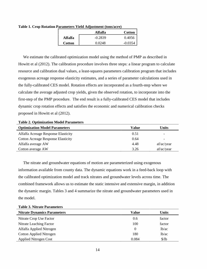
and maximize the Entropy measure of the system. Table 1 summarizes the estimated parameter

values for the dynamic crop rotation problem and shows the marginal yield effect implied from

the observed rotation when crop (row) follows crop (column). For example, cotton-cotton results

in an average reduction of 0.035 tons/acre which is a 4.9% decrease in average yields. When

cotton follows alfalfa, average yields increase by 0.024 tons/acre, or 3.4% above average yield.

14

Table 1. Crop Rotation Parameters Yield Adjustment (tons/acre)

Alfalfa Cotton

Alfalfa -0.2839 0.4056

Cotton 0.0248 -0.0354

We estimate the calibrated optimization model using the method of PMP as described in

Howitt et al (2012). The calibration procedure involves three steps: a linear program to calculate

resource and calibration dual values, a least-squares parameters calibration program that includes

exogenous acreage response elasticity estimates, and a series of parameter calculations used in

the fully-calibrated CES model. Rotation effects are incorporated as a fourth-step where we

calculate the average adjusted crop yields, given the observed rotation, to incorporate into the

first-step of the PMP procedure. The end result is a fully-calibrated CES model that includes

dynamic crop rotation effects and satisfies the economic and numerical calibration checks

proposed in Howitt et al (2012).

Table 2. Optimization Model Parameters

Optimization Model Parameters Value Units

Alfalfa Acreage Response Elasticity 0.51 -

Cotton Acreage Response Elasticity 0.64 -

Alfalfa average AW 4.48 af/ac/year

Cotton average AW 3.26 af/ac/year

The nitrate and groundwater equations of motion are parameterized using exogenous

information available from county data. The dynamic equations work in a feed-back loop with

the calibrated optimization model and track nitrates and groundwater levels across time. The

combined framework allows us to estimate the static intensive and extensive margin, in addition

the dynamic margin. Tables 3 and 4 summarize the nitrate and groundwater parameters used in

the model.

Table 3. Nitrate Parameters

Nitrate Dynamics Parameters Value Units

Nitrate Crop Use Factor 0.6 factor

Nitrate Leaching Factor 100 factor

Alfalfa Applied Nitrogen 0 lb/ac

Cotton Applied Nitrogen 180 lb/ac

Applied Nitrogen Cost 0.084 $/lb

15

Table 4. Groundwater Parameters

Groundwater Dynamics Parameters Value Units

Deep Percolation Factor Alfalfa 0.13 factor

Deep Percolation Factor Cotton 0.1 factor

Natural Recharge 0.02 af/year

Groundwater Basin Size 1000 ac

Aggregate Rotation Dynamics and Sustainability

Before we proceed with policy simulations we want to emphasize the interaction between

rotations, production, and externalities. In this section we fix the alfalfa – cotton ratio on the

farm and consequently fix the average farm rotation. Conceptually, we can simplify our set of

control variables to changing the ratio of alfalfa to cotton acres over a given unit of land. As the

ratio of alfalfa to cotton increases, the level of nitrogen applied decreases along with the excess

nitrates that percolate to the groundwater for two reasons. First, on average, cotton acreage is

smaller and thus the total burden of nitrogen applied is reduced. Second, the increased alfalfa

area will fix increasing quantities of nitrogen which then can be utilized by the cotton. At some

point in the alfalfa to cotton ratio will reach equilibrium where the quantity of nitrogen being

removed from the groundwater in the irrigation water pumped is equal to the quantity percolating

down from the cotton acreage, and the net nitrogen applied to cotton through artificial fertilizer is

removed in the crop itself. Essentially when the cotton crop that was grown to make your jeans

requires no more imported nitrogen than that embodied in the fiber of your jeans, the system will

be in nitrate, and thus water quality, steady-state.

Figure 1 illustrates the trade-off between nitrate pollution and groundwater levels, holding

other factors constant. As the ratio of alfalfa to cotton increases there is a reduction in fertilizer

application and a corresponding decrease in nitrates leached into the groundwater. However,

alfalfa is also more water-intensive than cotton and this requires the grower to deplete the

groundwater resource at an increased rate. As the depth to groundwater increases, the total

dynamic lift and pumping costs increase.

A similar logic applies to the use of water to grow crops, but interestingly, the water use

function has the opposite slope to the nitrate function for given shift in the alfalfa to cotton ratio.

As in the nitrogen example, think of an increase in the alfalfa to cotton ratio which reduces the

16

nitrogen burden on groundwater, but will, in this case, increase the pumping burden on

groundwater due to the higher evapotranspiration requirements of alfalfa. Alfalfa is typically

irrigated twice a month for seven months per season, as opposed to cotton which has a shorter

growing season and is deliberately stress irrigated at the end of the season to improve the yield in

terms of the ratio of boll to vegetative growth.

Figure 1. Change in Nitrates and Groundwater Depth as Rotation Shifts

We want to strike a steady-state balance between groundwater depletion, nitrates, and farm

profitability. As the grower shifts to a more alfalfa-dependent rotation this leads to lower

0

0.2

0.4

0.6

0.8

1

1.2

0.15 0.2 0.25 0.3 0.35 0.4 0.45 0.5 0.55 0.6 0.65 0.7 0.75 0.8 0.85 0.9 0.95

Ch

an

ge

in N

itra

tes

Lea

ched

Ratio of Alfalfa to Cotton

-120

-100

-80

-60

-40

-20

0

0.15 0.2 0.25 0.3 0.35 0.4 0.45 0.5 0.55 0.6 0.65 0.7 0.75 0.8 0.85 0.9 0.95

Ch

an

ge

in G

rou

nd

wate

r D

epth

Ratio of Alfalfa to Cotton

17

profitability. Although cotton is the higher-value crop, alfalfa monoculture will further decrease

yields.

Policy Simulations

In this section we simulate the dynamics of the rotation system. We simulate the model for the

years 2013 – 2025 using observed acreage decisions for 2009 – 2012 as initial conditions for the

rotation dynamics. In all simulations we hold relative crop prices and production costs constant

to isolate the effect of water quality and quantity. Surface water supplies are held constant at the

calibrated baseline average. In future iterations of this model we intend to include stochastic

surface water deliveries, reflecting the uncertain nature of district deliveries and seasonal

precipitation. Similarly, average crop yields are assumed known and held constant in the

analysis.

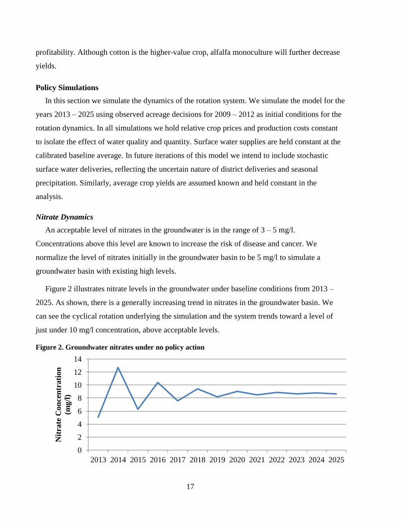
Nitrate Dynamics

An acceptable level of nitrates in the groundwater is in the range of 3 – 5 mg/l.

Concentrations above this level are known to increase the risk of disease and cancer. We

normalize the level of nitrates initially in the groundwater basin to be 5 mg/l to simulate a

groundwater basin with existing high levels.

Figure 2 illustrates nitrate levels in the groundwater under baseline conditions from 2013 –

2025. As shown, there is a generally increasing trend in nitrates in the groundwater basin. We

can see the cyclical rotation underlying the simulation and the system trends toward a level of

just under 10 mg/l concentration, above acceptable levels.

Figure 2. Groundwater nitrates under no policy action

0

2

4

6

8

10

12

14

2013 2014 2015 2016 2017 2018 2019 2020 2021 2022 2023 2024 2025

Nit

rate

Con

cen

trati

on

(mg/l

)

18

It is clear from figure 2 that the level of nitrates in the groundwater exceeds acceptable levels

under the current production system. A commonly proposed strategy to reduce nitrates is to

discourage excess application of fertilizers. We can simulate this effect with a tax per pound

applied nitrogen. To illustrate this situation we impose a tax of $30/lb of applied nitrogen. Figure

3 illustrates nitrate levels under the baseline simulation and under a tax of $30 per pound of

applied nitrogen.

Figure 3. Groundwater nitrates under no policy and fertilizer tax

The fertilizer tax reduces the relative profitability of cotton and encourages a shift toward

alfalfa. If the grower were only able to adjust along the static intensive and extensive margins

then we would expect a corresponding decrease in cotton yields and farm profitability. The

presence of a rotation, included in our model framework, allows for adjustment along the

dynamic margin and substitution of alfalfa for cotton as part of a multi-year rotation. This may

partially or totally offset some of the yields losses, thereby allowing the grower to move toward

more sustainable groundwater nitrates at a lower cost to farm profits and the regional economy.

Figures 4 and 5 illustrate the intensive margin response to a fertilizer tax. Baseline average

applied nitrogen per acre for cotton is 180 pounds per acre. Under a fertilizer tax we see a

substantial intensive margin response as the grower reduces applied nitrogen. This has a

0

2

4

6

8

10

12

14

2013 2014 2015 2016 2017 2018 2019 2020 2021 2022 2023 2024 2025

Nit

rate

Con

cen

trati

on

(m

g/l

)

Baseline

Tax

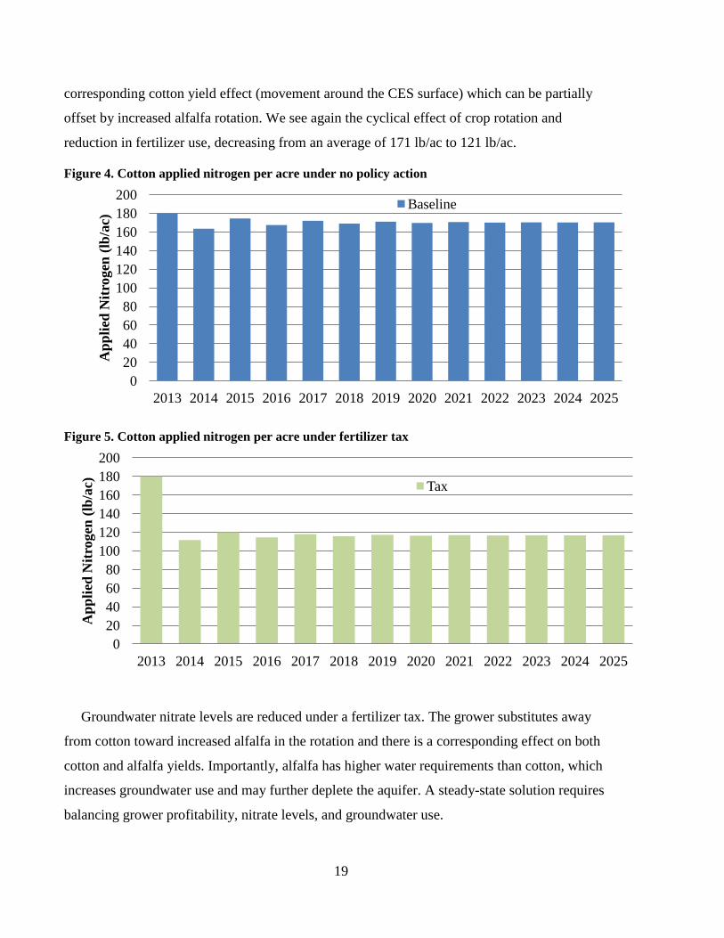
19

corresponding cotton yield effect (movement around the CES surface) which can be partially

offset by increased alfalfa rotation. We see again the cyclical effect of crop rotation and

reduction in fertilizer use, decreasing from an average of 171 lb/ac to 121 lb/ac.

Figure 4. Cotton applied nitrogen per acre under no policy action

Figure 5. Cotton applied nitrogen per acre under fertilizer tax

Groundwater nitrate levels are reduced under a fertilizer tax. The grower substitutes away

from cotton toward increased alfalfa in the rotation and there is a corresponding effect on both

cotton and alfalfa yields. Importantly, alfalfa has higher water requirements than cotton, which

increases groundwater use and may further deplete the aquifer. A steady-state solution requires

balancing grower profitability, nitrate levels, and groundwater use.

0

20

40

60

80

100

120

140

160

180

200

2013 2014 2015 2016 2017 2018 2019 2020 2021 2022 2023 2024 2025

Ap

pli

ed N

itro

gen

(lb

/ac)

Baseline

0

20

40

60

80

100

120

140

160

180

200

2013 2014 2015 2016 2017 2018 2019 2020 2021 2022 2023 2024 2025

Ap

pli

ed N

itro

gen

(lb

/ac)

Tax

20

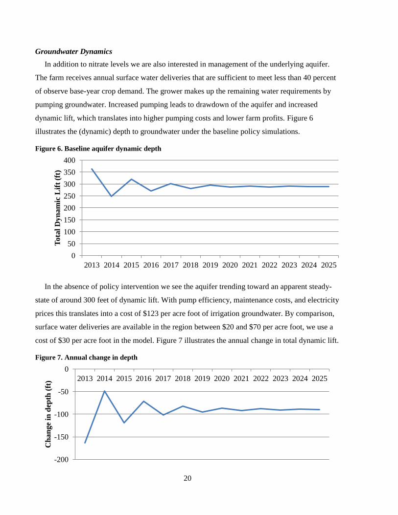
Groundwater Dynamics

In addition to nitrate levels we are also interested in management of the underlying aquifer.

The farm receives annual surface water deliveries that are sufficient to meet less than 40 percent

of observe base-year crop demand. The grower makes up the remaining water requirements by

pumping groundwater. Increased pumping leads to drawdown of the aquifer and increased

dynamic lift, which translates into higher pumping costs and lower farm profits. Figure 6

illustrates the (dynamic) depth to groundwater under the baseline policy simulations.

Figure 6. Baseline aquifer dynamic depth

In the absence of policy intervention we see the aquifer trending toward an apparent steady-

state of around 300 feet of dynamic lift. With pump efficiency, maintenance costs, and electricity

prices this translates into a cost of $123 per acre foot of irrigation groundwater. By comparison,

surface water deliveries are available in the region between $20 and $70 per acre foot, we use a

cost of $30 per acre foot in the model. Figure 7 illustrates the annual change in total dynamic lift.

Figure 7. Annual change in depth

0

50

100

150

200

250

300

350

400

2013 2014 2015 2016 2017 2018 2019 2020 2021 2022 2023 2024 2025

Tota

l D

yn

am

ic L

ift

(ft)

-200

-150

-100

-50

0

2013 2014 2015 2016 2017 2018 2019 2020 2021 2022 2023 2024 2025

Ch

an

ge

in d

epth

(ft

)

21

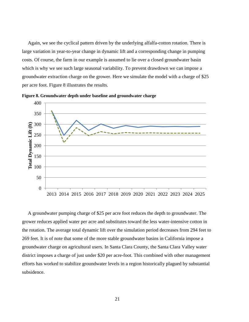
Again, we see the cyclical pattern driven by the underlying alfalfa-cotton rotation. There is

large variation in year-to-year change in dynamic lift and a corresponding change in pumping

costs. Of course, the farm in our example is assumed to lie over a closed groundwater basin

which is why we see such large seasonal variability. To prevent drawdown we can impose a

groundwater extraction charge on the grower. Here we simulate the model with a charge of $25

per acre foot. Figure 8 illustrates the results.

Figure 8. Groundwater depth under baseline and groundwater charge

A groundwater pumping charge of $25 per acre foot reduces the depth to groundwater. The

grower reduces applied water per acre and substitutes toward the less water-intensive cotton in

the rotation. The average total dynamic lift over the simulation period decreases from 294 feet to

269 feet. It is of note that some of the more stable groundwater basins in California impose a

groundwater charge on agricultural users. In Santa Clara County, the Santa Clara Valley water

district imposes a charge of just under $20 per acre-foot. This combined with other management

efforts has worked to stabilize groundwater levels in a region historically plagued by substantial

subsidence.

0

50

100

150

200

250

300

350

400

2013 2014 2015 2016 2017 2018 2019 2020 2021 2022 2023 2024 2025

Tota

l D

yn

am

ic L

ift

(ft)

22

Total surface water supplies are held constant in the analysis. If instead we were to simulate

additional surface water available we could estimate the corresponding change in groundwater

depth and the implicit benefits of the additional surface water. As with the nitrogen tax, there are

intensive and extensive margin adjustments underlying the policy simulations.

Summary and Steady-State Solution and Social Costs

One definition of a steady-state sustainable solution requires that the rate of change in nitrates

and depth to groundwater are constant and consistent with long-run utility maximization for the

grower. We can alternatively conceptualize sustainability from a physical perspective and

impose threshold levels of groundwater levels and nitrates. We will extend this work in the

future to model the formal dynamic steady-state solution. Other areas for further refinement

include incorporating a sequential dynamic PMP procedure, incorporating a dynamic feedback

between groundwater quality and crop yields and production costs, and expanding the model

from the farm to a larger basin.

In summary, we have proposed a three-step estimation framework to evaluate sustainable

policies. The framework allows for estimation of the intensive, extensive, and dynamic margin

response. We estimate grower response to policies designed to encourage a more sustainable

agriculture and discuss further steps to estimate the full steady-state sustainable solution.

In the framework presented in this paper, to reach steady-state of fertility can only be

achieved by rotating net nitrogen using crops, which may or may not need additional fertilizer,

with net nitrogen increasing crops such as legumes. In general, net nitrogen using crops such as

cotton are characterized by higher profits per unit land, and lower water use per unit land.

Conversely, net nitrogen increasing crops such as dry beans or alfalfa, have lower net revenues

per acre than cotton, but a high water requirement per acre than cotton. We have shown this

explicit trade-off between the rates of change of fertility stocks and resource stocks and we have

presented the sustainability problem as one of simultaneously striking a steady-state balance

between the rates of fertility change and changes in stocks of groundwater.

We feel that the framework presented in this paper will be of value for evaluating sustainable

intensification strategies, for example in developing countries. In most cases the adoption of crop

intensification technologies results in greater use of nitrogen and water. Sustainable

intensification recognizes that, to offset these, we must have a change in the rotation to preserve

23

the physical steady-state between groundwater and nitrogen use. Intensification that is also

sustainable must balance both the rotation and the productivity of new technology.

24

References

Ghassemi, Fereidoun A., A.J. Jakeman, and H.A. Nix. 1995. “Salinisation of land and water

resources: Human causes, extent, management and case studies.” UNSW Press, Sydney,

Australia, and CAB International, Wallingford, UK.

Gleeson, T., Yoshihide Wada, Marc F.P. Bierkens, and Ludovicus P.H. van Beek. 2012. “Water

balance of global aquifers revealed by groundwater footprint.” Nature (488) (August): 197-

200

Golan, Amos, George Judge, and Douglas Miller. (1996), Maximum Entropy Econometrics:

Robust Estimation with Limited Data, Chichester, England: John Wiley & Sons.

Harter, Thomas and Jay R. Lund (PI’s). 2012. “Addressing Nitrate in California’s Drinking

Water.” Prepared for the California State Water Resources Board. California Nitrate Project,

Implementation of Senate Bill X2 1. Center for Watershed Sciences University of California,

Davis.

Howitt, Richard. E., Josué Medellín-Azuara, Duncan MacEwan, Jay R. Lund. 2012. “Calibrating

disaggregate economic models of agricultural production and water management.”

Environmental Modelling & Software (38) (December): 244-258.

MacEwan, Duncan. and Richard E. Howitt. 2013. “An Empirical Model of Crop Rotations.”

University of California. Department of Agricultural and Resource Economics. Davis, CA.

Pitman, Michael G., & André Läuchli. (2002). “Global impact of salinity and agricultural

ecosystems.” Salinity: environment–plants–molecules. Dordrecht: Kluwer, 3-20.

Schoups, Gerrit, Jan W. Hopmans, Chuck A. Young, Jasper A. Vrugt, Wesley W. Wallender,

Ken K. Tanji, Sorab Panday. 2005. “Sustainability of irrigated agriculture in the San Joaquin

Valley, California.” Proceedings of the National Academy of Sciences, USA (102): 15352–

15356.

Sneed, Michelle, Justin Brandt, Mike Solt. 2013. “Land Subsidence along the Delta-Mendota

Canal in the Northern Part of the San Joaquin Valley, California, 2003-10.” U.S. Geological

Survey Scientific Investigations Report 2013-5142, 87 p.

Spence, Michael A. 1975. “Blue Whales and Applied Control Theory,” in System Approaches

and Environmental Problems, H. W. Gottinger (ed.), Vandenhoeck and Ruprecht (Gottingen).