ORIGINAL ARTICLE

Modeling of the residual kinematic errors of coordinatemeasuring machines using LaserTracer system

Adam Gąska & Marcin Krawczyk & Robert Kupiec &

Ksenia Ostrowska & Piotr Gąska & Jerzy Sładek

Received: 29 August 2013 /Accepted: 1 April 2014 /Published online: 25 April 2014# The Author(s) 2014. This article is published with open access at Springerlink.com

Abstract The following article examines the methodology ofidentifying and modeling kinematic errors of coordinate mea-suring machines with the use of a modern and precise inter-ferometric system—the LaserTracer. Since the kinematic er-rors of coordinate measuring machines (CMMs) are by far themost prevalent factor in measurement uncertainty, a speciallydeveloped model could be used for efficient uncertainty eval-uation as an additional module of the virtual measuring ma-chine responsible for simulation of the CMM kinematic er-rors. The model could also be of use for determining optimalmeasurement strategy, and would potentially improve theuncertainty of measurements performed.

Keywords CMM . LaserTracer . Accuracy .Monte Carlomethod

1 Introduction

One of the most important problems a metrologist must faceinvolves the correct assessment of measurement uncertainty,which can be regarded as a quantitative representation ofmeasurement accuracy. It is commonly known that the resultof any measurement given without the corresponding uncer-tainty is very unreliable and offers little practical value. How-ever, in the case of coordinate measuring techniques (CMT),determining measurement uncertainty may be particularlydifficult, and the results may not be very straightforward[1–4]. It is a common practice among metrologists (as wellas the manufacturers of measuring systems) to circumvent the

problem by providing the accuracy of the measuring devicesrather than individual measurements. This approach describesaccuracy in relation to the maximum permissible error (MPE),and the measurement itself is regarded as a measurement ofdistance, which seems to be a significant oversimplificationfor the majority of tasks. In most cases, measurement accuracydetermined in this way tends to vary significantly from theaccuracy of a real measurement task, and may lead to incorrectconclusions as far as compliance with the specifications of agiven product is concerned [2, 5–11]. Therefore, it is crucial toemploy more reliable and metrologically validated methodsfor coordinate measurement uncertainty estimation.

One of the primary factors affecting measurement accuracyinvolves errors of the measuring machine’s kinematic system[12]. The initial models of the kinematic errors of coordinatemeasuring machines (CMMs) were created and implementedduring the 1970s [13], but the very first attempts aimed ateliminating the geometric errors of machine tools date back toas early as the second half of the nineteenth century [14, 15].However, the first attempts of eliminating the machine toolsgeometric errors were made at the second half of nineteenthcentury [14, 15]. Nowadays, in the era of cost minimization,the vast majority of measuring and machining devices isequipped with their own geometric error software correctionsystems, because it is generally more profitable to mass-produce parts (which form the kinematic system of machine)which are more distant from the ideal geometry, and to com-pensate the geometric errors influenced by these faults ratherthan to produce expensive parts with very narrow shape anddimension tolerances.

There are only a few available models of CMM errors (i.e.,full rigid body, reduced rigid body) which are used to deter-mine the geometrical errors described by a varying number ofgeometrical components.More often, models are supplementedwith elastic errors of the machine. The most commonly en-countered model consists of 21 geometric error components,

A. Gąska (*) :M. Krawczyk :R. Kupiec :K. Ostrowska :P. Gąska : J. SładekLaboratory of Coordinate Metrology, Cracow University ofTechnology, al. Jana Pawla II 37, 31-864 Cracow, Polande-mail: agaska@mech.pk.edu.pl

Int J Adv Manuf Technol (2014) 73:497–507DOI 10.1007/s00170-014-5836-1

which includes translation, rotation, and squareness errors [16].Based on that, it can be stated that the current CMM modelsregard kinematic errors only as the source of systematic errors,and identify their vales in order to correct themmathematically.This paper presents a possible expansion of the models current-ly in use. The described approach involves the assumption thatthe systematic parts of CMM kinematic errors are properlycompensated using one of the mentioned models, and showsthe method for assessing the impact of uncompensated kine-matic errors.

In most contemporary CMMs, the analysis of the distribu-tion of kinematic errors is performed by the manufacturerduring the development of the computer-aided accuracy(CAA) correction matrix. As a result, the end user receives aproduct for which the impact of geometric errors on measure-ment accuracy is already partly reduced. However, not allkinematic errors can be corrected in this way. Residual errorswhich remain uncompensated after the correction process mayalso influence the accuracy of measurements. Therefore, it isimportant to identify the field of these errors. This articledescribes the methodology for identifying and modeling re-sidual errors associated with the kinematic system of CMMs.

A specially designed model, the so-called virtual measur-ing machine (VCMM), can be used as part of an online systemfor assessing the accuracy of coordinate measurements. Thismethod is based on identifying the factors affecting measure-ment accuracy, designation of their variability and, finally,simulation of their value. The components affecting measure-ment uncertainty which are usually taken into account arekinematic system errors of the CMM, probe head errors,influences of measured object, and other types of errors influ-enced by the ambient conditions. These components may besuccessfully simulated by specially created modules. Thevalues obtained from each module may then be added up todetermine the total measurement uncertainty. Many interest-ing solutions for VCMM design are discussed in [17–33].Additionally, the described model could also be of aid indetermining the optimal measurement strategy for each pro-ject. Examples of such application will also be presented inthis article.

2 The concept of identifying and modeling of CMMkinematic errors

The first concepts of modeling of CMM kinematic errorsrelied upon the designation of individual components of themeasuring machine geometric errors (21 components) at dif-ferent points in the measuring volume. The hole-plate stan-dards were most commonly used for this purpose. The stan-dards were repeatedly measured at different positions so as tocover the maximum possible part of the machine’s measuringvolume. This concept is described at length in [18, 32, 33]. A

more recent approach involves the use of the matrix methodwhich describes the vector character of errors [29, 34]. Thematrix method employs a grid of reference points and de-scribes points located in the nodes of the grid by assigning avector expressing the error of measuring point reproducibility.Quite expectedly, the kinematic errors constitute a significantsubset of all errors in this method. Up to this point, themeasuring point reproducibility errors were modeled througha grid of reference points describing the machine’s measuringvolume, in which the values of components affecting this errorwere determined. These components were then divided intocomponents of a systematic and random character. The sys-tematic components were caused by the kinematic errors ofthe machine, whereas random errors signified other unidenti-fied errors influencing the reproduction of measuring point. Inthis article, the authors present a new method for describingthe field of CMM kinematic errors.

Bearing in mind that in most CMM kinematic errors arecompensated by the correction matrix and that most machinesare equipped with their own temperature compensation sys-tems, it comes as a natural conclusion that the inaccuratereproduction of the measuring point must, in fact, be attributedto the residual and random errors. Figure 1 shows a schematicgrid of reference points within the distribution of probability(the t distribution seems to work best in this context), asreproduced by the machine. However, it is still necessary toconstruct a system which would be able to determine thedistribution of errors in reference points experimentally, andwithin required accuracy. The lack of such systems in placeseems to constitute a major obstacle for a successful imple-mentation of the concept described previously. One specificdevice which satisfies those requirements is the LaserTracer(LT) developed by Etalon AG.

LaserTracer is an interferometric device that allows fortracking of reflector movements. The reflector is usuallymounted on the probe head of a measuring device or on thetool holder of a machine tool. The uncertainty of lengthmeasurement of this device is presented in Eq. 1:

U ¼ 0:2� 0:3 � L=1; 000 μm ð1Þ

where L is the measured value given in mm.Such high level of accuracy can be achieved; thanks to the

implementation of novel solutions used in the constructionprocess of the device whose form errors do not exceed 30 nm.The reference sphere is located in the center of rotation of theLT rotary system. A schematic of the LaserTracer is presentedin Fig. 2.

In LaserTracer, the interferometer moves on a gimbalmount around a fixed precision sphere serving as a referencemirror which reflects the laser beam, and radial and lateraldeviations of the mechanical rotation axes do not have a

498 Int J Adv Manuf Technol (2014) 73:497–507

significant effect on measurement accuracy [35]. It is alsoimportant to observe that the LaserTracer does only measurethe distance from device to reflector, which indicates that it isstill necessary to use a multilateration technique in order todetermine the coordinates of a measuring point.

The LaserTracer allows to determine the probability ofreproduction of the measuring point, as well as probabilitydistribution, by showing the distribution of residual errors forthe entire measuring space of the CMM.

Once the grid of reference points is described (Table 1), theproblem of grid compaction remains to be tackled. It is knownthat during measurements, the majority of points described isfound between nodes of the grid. Thus, the strategy for gridcondensation should be selected in a way which would allowto simulate (through the use of the Monte Carlo method)achieving all possible points within the measuring space.There are several ways to do this, e.g., the method proposedin [29], which suggests the application of a neural network forthis purpose. The authors of this article have developed analternative method, which relies on the use of b-spline curvesin conjunction with the “nearest neighbor” or bilinear

interpolation methods, implemented according to MonteCarlo method simulations. A detailed description of this meth-od will be discussed later on in this article.

3 Identification of residual errors

Adopting the assumptions described in the previous chapter,the residual and random errors were estimated (Fig. 4,Table 2). Together, these errors form the starting point fordeveloping a model of the CMM kinematic errors. As men-tioned previously, this model is based on the concept of themeasuring point reproducibility error. To successfully modelthese errors, it is necessary to create a grid of reference pointswhich would be linked closely to the grid on which themachine correction matrix is described. It is also necessaryto assume a degree of overlapping between nodes of thereference grid and the correction matrix as dictated by theconcept of the model. The model remains in an active con-nection with the correction matrix and uses residual andrandom errors as its computational basis. This allows

Fig. 1 a Grid of reference points.b Residual errors (in nodes ofreference grid) and method oftheir identification

Fig. 2 LaserTracer: 1 referencesphere, 2 laser beam, 3 LTcolumn(www.etalon-ag.com)

Int J Adv Manuf Technol (2014) 73:497–507 499

modification of the model depending on the matrices obtainedin the future and also performing the interpolation based onthe same nodes.

The number of reference points should be selected insuch a way so as to cover the entire measuring space ofthe machine evenly, bearing in mind that a greaternumber of reference points would also mean more timeand effort spent on developing the model without nec-essarily yielding more accurate results. The authors cre-ated a grid consisting of 52 reference points in themeasuring space of the machine. This number of pointsis sufficient to faithfully reproduce the field of residualand random errors, as shown in [34].

The values of random errors for points located in thenodes of the reference grid were determined experimen-tally through repeated approaching at each point fromdifferent directions. The measuring machine used for thetask was Leitz PMM 12106. Instead of using the defaultLeitz stylus, a “cateye” retroreflector was mounted(Fig. 3).

The position of the retroreflector was tracked in dynamicmode by a LaserTracer installed in the measuring volume ofthe machine. For each measuring point, the sequenceconsisting of 14 approaches was performed (and distance

from LT was measured): six in directions consistent with thethree axes of the machine (with negative and positive orien-tation) and eight in direction inclined at a 45° angle to eachaxis (with negative and positive orientation). After each se-quence of approaches at the point, the machine reached thenext one and the cycle was repeated, in order to carry out thesequence for all points in the nodes of the reference grid. Thenominal coordinates of all reference points are displayed inTable 1.

The described measuring path was repeated five times withthe position of the LT being changed every time. With the useof the multilateration method, the final coordinates of thenodes (14 sets of coordinates for one point) were determined.The coordinates of these points were determined according toEq. 2 [36]:

Wij ¼ lij þ l0 j −ffiffiffiffiffiffiffiffiffiffiffiffiffiffiffiffiffiffiffiffiffiffiffiffiffiffiffiffiffiffiffiffiffiffiffiffiffiffiffiffiffiffiffiffiffiffiffiffiffiffiffiffiffiffiffiffiffiffiffiffiffiffiffiffiffiffiffiffi

xi−X 0 j

� �2 þ yi−Y 0 j

� �2 þ zi−Z0 j

� �2q

ð2Þ

whereai—the number of the ith point; j—number of the jth

position of LaserTracer;wij—minimized residue; lij—distanceto the ith point measured by LaserTracer located in the jthposition; l0j—“dead path” length for LaserTracer at jth

Table 2 The results of measurements presented for selected points: X, Y, Z—nominal coordinates of reference points, mm; d (X), d (Y), d (Z)—standarddeviations of reproduction of certain coordinates of points calculated from results for all approaches at the point, mm

Lp. X Y Z d (X) d (Y) d (Z) Lp. X Y Z d (X) d (Y) d (Z)

1 310 190 50 0.00063 0.00066 0.00065 5 475 50 50 0.00212 0.00169 0.00097

2 310 190 200 0.00020 0.00023 0.00089 6 475 50 200 0.00101 0.00073 0.00058

3 310 190 350 0.00023 0.00053 0.00127 7 475 50 350 0.00118 0.00070 0.00061

4 310 190 500 0.00025 0.00043 0.00046 8 475 50 500 0.00129 0.00092 0.00021

Table 1 Nominal coordinates of reference points (when the modeled area has dimensions of 700:600:500 mm and with the 150-, 50-, and 50-mm pointtaken as the starting point)

No. X Y Z No. X Y Z No. X Y Z No. X Y Z

1 150 50 50 14 310 460 200 27 475 325 350 40 640 190 500

2 150 50 200 15 310 460 350 28 475 325 500 41 800 50 50

3 150 50 350 16 310 460 500 29 475 600 50 42 800 50 200

4 150 50 500 17 310 190 50 30 475 600 200 43 800 50 350

5 150 325 50 18 310 190 200 31 475 600 350 44 800 50 500

6 150 325 200 19 310 190 350 32 475 600 500 45 800 325 50

7 150 325 350 20 310 190 500 33 640 460 50 46 800 325 200

8 150 325 500 21 475 50 50 34 640 460 200 47 800 325 350

9 150 600 50 22 475 50 200 35 640 460 350 48 800 325 500

10 150 600 200 23 475 50 350 36 640 460 500 49 800 600 50

11 150 600 350 24 475 50 500 37 640 190 50 50 800 600 200

12 150 600 500 25 475 325 50 38 640 190 200 51 800 600 350

13 310 460 50 26 475 325 200 39 640 190 350 52 800 600 500

500 Int J Adv Manuf Technol (2014) 73:497–507

position; xi, yi, zi—coordinates of ith point; and X0j, Y0j, Z0j—coordinates of LaserTracer in jth position.

The final value of coordinates for each reference point isobtained by minimizing the sum of squared residues wij. Theresults of the analysis performed are shown in Fig. 4 andTable 2.

The maximum values of the deviations (difference be-tween nominal and actual coordinates) in directions of eachaxis were as follows: dmax (X)=0.0026 mm, dmax (Y)=0.0018 mm, dmax (Z)=0.0015 mm; mean value of devia-

tions, d Zð Þ ¼ 0:0009 mm , d Yð Þ ¼ 0:0008 mm , d Zð Þ ¼0:0007 mm . The data obtained in accordance with thedescribed methodology provide the basis for functioning ofthe model of CMM kinematic errors [34, 36].

4 Modeling of kinematic system residual errors

The primary purpose of the described model is to determinethe variability of reproduction of each point with its own set ofcoordinates, which can be expressed as a standard deviation ofpoint coordinates found by performing repeated approachingon the points located in the nodes of the reference grid. Then,the reproduction of each point is simulated with the use of aMonte Carlo simulation. The Monte Carlo method was cho-sen for this purpose not because of complexity of numericalproblem but because of its suitability for dealing with repeatedrandom samplings of points with varying probabilitydistribution.

The reproduction variability for points located in the nodesof the reference grid can be determined experimentally, asdescribed in sections 2 and 3. In the case described, thesimulation is performed on data corresponding to referencepoints taken directly from the input matrix of the model,which contains the following values (sorted in rows): X, Y, Znominal point coordinates, d (X), d (Y), and d (Z) standardreproduction deviations for each coordinate. This simulationcovers only a small subset of possibilities considering the totalnumber of points included in measurements. It is also knownthat most of the points will be located between the nodes of thereference grid. This necessitates further use of interpolationmethods, in addition to the Monte Carlo simulation.

The first step in the interpolation method is to form three-dimensional b-spline functions describing the variability ofcoordinate values for reference points situated in the directionof the z axis (as shown in Table 1; reference points arearranged in vertical columns consisting of four points). There-fore, 13 b-spline curves have to be created; each spread overfour reference points (an example of such curve, spread overpoints nos. 17–20 from Table 1, is shown in Fig. 5). The

Fig. 3 “Cateye” retroreflector mounted on measuring machine

Fig. 4 Ellipsoids of pointreproduction error

Int J Adv Manuf Technol (2014) 73:497–507 501

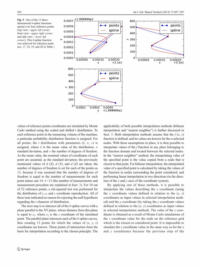
values of reference points coordinates are simulated byMonteCarlo method using the scaled and shifted t distribution. Toeach reference point in the measuring volume of the machine,a particular probability distribution function is assigned. Forall points, the t distribution with parameters (x, σ, υ) isassigned, where x is the mean value of the distribution, σstandard deviation, and υ the number of degrees of freedom.As the mean value, the nominal values of coordinates of eachpoint are assumed, as the standard deviation; the previouslymentioned values of d (X), d (Y), and d (Z) are taken; thenumber of degrees of freedom is set for each of the points as13, because it was assumed that the number of degrees offreedom is equal to the number of measurements for eachpoint minus one 14–1=13 (the number of measurements andmeasurement procedure are explained in Sect. 3). For 10 outof 52 reference points, a chi-squared test was performed forthe distribution of x, y, and z coordinate reproduction. All ofthese tests indicated no reason for rejecting the null hypothesisregarding the t character of distribution.

The next step is to intersect all of the b-spline curves with aplane parallel to the XYplane, whose distance from this planeis equal to z1, where z1 is the z coordinate of the simulatedpoint. The parallel plane intersects each of the b-spline curves,thus creating 13 points for which the values of (x, y, z)coordinates are known. These points of intersection form thebasis for interpolation according to the chosen principle. The

applicability of both possible interpolation methods (bilinearinterpolation and “nearest neighbor”) is further discussed inSect. 5. Both interpolation methods assume that the f (x, y)function is defined, and its values are known for the n-selectednodes. With those assumptions in place, it is then possible tointerpolate values of the f function in any place belonging tothe function domain and located between the selected nodes.In the “nearest neighbor” method, the interpolating value ofthe specified point is the value copied from a node that isclosest to that point. For bilinear interpolation, the interpolatedvalue of a specified point is calculated by taking the values ofthe function in nodes surrounding the point considered, andperforming linear interpolation in two directions (in the direc-tion of the x and y axes of the coordinate system).

By applying one of these methods, it is possible tointerpolate the values describing the x coordinate (usingthe x coordinate values defined in relation to the (y, z)coordinates as input values in selected interpolation meth-od) and the y coordinate (by taking the y coordinate valuesdefined in relation to the (x, z) coordinates as input valuesin selected interpolation method). The value of the z coor-dinate is obtained as a result of Monte Carlo simulations ofthe z coordinate value for the node on the reference gridwhich is the closest to considered point. It is impossible tosimulate the z coordinate value in the same way as for the xand y coordinates because the previous step of the

Fig. 5 One of the 13 three-dimensional b-spline functionsspread over four reference points(top view—upper left corner,front view—upper right corner,and side view—lower leftcorner). This b-spline functionwas achieved for reference pointnos. 17, 18, 19, and 20 in Table 1

502 Int J Adv Manuf Technol (2014) 73:497–507

simulation assumes that the z coordinate of the intersectingplane is taken as a constant.

The obtained (x1, y1, z1) coordinates of the point are thensimulated n times, where n is the number of Monte Carlosimulations. A schematic algorithm of the residual error sim-ulation process for a single measuring point is shown in Fig. 6.

The proposed model of kinematic error simulation can beused as part of VCMM. Further examples proving its possibleapplication for this task can be found in [34, 36]. The modelcould also be of use for determining the optimal position of ameasured workpiece in the measuring volume of the machine.An optimal position indicates the position for which theuncertainty of measurement is reduced.

5 Determining the optimal position of a measuredworkpiece in the measuring volume

For the purposes of the experiment presented below, it isassumed that the workpiece is going to be measured using

the same probing points and measuring program for allof its positions. If the ambient conditions remain stable,it can be concluded that differences in the uncertaintiesof measurements performed in different positions in themeasuring volume of the machine are caused by kine-matic errors of the machine. Using the CAA compensa-tion matrix, it is then possible to determine that theresidual errors of the machine are a primary factor inuncertainty differences. Leitz PMM 12106 was used forall experiments presented in this section. The machine isinstalled in a strictly air-conditioned room (temperaturevariation in the measuring volume of the machine is±0.05 °C), which provides very good stabilization ofambient conditions.

Figure 7 (found below) illustrates the simulated values forthe reproduction error of coordinates (for each coordinateseparately) obtained through the simulations described previ-ously in Sect. 4. For the x and y coordinates, the results ofsimulation were shown for both possible interpolationmethods: the “nearest neighbor” method and bilinear

Fig. 6 Schematic algorithm of residual error simulation process when nearest neighbor interpolation is used

Int J Adv Manuf Technol (2014) 73:497–507 503

interpolation. For the z coordinate, only one method of inter-polation is used (“nearest neighbor”).

The experiment consisted of repeated measurements of acompressor body (shown in Fig. 8) placed in various positionsin the measuring volume of the machine. The same sampling

strategy was used for all positions. In this case, the errors ofthe probe head (which are mainly dependent on the directionof approach) can be treated as being the same for correspond-ing measuring points (in different positions of the measuredobject). Because of that, the probe head errors would have the

Fig. 7 Results of simulation of coordinate reproduction error values. aFor the x coordinate obtained using bilinear interpolation. b For the xcoordinate obtained using “nearest neighbor” interpolation. c For the y

coordinate obtained using bilinear interpolation. d For the y coordinateobtained using “nearest neighbor” interpolation. e For the z coordinateobtained using “nearest neighbor” interpolation

504 Int J Adv Manuf Technol (2014) 73:497–507

same influence on all of the measurements regardless ofposition of the measured body. The form error of one of thecylinders and the distance between the front planes of thebody were measured for each respective position. All mea-surements were conducted according to [37], and for eachposition, the results of measurement, and the correspondinguncertainty, were calculated. The standards used during mea-surements were the Koba-step and the ring-shaped internaldiameter standard.

Detailed results of measurements are presented in Table 3.By analyzing Fig. 7, it can be observed that the lowest valuesof coordinate reproduction errors were achieved for positions3 and 5. Based on these observations, it can be concluded thatit would be possible to determine the optimal position of themeasured workpiece by utilizing diagrams used in the de-scribed model.

The differences between uncertainty values shown inTable 3 are relatively small (differences do not exceed0.4 μm). However, for high-end machines like the PMM12106, such scale of differences can be regarded as sig-nificant, especially if the machine is used for performingcalibration measurements in an accredited calibration lab-oratory. What is more, the differences in uncertaintyvalues correlate with changes in the coordinate reproduc-tion errors shown in Fig. 7.

6 Conclusion

The presented model of kinematic errors focuses only on thesimulation of random errors, and assumes that the systematicerrors are already compensated. This approach, as demonstrat-ed in the experiments developed and conducted by the au-thors, reduces the time needed for identifying kinematic errorsthroughout the volume of the machine. Thanks to the modernsystem LaserTracer (used for the first time for residual errorsmodeling) and the Trac-Cal software; all data necessary tobuild the model can be collected within 6 h, which is less thanthe duration of a standard factory shift.

Furthermore, the model can be successfully used as part ofa measurement uncertainty evaluation system. It can also beused for determining the optimal position of a measuredworkpiece on the machine volume in order to reduce mea-surement uncertainty. The idea of uncertainty reduction isbased around the fact that the random errors cannot be com-pensated, which indicates that in order to reduce their influ-ence on measurement uncertainty, it is necessary to identifythe area in which they are significantly smaller. This functioncould be extremely important for high-accuracy coordinatemeasuring machines used in calibration laboratories, where itis crucial to reduce measurement uncertainty even by thetiniest fraction of a micron. As far as directions for furtherresearch are concerned, subsequent experiments aiming toreduce the amount of data needed to create a model of themachine’s residual errors have to be performed. The authorsare fully convinced that it should be possible to further reducethe number of reference points required. However, the remain-ing question is whether and how a reduced number of refer-ence points would affect the correct function of the model.

The optimal position of a measured workpiece is currentlydetermined only through a graphical analysis of the simulatedresidual errors. However, it is certainly possible to create anapplication which would automatically detect the optimalplacement of a measured workpiece using the discussed mod-el and additional data concerning the shape of the object. Itcould also be possible to combine this application with themodule responsible for the simulation of probe head errors(like the one presented in [36]), which would allow to limit

Fig. 8 Different positions of the workpiece during measurements per-formed on a PMM machine. Red arrows indicate directions of machinecoordinate system axes

Table 3 Results of the measurements performed

Measured feature Localization 1 Localization 2 Localization 3 Localization 4 Localization 5

Result U Result U Result U Result U Result U

Form error 0.0117 0.0006 0.0116 0.0008 0.0114 0.0005 0.0113 0.0009 0.0116 0.0005

Distance 188.9299 0.0004 188.9295 0.0005 188.9298 0.0004 188.9292 0.0006 188.9297 0.0003

All values are given in mm

Int J Adv Manuf Technol (2014) 73:497–507 505

measurement uncertainty even further by suggesting the opti-mal number of probing points and their distribution. In thisway, it should be possible to definitely design the most opti-mal measurement strategy.

Acknowledgments Reported research were realized within confines ofprojects financed by Polish National Center for Research and Develop-ment No: 0869/R/T022010/10/and LIDER/06/117/L-3/11/NCBR/2012.

Open Access This article is distributed under the terms of the CreativeCommons Attribution License which permits any use, distribution, andreproduction in any medium, provided the original author(s) and thesource are credited.

References

1. Barini EM, Tosello G,DeChiffre L (2010)Uncertainty analysis of point-by-point sampling complex surfaces using touch probe CMMs:DOE forcomplex surfaces verification with CMM. Precis Eng 34(1):16–21

2. Beaman J, Morse E (2010) Experimental evaluation of softwareestimates of task specific measurement uncertainty for CMMs.Precis Eng 34(1):28–33

3. Bleys P, Van Gestel N, Cuypers S, Kruth JP (2007) Uncertainty dueto limited sampling of circular features on coordinate measuringmachine. Proc. of the 10th CIRP Conference on Computer AidedTolerancing, Erlangen

4. Jakubiec W (2008) Analytical determination of uncertainty of mea-surement in coordinate measuring technique, Scientific Dissertations22, University of Bielsko-Biala

5. Germani M, Mandorli F, Mengoni M, Raffaeli R (2010) CAD-basedenvironment to bridge the gap between product design and tolerancecontrol. Precis Eng 34(1):7–15

6. Geus DA (1998) Comparison of measurement data from 3D-measurement in metrology for quality control in production. Proc. of6th ISMQC IMEKO Symposium –Wien, Austria, September 8–10

7. Pedone P, Romano D (2011) Designing small samples for form errorestimation with coordinate measuring machines. Precis Eng 35(2):262–270

8. Phillips SD, Borchardt B, Abackerli AJ, Shakarji C, Sawyer D (2003)The validation of CMM task specific measurement uncertainty soft-ware, Proc. of the ASPE 2003 summer topical metting “CoordinateMeasuring Machines” Charlotte, North Carolina June 25–26

9. Ramu P, Yagüe JA, Hocken RJ, Miller J (2011) Development of aparametric model and virtual machine to estimate task specific mea-surement uncertainty for a five-axis multi-sensor coordinate measur-ing machine. Precis Eng 35(3):431–439

10. Schwenke H, Neuschaefer-Rube U, Pfeifer T, Kunzmann H (2002)Optical methods for dimensional metrology in production engineer-ing. CIRPAnn Manuf Technol 51(2):685–699

11. Wilhelm RG, Hocken RJ, Schwenke H (2001) Task specific uncertaintyin coordinate measurement. CIRPAnn Manuf Technol 50(2):553–563

12. Schwenke H, Knapp W, Haitjema H, Weckenmann A, Schmitt R,Delbressine F (2008) Geometric error measurement and compensa-tion of machines—an update. CIRPAnn 57(2):660–675

13. Hocken RJ, Simpson J, Borchardt B, Lazar J, Stein P (1977) Threedimensional metrology. Ann CIRP 28:403–408

14. Sartori S, Zhang GX (1995) Geometric error measurement andcompensation of machines. Ann CIRP 44(2)

15. Evans CJ (1989) Precision engineering: an evolutionary view.Cranfield Press, Cranfield

16. Hocken RJ, Pereira PH (2012) Coordinate measuring machines andsystems second edition (2012) CRC Press

17. Aggogeri F, Barbato G, Modesto Barini E, Genta G, Levi R (2011)Measurement uncertainty assessment of coordinate measuring machinesby simulation and planned experimentation. CIRP J Manuf Sci Technol

18. Giusca CL, Leach RK, Forbes AB (2011) A virtual machine-baseduncertainty evaluation for a traceable areal surface texture measuringinstrument. Measurement 44(5):988–993

19. Härtig F (1997) How to work with the on-line virtual CMM, Proc. ofWorkshop on Tracebility of CMM, PTB, Braunschweig, October 9–10

20. Mailhe J, Linares JM, Sprauel JM, Bourdet P (2008) Geometricalchecking by virtual gauge, including measurement uncertainties.CIRPAnn Manuf Technol 57:513–516

21. Maihle J, Linares JM, Sprauel JM (2009) The statistical gauge ingeometrical verification: Part I. Field of probability of the presence ofmatter. Precis Eng 33(4):333–341

22. Maihle J, Linares JM, Sprauel JM (2009) The statistical gauge ingeometrical verification. Part II. The virtual gauge and verificationprocess. Precis Eng 33(4):342–352

23. Oberkampf WL, DeLand SM, Rutherford BM, Diegert KV, AlvinKF (2002) Error and uncertainty in modeling and simulation. ReliabEng Syst Saf 75(3):333–357

24. Ostrowska K (2009) Methods of evaluation of accuracy of measure-ments performed on coordinate measuring arms, Ph.D. Dissertation,Cracow University of Technology

25. Sładek J, Krawczyk M, Ostrowska K, Gąska A (2008) Usage ofMonte Carlo method in estimation of uncertainty of coordinatemeasurements in example of multiple measurement method,Scientific Books ATH Bielsko Biala no 81–2008

26. Sładek J, Kupiec R, Gąska A, Kmita A (2010) Modeling of uncer-tainty changes caused by temperature with use of Monte Carlomethod. Meas Autom Monit 01

27. Sładek J, Ostrowska K, Gąska A (2010) Virtual portable arm. MeasAutom Monit 01

28. Sładek J (2011) Accuracy of coordinate measurement. CracowUniversity of Technology Publishing House, Cracow

29. Sładek J (2001) Modeling and evaluation of coordinate measuringmachines accuracy. Cracow University of Technology PublishingHouse, Cracow

30. Sładek J, Krawczyk M, Gawlik K (2007) The assessment of thecoordinate measurement accuracy based on Matrix Method withuse of artificial neural networks. Proc. of 10th CIRP Conference onComputer Aided Tolerancing, Erlangen

31. Summerhays KD, Baldwin JM, Campbell DA, Henke RP (2004)Application of simulation software to coordinate measurement un-certainty evaluation. Proc. of Aspe “Uncertainty Analysis inMeasurement and Design”

32. Trapet E, Franke M, Hartig F, Schwenke H, Wadele F, Cox M, ForbersA, Delbressine F, Schellekens P, Trenk M, Meyer H, Morltz G, Guth T,Wanner N (1999) Traceability of coordinatemeasuringmachines accord-ing to the method of the virtual measuring machines, PTB F-35,Braunschweig, Germany

33. Trenk M, Franke M, Schwenke H (2004) The “Virtual CMM”, asoftware tool for uncertainty evaluation—practical application in anaccredited calibration Lab. Proc. of ASPE: Uncertainty Analysis inMeasurement and Design

34. Gaska A (2011) Modeling of accuracy of coordinate measurement withuse of Monte Carlo method, PhD Dissertation, Cracow University ofTechnology, available at http://suw.biblos.pk.edu.pl/resources/i5/i2/i3/i4/r5234/GaskaA_ModelowanieDokladnosci.pdf (in Polish)

35. Huo D, Marapoulos PG, Cheng CH (2010) The framework of thevirtual laser tracker—a systematic approach to the assessment oferror sources and uncertainty in laser tracker measurement. Proc. ofthe 6th CIRP-Sponsored International Conference on DigitalEnterprise Technology, part II, 507–523

506 Int J Adv Manuf Technol (2014) 73:497–507

36. Sładek J, Gąska A, Olszewska M, Kupiec R, Krawczyk M(2013) Virtual coordinate measuring machine built usingLaserTracer system and spherical standard. Metrol Meas Syst20(1):77–86

37. ISO 15530–3 (2011) Geometrical product specifications (GPS)—Coordinate measuring machines (CMM): technique for determiningthe uncertainty of measurement—Part 3: Use of calibrated work-pieces or measurement standards.

Int J Adv Manuf Technol (2014) 73:497–507 507