modeling of the auroral thermal structure and … · dernière comprend un rappel sur les...
TRANSCRIPT
Université de Liège
Faculté des Sciences
Modeling of the auroral thermal structureand morphology of Jupiter
Modélisation de la structure thermique et dela morphologie aurorales de Jupiter
Dissertation présentée par
Denis Grodent
en vue de l'obtention du grade de Docteur en Sciences
2000

Avant-propos — Foreword
"Un coq disait à ses poules en leur montrant un œuf d'autruche : je ne vous propose pas un modèle, je veux simplement
vous montrer ce qui se fait ailleurs". Anonyme
Il y a quelque chose de merveilleux dans la rédaction d'une thèse, surtout à
l'heure de la conclusion. On prend enfin le temps de rassembler ses idées, d'avoir une
vision globale du problème et, petit à petit, tout devient plus clair, on a l'impression
d'avoir construit un mécanisme dans lequel tous les engrenages se mettent enfin à
tourner de concert.
Un jour, une personne rencontrée à l'étranger m'a dit qu'elle m'enviait de
travailler sur Jupiter, que la noblesse qui se dégage de cette planète géante devait me
procurer une certaine fierté. Je commence seulement à réaliser ce que cette personne
voulait dire; ce qui n'était pour moi qu'une "étoile ratée" s'est rapidement révélé, au
travers des images fantastiques prise par le Télescope Spatial Hubble (HST), un objet
grandiose. Les dimensions gigantesques, oserais-je dire olympiques, de Jupiter et
l'amplitude des phénomènes qui s'y déroulent ne peuvent que forcer l'émerveillement,
voire le respect.
Je dois confesser être un fanatique de films de science-fiction. J'ai d'ailleurs été
rassuré de voir que je partageais cette passion avec de très sérieux collègues... Les
voyages dans l'espace (pas toujours très pacifiques au cinéma) m'ont toujours fait rêver.
En travaillant sur les images de Jupiter prises par HST j'ai pu, en quelque sorte, faire
mon propre voyage dans le système solaire. Ce fut aussi un voyage initiatique puisqu'au
fil de ces années j'ai appris mon métier de chercheur, avec tout ce que cela implique au
niveau scientifique, mais aussi au niveau humain. J'ai eu l'occasion d'effectuer une série
de voyages à l'étranger (pour des congrès ou des séjours de travail) et d'y rencontrer un
grand nombre de personnes, scientifiques ou non et souvent de sympathiser avec elles.
Cela m'a permis de découvrir d'autres cultures, d'autres paysages et surtout, cela m'a
montré ce qui se fait ailleurs ...
I
Je tiens à exprimer ma reconnaissance au Professeur Jean-ClaudeGérard qui, en m'accueillant dans son laboratoire, m'a fourni les moyens demener à bien cette étude. Durant ces années, j'ai bénéficié de sescompétences scientifiques et de sa patience. Je ne peux négliger laconvivialité dont il a fait preuve, surtout lors des congrès et des conférencesà l'étranger.
I am deeply indebted to Dr. J.H. Waite, Jr. and to Dr. G.R. Gladstonewho welcomed me at the Southwest Research Institute (San Antonio). Theirguidance was invaluable in the stage of development of two of the majormodels presented in this work. I thank them for their patience (being awareof their extremely high workload) and for making my stays at SwRI anenjoyable and fruitful scientific and human experience.
Vincent Dols m'a appris énormément sur les aurores de Jupiter, ainsique sur les aspects pratiques de l'étude des images et des spectres obtenuspar HST. Je le remercie d'avoir pris le temps de m'expliquer les choses àfond. Je tiens à dire qu'il a été pour moi plus qu'un simple collaborateur,presqu'un grand frère.
J'ai bénéficié des conseils scientifiques et techniques de BernardNemry, Benoît Hubert et Guy Munhoven. Je les remercie de m'avoir donnéun peu de leur temps. Jacques Gustin a récemment remplacé V. Dols (quiest parti tenté l'aventure dans le Grand Nord) aux commandes du générateurde spectres. Je le remercie pour sa collaboration et pour l'ambiance qu'il metdans notre bureau.
Un grand merci aussi aux autres collègues du LPAP : Yves, Daniel,Angela, Pierre, Dominique, Anne, Louis, Christine, Nadine, Bernard,Frédéric, Geoffrey, Gilles. Sans oublier la ribambelle d'informaticiens quise sont succédés au LPAP : Thierry, Claude, Olivier... Par leur bonnehumeur, ils ont, à leur manière, contribué à rendre ce long travailtechniquement et humainement possible.
Je remercie mon épouse Catherine de m'avoir donné deuxmerveilleux enfants, Elise et Clément, qui ont grandi en même temps que cetravail. Durant ces dernières semaines leur affection et leur soutien ont étéprimordiaux. J'espère qu'ils ne m'en voudront pas de les avoir un peudélaissés.
Enfin, mes remerciements vont à toute ma famille qui m'a toujourssoutenu pendant toutes ces années d'études.
Ce travail a été financé par le programme PRODEX (S.S.T.C.) et par uncontrat d'assistant de la Communauté Française (Université de Liège).
II

à mon père,
je crois qu'il aurait été fier.
III

Résumé
L'introduction générale de ce travail présente les caractéristiques principales
de la planète Jupiter ainsi qu'une description plus détaillée de sa magnétosphère. Cette
dernière comprend un rappel sur les mouvements de base d'une particule chargée dans
un champ magnétique. On y décrit le champ magnétique interplanétaire et sa
reconnexion avec la magnétosphère d'une planète. Les notions de champs de corotation
et de convection magnétosphériques sont utilisées pour différencier la Terre et Jupiter.
Parmi ces différences, on met en évidence l'interaction de Jupiter avec le satellite Io qui
pourvoit au plasma magnétosphérique. Ces notions permettent de discuter l'origine
possible des particules qui provoquent les aurores terrestres et, par analogie, les aurores
joviennes. On y montre que les particules aurorales sont liées à la présence de courants
et de champs alignés le long des lignes du champ magnétique. Les caractéristiques
principales du Télescope Spatial Hubble et des instruments WFPC2 et GHRS, dont nous
utilisons les observations, sont brièvement décrites à la fin de cette introduction.
Dans la première partie, nous décrivons un modèle morphologique qui simule
des vues des arcs auroraux et des émissions diffuses ultraviolettes. Des cas
géométriques simples sont décrits pour illustrer l'effet de l'altitude, de la hauteur
d'échelle et de la longitude du méridien central sur une morphologie aurorale idéalisée,
vue depuis la Terre. En guise d'application du modèle de simulation, quatre images
obtenues avec la caméra WFPC2 à bord du Télescope Spatial Hubble sont utilisées
pour déterminer les caractéristiques des structures aurorales qui y apparaissent. Une
distribution moyenne déduite de la superposition de 10 images, du même groupe
d'observations, est construite pour illustrer la dichotomie fréquemment observée entre
une structure en forme d'arc mince, apparaissant dans le secteur du matin et une
structure diffuse contenant des arcs multiples dans le secteur de l'après-midi. La
position de ces structures est exprimée et contrainte dans un référentiel lié au modèle de
champ magnétique GSFC-O6.
Nous décrivons ensuite l'application du modèle au rapport de couleur UV lointain.
Cette quantité représente le rapport entre l'intensité dans une bande spectrale UV non-
absorbée et une bande spectrale UV absorbée par le méthane. Les résultats obtenus par
IV
le simulateur, à partir de géométries déduites d'images HST, sont comparés aux
observations du spectrographe IUE. Nous tentons de reproduire les observations IUE en
imposant une variation longitudinale intrinsèque de la colonne de méthane située au
dessus du niveau de l'émission aurorale.
La deuxième partie est consacrée au modèle de dégradation de l'énergie des
électrons auroraux dans l'atmosphère Jovienne et au couplage de celui-ci avec un
modèle de conduction thermique. La section théorique comprend une introduction sur
l'atmosphère de Jupiter dans laquelle nous décrivons le découpage de l'atmosphère en
régions, selon un critère dynamique puis, selon un critère thermique. Nous rappelons
les notions d'équilibre hydrostatique et nous l'utilisons pour obtenir une relation entre la
pression et l'altitude. Nous décrivons le modèle de transport électronique de Banks et
Nagy ainsi que la méthode de résolution numérique que nous lui avons appliquée. Le
jeu de sections efficaces de perte d'énergie est entièrement décrit ainsi que le traitement
numérique de la perte d'énergie par les électrons auroraux.
Le calcul du profil vertical de température est obtenu à partir de la résolution de
l'équation de conduction thermique dont nous décrivons la résolution numérique. Parmi
les sources de chaleur nous considérons, entre autre, la dissociation de H2, le chauffage
dû aux collisions avec les électrons thermiques et le chauffage chimique. D'autres
sources, comme la dissipation des ondes de gravité, sont prises en compte de manière
indirecte. Les puits de chaleur sont représentés par le refroidissement radiatif infrarouge
de H3+, CH4 et C2H2. Pour ceux-ci, nous discutons la correction de l'écart à l'équilibre
thermodynamique local. Pour calculer la réponse de la structure atmosphérique à la
précipitation aurorale, le code de dégradation résout itérativement l'équation de
diffusion des constituants majoritaires. Nous discutons des profils verticaux des
coefficients de diffusion turbulente et moléculaire ainsi que de leur interaction. Une
méthode estimant la densité de H3+ dans l'ionosphère, en fonction de l'activité aurorale,
est décrite ainsi que son rôle thermostatique dans la thermosphère.
L'équation de conduction de la chaleur, l'équation de diffusion et le système d'équations
du transport électronique sont intimement liés. La résolution simultanée de ces
équations requiert un processus itératif pour lequel nous décrivons une stratégie limitant
la vitesse de convergence.
Dans la section portant sur les applications du code de dégradation nous analysons les
V
effets de la précipitation d'électrons caractérisés par différentes distributions d'énergie
sur l'équilibre thermique de la thermosphère.
Pour contraindre les paramètres de ces distributions, nous utilisons les valeurs de
différentes quantités observables, comme l'altitude du pic d'émission UV de H2, les
émissions IR et UV, le rapport de couleur FUV, ainsi que les températures associées à
différentes signatures optiques. Une série de tests de sensibilité sont effectués sur
différents paramètres, comme par exemple, la valeur du coefficient de diffusion
turbulente à l'homopause.
La troisième et dernière partie décrit le générateur de spectre H2 UV à haute
résolution ainsi que le couplage global des différents modèles.
Nous commençons par une revue des notions de spectroscopie de H2 dans l'ultraviolet
lointain qui sont utilisées dans le générateur de spectre. Ces notions sont appliquées
spécifiquement aux bandes de Lyman et de Werner. Pour les bandes de Werner nous
considérons, en plus, l'effet de cascade de l'état E,F et nous décrivons la manière dont il
a été pris en compte dans le générateur. Les sections suivantes décrivent le couplage du
code de dégradation d'énergie avec le générateur de spectre avec, dans un premier
temps, un profil de température fixe. Les effets de la distribution d'énergie des électrons
auroraux sur les spectres sont illustrés par trois exemples. Les effets de température, via
la population des niveaux rotationnels, sont également mis en évidence. Une méthode
d'ajustement des spectres théoriques aux spectres observés est appliquée à deux spectres
GHRS. Cette méthode permet d'estimer la température de H2. Dans le cas des deux
spectres GHRS cette température est de l'ordre de 600 K, en désaccord avec la
température prédite par le code de dégradation d'énergie qui donne une température
moyenne, pondérée par l'émission UV de H2, de 200 K. L'utilisation des profils de
températures convergés n'apporte aucune solution à cette contradiction.
Le couplage global des trois modèles (dégradation d'énergie, générateur spectral et
modèle de morphologie) est étudié dans la dernière section. Ce couplage met en
évidence un effet en longueur d'onde et en géométrie d'observation sur la température
déduite des observations spectrales. Nous montrons comment ces effets peuvent se
combiner avec les profils verticaux de température, de densité et d'émission pour donner
une température effective de 600 K, en accord avec les observations.
Pour terminer, nous discutons des perspectives offertes par ce couplage global et
VI

notamment de la possibilité d'effectuer un sondage spectroscopique du profil de
température.
VII
Summary
The general introduction of this work presents the main characteristics of the
planet Jupiter and a detailed description of its magnetosphere. The latter reminds the
basic motion of a charged particle in a magnetic field. It describes the interplanetary
magnetic field and its reconnection with the planetary magnetosphere. The notions of
corotating field and magnetospheric convection are used to differentiate the Earth and
Jovian magnetospheres. Among these differences the interaction with the satellite Io is
stressed out as Io provides most of the magnetospheric plasma material. These notions
allow to discuss the potential origin of the particles responsible for the Earth aurorae
and, by extension, the Jovian aurorae. It is postulated that the auroral particles are
related to the presence of field-aligned currents and fields. The main characteristics of
the Hubble Space Telescope and of the WFPC2 and GHRS instruments, which were
used for this work, are briefly described at the end of the introduction.
The first part describes a model simulating Earth views of UV auroral arcs and
diffuse emissions in the Jovian north polar region. Simple geometric cases are
described to illustrate the dependence of the altitude, atmospheric scale height and
central meridian longitude of an idealized auroral morphology seen from Earth orbit.
As an application of the simulation model, four images obtained with the WFPC2
camera on board the Hubble Space Telescope are used to determine the characteristics
of their auroral (discrete and diffuse) structures. A composite average auroral
distribution is built by mapping 10 WFPC2 images from the same dataset. It illustrates
the dichotomy frequently observed between a narrow single structure confined to the
morning sector, and the multiple arc and broad diffuse emission in the afternoon sector.
Location of these structures are given and constrained in a reference frame linked to the
GSFC-O6 magnetic field model.
This model is then applied to assess the role of the viewing geometry on the auroral far
UV color ratio. This value gives the ratio between the intensity measured in an
unabsorbed spectral band and the intensity in a methane-absorbed band. The simulated
color ratios, obtained from a geometry deduced from images taken with HST, are
compared to the color ratio measurements obtained with the IUE spectrograph. We
VIII
attempt to reproduce the IUE observations by imposing an intrinsic longitudinal
dependence of the column of methane above the level of the auroral emission.
The second part is devoted to the energy degradation model of the auroral
electrons in the jovian atmosphere. It then describes the coupling of this model with a
thermal conduction model. The theoretical section includes an introduction on the
jovian atmosphere and its confinement in regions characterized by different dynamical
and thermal regimes. The notion of hydrostatic equilibrium is reminded and used to
establish a pressure-altitude relationship. We describe the electron transport model of
Banks and Nagy and the numerical resolution method that we applied to it. The set of
cross sections used to quantify the energy loss processes is described along with the
numerical treatment of the energy "reapportionment" of the auroral electrons.
The vertical thermal profile is calculated from the heat conduction equation. Among the
different heat sources we consider H2 dissociation, thermal electron heating, and
chemical heating. Other sources, such as the breaking gravity waves, are indirectly
accounted for. The heat sinks account for the IR radiative cooling from H3+, CH4 and
C2H2. A correction regarding the departure from local thermodynamic equilibrium is
applied for these species.
In order to calculate the response of the atmospheric structure to the auroral
precipitation, the model iteratively solves the diffusion equation for the major
constituents. The vertical profiles of the eddy and molecular diffusion coefficients and
their connection are addressed. The adopted method for the approximation of the H3+
density in the ionosphere as a function of the auroral activity is presented. The
thermostatic role of H3+ in the thermosphere is then discussed.
The heat conduction equation, the diffusion equation and the electron transport
equations are tightly coupled. The resolution of this set of equations therefore requires
an iterative approch for which we describe a strategy meant to limit the convergence
speed.
The energy degradation model is then applied with different energy distributions to
assess the importance of the energy spectrum of the incident electrons for the thermal
balance of Jupiter's auroral thermosphere. The values of observable quantities such as
the altitude of the H2 emission peak, the IR and UV emissions, the FUV color ratio and
IX

temperatures associated with various optical signatures are used to constrain the
parameters of these energy distributions. A series of sensitivity tests are carried out to
analyse the role of critical parameters such as the value of the eddy diffusion coefficient
at the homopause.
The third part describes the H2 UV high-resolution spectral generator and the
global coupling of the different models.
We begin with an overview of H2 far-UV spectroscopy notions that are used in the
spectral generator, especially regarding the Lyman and Werner band systems. For the
Werner bands, the cascade effect from the E,F state is considered. The coupling of the
energy degradation model with the spectral generator is described. In a first stage an
unconverged thermal profile is adopted. Three examples are used to illustrate the effect
of the electron energy distribution on the spectra. The temperature effect is also
highlighted. The H2 temperature is determined from two GHRS spectra. It gives a best
fit temperature of 600 K, in disagreement with the temperature predicted by the energy
degradation model. The latter predicts an average temperature, weighted by the H2 UV
emission profile, of the order of 200 K. It is shown that the use of converged thermal
profiles, obtained with the heat conduction equation, does not remove the contradiction.
The coupling of the three models (energy degradation, spectral generator, and
morphology) is performed in the last section. This coupling reveals a wavelength and a
viewing geometry effect on the temperature deduced from the observed spectra. It is
shown how these effects impinge on the thermal, density and emission vertical profiles
to produce an effective H2 temperature of 600 K in agreement with the temperature
deduced from the observed spectra.
We finally discuss a possible application of the coupled models that would allow a
spectroscopic probing of the jovian thermal profile.
X

Table of contents
IntroductionI The Planet Jupiter..........................................................................................................1
I.1 Coordinate systems..................................................................................................4II The planetary magnetosphere.......................................................................................8
II.1 Introduction............................................................................................................8II.1.1 Background.....................................................................................................8
II.1.1.1 Gyromotion.............................................................................................9II.1.1.2 Particle drifts.........................................................................................10II.1.1.3 Magnetic mirroring...............................................................................12
II.2 Magnetospheric morphology................................................................................14II.2.1 The interplanetary magnetic field.................................................................17II.2.2 Magnetic Reconnection................................................................................18II.2.3 Magnetospherespheric electric fields and convection..................................20
II.2.3.1 The corotation field...............................................................................20II.2.3.2 Magnetospheric convection field..........................................................22
II.2.4 The Earth magnetosphere.............................................................................23II.2.5 The Jovian magnetosphere............................................................................25
II.2.5.1 Thermal plasma charecteristics.............................................................28II.2.5.2 The Io plasma torus...............................................................................29II.2.5.3 The Io-plasma interaction.....................................................................30II.2.5.4 The plasma sheet...................................................................................31II.2.5.5 Energetic particle population................................................................32
II.2.6 Jovian magnetospheric models (VIP4, GSFC-O6).......................................34II.2.6.1 The VIP4 model....................................................................................34II.2.6.2 The GSFC-O6 model............................................................................35
II.3 Origin of the auroral particles...............................................................................36II.3.1 Introduction...................................................................................................36II.3.2 Diffuse and discrete auroræ on Earth...........................................................37II.3.3 Magnetic field-aligned potential drops.........................................................38II.3.4 Pitch angle scattering....................................................................................39
II.3.4.1 wave-particle interaction.......................................................................40II.3.4.2 The "windshield wiper" effect...............................................................40
II.3.5 The Jovian auroral field-aligned currents.....................................................41II.3.6 Evidence of solar wind driven auroras on Jupiter.........................................42
III The Hubble Space Telescope....................................................................................44III.1The Wide Field and Planetary Camera 2 (WFPC2).............................................46III.2 The Goddard High Resolution Spectrograph (GHRS)........................................48
Part 1IV Simulation of the Morphology of the Jovian UV North Aurora Observed with theHubble Space Telescope................................................................................................50
IV.1 Introduction.........................................................................................................52IV.2 The auroral simulation model ............................................................................54
IV.2.1 Model description ......................................................................................54IV.2.2 Limb brightening estimate..........................................................................59
IV.3 Simulation of simple test cases...........................................................................62IV.4 Auroral image simulations..................................................................................64
XI

IV.4.1 The WFPC2 dataset ...................................................................................64IV.4.2 Simulation of observed images...................................................................65
IV.4.2.1 Image 0503..........................................................................................68IV.4.2.2 Image 0E01..........................................................................................72IV.4.2.3 Image 1701..........................................................................................73IV.4.2.4 Image 1502..........................................................................................76
IV.5 The statistical equatorial boundary oval ...........................................................79IV.6 Discussion and conclusion..................................................................................82
V The longitudinal variation of the color ratio of the Jovian ultraviolet aurora : ageometric effect ?...........................................................................................................85
V.1 Introduction..........................................................................................................86V.2 The geometric simulation model..........................................................................88V.3 Comparison with observations.............................................................................90V.4 Discussion............................................................................................................95
Part 2VI Theory.......................................................................................................................96
VI.1 Introduction.........................................................................................................96VI.2 The Jovian atmosphere.....................................................................................100
VI.2.1 Atmospheric regions.................................................................................100VI.2.1.1 Dynamical regime criterion...............................................................100
VI.2.1.1.1 The homosphere.........................................................................100VI.2.1.1.2 The heterosphere........................................................................102VI.2.1.1.3 The exosphere............................................................................102
VI.2.1.2 Temperature profile...........................................................................103VI.2.1.2.1 The troposphere.........................................................................104VI.2.1.2.2 The lower and upper stratosphere..............................................104VI.2.1.2.3 The thermosphere......................................................................104
VI.2.2 The hydrostatic equilibrium......................................................................105VI.2.2.1 General concepts...............................................................................105VI.2.2.2 Pressure-altitude relationship............................................................107
VI.3 The electron energy degradation model............................................................109VI.3.1 Introduction...............................................................................................109VI.3.2 Auroral electron transport model..............................................................109
VI.3.2.1 Numerical resolution of the differential equations system................112VI.3.2.2 Lower boundary conditions...............................................................115VI.3.2.3 Average pitch angle...........................................................................116
VI.3.3 Two-point Gauss-Legendre quadrature.....................................................118VI.4 Cross-sections...................................................................................................120
VI.4.1 Total inelastic cross-section......................................................................121VI.4.2 Backscattering...........................................................................................126
VI.5 Numerical treatment of the electron energy loss...............................................129VI.5.1 Energy reapportionment............................................................................129VI.5.2 Energy reapportionment following inelastic collisons..............................129VI.5.3 Energy reapportionment following ionizing collisions.............................132
VI.6 Calculation of the neutral temperature profile..................................................133VI.6.1 The heat conduction equation...................................................................133VI.6.2 Numerical resolution.................................................................................134VI.6.3 Boundary conditions.................................................................................135VI.6.4 Heat sources..............................................................................................136
XII
VI.6.4.1 H2 dissociation...................................................................................136VI.6.4.2 Thermal electron heating...................................................................137VI.6.4.3 Chemical heating...............................................................................138VI.6.4.4 Unspecified heat sources...................................................................139VI.6.4.5 Breaking gravity waves.....................................................................139
VI.6.5 Heat sinks..................................................................................................142VI.6.5.1 Estimation of the radiative cooling...................................................142VI.6.5.2 The local thermodynamic equilibrium (LTE)...................................143VI.6.5.3 H3
+ density and radiative cooling......................................................144VI.6.5.4 Collisional deexcitation for hydrocarbons and radiative cooling......149VI.6.5.5 Departure from the optically thin approximation..............................151
VI.7 Response of the atmospheric structure to auroral electron precipitation..........152VI.7.1 The initial model atmosphere....................................................................152VI.7.2 Effects of electron precipitation................................................................152
VI.7.2.1 Diffusion of the neutral species.........................................................152VI.7.2.1.1 The diffusion equation...............................................................154VI.7.2.1.2 Hydrocarbon species..................................................................157VI.7.2.1.3 Boundary conditions..................................................................158VI.7.2.1.4 Characteristic times for diffusion..............................................158
VI.7.2.2 Molecular and eddy diffusion profiles...............................................159VI.7.2.2.1 The eddy diffusion coefficient...................................................159VI.7.2.2.2 The molecular diffusion coefficient...........................................161VI.7.2.2.3 The thermal diffusion factor......................................................162VI.7.2.2.4 Relationship between molecular and eddy diffusion.................163
VI.7.3 Chemical reactions....................................................................................166VI.7.3.1 Atomic hydrogen chemistry..............................................................166VI.7.3.2 Hydrocarbon photochemistry............................................................166VI.7.3.3 The H3
+ density profile......................................................................167VI.8 Iteration process................................................................................................170
VI.8.1 Convergence strategy................................................................................172VII Model application..................................................................................................174
VII.1 Abstract............................................................................................................174VII.2 Energy distribution of auroral electrons..........................................................176
VII.2.1 H2+ and H+ production rate profiles.........................................................178
VII.2.2 Heating and cooling profiles....................................................................181VII.3 Observational constraints................................................................................185
VII.3.1 Thermal profile........................................................................................185VII.3.2 UV emission............................................................................................187VII.3.3 Color ratio and CH4 column density........................................................190VII.3.4 IR emission..............................................................................................191
VII.4 Model results...................................................................................................194VII.4.1 Energy distribution...................................................................................194
VII.4.1.1 Effect of a soft electron component : double Maxwellian energydistribution (case B)........................................................................................194VII.4.1.2 Kappa energy distribution (case C)..................................................197VII.4.1.3 Effect of the auroral precipitation on the atmospheric composition.........................................................................................................................198
VII.4.2 Thermostatic role of H3+..........................................................................199
VII.4.3 Sensitivity study.......................................................................................201VII.4.3.1 Sensitivity to the altitude of the emission peak (case D).................201VII.4.3.2 Sensitivity to the altitude of the homopause (cases E and F)...........205
XIII

VII.4.3.3 Sensitivity to the H3+ quenching rate coefficient (case G)...............207
VII.4.3.4 Sensitivity to the stratospheric temperature profile (case H)...........208VII.5 Conclusion.......................................................................................................211
Part 3VIII The spectral generator..........................................................................................214
VIII.1 H2 far ultraviolet spectroscopy.......................................................................214VIII.1.1 Conventions............................................................................................216
VIII.1.1.1 X,.....................................................................................................216VIII.1.1.2 2S+1................................................................................................217VIII.1.1.3 (+,−)................................................................................................217VIII.1.1.4 (g,u).................................................................................................218VIII.1.1.5 Other symmetry properties..............................................................218
VIII.1.2 Λ-type doubling......................................................................................220VIII.1.3 Selection rules for electronic transitions.................................................220VIII.1.4 General selection rules............................................................................221VIII.1.5 Influence of the nuclear spin...................................................................222VIII.1.6 Emission intensity...................................................................................223
VIII.1.6.1 Population of the ground level........................................................224VIII.1.6.2 vibrational levels.............................................................................224VIII.1.6.3 Rotational levels.............................................................................225
VIII.1.7 Transition wave number.........................................................................226VIII.2 Application to the Lyman and Werner band spectra of H2.............................227
VIII.2.1 The B state..............................................................................................227VIII.2.1.1 E,F Cascade.....................................................................................230
VIII.2.2 The C state..............................................................................................234VIII.2.3 Continuum emission...............................................................................237VIII.2.4 Self absorption........................................................................................239
VIII.3 Coupling of the two-stream model with the spectral generator.....................240VIII.3.1 Introduction.............................................................................................240VIII.3.2 Vertical distribution................................................................................242VIII.3.3 Model validation and sensitivity.............................................................246VIII.3.4 Echelle H2 spectroscopy..........................................................................256
VIII.4 Use of converged temperature profiles...........................................................259IX Coupling of the three models..................................................................................262
IX.1 Introduction.......................................................................................................262IX.2 Modified morphology model............................................................................263IX.3 Methane absorption...........................................................................................263IX.4 Viewing geometry effect...................................................................................264
IX.4.1 Application to case B................................................................................264IX.4.2 Line of sight pointing inside the planetary disk........................................264IX.4.3 Line of sight pointing above the limb.......................................................270
IX.5 Application to cases D and H...........................................................................276IX.6 Perspectives : spectroscopic probing of the thermal profile.............................280
IX.6.1 Simple example.........................................................................................280IX.6.2 Further improvement.................................................................................281
IX.7 Conclusion........................................................................................................283 References...................................................................................................................284 Appendix -A. Effect of the geometry of observation on the average temperature......294
-B. Papers
XIV

Introduction
I The Planet Jupiter
Jupiter's system is very complex, yet many of its processes resemble processes
that exist on Earth, magnified by the enormity and extremity of Jupiter. In studying
Jupiter, we can learn more about atmospheric effects and interactions that are observed
on Earth, such as interactions between the magnetosphere and the atmosphere.
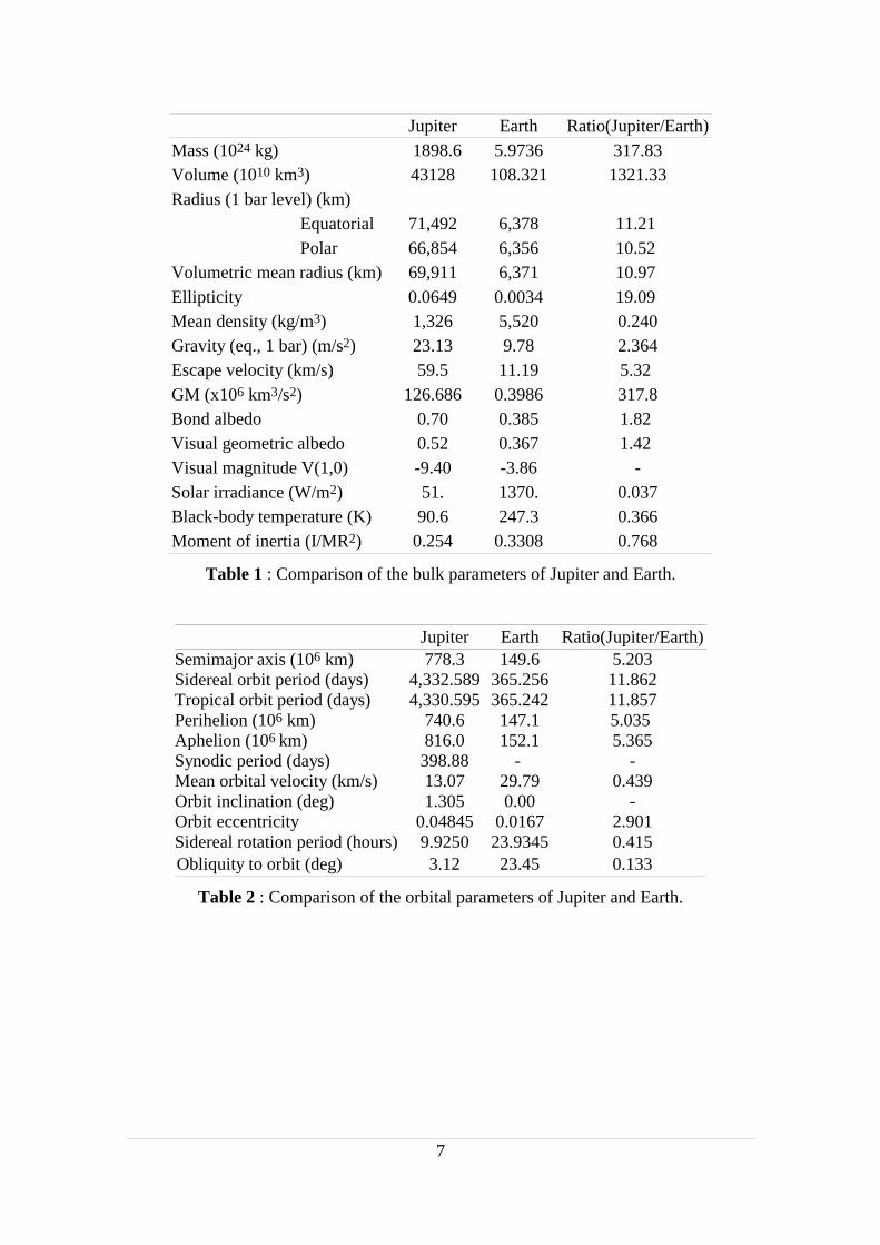
Jupiter is the largest of the nine planets of our solar system, more than 10 times
the diameter of the Earth and more than 300 times its mass. In fact, the mass of Jupiter
is almost 2.5 times that of all the other planets combined. (A comparison of the bulk
1
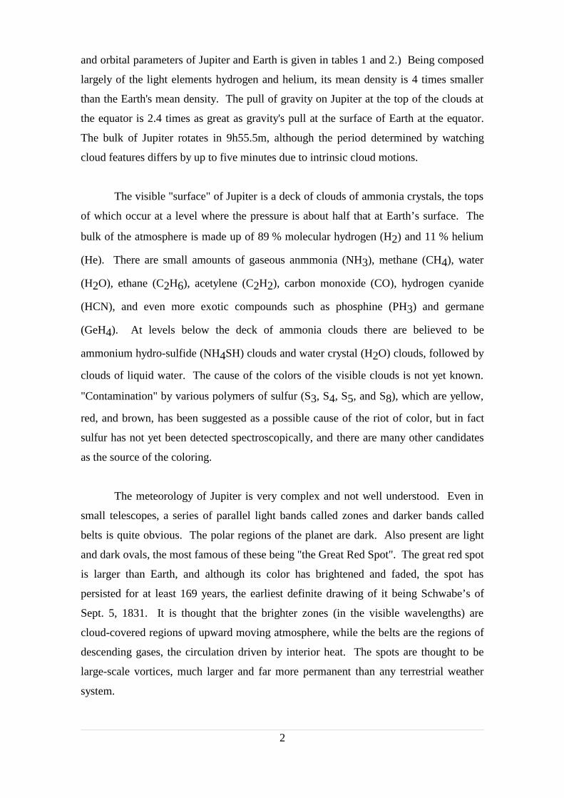
Figure 1 : WFPC2 (HST) near ultraviolet image showing Jupiter's moon
Io passing above the turbulent clouds of the giant planet.
and orbital parameters of Jupiter and Earth is given in tables 1 and 2.) Being composed
largely of the light elements hydrogen and helium, its mean density is 4 times smaller
than the Earth's mean density. The pull of gravity on Jupiter at the top of the clouds at
the equator is 2.4 times as great as gravity's pull at the surface of Earth at the equator.
The bulk of Jupiter rotates in 9h55.5m, although the period determined by watching
cloud features differs by up to five minutes due to intrinsic cloud motions.
The visible "surface" of Jupiter is a deck of clouds of ammonia crystals, the tops
of which occur at a level where the pressure is about half that at Earth’s surface. The
bulk of the atmosphere is made up of 89 % molecular hydrogen (H2) and 11 % helium
(He). There are small amounts of gaseous anmmonia (NH3), methane (CH4), water
(H2O), ethane (C2H6), acetylene (C2H2), carbon monoxide (CO), hydrogen cyanide
(HCN), and even more exotic compounds such as phosphine (PH3) and germane
(GeH4). At levels below the deck of ammonia clouds there are believed to be
ammonium hydro-sulfide (NH4SH) clouds and water crystal (H2O) clouds, followed by
clouds of liquid water. The cause of the colors of the visible clouds is not yet known.
"Contamination" by various polymers of sulfur (S3, S4, S5, and S8), which are yellow,
red, and brown, has been suggested as a possible cause of the riot of color, but in fact
sulfur has not yet been detected spectroscopically, and there are many other candidates
as the source of the coloring.
The meteorology of Jupiter is very complex and not well understood. Even in
small telescopes, a series of parallel light bands called zones and darker bands called
belts is quite obvious. The polar regions of the planet are dark. Also present are light
and dark ovals, the most famous of these being "the Great Red Spot". The great red spot
is larger than Earth, and although its color has brightened and faded, the spot has
persisted for at least 169 years, the earliest definite drawing of it being Schwabe’s of
Sept. 5, 1831. It is thought that the brighter zones (in the visible wavelengths) are
cloud-covered regions of upward moving atmosphere, while the belts are the regions of
descending gases, the circulation driven by interior heat. The spots are thought to be
large-scale vortices, much larger and far more permanent than any terrestrial weather
system.
2

The interior of Jupiter is totally unlike that of the Earth. Earth has a solid crust
"floating" on a denser mantle that is fluid on top and solid beneath, underlain by a fluid
outer core that extends out to about half of Earth's radius and a solid inner core of about
1220 km radius. The core is probably 75 % iron, with the remainder nickel, perhaps
silicon, and many different metals in small amounts. Jupiter on the other hand may well
be fluid throughout, although it could have a "small" solid core (up to 15 times the mass
of Earth) of heavier elements such as iron and silicon extending out to perhaps 15 % of
its radius. The bulk of Jupiter is fluid hydrogen in two forms or phases, liquid
molecular hydrogen on top and liquid metallic hydrogen below; the latter phase exists
where the pressure is high enough, about 3-4x10⁶ atmospheres. There could be a small
layer of liquid helium below the hydrogen, separated out gravitationally, and there is
clearly some helium mixed in with the hydrogen. The hydrogen is convecting heat from
the interior, and that heat is easily detected by infrared measurements, since Jupiter
radiates twice as much heat as it receives from the Sun. The heat is generated largely by
gravitational contraction and perhaps by gravitational separation of helium and other
heavier elements from hydrogen, in other words, by the conversion of gravitational
potential energy to thermal energy. The moving metallic hydrogen in the interior is
believed to be the source of Jupiter's strong magnetic field.
Jupiter's magnetic field is much stronger than that of the Earth. It is tipped about
10° to Jupiter's axis of rotation, similar to Earth's, but it is also offset from the center of
Jupiter by about 10000 km. The magnetosphere of charged particles which it affects
extends from 3.5 to 7x10⁶ km in the direction toward the Sun, depending upon solar
wind conditions, and at least 10 times as far in the anti-Sun direction. The plasma
trapped in this rotating, wobbling magnetosphere emits radio frequency radiation
measurable from Earth at wavelengths from less than 1 m to as much as 30 km. These
trapped charged particles make the inner portions of Jupiter's magnetosphere a very
harsh radiation environment.
When the Voyager 1 spacecraft passed through Jupiter's realm in 1979, it spotted
nine active volcanoes on Io, the innermost of the four Galilean satellites of Jupiter,
spewing sulfur and sulfur dioxide gases and solids as high as 300 km above the surface
3

at velocities up to 1 km s-1. Most of the material emitted falls back onto the surface, but
a small part of it escapes the satellite. In space this material is rapidly dissociated and
ionized. Once it becomes charged, the material is trapped by Jupiter's magnetic field
and forms a torus along Io's orbit. Accompanying the volcanic sulfur and oxygen are
many sodium ions (and perhaps some of the sulfur and oxygen as well) that have been
sputtered from Io by high energy electrons in Jupiter's magnetosphere. The torus also
contains protons and electrons which can be precipitated in the Jovian atmosphere and
give rise to auroræ as will be discussed later.
I.1 Coordinate systems
The standard coordinate system usually used to represent Jupiter's longitudes is a
left-handed system known as System III, formulated for astronomical use, in which
longitude (called West-longitude) is measured against the direction of rotation. This
rotating coordinate system is defined by the mean rotational period of decametric radio
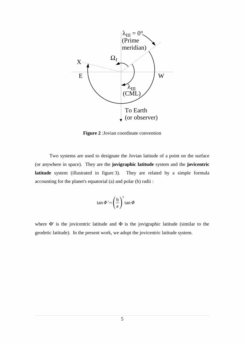
sources in Jupiter's atmosphere. Figure 2 is a view from above the north pole of the
Jovian coordinate system. The standard astronomical definition of the eastern and
western sides of Jupiter as seen from the Earth are indicated by an E and W,
respectively. The prime meridian rotates counterclockwise at a constante rate ΩJ.
Longitude is measured clockwise from this prime meridian. The System III sub-Earth
longitude is called the Central Meridian Longitude (CML). This illustration also shows
the longitude of some feature (an auroral emission, for example) marked X.
4
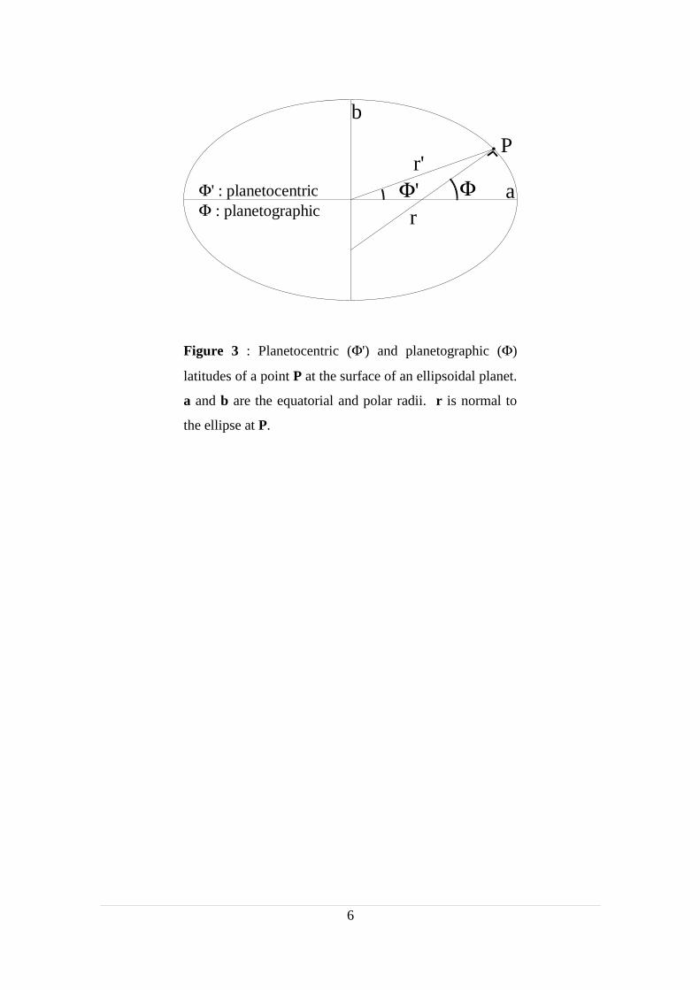
Two systems are used to designate the Jovian latitude of a point on the surface
(or anywhere in space). They are the jovigraphic latitude system and the jovicentric
latitude system (illustrated in figure 3). They are related by a simple formula
accounting for the planet's equatorial (a) and polar (b) radii :
tan 'ba
2
tan
where Φ' is the jovicentric latitude and Φ is the jovigraphic latitude (similar to the
geodetic latitude). In the present work, we adopt the jovicentric latitude system.
5
Figure 2 :Jovian coordinate convention
E W
XΩJ
To Earth(or observer)
λIII
λIII = 0°(Primemeridian)
(CML)
6
Figure 3 : Planetocentric (Φ') and planetographic (Φ)
latitudes of a point P at the surface of an ellipsoidal planet.
a and b are the equatorial and polar radii. r is normal to
the ellipse at P.
Pr'
rΦΦ'Φ' : planetocentric
Φ : planetographica
b
Jupiter Earth Ratio(Jupiter/Earth)Mass (1024 kg) 1898.6 5.9736 317.83Volume (1010 km3) 43128 108.321 1321.33Radius (1 bar level) (km) Equatorial 71,492 6,378 11.21 Polar 66,854 6,356 10.52Volumetric mean radius (km) 69,911 6,371 10.97Ellipticity 0.0649 0.0034 19.09Mean density (kg/m3) 1,326 5,520 0.240Gravity (eq., 1 bar) (m/s2) 23.13 9.78 2.364Escape velocity (km/s) 59.5 11.19 5.32GM (x106 km3/s2) 126.686 0.3986 317.8Bond albedo 0.70 0.385 1.82Visual geometric albedo 0.52 0.367 1.42Visual magnitude V(1,0) -9.40 -3.86 -Solar irradiance (W/m2) 51. 1370. 0.037Black-body temperature (K) 90.6 247.3 0.366Moment of inertia (I/MR2) 0.254 0.3308 0.768
Table 1 : Comparison of the bulk parameters of Jupiter and Earth.
Jupiter Earth Ratio(Jupiter/Earth)Semimajor axis (106 km) 778.3 149.6 5.203Sidereal orbit period (days) 4,332.589 365.256 11.862Tropical orbit period (days) 4,330.595 365.242 11.857Perihelion (106 km) 740.6 147.1 5.035Aphelion (106 km) 816.0 152.1 5.365Synodic period (days) 398.88 - -Mean orbital velocity (km/s) 13.07 29.79 0.439Orbit inclination (deg) 1.305 0.00 -Orbit eccentricity 0.04845 0.0167 2.901Sidereal rotation period (hours) 9.9250 23.9345 0.415Obliquity to orbit (deg) 3.12 23.45 0.133
Table 2 : Comparison of the orbital parameters of Jupiter and Earth.
7

II The planetary magnetosphere
II.1 Introduction
As its name suggests, a planet’s magnetosphere is the region of space
magnetically controlled by the planet’s magnetic field. The Voyager tour of the outer
solar system has confirmed that, like Earth, all four giant planets (Jupiter, Saturn,
Uranus, and Neptune) have extensive magnetospheres due to their strong magnetic
fields, generated by convective motions in an electrically-conducting region in the
planet’s interior. The magnetosphere of Jupiter is a large structure dominated by strong
planetary magnetic fields that contain thermal plasma. There are processes that
accelerate the thermal plasma to produce populations of energetic particles trapped in
radiation belts around the planet. Significant interactions occur between the plasma and
satellites that are embedded in the magnetosphere. The magnetosphere produces
different types of plasma waves, radio emissions, and aurorae.
This chapter is largely inspired by Fran Bagenal's review of the giant planet
magnetospheres (Bagenal, 1992), the reader is referred to this paper for additional
references on the different topics that will be discuss in the following sections. Specific
information on the Jovian magnetosphere can be found in the book edited by J.A
Dessler (1983) collecting published papers discussing particular aspects of the physics
of the Jovian magnetosphere. Useful information can also be found in David Stern's
review of the large scale electric fields in the Earth's magnetosphere (Stern, 1977).
Most of the figures appearing in this chapter were taken from T. Tascione (1994).
II.1.1 Background
8
Before going into the very complex domain of planetary magnetospheres it is
useful to remember some basic processes describing the motion of a charged particle in
a magnetic field. These relations stand for the basic motions of electrons and ions in the
magnetosphere :
gyromotion around a magnetic field line,
bounce motion between mirror points, and
drift due to the configuration of the magnetic field or to the presence of an external
force (for example an electric field).
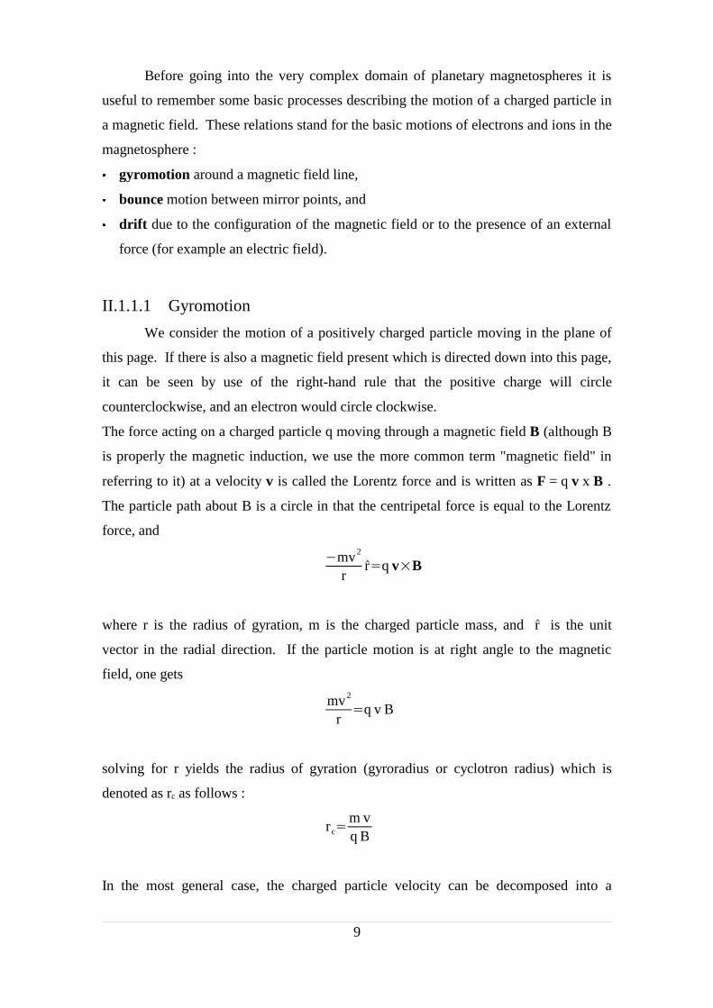
II.1.1.1 Gyromotion
We consider the motion of a positively charged particle moving in the plane of
this page. If there is also a magnetic field present which is directed down into this page,
it can be seen by use of the right-hand rule that the positive charge will circle
counterclockwise, and an electron would circle clockwise.
The force acting on a charged particle q moving through a magnetic field B (although B
is properly the magnetic induction, we use the more common term "magnetic field" in
referring to it) at a velocity v is called the Lorentz force and is written as F = q v x B .
The particle path about B is a circle in that the centripetal force is equal to the Lorentz
force, and
mv2
rrq vB
where r is the radius of gyration, m is the charged particle mass, and r is the unit
vector in the radial direction. If the particle motion is at right angle to the magnetic
field, one gets
mv2
rq v B
solving for r yields the radius of gyration (gyroradius or cyclotron radius) which is
denoted as rc as follows :
rcm vq B
In the most general case, the charged particle velocity can be decomposed into a
9
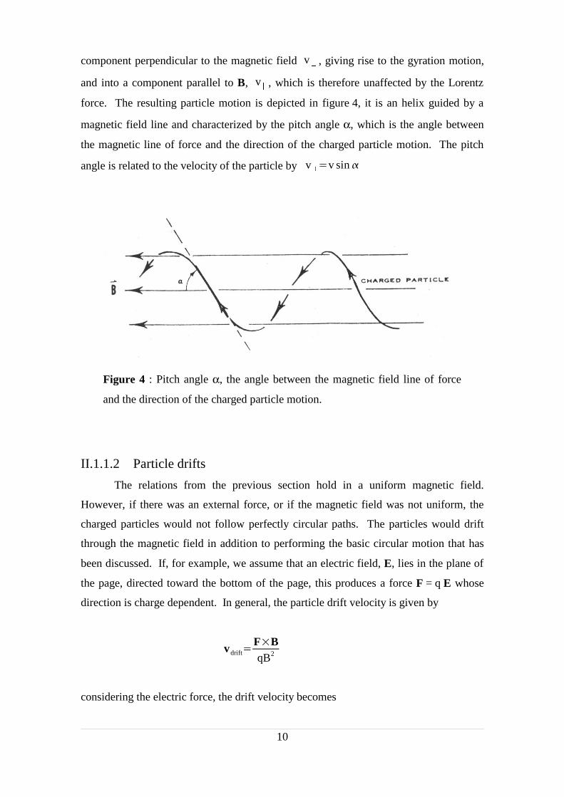
component perpendicular to the magnetic field v , giving rise to the gyration motion,
and into a component parallel to B, v , which is therefore unaffected by the Lorentz
force. The resulting particle motion is depicted in figure 4, it is an helix guided by a
magnetic field line and characterized by the pitch angle α, which is the angle between
the magnetic line of force and the direction of the charged particle motion. The pitch
angle is related to the velocity of the particle by v v sin
II.1.1.2 Particle drifts
The relations from the previous section hold in a uniform magnetic field.
However, if there was an external force, or if the magnetic field was not uniform, the
charged particles would not follow perfectly circular paths. The particles would drift
through the magnetic field in addition to performing the basic circular motion that has
been discussed. If, for example, we assume that an electric field, E, lies in the plane of
the page, directed toward the bottom of the page, this produces a force F = q E whose
direction is charge dependent. In general, the particle drift velocity is given by
vdriftFBqB2
considering the electric force, the drift velocity becomes
10
Figure 4 : Pitch angle α, the angle between the magnetic field line of force
and the direction of the charged particle motion.

vEq EB
qB2 EB
B2
and the resulting EB drift is charge independent. Therefore, electrons and protons
drift in the same direction and velocity, as illustrated in figure 5.
We now assume that the magnetic field is uniform except for some small variations
which give the total field some curvature in a particular direction (as is the case for a
dipolar planetary field). As the gyrating particles move along a curved field line, some
external force must act on the particle to make it turn and follow the field line geometry.
If there are no external electric field, this force must be provided by the magnetic field.
As the charged particles follow B, then a force of
Fmv
2
RR
is needed to turn the particle where v is the particle velocity parallel to B and R is the
radius of curvature (not gyroradius) of the magnetic field line. Therefore, we find
v cmv
2 RB
q R2 B2
where the explicit appearance of q indicates that positive and negative particles will
undergo curvature drift in opposite directions, and then produce a net electric current.
11
Figure 5 : Cross B field drift due to an external electric field (E x B drift).
The positive and negative charged particles drift in the same direction and no
net current is produced
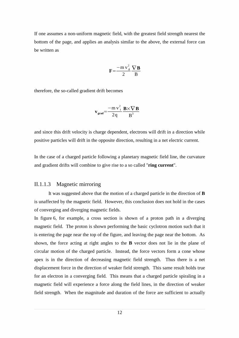
If one assumes a non-uniform magnetic field, with the greatest field strength nearest the
bottom of the page, and applies an analysis similar to the above, the external force can
be written as
Fm v
2
2 B
B
therefore, the so-called gradient drift becomes
vgradm v
2
2qB B
B3
and since this drift velocity is charge dependent, electrons will drift in a direction while
positive particles will drift in the opposite direction, resulting in a net electric current.
In the case of a charged particle following a planetary magnetic field line, the curvature
and gradient drifts will combine to give rise to a so called "ring current".
II.1.1.3 Magnetic mirroring
It was suggested above that the motion of a charged particle in the direction of B
is unaffected by the magnetic field. However, this conclusion does not hold in the cases
of converging and diverging magnetic fields.
In figure 6, for example, a cross section is shown of a proton path in a diverging
magnetic field. The proton is shown performing the basic cyclotron motion such that it
is entering the page near the top of the figure, and leaving the page near the bottom. As
shown, the force acting at right angles to the B vector does not lie in the plane of
circular motion of the charged particle. Instead, the force vectors form a cone whose
apex is in the direction of decreasing magnetic field strength. Thus there is a net
displacement force in the direction of weaker field strength. This same result holds true
for an electron in a converging field. This means that a charged particle spiraling in a
magnetic field will experience a force along the field lines, in the direction of weaker
field strength. When the magnitude and duration of the force are sufficient to actually
12

cause the charged particle to reverse direction of motion along the line of magnetic
force, the effect is known as magnetic mirroring and the location of the particle's path
reversal is known as the mirror point for that particle.
This means that a charged particle spiraling in a magnetic field will experience a force
along the field lines, in the direction of weaker field strength. When the magnitude and
duration of the force are sufficient to actually cause the charged particle to reverse
direction of motion along the line of magnetic force, the effect is known as magnetic
mirroring and the location of the particle path reversal is known as the mirror point
for that particle.
It can be shown from the first adiabatic invariant, which states that the magnetic
moment of a particle remains constant during one gyro-orbit eventhough B may be
changing slowly, that
sin2B
Bm
where Bm is the magnetic field strength at the mirror point.
This relation means that the pitch angle of the particle α varies with the magnetic field
13
Figure 6 : Forces acting on a gyrating proton in a diverging magnetic field.

strength along a field line so as to conserve sin2B . The pitch angle of most particles
reaches 90° before the particles reach the top of the atmosphere. Such particles bounce
back and forth along magnetic field lines between the points where α = 90° and are
trapped in the planetary magnetic field. Particles with sufficiently small pitch angles
reach the top of the atmosphere before α reaches 90°. Such particles are said to be in
the loss cone, and they are absorbed into the atmosphere by collisions.
In summary, charged particles can be trapped in a planetary magnetic field.
Their basic motion is circular (gyro-motion), with a superimposed longitudinal drift
around the planet ( EB drift), and a latitudinal reflection (or "bounce") between
mirror points at high latitudes as illustrated in figure 7 for the Earth.
II.2 Magnetospheric morphology
The term magnetosphere was coined by Gold (1959) to describe the region of
space wherein the principal forces on a plasma are electrodynamic in nature and are a
result of the planet’s magnetic field. Planetary magnetospheres are embedded in the
solar wind, which is the outward expansion of the solar corona. At Earth’s orbit and
14
Figure 7 : Basic motion of a charged particle in the Earth magnetic field.

beyond, the solar wind has an average speed of about 400 km s-1. The density of
particles (mainly electrons and protons) is observed to decrease, from values of about 3
to 10 cm-3 at the Earth, as the inverse square of the distance from the Sun, consistent
with a steady radial expansion of the solar gas into a spherical volume. The solar wind
speed, while varying between about 300 and 700 km s-1, always greatly exceeds the
speed of waves characteristic of a low density, magnetized, and completely ionized gas
(Alfvén waves). Thus a shock is formed upstream of an obstacle, such as a planetary
magnetosphere that is imposed on the super-Alfvénic solar wind flow. A planetary bow
shock can be described in fluid terms as a discontinuity in bulk parameters of the solar
wind plasma. As the flow of solar plasma traverses the shock it is decelerated and
heated so that the flow can be deflected around the magnetosphere.
To first approximation, the magnetic field of a planet deflects the plasma flow
around it, carving out a cavity in the solar wind. The layer of deflected solar wind
behind the bow shock is called the magnetosheath and the boundary between the
magnetosphere and the solar wind plasma is called the magnetopause. The
magnetopause is a current layer resulting from the kinetic interaction between the solar
wind and the planetary magnetic field. This current shields a large portion of the
interplanetary magnetic field from the region interior to the magnetopause. As a result,
the magnetopause is a sharp boundary that separates the interplanetary medium from a
region of space which is dominated by the planetary magnetic field : the magnetosphere.
The solar wind generally pulls out part of the planetary magnetic field into a long
cylindrical magnetotail, extending far downstream behind the planet.
Table 3 shows a comparison between the Jovian and Earth magnetic fields.
While the net magnetic moment of Jupiter is many times greater than that of the Earth,
its large radius result in a surface magnetic field on the order of a Gauss. None of the
planetary magnetic fields are purely dipolar but the dipole (first order) approximation
gives an indication of the strength (B0) and orientation of the field. Jupiter has a
magnetic field like that of the Earth, where the magnetic axis is roughly aligned with the
rotation axis and has only moderate deviation from a dipole.
15

Earth JupiterRadius (km) 6373 71398Spin period (hours) 24 9.9Magnetic moment / MEarth 20000 600
Surface magnetic field(Gauss)
dipole equator, B0
0.31 4.28
minimum 0.24 3.2maximum 0.68 14.3Dipole tilt and sense +11.3° -9.6°Distance (A.U.) 1 5.2Solar wind density (cm-3) 10 0.4RCorotating Plasma 8 RE 30 RJ
Size of magnetosphere 11 RE 50-100 RJ
Table 3 : Comparison of Earth and Jupiter magnetic fields.(MEarth = 7.906x1025 Gauss cm3)
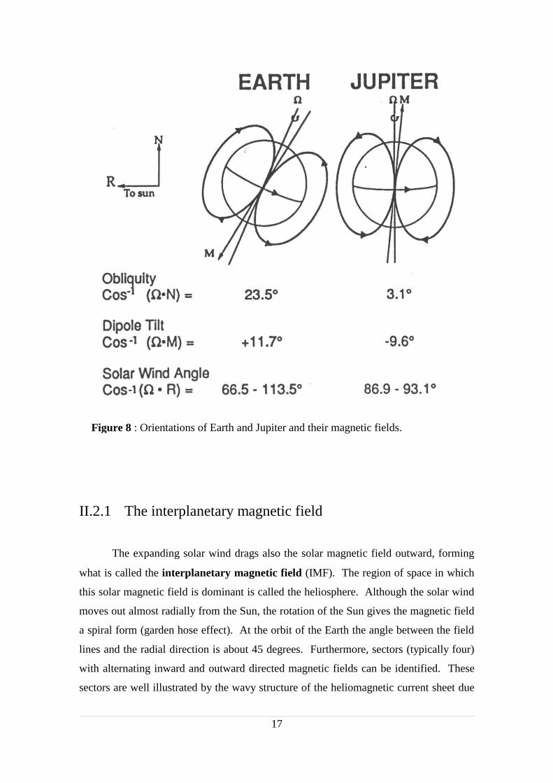
While the size of a planetary magnetosphere depends on the strength of the
planet’s magnetic field, the configuration and internal dynamics depend on the field
orientation (illustrated in figure 8) which is described by two angles: the tilt of the
magnetic field with respect to the spin axis of the planet and the angle between this spin
axis and the solar wind direction which is generally within a few degrees of radially
outward from the Sun. Since the direction of the spin axis with respect to the solar wind
direction only varies over a planetary year (many Earth years for the outer planets) and
the planet’s magnetic field is assumed to vary only on geological time scales, these two
angles are constant for the purposes of describing the magnetospheric configuration at a
particular epoch. Earth and Jupiter have both small dipole tilts and small obliquities.
This means that the orientation of the magnetic field with respect to the solar wind does
not vary appreciably over a planetary rotation period and that seasonal effects are small.
Thus Earth and Jupiter have symmetric and quasi-stationary magnetospheres exhibiting
only a small wobble due to their 10° dipole tilts.
16
II.2.1 The interplanetary magnetic field
The expanding solar wind drags also the solar magnetic field outward, forming
what is called the interplanetary magnetic field (IMF). The region of space in which
this solar magnetic field is dominant is called the heliosphere. Although the solar wind
moves out almost radially from the Sun, the rotation of the Sun gives the magnetic field
a spiral form (garden hose effect). At the orbit of the Earth the angle between the field
lines and the radial direction is about 45 degrees. Furthermore, sectors (typically four)
with alternating inward and outward directed magnetic fields can be identified. These
sectors are well illustrated by the wavy structure of the heliomagnetic current sheet due
17
Figure 8 : Orientations of Earth and Jupiter and their magnetic fields.
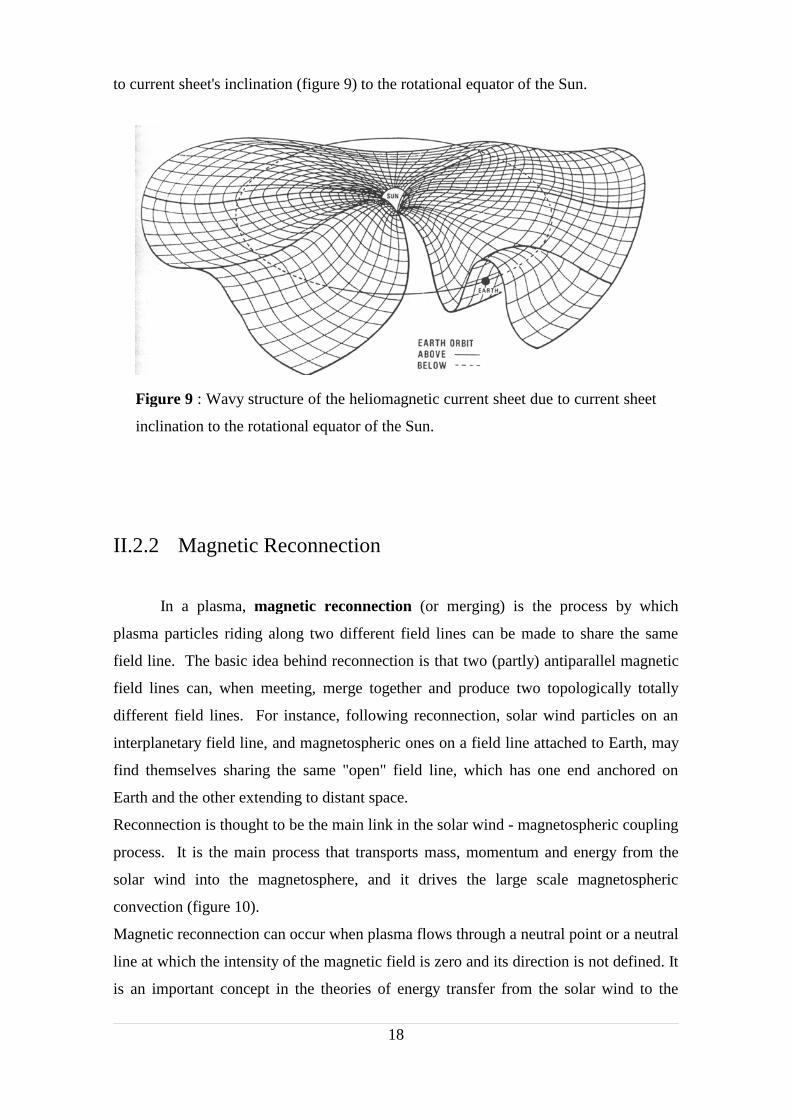
to current sheet's inclination (figure 9) to the rotational equator of the Sun.
II.2.2 Magnetic Reconnection
In a plasma, magnetic reconnection (or merging) is the process by which
plasma particles riding along two different field lines can be made to share the same
field line. The basic idea behind reconnection is that two (partly) antiparallel magnetic
field lines can, when meeting, merge together and produce two topologically totally
different field lines. For instance, following reconnection, solar wind particles on an
interplanetary field line, and magnetospheric ones on a field line attached to Earth, may
find themselves sharing the same "open" field line, which has one end anchored on
Earth and the other extending to distant space.
Reconnection is thought to be the main link in the solar wind - magnetospheric coupling
process. It is the main process that transports mass, momentum and energy from the
solar wind into the magnetosphere, and it drives the large scale magnetospheric
convection (figure 10).
Magnetic reconnection can occur when plasma flows through a neutral point or a neutral
line at which the intensity of the magnetic field is zero and its direction is not defined. It
is an important concept in the theories of energy transfer from the solar wind to the
18
Figure 9 : Wavy structure of the heliomagnetic current sheet due to current sheet
inclination to the rotational equator of the Sun.

magnetosphere and of energy release in substorms.
19
Figure 10 : (A) Magnetic field topology in the merging region of an openmagnetosphere. Large arrows indicate plasma flow direction and arrows on fieldlines show field line direction. (B) The dashed line represents the magnetopauseboundary. The large arrows show the convection system set up inside themagnetosphere by magnetic reconnection.
II.2.3 Magnetospherespheric electric fields and convection
The magnetospheric configuration is generally well described by
magnetohydrodynamics (MHD) in which the magnetic field can be considered to be
frozen into the plasma flow (i.e. the solar magnetic field is carried along within the
plasma virtually unchanged) with an infinite conductivity.
There are two main sources of magnetospheric electric fields. The first one is the solar
wind related, dawn-to-dusk directed convection field, and the other is the corotation
electric field related to the rotation of the planet about its spin axis. The low energy
particles move primarily under the ExB drift, and are less affected by the gradient and
curvature drifts which depend only on magnetic field. The energetic particles, following
the magnetic drifts more readily, are also affected by the convection field.
II.2.3.1 The corotation field
20
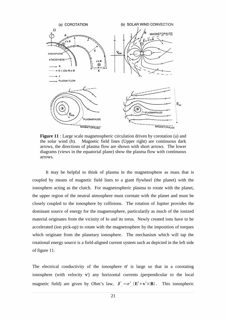
It may be helpful to think of plasma in the magnetosphere as mass that is
coupled by means of magnetic field lines to a giant flywheel (the planet) with the
ionosphere acting as the clutch. For magnetospheric plasma to rotate with the planet,
the upper region of the neutral atmosphere must corotate with the planet and must be
closely coupled to the ionosphere by collisions. The rotation of Jupiter provides the
dominant source of energy for the magnetosphere, particularily as much of the ionized
material originates from the vicinity of Io and its torus. Newly created ions have to be
accelerated (ion pick-up) to rotate with the magnetosphere by the imposition of torques
which originate from the planetary ionosphere. The mechanism which will tap the
rotational energy source is a field-aligned current system such as depicted in the left side
of figure 11.
The electrical conductivity of the ionosphere σi is large so that in a corotating
ionosphere (with velocity vi) any horizontal currents (perpendicular to the local
magnetic field) are given by Ohm’s law, J i
i Eiv iB . This ionospheric
21
Figure 11 : Large scale magnetospheric circulation driven by corotation (a) andthe solar wind (b). Magnetic field lines (Upper right) are continuous darkarrows, the directions of plasma flow are shown with short arrows. The lowerdiagrams (views in the equatorial plane) show the plasma flow with continuousarrows.
(Pedersen) current is driven by friction between ions and neutrals. The transverse
current flowing in the equatorial magnetosphere and closing the current loop transfers
the angular momentum absorbed in the ionosphere to the magnetospheric plasma.
Just above the ionosphere, the conductivity perpendicular to the magnetic field in the
(collision-free) magnetosphere, i , is essentially zero. Moreover, the magnetospheric
electric field Em in the corotating region is Emv mB where vm is the
magnetospheric plasma velocity. (For the corotating plasmasphere, the plasma is
stationary in its local frame of reference and therefore E = 0. However, to an observer
on the planet, the plasmasphere plasma is kept in balance by an electric field which has
to balance the Lorentz force or Emv mB0 ).
Because plasma particles are far more mobile in the direction of the local magnetic field,
the parallel conductivity i is large and the field lines can be considered to be
equipotentials EB0 . Thus the electric field in the magnetosphere can be mapped
into the ionosphere (figure 11). There may exist conditions under which this
approximation does not hold, such fields ( E0 ) are obviously of great interest since
they are capable of accelerating charged particles directly. Because the ionosphere is
relatively thin, the electric field Em just above the ionosphere is the same as Ei so that
we can write J i
i v iv m B . The condition for corotation of the
magnetospheric plasma is that the ratio Ji/σi be sufficiently small so that
v mv ir where Ω is the angular frequency of corotation and r is the radial
distance. For a dipolar magnetic field that is aligned with the rotation axis B=B0/r3 and
the corotational electric field (in the equatorial plane) is therefore radial with magnitude
Eco = Ω B0 / r2.
Large ionospheric conductivities facilitate corotation. The large
m also
means that any currents in the magnetosphere that result from mechanical stresses on the
plasma are directly coupled by field-aligned currents (Birkeland currents) to the
ionosphere. Thus corotation breaks down when mechanical stresses on the
magnetospheric plasma drive ionospheric currents that are sufficiently large for the ratio
Ji/σi to become significant.
II.2.3.2 Magnetospheric convection field
22

We now consider how the momentum of the solar wind may be harnessed by
processes occurring near the magnetopause where the external solar magnetic field
interconnects with the planetary magnetic field. Figure 11 (right) shows that at the poles
the planetary magnetic field lines are open to the solar wind. The solar wind drives a
plasma flow across the polar caps and the field lines from the polar region move in the
direction of the solar wind flow, being pulled by the solar wind over the poles and back
into the extended magnetotail. Conservation of flux requires that field lines are further
cut and reconnected in the tail.
The MHD condition of the field being frozen to the flow can be written as
EvB0 (for an observer on the planet), which allows the convection electric
field (the electric field associated to the solar wind) to be written as
Ecvv swB0R m3 (where η is the efficiency of the reconnection process in
harnessing the solar wind momentum, 0.1 for the Earth, and where we have assumed a
simple dipole field B=B0/r3). In simple magnetospheric models Ecv is assumed constant
throughout the magnetosphere. The corresponding circulation is given by the
E x B drift, vcvvsw r R m 3 where Rm, is the magnetopause distance. After being
carried tailward at high latitudes, the plasma drifts towards the equatorial plane and
eventually returns in a sunward flow to the dayside magnetopause.
Comparison of the corresponding electric fields indicates whether the
magnetospheric circulation is driven primarily by the solar wind or by the planetary
rotation. Since Eco is proportional to r-2 and Ecv proportional to r-3, corotation is
expected to dominate within a short distance from the planet while the solar wind driven
convection dominates outside a critical distance Rc. It can be shown that
magnetospheres of rapidly rotating planets with strong magnetic fields (such as
Jupiter's) are dominated by rotation while the solar wind controls the plasma flow in
smaller magnetospheres of slowly rotating planets (such as the Earth's).
II.2.4 The Earth magnetosphere
The following section is a brief description of the Earth’s magnetosphere
(figure 12) for the purpose of comparison with the Jovian magnetosphere. The Earth
23
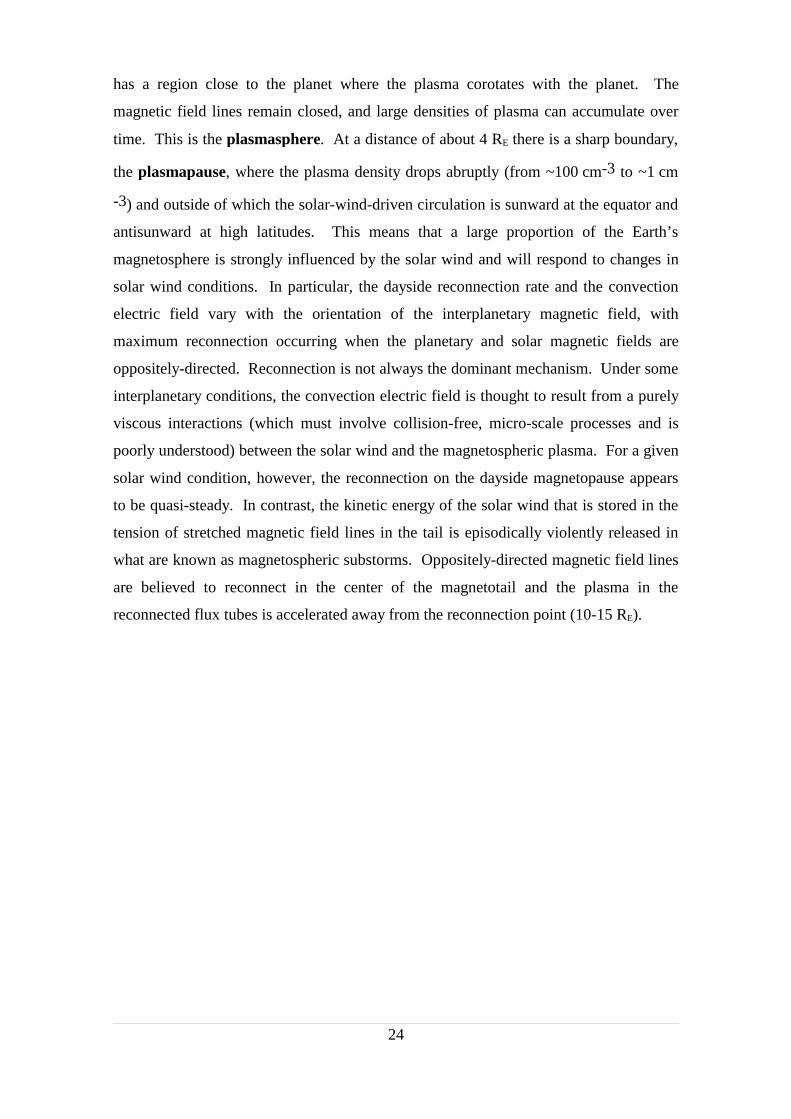
has a region close to the planet where the plasma corotates with the planet. The
magnetic field lines remain closed, and large densities of plasma can accumulate over
time. This is the plasmasphere. At a distance of about 4 RE there is a sharp boundary,
the plasmapause, where the plasma density drops abruptly (from ~100 cm-3 to ~1 cm
-3) and outside of which the solar-wind-driven circulation is sunward at the equator and
antisunward at high latitudes. This means that a large proportion of the Earth’s
magnetosphere is strongly influenced by the solar wind and will respond to changes in
solar wind conditions. In particular, the dayside reconnection rate and the convection
electric field vary with the orientation of the interplanetary magnetic field, with
maximum reconnection occurring when the planetary and solar magnetic fields are
oppositely-directed. Reconnection is not always the dominant mechanism. Under some
interplanetary conditions, the convection electric field is thought to result from a purely
viscous interactions (which must involve collision-free, micro-scale processes and is
poorly understood) between the solar wind and the magnetospheric plasma. For a given
solar wind condition, however, the reconnection on the dayside magnetopause appears
to be quasi-steady. In contrast, the kinetic energy of the solar wind that is stored in the
tension of stretched magnetic field lines in the tail is episodically violently released in
what are known as magnetospheric substorms. Oppositely-directed magnetic field lines
are believed to reconnect in the center of the magnetotail and the plasma in the
reconnected flux tubes is accelerated away from the reconnection point (10-15 RE).
24

25
Figure 12 : The magnetosphere of the Earth.

II.2.5 The Jovian magnetosphere
Jupiter is a huge object about 1000 times the volume of the Sun with a tail that
extends at least 6 AU in the antisunward direction, beyond the orbit of Saturn. If the
Jovian magnetosphere were visible from Earth its angular size would be twice that of
the Sun even though it is at least four times farther away.
It has become customary to describe the Jovian magnetosphere in terms of three
principal regions. The inner magnetosphere is the region where the magnetic field
generated by currents flowing in the interior of the planet dominates, and contributions
from current systems external to the planet are not significant. This region extends from
the planetary surface to a distance of approximately 6 RJ (Jovian radii), the orbit of Io.
Outside of this region, the effects of an azimuthal current sheet in the equatorial plane
produce a significant pertubation, leading to the stretching of the magnetic field lines in
the radial direction. The region in which the equatorial current flows is denoted as the
middle magnetosphere, and extends from ~6 RJ to approximately 30-50 RJ where the
local-time asymmetry due to the magnetopause and tail current systems become
important. Inside this region the Jovian internal field is adequately represented as a
tilted dipole field, and the magnetic field of the magnetopause and tail currents is small.
In the outer magnetosphere, the cylindrical symmetry prevalent in the inner regions
disappears due to the effects of the solar wind interaction with the magnetosphere. We
thus have to differentiate between a "sunward side" outermagnetosphere and a
"magnetospheric tail" extending away from the planet in the antisolar direction. The
field has a large southward component and exhibits large temporal and/or spatial
variations in magnitude and direction in response to changes in solar wind pressure.
This region extends from the magnetopause boundary to approximately 30-50 RJ, and
includes the extensive Jovian magnetic tail.
26

The Voyager Plasma Science instruments confirmed that the bulk motion of the
plasma in the magnetosphere of Jupiter is largely azimuthal but measured significant
deviations from rigid rotation. The magnetosphere of Jupiter is sketched in figure 13,
the plasma flow was measured to be within 1 % of rigid corotation in the inner region at
5 RJ. At larger distances, the Voyager observations confirmed that the angular
momentum required to accelerate plasma to higher azimuthal velocities in order to
maintain corotation with the planet generates an increasing strain on the frictional
coupling between the Jovian ionosphere and neutral atmosphere and the flow lags
behind corotation. McNutt et al. (1979) reported departure from corotation occurring
from about 12 RJ outwards with the azimuthal flow tending towards a constant speed of
about 200 km s-1 beyond 20 RJ. The large plasma source near Jupiter’s satellite Io and
the subsequent outward transport of this material are the source of the mechanical
stresses in the magnetosphere causing departure from corotation.
In order to estimate the plasma flow in the magnetotail, Vasyliunas (1983) proposed a
planetary wind model (figure 14) in which at some distance from the planet the kinetic
energy of the rotational flow becomes greater than the energy of the magnetic field, i.e.
27
Figure 13 : The magnetosphere of Jupiter.
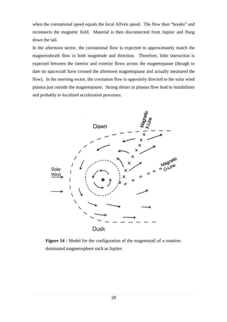
when the corotational speed equals the local Alfvén speed. The flow then “breaks” and
reconnects the magnetic field. Material is then disconnected from Jupiter and flung
down the tail.
In the afternoon sector, the corotational flow is expected to approximately match the
magnetosheath flow in both magnitude and direction. Therefore, little interaction is
expected between the interior and exterior flows across the magnetopause (though to
date no spacecraft have crossed the afternoon magnetopause and actually measured the
flow). In the morning sector, the corotation flow is oppositely directed to the solar wind
plasma just outside the magnetopause. Strong shears in plasma flow lead to instabilities
and probably to localized acceleration processes.
28
Figure 14 : Model for the configuration of the magnetotail of a rotation-
dominated magnetosphere such as Jupiter.

II.2.5.1 Thermal plasma charecteristics
It is rather misleading to describe a magnetosphere as an empty cavity from
which the solar wind is excluded. Magnetospheres contain considerable amounts of
plasma which have “leaked in” from various sources (table 4). First, the magnetopause
is not entirely “plasma-tight.” Solar wind plasma enters through the polar cusp and,
whenever the interplanetary magnetic field has a component antiparallel to the planetary
field at the magnetopause, magnetic reconnection is likely to occur and solar wind
plasma will leak into the magnetosphere. Secondly, although ionospheric plasma is
generally cold and gravitationally bound to the planet, a small fraction has sufficient
energy to escape up magnetic field lines and flow into the magnetosphere. Thirdly, the
interaction of magnetospheric plasma with any natural satellites that are embedded in
the magnetosphere can generate significant quantities of plasma.
Earth JupiterMaximum density (cm-3) 1 - 4000 > 3000Primary sources O+, H+ (ionosphere) On+, Sn+ (Io)Secondary sources H+ (solar wind) H+ (ionosphere)Source strength (ions/s)
(kg/s)
2x1026
5
>1028
700
Table 4 : Plasma characteristics of the Earth and the Jovian magnetospheres.
At the same time, the planetary magnetosphere supports a variety of plasma
waves which have various energy sources and cover a wide range of frequencies.
Interactions between these waves and particle populations are thought to be responsible
for thermalizing the bulk of the plasma as well as accelerating or scattering particles at
higher energies.
In 1979 the Voyager I spacecraft confirmed that Io is the major source of plasma in the
Jovian magnetosphere. Io’s volcanoes are believed to be responsible for a tenuous
(~10-9 bar) atmosphere mostly composed of SO2, either via direct venting or
sublimation of volcanic frosts deposited on the surface. The atmosphere is probably
patchy and is expected to vary with Io’s volcanic activity. Io orbits well inside Jupiter’s
magnetosphere, embedded in the corotating magnetospheric plasma and high fluxes of
energetic particles which collide with atmospheric constituents, heat Io's upper
29
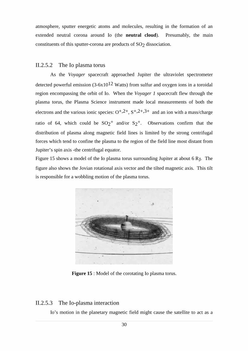
atmosphere, sputter energetic atoms and molecules, resulting in the formation of an
extended neutral corona around Io (the neutral cloud). Presumably, the main
constituents of this sputter-corona are products of SO2 dissociation.
II.2.5.2 The Io plasma torus
As the Voyager spacecraft approached Jupiter the ultraviolet spectrometer
detected powerful emission (3-6x10¹² Watts) from sulfur and oxygen ions in a toroidal
region encompassing the orbit of Io. When the Voyager 1 spacecraft flew through the
plasma torus, the Plasma Science instrument made local measurements of both the
electrons and the various ionic species: O+,2+, S+,2+,3+ and an ion with a mass/charge
ratio of 64, which could be SO2+ and/or S2+. Observations confirm that the
distribution of plasma along magnetic field lines is limited by the strong centrifugal
forces which tend to confine the plasma to the region of the field line most distant from
Jupiter’s spin axis -the centrifugal equator.
Figure 15 shows a model of the Io plasma torus surrounding Jupiter at about 6 RJ. The
figure also shows the Jovian rotational axis vector and the tilted magnetic axis. This tilt
is responsible for a wobbling motion of the plasma torus.
II.2.5.3 The Io-plasma interaction
Io’s motion in the planetary magnetic field might cause the satellite to act as a
30
Figure 15 : Model of the corotating Io plasma torus.
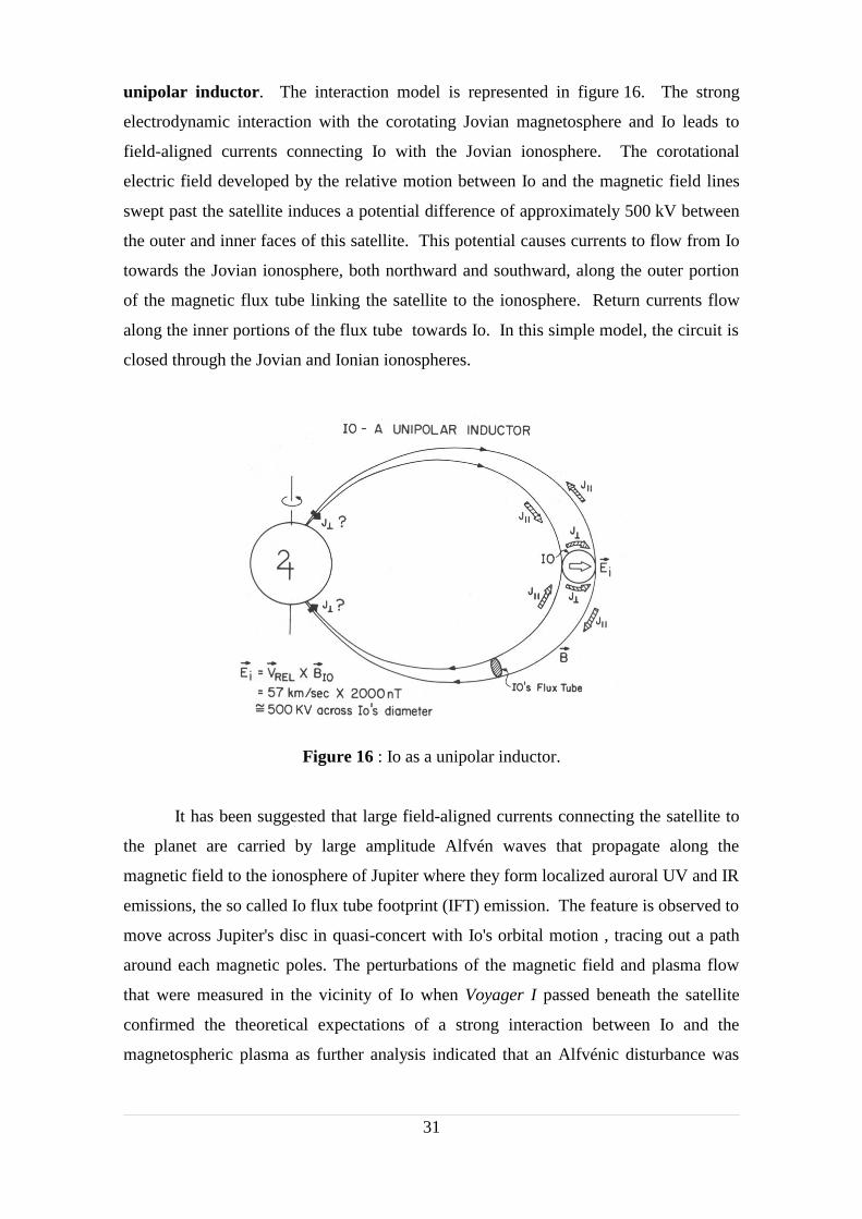
unipolar inductor. The interaction model is represented in figure 16. The strong
electrodynamic interaction with the corotating Jovian magnetosphere and Io leads to
field-aligned currents connecting Io with the Jovian ionosphere. The corotational
electric field developed by the relative motion between Io and the magnetic field lines
swept past the satellite induces a potential difference of approximately 500 kV between
the outer and inner faces of this satellite. This potential causes currents to flow from Io
towards the Jovian ionosphere, both northward and southward, along the outer portion
of the magnetic flux tube linking the satellite to the ionosphere. Return currents flow
along the inner portions of the flux tube towards Io. In this simple model, the circuit is
closed through the Jovian and Ionian ionospheres.
It has been suggested that large field-aligned currents connecting the satellite to
the planet are carried by large amplitude Alfvén waves that propagate along the
magnetic field to the ionosphere of Jupiter where they form localized auroral UV and IR
emissions, the so called Io flux tube footprint (IFT) emission. The feature is observed to
move across Jupiter's disc in quasi-concert with Io's orbital motion , tracing out a path
around each magnetic poles. The perturbations of the magnetic field and plasma flow
that were measured in the vicinity of Io when Voyager I passed beneath the satellite
confirmed the theoretical expectations of a strong interaction between Io and the
magnetospheric plasma as further analysis indicated that an Alfvénic disturbance was
31
Figure 16 : Io as a unipolar inductor.
radiated by Io, carrying a 106 A field-aligned current towards the ionosphere of Jupiter.
II.2.5.4 The plasma sheet
While the high plasma densities (>1000 cm-3) are confined to a toroidal region
within 1 RJ, of Io’s orbit, the iogenic material extends out to at least 40 RJ, forming a
thin (< 5 RJ thick) sheet of warm (10’s of eV) plasma with densities decreasing to a few
per cm3 by 20 RJ and dominated by sulfur and oxygen ions. This is the magnetodisc,
where the centrifugal forces on the corotating plasma stretch out the magnetic field at
the equator. In addition to the warm iogenic plasma there is a hot (~30 keV) thermal
plasma (with Maxwellian distributions) in the middle magnetosphere, beyond 10 RJ.
This hot plasma has an energy density greater than the local magnetic field and inflates
the magnetosphere, making it flatter at the poles and more compressible than a vacuum
dipole magnetosphere. The magnetodisc is characterized by a strong ring current known
as the azimuthal current sheet. Once the plasmas are injected in the vicinity of Io,
they start to drift around in azimuth by means of the combined effects of magnetic
gradient and field curvature drifts, and the corotational electric drift. The energy
dependent magnetic gradient drift of the electrons has a direction that opposes the more
rapid electric corotational field, while for ions, the gradient drift augments the
corotational drift. This axisymmetric current is flowing in the vicinity of the magnetic
equatorial plane. The ring current is an essential feature of the Jovian magnetosphere.
In the middle magnetosphere the magnetic field is dominated by the external current
sheet. The electromagnetic force associated with current is balancing a combination of
centrifugal and hot plasma pressure forces.
The current flowing in the Earth plasma sheet is different from the Jovian current sheet
in that the Earth plasma sheet current (also referred as the cross-tail current) is entirely
driven by magnetospheric convection. It has already been seen that this convection
gives rise to a convection electric field oriented from dawn to dusk. The resulting cross-
tail current flows across the plasma sheet from dawn to dusk.
32
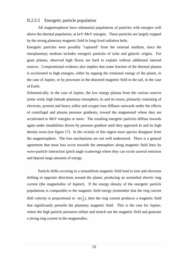
II.2.5.5 Energetic particle population
All magnetospheres have substantial populations of particles with energies well
above the thermal population, at keV-MeV energies. These particles are largely trapped
by the strong planetary magnetic field in long-lived radiation belts.
Energetic particles were possibly "captured" from the external medium, since the
interplanetary medium includes energetic particles of solar and galactic origins. For
giant planets, observed high fluxes are hard to explain without additional internal
sources. Compositional evidence also implies that some fraction of the thermal plasma
is accelerated to high energies, either by tapping the rotational energy of the planet, in
the case of Jupiter, or by processes in the distorted magnetic field in the tail, in the case
of Earth.
Schematically, in the case of Jupiter, the low energy plasma from the various sources
(solar wind, high latitude planetary ionosphere, Io and its torus), primarily consisting of
electrons, protons and heavy sulfur and oxygen ions diffuses outwards under the effects
of centrifugal and plasma pressure gradients, toward the magnetotail where they are
accelerated to MeV energies or more. The resulting energetic particles diffuse inwards
again under instabilities driven by pressure gradient until they approach Io and its high
density torus (see figure 17). In the vicinity of this region most species disappear from
the magnetosphere. The loss mechanisms are not well understood. There is a general
agreement that most loss occur towards the atmosphere along magnetic field lines by
wave-particle interaction (pitch angle scattering) where they can excite auroral emission
and deposit large amounts of energy.
Particle drifts occuring in a nonuniform magnetic field lead to ions and electrons
drifting in opposite directions around the planet, producing an azimuthal electric ring
current (the magnetodisc of Jupiter). If the energy density of the energetic particle
populations is comparable to the magnetic field energy (remember that the ring current
drift velocity is proportional to mv2 ), then the ring current produces a magnetic field
that significantly perturbs the planetary magnetic field. This is the case for Jupiter,
where the high particle pressures inflate and stretch out the magnetic field and generate
a strong ring current in the magnetodisc.
33
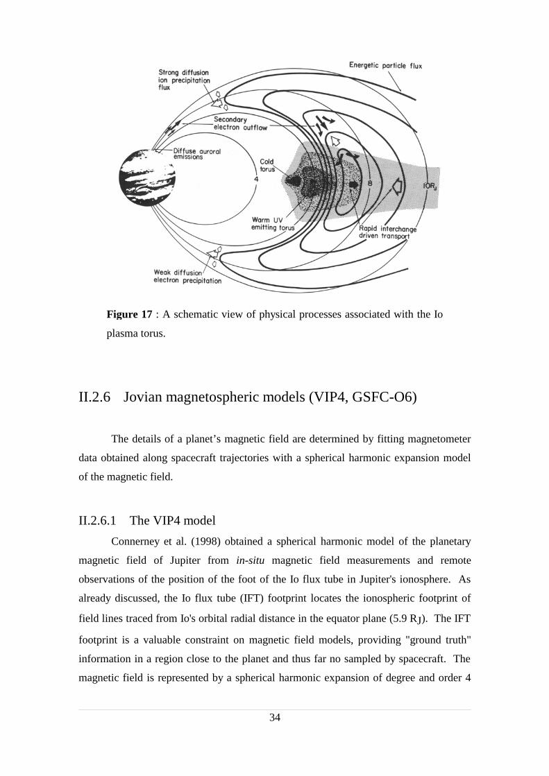
II.2.6 Jovian magnetospheric models (VIP4, GSFC-O6)
The details of a planet’s magnetic field are determined by fitting magnetometer
data obtained along spacecraft trajectories with a spherical harmonic expansion model
of the magnetic field.
II.2.6.1 The VIP4 model
Connerney et al. (1998) obtained a spherical harmonic model of the planetary
magnetic field of Jupiter from in-situ magnetic field measurements and remote
observations of the position of the foot of the Io flux tube in Jupiter's ionosphere. As
already discussed, the Io flux tube (IFT) footprint locates the ionospheric footprint of
field lines traced from Io's orbital radial distance in the equator plane (5.9 RJ). The IFT
footprint is a valuable constraint on magnetic field models, providing "ground truth"
information in a region close to the planet and thus far no sampled by spacecraft. The
magnetic field is represented by a spherical harmonic expansion of degree and order 4
34
Figure 17 : A schematic view of physical processes associated with the Io
plasma torus.
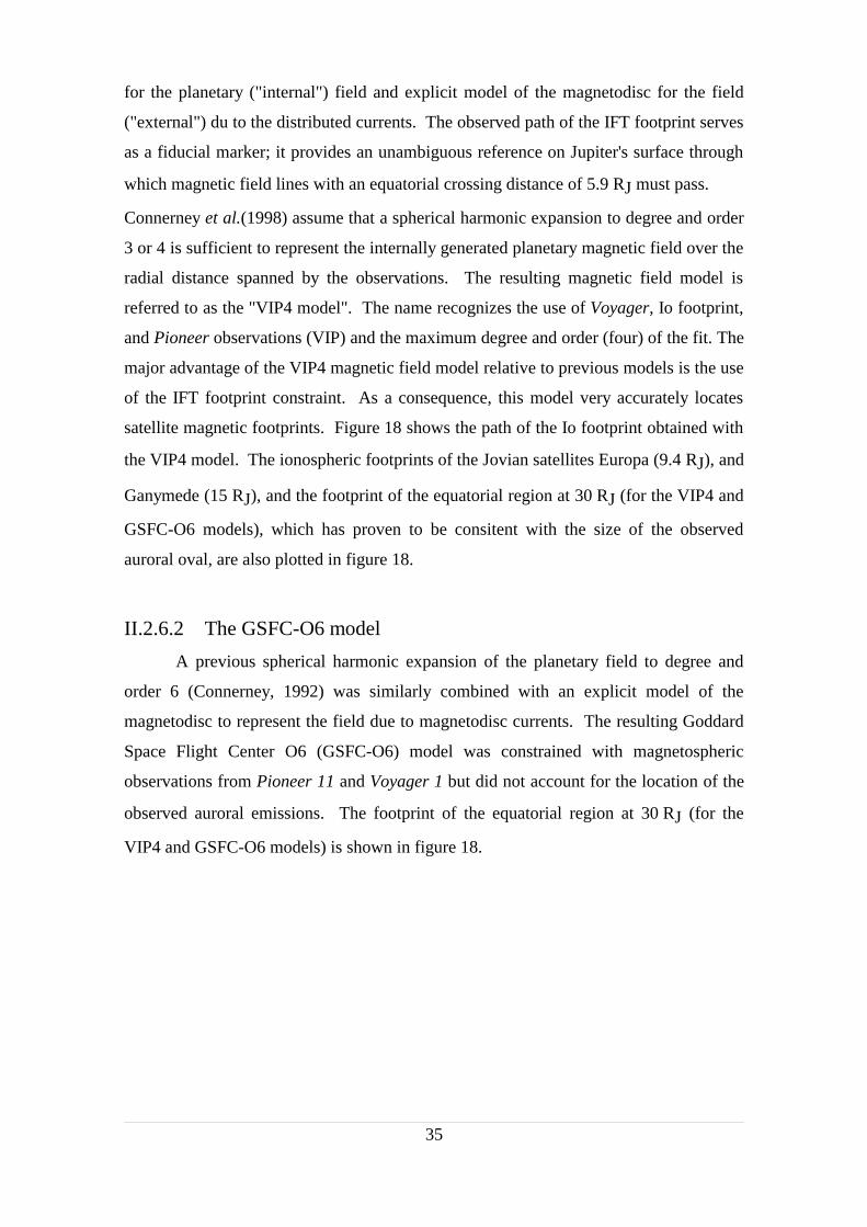
for the planetary ("internal") field and explicit model of the magnetodisc for the field
("external") du to the distributed currents. The observed path of the IFT footprint serves
as a fiducial marker; it provides an unambiguous reference on Jupiter's surface through
which magnetic field lines with an equatorial crossing distance of 5.9 RJ must pass.
Connerney et al.(1998) assume that a spherical harmonic expansion to degree and order
3 or 4 is sufficient to represent the internally generated planetary magnetic field over the
radial distance spanned by the observations. The resulting magnetic field model is
referred to as the "VIP4 model". The name recognizes the use of Voyager, Io footprint,
and Pioneer observations (VIP) and the maximum degree and order (four) of the fit. The
major advantage of the VIP4 magnetic field model relative to previous models is the use
of the IFT footprint constraint. As a consequence, this model very accurately locates
satellite magnetic footprints. Figure 18 shows the path of the Io footprint obtained with
the VIP4 model. The ionospheric footprints of the Jovian satellites Europa (9.4 RJ), and
Ganymede (15 RJ), and the footprint of the equatorial region at 30 RJ (for the VIP4 and
GSFC-O6 models), which has proven to be consitent with the size of the observed
auroral oval, are also plotted in figure 18.
II.2.6.2 The GSFC-O6 model
A previous spherical harmonic expansion of the planetary field to degree and
order 6 (Connerney, 1992) was similarly combined with an explicit model of the
magnetodisc to represent the field due to magnetodisc currents. The resulting Goddard
Space Flight Center O6 (GSFC-O6) model was constrained with magnetospheric
observations from Pioneer 11 and Voyager 1 but did not account for the location of the
observed auroral emissions. The footprint of the equatorial region at 30 RJ (for the
VIP4 and GSFC-O6 models) is shown in figure 18.
35
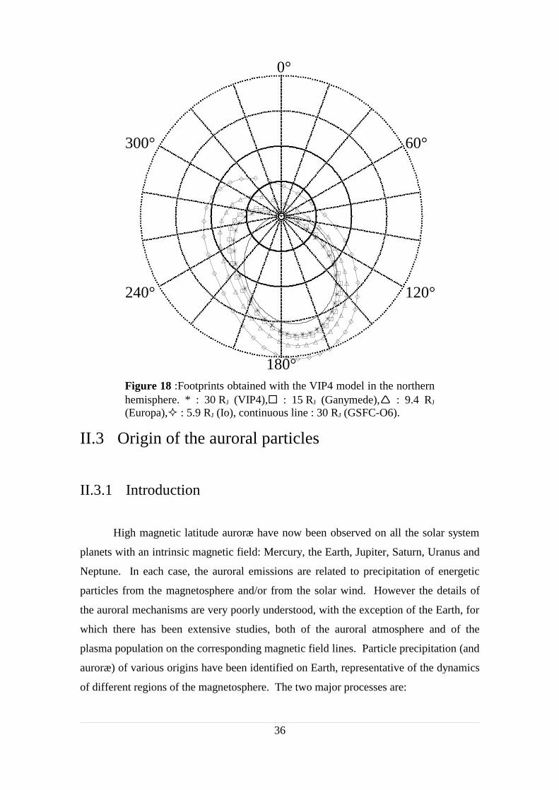
II.3 Origin of the auroral particles
II.3.1 Introduction
High magnetic latitude auroræ have now been observed on all the solar system
planets with an intrinsic magnetic field: Mercury, the Earth, Jupiter, Saturn, Uranus and
Neptune. In each case, the auroral emissions are related to precipitation of energetic
particles from the magnetosphere and/or from the solar wind. However the details of
the auroral mechanisms are very poorly understood, with the exception of the Earth, for
which there has been extensive studies, both of the auroral atmosphere and of the
plasma population on the corresponding magnetic field lines. Particle precipitation (and
auroræ) of various origins have been identified on Earth, representative of the dynamics
of different regions of the magnetosphere. The two major processes are:
36
Figure 18 :Footprints obtained with the VIP4 model in the northernhemisphere. * : 30 RJ (VIP4), : 15 RJ (Ganymede), : 9.4 RJ
(Europa), : 5.9 RJ (Io), continuous line : 30 RJ (GSFC-O6).
180°
240°
300°
0°
60°
120°

1. the diffuse auroral precipitation of energetic particles outside the plasmapause by
wave-particle interaction and pitch-angle diffusion along magnetic field lines,
producing a closed oval of moderate diffuse auroral emission and brightening with
magnetic activity,
2. the impulsive precipitation of particles accelerated along field lines by parallel
potential drops, leading to intense discrete auroral arcs during solar-wind driven
"substorms".
Additional particle precipitation is observed at very high latitudes which results from
mechanisms in the outer magnetosphere, and even from direct entry of solar wind
particles in the cusps.
Similar mechanisms can in principle be expected in all magnetospheres.
Nevertheless, different convection/corotation regimes, solar wind/magnetosphere
coupling and plasma sources, result in different energetic particles dynamic, and are
expected to favor differently one or the other of the precipitation processes at the
various planets. In addition to Earth-like mechanisms, the abundance of hot plasma, the
fast planetary rotation of Jupiter, and even the resulting streched magnetosphere, might
also give rise to instabilities, ultimatly generating field-aligned currents and parallel
particle acceleration in the middle magnetosphere.
II.3.2 Diffuse and discrete auroræ on Earth
The presence of diffuse and discrete auroral structures in the Jovian atmosphere
might be explained by analogy with the theories developed for the corresponding
structures appearing in the Earth aurora (figure 19).
37
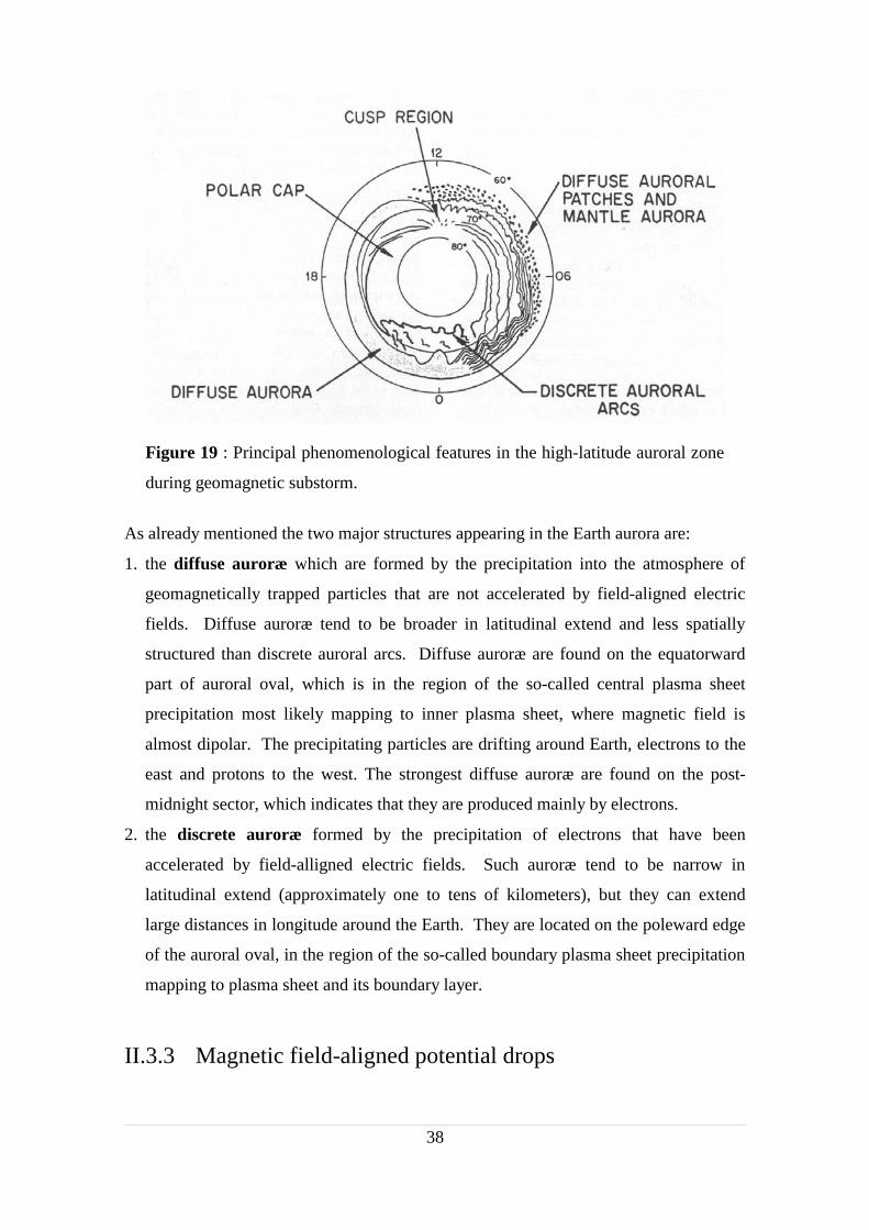
As already mentioned the two major structures appearing in the Earth aurora are:
1. the diffuse auroræ which are formed by the precipitation into the atmosphere of
geomagnetically trapped particles that are not accelerated by field-aligned electric
fields. Diffuse auroræ tend to be broader in latitudinal extend and less spatially
structured than discrete auroral arcs. Diffuse auroræ are found on the equatorward
part of auroral oval, which is in the region of the so-called central plasma sheet
precipitation most likely mapping to inner plasma sheet, where magnetic field is
almost dipolar. The precipitating particles are drifting around Earth, electrons to the
east and protons to the west. The strongest diffuse auroræ are found on the post-
midnight sector, which indicates that they are produced mainly by electrons.
2. the discrete auroræ formed by the precipitation of electrons that have been
accelerated by field-alligned electric fields. Such auroræ tend to be narrow in
latitudinal extend (approximately one to tens of kilometers), but they can extend
large distances in longitude around the Earth. They are located on the poleward edge
of the auroral oval, in the region of the so-called boundary plasma sheet precipitation
mapping to plasma sheet and its boundary layer.
II.3.3 Magnetic field-aligned potential drops
38
Figure 19 : Principal phenomenological features in the high-latitude auroral zone
during geomagnetic substorm.

Observation by low-altitude polar satellites of "inverted V" electron precipitation
events suggests that electric fields parallel to the magnetic field lines (field-aligned
fields or field-aligned potential drops) may occasionally exist on closed field lines in the
Earth magnetosphere. In such an event (figure 20), as the spacecraft crosses high
auroral latitudes, a band of electron precipitation is observed in which the mean energy
rises from ~100 to ~104 eV and then decreases again, forming a spectrogram resembling
an inverted letter V. This is often explained by a field-aligned configuration of electric
equipotentials.
In the simplified discussion of magnetosphere-ionosphere coupling, we treated
magnetic field-lines as perfect conductors (E//=0). However significant potential drops
are observed along auroral zone magnetic field lines. These potential drops usually
occur in regions of strong upward field-aligned current. Downward field-aligned
current can be carried relatively easily by upward flow of ionospheric electrons, which
are available in great numbers and are easy for electric fields to move. However,
upward field-aligned current requires either an upward flow of ionospheric ions, which
is somewhat difficult because of their relatively large mass, or a downward flow of
electrons from the plasma sheet, which can be difficult if the electrodynamically
required current exceeds what can be supplied by electrons in the loss cone. Iindeed the
electrons that are not in the loss cone bounce back and forth between their mirror points,
leading to a zero net current. Only the electrons that are "absorbed" by the atmosphere
39
Figure 20 : Schematic view of the electron spectrum observed
during an inverted V event and its interpretation in terms of E//.
,i.e. the loss cone electrons, can contribute an electric current.
If the field line has difficulty carrying the required amount of upward current, an electric
field is created upward along the field line. The most dramatic effect of these potential
drops is acceleration of downcoming plasma-sheet electrons to energies above those
characteristic of normal plasmasheet. These electrons are responsible for most bright
auroral forms.
According to Lyons (1992) these potential drops could be directly linked to the
magnetospheric convection field. The mapping of the magnetospheric electric field to
the ionosphere gives an electric field reversal in the auroral zones lying near the
ionospheric mapping of the open-closed field line boundary. This electric field reversal
drives ionospheric currents, which leads to magnetic field-aligned currents. A field-
aligned potential difference of 1-10 keV is required to maintain ionospheric current
continuity, and it accelerates electrons downward, toward the atmosphere. The
accelerated electrons impinge upon the atmosphere leading to discrete auroral arcs.
II.3.4 Pitch angle scattering
It has already been mentioned that only particles within the loss cone can
contribute to a field-aligned current, and that auroral emission results from the collisions
of these particles with the atmosphere. The loss cone is very small along auroral
magnetic field lines, so that only a small fraction of the magnetospheric electrons can
contribute to the field-aligned current. However, a field-aligned potential difference that
accelerates particles toward the atmosphere causes the particle v// to increase, which
causes their pitch angle to become more field-aligned. This increases the number of
particles in the loss cone and is called pitch angle scattering.
II.3.4.1 wave-particle interaction
Angular scattering can result from interactions with electromagnetic waves. An
example of which is gyro (or cyclotron) resonance: radiation belt particle spiraling
around a magnetic line of force will gyrate at a rate determined by the magnetic field
strength, mass, and charge of the particle. An electromagnetic wave (with electric and
magnetic vectors) also propagating along that field line will rotate according to its wave
frequency. When both the sense of rotation and the rotation frequency match for both
40

wave and particle, the particle will be subject to an essentially constant "wave" field for
the duration of the encounter. The particle can exchange energy with the wave through
the electrical interaction and/or deflection can occur through the magnetic interaction.
When the particle-wave interaction is primarily occurring via the magnetic wave vector
the result is primarily angular scattering; this is the pure pitch angle scattering limit.
Since the loss cone particles are lost from the radiation belts upon entering the
atmosphere it is clear that interaction between energetic particles and plasma waves can
significantly affect the energy of the trapped particle population and the angular
distribution. When the strong diffusion limit is reached, the scattering mechanism is
faster than the loss mechanism and the particle pitch angle distribution essentially
remains isotropic.
II.3.4.2 The "windshield wiper" effect
In an asymmetric magnetosphere, pitch angle scattering gives rise to the so
called "windshield wiper" effect. In this process, magnetically trapped charged particles
are pitch angle scattered such that their mirror point is above the atmosphere at one
magnetic longitude, but below it at another. If the rate of pitch angle scattering is less
then the time required for the particles to circle the magnetosphere via ∇B drift, then the
particle will drift into a region where it precipitates, and will be lost. If this mechanism
takes place in the Jovian aurora, it woud point to a particle source dominated by
westward drifting electrons (20-30 eV) or by low energy (1 MeV) ions lagging behind
the corotation velocity in the Io torus. The latter of these sources implies the existence
of a secondary enhancement in the vicinity of 0° longitude due to eastward high energy
(≥ 2 - 3 MeV) ion infall. No indication of this secondary enhancement was observed by
Voyager.
The concept of windshield wiper effect was tested by Prangé and Elkamsi (1991)
who modeled the longitudinal distribution of auroral emission produced by particles
azimuthally drifting in the Jovian magnetic field from a longitudinally uniform source.
They predicted the possibility of a maximum in the flux precipitated in the north aurora
due to electrons near λIII = 180°, close to where we observe the western limit of the
discrete structures and a maximum due to ions near λIII = 250°. Prangé and Eikamsi
(1991) also predicted that at high latitudes, the electron precipitation by pitch angle
41

diffusion should occur preferentially in the southern hemisphere, due to the relative
longitudinal variation of the surface magnetic field strengths. In any case, this
mechanism would only generate unstructured emission such as the diffuse aurora
underlying the brighter structures but would not account for the discrete arcs observed
at λIII ≥ 180°.
In contrast, the narrow structure of the auroral arc observed with HST and the presence
of very localized impulsive bright spots are more reminiscent of discrete auroral
emissions triggered by field-aligned potential drops as in Earth’s auroræ.
II.3.5 The Jovian auroral field-aligned currents
The primary source of field-aligned currents at Earth is the solar wind-
magnetosphere interaction. High-latitude current systems result in the imposition of
solar-wind-induced magnetospheric circulation on the ionosphere. In the case of
Jupiter, the much higher rotation speeds than those observed at Earth mean that the
primary source of field-aligned currents is likely to be in the torques associated with the
(partial) imposition of corotation on the magnetospheric plasma. Departures from
corotation on any magnetic shell or set of shells will result in sheets of field-aligned
currents being set up which may be quite localized in the local meridian direction
transverse to the field, but which would vary little in the azimuthal direction. The
resulting magnetic signature consists of gradients in the azimuthal component of the
field (i.e. in the direction of rotation) across the ambient field direction in the meridian.
Such current signatures were detected in the outer Jovian magnetosphere during the
Ulysses flyby of Jupiter in 1992 beyond ~15 RJ and near the magnetopause. In
particular, the Ulysses magnetometer observed changes of magnetic field associated
with sheets of field-aligned currents near 15 and 20 RJ in the dusk sector (Dougherty et
al., 1993). When mapped down along magnetic field lines, these currents were shown
to close along the high latitude auroral arc in the Lyman α images (Prangé et al., 1994).
They were also shown to originate from the boundary between open and closed field
lines (50-60 RJ in the equatorial plane).
42
II.3.6 Evidence of solar wind driven auroras on Jupiter
HST WFPC2 images have demonstrated that the main auroral oval rotates with
the magnetic field, implying that the main aurora maps to the corotating current sheet
and is driven energetically by Jupiter's rotation and plasma processes inside Jupiter's
magnetosphere. It is not known how the solar wind acts to modulate this energy release
in the form of auroral emission. Recent STIS time-tag images have shown that rapid
variations in Jupiter's aurora occur in the polar caps, where dramatic flaring on
timescales of 1-10 s is commonly observed. These transient brightenings map to the
dusk flank of the Jovian magnetotail near the magnetopause boundary (Waite et al.,
1999). The rapid variability of the STIS data suggests that reconnection events triggered
by the passage of the solar wind and its embedded interplanetary magnetic field are the
source of the auroral brightenings. However, this suggestion cannot be verified owing
to the lack of solar wind data near Jupiter. By contrast, all other emissions (including
the main oval and satellite footprint emissions) vary more slowly, on timescales of
minutes to hours. One example is the "equatorward surge" of part of the oval as it
moves from local morning to afternoon (Clarke et al., 1996; Ballester et al., 1996). The
motion appears consistent with the dynamics of Jupiter's corotating magnetospheric
plasma, which is compressed during local morning and expands in local evening. This
may be related to the common appearance of the polar cap emissions, which tend to fill
in the dusk side of the polar cap but not the dawn side. Occasional "dawn storms"
emissions are observed along the main oval near local dawn which can brighten rapidly
(Gérard et al., 1994; Clarke et al., 1998). These emissions remain fixed above magnetic
local dawn, while the rest of the main oval emissions rotate with the planet. Their
origin is not understood but their location fixed above local dawn requires a solar wind
influence on Jupiter's magnetosphere.
The overall variability of Jupiter's aurora is very complex, resulting from the combined
influence of internal, rotationally-driven magnetospheric processes and external, solar
wind-interaction driven processes. While the former dominate magnetospheric
dynamics and energetics, there is an increasing evidence that the solar wind has a
substantial influence on auroral processes.
43
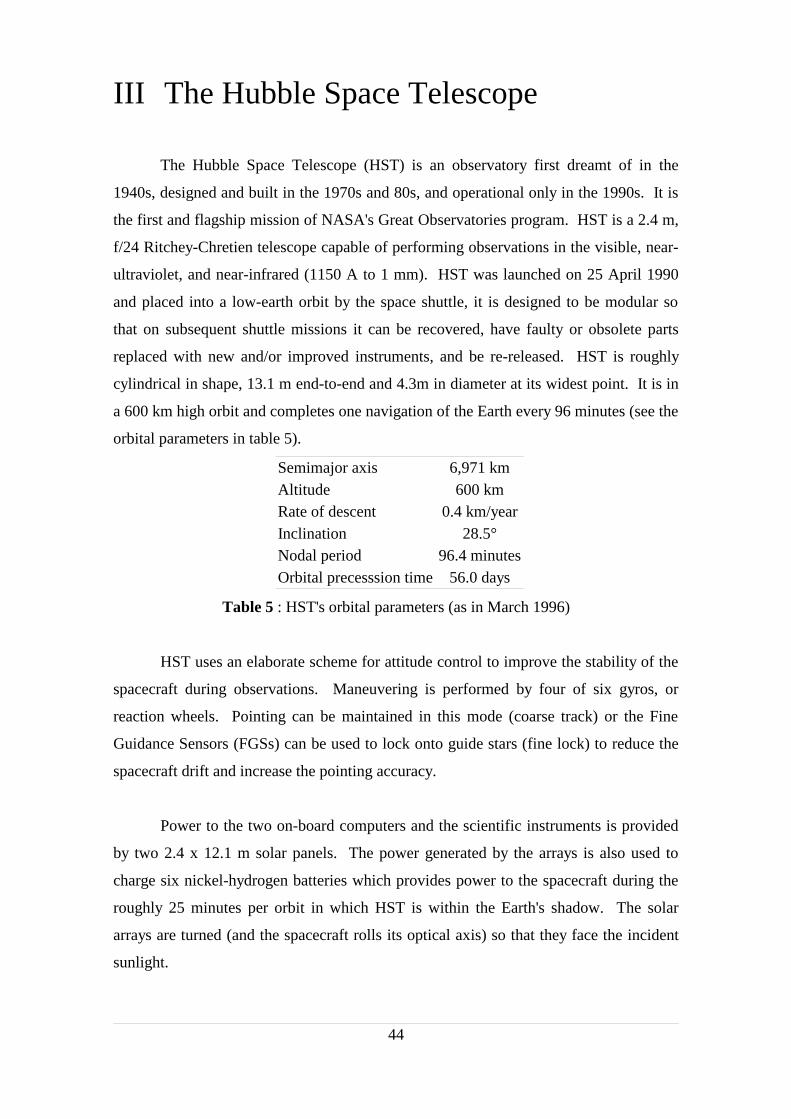
III The Hubble Space Telescope
The Hubble Space Telescope (HST) is an observatory first dreamt of in the
1940s, designed and built in the 1970s and 80s, and operational only in the 1990s. It is
the first and flagship mission of NASA's Great Observatories program. HST is a 2.4 m,
f/24 Ritchey-Chretien telescope capable of performing observations in the visible, near-
ultraviolet, and near-infrared (1150 A to 1 mm). HST was launched on 25 April 1990
and placed into a low-earth orbit by the space shuttle, it is designed to be modular so
that on subsequent shuttle missions it can be recovered, have faulty or obsolete parts
replaced with new and/or improved instruments, and be re-released. HST is roughly
cylindrical in shape, 13.1 m end-to-end and 4.3m in diameter at its widest point. It is in
a 600 km high orbit and completes one navigation of the Earth every 96 minutes (see the
orbital parameters in table 5).
Semimajor axis 6,971 kmAltitude 600 kmRate of descent 0.4 km/yearInclination 28.5°Nodal period 96.4 minutesOrbital precesssion time 56.0 days
Table 5 : HST's orbital parameters (as in March 1996)
HST uses an elaborate scheme for attitude control to improve the stability of the
spacecraft during observations. Maneuvering is performed by four of six gyros, or
reaction wheels. Pointing can be maintained in this mode (coarse track) or the Fine
Guidance Sensors (FGSs) can be used to lock onto guide stars (fine lock) to reduce the
spacecraft drift and increase the pointing accuracy.
Power to the two on-board computers and the scientific instruments is provided
by two 2.4 x 12.1 m solar panels. The power generated by the arrays is also used to
charge six nickel-hydrogen batteries which provides power to the spacecraft during the
roughly 25 minutes per orbit in which HST is within the Earth's shadow. The solar
arrays are turned (and the spacecraft rolls its optical axis) so that they face the incident
sunlight.
44

Communications with the satellite are maintained with the Tracking and Data
Relay Satellites (TDRS) via HST's two high-gain antennas. Observations taken during
the time when neither TDRS is visible from the spacecraft are recorded on tape recorder
and dumped during periods of visibility. The spacecraft also supported real-time
interactions with the ground system during times of TDRS visibility, enabling observers
to make small offsets in the spacecraft pointing to perform their observations.
The mission was troubled soon after launch by the discovery that the primary
mirror was spherically aberrated. In addition, problems with the solar panels flexing as
the spacecraft passed from the Earth's shadow into sunlight caused difficulties with the
pointing stability. Steps were taken to correct these problems, including replacement of
the solar panels, replacement of the Wide Field and Planetary Camera with a second-
generation version with built-in corrective optics, and replacement of the High-Speed
Photometer with COSTAR (Corrective Optics Space Telescope Axial Replacement) to
correct the aberration for the remaining instruments.
As shown in figure 21, HST's scientific instruments are mounted in bays behind
the primary mirror. The Wide Field Planetary Camera 2 occupies one of the radial bays,
with an attached 45 degree pickoff mirror that allows it to receive the on-axis beam.
45
Figure 21 : The Hubble Space Telescope
Three scientific instruments (Faint Object Camera, Near Infrared Camera and Multi-
Object Spectrometer, and Space Telescope Imaging Spectrograph) are mounted in the
axial bays (figure 23) and receive images several arcminutes off-axis. During the
servicing mission in December 1993, the astronauts installed COSTAR in the fourth
axial bay (in place of the High Speed Photometer).
Because the primary mirror has about one-half wave of spherical aberration, the Optical
Telescope Assembly did not achieve its design performance until after the December
1993 servicing mission. Table 6 gives a summary of the optical performance now being
achieved.
Aperture 2.4 mWavelength coverage 1100 Å to 2.6 μmFocal ratio (without COSTAR) f/24Plate scale (on axis without COSTAR) 3.58 arsec/mmFWHM of WFPC2 images (at 6328 Å) 0.053 arcsecWFPC2 encircled energy within
0.1'' radius (at 6328 Å) 55-65%
Table 6 : HST Optical Characteristics and Performance
III.1 The Wide Field and Planetary Camera 2 (WFPC2)
The Wide Field and Planetary Camera 2 (WFPC2) is a two-dimensional imaging
device covering a wavelength range from Lyman-α to about 1 µm. It is HST's only axis
instrument and was built as a replacement for the first Wide Field and Planetary Camera
(WF/PC). It includes built-in correction for the spherical aberration of the HST optical
telescope assembly and was installed in HST during the first servicing mission in
December 1993. The scientific objective of the WFPC2 is to provide photometrically
and geometrically accurate images of astronomical objects over a relatively wide field-
of-view, with high angular resolution across a broad range of wavelengths. The WFPC2
has three "wide-field" charge-coupled devices (CCDs), and one high-resolution (or
"planetary") CCD. Each CCD covers 800 x 800 pixels and is sensitive from 1200 to
11,000 Å. All four CCDs are exposed simultaneously, with the target of interest being
placed as desired within the field-of-view.
46

The three Wide Field Camera (WF1, WF2, WF3) CCDs are arranged in an "L"-
shaped field-of-view (figures 22 and 23) whose long side projects to 2.5', with a
projected pixel size of 0.10". The optics of three of the four cameras are essentially
identical and produce a final focal ratio of f/12.9, each CCD covers a 77''x77'' field-of-
view. The Planetary Camera (PC) CCD has a field-of-view of 35" x 35", a projected
pixel size of 0.0455", and a focal ratio of f/28.3. A total of 48 spectral elements and
polarizers are contained in an assembly of 12 filter wheels which may be inserted into
the optical path.
The Wide Field Camera configuration provides the largest field-of-view
available on HST, but undersamples the cores of stellar images; the Planetary Camera
configuration samples the images better, over its smaller field-of-view.
The Planetary Camera provides a field of view sufficient to obtain full disk images of all
planets except for Jupiter (about a quarter of the disk is imaged in the camera).
However, even with this high resolution camera, the pixels undersample the point
spread function of the telescope and camera optics by a factor of two at 5800 Å. The
WF pixels are over a factor of two larger, and thus undersample the image by a factor of
four at visual wavelengths.
47
Figure 22 : WFPC2 field-of-view projected on
the sky.
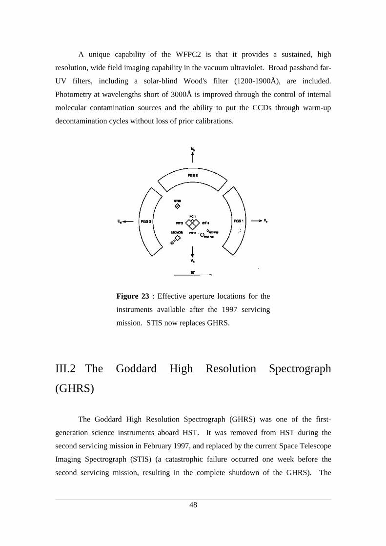
A unique capability of the WFPC2 is that it provides a sustained, high
resolution, wide field imaging capability in the vacuum ultraviolet. Broad passband far-
UV filters, including a solar-blind Wood's filter (1200-1900Å), are included.
Photometry at wavelengths short of 3000Å is improved through the control of internal
molecular contamination sources and the ability to put the CCDs through warm-up
decontamination cycles without loss of prior calibrations.
III.2 The Goddard High Resolution Spectrograph
(GHRS)
The Goddard High Resolution Spectrograph (GHRS) was one of the first-
generation science instruments aboard HST. It was removed from HST during the
second servicing mission in February 1997, and replaced by the current Space Telescope
Imaging Spectrograph (STIS) (a catastrophic failure occurred one week before the
second servicing mission, resulting in the complete shutdown of the GHRS). The
48
Figure 23 : Effective aperture locations for the
instruments available after the 1997 servicing
mission. STIS now replaces GHRS.
GHRS spectrograph was designed to provide a variety of spectral resolutions, high
photometric precision, and excellent sensitivity in the wavelength range 1100 to 3200 Å.
The GHRS was a modified Czerny-Turner spectrograph with two science apertures
(large: LSA, and small: SSA), two photon counting detectors (D1 and D2), several
dispersers, and camera mirrors. There were also a wavelength calibration lamp, flatfield
lamps, and mirrors to acquire and center objects in the observing apertures.
The GHRS was installed as one of the axial scientific instruments (figure 23),
with the entrance aperture adjacent to FGS 2 and FGS 3. With the installation of
COSTAR, the entrance apertures were at the former position of the High Speed
Photometer. The GHRS had two science apertures, designated Large Science Aperture
(LSA or 2.0) and Small Science Aperture (SSA or 0.25). The 2.0 and 0.25 designations
were the pre-COSTAR size of the apertures in arcseconds. The post-COSTAR size of
the LSA was 1.74 arcsec square and the SSA was 0.22 arcsec square. The separation of
the two apertures was approximately 3.7 arcsec on the sky and 1.05 mm on the slit plate.
The dispersers were mounted on a rotating carrousel, together with several plane
mirrors used for acquisition. The first-order gratings were designated as G140L,
G140M, G160M, G200M, and G270M, where "G" indicates a grating, the number
indicates the blaze wavelength (in nm), and the "L" or "M" suffix denotes a "low" or
"medium" resolution grating, respectively. The carrousel also had an echelle grating.
The higher orders were designated as mode Ech-A, and they were imaged onto D1 by
the cross-disperser CD1. The lower orders are designated as mode Ech-B, and they are
directed to D2 by CD2. Detector D1 was solar-blind, that is only far-ultraviolet photons
(1060 to 1800 Å) could be detected. Use of the various gratings or mirrors in concert
with the camera mirrors produced one of three kinds of image at the camera focus: 1) an
image of the entrance aperture, which may be mapped to find and center the object of
interest; 2) a single-order spectrum; or 3) a cross-dispersed, two-dimensional echelle
spectrum.
49

Part 1
IV Simulation of the Morphology of the
Jovian UV North Aurora Observed with the
Hubble Space Telescope
This chapter is a transcription of a paper written by D. Grodent, G.R. Gladstone, J.-C.
Gérard, V. Dols and J.H. Waite and published in Icarus 128, 306-321 (1997)
Abstract
A model simulating Earth views of UV auroral arcs and diffuse emissions in the
Jovian north polar region is described. It assumes a Chapman profile of vertical
brightness distribution and various horizontal structures. Simple geometric cases are
described to illustrate the dependence of the altitude, atmospheric scale height and
central meridian planetary longitude (CML) of an idealized auroral morphology seen
from Earth orbit. The numerical simulation makes it possible to assess the importance
of limb brightening and the contribution from high altitude auroral emission located
behind the planetary limb. As an application of the simulation model, four images
obtained with the Wide Field and Planetary Camera 2 (WFPC2) on board the Hubble
Space Telescope are used to determine the characteristics of their auroral (discrete and
diffuse) structures. The apparent brightness distribution along the arcs may only be
reproduced if intrinsic longitudinal (or local time) variations are introduced, in addition
to the path length effects of the viewing geometry. A composite average auroral
distribution is built by mapping 10 WFPC2 images from the same dataset. It illustrates
the dichotomy frequently observed between a narrow single structure arc at System III
longitudes larger than 180° (or morning sector) and the multiple arc and broad diffuse
50
emission at longitudes less than 180° (or afternoon sector). It is shown that the
equatorial auroral emission boundary is located between the 6 RJ and the 30 RJ magnetic
field line footprints of the Goddard Space flight Center (GSFC) O6 model.
51

IV.1 Introduction
The ultraviolet Jovian aurora was first observed with the ultraviolet spectrometer
(UVS) on board the Voyager 1 and 2 spacecraft (Sandel et al., 1979; Broadfoot et al.,
1979). It is characterized by strong emissions of the 121.6 nm Lyman-α line of atomic
hydrogen and H2 Lyman and Werner bands. A crude description of the morphology of
the auroral emission was obtained by North-South scans of the UVS slit across the
planetary disk (Broadfoot et al., 1981; Herbert et al., 1987). Analysis of these data
concluded that the equatorward boundary of the auroral emission is defined by the
footprint of the Io torus magnetic field lines into the Jovian atmosphere. The existence
of emission at a higher L-values was considered compatible with the observations. No
indication of a local time intensity variation could be deduced from the pre- and post-
encounter sequences of both spacecraft (Herbert et al., 1987). By contrast, a strong
longitudinal dependence of the emission rate was observed and explained in terms of the
"windshield wiper effect".
The main features of the Voyager view of the Jovian morphology were
confirmed with the observations by the International Ultraviolet Explorer (IUE) which
has limited imaging within the aperture. Its spectrograph obtained ultraviolet spectra as
the planet rotated during the exposures (Clarke et al., 1980; Yung et al., 1982;
Livengood et al., 1990). In the northern aurora, a maximum brightness is statistically
observed near System III longitudes λIII = 180°. This conclusion rests on assumptions
concerning the morphology of the emission which was represented by a simple arc with
a defined analytical longitudinal dependence (Livengood et al., 1992).
A new era opened when high resolution ultraviolet images became available
with the Faint Object Camera (FOC) on board the Hubble Space Telescope (HST) (Dols
et al., 1992; Caldwell et al., 1992). These images showed that the auroral emissions do
not exactly follow the footprint of a constant L-shell as represented by the GSFC-O6
model, whose accuracy is on the order of 5 to 10° (Connerney, 1992). Observations at
153 nm (Gérard et al., 1993, 1994a,b) showed the presence of a narrow discrete arc
close to the 30 RJ oval for System III longitudes exceeding ~ 180°. In constrast, a
52
broader diffuse emission region is generally observed at λIII < 180°. It was not possible,
however, to discriminate between a pattern fixed in longitude from a local time
dependent morphology. FOC images at shorter wavelengths (Grodent et al., 1996)
indicated that the equatorward auroral boundary is nearly coincident with the 6 RJ - O6
GSFC auroral oval.
Recently, Jovian auroral images have also been obtained with the second Wide
Field-Planetary Camera (WFPC2) (Clarke et al., 1995, 1996 ; Ballester et al., 1996).
This camera has an increased ultraviolet sensitivity as its Woods filters transmit a much
broader portion of the auroral UV emission. The WFPC2 images limiting sensitivity is
estimated on the order of 10 kiloRayleighs (kR) of total H2 emission (~ 15 kR when the
F130LP blocker is used), to be compared with the > 100 kR threshold of the FOC. As a
consequence, additional weaker structures are seen in the WFPC2 images but they
require a detailed analysis to untangle real brightness variations from purely geometrical
effects, such as limb brightening of structured emitting regions seen from Earth orbit. In
particular, the WFPC2 images show an apparently closed auroral oval, possibly due to
emission originating from behind the limb or diffuse emission inside the polar cap. This
goal may only be reached by using a numerical auroral simulation model.
We first describe the main components and the parameters of the simulation
code. A few selected test cases are then presented and analyzed to describe some of the
characteristics of the apparent brightness variations due to geometric effects. Four
sample individual WFPC2 ultraviolet images of the north Jovian aurora are modelled
using the simulation code. These simulations are used to determine simple discrete or
diffuse structures able to match auroral UV observations from Earth orbit. Finally, a set
of 10 WFPC2 ultraviolet images is used to determine a statistical equatorial boundary of
the emission and derive a statistical picture of the morphology of the north Jovian UV
aurora. It must be stated that these 10 WFPC2 images are taken from the July 1994
dataset, during the period of collision of comet Shoemaker-Levy 9 fragments with
Jupiter. Even though the polar northern aurora looked fainter than usual, there is no
evidence to date that the auroral morphology was biased by the impacts (Clarke et al.,
1995, 1996). Accordingly, the polar auroral morphology deduced from these images
may be considered as typical.
53

IV.2 The auroral simulation model
IV.2.1 Model description
The purpose of these simulations is to visualize an auroral-like emission
distribution on the planet as would be seen from Earth orbit for various possible
geometries. It uses simplified emission structures which, by geometrical effect, are able
to reproduce the main features of the observed auroral emission distribution.
The viewing geometry is defined by the sub-Earth planetocentric latitude, the
sub-Earth System III longitude and the geometrical elements of the planet (polar and
equatorial radii). The main task of the simulation code is to perform a coordinate
system transformation from a general rectangular cartesian coordinate system (x,y,z) to
one or more local coordinate systems (αi,βi,Z) in which auroral characteristics are more
easily described.
Once the viewing geometry parameters have been set, a two-dimensional model image
of the jovian disk seen from Earth orbit is generated. The northern auroral emission
zone is enclosed in a rectangle 90,000 km wide and 18,000 km high (23.9"x4.8" for
Jupiter, 5.2 AU from Earth), approximately centered on the jovicentric north pole ( the
exact location of the center depends on the sub-Earth latitude and the polar radius).
This rectangle is mapped with a 100 by 100 km2 (0.027"x0.027") grid along the x and y
directions. For every point (x,y) of the rectangle, a line of sight (LOS) is defined along
the z direction (normal to the x,y plane) and divided into 100 km segments.
The auroral emission is therefore described on a 3-dimensional cartesian grid where one
point represents the emission from a 100x100x100 km3 cube in the Jovian atmosphere.
It should be noted that the alignment of the lines of sight is an approximation which is
valid for observers far from the planet (e.g. at Earth). Each local coordinate system
(indexed by the subscript i) is based on a reference oval on the jovian surface (figure 24)
defined as the 1 bar pressure level.
54

Figure 24 : Schematic representation of the local coordinates αi, βi and Z
localizing a point P on the surface in the reference oval i. The orientation
parameter of the oval (α0i) is also shown.
An auroral oval is characterized by 5 parameters that define its center, size, and
orientation :
the oval center is located on the jovian surface by its longitude and planetocentric
latitude
the size is defined by its semi-major and semi-minor axes. They are expressed as
spherical distances on the surface.
the orientation is given by the angle (α0i) between the semi-major axis and the
longitude meridian intercepting the center of the oval.
In these local coordinate sets, a position is defined by :
αi : the surface angle between the semi-major axis and the intersection of the LOS
55
βoval iauroral
iαi
α0i
Northern hemisphere
P
Z

point and the jovian surface
βi : the length of the great circle distance between the center of the oval and the
projected point
Z : the altitude of the point, which is measured from the surface along the radial
vector connecting the center of the planet to the position (αi, βi).
The auroral emission is reproduced by the combination of auroral structures
defined in the coordinate systems of these reference ovals (different structures may be
defined from the same oval). Two kinds of auroral brightness distribution structures are
used : arcs and diffuse zones. In the following simulations, we refer to these arcs as
ARC1, ARC2, ARC3, and to the diffuse zones as GLOW1, GLOW2 and GLOW3. The
arcs follow the description of the oval from which they are defined. The brightness
distribution across the arc (the thickness of the arc) can be a boxcar function or a
Gaussian function of the great circle distance βi. In both cases, the function is centered
on the oval and the width is controlled by a single parameter.
The length and the position of an arc along the oval are controlled by two System III
longitudes, (one for the begining, one for the end) which are converted in local
coordinates : αi,start and αi,end. An optional modulation of the auroral brightness
along the arc may be imposed by a sine to the 4th power. This function is applied
between two System III longitudes converted in local coordinates α'i,start and α'i,end.
A filled zone is a region inside the oval which has a uniform horizontal brightness
distribution. It can either fill the inside of a whole oval or be limited by two System III
longitudes converted in local coordinates. In the latter case, the filled region is defined
by the center of the oval and the two local angles α''i,start and α''i,end.
We assume that the H2 auroral vertical emission rate distribution V(Z) can be
approximated by a Chapman profile applied to an isothermal exponential atmosphere :
V Z4 I thin
HexpZZ0
H expexpZZ0
H where Z is the altitude (km) defined in the local coordinate system,
Z0 is the peak altitude (km) of the Chapman profile
56

H is the H2 atmospheric scale height.
Ithin is the vertically observed surface brightness for an optically thin atmosphere,
it is expressed in units of 106 photons cm-2 s-1 ster-1
Integrating the previous equation along altitude gives the normalization relation :
0
V ZdZ4 I thin 106
where 4π Ithin is the brightness expressed in Rayleighs.
The auroral structures are easily parameterized in the ith local coordinate system.
The arcs are formulated by the combination of :
Length of the arc L(αi)
L i1, if i,startii,end
0, else.
Gaussian width G(βi)
G iexp i0i
wi
2
where β0i is the great circle distance of the boundary of the ith oval
βwi is the e-folding half width of the brightness distribution in the direction
perpendicular to the length of the arc
Boxcar width R(βi)
R i1, if 0iwi
2 i0iwi
2 0, else.
57

where βwi is the width of the brightness distribution in the direction perpendicular to
the length of the arc.
Enhancement function E(αi) (intensification zone)
E i12sin4ialpha'i,end
'i,end 'i,start , if 'i,starti 'i,end
1, else. with these notations, any arc segment brightness distribution may be written as
Si i ,i, ZV ZL iG i
R iE i
where the braces allow selection of either a Gaussian or a boxcar shape and the brackets
indicate that the enhancement is optional.
Similarly, the filled zones can be formulated with a single function F(αi,βi)
Fi, i1, if ''i,starti ''i,endi i0
0, else.
This diffuse zone is called GLOW2. If it fills the entire polar cap (α''i,start = α''i,end) then it
is called GLOW1. As will be illustrated in the image simulations, it is usefull to define
a modulation of the poleward boundary of a diffuse zone. This modulation gives rise to
a moon quarter shape diffuse zone (GLOW3). It is imposed by a relation of the form :
Ki, i1, if i sin i '''i,end
'''i,end '''i,startconstant
and '''i,endi '''i,end
0,else.
Therefore a filled zone brightness distribution is given by :
58

Si i, i, ZV ZFi, iKi, i
the brackets indicate that the poleward boundary is optional. Accordingly, the auroral
volume emission rate associated with any (x,y,z) point can be written as
A x,y,z i
si Sii x,y,z ,i x,y,z ,Z x,y,z
where si is a weighting factor controling the contribution of the different auroral
structures at the point considered. The integration along a line of sight (z direction)
gives the simulated auroral brightness at the (x,y) position of the jovian disk image as
seen from Earth orbit. This integration is numerically achieved by a step summation
along the z axis :
Br x,yz
A x,y,z j z,
where Δz is the length element along the line of sight.
IV.2.2 Limb brightening estimate
Observations of auroral emission on Earth as well on Jupiter indicate that limb
brightening is an important factor which affects the apparent brightness of both discrete
and diffuse emissions. It is therefore of prime importance to estimate the expected
brightness limb enhancement, using an analytical approach applied to a simple case.
This evaluation is also useful as a comparison to the results of the more sophisticated
model described previously.
The expected ratio of the limb to CML brightness at 70° of latitude for an aurora
uniformly covering the surface of a spherical planet can be estimated from the Chapman
function (which should not be confused with the Chapman profile used in the previous
section). This function gives the ratio of the slant column emission rate to the vertical
column emission rate line. Since the latter integral is given, in any case, by the
normalization relation (equ. 2), the limb brightening factor is given by the ratio of the
59
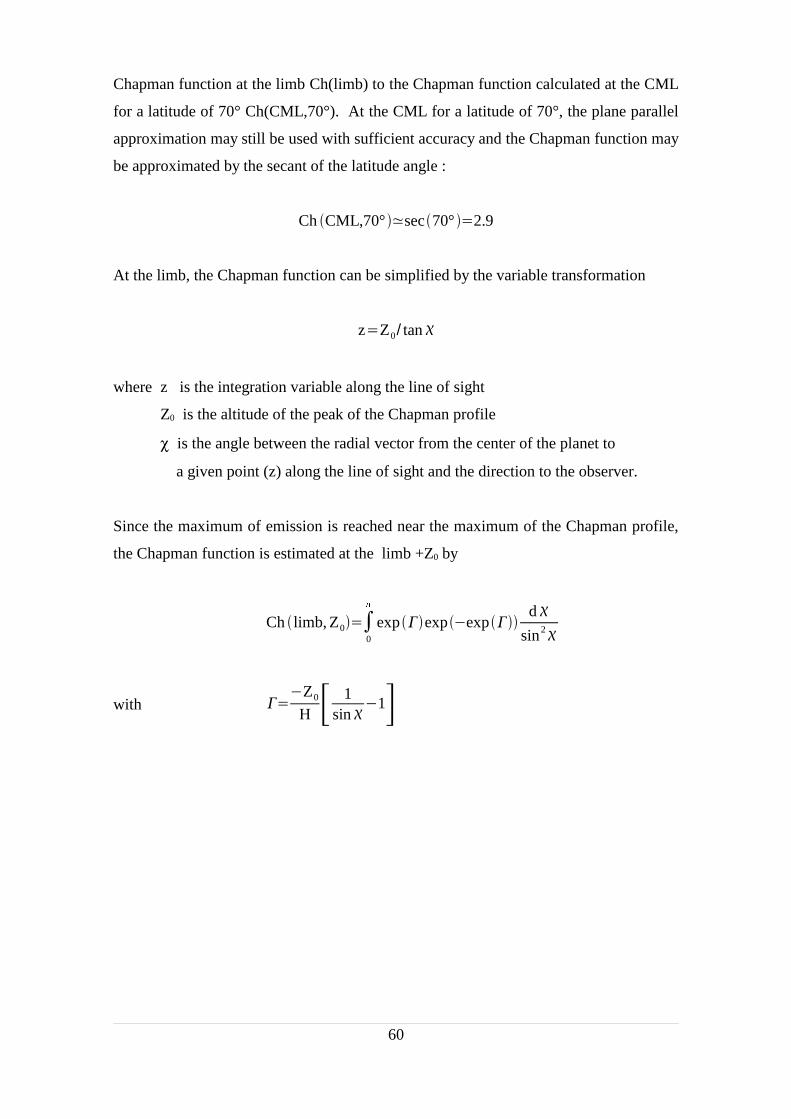
Chapman function at the limb Ch(limb) to the Chapman function calculated at the CML
for a latitude of 70° Ch(CML,70°). At the CML for a latitude of 70°, the plane parallel
approximation may still be used with sufficient accuracy and the Chapman function may
be approximated by the secant of the latitude angle :
Ch CML,70°sec70° 2.9
At the limb, the Chapman function can be simplified by the variable transformation
zZ0 tan
where z is the integration variable along the line of sight
Z0 is the altitude of the peak of the Chapman profile
χ is the angle between the radial vector from the center of the planet to
a given point (z) along the line of sight and the direction to the observer.
Since the maximum of emission is reached near the maximum of the Chapman profile,
the Chapman function is estimated at the limb +Z0 by
Ch limb, Z00
exp expexpd
sin2
with Z0
H 1sin
1
60
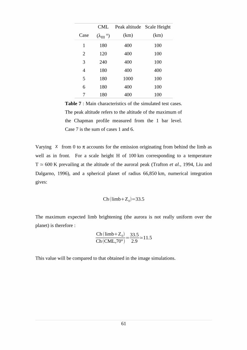
CML Peak altitude Scale Height
Case (λIII °) (km) (km)
1 180 400 100
2 120 400 100
3 240 400 100
4 180 400 400
5 180 1000 100
6 180 400 100
7 180 400 100
Table 7 : Main characteristics of the simulated test cases.
The peak altitude refers to the altitude of the maximum of
the Chapman profile measured from the 1 bar level.
Case 7 is the sum of cases 1 and 6.
Varying from 0 to π accounts for the emission originating from behind the limb as
well as in front. For a scale height H of 100 km corresponding to a temperature
T 600 K prevailing at the altitude of the auroral peak (Trafton et al., 1994, Liu and
Dalgarno, 1996), and a spherical planet of radius 66,850 km, numerical integration
gives:
Ch limbZ033.5
The maximum expected limb brightening (the aurora is not really uniform over the
planet) is therefore :
Ch limbZ0
Ch CML,70°
33.52.9
11.5
This value will be compared to that obtained in the image simulations.
61
IV.3 Simulation of simple test cases
In order to assess the influence of the geometrical features of the auroral
morphology on the limb brightening effect, we have simulated a simple realistic
northern jovian auroral oval in seven different configurations. In each case, the sub-
Earth latitude is 3° S and the polar and equatorial radii are 66,854 km and 71,492 km,
respectively. The parameters of the oval used in this section correspond to the fit of the
equatorial auroral boundary that will be discussed in the statistical equatorial boundary
oval section. The arc has a 1° wide boxcar shape along the local coordinate βi. The
other parameters (CML, peak altitude of the Chapman profile and scale height) are
listed in table 7.
In test case 1, (figure 25.1) the peak altitude of the Chapman profile is set to
400 km and the scale height is 100 km. With these realistic values and a CML of 180°,
the maxima of limb brightening appear close to the dawn and dusk limbs, well inside
the planetary disk. Indeed, only a fraction of the auroral emission originating from
behind the planet exceeds the critical altitude to stand above the planetary limb. The
brightness ratio between the Earth facing section of the oval at the CML and the
maximum brightness is on the order of 5.
Test cases 2 and 3 (figure 25.2 and 25.3) present the same oval as in case 1 with
different CMLs (120° and 240°, respectively). The maxima still appear near the ansae
of the oval. Two features are readily observed :
1. the oval appears as an incomplete structure. The section of the oval around
midnight is obscured by the planetary disk. This is because the emission from
behind the planet is not located high enough for the considered viewing geometry
(in particular the planet's tilt angle from the observer) and the parameters of the
oval.
2. the overall shapes of these two cases are very different : with its larger CML, case
3 shows a longer Earth facing section of the oval. This is due to the orientation of
the major-axis of the oval. Had this axis been aligned along a meridian, cases 2
and 3 would have produced two symetrical images.
62
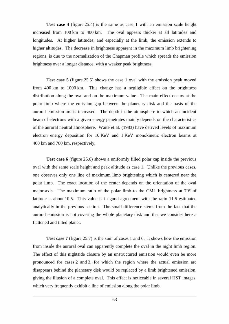
Test case 4 (figure 25.4) is the same as case 1 with an emission scale height
increased from 100 km to 400 km. The oval appears thicker at all latitudes and
longitudes. At higher latitudes, and especially at the limb, the emission extends to
higher altitudes. The decrease in brightness apparent in the maximum limb brightening
regions, is due to the normalization of the Chapman profile which spreads the emission
brightness over a longer distance, with a weaker peak brightness.
Test case 5 (figure 25.5) shows the case 1 oval with the emission peak moved
from 400 km to 1000 km. This change has a negligible effect on the brightness
distribution along the oval and on the maximum value. The main effect occurs at the
polar limb where the emission gap between the planetary disk and the basis of the
auroral emission arc is increased. The depth in the atmosphere to which an incident
beam of electrons with a given energy penetrates mainly depends on the characteristics
of the auroral neutral atmosphere. Waite et al. (1983) have derived levels of maximum
electron energy deposition for 10 KeV and 1 KeV monokinetic electron beams at
400 km and 700 km, respectively.
Test case 6 (figure 25.6) shows a uniformly filled polar cap inside the previous
oval with the same scale height and peak altitude as case 1. Unlike the previous cases,
one observes only one line of maximum limb brightening which is centered near the
polar limb. The exact location of the center depends on the orientation of the oval
major-axis. The maximum ratio of the polar limb to the CML brightness at 70° of
latitude is about 10.5. This value is in good agreement with the ratio 11.5 estimated
analytically in the previous section. The small difference stems from the fact that the
auroral emission is not covering the whole planetary disk and that we consider here a
flattened and tilted planet.
Test case 7 (figure 25.7) is the sum of cases 1 and 6. It shows how the emission
from inside the auroral oval can apparently complete the oval in the night limb region.
The effect of this nightside closure by an unstructured emission would even be more
pronounced for cases 2 and 3, for which the region where the actual emission arc
disappears behind the planetary disk would be replaced by a limb brightened emission,
giving the illusion of a complete oval. This effect is noticeable in several HST images,
which very frequently exhibit a line of emission along the polar limb.
63

IV.4 Auroral image simulations
This work is organized as a global approach of the auroral morphology
simulation which consists in determining the most likely simple geometrical structures
which are able to simulate the main auroral features observed with the WFPC2 camera.
It is clear that with such simple structures, the simulation code cannot reproduce each
pixel of the observed image. An inverse method like the one presented by Satoh et al.
(1996) for the infrared H3+ aurora is not applicable here since the signal to noise ratio is
too low for most pixels and our dataset is too restricted in longitudinal range. In
addition, it is not possible to analyze the available UV images as a unique set of
homogeneous observations, since the UV aurora exhibits temporal variations on a time
scale of about 10 minutes and more (Gérard et al., , 1993, 1994a; Ballester et al., 1996).
We therefore use a direct method to visually adjust the parameters of the simulation for
one image at the time.
Ovals are defined with the 5 parameters described in Section 2.1 which we
compare with the observed image. The parameters are adjusted until an oval intercepts
the central part and/or the brightest pixels of an auroral feature, or the equatorward limit
of a diffuse emission zone. The analytical representation of the oval determined this
way is not unique as more than one oval may meet the adjustment. In many cases, more
than one structure can reproduce the same auroral feature, especially when the signal to
noise ratio of the pixels defining a feature is low. In any case, this approach is useful to
determine and test the most likely structures able to reproduce the main observed auroral
features.
IV.4.1 The WFPC2 dataset
The images of Jupiter's ultraviolet aurora used in this work have been selected in
a dataset of HST observations obtained in July 1994, at the time of the impact of comet
Shoemaker-Levy 9 (SL9) with Jupiter (Clarke et al., 1994) and in March 1995. These
images consist of exposures with the wide field CCD detector #3 and #4 of the WFPC2
instrument, providing a 800 x 800 pixel format with a pixel size of 0.10" x 0.10" at the
center of the CCD. At the distance of Jupiter, a pixel represents a distance of 350 km on
64

Jupiter projected area in July 1994 and 380 km in March 1995. For CCD #4, the
F160BW (1150 to 2100 Å) filter was used to isolate the H2 Lyman and Werner bands
UV emission. For CCD #3 the same bandpass is isolated with the partially rotated filter
position F160BN15. In both cases, the filter is crossed with the F130LP blocker to filter
out the emissions below ~1230 Å, including the H Lyman-α emission which may
introduce morphological differences.
The effects of methane absorption have been neglected as less than 20% of the total H2
emission transmitted by the filter set is absorbed by CH4. Table 8 lists the dates, times,
durations, central meridian longitudes and identifications of the 11 images used in this
paper. As part of the standard data processing, the images were field flattened after
correction of the bias level and dark frames. In these images, Jupiter was targeted to
display the northern auroral region near the center of the chip, where the geometric
distorsion is on the order of a few tenths of a pixel. A correction was applied to remove
this geometric distortion and the shift introduced by the MgF2 field flattener on the CCD
detector (Gilmozzi et al., 1995; Holtzman et al., 1995; E. Kinney, pers. Comm. 1995).
We used a limb fitting method similar to that described by Clarke et al. (1995), its
accuracy is better than 2 pixels. The inaccuracy introduced by the WFPC2 (WF) point
spread function is on the order of 1 to 2 pixels, resulting in a cumulated positional
systematic inaccuracy of 2 to 3 pixels. The traces of the cosmic rays have been removed
for presentation. Their intensity has been interpolated from nearby pixels.
IV.4.2 Simulation of observed images
In this section, we describe the simulation of four observed auroral images.
Three of them belong to the July 1994 dataset while the fourth image is extracted from
the recently available set of WFPC2 images obtained in March 1995. This latter image
belongs to the set of images recently described by Clarke et al. (1996) and was used by
these authors to define a reference auroral oval. In each simulation, the smearing effect
due to the rotation of the auroral region with the planet during the exposure depends,
among other parameters, upon the mean central longitude, the size and the orientation of
the auroral structures. Its effect is approximately reproduced by imposing different
Gaussian-shaped widths to the arcs of oval, instead of a single boxcar shape. The
smoothing effect of the WFPC2 point spread function (PSF) has been reproduced by
65

convolving the simulated images by a model PSF kernel determined at 2000 Å,
accounting for the observed wavefront and the pixel response function (Burrows et al.,
1995). Its effect is individually discussed for each simulation. In the following
description, the default value for the peak altitude of the Chapman profile (refered in the
text as the altitude of the emission) is set to 400 km above the NH3 clouds top, that is at
an altitude nearly coincident with the altitude of the unit tangential optical depth for
CH4 absorption (i.e. The methane homopause). The default value of the scale height is
set to 100 km. The various structures (arcs and zones) are represented in figure 27 in an
equidistant polar projection. The relative brightness of each structure and its variation
along the arc are represented in an overlaid box.
66

67
Figure 25 : Simulation of simple test cases (see table 7). Parallels of
planetocentric latitudes are drawn every10°. Local time longitudes,
measured from the CML, increase by 20° increments.
2
3
5
6
7
1
4

IV.4.2.1 Image 0503
This first image, obtained in March 1995 (figure 27.A), shows an apparently
simple geometry which comes down to a single auroral oval. Figure 26.A shows a
simulation obtained with one single oval. The brightness distribution is uniform along
the oval and with a Gaussian-shape across it. The comparison with the observed image
(figure 27.A) clearly shows that this simple brightness distribution cannot reproduce the
observation. The locations of the morning and evening limbs brightening are different
from the observation. In addition, the observation shows that the front section of the
oval is brighter than the rear section, that is the opposite of what is expected from the
limb brightning effect. Three phenomena could explain this behavior : 1) a brightness
weakening of the rear section of the oval, 2) a fraction of the emission arising from the
section of the oval near 0° could be occulted by the planetary disk, 3) the limb
brightening of a diffuse zone is sufficient to apparently close the limb section of the
oval, without the presence of an arc near the limb. This third possibility seems the most
likely since a weak glow emission is indeed observed in the polar cap.
The fact that the positions of the maxima at the morning and evening limbs of the
simulated image do not correspond to the observed positions and the presence of bright
localized zones along the front section of the oval can only be simulated by intrinsic
brightness variations along the arc. Figure 26.B illustrates two major effects of the point
spread function of the WFPC2 camera on the single oval simulation.
The spread of the thin limb brightened line along the limb conspicuously shows the
dilution effect of the PSF. This dilution reduces the maximum brightness value in this
region by a factor 2. A less pronounced effect of the PSF is the slight shift equatorward
of the position of the brightness maxima at the morning and evening limb. Figure 27.B
shows the final simulation of the observed image.
We will now describe and discuss the different structures that we added to and/or
removed from the original single oval in order to reproduce the main auroral features of
figure 27.A.
68

ID date UT exposure mean CML (mm/dd/yy) (hh:mm) time (s) (System III)
0E01 07/17/94 09:06:00 700 193° 0j01 07/17/94 18:56:00 400 186° 0s01 07/18/94 13:55:00 700 158° 0y01 07/19/94 11:07:00 400 205° 1501 07/20/94 14:10:00 400 107°
1502 07/20/94 14:19:00 400 112°
1701 07/20/94 16:12:00 400 180° 1b01 07/21/94 08:09:00 400 39° 1f01 07/21/94 13:01:00 400 215° 1p01 07/22/94 09:54:00 400 253°
0503 03/06/95 20:33:00 600 211°
Table 8 : Main characteristics of the WFPC2 images used in this work. All
the images were acquired in July 1994 with the F160BW + F130LP filter
set, excepted 0503 which was taken in March 1995 with the F160BN15 +
F130LP filter set. The bold IDs show the 4 images selected for the
simulations. The ID names are extracted from the full HST archive file
names.
1. In the simulation, the rear section is closed by a diffuse zone uniformely filling the
inside of the oval. As already discussed, the presence of an arc in this sector is not
required since the limb brightening of the diffuse zone, which we call GLOW1,
gives an apparent closing with a pronounced line of maximum brightness above
the limb, at an altitude close to the peak of the Chapman profile. The PSF dilutes
this bright emission line, but its trace is still visible. Such a trace is not clearly
seen on the observed image. This could mean that the diffuse emission GLOW1
is not peaked like a Chapman layer with a well defined maximum altitude, but
would spread in altitude according to a distribution flatter than the Chapman
profile. Another reason could stem from the large inhomogeneity of the diffuse
emission filling the observed oval which appears to include many faint pixels
spots rather than a uniformely filled zone.
69

2. Another diffuse emission (not simulated) appears at the left side of the bright
morning arc. This feature could be reproduced by a faint localized glow region
which is revealed by limb brightening. The shape of the diffuse region which
produces this emission is hardly determined. In any case, as shown by
figure 27.B, it cannot result from the effect of the PSF on the bright morning
emission.
3. An arc of oval (ARC3, plotted in red in figure 27.C) defined between 225° and
250° can simulate the morphology of the bright morning feature. However, as
already mentioned, the observed maximum brightness of this feature does not
coincide with the position of the maximum of the limb brightening which is
therefore closer to the limb. A shift of the position of the brightness maximum
requires the presence of an intrinsic brightening effect along ARC3. The shift is
reproduced by using an intensification zone (defined in the model description
section) centered on the position of the observed brightness maximum, that is
between 220° and 250°. The relative brightness distribution of ARC3 is
represented in red in the overlaid bar-plot of figure 27.C. In this bar-plot, the
rectangular base represents the brightness of the arc without intensification and the
top Gaussian-like shape represents the effect of the intrinsic intensification with a
peak value 3 times the base brightness of ARC3. In the polar plot, the
intensification zone is materialized by a black curve inside the arc.
4. Another intensification zone between 180° and 230° has to be used to reproduce
70
Figure 26 : (A) Localization of the maxima and (B) effect of the PSF on a
single auroral oval defined from image 0503.
A
B with PSF

the brightness distribution of ARC2 : the arc of oval defined between 190° and
225° on the same oval than ARC3. It is represented in yellow in figure 27.C.
Once more, this intensification is clearly independent of the limb brightening and
reveals an intrinsic brightness variation along the arc. Another possible
interpretation of the brightness distribution of ARC2 could be a weakening of the
brightness at the edges of the arc rather than an intensification around the center of
ARC2. Its relative brightness is represented in figure 27.C by the yellow bar and
the effect of the intrinsic intensification is represented by plotting a Gaussian-like
shape above the bar.
5. The long arc of oval ARC1 defined on the same oval than ARC2 and ARC3
between 125° and 190° (the green arc and the green bar with its intensification in
figure 27.C) is a bit more complex. The brightness intensification between 140°
and 195° cannot be explained by a limb brightening effect and we use an intrinsic
intensification zone to simulate it. By contrast, the brightness of the section of
ARC1 between 125° and 140° is solely due to the limb brightening effect. It
should be noted that this latter section of ARC1 might as well be reproduced by
the limb brightening of a localized accumulation of diffuse emission. However,
the continuity of the brightness distribution along the whole bright feature favors
the idea of a long arc of oval.
6. The effect of the PSF on the limb brightened section of ARC1 cannot by itself
reproduce the small discontinuity in the emission altitude observed at the limb,
just above the low longitude end of ARC1. In order to account for this
discontinuity, the peak altitude of the Chapman profile of ARC1 was set to
600 km and the scale height was set to 200 km.
7. As for ARC3, the effect of the PSF on ARC1 is not sufficient to reproduce the
equatorward diffuse emission below ARC1. A low latitude localized diffuse
emission (not simulated here) would therefore be required.
The detailed analysis of this image with the Earth-viewing geometry code
indicates that, within individual structures, intrinsic variations are present along the arcs
which cannot be ascribed to geometric effects. It is also possible to explain the apparent
closing of the oval behind the polar cap by limb brightening of a high altitude weak
diffuse emisison not observable elsewhere.
71
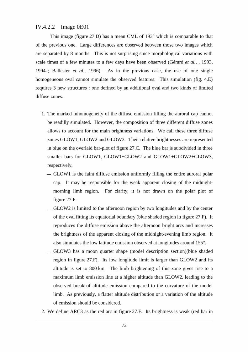
IV.4.2.2 Image 0E01
This image (figure 27.D) has a mean CML of 193° which is comparable to that
of the previous one. Large differences are observed between those two images which
are separated by 8 months. This is not surprising since morphological variations with
scale times of a few minutes to a few days have been observed (Gérard et al., , 1993,
1994a; Ballester et al., 1996). As in the previous case, the use of one single
homogeneous oval cannot simulate the observed features. This simulation (fig. 4.E)
requires 3 new structures : one defined by an additional oval and two kinds of limited
diffuse zones.
1. The marked inhomogeneity of the diffuse emission filling the auroral cap cannot
be readilly simulated. However, the composition of three different diffuse zones
allows to account for the main brightness variations. We call these three diffuse
zones GLOW1, GLOW2 and GLOW3. Their relative brightnesses are represented
in blue on the overlaid bar-plot of figure 27.C. The blue bar is subdivided in three
smaller bars for GLOW1, GLOW1+GLOW2 and GLOW1+GLOW2+GLOW3,
respectively.
GLOW1 is the faint diffuse emission uniformly filling the entire auroral polar
cap. It may be responsible for the weak apparent closing of the midnight-
morning limb region. For clarity, it is not drawn on the polar plot of
figure 27.F.
GLOW2 is limited to the afternoon region by two longitudes and by the center
of the oval fitting its equatorial boundary (blue shaded region in figure 27.F). It
reproduces the diffuse emission above the afternoon bright arcs and increases
the brightness of the apparent closing of the midnight-evening limb region. It
also simulates the low latitude emission observed at longitudes around 155°.
GLOW3 has a moon quarter shape (model description section)(blue shaded
region in figure 27.F). Its low longitude limit is larger than GLOW2 and its
altitude is set to 800 km. The limb brightening of this zone gives rise to a
maximum limb emission line at a higher altitude than GLOW2, leading to the
observed break of altitude emission compared to the curvature of the model
limb. As previously, a flatter altitude distribution or a variation of the altitude
of emission should be considered.
2. We define ARC3 as the red arc in figure 27.F. Its brightness is weak (red bar in
72

bar-plot of figure 27.F) and no intensification had to be used in the simulation.
The extension of this arc to longitudes close to 180° reproduces the observed
closing of the equatorward Earth facing section of the aurora.
3. The afternoon region of the aurora shows a fork-like bright feature that we
attributed to the crossing of two arcs of oval, ARC1 and ARC2, that are defined
on different ovals and represented in figure 27.F by the green and yellow arcs and
bars, respectively. The equatorward arc, ARC1, bears an intrinsic intensification
zone. It is much shorter than its counterpart in the previous simulation as no
bright feature appears in the evening region of the aurora. The poleward arc,
ARC2, also requires an intensification zone in order to simulate the observed
brightness enhancement which is not simulated by the addition of the two arcs in
this region. This set of arcs reasonably simulates the observed fork-like feature
but it is clear that it is only one of the many possible structures able to match the
observation.
4. The low longitude ends of ARC1 and ARC2 are not straightfully determined
because inhomogeneities observed in the evening diffuse region tend to form a
structured emission. This structuring phenomenon is best observed in the next
image.
IV.4.2.3 Image 1701
With a mean CML close to 180°, much of the auroral region is visible from
Earth orbit. This image (figure 27.G) was taken 3 days after the previous one and shows
morphological variations, some of which might be attributed to the temporal variability
of the Jovian aurora. The most striking difference is the disappearance of the fork-like
afternoon bright feature which is replaced by two individual bright structures that we
have simulated (figure 27.H) with a 2 distinct arcs.
73
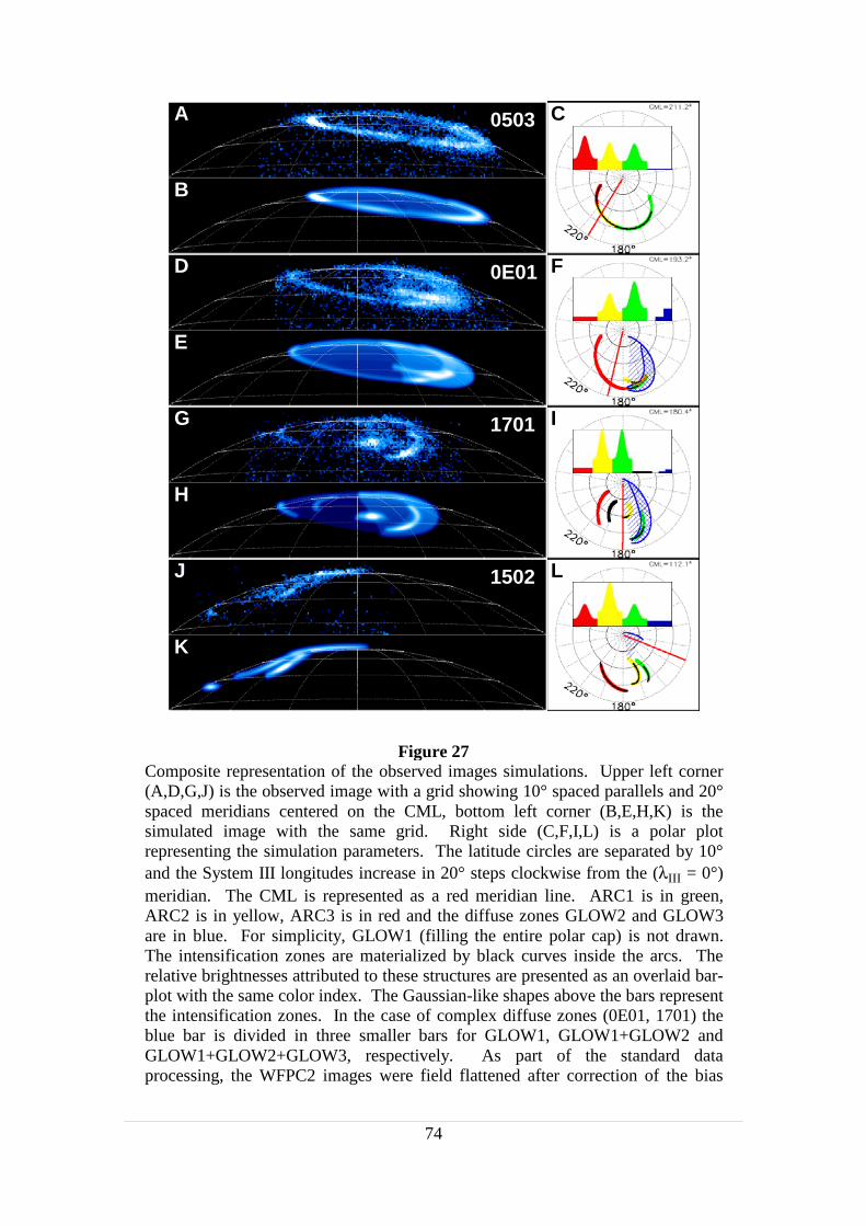
Composite representation of the observed images simulations. Upper left corner(A,D,G,J) is the observed image with a grid showing 10° spaced parallels and 20°spaced meridians centered on the CML, bottom left corner (B,E,H,K) is thesimulated image with the same grid. Right side (C,F,I,L) is a polar plotrepresenting the simulation parameters. The latitude circles are separated by 10°and the System III longitudes increase in 20° steps clockwise from the (λIII = 0°)meridian. The CML is represented as a red meridian line. ARC1 is in green,ARC2 is in yellow, ARC3 is in red and the diffuse zones GLOW2 and GLOW3are in blue. For simplicity, GLOW1 (filling the entire polar cap) is not drawn.The intensification zones are materialized by black curves inside the arcs. Therelative brightnesses attributed to these structures are presented as an overlaid bar-plot with the same color index. The Gaussian-like shapes above the bars representthe intensification zones. In the case of complex diffuse zones (0E01, 1701) theblue bar is divided in three smaller bars for GLOW1, GLOW1+GLOW2 andGLOW1+GLOW2+GLOW3, respectively. As part of the standard dataprocessing, the WFPC2 images were field flattened after correction of the bias
74
Figure 27
0E01
1701
1502
0503A
D
G
J
B
E
H
K
C
F
I
L
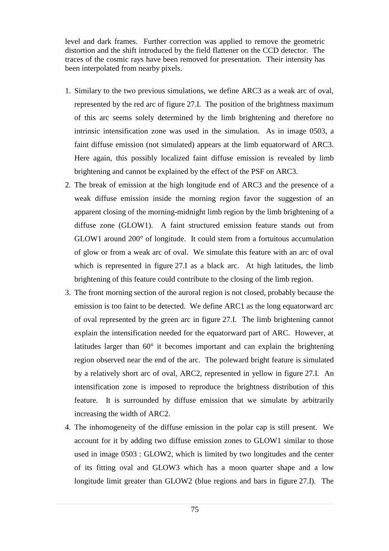
level and dark frames. Further correction was applied to remove the geometricdistortion and the shift introduced by the field flattener on the CCD detector. Thetraces of the cosmic rays have been removed for presentation. Their intensity hasbeen interpolated from nearby pixels.
1. Similary to the two previous simulations, we define ARC3 as a weak arc of oval,
represented by the red arc of figure 27.I. The position of the brightness maximum
of this arc seems solely determined by the limb brightening and therefore no
intrinsic intensification zone was used in the simulation. As in image 0503, a
faint diffuse emission (not simulated) appears at the limb equatorward of ARC3.
Here again, this possibly localized faint diffuse emission is revealed by limb
brightening and cannot be explained by the effect of the PSF on ARC3.
2. The break of emission at the high longitude end of ARC3 and the presence of a
weak diffuse emission inside the morning region favor the suggestion of an
apparent closing of the morning-midnight limb region by the limb brightening of a
diffuse zone (GLOW1). A faint structured emission feature stands out from
GLOW1 around 200° of longitude. It could stem from a fortuitous accumulation
of glow or from a weak arc of oval. We simulate this feature with an arc of oval
which is represented in figure 27.I as a black arc. At high latitudes, the limb
brightening of this feature could contribute to the closing of the limb region.
3. The front morning section of the auroral region is not closed, probably because the
emission is too faint to be detected. We define ARC1 as the long equatorward arc
of oval represented by the green arc in figure 27.I. The limb brightening cannot
explain the intensification needed for the equatorward part of ARC. However, at
latitudes larger than 60° it becomes important and can explain the brightening
region observed near the end of the arc. The poleward bright feature is simulated
by a relatively short arc of oval, ARC2, represented in yellow in figure 27.I. An
intensification zone is imposed to reproduce the brightness distribution of this
feature. It is surrounded by diffuse emission that we simulate by arbitrarily
increasing the width of ARC2.
4. The inhomogeneity of the diffuse emission in the polar cap is still present. We
account for it by adding two diffuse emission zones to GLOW1 similar to those
used in image 0503 : GLOW2, which is limited by two longitudes and the center
of its fitting oval and GLOW3 which has a moon quarter shape and a low
longitude limit greater than GLOW2 (blue regions and bars in figure 27.I). The
75

altitude of emission of GLOW2 is 400 km and the altitude of GLOW3 is set to
800 km. Both diffuse emissions are responsible for the apparent closing of the
midnight-evening limb region and for the diffuse emission equatorward of ARC1.
In this simulation, one cannot really discriminate the diffuse emission simulated
by GLOW2 and GLOW3 from the diffuse emission that surrounds ARC1 and
ARC2 and which is notan effect of the PSF.
Oval Center semi-major semi-minor
latitude longitude axis axis orientation
O6 30 RJ 75.1° 170.7° 15.6° 12.8° -5.0°
O6 6 RJ 75.9° 175.7° 25.3° 20.3° -14.5°
0503 75.0 ° 177.8° 17.3° 14.4° -15.°
IR 28 feb 92 77.5° 181.1° 17.7° 14.6° -5.0°
IR 22 mar 92 77.4° 179.4° 17.3° 14.2° -5.0°
Boundary oval 74.2° 173.0 ° 21.0 ° 17.5° -50.°
Table 9 : Simulation parameters of several ovals (see section 2.1 for complete
description of these parameters). The centers are defined by jovicentric latitudes
and System III longitudes. IR 28 Feb 92 and IR 22 Mar 92 are the uniformly
bright infrared ovals determined by Satoh et al. (1996) (see section 6). The
characteristics of the boundary oval are displayed for information, they should not
be directly compared with the other parameters.
IV.4.2.4 Image 1502
This last image (figure 27.J) is selected because of its different viewing geometry
(CML around 112°). For such CMLs, most of the auroral information is concentrated
near the morning limb, where the effects of the limb brightening and of the viewing
geometry complexify the appearance of the auroral region, and increase the number of
structures able to simulate the observed features. In the present case, we show that the
aurora, which might look atypical, is in fact made of auroral structures similar to those
used in the previous three simulations (figure 27.K).
76

1. ARC3, the arc located by the red arc of figure 27.L, is so weak that no discrete
maximum can be localized. However, ARC3 is not affected by the limb
brightening and an intensification zone is applied to shift the brightness
distribution away from the limb.
77
Figure 28
Equ
idis
tant
cyl
indr
ical
pro
ject
ion
of t
he a
vera
ge m
ap.
Tw
o S
yste
m I
II lo
ngitu
des
and
two
jovi
cent
ric
latit
udes
are
disp
laye
d. T
he b
ound
ary
oval
is d
efin
ed b
y th
e po
ints
. T
he f
ootp
rint
s of
the
6R
J (e
quat
orw
ard
gray
line
) an
d 30
RJ
(pol
ewar
d gr
ay li
ne)
oval
s of
the
GS
FC O
6 m
odel
are
dis
play
ed fo
r co
mpa
riso
n.
70 d
eg N
orth
50 d
eg N
orth
180
deg
160
deg
S I I
I

2. There is no clear closing of the half left part of the limb region, nor of the front
section at the right of ARC3. ARC1, the equatorward arc of oval plotted as a
green arc in figure 27.L, has a higher signal to noise ratio. It simulates the bright
feature with an intrinsic intensification zone.
3. A faint feature stands out from the diffuse emission region located between ARC1
and the limb. It is simulated with a weak arc of oval, ARC2 in yellow in
figure 27.L. It is clear that according to its location and to the bright diffuse
emission surrounding it different emission zones, such as a localized accumulation
of glow, are able to simulate that feature.
4. The most striking feature of this image is probably the bright emission appearing
at the right part of the limb. The simulations show that a localized diffuse
emission zone, GLOW2 (blue zone in figure 27.L), similar to those used in the
previous simulations, is able to reproduce the observed limb emission through
limb brightening effect. However, inhomogeneities account for the position of the
maximum brightness along the limb. Localized diffuse emission at the edge and
below ARC1 and between ARC2 and the limb can not be simulated by a uniform
diffuse zone such as GLOW2.
5. A very weak diffuse emission, revealed by its limb brightening, is observed
equatorward of ARC3. Once more, it is not due to the effect of the PSF on ARC3.
78
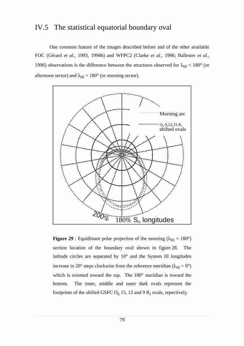
IV.5 The statistical equatorial boundary oval
One common feature of the images described before and of the other available
FOC (Gérard et al., 1993, 1994b) and WFPC2 (Clarke et al., 1996; Ballester et al.,
1996) observations is the difference between the structures observed for λIII < 180° (or
afternoon sector) and λIII > 180° (or morning sector).
79
Figure 29 : Equidistant polar projection of the morning (λIII < 180°)
section location of the boundary oval shown in figure 28. The
latitude circles are separated by 10° and the System III longitudes
increase in 20° steps clockwise from the reference meridian (λIII = 0°)
which is oriented toward the top. The 180° meridian is toward the
bottom. The inner, middle and outer dark ovals represent the
footprints of the shifted GSFC O6 15, 12 and 9 RJ ovals, repectively.
O6 9,12,15 RJ
shifted ovals
Morning arc
180% SIII longitudes200%
In addition to the main oval (ARC1 in figure 27) generally observed for λIII > 180°,
patchy and multiple structured emissions are frequently observed for λIII < 180°. The
10 images from July 17 to 22, 1994 (table 8) were co-added to visualize the statistical
distribution of the auroral emission and to determine the equatorward boundary of the
north aurora. In order to account for the different sub-Earth longitudes (CML), and for
the roll angles of the spacecraft about the optical axis of the telescope, each image was
projected on an equidistant cylindrical map. An average map (figure 28) was created
where the intensity of each pixel, located by its planetocentric latitude and System III
longitude, is the average of the corresponding pixels of the maps that cover this
particular position. The equatorial boundary of the auroral emission zone is located on
the average map by a series of latitude-longitude points. As apparent from the
inspection of individual images, the auroral emission divides into two distinct regions
showing different auroral morphologies (Gérard et al., 1993, 1994b; Clarke et al.,
1996). The left side region, corresponding to System III longitudes between 180° and
260°, displays a single, long and thin auroral arc that results in the summation of several
smaller overlapping arcs. The right side region, corresponding to longitudes between
100° and 180°, is completely filled by auroral emission with brighter features near the
equatorial boundary and near the limb. Since the viewing geometry has not been
corrected prior to cylindrical projection, it must be noted that these bright features could
be attributed to geometrical effects. This region is the result of the accumulation of
emission spread between the equatorial boundary and the pole in the individual images.
This average map resembles those derived from previous studies of the ultraviolet
Jovian auroral morphology made with the FOC (Gérard et al., 1993, 1994b) which
indicated a clear dichotomy between the longitude zones on each side of the 180°
System III meridian. The equatorward emission boundary can be fit by an oval
characterized by the 5 parameters defining a local coordinate set described in the model
description section (these parameters have been used for the test cases simulation). For
longitudes above 180°, the boundary follows the bright linear arc structure conspicuous
in figure 28. At longitudes less than 180°, where no clear arc structure is apparent, it is
defined by the equatorial limit of the diffuse emission. The equatorial boundary oval so
defined is plotted in figure 28. It is located between the footprints of the magnetic field
lines at 6 RJ and 30 RJ in the GSFC O6 model (Connerney et al., 1992). It should be
noted that these O6 ovals are frequently used as standard references for comparison with
80
the morphological results presented in the literature. Table 9 lists the simulation
parameters defining the centers and sizes of the boundary oval and the 6 RJ and 30 RJ
ovals in the GSFC O6 model. It shows that the latitude of the center of the boundary
oval is close to that of both the 6 and 30 RJ ovals. Its size is intermediate between these
two ovals but closer to that of the 6 RJ boundary. A gap of 4°- 6° of latitude is observed
between the foot of the Io flux tube and the oval detected by Clarke et al. (1996) with
the WFPC2 camera.
Gérard et al. (1994b) and more recently Satoh et al. (1996), have shown that the best
agreement with the observed bright auroral oval in the northern hemisphere is obtained
by shifting the center of the O6 30 RJ oval about 10° parallel to the 270° meridian.
Figure 29 shows a polar projection of the equatorial boundary morning section, i.e. the
location of the composite thin morning arc. Three theoretical ovals are overplotted and
represent the footprints of the shifted (11° parallel to the 270° meridian) 9, 12 and 15 RJ
ovals of the O6 model (whose accuracy is on the order of 5 to 10°). It clearly illustrates
that the thin morning arc can be bracketted by the shifted 9 and 15 RJ ovals and might
be fit by the the shifted 12 RJ oval. This result corroborates those derived by Clarke et
al. (1996) on the analysis of WFPC2 images taken in March 1995.
81
IV.6 Discussion and conclusion
A model simulating Earth view of UV auroral emissions in the jovian north
polar region has been developed. This model untangles the real brightness variations
from purely geometrical effects, such as limb brightening, of structured and unstructured
emitting regions. The application of the model to simple geometric cases shows the
characteristics of the apparent brightness variations due to the altitude, the scale height
and the CML of idealized auroral structures. It demonstrates how faint diffuse auroral
emission inside the polar cap is able to apparently close the auroral oval along the limb.
As an application of the model, we have simulated 4 images selected in the WFPC2
dataset. The model does not account for hydrocarbons absorption since its effects have
been neglected in these images. Some general features can be derived from the set of
simulations :
1. In the first three simulations, the limb brightening of an observed weak diffuse
emission zone (GLOW1) may account for the apparent closing of the auroral oval.
2. The arc of oval ARC3 is present in the four simulations. It always appears at the
morning limb of the auroral region and therfore could be linked to a phenomenon
fixed in local time.
3. The emission in the afternoon region of the last three images is made of
inhomogeneous diffuse zones (GLOW2, GLOW3) and of bright arcs (ARC1,
ARC2). The emission altitude of this sector spreads between 400 km and 800 km.
This could stem from a variation of the energies of the precipitating particles.
4. Longitudinal and/or local time variations along the auroral arcs are present in
addition to the apparent brightness variations due to limb brightening effects.
It must be mentioned that the notion of "altitude of emission" is closely
connected to the Chapman profile. The change in the altitude of emission between
different parts of the aurora to reproduce the observed images is only valid if we
consider that the vertical distribution of the brightness follows the Chapman profile
everywhere in the auroral region. A composite average auroral structure was built by
mapping 10 images obtained with the WFPC2 camera, covering observations taken in
July 1994 (table 8). It shows a clear dichotomy between a narrow structure emission at
82
System III longitudes > 180° (or morning sector) and broad diffuse emission at
longitudes < 180° (or afternoon sector). This statistical structure defines the UV
equatorward boundary which is located between the 30 RJ and 6 RJ ovals of the GSFC
O6 model.
Since most of the auroral observations were made for CMLs close to 180°, it is
difficult to discriminate between true longitudinal and local time effects. However, for
CMLs around 180°, the morning section appears quite thin in latitude and the auroral
arc tends to follow the same distribution as clearly demonstrated by figure 29. It maps
equatorial regions bracketed by the 9 RJ and 15 RJ O6 ovals. The afternoon side, by
contrast, frequently shows multiple arcs and diffuse emission regions. Some of them
extend close to the pole. Such a morphological dichotomy, conspicuous both in single
images and in the statistical map, could be attributed to a local time effect which is
clearly detected (though not understood) in the X-ray pattern observed with the ROSAT
High Resolution Imager in July 1994 (Waite et al.,1997)
Our conclusions present both similarities and discrepancies with those reached
by Satoh et al. (1996) based on their inversion of eight H3+ auroral images obtained with
the ProtoCAM instrument at the NASA IRTF in 1992. They concluded that, in addition
to a slight shift from the nominal positions of O6 plus current sheet model, a better fit is
obtained by adding two anomalies. The main one is a thin arc fixed in System III
longitude with a maximum brightness near λIII = 230°. In the northern polar region, it
exceeds a second weaker anomaly fixed in local time showing broad and bright
emission in the afternoon section. In addition, the infrared (IR) observations indicate
the presence of weaker diffuse emissions both poleward and equatorward of the main
oval. The IR equatorial boundary extends approximately to the footprint of the Io torus.
The dataset used in the present work is heavily weighted by images taken at CML close
to 180° and therefore, the auroral structures that we have derived cannot be reliably
fixed in longitude nor in local time. Accordingly, the comparison with the IR anomalies
is somewhat ambiguous. It should be noted, however, that at CMLs close to 180°
ARC3 is similar to the infered thin morning arc, while ARC1, ARC2 and GLOW2
could be correlated to the infrared bright and broad emission in the afternoon section.
Table 9 compares the centers and the sizes of the uniformly bright infrared auroral ovals
83

determined for images acquired on February 28 and on March 22, 1992 (Satoh et al.,
1996).
This work represents a first step in the analysis, with a simulation code, of the
geometrical effects of the Jovian UV auroral images observed from Earth orbit. It
demonstrates some of the considerable potentialities of the simulation code. In a near
future, as more images (HST and other) become available, this code could be used to
address different problems. These include the discrimination of local time and System
III longitude effects, the longitudinal variation of the color ratio, the analysis of
localized effects of the auroral emission such as the lag to corotation (Ballester et al.,
1996) or more complex details of the auroral emission structures. Many improvements
of the code are possible in order to analyze specific matters. In particular, it could be
coupled to an energy deposition model in the frame of a Jovian thermospheric general
circulation study.
84

V The longitudinal variation of the color
ratio of the Jovian ultraviolet aurora : a
geometric effect ?
This chapter describes a second application of the morphology model. The text is taken
from a paper written by Jean-Claude Gérard, Denis Grodent, Vincent Dols, J. Hunter
Waite, Jr. and published in Geophysical Resarch Letters, 25, 1601-1604, 1998.
abstract
A three-dimensional model is used to assess the role of the viewing geometry on
the auroral color ratio. The simulations show that both an auroral arc with a geometry
deduced from images obtained with the Hubble Space Telescope (HST) and a uniform
polar cap emission produce no modulation or a minimum absorption when the
longitude of the Jovian central meridian (CML) is close to 200°. This result is in
contrast with the statistical measurements made with the International Ultraviolet
Explorer (IUE) spectrograph that the hydrocarbon optical depth above the auroral
emission maximizes for CMLs about 180°. In the frame of this simplified model, we
examine a possible way to reconcile the model with the IUE data. An intrinsic
longitudinal dependence of the column of methane above the level of the auroral
emission is introduced in the simulation. It may result from a combination of a vigorous
upwelling in sectors of strong and stable precipitation and/or a longitudinal dependence
of the characteristic energy of the auroral particles.
85

V.1 Introduction
The characteristics of the Jovian auroral ultraviolet emissions bear to some
extent the signature of the precipitation processes. In addition to their morphology,
they exhibit systematic variations in their spectral distribution. The color ratio
CI 15501620I 12301300
is related to the considerable drop in the CH4 absorption cross section at wavelengths
above 1350 Å (Yung et al., 1982). It leaves the bulk of the longer wavelength H2 Lyman
band emissions unattenuated, while the H Ly-α and H2 Werner and Lyman band
emissions at wavelengths less than 1350 Å are substantially absorbed.
Based on eleven years of IUE spectral observations, Livengood and Moos (1990)
and Harris et al. (1996) have shown that the brightness and relative intensity of the
components of the auroral spectrum exhibit a systematic statistical dependence on the
System III central meridian longitude λCML.
Recently, Kim et al. (1997) determined the absorption by methane using the Goddard
High Resolution Spectrometer (GHRS) on board the HST. Their results indicate that
the overlying CH4 column density varies between 1 and 7 x 1016 cm-2 and that the
highest CH4 columns tend to be associated with the lowest temperatures derived from
the H2 rotational intensity distribution.
The correlation between the peaks of C and of the emission brightness suggests
that the longitudinal maximum in the flux coincides with the highest characteristic
energy of the auroral particles (Livengood et al., 1990). An alternative explanation is
that the maximum color ratio occurs in the longitude sector with major atmospheric
perturbations generating an increased hydrocarbon column density.
A difficulty with the interpretation of the IUE observations stems from the large field of
view of its aperture (21.4 x 8.9 arc sec2) used for the auroral observations. A
considerable fraction of the dayside auroral emission is spatially integrated making it
86
difficult to untangle real from geometrical effects. The variation of the H2 color ratio,
including the effects of the limb brightening and the variation of the slant path in the
IUE aperture was modeled in a simplified way by Livengood et al. (1980). However,
the auroral morphology was not correctly represented due to the lack of imaging
observations. Furthermore, the effect of the IUE point spread function (PSF) (Ballester
et al., 1996; Prangé et al., 1997) was not accounted for. The PSF introduces into the
measurements contributions at large slant angles from the limb which were not included
in previous analyses.
This question can now be addressed with a model simulation integrating the geometrical
complexity of a Jovian auroral observation from Earth orbit and data recently obtained
with the new generation of imaging instruments. The HST auroral UV images (Gérard
et al., 1994; Clarke et al., 1996; Ballester et al., 1996; Grodent et al., 1997) show that
the morphology of the aurora is different from that based on the IUE - Voyager
paradigm. They show that the discrete aurora is more closely connected with the
distant magnetosphere than with the Io plasma torus region.
87

V.2 The geometric simulation model
The results presented in this paper are based on the model described by Grodent
et al. (1997). For the simulations described below, two simple morphological structures
are adopted :
1. a continuous oval with a constant peak altitude and a latitudinal Gaussian distribution
with an e-folding value of 1°. Its position, orientation and size are fitted to the
"reference oval" described by Clarke et al. (1996)
2. a uniform auroral glow filling the polar cap inside the oval structure described before.
Such a polar cap diffuse aurora appears in some HST images. It provides a second
component of the auroral morphology with a distribution of slant view angles
different from a simple oval.
The sub-Earth latitude is set to 3° S and the sub-Earth longitude is varied from 0° to
360°. As an approximation (Gladstone and Skinner, 1989), a Chapman profile with a
topside scale height arbitrarily fixed at 50 km is used to describe the vertical auroral
88
Figure 30 : Geometry of the model simulations. The vertical
distribution of the auroral emission is represented by a Chapman layer
(not to scale). The dashed line corresponds to the altitude of the
methane unit optical depth for the observer (see text).
Aurora
Line of sight
τ =1
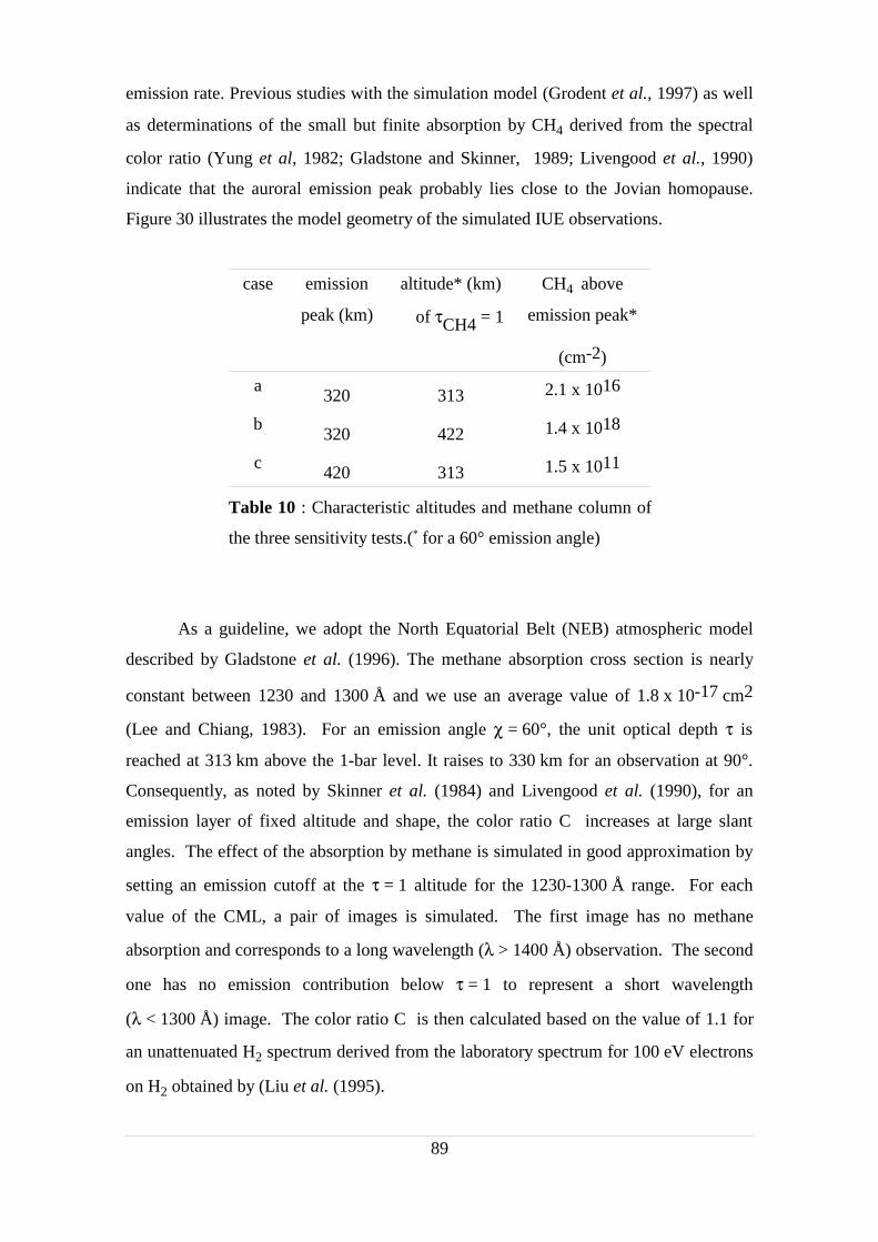
emission rate. Previous studies with the simulation model (Grodent et al., 1997) as well
as determinations of the small but finite absorption by CH4 derived from the spectral
color ratio (Yung et al, 1982; Gladstone and Skinner, 1989; Livengood et al., 1990)
indicate that the auroral emission peak probably lies close to the Jovian homopause.
Figure 30 illustrates the model geometry of the simulated IUE observations.
case emission altitude* (km) CH4 above
peak (km) of τCH4 = 1 emission peak*
(cm-2)
a 320 313 2.1 x 10¹⁶
b 320 422 1.4 x 10¹⁸
c 420 313 1.5 x 10¹¹
Table 10 : Characteristic altitudes and methane column of
the three sensitivity tests.(* for a 60° emission angle)
As a guideline, we adopt the North Equatorial Belt (NEB) atmospheric model
described by Gladstone et al. (1996). The methane absorption cross section is nearly
constant between 1230 and 1300 Å and we use an average value of 1.8 x 10⁻¹⁷ cm2
(Lee and Chiang, 1983). For an emission angle χ = 60°, the unit optical depth τ is
reached at 313 km above the 1-bar level. It raises to 330 km for an observation at 90°.
Consequently, as noted by Skinner et al. (1984) and Livengood et al. (1990), for an
emission layer of fixed altitude and shape, the color ratio C increases at large slant
angles. The effect of the absorption by methane is simulated in good approximation by
setting an emission cutoff at the τ = 1 altitude for the 1230-1300 Å range. For each
value of the CML, a pair of images is simulated. The first image has no methane
absorption and corresponds to a long wavelength (λ > 1400 Å) observation. The second
one has no emission contribution below τ = 1 to represent a short wavelength
(λ < 1300 Å) image. The color ratio C is then calculated based on the value of 1.1 for
an unattenuated H2 spectrum derived from the laboratory spectrum for 100 eV electrons
on H2 obtained by (Liu et al. (1995).
89
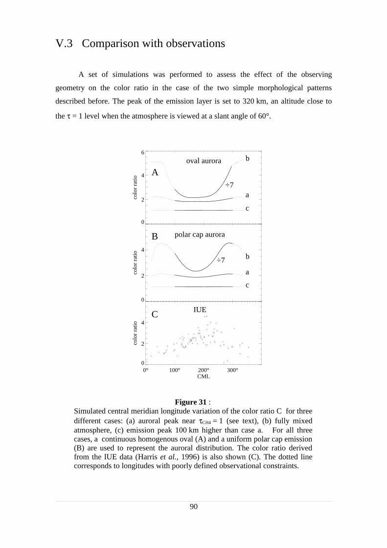
V.3 Comparison with observations
A set of simulations was performed to assess the effect of the observing
geometry on the color ratio in the case of the two simple morphological patterns
described before. The peak of the emission layer is set to 320 km, an altitude close to
the τ = 1 level when the atmosphere is viewed at a slant angle of 60°.
Simulated central meridian longitude variation of the color ratio C for threedifferent cases: (a) auroral peak near τCH4 = 1 (see text), (b) fully mixedatmosphere, (c) emission peak 100 km higher than case a. For all threecases, a continuous homogenous oval (A) and a uniform polar cap emission(B) are used to represent the auroral distribution. The color ratio derivedfrom the IUE data (Harris et al., 1996) is also shown (C). The dotted linecorresponds to longitudes with poorly defined observational constraints.
90
Figure 31 :
0
2
4
6
colo
r ra
tio
oval aurora
÷7
A
c
a
b
0
2
4
colo
r ra
tio
polar cap aurora
÷7
B
c
a
b
0° 100° 200° 300° CML
0
2
4
colo
r ra
tio
C IUE
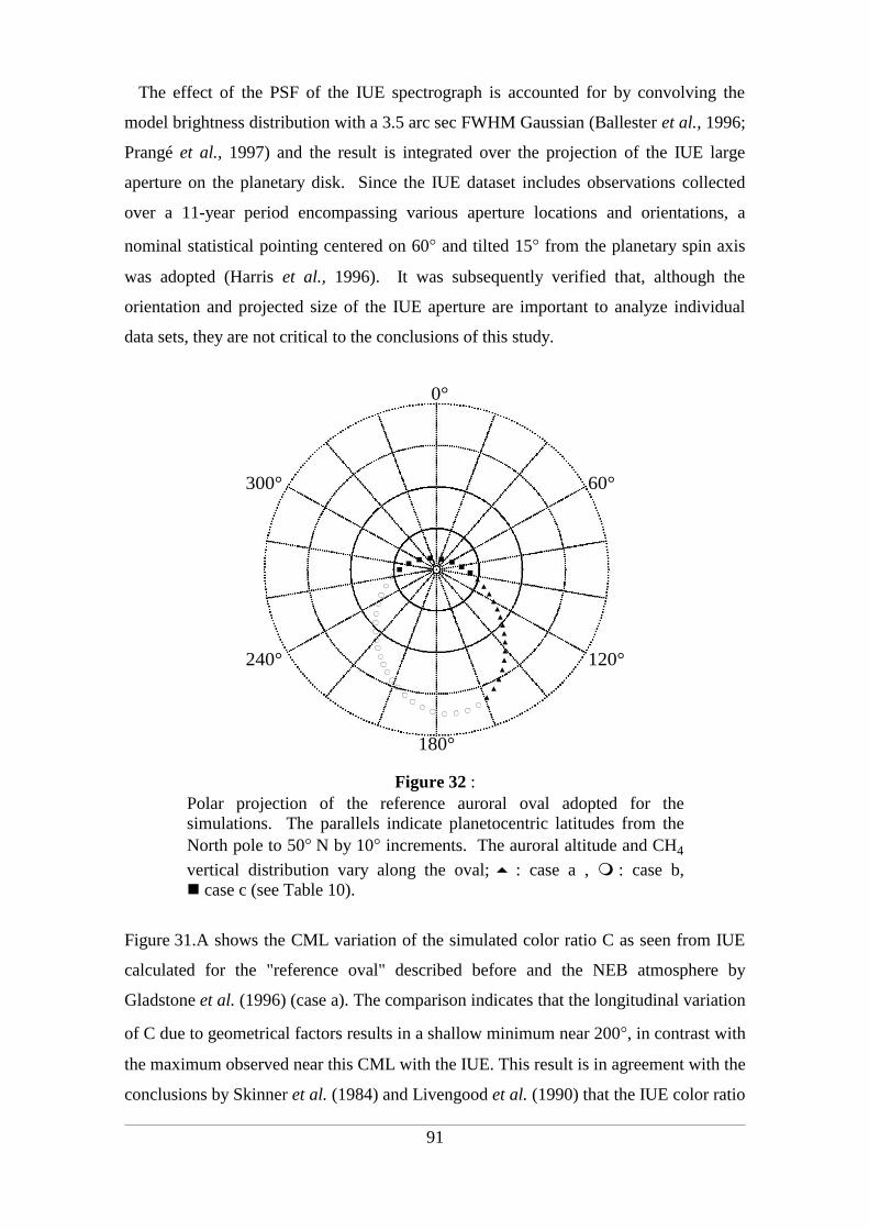
The effect of the PSF of the IUE spectrograph is accounted for by convolving the
model brightness distribution with a 3.5 arc sec FWHM Gaussian (Ballester et al., 1996;
Prangé et al., 1997) and the result is integrated over the projection of the IUE large
aperture on the planetary disk. Since the IUE dataset includes observations collected
over a 11-year period encompassing various aperture locations and orientations, a
nominal statistical pointing centered on 60° and tilted 15° from the planetary spin axis
was adopted (Harris et al., 1996). It was subsequently verified that, although the
orientation and projected size of the IUE aperture are important to analyze individual
data sets, they are not critical to the conclusions of this study.
Polar projection of the reference auroral oval adopted for thesimulations. The parallels indicate planetocentric latitudes from theNorth pole to 50° N by 10° increments. The auroral altitude and CH4
vertical distribution vary along the oval; : case a , : case b, case c (see Table 10).
Figure 31.A shows the CML variation of the simulated color ratio C as seen from IUE
calculated for the "reference oval" described before and the NEB atmosphere by
Gladstone et al. (1996) (case a). The comparison indicates that the longitudinal variation
of C due to geometrical factors results in a shallow minimum near 200°, in contrast with
the maximum observed near this CML with the IUE. This result is in agreement with the
conclusions by Skinner et al. (1984) and Livengood et al. (1990) that the IUE color ratio
91
Figure 32 :
180°
240°
300°
0°
60°
120°
varies in the opposite sense of that required by simple geometric considerations.
The presence of the shallow color ratio seen in figure 31.A (a) above λCML = 200°
is explained by considering the path length of the auroral emission for Earth orbit
observations. The main contribution at this longitude originates from the section of the
oval facing the Earth with some contribution from the ansae and from the high altitude
emission above the polar limb. The color ratio remains relatively small and varies only
moderately along most of the oval. In contrast, the contribution near λCML = 0° is due to
an edge viewing of the emission near the pole. Larger color ratios are associated with
these viewing conditions since, for large zenith angles, much of the optical path
penetrates into the absorbing hydrocarbon region.
The deposition of large amounts of heat by auroral particles below the
homopause may cause upwelling of CH4-rich gas. In order to simulate vigorous
upwelling (case b), a limiting case is considered where the methane mixing ratio is
constant throughout the thermosphere at its value below the homopause (2.5 x 10⁻³).
In this "fully mixed" atmosphere, the unit optical depth in the 1230-1300 Å region is
reached at 422 km for χ = 60°, that is about 100 km higher than in case a.
Table 10 lists the altitude of the emission peak and of the τ = 1 level and the overlying
CH4 column for an emission angle of 60° in the Gladstone et al. (1996) model. As seen
in figure 31.A (b), the color ratio simulated in this case is much larger than in case a and
the dependence on the CML is much more pronounced.
Finally, case c is simulated for the NEB atmosphere for an emission peak located
at 420 km, 100 km above τ = 1, corresponding to a softer particle precipitation. In this
case, the color ratio remains constant at its unabsorbed value of 1.1. It is expected that
these three cases represent an extreme range of methane columns encountered in the
Jovian aurora.
The simulated CML dependence of the color ratio for a uniform polar cap emission with
the reference oval as an equatorward boundary exhibits a shape similar to the discrete
oval case (figure 31.B). The major discrepancy between the observations and the
simulations remains for reasonable variations of the planetary tilt, auroral oval width,
size and orientation. From these simulations covering two distinct types of auroral
92

morphology and various peak altitudes with respect to the methane absorption, it may be
concluded that geometrical effects cannot account for the observed CML dependence of
the color ratio.
93
Figure 33 : CML distribution of the simulated color ratio C of
an aurora with altitude characteristics varying along the oval
as illustrated in figure 32 (solid line). The dotted line
corresponds to longitudes with poorly defined observational
constraints. For comparison, the IUE observations are also
shown as circles.
012345
color ratio
0°10
0°20
0°30
0°
CM
L

As suggested by Skinner et al. (1984) and modeled by Livengood et al.(1990), a
statistical System III longitudinal dependence (λIII) of the column of methane in front of
the auroral emission is required to explain the IUE observations. The present state of
knowledge of the Jovian magnetospheric and auroral acceleration processes and of the
auroral atmospheric composition does not permit a well constrained and unique solution
to this problem. We have used the simulation model to verify that, using a prescribed
longitude dependence of the methane column overlying the emission peak, an adequate
shape of the C ratio CML variation could be obtained.
Figure 32 shows an example of such an hypothetical dependence. The oval is divided
into three sectors corresponding to case a in the λIII 100°-160° sector, case b between
160° and 260° and case c from 260° to 100°. The corresponding color ratio variation
with the CML as viewed through the IUE aperture is shown in Figure 33. It is seen that
a maximum at 200° and a minimum near 0° are now obtained. However, the agreement
with the IUE observations deteriorates in the 300°-100° region which was poorly
sampled with the IUE and whose visibility from Earth orbit is at best marginal.
94
V.4 Discussion
Detailed model simulations show that a morphology with a uniform aurora
compatible with recent HST imaging observations leads to a CML dependence of the
color ratio in the opposite sense to that of the IUE observations. A longitudinal
variation integrated over the IUE aperture resembling the IUE dataset may be obtained if
the altitude of the emission varies with respect to the methane absorption level. No
independent evidence exists for a longitudinal dependence of the mean energy of the
auroral particles. Another possibility is that the CH4 column varies along the oval,
leading to differential absorption as a function of longitude, possibly also reflecting
changes with latitude. Upwelling of methane due to the large amount of auroral energy
deposited near the homopause may indeed cause redistribution of the CH4 mixing ratio
above the homopause similar to the N2/O enrichment observed in the Earth's auroral
thermosphere.
A System III dependence of the characteristic auroral energy, flux and/or
atmospheric composition properties may be linked to the morphological features
observed in the HST ultraviolet images. Examination of the HST images of the north
aurora (Gérard et al., 1994; Clarke et al., 1996; Grodent et al., 1997) have led to the
conclusion that the aurora at λIII > 180° is characterized by a narrow and
morphologically stable bright oval. In contrast, the aurora is generally diffuse and
widespread at λIII < 180°, with much more variable structures in this sector. Concerning
the three-sector oval described in Figure 32, it may be speculated that the sector
λIII > 180° is characterized by an efficient upwelling of CH4 due to the stability of the
morphology in this sector. Alternatively, it may correspond to a region of more energetic
precipitation depositing its energy at a lower altitude than the more diffuse aurora in the
λIII < 180° sector.
95

Part 2
Self-consistent model of the jovian
auroral thermal structure
VI Theory
VI.1 Introduction
Recent progress in imaging and spectroscopy of the jovian aurora have
considerably increased and improved our knowledge of the energetics induced by
particle input and its potential effect on the thermospheric thermal structure of the
planet. Spectroscopic observations of the UV aurora with the International Ultraviolet
Explorer (IUE) satellite (Clarke et al., 1979) and the ultraviolet spectrometer (UVS)
onboard the Voyager spacecraft (Broadfoot et al., 1979) suggest a total auroral particle
input flux on the order of 1013-1014 W in each hemisphere, about 3 orders of
magnitude stronger than the corresponding value for the Earth's aurora. Such a large
energy flux has been confirmed by UV images of the jovian aurora obtained with the
Faint Object Camera (FOC) (Gérard et al., 1993, 1994) and the Wide Field Planetary
Camera (WFPC2) (Clarke et al., 1998; Morrisey et al., 1997) on board the Hubble
Space Telescope (HST). The large amount of energy input into the atmosphere (about
100 times the global extreme ultraviolet (EUV) solar energy input) produces ionization,
radiation, and particle heating in the planet's upper atmosphere. Since the energy flux in
the auroral regions is so much larger than the solar heating in the thermosphere it is
expected that the auroral processes maintain the large exospheric temperature observed
at mid- and high-latitudes.
96
One-dimensional models of the interaction between energetic primary particles and the
jovian atmosphere have been developed in the past on the basis of the continuous slow
down approximation (Heaps et al., 1973; Gérard and Singh, 1983), the two-stream
(Waite et al., 1983) or the multistream approximation (Kim et al., 1992). These studies
assumed that most of the energy input is associated with electrons rather than protons or
heavy ions. This assumption rests on the lack of evidence for strong proton
precipitation in the Lyman-α line profile (Clarke et al., 1994) and the absence of
characteristic lines expected for O+ and S+ ion precipitation (Trafton et al., 1998).
Furthermore, model studies indicate that about 50% of the electron beam energy is
ultimately converted into heating of the neutral atmosphere (Gérard and Singh, 1982;
Waite et al, 1983, 1997). However, in previous studies, the thermal vertical structure
and the atmospheric composition were prescribed, based on data collected by UV
occultation in the equatorial regions.
Information on the thermospheric thermal structure has three principal components
covering different altitude regions : 1) hydrocarbon infrared measurements at pressures
around 10-4 to 10-6 bar, 2) H2 rovibrational temperatures derived from ultraviolet
spectra in the 10-5 to 10-8 bar range, and 3) H3+ spectra in the 10-6 to 10-10 bar
pressure range. A re-analysis of the temperature structure in the North auroral region
was performed by Drossart et al. (1993) using the Voyager-1 infrared interferometer
and radiometer spectrometer (IRIS) data. The infrared (IR) excess emission rate by the
hydrocarbons was found to be ∼93 ergs cm-2 s-1 by methane and ∼86 ergs cm-2 s-1 by
acetylene averaged over an auroral hot spot. Good agreement with the data was
obtained by adopting a steep temperature near the homopause reaching lapse rate values
of about 2 K/km.
Rovibrational H2 temperatures have been determined from observations of high
resolution (0.3-0.5 Å) UV spectra obtained with the Goddard High Resolution
Spectrograph (GHRS) on board HST (Trafton et al., 1994, 1998; Kim et al., 1997;
Clarke et al., 1994; Dols et al., 1999). The H2 temperature reflects the temperature
along the line of sight weighted by the auroral volume emission rate. It was found to
vary between 300 to 700 K with little correlation to the H2 emission brightness.
Additional information on the thermospheric auroral temperature is provided by the
97

analysis of the rovibrational structure of the H3+ fundamental band near 3.5 µm
(Trafton et al., 1989; Drossart et al., 1989; Miller et al., 1990; Lam et al., 1990). These
measurements indicate that the H3+ temperature, which was shown to be close to the
gas kinetic temperature, varies between 700 and 1000 K (in addition a strong anti-
correlation was found between the temperature and the H3+ column density). A neutral
temperature structure constrained by these three sets of measurements, ranging from 200
K at 10-7 bar to 2100 K at 10-14 bar, was presented by Trafton et al. (1994). However,
this profile is empirical and, so far, no attempt was made to link a model of particle
energy deposition (and emission) with a consistent calculation of the thermal profile.
No in situ measurement of Jupiter's auroral atmosphere vertical structure is available.
The recent vertical profile derived from the Galileo probe (Seiff et al., 1998) concerns a
low latitude site. The equilibrium exospheric temperature is controlled by the total
particle energy input and the energy spectrum of the primary electrons. The H3+
concentration enhancement generated by the deposition of soft primary particles and
secondary electrons acts as an efficient cooling process for the thermosphere by
transferring a large fraction of the energy input to the ionosphere and subsequently
radiating most of it away into space. Another fraction of the heat input is conducted
downward into the hydrocarbon layer where it radiatively cools to space. The relative
location of the heat source from auroral energy deposition and the altitude of the
homopause will determine, in a complex way, the relative importance of H3+ cooling,
direct hydrocarbon radiation to space and downward conduction from the region of heat
production to the hydrocarbon layer. The vertical distribution of hydrocarbons may
also, in part, be controlled by the amount of heat dissipation below the homopause.
Upwelling of hydrocarbon-rich gas due to the release of large amounts of auroral heat
has been invoked as a possible source of hydrocarbon enhancement above a region of
strong precipitation (Livengood et al., 1990), similar to the N2/O enhancement observed
in the Earth's thermosphere during strong auroral disturbances. Inversely, a large
auroral energy input near or below the homopause may cause a local temperature
increase, resulting in a thermal expansion of the overlying atmosphere, a change of the
altitude of the deposition peak and a resulting perturbation of the hydrocarbon cooling
efficiency.
98
A one-dimensional model has been developed to address the question of the close
coupling between auroral heat input, and the atmospheric temperature and composition
structure. It couples a two-stream electron transport model of energy deposition with a
1-D thermal conduction model including particle heating and CH4, C2H2 and H3+
cooling (Waite et al., 1997). In the absence of in situ measurements of the energy
distribution of the primary auroral electrons, different distributions are used to
investigate the effect on the thermal profile. The values of observable quantities such as
the altitude of the H2 emission peak, IR and UV emissions and temperatures associated
with various optical signatures are used to constrain the parameters of these
distributions. Sensitivity tests are performed to evaluate the importance of the energy
spectrum of the incident electrons for the thermal balance of Jupiter's auroral
thermosphere.
99

VI.2 The Jovian atmosphere
VI.2.1 Atmospheric regions
The atmosphere of Jupiter can be divided into several regions that are defined
according to the different dynamical regimes and to the behavior of the temperature
profile. The nomenclature defined hereafter will be used throughout the text.
VI.2.1.1 Dynamical regime criterion
Like the Earth, the jovian atmosphere can be divided into three main regions
(figure 34) characterized by the different dynamical regimes occurring in these
atmospheric layers. They are the homosphere below ~300 km (measured from the 1
bar pressure level approximately corresponding to the NH3 cloud deck), the
heterosphere between ~300 km and ~2000 km, and the exosphere above ~2000 km
(this latter altitude depends on temperature).
VI.2.1.1.1 The homosphere
The homosphere is the atmospheric region where mixing phenomena, such as
wind and turbulence are sufficiently fast and important to keep the bulk composition of
the major constituents constant in altitude. The major constituents are said to be in
perfect mixing. As a consequence, the mixing ratio f ini ni , where ni is the
density number of any constituent, is independent of altitude. The homogeneity of the
major constituents disappears at an approximate altitude of 300 km known as the
homopause. This term is often used to characterize the altitude from which turbulence
phenomena are no longer efficient enough to sustain perfect mixing. The homopause is
not really set at a well defined altitude but should be considered as a transition zone
between homosphere and heterosphere. Numerically speaking, the homopause is
defined by the altitude where the eddy diffusion coefficient becomes equal to the
molecular diffusion coefficient. Since each constituent has its own molecular diffusion
100

coefficient, a different homopause should be defined for each species. However, these
homopause altitudes are very close to each other and we therefore conveniently use the
methane diffusion coefficient to calculate the altitude of the homopause.
101
Figure 34 : The different regions of the jovian atmosphere
Galileo temperature profile adapted to polar gravity
0 200 400 600 800 1000 1200Temperature (K)
10−4
10−6
10−8
10−10
10−12
Pres
sure
(ba
r)
Galileo temperature profile adapted to polar gravity
0 200 400 600 800 1000 1200Temperature (K)
10−4
10−6
10−8
10−10
10−12
Pres
sure
(ba
r)
200
250
300
400
500
1000
Alti
tude
(km
)
HO
MO
SPH
ER
EH
ET
ER
OSP
HE
RE
EX
OSP
HE
RE
TH
ER
MO
SPH
ER
E
LOWER
STRATOSPHERE
UPPER
STRATOSPHERE
homopause
exobase
VI.2.1.1.2 The heterosphere
In the heterosphere, molecular diffusion in the gravity field tends to separate the
major constituents according to their own mass (and scale height). Molecular diffusion
is also present in the homosphere but is eventually dominated by the mixing processes.
Therefore, the dynamic regime in the heterosphere is completely different from the
homosphere. Molecular diffusion leads to an altitude variation of the mixing ratio of the
major constituents. The lighter species having a larger scale height, their concentration
decrease with altitude is less pronounced than for heavier components. This can be
illustrated at high altitudes where atomic hydrogen density becomes more important
than molecular hydrogen density.
VI.2.1.1.3 The exosphere
Above a temperature dependent altitude, collisions between atmospheric
particles become so rare that they can be neglected. This altitude is the heteropause or
exobase and corresponds to the level from which atmospheric particles can follow
parabolic, elliptic or hyperbolic paths in the gravity field. This altitude may be defined
in such a way that a proportion exp(-1) of a group of very fast particles moving
vertically upwards will experience no collisions as they move out of the atmosphere.
For molecules of diameter d, the probability of no collision being made in a vertical path
dz is given by exp d2 n z dz (Houghton, 1977) where n(z) is the particle density
at height z.. For a proportion exp(-1) of no collision, it comes
exp d2 n z dz exp 1 ,
The probability for no collision in the altitude range zzexo z is
zexo
d2 n z dz1 .
Substituting for n(z) from the hydrostatic equation (see next section for details) :
102
n z nexoexpzzexo
H ,
the condition for the exobase level zexo is
zexo
d2 nexoexp zzexo
Hdz1 .
Considering that T and g (the acceleration of gravity) are constant in this altitude range,
the scale height H is constant and the integral of the exponential is exactly equal to H.
The condition finally becomes :
nexod2 H1
Since n z d21 is the mean free path in the horizontal direction at level z, the
exobase may also be defined as the altitude at which the mean free path in the horizontal
direction is equal to the scale height H. For a high altitude auroral region of Jupiter at
latitude 60° (the acceleration of gravity g = 2622 cm s-2), a limiting temperature of
1000 K may be assumed. Considering that H2 is still the dominant species, one
estimates that the H2 density at the exobase nexo is on the order of 3x107 cm-3. In the
auroral atmospheric model which is used in this work, this density corresponds to an
altitude of ~1700 km (5.4x10⁻¹² bar).
VI.2.1.2 Temperature profile
The atmosphere of Jupiter may also be divided according to the temperature
profile. According to Hunten (1976) four regions of the non-auroral atmosphere can be
highlighted : the troposphere, the stratosphere, the mesosphere and the thermosphere.
103
VI.2.1.2.1 The troposphere
The troposphere (below ~100 km and therefore out of reach of the present
model) is rapidly stirred by vertical motions made of some combination of free
convection and the vertical components of the large-scale circulation. It is characterized
by a negative vertical temperature gradient which leads to temperatures between 100
and 120 K (deduced from Galileo probe observations at the equator).
VI.2.1.2.2 The lower and upper stratosphere
The stratosphere and mesosphere are regions of radiative balance : the heat
sources are planetary and solar radiation (and auroral precipitation), and the sink is
infrared cooling. The stratopause on Earth is located by a temperature peak near 50 km,
but for Jupiter this peak is either absent or not very pronounced. The notion of
mesosphere appears inappropriate for the jovian atmosphere and is not used here.
Instead, we suggest that the region between the tropopause and the homopause be
referred to as the stratosphere. So defined, the stratosphere may be divided into 2 sub-
regions : the lower stratosphere, between the bottom of our model (~100 km) and
approximately the level of τ =1 methane absorption of the Ly-α line (~225 km), and the
upper stratosphere between ~225 km and the homopause(~320 km). The upper
stratosphere corresponds to the region where the auroral effects are the most important.
The lower stratosphere is a cold region largely influenced by the strong hydrocarbon
cooling (and the unspecified heating processes). At the bottom of this region the
temperature is assumed to be constant (boundary condition for the resolution of the heat
conduction equation) and we refer to it as the tropospheric temperature.
VI.2.1.2.3 The thermosphere
Above the upper stratosphere is the thermosphere where temperature increases
with altitude until a constant temperature (isothermal regime) is reached refereed to as
the thermospheric or exospheric temperature.
104
VI.2.2 The hydrostatic equilibrium
The stratification of the jovian atmosphere is controlled by the law of hydrostatic
equilibrium which determines the variation of the gas pressure under the action of the
weight of the atmospheric gas.
VI.2.2.1 General concepts
The general motion equation of a fluid element in an external force field is given
by
D VDt
pFext
where V is the macroscopic group velocity vector of the fluid element resulting from
external macroscopic forces Fext and pressure gradient and
D Dt
t
v is the Eulerian derivative.
In the conditions of hydrostatic equilibrium D VDt
0 and we can write
pFext
Limiting ourselves to vertical motions in an atmosphere controlled by gravitational
forces, this equality becomes the hydrostatic equation
d pd z
g
in which p denotes the atmospheric pressure, ρ the atmospheric density, and g is the
acceleration of gravity at height z.
The hydrostatic equation tells us that in the conditions of hydrostatic equilibrium the
vertical atmospheric pressure gradient is balanced by gravitational force at all altitudes.
105
To a first approximation the atmospheric density is governed by this equation. This
means that other transport processes, such as convection or diffusion, play a negligible
role compared to pressure gradient and weight and can be considered as low order
corrective terms.
For an ideal gas, the pressure p is related to the neutral gas temperature by
p = nkT
where n is the number density and k is the Boltzmann's constant.
With ρ = nm (m being the mean molecular mass), the hydrostatic equation can be
written in the following form :
dpp
dnn
dTT
d
dTT
dmm
dz
kT mg
This differential equation introduces the atmospheric scale height parameter H(z)
H z kT z
m z g z
with this parameter, the hydrostatic equation can now be written as
dpp
dzH
which has the formal solution
pp0exp z0
zdz'H
where z0 is a reference altitude at which pressure p0 = p(z0) is known.
The atmospheric scale height can therefore be viewed as the vertical length required to
decrease the atmospheric pressure by a factor e.
106
The perfect gas law can be applied to this equation to derive the relation giving the
numerical density (n) as a function of altitude (density profile) :
nn0
T0
T z exp
z0
zdz'H
where T0 = T(z0) and n0 = n(z0).
If both T and g are constant, the scale height H is constant and the equations can be
analytically integrated and give :
nn0
pp0
expzz0
H0
where : H0kT0
m g0
giving rise to an exponential variation of pressure and number density above the
reference level z0.
VI.2.2.2 Pressure-altitude relationship
All the equations developed in this model are calculated with the altitude
variable (z). However for some practical reasons that we shall discuss, it is more
convenient to express the different outputs of the code according to a pressure grid. The
pressure grid which we consider is characterized by a linear variation of the base-10-
logarithm of the pressure. This allows to tighten the atmospheric layer steps in the
region of maximum energy deposition and, conversely, to expand them in the upper
thermosphere where little interaction is expected. Another important reason for using a
pressure grid is that pressure is an absolute variable, while the altitude is a relative
variable which has to be defined according to a reference level. The reference is set to
the generally admitted 1 bar pressure level (corresponding to the NH3 cloud deck),
107

however other references have been used in the literature (like the 1 µbar or the .2 µbar
levels).
The hydrostatic law can be numerically integrated to provide a relation between pressure
and altitude
z0
z
dz' p0
pH p'
p'dp'
if the integrals are evaluated over sufficiently small intervals, the scale height can be
considered as constant and can be taken out of the integral. Therefore :
zz0H ln pp0 where H is an average scale height.
This numerically translates in a recurrence formula :
z n1z nH nH n12 lnpn1
pn for n=1, ... , NZ-1
and z 1z0 , p1p0 .
108
VI.3 The electron energy degradation model
As will be discussed later, the calculation of the thermal structure of the jovian
atmosphere requires the knowledge of the heating and cooling rate profiles. As far as
the auroral region is concerned, the heating rate is related to the heat released by the
interaction of the precipitating auroral electrons with the neutral atmospheric species.
Therefore, the calculation of the auroral heating rate is achieved by an energy
degradation model which is described below.
VI.3.1 Introduction
The energy degradation scheme used in the present model is an updated version
of the model described by Waite et al. (1983). It is based on a two-stream electron
transport method for the energetic electron flux in a planetary atmosphere, as described
by Nagy and Banks (1970) and Banks and Nagy (1970). A mean pitch angle is assumed
for all transported electrons so that their distribution is approximated by an upward and
a downward stream of electrons. The two-stream transport code calculates the flow and
redistribution of the electron energy as a function of altitude from atomic and molecular
processes by means of discrete energy bins. The use of a variable energy bin structure,
with small 0.5 eV wide energy bins below 10 eV gradually increasing to 25 keV wide
bins near 1 MeV, allows the treatment of complex energetic electron flux distributions
spanning energies from 0.5 eV to 1 MeV. Once the electron fluxes are calculated, the
rates of ionization, dissociation, heating and emission processes can be determined.
Auroral intensities from various spectral features are also calculated.
VI.3.2 Auroral electron transport model
A simple model of electron transport (Banks and Nagy, Nagy and Banks, 1970)
that takes into account both elastic and inelastic collisions between electrons and the
neutral and ionized particles of the upper atmosphere is outlined in this section. To treat
this problem, it is assumed that the electron flux in the energy range (ε,ε+dε) along a
109

magnetic field line (coordinate s) consists of two components; one component Φ+(ε,s)
directed upward along the field line (or away from the planet) and the other, Φ−(ε,s)
directed downward along the field line (or toward the planet). Electrons are assumed to
be created within the atmosphere by ionization or other processes at a rate q(ε, s) per
unit energy and volume, such that q/2 contributes to Φ+ and to Φ− (Mariani, 1964).
In traveling along magnetic field lines, it is assumed that the electrons interact
with the neutral and charged particles of the atmosphere through elastic collisions of
cross section σε(ε) and inelastic collisions of cross section σa(ε). An elastic collision
can convert a downward moving electron into one moving upward and vice versa; the
fraction of electrons that are backscattered by the kth atmospheric species in an elastic
collision of cross section σε(ε) is taken as pek(ε). Due to the mass factor involved in the
electron-neutral or electron-ion elastic energy transfer rate, it is assumed that elastic
collisions do not result in appreciable electron energy degradation.
Inelastic collisions, in contrast, cause cascading between the various electron energy
groups, with the electrons absorbed at higher energies reappearing at appropriate lower
energies. The fraction of backscattered electrons resulting from an inelastic collision
leading to the jth excitation level of the kth species particle is taken as pajk (ε1 →ε2)
As already mentioned, the electron flux is divided into two angular groups, the
upward flux Φ+ for which the pitch angle of the electron belongs to the interval
0 90° and the downward flux Φ− for which 90° 180° . The value of
the resulting mean pitch angle <cos> is discussed at the end of this section.
Under these conditions and neglecting gravity, thermal electric fields, and the
converging nature of the magnetic field, the steady state continuity equations for the
upward and downward moving electron fluxes in the range (ε,ε+dε) are :
d +
ds
1
cos
k
n k akpe
k ek+
1
cos
k
n k pek e
k -q2
q+
cos
-d -
ds
1
cos
k
n k akpe
k ek -
1
cos
k
n k pek e
k+q2
q-
cos
110

where :
q ,sk
n ks i E >
pa ik E a i
k E E ,s1pa ik E a i
k E E ,s
and
s, distance along a magnetic field line (positive outward)
Φ+(ε,s) , electron flux outward along s
Φ−(ε,s) , electron flux inward along s
nk(s) , kth species number density
pek(ε), electron backscatter probability for elastic collisions with kth species
q(ε,s) , photoelectron production rate in the range (ε,ε+dε) due to direct
ionization process
q± , electron production in the range (ε,ε+dε) due to cascading for higher
energy electrons undergoing inelastic collisions
paik , electron backscatter probability for collision with the kth species
resulting in the ith inelastic process
σaik , inelastic cross section for the ith excitation of the kth particle species.
By letting
T11
cos
k
n k pek e
k
T21
cos
k
n k akpe
k ek
pq2
q
cos
and assuming that the two streams of electrons are perpendicular to the plane of the
atmosphere (in the plane parallel approximation), ds≈dz and we can write the system of
111

coupled differential equations :
d +
dzT2
+T1-p+ 1)
d -
dzT 2
-T 1+ p-
2)
From this system of equations, the roles of T1 and T2 are readily understood. T2
is the loss term which controls the electrons leaving a stream as a result of inelastic
collision or elastic collision followed by backscattering. T1 is the backscattering
(production) term which controls the electron flux leaving the opposite stream to
integrate the actual ones; p+ and p- are the electron production terms injecting the
electrons that loose their energy as a result of an inelastic collision, and the secondary
electrons produced by ionization.
VI.3.2.1 Numerical resolution of the differential equations system
It is possible to turn this sets of two coupled differential equations of the first
order into one single 2nd order differential equation. Indeed, from 2) Φ+ can be written
in terms of Φ−. The derivative of this new relation is equal to 1). From this equality one
derives the 2nd order differential equation
d2 -
dz2 d -
dz -0
with T1
ddz
1T1
T12T2
2T1
ddz
T2
T1
T1 p+T2 p-d p-
dz
p-
T1
d T1
dz
Discretization of the derivatives over NZ altitude points gives the following relation, by
temporarily removing the minus exponent of the downward flux :
112
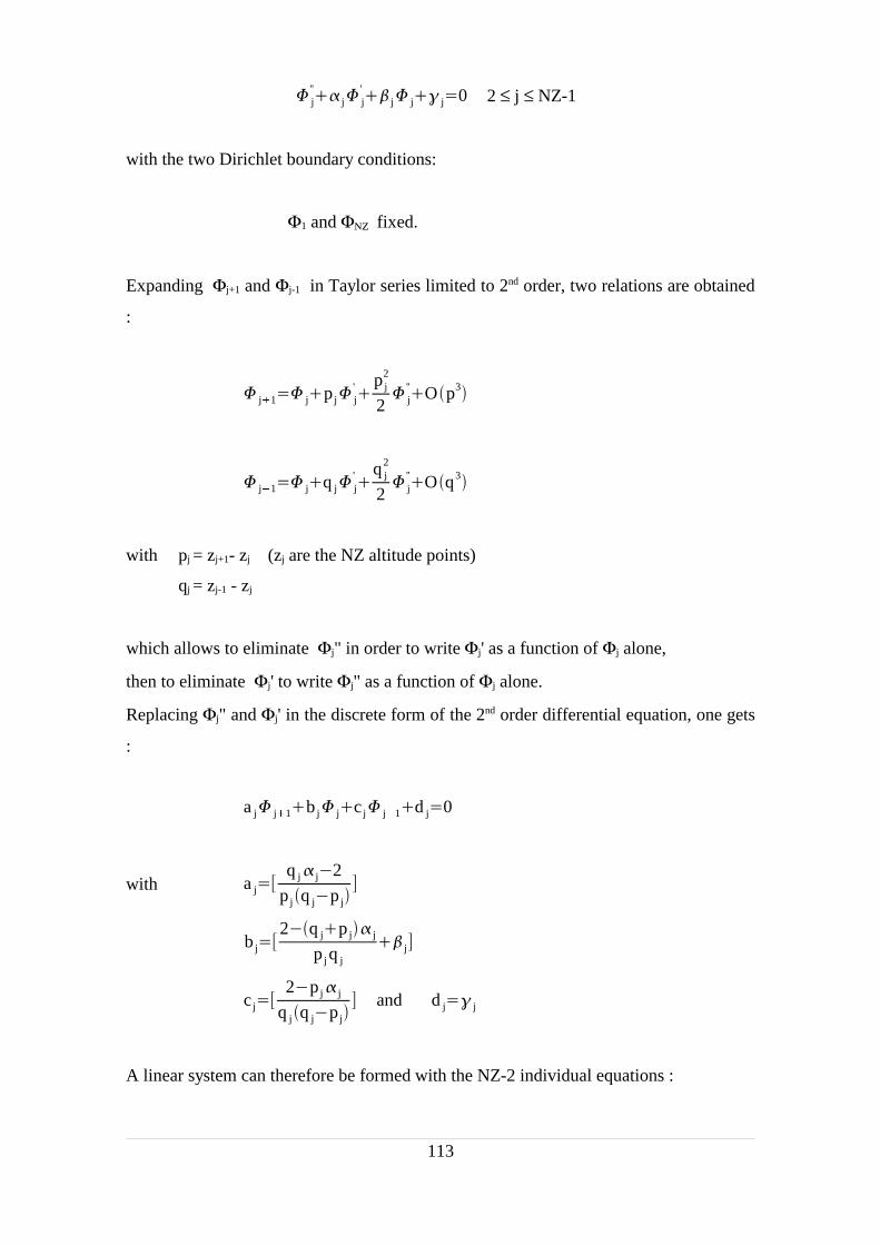
j'' j j
' j j j0 2 ≤ j ≤ NZ-1
with the two Dirichlet boundary conditions:
Φ1 and ΦΝΖ fixed.
Expanding Φj+1 and Φj-1 in Taylor series limited to 2nd order, two relations are obtained
:
j1 jpj j'
pj2
2 j
''Op3
j1 jq j j'
q j2
2 j
''Oq3
with pj = zj+1- zj (zj are the NZ altitude points)
qj = zj-1 - zj
which allows to eliminate Φj" in order to write Φj' as a function of Φj alone,
then to eliminate Φj' to write Φj" as a function of Φj alone.
Replacing Φj" and Φj' in the discrete form of the 2nd order differential equation, one gets
:
a j j1bj jcj j1d j0
with a jq j j2
pjq jpj
bj2q jpj j
p j q j
j
cj2pj j
q jq jpj and d j j
A linear system can therefore be formed with the NZ-2 individual equations :
113

b2 a2
c3 b3 a3
c4 b4 a4 0
0 cNZ2 bNZ2 aNZ2
cNZ1 bNZ1
2
3
4
NZ2
NZ1
d2c21
d3
d4
dNZ2
dNZ1cNZ1NZ1
The tridiagonal matrix can be transformed into an upper triangular matrix by
eliminating the cj elements from the lower diagonal. This is done by subtracting a
multiple of the j-1 line from each line with j≥3 i.e. :
c' jcj j b' j1
b' jbj j a' j1
a' ja j j 0d' jd j j d' j1 j3,4,, NZ1
with
b'2b2
a'2a2
d'2d2c21
and j is such that c' j0 therefore jcj
b' j1
b'2 a2
0 b'3 a3
0 b'4 a4 0
0 0 b'NZ2 aNZ2
0 b'NZ1
2
3
4
NZ2
NZ1
d2c21
d'3d'4
d'NZ2
d'NZ1
Finally, this system of equations is solved with a recurrent method :
NZ1d'NZ1
b'NZ1
jd'ja j j1
b'j
jNZ2,,2
114
So far, we have obtained a method allowing complete determination of the
downward electron flux Φj− along the NZ points, with the two Dirichlet boundary
conditions fixing the values of Φ−1 and Φ−
ΝΖ−1 . The upward electron flux can be
calculated from the downward flux. Indeed, from equation 1), on gets the relation :
+R11T2
d +
dz with R1
T1
2 -
p+
T2
First order development of the derivative leads to a recurrence relation between Φ+j and
Φ+j+1
j+R1
j1+ R1
1T2z jz j1 for j ≥ 2
and we can apply the lower boundary condition 1+1
- (which must be close to 0)
VI.3.2.2 Lower boundary conditions
We have described a numerical method solving the coupled differential equation
system 1) and 2) which requires two Dirichlet boundary conditions. It is however
possible to apply the method to a Neumann lower boundary condition. Indeed, if Φ−1
equals Φ−2 then
d -
dz0 at the bottom of the atmosphere. Consequently
d2 -
dz2 0
and the second order numerical differential equation locally becomes: -0
that is 1-
2
2
which is the required Dirichlet boundary condition.
This method allows to choose between a Dirichlet or a Neumann lower boundary
condition by simply commenting out one line in the FORTRAN program.
115

VI.3.2.3 Average pitch angle
We have not given yet a numerical value to the average cosine of the electron
pitch angle <cosθ>. In the remaining of the text we write µ = cosθ where θ is the
electron pitch angle. In the two-stream approximation, the upward flux is usually
defined as Φ+ = Φ(µ) for 0 < µ < 1 and the downward flux is defined as Φ− = Φ(µ) for
-1 < µ < 0 and
1
1
d 1
0
d 0
1
d
If the electron pitch angle distribution is isotropic, <cosθ> = ½ for both streams. A
more general approach can be invoked to derive a more appropriate value for <cosθ> in
better agreement with the numerical resolution method of the integrals.
Strickland et al. (1976) derived a general equation (from the Boltzmann transport
equation) describing the behavior of an incident electron beam along a magnetic field
line. It can be written as follows :
d
dz
l
n l l l
nl l E'E
1
1
Rl E, E', , ' 'dE'd '
where nl is the lth species number density
σl is the total scattering cross section for collision with the lth species
Rl is the redistribution function in energy and direction, it is related to cross
sections by
R ', , E', E j
all processes j ', , E', E
E
The integral over dµ can be numerically approached by summation using Gauss's
numerical quadrature formula. In Gauss's formula the interval (-1,+1) is divided
according to the zeros (µj) of the Legendre polynomial Pm(µ) and the integral of a
116

function f(µ) over the interval (-1,+1) is expressed as a sum in the form
1
1
f d j1
m
a j f j
where the weights aj (also referred as the Christoffel's numbers) are given by
a j1
P'm j 1
1 Pm j
j
d .
The Rodrigues formula gives
Pm 1
2m m!
d m
dm 21m
In the two-stream approximation m=2 and the two zeros of P2(µ)=0 are 13
where the + and - indices refer to the upward and downward fluxes, respectively. The
associated Christoffel's numbers are a± = ± 1.
Dividing the electron flux into 2 streams in the directions µ+ and µ- , we can replace the
general electron transport equation by the 2 linear equations similar to those of Banks
and Nagy, but where
cos !13
.
The reason Gauss's formula is superior to other formulae for quadratures in the
interval 1,1 is that for a given m it evaluates the integral exactly for all
polynomials of degree less than 2m and not merely those of degree less than m; in other
words, Gauss's formula is almost twice as accurate as a formula using only m values of
the function in the interval would be expected to be.
From these considerations, cos !13
appears to be a value in a better agreement
with the general multistream approach and is therefore adopted in this work.
117
VI.3.3 Two-point Gauss-Legendre quadrature
We already introduced the concept of Gaussian quadrature in the two-stream
approximation (previous section) in order to estimate the average cosine of the pitch
angle distribution (<cosθ>).
The Gauss-Legendre quadrature approximates the integral
1
1
f x dxk1
N
wN,k f N,k
by sampling f(x) at the n unequally spaced abscissas xN,1, xN,2, ..., xN,N , where the
corresponding weights are wN,1, wN,2, ..., wN,N . We have seen that the abscissas and
weights are obtained from the Legendre Polynomials using the Rodrigues formula.
For the 2-point Gauss-Legendre rule, N=2 and we have :
w1 = 1.0 ;
w2 = 1.0 ;
x1 = 1
3;
x2 = 13
;
and 1
1
f x dxf x1f x2 .
To approximate the integral a
b
f tdt we use the shifted Gauss-Legendre rule for
[a,b].
Introducing the change of variable tab
2
ab2
x and dtba
2dx , and
letting g x f ab2
ab
2x ,
118

we can apply the previous Gauss-Legendre rule for the integral ba
2 1
1
g x dx
This method is used throughout when numerical approximation of an integral is
required.
119

VI.4 Cross-sections
While traveling along magnetic field lines, the electrons undergo elastic and
inelastic collisions with the major neutral constituents of the jovian atmosphere H2, H,
and He. The elastic electron impact cross section is taken from Moiseiwitsch (1962) for
He and from Callaway (1993) for H. The H2 elastic cross section, the elastic
backscatter probability and the inelastic H2 backscatter probability are derived from
Shyn and Sharp (1980, 1981). Most of the inelastic electron impact cross sections are
computed with the analytical formulation described by Garvey et al. (1977). The
B1u+ state, hereafter noted B (upper level of the H2 Lyman band system) and the
C1 "ustate, hereafter noted C (upper level of the H2 Werner band system) are taken
from Liu et al. (1998). The B'1u+ , B''1u
+ , D1 "u, D'1 "u
H2 Rydberg states
(hereafter noted B', B'', D, D', respectively) and the E,Fg+ (E,F) excitation rates are
computed with the analytical representation of Shemansky et al. (1987). The a3g+
triplet state (a3) of H2 cross section is compatible with Ajello et al. (1993) and Khakoo
et al. (1994) and the b3u+ state (b3) excitation cross section is comparable with the
measurements of Rescigno et al. (1993). The c3 "g (c3) excitation cross section is
compatible with Khakoo et al. (1986). According to Cravens et al. (1975) little error is
introduced by assuming that it completely decays to the b3 level and then dissociates.
The Lyman-α emission resulting from electron impact is produced by two mechanisms.
The dominant mechanism is dissociative excitation of H2. The cross section for this
process is taken from Ajello et al. (1995). The other mechanism is direct excitation of
H, with the cross section from James et al. (1997). The Lyman-β emission cross section
from dissociative excitation of H2 is from Ajello et al. (1996).
The differential ionization cross sections are computed following the formulation of
Green and Sawada (1972), Jackman et al. (1977) and the relativistic formulation of
Garvey et al. (1977). They are adjusted to match the total ionization cross sections
measured by Straub et al. (1996) for H2, Bandyopadhyay et al. (1995) for H, and
Stephan et al. (1980) for He.
120

Rovibrational excitation by H2 is a very efficient cooling process for low energy
electrons. The cross section for vibrational excitation of H2 used is in agreement with
Buckman et al. (1990) and Miles et al. (1972) and the rotational excitation cross section
of H2 has been fitted to the measurements of Linder-Schmidt (1971). The analytical
excitation cross sections described by Ajello et al. (1995) are adopted to account for
doubly excited states of H2. These states are responsible for the dissociation of H2 in
fast H(2p) and H(2s) fragments which are involved in the neutral heating process.
VI.4.1 Total inelastic cross-section
The total differential inelastic collision cross section σk(E,E') is constructed from
the differential cross sections of the individual processes involving the kth neutral
species. Collisions of suprathermal electrons with the ambient electrons are not
included in this cross section and are treated separately during the degradation process.
The total differential cross section is of major importance in the energy degradation
problem since it is used to calculate the "production" of electrons at energy E' (degraded
primaries or secondaries) due to electrons of energy E colliding with neutral species (q±
in the formulation of Nagy and Banks).
Figure 35 is a plot of a E 0
E
E,E' dE' for inelastic collisions of electrons with
H2, which is the dominant neutral species in the upper stratosphere.
This cross section gives the probability that an electron of energy E undergoing an
inelastic collision with H2 will loose enough energy to end up in a lower energy bin.
For energies less than 10 eV, σa(E) is essentially due to the energy loss by excitation of
vibrational and rotational levels of the H2 ground state.
Between 10 and 20 eV excitation of triplet states of H2 a3g+ , b3u
+ ,c3 "g becomes
the major loss process. The energy separation between these two kinds of processes
gives rise to an important cross section gap around 10 eV.
From 15 eV, the most efficient loss processes rapidly increase. They are ionization and
excitation of the Lyman B'u+ and Werner C'"u singly excited states of H2.
Other processes involving higher energy levels of H2, such as the Rydberg states and
121

doubly excited states (Q1), have much smaller cross sections but cannot be neglected
since they give rise to important energy losses.
122
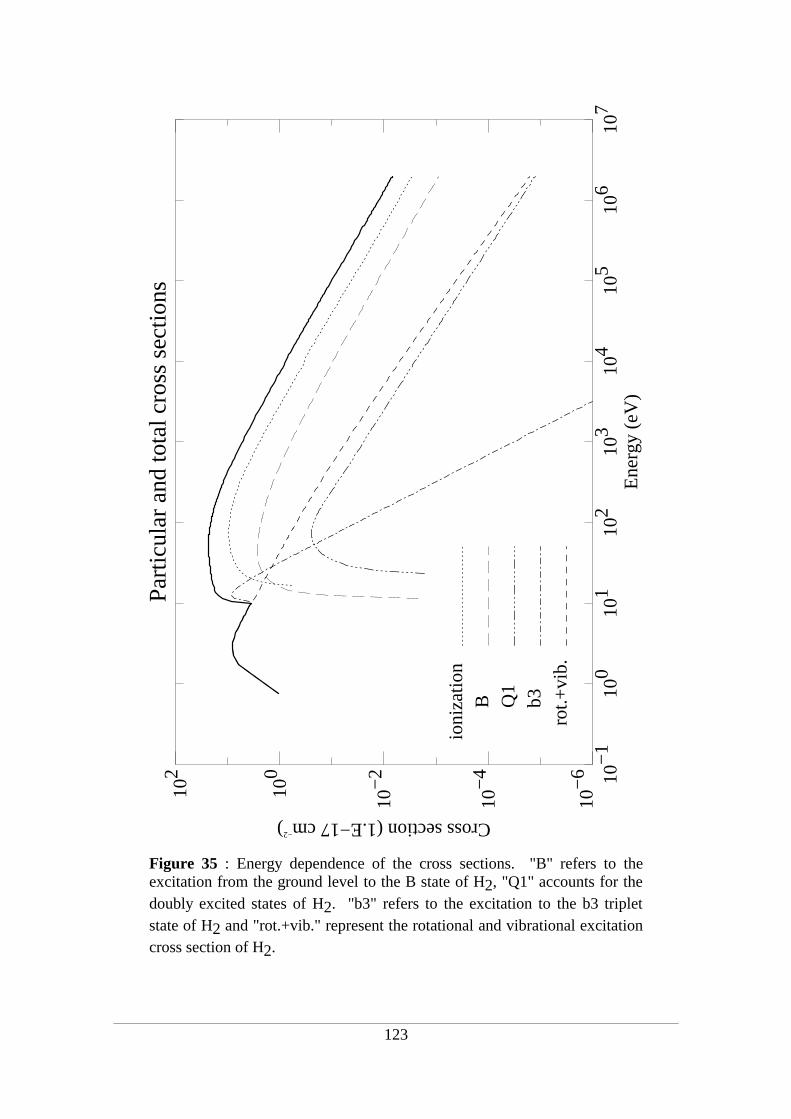
123
Figure 35 : Energy dependence of the cross sections. "B" refers to theexcitation from the ground level to the B state of H2, "Q1" accounts for thedoubly excited states of H2. "b3" refers to the excitation to the b3 tripletstate of H2 and "rot.+vib." represent the rotational and vibrational excitationcross section of H2.
Part
icul
ar a
nd to
tal c
ross
sec
tions
10−
110
010
110
210
310
410
510
610
7
Ene
rgy
(eV
)
10−
6
10−
4
10−
2
100
102
Cross section (1.E−17 cm−2)
B Q1
b3ro
t.+vi
b.
ioni
zatio
n

Figure 36 compares the total cross sections for inelastic collision with H2, He and H.
The major difference obviously stems from the absence of vibrational and rotational
excitation for the He and H atoms; they are transparent to low energy electrons. For
energies higher than 10 eV, excitation of the electronic states of He and H rapidly takes
place and finally leads to ionization. The high energy tail of the cross sections is almost
equal for the three species. This means that the energy degradation of high energy
electrons will not depend on the distribution among the neutral densities.
124
Figure 36 : Energy dependence of the total cross sections for inelastic collisions withH2, He, and H. The stairs shape of the curves is due to the method of "energyreapportionement".
10−2 100 102 104 106 108
energy (eV)
10−6
10−4
10−2
100
102
104
cros
s se
ctio
n (1
.E−
17 c
m−
2)
H2 _____
He −−−−−
H −.−.−
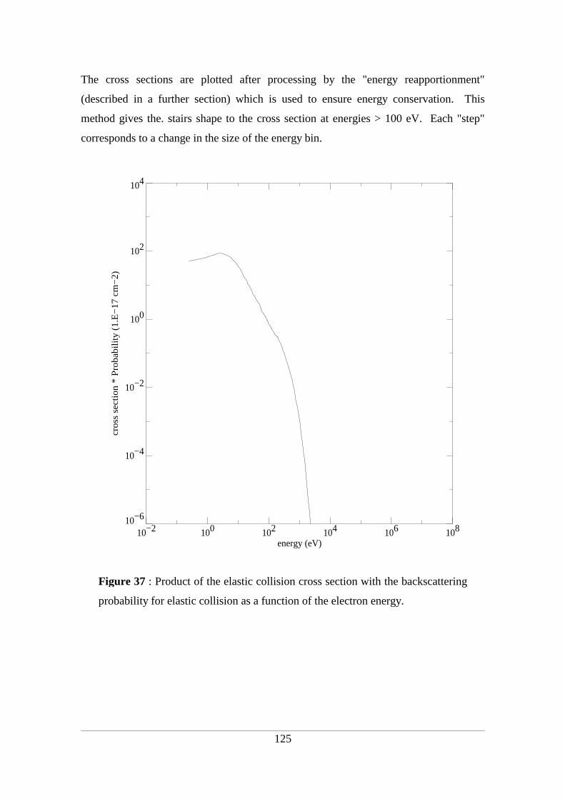
The cross sections are plotted after processing by the "energy reapportionment"
(described in a further section) which is used to ensure energy conservation. This
method gives the. stairs shape to the cross section at energies > 100 eV. Each "step"
corresponds to a change in the size of the energy bin.
125
Figure 37 : Product of the elastic collision cross section with the backscattering
probability for elastic collision as a function of the electron energy.
10−2 100 102 104 106 108
energy (eV)
10−6
10−4
10−2
100
102
104
cros
s se
ctio
n *
Pro
babi
lity
(1.
E−
17 c
m−
2)

VI.4.2 Backscattering
Figure 37 represents the product of the elastic collision cross section with the
backscattering probability for elastic collision as a function of the electron energy. This
process, which only changes the direction of the electron, is more efficient than the
inelastic collisions in the 0-100 eV energy range, with a peak at 10 eV, and rapidly
vanishes with increasing energy. Backscattering can also occur during inelastic
collision. Its probability as a function of energy is on the same order than that of elastic
collision.
The major effect of backscattering is to balance the energy distributions between
the upward and downward electron streams. However, this balance is mostly efficient at
low to medium energies and departures in the energy distributions of the beams appear
at high energies. As a result, the upward stream carries very few high energy electrons
compared to the downward stream. Another effect of the negligible backscattering
efficiency at high energy is that energetic primary electrons (E >1 keV) injected at the
top of the atmosphere have a chance to reach the lower region of the atmosphere where
they will deposit most of their energy. On the other hand, injected soft primary
electrons with energy less than 10 eV have a non-negligible probability to be
backscattered to space and thus to be definitely lost for the beam. For other energies,
the exact path followed by a primary electron after injection and prior to thermalization
is unpredictable. We can however take the example of a 100 eV primary electron.
After downward injection, backscattering probability is relatively weak and the first few
collisions (elastic or inelastic) with a neutral will probably not modify its direction. As
it looses energy and reaches denser regions, the backscattering probability progressively
increases. At some altitude, the direction of the electron is reversed. After further
collisions the electron is again backscattered downward and so on. As the frequency of
direction change increases, the altitude of the electron tends toward a limiting value
proportional to the initial energy. After a series of rapid bounces back and forth, the
electron is finally thermalized and as far as this electron is concerned, the degradation
process is over.
126

The different cross sections that are used in the energy degradation model are
summarized in tables 11 to 14. They correspond to electron-H2, electron-He, electron-
H and electron-electron collisions, respectively. In each table, the first column
characterizes the energy loss process, the second column gives the reference for an
analytical fit to the observed cross section, and the third column eventually gives
reference for recent observations still matched by the analytical representation given in
the reference of the second column. In the case of H2, He, and H ionization, the
analytical fits were scaled to the new references.
electron-H2 impact cross-sections
elastic collision Shyn and Sharp (1980,1981)
elastic backscatter probability ''inelastic backscatter probability ''
B'u+ C '"u Liu et al. (1998)
B'1u+ B''1u
+ D'"u
D''"u E,Fg+
Shemansky et al. (1985)
a3g+ Garvey et al. (1977) Khakoo et al. (1994)
b3u+ '' Rescigno et al. (1993)
c3 "g'' Khakoo et al. (1980)
d, e, f, g, h, i, j, k, p, r, s, v tripletstates
''
Ly α (dissociation) Ajello et al. (1995)
ionization Garvey et al. (1977) Straub et al. (1996)vibrational excitation Miles et al. (1972)rotational excitation Linder-Schmidt (1971)doubly excited states (Q1) Ajello et al. (1985)
Table 11
127
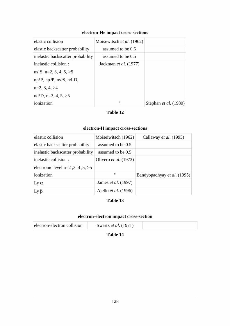
electron-He impact cross-sections
elastic collision Moisewitsch et al. (1962)
elastic backscatter probability assumed to be 0.5
inelastic backscatter probability assumed to be 0.5
inelastic collision :
ns1S, n=2, 3, 4, 5, >5
np1P, np3P, ns3S, nd1D,
n=2, 3, 4, >4
nd1D, n=3, 4, 5, >5
Jackman et al. (1977)
ionization '' Stephan et al. (1980)
Table 12
electron-H impact cross-sections
elastic collision Moiseiwitsch (1962) Callaway et al. (1993)
elastic backscatter probability assumed to be 0.5
inelastic backscatter probability assumed to be 0.5
inelastic collision :
electronic level n=2 ,3 ,4 ,5, >5
Olivero et al. (1973)
ionization '' Bandyopadhyay et al. (1995)
Ly α James et al. (1997)
Ly β Ajello et al. (1996)
Table 13
electron-electron impact cross-section
electron-electron collision Swartz et al. (1971)
Table 14
128

VI.5 Numerical treatment of the electron energy loss
The discrete energy degradation procedure used in the electron transport code
rests on the "energy reapportionment" method described by Swartz (1985). This method
allows us to use an optimized variable energy bin structure, with small 0.5 eV energy
bins below 10 eV gradually increasing to 25 keV wide bins near 1 MeV. With such a
variable energy grid, it is possible to account for a wide range of energies while
introducing a minimum of numerical discontinuities and using a reasonably small
number of energy bins.
VI.5.1 Energy reapportionment
The term "energy reapportionment" refers to the redistribution of electron energy
to the various neutral, ion, and electron species as a result of collisions. lndividual
inelastic collisions with the neutrals cause discrete step losses of energy from the
electrons that vary from a fraction of eV to many tens of electron volts, while
interactions with the ambient electrons result in a continuous loss. Ionizing collisions
result in a step plus a continuum energy loss from the incident electron due to the
variable energy of the secondary electron. The present method provides a practical
means for achieving the best energy conservation and the most accurate repartition of
energy to secondaries and the various excited states, with the smallest number of energy
cells and therefore minimize computing costs.
The optimized scheme described here uses the same discrete formalism at all energies,
and guarantees numerical energy conservation independently of the energy grid size or
configuration. The cells of the energy grid rapidly increase in width with increasing
energy, and the cells can even be larger than the excitation thresholds.
VI.5.2 Energy reapportionment following inelastic collisons
With any discrete energy grid, there will always be incompatibilities between the
true electron energies, the mean cell energies, and the discrete losses, as shown in Figure
38. In this figure the mean energies of the cell are labeled by Ei and the cell boundaries
129

appear at equal distances on either side. We would like to use large energy cells to
minimize the number of cells required, however, if the grid is too coarse (as in the upper
portion of the figure), excitation of a state whose threshold is much less than the width
of the energy cell may not actually provide a loss from that cell in just one collision.
(figure 38 refers to a case where three collisions were required for full
degradation from one cell to the next). Even when the cell width is less than the
excitation energy (i.e., the discrete loss), there can still be energy mismatches of the
order of ½∆E like that shown in the bottom portion of figure 38. Of course, it should
again be emphasized that such energy mismatches can be made arbitrarily small using a
sufficiently fine energy grid with any of the basic codes used in the past, but there is a
better way.
For perfect matching of the initial and degraded energies, effective cross sections (σa')
for each excitation should be generated as products of the actual cross section (σa) times
the ratio of the threshold (T) divided by the difference between the original energy (Ei)
and the grid cell energy nearest to Ei - T. Designating this nearest cell energy as Ek, we
have
a ' a
TEiE k
130
Figure 38
Energy Mismatch T
Ei-1 Ei
∆E i-1 ∆E i
T
Energy Mismatch
Ei-1 EiEk
Ei-1 Ei - T<
Ek Ei - T<Ei-1<
(a)
(b)

where Ek must always be strictly less than E. For example, if three inelastic collisions
(that excite a given state) are required to degrade an electron from the mean energy of
one cell to the next lower cell (as in figure 38a), then the cross section is reduced by a
factor of three to make such a total degradation just one-third less probable.
If the electrons of a large energy cell are entirely degraded into a smaller cell, the shape
of the spectral distribution will be distorted even though energy is conserved. This
situation is diagrammed in figure 39a. Assume for the moment that the cell sizes are
less than the excitation energy. A simple discrete calculation would take all the
electrons in cell Ei and dump them into cell Ek. In fact, the electrons would have some
energy distribution over the source cell Ei, so that some being degraded (by the given
process with threshold T) near the lower cell boundary of Ei should be placed into cell
Ek - 1, while those near the upper cell boundary of Ei should go into Ek + 1, as shown in
figure 39b. Hence, if all of these electrons were degraded into cell Ek only, the
distribution at Ek would be artificially enhanced in relation to the adjacent energy cells.
The use of rapidly increasing energy cell sizes is contingent on means for eliminating
this effect, and the key is to simply spread the electrons from the large cell over a group
of smaller cells having the same total width, so long as T is greater than the cell widths.
This assumes that the true spectral distribution varies slowly over any given cell.
131
Figure 39
Ei
<(a)T
Ek
∆E k
∆E k ∆E i
Ek+1Ek-1
Ei
(b)
Ek Ek+1Ek-1
∆E i ∆E i
∆E i
T
T
∆Ei = ∆E
k-1 + ∆E
k + ∆E
k-1

VI.5.3 Energy reapportionment following ionizing collisions
Implementing the scheme to guarantee energy conservation for ionizing
collisions is only slightly more involved than for simple inelastic collisions. Since the
energy of the secondary electron is a random quantity, we must deal with functions
describing distributions of secondary energies, i.e. the partial ionization cross sections.
All the above arguments can then be applied to the emergent primary electrons produced
by the partial ionization cross sections applied to each secondary energy. If a given
secondary has an energy Es, then the actual primary energy is
Ep =Ei - TI - Es
where Ei is the initial primary energy and TI, is the ionization threshold. To compute the
rates by which emergent primaries of this energy are deposited in the cell nearest to Ep,
the partial ionization cross section is modified in a manner similar to that used before,
giving
i 'E k i EsTIEs
EiE k
where σ(Es) is the true partial ionization cross section corresponding to the given
secondary energy (Es) and the incident primary energy (Ei). The modified cross sections
are summed to yield the total ionization cross section, which will be used to compute
the loss rate from the initial primary energy cell. However, the reapportionment of
secondaries is determined from the unmodified partial cross section, while the
reapportionment of primaries follows the modified form. Hence the use of small energy
cells at low energies will imply that the primaries cascading into a large high energy cell
correspond to secondaries going into several adjacent cells of approximately the same
combined width in energy.
132
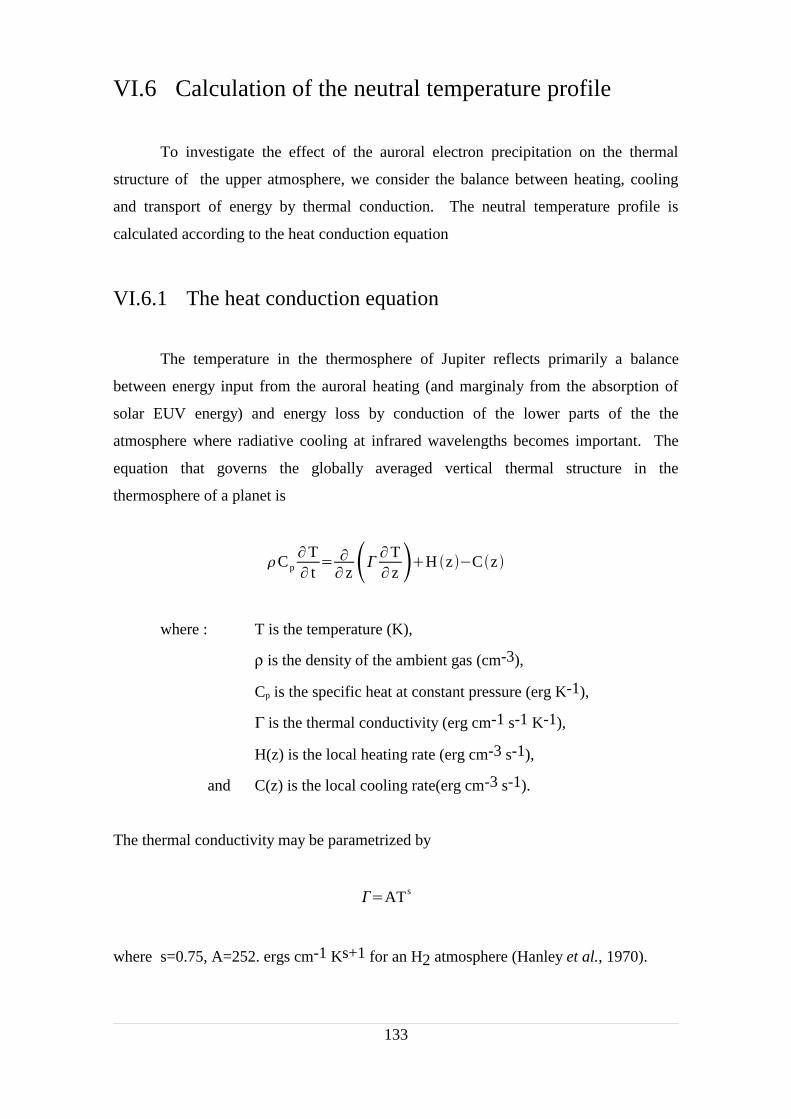
VI.6 Calculation of the neutral temperature profile
To investigate the effect of the auroral electron precipitation on the thermal
structure of the upper atmosphere, we consider the balance between heating, cooling
and transport of energy by thermal conduction. The neutral temperature profile is
calculated according to the heat conduction equation
VI.6.1 The heat conduction equation
The temperature in the thermosphere of Jupiter reflects primarily a balance
between energy input from the auroral heating (and marginaly from the absorption of
solar EUV energy) and energy loss by conduction of the lower parts of the the
atmosphere where radiative cooling at infrared wavelengths becomes important. The
equation that governs the globally averaged vertical thermal structure in the
thermosphere of a planet is
CpT t
z# T
z H z Cz
where : T is the temperature (K),
ρ is the density of the ambient gas (cm-3),
Cp is the specific heat at constant pressure (erg K-1),
Γ is the thermal conductivity (erg cm-1 s-1 K-1),
H(z) is the local heating rate (erg cm-3 s-1),
and C(z) is the local cooling rate(erg cm-3 s-1).
The thermal conductivity may be parametrized by
#ATs
where s=0.75, A=252. ergs cm-1 Ks+1 for an H2 atmosphere (Hanley et al., 1970).
133

The time constant is sufficiently long that we can drop the time-dependent term.
With this simplifying assumption we can use the following heat conduction equation to
calculate the neutral temperature profile from the altitude dependent heating and cooling
rates :
ddz
Fz H z Cz
where Fz #dTdz is the local heat flux in erg cm-2 s-1.
VI.6.2 Numerical resolution
Integrating the equation from altitude z to infinity gives the heat flux F(z) in
erg cm-2 s-1 at altitude z (cm)
Fz z
H z'Cz'dz'A Tsz dTdz
z
As1
ddz
Ts1z
Integration between two altitude steps z1 and z2 gives
s1 z1
z2
Fz dzTs1z1Ts1z2
Letting $s1 z1
z2
Fz dz we finally get T z2T z1s1$
1s1
which leads to the recurrence relation
T n1T ns1$
1s1 n=1, ..., NZ-1
134
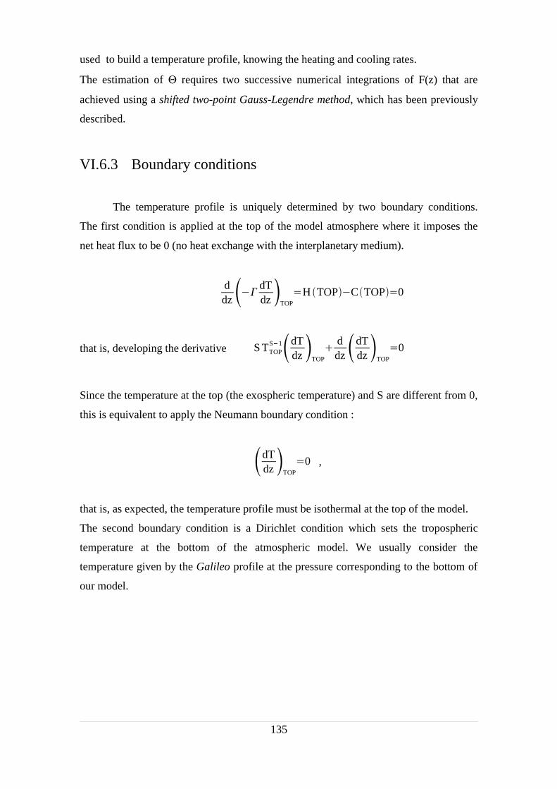
used to build a temperature profile, knowing the heating and cooling rates.
The estimation of Θ requires two successive numerical integrations of F(z) that are
achieved using a shifted two-point Gauss-Legendre method, which has been previously
described.
VI.6.3 Boundary conditions
The temperature profile is uniquely determined by two boundary conditions.
The first condition is applied at the top of the model atmosphere where it imposes the
net heat flux to be 0 (no heat exchange with the interplanetary medium).
ddz#
dTdz TOP
H TOPCTOP0
that is, developing the derivative S TTOPS1dT
dz TOP
ddzdT
dz TOP
0
Since the temperature at the top (the exospheric temperature) and S are different from 0,
this is equivalent to apply the Neumann boundary condition :
dTdz TOP
0 ,
that is, as expected, the temperature profile must be isothermal at the top of the model.
The second boundary condition is a Dirichlet condition which sets the tropospheric
temperature at the bottom of the atmospheric model. We usually consider the
temperature given by the Galileo profile at the pressure corresponding to the bottom of
our model.
135
VI.6.4 Heat sources
The major electron heating mechanisms that we considered are :
electron impact dissociation of H2
thermal electron cooling of the energetic electrons, and subsequent H2 vibrational
and rotational cooling of the thermal electrons
vibrational excitation of the ground electronic state of H2 following Lyman and
Werner band transitions
chemical heating due to the formation of H2+ and H and subsequent reactions
resulting in dissociative recombination of H3+ to produce H2 and H
excess kinetic energy from the dissociation of H2.
The energy stored into H+ is not available for heating, since H+ recombines radiatively
unless charge exchange with H2 (v ≥ 4) occurs.
VI.6.4.1 H2 dissociation
The average fractions of the transitions from the B state, including cascade from
EF and from the C state terminating into the vibrational continuum of the ground state
X1g+ , are calculated from Dalgarno and Stephens (1970), and Stephens and
Dalgarno (1972). The average kinetic energy of the fragments is determined from
Stephens and Dalgarno (1973) and is consistent within 5% with the temperature
sensitive values given by Abgrall et al. (1997). For the B'', D and D' excited states, we
used the branching ratios determined by Ajello et al. (1984) at 100 eV to discriminate
the direct transitions to the ground state from the predissociation to the B' state. These
branching ratios to the ground state are 3.3%, 70.2% and 42.1%, respectively. The
fraction of the transitions from the D excited state to the vibrational continuum of the
ground state is from Glass-Maujean et al. (1984). For the B' excited state we use Kwok
et al. (1985) which is in agreement with Liu et al. (1996). According to Liu et al.
(1996), B'' the and staD' tes have approximately the same equilibrium separation as the
B' and D states respectively. We thus consider the same fractions of transitions ending
136
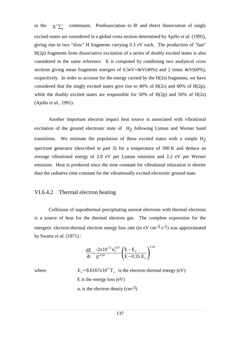
in the X1g+ continuum. Predissociation to B' and direct dissociation of singly
excited states are considered in a global cross section determined by Ajello et al. (1995),
giving rise to two "slow" H fragments carrying 0.3 eV each. The production of "fast"
H(2p) fragments from dissociative excitation of a series of doubly excited states is also
considered in the same reference. It is computed by combining two analytical cross
sections giving mean fragments energies of 6.5eV+4eV(40%) and 2 times 4eV(60%),
respectively. In order to account for the energy carried by the H(2s) fragments, we have
considered that the singly excited states give rise to 40% of H(2s) and 60% of H(2p),
while the doubly excited states are responsible for 50% of H(2p) and 50% of H(2s)
(Ajello et al., 1991).
Another important electron impact heat source is associated with vibrational
excitation of the ground electronic state of H2 following Lyman and Werner band
transitions. We estimate the population of these excited states with a simple H2
spectrum generator (described in part 3) for a temperature of 500 K and deduce an
average vibrational energy of 2.8 eV per Lyman emission and 2.2 eV per Werner
emission. Heat is produced since the time constant for vibrational relaxation is shorter
than the radiative time constant for the vibrationally excited electronic ground state.
VI.6.4.2 Thermal electron heating
Collisions of suprathermal precipitating auroral electrons with thermal electrons
is a source of heat for the thermal electron gas. The complete expression for the
energetic electron-thermal electron energy loss rate (in eV cm-3 s-1) was approximated
by Swartz et al. (1971) :
dEdt
-2x10-12 ne
0.97
E0.94 EEe
E0.35 Ee
2.36
where Ee8.6167x10-5 Te is the electron thermal energy (eV)
E is the energy loss (eV)
ne is the electron densiy (cm-3)
137
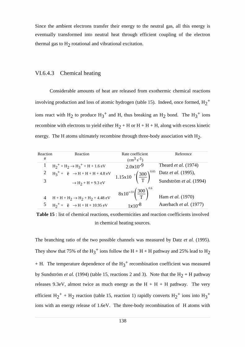
Since the ambient electrons transfer their energy to the neutral gas, all this energy is
eventually transformed into neutral heat through efficient coupling of the electron
thermal gas to H2 rotational and vibrational excitation.
VI.6.4.3 Chemical heating
Considerable amounts of heat are released from exothermic chemical reactions
involving production and loss of atomic hydrogen (table 15). Indeed, once formed, H2+
ions react with H2 to produce H3+ and H, thus breaking an H2 bond. The H3
+ ions
recombine with electrons to yield either H2 + H or H + H + H, along with excess kinetic
energy. The H atoms ultimately recombine through three-body association with H2.
Reaction#
Reaction Rate coefficient
(cm3 s-1)
Reference
1 H2+ + H2 → H3
+ + H + 1.6 eV 2.0x10⁻⁹ Theard et al. (1974)
2
3
H3+ + %e → H + H + H + 4.8 eV
→ H2 + H + 9.3 eV1.15x107300
T 0.65 Datz et al. (1995),
Sundström et al. (1994)
4 H + H + H2 → H2 + H2 + 4.48 eV8x1033300
T 0.6
Ham et al. (1970)
5 H2+ + %e → H + H + 10.95 eV 1x10⁻⁸ Auerbach et al. (1977)
Table 15 : list of chemical reactions, exothermicities and reaction coefficients involved
in chemical heating sources.
The branching ratio of the two possible channels was measured by Datz et al. (1995).
They show that 75% of the H3+ ions follow the H + H + H pathway and 25% lead to H2
+ H. The temperature dependence of the H3+ recombination coefficient was measured
by Sundström et al. (1994) (table 15, reactions 2 and 3). Note that the H2 + H pathway
releases 9.3eV, almost twice as much energy as the H + H + H pathway. The very
efficient H2+ + H2 reaction (table 15, reaction 1) rapidly converts H2
+ ions into H3+
ions with an energy release of 1.6eV. The three-body recombination of H atoms with
138
H2 (table 15, reaction 4) provides 4.48eV of kinetic energy. These very large auroral
heat sources will certainly generate strong thermospheric winds that will globally
redistribute both heat and neutral constituents like H, however, we have considered that
this reaction chain occurs in the same layer and that heat is produced at the same level.
The H2+ + e → H + H dissociative recombination (table 15, reaction 5) is also
considered. It is less efficient than reaction (1) but provides 10.95 eV to the ambient
gas.
VI.6.4.4 Unspecified heat sources
So far, we have considered heat sources resulting from auroral particle
precipitation in the atmosphere, other non-auroral heat sources might play an important
role in the temperature budget but have not been directly taken into account in this
study. Joule heating generated by the presence of a perpendicular electric field in the
presence of Pedersen conductivity is an important heating process in the auroral
ionosphere (in the Earth atmosphere, it represents almost 50% of the heating). It is
difficult to quantify since the jovian ionospheric electric field is largely unknown.
Therefore, it was neglected in this study.
Solar EUV heating has been neglected as well which restricts the validity of the model
to night time conditions or to daytime aurora where the particle flux exceeds the solar
EUV input of 0.1 erg cm-2 s-1.
The exothermic hydrocarbon chemistry might as well play an important role in the
stratosphere but has not been addressed in the code.
VI.6.4.5 Breaking gravity waves
Young et al. (1997) showed that the energy viscously dissipated by breaking
gravity waves is comparable to that needed to heat the equatorial atmosphere. However,
this conclusion was recently challenged (Matcheva et al., 1999). For reasons described
below, this potentially produced heat is not included in our model.
Heating of Jupiter's thermosphere by viscous dissipation of upward propagating
139

gravity waves due to molecular heat conduction and viscosity has been recently
evaluated by Matcheva and Stobel (1999). According to Schroeberl et al. (1983) the
large sensible heat flux associated with dissipating gravity waves and induced
turbulence lead to a redistribution of sensible heat so that cooling predominates in the
upper part of the wave breaking region, whereas net heating occurs in the lowest,
highest pressure levels of wave breaking. By accounting for these heating and cooling
regions Matcheva and Strobel found that gravity waves with amplitudes and properties
consistent with those inferred from temperature variations in the Galileo probe
temperature profile by Young et al. (1997) are incapable of heating Jupiter’s
thermosphere sufficiently to account for the large temperature gradients and high
temperatures derived from probe data. The total wave energy flux at the homopause
level is 0.39 erg cm2 s-1, which produces a maximum temperature gradient of
2.8 K km-1 at 355 km and maximum thermospheric temperature of 380 K at 552 km
above the 1-bar pressure level. The resulting thermal profile is compared to the Galileo
profile in figure 40.
140
Figure 40 : Comparison of temperaure profiles generated by model 1(thin continuous line) with the thermospheric temperature profile ofJupiter inferred from Galileo probe data (thick line). Taken fromMatcheva and Strobel (1999)
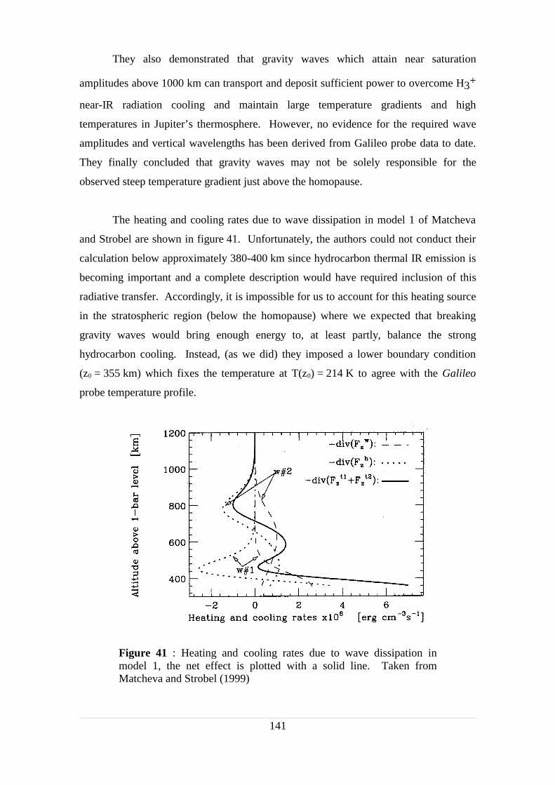
They also demonstrated that gravity waves which attain near saturation
amplitudes above 1000 km can transport and deposit sufficient power to overcome H3+
near-IR radiation cooling and maintain large temperature gradients and high
temperatures in Jupiter’s thermosphere. However, no evidence for the required wave
amplitudes and vertical wavelengths has been derived from Galileo probe data to date.
They finally concluded that gravity waves may not be solely responsible for the
observed steep temperature gradient just above the homopause.
The heating and cooling rates due to wave dissipation in model 1 of Matcheva
and Strobel are shown in figure 41. Unfortunately, the authors could not conduct their
calculation below approximately 380-400 km since hydrocarbon thermal IR emission is
becoming important and a complete description would have required inclusion of this
radiative transfer. Accordingly, it is impossible for us to account for this heating source
in the stratospheric region (below the homopause) where we expected that breaking
gravity waves would bring enough energy to, at least partly, balance the strong
hydrocarbon cooling. Instead, (as we did) they imposed a lower boundary condition
(z0 = 355 km) which fixes the temperature at T(z0) = 214 K to agree with the Galileo
probe temperature profile.
141
Figure 41 : Heating and cooling rates due to wave dissipation inmodel 1, the net effect is plotted with a solid line. Taken fromMatcheva and Strobel (1999)
Another consequence of this limitation is that the origin for the stratospheric
temperature remains unexplained, although breaking gravity waves might be a good
candidate.
As will be illustrated in the next sections, these non-auroral heat sources are
required to balance the hydrocarbon cooling in the polar regions and to sustain the
thermal profile observed in the equatorial regions. Their effect is, at least partly,
mimicked by preventing the temperature, deeper than a critical pressure, to drop below
the initial temperature profile.
VI.6.5 Heat sinks
Altitude-dependent radiative cooling by thermal infrared band emissions from
H3+ , CH4 and C2H2 is considered following the method described by Drossart et al.
(1993).
VI.6.5.1 Estimation of the radiative cooling
To obtain the cooling term used in the heat conduction equation, we calculate
altitude dependent rates for radiative cooling by thermal infrared band emissions from
CH4, C2H2 and H3+.
For the hydrocarbon species, we assume an optically thin regime and calculate thermal
emission rates as a function of altitude for the v4 band of CH4 and the v5 band of C2H2.
Infrared emissions from these bands play a dominant role in radiative cooling just above
the homopause. The method used to calculate the hydrocarbon cooling is based on
Drossart et al. (1993). Non-local thermodynamic equilibrium (non-LTE) effects were
accounted for through the use of the cool-to-space approximation (Appleby, 1990)
which neglects radiative exchange between layers compared with energy that escapes
directly to space. To calculate the H3+ cooling, we employed a method similar to that
used for methane and acetylene for the v2 fundamental band of H3+. In most cases H3+
is found to be optically thin (Lam et al., 1997).
142
VI.6.5.2 The local thermodynamic equilibrium (LTE)
In the local thermodynamic equilibrium (LTE) approximation, the infrared
emission of H3+, CH4 and C2H2 is proportional to the number of molecules in the first
vibrational level, which is an increasing function of temperature. The non-LTE
correction depends on the quenching rate for each molecule. It does not significantly
modify this temperature dependence and therefore, the radiative cooling efficiencies
remain proportional to the gas temperature.
The internal energy of a gas in local thermodynamic equilibrium (LTE) is
characterized by a single temperature, applicable to all degrees of freedom. This
temperature specifies the populations of states according to a Boltzmann distribution
which, within many atmospheric levels of interest, is maintained by collisions. At
relatively low pressures, however, radiative processes usually control the populations of
states, departures from a Boltzmann distribution occur, and the corresponding
atmospheric temperatures can significantly differ from values that would hold in LTE.
If a is the collisional deexcitation rate for the transition, we define
ξ = a/A ,
where A is the Einstein coefficient for spontaneous emission. In general, ξ is the
parameter of importance concerning transfer of energy between the radiation field and
matter.
In LTE, collisional deexcitation predominates, i.e., ξ&1, and the radiation field is
coupled to the kinetic temperature of the gas. Conversely, non-LTE means that
radiative decay is dominant, i.e., ξ'1, which implies, in an optically thick atmosphere,
complete scattering (true absorption, followed by emission). If, as is the case for H3+,
the atmosphere is assumed to be optically thin, then complete departure from LTE will
lead to almost no excitation and therefore no emission.
Since the value of a depends on pressure and temperature, ξ provides an estimate of the
143

importance of non-LTE processes.
VI.6.5.3 H3+ density and radiative cooling
We can now address the question : how does quenching of H3+ by H2 influence
the H3+ radiative cooling ?
We only consider quenching by H2 which is dominant in the upper stratosphere and
lower thermosphere. H3+ has two vibrational modes, a symmetric breathing mode with
quantum number v1, and a doubly degenerate asymmetric bending mode with quantum
number v2.
Quenching (deactivation) of excited H3+ by H2 may be described as
H3+ (v1,v2) + H2(v=0)→ H3+ (0,0) + H2(v' )
with a rate coefficient kd = 2.7 ±0.6 10-10 cm3 s-1 (Kim et al., 1974) (we consider
complete deactivation of H3+ to its vibrational ground state).
At thermodynamical equilibrium, the concentration of vibrationally excited H3+ is
given by
H3+v1 ,v2N
g v
QexpE H3
+v1 ,v2
kT
where EH3+ (v1,v2) is the energy associated with the vibrational level (v1 , v2)
gv is the degeneracy of this level
Q is the vibrational partition function
N is the total number of H3+ molecules
According to Drossart et al. (1989), the H3+ infrared emission observed in the polar
144
regions of Jupiter does not arise from H3+(v2) produced directly in the reaction
H2+ + H2 → H3+(v2) + H
but from collisional excitation of H3+(v1=0 ,v2=0) by H2 with a rate coefficient k'd.
Therefore, under steady-state conditions, the production of H3+ excited by H2 collision
equals the loss of excited H3+ by quenching, i.e.
k'd H2 H3+kd H2 H3
+v1, v2
where [H3+] represents the concentration of H3+ molecules in the (v1=0,v2=0)
vibrational ground state, and [H2] is the molecular hydrogen concentration in the ground
state.
Since in the optically thin approximation, production by optical excitation can be
neglected compared to collisional excitation, and since N ≈ [H3+(v1=0,v2=0)], the rate
coefficient k'd for the excitation reaction is related to kd by
k'dkd
g v
QexpE H3
+v1 , v2
kT
The non-LTE correction may be brought into the production-loss balance by
including a radiative loss term of H3+ so that the production by collisional excitation is
balanced by quenching and radiative losses. We only consider the fundamental
transition v1=0, v2=1 → v1=0, v2=0 which is dominant in the infrared spectrum of H3+.
The production-loss balance may be written as
kd H2 H3+
g v
QexpE H3
+v2
kT kd H2 H3+v2A H3
+v2
145

where H3+(v2) refers to H3+ excited in the v1=0, v2=1 vibrational level,
and A is the Einstein coefficient (in s-1) for the radiative deexcitation
H3+ (0,1) → H3+ (0,0) + hν
at the central wavelength 2521.31 cm-1 ( 3.97 µm). An optically thick regime would
have implied an additional production term (left side) due to the radiative excitation.
By letting (kd H2
A v2
(previously introduced)
where the product kd [H2] represents the collisional deexcitation rate (a) for the
transition, we can estimate the number of H3+ molecules in the vibrationally excited
state with
H3+v2H3
+g v
QexpE H3
+v2
kT fLTE
where fLTE(
1(is the correction factor due to non-LTE effects, and depends on
the quenching rate for H2. It is such that
if ξ >>1, collisions are dominant (atmosphere in LTE) and fLTE →1 ,while
if ξ <<1, radition is dominant (non-LTE atmosphere) and fLTE →0.
Finally, the local emission within 2π steradians I(H3+) radiated by a volume element of
H3+ (in other words, the local H3+ cooling rate) is given by the relation
I(H3+) = [H3+(v2)] Av2 hcσ(H3+) in erg cm-3s-1,
where hcσ(H3+) is the energy of the transition (0.31 eV), so that
I (H3+) is proportional to fLTE
146
Since fLTE can be rewritten in the form fLTEkd H2
kd H2A v2
it is directly seen that
if kd >>A1,0
H2, fLTE → 1 (LTE) and I(H3+) tends toward its maximum
value, while
if kd << A1,0
H2, fLTE → 0 (non-LTE) and I(H3+) vanishes.
From this discussion it appears that the effect of the quenching rate is solely due
to the non-LTE correction factor.
This relation also shows that the H3+ radiative cooling efficiency is temperature
dependent. Indeed, I(H3+) is proportional to the excited population [H3+(v2)] which
has just been shown to be proportional to the exponential term
expE H3+v2
kT
A plot of this exponential as a function of temperature is presented in figure 42 in
arbitrary units. It clearly shows that the cooling efficiency increases as the temperature
increases. This temperature effect is extremely pronounced in the 100-1000 K region
(that is the range of temperatures observed in the Jovian atmosphere) as the exponential
spans 13 orders of magnitude in that range.
147

Quenching of H3+ by H2 can occur either by vibrational transfer without atom
transfer or by chemical reaction such as proton transfer. Kim et al. (1974) measured a
"phenomenological" rate coefficient of 2.7 ±0.6x10⁻¹⁰ cm3 s-1 for the deactivation of
H3+ with vibrational energies of 0.5-2.5 eV by H2. It is to be compared with the
experimental vibration-to-translation (VT) quenching rate of H3+ by H2 which is on
the order of 10-12 cm3 s-1 (Blakley et al., 1977), and to the rate constant for resonant
148
Figure 42 : Temperature dependence of the H3+ cooling efficiency.
E(H3+[v2 =1])=0.315 eV
0 200 400 600 800 1000Temperature (K)
10−5
100
105
1010
1015H
3+ c
oolin
g ef
ficie
ncy
(arb
itrar
y un
its)

proton transfer between H3+ and H2, i.e.
H3+* + D2 → HD2+ + H2*
for which the Langevin gas kinetic rate constant is 3x10⁻¹⁰ cm3s-1.
Comparison between the rate coefficients of these processes show that resonant proton
transfer may in fact be the mechanism for energy transfer in the collisions.
VI.6.5.4 Collisional deexcitation for hydrocarbons and radiative cooling
Two collision relaxation rates are identifed for methane and acetylene, aVV and
aVT.
"VT" (vibration-to-translation) refers to the collisional deexcitation from a molecule's
lowest energy vibrational mode to the ground vibrational state. In other words, all
vibrational energy in the molecule is transferred to translational degrees of freedom. For
CH4 in Jupiter, the VT transition is v4 → ground.
"VV" relaxation refers to the faster vibration-to-vibration transitions between the
sublevels of each band group. These mechanisms result in LTE distributions within
each group, if pressure and temperature are high enough. A molecule excited to a given
level will generally undergo multiple VV transitions prior to a VT relaxation. Much
smaller energies are exchanged in VV, as compared with VT processes. In general,
aVV&aVT, which means all rate-determining steps involve VT transitions. We therefore
only considered aVT as the collisional deexcitation rate for the transition (a ≈ aVT ).
For non-LTE "nominal" models considering a mixture of CH4 and H2, the following
CH4 VT collisional relaxation time tVT (= aVT-1) was employed :
tVTt0VTPH2 (P(H2) is the H2 pressure),
and t0VT is temperature dependent and is given by
ln t0VT35.6 T136.838
149

This collisional relation time can be used to define the non-LTE correction factor fLTE
(equivalent to the correction factor defined for H3+) giving the fraction of v4 vibrational
energy which is converted to kinetic energy at the atmospheric level in question.
ξ = a/Av4 (or ξ = (tVT Av4 )-1)
and,
fLTE≡ (1 + ξ−1)-1
where Av4 is the Einstein coefficient (in s-1) for radiative deexcitation
CH4 (v4) → CH4 (0) + hν
and the central wavelength is 1306 cm-1 ( 7.7 µm).
As already mentionned, fLTE is bounded by 0 (non-LTE ; ξ= 0) and 1 (LTE ; ξ&1).
Using the same considerations as with H3+, we can estimate the local emission within
2π steradians I(CH4) radiated by a volume element of CH4 (in other words, the local
CH4 cooling rate) with the relation
I(CH4) = [CH4(v4)] Av4 hcσ(CH4) in erg cm-3s-1,
where hcσ(CH4) is the energy of the v4 → ground transition, and the concentration of
excited methane is given by
CH4v4CH40g v
QexpE CH4v4
kT fLTE
The case of acetylene is treated in exactly the same way. Following Appleby (1990), the
CH4 VT collisional relaxation time tVT can be applied directly to C2H2 v5 without
modification. Accordingly, we can estimate the local emission within 2π steradians
150
I(C2H2) radiated by a volume element of C2H2 (the local C2H2 cooling rate) with the
relation
I(C2H2) = [C2H2(v5)] Av5 hcσ(C2H2) in erg cm-3s-1,
where hcσ(C2H2) is the energy of the v5 → ground transition, and
C2 H2v5C2 H20g v
QexpE C2 H2v5
kT fLTE
with fLTE≡ (1 + ξ−1)-1, and ξ = (tVT Av5 )-1
where Av5 is the Einstein coefficient for the radiative deexcitation
C2H2 (v5) → C2H2 (0) + hν
and the v5 central wavelength is 729 cm-1 ( 1.4 µm).
VI.6.5.5 Departure from the optically thin approximation
The optically thin condition can be viewed as the probability that a photon,
emitted at an altitude z, will be reabsorbed in the atmosphere is smaller than 0.5. This
implies (Drossart et al., 1993) that the pressure level P ≤40 µbars for C2H2, and
P ≤50 µbars for CH4. Below this level, the observed infrared emission does not remain
a reliable indicator of the atmospheric cooling due to methane and acetylene. However,
the cooling efficiency should not be reduced in the optically thick regime. Indeed, since
the excited population can always be neglected compared to the ground state population,
the optical excitation of CH4 and C2H2 will not reduce the (cooling) collisional
excitation process but increase the (trapped) infrared emission.
151

VI.7 Response of the atmospheric structure to auroral
electron precipitation
VI.7.1 The initial model atmosphere
The initial model atmosphere is based on an analytical fit using a Bates function
fitted to the thermal profile determined by Seiff et al. (1998) from the Galileo probe
data (Figure 43). This thermal profile was calculated from the atmospheric density
deduced from the deceleration measurement of the probe during its entry and descent in
the Jovian atmosphere. It assumes an exospheric temperature of 900 K.
VI.7.2 Effects of electron precipitation
As a consequence of the heating processes previously described, precipitating
auroral electrons modify the thermal profile of the jovian thermosphere. In order to self-
consistently account for the adjustment of the densities to the resulting temperature
profile, the code iteratively solves a diffusion equation for the major constituents.
VI.7.2.1 Diffusion of the neutral species
The neutral atmosphere of Jupiter is mainly composed of H2. Other important
neutral gases considered in this model are He, H, CH4, and C2H2.
152

153
Figure 43 : Initial model atmosphere : the temperature profile is an analyticalfit to the equatorial thermal profile determined from the Galileo probe dataadapted to the larger acceleration of gravity at 60° N and thermosphericaltitudes. The density profiles are calculated as discussed in the text. Theenergy distribution of case A determines the ionization rate from which the
H3+ density is estimated.
102
104
106
108
1010
1012
1014
1016
Num
ber
dens
ity (
cm−
3 )
10−
2
10−
4
10−
6
10−
8
10−
10
10−
12
10−
14
Pressure (bar)
200
250
300
400
500
1000
Altitude (km)
20
0
400
60
0
800
10
00T
empe
ratu
re (
K)
T
H2
He
CH
4C
2H2
H
H3+
VI.7.2.1.1 The diffusion equation
For a binary mixture the general diffusion equation giving the relative diffusion
velocity v = v1 - v2 of gas 1 with respect to gas 2, can be written as (Chapman and
Cowling, 1970)
vD12 n2
n1 n2
)n1
n
m2m1
m) ln pT )ln T
m1 m2
mkTF1F2.
In this equation, n1, n2 are the respective concentrations of particles 1 and 2, n = n1 + n2
is the total concentration of the binary mixture, T is the absolute neutral gas
temperature, p = p1
+ p2
is the total pressure, k is the Boltzmann constant, m1, m2 are the
masses of particles 1 and 2, m = (n1m1 + n2m2)/(n1+n2) is the mean molecular mass, F1,
F2 are the acceleration vectors of particles 1 and 2 due to external forces, D12 is the
molecular diffusion coefficient of gas 1 in gas 2, and αT is the thermal diffusion factor.
According to gas kinetic theory, the molecular diffusion coefficient may be written
D123 k T m1m2
16 n m1 m2*12
,
with *12 12 v
2
f r122
2
2 k T m1m2
m1 m2
.
Here Ω12 is the collision integral between particles 1 and 2, with a collision cross section
σ12, f is a correction factor to the collision cross section for rigid elastic spheres and %v
is the average relative velocity.
When neutral gases diffuse in a gravitational field and no other external force is applied
on the gas, the term F1-F2 is zero. Taking the vertical component of the equation and
assuming that there is no net flow through an elementary surface at height z, i.e., if n1v1
+ n2v2 = 0 (with v being the vertical component of v), the equation can be transformed
into
154
v1D12 1n1
dn1
dz
1H1
1T1T
dTdz
with H1kT
m1 g
where we have used the hydrostatic equation and the perfect gas law. It was further
assumed that gas 1 is a minor constituent (n1 << n2, and therefore m2 ≈ m).
This equation shows that diffusion is caused by concentration gradients, pressure
gradients, and temperature gradients. However, there are other possibilities giving rise
to a vertical transport as well. Molecular diffusion tends to separate the atmospheric
constituents according to their masses. Turbulence tends to mix them preventing their
separation by molecular diffusion.
The vertical eddy diffusion velocity vE for the constituent n1 can be defined by analogy
with molecular diffusion velocity
vEK d n1ndz
n1n
where K is the vertical eddy diffusion coefficient. Using the hydrostatic equation and
the perfect gas law, the total transport velocity, v = v1 + vE, can be written as
vD12 1n1
dn1
dz
1H1
1T1T
dTdz
K 1n1
dn1
dz
1Ha
1T
dTdz
If we assume that H2 is the dominant atmospheric component and that all other species
can be considered as minor constituents, this equation can be used for each, with the
index 1 replaced by i.
Remembering that the flux of neutral species i is Φi = ni vi , we may rearrange the
previous equation as
iKDid ni
d zni
Di
Hi
KHa
ni KDi 1i1T
d Td z
where Φi = flux of neutral species i
ni = number density of species i
z = altitude
155
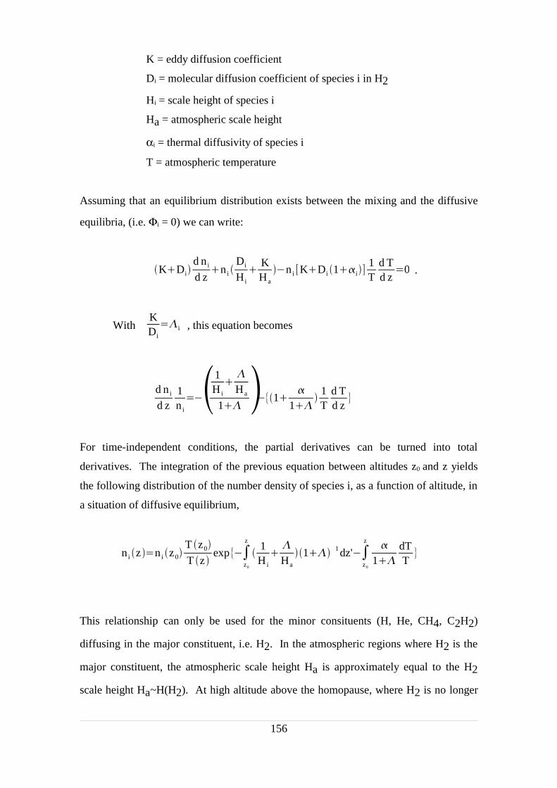
K = eddy diffusion coefficient
Di = molecular diffusion coefficient of species i in H2
Hi = scale height of species i
Ha = atmospheric scale height
αi = thermal diffusivity of species i
T = atmospheric temperature
Assuming that an equilibrium distribution exists between the mixing and the diffusive
equilibria, (i.e. Φi = 0) we can write:
KDid ni
d zni
Di
Hi
KHa
ni KDi 1i1T
d Td z
0 .
With KDi
+i , this equation becomes
d ni
d z1ni
1Hi
+
Ha
1+ 1
1+
1T
d Td z
For time-independent conditions, the partial derivatives can be turned into total
derivatives. The integration of the previous equation between altitudes z0 and z yields
the following distribution of the number density of species i, as a function of altitude, in
a situation of diffusive equilibrium,
ni z ni z0T z0
T z exp
z0
z
1Hi
+
Ha
1+1dz' z0
z
1+dTT
This relationship can only be used for the minor consituents (H, He, CH4, C2H2)
diffusing in the major constituent, i.e. H2. In the atmospheric regions where H2 is the
major constituent, the atmospheric scale height Ha is approximately equal to the H2
scale height Ha~H(H2). At high altitude above the homopause, where H2 is no longer
156

the major consituent, molecular diffusion is the dominant process, ΛH2 → 0 and the
+H2Ha term vanishes. After simplification, the diffusion terms disappear and the
diffusion equation becomes :
nH2nH
2z0
T z0
T z exp
z0
zdz'HH
2
which is equivalent to the hydrostatic equilibrium, or diffusive equilibrium since in both
cases Ha is the molecular hydrogen scale height. In fact H2 remains in diffusive
equilibrium at all altitudes. Its vertical distribution is thus determined solely by the
neutral temperature profile.
The Fickian diffusion coefficients for He and H diffusing in H2, and for He in H
were taken from the compilation of Mason and Marrero (1970). The thermal diffusion
coefficients for He in H2 has a value of 0.145 (Chapman and Cowling, 1970). All other
thermal diffusion coefficients were assumed to be zero.
VI.7.2.1.2 Hydrocarbon species
In the case of methane and acetylene, the resolution method can be simplified by
assuming that the temperature gradient is negligible in one thin layer, in the lower
atmosphere (where the altitude grid is dense) so that dT→ 0 and 1Hi
+
Ha
1+1
is approximately constant over a given layer. The diffusion equation for CH4 takes the
form
nCH4z nCH
4z0
T z0
T z exp
1HCH
4
+
Ha
1+1zz0 .
A similar equation is deduced for C2H2.
157
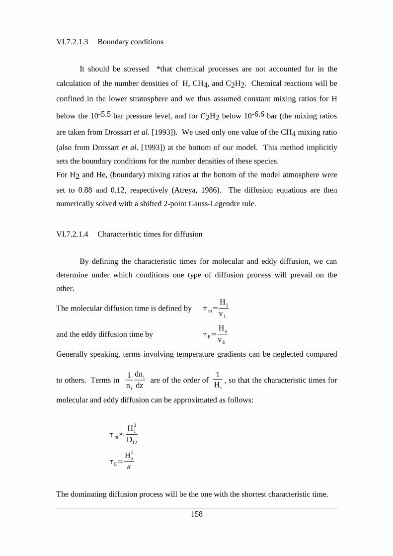
VI.7.2.1.3 Boundary conditions
It should be stressed *that chemical processes are not accounted for in the
calculation of the number densities of H, CH4, and C2H2. Chemical reactions will be
confined in the lower stratosphere and we thus assumed constant mixing ratios for H
below the 10-5.5 bar pressure level, and for C2H2 below 10-6.6 bar (the mixing ratios
are taken from Drossart et al. [1993]). We used only one value of the CH4 mixing ratio
(also from Drossart et al. [1993]) at the bottom of our model. This method implicitly
sets the boundary conditions for the number densities of these species.
For H2 and He, (boundary) mixing ratios at the bottom of the model atmosphere were
set to 0.88 and 0.12, respectively (Atreya, 1986). The diffusion equations are then
numerically solved with a shifted 2-point Gauss-Legendre rule.
VI.7.2.1.4 Characteristic times for diffusion
By defining the characteristic times for molecular and eddy diffusion, we can
determine under which conditions one type of diffusion process will prevail on the
other.
The molecular diffusion time is defined by ,mH1
v1
and the eddy diffusion time by ,EHa
vE
Generally speaking, terms involving temperature gradients can be neglected compared
to others. Terms in1ni
dni
dzare of the order of
1Hi
, so that the characteristic times for
molecular and eddy diffusion can be approximated as follows:
,m-H1
2
D12
,EHa
2
.
The dominating diffusion process will be the one with the shortest characteristic time.
158
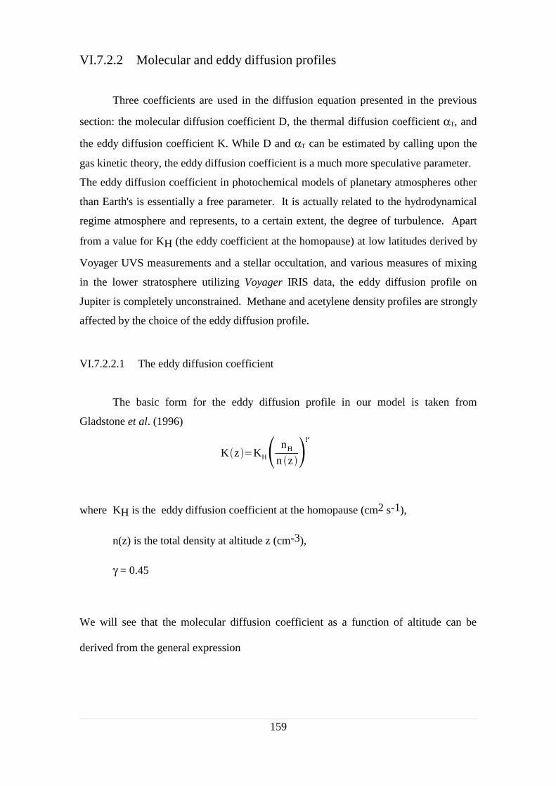
VI.7.2.2 Molecular and eddy diffusion profiles
Three coefficients are used in the diffusion equation presented in the previous
section: the molecular diffusion coefficient D, the thermal diffusion coefficient αT, and
the eddy diffusion coefficient K. While D and αT can be estimated by calling upon the
gas kinetic theory, the eddy diffusion coefficient is a much more speculative parameter.
The eddy diffusion coefficient in photochemical models of planetary atmospheres other
than Earth's is essentially a free parameter. It is actually related to the hydrodynamical
regime atmosphere and represents, to a certain extent, the degree of turbulence. Apart
from a value for KH (the eddy coefficient at the homopause) at low latitudes derived by
Voyager UVS measurements and a stellar occultation, and various measures of mixing
in the lower stratosphere utilizing Voyager IRIS data, the eddy diffusion profile on
Jupiter is completely unconstrained. Methane and acetylene density profiles are strongly
affected by the choice of the eddy diffusion profile.
VI.7.2.2.1 The eddy diffusion coefficient
The basic form for the eddy diffusion profile in our model is taken from
Gladstone et al. (1996)
Kz KH nH
n z
where KH is the eddy diffusion coefficient at the homopause (cm2 s-1),
n(z) is the total density at altitude z (cm-3),
γ = 0.45
We will see that the molecular diffusion coefficient as a function of altitude can be
derived from the general expression
159
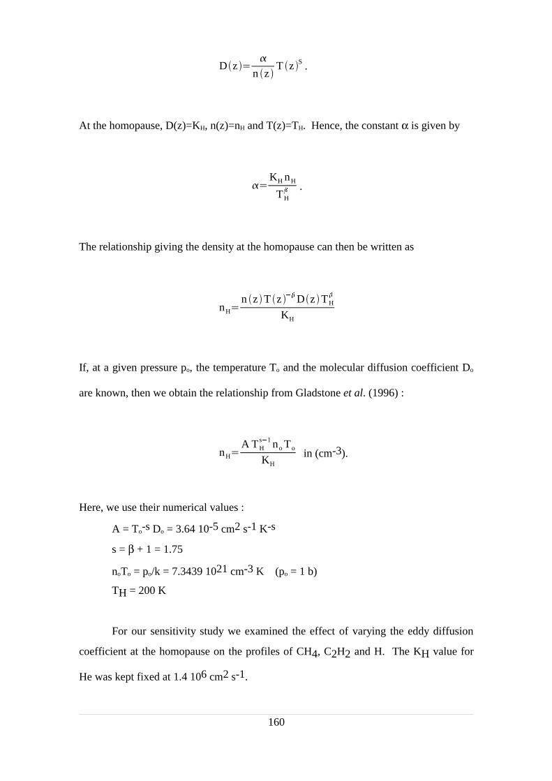
Dz
n z T z S .
At the homopause, D(z)=KH, n(z)=nH and T(z)=TH. Hence, the constant α is given by
KH nH
TH .
The relationship giving the density at the homopause can then be written as
nHn z T z Dz TH
KH
If, at a given pressure po, the temperature To and the molecular diffusion coefficient Do
are known, then we obtain the relationship from Gladstone et al. (1996) :
nHA TH
s1 no To
KH
in (cm-3).
Here, we use their numerical values :
A = To-s Do = 3.64 10-5 cm2 s-1 K-s
s = β + 1 = 1.75
noTo = po/k = 7.3439 1021 cm-3 K (po = 1 b)
TH = 200 K
For our sensitivity study we examined the effect of varying the eddy diffusion
coefficient at the homopause on the profiles of CH4, C2H2 and H. The KH value for
He was kept fixed at 1.4 106 cm2 s-1.
160

VI.7.2.2.2 The molecular diffusion coefficient
The molecular diffusion coefficient can be estimated from the gas kinetic theory.
The following general expression for D12, the coefficient for the diffusion of gas 1 in
gas 2, is obtained (Chapman and Cowling, 1970) :
D123
32 %QD nv12 ,
where %QD is the mean momentum transfer cross-section, n = n1 + n2 is the total gas
concentration, v12 is the velocity of gas 1 relative to gas 2, given by
v128 kT 12 ,
where,
1m11m21
is the reduced mass.
For a minor constituent diffusing through the background atmosphere, n becomes the
atmospheric density (n≈n2), and the mean molecular weight is close to m2. The
diffusion coefficient D then becomes
DB
n %QD
T12.
The mean momentum transfer cross-section %QD also depends on T. The molecular
diffusion coefficient can thus be written in the general form
D
nTS
where ½ ≤ S ≤ 1. The value S = 1 corresponds to Maxwellian molecules and the value
S = ½ corresponds to elastic spheres.
161

The molecular diffusion profile of CH4 (and C2H2) in H2 is given by (Gladstone,
1982)
Dz 2.3x10¹⁷ T z 0.765
n z 16.04
mm2.016
18.059
where m is the molecular mass of the hydrocarbon constituent diffusing in H2 (amu),
n(z) is the total density (cm-3), and T(z) is the temperature (K). D(z) is in cm2 s-1
The molecular diffusion profile for He in H2 may be given by (Gladstone, 1982)
Dz 1.98x10²⁰ T z 0.51
ln 5.34x10⁶T z 2 n z ,
and the molecular diffusion profile for H in H2 by
Dz 8.19x10¹⁷ T z 0.728
n z
Since the homopause is defined as the level where K(z)=D(z) and since each of the
previous species is characterized by a different molecular diffusion profile, a different
homopause should be defined for each of these species. For convenience we adopt
the homopause as the main methane homopause.
VI.7.2.2.3 The thermal diffusion factor
The final parameter involved in the diffusion equation is the thermal diffusion
factor αT. It is associated with the temperature gradient and is significantly different
from 0 for H, H2 and He.
The thermal diffusion coefficient for He in H2 has a value of 0.145. All other thermal
diffusion coefficients were assumed to be zero.
162

VI.7.2.2.4 Relationship between molecular and eddy diffusion
So far, we have presented the eddy and the molecular diffusion coefficients
independently. However, they are indirectly linked. It can be seen from the general
form of the molecular coefficient that this parameter is proportional to the atmospheric
temperature and inversely proportional to the total atmospheric density.
One could be surprised that the eddy coefficient could significantly influence the
molecular coefficient since eddy diffusion mainly affects the density profiles of the
minor species, and has no relevant effect on the major species, i.e. molecular hydrogen.
Therefore, it should leave the bulk atmospheric density almost unaffected. However
this argumentation is incomplete because methane, a minor species strongly affected by
eddy diffusion, is an important radiative cooler in the lower stratosphere. Any density
variation of CH4 will, in turn, have an important feedback on the thermal profile (which
controls diffusion processes to a large extent) and thus the density profiles of the major
species. The situation becomes very complex because the eddy coefficient itself is
inversely proportional to the total atmospheric density. The iterative processing of our
code allows to account for the multiple interconnections between these parameters. The
indirect link between K(z) and D(z) may be illustrated with cases B, E and F which only
differ by the value adopted for the eddy diffusion coefficient at the homopause
(KH=1.4x106 cm2 s-1, 1.4x105 cm2 s-1, and 1.4x107 cm2 s-1, respectively).
The three plots of figure 44 show that the main effect of KH on the eddy coefficient is a
shift of the profile toward higher values of K(z) as KH increases. In the region above
~300 km, modifying KH by one order of magnitude corresponds to a shift characterized
by a multiplicative factor of the order of 5. Below this altitude the multiplicative factor
is of the order of 3. As we shall see below, the variation of this multiplicative factor is
due to the feedback effect of the temperature profile below ~300 km (1 µbar).
A similar shift (by a factor 3.2) for the molecular diffusion coefficient profiles D(z) is
observed above ~300 km. Below this altitude, D(z) is unaffected by KH. This is partly
due to a restriction that we have to apply to the lower part of the thermal profile (below
the 1 µbar level). In order to prevent an excessive (and unobserved) cooling of this
region by the hydrocarbons, the lower part of the thermal profile is artificially fixed and
is therefore unaffected by KH.
163
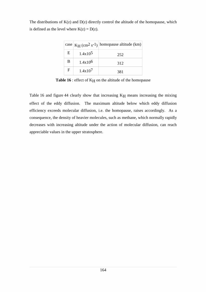
The distributions of K(z) and D(z) directly control the altitude of the homopause, which
is defined as the level where K(z) = D(z).
case KH (cm2 s-1) homopause altitude (km)
E 1.4x10⁵ 252
B 1.4x10⁶ 312
F 1.4x10⁷ 381
Table 16 : effect of KH on the altitude of the homopause
Table 16 and figure 44 clearly show that increasing KH means increasing the mixing
effect of the eddy diffusion. The maximum altitude below which eddy diffusion
efficiency exceeds molecular diffusion, i.e. the homopause, raises accordingly. As a
consequence, the density of heavier molecules, such as methane, which normally rapidly
decreases with increasing altitude under the action of molecular diffusion, can reach
appreciable values in the upper stratosphere.
164

165
Figure 44 : Effect of the eddy coefficient at the homopause (KH) on the
molecular diffusion D(z) and eddy diffusion K(z) coefficients.
104 105 106 107 108 109 10100
500
1000
1500
2000
Alt
itud
e (k
m)
KH=1.4E5 cm2/s
104 105 106 107 108 109 10100
500
1000
1500
2000
Alt
itud
e (k
m) EDDY (K[z])
MOLECULAR (D[z])
KH=1.4E6 cm2/s
104 105 106 107 108 109 1010
Diffusion coefficient (cm2/s)
0
500
1000
1500
2000
Alt
itud
e (k
m)
KH=1.4E7 cm2/s

VI.7.3 Chemical reactions
VI.7.3.1 Atomic hydrogen chemistry
We already mentioned in the section describing the diffusion equation that, as far
as the minor constituents are concerned, the composition of the atmospheric gas is not
solely controlled by diffusion processes. In the case of atomic hydrogen, the distribution
is also controlled by the balance between the thermospheric sources of H (i.e., H2
dissociation and ionization) and the sinks that exist in the lower atmospheric
hydrocarbon layer. The main sink in the hydrocarbon layer is the catalytic
recombination of H by C2H2. Other sinks include three-body reactions of H with CH3
and with itself. In order to indirectly account for these atomic hydrogen production and
loss processes, we adopt the auroral H mixing ratio profile derived by Drossart et al.
(1993) from the bottom of the model (1 mbar) to a pressure level of 10-6.6 bar. From
this level we assume that H concentration is determined by diffusion alone, and not
affected by chemical reactions.
VI.7.3.2 Hydrocarbon photochemistry
The hydrocarbon photochemistry is not included in the present model. A
comprehensive study on this complex chemistry for the solar-driven low and mid-
latitude Jovian atmosphere can be found in Gladstone et al. (1996). It should be noted
however that the photochemistry of methane and other hydrocarbons in the upper
atmosphere of Jupiter is important in a number of ways. Photochemistry represents the
major source of disequilibrium species in the upper atmosphere, although the aurora
also represents an important source. Many of the long-lived photochemical products are
optically active and contribute to the opacity of the atmosphere at wavelengths shorter
than 2000 Å. Although the circulation patterns of the upper atmosphere are currently
unknown, it is likely that many species of photochemical origin are important sources
and/or sinks of heat, and thus contribute to the upper atmospheric dynamics.
Hydrocarbon photochemistry may also be an important source for aerosol formation
through the production of long-chain polymers.
166
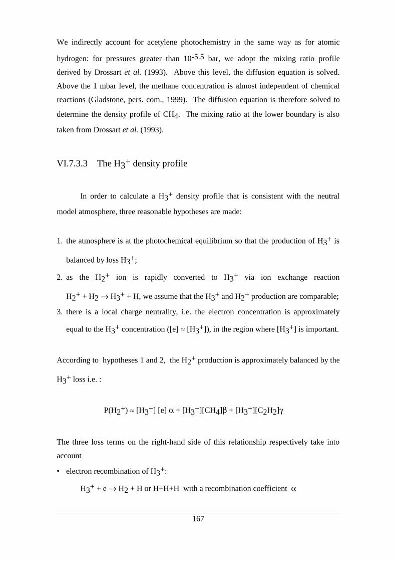
We indirectly account for acetylene photochemistry in the same way as for atomic
hydrogen: for pressures greater than 10-5.5 bar, we adopt the mixing ratio profile
derived by Drossart et al. (1993). Above this level, the diffusion equation is solved.
Above the 1 mbar level, the methane concentration is almost independent of chemical
reactions (Gladstone, pers. com., 1999). The diffusion equation is therefore solved to
determine the density profile of CH4. The mixing ratio at the lower boundary is also
taken from Drossart et al. (1993).
VI.7.3.3 The H3+ density profile
In order to calculate a H3+ density profile that is consistent with the neutral
model atmosphere, three reasonable hypotheses are made:
1. the atmosphere is at the photochemical equilibrium so that the production of H3+ is
balanced by loss H3+;
2. as the H2+ ion is rapidly converted to H3+ via ion exchange reaction
H2+ + H2 → H3+ + H, we assume that the H3+ and H2+ production are comparable;
3. there is a local charge neutrality, i.e. the electron concentration is approximately
equal to the H3+ concentration ([e] ≈ [H3+]), in the region where [H3+] is important.
According to hypotheses 1 and 2, the H2+ production is approximately balanced by the
H3+ loss i.e. :
P(H2+) ≈ [H3+] [e] α + [H3+][CH4]β + [H3+][C2H2]γ
The three loss terms on the right-hand side of this relationship respectively take into
account
electron recombination of H3+:
H3+ + e → H2 + H or H+H+H with a recombination coefficient α
167
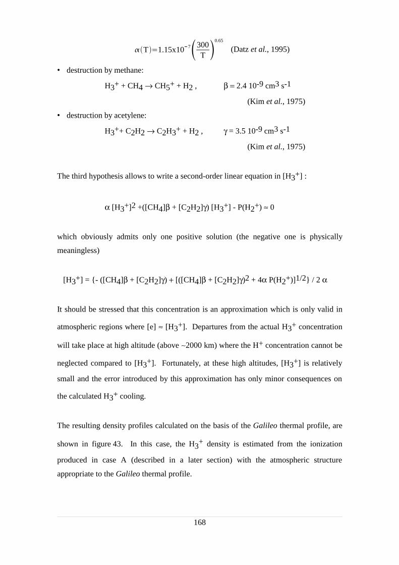
T1.15x107300T
0.65
(Datz et al., 1995)
destruction by methane:
H3+ + CH4 → CH5+ + H2 , β = 2.4 10-9 cm3 s-1
(Kim et al., 1975)
destruction by acetylene:
H3++ C2H2 → C2H3+ + H2 , γ = 3.5 10-9 cm3 s-1
(Kim et al., 1975)
The third hypothesis allows to write a second-order linear equation in [H3+] :
α [H3+]2 +([CH4]β + [C2H2]γ) [H3+] - P(H2+) ≈ 0
which obviously admits only one positive solution (the negative one is physically
meaningless)
[H3+] = - ([CH4]β + [C2H2]γ) + [([CH4]β + [C2H2]γ)2 + 4α P(H2+)]1/2 / 2 α
It should be stressed that this concentration is an approximation which is only valid in
atmospheric regions where [e] ≈ [H3+]. Departures from the actual H3+ concentration
will take place at high altitude (above ∼2000 km) where the H+ concentration cannot be
neglected compared to [H3+]. Fortunately, at these high altitudes, [H3+] is relatively
small and the error introduced by this approximation has only minor consequences on
the calculated H3+ cooling.
The resulting density profiles calculated on the basis of the Galileo thermal profile, are
shown in figure 43. In this case, the H3+ density is estimated from the ionization
produced in case A (described in a later section) with the atmospheric structure
appropriate to the Galileo thermal profile.
168
Since the temperature profile, the atmospheric composition, and the heating and
cooling efficiencies are intimately related, an iterative approach has to be adopted to
calculate the steady-state composition of the atmosphere under auroral precipitation.
The heating and cooling vertical profiles are calculated at each time step. The energy
balance equation resulting from the energetic electron energy deposition is then iterated
with the new temperature and density profiles until stable steady-state temperature and
density profiles are achieved.
Little is known about non-auroral heating processes below the homopause. Neglecting
these additional heating sources would cause radiative cooling by CH4 and C2H2 not to
be balanced and the stratospheric temperature would drop below its observed value. In
order to maintain an appropriate stratospheric temperature without arbitrary assumptions
regarding unspecified heating processes, we define a critical (threshold) pressure such
that for pressures exceeding this value, a) only net heating is allowed, and b) if heating
is insufficient, the temperature is not allowed to decrease below its initial value. This
critical pressure will obviously influence the thermospheric thermal structure, but it is
set in such a manner that it does not substitute for auroral heating where it is sufficient
to dominate cooling.
169

VI.8 Iteration process
As discussed before, the heat conduction equation, the diffusion equation
(including the equations for eddy and molecular diffusion), and the electron transport
differential equation system are tightly coupled.
The diffusion equation, which provides the density profiles of the different atmospheric
constituents, depends upon the thermal structure of the atmosphere which is calculated
from the heat conduction equation. The heat conduction uses the heating and cooling
rates which are derived from the electron transport. Since electron transport deals with
energy degradation of electrons colliding with neutral species, it is directly linked to the
atmospheric composition calculated with the diffusion equation.
The easiest way to handle this kind of problem is to assume a set of realistic
starting values, compatible with the boundary conditions, and to iteratively solve the
equations until a steady state is reached. The Galileo equatorial thermal profile
(corrected for the higher acceleration of gravity at the pole) is taken as the starting
thermal profile. An initial atmospheric composition is then established by solving the
diffusion equation using that thermal profile.
As illustrated in figure 45, the resulting initial atmospheric structure (ni(z), T(z)) and the
auroral electron energy distribution at the top of the atmosphere (Φ∞(E)) are then
introduced into the equations. Then, an iterative process is started, where the equations
for electron transport (the energy degradation), heat conduction, and diffusion are solved
in turn. The process is iterated until a steady-state thermal profile is reached. The final
atmospheric structure, the upward and downward profiles of the energy flux of electrons
obtained with this method are consistent with the energy distribution of the precipitating
electrons. They can be used as inputs for other codes such as the H2 UV spectral
generator (described in part 3). We have seen in a previous section that other outputs,
such as the cooling rate profile, can further be used, for example, to calculate the
hydrocarbons and H3+ infrared emission profiles. These optical signatures, consistent
with the atmospheric structure, can in turn be used to constrain the energy distribution
of the auroral electrons.
170

171
Figure 45 : Iteration process used in the two-stream model
Initialatmospheric
structureni(z), T(z)
Auroral electronenergy
distributionΦ∞(E)
ni(z)
C(z), H(z), Φ±(E,z)
T(z)
Finalatmospheric
structureni(z), T(z), Φ±(E,z)
Infraredemissionprofile
H2 UVprofile
color ratio
KH
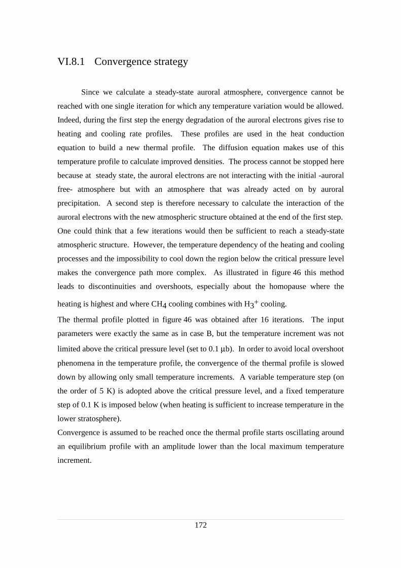
VI.8.1 Convergence strategy
Since we calculate a steady-state auroral atmosphere, convergence cannot be
reached with one single iteration for which any temperature variation would be allowed.
Indeed, during the first step the energy degradation of the auroral electrons gives rise to
heating and cooling rate profiles. These profiles are used in the heat conduction
equation to build a new thermal profile. The diffusion equation makes use of this
temperature profile to calculate improved densities. The process cannot be stopped here
because at steady state, the auroral electrons are not interacting with the initial -auroral
free- atmosphere but with an atmosphere that was already acted on by auroral
precipitation. A second step is therefore necessary to calculate the interaction of the
auroral electrons with the new atmospheric structure obtained at the end of the first step.
One could think that a few iterations would then be sufficient to reach a steady-state
atmospheric structure. However, the temperature dependency of the heating and cooling
processes and the impossibility to cool down the region below the critical pressure level
makes the convergence path more complex. As illustrated in figure 46 this method
leads to discontinuities and overshoots, especially about the homopause where the
heating is highest and where CH4 cooling combines with H3+ cooling.
The thermal profile plotted in figure 46 was obtained after 16 iterations. The input
parameters were exactly the same as in case B, but the temperature increment was not
limited above the critical pressure level (set to 0.1 µb). In order to avoid local overshoot
phenomena in the temperature profile, the convergence of the thermal profile is slowed
down by allowing only small temperature increments. A variable temperature step (on
the order of 5 K) is adopted above the critical pressure level, and a fixed temperature
step of 0.1 K is imposed below (when heating is sufficient to increase temperature in the
lower stratosphere).
Convergence is assumed to be reached once the thermal profile starts oscillating around
an equilibrium profile with an amplitude lower than the local maximum temperature
increment.
172

173
Figure 46 : Thermal profile obtained after 16 iterations without slowing down the
convergence. A huge temperature overshoot appears above 300 km.
020
040
060
080
010
0012
0014
00T
empe
ratu
re (
K)
10−
2
10−
4
10−
6
10−
8
10−
10
10−
12
10−
14
Pressure (bar)
200
250
300
400
500
1000
Altitude (km)
VII Model application
The present chapter was taken and adapted from a paper written by Denis
Grodent, J. Hunter Waite, Jr. and Jean-Claude Gérard that was submitted to J. Geophys.
Res. (Space Physics) in August, 1999.
VII.1 Abstract
A one-dimensional (1D) model coupling a two-stream electron transport model
of energy deposition with a 1D thermal conduction model has been described in the
theoretical part. It is used to investigate the links between the auroral heat input and the
atmospheric temperature and composition structures of Jupiter. Different energy
distributions are used to evaluate the importance of the energy spectrum of the incident
electrons for the thermal balance of Jupiter's auroral thermosphere. The values of
observable quantities such as the altitude of the H2 emission peak, infrared (IR) and
ultraviolet (UV) emissions and temperatures associated with various optical signatures
are used to constrain the parameters of these distributions. From these simulations, it
appears that the H3+ and exospheric temperatures are mainly due to the level of soft
electron influx and that they are almost independent on the H2 UV and hydrocarbon IR
emissions and temperatures which are controlled by the high-energy component of the
energy distribution. In order to meet the H2 integrated brightness constraint, a trade-off
is necessary between the far-UV color ratio and the H2 rovibrational temperature. H3+
plays an important thermostatic role and a similar trade-off exists between the H3+
temperature and the observed H3+ IR emission intensity which also increases with the
low-energy component of the energy distribution. The precipitated auroral energy is
not able to directly provide the necessary heat to balance the hydrocarbon cooling below
the homopause but it is suggested that the auroral upper stratosphere is probably warmer
than the equatorial upper stratospheric temperature deduced from Galileo data.
174
A kappa energy distribution, fitted on in-situ Galileo measurements at the distance of
Ganymede's orbit, does not produce results in agreement with observations. Such an
energy distribution does probably not reflect acceleration processes undergone by the
auroral electron sduring their travel along the magnetic field lines. A Maxwellian
energy distribution with a total flux of 20 ergs cm-2 s-1 and a characteristic energy of
22 keV added to a soft Maxwellian component of 1 erg cm-2 s-1 and a characteristic
energy of 350 eV produces results in good agreement with thermospheric observations.
175

VII.2 Energy distribution of auroral electrons
Three energy distributions of the precipitating particles are selected from
theoretical considerations and in-situ measurements ; case A: a Maxwellian energy
distribution, case B : a double Maxwellian distribution, mixing case A with a soft
electron Maxwellian component, case C : a kappa distribution fitting the observations
from the Energetic Particle Detector (EPD) experiment onboard Galileo. In the
following section, we will first concentrate on case A: a single Maxwellian distribution
with a characteristic energy of 22 keV and a total energy flux of 20 ergs cm-2 s-1.
The detailed parameters of these distributions are listed in table 19 and will be discussed
below. It should be pointed out that the distributions A and B produce an H2 FUV
emission that peaks at an altitude close to 245 km. Recent visible-wavelength images
obtained by the Galileo Solid State Imaging (SSI) system (Ingersoll et al., 1998) have
determined the altitude of this auroral night side emission to be 245 ±30 km above the 1
bar level (Vasavada et al., 1999). James et al. (1998) have shown that these visible-
wavelength emissions could be ascribed to the H2 (a3 → b3) continuum, together with
strong lines assigned to the radiative decay of the gerade singlet states of H2, and to
members of the H Balmer series resulting from dissociative excitation of H2. Since
these emissions are presumably excited by auroral electron impact on H2, it is assumed
that the H2 FUV and the visible emissions peak at the same altitude.
Figure 47 illustrates the dependence of the energy spectrum of the auroral electron flux
on altitude for case A. As the primary electron beam reaches deeper pressure levels, the
electrons degrade their energy, partly backscatter and produce secondary electrons. Four
altitude levels are illustrated: 1) initial energy distribution at the top of the atmosphere,
2) degraded energy distribution above the H2 emission peak (600 km), 3) at the
emission peak (242 km), and 4) below the emission peak (200 km).
The flux profiles result from the balance between production and loss into the different
energy bins. Since all degrading processes occur simultaneously, it is impossible to
discriminate their individual action. The degradation rate of the electron flux along its
path is mainly controlled by the H2 density profile.
176

177
Figure 47 : Evolution of the Maxwellian energy flux distribution of case A(E0=22 keV) as the electron beam penetrates into the atmosphere. Four
altitude levels are considered: 1) initial energy distribution at the top of theatmosphere (———), 2) degraded energy distribution above the H2 emission
peak (600 km) (·······), 3) at the emission peak (242 km)(-----), and 4) belowthe emission peak (200 km) (–·–·–).
100
101
102
103
104
105
Ene
rgy
(eV
)
2468
Log10(Flux) (cm−2 eV
−1 s
−1)

Below the level of the peak H2 emission, where energy deposition is highest, the
electron flux rapidly vanishes. This level is determined by the shape of the initial
energy distribution of the electrons; in the case of a monoenergetic electron beam, the
pressure level of the peak is proportional to the energy, and for more complex
distributions, such as the Maxwellian distribution used in case A, the altitude mainly
depends on the mean energy which is twice the characteristic energy E0 of the
Maxwellian distribution.
The shape of the electron flux distributions in figure 47 can be explained with simple
physical considerations. For energies higher than 20 eV, the total electron interaction
cross section rapidly decreases, thus leading to a slower degradation of high energy
electrons. An efficient depopulation of the low energy bins occurs at all altitudes. With
a mean energy per ion pair of 40 eV, one single 40 keV electron is able to produce about
1000 secondary electrons which will rapidly populate these low energy bins. At the top
of the atmosphere, the population processes of the low energy bins are relatively
efficient compared to loss processes. As the electron beam penetrates into the
atmosphere, this tendency is reversed and the flux drops at all energies. The abrupt rise
of the electron flux below 10 eV corresponds to a minimum in the total inelastic cross
section between rotational and vibrational excitation and other processes having a
threshold energy of the order of 10 eV. In order to avoid numerical problems, we
assume that all cascading energy which populates the lowest energy bin under
consideration here (0.25 eV) is ultimately converted into electron heating.
VII.2.1 H2+ and H+ production rate profiles
The ionization produced by the electron energy spectrum of case A is illustrated
in figure 48. The integrated ion production rates of the various processes are listed in
table 17.
H2+ presents the largest ion production rate in the jovian ionosphere, about 1 order of
magnitude higher than the dissociative ionization rate of H2. However, the efficient
reactions described in table 15 rapidly convert H2+ into H3
+, which is dominant in the
jovian ionosphere.
178
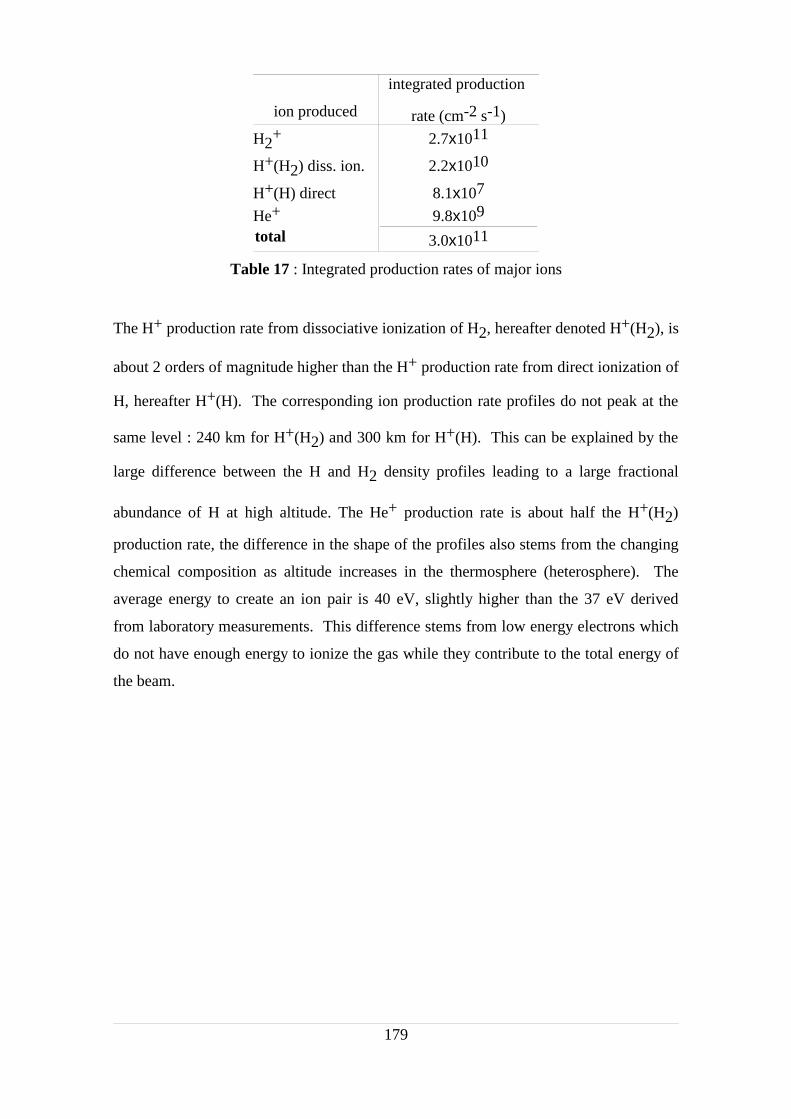
ion produced
integrated production
rate (cm-2 s-1)
H2+ 2.7x10¹¹
H+(H2) diss. ion. 2.2x10¹⁰
H+(H) direct 8.1x10⁷
He+ 9.8x10⁹
total 3.0x10¹¹
Table 17 : Integrated production rates of major ions
The H+ production rate from dissociative ionization of H2, hereafter denoted H+(H2), is
about 2 orders of magnitude higher than the H+ production rate from direct ionization of
H, hereafter H+(H). The corresponding ion production rate profiles do not peak at the
same level : 240 km for H+(H2) and 300 km for H+(H). This can be explained by the
large difference between the H and H2 density profiles leading to a large fractional
abundance of H at high altitude. The He+ production rate is about half the H+(H2)
production rate, the difference in the shape of the profiles also stems from the changing
chemical composition as altitude increases in the thermosphere (heterosphere). The
average energy to create an ion pair is 40 eV, slightly higher than the 37 eV derived
from laboratory measurements. This difference stems from low energy electrons which
do not have enough energy to ionize the gas while they contribute to the total energy of
the beam.
179
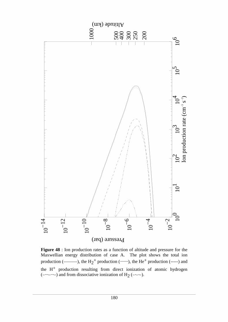
180
Figure 48 : Ion production rates as a function of altitude and pressure for theMaxwellian energy distribution of case A. The plot shows the total ion
production (———), the H2+ production (·······), the He+ production (-----) and
the H+ production resulting from direct ionization of atomic hydrogen(–···–···–) and from dissociative ionization of H2 (–·–·–).
100
101
102
103
104
105
106
Ion
prod
uctio
n ra
te (
cm−
3 s−
1 )
10−
2
10−
4
10−
6
10−
8
10−
10
10−
12
10−
14
Pressure (bar)
200
250
300
400
500
1000
Altitude (km)
VII.2.2 Heating and cooling profiles
Figure 49 shows the cooling and heating rate profiles for case A (single
Maxwellian distribution). As mentioned before, we consider here the cooling associated
with thermal IR radiations from H3+, CH4 and C2H2. These molecules cool different
regions of the atmosphere because the heavier hydrocarbon molecules are mostly
confined below the homopause (312 km) while the H3+ ion, which is destroyed by
hydrocarbons below the homopause, has a density profile peaking ∼40 km above the
homopause.
Turbulent transport controls the CH4 density and therefore plays an important role on
the cooling rate in the vicinity of the homopause, i.e. in the region that includes the level
of maximum energy deposition. The effect of change of the eddy diffusion coefficient
on the thermal profile and on the absorption of H2 UV emission by CH4 will be
considered later. The aboundance of H3+, on the other hand, mainly controls the
ionospheric region of the temperature profile and directly regulates the exospheric
temperature.
The different heat sources have been described previously. Their individual and total
heating rate profiles for case A are shown in figure 49. Table 18 lists their contribution
to the total heating. For the Maxwellian energy distribution of case A, the heating
efficiency of the atmosphere represents exactly 50% of the total auroral energy. For the
electron energy distribution of case A, more than half of the auroral heat is produced
below the homopause where it is efficiently lost to the hydrocarbon cooling. The main
contribution of the auroral particles on the thermal profile is associated with the heat
produced above the homopause, in a region where cooling is controlled by H3+ infrared
radiation.
Heating of the jovian atmosphere is largely dominated by chemical heating which
results from the reaction chain initiated by the ionization of H2. The excitation of the
vibrational and rotational levels of the ground state of H2 molecules is the second most
important heat source. Its importance reflects the large excitation cross sections of these
processes occurring at low energies for which energy bins are highly populated.
181
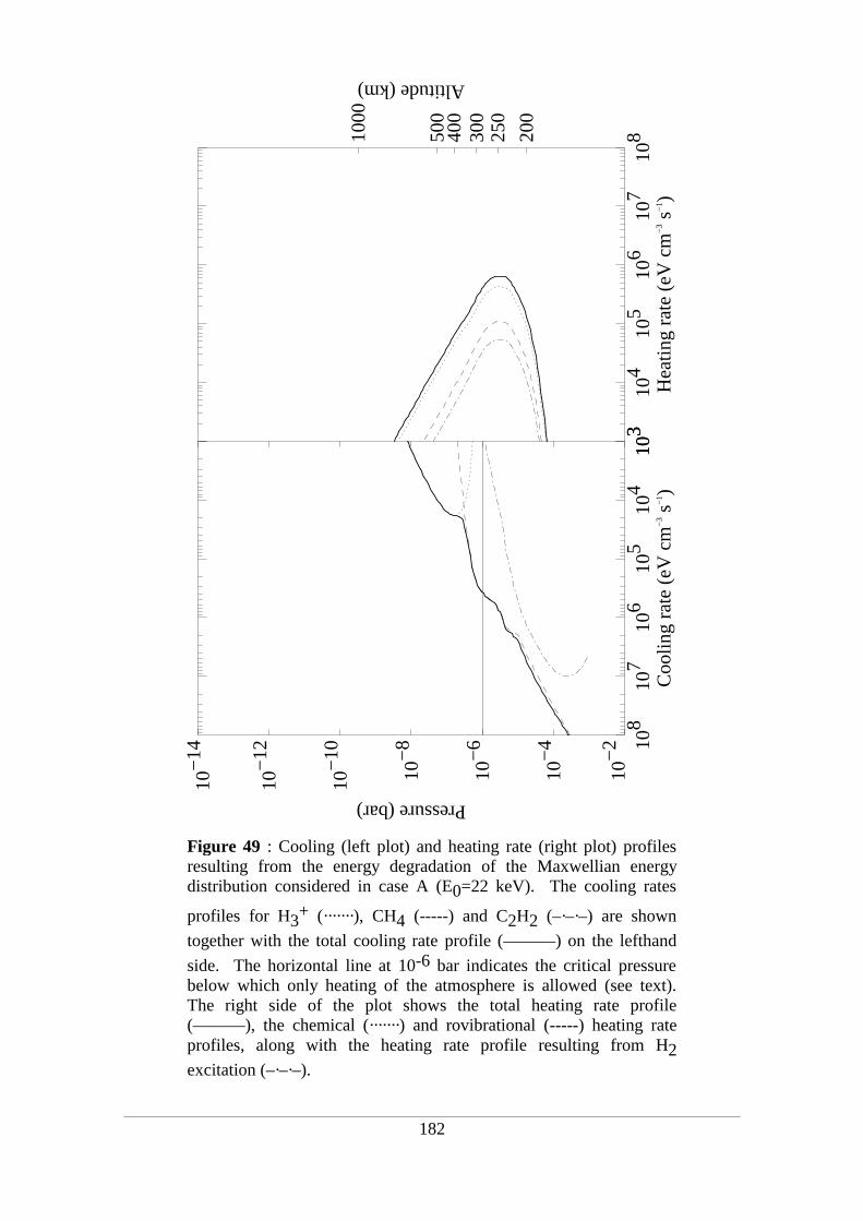
182
Figure 49 : Cooling (left plot) and heating rate (right plot) profilesresulting from the energy degradation of the Maxwellian energydistribution considered in case A (E0=22 keV). The cooling rates
profiles for H3+ (·······), CH4 (-----) and C2H2 (–·–·–) are shown
together with the total cooling rate profile (———) on the lefthand
side. The horizontal line at 10-6 bar indicates the critical pressurebelow which only heating of the atmosphere is allowed (see text).The right side of the plot shows the total heating rate profile(———), the chemical (·······) and rovibrational (-----) heating rateprofiles, along with the heating rate profile resulting from H2excitation (–·–·–).
108
107
106
105
104
103
Coo
ling
rate
(eV
cm
−3 s
−1 )
10−
2
10−
4
10−
6
10−
8
10−
10
10−
12
10−
14
Pressure (bar)
103
104
105
106
107
108
Hea
ting
rate
(eV
cm
−3 s
−1 )
200
250
300
400
500
1000
Altitude (km)

The heat produced by the dissociation of excited H2 singlet states and by excitation of
the H2 ground level following radiative transition from the B and C electronic states are
comparable. These two processes are linked as they both result from deexcitation of
excited singlet states. The heat released by H2 dissociation from doubly excited states
represents only a marginal contribution to the total heat produced because of the high
threshold energies of these processes and their low cross sections. All heating rate
profiles have similar shapes. The imbalance between heat sources and heat sinks is
accounted for by downward heat conduction equation and gives rise to the thermal
profile presented in figure 50 for case A.
Above the homopause, heating exceeds cooling and the difference is sufficient to
sustain an exospheric temperature of 599 K. As will be discussed in the next section,
this temperature is too low to match the observation and the initial electron energy
distribution must be modified to raise the temperature. Below the homopause, the
heating processes we consider cannot compensate the efficient hydrocarbon cooling. A
critical pressure of 1 µbar, corresponding roughly to the level of the homopause, is
therefore imposed (horizontal bar in figure 49) which defines the level below which
unspecified heating sources will prevent the thermal profile from cooling down. If
heating is sufficient to increase temperature at some level below this critical level, any
temperature increase will be allowed.
heating sources contribution to totalchemical heating 66.8 %vibrations + rotations 16.5 %H2 dissociation from singly excited states 7.4 %
Lyman and Werner bands heating 6.2 %electron heating 2.3 %H2 dissociation from doubly excited states 0.8 %
Table 18 : Contribution of the different heat sources to the total heating for case A
183

184
Figure 50 : Observational constraints on the auroral temperatureprofile. The first shaded region (between 160 and 400 K) is derivedfrom hydrocarbon (mainly CH4 and C2H2) IR thermal emissions in
the auroral hot spot (Drossart et al., 1993). The second shaded region(between 400 and 850 K) is defined from H2 FUV auroral spectra (◊ :
Liu et al.,1996; : Trafton et al., 1994, 1998; × : Clarke et al., 1994;∆ : Kim et al., 1997). The third region (between 700 and 1100 K) is
inferred from H3+ near-IR emissions in the aurora ( : Maillard et al.,
1990; × : Lam et al., 1997; ◊ : Drossart et al., 1989). The solid line isthe temperature profile calculated for case A. The dashed linerepresents the equatorial temperature profile deduced from the in-situGalileo measurements. The altitude scale is calculated from theinitial model atmosphere (Galileo).
020
040
060
080
010
0012
00T
empe
ratu
re (
K)
10−
2
10−
4
10−
6
10−
8
10−
10
10−
12
10−
14
Pressure (bar)
200
250
300
400
500
1000
Altitude (km)

VII.3 Observational constraints
The values of various observable quantities such as the altitude of the H2
emission peak, IR and UV emissions and temperatures associated with various optical
signatures are used to constrain the parameters of the energy distribution of the
precipitating electrons.
- A domain of observational constraints on the auroral temperature profile is constructed
on the basis of multispectral analysis of the auroral region emissions.
- A general FUV emission rate deduced from spectra and images is used to provide an
order of magnitude for the total precipitated energy, while the emission profile
(including H2 visible emission) gives important clues regarding the distribution of the
auroral particle energy deposition with altitude and more specifically regarding the
altitude of the H2 emission peak.
- The FUV color ratio and the associated CH4 column density are used to estimate the
penetration depth of the degraded beam below the methane homopause.
- IR emission processes are diagnostic of the cooling processes in the mesosphere from
CH4 and C2H2 at wavelengths between 7 and 14 µm and also an important diagnostic
of the upper thermosphere and ionosphere from H3+ emission near 3.5 microns.
It should be noticed that all these observations are not simultaneous in time and space,
and do not necessarily stem from the same processes. Knowing the temporal and spatial
variability of the jovian aurora, one needs to be careful when comparing quantities
resulting from different mechanisms and appearing at different times and locations.
VII.3.1 Thermal profile
A range of observational constraints on the auroral temperature profile can be
constructed from observations spanning three different overlapping pressure level
regions (shaded regions in figure 50).
The first region (between 160-400 K) is constrained by the hydrocarbon (mainly CH4
and C2H2) thermal infrared emissions observed with the Voyager IRIS and reanalyzed
185

by Drossart et al. (1993). They derived two temperature profiles based on different CH4
density profiles :
a. a warm upper boundary corresponding to the best fit for hydrocarbon emission for
the hydrocarbon distribution derived from Voyager UVS observations (Atreya et al.,
1981),
b. a cold boundary inferred from the thermal profile derived from the hydrocarbon
distribution of Gladstone et al. (1982).
The second region constraining the temperature profile (400-850 K) is defined by the
temperature values derived from H2 FUV auroral emission. Different H2 rovibrational
temperature ranges were derived by fitting synthetic spectra to various spectral ranges
observed with GHRS (Trafton et al., 1994, 1998; Clarke et al., 1994; Liu et al., 1996;
Kim et al., 1997). These measurements define an H2 temperature range of 400-850 K
corresponding to emissions occurring between the10-5 and 10-8 bar pressure levels.
The third region (700-1100 K) is defined on the basis of the temperatures inferred from
the H3+ near-IR emission (Drossart et al., 1989; Maillard et al., 1990; Lam et al., 1997).
They define an ionospheric temperature range of 700-1100 K for the region where the
H3+ emission originates, that is approximately between the 10-6 and 10-10 bar levels.
The equatorial temperature profile deduced from the in-situ Galileo measurements,
which is used as the initial thermal distribution of the atmosphere, was shown in
figure 43. It is imposed as the coldest permitted limit to the calculated temperature
profile.
The effective H2 temperature has been deduced from the H2 UV rovibrational spectra
and from the IR line of H2 quadrupole emission. It can be roughly estimated in the
model by weighting the temperature profile with the calculated H2 UV emission rate
profile. A similar method is applied to estimate the H3+ temperature from the
calculated H3+ emission profile. This method does not make use of the detailed
calculated thermal structure, however, it allows a direct comparison of the converged
thermal profile with the observational constraints, without making any assumption on
the altitude range of the emitting regions.
186
The thermal profile derived from case A is presented in figure 50. As already stated in
the previous section, the profile clearly demonstrates that the energy distribution of
auroral electrons considered in case A does not produce the temperature required above
the homopause. This is especially true in the upper thermosphere, where the
temperature is about 340 K colder than in the Galileo equatorial temperature profile
(940 K). The temperatures reached in the upper stratosphere (10-4-10-6 bar) are
considerably lower than the cold auroral hydrocarbon-IR boundary. They are, however,
significantly higher than the initial Galileo equatorial profile. At 10-7 bar, the
calculated profile reaches its isothermal limit at a colder value than the one observed at
the equator.
A first conclusion can be drawn from test case A. Since the calculated profile is too
cold above the homopause and reasonably warm below the homopause, more heat
deposition is required above the homopause, i.e. above the 10-6 bar level. However, the
Maxwellian energy distribution of case A sets the maximum energy deposition at about
10-5 bar, approximately 70 km below the methane homopause. This implies that more
than half of the released auroral heat is used to balance the efficient hydrocarbon
cooling. The Galileo equatorial profile suggests that this role can, at least partly, be
attributed to non-auroral processes, the corresponding auroral energy being more
efficiently used above the homopause.
In the next sections, we will examine how the electron energy distribution of case A can
be reasonably modified in order to produce a thermal profile in better agreement with
the observations. However, before testing other distributions, it is important to consider
other observational constraints such as the UV and IR auroral emissions which will
reduce the range of possible energy distributions.
VII.3.2 UV emission
Total Lyman band emission rates of 20-270 kR were measured by Kim et al.
(1997) with the Large Science Aperture (LSA) of the GHRS spectrometer. The
estimated total Lyman band intensity depends on the filling factor of the auroral
emission in the LSA. The authors have assumed that the LSA aperture is completely
187

filled with the auroral emission, however recent UV images have show thin bright
auroral structures which only partially fill the LSA. Their emission rates should
therefore be regarded as lower limits to the actual UV auroral emission intensities
corresponding to a viewing angle of approximately 60°. Trafton et al. (1998) obtained
similar GHRS spectra with total integrated intensity (Lyman and Werner bands)
averaged over the aperture varying from 54 to 228 kR. These derived apparent emission
rates are attenuated by hydrocarbon absorption and also assume that the aperture is fully
filled with auroral emission. They therefore also represent a lower limit to the emission.
Morrissey et al. (1997) measured a mean H2 brightness of 106 kR with HUT however
these measurements suffer from large uncertainties on the auroral area integrated in the
aperture.
The recent study of HST WFPC2 images obtained close in time with Galileo UVS
spectra and in situ particles, fields, and plasma wave measurements (Clarke et al., 1998)
show that a more typical emission brightness of 300 to 400 kR is to be considered along
the main auroral oval.
To synthesize these results, a vertically integrated excitation rate of the B u+1 ,
including cascade, and C "u1 states of 200 kR (unattenuated), approximately
corresponding to 400 kR for a viewing angle of 60° is adopted.
Little information on the FUV vertical emission profile has been deduced so far from
images taken by the FOC and the WFPC2 on board HST. The emission profile can
only be determined at the limb where the apparent brightness distribution is biased by
the viewing geometry, the spatial limitations of HST, and the instrument's point spread
function (PSF) (Grodent et al., 1997; Gérard et al., 1998). However, Galileo images
taken during orbit G7 show that the H2 visible emission profile is characterized by a
vertical full width at half maximum of 120 ± 30 km (Vasavada et al., 1999) and drops
below the detection limit at a full width of 350 ± 70 km. The UV emission profile can
also be crudely constrained by the H2 - FUV color ratio. As explained below, this
constraint gives some indication on the distribution of the emission profile above and
below the homopause.
188

189
Figure 51 : Temperature profiles calculated for cases A (———), B(·······), C (–···–···–). The Galileo equatorial temperature profile is shownfor comparison (-----). The altitude scale refers to case B. The shadedareas are the regions of observational constraints defined in text.
020
040
060
080
010
0012
00T
empe
ratu
re (
K)
10−
2
10−
4
10−
6
10−
8
10−
10
10−
12
10−
14
Pressure (bar)
200
250
300
400
500
1000
Altitude (km) (case B)
CA
B
Galileo

VII.3.3 Color ratio and CH4 column density
The H2 -FUV color ratio CI 15501620I 12301300
is related to the considerable
drop in the CH4 absorption cross section at wavelengths above 1350 Å (Yung et al.,
1982; Harris et al., 1996; Gérard et al., 1998). It leaves the bulk of the longer
wavelength H2 Lyman band emissions unattenuated, while the Werner and Lyman band
emissions at wavelengths less than 1350 Å are substantially absorbed by methane. The
color ratio C is calibrated to give a value of 1.13 for an unattenuated H2 spectrum,
compatible with the value derived from the laboratory H2 spectrum for 100 eV electrons
obtained by Liu et al. (1995). The color ratio is linked to the ratio of emission above
and below the homopause and is therefore a proxy for the penetration depth of the
electron beam below the homopause.
In order to evaluate the color ratio associated with the energy distribution of the
precipitating electrons, a synthetic spectral generator is used to calculate the UV
emission intensity in a prescribed spectral band for each atmospheric layer. The spectral
model will be fully described in the next part.
At the temperature of the jovian atmosphere, the H2 molecules in the ground state are
mostly in the ground vibrational level (v"=0). The population of the vibrational levels
(v') of the B, C and E,F states, excited by the electron impact, are calculated with the
analytical energy-dependent excitation cross sections from Shemansky et al. (1987),
updated by Liu et al. (1998). The transition probabilities from these excited states to the
ground level are taken from Allison and Dalgarno (1970). The corresponding
wavelengths of these transitions are deduced from the calculated energy levels from
Dabrowsky et al. (1984). At each altitude step, a spectrum is generated, depending on
the local electron energy distribution calculated with the energy degradation model and
H2 density. In order to account for the continuum emission, the spectra are normalized
to the column excitation rate of the B, E,F and C levels from the ground levels. The
synthetic spectra generated at each altitude step are attenuated by absorption from the
overlying methane column and integrated along a line of sight, assuming a slant path
190

angle of 60°. A wavelength-dependent CH4 absorption cross section (Mount and Moos,
1978) is used along with the methane density profile calculated by the model.
Based on eleven years of IUE spectral observations, Harris et al. (1996) deduced
an average C color ratio of 2.5 in the north corresponding to the best linear fit to auroral
H2 archival bandpass intensities. Galileo FUV observations in the northern hemisphere
provide a similar mean value (W.R. Pryor, private communication). The color ratio is
often expressed in terms of a corresponding vertically integrated CH4 column density
above the emission peak. This integrated column only depends on the CH4 density
profile and can be directly used to attenuate any bandpass of the H2 UV spectrum.
However, it should be noted that such an expression assumes that all of the emission is
concentrated at the emission peak and it does not account for the decreasing attenuation
of the emission above the peak. Kim et al. (1997) observed high-resolution GHRS
spectra of the aurora in the two wavelength ranges 1257-1293 Å and 1587-1621 Å and
estimated methane column densities in the range (1.5-6.5)x1016 cm-2, corresponding to
an altitude variation of about one scale height.
The value of the C color ratio (at 60°) and the associated vertically integrated CH4
column density are listed in table13 for cases A to C. For case A, they are 1.8 and
2.8x1016 cm-2, respectively. These values, although somewhat low, are bracketed by
the observations. Higher values could be obtained by increasing the characteristic
energy of the Maxwellian distribution (deeper aurora) or by raising the CH4 homopause
altitude (higher absorption). These options will be discussed in later.
VII.3.4 IR emission
Drossart et al. (1993) estimated the hydrocarbon IR excess emission from IRIS
Voyager observations in the northern auroral hot spot. These emissions were viewed at
about 60° emission angle and the IRIS projected field of view was 23,000 km in latitude
and 11,500 km in longitude, which is larger than the auroral hot spot. They deduced
CH4 and C2H2 IR emissions, integrated over 2π and averaged over the global IRIS field
of view, of 93 ± 9 ergs cm-2 s-1 and 26 ± 13 ergs cm-2 s-1, respectively. They
191

correspond to a filling factor of the aperture by the auroral emission on the order of 0.4.
Therefore, these values could easily be doubled. The assumption of an optically thin
hydrocarbon emission layer restricts the range of pressure to which their model can be
applied. It is roughly defined by the pressure levels corresponding to a CH4 integrated
column of 5.3x1017 cm-2 and a C2H2 integrated column of 7x1015 cm-2, respectively.
We use these column densities to determine the altitude at which the thermal IR
radiation is able to leave the hydrocarbon layer. We also assume that half of the
emission produced above this level finally escapes the atmosphere while the remaining
half is directed downward and is ultimately lost to the optically thick layers. For case A,
the altitudes of the top of the layers of unit optical depths are 206 km (1.9x10⁻⁵ bar) and
183 km (5.x10-5 bar), for CH4 and C2H2 layers respectively.
Lam et al. (1997) observed the H3+ infrared auroral emission with the United Kingdom
Infrared Telescope (UKIRT) high spectral resolution instrument. They found a total
emission power (integrated over 4π and corrected for line of sight effects) of the order
of 1.5 erg cm-2 s-1 at 60°, corresponding to a H3+ column density 2.5-12.5x10⁻¹²
cm-2. These values were averaged over a 3" x 3" pixel, which covered an area on
Jupiter of approximately 9800 x 9800 km2 at the time of the observations. The total
H3+ emission and column density should therefore be taken as lower limits to the actual
auroral values. It should also be emphasized that since this thermal emission is
dependent on both temperature and column density, a single emission spectrum can be
fitted by different temperature/column density pairs. It is therefore impossible to
determine the temperature and the column density independently from an observed
spectrum. Lam et al. (1997) observed confined auroral zones showing a strong
anticorrelation between temperature and column density. A strong H3+ IR emission is
therefore not necessarily related to a high temperature.
It should be emphasized again that no simultaneous H3+ or hydrocarbon IR and H2
-FUV auroral emission data sets are currently available. The relationship between these
emissions, probing different altitude regions and excited by different mechanisms, has
therefore never been directly observed. The spatial-temporal variability of the H2-FUV
192

emission is not necessarily directly linked to the variability of the hydrocarbon and H3+
IR thermal emissions. Nevertheless, the simultaneous use of the UV and IR average
emissions is still of considerable interest to constrain the radiative signature of a general
energy distribution, compatible with the thermal profile.
193
VII.4 Model results
VII.4.1 Energy distribution
We now describe electron energy distributions different from case A and
compare the outputs of the model to the observational constraints that were just
described. All the results are listed along with the observational summary in table 13.
VII.4.1.1 Effect of a soft electron component : double Maxwellian
energy distribution (case B)
We have already shown that the energy distribution of case A could be modified
to increase the temperature above the homopause. One straightforward way to do so
would be to increase the total integrated flux of the precipitated electrons. However,
calculations performed with case A show that (table 13) with a 20 ergs cm-2 s-1 aurora,
a vertically integrated H2 emission excitation of 200 kR (400 kR at 60°) is reached,
while the integrated H3+ emission and the exospheric temperature are below their
observed values. This suggests that only the upper part of the atmosphere needs
additional energy input. This result may be achieved by adding a weak soft electron
contribution to the energy distribution. In case B, this soft electron component is
specified by a Maxwellian distribution of 1 erg cm-2 s-1 and a characteristic energy of
350 eV. The energy of this second component is totally degraded above the homopause,
between 10-8 and 10-10 bar and raises the exospheric temperature to 1005 K, higher
than the equatorial Galileo value. The integrated H3+ emission increases to a larger
value of 2 ergs cm-2 s-1 and the estimated H3+ rovibrational temperature increases
from 542 K to 648 K, very close to the lower limit of the observed H3+ temperature
(700 K). The FUV color ratio of case A (1.83) is lower than the average IUE value of
2.5. It is slightly reduced by the soft electron component in case B (1.8) which
generates unattenuated emission between the 10-8-10-10 bar levels. The corresponding
194
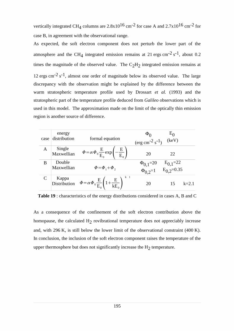
vertically integrated CH4 columns are 2.8x1016 cm-2 for case A and 2.7x1016 cm-2 for
case B, in agreement with the observational range.
As expected, the soft electron component does not perturb the lower part of the
atmosphere and the CH4 integrated emission remains at 21 ergs cm-2 s-1, about 0.2
times the magnitude of the observed value. The C2H2 integrated emission remains at
12 ergs cm-2 s-1, almost one order of magnitude below its observed value. The large
discrepancy with the observation might be explained by the difference between the
warm stratospheric temperature profile used by Drossart et al. (1993) and the
stratospheric part of the temperature profile deduced from Galileo observations which is
used in this model. The approximation made on the limit of the optically thin emission
region is another source of difference.
case energy
distribution formal equationΦ0
(erg cm-2 s-1)
E0
(keV)
A Single Maxwellian 0
EE0
exp EE0 20 22
B Double Maxwellian 12
Φ0,1=20
Φ0,2=1
E0,1=22
E0,2=0.35
C Kappa Distribution 0
EE01
EkE0k1
20 15 k=2.1
Table 19 : characteristics of the energy distributions considered in cases A, B and C
As a consequence of the confinement of the soft electron contribution above the
homopause, the calculated H2 rovibrational temperature does not appreciably increase
and, with 296 K, is still below the lower limit of the observational constraint (400 K).
In conclusion, the inclusion of the soft electron component raises the temperature of the
upper thermosphere but does not significantly increase the H2 temperature.
195

196
Figure 52 : Effect of the auroral precipitation on the atmosphericcomposition. Each color is associated with a different case: A, darkgrey; B, light grey; C, black. Four different profiles are shown for each
case : temperature (———), H2 density (·······), H3+ density (-----), CH4
density (–·–·–). The star symbol at the upper end of each H2 density
profile corresponds to a pressure of 2.5x10⁻¹⁴ bar. The shaded areasare the regions of observational constraints defined in text.
102
104
106
108
1010
1012
1014
1016
Num
ber
dens
ity (
cm−
3 )
150
200
250
300
400
500
1000
2000
4000
Altitude (km)
200
40
0
600
80
0
1000
Tem
pera
ture
(K
)
A,
B,
C
VII.4.1.2 Kappa energy distribution (case C)
Case C is derived by fitting measured Galileo Energetic Particle Detector (EPD,
Williams et al.,1992) near-isotropic distributions with a kappa function (Bhattacharya et
al., 1998). The near-isotropic distribution in the equatorial magnetosphere implies a
loss cone that is filled as a result of plasma wave scattering of energetic particles, which
subsequently precipitate into the atmosphere. The kappa distribution combines a power
law distribution for high energy electrons and a linear distribution for the low energy
electrons. The fit parameters used (table 19) are derived from multiple fits to the EPD
energetic electron distribution measured between 10 and 20 RJ. It should be noted that
at this distance from the jovian atmosphere, the observed energy distribution may not
represent the accelerated electron component of the auroral electron precipitation. Also,
the EPD is designed to measure the spectra and angular distributions of electrons with
energy >15 keV and therefore does not include the low energy electrons responsible for
heating the upper atmosphere. The low energy part of the distribution is extrapolated
with the linear part of the kappa distribution.
The integrated energy flux of the kappa distribution was set to 20.0 ergs cm-2 s-1 to
meet the 200 kR of H2 UV excitation constraint. This emission sharply peaks at 180
km, that is 134 km below the methane homopause (314 km). With this emission profile,
the color ratio is equal to 5.7, a very high value which can be explained by the
confinement of about 95% of the emission below the methane homopause. The
corresponding overlying CH4 column densities is 9.1x1016 cm-2, above the GHRS
range.
The integrated H3+ emission (0.04 erg cm-2 s-1) is two orders of magnitude below the
average observed emission. It corresponds to an H3+ column of 1.7x1012 cm-2,
smaller than the observed range. The resulting thermal profile (figure 51) is much
colder than the Galileo equatorial profile (except in the lower stratosphere where the
temperature is not allowed to be lower than the equatorial one). The H2 temperature is
only 185 K, that is 215 K below the observed H2 cold limit. The H3+ logically follows
the same trend and is 403 K, that is 300 K colder than the lower limit of the observed
range. Finally, the temperature profile reaches an isothermal value 500 K colder than
197
the equatorial exospheric temperature. The hydrocarbon IR emissions (14 ergs cm-2 s-1
for CH4 and 12 ergs cm-2 s-1 for C2H2) are not enhanced compared to cases A and B.
Indeed, even though most of the energy is deposited below the methane homopause, less
than 50% of the resulting hydrocarbon IR emission appears above the optically thick
layers. The unsuitability of the results obtained with the kappa energy distribution used
in case C and the observational constraints suggests that this distribution is modified by
acceleration processes undergone by the auroral electron as they travel along the
magnetic field lines.
VII.4.1.3 Effect of the auroral precipitation on the atmospheric
composition
Figure 52 illustrates the effect of the different energy distributions (A, B, C) on
the composition of the atmosphere. The major effect comes from the expansion or
contraction of the atmosphere following a temperature variation. Dramatic differences
are observed at the top of the model atmosphere where the altitude corresponding to a
pressure of 2.5x10⁻¹⁴ bar varies from 1620 km (case C) to 3111 km (case B). The
expansion effect is not as pronounced near the homopause but it is sufficient to modify
the pressure corresponding to the altitude of the H2 emission peak (245 km) which
varies from 1.35x10⁻⁷ bar, for case A, to 4.1x10⁻⁶ bar, for case B. The pressure-altitude
relationship is of great importance for the intercomparison of images and spectra.
Indeed, some quantities are measured relative to a pressure vertical scale while others
such as the Galileo SSI data refer to an altitude scale above the cloud deck.
The atmospheric composition is also affected by the ionization produced by the auroral
electrons. This effect is well illustrated by case B for which the soft electron component
significantly raises the H3+ density above 600 km.
198
VII.4.2 Thermostatic role of H3+
We have checked the thermostatic role of H3+ by canceling its cooling effect in
two different cases. The first case uses the double Maxwellian energy distribution of
case B while for the second case we multiplied by 10 the soft electron component of
case B.
We have seen previously that the soft electrons of case B release most of their energy in
the upper atmosphere. Therefore, they have a strong influence on the exospheric
temperature. Cooling by H3+ has been shown to be efficient at high altitudes, i.e.
around 400 km where the H3+ density is peaking. In case B the competition between
soft electron heating and H3+ cooling leads to an exospheric temperature of 1020 K. If
cooling by H3+ is turned off, the heat released by the soft electrons is no longer
balanced at high altitude and an exospheric temperature of 2040 K is reached.
Neglecting H3+ cooling does, with the electron energy distribution of case B, double the
exospheric temperature. In such a case, this limited effect also shows the importance of
the downward heat conduction. Indeed, eventhough H3+ substantially prevents a large
increase of the exospheric temperature, its suppression does not lead to an "explosion"
of the thermosphere characterized by extremely high temperatures. This means that
considerable amounts of heat are conducted downward in colder regions.
However, downward heat conduction has limited effects and the situation becomes
critical if the soft electron component of case B is raised to 10 ergs cm-2 s-1 (instead
of 1). Without H3+ cooling, the exospheric temperature reaches a (never observed)
value of 18400 K, to be compared to 2040 K obtained with case B without H3+ cooling.
Accounting for the H3+ cooling with this electron energy distribution decreases the
exospheric temperature to a more reasonable value of 3920 K, that is, a temperature
5 times colder. All these temperatures are summarized in table 20.
199

Energy distribution case B case B + increased
soft electron component
with H3+ cooling 1020 K 3920 K
no H3+ cooling 2040 K 18400 K
Table 20 : Exospheric temperatures obtained with two differentsoft electron components, with and without H3+ cooling.
From this table it is seen that increasing by 10 the soft electron component of the energy
distribution of case B increases the exospheric temperature :
by a factor 9, if H3+ cooling is turned off
by a factor 4, else.
This non-linearity clearly shows the temperature dependence of the H3+ cooling
efficiency : the higher the temperature, the more efficient the cooling (this temperature
dependence was already illustrated in figure 42). It also demonstrates the thermostatic
role of H3+ which prevents an overheating of the thermosphere, especially when
downward heat conduction is not sufficient to evacuate heat toward colder regions.
200

VII.4.3 Sensitivity study
We now consider the sensitivity of the outputs of case B (giving the best results)
to four important parameters: 1) the altitude of the H2 emission peak, 2) the H3+
quenching rate for the translation-vibration reaction, 3) the eddy diffusion coefficient,
and 4) the temperature of the stratosphere. The altitude of the H2 emission peak is
mainly controlled by the characteristic energy of the electrons. This altitude also
determines the region of the atmosphere which is heated by the precipitating electrons.
It also constrains the region where ionization occurs and therefore controls the H3+
density profile and the associated cooling efficiency. Consequently, the altitude of the
H2 emission peak can be considered as a major parameter for the control of the thermal
profile.
The H3+ cooling efficiency is also dependent on the quenching rate of H3
+ by H2. This
parameter modifies the upper part of the thermal profile, especially the exospheric
temperature.
We have shown that methane and acetylene are important heat sinks in the stratosphere
which control the thermal profile in this region. The CH4 cooling rate profile depends
on the CH4 density profile which in turn is determined by the eddy coefficient near the
homopause. The relative altitudes of the H2 emission and the hydrocarbon homopause
determine the value of the H2 FUV color ratio. The stratospheric part of the thermal
profile has direct effect on the efficiency of the hydrocarbon radiative cooling. Results
of the following sensitivity tests are summarized in table 12.
VII.4.3.1 Sensitivity to the altitude of the emission peak (case D)
So far we have considered that the peak of the H2 emission is located at an
altitude of 245 km, determined from the H2 visible emission profile observed with
Galileo. However, this altitude is uncertain within a range of ± 30 km. Moreover,
Pryor et al. (1999) used the FUV/MUV/violet ratios on a Galileo spectrum acquired
along orbit G7 to deduce a peak altitude between 275 and 295 km for a Chapman
201

function representing the auroral excitation in the Gladstone et al. (1998) atmospheric
model. These results suggest that an emission altitude peak of 275 km, corresponding
to the upper limit set by the visible Galileo images, might be reasonable.
Observation case A case B case CMaxwellian double
MaxwellianKappa
exospheric temperature (K) 940 (equat.) 599 1019 438H2 temperature (K) 400-800 265 296 185
H3+ temperature (K) 700-1200 542 648 403
vertically integrated H2 excitation (kR) 200 200 200 200
H2 emission peak altitude (km) 245 (± 30) 242 246 179
CH4 homopause altitude (km) 312 312 314
H2 FUV color ratio (60°) 2.5 1.83 1.8 5.7
integrated CH4 column (1016 cm-2) 1.5-6.5 2.8 2.7 9.1
integrated H3+ emission (60°)
(erg cm-2 s-1)
1.5 1. 2. 0.04
H3+ column (1012 cm-2) 2.5-12.5 4.2 8.6 1.7
integrated CH4 emission (60°)
(erg cm-2 s-1)
93 (± 9) 20.5 21 14
integrated C2H2 emission (60°)
(erg cm-2 s-1)
86 (± 5) 12 12 12
Table 21 : Main outputs resulting from the energy degradation of cases A, B and C
compared with the observation.
Such an altitude is reached with the double Maxwellian energy distribution of case B if
the characteristic energy of the fast electron component is set to 13 keV. This energy
distribution is considered in case D, the major results are presented in table 12 and
should be compared with those of case B in table 13. As expected, the thermal profile is
mainly modified in the region of the H2 emission peak, i.e. in the 10-5-10-7 bar pressure
region. This results into a higher H2 temperature which increases from 296 K to 410 K.
It should be pointed out that in this case the hydrocarbon cooling must be balanced by
unspecified heat sources. Since a non negligible part of the CH4 density profile lies in a
202
warmer region, the integrated CH4 infrared radiative cooling emission is increased by
15%. The C2H2 emission remains unchanged.
The exospheric temperature increases by 40 K and the H3+ (emission weighted)
temperature increases by 15 K. The lower H3+ temperature increase can be explained
by the higher H3+ production between 250 km and 800 km. The H3
+ temperature is
indeed estimated from the H3+ emission profile which, in case D, puts more weight on a
colder region. Another consequence of the higher H3+ production is the enhanced
integrated H3+ IR emission which is about 2.5 that of case B . This clearly illustrates
the hydrostatic role played by the H3+ ions: a temperature increase raises the H3
+
radiative cooling efficiency and prevents any dramatic increase of temperature in the
thermosphere. Moreover, if the thermospheric temperature increase is due to the
injection of soft electrons then the cooling efficiency is also strengthened by the
production of H3+ resulting from the ionization parallel to heat deposition.
The FUV color ratio (1.2) is very close to the unattenuated ratio (1.1) since most of the
H2 FUV emission originates from above the CH4 absorbing layer. This very low
attenuation is in disagreement with the observation. A (double) Maxwellian energy
distribution resulting in a H2 emission peak at 275 km might therefore not be
compatible with the average observed FUV-color ratio. Either the emission profile is not
correctly shaped and requires more emission below the peak, as would be obtained with
another energy distribution including more high energy electrons, or the methane
column is too low resulting in too little attenuation of the H2 emission. The dependence
of the outputs on the methane column is illustrated in the following section.
203
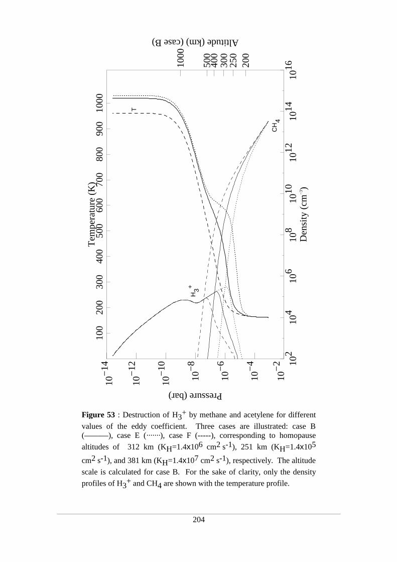
204
Figure 53 : Destruction of H3+ by methane and acetylene for different
values of the eddy coefficient. Three cases are illustrated: case B(———), case E (·······), case F (-----), corresponding to homopause
altitudes of 312 km (KH=1.4x106 cm2 s-1), 251 km (KH=1.4x10⁵
cm2 s-1), and 381 km (KH=1.4x107 cm2 s-1), respectively. The altitude
scale is calculated for case B. For the sake of clarity, only the density
profiles of H3+ and CH4 are shown with the temperature profile.
102
104
106
108
1010
1012
1014
1016
Den
sity
(cm
−3 )
10−
2
10−
4
10−
6
10−
8
10−
10
10−
12
10−
14
Pressure (bar)
200
250
300
400
500
1000
Altitude (km) (case B)
100
200
300
400
500
600
700
800
900
1000
Tem
pera
ture
(K
)
T
CH
4
H3+
VII.4.3.2 Sensitivity to the altitude of the homopause (cases E and F)
The eddy coefficient at the homopause (KH) plays a key role in the
establishment of the methane density profile, especially in the region of the H2 emission
peak since it defines the altitude of the homopause. Two cases are simulated, E and F,
for which KH differs from case B by 1 order of magnitude.
In case E, KH=1.4x105 cm2 s-1 and the altitude of the homopause is 251 km,
significantly lower than in case B where the altitude of the homopause was 312 km.
The lower CH4 density has direct effects on the temperature profile: the H2
rovibrational temperature increases by 40% as a result of the lower CH4 (and C2H2)
cooling, while the H3+ temperature decreases by 4% due to the higher H3
+ density
resulting from a lower destruction by CH4. This higher H3+ cooling efficiency
translates to an increase of the H3+ IR emission by a factor 3.3. The modification of the
H3+ density profile resulting from the lower destruction by methane and acetylene is
compared with the density profile of case B in figure 53. The strong temperature
increase at 300 km and the raise of the H3+ density between 250 and 400 km are clearly
related to the drop the homopause altitude.
Since the temperature profile is substantially modified in the region of the emission
peak, the altitude-pressure relationship is modified accordingly and the energy
distribution, similar to that of case B, leads to a peak of H2 emission at 238 km
(compared to 246 km in case B) . As expected, the lower eddy coefficient decreases the
FUV color ratio to 1.2, close to the unattenuated value. The integrated CH4 column
density (0.4x1016 cm-2) is much below the observational range.
An interesting conclusion might be drawn from the similarities between cases D and E.
In both cases the H2 emission peaks about 20 km below the homopause. As far as
methane attenuation of the H2 FUV spectrum is concerned, cases D and E are therefore
almost equivalent. There is indeed no net difference between the color ratios (∼1.2) and
between the integrated CH4 columns above the emission peak (∼0.5x1016 cm-2 ). The
205
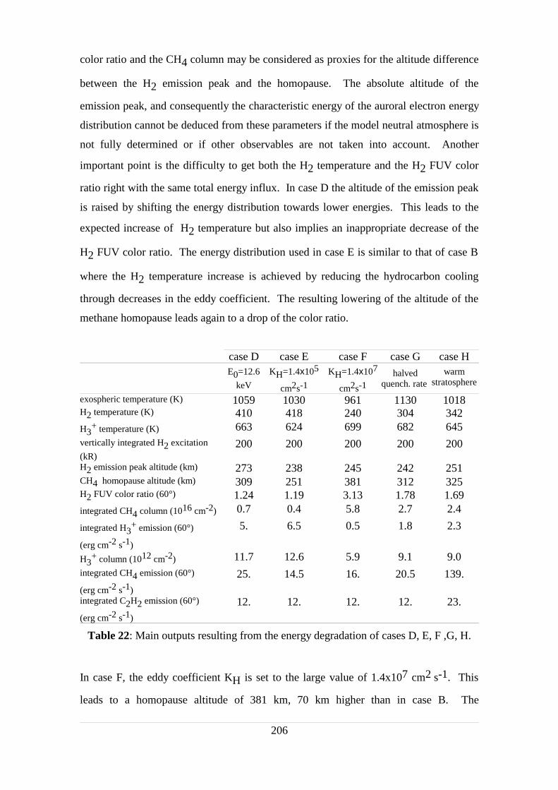
color ratio and the CH4 column may be considered as proxies for the altitude difference
between the H2 emission peak and the homopause. The absolute altitude of the
emission peak, and consequently the characteristic energy of the auroral electron energy
distribution cannot be deduced from these parameters if the model neutral atmosphere is
not fully determined or if other observables are not taken into account. Another
important point is the difficulty to get both the H2 temperature and the H2 FUV color
ratio right with the same total energy influx. In case D the altitude of the emission peak
is raised by shifting the energy distribution towards lower energies. This leads to the
expected increase of H2 temperature but also implies an inappropriate decrease of the
H2 FUV color ratio. The energy distribution used in case E is similar to that of case B
where the H2 temperature increase is achieved by reducing the hydrocarbon cooling
through decreases in the eddy coefficient. The resulting lowering of the altitude of the
methane homopause leads again to a drop of the color ratio.
case D case E case F case G case HE0=12.6
keV
KH=1.4x10⁵
cm2s-1
KH=1.4x10⁷
cm2s-1halved
quench. rate warm
stratosphere
exospheric temperature (K) 1059 1030 961 1130 1018H2 temperature (K) 410 418 240 304 342H3
+ temperature (K) 663 624 699 682 645vertically integrated H2 excitation
(kR)200 200 200 200 200
H2 emission peak altitude (km) 273 238 245 242 251CH4 homopause altitude (km) 309 251 381 312 325H2 FUV color ratio (60°) 1.24 1.19 3.13 1.78 1.69integrated CH4 column (1016 cm-2) 0.7 0.4 5.8 2.7 2.4
integrated H3+ emission (60°)
(erg cm-2 s-1)
5. 6.5 0.5 1.8 2.3
H3+ column (1012 cm-2) 11.7 12.6 5.9 9.1 9.0
integrated CH4 emission (60°)
(erg cm-2 s-1)
25. 14.5 16. 20.5 139.
integrated C2H2 emission (60°)
(erg cm-2 s-1)
12. 12. 12. 12. 23.
Table 22: Main outputs resulting from the energy degradation of cases D, E, F ,G, H.
In case F, the eddy coefficient KH is set to the large value of 1.4x107 cm2 s-1. This
leads to a homopause altitude of 381 km, 70 km higher than in case B. The
206
corresponding higher CH4 density is responsible for the drop (20%) of the H2
temperature as CH4 cools down the region where most of the auroral energy is
converted into heat. As a result of the smaller H3+ column, which is destroyed by the
CH4 excess (figure 53), the H3+ temperature increases by 50 K. The decrease of the
H3+ column also implies a decrease of the H3
+ IR emission by a factor 4. The
integrated CH4 column above the H2 emission peak (5.8x1016 cm-2) and the FUV
color ratio (3.13) are almost twice as large as the values in case B. Upwelling of
methane due to the large amount of auroral energy deposited near the homopause may
indeed cause redistribution of the CH4 mixing ratio above the homopause similar to the
O2/N enrichment observed in the Earth auroral thermosphere.
VII.4.3.3 Sensitivity to the H3+ quenching rate coefficient (case G)
The quenching rate of H3+ by H2 is an important parameter which determines
the H3+ cooling efficiency directly acting on the upper thermospheric thermal profile.
To date, there are no direct measurements of rate coefficients of elementary processes
occurring during quenching of H3+ by H2 and we considered the "phenomenological"
rate coefficient (2.7 ± 0.6)x10-10 cm3 s-1 determined by Kim et al. (1974). It is based
on a simplified reaction rate which does not account for the distribution of excited states
of H3+. Also, it is not known whether deactivation occurs directly from each
vibrational state to the ground state or by sequential deactivation in a number of
collisions. This quenching coefficient therefore represents only an average or overall
value.
Case G uses the same set of parameters as case B, but in order to test the effect of a
different quenching rate, this parameter has been arbitrarily halved (1.35x10⁻¹⁰
cm-3 s-1). The resulting reduced H3+ radiative cooling increases the H3
+ temperature
by 34 K while the H2 temperature remains almost unchanged, mainly because the two
207
regions are spatially separated. Indeed, the thermal profile departs from the profile of
case B at an altitude of 400 km. The H3+ column is higher than in case B. This might
be explained by the lower efficiency of the H3+ loss term (reactions 1 and 2 in table 15)
which is inversely proportional to the temperature. The exospheric temperature slightly
increases by 10 K. A lower quenching rate might therefore be an alternative to the soft
electron component to increase the thermospheric temperature and especially the H3+
temperature.
VII.4.3.4 Sensitivity to the stratospheric temperature profile (case H)
Cases A to G, described in tables 13 and 12, illustrate the difficulty to increase
the CH4 and C2H2 IR emissions. One straightforward solution is to raise the
stratospheric temperature. However, we showed that the degradation of the auroral
energy could not increase that temperature and we therefore assumed that non-auroral
processes, such as breaking gravity waves, could sustain the stratospheric part of the
equatorial thermal profile deduced from Galileo observations. In case H, we assume
that these non-auroral processes and probably exothermic processes triggered by the
aurora (such as the hydrocarbon chemistry) produce a stratospheric temperature profile
similar to the auroral (hot spot) IRIS cold boundary previously described. The upper
part of the thermal profile is approximated by shifting the Galileo profile downward
until a continuous profile is obtained. This new thermal structure is used as an initial
profile and the energy flux of case B is iteratively degraded until a steady state thermal
profile is reached. As expected, the IR methane emission is multiplied by 7 and reaches
a value (139 ergs cm-2 s-1), in better agreement with the observation. The C2H2
emission increase (factor two) is limited by the lower temperature increase in the lower
stratospheric region (below 200 km). The resulting temperature profile is shown in
figure 54. It is compared to the equatorial Galileo profile and to the domain of
observational constraints previously defined. Below the 10-7 bar pressure level the
converged temperature profile is somewhat warmer than that of case B. Above this
level, the two profiles are equivalent. As a result, the H2 temperature increases by 46 K
208
while the H3+ temperature remains the same.
The IRIS warm upper boundary has been tested similarly. In these conditions the energy
flux of case B is unable to sustain the thermal profile. The thermal energy radiated by
methane (1270 ergs cm-2 s-1) is so important that this deep heat sink drives most of the
auroral heat and prevents any further heating of the atmosphere. This unlikely situation
might be explained by an incompatibility between the IRIS warm upper boundary and
the methane density profile calculated by the degradation model. Indeed, as was already
the case for H3+, methane IR emission is intimately linked to the temperature-density
pair.
209
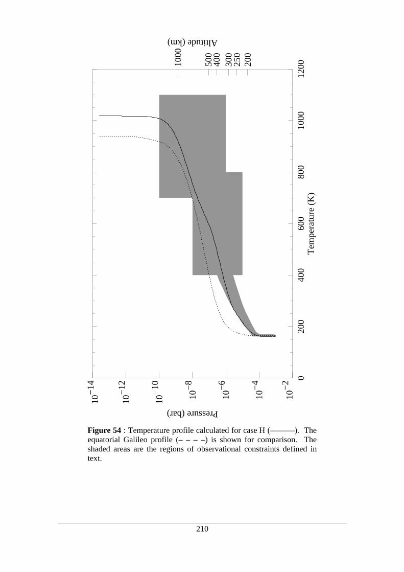
210
Figure 54 : Temperature profile calculated for case H (———). Theequatorial Galileo profile (– – – –) is shown for comparison. Theshaded areas are the regions of observational constraints defined intext.
020
040
060
080
010
0012
00T
empe
ratu
re (
K)
10−
2
10−
4
10−
6
10−
8
10−
10
10−
12
10−
14
Pressure (bar)
200
250
300
400
500
1000
Altitude (km)
VII.5 Conclusion
A one-dimensional model has been developed which couples a two-stream
electron transport model of energy deposition with a 1-D thermal conduction model
including particle heating, CH4, C2H2 and H3+ cooling. The initial atmospheric
structure is defined by a thermal profile deduced from Galileo observations. The code
allows us to monitor the energy degradation of an electron beam as it penetrates into this
atmosphere which self-consistently adapts to the auroral conditions. The resulting
thermal profile, UV and IR emissions profiles, FUV color ratio, and densities generated
by various choices of the precipitating electron energy distibution are constrained by
data derived from spectra and images taken in different bandpasses. Sensitivity tests are
performed to evaluate the importance of the energy spectrum of the incident electrons
for the thermal balance of Jupiter's auroral thermosphere and to show the limitations of
the degradation code.
Different conclusions can be drawn from the eight test cases considered. In order to
meet the H2 integrated brightness constraint, a trade-off is necessary between the FUV
color ratio and the H2 rovibrational temperature. Indeed, case D shows that the easiest
way to get a sufficiently high H2 temperature is to shift the H2 emission profile towards
higher altitudes. However, this shift places most of the H2 emission above the methane
homopause and the FUV color ratio almost equal to its unattenuated value. A second
way to increase the H2 temperature is to reduce the hydrocarbon cooling by assuming a
lower eddy coefficient. However, this also lowers the altitude of the homopause which
in turn reduces the FUV color ratio. Similarities between the results of cases D and E
demonstrate that the FUV color ratio deduced from spectral observations cannot be used
to determine the absolute altitude of H2 emission but rather the altitude of H2 emission
relative to the altitude of the methane homopause.
The H3+ and exospheric temperatures are mainly due to the level of soft electron influx
and are almost independent from the H2 UV and hydrocarbon IR emissions and
temperatures (which are partly controlled by the high energy component of the energy
distribution). The H3+ temperature can be raised independently from the H2 and
211

hydrocarbon observables by increasing the soft electron component, but it must be
traded off with the observed H3+ IR emission intensity, which also increases with the
low energy component of the distribution. It was shown in case G that reducing the
H3+ quenching rate leads to a higher H3
+ temperature and a lower integrated H3+
brightness. These cases illustrate the essential thermostatic role played by H3+ which
regulates the heating in the thermosphere and thus the atmosphere expansion.
Case H suggests that the auroral upper stratosphere is probably warmer than the
equatorial upper stratosphere measured by Galileo. With case C, it also shows that the
auroral energy precipitated is not able to provide the necessary heat to balance the
hydrocarbon cooling. Non-auroral processes, such as Joule heating or breaking gravity
waves, and indirect auroral processes, like exothermic hydrocarbon chemistry, need to
be specified as well.
The kappa energy distribution used in case C produces outputs that do not match the
observational constraints. This might be explained by the fact that this distribution
which fits Galileo EPD measurements between 10 and 20 RJ may not reflect the
accelerating processes undergone by the auroral electron as they travel along the
magnetic field lines.
The different cases show that the IR H3+ emission probes a region sensitive to the soft
electron component of the energy distribution, while the H2 FUV emission is sensitive
to energetic electrons. The IR hydrocarbon emissions give information on the non-
auroral and indirect auroral processes controlling the temperature in the lower
stratosphere.
The H2 extreme ultraviolet emission (EUV) could be used to probe the region sensitive
to the soft electrons. Indeed, the EUV photons produced by electron impact on H2 are
subject to self-absorption. They will therefore escape the optically thick region at an
altitude higher than the level where the initial electron impact occured. EUV Galileo
and HUT (Wolven et al. 1998) observations already exist and observations spanning the
900-1200 Å range will soon be available with the Far Ultraviolet Spectroscopic
Explorer (FUSE) satellite. However before these data can be used, an important effort is
required (in progress) to include the self-absorption of H2 Lyman and Werner emission
below 1000 Å in synthetic spectra.
212

It has been stressed that the multispectral observational constraints have been
established from measurements that are not simultaneous in time and space. Moreover
since these observations probe different altitude regions of the atmosphere, they do not
necessarily stem from the same processes. A campaign of simultaneous multispectral
observations of Jupiter's aurora would allow a more reliable determination of the
complete energy budget of the precipitating electrons and would give some clues on the
possible link between the different auroral signatures.
213
Part 3
VIII The spectral generator
VIII.1 H2 far ultraviolet spectroscopy
A detailed study of molecular spectroscopy is largely out of the scope of the
present work. We restrict ourselves to an overview of the main processes that are taken
into account by the generator synthesizing high resolution H2 spectra within the UV
range 900-1700 Å.
These processes include :
1. electron impact excitation of the H2 X g+1 ground state to the different rovibrational
states of the B u+1 , C u
1 and E,F g+1 excited electronic states
2. radiative deexcitation from the B u+1 , C u
1 states to the X g+1 ground state.
The effect of the B' u+1 , B'' u
+1 , D u1 and D' u
1 Rydberg states are not included
in the present model as their contribution to the jovian spectrum is very small above
1200 Å (Ajello et al., 1984).
In the following section, useful notations and conventions applying to H2 are
reviewed. They are used to introduce the quantum numbers that are relevant to
characterize the rovibrational levels of the H2 molecule. The principal selection rules
applying to dipole transitions are then summarized. Finally we give the formulae that
are used to calculate the line intensity for the radiative deexcitation from the B u+1 and
214
C u1 electronic states to the X g
+1 ground state of H2.
215

VIII.1.1 Conventions
Selection rules for radiative deexcitation involve quantum numbers and
symmetry properties of the various energy levels of a molecule. These characteristics
are conventionally summarized by symbols in the spectroscopic term of the molecule.
For the H2 molecule, the following notation is used :
X g,u +,-2S1
VIII.1.1.1 X,
The letter in front of the term symbol (X) designates different electronic states
which may be of the same type. This letter may be X, A, B, C, ..., a, b, c, ... (states
represented by a lower-case letter do not have the same multiplicity than those
represented by an upper-case letter) and X is usually used for the ground state of the
molecule.
is a symbol related to Λ : the quantum number associated to the Λ vector
which is the component of the electronic orbital angular momentum L along the
internuclear axis (vectors are represented with bold characters).
Following the international nomenclature,
ML
and ML can take only the values
ML = L, L-1, L-2, ... , -L
where L is the quantum number characterizing the magnitude of L.
For a given value of L, the quantum number Λ can take the values
Λ = 0, 1, 2, ..., L.
Thus in the molecule for each value of L there are L+1 distinct states with different
energies (in diatomic molecules, states differing only in the sign of ML have the same
energy). According as Λ = 0, 1, 2, 3, ..., the corresponding molecular state is designated
as Σ, Π, Δ, ... state, analogous to the mode of designation for atoms.
Π, Δ, ... states are doubly degenerate since ML can have the two values +Λ and -Λ; Σ
216
states are non-degenerate since ML can only have one value (zero).
VIII.1.1.2 2S+1
The left superscript 2S+1 is called the multiplicity of the state and is due to the
electron spin. Under the action of electrostatic forces the spins of the individual
electrons form a resultant vector S, the corresponding quantum number S being integral
or half integral according as the total number of electrons in the molecule is even or
odd. For the H2 molecule, S=0 or S=1 (antiparallel or parallel spins) and give rise to
singlet or triplet states, respectively. In Σ states (Λ = 0), the resultant spin S, since it is
unaffected by an electric field, is fixed in space as long as the molecule does not rotate
and if there is no external magnetic field. Consequently, these states remain single. On
the other hand, if Λ ≠ 0, (Π, Δ, ... states), there is an internal magnetic field in the
direction of the internuclear axis resulting from the orbital motion of the electrons. This
field causes a precession of S about the internuclear axis and the electronic term splits
into a multiplet of 2S+1 components. Each component is characterized by the quantum
number MS which can take the values MS = S, S-1, ... ,-S.
VIII.1.1.3 (+,−)
The right superscript (+,-) refers to the symmetry properties of the electronic
eigenfunctions of Σ states. These properties depend on the symmetry properties of the
field in which the electrons move. In a diatomic molecule any plane through the
internuclear axis is a plane of symmetry. Therefore the electronic eigenfunctions of a
non-degenerate state (Σ state) either remains unchanged or changes sign when reflected
at any plane passing through both nuclei. In the first case, the state is called a Σ+ state,
and in the second case it is called a Σ- state.
217

VIII.1.1.4 (g,u)
The right subscript (g,u) refers to the symmetry properties of the electronic
eigenfunctions. These properties apply to diatomic molecules for which the two nuclei
have the same charge. In this case, the field in which the electrons move has, in
addition to the symmetry axis, a center of symmetry at the midpoint of the internuclear
axis. The field remains unaltered by a reflection of the nuclei at this center of
symmetry. As a consequence, the electronic eigenfunctions remain either unchanged or
only change sign when reflected at the center (that is, when the coordinates of all the
electrons xi, yi, zi, are replaced by their negative -xi,-yi,-zi). In the first case, the state to
which the eigenfunction belongs is called an even state ("gerade" g state), in the second
case an odd state ("ungerade" u state). Thus for molecules with like nuclei we have Σg,
Σu, Πg, Πu, ... states.
VIII.1.1.5 Other symmetry properties
The symmetry properties of the rotational levels are not represented in the
spectroscopic term but they are taken into consideration in the selection rules. We have
seen above that the electronic eigenfunctions of an atomic system may remain
unchanged or just change sign when reflection at the origin (replacement of all xk, yk, zk
by -xk, -yk, -zk) is applied. A closer investigation of the rotator functions (Ψr) shows that
for such a reflection they remain unchanged for even values of J (the rotational quatum
number) but change to -Ψr for odd values of J. Therefore, a rotational level is called
positive or negative depending on whether the total eigenfunction remains unchanged or
changes sign for such a reflection. This property is also called the parity.
The complete eigenfunction of a molecule, in the Born-Oppenheimer approximation, is
a product of an electronic, a vibrational, and a rotational contribution
e
1rv r .
218
Since, as we saw above, Ψe may itself change sign by reflection at the origin (as is the
case for Σ states), the total eigenfunction remains unaltered for odd J and changes sign
for even J. In this case the + and - have to be changed for the rotational levels.
In homonuclear molecules like H2, it can be shown that for an exchange of the two
nuclei the total eigenfunction either remains unchanged or changes its sign. According
as the former or the latter is the case, the state under consideration is said to be
symmetric (s) or antisymmetric (a) in the nuclei. Again, for electronic states whose Ψe
change sign upon such a reflection, s and a have to be reversed.
In the actual molecule rotation and vibration take place simultaneously with the
electronic motions. We must find out by what quantum numbers we can describe the
rotational levels in the different types of electronic states, how their energy depend on
these quantum numbers, and what symmetry properties the corresponding
eigenfunctions possess. All this is essential for the determination of the selection rules.
219
VIII.1.2 Λ-type doubling
In most diatomic molecules the interaction between the rotation of the nuclei and
L is neglected. However, for light molecules like H2, the speed of nuclear rotation is
larger and this interaction must be taken into account. For H2 states with Λ ≠ 0 it is
found to produce a splitting into two components, with their own symmetry properties,
for each J value which are doubly degenerate (ML can have the two values +Λ and -Λ).
This splitting is called Λ -type doubling. We will see its effects on the electric dipole
transitions from the C u1 state to the X g
+1 ground state of H2.
VIII.1.3 Selection rules for electronic transitions
The quantum numbers and symmetry properties that we just introduced affect the
spectra of diatomic molecules through the selection rules that hold for them.
The selection rules are obtained by evaluating the matrix element Rnm of the electric
dipole moment. Indeed, the interaction of an electromagnetic wave having an electric
vector E, with a molecular system is in first approximation the interaction with the
(variable) electric dipole moment M .
If the interaction energy M.E is introduced into the wave equation it is found that the
probability of a transition between two states n and m produced by the interaction is
proportional to the square of the magnitude of certain vector quantities Rnm -the matrix
elements of the dipole moment- whose components depend in the following manner on
the eigenfunctions Ψn and Ψm of the two states:
R xyz
nmn* M x
yz
m d
If the matrix element Rnm differs from zero for two states n and m, the two states
combine with each other with a certain probability with emission or absorption of
radiation; if it is zero the transition under consideration is forbidden as a dipole
transition. A non-zero transition probability may also be produced by the interaction of
220

an electromagnetic wave with the magnetic dipole moment, the quadrupole moment, or
higher moments of the molecular system.
For reasons of symmetry the H2 molecule has no permanent electric dipole, in other
words the diagonal elements of the Rnm matrix are all zero. As a result, (dipole)
transitions between rovibrational levels of a single electronic state are forbidden. We
therefore only consider transitions involving two different electronic states (m ≠ n).
VIII.1.4 General selection rules
For any atomic system the selection rule for the quantum number J of the total
angular momentum is
ΔJ = J' - J'' = 0, ±1, with the restriction J = 0 J = 0
where J' refers to the upper state and J'' refers to the final state.
This rule holds rigorously for electric dipole radiation. Thus, from this selection rule one
expects three or two branches. These are known as the P, Q and R branches. They are
related to the value of J jump :
P branch, ΔJ = J' - J'' = -1
Q branch, ΔJ = 0
R branch, ΔJ = +1
Positive terms combine only with negative, and vice versa, or symbolically
+ -, + +, - -
It should be noted that, in the case of a Σ state, the sign (+ or -) refers to the complete
eigenfunction of the molecule and not only to the electronic eigenfunction (right
upperscript of the spectroscopic term).
H2 having identical nuclei symmetric terms combine only with symmetric and
221

antisymmetric only with antisymmetric, or
s s, a a, s a
Finally, in the case of a molecule with nuclei of equal charge (again H2) even electronic
states combine only with odd; that is,
g u, g g, u u.
VIII.1.5 Influence of the nuclear spin
The nuclear spin vector has a strong influence on the population of the
symmetric and antisymmetric levels. The spin vectors I of the two nuclei of a diatomic
molecule form a resultant T, the total nuclear spin of the molecule. According to the
rules of addition of the angular momentum vectors, for two identical nuclei the quatum
number of the total nuclear spin is given by
T= 2 I, 2 I -1, ..., 0
In the case of H2, I=1/2 and the possible values of T are T=1 (parallel nuclear spins, ↑
↑) and T=0 (antiparallel spins, ↑↓). The first value is associated with the antisymmetric
levels and the second with the symmetric levels. It is shown that the statistical weights
are 3 and 1, respectively (Fermi statistics). In the case of H2, the antisymmetric
rotational levels occur three times as frequently as the symmetric; that is , the total
statistic weights are 3 × (2J + 1) and 1 × (J + 1), respectively. Since the configuration
having the greater statistical weight is usually called the ortho modification, an ortho-H2
corresponds to parallel nuclear spins and a para-H2 corresponds to antiparallel nuclear
spins.
222

VIII.1.6 Emission intensity
The intensity of an electronic transition from an upper state n to a lower state m
is determined by the transition probability Anm in emission. The transition probability
Anm is determined by the matrix element Rnm of the dipole moment acoording to
A nm644nm
3
3hR nm2 .
Frequently the experimental data are expressed in terms of the oscillator strength fnm
which is relared to Rnm2 by
f nm82 cnm
3h 2 R nm2
where μ and ε are mass and charge of the electron and it finally comes
f nmA nm c
82nm2 2 .
For electronic transitions
Renmn
* Mem d e
where m and n are electronic eigenfunctions, Me is the part of the dipole moment
depending on the electrons and dτe is the volume element of the configuration space of
the electrons. For non-degenerate electronic states the transition probability Anm is
simply proportional to Renm2, for degenerate electronic states to
1d n
R ni mk2
where dn is the degree of degeneracy of the upper state and where the summation is over
all combinations of the sublevels ni and mk.
223
The total matrix element for a given rotational and vibrational transition system may be
written
RRenm R vib
v' v'' R rotJ' J''
The transition probability Anm,v'v'',J'J'' is given by
A nm,v'v'',J'J''6443
3hRe
nm2R vibv' v''2
M'M''
R rotJ' J''2
2J''1
where summation is over all values of the magnetic quantum numbers M', M'' (M = J, J-
1, ..., -J), and where it is assumed that the wave numbers ν of the transitions occurring
in the summation do not differ too much. For degenerate electronic states with
degeneracies dn and dm, the quantity Renm2 has to be replaced by
1d n
Reni mk2
where i and k number the degenerate sublevels of the upper state level, and the lower
state m; and where the summation is over all possible combinations of the sublevels of
the upper with those of the lower state.
VIII.1.6.1 Population of the ground level
It is assumed that the molecules in the ground state are in thermal equilibrium.
Therefore, we need only consider the distribution of the molecules over the different
quantum states in thermal equilibrium.
VIII.1.6.2 vibrational levels
The relative number of molecules in each of the vibrational levels referred to the
number of molecules in the lowest vibrational level is determined by the Boltzmann
224
factor
expEkT
exp G 0vhc
kT
where G0 is the energy of the anharmonic oscillator referred to the zero-point energy.
If we wish to refer to the total number of molecules N we have to consider that N is
proportional to the sum of the Boltzmann factors over all states, that is the so called
partition function
Qv1expG 01hc
kTexp
G 02hc
kT...
Therefore the number of molecules in the vibrational state v is given by
N vNQv
expG 0vhc
kT
VIII.1.6.3 Rotational levels
The population of the rotational levels follows a thermal distribution which is
not simply given by the Boltzmann factor exp(-E/kT); the degeneracy of the rotational
level (2J+1) must be taken into account. The number of molecules NJ in the rotational
level J of the lowest vibrational state at temperature T is thus proportional to
2J1expE J
kT
Assuming that the transition probability is the same for all lines of a band, the actual
number of molecules in the rotational states may be obtained by multiplying by N and
dividing by the rotational state sum (the rotational partition function Qr)
NJ3 j
4NQr
2J1expBJ J1hc
kT
225
where B is the rotational constant (prevailing for a particular vibrational level) and N is
the total number of molecules. The factor (3)j/4 accounts for the degeneracy due to the
nuclear spin which, in the case of H2, is 3 (j=1) for antisymmetric rotational levels and 1
(j=0) for symmetric levels. Dividing by 4 preserves the normalization of the total
partition function (4*Qr).
VIII.1.7 Transition wave number
The wave number of a transition is given by
m0B'B''mB'B''D'D''m22 D'D''m3D'D''m4...
where the initial state is, as usual, denoted by a single prime (') and the final state by a
double prime (''), ν0 is the wave number of the pure vibrational transition without taking
account of rotation, B is the rotational constant of the vibrational state and D brings a
correction due to centrifugal force for that vibrational state, and m equals J' (the
roatational level of the excited state).
For the H2 molecule, experimental values for these constants are tabulated in
Dabrowski (1984)
226

VIII.2 Application to the Lyman and Werner band
spectra of H2
VIII.2.1 The B u+1 state
In this section we study the H2 Lyman band spectrum arising from the radiative
deexcitaion of the B u+1 electronic state into the X g
+1 ground state.
In the following sections, we will follow the generally admitted convention for the
vibrational and rotational quantum numbers :
v, J refer to the initial state,
v', J' refer to the excited state,
v'', J'' refer to the final state.
The volume emission rate η from an upper level (v', J') of the excited H2
B u+1 state (hereafter often designated by the letter B) to a lower rovibrational level
(v'', J'') of the X g+1 ground state (hereafter often designated by the letter X) is given
by :
BX v',J',v'',J''nv',J'B A
v',J',v'',J''
where nv',J'B
is the population of the upper state. This latter population can be
estimated from the equilibrium between excitation to and deexcitation from the upper
level. It takes the form
gX Bv0,J v',J'nv',J'B
v'', J''
Av',J',v'',J''
where gX Bv0,J v',J' represents the excitation rate from the ground state
X(v=0, J) to the rovibrational level (v',J') of the B state. It is estimated by assuming that
227

the direct population rate of the B state is governed by direct electron (primary or
secondary) impact on ground state H2 molecules and it is assumed that the same rules
apply as for radiative transitions:
gX Bv0,J v',J'J
N X, v0, J E X Bv,J,v',J',EdE
where N(X,0,J) denotes the number density of H2 molecules in the X(v=0,J)
rovibrational level, Φ(E) is the total energetic electron flux at energy E and
σX→B(v,J,v',J',E) is the electron impact excitation cross section from X(v,J) into the
B(v',J') level. The sum extends over 2 terms corresponding to the P (ΔJ = -1) and R (ΔJ
= +1) branches of the excitation transitions.
According to Shemansky et al. (1985), the electron impact cross section may be given
by
v,J,v',J',EX
E with X
EE v,J,v',J'
and
Xff XC7 ln X
where ff(X) is a function (see Shemansky et al. [1985] for the detailed relation and
coefficients) of X and C7 is related to the oscillator strength
C74.f v,J,v',J'E v,J,v',J'
that is C74.A nm c
82nm2 2 E v,J,v',J'
Using the equilibrium relation to express the population of the B(v',J') excited state one
can derive a general form for the volume emission rate of the B(v',J') → X(v'',J'') line
BX v',J',v'',J''gX Bv0,J v',J'A
v',J',v'',J''
v'', J''
Av',J',v'',J''
228

As will be explained in a next section, the transitions from B(v',J') to the continuum of
the ground state (B → cont) may be taken into account and the previous relation
becomes
BX v',J',v'',J''gX Bv0,J v',J'A
v',J',v'',J''
v'', J''A
v',J',v'',J''A
v',J',c'',J''B cont
The electron impact excitation cross sections into individual rovibrational levels of the
B state is obtained from the line transition probabilities by Abgrall et al. (1993a,b) in
229
Figure 55 : Schematic representation of the excitation process from the ground state
to the excited B state followed by the radiative deexcitation to the ground state (the
potential curves are not to scale).
X g+1 X g
+1
B u+1
v0, J N v0,J
initial state final state
excitedstate
v', J' nBv',J'
gX Bv0,J v',J' A v',J',v'',J''hν
conjunction with the energy dependence formulation by Shemansky et al. (1985)
upgraded by Liu et al. (1998).
In addition to the direct collisional excitation, the population of the B u+1 state is
enhanced by the cascade process E,F g+1 B u
+1 following direct excitation of the
E,F g+1 state (hereafter often designated by E,F). It can be written :
g (B,v',J') = gd (B,v',J') + gc (B,v',J')
where the first term corresponds to the direct impact excitation and has the same form as
gX Bv0,J v',J' ; the second term is a two-step process where electron impact
populates the (E,F) state which selectively cascades into the B state. This latter process
is explained in the following section.
VIII.2.1.1 E,F Cascade
The potential-energy curve for the E,F g+1 is known (Davidson, 1960) to have
a double minimum resulting from avoided crossing of the potential-energy curves for
the 1 g 2s g+1 and 1 u
2 g+1 configurations. The two minima are sometimes
refered to as the E g+1 and F g
+1 states, respectively. Both minima are located in
roughly the same energy region, but since the equilibrium internuclear distances are
considerably different and since the Franck-Condon principle assumes vertical
transitions, we only consider the E g+1 minimum which has the closest equilibrium
internuclear distance to that of the X ground state.
As already mentioned, the B rovibrational levels may be populated by two different
processes :
1. electron impact excitation as previously described
2. cascade from the E,F g+1 excited state to the rovibrational levels of the B state.
The estimation of the contribution from this second process assumes that excitation
from the X ground state to the E,F state is controlled by electron impact. In order to
calculate this contribution numerical values for the transition probabilities would be
required
230
Av0,J v'EF ,J'EFX E,F
and Av'EF ,J'EFv''B,J''BE,FB
however these have never been measured.
To date, the only available information are the vibrational transition probabilities
Av0v'EFX E,F
and the Franck-Condon factors calculated by Lin (1974)
qB,EFv'BB
v'EF
EF 2,
giving an estimation of the transition probability between the two vibrational states.
231
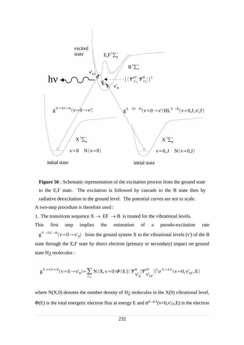
A two-step procedure is therefore used :
1. The transitions sequence X → EF → B is treated for the vibrational levels.
This first step implies the estimation of a pseudo-excitation rate
gX E,FBv0v'B from the ground system X to the vibrational levels (v') of the B
state through the E,F state by direct electron (primary or secondary) impact on ground
state H2 molecules :
gX E,FBv0v'Bv'EF
N X, v0 Ev'BB
v'EF
EF 2 X E,F v0, v'EF , E
where N(X,0) denotes the number density of H2 molecules in the X(0) vibrational level,
Φ(E) is the total energetic electron flux at energy E and σX→E,F(v=0,v'EF,E) is the electron
232
Figure 56 : Schematic representation of the excitation process from the ground state
to the E,F state. The excitation is followed by cascade to the B state then by
radiative deexcitation to the ground level. The potential curves are not to scale.
X g+1
E,F g+1
B u+1
v0 N v0
initial state
excitedstate
v'Bhν
X g+1
v0, J N v0,J
initial state
gX EFBv0v' gX EFBv0v'HLX Bv0,J ,v',J'
v'EF
v'EF
EFv'B
B 2

impact excitation cross section from X(v=0) into the E,F(v') level.
2. Partitioning of the rotational levels is approximated by using Hönl-London factors.
Due to the lack of transition probabilities for individual rovibrational transitions the
population of the rotational levels of E,F state is unknown. Accordingly, the following
crude approximation is made. It is assumed that the redistribution over the rotational
levels of B due to cascade from E,F is similar to that obtained from direct excitation
from X to B. Therefore the E,F state is short-circuited and the Höhnl-London factors
corresponding to the X→B transition are directly applied to the X→E,F→B transitions
series. The pseudo-excitation rate then becomes
gX E,FBv0, J v'B J'BgX E,FBv0v'BHLX B
It should be emphasized that the Hönl-London factors were derived under the
assumption of negligible interaction of rotation and electronic motion. Such an
assumption is reasonable for the X and B states of H2, but not for the E,F state.
Therefore it would be incorrect to apply the Hönl-London factors of the X to E,F and
E,F to B transtions.
233
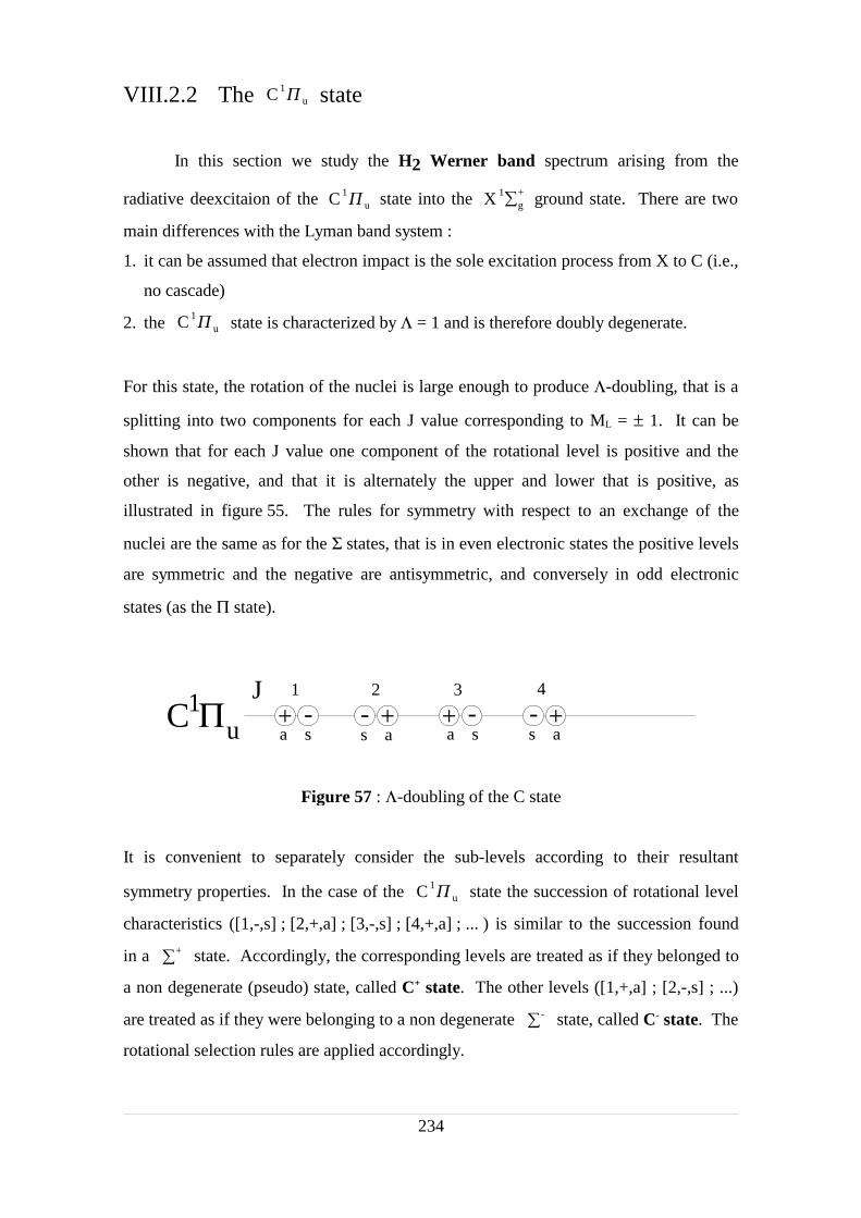
VIII.2.2 The C u1 state
In this section we study the H2 Werner band spectrum arising from the
radiative deexcitaion of the C u1 state into the X g
+1 ground state. There are two
main differences with the Lyman band system :
1. it can be assumed that electron impact is the sole excitation process from X to C (i.e.,
no cascade)
2. the C u1 state is characterized by Λ = 1 and is therefore doubly degenerate.
For this state, the rotation of the nuclei is large enough to produce Λ-doubling, that is a
splitting into two components for each J value corresponding to ML = ± 1. It can be
shown that for each J value one component of the rotational level is positive and the
other is negative, and that it is alternately the upper and lower that is positive, as
illustrated in figure 55. The rules for symmetry with respect to an exchange of the
nuclei are the same as for the Σ states, that is in even electronic states the positive levels
are symmetric and the negative are antisymmetric, and conversely in odd electronic
states (as the Π state).
It is convenient to separately consider the sub-levels according to their resultant
symmetry properties. In the case of the C u1 state the succession of rotational level
characteristics ([1,-,s] ; [2,+,a] ; [3,-,s] ; [4,+,a] ; ... ) is similar to the succession found
in a + state. Accordingly, the corresponding levels are treated as if they belonged to
a non degenerate (pseudo) state, called C+ state. The other levels ([1,+,a] ; [2,-,s] ; ...)
are treated as if they were belonging to a non degenerate - state, called C- state. The
rotational selection rules are applied accordingly.
234
Figure 57 : Λ-doubling of the C state
1 2 3 4
a s a ss a s a+ ++ +- - - -
JC Πu
1
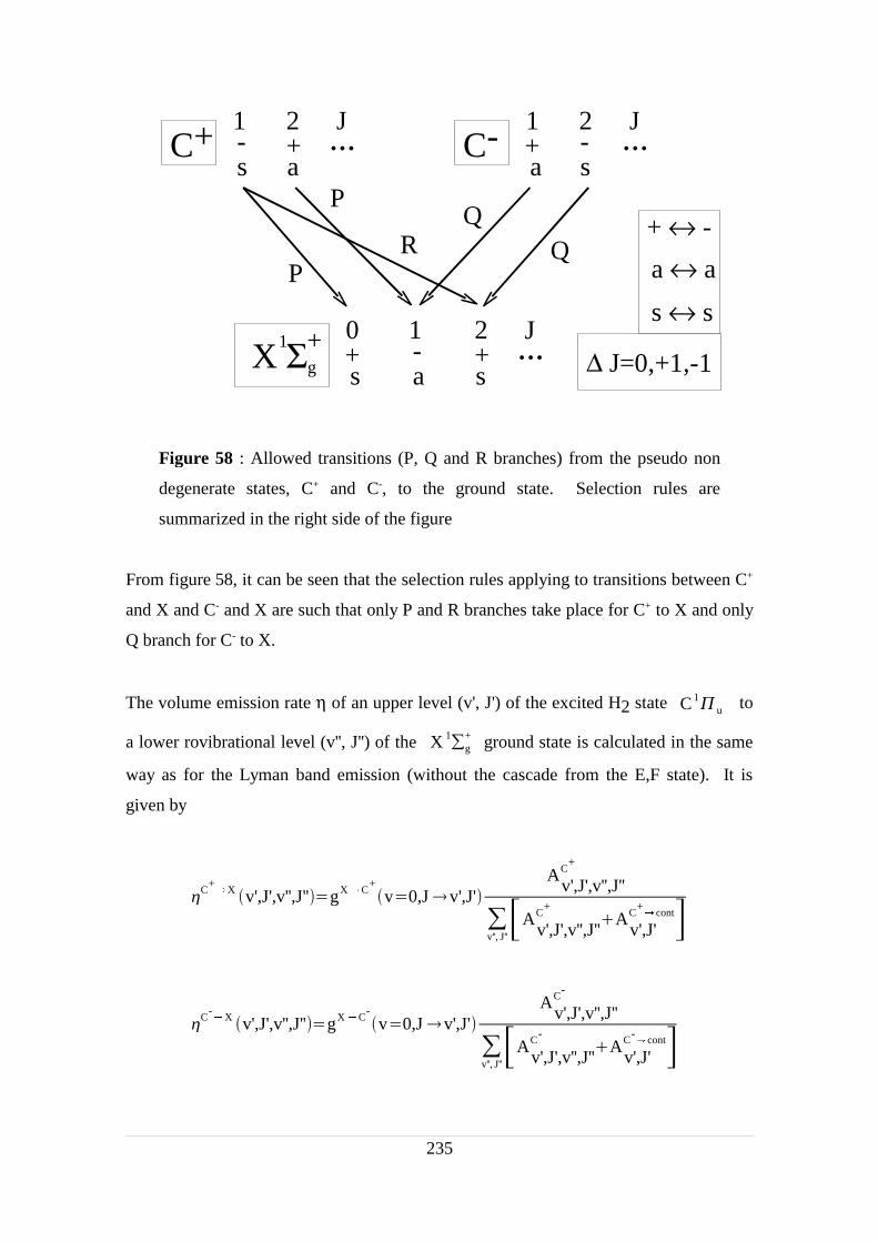
From figure 58, it can be seen that the selection rules applying to transitions between C+
and X and C- and X are such that only P and R branches take place for C+ to X and only
Q branch for C- to X.
The volume emission rate η of an upper level (v', J') of the excited H2 state C u1 to
a lower rovibrational level (v'', J'') of the X g+1 ground state is calculated in the same
way as for the Lyman band emission (without the cascade from the E,F state). It is
given by
C+X v',J',v'',J''gX C
+v0,J v',J'
Av',J',v'',J''C
+
v'', J''A
v',J',v'',J''C
+A
v',J'C
+ cont
C-X v',J',v'',J''gX C
-v0,J v',J'
Av',J',v'',J''C
-
v'', J''A
v',J',v'',J''C
-A
v',J'C
- cont
235
Figure 58 : Allowed transitions (P, Q and R branches) from the pseudo non
degenerate states, C+ and C-, to the ground state. Selection rules are
summarized in the right side of the figure
C1 2- +s a
...+ C1 2
-+sa
...-
1 2- +a s
...+ 0
s+X Σg
1
PR
+ ↔ -a ↔ a
s ↔ s
Δ J=0,+1,-1
P
J J
J

where the AC+ and AC- line transition probabilities are given by Abgrall et al. (1993 a,b).
The electron impact excitation cross sections into individual rovibrational levels of the
C state is obtained from the same line transition probabilities in conjunction with the
energy dependence formulation by Shemansky et al. (1985).
236
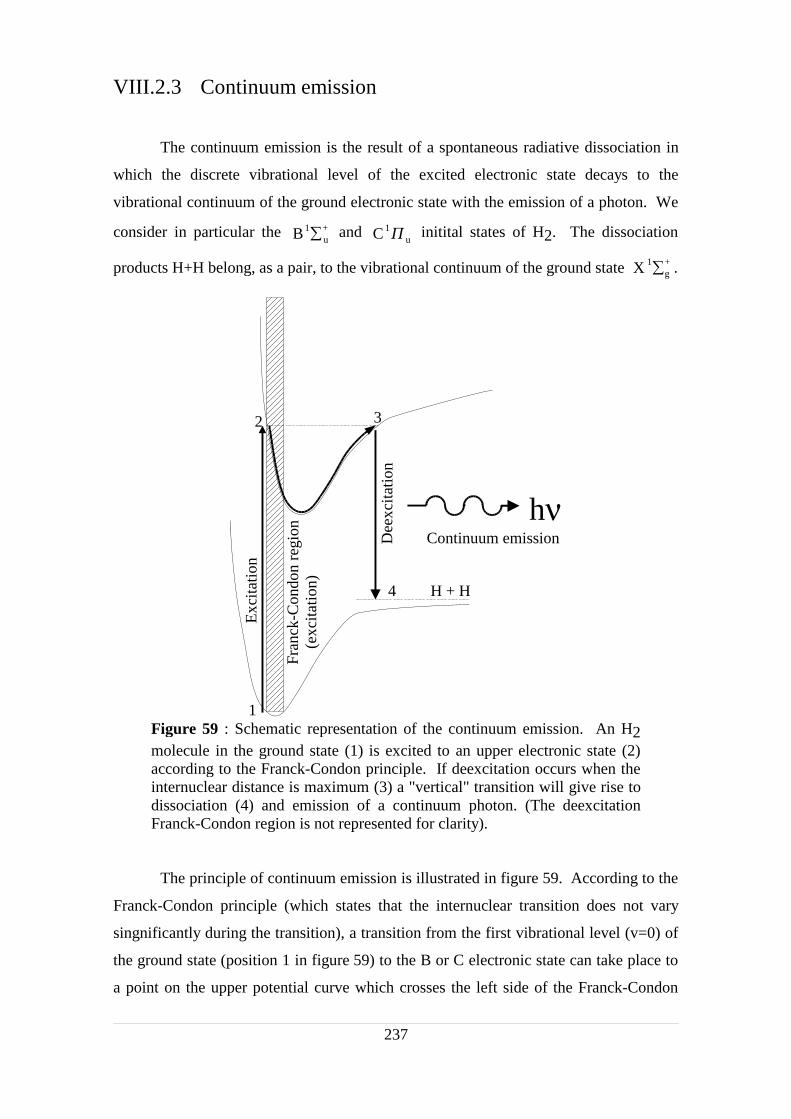
VIII.2.3 Continuum emission
The continuum emission is the result of a spontaneous radiative dissociation in
which the discrete vibrational level of the excited electronic state decays to the
vibrational continuum of the ground electronic state with the emission of a photon. We
consider in particular the B u+1 and C u
1 initital states of H2. The dissociation
products H+H belong, as a pair, to the vibrational continuum of the ground state X g+1 .
The principle of continuum emission is illustrated in figure 59. According to the
Franck-Condon principle (which states that the internuclear transition does not vary
singnificantly during the transition), a transition from the first vibrational level (v=0) of
the ground state (position 1 in figure 59) to the B or C electronic state can take place to
a point on the upper potential curve which crosses the left side of the Franck-Condon
237
Figure 59 : Schematic representation of the continuum emission. An H2molecule in the ground state (1) is excited to an upper electronic state (2)according to the Franck-Condon principle. If deexcitation occurs when theinternuclear distance is maximum (3) a "vertical" transition will give rise todissociation (4) and emission of a continuum photon. (The deexcitationFranck-Condon region is not represented for clarity).
1
2 3
4
Fran
ck-C
ondo
n re
gion
(
exci
tatio
n)
Exc
itatio
n
Dee
xcita
tion
hνContinuum emission
H + H
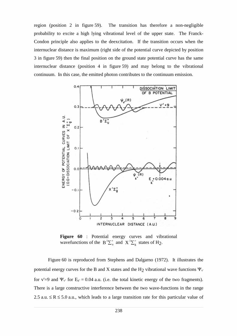
region (position 2 in figure 59). The transition has therefore a non-negligible
probability to excite a high lying vibrational level of the upper state. The Franck-
Condon principle also applies to the deexcitation. If the transition occurs when the
internuclear distance is maximum (right side of the potential curve depicted by position
3 in figure 59) then the final position on the ground state potential curve has the same
internuclear distance (position 4 in figure 59) and may belong to the vibrational
continuum. In this case, the emitted photon contributes to the continuum emission.
Figure 60 is reproduced from Stephens and Dalgarno (1972). It illustrates the
potential energy curves for the B and X states and the H2 vibrational wave functions Ψv'
for v'=9 and Ψv'' for Ek'' = 0.04 a.u. (i.e. the total kinetic energy of the two fragments).
There is a large constructive interference between the two wave-functions in the range
2.5 a.u. ≤ R ≤ 5.0 a.u., which leads to a large transition rate for this particular value of
238
Figure 60 : Potential energy curves and vibrationalwavefunctions of the B u
+1 and X g+1 states of H2.
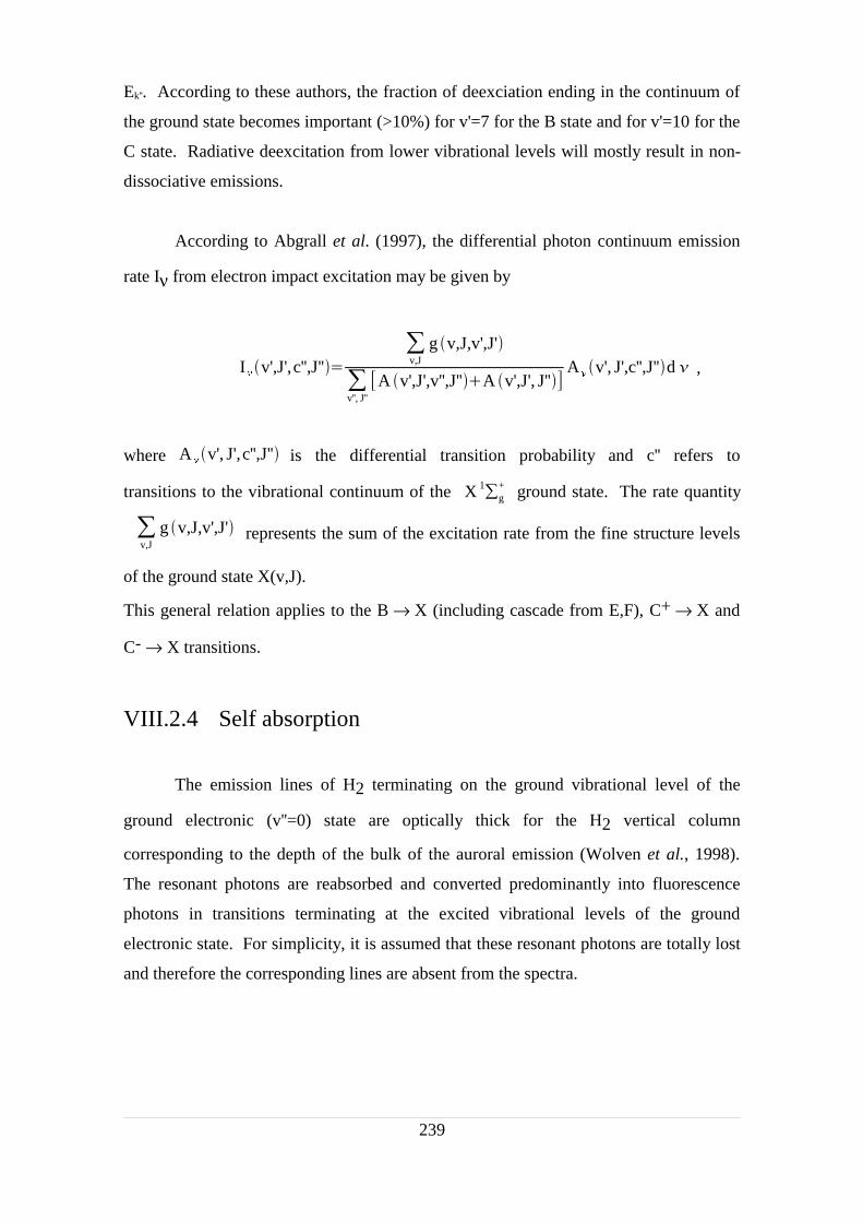
Ek''. According to these authors, the fraction of deexciation ending in the continuum of
the ground state becomes important (>10%) for v'=7 for the B state and for v'=10 for the
C state. Radiative deexcitation from lower vibrational levels will mostly result in non-
dissociative emissions.
According to Abgrall et al. (1997), the differential photon continuum emission
rate Iν from electron impact excitation may be given by
Iv',J',c'',J''
v,J
g v,J,v',J'
v'', J''
A v',J',v'',J''A v',J', J''Av', J',c'',J''d ,
where Av', J',c'',J'' is the differential transition probability and c'' refers to
transitions to the vibrational continuum of the X g+1 ground state. The rate quantity
v,J
g v,J,v',J' represents the sum of the excitation rate from the fine structure levels
of the ground state X(v,J).
This general relation applies to the B → X (including cascade from E,F), C+ → X and
C- → X transitions.
VIII.2.4 Self absorption
The emission lines of H2 terminating on the ground vibrational level of the
ground electronic (v''=0) state are optically thick for the H2 vertical column
corresponding to the depth of the bulk of the auroral emission (Wolven et al., 1998).
The resonant photons are reabsorbed and converted predominantly into fluorescence
photons in transitions terminating at the excited vibrational levels of the ground
electronic state. For simplicity, it is assumed that these resonant photons are totally lost
and therefore the corresponding lines are absent from the spectra.
239
VIII.3 Coupling of the two-stream model with the
spectral generator
VIII.3.1 Introduction
In this section we report preliminary results obtained with a model coupling the
electron energy degradation code with the detailed synthetic spectral model of the H2
Lyman and Werner band system previously described. It is used to calculate the
emerging auroral ultraviolet spectra from Jupiter’s atmosphere excited by electrons with
different initial energy distributions. The atmospheric model is adapted from the low
latitude vertical P-T profile measured by the Galileo probe and mid-latitude
hydrocarbon photochemistry. In contrast to earlier studies, the vertical dependence of
the auroral emission, H2 temperature and chemical composition are explicitly
considered. Each layer, with its gas temperature, contributes to the emergent spectrum
and the absorbers are vertically distributed within the source region. Examples of the
calculated spectra are shown to validate the synthetic spectrum and to illustrate the
importance of the electron energy distribution and the vertical dimension. The spectral
model with a fixed thermal structure has been applied to the analysis of seven GHRS
(HST) spectra of the 1200-1700 Å region obtained with a 5 Å resolution at various
locations in the north and south Jovian aurora. These results are reported in a paper in
press (Dols et al., 2000) and will not be repeated here. Instead, we discuss additional
electron energy distribution cases for which synthetic spectra are compared with two
echelle spectra that were not satisfactorily fitted in the work of Dols et al.
Previous studies of the sensitivity of the electron excited H2 ultraviolet spectrum
to temperature, with the exception of those by Liu and Dalgarno (1996) and Kim and
Fox (1997), assumed a monoenergetic electron beam, generally 100 eV, meant to
represent the mean energy of the exciting secondary electrons. The effect of the energy
of the (primary + secondary) electrons on the line brightness distribution was shown to
be small between 100 keV and 1 keV by Liu and Dalgarno (1996). They concluded that
the auroral UV spectrum is not a sensitive indicator of the primary electron energy
240

distribution (we will see that this conclusion only applies for laboratory measurements
where the excited gas is confined in a small cell which is not representative of the
Jovian atmosphere characterized by complex thermal and chemical vertical structures).
Below about 50 eV, the intensity of the Werner band decreases relative to the Lyman
band and continuum because the excitation cross section of the C u1 state peaks at
higher energies than the B u+1 state. Similarly, cascading effects E,F g
+1 B u+1
are enhanced at low energies, near the threshold of the transition. These cascades
preferentially populate the low vibrational levels v = 0 to 4 of the B u+1 state and
originate mostly from excitation of low rotational J levels of the ground state.
Consequently, cascade effects are most conspicuous for excitation of low temperature
H2 by low energy electrons.
A common feature of all previous studies of the H2 auroral spectrum is that a
thin slab approach was adopted. In this schematic view, the aurora is represented by a
homogeneous emission layer characterized by a H2 rovibrational temperature to be
determined by the fit to the observed spectrum. A hydrocarbon layer, usually limited to
methane, overlies the emission layer and its column density is adjusted to match the
color ratio in the observed spectrum. In this work, the vertical dimension, including the
temperature, composition and emission rate vertical gradients are explicitly considered.
A primary electron beam with a prescribed energy distribution interacts with the high
latitude Jovian thermosphere described by a model atmosphere. Each layer,
characterized by its own temperature, contributes to the emergent spectrum and the
absorbers are vertically distributed within the source region.
241
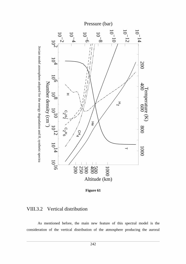
VIII.3.2 Vertical distribution
As mentioned before, the main new feature of this spectral model is the
consideration of the vertical distribution of the atmosphere producing the auroral
242
Figure 61
Jovian model atm
osphere adopted for the energy degradation and H2 synthetic spectra
10 210 4
10 610 8
10 1010 12
10 1410 16
Num
ber density (cm−
3)
10 −2
10 −4
10 −6
10 −8
10 −10
10 −12
10 −14
Pressure (bar)
200250300400500
1000
Altitude (km)
200
400
600
800
1000
Tem
perature (K)
T
H2
He
CH
4
C2 H
2H
C2 H
6

emission and absorption. The local electron flux energy distribution (ΦE) which appears
in the excitation rate formula (for example in the first equation of page 228) is
calculated with the energy degradation model.
In a first stage we have tested the effect of varying the electron flux energy
distribution only. This means that the temperature profile and the atmospheric structure
are set to prescribed (unconverged) values. For this purpose, we adopted a neutral model
atmosphere based on the NEB model of Gladstone et al. (1996) where the densities of
H, H2, He and CH4 have been scaled to a double-sided Bates fit to the pressure-
temperature profile determined by Seiff et al. (1997) from the Galileo probe data. The
reference altitude corresponds to a pressure of 1 bar and the P-T profile has been
adjusted to the larger gravity at 60° N. The hydrocarbon mixing ratios at a given
pressure are initially based on the modified NEB profile but their mixing ratios are
adjusted with a scaling factor, as described in section 4 of Dols et al. (1999). Figure 61
shows the temperature and density profiles adopted. The altitude of the methane
homopause in this model is 318 km (3.6 x10⁻⁷ bar).
A Maxwellian initial energy spectrum is assumed for the auroral electrons at the
top of the atmosphere with the characteristic energy left as a free parameter. Recent
visible-wavelength images obtained by the Galileo solid state imaging (SSI) system
indicate that the peak of the visible night side emission is consistently located 245 ± 30
km above the 1-bar level (Vasavada et al. 1999). We use this observation as a
constraint on the characteristic energy of the incident electron energy spectrum. The
atmosphere is vertically divided into 20 layers with equal log-pressure spacing. Tthe
energy degradation model divides the same atmosphere into 200 layers but tests have
shown that spectra calculated with 20 layers do not significantly differ from the spectra
calculated with 200 layers. The detailed H2 spectrum is generated in each layer based
on the local electron flux energy distribution, H2 density and temperature.
The emerging spectrum for an Earth observer is obtained in physical units for
any location and view angle by integrating the volume emission rate of each line or
continuum interval along the line of sight, after attenuation by the hydrocarbon
absorbers:
243
4 I106
0
z exp
dl
where 4π Iν is the line brightness expressed in Rayleighs, ην the local volume emission
rate, τν the total optical thickness of hydrocarbons at the line or continuum wavelength
between the emitting volume and the top of the atmosphere, and dl is the path length
along the line of sight. The CH4 absorption cross section by Mount et al. (1977, 1978)
and the C2H2 values by Smith et al. (1991) are adopted.
244
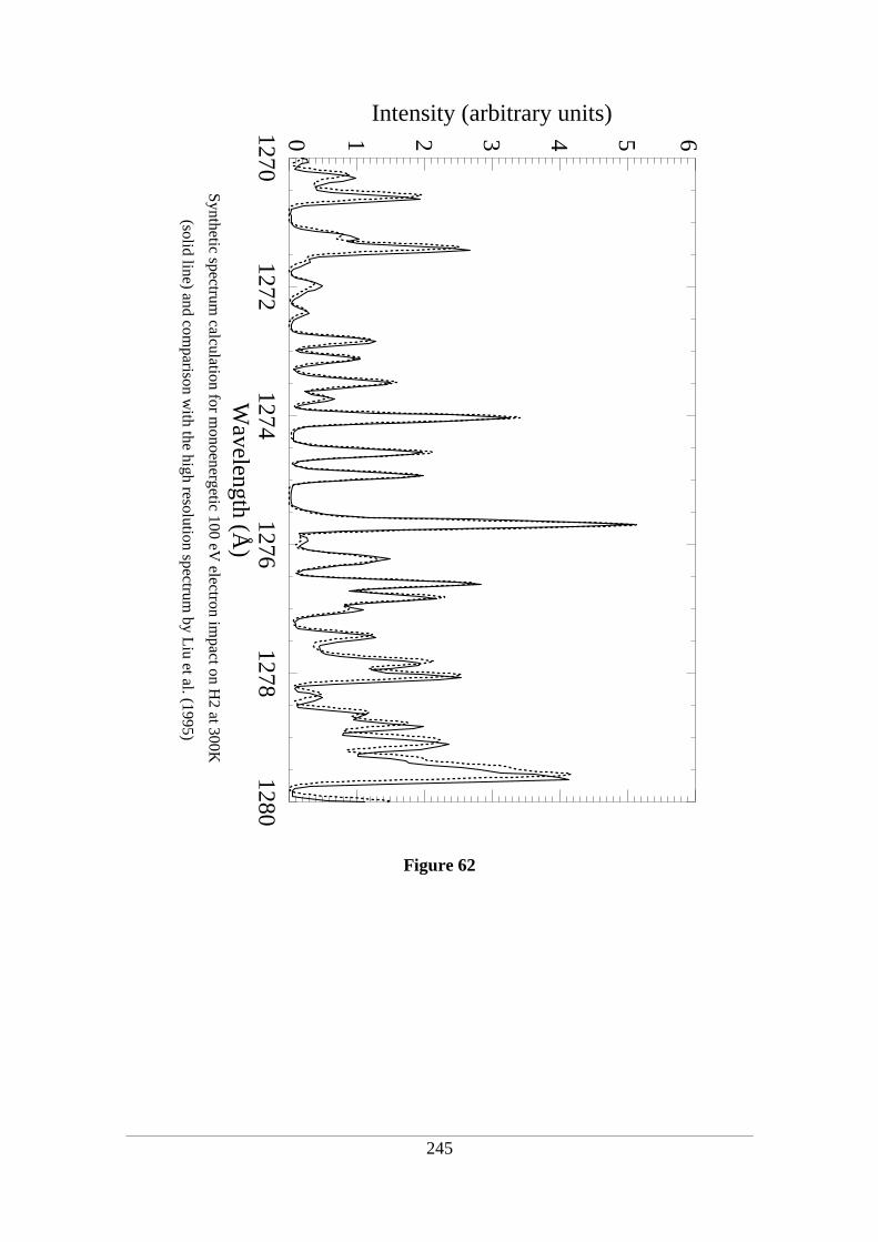
245
Figure 62
Synthetic spectrum calculation for m
onoenergetic 100 eV electron im
pact on H2 at 300K
(solid line) and comparison w
ith the high resolution spectrum by L
iu et al. (1995)
12701272
12741276
12781280
Wavelength (Å
)
0 1 2 3 4 5 6
Intensity (arbitrary units)

VIII.3.3 Model validation and sensitivity
Various tests were conducted to assess the validity of the coupled spectral-
energy degradation model and to assess the importance of difference factors on the
spectral characteristics. The approach adopted may be described as follows :
1. validation of the intensity distribution of the Lyman and Werner lines and continuum
by comparison with high-resolution laboratory spectra
2. study of the sensitivity of the vertically integrated H2 spectrum to the initial electron
energy distribution
3. evaluation of the observability of these effects on a mid-resolution (5 Å) spectrum of
the UV aurora such as those analyzed in the follow section.
As already mentionned, the third point is out of the scope of the present work and is
developed in Dols et al. (2000). Instead, additional cases are synthesized using the full
capabilities of the energy degradation model.
The synthetic spectrum from 1200 Å to 1700 Å was compared in details to the
high-resolution laboratory spectrum obtained at 300 K by Liu et al. (1995). An
excellent agreement is obtained for virtually all relative line intensities. A comparison
is shown in figure 62 for the 1270-1280 Å range as an example. The synthetic spectrum
has been smoothed at the resolution of the spectrometer (0.1 Å). The slight shift in
wavelength between the observed and calculated spectra is caused by a thermal
expansion of the spectrometer during the laboratory measurements. Since this spectral
region includes both Lyman and Werner bands, the match of the relative brightness of
lines belonging to both transitions also confirms the correct relative magnitude of the B
and C state cross sections. It may be concluded from this and comparisons at other
wavelengths and for different electron energies that the synthetic spectrum model
produces a quasi perfect fit to the best laboratory data available today.
The importance of the vertical distribution of the emission rate, temperature and
hydrocarbon absorption is best illustrated by simulating different H2 UV spectra
corresponding to different vertical emission profiles. The emergent spectrum obtained
246

by integrating the contribution from all layers is then compared to the thin slab
approximation. This comparison was performed for 3 initial electron energy
distributions :
• case 1 has a Maxwellian distribution with a characteristic energy E0 = 35 keV (mean
energy = 70 keV) and a 40 ergs cm-2 s-1 energy flux. The value of E0 is selected to
produce a peak near 240 km, in agreement with the Galileo SSI observations
• case 2 has the same primary electron component with the addition of a softer
Maxwellian electron contribution (0.35 keV) carrying a 4 ergs cm-2 s-1 energy flux
• case 3 is similar to case 2 but the soft component carries 40 ergs cm-2 s-1 flux, that
is the same amount as the harder component.
The total H2 volume emission rate is shown for all three cases in figure 63. It
may be seen that the soft component has a lower emission efficiency as the result of the
increased competition with other processes leading to neutral and electron heating.
Figure 64 compares two unconvolved 100 eV synthetic spectra obtained at T = 300 K
and T = 1000 K, respectively, in the 1310-1320 Å region dominated by the Lyman band
transitions. It clearly shows that all rovibrational lines are more or less affected by a
change of temperature.
247
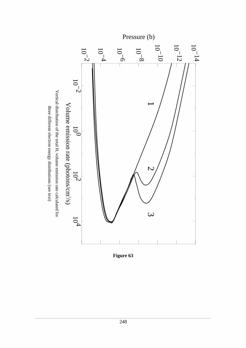
248
Figure 63
Vertical distribution of the total H
2 volume em
ission rate calculated for
three different electron energy distributions (see text)
10 −2
10 010 2
10 4
Volum
e emission rate (photons/cm
3/s)
10 −2
10 −4
10 −6
10 −8
10 −10
10 −12
10 −14
Pressure (b)
12
3

249
Figure 64 : Illustration of the temperature effect. Upper plot : unconvolvedspectrum at 300 K. Lower plot : difference between the spectrum at 1000 Kand the spectrum at 300 K.
0.0
0.2
0.4
0.6
0.8
1.0
spectrum at 300K Intensity (a.u.)
1310
1312
1314
1316
1318
1320
Wav
elen
gth
(Å)
−0.
4
−0.
2
0.0
0.2
0.4
spectrum at 1000K minus spectrum at 300K

A similar comparison is presented in figure 65 which shows two unconvolved
250
Figure 65 : Illustration of the E,F cascade effect. Upper plot : unconvolvedspectrum with cascade. Lower plot : difference between the spectrumincluding the E,F cascade and the spectrum without the E,F cascade.
0.0
0.2
0.4
0.6
0.8
1.0
with EF cascade Intensity (a.u.)
1310
1312
1314
1316
1318
1320
Wav
elen
gth
(Å)
−0.
4
−0.
2
0.0
0.2
0.4
with EF minus without EF

100 eV spectra at T=300 K with and without E,F cascade, respectively. It is seen that
most of the transitions, but not all, are sensitive to the amount of cascade increasing the
population of the B state.
The major difference between temperature and cascade effects stems from the
fact that the temperature can either increase or decrease the intensity of a line, while
cascades can only increase it. Since the two effects are on the same order of magnitude,
an interplay of compensation or addition of the two effects is expected to occur when
both cascade and temperature are modified. These combined effects are presented in
figure 66 and 67 which show a comparison between the three cases (1, 2 and 3) and the
monoenergetic (100 eV) – isothermal (300 K) case frequently adopted in previous
studies. Panels 1, 2 and 3 illustrate the effect of the vertical integration including the
variation of the local electron energy distribution, vertical temperature gradient and
vertical differential absorption below 1400 Å. Panel 1 corresponds to a spectral region
dominated by the Lyman band system. The 100-eV and the calculated spectra have
been normalized for the 3 cases on the 1316.7 Å line which is due to a blend of the L19-
11P(7), L16-10P(3) and L9-7P(4) transitions. In this spectroscopic notation, L
designates a Lyman transition (W for a Werner transition), the two next numbers are the
initial (v') and final (v'') vibrational numbers, P stands for a P branch (ΔJ=-1) and the
final number is the initial excited rotational quantum number (J'). The distributed
electron energy spectrum increases the cascade contribution from the E,F g+1 state as
shown by both laboratory and synthetic spectra for low electron energies close to the
excitation threshold. The temperature effect is due to the increased weight of the upper
emission layer at higher temperatures as the contribution of the soft electron increases.
Three kinds of effects are present in figure 66 :
1. a strong enhancement of a line intensity resulting from the addition of a brightness
increase due to the higher temperature and from a brightness increase due to the
increased E,F cascade. This effect is illustrated by the lines at 1314.6 Å (L1-4R(3))
and at 1315.4 Å (L1-4P(2))
2. persistence of a line intensity stemming from the compensation of the temperature
and cascade effects which are decreasing and increasing, respectively, the intensity of
the line. It is illustrated by a large number of lines, the brightest being at 1310.85 Å
251

(L1-4R(1)), 1312.8 Å (L1-4P(1)) and 1319 Å (L1-4P(3)).
3. a strong enhancement or the appearance of a line solely due to the temperature
increase. This applies, for example, to the lines at 1311.4 Å (L7-6P(5)), 1312.5 Å
(L5-5P(7)), 1317.1 Å (L7-6P(6)).
Figure 67 shows a similar comparison for the 1500-1510 Å region where all
lines also belong to the Lyman system. All three cases (1, 2 and 3) have been
normalized to the (10-13) P(2) transition at 1505.7 Å. Only the (1-7) P(5) line at
1504.76 Å is partly populated by cascade from the E,F g+1 state. Panel 1 shows that
this line is considerably brighter in the energetically and spatially integrated case 1 than
the 100 eV–300 K case. A temperature dependence is also observed at 1507.06 Å,
1507.65 Å and 1508.17-1508.31 Å. Further increases of the line intensity are observed
in cases 2 and 3. The latter shows that weak lines in case 1 are enhanced by the
presence of the high altitude secondary emission peak.
These examples are illustrative of the changes induced in the H2 spectrum by the
consideration of the vertical dimension of the aurora and the integration along the line of
sight of layers with changing temperature and electron energy distribution. Such effects,
however, are only unambiguously measured provided that the spectral resolution is high
enough to distinguish the line brightness redistribution. At low spectral resolution
(~5 Å), the convolution by the instrument line spread function will, to a large extent,
smooth and remove the signature of the emission altitude dependence and provides only
limited useful temperature information.
252

253
Figure 66
1
2
3
Inte
nsity
(ar
bitr
ary
units
)
1
1
2
3
Inte
nsity
(ar
bitr
ary
units
)
2
Synthetic spectrum calculated from three different electron energy distributions
(dashed line) and comparison with the spectrum for a 100−eV impact at 300 K (solid line)
1310 1312 1314 1316 1318 1320Wavelength (Å)
1
2
3
Inte
nsity
(ar
bitr
ary
units
)
3_ L
1−
4 R
(3)
_ L
1−
4 P(
2)
_ L
1−
4 R
(1)
_ L
1−
4 P(
3)
_ L
7−
6 P(
5)
_ L
5−
5 P(
7)
_ L
7−
6 P(
6)
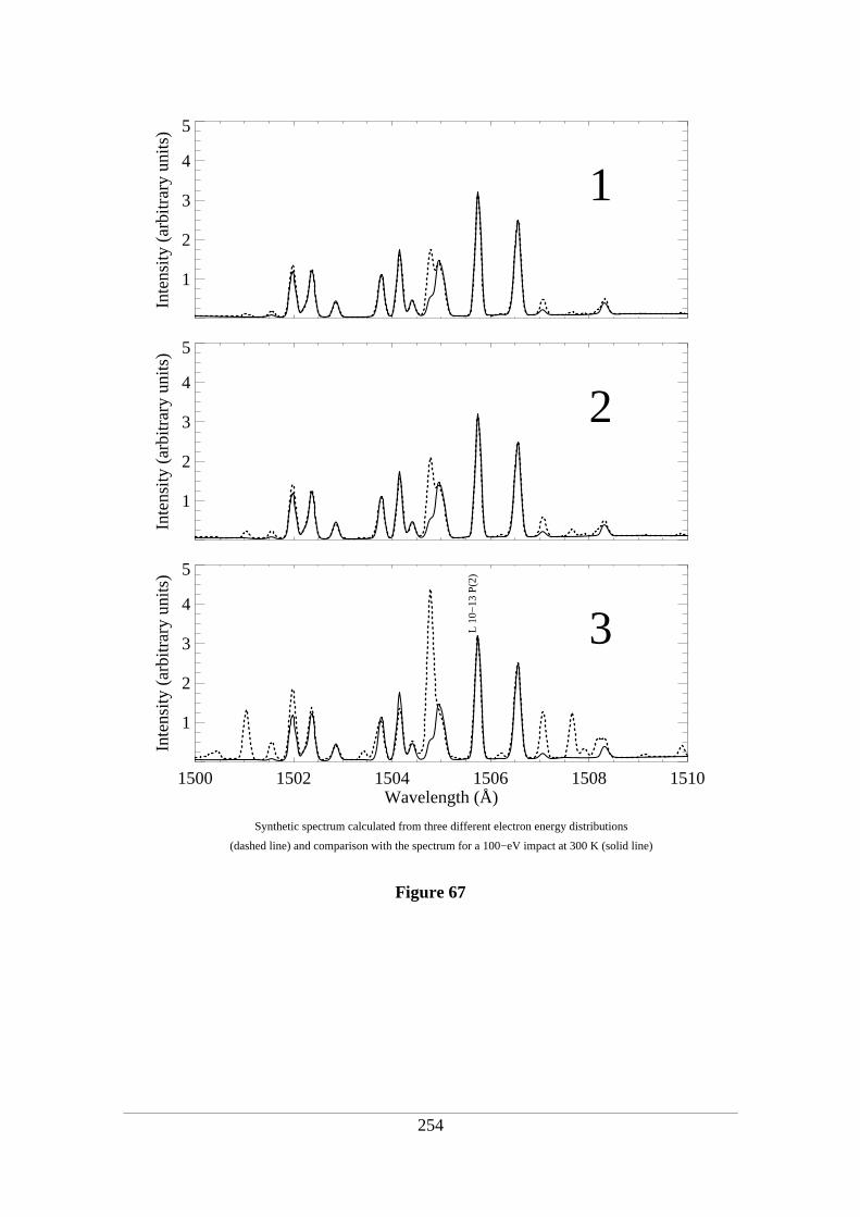
254
Figure 67
1
2
3
4
5
Inte
nsity
(ar
bitr
ary
units
)
1
1
2
3
4
5
Inte
nsity
(ar
bitr
ary
units
)
2
Synthetic spectrum calculated from three different electron energy distributions
(dashed line) and comparison with the spectrum for a 100−eV impact at 300 K (solid line)
1500 1502 1504 1506 1508 1510Wavelength (Å)
1
2
3
4
5
Inte
nsity
(ar
bitr
ary
units
)
3_ L
10−
13 P
(2)
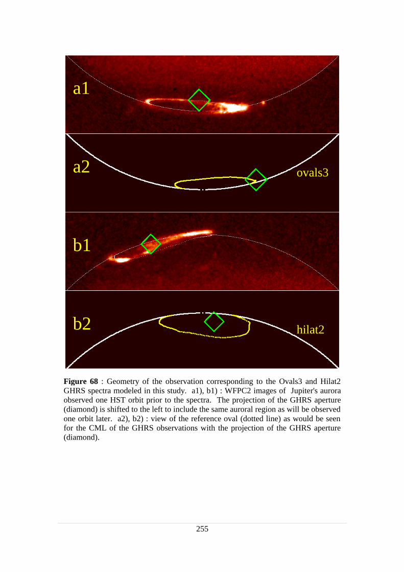
255
Figure 68 : Geometry of the observation corresponding to the Ovals3 and Hilat2GHRS spectra modeled in this study. a1), b1) : WFPC2 images of Jupiter's auroraobserved one HST orbit prior to the spectra. The projection of the GHRS aperture(diamond) is shifted to the left to include the same auroral region as will be observedone orbit later. a2), b2) : view of the reference oval (dotted line) as would be seenfor the CML of the GHRS observations with the projection of the GHRS aperture(diamond).
ovals3
hilat2
a1
a2
b1
b2
VIII.3.4 Echelle H2 spectroscopy
High resolution ultraviolet echelle spectra of H2 analyzed in conjunction with
our auroral model is an indicator of the conditions prevailing in the auroral regions. To
illustrate its application to the analysis of the echelle GHRS data (Dols et al., 2000),
figure 69 shows synthetic spectra in the 1216-1220 Å region for three temperatures at
the echelle resolution (0.07 Å). The electron energy distribution was calculated with the
degradation model at the altitude of the peak of case 1. As may be seen, some lines
show little brightness dependence on temperature. Others dramatically increase as a
result of the redistribution of the population among the rotational levels of the H2 v=0
ground state.
Among the ten echelle spectra described by Dols et al. (2000), only two (Ovals3
and Hilat2) show sufficiently bright H2 lines to allow a quantitative analysis. The
brightest lines belong to the (2,6) Werner band with some additional Lyman and Werner
lines. The approach used was to fit the H2 emissions with the parameters of the best fits
to the G140L spectra obtained 25 minutes later on the same HST orbit. This procedure
allows to verify whether the effective model temperature, resulting from the vertical
distribution emission and hydrocarbon absorption is in agreement with the relative line
strengths.
Figure 70 compares the resulting Ovals3 H2 spectrum (in which the Ly-α contribution
was removed) above 1216 Å with the model spectrum calculated from the energy fluxes
derived by the two-stream code with a single Maxwellian distribution set to E0 = 17 keV
(panel a). The match is good for several lines but the brightness of the W 1-5 P(5), 2-6
P(2), P(4) and Q(2) lines are clearly underestimated in the model spectrum. By contrast,
a good fit is obtained for T = 600 K (panel b), a value reached near 400 km in the
neutral model shown in figure 61 but substantially higher than the emission rate
weighted temperature associated with the E0 = 17 keV precipitation which resulted in a
mean H2 temperature of about 228 K. Similar conclusions apply to the Hilat2 spectrum,
since the brightness of the temperature-sensitive lines is underestimated and a better fit
is obtained using again an effective temperature T = 600 K.
256

257
Figure 69 : Synthetic spectra at three temperatures at the echelle resolution
(0.07 Å). The electron energy distribution was calculated with the degradation
model at the altitude of the peak of case 1.
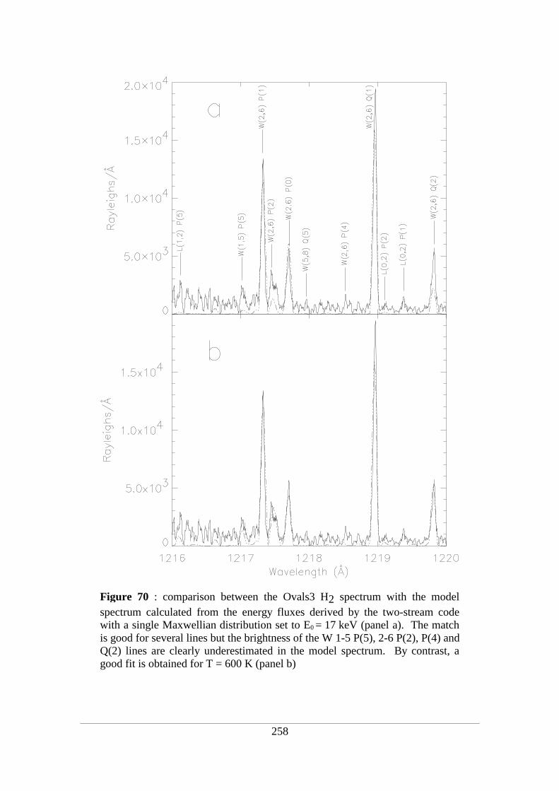
258
Figure 70 : comparison between the Ovals3 H2 spectrum with the modelspectrum calculated from the energy fluxes derived by the two-stream codewith a single Maxwellian distribution set to E0 = 17 keV (panel a). The matchis good for several lines but the brightness of the W 1-5 P(5), 2-6 P(2), P(4) andQ(2) lines are clearly underestimated in the model spectrum. By contrast, agood fit is obtained for T = 600 K (panel b)

VIII.4 Use of converged temperature profiles
The model of energy degradation coupled to heat conduction equation which we
described was partly developed to address discrepancies of the nature just depicted. It
provides, in a consistent way, the local electron flux energy distribution and the
temperature and density profiles which result from heating by these electrons.
In order to illustrate the effect of a complex temperature profile compatible with
the electron energy distribution on the synthetic spectra, four cases (hereafter referred to
cases B, B', B'', and H), two of which are taken from the two-stream section (cases B
and H), have been applied to the spectral generator. Cases B, B' and H share the same
energy flux distribution (double Maxwellian distribution). The difference arises in the
temperature profile : case B' uses a fixed NEB atmospheric structure (temperature,
densities) similar to that used in the previous section and is therefore not compatible
with the electron flux, cases B and H come with their own converged atmospheric
structures as described in the two-stream section. B'' is a single layer case acted on by a
monoenergetic electron beam of 100 eV. It assumes a fixed (incompatible) temperature
of 600 K.
As already mentioned, cases B and H bear the same energy distribution, but case
H has a warmer temperature profile in the stratospheric region (a different boundary
condition was applied to the thermal profile in the lower atmosphere). Figure 71 shows
the synthetic spectrum obtained with cases B', B, and H in the 1216-1220 Å region and
compares them with the observed Ovals3 spectrum. It can be seen that the synthetic
spectrum calculated with case B' is not in good agreement with the observed spectrum.
The obtained fit is characterized by a chi-squares value of 3.0 (arbitrary units). Using
the atmospheric structure compatible with the electron flux, as in case B, significantly
improves the fit which is then characterized by a chi-squares value of 2.8. The
compatibility of the thermal structure with the electron energy distribution does not by
itself explain the improvement of the fit. Instead, the key point is the temperature
increase (B has a warmer temperature profile than B').
259

This can be verified with the spectrum of case H which implies a warmer profile (in the
stratosphere) than case B and for which the fit is again improved. It is now
characterized by a chi-squares value of 2.7. It may already be concluded that
synthesizing a spectrum with a warm temperature profile, compatible with the energy
distribution of the electrons, substantially improves the fit to the observed spectrum.
The spectrum obtained with case B'' is an illustration of the former rovibrational
260
Figure 71
1
2
3
4
5
6
Inte
nsity
(ar
bitr
ary
units
)
B,
1
2
3
4
5
6
Inte
nsity
(ar
bitr
ary
units
)
B
Synthetic spectrum calculated from three different electron energy distributions
(solid line) and comparison with the ovals3 spectrum (dashed line)
1216 1217 1218 1219 1220Wavelength (Å)
1
2
3
4
5
6
Inte
nsity
(ar
bitr
ary
units
)
H
temperature fitting method which assumed a monoenergetic beam (100 eV) interacting
with the components of a single layer isothermal atmosphere. This method predicts a
best fit temperature of 600 K meant to represent the H2 temperature. On the other hand,
the mean H2 temperature wheighted by the unabsorbed H2 Lyman and Werner emission
for a zenith angle of 60° (we will see in a next section that methane absorption modifies
the H2 temperature) is 342 K for case H and 296 K for case B.
Comparison between the fits obtained with cases B'' and H shows that increasing
the stratospheric temperature is not the ultimate solution to get a synthetic spectrum
fitting the observed spectrum just as well as the monokinetic case at 600 K. It should be
pointed out that an H2 temperature in the auroral region of 296 K is more compatible
with the predictions of the energy degradation model. Indeed, it can be shown that an
H2 temperature on the order of 600 K could hardly be obtained by injecting a very large
flux of energetic auroral electrons. However such an electron precipitation would be
inevitably characterized by very strong H2 UV and IR emissions that are not observed.
In summary, a source of inconsistency between the temperatures derived by the
former and the present methods is that the H2 temperature is usually represented by a
single value. In the next section we show that the H2 temperature depends on the
wavelength and on the geometry of the observation. In fact, the geometry effect is
expected to be as important as it was for the color ratio (see part 1). An example
applied to case B shows that the maximum difference between the H2 temperature
calculated from the thermal profile and the temperature obtained by accounting for the
viewing geometry and wavelength can be greater than 300 K
261

"Le tout est plus que la somme de ses parties". Aristote
IX Coupling of the three models
IX.1 Introduction
For the first time in this work, we invoke the coupling between the three models
presented before :
the energy degradation model,
the spectral generator,
the morphology simulation model.
Preliminary remarks concerning this coupling first need to be formulated. The
examples given in this section which estimate the effect of wavelength and observation
geometry on the H2 temperature, obviously represent one of the many possible
applications of the coupling. A systematic description of all possible applications
represents a natural continuation of this work but is actually out of the scope since we
mainly concentrated on the developement of the separate models. Also, the following
examples consist in a preliminary application for which a reduced version of the spectral
generator and a modified morphology simulation model were used. The reduced
version of the spectral generator, which is already used in the energy degradation model
to estimate the H2 color ratio and emission profiles, does not account for the rotational
levels but calculates the vibration transitions only. The modified morphology model
required more extensive adaptations which are described below.
262
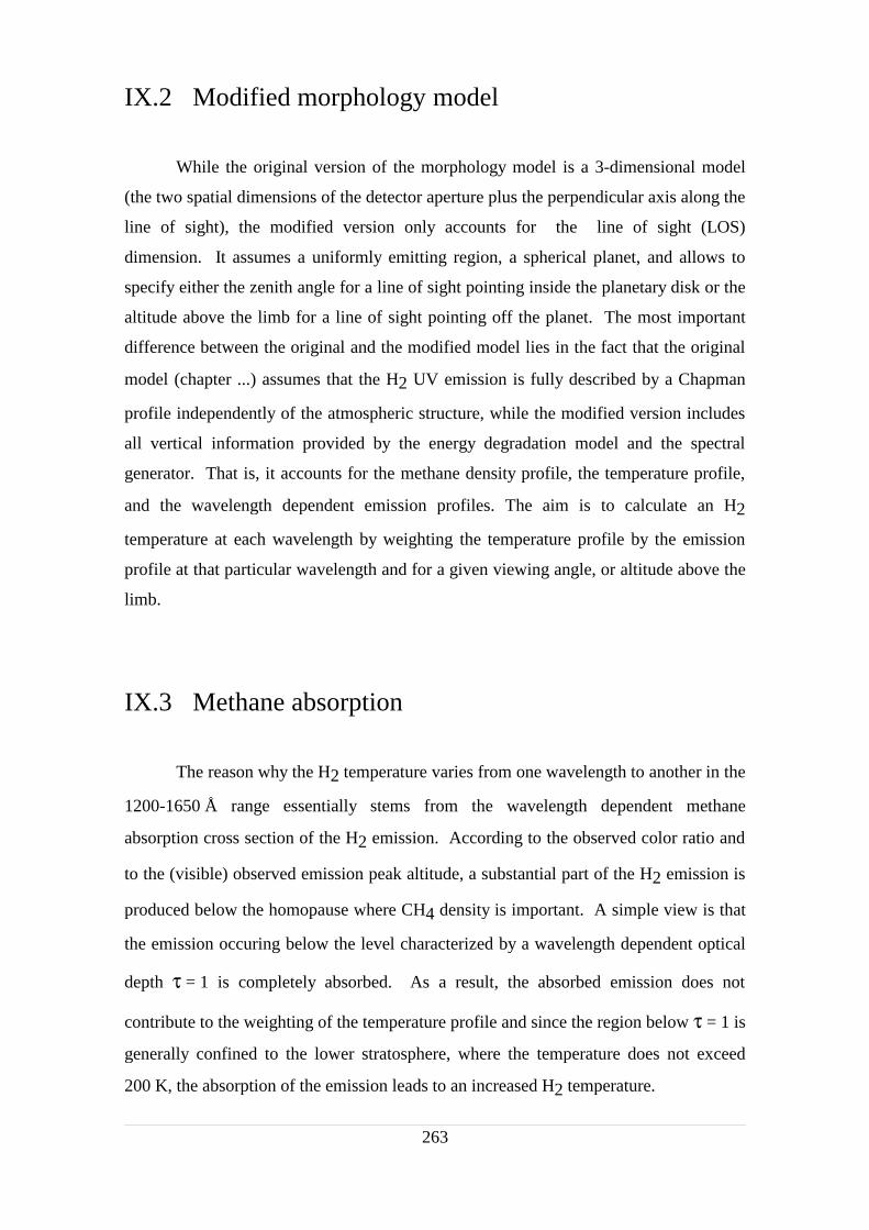
IX.2 Modified morphology model
While the original version of the morphology model is a 3-dimensional model
(the two spatial dimensions of the detector aperture plus the perpendicular axis along the
line of sight), the modified version only accounts for the line of sight (LOS)
dimension. It assumes a uniformly emitting region, a spherical planet, and allows to
specify either the zenith angle for a line of sight pointing inside the planetary disk or the
altitude above the limb for a line of sight pointing off the planet. The most important
difference between the original and the modified model lies in the fact that the original
model (chapter ...) assumes that the H2 UV emission is fully described by a Chapman
profile independently of the atmospheric structure, while the modified version includes
all vertical information provided by the energy degradation model and the spectral
generator. That is, it accounts for the methane density profile, the temperature profile,
and the wavelength dependent emission profiles. The aim is to calculate an H2
temperature at each wavelength by weighting the temperature profile by the emission
profile at that particular wavelength and for a given viewing angle, or altitude above the
limb.
IX.3 Methane absorption
The reason why the H2 temperature varies from one wavelength to another in the
1200-1650 Å range essentially stems from the wavelength dependent methane
absorption cross section of the H2 emission. According to the observed color ratio and
to the (visible) observed emission peak altitude, a substantial part of the H2 emission is
produced below the homopause where CH4 density is important. A simple view is that
the emission occuring below the level characterized by a wavelength dependent optical
depth τ = 1 is completely absorbed. As a result, the absorbed emission does not
contribute to the weighting of the temperature profile and since the region below τ = 1 is
generally confined to the lower stratosphere, where the temperature does not exceed
200 K, the absorption of the emission leads to an increased H2 temperature.
263

A similar behavior is expected for the C2H2 absorption, however, due to its lower
absorption it has not been accounted for.
IX.4 Viewing geometry effect
The viewing geometry modifies the H2 temperature whether or not hydrocarbon
absorption occurs. Its effect depends, in a complex way, on the relative shapes of the
thermal and emission profiles.
IX.4.1 Application to case B
We have applied the coupled model to case B for various viewing angles at the
central meridian longitude (CML) ranging from 0° (LOS along the local normal, or
vertical path) to 90° (LOS perpendicular to the local normal) inside the planetary disk,
and for different altitudes above the limb, ranging from 50 km to 1000 km.
IX.4.2 Line of sight pointing inside the planetary disk
Since a local temperature T(s) and a local emission line intensity I(s,λ) are
intercepted at each step s along a given LOS, the H2 temperature associated to this LOS
my be calculated by averaging T(s) with I(s,λ) weighs, i.e.
TH2
T s I s,ds
I s,ds
where ds is the distance step along the LOS.
In this preliminary study we assume that the emission is horizontally uniform over the
planet (i.e. unstructured emission only).
264
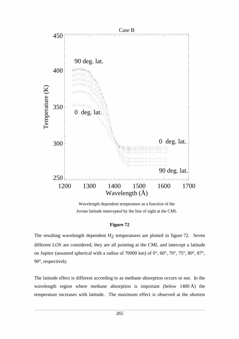
The resulting wavelength dependent H2 temperatures are plotted in figure 72. Seven
different LOS are considered, they are all pointing at the CML and intercept a latitude
on Jupiter (assumed spherical with a radius of 70000 km) of 0°, 60°, 70°, 75°, 80°, 87°,
90°, respectively.
The latitude effect is different according to as methane absorption occurs or not. In the
wavelength region where methane absorption is important (below 1400 Å) the
temperature increases with latitude. The maximum effect is observed at the shortest
265
Figure 72
Case B
Wavelength dependent temperature as a function of the
Jovian latitude intercepted by the line of sight at the CML
1200 1300 1400 1500 1600 1700Wavelength (Å)
250
300
350
400
450
Tem
pera
ture
(K
)
90 deg. lat.
90 deg. lat.
0 deg. lat.
0 deg. lat.

wavelength (~ 1200 Å) for which the temperature increases from 350 K at 0° to 400 K
at 90° latitude. The effect decreases as the wavelength increases (as CH4 absorption
becomes smaller) and finally vanishes around 1400 Å. Beyond this wavelength,
methane absorption is negligible and the effect is reversed since temperature decreases
as latitude increases (this effect is explained in the appendix).
Since methane absorption is very small in this region a plateau is rapidly reached and
the wavelength dependence disappears. The latitude effect is weak as the temperature
266
Figure 73
Case B
Wavelength dependent temperature averaged over the field of view
of a GHRS like aperture pointing below the limb
1200 1300 1400 1500 1600 1700Wavelength (Å)
250
300
350
400
Tem
pera
ture
(K
)

only decreases from 295 K at 0° latitude to 275 K at 90° latitude. It should be reminded
that C2H2 absorption is not considered here and similar, but smaller, effects to those
observed for CH4 absorption are expected.
The GHRS aperture subtends an angle of 1.74 x 1.74 arcsec2 on the sky. The Jovian
latitude range intercepted by this aperture obviously depends on the geometry of the
observation. If one imagines that the top edge of the aperture is located at the limb, the
bottom edge is located at a latitude of about 60°. An average temperature weighted by
the total emission line intensities I LOS, integrated along the LOS, as a function of
the wavelength, may be obtained from
TH2
LOS
TH2LOS, I LOS,dz
LOS
I LOS,dz
where dz is the distance between two contiguous LOS. It is expected to follow the
curve plotted in figure 73 and is essentially similar to the 75° curve plotted in figure 72.
The latitudes used to calculate the average temperature where chosen so that the
267
Figure 74
Latitude
Lines of sight Observer
GHRS field of view
Jovian planetary disk
CM
L
60° latitude
Limb
Side view
Jupiter
Front view
CH4 layer
Schematic representation of the field of view of GHRS projected on Jupiter. The side view shows equidistant lines of sight and their relation with the Jovian latitude. The front view shows the portion of the Jovian disk intercepted by a GHRS like aperture positioned as described in the text.

corresponding LOS are equally spaced in the aperture (dz constant).
Even at short wavelengths the average temperature remains below 400 K, that is less
than deduced from the Echelle spectra (Ovals3, Hilat2). A further increase of the H2
temperature arises by considering the fact that for these spectra, as seen on figure 57
(panels a2 and b2), the aperture is centered very close to the limb and therefore a
substantial portion of the emission may originate from above the limb and from regions
located at high latitudes. It is shown below that emissions observed above the limb give
rise to higher temperatures. Since the limb brightening increases the weight of this
emission over the emission coming from the planetary disk, it is expected that the
emission from above the limb plays a dominant role in the observed H2 temperature as
discussed below.
268

269
Figure 75
Case B
Wavelength dependent temperature as a function of the altitude
above the limb intercepted by the line of sight
1200 1300 1400 1500 1600 1700Wavelength (Å)
200
400
600
800
1000T
empe
ratu
re (
K)
1000 km
600 km
400 km
350 km
300 km
250 km
50 km

IX.4.3 Line of sight pointing above the limb
The direction of a line of sight pointing off the planet may be specified by its
altitude above the limb (figure 76). Ten different altitudes are considered : 50 km, 100,
150, 200, 250, 300, 350, 400, 600 and 1000 km. Above an altitude of 1000 km the H2
UV emission rapidly vanishes and can therefore be neglected. The wavelength
dependent H2 temperatures associated with the 10 altitudes are plotted on figure 78. It
is readilly seen that two different regimes apply according to as methane absorption
occurs or not. The temperature curves associated to lines of sight passing above the
homopause (~300 km) are flat (no absorption and no wavelength effect) since the CH4
density is negligible compared to that of H2. On the other hand, the temperature curves
corresponding to LOS below the homopause behave like those obtained with a LOS
pointing inside the planetary disk.
Below the homopause, the maximum wavelength-effect is on the order of 250 K (at
50 km) while the maximum altitude-effect does not exceed 30 K (at 1600Å). Above the
270
Figure 76
Line of sight
Side view
CH4 layer
Jupiter
HomopauseLimb
Emiss
ion
prof
ile
Altitudeabovethe limb
Side view of Jupiter showing the relation between a line of sight and its altitude above the limb. The CH4 layer is represented as a grey shell covering all the planet. The emission profiles intercepted by the line of sight are represented by straight lines. The emission is assumed to be uniform over the planet.
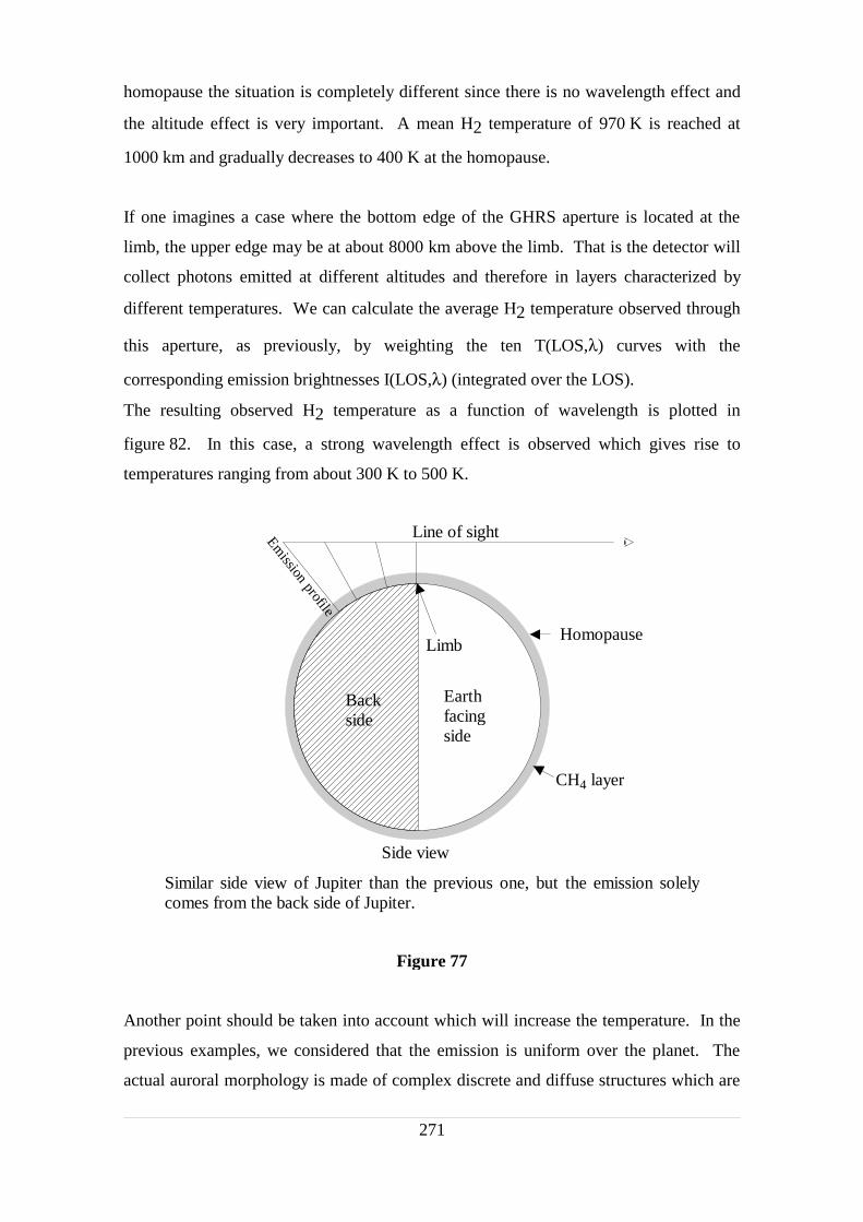
homopause the situation is completely different since there is no wavelength effect and
the altitude effect is very important. A mean H2 temperature of 970 K is reached at
1000 km and gradually decreases to 400 K at the homopause.
If one imagines a case where the bottom edge of the GHRS aperture is located at the
limb, the upper edge may be at about 8000 km above the limb. That is the detector will
collect photons emitted at different altitudes and therefore in layers characterized by
different temperatures. We can calculate the average H2 temperature observed through
this aperture, as previously, by weighting the ten T(LOS,λ) curves with the
corresponding emission brightnesses I(LOS,λ) (integrated over the LOS).
The resulting observed H2 temperature as a function of wavelength is plotted in
figure 82. In this case, a strong wavelength effect is observed which gives rise to
temperatures ranging from about 300 K to 500 K.
Another point should be taken into account which will increase the temperature. In the
previous examples, we considered that the emission is uniform over the planet. The
actual auroral morphology is made of complex discrete and diffuse structures which are
271
Figure 77
Line of sight
Side view
CH4 layer
HomopauseLimb
Emission profile
Earthfacingside
Backside
Similar side view of Jupiter than the previous one, but the emission solely comes from the back side of Jupiter.

not always present on the Earth facing portion of the Jovian disk. In the following
example we consider that the emission is originating from the back side of Jupiter so
that it only appears above the limb (figure 77). The wavelength dependent temperature
as a function of altitude is plotted in figure 68.
Below the homopause the wavelength effect is only partly observed. This can be
explained by the complete methane absorption of the emission, especially below 250 km
where the temperature does not exceed 250 K. At 200 km a partial wavelength effect
changes the temperature from ~150 K to ~250 K. The complete absorption also implies
that the emission appearing below the homopause is mostly produced in the Earth facing
region of Jupiter. As a consequence, the presence of a gap in the H2 UV images
between the limb and the homopause is a sign that the observed photons mainly come
272
Figure 78
Case B
Wavelength dependent temperature averaged over the field of view
of a GHRS like aperture pointing above the limb
1200 1300 1400 1500 1600 1700Wavelength (Å)
200
300
400
500
600
Tem
pera
ture
(K
)
from the back side of Jupiter.
As was already the case for a uniformly emitting planet, no wavelength-effect is
observed above the homopause. A wavelength independent temperature is reached
which varies from ~400 K at the homopause (~300 km) to ~970 K at 1000 km. The
mean H2 temperature characterizing the emitting region observed through a GHRS like
aperture with the bottom edge located at the limb (and the top edge at approximately
10000 km above the limb) would lead to a wavelength dependent curve plotted in
figure 80. As can be seen a warmer temperature on the order of 600 K is reached in the
absorbed region of the spectrum (like Ovals3 and Hilat2). The wavelength effect is on
the order of 200 K as the temperature in the unabsorbed region decreases to ~300 K.
In conclusion, this example clearly shows that a thermal structure similar to that
of case B, that we characterized by a rather low H2 temperature of 296 K by weighting
the temperature profile with the unabsorbed emission seen at 60°, may in some
cicumstances be compatible with the higher H2 temperature of 600 K derived by fitting
observed high resolution spectra with synthetic spectra. The compatibility rests on the
consideration of the wavelength dependence of the measured temperature and on the
effect of the viewing geometry.
273
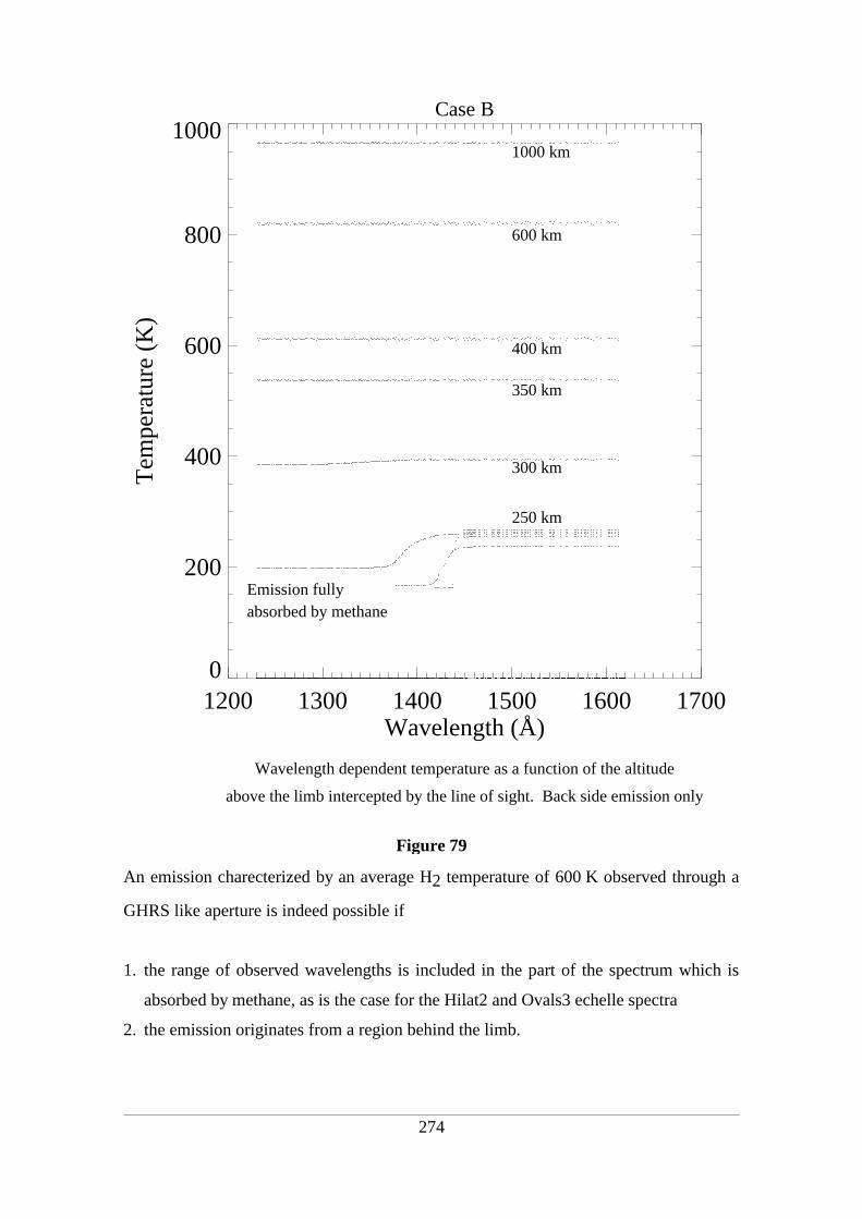
An emission charecterized by an average H2 temperature of 600 K observed through a
GHRS like aperture is indeed possible if
1. the range of observed wavelengths is included in the part of the spectrum which is
absorbed by methane, as is the case for the Hilat2 and Ovals3 echelle spectra
2. the emission originates from a region behind the limb.
274
Figure 79
Case B
Wavelength dependent temperature as a function of the altitude
above the limb intercepted by the line of sight. Back side emission only
1200 1300 1400 1500 1600 1700Wavelength (Å)
0
200
400
600
800
1000T
empe
ratu
re (
K)
1000 km
600 km
400 km
350 km
300 km
250 km
Emission fullyabsorbed by methane
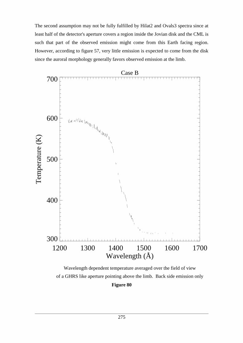
The second assumption may not be fully fulfilled by Hilat2 and Ovals3 spectra since at
least half of the detector's aperture covers a region inside the Jovian disk and the CML is
such that part of the observed emission might come from this Earth facing region.
However, according to figure 57, very little emission is expected to come from the disk
since the auroral morphology generally favors observed emission at the limb.
275
Figure 80
Case B
Wavelength dependent temperature averaged over the field of view
of a GHRS like aperture pointing above the limb. Back side emission only
1200 1300 1400 1500 1600 1700Wavelength (Å)
300
400
500
600
700
Tem
pera
ture
(K
)
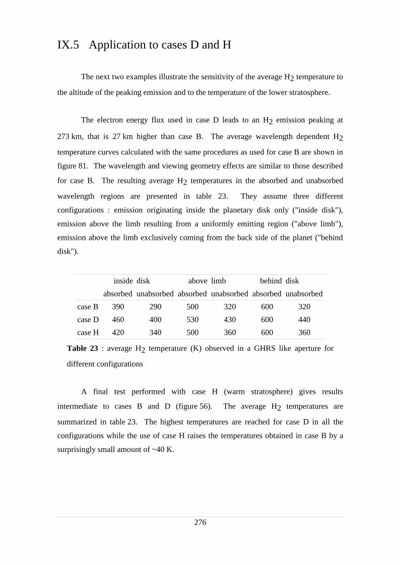
IX.5 Application to cases D and H
The next two examples illustrate the sensitivity of the average H2 temperature to
the altitude of the peaking emission and to the temperature of the lower stratosphere.
The electron energy flux used in case D leads to an H2 emission peaking at
273 km, that is 27 km higher than case B. The average wavelength dependent H2
temperature curves calculated with the same procedures as used for case B are shown in
figure 81. The wavelength and viewing geometry effects are similar to those described
for case B. The resulting average H2 temperatures in the absorbed and unabsorbed
wavelength regions are presented in table 23. They assume three different
configurations : emission originating inside the planetary disk only ("inside disk"),
emission above the limb resulting from a uniformly emitting region ("above limb"),
emission above the limb exclusively coming from the back side of the planet ("behind
disk").
inside disk above limb behind disk
absorbed unabsorbed absorbed unabsorbed absorbed unabsorbed
case B 390 290 500 320 600 320
case D 460 400 530 430 600 440
case H 420 340 500 360 600 360
Table 23 : average H2 temperature (K) observed in a GHRS like aperture for
different configurations
A final test performed with case H (warm stratosphere) gives results
intermediate to cases B and D (figure 56). The average H2 temperatures are
summarized in table 23. The highest temperatures are reached for case D in all the
configurations while the use of case H raises the temperatures obtained in case B by a
surprisingly small amount of ~40 K.
276
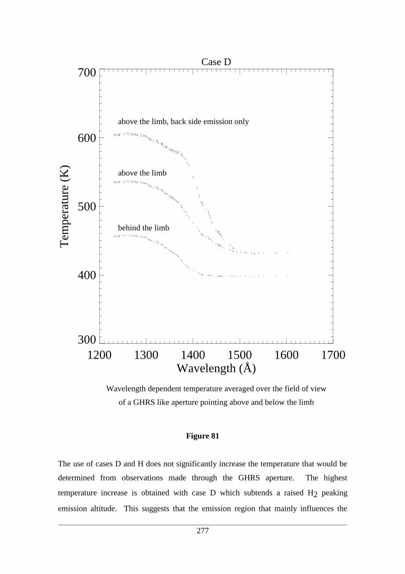
The use of cases D and H does not significantly increase the temperature that would be
determined from observations made through the GHRS aperture. The highest
temperature increase is obtained with case D which subtends a raised H2 peaking
emission altitude. This suggests that the emission region that mainly influences the
277
Figure 81
Case D
Wavelength dependent temperature averaged over the field of view
of a GHRS like aperture pointing above and below the limb
1200 1300 1400 1500 1600 1700Wavelength (Å)
300
400
500
600
700T
empe
ratu
re (
K)
behind the limb
above the limb
above the limb, back side emission only

average H2 temperature is located above the homopause. The temperature of this region
is mainly controlled by the soft electron component of the auroral energy flux.
In a near future this method will be applied to observations obtained by Kim et
278
Figure 82
Case H
Wavelength dependent temperature averaged over the field of view
of a GHRS like aperture pointing above and below the limb
1200 1300 1400 1500 1600 1700Wavelength (Å)
300
400
500
600
700
Tem
pera
ture
(K
)
behind the limb
above the limb
above the limb, back side emission only
al. (1997) with GHRS in 1995. These observations perfectly suit our purpose since they
were made in pairs in the two wavelength ranges 1257-1293 Å and 1587-1621 Å.
Spectra in the short wavelength range are mostly due to emisson in the H2 Lyman and
Werner band systems. Their intensities are attenuated by hydrocarbon absorption
(especially methane). The spectra in the long wavelength range are dominated by
unabsorbed emissions of the H2 Lyman band system. The temperature derived from the
latter wavelength region are in the range 400-850 K. Although the authors state a
possible tendency toward lower temperatures for higher methane column densities they
did not derived temperature from the absorbed spectra. It would be useful to determine
the effective temperature from these spectra and see if, as expected from our global
model, a systematic difference of the effective temperature is indeed observed between
the two spectral windows.
279

IX.6 Perspectives : spectroscopic probing of the thermal
profile
The examples that we have described illustrate one of the many aspects of the
full coupling of the three models that we developed. Following the above
considerations, it is possible to elaborate a simple observational strategy based on the
wavelength and viewing geometry effects. It would allow us to estimate the
atmospheric temperature characterizing different altitude regions. This "spectroscopic
probing" of the thermal structure would provide very helpful information to better
constrain the thermal profile determined with the energy degradation model.
IX.6.1 Simple example
In order to illustrate this application, a simple idealized example is now
described which allows to estimate the average atmospheric temperature in a region
confined between approximatively 200 km and 300 km. This region is of major interest
since it corresponds to the region of maximum auroral energy deposition. The
temperature reached in this region is therefore a good indicator for the total precipitating
flux. It also gives important information on the portion of electrons having enough
energy to reach these altitudes and therfore constrains the energy distribution of the
precipitating electrons.
If one assumes that
1. the auroral emission region is well represented by a uniformly emitting region limited
by a realistic auroral oval in corotation with the planet,
2. a GHRS like aperture is used to obtain high resolution spectra with sufficient signal
to noise ratio to allow a reliable fit of the spectra,
3. the observed UV and IR emissions are compatible with the electron energy flux
distribution of case B,
then :
if the observation is performed while the CML is close to 0° the auroral oval will be
280
backed out by the planetary disk. This configuration gives rise to an emission that can
only be observed above the limb. This case has been described previously and was
shown to lead to an average H2 temperature ranging from 300 K in the unabsorbed
region of the spectrum to 600 K in the absorbed region. Ovals3 and Hilat2 indeed give
a temperature of 600 K in the absorbed spectral region however no observed spectra are
available in the unabsorbed region to confirm that a temperature of 300 K is actually
measured. As already discussed, this large temperature difference stems from the
complete absorption by methane of the emission below the homopause.
It can be shown from the emission profile derived by the energy degradation model that,
for case B, about 4/5 of the integrated unabsorbed emission originates from below the
homopause. The temperature derived from the absorbed emission represents the
average temperature above the homopause, while the temperature derived from the
unabsorbed emission represents the average temperature above the homopause plus the
average temperature below the homopause. It can therefore be written that
45
x15
yz
where x = the average temperature below the homopause
y = the absorbed emission temperature, that is 600 K
z = the unabsorbed emission temperature, that is 300 K
and the average temperature below the homopause (x) is 225 K. More precisely, within
the assumptions made for case B and the emitting morphology, the region represented
by this average temperature is located between 200 km and 300 km (the homopause)
since the unabsorbed emission profile vanishes below 200 km.
IX.6.2 Further improvement
Further improvement could be brought by accounting for the complex
morphology of the observed auroral zones. It has been shown in part 1 that the
morphology of the bright auroral emissions is made of recurrent arcs of oval rather than
from uniform zones only. The morphology model would allow to estimate the
configuration of these complex auroral structures during the time of the exposure.
Similar effects to those due to methane absorption are expected to arise for acetylene
281
absorption. They have been neglected because of the lower absorption by C2H2. The
acetylene absorption cross section, however, shows strong peaking values around
1500 Å. Since this region is mostly unaffected by methane absorption, we could take
advantage of these peaks to probe the temperature of the lower stratosphere in a manner
similar to that previously described (the C2H2 homopause is approximately 50 km
deeper than the CH4 homopause). That is, it is possible to isolate absorbed and
unabsorbed spectral regions showing sufficiently different temperatures at the limb
(because of the complete absorption of the emission below the C2H2 homopause) so
that an estimation of the temperature of the fully absorbed emission is feasible.
Future versions of the spectral generator should include the FUV emission due to
the Rydberg states ( B' u+1 , B'' u
+1 , D u1 and D' u
1 ) and should account for self
absorption. The Rydberg emission arises below 1200 Å , that is in an optically thick
spectral region which deserves a radiative transfer treatment. We could then take
advantage of this optically thick emission because it is expected to emerge from the
atmosphere at a relatively high altitude (~1000 km). This emission would therefore bear
the thermal signature of this high atmospheric region and would constraint the upper
part of the thermal profile independently from the IR emissions.
282

IX.7 Conclusion
A detailed altitude and energy model of the UV emission resulting from the
interaction of an incident electron distribution with the Jovian atmosphere has been
constructed. It combines the two-stream electron energy degradation model with a
detailed synthetic spectral model of the main three singlet states of H2 using up-to-date
cross sections and molecular constants. In contrast to most earlier studies, the vertical
dependence of the auroral emission, H2 temperature and chemical composition are
explicitely considered. Test cases illustrate that the conjunction of the altitude variation
of the electron energy spectrum and the atmospheric structure combine to modify the
resulting H2 spectrum integrated along the line of sight. High resolution synthetic
spectra fitted to two GHRS echelle spectra of the auroral suggest an H2 temperature of
600 K. This temperature is in disagreement with the energy degradation model which
gives an average temperature (weighted by the emission profile) of 200 K. It is shown
that the use of converged (self-consistent) thermal profiles do not remove the
discrepancy.
The global coupling of the three models : energy degradation, spectral generator, and
morphology is used, as an exploratory application, to estimate the average temperature
deduced from the spectrum obtained through a GHRS like aperture. It is shown that the
deduced temperature depends both on the wavelength range and on the viewing
geometry of the observation. We show how these effects combine to increase an H2
temperaure of 200 K, deduced from the energy degradation model, to an effective H2
temperature of 600 K (for a particular viewing geometry) that would be deduced by
fitting the resulting observed spectrum.
We finally discuss a possible application of the global coupling of the three models that
would allow a spectroscopic probing of the jovian thermal vertical profile.
283
References
Abgrall, H., E. Roueff, F. Launay, J.Y. Roncin, and J.L. Subtil, Table of the Lymanband system of molecular hydrogen. Astron. Astrophys. Suppl., 101, 273-321,1993a
Abgrall, H., E. Roueff, F. Launay, J.Y. Roncin, and J.L. Subtil, Table of the Wernerband system of molecular hydrogen. Astron. Astrophys. Suppl., 101, 323-362,1993b
Abgrall, H., E. Roueff, X. Liu, and D.E. Shemansky, The emission continuum ofelectron excited molecular hydrogen. Astrophys. J., 481, 557-566, 1997
Ajello, J.M., D.E Shemansky and G.K. James, Cross sections for production of H(2p,2s, 1s) by electron collisional dissociation of H2, Astrophys. J., 371, 422-431,
1991
Ajello, J.M., D. Shemansky, T.L. Kwok and Y.L. Yung, Studies of extreme-ultravioletemission from Rydberg series of H2 by electron impact, Phys. Rev. A, 29, 636-
653, 1984
Ajello, J.M., I. Kanik, S.M. Ahmed, Line profile of H Lyman α from dissociativeexcitation of H2 with application to Jupiter, J. Geophys. Res., 100, 26,411-26,420,
1995
Ajello, J.M., S.M. Ahmed and X. Liu, Line profile of H Lyman β from dissociativeexcitation of H2, Phys. Rev., 53, 2302-2308, 1996
Ajello, J.M. and D.E. Shemansky, Electron excitation of the H2( a3g+ b3u
+ )
continuum in the vacuum ultraviolet, Astrophys. J., 407, 820-825, 1993
Allison , A.C. and A. Dalgarno, Band oscillator strengths and transitions probabilitiesfor the Lyman and Werner systems of H2, HD, and D2, at. data ,1, 289-304, 1970
Atreya, S.K., Atmospheres and ionospheres of the outer planets and their satellites, inPhysics and chemistry in space 15, Edited by L.J. Lanzerotti, M. Hill and D.Stöffler, Springer-Verlag Berlin Heidelberg, 1986
Auerbach, D., R. Cacak, R. Candano, T.D. Gaily, C.J. Keyser, J.W. McGowan, J.B.A.Mitchell, S.F.J. Wilk, Merged electron-ion beam experiments. I. Methods and
measurements of (e-H2+) and (e-H3
+) dissociative recombination cross sections,
J. Phys. B, 10, 3797-3820, 1977
284

Bagenal F., Giant Planet Magnetospheres, Annu. Rev. Earth Planet. Sci., 20, 289-328,1992
Ballester, G. E. and 21 colleagues, Time-Resolved Observations of Jupiter's Far-Ultraviolet Aurora, Science, 274, 409-412, 1996.
Bandyopadhyay, A., K. Roy, P. Mandal and N.C. Sil, Single-differential total ionizationcross sections of hydrogen atom by electron impact, Phys. Rev. A, 51, 2151-2155,1995
Banks, P.M., and A.F. Nagy, Concerning the influence of elastic scattering uponphotoelectron transport and escape, J. Geophys. Res., 75, 1902-1910, 1970
Banks, P.M. and G. Kockarts, Aeronomy, Part B, Academic Press, New York andLondon, 1973
Bhattacharya, B., R.M. Thorne, S.J. Bolton, D.J. Williams, D. Gurnett, RecirculatingMagnetospheric Electrons as a Source for the Jovian Aurora, Eos Trans. AGUFall Suppl., 79, P31D-06, F549, 1998
Broadfoot, A. L., B. R. Sandel, D. E. Shemansky, J. C. McConnell, G. R. Smith, J. B.Holberg, S. K. Atreya, T. M. Donahue, D. F. Strobel, and J. L. Bertaux, Overviewof the Voyager ultraviolet spectrometry results through Jupiter encounter, J.Geophys. Res., 86 8259-8284, 1981
Broadfoot, A. L., M. J. S. Belton, and P. Z. Takacs, Extreme ultraviolet from Voyager 1encounter with Jupiter, Science, 204, 979-982, 1979
Buckman, J.B., M.J. Brunger, D.S. Newman, G. Snitchler, S. Alston, D.W. Norcross,M.A. Morrison, B.C. Saha, G. Dandy, and W.K. Trail, Phys. Rev. Lett., 65, 3253-3256, 1990
Burrows, C. J., and 10 colleagues 1995. Wide Field and Planetary Camera 2 InstrumentHandbook, pp. 56-61. STScI publication.
Caldwell, J. A., B. Turgeon, and X. M. Hua, Hubble Space Telescope imaging of thenorth polar aurora on Jupiter, Science, 257, 1512-1515, 1992
Callaway, J., K. Unnikrishnan, Electron impact excitation of the n=3 and n=2 states ofhydrogen atom at intermediate (14-100 eV) energies, Phys. Rev. A, 48, 4292-4298,1993
Clarke, J. T., and 20 colleagues, Hubble Space Telescope Far-Ultraviolet Imaging ofJupiter During the Impacts of Comet Shoemaker-Levy 9, Science, 267, 1302-1306, 1995
Clarke, J. T., and 20 colleagues, Far-Ultraviolet Imaging of Jupiter's Aurora and the Io"Footprint", Science, 274, 404-409, 1996
285
Clarke, J.T., G. Ballester, J. Trauger, J Ajello, W. Pryor, K. Tobiska, J.EP. Connerney,G.R. Gladstone, J.H. Waite, Jr., L. Ben Jaffel, J.-C. Gérard, Hubble SpaceTelescope imaging of Jupiter's UV aurora during the Galileo orbiter mission, J.Geophys. Res., 103, 20,217-20,236, 1998
Clarke, J. T., H. W. Moos, S. K, Atreya, and A. L. Lane. Observations from earth andvariability of the polar aurora of Jupiter. Astrophys. J. Lett., 241, 179-18, 1980
Clarke, J.T., L. Ben Jaffel, A. Vidal-Madjar, G.R. Gladstone, J.H. Waite, Jr., R. Prangé,J.-C. Gérard, J. Ajello, G. James, Hubble Space Telescope Goddard High-Resolution Spectrograph H2 rotational spectra of Jupiter's aurora, Astrophys. J.,
430, L73-L76, 1994
Connerney, J. E. P, Jupiter's magnetic field. In Planetary radio emission III (H. Rucker,M. L. Kaiser, S. J. Bauer Eds.), pp. 13-33. Austrian Academy of Sciences Press,Vienna, 1992
Connerney J.E.P, Magnetic Fields of the Outer Plantes, J. Geophys. Res., 98, 18659-18679, 1993
Connerney J.E.P., M.H. Acuña, N.F. Ness, T. Satoh, New models of Jupiter's magneticfield constrained by the Io flux tube footprint, J. Geophys. Res., 103, 11929-11939, 1998
Coroniti, F. V. and C.F. Kennel, Electron precipitation pulsations, J. Geophys. Res., 75,1279, 1970
Cravens, T.E., G.A. Victor, and A. Dalgarno, The absorption of energetic electrons bymolecular hydrogen gas, Planet. Space Sci., 23, 1059-1070, 1975
Dabrowski, L., The Lyman and Werner bands of H2. Can. J. Phys., 62, 1639-1664,1984
Dalgarno, A., and T.L. Stephens, Discrete absorption and photodissociation ofmolecular hydrogen, Astrophys. J., 160, L107-L109, 1970
Datz, S., G. Sundström, Ch. Biedermann, L. Brodström, H. Danared, S. Mannervik, J.R.Mowar, and L. Larsson, Branching processes in the dissociative recombination of
H3+, Phys. Rev. Lett., 74, 896-899, 1995
Davidson, G.T. and Y.T. Chiu, An unusual nonlinear system in the magnetosphere: apossible driver for auroral pulsations, J. Geophys. Res., 96, 19353, 1991
Dessler, A.J., ed., Physics of the Jovian magnetosphere, Cambridge Univ. Press., 544pp, 1983
Dols, V., J. C. Gérard, F. Paresce, R. Prangé, and A. Vidal-Madjar, Ultraviolet imagingof the Jovian aurora with the Hubble Space Telescope, Geophys. Res. Lett., 19,1803-1806, 1992
286

Dols, V., J.-C. Gérard, J.T. Clarke, J. Gustin and D. Grodent, Diagnostic of the Jovianaurora deduced from ultraviolet spectroscopy : model and GHRS observations,Icarus, accepted for publication, 2000 (see appendix)
Dougherty, M.K., D.J. Southwood, A. Balogh and E.J. Smith, Field -aligned currentsinthe Jovian magnetosphere during the Ulysses flyby, Planet. Space Sci., 41, 291-300, 1993
Drossart, P., J-.P. Maillard, J. Caldwell, and J Rosenqvist, Line-resolved spectroscopy
of the jovian H3+ auroral emission at 3.5 micrometers, Astrophys. J., 402, L25-
L28, 1993
Drossart, P., J.-P. Maillard, J. Caldwell, S.J. Kim, J.K.G. Watson, W.A. Majewski, J.Tennyson, S. Miller, S.K. Atreya, J.T. Clarke, J.H. Waite Jr., R. Wagener,
Detection of H3+ on Jupiter, Nature, 340, 539-541, 1989
Garvey , R.H., H.S. Porter, and A.E.S. Green, Relativistic yield spectra for H2, J. Appl.
Phys., 48, 4353-4359, 1977
Gérard, J. C., D. Grodent, R. Prangé, J. H. Waite, G. R. Gladstone, V. Dols, F. Paresce,A. Storrs, L. Ben Jaffel and K. A. Franke, A remarkable auroral event on Jupiterobserved in ultraviolet with the Hubble Space Telescope, Science, 266, 1675-1677, 1994 (see appendix)
Gérard, J.-C., D. Grodent, V. Dols, J.H. Waite, Jr., The longitudinal variation of thecolor ratio of the Jovian ultraviolet aurora : a geometric effect ?, Geophys. Res.Lett., 25, 1601-1604, 1998
Gérard, J. C., V. Dols, F. Paresce and R. Prangé. Morphology and time variation of thejovian far UV aurora : Hubble Space Telescope observations, J. Geophys. Res.,98, 18793-18801, 1993
Gérard, J. C., V. Dols, R. Prangé, and F. Paresce, The morphology of the north Jovianultraviolet aurora observed with the Hubble Space Telescope: a full longitudinalmapping, Planet. Space Sci., 42, 905-917, 1994.
Gérard, J.-C. and V. Singh, A model of energetic electrons and EUV emission in theJovian and Saturnian Atmospheres and implications, J. Geophys. Res., 87, 4525,1982
Gilmozzi, R., E. Shawn, and E. Kinney, The Geometric Distortion Correction for theWFPC Cameras. In Instrument Science Report, pp. 95-02, STScI Publication,1995
Gladstone, G.R., M. Allen, and Y.L. Yung, Hydrocarbon Photochemistry in the upperatmosphere of Jupiter, Icarus, 119, 1-52, 1996.
287

Gladstone, G.R. and T.E. Skinner, Spectral analysis of Jovian auroral emissions,Proceedings of the workshop on time-variable phenomena in the Jovian system,NASA Spec. Publ. SP-494, 221-228, 1989.
Gladstone, G.R., Radiative transfer and photochemistry in the Upper atmosphere ofJupiter, Ph.D. Thesis, California Institute of Technology, Pasadena, 1982
Glass-Maujean, M, Transition probabilities for the D and B' vibrational levels to the Xvibrational levels and continuum of H2, ADNDT, 30, 301-311, 1984
Gold, T, Symposium on the exploration of space, 64, 1665-1674, 1959
Green, A. E. S., T. Sawada, Ionization cross sections and secondary electrondistributions, J. Atmos.Terr. Phys., 34, 1719-1728, 1972
Grodent, D., G.R. Gladstone, J.C. Gérard, V. Dols and J.H. Waite, Simulation of themorphology of the Jovian UV north aurora observed with the Hubble SpaceTelescope, Icarus, 128, 306-321, 1997.
Grodent D., V. Dols, J. C. Gérard and D. Rego 1996. The equatorial boundary of theultraviolet Jovian north aurora observed with multispectral Hubble SpaceTelescope images. J. Geophys. Res. 101 2163-2168. (see appendix)
Grodent, D., J.-C. Gérard, and H.J. Waite, Jr., A self-consistent model of the Jovianauroral thermal structure, J. Geophys. Res., accepted for publication, 2000
Ham, D.O., D.W. Trainor, F. Kaufman, Gas phase kinetics of H + H + H2 → 2H2, J.
Chem. Phys., 53, 4395, 1970
Hanley, H.J.M., R.D. McCarty and H. Inteman, The viscosity and thermal conductivityof dilute gaseous hydrogen from 15 to 5000 K, J. Res. Natl. Bur. Stand., 74A, 331,1970
Harris, W.M., J.T. Clarke, M.A. Mc Grath, and G.E. Ballester, Analysis of JovianAuroral H Ly-α Emission (1981-1991), Icarus, 124, 350-365, 1996.
Herbert, F., B. R. Sandel, and A. L. Broadfoot 1987. Observations of the jovian UVaurora by Voyager J. Geophys. Res. 92 3141-3154.
Herzberg, G., Spectra of diatomic molecules, Van Nostrand Company, New York, 658pp, 1950
Holtzman J. A., and 17 colleagues, The Performance and Calibration of the WFPC2 onthe Hubble Space Telescope, Publ. Astron. Soc. Pacific, 107, 156-178, 1995
Ingersoll, A.P., A.R. Vasavada, B. Little, C.D. Anger, S.J. Bolton, C. Alexander, K.P.Klaasen, W.K. Tobiska, Imaging Jupiter's Aurora at Visible Wavelengths, Icarus,135, 251-264, 1998
288
Jackman, C.H., R.H. Garvey, and A.E.S. Green, Electron impact on atmospheric gases,a, Updated cross sections, J. Geophys. Res., 82, 5081-5090, 1977
James, G.K., J.A. Slevin, D.E. Shemansky, J.W. McConkey, I. Bray, D. Dziczek, I.Kanik, and J.M. Ajello, Optical excitation function of H(1s-2p) produced byelectron impact from threshold to 1.8 keV, Phys. Rev. A, 55, 1069-1087, 1997
James, G.K., J.M. Ajello, W.R. Pryor, The middle ultraviolet visible spectrum of H2excited by electron impact, J. Geophys. Res., 103, 20,113-20,123, 1998
Khakoo, M.A., and J. Segura, Differential cross sections for the electron impactexcitation of the b3u
+ continuum of molecular hydrogen, J. Phys. B, 27, 2355-2368, 1994
Khakoo, M.A., S. Trajmar, Electron-impact of the a3g+ , B1u
+ , b3u+ and C1u
states of H2, Phys. Rev. A, 34, 146-156, 1986
Kim, J.K., L.P. Theard, W.T. Huntress Jr., Reactions of excited and ground state H3+
ions with simple hydrides and hydrocarbons: collisional deactivation of
vibrationally excited H3+ ions, Int.J. Mass Spectrom. Ion Phys., 15, 223-244,
1974
Kim, Y.H., J.L. Fox, H.S. Porter, Densities and Vibrational distribution of H3+ in the
jovian auroral ionosphere, J. Geophys. Res., 97, 6093-6101, 1992
Kim Y.H., J.L. Fox, J.J. Caldwell, Temperatures and altitudes of Jupiter's UltravioletAurora Inferred from GHRS Observations with the Hubble Space Telescope,Icarus, 128, 189-201, 1997
Kivelson, M.G., C.T. Russell, Introduction to Space Physics, Cambridge UniversityPress, 1995
Kwok, T.L., A. Dalgarno, and A. Posen, Transition probabilities of the B'1u+ X1g
+
system of molecular hydrogen , Phys. Rev. A, 32, 646-649,1985
Lam, H.A., N. Achilleos, S. Miller, J. Tennyson, L.M. Trafton, T.R. Geballe, and G.E.Ballester, A baseline spectroscopic study of the infrared auroras of Jupiter, Icarus,127, 379-393, 1997
Lee, L. C. and C. C. Chiang, Fluorescence yield from photodissociation of CH4 at 1060-1420 Å, J. Chem. Phys., 78, 688-691,1983.
Lin, C.S., Theoretical analysis of the vibrational structure of the electronic transitionsinvolving a state with double minimum: E,F g
+1 of H2 . J. Chem. Phys., 60, 4660,1974
289
Linder, F., and H. Schmidt, Rotational and vibrational excitation of H2 by slow electron
impact, Zeitschrift für Natürforschung, 260, 10, 197
Liu, W., and A. Dalgarno, The ultraviolet spectrum of the jovian aurora, Astrophys. J.,467, 446-453, 1996
Liu, X, S.M. Ahmed, R.A. Multari, G.K. James and J.M. Ajello, High-resolutionelectron-impact study of far-ultraviolet emission spectrum of molecular hydrogen,Astrophys. J. Supp., 101, 375-399, 1995.
Liu, X., D.E. Shemansky, S.M. Ahmed, G.K. James, J.M. Ajello, Electron-impactexcitation and emission cross sections of the H2 Lyman and Werner systems, J.
Geophys. Res., 103, 26,739-26,758, 1998
Livengood, T. A, and H. W. Moos, Jupiter's north and south polar aurorae with IUEdata, Geophys. Res. Lett., 17, 2265-2268, 1990.
Livengood, T. A., D. F. Strobel, and H. W. Moos, Long-term study of longitudinaldependence in primary particle precipitation in the north jovian aurora, J.Geophys. Res., 95, 10,375-10,383, 1990.
Livengood, T. A., H. W. Moos, G. E. Ballester, and R. Prangé, Jovian ultraviolet auroralactivity, 1981-1991. Icarus, 97, 26-45, 1992
Lyons, L.R., Formation of auroral arcs via magnetospheric-ionosphere coupling, Rev.Geophys., 30, 93-112, 1992
Maillard, J.P., P. Drossart, J.K.G. Watson, S.J. Kim, J. Caldwell, H3+ fundamental
band in Jupiter's auroral zones at high resolution from 2400 to 2900 inversecentimeters, Astrophys. J., 363, L37-L41, 1990
Matcheva, K.I., and D.F. Strobel, Heating of Jupiter's Thermosphere by Dissipation ofGravity Waves due to Molecular Viscosity and Heat Conduction, Icarus, 140,328-340, 1999
McNutt, R.L., J.W. Belcher, H.S. Bridge, Departure from rigid corotation of plasma inJupiter's dayside magnetosphere, Nature, 280, 803, 1979
Miles, W.T., R. Thompson, and A.E.S. Green, Electron impact cross sections andenergy deposition in molecular hydrogen, J. Appl. Phys., 43, 678-686,1972
Moiseiwitsch, B.L., Elastic scattering of electrons, Atmos. Mol. Process., 280, 1962
Morrissey, P.F., P.D. Feldman, J.T. Clarke, B.C. Wolven, D.F. Strobel, S.T. Durrance,J.T. Trauger, Simultaneous spectroscopy and imaging of the jovian aurora withthe Hopkins Ultraviolet Telescope and the Hubble Space Telescope, Astrophys. J.,476, 918-923, 1997
290
Mount, G., E.S. Warden, and H.W. Moos, Photoabsorption cross sections of methaneand ethane from 11380 to 1600 Å at T = 295 K and T = 200 K. Astrophys. J., 224,L35-L38, 1978
Mount, G., E.S. Warden, and H.W. Moos, Photoabsorption cross sections of methanefrom 1400 to 1850 Å. Astrophys. J., 214, L47-L49, 1977
Nagy, A.F., P.M. Banks, Photoelectron fluxes in the ionosphere, J. Geophys. Res., 75,6260-6270, 1970
Neale, L., and J. Tennyson, A high-temperature partition function for H3+, Astrophys.
J.,454, L169-L173, 1995
Prangé, R., Dougherty, M. and V. Dols, Identification d'une aurore "current-driven" surJupiter à l'aide d'observations corélées avec HST et Ulysse, Proc. SéminaireScientifique du GdR Plasma, 1994
Prangé, R.,S. Maurice, W.M. Harris, D. Rego, and T. Livengood, Comparison of IUEand HST diagnostics of the Jovian aurorae, J. Geophys. Res., 102, 9289-9301,1997.
Prangé, R. and M., Elkhamsi, Modeling the precipitation flux in the Jovian auroralzones. 1, The model and its application to the UV auroral emissions, J. Geophys.Res., 96, 21371-21389, 1998
Pryor, W.R., A.I.F. Stewart, K.E. Simmons, W.E. McClintock, W. Sweet, J.M. Ajello,G.K. James, W.K. Tobiska, G.R. Gladstone, D.E. Shemansky, A.P. Ingersoll,A.R. Vasavada, J.T. Clarke, Jupiter's UV Aurora on Galileo Orbit G7, Submittedto Icarus, 1999
Rescigno, T.N, B.K. Elza, and B.H. Lengsfield III, An ab initio treatment of near-threshold vibrational excitation of H2 by electron impact: new perspectives on
discrepancies between crossed-beam and swarn data, J. Phys. B, 26 , L567-L573,1993
Sandel, B. R., and 16 colleagues, Extreme ultraviolet observations from Voyager 2encounter with Jupiter, Science, 206, 962-966, 1979
Satoh, T., J. E. P. Connerney and R. L. Baron. Emission source model of Jupiter's H3+
aurorae : a generalized inverse analysis of images, Icarus, 122, 1-23, 1996
Seiff, A., D.B. Kirk, T.C.D. Knight, R.E. Young, J.D. Mihalov, L.A. Young, F.S. Milos,G. Schubert, R.C. Blanchard, and D. Atkinson, Thermal structure of Jupiter'satmosphere near the edge of a 5-μm hot spot in the north equatorial belt. J.Geophys. Res., 103, 22857-22890, 1998
Seiff, A. and 10 colleagues, Thermal Structure of Jupiter's upper atmosphere derivedfrom the Galileo probe, Science, 276, 102-104, 1997
291
Shemansky, D.E., J.M. Ajello, D.T. Hall, Electron impact excitation of H2 : Rydbergband systems and the benchmark dissociative cross section for H Lyman-alpha,Astrophys. J., 296, 765-773, 1985
Shemansky D.E., J.M. Ajello, D.T. Hall, Electron impact excitation of H2 : Rydberg
band systems and the benchmark dissociative cross section for H Lyman-alpha,Astrophys. J., 315, 408-409, 1987
Shyn, T.W., and W.E. Sharp, Angular distribution of electrons elastically scattered fromH2, Phys. Rev. A, 24, 1734-1740, 1981
Shyn, T.W., and W.E. Sharp, Double differential cross sections of secondary electronsejected from gases by electron impact: 25-250 eV on H2 (abstract), Eos. Trans.
AGU, 61, 285, 1980
Skinner, T.E., S.T. Durrance, P.D. Feldman and H.W. Moos, IUE observations oflongitudinal and temporal variations in the Jovian auroral emission, Astrophys. J.,278, 441-448, 1984.
Smith P.L., K. Ito, and G. Stark, High-resolution, VUV (147-201 nm) photoabsorptioncross sections for C2H2 at 195 and 295 K. J. Geophys. Res. 96, 17529-17533, 1991
Stephan, K., H. Helm, and T.D. Märk, Mass spectrometric determination of partialelectron impact ionization cross sections of He, Ne, Ar and Kr from threshold upto 180 eV, J. Chem. Phys., 73, 3763-3778, 1980
Stephens, T.L., and A. Dalgarno, Kinetic energy in the spontaneous radiativedissociation of molecular hydrogen, Astrophys. J., 186, 165-167, 1973
Stephens, T.L., and A. Dalgarno, Spontaneous radiative dissociation in molecularhydrogen, J. Quant. Spectrosc. Radiat. Transf., 12, 569-586, 1972
Stern, D.P., Large-Scale Electric Fields in the Earth's Magnetosphere, Rev. Geophys.Space Phys., 15, 156-194, 1977
Straub, H.C., P. Renault, B.G. Lindsay, K.A. Smith, and R.F. Stebbings, Absolutepartial cross sections for electron-impact ionization of H2, N2,and O2 from
threshold to 1000 eV, Phys. Rev. A, 54, 2146-2153, 1996
Sundström, G., J.R. Mowat, H. Danared, S. Datz, L. Broström, A. Filevich, A. Källberg,S. Mannervik, K.G. Rensfelt, P. Sigray, M. af Ugglas, M. Larsson, Destruction
rate of H3+ by low energy electrons measured in a storage-ring experiment,
Science, 263, 785, 1994
Swartz, W.E., J.S. Nisbet, and A.E.S. Green, Analytic expression for the energy transferrate from photoelectrons to thermal electrons, J. Geophys. Res., 76, 8425, 1971
Tascione, T.F., Introduction to the space environment, second edition, KriegerPublishing Company, Malabar, Florida, 1994
292
Theard, L.P., and W. T. Huntress, Jr., Ion molecule reactions and vibrational
deactivation of H3+ ions in mixtures of hydrogen and helium, J. Chem. Phys., 60,
2840 1974
Trafton, L. M., J. C. Gérard, G. Munhoven, and J. H. Waite, High-resolution spectra ofJupiter's northern auroral ultraviolet emission with the Hubble Space Telescope,Astrophys. J. Lett., 421, 816-827, 1994
Trafton, L.M., V. Dols, J.-C. Gérard, J.H. Waite, Jr., G.R. Gladstone, G. Munhoven,HST spectra of the jovian ultraviolet aurora: search for heavy ion precipitation,Astrophys. J., 507, 955-967, 1998
Vasavada, A.R., A.H. Bouchez, A.P. Ingersoll, B. Little, C. D. Anger and the GalileoSSI Team, Jupiter’s visible aurora and Io footprint, submitted to Science, 1999
Vasyliunas, V.M., Plasma Plasma distribution and flow,. See Dessler, 395-453, 1983
Waite, J. H,, T. E. Cravens, J. Kozyra, A. F. Nagy, S. K. Atreya, R. H. Chen, ElectronPrecipitation and Related Aeronomy of the Jovian Thermosphere and Ionosphere,J. Geophys. Res., 88, 6143-6163, 1983
Waite, J.H., Jr, et al., "Magnetospheres of the Outer Planets" (August 1999), 153, 1999
Waite, J.H., Jr., G.R. Gladstone, W.S. Lewis, P. Drossart, T.E. Cravens, A.N. Maurellis,B.H. Mauk, S. Miller, Equatorial X-ray Emissions: Implications for Jupiter's HighExospheric Temperatures, Science, 276, 104-108, 1997
Waite J.H., Jr., G.R. Gladstone, P. Robertson, T. Majeed, J.T. Clarke, Rapidly VaryingEmissions in Jupiter's Polar Cap: A Signature of Reconnection in the JovianMagnetotail? 31st meeting of the Division of Planetary Science, Padova (It), 1999
Williams, D.J., R.W. McEntire, The Galileo Energetic Particles Detector, Space Sci.Rev., 60, 385-412 , 1992
Wolven, B.C. and P. Feldman, Self-absorption by vibrationally excited H2 in the Astro-
2 Hopkins Ultraviolet Telescope spectrum of the jovian aurora, Geophys. Res.Lett., 25, 1537-1540, 1998
Young, L.A., R.V. Yelle, R.E. Young, A. Seiff, D.B. Kirk, Gravity waves in Jupiter'sthermosphere, Science, 276, 108-111, 1997
Yung, Y. L., G. R. Gladstone, K. M., Chang, J. M., Ajello, and S. K. Srivastava, H2
fluorescence spectrum from 1200 to 1700Å, by electron impact : Laboratory studyand application to Jovian aurora, Astrophys. J. Lett., 254, L65-L69, 1982.
293

Appendix
A. Effect of the geometry of observation on the average
temperature
It is possible to estimate the effect of the viewing geometry on the average value of the
temperature integrated over a line of sight (LOS) by means of simple trigonometric
considerations.
Assuming that Jupiter is a spherical planet with radius R, and that the thermal profile
can be approached by two values (as in figure below) relevant for two atmospheric
layers having the same thickness :
T1 for a lower atmospheric layer located between R and R(1+δ)
T2 for an upper atmospheric layer located between R(1+δ) and R(1+2δ)
where δR is the thickness of each layer and we assume that T1 < T2.
The following relations can be derived from the above drawing :
dR sin R 1sin R 12sin
294
α β γ
δR
δR
R
R+δR
R+2δR
c a b
d
LOS
Planet
Layer 1
Layer 2
T1
T2
R
R+δR
R+2δR
T1 T2
T
Altitude(from center)

cR cosacR 1cosabcR 12cos
from which one can derive the ratio between b and a, that is the ratio between the
portion of LOS crossing layer 2 and the portion of LOS crossing layer 1, as a function of
the latitude angle (α) intercepted by the LOS :
ba
12cosasin sin
121cosasin
sin
1
1cosasin sin
1cos
This ratio is plotted in the following figure as a function of the latitude angle intercepted
by the LOS for δ = 0.01 :
It is directly seen that the b/a ratio decreases as latitude increases. From 0 to 45° the
portion of LOS passing through layer 1 is approximately equal to the portion crossing
layer 2, that is both layers equally weigh the average temperature so that
T12
T112
T2 .
295
40 45 50 55 60 65 70 75 80 85 900
0,1
0,2
0,3
0,4
0,5
0,6
0,7
0,8
0,9
1
Latitude intercepted by the LOS (deg.)
b/a

For higher latitudes, the portion of the LOS crossing layer 1 becomes longer than the
portion crossing layer 2 and the lower (colder) layer 1 contributes more to the average
temperature than layer 2. For example, at 88° the b/a ratio is 0.5 and the average
temperature is given by
T23
T113
T2
which is colder than the temperature derived at 0° latitude.
B. Papers
296