modeling of load interfaces for a drive train of a wind...
TRANSCRIPT
Improving landfill monitoring programswith the aid of geoelectrical - imaging techniquesand geographical information systems Master’s Thesis in the Master Degree Programme, Civil Engineering
KEVIN HINE
Department of Civil and Environmental Engineering Division of GeoEngineering Engineering Geology Research GroupCHALMERS UNIVERSITY OF TECHNOLOGYGöteborg, Sweden 2005Master’s Thesis 2005:22
Modeling of Load Interfaces for a DriveTrain of a Wind Turbine
Master’s Thesis in the Master programme AppliedMechanics
FABIO BALDO
Department of Applied Mechanics
Division of Dynamics
Swedish Wind Power Technology Center
Chalmers University of Technology
Gothenburg, Sweden 2012
Master’s Thesis 2012:10
Modeling of Load Interfaces for a Drive Train of a Wind Turbine
FABIO BALDO
c©FABIO BALDO, 2012
Master’s Thesis 2012:10
ISSN 1652-8557
Department of Applied Mechanics
Division of Dynamic
Swedish Wind Power Technology (SWPT)
Chalmers University of Technology
SE-412 96 Gteborg
Sweden
Telephone: + 46 (0)31-772 1000
Cover: A wind farm in eastern Oregon
Chalmers reproservice
Gteborg, Sweden 2012

“Vola solo chi osa farlo”
Luis Sepulveda
Abstract
The increasing problems of environmental pollution and the urgent government re-
quests to reduce the CO2 emissions have motivated energy companies to focus their
attention on Green Power technologies. Wind turbine starts to assume a significant
role in terms of amount of green energy production. Hence companies decided to design
larger wind turbines in order to harvest more power from wind, building multi-MW
wind turbines; these turbines are subjected to high loads and, since the components are
more flexible, they present significant deformations. As the multi-MW wind turbine re-
quires high investment, energy companies are leading strong researches in order to have
a deeper comprehension of their behavior and as a consequence reduce as much as pos-
sible the downtime due to failure causes and guarantee the payback of the initial cost.
Large part of research work is focused on the simulation of wind turbine components
in order to define the loads and deformations that occur during different operational
scenarios and using the data for designing them instead of using field measurements
that requires higher cost. Hence several models of wind turbine with different level of
complexity can be found in literature.
This Master project aims to model the load acting on the interface of the drivetrain
system which are respectively: rotor, generator and tower interface. A Multi body
system is proposed for the Rotor Load Interface model (RLI), which includes also the
gyroscopic effect caused by yaw moment. Two techniques for calculating the aero-
dynamic forces are proposed, specifically Uniform Forces Distribution (UFD) method
and Real Forces Distribution (RDF) method. A series of simulations under different
wind conditions, according to IEC standard, are presented and the results discussed. A
sensitivity analysis of RDF method is performed in order to obtain a good compromise
between load blade calculation accuracy and computational time. Furthermore the
RLI model is validated against field measurements.
The Generator Load Interface (GLI) model proposed to evaluate the loads coming from
the electrical components for both an induction machine and for a PM machine which
are based on third-order differential equations generator model. Various simulations
are performed, in particular different mechanical torques are implemented in order to
analyze the response of electromagnetic torque, additionally, network fault conditions
are simulated as well.
The Tower Load Interface (TLI) model is a multi-body system, designed with mass

lumped-parameter technique, and it can evaluate the load of the drivetrain system
supports when the tower is subjected to vibrations. The off-shore tower is also imple-
mented in TLI model. Simulations of on-shore wind turbine tower under constant wind
condition are performed. Furthermore the effects of periodic waves on the drivetrain
system of an off-shore wind turbine are investigated.
Key words: Wind turbine, Modeling, Drive train system, Generator model, Tower
model, Rotor model.


Acknowledgements
To increase the knowledge within the field of wind power, Chalmers University of Tech-
nology has been an active partner when the Swedish Wind Power Technology Canter
was created (http://www.chalmers.se/ee/swptc-en).The department of Applied Me-
chanics at Chalmers is one of the important actors in the center.
This Master thesis project is developed for the Master programme in Applied Me-
chanics, at Chalmers University of Technology, Gothenburg, Sweden. The examiner is
Professor Viktor Berbyuk and the supervisor Stephan Struggl.
Firstly I would thank Viktor Berbyuk and Stephan Struggl for the constant support
they gave me during the project. Then I would thank all friends that I met during
my exchange experience in Sweden, in particular Mattieu Jacques, Caroline, Eva, Nick,
Mattieu Big friends of a lot of adventures, and to my thesis neighbors Senad and Alexey
for all the chilling time spent together.
Special thanks to my parents and Giulia for always supporting me specially during
discouragement time and helping me to believe in myself.
Last, but not least, I would thank my Italian friends Bobo, Poalo Pozzi, Marsupanna,
Lorenzo, Mattia, Pelmo for the unforgettable moments, that I will preserve forever in
my heart.
Fabio Baldo, Sweden 11/06/12

Contents
List of Figures iv
List of Tables vii
1 Introduction 1
1.1 Thesis background . . . . . . . . . . . . . . . . . . . . . . . . . . . . . 1
1.2 Thesis objective . . . . . . . . . . . . . . . . . . . . . . . . . . . . . . . 2
1.3 Thesis overview . . . . . . . . . . . . . . . . . . . . . . . . . . . . . . . 4
2 Wind Turbines State of the Art 5
2.1 Introduction . . . . . . . . . . . . . . . . . . . . . . . . . . . . . . . . . 5
2.2 HAWT . . . . . . . . . . . . . . . . . . . . . . . . . . . . . . . . . . . . 6
2.3 Rotor . . . . . . . . . . . . . . . . . . . . . . . . . . . . . . . . . . . . 6
2.4 Drivetrain . . . . . . . . . . . . . . . . . . . . . . . . . . . . . . . . . . 7
2.5 Generator . . . . . . . . . . . . . . . . . . . . . . . . . . . . . . . . . . 8
2.6 Tower . . . . . . . . . . . . . . . . . . . . . . . . . . . . . . . . . . . . 10
3 Rotor Interface 11
3.1 Introduction . . . . . . . . . . . . . . . . . . . . . . . . . . . . . . . . . 11
3.2 Rotor load . . . . . . . . . . . . . . . . . . . . . . . . . . . . . . . . . . 12
3.3 Modeling Techniques . . . . . . . . . . . . . . . . . . . . . . . . . . . . 16
3.4 RLI model . . . . . . . . . . . . . . . . . . . . . . . . . . . . . . . . . . 17
3.4.1 Wind conditions library . . . . . . . . . . . . . . . . . . . . . . 19
3.4.2 Blade loads library . . . . . . . . . . . . . . . . . . . . . . . . . 20
3.4.3 Rotor Library . . . . . . . . . . . . . . . . . . . . . . . . . . . 24
i

CONTENTS
3.4.4 Generator . . . . . . . . . . . . . . . . . . . . . . . . . . . . . . 25
3.5 2 MW Siemens r Wind Turbine . . . . . . . . . . . . . . . . . . . . . 27
3.5.1 Constant wind condition . . . . . . . . . . . . . . . . . . . . . . 29
3.5.2 Normal turbulence wind condition . . . . . . . . . . . . . . . . . 33
3.6 Sensitivity analysis . . . . . . . . . . . . . . . . . . . . . . . . . . . . . 35
3.7 Validation of RLI model . . . . . . . . . . . . . . . . . . . . . . . . . . 37
3.8 Further effects . . . . . . . . . . . . . . . . . . . . . . . . . . . . . . . . 39
3.9 Future works . . . . . . . . . . . . . . . . . . . . . . . . . . . . . . . . 41
4 Generator interface 42
4.1 Introduction . . . . . . . . . . . . . . . . . . . . . . . . . . . . . . . . . 42
4.2 Generator models . . . . . . . . . . . . . . . . . . . . . . . . . . . . . . 44
4.3 GLI model . . . . . . . . . . . . . . . . . . . . . . . . . . . . . . . . . . 46
4.3.1 ABC to DQ0 conversion . . . . . . . . . . . . . . . . . . . . . . 47
4.3.2 Induction and PM generator . . . . . . . . . . . . . . . . . . . . 48
4.3.3 Drivetrain . . . . . . . . . . . . . . . . . . . . . . . . . . . . . . 50
4.4 Simulations . . . . . . . . . . . . . . . . . . . . . . . . . . . . . . . . . 51
4.4.1 Induction generator . . . . . . . . . . . . . . . . . . . . . . . . . 52
4.4.2 PM generator . . . . . . . . . . . . . . . . . . . . . . . . . . . . 62
4.5 Cogging torque . . . . . . . . . . . . . . . . . . . . . . . . . . . . . . . 64
4.6 Future works . . . . . . . . . . . . . . . . . . . . . . . . . . . . . . . . 65
5 Tower interface 66
5.1 Introduction . . . . . . . . . . . . . . . . . . . . . . . . . . . . . . . . . 66
5.2 Tower load . . . . . . . . . . . . . . . . . . . . . . . . . . . . . . . . . . 66
5.3 TLI . . . . . . . . . . . . . . . . . . . . . . . . . . . . . . . . . . . . . . 69
5.4 Simulations . . . . . . . . . . . . . . . . . . . . . . . . . . . . . . . . . 72
5.4.1 On-shore Wind Turbine . . . . . . . . . . . . . . . . . . . . . . 73
5.4.2 Off-shore Wind Turbine . . . . . . . . . . . . . . . . . . . . . . 75
5.5 Future works . . . . . . . . . . . . . . . . . . . . . . . . . . . . . . . . 77
6 Conclusions 78
Bibliography 81
A Wind Turbines parameters and IEC:2005 standard 85
ii

CONTENTS
B Wave Loads Derivation 91
C Simulink models 92
C.1 MatWorks r Wind Turbine . . . . . . . . . . . . . . . . . . . . . . . . 92
C.2 MatWorks r GBE . . . . . . . . . . . . . . . . . . . . . . . . . . . . . 93
D List of Symbols and Abbreviations 94
iii

List of Figures
1.1 Distribution of downtime for failure in Finland 2000-2004 [22]. . . . . . 2
1.2 Drivetrain interfaces illustration - modified from [39]. . . . . . . . . . . 3
2.1 Example of wind turbine blades [25]. . . . . . . . . . . . . . . . . . . . 7
2.2 2P 2.9 GE Gearbox, two stage planetary with one stage parallel shaft -
Indirect drive system [24]. . . . . . . . . . . . . . . . . . . . . . . . . . 8
2.3 Different type of generators for Wind Turbine technology [16]. . . . . . 9
2.4 Different tower structures [5]. . . . . . . . . . . . . . . . . . . . . . . . 10
3.1 Forces and velocities acting on a blades, axial wind direction frame system. 12
3.2 Frame system from Simscape, Matlab r [36]. . . . . . . . . . . . . . . 14
3.3 Rotor Load Interface Simulink model. . . . . . . . . . . . . . . . . . . . 18
3.4 Normal turbulence model example - wind average speed of 15 m/s. . . . 20
3.5 NACA 0015 airfoil - Lift and Drag coefficient VS angle of attack. . . . 21
3.6 Lift force distribution comparison. . . . . . . . . . . . . . . . . . . . . . 22
3.7 RLI model - Uniform Forces Distribution (UFD) block. . . . . . . . . . 23
3.8 RLI model - Real Forces Distribution (RFD) block. . . . . . . . . . . . 24
3.9 Rigid body parameters specification. . . . . . . . . . . . . . . . . . . . . 25
3.10 RLI model - Generator block. . . . . . . . . . . . . . . . . . . . . . . . 25
3.11 Wind Turbine input parameters - mask interface. . . . . . . . . . . . . 27
3.12 2MW Siemens wind turbine Post-processing, Pitch angle=20[deg], Wind
speed=15[m/s], Constant wind condition. . . . . . . . . . . . . . . . . . 29
3.13 2MW Siemens wind turbine Rotor Power, Pitch angle=20[deg], Wind
speed=15[m/s], Constant wind condition. . . . . . . . . . . . . . . . . . 30
iv
LIST OF FIGURES
3.14 Yaw Motion Law . . . . . . . . . . . . . . . . . . . . . . . . . . . . . . 31
3.15 2MW Siemens wind turbine Gyroscopic Moment, Pitch angle=20[deg],
Wind speed=15[m/s], Constant wind condition. . . . . . . . . . . . . . 31
3.16 2MW Siemens wind turbine Post-processing, Pitch angle=20[deg], Wind
speed=15[m/s], Normal turbulence wind condition. . . . . . . . . . . . . 33
3.17 2MW Siemens wind turbine Rotor Power, Pitch angle=20[deg], Wind
speed=15[m/s], Normal turbulence wind condition. . . . . . . . . . . . . 34
3.18 2MW Siemens wind turbine Gyroscopic Moment, Pitch angle=20[deg],
Wind speed=15[m/s], Normal turbulence wind condition. . . . . . . . . 35
3.19 2MW Siemens wind turbine Sensitivity analysis, Pitch angle=20[deg]
Wind speed=15[m/s], Constant wind condition. . . . . . . . . . . . . . 36
3.20 Output power comparison between Hono and RLI model. . . . . . . . . 38
3.21 Tower shadow effect. . . . . . . . . . . . . . . . . . . . . . . . . . . . . 39
3.22 Wind shear effect - Height Vs Wind speed. a=0.2 . . . . . . . . . . . . 40
4.1 Different wind turbine configurations [17]. . . . . . . . . . . . . . . . . 43
4.2 Equivalent circuit of a induction generator - Fifth order model [20]. . . 44
4.3 Equivalent circuit of a induction generator - First order model [14]. . . 46
4.4 Generator Load Interface model, Induction generator - Simulink block set. 47
4.5 GLI model - ABC to DQ0 conversion block set. . . . . . . . . . . . . . 47
4.6 Chalmers model - Induction Generator Machine. . . . . . . . . . . . . . 48
4.7 Risø National Laboratory model - PM Generator Machine. . . . . . . . 49
4.8 GLI model - One Mass Drive train. . . . . . . . . . . . . . . . . . . . . 50
4.9 GLI model - two-mass Drive train [4]. . . . . . . . . . . . . . . . . . . 50
4.10 180 kW Induction Generator - Generator characteristic, Voltage, Elec-
trical torque, Rotor speed; Mechanical Torque constant and One-mass
drivetrain . . . . . . . . . . . . . . . . . . . . . . . . . . . . . . . . . . 52
4.11 180 kW Induction Generator - Electrical and Mechanical power, Power
Losses; Mechanical Torque constant and One-mass drivetrain. . . . . . 53
4.12 180 kW Induction Generator - Generator characteristic, Voltage, Elec-
trical torque, Rotor speed; Mechanical Torque constant and Two-mass
drivetrain. . . . . . . . . . . . . . . . . . . . . . . . . . . . . . . . . . . 54
4.13 180 kW Induction Generator - Electrical and Mechanical power, Power
Losses; Mechanical Torque constant and Two-mass drivetrain. . . . . . 55
v

LIST OF FIGURES
4.14 180 kW Induction Generator - Generator characteristic, Voltage, Elec-
trical torque, Rotor speed; Mechanical Torque drop and Two-mass driv-
etrain. . . . . . . . . . . . . . . . . . . . . . . . . . . . . . . . . . . . . 56
4.15 180 kW Induction Generator - Generator characteristic, Voltage, Elec-
trical torque, Rotor speed; Network fault 250 ms and One-mass drivetrain. 57
4.16 180 kW Induction Generator - Electrical and Mechanical power, Power
Losses; Network fault 250 ms and One-mass drivetrain. . . . . . . . . . 58
4.17 180 kW Induction Generator - Generator characteristic, Voltage, Elec-
trical torque, Rotor speed; Network fault 250 ms and Two-mass drivetrain. 59
4.18 180 kW Induction Generator - Electrical and Mechanical power, Power
Losses; Network fault 250 ms and Two-mass drivetrain. . . . . . . . . . 60
4.19 180 kW Generator Network fault 250 ms - Comparison of the rotor speed
with One-mass and Two-mass drivetrain. . . . . . . . . . . . . . . . . . 61
4.20 4.5 MW PM Generator; Mechanical Torque drop - Two-mass drivetrain. 62
4.21 4.5 MW PM Generator - Network fault 250 ms and Two-mass drivetrain. 63
4.22 Cogging torque of a 4.5 MW direct-driven PMSG, time domain and FFT
analysis [21]. . . . . . . . . . . . . . . . . . . . . . . . . . . . . . . . . 64
5.1 Loads of an off-shore wind turbine tower. . . . . . . . . . . . . . . . . . 67
5.2 Representation of tower model. . . . . . . . . . . . . . . . . . . . . . . 70
5.3 Tower Load Interface Simulink block set - On-shore tower. . . . . . . . 71
5.4 Deflection and FFT analysis of 100 m - On-shore tubular steel tower,
thrust force of 106 N. . . . . . . . . . . . . . . . . . . . . . . . . . . . . 73
5.5 Moment of deflection, Reaction force of Drivetrain supports, Reaction
force of generator supports - On-shore tubular steel tower, thrust force
of 106 N. . . . . . . . . . . . . . . . . . . . . . . . . . . . . . . . . . . . 74
5.6 Wave Force, deflection and FFT analysis of 65 m - Off-shore tubular
steel tower, thrust force of 106 N and Wave load. . . . . . . . . . . . . . 75
5.7 Moment of deflection, Reaction force of drivetrain supports, Reaction
force of generator supports - Off-shore tubular steel tower, thrust force
of 106 and Wave load. . . . . . . . . . . . . . . . . . . . . . . . . . . . 76
C.1 MatWorks wind turbine by Steve Miller. . . . . . . . . . . . . . . . . . 92
C.2 MatWorks GBE by Dallas Kennedy. . . . . . . . . . . . . . . . . . . . . 93
vi
List of Tables
3.1 List of Rotor Loads . . . . . . . . . . . . . . . . . . . . . . . . . . . . . 16
3.2 Validation of RLI model, comparison with Hono measurements. . . . . 37
5.1 List of Tower Loads. . . . . . . . . . . . . . . . . . . . . . . . . . . . . 69
A.1 Wind Turbine SWT-2.3-82 parameters [26]. . . . . . . . . . . . . . . . 86
A.2 Wind Turbine Hono parameters [38]. . . . . . . . . . . . . . . . . . . . 86
A.3 180 kW Induction Generator [38]. . . . . . . . . . . . . . . . . . . . . . 87
A.4 4.5 MW PM Generator [21]. . . . . . . . . . . . . . . . . . . . . . . . . 87
A.5 Data of on-shore wind turbine tower [34]. . . . . . . . . . . . . . . . . . 88
A.6 Data of on-shore wind turbine nacelle. . . . . . . . . . . . . . . . . . . 88
A.7 Data of off-shore wind turbine tower [33]. . . . . . . . . . . . . . . . . 89
A.8 Data of off-shore wind turbine nacelle. . . . . . . . . . . . . . . . . . . 89
A.9 Data of off-shore wind turbine foundation [33]. . . . . . . . . . . . . . . 90
vii

Chapter 1
Introduction
1.1 Thesis background
The increasing problem of global warming, combined with the reduction of fossil
fuel sources, contributes to make wind turbine an establish renewable technology for
the future energetic scenario. Wind turbines have been subjected of an intense research
programme in the last decades and actually wind power technology presents an annual
growing rate of 23.6 %, with a total worldwide power installed capacity of 196 630
Megawatt and 2,5% of the global electricity consumption [23]. The increasing demand
of wind power production led several energy companies (GE, Siemens, Vestas) and the
reaserch centers to start a severe development work, with the attempt to improve the
performances and at the same time to reduce both maintenance and investment costs.
This task can be achieved through the employment of simulation tools and wind tur-
bine models.
Particular attention is paid on the drivetrain system that represents the set of com-
ponents necessary to transmit the power from the rotor to the generator, specifically
shafts, bearings, gearbox, coupling and gearbox, if presents.
The new generation of wind turbines becomes bigger and heavier, therefore the com-
ponents are consequently more flexible and deformable, and this necessarily leads to
significant vibrations that put the wind turbine system under high variational stresses.
In fact, the wind is for definition highly random which implies that loads transferred
from the blades to the transmission system are also random, so the drivetrain system
is subjected to high variable loads determining high fatigue loads and consequently to
a reduction of lifetime.
1

1.2. THESIS OBJECTIVE CHAPTER 1. INTRODUCTION
Recent researches [22] show that statistically the drivetrain system represents one of
the main causes of downtime for failure. Hereinafter a statistical distribution of the
downtime for failure of all wind turbines operating Finland from 2000 to 2004 is re-
ported
Figure 1.1: Distribution of downtime for failure in Finland 2000-2004 [22].
From the pie chart it can be observed that about 6% of the downtime is caused by
drivetrain and hub system failures, but if the gearbox failures are included on drivetrain
downtime for failure the percentege becomes the 38% yielding, therefore, the drivetrain
system to be the main cause of downtime.
1.2 Thesis objective
The main target of this Master thesis project is to cover the lack of knowledge
about the loads on wind turbine drivetrain systems interfaces. Nowadays it is possible
to find in literature a large number of advanced drivetrain models with different level
of complexity, that enable to evaluate loads, displacements and deformations with high
2
1.2. THESIS OBJECTIVE CHAPTER 1. INTRODUCTION
level of accuracy. The results obtained with such models had yielded to a significant
improvements of the wind turbine performance and reliability, nevertheless cases of
drivetrain failure are still often experienced.
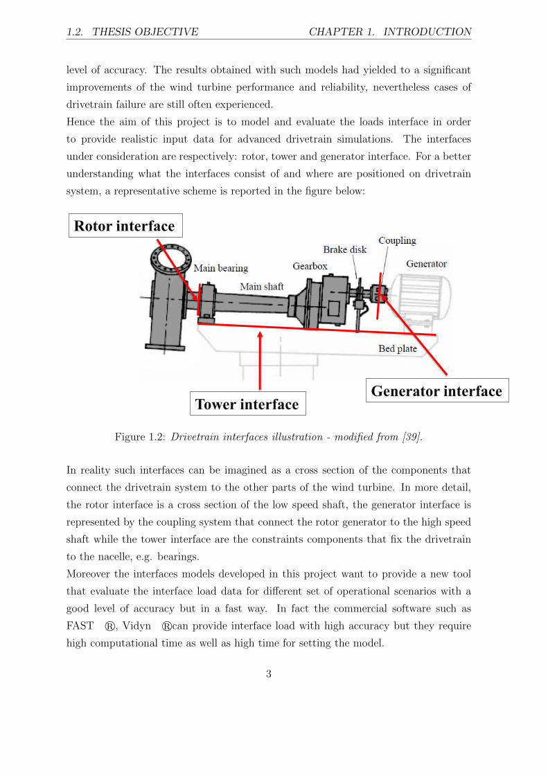
Hence the aim of this project is to model and evaluate the loads interface in order
to provide realistic input data for advanced drivetrain simulations. The interfaces
under consideration are respectively: rotor, tower and generator interface. For a better
understanding what the interfaces consist of and where are positioned on drivetrain
system, a representative scheme is reported in the figure below:
Rotor interface
Tower interfaceGenerator interface
Figure 1.2: Drivetrain interfaces illustration - modified from [39].
In reality such interfaces can be imagined as a cross section of the components that
connect the drivetrain system to the other parts of the wind turbine. In more detail,
the rotor interface is a cross section of the low speed shaft, the generator interface is
represented by the coupling system that connect the rotor generator to the high speed
shaft while the tower interface are the constraints components that fix the drivetrain
to the nacelle, e.g. bearings.
Moreover the interfaces models developed in this project want to provide a new tool
that evaluate the interface load data for different set of operational scenarios with a
good level of accuracy but in a fast way. In fact the commercial software such as
FAST r, Vidyn rcan provide interface load with high accuracy but they require
high computational time as well as high time for setting the model.
3

1.3. THESIS OVERVIEW CHAPTER 1. INTRODUCTION
1.3 Thesis overview
• Chapter 1 - Introduction and Background
This chapter shows briefly the background of the project and illustrates the task
of the work.
• Chapter 2 - Wind Turbine State of the Art
The most recent wind power technologies are presented and a global overview of
the wind turbine main components is presented.
• Chapter 3 - Rotor Interface
The definition of the rotor loads from theoretical point of view is presented.
Briefly description of the most wide speared techniques for rotor model is also
reported. The Rotor Load Interface (RLI) Simulink model is presented and each
constitutive blocks are detailed described. Different simulations with various
wind conditions are shown and the results analyzed. Additionally, a sensitivity
analysis of RFD method has been conducted. Lastly the validation of the RLI
model against measurement field is presented.
• Chapter 4 - Generator Interface
Description the different generator models is presented. The Generator Load
Interface (GLI) Simulink model is illustrated, describing all blocks. Simulations
with different mechanical torque have been conducted in order to analyze the
response of the generator as well as simulations of network fault for studying
the variations of the loads due to electrical issues. Furthermore the issue of the
cogging torque is also presented and illustrated with an example.
• Chapter 5 - Tower Interface
The set of mathematical equations of tower loads are presented. The Tower Load
Interfaces (TLI) model is presented and the simulations of an on-shore tower as
well as off-shore tower under constant wind speed are shown.
• Chapter 6 - Conclusion
An overview of the project work and briefly illustration the main features of each
interface model developed are presented. General conclusions on Msc project
work and the contribution to the modeling of wind turbine drivretrain systems
are stated.
4

Chapter 2
Wind Turbines State of the Art
This chapter is an introduction to the state of the art of wind turbine technology.
A classification and description of the most widespread solutions for the components
of modern wind turbine are presented.
2.1 Introduction
In the actual scenario of wind power technology it is possible to identify a large
quantity of solutions to extract energy from wind. The main classification of wind
turbines is based on rotor spatial orientation and basically it can be distinguished
two categories: horizontal axis wind turbine (HAWT) and vertical axis wind turbine
(VAWT). The latter solution was substantially neglected in the past due to a low effi-
ciency available of about 30% estimated, nevertheless, nowadays this technology begins
to widespred again thanks to its low capital cost and less mantainance compared to
HAWT technology. Hence energy industries strarts to increase the reasearches of this
wind turbine technology in order to improve the amount power extracted from the
wind as well as the efficiency.
Considering the worldwide installed wind turbines it can be observed that the domi-
nant technology of wind power market is the horizontal axis. HAWT technology is the
product of more than four decays of research and production, particularly during the
last years, from big manufactures such as GE, Siemens and Vestas, just to mention
some . The level of technology reached in fields of material, electronic and mechanics
allows to build wind turbine capable of generate 6 MW with dimensions of e.g. 60
meters for the rotor blades length and around 100 meters for tower height.
5
2.2. HAWT CHAPTER 2. WIND TURBINES STATE OF THE ART
2.2 HAWT
Modern HAWTs are a complex electro-mechanical systems that involves several
engineering disciplines, starting from aerodynamics, mechanical engineering coming
to electrical and control engineering. An efficient operation of wind turbines need a
strong integration of all constitutive components in order to harvest the maximum
energy possible from wind, and this can be achieved combining different solutions.
In the following sections the main components and solutions of modern horizontal
HAWT are presented and discussed.
2.3 Rotor
The rotor represents one of the main component of a wind turbine because it is the
system responsible for extracting the power from the wind. It can be divided into two
different parts: the rotor blades and the rotor hub.
When the wind strikes on rotor blades, they generate respectively lift force and drag
force. Basically the lift force is responsible of the rotation of the blades instead the
drag force causes bending of the blades. Modern blades exploit the experience gained
in the aerospace field and are manufactured with complex shapes in order to generate
high lift force and reduces significantly the turbulence phenomenas occurring on tip of
the blade.
Multi MW wind turbine blades should be designed as a compromise between stiffness
and lightness because they can avoid large deformations during high turbulence wind
conditions and possible catastrophic impact with the tower and they must have low in-
ertia for rapidly adapting to the variations of the wind speed. Commonly the material
engaged in wind turbine, which can satisfy such properties, is fiberglass. Recently for
multi-MW wind turbine the carbon fiber starts also to be used.
Concerning the rotor hub, this component represents the connection device between
the blades and low speed shaft. For stall control wind turbines the blades are rigid
connected to the rotor hub while, for pitch control wind turbines, the pitch actuators
are situated into the rotor hub allowing to regulate the rotor angular position.
6

2.4. DRIVETRAIN CHAPTER 2. WIND TURBINES STATE OF THE ART
Figure 2.1: Example of wind turbine blades [25].
2.4 Drivetrain
A drivetrain system can be identified with all transmission components that connect
the rotor system with the generator. The most widespread technology is indirect drive
system that is composed of a low speed shaft supported by bearings, a gearbox system
necessary for multiplying the rotational speed and a coupling system that connect the
high speed shaft to the generator. Recently thanks to the development of the electronic,
the modern generators can support a large number of poles pairs that allow them to
rotate at speed close to rotor one; for this reason energy companies starts to develop
different drivetrain system configurations. Nowadays the drivetrain configurations can
be classified into three main categories:
• Indirect drive system
• Hybrid drive system
• Direct drive system
The first two concepts are characterized by the presence of a gearbox which transfers
the power from low speed shaft to the high speed shaft. The main difference that dis-
tinguishes these solutions is the transmission ratio value; the indirect drive system is
typically designed with a three stages gearbox with a coupling system which connects
the generator to the high speed shaft, and for instance it can perform a transmission ra-
tio of 1:136 [24]. Hybrid drive system consists of two stages gearbox and the generator
7
2.5. GENERATOR CHAPTER 2. WIND TURBINES STATE OF THE ART
can be integrated to the last stage and the transmission ratio is normally around 1:20.
The third technology, direct drive system, is the simplest from the mechanical point of
view since it consists of a single shaft the directly connects the rotor to the generator
without any intermediate gearbox stage; that means that the rotation of rotor blades
exactly corresponds to the generator one.
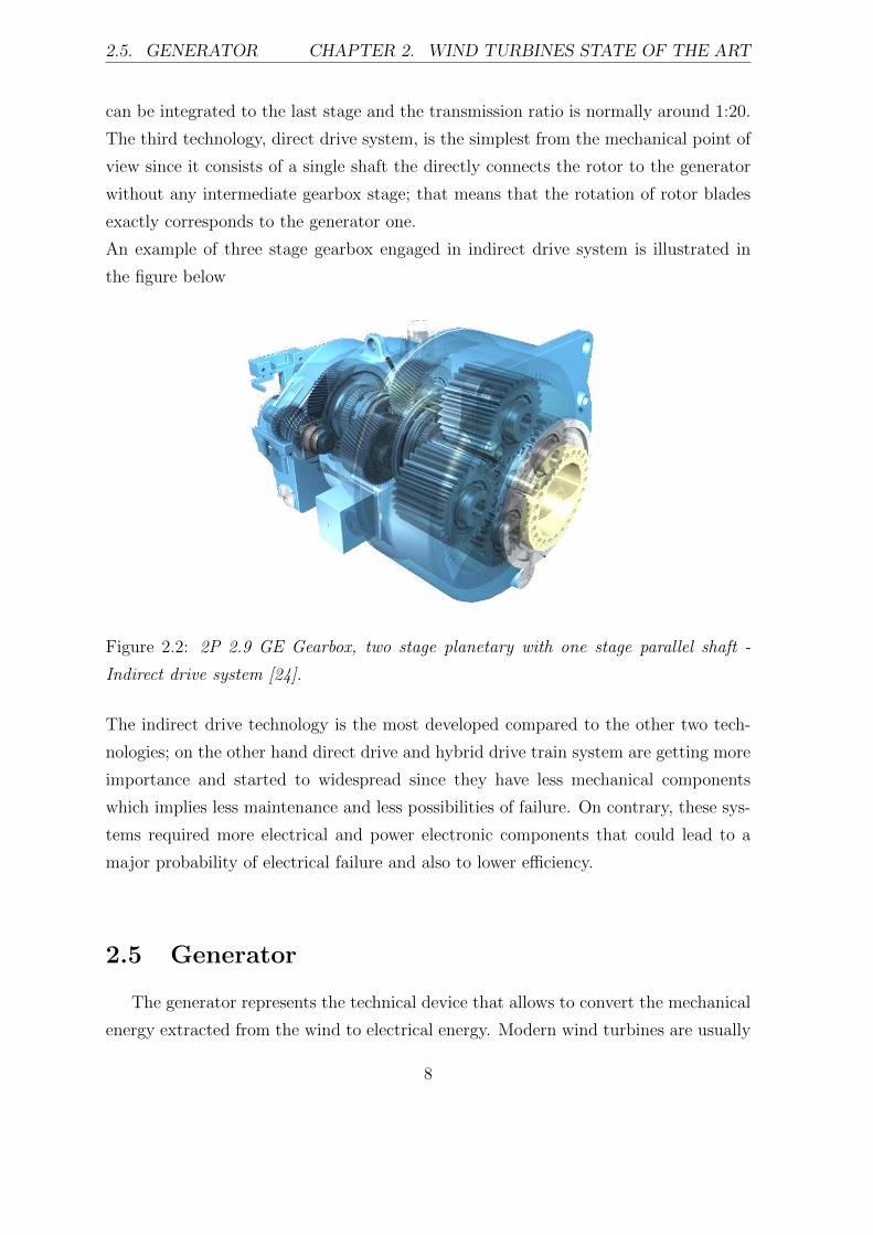
An example of three stage gearbox engaged in indirect drive system is illustrated in
the figure below
Figure 2.2: 2P 2.9 GE Gearbox, two stage planetary with one stage parallel shaft -
Indirect drive system [24].
The indirect drive technology is the most developed compared to the other two tech-
nologies; on the other hand direct drive and hybrid drive train system are getting more
importance and started to widespread since they have less mechanical components
which implies less maintenance and less possibilities of failure. On contrary, these sys-
tems required more electrical and power electronic components that could lead to a
major probability of electrical failure and also to lower efficiency.
2.5 Generator
The generator represents the technical device that allows to convert the mechanical
energy extracted from the wind to electrical energy. Modern wind turbines are usually
8

2.5. GENERATOR CHAPTER 2. WIND TURBINES STATE OF THE ART
equipped with either an induction generator or a synchronous generator according to
the drivetrain system installed. Hereinafter the types of generator commonly engaged
in wind turbines technology are listed
Generators
Induction
generator
Synchronous
generator
Squirrel
cage
Wound
rotor
Electric
excitation
Permanent
magnet
generator
Figure 2.3: Different type of generators for Wind Turbine technology [16].
The induction generator is an asynchronous machine which means that rotates asyn-
chronously respect to the magnetic field. With this type of machine the rotor speed
varies according to the load applied on the shaft, more is the load higher is the rotor
speed, and if any load is applied the generator rounds at synchronous speed. As shown
in the figure above, the induction generators can be classified into two categories, re-
spectively: wound rotor and squirrel cage. Both generator types are commonly used
for indirect drive wind turbine, therefore they require limited space inside nacelle as
well as limited power electronic.
On the contrary, for synchronous generators, the rotor speed is unique and it is the
magnetic field, namely the synchronous speed. In wind turbine industry, two configura-
tions are commonly used, specifically electric excitation and permanent magnet (PM).
9
2.6. TOWER CHAPTER 2. WIND TURBINES STATE OF THE ART
The first model is basically installed in small turbines, instead permanent magnet is
mostly designed for direct drive wind turbines. PM generators, for direct drive tech-
nology, present large sizes because they needs a several numbers of pair pole in order to
round at same speed of the rotor blade (e.g. max 15 rpm), so they require large space
inside nacelle and also additional space for the cooling system of the power electronic.
More details on generators properties can be found in literature reference, for instance
on paper [20].
2.6 Tower
The tower is the component responsible of lifting up the turbine system in the air.
The design of this part required a particular attention from the structural point of view
since this support undergoes turbine loads, such as thrust force or gyroscopic force, and
from the wind pressure which is distributed along the entire height. Moreover off-shore
wind turbine towers also have to resist to wave forces. The tower is designed in order
to have a limited bending, under critical wind conditions, and avoid large potential
catastrophic crashes with blades during operation.
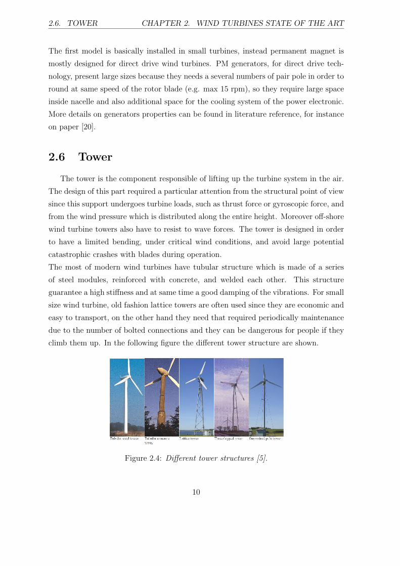
The most of modern wind turbines have tubular structure which is made of a series
of steel modules, reinforced with concrete, and welded each other. This structure
guarantee a high stiffness and at same time a good damping of the vibrations. For small
size wind turbine, old fashion lattice towers are often used since they are economic and
easy to transport, on the other hand they need that required periodically maintenance
due to the number of bolted connections and they can be dangerous for people if they
climb them up. In the following figure the different tower structure are shown.
Figure 2.4: Different tower structures [5].
10
Chapter 3
Rotor Interface
The definition of rotor load from a theoretical point of view is presented. Different
modeling techniques for rotor are discussed. The Rotor Load Interface (RLI) model
is presented and described in details. A series of simulation examples of 2 MW wind
turbine are illustrated and examined. The sensitivity analysis of the RFD aerodynamic
loads calculation block is also shown. Moreover the validation of the RLI model against
field measurements is presented.
3.1 Introduction
The rotor is characterized by rotor blades and rotor hub, which is the connection
device between blades and shaft, and it is responsible of harvesting power from the
wind. When an airflow impacts on the blades surface, a pressure distribution is gen-
erated on them so that the rotor starts to round, producing torque. The interaction
between wind and blades has further effects that must be carefully take under consid-
eration since they can significantly affect the life-time of the wind turbine components.
For instance the drag force on the blades results in high variable thrust force along the
shaft that subject the drive train supports to high variable fatigue load cycles.
The magnitude of the loads strongly depends on the size of the wind turbine, for in-
stance the gyroscopic moment which occurs with yaw controlled wind turbines can be
normally considered negligible for small wind turbine but, for multi MW wind tur-
bines, become significant and they can considerably affect the durability of drivetrain
components e.g. bearings.
Hence it is clearly important to define the rotor loads that are transmitted to the
11

3.2. ROTOR LOAD CHAPTER 3. ROTOR INTERFACE
drivetrain. The rotor interface can be identified and for indirect drive wind turbine is
located on the low speed shaft,instead for direct drive wind turbine, main shaft that
directly connects the rotor to the generator.
3.2 Rotor load
When an airflow strikes the blades of wind turbine, it starts to rotate thanks to the
aerodynamic forces generated along the blades. The revolution speed highly depends
on the aerodynamic profile of the rotor blades. From the basics of the aerodynamic
a wind turbine blade can be imagined as an airfoil which passes through an airflow
with a constant speed. The contact between the air and the airfoil creates a pressure
distribution on blade surface that consequently generate the lift and the drag forces.
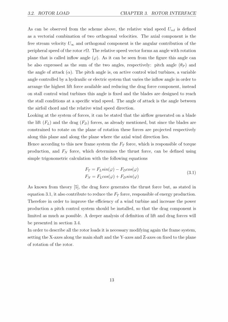
Considering a frame system where the plane of rotation of the rotor is perpendicular
to the axial wind direction, the system of forces and the system of speeds of a wind
turbine blade can be represented with the following scheme
FT
FN
FD
FL θp
φ
φ
α
Urel
-rΩ
U∞
Plan
e o
f Ro
tation
Axial Wind Direction
Figure 3.1: Forces and velocities acting on a blades, axial wind direction frame system.
12
3.2. ROTOR LOAD CHAPTER 3. ROTOR INTERFACE
As can be observed from the scheme above, the relative wind speed Urel is defined
as a vectorial combination of two orthogonal velocities. The axial component is the
free stream velocity U∞ and orthogonal component is the angular contribution of the
peripheral speed of the rotor rΩ. The relative speed vector forms an angle with rotation
plane that is called inflow angle (ϕ). As it can be seen from the figure this angle can
be also expressed as the sum of the two angles, respectively: pitch angle (θP ) and
the angle of attack (α). The pitch angle is, on active control wind turbines, a variable
angle controlled by a hydraulic or electric system that varies the inflow angle in order to
arrange the highest lift force available and reducing the drag force component, instead
on stall control wind turbines this angle is fixed and the blades are designed to reach
the stall conditions at a specific wind speed. The angle of attack is the angle between
the airfoil chord and the relative wind speed direction.
Looking at the system of forces, it can be stated that the airflow generated on a blade
the lift (FL) and the drag (FD) forces, as already mentioned, but since the blades are
constrained to rotate on the plane of rotation these forces are projected respectively
along this plane and along the plane where the axial wind direction lies.
Hence according to this new frame system the FT force, which is responsible of torque
production, and FN force, which determines the thrust force, can be defined using
simple trigonometric calculation with the following equations
FT = FLsin(ϕ)− FDcos(ϕ)
FN = FLcos(ϕ) + FDsin(ϕ)(3.1)
As known from theory [5], the drag force generates the thrust force but, as stated in
equation 3.1, it also contribute to reduce the FT force, responsible of energy production.
Therefore in order to improve the efficiency of a wind turbine and increase the power
production a pitch control system should be installed, so that the drag component is
limited as much as possible. A deeper analysis of definition of lift and drag forces will
be presented in section 3.4.
In order to describe all the rotor loads it is necessary modifying again the frame system,
setting the X-axes along the main shaft and the Y-axes and Z-axes on fixed to the plane
of rotation of the rotor.
13

3.2. ROTOR LOAD CHAPTER 3. ROTOR INTERFACE
The new frame system is reported in the figure below
Figure 3.2: Frame system from Simscape, Matlab r [36].
According to this system it is possible to define a vector of generalized forces as follow
Q =
Fx
Fy
Fz
Mx
My
Mz
(3.2)
This vector expresses respectively the force and the moments along the three directions
of the frame system. The Fx force is the thrust force, defined with equation 3.1. The
Fy force represents the total weight force of the rotor system which consists of the
weight of the three blades plus the rotor hub weight. The force on Z direction, Fz, can
be set equal to zero since this force arises only if an eccentricity between the center of
mass of the rotor and the shaft axis occurs; for instance this issues arises when there
are misalignment errors during assembly phase. This force causes a periodical load
14

3.2. ROTOR LOAD CHAPTER 3. ROTOR INTERFACE
which depends on the rotor speed as well as on the value of the eccentricity. Fz can be
expressed with the following equation
FZ = mεω2sinωt (3.3)
where ε is the eccentricity, and ω is the rotor speed.
In general for the modern wind turbines the Fz force can be considered negligible since
they are assembled with advanced techniques and the rotor is designed in order to
guarantee the correct balance both in static and dynamic conditions.
Concerning the three moment components, the moment along X-axes simply represents
the torque transmitted to the drivetrain system, calculated as the product between the
spinning force and the distance of the its point of application to the center of rotation.
The moments My and Mz should be considered only for the wind turbines equipped
with a yaw system. When such a device is present, according to the frame system
My is defined as yaw moment. This moment comes from the energy necessary to
overcome the frictions between the surface of motion of the yaw mechanism and under
dynamic condition depends on the inertia of the entire nacelle. The yaw moment can
be expressed with the following expression
My = cθ + Iθ (3.4)
Where c represents the friction coefficient that must be estimated either theoreti-
cally or empirically while the I is the nacelle inertia. The formula 3.4 does not include
the aerodynamic resistance of blades because it is a second order effect as the yaw
motion is small.
The moment along the Z-axes Mz represents the gyroscopic moment arising from the
presence of a yaw motion. The gyroscopic effect occurs when external torque is per-
pendicularly applied to the axis of rotation of a spinning system with a torque applied,
giving rise to a moment orthogonal to both torque directions, the gyroscopic moment.
According to [5] the gyroscopic moment for a three blades wind turbine can be analyt-
ically described with the following equation
Mz = 3ωkωn∑i=1
mir2i (3.5)
Where ωk is the angular yaw speed, ω the rotor speed, mi the ith discrete mass of the
rotor blade discretization and ri is the distance from the rotor center to middle point
15
3.3. MODELING TECHNIQUES CHAPTER 3. ROTOR INTERFACE
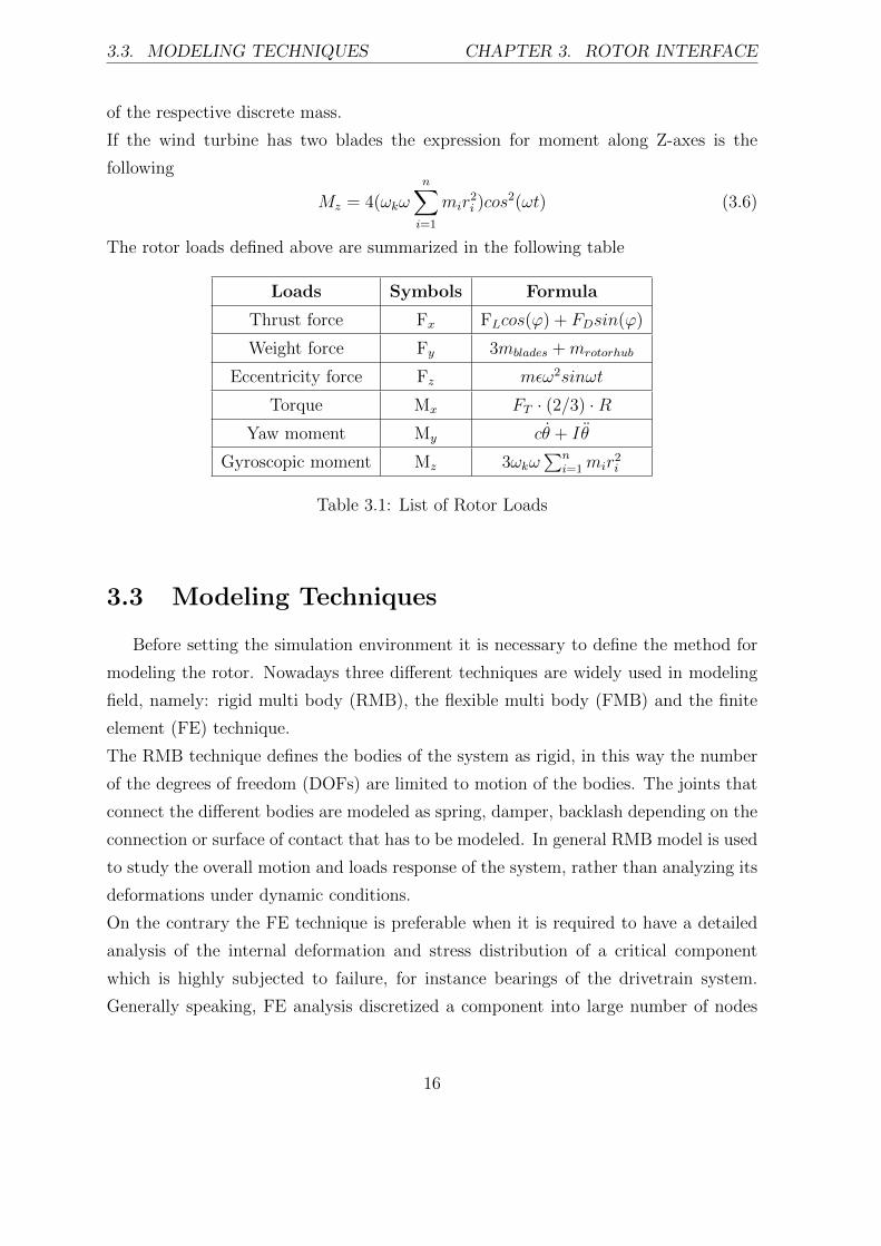
of the respective discrete mass.
If the wind turbine has two blades the expression for moment along Z-axes is the
following
Mz = 4(ωkωn∑i=1
mir2i )cos
2(ωt) (3.6)
The rotor loads defined above are summarized in the following table
Loads Symbols Formula
Thrust force Fx FLcos(ϕ) + FDsin(ϕ)
Weight force Fy 3mblades +mrotorhub
Eccentricity force Fz mεω2sinωt
Torque Mx FT · (2/3) ·RYaw moment My cθ + Iθ
Gyroscopic moment Mz 3ωkω∑n
i=1 mir2i
Table 3.1: List of Rotor Loads
3.3 Modeling Techniques
Before setting the simulation environment it is necessary to define the method for
modeling the rotor. Nowadays three different techniques are widely used in modeling
field, namely: rigid multi body (RMB), the flexible multi body (FMB) and the finite
element (FE) technique.
The RMB technique defines the bodies of the system as rigid, in this way the number
of the degrees of freedom (DOFs) are limited to motion of the bodies. The joints that
connect the different bodies are modeled as spring, damper, backlash depending on the
connection or surface of contact that has to be modeled. In general RMB model is used
to study the overall motion and loads response of the system, rather than analyzing its
deformations under dynamic conditions.
On the contrary the FE technique is preferable when it is required to have a detailed
analysis of the internal deformation and stress distribution of a critical component
which is highly subjected to failure, for instance bearings of the drivetrain system.
Generally speaking, FE analysis discretized a component into large number of nodes
16

3.4. RLI MODEL CHAPTER 3. ROTOR INTERFACE
that represent the DOFs; such number essentially depends on the accuracy of the re-
sults desired, and usually starts from 5000 up to millions. On the other hand higher is
the number of DOFs higher is the computational time needed.
The FMB technique can be seen as a combination of MBS and FE method. FMB
method defines the system RMB in the same way of the RMB technique, setting the
DOFs of the bodies motions but each component is replaced with a flexible body instead
of a rigid body. The flexible body is reduced to its modal representation, including
the dynamic and static response properties. The FMB method requires lower compu-
tational time than FE technique and allows to analyze the influence of the flexibility
on the interfaces of the components.
The RMB technique suits perfectly the task of the project and for simulation of the
Rotor Load Interface, however the FE and FMB approaches can provide a deeper anal-
ysis of the rotor loads and they can be proposed for future outlooks.
The entire project, included the other two sections GLI and TLI, is developed with
Simulink software, from Matworks r. The choice of the software is based on the
large possibilities of modeling which it offers as well as the possibility of interfacing
with other softwares.
Additionally Simulink offers a large number of libraries dedicated to different fields
such as aerospace, hydraulic and, in particular, the Simscape library provides specific
tools for RMB modeling.
3.4 RLI model
The starting point of Rotor Load Interface model is the Wind Turbine model de-
veloped by Steve Miller from MatWorks r [35], reported in Appendix C. This model
provides a complete wind turbine system including for instance tower model, advanced
hydraulic yaw system and so on. The intention of RLI model is to define a tool the
evaluate the rotor loads, therefore the level of complexity of the MatWorks model has
been reduced removing the extra blocks that are not necessary to achieve the task.
The RLI model maintains two concepts of MatWorks model: Rigid Multi Body sys-
tem of rotor blades and rotor hub and technique used for calculating the aerodynamic
forces, in particular the method defined as Uniform Force Distribution. The rest of the
blocks has been removed or substituted by others that fit for the RLI model.
17
3.4. RLI MODEL CHAPTER 3. ROTOR INTERFACE
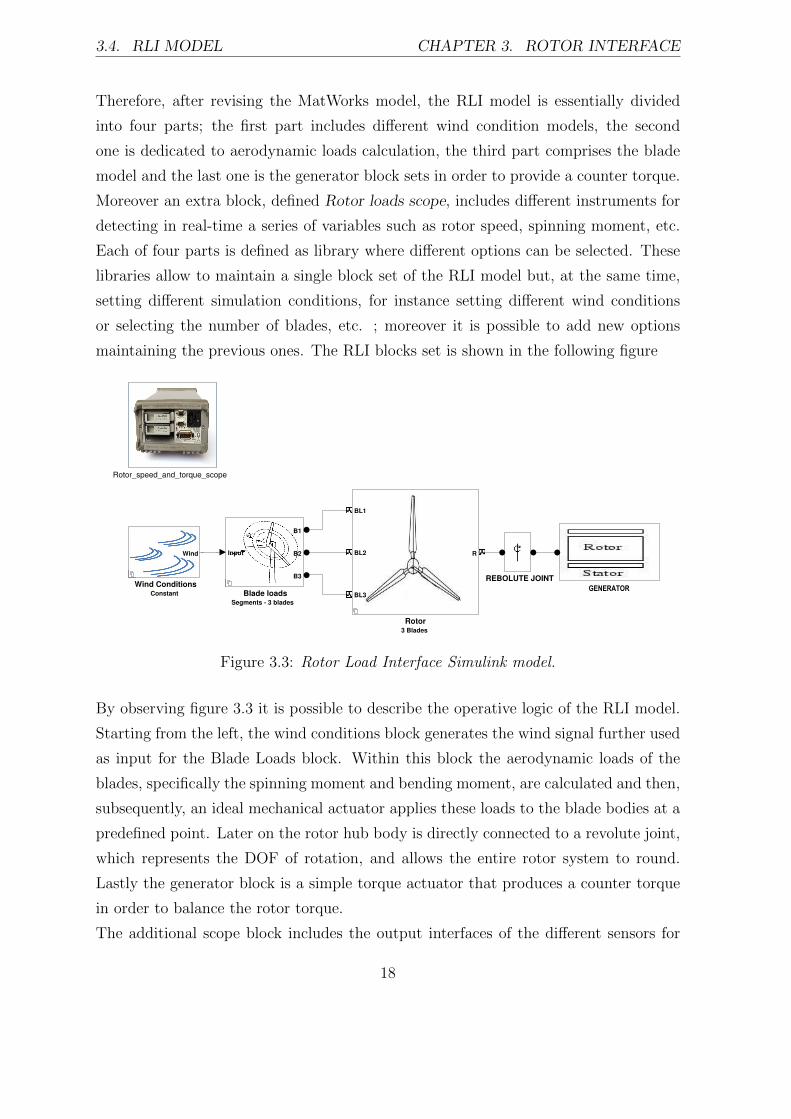
Therefore, after revising the MatWorks model, the RLI model is essentially divided
into four parts; the first part includes different wind condition models, the second
one is dedicated to aerodynamic loads calculation, the third part comprises the blade
model and the last one is the generator block sets in order to provide a counter torque.
Moreover an extra block, defined Rotor loads scope, includes different instruments for
detecting in real-time a series of variables such as rotor speed, spinning moment, etc.
Each of four parts is defined as library where different options can be selected. These
libraries allow to maintain a single block set of the RLI model but, at the same time,
setting different simulation conditions, for instance setting different wind conditions
or selecting the number of blades, etc. ; moreover it is possible to add new options
maintaining the previous ones. The RLI blocks set is shown in the following figure
Wind ConditionsConstant
Wind
Rotor_speed_and_torque_scope
Rotor3 Blades
BL1
BL2
BL3
R
REBOLUTE JOINT
GENERATOR Blade loads
Segments - 3 blades
Input
B1
B2
B3
Figure 3.3: Rotor Load Interface Simulink model.
By observing figure 3.3 it is possible to describe the operative logic of the RLI model.
Starting from the left, the wind conditions block generates the wind signal further used
as input for the Blade Loads block. Within this block the aerodynamic loads of the
blades, specifically the spinning moment and bending moment, are calculated and then,
subsequently, an ideal mechanical actuator applies these loads to the blade bodies at a
predefined point. Later on the rotor hub body is directly connected to a revolute joint,
which represents the DOF of rotation, and allows the entire rotor system to round.
Lastly the generator block is a simple torque actuator that produces a counter torque
in order to balance the rotor torque.
The additional scope block includes the output interfaces of the different sensors for
18

3.4. RLI MODEL CHAPTER 3. ROTOR INTERFACE
the measurement of the variables under investigation.
3.4.1 Wind conditions library
The Wind conditions library includes four wind conditions that define the wind
signal in time-domain, necessary to calculate the aerodynamic forces of the blades.
The definition of the wind conditions is based on IEC:2005 standard. These standard
provide different wind models that are taken into account by setting different factors,
for instance the wind direction. For RLI model, the four wind conditions implemented
are: normal turbulence model, extreme wind speed model, extreme operating gust
model and extreme turbulence model; furthermore a empty and a constant blocks are
set in order to allow future implementations of the wind condition model developed at
Chalmers and to define a constant wind signal, respectively.
According to IEC:2005 standard, before defining of the four wind signals it is required
to specify the environment characteristics. The IEC:2005 standards ranks the envi-
ronment conditions into three categories depending on the level of turbulence intensity
[28]. For RLI model the environment category chosen is the one with low turbulence
characteristics.
The definition of the signal of the four wind conditions is given by the following equation
Winput = Waverage + random(σ1) (3.7)
Where Winput is the input signal of the aerodynamic loads block, Waverage is the average
speed value of the wind that usually is experienced on the site where the wind turbine is
located, and σ1 represents the standard deviation that is defined with a specific formula
for each the wind conditions listed above; the equations are reported in Appendix A.
Hence, since the nature of the wind is not deterministic, in order to define a realistic
wind model, the wind signal is defined as random function within the interval of speed
is defined by upper and lower limits established with deviation standard value σ1.
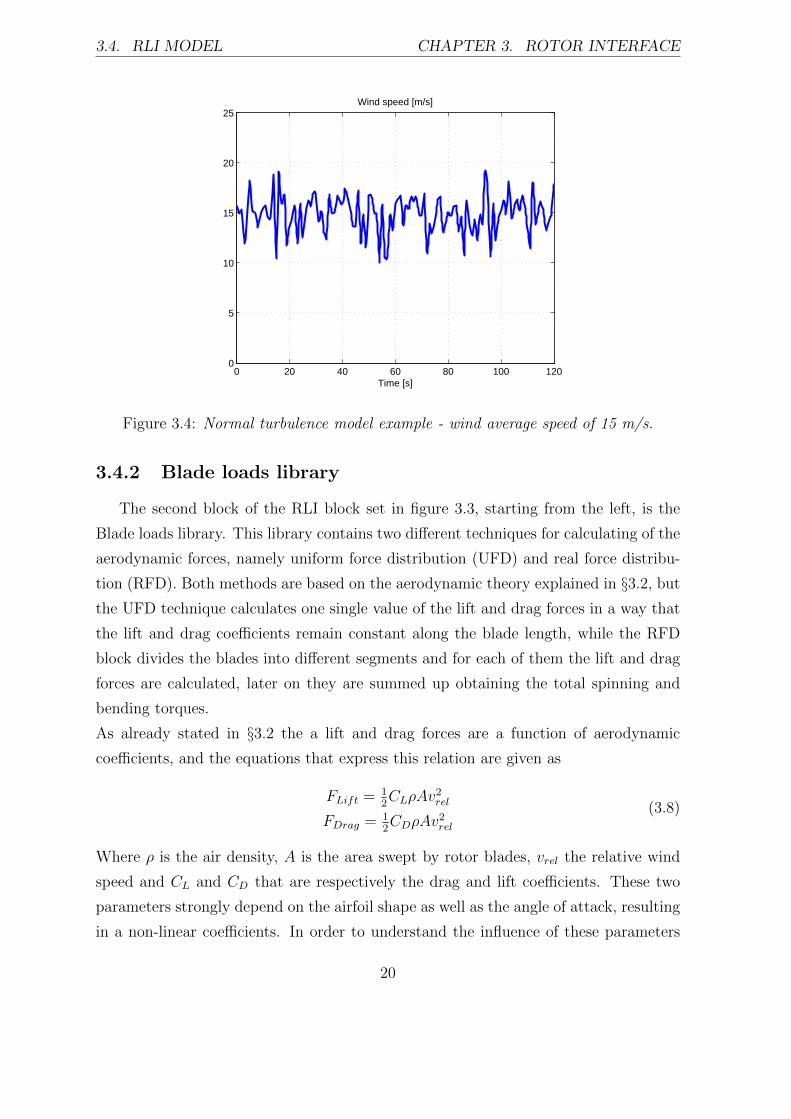
In the following page an example of normal turbulence wind condition signal, set with
an average speed of 15 m/s, is reported
19
3.4. RLI MODEL CHAPTER 3. ROTOR INTERFACE
0 20 40 60 80 100 1200
5
10
15
20
25
Time [s]
Wind speed [m/s]
Figure 3.4: Normal turbulence model example - wind average speed of 15 m/s.
3.4.2 Blade loads library
The second block of the RLI block set in figure 3.3, starting from the left, is the
Blade loads library. This library contains two different techniques for calculating of the
aerodynamic forces, namely uniform force distribution (UFD) and real force distribu-
tion (RFD). Both methods are based on the aerodynamic theory explained in §3.2, but
the UFD technique calculates one single value of the lift and drag forces in a way that
the lift and drag coefficients remain constant along the blade length, while the RFD
block divides the blades into different segments and for each of them the lift and drag
forces are calculated, later on they are summed up obtaining the total spinning and
bending torques.
As already stated in §3.2 the a lift and drag forces are a function of aerodynamic
coefficients, and the equations that express this relation are given as
FLift = 12CLρAv
2rel
FDrag = 12CDρAv
2rel
(3.8)
Where ρ is the air density, A is the area swept by rotor blades, vrel the relative wind
speed and CL and CD that are respectively the drag and lift coefficients. These two
parameters strongly depend on the airfoil shape as well as the angle of attack, resulting
in a non-linear coefficients. In order to understand the influence of these parameters
20

3.4. RLI MODEL CHAPTER 3. ROTOR INTERFACE
on the aerodynamic forces, a diagram of NACA 0015 airfoil of lift and drag coefficient
as a function of the angle of attack is reported below
0 50 100 150 200 250 300 350−1.5
−1
−0.5
0
0.5
1
1.5
2NACA 0015 Airfoil data
Angle of attack [deg]
CL, C
D
C
L
CD
Figure 3.5: NACA 0015 airfoil - Lift and Drag coefficient VS angle of attack.
As it can be noticed, for small angle of attack, the lift coefficient starts from zero
and rapidly reaches the maximum value whilst drag coefficient remains approximately
equal to zero. When a specific angle of attack, which varies accordingly to aerodynamic
characteristics of the airfoil, is reached the stall condition occurs and the lift coefficient
value has a relevant drop, whereas, at the same time, the drag coefficient starts to
increase considerably. After 90 degrees the lift and drag coefficients have an opposite
trend although for wind turbine applications such angles of attack are never swept. In
general the interval of the angle of attack for wind turbine blades defined between 0
and 30 degrees.
From this considerations it can be affirmed that the lift and drag forces along the blade
length are highly non-linear, moreover in reality the turbulence at rotor hub zone as
well as at tip of the blades affect significantly the aerodynamic of the rotor.
With these observations, it becomes important defining models that can simulate the
force distribution along the blade as realistic as possible. UFD and RFD methods
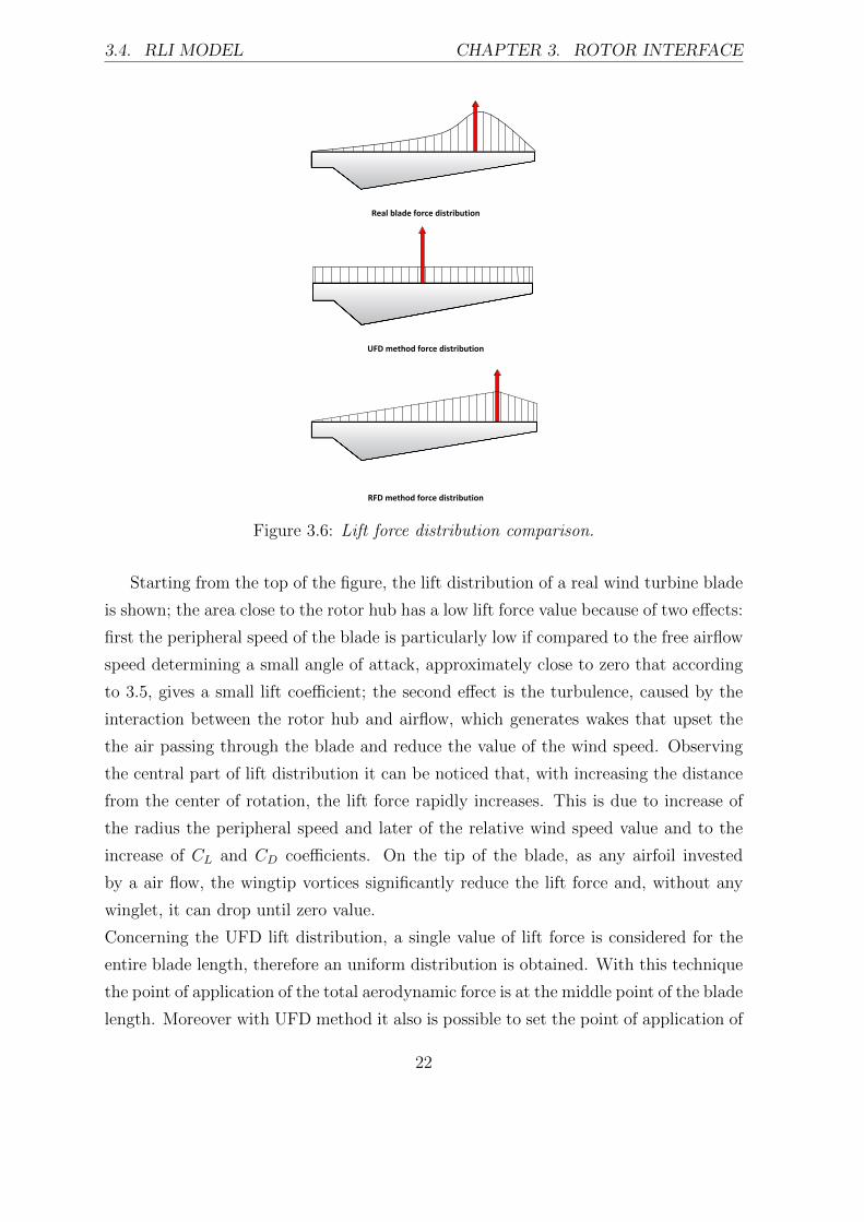
provides different shape of the force distribution. A comparison of lift force distribution
among the two techniques and a real blade force distribution is reported.
21
3.4. RLI MODEL CHAPTER 3. ROTOR INTERFACE
Real blade force distribution
UFD method force distribution
RFD method force distribution
Figure 3.6: Lift force distribution comparison.
Starting from the top of the figure, the lift distribution of a real wind turbine blade
is shown; the area close to the rotor hub has a low lift force value because of two effects:
first the peripheral speed of the blade is particularly low if compared to the free airflow
speed determining a small angle of attack, approximately close to zero that according
to 3.5, gives a small lift coefficient; the second effect is the turbulence, caused by the
interaction between the rotor hub and airflow, which generates wakes that upset the
the air passing through the blade and reduce the value of the wind speed. Observing
the central part of lift distribution it can be noticed that, with increasing the distance
from the center of rotation, the lift force rapidly increases. This is due to increase of
the radius the peripheral speed and later of the relative wind speed value and to the
increase of CL and CD coefficients. On the tip of the blade, as any airfoil invested
by a air flow, the wingtip vortices significantly reduce the lift force and, without any
winglet, it can drop until zero value.
Concerning the UFD lift distribution, a single value of lift force is considered for the
entire blade length, therefore an uniform distribution is obtained. With this technique
the point of application of the total aerodynamic force is at the middle point of the blade
length. Moreover with UFD method it also is possible to set the point of application of
22
3.4. RLI MODEL CHAPTER 3. ROTOR INTERFACE
the total force at 2/3 of the blade length in order to have more realistic lift distribution.
On contrary RFD technique presents a distribution that can be assumed as quasi-linear.
In fact when the blade is divided into different segments the values of the angle of attack
and consequently of CL and CD change from one segment to another, so that the effect
of the lift reduction on the rotor hub zone is considered.
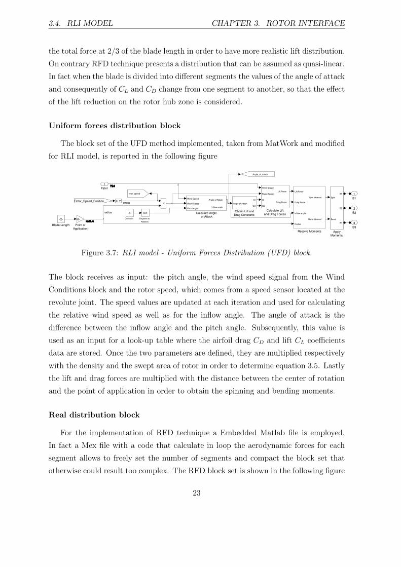
Uniform forces distribution block
The block set of the UFD method implemented, taken from MatWork and modified
for RLI model, is reported in the following figure
B3
3
B2
2
B1
1
U Y
Resolve Moments
Lift Force
Drag Force
inflow angle
Radius
Spin Moment
Bend Moment
Point of
Application
-K-
Obtain Lift and
Drag Constants
Angle of Attack
Cl
Cd
Rotor_Speed_Position
Degrees to
Radians
D2R
Constant
-C-Calculate Lift
and Drag Forces
Wind Speed
Blade Speed
Cl
Cd
Lift Force
Drag Force
Calculate Angle
of Attack
Wind Speed
Blade Speed
Pitch Angle
Angle of Attack
Inflow angle
Blade Length
-C-
Apply
Moments
Spin
Bend
B1
B2
B3
Angle_of_attack
rotor_speed
Input
1
radius
radiusradiusradiusradiusradiusradiusradiusradiusradiusradiusradiusradiusradius
VinfVinfVinfVinfVinfVinfVinfVinfVinfVinfVinfVinfVinfVinfVinfVinfVinfVinfVinf
omegaomega
Figure 3.7: RLI model - Uniform Forces Distribution (UFD) block.
The block receives as input: the pitch angle, the wind speed signal from the Wind
Conditions block and the rotor speed, which comes from a speed sensor located at the
revolute joint. The speed values are updated at each iteration and used for calculating
the relative wind speed as well as for the inflow angle. The angle of attack is the
difference between the inflow angle and the pitch angle. Subsequently, this value is
used as an input for a look-up table where the airfoil drag CD and lift CL coefficients
data are stored. Once the two parameters are defined, they are multiplied respectively
with the density and the swept area of rotor in order to determine equation 3.5. Lastly
the lift and drag forces are multiplied with the distance between the center of rotation
and the point of application in order to obtain the spinning and bending moments.
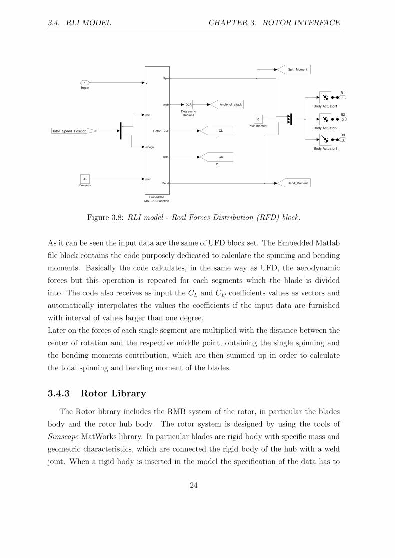
Real distribution block
For the implementation of RFD technique a Embedded Matlab file is employed.
In fact a Mex file with a code that calculate in loop the aerodynamic forces for each
segment allows to freely set the number of segments and compact the block set that
otherwise could result too complex. The RFD block set is shown in the following figure
23
3.4. RLI MODEL CHAPTER 3. ROTOR INTERFACE
B3
3
B2
2
B1
1
Pitch moment
0
Rotor_Speed_Position
Embedded
MATLAB Function
V
psi0
omega
pitch
Spin
aoab
CLs
CDs
Bend
Rotor
Degrees to
Radians
D2R
Constant
-C-
Body Actuator3
Body Actuator2
Body Actuator1
2
CD
1
CL
Bend_Moment
Spin_Moment
Angle_of_attack
Input
1
Figure 3.8: RLI model - Real Forces Distribution (RFD) block.
As it can be seen the input data are the same of UFD block set. The Embedded Matlab
file block contains the code purposely dedicated to calculate the spinning and bending
moments. Basically the code calculates, in the same way as UFD, the aerodynamic
forces but this operation is repeated for each segments which the blade is divided
into. The code also receives as input the CL and CD coefficients values as vectors and
automatically interpolates the values the coefficients if the input data are furnished
with interval of values larger than one degree.
Later on the forces of each single segment are multiplied with the distance between the
center of rotation and the respective middle point, obtaining the single spinning and
the bending moments contribution, which are then summed up in order to calculate
the total spinning and bending moment of the blades.
3.4.3 Rotor Library
The Rotor library includes the RMB system of the rotor, in particular the blades
body and the rotor hub body. The rotor system is designed by using the tools of
Simscape MatWorks library. In particular blades are rigid body with specific mass and
geometric characteristics, which are connected the rigid body of the hub with a weld
joint. When a rigid body is inserted in the model the specification of the data has to
24
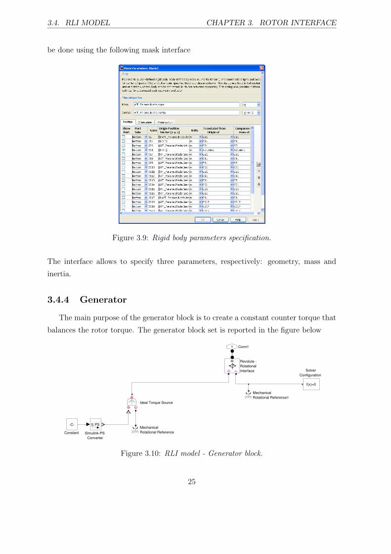
3.4. RLI MODEL CHAPTER 3. ROTOR INTERFACE
be done using the following mask interface
Figure 3.9: Rigid body parameters specification.
The interface allows to specify three parameters, respectively: geometry, mass and
inertia.
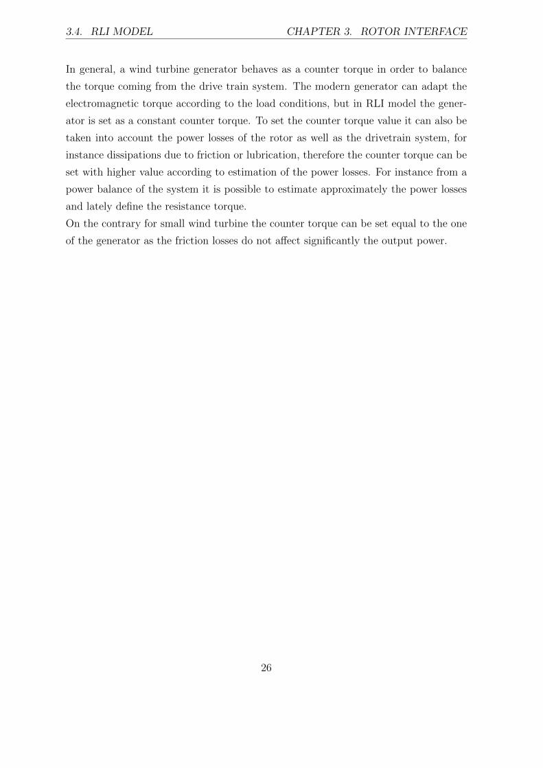
3.4.4 Generator
The main purpose of the generator block is to create a constant counter torque that
balances the rotor torque. The generator block set is reported in the figure below
Conn11
Solver
Configuration
f(x)=0
Simulink-PS
Converter
PSS
Revolute -
Rotational
InterfaceB FR
Mechanical
Rotational Reference1
Mechanical
Rotational Reference
Ideal Torque Source
S CR
Constant
-C-
Figure 3.10: RLI model - Generator block.
25
3.4. RLI MODEL CHAPTER 3. ROTOR INTERFACE
In general, a wind turbine generator behaves as a counter torque in order to balance
the torque coming from the drive train system. The modern generator can adapt the
electromagnetic torque according to the load conditions, but in RLI model the gener-
ator is set as a constant counter torque. To set the counter torque value it can also be
taken into account the power losses of the rotor as well as the drivetrain system, for
instance dissipations due to friction or lubrication, therefore the counter torque can be
set with higher value according to estimation of the power losses. For instance from a
power balance of the system it is possible to estimate approximately the power losses
and lately define the resistance torque.
On the contrary for small wind turbine the counter torque can be set equal to the one
of the generator as the friction losses do not affect significantly the output power.
26
3.5. 2 MW SIEMENS r WIND TURBINE CHAPTER 3. ROTOR INTERFACE
3.5 2 MW Siemens r Wind Turbine
In this section the rotor 2 MW Siemens wind turbine is used to perform a differ-
ent simulations. The choice of the 2 MW Siemens wind turbine is based on the large
number of data that are available on Siemens website [26] and that are required to set
the RLI model parameters.
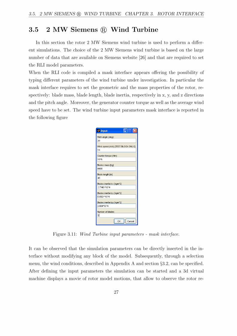
When the RLI code is compiled a mask interface appears offering the possibility of
typing different parameters of the wind turbine under investigation. In particular the
mask interface requires to set the geometric and the mass properties of the rotor, re-
spectively: blade mass, blade length, blade inertia, respectively in x, y, and z directions
and the pitch angle. Moreover, the generator counter torque as well as the average wind
speed have to be set. The wind turbine input parameters mask interface is reported in
the following figure
Figure 3.11: Wind Turbine input parameters - mask interface.
It can be observed that the simulation parameters can be directly inserted in the in-
terface without modifying any block of the model. Subsequently, through a selection
menu, the wind conditions, described in Appendix A and section §3.2, can be specified.
After defining the input parameters the simulation can be started and a 3d virtual
machine displays a movie of rotor model motions, that allow to observe the rotor re-
27
3.5. 2 MW SIEMENS r WIND TURBINE CHAPTER 3. ROTOR INTERFACE
sponses under different set of operational scenarios.
When the simulation ends, the spinning moment, the bending moment, the rotor speed,
the electrical torque, the angle of attack and power are automatically post-precessed
and outputs are reported in time domain. Moreover using the RLI model is also pos-
sible to simulate the gyroscopic loads, defined with equations 3.5 and 4.1, occurring
with wind turbines equipped with yaw motion system.
In the following sections a set of simulations of 2.0 MW Siemens wind turbine are
presented. All the simulation are performed using both aerodynamic loads calculation
techniques, specifically UFD and RFD, and the RFD is set with a number of segments
of 20.
Although in reality a pure constant wind speed condition rarely occurs, the first simu-
lation is performed with a constant wind speed signal. In this manner it is possible to
observe the main differences of rotor responses with the two aerodynamic loads calcu-
lation methods that otherwise, with complex signal (e.g. turbulence signal), it could
be difficult to recognize.
28
3.5. 2 MW SIEMENS r WIND TURBINE CHAPTER 3. ROTOR INTERFACE
3.5.1 Constant wind condition
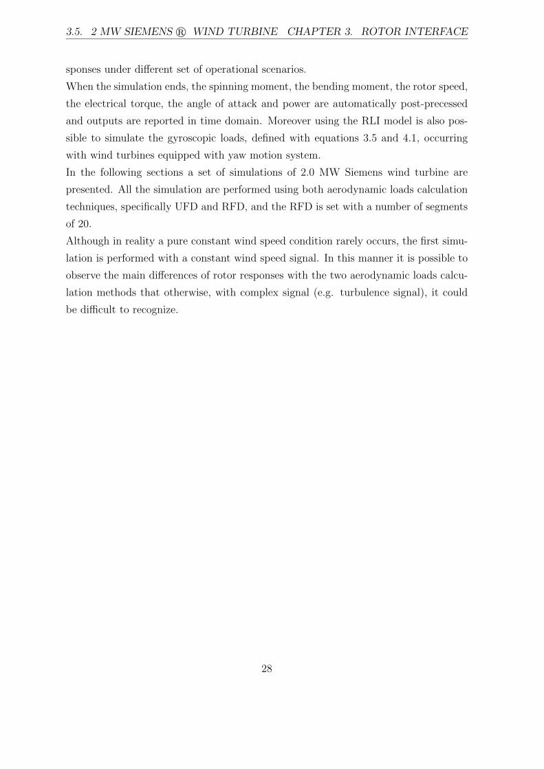
The settings for the first simulation are: constant wind speed signal of 15 m/s, pitch
angle of 20 degrees and counter torque of 106 Nm whereas the technical specification of
the rotor are reported in Appendix A. The time-simulation is set on 120 seconds which
is considered a sufficient time for reaching the steady state condition. The results of
the simulation are reported in the figure below
0 20 40 60 80 100 1200
5
10
15
Time [s]
Rotor speed [RPM]
0 20 40 60 80 100 1200
20
40
60
80
Time [s]
Angle of attack [deg]
0 20 40 60 80 100 120−12
−10
−8
−6
−4
−2x 10
5
Time [s]
Bend Moment [Nm]
0 20 40 60 80 100 1200
2
4
6
8x 10
5
Time [s]
Spin moment [Nm]
RFD methodUFD method
Figure 3.12: 2MW Siemens wind turbine Post-processing, Pitch angle=20[deg], Wind
speed=15[m/s], Constant wind condition.
Observing the figure it can be affirmed that UFD and RFD have a different response.
29
3.5. 2 MW SIEMENS r WIND TURBINE CHAPTER 3. ROTOR INTERFACE
Starting from rotor speed, the UFD model presents higher values than RFD. The same
observation can be done for the angle of attack and the spinning moment while the
bending moment has a lower value overall the simulation time. The reason of these
results is that RFD presents lower aerodynamic load on blades since the effect of the
low rotor speeds in rotor hub area is taken into account while with UFD technique the
same load is applied along the entire blade and this leads to higher spinning moment
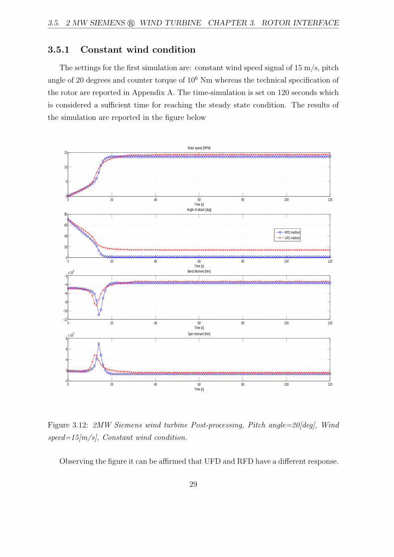
and consequently higher rotor speed as well as angle of attack. Moreover with the RFD
technique also the output power results lower than UFD method because of the lower
loads on the blades, as shown in plot below.
0 20 40 60 80 100 1200
0.5
1
1.5
Time [s]
Power [MW]
RFD methodUFD method
Figure 3.13: 2MW Siemens wind turbine Rotor Power, Pitch angle=20[deg], Wind
speed=15[m/s], Constant wind condition.
Looking at initial transient phase, in particular from the starting point, the response
of both techniques is approximately the same because, at low wind speed, the effect of
the rotor hub is not relevant making output power of the two methods comparable.
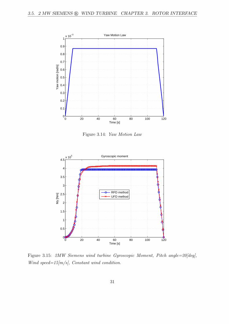
Furthermore the gyroscopic moment is also investigated under constant wind condition,
therefore a yaw motion of the nacelle is implemented. Specifically the yaw motion is set
with a constant angular speed of 1 degrees per second at steady state speed condition
and a ramp-up and ramp-down for the starting phase and final phase respectively. The
yaw motion law and the gyroscopic loads, in time domain, are reported in the following
figure.
30
3.5. 2 MW SIEMENS r WIND TURBINE CHAPTER 3. ROTOR INTERFACE
0 20 40 60 80 100 1200
0.1
0.2
0.3
0.4
0.5
0.6
0.7
0.8
0.9
1x 10
−3
Time [s]
Yaw
mot
ion
[rad
/s]
Yaw Motion Law
Figure 3.14: Yaw Motion Law
0 20 40 60 80 100 1200
0.5
1
1.5
2
2.5
3
3.5
4
4.5x 10
5
Time [s]
My
[Nm
]
Gyroscopic moment
RFD methodUFD method
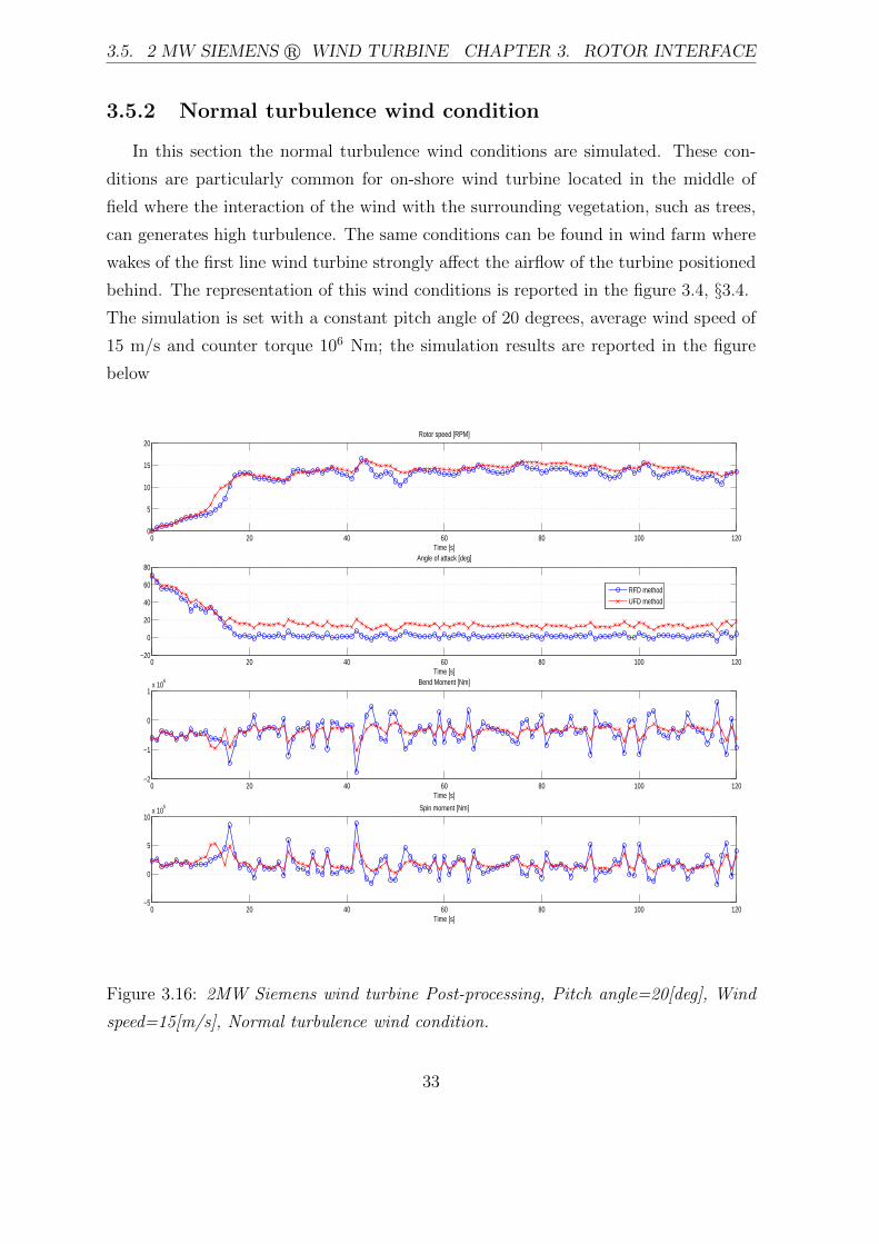
Figure 3.15: 2MW Siemens wind turbine Gyroscopic Moment, Pitch angle=20[deg],
Wind speed=15[m/s], Constant wind condition.
31

3.5. 2 MW SIEMENS r WIND TURBINE CHAPTER 3. ROTOR INTERFACE
From the figure above it can be immediately observed that the gyroscopic loads are
two orders of magnitude lower than the spinning as well as the bending moments and
for this reason the gyroscopic moment is not always considered. For small wind turbine
this assumption can be accepted but for multi-MW wind turbines the gyroscopic load
should be considered during the design phase in order to certificate the durability of
the wind turbine of 20 years, especially for bearings.
32
3.5. 2 MW SIEMENS r WIND TURBINE CHAPTER 3. ROTOR INTERFACE
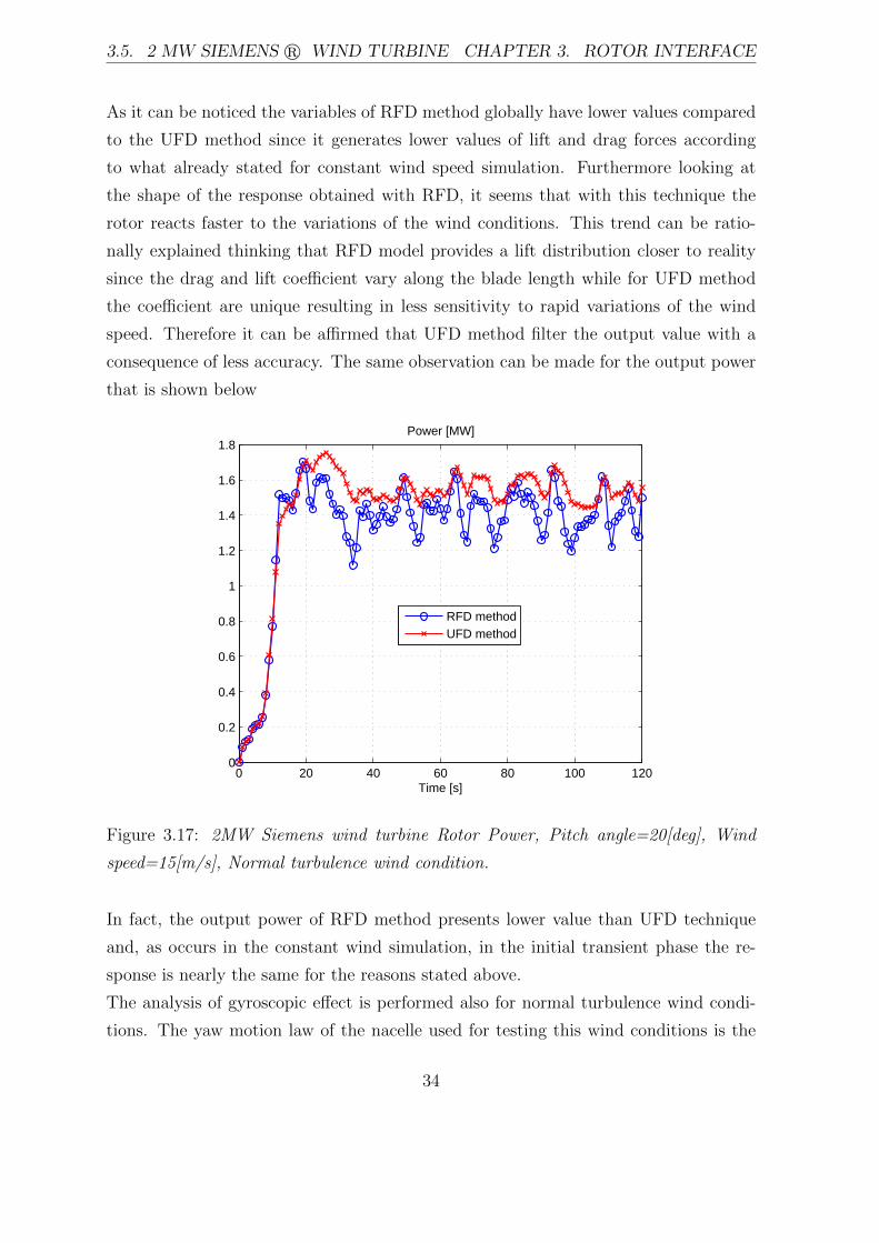
3.5.2 Normal turbulence wind condition
In this section the normal turbulence wind conditions are simulated. These con-
ditions are particularly common for on-shore wind turbine located in the middle of
field where the interaction of the wind with the surrounding vegetation, such as trees,
can generates high turbulence. The same conditions can be found in wind farm where
wakes of the first line wind turbine strongly affect the airflow of the turbine positioned
behind. The representation of this wind conditions is reported in the figure 3.4, §3.4.
The simulation is set with a constant pitch angle of 20 degrees, average wind speed of
15 m/s and counter torque 106 Nm; the simulation results are reported in the figure
below
0 20 40 60 80 100 1200
5
10
15
20
Time [s]
Rotor speed [RPM]
0 20 40 60 80 100 120−20
0
20
40
60
80
Time [s]
Angle of attack [deg]
0 20 40 60 80 100 120−2
−1
0
1x 10
6
Time [s]
Bend Moment [Nm]
0 20 40 60 80 100 120−5
0
5
10x 10
5
Time [s]
Spin moment [Nm]
RFD methodUFD method
Figure 3.16: 2MW Siemens wind turbine Post-processing, Pitch angle=20[deg], Wind
speed=15[m/s], Normal turbulence wind condition.
33
3.5. 2 MW SIEMENS r WIND TURBINE CHAPTER 3. ROTOR INTERFACE
As it can be noticed the variables of RFD method globally have lower values compared
to the UFD method since it generates lower values of lift and drag forces according
to what already stated for constant wind speed simulation. Furthermore looking at
the shape of the response obtained with RFD, it seems that with this technique the
rotor reacts faster to the variations of the wind conditions. This trend can be ratio-
nally explained thinking that RFD model provides a lift distribution closer to reality
since the drag and lift coefficient vary along the blade length while for UFD method
the coefficient are unique resulting in less sensitivity to rapid variations of the wind
speed. Therefore it can be affirmed that UFD method filter the output value with a
consequence of less accuracy. The same observation can be made for the output power
that is shown below
0 20 40 60 80 100 1200
0.2
0.4
0.6
0.8
1
1.2
1.4
1.6
1.8
Time [s]
Power [MW]
RFD methodUFD method
Figure 3.17: 2MW Siemens wind turbine Rotor Power, Pitch angle=20[deg], Wind
speed=15[m/s], Normal turbulence wind condition.
In fact, the output power of RFD method presents lower value than UFD technique
and, as occurs in the constant wind simulation, in the initial transient phase the re-
sponse is nearly the same for the reasons stated above.
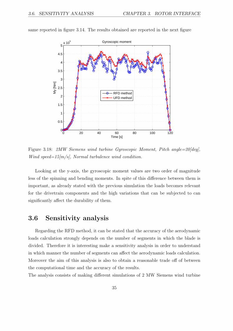
The analysis of gyroscopic effect is performed also for normal turbulence wind condi-
tions. The yaw motion law of the nacelle used for testing this wind conditions is the
34
3.6. SENSITIVITY ANALYSIS CHAPTER 3. ROTOR INTERFACE
same reported in figure 3.14. The results obtained are reported in the next figure
0 20 40 60 80 100 1200
0.5
1
1.5
2
2.5
3
3.5
4
4.5
5x 10
5
Time [s]
My
[Nm
]
Gyroscopic moment
RFD methodUFD method
Figure 3.18: 2MW Siemens wind turbine Gyroscopic Moment, Pitch angle=20[deg],
Wind speed=15[m/s], Normal turbulence wind condition.
Looking at the y-axis, the gyroscopic moment values are two order of magnitude
less of the spinning and bending moments. In spite of this difference between them is
important, as already stated with the previous simulation the loads becomes relevant
for the drivetrain components and the high variations that can be subjected to can
significantly affect the durability of them.
3.6 Sensitivity analysis
Regarding the RFD method, it can be stated that the accuracy of the aerodynamic
loads calculation strongly depends on the number of segments in which the blade is
divided. Therefore it is interesting make a sensitivity analysis in order to understand
in which manner the number of segments can affect the aerodynamic loads calculation.
Moreover the aim of this analysis is also to obtain a reasonable trade off of between
the computational time and the accuracy of the results.
The analysis consists of making different simulations of 2 MW Siemens wind turbine
35
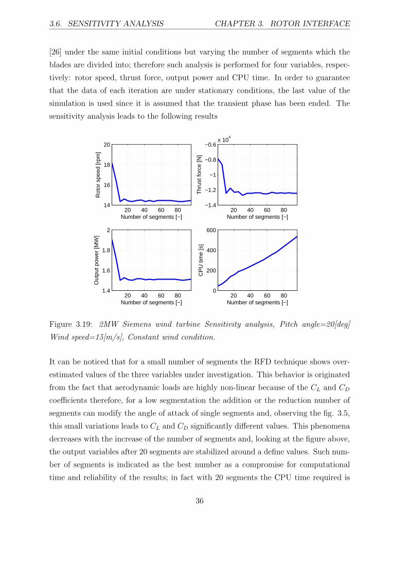
3.6. SENSITIVITY ANALYSIS CHAPTER 3. ROTOR INTERFACE
[26] under the same initial conditions but varying the number of segments which the
blades are divided into; therefore such analysis is performed for four variables, respec-
tively: rotor speed, thrust force, output power and CPU time. In order to guarantee
that the data of each iteration are under stationary conditions, the last value of the
simulation is used since it is assumed that the transient phase has been ended. The
sensitivity analysis leads to the following results
20 40 60 8014
16
18
20
Number of segments [−]
Rot
or s
peed
[rpm
]
20 40 60 80−1.4
−1.2
−1
−0.8
−0.6x 10
4
Number of segments [−]
Thr
ust f
orce
[N]
20 40 60 801.4
1.6
1.8
2
Number of segments [−]
Out
put p
ower
[MW
]
20 40 60 800
200
400
600
Number of segments [−]
CP
U ti
me
[s]
Figure 3.19: 2MW Siemens wind turbine Sensitivity analysis, Pitch angle=20[deg]
Wind speed=15[m/s], Constant wind condition.
It can be noticed that for a small number of segments the RFD technique shows over-
estimated values of the three variables under investigation. This behavior is originated
from the fact that aerodynamic loads are highly non-linear because of the CL and CD
coefficients therefore, for a low segmentation the addition or the reduction number of
segments can modify the angle of attack of single segments and, observing the fig. 3.5,
this small variations leads to CL and CD significantly different values. This phenomena
decreases with the increase of the number of segments and, looking at the figure above,
the output variables after 20 segments are stabilized around a define values. Such num-
ber of segments is indicated as the best number as a compromise for computational
time and reliability of the results; in fact with 20 segments the CPU time required is
36
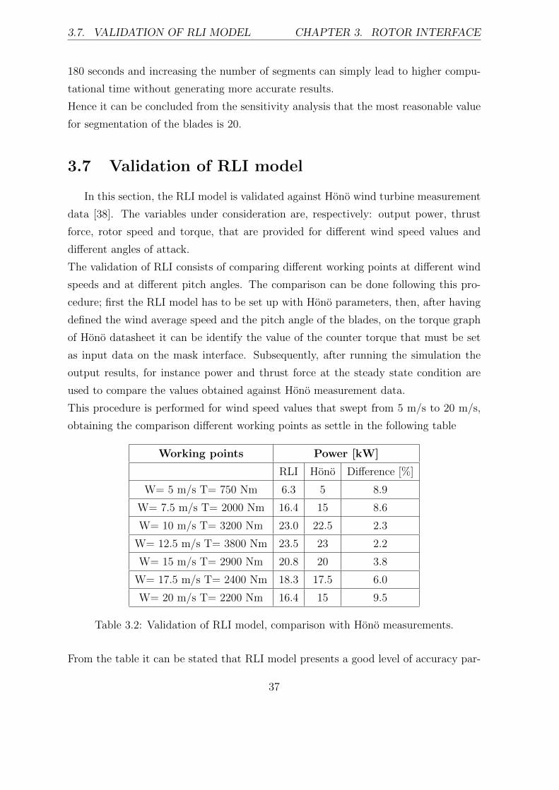
3.7. VALIDATION OF RLI MODEL CHAPTER 3. ROTOR INTERFACE
180 seconds and increasing the number of segments can simply lead to higher compu-
tational time without generating more accurate results.
Hence it can be concluded from the sensitivity analysis that the most reasonable value
for segmentation of the blades is 20.
3.7 Validation of RLI model
In this section, the RLI model is validated against Hono wind turbine measurement
data [38]. The variables under consideration are, respectively: output power, thrust
force, rotor speed and torque, that are provided for different wind speed values and
different angles of attack.
The validation of RLI consists of comparing different working points at different wind
speeds and at different pitch angles. The comparison can be done following this pro-
cedure; first the RLI model has to be set up with Hono parameters, then, after having
defined the wind average speed and the pitch angle of the blades, on the torque graph
of Hono datasheet it can be identify the value of the counter torque that must be set
as input data on the mask interface. Subsequently, after running the simulation the
output results, for instance power and thrust force at the steady state condition are
used to compare the values obtained against Hono measurement data.
This procedure is performed for wind speed values that swept from 5 m/s to 20 m/s,
obtaining the comparison different working points as settle in the following table
Working points Power [kW]
RLI Hono Difference [%]
W= 5 m/s T= 750 Nm 6.3 5 8.9
W= 7.5 m/s T= 2000 Nm 16.4 15 8.6
W= 10 m/s T= 3200 Nm 23.0 22.5 2.3
W= 12.5 m/s T= 3800 Nm 23.5 23 2.2
W= 15 m/s T= 2900 Nm 20.8 20 3.8
W= 17.5 m/s T= 2400 Nm 18.3 17.5 6.0
W= 20 m/s T= 2200 Nm 16.4 15 9.5
Table 3.2: Validation of RLI model, comparison with Hono measurements.
From the table it can be stated that RLI model presents a good level of accuracy par-
37

3.7. VALIDATION OF RLI MODEL CHAPTER 3. ROTOR INTERFACE
ticularly in the wind speed range between 10 m/s to 17,5 m/s, where the maximum
difference is 6%. This gap is essentially due to choice of setting the RLI model para-
menters using a NACA 63-200 airfoil while the Hono airfoil is manually shaped in order
to be a mix of NACA 63-200 and FFA-W3-xxx, therefore the CL and CD coefficients
are different and can affect the values of aerdoynamic forces. Concerning low and high
wind speed, the RLI data and from Hono measurement data differ of more than 7%;
the values power obtained with the simulation and the Hono data are reported in the
following plot which shows the gap that lag between the two data series overall the
wind speed range
5 10 15 204
6
8
10
12
14
16
18
20
22
24
Wind speed [m/s]
Pow
er [k
W]
RLI modelHono measurament
Figure 3.20: Output power comparison between Hono and RLI model.
besides the different airofil shape implemented, for low wind speed, the different
between Hono data and RLI response is also due to the friction of components that
usually is a non-linear function of speed, and in RLI model in not considered. This
observation can be also extended for high wind speed since with at high rotor speed the
losses on rotational components such as bearing increase and higher is the friction higher
are the losses. For this reason the RLI model shows higher output power compared to
Hono data.
As conclusion RLI model globally presents a good accuracy of the results and good
38
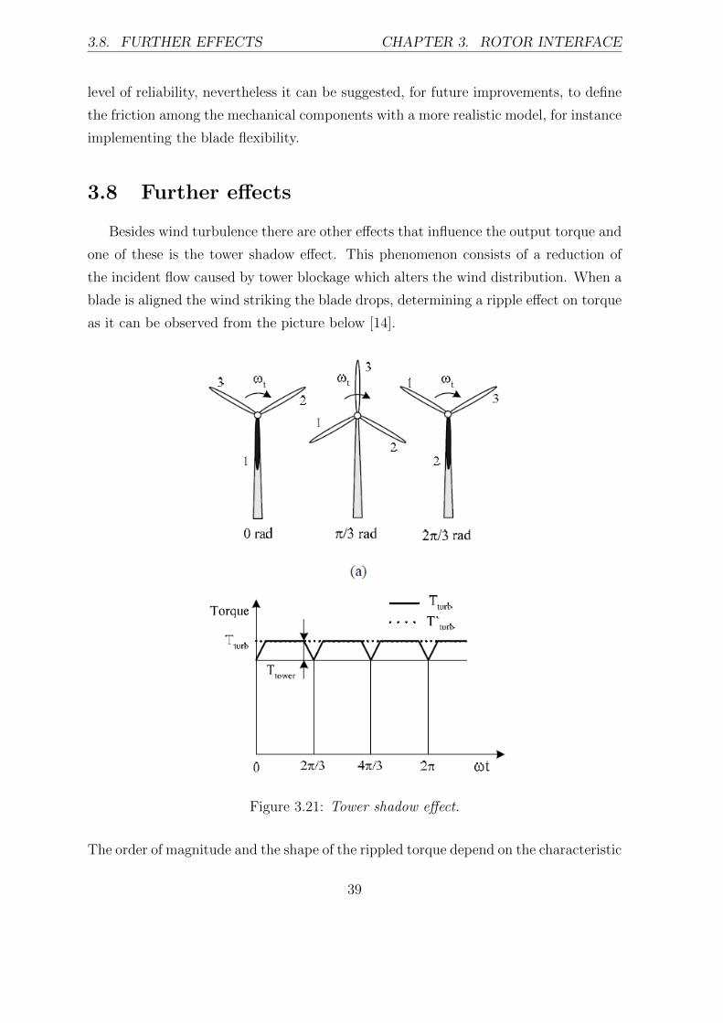
3.8. FURTHER EFFECTS CHAPTER 3. ROTOR INTERFACE
level of reliability, nevertheless it can be suggested, for future improvements, to define
the friction among the mechanical components with a more realistic model, for instance
implementing the blade flexibility.
3.8 Further effects
Besides wind turbulence there are other effects that influence the output torque and
one of these is the tower shadow effect. This phenomenon consists of a reduction of
the incident flow caused by tower blockage which alters the wind distribution. When a
blade is aligned the wind striking the blade drops, determining a ripple effect on torque
as it can be observed from the picture below [14].
Figure 3.21: Tower shadow effect.
The order of magnitude and the shape of the rippled torque depend on the characteristic
39

3.8. FURTHER EFFECTS CHAPTER 3. ROTOR INTERFACE
of the structure.
Another effect is the wind shear that it is particularly important for the multi-MW
wind turbine due to the height of the tower that can be reached around 120 meters.
The wind shear profile can be expressed by the formula [29](W
W0
)=
(z
z0
)a(3.9)
where a is the wind shear exponent and W and W0 are the wind speeds at the heights
above the ground Z and Z0. In order to understand how the wind speed varies with
height, the wind shear function, with a = 0.2 and a wind average speed of 6 m/s, is
plotted below
0 1 2 3 4 5 6 7 8 90
10
20
30
40
50
60
70
80
90
100
Wind speed [m/s]
Hub
hei
ght [
m]
Figure 3.22: Wind shear effect - Height Vs Wind speed. a=0.2
At ground level the wind speed is practically absent due to the friction between airflow
and the ground. With the increase of the height, the wind speed increases significantly
and becomes exploitable for wind energy application over 40 meters from the ground
level [6].
40
3.9. FUTURE WORKS CHAPTER 3. ROTOR INTERFACE
3.9 Future works
The RLI model represents a starting point of the Rotor Load Interface calculation,
therefore the RLI model can be improved from different points of view. Hereinafter
two suggestions are discussed:
1. The blades are modeled as rigid body without considering any flexibility. This
assumption can be made if one wants to have an indicative the amount of loads
on rotor interface and can also provide quite accurate results, in particular for
small size with turbines. Considering a multi MW wind turbine, the blade length
can reach 40 m of length, so it becomes relevant modeling the blades as a flexible
body.
The flexibility of blades can be modeled on RLI model using two methods, namely:
mass lumped-parameter and FE. The first approach consists of a discretization
of the blade into different masses and connect each of them with spring and
damper, while the FE method provides to import the nodes from an FE model
of the model generated with an external software (e.g. Abacus).
2. The RLI model presents different wind conditions that define the wind signal
along axial direction of the wind turbine. In order to dispose a more realistic
and more accurate wind model, the turbulent components along the orthogonal
direction with respect to the axial one must be taken into account. Thereby if
the axial wind direction lies on a X-axis the other two components on the wind
lies respectively on Y and Z axis.
The IEC:2005 standard provides a set of equations for defining analytically three
dimensions wind model or alternatively it is possible to implement the wind model
developed by Applied Mechanics department at Chalmers.
Furthermore the RLI model needs to be validated also against the data from com-
plete wind turbine commercial software such as Vydin, FAST, AdamsWT in order to
guarantee that the rotor load interface data are reliable and quite accurate.
41

Chapter 4
Generator interface
The main wind turbine configurations from the electrical point of view are briefly
introduced. Different modeling techniques of wind turbine generators are discussed.
The Generator Load Interface model is presented and different operational scenarios
are simulated, including network fault. The issue of cogging torque is introduced and
explained with an example.
4.1 Introduction
The Generator, together with the rotor and drivetrain, represents the core of a
wind turbine. As already mentioned on Wind Turbines State of the Art chapter the
generator is the device that converts the mechanical power extract from the wind into
electrical power. Nowadays the generators of modern wind turbine, especially for multi-
MW application are equipped with sophisticated power electronic which can control
the electrical torque and rapidly change it if some problem occurs during normal op-
erational time.
The generator and power electronic can be combined together forming different configu-
rations, but in general the most widespread are, respectively: fixed-speed wind turbines
with a squirrel cage induction generator, double fed induction generator (DFIG) and
full power converter (FCWT). The fixed-speed wind turbine configuration is one of the
first technology developed and is still used for small size wind turbines, on the other
hand large size wind turbines are commonly built with DFIG and FCWT concepts.
Hereinafter the functional scheme of each configuration is reported in the figure.
42
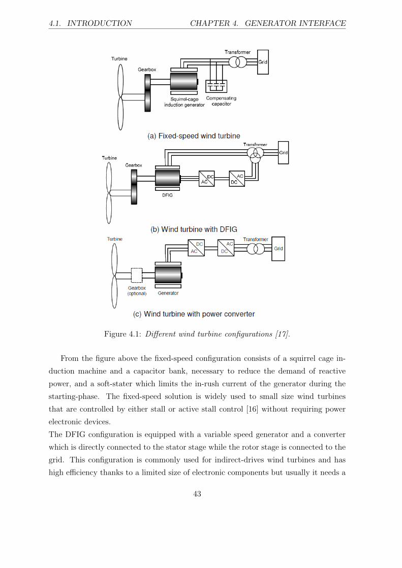
4.1. INTRODUCTION CHAPTER 4. GENERATOR INTERFACE
Figure 4.1: Different wind turbine configurations [17].
From the figure above the fixed-speed configuration consists of a squirrel cage in-
duction machine and a capacitor bank, necessary to reduce the demand of reactive
power, and a soft-stater which limits the in-rush current of the generator during the
starting-phase. The fixed-speed solution is widely used to small size wind turbines
that are controlled by either stall or active stall control [16] without requiring power
electronic devices.
The DFIG configuration is equipped with a variable speed generator and a converter
which is directly connected to the stator stage while the rotor stage is connected to the
grid. This configuration is commonly used for indirect-drives wind turbines and has
high efficiency thanks to a limited size of electronic components but usually it needs a
43

4.2. GENERATOR MODELS CHAPTER 4. GENERATOR INTERFACE
mechanical brake in order to avoid possible failure. In fact if a longer lasting network
fault occurs, the generator starts to accelerate without control because the mechanical
torque of the rotor is not counter balanced by any electromagnetic torque.
The FCWT configuration is normally used for direct drive wind turbines, equipped
with a PM generators. The FCWT can resit to any network problems because the
entire power pass trough a converter but on the other hand a large amount of elec-
tronic components and large cooling system are required, leading inevitably to a lower
efficiency of the wind turbine.
4.2 Generator models
According to figure 2.3 of §2.5, the types of generator can be divided in synchronous
and asynchronous. Both generators are defined with a set of the electromagnetic equa-
tions that describe its operation in dynamic as well as steady state conditions.
Referring to [7] the classification of generator models is based on the number of differ-
ential equations involved, in particular it is possible to define three models: first order
model, third order model and fifth order model [7].
The fifth order model represents the most detailed since both rotor and stator flux
dynamic are taken under consideration. The fifth order model consists of four elec-
tromagnetic equations and one mechanical equation. The definition of the equations
is done using the a equivalent circuit of the generator, which is reported in the figure
below
Figure 4.2: Equivalent circuit of a induction generator - Fifth order model [20].
The equations that governs the stator and rotor can be stated as
~vs = ~isRs + jωe ~ψs +d ~ψsdt
(4.1)
44
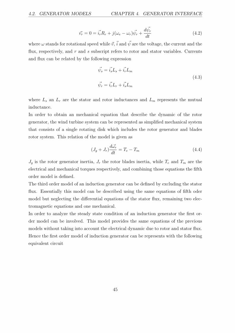
4.2. GENERATOR MODELS CHAPTER 4. GENERATOR INTERFACE
~vr = 0 = ~irRr + j(ωe − ωr) ~ψr +d ~ψrdt
(4.2)
where ω stands for rotational speed while ~v,~i and ~ψ are the voltage, the current and the
flux, respectively, and r and s subscript refers to rotor and stator variables. Currents
and flux can be related by the following expression
~ψs = ~isLs + ~irLm
~ψr = ~irLr + ~isLm
(4.3)
where Ls an Lr are the stator and rotor inductances and Lm represents the mutual
inductance.
In order to obtain an mechanical equation that describe the dynamic of the rotor
generator, the wind turbine system can be represented as simplified mechanical system
that consists of a single rotating disk which includes the rotor generator and blades
rotor system. This relation of the model is given as
(Jg + Jr)d ~ωrdt
= Te − Tm (4.4)
Jg is the rotor generator inertia, Jr the rotor blades inertia, while Te and Tm are the
electrical and mechanical torques respectively, and combining those equations the fifth
order model is defined.
The third order model of an induction generator can be defined by excluding the stator
flux. Essentially this model can be described using the same equations of fifth oder
model but neglecting the differential equations of the stator flux, remaining two elec-
tromagnetic equations and one mechanical.
In order to analyze the steady state condition of an induction generator the first or-
der model can be involved. This model provides the same equations of the previous
models without taking into account the electrical dynamic due to rotor and stator flux.
Hence the first order model of induction generator can be represents with the following
equivalent circuit
45
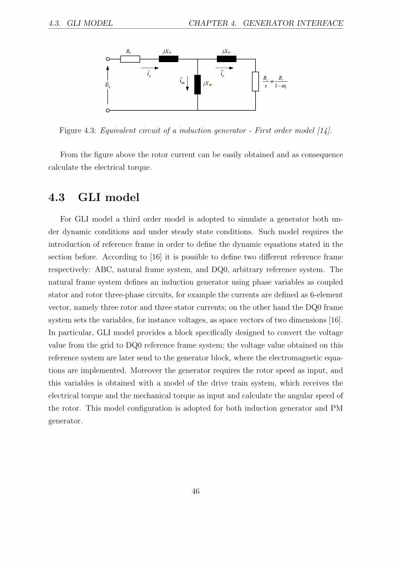
4.3. GLI MODEL CHAPTER 4. GENERATOR INTERFACE
Figure 4.3: Equivalent circuit of a induction generator - First order model [14].
From the figure above the rotor current can be easily obtained and as consequence
calculate the electrical torque.
4.3 GLI model
For GLI model a third order model is adopted to simulate a generator both un-
der dynamic conditions and under steady state conditions. Such model requires the
introduction of reference frame in order to define the dynamic equations stated in the
section before. According to [16] it is possible to define two different reference frame
respectively: ABC, natural frame system, and DQ0, arbitrary reference system. The
natural frame system defines an induction generator using phase variables as coupled
stator and rotor three-phase circuits, for example the currents are defined as 6-element
vector, namely three rotor and three stator currents; on the other hand the DQ0 frame
system sets the variables, for instance voltages, as space vectors of two dimensions [16].
In particular, GLI model provides a block specifically designed to convert the voltage
value from the grid to DQ0 reference frame system; the voltage value obtained on this
reference system are later send to the generator block, where the electromagnetic equa-
tions are implemented. Moreover the generator requires the rotor speed as input, and
this variables is obtained with a model of the drive train system, which receives the
electrical torque and the mechanical torque as input and calculate the angular speed of
the rotor. This model configuration is adopted for both induction generator and PM
generator.
46
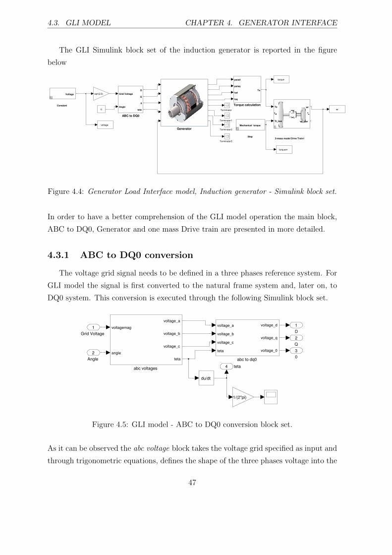
4.3. GLI MODEL CHAPTER 4. GENERATOR INTERFACE
The GLI Simulink block set of the induction generator is reported in the figure
below
Torque calculation
psisd
psisq
isd
isq
Te
Time scope
Terminator3
Terminator2
Terminator1
Terminator
Generator
ABC to DQ0
Grid Voltage
Angle
D
Q
0
teta
torquem
torque
wr
sqrt(2/3)
0
Constant
Voltage
2-mass model Drive Train1
Te
Tt_low
wr
wt_low
voltage
Step
Mechanical torque
Figure 4.4: Generator Load Interface model, Induction generator - Simulink block set.
In order to have a better comprehension of the GLI model operation the main block,
ABC to DQ0, Generator and one mass Drive train are presented in more detailed.
4.3.1 ABC to DQ0 conversion
The voltage grid signal needs to be defined in a three phases reference system. For
GLI model the signal is first converted to the natural frame system and, later on, to
DQ0 system. This conversion is executed through the following Simulink block set.
teta4
0
3
Q
2
D
1
abc voltages
voltagemag
angle
voltage_a
voltage_b
voltage_c
teta abc to dq0
voltage_a
voltage_b
voltage_c
teta
voltage_d
voltage_q
voltage_0
du/dt
1/(2*pi)
Angle
2
Grid Voltage
1
Figure 4.5: GLI model - ABC to DQ0 conversion block set.
As it can be observed the abc voltage block takes the voltage grid specified as input and
through trigonometric equations, defines the shape of the three phases voltage into the
47
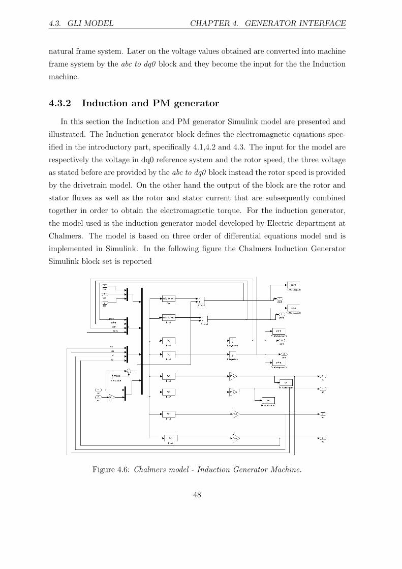
4.3. GLI MODEL CHAPTER 4. GENERATOR INTERFACE
natural frame system. Later on the voltage values obtained are converted into machine
frame system by the abc to dq0 block and they become the input for the the Induction
machine.
4.3.2 Induction and PM generator
In this section the Induction and PM generator Simulink model are presented and
illustrated. The Induction generator block defines the electromagnetic equations spec-
ified in the introductory part, specifically 4.1,4.2 and 4.3. The input for the model are
respectively the voltage in dq0 reference system and the rotor speed, the three voltage
as stated before are provided by the abc to dq0 block instead the rotor speed is provided
by the drivetrain model. On the other hand the output of the block are the rotor and
stator fluxes as well as the rotor and stator current that are subsequently combined
together in order to obtain the electromagnetic torque. For the induction generator,
the model used is the induction generator model developed by Electric department at
Chalmers. The model is based on three order of differential equations model and is
implemented in Simulink. In the following figure the Chalmers Induction Generator
Simulink block set is reported
Figure 4.6: Chalmers model - Induction Generator Machine.
48

4.3. GLI MODEL CHAPTER 4. GENERATOR INTERFACE
Concerning the PM generator, a similar model is proposed. The starting point is the
Simulink PM generator model developed by Risø National Laboratory [36]. The model
provides a third order PM generator which is described by 4.2 equations but without
considering the slip on voltage rotor equation. As for the induction generator the input
of Risø model are respectively, the rotor speed and the three voltage, while the output
data are stator fluxes, the rotor and stator currents and the electromagnetic torque.
Hereinafter the Risø PM generator Simulink block set is presented.
is_UVW
2
Te
1
isq
U Yisd
U Y
dq / abc
D
Q
theta
A
B
C
disq/dt
a21*u[9]*u[1]+a22*u[2]+a23*u[9]*u[3]+a24*u[9]*u[4]+a25*u[5]+a26*u[7]
disd/dt
a11*u[1]+a12*u[9]*u[2]+a13*u[3]+a14*u[4]+a15*u[9]*u[5]+a16*u[6]+a17*u[8]
dirq/dt
a51*u[9]*u[1]+a52*u[2]+a53*u[9]*u[3]+a54*u[9]*u[4]+a55*u[5]+a56*u[7]
dird/dt
a41*u[1]+a42*u[9]*u[2]+a43*u[3]+a44*u[4]+a45*u[9]*u[5]+a46*u[6]+a47*u[8]
dif/dt
a31*u[1]+a32*u[9]*u[2]+a33*u[3]+a34*u[4]+a35*u[9]*u[5]+a36*u[6]+a37*u[8]
Telm
1.5*np*((Lmd-Lmq)*u[1]*u[2]+Lmq*u[2]*(u[3]+u[4])-Lmq*u[5]*u[1])
Mux
1
s
1
s
1
s
1
s
1
s
theta
Demux
omgr
3
uf
2
usdq
1
<>
<>
Figure 4.7: Risø National Laboratory model - PM Generator Machine.
49

4.3. GLI MODEL CHAPTER 4. GENERATOR INTERFACE
4.3.3 Drivetrain
As stated in the introductory section, the third order generator required a mechan-
ical equation in order to determine the rotor speed that represents the input of the
Induction and the PM Simulink generator models. The rotor speed varies according
to the dynamic response of the dirvetrain system, therefore the rotor speed is a func-
tion of generator, rotor and gearbox inertias as well as the electromagnetic torque and
rotor mechanical torque. With GLI model two different drivetrain models are imple-
mented, namely one-mass and two-mass drivetrain model. The first model is essentially
one rotating mass including both rotor and generator inertia, on which a mechanical
torque and electromagnetic torque are applied with opposite direction and the balance
equation is the 4.3 relation. Hereinafter the Simulink model of one mass dirvetrain is
reported
wr
1
To Workspace3
wt
Integrator2
1
s
1/gr
1/gr
1/(Jg+Jt)
Tt_low
2
Te
1
Figure 4.8: GLI model - One Mass Drive train.
On the contrary the Two-mass drivetrain model is a unique shaft with a torsion spring
and damper which connected the rotating mass of the rotor with the generator one and
the model can be represented with the following scheme.
Figure 4.9: GLI model - two-mass Drive train [4].
50
4.4. SIMULATIONS CHAPTER 4. GENERATOR INTERFACE
According to the notations of the picture above the mathematical equations of a
two-mass drivetrain model are given as [4]
Jtdωtdt
= Tt −Ks(θr − θt)−Dm(ωr − ωt) (4.5)
Jgdωrdt
= −Te −Ks(θr − θt)−Dm(ωr − ωt) (4.6)
dθtdt
= ωt (4.7)
dθrdt
= ωr (4.8)
4.4 Simulations
In this section different simulations of an induction and PM generator are pre-
sented. The induction generator under consideration is a 180 kW power and the PM
generator is a 4.5 MW power and for both, the construction characteristic are reported
on Appendix A, respectively on table A.3 and A.4. Basically with these simulations,
the response of the generator under different scenarios are investigated; specifically the
electromagnetic torque response subject to a constant mechanical torque as well as to
a drop, furthermore the influence of network emergency is also simulated, in particular
a network fault.
The set of variables under investigation for both types of generator are: generator char-
acteristic, the grid voltage, electromagnetic torque and rotor speed. All the variables
are detected in time domain. Additionally the electrical and mechanical power and the
power losses are investigated as well.
51
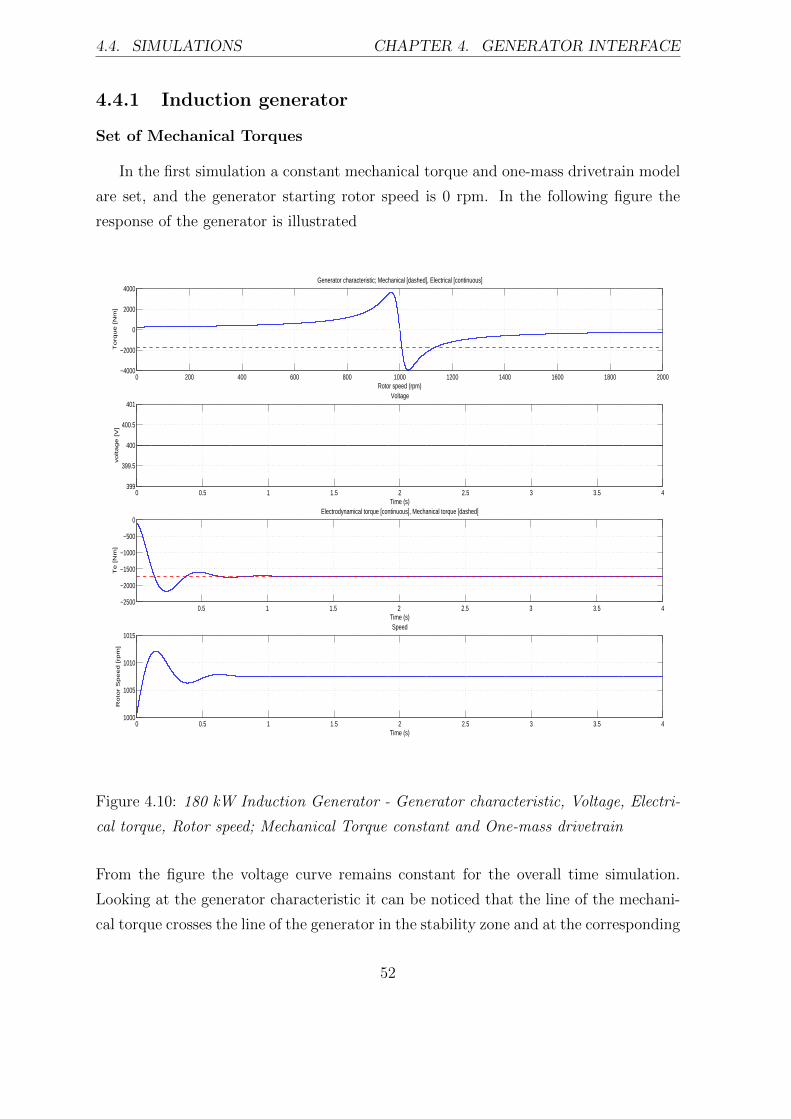
4.4. SIMULATIONS CHAPTER 4. GENERATOR INTERFACE
4.4.1 Induction generator
Set of Mechanical Torques
In the first simulation a constant mechanical torque and one-mass drivetrain model
are set, and the generator starting rotor speed is 0 rpm. In the following figure the
response of the generator is illustrated
0 200 400 600 800 1000 1200 1400 1600 1800 2000−4000
−2000
0
2000
4000
Rotor speed (rpm)
To
rqu
e [N
m]
Generator characteristic; Mechanical [dashed], Electrical [continuous]
0 0.5 1 1.5 2 2.5 3 3.5 4399
399.5
400
400.5
401
Time (s)
vo
lta
ge
[V
]
Voltage
0.5 1 1.5 2 2.5 3 3.5 4−2500
−2000
−1500
−1000
−500
0
Time (s)
Te
[N
m]
Electrodynamical torque [continuous], Mechanical torque [dashed]
0 0.5 1 1.5 2 2.5 3 3.5 41000
1005
1010
1015
Time (s)
Ro
tor
Sp
ee
d [rp
m]
Speed
Figure 4.10: 180 kW Induction Generator - Generator characteristic, Voltage, Electri-
cal torque, Rotor speed; Mechanical Torque constant and One-mass drivetrain
From the figure the voltage curve remains constant for the overall time simulation.
Looking at the generator characteristic it can be noticed that the line of the mechani-
cal torque crosses the line of the generator in the stability zone and at the corresponding
52
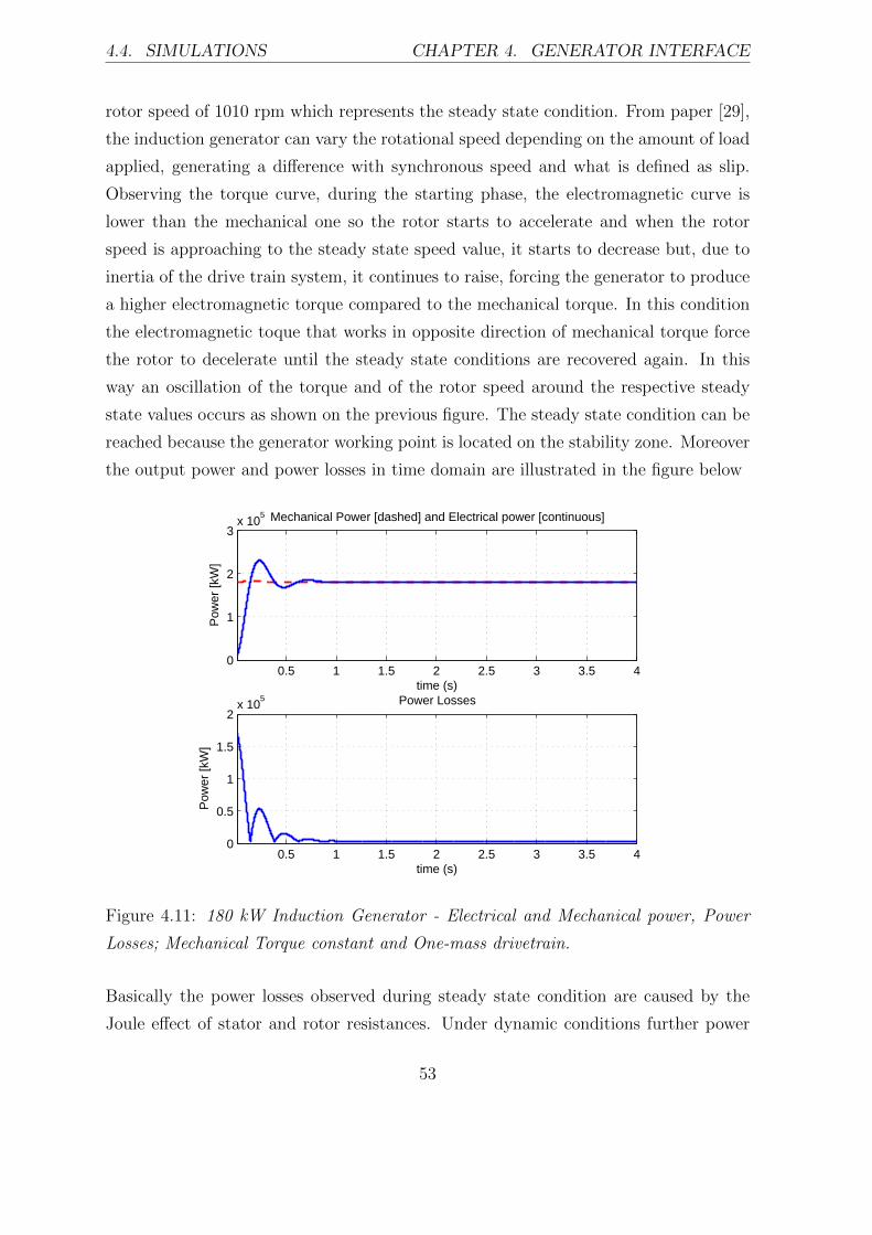
4.4. SIMULATIONS CHAPTER 4. GENERATOR INTERFACE
rotor speed of 1010 rpm which represents the steady state condition. From paper [29],
the induction generator can vary the rotational speed depending on the amount of load
applied, generating a difference with synchronous speed and what is defined as slip.
Observing the torque curve, during the starting phase, the electromagnetic curve is
lower than the mechanical one so the rotor starts to accelerate and when the rotor
speed is approaching to the steady state speed value, it starts to decrease but, due to
inertia of the drive train system, it continues to raise, forcing the generator to produce
a higher electromagnetic torque compared to the mechanical torque. In this condition
the electromagnetic toque that works in opposite direction of mechanical torque force
the rotor to decelerate until the steady state conditions are recovered again. In this
way an oscillation of the torque and of the rotor speed around the respective steady
state values occurs as shown on the previous figure. The steady state condition can be
reached because the generator working point is located on the stability zone. Moreover
the output power and power losses in time domain are illustrated in the figure below
0.5 1 1.5 2 2.5 3 3.5 40
1
2
3x 10
5
time (s)
Pow
er [k
W]
Mechanical Power [dashed] and Electrical power [continuous]
0.5 1 1.5 2 2.5 3 3.5 40
0.5
1
1.5
2x 10
5
time (s)
Pow
er [k
W]
Power Losses
Figure 4.11: 180 kW Induction Generator - Electrical and Mechanical power, Power
Losses; Mechanical Torque constant and One-mass drivetrain.
Basically the power losses observed during steady state condition are caused by the
Joule effect of stator and rotor resistances. Under dynamic conditions further power
53

4.4. SIMULATIONS CHAPTER 4. GENERATOR INTERFACE
losses occur, in particular the magnetizing power of inductances and capacitors that
are not considered a contribution to electric power as well as the power absorbed from
the grid when the electromagnetic torque is higher than the mechanical one. From the
figure 4.11, the losses on the starting phase correspond to the energy requires to mag-
netize the circuits, while on the following peaks are the effect of the power absorbed
from the grid.
Maintaining the same scenario and value of the mechanical torque as well as the same
generator parameters, a simulation of the induction generator with the two-mass driv-
etrain model is performed. The simulation results obtained are shown below
0 200 400 600 800 1000 1200 1400 1600 1800 2000−4000
−2000
0
2000
4000
Rotor speed (rpm)
To
rqu
e [N
m]
Generator characteristic; Mechanical [dashed], Electrical [continuous]
0 0.5 1 1.5 2 2.5 3 3.5 4399
399.5
400
400.5
401
Time (s)
vo
lta
ge
[V
]
Voltage
0.5 1 1.5 2 2.5 3 3.5 4−3000
−2000
−1000
0
1000
Time (s)
Te
[N
m]
Electrodynamical torque [continuous], Mechanical torque [dashed]
0 0.5 1 1.5 2 2.5 3 3.5 4990
995
1000
1005
1010
1015
Time (s)
Ro
tor
Sp
ee
d [rp
m]
Speed
Figure 4.12: 180 kW Induction Generator - Generator characteristic, Voltage, Electri-
cal torque, Rotor speed; Mechanical Torque constant and Two-mass drivetrain.
54

4.4. SIMULATIONS CHAPTER 4. GENERATOR INTERFACE
The generator characteristic and voltage curve are the same as the previous simulation,
the main differences are the responses of rotor speed and of the electromagnetic curve.
In fact one can observe that both variables are subject to larger variations which also
last longer compared to the case with one-mass drivetrain model. The cause of these
oscillations is the shaft flexibility which establishes torsion vibrations along the drive-
train system. This oscillations influence also the power response as it can be observed
on figure below
0.5 1 1.5 2 2.5 3 3.5 4−1
0
1
2
3x 10
5
time (s)
Pow
er [k
W]
Mechanical Power [dashed] and Electrical power [continuous]
0.5 1 1.5 2 2.5 3 3.5 40
1
2
3x 10
5
time (s)
Pow
er [k
W]
Power Losses
Figure 4.13: 180 kW Induction Generator - Electrical and Mechanical power, Power
Losses; Mechanical Torque constant and Two-mass drivetrain.
Comparing the results with the one-mass drivetrain model simulation of figure 4.11, it
can be noticed that the simulation with the Two-mass drivetrain model leads to higher
losses because the oscillations, that occur on the shaft, force the generator to produce
an electromagnetic torque higher than mechanical one, by taking energy from the grid,
necessary to reach the steady state condition.
55

4.4. SIMULATIONS CHAPTER 4. GENERATOR INTERFACE
The second operational scenario investigated is a sudden mechanical step, which
in reality, can be caused by a emergency rotor braking. Specifically the step occurs
after 20 seconds, when the the steady state condition are reached, and it lasts for 1
second. The magnitude drop is the 80% the rated mechanical torque. Moreover for
this simulation the two-mass drivetrain model is adopted. The simulation results are
the following
0 200 400 600 800 1000 1200 1400 1600 1800 2000−4000
−2000
0
2000
4000
Rotor speed (rpm)
To
rqu
e [N
m]
Generator characteristic; Mechanical [dashed], Electrical [continuous]
0 5 10 15 20 25 30 35 40399
399.5
400
400.5
401
Time (s)
vo
lta
ge
[V
]
Voltage
5 10 15 20 25 30 35 40−3000
−2000
−1000
0
1000
Time (s)
Te
[N
m]
Electrodynamical torque [continuous], Mechanical torque [dashed]
0 5 10 15 20 25 30 35 40990
995
1000
1005
1010
1015
Time (s)
Ro
tor
Sp
ee
d [rp
m]
Speed
Figure 4.14: 180 kW Induction Generator - Generator characteristic, Voltage, Electri-
cal torque, Rotor speed; Mechanical Torque drop and Two-mass drivetrain.
When the step occurs the electromagnetic as well as the rotor speed are subjected to
a significant change that implies a variation of rotor speed. The rotor speed presents
56

4.4. SIMULATIONS CHAPTER 4. GENERATOR INTERFACE
a drop of 1% going from 1007 rpm to 996 rpm, then when the step of mechanical
torque ends the electromagnetic torque is restored and the rotor speed is subjected to
a oscillation transimitted to the drivetrain.
Network fault
In this section the response of the induction generator subjected to a network fault
is illustrated. Specifically the simulation of the network fault consists of a drop 90%
of the grid voltage for a time of 250 ms, that corresponds to the maximum fault time
accettable in Sweden [26]. The response of the generator is reported in the figure below
0 200 400 600 800 1000 1200 1400 1600 1800 2000−4000
−2000
0
2000
4000
Rotor speed (rpm)
To
rqu
e [N
m]
Generator characteristic; Mechanical [dashed], Electrical [continuous]
0 5 10 15 20 25 30 35 400
100
200
300
400
Time (s)
vo
lta
ge
[V
]
Voltage
5 10 15 20 25 30 35 40−4000
−3000
−2000
−1000
0
Time (s)
Te
[N
m]
Electrodynamical torque [continuous], Mechanical torque [dashed]
0 5 10 15 20 25 30 35 401000
1010
1020
1030
1040
1050
Time (s)
Ro
tor
Sp
ee
d [rp
m]
Speed
Figure 4.15: 180 kW Induction Generator - Generator characteristic, Voltage, Electri-
cal torque, Rotor speed; Network fault 250 ms and One-mass drivetrain.
57
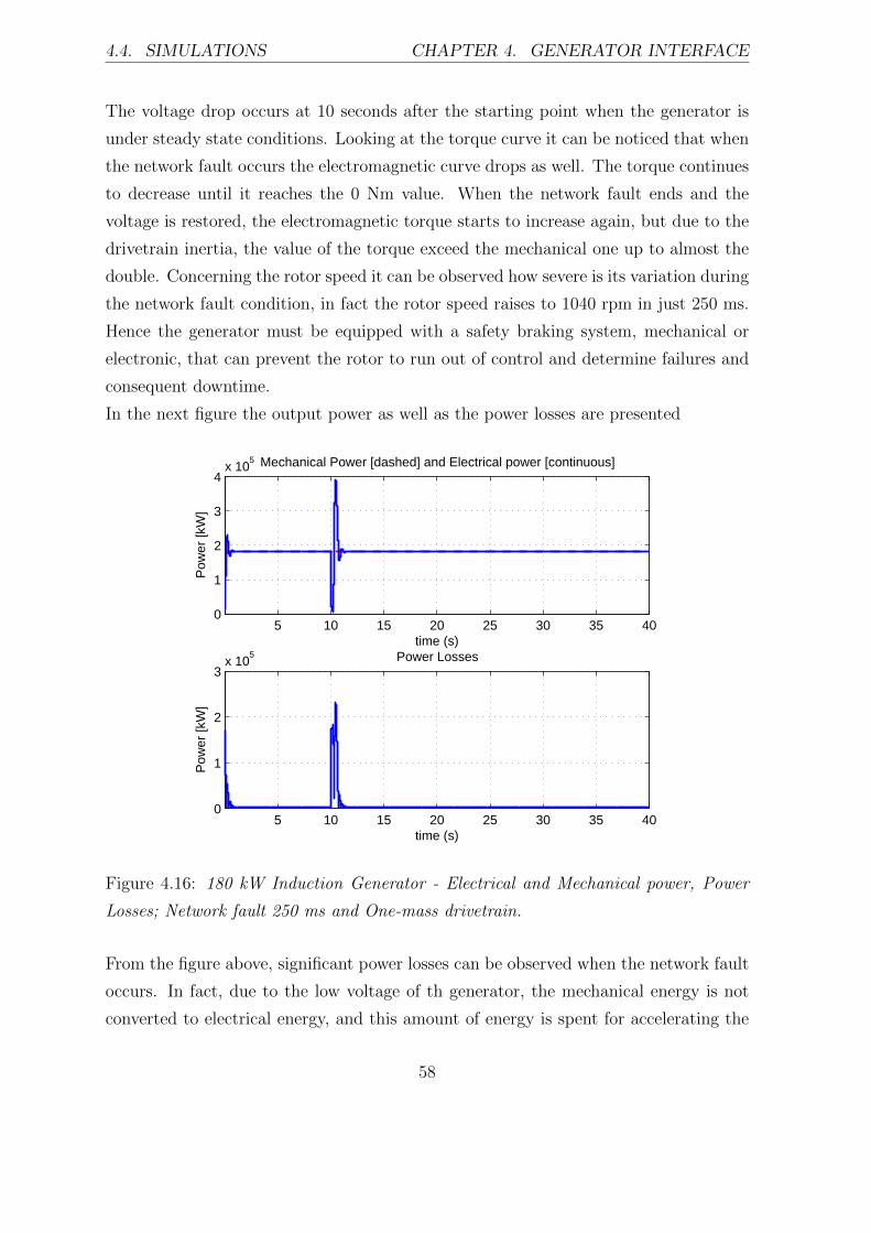
4.4. SIMULATIONS CHAPTER 4. GENERATOR INTERFACE
The voltage drop occurs at 10 seconds after the starting point when the generator is
under steady state conditions. Looking at the torque curve it can be noticed that when
the network fault occurs the electromagnetic curve drops as well. The torque continues
to decrease until it reaches the 0 Nm value. When the network fault ends and the
voltage is restored, the electromagnetic torque starts to increase again, but due to the
drivetrain inertia, the value of the torque exceed the mechanical one up to almost the
double. Concerning the rotor speed it can be observed how severe is its variation during
the network fault condition, in fact the rotor speed raises to 1040 rpm in just 250 ms.
Hence the generator must be equipped with a safety braking system, mechanical or
electronic, that can prevent the rotor to run out of control and determine failures and
consequent downtime.
In the next figure the output power as well as the power losses are presented
5 10 15 20 25 30 35 400
1
2
3
4x 10
5
time (s)
Pow
er [k
W]
Mechanical Power [dashed] and Electrical power [continuous]
5 10 15 20 25 30 35 400
1
2
3x 10
5
time (s)
Pow
er [k
W]
Power Losses
Figure 4.16: 180 kW Induction Generator - Electrical and Mechanical power, Power
Losses; Network fault 250 ms and One-mass drivetrain.
From the figure above, significant power losses can be observed when the network fault
occurs. In fact, due to the low voltage of th generator, the mechanical energy is not
converted to electrical energy, and this amount of energy is spent for accelerating the
58
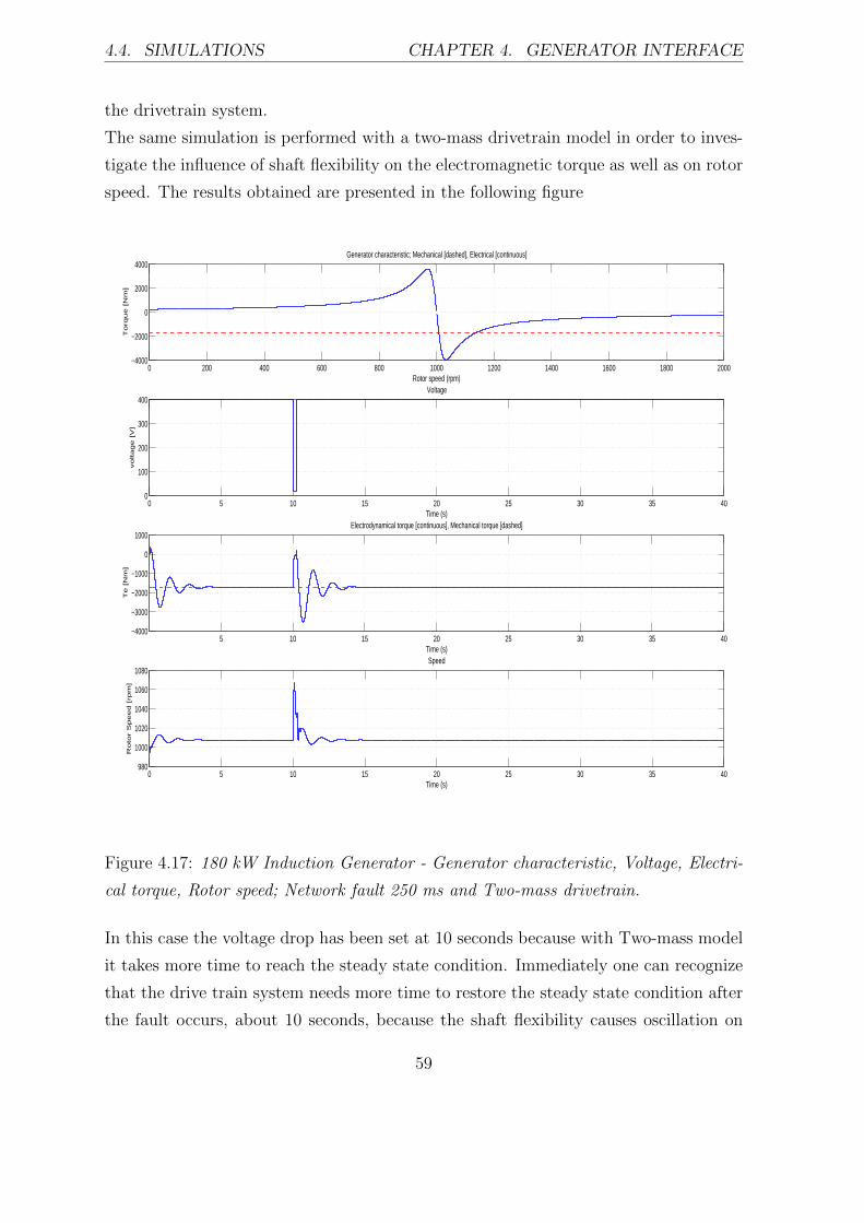
4.4. SIMULATIONS CHAPTER 4. GENERATOR INTERFACE
the drivetrain system.
The same simulation is performed with a two-mass drivetrain model in order to inves-
tigate the influence of shaft flexibility on the electromagnetic torque as well as on rotor
speed. The results obtained are presented in the following figure
0 200 400 600 800 1000 1200 1400 1600 1800 2000−4000
−2000
0
2000
4000
Rotor speed (rpm)
To
rqu
e [N
m]
Generator characteristic; Mechanical [dashed], Electrical [continuous]
0 5 10 15 20 25 30 35 400
100
200
300
400
Time (s)
vo
lta
ge
[V
]
Voltage
5 10 15 20 25 30 35 40−4000
−3000
−2000
−1000
0
1000
Time (s)
Te
[N
m]
Electrodynamical torque [continuous], Mechanical torque [dashed]
0 5 10 15 20 25 30 35 40980
1000
1020
1040
1060
1080
Time (s)
Ro
tor
Sp
ee
d [rp
m]
Speed
Figure 4.17: 180 kW Induction Generator - Generator characteristic, Voltage, Electri-
cal torque, Rotor speed; Network fault 250 ms and Two-mass drivetrain.
In this case the voltage drop has been set at 10 seconds because with Two-mass model
it takes more time to reach the steady state condition. Immediately one can recognize
that the drive train system needs more time to restore the steady state condition after
the fault occurs, about 10 seconds, because the shaft flexibility causes oscillation on
59
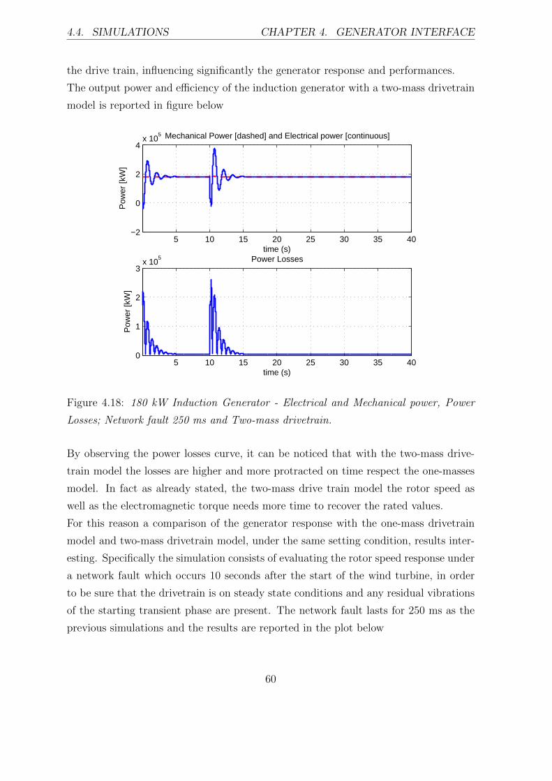
4.4. SIMULATIONS CHAPTER 4. GENERATOR INTERFACE
the drive train, influencing significantly the generator response and performances.
The output power and efficiency of the induction generator with a two-mass drivetrain
model is reported in figure below
5 10 15 20 25 30 35 40−2
0
2
4x 10
5
time (s)
Pow
er [k
W]
Mechanical Power [dashed] and Electrical power [continuous]
5 10 15 20 25 30 35 400
1
2
3x 10
5
time (s)
Pow
er [k
W]
Power Losses
Figure 4.18: 180 kW Induction Generator - Electrical and Mechanical power, Power
Losses; Network fault 250 ms and Two-mass drivetrain.
By observing the power losses curve, it can be noticed that with the two-mass drive-
train model the losses are higher and more protracted on time respect the one-masses
model. In fact as already stated, the two-mass drive train model the rotor speed as
well as the electromagnetic torque needs more time to recover the rated values.
For this reason a comparison of the generator response with the one-mass drivetrain
model and two-mass drivetrain model, under the same setting condition, results inter-
esting. Specifically the simulation consists of evaluating the rotor speed response under
a network fault which occurs 10 seconds after the start of the wind turbine, in order
to be sure that the drivetrain is on steady state conditions and any residual vibrations
of the starting transient phase are present. The network fault lasts for 250 ms as the
previous simulations and the results are reported in the plot below
60

4.4. SIMULATIONS CHAPTER 4. GENERATOR INTERFACE
0 5 10 15 20 25 30 35 40990
1000
1010
1020
1030
1040
1050
1060
1070
Time (s)
[rpm
]
Rotor Speed
One−massTwo mass
Figure 4.19: 180 kW Generator Network fault 250 ms - Comparison of the rotor speed
with One-mass and Two-mass drivetrain.
The figure shows that the rotor speed for the Induction generator with Two-mass
drivetrain model reaches the highest value of 1068 rpm when the network fault occurs.
On the contrary the highest rotor speed of Induction generator with One-mass drive-
train model is 1040 rpm. Although the difference between the two rotor speed peaks is
20 %, when a network fault occurs, the generator charcteristic is different and if, after
the normal condition are restored, the new working point is situated in the instability
zone, the generator could run out of control. So if the shaft is too flexible, under critical
conditions, it can avoid the generator to run out of control and causing damages of the
electrical componets.
Furthermore as already stated for the previous simulations the Two-mass model es-
tablishes more vibrations that need longer time to be extinguished. Hence with the
Two-mass drivetrain model the generator, during dynamic conditions, shows a less
power production than with one-mass model, concluding that the vibrations of the
drivetrain system can affect the power production.
61

4.4. SIMULATIONS CHAPTER 4. GENERATOR INTERFACE
4.4.2 PM generator
Step of Mechanical Torque
The PM generator model under investigation is set with Two-mass drivetrain whose
transmission ratio value is equal to one in order to define a direct drive transmission
system. The simulation condition is a drop of 90 % of mechanical torque rated vaule
which lasts for 2 seconds. The results of the simulation are the following
0 2 4 6 8 10 12 14 16 18 20 22−4
−3
−2
−1
0x 10
6
Rotor speed (rpm)
To
rqu
e [N
m]
Electrodynamical torque [continuous], Mechanical torque [dashed]
0 5 10 15 20 25 30 35 400
100
200
300
400
500
Time (s)
vo
lta
ge
[V
]
Voltage
5 10 15 20 25 30 35 40−6
−4
−2
0
2x 10
6
Time (s)
Te
[N
m]
Mechanical Power [dashed] and Electrical power [continuous]
5 10 15 20 25 30 35 4011
11.5
12
12.5
Time (s)
Ro
tor
Sp
ee
d [rp
m]
Speed
Figure 4.20: 4.5 MW PM Generator; Mechanical Torque drop - Two-mass drivetrain.
The mechanical drop occurs after 30 seconds from the starting point, allowing the
generator to reach the steady state conditions. From the generator characteristic the
62

4.4. SIMULATIONS CHAPTER 4. GENERATOR INTERFACE
synchronous speed of the generator is 12 rpm. This speed remains constant until the
mechanical drop occurs, then the generator tries to follow the mechanical torque in
order to maintain the synchronous speed. The torque curves show that the response
of the electromagnetic curve is characterized by high amplitude oscillations around the
mechanical torque while the rotor speed shows small variations of synchronous speed,
around 0.08%.
Network fault
As for the induction generator a network fault is simulated for the PM generator.
The voltage drop is set after 25 seconds of the starting point and it lasts for 250 ms.
0 2 4 6 8 10 12 14 16 18 20 22−4
−3
−2
−1
0x 10
6
Rotor speed (rpm)
To
rqu
e [N
m]
Electrodynamical torque [continuous], Mechanical torque [dashed]
0 5 10 15 20 25 30 35 400
100
200
300
400
500
Time (s)
vo
lta
ge
[V
]
Voltage
5 10 15 20 25 30 35 40−1
−0.5
0
0.5
1x 10
8
Time (s)
Te
[N
m]
Mechanical Power [dashed] and Electrical power [continuous]
5 10 15 20 25 30 35 400
5
10
15
20
Time (s)
Ro
tor
Sp
ee
d [rp
m]
Speed
Figure 4.21: 4.5 MW PM Generator - Network fault 250 ms and Two-mass drivetrain.
According to the torque curves, the electromagnetic torque undergoes to significant
63
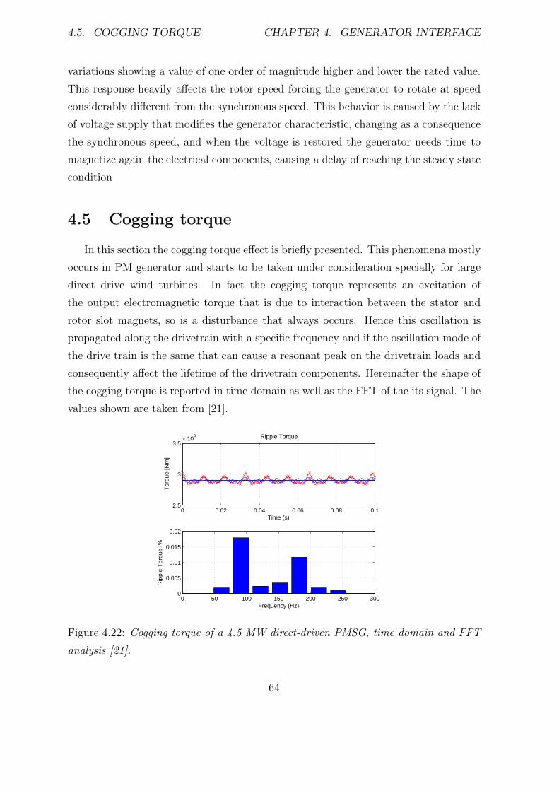
4.5. COGGING TORQUE CHAPTER 4. GENERATOR INTERFACE
variations showing a value of one order of magnitude higher and lower the rated value.
This response heavily affects the rotor speed forcing the generator to rotate at speed
considerably different from the synchronous speed. This behavior is caused by the lack
of voltage supply that modifies the generator characteristic, changing as a consequence
the synchronous speed, and when the voltage is restored the generator needs time to
magnetize again the electrical components, causing a delay of reaching the steady state
condition
4.5 Cogging torque
In this section the cogging torque effect is briefly presented. This phenomena mostly
occurs in PM generator and starts to be taken under consideration specially for large
direct drive wind turbines. In fact the cogging torque represents an excitation of
the output electromagnetic torque that is due to interaction between the stator and
rotor slot magnets, so is a disturbance that always occurs. Hence this oscillation is
propagated along the drivetrain with a specific frequency and if the oscillation mode of
the drive train is the same that can cause a resonant peak on the drivetrain loads and
consequently affect the lifetime of the drivetrain components. Hereinafter the shape of
the cogging torque is reported in time domain as well as the FFT of the its signal. The
values shown are taken from [21].
0 0.02 0.04 0.06 0.08 0.12.5
3
3.5x 10
6
Time (s)
Tor
que
[Nm
]
Ripple Torque
0 50 100 150 200 250 3000
0.005
0.01
0.015
0.02
Frequency (Hz)
Rip
ple
Tor
que
[%]
Figure 4.22: Cogging torque of a 4.5 MW direct-driven PMSG, time domain and FFT
analysis [21].
64

4.6. FUTURE WORKS CHAPTER 4. GENERATOR INTERFACE
In time domain signal, blue curves represents the different harmonics while the
red one is the total signal. Furthermore the relative amplitude and frequencies of each
ripple torque are reported in the bar plot. The percentage of the amplitude is calculated
as relative torque value with the respect of the rated torque one.
4.6 Future works
The modern generators are equipped with advanced electronic controls in order to
prevent failures as well as to improve the performances and the efficiency. The GLI
model is characterized by an induction generator and a synchronous generator without
any kind of electronic control. Hence one suggestion for future outlooks is to implement
a control of active and reactive powers for both generator types. This modification will
affect the response of the generators under different conditons and avoiding potential
dangerous conditions that can cause damage of the generator.
Furthermore, concerning the Induction generator, a more advanced model for the driv-
etrain system can be implemented in order to have a more realistic response of the
generator under different operational scenarios. For instance [32] suggests to define a
model which takes into account both the inertia of the gears of the gearbox and the
efficiency of the entire transmission.
In the end it is recommended to validate the GLI model with measurement data, if
available, as well as with the data from commercial software products.
65
Chapter 5
Tower interface
The set of mathematical equations of the loads acting on an on-shore and an off-
shore wind turbine towers are presented. The Tower Load Interface model is presented
showing the Simulink block set. The response of an on-shore tower under different
constant wind speed conditions is performed. Moreover an off-shore wind turbine tower
is tested under constant wind speed conditions and a periodic function representing the
interaction between waves and foundations.
5.1 Introduction
The modern wind turbines are subjected to significant loads on tower due to wind
pressure but also due to waves in case of off-shore wind turbines. According to the
environmental conditions, the interaction between wind and tower as well as waves
and foundations generates periodic or random loads that cause vibrations that are
directly transmitted to the drivetrain system through connection supports with the
tower, e.g. bearings. Moreover for wind turbines equipped with yaw motion system,
the gyroscopic effect can establish vibrations that, combined with the ones produced
by wind, could yield to critical resonance condition.
5.2 Tower load
The main source of loads for wind turbine tower comes from the wind, from the
gravity and, for off-shore application, from the waves. Referring to [33] the loads
sustained by tower can be represented as in the following figure
66

5.2. TOWER LOAD CHAPTER 5. TOWER INTERFACE
Fwind
Fwave
Fg
Fr
Y
X
Figure 5.1: Loads of an off-shore wind turbine tower.
Specifically the gravity load (Fg) which consists of tower, nacelle and rotor weights,
the wave load (Fwave) which is the effect of interaction between wave and foundation
of the tower, and the wind loads that act on the tower in two different manners. In
particular when an air flow invests the wind turbine, the thrust force (Fr) generated
on rotor blades is transmitted to the drivetrain and then forwarded to top of the
67
5.2. TOWER LOAD CHAPTER 5. TOWER INTERFACE
tower through the supports. Additionally, the interaction between air flow and tower
produces a pressure distribution (Fwind) along the tower itself which depends on the
height according to the wind shear equation 4.5, stated in §3.8.
Each loads are defined with a specific equation, in particular the wind load equation
for what concern the thrust force is specified as [33]
Fr =1
2CdρairV
2SA ·B · S (5.1)
where Cd is the drag coefficient, ρair is the air density, VS is wind speed, A the area
swept by the rotor blades, B the number of the blades and S a defined safety factor.
Alternatively it is possible to specified the thrust force directly using the RLI model
with the possibility to have a time-domain thrust force signal as input for TLI model
and not only a single value derivable with 5.1. Regarding the wind force distribution
on tower, the resistance force that the tower bears is the formula [33]
FD = pA(CDS + CDF ei2wt) (5.2)
Where, A is the area of the interaction between the flow and the tower, p is the dynamic
pressure, p = ρwindV2/2, CDS is the steady resistance coefficient, CDF is vibration
resistance coefficient and w is the vortex frequency. The latter factor can be expressed
with the Struhal number and is given as w = 2s/D, where D and VS are the diameter
and the wind speed at a specific height.
The gravity force can be simply expressed with the following equation
Fg = (mtower +mnacelle +mrotorblades)g (5.3)
where g is the gravity force that is multiply for the respective mass lifted up by the
tower.
The wave load, according to [33], can be estimated using the semi-theoretical Morison
equation which expresses the wave force as a combination of inertial force and viscous
resistance. The inertial force and viscous forces are related to water particle acceleration
and velocity, respectively. Hence the Morison equation is defined as:
Fwave = CmρswπD
2
4(awave−as)+ρswAawave+Cd+
ρswD
2(uwave−us) |uwave − us| (5.4)
Where, Cm is inertia coefficient, Cd is drag coefficient, ρsw is density of sea water, D is
tower diameter, A is area tower, uwave is velocity of water particle, us the velocity of
68

5.3. TLI CHAPTER 5. TOWER INTERFACE
tower, awave is the accelerations of water particle and as the acceleration of tower. The
explanation for the calculation of acceleration and speed water particle is reported in
Appendix B.
Hereinafter the loads acting on a wind turbine tower are summed up in a table
Loads Symbols Formula
Gravity force Fg (mtower +mnacelle +mrotorblades)g
Wind thrust force Fr pA(CDS + CDFei2wt)
Wind tower force Fwind pA(CDS + CDFei2wt)
Wave force Fwave 5.4
Table 5.1: List of Tower Loads.
5.3 TLI
The TLI model is essentially divided into two components, the tower and the na-
celle. The tower can be figured as a beam subjected to a concentrate load positioned
on tip and constrained on the base. The tower is modeled using the lumped parameter
technique, in particular this method defines a flexible body as a series of rigid body con-
nected with springs and dampers, which the respective coefficients can be expressed as
a function of geometry and material properties of the flexible body under consideration.
Referring to [31] a tower of L length can be divided into n elements, called Generalized
Beam Elements (GBE), which are a combination of body-joint-body, where the joint
is a prismatic joint and each GBEs are welded together in order to obtain the flexible
tower.
The second component of TLI model, the nacelle, has been designed simply as two
rigid bodies, with a specific mass and inertia, connected each other by two couples of
spring-damper in parallel. These two bodies are, namely the bed plate and the drive-
train, which includes the rotor and generator masses. The bed plate is welded to the
last rigid body of the tower in order to reproduce exactly the same motion of the tower
bending. The two connection elements are used to model the drive train and generator
supports, therefore the first couple, spring-damper, represents the drivetrain supports
while the second one model the generator support. In order to figure how the model is
set, a scheme is reported in the next page
69

5.3. TLI CHAPTER 5. TOWER INTERFACETower Loads Interface
Fabio Baldo Modelling of loads interfaces of a wind turbine
1. Generator Load
Interfaces
2 . Simulation examples
3. Tower Loads Interface
5. Next steps
Drivetrain mass
DrivetrainSping & Damper
GeneratorSping & Damper
Bedplate
Thrust & Wind LOADS
LOADS INTERFACE
TLI model=MBS Tower model + Nacelle
Figure 5.2: Representation of tower model.
From the figure, it can be deduced that, if for instance the tower bend to left
direction due to thrust force the first interface spring and damper, specifically the
drivetrain, is subjected to compression instead the generator spring and damper are
stretched. The opposite situation occurs when the tower bend on the opposite side
because of the recall force generated by the elasticity of the tower. This behavior
established vibrations that are transmitted on the supports and that can affect lifetime
of these components.
The TLI model is entirely realized within Simscape environment, where a flexible body
can be modeled using the GBE element developed by MatWorks [37], which is reported
in Appendix C. The MatWorks GBEs have been designed for simulating a flexible beam.
With TLI model, the GBEs are completely redefined in order to obtain a flexible tower,
therefore the rigid bodies are set with tower parameters as well as the damping and
stiffness coefficients. In the next page the TLI block-set of an On-shore tower model is
given
70
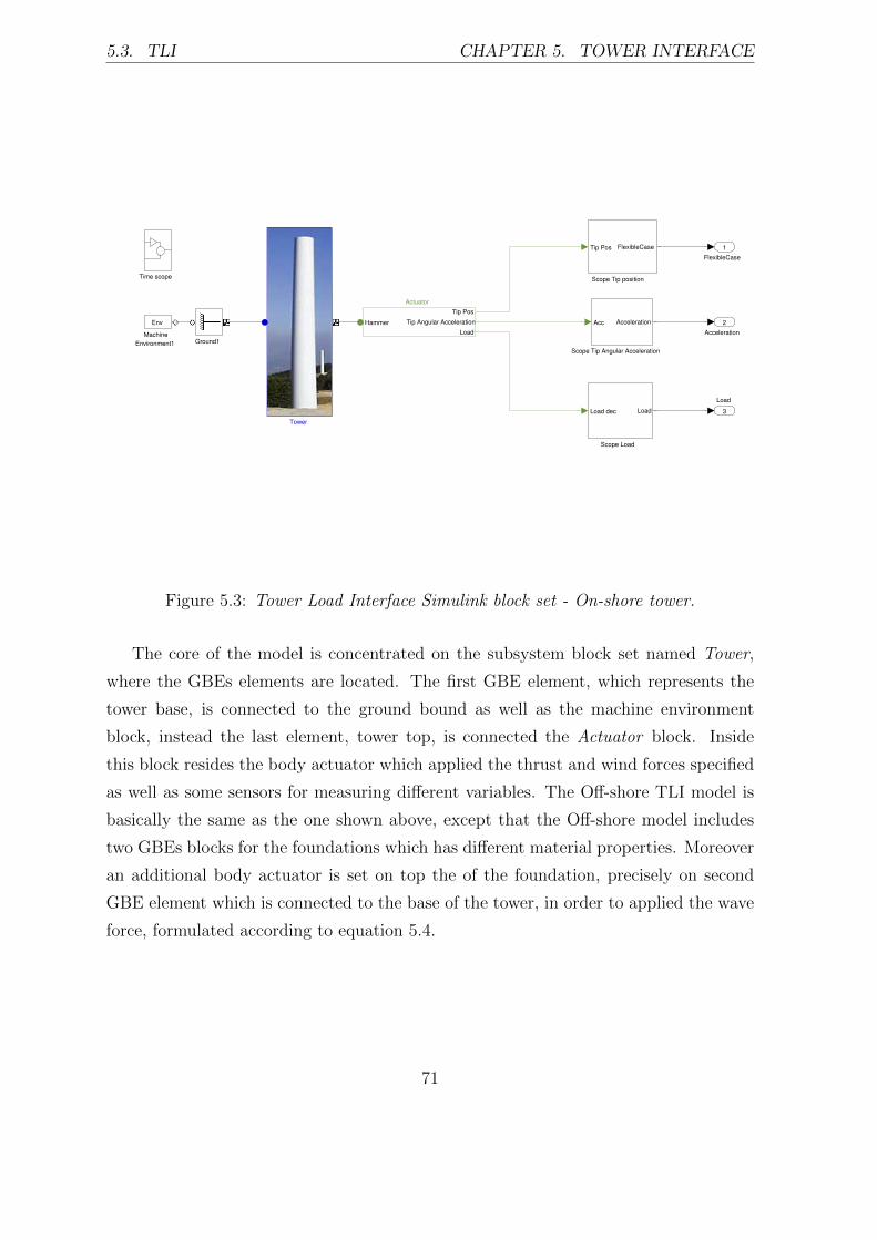
5.3. TLI CHAPTER 5. TOWER INTERFACE
Load
3
Acceleration
2
FlexibleCase
1
Tower
Time scope Scope Tip position
Tip Pos FlexibleCase
Scope Tip Angular Acceleration
Acc Acceleration
Scope Load
Load dec Load
Machine
Environment1
Env
Ground1
Actuator
Tip Pos
Tip Angular Acceleration
Load
Hammer
Figure 5.3: Tower Load Interface Simulink block set - On-shore tower.
The core of the model is concentrated on the subsystem block set named Tower,
where the GBEs elements are located. The first GBE element, which represents the
tower base, is connected to the ground bound as well as the machine environment
block, instead the last element, tower top, is connected the Actuator block. Inside
this block resides the body actuator which applied the thrust and wind forces specified
as well as some sensors for measuring different variables. The Off-shore TLI model is
basically the same as the one shown above, except that the Off-shore model includes
two GBEs blocks for the foundations which has different material properties. Moreover
an additional body actuator is set on top the of the foundation, precisely on second
GBE element which is connected to the base of the tower, in order to applied the wave
force, formulated according to equation 5.4.
71
5.4. SIMULATIONS CHAPTER 5. TOWER INTERFACE
5.4 Simulations
In this section the simulations of an on-shore and an off-shore wind turbine towers
under specific wind conditions are presented. The on-shore wind turbine tower under
investigation is a 100 m tubular tower built with steel material while the off-shore tower
is a 65 m tubular tower with foundation of 20 m depth under sea level. The parameters
of the on-shore and off-shore towers are reported on appendix A, respectively on table
A.5, A.6 and A.7, A.8, A.9. The constant wind speed conditions are set for both towers.
The variables investigated for both models are the deflection of the tower, moment on
tip of the tower and the most important interface loads, namely generator support and
drivetrain support loads. All the variables are reported in time-domain except for the
deflection which is analyzed also in frequency domain.
72
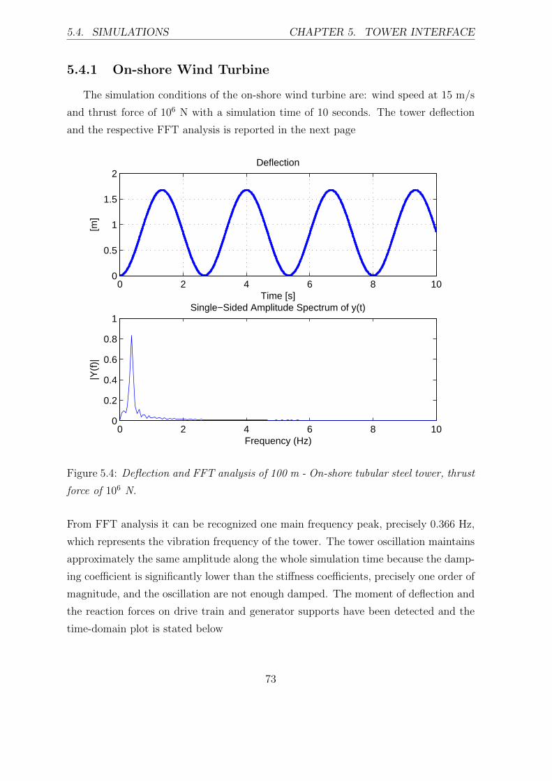
5.4. SIMULATIONS CHAPTER 5. TOWER INTERFACE
5.4.1 On-shore Wind Turbine
The simulation conditions of the on-shore wind turbine are: wind speed at 15 m/s
and thrust force of 106 N with a simulation time of 10 seconds. The tower deflection
and the respective FFT analysis is reported in the next page
0 2 4 6 8 100
0.5
1
1.5
2
Time [s]
[m]
Deflection
0 2 4 6 8 100
0.2
0.4
0.6
0.8
1Single−Sided Amplitude Spectrum of y(t)
Frequency (Hz)
|Y(f
)|
Figure 5.4: Deflection and FFT analysis of 100 m - On-shore tubular steel tower, thrust
force of 106 N.
From FFT analysis it can be recognized one main frequency peak, precisely 0.366 Hz,
which represents the vibration frequency of the tower. The tower oscillation maintains
approximately the same amplitude along the whole simulation time because the damp-
ing coefficient is significantly lower than the stiffness coefficients, precisely one order of
magnitude, and the oscillation are not enough damped. The moment of deflection and
the reaction forces on drive train and generator supports have been detected and the
time-domain plot is stated below
73
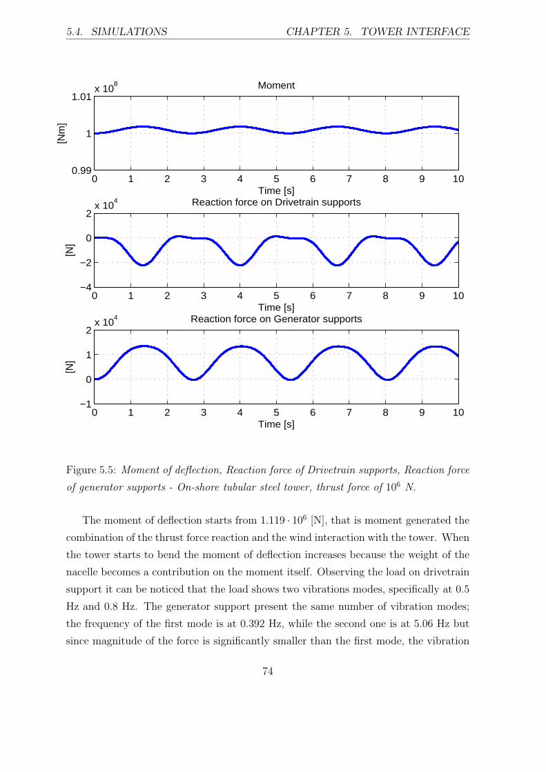
5.4. SIMULATIONS CHAPTER 5. TOWER INTERFACE
0 1 2 3 4 5 6 7 8 9 100.99
1
1.01x 10
8
Time [s]
[Nm
]
Moment
0 1 2 3 4 5 6 7 8 9 10−4
−2
0
2x 10
4
Time [s]
[N]
Reaction force on Drivetrain supports
0 1 2 3 4 5 6 7 8 9 10−1
0
1
2x 10
4
Time [s]
[N]
Reaction force on Generator supports
Figure 5.5: Moment of deflection, Reaction force of Drivetrain supports, Reaction force
of generator supports - On-shore tubular steel tower, thrust force of 106 N.
The moment of deflection starts from 1.119 · 106 [N], that is moment generated the
combination of the thrust force reaction and the wind interaction with the tower. When
the tower starts to bend the moment of deflection increases because the weight of the
nacelle becomes a contribution on the moment itself. Observing the load on drivetrain
support it can be noticed that the load shows two vibrations modes, specifically at 0.5
Hz and 0.8 Hz. The generator support present the same number of vibration modes;
the frequency of the first mode is at 0.392 Hz, while the second one is at 5.06 Hz but
since magnitude of the force is significantly smaller than the first mode, the vibration
74

5.4. SIMULATIONS CHAPTER 5. TOWER INTERFACE
mode becomes hard to recognize on the time domain signal.
5.4.2 Off-shore Wind Turbine
The set of wind condition for the off-shore wind turbine are the same of the on-
shore wind turbine simulation, additionally the wave force, expressed by the equation
5.4 in time-domain, is included. The wave force acting on foundation and the tower
top deflection with the its FFT analysis are given below
0 20 40 60 80 100 120−500
0
500
Time [s]
[N]
Wave Force
0 20 40 60 80 100 1200
1
2
Time [s]
[m]
Deflection
0 2 4 6 8 100
0.5
1Single−Sided Amplitude Spectrum of y(t)
Frequency (Hz)
|Y(f
)|
Figure 5.6: Wave Force, deflection and FFT analysis of 65 m - Off-shore tubular steel
tower, thrust force of 106 N and Wave load.
The FFT analysis shows a peak at the frequency of 0.432 Hz. The deflection of the tower
on X direction reaches a maximum value of 1.6 meters showing a discrete stiffness of the
tower. The same observations, stated for the on-shore tower, can be also extended for
the off-shore wind tower simulation, hence the deflection response is not significantly
influenced by the internal damping of the tower structure, in sense of reducing the
75
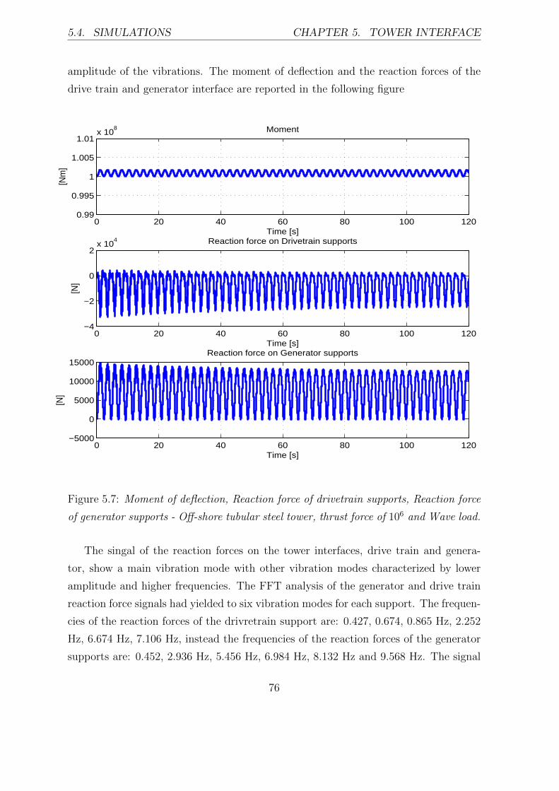
5.4. SIMULATIONS CHAPTER 5. TOWER INTERFACE
amplitude of the vibrations. The moment of deflection and the reaction forces of the
drive train and generator interface are reported in the following figure
0 20 40 60 80 100 1200.99
0.995
1
1.005
1.01x 10
8
Time [s]
[Nm
]
Moment
0 20 40 60 80 100 120−4
−2
0
2x 10
4
Time [s]
[N]
Reaction force on Drivetrain supports
0 20 40 60 80 100 120−5000
0
5000
10000
15000
Time [s]
[N]
Reaction force on Generator supports
Figure 5.7: Moment of deflection, Reaction force of drivetrain supports, Reaction force
of generator supports - Off-shore tubular steel tower, thrust force of 106 and Wave load.
The singal of the reaction forces on the tower interfaces, drive train and genera-
tor, show a main vibration mode with other vibration modes characterized by lower
amplitude and higher frequencies. The FFT analysis of the generator and drive train
reaction force signals had yielded to six vibration modes for each support. The frequen-
cies of the reaction forces of the drivretrain support are: 0.427, 0.674, 0.865 Hz, 2.252
Hz, 6.674 Hz, 7.106 Hz, instead the frequencies of the reaction forces of the generator
supports are: 0.452, 2.936 Hz, 5.456 Hz, 6.984 Hz, 8.132 Hz and 9.568 Hz. The signal
76
5.5. FUTURE WORKS CHAPTER 5. TOWER INTERFACE
of the first two vibration modes of the each reaction forces are characterized by the
highest magnitude since they are generated by the wind loads which are significantly
greater than wave loads on foundations.
Although the amplitude of the reaction forces has not the same order of magnitude of
the main loads coming from the rotor blades, it is advisable to consider them during the
design phase in order to avoid any resonance condition on the supports and, therefore,
reducing significantly their lifetime.
5.5 Future works
The TLI model represents a initial step for the evaluation of the tower load inter-
face and different improvements can be proposed in order to improve the model and
provide more realistic results. The first suggestion is to modify the the connection
between the bed plate and the nacelle adding further connection points still using the
springs and dampers in parallel in order to have a more realistic representation of the
interface. Then setting a proper values for the interface connections, specifically spring
and damper. The number of this joints depends of the number of the drivetrain sup-
ports, therefore it is possible to have a specific amount of the loads that act on each
supports. Moreover a more accurate model of the tower can be implemented using FE
theory. Matlab/Simulink allow to use this technique through the procedure developed
on [31]. Theoretically this model can provide more accurate results about the deflec-
tions of tower.
Moreover the TLI model should be validated against the data coming from FE com-
mercial software for what concerns the tower bending, and the measurement data from
what concerns the load on the supports, e.g. bearing loads.
77

Chapter 6
Conclusions
The main task of this project is to model the loads acting on the drivetrain inter-
faces of a wind turbine, specifically rotor, generator and tower interfaces. The report
begins stating that the large part of downtime of wind turbines is caused by drivetrain
failures. This fact have encouraged energy companies to start a strong researches in
order to limit this issue. A lack of knowledge about the loads which a wind turbine
drivetrain system is subjected to is highlighted. Therefore the investigation of the
drivetrain loads of each interface is a meaningful work. The report continues with a
chapter for each interface, RLI, GLI and TLI.
After revising the MatWorks wind turbine model [36], the Rotor Load Interface is
obtained, which is a multi-body system and is divided into four blocks, respectively:
wind conditions, aerodynamic loads, rotor blades and generator. The wind conditions
block set defines a set of different wind condition according to EIC standards; the aero-
dynamic loads block is responsible of calculating the loads that are generated by the
interaction between the air flow and blades. The block provides two different methods
for the calculation of the aerodynamic loads, namely UFD and RFD. The first method
calculates the aerodynamic forces as a single value for the entire blade, instead the RFD
technique divides the blades into a different segments and for each of them calculates
the respective lift and drag force, then the values are summed up and a more realistic
load is obtained. The blades block includes the rigid bodies representing the blades,
each of them are defined by inertia and mass properties. Lastly the generator block is
set as a counter torque for balancing the rotor torque. Simulations of constant wind
speed wind speed conditions underlines that the RFD technique provides in general a
78
CHAPTER 6. CONCLUSIONS
lower output torque and power production. The same conclusion can be extended for
normal turbulence wind condition simulations and moreover the RFD technique has
a more realistic response under dynamic condition compared to UFD method. The
sensitivity analysis of RFD block shows that 20 segments represents a number that
gives a good compromise between accuracy and computational time. Furthermore the
validation of RLI model against Hono measurement data shows that the RLI model re-
sults has good accuracy with a maximum difference of 9.5 % considering the worst case.
The Generator Load Interface model defines an induction and a PM generator with a
third order differential equations generator, consisting of two electromagnetic differen-
tial equations, for calculating the electromagnetic torque, and a mechanical differential
equation, which is the torque balance equation of the drive train system. The GLI
model presents two drivetrain system models, namely one-mass, which considers the
consists of one single mass rotating, and two-masses, which takes under consideration
the shaft flexibility. Both Induction and PM generators responses under a constant
mechanical torque as well as a step of mechanical torque are analyzed. Moreover a
network fault simulation for both types of generators is performed. The simulation of
the Induction generator are executed with one mass and two mass drive train in order
to observe the influence of the drive train system model on the generator response,
concluding that two mass drive train model provides a more realistic model that shows
the oscillations on the rotor speed and on the electromagnetic torque responses.
The Tower Load Interface models the loads of drivetrain supports coming from the
tower vibrations generated by the interaction with wind or also with wave, in case of
an off-shore wind turbines. The tower is modeled as a multi-body system designed
with the mass lumped-parameters technique. The top of the tower is welded with the
bed plate that is connected by a couple of spring and damper with a rigid body which
represents drive train and generator combined together. The same model is proposed
for off-shore wind turbines, which includes the foundation equally represented as rigid
bodies but characterized by different material properties. A simulation of an on-shore
tower under constant wind speed condition is presented. Equal wind condition have
been used for an off-shore tower simulation with the introduction of a periodic wave
loads acting on foundations. The simulation of the on-shore wind turbine tower shows
period loads on drivetrain supports with a specific frequency modes. On the contrary
79

CHAPTER 6. CONCLUSIONS
the off-shore tower simulation presents six vibration modes generated by both wave
and wind. Although the amplitude of the loads is not comparable to one coming from
rotor blades, they should be considered in any case during the design phase in order to
improve the durability of the supports.
As conclusion, with this Msc project, a new tool has been developed that can be used
for two different tasks. First, the three interface models can provide the input data
for dynamic analysis of advanced drive train models in order to evaluate the internal
loads as well as the deformations responses of the drivretrain components under dif-
ferent set of operational scenarios. The strength of this tool is possibility of providing
input data with a good accuracy, for different operational conditions, in a faster way
compared to the commercial codes such as ADAMSWT r, FAST r, that require
high computational time as well as long time for setting the models.
Second, the data of the models can also be used to design new wind turbines; indeed
it possible to estimate the amounts loads under critical operational scenarios, for in-
stance high turbulence condition, that allow to properly design the drivetrain system
components (e.g. gears) and possibly guarantee the durability of 20 years [15].
80
Bibliography
[1] Andreas Heege, Jaume Betran, Elisabet Lens, Computation of Dynamic
Loads in Wind Turbine Power Trains, DEWI Magazin Nr. 23, 2003.
[2] Brian Petersen , Marty Pollack , Benjamin Connell , David Gree-
ley , Dwight Davis , Charles Slavik , Benjamin Goldman, Evaluate the
effect of turbine period of vibration requirements on structural design parameters:
technical reports of findings, Applied Physical Sciences Corp., September 1, 2010.
[3] J. F. Manwell, J.G.McGowan, A.L. Rogers, Wind Energy Explained, John
Wiley & Sons, pp.165-195, 2009.
[4] J.Peeters, D. Vandepitte, P. Sas, Structural analysis of a wind turbine
and its drive train using the flexible multibody simulation technique, proceeding
of ISMA 2006.
[5] Det Norske Veritas, Copenhagen, and Wind Energy Department,
Risø National Laboratory, Guidelines for design of wind turbines, 2nd Edi-
tion, Jydsk Centraltrykkeri, Denmark 2002.
[6] Dazhi Wangl, Huaming Wangl, Yupeng Shi, Jun Li, Keling Song,
Shengli Liu, Yiqi Li, Wind Turbine Simulation of Offshore Environmental
Conditions, Second International Conference on Computational Intelligence and
Natural Computing (CINC), 2010.
[7] A. Perdana, Dynamic Models of Wind Turbines, Chalmers University of Tech-
nology, Goteborg, Sweden 2008.
81

BIBLIOGRAPHY 82
[8] Stefan S. A. Ivanell, Numerical Computations of Wind Turbine Wakes,Royal
Institute of Technology, Department of Mechanics, Stockholm, January 2009.
[9] Peter Hauge Madsen, Sten Frandsen, William E. Holley and Jens
Carsten Hansen, Dynamics and Fatigue Damage of Wind Turbine Rotors dur-
ing Steady Operation, RisØNational Laboratory, DK-4000 Roskilde, Denmark,
July 1984.
[10] M.Todorov, I. Dobrev, F. Massouh, Analysis of Torsional Oscillation of the
Drive Train in Horizontal-Axis Wind Turbine, ELECTROMOTION 2009 EPE
Chapter Electric Drives Joint Symposium, 1-3 July 2009.
[11] Thomas P. Fuglseth, Modelling a 2.5 MW direct driven wind turbine with
permanent magnet generator, Department of Electrical, Power Engineering Nor-
wegian University of Science and Technology, NO-7491 Trondheim, Norway, June
2005
[12] Donghoon Lee, Dewey H. Hodges. and Mayuresh J. Patil, Multi-
flexible-body Dynamic Analysis of Horizontal Axis Wind Turbines, School of
Aerospace Engineering, Georgia Institute of Technology, John Wiley & Sons, Au-
gust 2002.
[13] Grant Ingram, Wind Turbine Blade Analysis using the Blade Element Momen-
tum Method, Grant Ingram, 2011.
[14] Bunlung Neammanee, Somporn Sirisumrannukul, Somchai Cha-
tratana, Development of a Wind Turbine Simulator for Wind Generator Testing,
B. Neammanee et al. / International Energy Journal 8, 2007.
[15] Anders Ahlstrm, Simulating Dynamical Behaviour of Wind Power Structures,
Royal Institute of Technology, Department of Mechanics, Stockholm, 2002.
[16] Olimpo Anaya-Lara, Nick Jenkins, Janaka Ekanayake, Phill
Cartwright, Michael Hughes, Wind Energy Generation: Modelling and
Control, John Wiley & Sons, pp.126-132 2009.
[17] Hans Øverseth Røstøen, Tore M. Undeland, Terje Gjengedal, Doubly
Fed Induction Generator in a Wind Turbine, University of Minnesota, 2002.
82
BIBLIOGRAPHY 83
[18] Hernan De Battista, Ricardo Julib Mantz, Sliding Mode Control of
Torque Ripple in Wind Energy Conversion Systems with Slip Power Recovery,
Conference of IEEE Industrial Electronics Society, 1998.
[19] Ake Larsson, Power Quality of Wind Turbine Generating System and their in-
teraction with the Grid, Chalmers University of Technology, Department of Elec-
trical Power Engineering, Goteborg, Sweden, 2000.
[20] H. Li, Z. Chen, Overview of different wind generator systems and their compar-
isons, ET Renew. Power Gener., vol. 2, no. 2, pp. 123-138, 2008.
[21] Jussi Sopanen, Vesa Ruuskanen, Janne Nerg, Juha Pyrhonen, Dynamic
Torque Analysis of a Wind Turbine Drive Train Including a Direct-Driven Perma-
nent Magnet Generator, Conference of IEEE Industrial Electronic Society, 2010.
[22] Johan Ribrant, Reliability performance and maintenance - A survey of fail-
ures in wind power systems, Royal Institute of Technology, School of Electrical
Engineering, September 2011.
[23] Johan Ribrant, 10th World Wind Energy Conference and Renewable Energy
Exhibition, Cairo, Egypt 31 October - 2 November 2011.
[24] GE r Drivetrain Technologies; Available from: http://www.gedrivetrain.com,
2012/03/10.
[25] LORD r; Available from: www.lord.com, 2012/03/15.
[26] Siemens r Wind turbine; Available from:
http://www.energy.siemens.com/fi/en/power-generation/renewables/wind-
power/, 2012/03/23.
[27] Perdana, A., Dynamics Models of wind Turbines: A Contribution towards the
Establishment of Standardized Models of Wind Turbines for Power System Stabil-
ity Studies, Chalmers University of Technology, Department of Electrical Power
Engineering, Goteborg, Sweden, 2008.
[28] IEC standard 2005, Available from: http://www.iec.ch/.
[29] Christian LeBlanc, Design of Offshore Wind Turbine Support Structures,
M.Sc. (Civil Engineering), Technical University of Denmark, 2004.
83

BIBLIOGRAPHY
[30] Shaolin Li, Xing Zhang, Zhen Xie, Shuying Yang, Chongwei Zhang,
Renxian Cao, A Study on Dynamic Model And Analyse of Wind Turbine Gen-
eration System, Conference of IEEE Industrial Electronic Society, 2010.
[31] Victor Chudnovsky, Arnav Mukherjee, Jeff Wendlandt, and Dal-
las Kennedy, Modeling Flexible Bodies in SimMechanics, August 30, 2006:
http://www.mathworks.com.
[32] Alejandro Rolan’, Alvaro Luna, Gerardo Vazquez, Daniel Aguilar,
Modeling of a Variable Speed Wind Turbine with a Permanent Magnet Syn-
chronous Generator,Conference of IEEE Industrial Electronic Society, July 5-8,
2009.
[33] Caiyun Ji, Longbiao Zhu and Zhisong Zhu, Load Analysis of 2.5MW
Offshore Wind Turbine Tower, Applied Mechanics and Materials Vols. 121-126 pp
206-212, 2012.
[34] Claes Dyrbye, Svend Ole Hansen, Wind loads on structures, John Wiley
& Sons, pp 75-78,1997.
[35] matworks r; http://www.mathworks.com/matlabcentral/fileexchange/25752-
wind-turbine-model, 15 Apr 2011.
[36] Florin Iov, Anca Daniela Hansen, Poul Srensen, Frede Blaabjerg,
MarchWind Turbine Blockset in Matlab/Simulink, Risø National Laboratory,
March 2004.
[37] matworks r; http://www.mathworks.com/matlabcentral/fileexchange/11027,
06 October 2009.
[38] http://http://www.chalmers.se/ee/swptc-en, March 2012.
[39] J.Peeters, Simulation of dynamic drivetrain loads in a wind turbine, University
of Leuven, June 2006.
84

Appendix A
Wind Turbines parameters and
IEC:2005 standard
IEC:2005 standard, wind models
Normal turbulence model
σ1 = Iref (0.75Vaverage + 5.6)
Extreme wind speed
V50 = 1.4Vref
V1 = 0.8V50
σ1 = 0.11Vaverage
Extreme operating gust
Vgust = Min
1.35 (1.12V1 − Vaverage) ; 3.3(
σ11+0.1(D/Λ1)
)V = Vaverage − 0.27Vgustsin(3πt/T )(1− cos(2πt/T ))
Extreme turbulence model
σ1 = cIref
(0.072
(Vavec
+ 3
)(Vaverage
c− 4
)+ 10
)
85
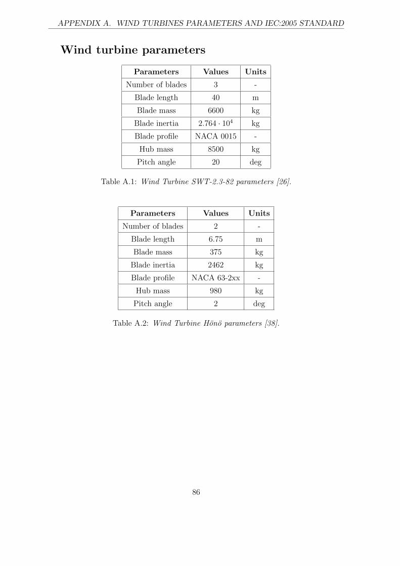
APPENDIX A. WIND TURBINES PARAMETERS AND IEC:2005 STANDARD
Wind turbine parameters
Parameters Values Units
Number of blades 3 -
Blade length 40 m
Blade mass 6600 kg
Blade inertia 2.764 · 104 kg
Blade profile NACA 0015 -
Hub mass 8500 kg
Pitch angle 20 deg
Table A.1: Wind Turbine SWT-2.3-82 parameters [26].
Parameters Values Units
Number of blades 2 -
Blade length 6.75 m
Blade mass 375 kg
Blade inertia 2462 kg
Blade profile NACA 63-2xx -
Hub mass 980 kg
Pitch angle 2 deg
Table A.2: Wind Turbine Hono parameters [38].
86

APPENDIX A. WIND TURBINES PARAMETERS AND IEC:2005 STANDARD
Generator parameters
Parameters Values Units
Rated Power 180 kW
Rated Voltage 415 V
Stator resistance 0.0092 Ω
Stator leakage inductance 0.182 mH
Mutual inductance 6.7 mH
Rotor Resistance 0.0061 Ω
Rotor leakage inductance 0.427 mH
Number of pole pair 3 -
Shaft Stiffness 2700 Nm/rad
Shaft Damper 100 Nm.sec/rad
Table A.3: 180 kW Induction Generator [38].
Parameters Values Units
Rated Power 4.5 MW
Rated Voltage 400 V
Stator resistance 2.34e-3 Ω
Stator leakage inductance 0.182 mH
Mutual inductance 6.7 mH
Rotor Resistance 17.36e-3 Ω
Rotor leakage inductance 0.125 mH
Number of pole pair 60 -
Rotor inertia 107 kgm2
Generator inertia 97030 kgm2
Shaft stiffness coefficient 3.67 · 108 Nm.sec/rad
Shaft damping coefficient 0.2 · 108 Nm/rad
Table A.4: 4.5 MW PM Generator [21].
87

APPENDIX A. WIND TURBINES PARAMETERS AND IEC:2005 STANDARD
On-shore tower parameters
Parameters Values Units
Module mass 100 Kg
Module inertia (Ix) 105 kgm2
Module inertia (Iy) 103 kgm2
Module inertia (Iz) 105 kgm2
Tower height 100 m
Module stiffness property (EI) 2.3 · 1011 Nm2
Module damping coefficient 106 Ns/m
Table A.5: Data of on-shore wind turbine tower [34].
Parameters Values Units
Nacelle mass 107500 Kg
Nacelle inertia (Ix) 103 kgm2
Nacelle inertia (Iy) 101 kgm2
Nacelle inertia (Iz) 103 kgm2
Generator spring stiffness 0.3 · 106 Nm
Generator damping coefficient 0.5 · 105 Ns/m
Drivetrain spring stiffness 106 Nm
Drivetrain damping coefficient 105 Ns/m
Table A.6: Data of on-shore wind turbine nacelle.
88
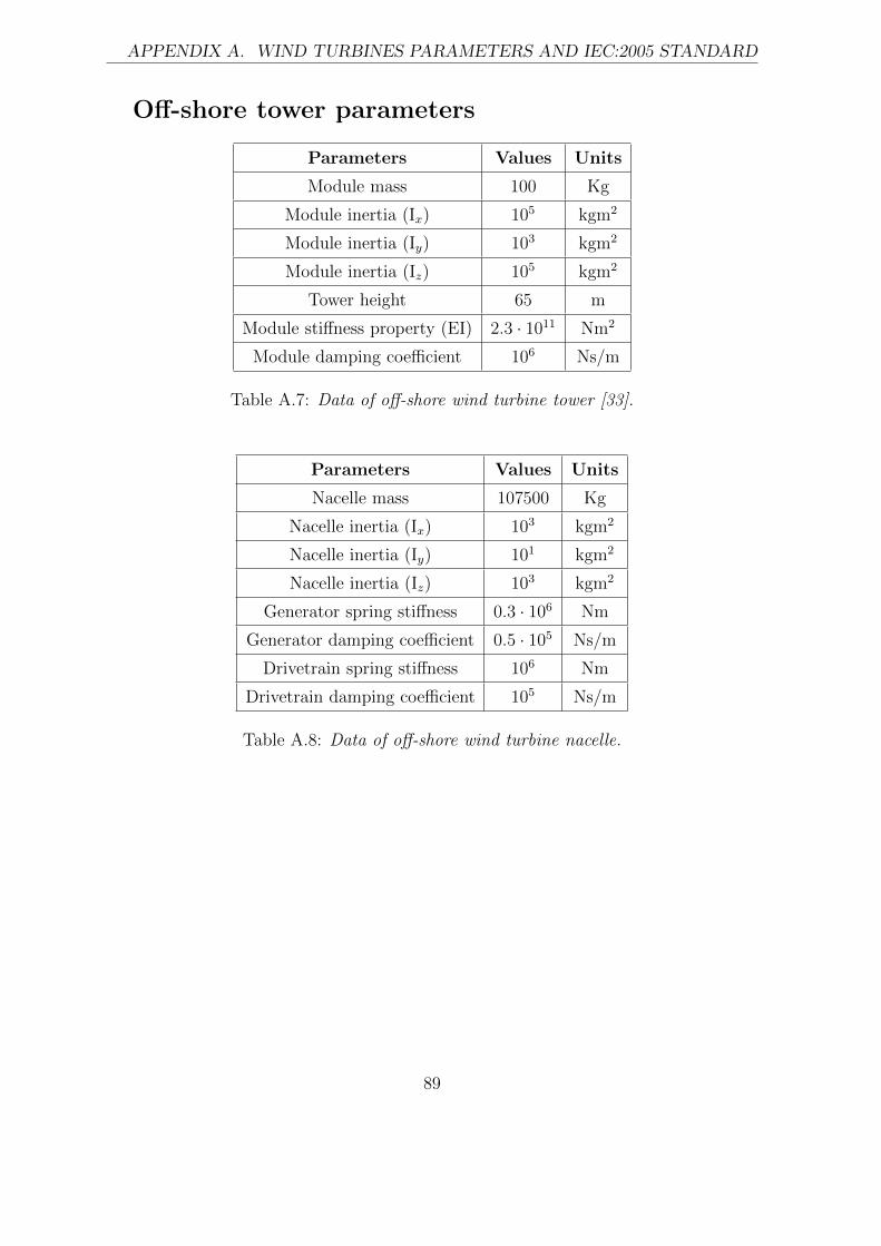
APPENDIX A. WIND TURBINES PARAMETERS AND IEC:2005 STANDARD
Off-shore tower parameters
Parameters Values Units
Module mass 100 Kg
Module inertia (Ix) 105 kgm2
Module inertia (Iy) 103 kgm2
Module inertia (Iz) 105 kgm2
Tower height 65 m
Module stiffness property (EI) 2.3 · 1011 Nm2
Module damping coefficient 106 Ns/m
Table A.7: Data of off-shore wind turbine tower [33].
Parameters Values Units
Nacelle mass 107500 Kg
Nacelle inertia (Ix) 103 kgm2
Nacelle inertia (Iy) 101 kgm2
Nacelle inertia (Iz) 103 kgm2
Generator spring stiffness 0.3 · 106 Nm
Generator damping coefficient 0.5 · 105 Ns/m
Drivetrain spring stiffness 106 Nm
Drivetrain damping coefficient 105 Ns/m
Table A.8: Data of off-shore wind turbine nacelle.
89

APPENDIX A. WIND TURBINES PARAMETERS AND IEC:2005 STANDARD
Parameters Values Units
Module mass 250 Kg
Module inertia (Ix) 106 kgm2
Module inertia (Iy) 1.3·104 kgm2
Module inertia (Iz) 106 kgm2
Foundation height 20 m
Module stiffness property (EI) 2.75 · 1012 Nm2
Module damping coefficient 106 Ns/m
Table A.9: Data of off-shore wind turbine foundation [33].
90
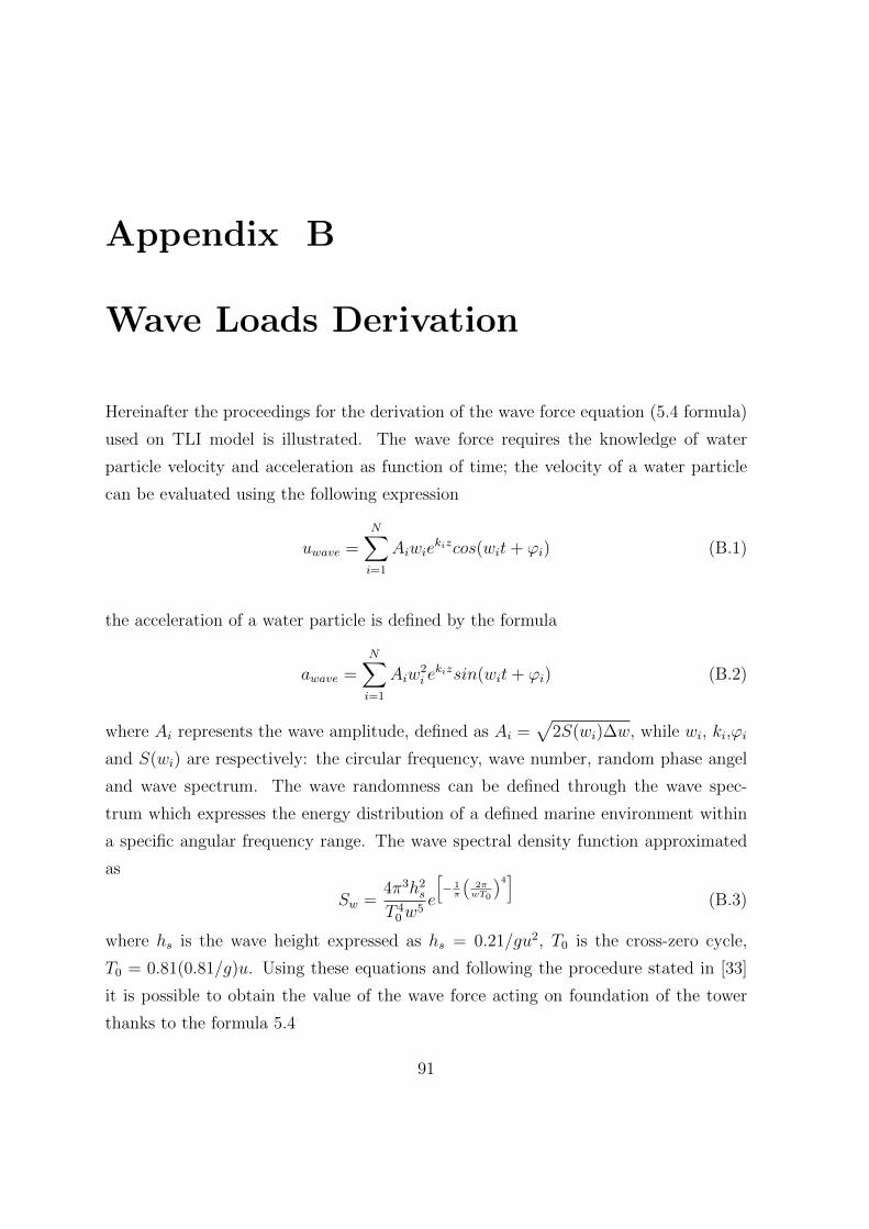
Appendix B
Wave Loads Derivation
Hereinafter the proceedings for the derivation of the wave force equation (5.4 formula)
used on TLI model is illustrated. The wave force requires the knowledge of water
particle velocity and acceleration as function of time; the velocity of a water particle
can be evaluated using the following expression
uwave =N∑i=1
Aiwiekizcos(wit+ ϕi) (B.1)
the acceleration of a water particle is defined by the formula
awave =N∑i=1
Aiw2i ekizsin(wit+ ϕi) (B.2)
where Ai represents the wave amplitude, defined as Ai =√
2S(wi)∆w, while wi, ki,ϕi
and S(wi) are respectively: the circular frequency, wave number, random phase angel
and wave spectrum. The wave randomness can be defined through the wave spec-
trum which expresses the energy distribution of a defined marine environment within
a specific angular frequency range. The wave spectral density function approximated
as
Sw =4π3h2
s
T 40w
5e
[− 1π
(2πwT0
)4]
(B.3)
where hs is the wave height expressed as hs = 0.21/gu2, T0 is the cross-zero cycle,
T0 = 0.81(0.81/g)u. Using these equations and following the procedure stated in [33]
it is possible to obtain the value of the wave force acting on foundation of the tower
thanks to the formula 5.4
91
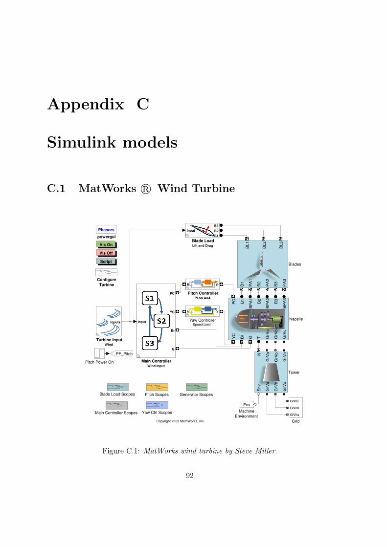
Appendix C
Simulink models
C.1 MatWorks r Wind Turbine
Copyright 2009 MathWorks, Inc.
Script
powergui
Phasors
Yaw Ctrl Scopes
Yaw ControllerSpeed Limit
M Y
Vis On
Vis Off
Turbine InputWind
Inputs
Tower
En
v
Gr V
a
Gr V
b
Gr V
c
N
Gr V
a
Gr V
b
Gr V
c
Pitch Scopes
Pitch Power On
Pitch ControllerPI on AoA
M P
Nacelle
YC
Br
G T Gr V
a
Gr V
b
Gr V
c
PC
B1
BP
A1
B2
BP
A2
B3
BP
A3
Main Controller Scopes
Main ControllerWind Input
Input
PC
YC
Br
G
Machine
Environment
Env
Grid
GNVc
GNVb
GNVa
PF_Pitch
Generator Scopes
Configure
Turbine
Blades
B1
PA
1
B2
PA
2
B3
PA
3
BL
1
BL
2
BL
3
BL
1
BL
2
BL
3
B1
PA
1
B2
PA
2
B3
PA
3
Blade Load Scopes
Blade LoadLift and Drag
Input
B3
B2
B1
Figure C.1: MatWorks wind turbine by Steve Miller.
92
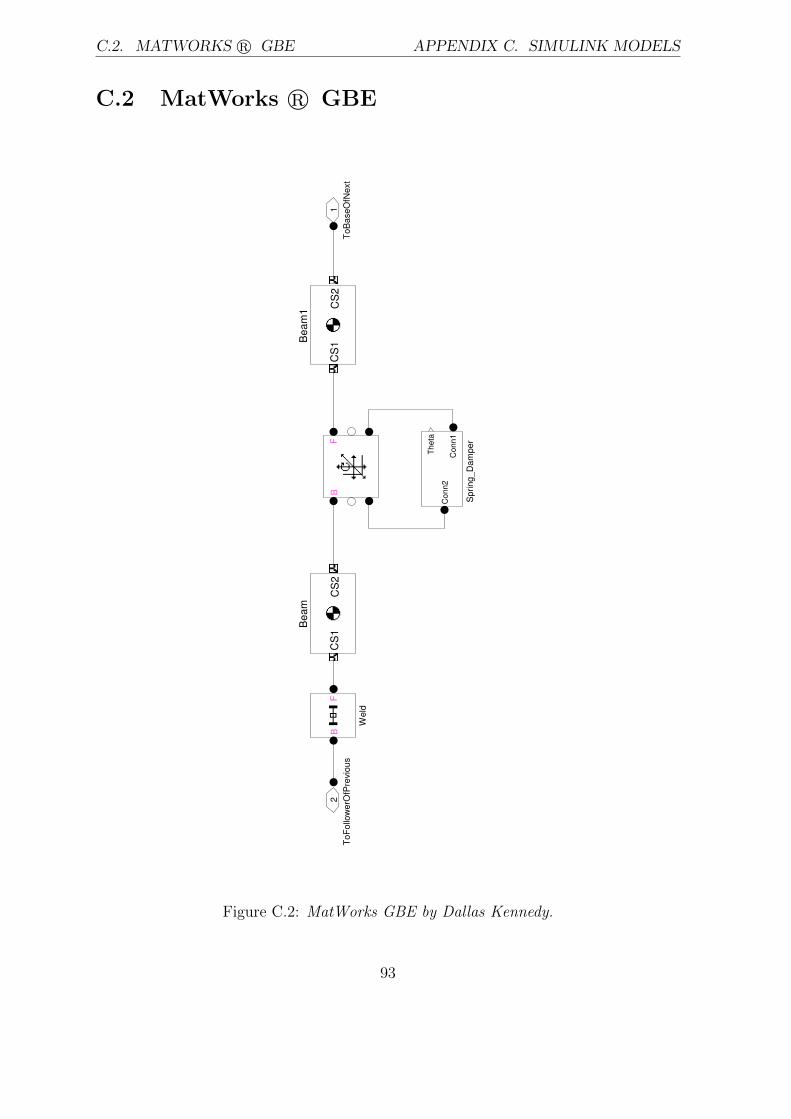
C.2. MATWORKS r GBE APPENDIX C. SIMULINK MODELS
C.2 MatWorks r GBE
ToF
ollo
werO
fPre
vio
us
2
ToB
aseO
fNext
1
Weld
BF
Spring_D
am
per
Th
eta
Co
nn
2C
on
n1
BF
Be
am
1
CS
1C
S2
Be
am
CS
1C
S2
Figure C.2: MatWorks GBE by Dallas Kennedy.
93

Appendix D
List of Symbols and Abbreviations
Symbols
awave Acceleration of water particle
c Friction coefficient
CD Drag coefficient
CDF vibration resistance coefficient
CDS Steady resistance coefficient
CL Lift coefficient
CM Wave inertia coefficient
FD Drag force
FL Lift force
FN Thrust force
FT Torque force
ir Rotor current
is Stator current
I Inertia
j Imaginary operator,√−1
Jg Generator inertia
Jr Rotor inertia
Lm Mutual inductance
Lr Rotor inductance
94

APPENDIX D. LIST OF SYMBOLS AND ABBREVIATIONS
Ls Stator inductance
Rr Rotor resistance
Rs Stator resistance
Te Electrical torque
Tm Mechanical torque
uwave Velocity of water particle
vr Rotor voltage
vrel Relative speed
vs Stator voltage
β Pitch angle
ωk Yaw speed
ω Rotor speed
ρair Air Density
ρsw Sea Water Density
ψr,ψs Rotor and stator flux
Abbreviations
DFIG Double fed induction generator
DOF Degree of freedom
FCWT Full converter wind power
FE Finite element
FMB Flexible multi body
GBE Generalized beam elements
GLI Generator load interface
HAWT Horizontal axis wind turbine
PM Permanent Magnet
RFD Real forces distribution
RMB Rigid multi body
RLI Rotor load interface
TLI Tower load interface
UFD Uniform forces distribution
V AWT Vertical axis wind turbine
95