modeling of fuel injection system for troubleshooting · modeling of fuel injection system for...
TRANSCRIPT

Modeling of Fuel Injection System for Troubleshooting
A L E X A N D E R G E O R G I I - H E M M I N G C Y O N
Master of Science Thesis Stockholm, Sweden 2013

Modeling of Fuel Injection System for Troubleshooting
A L E X A N D E R G E O R G I I - H E M M I N G C Y O N
DD221X, Master’s Thesis in Computer Science (30 ECTS credits) Degree Progr. in Computer Science and Engineering 300 credits Master Programme in Computer Science 120 credits Royal Institute of Technology year 2013 Supervisor at CSC was Johan Karlander Examiner was Anders Lansner TRITA-CSC-E 2013:008 ISRN-KTH/CSC/E--13/008--SE ISSN-1653-5715 Royal Institute of Technology School of Computer Science and Communication KTH CSC SE-100 44 Stockholm, Sweden URL: www.kth.se/csc

Abstract
With the technology progressing further, making heavy duty vehicles more complex, more computerized, itbecomes necessary to update the troubleshooting process of such vehicles. From the vehicles´ computers,diagnosis trouble codes can be extracted, informing the mechanic about the health of the vehicle. Usingthose codes, together with physical observations, as input for a diagnosing software, the software cangive educated troubleshooting advice to the mechanic. Such diagnosing software requires a model of thevehicle or one of its system, which mimics the behavior of the real one. If there would be a one-to-onecorrespondence between observations and diagnosis, the model would be completely accurate. However,no such one-to-one correspondence exists. This makes the system non-deterministic. therefore the modelhas to be constructed using another approach. This master thesis presents a statistical model of a fuelinjection system called XPI. The XPI-system is modeled using a statistical model called a Bayesiannetwork which is a convenient way to model a non-deterministic system. The purpose of this model isto be able to make diagnosis of the XPI-system, but also to ease the understanding of the dependencybetween components and faults in the XPI-system. The model is also used to evaluate detectability andisolability of faults in the XPI-system.
SammanfattningModellering av bränslesystem för felsökning
Då teknologins utveckling gör tunga fordon mer komplexa, mer datorberoende, blir det nödvändigt attmodernisera felsökning av dessa fordon. Från fordonens datorer kan felkoder avläsas. Dessa felkoder med-delar mekanikern om fordonets skick. Felkoderna, i kombination med fysiska observationer, kan användassom indata till en diagnostiseringsmjukvara, som kan förse mekanikerna med kvalificerade felsöknings-råd. En sådan diagnostiseringsmjukvara kräver en modell av fordonet, eller ett delsystem av det, vilkenmodellerar beteendet av det riktiga systemet. Om det skulle finnas en ett-till-ett mappning mellan obser-vationer och diagnoser, skulle modellen ha fullständig precision. Dessvärre finns det ingen sådan ett-till-ettmappning. Modellen måste således konstrueras med en annan metod. Detta examensarbete presenteraren statistisk modell av ett bränslesystem kallat XPI. Denna typ av statistiska modell kallas för ett Baye-sianskt nätverk, som är lämpligt att använda vid modellering av icke-deterministiska system. Syftet meddenna modell är att den ska kunna diagnostisera XPI-systemet samt underlätta förståelse för beroendetmellan komponenter och fel. Modellen kan också användas för att utvärdera urskiljbarhet och isolerbarhethos fel i XPI-systemet.

Alexander Georgii-Hemming Cyon

Acknowledgement
Håkan Warnquist, YSNS, for guidance and feedback.
Johan Karlander, KTH, for your input.
Anders Lanser, KTH, for help and feedback on the report.
Johan Svensson, YQN, for giving be detailed information about the XPI-system and feedback about mymodel.
Jonas Biteus, YSNS, for showing me around at Scania and showing me engines and the XPI-systemphysically.
Joe Mohs, NMKB, for giving me detailed information about XPI.
Mikael Åkerfelt, YSNB, for giving me the basic knowledge of the components and faults of the XPI-system.
Frida Larsson, TIKAB (contractor), for doing the illustrations of the engine and cylinders.
Isabella Chowra, my wonderful girlfriend for help with graphics.

Alexander Georgii-Hemming Cyon
Contents
I Introduction
1 Background 11.1 Problem formulation . . . . . . . . . . . . . . . . . . . . . . . . . . . . . . . . . . . . . . . 1
1.1.1 Goal . . . . . . . . . . . . . . . . . . . . . . . . . . . . . . . . . . . . . . . . . . . . 11.1.2 Thesis delimitations . . . . . . . . . . . . . . . . . . . . . . . . . . . . . . . . . . . 2
1.2 Thesis Outline . . . . . . . . . . . . . . . . . . . . . . . . . . . . . . . . . . . . . . . . . . 2
2 Theory 32.1 The diesel engine . . . . . . . . . . . . . . . . . . . . . . . . . . . . . . . . . . . . . . . . . 3
2.1.1 The combustion process. . . . . . . . . . . . . . . . . . . . . . . . . . . . . . . . . . 42.1.2 Fuel injection . . . . . . . . . . . . . . . . . . . . . . . . . . . . . . . . . . . . . . . 5
2.2 Basic calculus of probability . . . . . . . . . . . . . . . . . . . . . . . . . . . . . . . . . . . 62.2.1 Stochastic variables . . . . . . . . . . . . . . . . . . . . . . . . . . . . . . . . . . . 62.2.2 Dependence and independence . . . . . . . . . . . . . . . . . . . . . . . . . . . . . 62.2.3 Joint probability distribution . . . . . . . . . . . . . . . . . . . . . . . . . . . . . . 72.2.4 Conditional probability . . . . . . . . . . . . . . . . . . . . . . . . . . . . . . . . . 8
2.3 Bayesian networks . . . . . . . . . . . . . . . . . . . . . . . . . . . . . . . . . . . . . . . . 92.3.1 Small Bayesian network model . . . . . . . . . . . . . . . . . . . . . . . . . . . . . 92.3.2 Component variables . . . . . . . . . . . . . . . . . . . . . . . . . . . . . . . . . . . 102.3.3 Observation variables . . . . . . . . . . . . . . . . . . . . . . . . . . . . . . . . . . 122.3.4 Inference in Bayesian networks . . . . . . . . . . . . . . . . . . . . . . . . . . . . . 13
3 Methodology 153.1 Methods for modeling . . . . . . . . . . . . . . . . . . . . . . . . . . . . . . . . . . . . . . 15
3.1.1 Creating the model . . . . . . . . . . . . . . . . . . . . . . . . . . . . . . . . . . . . 153.1.2 Analyzing and formatting the data . . . . . . . . . . . . . . . . . . . . . . . . . . . 16
3.2 Methods for verifying the model . . . . . . . . . . . . . . . . . . . . . . . . . . . . . . . . 16
II System Modeling 19
4 Modeling the XPI-system 214.1 About the XPI-system . . . . . . . . . . . . . . . . . . . . . . . . . . . . . . . . . . . . . . 21
4.1.1 Components . . . . . . . . . . . . . . . . . . . . . . . . . . . . . . . . . . . . . . . 214.1.2 The route of the fuel in the engine . . . . . . . . . . . . . . . . . . . . . . . . . . . 21
4.2 Model assumptions and delimitations . . . . . . . . . . . . . . . . . . . . . . . . . . . . . . 234.2.1 Assumptions . . . . . . . . . . . . . . . . . . . . . . . . . . . . . . . . . . . . . . . 234.2.2 Delimitations . . . . . . . . . . . . . . . . . . . . . . . . . . . . . . . . . . . . . . . 23
4.3 The model . . . . . . . . . . . . . . . . . . . . . . . . . . . . . . . . . . . . . . . . . . . . . 244.3.1 Component Variables . . . . . . . . . . . . . . . . . . . . . . . . . . . . . . . . . . 244.3.2 Observation Variables . . . . . . . . . . . . . . . . . . . . . . . . . . . . . . . . . . 27

CONTENTS Alexander Georgii-Hemming Cyon
4.4 Generating the model . . . . . . . . . . . . . . . . . . . . . . . . . . . . . . . . . . . . . . 294.4.1 Leaky-Noisy-Or-Nodes . . . . . . . . . . . . . . . . . . . . . . . . . . . . . . . . . . 294.4.2 Limits in GeNIe . . . . . . . . . . . . . . . . . . . . . . . . . . . . . . . . . . . . . 314.4.3 The complete model . . . . . . . . . . . . . . . . . . . . . . . . . . . . . . . . . . . 35
III Result 37
5 Verifying the XPI-model 395.1 Correctness of the model . . . . . . . . . . . . . . . . . . . . . . . . . . . . . . . . . . . . . 39
5.1.1 Test one - expert interview . . . . . . . . . . . . . . . . . . . . . . . . . . . . . . . 395.1.2 Test two - case-studies . . . . . . . . . . . . . . . . . . . . . . . . . . . . . . . . . . 40
6 Conclusion 436.1 Discussion . . . . . . . . . . . . . . . . . . . . . . . . . . . . . . . . . . . . . . . . . . . . . 436.2 Future work . . . . . . . . . . . . . . . . . . . . . . . . . . . . . . . . . . . . . . . . . . . . 446.3 Final words . . . . . . . . . . . . . . . . . . . . . . . . . . . . . . . . . . . . . . . . . . . . 44
7 Bibliography 47
A Acronyms 51
B Notation 53
C Pseudocode 55

Part I
Introduction

Chapter 1
Background
It has become difficult for mechanics to troubleshoot a faulty truck due to the increasing complexity ofits systems. Trucks are nowadays composed of several complex systems containing components, sensors,computers and connections between them.
Troubleshooting refers to the act of determining which component is faulty and performing an actionin order to mend this fault. Identifying the fault is not trivial, since the systems are so complex. Themechanics identifies a fault by analyzing diagnosis trouble codes (DTC) generated by the sensors in thetrucks system but also by doing physical observations.
It is therefore desirable to help the mechanics with the troubleshooting process, one way of doing so is tomodel the truck´s systems with a statistical model that “behaves” like the real system. A certain fault inone of the truck´s systems can lead to multiple DTCs and the same DTC can be derived from differentfaults. This makes fault determination non-deterministic and therefore we cannot model the system witha deterministic model. Instead we represent the system´s behavior with a statistical model, so that givensome observations we believe with a certain probability that a certain component is faulty.
Since it is difficult for mechanics to identify the faulty component, a quick solution would be to replacefor example the whole engine instead of a small part of the engine. Isolating the fault and only doingrepairs or replacements of faulty components costs less than changing whole systems in terms of materialcost, but might cost more in terms of time. Because of the strong correlation between time and money,a reparation system needs to weigh material cost against time cost.
In this master thesis a model of one of the truck´s system is modeled, the eXtreme high Pressure fuelInjection system (XPI). This model will hopefully serve two purposes; to help XPI experts to understandthe system even further as well as to help the supervisor of this thesis, Håkan Warnquist, in his researchof automated troubleshooting using mathematical models.
1.1 Problem formulation
1.1.1 Goal
The purpose of this master thesis is to develop a statistical model of one of Scania´s systems called XPI.The XPI-system has not been modeled as thoroughly before, hence the thesis´s main contribution is to,in a correct and accurate manner, model this system. Where great difficulty lies within defining correctand accurate as well as fulfilling those definitions. In other words, the model´s behavior should mirrorthat of the real system’s. More specifically, if the XPI-system would indicate a certain DTC or physical
1
1.2. THESIS OUTLINE Alexander Georgii-Hemming Cyon
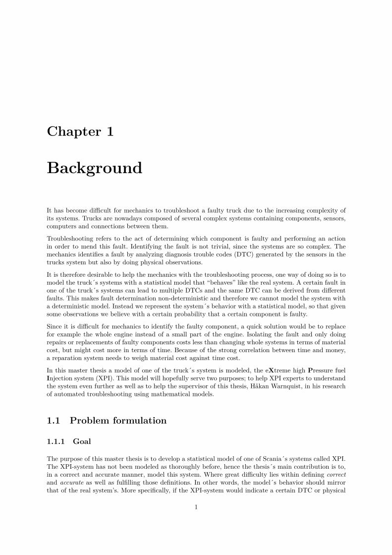
Figure 1.1: The concept of a troubleshooting framework, in this thesis only the diagnoser will be developed.The system to troubleshoot is the XPI-system, the user could for example be a mechanic, the systeminformation consists of DTCs and physical observations. Image found in [1].
event for a certain fault, then so should the model. If a set of observations (the size of the set could beone) would lead to a fault-diagnosis by a mechanic, then the model should make the same diagnosis.Continue reading more about the behavior of the model in section Correctness of the model (5.1).
The model must be represented or implemented in a computer program somehow so that it is possible tointeract with it. The model presented in this thesis has been represented in a graphical network programcalled GeNIe [2]. The model can not be created in GeNIe manually, since it is way to much work due tothe complexity of the model, instead it is generated by a program, developed and presented in this thesis.This model-generating program can be reused for modeling of other systems, given that the necessarydata files are available and on the correct format, described in section Limits in GeNIe (4.4.2).
1.1.2 Thesis delimitations
The work presented in this thesis will hopefully be useful for other systems than the XPI-systems. How-ever, the thesis will be limited to modeling the XPI-system only. This model will have some restrictions.The XPI-system is, in fact, used in three different engine types, the 9, 13 and 16 liter engines. The 9and the 13 liter versions does, however, differ very little in ways of design and functionality. The 16liter version has a slightly different configuration then the other two. The XPI-system being modeledin this thesis is the 13 liter version, although the difference between it and the 9 liter version is verysmall1.
1.2 Thesis Outline
First necessary theory needed to understand this thesis is explained, the reader will be introduced to howa diesel engine works in section The diesel engine (2.1), calculus of probability in section Basic calculusof probability (2.2) and what Bayesian networks are in section Bayesian networks (2.3). Section Methodsfor modeling (3.1) is about modeling techniques, followed by a short introduction to the model evaluationprocess in section Methods for verifying the model (3.2). After that the XPI-model is presented andthoroughly explained followed by the verification of the model. The thesis ends with a conclusion anddiscussion about the results in chapter Conclusion (6).
1The primary difference is that the 13 liter version has one cylinder more.
2

Chapter 2
Theory
The purpose of this section is to introduce the reader to the fundamental theory, necessary to understandthe thesis. Two major fields are presented, firstly the reader is introduced to the basics of a diesel engineand fuel-injection. An insight of how a diesel engine works is important, because the sole purpose of thisthesis is to model the fuel injection system in such an engine.
Secondly, a presentation of statistics is given, since XPI will be modeled using a statistical model, thereforeit is important to have basic knowledge of the theory of statistics and calculus of probability.
A various number of concepts and their notation is presented, for the reader’s convenience a summary ofthe notation can be found in appendix Notation (B).
2.1 The diesel engine
This section will explain how a diesel engine works, without the requirement of any prior knowledge ofengines. A diesel engine is a combustion engine fueled by diesel1. When introduced, they were workhorseengines, i.e. powering heavy-duty vehicles, such as trucks, tractors, buses and trains [3]. Today nearly 70%of the automobiles on the Swedish market are powered by diesel engines [4]. The corresponding numberfor Europe overall is 50%, and in the global market it is predicted to be 12% globally by 2018 [5].
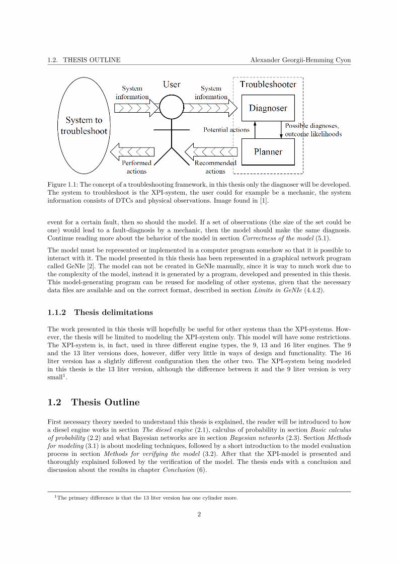
A combustion engine converts chemical energy in fuel to mechanical energy by burning the fuel whichcauses motion. The combustion, which takes place in the engines cylinders, creates a small and controlledexplosion which pushes the piston in the cylinder down, giving it kinetic energy. The movement of thepiston transfers force to the crankshaft making it rotate. Such a combustion takes place in every cylinderin the engine. The more cylinders, the more mechanical energy the engine creates. The volume of thecylinders also affects the power, the bigger, the more powerful and more fuel consuming. For an illustrationof the cylinders see figure 2.1.
In light- to medium duty engines, such as cars and small trucks, the most common cylinder configuration isthe inline-six-cylinder (also called straight-six engine). In heavy-duty engines, such as trucks and buses, theV6 and V8 cylinder configuration is typically used. The “V” describes the shape the cylinders constitutewhen having them in two planes (rows) almost perpendicular to each other, forming a V-shape, pleasesee figure 2.1.
1In contrast to the “traditional” engine, fueled by petrol.
3
2.1. THE DIESEL ENGINE Alexander Georgii-Hemming Cyon
Figure 2.1: This figure shows the V-shaped configuration of the cylinders. Pistons move up and down inthe cylinder, the movement of the pistons causes the crankshaft to move creating mechanical energy. 1)Piston, 2) connecting rod, 3) flywheel, 4) intake and exhaust valve, 5) cylinder, 6) counterweight
2.1.1 The combustion process.
The combustion process is classically either a two or four-stroke (step) cycle. Both the two and the four-stroke cycle is used in diesel engines. The two-stroke was more popular before, when emission control wasnot as strict. The two-stroke engine is cheap to produce, repair and rebuild, it is light weight but has poorexhaust emission features. Today, the four-stroke is most common [6]. Here follows a simple explanationof the combustion process of the four-stroke cycle:
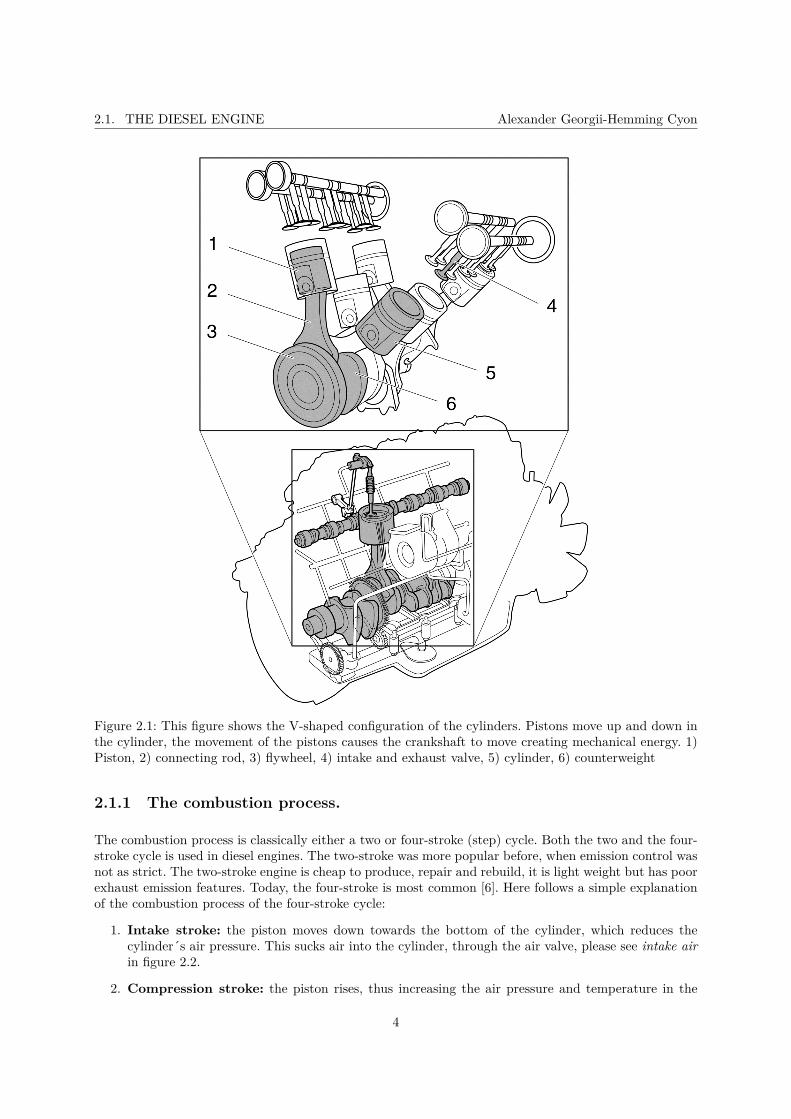
1. Intake stroke: the piston moves down towards the bottom of the cylinder, which reduces thecylinder´s air pressure. This sucks air into the cylinder, through the air valve, please see intake airin figure 2.2.
2. Compression stroke: the piston rises, thus increasing the air pressure and temperature in the
4

2.1. THE DIESEL ENGINE Alexander Georgii-Hemming Cyon
cylinder.
3. Power/Combustion stroke: diesel fuel is injected with high pressure, see fuel injector in fig-ure 2.2. and self-ignites due to the high pressure and temperature of the air and the fuel, thispushes the piston down with a strong force, giving the crankshaft kinetic energy.
4. Exhaust stroke: the exhaust valve opens and the piston returns to the top of the cylinder pushingthe exhaust out and then the cycle restarts at stroke 1.
Figure 2.2: A cross section of a cylinder in a diesel engine. 1) Piston, 2) intake air, 3) intake valve, 4) fuelinjector, 5) exhaust valve, 6) exhaust gases, 7) cylinder, 8) counterweight, 9) crankshaft, 10) flywheel,11) connecting rod.
2.1.2 Fuel injection
What makes diesel engines unique is that the fuel self ignites due to the increased heat caused by thecompression of the air, instead of igniting the fuel with a spark plug used in petrol engines. An importantpart of the diesel engine’s combustion process is the fuel injection. Injecting the diesel into the cylinderswith high pressure leads to a better spread of the diesel particles which increases the efficiency of thecombustion [7]. Thus the fuel consumption is reduced. Another benefit is reduced exhaust gas levels andincreased performance of the engine [8]. Developing a high pressure fuel injection system is therefore ofinterest for vehicle manufacturers. For further information about fuel injection, read the explanation ofthe XPI-system in section About the XPI-system (4.1).
5
2.2. BASIC CALCULUS OF PROBABILITY Alexander Georgii-Hemming Cyon
2.2 Basic calculus of probability
Here follows a very brief repetition on basic probability concepts and calculation, readers with a clearunderstanding of calculus of probability can either skim through this section or continue reading sec-tion Bayesian networks (2.3). For a comprehensive introduction to statistics and probability, see [9].
2.2.1 Stochastic variables
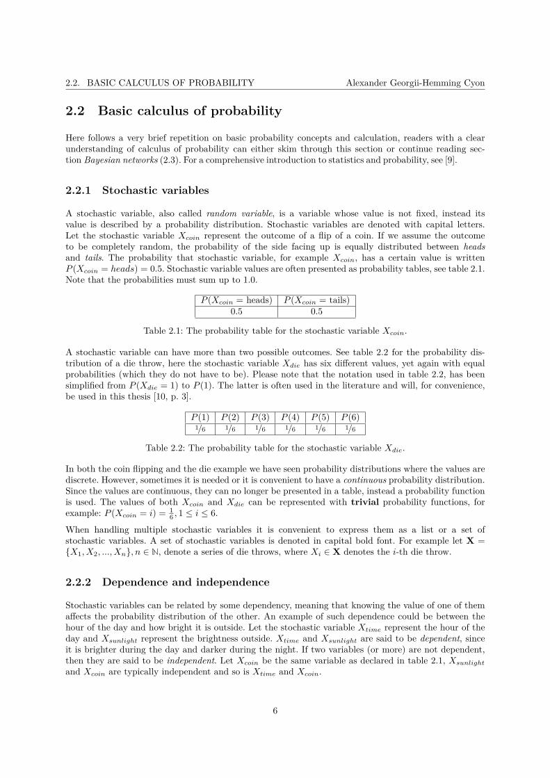
A stochastic variable, also called random variable, is a variable whose value is not fixed, instead itsvalue is described by a probability distribution. Stochastic variables are denoted with capital letters.Let the stochastic variable Xcoin represent the outcome of a flip of a coin. If we assume the outcometo be completely random, the probability of the side facing up is equally distributed between headsand tails. The probability that stochastic variable, for example Xcoin, has a certain value is writtenP (Xcoin = heads) = 0.5. Stochastic variable values are often presented as probability tables, see table 2.1.Note that the probabilities must sum up to 1.0.
P (Xcoin = heads) P (Xcoin = tails)0.5 0.5
Table 2.1: The probability table for the stochastic variable Xcoin.
A stochastic variable can have more than two possible outcomes. See table 2.2 for the probability dis-tribution of a die throw, here the stochastic variable Xdie has six different values, yet again with equalprobabilities (which they do not have to be). Please note that the notation used in table 2.2, has beensimplified from P (Xdie = 1) to P (1). The latter is often used in the literature and will, for convenience,be used in this thesis [10, p. 3].
P (1) P (2) P (3) P (4) P (5) P (6)1/6 1/6 1/6 1/6 1/6 1/6
Table 2.2: The probability table for the stochastic variable Xdie.
In both the coin flipping and the die example we have seen probability distributions where the values arediscrete. However, sometimes it is needed or it is convenient to have a continuous probability distribution.Since the values are continuous, they can no longer be presented in a table, instead a probability functionis used. The values of both Xcoin and Xdie can be represented with trivial probability functions, forexample: P (Xcoin = i) = 1
6 , 1 ≤ i ≤ 6.
When handling multiple stochastic variables it is convenient to express them as a list or a set ofstochastic variables. A set of stochastic variables is denoted in capital bold font. For example let X =X1, X2, ..., Xn, n ∈ N, denote a series of die throws, where Xi ∈ X denotes the i-th die throw.
2.2.2 Dependence and independence
Stochastic variables can be related by some dependency, meaning that knowing the value of one of themaffects the probability distribution of the other. An example of such dependence could be between thehour of the day and how bright it is outside. Let the stochastic variable Xtime represent the hour of theday and Xsunlight represent the brightness outside. Xtime and Xsunlight are said to be dependent, sinceit is brighter during the day and darker during the night. If two variables (or more) are not dependent,then they are said to be independent. Let Xcoin be the same variable as declared in table 2.1, Xsunlight
and Xcoin are typically independent and so is Xtime and Xcoin.
6

2.2. BASIC CALCULUS OF PROBABILITY Alexander Georgii-Hemming Cyon
Definition 2.2.1 (Independence). Two stochastic variables, X and Y , are independent if and only if, forall values x of X and all values y of Y the following equality holds: P (X = x, Y = y) = P (X = x)P (Y =y).
Definition 2.2.2 (Dependence). Two stochastic variables are said to be dependent, if they are notindependent. Thus, for all values x of X and all values y of Y the following inequality holds: P (X =x, Y = y) = P (X = x)P (Y = y). This means that knowing the value of one of them affects the probabilityof the other.
2.2.3 Joint probability distribution
Joint probability distribution describes the probability of two stochastic variables X, Y having somevalues simultaneously, i.e. P (X = x, Y = y). This can be denoted with a shorter version: P (x, y). Thereis also another common notation, let A denote the event that X = x and B that Y = y, then P (A ∩B)denotes that A and B occurs at the same time, however the former notation is the one used in thisthesis.
Let us demonstrate with a simple example. Let Xeven = True, False be a stochastic variable denotingwhether a die throw results in an even number or not, let Xlow = True, False denote whether thevalue is low (number 1, 2 or 3) or not. It is trivial to see that P (Xeven = True) = 1
2 and P (Xlow =True) = 1
2 respectively. Xeven and Xlow are dependent since P (Xeven = T )P (Xlow = T ) = 1/4 butP (Xeven = T,Xlow = T ) ≈ 1/6. The joint probability distribution for the combination of those variablesis shown in table 2.3.
Xeven Xlow P (Xeven, Xlow)
True True 1/6
True False 1/3
False True 1/3
False False 1/6
Table 2.3: The joint probability table for two stochastic variables. The combination of P (Xeven =True,Xlow = True) yields that the number must be even and either number 1, 2 or 3. The only numberthat fulfills those criteria is the number 2, i.e. only one number of six fulfills those criteria, which yields aprobability of 1
6 . P (Xeven = True,Xlow = False) yields an even number in the range 4-6, which is eithernumber 4 or 6. Two possible outcomes out of six gives the probability 2
6 = 13 .
The joint probability for two independent variables are the product of their individual probability:P (A,B) = P (A)P (B). Note the important difference when A and B are dependent which yields theinequality P (A,B) = P (A)P (B).
The example presented above shows joint probability of two stochastic variables, however, it is possible tocalculate the joint probability of a set of stochastic variables, X. The calculation of the joint probabilitydistribution of a set of stochastic variables is the product of the probability for each individual variables
7
2.2. BASIC CALCULUS OF PROBABILITY Alexander Georgii-Hemming Cyon
in the set, or expressed mathematically:
P (X) = P (X0 = x0, ..., XN−1 = xN−1) =
∏
X∈XP (X) if X ∈ X is independent.
N−1∏i=0
P (Xi| ∩i−1j=0 Xj) if X ∈ X is dependent.
(2.1)
2.2.4 Conditional probability
Conditional probability expresses the probability of some event A, given the knowledge that some otherevent B is known to have occurred, and is denoted as P (A|B). The conditional probability can becalculated according to definition 2.2.3.
Definition 2.2.3 (Conditional probability). The conditional probability between the stochastic variablesA and B is expressed by the following equation P (A|B) = P (A,B)
P (B) , where P (B) > 0 and P (A,B) is theprobability that A and B occurs simultaneously (joint probability). If A and B are independent, thenP (A|B) = P (A), i.e. knowing that B has occurred does not change the probability of A.
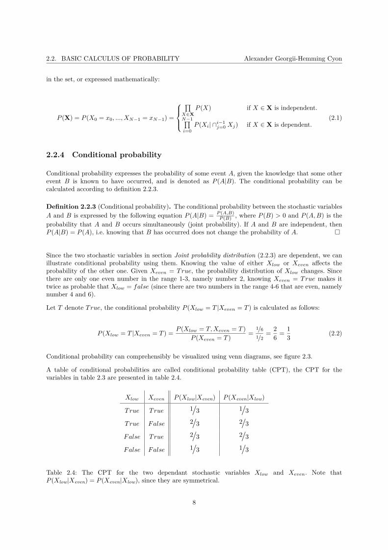
Since the two stochastic variables in section Joint probability distribution (2.2.3) are dependent, we canillustrate conditional probability using them. Knowing the value of either Xlow or Xeven affects theprobability of the other one. Given Xeven = True, the probability distribution of Xlow changes. Sincethere are only one even number in the range 1-3, namely number 2, knowing Xeven = True makes ittwice as probable that Xlow = false (since there are two numbers in the range 4-6 that are even, namelynumber 4 and 6).
Let T denote True, the conditional probability P (Xlow = T |Xeven = T ) is calculated as follows:
P (Xlow = T |Xeven = T ) =P (Xlow = T,Xeven = T )
P (Xeven = T )=
1/61/2
=2
6=
1
3(2.2)
Conditional probability can comprehensibly be visualized using venn diagrams, see figure 2.3.
A table of conditional probabilities are called conditional probability table (CPT), the CPT for thevariables in table 2.3 are presented in table 2.4.
Xlow Xeven P (Xlow|Xeven) P (Xeven|Xlow)
True True 1/3 1/3
True False 2/3 2/3
False True 2/3 2/3
False False 1/3 1/3
Table 2.4: The CPT for the two dependant stochastic variables Xlow and Xeven. Note thatP (Xlow|Xeven) = P (Xeven|Xlow), since they are symmetrical.
8
2.3. BAYESIAN NETWORKS Alexander Georgii-Hemming Cyon
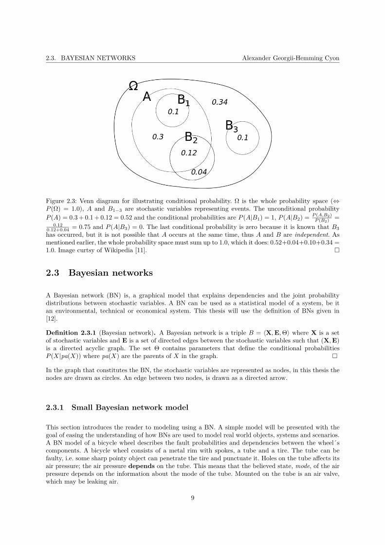
Figure 2.3: Venn diagram for illustrating conditional probability. Ω is the whole probability space (⇔P (Ω) = 1.0), A and B1−3 are stochastic variables representing events. The unconditional probabilityP (A) = 0.3+ 0.1+ 0.12 = 0.52 and the conditional probabilities are P (A|B1) = 1, P (A|B2) =
P (A,B2)P (B2)
=0.12
0.12+0.04 = 0.75 and P (A|B3) = 0. The last conditional probability is zero because it is known that B3
has occurred, but it is not possible that A occurs at the same time, thus A and B are independent. Asmentioned earlier, the whole probability space must sum up to 1.0, which it does: 0.52+0.04+0.10+0.34 =1.0. Image curtsy of Wikipedia [11].
2.3 Bayesian networks
A Bayesian network (BN) is, a graphical model that explains dependencies and the joint probabilitydistributions between stochastic variables. A BN can be used as a statistical model of a system, be itan environmental, technical or economical system. This thesis will use the definition of BNs given in[12].
Definition 2.3.1 (Bayesian network). A Bayesian network is a triple B = ⟨X,E,Θ⟩ where X is a setof stochastic variables and E is a set of directed edges between the stochastic variables such that (X,E)is a directed acyclic graph. The set Θ contains parameters that define the conditional probabilitiesP (X|pa(X)) where pa(X) are the parents of X in the graph.
In the graph that constitutes the BN, the stochastic variables are represented as nodes, in this thesis thenodes are drawn as circles. An edge between two nodes, is drawn as a directed arrow.
2.3.1 Small Bayesian network model
This section introduces the reader to modeling using a BN. A simple model will be presented with thegoal of easing the understanding of how BNs are used to model real world objects, systems and scenarios.A BN model of a bicycle wheel describes the fault probabilities and dependencies between the wheel´scomponents. A bicycle wheel consists of a metal rim with spokes, a tube and a tire. The tube can befaulty, i.e. some sharp pointy object can penetrate the tire and punctuate it. Holes on the tube affects itsair pressure; the air pressure depends on the tube. This means that the believed state, mode, of the airpressure depends on the information about the mode of the tube. Mounted on the tube is an air valve,which may be leaking air.
9

2.3. BAYESIAN NETWORKS Alexander Georgii-Hemming Cyon
Figure 2.4: Overview of a bicycle wheels components, 1) tube, 2) tire, 3) rim, 4) hub, 5) spoke, 6) airvalve.
2.3.2 Component variables
We would somehow like to represent the mode of the parts of the wheel in a model, or to be specific, thebelevied mode. This is done by representing them as stochastical variables.
Definition 2.3.2 (Component variable). A component variable is a stochastic variable. The values thata component variable (CV) holds are called fault modes. Each CV have at least two fault modes, one ofthem is the non-faulty (NF) mode2, which means that the component that the CV represents/models isworking correctly. Each CV have at least one faulty mode, with some specific name, e.g. Electrical fault, ifthe component that the CV models contains some electric circuit. Let M(C) denote the set of all possiblefault modes for some component variable C. As shown in table 2.3, each possible fault mode must have aprobability, and the sum of all modes must be 1.0. This can be expressed formally as follows: each mode
mi ∈M(C) must have some probability such thatMc(C)−1∑
i=0
P (C = mi) = 1.0, where Mc(C) is the size of
M(C), i.e. the number of possible fault modes of C.
In the wheel we model three of its components, Xhole holds information whether there is any hole onthe tube or not, Xvalve describes if the air valve is tightened or leaking and Xpressure describes the
2One could claim that it is an oxymoron to call the mode non-faulty a fault mode.
10

2.3. BAYESIAN NETWORKS Alexander Georgii-Hemming Cyon
air pressure in the tube. An overview of the variables used in the BN model of the bicycle wheel isgiven in table 2.5. Note that the non-faulty mode has been given a more specific name for the sake ofcomprehensibility.
Variable Non-faulty mode Faulty modeXtube Intact PuncturedXvalve Tightened LeakyXpressure High Low
Table 2.5: This table shows the three component variables in the BN model of the bicycle wheel. Thenon-faulty mode has been given a more specific name for the sake of comprehensibility.
Let Xpressure depend on Xhole and Xvalve, but the two latter be independent of each other. Xhole andXvalve have so called a priori probabilities, which expresses the probability for each fault modes, givenno information about the system. The a priori probabilities are presented in the tables next to the nodesin figure 2.5. The table next to variable Xpressure is its CPT.
...
Xtube
..
Xvalve
.. Xpressure.
P (Xtube)Intact Punctured
0.9 0.1
.
P (Xvalve)Tightened Leaky
0.8 0.2
.
P (Xpressure|Xtube, Xvalve)Xtube Xvalve High LowIntact Tightened 0.95 0.05Intact Leaky 0.70 0.30
Punctured Tightened 0.05 0.95Punctured Leaky 0.01 0.99
Figure 2.5: A small BN describing conditional probabilities of certain faults on a bicycle wheel.
The BN model of the bicycle wheel consists of the nodes (with their a priori probabilities): represent-ing components, the arcs: representing dependency and the CPT. For a comprehensive introduction tomodeling using BN see [13].
The a priori probabilities are typically calculated from data, but please note that the values in this bicyclewheel example are nothing but guessed values. More importantly, the values in the CPT of Xpressure arealso guessed and can not be calculated given the a priori probabilities of its parents. Given the tables infigure 2.5, we can calculate the probabilities of all possible scenarios, triples ⟨Xpressure, Xtube, Xvalve⟩, inthe wheel model. The calculated probabilities are presented in table 2.6.
From table 2.6 we can derive the total probability for high/low air pressure, by adding the four differentcombination which results in high and low air pressure respectively, which is done and presented intable 2.7. Even though the values in this table are nothing but calculation based on the original values infigure 2.5, it is one of the most relevant tables, from which we can conclude that the probability that theair pressure in the tube is high is 0.8142, given no information about the condition of the system.
11

2.3. BAYESIAN NETWORKS Alexander Georgii-Hemming Cyon
Xpressure Xtube Xvalve P (Xpressure, Xtube, Xvalve)High Intact Tightened 0.684High Intact Leaky 0.126High Punctuated Tightened 0.004High Punctuated Leaky 0.0002Low Intact Tightened 0.036Low Intact Leaky 0.054Low Punctuated Tightened 0.076Low Punctuated Leaky 0.0198
Table 2.6: CPT over different combination of the modes of the three stochastic variables. The rightmostcolumn shows the probability for the triple ⟨Xpressure, Xtube, Xvalve⟩. The probability in the first row iscalculated by: P (Intact)P (Tightened)P (High|Intact, T ightened) = 0.9∗0.8∗0.95 = 0.684. And the lastrow is calculated by: P (Punctuated)P (Leaky)P (Low|Punctuated, Leaky) = 0.1 ∗ 0.2 ∗ 0.99 = 0.0198.etc.
P (Xpressure|Xtube, Xvalve)P (High) P (Low)0.8142 0.1858
Table 2.7: This table groups the probabilities depending on the Xpressure variable. Where the value inthe left column is the sum if the first four rows in table 2.6 are P (High) = P (High, Intact, T ightened)+P (High, Intact, Leaky) + P (High, Punctuated, T ightened) + P (High, Punctuated, Leaky) = 0.684 +0.126 + 0.004 + 0.0002 = 0.8142 and P (Low) is calculated analogously, with the four last rows.
2.3.3 Observation variables
To identify which of the system´s components is faulty and make a diagnosis, observations has to be madeon the faulty system. It can either be a physical observation made by the mechanic or DTCs providedby the XPI-system´s computer system called engine management system (EMS)3. In the bicycle wheelexample such observations can be examination of the tube and the valve, with the purpose of determiningif the tube is punctuated and whether the valve is tightened or not.
Definition 2.3.3 (Observation variable). An observation variable is a stochastic variable. An observationvariable (OV) can only have two different modes, either indicating (ind) or non-indicating (nind). Edgesare directed from CVs to OVs. An OV may have multiple edges to it, i.e. multiple component nodes asparents.
As mentioned, pa(Oi) denotes the parent list for the observation variable Oi, i.e. a list of CVs.
M(Cj) denotes the set of fault modes of the component variable Cj , then there is a conditional probabilitythat parent to Oi, Cj , is in the mode mk.
P (Oi = ind|Cj = mk), ∀Cj ∈ pa(Oi) ∀mk ∈M(Cj)
Thus there is a CPT for each OV, withpac(Cj)−1∏
j=0
2∗M(Cj), ∀Cj ∈ pa(Oi), where pac(Cj) is the number of
parents to Oi. The factor 2 comes from that each of OVs Oi´s modes (ind/nind) must have a conditional
3A type of electronic control unit (ECU)
12
2.3. BAYESIAN NETWORKS Alexander Georgii-Hemming Cyon
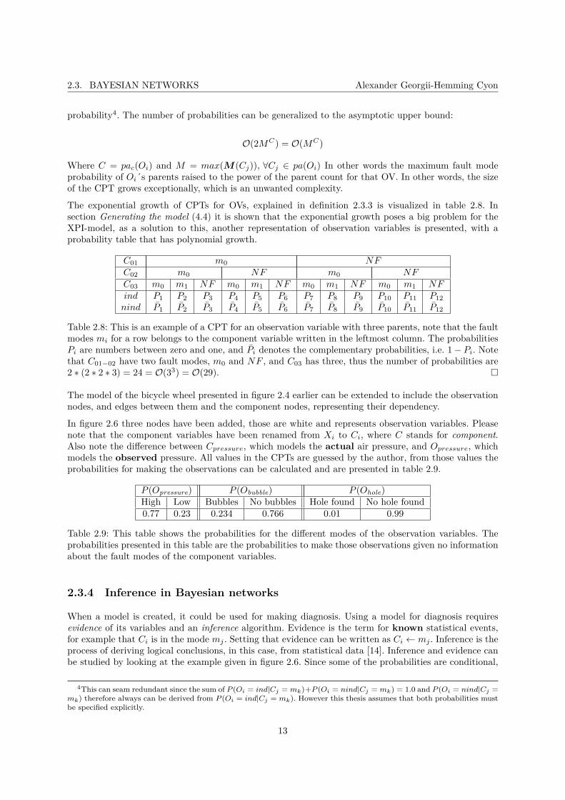
probability4. The number of probabilities can be generalized to the asymptotic upper bound:
O(2MC) = O(MC)
Where C = pac(Oi) and M = max(M(Cj)), ∀Cj ∈ pa(Oi) In other words the maximum fault modeprobability of Oi´s parents raised to the power of the parent count for that OV. In other words, the sizeof the CPT grows exceptionally, which is an unwanted complexity.
The exponential growth of CPTs for OVs, explained in definition 2.3.3 is visualized in table 2.8. Insection Generating the model (4.4) it is shown that the exponential growth poses a big problem for theXPI-model, as a solution to this, another representation of observation variables is presented, with aprobability table that has polynomial growth.
C01 m0 NFC02 m0 NF m0 NFC03 m0 m1 NF m0 m1 NF m0 m1 NF m0 m1 NFind P1 P2 P3 P4 P5 P6 P7 P8 P9 P10 P11 P12
nind P1 P2 P3 P4 P5 P6 P7 P8 P9 P10 P11 P12
Table 2.8: This is an example of a CPT for an observation variable with three parents, note that the faultmodes mi for a row belongs to the component variable written in the leftmost column. The probabilitiesPi are numbers between zero and one, and Pi denotes the complementary probabilities, i.e. 1− Pi. Notethat C01−02 have two fault modes, m0 and NF , and C03 has three, thus the number of probabilities are2 ∗ (2 ∗ 2 ∗ 3) = 24 = O(33) = O(29).
The model of the bicycle wheel presented in figure 2.4 earlier can be extended to include the observationnodes, and edges between them and the component nodes, representing their dependency.
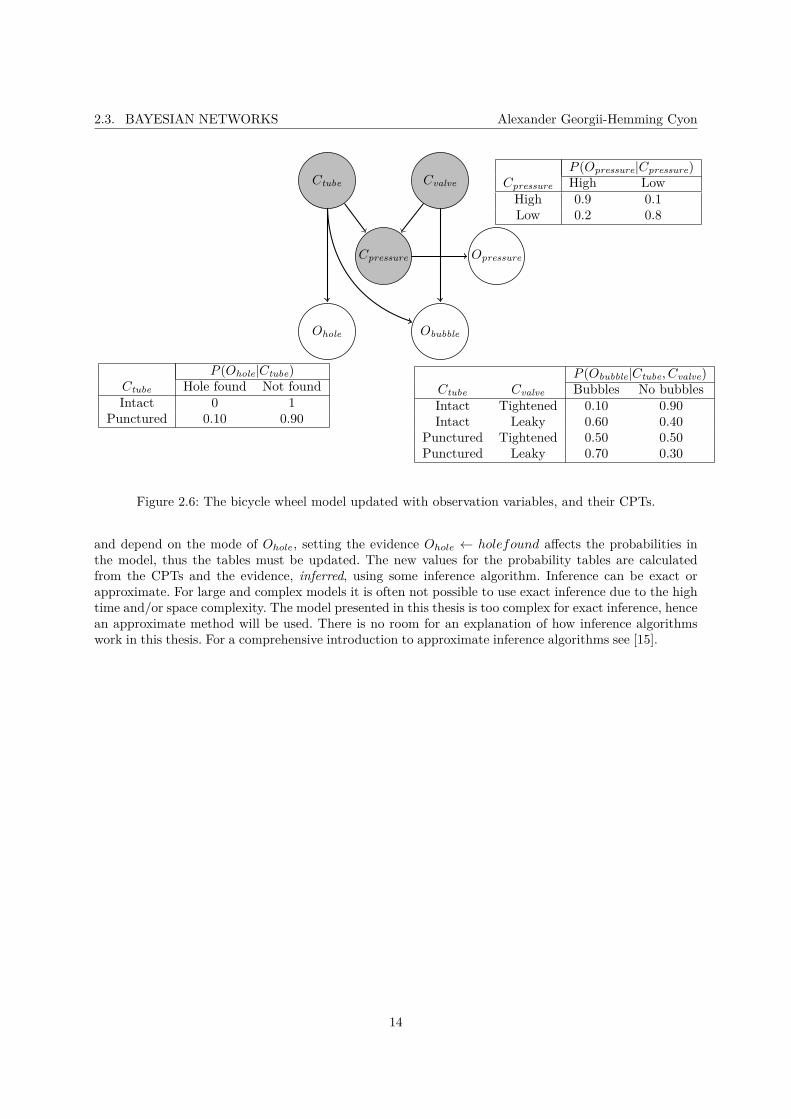
In figure 2.6 three nodes have been added, those are white and represents observation variables. Pleasenote that the component variables have been renamed from Xi to Ci, where C stands for component.Also note the difference between Cpressure, which models the actual air pressure, and Opressure, whichmodels the observed pressure. All values in the CPTs are guessed by the author, from those values theprobabilities for making the observations can be calculated and are presented in table 2.9.
P (Opressure) P (Obubble) P (Ohole)High Low Bubbles No bubbles Hole found No hole found0.77 0.23 0.234 0.766 0.01 0.99
Table 2.9: This table shows the probabilities for the different modes of the observation variables. Theprobabilities presented in this table are the probabilities to make those observations given no informationabout the fault modes of the component variables.
2.3.4 Inference in Bayesian networks
When a model is created, it could be used for making diagnosis. Using a model for diagnosis requiresevidence of its variables and an inference algorithm. Evidence is the term for known statistical events,for example that Ci is in the mode mj . Setting that evidence can be written as Ci ← mj . Inference is theprocess of deriving logical conclusions, in this case, from statistical data [14]. Inference and evidence canbe studied by looking at the example given in figure 2.6. Since some of the probabilities are conditional,
4This can seam redundant since the sum of P (Oi = ind|Cj = mk)+P (Oi = nind|Cj = mk) = 1.0 and P (Oi = nind|Cj =mk) therefore always can be derived from P (Oi = ind|Cj = mk). However this thesis assumes that both probabilities mustbe specified explicitly.
13
2.3. BAYESIAN NETWORKS Alexander Georgii-Hemming Cyon
...
Ctube
..
Cvalve
..
Cpressure
..Ohole.. Obubble..
Opressure
.
P (Opressure|Cpressure)Cpressure High Low
High 0.9 0.1Low 0.2 0.8
.
P (Ohole|Ctube)Ctube Hole found Not foundIntact 0 1
Punctured 0.10 0.90
.
P (Obubble|Ctube, Cvalve)Ctube Cvalve Bubbles No bubblesIntact Tightened 0.10 0.90Intact Leaky 0.60 0.40
Punctured Tightened 0.50 0.50Punctured Leaky 0.70 0.30
Figure 2.6: The bicycle wheel model updated with observation variables, and their CPTs.
and depend on the mode of Ohole, setting the evidence Ohole ← holefound affects the probabilities inthe model, thus the tables must be updated. The new values for the probability tables are calculatedfrom the CPTs and the evidence, inferred, using some inference algorithm. Inference can be exact orapproximate. For large and complex models it is often not possible to use exact inference due to the hightime and/or space complexity. The model presented in this thesis is too complex for exact inference, hencean approximate method will be used. There is no room for an explanation of how inference algorithmswork in this thesis. For a comprehensive introduction to approximate inference algorithms see [15].
14

Chapter 3
Methodology
In this chapter the methodology used in the thesis will be presented and motivated.
3.1 Methods for modeling
The model presented in this thesis uses Bayesian networks. The main reason why XPI is modeled usingBN is that the XPI-system is non-deterministic and therefore it is suitable to use a BN, due to theirstatistical nature. Fault counts for each component are available, from which we can calculate the a prioriprobabilities. The set of fault modes for each component are also provided.
Furthermore, BNs are typically well suited for modeling when you have system experts available, that candescribe the system and help understanding the data[16]. Using BNs have been shown to be a convenientmethodology for modeling complex system, such as ecosystems[17][18][19].
Another reason why BN was used is that the provider of the project have worked with BN in his licentiatethesis[1]. Since this thesis is closely related to the supervisor’s work it was natural to use BNs too.
3.1.1 Creating the model
The model will be presented in the modeling program GeNIe[2]. GeNIe is used to create BNs and enablesto interact with the model by setting evidence, i.e. setting a node to a certain mode, after which the modelis updated and presents the different diagnoses (conditional probabilities given the evidence). Howeverit would be intractable to create this model manually, due to its size and the cardinality1 of some of itsnodes. Furthermore, there is no feature that allows automatic placement of the nodes in order to makethe graph planar2 (if possible), or rearrange the nodes´ positions such that a minimum number of edgesintersects. The graph will therefore be made in a graph making program called yED [20], which has thewanted feature of node rearrangement. Please observe that the yED-model only contains the graph usedin the BN-model, it has no probability data. This introduces the need of converting the yED-model to aGeNIe model and somehow insert the probability data.
The author of this thesis developed a Java program called yED to GeNIe, or Y2G for short. Y2G takes ayED graph together with XML data files as input and outputs a GeNIe model. Continue reading aboutY2G in section Generating the model (4.4).
1The cardinality is the number of neighboring nodes, i.e. the number of parent or child nodes for some node.2A planar graph is a graph were no edges intersect other than in the endpoint of a node.
15

3.2. METHODS FOR VERIFYING THE MODEL Alexander Georgii-Hemming Cyon
3.1.2 Analyzing and formatting the data
The data used in the creation of the a priori probabilities comes from service workshops all over the world.Unfortunately the data3 is not formated on any standard format, the data have been saved on differentformats by different people. The reason for this is partially that the data is reported in by mechanics whohave no insight in statistics and partially because the mechanics have not been instructed well enough onhow they should report the data or that they simple have been ignoring any instructions. This results innoisy data. For example, a mechanic may report that component C is faulty and having the fault modeLeakage, when the true fault mode of C actually was cracked or broken (CB), which led to the symptomnamed Leakage, this results in an incorrect internal fault mode distribution between the fault modes ofC. therefore certain fault modes has been grouped together. The fault modes for the pipes have beenchanged, the mode CB has been merged into fuel leakage (FL), since this probably is what the mechanicswho reported it meant4.
The fault frequency for the fault mode CB has been merged into electrical fault (EF) for the componentpressure sensor (C22), since it probably is what the mechanics meant.
Some DTCs that are very similar have been grouped together since they are caused by the same faultmode. For example, some components can lead to multiple DTCs that are caused by electrical faults,where the DTCs could be named short circuit to ground and short circuit to battery, those DTCs hasbeen merged into one single observation variable named electrical fault, for each component potentiallygenerating multiple electrical DTCs.
The data consists of number of warranty claims per component. This constitutes the fault frequency dataneeded to create the a priori probabilities for each component variable in the model. The probabilities arecreated by dividing the fault frequencies with the size of the truck population examined, denoted POP .Choosing POP as the denominator results in that the a priori probabilities will be the probabilitiesthat a certain component is faulty given that we take any truck, t ∈ POP randomly “from the street”and examining it. Determining the denominator is not a trivial task, since it affects the whole model,the problem of choosing the denominator is known as the reference class problem[21], and is a classicstatistical problem. Instead of POP , the denominator could have been the set of all trucks that havebeen to service or only trucks that have been to service because of known faults.
Some of the components have no reported warranty claims, this would result in probability P (Ci =Faulty) = 0, ∀i ∈ S, where S is a set of components with zero reported claims. In other words, the modelwould say that it is impossible for the components in S to be faulty, which is a dangerous assumptionand would limit the model dramatically5. To solve this problem we use a common method to handle zero-probability entries called add-one smoothing (also called Laplace smoothing)[22]. It has been shown thatthere are more effective techniques than add-one smoothing[23], however this method meets our needsand is very simple to use. For a further reading about smoothing methods, please see[24][25].
3.2 Methods for verifying the model
The use of BNs for modeling have steadily increased during the last decades, thanks to their suitability formodeling using statistics. But few models are verified or validated. [16, p. 3064]. The difference betweenvalidation and verification might be hard to distinguish, but here is a good definition: [26]
3Taken from Scania´s statistics program.4This has been done for components: C07-C12, C14-C19, C20, C23, C27, C32, C33, C36, C38, which all are component
variables presented in table 4.25Since the model only could behave according to how the XPI-systems in the truck population that the data is taken
from have been behaved.
16

3.2. METHODS FOR VERIFYING THE MODEL Alexander Georgii-Hemming Cyon
Validation “Are we building the right system?”Verification “Are we building the system right?”
This thesis will perform a verification of the model and not a validation. The verification techniques usedin this thesis is case-based evaluation.[27, p. 284] In fact two different case studies will be performed, oneof them supervised, i.e. an expert of the XPI-system will be present and give his expert opinion on eachcase result. The second is unsupervised, without the presence of an XPI-expert.
The verification process is explained in detail in chapter Verifying the XPI-model (5).
17

3.2. METHODS FOR VERIFYING THE MODEL Alexander Georgii-Hemming Cyon
18
Part II
System Modeling
19


Chapter 4
Modeling the XPI-system
In this chapter the theory learned in chapter Theory (2) and chapter Methodology (3) will be applied onthe data, creating the model of the XPI-system.
4.1 About the XPI-system
The purpose of the XPI-system is to supply the engine with the right amount of fuel at the right timeand with high pressure. It increases the diesel injection pressure to around 2000 bar. The system consistsof pumps, pipes, filters and nozzles, amongst other components. The purpose of this section is to give anexplanation of how the system works so that the reader has a fundamental understanding of the systemin prior to the modeling of it.
4.1.1 Components
Some of the components in the XPI-system are presented in figure 4.1. The description of the XPI-systemin section The route of the fuel in the engine (4.1.2) will refer to the components presented in the listbelow, using the components index in parenthesis.
4.1.2 The route of the fuel in the engine
This section explains the route of the fuel in the XPI-system, giving the reader an insight on how thesystem works.
Fuel is sucked from the fuel tank by the feed pump (22). The fuel enters through connection (1) and getsdrawn through the suction filter (21) into the engine management system (EMS) with cooler (24) via thefuel hose (2). The fuel is drawn from the EMS (24) and its cooler to the feed pump (22) via the fuel hose(3).
The feed pump increases the fuel pressure to between 9 and 12 bar and, via the fuel pipe (4), forces thefuel through the pressure filter (6). From the pressure filter the fuel flows, via the fuel pipe (5), into thefuel inlet metering valve (IMV) (19), fitted on the high pressure pump (HPP) (23).
The IMV controls the amount of fuel that flows into the HPP and is controlled by he EMS.
The HPP increases the pressure dramatically, from previous 9 to 12 bar to a maximum of 3000 bar. Viaa high pressure pipe (7), the fuel continues to the accumulator (14).
21

4.1. ABOUT THE XPI-SYSTEM Alexander Georgii-Hemming Cyon
Figure 4.1: Drawing of the XPI-system, with the major components indexed. A) high pressure fuel pipe,B) low pressure pipe/hose, C) pipe for return fuel, 1) pipe from fuel tank, 2) hose to EMS cooler, 3) hoseto feed pump, 4) pipe to pressure filter, 5) pipe to IMV, 6) pressure filter 7) pipe to accumulator, 8) pipeto high pressure connector, 9) safety valve, 10) pipe to fuel manifold, 11) pipe to fuel tank, 12) HPC, 13)injector, 14) accumulator, 15) pressure sensor, 16) fuel manifold, 17) bleed nibble, 18) overflow valve, 19)IMV, 20) hand pump, 21) suction filter, 22) feed pump, 23) HPP, 24) EMS with cooler
A high pressure pipe (8) connects the accumulator to each high pressure connector (HPC) (12) bringingfuel to the injectors (13). When the solenoid1 valve in the injector is supplied with voltage, the injectoropens and fuel is injected into the cylinder.
Since the XPI-system operates with high fuel pressure it is important that the fuel is free from water,because water leads to corrosion of the components. The system tolerance is tight and damaged compo-nents could cause the system to not function properly. To prevent this, water is separated from the fuelin the suction filter (21).
If a fault that results in too high pressure occurs, the safety valve (9) on the accumulator opens and thefuel is returned to the HPP via the pipe (10). The threshold for this safety procedure is > 3000 bar anddrops the pressure to 1000 bar, the safety valve continues to regulate the pressure so that a pressure inthe range 700-1300 bar is maintained.
Excess fuel from the injectors flows from the fuel manifold (16) back to the fuel tank via the pipe(11).
The route of the fuel is summarized in figure 4.2.
1A type of electromagnet.
22

4.2. MODEL ASSUMPTIONS AND DELIMITATIONS Alexander Georgii-Hemming Cyon
..Fuel tank. Waterseparation
. Pressureto 12 bar
. Fuel particlefiltering
. Pressure to3000 bar
. Injected incylinders
Figure 4.2: A summary of what happens in the XPI-system.
4.2 Model assumptions and delimitations
A model is, in its essence, a description of something real, therefore, disregarding how detailed the modelis, there will always be some aspects and characteristics of the reality that the model will not cover. Wecan call this incongruence a gap. There will be a gap between the behavior of the real XPI-system and themodel presented in chapter Modeling the XPI-system (4). Closing this gap requires a vastly detailed andcomplex model. This is not always wanted since it is difficult to get an overview of the system, makingit hard to understand. Limiting the scope of the model is not only convenient, but also necessary, sinceit gets unmanageable to make calculations on it otherwise due to the large search space [28].
4.2.1 Assumptions
To make the modeling of the XPI-system feasible, some assumptions have to be made, otherwise themodel will be too complex.
Assumption 1 (Components are independent). The component variables are independent and faultsoccur independently. This is a strong assumption.
Assumption 2 (All components can be faulty). Even though some components have a fault count ofzero in the warranty claims, they have a non-zero probability of being faulty in the model, this is an effectof the additive smoothing mentioned in section Analyzing and formatting the data (3.1.2).
4.2.2 Delimitations
The XPI-system is a dynamic system that has been developed during several years. More importantly,it is still in development. The version of the system being modeled in this thesis is called generation S7and is installed in the heavy duty vehicles being used on the market today. The model presented in thischapter will thus only model the components, faults and observations taken from the S7 XPI-system,therefore ignoring all the updates, improvements that has been made on the XPI-system since.
The CPTs used in the XPI-model are based on statistical data derived from technical reports on vehiclesduring the one year warranty period sent from workshops from the whole global market. Customersare experiencing different problems e.g. due to their local whether conditions, such as temperature andhumidity. another important factor is the quality of the diesel. In Sweden the diesel is very clean, almostfree from water and with low paraffin2 concentrations. However, if a vehicle is fueled with diesel withhigh paraffin concentrations in a country in southern Europe and enters Sweden during the winter, theparaffin often deposits into paraffin wax, clogging the fuel filters. Markets all over the world are differentand in order to get a feasible and applicable model, global workshop data will be used.
Most of the pipes in the XPI-system will be included in the model. These components represents thepipes themselves but also the connection in both ends. Hoses are treated as pipes.
2Paraffin is a hydrocarbon compound found in diesel that can take a solid wax form if the temperature is below 37degrees Celsius [29].
23
4.3. THE MODEL Alexander Georgii-Hemming Cyon
The XPI-system is not independent of other systems, the healthiness of its components may be affectedby other systems in the vehicle, but it is also affected by environmental factors. The fuel filters can easilyget clogged due to paraffin. As mentioned above, the fuel clogs if the fuel has a bad quality, i.e. highparaffin level in the diesel, in combination with low temperatures. These factors, as well as the othersystems or parts of systems in the vehicle will not be included in this model. The reason for this is to tryto limit the fault detection of the system to its components.
Since the model is suppose to reflect the reality, it can be modeled with the same limits and crassness asthe reality has. In the troubleshooting manual, the mechanic is often instructed to replace whole partsof the XPI-system, consisting of several components, instead of identifying the individual component inthat part. E.g. if the suction filter is broken, both that component and the pressure filter is replaced, sincethese components are connected and installed as a single part. therefore it is not necessary to model everysingle part in the XPI-system, instead the model will sometimes use one single component to representpart of the XPI-system.
4.3 The model
The data that the model is based on is sensitive to Scania, thus the data presented in this thesis arefictive. All values in tables and the model is fictive. However, the result and conclusion is based on theoriginal data.
4.3.1 Component Variables
Deciding which components to include in the model is not an easy task, and it is one of the factors thataffects the model the most.
Figure 4.1 shows the most important components in the XPI-system, but not all. The model will includethose components together with some other ones. In table 4.2 all component variables in the XPI-modelare presented. If a component is working correctly it is said to be non-faulty (NF), this mode is left outin table 4.2.
The different fault modes for the components are presented in table 4.1.
Abbreviation Fault modeIV imbalance or vibrationFL fuel leakageCB cracked or brokenEF electrical faultSC stuck or cloggedWP wrong pressureEMF emission faultAL air leakage
Table 4.1: A table presenting the possible fault modes for the component nodes.
Please note that all values in table 4.2 are fictive (randomly generated) since the real values are sensitivefor Scania´s business. Since the data is fictive, the fault mode list for the components may seem strangeor illogical. If the reasoning in section Discussion (6.1) seams illogical because of inconsistency with thedata, it is because the conclusion is based on the original data.
24

4.3. THE MODEL Alexander Georgii-Hemming Cyon
Component variable Description P (F )1 Fault modes
C01 Accumulator (acc.) Thick high pressure pipe/fuel rail. 5.539 EMF:100.0
C02 Feed Pump (FP) Sucks fuel from fuel tank. 0.005 FL:67.4, CB:32.6
C03 Filter Housing Case for C24 and C21. 5.368 FL:60.2, IV:26.1, EF:1.1,
WP:12.7
C04 Fuel Heater Heats the fuel.2 3.296 IV:38.0, WP:41.7,
EF:10.1, FL:10.2
C05 Fuel Manifold (FM) Manifold for return/excess fuel. 9.496 WP:30.6, EMF:47.8,
EF:21.6
C06 Hand Pump Hand pump used for fault-diagnosis. 7.027 SC:50.5, IV:49.5
C07 HPC1 Connector between C26 and C14. 4.315 IV:98.0, WP:1.4, CB:0.2,
AL:0.3
C08 HPC2 Connector between C27 and C15. 3.291 CB:33.4, AL:52.6, SC:3.5,
WP:10.5
C09 HPC3 Connector between C28 and C16. 4.452 EF:15.8, IV:57.8, FL:18.4,
AL:8.0
C10 HPC4 Connector between C29 and C17. 3.819 IV:66.6, EF:10.9,
EMF:18.6, SC:4.0
C11 HPC5 Connector between C30 and C18. 6.983 AL:1.6, EF:4.3, IV:82.1,
CB:12.0
C12 HPC6 Connector between C31 and C19. 0.801 IV:38.6, EF:6.7, WP:52.1,
EMF:2.6
C13 High Pressure Pump (HPP) Increases pressure to max. 3000 bar. 9.804 IV:100.0
C14 Injector1 Injects fuel into cylinder 1. 0.510 FL:25.9, CB:74.1
C15 Injector2 Injects fuel into cylinder 2. 0.510 FL:25.9, CB:74.1
C16 Injector3 Injects fuel into cylinder 3. 0.510 FL:25.9, CB:74.1
C17 Injector4 Injects fuel into cylinder 4. 0.510 FL:25.9, CB:74.1
C18 Injector5 Injects fuel into cylinder 5. 0.510 FL:25.9, CB:74.1
C19 Injector6 Injects fuel into cylinder 6. 0.510 FL:25.9, CB:74.1
C20 Inlet Metering Valve (IMV) Controls fuel amount into C01. 8.633 EMF:1.8, SC:72.8,
CB:21.2, IV:4.3
Continued on next page…
1Probability that component Ci is faulty, expressed in ‰2If the fuel gets cold, the risk of parrafin clogging increasesd dramatically.
25
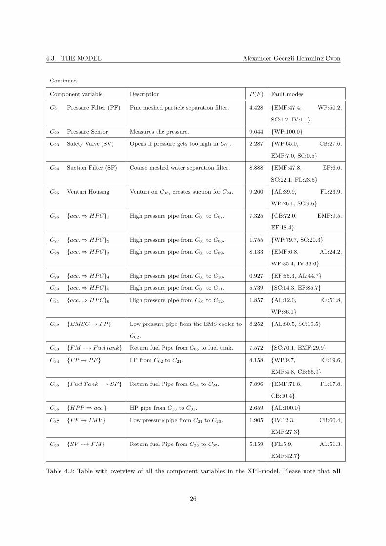
4.3. THE MODEL Alexander Georgii-Hemming Cyon
Continued
Component variable Description P (F ) Fault modes
C21 Pressure Filter (PF) Fine meshed particle separation filter. 4.428 EMF:47.4, WP:50.2,
SC:1.2, IV:1.1
C22 Pressure Sensor Measures the pressure. 9.644 WP:100.0
C23 Safety Valve (SV) Opens if pressure gets too high in C01. 2.287 WP:65.0, CB:27.6,
EMF:7.0, SC:0.5
C24 Suction Filter (SF) Coarse meshed water separation filter. 8.888 EMF:47.8, EF:6.6,
SC:22.1, FL:23.5
C25 Venturi Housing Venturi on C03, creates suction for C24. 9.260 AL:39.9, FL:23.9,
WP:26.6, SC:9.6
C26 acc. ⇒ HPC1 High pressure pipe from C01 to C07. 7.325 CB:72.0, EMF:9.5,
EF:18.4
C27 acc. ⇒ HPC2 High pressure pipe from C01 to C08. 1.755 WP:79.7, SC:20.3
C28 acc. ⇒ HPC3 High pressure pipe from C01 to C09. 8.133 EMF:6.8, AL:24.2,
WP:35.4, IV:33.6
C29 acc. ⇒ HPC4 High pressure pipe from C01 to C10. 0.927 EF:55.3, AL:44.7
C30 acc. ⇒ HPC5 High pressure pipe from C01 to C11. 5.739 SC:14.3, EF:85.7
C31 acc. ⇒ HPC6 High pressure pipe from C01 to C12. 1.857 AL:12.0, EF:51.8,
WP:36.1
C32 EMSC → FP Low pressure pipe from the EMS cooler to
C02.
8.252 AL:80.5, SC:19.5
C33 FM 99K Fuel tank Return fuel Pipe from C05 to fuel tank. 7.572 SC:70.1, EMF:29.9
C34 FP → PF LP from C02 to C21. 4.158 WP:9.7, EF:19.6,
EMF:4.8, CB:65.9
C35 Fuel Tank 99K SF Return fuel Pipe from C24 to C24. 7.896 EMF:71.8, FL:17.8,
CB:10.4
C36 HPP ⇒ acc. HP pipe from C13 to C01. 2.659 AL:100.0
C37 PF → IMV Low pressure pipe from C21 to C20. 1.905 IV:12.3, CB:60.4,
EMF:27.3
C38 SV 99K FM Return fuel Pipe from C23 to C05. 5.159 FL:5.9, AL:51.3,
EMF:42.7
Table 4.2: Table with overview of all the component variables in the XPI-model. Please note that all
26

4.3. THE MODEL Alexander Georgii-Hemming Cyon
values in this table are fictive. A→ B means low pressure pipe between A and B, A⇒ B means high
pressure pipe between A and B, A 99K B means pipe between A and B for return fuel.
4.3.2 Observation Variables
The observation variables can be classified into two different categories, DTCs taken from the EMScalled Diagnosis Trouble Codes (DTC) and physical observations. The physical observations may havebeen made by the truck driver prior to entering the workshop, or by the mechanic during service. Suchobservations can be for example:
• Something smell differently than usual, maybe burnt.
• Some abnormal sound.
• Vibrations made by the engine.
• Something is visible wrong, maybe a pipe is leaking fuel.
DTCs are either indicating or non-indicating. The observation variables for the XPI-model is presentedin table 4.3.
OV Type Description Components
O01 DTC Accumulator pressure too low. Leakage, C07−12, C24
O02 DTC Accumulator pressure too high. Leakage.
O03 DTC Accumulator pressure too low, due to leakage in the HP part. Leakage in HP part.
O04 DTC Accumulator pressure is excessively high. Leakage.
O05 DTC Pressure sensor faulty. C22
O06 DTC Pressure sensor, electrical fault. C22
O07 DTC Engine over speed, possible leakage from injectors. C14−19
O08 DTC Particulate filter too hot, possible leakage inj. C14−19
O09 DTC Injectors 4-6, electrical fault. C17−19
O10 DTC Injectors 1-3, electrical fault. C14−16
O11 DTC Injection error, injectors 1-3. C14−16
O12 DTC Inj. 1 leaking, cyl. giving incorrect power. C14, C20, C32
O13 DTC Inj. 2 leaking, cyl. giving incorrect power. C15, C20, C32
O14 DTC Inj. 3 leaking, cyl. giving incorrect power. C16, C20, C32
O15 DTC Inj. 4 leaking, cyl. giving incorrect power. C17, C20, C32
O16 DTC Inj. 5 leaking, cyl. giving incorrect power. C18, C20, C32
Continued on next page…
27
4.3. THE MODEL Alexander Georgii-Hemming Cyon
Continued
OV Type Description Components
O17 DTC Inj. 6 leaking, cyl. giving incorrect power. C19, C20, C32
O18 DTC Inj. 1, electrical fault. C14
O19 DTC Inj. 2, electrical fault. C15
O20 DTC Inj. 3, electrical fault. C16
O21 DTC Inj. 4, electrical fault. C17
O22 DTC Inj. 5, electrical fault. C18
O23 DTC Inj. 6, electrical fault. C19
O24 DTC Inj. 1, over or under fueling. C14, C20
O25 DTC Inj. 2, over or under fueling. C15, C20
O26 DTC Inj. 3, over or under fueling. C16, C20
O27 DTC Inj. 4, over or under fueling. C17, C20
O28 DTC Inj. 5, over or under fueling. C18, C20
O29 DTC Inj. 6, over or under fueling. C19, C20
O30 DTC IMV, electrical fault. C20
O31 DTC IMV has one or several faults. C20
O32 DTC Plausible leakage in the IMV. C20, C37
O33 DTC Safety valve tripped, accumulator pressure above 2800 bar. Leakage.
O34 Visual Fuel leakage on pipe between HPC1 and accumulator. C26
O35 Visual Fuel leakage on pipe between HPC2 and accumulator. C27
O36 Visual Fuel leakage on pipe between HPC3 and accumulator. C28
O37 Visual Fuel leakage on pipe between HPC4 and accumulator. C29
O38 Visual Fuel leakage on pipe between HPC5 and accumulator. C30
O39 Visual Fuel leakage on pipe between HPC6 and accumulator. C31
O40 Visual Fuel leakage on pipe between EMS cooler and FP. C32
O41 Visual Fuel leakage on pipe between FM and fuel tank. C33
O42 Visual Fuel leakage on pipe between FP and PF. C34
O43 Visual Fuel leakage on pipe between fuel tank and SF. C35
O44 Visual Fuel leakage on pipe between HPP and acc. C36
Continued on next page…
28
4.4. GENERATING THE MODEL Alexander Georgii-Hemming Cyon
Continued
OV Type Description Components
O45 Visual Fuel leakage on pipe between PF and IMV. C37
O46 Visual Fuel leakage on pipe between SV and FM. C38
O47 Visual Black smoke from exhaust pipe. Could be leaking injector. C14−19
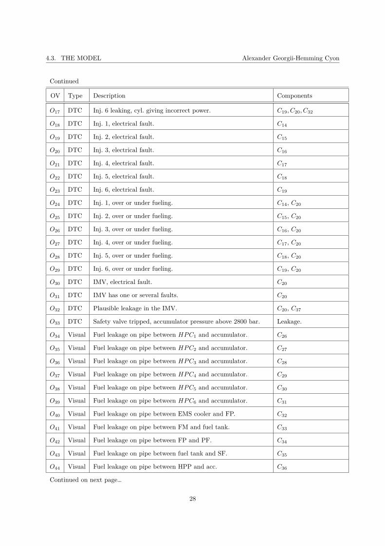
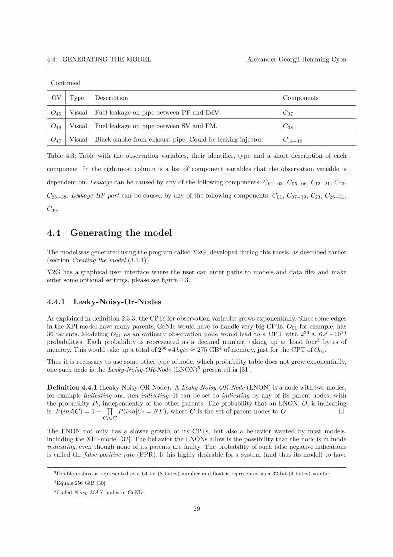
Table 4.3: Table with the observation variables, their identifier, type and a short description of each
component. In the rightmost column is a list of component variables that the observation variable is
dependent on. Leakage can be caused by any of the following components: C01−03, C05−06, C13−21, C23,
C25−38. Leakage HP part can be caused by any of the following components: C01, C07−19, C23, C26−31,
C36.
4.4 Generating the model
The model was generated using the program called Y2G, developed during this thesis, as described earlier(section Creating the model (3.1.1)).
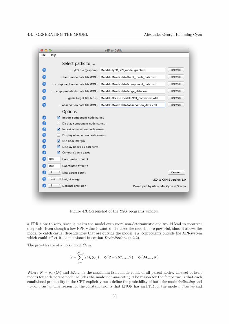
Y2G has a graphical user interface where the user can enter paths to models and data files and makeenter some optional settings, please see figure 4.3.
4.4.1 Leaky-Noisy-Or-Nodes
As explained in definition 2.3.3, the CPTs for observation variables grows exponentially. Since some edgesin the XPI-model have many parents, GeNIe would have to handle very big CPTs. O01 for example, has36 parents. Modeling O01 as an ordinary observation node would lead to a CPT with 236 ≈ 6.8 ∗ 1010probabilities. Each probability is represented as a decimal number, taking up at least four3 bytes ofmemory. This would take up a total of 236 ∗4 byte ≈ 275 GB4 of memory, just for the CPT of O01.
Thus it is necessary to use some other type of node, which probability table does not grow exponentially,one such node is the Leaky-Noisy-OR-Node (LNON)5 presented in [31].
Definition 4.4.1 (Leaky-Noisy-OR-Node). A Leaky-Noisy-OR-Node (LNON) is a node with two modes,for example indicating and non-indicating. It can be set to indicating by any of its parent nodes, withthe probability Pi, independently of the other parents. The probability that an LNON, O, is indicatingis: P (ind|C) = 1−
∏Ci∈C
P (ind|Ci = NF ), where C is the set of parent nodes to O.
The LNON not only has a slower growth of its CPTs, but also a behavior wanted by most models,including the XPI-model [32]. The behavior the LNONs allow is the possibility that the node is in modeindicating, even though none of its parents are faulty. The probability of such false negative indicationsis called the false positive rate (FPR). It his highly desirable for a system (and thus its model) to have
3Double in Java is represented as a 64-bit (8 bytes) number and float is represented as a 32-bit (4 bytes) number.4Equals 256 GiB [30].5Called Noisy-MAX nodes in GeNIe.
29
4.4. GENERATING THE MODEL Alexander Georgii-Hemming Cyon
Figure 4.3: Screenshot of the Y2G programs window.
a FPR close to zero, since it makes the model even more non-deterministic and would lead to incorrectdiagnosis. Even though a low FPR value is wanted, it makes the model more powerful, since it allows themodel to catch casual dependencies that are outside the model, e.g. components outside the XPI-systemwhich could affect it, as mentioned in section Delimitations (4.2.2).
The growth rate of a noisy node Oi is:
2 +N−1∑j=0
2Mc(Cj) = O(2 + 2MmaxN) = O(MmaxN)
Where N = pac(Oi) and Mmax is the maximum fault mode count of all parent nodes. The set of faultmodes for each parent node includes the mode non-indicating. The reason for the factor two is that eachconditional probability in the CPT explicitly must define the probability of both the mode indicating andnon-indicating. The reason for the constant two, is that LNON has an FPR for the mode indicating and
30
4.4. GENERATING THE MODEL Alexander Georgii-Hemming Cyon
its complement, for non-indicating.
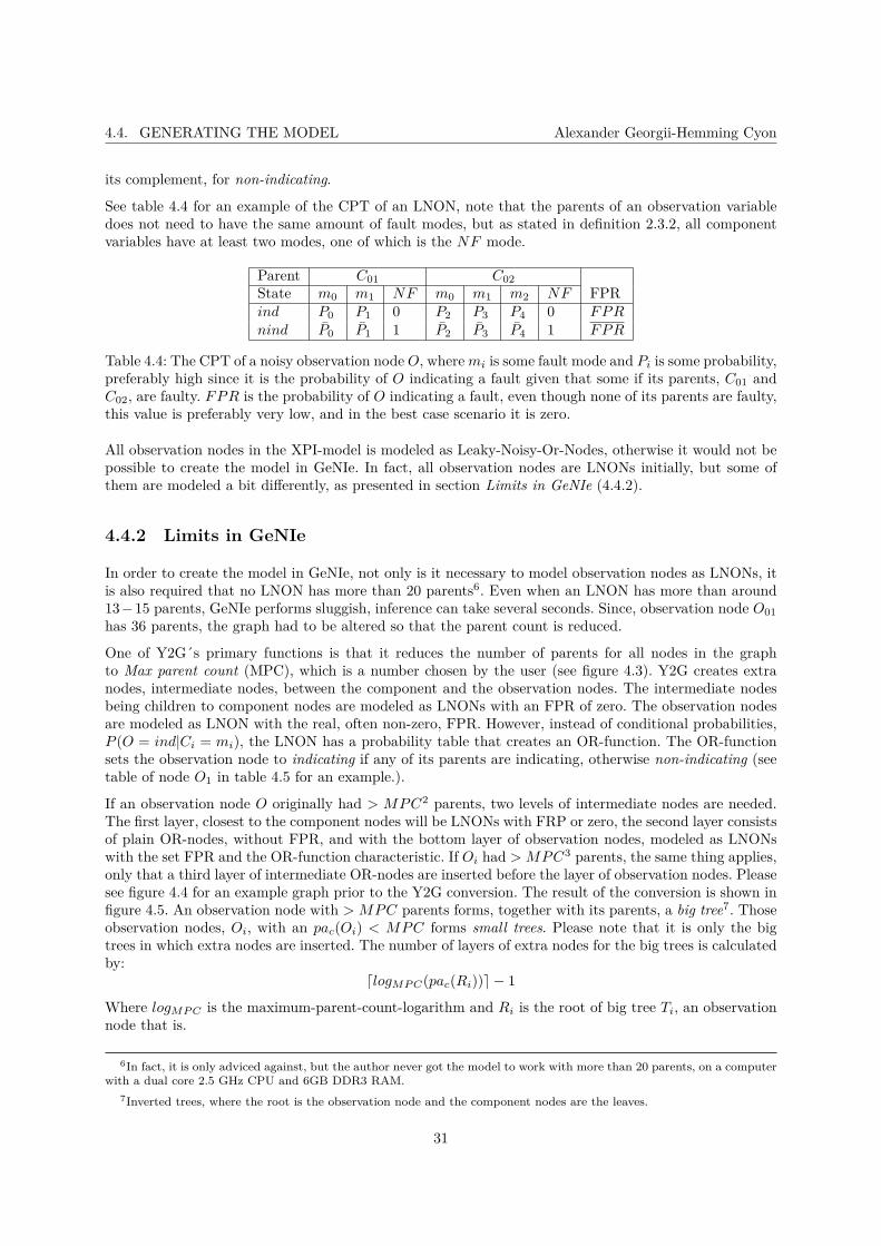
See table 4.4 for an example of the CPT of an LNON, note that the parents of an observation variabledoes not need to have the same amount of fault modes, but as stated in definition 2.3.2, all componentvariables have at least two modes, one of which is the NF mode.
Parent C01 C02
State m0 m1 NF m0 m1 m2 NF FPRind P0 P1 0 P2 P3 P4 0 FPRnind P0 P1 1 P2 P3 P4 1 FPR
Table 4.4: The CPT of a noisy observation node O, where mi is some fault mode and Pi is some probability,preferably high since it is the probability of O indicating a fault given that some if its parents, C01 andC02, are faulty. FPR is the probability of O indicating a fault, even though none of its parents are faulty,this value is preferably very low, and in the best case scenario it is zero.
All observation nodes in the XPI-model is modeled as Leaky-Noisy-Or-Nodes, otherwise it would not bepossible to create the model in GeNIe. In fact, all observation nodes are LNONs initially, but some ofthem are modeled a bit differently, as presented in section Limits in GeNIe (4.4.2).
4.4.2 Limits in GeNIe
In order to create the model in GeNIe, not only is it necessary to model observation nodes as LNONs, itis also required that no LNON has more than 20 parents6. Even when an LNON has more than around13−15 parents, GeNIe performs sluggish, inference can take several seconds. Since, observation node O01
has 36 parents, the graph had to be altered so that the parent count is reduced.
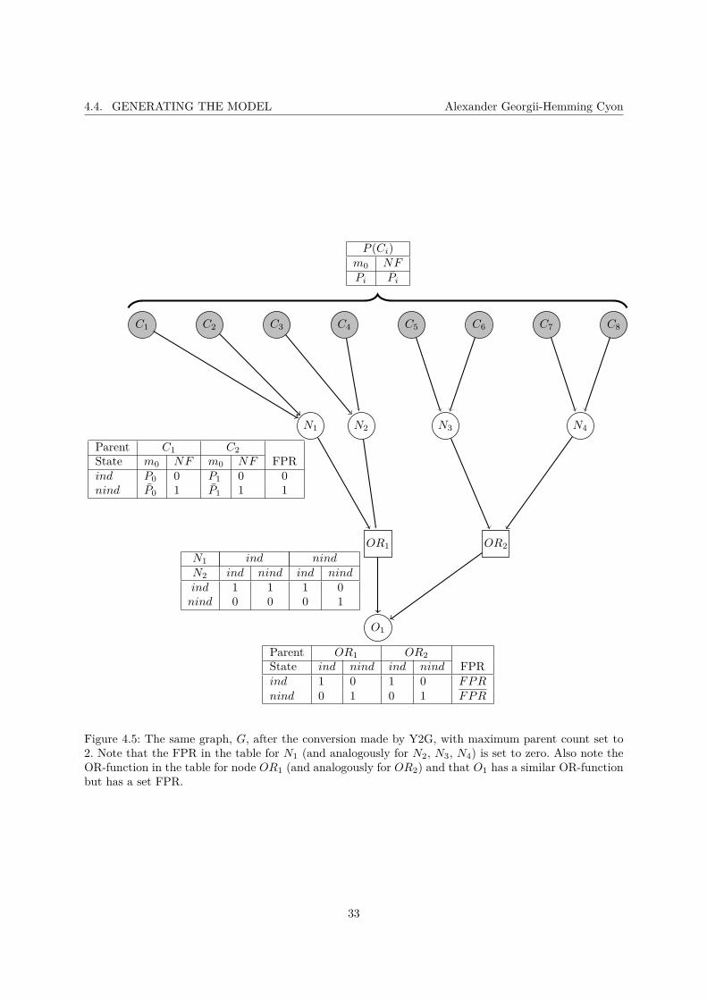
One of Y2G´s primary functions is that it reduces the number of parents for all nodes in the graphto Max parent count (MPC), which is a number chosen by the user (see figure 4.3). Y2G creates extranodes, intermediate nodes, between the component and the observation nodes. The intermediate nodesbeing children to component nodes are modeled as LNONs with an FPR of zero. The observation nodesare modeled as LNON with the real, often non-zero, FPR. However, instead of conditional probabilities,P (O = ind|Ci = mi), the LNON has a probability table that creates an OR-function. The OR-functionsets the observation node to indicating if any of its parents are indicating, otherwise non-indicating (seetable of node O1 in table 4.5 for an example.).
If an observation node O originally had > MPC2 parents, two levels of intermediate nodes are needed.The first layer, closest to the component nodes will be LNONs with FRP or zero, the second layer consistsof plain OR-nodes, without FPR, and with the bottom layer of observation nodes, modeled as LNONswith the set FPR and the OR-function characteristic. If Oi had > MPC3 parents, the same thing applies,only that a third layer of intermediate OR-nodes are inserted before the layer of observation nodes. Pleasesee figure 4.4 for an example graph prior to the Y2G conversion. The result of the conversion is shown infigure 4.5. An observation node with > MPC parents forms, together with its parents, a big tree7. Thoseobservation nodes, Oi, with an pac(Oi) < MPC forms small trees. Please note that it is only the bigtrees in which extra nodes are inserted. The number of layers of extra nodes for the big trees is calculatedby:
⌈logMPC(pac(Ri))⌉ − 1
Where logMPC is the maximum-parent-count-logarithm and Ri is the root of big tree Ti, an observationnode that is.
6In fact, it is only adviced against, but the author never got the model to work with more than 20 parents, on a computerwith a dual core 2.5 GHz CPU and 6GB DDR3 RAM.
7Inverted trees, where the root is the observation node and the component nodes are the leaves.
31

4.4. GENERATING THE MODEL Alexander Georgii-Hemming Cyon
...
C1
..
C2
..
C3
..
C4
..
C5
..
C6
..
C7
..
C8
.. O1
.
P (Ci)m0 NFPi Pi
.
Parent C0 ... C1
State m0 NF ... m0 NF FPRind P0 0 ... Pi 0 FPRnind P0 1 ... Pi 1 FPR
Figure 4.4: Graph G, before the conversion made by Y2G.
See appendix Pseudocode (C) for pseudocode of the algorithm that makes the graph conversion.
In order to create the probability tables for each node, Y2G needs data with probabilities (a priori,conditinal and FPR), but also data with list of fault modes for each component node and optionally aname for each node8. The data is declared in separate XML files, that is passed as input to Y2G alongwith the yED-graph.
8It is convenient to use an index as unique identifier for each node, as shown in this thesis (C01 and O01 etc.) and thendeclare a name for each node, that can be displayed in GeNIe.
32
4.4. GENERATING THE MODEL Alexander Georgii-Hemming Cyon
...
C1
..
C2
..
C3
..
C4
..
C5
..
C6
..
C7
..
C8
.. N1
.. N2
.. N3
.. N4
..
O1
..
OR1
..
OR2
.
P (Ci)m0 NFPi Pi
.
Parent C1 C2
State m0 NF m0 NF FPRind P0 0 P1 0 0nind P0 1 P1 1 1
.
N1 ind nindN2 ind nind ind nindind 1 1 1 0nind 0 0 0 1
.
Parent OR1 OR2
State ind nind ind nind FPRind 1 0 1 0 FPRnind 0 1 0 1 FPR
Figure 4.5: The same graph, G, after the conversion made by Y2G, with maximum parent count set to2. Note that the FPR in the table for N1 (and analogously for N2, N3, N4) is set to zero. Also note theOR-function in the table for node OR1 (and analogously for OR2) and that O1 has a similar OR-functionbut has a set FPR.
33

4.4. GENERATING THE MODEL Alexander Georgii-Hemming Cyon
34

4.4. GENERATING THE MODEL Alexander Georgii-Hemming Cyon
4.4.3 The complete model
Figure 4.6: This is the complete model, with an FPR of 4. The nodes on the left side are componentnodes, and on the right side observation nodes. The two layers of nodes in between the component andthe observation nodes are the intermediate nodes. Many of the intermediate nodes are stacked, the areplaced on top of each other. The reason for this is that Y2G places the intermediate nodes dependingof the components nodes, this results in the same placement of intermediate nodes for observation nodesthat have a similiar set of component nodes as parents.
35

4.4. GENERATING THE MODEL Alexander Georgii-Hemming Cyon
36

Part III
Result
37

Chapter 5
Verifying the XPI-model
An important part of the modeling of a system is to be able to evaulate the model. There are severalways to evaluate a model, the evauluation done in this section is a verification that tries to determine ifthe model is correct.
5.1 Correctness of the model
By correctness we mean if the model of the XPI-system is realistic, if it behaves correctly. The verificationof the XPI-model consists of two separate tests.
5.1.1 Test one - expert interview
The first case study was an expert interview with an engineer at Scania who has several years of experiencewith troubleshooting the XPI-system. For the system to be viewed as correct, two requirements has tobe met.
Requirement one
The first step of the evaluation was studying different cases together with the XPI expert and lettinghim judge whether or not the model behaves correctly. By “behave correctly” we mean that the modelrepresents the real system, by behaving reasonably much similar to the real system. Prior to the interviewwith the expert some formal definition of a realistic model had to be done. So the following requirementwas defined:
Definition 5.1.1 (Realistic model). P (C = faulty|O)reality >> 0 ⇒ P (C = faulty|O)model >>0, ∀C where P (O|C) > 0.
In other words, a model is realistic if for every observation, O, examined, the probability P (C =faulty|O = ind) >> 0 in the model if it is in reality, for all C that can cause O.
In total 12 observation variables where examined, namely: O01, O03, O07, O33, O30, O06, O28, O29, O24,O26, O32, O02. The expert confirmed that the model was realistic according to definition definition 5.1.1.Not only did he confirm the correctness of the model, but was also impressed that the model could confirm
39

5.1. CORRECTNESS OF THE MODEL Alexander Georgii-Hemming Cyon
that the conditional probability P (C20|O29) was significantly higher than P (C18|O29), as he already hadsuspected1.
Requirement two
The second part of the test was to determine that the model suggests the components in the rightorder.
The expert agreed that the model did so. In the model the observation O01 was set to indicating, themodel then proposed the correct set of components to be faulty in an order the expert thought was likely.2
5.1.2 Test two - case-studies
The model was also evaluated to see that the correct observation variable was indicating for a certainfault on a certain component, and that the correct fault mode for the same component was diagnosedwhen setting the same observation variables to indicating.
Here follows two measurements of how well the model diagnoses have been defined [33].
Definition 5.1.2 (Isolable). A fault mode, mi, is isolable from another fault mode, mj , if there existssome observation O such that mi is diagnosis but mj is not, ∀i = j, mi,mj ∈M(O).
Definition 5.1.3 (Detectable). A fault mode, mi, is detectable in a model if mi is isolable from themode NF in the model. The five most relevant components were studied, the components with the highest a priori probabilityto be faulty that is. Those were : C20, C23, C02, C13, C14
3. For each of those five components, it wasinvestigated whether or not their most likely fault mode, mmax was isolable or not. This was done inGeNIe, by setting the evidence that Ci was in fault mode mmax and all other components to the modenon-faulty.
After all the evidence was set, it was noted which OVs had the probability P (indicating|Ci = mi) >thresholdobs, where thresholdobs = 0.99, those OVs are denoted Oind. The value 0.99 was chosen torepresent “certainty”.
Then the evidence on Ci was cleared and all the observations in Oind was set to indicating and all otherOVs to non-indicating. After all the evidence was set, it was noted whether or not P (mCi
max|Oind) >thresholdcomp, where thresholdcomp = 0.10, which was chosen to represent “certainty”4.
The model used for the results in the table 5.1 below had an MPC set to 4.
Since the model only could handle the first case study due to high complexity the case studies hadto be altered. The model was too complex for an exact inference algorithm to be able to compute theconditional probabilities, probably because some nodes have a lot of parents. The alterations done was thatthe evidence non-indicating was removed for all observation nodes not in Oind. However, this did not help.
1The troubleshooting guide available for mechanics today states the reversed, which the expert suspected was incorrect,now this could be verified by the model.
2There is no more precise answer than that, since there is no formal way of determining the truth. The XPI-modelpresented in this thesis may very well be the first formal measurement of this.
3In fact one can say that the top 10 most relevant components was studied since C14 is injector 1 and injector 2-6 aresymmetrical with this component.
4Sometimes several components are diagnosed, and several of those components fault modes, making the probabilitiespretty low for each fault mode, why 0.10 is a rather high value, representing some kind of “certainty”
40
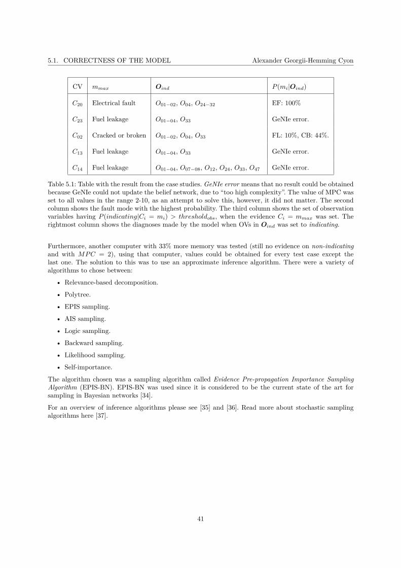
5.1. CORRECTNESS OF THE MODEL Alexander Georgii-Hemming Cyon
CV mmax Oind P (mi|Oind)
C20 Electrical fault O01−02, O04, O24−32 EF: 100%
C23 Fuel leakage O01−04, O33 GeNIe error.
C02 Cracked or broken O01−02, O04, O33 FL: 10%, CB: 44%.
C13 Fuel leakage O01−04, O33 GeNIe error.
C14 Fuel leakage O01−04, O07−08, O12, O24, O33, O47 GeNIe error.
Table 5.1: Table with the result from the case studies. GeNIe error means that no result could be obtainedbecause GeNIe could not update the belief network, due to “too high complexity”. The value of MPC wasset to all values in the range 2-10, as an attempt to solve this, however, it did not matter. The secondcolumn shows the fault mode with the highest probability. The third column shows the set of observationvariables having P (indicating|Ci = mi) > thresholdobs, when the evidence Ci = mmax was set. Therightmost column shows the diagnoses made by the model when OVs in Oind was set to indicating.
Furthermore, another computer with 33% more memory was tested (still no evidence on non-indicatingand with MPC = 2), using that computer, values could be obtained for every test case except thelast one. The solution to this was to use an approximate inference algorithm. There were a variety ofalgorithms to chose between:
• Relevance-based decomposition.
• Polytree.
• EPIS sampling.
• AIS sampling.
• Logic sampling.
• Backward sampling.
• Likelihood sampling.
• Self-importance.
The algorithm chosen was a sampling algorithm called Evidence Pre-propagation Importance SamplingAlgorithm (EPIS-BN). EPIS-BN was used since it is considered to be the current state of the art forsampling in Bayesian networks [34].
For an overview of inference algorithms please see [35] and [36]. Read more about stochastic samplingalgorithms here [37].
41

5.1. CORRECTNESS OF THE MODEL Alexander Georgii-Hemming Cyon
Using EPIS-BN inference instead of the exact inference algorithm, we could obtain results for every testcase when MPC was set to 2 on the 8gb RAM computer, with all the correct evidence set (non-indicatingmode on all observation nodes not in Oind).5
CV mmax Oind P (mi|Oind)
C20 Electrical fault O01−02, O04, O24−32 EF: 100%
C23 Fuel leakage O01−04, O33 FL 56.21%
C02 Cracked or broken O01−02, O04, O33 FL: 9.12%, CB: 45.89%.
C13 Fuel leakage O01−04, O33 FL: 26.1%, CB: 7.72%
C14 Fuel leakage O01−04, O07−08, O12, O24, O33, O47 FL: 66.81%, SC: 33.19%.
Table 5.2: Table with the result from the case studies, using EPIS-BN as inference algorithm, with 100iterations (maximum in GeNIe). But the values differed much between runs so each case was run 100times each, for a total of 100 ∗ 100 = 10000 iterations. The average value for those 10000 iterations isdisplayed in the rightmost column.
From the table 5.2 we can deduce two important things:
1. Using EPIS-BN (10000 iterations) as inference algorithm generated similar result as the exactinference algorithm, 9.12 vs 10 and 45.89 vs 44.
2. For each case, the correct fault mode was diagnosed as the most likely fault mode, i.e. if both faultmode mi,mj are diagnosed, then P (mi|Oind) >> P (mj |Oind) if mi is the correct diagnosis, where“>>” was defined as P (mi|Oind) = 2P (mj |Oind)
5When an MPC of 4 was tested, no result could be obtained for the last test case. The reason for this is probably thatfour parents were too many for the inference algorithm.
42

Chapter 6
Conclusion
6.1 Discussion
The model presented in this thesis correctly mimics the behavior of the XPI-system. It is also compatiblewith the project provider´s research. The program, yED to GeNIe, developed by the author, and themethod used for modeling can be reused to generate models of other systems, this will hopefully behelpful for the provider of the project.
The data on which the a priori CPTs are created only measures the number of times component C hasbeen replaced, nothing else. It is important to understand that this does not necessarily mean that C hasbeen faulty that amount of times. The mechanic that has chosen to replace C may have done so due tothe simple fact that they have been instructed to, maybe because it is cheap and simple to replace C andthat it may fix the problem. It has become clear, during interviews with experts of the XPI-system, thatthe pressure sensor (C22) is one example of such a component. When a DTC that indicates abnormalfuel pressure is observed, the standard procedure have during a long time been to replace the pressuresensor first, even though it seldom is the culprit. Thus the model presented in this thesis is based on dataderived from the incorrect fault-diagnosis done in the workshops during 2010 and 2011.
The assumptions and delimitations regarding the model may also have affected the model. Assumption 1is a particularly strong assumption that may be true for some components and false for others. Sincethe fuel passes through the system in linear manner, first Ci, then Cj etc, it is quite possible that if Ci
becomes faulty, the risk of Cj becomes faulty increases. For example, if the fuel heater (C04) is faulty,the risk that the suction filter (C24) or the pressure filter (C21) clogs is increased.
In section Analyzing and formatting the data (3.1.2), the data was analyzed and manipulated, foremostdata was grouped and split. This affected the model a lot, especially the grouping and splitting. It is verydifficult to understand how it affected the model. The injectors was modeled individually although eachinjector have the same part number, and the fault count data for the injector part was divided by six.This may have been a bad modeling decision.
One of the biggest challenges when developing this model was the format in which the data was accessible.It was desired to start the modeling process by looking at the real system, and how it functions (asdescribed in section About the XPI-system (4.1)). Knowing how the XPI-system functions, the next stepwas to identify the key component and include them as component variables in the model. But thedescription of the system was an abstraction of how the real system really functions. There was already agap between the system and its description, this gap may have widened the gap between the system andthe model. This poses a problem for the creation of the a priori probability tables. The reason for this isthat some components actually are composed of a set of smaller parts. Thus there were no fault count
43
6.2. FUTURE WORK Alexander Georgii-Hemming Cyon
for those components, but for the parts instead. Some of those parts were used in several components,making it impossible to use the fault counts for those parts. If part p can be found in component C1 andC2, should the number of reported faults for p be added (merged) to C1 or C2 or equally divided betweenboth? The fault counts for those parts were not merged into the fault count for those components, makingthe imprecise fault counts even more imprecise.
Some of the weaknesses and in the XPI-system may already have been fixed, since the version of XPImodeled is outdated by a couple of years.
Hoses were treated as pipes, which might have been a bad modeling decision, since they may “behave”differently than pipes.
The decisions made for all challenging problems above mentioned has affected the behavior of the model,and probably not always in the best of ways. It is difficult, maybe impossible to judge which decision isthe right one though.
6.2 Future work
In this section suggestions for how to continue the work is presented. Those suggestions includes bothimprovements on the work presented but also new features and studies.
Even though the verification of the model presented in chapter Verifying the XPI-model (5) showed thatthe model behaves correctly, it is likely that it can be improved. The biggest reason to believe this isthat all the conditional probabilities and the false positive rates were set by the author together withthe supervisor, i.e. no expert of the XPI-systems were consulted during this process, due to limitedresources. It is likely that the model will be even more accurate if those probabilities were set by an XPIexpert.
The components included in the model might be changed, maybe it is better to include more, removingsome, or grouping some component variables together. The injectors, component variables C14−19, couldfor example be modeled as a single component, since their fault frequency was grouped together andthen split in six equal probabilities to be modeled as six different components. The model could havemodeled the dependency between fuel quality, temperature in the country and the fuel filters (C21 andC24).
Other smoothing techniques than add-one smoothing could be used to solve zero-probability diagnosis,as mentioned in section Analyzing and formatting the data (3.1.2). In fact, this has not been investigatedat all.
The model-generating program Y2G, programmed during this thesis maybe extended to have more dy-namic input. It could e.g. be convenient to be able to enter the FPRs for the observations in the programinstead of having to declaring them in XML files or enter names for the nodes.
6.3 Final words
Modeling a system as complex as XPI is difficult. The model never gets better than the that it is basedon, and the data used for the XPI-model presented in this thesis is very noisy. It was, however, showedduring the verification process that the model seamed to behave correct. The model was also able toconfirm a theory that the expert of the XPI-system have had for some time. It is easy to understand howBayesian networks are used for modeling, but it is hard to judge how data manipulation and modelingdecisions affects the behavior of the model. There is plenty of room for improvements of the model,primary choosing the conditional probabilities for the observation variables in a better way, preferably
44

6.3. FINAL WORDS Alexander Georgii-Hemming Cyon
together with an XPI expert. The work presented in this master thesis will hopefully be of use for furtherresearch about computer assisted troubleshooting.
45

6.3. FINAL WORDS Alexander Georgii-Hemming Cyon
46

Chapter 7
Bibliography
[1] H. Warnquist, Computer-Assisted Troubleshooting for Efficient Off-board Diagnosis. PhD thesis,Linköping Universitet, 2011. Accessed online 2012-06-20.
[2] T. Loboda and M. Voortman, “Genie and smile.” http://genie.sis.pitt.edu, 2012. Accessedonline 2012-11-01.
[3] U. D. of Energy, “Just the basics: Diesel engine,” tech. rep., Office of Energy Efficiency and RenewableEnergy, 2003. Accessed online 2012-06-29.
[4] O. Adlercreutz, “Nära sju av tio bilar en diesel.” http://www.teknikensvarld.se/2012/05/02/30924/nara-sju-av-tio-bilar-en-diesel, 2012. Accessed online 2012-06-29.
[5] R. Martin, “Clean diesel vehicles to represent more than 12 percent of global light-dutyvehicle sales by 2018.” http://www.pikeresearch.com/newsroom/clean-diesel-vehicles-to-represent-more-than-12-percent-of-global-light-duty-vehicle-sales-by-2018, 2012. Ac-cessed online 2012-06-29.
[6] Wikipedia, “Two-stroke engine.” http://en.wikipedia.org/wiki/Two-stroke_engine, 2012. Ac-cessed online 2012-11-22.
[7] Future and Potential of Diesel Injection Systems, Springer Verlag, 2002.
[8] V. Hariharana and R. K. Vijayakumar, “Effect of injection pressure on diesel engine performancewith sea lemon oil,” Indian Journal of Science and Technology, 2001. Accessed online 2012-07-01.
[9] F. Dekking, C. Kraaikamp, and H. Lopuhaä, A Modern Introduction To Probability And Statistics.New York, USA: Springer, 2009.
[10] G. Simon, “Discrete random variables,” tech. rep., Stern School of Business, 2007. Accessed online2012-06-27.
[11] Wikipedia, “Conditional probability.” http://en.wikipedia.org/wiki/Conditional_probability, 2012. Accessed online 2012-11-08.
[12] F. V. Jensen and T. D. Nielsen, Bayesian Networks and Decision Graphs. Springer Verlag, 2007.
[13] A. Nicholson, O. Woodberry, and C. Twardy, “The ”native fish” bayesian networks,” tech. rep.,Bayesian-Intelligence, 2010. Accessed online 2012-06-21.
[14] Wikipedia, “Inference.” http://en.wikipedia.org/wiki/Inference, 2012. Accessed online 2012-11-20.
47

Alexander Georgii-Hemming Cyon
[15] S. Thrun, W. Burgard, and D. Fox, Robotics. Intelligent Robotics and Autonomous Agents Series,Mit Press, 2005.
[16] B. G. Marcot, J. D. Steventon, G. D. Sutherland, and R. K. Mccann, “Guidelines for developingand updating bayesian belief networks applied to ecological modeling and conservation,” CanadianJournal of Forest Research, vol. 36, pp. 3063–3074, dec 2006.
[17] F. Crome, M. Thomas, and L. Moore, “A novel bayesian approach to assessing impacts of rain forestlogging,” Ecological Applications, vol. 6, no. 4, pp. 1104–1123, 1996.
[18] Y. Cohen, “Bayesian estimation of clutch size for scientific and management purposes,” Journal ofWildlife Management, vol. 52, no. 4, pp. 787–793, 1988.
[19] T. C. Haas, “Partial validation of bayesian belief network advisory systems,” Artificial IntelligenceApplications, vol. 5, pp. 59–71, 1991.
[20] yWorks, “yed graph editor.” http://www.yworks.com/en/products_yed_about.html, 2012. Ac-cessed online 2012-11-08.
[21] Wikipedia, “Reference class problem.” http://en.wikipedia.org/wiki/Reference_class_problem, 2012. Accessed online 2012-10-10.
[22] C. D. Manning, P. Raghavan, and H. Schütze, Introduction to Information Retrieval. New York,NY, USA: Cambridge University Press, 2008.
[23] F. C. Stanley and J. Goodman, “An empirical study of smoothing techniques for language modeling,”tech. rep., Harvard University and Cambridge, 1998.
[24] C. D. Manning and H. Schütze, Foundations of Statistical Natural Language Processing. Cambridge,MA: MIT Press, 1999.
[25] D. Jurafsky and J. H. Martin, Speech and Language Processing: An Introduction to Natural LanguageProcessing, Computational Linguistics and Speech Recognition. Englewood Cliffs, NJ: Prentice Hall,2000.
[26] S. Easterbrook, “The difference between verification and validation.” http://www.easterbrook.ca/steve/?p=2030, 2012. Accessed online 2012-06-29.
[27] K. Korb and A. Nicholson, Bayesian Artificial Intelligence. Chapman and Hall, 1 ed., sep 2003.
[28] J. Rintanen, “Complexity of planning with partial observability,” in Proceedings of the 14th In-ternational Conference on Automated Planning (ICAPS’04), pp. 345–354, 2004. Accessed online2012-06-21.
[29] Wikipedia, “Paraffin.” http://en.wikipedia.org/wiki/Paraffin, 2012. Accessed online 2012-11-13.
[30] Wikipedia, “Gibibyte.” http://en.wikipedia.org/wiki/Gibibyte, 2012. Accessed online 2012-11-13.
[31] M. Henrion, “Practical issues in constructing a bayes’ belief network,” in Proceedings of the ThirdConference Annual Conference on Uncertainty in Artificial Intelligence (UAI-87), (Corvallis, Ore-gon), pp. 132–139, AUAI Press, 1987.
[32] A. Onisko, M. J. Druzdzel, and H. Wasyluk, “Learning bayesian network parameters from small datasets: application of noisy-or gates,” Int. J. Approx. Reasoning, vol. 27, no. 2, pp. 165–182, 2001.
[33] M. Krysander, Design and Analysis of Diagnosis Systems Using Structural Methods. PhD thesis,Linköpings universitet, June 2006.
[34] F. van Harmelen, V. Lifschitz, and B. Porter, Handbook of Knowledge Representation. San Diego,USA: Elsevier Science, 2007.
48

Alexander Georgii-Hemming Cyon
[35] M. Henrion and M. Morgan, Uncertainty: A Guide to Dealing with Uncertainty in Quantitative Riskand Policy Analysis. Cambridge University Press, 1992.
[36] C. Huang and A. Darwiche, “Inference in belief networks: A procedural guide,” International Journalof Approximate Reasoning, vol. 15, pp. 225–263, 1996.
[37] R. D. Shachter and M. A. Peot, “Simulation approaches to general probabilistic inference on beliefnetworks,” in Proceedings of the Fifth Annual Conference on Uncertainty in Artificial Intelligence,UAI ’89, (Amsterdam, The Netherlands, The Netherlands), pp. 221–234, North-Holland PublishingCo., 1990.
49

Alexander Georgii-Hemming Cyon
50
Appendix A
Acronyms
AL Air leakageBN Bayesian NetworkCB Cracked or brokenCV Component variableCPT Conditional Probability TableDTC Diagnosis Trouble CodeECU Electric Control UnitEF Electrical faultEMS Engine Management SystemEPIS Evidence Pre-propagation Importance SamplingFL Fuel leakageFPR False positive rateHP High PressureHPC High Pressure ConnectorHPP High Pressure PumpIMV Inlet Metering ValveLNON Leaky-noisy-OR-nodeMPC Maximum parent countOV Observation variableNF Non-faultySC Stuck or cloggedXPI Extreme High Pressure Fuel-Injection
51

Alexander Georgii-Hemming Cyon
52

Appendix B
Notation
Here follows a list of the most fundamental notation used in this thesis.
X A stochastic variable.X A set of stochastic variables.pa(X) List of parent nodes to X.pac(X) Size of parent list to X.M(X) List of fault modes of X.Mc(X) Size of fault mode list .
53

Alexander Georgii-Hemming Cyon
54

Appendix C
Pseudocode
55

Alexander Georgii-Hemming Cyon
function generateIntermediateNodesbigTrees← getBigTrees()for all tree ∈ bigTrees do
leaf ← tree.getLeaf()nodeLayers← getLayers(tree.getRoots())lowerLayer ← ∅upperLayer ← tree.getRoots()for all nodeLayer ∈ nodeLayers do
lowerLayer ← nodeLayercountUpperLayer ← 0countLowerLayer ← 0child← owerLayer.getNode(countLowerLayer)for all parent ∈ upperLayer do
if child = noisyNode then ▷ Let child be the new child of node parent, instead of leafCopy probabilities and fault modes
changeParent(parent, leaf, child)end ifchild.addParent(parent)countUpperLayer ++if countUpperLayer = MAX_PARENT_COUNT then
countUpperLayer ← 0countLowerLayer ++if countLowerLayer < lowerLayer.size then
child← lowerLayer.getNode(countLowerLayer)end if
end ifend forupperLayer ← lowerLayer
end for▷ Add bottom layer as parents to leaf node
for all parent ∈ lowerLayer doleaf.addParent(parent)
end forend for
end function
function getBigTreesbigTrees← ∅for all node ∈ nodesWithTooManyParents do
tree← setOfTrees(nodeWithTooManyParents)leaf ← tree.leafleaf.purgeParentList()bigTrees ∪ tree
end forreturn bigTrees
end function
56
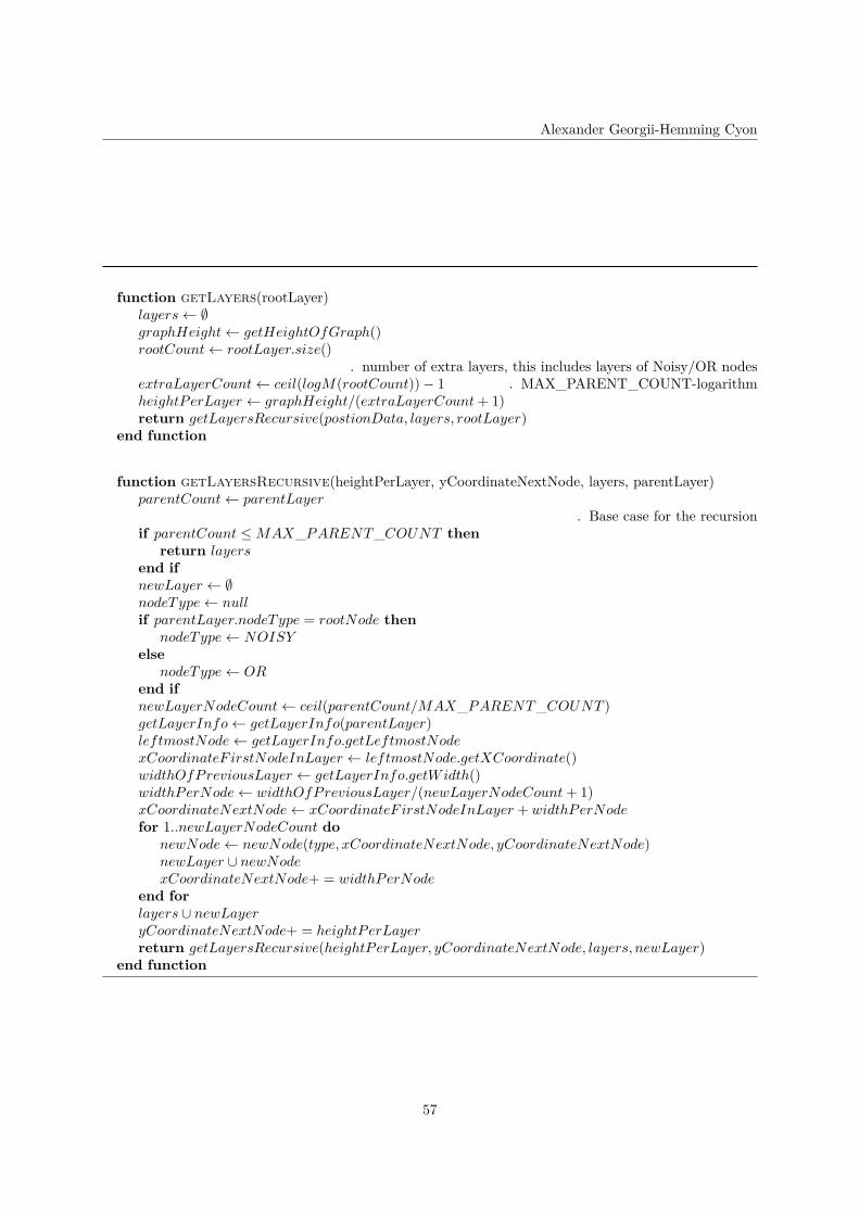
Alexander Georgii-Hemming Cyon
function getLayers(rootLayer)layers← ∅graphHeight← getHeightOfGraph()rootCount← rootLayer.size()
▷ number of extra layers, this includes layers of Noisy/OR nodesextraLayerCount← ceil(logM(rootCount))− 1 ▷ MAX_PARENT_COUNT-logarithmheightPerLayer ← graphHeight/(extraLayerCount+ 1)return getLayersRecursive(postionData, layers, rootLayer)
end function
function getLayersRecursive(heightPerLayer, yCoordinateNextNode, layers, parentLayer)parentCount← parentLayer
▷ Base case for the recursionif parentCount ≤MAX_PARENT_COUNT then
return layersend ifnewLayer ← ∅nodeType← nullif parentLayer.nodeType = rootNode then
nodeType← NOISYelse
nodeType← ORend ifnewLayerNodeCount← ceil(parentCount/MAX_PARENT_COUNT )getLayerInfo← getLayerInfo(parentLayer)leftmostNode← getLayerInfo.getLeftmostNodexCoordinateF irstNodeInLayer ← leftmostNode.getXCoordinate()widthOfPreviousLayer ← getLayerInfo.getWidth()widthPerNode← widthOfPreviousLayer/(newLayerNodeCount+ 1)xCoordinateNextNode← xCoordinateF irstNodeInLayer + widthPerNodefor 1..newLayerNodeCount do
newNode← newNode(type, xCoordinateNextNode, yCoordinateNextNode)newLayer ∪ newNodexCoordinateNextNode+ = widthPerNode
end forlayers ∪ newLayeryCoordinateNextNode+ = heightPerLayerreturn getLayersRecursive(heightPerLayer, yCoordinateNextNode, layers, newLayer)
end function
57

TRITA-CSC-E 2013:008 ISRN-KTH/CSC/E--13/008-SE
ISSN-1653-5715
www.kth.se