Nat. Hazards Earth Syst. Sci., 20, 1219–1232, 2020https://doi.org/10.5194/nhess-20-1219-2020© Author(s) 2020. This work is distributed underthe Creative Commons Attribution 4.0 License.

Modeling of E. coli distribution for hazard assessment of bathingwaters affected by combined sewer overflowsLuca Locatelli1, Beniamino Russo1,2, Alejandro Acero Oliete2, Juan Carlos Sánchez Catalán2,Eduardo Martínez-Gomariz3, and Montse Martínez1

1AQUATEC – Suez Advanced Solutions, Ps. Zona Franca 46-48, 08038, Barcelona, Spain2Group of Hydraulic and Environmental Engineering (GIHA), Technical College of La Almunia (EUPLA),University of Zaragoza, Mayor St. 5, 50100, Zaragoza, Spain3Cetaqua, Water Technology Centre, Environment, Society and Economics Department,Cornellà de Llobregat, 08940, Spain

Correspondence: Luca Locatelli (luca.locatelli@aquatec.es)

Received: 6 September 2019 – Discussion started: 30 September 2019Revised: 27 February 2020 – Accepted: 23 March 2020 – Published: 5 May 2020

Abstract. Combined sewer overflows (CSOs) affect bathingwater quality of receiving water bodies by bacterial pollution.The aim of this study is to assess the health hazard of bathingwaters affected by CSOs. This is useful for bathing watermanagers, for risk assessment purposes, and for further im-pact and economic assessments. Pollutant hazard was evalu-ated based on two novel indicators proposed in this study: themean duration of insufficient bathing water quality (1) overa period of time (i.e., several years) and (2) after singleCSO/rain events. In particular, a novel correlation betweenthe duration of seawater pollution and the event rainfall vol-ume was developed. Pollutant hazard was assessed through acoupled urban drainage and seawater quality model that wasdeveloped, calibrated and validated based on local observa-tions. Furthermore, hazard assessment was based on a novelstatistical analysis of continuous simulations over a 9-yearperiod using the coupled model. Finally, a validation of theestimated hazard is also shown. The health hazard was eval-uated for the case study of Badalona (Spain) even though themethodology presented can be considered generally applica-ble to other urban areas and related receiving bathing waterbodies. The case study presented is part of the EU-fundedH2020 project BINGO (Bringing INnovation to OnGOingwater management – a better future under climate change).

1 Introduction

Bathing water quality is regulated by the Bathing Water Di-rective (2006/7/EC) (BWD) and the corresponding transpo-sition law within each EU nation. For instance, in Spain itis the Real Decreto 1341/2007. The BWD sets the guide-lines for the bathing water monitoring and classification, themanagement, and the provision of information to the pub-lic. Short-term pollution events (having usual durations ofless than 72 h) like the ones caused by combined sewer over-flows (CSOs) lead to insufficient bathing water quality andrequire additional monitoring/sampling of bathing waters.Model simulations can be used to predict the pollutant plumespatial and temporal evolution in bathing water bodies; how-ever, such tools are not widespread (Andersen et al., 2013). Inthe case of moderate and heavy rains, CSOs discharge highconcentrations and loads of the bacteria E. coli (Escherichiacoli) and intestinal enterococci (coming from wastewater andstormwater runoff) in the receiving water bodies where con-centrations can exceed the bathing water quality standards.If bathing water quality is insufficient, then local authori-ties should inform end users, discourage bathing and collectwater samples to monitor bacterial pollution. Generally, safebathing can be reestablished after a collected water samplehas shown acceptable bathing water quality.

In the field of risk management and considering a social-based risk approach, the risk can be assessed through thecombination of the hazard likelihood and the vulnerability

Published by Copernicus Publications on behalf of the European Geosciences Union.

1220 L. Locatelli et al.: Modeling of E. coli distribution for hazard assessment of bathing waters

of the system referring to the propensity of exposed ele-ments – such as human beings, their livelihoods, and assets– to suffer adverse effects when impacted by hazard events(BINGO D4.1, 2016). In this framework, risk can be definedas the combination of hazard and vulnerability (including ex-posure, sensitivity and recovering capacity) according to theliterature (Turner et al., 2003; Velasco et al., 2018). Dono-van et al. (2008) and Viau et al. (2011) evaluated the riskof gastrointestinal disease associated with exposure of peo-ple to pathogens like E. coli and enterococci. In the formerstudy, hazard was assessed by statistical analysis of observedbacterial concentrations during 6 d in a year that was con-sidered representative, whereas in the latter one it was es-timated by simple assumptions. Andersen et al. (2013) pre-sented a coupled urban drainage and seawater quality modelto quantify microbial risk during a swimming competitionwhere lots of gastrointestinal illnesses occurred due to thepresence of CSO in seawater. O’Flaherty et al. (2019) evalu-ated human exposure to antibiotic-resistant Escherichia colithrough recreational water.

Several water quality models of receiving water bodieswere developed to simulate spatial and temporal variationsof bacterial concentrations originating from CSOs and othersources. These water quality models also include hydrody-namic models most of the time. Scroccaro et al. (2010)developed a 3D seawater quality model to simulate bac-terial concentrations originating from wastewater treatmentplant discharges. Jalliffier-Verne et al. (2016) and Passeratet al. (2011) developed river water quality models. Liu andHuang (2012) developed a 2D model of an estuary exposedto tides. Sokolova et al. (2013) and Thupaki et al. (2010)presented hydrodynamic 3D models of lakes to simulate E.coli based on pollutant discharges estimated from observa-tions at affluent rivers and/or sewers. Also, coupled urbandrainage and water quality models of receiving water bodieswere developed to simulate spatial and temporal variationsof bacterial concentrations for bathing water quality affectedby CSOs (Andersen et al., 2013; De Marchis et al., 2013).

None of the studies presented above provided a method-ology that combined simulated E. coli concentration withhazard criteria to evaluate the health hazard of bathing wa-ters affected by CSOs that is the main aim of this study.Health hazard was evaluated based on two novel indicatorsproposed: the mean duration of insufficient bathing waterquality (1) over a period of time (i.e., several years) and(2) after single CSO/rain events. In particular, a novel cor-relation between the duration of seawater pollution and theevent rainfall volume is presented. This is useful for bathingwater managers, for risk assessment purposes, and for fur-ther impact and economic assessments. For example, the pre-sented correlation can be useful to water managers and reg-ulators to predict how long a rainfall event is going to af-fect the bathing water quality and when the optimal time tocollect bathing water samples is. Also, it can be useful toestimate direct and indirect economic impacts of CSOs on

Figure 1. Plan view of Badalona together with the drainage net-work, the name of some of the beaches, the CSO points, the raingauges, the limnimeters and the pedestrian bridge Pont del Petroli.Background image from © Google Maps.

coastal economies as was done in the BINGO project. E. coliconcentration in the receiving water body was simulated by acoupled urban drainage and seawater quality model that wasdeveloped, calibrated and validated based on local observa-tions. The health hazard was then quantified through the cou-pling of simulated E. coli concentrations and hazard criteriathat were defined based on the BWD specifications. Further-more, a novel statistical analysis of continuous simulationsover a 9-year period using the coupled model is presented.Finally, a validation of the estimated hazard is also shown.The health hazard of bathing waters affected by CSOs wasevaluated for the case study of Badalona (Spain).

2 Materials and methods

2.1 The case study

Figure 1 shows the case study area of Badalona (Spain).Badalona, the fourth largest city of the Catalonia region, ispart of the metropolitan area of Barcelona, with an area of21 km2, 215 000 inhabitants and high urbanization. It hasapproximately 5 km of sandy bathing beaches facing theMediterranean Sea. Several CSO points discharge combinedsewers along the beaches. Generally, rainfall events largerthan a few millimeters cause CSOs, and during the bathingseason bathing is usually forbidden during at least the 24 hfollowing a CSO event.

Nat. Hazards Earth Syst. Sci., 20, 1219–1232, 2020 www.nat-hazards-earth-syst-sci.net/20/1219/2020/

L. Locatelli et al.: Modeling of E. coli distribution for hazard assessment of bathing waters 1221

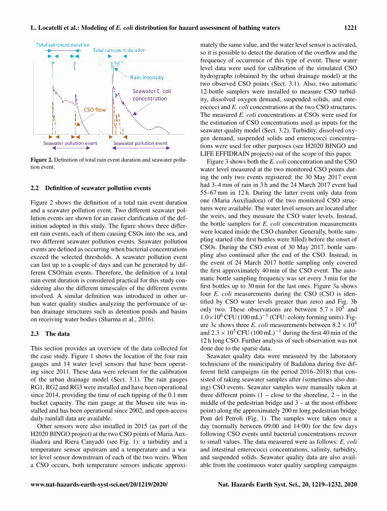
Figure 2. Definition of total rain event duration and seawater pollu-tion event.

2.2 Definition of seawater pollution events

Figure 2 shows the definition of a total rain event durationand a seawater pollution event. Two different seawater pol-lution events are shown for an easier clarification of the def-inition adopted in this study. The figure shows three differ-ent rain events, each of them causing CSOs into the sea, andtwo different seawater pollution events. Seawater pollutionevents are defined as occurring when bacterial concentrationsexceed the selected thresholds. A seawater pollution eventcan last up to a couple of days and can be generated by dif-ferent CSO/rain events. Therefore, the definition of a totalrain event duration is considered practical for this study con-sidering also the different timescales of the different eventsinvolved. A similar definition was introduced in other ur-ban water quality studies analyzing the performance of ur-ban drainage structures such as detention ponds and basinson receiving water bodies (Sharma et al., 2016).

2.3 The data

This section provides an overview of the data collected forthe case study. Figure 1 shows the location of the four raingauges and 14 water level sensors that have been operat-ing since 2011. These data were relevant for the calibrationof the urban drainage model (Sect. 3.1). The rain gaugesRG1, RG2 and RG3 were installed and have been operationalsince 2014, providing the time of each tipping of the 0.1 mmbucket capacity. The rain gauge at the Museu site was in-stalled and has been operational since 2002, and open-accessdaily rainfall data are available.

Other sensors were also installed in 2015 (as part of theH2020 BINGO project) at the two CSO points of Maria Aux-iliadora and Riera Canyadó (see Fig. 1): a turbidity and atemperature sensor upstream and a temperature and a wa-ter level sensor downstream of each of the two weirs. Whena CSO occurs, both temperature sensors indicate approxi-

mately the same value, and the water level sensor is activated,so it is possible to detect the duration of the overflow and thefrequency of occurrence of this type of event. These waterlevel data were used for calibration of the simulated CSOhydrographs (obtained by the urban drainage model) at thetwo observed CSO points (Sect. 3.1). Also, two automatic12-bottle samplers were installed to measure CSO turbid-ity, dissolved oxygen demand, suspended solids, and ente-rococci and E. coli concentrations at the two CSO structures.The measured E. coli concentrations at CSOs were used forthe estimation of CSO concentrations used as inputs for theseawater quality model (Sect. 3.2). Turbidity, dissolved oxy-gen demand, suspended solids and enterococci concentra-tions were used for other purposes (see H2020 BINGO andLIFE EFFIDRAIN projects) out of the scope of this paper.

Figure 3 shows both the E. coli concentration and the CSOwater level measured at the two monitored CSO points dur-ing the only two events registered: the 30 May 2017 eventhad 3–4 mm of rain in 3 h and the 24 March 2017 event had55–67 mm in 12 h. During the latter event only data fromone (Maria Auxiliadora) of the two monitored CSO struc-tures were available. The water level sensors are located afterthe weirs, and they measure the CSO water levels. Instead,the bottle samplers for E. coli concentration measurementswere located inside the CSO chamber. Generally, bottle sam-pling started (the first bottles were filled) before the onset ofCSOs. During the CSO event of 30 May 2017, bottle sam-pling also continued after the end of the CSO. Instead, inthe event of 24 March 2017 bottle sampling only coveredthe first approximately 40 min of the CSO event. The auto-matic bottle sampling frequency was set every 3 min for thefirst bottles up to 30 min for the last ones. Figure 3a showsfour E. coli measurements during the CSO (CSO is iden-tified by CSO water levels greater than zero) and Fig. 3bonly two. These observations are between 5.7× 105 and1.0×106 CFU (100 mL)−1 (CFU: colony forming units). Fig-ure 3c shows three E. coli measurements between 8.2× 104

and 2.3× 105 CFU (100 mL)−1 during the first 40 min of the12 h long CSO. Further analysis of such observation was notdone due to the sparse data.

Seawater quality data were measured by the laboratorytechnicians of the municipality of Badalona during five dif-ferent field campaigns (in the period 2016–2018) that con-sisted of taking seawater samples after (sometimes also dur-ing) CSO events. Seawater samples were manually taken atthree different points (1 – close to the shoreline, 2 – in themiddle of the pedestrian bridge and 3 – at the most offshorepoint) along the approximately 200 m long pedestrian bridgePont del Petroli (Fig. 1). The samples were taken once aday (normally between 09:00 and 14:00) for the few daysfollowing CSO events until bacterial concentrations recoverto small values. The data measured were as follows: E. coliand intestinal enterococci concentrations, salinity, turbidity,and suspended solids. Seawater quality data are also avail-able from the continuous water quality sampling campaigns

www.nat-hazards-earth-syst-sci.net/20/1219/2020/ Nat. Hazards Earth Syst. Sci., 20, 1219–1232, 2020

1222 L. Locatelli et al.: Modeling of E. coli distribution for hazard assessment of bathing waters

Figure 3. E. coli concentration and CSO water level measured at the two CSO structures of Riera Canyadó (R.C.) and Maria Auxiliadora(M.A.).

that are mandatory in order to classify the water quality at thedifferent bathing locations. For instance, during recent years,more than 400 water samples were collected (and analyzed)at each of the four beaches shown in Fig. 1 with a samplingfrequency of approximately once every couple of weeks.All the water quality indicators were obtained from labora-tory analysis of the collected samples. Observed seawater E.coli and salinity concentrations were used for the calibrationand validation of the seawater quality model (Sect. 3.2), andE. coli concentrations were also used for the validation ofthe hazard assessment (Sect. 3.3.1). Seawater turbidity, sus-pended solids and potential oxygen reduction data were notused in this study.

2.4 The model

A coupled urban drainage and seawater quality model wasdeveloped, calibrated and validated based on local observa-tions. The urban drainage model is used to simulate CSO hy-drographs at all the CSO points of Badalona. These hydro-graphs are used as inputs for the seawater quality model tosimulate nearshore water quality. The two models are cou-pled in a sequential way; this means that first the urbandrainage and then the seawater quality model are executed.This is acceptable as the physical processes occurring in thesea do not affect CSO hydrographs in Badalona.

2.4.1 The urban drainage model

The urban drainage model aims to simulate CSO hydro-graphs at all the CSO structures of Badalona that will thenbe used as inputs for the seawater quality model. The model

simulates rainfall-runoff processes, domestic and industrialsewage water fluxes, and hydrodynamics in the drainage net-work over the whole area of Badalona.

The model was originally developed in MIKE URBAN(https://www.mikepoweredbydhi.com/, last access: 1 April2020) for the 2012 drainage management plan (DMP) ofBadalona. As part of this study, the model was importedinto InfoWorks ICM 8.5 (https://www.innovyze.com/en-us,last access: 1 April 2020), updated to include the new pipesand one detention tank of approximately 30 000 m3 that wereconstructed during recent years and calibrated and validatedwith new data. Figure 1 shows the modeled drainage net-work. Overall, the model includes approximately 368 km ofpipes, 11 338 manholes, 11 954 sub-catchments, 62 weirs, 4sluice gates and 1 detention tank.

The sewer flows were simulated by the full 1D Saint-Venant equations. Rainfall-runoff processes were simulatedfor each sub-catchment using a single nonlinear reservoirwith a routing coefficient that is a function of surface rough-ness, surface area, terrain slope and catchment width. Ini-tial losses are generally small for both impervious urbanareas and green areas (≤ 1 mm), and continuous losses forgreen areas are simulated using the Horton model. The areaof Badalona was divided into 11 954 computational sub-catchments of different areas. The sub-catchments were ob-tained by GIS analysis of the digital terrain model (2 m× 2 mresolution) and have areas in the range of 0.01–1 ha in the ur-ban areas and 1–100 ha in the upstream rural areas. Each sub-catchment includes the GIS-derived information of impervi-ous areas and pervious areas that are used to apply either theimpervious or the pervious rainfall-runoff model. Impervi-

Nat. Hazards Earth Syst. Sci., 20, 1219–1232, 2020 www.nat-hazards-earth-syst-sci.net/20/1219/2020/

L. Locatelli et al.: Modeling of E. coli distribution for hazard assessment of bathing waters 1223

ous areas do not have continuous hydrological losses, mean-ing that all the net rainfall (after initial losses) contributes tostormwater runoff.

Calibration and validation of the urban drainage model

The urban drainage model was calibrated using a trial-and-error approach with the objective of minimizing the sum ofall the root mean square errors (RMSEs) calculated for eachof the observation points. The RMSE was calculated for theduration of each simulated event, usually an hour before thebeginning of the rainfall and some hours after the end. Ta-ble 1 shows the three events selected for calibration and theone for validation. In addition, the different rainfall inten-sities, volumes and return periods evaluated based on localrainfall intensity–duration–frequency curves are shown foreach event. It is noted that the selected calibration eventshave generally high intensities and volumes compared to themajority of the events that can cause CSOs (as mentionedabove, events larger than a few millimeters usually causeCSOs in Badalona). These events were considered ideal forcalibration and validation because of both (i) the significantobserved water level variations in the drainage pipes and(ii) the overall quality and quantity of the collected rainfalland water level data. Rain data from the rain gauges wereapplied in the model using Thiessen polygons.

The calibrated Horton parameters were as follows: an ini-tial infiltration capacity of 20 mm h−1 and a final infiltrationcapacity of 7 mm h−1 (BINGO D3.3, 2019). The initial losswas not calibrated and it was calculated as value/slope0.5,where value was set to 0.000071 and 0.00028 m for imper-vious and pervious surfaces respectively and slope was theaverage slope of the sub-catchment calculated with GIS. Thecalibrated Manning roughness coefficient of surface imper-vious areas was set to 0.013, and the coefficient of pipeswas set to 0.012. The calibrated Manning roughness coef-ficients are in the lowest parts of the ranges proposed in sim-ilar urban drainage studies (Fraga et al., 2017; Locatelli etal., 2017; Russo et al., 2015) and more general hydrologicstudies (Dingman, 2015; Henriksen et al., 2003).

Figure 4 shows two examples of simulated and observedwater levels at two different locations during two differentrain events. All the other graphs can be found in BINGOD3.3 (2019). Table 2 shows the computed RMSE and ab-solute maximum error (AME) (Bennett et al., 2013) for thecalibration and validation events. The magnitude of the er-rors is similar to the ones reported in other urban drainagemodels (Russo et al., 2015). Overall, the model simulates theobserved water levels in the sewer network in an acceptableway.

Finally, after the calibration and validation, a further man-ual adjustment of the simulated CSO flows at the two mon-itored CSO structures was performed using measurementsof CSO water levels during three different CSO events from2017 (67 mm on 24 March, 22 mm on 27 April and 4.2 mm

Figure 4. Example of simulated and measured water levels in thesewer pipes at the location BA15 during the rain event of 3 October2015 (a) and at BA2 on 14 September 2016 (b).

on 30 May) and CSO structure geometry (weir crest leveland width) of the two monitored CSO structures. The sim-ulated crest level of these two weirs was manually adjustedby a few centimeters so that the simulated CSO water levelswould better fit (visual judgment) the observed ones. It wasverified that this further model adjustment did not affect theerrors provided in Table 2. The crest level and width values ofall the other CSO structures were obtained from the databaseof the network that came from the DMP of Badalona of 2012.

2.4.2 The seawater quality model

The seawater quality model aims at simulating nearshore(within few hundred meters from the shoreline) bacterialconcentrations in the Badalona seawater during and afterCSO events. The water quality model was developed for thearea of Barcelona (Gutiérrez et al., 2010), and it has been op-erating since 2007 for real-time simulations of bathing waterquality of the Barcelona beaches. This model was updated,calibrated and validated for Badalona as part of this study.

The seawater quality model was developed using the soft-ware MOHID by MARETEC (Marine and EnvironmentalTechnology Research Center) of the Instituto Superior Téc-nico (IST). The model simulates both the hydrodynamics ofthe sea in the coastal region and the pollutant transport re-sulting from CSOs.

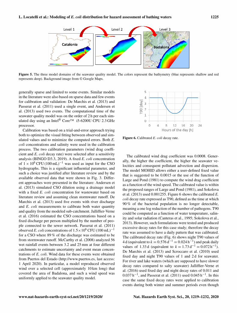
Simulation of nearshore water quality and hydrodynamicsduring and after CSOs requires spatial discretization scaleson the order of tens of meters, whereas other coastal hydro-dynamic processes can occur at much larger scales. There-fore, three model domains are used to simulate hydrody-namic processes from the large regional scale to the localnearshore scale of Badalona. Figure 5 shows the three modellevels. Level 3 represents city-scale processes; and is nestedinto Level 2, which represents subregional scale processes;and is further nested into Level 1 that represents regionalscale processes. The three levels continuously interact witheach other during simulations. Level 1 covers an area of ap-proximately 20 000 km2 with 6500 squared cells of approx-imately 1 km2. At this domain, the hydrodynamic processesof astronomic tides and wind-induced waves and currents aresimulated in 2D mode (barotropic). Level 2 covers an area

www.nat-hazards-earth-syst-sci.net/20/1219/2020/ Nat. Hazards Earth Syst. Sci., 20, 1219–1232, 2020

1224 L. Locatelli et al.: Modeling of E. coli distribution for hazard assessment of bathing waters

Table 1. Events used for calibration and validation of the urban drainage model.

Date event P (mm) I20 min (mm h−1) I5 min (mm h−1) Event usedcumulative rainfall maximum 20 min rainfall maximum 5 min rainfall for

RG1, RG2, RG3 intensity (T = return period) intensity (T = return period)

22 August 2014 18.6, 17.4, 26.0 42.6 (T = 0.4 years) 74.4 (T = 0.6 years) Calibration28–29 July 2014 46.5, 36.0, 2.8 56.4 (T = 0.7 years) 91.2 (T = 0.8 years) Calibration3 October 2015 33.4, 34.1, 26.0 81 (T = 2.3 years) 122.4 (T = 1.1 years) Calibration13–14 September 2016 30.2, 25.2, 20.2 64.5 (T = 1.1 years) 142.8 (T = 1.3 years) Validation

Table 2. Root mean square error (RMSE) and absolute maximum error (AME) for the calibration and validation events.

Calibration Validation

22 August 2014 28 July 2014 3 October 2015 14 September 2016

Water level RMSE AME RMSE AME RMSE AME RMSE AMEsensor (m) (m) (m) (m) (m) (m) (m) (m)

L2 0.066 0.062 0.065 0.028 0.200 0.215 0.181 0.102L4 0.045 0.033 0.049 0.218 0.150 1.422 0.057 0.022L8 0.008 0.075 0.005 0.032 0.011 0.055 0.021 0.027L9 0.157 0.666 0.000 0.322 0.006 0.733 0.001 0.321L10 0.103 0.725 0.098 0.501 0.087 0.472 0.101 0.128L11 0.212 0.627 0.222 1.150 0.495 2.390 0.244 1.333L12 0.123 0.019 0.167 0.340 0.295 0.790 0.189 0.169L13 0.094 0.315 0.094 0.565 0.713 0.907 0.238 0.631L15 0.236 1.036 0.195 0.656 0.322 0.315 0.183 0.791L16 0.264 0.537 0.032 2.065 0.850 1.828 0.147 0.357L19 0.131 0.214 0.099 0.617 0.209 0.686 – –L20 0.346 0.387 0.148 0.190 0.333 0.059 0.096 0.159L21 0.056 0.290 0.082 0.222 0.099 0.190 0.181 0.300

of approximately 1000 km2 with 54 000 rectangular cells ofsides from 500 to 200 m (finer cells close to the shoreline).Level 3 covers an area of approximately 50 km2 with 117 528rectangular cells of sides from 200 to 40 m (finer cells closeto the shoreline). The vertical discretization of Levels 2 and 3was defined with a sigma approach with thinner cells close tothe sea surface and thicker ones close to the seabed. The per-centages used to define the thickness of each of the eight ver-tical layers as a function of the water depth were as follows:0.458, 0.227, 0.134, 0.079, 0.047, 0.028, 0.017 and 0.01 (thethinnest layer at the sea surface is 1 % of the water depth atthat location). At Level 2 and Level 3 domains the processesof currents and waves, density, temperature and salinity vari-ations; nearshore currents generated by CSOs and river dis-charges; and advection and dispersion of E. coli from CSOsare simulated in baroclinic mode with a 3D mesh.

CSOs are simulated in the seawater model as both waterdischarges and concentration inputs. Water discharge timeseries at the CSO points were obtained from the urbandrainage model, and the input concentrations used for CSOdischarges were assumed to be fixed (further details are givenin the following section).

The hydrodynamic model solves the primitive continuityand momentum equations for the surface elevation and 3Dvelocity field for incompressible flows, in orthogonal hori-zontal coordinates and generic vertical coordinates, assum-ing hydrostatic equilibrium and Boussinesq approximations(http://wiki.mohid.com, last access: 23 April 2020). The se-lected turbulence model was the Smagorinsky model withdefault values. Wave height and period were computed as afunction of wind speed, according to ADIOS model formu-lations (NOAA, 1994).

Calibration and validation of the seawater quality model

Three different events were used: two for calibration (one inJanuary 2018 and one in September 2016) and one for val-idation (October 2016). These events were selected becausethey were the ones with the largest number of seawater E. coliand salinity measurements mainly due to both the relativelyhigh E. coli concentrations observed and their slow recov-ering pollutographs. Three events may sound like a limitednumber for calibration and validation. This was because ofthe long computational time of the coupled model and be-cause the data required for bathing water quality models are

Nat. Hazards Earth Syst. Sci., 20, 1219–1232, 2020 www.nat-hazards-earth-syst-sci.net/20/1219/2020/

L. Locatelli et al.: Modeling of E. coli distribution for hazard assessment of bathing waters 1225

Figure 5. The three model domains of the seawater quality model. The colors represent the bathymetry (blue represents shallow and redrepresents deep). Background image from © Google Maps.

generally sparse and limited to some events. Similar modelsin the literature were also based on sparse data and few eventsfor calibration and validation: De Marchis et al. (2013) andPasserat et al. (2011) used a single event, and Andersen etal. (2013) used two events. The computational time of theseawater quality model was on the order of 2 h per each sim-ulated day using an Intel® Core™ i5-6200U CPU 2.3 GHzprocessor.

Calibration was based on a trial-and-error approach tryingboth to optimize the visual fitting between observed and sim-ulated values and to minimize the computed errors. Both E.coli concentrations and salinity were used in the calibrationprocess. The two calibration parameters (wind drag coeffi-cient and E. coli decay rate) were selected after a sensitivityanalysis (BINGO D3.3, 2019). A fixed E. coli concentrationof 1× 106 CFU (100 mL)−1 was used as input for the CSOhydrographs. This is a significant influential parameter, andsuch a choice was justified after literature review and by theavailable observed data that were shown in Fig. 3. Differ-ent approaches were presented in the literature: Andersen etal. (2013) simulated CSO dilution using a drainage modelwith a fixed E. coli concentration for wastewater based onliterature review and assuming clean stormwater runoff. DeMarchis et al. (2013) used five events with river dischargeand E. coli measurements to calibrate both water quantityand quality from the modeled sub-catchment. Jalliffier-Verneet al. (2016) estimated the CSO concentrations based on afixed discharge per person multiplied by the number of peo-ple connected to the sewer network. Passerat et al. (2011)observed E. coli concentrations of 1.5×106 CFU (100 mL)−1

for a CSO where 89 % of the discharge was estimated to befrom stormwater runoff. McCarthy et al. (2008) analyzed 56wet rainfall events between 3.2 and 25 mm at four differentcatchments to estimate uncertainty and event mean concen-trations of E. coli. Wind data for these events were obtainedfrom Puertos del Estado (http://www.puertos.es, last access:1 April 2020). In particular, a model reproduced observedwind over a selected cell (approximately 10 km long) thatcovered the area of Badalona, and such a wind speed wasuniformly applied to the seawater quality model.

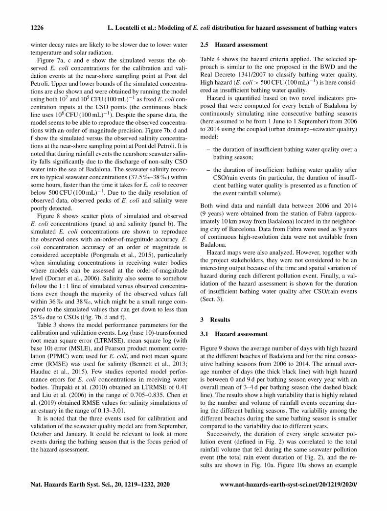
Figure 6. Calibrated E. coli decay rate.

The calibrated wind drag coefficient was 0.0008. Gener-ally, the higher the coefficient, the higher the seawater ve-locities and consequent pollutant advection and dispersion.The model MOHID allows either a user-defined fixed valuethat is suggested to be 0.0015 or the use of the function ofLarge and Pond (1981) to compute the wind drag coefficientas a function of the wind speed. The calibrated value is withinthe proposed ranges of Large and Pond (1981), and Sokolovaet al. (2013) used 0.001255. Figure 6 shows the calibrated E.coli decay rate expressed as T90, defined as the time at which90 % of the bacterial population is no longer detectable,meaning a one log reduction of the number of pathogens. T90could be computed as a function of water temperature, salin-ity and solar radiation (Canteras et al., 1995; Sokolova et al.,2013). However, such formulations were tested and producedexcessive decay rates for this case study; therefore the decayrate was assumed to have a daily pattern that was calibrated.The calibrated decay rate (Fig. 6) shows night T90 values of4 d (equivalent to k = 0.576 d−1

= 0.024 h−1) and peak dailyvalues of 1.33 d (equivalent to k = 1.73 d−1

= 0.072 h−1).De Marchis et al. (2013) and Scroccaro et al. (2010) usedfixed day and night T90 values of 1 and 2 d for seawater.For river and lake waters (which are supposed to have slowerdecay rates compared to salty seawater) Jalliffier-Verne etal. (2016) used fixed day and night decay rates of 0.011 and0.037 h−1, and Passerat et al. (2011) used 0.045 h−1. In thiscase the same fixed decay rates were applied to calibrationevents during both winter and summer periods even though

www.nat-hazards-earth-syst-sci.net/20/1219/2020/ Nat. Hazards Earth Syst. Sci., 20, 1219–1232, 2020

1226 L. Locatelli et al.: Modeling of E. coli distribution for hazard assessment of bathing waters

winter decay rates are likely to be slower due to lower watertemperature and solar radiation.

Figure 7a, c and e show the simulated versus the ob-served E. coli concentrations for the calibration and vali-dation events at the near-shore sampling point at Pont delPetroli. Upper and lower bounds of the simulated concentra-tions are also shown and were obtained by running the modelusing both 107 and 105 CFU (100 mL)−1 as fixed E. coli con-centration inputs at the CSO points (the continuous blackline uses 106 CFU (100 mL)−1). Despite the sparse data, themodel seems to be able to reproduce the observed concentra-tions with an-order-of-magnitude precision. Figure 7b, d andf show the simulated versus the observed salinity concentra-tions at the near-shore sampling point at Pont del Petroli. It isnoted that during rainfall events the nearshore seawater salin-ity falls significantly due to the discharge of non-salty CSOwater into the sea of Badalona. The seawater salinity recov-ers to typical seawater concentrations (37.5 ‰–38 ‰) withinsome hours, faster than the time it takes for E. coli to recoverbelow 500 CFU (100 mL)−1. Due to the daily resolution ofobserved data, observed peaks of E. coli and salinity werepoorly detected.

Figure 8 shows scatter plots of simulated and observedE. coli concentrations (panel a) and salinity (panel b). Thesimulated E. coli concentrations are shown to reproducethe observed ones with an-order-of-magnitude accuracy. E.coli concentration accuracy of an order of magnitude isconsidered acceptable (Pongmala et al., 2015), particularlywhen simulating concentrations in receiving water bodieswhere models can be assessed at the order-of-magnitudelevel (Dorner et al., 2006). Salinity also seems to somehowfollow the 1 : 1 line of simulated versus observed concentra-tions even though the majority of the observed values fallwithin 36 ‰ and 38 ‰, which might be a small range com-pared to the simulated values that can get down to less than25 ‰ due to CSOs (Fig. 7b, d and f).

Table 3 shows the model performance parameters for thecalibration and validation events. Log (base 10)-transformedroot mean square error (LTRMSE), mean square log (withbase 10) error (MSLE), and Pearson product moment corre-lation (PPMC) were used for E. coli, and root mean squareerror (RMSE) was used for salinity (Bennett et al., 2013;Hauduc et al., 2015). Few studies reported model perfor-mance errors for E. coli concentrations in receiving waterbodies. Thupaki et al. (2010) obtained an LTRMSE of 0.41and Liu et al. (2006) in the range of 0.705–0.835. Chen etal. (2019) obtained RMSE values for salinity simulations ofan estuary in the range of 0.13–3.01.

It is noted that the three events used for calibration andvalidation of the seawater quality model are from September,October and January. It could be relevant to look at moreevents during the bathing season that is the focus period ofthe hazard assessment.

2.5 Hazard assessment

Table 4 shows the hazard criteria applied. The selected ap-proach is similar to the one proposed in the BWD and theReal Decreto 1341/2007 to classify bathing water quality.High hazard (E. coli > 500 CFU (100 mL)−1) is here consid-ered as insufficient bathing water quality.

Hazard is quantified based on two novel indicators pro-posed that were computed for every beach of Badalona bycontinuously simulating nine consecutive bathing seasons(here assumed to be from 1 June to 1 September) from 2006to 2014 using the coupled (urban drainage–seawater quality)model:

– the duration of insufficient bathing water quality over abathing season;

– the duration of insufficient bathing water quality afterCSO/rain events (in particular, the duration of insuffi-cient bathing water quality is presented as a function ofthe event rainfall volume).

Both wind data and rainfall data between 2006 and 2014(9 years) were obtained from the station of Fabra (approx-imately 10 km away from Badalona) located in the neighbor-ing city of Barcelona. Data from Fabra were used as 9 yearsof continuous high-resolution data were not available fromBadalona.

Hazard maps were also analyzed. However, together withthe project stakeholders, they were not considered to be aninteresting output because of the time and spatial variation ofhazard during each different pollution event. Finally, a val-idation of the hazard assessment is shown for the durationof insufficient bathing water quality after CSO/rain events(Sect. 3).

3 Results

3.1 Hazard assessment

Figure 9 shows the average number of days with high hazardat the different beaches of Badalona and for the nine consec-utive bathing seasons from 2006 to 2014. The annual aver-age number of days (the thick black line) with high hazardis between 0 and 9 d per bathing season every year with anoverall mean of 3–4 d per bathing season (the dashed blackline). The results show a high variability that is highly relatedto the number and volume of rainfall events occurring dur-ing the different bathing seasons. The variability among thedifferent beaches during the same bathing season is smallercompared to the variability due to different years.

Successively, the duration of every single seawater pol-lution event (defined in Fig. 2) was correlated to the totalrainfall volume that fell during the same seawater pollutionevent (the total rain event duration of Fig. 2), and the re-sults are shown in Fig. 10a. Figure 10a shows an example

Nat. Hazards Earth Syst. Sci., 20, 1219–1232, 2020 www.nat-hazards-earth-syst-sci.net/20/1219/2020/

L. Locatelli et al.: Modeling of E. coli distribution for hazard assessment of bathing waters 1227

Figure 7. Near-shore simulated and observed E. coli concentrations (a, c, e) and salinity (b, d, f) for the calibration and validation events.

Figure 8. Scatter plots of simulated and observed E. coli concentrations (a) and salinity (b).

www.nat-hazards-earth-syst-sci.net/20/1219/2020/ Nat. Hazards Earth Syst. Sci., 20, 1219–1232, 2020

1228 L. Locatelli et al.: Modeling of E. coli distribution for hazard assessment of bathing waters

Table 3. Model performance parameters.

Calibration and E. coli concentration MSLE 0.44validation events LTRMSE 0.66

Pearson correlation coefficient 0.83

Salinity concentration RMSE (‰) 0.73

Table 4. Hazard criteria based on E. coli concentration in seawater.

Hazard E. coli concentrationcriteria (CFU (100 mL)−1)

Low < 250Medium 250 < x < 500High > 500

Figure 9. Simulated number of days per bathing season with highhazard (E. coli concentrations > 500 CFU (100 mL)−1) at all thedifferent beaches of Badalona.

of the results from Coco Beach, even though all beacheswere analyzed and all the graphs can be found in the deliv-ery D4.4 of the BINGO project. Overall, the results showthat the higher the rainfall volume, the longer the time pe-riod the beach is exposed to E. coli concentrations abovethreshold; however, above 15–25 mm of rain volume the in-creasing tendency seems to vanish, and only rainfall abovea few millimeters can cause seawater E. coli concentrations> 500 CFU (100 mL)−1. The large spreading of the correla-tion plots is mainly due to the different total rain event du-ration and the magnitude of marine currents. Overall, longerrain events produce longer CSOs and therefore longer seawa-ter pollution events. Similarly, stronger winds and a roughersea produce shorter seawater pollution events.

Figure 10b is a rearrangement of Fig. 10a and showsthe probability distribution of seawater pollution events asa function of the rainfall volume. The discretization of therainfall volume (x axes) into four ranges was chosen in orderto obtain both a reasonable number of events simulated ineach range and volume ranges that are considered reasonablefor local applications. This statistical approach that consid-ered the total rainfall volume was considered the best oneamong several attempts of correlation between seawater pol-lution duration and rain intensities of different duration (e.g.,30, 60, 120 min rainfall).

Figure 10b provides one of the two main indicators pro-posed in this study: the duration of high hazard (insufficientbathing water quality) as a function of the event rainfall vol-ume. For instance, an event of 12 mm rainfall (which wouldfall in the bin of 8≤ x < 16 mm of Fig. 10b) is estimatedto produce a median of 0.5 d of high hazard at Coco Beach.The percentiles provided with the whisker boxes include anestimation of inter-event uncertainty obtained by continuoussimulations using the deterministic coupled model. Other un-certainties like the ones associated with selected and cali-brated parameters were not addressed.

Validation of the hazard assessment

A validation was performed only for the indicator of highhazard as a function of the event rainfall. The validation ofthe mean duration of high hazard per bathing season was notdone due to lack of observed data. The number of days whenbathing was forbidden during bathing seasons is available.However, these data cannot be compared with the simulatedhigh hazard because bathing-forbidden days are dependenton local protocols that, for instance in the case of Badalona,allow the reestablishment of bathing permissions only afterpositive bathing water quality measurements which usuallytake more than 24 h to obtain.

Figure 11 shows an example of how the duration of aseawater pollution event was graphically obtained based onrainfall data and observed E. coli concentrations. The sea-water pollution event is assumed to start when the accumu-lated rainfall exceeds 1 mm. An analysis of the simulationresults showed that a seawater pollution event can start upto an hour later compared to the proposed beginning point.This depends on how far from the CSO the control pointis and also on the CSO events which can start with a de-lay compared to the rainfall. The seawater pollution event

Nat. Hazards Earth Syst. Sci., 20, 1219–1232, 2020 www.nat-hazards-earth-syst-sci.net/20/1219/2020/

L. Locatelli et al.: Modeling of E. coli distribution for hazard assessment of bathing waters 1229

Figure 10. (a) Correlation between the simulated number of days with seawater E. coli concentrations above 500 CFU (100 mL)−1 at CocoBeach and the rainfall volume. (b) The rainfall volume is categorized into four different ranges. The whisker boxes show 1st, 25th, 50th, 75thand 99th percentiles.

Figure 11. Example of how the duration of a seawater pollutionevent was graphically obtained.

is supposed to end when the simple linear interpolation (thedashed red line of Fig. 11) between measured concentrationscrosses the selected threshold of 500 CFU (100 mL)−1. Thetotal rainfall associated with the seawater pollution event isthe average total volume (from the available rain gauges) thatfell during the pollution event.

Figure 12a shows the comparison between the simulatedand observed high hazard duration. Eight events were usedfor the comparison. Overall, the majority of the observeddurations fall within the simulated 1st and 99th percentiles.However, there are some outliers. The two outliers at MoraBeach are likely because this beach is close to the mouth ofthe Besòs river, which might not be properly represented inthe model. Also, there are several model uncertainties thatwere not simulated (for example, input parameters and cali-bration uncertainties). Further, it seems that the observed val-ues are in the higher range of the simulated percentiles; thiscan be because all the CSO events that caused little seawaterpollution could not be measured by the available sampling

resolutions (approximately a sample per day). Overall, thiscan be considered as a preliminary visual validation.

For risk assessment purposes (as part of the BINGOproject), together with the project stakeholders, it was de-cided to adjust/calibrate the proposed percentile duration inorder to obtain the deterministic maximum durations of highhazard that are shown in Fig. 12b. For this purpose, severalsteps were applied: the observed seawater pollution durationderived from intestinal enterococci observations was com-pared to the simulated E. coli percentile durations of Fig. 12a;all the beaches were merged into a unique representativevalue of pollution duration obtained from the worst 99.9thpercentile among all the beaches; finally, a further safety fac-tor of 5 % was applied so that all the outliers would be ac-commodated within the newly developed bars, representinga practical deterministic value of maximum seawater pollu-tion duration as a function of four different rainfall ranges.

4 Conclusions

This study quantified the health hazard of bathing waters af-fected by CSOs based on two novel indicators: the mean du-ration of insufficient bathing water quality (1) per bathingseason and (2) after single CSO/rain events. Overall, a greatuncertainty is associated with the evaluated pollutant hazard,mainly due to the variability of water quality variables, rain-fall patterns and seawater currents. A novel correlation be-tween the duration of seawater pollution and the event rain-fall volume was presented. Also, a coupled urban drainageand seawater quality model was developed, calibrated andvalidated based on local observations. Furthermore, hazardassessment was based on a statistical analysis of the continu-ous simulation results of nine consecutive bathing seasonsusing the coupled model. Finally, a validation of the esti-mated hazard was also shown.

The pollutant hazard of bathing waters affected by CSOswas assessed for the case study of Badalona (Spain) even

www.nat-hazards-earth-syst-sci.net/20/1219/2020/ Nat. Hazards Earth Syst. Sci., 20, 1219–1232, 2020

1230 L. Locatelli et al.: Modeling of E. coli distribution for hazard assessment of bathing waters

Figure 12. (a) Comparison between the estimated and the observed duration of high hazard (seawater E. coli > 500 CFU (100 mL)−1). Thewhisker boxes show 1st, 25th, 50th, 75th and 99th percentiles of the duration of seawater pollution. (b) Maximum seawater pollution duration(orange bars) as a function of four different rainfall ranges.

though the methodology presented can be considered gen-erally applicable to other urban areas and related receivingbathing water bodies. The results of this study were usefulas inputs for risk assessment and to analyze direct, indirect,tangible, and intangible impacts related to CSO events andconsequent pollution of seawater. Also, the correlation pre-sented to predict the duration of insufficient bathing waterquality as a function of the observed rainfall volume can beuseful to bathing water managers.

Code and data availability. Model files and data are not provideddue to the confidentiality of the data and models shared among thelocal project stakeholders of Badalona. Notwithstanding, in agree-ment with the other project local stakeholders, the authors of thispaper will try to address specific requests for scientific purposes.

Author contributions. BR, MM and LL coordinated the researchproject. AAO and JCSC managed the data collection. LL, BR andEMG developed the conceptual model, and LL set up the model,wrote the code and performed the simulations. LL prepared the pa-per with the contributions of all co-authors.

Competing interests. The authors declare that they have no conflictof interest.

Special issue statement. This article is part of the special issue “In-tegrated assessment of climate change impacts at selected Europeanresearch sites – from climate and hydrological hazards to risk anal-ysis and measures”. It is not associated with a conference.

Acknowledgements. This study was conducted as part of theBINGO European H2020 project (http://www.projectbingo.eu/, lastaccess: 1 April 2020). The authors thank the Municipality ofBadalona and particularly Antonio Gerez Angulo, Maria Luisa For-cadell Berenguer, Gregori Muñoz-Ramos Trayter and Josep An-ton Montes Carretero for their valuable contributions. Also, theauthors wish to thank the LIFE EFFIDRAIN project (LIFE14ENV/ES/000860, http://www.life-effidrain.eu/, last access: 1 April2020) for sharing data.

Financial support. This research has been supported by theBINGO European H2020 project (grant no. 641739).

Review statement. This paper was edited by Adriana Bruggemanand reviewed by Ekaterina Sokolova and Vasilis Bellos.

Nat. Hazards Earth Syst. Sci., 20, 1219–1232, 2020 www.nat-hazards-earth-syst-sci.net/20/1219/2020/

L. Locatelli et al.: Modeling of E. coli distribution for hazard assessment of bathing waters 1231

References

Andersen, S. T., Erichsen, A. C., Mark, O., and Albrechtsen,H. J.: Effects of a 20 year rain event: A quantitative micro-bial risk assessment of a case of contaminated bathing wa-ter in Copenhagen, Denmark, J. Water Health, 11, 636–646,https://doi.org/10.2166/wh.2013.210, 2013.

Bennett, N. D., Croke, B. F. W., Guariso, G., Guillaume, J. H. A.,Hamilton, S. H., Jakeman, A. J., Marsili-Libelli, S., Newham, L.T. H., Norton, J. P., Perrin, C., Pierce, S. A., Robson, B., Sep-pelt, R., Voinov, A. A., Fath, B. D., and Andreassian, V.: Charac-terising performance of environmental models, Environ. Model.Softw., 40, 1–20, https://doi.org/10.1016/j.envsoft.2012.09.011,2013.

BINGO D3.3: Calibrated water resources models for past con-ditions, H2020 BINGO. Bringing Innov. to onGOing wa-ter Manag. – a better Futur. under Clim. Chang. GrantAgreem. no. 641739, available at: http://www.projectbingo.eu/downloads/BINGO_Deliverable3.3_submitted.pdf (last access:1 April 2020), 2019.

BINGO D4.1: Context for risk assessment at the six re-search sites, including criteria to be used in risk assess-ment, H2020 BINGO. Bringing Innov. to onGOing waterManag. – a better Futur. under Clim. Chang. Grant Agreem.no. 641739, available at: http://www.projectbingo.eu/downloads/BINGO_Deliverable4.1.pdf (last access: 1 April 2020), 2016.

Canteras, J. C., Juanes, J. A., Pérez, L., and Koev, K. N.: Mod-elling the coliforms inactivation rates in the Cantabrian Sea (Bayof Biscay) from in situ and laboratory determinations of t90,Water Sci. Technol., 32, 37–44, https://doi.org/10.1016/0273-1223(95)00567-7, 1995.

Chen, J., Liu, Y., Gitau, M. W., Engel, B. A., Flanagan, D. C.,and Harbor, J. M.: Evaluation of the effectiveness of greeninfrastructure on hydrology and water quality in a combinedsewer overflow community, Sci. Total Environ., 665, 69–79,https://doi.org/10.1016/j.scitotenv.2019.01.416, 2019.

De Marchis, M., Freni, G., and Napoli, E.: Modelling ofE. coli distribution in coastal areas subjected to combinedsewer overflows, Water Sci. Technol., 68(5), 1123–1136,https://doi.org/10.2166/wst.2013.353, 2013.

Dingman, S. L.: Physical Hydrology: Third Edition, WavelandPress, Inc., Long Grove, Illinois, USA, 2015.

Donovan, E., Unice, K., Roberts, J. D., Harris, M., and Fin-ley, B.: Risk of gastrointestinal disease associated withexposure to pathogens in the water of the Lower Pas-saic River, Appl. Environ. Microbiol., 74, 994–1003,https://doi.org/10.1128/AEM.00601-07, 2008.

Dorner, S. M., Anderson, W. B., Slawson, R. M., Kouwen,N., and Huck, P. M.: Hydrologic modeling of pathogenfate and transport, Environ. Sci. Technol., 40, 4746–4753,https://doi.org/10.1021/es060426z, 2006.

Fraga, I., Cea, L., and Puertas, J.: Validation of a 1D-2D dual drainage model under unsteady part-full and sur-charged sewer conditions, Urban Water J., 14, 74–84,https://doi.org/10.1080/1573062X.2015.1057180, 2017.

Gutiérrez, E., Malgrat, P., Suñer, D., and Otheguy, P.: Real TimeManagement of Bathing Water Quality in Barcelona, Conf.Pap. NOVATECH., 27 June–1 July 2010, Groupe de RechercheRhône-Alpes sur les Infrastructures et l’Eau (GRAIE), Lyon,France, 1–10, 2010.

Hauduc, H., Neumann, M. B., Muschalla, D., Gamerith, V., Gillot,S., and Vanrolleghem, P. A.: Efficiency criteria for environ-mental model quality assessment: Areview and its applicationto wastewater treatment, Environ. Model. Softw., 68, 196–204,https://doi.org/10.1016/j.envsoft.2015.02.004, 2015.

Henriksen, H. J., Troldborg, L., Nyegaard, P., Sonnenborg, T. O.,Refsgaard, J. C., and Madsen, B.: Methodology for construction,calibration and validation of a national hydrological model forDenmark, J. Hydrol., 280, 52–71, https://doi.org/10.1016/S0022-1694(03)00186-0, 2003.

Jalliffier-Verne, I., Heniche, M., Madoux-Humery, A. S., Galarneau,M., Servais, P., Prévost, M., and Dorner, S.: Cumulative effectsof fecal contamination from combined sewer overflows: Man-agement for source water protection, J. Environ. Manage., 174,62–70, https://doi.org/10.1016/j.jenvman.2016.03.002, 2016.

Large, W. G. and Pond, S.: Open Ocean Momentum FluxMeasurements in Moderate to Strong Winds, J. Phys.Oceanogr., 11, 324–336, https://doi.org/10.1175/1520-0485(1981)011<0324:OOMFMI>2.0.CO;2, 1981.

Liu, L., Phanikumar, M. S., Molloy, S. L., Whitman, R. L., Shively,D. A., Nevers, M. B., Schwab, D. J., and Rose, J. B.: Modelingthe transport and inactivation of E. coli and enterococci in thenear-shore region of Lake Michigan, Environ. Sci. Technol., 40,5022–5028, https://doi.org/10.1021/es060438k, 2006.

Liu, W. C. and Huang, W. C.: Modeling the transport and distribu-tion of fecal coliform in a tidal estuary, Sci. Total Environ., 431,1–8, https://doi.org/10.1016/j.scitotenv.2012.05.016, 2012.

Locatelli, L., Mark, O., Mikkelsen, P. S., Arnbjerg-Nielsen, K.,Deletic, A., Roldin, M., and Binning, P. J.: Hydrologic impact ofurbanization with extensive stormwater infiltration, J. Hydrol.,544, 524–537, https://doi.org/10.1016/j.jhydrol.2016.11.030,2017.

McCarthy, D. T., Deletic, A., Mitchell, V. G., Fletcher, T. D., and Di-aper, C.: Uncertainties in stormwater E. coli levels, Water Res.,42, 1812–1824, https://doi.org/10.1016/j.watres.2007.11.009,2008.

NOAA: ADIOSTM (Automated Data Inquiry for Oil Spills) user’smanual, Hazardous Materials Response and Assessment Divi-sion, NOAA, Seattle, USA, 1994.

O’Flaherty, E., Solimini, A., Pantanella, F., and Cummins, E.: Thepotential human exposure to antibiotic resistant-Escherichia colithrough recreational water, Sci. Total Environ., 650, 786–795,https://doi.org/10.1016/j.scitotenv.2018.09.018, 2019.

Passerat, J., Ouattara, N. K., Mouchel, J. M., Rocher, V., and Ser-vais, P.: Impact of an intense combined sewer overflow eventon the microbiological water quality of the Seine River, WaterRes., 45, 893–903, https://doi.org/10.1016/j.watres.2010.09.024,2011.

Pongmala, K., Autixier, L., Madoux-Humery, A. S., Fuamba,M., Galarneau, M., Sauvé, S., Prévost, M., and Dorner,S.: Modelling total suspended solids, E. coli and car-bamazepine, a tracer of wastewater contamination fromcombined sewer overflows, J. Hydrol., 531, 830–839,https://doi.org/10.1016/j.jhydrol.2015.10.042, 2015.

Russo, B., Sunyer, D., Velasco, M., and Djordjevic, S.: Analysisof extreme flooding events through a calibrated 1D/2D coupledmodel: the case of Barcelona (Spain), J. Hydroinform., 17, 473–491, https://doi.org/10.2166/hydro.2014.063, 2015.

www.nat-hazards-earth-syst-sci.net/20/1219/2020/ Nat. Hazards Earth Syst. Sci., 20, 1219–1232, 2020

1232 L. Locatelli et al.: Modeling of E. coli distribution for hazard assessment of bathing waters

Scroccaro, I., Ostoich, M., Umgiesser, G., De Pascalis, F., Colug-nati, L., Mattassi, G., Vazzoler, M., and Cuomo, M.: Sub-marine wastewater discharges: Dispersion modelling in theNorthern Adriatic Sea, Environ. Sci. Pollut. R., 17, 844–855,https://doi.org/10.1007/s11356-009-0273-7, 2010.

Sharma, A. K., Vezzaro, L., Birch, H., Arnbjerg-Nielsen, K.,and Mikkelsen, P. S.: Effect of climate change on stormwa-ter runoff characteristics and treatment efficiencies of stormwa-ter retention ponds: a case study from Denmark usingTSS and Cu as indicator pollutants, Springerplus, 5, 1984,https://doi.org/10.1186/s40064-016-3103-7, 2016.

Sokolova, E., Pettersson, T. J. R., Bergstedt, O., and Her-mansson, M.: Hydrodynamic modelling of the micro-bial water quality in a drinking water source as inputfor risk reduction management, J. Hydrol., 497, 15–23,https://doi.org/10.1016/j.jhydrol.2013.05.044, 2013.

Thupaki, P., Phanikumar, M. S., Beletsky, D., Schwab, D. J., Nevers,M. B., and Whitman, R. L.: Budget analysis of Escherichia coliat a Southern Lake Michigan Beach., Environ. Sci. Technol., 44,1010–1016, https://doi.org/10.1021/es902232a, 2010.

Turner, B. L., Kasperson, R. E., Matsone, P. A., McCarthy, J.J., Corell, R. W., Christensene, L., Eckley, N., Kasperson, J.X., Luers, A., Martello, M. L., Polsky, C., Pulsipher, A., andSchiller, A.: A framework for vulnerability analysis in sus-tainability science, P. Natl. Acad. Sci. USA, 100, 8074–8079,https://doi.org/10.1073/pnas.1231335100, 2003.

Velasco, M., Russo, B., Cabello, Termes, M., Sunyer, D., andMalgrat, P.: Assessment of the effectiveness of structuraland nonstructural measures to cope with global change im-pacts in Barcelona, J. Flood Risk Manag., 11, S55–S68,https://doi.org/10.1111/jfr3.12247, 2018.

Viau, E. J., Lee, D., and Boehm, A. B.: Swimmer risk of gas-trointestinal illness from exposure to tropical coastal waters im-pacted by terrestrial dry-weather runoff, Environ. Sci. Technol.,45, 7158–7165, https://doi.org/10.1021/es200984b, 2011.

Nat. Hazards Earth Syst. Sci., 20, 1219–1232, 2020 www.nat-hazards-earth-syst-sci.net/20/1219/2020/