Modeling of Dense Water Production and Salt Transport

from Alaskan Coastal Polynyas

Sergio R. Signorini

SAIC General Sciences Corporation

Beltsville, Maryland

Donald J. Cavalieri

Laboratory for Hydrospheric Processes

NASA Goddard Space Flight Center

Greenbelt, Maryland

The main significance of this paper is that a realistic, three-dimensional, high-resolution

primitive equation model has been developed to study the effects of dense water formation in

Arctic coastal polynyas. The model includes realistic ambient stratification, realistic bottom

topography, and is forced by time-variant surface heat flux, surface salt flux, and time-dependentcoastal flow. The salt and heat fluxes, and the surface ice drift, are derived from satellite

observations (SSM/I and NSCAT sensors). The model is used to study the stratification, salt

transport, and circulation in the vicinity of Barrow Canyon during the 1996/97 winter season.The coastal flow (Alaska coastal current), which is an extension of the Bering Sea throughflow,

is formulated in the model using the wind-transport regression. The results show that for the

1996/97 winter the northeastward coastal current exports 13% to 26% of the salt produced by

coastal polynyas upstream of Barrow Canyon in 20 to 30 days. The salt export occurs more

rapidly during less persistent polynyas. The inclusion of ice-water stress in the model makes the

coastal current slightly weaker and much wider due to the combined effects of surface drag and

offshore Ekman transport.

https://ntrs.nasa.gov/search.jsp?R=20000070723 2019-02-03T11:31:16+00:00Z

Submitted to the .Journal of Geophgstcal Research, 2000.

Modeling of Dense Water Production and Salt Transport from

Alaskan Coastal Polynyas

Sergio R. Signorini

SAIC General Sciences Corporation, Beltsville, Maryland.

Donald J. Cavalieri

Laboratory for Hydrospheric Processes, NASA Goddard Space Flight Center, Greenbelt, Maryland

Abstract

A three-dimensional, primitive equation model was used to assess the effects of dense water

formation from winter (1996/1997) polynyas on the stratification, salt transport, and circulation

in the vicinity of Barrow Canyon. The model includes ambient stratification, bottom

topography, and is forced by time-variant surface heat flux, surface salt flux, and time-dependent

coastal flow. The influence of sea ice on the circulation and salt transport is also analyzed by

prescribing ice-water stress at the sea surface. The salt and heat fluxes, and the surface ice drift,

are derived from satellite observations (SSM/I and NSCAT sensors). The coastal flow (Alaska

coastal current), which is an extension of the Bering Sea throughflow, is formulated in the model

using the wind-transport regression. Two types of numerical experiments were conducted. One

set of experiments was forced by strong and persistent polynyas, simulated by 20-day averaged

heat and salt fluxes originating from the largest events, and another set of experiments was

forced by weaker and less persistent polynyas using time-dependent forcing. The results show

that the northeastward coastal current can export 13 to 26% of the salt produced by polynyas

upstream of Barrow Canyon in 20 to 30 days. The salt export occurs more rapidly during less

persistent polynyas. The inclusion of ice-water stress in the model makes the coastal current

slightly weaker and much wider due to the combined effects of surface drag and offshore Ekman

transport. However, the effect of sea ice drift on the salt advection is relatively small. During the

more persistent polynya event (December 17, 1996 to January 7, 1997), 380x109 kg of salt were

produced in 20 days and ll2x 109 kg (30%) of salt were exported offshore of the generation area.

Salt advection by the coastal current was 17%, while the other 13% were due to a combination of

gravitational circulation and lateral diffusion. During the less persistent polynya event (January

28-February 28, 1997), 223x 109 kg of salt were produced in :32 days and 127x 109 kg were

exported offshore. For this rapidly changing event, 26% of the total salt generated was exported

via advection by the coastal current and about 3I% was exported via a combination of

gravitational flow, Ekman transport, and lateral diffusion. A shallow halocline (--_30 m), formed

during the previous summer-fall melt, limits convective mixing within the upper :30 meters,

except for near the coast and the shallow shelf where horizontal current shear and bottom layer

turbulence erodes the shallow halocline. The salinity of the dense water (---:31 psu) simulated by

the model for the 1996/i997 winter was not large enough to ventilate the Arctic halocline, which

has a salinity of 34 psu at a depth of approximately 200 meters. However, the ambient surface

salinity in the vicinity of Point Barrow may occasionally reach 32 psu, which, combined with

vigorous ice growth (about 4 meters), can generate dense water with salinities of about 34 psu

and ventilate the Arctic halocline. We suggest future studies, using the upgraded version of the

model developed in this investigation, to address these extreme episodical events that occur

during certain winters with an extended regional domain to include polynya generation areas

farther to the east (e.g., Mackenzie Bay).

1. Introduction

The purpose of this study is to estimate the ef-

fects of Arctic coastal polynyas on the circulationand stratification of the western Arctic Ocean. These

polynyas, which are located over the continental shelvesof the peripheral seas of the Arctic Ocean, provide a

mechanism for the growth of large amounts of ice in

limited geographic areas and thus contribute relative

large amounts of brine to the halocline layer. Re-

current polynyas form on the Canadian and Alaskan

coasts from Banks Island to the Bering Strait and

on the Siberian coast from the Bering Strait to the

New Siberian Islands. Two regions that account for

almost 50% of the total dense water production are

the Siberian coastal polynyas in the adjacent regions

of the Gulf of Anadyr and Anadyr Strait and the

Alaskan coastal polynyas which occur along the coast

from Cape Lisburne to Point Barrow. All the com-

bined western Arctic coastal polynyas account for amean annual brine flux of 0.5 5:0.2 Sv. Combination

of this flux with the contribution from the Barents,

Kara, and Laptev Seas, shows that over the entire

Arctic coastal polynyas generate about 0.7-1.2 Sv of

dense water [Cavalieri and Martin, 1994].

Another objective of this study is to analyze the ef-

fects of bottom topography in the channeling of dense

water from the coastal polynyas on the shelves to theArctic halocline. For example, during February 1992

an intense storm generated a large region of low iceconcentration in the eastern Chukchi Sea over Barrow

Canyon. The refreezing of the region was followed by

a flow of a dense plume down Barrow Canyon [Cav-alieri and Martin, 1994]. This study addresses the

ocean dynamical response to these events and evalu-

ates their impact on the Arctic Ocean halocline.

It is well known that there are large lateral influxesof shelf waters to the central basins of the Arctic

Ocean. These influxes originate from the formation

of dense water on the shelves during winter through

brine rejection associated with freezing of sea water

in coastal polynyas. The Canadian Basin has as its

source low-salinity Pacific waters that have enteredthe Arctic Ocean through the Bering Strait, cooled,

and then had their salinity increased on the shelf

[Aagaard and Carmac, 1994]. Weingartner et al.,

[1998] showed that most of the dense water formed ontile Chukchi shelf in 1991-1992 flowed into the Arc-

tic Ocean through Barrow Canyon. Tile fate of the

plume of dense water depends on the volume of am-

bient shelf and slope water that the plume entrains

as it sinks. 'File saltier, swifter along canyon flow

hugged the eastern wall of the canyon and the isoha-

lines tilted upward to the east. Their results suggest a

gravity current wherein rotation and bottom friction

are important dynamically, but entrainment is not.

Previous modeling studies [Chapman and

Gawarkiewicz, 1995; Gawarkiewzcz and Chapman,

1995] addressed the problem of dense water formation

and transport on shallow sloping shelves and canyons.

These studies focussed on process-oriented experi-

ments with idealized topography and non-stratified

far fields. Some modeling studies of outflow of densewater have considered spatially structured (stratified)

water bodies but stagnant ambient flow [Junkclaus

and Backhaus, 1994; Junkclaus et al., 1995]. In the

present study we conduct our numerical experiments

using realistic topography, ambient stratification, andambient flow for the Chukchi and Beaufort Seas us-

ing a high resolution numerical grid (1 to 5 kin). The

focus of our analysis is Barrow Canyon where mostof the dense water formed on the Chukchi shelf is

channeled into the Arctic Ocean [Weingartner et al.,

1999].

2. Data Sources

2.1. Meteorological and Oceanic Data

The meteorological data required for this study,

consisting of wind speed and direction, specific hu-

midity, surface pressure, and air temperature, wereobtained from the NOAA's National Center for En-

vironmental Prediction (NCEP). These daily data

originate from the NCEP/NCAR 40-year reanalysis

project (Kalnay et al., 1994) and were used to calcu-

late the daily surface heat flux. The daily wind speedand direction were also used to derive the Bering

Strait throughflow transport using the formulation

given by Coachman and Aagaard [1988]. The hydro-

graphic data of Carmack and Miinchow [1997] wereused to initialize the salinity and temperature fieldsfor the model.

2.2. Satellite Data

The model does not include an explicit formulationfor sea ice. Instead, satellite-derived sea ice concen-

trations provide a measure of the open water within

leads and polynyas needed to calculate FT and Fs.

The sea ice concentrations are computed from daily

gridded radiances obtained from the special sensor

microwave/imager (SSM/I) onboard the DMSP FI3

satellite using a modified version of the NASA Team

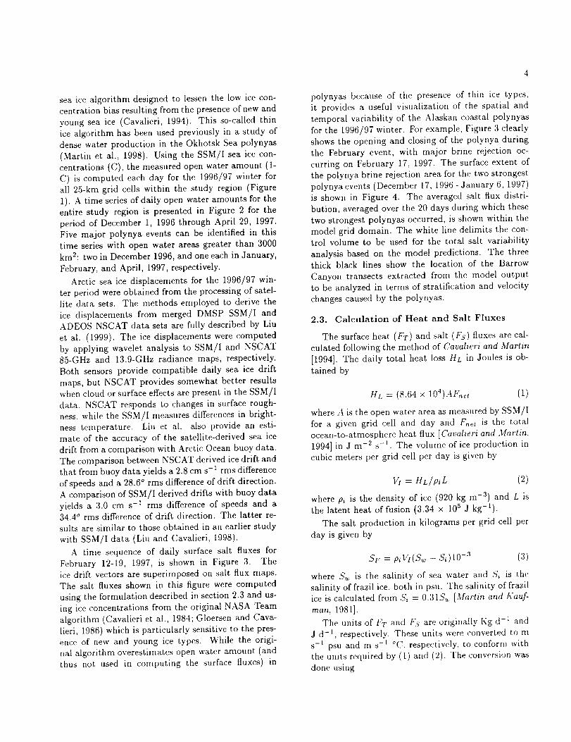
seaicealgorithmdesignedto lessenthelowicecon-centrationbiasresultingfromthepresenceofnewandyoungseaice(Cavalieri,1994).Thisso-calledthinicealgorithmhasbeenusedpreviouslyin astudyofdensewaterproductionin theOkhotskSeapolynyas(Martinet al., 1998).UsingtheSSM/Iseaicecon-centrations(C),themeasuredopenwateramount(l-C) iscomputedeachdayfor the1996/97winterforall 25-kingrid cellswithin thestudyregion(Figure1).A timeseriesofdailyopenwateramountsfor theentirestudyregionis presentedin Figure2 for theperiodof December1, 1996throughApril 29,1997.Fivemajorpolynyaeventscanbe identifiedin thistimeserieswith openwaterareasgreaterthan3000km2:twoinDecember1996,andoneeachinJanuary,February,andApril, 1997,respectively.

Arcticseaicedisplacementsforthe 1996/97win-terperiodwereobtained from the processing of satel-

lite data sets. The methods employed to derive the

ice displacements from merged DMSP SSM/I and

ADEOS NSCAT data sets are fully described by Liu

et al. (1999). The ice displacements were computed

by applying wavelet analysis to SSM/I and NSCAT

85-GHz and 13.9-GHz radiance maps, respectively.

Both sensors provide compatible daily sea ice drift

maps, but NSCAT provides somewhat better results

when cloud or surface effects are present in the SSM/I

data. NSCAT responds to changes in surface rough-

ness, while the SSM/[ measures differences in bright-

ness temperature. Liu et al. also provide an esti-

mate of the accuracy of the satellite-derived sea ice

drift from a comparison with Arctic Ocean buoy data.The comparison between NSCAT derived ice drift and

that from buoy data yields a 2.8 cm s-1 rms difference

of speeds and a 28.6 ° rms difference of drift direction.

A comparison of SSM/I derived drifts with buoy data

yields a 3.0 cm s-1 rms difference of speeds and a34.4 ° rms difference of drift direction. The latter re-

sults are similar to those obtained in an earlier study

with SSM/I data (Liu and Cavalieri, 1998).

A time sequence of daily surface salt fluxes for

February 12-19, 1997, is shown in Figure 3. The

ice drift vectors are superimposed on salt flux maps.

The salt fluxes shown in this figure were computed

using the formulation described in section 2.3 and us-

ing ice concentrations from the original NASA Team

algorithm (Cavalieri et al., 1984; Gloersen and Cava-

[ieri, 1986) which is particularly sensitive to the pres-

ence of new and young ice types. While the origi-nal algorithm overestimates open water amount (and

thus not used in computing the surface fluxes) in

polynyas because of the presence of thin ice types,

it provides a useful visualization of the spatial and

temporal variability of the Alaskan coastal polynyas

for the 1996/97 winter. For example, Figure 3 dearly

shows the opening and closing of tile polynya duringthe February event, with major brine rejection oc-

curring on February 17, 1997. The surface extent ofthe polynya brine rejection area for the two strongest

polynya events (December [7, 1996- January 6, 1997)is shown in Figure 4. The averaged salt flux distri-

bution, averaged over the 20 days during which these

two strongest polynyas occurred, is shown within themodel grid domain. The white line delimits the con-

trol volume to be used for the total salt variability

analysis based on the model predictions. The threethick black lines show the location of the Barrow

Canyon transects extracted from the model output

to be analyzed in terms of stratification and velocitychanges caused by the polynyas.

2.3. Calculation of Heat and Salt Fluxes

The surface heat (FT) and salt (Fs) fluxes are cal-

culated following the method of Cavaliers and Martin

[1994]. The daily total heat loss HL in Joules is ob-

tained by

HL = (8.64 × 104)AFoot (1)

where A is the open water area as measured by SSM/I

for a given grid cell and day and F,_t is the total

ocean-to-atmosphere heat flux [ Cavalzeri and Martin,1994] in J m -2 s -1. The volume of ice production in

cubic meters per grid cell per day is given by

VI = HL/piL (2)

where Pi is the density of ice (920 kg m -a) and L is

the latent heat of fusion (3.34 × 105 J kg-1).

The salt production in kilograms per grid cell per

day is given by

Sr = p_Vt(Sw - S_)10 -3 (3)

where S_ is the salinity of sea water and Si is the

salinity of frazil ice, both in psu. The salinity of frazil

ice is calculated from S, = 0.31S_ [Martin and h'auf-

man, 1981].

The units of FT and Fs are originally Kg d- l and

J d -t, respectively. These units were converted to m

s-' psu and m s-1 °C, respectively, to conform with

the units required by (I) and (2). The conversion was

done using

FT = HL/(8.64 x 104Ap_cp) (4)

Fs = 103SF/(8.64 × 104Api) (5)

where cp is the specific heat of sea water (4186 Jkg -l °C-l) and flw is the density of sea water in kg

m -3. Sea water density pw is calculated from salin-

ity, temperature, and pressure using the equation of

state formulation derived by Jackett and McDougall

(1992, unpublished manuscript) adopted for the oceanmodel.

3. Model Approach

We use a three-dimensional, rigid lid, primitive

equation model with orthogonal curvilinear coordi-

nates in the horizontal and a generalized coordinate in

the vertical (S Coordinate Primitive Equation Model,

SPEM5.1). The generalized vertical coordinate allows

high resolution in the upper ocean while maintaining

the bathymetry-following properties of the c_ coordi-

nate [Song and Haidvogel, 1994]. Table 1 shows the

level thicknesses at minimum depth, at the slope, and

at the maximum depth to illustrate the stretching of

vertical resolution across the grid domain. The modelwas previously applied and validated in the Barrow

Canyon region [Signorini et al., 1997].

3.1. Governing Equations

The primitive equations in Cartesian coordinates

governing the model dynamics are

t0U

c9--[+ _'' Vu - fv =

-y;+_ Kh @[ @j+ : K_ (6)

0---[+ _ " Vv + fu =

[ ° [ ÷[ °v]@ 0x f_'h +_ _h + : [,'_ (7)

OTo-7+ ¢' vv =

. OT

0-7 _ :

+

OS

0-7 + ¢ vs =

0 Eh _y + ](TS (9)

p = p(T,S,P) (I0)

a¢_ P9 (11)Oz Po

Ou Ov Ow

0-7+ _ + _ = o (t2)

where

(u, v, w) = the (x, y, z) components of vector ve-

locity V

po + p(x, y, z, t) = total in situ density

T(x, y, z, t) = potential temperature

S(ac, y, z, t) = salinity

P = total pressure P _ -pgz

¢(z,9, z,t) = dynamic pressure _ = (P/p)

f(z, y) = Coriolis parameter

g = acceleration of gravity

(Ka, K_, Krs) = horizontal and vertical eddy dif-fusion coefficients

3.2. Surface Forcing

The grid has been adapted and expanded for the

po[ynya investigation to include the brine formation

areas of the Chukchi Sea (Figure 1). The initial and

open boundary conditions are essentially the same as

in [Signorini et al., 1997]. The boundary conditionsfor surface heat and salt fluxes were formulated as

OTKrs-a-- = FT (13)

OZ

0S

I'(TS _ : Fs (14)

where KTS is in m'-/s , T is in °C, S is [n psu, and FT

and Fs are the surface heat and salt fluxes, respec-

tively. The vertical eddy diffusivity I(_ is calculated

following Pacanowskt and Philander, [198I]

[£v 11°- + _'b (15)(t + a&) _

KTs -- + _ (16)(t + aR,)

where Ri is the Richardson number, ub and nb are

background dissipation parameters and no, a and n

are adustable parameters. These were set to

Uo=0.01m2s -1, n=2, a=5

Vb = 10-4 m 2 s-l, t% = 10 -5 m 2 s -I

The heat and salt fluxes at the top layer of the

model are assumed zero when the grid cells are totally

ice covered and the water temperature is set to its

freezing value (T ice) according to

T ic_ = 0.094 - 0.00753p - 0.057S (17)

where p is given in bars and S is the salinity in psu

[Millero, 1975]. For grid cells containing open water

FT and Fs are imposed at the top layer following (13)

and (14).

Surface ice-water stress was implemented in themodel to evaluate the effect of ice drift on the cir-

culation and salt transport. The ice water stress wascalculated from satellite-derived ice drift data, as de-

scribed in section 2.2, using the following formulation,

ri_ = CiwUi_ [ui - u_] C (18)

m

(19)

1

(2o)

where r[_ and rf_ are the ice-water stress compo-nents, Ciw = 5.5 x 10 -a is the ice-water drag coeffi-

cient, ui and vi are the ice drift velocity components,

u_ and v_ are the surface water velocity components,

and C is the ice concentration. The boundary condi-tions for ice-water stress momentum transfer are for-nmlated as

% (21)K,, Oz - p

I\'_ Oz - p

3.3. Coastal Flow

The Alaskan coastal flow in the Chukchi Sea is pri-

marily influenced by the flow through Bering Strait.

The mean Bering Strait northward transport was esti-

mated at 1 Sv [Coachman et al., 1975], and this influxis a major consequence of the density structure of the

Arctic Ocean [Coachman and Barnes, 1961; Aagaard

et al., 1981; Nillworth and Smith, 1984]. The mean

flow appears driven by the sea surface slope down-

ward toward the north of the order of 10 -6 [Coachman

and Aagaard, 1966] which is probably of steric origin

]Coachman et al., 1975; Stigebrandt, 1984] and asso-

ciated with the mean density difference between theNorth Pacific and the Arctic Ocean. However, there is

substantial evidence of atmospherically forced major

variability in the flow, including reversals to south-

ward transport [Aagaard et al., 1985].

Coachman and Aagaard [1988] suggest the follow-

ing transport equation for the Bering Strait flow

Tr = 1.06- 0.112W (_3)

where Tr is the transport in sverdrups and W is the

component of the surface wind along 192°T in me-

ters per second. We use daily NCEP winds near

Bering Strait to calculate the time-varying transport.

The Cape Lisburne transport is taken to be 1/3 of

the Bering Strait transport and is used to force the

model coastal flow in the vicinity of Cape Lisburne

(T. Weingartner's personal communication). Figure

5 shows a time-series stack of the daily east and

north wind components in Bering Strait, the windcomponent towards 192°T in Bering Strait, the de-

rived Bering Strait volume transport, and the de-

rived Cape Lisburne volume transport for January-

March, 1997. Note that the wind component towards

192°T in Bering Strait and the volume transport in

Bering Strait and Cape Lisburne are inversely cor-

related [Aagaard et al., 1985]. The Cape Lisburne

transport exhibits significant variability. The largest

sustained transport occurs in January when the winds

were weaker in Bering Strait. The January-March av-erage transport is about 0.25 Sv. In our numerical

experiments we use time-variant and steady coastal

flow forcing. The steady coastal flow is obtained

by averaging the time-variant transport at Cape Lis-

burne over the entire duration of the run prior to each

numericalsimulation.Differencesbetweenthe twomethodsareanalyzedinsection4.

4. Model Experiments and Discussion

A seriesof sevennumericalexperimentswerecon-ductedto determinetheeffectsof differentcombina-tionsof modelforcingon thesalt transport,stratifi-cation,andcirculation.Theseincluderunswithandwithoutcoastalflowandrunswithandwithoutheatandsaltsurfacefluxes.Theforcingwasalsoconfig-uredfor time-averagedandtime-varyingcoastalflowandsurfacefluxes.Theexperimentscanbedividedintotwomajorcategories, those conducted with time-

averaged surface flux forcing, and those conducted

with time-variant flux forcing. Several forcing combi-

nations were imposed under each of these two major

categories. One experiment also included surface mo-

mentum forcing from ice-water stresses. The forcing

fields were spatially interpolated off-line from 25 km

resolution to the grid resolution of the model, which

averages 3 km. The daily fluxes and ice drift were

then linearly interpolated on-line to the time resolu-

tion required by the model time steps (2 minutes).Table 2 summarizes all experiment cases. Cases 1

through 4 fall in the first category and were designed

to evaluate the impact of strong polynya events onthe circulation, stratification, and salt generation in

the study region. Case 1 was forced with a steady

coastal flow by imposing a volume transport of 0.25

Sv at the model's western boundary (Cape Lisburne),but with zero surface heat and salt fluxes. Case 2 was

forced with the 20-day averaged salt and heat fluxes

and steady coastal flow. Case 3 included the mean

surface fluxes but the coastal flow transport was re-

duced to a very small value (0.0025 Sv). In case 4

the mean surface fluxes were imposed but the coastal

flow was allowed to vary in time.

Cases 5 through 7 fall in the second category and

were designed to evaluate the effects of weaker and

more rapidly changing polynyas on the stratification,

circulation, and salt generation in the study region.Case 5 was forced with time-variant (January 28-

February 28, 1997) surface fluxes and time-variantcoastal flow. In case 6 the coastal flow transport

was reduced to a minimum (0.0025 Sv). Finally,case 7 was forced with time-variant surface fluxes and

coastal flow as in case 5, but the surface ice-water

stresses were also imposed to evaluate the impact of

ice drift momentum transfer on the water properties.

4.1. Mean Salt Flux Forcing Experiments

The effects of different forcing scenarios on the salt

distribution and circulation for the first category of

experiments (cases 1 through 4) are shown in Figures

6 and 7. Figure 6 shows the 32-day time series of

the total salt increment for the four numerical exper-

iments (cases 1 through 4). The experiment forced

by coastal flow without surface fluxes (case 1) shows

that there was negligible variability in salt contentwhen compared with the other 3 experiments, whichwere forced with heat and salt surface fluxes. The

amount of salt accumulated within the polynya gener-

ation area is proportional to the intensity and steadi-

ness of the coastal current. The experiment forced

with a steady coastal current yielded the least salt

accumulation at the end of the 32 days of simula-

tion. The experiment forced with a very weak coastal

current yielded the highest salt accumualtion, while

the experiment forced with a time-variant coastal flow

produces salt amounts lying between the two extreme

cases. Figure 7 shows the salinity and currents at 20

meters for the four different numerical experiments

after 30 days of simulation. Only a subset (166°W -

156°W, 69.5°N-72°N) of the grid domain, which con-

tains the brine generation area and nearby areas, is

shown. The white rectangle delimits the control vol-

ume for the calculation of the salt production budget.

The location of Barrow Canyon is represented by the

40- and 50-meter isobaths (thick black lines). The

20-day (December 17, t996 to January 6, 1997) av-

eraged salt production from the two strongest events

occurring during that period is 380x 109 kg.

For case 1 (steady coastal flow and no surface

fluxes) the salinity is horizontally homogeneous andthere is relatively negligible change in the salt con-

tent within the control volume. In case 2 (steady

coastal flow and 20-day mean surface fluxes) the hori-

zontal salinity stratification is much stronger, reflect-

ing the salt production inside the polynya. Strongsalt advection is evident in the southern flank of Bar-

row Canyon, just offshore of Point Barrow, judging

from the swift (30-40 cm/s) and narrow (50 kin)

coastal current associated with a downstream gradi-

ent in salinity. A cyclonic recirculation is generatedeast of 160°W and north of the swift coastal current.

This recirculation seems to be bathymetrically steered

by the canyon topography and is a result of entrain-

ment of offshore canyon water into the narrow andswift coastal flow. Note that some surface freshwater

makes its way into the control volume at the west-

ern boundary carried by the strong coastal jet. The

totalsalt retainedin thecontrolvolumefor thisex-perimentafter20daysof simulationis213×109 kg.

Thus, 167× 109 kg (about 44% of the polynya's salt

production) were exported by the coastal current. Incase 3, for which the coastal current was replaced by

a very weak flow, the retention of salt within the con-

trol volume is much larger (331x109 kg). The salt

export, 49x 109 kg, is realized by a combination of the

weak and localized downcanyon gravitational flow (_<

10 cm/s) generated by the salinity gradient along the

coast near Point Barrow, and lateral diffusion. When

the time-variant coastal flow is used (case 4), the saltretention in the control volume is about 26% larger

(268 x 109 kg) than the steady coastal flow experiment

(case 2). The total salt exported by advection (380-268x 109 kg) after 20 days of simulation is l12x 109

kg, about 30% of the salt generated by the polynyafor the same time period. This result emphasizes the

need for realistic time-variant forcing to more accu-

rately assess the salt budget and dense water trans-

port. The difference in salt retention between case 2

and case 4 is most likely due to non-linear interactions

of momentum, salt conservation, and topography. Al-

though the majority of the salt produced by polynyas

is exported via the strong jet off of Point Barrow, rela-

tively small amounts of salt escape the control volume

via the northern boundary towards the Chukchi Sea

via gravitational circulation and horizontal diffusion.This is clearly shown in Figure 6 (cases 2, 3, and 4)

by the tongue-like shape of the isohalines protrudingout of the domain. As shown in case 3, there is also

salt transport via the gravitational current generated

by the salinity gradient in the vicinity of Point Bar-

row. The combined effect of gravitational circulationand diffusion accounts for 13% of the salt exported

in 20 days. The other mechanism for transporting

salt from the production area offshore of the Barrow

Canyon region (17% of the total salt produced) is the

strong salt advection resulting from the swift coastalcurrent originating from the Bering Strait through-

flow.

All numerical experiments were conducted with

initial temperature and salinity stratifications based

on fall CTD transects [Signorini et al., 1997]. Theinitial stratification is allowed to change in the model

under the influence of surface heat and salt fluxes,

and diffusion-advection processes computed by theheat and salt conservation equations. We will now

proceed to analyze the impact of the polynya salt pro-duction on the temperature and salinity stratification,

focussing on tile three cross-canyon transects shown

in Figures 1 arid 4. Figures 8 and 9 show the tem-

perature and salinity stratification along those threetransects at time equal zero (left column) and after

30 days of simulation (right column), forced with 20-

day averaged heat and salt fluxes at the surface and

steady coastal flow (case 2). The shallowest (west-

ernmost) transect is plotted at the top of the figuresand the deepest (easternmost) transect is plotted at

the bottom of the figures. Both salinity and temper-ature initial stratifications are horizontally weak but

have a significant vertical gradient. The mixed layer

homogeneity is apparent down to about 30 meters inboth salinity and temperature fields (-1.66 °C and

30.5 psu). There is a relatively sharp halocline belowthe mixed layer and a homogeneous salinity sublayer

between 75 and 100 meters. The mixeed layer water is

at freezing temperatures throughout. There is a sharp

vertical temperature gradient at 70 meters. These ini-tial conditions are representative of the fall season in

the Barrow Canyon region [Miinchow and Carmack,

1997]. Note the significant change in the salinity and

temperature distributions at 30 days when comparedto initial conditions. In the shallowest transect the

halocline is eroded by the convective mixing due to

the dense water formation in the polynya, and the

strong bottom mixing due to the nearshore (south-

east side of the canyon) coastal current. Below 40

meters (bottom of the canyon) there is vertical strat-ification in the salinity and temperature fields where

vertical mixing is much weaker. The influence of the

saltier (30.6 to 30.8 psu) and relatively colder (-1.68

°C) water generated in the polynya region is evidentin the top 30 meters by a vertically homogeneous layer

extending 350 to 400 km offshore. For the other twotransects further downstream the offshore extent of

the polynya decreases to 300 and 150 km, respectively,

and the mixing depth becomes shallower (25 meters)

due to the reduced salt production. There is a strong

horizontal gradient of temperature and salinity below40 meters, and at a distance of less than 100 km off-

shore, resulting from the baroclinic response of thedensity field to the strong coastal flow. It is within

this 100-km coastal boundary that most of the salt

exchange between the polynya-driven salt generationarea and the Beaufort Sea shelf break takes place.

A comparison between the salinity and tempera-ture stratifications with and without the polynya heat

and salt surface fluxes is shown in Figures 10 and ll.The left side shows the results for case 1 (no sur-

face fluxes) and the right side shows reults for case

2 (with surface fluxes). The effect of the denser wa-

ter injectionbythepolynyaisquiteevidentby thehorizontaltemperatureandsalinitygradientswithinthemixedlayer,whichforma frontalongtheedgesof thepo[ynya.Thiscontrastswith theresultsfromcaseI wherea horizontallyuniformmixedlayerispresentinall threetransects.Figures12and13com-parethetemperatureandsalinitystratifications,re-spectively,betweencase3(leftside)andcase2(rightside).Thesefiguresareintendedto contrasttheef-fectsof thepolynya-inducedheatandsaltfluxeswith(right side)andwithout(left side)the presenceoftheswiftcoastalcurrent.Notethat thecoastalcur-rentenablesdeepermixingnearthecoastby erod-ingtheshallowhalocline(,--30m) all thewayto thebottom.Withoutthecoastalcurrent,thecolderandsaltierwateroriginatingfromthepolynyais limitedto spreadhorizontallybydiffusionandweakgravi-tationaladvectionwithin themixedlayer(upper30meters).Thismechanismcontrastswith theArctichaloclineventilationon the MackenzieShelf,whichoccursduringsomewintersin responsetowind-drivenupwellingcombinedwithconvectioninducedby thesaltexpelledfromgrowingseaice. Thewaterover-lying Mackenzie shelf in the southeastern Beaufort

Sea becomes quite saline (33-35 psu) and at freez-

ing temperature throughout [Melling, 1993]. Themodel-predicted denser water produced on the shelf

in the vicinity of Barrow Canyon during the winter

of 1996/1997 was much less saline (30.6 to 30.8 psn)

and it was not dense enough to ventilate the Arc-

tic halocline. The question still remains on whether

more intense polynyas that may occur on the Chukchi

Shelf upstream of Barrow Canyon are capable of ven-

tilating the Arctic halocline. Cavalieri and Martin,

[1994], based on nine years (1978-1986) of data, sug-

gest that dense water formation from polynyas in the

vicinity of Barrow Canyon may ventilate the Arctic

halocline when the pre-polynya ambient surface salin-ity reaches 32 psu. With this ambient salinity, it takes

approximately 4 meters of ice growth to bring the

water column ('--50 m) to a salinity of 34 psu andventilate the halocline layer. However, these extreme

salinity values are not very common in the surface wa-

ters upstream of Barrow Canyon (Point Lay to Point

Barrow).

4.2. Time-Variant Salt Flux Forcing

Experiments

The effects of different forcing scenarios on the salt

distribution and circulation for the second category of

experiments (cases 5, 6, and 7) are shown in Figures

14 and 15. Figure 14 shows the time series of totalsalt accumulated within the control volume for the

time period of January 28 - February 28, 1997, duringwhich a fast evolving polynya occurred. The three ex-

periments shown are all forced by time-variant surface

fluxes but differ in the way the coastal flow and sur-

face stress are applied to the model. Case 5 was forced

with time-variant coastal flow, case 6 was forced with

a weak and steady flow, and case 7 was forced byboth time-variant coastal flow and ice-water stress.

The total polynya salt production for this time pe-

riod was 223×109 kg. The total salt accumulated

within the control volume after 32 days of simula-

tion for cases 5, 6, and 7 are, respectively, 92×109

kg, 155×109 kg, and 96×109 kg. Therefore, 131×109

kg of salt are exported in case 5, 68×109 kg in case

6, and 127× 109 kg in case 7. The largest salt ex-

port, 59% of the polynya production, occurs in case

5 where salt advection is larger because of the effectof the time-variant coastal flow. The smallest salt ex-

port, 31% of the polynya production, occurs in case 6because the coastal flow was reduced to a minimum

(0.0025 Sv). The salt export mechanisms in this easeare mainly lateral diffusion and gravitational flow. In

case 7, where the forcing includes time-variant coastal

current and ice-water stress, the salt export is slightlyless than in case 5 (57% of the polynya production)

resulting from a reduction of the coastal current speed

due to the ice-water drag forces.

Figure 15 shows time series of coastal flow trans-

port, surface salt flux generated by the polynya, and

net salt change within the control volume due to the

combine effects of salt expelled by ice growth and salt

exported by lateral advection and diffusion. The net

salt change time series are shown for cases 5, 6, and

7. There were two events during which the coastal

flow transport was relatively high (>0.2 Sv) and the

surface salt flux was very low. These were: Febru-

ary 1 and February 10, 1997. These events led thepeak of salt draining, shown by the throughs in the

net salt change time series. There were two peak

polynya activity events during which the coastal flow

transport was relatively low, one on January 30 and

one centered on February 4. These events were fol-lowed by peaks of net salt change after 1 to 2 days,

indicating the approximate advective time scale of

polynya-generated salt export from the shelf during

weak polynya activity, The time scale response for

large salt injections from polynyas associated with

very weak coastal [tow (case 6) is much more rapid

(order of hours) judging from the fast response shown

fortheFebruary10-18event(themaximumsaltinjec-tion fromthepolynyafor theJanuary28- February28timeperiod).

Thedepth-(surfaceto 30meters)andtime-(30days)averagedmixed-layersalinityandcurrentsforcases5 and7 areshownin Figure16.A comparisonof case5 (Figure16a,no ice-waterstress)with case7 (Figure16c,with ice-waterstress)revealsthat theinclusionof the ice-waterstressin themodelforcingresultsin thewideningofthecoastalflowandanover-allreductionofthecurrentspeeds.Alsonotethatthecyclonicflowin theeasternsideofthecontrolvolumeshownincase5isdampenedbythesurfaceicestressincase7(Figure16c).Figure16bshowsthemeanicedrift vectors and salt production for the entire simula-

tion period. The mean ice drift (--_ 3-4 cm/s) is west-

northwestward, mainly against the eastward flowingcoastal current. The ice motion effect on the circu-

lation is twofold: it reduces the surface flow by ice-

water drag, and it widens the coastal current due to

offshore Ekman transport. The effect in the velocity

and salinity transects across Barrow Canyon is shown

in Figures 17 and 18. The transects are shown on theleft side for case 5 (no ice stress), and on the right for

case 7 (with ice stress). Note that the coastal current

(Figure 17) is much swifter and narrow (_ 50 kin) incase 5 than in case 7 where the width of the current

is about 100 to 150 kin. In addition, the return flow

(negative velocities) in case 7 is very weak for the top

and middle transects, and absent in the bottom tran-

sect. The salinity transects in Figure 18 show that

the spreading of the salt produced by the polynya is

confined to the mixed layer. Also, the offshore extent

of the polynya front, indicated by the 30.3 isohaline in

the top and middle transects, is wider in case 7 than

in case 5. The polynya influence is stronger and wider

further upstream (Figure 16) where surface salinity is

greater than 30.5 psu (transects not shown).

Figure 19 shows the mean salinity distribution and

a three dimensional rendition of bottom topographywithin the domain of the control volume box. The

salt exchange pathways are shown by the large ar-

rows. The polynya salt production enters the control

volume via the surface flux (1). Most of the exportedsalt leaves the control volume via strong advection im-

parted by the swift flow at the southern flank of Bar-

row Canyon (4). The lateral exchange via the west

(2) and northern boundaries (3) is relatively much

smaller. The mixing depth is a function of the inten-sity of the polynya salt production and the strength

of the coastal current. The salt exchange from weak

10

polynyas is confined to the mixed layer while salt from

strong polynyas combined with swift coastal current

mixes all the way to the bottom of the canyon near the

coast. For case 7, for which the forcing fields are the

most realistic (time-variant surface salt flux, coastal

current, and surface ice-water stress), the total salt

accumulated for the 32-day simulation (January 28 -

February 28, 1997) within the shelf region delimited

by the control volume is 96x109 kg. The total salt

production by the polynya for the same time period

is 223x109 kg. The difference of 127x109 kg is pri-

marily exported via Barrow Canyon by the coastalcurrent.

5. Summary and Conclusions

Numerical experiments were conducted using a

high resolution (1 to 5 kin) numerical model with real-

istic topography, ambient stratification, and ambientflow for the Chukchi and Beaufort Seas. A total of

seven numerical experiments were conducted to de-termine the effects of different combinations of model

forcing on the salt transport, stratification, and cir-

culation. The experiments can be divided into two

major categories, those conducted with time-averagedsurface flux forcing, and those conducted with time-

variant flux forcing. Several forcing combinations

were imposed under each of these two major cate-

gories. One experiment also included surface momen-

tum forcing from ice-water stresses.

Results from this study show that the ambient

stratification plays a major role in controlling the

spreading of salt produced by the polynyas. Pre-

vious modeling experiments have shown that withstrong stratification dense water is transported across

the shelfbreak at intermediate depths, whereas with

weak stratification dense water moves downslope and

is trapped near the bottom (Gawarkiewicz, [2000]).

The summer-fall melting produces a shallow (--,30 m)

halocline in the Chukchi Sea which provides a bar-

rier layer for the vertical mixing of poiynya-generated

saltier water in the winter. During the polynya events

of 1996/1997, the brine rejection did not produce wa-

ter densities sufficiently high to erode the shallow

halocline barrier layer. The only exception were the

shallow (_< 30 m) areas of the Chukchi Sea whero bot-tom boundary turbulence produces intense mixing,

and the coastal boundary layer where lateral shearfrom the swift Alaska coastal current entrains and

mixes the saltier water. The coastal current promotes

40 to 60% of the total salt exported offshore via Bar-

row Canyon. The inclusion of an ice-water boundary

layer in the model broadens and slightly weakens the

coastal current, thus reducing the salt export from

59% to 57% of the total polynya salt production in

32 days.

One question that still remains is whether Chukchi

Sea polynyas in the vicinity of Barrow Canyon can

produce enough salt to ventilate the Arctic halocline

during some winters. As noted earlier, Cavalieri and

Martin [1994] argued that an ambient surface salin-

ity of about 32 psu and approximately 4 meters of

ice growth would be required to bring a 50 meter

water column to a salinity of 34 psu. Under these

conditions, the water formed by the polynya is suffi-

ciently dense to ventilate the Arctic halocline. These

conditions were not encountered during the winter of

1996/1997. As future work, we propose to extend

the regional domain to include a larger number of

polynya areas and multi-year events to capture a more

complete range of forcing conditions for the model.

For example, during the winter of 1991/1992 daily

salt rejection from polynyas in the vicinity of Bar-

row Canyon peaked at ,--40-50× 109 kg (Weingartner

et al., 1998), a value five times larger than the peak

daily salt rejection during the winter of 1996/1997.

These large interannual changes in polynya activity

are consistent with the recent study of Winsor and

Bj rk [2000].One particular area of interest not covered by this

study is the Mackenzie shelf region. During some

winters, the water overlying Mackenzie shelf in the

southeastern Beaufort Sea becomes quite saline (33-

35 psu) and at freezing temperature throughout as a

result of salt expelled from growing sea ice [Melling,

1993]. Therefore, areas such as the Mackenzie shelf

are likely candidates for further numerical studies of

the oceanic response to dense water formation and an

evaluation ot its impact on the Arctic halocline.

II

Acknowledgments. We are thankful to Jodi Humphreys

of SA[C General Sciences Corporation and X. Zhang of

Raytheon ITSS for providing the heat and salt fluxes de-

rived from SSM/I data. 'eVe are also thankful to A. Liu of

the NASA-GSFC Laboratory for Hydrospheric Processes

and Y. Zhao of CAELUM for providing the ice drift data

derived from SSM/I and NSCAT data. This work was

sponsored by the Office of Naval Research under contract

No. N00014-98-C-0022 MOD P00003.

References

Aagaard, K., L. K. Coachman, and E. C. Carmack, Onthe halocline of the Arctic Ocean, Deep Sea Res., 29,

529-545, 1981.

Aagaard, K., A. T. Roach, and J. D. Schumacher, On

the wind-driven variability of the flow through Bering

Strait, J. Geophys. Res., 90, 7213-7221, 1985.

Aagaard, K., and E. Carmac, The Arctic Ocean and cli-

mate: A perspective, in The Polar Oceans and Their

Role in Shaping the Global Environment, Geophys.

Mono. Set., vol. 85, edited by O. M. Joharmessen,

R. D. Muench, and J. E. Overland, pp. 5-20, AGU,

Washington D. C., 1994.

Cavalieri, D. J., P. Gloersen, and W. J. Campbell, De-

termination of sea ice parameters with the Nimbus 7

SMMR, J. Geophys. Res., 89, 5355-5369, 1984.

Cavalieri, D. J., and S. Martin, The contribution of

Alaskan, Siberian, and Canadian coastal polynyas to

the cold halocline layer of the Arctic Ocean, J. Geo-

phys. Res., 99, 18,343-18,362, 1994.

Chapman, D. C., and G. Gawarkiewicz, Offshore trans-

port of dense shelf water in the presence of a submarine

canyon, J. Geophys. Res., 100, 13,373-13,387, 1995.

Coachman, L. K., and C. A. Barnes, The contribution

of Bering Sea water to the Arctic Ocean, Arctic, 14,

147-161, 1961.

Coachman, L. K., and K. Aagaard, On the water exchange

through Bering Strait, Limnol. Oceanogr., 11, 44-59,

1966.

Coachman, L. K., K. Aagaard, and R. B. Tripp, Bering

Strait: The Regional Physical Oceanography, 172 pp.,

University of Washington Press, Seattle, 1975.

Coachman, L. K., and K. Aagaard, Transports through

Bering Strait: Annual and interannual variability, J.

Geophys. Res., 93, 15,535-15,539, 1988.

Gloersen, P., and D. J. Cavalieri, Reduction of weather

effects in the calculation of sea ice concentration from

microwave radiances, J. Geophys. Res., 9l, 3913-3919,

1986.

Gawarkiewicz, G., and D. C. Chapman, A numerical

study of dense water formation and transport on a shal-

low, sloping continental shelf, J. Geophys. Res., 100,

4489-4507, 1995.

Gawarkiewicz, G., Effects of ambient stratification and

shelfbreak topography on offshore transport of dense

wateroil continentalshelves.J. Geophys. Res., 105,

3307-3324, 2,000.

Junkclaus, J. H. , and J. O. Backhaus, Application of

a transient reduced gravity plume model to Denmark

Strait Overflow, J. Geophys. Res., 99, 12,,375-12,396,

1994.

Junkclaus, J. H. , J. O. Backhaus, H. Fohrmann, Out-

flow of dense water from the Storfjord in Svalbard: A

numerical model study, J. Geophys. Res., 100, 24,719-

2`4,728, 1995.

KaJnay, E., et al., The NCEP/NCAR 40-year reanalysis

project, Bull. Amer. Met. Soc., 77, 437-471, 1996.

Killworth, P. D., and J. M. Smith, A one-and-a-half di-

mensional model for the Arctic halocline, Deep Sea

Res., 31,271-293, 1984.

Liu, A.K. and D. J. CavaJieri, On sea ice drift from the

wavelet analysis of the Defense Meteorological Satel-

kite Program (DMSP) Special Sensor Microwave lmager

(SSMf[) Data, Int. J. Remote Sensing, 19, 1415-1423,

1998.

Liu, A. K., Y. Zhao, and S. Y. Wu, Arctic sea ice drift

from wavelet analysis of NSCAT and special sensor mi-

crowave imager data, J. Geophys. Res., 104, 11,529-

11,538, 1999.

Martin, S., and P. Kaufman, A field and laboratory study

of wave damping by grease ice, J. Glaciol., 27, 283-314,

1981.

Melting, H., The formation of a haline shelf front in win-

tertime in an ice-covered arctic sea, Cont. Shell Res.,

13, 1123-1147, 1993.

Millero, F.L., Freezing point of sea water. Eighth report

of the Joint Panel of Oceanographic Tables and Stan-

dards, Appendix 6, UNESCO Tech. Pap. Mar. Sci.,

28, 29-31, 1975.

M_nchow, A., and E. C. Carmack, Synoptic flow and den-

sity observations near an Arctic shelf break, J. Phgs.

Oceanogr., 27, 1402-1419, 1997.

Pacanowski, R. C., and G. H. Philander, Parameteriza-

tion of vertical mixing in numerical models of tropical

oceans, J. Phys. Oceanogr., 11, 1443-1451, 1981.

Pease, C. H., The size of wind-driven coastal polynyas, J.

Geophys. Res., 92, 7049-7059, 1987.

Signorini, S. R., A. M6nchow, and D. Haidvogel, Flow

dynamics of a wide Arctic canyon, J. Geophys. Res.,

102, 18,661-18,680, 1997.

Song Y. and D. Haidvogel, A Semi-implicit Ocean Circula-

tion Model Using a Generalized Topography-Following

Coordinate System, J. of Comp. Phys. , 115, 228-244,

1994.

Stigebrandt, A., The North Pacific: A global scale estuary,

J. Phgs. Oveanoyr., 14,464-470, 1984.

Weingartner, T. J., D. J. Cavalieri, K. Aagard, and Y.

Sasaki, Circulation, dense water formation, and outflow

or: the northeast Chukchi shelf, J. Geophys. Res., 103,

7647-7661, 1998.

Winsor, P., and G. BjSrk, Polynya activity in the Arctic

12

Ocean from 1958 to 1997, J. Geophys. Res., 105, 8789-

8803, 2000.

D. Cavalieri, Code 971, Laboratory for Hydro-

spheric Processes, NASA Goddard Space Flight Cen-

ter, Greenbelt, MD 20771.

S. R. Signorini, SAIC General Sciences Corpora-

tion, 4600 Powder Mill Road Beltsville, Maryland

20705-2675 (e-mail: sergio@bluefin.gsfc.nasa.gov)

This preprint was prepared with AGU's LaT_'_ macros v,t.File paper'po[ynya'revl formatted June 1, 2000.

13

Figure 1. Map of the study region showing the model grid and topography. The dots within the grid domain

represent every second grid point. The three thick lines show the location of the Barrow Canyon transects analyzed

in this study.

Figure 2. Time series of daily open water amounts for the entire study region.

Figure 3. SSM/I-derived salt fluxes (in Gg/d) for clays 43 through 50 (February 12-19, 1997). Note that the

strongest event occurs on February 17. The daily ice drift is shown by the superimposed black vectors.

Figure 4. Mean salt production (106 kg/d) for polynya events during the period of December 17, 1996 throughJanuary 6, 1997. The white line delimits the control volume for total salt variability. The three thick black lines

show the location of the Barrow Canyon transects analyzed in this study.

Figure 5. Time series of daily east and north wind components in Bering Strait, wind component towards 192°T

in Bering Strait, derived Bering Strait volume transport, and derived Cape Lisburne volume transport.

Figure 6. Total salt increment, in 109 kg, within the control volume shown in Figure 4 for four different numerical

experiments (cases 1, 2, 3, and 4). Case 1 is the baseline experiment (no surface flux with coastal flow forcing)which shows a relatively small salt change. Case 2 is forced by 20-day averaged salt flux and steady 0.25 sv coastal

flow. Case 3 is forced by 20-day averaged salt flux with weak coastal flow. Case 4 is forced by 20-day averaged salt

flux and time-variant coastal flow (e. g., wind modulated).

Figure 7. Salinity and currents at 20 meters from four different numerical experiments after 30 days of simulation.

The white rectangle delimits the control volume for the calculation of the salt production budget. The 40 and 50

meter isobaths are represented by the thick black lines. The top left plate shows results from case 1 (no surface

fluxes with steady coastal flow), the top right plate shows results from case 2 (surface fluxes with steady coastal

flow), the bottom left plate shows results from case 3 (surface fluxes with very weak coastal flow), and the bottom

right plate shows results from case 4 (surface fluxes with time-variant coastal flow).

Figure 8. Initial temperature section (left) and temperature section after 30 days (right) at 3 transects perpendic-ular to the coast and across the polynya brine generation area. Note that these transects are also perpendicular to

Barrow Canyon. The contours are 0.02 for T _< -1.6°C and 0.2 for T __ -1.6°C. These are results from experiment

No. 2 (20-day averaged heat and salt fluxes with steady coastal flow).

Figure 9. Initial salinity section (left) and salinity section after 30 days (right) at 3 transects perpendicular to

the coast and across the polynya brine generation area. Note that these transects are also perpendicular to Barrow

Canyon. The contours are 0.1 for S _< 30.7 psu and 0.2 for S >_ 30.7 psu. These are results from experiment No. 2

(20-day averaged heat and salt fluxes with steady coastal flow).

Figure 10. Temperature sections after 30 days from model runs with (case 2, right) and without (case 1, left) heatand salt surface fluxes from polynya. A steady, 0.25 Sverdrup coastal flow is imposed in both runs. Temperatures

are shown at 3 transects perpendicular to the coast and across the polynya brine generation area. Note that these

transects are also perpendicular to Barrow Canyon. The contours are 0.02 for T < -1.6°C and 0.2 for T _> -1.6°C.

Figure 11. Salinity sections after 30 days from model runs with (case 2 right) and without (case 1, left) heat andsalt surface fluxes from polynya. A steady, 0.25 Sverdrup coastal flow is imposed in both runs. Salinities are shown

at 3 transects perpendicular to the coast and across the polynya brine generation area. Note that these transects

are also perpendicular to Barrow Canyon. The contours are 0.1 for S _< 30.7 psu and 0.2 for S _> 30.7 psu.

Figure 12. Temperature sections after 30 days from model runs with (case2, right) and without (case 3, left)coastal flow. Heat and salt surface fluxes from polynya are imposed on both cases. Temperatures are shown at 3

transects perpendicular to the coast and across the polynya brine generation area. Note that these transects are

also perpendicular to Barrow Canyon. The contours are 0.02 for T _< -1.6°C and 0.2 for T _> -I.6°C.

14

Figure 13. Salinitysectionsafter30daysfrommodelrunswith (case2,right) andwithout(case3, left)coastalflow.Heatandsaltsurfacefluxesfrompolynyaareimposedonbothcases.Salinitiesareshownat 3 transectsperpendicularto thecoastandacrossthe polynyabrinegenerationarea. Notethat thesetransectsarealsoperpendicularto BarrowCanyon.Thecontoursare0.1forS_<30.7psuand0.2for S> 30.7 psu.

Figure 14. Total salt increment, in 10 9 kg, within the control volume shown in Figure 4 for three different

numerical experiments (cases 5, 6, and 7). The simulation was conducted for the period of January 28 throughFebruary 28, 1997. The total potynya salt production for this time period was 223x109 kg. Case 5 was forced

by time-variant surface fluxes (salt and heat) and time-variant coastal current. Case 6 was forced by time-variant

surface fluxes and a very weak and steady coastal current. The forcing for case 7 was similar to case 5, except that

time-variant ice-water stress was also imposed at the surface.

Figure 15. Time series of coastal flow transport, surface salt flux from polynyas, and net salt change due to

polynya production and horizontal transport for January 28-February 28, 1997. The net salt change time series

are shown for 3 simulations: (1) surface heat/salt flux forcing with coastal flow (case 5); (2) surface heat/salt flux

forcing with weak and steady coastal flow (case 6); and (3) surface heat/salt flux forcing, surface ice stress forcing,

and coastal flow (case 7). Daily salt/heat fluxes and coastal flow transport are used in these simulations. Dailysurface ice stress is also used to force the run for case 7.

Figure 16. Salinity distribution and currents for case 5 (a) and case 7 (c) simulations, and ice drift and salt

production (b) for January 28 - February 28, 1997. The white rectangle delimits the control volume for the

calculation of the salt production budget. Case 5 is forced with time-variant salt/heat fluxes and coastal flow. Case

7 is forced with time variant salt/heat fluxes, coastal flow, plus ice-ocean surface stress. The ice drift is primarily

against the coastal flow, thus reducing its intensity. Note that the cyclonic flow in the eastern side of the controlvolume shown in case 5 is dampened by the surface ice stress in case 7. Both salinity and currents were depth-

(surface to 30 meters) and time-averaged (30 days). The ice drift was averaged over the 30-day period while thesalt production is summed over the same time period. Current and ice drift vectors with amplitude < 2 cm/s are

not plotted.

Figure 17, Thirty-day averaged sections of u-component of velocity from model runs with (case 6, right) and

without (case 5, left) surface ice stress. The u-component is shown at 3 transects perpendicular to the coast and

across the polynya brine generation area. Note that these transects are also perpendicular to Barrow Canyon. The

contour intervals are 1 cm/s for u _< 10 cm/s and 5 cm/s for u _> 10 cm/s.

Figure 18. Thirty-day averaged sections of salinity from model runs with (case 6, right) and without (case 5, left)surface ice stress. The salinity is shown at 3 transects perpendicular to the coast and across the polynya brine

generation area. Note that these transects are also perpendicular to Barrow Canyon. The contour intervals are 0.1

for S < 30.7 psu and 0.2 for S _> 30.7 psu.

Figure 19. Mean salinity distribution and three dimensional rendition of bottom topography within the domain of

the control volume box. The salt exchange pathways are shown by the large arrows. The polynya salt production

enters the control volume via the surface flux (1). Most of the exported salt leaves the control volume via strong

advection imparted by the swift flow at the southern flank of Barrow Canyon (4). The lateral exchange via the

west (2) and northern boundaries (3) is relatively much smaller.

15

Table 1. Layer depth in meters for model grid points at mininmnl depth (H,,,,_=20 m), over the slope

(H,_ope=i0t0 m), and at maximum depth (Hma,=2000 m).

Level sa Hmin H slope Hmar

25 0.00 0.00 0.00 0,0024 -0.04 -0.80 - 16.21 -31.61

23 -0.08 - 1.60 -32.58 -63.56

22 -0.12 -2.40 -49.29 -96.18

21 -0.16 -3.20 -66.51 -129.8120 -0.20 -4.00 -84.41 -164.82

19 -0.24 -4.80 -103.18 -201.56

18 -0.28 -5.60 -123.02 -240.44

17 -0.32 -6.40 -144.13 -281.86

16 -0.36 -7.20 -166.73 -326.26

15 -0.40 -8.00 -191.05 -374.11

14 -0.44 -8.80 -217.36 -425.93

13 -0.48 -9.60 -245.93 -482.26

12 -0.52 -10.40 -277.05 -543.71

11 -0.56 -11.20 -311.07 -610.93

10 -0.60 -12.00 -348.32 -684.65

9 -0.64 -12.80 -389.22 -765.658 -0.68 -13.60 -434.20 -854.79

7 -0.72 -14.40 -483.72 -953.05

6 -0.76 -15.20 -538.33 -1061.46

5 -0.80 -16.00 -598.60 -ii81.2i

4 -0.84 -16.80 -665.18 -1313.56

3 -0.88 -17.60 -738.78 -1459.96

2 -0.92 -18.40 -820.18 -1621.97

1 -0.96 -19.20 -910.27 -1801.34

0 -1.00 -20.00 -1010.00 -2000.00

_Generalized s coordinate (Song and Haidvogel, [1994]).

75°N

72°N

71 °N

70°N

69°N

68"N

67°N

66°N

iii,i_ ""'"" .--.::.!_

_'_" ..:.-

,4 1 ZI _14 "11f • L--4" !ll_.Jl TIJ •

L • !., ! '

2

"

_.._(._hu, Se._ L_

65°N172°W 168°W 164°W 160°W 156°W 152°W 148°W

Figure 1. Map of the sudy region showing the model grid and topography. "Fhe dots within the grid domain

represent every second grid point,. The three thick lines show the location of the Barrow Canyon transects analyzed

in this study•

Open Water Area

E

o

0.8

0.6

0.4

0.2

0.0Dec 11 Dec 31

1996

I I I

Jan 20 Feb 9 Feb 29 Mar 20 Apr 9 Apr 291997

Figure 2. Time series of daily open water amounts for the entire study region after freezeup. The series starts on

December 1, 1996, and ends on April 29, 1997.

73"N

72"N

71 °N

70"N

69"N

68°N

73"N

72"N

71 °N

70°N

69"N

68"N

_ 10 km/d

73"N

72"N

71 °N

70°N

69"N

68"N

Feb. 12, 1997, Salt Flux

170"W 160°W 150°W

Feb. 13, 1997, Salt Flux

170°W 160°W 150°W

Feb. 14, 1997, Salt Flux

Feb. 16, 1997, Salt Flux

170°W 160°W 150°W

Feb. 17, 1997, Salt Flux

170°w 160°w 150"w

Feb. 18, 1997, Salt Flux

170°W 160°W 150°W 170"W 160"W 150°W

300

240

180

120

6O

0

300

240

180

120

60

0

3O0

240

180

120

60

0

73"N

72°N

71 "N

70"N

69"N

68°N

Feb. 15, 1997, Salt Flux Feb. 19, 1997, Salt Flux

170°W 160°W 150"W 170°W 160°W 150°W

300

240

180

120

60

0

Figure 3. SSM/I-derived salt production (in 106 kg/d) for February 12-19. 1!)97. Note that the strongest event

occurs on February 17. The ice drift vectors (in km/d) derived from mero_ied I)MSP SSM/I and AI)EOS NSCAT

data sets are superimposed on the daily salt fluxes.

74"N

73"N

72'N

71 "N

70'N

69"N

68"N

67"N

172"W 168"W 164°W 160"W 156"W 152"W 148"W

0 15 30 45 60 75 90 105 120 135 150

Figure 4. Mean salt production (106 kg/d) for polynya events during the period of December 17, 1996 throughJanuary 6, 1997. The white line delimits the control volume for total salt variability. The three thick black lines

show the location of the Barrow Canyon transects analyzed in this study.

2O

10

v

LU 0

_: -IO

-20

20

_" 10

z, o"o._c

-lo

-20

20

10

v

_- 0cJo_

-10

-20

3

> 209v

I--o_ 1i-

05m 0

-1

1.0

0.5O.I--

J 0.00

-0.5

I !

JAN i FEB t MAR

I I

JAN i FEB i MAR

I I

JAN FEB MAR

1997

Figure 5. Time series of daily east and north wind components in Bering Strait, wind component, towards 192°'1"

in Bering Strait, derived Bering Strait volume transport, and derived Cape l, isburne volume transport.

I , I , I | , I , I , i , t , I , I , t _ I i I _ L _ J ' ! '700

] Solid = coastal flow without salt flux (Case 1)1 Dashed = salt flux + coastal flow (Case 2)._] Dotted = salt flux with weak coastal flow (Case 3)

600 Triangles = salt flux + time-variant coastal flow (Case 4)

! ....! ............

400 .....................

"_ o.OOOO°o*°°***°'°°°°°°°°°°°*'°°°°*°'°°'°°°°'*°°*_°°*°° "°°°°°_°°°i

_ aoo

r° 200 ............. ....---'" "" "--" -" "" -"

............._ _ ""

_ 100

o

-100

-2002 4 6 8 10 12 14 16 18 20 22 24 26 28 30 32 34

Days After Start

Figure 6. Total salt increment, in 109 kg, within the control volume shown in Figure 4 for four different numerical

experiments (cases 1, 2, 3, and 4). Case 1 is the baseline experiment (no surface flux with coastal flow forcing) which

shows a relatively small salt change. Case 2 is forced by 20-day averaged salt flux and steady 0.25 sv coastal flow.

Case 3 is forced by 20-day averaged salt flux with weak coastal flow. Case 4 is forced by 20-day averaged salt flux

and time-variant coastal flow (e. g., wind modulated). The total salt stored within the control volume for cases 2.

3, and 4 is 213× l09 kg, 331× l09 kg, and 268x 10 9 kg, respectively. For case 4, which is forced by the more realistictime-variant coastal current, the total salt exported by advection for the 20-day simulation period is 76×109 kg

(380-268=112× l09 kg). This amounts to 30% of the 380x l09 kg of salt generated by the polynya in 20 days. The

majority of the salt export occurs via Barrow Canyon at its southeastern flank near the coast.

72"N

71"N !

70"N

166"W 164"W 162"W 160"W 158"W 156"W

30.8830.8630.8430.8230.8030.7830.7630.7430.7230.70

• 30.68• 30.66• 30.84• 30,62• 30.60• 30.58

• 30,56• 30.54

30.5230.5030.48

72"N

71 "N

70"N

166"W 164"W 162"W 160'W 158"W 156'W

30.8830.86

30.8430.8230.8030.7830.7630.7430.7230.7030.6830.6630.6430.62

30.6030.5830.5630.5430.5230.5030.48

72"N

71"N

70"N

30.88 72"N30.8630.8430.8230.8030.7830.7630.74

30,72 71 "N30.7030.6830,6630.64

• 30.62

• 30•60• 30.58

• 30,56 70"N,30.54• 30.52• 30.50

30.48

166'W 164'W 162"W 160"W 158"W 156"W 166"W 164"W 162"W 160"W 158"W 156"W

• 30.8830.8630.8430.8230.80

- 30.78- 30.76- 30.74- 30.72

- 30.70- 30.68

30.6630.6430.6230.6030.5830.5630.5430.5230.5030.48

Figure 7. Salinity and currents at 20 meters from four different numerical experiments after 30 days of simulation.

The white rectangle delimits the control volume for the calculation of the salt production budget• The 40 and 50

meter isobaths are represented by the thick black lines. The top left plate shows results from case 1 (no surface fluxes

with steady coastal flow), the top right plate shows results from case 2 (s,rface fluxes with steady coastal flow), the

bottom left plate shows results from case 3 (surface fluxes with very weak coastal flow), and the bottom right plate

shows results from case 4 (surface fluxes with time-variant coastal flow).

oS

-10 -

-20

-30

-40 -

-50 '

E -60-N -70 '

-80 :

-90 :

-100 :-110 :

-1200

N.... L , , i - l .... I .... i .... ..

t 66 t66

-1.68 t G8

-- -1.7

1 72

-1,74 --

1,76-- . ....78-

i .....

100 200 300 400

Distance (kin)

5OO

os

-10

-20

-30

-40

-50

E -60

N -70

-80

-90

-100

-110

-120

0

E .... A , = - - J .... i .... i .... N

, : ' i _:•.!:::i::_::, :

.... i .... i .... i .... i

100 200 300 400 500

Distance (kin)

os-10

"20

-30

-40

-50

E,,llll...I .... I .... I .... N

168 1.68

1 08 1.68

1 72 1.72---

-1.76 _ - . ".60 , i- !i ' ' i:

N -70 ::: _ :'_:::_"i' : ::::_i:_:i::/ :::/:::::: _

oo o Ol i! !iiii !-110 : i

-1200 100 200 300 400 500

Distance (km)

n/

-10

-20

-30

-40

-50

-60

N -70

-80

-90

-100

-110

-120

100 200 300 400

Distance (km)

5OO

o$

-10

-20

-30

-40

-50

E .60

N "70

-80

-90

-100

-110

-120

._........................ NW oS.

168 _ -10

-20

-30-1.68

:_ .I.7 -40

172 -50

_" ' -I._.__ E" .60

- --,_ -I =_,..F..1 _ ,....._._

_, _f-----,___.__-90

-100

_-o.e_ -110

, . . . . , .... , ._'-. • , ..... 1200 100 200 300 400 500 200 300

Distance (km) Distance (km)

i

0 1O0 400 500

Figure 8. Initial temperature section (left) and temperature section after 30 days (right) at 3 transects perpendicular

to the coast and across the polynya brine generation area. Note that these transects are also perpendicular to Barrow

Canyon. The contours are 0.02 for T _< -l.6°C and 0.2 for T >_ -1.6°C, These are results from experiment No. 2

(20-day averaged heat and salt fluxes with steady coastal flow).

0S

o10

-20

-30 :

-40

-50

-60 -

N -70 -

-80 _

-90 -

-loo :

-110

-1200

.... I .... I , , - - i .... i .... N N

--30.8-- 31--_- 31.2• 31.4

31.6 -- : '

.... i '. . • • i' . .' . • i .... J

100 200 300 400 500

Distance (kin)

oS

-10

-20

-30 :

-40 :

-50 :-60

N-70

-80

-90

-100

-110

-120

0

E .... = .... i .... I .... J .... N'

.... i .... i .... i ....

100 200 300 400 500

Distance (km)

0E

-20

"40

E -60N

-80

-100

-120

0

.... i .... i .... I .... i .... !_

'_ ' ' 30.10 30.6 30._ 30.E30 8 30.8

31 31

31 4 : " : • " " --31.6

--31.832 . - . " ' : :.,_32.2- :., " :

• :' ...... i .... i .... i

100 200 300 400

Distance (kin)

5OO

oS,E ........................ Nirl I

-120 "

0 1O0 200 300 400 500

Distance (km)

o_-10

-20

-30

-40

-50

-60N

-70

-80

-90

-100

-110

-120

31 631 8

--32322

_32.4

[

0 100 200 300 400 500

Distance (km)

oE

-10

-20

-30

-4O

.._. -50

-60

N -70

-80

-90

-100

-110

-120

E........................ N_

I J .... r .... i ....

0 100 200 300 400 500

Distance (kin)

Figure 9. Initial salinity section (left) and salinity section after 30 days (right) at 3 transects perpendicular tothe coast and across the polynya brine generation area. Note that these transects are also perpendicular to Barrow

Canyon. The contours are 0.1 for S < 30.7 psu and 0.2 for S > 30.7 psu. These are results from experiment No. 2

(20-day averaged heat and salt fluxes with steady coastal flow)•

0s

-10 _

-20 -

-30 _

-40 -_

-50 -:E,E -60

N -70

-80

-90

-100

-110

-120

E..,ll,l,,ll,,.l .... _ .... N'

:::: ilia:ill!i( : '/:i :::i i: ¸¸_

0 100 200 300 400 500

Distance (kin)

oS

-10

-20

-30

-40 _

-50 _

E -8oN -70 1

-80 _

-90

-100

-110

-120

0

E.... , .... , .... , .... i .... N

I-_.___---_

100 200 300 400

Distance (km)

500

-10

-20

-30

-40

-50

-60

N -70

-80

-100 _

-110 -_

-1200

- • .rk

100 200 300 400 500

Distance (km)

°T....l ..............."-10

-20 1._ -,_/

_ -50

N -70 ' "

. ,," i-90 " " " " _ ' "

-lOOtl _•_i _-110 -_

-120t_ ;... , .... , - ,

0 100 200 300 400 500

Distance (kin)

o_-10

-20

-30

-40

-50

"E" -60

N -70

-80

-90

-100

-110

-120 i

0 100

N _ os

-10

-20

: .1_ _ -30

-40

-50

E" -60

.. N -70

//-, _ _-,.2 _ -90"80

-100

"------------- _,8 _-_ -110

, . • • . , .... ,_ -120

200 300 400 500

Distance (kin)

//1 _.1._ _

"_--_---_---- 43 B J

|

0 100 400 500200 300

Distance (km)

Figure 10. Temperature sections after 30 days from model runs with (case 2, right) and without (case l, left) heat.

and salt surface fluxes from polynya. A steady, 0.25 Sverdrup coastal flow is imposed in both runs. Temperaturesare shown at 3 transects perpendicular to the coast and across the polynya brine generation area. Note that, these

transect, s are also perpendicular to Barrow Canyon. The contours are 0.02 for T < -l.6'_C and 0.2 for T _> -l.6°C.

S .... l .... i . • • - i .... l .... N

100 200 300 400 500

Distance (kin)

-10

-20_-30-40

-50

E.E -60

N -70

-80

-90

-100

-110

-120

0

i"

w .... i .... i

200 300 400

Distance (kin)

.... i

100 500

-40 (E -60

N

-100

-1200 100

r

200 300 400

Distance (kin)

500

-20

.,+vI \ f 2,'+----__ ,, _i_

-12ol ......... , . . .\ -- " ,0 100 200 300 400 500

Distance (km)

0S

-10 _

-20 _

-30 _

-40 :

,_. -50

-60

N -70

-80

-90

-100

-110

-120

.... l .... I , , * - I .... I .... N N

100 200 300 400 500

Distance (kin)

0 i * i * i * ..............

-100 ] _

-110

-120 , , - • • • , ,.." "--0 100 200 300 400 500

Distance (km)

Figure 11. Salinity sections after 30 days from model runs with (case 2, right) and without (case 1, left) heat and

salt surface fluxes from polynya. A steady 0.25 Sverdrup coastal flow is imposed in both runs. Salinities are shown

at 3 transects perpendicular to the coast and across the polynya brine generation area. Note that, these transects

are also perpendicular to _arrow Canyon. The contolirs are 0.l for S < 30.7 psu and 0.2 for S > 30.7 psu.

0 .¢

-10

-20

-30

-40

-50

-60

N -70

-80

-90

-100

-110

-120

.... L .... t .... A .... I ....

._IB6

: : i i:::i_iiii:(iiii:_::/iii_: ii :i_i__ :_

100 200 300 400 500

Distance (km)

_/ os

-10

-20

-30

-40

-50

-60

N -70

-80

-90

-I00

-110

-1200

E.... I , , , - i .... t .... i .... N

I

100i i ........

200 300 400 500

Distance (kin)

N)No_. .... , ...................

,o-20 . .1._ ......

-30 -I .ca....... i.__-1 7 ...... 1.7

-80 :._o-100.110 "

-120

0 100 200 300 400 500

Distance (km)

-80

-90

-100

-110

-120

..... N)N

2olOll° .........ill1......:.so"°3°.°o

N -70 " "

i

100 200 3 0 400 500

Distance (km)

oS ,,, , ................... N}N 0NI_pe,_______

-10: ,_ "•_ -20"10-20 ' .1.r_ 1_ -30

-40 2 -40

-5o: i 0 -so

E -6o: E -6oN .70i N .70t ///y ---1 , ___-

-80 . -90

-90 / - 100

-100 i-110_ .... . . , •""_-'_---"" .1101 ..... .._-120 _ • • , .... ,

0 1O0 200 300 400 500 0 1O0 200 300 400 500

Distance (km) Distance (km)

Figure 12. Temperature sections after 30 days from model runs with (case2, right) and without (case 3, left.)coastal flow. Heat and salt surface fluxes from polynya are imposed on both cases. Temperatures are shown at 3

transects perpendicular to the coast and across the polynya brine generation area. Note that these transects are also

perpendicular to Barrow Canyon. The contours are 0.02 for T < -1.6'_C and 0.2 for T > -1.6°C.

o,_E ............ _' ........ NW o o-O1 i-40

_ -50 -'-_I 4-

-60 "I_I-'-

70 ;i: i-80 .

-90 "

-100 " _

-110

-120 .... , L , , ,0 100 200 300 400 ;00

Distance (km)

oSJE...................... NW

-20 e ---_

-30

-40

-50E -60N "70 " "'_

-90 " "

-100

-110-120 .... , ..... , , •. '. • ,

100 200 300 400 500

Distance (kin)

oS

-20

-40

E,E -60N

-80

-100 •

-1200

........................ NW

A • ' 8 --t_...f

100 200 300 400

Distance (kin)

_00

0S,E. ....................... NW

gM

"°°t . i-120 •..., • • • , .... , -

0 100 200 300 400 500

Distance (kin)

-10

-20

"30

-40

-50-60

N -70 _

-80 _

-90 _

-100 _

-110 _

-1200

.............. j ......... NV

.|

100 200 300 400 _00

Distance (kin)

o3-10

-20

"30

-40

-50-60

N "70

-80

-90

-100

-110 _

-1200

E........................ NW

.... i .... t i .... | ....100 200 300 400 500

Distance (km)

Figure 13. Salinity sections after 30 days from model runs with (ca.se2, right) and without (case 3, left) coastal flow•

Heat and salt surface fluxes from polynya are imposed on both cases. Salinities are shown at 3 transects perpendicular

to the coast and across the polynya brine generation area. Note that these t.ransects are also perpendicular to Barrow

Canyon. The contours are 0.1 for S < 30.7 psu and 0.2 for S > 30.7 psu.

300

275

c_ 250

225

"-" 200¢.-

175E,¢ 150tO

--_ 125

¢0 100

750

i-- 50

25

0

I I I I I I I I I I I I I I I I

" Ti'rne variant salt flux and coastal flow i Case 5)!

.... Time variant-salt flux wi_h _veak.ooastatfiow (Case 6) ...................................

Time variant salt flux,,coastal flow, and ice stress (Case 7)

................ t ....... ' .................

........................ L-..-_..- : ............ ,- -, ........ ;--- .J ........................................... ! ...........

=

29 31 2 4 6 8 10 12 14 16 18 20 22 24 26 28

January-February, 1997

Figure 14. Total salt increment, in 109 kg, within the control volume shown in Figure 4 for three different numerical

experiments (cases 5, 6, and 7). The simulation was conducted for the period of January 28 through February 28,

1997. The total polynya salt production for this time period was 223x 109 kg. Case 5 was forced by time-variant

surface fluxes (salt and heat) and time-variant coastal current. Case 6 was forced by time-variant surface fluxes

and a very weak and steady coastal current. The forcing for case 7 was similar to case 5, except that time-variant

ice-water stress was also imposed at the surface. The total salt accumulated within the control volume after 32 days

of simulation for cases 5, 6, and 7 are, respectively, 92x 109 kg, 155x 109 kg, and 96× ]09 kg.

CO

0o5_ ,i,l,l,l,l,l,l*i']'l'l'l'l'l'l

0.4

0.3

0.2

0.1

0.0 . , . , . , • , . , ' , • , ' , ' , ' , ' , • , ' , • , ' ,

10"_ ' I , i _ I , I , I , I , I _ i . i . n , l , I , I , I , I

i

2

" I ' I ' I ' I

15

10

o

, I , 1 , I , I _ I , I , I , I , I , I , I , I , I , I , I

Wet salt change with ccastaf flow (Case 5)_let salt change without coastal flow (Case 6)_let salt change with coastal flow and ice stress (Case 7)

I I ' I ' I ' I ' I I ' I ' t ' I ' I " I I

31 2 4 6 8 10 12 14 16 18 20 22 24

January-February, 1997

qr---

-5

-10

29

] I

26 28

Figure 15. Time series of coastal flow transport, surface salt flux from polynyas, and net salt change due to polynya

production and horizontal transport for January 28-February 28, 1997. The net salt change time series are shown

for 3 simulations: (1) surface heat/salt flux forcing with coastal flow (case 5); (2) surface heat/salt flux forcing with

weak and steady coastal flow (case 6); and (3) surface heat/salt flux forcing, surface ice stress forcing, and coastal

flow (case 7). Daily salt/heat fluxes and coastal flow transport are used in these simulations. Daily surface ice stress

is also used to force the run for case 7.

72"N

71 "N

70"N

166"W 164"W 162"W 180"W 158"W 156"W

a) Mixed-Layer Salinity (psu) and Currents (cm/s) for Case 5

72"N

71"N

70"N

166"W

72"N

lr_'w 182"w t60"w 158"wb) Ice Drift (cm/s) and Salt Production (10 g kg)

156"W

71 "N

70"N

30.60

30.59

30.58

30.57

30.56

30.55

30.54

30.53

30.52

30.51

30.50

- 4.0

' 3.6

- 3.2

- 2.8

- 2.4

- 2.0

- 1.6

- 1.2

0.8

0.4

0.0

30.60

30.59

30.58

30.57

30.56

30.55

30.54

30.53

30.52

30.51

' 30.50

166'w l_'w 162"w 160"w 158"w 158"wc).Mixed-Layer Salinity (psu) and Currents (cm/s) for Case 7

Figure 16. Salinity distribution and currents for case 5 (a) and case 7 (c) simulations, and ice drift and salt,

production (b) for January 28 - February 28. 1!)!)7. "rhe white rectangle delimits the control volume for the calculation

of the salt production budget. Case 5 is forced with time-variant salt/heat fluxes and coastal flow. Case 7 is forced

with time variant salt/heat tluxes, coastal flow. plus ice-ocean surface stress. The ice drift is primarily against thecoastal flow, thus reducing its inlensity. Note that the cyclonic flow in the eastern side of the control volume shown

in case 5 is dampened by the surface ice stress in case 7. t3oth salinity and currents were depth- (surface to 30

meters) and time-averaged (3(} days}. The ice drift, was averaged over the 30-day period while the salt production issummed over the same time pori,_d. Current and ice drift vectors with amplitude _< 2 cm/s are not plotted.

oS

-10

-20

-30

-40

-50

E -60

N -70

-80

-90

-100

-110

-120

0

.................. NWIII I I I I

III I I I "2 I

Ill I I . I I

|ll I I / I

Ul I -4 I I !

I i-I

l;:'

). - : , .

tL

5 F" _ i_ •

100 200 300 400

Distance (km)

500

o,i-10 _'J_0 '_-20

-30

-40 \<-50

EE -60

N -70 l

-80

-90

-100

-110J

-120 1 .... ,

0 100

1'

i .... r

200 300

Distance (kin)

i

400 500

S,E ................... I_N

-10 "' ' i ' iII I I I I-20 , -_ ' II I I "_ I

-30 i _ ' ' '

.5o. /ym ,,,, ' 3'

--E" -60 !N /11t'4"3¢''2""_ 5 " " r

_70

imm(

..o_ '_' _ i: _-90 _-, -- : i."' :L, . _ L L _ .

_100

J .,L-110 . " " " "-120 .... , .... , ......... ,

0 100 200 300 400 500

Distance (kin)

o$

-10

-20

-30

-40

-50E -6oN "70 j

-80 -

-100

-110 1-120 / .... , , , ,

0 100 200 300 400

Distance (krn)

i

500

O_ ..... : TI . .............. NW OP,J= , ._, _ ...... _ ....... .N

o .,UlH/ \\_ _hl'_(C(_.__ )._...-;'. 7___.__ ,----_..____,-2o ' :',', -2o , ,_--.'-_,__ ._,

I III III

-30 it

-40 ._, ,,, V///I///tT,it!lo 'GI/III_.# ,,,,I

-60 qllllP_,'l, ' ""1

N -70 _1_,,14t,_ ,,ttii ! _,

-80 ir_"

-90

-100 1

-11o_-120 t , " ...........

0 1O0 200 300 400 500 0 1O0 200 300 400 500

Distance (kin) Distance (kin)

Figure 17. Thirty-day averaged sections of u-component of velocity from model runs with (case 6, right) and

without (case 5, left) surface ice stress. The u-component is shown at. 3 transects perpendicular to the coast and

across the polynya brine generation area. Note that these transects are also perpendicular to Barrow Canyon. The

contour intervals are l cm/s for u _< 10 cm/s and 5 cm/s for u _ 10 cm/s.

0 SE. • , _ .... I , - - - , .... , .... IN

1°t!-20

-sot '__

_oI _'_ _-50 _T L----

N

-70

-80

-90 :

-100 :

-110 :

-120 ..... ,

0 100

i • " '' .... i

200 300 400

Distance (kin)

500

oS,E ........................ NW

-20

EE -60

N -70

-80

-90

-100

-110

-120

0 100 200 300 400 500

Distance (km)

-4O

A

E -60N

-80 j3"

-100 " .

-120 -_ 1

0 100 200 300 400

Distance (kin)

___ :_._"

5OO

oSJE....................... N

-40 . _;,_ .3'-------_-----_

-80 : '

-100 "

-120 i .... = .... = .... =

0 100 200 300 400 500

Distance (km)

o_-10

-20

-30

-40

-50

,EE -60

N -70

-80

-90

-100

-110

-120

0 100 400200 300

Distance (kin)

V oSE ........................ N,oi -20

-130

-401_ -60

-80

-90

-100

500 0 100 200 300 400 500

Distance (kin)

Figure 18. Thirty-day averaged sections of salinity from model runs with (case 6, right) and without (case 5, left,)surface ice stress. The salinity is shown at 3 transects perpendicular to the coast and across the polynya brine

generation area. Note that these transects are also perpendicular to Barrow Canyon. The contour intervals are 0.1

for S < 30.7 psu and 0.2 for S > 30.7 psu.

Figure 19. Mean salinity distribution and three dimensional rendition of bottom topography within the domain ofthe control volume box. The salt exchange pathways are shown by the large arrows. The polynya salt production

enters the control volume via the surface flux (1). Most of the exported salt leaves the control volume via strong

advection imparted by the swift, flow at the southern flank of Barrow Canyon (4). The lateral exchange via the west

(2) and northern boundaries (3) is relatively much smaller. For case 7, for which the forcing fields are the most

realistic (time-variant surface salt flux, coastal current, and surface ice-water stress), the total salt accumulated forthe 32-day simulation (January 28 - February 28: 1997) within the shelf region delimited by the control volume is

96× l0 "_ kg. The total salt production by the polynya for the same time period is 223× l09 kg. The difference of

127× 109 kg is primarily exported via Barrow Canyon by the coastal current.