modeling of cost-rate curves
TRANSCRIPT

1
Costs of Generating Electrical Energy
10 Overview
The costs of electrical energy generation can be
divided into two broad areas ownership or sunk costs
and operating or avoidable costs These costs are
illustrated in Fig 1 below
Fig 1
Typical values of these costs are given in the
following Table 1 [1] Some notes of interest follow
The ldquoovernight costrdquo is the cost of constructing
the plant in $kW if the plant could be
constructed in a single day
The ldquovariable OampMrdquo is in millskWhr (a mill is
01cent)These values represent mainly maintenance
costs They do not include fuel costs
Fuel costs are computed through the heat rate
We will discuss this calculation in depth
The heat rate values given are average values
Ownership
(sunk) costs
Operating
(avoidable) costs
Interest on bonds
Return to stockholders
Property taxes
Insurance
Depreciation
Fixed OampM
Fuel costs
Variable OampM
2
Table 1
3
We focus on operating costs in these notes Our goal
is to characterize the relation between the cost and
the amount of electric energy out of the power plant
20 Fuels
Fuel costs dominate the operating costs necessary to
produce electrical energy (MW) from the plant
sometimes called production costs We begin with
nuclear Enriched uranium (35 U-235) in a light
water reactor has an energy content of 960MWhrkg
[2] or multiplying by 341 MBTUMWhr we get
3274MBTUkg The total cost of bringing uranium to
the fuel rods of a nuclear power plant considering
mining transportation conversion1 enrichment and
fabrication has been estimated to be $2770kg [3]
Therefore the cost per MBTU of nuclear fuel is
about $2770kg 3274MBTUkg =$085MBTU2
To give some idea of the difference between costs
of different fossil fuels some typical average costs of
fuel are given in the Table 2 for coal petroleum and
natural gas One should note in particular
The difference between lowest and highest average
price over this 20-year period for coal petroleum
and natural gas are by factors of 172 727 and
1 ldquoConversionrdquo here does not mean to electric energy Rather uranium concentrates are purified and
converted to uranium hexafluoride (UF6) or feed (F) the feed for uranium enrichment plants See EPRI
Report 1020659 ldquoParametric Study of Front-End Nuclear Fuel Cycle Costs Using Reprocessed Uraniumrdquo
January 2010 2 This is a very low fuel cost However it is balanced by a relatively high investment (overnight) cost ndash see
Table 1
4
460 respectively so coal has had more stable
price variability than petroleum and natural gas
During 2011 coal is $240MBTU petroleum
$2011MBTU and natural gas $471MBTU so
coal is clearly a more economically attractive fuel
for producing electricity (gas may begin to look
much better if a CO2 cap-n-trade system is begun)
Table 2 Receipts Average Cost and Quality of Fossil Fuels for the Electric Power Industry 1991 through 2011 obtained from [4]
Table 45 Receipts Average Cost and Quality of Fossil Fuels for the Electric Power Industry 1992 through 2011
Period
Coal [1] Petroleum [2] Natural Gas [3] All Fossil
Fuels
Receipts (Billion BTU)
Average Cost Avg
Sulfur Percent
by Weight
Receipts (billion BTU)
Average Cost Avg
Sulfur Percent
by Weight
Receipts (Billion BTUs)
Average Cost
(cents 10 6 Btu)
Average Cost
(cents 10 6 Btu)
($ per 10 6 Btu)
(dollars ton)
($ per 10 6 Btu)
(dollars barrel)
1992 141 2936 129 232 15
1993 138 2858 118 256 159
1994 135 2803 117 223 152
1995 16946807 132 2701 108 532564 268 1693 09 3081506 198 145
1996 17707127 129 2645 110 673845 316 1995 1 2649028 264 152
1997 18095870 127 2616 111 748634 288 183 11 2817639 276 152
1998 19036478 125 2564 106 1048098 214 1355 11 2985866 238 144
1999 18460617 122 2472 101 833706 253 1603 11 2862084 257 144
2000 15987811 12 2428 093 633609 445 2824 1 2681659 43 174
2001 15285607 123 2468 089 726135 392 2486 11 2209089 449 173
2002[4] 17981987 125 2552 094 623354 387 2445 09 5749844 356 186
2003[5] 19989772 128 2591 094 980983 494 3102 08 5663023 539 228
2004 20188633 136 2742 097 958046 5 3158 09 5890750 596 248
2005 20647307 154 3120] 098 986258 759 4761 08 6356868 821 325
2006 21735101 169 3409 097 406869 868 5435 07 6855680 694 302
2007 21152358 177 3548 10 375260 959 5993 07 7396233 711 323
2008 21356514 207 4124 10 375684 1552 9538 06 8036838 902 411
2009 19437966 221 4374 10 330043 1026 6247 05 8319329 474 304
2010 19181518 227 4464 12 275058 1402 8480 05 8867396 520 326
2011 18471837 240 4679 12 206361 2010 12075 06 9220328 471 329
[1] Anthracite bituminous coal subbituminous coal lignite waste coal and synthetic coal [2] Distillate fuel oil (all diesel and No 1 No 2 and No 4 fuel oils) residual fuel oil (No 5 and No 6 fuel oils and bunker C fuel oil) jet fuel kerosene petroleum coke (converted to liquid petroleum see Technical Notes for conversion methodology) and waste oil [3] Natural gas including a small amount of supplemental gaseous fuels that cannot be identified separately Natural gas values for 2001 forward do not include blast furnace gas or other gas [4] Beginning in 2002 data from the Form EIA-423 Monthly Cost and Quality of Fuels for Electric Plants Report for independent power producers and combined heat and power producers are included in this data dissemination Prior to 2002 these data were not collected the data for 2001 and previous years include only data collected from electric utilities via the FERC Form 423 [5] For 2003 only estimates were developed for missing or incomplete data from some facilities reporting on the FERC Form 423 This was not done for earlier years Therefore 2003 data cannot be directly compared to previous years data Additional information regarding the estimation procedures that were used is provided in the Technical Notes R = Revised Notes Totals may not equal sum of components because of independent rounding Receipts data for regulated utilities are compiled
5
by EIA from data collected by the Federal Energy Regulatory Commission (FERC) on the FERC Form 423 These data are collected by FERC for regulatory rather than statistical and publication purposes The FERC Form 423 data published by EIA have been reviewed for consistency between volumes and prices and for their consistency over time Nonutility data include fuel delivered to electric generating plants with a total fossil-fueled nameplate generating capacity of 50 or more megawatts utility data include fuel delivered to plants whose total fossil-fueled steam turbine electric generating capacity andor combined-cycle (gas turbine with associated steam
turbine) generating capacity is 50 or more megawatts Mcf = thousand cubic feet Monetary values are expressed in nominal terms Sources Energy Information Administration Form EIA-423 Monthly Cost and Quality of Fuels for Electric Plants Report Federal Energy Regulatory Commission FERC Form 423 Monthly Report of Cost and Quality of Fuels for Electric Plants
Despite the high price of natural gas as a fuel relative
to coal the 2000-2009 time period saw new
combined cycle gas-fired plants far outpace new
coal-fired plants with gas accounting for over 85
of new capacity in this time period [5] (of the
remaining 14 was wind) The reason for this has
been that gas-fired combined cycle plants have low
capital costs high fuel efficiency short construction
lead times and low emissions
This trend has been ongoing for some time as
observed in Fig 2 [6] where the sharply rising curve
from 1990 onwards is gas consumption for electric
Fig 2 US Natural Gas Consumption
6
Natural gas prices have declined significantly during
the past several years mainly due to the increase of
supply from shale gas as indicated in Fig 3 and Fig
4 [6] and so it is likely natural gas will remain a
central player for some years to come
Fig 3
Fig 4
Planned capacity will continue to emphasize gas and
wind plants as indicated in Fig 5 below [7] This
figure reflects predicted cumulative capacity in each
7
year Careful inspection of the figure indicates most
of the 100GW growth occurs in natural gas and
renewable resources The report indicates that most
of the renewable resources is wind
Fig 5
30 Fuels continued ndash transportation amp emissions
The ways of moving bulk quantities of energy in the
nation are via rail amp barge (for coal) gas pipeline amp
electric transmission illustrated in Fig 6
8
Coal
Subsystem
Gas
Subsystem
Electric
Subsystem
Fig 6
An important influence in the way fuel is moved is
the restriction on sulfur dioxide (SO2)
bull Cap-and-trade control SO2 emissions
bull 1 allowance=1 ton SO2 compliance period 1 yr
Compliance strategies
ndash Retrofit units with scrubbers
ndash Build new power plants w low emission rates
ndash Switch fuel (or source of fuel)
ndash Trade allowances with other organizations
ndash Bank allowances
ndash Purchase power
bull National annual emission limit ~ 9 million tons
9
bull Emissions produced depends on fuel used
pollution control devices installed and amount of
electricity generated
bull Allowance trading occurs directly among power
plants (with a significant amount representing
within-company transfers) through brokers and in
annual auctions conducted by the US
Environmental Protection Agency (EPA)
The US Environmental Protection Agency (EPA)
modified the cap and trade system for SO2 via its
Cross-State Air Pollution Rule (CSAPR) CSAPR
expanded the SO2 cap-and-trade program to four
cap-and-trade programs one each for SO2 group 1
(more stringent limits) SO2 group 2 NOX annual
and NOX seasonal However this EPA ruling was
challenged in the courts and no final decision has
been rendered yet
Coal is classified into four ranks lignite (Texas N
Dakota) sub-bituminous (Wyoming) bituminous
(central Appalachian) anthracite (Penn) reflecting
the progressive increase in age carbon content and
heating value per unit of weight
Table 3 below illustrates differences among coal
throughout the country in terms of capacity heat
value sulfur content and minemouth price
Appalachian coal is primarily bituminous mainly
10
mined underground whereas Wyoming coal is
subbituminous mainly mined from the surface
Table 3
Although the above table is a little dated its general
message is still relevant as confirmed by the figures
below [8] where we see western coal production
climbing due to facts that (a) its $BTU is much
more attractive and (b) it has low sulfur content
As a result a great deal of coal is transported from
Wyoming eastward as illustrated in Fig 7
11
23
AZNM
NWPPMAPP
MAIN
ECAR
PRB
The Coal Doghellip
Powder River Basin Coal
Movement
Fig 7
We do not have a national CO2 cap and trade market
yet but there is a regional one called the Regional
Greenhouse Gas Initiative (RGGI) ndash see
httpwwwrggiorghome In 2008 there was serious
discussion ongoing to develop a national one as the
Waxman-Markey bill passed the house However its
companion Kerry-Boxer bill in the senate did not
pass Kerry-Lieberman-Graham unveiled a 2nd
version of the senate bill on 121009 which also did
not pass This would have been very important to
costs of energy production For example a ldquolowrdquo
CO2 cost would be about $10ton of CO2 emitted
which would increase energy cost from a typical
coal-fired plant from about $60MWhr to about
$70MWhr All indications are that today it is dead
12
40 CO2 Emissions - overview There is increased acceptance worldwide that global
warming is caused by emission of greenhouse gasses into
the atmosphere These greenhouse gases are (in order of
their contribution to the greenhouse effect on Earth) [9]
Water vapor causes 36-70 of the effect
Carbon dioxide (CO2) causes 9-26 of the effect
Methane (CH4) causes 4-9 of the effect
Nitrous oxide (N2O)
Ozone (O3) causes 3-7 of the effect
Chlorofluorocarbons (CFCs) are compounds containing
chlorine fluorine and carbon (no H2) CFCs are
commonly used as refrigerants (eg Freon)
The DOE EIA was publishing an excellent annual report on
annual greenhouse gas emissions in the US for example
the one published in November 2007 (for 2006) is [10] and
the one published in December 2009 (for 2008) is [11] All
such reports since 1995 may be found at [12] One figure
from the report for 2006 is provided below as Figure 8 The
information that is of most interest to us in this table is in
the center which is summarized in Table 4
Note that each greenhouse gas is quantified by ldquomillion
metric tons of carbon dioxide equivalentsrdquo or MMTCO2e
Carbon dioxide equivalents are the amount of carbon
dioxide by weight emitted into the atmosphere that would
produce the same estimated radiative forcing as a given
weight of another radiatively active gas [10]
13
Fig 8 Summary of US Greenhouse Gas Emissions 2006
Table 4 Greenhouse Gas Total 2006
Sectors MMTCO2e total CO2 total GHG
From Power Sector 2344 391 328
From DFU-transp 1885 314 264
From DFU-other 1661 277 233
From ind processes 109 18 15
Total CO2 5999 100 840
Non-CO2 GHG 1141 160
Total GHG 7140 100 The direct fuel use (DFU) sector includes transportation industrial process heat space heating and cooking fueled by
petroleum natural gas or coal The DFU-transportation CO2 emissions of 1885 MMT was obtained from the lower
right-hand-side of Fig 9a The DFU-other CO2 emissions of 1661 MMT was obtained as the difference between total
DFU emissions of 3546 MMT (given at top-middle of Fig 9a) and the DFU-transportation emissions of 1885 MMT
The ldquo total GHGrdquo for the 4 sectors (power DFU-transp DFU-other and ind processes) do not include the Non-
CO2 GHG emitted from these four sectors which are lumped into the single row ldquoNon-CO2 GHGrdquo If we assume that
each sector emits the same percentage of Non-CO2 GHG as CO2 then the numbers under ldquo total CO2rdquo are
representative of each sectorrsquos aggregate contribution to CO2 emissions The only sector we can check this for is
transportation where we know Non-CO2 emissions are 126MMT which is only 11 of the 1141 MMT total non-CO2
significantly less than the of total CO2 for transportation which is 314
14
Figure 9 [11] is the same picture as Fig 8 except it is for
the year 2008 the information is summarized in Table 5
Fig 9 Summary of US Greenhouse Gas Emissions 2008
Table 5 Greenhouse Gas Total 2008
Sectors MMTCO2e total CO2 total GHG
From Power Sector 2359 398 3318
From DFU-transp 1819 308 255
From DFU-other 1636 276 229
From ind processes 104 18 15
Total CO2 5918 100 830
Non-CO2 GHG 1213 170
Total GHG 7131 100 The direct fuel use (DFU) sector includes transportation industrial process heat space heating and cooking fueled by
petroleum natural gas or coal The DFU-transportation CO2 emissions of 1819 MMT was obtained from the lower
right-hand-side of Fig 9b The DFU-other CO2 emissions of 1636 MMT was obtained as the difference between total
DFU emissions of 3555 MMT (given at top-middle of Fig 9b) and the DFU-transportation emissions of 1819 MMT
The ldquo total GHGrdquo for the 4 sectors (power DFU-transp DFU-other and ind processes) do not include the Non-
CO2 GHG emitted from these four sectors which are lumped into the single row ldquoNon-CO2 GHGrdquo If we assume that
each sector emits the same percentage of Non-CO2 GHG as CO2 then the numbers under ldquo total CO2rdquo are
representative of each sectorrsquos aggregate contribution to CO2 emissions The only sector we can check this for is
transportation where we know Non-CO2 emissions are 127MMT which is only 105 of the 1213 MMT total non-
CO2 significantly less than the of total CO2 for transportation which is 308
15
Some numbers to remember from Tables 4 and 5 are
Total US GHG emissions are about 7100 MMTyear
Of these about 83-84 are CO2
Percentage of GHG emissions from power sector is
about 40 (see note for Tables 4 and 5)
Percentage of GHG emissions from transportation sector
is about 31 (see note for Tables 4 and 5)
Total Power Sector + Transportation Sector emissions is
about 71 (see note for Tables 4 and 5)
50 CO2 Emissions ndash power sector
Figure 10 [11] shows that CO2 emissions from the electric
power sector have been generally rising from 1990 to 2008
but the fact that they are rising more slowly than power
sector sales suggests that emissions per unit of energy
consumed is decreasing Note that the emissions values
given in Fig 10 have been normalized by the value in the
year 2000 which was 22935 MMT
Fig 10 Electric power sector CO2 emissions by year
Figure 11 [6] provides another view of CO2 emissions by
fuel where it is clear that recently emissions from coal and
petroleum dropped whereas that from natural gas increased
16
Fig 11
Table 6 [11] shows the year-by-year breakdown of electric
power sector CO2 emissions by fuel We see the dominant
contributor is coal with natural gas a distant second
Table 6Yearly breakdown of electric sector CO2 emissions
Table 6 is for CO2 emissions only ndash it does not include
Non-CO2 emissions
Coal is the largest contributor to CO2 emissions For
example in year 2008 it contributed 19459 MMT 825
17
of the total power sector CO2 emissions The next highest
contributor was natural gas at 362 MMT which is 153
of the total The two combined account for 978 of power
sector CO2 emissions
Total CO2 emissions from gas are only 186 of Total CO2
emissions from coal This does NOT imply that
CO2 emissions per MWhr from a natural gas power plant
are 186 of the
CO2 emissions per MWhr from a coal-fired power
plant
The fact that coal is the largest contributor to GHG
emissions is due to
(a) it is used to produce just under half of US electricity
(b) it has the highest emissionsenergy content ratio as
indicated by Table 7 below [13]
(c) its average conversion efficiency is not very good
18
Table 7 Emission Coefficients for Different Fuels
Pounds CO2
per
Million Btu
Aviation Gasoline AV 18355 per gallon 152717
Distillate Fuel (No 1 No 2 No 4
Fuel Oil and Diesel) DF 22384 per gallon 161386
Jet Fuel JF 21095 per gallon 156258
Kerosene KS 21537 per gallon 159535
Liquified Petroleum Gases (LPG) LG 12805 per gallon 139039
Motor Gasoline MG 19564 per gallon 156425
Petroleum Coke PC 32397 per gallon 22513
Residual Fuel (No 5 and No 6
Fuel Oil) RF 26033 per gallon 173906
Methane ME 116376 per 1000 ft3 115258
Landfill Gas LF 1 per 1000 ft3 115258
Flare Gas FG 133759 per 1000 ft3 120721
Natural Gas (Pipeline) NG 120593 per 1000 ft3 11708
Propane PR 12669 per gallon 139178
Coal CL
Anthracite AC 5685 per short ton 2274
Bituminous BC 49313 per short ton 2053
Subbituminous SB 37159 per short ton 2127
Lignite LC 27916 per short ton 2154
Biomass BM
Geothermal Energy GE 0 0
Wind WN 0 0
Photovoltaic and Solar Thermal PV 0 0
Hydropower HY 0 0
TiresTire-Derived Fuel TF 6160 per short ton 189538
Wood and Wood Waste 2 WW 3812 per short ton 195
Municipal Solid Waste 2 MS 1999 per short ton 199854
Nuclear NU 0 0
Renewable Sources Varies depending on the composition of the biomass
Petroleum Products
Natural Gas and Other Gaseous Fuels
Fuel Code
Emission Coefficients
Pounds CO2 per Unit
Volume or Mass
One indication from Table 7 that the pounds CO2MBTU
is based on energy content of the fuel could be misleading
What is of more interest is the CO2MWhr obtained from
the fuel together with a particular generation technology
To get this we need efficiencies of the generation
technologies Fig 12 provides such efficiencies the
resource from which it came [14] provides a good overview
of various factors affecting generation efficiencies
19
0
10
20
30
40
50
60
70
80
90
100
Hyd
ro p
ower
plant
Tidal p
ower
plant
Larg
e ga
s fir
ed C
CGT p
ower
plant
Melte
d ca
rbon
ates
fuel cell (
MCFC
)
Pulve
rised
coa
l boilers
with
ultr
a-cr
itica
l ste
am p
aram
eter
s
Solid o
xide
fuel cell (
SOFC
)
Coa
l fire
d IG
CC
Atmos
pher
ic C
irculat
ing
Fluidised
Bed
Com
bustion
(CFB
C)
Press
urised
Flu
idised
Bed
Com
bustion
(PFB
C)
Larg
e ga
s tu
rbine
(MW
rang
e)
Steam
turb
ine
coal-fi
red
power
plant
Steam
turb
ine
fuel-o
il po
wer
plant
Wind
turb
ine
Nuc
lear
pow
er p
lant
Biom
ass an
d biog
as
Was
te-to
-electric
ity p
ower
plant
Diese
l eng
ine
as d
ecen
tralis
ed C
HP u
nit (
elec
trica
l sha
re)
Small a
nd m
icro
turb
ines
(up
to 1
00 kW
)
Photo
volta
ic cells
Geo
ther
mal p
ower
plant
Solar
pow
er to
wer
Eff
icie
nc
y (
)
Fig 12 Generation efficiencies
Table 7 and Fig 12 provide the ability to compare different
technologies in terms of CO2MWhr For example letrsquos
compare a natural gas combined cycle (NGCC) plant
(η=58) a gas turbine (η=39) and a coal-fired power plant
(η=39) where the CO2 content of the natural gas is 11708
lbsMBTU and the CO2 content of the coal assuming it
uses (Powder River Basin) sub-bituminous coal is 2127
lbsMBTU (Note that coal has a different energy amp CO2
content depending on type as shown below [15])
20
NGCC MWhrlbsMWhr
MBTU
MBTU
MBTU
MBTU
lbs
OUT
IN
IN
5688413
58
108117
Gas turbine
MWhrlbsMWhr
MBTU
MBTU
MBTU
MBTU
lbs
OUT
IN
IN
71023413
39
108117
Coal-fired plant
MWhrlbsMWhr
MBTU
MBTU
MBTU
MBTU
lbs
OUT
IN
IN
81859413
39
17212
Table 8 below from [16] indicates similar numbers for a
pulverized coal (PC) plant a circulating fluidized bed
(CFB) plant an integrated gasification combined cycle
(IGCC) plant and a combined cycle plant Note that the
fuels for the first three of these are all coal and they have
similar emissionsMWhr ratios The combined cycle plant
has a bit higher ratio (810 instead of 6885) because it used
a lower efficiency (493 instead of 58)
Table 8
21
In the calculations at the top of the previous page one can
recognize that the 341η factor in each equation is just the
unit heat rate in MBTUMWhr This means the same
calculation can be done by multiplying the lbsMBTUIN
factor from Table 7 by the average heat rate for the plant
We can also convert the above to Metric tonsMWhr by
dividing by 2204 lbsMetric ton to get the following
figures
NGCC 0464 MTMWhr
Gas turbine 0312 MTMWhr
Coal-fired plant 0844 MTMWhr
It is interesting to compare these values with the emission
coefficients given by regionstate at [17] A sample of some
of these coefficients are provided below (this is 2002 data)
New York 0389
Vermont 0013
Penn 0574
Ohio 0817
Iowa 0854
N Dakota 1017
Georgia 0619
Kentucky 0911
Texas 0664
California 0275
Washington 0111
US Average 0606
Why is Iowa so high
Why are NDakota amp Kentucky so high
Why is California so low
Why is Washington so low
Why is Vermont so low
22
Vermont is so low because it has only one small fossil-fired
unit (a diesel unit) and it is a peaker and so does not often
run [18] Almost 75 of Vermontrsquos electric energy comes
from a large nuclear facility (Vermont Yankee) and most of
the rest comes from outside the state via the ISO-NE
market Iowa was in 2002 heavily dependent on coal
Today with Iowarsquos wind growth it is less so but still coal
is by far the dominant part of Iowarsquos generation portfolio
60 Heat rates
The values of Table 1 (fuel cost table) reflect only the
cost of fuel input to a generation plant they do not
reflect the actual costs of producing electrical energy as
output from the plant because substantial losses occur
during production Some power plants have overall
efficiencies as low as 30 in addition the plant
efficiency varies as a function of the generation level Pg
We illustrate this point in what follows
We represent plant efficiency by η Then η=energy
outputenergy input We obtain η as a function of Pg by
measuring the energy output of the plant in MWhrs and
the energy input to the plant in MBTU
We could get the energy output by using a wattmeter to
obtain Pg over a given period of time say an hour and
we could get the energy input by measuring the coal
tonnage used during the hour and then multiplying by
the coal energy content in MBTUton
23
We could then plot the fuel input in MBTUhr as a
function of the power output Pg in MW Such a plot is
called an input-output curve indicating how much fuel
rate is required to produce a power level A typical
input-output curve is shown in Fig 13 We denote fuel
rate (input vertical axis of Fig 1a) as R (WampW denote
fuel rate as H ndash see p 8 )
One notes that the IO curve of Fig 13 does not go to
Pg=0 A generating unit has a minimum stable output
typically 10-30 for oil and natural gas-fired steam
units and 20-50 for coal-fired steam units [19]
Pg
Fuel rate
MBTUhr
R
OUTPUT
INPUT
Fig 13 Input-output curve
One interesting feature with respect to Fig 13 is that
as fuel input is increased the power output per unit
fuel input begins to decrease We can see this more
clearly if we invert the axes as in Fig 14 yielding a
production function where for high enough fuel
rates we will get no additional power output
24
Pg
Fuel rate
MBTUhr
R Fig 14 Production function
Physically this happens because the furnace boiler
steam pipes leak a larger percentage of input heat as
temperatures increase Economists call this the [20]
law of diminishing marginal product for almost all
processes the rate of increase in output decreases as
the input increases assuming other inputs are fixed
To obtain η we want the output energy divided by
the input energy which is
η ~ Pg divide R
which in terms of units is MW divide MBTUhr to give
units of MWhrMBTU Notice that these units are
energyenergy as they should be when computing η
However the MBTU and MWhr are different units of
energy and so we are not getting η exactly but we
are getting something proportional to η
So letrsquos obtain the ratio of the power to the fuel rate
25
(Pg divide R) for every point on the input-output curve
and plot the results against Pg Fig 15 shows a plot of
the ratio PgR (units of MWHRMBTU) versus Pg
Fig 15 Plot of MWhrMBTU vs Pg
Figure 15 indicates that efficiency is poor for low
generation levels (a connected plant that is operating
at zero MW output still has to supply station loads)
and increases with generation but at some optimum
level it begins to diminish Most power plants are
designed so that the optimum level is close to the
rated output
The heat rate curve is similar to Fig 15 except that
the y-axis is inverted to yield MBTUMWhrs which
is proportional to 1η This curve is illustrated in Fig
16 We denote heat rate by H (WampW use H for fuel
rate) Since the heat rate depends on operating point
we write H=H(Pg)
26
Fig 16 Plot of Heat Rate (H) vs Generation (Pg)
Some typical heat rates for units at maximum output
are (in MBTUMWhrs) 95-105 for fossil-steam
units and nuclear units 130-150 for combustion
turbines [21] and 70-95 for combined cycle units
Future combined cycle units may reach heat rates of
65-70 It is important to understand that the lower
the heat rate the more efficient the unit
An easy way to remember the meaning of heat rate
H=H(Pg) is it is the amount of input energy (MBTU)
required to produce a MWhr at generation level Pg
How does H relate to efficiency To answer this
question we need to know that there are 105485
joules per BTU
413
4133600
8510541
sec3600sec)(
)851054(
61
61~
1
HH
H
j
BTUjBTUH
Whr
BTU
E
EH
MWhr
MBTUH
27
Observe We have seen this before when we
computed CO2 emissions per MWhr out (see pg 20)
eg for the NGCC plant
MWhrlbsMWhr
MBTU
MBTU
MBTU
MBTU
lbs
OUT
IN
IN
5688413
58
108117
We can see now that the above calculation can be
thought of as
MWhrlbsMBTU
MBTU
MBTU
MBTU
MBTU
lbs
OUT
IN
OUT
IN
IN
5688413
58
41308117
or
MWhrlbsHMBTU
lbs
IN
568808117
where H in this case is 34158=588 MBTUMWhr
The heat rate curve is a fixed characteristic of the plant
although it can change if the cooling water temperature
changes significantly (and engineers may sometimes
employ seasonal heat rate curves) The heat rate curve
may also be influenced by the time between
maintenance periods as steam leakages and other heat
losses accumulate
The above use of the term ldquoheat raterdquo is sometimes also
called the ldquoaverage heat raterdquo This is because we get it
by dividing absolute values of fuel input rate by
absolute values of electric output power For example if
you buy an apple at $50 and a second one at $10 the
average cost of apples after buying the first apple is
$50apple but after buying the second apple is
$(50+10)2=$30apple
28
This is different than incremental heat rate as will be
illustrated in the following example
Example [22] Consider the input-output curve for
Plant X in Fig 17
Fig 17
Compute the average heat rate characteristic and the
incremental heat rate characteristic
Average heat rates are computed by dividing the fuel
rate by the generation level H=RPg as follows
Block 1 200001=20000
Block 2 240002=12000
Block 3 300003=10000
Incremental heat rates computed by dividing the
increment of fuel rate by the increment of power
IH=∆R∆Pg as follows
Block 1 200001=20000
Block 2 40001=4000
Block 3 60001=6000
These results are summarized in Table 9 below
29
Table 9
Figure 18 below illustrates the input-output curve the
average heat rate curve and the incremental heat rate
curve
Fig 18
We should note however that our first incremental
heat rate value of 20000 has a problem This value
assumes that the IO curve extends as shown on the
left hand side in Fig 19 below Probably a better
30
approximation would be to extend it as indicated on
the right hand side of Fig 19
Fig 19
Actually it does not extend to 0 MW output because
the unit like all real units has a minimum generation
level
Although you may see data entered which reflects a
ldquohigh initial incremental valuerdquo you should know
that a value so computed does not represent a true
incremental heat rate value at all
Reference [22] also provides some actual data for
units in California The one below Fig 20 is one of
the most efficient gas-fired units in the PGampE
system On the coast about 100 miles south of San
Francisco it is called Moss Landing Unit 7
31
Fig 20
Note that the Moss Landing unit 7 full-load average
heat rate is 8917 MBTUMWhr which gives an
efficiency of 3418917=382
The next one Fig 21 is an old oil-fired unit in San
Francisco called Hunterrsquos Point
32
Fig 21
Note the full-load average heat rate of this plant is
12598 MBTUMWhr which corresponds to an
efficiency of 34112598=271
This plant was built in 1927 and demolished in 2008
70 Cost rates
We are primarily interested in how the cost per
MWhr changes with Pg because that will tell us
something about how to achieve the most economic
dispatch of generation for a given demand (we will
see that optimality is achieved when marginal or
incremental costs of all regulating units are equal)
33
To get cost per MWhr as a function of Pg we will
assume that we know K the cost of the input fuel in
$MBTU Also recall that
R is the rate at which the plant uses fuel in
MBTUhr (which is dependent on Pg) ndash it is just
the input-output curve (see Fig 13)
And we will denote
C as the cost per hour in $hour
Then if H(Pg) the heat rate is the input energy used
per MW per hour then multiplying H by Pg gives
input energy per hour ie R=PgH(Pg) where H must
be evaluated at Pg Therefore C = RK = PgH(Pg)K
ie the cost rate function C is just the fuel rate
function R scaled by the fuel cost
A typical plot of C vs Pg is illustrated in Fig 22
Note that because H(Pg) is convex C(Pg) is also
convex ie the set of points lying on or above C
contain all line segments between any pair of points
Fig 22 Plot of cost per hr (C) vs generation (Pg)
34
Fig 22 shows that costhour increases with
generation a feature that one would expect since
higher generation levels require greater fuel intake
per hour
The incremental cost curve for the plant can be
obtained by differentiating the plot in Fig 22 ie by
computing dCdPg A typical incremental cost curve
is shown in Fig 23 Note that because C is convex
dCdPg is a non-decreasing function
Fig 23 Plot of incremental cost dCdPg vs gen Pg
One last thing about getting incremental cost
Recall that the cost per hour is given by
C = RK where R is just the input-output curve
Therefore IC=dCdPg=K(dRdPg) The derivative
is the incremental heat rate which we denoted by
IH Therefore in summary
C=RK=PgH(Pg)K
IC=dCdPg=(dRdPg)K=(IH)K
35
Example 1 An 100 MW coal-fired plant uses a type of coal
having an energy content of 12000 BTUlb The coal
cost is $15MMBTU Typical coal usage
corresponding to the daily loading schedule for the
plant is as follows
Table 10
Time of
Day
Electric
Output (MW)
Coal Used
(tons)
1200am-
600am
40 1050
600am-
1000am
70 945
1000am-
400pm
80 1560
400pm-
1200am
100 2700
For each of the four load levels find (a) the
efficiency η (b) the heat rate H (MMBTUMWhr)
(c) the cost per hour C ($hr) Also for the loading
levels of 40 70 and 80 MW use a piecewise linear
plot of C vs P to obtain incremental cost IC as a
function of unit loading P Then plot incremental cost
as a function of unit loading The conversion factor
from joules to BTU is 105485 joulesBTU and the
units for coal used tons are short-tons 2000 lbton
36
Solution Let T be the number of hours the plant is producing P
MW while using y tons of coal We need to compute
the total energy out of the plant and divide by the
total energy into the plant but we need both
numerator and denominator to be in the same units
We will convert both to joules (recall a watt is a
joulesec)
(a)
BTU
joules851054
lb
BTU00012
ton
lb2000 tons
hr
sec3600
MW
watts10hr MW 6
y
TP
Note that the above expression for efficiency is
dimensionless
(b) The heat rate is the amount of MMBTUs
used in the amount of time T divided by the
number of MW-hrs output in the amount of time
T
TP
y
H
BTU10
MMBTU1
lb
BTU00012
ton
lb2000 tons
6
37
Note that
413
851054
36001H and the above
expression has units of MMBTUMWhr Thus if a
unit is 100 efficient then it will have a heat rate
of 341 MMBTUMWhr the absolute best (lowest)
heat rate possible
(c) C = RK where R is the rate at which the plant
uses fuel and K is fuel cost in $MMBTU Note
from units of P and H that
R = PH C = PHK where H is a function of P
Application of these expressions for each load level
yields the following results
Table 11
T (hrs) P
(MW)
y
(tons)
η H
(mbtum
whr)
C
($hr)
6 40 1050 033 105 630
4 70 945 042 81 850
6 80 1560 044 78 936
8 100 2700 042 81 1215
To obtain incremental cost dP
dCIC we can plot C vs
P and then get an approximation on the derivative by
assuming a piecewise linear model as shown in
Figure 24
38
Figure 24 Calculation of Incremental Cost
The incremental costs are plotted as a function of
loading in Fig 25
20
4
2
6
8
10
40 60 80
12
IC ($MWhr)
Pg (MW)
Fig 25 Incremental cost curve from piecewise-linear
cost curve
39
We may use another procedure to model the
incremental costs In this procedure we first fit the
data to a quadratic polynomial Matlab commands for
doing so are below
gtgt p=[40 70 80 100]
gtgt c=[630 850 936 1215]
gtgt X = [ones(size(p)) p p^2]
gtgt a=Xc
a =
6048533
-29553
00903
gtgt T = (01100)
gtgt Y = [ones(size(T)) T T^2]a
gtgt plot(TY-tyo) grid on
The quadratic function is therefore
C(P)=00903P2-29553P+60485
Figure 26 shows the plot obtained from Matlab
40
Fig 26 Quadratic Curve Fit for Cost Rate Curve
Clearly the curve is inaccurate for very low values of
power (note it is above $605hr at P=0 and decreases
to about $590hr at P=10) We can get the
incremental cost curve by differentiating C(P)
IC(P)=01806P-29553
This curve is overlaid on the incremental cost curve
of Fig 25 resulting in Fig 27 Both linear and
discrete functions are approximate Although the
linear one appears more accurate in this case it
would be easy to improve accuracy of the discrete
one by taking points at smaller intervals of Pg Both
functions should be recognized as legitimate ways to
represent incremental costs The linear function is
often used in traditional economic dispatching the
discrete one is typical of market-based offers
41
20
4
2
6
8
10
40 60 80
12
14
Fig 27 Comparison of incremental cost curve
obtained from piecewise linear cost curve (solid line)
and from quadratic cost curve (dotted line)
80 Market-based offers
As indicated in the last section electricity markets
typically allow only piecewise linear representation
of generator incremental cost curves
The real-time and the day-ahead markets are implemented
via computer programs based on optimization theory The
program used for the real-time market is called the
security-constrained economic dispatch (SCED) This
program the SCED is used together with a program called
the security-constrained unit commitment (SCUC) program
for the day-ahead market Both the SCED and the SCUC
42
also solve for the ancillary service prices through a
formulation known as co-optimization We will say no
more about SCED and SCUC because we cannot assume
that students taking this course have the necessary
background on optimization theory Instead we will
provide a simple description of how the energy market
price is determined This description is based on standard
microeconomic theory but can be followed without
background in microeconomics However one should note
that the description necessarily omits some important
concepts related to losses and congestion
The following example is adapted from [23] Consider that
our electric energy market has three buyers B1 B2 B3 and
two sellers S1 S2 The buyers represent load-serving
entities and the sellers represent generation owners
Consider that these buyers and sellers submit their bids (to
buy) and their offers (to sell) via an internet system as
shown in Fig 28
Figure 28 Illustration of buyer-seller interaction with internet-based market
Each seller has energy to sell but the price they are willing
to sell it for increases with the amount they sell This is a
reflection of the fact that the cost of producing 1 more unit
of energy (MWhr) increases as a unit is loaded higher
Internet System
B1
B2
B3
S1
S2
43
Likewise each buyer wants to purchase energy but the
price they are willing to pay to obtain it decreases with the
amount that they buy This is just a reflection of the fact
that our first unit of energy will be used to supply our most
critical needs and after those needs are satisfied the next
units of energy will be used to satisfy less critical needs so
that we are unwilling to pay as much for it
Tabl2 illustrates a representative set of bids and offers
submitted by the buyers and sellers
Table 12 Offers and bids for examples
Offers to sell Bids to buy
S1 S2 B1 B2 B3
$1000 $1000 $7000 $7000 $2500
$5000 $5000 $7000 $5000 0
$6500 $7000 $6500 $2500 0
$7000 $7000 $6500 0 0
infin infin 0 0 0
infin infin 0 0 0
infin infin 0 0 0
Once each buyer and seller enters their data according to
Table 12 the internet system will reconstruct the
information according to Table 13 where
Table 13 Reconstructed offers and bids
Offerbid
order
Offers to sell 1 MWhr Bids to buy 1 MWhr
Seller Price Buyer Price
1 S1 $1000 B1 $7000
2 S2 $1000 B1 $7000
3 S1 $5000 B2 $7000
4 S2 $5000 B1 $6500
5 S1 $6500 B1 $6500
6 S2 $7000 B2 $5000
7 S1 $7000 B2 $2500
8 S2 $7000 B3 $2500
44
We can visualize the data in Table by plotting the price
against quantity for the offers and for the bids This
provides us with the supply and demand schedules of
Figure 29 [23]
Figure 29 Supply-demand schedules illustrating electricity market operation [23]
The point (or those points) where the supply schedule
intersects the demand schedule determines the market
clearing price This is the price that all sellers are paid to
supply their energy and it is the price that all buyers pay to
receive their energy In Figure this price is $65MWhr It is
the very best price to choose because it maximizes the total
ldquosatisfactionrdquo felt by the buyers and sellers
This satisfaction for the sellers can be measured by the
difference between the price they offered and the price they
were actually paid for the energy they supplied If we add
up all of these differences for all sellers then we obtain the
net seller surplus This satisfaction for the buyers can be
measured by the difference between the price they bid and
the price they actually had to pay for the energy they
45
received If we add up all of these differences for all sellers
then we obtain the net buyer surplus The net seller surplus
and the net buyer surplus are illustrated in Fig 30 [23]
Figure 30 Illustration of net seller and net buyer surplus [23]
The total net surplus is the sum of the buyer and seller net
surpluses The market clearing price is the price that
maximizes the total net surplus
In Fig 30 the quantity traded could be either 4 or 5
MWhrs but the 5th MWhr would neither increase nor
decrease the total net surplus The decision on whether to
trade 4 or 5 MWhrs in such as case is determined by market
rules
The example of this section illustrates the way electricity
markets would clear if there are no losses and if the
transmission capacity of each line was infinite One
conceptualization of such a situation is when all generators
and all loads are located at the same electric node In such a
case there is a single price by which all sellers are paid and
all buyers pay
46
In reality of course each transmission circuit does have
some resistance and therefore incurs some losses as current
flows through it and each transmission circuit also has an
upper bound for the amount of power that can flow across
it These two attributes losses and transmission limits
result in locational variation in prices throughout the
network which are called as we have already seen the
locational marginal prices (LMPs)
90 Effect of Valve Points in Fossil-Fired Units
Figures 22 and 24 well represent cost curves of small
steam power plants but actual cost curves of large
steam power plants differ in one important way from
the curves shown in Figs 22 and 24 ndash they are not
smooth The light curve of Fig 31 [24] more closely
captures the cost variation of a large steam power
plant
Fig 31 Cost rate curve for large steam power plant [24]
47
The reason for the discontinuities in the cost curve of
Fig 31 is because of multiple steam valves In this
case there are 5 different steam valves Large steam
power plants are operated so that valves are opened
sequentially ie power production is increased by
increasing the opening of only a single valve and the
next valve is not opened until the previous one is
fully opened So the discontinuities of Fig 31
represent where each valve is opened
The cost curve increases at a greater rate with power
production just as a valve is opened The reason for
this is that the so-called throttling losses due to
gaseous friction around the valve edges are greatest
just as the valve is opened and taper off as the valve
opening increases and the steam flow smoothens
The significance of this effect is that the actual cost
curve function of a large steam plant is not
continuous but even more important it is non-
convex A simple way (and the most common way)
to handle these two issues is to approximate the
actual curve with a smooth convex curve similar to
the dark line of Fig 31
48
100 Combined cycle units
The following information was developed from [21
25 26 27] The below figure shows recent US
growth in combined cycle power plants [28]
Fig x
Combined cycle units utilize both gas turbines (based
on the Brayton cycle) and steam turbines (based on
the Rankine cycle) Gas turbines are very similar to
jet engines where fuel (can be either liquid or gas)
mixed with compressed air is ignited The
combustion increases the temperature and volume of
the gas flow which when directed through a valve-
controlled nozzle over turbine blades spins the
turbine which drives a synchronous generator On the
49
other hand steam turbines utilize a fuel (coal natural
gas petroleum or uranium) to create heat which
when applied to a boiler transforms water into high
pressure superheated (above the temperature of
boiling water) steam The steam is directed through a
valve-controlled nozzle over turbine blades which
spins the turbine to drive a synchronous generator
A combined cycle power plant combines gas turbine
(also called combustion turbine) generator(s) with
turbine exhaust waste heat boiler(s) (also called heat
recovery steam generators or HRSG) and steam
turbine generator(s) for the production of electric
power The waste heat from the combustion
turbine(s) is fed into the boiler(s) and steam from the
boiler(s) is used to run steam turbine(s) Both the
combustion turbine(s) and the steam turbine(s)
produce electrical energy Generally the combustion
turbine(s) can be operated with or without the
boiler(s)
A combustion turbine is also referred to as a simple
cycle gas turbine generator They are relatively
inefficient with net heat rates at full load of some
plants at 15 MBtuMWhr as compared to the 90 to
105 MBtuMWhr heat rates typical of a large fossil
fuel fired utility generating station This fact
combined with what can be high natural gas prices
50
make the gas turbine expensive Yet they can ramp
up and down very quickly so as a result combustion
turbines have mainly been used only for peaking or
standby service
The gas turbine exhausts relatively large quantities of
gases at temperatures over 900 degF In combined cycle
operation then the exhaust gases from each gas
turbine will be ducted to a waste heat boiler The heat
in these gases ordinarily exhausted to the
atmosphere generates high pressure superheated
steam This steam will be piped to a steam turbine
generator The resulting combined cycle heat rate is
in the 70 to 95 MBtuMWhr range significantly less
than a simple cycle gas turbine generator
In addition to the good heat rates combined cycle
units have flexibility to utilize different fuels (natural
gas heavy fuel oil low Btu gas coal-derived gas)
[29] (In fact there are some advanced technologies
under development right now including the
integrated gasification combined cycle (IGCC) plant
which makes it possible to run combined cycle on
solid fuel (eg coal or biomass) [30] The first two
operational IGCC plants in the US were the Polk
Station Plant in Tampa and the Wabash River Plant
in Indiana [31] The Ratcliffe-Kemper plant
currently under construction by Mississippi Power (a
51
subsidiary of Southern Company) is a 582 MW
IGCC plant to be completed in 2014 [32 33])
The flexibility of combined cycle plants together
with the fast ramp rates of the combustion turbines
and relatively low heat rates has made the combined
cycle unit the unit of choice for a large percentage of
recent new power plant installations The potential
for increased gas supply and lowered gas prices has
further stimulated this tendency
Fig 32 shows the simplest kind of combined cycle
arrangement where there is one combustion turbine
and one HRSG driving a steam turbine
ChillerCooler
Inlet Air
Gas Supply
Duct firing
HRSG
Condenser
CTG STG
Fig 32 A 1 times 1 configuration
An additional level of complexity would have two
combustion turbines (CT A and B) and their HRSGs
driving one steam turbine generator (STG) as shown
in Fig 33
52
ChillerCooler
Inlet Air
Gas Supply
Duct firing
HRSG
ChillerCooler
Inlet Air
Gas Supply
Duct firing
HRSG
Condenser
CTG
CTG STG
Fig 33 a 2 times 1 configuration
In such a design the following six combinations are
possible
CT A alone
CT B alone
CT A and CT B together
CT A and STG
CT B and STG
CT A and B and STG
The modes with the STG are more efficient than the
modes without the STG (since the STG utilizes CT
exhaust heat that is otherwise wasted) with the last
mode listed being the most efficient
If we model a combined cycle plant as a single plant
we run into a problem Consider the transition
between the combined cycle power plant operation
53
just as the STG is ramped up Previous to STG start-
up only the CT is generating with a specified
amount of fuel per hour being consumed as a
function of the CT power generation level Then
after STG start-up the fuel input remains almost
constant but the MW output of the (now) two
generation units has increased by the amount of
power produced by the steam turbine driven by the
STG A typical cost curve for this situation is shown
in Fig 34
C ($hr)
PG (MW)
Fig 34 Cost curve for a combined cycle plant
An important feature of the curve in Fig 34 is that it
is not convex which means its slope (ie its
incremental cost) does not monotonically increase
with PG Figure 35 illustrates incremental cost
variation with PG
54
dCdPG ($MWhr)
PG (MW)
Fig 35 Incremental cost curve for a combined cycle plant
The key attribute of the incremental cost curve in
order to satisfy convexity is that it must be non-
decreasing Clearly the curve of Fig 35 does not
satisfy this requirement
110 Economic dispatch and convexity of objective
functions in optimization
The traditional economic dispatch (ED) approach
used by electric utilities for many years is very well
described in [34]
This approach is still used directly by owners of
multiple generation facilities when they make one
offer to the market and then need to dispatch their
units in the most economic fashion to deliver on this
offer This approach also provides one way to view
the method by which locational marginal prices are
computed in most of todayrsquos real-time market
systems
The simplest form of the ED problem is as follows
55
Minimize
n
i
iiT PFF1
(1)
Subject to
0)(11
N
i
iloadiload
n
i
i PPPPP (2)
0max
minmin
i
ii
iiii
PPP
PPPP
(3)
Here we note that the equality constraint is linear in
the decision variables Pi In the Newton approach to
solving this problem ([34]) we form the Lagrangian
according to
)()( iiT PPF L (4)
If each and every individual cost curve Ci(Pi) i=1n
is quadratic then they are all convex Because the
sum of convex functions is also a convex function
when all cost curves are convex then the objective
function FT(Pi) of the above problem is also convex
If φ(Pi) is linear then it is convex and therefore L is
convex This fact allows us to find the solution by
applying first order conditions
56
First order conditions for multi-variable calculus are
precisely analogous to first order conditions to single
variable calculus In single variable calculus we
minimize f(x) by solving frsquo(x)=0 on the condition
that f(x) is convex or equivalently that frsquorsquo(x)gt0
In multivariable calculus where x=[x1 x2hellip xn]T we
minimize f(x) by solving frsquo(x)=0 that is
nix
f
i
1 0
(5)
on the condition that f(x) is convex or equivalently
that the Hessian matrix frsquorsquo(x) is positive definite
We recall that in single variable calculus if f(x) is
not convex then the first order conditions do not
guarantee that we find a global minimum We could
find a maximum or a local minimum or an inflection
point as illustrated in Fig 36 below
f(x)
x x
f(x)
Fig 36 Non-convex functions
57
The situation is the same in the multivariable case
ie if f(x) is not convex then the first order
conditions of (5) do not guarantee a global minimum
Now returning to the Lagrangian function of our
constrained optimization problem repeated here for
convenience
)()( iiT PPF L (4)
we recall that solution to the original problem is
found by minimizing FT But to use what we now
know we are only guaranteed to find a global
minimum of F if L is convex In this case the first
order conditions results in
0
1 0
L
LNi
Pi
from which we may find our solution (Inequality
constraints may be handled by checking the resulting
solution against them and for any violation setting
up another equality constraint which binds the given
decision variable to the limit which was violated)
But if one of the units is a combined cycle unit the
FT and therefore L will not be convex So first
58
order conditions do not guarantee a global minimum
In other words there may be a lower-cost solution
than the one we will obtain from applying first order
conditions This makes engineers and managers
concerned because they worry they are spending
money unnecessarily
120 General solutions for non-convex
optimization problems
Generation owners who utilize combined cycle units
must use special techniques to solve the EDC
problem Some general methods that have been
proposed for solving non-convex optimization
problems are below However I am not aware that
any of these techniques have been implemented
within an electricity market today
1 EnumerationIteration In this method all possible
solutions are enumerated and evaluated and then the
lowest cost solution is identified This method will
always work but can be quite computational
2 Dynamic programming See pp 51-54 of reference
[21]
59
3 Sequential unconstrained minimization technique
(SUMT) This method is described on pp 473-477 of
reference [35]
4 Heuristic optimization methods There are a
number of methods in this class including Genetic
Algorithm simulated annealing tabu search and
particle swarm A good reference on these methods is
[36]
5 There is a matlab toolbox for handling non-convex
optimization It provides 2 different algorithms
together with references on papers that describe the
algorithms located at httptomlabbiz There are
two methods provided
(a) Radial Basis Function (RBF) interpolation
(b) Efficient Global Optimization (EGO) algorithm
The idea of the EGO algorithm is to first fit a
response surface to data collected by evaluating the
objective function at a few points Then EGO
balances between finding the minimum of the surface
and improving the approximation by sampling where
the prediction error may be high
130 Practical solutions to modeling combined
cycle units in optimization
60
Reference [37] developed by engineers at ERCOT and
Ventyx (now ABB) is an excellent summary of practical
methods to modeling combined cycle units It provides
references to a number of other good resources on the
subject The methods it outlines are as follows
Aggregate modeling Here the combined cycle unit is
simply modeled with a ldquobest-fitrdquo convex cost curve This
approach does not handle the non-convexity of the actual
cost characteristic
Pseudo-unit modeling Here a number of pseudo-units
equal to N the number of combustion turbines are
represented each with 1N of the steam unit This works
for an Ntimes1 combined cycle unit For example a 3 times 1
combined cycle unit would be modeled as three separate
pseudo-units each of the three pseudo-units would be
one gas turbine plus one third of a steam turbine [38]
This approach has been implemented within several
markets including ISO NE NYISO MISO PJM and
IESO This approach does not handle the non-convexity
of the actual cost characteristic
Configuration-based modeling This approach is also
referred to as psuedo-plant modeling Here a cost-curve
(or incremental cost curve) is provided for each
configuration of the combined cycle plant Additional
logic is provided in the security-constrained unit
commitment (SCUC which is the mixed integer
programming software for the day-ahead market) to
ensure that only one configuration can be selected and
that the selection depends on the configuration of the
previous time period as illustrated in Fig 37 below for a
2times1 combined cycle plant [37] The configuration
61
chosen by SCUC for any one hour is maintained for the
entire hour in the real-time market CAISO has
implemented this approach it is well-described in [38]
Fig 37
Physical-unit modeling Here each CT and STG is
considered to be an individual resource with its own
individual offers This is a bad market model but it
provides good fidelity in terms of MW that the power
plant can actually produce ERCOT reports in [38] that it
utilizes configuration-based models for its markets and
physical unit modeling for its network security
applications
References [1] J McCalley W Jewell T Mount D Osborn and J Fleeman ldquoA wider horizon Technologies Tools
and Procedures for Energy System Planning at the National Levelrdquo IEEE Power and Energy Magazine
MayJune 2011
[2] J Morgan ldquoEnergy Density and Waste Comparison of Energy Productionrdquo Nuclear Science and
Technology June 2010 available at httpnuclearfissionarycom20100609energy-density-and-waste-
comparison-of-energy-production
[3] The World Nuclear Association ldquoThe Economics of Nuclear Powerrdquo available at httpwwwworld-
nuclearorginfoinf02html
[4] US Department of Energy Energy Information Administration website located at
httpwwweiagovcneafelectricityepmepmxlfile4_1xls and
httpwwweiadoegovcneafelectricityepmepmxlfile4_1_contxls
[5] US Department of Energy Energy Information Administration website located at
httpwwweiadoegovemeuaertxtptb0811bhtml
[6] ldquoEnergy perspectives 2011 US Department of Energy Energy Information Administration website
httpwwweiagovtotalenergydataannualpdfperspectives_2011pdf
62
[7] North American Reliability Corporation (NERC) ldquo2011 Long Term Reliability Assessmentrdquo
November 2011 available at wwwnerccom
[8] US Department of Energy Energy Information Administration website located at
httpwwweiadoegovoiafaeocoalhtml
[9] Wikipedia page on ldquoGreenhouse gasrdquo httpenwikipediaorgwikiCarbon_emissions
[10] US Department of Energy Energy Information Administration ldquoEmissions of Greenhouse Gases in
the United States 2006rdquo November 2007 available at httpwwweiadoegovoiaf1605ggrptindexhtml
[11] US Department of Energy Energy Information Administration ldquoEmissions of Greenhouse Gases in
the United States 2008rdquo December 2009 available at httpwwweiadoegovoiaf1605ggrptindexhtml
[12] wwweiadoegovoiaf16051605aoldhtml
[13] DOE EIA Data from Voluntary Reporting of Greenhouse Gasses Program available at
httpwwweiadoegovoiaf1605coefficientshtml
[14] F Van Aart ldquoEnergy efficiency in power plantsrdquo October 21 Vienna available from Dr McCalley
(see ldquoNew Generationrdquo folder) but you must make request
[15] EPA report wwwepagovairmarktprogsregsepa-ipmdocschapter8-v2_1-updatepdf
[16] Black amp Veatch ldquoPlanning for Growing Electric Generation Demandsrdquo slides from a presentation to
Kansas Energy Council ndash Electric Subcommittee March 12 2008 available at
httpwwwgooglecomsearchhl=enampsource=hpampq=22Planning+for+Growing+Electric+Generation+D
emands22ampbtnG=Google+Searchampaq=fampaqi=ampaql=ampoq=ampgs_rfai=C5Ekv4uV7TP7ECIzmNJHV_MIE
AAAAqgQFT9Dr5Lw
[17] DOE EIA Website for US locations emission coefficients httpwwweiadoegovoiaf1605ee-
factorshtml
[18] wwwrutlandheraldcomappspbcsdllarticleAID=20080706NEWS048070604571024NEWS04
[19]H Stoll ldquoLeast-cost electric utility planningrdquo 1989 John Wiley
[20] D Kirschen and G Strbac ldquoFundamentals of Power System Economicsrdquo Wiley 2004
[21] A J Wood and B F Wollenberg Power Generation Operation and Control second edition John
Wiley amp Sons New York NY 1996
[22] J Klein ldquoThe Use of Heat Rates in Production Cost Modeling and Market Modelingrdquo California
Energy Commission Report 1998
[23] L Tesfatsion ldquoAuction Basics for Wholesale Power Markets Objectives and Pricing Rulesrdquo
Proceedings of the 2009 IEEE Power and Energy Society General Meeting July 2009
[24] J Kim D Shin J Park and C Singh ldquoAtavistic genetic algorithm for economic dispatch with valve
point effectrdquo Electric Power Systems Research 62 2002 pp 201-207
[25] ldquoElectric power plant designrdquo chapter 8 publication number TM 5-811-6 Office of the Chief of
Engineers United States Army January 20 1984 located at
httpwwwusacearmymilpublicationsarmytmtm5-811-6 not under copyright
[26] A Cohen and G Ostrowski ldquoScheduling units with multiple operating modes in unit commitmentrdquo
IEEE 1995
[27] A Birch M Smith and C Ozveren ldquoScheduling CCGTs in the Electricity Poolrdquo in ldquoOpportunities
and Advances in International Power Generation March 1996
[28] 2011 State of the Markets a FERC presentation April 2012 at httpswwwfercgovmarket-
oversightreports-analysesst-mkt-ovrsom-rpt-2011pdf
[29] R Tawney K Kamali W Yeager ldquoImpact of different fuels on reheat and nonreheat combined cycle
plant performancerdquo Proceedings of the American Power Conference VolIssue 50 American power
conference 18-20 Apr 1988 Chicago IL (USA)
[30] I Burdon ldquoWinning combination [integrated gasification combined-cycle process]rdquo IEE Review
Volume 52 Issue 2 2006 pp 32 ndash 36 IET Journals amp Magazines
[31] wwwfossilenergygovprogramspowersystemsgasificationgasificationpioneerhtml
[32] ldquoSouthern Company on track with new generationrdquo Investopedia March 23 2011 available at
httpwwwinvestopediacomstock-analysis2011southern-company-on-track-with-new-generation-so-d-
duk0323aspxaxzz28iY0dqaR
[33] wwwsoutherncompanycomsmart_energysmart_power_vogtle-kemperhtml
[34] G Sheble and J McCalley ldquoModule E3 Economic dispatch calculationrdquo used in EE 303 at Iowa
State University
[35] F Hillier and G Lieberman ldquoIntroduction to Operations Researchrdquo fourth edition Holden-Day 1986
63
[36] ldquoTutorial on modern Heuristic Optimization Techniques with Applications to Power Systemsrdquo IEEE
PES Special Publication 02TP160 edited by K Lee and M El-Sharkawi 2002
[37] H Hui C Yu F Gao and R Surendran ldquoCombined cycle resource scheduling in ERCOT nodal
marketrdquo Proc of the 2011 IEEE PES General Meeting 2011
[38]ldquoModeling of Multi-Stage Generating Unitsrdquo CAISO Available at
wwwcaisocom23582358e27f11070pdf

2
Table 1
3
We focus on operating costs in these notes Our goal
is to characterize the relation between the cost and
the amount of electric energy out of the power plant
20 Fuels
Fuel costs dominate the operating costs necessary to
produce electrical energy (MW) from the plant
sometimes called production costs We begin with
nuclear Enriched uranium (35 U-235) in a light
water reactor has an energy content of 960MWhrkg
[2] or multiplying by 341 MBTUMWhr we get
3274MBTUkg The total cost of bringing uranium to
the fuel rods of a nuclear power plant considering
mining transportation conversion1 enrichment and
fabrication has been estimated to be $2770kg [3]
Therefore the cost per MBTU of nuclear fuel is
about $2770kg 3274MBTUkg =$085MBTU2
To give some idea of the difference between costs
of different fossil fuels some typical average costs of
fuel are given in the Table 2 for coal petroleum and
natural gas One should note in particular
The difference between lowest and highest average
price over this 20-year period for coal petroleum
and natural gas are by factors of 172 727 and
1 ldquoConversionrdquo here does not mean to electric energy Rather uranium concentrates are purified and
converted to uranium hexafluoride (UF6) or feed (F) the feed for uranium enrichment plants See EPRI
Report 1020659 ldquoParametric Study of Front-End Nuclear Fuel Cycle Costs Using Reprocessed Uraniumrdquo
January 2010 2 This is a very low fuel cost However it is balanced by a relatively high investment (overnight) cost ndash see
Table 1
4
460 respectively so coal has had more stable
price variability than petroleum and natural gas
During 2011 coal is $240MBTU petroleum
$2011MBTU and natural gas $471MBTU so
coal is clearly a more economically attractive fuel
for producing electricity (gas may begin to look
much better if a CO2 cap-n-trade system is begun)
Table 2 Receipts Average Cost and Quality of Fossil Fuels for the Electric Power Industry 1991 through 2011 obtained from [4]
Table 45 Receipts Average Cost and Quality of Fossil Fuels for the Electric Power Industry 1992 through 2011
Period
Coal [1] Petroleum [2] Natural Gas [3] All Fossil
Fuels
Receipts (Billion BTU)
Average Cost Avg
Sulfur Percent
by Weight
Receipts (billion BTU)
Average Cost Avg
Sulfur Percent
by Weight
Receipts (Billion BTUs)
Average Cost
(cents 10 6 Btu)
Average Cost
(cents 10 6 Btu)
($ per 10 6 Btu)
(dollars ton)
($ per 10 6 Btu)
(dollars barrel)
1992 141 2936 129 232 15
1993 138 2858 118 256 159
1994 135 2803 117 223 152
1995 16946807 132 2701 108 532564 268 1693 09 3081506 198 145
1996 17707127 129 2645 110 673845 316 1995 1 2649028 264 152
1997 18095870 127 2616 111 748634 288 183 11 2817639 276 152
1998 19036478 125 2564 106 1048098 214 1355 11 2985866 238 144
1999 18460617 122 2472 101 833706 253 1603 11 2862084 257 144
2000 15987811 12 2428 093 633609 445 2824 1 2681659 43 174
2001 15285607 123 2468 089 726135 392 2486 11 2209089 449 173
2002[4] 17981987 125 2552 094 623354 387 2445 09 5749844 356 186
2003[5] 19989772 128 2591 094 980983 494 3102 08 5663023 539 228
2004 20188633 136 2742 097 958046 5 3158 09 5890750 596 248
2005 20647307 154 3120] 098 986258 759 4761 08 6356868 821 325
2006 21735101 169 3409 097 406869 868 5435 07 6855680 694 302
2007 21152358 177 3548 10 375260 959 5993 07 7396233 711 323
2008 21356514 207 4124 10 375684 1552 9538 06 8036838 902 411
2009 19437966 221 4374 10 330043 1026 6247 05 8319329 474 304
2010 19181518 227 4464 12 275058 1402 8480 05 8867396 520 326
2011 18471837 240 4679 12 206361 2010 12075 06 9220328 471 329
[1] Anthracite bituminous coal subbituminous coal lignite waste coal and synthetic coal [2] Distillate fuel oil (all diesel and No 1 No 2 and No 4 fuel oils) residual fuel oil (No 5 and No 6 fuel oils and bunker C fuel oil) jet fuel kerosene petroleum coke (converted to liquid petroleum see Technical Notes for conversion methodology) and waste oil [3] Natural gas including a small amount of supplemental gaseous fuels that cannot be identified separately Natural gas values for 2001 forward do not include blast furnace gas or other gas [4] Beginning in 2002 data from the Form EIA-423 Monthly Cost and Quality of Fuels for Electric Plants Report for independent power producers and combined heat and power producers are included in this data dissemination Prior to 2002 these data were not collected the data for 2001 and previous years include only data collected from electric utilities via the FERC Form 423 [5] For 2003 only estimates were developed for missing or incomplete data from some facilities reporting on the FERC Form 423 This was not done for earlier years Therefore 2003 data cannot be directly compared to previous years data Additional information regarding the estimation procedures that were used is provided in the Technical Notes R = Revised Notes Totals may not equal sum of components because of independent rounding Receipts data for regulated utilities are compiled
5
by EIA from data collected by the Federal Energy Regulatory Commission (FERC) on the FERC Form 423 These data are collected by FERC for regulatory rather than statistical and publication purposes The FERC Form 423 data published by EIA have been reviewed for consistency between volumes and prices and for their consistency over time Nonutility data include fuel delivered to electric generating plants with a total fossil-fueled nameplate generating capacity of 50 or more megawatts utility data include fuel delivered to plants whose total fossil-fueled steam turbine electric generating capacity andor combined-cycle (gas turbine with associated steam
turbine) generating capacity is 50 or more megawatts Mcf = thousand cubic feet Monetary values are expressed in nominal terms Sources Energy Information Administration Form EIA-423 Monthly Cost and Quality of Fuels for Electric Plants Report Federal Energy Regulatory Commission FERC Form 423 Monthly Report of Cost and Quality of Fuels for Electric Plants
Despite the high price of natural gas as a fuel relative
to coal the 2000-2009 time period saw new
combined cycle gas-fired plants far outpace new
coal-fired plants with gas accounting for over 85
of new capacity in this time period [5] (of the
remaining 14 was wind) The reason for this has
been that gas-fired combined cycle plants have low
capital costs high fuel efficiency short construction
lead times and low emissions
This trend has been ongoing for some time as
observed in Fig 2 [6] where the sharply rising curve
from 1990 onwards is gas consumption for electric
Fig 2 US Natural Gas Consumption
6
Natural gas prices have declined significantly during
the past several years mainly due to the increase of
supply from shale gas as indicated in Fig 3 and Fig
4 [6] and so it is likely natural gas will remain a
central player for some years to come
Fig 3
Fig 4
Planned capacity will continue to emphasize gas and
wind plants as indicated in Fig 5 below [7] This
figure reflects predicted cumulative capacity in each
7
year Careful inspection of the figure indicates most
of the 100GW growth occurs in natural gas and
renewable resources The report indicates that most
of the renewable resources is wind
Fig 5
30 Fuels continued ndash transportation amp emissions
The ways of moving bulk quantities of energy in the
nation are via rail amp barge (for coal) gas pipeline amp
electric transmission illustrated in Fig 6
8
Coal
Subsystem
Gas
Subsystem
Electric
Subsystem
Fig 6
An important influence in the way fuel is moved is
the restriction on sulfur dioxide (SO2)
bull Cap-and-trade control SO2 emissions
bull 1 allowance=1 ton SO2 compliance period 1 yr
Compliance strategies
ndash Retrofit units with scrubbers
ndash Build new power plants w low emission rates
ndash Switch fuel (or source of fuel)
ndash Trade allowances with other organizations
ndash Bank allowances
ndash Purchase power
bull National annual emission limit ~ 9 million tons
9
bull Emissions produced depends on fuel used
pollution control devices installed and amount of
electricity generated
bull Allowance trading occurs directly among power
plants (with a significant amount representing
within-company transfers) through brokers and in
annual auctions conducted by the US
Environmental Protection Agency (EPA)
The US Environmental Protection Agency (EPA)
modified the cap and trade system for SO2 via its
Cross-State Air Pollution Rule (CSAPR) CSAPR
expanded the SO2 cap-and-trade program to four
cap-and-trade programs one each for SO2 group 1
(more stringent limits) SO2 group 2 NOX annual
and NOX seasonal However this EPA ruling was
challenged in the courts and no final decision has
been rendered yet
Coal is classified into four ranks lignite (Texas N
Dakota) sub-bituminous (Wyoming) bituminous
(central Appalachian) anthracite (Penn) reflecting
the progressive increase in age carbon content and
heating value per unit of weight
Table 3 below illustrates differences among coal
throughout the country in terms of capacity heat
value sulfur content and minemouth price
Appalachian coal is primarily bituminous mainly
10
mined underground whereas Wyoming coal is
subbituminous mainly mined from the surface
Table 3
Although the above table is a little dated its general
message is still relevant as confirmed by the figures
below [8] where we see western coal production
climbing due to facts that (a) its $BTU is much
more attractive and (b) it has low sulfur content
As a result a great deal of coal is transported from
Wyoming eastward as illustrated in Fig 7
11
23
AZNM
NWPPMAPP
MAIN
ECAR
PRB
The Coal Doghellip
Powder River Basin Coal
Movement
Fig 7
We do not have a national CO2 cap and trade market
yet but there is a regional one called the Regional
Greenhouse Gas Initiative (RGGI) ndash see
httpwwwrggiorghome In 2008 there was serious
discussion ongoing to develop a national one as the
Waxman-Markey bill passed the house However its
companion Kerry-Boxer bill in the senate did not
pass Kerry-Lieberman-Graham unveiled a 2nd
version of the senate bill on 121009 which also did
not pass This would have been very important to
costs of energy production For example a ldquolowrdquo
CO2 cost would be about $10ton of CO2 emitted
which would increase energy cost from a typical
coal-fired plant from about $60MWhr to about
$70MWhr All indications are that today it is dead
12
40 CO2 Emissions - overview There is increased acceptance worldwide that global
warming is caused by emission of greenhouse gasses into
the atmosphere These greenhouse gases are (in order of
their contribution to the greenhouse effect on Earth) [9]
Water vapor causes 36-70 of the effect
Carbon dioxide (CO2) causes 9-26 of the effect
Methane (CH4) causes 4-9 of the effect
Nitrous oxide (N2O)
Ozone (O3) causes 3-7 of the effect
Chlorofluorocarbons (CFCs) are compounds containing
chlorine fluorine and carbon (no H2) CFCs are
commonly used as refrigerants (eg Freon)
The DOE EIA was publishing an excellent annual report on
annual greenhouse gas emissions in the US for example
the one published in November 2007 (for 2006) is [10] and
the one published in December 2009 (for 2008) is [11] All
such reports since 1995 may be found at [12] One figure
from the report for 2006 is provided below as Figure 8 The
information that is of most interest to us in this table is in
the center which is summarized in Table 4
Note that each greenhouse gas is quantified by ldquomillion
metric tons of carbon dioxide equivalentsrdquo or MMTCO2e
Carbon dioxide equivalents are the amount of carbon
dioxide by weight emitted into the atmosphere that would
produce the same estimated radiative forcing as a given
weight of another radiatively active gas [10]
13
Fig 8 Summary of US Greenhouse Gas Emissions 2006
Table 4 Greenhouse Gas Total 2006
Sectors MMTCO2e total CO2 total GHG
From Power Sector 2344 391 328
From DFU-transp 1885 314 264
From DFU-other 1661 277 233
From ind processes 109 18 15
Total CO2 5999 100 840
Non-CO2 GHG 1141 160
Total GHG 7140 100 The direct fuel use (DFU) sector includes transportation industrial process heat space heating and cooking fueled by
petroleum natural gas or coal The DFU-transportation CO2 emissions of 1885 MMT was obtained from the lower
right-hand-side of Fig 9a The DFU-other CO2 emissions of 1661 MMT was obtained as the difference between total
DFU emissions of 3546 MMT (given at top-middle of Fig 9a) and the DFU-transportation emissions of 1885 MMT
The ldquo total GHGrdquo for the 4 sectors (power DFU-transp DFU-other and ind processes) do not include the Non-
CO2 GHG emitted from these four sectors which are lumped into the single row ldquoNon-CO2 GHGrdquo If we assume that
each sector emits the same percentage of Non-CO2 GHG as CO2 then the numbers under ldquo total CO2rdquo are
representative of each sectorrsquos aggregate contribution to CO2 emissions The only sector we can check this for is
transportation where we know Non-CO2 emissions are 126MMT which is only 11 of the 1141 MMT total non-CO2
significantly less than the of total CO2 for transportation which is 314
14
Figure 9 [11] is the same picture as Fig 8 except it is for
the year 2008 the information is summarized in Table 5
Fig 9 Summary of US Greenhouse Gas Emissions 2008
Table 5 Greenhouse Gas Total 2008
Sectors MMTCO2e total CO2 total GHG
From Power Sector 2359 398 3318
From DFU-transp 1819 308 255
From DFU-other 1636 276 229
From ind processes 104 18 15
Total CO2 5918 100 830
Non-CO2 GHG 1213 170
Total GHG 7131 100 The direct fuel use (DFU) sector includes transportation industrial process heat space heating and cooking fueled by
petroleum natural gas or coal The DFU-transportation CO2 emissions of 1819 MMT was obtained from the lower
right-hand-side of Fig 9b The DFU-other CO2 emissions of 1636 MMT was obtained as the difference between total
DFU emissions of 3555 MMT (given at top-middle of Fig 9b) and the DFU-transportation emissions of 1819 MMT
The ldquo total GHGrdquo for the 4 sectors (power DFU-transp DFU-other and ind processes) do not include the Non-
CO2 GHG emitted from these four sectors which are lumped into the single row ldquoNon-CO2 GHGrdquo If we assume that
each sector emits the same percentage of Non-CO2 GHG as CO2 then the numbers under ldquo total CO2rdquo are
representative of each sectorrsquos aggregate contribution to CO2 emissions The only sector we can check this for is
transportation where we know Non-CO2 emissions are 127MMT which is only 105 of the 1213 MMT total non-
CO2 significantly less than the of total CO2 for transportation which is 308
15
Some numbers to remember from Tables 4 and 5 are
Total US GHG emissions are about 7100 MMTyear
Of these about 83-84 are CO2
Percentage of GHG emissions from power sector is
about 40 (see note for Tables 4 and 5)
Percentage of GHG emissions from transportation sector
is about 31 (see note for Tables 4 and 5)
Total Power Sector + Transportation Sector emissions is
about 71 (see note for Tables 4 and 5)
50 CO2 Emissions ndash power sector
Figure 10 [11] shows that CO2 emissions from the electric
power sector have been generally rising from 1990 to 2008
but the fact that they are rising more slowly than power
sector sales suggests that emissions per unit of energy
consumed is decreasing Note that the emissions values
given in Fig 10 have been normalized by the value in the
year 2000 which was 22935 MMT
Fig 10 Electric power sector CO2 emissions by year
Figure 11 [6] provides another view of CO2 emissions by
fuel where it is clear that recently emissions from coal and
petroleum dropped whereas that from natural gas increased
16
Fig 11
Table 6 [11] shows the year-by-year breakdown of electric
power sector CO2 emissions by fuel We see the dominant
contributor is coal with natural gas a distant second
Table 6Yearly breakdown of electric sector CO2 emissions
Table 6 is for CO2 emissions only ndash it does not include
Non-CO2 emissions
Coal is the largest contributor to CO2 emissions For
example in year 2008 it contributed 19459 MMT 825
17
of the total power sector CO2 emissions The next highest
contributor was natural gas at 362 MMT which is 153
of the total The two combined account for 978 of power
sector CO2 emissions
Total CO2 emissions from gas are only 186 of Total CO2
emissions from coal This does NOT imply that
CO2 emissions per MWhr from a natural gas power plant
are 186 of the
CO2 emissions per MWhr from a coal-fired power
plant
The fact that coal is the largest contributor to GHG
emissions is due to
(a) it is used to produce just under half of US electricity
(b) it has the highest emissionsenergy content ratio as
indicated by Table 7 below [13]
(c) its average conversion efficiency is not very good
18
Table 7 Emission Coefficients for Different Fuels
Pounds CO2
per
Million Btu
Aviation Gasoline AV 18355 per gallon 152717
Distillate Fuel (No 1 No 2 No 4
Fuel Oil and Diesel) DF 22384 per gallon 161386
Jet Fuel JF 21095 per gallon 156258
Kerosene KS 21537 per gallon 159535
Liquified Petroleum Gases (LPG) LG 12805 per gallon 139039
Motor Gasoline MG 19564 per gallon 156425
Petroleum Coke PC 32397 per gallon 22513
Residual Fuel (No 5 and No 6
Fuel Oil) RF 26033 per gallon 173906
Methane ME 116376 per 1000 ft3 115258
Landfill Gas LF 1 per 1000 ft3 115258
Flare Gas FG 133759 per 1000 ft3 120721
Natural Gas (Pipeline) NG 120593 per 1000 ft3 11708
Propane PR 12669 per gallon 139178
Coal CL
Anthracite AC 5685 per short ton 2274
Bituminous BC 49313 per short ton 2053
Subbituminous SB 37159 per short ton 2127
Lignite LC 27916 per short ton 2154
Biomass BM
Geothermal Energy GE 0 0
Wind WN 0 0
Photovoltaic and Solar Thermal PV 0 0
Hydropower HY 0 0
TiresTire-Derived Fuel TF 6160 per short ton 189538
Wood and Wood Waste 2 WW 3812 per short ton 195
Municipal Solid Waste 2 MS 1999 per short ton 199854
Nuclear NU 0 0
Renewable Sources Varies depending on the composition of the biomass
Petroleum Products
Natural Gas and Other Gaseous Fuels
Fuel Code
Emission Coefficients
Pounds CO2 per Unit
Volume or Mass
One indication from Table 7 that the pounds CO2MBTU
is based on energy content of the fuel could be misleading
What is of more interest is the CO2MWhr obtained from
the fuel together with a particular generation technology
To get this we need efficiencies of the generation
technologies Fig 12 provides such efficiencies the
resource from which it came [14] provides a good overview
of various factors affecting generation efficiencies
19
0
10
20
30
40
50
60
70
80
90
100
Hyd
ro p
ower
plant
Tidal p
ower
plant
Larg
e ga
s fir
ed C
CGT p
ower
plant
Melte
d ca
rbon
ates
fuel cell (
MCFC
)
Pulve
rised
coa
l boilers
with
ultr
a-cr
itica
l ste
am p
aram
eter
s
Solid o
xide
fuel cell (
SOFC
)
Coa
l fire
d IG
CC
Atmos
pher
ic C
irculat
ing
Fluidised
Bed
Com
bustion
(CFB
C)
Press
urised
Flu
idised
Bed
Com
bustion
(PFB
C)
Larg
e ga
s tu
rbine
(MW
rang
e)
Steam
turb
ine
coal-fi
red
power
plant
Steam
turb
ine
fuel-o
il po
wer
plant
Wind
turb
ine
Nuc
lear
pow
er p
lant
Biom
ass an
d biog
as
Was
te-to
-electric
ity p
ower
plant
Diese
l eng
ine
as d
ecen
tralis
ed C
HP u
nit (
elec
trica
l sha
re)
Small a
nd m
icro
turb
ines
(up
to 1
00 kW
)
Photo
volta
ic cells
Geo
ther
mal p
ower
plant
Solar
pow
er to
wer
Eff
icie
nc
y (
)
Fig 12 Generation efficiencies
Table 7 and Fig 12 provide the ability to compare different
technologies in terms of CO2MWhr For example letrsquos
compare a natural gas combined cycle (NGCC) plant
(η=58) a gas turbine (η=39) and a coal-fired power plant
(η=39) where the CO2 content of the natural gas is 11708
lbsMBTU and the CO2 content of the coal assuming it
uses (Powder River Basin) sub-bituminous coal is 2127
lbsMBTU (Note that coal has a different energy amp CO2
content depending on type as shown below [15])
20
NGCC MWhrlbsMWhr
MBTU
MBTU
MBTU
MBTU
lbs
OUT
IN
IN
5688413
58
108117
Gas turbine
MWhrlbsMWhr
MBTU
MBTU
MBTU
MBTU
lbs
OUT
IN
IN
71023413
39
108117
Coal-fired plant
MWhrlbsMWhr
MBTU
MBTU
MBTU
MBTU
lbs
OUT
IN
IN
81859413
39
17212
Table 8 below from [16] indicates similar numbers for a
pulverized coal (PC) plant a circulating fluidized bed
(CFB) plant an integrated gasification combined cycle
(IGCC) plant and a combined cycle plant Note that the
fuels for the first three of these are all coal and they have
similar emissionsMWhr ratios The combined cycle plant
has a bit higher ratio (810 instead of 6885) because it used
a lower efficiency (493 instead of 58)
Table 8
21
In the calculations at the top of the previous page one can
recognize that the 341η factor in each equation is just the
unit heat rate in MBTUMWhr This means the same
calculation can be done by multiplying the lbsMBTUIN
factor from Table 7 by the average heat rate for the plant
We can also convert the above to Metric tonsMWhr by
dividing by 2204 lbsMetric ton to get the following
figures
NGCC 0464 MTMWhr
Gas turbine 0312 MTMWhr
Coal-fired plant 0844 MTMWhr
It is interesting to compare these values with the emission
coefficients given by regionstate at [17] A sample of some
of these coefficients are provided below (this is 2002 data)
New York 0389
Vermont 0013
Penn 0574
Ohio 0817
Iowa 0854
N Dakota 1017
Georgia 0619
Kentucky 0911
Texas 0664
California 0275
Washington 0111
US Average 0606
Why is Iowa so high
Why are NDakota amp Kentucky so high
Why is California so low
Why is Washington so low
Why is Vermont so low
22
Vermont is so low because it has only one small fossil-fired
unit (a diesel unit) and it is a peaker and so does not often
run [18] Almost 75 of Vermontrsquos electric energy comes
from a large nuclear facility (Vermont Yankee) and most of
the rest comes from outside the state via the ISO-NE
market Iowa was in 2002 heavily dependent on coal
Today with Iowarsquos wind growth it is less so but still coal
is by far the dominant part of Iowarsquos generation portfolio
60 Heat rates
The values of Table 1 (fuel cost table) reflect only the
cost of fuel input to a generation plant they do not
reflect the actual costs of producing electrical energy as
output from the plant because substantial losses occur
during production Some power plants have overall
efficiencies as low as 30 in addition the plant
efficiency varies as a function of the generation level Pg
We illustrate this point in what follows
We represent plant efficiency by η Then η=energy
outputenergy input We obtain η as a function of Pg by
measuring the energy output of the plant in MWhrs and
the energy input to the plant in MBTU
We could get the energy output by using a wattmeter to
obtain Pg over a given period of time say an hour and
we could get the energy input by measuring the coal
tonnage used during the hour and then multiplying by
the coal energy content in MBTUton
23
We could then plot the fuel input in MBTUhr as a
function of the power output Pg in MW Such a plot is
called an input-output curve indicating how much fuel
rate is required to produce a power level A typical
input-output curve is shown in Fig 13 We denote fuel
rate (input vertical axis of Fig 1a) as R (WampW denote
fuel rate as H ndash see p 8 )
One notes that the IO curve of Fig 13 does not go to
Pg=0 A generating unit has a minimum stable output
typically 10-30 for oil and natural gas-fired steam
units and 20-50 for coal-fired steam units [19]
Pg
Fuel rate
MBTUhr
R
OUTPUT
INPUT
Fig 13 Input-output curve
One interesting feature with respect to Fig 13 is that
as fuel input is increased the power output per unit
fuel input begins to decrease We can see this more
clearly if we invert the axes as in Fig 14 yielding a
production function where for high enough fuel
rates we will get no additional power output
24
Pg
Fuel rate
MBTUhr
R Fig 14 Production function
Physically this happens because the furnace boiler
steam pipes leak a larger percentage of input heat as
temperatures increase Economists call this the [20]
law of diminishing marginal product for almost all
processes the rate of increase in output decreases as
the input increases assuming other inputs are fixed
To obtain η we want the output energy divided by
the input energy which is
η ~ Pg divide R
which in terms of units is MW divide MBTUhr to give
units of MWhrMBTU Notice that these units are
energyenergy as they should be when computing η
However the MBTU and MWhr are different units of
energy and so we are not getting η exactly but we
are getting something proportional to η
So letrsquos obtain the ratio of the power to the fuel rate
25
(Pg divide R) for every point on the input-output curve
and plot the results against Pg Fig 15 shows a plot of
the ratio PgR (units of MWHRMBTU) versus Pg
Fig 15 Plot of MWhrMBTU vs Pg
Figure 15 indicates that efficiency is poor for low
generation levels (a connected plant that is operating
at zero MW output still has to supply station loads)
and increases with generation but at some optimum
level it begins to diminish Most power plants are
designed so that the optimum level is close to the
rated output
The heat rate curve is similar to Fig 15 except that
the y-axis is inverted to yield MBTUMWhrs which
is proportional to 1η This curve is illustrated in Fig
16 We denote heat rate by H (WampW use H for fuel
rate) Since the heat rate depends on operating point
we write H=H(Pg)
26
Fig 16 Plot of Heat Rate (H) vs Generation (Pg)
Some typical heat rates for units at maximum output
are (in MBTUMWhrs) 95-105 for fossil-steam
units and nuclear units 130-150 for combustion
turbines [21] and 70-95 for combined cycle units
Future combined cycle units may reach heat rates of
65-70 It is important to understand that the lower
the heat rate the more efficient the unit
An easy way to remember the meaning of heat rate
H=H(Pg) is it is the amount of input energy (MBTU)
required to produce a MWhr at generation level Pg
How does H relate to efficiency To answer this
question we need to know that there are 105485
joules per BTU
413
4133600
8510541
sec3600sec)(
)851054(
61
61~
1
HH
H
j
BTUjBTUH
Whr
BTU
E
EH
MWhr
MBTUH
27
Observe We have seen this before when we
computed CO2 emissions per MWhr out (see pg 20)
eg for the NGCC plant
MWhrlbsMWhr
MBTU
MBTU
MBTU
MBTU
lbs
OUT
IN
IN
5688413
58
108117
We can see now that the above calculation can be
thought of as
MWhrlbsMBTU
MBTU
MBTU
MBTU
MBTU
lbs
OUT
IN
OUT
IN
IN
5688413
58
41308117
or
MWhrlbsHMBTU
lbs
IN
568808117
where H in this case is 34158=588 MBTUMWhr
The heat rate curve is a fixed characteristic of the plant
although it can change if the cooling water temperature
changes significantly (and engineers may sometimes
employ seasonal heat rate curves) The heat rate curve
may also be influenced by the time between
maintenance periods as steam leakages and other heat
losses accumulate
The above use of the term ldquoheat raterdquo is sometimes also
called the ldquoaverage heat raterdquo This is because we get it
by dividing absolute values of fuel input rate by
absolute values of electric output power For example if
you buy an apple at $50 and a second one at $10 the
average cost of apples after buying the first apple is
$50apple but after buying the second apple is
$(50+10)2=$30apple
28
This is different than incremental heat rate as will be
illustrated in the following example
Example [22] Consider the input-output curve for
Plant X in Fig 17
Fig 17
Compute the average heat rate characteristic and the
incremental heat rate characteristic
Average heat rates are computed by dividing the fuel
rate by the generation level H=RPg as follows
Block 1 200001=20000
Block 2 240002=12000
Block 3 300003=10000
Incremental heat rates computed by dividing the
increment of fuel rate by the increment of power
IH=∆R∆Pg as follows
Block 1 200001=20000
Block 2 40001=4000
Block 3 60001=6000
These results are summarized in Table 9 below
29
Table 9
Figure 18 below illustrates the input-output curve the
average heat rate curve and the incremental heat rate
curve
Fig 18
We should note however that our first incremental
heat rate value of 20000 has a problem This value
assumes that the IO curve extends as shown on the
left hand side in Fig 19 below Probably a better
30
approximation would be to extend it as indicated on
the right hand side of Fig 19
Fig 19
Actually it does not extend to 0 MW output because
the unit like all real units has a minimum generation
level
Although you may see data entered which reflects a
ldquohigh initial incremental valuerdquo you should know
that a value so computed does not represent a true
incremental heat rate value at all
Reference [22] also provides some actual data for
units in California The one below Fig 20 is one of
the most efficient gas-fired units in the PGampE
system On the coast about 100 miles south of San
Francisco it is called Moss Landing Unit 7
31
Fig 20
Note that the Moss Landing unit 7 full-load average
heat rate is 8917 MBTUMWhr which gives an
efficiency of 3418917=382
The next one Fig 21 is an old oil-fired unit in San
Francisco called Hunterrsquos Point
32
Fig 21
Note the full-load average heat rate of this plant is
12598 MBTUMWhr which corresponds to an
efficiency of 34112598=271
This plant was built in 1927 and demolished in 2008
70 Cost rates
We are primarily interested in how the cost per
MWhr changes with Pg because that will tell us
something about how to achieve the most economic
dispatch of generation for a given demand (we will
see that optimality is achieved when marginal or
incremental costs of all regulating units are equal)
33
To get cost per MWhr as a function of Pg we will
assume that we know K the cost of the input fuel in
$MBTU Also recall that
R is the rate at which the plant uses fuel in
MBTUhr (which is dependent on Pg) ndash it is just
the input-output curve (see Fig 13)
And we will denote
C as the cost per hour in $hour
Then if H(Pg) the heat rate is the input energy used
per MW per hour then multiplying H by Pg gives
input energy per hour ie R=PgH(Pg) where H must
be evaluated at Pg Therefore C = RK = PgH(Pg)K
ie the cost rate function C is just the fuel rate
function R scaled by the fuel cost
A typical plot of C vs Pg is illustrated in Fig 22
Note that because H(Pg) is convex C(Pg) is also
convex ie the set of points lying on or above C
contain all line segments between any pair of points
Fig 22 Plot of cost per hr (C) vs generation (Pg)
34
Fig 22 shows that costhour increases with
generation a feature that one would expect since
higher generation levels require greater fuel intake
per hour
The incremental cost curve for the plant can be
obtained by differentiating the plot in Fig 22 ie by
computing dCdPg A typical incremental cost curve
is shown in Fig 23 Note that because C is convex
dCdPg is a non-decreasing function
Fig 23 Plot of incremental cost dCdPg vs gen Pg
One last thing about getting incremental cost
Recall that the cost per hour is given by
C = RK where R is just the input-output curve
Therefore IC=dCdPg=K(dRdPg) The derivative
is the incremental heat rate which we denoted by
IH Therefore in summary
C=RK=PgH(Pg)K
IC=dCdPg=(dRdPg)K=(IH)K
35
Example 1 An 100 MW coal-fired plant uses a type of coal
having an energy content of 12000 BTUlb The coal
cost is $15MMBTU Typical coal usage
corresponding to the daily loading schedule for the
plant is as follows
Table 10
Time of
Day
Electric
Output (MW)
Coal Used
(tons)
1200am-
600am
40 1050
600am-
1000am
70 945
1000am-
400pm
80 1560
400pm-
1200am
100 2700
For each of the four load levels find (a) the
efficiency η (b) the heat rate H (MMBTUMWhr)
(c) the cost per hour C ($hr) Also for the loading
levels of 40 70 and 80 MW use a piecewise linear
plot of C vs P to obtain incremental cost IC as a
function of unit loading P Then plot incremental cost
as a function of unit loading The conversion factor
from joules to BTU is 105485 joulesBTU and the
units for coal used tons are short-tons 2000 lbton
36
Solution Let T be the number of hours the plant is producing P
MW while using y tons of coal We need to compute
the total energy out of the plant and divide by the
total energy into the plant but we need both
numerator and denominator to be in the same units
We will convert both to joules (recall a watt is a
joulesec)
(a)
BTU
joules851054
lb
BTU00012
ton
lb2000 tons
hr
sec3600
MW
watts10hr MW 6
y
TP
Note that the above expression for efficiency is
dimensionless
(b) The heat rate is the amount of MMBTUs
used in the amount of time T divided by the
number of MW-hrs output in the amount of time
T
TP
y
H
BTU10
MMBTU1
lb
BTU00012
ton
lb2000 tons
6
37
Note that
413
851054
36001H and the above
expression has units of MMBTUMWhr Thus if a
unit is 100 efficient then it will have a heat rate
of 341 MMBTUMWhr the absolute best (lowest)
heat rate possible
(c) C = RK where R is the rate at which the plant
uses fuel and K is fuel cost in $MMBTU Note
from units of P and H that
R = PH C = PHK where H is a function of P
Application of these expressions for each load level
yields the following results
Table 11
T (hrs) P
(MW)
y
(tons)
η H
(mbtum
whr)
C
($hr)
6 40 1050 033 105 630
4 70 945 042 81 850
6 80 1560 044 78 936
8 100 2700 042 81 1215
To obtain incremental cost dP
dCIC we can plot C vs
P and then get an approximation on the derivative by
assuming a piecewise linear model as shown in
Figure 24
38
Figure 24 Calculation of Incremental Cost
The incremental costs are plotted as a function of
loading in Fig 25
20
4
2
6
8
10
40 60 80
12
IC ($MWhr)
Pg (MW)
Fig 25 Incremental cost curve from piecewise-linear
cost curve
39
We may use another procedure to model the
incremental costs In this procedure we first fit the
data to a quadratic polynomial Matlab commands for
doing so are below
gtgt p=[40 70 80 100]
gtgt c=[630 850 936 1215]
gtgt X = [ones(size(p)) p p^2]
gtgt a=Xc
a =
6048533
-29553
00903
gtgt T = (01100)
gtgt Y = [ones(size(T)) T T^2]a
gtgt plot(TY-tyo) grid on
The quadratic function is therefore
C(P)=00903P2-29553P+60485
Figure 26 shows the plot obtained from Matlab
40
Fig 26 Quadratic Curve Fit for Cost Rate Curve
Clearly the curve is inaccurate for very low values of
power (note it is above $605hr at P=0 and decreases
to about $590hr at P=10) We can get the
incremental cost curve by differentiating C(P)
IC(P)=01806P-29553
This curve is overlaid on the incremental cost curve
of Fig 25 resulting in Fig 27 Both linear and
discrete functions are approximate Although the
linear one appears more accurate in this case it
would be easy to improve accuracy of the discrete
one by taking points at smaller intervals of Pg Both
functions should be recognized as legitimate ways to
represent incremental costs The linear function is
often used in traditional economic dispatching the
discrete one is typical of market-based offers
41
20
4
2
6
8
10
40 60 80
12
14
Fig 27 Comparison of incremental cost curve
obtained from piecewise linear cost curve (solid line)
and from quadratic cost curve (dotted line)
80 Market-based offers
As indicated in the last section electricity markets
typically allow only piecewise linear representation
of generator incremental cost curves
The real-time and the day-ahead markets are implemented
via computer programs based on optimization theory The
program used for the real-time market is called the
security-constrained economic dispatch (SCED) This
program the SCED is used together with a program called
the security-constrained unit commitment (SCUC) program
for the day-ahead market Both the SCED and the SCUC
42
also solve for the ancillary service prices through a
formulation known as co-optimization We will say no
more about SCED and SCUC because we cannot assume
that students taking this course have the necessary
background on optimization theory Instead we will
provide a simple description of how the energy market
price is determined This description is based on standard
microeconomic theory but can be followed without
background in microeconomics However one should note
that the description necessarily omits some important
concepts related to losses and congestion
The following example is adapted from [23] Consider that
our electric energy market has three buyers B1 B2 B3 and
two sellers S1 S2 The buyers represent load-serving
entities and the sellers represent generation owners
Consider that these buyers and sellers submit their bids (to
buy) and their offers (to sell) via an internet system as
shown in Fig 28
Figure 28 Illustration of buyer-seller interaction with internet-based market
Each seller has energy to sell but the price they are willing
to sell it for increases with the amount they sell This is a
reflection of the fact that the cost of producing 1 more unit
of energy (MWhr) increases as a unit is loaded higher
Internet System
B1
B2
B3
S1
S2
43
Likewise each buyer wants to purchase energy but the
price they are willing to pay to obtain it decreases with the
amount that they buy This is just a reflection of the fact
that our first unit of energy will be used to supply our most
critical needs and after those needs are satisfied the next
units of energy will be used to satisfy less critical needs so
that we are unwilling to pay as much for it
Tabl2 illustrates a representative set of bids and offers
submitted by the buyers and sellers
Table 12 Offers and bids for examples
Offers to sell Bids to buy
S1 S2 B1 B2 B3
$1000 $1000 $7000 $7000 $2500
$5000 $5000 $7000 $5000 0
$6500 $7000 $6500 $2500 0
$7000 $7000 $6500 0 0
infin infin 0 0 0
infin infin 0 0 0
infin infin 0 0 0
Once each buyer and seller enters their data according to
Table 12 the internet system will reconstruct the
information according to Table 13 where
Table 13 Reconstructed offers and bids
Offerbid
order
Offers to sell 1 MWhr Bids to buy 1 MWhr
Seller Price Buyer Price
1 S1 $1000 B1 $7000
2 S2 $1000 B1 $7000
3 S1 $5000 B2 $7000
4 S2 $5000 B1 $6500
5 S1 $6500 B1 $6500
6 S2 $7000 B2 $5000
7 S1 $7000 B2 $2500
8 S2 $7000 B3 $2500
44
We can visualize the data in Table by plotting the price
against quantity for the offers and for the bids This
provides us with the supply and demand schedules of
Figure 29 [23]
Figure 29 Supply-demand schedules illustrating electricity market operation [23]
The point (or those points) where the supply schedule
intersects the demand schedule determines the market
clearing price This is the price that all sellers are paid to
supply their energy and it is the price that all buyers pay to
receive their energy In Figure this price is $65MWhr It is
the very best price to choose because it maximizes the total
ldquosatisfactionrdquo felt by the buyers and sellers
This satisfaction for the sellers can be measured by the
difference between the price they offered and the price they
were actually paid for the energy they supplied If we add
up all of these differences for all sellers then we obtain the
net seller surplus This satisfaction for the buyers can be
measured by the difference between the price they bid and
the price they actually had to pay for the energy they
45
received If we add up all of these differences for all sellers
then we obtain the net buyer surplus The net seller surplus
and the net buyer surplus are illustrated in Fig 30 [23]
Figure 30 Illustration of net seller and net buyer surplus [23]
The total net surplus is the sum of the buyer and seller net
surpluses The market clearing price is the price that
maximizes the total net surplus
In Fig 30 the quantity traded could be either 4 or 5
MWhrs but the 5th MWhr would neither increase nor
decrease the total net surplus The decision on whether to
trade 4 or 5 MWhrs in such as case is determined by market
rules
The example of this section illustrates the way electricity
markets would clear if there are no losses and if the
transmission capacity of each line was infinite One
conceptualization of such a situation is when all generators
and all loads are located at the same electric node In such a
case there is a single price by which all sellers are paid and
all buyers pay
46
In reality of course each transmission circuit does have
some resistance and therefore incurs some losses as current
flows through it and each transmission circuit also has an
upper bound for the amount of power that can flow across
it These two attributes losses and transmission limits
result in locational variation in prices throughout the
network which are called as we have already seen the
locational marginal prices (LMPs)
90 Effect of Valve Points in Fossil-Fired Units
Figures 22 and 24 well represent cost curves of small
steam power plants but actual cost curves of large
steam power plants differ in one important way from
the curves shown in Figs 22 and 24 ndash they are not
smooth The light curve of Fig 31 [24] more closely
captures the cost variation of a large steam power
plant
Fig 31 Cost rate curve for large steam power plant [24]
47
The reason for the discontinuities in the cost curve of
Fig 31 is because of multiple steam valves In this
case there are 5 different steam valves Large steam
power plants are operated so that valves are opened
sequentially ie power production is increased by
increasing the opening of only a single valve and the
next valve is not opened until the previous one is
fully opened So the discontinuities of Fig 31
represent where each valve is opened
The cost curve increases at a greater rate with power
production just as a valve is opened The reason for
this is that the so-called throttling losses due to
gaseous friction around the valve edges are greatest
just as the valve is opened and taper off as the valve
opening increases and the steam flow smoothens
The significance of this effect is that the actual cost
curve function of a large steam plant is not
continuous but even more important it is non-
convex A simple way (and the most common way)
to handle these two issues is to approximate the
actual curve with a smooth convex curve similar to
the dark line of Fig 31
48
100 Combined cycle units
The following information was developed from [21
25 26 27] The below figure shows recent US
growth in combined cycle power plants [28]
Fig x
Combined cycle units utilize both gas turbines (based
on the Brayton cycle) and steam turbines (based on
the Rankine cycle) Gas turbines are very similar to
jet engines where fuel (can be either liquid or gas)
mixed with compressed air is ignited The
combustion increases the temperature and volume of
the gas flow which when directed through a valve-
controlled nozzle over turbine blades spins the
turbine which drives a synchronous generator On the
49
other hand steam turbines utilize a fuel (coal natural
gas petroleum or uranium) to create heat which
when applied to a boiler transforms water into high
pressure superheated (above the temperature of
boiling water) steam The steam is directed through a
valve-controlled nozzle over turbine blades which
spins the turbine to drive a synchronous generator
A combined cycle power plant combines gas turbine
(also called combustion turbine) generator(s) with
turbine exhaust waste heat boiler(s) (also called heat
recovery steam generators or HRSG) and steam
turbine generator(s) for the production of electric
power The waste heat from the combustion
turbine(s) is fed into the boiler(s) and steam from the
boiler(s) is used to run steam turbine(s) Both the
combustion turbine(s) and the steam turbine(s)
produce electrical energy Generally the combustion
turbine(s) can be operated with or without the
boiler(s)
A combustion turbine is also referred to as a simple
cycle gas turbine generator They are relatively
inefficient with net heat rates at full load of some
plants at 15 MBtuMWhr as compared to the 90 to
105 MBtuMWhr heat rates typical of a large fossil
fuel fired utility generating station This fact
combined with what can be high natural gas prices
50
make the gas turbine expensive Yet they can ramp
up and down very quickly so as a result combustion
turbines have mainly been used only for peaking or
standby service
The gas turbine exhausts relatively large quantities of
gases at temperatures over 900 degF In combined cycle
operation then the exhaust gases from each gas
turbine will be ducted to a waste heat boiler The heat
in these gases ordinarily exhausted to the
atmosphere generates high pressure superheated
steam This steam will be piped to a steam turbine
generator The resulting combined cycle heat rate is
in the 70 to 95 MBtuMWhr range significantly less
than a simple cycle gas turbine generator
In addition to the good heat rates combined cycle
units have flexibility to utilize different fuels (natural
gas heavy fuel oil low Btu gas coal-derived gas)
[29] (In fact there are some advanced technologies
under development right now including the
integrated gasification combined cycle (IGCC) plant
which makes it possible to run combined cycle on
solid fuel (eg coal or biomass) [30] The first two
operational IGCC plants in the US were the Polk
Station Plant in Tampa and the Wabash River Plant
in Indiana [31] The Ratcliffe-Kemper plant
currently under construction by Mississippi Power (a
51
subsidiary of Southern Company) is a 582 MW
IGCC plant to be completed in 2014 [32 33])
The flexibility of combined cycle plants together
with the fast ramp rates of the combustion turbines
and relatively low heat rates has made the combined
cycle unit the unit of choice for a large percentage of
recent new power plant installations The potential
for increased gas supply and lowered gas prices has
further stimulated this tendency
Fig 32 shows the simplest kind of combined cycle
arrangement where there is one combustion turbine
and one HRSG driving a steam turbine
ChillerCooler
Inlet Air
Gas Supply
Duct firing
HRSG
Condenser
CTG STG
Fig 32 A 1 times 1 configuration
An additional level of complexity would have two
combustion turbines (CT A and B) and their HRSGs
driving one steam turbine generator (STG) as shown
in Fig 33
52
ChillerCooler
Inlet Air
Gas Supply
Duct firing
HRSG
ChillerCooler
Inlet Air
Gas Supply
Duct firing
HRSG
Condenser
CTG
CTG STG
Fig 33 a 2 times 1 configuration
In such a design the following six combinations are
possible
CT A alone
CT B alone
CT A and CT B together
CT A and STG
CT B and STG
CT A and B and STG
The modes with the STG are more efficient than the
modes without the STG (since the STG utilizes CT
exhaust heat that is otherwise wasted) with the last
mode listed being the most efficient
If we model a combined cycle plant as a single plant
we run into a problem Consider the transition
between the combined cycle power plant operation
53
just as the STG is ramped up Previous to STG start-
up only the CT is generating with a specified
amount of fuel per hour being consumed as a
function of the CT power generation level Then
after STG start-up the fuel input remains almost
constant but the MW output of the (now) two
generation units has increased by the amount of
power produced by the steam turbine driven by the
STG A typical cost curve for this situation is shown
in Fig 34
C ($hr)
PG (MW)
Fig 34 Cost curve for a combined cycle plant
An important feature of the curve in Fig 34 is that it
is not convex which means its slope (ie its
incremental cost) does not monotonically increase
with PG Figure 35 illustrates incremental cost
variation with PG
54
dCdPG ($MWhr)
PG (MW)
Fig 35 Incremental cost curve for a combined cycle plant
The key attribute of the incremental cost curve in
order to satisfy convexity is that it must be non-
decreasing Clearly the curve of Fig 35 does not
satisfy this requirement
110 Economic dispatch and convexity of objective
functions in optimization
The traditional economic dispatch (ED) approach
used by electric utilities for many years is very well
described in [34]
This approach is still used directly by owners of
multiple generation facilities when they make one
offer to the market and then need to dispatch their
units in the most economic fashion to deliver on this
offer This approach also provides one way to view
the method by which locational marginal prices are
computed in most of todayrsquos real-time market
systems
The simplest form of the ED problem is as follows
55
Minimize
n
i
iiT PFF1
(1)
Subject to
0)(11
N
i
iloadiload
n
i
i PPPPP (2)
0max
minmin
i
ii
iiii
PPP
PPPP
(3)
Here we note that the equality constraint is linear in
the decision variables Pi In the Newton approach to
solving this problem ([34]) we form the Lagrangian
according to
)()( iiT PPF L (4)
If each and every individual cost curve Ci(Pi) i=1n
is quadratic then they are all convex Because the
sum of convex functions is also a convex function
when all cost curves are convex then the objective
function FT(Pi) of the above problem is also convex
If φ(Pi) is linear then it is convex and therefore L is
convex This fact allows us to find the solution by
applying first order conditions
56
First order conditions for multi-variable calculus are
precisely analogous to first order conditions to single
variable calculus In single variable calculus we
minimize f(x) by solving frsquo(x)=0 on the condition
that f(x) is convex or equivalently that frsquorsquo(x)gt0
In multivariable calculus where x=[x1 x2hellip xn]T we
minimize f(x) by solving frsquo(x)=0 that is
nix
f
i
1 0
(5)
on the condition that f(x) is convex or equivalently
that the Hessian matrix frsquorsquo(x) is positive definite
We recall that in single variable calculus if f(x) is
not convex then the first order conditions do not
guarantee that we find a global minimum We could
find a maximum or a local minimum or an inflection
point as illustrated in Fig 36 below
f(x)
x x
f(x)
Fig 36 Non-convex functions
57
The situation is the same in the multivariable case
ie if f(x) is not convex then the first order
conditions of (5) do not guarantee a global minimum
Now returning to the Lagrangian function of our
constrained optimization problem repeated here for
convenience
)()( iiT PPF L (4)
we recall that solution to the original problem is
found by minimizing FT But to use what we now
know we are only guaranteed to find a global
minimum of F if L is convex In this case the first
order conditions results in
0
1 0
L
LNi
Pi
from which we may find our solution (Inequality
constraints may be handled by checking the resulting
solution against them and for any violation setting
up another equality constraint which binds the given
decision variable to the limit which was violated)
But if one of the units is a combined cycle unit the
FT and therefore L will not be convex So first
58
order conditions do not guarantee a global minimum
In other words there may be a lower-cost solution
than the one we will obtain from applying first order
conditions This makes engineers and managers
concerned because they worry they are spending
money unnecessarily
120 General solutions for non-convex
optimization problems
Generation owners who utilize combined cycle units
must use special techniques to solve the EDC
problem Some general methods that have been
proposed for solving non-convex optimization
problems are below However I am not aware that
any of these techniques have been implemented
within an electricity market today
1 EnumerationIteration In this method all possible
solutions are enumerated and evaluated and then the
lowest cost solution is identified This method will
always work but can be quite computational
2 Dynamic programming See pp 51-54 of reference
[21]
59
3 Sequential unconstrained minimization technique
(SUMT) This method is described on pp 473-477 of
reference [35]
4 Heuristic optimization methods There are a
number of methods in this class including Genetic
Algorithm simulated annealing tabu search and
particle swarm A good reference on these methods is
[36]
5 There is a matlab toolbox for handling non-convex
optimization It provides 2 different algorithms
together with references on papers that describe the
algorithms located at httptomlabbiz There are
two methods provided
(a) Radial Basis Function (RBF) interpolation
(b) Efficient Global Optimization (EGO) algorithm
The idea of the EGO algorithm is to first fit a
response surface to data collected by evaluating the
objective function at a few points Then EGO
balances between finding the minimum of the surface
and improving the approximation by sampling where
the prediction error may be high
130 Practical solutions to modeling combined
cycle units in optimization
60
Reference [37] developed by engineers at ERCOT and
Ventyx (now ABB) is an excellent summary of practical
methods to modeling combined cycle units It provides
references to a number of other good resources on the
subject The methods it outlines are as follows
Aggregate modeling Here the combined cycle unit is
simply modeled with a ldquobest-fitrdquo convex cost curve This
approach does not handle the non-convexity of the actual
cost characteristic
Pseudo-unit modeling Here a number of pseudo-units
equal to N the number of combustion turbines are
represented each with 1N of the steam unit This works
for an Ntimes1 combined cycle unit For example a 3 times 1
combined cycle unit would be modeled as three separate
pseudo-units each of the three pseudo-units would be
one gas turbine plus one third of a steam turbine [38]
This approach has been implemented within several
markets including ISO NE NYISO MISO PJM and
IESO This approach does not handle the non-convexity
of the actual cost characteristic
Configuration-based modeling This approach is also
referred to as psuedo-plant modeling Here a cost-curve
(or incremental cost curve) is provided for each
configuration of the combined cycle plant Additional
logic is provided in the security-constrained unit
commitment (SCUC which is the mixed integer
programming software for the day-ahead market) to
ensure that only one configuration can be selected and
that the selection depends on the configuration of the
previous time period as illustrated in Fig 37 below for a
2times1 combined cycle plant [37] The configuration
61
chosen by SCUC for any one hour is maintained for the
entire hour in the real-time market CAISO has
implemented this approach it is well-described in [38]
Fig 37
Physical-unit modeling Here each CT and STG is
considered to be an individual resource with its own
individual offers This is a bad market model but it
provides good fidelity in terms of MW that the power
plant can actually produce ERCOT reports in [38] that it
utilizes configuration-based models for its markets and
physical unit modeling for its network security
applications
References [1] J McCalley W Jewell T Mount D Osborn and J Fleeman ldquoA wider horizon Technologies Tools
and Procedures for Energy System Planning at the National Levelrdquo IEEE Power and Energy Magazine
MayJune 2011
[2] J Morgan ldquoEnergy Density and Waste Comparison of Energy Productionrdquo Nuclear Science and
Technology June 2010 available at httpnuclearfissionarycom20100609energy-density-and-waste-
comparison-of-energy-production
[3] The World Nuclear Association ldquoThe Economics of Nuclear Powerrdquo available at httpwwwworld-
nuclearorginfoinf02html
[4] US Department of Energy Energy Information Administration website located at
httpwwweiagovcneafelectricityepmepmxlfile4_1xls and
httpwwweiadoegovcneafelectricityepmepmxlfile4_1_contxls
[5] US Department of Energy Energy Information Administration website located at
httpwwweiadoegovemeuaertxtptb0811bhtml
[6] ldquoEnergy perspectives 2011 US Department of Energy Energy Information Administration website
httpwwweiagovtotalenergydataannualpdfperspectives_2011pdf
62
[7] North American Reliability Corporation (NERC) ldquo2011 Long Term Reliability Assessmentrdquo
November 2011 available at wwwnerccom
[8] US Department of Energy Energy Information Administration website located at
httpwwweiadoegovoiafaeocoalhtml
[9] Wikipedia page on ldquoGreenhouse gasrdquo httpenwikipediaorgwikiCarbon_emissions
[10] US Department of Energy Energy Information Administration ldquoEmissions of Greenhouse Gases in
the United States 2006rdquo November 2007 available at httpwwweiadoegovoiaf1605ggrptindexhtml
[11] US Department of Energy Energy Information Administration ldquoEmissions of Greenhouse Gases in
the United States 2008rdquo December 2009 available at httpwwweiadoegovoiaf1605ggrptindexhtml
[12] wwweiadoegovoiaf16051605aoldhtml
[13] DOE EIA Data from Voluntary Reporting of Greenhouse Gasses Program available at
httpwwweiadoegovoiaf1605coefficientshtml
[14] F Van Aart ldquoEnergy efficiency in power plantsrdquo October 21 Vienna available from Dr McCalley
(see ldquoNew Generationrdquo folder) but you must make request
[15] EPA report wwwepagovairmarktprogsregsepa-ipmdocschapter8-v2_1-updatepdf
[16] Black amp Veatch ldquoPlanning for Growing Electric Generation Demandsrdquo slides from a presentation to
Kansas Energy Council ndash Electric Subcommittee March 12 2008 available at
httpwwwgooglecomsearchhl=enampsource=hpampq=22Planning+for+Growing+Electric+Generation+D
emands22ampbtnG=Google+Searchampaq=fampaqi=ampaql=ampoq=ampgs_rfai=C5Ekv4uV7TP7ECIzmNJHV_MIE
AAAAqgQFT9Dr5Lw
[17] DOE EIA Website for US locations emission coefficients httpwwweiadoegovoiaf1605ee-
factorshtml
[18] wwwrutlandheraldcomappspbcsdllarticleAID=20080706NEWS048070604571024NEWS04
[19]H Stoll ldquoLeast-cost electric utility planningrdquo 1989 John Wiley
[20] D Kirschen and G Strbac ldquoFundamentals of Power System Economicsrdquo Wiley 2004
[21] A J Wood and B F Wollenberg Power Generation Operation and Control second edition John
Wiley amp Sons New York NY 1996
[22] J Klein ldquoThe Use of Heat Rates in Production Cost Modeling and Market Modelingrdquo California
Energy Commission Report 1998
[23] L Tesfatsion ldquoAuction Basics for Wholesale Power Markets Objectives and Pricing Rulesrdquo
Proceedings of the 2009 IEEE Power and Energy Society General Meeting July 2009
[24] J Kim D Shin J Park and C Singh ldquoAtavistic genetic algorithm for economic dispatch with valve
point effectrdquo Electric Power Systems Research 62 2002 pp 201-207
[25] ldquoElectric power plant designrdquo chapter 8 publication number TM 5-811-6 Office of the Chief of
Engineers United States Army January 20 1984 located at
httpwwwusacearmymilpublicationsarmytmtm5-811-6 not under copyright
[26] A Cohen and G Ostrowski ldquoScheduling units with multiple operating modes in unit commitmentrdquo
IEEE 1995
[27] A Birch M Smith and C Ozveren ldquoScheduling CCGTs in the Electricity Poolrdquo in ldquoOpportunities
and Advances in International Power Generation March 1996
[28] 2011 State of the Markets a FERC presentation April 2012 at httpswwwfercgovmarket-
oversightreports-analysesst-mkt-ovrsom-rpt-2011pdf
[29] R Tawney K Kamali W Yeager ldquoImpact of different fuels on reheat and nonreheat combined cycle
plant performancerdquo Proceedings of the American Power Conference VolIssue 50 American power
conference 18-20 Apr 1988 Chicago IL (USA)
[30] I Burdon ldquoWinning combination [integrated gasification combined-cycle process]rdquo IEE Review
Volume 52 Issue 2 2006 pp 32 ndash 36 IET Journals amp Magazines
[31] wwwfossilenergygovprogramspowersystemsgasificationgasificationpioneerhtml
[32] ldquoSouthern Company on track with new generationrdquo Investopedia March 23 2011 available at
httpwwwinvestopediacomstock-analysis2011southern-company-on-track-with-new-generation-so-d-
duk0323aspxaxzz28iY0dqaR
[33] wwwsoutherncompanycomsmart_energysmart_power_vogtle-kemperhtml
[34] G Sheble and J McCalley ldquoModule E3 Economic dispatch calculationrdquo used in EE 303 at Iowa
State University
[35] F Hillier and G Lieberman ldquoIntroduction to Operations Researchrdquo fourth edition Holden-Day 1986
63
[36] ldquoTutorial on modern Heuristic Optimization Techniques with Applications to Power Systemsrdquo IEEE
PES Special Publication 02TP160 edited by K Lee and M El-Sharkawi 2002
[37] H Hui C Yu F Gao and R Surendran ldquoCombined cycle resource scheduling in ERCOT nodal
marketrdquo Proc of the 2011 IEEE PES General Meeting 2011
[38]ldquoModeling of Multi-Stage Generating Unitsrdquo CAISO Available at
wwwcaisocom23582358e27f11070pdf

4
460 respectively so coal has had more stable
price variability than petroleum and natural gas
During 2011 coal is $240MBTU petroleum
$2011MBTU and natural gas $471MBTU so
coal is clearly a more economically attractive fuel
for producing electricity (gas may begin to look
much better if a CO2 cap-n-trade system is begun)
Table 2 Receipts Average Cost and Quality of Fossil Fuels for the Electric Power Industry 1991 through 2011 obtained from [4]
Table 45 Receipts Average Cost and Quality of Fossil Fuels for the Electric Power Industry 1992 through 2011
Period
Coal [1] Petroleum [2] Natural Gas [3] All Fossil
Fuels
Receipts (Billion BTU)
Average Cost Avg
Sulfur Percent
by Weight
Receipts (billion BTU)
Average Cost Avg
Sulfur Percent
by Weight
Receipts (Billion BTUs)
Average Cost
(cents 10 6 Btu)
Average Cost
(cents 10 6 Btu)
($ per 10 6 Btu)
(dollars ton)
($ per 10 6 Btu)
(dollars barrel)
1992 141 2936 129 232 15
1993 138 2858 118 256 159
1994 135 2803 117 223 152
1995 16946807 132 2701 108 532564 268 1693 09 3081506 198 145
1996 17707127 129 2645 110 673845 316 1995 1 2649028 264 152
1997 18095870 127 2616 111 748634 288 183 11 2817639 276 152
1998 19036478 125 2564 106 1048098 214 1355 11 2985866 238 144
1999 18460617 122 2472 101 833706 253 1603 11 2862084 257 144
2000 15987811 12 2428 093 633609 445 2824 1 2681659 43 174
2001 15285607 123 2468 089 726135 392 2486 11 2209089 449 173
2002[4] 17981987 125 2552 094 623354 387 2445 09 5749844 356 186
2003[5] 19989772 128 2591 094 980983 494 3102 08 5663023 539 228
2004 20188633 136 2742 097 958046 5 3158 09 5890750 596 248
2005 20647307 154 3120] 098 986258 759 4761 08 6356868 821 325
2006 21735101 169 3409 097 406869 868 5435 07 6855680 694 302
2007 21152358 177 3548 10 375260 959 5993 07 7396233 711 323
2008 21356514 207 4124 10 375684 1552 9538 06 8036838 902 411
2009 19437966 221 4374 10 330043 1026 6247 05 8319329 474 304
2010 19181518 227 4464 12 275058 1402 8480 05 8867396 520 326
2011 18471837 240 4679 12 206361 2010 12075 06 9220328 471 329
[1] Anthracite bituminous coal subbituminous coal lignite waste coal and synthetic coal [2] Distillate fuel oil (all diesel and No 1 No 2 and No 4 fuel oils) residual fuel oil (No 5 and No 6 fuel oils and bunker C fuel oil) jet fuel kerosene petroleum coke (converted to liquid petroleum see Technical Notes for conversion methodology) and waste oil [3] Natural gas including a small amount of supplemental gaseous fuels that cannot be identified separately Natural gas values for 2001 forward do not include blast furnace gas or other gas [4] Beginning in 2002 data from the Form EIA-423 Monthly Cost and Quality of Fuels for Electric Plants Report for independent power producers and combined heat and power producers are included in this data dissemination Prior to 2002 these data were not collected the data for 2001 and previous years include only data collected from electric utilities via the FERC Form 423 [5] For 2003 only estimates were developed for missing or incomplete data from some facilities reporting on the FERC Form 423 This was not done for earlier years Therefore 2003 data cannot be directly compared to previous years data Additional information regarding the estimation procedures that were used is provided in the Technical Notes R = Revised Notes Totals may not equal sum of components because of independent rounding Receipts data for regulated utilities are compiled
5
by EIA from data collected by the Federal Energy Regulatory Commission (FERC) on the FERC Form 423 These data are collected by FERC for regulatory rather than statistical and publication purposes The FERC Form 423 data published by EIA have been reviewed for consistency between volumes and prices and for their consistency over time Nonutility data include fuel delivered to electric generating plants with a total fossil-fueled nameplate generating capacity of 50 or more megawatts utility data include fuel delivered to plants whose total fossil-fueled steam turbine electric generating capacity andor combined-cycle (gas turbine with associated steam
turbine) generating capacity is 50 or more megawatts Mcf = thousand cubic feet Monetary values are expressed in nominal terms Sources Energy Information Administration Form EIA-423 Monthly Cost and Quality of Fuels for Electric Plants Report Federal Energy Regulatory Commission FERC Form 423 Monthly Report of Cost and Quality of Fuels for Electric Plants
Despite the high price of natural gas as a fuel relative
to coal the 2000-2009 time period saw new
combined cycle gas-fired plants far outpace new
coal-fired plants with gas accounting for over 85
of new capacity in this time period [5] (of the
remaining 14 was wind) The reason for this has
been that gas-fired combined cycle plants have low
capital costs high fuel efficiency short construction
lead times and low emissions
This trend has been ongoing for some time as
observed in Fig 2 [6] where the sharply rising curve
from 1990 onwards is gas consumption for electric
Fig 2 US Natural Gas Consumption
6
Natural gas prices have declined significantly during
the past several years mainly due to the increase of
supply from shale gas as indicated in Fig 3 and Fig
4 [6] and so it is likely natural gas will remain a
central player for some years to come
Fig 3
Fig 4
Planned capacity will continue to emphasize gas and
wind plants as indicated in Fig 5 below [7] This
figure reflects predicted cumulative capacity in each
7
year Careful inspection of the figure indicates most
of the 100GW growth occurs in natural gas and
renewable resources The report indicates that most
of the renewable resources is wind
Fig 5
30 Fuels continued ndash transportation amp emissions
The ways of moving bulk quantities of energy in the
nation are via rail amp barge (for coal) gas pipeline amp
electric transmission illustrated in Fig 6
8
Coal
Subsystem
Gas
Subsystem
Electric
Subsystem
Fig 6
An important influence in the way fuel is moved is
the restriction on sulfur dioxide (SO2)
bull Cap-and-trade control SO2 emissions
bull 1 allowance=1 ton SO2 compliance period 1 yr
Compliance strategies
ndash Retrofit units with scrubbers
ndash Build new power plants w low emission rates
ndash Switch fuel (or source of fuel)
ndash Trade allowances with other organizations
ndash Bank allowances
ndash Purchase power
bull National annual emission limit ~ 9 million tons
9
bull Emissions produced depends on fuel used
pollution control devices installed and amount of
electricity generated
bull Allowance trading occurs directly among power
plants (with a significant amount representing
within-company transfers) through brokers and in
annual auctions conducted by the US
Environmental Protection Agency (EPA)
The US Environmental Protection Agency (EPA)
modified the cap and trade system for SO2 via its
Cross-State Air Pollution Rule (CSAPR) CSAPR
expanded the SO2 cap-and-trade program to four
cap-and-trade programs one each for SO2 group 1
(more stringent limits) SO2 group 2 NOX annual
and NOX seasonal However this EPA ruling was
challenged in the courts and no final decision has
been rendered yet
Coal is classified into four ranks lignite (Texas N
Dakota) sub-bituminous (Wyoming) bituminous
(central Appalachian) anthracite (Penn) reflecting
the progressive increase in age carbon content and
heating value per unit of weight
Table 3 below illustrates differences among coal
throughout the country in terms of capacity heat
value sulfur content and minemouth price
Appalachian coal is primarily bituminous mainly
10
mined underground whereas Wyoming coal is
subbituminous mainly mined from the surface
Table 3
Although the above table is a little dated its general
message is still relevant as confirmed by the figures
below [8] where we see western coal production
climbing due to facts that (a) its $BTU is much
more attractive and (b) it has low sulfur content
As a result a great deal of coal is transported from
Wyoming eastward as illustrated in Fig 7
11
23
AZNM
NWPPMAPP
MAIN
ECAR
PRB
The Coal Doghellip
Powder River Basin Coal
Movement
Fig 7
We do not have a national CO2 cap and trade market
yet but there is a regional one called the Regional
Greenhouse Gas Initiative (RGGI) ndash see
httpwwwrggiorghome In 2008 there was serious
discussion ongoing to develop a national one as the
Waxman-Markey bill passed the house However its
companion Kerry-Boxer bill in the senate did not
pass Kerry-Lieberman-Graham unveiled a 2nd
version of the senate bill on 121009 which also did
not pass This would have been very important to
costs of energy production For example a ldquolowrdquo
CO2 cost would be about $10ton of CO2 emitted
which would increase energy cost from a typical
coal-fired plant from about $60MWhr to about
$70MWhr All indications are that today it is dead
12
40 CO2 Emissions - overview There is increased acceptance worldwide that global
warming is caused by emission of greenhouse gasses into
the atmosphere These greenhouse gases are (in order of
their contribution to the greenhouse effect on Earth) [9]
Water vapor causes 36-70 of the effect
Carbon dioxide (CO2) causes 9-26 of the effect
Methane (CH4) causes 4-9 of the effect
Nitrous oxide (N2O)
Ozone (O3) causes 3-7 of the effect
Chlorofluorocarbons (CFCs) are compounds containing
chlorine fluorine and carbon (no H2) CFCs are
commonly used as refrigerants (eg Freon)
The DOE EIA was publishing an excellent annual report on
annual greenhouse gas emissions in the US for example
the one published in November 2007 (for 2006) is [10] and
the one published in December 2009 (for 2008) is [11] All
such reports since 1995 may be found at [12] One figure
from the report for 2006 is provided below as Figure 8 The
information that is of most interest to us in this table is in
the center which is summarized in Table 4
Note that each greenhouse gas is quantified by ldquomillion
metric tons of carbon dioxide equivalentsrdquo or MMTCO2e
Carbon dioxide equivalents are the amount of carbon
dioxide by weight emitted into the atmosphere that would
produce the same estimated radiative forcing as a given
weight of another radiatively active gas [10]
13
Fig 8 Summary of US Greenhouse Gas Emissions 2006
Table 4 Greenhouse Gas Total 2006
Sectors MMTCO2e total CO2 total GHG
From Power Sector 2344 391 328
From DFU-transp 1885 314 264
From DFU-other 1661 277 233
From ind processes 109 18 15
Total CO2 5999 100 840
Non-CO2 GHG 1141 160
Total GHG 7140 100 The direct fuel use (DFU) sector includes transportation industrial process heat space heating and cooking fueled by
petroleum natural gas or coal The DFU-transportation CO2 emissions of 1885 MMT was obtained from the lower
right-hand-side of Fig 9a The DFU-other CO2 emissions of 1661 MMT was obtained as the difference between total
DFU emissions of 3546 MMT (given at top-middle of Fig 9a) and the DFU-transportation emissions of 1885 MMT
The ldquo total GHGrdquo for the 4 sectors (power DFU-transp DFU-other and ind processes) do not include the Non-
CO2 GHG emitted from these four sectors which are lumped into the single row ldquoNon-CO2 GHGrdquo If we assume that
each sector emits the same percentage of Non-CO2 GHG as CO2 then the numbers under ldquo total CO2rdquo are
representative of each sectorrsquos aggregate contribution to CO2 emissions The only sector we can check this for is
transportation where we know Non-CO2 emissions are 126MMT which is only 11 of the 1141 MMT total non-CO2
significantly less than the of total CO2 for transportation which is 314
14
Figure 9 [11] is the same picture as Fig 8 except it is for
the year 2008 the information is summarized in Table 5
Fig 9 Summary of US Greenhouse Gas Emissions 2008
Table 5 Greenhouse Gas Total 2008
Sectors MMTCO2e total CO2 total GHG
From Power Sector 2359 398 3318
From DFU-transp 1819 308 255
From DFU-other 1636 276 229
From ind processes 104 18 15
Total CO2 5918 100 830
Non-CO2 GHG 1213 170
Total GHG 7131 100 The direct fuel use (DFU) sector includes transportation industrial process heat space heating and cooking fueled by
petroleum natural gas or coal The DFU-transportation CO2 emissions of 1819 MMT was obtained from the lower
right-hand-side of Fig 9b The DFU-other CO2 emissions of 1636 MMT was obtained as the difference between total
DFU emissions of 3555 MMT (given at top-middle of Fig 9b) and the DFU-transportation emissions of 1819 MMT
The ldquo total GHGrdquo for the 4 sectors (power DFU-transp DFU-other and ind processes) do not include the Non-
CO2 GHG emitted from these four sectors which are lumped into the single row ldquoNon-CO2 GHGrdquo If we assume that
each sector emits the same percentage of Non-CO2 GHG as CO2 then the numbers under ldquo total CO2rdquo are
representative of each sectorrsquos aggregate contribution to CO2 emissions The only sector we can check this for is
transportation where we know Non-CO2 emissions are 127MMT which is only 105 of the 1213 MMT total non-
CO2 significantly less than the of total CO2 for transportation which is 308
15
Some numbers to remember from Tables 4 and 5 are
Total US GHG emissions are about 7100 MMTyear
Of these about 83-84 are CO2
Percentage of GHG emissions from power sector is
about 40 (see note for Tables 4 and 5)
Percentage of GHG emissions from transportation sector
is about 31 (see note for Tables 4 and 5)
Total Power Sector + Transportation Sector emissions is
about 71 (see note for Tables 4 and 5)
50 CO2 Emissions ndash power sector
Figure 10 [11] shows that CO2 emissions from the electric
power sector have been generally rising from 1990 to 2008
but the fact that they are rising more slowly than power
sector sales suggests that emissions per unit of energy
consumed is decreasing Note that the emissions values
given in Fig 10 have been normalized by the value in the
year 2000 which was 22935 MMT
Fig 10 Electric power sector CO2 emissions by year
Figure 11 [6] provides another view of CO2 emissions by
fuel where it is clear that recently emissions from coal and
petroleum dropped whereas that from natural gas increased
16
Fig 11
Table 6 [11] shows the year-by-year breakdown of electric
power sector CO2 emissions by fuel We see the dominant
contributor is coal with natural gas a distant second
Table 6Yearly breakdown of electric sector CO2 emissions
Table 6 is for CO2 emissions only ndash it does not include
Non-CO2 emissions
Coal is the largest contributor to CO2 emissions For
example in year 2008 it contributed 19459 MMT 825
17
of the total power sector CO2 emissions The next highest
contributor was natural gas at 362 MMT which is 153
of the total The two combined account for 978 of power
sector CO2 emissions
Total CO2 emissions from gas are only 186 of Total CO2
emissions from coal This does NOT imply that
CO2 emissions per MWhr from a natural gas power plant
are 186 of the
CO2 emissions per MWhr from a coal-fired power
plant
The fact that coal is the largest contributor to GHG
emissions is due to
(a) it is used to produce just under half of US electricity
(b) it has the highest emissionsenergy content ratio as
indicated by Table 7 below [13]
(c) its average conversion efficiency is not very good
18
Table 7 Emission Coefficients for Different Fuels
Pounds CO2
per
Million Btu
Aviation Gasoline AV 18355 per gallon 152717
Distillate Fuel (No 1 No 2 No 4
Fuel Oil and Diesel) DF 22384 per gallon 161386
Jet Fuel JF 21095 per gallon 156258
Kerosene KS 21537 per gallon 159535
Liquified Petroleum Gases (LPG) LG 12805 per gallon 139039
Motor Gasoline MG 19564 per gallon 156425
Petroleum Coke PC 32397 per gallon 22513
Residual Fuel (No 5 and No 6
Fuel Oil) RF 26033 per gallon 173906
Methane ME 116376 per 1000 ft3 115258
Landfill Gas LF 1 per 1000 ft3 115258
Flare Gas FG 133759 per 1000 ft3 120721
Natural Gas (Pipeline) NG 120593 per 1000 ft3 11708
Propane PR 12669 per gallon 139178
Coal CL
Anthracite AC 5685 per short ton 2274
Bituminous BC 49313 per short ton 2053
Subbituminous SB 37159 per short ton 2127
Lignite LC 27916 per short ton 2154
Biomass BM
Geothermal Energy GE 0 0
Wind WN 0 0
Photovoltaic and Solar Thermal PV 0 0
Hydropower HY 0 0
TiresTire-Derived Fuel TF 6160 per short ton 189538
Wood and Wood Waste 2 WW 3812 per short ton 195
Municipal Solid Waste 2 MS 1999 per short ton 199854
Nuclear NU 0 0
Renewable Sources Varies depending on the composition of the biomass
Petroleum Products
Natural Gas and Other Gaseous Fuels
Fuel Code
Emission Coefficients
Pounds CO2 per Unit
Volume or Mass
One indication from Table 7 that the pounds CO2MBTU
is based on energy content of the fuel could be misleading
What is of more interest is the CO2MWhr obtained from
the fuel together with a particular generation technology
To get this we need efficiencies of the generation
technologies Fig 12 provides such efficiencies the
resource from which it came [14] provides a good overview
of various factors affecting generation efficiencies
19
0
10
20
30
40
50
60
70
80
90
100
Hyd
ro p
ower
plant
Tidal p
ower
plant
Larg
e ga
s fir
ed C
CGT p
ower
plant
Melte
d ca
rbon
ates
fuel cell (
MCFC
)
Pulve
rised
coa
l boilers
with
ultr
a-cr
itica
l ste
am p
aram
eter
s
Solid o
xide
fuel cell (
SOFC
)
Coa
l fire
d IG
CC
Atmos
pher
ic C
irculat
ing
Fluidised
Bed
Com
bustion
(CFB
C)
Press
urised
Flu
idised
Bed
Com
bustion
(PFB
C)
Larg
e ga
s tu
rbine
(MW
rang
e)
Steam
turb
ine
coal-fi
red
power
plant
Steam
turb
ine
fuel-o
il po
wer
plant
Wind
turb
ine
Nuc
lear
pow
er p
lant
Biom
ass an
d biog
as
Was
te-to
-electric
ity p
ower
plant
Diese
l eng
ine
as d
ecen
tralis
ed C
HP u
nit (
elec
trica
l sha
re)
Small a
nd m
icro
turb
ines
(up
to 1
00 kW
)
Photo
volta
ic cells
Geo
ther
mal p
ower
plant
Solar
pow
er to
wer
Eff
icie
nc
y (
)
Fig 12 Generation efficiencies
Table 7 and Fig 12 provide the ability to compare different
technologies in terms of CO2MWhr For example letrsquos
compare a natural gas combined cycle (NGCC) plant
(η=58) a gas turbine (η=39) and a coal-fired power plant
(η=39) where the CO2 content of the natural gas is 11708
lbsMBTU and the CO2 content of the coal assuming it
uses (Powder River Basin) sub-bituminous coal is 2127
lbsMBTU (Note that coal has a different energy amp CO2
content depending on type as shown below [15])
20
NGCC MWhrlbsMWhr
MBTU
MBTU
MBTU
MBTU
lbs
OUT
IN
IN
5688413
58
108117
Gas turbine
MWhrlbsMWhr
MBTU
MBTU
MBTU
MBTU
lbs
OUT
IN
IN
71023413
39
108117
Coal-fired plant
MWhrlbsMWhr
MBTU
MBTU
MBTU
MBTU
lbs
OUT
IN
IN
81859413
39
17212
Table 8 below from [16] indicates similar numbers for a
pulverized coal (PC) plant a circulating fluidized bed
(CFB) plant an integrated gasification combined cycle
(IGCC) plant and a combined cycle plant Note that the
fuels for the first three of these are all coal and they have
similar emissionsMWhr ratios The combined cycle plant
has a bit higher ratio (810 instead of 6885) because it used
a lower efficiency (493 instead of 58)
Table 8
21
In the calculations at the top of the previous page one can
recognize that the 341η factor in each equation is just the
unit heat rate in MBTUMWhr This means the same
calculation can be done by multiplying the lbsMBTUIN
factor from Table 7 by the average heat rate for the plant
We can also convert the above to Metric tonsMWhr by
dividing by 2204 lbsMetric ton to get the following
figures
NGCC 0464 MTMWhr
Gas turbine 0312 MTMWhr
Coal-fired plant 0844 MTMWhr
It is interesting to compare these values with the emission
coefficients given by regionstate at [17] A sample of some
of these coefficients are provided below (this is 2002 data)
New York 0389
Vermont 0013
Penn 0574
Ohio 0817
Iowa 0854
N Dakota 1017
Georgia 0619
Kentucky 0911
Texas 0664
California 0275
Washington 0111
US Average 0606
Why is Iowa so high
Why are NDakota amp Kentucky so high
Why is California so low
Why is Washington so low
Why is Vermont so low
22
Vermont is so low because it has only one small fossil-fired
unit (a diesel unit) and it is a peaker and so does not often
run [18] Almost 75 of Vermontrsquos electric energy comes
from a large nuclear facility (Vermont Yankee) and most of
the rest comes from outside the state via the ISO-NE
market Iowa was in 2002 heavily dependent on coal
Today with Iowarsquos wind growth it is less so but still coal
is by far the dominant part of Iowarsquos generation portfolio
60 Heat rates
The values of Table 1 (fuel cost table) reflect only the
cost of fuel input to a generation plant they do not
reflect the actual costs of producing electrical energy as
output from the plant because substantial losses occur
during production Some power plants have overall
efficiencies as low as 30 in addition the plant
efficiency varies as a function of the generation level Pg
We illustrate this point in what follows
We represent plant efficiency by η Then η=energy
outputenergy input We obtain η as a function of Pg by
measuring the energy output of the plant in MWhrs and
the energy input to the plant in MBTU
We could get the energy output by using a wattmeter to
obtain Pg over a given period of time say an hour and
we could get the energy input by measuring the coal
tonnage used during the hour and then multiplying by
the coal energy content in MBTUton
23
We could then plot the fuel input in MBTUhr as a
function of the power output Pg in MW Such a plot is
called an input-output curve indicating how much fuel
rate is required to produce a power level A typical
input-output curve is shown in Fig 13 We denote fuel
rate (input vertical axis of Fig 1a) as R (WampW denote
fuel rate as H ndash see p 8 )
One notes that the IO curve of Fig 13 does not go to
Pg=0 A generating unit has a minimum stable output
typically 10-30 for oil and natural gas-fired steam
units and 20-50 for coal-fired steam units [19]
Pg
Fuel rate
MBTUhr
R
OUTPUT
INPUT
Fig 13 Input-output curve
One interesting feature with respect to Fig 13 is that
as fuel input is increased the power output per unit
fuel input begins to decrease We can see this more
clearly if we invert the axes as in Fig 14 yielding a
production function where for high enough fuel
rates we will get no additional power output
24
Pg
Fuel rate
MBTUhr
R Fig 14 Production function
Physically this happens because the furnace boiler
steam pipes leak a larger percentage of input heat as
temperatures increase Economists call this the [20]
law of diminishing marginal product for almost all
processes the rate of increase in output decreases as
the input increases assuming other inputs are fixed
To obtain η we want the output energy divided by
the input energy which is
η ~ Pg divide R
which in terms of units is MW divide MBTUhr to give
units of MWhrMBTU Notice that these units are
energyenergy as they should be when computing η
However the MBTU and MWhr are different units of
energy and so we are not getting η exactly but we
are getting something proportional to η
So letrsquos obtain the ratio of the power to the fuel rate
25
(Pg divide R) for every point on the input-output curve
and plot the results against Pg Fig 15 shows a plot of
the ratio PgR (units of MWHRMBTU) versus Pg
Fig 15 Plot of MWhrMBTU vs Pg
Figure 15 indicates that efficiency is poor for low
generation levels (a connected plant that is operating
at zero MW output still has to supply station loads)
and increases with generation but at some optimum
level it begins to diminish Most power plants are
designed so that the optimum level is close to the
rated output
The heat rate curve is similar to Fig 15 except that
the y-axis is inverted to yield MBTUMWhrs which
is proportional to 1η This curve is illustrated in Fig
16 We denote heat rate by H (WampW use H for fuel
rate) Since the heat rate depends on operating point
we write H=H(Pg)
26
Fig 16 Plot of Heat Rate (H) vs Generation (Pg)
Some typical heat rates for units at maximum output
are (in MBTUMWhrs) 95-105 for fossil-steam
units and nuclear units 130-150 for combustion
turbines [21] and 70-95 for combined cycle units
Future combined cycle units may reach heat rates of
65-70 It is important to understand that the lower
the heat rate the more efficient the unit
An easy way to remember the meaning of heat rate
H=H(Pg) is it is the amount of input energy (MBTU)
required to produce a MWhr at generation level Pg
How does H relate to efficiency To answer this
question we need to know that there are 105485
joules per BTU
413
4133600
8510541
sec3600sec)(
)851054(
61
61~
1
HH
H
j
BTUjBTUH
Whr
BTU
E
EH
MWhr
MBTUH
27
Observe We have seen this before when we
computed CO2 emissions per MWhr out (see pg 20)
eg for the NGCC plant
MWhrlbsMWhr
MBTU
MBTU
MBTU
MBTU
lbs
OUT
IN
IN
5688413
58
108117
We can see now that the above calculation can be
thought of as
MWhrlbsMBTU
MBTU
MBTU
MBTU
MBTU
lbs
OUT
IN
OUT
IN
IN
5688413
58
41308117
or
MWhrlbsHMBTU
lbs
IN
568808117
where H in this case is 34158=588 MBTUMWhr
The heat rate curve is a fixed characteristic of the plant
although it can change if the cooling water temperature
changes significantly (and engineers may sometimes
employ seasonal heat rate curves) The heat rate curve
may also be influenced by the time between
maintenance periods as steam leakages and other heat
losses accumulate
The above use of the term ldquoheat raterdquo is sometimes also
called the ldquoaverage heat raterdquo This is because we get it
by dividing absolute values of fuel input rate by
absolute values of electric output power For example if
you buy an apple at $50 and a second one at $10 the
average cost of apples after buying the first apple is
$50apple but after buying the second apple is
$(50+10)2=$30apple
28
This is different than incremental heat rate as will be
illustrated in the following example
Example [22] Consider the input-output curve for
Plant X in Fig 17
Fig 17
Compute the average heat rate characteristic and the
incremental heat rate characteristic
Average heat rates are computed by dividing the fuel
rate by the generation level H=RPg as follows
Block 1 200001=20000
Block 2 240002=12000
Block 3 300003=10000
Incremental heat rates computed by dividing the
increment of fuel rate by the increment of power
IH=∆R∆Pg as follows
Block 1 200001=20000
Block 2 40001=4000
Block 3 60001=6000
These results are summarized in Table 9 below
29
Table 9
Figure 18 below illustrates the input-output curve the
average heat rate curve and the incremental heat rate
curve
Fig 18
We should note however that our first incremental
heat rate value of 20000 has a problem This value
assumes that the IO curve extends as shown on the
left hand side in Fig 19 below Probably a better
30
approximation would be to extend it as indicated on
the right hand side of Fig 19
Fig 19
Actually it does not extend to 0 MW output because
the unit like all real units has a minimum generation
level
Although you may see data entered which reflects a
ldquohigh initial incremental valuerdquo you should know
that a value so computed does not represent a true
incremental heat rate value at all
Reference [22] also provides some actual data for
units in California The one below Fig 20 is one of
the most efficient gas-fired units in the PGampE
system On the coast about 100 miles south of San
Francisco it is called Moss Landing Unit 7
31
Fig 20
Note that the Moss Landing unit 7 full-load average
heat rate is 8917 MBTUMWhr which gives an
efficiency of 3418917=382
The next one Fig 21 is an old oil-fired unit in San
Francisco called Hunterrsquos Point
32
Fig 21
Note the full-load average heat rate of this plant is
12598 MBTUMWhr which corresponds to an
efficiency of 34112598=271
This plant was built in 1927 and demolished in 2008
70 Cost rates
We are primarily interested in how the cost per
MWhr changes with Pg because that will tell us
something about how to achieve the most economic
dispatch of generation for a given demand (we will
see that optimality is achieved when marginal or
incremental costs of all regulating units are equal)
33
To get cost per MWhr as a function of Pg we will
assume that we know K the cost of the input fuel in
$MBTU Also recall that
R is the rate at which the plant uses fuel in
MBTUhr (which is dependent on Pg) ndash it is just
the input-output curve (see Fig 13)
And we will denote
C as the cost per hour in $hour
Then if H(Pg) the heat rate is the input energy used
per MW per hour then multiplying H by Pg gives
input energy per hour ie R=PgH(Pg) where H must
be evaluated at Pg Therefore C = RK = PgH(Pg)K
ie the cost rate function C is just the fuel rate
function R scaled by the fuel cost
A typical plot of C vs Pg is illustrated in Fig 22
Note that because H(Pg) is convex C(Pg) is also
convex ie the set of points lying on or above C
contain all line segments between any pair of points
Fig 22 Plot of cost per hr (C) vs generation (Pg)
34
Fig 22 shows that costhour increases with
generation a feature that one would expect since
higher generation levels require greater fuel intake
per hour
The incremental cost curve for the plant can be
obtained by differentiating the plot in Fig 22 ie by
computing dCdPg A typical incremental cost curve
is shown in Fig 23 Note that because C is convex
dCdPg is a non-decreasing function
Fig 23 Plot of incremental cost dCdPg vs gen Pg
One last thing about getting incremental cost
Recall that the cost per hour is given by
C = RK where R is just the input-output curve
Therefore IC=dCdPg=K(dRdPg) The derivative
is the incremental heat rate which we denoted by
IH Therefore in summary
C=RK=PgH(Pg)K
IC=dCdPg=(dRdPg)K=(IH)K
35
Example 1 An 100 MW coal-fired plant uses a type of coal
having an energy content of 12000 BTUlb The coal
cost is $15MMBTU Typical coal usage
corresponding to the daily loading schedule for the
plant is as follows
Table 10
Time of
Day
Electric
Output (MW)
Coal Used
(tons)
1200am-
600am
40 1050
600am-
1000am
70 945
1000am-
400pm
80 1560
400pm-
1200am
100 2700
For each of the four load levels find (a) the
efficiency η (b) the heat rate H (MMBTUMWhr)
(c) the cost per hour C ($hr) Also for the loading
levels of 40 70 and 80 MW use a piecewise linear
plot of C vs P to obtain incremental cost IC as a
function of unit loading P Then plot incremental cost
as a function of unit loading The conversion factor
from joules to BTU is 105485 joulesBTU and the
units for coal used tons are short-tons 2000 lbton
36
Solution Let T be the number of hours the plant is producing P
MW while using y tons of coal We need to compute
the total energy out of the plant and divide by the
total energy into the plant but we need both
numerator and denominator to be in the same units
We will convert both to joules (recall a watt is a
joulesec)
(a)
BTU
joules851054
lb
BTU00012
ton
lb2000 tons
hr
sec3600
MW
watts10hr MW 6
y
TP
Note that the above expression for efficiency is
dimensionless
(b) The heat rate is the amount of MMBTUs
used in the amount of time T divided by the
number of MW-hrs output in the amount of time
T
TP
y
H
BTU10
MMBTU1
lb
BTU00012
ton
lb2000 tons
6
37
Note that
413
851054
36001H and the above
expression has units of MMBTUMWhr Thus if a
unit is 100 efficient then it will have a heat rate
of 341 MMBTUMWhr the absolute best (lowest)
heat rate possible
(c) C = RK where R is the rate at which the plant
uses fuel and K is fuel cost in $MMBTU Note
from units of P and H that
R = PH C = PHK where H is a function of P
Application of these expressions for each load level
yields the following results
Table 11
T (hrs) P
(MW)
y
(tons)
η H
(mbtum
whr)
C
($hr)
6 40 1050 033 105 630
4 70 945 042 81 850
6 80 1560 044 78 936
8 100 2700 042 81 1215
To obtain incremental cost dP
dCIC we can plot C vs
P and then get an approximation on the derivative by
assuming a piecewise linear model as shown in
Figure 24
38
Figure 24 Calculation of Incremental Cost
The incremental costs are plotted as a function of
loading in Fig 25
20
4
2
6
8
10
40 60 80
12
IC ($MWhr)
Pg (MW)
Fig 25 Incremental cost curve from piecewise-linear
cost curve
39
We may use another procedure to model the
incremental costs In this procedure we first fit the
data to a quadratic polynomial Matlab commands for
doing so are below
gtgt p=[40 70 80 100]
gtgt c=[630 850 936 1215]
gtgt X = [ones(size(p)) p p^2]
gtgt a=Xc
a =
6048533
-29553
00903
gtgt T = (01100)
gtgt Y = [ones(size(T)) T T^2]a
gtgt plot(TY-tyo) grid on
The quadratic function is therefore
C(P)=00903P2-29553P+60485
Figure 26 shows the plot obtained from Matlab
40
Fig 26 Quadratic Curve Fit for Cost Rate Curve
Clearly the curve is inaccurate for very low values of
power (note it is above $605hr at P=0 and decreases
to about $590hr at P=10) We can get the
incremental cost curve by differentiating C(P)
IC(P)=01806P-29553
This curve is overlaid on the incremental cost curve
of Fig 25 resulting in Fig 27 Both linear and
discrete functions are approximate Although the
linear one appears more accurate in this case it
would be easy to improve accuracy of the discrete
one by taking points at smaller intervals of Pg Both
functions should be recognized as legitimate ways to
represent incremental costs The linear function is
often used in traditional economic dispatching the
discrete one is typical of market-based offers
41
20
4
2
6
8
10
40 60 80
12
14
Fig 27 Comparison of incremental cost curve
obtained from piecewise linear cost curve (solid line)
and from quadratic cost curve (dotted line)
80 Market-based offers
As indicated in the last section electricity markets
typically allow only piecewise linear representation
of generator incremental cost curves
The real-time and the day-ahead markets are implemented
via computer programs based on optimization theory The
program used for the real-time market is called the
security-constrained economic dispatch (SCED) This
program the SCED is used together with a program called
the security-constrained unit commitment (SCUC) program
for the day-ahead market Both the SCED and the SCUC
42
also solve for the ancillary service prices through a
formulation known as co-optimization We will say no
more about SCED and SCUC because we cannot assume
that students taking this course have the necessary
background on optimization theory Instead we will
provide a simple description of how the energy market
price is determined This description is based on standard
microeconomic theory but can be followed without
background in microeconomics However one should note
that the description necessarily omits some important
concepts related to losses and congestion
The following example is adapted from [23] Consider that
our electric energy market has three buyers B1 B2 B3 and
two sellers S1 S2 The buyers represent load-serving
entities and the sellers represent generation owners
Consider that these buyers and sellers submit their bids (to
buy) and their offers (to sell) via an internet system as
shown in Fig 28
Figure 28 Illustration of buyer-seller interaction with internet-based market
Each seller has energy to sell but the price they are willing
to sell it for increases with the amount they sell This is a
reflection of the fact that the cost of producing 1 more unit
of energy (MWhr) increases as a unit is loaded higher
Internet System
B1
B2
B3
S1
S2
43
Likewise each buyer wants to purchase energy but the
price they are willing to pay to obtain it decreases with the
amount that they buy This is just a reflection of the fact
that our first unit of energy will be used to supply our most
critical needs and after those needs are satisfied the next
units of energy will be used to satisfy less critical needs so
that we are unwilling to pay as much for it
Tabl2 illustrates a representative set of bids and offers
submitted by the buyers and sellers
Table 12 Offers and bids for examples
Offers to sell Bids to buy
S1 S2 B1 B2 B3
$1000 $1000 $7000 $7000 $2500
$5000 $5000 $7000 $5000 0
$6500 $7000 $6500 $2500 0
$7000 $7000 $6500 0 0
infin infin 0 0 0
infin infin 0 0 0
infin infin 0 0 0
Once each buyer and seller enters their data according to
Table 12 the internet system will reconstruct the
information according to Table 13 where
Table 13 Reconstructed offers and bids
Offerbid
order
Offers to sell 1 MWhr Bids to buy 1 MWhr
Seller Price Buyer Price
1 S1 $1000 B1 $7000
2 S2 $1000 B1 $7000
3 S1 $5000 B2 $7000
4 S2 $5000 B1 $6500
5 S1 $6500 B1 $6500
6 S2 $7000 B2 $5000
7 S1 $7000 B2 $2500
8 S2 $7000 B3 $2500
44
We can visualize the data in Table by plotting the price
against quantity for the offers and for the bids This
provides us with the supply and demand schedules of
Figure 29 [23]
Figure 29 Supply-demand schedules illustrating electricity market operation [23]
The point (or those points) where the supply schedule
intersects the demand schedule determines the market
clearing price This is the price that all sellers are paid to
supply their energy and it is the price that all buyers pay to
receive their energy In Figure this price is $65MWhr It is
the very best price to choose because it maximizes the total
ldquosatisfactionrdquo felt by the buyers and sellers
This satisfaction for the sellers can be measured by the
difference between the price they offered and the price they
were actually paid for the energy they supplied If we add
up all of these differences for all sellers then we obtain the
net seller surplus This satisfaction for the buyers can be
measured by the difference between the price they bid and
the price they actually had to pay for the energy they
45
received If we add up all of these differences for all sellers
then we obtain the net buyer surplus The net seller surplus
and the net buyer surplus are illustrated in Fig 30 [23]
Figure 30 Illustration of net seller and net buyer surplus [23]
The total net surplus is the sum of the buyer and seller net
surpluses The market clearing price is the price that
maximizes the total net surplus
In Fig 30 the quantity traded could be either 4 or 5
MWhrs but the 5th MWhr would neither increase nor
decrease the total net surplus The decision on whether to
trade 4 or 5 MWhrs in such as case is determined by market
rules
The example of this section illustrates the way electricity
markets would clear if there are no losses and if the
transmission capacity of each line was infinite One
conceptualization of such a situation is when all generators
and all loads are located at the same electric node In such a
case there is a single price by which all sellers are paid and
all buyers pay
46
In reality of course each transmission circuit does have
some resistance and therefore incurs some losses as current
flows through it and each transmission circuit also has an
upper bound for the amount of power that can flow across
it These two attributes losses and transmission limits
result in locational variation in prices throughout the
network which are called as we have already seen the
locational marginal prices (LMPs)
90 Effect of Valve Points in Fossil-Fired Units
Figures 22 and 24 well represent cost curves of small
steam power plants but actual cost curves of large
steam power plants differ in one important way from
the curves shown in Figs 22 and 24 ndash they are not
smooth The light curve of Fig 31 [24] more closely
captures the cost variation of a large steam power
plant
Fig 31 Cost rate curve for large steam power plant [24]
47
The reason for the discontinuities in the cost curve of
Fig 31 is because of multiple steam valves In this
case there are 5 different steam valves Large steam
power plants are operated so that valves are opened
sequentially ie power production is increased by
increasing the opening of only a single valve and the
next valve is not opened until the previous one is
fully opened So the discontinuities of Fig 31
represent where each valve is opened
The cost curve increases at a greater rate with power
production just as a valve is opened The reason for
this is that the so-called throttling losses due to
gaseous friction around the valve edges are greatest
just as the valve is opened and taper off as the valve
opening increases and the steam flow smoothens
The significance of this effect is that the actual cost
curve function of a large steam plant is not
continuous but even more important it is non-
convex A simple way (and the most common way)
to handle these two issues is to approximate the
actual curve with a smooth convex curve similar to
the dark line of Fig 31
48
100 Combined cycle units
The following information was developed from [21
25 26 27] The below figure shows recent US
growth in combined cycle power plants [28]
Fig x
Combined cycle units utilize both gas turbines (based
on the Brayton cycle) and steam turbines (based on
the Rankine cycle) Gas turbines are very similar to
jet engines where fuel (can be either liquid or gas)
mixed with compressed air is ignited The
combustion increases the temperature and volume of
the gas flow which when directed through a valve-
controlled nozzle over turbine blades spins the
turbine which drives a synchronous generator On the
49
other hand steam turbines utilize a fuel (coal natural
gas petroleum or uranium) to create heat which
when applied to a boiler transforms water into high
pressure superheated (above the temperature of
boiling water) steam The steam is directed through a
valve-controlled nozzle over turbine blades which
spins the turbine to drive a synchronous generator
A combined cycle power plant combines gas turbine
(also called combustion turbine) generator(s) with
turbine exhaust waste heat boiler(s) (also called heat
recovery steam generators or HRSG) and steam
turbine generator(s) for the production of electric
power The waste heat from the combustion
turbine(s) is fed into the boiler(s) and steam from the
boiler(s) is used to run steam turbine(s) Both the
combustion turbine(s) and the steam turbine(s)
produce electrical energy Generally the combustion
turbine(s) can be operated with or without the
boiler(s)
A combustion turbine is also referred to as a simple
cycle gas turbine generator They are relatively
inefficient with net heat rates at full load of some
plants at 15 MBtuMWhr as compared to the 90 to
105 MBtuMWhr heat rates typical of a large fossil
fuel fired utility generating station This fact
combined with what can be high natural gas prices
50
make the gas turbine expensive Yet they can ramp
up and down very quickly so as a result combustion
turbines have mainly been used only for peaking or
standby service
The gas turbine exhausts relatively large quantities of
gases at temperatures over 900 degF In combined cycle
operation then the exhaust gases from each gas
turbine will be ducted to a waste heat boiler The heat
in these gases ordinarily exhausted to the
atmosphere generates high pressure superheated
steam This steam will be piped to a steam turbine
generator The resulting combined cycle heat rate is
in the 70 to 95 MBtuMWhr range significantly less
than a simple cycle gas turbine generator
In addition to the good heat rates combined cycle
units have flexibility to utilize different fuels (natural
gas heavy fuel oil low Btu gas coal-derived gas)
[29] (In fact there are some advanced technologies
under development right now including the
integrated gasification combined cycle (IGCC) plant
which makes it possible to run combined cycle on
solid fuel (eg coal or biomass) [30] The first two
operational IGCC plants in the US were the Polk
Station Plant in Tampa and the Wabash River Plant
in Indiana [31] The Ratcliffe-Kemper plant
currently under construction by Mississippi Power (a
51
subsidiary of Southern Company) is a 582 MW
IGCC plant to be completed in 2014 [32 33])
The flexibility of combined cycle plants together
with the fast ramp rates of the combustion turbines
and relatively low heat rates has made the combined
cycle unit the unit of choice for a large percentage of
recent new power plant installations The potential
for increased gas supply and lowered gas prices has
further stimulated this tendency
Fig 32 shows the simplest kind of combined cycle
arrangement where there is one combustion turbine
and one HRSG driving a steam turbine
ChillerCooler
Inlet Air
Gas Supply
Duct firing
HRSG
Condenser
CTG STG
Fig 32 A 1 times 1 configuration
An additional level of complexity would have two
combustion turbines (CT A and B) and their HRSGs
driving one steam turbine generator (STG) as shown
in Fig 33
52
ChillerCooler
Inlet Air
Gas Supply
Duct firing
HRSG
ChillerCooler
Inlet Air
Gas Supply
Duct firing
HRSG
Condenser
CTG
CTG STG
Fig 33 a 2 times 1 configuration
In such a design the following six combinations are
possible
CT A alone
CT B alone
CT A and CT B together
CT A and STG
CT B and STG
CT A and B and STG
The modes with the STG are more efficient than the
modes without the STG (since the STG utilizes CT
exhaust heat that is otherwise wasted) with the last
mode listed being the most efficient
If we model a combined cycle plant as a single plant
we run into a problem Consider the transition
between the combined cycle power plant operation
53
just as the STG is ramped up Previous to STG start-
up only the CT is generating with a specified
amount of fuel per hour being consumed as a
function of the CT power generation level Then
after STG start-up the fuel input remains almost
constant but the MW output of the (now) two
generation units has increased by the amount of
power produced by the steam turbine driven by the
STG A typical cost curve for this situation is shown
in Fig 34
C ($hr)
PG (MW)
Fig 34 Cost curve for a combined cycle plant
An important feature of the curve in Fig 34 is that it
is not convex which means its slope (ie its
incremental cost) does not monotonically increase
with PG Figure 35 illustrates incremental cost
variation with PG
54
dCdPG ($MWhr)
PG (MW)
Fig 35 Incremental cost curve for a combined cycle plant
The key attribute of the incremental cost curve in
order to satisfy convexity is that it must be non-
decreasing Clearly the curve of Fig 35 does not
satisfy this requirement
110 Economic dispatch and convexity of objective
functions in optimization
The traditional economic dispatch (ED) approach
used by electric utilities for many years is very well
described in [34]
This approach is still used directly by owners of
multiple generation facilities when they make one
offer to the market and then need to dispatch their
units in the most economic fashion to deliver on this
offer This approach also provides one way to view
the method by which locational marginal prices are
computed in most of todayrsquos real-time market
systems
The simplest form of the ED problem is as follows
55
Minimize
n
i
iiT PFF1
(1)
Subject to
0)(11
N
i
iloadiload
n
i
i PPPPP (2)
0max
minmin
i
ii
iiii
PPP
PPPP
(3)
Here we note that the equality constraint is linear in
the decision variables Pi In the Newton approach to
solving this problem ([34]) we form the Lagrangian
according to
)()( iiT PPF L (4)
If each and every individual cost curve Ci(Pi) i=1n
is quadratic then they are all convex Because the
sum of convex functions is also a convex function
when all cost curves are convex then the objective
function FT(Pi) of the above problem is also convex
If φ(Pi) is linear then it is convex and therefore L is
convex This fact allows us to find the solution by
applying first order conditions
56
First order conditions for multi-variable calculus are
precisely analogous to first order conditions to single
variable calculus In single variable calculus we
minimize f(x) by solving frsquo(x)=0 on the condition
that f(x) is convex or equivalently that frsquorsquo(x)gt0
In multivariable calculus where x=[x1 x2hellip xn]T we
minimize f(x) by solving frsquo(x)=0 that is
nix
f
i
1 0
(5)
on the condition that f(x) is convex or equivalently
that the Hessian matrix frsquorsquo(x) is positive definite
We recall that in single variable calculus if f(x) is
not convex then the first order conditions do not
guarantee that we find a global minimum We could
find a maximum or a local minimum or an inflection
point as illustrated in Fig 36 below
f(x)
x x
f(x)
Fig 36 Non-convex functions
57
The situation is the same in the multivariable case
ie if f(x) is not convex then the first order
conditions of (5) do not guarantee a global minimum
Now returning to the Lagrangian function of our
constrained optimization problem repeated here for
convenience
)()( iiT PPF L (4)
we recall that solution to the original problem is
found by minimizing FT But to use what we now
know we are only guaranteed to find a global
minimum of F if L is convex In this case the first
order conditions results in
0
1 0
L
LNi
Pi
from which we may find our solution (Inequality
constraints may be handled by checking the resulting
solution against them and for any violation setting
up another equality constraint which binds the given
decision variable to the limit which was violated)
But if one of the units is a combined cycle unit the
FT and therefore L will not be convex So first
58
order conditions do not guarantee a global minimum
In other words there may be a lower-cost solution
than the one we will obtain from applying first order
conditions This makes engineers and managers
concerned because they worry they are spending
money unnecessarily
120 General solutions for non-convex
optimization problems
Generation owners who utilize combined cycle units
must use special techniques to solve the EDC
problem Some general methods that have been
proposed for solving non-convex optimization
problems are below However I am not aware that
any of these techniques have been implemented
within an electricity market today
1 EnumerationIteration In this method all possible
solutions are enumerated and evaluated and then the
lowest cost solution is identified This method will
always work but can be quite computational
2 Dynamic programming See pp 51-54 of reference
[21]
59
3 Sequential unconstrained minimization technique
(SUMT) This method is described on pp 473-477 of
reference [35]
4 Heuristic optimization methods There are a
number of methods in this class including Genetic
Algorithm simulated annealing tabu search and
particle swarm A good reference on these methods is
[36]
5 There is a matlab toolbox for handling non-convex
optimization It provides 2 different algorithms
together with references on papers that describe the
algorithms located at httptomlabbiz There are
two methods provided
(a) Radial Basis Function (RBF) interpolation
(b) Efficient Global Optimization (EGO) algorithm
The idea of the EGO algorithm is to first fit a
response surface to data collected by evaluating the
objective function at a few points Then EGO
balances between finding the minimum of the surface
and improving the approximation by sampling where
the prediction error may be high
130 Practical solutions to modeling combined
cycle units in optimization
60
Reference [37] developed by engineers at ERCOT and
Ventyx (now ABB) is an excellent summary of practical
methods to modeling combined cycle units It provides
references to a number of other good resources on the
subject The methods it outlines are as follows
Aggregate modeling Here the combined cycle unit is
simply modeled with a ldquobest-fitrdquo convex cost curve This
approach does not handle the non-convexity of the actual
cost characteristic
Pseudo-unit modeling Here a number of pseudo-units
equal to N the number of combustion turbines are
represented each with 1N of the steam unit This works
for an Ntimes1 combined cycle unit For example a 3 times 1
combined cycle unit would be modeled as three separate
pseudo-units each of the three pseudo-units would be
one gas turbine plus one third of a steam turbine [38]
This approach has been implemented within several
markets including ISO NE NYISO MISO PJM and
IESO This approach does not handle the non-convexity
of the actual cost characteristic
Configuration-based modeling This approach is also
referred to as psuedo-plant modeling Here a cost-curve
(or incremental cost curve) is provided for each
configuration of the combined cycle plant Additional
logic is provided in the security-constrained unit
commitment (SCUC which is the mixed integer
programming software for the day-ahead market) to
ensure that only one configuration can be selected and
that the selection depends on the configuration of the
previous time period as illustrated in Fig 37 below for a
2times1 combined cycle plant [37] The configuration
61
chosen by SCUC for any one hour is maintained for the
entire hour in the real-time market CAISO has
implemented this approach it is well-described in [38]
Fig 37
Physical-unit modeling Here each CT and STG is
considered to be an individual resource with its own
individual offers This is a bad market model but it
provides good fidelity in terms of MW that the power
plant can actually produce ERCOT reports in [38] that it
utilizes configuration-based models for its markets and
physical unit modeling for its network security
applications
References [1] J McCalley W Jewell T Mount D Osborn and J Fleeman ldquoA wider horizon Technologies Tools
and Procedures for Energy System Planning at the National Levelrdquo IEEE Power and Energy Magazine
MayJune 2011
[2] J Morgan ldquoEnergy Density and Waste Comparison of Energy Productionrdquo Nuclear Science and
Technology June 2010 available at httpnuclearfissionarycom20100609energy-density-and-waste-
comparison-of-energy-production
[3] The World Nuclear Association ldquoThe Economics of Nuclear Powerrdquo available at httpwwwworld-
nuclearorginfoinf02html
[4] US Department of Energy Energy Information Administration website located at
httpwwweiagovcneafelectricityepmepmxlfile4_1xls and
httpwwweiadoegovcneafelectricityepmepmxlfile4_1_contxls
[5] US Department of Energy Energy Information Administration website located at
httpwwweiadoegovemeuaertxtptb0811bhtml
[6] ldquoEnergy perspectives 2011 US Department of Energy Energy Information Administration website
httpwwweiagovtotalenergydataannualpdfperspectives_2011pdf
62
[7] North American Reliability Corporation (NERC) ldquo2011 Long Term Reliability Assessmentrdquo
November 2011 available at wwwnerccom
[8] US Department of Energy Energy Information Administration website located at
httpwwweiadoegovoiafaeocoalhtml
[9] Wikipedia page on ldquoGreenhouse gasrdquo httpenwikipediaorgwikiCarbon_emissions
[10] US Department of Energy Energy Information Administration ldquoEmissions of Greenhouse Gases in
the United States 2006rdquo November 2007 available at httpwwweiadoegovoiaf1605ggrptindexhtml
[11] US Department of Energy Energy Information Administration ldquoEmissions of Greenhouse Gases in
the United States 2008rdquo December 2009 available at httpwwweiadoegovoiaf1605ggrptindexhtml
[12] wwweiadoegovoiaf16051605aoldhtml
[13] DOE EIA Data from Voluntary Reporting of Greenhouse Gasses Program available at
httpwwweiadoegovoiaf1605coefficientshtml
[14] F Van Aart ldquoEnergy efficiency in power plantsrdquo October 21 Vienna available from Dr McCalley
(see ldquoNew Generationrdquo folder) but you must make request
[15] EPA report wwwepagovairmarktprogsregsepa-ipmdocschapter8-v2_1-updatepdf
[16] Black amp Veatch ldquoPlanning for Growing Electric Generation Demandsrdquo slides from a presentation to
Kansas Energy Council ndash Electric Subcommittee March 12 2008 available at
httpwwwgooglecomsearchhl=enampsource=hpampq=22Planning+for+Growing+Electric+Generation+D
emands22ampbtnG=Google+Searchampaq=fampaqi=ampaql=ampoq=ampgs_rfai=C5Ekv4uV7TP7ECIzmNJHV_MIE
AAAAqgQFT9Dr5Lw
[17] DOE EIA Website for US locations emission coefficients httpwwweiadoegovoiaf1605ee-
factorshtml
[18] wwwrutlandheraldcomappspbcsdllarticleAID=20080706NEWS048070604571024NEWS04
[19]H Stoll ldquoLeast-cost electric utility planningrdquo 1989 John Wiley
[20] D Kirschen and G Strbac ldquoFundamentals of Power System Economicsrdquo Wiley 2004
[21] A J Wood and B F Wollenberg Power Generation Operation and Control second edition John
Wiley amp Sons New York NY 1996
[22] J Klein ldquoThe Use of Heat Rates in Production Cost Modeling and Market Modelingrdquo California
Energy Commission Report 1998
[23] L Tesfatsion ldquoAuction Basics for Wholesale Power Markets Objectives and Pricing Rulesrdquo
Proceedings of the 2009 IEEE Power and Energy Society General Meeting July 2009
[24] J Kim D Shin J Park and C Singh ldquoAtavistic genetic algorithm for economic dispatch with valve
point effectrdquo Electric Power Systems Research 62 2002 pp 201-207
[25] ldquoElectric power plant designrdquo chapter 8 publication number TM 5-811-6 Office of the Chief of
Engineers United States Army January 20 1984 located at
httpwwwusacearmymilpublicationsarmytmtm5-811-6 not under copyright
[26] A Cohen and G Ostrowski ldquoScheduling units with multiple operating modes in unit commitmentrdquo
IEEE 1995
[27] A Birch M Smith and C Ozveren ldquoScheduling CCGTs in the Electricity Poolrdquo in ldquoOpportunities
and Advances in International Power Generation March 1996
[28] 2011 State of the Markets a FERC presentation April 2012 at httpswwwfercgovmarket-
oversightreports-analysesst-mkt-ovrsom-rpt-2011pdf
[29] R Tawney K Kamali W Yeager ldquoImpact of different fuels on reheat and nonreheat combined cycle
plant performancerdquo Proceedings of the American Power Conference VolIssue 50 American power
conference 18-20 Apr 1988 Chicago IL (USA)
[30] I Burdon ldquoWinning combination [integrated gasification combined-cycle process]rdquo IEE Review
Volume 52 Issue 2 2006 pp 32 ndash 36 IET Journals amp Magazines
[31] wwwfossilenergygovprogramspowersystemsgasificationgasificationpioneerhtml
[32] ldquoSouthern Company on track with new generationrdquo Investopedia March 23 2011 available at
httpwwwinvestopediacomstock-analysis2011southern-company-on-track-with-new-generation-so-d-
duk0323aspxaxzz28iY0dqaR
[33] wwwsoutherncompanycomsmart_energysmart_power_vogtle-kemperhtml
[34] G Sheble and J McCalley ldquoModule E3 Economic dispatch calculationrdquo used in EE 303 at Iowa
State University
[35] F Hillier and G Lieberman ldquoIntroduction to Operations Researchrdquo fourth edition Holden-Day 1986
63
[36] ldquoTutorial on modern Heuristic Optimization Techniques with Applications to Power Systemsrdquo IEEE
PES Special Publication 02TP160 edited by K Lee and M El-Sharkawi 2002
[37] H Hui C Yu F Gao and R Surendran ldquoCombined cycle resource scheduling in ERCOT nodal
marketrdquo Proc of the 2011 IEEE PES General Meeting 2011
[38]ldquoModeling of Multi-Stage Generating Unitsrdquo CAISO Available at
wwwcaisocom23582358e27f11070pdf
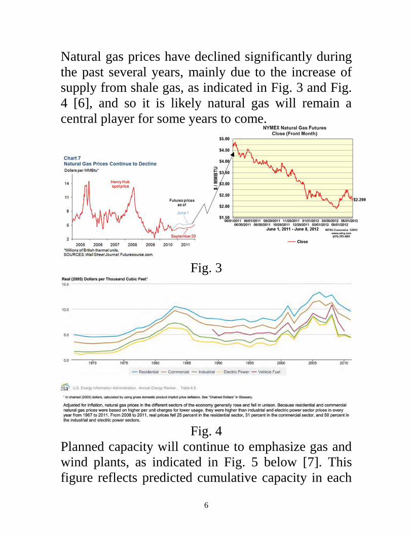
6
Natural gas prices have declined significantly during
the past several years mainly due to the increase of
supply from shale gas as indicated in Fig 3 and Fig
4 [6] and so it is likely natural gas will remain a
central player for some years to come
Fig 3
Fig 4
Planned capacity will continue to emphasize gas and
wind plants as indicated in Fig 5 below [7] This
figure reflects predicted cumulative capacity in each
7
year Careful inspection of the figure indicates most
of the 100GW growth occurs in natural gas and
renewable resources The report indicates that most
of the renewable resources is wind
Fig 5
30 Fuels continued ndash transportation amp emissions
The ways of moving bulk quantities of energy in the
nation are via rail amp barge (for coal) gas pipeline amp
electric transmission illustrated in Fig 6
8
Coal
Subsystem
Gas
Subsystem
Electric
Subsystem
Fig 6
An important influence in the way fuel is moved is
the restriction on sulfur dioxide (SO2)
bull Cap-and-trade control SO2 emissions
bull 1 allowance=1 ton SO2 compliance period 1 yr
Compliance strategies
ndash Retrofit units with scrubbers
ndash Build new power plants w low emission rates
ndash Switch fuel (or source of fuel)
ndash Trade allowances with other organizations
ndash Bank allowances
ndash Purchase power
bull National annual emission limit ~ 9 million tons
9
bull Emissions produced depends on fuel used
pollution control devices installed and amount of
electricity generated
bull Allowance trading occurs directly among power
plants (with a significant amount representing
within-company transfers) through brokers and in
annual auctions conducted by the US
Environmental Protection Agency (EPA)
The US Environmental Protection Agency (EPA)
modified the cap and trade system for SO2 via its
Cross-State Air Pollution Rule (CSAPR) CSAPR
expanded the SO2 cap-and-trade program to four
cap-and-trade programs one each for SO2 group 1
(more stringent limits) SO2 group 2 NOX annual
and NOX seasonal However this EPA ruling was
challenged in the courts and no final decision has
been rendered yet
Coal is classified into four ranks lignite (Texas N
Dakota) sub-bituminous (Wyoming) bituminous
(central Appalachian) anthracite (Penn) reflecting
the progressive increase in age carbon content and
heating value per unit of weight
Table 3 below illustrates differences among coal
throughout the country in terms of capacity heat
value sulfur content and minemouth price
Appalachian coal is primarily bituminous mainly
10
mined underground whereas Wyoming coal is
subbituminous mainly mined from the surface
Table 3
Although the above table is a little dated its general
message is still relevant as confirmed by the figures
below [8] where we see western coal production
climbing due to facts that (a) its $BTU is much
more attractive and (b) it has low sulfur content
As a result a great deal of coal is transported from
Wyoming eastward as illustrated in Fig 7
11
23
AZNM
NWPPMAPP
MAIN
ECAR
PRB
The Coal Doghellip
Powder River Basin Coal
Movement
Fig 7
We do not have a national CO2 cap and trade market
yet but there is a regional one called the Regional
Greenhouse Gas Initiative (RGGI) ndash see
httpwwwrggiorghome In 2008 there was serious
discussion ongoing to develop a national one as the
Waxman-Markey bill passed the house However its
companion Kerry-Boxer bill in the senate did not
pass Kerry-Lieberman-Graham unveiled a 2nd
version of the senate bill on 121009 which also did
not pass This would have been very important to
costs of energy production For example a ldquolowrdquo
CO2 cost would be about $10ton of CO2 emitted
which would increase energy cost from a typical
coal-fired plant from about $60MWhr to about
$70MWhr All indications are that today it is dead
12
40 CO2 Emissions - overview There is increased acceptance worldwide that global
warming is caused by emission of greenhouse gasses into
the atmosphere These greenhouse gases are (in order of
their contribution to the greenhouse effect on Earth) [9]
Water vapor causes 36-70 of the effect
Carbon dioxide (CO2) causes 9-26 of the effect
Methane (CH4) causes 4-9 of the effect
Nitrous oxide (N2O)
Ozone (O3) causes 3-7 of the effect
Chlorofluorocarbons (CFCs) are compounds containing
chlorine fluorine and carbon (no H2) CFCs are
commonly used as refrigerants (eg Freon)
The DOE EIA was publishing an excellent annual report on
annual greenhouse gas emissions in the US for example
the one published in November 2007 (for 2006) is [10] and
the one published in December 2009 (for 2008) is [11] All
such reports since 1995 may be found at [12] One figure
from the report for 2006 is provided below as Figure 8 The
information that is of most interest to us in this table is in
the center which is summarized in Table 4
Note that each greenhouse gas is quantified by ldquomillion
metric tons of carbon dioxide equivalentsrdquo or MMTCO2e
Carbon dioxide equivalents are the amount of carbon
dioxide by weight emitted into the atmosphere that would
produce the same estimated radiative forcing as a given
weight of another radiatively active gas [10]
13
Fig 8 Summary of US Greenhouse Gas Emissions 2006
Table 4 Greenhouse Gas Total 2006
Sectors MMTCO2e total CO2 total GHG
From Power Sector 2344 391 328
From DFU-transp 1885 314 264
From DFU-other 1661 277 233
From ind processes 109 18 15
Total CO2 5999 100 840
Non-CO2 GHG 1141 160
Total GHG 7140 100 The direct fuel use (DFU) sector includes transportation industrial process heat space heating and cooking fueled by
petroleum natural gas or coal The DFU-transportation CO2 emissions of 1885 MMT was obtained from the lower
right-hand-side of Fig 9a The DFU-other CO2 emissions of 1661 MMT was obtained as the difference between total
DFU emissions of 3546 MMT (given at top-middle of Fig 9a) and the DFU-transportation emissions of 1885 MMT
The ldquo total GHGrdquo for the 4 sectors (power DFU-transp DFU-other and ind processes) do not include the Non-
CO2 GHG emitted from these four sectors which are lumped into the single row ldquoNon-CO2 GHGrdquo If we assume that
each sector emits the same percentage of Non-CO2 GHG as CO2 then the numbers under ldquo total CO2rdquo are
representative of each sectorrsquos aggregate contribution to CO2 emissions The only sector we can check this for is
transportation where we know Non-CO2 emissions are 126MMT which is only 11 of the 1141 MMT total non-CO2
significantly less than the of total CO2 for transportation which is 314
14
Figure 9 [11] is the same picture as Fig 8 except it is for
the year 2008 the information is summarized in Table 5
Fig 9 Summary of US Greenhouse Gas Emissions 2008
Table 5 Greenhouse Gas Total 2008
Sectors MMTCO2e total CO2 total GHG
From Power Sector 2359 398 3318
From DFU-transp 1819 308 255
From DFU-other 1636 276 229
From ind processes 104 18 15
Total CO2 5918 100 830
Non-CO2 GHG 1213 170
Total GHG 7131 100 The direct fuel use (DFU) sector includes transportation industrial process heat space heating and cooking fueled by
petroleum natural gas or coal The DFU-transportation CO2 emissions of 1819 MMT was obtained from the lower
right-hand-side of Fig 9b The DFU-other CO2 emissions of 1636 MMT was obtained as the difference between total
DFU emissions of 3555 MMT (given at top-middle of Fig 9b) and the DFU-transportation emissions of 1819 MMT
The ldquo total GHGrdquo for the 4 sectors (power DFU-transp DFU-other and ind processes) do not include the Non-
CO2 GHG emitted from these four sectors which are lumped into the single row ldquoNon-CO2 GHGrdquo If we assume that
each sector emits the same percentage of Non-CO2 GHG as CO2 then the numbers under ldquo total CO2rdquo are
representative of each sectorrsquos aggregate contribution to CO2 emissions The only sector we can check this for is
transportation where we know Non-CO2 emissions are 127MMT which is only 105 of the 1213 MMT total non-
CO2 significantly less than the of total CO2 for transportation which is 308
15
Some numbers to remember from Tables 4 and 5 are
Total US GHG emissions are about 7100 MMTyear
Of these about 83-84 are CO2
Percentage of GHG emissions from power sector is
about 40 (see note for Tables 4 and 5)
Percentage of GHG emissions from transportation sector
is about 31 (see note for Tables 4 and 5)
Total Power Sector + Transportation Sector emissions is
about 71 (see note for Tables 4 and 5)
50 CO2 Emissions ndash power sector
Figure 10 [11] shows that CO2 emissions from the electric
power sector have been generally rising from 1990 to 2008
but the fact that they are rising more slowly than power
sector sales suggests that emissions per unit of energy
consumed is decreasing Note that the emissions values
given in Fig 10 have been normalized by the value in the
year 2000 which was 22935 MMT
Fig 10 Electric power sector CO2 emissions by year
Figure 11 [6] provides another view of CO2 emissions by
fuel where it is clear that recently emissions from coal and
petroleum dropped whereas that from natural gas increased
16
Fig 11
Table 6 [11] shows the year-by-year breakdown of electric
power sector CO2 emissions by fuel We see the dominant
contributor is coal with natural gas a distant second
Table 6Yearly breakdown of electric sector CO2 emissions
Table 6 is for CO2 emissions only ndash it does not include
Non-CO2 emissions
Coal is the largest contributor to CO2 emissions For
example in year 2008 it contributed 19459 MMT 825
17
of the total power sector CO2 emissions The next highest
contributor was natural gas at 362 MMT which is 153
of the total The two combined account for 978 of power
sector CO2 emissions
Total CO2 emissions from gas are only 186 of Total CO2
emissions from coal This does NOT imply that
CO2 emissions per MWhr from a natural gas power plant
are 186 of the
CO2 emissions per MWhr from a coal-fired power
plant
The fact that coal is the largest contributor to GHG
emissions is due to
(a) it is used to produce just under half of US electricity
(b) it has the highest emissionsenergy content ratio as
indicated by Table 7 below [13]
(c) its average conversion efficiency is not very good
18
Table 7 Emission Coefficients for Different Fuels
Pounds CO2
per
Million Btu
Aviation Gasoline AV 18355 per gallon 152717
Distillate Fuel (No 1 No 2 No 4
Fuel Oil and Diesel) DF 22384 per gallon 161386
Jet Fuel JF 21095 per gallon 156258
Kerosene KS 21537 per gallon 159535
Liquified Petroleum Gases (LPG) LG 12805 per gallon 139039
Motor Gasoline MG 19564 per gallon 156425
Petroleum Coke PC 32397 per gallon 22513
Residual Fuel (No 5 and No 6
Fuel Oil) RF 26033 per gallon 173906
Methane ME 116376 per 1000 ft3 115258
Landfill Gas LF 1 per 1000 ft3 115258
Flare Gas FG 133759 per 1000 ft3 120721
Natural Gas (Pipeline) NG 120593 per 1000 ft3 11708
Propane PR 12669 per gallon 139178
Coal CL
Anthracite AC 5685 per short ton 2274
Bituminous BC 49313 per short ton 2053
Subbituminous SB 37159 per short ton 2127
Lignite LC 27916 per short ton 2154
Biomass BM
Geothermal Energy GE 0 0
Wind WN 0 0
Photovoltaic and Solar Thermal PV 0 0
Hydropower HY 0 0
TiresTire-Derived Fuel TF 6160 per short ton 189538
Wood and Wood Waste 2 WW 3812 per short ton 195
Municipal Solid Waste 2 MS 1999 per short ton 199854
Nuclear NU 0 0
Renewable Sources Varies depending on the composition of the biomass
Petroleum Products
Natural Gas and Other Gaseous Fuels
Fuel Code
Emission Coefficients
Pounds CO2 per Unit
Volume or Mass
One indication from Table 7 that the pounds CO2MBTU
is based on energy content of the fuel could be misleading
What is of more interest is the CO2MWhr obtained from
the fuel together with a particular generation technology
To get this we need efficiencies of the generation
technologies Fig 12 provides such efficiencies the
resource from which it came [14] provides a good overview
of various factors affecting generation efficiencies
19
0
10
20
30
40
50
60
70
80
90
100
Hyd
ro p
ower
plant
Tidal p
ower
plant
Larg
e ga
s fir
ed C
CGT p
ower
plant
Melte
d ca
rbon
ates
fuel cell (
MCFC
)
Pulve
rised
coa
l boilers
with
ultr
a-cr
itica
l ste
am p
aram
eter
s
Solid o
xide
fuel cell (
SOFC
)
Coa
l fire
d IG
CC
Atmos
pher
ic C
irculat
ing
Fluidised
Bed
Com
bustion
(CFB
C)
Press
urised
Flu
idised
Bed
Com
bustion
(PFB
C)
Larg
e ga
s tu
rbine
(MW
rang
e)
Steam
turb
ine
coal-fi
red
power
plant
Steam
turb
ine
fuel-o
il po
wer
plant
Wind
turb
ine
Nuc
lear
pow
er p
lant
Biom
ass an
d biog
as
Was
te-to
-electric
ity p
ower
plant
Diese
l eng
ine
as d
ecen
tralis
ed C
HP u
nit (
elec
trica
l sha
re)
Small a
nd m
icro
turb
ines
(up
to 1
00 kW
)
Photo
volta
ic cells
Geo
ther
mal p
ower
plant
Solar
pow
er to
wer
Eff
icie
nc
y (
)
Fig 12 Generation efficiencies
Table 7 and Fig 12 provide the ability to compare different
technologies in terms of CO2MWhr For example letrsquos
compare a natural gas combined cycle (NGCC) plant
(η=58) a gas turbine (η=39) and a coal-fired power plant
(η=39) where the CO2 content of the natural gas is 11708
lbsMBTU and the CO2 content of the coal assuming it
uses (Powder River Basin) sub-bituminous coal is 2127
lbsMBTU (Note that coal has a different energy amp CO2
content depending on type as shown below [15])
20
NGCC MWhrlbsMWhr
MBTU
MBTU
MBTU
MBTU
lbs
OUT
IN
IN
5688413
58
108117
Gas turbine
MWhrlbsMWhr
MBTU
MBTU
MBTU
MBTU
lbs
OUT
IN
IN
71023413
39
108117
Coal-fired plant
MWhrlbsMWhr
MBTU
MBTU
MBTU
MBTU
lbs
OUT
IN
IN
81859413
39
17212
Table 8 below from [16] indicates similar numbers for a
pulverized coal (PC) plant a circulating fluidized bed
(CFB) plant an integrated gasification combined cycle
(IGCC) plant and a combined cycle plant Note that the
fuels for the first three of these are all coal and they have
similar emissionsMWhr ratios The combined cycle plant
has a bit higher ratio (810 instead of 6885) because it used
a lower efficiency (493 instead of 58)
Table 8
21
In the calculations at the top of the previous page one can
recognize that the 341η factor in each equation is just the
unit heat rate in MBTUMWhr This means the same
calculation can be done by multiplying the lbsMBTUIN
factor from Table 7 by the average heat rate for the plant
We can also convert the above to Metric tonsMWhr by
dividing by 2204 lbsMetric ton to get the following
figures
NGCC 0464 MTMWhr
Gas turbine 0312 MTMWhr
Coal-fired plant 0844 MTMWhr
It is interesting to compare these values with the emission
coefficients given by regionstate at [17] A sample of some
of these coefficients are provided below (this is 2002 data)
New York 0389
Vermont 0013
Penn 0574
Ohio 0817
Iowa 0854
N Dakota 1017
Georgia 0619
Kentucky 0911
Texas 0664
California 0275
Washington 0111
US Average 0606
Why is Iowa so high
Why are NDakota amp Kentucky so high
Why is California so low
Why is Washington so low
Why is Vermont so low
22
Vermont is so low because it has only one small fossil-fired
unit (a diesel unit) and it is a peaker and so does not often
run [18] Almost 75 of Vermontrsquos electric energy comes
from a large nuclear facility (Vermont Yankee) and most of
the rest comes from outside the state via the ISO-NE
market Iowa was in 2002 heavily dependent on coal
Today with Iowarsquos wind growth it is less so but still coal
is by far the dominant part of Iowarsquos generation portfolio
60 Heat rates
The values of Table 1 (fuel cost table) reflect only the
cost of fuel input to a generation plant they do not
reflect the actual costs of producing electrical energy as
output from the plant because substantial losses occur
during production Some power plants have overall
efficiencies as low as 30 in addition the plant
efficiency varies as a function of the generation level Pg
We illustrate this point in what follows
We represent plant efficiency by η Then η=energy
outputenergy input We obtain η as a function of Pg by
measuring the energy output of the plant in MWhrs and
the energy input to the plant in MBTU
We could get the energy output by using a wattmeter to
obtain Pg over a given period of time say an hour and
we could get the energy input by measuring the coal
tonnage used during the hour and then multiplying by
the coal energy content in MBTUton
23
We could then plot the fuel input in MBTUhr as a
function of the power output Pg in MW Such a plot is
called an input-output curve indicating how much fuel
rate is required to produce a power level A typical
input-output curve is shown in Fig 13 We denote fuel
rate (input vertical axis of Fig 1a) as R (WampW denote
fuel rate as H ndash see p 8 )
One notes that the IO curve of Fig 13 does not go to
Pg=0 A generating unit has a minimum stable output
typically 10-30 for oil and natural gas-fired steam
units and 20-50 for coal-fired steam units [19]
Pg
Fuel rate
MBTUhr
R
OUTPUT
INPUT
Fig 13 Input-output curve
One interesting feature with respect to Fig 13 is that
as fuel input is increased the power output per unit
fuel input begins to decrease We can see this more
clearly if we invert the axes as in Fig 14 yielding a
production function where for high enough fuel
rates we will get no additional power output
24
Pg
Fuel rate
MBTUhr
R Fig 14 Production function
Physically this happens because the furnace boiler
steam pipes leak a larger percentage of input heat as
temperatures increase Economists call this the [20]
law of diminishing marginal product for almost all
processes the rate of increase in output decreases as
the input increases assuming other inputs are fixed
To obtain η we want the output energy divided by
the input energy which is
η ~ Pg divide R
which in terms of units is MW divide MBTUhr to give
units of MWhrMBTU Notice that these units are
energyenergy as they should be when computing η
However the MBTU and MWhr are different units of
energy and so we are not getting η exactly but we
are getting something proportional to η
So letrsquos obtain the ratio of the power to the fuel rate
25
(Pg divide R) for every point on the input-output curve
and plot the results against Pg Fig 15 shows a plot of
the ratio PgR (units of MWHRMBTU) versus Pg
Fig 15 Plot of MWhrMBTU vs Pg
Figure 15 indicates that efficiency is poor for low
generation levels (a connected plant that is operating
at zero MW output still has to supply station loads)
and increases with generation but at some optimum
level it begins to diminish Most power plants are
designed so that the optimum level is close to the
rated output
The heat rate curve is similar to Fig 15 except that
the y-axis is inverted to yield MBTUMWhrs which
is proportional to 1η This curve is illustrated in Fig
16 We denote heat rate by H (WampW use H for fuel
rate) Since the heat rate depends on operating point
we write H=H(Pg)
26
Fig 16 Plot of Heat Rate (H) vs Generation (Pg)
Some typical heat rates for units at maximum output
are (in MBTUMWhrs) 95-105 for fossil-steam
units and nuclear units 130-150 for combustion
turbines [21] and 70-95 for combined cycle units
Future combined cycle units may reach heat rates of
65-70 It is important to understand that the lower
the heat rate the more efficient the unit
An easy way to remember the meaning of heat rate
H=H(Pg) is it is the amount of input energy (MBTU)
required to produce a MWhr at generation level Pg
How does H relate to efficiency To answer this
question we need to know that there are 105485
joules per BTU
413
4133600
8510541
sec3600sec)(
)851054(
61
61~
1
HH
H
j
BTUjBTUH
Whr
BTU
E
EH
MWhr
MBTUH
27
Observe We have seen this before when we
computed CO2 emissions per MWhr out (see pg 20)
eg for the NGCC plant
MWhrlbsMWhr
MBTU
MBTU
MBTU
MBTU
lbs
OUT
IN
IN
5688413
58
108117
We can see now that the above calculation can be
thought of as
MWhrlbsMBTU
MBTU
MBTU
MBTU
MBTU
lbs
OUT
IN
OUT
IN
IN
5688413
58
41308117
or
MWhrlbsHMBTU
lbs
IN
568808117
where H in this case is 34158=588 MBTUMWhr
The heat rate curve is a fixed characteristic of the plant
although it can change if the cooling water temperature
changes significantly (and engineers may sometimes
employ seasonal heat rate curves) The heat rate curve
may also be influenced by the time between
maintenance periods as steam leakages and other heat
losses accumulate
The above use of the term ldquoheat raterdquo is sometimes also
called the ldquoaverage heat raterdquo This is because we get it
by dividing absolute values of fuel input rate by
absolute values of electric output power For example if
you buy an apple at $50 and a second one at $10 the
average cost of apples after buying the first apple is
$50apple but after buying the second apple is
$(50+10)2=$30apple
28
This is different than incremental heat rate as will be
illustrated in the following example
Example [22] Consider the input-output curve for
Plant X in Fig 17
Fig 17
Compute the average heat rate characteristic and the
incremental heat rate characteristic
Average heat rates are computed by dividing the fuel
rate by the generation level H=RPg as follows
Block 1 200001=20000
Block 2 240002=12000
Block 3 300003=10000
Incremental heat rates computed by dividing the
increment of fuel rate by the increment of power
IH=∆R∆Pg as follows
Block 1 200001=20000
Block 2 40001=4000
Block 3 60001=6000
These results are summarized in Table 9 below
29
Table 9
Figure 18 below illustrates the input-output curve the
average heat rate curve and the incremental heat rate
curve
Fig 18
We should note however that our first incremental
heat rate value of 20000 has a problem This value
assumes that the IO curve extends as shown on the
left hand side in Fig 19 below Probably a better
30
approximation would be to extend it as indicated on
the right hand side of Fig 19
Fig 19
Actually it does not extend to 0 MW output because
the unit like all real units has a minimum generation
level
Although you may see data entered which reflects a
ldquohigh initial incremental valuerdquo you should know
that a value so computed does not represent a true
incremental heat rate value at all
Reference [22] also provides some actual data for
units in California The one below Fig 20 is one of
the most efficient gas-fired units in the PGampE
system On the coast about 100 miles south of San
Francisco it is called Moss Landing Unit 7
31
Fig 20
Note that the Moss Landing unit 7 full-load average
heat rate is 8917 MBTUMWhr which gives an
efficiency of 3418917=382
The next one Fig 21 is an old oil-fired unit in San
Francisco called Hunterrsquos Point
32
Fig 21
Note the full-load average heat rate of this plant is
12598 MBTUMWhr which corresponds to an
efficiency of 34112598=271
This plant was built in 1927 and demolished in 2008
70 Cost rates
We are primarily interested in how the cost per
MWhr changes with Pg because that will tell us
something about how to achieve the most economic
dispatch of generation for a given demand (we will
see that optimality is achieved when marginal or
incremental costs of all regulating units are equal)
33
To get cost per MWhr as a function of Pg we will
assume that we know K the cost of the input fuel in
$MBTU Also recall that
R is the rate at which the plant uses fuel in
MBTUhr (which is dependent on Pg) ndash it is just
the input-output curve (see Fig 13)
And we will denote
C as the cost per hour in $hour
Then if H(Pg) the heat rate is the input energy used
per MW per hour then multiplying H by Pg gives
input energy per hour ie R=PgH(Pg) where H must
be evaluated at Pg Therefore C = RK = PgH(Pg)K
ie the cost rate function C is just the fuel rate
function R scaled by the fuel cost
A typical plot of C vs Pg is illustrated in Fig 22
Note that because H(Pg) is convex C(Pg) is also
convex ie the set of points lying on or above C
contain all line segments between any pair of points
Fig 22 Plot of cost per hr (C) vs generation (Pg)
34
Fig 22 shows that costhour increases with
generation a feature that one would expect since
higher generation levels require greater fuel intake
per hour
The incremental cost curve for the plant can be
obtained by differentiating the plot in Fig 22 ie by
computing dCdPg A typical incremental cost curve
is shown in Fig 23 Note that because C is convex
dCdPg is a non-decreasing function
Fig 23 Plot of incremental cost dCdPg vs gen Pg
One last thing about getting incremental cost
Recall that the cost per hour is given by
C = RK where R is just the input-output curve
Therefore IC=dCdPg=K(dRdPg) The derivative
is the incremental heat rate which we denoted by
IH Therefore in summary
C=RK=PgH(Pg)K
IC=dCdPg=(dRdPg)K=(IH)K
35
Example 1 An 100 MW coal-fired plant uses a type of coal
having an energy content of 12000 BTUlb The coal
cost is $15MMBTU Typical coal usage
corresponding to the daily loading schedule for the
plant is as follows
Table 10
Time of
Day
Electric
Output (MW)
Coal Used
(tons)
1200am-
600am
40 1050
600am-
1000am
70 945
1000am-
400pm
80 1560
400pm-
1200am
100 2700
For each of the four load levels find (a) the
efficiency η (b) the heat rate H (MMBTUMWhr)
(c) the cost per hour C ($hr) Also for the loading
levels of 40 70 and 80 MW use a piecewise linear
plot of C vs P to obtain incremental cost IC as a
function of unit loading P Then plot incremental cost
as a function of unit loading The conversion factor
from joules to BTU is 105485 joulesBTU and the
units for coal used tons are short-tons 2000 lbton
36
Solution Let T be the number of hours the plant is producing P
MW while using y tons of coal We need to compute
the total energy out of the plant and divide by the
total energy into the plant but we need both
numerator and denominator to be in the same units
We will convert both to joules (recall a watt is a
joulesec)
(a)
BTU
joules851054
lb
BTU00012
ton
lb2000 tons
hr
sec3600
MW
watts10hr MW 6
y
TP
Note that the above expression for efficiency is
dimensionless
(b) The heat rate is the amount of MMBTUs
used in the amount of time T divided by the
number of MW-hrs output in the amount of time
T
TP
y
H
BTU10
MMBTU1
lb
BTU00012
ton
lb2000 tons
6
37
Note that
413
851054
36001H and the above
expression has units of MMBTUMWhr Thus if a
unit is 100 efficient then it will have a heat rate
of 341 MMBTUMWhr the absolute best (lowest)
heat rate possible
(c) C = RK where R is the rate at which the plant
uses fuel and K is fuel cost in $MMBTU Note
from units of P and H that
R = PH C = PHK where H is a function of P
Application of these expressions for each load level
yields the following results
Table 11
T (hrs) P
(MW)
y
(tons)
η H
(mbtum
whr)
C
($hr)
6 40 1050 033 105 630
4 70 945 042 81 850
6 80 1560 044 78 936
8 100 2700 042 81 1215
To obtain incremental cost dP
dCIC we can plot C vs
P and then get an approximation on the derivative by
assuming a piecewise linear model as shown in
Figure 24
38
Figure 24 Calculation of Incremental Cost
The incremental costs are plotted as a function of
loading in Fig 25
20
4
2
6
8
10
40 60 80
12
IC ($MWhr)
Pg (MW)
Fig 25 Incremental cost curve from piecewise-linear
cost curve
39
We may use another procedure to model the
incremental costs In this procedure we first fit the
data to a quadratic polynomial Matlab commands for
doing so are below
gtgt p=[40 70 80 100]
gtgt c=[630 850 936 1215]
gtgt X = [ones(size(p)) p p^2]
gtgt a=Xc
a =
6048533
-29553
00903
gtgt T = (01100)
gtgt Y = [ones(size(T)) T T^2]a
gtgt plot(TY-tyo) grid on
The quadratic function is therefore
C(P)=00903P2-29553P+60485
Figure 26 shows the plot obtained from Matlab
40
Fig 26 Quadratic Curve Fit for Cost Rate Curve
Clearly the curve is inaccurate for very low values of
power (note it is above $605hr at P=0 and decreases
to about $590hr at P=10) We can get the
incremental cost curve by differentiating C(P)
IC(P)=01806P-29553
This curve is overlaid on the incremental cost curve
of Fig 25 resulting in Fig 27 Both linear and
discrete functions are approximate Although the
linear one appears more accurate in this case it
would be easy to improve accuracy of the discrete
one by taking points at smaller intervals of Pg Both
functions should be recognized as legitimate ways to
represent incremental costs The linear function is
often used in traditional economic dispatching the
discrete one is typical of market-based offers
41
20
4
2
6
8
10
40 60 80
12
14
Fig 27 Comparison of incremental cost curve
obtained from piecewise linear cost curve (solid line)
and from quadratic cost curve (dotted line)
80 Market-based offers
As indicated in the last section electricity markets
typically allow only piecewise linear representation
of generator incremental cost curves
The real-time and the day-ahead markets are implemented
via computer programs based on optimization theory The
program used for the real-time market is called the
security-constrained economic dispatch (SCED) This
program the SCED is used together with a program called
the security-constrained unit commitment (SCUC) program
for the day-ahead market Both the SCED and the SCUC
42
also solve for the ancillary service prices through a
formulation known as co-optimization We will say no
more about SCED and SCUC because we cannot assume
that students taking this course have the necessary
background on optimization theory Instead we will
provide a simple description of how the energy market
price is determined This description is based on standard
microeconomic theory but can be followed without
background in microeconomics However one should note
that the description necessarily omits some important
concepts related to losses and congestion
The following example is adapted from [23] Consider that
our electric energy market has three buyers B1 B2 B3 and
two sellers S1 S2 The buyers represent load-serving
entities and the sellers represent generation owners
Consider that these buyers and sellers submit their bids (to
buy) and their offers (to sell) via an internet system as
shown in Fig 28
Figure 28 Illustration of buyer-seller interaction with internet-based market
Each seller has energy to sell but the price they are willing
to sell it for increases with the amount they sell This is a
reflection of the fact that the cost of producing 1 more unit
of energy (MWhr) increases as a unit is loaded higher
Internet System
B1
B2
B3
S1
S2
43
Likewise each buyer wants to purchase energy but the
price they are willing to pay to obtain it decreases with the
amount that they buy This is just a reflection of the fact
that our first unit of energy will be used to supply our most
critical needs and after those needs are satisfied the next
units of energy will be used to satisfy less critical needs so
that we are unwilling to pay as much for it
Tabl2 illustrates a representative set of bids and offers
submitted by the buyers and sellers
Table 12 Offers and bids for examples
Offers to sell Bids to buy
S1 S2 B1 B2 B3
$1000 $1000 $7000 $7000 $2500
$5000 $5000 $7000 $5000 0
$6500 $7000 $6500 $2500 0
$7000 $7000 $6500 0 0
infin infin 0 0 0
infin infin 0 0 0
infin infin 0 0 0
Once each buyer and seller enters their data according to
Table 12 the internet system will reconstruct the
information according to Table 13 where
Table 13 Reconstructed offers and bids
Offerbid
order
Offers to sell 1 MWhr Bids to buy 1 MWhr
Seller Price Buyer Price
1 S1 $1000 B1 $7000
2 S2 $1000 B1 $7000
3 S1 $5000 B2 $7000
4 S2 $5000 B1 $6500
5 S1 $6500 B1 $6500
6 S2 $7000 B2 $5000
7 S1 $7000 B2 $2500
8 S2 $7000 B3 $2500
44
We can visualize the data in Table by plotting the price
against quantity for the offers and for the bids This
provides us with the supply and demand schedules of
Figure 29 [23]
Figure 29 Supply-demand schedules illustrating electricity market operation [23]
The point (or those points) where the supply schedule
intersects the demand schedule determines the market
clearing price This is the price that all sellers are paid to
supply their energy and it is the price that all buyers pay to
receive their energy In Figure this price is $65MWhr It is
the very best price to choose because it maximizes the total
ldquosatisfactionrdquo felt by the buyers and sellers
This satisfaction for the sellers can be measured by the
difference between the price they offered and the price they
were actually paid for the energy they supplied If we add
up all of these differences for all sellers then we obtain the
net seller surplus This satisfaction for the buyers can be
measured by the difference between the price they bid and
the price they actually had to pay for the energy they
45
received If we add up all of these differences for all sellers
then we obtain the net buyer surplus The net seller surplus
and the net buyer surplus are illustrated in Fig 30 [23]
Figure 30 Illustration of net seller and net buyer surplus [23]
The total net surplus is the sum of the buyer and seller net
surpluses The market clearing price is the price that
maximizes the total net surplus
In Fig 30 the quantity traded could be either 4 or 5
MWhrs but the 5th MWhr would neither increase nor
decrease the total net surplus The decision on whether to
trade 4 or 5 MWhrs in such as case is determined by market
rules
The example of this section illustrates the way electricity
markets would clear if there are no losses and if the
transmission capacity of each line was infinite One
conceptualization of such a situation is when all generators
and all loads are located at the same electric node In such a
case there is a single price by which all sellers are paid and
all buyers pay
46
In reality of course each transmission circuit does have
some resistance and therefore incurs some losses as current
flows through it and each transmission circuit also has an
upper bound for the amount of power that can flow across
it These two attributes losses and transmission limits
result in locational variation in prices throughout the
network which are called as we have already seen the
locational marginal prices (LMPs)
90 Effect of Valve Points in Fossil-Fired Units
Figures 22 and 24 well represent cost curves of small
steam power plants but actual cost curves of large
steam power plants differ in one important way from
the curves shown in Figs 22 and 24 ndash they are not
smooth The light curve of Fig 31 [24] more closely
captures the cost variation of a large steam power
plant
Fig 31 Cost rate curve for large steam power plant [24]
47
The reason for the discontinuities in the cost curve of
Fig 31 is because of multiple steam valves In this
case there are 5 different steam valves Large steam
power plants are operated so that valves are opened
sequentially ie power production is increased by
increasing the opening of only a single valve and the
next valve is not opened until the previous one is
fully opened So the discontinuities of Fig 31
represent where each valve is opened
The cost curve increases at a greater rate with power
production just as a valve is opened The reason for
this is that the so-called throttling losses due to
gaseous friction around the valve edges are greatest
just as the valve is opened and taper off as the valve
opening increases and the steam flow smoothens
The significance of this effect is that the actual cost
curve function of a large steam plant is not
continuous but even more important it is non-
convex A simple way (and the most common way)
to handle these two issues is to approximate the
actual curve with a smooth convex curve similar to
the dark line of Fig 31
48
100 Combined cycle units
The following information was developed from [21
25 26 27] The below figure shows recent US
growth in combined cycle power plants [28]
Fig x
Combined cycle units utilize both gas turbines (based
on the Brayton cycle) and steam turbines (based on
the Rankine cycle) Gas turbines are very similar to
jet engines where fuel (can be either liquid or gas)
mixed with compressed air is ignited The
combustion increases the temperature and volume of
the gas flow which when directed through a valve-
controlled nozzle over turbine blades spins the
turbine which drives a synchronous generator On the
49
other hand steam turbines utilize a fuel (coal natural
gas petroleum or uranium) to create heat which
when applied to a boiler transforms water into high
pressure superheated (above the temperature of
boiling water) steam The steam is directed through a
valve-controlled nozzle over turbine blades which
spins the turbine to drive a synchronous generator
A combined cycle power plant combines gas turbine
(also called combustion turbine) generator(s) with
turbine exhaust waste heat boiler(s) (also called heat
recovery steam generators or HRSG) and steam
turbine generator(s) for the production of electric
power The waste heat from the combustion
turbine(s) is fed into the boiler(s) and steam from the
boiler(s) is used to run steam turbine(s) Both the
combustion turbine(s) and the steam turbine(s)
produce electrical energy Generally the combustion
turbine(s) can be operated with or without the
boiler(s)
A combustion turbine is also referred to as a simple
cycle gas turbine generator They are relatively
inefficient with net heat rates at full load of some
plants at 15 MBtuMWhr as compared to the 90 to
105 MBtuMWhr heat rates typical of a large fossil
fuel fired utility generating station This fact
combined with what can be high natural gas prices
50
make the gas turbine expensive Yet they can ramp
up and down very quickly so as a result combustion
turbines have mainly been used only for peaking or
standby service
The gas turbine exhausts relatively large quantities of
gases at temperatures over 900 degF In combined cycle
operation then the exhaust gases from each gas
turbine will be ducted to a waste heat boiler The heat
in these gases ordinarily exhausted to the
atmosphere generates high pressure superheated
steam This steam will be piped to a steam turbine
generator The resulting combined cycle heat rate is
in the 70 to 95 MBtuMWhr range significantly less
than a simple cycle gas turbine generator
In addition to the good heat rates combined cycle
units have flexibility to utilize different fuels (natural
gas heavy fuel oil low Btu gas coal-derived gas)
[29] (In fact there are some advanced technologies
under development right now including the
integrated gasification combined cycle (IGCC) plant
which makes it possible to run combined cycle on
solid fuel (eg coal or biomass) [30] The first two
operational IGCC plants in the US were the Polk
Station Plant in Tampa and the Wabash River Plant
in Indiana [31] The Ratcliffe-Kemper plant
currently under construction by Mississippi Power (a
51
subsidiary of Southern Company) is a 582 MW
IGCC plant to be completed in 2014 [32 33])
The flexibility of combined cycle plants together
with the fast ramp rates of the combustion turbines
and relatively low heat rates has made the combined
cycle unit the unit of choice for a large percentage of
recent new power plant installations The potential
for increased gas supply and lowered gas prices has
further stimulated this tendency
Fig 32 shows the simplest kind of combined cycle
arrangement where there is one combustion turbine
and one HRSG driving a steam turbine
ChillerCooler
Inlet Air
Gas Supply
Duct firing
HRSG
Condenser
CTG STG
Fig 32 A 1 times 1 configuration
An additional level of complexity would have two
combustion turbines (CT A and B) and their HRSGs
driving one steam turbine generator (STG) as shown
in Fig 33
52
ChillerCooler
Inlet Air
Gas Supply
Duct firing
HRSG
ChillerCooler
Inlet Air
Gas Supply
Duct firing
HRSG
Condenser
CTG
CTG STG
Fig 33 a 2 times 1 configuration
In such a design the following six combinations are
possible
CT A alone
CT B alone
CT A and CT B together
CT A and STG
CT B and STG
CT A and B and STG
The modes with the STG are more efficient than the
modes without the STG (since the STG utilizes CT
exhaust heat that is otherwise wasted) with the last
mode listed being the most efficient
If we model a combined cycle plant as a single plant
we run into a problem Consider the transition
between the combined cycle power plant operation
53
just as the STG is ramped up Previous to STG start-
up only the CT is generating with a specified
amount of fuel per hour being consumed as a
function of the CT power generation level Then
after STG start-up the fuel input remains almost
constant but the MW output of the (now) two
generation units has increased by the amount of
power produced by the steam turbine driven by the
STG A typical cost curve for this situation is shown
in Fig 34
C ($hr)
PG (MW)
Fig 34 Cost curve for a combined cycle plant
An important feature of the curve in Fig 34 is that it
is not convex which means its slope (ie its
incremental cost) does not monotonically increase
with PG Figure 35 illustrates incremental cost
variation with PG
54
dCdPG ($MWhr)
PG (MW)
Fig 35 Incremental cost curve for a combined cycle plant
The key attribute of the incremental cost curve in
order to satisfy convexity is that it must be non-
decreasing Clearly the curve of Fig 35 does not
satisfy this requirement
110 Economic dispatch and convexity of objective
functions in optimization
The traditional economic dispatch (ED) approach
used by electric utilities for many years is very well
described in [34]
This approach is still used directly by owners of
multiple generation facilities when they make one
offer to the market and then need to dispatch their
units in the most economic fashion to deliver on this
offer This approach also provides one way to view
the method by which locational marginal prices are
computed in most of todayrsquos real-time market
systems
The simplest form of the ED problem is as follows
55
Minimize
n
i
iiT PFF1
(1)
Subject to
0)(11
N
i
iloadiload
n
i
i PPPPP (2)
0max
minmin
i
ii
iiii
PPP
PPPP
(3)
Here we note that the equality constraint is linear in
the decision variables Pi In the Newton approach to
solving this problem ([34]) we form the Lagrangian
according to
)()( iiT PPF L (4)
If each and every individual cost curve Ci(Pi) i=1n
is quadratic then they are all convex Because the
sum of convex functions is also a convex function
when all cost curves are convex then the objective
function FT(Pi) of the above problem is also convex
If φ(Pi) is linear then it is convex and therefore L is
convex This fact allows us to find the solution by
applying first order conditions
56
First order conditions for multi-variable calculus are
precisely analogous to first order conditions to single
variable calculus In single variable calculus we
minimize f(x) by solving frsquo(x)=0 on the condition
that f(x) is convex or equivalently that frsquorsquo(x)gt0
In multivariable calculus where x=[x1 x2hellip xn]T we
minimize f(x) by solving frsquo(x)=0 that is
nix
f
i
1 0
(5)
on the condition that f(x) is convex or equivalently
that the Hessian matrix frsquorsquo(x) is positive definite
We recall that in single variable calculus if f(x) is
not convex then the first order conditions do not
guarantee that we find a global minimum We could
find a maximum or a local minimum or an inflection
point as illustrated in Fig 36 below
f(x)
x x
f(x)
Fig 36 Non-convex functions
57
The situation is the same in the multivariable case
ie if f(x) is not convex then the first order
conditions of (5) do not guarantee a global minimum
Now returning to the Lagrangian function of our
constrained optimization problem repeated here for
convenience
)()( iiT PPF L (4)
we recall that solution to the original problem is
found by minimizing FT But to use what we now
know we are only guaranteed to find a global
minimum of F if L is convex In this case the first
order conditions results in
0
1 0
L
LNi
Pi
from which we may find our solution (Inequality
constraints may be handled by checking the resulting
solution against them and for any violation setting
up another equality constraint which binds the given
decision variable to the limit which was violated)
But if one of the units is a combined cycle unit the
FT and therefore L will not be convex So first
58
order conditions do not guarantee a global minimum
In other words there may be a lower-cost solution
than the one we will obtain from applying first order
conditions This makes engineers and managers
concerned because they worry they are spending
money unnecessarily
120 General solutions for non-convex
optimization problems
Generation owners who utilize combined cycle units
must use special techniques to solve the EDC
problem Some general methods that have been
proposed for solving non-convex optimization
problems are below However I am not aware that
any of these techniques have been implemented
within an electricity market today
1 EnumerationIteration In this method all possible
solutions are enumerated and evaluated and then the
lowest cost solution is identified This method will
always work but can be quite computational
2 Dynamic programming See pp 51-54 of reference
[21]
59
3 Sequential unconstrained minimization technique
(SUMT) This method is described on pp 473-477 of
reference [35]
4 Heuristic optimization methods There are a
number of methods in this class including Genetic
Algorithm simulated annealing tabu search and
particle swarm A good reference on these methods is
[36]
5 There is a matlab toolbox for handling non-convex
optimization It provides 2 different algorithms
together with references on papers that describe the
algorithms located at httptomlabbiz There are
two methods provided
(a) Radial Basis Function (RBF) interpolation
(b) Efficient Global Optimization (EGO) algorithm
The idea of the EGO algorithm is to first fit a
response surface to data collected by evaluating the
objective function at a few points Then EGO
balances between finding the minimum of the surface
and improving the approximation by sampling where
the prediction error may be high
130 Practical solutions to modeling combined
cycle units in optimization
60
Reference [37] developed by engineers at ERCOT and
Ventyx (now ABB) is an excellent summary of practical
methods to modeling combined cycle units It provides
references to a number of other good resources on the
subject The methods it outlines are as follows
Aggregate modeling Here the combined cycle unit is
simply modeled with a ldquobest-fitrdquo convex cost curve This
approach does not handle the non-convexity of the actual
cost characteristic
Pseudo-unit modeling Here a number of pseudo-units
equal to N the number of combustion turbines are
represented each with 1N of the steam unit This works
for an Ntimes1 combined cycle unit For example a 3 times 1
combined cycle unit would be modeled as three separate
pseudo-units each of the three pseudo-units would be
one gas turbine plus one third of a steam turbine [38]
This approach has been implemented within several
markets including ISO NE NYISO MISO PJM and
IESO This approach does not handle the non-convexity
of the actual cost characteristic
Configuration-based modeling This approach is also
referred to as psuedo-plant modeling Here a cost-curve
(or incremental cost curve) is provided for each
configuration of the combined cycle plant Additional
logic is provided in the security-constrained unit
commitment (SCUC which is the mixed integer
programming software for the day-ahead market) to
ensure that only one configuration can be selected and
that the selection depends on the configuration of the
previous time period as illustrated in Fig 37 below for a
2times1 combined cycle plant [37] The configuration
61
chosen by SCUC for any one hour is maintained for the
entire hour in the real-time market CAISO has
implemented this approach it is well-described in [38]
Fig 37
Physical-unit modeling Here each CT and STG is
considered to be an individual resource with its own
individual offers This is a bad market model but it
provides good fidelity in terms of MW that the power
plant can actually produce ERCOT reports in [38] that it
utilizes configuration-based models for its markets and
physical unit modeling for its network security
applications
References [1] J McCalley W Jewell T Mount D Osborn and J Fleeman ldquoA wider horizon Technologies Tools
and Procedures for Energy System Planning at the National Levelrdquo IEEE Power and Energy Magazine
MayJune 2011
[2] J Morgan ldquoEnergy Density and Waste Comparison of Energy Productionrdquo Nuclear Science and
Technology June 2010 available at httpnuclearfissionarycom20100609energy-density-and-waste-
comparison-of-energy-production
[3] The World Nuclear Association ldquoThe Economics of Nuclear Powerrdquo available at httpwwwworld-
nuclearorginfoinf02html
[4] US Department of Energy Energy Information Administration website located at
httpwwweiagovcneafelectricityepmepmxlfile4_1xls and
httpwwweiadoegovcneafelectricityepmepmxlfile4_1_contxls
[5] US Department of Energy Energy Information Administration website located at
httpwwweiadoegovemeuaertxtptb0811bhtml
[6] ldquoEnergy perspectives 2011 US Department of Energy Energy Information Administration website
httpwwweiagovtotalenergydataannualpdfperspectives_2011pdf
62
[7] North American Reliability Corporation (NERC) ldquo2011 Long Term Reliability Assessmentrdquo
November 2011 available at wwwnerccom
[8] US Department of Energy Energy Information Administration website located at
httpwwweiadoegovoiafaeocoalhtml
[9] Wikipedia page on ldquoGreenhouse gasrdquo httpenwikipediaorgwikiCarbon_emissions
[10] US Department of Energy Energy Information Administration ldquoEmissions of Greenhouse Gases in
the United States 2006rdquo November 2007 available at httpwwweiadoegovoiaf1605ggrptindexhtml
[11] US Department of Energy Energy Information Administration ldquoEmissions of Greenhouse Gases in
the United States 2008rdquo December 2009 available at httpwwweiadoegovoiaf1605ggrptindexhtml
[12] wwweiadoegovoiaf16051605aoldhtml
[13] DOE EIA Data from Voluntary Reporting of Greenhouse Gasses Program available at
httpwwweiadoegovoiaf1605coefficientshtml
[14] F Van Aart ldquoEnergy efficiency in power plantsrdquo October 21 Vienna available from Dr McCalley
(see ldquoNew Generationrdquo folder) but you must make request
[15] EPA report wwwepagovairmarktprogsregsepa-ipmdocschapter8-v2_1-updatepdf
[16] Black amp Veatch ldquoPlanning for Growing Electric Generation Demandsrdquo slides from a presentation to
Kansas Energy Council ndash Electric Subcommittee March 12 2008 available at
httpwwwgooglecomsearchhl=enampsource=hpampq=22Planning+for+Growing+Electric+Generation+D
emands22ampbtnG=Google+Searchampaq=fampaqi=ampaql=ampoq=ampgs_rfai=C5Ekv4uV7TP7ECIzmNJHV_MIE
AAAAqgQFT9Dr5Lw
[17] DOE EIA Website for US locations emission coefficients httpwwweiadoegovoiaf1605ee-
factorshtml
[18] wwwrutlandheraldcomappspbcsdllarticleAID=20080706NEWS048070604571024NEWS04
[19]H Stoll ldquoLeast-cost electric utility planningrdquo 1989 John Wiley
[20] D Kirschen and G Strbac ldquoFundamentals of Power System Economicsrdquo Wiley 2004
[21] A J Wood and B F Wollenberg Power Generation Operation and Control second edition John
Wiley amp Sons New York NY 1996
[22] J Klein ldquoThe Use of Heat Rates in Production Cost Modeling and Market Modelingrdquo California
Energy Commission Report 1998
[23] L Tesfatsion ldquoAuction Basics for Wholesale Power Markets Objectives and Pricing Rulesrdquo
Proceedings of the 2009 IEEE Power and Energy Society General Meeting July 2009
[24] J Kim D Shin J Park and C Singh ldquoAtavistic genetic algorithm for economic dispatch with valve
point effectrdquo Electric Power Systems Research 62 2002 pp 201-207
[25] ldquoElectric power plant designrdquo chapter 8 publication number TM 5-811-6 Office of the Chief of
Engineers United States Army January 20 1984 located at
httpwwwusacearmymilpublicationsarmytmtm5-811-6 not under copyright
[26] A Cohen and G Ostrowski ldquoScheduling units with multiple operating modes in unit commitmentrdquo
IEEE 1995
[27] A Birch M Smith and C Ozveren ldquoScheduling CCGTs in the Electricity Poolrdquo in ldquoOpportunities
and Advances in International Power Generation March 1996
[28] 2011 State of the Markets a FERC presentation April 2012 at httpswwwfercgovmarket-
oversightreports-analysesst-mkt-ovrsom-rpt-2011pdf
[29] R Tawney K Kamali W Yeager ldquoImpact of different fuels on reheat and nonreheat combined cycle
plant performancerdquo Proceedings of the American Power Conference VolIssue 50 American power
conference 18-20 Apr 1988 Chicago IL (USA)
[30] I Burdon ldquoWinning combination [integrated gasification combined-cycle process]rdquo IEE Review
Volume 52 Issue 2 2006 pp 32 ndash 36 IET Journals amp Magazines
[31] wwwfossilenergygovprogramspowersystemsgasificationgasificationpioneerhtml
[32] ldquoSouthern Company on track with new generationrdquo Investopedia March 23 2011 available at
httpwwwinvestopediacomstock-analysis2011southern-company-on-track-with-new-generation-so-d-
duk0323aspxaxzz28iY0dqaR
[33] wwwsoutherncompanycomsmart_energysmart_power_vogtle-kemperhtml
[34] G Sheble and J McCalley ldquoModule E3 Economic dispatch calculationrdquo used in EE 303 at Iowa
State University
[35] F Hillier and G Lieberman ldquoIntroduction to Operations Researchrdquo fourth edition Holden-Day 1986
63
[36] ldquoTutorial on modern Heuristic Optimization Techniques with Applications to Power Systemsrdquo IEEE
PES Special Publication 02TP160 edited by K Lee and M El-Sharkawi 2002
[37] H Hui C Yu F Gao and R Surendran ldquoCombined cycle resource scheduling in ERCOT nodal
marketrdquo Proc of the 2011 IEEE PES General Meeting 2011
[38]ldquoModeling of Multi-Stage Generating Unitsrdquo CAISO Available at
wwwcaisocom23582358e27f11070pdf
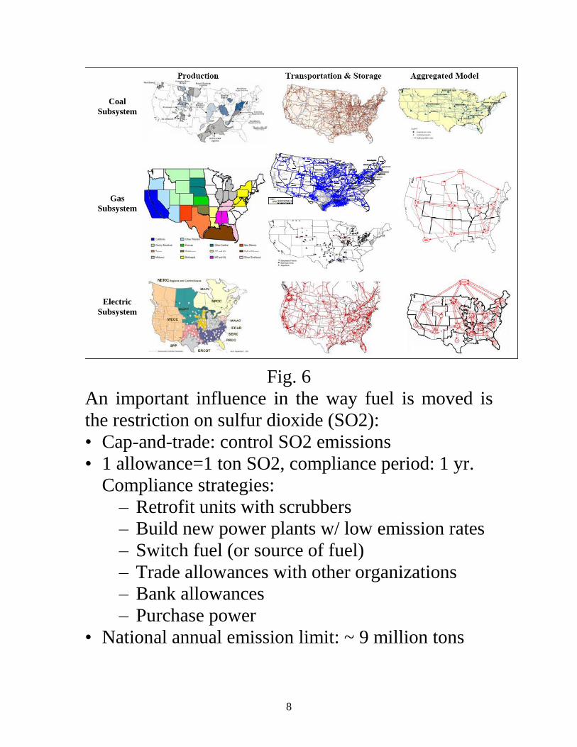
8
Coal
Subsystem
Gas
Subsystem
Electric
Subsystem
Fig 6
An important influence in the way fuel is moved is
the restriction on sulfur dioxide (SO2)
bull Cap-and-trade control SO2 emissions
bull 1 allowance=1 ton SO2 compliance period 1 yr
Compliance strategies
ndash Retrofit units with scrubbers
ndash Build new power plants w low emission rates
ndash Switch fuel (or source of fuel)
ndash Trade allowances with other organizations
ndash Bank allowances
ndash Purchase power
bull National annual emission limit ~ 9 million tons
9
bull Emissions produced depends on fuel used
pollution control devices installed and amount of
electricity generated
bull Allowance trading occurs directly among power
plants (with a significant amount representing
within-company transfers) through brokers and in
annual auctions conducted by the US
Environmental Protection Agency (EPA)
The US Environmental Protection Agency (EPA)
modified the cap and trade system for SO2 via its
Cross-State Air Pollution Rule (CSAPR) CSAPR
expanded the SO2 cap-and-trade program to four
cap-and-trade programs one each for SO2 group 1
(more stringent limits) SO2 group 2 NOX annual
and NOX seasonal However this EPA ruling was
challenged in the courts and no final decision has
been rendered yet
Coal is classified into four ranks lignite (Texas N
Dakota) sub-bituminous (Wyoming) bituminous
(central Appalachian) anthracite (Penn) reflecting
the progressive increase in age carbon content and
heating value per unit of weight
Table 3 below illustrates differences among coal
throughout the country in terms of capacity heat
value sulfur content and minemouth price
Appalachian coal is primarily bituminous mainly
10
mined underground whereas Wyoming coal is
subbituminous mainly mined from the surface
Table 3
Although the above table is a little dated its general
message is still relevant as confirmed by the figures
below [8] where we see western coal production
climbing due to facts that (a) its $BTU is much
more attractive and (b) it has low sulfur content
As a result a great deal of coal is transported from
Wyoming eastward as illustrated in Fig 7
11
23
AZNM
NWPPMAPP
MAIN
ECAR
PRB
The Coal Doghellip
Powder River Basin Coal
Movement
Fig 7
We do not have a national CO2 cap and trade market
yet but there is a regional one called the Regional
Greenhouse Gas Initiative (RGGI) ndash see
httpwwwrggiorghome In 2008 there was serious
discussion ongoing to develop a national one as the
Waxman-Markey bill passed the house However its
companion Kerry-Boxer bill in the senate did not
pass Kerry-Lieberman-Graham unveiled a 2nd
version of the senate bill on 121009 which also did
not pass This would have been very important to
costs of energy production For example a ldquolowrdquo
CO2 cost would be about $10ton of CO2 emitted
which would increase energy cost from a typical
coal-fired plant from about $60MWhr to about
$70MWhr All indications are that today it is dead
12
40 CO2 Emissions - overview There is increased acceptance worldwide that global
warming is caused by emission of greenhouse gasses into
the atmosphere These greenhouse gases are (in order of
their contribution to the greenhouse effect on Earth) [9]
Water vapor causes 36-70 of the effect
Carbon dioxide (CO2) causes 9-26 of the effect
Methane (CH4) causes 4-9 of the effect
Nitrous oxide (N2O)
Ozone (O3) causes 3-7 of the effect
Chlorofluorocarbons (CFCs) are compounds containing
chlorine fluorine and carbon (no H2) CFCs are
commonly used as refrigerants (eg Freon)
The DOE EIA was publishing an excellent annual report on
annual greenhouse gas emissions in the US for example
the one published in November 2007 (for 2006) is [10] and
the one published in December 2009 (for 2008) is [11] All
such reports since 1995 may be found at [12] One figure
from the report for 2006 is provided below as Figure 8 The
information that is of most interest to us in this table is in
the center which is summarized in Table 4
Note that each greenhouse gas is quantified by ldquomillion
metric tons of carbon dioxide equivalentsrdquo or MMTCO2e
Carbon dioxide equivalents are the amount of carbon
dioxide by weight emitted into the atmosphere that would
produce the same estimated radiative forcing as a given
weight of another radiatively active gas [10]
13
Fig 8 Summary of US Greenhouse Gas Emissions 2006
Table 4 Greenhouse Gas Total 2006
Sectors MMTCO2e total CO2 total GHG
From Power Sector 2344 391 328
From DFU-transp 1885 314 264
From DFU-other 1661 277 233
From ind processes 109 18 15
Total CO2 5999 100 840
Non-CO2 GHG 1141 160
Total GHG 7140 100 The direct fuel use (DFU) sector includes transportation industrial process heat space heating and cooking fueled by
petroleum natural gas or coal The DFU-transportation CO2 emissions of 1885 MMT was obtained from the lower
right-hand-side of Fig 9a The DFU-other CO2 emissions of 1661 MMT was obtained as the difference between total
DFU emissions of 3546 MMT (given at top-middle of Fig 9a) and the DFU-transportation emissions of 1885 MMT
The ldquo total GHGrdquo for the 4 sectors (power DFU-transp DFU-other and ind processes) do not include the Non-
CO2 GHG emitted from these four sectors which are lumped into the single row ldquoNon-CO2 GHGrdquo If we assume that
each sector emits the same percentage of Non-CO2 GHG as CO2 then the numbers under ldquo total CO2rdquo are
representative of each sectorrsquos aggregate contribution to CO2 emissions The only sector we can check this for is
transportation where we know Non-CO2 emissions are 126MMT which is only 11 of the 1141 MMT total non-CO2
significantly less than the of total CO2 for transportation which is 314
14
Figure 9 [11] is the same picture as Fig 8 except it is for
the year 2008 the information is summarized in Table 5
Fig 9 Summary of US Greenhouse Gas Emissions 2008
Table 5 Greenhouse Gas Total 2008
Sectors MMTCO2e total CO2 total GHG
From Power Sector 2359 398 3318
From DFU-transp 1819 308 255
From DFU-other 1636 276 229
From ind processes 104 18 15
Total CO2 5918 100 830
Non-CO2 GHG 1213 170
Total GHG 7131 100 The direct fuel use (DFU) sector includes transportation industrial process heat space heating and cooking fueled by
petroleum natural gas or coal The DFU-transportation CO2 emissions of 1819 MMT was obtained from the lower
right-hand-side of Fig 9b The DFU-other CO2 emissions of 1636 MMT was obtained as the difference between total
DFU emissions of 3555 MMT (given at top-middle of Fig 9b) and the DFU-transportation emissions of 1819 MMT
The ldquo total GHGrdquo for the 4 sectors (power DFU-transp DFU-other and ind processes) do not include the Non-
CO2 GHG emitted from these four sectors which are lumped into the single row ldquoNon-CO2 GHGrdquo If we assume that
each sector emits the same percentage of Non-CO2 GHG as CO2 then the numbers under ldquo total CO2rdquo are
representative of each sectorrsquos aggregate contribution to CO2 emissions The only sector we can check this for is
transportation where we know Non-CO2 emissions are 127MMT which is only 105 of the 1213 MMT total non-
CO2 significantly less than the of total CO2 for transportation which is 308
15
Some numbers to remember from Tables 4 and 5 are
Total US GHG emissions are about 7100 MMTyear
Of these about 83-84 are CO2
Percentage of GHG emissions from power sector is
about 40 (see note for Tables 4 and 5)
Percentage of GHG emissions from transportation sector
is about 31 (see note for Tables 4 and 5)
Total Power Sector + Transportation Sector emissions is
about 71 (see note for Tables 4 and 5)
50 CO2 Emissions ndash power sector
Figure 10 [11] shows that CO2 emissions from the electric
power sector have been generally rising from 1990 to 2008
but the fact that they are rising more slowly than power
sector sales suggests that emissions per unit of energy
consumed is decreasing Note that the emissions values
given in Fig 10 have been normalized by the value in the
year 2000 which was 22935 MMT
Fig 10 Electric power sector CO2 emissions by year
Figure 11 [6] provides another view of CO2 emissions by
fuel where it is clear that recently emissions from coal and
petroleum dropped whereas that from natural gas increased
16
Fig 11
Table 6 [11] shows the year-by-year breakdown of electric
power sector CO2 emissions by fuel We see the dominant
contributor is coal with natural gas a distant second
Table 6Yearly breakdown of electric sector CO2 emissions
Table 6 is for CO2 emissions only ndash it does not include
Non-CO2 emissions
Coal is the largest contributor to CO2 emissions For
example in year 2008 it contributed 19459 MMT 825
17
of the total power sector CO2 emissions The next highest
contributor was natural gas at 362 MMT which is 153
of the total The two combined account for 978 of power
sector CO2 emissions
Total CO2 emissions from gas are only 186 of Total CO2
emissions from coal This does NOT imply that
CO2 emissions per MWhr from a natural gas power plant
are 186 of the
CO2 emissions per MWhr from a coal-fired power
plant
The fact that coal is the largest contributor to GHG
emissions is due to
(a) it is used to produce just under half of US electricity
(b) it has the highest emissionsenergy content ratio as
indicated by Table 7 below [13]
(c) its average conversion efficiency is not very good
18
Table 7 Emission Coefficients for Different Fuels
Pounds CO2
per
Million Btu
Aviation Gasoline AV 18355 per gallon 152717
Distillate Fuel (No 1 No 2 No 4
Fuel Oil and Diesel) DF 22384 per gallon 161386
Jet Fuel JF 21095 per gallon 156258
Kerosene KS 21537 per gallon 159535
Liquified Petroleum Gases (LPG) LG 12805 per gallon 139039
Motor Gasoline MG 19564 per gallon 156425
Petroleum Coke PC 32397 per gallon 22513
Residual Fuel (No 5 and No 6
Fuel Oil) RF 26033 per gallon 173906
Methane ME 116376 per 1000 ft3 115258
Landfill Gas LF 1 per 1000 ft3 115258
Flare Gas FG 133759 per 1000 ft3 120721
Natural Gas (Pipeline) NG 120593 per 1000 ft3 11708
Propane PR 12669 per gallon 139178
Coal CL
Anthracite AC 5685 per short ton 2274
Bituminous BC 49313 per short ton 2053
Subbituminous SB 37159 per short ton 2127
Lignite LC 27916 per short ton 2154
Biomass BM
Geothermal Energy GE 0 0
Wind WN 0 0
Photovoltaic and Solar Thermal PV 0 0
Hydropower HY 0 0
TiresTire-Derived Fuel TF 6160 per short ton 189538
Wood and Wood Waste 2 WW 3812 per short ton 195
Municipal Solid Waste 2 MS 1999 per short ton 199854
Nuclear NU 0 0
Renewable Sources Varies depending on the composition of the biomass
Petroleum Products
Natural Gas and Other Gaseous Fuels
Fuel Code
Emission Coefficients
Pounds CO2 per Unit
Volume or Mass
One indication from Table 7 that the pounds CO2MBTU
is based on energy content of the fuel could be misleading
What is of more interest is the CO2MWhr obtained from
the fuel together with a particular generation technology
To get this we need efficiencies of the generation
technologies Fig 12 provides such efficiencies the
resource from which it came [14] provides a good overview
of various factors affecting generation efficiencies
19
0
10
20
30
40
50
60
70
80
90
100
Hyd
ro p
ower
plant
Tidal p
ower
plant
Larg
e ga
s fir
ed C
CGT p
ower
plant
Melte
d ca
rbon
ates
fuel cell (
MCFC
)
Pulve
rised
coa
l boilers
with
ultr
a-cr
itica
l ste
am p
aram
eter
s
Solid o
xide
fuel cell (
SOFC
)
Coa
l fire
d IG
CC
Atmos
pher
ic C
irculat
ing
Fluidised
Bed
Com
bustion
(CFB
C)
Press
urised
Flu
idised
Bed
Com
bustion
(PFB
C)
Larg
e ga
s tu
rbine
(MW
rang
e)
Steam
turb
ine
coal-fi
red
power
plant
Steam
turb
ine
fuel-o
il po
wer
plant
Wind
turb
ine
Nuc
lear
pow
er p
lant
Biom
ass an
d biog
as
Was
te-to
-electric
ity p
ower
plant
Diese
l eng
ine
as d
ecen
tralis
ed C
HP u
nit (
elec
trica
l sha
re)
Small a
nd m
icro
turb
ines
(up
to 1
00 kW
)
Photo
volta
ic cells
Geo
ther
mal p
ower
plant
Solar
pow
er to
wer
Eff
icie
nc
y (
)
Fig 12 Generation efficiencies
Table 7 and Fig 12 provide the ability to compare different
technologies in terms of CO2MWhr For example letrsquos
compare a natural gas combined cycle (NGCC) plant
(η=58) a gas turbine (η=39) and a coal-fired power plant
(η=39) where the CO2 content of the natural gas is 11708
lbsMBTU and the CO2 content of the coal assuming it
uses (Powder River Basin) sub-bituminous coal is 2127
lbsMBTU (Note that coal has a different energy amp CO2
content depending on type as shown below [15])
20
NGCC MWhrlbsMWhr
MBTU
MBTU
MBTU
MBTU
lbs
OUT
IN
IN
5688413
58
108117
Gas turbine
MWhrlbsMWhr
MBTU
MBTU
MBTU
MBTU
lbs
OUT
IN
IN
71023413
39
108117
Coal-fired plant
MWhrlbsMWhr
MBTU
MBTU
MBTU
MBTU
lbs
OUT
IN
IN
81859413
39
17212
Table 8 below from [16] indicates similar numbers for a
pulverized coal (PC) plant a circulating fluidized bed
(CFB) plant an integrated gasification combined cycle
(IGCC) plant and a combined cycle plant Note that the
fuels for the first three of these are all coal and they have
similar emissionsMWhr ratios The combined cycle plant
has a bit higher ratio (810 instead of 6885) because it used
a lower efficiency (493 instead of 58)
Table 8
21
In the calculations at the top of the previous page one can
recognize that the 341η factor in each equation is just the
unit heat rate in MBTUMWhr This means the same
calculation can be done by multiplying the lbsMBTUIN
factor from Table 7 by the average heat rate for the plant
We can also convert the above to Metric tonsMWhr by
dividing by 2204 lbsMetric ton to get the following
figures
NGCC 0464 MTMWhr
Gas turbine 0312 MTMWhr
Coal-fired plant 0844 MTMWhr
It is interesting to compare these values with the emission
coefficients given by regionstate at [17] A sample of some
of these coefficients are provided below (this is 2002 data)
New York 0389
Vermont 0013
Penn 0574
Ohio 0817
Iowa 0854
N Dakota 1017
Georgia 0619
Kentucky 0911
Texas 0664
California 0275
Washington 0111
US Average 0606
Why is Iowa so high
Why are NDakota amp Kentucky so high
Why is California so low
Why is Washington so low
Why is Vermont so low
22
Vermont is so low because it has only one small fossil-fired
unit (a diesel unit) and it is a peaker and so does not often
run [18] Almost 75 of Vermontrsquos electric energy comes
from a large nuclear facility (Vermont Yankee) and most of
the rest comes from outside the state via the ISO-NE
market Iowa was in 2002 heavily dependent on coal
Today with Iowarsquos wind growth it is less so but still coal
is by far the dominant part of Iowarsquos generation portfolio
60 Heat rates
The values of Table 1 (fuel cost table) reflect only the
cost of fuel input to a generation plant they do not
reflect the actual costs of producing electrical energy as
output from the plant because substantial losses occur
during production Some power plants have overall
efficiencies as low as 30 in addition the plant
efficiency varies as a function of the generation level Pg
We illustrate this point in what follows
We represent plant efficiency by η Then η=energy
outputenergy input We obtain η as a function of Pg by
measuring the energy output of the plant in MWhrs and
the energy input to the plant in MBTU
We could get the energy output by using a wattmeter to
obtain Pg over a given period of time say an hour and
we could get the energy input by measuring the coal
tonnage used during the hour and then multiplying by
the coal energy content in MBTUton
23
We could then plot the fuel input in MBTUhr as a
function of the power output Pg in MW Such a plot is
called an input-output curve indicating how much fuel
rate is required to produce a power level A typical
input-output curve is shown in Fig 13 We denote fuel
rate (input vertical axis of Fig 1a) as R (WampW denote
fuel rate as H ndash see p 8 )
One notes that the IO curve of Fig 13 does not go to
Pg=0 A generating unit has a minimum stable output
typically 10-30 for oil and natural gas-fired steam
units and 20-50 for coal-fired steam units [19]
Pg
Fuel rate
MBTUhr
R
OUTPUT
INPUT
Fig 13 Input-output curve
One interesting feature with respect to Fig 13 is that
as fuel input is increased the power output per unit
fuel input begins to decrease We can see this more
clearly if we invert the axes as in Fig 14 yielding a
production function where for high enough fuel
rates we will get no additional power output
24
Pg
Fuel rate
MBTUhr
R Fig 14 Production function
Physically this happens because the furnace boiler
steam pipes leak a larger percentage of input heat as
temperatures increase Economists call this the [20]
law of diminishing marginal product for almost all
processes the rate of increase in output decreases as
the input increases assuming other inputs are fixed
To obtain η we want the output energy divided by
the input energy which is
η ~ Pg divide R
which in terms of units is MW divide MBTUhr to give
units of MWhrMBTU Notice that these units are
energyenergy as they should be when computing η
However the MBTU and MWhr are different units of
energy and so we are not getting η exactly but we
are getting something proportional to η
So letrsquos obtain the ratio of the power to the fuel rate
25
(Pg divide R) for every point on the input-output curve
and plot the results against Pg Fig 15 shows a plot of
the ratio PgR (units of MWHRMBTU) versus Pg
Fig 15 Plot of MWhrMBTU vs Pg
Figure 15 indicates that efficiency is poor for low
generation levels (a connected plant that is operating
at zero MW output still has to supply station loads)
and increases with generation but at some optimum
level it begins to diminish Most power plants are
designed so that the optimum level is close to the
rated output
The heat rate curve is similar to Fig 15 except that
the y-axis is inverted to yield MBTUMWhrs which
is proportional to 1η This curve is illustrated in Fig
16 We denote heat rate by H (WampW use H for fuel
rate) Since the heat rate depends on operating point
we write H=H(Pg)
26
Fig 16 Plot of Heat Rate (H) vs Generation (Pg)
Some typical heat rates for units at maximum output
are (in MBTUMWhrs) 95-105 for fossil-steam
units and nuclear units 130-150 for combustion
turbines [21] and 70-95 for combined cycle units
Future combined cycle units may reach heat rates of
65-70 It is important to understand that the lower
the heat rate the more efficient the unit
An easy way to remember the meaning of heat rate
H=H(Pg) is it is the amount of input energy (MBTU)
required to produce a MWhr at generation level Pg
How does H relate to efficiency To answer this
question we need to know that there are 105485
joules per BTU
413
4133600
8510541
sec3600sec)(
)851054(
61
61~
1
HH
H
j
BTUjBTUH
Whr
BTU
E
EH
MWhr
MBTUH
27
Observe We have seen this before when we
computed CO2 emissions per MWhr out (see pg 20)
eg for the NGCC plant
MWhrlbsMWhr
MBTU
MBTU
MBTU
MBTU
lbs
OUT
IN
IN
5688413
58
108117
We can see now that the above calculation can be
thought of as
MWhrlbsMBTU
MBTU
MBTU
MBTU
MBTU
lbs
OUT
IN
OUT
IN
IN
5688413
58
41308117
or
MWhrlbsHMBTU
lbs
IN
568808117
where H in this case is 34158=588 MBTUMWhr
The heat rate curve is a fixed characteristic of the plant
although it can change if the cooling water temperature
changes significantly (and engineers may sometimes
employ seasonal heat rate curves) The heat rate curve
may also be influenced by the time between
maintenance periods as steam leakages and other heat
losses accumulate
The above use of the term ldquoheat raterdquo is sometimes also
called the ldquoaverage heat raterdquo This is because we get it
by dividing absolute values of fuel input rate by
absolute values of electric output power For example if
you buy an apple at $50 and a second one at $10 the
average cost of apples after buying the first apple is
$50apple but after buying the second apple is
$(50+10)2=$30apple
28
This is different than incremental heat rate as will be
illustrated in the following example
Example [22] Consider the input-output curve for
Plant X in Fig 17
Fig 17
Compute the average heat rate characteristic and the
incremental heat rate characteristic
Average heat rates are computed by dividing the fuel
rate by the generation level H=RPg as follows
Block 1 200001=20000
Block 2 240002=12000
Block 3 300003=10000
Incremental heat rates computed by dividing the
increment of fuel rate by the increment of power
IH=∆R∆Pg as follows
Block 1 200001=20000
Block 2 40001=4000
Block 3 60001=6000
These results are summarized in Table 9 below
29
Table 9
Figure 18 below illustrates the input-output curve the
average heat rate curve and the incremental heat rate
curve
Fig 18
We should note however that our first incremental
heat rate value of 20000 has a problem This value
assumes that the IO curve extends as shown on the
left hand side in Fig 19 below Probably a better
30
approximation would be to extend it as indicated on
the right hand side of Fig 19
Fig 19
Actually it does not extend to 0 MW output because
the unit like all real units has a minimum generation
level
Although you may see data entered which reflects a
ldquohigh initial incremental valuerdquo you should know
that a value so computed does not represent a true
incremental heat rate value at all
Reference [22] also provides some actual data for
units in California The one below Fig 20 is one of
the most efficient gas-fired units in the PGampE
system On the coast about 100 miles south of San
Francisco it is called Moss Landing Unit 7
31
Fig 20
Note that the Moss Landing unit 7 full-load average
heat rate is 8917 MBTUMWhr which gives an
efficiency of 3418917=382
The next one Fig 21 is an old oil-fired unit in San
Francisco called Hunterrsquos Point
32
Fig 21
Note the full-load average heat rate of this plant is
12598 MBTUMWhr which corresponds to an
efficiency of 34112598=271
This plant was built in 1927 and demolished in 2008
70 Cost rates
We are primarily interested in how the cost per
MWhr changes with Pg because that will tell us
something about how to achieve the most economic
dispatch of generation for a given demand (we will
see that optimality is achieved when marginal or
incremental costs of all regulating units are equal)
33
To get cost per MWhr as a function of Pg we will
assume that we know K the cost of the input fuel in
$MBTU Also recall that
R is the rate at which the plant uses fuel in
MBTUhr (which is dependent on Pg) ndash it is just
the input-output curve (see Fig 13)
And we will denote
C as the cost per hour in $hour
Then if H(Pg) the heat rate is the input energy used
per MW per hour then multiplying H by Pg gives
input energy per hour ie R=PgH(Pg) where H must
be evaluated at Pg Therefore C = RK = PgH(Pg)K
ie the cost rate function C is just the fuel rate
function R scaled by the fuel cost
A typical plot of C vs Pg is illustrated in Fig 22
Note that because H(Pg) is convex C(Pg) is also
convex ie the set of points lying on or above C
contain all line segments between any pair of points
Fig 22 Plot of cost per hr (C) vs generation (Pg)
34
Fig 22 shows that costhour increases with
generation a feature that one would expect since
higher generation levels require greater fuel intake
per hour
The incremental cost curve for the plant can be
obtained by differentiating the plot in Fig 22 ie by
computing dCdPg A typical incremental cost curve
is shown in Fig 23 Note that because C is convex
dCdPg is a non-decreasing function
Fig 23 Plot of incremental cost dCdPg vs gen Pg
One last thing about getting incremental cost
Recall that the cost per hour is given by
C = RK where R is just the input-output curve
Therefore IC=dCdPg=K(dRdPg) The derivative
is the incremental heat rate which we denoted by
IH Therefore in summary
C=RK=PgH(Pg)K
IC=dCdPg=(dRdPg)K=(IH)K
35
Example 1 An 100 MW coal-fired plant uses a type of coal
having an energy content of 12000 BTUlb The coal
cost is $15MMBTU Typical coal usage
corresponding to the daily loading schedule for the
plant is as follows
Table 10
Time of
Day
Electric
Output (MW)
Coal Used
(tons)
1200am-
600am
40 1050
600am-
1000am
70 945
1000am-
400pm
80 1560
400pm-
1200am
100 2700
For each of the four load levels find (a) the
efficiency η (b) the heat rate H (MMBTUMWhr)
(c) the cost per hour C ($hr) Also for the loading
levels of 40 70 and 80 MW use a piecewise linear
plot of C vs P to obtain incremental cost IC as a
function of unit loading P Then plot incremental cost
as a function of unit loading The conversion factor
from joules to BTU is 105485 joulesBTU and the
units for coal used tons are short-tons 2000 lbton
36
Solution Let T be the number of hours the plant is producing P
MW while using y tons of coal We need to compute
the total energy out of the plant and divide by the
total energy into the plant but we need both
numerator and denominator to be in the same units
We will convert both to joules (recall a watt is a
joulesec)
(a)
BTU
joules851054
lb
BTU00012
ton
lb2000 tons
hr
sec3600
MW
watts10hr MW 6
y
TP
Note that the above expression for efficiency is
dimensionless
(b) The heat rate is the amount of MMBTUs
used in the amount of time T divided by the
number of MW-hrs output in the amount of time
T
TP
y
H
BTU10
MMBTU1
lb
BTU00012
ton
lb2000 tons
6
37
Note that
413
851054
36001H and the above
expression has units of MMBTUMWhr Thus if a
unit is 100 efficient then it will have a heat rate
of 341 MMBTUMWhr the absolute best (lowest)
heat rate possible
(c) C = RK where R is the rate at which the plant
uses fuel and K is fuel cost in $MMBTU Note
from units of P and H that
R = PH C = PHK where H is a function of P
Application of these expressions for each load level
yields the following results
Table 11
T (hrs) P
(MW)
y
(tons)
η H
(mbtum
whr)
C
($hr)
6 40 1050 033 105 630
4 70 945 042 81 850
6 80 1560 044 78 936
8 100 2700 042 81 1215
To obtain incremental cost dP
dCIC we can plot C vs
P and then get an approximation on the derivative by
assuming a piecewise linear model as shown in
Figure 24
38
Figure 24 Calculation of Incremental Cost
The incremental costs are plotted as a function of
loading in Fig 25
20
4
2
6
8
10
40 60 80
12
IC ($MWhr)
Pg (MW)
Fig 25 Incremental cost curve from piecewise-linear
cost curve
39
We may use another procedure to model the
incremental costs In this procedure we first fit the
data to a quadratic polynomial Matlab commands for
doing so are below
gtgt p=[40 70 80 100]
gtgt c=[630 850 936 1215]
gtgt X = [ones(size(p)) p p^2]
gtgt a=Xc
a =
6048533
-29553
00903
gtgt T = (01100)
gtgt Y = [ones(size(T)) T T^2]a
gtgt plot(TY-tyo) grid on
The quadratic function is therefore
C(P)=00903P2-29553P+60485
Figure 26 shows the plot obtained from Matlab
40
Fig 26 Quadratic Curve Fit for Cost Rate Curve
Clearly the curve is inaccurate for very low values of
power (note it is above $605hr at P=0 and decreases
to about $590hr at P=10) We can get the
incremental cost curve by differentiating C(P)
IC(P)=01806P-29553
This curve is overlaid on the incremental cost curve
of Fig 25 resulting in Fig 27 Both linear and
discrete functions are approximate Although the
linear one appears more accurate in this case it
would be easy to improve accuracy of the discrete
one by taking points at smaller intervals of Pg Both
functions should be recognized as legitimate ways to
represent incremental costs The linear function is
often used in traditional economic dispatching the
discrete one is typical of market-based offers
41
20
4
2
6
8
10
40 60 80
12
14
Fig 27 Comparison of incremental cost curve
obtained from piecewise linear cost curve (solid line)
and from quadratic cost curve (dotted line)
80 Market-based offers
As indicated in the last section electricity markets
typically allow only piecewise linear representation
of generator incremental cost curves
The real-time and the day-ahead markets are implemented
via computer programs based on optimization theory The
program used for the real-time market is called the
security-constrained economic dispatch (SCED) This
program the SCED is used together with a program called
the security-constrained unit commitment (SCUC) program
for the day-ahead market Both the SCED and the SCUC
42
also solve for the ancillary service prices through a
formulation known as co-optimization We will say no
more about SCED and SCUC because we cannot assume
that students taking this course have the necessary
background on optimization theory Instead we will
provide a simple description of how the energy market
price is determined This description is based on standard
microeconomic theory but can be followed without
background in microeconomics However one should note
that the description necessarily omits some important
concepts related to losses and congestion
The following example is adapted from [23] Consider that
our electric energy market has three buyers B1 B2 B3 and
two sellers S1 S2 The buyers represent load-serving
entities and the sellers represent generation owners
Consider that these buyers and sellers submit their bids (to
buy) and their offers (to sell) via an internet system as
shown in Fig 28
Figure 28 Illustration of buyer-seller interaction with internet-based market
Each seller has energy to sell but the price they are willing
to sell it for increases with the amount they sell This is a
reflection of the fact that the cost of producing 1 more unit
of energy (MWhr) increases as a unit is loaded higher
Internet System
B1
B2
B3
S1
S2
43
Likewise each buyer wants to purchase energy but the
price they are willing to pay to obtain it decreases with the
amount that they buy This is just a reflection of the fact
that our first unit of energy will be used to supply our most
critical needs and after those needs are satisfied the next
units of energy will be used to satisfy less critical needs so
that we are unwilling to pay as much for it
Tabl2 illustrates a representative set of bids and offers
submitted by the buyers and sellers
Table 12 Offers and bids for examples
Offers to sell Bids to buy
S1 S2 B1 B2 B3
$1000 $1000 $7000 $7000 $2500
$5000 $5000 $7000 $5000 0
$6500 $7000 $6500 $2500 0
$7000 $7000 $6500 0 0
infin infin 0 0 0
infin infin 0 0 0
infin infin 0 0 0
Once each buyer and seller enters their data according to
Table 12 the internet system will reconstruct the
information according to Table 13 where
Table 13 Reconstructed offers and bids
Offerbid
order
Offers to sell 1 MWhr Bids to buy 1 MWhr
Seller Price Buyer Price
1 S1 $1000 B1 $7000
2 S2 $1000 B1 $7000
3 S1 $5000 B2 $7000
4 S2 $5000 B1 $6500
5 S1 $6500 B1 $6500
6 S2 $7000 B2 $5000
7 S1 $7000 B2 $2500
8 S2 $7000 B3 $2500
44
We can visualize the data in Table by plotting the price
against quantity for the offers and for the bids This
provides us with the supply and demand schedules of
Figure 29 [23]
Figure 29 Supply-demand schedules illustrating electricity market operation [23]
The point (or those points) where the supply schedule
intersects the demand schedule determines the market
clearing price This is the price that all sellers are paid to
supply their energy and it is the price that all buyers pay to
receive their energy In Figure this price is $65MWhr It is
the very best price to choose because it maximizes the total
ldquosatisfactionrdquo felt by the buyers and sellers
This satisfaction for the sellers can be measured by the
difference between the price they offered and the price they
were actually paid for the energy they supplied If we add
up all of these differences for all sellers then we obtain the
net seller surplus This satisfaction for the buyers can be
measured by the difference between the price they bid and
the price they actually had to pay for the energy they
45
received If we add up all of these differences for all sellers
then we obtain the net buyer surplus The net seller surplus
and the net buyer surplus are illustrated in Fig 30 [23]
Figure 30 Illustration of net seller and net buyer surplus [23]
The total net surplus is the sum of the buyer and seller net
surpluses The market clearing price is the price that
maximizes the total net surplus
In Fig 30 the quantity traded could be either 4 or 5
MWhrs but the 5th MWhr would neither increase nor
decrease the total net surplus The decision on whether to
trade 4 or 5 MWhrs in such as case is determined by market
rules
The example of this section illustrates the way electricity
markets would clear if there are no losses and if the
transmission capacity of each line was infinite One
conceptualization of such a situation is when all generators
and all loads are located at the same electric node In such a
case there is a single price by which all sellers are paid and
all buyers pay
46
In reality of course each transmission circuit does have
some resistance and therefore incurs some losses as current
flows through it and each transmission circuit also has an
upper bound for the amount of power that can flow across
it These two attributes losses and transmission limits
result in locational variation in prices throughout the
network which are called as we have already seen the
locational marginal prices (LMPs)
90 Effect of Valve Points in Fossil-Fired Units
Figures 22 and 24 well represent cost curves of small
steam power plants but actual cost curves of large
steam power plants differ in one important way from
the curves shown in Figs 22 and 24 ndash they are not
smooth The light curve of Fig 31 [24] more closely
captures the cost variation of a large steam power
plant
Fig 31 Cost rate curve for large steam power plant [24]
47
The reason for the discontinuities in the cost curve of
Fig 31 is because of multiple steam valves In this
case there are 5 different steam valves Large steam
power plants are operated so that valves are opened
sequentially ie power production is increased by
increasing the opening of only a single valve and the
next valve is not opened until the previous one is
fully opened So the discontinuities of Fig 31
represent where each valve is opened
The cost curve increases at a greater rate with power
production just as a valve is opened The reason for
this is that the so-called throttling losses due to
gaseous friction around the valve edges are greatest
just as the valve is opened and taper off as the valve
opening increases and the steam flow smoothens
The significance of this effect is that the actual cost
curve function of a large steam plant is not
continuous but even more important it is non-
convex A simple way (and the most common way)
to handle these two issues is to approximate the
actual curve with a smooth convex curve similar to
the dark line of Fig 31
48
100 Combined cycle units
The following information was developed from [21
25 26 27] The below figure shows recent US
growth in combined cycle power plants [28]
Fig x
Combined cycle units utilize both gas turbines (based
on the Brayton cycle) and steam turbines (based on
the Rankine cycle) Gas turbines are very similar to
jet engines where fuel (can be either liquid or gas)
mixed with compressed air is ignited The
combustion increases the temperature and volume of
the gas flow which when directed through a valve-
controlled nozzle over turbine blades spins the
turbine which drives a synchronous generator On the
49
other hand steam turbines utilize a fuel (coal natural
gas petroleum or uranium) to create heat which
when applied to a boiler transforms water into high
pressure superheated (above the temperature of
boiling water) steam The steam is directed through a
valve-controlled nozzle over turbine blades which
spins the turbine to drive a synchronous generator
A combined cycle power plant combines gas turbine
(also called combustion turbine) generator(s) with
turbine exhaust waste heat boiler(s) (also called heat
recovery steam generators or HRSG) and steam
turbine generator(s) for the production of electric
power The waste heat from the combustion
turbine(s) is fed into the boiler(s) and steam from the
boiler(s) is used to run steam turbine(s) Both the
combustion turbine(s) and the steam turbine(s)
produce electrical energy Generally the combustion
turbine(s) can be operated with or without the
boiler(s)
A combustion turbine is also referred to as a simple
cycle gas turbine generator They are relatively
inefficient with net heat rates at full load of some
plants at 15 MBtuMWhr as compared to the 90 to
105 MBtuMWhr heat rates typical of a large fossil
fuel fired utility generating station This fact
combined with what can be high natural gas prices
50
make the gas turbine expensive Yet they can ramp
up and down very quickly so as a result combustion
turbines have mainly been used only for peaking or
standby service
The gas turbine exhausts relatively large quantities of
gases at temperatures over 900 degF In combined cycle
operation then the exhaust gases from each gas
turbine will be ducted to a waste heat boiler The heat
in these gases ordinarily exhausted to the
atmosphere generates high pressure superheated
steam This steam will be piped to a steam turbine
generator The resulting combined cycle heat rate is
in the 70 to 95 MBtuMWhr range significantly less
than a simple cycle gas turbine generator
In addition to the good heat rates combined cycle
units have flexibility to utilize different fuels (natural
gas heavy fuel oil low Btu gas coal-derived gas)
[29] (In fact there are some advanced technologies
under development right now including the
integrated gasification combined cycle (IGCC) plant
which makes it possible to run combined cycle on
solid fuel (eg coal or biomass) [30] The first two
operational IGCC plants in the US were the Polk
Station Plant in Tampa and the Wabash River Plant
in Indiana [31] The Ratcliffe-Kemper plant
currently under construction by Mississippi Power (a
51
subsidiary of Southern Company) is a 582 MW
IGCC plant to be completed in 2014 [32 33])
The flexibility of combined cycle plants together
with the fast ramp rates of the combustion turbines
and relatively low heat rates has made the combined
cycle unit the unit of choice for a large percentage of
recent new power plant installations The potential
for increased gas supply and lowered gas prices has
further stimulated this tendency
Fig 32 shows the simplest kind of combined cycle
arrangement where there is one combustion turbine
and one HRSG driving a steam turbine
ChillerCooler
Inlet Air
Gas Supply
Duct firing
HRSG
Condenser
CTG STG
Fig 32 A 1 times 1 configuration
An additional level of complexity would have two
combustion turbines (CT A and B) and their HRSGs
driving one steam turbine generator (STG) as shown
in Fig 33
52
ChillerCooler
Inlet Air
Gas Supply
Duct firing
HRSG
ChillerCooler
Inlet Air
Gas Supply
Duct firing
HRSG
Condenser
CTG
CTG STG
Fig 33 a 2 times 1 configuration
In such a design the following six combinations are
possible
CT A alone
CT B alone
CT A and CT B together
CT A and STG
CT B and STG
CT A and B and STG
The modes with the STG are more efficient than the
modes without the STG (since the STG utilizes CT
exhaust heat that is otherwise wasted) with the last
mode listed being the most efficient
If we model a combined cycle plant as a single plant
we run into a problem Consider the transition
between the combined cycle power plant operation
53
just as the STG is ramped up Previous to STG start-
up only the CT is generating with a specified
amount of fuel per hour being consumed as a
function of the CT power generation level Then
after STG start-up the fuel input remains almost
constant but the MW output of the (now) two
generation units has increased by the amount of
power produced by the steam turbine driven by the
STG A typical cost curve for this situation is shown
in Fig 34
C ($hr)
PG (MW)
Fig 34 Cost curve for a combined cycle plant
An important feature of the curve in Fig 34 is that it
is not convex which means its slope (ie its
incremental cost) does not monotonically increase
with PG Figure 35 illustrates incremental cost
variation with PG
54
dCdPG ($MWhr)
PG (MW)
Fig 35 Incremental cost curve for a combined cycle plant
The key attribute of the incremental cost curve in
order to satisfy convexity is that it must be non-
decreasing Clearly the curve of Fig 35 does not
satisfy this requirement
110 Economic dispatch and convexity of objective
functions in optimization
The traditional economic dispatch (ED) approach
used by electric utilities for many years is very well
described in [34]
This approach is still used directly by owners of
multiple generation facilities when they make one
offer to the market and then need to dispatch their
units in the most economic fashion to deliver on this
offer This approach also provides one way to view
the method by which locational marginal prices are
computed in most of todayrsquos real-time market
systems
The simplest form of the ED problem is as follows
55
Minimize
n
i
iiT PFF1
(1)
Subject to
0)(11
N
i
iloadiload
n
i
i PPPPP (2)
0max
minmin
i
ii
iiii
PPP
PPPP
(3)
Here we note that the equality constraint is linear in
the decision variables Pi In the Newton approach to
solving this problem ([34]) we form the Lagrangian
according to
)()( iiT PPF L (4)
If each and every individual cost curve Ci(Pi) i=1n
is quadratic then they are all convex Because the
sum of convex functions is also a convex function
when all cost curves are convex then the objective
function FT(Pi) of the above problem is also convex
If φ(Pi) is linear then it is convex and therefore L is
convex This fact allows us to find the solution by
applying first order conditions
56
First order conditions for multi-variable calculus are
precisely analogous to first order conditions to single
variable calculus In single variable calculus we
minimize f(x) by solving frsquo(x)=0 on the condition
that f(x) is convex or equivalently that frsquorsquo(x)gt0
In multivariable calculus where x=[x1 x2hellip xn]T we
minimize f(x) by solving frsquo(x)=0 that is
nix
f
i
1 0
(5)
on the condition that f(x) is convex or equivalently
that the Hessian matrix frsquorsquo(x) is positive definite
We recall that in single variable calculus if f(x) is
not convex then the first order conditions do not
guarantee that we find a global minimum We could
find a maximum or a local minimum or an inflection
point as illustrated in Fig 36 below
f(x)
x x
f(x)
Fig 36 Non-convex functions
57
The situation is the same in the multivariable case
ie if f(x) is not convex then the first order
conditions of (5) do not guarantee a global minimum
Now returning to the Lagrangian function of our
constrained optimization problem repeated here for
convenience
)()( iiT PPF L (4)
we recall that solution to the original problem is
found by minimizing FT But to use what we now
know we are only guaranteed to find a global
minimum of F if L is convex In this case the first
order conditions results in
0
1 0
L
LNi
Pi
from which we may find our solution (Inequality
constraints may be handled by checking the resulting
solution against them and for any violation setting
up another equality constraint which binds the given
decision variable to the limit which was violated)
But if one of the units is a combined cycle unit the
FT and therefore L will not be convex So first
58
order conditions do not guarantee a global minimum
In other words there may be a lower-cost solution
than the one we will obtain from applying first order
conditions This makes engineers and managers
concerned because they worry they are spending
money unnecessarily
120 General solutions for non-convex
optimization problems
Generation owners who utilize combined cycle units
must use special techniques to solve the EDC
problem Some general methods that have been
proposed for solving non-convex optimization
problems are below However I am not aware that
any of these techniques have been implemented
within an electricity market today
1 EnumerationIteration In this method all possible
solutions are enumerated and evaluated and then the
lowest cost solution is identified This method will
always work but can be quite computational
2 Dynamic programming See pp 51-54 of reference
[21]
59
3 Sequential unconstrained minimization technique
(SUMT) This method is described on pp 473-477 of
reference [35]
4 Heuristic optimization methods There are a
number of methods in this class including Genetic
Algorithm simulated annealing tabu search and
particle swarm A good reference on these methods is
[36]
5 There is a matlab toolbox for handling non-convex
optimization It provides 2 different algorithms
together with references on papers that describe the
algorithms located at httptomlabbiz There are
two methods provided
(a) Radial Basis Function (RBF) interpolation
(b) Efficient Global Optimization (EGO) algorithm
The idea of the EGO algorithm is to first fit a
response surface to data collected by evaluating the
objective function at a few points Then EGO
balances between finding the minimum of the surface
and improving the approximation by sampling where
the prediction error may be high
130 Practical solutions to modeling combined
cycle units in optimization
60
Reference [37] developed by engineers at ERCOT and
Ventyx (now ABB) is an excellent summary of practical
methods to modeling combined cycle units It provides
references to a number of other good resources on the
subject The methods it outlines are as follows
Aggregate modeling Here the combined cycle unit is
simply modeled with a ldquobest-fitrdquo convex cost curve This
approach does not handle the non-convexity of the actual
cost characteristic
Pseudo-unit modeling Here a number of pseudo-units
equal to N the number of combustion turbines are
represented each with 1N of the steam unit This works
for an Ntimes1 combined cycle unit For example a 3 times 1
combined cycle unit would be modeled as three separate
pseudo-units each of the three pseudo-units would be
one gas turbine plus one third of a steam turbine [38]
This approach has been implemented within several
markets including ISO NE NYISO MISO PJM and
IESO This approach does not handle the non-convexity
of the actual cost characteristic
Configuration-based modeling This approach is also
referred to as psuedo-plant modeling Here a cost-curve
(or incremental cost curve) is provided for each
configuration of the combined cycle plant Additional
logic is provided in the security-constrained unit
commitment (SCUC which is the mixed integer
programming software for the day-ahead market) to
ensure that only one configuration can be selected and
that the selection depends on the configuration of the
previous time period as illustrated in Fig 37 below for a
2times1 combined cycle plant [37] The configuration
61
chosen by SCUC for any one hour is maintained for the
entire hour in the real-time market CAISO has
implemented this approach it is well-described in [38]
Fig 37
Physical-unit modeling Here each CT and STG is
considered to be an individual resource with its own
individual offers This is a bad market model but it
provides good fidelity in terms of MW that the power
plant can actually produce ERCOT reports in [38] that it
utilizes configuration-based models for its markets and
physical unit modeling for its network security
applications
References [1] J McCalley W Jewell T Mount D Osborn and J Fleeman ldquoA wider horizon Technologies Tools
and Procedures for Energy System Planning at the National Levelrdquo IEEE Power and Energy Magazine
MayJune 2011
[2] J Morgan ldquoEnergy Density and Waste Comparison of Energy Productionrdquo Nuclear Science and
Technology June 2010 available at httpnuclearfissionarycom20100609energy-density-and-waste-
comparison-of-energy-production
[3] The World Nuclear Association ldquoThe Economics of Nuclear Powerrdquo available at httpwwwworld-
nuclearorginfoinf02html
[4] US Department of Energy Energy Information Administration website located at
httpwwweiagovcneafelectricityepmepmxlfile4_1xls and
httpwwweiadoegovcneafelectricityepmepmxlfile4_1_contxls
[5] US Department of Energy Energy Information Administration website located at
httpwwweiadoegovemeuaertxtptb0811bhtml
[6] ldquoEnergy perspectives 2011 US Department of Energy Energy Information Administration website
httpwwweiagovtotalenergydataannualpdfperspectives_2011pdf
62
[7] North American Reliability Corporation (NERC) ldquo2011 Long Term Reliability Assessmentrdquo
November 2011 available at wwwnerccom
[8] US Department of Energy Energy Information Administration website located at
httpwwweiadoegovoiafaeocoalhtml
[9] Wikipedia page on ldquoGreenhouse gasrdquo httpenwikipediaorgwikiCarbon_emissions
[10] US Department of Energy Energy Information Administration ldquoEmissions of Greenhouse Gases in
the United States 2006rdquo November 2007 available at httpwwweiadoegovoiaf1605ggrptindexhtml
[11] US Department of Energy Energy Information Administration ldquoEmissions of Greenhouse Gases in
the United States 2008rdquo December 2009 available at httpwwweiadoegovoiaf1605ggrptindexhtml
[12] wwweiadoegovoiaf16051605aoldhtml
[13] DOE EIA Data from Voluntary Reporting of Greenhouse Gasses Program available at
httpwwweiadoegovoiaf1605coefficientshtml
[14] F Van Aart ldquoEnergy efficiency in power plantsrdquo October 21 Vienna available from Dr McCalley
(see ldquoNew Generationrdquo folder) but you must make request
[15] EPA report wwwepagovairmarktprogsregsepa-ipmdocschapter8-v2_1-updatepdf
[16] Black amp Veatch ldquoPlanning for Growing Electric Generation Demandsrdquo slides from a presentation to
Kansas Energy Council ndash Electric Subcommittee March 12 2008 available at
httpwwwgooglecomsearchhl=enampsource=hpampq=22Planning+for+Growing+Electric+Generation+D
emands22ampbtnG=Google+Searchampaq=fampaqi=ampaql=ampoq=ampgs_rfai=C5Ekv4uV7TP7ECIzmNJHV_MIE
AAAAqgQFT9Dr5Lw
[17] DOE EIA Website for US locations emission coefficients httpwwweiadoegovoiaf1605ee-
factorshtml
[18] wwwrutlandheraldcomappspbcsdllarticleAID=20080706NEWS048070604571024NEWS04
[19]H Stoll ldquoLeast-cost electric utility planningrdquo 1989 John Wiley
[20] D Kirschen and G Strbac ldquoFundamentals of Power System Economicsrdquo Wiley 2004
[21] A J Wood and B F Wollenberg Power Generation Operation and Control second edition John
Wiley amp Sons New York NY 1996
[22] J Klein ldquoThe Use of Heat Rates in Production Cost Modeling and Market Modelingrdquo California
Energy Commission Report 1998
[23] L Tesfatsion ldquoAuction Basics for Wholesale Power Markets Objectives and Pricing Rulesrdquo
Proceedings of the 2009 IEEE Power and Energy Society General Meeting July 2009
[24] J Kim D Shin J Park and C Singh ldquoAtavistic genetic algorithm for economic dispatch with valve
point effectrdquo Electric Power Systems Research 62 2002 pp 201-207
[25] ldquoElectric power plant designrdquo chapter 8 publication number TM 5-811-6 Office of the Chief of
Engineers United States Army January 20 1984 located at
httpwwwusacearmymilpublicationsarmytmtm5-811-6 not under copyright
[26] A Cohen and G Ostrowski ldquoScheduling units with multiple operating modes in unit commitmentrdquo
IEEE 1995
[27] A Birch M Smith and C Ozveren ldquoScheduling CCGTs in the Electricity Poolrdquo in ldquoOpportunities
and Advances in International Power Generation March 1996
[28] 2011 State of the Markets a FERC presentation April 2012 at httpswwwfercgovmarket-
oversightreports-analysesst-mkt-ovrsom-rpt-2011pdf
[29] R Tawney K Kamali W Yeager ldquoImpact of different fuels on reheat and nonreheat combined cycle
plant performancerdquo Proceedings of the American Power Conference VolIssue 50 American power
conference 18-20 Apr 1988 Chicago IL (USA)
[30] I Burdon ldquoWinning combination [integrated gasification combined-cycle process]rdquo IEE Review
Volume 52 Issue 2 2006 pp 32 ndash 36 IET Journals amp Magazines
[31] wwwfossilenergygovprogramspowersystemsgasificationgasificationpioneerhtml
[32] ldquoSouthern Company on track with new generationrdquo Investopedia March 23 2011 available at
httpwwwinvestopediacomstock-analysis2011southern-company-on-track-with-new-generation-so-d-
duk0323aspxaxzz28iY0dqaR
[33] wwwsoutherncompanycomsmart_energysmart_power_vogtle-kemperhtml
[34] G Sheble and J McCalley ldquoModule E3 Economic dispatch calculationrdquo used in EE 303 at Iowa
State University
[35] F Hillier and G Lieberman ldquoIntroduction to Operations Researchrdquo fourth edition Holden-Day 1986
63
[36] ldquoTutorial on modern Heuristic Optimization Techniques with Applications to Power Systemsrdquo IEEE
PES Special Publication 02TP160 edited by K Lee and M El-Sharkawi 2002
[37] H Hui C Yu F Gao and R Surendran ldquoCombined cycle resource scheduling in ERCOT nodal
marketrdquo Proc of the 2011 IEEE PES General Meeting 2011
[38]ldquoModeling of Multi-Stage Generating Unitsrdquo CAISO Available at
wwwcaisocom23582358e27f11070pdf
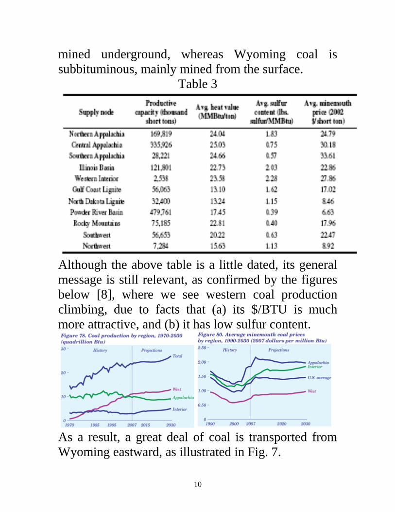
10
mined underground whereas Wyoming coal is
subbituminous mainly mined from the surface
Table 3
Although the above table is a little dated its general
message is still relevant as confirmed by the figures
below [8] where we see western coal production
climbing due to facts that (a) its $BTU is much
more attractive and (b) it has low sulfur content
As a result a great deal of coal is transported from
Wyoming eastward as illustrated in Fig 7
11
23
AZNM
NWPPMAPP
MAIN
ECAR
PRB
The Coal Doghellip
Powder River Basin Coal
Movement
Fig 7
We do not have a national CO2 cap and trade market
yet but there is a regional one called the Regional
Greenhouse Gas Initiative (RGGI) ndash see
httpwwwrggiorghome In 2008 there was serious
discussion ongoing to develop a national one as the
Waxman-Markey bill passed the house However its
companion Kerry-Boxer bill in the senate did not
pass Kerry-Lieberman-Graham unveiled a 2nd
version of the senate bill on 121009 which also did
not pass This would have been very important to
costs of energy production For example a ldquolowrdquo
CO2 cost would be about $10ton of CO2 emitted
which would increase energy cost from a typical
coal-fired plant from about $60MWhr to about
$70MWhr All indications are that today it is dead
12
40 CO2 Emissions - overview There is increased acceptance worldwide that global
warming is caused by emission of greenhouse gasses into
the atmosphere These greenhouse gases are (in order of
their contribution to the greenhouse effect on Earth) [9]
Water vapor causes 36-70 of the effect
Carbon dioxide (CO2) causes 9-26 of the effect
Methane (CH4) causes 4-9 of the effect
Nitrous oxide (N2O)
Ozone (O3) causes 3-7 of the effect
Chlorofluorocarbons (CFCs) are compounds containing
chlorine fluorine and carbon (no H2) CFCs are
commonly used as refrigerants (eg Freon)
The DOE EIA was publishing an excellent annual report on
annual greenhouse gas emissions in the US for example
the one published in November 2007 (for 2006) is [10] and
the one published in December 2009 (for 2008) is [11] All
such reports since 1995 may be found at [12] One figure
from the report for 2006 is provided below as Figure 8 The
information that is of most interest to us in this table is in
the center which is summarized in Table 4
Note that each greenhouse gas is quantified by ldquomillion
metric tons of carbon dioxide equivalentsrdquo or MMTCO2e
Carbon dioxide equivalents are the amount of carbon
dioxide by weight emitted into the atmosphere that would
produce the same estimated radiative forcing as a given
weight of another radiatively active gas [10]
13
Fig 8 Summary of US Greenhouse Gas Emissions 2006
Table 4 Greenhouse Gas Total 2006
Sectors MMTCO2e total CO2 total GHG
From Power Sector 2344 391 328
From DFU-transp 1885 314 264
From DFU-other 1661 277 233
From ind processes 109 18 15
Total CO2 5999 100 840
Non-CO2 GHG 1141 160
Total GHG 7140 100 The direct fuel use (DFU) sector includes transportation industrial process heat space heating and cooking fueled by
petroleum natural gas or coal The DFU-transportation CO2 emissions of 1885 MMT was obtained from the lower
right-hand-side of Fig 9a The DFU-other CO2 emissions of 1661 MMT was obtained as the difference between total
DFU emissions of 3546 MMT (given at top-middle of Fig 9a) and the DFU-transportation emissions of 1885 MMT
The ldquo total GHGrdquo for the 4 sectors (power DFU-transp DFU-other and ind processes) do not include the Non-
CO2 GHG emitted from these four sectors which are lumped into the single row ldquoNon-CO2 GHGrdquo If we assume that
each sector emits the same percentage of Non-CO2 GHG as CO2 then the numbers under ldquo total CO2rdquo are
representative of each sectorrsquos aggregate contribution to CO2 emissions The only sector we can check this for is
transportation where we know Non-CO2 emissions are 126MMT which is only 11 of the 1141 MMT total non-CO2
significantly less than the of total CO2 for transportation which is 314
14
Figure 9 [11] is the same picture as Fig 8 except it is for
the year 2008 the information is summarized in Table 5
Fig 9 Summary of US Greenhouse Gas Emissions 2008
Table 5 Greenhouse Gas Total 2008
Sectors MMTCO2e total CO2 total GHG
From Power Sector 2359 398 3318
From DFU-transp 1819 308 255
From DFU-other 1636 276 229
From ind processes 104 18 15
Total CO2 5918 100 830
Non-CO2 GHG 1213 170
Total GHG 7131 100 The direct fuel use (DFU) sector includes transportation industrial process heat space heating and cooking fueled by
petroleum natural gas or coal The DFU-transportation CO2 emissions of 1819 MMT was obtained from the lower
right-hand-side of Fig 9b The DFU-other CO2 emissions of 1636 MMT was obtained as the difference between total
DFU emissions of 3555 MMT (given at top-middle of Fig 9b) and the DFU-transportation emissions of 1819 MMT
The ldquo total GHGrdquo for the 4 sectors (power DFU-transp DFU-other and ind processes) do not include the Non-
CO2 GHG emitted from these four sectors which are lumped into the single row ldquoNon-CO2 GHGrdquo If we assume that
each sector emits the same percentage of Non-CO2 GHG as CO2 then the numbers under ldquo total CO2rdquo are
representative of each sectorrsquos aggregate contribution to CO2 emissions The only sector we can check this for is
transportation where we know Non-CO2 emissions are 127MMT which is only 105 of the 1213 MMT total non-
CO2 significantly less than the of total CO2 for transportation which is 308
15
Some numbers to remember from Tables 4 and 5 are
Total US GHG emissions are about 7100 MMTyear
Of these about 83-84 are CO2
Percentage of GHG emissions from power sector is
about 40 (see note for Tables 4 and 5)
Percentage of GHG emissions from transportation sector
is about 31 (see note for Tables 4 and 5)
Total Power Sector + Transportation Sector emissions is
about 71 (see note for Tables 4 and 5)
50 CO2 Emissions ndash power sector
Figure 10 [11] shows that CO2 emissions from the electric
power sector have been generally rising from 1990 to 2008
but the fact that they are rising more slowly than power
sector sales suggests that emissions per unit of energy
consumed is decreasing Note that the emissions values
given in Fig 10 have been normalized by the value in the
year 2000 which was 22935 MMT
Fig 10 Electric power sector CO2 emissions by year
Figure 11 [6] provides another view of CO2 emissions by
fuel where it is clear that recently emissions from coal and
petroleum dropped whereas that from natural gas increased
16
Fig 11
Table 6 [11] shows the year-by-year breakdown of electric
power sector CO2 emissions by fuel We see the dominant
contributor is coal with natural gas a distant second
Table 6Yearly breakdown of electric sector CO2 emissions
Table 6 is for CO2 emissions only ndash it does not include
Non-CO2 emissions
Coal is the largest contributor to CO2 emissions For
example in year 2008 it contributed 19459 MMT 825
17
of the total power sector CO2 emissions The next highest
contributor was natural gas at 362 MMT which is 153
of the total The two combined account for 978 of power
sector CO2 emissions
Total CO2 emissions from gas are only 186 of Total CO2
emissions from coal This does NOT imply that
CO2 emissions per MWhr from a natural gas power plant
are 186 of the
CO2 emissions per MWhr from a coal-fired power
plant
The fact that coal is the largest contributor to GHG
emissions is due to
(a) it is used to produce just under half of US electricity
(b) it has the highest emissionsenergy content ratio as
indicated by Table 7 below [13]
(c) its average conversion efficiency is not very good
18
Table 7 Emission Coefficients for Different Fuels
Pounds CO2
per
Million Btu
Aviation Gasoline AV 18355 per gallon 152717
Distillate Fuel (No 1 No 2 No 4
Fuel Oil and Diesel) DF 22384 per gallon 161386
Jet Fuel JF 21095 per gallon 156258
Kerosene KS 21537 per gallon 159535
Liquified Petroleum Gases (LPG) LG 12805 per gallon 139039
Motor Gasoline MG 19564 per gallon 156425
Petroleum Coke PC 32397 per gallon 22513
Residual Fuel (No 5 and No 6
Fuel Oil) RF 26033 per gallon 173906
Methane ME 116376 per 1000 ft3 115258
Landfill Gas LF 1 per 1000 ft3 115258
Flare Gas FG 133759 per 1000 ft3 120721
Natural Gas (Pipeline) NG 120593 per 1000 ft3 11708
Propane PR 12669 per gallon 139178
Coal CL
Anthracite AC 5685 per short ton 2274
Bituminous BC 49313 per short ton 2053
Subbituminous SB 37159 per short ton 2127
Lignite LC 27916 per short ton 2154
Biomass BM
Geothermal Energy GE 0 0
Wind WN 0 0
Photovoltaic and Solar Thermal PV 0 0
Hydropower HY 0 0
TiresTire-Derived Fuel TF 6160 per short ton 189538
Wood and Wood Waste 2 WW 3812 per short ton 195
Municipal Solid Waste 2 MS 1999 per short ton 199854
Nuclear NU 0 0
Renewable Sources Varies depending on the composition of the biomass
Petroleum Products
Natural Gas and Other Gaseous Fuels
Fuel Code
Emission Coefficients
Pounds CO2 per Unit
Volume or Mass
One indication from Table 7 that the pounds CO2MBTU
is based on energy content of the fuel could be misleading
What is of more interest is the CO2MWhr obtained from
the fuel together with a particular generation technology
To get this we need efficiencies of the generation
technologies Fig 12 provides such efficiencies the
resource from which it came [14] provides a good overview
of various factors affecting generation efficiencies
19
0
10
20
30
40
50
60
70
80
90
100
Hyd
ro p
ower
plant
Tidal p
ower
plant
Larg
e ga
s fir
ed C
CGT p
ower
plant
Melte
d ca
rbon
ates
fuel cell (
MCFC
)
Pulve
rised
coa
l boilers
with
ultr
a-cr
itica
l ste
am p
aram
eter
s
Solid o
xide
fuel cell (
SOFC
)
Coa
l fire
d IG
CC
Atmos
pher
ic C
irculat
ing
Fluidised
Bed
Com
bustion
(CFB
C)
Press
urised
Flu
idised
Bed
Com
bustion
(PFB
C)
Larg
e ga
s tu
rbine
(MW
rang
e)
Steam
turb
ine
coal-fi
red
power
plant
Steam
turb
ine
fuel-o
il po
wer
plant
Wind
turb
ine
Nuc
lear
pow
er p
lant
Biom
ass an
d biog
as
Was
te-to
-electric
ity p
ower
plant
Diese
l eng
ine
as d
ecen
tralis
ed C
HP u
nit (
elec
trica
l sha
re)
Small a
nd m
icro
turb
ines
(up
to 1
00 kW
)
Photo
volta
ic cells
Geo
ther
mal p
ower
plant
Solar
pow
er to
wer
Eff
icie
nc
y (
)
Fig 12 Generation efficiencies
Table 7 and Fig 12 provide the ability to compare different
technologies in terms of CO2MWhr For example letrsquos
compare a natural gas combined cycle (NGCC) plant
(η=58) a gas turbine (η=39) and a coal-fired power plant
(η=39) where the CO2 content of the natural gas is 11708
lbsMBTU and the CO2 content of the coal assuming it
uses (Powder River Basin) sub-bituminous coal is 2127
lbsMBTU (Note that coal has a different energy amp CO2
content depending on type as shown below [15])
20
NGCC MWhrlbsMWhr
MBTU
MBTU
MBTU
MBTU
lbs
OUT
IN
IN
5688413
58
108117
Gas turbine
MWhrlbsMWhr
MBTU
MBTU
MBTU
MBTU
lbs
OUT
IN
IN
71023413
39
108117
Coal-fired plant
MWhrlbsMWhr
MBTU
MBTU
MBTU
MBTU
lbs
OUT
IN
IN
81859413
39
17212
Table 8 below from [16] indicates similar numbers for a
pulverized coal (PC) plant a circulating fluidized bed
(CFB) plant an integrated gasification combined cycle
(IGCC) plant and a combined cycle plant Note that the
fuels for the first three of these are all coal and they have
similar emissionsMWhr ratios The combined cycle plant
has a bit higher ratio (810 instead of 6885) because it used
a lower efficiency (493 instead of 58)
Table 8
21
In the calculations at the top of the previous page one can
recognize that the 341η factor in each equation is just the
unit heat rate in MBTUMWhr This means the same
calculation can be done by multiplying the lbsMBTUIN
factor from Table 7 by the average heat rate for the plant
We can also convert the above to Metric tonsMWhr by
dividing by 2204 lbsMetric ton to get the following
figures
NGCC 0464 MTMWhr
Gas turbine 0312 MTMWhr
Coal-fired plant 0844 MTMWhr
It is interesting to compare these values with the emission
coefficients given by regionstate at [17] A sample of some
of these coefficients are provided below (this is 2002 data)
New York 0389
Vermont 0013
Penn 0574
Ohio 0817
Iowa 0854
N Dakota 1017
Georgia 0619
Kentucky 0911
Texas 0664
California 0275
Washington 0111
US Average 0606
Why is Iowa so high
Why are NDakota amp Kentucky so high
Why is California so low
Why is Washington so low
Why is Vermont so low
22
Vermont is so low because it has only one small fossil-fired
unit (a diesel unit) and it is a peaker and so does not often
run [18] Almost 75 of Vermontrsquos electric energy comes
from a large nuclear facility (Vermont Yankee) and most of
the rest comes from outside the state via the ISO-NE
market Iowa was in 2002 heavily dependent on coal
Today with Iowarsquos wind growth it is less so but still coal
is by far the dominant part of Iowarsquos generation portfolio
60 Heat rates
The values of Table 1 (fuel cost table) reflect only the
cost of fuel input to a generation plant they do not
reflect the actual costs of producing electrical energy as
output from the plant because substantial losses occur
during production Some power plants have overall
efficiencies as low as 30 in addition the plant
efficiency varies as a function of the generation level Pg
We illustrate this point in what follows
We represent plant efficiency by η Then η=energy
outputenergy input We obtain η as a function of Pg by
measuring the energy output of the plant in MWhrs and
the energy input to the plant in MBTU
We could get the energy output by using a wattmeter to
obtain Pg over a given period of time say an hour and
we could get the energy input by measuring the coal
tonnage used during the hour and then multiplying by
the coal energy content in MBTUton
23
We could then plot the fuel input in MBTUhr as a
function of the power output Pg in MW Such a plot is
called an input-output curve indicating how much fuel
rate is required to produce a power level A typical
input-output curve is shown in Fig 13 We denote fuel
rate (input vertical axis of Fig 1a) as R (WampW denote
fuel rate as H ndash see p 8 )
One notes that the IO curve of Fig 13 does not go to
Pg=0 A generating unit has a minimum stable output
typically 10-30 for oil and natural gas-fired steam
units and 20-50 for coal-fired steam units [19]
Pg
Fuel rate
MBTUhr
R
OUTPUT
INPUT
Fig 13 Input-output curve
One interesting feature with respect to Fig 13 is that
as fuel input is increased the power output per unit
fuel input begins to decrease We can see this more
clearly if we invert the axes as in Fig 14 yielding a
production function where for high enough fuel
rates we will get no additional power output
24
Pg
Fuel rate
MBTUhr
R Fig 14 Production function
Physically this happens because the furnace boiler
steam pipes leak a larger percentage of input heat as
temperatures increase Economists call this the [20]
law of diminishing marginal product for almost all
processes the rate of increase in output decreases as
the input increases assuming other inputs are fixed
To obtain η we want the output energy divided by
the input energy which is
η ~ Pg divide R
which in terms of units is MW divide MBTUhr to give
units of MWhrMBTU Notice that these units are
energyenergy as they should be when computing η
However the MBTU and MWhr are different units of
energy and so we are not getting η exactly but we
are getting something proportional to η
So letrsquos obtain the ratio of the power to the fuel rate
25
(Pg divide R) for every point on the input-output curve
and plot the results against Pg Fig 15 shows a plot of
the ratio PgR (units of MWHRMBTU) versus Pg
Fig 15 Plot of MWhrMBTU vs Pg
Figure 15 indicates that efficiency is poor for low
generation levels (a connected plant that is operating
at zero MW output still has to supply station loads)
and increases with generation but at some optimum
level it begins to diminish Most power plants are
designed so that the optimum level is close to the
rated output
The heat rate curve is similar to Fig 15 except that
the y-axis is inverted to yield MBTUMWhrs which
is proportional to 1η This curve is illustrated in Fig
16 We denote heat rate by H (WampW use H for fuel
rate) Since the heat rate depends on operating point
we write H=H(Pg)
26
Fig 16 Plot of Heat Rate (H) vs Generation (Pg)
Some typical heat rates for units at maximum output
are (in MBTUMWhrs) 95-105 for fossil-steam
units and nuclear units 130-150 for combustion
turbines [21] and 70-95 for combined cycle units
Future combined cycle units may reach heat rates of
65-70 It is important to understand that the lower
the heat rate the more efficient the unit
An easy way to remember the meaning of heat rate
H=H(Pg) is it is the amount of input energy (MBTU)
required to produce a MWhr at generation level Pg
How does H relate to efficiency To answer this
question we need to know that there are 105485
joules per BTU
413
4133600
8510541
sec3600sec)(
)851054(
61
61~
1
HH
H
j
BTUjBTUH
Whr
BTU
E
EH
MWhr
MBTUH
27
Observe We have seen this before when we
computed CO2 emissions per MWhr out (see pg 20)
eg for the NGCC plant
MWhrlbsMWhr
MBTU
MBTU
MBTU
MBTU
lbs
OUT
IN
IN
5688413
58
108117
We can see now that the above calculation can be
thought of as
MWhrlbsMBTU
MBTU
MBTU
MBTU
MBTU
lbs
OUT
IN
OUT
IN
IN
5688413
58
41308117
or
MWhrlbsHMBTU
lbs
IN
568808117
where H in this case is 34158=588 MBTUMWhr
The heat rate curve is a fixed characteristic of the plant
although it can change if the cooling water temperature
changes significantly (and engineers may sometimes
employ seasonal heat rate curves) The heat rate curve
may also be influenced by the time between
maintenance periods as steam leakages and other heat
losses accumulate
The above use of the term ldquoheat raterdquo is sometimes also
called the ldquoaverage heat raterdquo This is because we get it
by dividing absolute values of fuel input rate by
absolute values of electric output power For example if
you buy an apple at $50 and a second one at $10 the
average cost of apples after buying the first apple is
$50apple but after buying the second apple is
$(50+10)2=$30apple
28
This is different than incremental heat rate as will be
illustrated in the following example
Example [22] Consider the input-output curve for
Plant X in Fig 17
Fig 17
Compute the average heat rate characteristic and the
incremental heat rate characteristic
Average heat rates are computed by dividing the fuel
rate by the generation level H=RPg as follows
Block 1 200001=20000
Block 2 240002=12000
Block 3 300003=10000
Incremental heat rates computed by dividing the
increment of fuel rate by the increment of power
IH=∆R∆Pg as follows
Block 1 200001=20000
Block 2 40001=4000
Block 3 60001=6000
These results are summarized in Table 9 below
29
Table 9
Figure 18 below illustrates the input-output curve the
average heat rate curve and the incremental heat rate
curve
Fig 18
We should note however that our first incremental
heat rate value of 20000 has a problem This value
assumes that the IO curve extends as shown on the
left hand side in Fig 19 below Probably a better
30
approximation would be to extend it as indicated on
the right hand side of Fig 19
Fig 19
Actually it does not extend to 0 MW output because
the unit like all real units has a minimum generation
level
Although you may see data entered which reflects a
ldquohigh initial incremental valuerdquo you should know
that a value so computed does not represent a true
incremental heat rate value at all
Reference [22] also provides some actual data for
units in California The one below Fig 20 is one of
the most efficient gas-fired units in the PGampE
system On the coast about 100 miles south of San
Francisco it is called Moss Landing Unit 7
31
Fig 20
Note that the Moss Landing unit 7 full-load average
heat rate is 8917 MBTUMWhr which gives an
efficiency of 3418917=382
The next one Fig 21 is an old oil-fired unit in San
Francisco called Hunterrsquos Point
32
Fig 21
Note the full-load average heat rate of this plant is
12598 MBTUMWhr which corresponds to an
efficiency of 34112598=271
This plant was built in 1927 and demolished in 2008
70 Cost rates
We are primarily interested in how the cost per
MWhr changes with Pg because that will tell us
something about how to achieve the most economic
dispatch of generation for a given demand (we will
see that optimality is achieved when marginal or
incremental costs of all regulating units are equal)
33
To get cost per MWhr as a function of Pg we will
assume that we know K the cost of the input fuel in
$MBTU Also recall that
R is the rate at which the plant uses fuel in
MBTUhr (which is dependent on Pg) ndash it is just
the input-output curve (see Fig 13)
And we will denote
C as the cost per hour in $hour
Then if H(Pg) the heat rate is the input energy used
per MW per hour then multiplying H by Pg gives
input energy per hour ie R=PgH(Pg) where H must
be evaluated at Pg Therefore C = RK = PgH(Pg)K
ie the cost rate function C is just the fuel rate
function R scaled by the fuel cost
A typical plot of C vs Pg is illustrated in Fig 22
Note that because H(Pg) is convex C(Pg) is also
convex ie the set of points lying on or above C
contain all line segments between any pair of points
Fig 22 Plot of cost per hr (C) vs generation (Pg)
34
Fig 22 shows that costhour increases with
generation a feature that one would expect since
higher generation levels require greater fuel intake
per hour
The incremental cost curve for the plant can be
obtained by differentiating the plot in Fig 22 ie by
computing dCdPg A typical incremental cost curve
is shown in Fig 23 Note that because C is convex
dCdPg is a non-decreasing function
Fig 23 Plot of incremental cost dCdPg vs gen Pg
One last thing about getting incremental cost
Recall that the cost per hour is given by
C = RK where R is just the input-output curve
Therefore IC=dCdPg=K(dRdPg) The derivative
is the incremental heat rate which we denoted by
IH Therefore in summary
C=RK=PgH(Pg)K
IC=dCdPg=(dRdPg)K=(IH)K
35
Example 1 An 100 MW coal-fired plant uses a type of coal
having an energy content of 12000 BTUlb The coal
cost is $15MMBTU Typical coal usage
corresponding to the daily loading schedule for the
plant is as follows
Table 10
Time of
Day
Electric
Output (MW)
Coal Used
(tons)
1200am-
600am
40 1050
600am-
1000am
70 945
1000am-
400pm
80 1560
400pm-
1200am
100 2700
For each of the four load levels find (a) the
efficiency η (b) the heat rate H (MMBTUMWhr)
(c) the cost per hour C ($hr) Also for the loading
levels of 40 70 and 80 MW use a piecewise linear
plot of C vs P to obtain incremental cost IC as a
function of unit loading P Then plot incremental cost
as a function of unit loading The conversion factor
from joules to BTU is 105485 joulesBTU and the
units for coal used tons are short-tons 2000 lbton
36
Solution Let T be the number of hours the plant is producing P
MW while using y tons of coal We need to compute
the total energy out of the plant and divide by the
total energy into the plant but we need both
numerator and denominator to be in the same units
We will convert both to joules (recall a watt is a
joulesec)
(a)
BTU
joules851054
lb
BTU00012
ton
lb2000 tons
hr
sec3600
MW
watts10hr MW 6
y
TP
Note that the above expression for efficiency is
dimensionless
(b) The heat rate is the amount of MMBTUs
used in the amount of time T divided by the
number of MW-hrs output in the amount of time
T
TP
y
H
BTU10
MMBTU1
lb
BTU00012
ton
lb2000 tons
6
37
Note that
413
851054
36001H and the above
expression has units of MMBTUMWhr Thus if a
unit is 100 efficient then it will have a heat rate
of 341 MMBTUMWhr the absolute best (lowest)
heat rate possible
(c) C = RK where R is the rate at which the plant
uses fuel and K is fuel cost in $MMBTU Note
from units of P and H that
R = PH C = PHK where H is a function of P
Application of these expressions for each load level
yields the following results
Table 11
T (hrs) P
(MW)
y
(tons)
η H
(mbtum
whr)
C
($hr)
6 40 1050 033 105 630
4 70 945 042 81 850
6 80 1560 044 78 936
8 100 2700 042 81 1215
To obtain incremental cost dP
dCIC we can plot C vs
P and then get an approximation on the derivative by
assuming a piecewise linear model as shown in
Figure 24
38
Figure 24 Calculation of Incremental Cost
The incremental costs are plotted as a function of
loading in Fig 25
20
4
2
6
8
10
40 60 80
12
IC ($MWhr)
Pg (MW)
Fig 25 Incremental cost curve from piecewise-linear
cost curve
39
We may use another procedure to model the
incremental costs In this procedure we first fit the
data to a quadratic polynomial Matlab commands for
doing so are below
gtgt p=[40 70 80 100]
gtgt c=[630 850 936 1215]
gtgt X = [ones(size(p)) p p^2]
gtgt a=Xc
a =
6048533
-29553
00903
gtgt T = (01100)
gtgt Y = [ones(size(T)) T T^2]a
gtgt plot(TY-tyo) grid on
The quadratic function is therefore
C(P)=00903P2-29553P+60485
Figure 26 shows the plot obtained from Matlab
40
Fig 26 Quadratic Curve Fit for Cost Rate Curve
Clearly the curve is inaccurate for very low values of
power (note it is above $605hr at P=0 and decreases
to about $590hr at P=10) We can get the
incremental cost curve by differentiating C(P)
IC(P)=01806P-29553
This curve is overlaid on the incremental cost curve
of Fig 25 resulting in Fig 27 Both linear and
discrete functions are approximate Although the
linear one appears more accurate in this case it
would be easy to improve accuracy of the discrete
one by taking points at smaller intervals of Pg Both
functions should be recognized as legitimate ways to
represent incremental costs The linear function is
often used in traditional economic dispatching the
discrete one is typical of market-based offers
41
20
4
2
6
8
10
40 60 80
12
14
Fig 27 Comparison of incremental cost curve
obtained from piecewise linear cost curve (solid line)
and from quadratic cost curve (dotted line)
80 Market-based offers
As indicated in the last section electricity markets
typically allow only piecewise linear representation
of generator incremental cost curves
The real-time and the day-ahead markets are implemented
via computer programs based on optimization theory The
program used for the real-time market is called the
security-constrained economic dispatch (SCED) This
program the SCED is used together with a program called
the security-constrained unit commitment (SCUC) program
for the day-ahead market Both the SCED and the SCUC
42
also solve for the ancillary service prices through a
formulation known as co-optimization We will say no
more about SCED and SCUC because we cannot assume
that students taking this course have the necessary
background on optimization theory Instead we will
provide a simple description of how the energy market
price is determined This description is based on standard
microeconomic theory but can be followed without
background in microeconomics However one should note
that the description necessarily omits some important
concepts related to losses and congestion
The following example is adapted from [23] Consider that
our electric energy market has three buyers B1 B2 B3 and
two sellers S1 S2 The buyers represent load-serving
entities and the sellers represent generation owners
Consider that these buyers and sellers submit their bids (to
buy) and their offers (to sell) via an internet system as
shown in Fig 28
Figure 28 Illustration of buyer-seller interaction with internet-based market
Each seller has energy to sell but the price they are willing
to sell it for increases with the amount they sell This is a
reflection of the fact that the cost of producing 1 more unit
of energy (MWhr) increases as a unit is loaded higher
Internet System
B1
B2
B3
S1
S2
43
Likewise each buyer wants to purchase energy but the
price they are willing to pay to obtain it decreases with the
amount that they buy This is just a reflection of the fact
that our first unit of energy will be used to supply our most
critical needs and after those needs are satisfied the next
units of energy will be used to satisfy less critical needs so
that we are unwilling to pay as much for it
Tabl2 illustrates a representative set of bids and offers
submitted by the buyers and sellers
Table 12 Offers and bids for examples
Offers to sell Bids to buy
S1 S2 B1 B2 B3
$1000 $1000 $7000 $7000 $2500
$5000 $5000 $7000 $5000 0
$6500 $7000 $6500 $2500 0
$7000 $7000 $6500 0 0
infin infin 0 0 0
infin infin 0 0 0
infin infin 0 0 0
Once each buyer and seller enters their data according to
Table 12 the internet system will reconstruct the
information according to Table 13 where
Table 13 Reconstructed offers and bids
Offerbid
order
Offers to sell 1 MWhr Bids to buy 1 MWhr
Seller Price Buyer Price
1 S1 $1000 B1 $7000
2 S2 $1000 B1 $7000
3 S1 $5000 B2 $7000
4 S2 $5000 B1 $6500
5 S1 $6500 B1 $6500
6 S2 $7000 B2 $5000
7 S1 $7000 B2 $2500
8 S2 $7000 B3 $2500
44
We can visualize the data in Table by plotting the price
against quantity for the offers and for the bids This
provides us with the supply and demand schedules of
Figure 29 [23]
Figure 29 Supply-demand schedules illustrating electricity market operation [23]
The point (or those points) where the supply schedule
intersects the demand schedule determines the market
clearing price This is the price that all sellers are paid to
supply their energy and it is the price that all buyers pay to
receive their energy In Figure this price is $65MWhr It is
the very best price to choose because it maximizes the total
ldquosatisfactionrdquo felt by the buyers and sellers
This satisfaction for the sellers can be measured by the
difference between the price they offered and the price they
were actually paid for the energy they supplied If we add
up all of these differences for all sellers then we obtain the
net seller surplus This satisfaction for the buyers can be
measured by the difference between the price they bid and
the price they actually had to pay for the energy they
45
received If we add up all of these differences for all sellers
then we obtain the net buyer surplus The net seller surplus
and the net buyer surplus are illustrated in Fig 30 [23]
Figure 30 Illustration of net seller and net buyer surplus [23]
The total net surplus is the sum of the buyer and seller net
surpluses The market clearing price is the price that
maximizes the total net surplus
In Fig 30 the quantity traded could be either 4 or 5
MWhrs but the 5th MWhr would neither increase nor
decrease the total net surplus The decision on whether to
trade 4 or 5 MWhrs in such as case is determined by market
rules
The example of this section illustrates the way electricity
markets would clear if there are no losses and if the
transmission capacity of each line was infinite One
conceptualization of such a situation is when all generators
and all loads are located at the same electric node In such a
case there is a single price by which all sellers are paid and
all buyers pay
46
In reality of course each transmission circuit does have
some resistance and therefore incurs some losses as current
flows through it and each transmission circuit also has an
upper bound for the amount of power that can flow across
it These two attributes losses and transmission limits
result in locational variation in prices throughout the
network which are called as we have already seen the
locational marginal prices (LMPs)
90 Effect of Valve Points in Fossil-Fired Units
Figures 22 and 24 well represent cost curves of small
steam power plants but actual cost curves of large
steam power plants differ in one important way from
the curves shown in Figs 22 and 24 ndash they are not
smooth The light curve of Fig 31 [24] more closely
captures the cost variation of a large steam power
plant
Fig 31 Cost rate curve for large steam power plant [24]
47
The reason for the discontinuities in the cost curve of
Fig 31 is because of multiple steam valves In this
case there are 5 different steam valves Large steam
power plants are operated so that valves are opened
sequentially ie power production is increased by
increasing the opening of only a single valve and the
next valve is not opened until the previous one is
fully opened So the discontinuities of Fig 31
represent where each valve is opened
The cost curve increases at a greater rate with power
production just as a valve is opened The reason for
this is that the so-called throttling losses due to
gaseous friction around the valve edges are greatest
just as the valve is opened and taper off as the valve
opening increases and the steam flow smoothens
The significance of this effect is that the actual cost
curve function of a large steam plant is not
continuous but even more important it is non-
convex A simple way (and the most common way)
to handle these two issues is to approximate the
actual curve with a smooth convex curve similar to
the dark line of Fig 31
48
100 Combined cycle units
The following information was developed from [21
25 26 27] The below figure shows recent US
growth in combined cycle power plants [28]
Fig x
Combined cycle units utilize both gas turbines (based
on the Brayton cycle) and steam turbines (based on
the Rankine cycle) Gas turbines are very similar to
jet engines where fuel (can be either liquid or gas)
mixed with compressed air is ignited The
combustion increases the temperature and volume of
the gas flow which when directed through a valve-
controlled nozzle over turbine blades spins the
turbine which drives a synchronous generator On the
49
other hand steam turbines utilize a fuel (coal natural
gas petroleum or uranium) to create heat which
when applied to a boiler transforms water into high
pressure superheated (above the temperature of
boiling water) steam The steam is directed through a
valve-controlled nozzle over turbine blades which
spins the turbine to drive a synchronous generator
A combined cycle power plant combines gas turbine
(also called combustion turbine) generator(s) with
turbine exhaust waste heat boiler(s) (also called heat
recovery steam generators or HRSG) and steam
turbine generator(s) for the production of electric
power The waste heat from the combustion
turbine(s) is fed into the boiler(s) and steam from the
boiler(s) is used to run steam turbine(s) Both the
combustion turbine(s) and the steam turbine(s)
produce electrical energy Generally the combustion
turbine(s) can be operated with or without the
boiler(s)
A combustion turbine is also referred to as a simple
cycle gas turbine generator They are relatively
inefficient with net heat rates at full load of some
plants at 15 MBtuMWhr as compared to the 90 to
105 MBtuMWhr heat rates typical of a large fossil
fuel fired utility generating station This fact
combined with what can be high natural gas prices
50
make the gas turbine expensive Yet they can ramp
up and down very quickly so as a result combustion
turbines have mainly been used only for peaking or
standby service
The gas turbine exhausts relatively large quantities of
gases at temperatures over 900 degF In combined cycle
operation then the exhaust gases from each gas
turbine will be ducted to a waste heat boiler The heat
in these gases ordinarily exhausted to the
atmosphere generates high pressure superheated
steam This steam will be piped to a steam turbine
generator The resulting combined cycle heat rate is
in the 70 to 95 MBtuMWhr range significantly less
than a simple cycle gas turbine generator
In addition to the good heat rates combined cycle
units have flexibility to utilize different fuels (natural
gas heavy fuel oil low Btu gas coal-derived gas)
[29] (In fact there are some advanced technologies
under development right now including the
integrated gasification combined cycle (IGCC) plant
which makes it possible to run combined cycle on
solid fuel (eg coal or biomass) [30] The first two
operational IGCC plants in the US were the Polk
Station Plant in Tampa and the Wabash River Plant
in Indiana [31] The Ratcliffe-Kemper plant
currently under construction by Mississippi Power (a
51
subsidiary of Southern Company) is a 582 MW
IGCC plant to be completed in 2014 [32 33])
The flexibility of combined cycle plants together
with the fast ramp rates of the combustion turbines
and relatively low heat rates has made the combined
cycle unit the unit of choice for a large percentage of
recent new power plant installations The potential
for increased gas supply and lowered gas prices has
further stimulated this tendency
Fig 32 shows the simplest kind of combined cycle
arrangement where there is one combustion turbine
and one HRSG driving a steam turbine
ChillerCooler
Inlet Air
Gas Supply
Duct firing
HRSG
Condenser
CTG STG
Fig 32 A 1 times 1 configuration
An additional level of complexity would have two
combustion turbines (CT A and B) and their HRSGs
driving one steam turbine generator (STG) as shown
in Fig 33
52
ChillerCooler
Inlet Air
Gas Supply
Duct firing
HRSG
ChillerCooler
Inlet Air
Gas Supply
Duct firing
HRSG
Condenser
CTG
CTG STG
Fig 33 a 2 times 1 configuration
In such a design the following six combinations are
possible
CT A alone
CT B alone
CT A and CT B together
CT A and STG
CT B and STG
CT A and B and STG
The modes with the STG are more efficient than the
modes without the STG (since the STG utilizes CT
exhaust heat that is otherwise wasted) with the last
mode listed being the most efficient
If we model a combined cycle plant as a single plant
we run into a problem Consider the transition
between the combined cycle power plant operation
53
just as the STG is ramped up Previous to STG start-
up only the CT is generating with a specified
amount of fuel per hour being consumed as a
function of the CT power generation level Then
after STG start-up the fuel input remains almost
constant but the MW output of the (now) two
generation units has increased by the amount of
power produced by the steam turbine driven by the
STG A typical cost curve for this situation is shown
in Fig 34
C ($hr)
PG (MW)
Fig 34 Cost curve for a combined cycle plant
An important feature of the curve in Fig 34 is that it
is not convex which means its slope (ie its
incremental cost) does not monotonically increase
with PG Figure 35 illustrates incremental cost
variation with PG
54
dCdPG ($MWhr)
PG (MW)
Fig 35 Incremental cost curve for a combined cycle plant
The key attribute of the incremental cost curve in
order to satisfy convexity is that it must be non-
decreasing Clearly the curve of Fig 35 does not
satisfy this requirement
110 Economic dispatch and convexity of objective
functions in optimization
The traditional economic dispatch (ED) approach
used by electric utilities for many years is very well
described in [34]
This approach is still used directly by owners of
multiple generation facilities when they make one
offer to the market and then need to dispatch their
units in the most economic fashion to deliver on this
offer This approach also provides one way to view
the method by which locational marginal prices are
computed in most of todayrsquos real-time market
systems
The simplest form of the ED problem is as follows
55
Minimize
n
i
iiT PFF1
(1)
Subject to
0)(11
N
i
iloadiload
n
i
i PPPPP (2)
0max
minmin
i
ii
iiii
PPP
PPPP
(3)
Here we note that the equality constraint is linear in
the decision variables Pi In the Newton approach to
solving this problem ([34]) we form the Lagrangian
according to
)()( iiT PPF L (4)
If each and every individual cost curve Ci(Pi) i=1n
is quadratic then they are all convex Because the
sum of convex functions is also a convex function
when all cost curves are convex then the objective
function FT(Pi) of the above problem is also convex
If φ(Pi) is linear then it is convex and therefore L is
convex This fact allows us to find the solution by
applying first order conditions
56
First order conditions for multi-variable calculus are
precisely analogous to first order conditions to single
variable calculus In single variable calculus we
minimize f(x) by solving frsquo(x)=0 on the condition
that f(x) is convex or equivalently that frsquorsquo(x)gt0
In multivariable calculus where x=[x1 x2hellip xn]T we
minimize f(x) by solving frsquo(x)=0 that is
nix
f
i
1 0
(5)
on the condition that f(x) is convex or equivalently
that the Hessian matrix frsquorsquo(x) is positive definite
We recall that in single variable calculus if f(x) is
not convex then the first order conditions do not
guarantee that we find a global minimum We could
find a maximum or a local minimum or an inflection
point as illustrated in Fig 36 below
f(x)
x x
f(x)
Fig 36 Non-convex functions
57
The situation is the same in the multivariable case
ie if f(x) is not convex then the first order
conditions of (5) do not guarantee a global minimum
Now returning to the Lagrangian function of our
constrained optimization problem repeated here for
convenience
)()( iiT PPF L (4)
we recall that solution to the original problem is
found by minimizing FT But to use what we now
know we are only guaranteed to find a global
minimum of F if L is convex In this case the first
order conditions results in
0
1 0
L
LNi
Pi
from which we may find our solution (Inequality
constraints may be handled by checking the resulting
solution against them and for any violation setting
up another equality constraint which binds the given
decision variable to the limit which was violated)
But if one of the units is a combined cycle unit the
FT and therefore L will not be convex So first
58
order conditions do not guarantee a global minimum
In other words there may be a lower-cost solution
than the one we will obtain from applying first order
conditions This makes engineers and managers
concerned because they worry they are spending
money unnecessarily
120 General solutions for non-convex
optimization problems
Generation owners who utilize combined cycle units
must use special techniques to solve the EDC
problem Some general methods that have been
proposed for solving non-convex optimization
problems are below However I am not aware that
any of these techniques have been implemented
within an electricity market today
1 EnumerationIteration In this method all possible
solutions are enumerated and evaluated and then the
lowest cost solution is identified This method will
always work but can be quite computational
2 Dynamic programming See pp 51-54 of reference
[21]
59
3 Sequential unconstrained minimization technique
(SUMT) This method is described on pp 473-477 of
reference [35]
4 Heuristic optimization methods There are a
number of methods in this class including Genetic
Algorithm simulated annealing tabu search and
particle swarm A good reference on these methods is
[36]
5 There is a matlab toolbox for handling non-convex
optimization It provides 2 different algorithms
together with references on papers that describe the
algorithms located at httptomlabbiz There are
two methods provided
(a) Radial Basis Function (RBF) interpolation
(b) Efficient Global Optimization (EGO) algorithm
The idea of the EGO algorithm is to first fit a
response surface to data collected by evaluating the
objective function at a few points Then EGO
balances between finding the minimum of the surface
and improving the approximation by sampling where
the prediction error may be high
130 Practical solutions to modeling combined
cycle units in optimization
60
Reference [37] developed by engineers at ERCOT and
Ventyx (now ABB) is an excellent summary of practical
methods to modeling combined cycle units It provides
references to a number of other good resources on the
subject The methods it outlines are as follows
Aggregate modeling Here the combined cycle unit is
simply modeled with a ldquobest-fitrdquo convex cost curve This
approach does not handle the non-convexity of the actual
cost characteristic
Pseudo-unit modeling Here a number of pseudo-units
equal to N the number of combustion turbines are
represented each with 1N of the steam unit This works
for an Ntimes1 combined cycle unit For example a 3 times 1
combined cycle unit would be modeled as three separate
pseudo-units each of the three pseudo-units would be
one gas turbine plus one third of a steam turbine [38]
This approach has been implemented within several
markets including ISO NE NYISO MISO PJM and
IESO This approach does not handle the non-convexity
of the actual cost characteristic
Configuration-based modeling This approach is also
referred to as psuedo-plant modeling Here a cost-curve
(or incremental cost curve) is provided for each
configuration of the combined cycle plant Additional
logic is provided in the security-constrained unit
commitment (SCUC which is the mixed integer
programming software for the day-ahead market) to
ensure that only one configuration can be selected and
that the selection depends on the configuration of the
previous time period as illustrated in Fig 37 below for a
2times1 combined cycle plant [37] The configuration
61
chosen by SCUC for any one hour is maintained for the
entire hour in the real-time market CAISO has
implemented this approach it is well-described in [38]
Fig 37
Physical-unit modeling Here each CT and STG is
considered to be an individual resource with its own
individual offers This is a bad market model but it
provides good fidelity in terms of MW that the power
plant can actually produce ERCOT reports in [38] that it
utilizes configuration-based models for its markets and
physical unit modeling for its network security
applications
References [1] J McCalley W Jewell T Mount D Osborn and J Fleeman ldquoA wider horizon Technologies Tools
and Procedures for Energy System Planning at the National Levelrdquo IEEE Power and Energy Magazine
MayJune 2011
[2] J Morgan ldquoEnergy Density and Waste Comparison of Energy Productionrdquo Nuclear Science and
Technology June 2010 available at httpnuclearfissionarycom20100609energy-density-and-waste-
comparison-of-energy-production
[3] The World Nuclear Association ldquoThe Economics of Nuclear Powerrdquo available at httpwwwworld-
nuclearorginfoinf02html
[4] US Department of Energy Energy Information Administration website located at
httpwwweiagovcneafelectricityepmepmxlfile4_1xls and
httpwwweiadoegovcneafelectricityepmepmxlfile4_1_contxls
[5] US Department of Energy Energy Information Administration website located at
httpwwweiadoegovemeuaertxtptb0811bhtml
[6] ldquoEnergy perspectives 2011 US Department of Energy Energy Information Administration website
httpwwweiagovtotalenergydataannualpdfperspectives_2011pdf
62
[7] North American Reliability Corporation (NERC) ldquo2011 Long Term Reliability Assessmentrdquo
November 2011 available at wwwnerccom
[8] US Department of Energy Energy Information Administration website located at
httpwwweiadoegovoiafaeocoalhtml
[9] Wikipedia page on ldquoGreenhouse gasrdquo httpenwikipediaorgwikiCarbon_emissions
[10] US Department of Energy Energy Information Administration ldquoEmissions of Greenhouse Gases in
the United States 2006rdquo November 2007 available at httpwwweiadoegovoiaf1605ggrptindexhtml
[11] US Department of Energy Energy Information Administration ldquoEmissions of Greenhouse Gases in
the United States 2008rdquo December 2009 available at httpwwweiadoegovoiaf1605ggrptindexhtml
[12] wwweiadoegovoiaf16051605aoldhtml
[13] DOE EIA Data from Voluntary Reporting of Greenhouse Gasses Program available at
httpwwweiadoegovoiaf1605coefficientshtml
[14] F Van Aart ldquoEnergy efficiency in power plantsrdquo October 21 Vienna available from Dr McCalley
(see ldquoNew Generationrdquo folder) but you must make request
[15] EPA report wwwepagovairmarktprogsregsepa-ipmdocschapter8-v2_1-updatepdf
[16] Black amp Veatch ldquoPlanning for Growing Electric Generation Demandsrdquo slides from a presentation to
Kansas Energy Council ndash Electric Subcommittee March 12 2008 available at
httpwwwgooglecomsearchhl=enampsource=hpampq=22Planning+for+Growing+Electric+Generation+D
emands22ampbtnG=Google+Searchampaq=fampaqi=ampaql=ampoq=ampgs_rfai=C5Ekv4uV7TP7ECIzmNJHV_MIE
AAAAqgQFT9Dr5Lw
[17] DOE EIA Website for US locations emission coefficients httpwwweiadoegovoiaf1605ee-
factorshtml
[18] wwwrutlandheraldcomappspbcsdllarticleAID=20080706NEWS048070604571024NEWS04
[19]H Stoll ldquoLeast-cost electric utility planningrdquo 1989 John Wiley
[20] D Kirschen and G Strbac ldquoFundamentals of Power System Economicsrdquo Wiley 2004
[21] A J Wood and B F Wollenberg Power Generation Operation and Control second edition John
Wiley amp Sons New York NY 1996
[22] J Klein ldquoThe Use of Heat Rates in Production Cost Modeling and Market Modelingrdquo California
Energy Commission Report 1998
[23] L Tesfatsion ldquoAuction Basics for Wholesale Power Markets Objectives and Pricing Rulesrdquo
Proceedings of the 2009 IEEE Power and Energy Society General Meeting July 2009
[24] J Kim D Shin J Park and C Singh ldquoAtavistic genetic algorithm for economic dispatch with valve
point effectrdquo Electric Power Systems Research 62 2002 pp 201-207
[25] ldquoElectric power plant designrdquo chapter 8 publication number TM 5-811-6 Office of the Chief of
Engineers United States Army January 20 1984 located at
httpwwwusacearmymilpublicationsarmytmtm5-811-6 not under copyright
[26] A Cohen and G Ostrowski ldquoScheduling units with multiple operating modes in unit commitmentrdquo
IEEE 1995
[27] A Birch M Smith and C Ozveren ldquoScheduling CCGTs in the Electricity Poolrdquo in ldquoOpportunities
and Advances in International Power Generation March 1996
[28] 2011 State of the Markets a FERC presentation April 2012 at httpswwwfercgovmarket-
oversightreports-analysesst-mkt-ovrsom-rpt-2011pdf
[29] R Tawney K Kamali W Yeager ldquoImpact of different fuels on reheat and nonreheat combined cycle
plant performancerdquo Proceedings of the American Power Conference VolIssue 50 American power
conference 18-20 Apr 1988 Chicago IL (USA)
[30] I Burdon ldquoWinning combination [integrated gasification combined-cycle process]rdquo IEE Review
Volume 52 Issue 2 2006 pp 32 ndash 36 IET Journals amp Magazines
[31] wwwfossilenergygovprogramspowersystemsgasificationgasificationpioneerhtml
[32] ldquoSouthern Company on track with new generationrdquo Investopedia March 23 2011 available at
httpwwwinvestopediacomstock-analysis2011southern-company-on-track-with-new-generation-so-d-
duk0323aspxaxzz28iY0dqaR
[33] wwwsoutherncompanycomsmart_energysmart_power_vogtle-kemperhtml
[34] G Sheble and J McCalley ldquoModule E3 Economic dispatch calculationrdquo used in EE 303 at Iowa
State University
[35] F Hillier and G Lieberman ldquoIntroduction to Operations Researchrdquo fourth edition Holden-Day 1986
63
[36] ldquoTutorial on modern Heuristic Optimization Techniques with Applications to Power Systemsrdquo IEEE
PES Special Publication 02TP160 edited by K Lee and M El-Sharkawi 2002
[37] H Hui C Yu F Gao and R Surendran ldquoCombined cycle resource scheduling in ERCOT nodal
marketrdquo Proc of the 2011 IEEE PES General Meeting 2011
[38]ldquoModeling of Multi-Stage Generating Unitsrdquo CAISO Available at
wwwcaisocom23582358e27f11070pdf

12
40 CO2 Emissions - overview There is increased acceptance worldwide that global
warming is caused by emission of greenhouse gasses into
the atmosphere These greenhouse gases are (in order of
their contribution to the greenhouse effect on Earth) [9]
Water vapor causes 36-70 of the effect
Carbon dioxide (CO2) causes 9-26 of the effect
Methane (CH4) causes 4-9 of the effect
Nitrous oxide (N2O)
Ozone (O3) causes 3-7 of the effect
Chlorofluorocarbons (CFCs) are compounds containing
chlorine fluorine and carbon (no H2) CFCs are
commonly used as refrigerants (eg Freon)
The DOE EIA was publishing an excellent annual report on
annual greenhouse gas emissions in the US for example
the one published in November 2007 (for 2006) is [10] and
the one published in December 2009 (for 2008) is [11] All
such reports since 1995 may be found at [12] One figure
from the report for 2006 is provided below as Figure 8 The
information that is of most interest to us in this table is in
the center which is summarized in Table 4
Note that each greenhouse gas is quantified by ldquomillion
metric tons of carbon dioxide equivalentsrdquo or MMTCO2e
Carbon dioxide equivalents are the amount of carbon
dioxide by weight emitted into the atmosphere that would
produce the same estimated radiative forcing as a given
weight of another radiatively active gas [10]
13
Fig 8 Summary of US Greenhouse Gas Emissions 2006
Table 4 Greenhouse Gas Total 2006
Sectors MMTCO2e total CO2 total GHG
From Power Sector 2344 391 328
From DFU-transp 1885 314 264
From DFU-other 1661 277 233
From ind processes 109 18 15
Total CO2 5999 100 840
Non-CO2 GHG 1141 160
Total GHG 7140 100 The direct fuel use (DFU) sector includes transportation industrial process heat space heating and cooking fueled by
petroleum natural gas or coal The DFU-transportation CO2 emissions of 1885 MMT was obtained from the lower
right-hand-side of Fig 9a The DFU-other CO2 emissions of 1661 MMT was obtained as the difference between total
DFU emissions of 3546 MMT (given at top-middle of Fig 9a) and the DFU-transportation emissions of 1885 MMT
The ldquo total GHGrdquo for the 4 sectors (power DFU-transp DFU-other and ind processes) do not include the Non-
CO2 GHG emitted from these four sectors which are lumped into the single row ldquoNon-CO2 GHGrdquo If we assume that
each sector emits the same percentage of Non-CO2 GHG as CO2 then the numbers under ldquo total CO2rdquo are
representative of each sectorrsquos aggregate contribution to CO2 emissions The only sector we can check this for is
transportation where we know Non-CO2 emissions are 126MMT which is only 11 of the 1141 MMT total non-CO2
significantly less than the of total CO2 for transportation which is 314
14
Figure 9 [11] is the same picture as Fig 8 except it is for
the year 2008 the information is summarized in Table 5
Fig 9 Summary of US Greenhouse Gas Emissions 2008
Table 5 Greenhouse Gas Total 2008
Sectors MMTCO2e total CO2 total GHG
From Power Sector 2359 398 3318
From DFU-transp 1819 308 255
From DFU-other 1636 276 229
From ind processes 104 18 15
Total CO2 5918 100 830
Non-CO2 GHG 1213 170
Total GHG 7131 100 The direct fuel use (DFU) sector includes transportation industrial process heat space heating and cooking fueled by
petroleum natural gas or coal The DFU-transportation CO2 emissions of 1819 MMT was obtained from the lower
right-hand-side of Fig 9b The DFU-other CO2 emissions of 1636 MMT was obtained as the difference between total
DFU emissions of 3555 MMT (given at top-middle of Fig 9b) and the DFU-transportation emissions of 1819 MMT
The ldquo total GHGrdquo for the 4 sectors (power DFU-transp DFU-other and ind processes) do not include the Non-
CO2 GHG emitted from these four sectors which are lumped into the single row ldquoNon-CO2 GHGrdquo If we assume that
each sector emits the same percentage of Non-CO2 GHG as CO2 then the numbers under ldquo total CO2rdquo are
representative of each sectorrsquos aggregate contribution to CO2 emissions The only sector we can check this for is
transportation where we know Non-CO2 emissions are 127MMT which is only 105 of the 1213 MMT total non-
CO2 significantly less than the of total CO2 for transportation which is 308
15
Some numbers to remember from Tables 4 and 5 are
Total US GHG emissions are about 7100 MMTyear
Of these about 83-84 are CO2
Percentage of GHG emissions from power sector is
about 40 (see note for Tables 4 and 5)
Percentage of GHG emissions from transportation sector
is about 31 (see note for Tables 4 and 5)
Total Power Sector + Transportation Sector emissions is
about 71 (see note for Tables 4 and 5)
50 CO2 Emissions ndash power sector
Figure 10 [11] shows that CO2 emissions from the electric
power sector have been generally rising from 1990 to 2008
but the fact that they are rising more slowly than power
sector sales suggests that emissions per unit of energy
consumed is decreasing Note that the emissions values
given in Fig 10 have been normalized by the value in the
year 2000 which was 22935 MMT
Fig 10 Electric power sector CO2 emissions by year
Figure 11 [6] provides another view of CO2 emissions by
fuel where it is clear that recently emissions from coal and
petroleum dropped whereas that from natural gas increased
16
Fig 11
Table 6 [11] shows the year-by-year breakdown of electric
power sector CO2 emissions by fuel We see the dominant
contributor is coal with natural gas a distant second
Table 6Yearly breakdown of electric sector CO2 emissions
Table 6 is for CO2 emissions only ndash it does not include
Non-CO2 emissions
Coal is the largest contributor to CO2 emissions For
example in year 2008 it contributed 19459 MMT 825
17
of the total power sector CO2 emissions The next highest
contributor was natural gas at 362 MMT which is 153
of the total The two combined account for 978 of power
sector CO2 emissions
Total CO2 emissions from gas are only 186 of Total CO2
emissions from coal This does NOT imply that
CO2 emissions per MWhr from a natural gas power plant
are 186 of the
CO2 emissions per MWhr from a coal-fired power
plant
The fact that coal is the largest contributor to GHG
emissions is due to
(a) it is used to produce just under half of US electricity
(b) it has the highest emissionsenergy content ratio as
indicated by Table 7 below [13]
(c) its average conversion efficiency is not very good
18
Table 7 Emission Coefficients for Different Fuels
Pounds CO2
per
Million Btu
Aviation Gasoline AV 18355 per gallon 152717
Distillate Fuel (No 1 No 2 No 4
Fuel Oil and Diesel) DF 22384 per gallon 161386
Jet Fuel JF 21095 per gallon 156258
Kerosene KS 21537 per gallon 159535
Liquified Petroleum Gases (LPG) LG 12805 per gallon 139039
Motor Gasoline MG 19564 per gallon 156425
Petroleum Coke PC 32397 per gallon 22513
Residual Fuel (No 5 and No 6
Fuel Oil) RF 26033 per gallon 173906
Methane ME 116376 per 1000 ft3 115258
Landfill Gas LF 1 per 1000 ft3 115258
Flare Gas FG 133759 per 1000 ft3 120721
Natural Gas (Pipeline) NG 120593 per 1000 ft3 11708
Propane PR 12669 per gallon 139178
Coal CL
Anthracite AC 5685 per short ton 2274
Bituminous BC 49313 per short ton 2053
Subbituminous SB 37159 per short ton 2127
Lignite LC 27916 per short ton 2154
Biomass BM
Geothermal Energy GE 0 0
Wind WN 0 0
Photovoltaic and Solar Thermal PV 0 0
Hydropower HY 0 0
TiresTire-Derived Fuel TF 6160 per short ton 189538
Wood and Wood Waste 2 WW 3812 per short ton 195
Municipal Solid Waste 2 MS 1999 per short ton 199854
Nuclear NU 0 0
Renewable Sources Varies depending on the composition of the biomass
Petroleum Products
Natural Gas and Other Gaseous Fuels
Fuel Code
Emission Coefficients
Pounds CO2 per Unit
Volume or Mass
One indication from Table 7 that the pounds CO2MBTU
is based on energy content of the fuel could be misleading
What is of more interest is the CO2MWhr obtained from
the fuel together with a particular generation technology
To get this we need efficiencies of the generation
technologies Fig 12 provides such efficiencies the
resource from which it came [14] provides a good overview
of various factors affecting generation efficiencies
19
0
10
20
30
40
50
60
70
80
90
100
Hyd
ro p
ower
plant
Tidal p
ower
plant
Larg
e ga
s fir
ed C
CGT p
ower
plant
Melte
d ca
rbon
ates
fuel cell (
MCFC
)
Pulve
rised
coa
l boilers
with
ultr
a-cr
itica
l ste
am p
aram
eter
s
Solid o
xide
fuel cell (
SOFC
)
Coa
l fire
d IG
CC
Atmos
pher
ic C
irculat
ing
Fluidised
Bed
Com
bustion
(CFB
C)
Press
urised
Flu
idised
Bed
Com
bustion
(PFB
C)
Larg
e ga
s tu
rbine
(MW
rang
e)
Steam
turb
ine
coal-fi
red
power
plant
Steam
turb
ine
fuel-o
il po
wer
plant
Wind
turb
ine
Nuc
lear
pow
er p
lant
Biom
ass an
d biog
as
Was
te-to
-electric
ity p
ower
plant
Diese
l eng
ine
as d
ecen
tralis
ed C
HP u
nit (
elec
trica
l sha
re)
Small a
nd m
icro
turb
ines
(up
to 1
00 kW
)
Photo
volta
ic cells
Geo
ther
mal p
ower
plant
Solar
pow
er to
wer
Eff
icie
nc
y (
)
Fig 12 Generation efficiencies
Table 7 and Fig 12 provide the ability to compare different
technologies in terms of CO2MWhr For example letrsquos
compare a natural gas combined cycle (NGCC) plant
(η=58) a gas turbine (η=39) and a coal-fired power plant
(η=39) where the CO2 content of the natural gas is 11708
lbsMBTU and the CO2 content of the coal assuming it
uses (Powder River Basin) sub-bituminous coal is 2127
lbsMBTU (Note that coal has a different energy amp CO2
content depending on type as shown below [15])
20
NGCC MWhrlbsMWhr
MBTU
MBTU
MBTU
MBTU
lbs
OUT
IN
IN
5688413
58
108117
Gas turbine
MWhrlbsMWhr
MBTU
MBTU
MBTU
MBTU
lbs
OUT
IN
IN
71023413
39
108117
Coal-fired plant
MWhrlbsMWhr
MBTU
MBTU
MBTU
MBTU
lbs
OUT
IN
IN
81859413
39
17212
Table 8 below from [16] indicates similar numbers for a
pulverized coal (PC) plant a circulating fluidized bed
(CFB) plant an integrated gasification combined cycle
(IGCC) plant and a combined cycle plant Note that the
fuels for the first three of these are all coal and they have
similar emissionsMWhr ratios The combined cycle plant
has a bit higher ratio (810 instead of 6885) because it used
a lower efficiency (493 instead of 58)
Table 8
21
In the calculations at the top of the previous page one can
recognize that the 341η factor in each equation is just the
unit heat rate in MBTUMWhr This means the same
calculation can be done by multiplying the lbsMBTUIN
factor from Table 7 by the average heat rate for the plant
We can also convert the above to Metric tonsMWhr by
dividing by 2204 lbsMetric ton to get the following
figures
NGCC 0464 MTMWhr
Gas turbine 0312 MTMWhr
Coal-fired plant 0844 MTMWhr
It is interesting to compare these values with the emission
coefficients given by regionstate at [17] A sample of some
of these coefficients are provided below (this is 2002 data)
New York 0389
Vermont 0013
Penn 0574
Ohio 0817
Iowa 0854
N Dakota 1017
Georgia 0619
Kentucky 0911
Texas 0664
California 0275
Washington 0111
US Average 0606
Why is Iowa so high
Why are NDakota amp Kentucky so high
Why is California so low
Why is Washington so low
Why is Vermont so low
22
Vermont is so low because it has only one small fossil-fired
unit (a diesel unit) and it is a peaker and so does not often
run [18] Almost 75 of Vermontrsquos electric energy comes
from a large nuclear facility (Vermont Yankee) and most of
the rest comes from outside the state via the ISO-NE
market Iowa was in 2002 heavily dependent on coal
Today with Iowarsquos wind growth it is less so but still coal
is by far the dominant part of Iowarsquos generation portfolio
60 Heat rates
The values of Table 1 (fuel cost table) reflect only the
cost of fuel input to a generation plant they do not
reflect the actual costs of producing electrical energy as
output from the plant because substantial losses occur
during production Some power plants have overall
efficiencies as low as 30 in addition the plant
efficiency varies as a function of the generation level Pg
We illustrate this point in what follows
We represent plant efficiency by η Then η=energy
outputenergy input We obtain η as a function of Pg by
measuring the energy output of the plant in MWhrs and
the energy input to the plant in MBTU
We could get the energy output by using a wattmeter to
obtain Pg over a given period of time say an hour and
we could get the energy input by measuring the coal
tonnage used during the hour and then multiplying by
the coal energy content in MBTUton
23
We could then plot the fuel input in MBTUhr as a
function of the power output Pg in MW Such a plot is
called an input-output curve indicating how much fuel
rate is required to produce a power level A typical
input-output curve is shown in Fig 13 We denote fuel
rate (input vertical axis of Fig 1a) as R (WampW denote
fuel rate as H ndash see p 8 )
One notes that the IO curve of Fig 13 does not go to
Pg=0 A generating unit has a minimum stable output
typically 10-30 for oil and natural gas-fired steam
units and 20-50 for coal-fired steam units [19]
Pg
Fuel rate
MBTUhr
R
OUTPUT
INPUT
Fig 13 Input-output curve
One interesting feature with respect to Fig 13 is that
as fuel input is increased the power output per unit
fuel input begins to decrease We can see this more
clearly if we invert the axes as in Fig 14 yielding a
production function where for high enough fuel
rates we will get no additional power output
24
Pg
Fuel rate
MBTUhr
R Fig 14 Production function
Physically this happens because the furnace boiler
steam pipes leak a larger percentage of input heat as
temperatures increase Economists call this the [20]
law of diminishing marginal product for almost all
processes the rate of increase in output decreases as
the input increases assuming other inputs are fixed
To obtain η we want the output energy divided by
the input energy which is
η ~ Pg divide R
which in terms of units is MW divide MBTUhr to give
units of MWhrMBTU Notice that these units are
energyenergy as they should be when computing η
However the MBTU and MWhr are different units of
energy and so we are not getting η exactly but we
are getting something proportional to η
So letrsquos obtain the ratio of the power to the fuel rate
25
(Pg divide R) for every point on the input-output curve
and plot the results against Pg Fig 15 shows a plot of
the ratio PgR (units of MWHRMBTU) versus Pg
Fig 15 Plot of MWhrMBTU vs Pg
Figure 15 indicates that efficiency is poor for low
generation levels (a connected plant that is operating
at zero MW output still has to supply station loads)
and increases with generation but at some optimum
level it begins to diminish Most power plants are
designed so that the optimum level is close to the
rated output
The heat rate curve is similar to Fig 15 except that
the y-axis is inverted to yield MBTUMWhrs which
is proportional to 1η This curve is illustrated in Fig
16 We denote heat rate by H (WampW use H for fuel
rate) Since the heat rate depends on operating point
we write H=H(Pg)
26
Fig 16 Plot of Heat Rate (H) vs Generation (Pg)
Some typical heat rates for units at maximum output
are (in MBTUMWhrs) 95-105 for fossil-steam
units and nuclear units 130-150 for combustion
turbines [21] and 70-95 for combined cycle units
Future combined cycle units may reach heat rates of
65-70 It is important to understand that the lower
the heat rate the more efficient the unit
An easy way to remember the meaning of heat rate
H=H(Pg) is it is the amount of input energy (MBTU)
required to produce a MWhr at generation level Pg
How does H relate to efficiency To answer this
question we need to know that there are 105485
joules per BTU
413
4133600
8510541
sec3600sec)(
)851054(
61
61~
1
HH
H
j
BTUjBTUH
Whr
BTU
E
EH
MWhr
MBTUH
27
Observe We have seen this before when we
computed CO2 emissions per MWhr out (see pg 20)
eg for the NGCC plant
MWhrlbsMWhr
MBTU
MBTU
MBTU
MBTU
lbs
OUT
IN
IN
5688413
58
108117
We can see now that the above calculation can be
thought of as
MWhrlbsMBTU
MBTU
MBTU
MBTU
MBTU
lbs
OUT
IN
OUT
IN
IN
5688413
58
41308117
or
MWhrlbsHMBTU
lbs
IN
568808117
where H in this case is 34158=588 MBTUMWhr
The heat rate curve is a fixed characteristic of the plant
although it can change if the cooling water temperature
changes significantly (and engineers may sometimes
employ seasonal heat rate curves) The heat rate curve
may also be influenced by the time between
maintenance periods as steam leakages and other heat
losses accumulate
The above use of the term ldquoheat raterdquo is sometimes also
called the ldquoaverage heat raterdquo This is because we get it
by dividing absolute values of fuel input rate by
absolute values of electric output power For example if
you buy an apple at $50 and a second one at $10 the
average cost of apples after buying the first apple is
$50apple but after buying the second apple is
$(50+10)2=$30apple
28
This is different than incremental heat rate as will be
illustrated in the following example
Example [22] Consider the input-output curve for
Plant X in Fig 17
Fig 17
Compute the average heat rate characteristic and the
incremental heat rate characteristic
Average heat rates are computed by dividing the fuel
rate by the generation level H=RPg as follows
Block 1 200001=20000
Block 2 240002=12000
Block 3 300003=10000
Incremental heat rates computed by dividing the
increment of fuel rate by the increment of power
IH=∆R∆Pg as follows
Block 1 200001=20000
Block 2 40001=4000
Block 3 60001=6000
These results are summarized in Table 9 below
29
Table 9
Figure 18 below illustrates the input-output curve the
average heat rate curve and the incremental heat rate
curve
Fig 18
We should note however that our first incremental
heat rate value of 20000 has a problem This value
assumes that the IO curve extends as shown on the
left hand side in Fig 19 below Probably a better
30
approximation would be to extend it as indicated on
the right hand side of Fig 19
Fig 19
Actually it does not extend to 0 MW output because
the unit like all real units has a minimum generation
level
Although you may see data entered which reflects a
ldquohigh initial incremental valuerdquo you should know
that a value so computed does not represent a true
incremental heat rate value at all
Reference [22] also provides some actual data for
units in California The one below Fig 20 is one of
the most efficient gas-fired units in the PGampE
system On the coast about 100 miles south of San
Francisco it is called Moss Landing Unit 7
31
Fig 20
Note that the Moss Landing unit 7 full-load average
heat rate is 8917 MBTUMWhr which gives an
efficiency of 3418917=382
The next one Fig 21 is an old oil-fired unit in San
Francisco called Hunterrsquos Point
32
Fig 21
Note the full-load average heat rate of this plant is
12598 MBTUMWhr which corresponds to an
efficiency of 34112598=271
This plant was built in 1927 and demolished in 2008
70 Cost rates
We are primarily interested in how the cost per
MWhr changes with Pg because that will tell us
something about how to achieve the most economic
dispatch of generation for a given demand (we will
see that optimality is achieved when marginal or
incremental costs of all regulating units are equal)
33
To get cost per MWhr as a function of Pg we will
assume that we know K the cost of the input fuel in
$MBTU Also recall that
R is the rate at which the plant uses fuel in
MBTUhr (which is dependent on Pg) ndash it is just
the input-output curve (see Fig 13)
And we will denote
C as the cost per hour in $hour
Then if H(Pg) the heat rate is the input energy used
per MW per hour then multiplying H by Pg gives
input energy per hour ie R=PgH(Pg) where H must
be evaluated at Pg Therefore C = RK = PgH(Pg)K
ie the cost rate function C is just the fuel rate
function R scaled by the fuel cost
A typical plot of C vs Pg is illustrated in Fig 22
Note that because H(Pg) is convex C(Pg) is also
convex ie the set of points lying on or above C
contain all line segments between any pair of points
Fig 22 Plot of cost per hr (C) vs generation (Pg)
34
Fig 22 shows that costhour increases with
generation a feature that one would expect since
higher generation levels require greater fuel intake
per hour
The incremental cost curve for the plant can be
obtained by differentiating the plot in Fig 22 ie by
computing dCdPg A typical incremental cost curve
is shown in Fig 23 Note that because C is convex
dCdPg is a non-decreasing function
Fig 23 Plot of incremental cost dCdPg vs gen Pg
One last thing about getting incremental cost
Recall that the cost per hour is given by
C = RK where R is just the input-output curve
Therefore IC=dCdPg=K(dRdPg) The derivative
is the incremental heat rate which we denoted by
IH Therefore in summary
C=RK=PgH(Pg)K
IC=dCdPg=(dRdPg)K=(IH)K
35
Example 1 An 100 MW coal-fired plant uses a type of coal
having an energy content of 12000 BTUlb The coal
cost is $15MMBTU Typical coal usage
corresponding to the daily loading schedule for the
plant is as follows
Table 10
Time of
Day
Electric
Output (MW)
Coal Used
(tons)
1200am-
600am
40 1050
600am-
1000am
70 945
1000am-
400pm
80 1560
400pm-
1200am
100 2700
For each of the four load levels find (a) the
efficiency η (b) the heat rate H (MMBTUMWhr)
(c) the cost per hour C ($hr) Also for the loading
levels of 40 70 and 80 MW use a piecewise linear
plot of C vs P to obtain incremental cost IC as a
function of unit loading P Then plot incremental cost
as a function of unit loading The conversion factor
from joules to BTU is 105485 joulesBTU and the
units for coal used tons are short-tons 2000 lbton
36
Solution Let T be the number of hours the plant is producing P
MW while using y tons of coal We need to compute
the total energy out of the plant and divide by the
total energy into the plant but we need both
numerator and denominator to be in the same units
We will convert both to joules (recall a watt is a
joulesec)
(a)
BTU
joules851054
lb
BTU00012
ton
lb2000 tons
hr
sec3600
MW
watts10hr MW 6
y
TP
Note that the above expression for efficiency is
dimensionless
(b) The heat rate is the amount of MMBTUs
used in the amount of time T divided by the
number of MW-hrs output in the amount of time
T
TP
y
H
BTU10
MMBTU1
lb
BTU00012
ton
lb2000 tons
6
37
Note that
413
851054
36001H and the above
expression has units of MMBTUMWhr Thus if a
unit is 100 efficient then it will have a heat rate
of 341 MMBTUMWhr the absolute best (lowest)
heat rate possible
(c) C = RK where R is the rate at which the plant
uses fuel and K is fuel cost in $MMBTU Note
from units of P and H that
R = PH C = PHK where H is a function of P
Application of these expressions for each load level
yields the following results
Table 11
T (hrs) P
(MW)
y
(tons)
η H
(mbtum
whr)
C
($hr)
6 40 1050 033 105 630
4 70 945 042 81 850
6 80 1560 044 78 936
8 100 2700 042 81 1215
To obtain incremental cost dP
dCIC we can plot C vs
P and then get an approximation on the derivative by
assuming a piecewise linear model as shown in
Figure 24
38
Figure 24 Calculation of Incremental Cost
The incremental costs are plotted as a function of
loading in Fig 25
20
4
2
6
8
10
40 60 80
12
IC ($MWhr)
Pg (MW)
Fig 25 Incremental cost curve from piecewise-linear
cost curve
39
We may use another procedure to model the
incremental costs In this procedure we first fit the
data to a quadratic polynomial Matlab commands for
doing so are below
gtgt p=[40 70 80 100]
gtgt c=[630 850 936 1215]
gtgt X = [ones(size(p)) p p^2]
gtgt a=Xc
a =
6048533
-29553
00903
gtgt T = (01100)
gtgt Y = [ones(size(T)) T T^2]a
gtgt plot(TY-tyo) grid on
The quadratic function is therefore
C(P)=00903P2-29553P+60485
Figure 26 shows the plot obtained from Matlab
40
Fig 26 Quadratic Curve Fit for Cost Rate Curve
Clearly the curve is inaccurate for very low values of
power (note it is above $605hr at P=0 and decreases
to about $590hr at P=10) We can get the
incremental cost curve by differentiating C(P)
IC(P)=01806P-29553
This curve is overlaid on the incremental cost curve
of Fig 25 resulting in Fig 27 Both linear and
discrete functions are approximate Although the
linear one appears more accurate in this case it
would be easy to improve accuracy of the discrete
one by taking points at smaller intervals of Pg Both
functions should be recognized as legitimate ways to
represent incremental costs The linear function is
often used in traditional economic dispatching the
discrete one is typical of market-based offers
41
20
4
2
6
8
10
40 60 80
12
14
Fig 27 Comparison of incremental cost curve
obtained from piecewise linear cost curve (solid line)
and from quadratic cost curve (dotted line)
80 Market-based offers
As indicated in the last section electricity markets
typically allow only piecewise linear representation
of generator incremental cost curves
The real-time and the day-ahead markets are implemented
via computer programs based on optimization theory The
program used for the real-time market is called the
security-constrained economic dispatch (SCED) This
program the SCED is used together with a program called
the security-constrained unit commitment (SCUC) program
for the day-ahead market Both the SCED and the SCUC
42
also solve for the ancillary service prices through a
formulation known as co-optimization We will say no
more about SCED and SCUC because we cannot assume
that students taking this course have the necessary
background on optimization theory Instead we will
provide a simple description of how the energy market
price is determined This description is based on standard
microeconomic theory but can be followed without
background in microeconomics However one should note
that the description necessarily omits some important
concepts related to losses and congestion
The following example is adapted from [23] Consider that
our electric energy market has three buyers B1 B2 B3 and
two sellers S1 S2 The buyers represent load-serving
entities and the sellers represent generation owners
Consider that these buyers and sellers submit their bids (to
buy) and their offers (to sell) via an internet system as
shown in Fig 28
Figure 28 Illustration of buyer-seller interaction with internet-based market
Each seller has energy to sell but the price they are willing
to sell it for increases with the amount they sell This is a
reflection of the fact that the cost of producing 1 more unit
of energy (MWhr) increases as a unit is loaded higher
Internet System
B1
B2
B3
S1
S2
43
Likewise each buyer wants to purchase energy but the
price they are willing to pay to obtain it decreases with the
amount that they buy This is just a reflection of the fact
that our first unit of energy will be used to supply our most
critical needs and after those needs are satisfied the next
units of energy will be used to satisfy less critical needs so
that we are unwilling to pay as much for it
Tabl2 illustrates a representative set of bids and offers
submitted by the buyers and sellers
Table 12 Offers and bids for examples
Offers to sell Bids to buy
S1 S2 B1 B2 B3
$1000 $1000 $7000 $7000 $2500
$5000 $5000 $7000 $5000 0
$6500 $7000 $6500 $2500 0
$7000 $7000 $6500 0 0
infin infin 0 0 0
infin infin 0 0 0
infin infin 0 0 0
Once each buyer and seller enters their data according to
Table 12 the internet system will reconstruct the
information according to Table 13 where
Table 13 Reconstructed offers and bids
Offerbid
order
Offers to sell 1 MWhr Bids to buy 1 MWhr
Seller Price Buyer Price
1 S1 $1000 B1 $7000
2 S2 $1000 B1 $7000
3 S1 $5000 B2 $7000
4 S2 $5000 B1 $6500
5 S1 $6500 B1 $6500
6 S2 $7000 B2 $5000
7 S1 $7000 B2 $2500
8 S2 $7000 B3 $2500
44
We can visualize the data in Table by plotting the price
against quantity for the offers and for the bids This
provides us with the supply and demand schedules of
Figure 29 [23]
Figure 29 Supply-demand schedules illustrating electricity market operation [23]
The point (or those points) where the supply schedule
intersects the demand schedule determines the market
clearing price This is the price that all sellers are paid to
supply their energy and it is the price that all buyers pay to
receive their energy In Figure this price is $65MWhr It is
the very best price to choose because it maximizes the total
ldquosatisfactionrdquo felt by the buyers and sellers
This satisfaction for the sellers can be measured by the
difference between the price they offered and the price they
were actually paid for the energy they supplied If we add
up all of these differences for all sellers then we obtain the
net seller surplus This satisfaction for the buyers can be
measured by the difference between the price they bid and
the price they actually had to pay for the energy they
45
received If we add up all of these differences for all sellers
then we obtain the net buyer surplus The net seller surplus
and the net buyer surplus are illustrated in Fig 30 [23]
Figure 30 Illustration of net seller and net buyer surplus [23]
The total net surplus is the sum of the buyer and seller net
surpluses The market clearing price is the price that
maximizes the total net surplus
In Fig 30 the quantity traded could be either 4 or 5
MWhrs but the 5th MWhr would neither increase nor
decrease the total net surplus The decision on whether to
trade 4 or 5 MWhrs in such as case is determined by market
rules
The example of this section illustrates the way electricity
markets would clear if there are no losses and if the
transmission capacity of each line was infinite One
conceptualization of such a situation is when all generators
and all loads are located at the same electric node In such a
case there is a single price by which all sellers are paid and
all buyers pay
46
In reality of course each transmission circuit does have
some resistance and therefore incurs some losses as current
flows through it and each transmission circuit also has an
upper bound for the amount of power that can flow across
it These two attributes losses and transmission limits
result in locational variation in prices throughout the
network which are called as we have already seen the
locational marginal prices (LMPs)
90 Effect of Valve Points in Fossil-Fired Units
Figures 22 and 24 well represent cost curves of small
steam power plants but actual cost curves of large
steam power plants differ in one important way from
the curves shown in Figs 22 and 24 ndash they are not
smooth The light curve of Fig 31 [24] more closely
captures the cost variation of a large steam power
plant
Fig 31 Cost rate curve for large steam power plant [24]
47
The reason for the discontinuities in the cost curve of
Fig 31 is because of multiple steam valves In this
case there are 5 different steam valves Large steam
power plants are operated so that valves are opened
sequentially ie power production is increased by
increasing the opening of only a single valve and the
next valve is not opened until the previous one is
fully opened So the discontinuities of Fig 31
represent where each valve is opened
The cost curve increases at a greater rate with power
production just as a valve is opened The reason for
this is that the so-called throttling losses due to
gaseous friction around the valve edges are greatest
just as the valve is opened and taper off as the valve
opening increases and the steam flow smoothens
The significance of this effect is that the actual cost
curve function of a large steam plant is not
continuous but even more important it is non-
convex A simple way (and the most common way)
to handle these two issues is to approximate the
actual curve with a smooth convex curve similar to
the dark line of Fig 31
48
100 Combined cycle units
The following information was developed from [21
25 26 27] The below figure shows recent US
growth in combined cycle power plants [28]
Fig x
Combined cycle units utilize both gas turbines (based
on the Brayton cycle) and steam turbines (based on
the Rankine cycle) Gas turbines are very similar to
jet engines where fuel (can be either liquid or gas)
mixed with compressed air is ignited The
combustion increases the temperature and volume of
the gas flow which when directed through a valve-
controlled nozzle over turbine blades spins the
turbine which drives a synchronous generator On the
49
other hand steam turbines utilize a fuel (coal natural
gas petroleum or uranium) to create heat which
when applied to a boiler transforms water into high
pressure superheated (above the temperature of
boiling water) steam The steam is directed through a
valve-controlled nozzle over turbine blades which
spins the turbine to drive a synchronous generator
A combined cycle power plant combines gas turbine
(also called combustion turbine) generator(s) with
turbine exhaust waste heat boiler(s) (also called heat
recovery steam generators or HRSG) and steam
turbine generator(s) for the production of electric
power The waste heat from the combustion
turbine(s) is fed into the boiler(s) and steam from the
boiler(s) is used to run steam turbine(s) Both the
combustion turbine(s) and the steam turbine(s)
produce electrical energy Generally the combustion
turbine(s) can be operated with or without the
boiler(s)
A combustion turbine is also referred to as a simple
cycle gas turbine generator They are relatively
inefficient with net heat rates at full load of some
plants at 15 MBtuMWhr as compared to the 90 to
105 MBtuMWhr heat rates typical of a large fossil
fuel fired utility generating station This fact
combined with what can be high natural gas prices
50
make the gas turbine expensive Yet they can ramp
up and down very quickly so as a result combustion
turbines have mainly been used only for peaking or
standby service
The gas turbine exhausts relatively large quantities of
gases at temperatures over 900 degF In combined cycle
operation then the exhaust gases from each gas
turbine will be ducted to a waste heat boiler The heat
in these gases ordinarily exhausted to the
atmosphere generates high pressure superheated
steam This steam will be piped to a steam turbine
generator The resulting combined cycle heat rate is
in the 70 to 95 MBtuMWhr range significantly less
than a simple cycle gas turbine generator
In addition to the good heat rates combined cycle
units have flexibility to utilize different fuels (natural
gas heavy fuel oil low Btu gas coal-derived gas)
[29] (In fact there are some advanced technologies
under development right now including the
integrated gasification combined cycle (IGCC) plant
which makes it possible to run combined cycle on
solid fuel (eg coal or biomass) [30] The first two
operational IGCC plants in the US were the Polk
Station Plant in Tampa and the Wabash River Plant
in Indiana [31] The Ratcliffe-Kemper plant
currently under construction by Mississippi Power (a
51
subsidiary of Southern Company) is a 582 MW
IGCC plant to be completed in 2014 [32 33])
The flexibility of combined cycle plants together
with the fast ramp rates of the combustion turbines
and relatively low heat rates has made the combined
cycle unit the unit of choice for a large percentage of
recent new power plant installations The potential
for increased gas supply and lowered gas prices has
further stimulated this tendency
Fig 32 shows the simplest kind of combined cycle
arrangement where there is one combustion turbine
and one HRSG driving a steam turbine
ChillerCooler
Inlet Air
Gas Supply
Duct firing
HRSG
Condenser
CTG STG
Fig 32 A 1 times 1 configuration
An additional level of complexity would have two
combustion turbines (CT A and B) and their HRSGs
driving one steam turbine generator (STG) as shown
in Fig 33
52
ChillerCooler
Inlet Air
Gas Supply
Duct firing
HRSG
ChillerCooler
Inlet Air
Gas Supply
Duct firing
HRSG
Condenser
CTG
CTG STG
Fig 33 a 2 times 1 configuration
In such a design the following six combinations are
possible
CT A alone
CT B alone
CT A and CT B together
CT A and STG
CT B and STG
CT A and B and STG
The modes with the STG are more efficient than the
modes without the STG (since the STG utilizes CT
exhaust heat that is otherwise wasted) with the last
mode listed being the most efficient
If we model a combined cycle plant as a single plant
we run into a problem Consider the transition
between the combined cycle power plant operation
53
just as the STG is ramped up Previous to STG start-
up only the CT is generating with a specified
amount of fuel per hour being consumed as a
function of the CT power generation level Then
after STG start-up the fuel input remains almost
constant but the MW output of the (now) two
generation units has increased by the amount of
power produced by the steam turbine driven by the
STG A typical cost curve for this situation is shown
in Fig 34
C ($hr)
PG (MW)
Fig 34 Cost curve for a combined cycle plant
An important feature of the curve in Fig 34 is that it
is not convex which means its slope (ie its
incremental cost) does not monotonically increase
with PG Figure 35 illustrates incremental cost
variation with PG
54
dCdPG ($MWhr)
PG (MW)
Fig 35 Incremental cost curve for a combined cycle plant
The key attribute of the incremental cost curve in
order to satisfy convexity is that it must be non-
decreasing Clearly the curve of Fig 35 does not
satisfy this requirement
110 Economic dispatch and convexity of objective
functions in optimization
The traditional economic dispatch (ED) approach
used by electric utilities for many years is very well
described in [34]
This approach is still used directly by owners of
multiple generation facilities when they make one
offer to the market and then need to dispatch their
units in the most economic fashion to deliver on this
offer This approach also provides one way to view
the method by which locational marginal prices are
computed in most of todayrsquos real-time market
systems
The simplest form of the ED problem is as follows
55
Minimize
n
i
iiT PFF1
(1)
Subject to
0)(11
N
i
iloadiload
n
i
i PPPPP (2)
0max
minmin
i
ii
iiii
PPP
PPPP
(3)
Here we note that the equality constraint is linear in
the decision variables Pi In the Newton approach to
solving this problem ([34]) we form the Lagrangian
according to
)()( iiT PPF L (4)
If each and every individual cost curve Ci(Pi) i=1n
is quadratic then they are all convex Because the
sum of convex functions is also a convex function
when all cost curves are convex then the objective
function FT(Pi) of the above problem is also convex
If φ(Pi) is linear then it is convex and therefore L is
convex This fact allows us to find the solution by
applying first order conditions
56
First order conditions for multi-variable calculus are
precisely analogous to first order conditions to single
variable calculus In single variable calculus we
minimize f(x) by solving frsquo(x)=0 on the condition
that f(x) is convex or equivalently that frsquorsquo(x)gt0
In multivariable calculus where x=[x1 x2hellip xn]T we
minimize f(x) by solving frsquo(x)=0 that is
nix
f
i
1 0
(5)
on the condition that f(x) is convex or equivalently
that the Hessian matrix frsquorsquo(x) is positive definite
We recall that in single variable calculus if f(x) is
not convex then the first order conditions do not
guarantee that we find a global minimum We could
find a maximum or a local minimum or an inflection
point as illustrated in Fig 36 below
f(x)
x x
f(x)
Fig 36 Non-convex functions
57
The situation is the same in the multivariable case
ie if f(x) is not convex then the first order
conditions of (5) do not guarantee a global minimum
Now returning to the Lagrangian function of our
constrained optimization problem repeated here for
convenience
)()( iiT PPF L (4)
we recall that solution to the original problem is
found by minimizing FT But to use what we now
know we are only guaranteed to find a global
minimum of F if L is convex In this case the first
order conditions results in
0
1 0
L
LNi
Pi
from which we may find our solution (Inequality
constraints may be handled by checking the resulting
solution against them and for any violation setting
up another equality constraint which binds the given
decision variable to the limit which was violated)
But if one of the units is a combined cycle unit the
FT and therefore L will not be convex So first
58
order conditions do not guarantee a global minimum
In other words there may be a lower-cost solution
than the one we will obtain from applying first order
conditions This makes engineers and managers
concerned because they worry they are spending
money unnecessarily
120 General solutions for non-convex
optimization problems
Generation owners who utilize combined cycle units
must use special techniques to solve the EDC
problem Some general methods that have been
proposed for solving non-convex optimization
problems are below However I am not aware that
any of these techniques have been implemented
within an electricity market today
1 EnumerationIteration In this method all possible
solutions are enumerated and evaluated and then the
lowest cost solution is identified This method will
always work but can be quite computational
2 Dynamic programming See pp 51-54 of reference
[21]
59
3 Sequential unconstrained minimization technique
(SUMT) This method is described on pp 473-477 of
reference [35]
4 Heuristic optimization methods There are a
number of methods in this class including Genetic
Algorithm simulated annealing tabu search and
particle swarm A good reference on these methods is
[36]
5 There is a matlab toolbox for handling non-convex
optimization It provides 2 different algorithms
together with references on papers that describe the
algorithms located at httptomlabbiz There are
two methods provided
(a) Radial Basis Function (RBF) interpolation
(b) Efficient Global Optimization (EGO) algorithm
The idea of the EGO algorithm is to first fit a
response surface to data collected by evaluating the
objective function at a few points Then EGO
balances between finding the minimum of the surface
and improving the approximation by sampling where
the prediction error may be high
130 Practical solutions to modeling combined
cycle units in optimization
60
Reference [37] developed by engineers at ERCOT and
Ventyx (now ABB) is an excellent summary of practical
methods to modeling combined cycle units It provides
references to a number of other good resources on the
subject The methods it outlines are as follows
Aggregate modeling Here the combined cycle unit is
simply modeled with a ldquobest-fitrdquo convex cost curve This
approach does not handle the non-convexity of the actual
cost characteristic
Pseudo-unit modeling Here a number of pseudo-units
equal to N the number of combustion turbines are
represented each with 1N of the steam unit This works
for an Ntimes1 combined cycle unit For example a 3 times 1
combined cycle unit would be modeled as three separate
pseudo-units each of the three pseudo-units would be
one gas turbine plus one third of a steam turbine [38]
This approach has been implemented within several
markets including ISO NE NYISO MISO PJM and
IESO This approach does not handle the non-convexity
of the actual cost characteristic
Configuration-based modeling This approach is also
referred to as psuedo-plant modeling Here a cost-curve
(or incremental cost curve) is provided for each
configuration of the combined cycle plant Additional
logic is provided in the security-constrained unit
commitment (SCUC which is the mixed integer
programming software for the day-ahead market) to
ensure that only one configuration can be selected and
that the selection depends on the configuration of the
previous time period as illustrated in Fig 37 below for a
2times1 combined cycle plant [37] The configuration
61
chosen by SCUC for any one hour is maintained for the
entire hour in the real-time market CAISO has
implemented this approach it is well-described in [38]
Fig 37
Physical-unit modeling Here each CT and STG is
considered to be an individual resource with its own
individual offers This is a bad market model but it
provides good fidelity in terms of MW that the power
plant can actually produce ERCOT reports in [38] that it
utilizes configuration-based models for its markets and
physical unit modeling for its network security
applications
References [1] J McCalley W Jewell T Mount D Osborn and J Fleeman ldquoA wider horizon Technologies Tools
and Procedures for Energy System Planning at the National Levelrdquo IEEE Power and Energy Magazine
MayJune 2011
[2] J Morgan ldquoEnergy Density and Waste Comparison of Energy Productionrdquo Nuclear Science and
Technology June 2010 available at httpnuclearfissionarycom20100609energy-density-and-waste-
comparison-of-energy-production
[3] The World Nuclear Association ldquoThe Economics of Nuclear Powerrdquo available at httpwwwworld-
nuclearorginfoinf02html
[4] US Department of Energy Energy Information Administration website located at
httpwwweiagovcneafelectricityepmepmxlfile4_1xls and
httpwwweiadoegovcneafelectricityepmepmxlfile4_1_contxls
[5] US Department of Energy Energy Information Administration website located at
httpwwweiadoegovemeuaertxtptb0811bhtml
[6] ldquoEnergy perspectives 2011 US Department of Energy Energy Information Administration website
httpwwweiagovtotalenergydataannualpdfperspectives_2011pdf
62
[7] North American Reliability Corporation (NERC) ldquo2011 Long Term Reliability Assessmentrdquo
November 2011 available at wwwnerccom
[8] US Department of Energy Energy Information Administration website located at
httpwwweiadoegovoiafaeocoalhtml
[9] Wikipedia page on ldquoGreenhouse gasrdquo httpenwikipediaorgwikiCarbon_emissions
[10] US Department of Energy Energy Information Administration ldquoEmissions of Greenhouse Gases in
the United States 2006rdquo November 2007 available at httpwwweiadoegovoiaf1605ggrptindexhtml
[11] US Department of Energy Energy Information Administration ldquoEmissions of Greenhouse Gases in
the United States 2008rdquo December 2009 available at httpwwweiadoegovoiaf1605ggrptindexhtml
[12] wwweiadoegovoiaf16051605aoldhtml
[13] DOE EIA Data from Voluntary Reporting of Greenhouse Gasses Program available at
httpwwweiadoegovoiaf1605coefficientshtml
[14] F Van Aart ldquoEnergy efficiency in power plantsrdquo October 21 Vienna available from Dr McCalley
(see ldquoNew Generationrdquo folder) but you must make request
[15] EPA report wwwepagovairmarktprogsregsepa-ipmdocschapter8-v2_1-updatepdf
[16] Black amp Veatch ldquoPlanning for Growing Electric Generation Demandsrdquo slides from a presentation to
Kansas Energy Council ndash Electric Subcommittee March 12 2008 available at
httpwwwgooglecomsearchhl=enampsource=hpampq=22Planning+for+Growing+Electric+Generation+D
emands22ampbtnG=Google+Searchampaq=fampaqi=ampaql=ampoq=ampgs_rfai=C5Ekv4uV7TP7ECIzmNJHV_MIE
AAAAqgQFT9Dr5Lw
[17] DOE EIA Website for US locations emission coefficients httpwwweiadoegovoiaf1605ee-
factorshtml
[18] wwwrutlandheraldcomappspbcsdllarticleAID=20080706NEWS048070604571024NEWS04
[19]H Stoll ldquoLeast-cost electric utility planningrdquo 1989 John Wiley
[20] D Kirschen and G Strbac ldquoFundamentals of Power System Economicsrdquo Wiley 2004
[21] A J Wood and B F Wollenberg Power Generation Operation and Control second edition John
Wiley amp Sons New York NY 1996
[22] J Klein ldquoThe Use of Heat Rates in Production Cost Modeling and Market Modelingrdquo California
Energy Commission Report 1998
[23] L Tesfatsion ldquoAuction Basics for Wholesale Power Markets Objectives and Pricing Rulesrdquo
Proceedings of the 2009 IEEE Power and Energy Society General Meeting July 2009
[24] J Kim D Shin J Park and C Singh ldquoAtavistic genetic algorithm for economic dispatch with valve
point effectrdquo Electric Power Systems Research 62 2002 pp 201-207
[25] ldquoElectric power plant designrdquo chapter 8 publication number TM 5-811-6 Office of the Chief of
Engineers United States Army January 20 1984 located at
httpwwwusacearmymilpublicationsarmytmtm5-811-6 not under copyright
[26] A Cohen and G Ostrowski ldquoScheduling units with multiple operating modes in unit commitmentrdquo
IEEE 1995
[27] A Birch M Smith and C Ozveren ldquoScheduling CCGTs in the Electricity Poolrdquo in ldquoOpportunities
and Advances in International Power Generation March 1996
[28] 2011 State of the Markets a FERC presentation April 2012 at httpswwwfercgovmarket-
oversightreports-analysesst-mkt-ovrsom-rpt-2011pdf
[29] R Tawney K Kamali W Yeager ldquoImpact of different fuels on reheat and nonreheat combined cycle
plant performancerdquo Proceedings of the American Power Conference VolIssue 50 American power
conference 18-20 Apr 1988 Chicago IL (USA)
[30] I Burdon ldquoWinning combination [integrated gasification combined-cycle process]rdquo IEE Review
Volume 52 Issue 2 2006 pp 32 ndash 36 IET Journals amp Magazines
[31] wwwfossilenergygovprogramspowersystemsgasificationgasificationpioneerhtml
[32] ldquoSouthern Company on track with new generationrdquo Investopedia March 23 2011 available at
httpwwwinvestopediacomstock-analysis2011southern-company-on-track-with-new-generation-so-d-
duk0323aspxaxzz28iY0dqaR
[33] wwwsoutherncompanycomsmart_energysmart_power_vogtle-kemperhtml
[34] G Sheble and J McCalley ldquoModule E3 Economic dispatch calculationrdquo used in EE 303 at Iowa
State University
[35] F Hillier and G Lieberman ldquoIntroduction to Operations Researchrdquo fourth edition Holden-Day 1986
63
[36] ldquoTutorial on modern Heuristic Optimization Techniques with Applications to Power Systemsrdquo IEEE
PES Special Publication 02TP160 edited by K Lee and M El-Sharkawi 2002
[37] H Hui C Yu F Gao and R Surendran ldquoCombined cycle resource scheduling in ERCOT nodal
marketrdquo Proc of the 2011 IEEE PES General Meeting 2011
[38]ldquoModeling of Multi-Stage Generating Unitsrdquo CAISO Available at
wwwcaisocom23582358e27f11070pdf
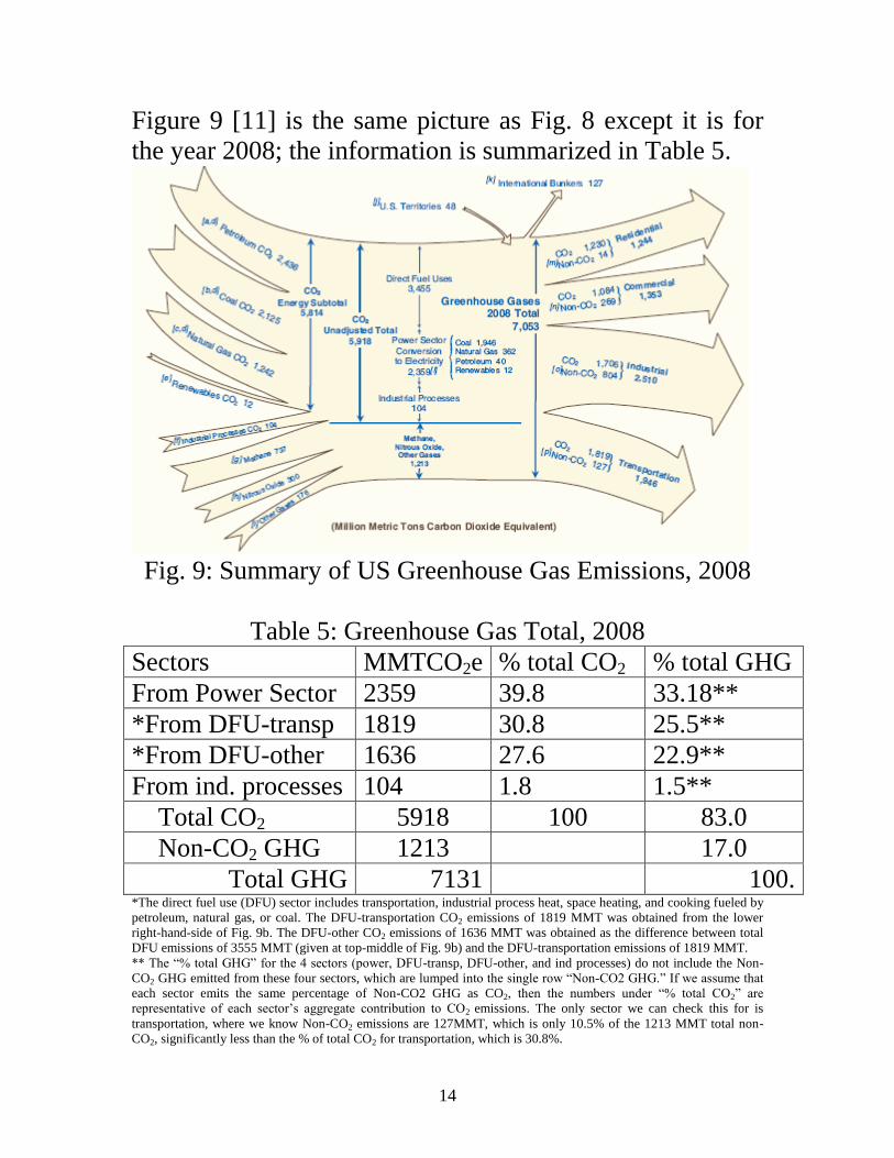
14
Figure 9 [11] is the same picture as Fig 8 except it is for
the year 2008 the information is summarized in Table 5
Fig 9 Summary of US Greenhouse Gas Emissions 2008
Table 5 Greenhouse Gas Total 2008
Sectors MMTCO2e total CO2 total GHG
From Power Sector 2359 398 3318
From DFU-transp 1819 308 255
From DFU-other 1636 276 229
From ind processes 104 18 15
Total CO2 5918 100 830
Non-CO2 GHG 1213 170
Total GHG 7131 100 The direct fuel use (DFU) sector includes transportation industrial process heat space heating and cooking fueled by
petroleum natural gas or coal The DFU-transportation CO2 emissions of 1819 MMT was obtained from the lower
right-hand-side of Fig 9b The DFU-other CO2 emissions of 1636 MMT was obtained as the difference between total
DFU emissions of 3555 MMT (given at top-middle of Fig 9b) and the DFU-transportation emissions of 1819 MMT
The ldquo total GHGrdquo for the 4 sectors (power DFU-transp DFU-other and ind processes) do not include the Non-
CO2 GHG emitted from these four sectors which are lumped into the single row ldquoNon-CO2 GHGrdquo If we assume that
each sector emits the same percentage of Non-CO2 GHG as CO2 then the numbers under ldquo total CO2rdquo are
representative of each sectorrsquos aggregate contribution to CO2 emissions The only sector we can check this for is
transportation where we know Non-CO2 emissions are 127MMT which is only 105 of the 1213 MMT total non-
CO2 significantly less than the of total CO2 for transportation which is 308
15
Some numbers to remember from Tables 4 and 5 are
Total US GHG emissions are about 7100 MMTyear
Of these about 83-84 are CO2
Percentage of GHG emissions from power sector is
about 40 (see note for Tables 4 and 5)
Percentage of GHG emissions from transportation sector
is about 31 (see note for Tables 4 and 5)
Total Power Sector + Transportation Sector emissions is
about 71 (see note for Tables 4 and 5)
50 CO2 Emissions ndash power sector
Figure 10 [11] shows that CO2 emissions from the electric
power sector have been generally rising from 1990 to 2008
but the fact that they are rising more slowly than power
sector sales suggests that emissions per unit of energy
consumed is decreasing Note that the emissions values
given in Fig 10 have been normalized by the value in the
year 2000 which was 22935 MMT
Fig 10 Electric power sector CO2 emissions by year
Figure 11 [6] provides another view of CO2 emissions by
fuel where it is clear that recently emissions from coal and
petroleum dropped whereas that from natural gas increased
16
Fig 11
Table 6 [11] shows the year-by-year breakdown of electric
power sector CO2 emissions by fuel We see the dominant
contributor is coal with natural gas a distant second
Table 6Yearly breakdown of electric sector CO2 emissions
Table 6 is for CO2 emissions only ndash it does not include
Non-CO2 emissions
Coal is the largest contributor to CO2 emissions For
example in year 2008 it contributed 19459 MMT 825
17
of the total power sector CO2 emissions The next highest
contributor was natural gas at 362 MMT which is 153
of the total The two combined account for 978 of power
sector CO2 emissions
Total CO2 emissions from gas are only 186 of Total CO2
emissions from coal This does NOT imply that
CO2 emissions per MWhr from a natural gas power plant
are 186 of the
CO2 emissions per MWhr from a coal-fired power
plant
The fact that coal is the largest contributor to GHG
emissions is due to
(a) it is used to produce just under half of US electricity
(b) it has the highest emissionsenergy content ratio as
indicated by Table 7 below [13]
(c) its average conversion efficiency is not very good
18
Table 7 Emission Coefficients for Different Fuels
Pounds CO2
per
Million Btu
Aviation Gasoline AV 18355 per gallon 152717
Distillate Fuel (No 1 No 2 No 4
Fuel Oil and Diesel) DF 22384 per gallon 161386
Jet Fuel JF 21095 per gallon 156258
Kerosene KS 21537 per gallon 159535
Liquified Petroleum Gases (LPG) LG 12805 per gallon 139039
Motor Gasoline MG 19564 per gallon 156425
Petroleum Coke PC 32397 per gallon 22513
Residual Fuel (No 5 and No 6
Fuel Oil) RF 26033 per gallon 173906
Methane ME 116376 per 1000 ft3 115258
Landfill Gas LF 1 per 1000 ft3 115258
Flare Gas FG 133759 per 1000 ft3 120721
Natural Gas (Pipeline) NG 120593 per 1000 ft3 11708
Propane PR 12669 per gallon 139178
Coal CL
Anthracite AC 5685 per short ton 2274
Bituminous BC 49313 per short ton 2053
Subbituminous SB 37159 per short ton 2127
Lignite LC 27916 per short ton 2154
Biomass BM
Geothermal Energy GE 0 0
Wind WN 0 0
Photovoltaic and Solar Thermal PV 0 0
Hydropower HY 0 0
TiresTire-Derived Fuel TF 6160 per short ton 189538
Wood and Wood Waste 2 WW 3812 per short ton 195
Municipal Solid Waste 2 MS 1999 per short ton 199854
Nuclear NU 0 0
Renewable Sources Varies depending on the composition of the biomass
Petroleum Products
Natural Gas and Other Gaseous Fuels
Fuel Code
Emission Coefficients
Pounds CO2 per Unit
Volume or Mass
One indication from Table 7 that the pounds CO2MBTU
is based on energy content of the fuel could be misleading
What is of more interest is the CO2MWhr obtained from
the fuel together with a particular generation technology
To get this we need efficiencies of the generation
technologies Fig 12 provides such efficiencies the
resource from which it came [14] provides a good overview
of various factors affecting generation efficiencies
19
0
10
20
30
40
50
60
70
80
90
100
Hyd
ro p
ower
plant
Tidal p
ower
plant
Larg
e ga
s fir
ed C
CGT p
ower
plant
Melte
d ca
rbon
ates
fuel cell (
MCFC
)
Pulve
rised
coa
l boilers
with
ultr
a-cr
itica
l ste
am p
aram
eter
s
Solid o
xide
fuel cell (
SOFC
)
Coa
l fire
d IG
CC
Atmos
pher
ic C
irculat
ing
Fluidised
Bed
Com
bustion
(CFB
C)
Press
urised
Flu
idised
Bed
Com
bustion
(PFB
C)
Larg
e ga
s tu
rbine
(MW
rang
e)
Steam
turb
ine
coal-fi
red
power
plant
Steam
turb
ine
fuel-o
il po
wer
plant
Wind
turb
ine
Nuc
lear
pow
er p
lant
Biom
ass an
d biog
as
Was
te-to
-electric
ity p
ower
plant
Diese
l eng
ine
as d
ecen
tralis
ed C
HP u
nit (
elec
trica
l sha
re)
Small a
nd m
icro
turb
ines
(up
to 1
00 kW
)
Photo
volta
ic cells
Geo
ther
mal p
ower
plant
Solar
pow
er to
wer
Eff
icie
nc
y (
)
Fig 12 Generation efficiencies
Table 7 and Fig 12 provide the ability to compare different
technologies in terms of CO2MWhr For example letrsquos
compare a natural gas combined cycle (NGCC) plant
(η=58) a gas turbine (η=39) and a coal-fired power plant
(η=39) where the CO2 content of the natural gas is 11708
lbsMBTU and the CO2 content of the coal assuming it
uses (Powder River Basin) sub-bituminous coal is 2127
lbsMBTU (Note that coal has a different energy amp CO2
content depending on type as shown below [15])
20
NGCC MWhrlbsMWhr
MBTU
MBTU
MBTU
MBTU
lbs
OUT
IN
IN
5688413
58
108117
Gas turbine
MWhrlbsMWhr
MBTU
MBTU
MBTU
MBTU
lbs
OUT
IN
IN
71023413
39
108117
Coal-fired plant
MWhrlbsMWhr
MBTU
MBTU
MBTU
MBTU
lbs
OUT
IN
IN
81859413
39
17212
Table 8 below from [16] indicates similar numbers for a
pulverized coal (PC) plant a circulating fluidized bed
(CFB) plant an integrated gasification combined cycle
(IGCC) plant and a combined cycle plant Note that the
fuels for the first three of these are all coal and they have
similar emissionsMWhr ratios The combined cycle plant
has a bit higher ratio (810 instead of 6885) because it used
a lower efficiency (493 instead of 58)
Table 8
21
In the calculations at the top of the previous page one can
recognize that the 341η factor in each equation is just the
unit heat rate in MBTUMWhr This means the same
calculation can be done by multiplying the lbsMBTUIN
factor from Table 7 by the average heat rate for the plant
We can also convert the above to Metric tonsMWhr by
dividing by 2204 lbsMetric ton to get the following
figures
NGCC 0464 MTMWhr
Gas turbine 0312 MTMWhr
Coal-fired plant 0844 MTMWhr
It is interesting to compare these values with the emission
coefficients given by regionstate at [17] A sample of some
of these coefficients are provided below (this is 2002 data)
New York 0389
Vermont 0013
Penn 0574
Ohio 0817
Iowa 0854
N Dakota 1017
Georgia 0619
Kentucky 0911
Texas 0664
California 0275
Washington 0111
US Average 0606
Why is Iowa so high
Why are NDakota amp Kentucky so high
Why is California so low
Why is Washington so low
Why is Vermont so low
22
Vermont is so low because it has only one small fossil-fired
unit (a diesel unit) and it is a peaker and so does not often
run [18] Almost 75 of Vermontrsquos electric energy comes
from a large nuclear facility (Vermont Yankee) and most of
the rest comes from outside the state via the ISO-NE
market Iowa was in 2002 heavily dependent on coal
Today with Iowarsquos wind growth it is less so but still coal
is by far the dominant part of Iowarsquos generation portfolio
60 Heat rates
The values of Table 1 (fuel cost table) reflect only the
cost of fuel input to a generation plant they do not
reflect the actual costs of producing electrical energy as
output from the plant because substantial losses occur
during production Some power plants have overall
efficiencies as low as 30 in addition the plant
efficiency varies as a function of the generation level Pg
We illustrate this point in what follows
We represent plant efficiency by η Then η=energy
outputenergy input We obtain η as a function of Pg by
measuring the energy output of the plant in MWhrs and
the energy input to the plant in MBTU
We could get the energy output by using a wattmeter to
obtain Pg over a given period of time say an hour and
we could get the energy input by measuring the coal
tonnage used during the hour and then multiplying by
the coal energy content in MBTUton
23
We could then plot the fuel input in MBTUhr as a
function of the power output Pg in MW Such a plot is
called an input-output curve indicating how much fuel
rate is required to produce a power level A typical
input-output curve is shown in Fig 13 We denote fuel
rate (input vertical axis of Fig 1a) as R (WampW denote
fuel rate as H ndash see p 8 )
One notes that the IO curve of Fig 13 does not go to
Pg=0 A generating unit has a minimum stable output
typically 10-30 for oil and natural gas-fired steam
units and 20-50 for coal-fired steam units [19]
Pg
Fuel rate
MBTUhr
R
OUTPUT
INPUT
Fig 13 Input-output curve
One interesting feature with respect to Fig 13 is that
as fuel input is increased the power output per unit
fuel input begins to decrease We can see this more
clearly if we invert the axes as in Fig 14 yielding a
production function where for high enough fuel
rates we will get no additional power output
24
Pg
Fuel rate
MBTUhr
R Fig 14 Production function
Physically this happens because the furnace boiler
steam pipes leak a larger percentage of input heat as
temperatures increase Economists call this the [20]
law of diminishing marginal product for almost all
processes the rate of increase in output decreases as
the input increases assuming other inputs are fixed
To obtain η we want the output energy divided by
the input energy which is
η ~ Pg divide R
which in terms of units is MW divide MBTUhr to give
units of MWhrMBTU Notice that these units are
energyenergy as they should be when computing η
However the MBTU and MWhr are different units of
energy and so we are not getting η exactly but we
are getting something proportional to η
So letrsquos obtain the ratio of the power to the fuel rate
25
(Pg divide R) for every point on the input-output curve
and plot the results against Pg Fig 15 shows a plot of
the ratio PgR (units of MWHRMBTU) versus Pg
Fig 15 Plot of MWhrMBTU vs Pg
Figure 15 indicates that efficiency is poor for low
generation levels (a connected plant that is operating
at zero MW output still has to supply station loads)
and increases with generation but at some optimum
level it begins to diminish Most power plants are
designed so that the optimum level is close to the
rated output
The heat rate curve is similar to Fig 15 except that
the y-axis is inverted to yield MBTUMWhrs which
is proportional to 1η This curve is illustrated in Fig
16 We denote heat rate by H (WampW use H for fuel
rate) Since the heat rate depends on operating point
we write H=H(Pg)
26
Fig 16 Plot of Heat Rate (H) vs Generation (Pg)
Some typical heat rates for units at maximum output
are (in MBTUMWhrs) 95-105 for fossil-steam
units and nuclear units 130-150 for combustion
turbines [21] and 70-95 for combined cycle units
Future combined cycle units may reach heat rates of
65-70 It is important to understand that the lower
the heat rate the more efficient the unit
An easy way to remember the meaning of heat rate
H=H(Pg) is it is the amount of input energy (MBTU)
required to produce a MWhr at generation level Pg
How does H relate to efficiency To answer this
question we need to know that there are 105485
joules per BTU
413
4133600
8510541
sec3600sec)(
)851054(
61
61~
1
HH
H
j
BTUjBTUH
Whr
BTU
E
EH
MWhr
MBTUH
27
Observe We have seen this before when we
computed CO2 emissions per MWhr out (see pg 20)
eg for the NGCC plant
MWhrlbsMWhr
MBTU
MBTU
MBTU
MBTU
lbs
OUT
IN
IN
5688413
58
108117
We can see now that the above calculation can be
thought of as
MWhrlbsMBTU
MBTU
MBTU
MBTU
MBTU
lbs
OUT
IN
OUT
IN
IN
5688413
58
41308117
or
MWhrlbsHMBTU
lbs
IN
568808117
where H in this case is 34158=588 MBTUMWhr
The heat rate curve is a fixed characteristic of the plant
although it can change if the cooling water temperature
changes significantly (and engineers may sometimes
employ seasonal heat rate curves) The heat rate curve
may also be influenced by the time between
maintenance periods as steam leakages and other heat
losses accumulate
The above use of the term ldquoheat raterdquo is sometimes also
called the ldquoaverage heat raterdquo This is because we get it
by dividing absolute values of fuel input rate by
absolute values of electric output power For example if
you buy an apple at $50 and a second one at $10 the
average cost of apples after buying the first apple is
$50apple but after buying the second apple is
$(50+10)2=$30apple
28
This is different than incremental heat rate as will be
illustrated in the following example
Example [22] Consider the input-output curve for
Plant X in Fig 17
Fig 17
Compute the average heat rate characteristic and the
incremental heat rate characteristic
Average heat rates are computed by dividing the fuel
rate by the generation level H=RPg as follows
Block 1 200001=20000
Block 2 240002=12000
Block 3 300003=10000
Incremental heat rates computed by dividing the
increment of fuel rate by the increment of power
IH=∆R∆Pg as follows
Block 1 200001=20000
Block 2 40001=4000
Block 3 60001=6000
These results are summarized in Table 9 below
29
Table 9
Figure 18 below illustrates the input-output curve the
average heat rate curve and the incremental heat rate
curve
Fig 18
We should note however that our first incremental
heat rate value of 20000 has a problem This value
assumes that the IO curve extends as shown on the
left hand side in Fig 19 below Probably a better
30
approximation would be to extend it as indicated on
the right hand side of Fig 19
Fig 19
Actually it does not extend to 0 MW output because
the unit like all real units has a minimum generation
level
Although you may see data entered which reflects a
ldquohigh initial incremental valuerdquo you should know
that a value so computed does not represent a true
incremental heat rate value at all
Reference [22] also provides some actual data for
units in California The one below Fig 20 is one of
the most efficient gas-fired units in the PGampE
system On the coast about 100 miles south of San
Francisco it is called Moss Landing Unit 7
31
Fig 20
Note that the Moss Landing unit 7 full-load average
heat rate is 8917 MBTUMWhr which gives an
efficiency of 3418917=382
The next one Fig 21 is an old oil-fired unit in San
Francisco called Hunterrsquos Point
32
Fig 21
Note the full-load average heat rate of this plant is
12598 MBTUMWhr which corresponds to an
efficiency of 34112598=271
This plant was built in 1927 and demolished in 2008
70 Cost rates
We are primarily interested in how the cost per
MWhr changes with Pg because that will tell us
something about how to achieve the most economic
dispatch of generation for a given demand (we will
see that optimality is achieved when marginal or
incremental costs of all regulating units are equal)
33
To get cost per MWhr as a function of Pg we will
assume that we know K the cost of the input fuel in
$MBTU Also recall that
R is the rate at which the plant uses fuel in
MBTUhr (which is dependent on Pg) ndash it is just
the input-output curve (see Fig 13)
And we will denote
C as the cost per hour in $hour
Then if H(Pg) the heat rate is the input energy used
per MW per hour then multiplying H by Pg gives
input energy per hour ie R=PgH(Pg) where H must
be evaluated at Pg Therefore C = RK = PgH(Pg)K
ie the cost rate function C is just the fuel rate
function R scaled by the fuel cost
A typical plot of C vs Pg is illustrated in Fig 22
Note that because H(Pg) is convex C(Pg) is also
convex ie the set of points lying on or above C
contain all line segments between any pair of points
Fig 22 Plot of cost per hr (C) vs generation (Pg)
34
Fig 22 shows that costhour increases with
generation a feature that one would expect since
higher generation levels require greater fuel intake
per hour
The incremental cost curve for the plant can be
obtained by differentiating the plot in Fig 22 ie by
computing dCdPg A typical incremental cost curve
is shown in Fig 23 Note that because C is convex
dCdPg is a non-decreasing function
Fig 23 Plot of incremental cost dCdPg vs gen Pg
One last thing about getting incremental cost
Recall that the cost per hour is given by
C = RK where R is just the input-output curve
Therefore IC=dCdPg=K(dRdPg) The derivative
is the incremental heat rate which we denoted by
IH Therefore in summary
C=RK=PgH(Pg)K
IC=dCdPg=(dRdPg)K=(IH)K
35
Example 1 An 100 MW coal-fired plant uses a type of coal
having an energy content of 12000 BTUlb The coal
cost is $15MMBTU Typical coal usage
corresponding to the daily loading schedule for the
plant is as follows
Table 10
Time of
Day
Electric
Output (MW)
Coal Used
(tons)
1200am-
600am
40 1050
600am-
1000am
70 945
1000am-
400pm
80 1560
400pm-
1200am
100 2700
For each of the four load levels find (a) the
efficiency η (b) the heat rate H (MMBTUMWhr)
(c) the cost per hour C ($hr) Also for the loading
levels of 40 70 and 80 MW use a piecewise linear
plot of C vs P to obtain incremental cost IC as a
function of unit loading P Then plot incremental cost
as a function of unit loading The conversion factor
from joules to BTU is 105485 joulesBTU and the
units for coal used tons are short-tons 2000 lbton
36
Solution Let T be the number of hours the plant is producing P
MW while using y tons of coal We need to compute
the total energy out of the plant and divide by the
total energy into the plant but we need both
numerator and denominator to be in the same units
We will convert both to joules (recall a watt is a
joulesec)
(a)
BTU
joules851054
lb
BTU00012
ton
lb2000 tons
hr
sec3600
MW
watts10hr MW 6
y
TP
Note that the above expression for efficiency is
dimensionless
(b) The heat rate is the amount of MMBTUs
used in the amount of time T divided by the
number of MW-hrs output in the amount of time
T
TP
y
H
BTU10
MMBTU1
lb
BTU00012
ton
lb2000 tons
6
37
Note that
413
851054
36001H and the above
expression has units of MMBTUMWhr Thus if a
unit is 100 efficient then it will have a heat rate
of 341 MMBTUMWhr the absolute best (lowest)
heat rate possible
(c) C = RK where R is the rate at which the plant
uses fuel and K is fuel cost in $MMBTU Note
from units of P and H that
R = PH C = PHK where H is a function of P
Application of these expressions for each load level
yields the following results
Table 11
T (hrs) P
(MW)
y
(tons)
η H
(mbtum
whr)
C
($hr)
6 40 1050 033 105 630
4 70 945 042 81 850
6 80 1560 044 78 936
8 100 2700 042 81 1215
To obtain incremental cost dP
dCIC we can plot C vs
P and then get an approximation on the derivative by
assuming a piecewise linear model as shown in
Figure 24
38
Figure 24 Calculation of Incremental Cost
The incremental costs are plotted as a function of
loading in Fig 25
20
4
2
6
8
10
40 60 80
12
IC ($MWhr)
Pg (MW)
Fig 25 Incremental cost curve from piecewise-linear
cost curve
39
We may use another procedure to model the
incremental costs In this procedure we first fit the
data to a quadratic polynomial Matlab commands for
doing so are below
gtgt p=[40 70 80 100]
gtgt c=[630 850 936 1215]
gtgt X = [ones(size(p)) p p^2]
gtgt a=Xc
a =
6048533
-29553
00903
gtgt T = (01100)
gtgt Y = [ones(size(T)) T T^2]a
gtgt plot(TY-tyo) grid on
The quadratic function is therefore
C(P)=00903P2-29553P+60485
Figure 26 shows the plot obtained from Matlab
40
Fig 26 Quadratic Curve Fit for Cost Rate Curve
Clearly the curve is inaccurate for very low values of
power (note it is above $605hr at P=0 and decreases
to about $590hr at P=10) We can get the
incremental cost curve by differentiating C(P)
IC(P)=01806P-29553
This curve is overlaid on the incremental cost curve
of Fig 25 resulting in Fig 27 Both linear and
discrete functions are approximate Although the
linear one appears more accurate in this case it
would be easy to improve accuracy of the discrete
one by taking points at smaller intervals of Pg Both
functions should be recognized as legitimate ways to
represent incremental costs The linear function is
often used in traditional economic dispatching the
discrete one is typical of market-based offers
41
20
4
2
6
8
10
40 60 80
12
14
Fig 27 Comparison of incremental cost curve
obtained from piecewise linear cost curve (solid line)
and from quadratic cost curve (dotted line)
80 Market-based offers
As indicated in the last section electricity markets
typically allow only piecewise linear representation
of generator incremental cost curves
The real-time and the day-ahead markets are implemented
via computer programs based on optimization theory The
program used for the real-time market is called the
security-constrained economic dispatch (SCED) This
program the SCED is used together with a program called
the security-constrained unit commitment (SCUC) program
for the day-ahead market Both the SCED and the SCUC
42
also solve for the ancillary service prices through a
formulation known as co-optimization We will say no
more about SCED and SCUC because we cannot assume
that students taking this course have the necessary
background on optimization theory Instead we will
provide a simple description of how the energy market
price is determined This description is based on standard
microeconomic theory but can be followed without
background in microeconomics However one should note
that the description necessarily omits some important
concepts related to losses and congestion
The following example is adapted from [23] Consider that
our electric energy market has three buyers B1 B2 B3 and
two sellers S1 S2 The buyers represent load-serving
entities and the sellers represent generation owners
Consider that these buyers and sellers submit their bids (to
buy) and their offers (to sell) via an internet system as
shown in Fig 28
Figure 28 Illustration of buyer-seller interaction with internet-based market
Each seller has energy to sell but the price they are willing
to sell it for increases with the amount they sell This is a
reflection of the fact that the cost of producing 1 more unit
of energy (MWhr) increases as a unit is loaded higher
Internet System
B1
B2
B3
S1
S2
43
Likewise each buyer wants to purchase energy but the
price they are willing to pay to obtain it decreases with the
amount that they buy This is just a reflection of the fact
that our first unit of energy will be used to supply our most
critical needs and after those needs are satisfied the next
units of energy will be used to satisfy less critical needs so
that we are unwilling to pay as much for it
Tabl2 illustrates a representative set of bids and offers
submitted by the buyers and sellers
Table 12 Offers and bids for examples
Offers to sell Bids to buy
S1 S2 B1 B2 B3
$1000 $1000 $7000 $7000 $2500
$5000 $5000 $7000 $5000 0
$6500 $7000 $6500 $2500 0
$7000 $7000 $6500 0 0
infin infin 0 0 0
infin infin 0 0 0
infin infin 0 0 0
Once each buyer and seller enters their data according to
Table 12 the internet system will reconstruct the
information according to Table 13 where
Table 13 Reconstructed offers and bids
Offerbid
order
Offers to sell 1 MWhr Bids to buy 1 MWhr
Seller Price Buyer Price
1 S1 $1000 B1 $7000
2 S2 $1000 B1 $7000
3 S1 $5000 B2 $7000
4 S2 $5000 B1 $6500
5 S1 $6500 B1 $6500
6 S2 $7000 B2 $5000
7 S1 $7000 B2 $2500
8 S2 $7000 B3 $2500
44
We can visualize the data in Table by plotting the price
against quantity for the offers and for the bids This
provides us with the supply and demand schedules of
Figure 29 [23]
Figure 29 Supply-demand schedules illustrating electricity market operation [23]
The point (or those points) where the supply schedule
intersects the demand schedule determines the market
clearing price This is the price that all sellers are paid to
supply their energy and it is the price that all buyers pay to
receive their energy In Figure this price is $65MWhr It is
the very best price to choose because it maximizes the total
ldquosatisfactionrdquo felt by the buyers and sellers
This satisfaction for the sellers can be measured by the
difference between the price they offered and the price they
were actually paid for the energy they supplied If we add
up all of these differences for all sellers then we obtain the
net seller surplus This satisfaction for the buyers can be
measured by the difference between the price they bid and
the price they actually had to pay for the energy they
45
received If we add up all of these differences for all sellers
then we obtain the net buyer surplus The net seller surplus
and the net buyer surplus are illustrated in Fig 30 [23]
Figure 30 Illustration of net seller and net buyer surplus [23]
The total net surplus is the sum of the buyer and seller net
surpluses The market clearing price is the price that
maximizes the total net surplus
In Fig 30 the quantity traded could be either 4 or 5
MWhrs but the 5th MWhr would neither increase nor
decrease the total net surplus The decision on whether to
trade 4 or 5 MWhrs in such as case is determined by market
rules
The example of this section illustrates the way electricity
markets would clear if there are no losses and if the
transmission capacity of each line was infinite One
conceptualization of such a situation is when all generators
and all loads are located at the same electric node In such a
case there is a single price by which all sellers are paid and
all buyers pay
46
In reality of course each transmission circuit does have
some resistance and therefore incurs some losses as current
flows through it and each transmission circuit also has an
upper bound for the amount of power that can flow across
it These two attributes losses and transmission limits
result in locational variation in prices throughout the
network which are called as we have already seen the
locational marginal prices (LMPs)
90 Effect of Valve Points in Fossil-Fired Units
Figures 22 and 24 well represent cost curves of small
steam power plants but actual cost curves of large
steam power plants differ in one important way from
the curves shown in Figs 22 and 24 ndash they are not
smooth The light curve of Fig 31 [24] more closely
captures the cost variation of a large steam power
plant
Fig 31 Cost rate curve for large steam power plant [24]
47
The reason for the discontinuities in the cost curve of
Fig 31 is because of multiple steam valves In this
case there are 5 different steam valves Large steam
power plants are operated so that valves are opened
sequentially ie power production is increased by
increasing the opening of only a single valve and the
next valve is not opened until the previous one is
fully opened So the discontinuities of Fig 31
represent where each valve is opened
The cost curve increases at a greater rate with power
production just as a valve is opened The reason for
this is that the so-called throttling losses due to
gaseous friction around the valve edges are greatest
just as the valve is opened and taper off as the valve
opening increases and the steam flow smoothens
The significance of this effect is that the actual cost
curve function of a large steam plant is not
continuous but even more important it is non-
convex A simple way (and the most common way)
to handle these two issues is to approximate the
actual curve with a smooth convex curve similar to
the dark line of Fig 31
48
100 Combined cycle units
The following information was developed from [21
25 26 27] The below figure shows recent US
growth in combined cycle power plants [28]
Fig x
Combined cycle units utilize both gas turbines (based
on the Brayton cycle) and steam turbines (based on
the Rankine cycle) Gas turbines are very similar to
jet engines where fuel (can be either liquid or gas)
mixed with compressed air is ignited The
combustion increases the temperature and volume of
the gas flow which when directed through a valve-
controlled nozzle over turbine blades spins the
turbine which drives a synchronous generator On the
49
other hand steam turbines utilize a fuel (coal natural
gas petroleum or uranium) to create heat which
when applied to a boiler transforms water into high
pressure superheated (above the temperature of
boiling water) steam The steam is directed through a
valve-controlled nozzle over turbine blades which
spins the turbine to drive a synchronous generator
A combined cycle power plant combines gas turbine
(also called combustion turbine) generator(s) with
turbine exhaust waste heat boiler(s) (also called heat
recovery steam generators or HRSG) and steam
turbine generator(s) for the production of electric
power The waste heat from the combustion
turbine(s) is fed into the boiler(s) and steam from the
boiler(s) is used to run steam turbine(s) Both the
combustion turbine(s) and the steam turbine(s)
produce electrical energy Generally the combustion
turbine(s) can be operated with or without the
boiler(s)
A combustion turbine is also referred to as a simple
cycle gas turbine generator They are relatively
inefficient with net heat rates at full load of some
plants at 15 MBtuMWhr as compared to the 90 to
105 MBtuMWhr heat rates typical of a large fossil
fuel fired utility generating station This fact
combined with what can be high natural gas prices
50
make the gas turbine expensive Yet they can ramp
up and down very quickly so as a result combustion
turbines have mainly been used only for peaking or
standby service
The gas turbine exhausts relatively large quantities of
gases at temperatures over 900 degF In combined cycle
operation then the exhaust gases from each gas
turbine will be ducted to a waste heat boiler The heat
in these gases ordinarily exhausted to the
atmosphere generates high pressure superheated
steam This steam will be piped to a steam turbine
generator The resulting combined cycle heat rate is
in the 70 to 95 MBtuMWhr range significantly less
than a simple cycle gas turbine generator
In addition to the good heat rates combined cycle
units have flexibility to utilize different fuels (natural
gas heavy fuel oil low Btu gas coal-derived gas)
[29] (In fact there are some advanced technologies
under development right now including the
integrated gasification combined cycle (IGCC) plant
which makes it possible to run combined cycle on
solid fuel (eg coal or biomass) [30] The first two
operational IGCC plants in the US were the Polk
Station Plant in Tampa and the Wabash River Plant
in Indiana [31] The Ratcliffe-Kemper plant
currently under construction by Mississippi Power (a
51
subsidiary of Southern Company) is a 582 MW
IGCC plant to be completed in 2014 [32 33])
The flexibility of combined cycle plants together
with the fast ramp rates of the combustion turbines
and relatively low heat rates has made the combined
cycle unit the unit of choice for a large percentage of
recent new power plant installations The potential
for increased gas supply and lowered gas prices has
further stimulated this tendency
Fig 32 shows the simplest kind of combined cycle
arrangement where there is one combustion turbine
and one HRSG driving a steam turbine
ChillerCooler
Inlet Air
Gas Supply
Duct firing
HRSG
Condenser
CTG STG
Fig 32 A 1 times 1 configuration
An additional level of complexity would have two
combustion turbines (CT A and B) and their HRSGs
driving one steam turbine generator (STG) as shown
in Fig 33
52
ChillerCooler
Inlet Air
Gas Supply
Duct firing
HRSG
ChillerCooler
Inlet Air
Gas Supply
Duct firing
HRSG
Condenser
CTG
CTG STG
Fig 33 a 2 times 1 configuration
In such a design the following six combinations are
possible
CT A alone
CT B alone
CT A and CT B together
CT A and STG
CT B and STG
CT A and B and STG
The modes with the STG are more efficient than the
modes without the STG (since the STG utilizes CT
exhaust heat that is otherwise wasted) with the last
mode listed being the most efficient
If we model a combined cycle plant as a single plant
we run into a problem Consider the transition
between the combined cycle power plant operation
53
just as the STG is ramped up Previous to STG start-
up only the CT is generating with a specified
amount of fuel per hour being consumed as a
function of the CT power generation level Then
after STG start-up the fuel input remains almost
constant but the MW output of the (now) two
generation units has increased by the amount of
power produced by the steam turbine driven by the
STG A typical cost curve for this situation is shown
in Fig 34
C ($hr)
PG (MW)
Fig 34 Cost curve for a combined cycle plant
An important feature of the curve in Fig 34 is that it
is not convex which means its slope (ie its
incremental cost) does not monotonically increase
with PG Figure 35 illustrates incremental cost
variation with PG
54
dCdPG ($MWhr)
PG (MW)
Fig 35 Incremental cost curve for a combined cycle plant
The key attribute of the incremental cost curve in
order to satisfy convexity is that it must be non-
decreasing Clearly the curve of Fig 35 does not
satisfy this requirement
110 Economic dispatch and convexity of objective
functions in optimization
The traditional economic dispatch (ED) approach
used by electric utilities for many years is very well
described in [34]
This approach is still used directly by owners of
multiple generation facilities when they make one
offer to the market and then need to dispatch their
units in the most economic fashion to deliver on this
offer This approach also provides one way to view
the method by which locational marginal prices are
computed in most of todayrsquos real-time market
systems
The simplest form of the ED problem is as follows
55
Minimize
n
i
iiT PFF1
(1)
Subject to
0)(11
N
i
iloadiload
n
i
i PPPPP (2)
0max
minmin
i
ii
iiii
PPP
PPPP
(3)
Here we note that the equality constraint is linear in
the decision variables Pi In the Newton approach to
solving this problem ([34]) we form the Lagrangian
according to
)()( iiT PPF L (4)
If each and every individual cost curve Ci(Pi) i=1n
is quadratic then they are all convex Because the
sum of convex functions is also a convex function
when all cost curves are convex then the objective
function FT(Pi) of the above problem is also convex
If φ(Pi) is linear then it is convex and therefore L is
convex This fact allows us to find the solution by
applying first order conditions
56
First order conditions for multi-variable calculus are
precisely analogous to first order conditions to single
variable calculus In single variable calculus we
minimize f(x) by solving frsquo(x)=0 on the condition
that f(x) is convex or equivalently that frsquorsquo(x)gt0
In multivariable calculus where x=[x1 x2hellip xn]T we
minimize f(x) by solving frsquo(x)=0 that is
nix
f
i
1 0
(5)
on the condition that f(x) is convex or equivalently
that the Hessian matrix frsquorsquo(x) is positive definite
We recall that in single variable calculus if f(x) is
not convex then the first order conditions do not
guarantee that we find a global minimum We could
find a maximum or a local minimum or an inflection
point as illustrated in Fig 36 below
f(x)
x x
f(x)
Fig 36 Non-convex functions
57
The situation is the same in the multivariable case
ie if f(x) is not convex then the first order
conditions of (5) do not guarantee a global minimum
Now returning to the Lagrangian function of our
constrained optimization problem repeated here for
convenience
)()( iiT PPF L (4)
we recall that solution to the original problem is
found by minimizing FT But to use what we now
know we are only guaranteed to find a global
minimum of F if L is convex In this case the first
order conditions results in
0
1 0
L
LNi
Pi
from which we may find our solution (Inequality
constraints may be handled by checking the resulting
solution against them and for any violation setting
up another equality constraint which binds the given
decision variable to the limit which was violated)
But if one of the units is a combined cycle unit the
FT and therefore L will not be convex So first
58
order conditions do not guarantee a global minimum
In other words there may be a lower-cost solution
than the one we will obtain from applying first order
conditions This makes engineers and managers
concerned because they worry they are spending
money unnecessarily
120 General solutions for non-convex
optimization problems
Generation owners who utilize combined cycle units
must use special techniques to solve the EDC
problem Some general methods that have been
proposed for solving non-convex optimization
problems are below However I am not aware that
any of these techniques have been implemented
within an electricity market today
1 EnumerationIteration In this method all possible
solutions are enumerated and evaluated and then the
lowest cost solution is identified This method will
always work but can be quite computational
2 Dynamic programming See pp 51-54 of reference
[21]
59
3 Sequential unconstrained minimization technique
(SUMT) This method is described on pp 473-477 of
reference [35]
4 Heuristic optimization methods There are a
number of methods in this class including Genetic
Algorithm simulated annealing tabu search and
particle swarm A good reference on these methods is
[36]
5 There is a matlab toolbox for handling non-convex
optimization It provides 2 different algorithms
together with references on papers that describe the
algorithms located at httptomlabbiz There are
two methods provided
(a) Radial Basis Function (RBF) interpolation
(b) Efficient Global Optimization (EGO) algorithm
The idea of the EGO algorithm is to first fit a
response surface to data collected by evaluating the
objective function at a few points Then EGO
balances between finding the minimum of the surface
and improving the approximation by sampling where
the prediction error may be high
130 Practical solutions to modeling combined
cycle units in optimization
60
Reference [37] developed by engineers at ERCOT and
Ventyx (now ABB) is an excellent summary of practical
methods to modeling combined cycle units It provides
references to a number of other good resources on the
subject The methods it outlines are as follows
Aggregate modeling Here the combined cycle unit is
simply modeled with a ldquobest-fitrdquo convex cost curve This
approach does not handle the non-convexity of the actual
cost characteristic
Pseudo-unit modeling Here a number of pseudo-units
equal to N the number of combustion turbines are
represented each with 1N of the steam unit This works
for an Ntimes1 combined cycle unit For example a 3 times 1
combined cycle unit would be modeled as three separate
pseudo-units each of the three pseudo-units would be
one gas turbine plus one third of a steam turbine [38]
This approach has been implemented within several
markets including ISO NE NYISO MISO PJM and
IESO This approach does not handle the non-convexity
of the actual cost characteristic
Configuration-based modeling This approach is also
referred to as psuedo-plant modeling Here a cost-curve
(or incremental cost curve) is provided for each
configuration of the combined cycle plant Additional
logic is provided in the security-constrained unit
commitment (SCUC which is the mixed integer
programming software for the day-ahead market) to
ensure that only one configuration can be selected and
that the selection depends on the configuration of the
previous time period as illustrated in Fig 37 below for a
2times1 combined cycle plant [37] The configuration
61
chosen by SCUC for any one hour is maintained for the
entire hour in the real-time market CAISO has
implemented this approach it is well-described in [38]
Fig 37
Physical-unit modeling Here each CT and STG is
considered to be an individual resource with its own
individual offers This is a bad market model but it
provides good fidelity in terms of MW that the power
plant can actually produce ERCOT reports in [38] that it
utilizes configuration-based models for its markets and
physical unit modeling for its network security
applications
References [1] J McCalley W Jewell T Mount D Osborn and J Fleeman ldquoA wider horizon Technologies Tools
and Procedures for Energy System Planning at the National Levelrdquo IEEE Power and Energy Magazine
MayJune 2011
[2] J Morgan ldquoEnergy Density and Waste Comparison of Energy Productionrdquo Nuclear Science and
Technology June 2010 available at httpnuclearfissionarycom20100609energy-density-and-waste-
comparison-of-energy-production
[3] The World Nuclear Association ldquoThe Economics of Nuclear Powerrdquo available at httpwwwworld-
nuclearorginfoinf02html
[4] US Department of Energy Energy Information Administration website located at
httpwwweiagovcneafelectricityepmepmxlfile4_1xls and
httpwwweiadoegovcneafelectricityepmepmxlfile4_1_contxls
[5] US Department of Energy Energy Information Administration website located at
httpwwweiadoegovemeuaertxtptb0811bhtml
[6] ldquoEnergy perspectives 2011 US Department of Energy Energy Information Administration website
httpwwweiagovtotalenergydataannualpdfperspectives_2011pdf
62
[7] North American Reliability Corporation (NERC) ldquo2011 Long Term Reliability Assessmentrdquo
November 2011 available at wwwnerccom
[8] US Department of Energy Energy Information Administration website located at
httpwwweiadoegovoiafaeocoalhtml
[9] Wikipedia page on ldquoGreenhouse gasrdquo httpenwikipediaorgwikiCarbon_emissions
[10] US Department of Energy Energy Information Administration ldquoEmissions of Greenhouse Gases in
the United States 2006rdquo November 2007 available at httpwwweiadoegovoiaf1605ggrptindexhtml
[11] US Department of Energy Energy Information Administration ldquoEmissions of Greenhouse Gases in
the United States 2008rdquo December 2009 available at httpwwweiadoegovoiaf1605ggrptindexhtml
[12] wwweiadoegovoiaf16051605aoldhtml
[13] DOE EIA Data from Voluntary Reporting of Greenhouse Gasses Program available at
httpwwweiadoegovoiaf1605coefficientshtml
[14] F Van Aart ldquoEnergy efficiency in power plantsrdquo October 21 Vienna available from Dr McCalley
(see ldquoNew Generationrdquo folder) but you must make request
[15] EPA report wwwepagovairmarktprogsregsepa-ipmdocschapter8-v2_1-updatepdf
[16] Black amp Veatch ldquoPlanning for Growing Electric Generation Demandsrdquo slides from a presentation to
Kansas Energy Council ndash Electric Subcommittee March 12 2008 available at
httpwwwgooglecomsearchhl=enampsource=hpampq=22Planning+for+Growing+Electric+Generation+D
emands22ampbtnG=Google+Searchampaq=fampaqi=ampaql=ampoq=ampgs_rfai=C5Ekv4uV7TP7ECIzmNJHV_MIE
AAAAqgQFT9Dr5Lw
[17] DOE EIA Website for US locations emission coefficients httpwwweiadoegovoiaf1605ee-
factorshtml
[18] wwwrutlandheraldcomappspbcsdllarticleAID=20080706NEWS048070604571024NEWS04
[19]H Stoll ldquoLeast-cost electric utility planningrdquo 1989 John Wiley
[20] D Kirschen and G Strbac ldquoFundamentals of Power System Economicsrdquo Wiley 2004
[21] A J Wood and B F Wollenberg Power Generation Operation and Control second edition John
Wiley amp Sons New York NY 1996
[22] J Klein ldquoThe Use of Heat Rates in Production Cost Modeling and Market Modelingrdquo California
Energy Commission Report 1998
[23] L Tesfatsion ldquoAuction Basics for Wholesale Power Markets Objectives and Pricing Rulesrdquo
Proceedings of the 2009 IEEE Power and Energy Society General Meeting July 2009
[24] J Kim D Shin J Park and C Singh ldquoAtavistic genetic algorithm for economic dispatch with valve
point effectrdquo Electric Power Systems Research 62 2002 pp 201-207
[25] ldquoElectric power plant designrdquo chapter 8 publication number TM 5-811-6 Office of the Chief of
Engineers United States Army January 20 1984 located at
httpwwwusacearmymilpublicationsarmytmtm5-811-6 not under copyright
[26] A Cohen and G Ostrowski ldquoScheduling units with multiple operating modes in unit commitmentrdquo
IEEE 1995
[27] A Birch M Smith and C Ozveren ldquoScheduling CCGTs in the Electricity Poolrdquo in ldquoOpportunities
and Advances in International Power Generation March 1996
[28] 2011 State of the Markets a FERC presentation April 2012 at httpswwwfercgovmarket-
oversightreports-analysesst-mkt-ovrsom-rpt-2011pdf
[29] R Tawney K Kamali W Yeager ldquoImpact of different fuels on reheat and nonreheat combined cycle
plant performancerdquo Proceedings of the American Power Conference VolIssue 50 American power
conference 18-20 Apr 1988 Chicago IL (USA)
[30] I Burdon ldquoWinning combination [integrated gasification combined-cycle process]rdquo IEE Review
Volume 52 Issue 2 2006 pp 32 ndash 36 IET Journals amp Magazines
[31] wwwfossilenergygovprogramspowersystemsgasificationgasificationpioneerhtml
[32] ldquoSouthern Company on track with new generationrdquo Investopedia March 23 2011 available at
httpwwwinvestopediacomstock-analysis2011southern-company-on-track-with-new-generation-so-d-
duk0323aspxaxzz28iY0dqaR
[33] wwwsoutherncompanycomsmart_energysmart_power_vogtle-kemperhtml
[34] G Sheble and J McCalley ldquoModule E3 Economic dispatch calculationrdquo used in EE 303 at Iowa
State University
[35] F Hillier and G Lieberman ldquoIntroduction to Operations Researchrdquo fourth edition Holden-Day 1986
63
[36] ldquoTutorial on modern Heuristic Optimization Techniques with Applications to Power Systemsrdquo IEEE
PES Special Publication 02TP160 edited by K Lee and M El-Sharkawi 2002
[37] H Hui C Yu F Gao and R Surendran ldquoCombined cycle resource scheduling in ERCOT nodal
marketrdquo Proc of the 2011 IEEE PES General Meeting 2011
[38]ldquoModeling of Multi-Stage Generating Unitsrdquo CAISO Available at
wwwcaisocom23582358e27f11070pdf
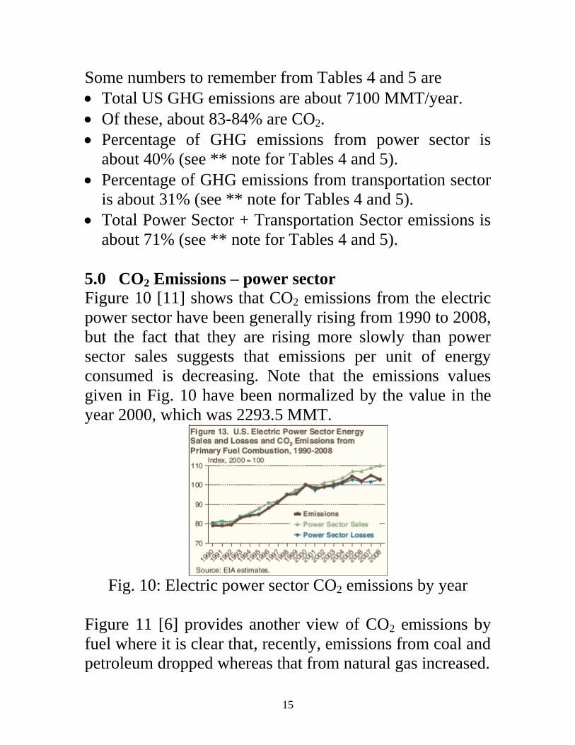
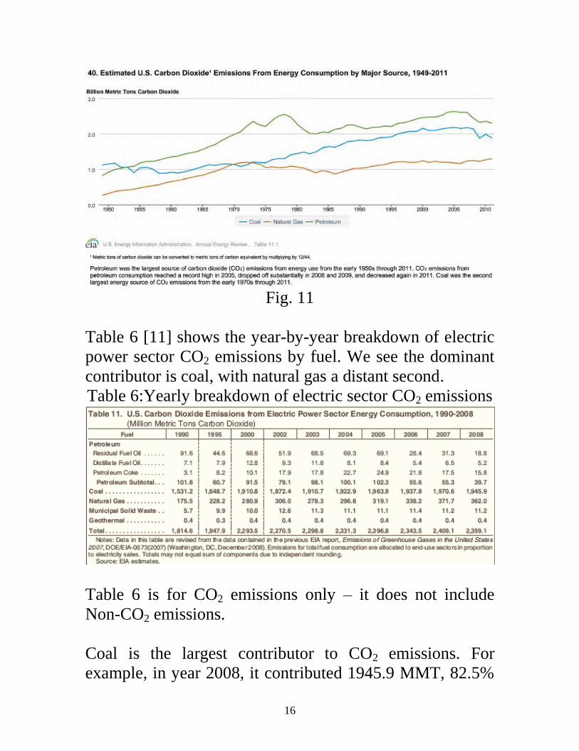
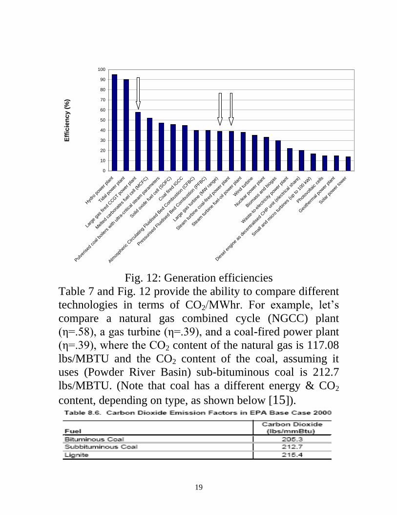
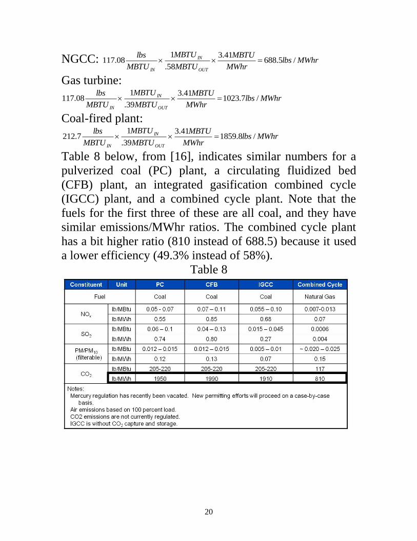
20
NGCC MWhrlbsMWhr
MBTU
MBTU
MBTU
MBTU
lbs
OUT
IN
IN
5688413
58
108117
Gas turbine
MWhrlbsMWhr
MBTU
MBTU
MBTU
MBTU
lbs
OUT
IN
IN
71023413
39
108117
Coal-fired plant
MWhrlbsMWhr
MBTU
MBTU
MBTU
MBTU
lbs
OUT
IN
IN
81859413
39
17212
Table 8 below from [16] indicates similar numbers for a
pulverized coal (PC) plant a circulating fluidized bed
(CFB) plant an integrated gasification combined cycle
(IGCC) plant and a combined cycle plant Note that the
fuels for the first three of these are all coal and they have
similar emissionsMWhr ratios The combined cycle plant
has a bit higher ratio (810 instead of 6885) because it used
a lower efficiency (493 instead of 58)
Table 8
21
In the calculations at the top of the previous page one can
recognize that the 341η factor in each equation is just the
unit heat rate in MBTUMWhr This means the same
calculation can be done by multiplying the lbsMBTUIN
factor from Table 7 by the average heat rate for the plant
We can also convert the above to Metric tonsMWhr by
dividing by 2204 lbsMetric ton to get the following
figures
NGCC 0464 MTMWhr
Gas turbine 0312 MTMWhr
Coal-fired plant 0844 MTMWhr
It is interesting to compare these values with the emission
coefficients given by regionstate at [17] A sample of some
of these coefficients are provided below (this is 2002 data)
New York 0389
Vermont 0013
Penn 0574
Ohio 0817
Iowa 0854
N Dakota 1017
Georgia 0619
Kentucky 0911
Texas 0664
California 0275
Washington 0111
US Average 0606
Why is Iowa so high
Why are NDakota amp Kentucky so high
Why is California so low
Why is Washington so low
Why is Vermont so low
22
Vermont is so low because it has only one small fossil-fired
unit (a diesel unit) and it is a peaker and so does not often
run [18] Almost 75 of Vermontrsquos electric energy comes
from a large nuclear facility (Vermont Yankee) and most of
the rest comes from outside the state via the ISO-NE
market Iowa was in 2002 heavily dependent on coal
Today with Iowarsquos wind growth it is less so but still coal
is by far the dominant part of Iowarsquos generation portfolio
60 Heat rates
The values of Table 1 (fuel cost table) reflect only the
cost of fuel input to a generation plant they do not
reflect the actual costs of producing electrical energy as
output from the plant because substantial losses occur
during production Some power plants have overall
efficiencies as low as 30 in addition the plant
efficiency varies as a function of the generation level Pg
We illustrate this point in what follows
We represent plant efficiency by η Then η=energy
outputenergy input We obtain η as a function of Pg by
measuring the energy output of the plant in MWhrs and
the energy input to the plant in MBTU
We could get the energy output by using a wattmeter to
obtain Pg over a given period of time say an hour and
we could get the energy input by measuring the coal
tonnage used during the hour and then multiplying by
the coal energy content in MBTUton
23
We could then plot the fuel input in MBTUhr as a
function of the power output Pg in MW Such a plot is
called an input-output curve indicating how much fuel
rate is required to produce a power level A typical
input-output curve is shown in Fig 13 We denote fuel
rate (input vertical axis of Fig 1a) as R (WampW denote
fuel rate as H ndash see p 8 )
One notes that the IO curve of Fig 13 does not go to
Pg=0 A generating unit has a minimum stable output
typically 10-30 for oil and natural gas-fired steam
units and 20-50 for coal-fired steam units [19]
Pg
Fuel rate
MBTUhr
R
OUTPUT
INPUT
Fig 13 Input-output curve
One interesting feature with respect to Fig 13 is that
as fuel input is increased the power output per unit
fuel input begins to decrease We can see this more
clearly if we invert the axes as in Fig 14 yielding a
production function where for high enough fuel
rates we will get no additional power output
24
Pg
Fuel rate
MBTUhr
R Fig 14 Production function
Physically this happens because the furnace boiler
steam pipes leak a larger percentage of input heat as
temperatures increase Economists call this the [20]
law of diminishing marginal product for almost all
processes the rate of increase in output decreases as
the input increases assuming other inputs are fixed
To obtain η we want the output energy divided by
the input energy which is
η ~ Pg divide R
which in terms of units is MW divide MBTUhr to give
units of MWhrMBTU Notice that these units are
energyenergy as they should be when computing η
However the MBTU and MWhr are different units of
energy and so we are not getting η exactly but we
are getting something proportional to η
So letrsquos obtain the ratio of the power to the fuel rate
25
(Pg divide R) for every point on the input-output curve
and plot the results against Pg Fig 15 shows a plot of
the ratio PgR (units of MWHRMBTU) versus Pg
Fig 15 Plot of MWhrMBTU vs Pg
Figure 15 indicates that efficiency is poor for low
generation levels (a connected plant that is operating
at zero MW output still has to supply station loads)
and increases with generation but at some optimum
level it begins to diminish Most power plants are
designed so that the optimum level is close to the
rated output
The heat rate curve is similar to Fig 15 except that
the y-axis is inverted to yield MBTUMWhrs which
is proportional to 1η This curve is illustrated in Fig
16 We denote heat rate by H (WampW use H for fuel
rate) Since the heat rate depends on operating point
we write H=H(Pg)
26
Fig 16 Plot of Heat Rate (H) vs Generation (Pg)
Some typical heat rates for units at maximum output
are (in MBTUMWhrs) 95-105 for fossil-steam
units and nuclear units 130-150 for combustion
turbines [21] and 70-95 for combined cycle units
Future combined cycle units may reach heat rates of
65-70 It is important to understand that the lower
the heat rate the more efficient the unit
An easy way to remember the meaning of heat rate
H=H(Pg) is it is the amount of input energy (MBTU)
required to produce a MWhr at generation level Pg
How does H relate to efficiency To answer this
question we need to know that there are 105485
joules per BTU
413
4133600
8510541
sec3600sec)(
)851054(
61
61~
1
HH
H
j
BTUjBTUH
Whr
BTU
E
EH
MWhr
MBTUH
27
Observe We have seen this before when we
computed CO2 emissions per MWhr out (see pg 20)
eg for the NGCC plant
MWhrlbsMWhr
MBTU
MBTU
MBTU
MBTU
lbs
OUT
IN
IN
5688413
58
108117
We can see now that the above calculation can be
thought of as
MWhrlbsMBTU
MBTU
MBTU
MBTU
MBTU
lbs
OUT
IN
OUT
IN
IN
5688413
58
41308117
or
MWhrlbsHMBTU
lbs
IN
568808117
where H in this case is 34158=588 MBTUMWhr
The heat rate curve is a fixed characteristic of the plant
although it can change if the cooling water temperature
changes significantly (and engineers may sometimes
employ seasonal heat rate curves) The heat rate curve
may also be influenced by the time between
maintenance periods as steam leakages and other heat
losses accumulate
The above use of the term ldquoheat raterdquo is sometimes also
called the ldquoaverage heat raterdquo This is because we get it
by dividing absolute values of fuel input rate by
absolute values of electric output power For example if
you buy an apple at $50 and a second one at $10 the
average cost of apples after buying the first apple is
$50apple but after buying the second apple is
$(50+10)2=$30apple
28
This is different than incremental heat rate as will be
illustrated in the following example
Example [22] Consider the input-output curve for
Plant X in Fig 17
Fig 17
Compute the average heat rate characteristic and the
incremental heat rate characteristic
Average heat rates are computed by dividing the fuel
rate by the generation level H=RPg as follows
Block 1 200001=20000
Block 2 240002=12000
Block 3 300003=10000
Incremental heat rates computed by dividing the
increment of fuel rate by the increment of power
IH=∆R∆Pg as follows
Block 1 200001=20000
Block 2 40001=4000
Block 3 60001=6000
These results are summarized in Table 9 below
29
Table 9
Figure 18 below illustrates the input-output curve the
average heat rate curve and the incremental heat rate
curve
Fig 18
We should note however that our first incremental
heat rate value of 20000 has a problem This value
assumes that the IO curve extends as shown on the
left hand side in Fig 19 below Probably a better
30
approximation would be to extend it as indicated on
the right hand side of Fig 19
Fig 19
Actually it does not extend to 0 MW output because
the unit like all real units has a minimum generation
level
Although you may see data entered which reflects a
ldquohigh initial incremental valuerdquo you should know
that a value so computed does not represent a true
incremental heat rate value at all
Reference [22] also provides some actual data for
units in California The one below Fig 20 is one of
the most efficient gas-fired units in the PGampE
system On the coast about 100 miles south of San
Francisco it is called Moss Landing Unit 7
31
Fig 20
Note that the Moss Landing unit 7 full-load average
heat rate is 8917 MBTUMWhr which gives an
efficiency of 3418917=382
The next one Fig 21 is an old oil-fired unit in San
Francisco called Hunterrsquos Point
32
Fig 21
Note the full-load average heat rate of this plant is
12598 MBTUMWhr which corresponds to an
efficiency of 34112598=271
This plant was built in 1927 and demolished in 2008
70 Cost rates
We are primarily interested in how the cost per
MWhr changes with Pg because that will tell us
something about how to achieve the most economic
dispatch of generation for a given demand (we will
see that optimality is achieved when marginal or
incremental costs of all regulating units are equal)
33
To get cost per MWhr as a function of Pg we will
assume that we know K the cost of the input fuel in
$MBTU Also recall that
R is the rate at which the plant uses fuel in
MBTUhr (which is dependent on Pg) ndash it is just
the input-output curve (see Fig 13)
And we will denote
C as the cost per hour in $hour
Then if H(Pg) the heat rate is the input energy used
per MW per hour then multiplying H by Pg gives
input energy per hour ie R=PgH(Pg) where H must
be evaluated at Pg Therefore C = RK = PgH(Pg)K
ie the cost rate function C is just the fuel rate
function R scaled by the fuel cost
A typical plot of C vs Pg is illustrated in Fig 22
Note that because H(Pg) is convex C(Pg) is also
convex ie the set of points lying on or above C
contain all line segments between any pair of points
Fig 22 Plot of cost per hr (C) vs generation (Pg)
34
Fig 22 shows that costhour increases with
generation a feature that one would expect since
higher generation levels require greater fuel intake
per hour
The incremental cost curve for the plant can be
obtained by differentiating the plot in Fig 22 ie by
computing dCdPg A typical incremental cost curve
is shown in Fig 23 Note that because C is convex
dCdPg is a non-decreasing function
Fig 23 Plot of incremental cost dCdPg vs gen Pg
One last thing about getting incremental cost
Recall that the cost per hour is given by
C = RK where R is just the input-output curve
Therefore IC=dCdPg=K(dRdPg) The derivative
is the incremental heat rate which we denoted by
IH Therefore in summary
C=RK=PgH(Pg)K
IC=dCdPg=(dRdPg)K=(IH)K
35
Example 1 An 100 MW coal-fired plant uses a type of coal
having an energy content of 12000 BTUlb The coal
cost is $15MMBTU Typical coal usage
corresponding to the daily loading schedule for the
plant is as follows
Table 10
Time of
Day
Electric
Output (MW)
Coal Used
(tons)
1200am-
600am
40 1050
600am-
1000am
70 945
1000am-
400pm
80 1560
400pm-
1200am
100 2700
For each of the four load levels find (a) the
efficiency η (b) the heat rate H (MMBTUMWhr)
(c) the cost per hour C ($hr) Also for the loading
levels of 40 70 and 80 MW use a piecewise linear
plot of C vs P to obtain incremental cost IC as a
function of unit loading P Then plot incremental cost
as a function of unit loading The conversion factor
from joules to BTU is 105485 joulesBTU and the
units for coal used tons are short-tons 2000 lbton
36
Solution Let T be the number of hours the plant is producing P
MW while using y tons of coal We need to compute
the total energy out of the plant and divide by the
total energy into the plant but we need both
numerator and denominator to be in the same units
We will convert both to joules (recall a watt is a
joulesec)
(a)
BTU
joules851054
lb
BTU00012
ton
lb2000 tons
hr
sec3600
MW
watts10hr MW 6
y
TP
Note that the above expression for efficiency is
dimensionless
(b) The heat rate is the amount of MMBTUs
used in the amount of time T divided by the
number of MW-hrs output in the amount of time
T
TP
y
H
BTU10
MMBTU1
lb
BTU00012
ton
lb2000 tons
6
37
Note that
413
851054
36001H and the above
expression has units of MMBTUMWhr Thus if a
unit is 100 efficient then it will have a heat rate
of 341 MMBTUMWhr the absolute best (lowest)
heat rate possible
(c) C = RK where R is the rate at which the plant
uses fuel and K is fuel cost in $MMBTU Note
from units of P and H that
R = PH C = PHK where H is a function of P
Application of these expressions for each load level
yields the following results
Table 11
T (hrs) P
(MW)
y
(tons)
η H
(mbtum
whr)
C
($hr)
6 40 1050 033 105 630
4 70 945 042 81 850
6 80 1560 044 78 936
8 100 2700 042 81 1215
To obtain incremental cost dP
dCIC we can plot C vs
P and then get an approximation on the derivative by
assuming a piecewise linear model as shown in
Figure 24
38
Figure 24 Calculation of Incremental Cost
The incremental costs are plotted as a function of
loading in Fig 25
20
4
2
6
8
10
40 60 80
12
IC ($MWhr)
Pg (MW)
Fig 25 Incremental cost curve from piecewise-linear
cost curve
39
We may use another procedure to model the
incremental costs In this procedure we first fit the
data to a quadratic polynomial Matlab commands for
doing so are below
gtgt p=[40 70 80 100]
gtgt c=[630 850 936 1215]
gtgt X = [ones(size(p)) p p^2]
gtgt a=Xc
a =
6048533
-29553
00903
gtgt T = (01100)
gtgt Y = [ones(size(T)) T T^2]a
gtgt plot(TY-tyo) grid on
The quadratic function is therefore
C(P)=00903P2-29553P+60485
Figure 26 shows the plot obtained from Matlab
40
Fig 26 Quadratic Curve Fit for Cost Rate Curve
Clearly the curve is inaccurate for very low values of
power (note it is above $605hr at P=0 and decreases
to about $590hr at P=10) We can get the
incremental cost curve by differentiating C(P)
IC(P)=01806P-29553
This curve is overlaid on the incremental cost curve
of Fig 25 resulting in Fig 27 Both linear and
discrete functions are approximate Although the
linear one appears more accurate in this case it
would be easy to improve accuracy of the discrete
one by taking points at smaller intervals of Pg Both
functions should be recognized as legitimate ways to
represent incremental costs The linear function is
often used in traditional economic dispatching the
discrete one is typical of market-based offers
41
20
4
2
6
8
10
40 60 80
12
14
Fig 27 Comparison of incremental cost curve
obtained from piecewise linear cost curve (solid line)
and from quadratic cost curve (dotted line)
80 Market-based offers
As indicated in the last section electricity markets
typically allow only piecewise linear representation
of generator incremental cost curves
The real-time and the day-ahead markets are implemented
via computer programs based on optimization theory The
program used for the real-time market is called the
security-constrained economic dispatch (SCED) This
program the SCED is used together with a program called
the security-constrained unit commitment (SCUC) program
for the day-ahead market Both the SCED and the SCUC
42
also solve for the ancillary service prices through a
formulation known as co-optimization We will say no
more about SCED and SCUC because we cannot assume
that students taking this course have the necessary
background on optimization theory Instead we will
provide a simple description of how the energy market
price is determined This description is based on standard
microeconomic theory but can be followed without
background in microeconomics However one should note
that the description necessarily omits some important
concepts related to losses and congestion
The following example is adapted from [23] Consider that
our electric energy market has three buyers B1 B2 B3 and
two sellers S1 S2 The buyers represent load-serving
entities and the sellers represent generation owners
Consider that these buyers and sellers submit their bids (to
buy) and their offers (to sell) via an internet system as
shown in Fig 28
Figure 28 Illustration of buyer-seller interaction with internet-based market
Each seller has energy to sell but the price they are willing
to sell it for increases with the amount they sell This is a
reflection of the fact that the cost of producing 1 more unit
of energy (MWhr) increases as a unit is loaded higher
Internet System
B1
B2
B3
S1
S2
43
Likewise each buyer wants to purchase energy but the
price they are willing to pay to obtain it decreases with the
amount that they buy This is just a reflection of the fact
that our first unit of energy will be used to supply our most
critical needs and after those needs are satisfied the next
units of energy will be used to satisfy less critical needs so
that we are unwilling to pay as much for it
Tabl2 illustrates a representative set of bids and offers
submitted by the buyers and sellers
Table 12 Offers and bids for examples
Offers to sell Bids to buy
S1 S2 B1 B2 B3
$1000 $1000 $7000 $7000 $2500
$5000 $5000 $7000 $5000 0
$6500 $7000 $6500 $2500 0
$7000 $7000 $6500 0 0
infin infin 0 0 0
infin infin 0 0 0
infin infin 0 0 0
Once each buyer and seller enters their data according to
Table 12 the internet system will reconstruct the
information according to Table 13 where
Table 13 Reconstructed offers and bids
Offerbid
order
Offers to sell 1 MWhr Bids to buy 1 MWhr
Seller Price Buyer Price
1 S1 $1000 B1 $7000
2 S2 $1000 B1 $7000
3 S1 $5000 B2 $7000
4 S2 $5000 B1 $6500
5 S1 $6500 B1 $6500
6 S2 $7000 B2 $5000
7 S1 $7000 B2 $2500
8 S2 $7000 B3 $2500
44
We can visualize the data in Table by plotting the price
against quantity for the offers and for the bids This
provides us with the supply and demand schedules of
Figure 29 [23]
Figure 29 Supply-demand schedules illustrating electricity market operation [23]
The point (or those points) where the supply schedule
intersects the demand schedule determines the market
clearing price This is the price that all sellers are paid to
supply their energy and it is the price that all buyers pay to
receive their energy In Figure this price is $65MWhr It is
the very best price to choose because it maximizes the total
ldquosatisfactionrdquo felt by the buyers and sellers
This satisfaction for the sellers can be measured by the
difference between the price they offered and the price they
were actually paid for the energy they supplied If we add
up all of these differences for all sellers then we obtain the
net seller surplus This satisfaction for the buyers can be
measured by the difference between the price they bid and
the price they actually had to pay for the energy they
45
received If we add up all of these differences for all sellers
then we obtain the net buyer surplus The net seller surplus
and the net buyer surplus are illustrated in Fig 30 [23]
Figure 30 Illustration of net seller and net buyer surplus [23]
The total net surplus is the sum of the buyer and seller net
surpluses The market clearing price is the price that
maximizes the total net surplus
In Fig 30 the quantity traded could be either 4 or 5
MWhrs but the 5th MWhr would neither increase nor
decrease the total net surplus The decision on whether to
trade 4 or 5 MWhrs in such as case is determined by market
rules
The example of this section illustrates the way electricity
markets would clear if there are no losses and if the
transmission capacity of each line was infinite One
conceptualization of such a situation is when all generators
and all loads are located at the same electric node In such a
case there is a single price by which all sellers are paid and
all buyers pay
46
In reality of course each transmission circuit does have
some resistance and therefore incurs some losses as current
flows through it and each transmission circuit also has an
upper bound for the amount of power that can flow across
it These two attributes losses and transmission limits
result in locational variation in prices throughout the
network which are called as we have already seen the
locational marginal prices (LMPs)
90 Effect of Valve Points in Fossil-Fired Units
Figures 22 and 24 well represent cost curves of small
steam power plants but actual cost curves of large
steam power plants differ in one important way from
the curves shown in Figs 22 and 24 ndash they are not
smooth The light curve of Fig 31 [24] more closely
captures the cost variation of a large steam power
plant
Fig 31 Cost rate curve for large steam power plant [24]
47
The reason for the discontinuities in the cost curve of
Fig 31 is because of multiple steam valves In this
case there are 5 different steam valves Large steam
power plants are operated so that valves are opened
sequentially ie power production is increased by
increasing the opening of only a single valve and the
next valve is not opened until the previous one is
fully opened So the discontinuities of Fig 31
represent where each valve is opened
The cost curve increases at a greater rate with power
production just as a valve is opened The reason for
this is that the so-called throttling losses due to
gaseous friction around the valve edges are greatest
just as the valve is opened and taper off as the valve
opening increases and the steam flow smoothens
The significance of this effect is that the actual cost
curve function of a large steam plant is not
continuous but even more important it is non-
convex A simple way (and the most common way)
to handle these two issues is to approximate the
actual curve with a smooth convex curve similar to
the dark line of Fig 31
48
100 Combined cycle units
The following information was developed from [21
25 26 27] The below figure shows recent US
growth in combined cycle power plants [28]
Fig x
Combined cycle units utilize both gas turbines (based
on the Brayton cycle) and steam turbines (based on
the Rankine cycle) Gas turbines are very similar to
jet engines where fuel (can be either liquid or gas)
mixed with compressed air is ignited The
combustion increases the temperature and volume of
the gas flow which when directed through a valve-
controlled nozzle over turbine blades spins the
turbine which drives a synchronous generator On the
49
other hand steam turbines utilize a fuel (coal natural
gas petroleum or uranium) to create heat which
when applied to a boiler transforms water into high
pressure superheated (above the temperature of
boiling water) steam The steam is directed through a
valve-controlled nozzle over turbine blades which
spins the turbine to drive a synchronous generator
A combined cycle power plant combines gas turbine
(also called combustion turbine) generator(s) with
turbine exhaust waste heat boiler(s) (also called heat
recovery steam generators or HRSG) and steam
turbine generator(s) for the production of electric
power The waste heat from the combustion
turbine(s) is fed into the boiler(s) and steam from the
boiler(s) is used to run steam turbine(s) Both the
combustion turbine(s) and the steam turbine(s)
produce electrical energy Generally the combustion
turbine(s) can be operated with or without the
boiler(s)
A combustion turbine is also referred to as a simple
cycle gas turbine generator They are relatively
inefficient with net heat rates at full load of some
plants at 15 MBtuMWhr as compared to the 90 to
105 MBtuMWhr heat rates typical of a large fossil
fuel fired utility generating station This fact
combined with what can be high natural gas prices
50
make the gas turbine expensive Yet they can ramp
up and down very quickly so as a result combustion
turbines have mainly been used only for peaking or
standby service
The gas turbine exhausts relatively large quantities of
gases at temperatures over 900 degF In combined cycle
operation then the exhaust gases from each gas
turbine will be ducted to a waste heat boiler The heat
in these gases ordinarily exhausted to the
atmosphere generates high pressure superheated
steam This steam will be piped to a steam turbine
generator The resulting combined cycle heat rate is
in the 70 to 95 MBtuMWhr range significantly less
than a simple cycle gas turbine generator
In addition to the good heat rates combined cycle
units have flexibility to utilize different fuels (natural
gas heavy fuel oil low Btu gas coal-derived gas)
[29] (In fact there are some advanced technologies
under development right now including the
integrated gasification combined cycle (IGCC) plant
which makes it possible to run combined cycle on
solid fuel (eg coal or biomass) [30] The first two
operational IGCC plants in the US were the Polk
Station Plant in Tampa and the Wabash River Plant
in Indiana [31] The Ratcliffe-Kemper plant
currently under construction by Mississippi Power (a
51
subsidiary of Southern Company) is a 582 MW
IGCC plant to be completed in 2014 [32 33])
The flexibility of combined cycle plants together
with the fast ramp rates of the combustion turbines
and relatively low heat rates has made the combined
cycle unit the unit of choice for a large percentage of
recent new power plant installations The potential
for increased gas supply and lowered gas prices has
further stimulated this tendency
Fig 32 shows the simplest kind of combined cycle
arrangement where there is one combustion turbine
and one HRSG driving a steam turbine
ChillerCooler
Inlet Air
Gas Supply
Duct firing
HRSG
Condenser
CTG STG
Fig 32 A 1 times 1 configuration
An additional level of complexity would have two
combustion turbines (CT A and B) and their HRSGs
driving one steam turbine generator (STG) as shown
in Fig 33
52
ChillerCooler
Inlet Air
Gas Supply
Duct firing
HRSG
ChillerCooler
Inlet Air
Gas Supply
Duct firing
HRSG
Condenser
CTG
CTG STG
Fig 33 a 2 times 1 configuration
In such a design the following six combinations are
possible
CT A alone
CT B alone
CT A and CT B together
CT A and STG
CT B and STG
CT A and B and STG
The modes with the STG are more efficient than the
modes without the STG (since the STG utilizes CT
exhaust heat that is otherwise wasted) with the last
mode listed being the most efficient
If we model a combined cycle plant as a single plant
we run into a problem Consider the transition
between the combined cycle power plant operation
53
just as the STG is ramped up Previous to STG start-
up only the CT is generating with a specified
amount of fuel per hour being consumed as a
function of the CT power generation level Then
after STG start-up the fuel input remains almost
constant but the MW output of the (now) two
generation units has increased by the amount of
power produced by the steam turbine driven by the
STG A typical cost curve for this situation is shown
in Fig 34
C ($hr)
PG (MW)
Fig 34 Cost curve for a combined cycle plant
An important feature of the curve in Fig 34 is that it
is not convex which means its slope (ie its
incremental cost) does not monotonically increase
with PG Figure 35 illustrates incremental cost
variation with PG
54
dCdPG ($MWhr)
PG (MW)
Fig 35 Incremental cost curve for a combined cycle plant
The key attribute of the incremental cost curve in
order to satisfy convexity is that it must be non-
decreasing Clearly the curve of Fig 35 does not
satisfy this requirement
110 Economic dispatch and convexity of objective
functions in optimization
The traditional economic dispatch (ED) approach
used by electric utilities for many years is very well
described in [34]
This approach is still used directly by owners of
multiple generation facilities when they make one
offer to the market and then need to dispatch their
units in the most economic fashion to deliver on this
offer This approach also provides one way to view
the method by which locational marginal prices are
computed in most of todayrsquos real-time market
systems
The simplest form of the ED problem is as follows
55
Minimize
n
i
iiT PFF1
(1)
Subject to
0)(11
N
i
iloadiload
n
i
i PPPPP (2)
0max
minmin
i
ii
iiii
PPP
PPPP
(3)
Here we note that the equality constraint is linear in
the decision variables Pi In the Newton approach to
solving this problem ([34]) we form the Lagrangian
according to
)()( iiT PPF L (4)
If each and every individual cost curve Ci(Pi) i=1n
is quadratic then they are all convex Because the
sum of convex functions is also a convex function
when all cost curves are convex then the objective
function FT(Pi) of the above problem is also convex
If φ(Pi) is linear then it is convex and therefore L is
convex This fact allows us to find the solution by
applying first order conditions
56
First order conditions for multi-variable calculus are
precisely analogous to first order conditions to single
variable calculus In single variable calculus we
minimize f(x) by solving frsquo(x)=0 on the condition
that f(x) is convex or equivalently that frsquorsquo(x)gt0
In multivariable calculus where x=[x1 x2hellip xn]T we
minimize f(x) by solving frsquo(x)=0 that is
nix
f
i
1 0
(5)
on the condition that f(x) is convex or equivalently
that the Hessian matrix frsquorsquo(x) is positive definite
We recall that in single variable calculus if f(x) is
not convex then the first order conditions do not
guarantee that we find a global minimum We could
find a maximum or a local minimum or an inflection
point as illustrated in Fig 36 below
f(x)
x x
f(x)
Fig 36 Non-convex functions
57
The situation is the same in the multivariable case
ie if f(x) is not convex then the first order
conditions of (5) do not guarantee a global minimum
Now returning to the Lagrangian function of our
constrained optimization problem repeated here for
convenience
)()( iiT PPF L (4)
we recall that solution to the original problem is
found by minimizing FT But to use what we now
know we are only guaranteed to find a global
minimum of F if L is convex In this case the first
order conditions results in
0
1 0
L
LNi
Pi
from which we may find our solution (Inequality
constraints may be handled by checking the resulting
solution against them and for any violation setting
up another equality constraint which binds the given
decision variable to the limit which was violated)
But if one of the units is a combined cycle unit the
FT and therefore L will not be convex So first
58
order conditions do not guarantee a global minimum
In other words there may be a lower-cost solution
than the one we will obtain from applying first order
conditions This makes engineers and managers
concerned because they worry they are spending
money unnecessarily
120 General solutions for non-convex
optimization problems
Generation owners who utilize combined cycle units
must use special techniques to solve the EDC
problem Some general methods that have been
proposed for solving non-convex optimization
problems are below However I am not aware that
any of these techniques have been implemented
within an electricity market today
1 EnumerationIteration In this method all possible
solutions are enumerated and evaluated and then the
lowest cost solution is identified This method will
always work but can be quite computational
2 Dynamic programming See pp 51-54 of reference
[21]
59
3 Sequential unconstrained minimization technique
(SUMT) This method is described on pp 473-477 of
reference [35]
4 Heuristic optimization methods There are a
number of methods in this class including Genetic
Algorithm simulated annealing tabu search and
particle swarm A good reference on these methods is
[36]
5 There is a matlab toolbox for handling non-convex
optimization It provides 2 different algorithms
together with references on papers that describe the
algorithms located at httptomlabbiz There are
two methods provided
(a) Radial Basis Function (RBF) interpolation
(b) Efficient Global Optimization (EGO) algorithm
The idea of the EGO algorithm is to first fit a
response surface to data collected by evaluating the
objective function at a few points Then EGO
balances between finding the minimum of the surface
and improving the approximation by sampling where
the prediction error may be high
130 Practical solutions to modeling combined
cycle units in optimization
60
Reference [37] developed by engineers at ERCOT and
Ventyx (now ABB) is an excellent summary of practical
methods to modeling combined cycle units It provides
references to a number of other good resources on the
subject The methods it outlines are as follows
Aggregate modeling Here the combined cycle unit is
simply modeled with a ldquobest-fitrdquo convex cost curve This
approach does not handle the non-convexity of the actual
cost characteristic
Pseudo-unit modeling Here a number of pseudo-units
equal to N the number of combustion turbines are
represented each with 1N of the steam unit This works
for an Ntimes1 combined cycle unit For example a 3 times 1
combined cycle unit would be modeled as three separate
pseudo-units each of the three pseudo-units would be
one gas turbine plus one third of a steam turbine [38]
This approach has been implemented within several
markets including ISO NE NYISO MISO PJM and
IESO This approach does not handle the non-convexity
of the actual cost characteristic
Configuration-based modeling This approach is also
referred to as psuedo-plant modeling Here a cost-curve
(or incremental cost curve) is provided for each
configuration of the combined cycle plant Additional
logic is provided in the security-constrained unit
commitment (SCUC which is the mixed integer
programming software for the day-ahead market) to
ensure that only one configuration can be selected and
that the selection depends on the configuration of the
previous time period as illustrated in Fig 37 below for a
2times1 combined cycle plant [37] The configuration
61
chosen by SCUC for any one hour is maintained for the
entire hour in the real-time market CAISO has
implemented this approach it is well-described in [38]
Fig 37
Physical-unit modeling Here each CT and STG is
considered to be an individual resource with its own
individual offers This is a bad market model but it
provides good fidelity in terms of MW that the power
plant can actually produce ERCOT reports in [38] that it
utilizes configuration-based models for its markets and
physical unit modeling for its network security
applications
References [1] J McCalley W Jewell T Mount D Osborn and J Fleeman ldquoA wider horizon Technologies Tools
and Procedures for Energy System Planning at the National Levelrdquo IEEE Power and Energy Magazine
MayJune 2011
[2] J Morgan ldquoEnergy Density and Waste Comparison of Energy Productionrdquo Nuclear Science and
Technology June 2010 available at httpnuclearfissionarycom20100609energy-density-and-waste-
comparison-of-energy-production
[3] The World Nuclear Association ldquoThe Economics of Nuclear Powerrdquo available at httpwwwworld-
nuclearorginfoinf02html
[4] US Department of Energy Energy Information Administration website located at
httpwwweiagovcneafelectricityepmepmxlfile4_1xls and
httpwwweiadoegovcneafelectricityepmepmxlfile4_1_contxls
[5] US Department of Energy Energy Information Administration website located at
httpwwweiadoegovemeuaertxtptb0811bhtml
[6] ldquoEnergy perspectives 2011 US Department of Energy Energy Information Administration website
httpwwweiagovtotalenergydataannualpdfperspectives_2011pdf
62
[7] North American Reliability Corporation (NERC) ldquo2011 Long Term Reliability Assessmentrdquo
November 2011 available at wwwnerccom
[8] US Department of Energy Energy Information Administration website located at
httpwwweiadoegovoiafaeocoalhtml
[9] Wikipedia page on ldquoGreenhouse gasrdquo httpenwikipediaorgwikiCarbon_emissions
[10] US Department of Energy Energy Information Administration ldquoEmissions of Greenhouse Gases in
the United States 2006rdquo November 2007 available at httpwwweiadoegovoiaf1605ggrptindexhtml
[11] US Department of Energy Energy Information Administration ldquoEmissions of Greenhouse Gases in
the United States 2008rdquo December 2009 available at httpwwweiadoegovoiaf1605ggrptindexhtml
[12] wwweiadoegovoiaf16051605aoldhtml
[13] DOE EIA Data from Voluntary Reporting of Greenhouse Gasses Program available at
httpwwweiadoegovoiaf1605coefficientshtml
[14] F Van Aart ldquoEnergy efficiency in power plantsrdquo October 21 Vienna available from Dr McCalley
(see ldquoNew Generationrdquo folder) but you must make request
[15] EPA report wwwepagovairmarktprogsregsepa-ipmdocschapter8-v2_1-updatepdf
[16] Black amp Veatch ldquoPlanning for Growing Electric Generation Demandsrdquo slides from a presentation to
Kansas Energy Council ndash Electric Subcommittee March 12 2008 available at
httpwwwgooglecomsearchhl=enampsource=hpampq=22Planning+for+Growing+Electric+Generation+D
emands22ampbtnG=Google+Searchampaq=fampaqi=ampaql=ampoq=ampgs_rfai=C5Ekv4uV7TP7ECIzmNJHV_MIE
AAAAqgQFT9Dr5Lw
[17] DOE EIA Website for US locations emission coefficients httpwwweiadoegovoiaf1605ee-
factorshtml
[18] wwwrutlandheraldcomappspbcsdllarticleAID=20080706NEWS048070604571024NEWS04
[19]H Stoll ldquoLeast-cost electric utility planningrdquo 1989 John Wiley
[20] D Kirschen and G Strbac ldquoFundamentals of Power System Economicsrdquo Wiley 2004
[21] A J Wood and B F Wollenberg Power Generation Operation and Control second edition John
Wiley amp Sons New York NY 1996
[22] J Klein ldquoThe Use of Heat Rates in Production Cost Modeling and Market Modelingrdquo California
Energy Commission Report 1998
[23] L Tesfatsion ldquoAuction Basics for Wholesale Power Markets Objectives and Pricing Rulesrdquo
Proceedings of the 2009 IEEE Power and Energy Society General Meeting July 2009
[24] J Kim D Shin J Park and C Singh ldquoAtavistic genetic algorithm for economic dispatch with valve
point effectrdquo Electric Power Systems Research 62 2002 pp 201-207
[25] ldquoElectric power plant designrdquo chapter 8 publication number TM 5-811-6 Office of the Chief of
Engineers United States Army January 20 1984 located at
httpwwwusacearmymilpublicationsarmytmtm5-811-6 not under copyright
[26] A Cohen and G Ostrowski ldquoScheduling units with multiple operating modes in unit commitmentrdquo
IEEE 1995
[27] A Birch M Smith and C Ozveren ldquoScheduling CCGTs in the Electricity Poolrdquo in ldquoOpportunities
and Advances in International Power Generation March 1996
[28] 2011 State of the Markets a FERC presentation April 2012 at httpswwwfercgovmarket-
oversightreports-analysesst-mkt-ovrsom-rpt-2011pdf
[29] R Tawney K Kamali W Yeager ldquoImpact of different fuels on reheat and nonreheat combined cycle
plant performancerdquo Proceedings of the American Power Conference VolIssue 50 American power
conference 18-20 Apr 1988 Chicago IL (USA)
[30] I Burdon ldquoWinning combination [integrated gasification combined-cycle process]rdquo IEE Review
Volume 52 Issue 2 2006 pp 32 ndash 36 IET Journals amp Magazines
[31] wwwfossilenergygovprogramspowersystemsgasificationgasificationpioneerhtml
[32] ldquoSouthern Company on track with new generationrdquo Investopedia March 23 2011 available at
httpwwwinvestopediacomstock-analysis2011southern-company-on-track-with-new-generation-so-d-
duk0323aspxaxzz28iY0dqaR
[33] wwwsoutherncompanycomsmart_energysmart_power_vogtle-kemperhtml
[34] G Sheble and J McCalley ldquoModule E3 Economic dispatch calculationrdquo used in EE 303 at Iowa
State University
[35] F Hillier and G Lieberman ldquoIntroduction to Operations Researchrdquo fourth edition Holden-Day 1986
63
[36] ldquoTutorial on modern Heuristic Optimization Techniques with Applications to Power Systemsrdquo IEEE
PES Special Publication 02TP160 edited by K Lee and M El-Sharkawi 2002
[37] H Hui C Yu F Gao and R Surendran ldquoCombined cycle resource scheduling in ERCOT nodal
marketrdquo Proc of the 2011 IEEE PES General Meeting 2011
[38]ldquoModeling of Multi-Stage Generating Unitsrdquo CAISO Available at
wwwcaisocom23582358e27f11070pdf
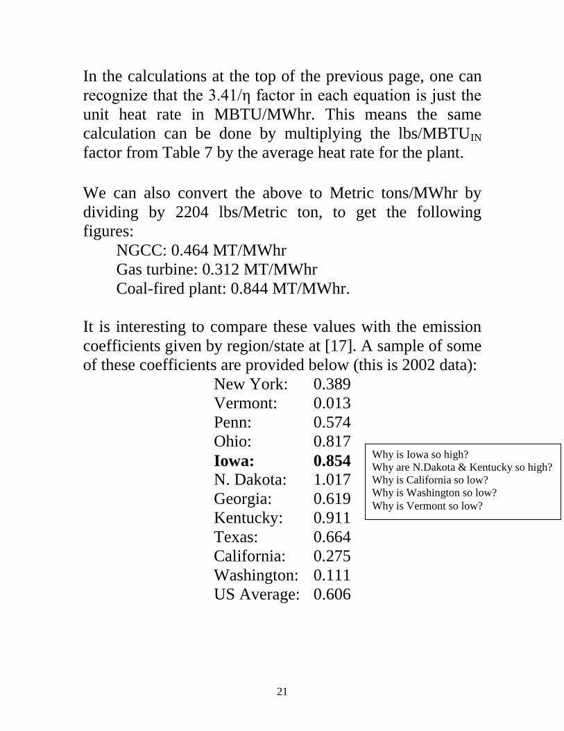
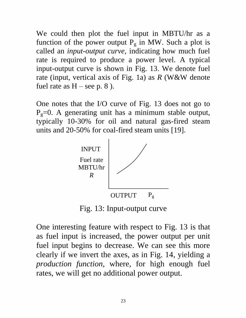
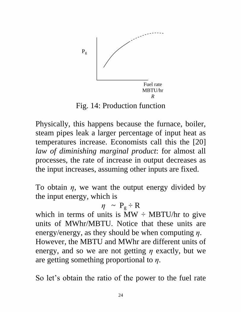
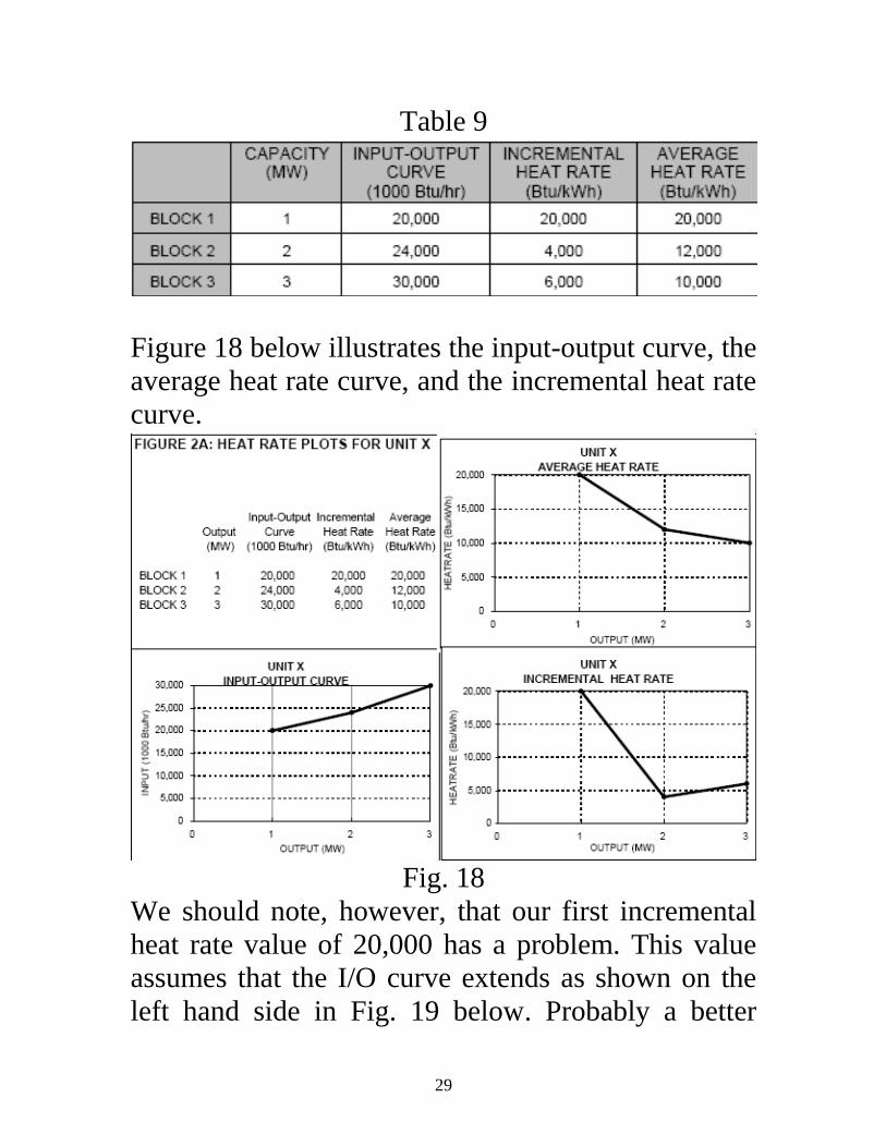
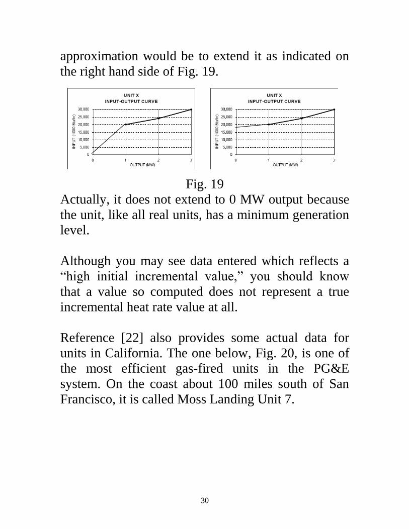
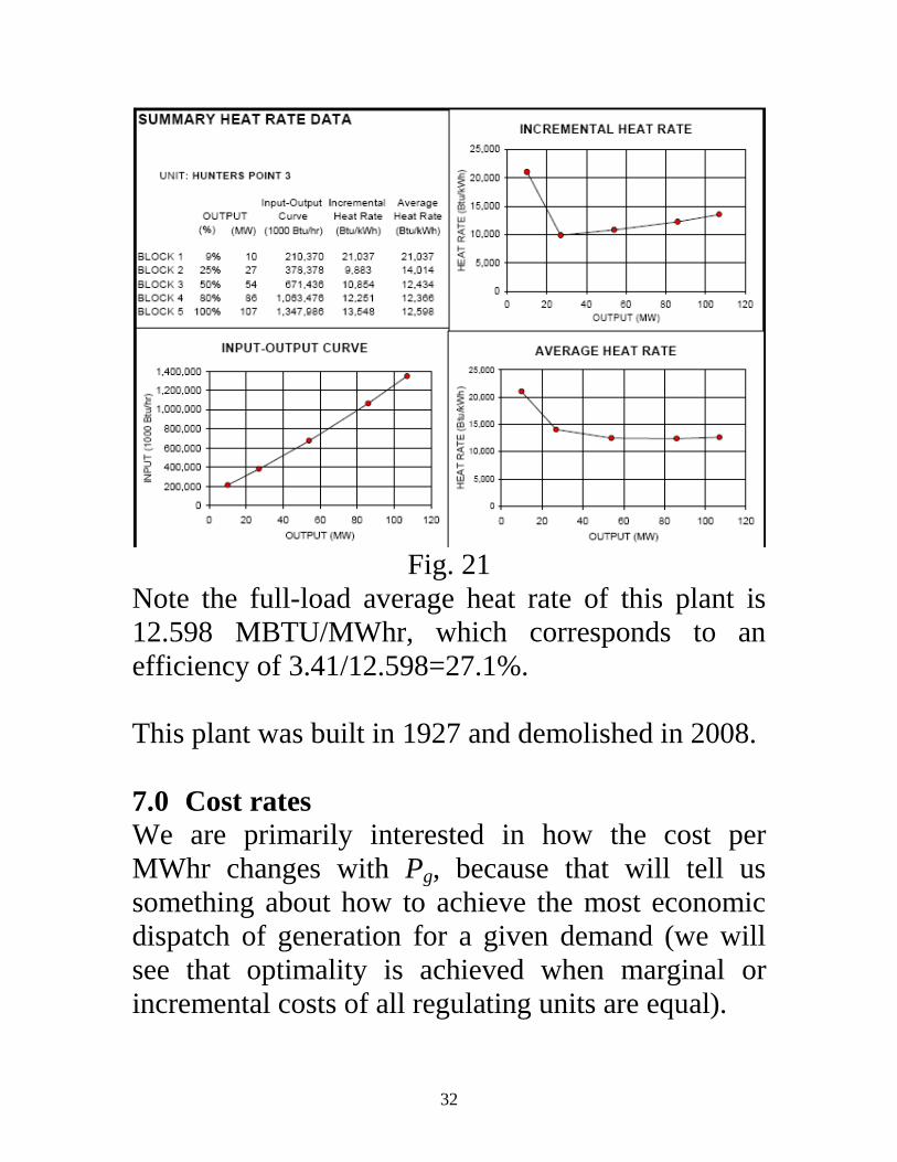
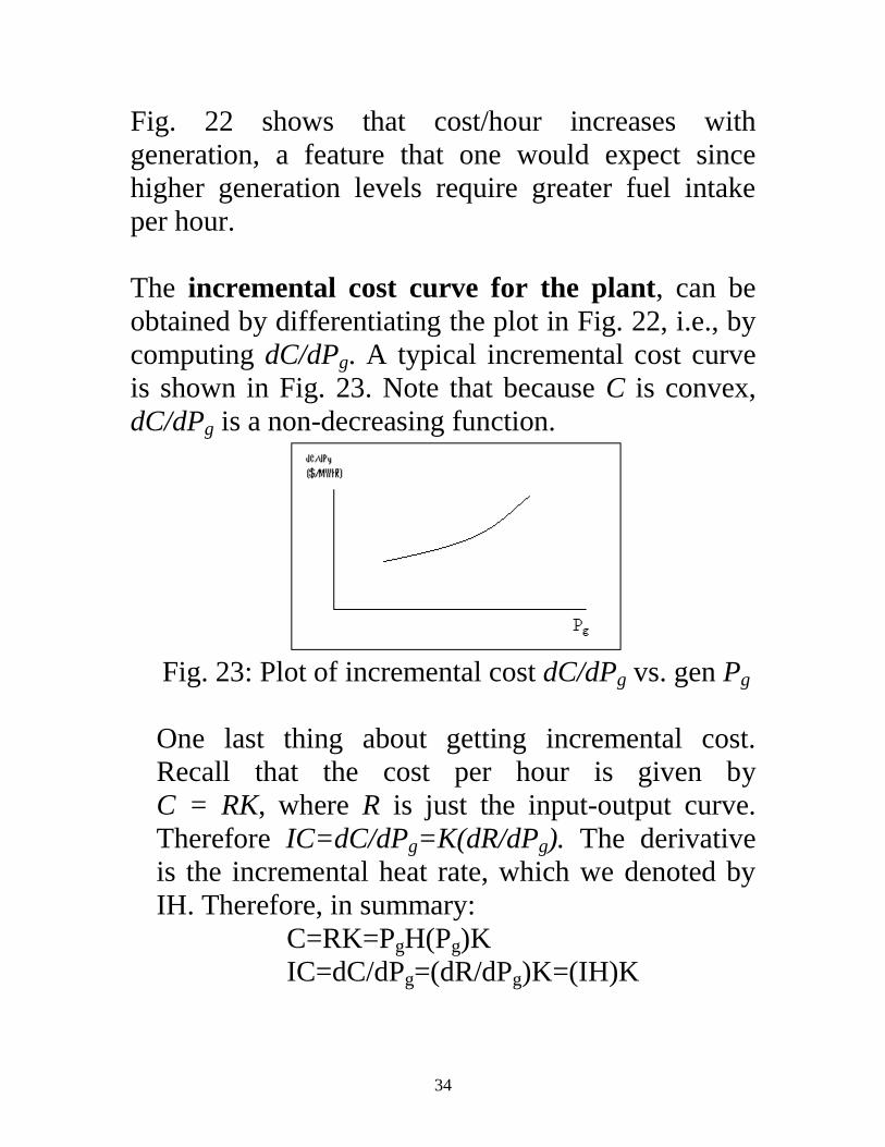
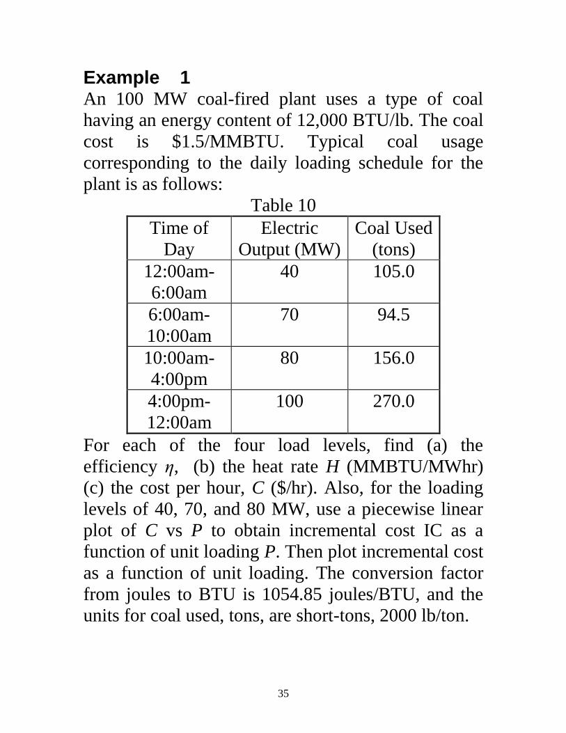
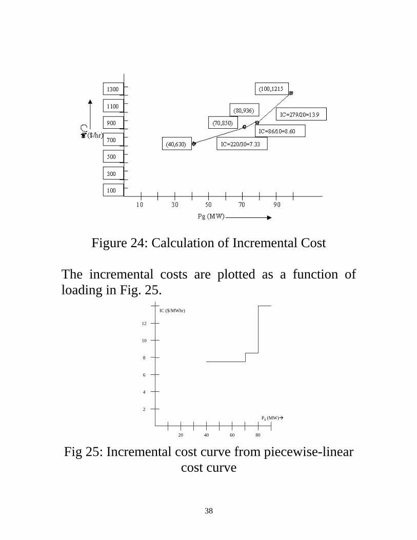
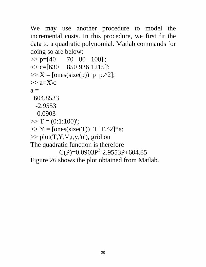
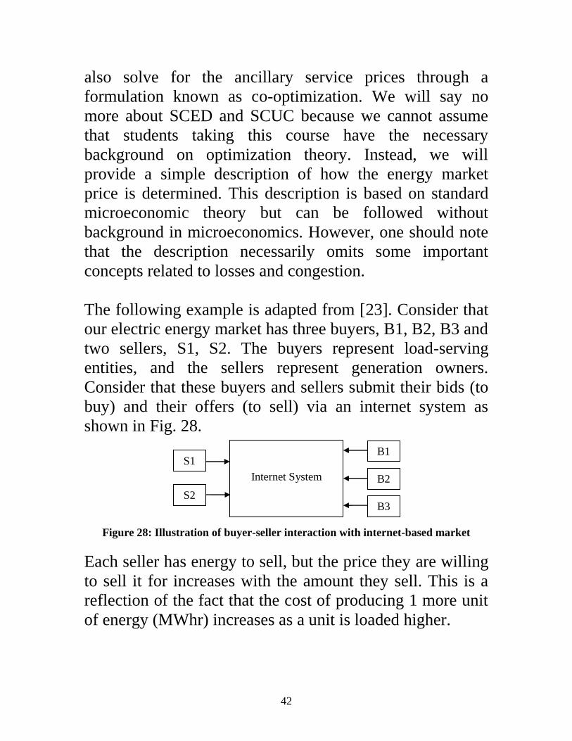
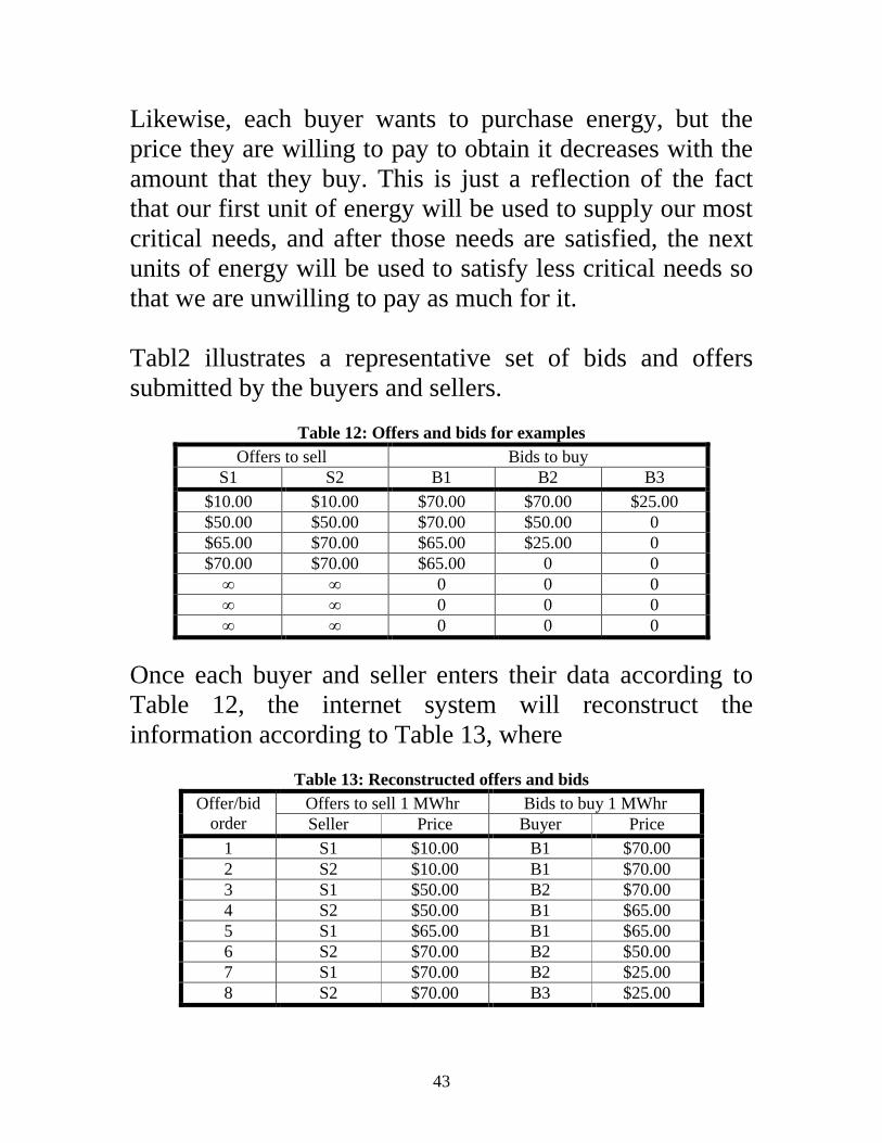
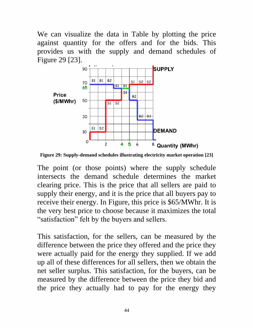
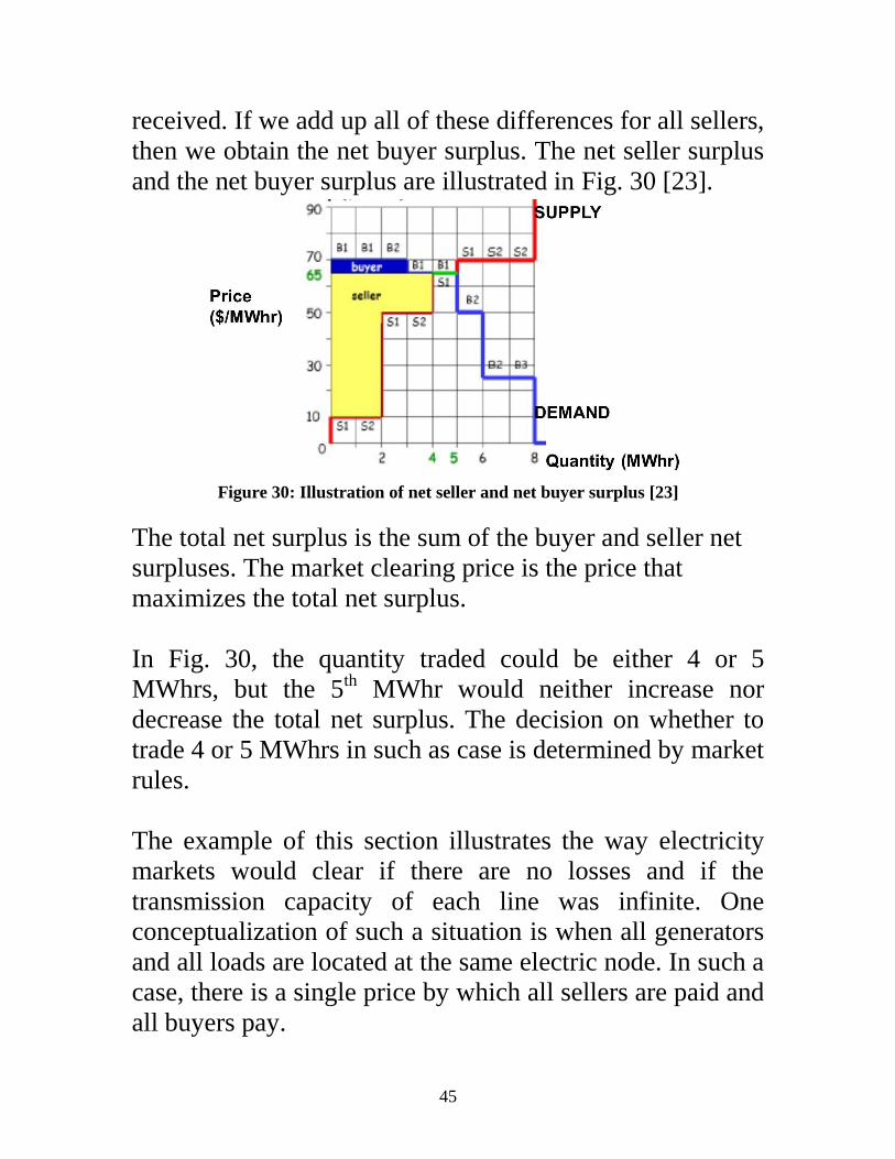
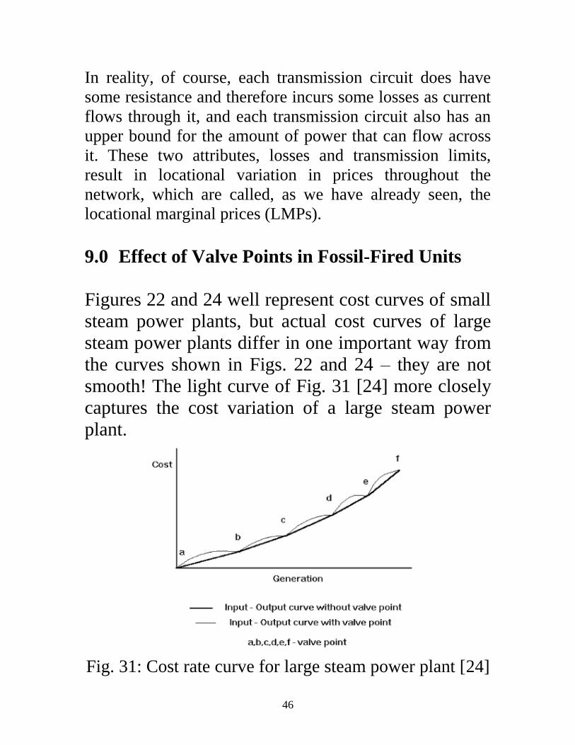
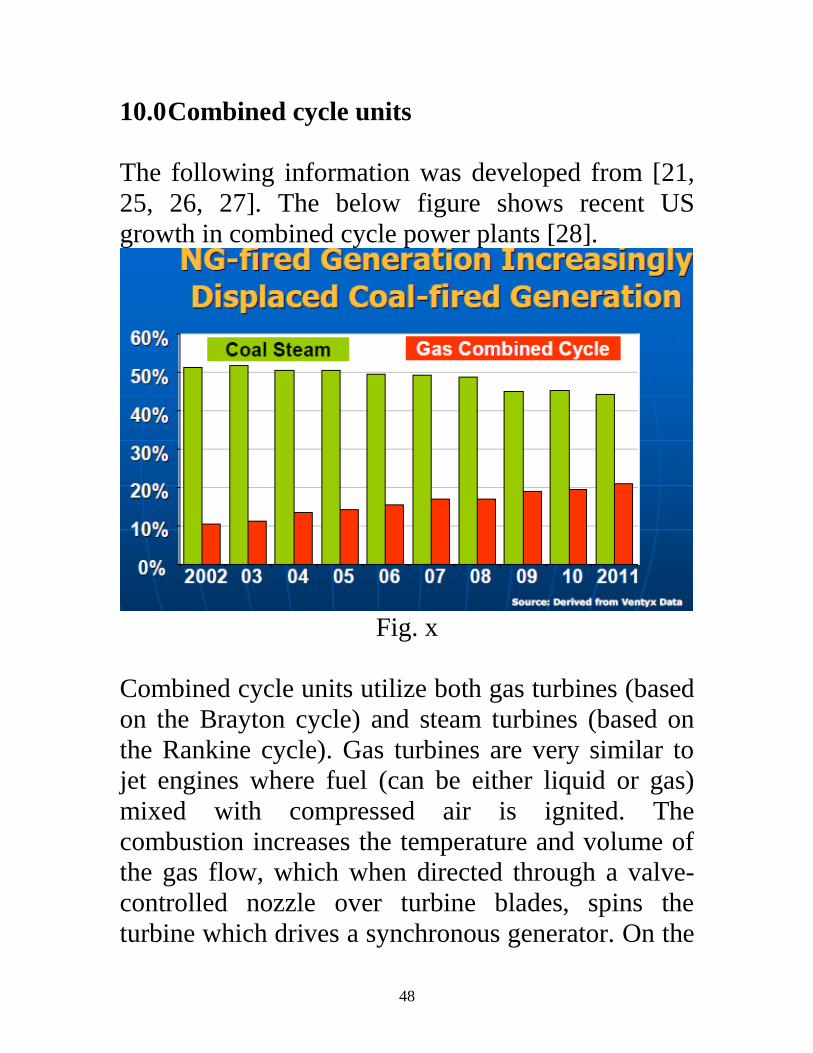
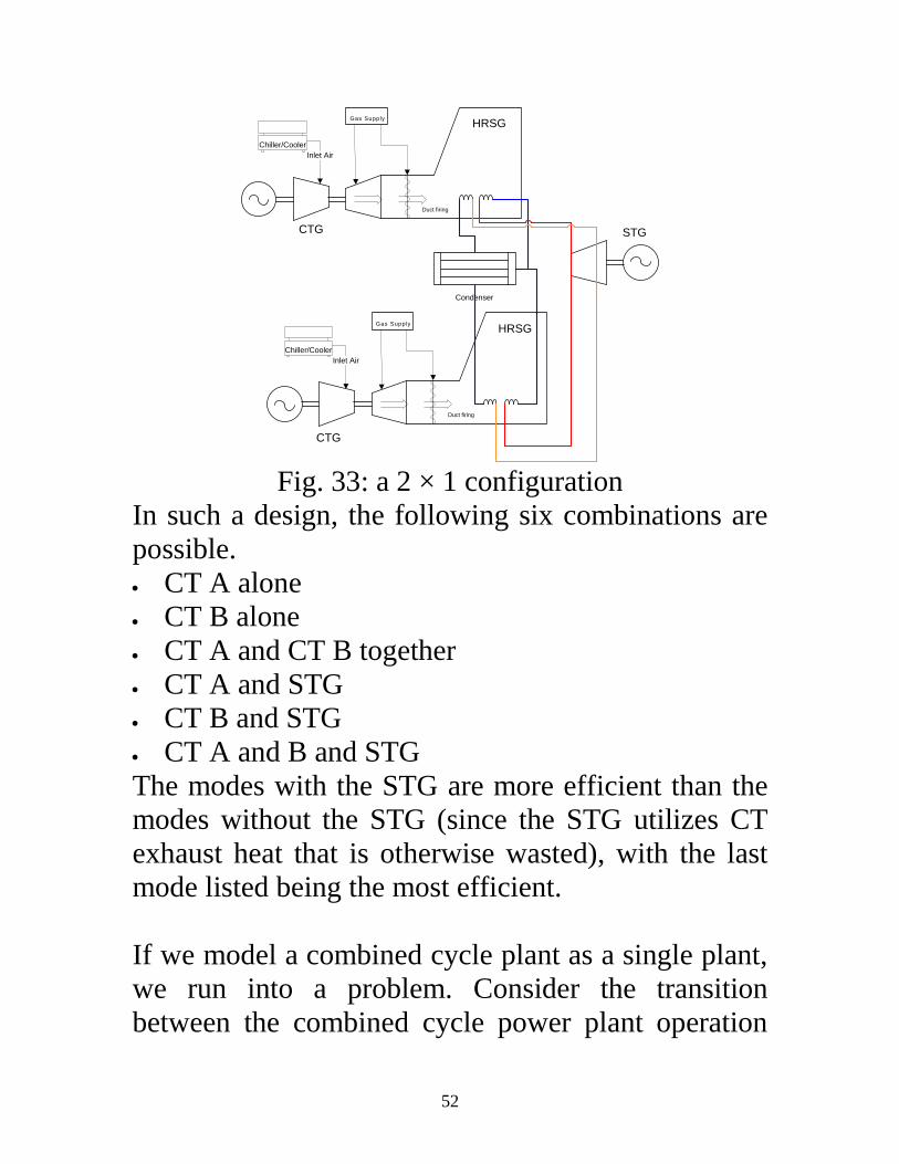
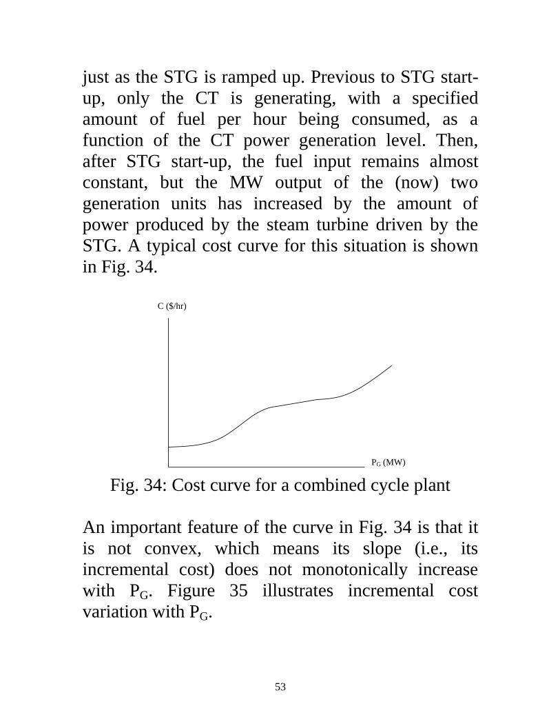
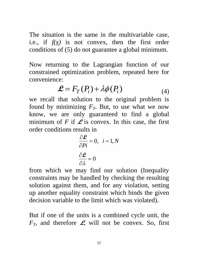
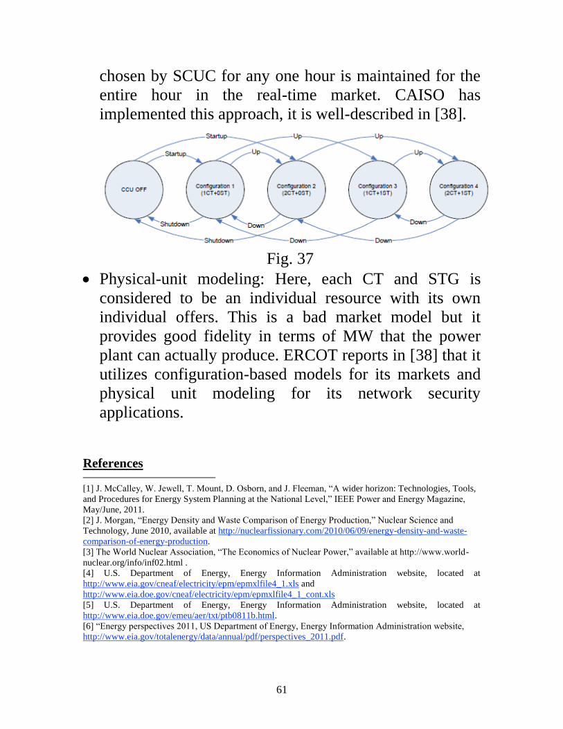