modeling of burden distribution

Tamoghna M

itra M

odeling of Burden Distribution in the Blast Furnace

2016

ISBN 978-952-12-3419-4Painosalama Oy

Turku/Åbo, Finland 2016

Modeling of Burden Distribution in the Blast Furnace

Tamoghna Mitra

Doctor of Technology Thesis

Thermal and Flow Engineering Laboratory

Faculty of Science and Engineering

Åbo Akademi University

Turku/Åbo, Finland 2016.


Tamoghna Mitra






Supervisor

Professor Henrik Saxén

Head of the Laboratory,

Thermal and Flow Engineering laboratory,

Åbo Akademi University, Åbo, Finland.

Reviewer

Dr. Joseph J. Poveromo

President,

RMI Global Consulting, USA.

Opponent and Reviewer

Dr. Paul Zulli

Professorial Fellow,

University of Wollongong, Australia.

ISBN 978-952-12-3419-4

Painosalama Oy

Turku/Äbo, Finland 2016

i

Preface

This doctoral dissertation is the result of my research work carried out at the Thermal and Flow

Engineering Laboratory, Åbo Akademi University, Finland in 2012-2016. I would like to thank the

Graduate School of Chemical Engineering, the Academy of Finland, FIMECC and its SIMP and

ELEMET programs and Tekes Finland, for providing the financial support to carry out this research.

Additionally, this work would not have been possible without the support from the industrial partners

including SSAB Europe (Raahe) and LKAB Sweden.

I would like to express my sincere thanks to my supervisor Professor Henrik Saxén whose guidance

and encouragement has made this thesis possible. His indefatigable spirit has been a constant motivation

for me in tiring times and I will always be grateful to him for making me love my work.

I would like to express my sincere gratitude to all my colleagues at the laboratory who have made my

work enjoyable. I would like to thank Professor Ron Zevenhoven, Docent Frank Pettersson and Dr.

Mikko Helle for the wonderful discussions and invaluable inputs to my research. I would like to thank

Alf Hermanson and Vivéca Sundberg for all the practical help at every stage of my work and my stay

in Finland. I will always be grateful to Professor Nirupam Chakraborti for supporting and encouraging

me to visit Finland for my Master’s programme and thereby making everything else possible. My stay

at the laboratory would not have been half as enjoyable without the great coffee breaks and wonderful

time spent with my dear colleagues from past and present: Johan, Calle, Martin, Markéta, Ines, Hamid,

Inga, Mathias, Lei, Yaowei, Evelina, Alice. A special thanks goes to H-P and Debanga for sharing the

office space and laughs.

I would like to thank Professor Tatsuro Ariyama of Tohoku University, Japan, for hosting me at their

esteemed laboratory in 2012 in order to study the reduction behavior of pellets. I would like to thank

Ueda-san, Kon-san, Kikuchi-san and Natsui-san for making my stay in Japan a great learning

experience.

My stay in Finland has been the most memorable because of all my amazing friends in Åbo: Vinay,

Rishabh, Rajesh, Megha, Kamesh, Ayush, Bhanu, Pramod, Manju, Susmita, Patrycja and many others.

All of you made Åbo a home away from home. A very special thanks goes to Pallavi for always

believing that I have what it takes and always being there for me.

I would like to thank my wonderful extended family, my grandmother, my grandfather, my uncles and

aunts and my little cousins whose constant love helped me to move ahead in life. Finally, I would like

to thank my wonderful parents, Madhumita Mitra and Nibir Kumar Mitra without whose

encouragement and inspiration I would not have been able to move ahead in every step that I have

taken.

Turku/Åbo, March 2016,

Tamoghna Mitra.

ii

Abstract

The blast furnace is the main ironmaking production unit in the world which converts iron ore with

coke and hot blast into liquid iron, hot metal, which is used for steelmaking. The furnace acts as a

counter-current reactor charged with layers of raw material of very different gas permeability. The

arrangement of these layers, or burden distribution, is the most important factor influencing the gas flow

conditions inside the furnace, which dictate the efficiency of the heat transfer and reduction processes.

For proper control the furnace operators should know the overall conditions in the furnace and be able

to predict how control actions affect the state of the furnace. However, due to high temperatures and

pressure, hostile atmosphere and mechanical wear it is very difficult to measure internal variables.

Instead, the operators have to rely extensively on measurements obtained at the boundaries of the

furnace and make their decisions on the basis of heuristic rules and results from mathematical models.

It is particularly difficult to understand the distribution of the burden materials because of the complex

behavior of the particulate materials during charging. The aim of this doctoral thesis is to clarify some

aspects of burden distribution and to develop tools that can aid the decision-making process in the

control of the burden and gas distribution in the blast furnace.

A relatively simple mathematical model was created for simulation of the distribution of the burden

material with a bell-less top charging system. The model developed is fast and it can therefore be used

by the operators to gain understanding of the formation of layers for different charging programs. The

results were verified by findings from charging experiments using a small-scale charging rig at the

laboratory.

A basic gas flow model was developed which utilized the results of the burden distribution model to

estimate the gas permeability of the upper part of the blast furnace. This combined formulation for gas

and burden distribution made it possible to implement a search for the best combination of charging

parameters to achieve a target gas temperature distribution. As this mathematical task is discontinuous

and non-differentiable, a genetic algorithm was applied to solve the optimization problem. It was

demonstrated that the method was able to evolve optimal charging programs that fulfilled the target

conditions.

Even though the burden distribution model provides information about the layer structure, it neglects

some effects which influence the results, such as mixed layer formation and coke collapse. A more

accurate numerical method for studying particle mechanics, the Discrete Element Method (DEM), was

used to study some aspects of the charging process more closely. Model charging programs were

simulated using DEM and compared with the results from small-scale experiments. The mixed layer

was defined and the voidage of mixed layers was estimated. The mixed layer was found to have about

12% less voidage than layers of the individual burden components.

Abstract

iii

Finally, a model for predicting the extent of coke collapse when heavier pellets are charged over a layer

of lighter coke particles was formulated based on slope stability theory, and was used to update the coke

layer distribution after charging in the mathematical model. In designing this revision, results from

DEM simulations and charging experiments for some charging programs were used. The findings from

the coke collapse analysis can be used to design charging programs with more stable coke layers.

iv

Sammanfattning

Masugnen är den huvudsakliga järnframställningsprocessen i världen som konverterar järnmalm med

hjälp av koks och varm bläster till råjärn, som används vid stålframställning. Processen fungerar som

en enorm motströmsreaktor där man chargerar partikelformiga råmaterial som bildar lager med olika

gaspermeabilitet. Fördelningen av dessa lager, den s.k. beskickningsfördelningen, spelar en avgörande

roll för gasfördelningen, vilket påverkar såväl värmeöverförings- som reduktionsprocesserna i ugnen.

För att kunna reglera processen borde operatörerna känna till ugnens interna tillstånd och även kunna

prediktera hur styråtgärderna påverkar processen. Höga temperaturer och högt tryck i kombination med

mekaniskt slitage och svåra omständigheter (korrosiv miljö, gaser med explosionsrisk, etc.) gör det

mycket svårt att mäta interna variabler i ugnen. Operatörerna måste därför förlita sig på mätningar som

finns tillgängliga vid processens ränder och basera sina beslut på processkunskap och resultat från

matematiska modeller. Beskickningsfördelningen är speciellt svår att förstå p.g.a. det komplexa

beteendet hos partikelformiga råmaterial under chargeringen. Målet med föreliggande

doktorsavhandling var att belysa några aspekter av beskickningsfördelningen samt att utveckla

matematiska modeller som kan fungera som beslutstöd vid reglering av beskicknings- och

gasfördelning i masugn.

En relativt förenklad modell utvecklades för simulering av beskickningsfördelningen i en masugn där

materialen chargeras med en roterande ränna (end. bell-less top charging). Modellen som utvecklades

är snabb och den kan därför användas av operatörerna interaktivt för att få förståelse för hur

materiallagren bildas vid chargeringen. Resultaten verifierades genom att jämföra dem med

observationer från försök i liten skala med hjälp av en pilotutrustning vid laboratoriet.

Vidare utvecklades för masugnsschaktet en grundläggande gasfördelningsmodell som utnyttjar

beskickningsfördelningsmodellens resultat. Den kombinerade modellen gjorde det även möjligt att

implementera sökning efter det chargeringsprogram som ger upphov till en önskad gasfördelning.

Emedan detta matematiska problem är såväl diskontinuerligt som icke-differentierbart användes en s.k.

genetisk algoritm för att lösa optimeringsproblemet. Resultaten visade att sökmetoden gradvis kunde

utveckla chargeringsprogram som allt bättre uppfyllde de uppsatta målen.

Fastän beskickningsfördelningsmodellen som utvecklats ger värdefull information om lagerstrukturen

kan den inte beskriva vissa komplexa förlopp, såsom uppkomsten av blandade lager samt kollaps av

kokslager. En mer sofistikerad numerisk metod för simulering av partikeldynamik, den diskreta

element-metoden (eng. Discrete Element Method, DEM), utnyttjades för att i detalj studera förloppen.

Några chargeringsprogram simulerades med DEM och resultaten jämfördes med observationer från

modellförsök i liten skala. En metod för bestämning av porositeten och omfattningen av blandade lager

utvecklades och tillämpades på de studerade chargeringsprogrammen. Blandlagren befanns uppvisa ca

12% lägre porositet än lagren som består av en enda partikeltyp.

Sammanfattning

v

Slutligen utvecklades på basis av stabilitetsteori en matematisk modell som uppskattade omfattningen

av kollaps av kokslager då (tyngre) pelletar chargeras på ytan. Denna modell, som utvärderades med

såväl DEM-simuleringar som småskaleförsök, användes för att uppdatera kokslagrens form i

beskickningsfördelningsmodellens resultat. Modellen kan även utnyttjas vid utveckling av

chargeringsprogram som leder till stabila kokslager som inte är benägna att kollapsa.

vi

List of Publications

I. Mitra, T. and Saxén, H. (2014). Model for Fast Evaluation of Charging Programs in the Blast

Furnace. Metallurgical and Material Transactions B, 45(6), 2382-2394.

II. Mitra, T. and Saxén, H. (2015). Evolution of Charging Programs for Achieving Required Gas

Temperature Profile in a Blast Furnace. Materials and Manufacturing Processes, 30(4), 474-

487.

III. Mitra, T. and Saxén, H. (2015). Discrete Element Simulation of Charging program and Mixed

Layer Formation in an Ironmaking Blast Furnace. Journal of Computational Particle

Mechanics, DOI 10.1007/s40571-015-0084-1.

IV. Mitra, T. and Saxén, H. (2016). Investigation of Coke Collapse in the Blast Furnace using

Mathematical Modeling and Small Scale Experiments. ISIJ International, 56(9).

Contribution of the author

The author of this thesis is the main author of the publications and has developed all the models

presented in them. All the simulations in DEM and some of the charging experiments using the scaled

model were performed by the author. Most of the charging program experiments were performed by

Simon Renlund and Mathias Sundqvist in close coordination with the author. The DEM simulation and

the charging experiments for slump tests for determining the particle properties were performed along

with Rikio Soda of Tohoku University, Japan.

vii

Related publications

Besides the listed publications, the author of this thesis has participated in various conferences related

to the thesis topic. The publications in the conference proceedings or in associated journals are listed

below. It also includes a book chapter which discusses the use of different evolutionary algorithms for

ironmaking applications.

V. Mitra, T., Saxén, H. and Chakraborti, N. (2016). Evolutionary Algorithms in Ironmaking

Applications. In A.M. Gujrathi and B.V. Babu (Eds.), Evolutionary Computation: Techniques

and Applications. Oakville: Apple Academic Press.

VI. Mitra, T. and Saxén, H. (2015). Simulation of Burden Distribution and Charging in an

Ironmaking Blast Furnace. IFAC-PapersOnLine, 48(17), 183-188.

VII. Mitra, T. and Saxén, H. (2015). Investigation of Burden Distribution in the Blast Furnace.

Proceedings of the 10th CSM Steel Congress & the 6th Baosteel Biennial Academic Conference.

Shanghai, China.

VIII. Mitra, T., Mondal, D.N., Pettersson, F. and Saxén, H. (2013). Evolution of Charging Programs

for Optimal Burden Distribution in the Blast Furnace. Computer Methods in Material Science,

13(1), 99-106.

IX. Mitra, T., Kon, T., Natsui, S., Ueda, S. and Saxén, H. (2013). Reduction Behaviour of Iron Ore

Pellet in a Non-Uniform Gas Flow Field. CAMP-ISIJ. Tokyo, Japan.

X. Mitra, T., Shao, L. and Saxén, H. (2012). Simulation of Burden and Gas Flow charecteristics

using a mathematical model of the upper shaft of the Blast Furnace. ScanMet IV, 2, 69-77.

XI. Mitra, T., Kinnunen, K. and Saxén, H. (2012). Evaluation of Alternatives to Raise the Blast

Temperature at Lean Blast Furnace Top Gas Operation. AISTech Conference Proceedings.

Atlanta, USA.

XII. Mitra, T., Helle, M., Petersson, F., Saxén, H. and Chakraborti, N. (2011). Multiobjective

Optimization of Top Gas Recycling Conditions in the Blast Furnace by Genetic Algorithms.

Materials and Manufacturing Processes, 26(3), 475-480.

viii

Contents

Preface ..................................................................................................................................................... i

Abstract ................................................................................................................................................... ii

Sammanfattning ..................................................................................................................................... iv

List of Publications ................................................................................................................................ vi

Contribution of the author ...................................................................................................................... vi

Related publications .............................................................................................................................. vii

Contents ............................................................................................................................................... viii

1. Introduction ..................................................................................................................................... 1

2. Blast furnace Ironmaking ................................................................................................................ 3

3. Burden distribution ......................................................................................................................... 5

3.1 Charging equipment .............................................................................................................................. 6

3.2 Measurement technology for blast furnace burden distribution .......................................................... 8

3.3 Complexity of burden distribution ....................................................................................................... 11

4. Discrete Element Method.............................................................................................................. 14

4.1 Fundamental equations ...................................................................................................................... 14

4.2 Properties of materials ........................................................................................................................ 18

4.3 Particle shape consideration ............................................................................................................... 20

5. Evolutionary algorithm ................................................................................................................. 23

5.1 Genetic Algorithm ............................................................................................................................... 23

6. Burden distribution modeling ....................................................................................................... 26

6.1 Modelling of top bunker and hopper system ...................................................................................... 26

6.2 Modelling of particle trajectory........................................................................................................... 27

6.3 Modelling of burden formation ........................................................................................................... 29

6.4 Modelling of burden descent............................................................................................................... 32

6.5 Gas flow modeling ............................................................................................................................... 33

7. Models developed ......................................................................................................................... 36

Contents

ix

7.1 Charging experiment (Paper I, III, IV) .................................................................................................. 38

7.2 Burden distribution and descent model (Paper I) ................................................................................ 39

7.3 Gas flow model (Paper II) .................................................................................................................... 45

7.4 Optimization using Genetic Algorithm (Paper II) ................................................................................ 50

7.5 DEM model of burden distribution (Papers III, IV) ............................................................................... 52

7.6 Mixed layer formulation (Paper III) ..................................................................................................... 54

7.7 Coke push formulation (Paper IV) ....................................................................................................... 58

8. Conclusions ................................................................................................................................... 63

9. Future prospects ............................................................................................................................ 65

References ............................................................................................................................................. 66

Original publications (I-IV) .................................................................................................................. 77

1

1. Introduction

The iron and steel industry is one of the key drivers of today’s world economy. This industry fueled the

industrial revolution in the 19th century and is the backbone of most of the industrial achievements until

today. Iron forms about 5.63% of earth’s crust [1] and the majority of it is in the form of oxides (mainly

hematite, magnetite and hydroxides). Ironmaking refers to a collection of processes for extraction of

metallic iron from these oxides and hydroxides, predominantly using a reductant such as carbon

monoxide. Metallic iron is relatively soft, so it is often alloyed with other elements, which improves or

imparts properties specific for an application. The alloys of iron are known as steel and the process of

alloying is known as “steelmaking”. An example of a steel alloy is “Hadfield steel” which contains about

13% manganese and is known for high impact strength and abrasion resistance.

The earliest ironmaking dates back to unrecorded history and the actual origin is contested by various

civilizations. Primitive ironmaking techniques involved burning of iron ore using wood in a covered

oven and subsequently hammering the slag away to obtain pure iron. Subsequently the process was

improved and furnaces called “bloomeries” were introduced during the early industrial era [2]. Modern

ironmaking techniques have evolved considerably and presently involve very high production rates, a

high degree of automation and sophisticated control strategies. The two most important modern routes

for ironmaking are the smelting route and the direct reduction (DR) route. In the smelting route, the

prepared agglomerate of iron oxide is reduced and melted and then transported to the steelmaking units.

On the other hand, in DR routes the reduction of iron oxides takes place at lower temperatures and the

raw material is retained in solid form. The end product is called DRI (Directly Reduced Iron) or sponge

iron because of its porous nature. DRI is mainly fed, along with steel scrap, into the Electric Arc

Furnaces (EAF) for steelmaking. The blast furnace route is the most important smelting technique,

which has existed and flourished for about 500 years. Today it accounts for about 70% of the iron used

for crude steel production [3], the rest being mainly recycled scrap melted in other units. It has been a

very successful process compared to its alternatives for producing liquid iron from ore because of its

fuel efficiency, productivity and scalability.

However, even with the increased production efficiency achieved, the steel industry is known to

contribute by a large portion (6-7% [4]) of the global anthropogenic greenhouse gas emissions. In a steel

plant, the blast furnace (BF) ironmaking unit is a major energy user [5]. To reduce the energy

consumption, a better understanding of the flow phenomena and reduction reactions in the blast furnace

is needed. This is particularly important for finding novel and more efficient ways of operating the

process. However, the complexity of the system has become the main obstacle for further improvement.

By the use of mathematical modeling, it is possible to analyze potential improvements of the process

and their effect on the overall performance without expensive full-scale tests.

1

Introduction

2

Blast furnace ironmaking is a complicated process due to its sheer size, large throughput and the

numerous physical and chemical phenomena that occur simultaneously. Various first principle and data-

driven models have been developed to study either parts of the system or the total process. The earliest

mathematical models were zero dimensional models which treated the process as an entity. These were

followed by models that divided the furnace into zones where different reactions and phenomena take

place. The thermal and chemical conditions were then calculated using thermodynamic relations [6]. In

order to understand the variation of solid and gas temperatures, and chemical composition, along the

height of the furnace, 1D models were introduced [7-9]. These models discretized the furnace vertically

into infinitesimal sections. The heat and mass transfer equations and expressions for the rates of

chemical reaction are used to calculate the temperature and composition at different vertical points. The

concept was later extended to 2D [10-12] and 3D models using Computational Fluid Dynamics (CFD)

and related techniques [13, 14]. An accurate gas flow description required a detailed description of the

solid conditions inside the furnace. Therefore, techniques such as the Discrete Element Method (DEM),

sometimes coupled with CFD for gas flow, have been increasingly used with the focus on the complex

interaction of solid, liquid and gas flow in the furnace [13, 15]. As an alternative approach, there are

also various data-driven models that use data from an actual blast furnace to predict different variables,

such as the hot metal silicon content [16] or top gas CO2 content [17].

A robust and accurate mathematical model is crucial for understanding the furnace operation, which

forms the basis for controlling the process. A model that can be rapidly executed is also useful for

searching the right parameters for achieving a particular output condition. Optimization techniques can

also be utilized, which systematically change the input variables of the model to find the state where an

objective is minimized (or maximized) to achieve certain goals, e.g., minimum production costs or

emission rates.

This doctoral work is focused on modeling with the aim to understand some aspects of the complex

burden distribution in the blast furnace. Simplified mathematical models and the more complex DEM

approach have been used to describe the burden distribution. The findings have been verified by small

scale experiments. Theories pertaining to burden descent, mixed layer formation and coke collapse are

proposed. One of the models developed was also optimized to meet targets set for the process conditions

using a metaheuristic search algorithm, the Genetic Algorithm. The models developed within this

research further the understanding of burden distribution in the blast furnace. The tools developed may

be used to help the furnace operators take faster and more appropriate decisions concerning actions

controlling the burden and gas distribution.

2

3

2. Blast furnace Ironmaking

A blast furnace is a vertical counter-current heat exchange and chemical reactor for producing hot metal.

Solid iron oxide burden is charged from top along with coke and flux, and as it descends in the furnace

it is heated up by the ascending gas and the iron oxides are reduced into hot metal by the reducing gas.

Figure 1(a) shows the cross section of a typical blast furnace along with the inputs and outputs.

The blast furnace parts may be classified depending on the shape of the region (Figure 1, a). The upper

cylindrical part of the furnace is known as the throat and is protected by refractory brick. Below the

throat, there is the region with increasing diameter known as the shaft which extends to a cylindrical

section or belly. After the belly, the diameter decreases again in the bosh region, where the blast enters

the furnace. The bottommost portion of the furnace is called the hearth where the molten hot metal and

the slag accumulate within a coke bed.

The inner volume of the blast furnace is also classified into different zones (Figure 1, b) depending on

the physical state of the burden and the chemical reactions occurring. The uppermost part of the furnace

constitutes of the lumpy zone, where the burden remains solid. The iron ore, usually charged as

haematite (Fe2O3) is first converted to magnetite (Fe3O4) and eventually to wustite1 (FeO) by the

ascending reducing gas containing carbon monoxide (CO) which produces carbon dioxide (CO2).

1 Non-stoichiometric compound, Fe𝑥O, with a mean value of 𝑥 = 0.95 [18]. For simplicity, wustite is here

referred to as FeO.

Raw materials (iron ore,

coke, limestone)

Top gas (carbon dioxide,

carbon monoxide,

nitrogen, hydrogen, water

vapor)

Hot blast (oxygen,

nitrogen) & Injection

(oil/pulverized coal)

Hot metal (Iron, Carbon)

and Slag (Insoluble oxides)

Throat

Shaft

Hearth

Figure 1: (a) Cross-section of a typical blast furnace, classification based on shape of the furnace

region. (b) Different zones of the blast furnace classified on the basis of internal state.

Lumpy zone

Cohesive zone

Active coke zone

Deadman

Raceway

Slag

Hot metal

Belly

Bosh

(a) (b)

3

Blast furnace Ironmaking

4

3Fe2O3 + CO → 2Fe3O4 + CO2 (2.1)

Fe3O4 + CO = 3FeO + CO2 (2.2)

Similar reduction reactions, but to a lesser extent, occur with hydrogen, forming water vapor. The

temperature of the burden increases from the ambient to a constant temperature (900 - 1000˚C) where

both the burden and the gas attain nearly the same temperature. This region is called the thermal reserve

zone. By contrast, the temperature of the gas decreases as it rises in the furnace and exits the top at 100-

250 ˚C.

After the end of the thermal reserve zone the wustite is reduced into iron (Fe).

FeO + CO = Fe + CO2 (2.3)

A large number of other reactions take place in this region, including reduction of the other metallic

oxides in the iron ore and the formation of slag. As some wustite always remains unreduced and the

burden reaches higher temperatures than 1000 ˚C, the Boudouard reaction (C + CO2 = 2CO), which is

highly endothermic, will occur simultaneously. The net reduction reaction is

FeO + C = Fe + CO (2.4)

Subsequently, the iron-bearing burden begins to soften and melt as the cohesive zone starts. This zone

has alternate layers of highly pervious coke and semi-pervious iron-slag mix. The pervious coke layers

or slits help the gas enter from the lower parts of the furnace to rise up towards the top. Therefore, an

adequate size of the coke slits is very important for achieving a smooth furnace operation. At the lower

end of the cohesive zone, the iron melts and percolates through the bed of solid coke. The upper part of

the coke region is called the active coke zone. Here the coke is constantly replenished from the burden,

as it slides to the combustion regions near the tuyeres known as the raceways. In the raceway, the coke

is combusted to carbon monoxide by the incoming blast which consists of oxygen and (practically inert)

nitrogen.

2C + O2 = 2CO (2.5)

At the core of the bosh region lies a closely packed column of coke which does not react rapidly and is

called the deadman. It provides support to the layered structures above. The hearth has a pool of liquid

iron called hot metal with slag floating on top of it. The hot metal and the slag are tapped at regular

intervals. The hot metal flows through a runner into a ladle or torpedo, which is transported to the steel

mill for further processing. The slag, which is separated by gravity, is usually tapped into a slag pit or

directly cooled and granulated. It is often sold as a by-product, e.g. to the cement or brick industries.

In basic terms, the main methods for controlling the conditions inside a blast furnace are by controlling

it ‘from below’ through the blast parameters, like temperature, pressure and moisture content, and ‘from

above’ by controlling the burden distribution. The latter is the main focus of the present thesis. The next

chapter describes the importance of burden distribution and different techniques for controlling it.

4

5

3. Burden distribution

The blast furnace is a continuous reactor but the raw materials are charged in alternate layers of ore and

coke intermittently. This layered structure is retained as the raw materials descend through the furnace.

Burden distribution refers to this arrangement of the layers of different materials inside the furnace and

mainly to the radial distribution (as axial symmetry is usually desired). The raw materials charged into

the furnace are very different from each other. Ore is about four times heavier than coke and the particle

size is 2-4 times smaller, which affects the gas permeability and heating of the charged layers.

As the reducing gas rises from below, it encounters the burden layers with very different permeability

conditions. The radial distribution of ore and coke is therefore an important factor governing the gas

flow distribution in the furnace [19]. Normally, the fraction of ore of the total volume or mass is used

to quantify this distribution. The (radial) region with higher fraction of ore results in a lower gas flow.

In some operating procedures, higher gas flow at the center of the furnace is preferred, because it is

effective in decreasing discontinuous motion of the solid burden, resulting in smooth operation [20].

Therefore, batches of large-sized coke, known as ‘center-coke’, or larger sinter and lump ore are

charged near the center of the furnace to improve the gas permeability in the region. Only a small

number of furnaces are specially equipped to charge coke directly into the furnace center. However,

higher gas flow also results in higher gas temperatures as the gas does not have enough time for heat

exchange and the thermal flow ratio (defined as the heat capacity ratio between burden and gas) is low.

The regions with higher gas temperature usually correspond to a higher cohesive zone level. Therefore,

the temperature readings from the above burden probe are an important indicator of burden distribution

inside the furnace.

As the burden descends into the furnace, the ore is reduced and at around 1200˚C (depending on the

quality of ore), it starts to soften and eventually melts at around 1350˚C. Coke, on the other hand,

maintains its form (except some consumption by the solution-loss reaction) until it reaches the tuyere

level. The semi-molten portion of the burden is extremely impermeable to the gas flow, so the gas has

to flow through more permeable regions, coke slits, in the cohesive zone where it changes to more

horizontal direction, until it reaches the lumpy zone. If the coke slits are blocked or not pervious enough,

furnace irregularities such as hanging or erratic burden descent may occur. The burden distribution has

a major role in affecting the size of coke slits in the cohesive zone, but it also influences the deadman

formation in the blast furnace and wear rate of the furnace lining by controlling the gas flow and thus

also the heat losses.

Most modern operation practices focus on the growing lack of high-quality raw material and improving

the furnace efficiency. These new practices require very precise control of the burden distribution and,

therefore, accurate modeling and fast calculations. Thus, simulation of the burden distribution is

becoming an increasingly important topic of research. In addition, high coal injection rates through the

5

Burden distribution

6

tuyeres in blast furnaces reduce the coke rates in the furnace, so the thickness of the coke layers is

becoming even less. This requires precise control of raw material distribution to allow sufficient

permeability and appropriately located coke slits in the cohesive zone. Some other examples of modern

charging practices include mixed charging schemes, where small coke is mixed with ore dumps [21] to

improve the permeability of the ore layer. Furnaces around the world are also gradually shifting to high

pellet (agglomerated ore) operation owing to its high reducibility, but pellets have lower repose angle,

high rolling and layer collapse tendencies [22], so it is very important to understand the layer formation

process.

Complex issues associated with burden distribution are coke collapse, segregation and mixed layer

formation. These issues have been modeled extensively in the thesis, and in subsequent chapters they

will be presented and discussed.

The burden distribution is manipulated by the charging equipment. Modern equipment gives better

options for the operator to affect the burden distribution. However, the operator has a limited access to

information about the conditions inside the furnace due to extremely high temperatures and the closed

nature of the furnace. Therefore, the operators have to rely strongly on existing measurement

technologies from where they have to indirectly deduce the conditions inside the furnace. In this chapter,

commercially available charging equipment types are discussed along with their differences.

Subsequently, some of the measurement technologies employed for understanding the burden

distribution conditions are detailed. Finally, the complexity of burden distribution is demonstrated using

an example.

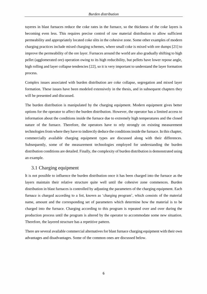
3.1 Charging equipment

It is not possible to influence the burden distribution once it has been charged into the furnace as the

layers maintain their relative structure quite well until the cohesive zone commences. Burden

distribution in blast furnaces is controlled by adjusting the parameters of the charging equipment. Each

furnace is charged according to a list, known as ‘charging program’, which consists of the material

name, amount and the corresponding set of parameters which determine how the material is to be

charged into the furnace. Charging according to this program is repeated over and over during the

production process until the program is altered by the operator to accommodate some new situation.

Therefore, the layered structure has a repetitive pattern.

There are several available commercial alternatives for blast furnace charging equipment with their own

advantages and disadvantages. Some of the common ones are discussed below.

6

Burden distribution

7

3.1.1 Bell top

A bell top charging system consists of a

bell and hopper arrangement. The bell

blocks the opening of the hopper when it

is raised and when the bell is lowered the

raw material falls into the furnace. The

hot “top gases” are rich in energy and

should therefore be recovered; so a single

bell hopper system cannot be used. To

avoid loss of the gas, a sealed double bell

system is used, as shown in Figure 2.

Such a charging system is extremely robust but provides very limited flexibility for the operators to

design the burden distribution, because there are very few parameters that the operator can influence.

Most of the raw material is charged near the wall. Sometimes a set of movable armors, whose position

may be set by the operator, is used to redirect the dump away from the furnace walls.

3.1.2 Bell-less top

Bell-less top charging systems (Figure 3) are relatively new

charging units which are becoming increasingly popular. This

system was developed by Paul Wurth with its first successful

industrial application in 1972. It consists of a gated hopper which

empties into a chute which is rotating about the axis of symmetry.

The inclination of the chute may be controlled and, therefore,

provides much higher flexibility to the operator as to choose the

size and position of the dump. This is one reason why bell-less

charging is preferred over the bell top charging. Yet this charging

system has its own limitations; for example, a precise center-coke

charge is difficult to achieve, as there is a limitation to how much

the chute may be tilted vertically.

The bell-less top has helped improve the productivity and coke rate in many furnaces. For example, in

an Indian blast furnace equipped with a bell-less charging system the decrease in coke rate exclusively

due to improvement of burden distribution was reported to be 10-12 kg/t hot metal [23].

3.1.3 Gimbal top

The Gimbal top (Figure 4) is a comparatively new burden distribution system introduced in 2003 by

Siemens VAI [24]. It utilizes a conical distribution chute with rings which allow multi-axis motion.

This technology gives more flexibility to the furnace operator compared to the bell-less top charging

Figure 2: Bell type charging system

Movable armour

Upper hopper and bell

Lower hopper and bell

Burden surface

Upper bell is lowered Lower bell is lowered

Figure 3: Bell-less top

charging system

7

Burden distribution

8

system. The charge may be directed to any point on the furnace stock

line. It allows sector charging, spot charging and formation of a true

center coke charge. This charging system has been applied to a few

FINEX and COREX furnaces along with the C Blast Furnace of Tata

Steel in Jamshedpur.

3.1.4 Bell-less rotary charging unit

A bell-less rotary charging system (Figure 5) was developed by Totem

Co. Ltd. [25]. It consists of a rotary chute, whose speed determines

the positions at which the material is charged. It charges thin layers of

the material, so the dump does not affect the burden surface on which

the dump is charged (referred as ‘soft dumping’). Some blast furnaces

in India have been equipped with this charging system.

3.1.5 No-bell top charging system

The no-bell charging system (Figure 6) was developed by

Zimmermann & Jansen Technologies (now IMI Z&J). It consists of a

double chute system with a rotating chute at a fixed angle with an

additional chute at the end to direct the charge to a particular radial

position on the burden surface.

3.2 Measurement technology for blast furnace

burden distribution

Efficient blast furnace control requires reliable measurements of the

conditions inside the furnace. The temperatures in the lower half of the

furnace may increase to more than 2000˚C, where most intrusive

measurement technologies would be unreliable, so most of the in-

furnace measurements are carried out above or near the burden

surface. The most important techniques for direct or indirect

quantification of the burden distribution

include:

i. Above burden probe

The above burden probe (Figure 7) has a

number of thermocouples attached to the

device to measure the gas temperatures at

different radial positions above the burden Figure 7: Measurement technology in a typical blast

furnace

Profile meter

Stockline radar

Above

burden probe

In-burden

probe

Figure 4: Gimbal type

charging system

Figure 5: Bell less rotary

charging system

Figure 6: No-bell top

charging system

8

Burden distribution

9

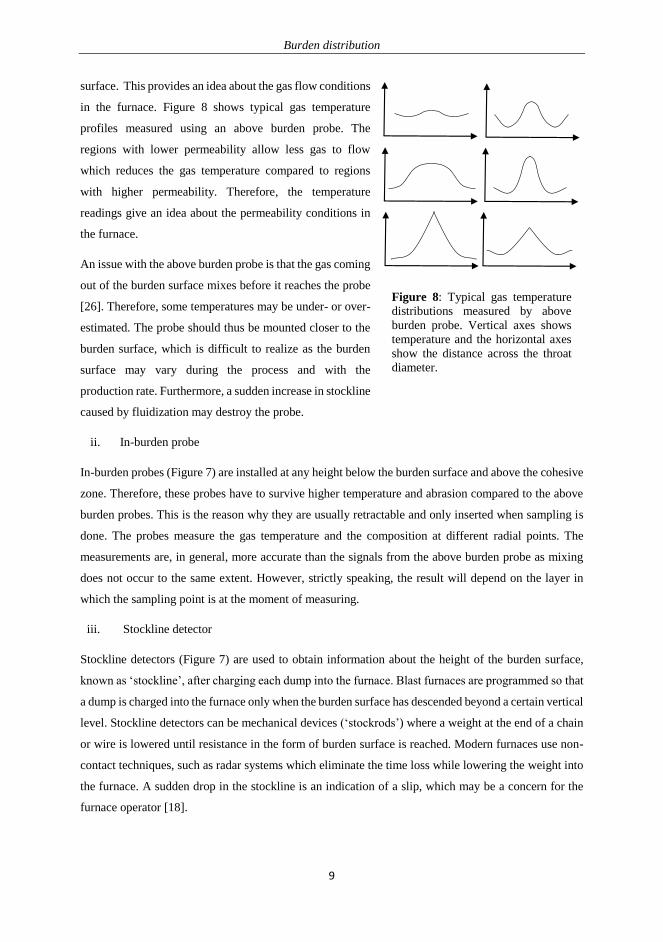
surface. This provides an idea about the gas flow conditions

in the furnace. Figure 8 shows typical gas temperature

profiles measured using an above burden probe. The

regions with lower permeability allow less gas to flow

which reduces the gas temperature compared to regions

with higher permeability. Therefore, the temperature

readings give an idea about the permeability conditions in

the furnace.

An issue with the above burden probe is that the gas coming

out of the burden surface mixes before it reaches the probe

[26]. Therefore, some temperatures may be under- or over-

estimated. The probe should thus be mounted closer to the

burden surface, which is difficult to realize as the burden

surface may vary during the process and with the

production rate. Furthermore, a sudden increase in stockline

caused by fluidization may destroy the probe.

ii. In-burden probe

In-burden probes (Figure 7) are installed at any height below the burden surface and above the cohesive

zone. Therefore, these probes have to survive higher temperature and abrasion compared to the above

burden probes. This is the reason why they are usually retractable and only inserted when sampling is

done. The probes measure the gas temperature and the composition at different radial points. The

measurements are, in general, more accurate than the signals from the above burden probe as mixing

does not occur to the same extent. However, strictly speaking, the result will depend on the layer in

which the sampling point is at the moment of measuring.

iii. Stockline detector

Stockline detectors (Figure 7) are used to obtain information about the height of the burden surface,

known as ‘stockline’, after charging each dump into the furnace. Blast furnaces are programmed so that

a dump is charged into the furnace only when the burden surface has descended beyond a certain vertical

level. Stockline detectors can be mechanical devices (‘stockrods’) where a weight at the end of a chain

or wire is lowered until resistance in the form of burden surface is reached. Modern furnaces use non-

contact techniques, such as radar systems which eliminate the time loss while lowering the weight into

the furnace. A sudden drop in the stockline is an indication of a slip, which may be a concern for the

furnace operator [18].

Figure 8: Typical gas temperature

distributions measured by above

burden probe. Vertical axes shows

temperature and the horizontal axes

show the distance across the throat

diameter.

9

Burden distribution

10

iv. Profile meter

Profile meters (Figure 7) were originally mechanical devices but today they have been replaced by non-

contact methods, e.g., movable radars (moving probe) along a horizontal channel which measure the

burden surface height at various radial points. The profile meter can also estimate the burden descent

velocity [27]. Modern profile meters have radars fixed on rotary joints and 3D burden surfaces may be

estimated, which gives a much better understanding than by measurements along a single direction.

v. Vertical probe

Vertical probes are used to provide the temperature and the gas composition along the height of the

furnace. They may consist of cables at different radial positions which are lowered to the burden surface

and are dragged down by moving solids until the tip is damaged, as the cables reach high temperatures

in the lower part of the furnace. The probes usually measure temperature and pressure and can sample

gas for composition. These probes can be equipped with a camera for particle size distribution [28]. The

lengths of the eroded probes also indicate the location of the cohesive zone in the furnace. Although

vertical probes provide maximum information about the furnace, they are seldom used as they are

expensive and require complex feeding equipment.

vi. Thermocouples

Blast furnace walls are lined with thermocouples which also

provide crucial information about the furnace operation. For

example, sudden changes in thermocouple readings may

indicate dropping of skull, which is a stagnant solidified

mass formed at furnace walls (Figure 9).

vii. Pressure gauges at the furnace wall

Gas pressure is measured at different points on the walls. As the gas flows through the coke slits the

direction is horizontal, so it affects the pressure at the walls. Therefore, the pressure information may

be used to estimate the cohesive zone shape.

viii. Other measurements

Some of the other measurements from the blast furnace include

1. Pressure, temperature and composition of the top gas

2. Flow rate and rise in temperature of the cooling water

3. Blast conditions

4. Hot metal and slag variables

5. Occasional use of belly probe, tuyere probe, etc.

Time

Tem

per

atu

re

Stable Skull dropping off

Figure 9: Thermocouple behavior

following the removal of skull

10

Burden distribution

11

6. Infrared cameras to measure burden surface temperature

7. Skin flow thermocouples (or mini-probes)

These measurements are indirectly affected by the burden distribution. Using different measurements

together with past experience, operators can obtain a holistic view of the conditions in the furnace and

identify the cause of improper furnace conditions.

3.3 Complexity of burden distribution

Different charging equipment provide different degrees of control over the charging process, which

ultimately determines the burden distribution. Even with a few options, though, the charging process

may become very complicated and can be counter-intuitive at times. In this section, this complexity has

been analyzed by conducting a sensitivity analysis of the burden distribution to charging parameters for

a simulated bell-less top charging system.

A charging program for a bell-less type charging system consists of the material, dump size (mass) and

chute angle. It provides reasonable but limited choice to the operator in terms of charging positions on

the burden surface. Usually the chute angles are discretized and the operator may select one of the

positions. For this exercise a simple reference nine-dump charging program is chosen, as shown in

Table 1. Four dumps of coke (C) are charged followed by center coke (CC) and consecutively four

dumps of agglomerated ore, or pellet (P), are charged. Chute position 1 indicates that the material is

charged near the furnace center, whereas chute position 11 indicates that the material is charged near

the wall. In this example, the charging position of each of the coke and pellet dumps varies within the

ranges 2-9 and 4-11, respectively, while maintaining the charging positons of the other dumps. The

radial distribution of ore-to-coke ratio is calculated using a burden distribution model (described in Sec.

7.2). The results are presented in Figure 10 and are coded as a combination of an alphabet and a number.

The alphabet corresponds to the dump number (A is first layer, B is second, etc., cf. Table 1) and the

number indicates the charging position of the dump which is altered. It is evident that the burden

distribution may be varied considerably by changing the charging position of certain dumps while the

results are insensitive to changes in others.

Table 1 Reference charging program for sensitivity analysis.

Layers 1 2 3 4 5 6 7 8 9

Material C C C C CC P P P P

Mass (kg) 1.75 1.75 1.75 1.75 0.40 7.50 7.50 7.50 7.50

Reference chute position 3 4 6 7 1 7 8 10 11

Chute position 2-9 2-9 2-9 2-9 1 4-11 4-11 4-11 4-11

Code A B C D E F G H

11

Burden distribution

12

Figure 10: Sensitivity of shifting a layer (dump) in the charging program. The right subpanel

for each case shows the radial distribution of the volumetric share of ore in the bed, and the left

subpanel the burden distribution. Coke dumps are depicted in grey, center coke in green and

pellet in red. Figures enclosed by squares correspond to the profile of the reference program

(cf. Table 1).

A2 A3 A4 A5

A6 A7 A8 A9

B2

B6

C2

C6

D2

D6

B3

C3

B7

C7

B4

B8

D3

C4

B9

B5

C5

E4

E8

F4

F8

G4

G8

H4

H8

E5

E9

F5

F9

G5

G9

H5

H9

E6

E10

F6

F10

G6

G10

H6

H10

E7

E11

F7

F11

G7

G11

H7

H11

C8

D4

D8

C9

D9

D5

D7

12

Burden distribution

13

Figure 11 shows a closer view of the arising burden distribution and the radial distribution of volumetric

ore fraction for two of the charging programs in Figure 10, C4 and C5. These charging programs are

almost identical, except that the third coke is charged at a difference of one chute position (chute angle

difference of 2.4˚). However, the results are quite different: At the intermediate position, the ore fraction

is about 10% higher for C5 than for C4, because in C5 the third and the fourth coke dumps create a

valley which traps the pellets and prevents them to overflow to the furnace center, as observed in C4.

However, such differences do not always arise, as is seen for charging programs A2 and B9: Even

though the charging positions of the coke dump are very different (Figure 12), the volumetric

distribution of ore is only slightly changed. This is so because the layers together form a very similar

coke layer. From these examples it may be concluded that it is very difficult to predict the burden

distribution without a mathematical model.

C4 C5

Figure 11: Burden distribution for charging program C4 (left) and C5 (right).

A2 B9

Figure 12: Burden distribution for charging program A2 (left) and B9 (right).

-2 0 2

R adial direc tion

-6

-5

-4

He

igh

t

0 0.5 1

R adial direc tion

0

0.2

0.4

0.6

0.8

1

Ore

/(o

re+

co

ke

)

13

14

4. Discrete Element Method

Discrete Element Modeling (DEM) is a numerical method for computing the interactions of a large

number of solid particles that undergo translational or rotational motion under the influence of external

force. DEM is used for simulating the flow and interaction of bulk solids and it has found wide use in

studying different phenomena related to particle packing, flow and fluidization [29]. Traditionally,

particulate systems have been modeled using continuum methods, similar to the methods used for fluid

systems. Unlike fluids, however, particulate systems at rest can transmit shear stress, so additional

equations are required to consider this behavior. DEM is a Lagrangian method where the motion of

individual particles is simulated explicitly and the bulk behavior is the result of interaction of the

particles. DEM also allows for a very detailed study of the interaction of particles, which is not possible

in continuum methods.

DEM has been used widely for ironmaking applications for studying the flow of the particles in various

stages of material handling and burden distribution inside the blast furnace. It often provides a better

insight into the different processes than the continuum techniques.

In DEM, the particles are usually represented by spheres which ’deform’ on the application of stress by

in contrast to hard spheres in other Lagrangian methods, such as event driven (ED) molecular dynamics.

The deformation implies that the particles impinge into each other and the distance between the centers

of the spheres is allowed to be less than the sum of their radii. The deformation causes a resistive force

in the direction of the collision and the magnitude of the force increases with the extent of deformation.

In this research, DEM was used to study the burden layer formation during the charging process. The

simulations were performed using EDEM [30], a commercial software. The fundamental equations used

by the software [31] for solution of the different cases are discussed

below.

4.1 Fundamental equations

As in any explicit method, the initial position and velocity of each

of the particles in the simulation domain are taken to be known.

Thereafter small time steps are taken and the motion of the spheres

during the step is calculated by integrating the acceleration of the

particle in each direction. The particles accelerate due to external

forces, such as gravity or contact forces when they interact with

other particles or walls.

This interaction between particles is described by Newton’s laws

of motion. Figure 13 presents a schematic of the interaction

between particles 𝑖 and 𝑗. The contact forces are represented by a

Figure 13: Contact model for

interaction forces between

particles

14

Discrete Element Method

15

spring and the damping forces are represented by a dashpot, which correspond to the elastic and plastic

nature of the particles. The tangential force is limited by the sliding friction, represented by the slider.

The translational and rotational acceleration of particles are calculated by summing up all the forces

and torques acting on the particles over a small time step. For a particle 𝑖 which is in contact with 𝐾

particles (𝑗 = 1,2…𝐾) the force equations may be derived as

where 𝑉𝑖, 𝐼𝑖, 𝜔𝑖 and 𝑚𝑖 are the translational velocity, moment of inertia, angular velocity and mass of

particle 𝑖 respectively.The translation of the particles is affected by normal and tangential components

of the contact forces (𝐹cn,𝑖𝑗 and 𝐹ct,𝑖𝑗), damping forces (𝐹dn,𝑖𝑗 and 𝐹dt,𝑖𝑗) for particle pairs 𝑖 and 𝑗 and the

gravitational force (𝑚𝑖𝑔). Likewise, the rotation is affected by torques due to the tangential force (𝑇t,𝑖𝑗)

and rolling friction (𝑇r,𝑖𝑗). The values of the torques and forces are described by the contact model.

The Hertz-Mindlin approach is the most widely used contact model, where the normal contact force

(𝐹cn,𝑖𝑗) is a function of the normal overlap (𝛿𝑛,𝑖𝑗) between the particles. According to Hertz [32], the

relationship is given by

𝐹cn,𝑖𝑗 = −𝑘𝑛𝛿𝑛,𝑖𝑗

32⁄

(4.3)

𝛿𝑛,𝑖𝑗 = 𝑅𝑖 + 𝑅𝑗 − (𝑟𝑖 − 𝑟�� ) ∙ �� (4.4)

�� =

(𝑟𝑖 − 𝑟�� )

|𝑟𝑖 − 𝑟�� |

(4.5)

where 𝑟𝑖 and 𝑟�� are the position of the particles and 𝑅𝑖 and 𝑅𝑗 are the radii, respectively, and �� is the

unit vector from 𝑖 to 𝑗. The stiffness constant 𝑘𝑛 is proportional to the equivalent Young’s modulus (𝐸∗)

and square root of the equivalent radius (𝑅∗)

𝑘n =

4

3𝐸∗√𝑅∗

(4.6)

1

𝐸∗=

(1 − 𝜈𝑖2)

𝐸𝑖+

(1 − 𝜈𝑗2)

𝐸𝑗

(4.7)

1

𝑅∗=

1

𝑅𝑖+

1

𝑅𝑗

(4.8)

𝑚𝑖

d𝑉𝑖

d𝑡= ∑(𝐹cn,𝑖𝑗 + 𝐹dn,𝑖𝑗 + 𝐹ct,𝑖𝑗 + 𝐹dt,𝑖𝑗) + 𝑚𝑖𝑔

𝐾

𝑗=1

(4.1)

𝐼𝑖d𝜔𝑖

d𝑡= ∑(𝑇t,𝑖𝑗 + 𝑇r,𝑖𝑗)

𝐾

𝑗=1

(4.2)

15


16

𝐸𝑖 and 𝐸𝑗 are Young’s modulus and 𝜈𝑖 and 𝜈𝑗 are Poisson’s ratio of the particles. The normal damping

force (𝐹dn,𝑖𝑗) is proportional to the relative velocity of the particles (𝑉𝑖𝑗) along the normal direction

(�� 𝑛,𝑖𝑗)

𝐹dn,𝑖𝑗 = −𝜂𝑛|�� 𝑛,𝑖𝑗| (4.9)

�� 𝑖𝑗 = �� 𝑗 − �� 𝑖 + �� 𝑗 × 𝑅𝑗�� − �� 𝑖 × 𝑅𝑖�� (4.10)

�� 𝑛,𝑖𝑗 = (�� 𝑖𝑗 ∙ ��)�� (4.11)

where �� 𝑖 and �� 𝑗 are the translational velocity and �� 𝑖 and �� 𝑗 are the angular velocity of particle 𝑖 and 𝑗.

The coefficient 𝜂𝑛 is given by

𝜂𝑛 = 2√5

6𝛽√𝑆𝑛𝑚

∗

(4.12)

𝛽 and 𝑆𝑛 depend on the stiffness of the particles in normal direction,

𝛽 =

ln 𝑒

√ln2 𝑒 + 𝜋2

(4.13)

𝑆𝑛 = 2𝐸∗√𝑅∗𝛿𝑛,𝑖𝑗

(4.14)

1

𝑚∗=

1

𝑚𝑖+

1

𝑚𝑗

(4.15)

where 𝑚∗ is the equivalent mass and 𝑒 is the coefficient of restitution. The tangential contact force

(𝐹ct,𝑖𝑗) is proportional to the tangential overlap (𝛿𝑡,𝑖𝑗)

𝐹ct,𝑖𝑗 = −𝑘𝑡𝛿𝑡,𝑖𝑗 (4.16)

where 𝑘𝑡 is the coefficient which depends on the equivalent shear modulus (𝐺∗), equivalent radius and

normal overlap (𝛿𝑛,𝑖𝑗)

𝑘𝑡 = 8𝐺∗√𝑅∗𝛿𝑛,𝑖𝑗

(4.17)

1

𝐺∗=

2 − 𝜈𝑖

𝐺𝑖+

2 − 𝜈𝑗

𝐺𝑗

(4.18)

In Eq. (4.18), 𝐺𝑖 and 𝐺𝑗 are the equivalent shear stress for particles 𝑖 and 𝑗. Cundall and Strack [33]

proposed that the tangential overlap be given by summing up the relative tangential velocity (�� 𝑡,𝑖𝑗) over

the time (∆𝑡) in which the particles are in contact with each other

𝛿𝑡,𝑖𝑗 = ∫ |�� 𝑡,𝑖𝑗|𝑑𝑡′

∆𝑡

0

(4.19)

�� 𝑡,𝑖𝑗 = �� 𝑖𝑗 − �� 𝑛,𝑖𝑗 (4.20)

16


17

The tangential damping force (𝐹dt,𝑖𝑗) is, in turn, given by

𝐹dt,𝑖𝑗 = −𝜂𝑡|�� 𝑡,𝑖𝑗| (4.21)

where the coefficient is defined as

𝜂𝑡 = 2√5

6𝛽√𝑘𝑡𝑚

∗

(4.22)

The tangential force is, however, limited by the Coulomb’s friction law, so

𝐹ct,𝑖𝑗 + 𝐹dt,𝑖𝑗 ≤ 𝜇𝑠𝐹cn,𝑖𝑗 (4.23)

where 𝜇𝑠 is the coefficient of static friction. The tangential torque for particle 𝑖 is

𝑇t,𝑖𝑗 = 𝑅𝑖 × (𝐹ct,𝑖𝑗 + 𝐹dt,𝑖𝑗) (4.24)

and the rolling torque is

𝑇r,𝑖𝑗 = −𝜇𝑟𝐹cn,𝑖𝑗𝑅𝑖𝜔𝑖 (4.25)

The time step for calculation is usually very small. If the time step is too big, the speed of energy transfer

becomes large, resulting in unphysical deformation which may lead to energy ‘generation’. The time

step for the force calculation is therefore limited by the time taken for the energy to propagate through

the particle by waves, known as Rayleigh waves. The limiting time step duration is called Rayleigh

time [34].

𝑇𝑅 =𝜋𝑅√2𝜌(1 + 𝜈)

𝐸0.163𝜈 + 0.8766

(4.26)

It is usually recommended that the time step be 10-30% of the Rayleigh time. The time step is usually

extremely small: in the simulations carried out in this thesis it was about 10-5 s. Therefore, simulating

even short time sequences (say 5 s) requires a very large number of iterations (0.5 million). The main

bottleneck for simulating different scenarios is, thus, the extremely large computation times. However,

due to the nature of the method it can be parallelized

very efficiently. Therefore, using a large number of

computer processing cores can decrease the

computation time considerably (Figure 14). If too

many processing cores are applied, the decrease in

processing time can be lost by overhead time, spent in

communicating between processors. There are also

other methods of decreasing simulation time.

Decreasing the Young’s modulus allows bigger time

steps as the Rayleigh time becomes bigger which

0

10

20

30

40

50

60

0 10 20 30 40 50 60

Tm

e ta

ken

(s)

Number of processors

Figure 14: Computation time for a sample

DEM problem as a function of number of

processors

17


18

shortens the simulation time. Ueda et al. [35] found that Young’s modulus has little influence on the

layer structure in simulating the burden distribution and therefore the computation time may be reduced

by artificially increasing the value of Young’s modulus.

4.2 Properties of materials

The interaction between the particles depends on various material parameters. The following parameters

are required for DEM simulation.

i. Density (𝜌)

ii. Young’s modulus (𝐸)

iii. Poisson’s ratio (𝜈)

iv. Coefficient of restitution (𝑒)

v. Static friction (𝜇𝑠)

vi. Rolling friction (𝜇𝑟)

In this work, the density of the particles were experimentally determined. Other parameters like

Young’s modulus, Poisson’s ratio, coefficient of restitution and friction coefficients between material

pairs were taken from the literature [15, 36, 37]. Table 2 presents the values of each of the parameters

used in the DEM simulations and their source. The coefficient of static friction between the coke

particles was taken from literature and the coefficient of rolling friction was determined by conducting

slump tests. For pellet particles, the inter-particle rolling friction coefficient was taken from literature,

whereas the static friction coefficient was determined heuristically by comparing the layer profiles from

DEM simulation with charging experiments, as values obtained from slump tests gave inconclusive

results.

4.2.1 Slump test

The slump test setup consists of two halves of a metallic

cylinder which were attached to hydraulic arms which

retracted automatically at very high speed (Figure 15). The

cylinder was filled with the material whose friction

parameters were to be determined. When the arms retract,

the material forms a heap, the contours of which give the

angle of repose of the material (Figure 16, bottom). Next, a

set of DEM simulations (Figure 16, top) were carried out

with identical conditions, but with different values of the

rolling and static friction. The angle of repose was also

calculated for each combination of friction parameters.

Figure 15: Schematic diagram of the

slump setup

Retractable arms

18


19

Figure 17 shows the angle of repose of the simulated condition as a function of the coefficient of rolling

friction for different static friction coefficients. It may be seen that similar angle of repose values may

be determined for different combinations of friction coefficients. Therefore, the value of the static

friction coefficient was chosen from the literature and the corresponding rolling friction value was

selected from these experimental findings.

Figure 16: (Top) DEM simulation of the slump test at different time steps during release. The colors

indicate the velocity of the particles, blue being lowest and red highest (Bottom) Slump test

experimental apparatus in closed (left) and open (right) position, with the angle of repose of the heap

indicated.

Angle of repose

5

7

9

11

13

15

17

19

21

23

0,00 0,20 0,40 0,60 0,80 1,00

An

gle

of

rep

ose

Rolling friction

0,2

0,4

0,5

0,6

0,7

0,8

exp

Static friction

chosen rolling friction

Figure 17: Effect of static friction and rolling friction on the angle of repose for coke

particles

19


20

Table 2 Values of properties of the burden particles (experimental scale) used in the DEM equations.

The asterisk (*) indicates measurement or experiment.

Material Parameter Value Source

Pellet

Diameter 3 mm *

Density 4800 kg/m3 *

Poisson’s ratio 0.25 [37]

Young’s modulus 25 MPa [37]

Coefficient of

restitution

pellet 0.6 [37]

coke 0.1 [36]

steel 0.3 [36]

Coefficient of static

friction

pellet 0.7 *

coke 0.43 [36]

steel 0.5 [36]

Coefficient of

rolling friction

pellet 0.15 [37]

coke 0.35 [36]

steel 0.35 [36]

Coke

Maximum diameter

Large coke 12.5 mm *

Small coke 7.5 mm *

Center coke 18 mm *

Density 1050 kg/m3 *

Poisson’s ratio 0.22 [37]

Young’s modulus 5.37 MPa [37]

Coefficient of

restitution

coke 0.2 [15]

steel 0.3 [36]

Coefficient of static

friction

coke 0.43 [37]

steel 0.5 [36]

Coefficient of rolling

friction

coke 0.5 *

steel 0.25 [36]

4.3 Particle shape consideration

Traditional DEM modeling is defined for perfect spherical particles. The motivation behind this

assumption is that the interaction between spherical particles is one-dimensional, so it is

computationally attractive. However, real particles are seldom spherical and their shapes may vary

largely depending on the production technique of the particles. The literature proposes several

approaches to solve the issue of particle shape [38]. Particles may be approximated using ellipses,

polyhedrals or splines, but in all these cases the computational requirements for calculating the overlap

between two particles grows considerably and for systems containing millions of particles this approach

is not practical. Another approach is to simulate the system using Event Driven (ED) methods, which

assume that the particles be absolutely rigid, which poses inaccuracy problems of its own. Another

method is Discontinuous Deformation Analysis (DDA) which transforms a particle in contact using a

‘stiffness matrix’, similar to Finite Element Method (FEM), but this approach is not suitable for systems

with a large number of particles.

20


21

The most common method for accounting for particle shape is to construct the approximate shape of

the particle using rigidly connected spheres, known as the clumped sphere or multi-sphere method. It

has the advantage of being simple to implement and faster to calculate than any of the other alternatives.

The multi-sphere technique still has its own disadvantages [39]. It is very difficult to implement flat

surfaces reliably without using a very large number of spheres. Using many spheres, again, would

increase the computational load as the positions of all the spheres need to be stored and considered in

the contact model. It may also lead to interlocking of particles, which may show unphysical behavior.

The ragged structure of the particles can also lead to inaccurate implementation of friction law. These

aspects should be kept in mind when the clumped sphere method is used. Yet its simplicity and speed

of implementation make it very attractive for DEM simulation of systems with non-spherical particles.

In the present work, two kinds of particles are used in DEM simulation, pellets and coke. Pellets are

relatively smooth and round particles and can justifiably be regarded as spheres, but coke particles vary

in shape and are far from spherical. Therefore, some sample coke particles were chosen as templates

and the shapes were mimicked using the multi-sphere method (Figure 18). In all the simulations

applying the multi-sphere method, a uniform size distribution was assumed and particles of each shape

were created with equal probability.

The difference between the spherical and multi-sphere implementation of particles is here demonstrated

by comparison of the results from simulation of a burden distribution charging program. The charging

program consisted of three coke dumps, with small coke, large coke and the center coke (largest size),

as well as pellets. The first layer of the charging program consisted of large coke which was charged at

moderately high chute angles. Subsequently, two dumps of small coke were charged at two different

positons, followed by two dumps of pellet at high chute angles. Figure 19 presents the isometric

screenshots of the simulation results after charging the dumps. Subplots a-f (top row) present the results

for the case where the coke particles were assumed to be clumped spheres, as discussed earlier, while

subplots 1-6 (bottom row) show the results for the case where the coke particles were spherical. The

results are seen to be qualitatively similar, but there are some differences: The largest difference is with

the large coke particles which tend to roll to the center, if spherical particles are assumed, affecting all

(1)

1)

(2)

(3) (4) (5)

Figure 18: Coke particles of different shape and their representation using the clumped sphere

model.

21


22

the layers charged subsequently. The second small coke

layer for clumped spheres (subfigure c) creates a distinct

ring, while the spherical coke (subfigure 3) particles roll

further making it difficult to distinguish the two layers.

Furthermore, the final pellet layer covers the coke surface

completely for spherical coke, while the clumped coke

particles prevent the pellet layer from doing so. Top view

comparison between the simulations is shown in Figure 20.

When charging the first layer for spherical large coke

particles the frictional torque is insufficient to create a heap,

so most of the particles slide to the center of the simulated

domain. This creates a vacancy near the wall which, in turn,

is filled with pellet particles. Therefore, the simulation with

spherical particles gives about 20% higher ore share at the

wall. From this one may conclude that the spherical

approximation of coke particles is not suited for this kind of

studies, unless some other model parameter (e.g., friction

coefficient) is adjusted to compensate for the undesired

behavior.

Figure 20: Top view comparisons

DEM simulation using spherical

model (lower sector) and clumped

sphere model (upper sector) for coke

particles, after charging each layer of

the charging program.

(a) (b) (c) (d) (e) (f)

(1) (2) (3) (4) (5) (6)

Figure 19: Isometric view of the DEM simulation using clumped sphere model (a-f) and spherical

approximation (1-6) for coke particles, after charging each layer of a charging program.

22

23

5. Evolutionary algorithm

Evolutionary algorithms (EA) are a set of metaheuristic algorithms which have been inspired by the

natural selection process in biology [40]. These algorithms are well suited for tackling optimization

problems which are non-linear, discontinuous and non-differentiable. In ironmaking a large number of

problems fall into this category and the EA has been successfully used for solving different kinds of

problems [41].

Figure 21 shows the general scheme of an

evolutionary algorithm. In this optimization

technique, a population of candidate solutions for a

particular objective function is generated randomly

in the first stage, which is called the initialization.

Each of the candidates represents a possible solution

of the problem at hand and, thus, corresponds to a

value of the objective function. Using the

evolutionary algorithm new candidates are

generated and tested whether they match the

required conditions. For generating new candidates a set of candidates are chosen as ‘parents’ which

participate in ‘reproduction’ resulting in ‘offspring’. The reproduction stage is basically a combination

of operators on the parent population, like recombination and mutation, which produces offspring.

Individuals from this pool of offspring are selected using some criteria to continue the search for better

candidates. The procedure is then repeated until a stopping criterion is satisfied. After a substantial

number of iterations the population is expected to converge to a solution, which is taken to be the

optimum.

In this thesis, an evolutionary algorithm was used for finding a combination of charging parameters to

achieve a particular gas temperature profile at the top of the blast furnace. The current chapter therefore

presents the basics of the particular kind of evolutionary algorithm, known as the Genetic Algorithm

(GA) [42], which was used for this purpose.

5.1 Genetic Algorithm

Genetic algorithms are the most widely recognized type of evolutionary algorithms. They follow the

general scheme of evolutionary algorithms: In a GA a candidate is represented as a string of numbers

(usually binary, so referred to as bits) called a chromosome. The binary representation makes the

optimization discrete in nature.

Figure 21: General scheme of Evolutionary

Algorithms

Population

Parents

Offspring

Initialisation

Termination

Parent

selection

Survivor

selection

selection

Recombination

selection Mutation

23

Evolutionary algorithm

24

5.1.1 Recombination and mutation

operators

The operators which are applied to the parent

population in GA are inspired by the crossover and

mutation mechanisms of biological chromosomes in

nature. The recombination operator in GA is also

called ’crossover’ like its biological counterpart. In

this method two candidates (‘parents’) are chosen

from the population and sections of their

chromosomes are swapped from a random position

(Figure 22). The mutation operator (Figure 23), on the

other hand, switches the value of a bit at a random

position. Crossover produces offspring which are

near the neighborhood of the parents so the search

proceeds towards the nearest minimum. Mutation, on

the other hand, produces offspring which may be

away from the parent (Figure 24). The use of these

operators creates candidates which represent new

points in the search space. Mutation is different from

crossover as it introduces greater diversity in the

population so that minima further away from the

parent population may also be identified. This gives

the evolutionary algorithm higher probability of

hitting the global optimum. The combination of these

two operators makes this search algorithm suitable for

tackling nonlinear and discontinuous problems, e.g.

Mixed Integer Nonlinear Programming (MINLP)

problems.

The difference between the crossover and mutation

operators may be demonstrated using a simple

example. A population of candidates is chosen, which

represent points in a two-dimensional space. These

points were converted into chromosomes of length

12. The chromosome was the binary representation of

the coordinates combined end-to-end. Therefore, a

point in this space, say (7, 19), was represented as

Figure 22: Crossover mechanism

0 1 0 1 0 0 1 1

1 0 0 1 0 1 1 0

0 0 0 1 0 1 1 1

1 1 0 1 0 0 1 0

Crossover point

Offspring

Parents

Figure 23: Mutation mechanism

0 1 0 1 0 0 1 1

After

Before

0 1 0 1 0 1 1 1

Mutation point

Figure 25: Distance of offspring from

parents using pure crossover (red lines) and

pure mutation (blue lines).

x

Figure 24: Local and global optimum for a

minimization problem. Difference

between mutation and crossover operators.

f(x)

Offspring from

crossover

Initial points Offspring from

mutation

Local optimum Global optimum

24

Evolutionary algorithm

25

‘00111-10011’. Thereafter, crossover and mutation operators were applied on the candidates at random

locations to produce the offspring. The spatial distance of the offspring from the parents was calculated.

Figure 25 shows the mean spatial distance of the offspring from mutation and crossover from their

parents for each candidate. On average, the distances of the offspring from mutation are much higher

than those from crossover, which demonstrates the difference in the nature of the two operators.

There are different crossover mechanisms, such as n-point crossover, uniform crossover, real valued

crossover (for chromosomes with real values) and mutation mechanisms such as bit-flipping, non-

uniform mutation, etc. The operators should be chosen based on the nature and complexity of the

problem.

5.1.2 Selection

After creating offspring population, candidates for the next iteration are selected. The chromosomes are

evaluated using the objective function. The function values are then scaled and ranked according to

their fitness (goodness) of the solution. In evolutionary methods, it is not necessary that only the best

candidates are chosen for the next iteration. The surviving population may consist of both good and not

so good candidates to preserve diversity; otherwise the search may lead to premature convergence to a

local minimum and the global optimum will not be found. A healthy diversity in the population is

achieved by probabilistic selection techniques such as tournament selection and roulette wheel

selection. In tournament selection, a set of members are chosen from the population and the best is

selected and added to the new population. This is repeated until the target population size is achieved.

In roulette wheel selection, the probability of selecting an offspring depends directly on the fitness of

the candidates. In elitist selection, the best candidates from the

parent population are always preserved and replace the worst

candidates from the offspring population.

The above operations (crossover, mutation and selection) are

repeated until a target fitness is achieved or a predefined

maximum number of iterations, called generations, have been

reached. At the end of the iterations, the population should

converge to the best solution in the domain (Figure 26). The

population from the final iteration should contain the optimum,

and possibly other promising candidates, as well.

iterations

Figure 26: Convergence of the

algorithm for a minimization

problem with objective function

f(x).

Min

imu

m f

(x)

in t

he

po

pu

lati

on

25

26

6. Burden distribution modeling

With increasing energy costs, depreciating quality of raw materials and lowering of coke rates in the

ironmaking process, a greater understanding of the burden distribution becomes essential for accurate

control of the blast furnace. The main issue in controlling the burden distribution is to obtain proper

radial distribution of ore and coke in the furnace and ensure control over the size segregation, since

these affect the gas permeability and thus the gas flow distribution. The charge can be fed into the

furnace via different distribution mechanisms (Sec. 3.1), the most common of which is the bell-less top

charging system. After being charged, the burden slowly descends into the furnace where the ore is

reduced by the ascending reducing gas. The burden preserves its physical properties until it reaches the

cohesive zone where the ore starts to soften and melt.

In this chapter, different models developed in literature are discussed, focusing on each stage of burden

handling.

6.1 Modelling of top bunker and hopper system

Hopper systems (Figure 27) are used in almost all industries where granular material is stored or

transported. After the raw materials are weighed in a surge hopper, the charged amounts are fed into

skips or on a conveyor belt, and are transported to the top bunker of the furnace. The storage bins, surge

hoppers and the top bunker are usually funnel type hoppers. The flow behavior in funnel type hoppers

has been studied extensively.

The flow rate from the hopper is primarily a function

of discharge orifice, the taper angle of the conical

base and possible inserts in the hopper for a

particular type of particle and hopper material [43].

These parameters decide the flow pattern inside the

hopper [44]. It may either have a funnel type flow or

plug flow. In plug flow (also called mass flow) the

particles uniformly descend across the whole bunker,

whereas in funnel flow a dead zone is created near

the walls (Figure 28). Continuum methods have

been traditionally used to predict the nature of the

flow. The most well-known is Jenike’s model which

predicts the boundary between plug flow and funnel

flow based on the internal friction angle, wall friction

angle and taper angle of the hopper [45]. Figure 28: Discharge order for plug flow

and funnel flow.

1

2

3

1

2 3 3

Plug flow Funnel flow

Figure 27: Schematic of hopper system

Bin

Surge hopper Top bunker

Hopper

Rotating chute

Blast furnace

Conveyor belt

26

Burden distribution modeling

27

Predominately funnel flow has been observed in blast

furnace hopper systems [21, 46].

Real life particles are seldom monodisperse and also

often vary in shape. Size segregation at any stage of the

hopper system is relegated to the next before the

material is charged into the furnace. In such cases,

funnel flow regime causes size segregation, which

leads to discharge of non-uniform particle distribution

over time (Figure 29, [47]). When using a rotating

chute for burden distribution, the charging is not truly axisymmetric and the particle size may also vary

according to where the charging process has started. It is, therefore, important to control the segregation

in the flow.

Recently, DEM methods have been used extensively to model hopper charging and discharging for

various applications. Different aspects of the discharging process have been studied extensively, such

as prediction of wall stresses [48], effect of particle shape [49] and discharge dynamics [50]. The authors

have suggested different ways of reducing segregation: Yu and Saxén [47] concluded that segregation

may be reduced by reducing the wall-particle friction or the amount of fines. Jung and Chung [46]

redesigned part of the hopper system and utilized the segregation behavior to control radial size

distribution in the blast furnace and to improve the gas flow conditions.

Usually small quantities (< 5 % wt.) of small coke (also called ‘nut coke’) is mixed with ore to improve

permeability of the ore layer, but the amount is limited as in higher amounts segregation may make

burden distribution control difficult. A more accurate control of the size segregation in the hopper

system facilitates the charging of a higher coke fraction in the ore layer, known as mixed coke charging.

This has been demonstrated to improve the reducibility of ore and has led to reduction of RAR by 3

kg/t hot metal in some trial runs with actual furnaces [51]. In order to minimize segregation during

material handling, the coke is mixed on the conveyor belt right before charging into the furnace rather

than in the surge hopper [21]. Also, modifying the hopper design may yield proper mixing [52].

6.2 Modelling of particle trajectory

Bell-less top with a rotating chute (Sec. 3.1.2) is the most common modern burden distribution system

used. The particles are emptied from a hopper system into a rotating chute which, in turn, distributes

the material at a particular radial position into the furnace.

The particle trajectory decides the impact point on the burden surface, which is useful for burden

distribution calculations. The path of the particles may be divided into three distinct zones (Figure 30).

i. Material falling from hopper onto the chute.

Discharge time

% o

f fi

nes

Figure 29: Particle segregation during

discharge from hopper

27


28

ii. Material sliding along the chute.

iii. Free fall from the chute tip.

Some authors have assumed that the particles are stationary

when they leave the hopper [53, 54]. Radhakrishnan and Ram

[43], on the other hand, used the following approximation for

calculating the velocity at the end of the hopper

𝑣ℎ𝑜𝑝𝑝𝑒𝑟 =(𝐷 − 𝑑)2.5

4𝐷2√𝑔 (

1 − cos𝛽

2 sin3 𝛽)

(6.1)

where 𝐷 is the orifice diameter, 𝑑 is the particle diameter, 𝑔 is

the acceleration due to gravity and 𝛽 is the acute angle between

horizontal and the cone wall. The particles fall on the chute under gravity through the ‘downcomer’ and

hit the chute. The velocity on reaching the chute is calculated by solving the energy conservation

equation. Investigators sometimes apply a correction factor due to the internal collisions in the particle

stream [43, 55]. In simplified mathematical models the collision of particles with the chute is assumed

to be perfectly elastic, so the particles lose their velocity perpendicular to the chute.

As the particles slide down the chute due to gravity, friction and Coriolis forces act on the particles.

The chute surface is not smooth and may be ribbed to reduce chute wear, inducing a braking force on

the particles. Therefore, the ‘effective’ chute length is sometimes considered to be more than the actual

chute length to account for the braking force [43]. Some authors have also calculated the deflection of

the particle stream in the chute due to the Coriolis force [53, 56]. The velocity distribution along the

chute cross-section becomes more uniform as the particles slide down the chute [37, 57]. Particle shape

affects the angular velocities, so it influences the overall velocity of the stream [37].

If the particle stream consists of a broader size

distribution, the larger particles tend to ‘float’ on the

smaller particles as they are discharged from the chute

[58]. Therefore, the bigger particles land near the wall

whereas the smaller particles enter closer to the furnace

center (Figure 31) [59]. Sometimes a damper is added

at the end of the chute to reduce particle segregation

[58]. Also the width of the burden flow increases due

to the Coriolis force [56, 60]. The heavier particles also

land slightly nearer to the wall due to higher velocity at

the end of the chute tip.

Distance from furnace center

Mea

n p

arti

cle

size

Figure 31: Radial particle segregation

after discharge on a flat surface depending

on the charging position: Near the furnace

wall (a) or center (b).

(a)

(b)

Figure 30: Particle trajectory

zones

Hopper

Blast furnace

(i)

(ii) (iii)

28


29

After leaving the chute tip, the particles flow under

gravity until they hit the stock line/burden surface. The

particles move through the ascending gas which may

provide some buoyancy and drag force, causing the

fines to divert from the furnace center [56, 61].

However, the effect of the gas flow is often ignored.

Most authors calculate the trajectory as a parabola

whose coefficients are calculated using Newton’s law

[53, 54, 62]. The material stream may also be assumed

to have some width described with an upper and lower

trajectory [43, 55]. Figure 32 shows the radial

distribution of mass as the material falls out of a chute and approaches the burden surface.

6.3 Modelling of burden formation

As the particles fall from the chute on the burden

surface they redistribute into a heap. Most

mathematical models are two-dimensional assuming

axial symmetry. Therefore, the upper surface or cross-

section of the arising heap is usually modelled either

by combination of two [43, 54, 55] or more [63]

straight lines or more complicated curves given by

cubic equations [64] or normal distributions [27, 65]

(Figure 33). More complicated representation

methods result in more realistic (looking) burden

surfaces, but the computational effort grows and

problematic numerical conditions may have to be

imposed.

For the straight-line representation the slope of the

lines depends mainly on the material properties and

position of charging. Park et al. [55] used

𝛼 = 𝐶𝐴𝑚𝑎𝑥

𝑑0.05

4𝑓0.05

(6.2)

𝛽 = 𝛼 (

𝐷2 − 𝑋1.4

5.8)

(6.3)

for calculating the inner repose angle (𝛼) and the outer repose angle (𝛽) for their scaled model

experiments. These are the acute angles formed by the line segments with the horizontal. 𝐴𝑚𝑎𝑥 is the


Hei

gh

t

Figure 33: Burden shape approximation

Normal distribution

Three line segments

Two line segments

Actual burden surface (lower) Actual burden surface (upper) Burden surface representation (lower) Burden surface representation (upper)

Cubic equation


Mas

s o

f ch

arge

Figure 32: Distribution of charge as the

material stream approaches burden

surface.

Charging position

29


30

maximum angle of repose for the material, 𝑑 is the particle diameter, 𝐷 is the throat diameter, X is the

intersection point of the trajectory and the burden surface and 𝐶 is a constant. 𝑓 is the shape factor,

which is the ratio of minimum and maximum diameters across the particle. Therefore, the inner repose

angle is proportional to the particle size and roughness of the particle. The outer repose angle decreases

as the falling point approaches the wall. This has been observed experimentally and may be explained

by the fact that the mass is spread towards the wall (Figure 32). The apex of the layer made of line

segments is usually located on the trajectory. Fu et al. [66] have used a different formulation for the

outer repose angle (𝛽) which is correlated to the product of chute inclination angle (𝜃) and rolling

coefficient (𝑘),

𝛽 = 𝛼 − 𝑘𝜃 (6.4)

The burden surface may also be represented by a cubic equation. The surface (𝑦) is represented by a

function of radius (𝑟)

𝑦(𝑟) = 𝑎1𝑟3 + 𝑎2𝑟

3 + 𝑎3𝑟 + 𝑎4 (6.5)

where the coefficients 𝑎1-𝑎4 are determined empirically. In a similar way, the normal distribution may

also be used for representing the surface

𝑦(𝑟) = 𝐴𝑒

−(𝑟−𝐵𝐶

)2

+ 𝐷𝑟 + 𝐸 (6.6)

where 𝐴 is proportional to peak height, 𝐵 is peak location, C gives the spread of the heap, 𝐷 compensates

for the influence of the base profile and 𝐸 is related to the stock level.

After the shape of the burden surface is defined, the location of the surface is found by equating the

volumes of the heap and the dump. This step, which involves locating the intersection of the new burden

surface with the old one, induces higher computational load for more complicated representations. Shi

et al. [67] utilized different schemes for modeling the burden surface and evaluated them by comparing

the results with experimental burden surfaces determined by image processing [68]. They found

different schemes to be accurate for different charging sequences, but concluded that the models were

more accurate when repose angles were considered to be a function of charging positon.

In most models axial symmetry is assumed, but chute rotation direction can also be an important factor

in causing cross-sectional inhomogeneity under charging. Xu et al. [69] advocated alternating the

hoppers without altering the charging direction for achieving the most uniform burden surface.

Most of the mathematical models do not consider effects of charging different kinds of material on top

of each other, like mixed layer formation, percolation and coke collapse.

30


31

6.3.1 Mixed layer

In reality, the layers are not distinct as presented in Figure 33, but there is a region between the layers

which contains particles of both types. This region is larger when the particle sizes are very different

and small particles are charged on large ones. This is because the smaller particles penetrate more into

the void between larger particles. This phenomenon was measured experimentally by Kajiwara et al.

[70] using magnetic impedance techniques. The voidage in the mixed region may be much lower than

that of the individual layers [71]. With reduced coke consumption, the coke layers in the blast furnace

are becoming thinner and the effect of mixed layers is becoming more predominant.

6.3.2 Coke collapse

Coke particles are much lighter than ore, so whenever ore is charged over coke, especially at higher

chute angles, the coke burden surface may deform or collapse depending on the kinetic energy carried

by the stream of ore particles. This results in a burden distribution which can be much different from

the expected one.

In one of the earliest studies on this phenomenon, Kajiwara et al. [70] arrived at an expression for the

increase of coke layer height (∆𝐿𝑐 , expressed in meters) at the center of the furnace with a bell-top

charging

∆𝐿𝑐 = 3.49 × 10−4𝐸𝑀 − 136 (6.7)

𝐸𝑀 is the formation energy, expressed in kg m2/s2, which was taken to be the total energy (kinetic and

potential) energy of the particle stream hitting the coke surface. The authors also concluded that the

affected region where the height of coke layer increased corresponded to a radius 0.36 times that of the

furnace throat.

Some authors [72, 73] have studied the effect of charging heavy particles on lighter particles through

an orifice experimentally and by DEM, concluding that the crater size depends on the ratio of input

energy (𝐸input) and inertial energy (𝐸inertial).

𝑆crater = 3.54 𝑒

−20.83 𝐸inertial𝐸input

(6.8)

𝐸input =

1

2𝑚𝑡𝑣0

2 + 𝑚𝑡𝑔𝐻 (6.9)

𝐸inertial = 𝑚𝑏𝑔𝑑𝑏 (6.10)

𝑆crater is the dimensionless crater size, 𝑚𝑡 and 𝑚𝑏 are mass of particles in the top and base layers, 𝑣0

is the velocity (at the end of chute), 𝐻 is discharge height and 𝑑𝑏 is the diameter of particles in the base

layer. The crater size is defined as

𝑆crater =

𝐴

𝐴0

𝑑𝑏2

𝑑𝑡2

(6.11)

31


32

where 𝐴 is the crater area, 𝐴0 is area of the orifice

and 𝑑𝑡 is the diameter of particles in the top layer.

The deformation of the coke layer due to the ore

stream also depends on the energy carried by the

particle stream and the shape of the underlying coke

layer. If the underlying coke layer is stable enough,

a collapse might not happen and only a part of the

layer is displaced by the ore particles. The two forms

of failure are termed ‘impact failure’ and ‘gravity

failure’ respectively (Figure 34). The stability of the

underlying coke layer is quantified using a coke collapse model [74-76], as discussed in Section 7.7.

6.4 Modelling of burden descent

The reduction of iron ore in the blast furnace is a continuous

process. The solid burden is consumed continuously at the lower

part of the furnace along with melting (of ore) and combustion and

dissolution (of coke). The iron bearing burden reduces to iron and

starts melting at the lower end of the cohesive zone, and the coke is

mainly consumed in the raceways. Pathlines for the solids are

schematically illustrated in Figure 35.

The burden descent is not much affected by the gas flow and

therefore the solid streamlines may be assumed independent of the

gas flow conditions. The descent velocity is usually assumed to be

a function of ore-to-coke distribution, shape of the deadman and

furnace irregularities, such as scaffolding.

In the literature, the burden descent has been modeled using the

geometric profile model [77], the potential flow model [66] or by

descending the layers one at a time [54]. Geometric profile models assume uniform velocity along all

the radial points. In reality the radial velocity component may vary along the radius of the furnace due

to the presence of the deadman and non-uniform reduction along the radial direction. Potential flow

models tackle this problem by solving equations for the potential function (𝜙𝑠) along the height (𝑦) and

radius (𝑟),

∇ ∙ (𝜌𝑠𝐾𝑏∇𝜙𝑠) = 𝑆𝑠 (6.12)

𝑣𝑠,𝑦 = −𝐾𝑏

𝜕𝜙𝑠

𝜕𝑦

(6.13)

Figure 35 : Solid pathlines

(schematic representation)

Tuyere Raceway

Cohesive zone

Impact failure Gravity failure

Figure 34 : Impact failure and gravity

failure

32


33

𝑣𝑠,𝑟 = −𝐾𝑏

𝜕𝜙𝑠

𝜕𝑟

(6.14)

where 𝜌𝑠 is the burden density, 𝑆𝑠 is the burden consumption rate, 𝑣𝑠,𝑦 and 𝑣𝑠,𝑟 are solid velocities along

height and radius, respectively. 𝐾𝑏 is the relative descending speed of the burden which depends on the

relative radius of the point, 𝑟

𝑟𝑚𝑎𝑥. Instead of solving this higher order equation, another approach can be

made where the layers are descended in sequence considering the radial velocity distribution.

The descending velocity is influenced by the ore-to-coke distribution, where, higher ore content

increases the burden velocity in that region [78]. It is difficult to gain better knowledge about the

descent behavior in actual furnaces because of the lack of measurements in the lower part of the furnace

other than stockrod and radar measurements. Therefore, a large number of DEM studies [35, 79, 80] of

the whole blast furnace have been performed for understanding the descent behavior under different

conditions and for describing the corresponding stresses on the blast furnace walls. Fan et al. [81]

studied the effect of furnace size on the burden descent and found some differences in descent velocities

close to the deadman for the furnaces above 5000 m3 because of larger relative deadman size.

Segregation behavior is also expected during burden descent mainly due to the change in diameter of

the furnace. Some authors [82, 83] used a scaled setup with movable base and wall to evaluate the

effects of changing diameter, physical properties and coke shape as the burden descends into the

furnace. They found higher percolation of smaller iron ore pellets near the wall.

6.5 Gas flow modeling

Blast furnace aerodynamics has been studied widely by different authors [12, 84-86]. They have

considered all or combinations of the factors which are of interest, including thermal conditions, solid

flow, gas flow, liquid flow and chemical reactions. The solid flow has often been modeled separately

independent of the gas flow and is relatively straight forward (Sec. 6.4) except in the cohesive zone

[87]. Gas flow in the upper lumpy part of the furnace is a function of the pressure drop, heat exchange

between solid and gas and the porosity of the bed. It is easier to model the flow in the upper part than

in the lower parts where melting occurs along with a large number of physiochemical reactions. The

latter region begins with the cohesive zone and modeling of this region is complicated [87]. Numerous

fundamental assumptions have been made by different investigators to make the calculations easier. In

the raceway region the coke is converted to mainly carbon monoxide and the conditions in this region

have been a topic of study in itself [88-90].

The flow simulations in the furnace are carried out by numerical methods, where the furnace is divided

into small homogeneous computational grids. The solution of an individual grid point is affected by the

conditions in the neighboring computational points, except the points at the boundary of the

computational grid, where the boundary conditions are applied. Proper boundary conditions are very

33


34

important for the reliability of the numerical results and different authors have applied different

assumptions. It should be stressed that it is extremely difficult to verify the results due to lack of access

to the interior of the furnace.

Blast furnaces are commonly simulated as a packed bed, through which the reducing gas flows upwards.

The pressure drop gradient across the computational unit of a packed bed is calculated using the Ergun

equation [91] which is represented in vector form as

−∇𝑃 = 𝜐𝑠 (

150𝜇(1 − 휀)2

휀3𝐷𝑝2 +

1.75𝜌(1 − 휀)

휀3𝐷𝑝

|𝜐𝑠 |) (6.15)

where 𝜇 is the dynamic viscosity of the gas and 𝜌 the density of the gas. 𝐷𝑝 is the diameter of a spherical

particle of volume equal to the particle, known as equivalent spherical diameter. 𝜐𝑠 is the superficial

velocity, which is the velocity of the gas assuming the same volume flow rate through an empty furnace

volume and 휀 is the bed void fraction which depends on the burden composition. This equation may be

used to evaluate the pressure drop in each direction of the computational domain.

The pressure drop equation is solved together with the continuity equation given by

∇ ∙ (𝜌𝜐𝑠 ) = 0 (6.16)

The two equations are solved using iterative techniques to minimize the residuals.

The gas temperature in the furnace depends on heat transfer and chemical reactions. Variables such as

viscosity, density etc. depend on temperature and composition of the gas, so each of these variables

need to be estimated accordingly.

The burden has a layered structure and the interface of two layers with different particles forms a mixed

layer which has a much lower voidage than the layers. Therefore,

as the number of layers and layer interface increases, the resistance

to the gas flow increases. The resistance is proportional to the ratio

of the particle sizes making up the interface [92] as increasing the

particle size ratio increases the particle-particle contact and results

in better packing at the interface. Higher gas flow rates, in turn,

may lead to lowering of the voidage because the smaller particles

have lower penetration [93].

The conditions in the lower part of the furnace do not radically

affect the gas flow in the upper part of the furnace: The gas follows

the path of least resistance, so any major pressure drop along the

radial direction leads to ’redistribution’ of the gas [94]. The

redistribution effect also results in a zig-zag path of the gas flow

Figure 36: Zig-zag path

followed by gas

34


35

(Figure 36). In the less porous ore layer, the gas encounters lower resistance by turning perpendicular

to the layer surface, thereby shortening the travel distance in the layer. The layer structure therefore

affects the local gas flow direction and flow rates [95]. Figure 37 shows velocity vectors at different

positions close to the burden surface. This overall redistribution of gas in the lumpy zone was used as

a motivation for describing the gas flow in the upper furnace part without simulating the lower part of

the furnace in the present work [96], simultaneously neglecting the effect of chemical reactions on the

conditions.

Recently, several authors [97-99] have utilized Computational Fluid Dynamics for three-dimensional

modelling of the blast furnace. In these models, the burden descent in the whole furnace has to be

modeled, including the coke motion below the cohesive zone and the coke consumption in the raceways.

The results of such models provide a very detailed description of the in-furnace phenomena and of the

individual phases (solid, liquid and gas) which may be characterized in terms of temperature, velocity,

volume fraction and component distributions. Such findings may be used to further improve the control

of the whole blast furnace operation by gaining a deeper understanding of the interrelation among the

different phenomena. However, the lack of verifying measurements and the non-ideality of the true

process still pose serious issues for the practical control of the blast furnace.

Figure 37: Local gas ‘redistribution’.

Velocity

magnitude (m/s)

35

36

7. Models developed

In this thesis, the author has made an attempt to shed light on certain aspects of the burden distribution

in a blast furnace with a bell-less charging system using mathematical modeling, supported by small

scale experiments. Figure 38 presents a schematic diagram describing the different parts of the work

collected in the thesis. The numbered papers refer to the publications in the Appendix.

In the first stages of the work, a simplified mathematical model for burden distribution estimation in a

bell-less top blast furnace was created based on a similar earlier work on bell-top charging [63].

Although the basic principles were similar, the work included a number of new aspects and

Figure 38: Flowchart depicting the models developed and approaches made in this thesis

Coke push

formulation

(Paper IV)

Optimization

(Paper II)

DEM model

(Paper III, IV)

Burden distribution

model

(Paper I, IV)

Gas flow model

(Paper II)

Charging program

Radial coordinate (m)

Heig

ht

(m)

-2 0 2

0

5

10 200

400

600

800


Heig

ht

(m)

-2 0 2

0

5

10200

400

600

800


Heig

ht

(m)

-2 0 2

0

5

10 200

400

600

800


Heig

ht

(m)

-2 0 2

0

5

10 200

400

600

800


Heig

ht

(m)

-2 0 2

0

5

10 200

400

600

800


Heig

ht

(m)

-2 0 2

0

5

10 200

400

600

800

Inp

ut

for

imp

rove

men

t

Mixed layer formulation

(Paper III)

Charging experiment

(Paper I, III, IV)

36

Models developed

37

improvements, especially pertaining to the burden descent model. New strategies were especially

required to handle the complexity introduced due to thin layers. The first article, Paper I, on the list of

publications (cf. page vi) details the burden distribution and descent model, and compares the simulation

results with the experiments performed using a small scale charging model. This mathematical model

is a simplified 2D model based on a large number of assumptions, yet the results were found to correlate

reasonably well with the experimental results. The lack of accuracy was compensated for by the speed

of calculation. It takes about 20 s to run a burden distribution and descent simulation of a charging

program with 20 layers using a processor with a speed of 3.30 GHz. The speed of calculation allows

the user to run multiple simulations of the burden distribution before deciding the one best suited for a

particular operation. Therefore, the industrial partner of the work (SSAB Europe, Raahe) has utilized

the model through a GUI implementation and has found the tool useful for the design of charging

programs.

The burden distribution model enabled the calculation of the burden material distribution in the furnace,

which makes it possible to estimate the gas permeability distribution. A simplified gas flow model was

therefore developed in Paper II to calculate the gas distribution. This model was partly based on the

ideas presented in [100]. However, the earlier model was extended to predict the gas temperature on

the top of the furnace assuming an isobaric inlet conditions for a simulated burden distribution. As

described in section 3.3, the design of burden distribution programs is a complicated task with numerous

alternatives. Paper II presents the results of a work where the burden distribution model was used for

designing charging programs with the goal to achieve a particular gas temperature profile. This design

task was tackled using a genetic algorithm.

Even though the simplified mathematical model gives insight about the burden distribution, it cannot

accurately describe complex interaction of the charged materials, which would be required for a detailed

understanding of the burden distribution process. Therefore, a DEM model was developed and utilized

to analyze the charging process more closely. Model charging programs were simulated using DEM

and small scale charging experiments in the laboratory were used to verify the simulation results. In the

third publication (Paper III), the phenomenon of mixed layer formation on charging particles of

different characteristics on each other was analyzed. The mixed layer was defined and quantified in this

work. In the final article (Paper IV), the conditions at the burden surface during charging were analyzed

more deeply, by simulating several model charging programs and focusing on the interaction between

the heavier pellets charged on the lighter coke. Conditions for collapse of the coke layer were identified

and slope stability theory was used to quantify the risk of coke collapse for different charging programs.

In the above studies, size segregation has not been considered.

37

Models developed

38

7.1 Charging experiment (Paper I, III, IV)

Charging experiments in the work were carried out using a physical model (Figure 39) of the bell-less

top burden charging apparatus with a rotating chute built before this work was started [101]. The

charging device consists of a bin which holds the dump until it is emptied into the hopper, where a

plunger valve controls the flow rate of particles, which fall on the rotating chute, eventually forming a

ring of particles on the burden surface. As the density, size and characteristics of the particles are

different, therefore the clearance of the plunger was adjusted to create a complete ring of each dump of

particles charged. The angle of the chute can be adjusted prior to charging. The charging angles were

discretized similar to the industrial charging setup (Table 3). The particles falling from the chute are

charged onto a steel cone which is mounted into a cylindrical throat section made of transparent

polycarbonate. A layer of coke particles was glued on the cone to create an initial burden layer

mimicking a coke layer with an inclination similar to the angle of repose of coke. This setup was applied

to create identical initial conditions for the experiments and to avoid the arduous filling procedure.

The physical model was scaled 1:10 of the dimensions of an actual Finnish furnace. Applying the same

scaling factors to the particles would have induced unwanted effects, such as strong dust formation and

unrealistic intra-particle forces, so a scale of 1:4 was instead chosen for the particles. Due to this

approximation, some of the observed phenomena were exaggerated or underreported compared to the

actual conditions. This issue was recognized before drawing definite conclusions from the results. The

pellet particles were provided by LKAB, Sweden, while Ruukki Oy (present SSAB Raahe) provided

the coke particles for the experiments. The raw materials included three sizes of coke, large coke (10

mm - 16 mm), small coke (5 mm - 10 mm) and center-coke (16 mm - 20 mm), and iron ore pellets (3

mm). The throat diameter of the model is 0.63 m and the distance between the chute tip at its lowest

position and the stockline was set to 0.2 m. The burden profile measurement was carried out by a

Profile measurement

Cone

Chute

Plunger

Hopper

Bin

Chute angle

Figure 39: (a) Schematic diagram of the burden charging setup. (b) Profile measurement device.

(c) Schematic profile measurement strategy. (d) Small-scale model of bell-less charging. (e) Scaled

model of the charging throat.

(a)

(b)

(c)

(d)

(e)

38

Models developed

39

mechanical device (Figure 39, b and c), by which the burden layer height at different radial points was

measured after charging each layer. The measurements were taken along two of the throat diameters,

away from the starting position of the coke dump, as it may induce errors. After measuring, the ‘furnace’

was lowered hydraulically until the aim charging height was reached. This procedure was repeated for

each charged ring of the program.

Table 3 Chute positions and corresponding chute angles

Chute position 1 2 3 4 5 6 7 8 9 10 11

Chute angle (˚) 15.0 26.7 29.9 32.7 35.1 37.5 39.6 41.7 43.7 45.6 47.4

7.2 Burden distribution and descent model (Paper I)

The burden distribution and descent model developed was based on simple mechanics and was aimed

at producing a fast prediction of the burden structure inside a blast furnace. The burden distribution

model predicts the flow of particles from the hopper to the formation of the layer. The descent model

describes the structure of the layers as they descend into the furnace shaft. The basic equations used for

the two models are discussed below.

7.2.1 Burden distribution model

Figure 40 presents a schematic diagram of the burden distribution domain. The flow of the material

from hopper to the layer surface was modelled for a single particle and the parameters were tuned, so

the radial position where the stream hits the burden surface at different chute angles agreed with values

observed in small-scale experiments. In this model the dump is assumed to be stationary as it leaves the

hopper. Some other authors who took similar approaches [43] have used a different formulation (eq.

6.1) for the velocity at the exit from the hopper. However, they eventually include a factor to reduce the

velocity artificially, because most of the kinetic energy of the particle is lost as it collides with the chute.

The current approach saves computation time as the velocity of the particle on hitting the chute is not

of interest for the goals of the model. The velocity of the particles as it reaches the chute (𝑣0) is therefore

expressed as

where 𝑔 is the acceleration due to gravity and 𝑑, ℎ0 and 𝛼 are defined in the left part of Figure 40. After

striking the chute, the particles are assumed to lose their velocity perpendicular to the chute. The force

balance of the particle (cf. insert in the left part of Figure 40) moving down the chute at a distance 𝑥

along 𝑙 gives the acceleration of particles (𝑎) along the chute

𝑣0 = √2𝑔 (ℎ0 +𝑑

sin𝛼)

(7.1)

39

Models developed

40

where 𝜔 is the rotation speed of the chute and 𝜇 is the friction coefficient between the particle and the

chute. The friction coefficient was exaggerated to consider particle collisions. The velocity at the end

of the chute (𝑢0) was found by integrating the acceleration along the distance, 𝑙, travelled by the particle

along the chute.

It is assumed that there is no rolling and that the only sliding friction that occurs is between the particles

and the chute. The velocity is used to calculate the falling trajectory of the particles with reference to

the axes (cf. Figure 40) and is given by

If the stock level and the trajectory is known at the moment when the dump is charged, the intersection

gives the impact point of the particle stream. This intersection may be solved mathematically to give

the radial coordinate of the initial apex of the heap to be formed.

𝑎 = 𝑔 sin𝛼 + 𝜔2𝑥 sin𝛼 cos𝛼 − 𝜇(𝑔 cos𝛼 − 𝜔2𝑥 sin2 𝛼) (7.2)

𝑢02 = 𝑣0

2 cos2 𝛼 + 𝜔2𝑙2 sin𝛼 (sin 𝛼 + 𝜇 cos𝛼) + 2𝑔𝑙(cos 𝛼 − 𝜇 sin𝛼) (7.3)

𝑧 = −𝑟2 (𝑔

2𝑢02 sin2 𝛼

) − 𝑟 (1

tan𝛼−

𝑔𝑙

𝑢02 sin𝛼

) − (𝑔𝑙2

2𝑢02+

𝑑

sin𝛼)

(7.4)

hopper

down-comer

chute

𝑟𝑐,𝑖

R

𝑟 = 0

𝑧𝑖(𝑟) = 𝑎1,𝑖𝑟 + 𝑎2,𝑖 𝑧𝑖(𝑟) = 𝑎3,𝑖𝑟 + 𝑎4,𝑖

𝑧𝑖−1(𝑟)

Figure 40: Left: Schematic diagram of the burden distribution model with an inset of force balance

of the particle at a point on the chute. Right: Charged layer with a crest at 𝑟 = 𝑟𝑐,𝑖. The burden

surface before charging is depicted by the thick solid line.

40

Models developed

41

The upper surface of the vertical cross-section of the burden (𝑧𝑖(𝑟)) of a charged dump (here numbered

𝑖) is assumed to be composed of two linear segments (cf. right part of Figure 40) given by

where 𝑟𝑐,𝑖 is the radial coordinate of the crest, which should satisfy eq. 7.4. The slope of the line

segments 𝑎1,𝑖 and 𝑎3,𝑖 are defined according to the material properties and the position of charging. 𝑎2,𝑖

and 𝑎4,𝑖 are determined to satisfy continuity at the crest (𝑎1,𝑖𝑟𝑐,𝑖 + 𝑎2,𝑖 = 𝑎3,𝑖𝑟𝑐,𝑖 + 𝑎4,𝑖) and the volume

balance. The volume of the 𝑖 th dump is given by

𝑉𝑖 = 𝑚𝑖 𝜌𝑖⁄ (7.6)

where 𝑚 is the mass and 𝜌 is the bulk density of the material. Assuming rotational symmetry and the

absence of a mixed layer, the physical volume of the dump should be equal to the computed volume

where 𝑧𝑖(𝑟) and 𝑧𝑖−1(𝑟) are the equations for the burden surface after and before the 𝑖th dump. Taking

the location of the computed crest of the dump as the starting point, the algorithm detects the intersection

between the lines of eq. 7.5 and the previous burden surface. In case the charged dump extends to the

furnace center or the wall, the conditions have to be handled accordingly.

A bell-less top charging system allows charging of thinner layers compared to a bell-top charging

system. This results in some computational challenges which need to be handled properly for robustness

of the mathematical model. Figure 41 describes one such special case that requires special attention

during the determination of the layer surface to avoid sudden changes in the volumes while solving the

problem numerically. 𝑉dump is the volume of the present dump to be charged on the burden surface.

The subfigure (a) shows the burden surfaces formed at different apex heights, h, while the (c)

schematically presents the volume of the formed burden surfaces at each of those apex heights. The

model bears the task of finding an apex height for which the volume of the layer formed equals 𝑉dump.

In the depicted case this is not possible, because there is an abrupt change in the layer volume for a

differential change in apex height, caused by the ridge of the bed. To avoid this problem, a break point

is added where the slope of the surface of the layer is changed to be greater than the slope of the lower

layer, as indicated in the subfigure (b) of Figure 41. This addition makes the change in volume gradual,

as shown in (d), so a computationally valid solution is achieved.

𝑧𝑖(𝑟) = {𝑎1,𝑖𝑟 + 𝑎2,𝑖 𝑖𝑓 𝑟 ≥ 𝑟𝑐,𝑖𝑎3,𝑖𝑟 + 𝑎4,𝑖 𝑖𝑓 𝑟 < 𝑟𝑐,𝑖

(7.5)

𝑉𝑖 = ∫ ∫(𝑧𝑖(𝑟) − 𝑧𝑖−1(𝑟))𝑟 𝑑𝑟 𝑑𝜃

𝑅

0

2𝜋

0

= 2𝜋 ∫(𝑧𝑖(𝑟) − 𝑧𝑖−1(𝑟))𝑟 𝑑𝑟

𝑅

0

(7.7)

41

Models developed

42

7.2.2 Burden Descent Model

The burden descent model moves the layers downwards computationally between the successive

dumps. It is based on the assumption that the material bulk density and other physical properties remain

constant as the layers slowly descend through the shaft. The model takes into account the adjustments

required for an increase in the diameter of the shaft. In the first version of the model discussed in Paper

I, the coke collapse phenomenon is neglected, but subsequently a correction for the collapse is added in

Paper IV (described in Sec. 7.7).

As discussed in Sec. 6.4, the particles in the present

model are assumed to maintain their relative

distance from the symmetry axis. Figure 42 presents

a schematic description of the descent philosophy:

Points 1-7 in the upper part of the figure represent a

series of points on the base surface which supports

the layer running through points a-e that exists at

this vertical level at time 𝑡 = 𝑡0. The points 3’-5’

and b’-d’ are points on the layer surface and the

base, lying on the path-lines passing through points

Vo

lum

e o

f la

yer

𝑉dump

h1 h

2 h

3 h

4

h

Distance from symmetry axis

h

Trajectory path

𝑉𝑑𝑢𝑚𝑝

Breakpoint

Figure 41: Schematic of layer formation and calculated volume of the charged layer. (a, c):

Original formulation leading to infeasible solution, as the volume of the dump (Vdump) cannot be

satisfied. (b, d): Modified approach, where segment extending over the apex is truncated by locally

increasing the repose angle at the apex, making the volume of the layer on the burden surface

continuous with the apex height h.

Distance from symmetry axis

h

Trajectory path

h1

h2

h3

h4

Vo

lum

e o

f la

yer

𝑉dump

h0

h

h0

(a)

(c)

(b)

(d)

b d

1 2

3

4

5

6

7

a

c

e b' c' d'

3' 4' 5'

𝑡 = 𝑡0

𝑡 = 𝑡1 1

2

3

4

5

6 7

a c

e b' c' d'

3' b 4' d 5'

Symmetry axis Wall

a

Figure 42 Burden descent procedure. The

height of a layer at every point where its

limiting surfaces show a discontinuous

derivative is considered to preserve the shape

and volume of the layer.

42

Models developed

43

3-5 and b-d respectively. At a later time, 𝑡 = 𝑡1, the layer descends to a level illustrated in the lower

part of the figure. In this model, the points 1-7, 3’-5’, a-e, b’-d’ are assumed to always maintain their

relative position with respect to the symmetry axis and the wall, so they lie on the same path-line.

Each of the points on the burden surface indicated above can be represented in two dimensions by

(𝑟𝑛, 𝑧𝑛), where 𝑟𝑛 is the radial distance from the symmetry axis and 𝑧𝑛 is vertical level of the point, for

𝑛 = 1, 2,…, a, b, … and 𝑛′ are the corresponding points as described earlier. These points are referred

to as bending points and the layer is defined by joining these points using lines which are assumed to

remain straight during the descent. However, the layer may be deformed at the bending point, in order

to maintain the relative radial distances. This results in the relation

where 𝑅𝑛 is the distance of the wall from the symmetry axis at 𝑧𝑛. The height of the layer at a particular

relative radius is defined as

In the present model the deformation of the layer during its descent is assumed to be uniform, i.e., the

ratio between the layer heights at the bending points remains constant during the descent

Since the formation of mixed layers is neglected, the layer volumes at time 𝑡0 and 𝑡1 should be equal

The points on the descended layer at time 𝑡1 are determined numerically using the above equations.

In the overall calculations, the lowest layer descends with a given velocity distribution, and the

remaining layers descend one after the other until the uppermost layer has descended. As the vertical

level of the uppermost burden surface at the radial coordinate for the set point has descended below a

given value, a new layer is charged and the descent procedure is repeated.

7.2.3 Validation and Use

The burden distribution model was validated using small scale burden distribution experiments. The

left part of Figure 43 presents the profiles from an experiment and the distribution predicted by the

mathematical model. The right hand part of the figure shows the corresponding ore-to-coke ratios. The

(𝑟𝑛𝑅𝑛

)𝑡= 𝑡0

= (𝑟𝑛𝑅𝑛

)𝑡=𝑡1

(7.8)

(𝑟𝑛′

𝑅𝑛′)𝑡= 𝑡0

= (𝑟𝑛′

𝑅𝑛′)𝑡=𝑡1

(7.9)

ℎ𝑛 = √(𝑧𝑛 − 𝑧𝑛′)2 + (𝑟𝑛 − 𝑟𝑛′)2 (7.10)

(ℎ1: ℎ2: … ∶ ℎ𝑛)𝑡= 𝑡0 = (ℎ1: ℎ2:… ∶ ℎ𝑛)𝑡= 𝑡1 (7.11)

(𝑉)𝑡=𝑡0 = (𝑉)𝑡=𝑡1 (7.12)

43

Models developed

44

results are quite comparable which demonstrates that the model can be used to predict the burden

distribution of a blast furnace fairly accurately.

The model was also used to predict the burden distribution in a real blast furnace for an actual charging

program which was fairly complicated with more than 120 rings of ore and coke (Figure 44). The gas

temperature profile measured on top of the furnace corresponds to the ore-to-coke distribution: The

radial regions with higher ore fraction have lower gas temperature and vice-versa. Regions of high coke

ratios have higher gas permeability and, therefore, correspond to higher gas temperatures. Thus, the gas

temperature and the ore-to-coke distribution correlate negatively with each other.

-0.3 -0.2 -0.1 0 0.1 0.2 0.30

0.05

0.1

0.15

0.2

0.25

0.3

0.35

Distance from the symmetry axis (m)

Hei

ght


Hei

ght

Figure 43: Results from a charging program. Left: Profiles measured in the experimental setup

(top) and results from mathematical model (bottom), where ore and coke are represented by light

and dark layers, respectively. Vertical coordinates are different due to different reference points.

Right: Corresponding O/(O+C) distributions.

44

Models developed

45

7.3 Gas flow model (Paper II)

A gas flow model is needed to predict the effect of the burden distribution on the gas flow distribution.

Usually the gas flow distribution in a blast furnace is calculated by solving the pressure and gas velocity

at 2D or 3D grid points using CFD solvers, but such solvers require a substantial computation time and

solution of partial differential equations. Therefore, a relatively simplified approach was taken to obtain

a fast solution avoiding the need for commercial CFD software.

Studies of gas flow in the blast furnace [86, 102] have shown that the direction of the gas flow above

the cohesive zone of is following the general streamlines as shown in Figure 36. Therefore, the gas flow

through the stack of the furnace was approximated to occur through a set of independent concentric

rings (Figure 45). The solid was assumed to be quasi stationary. Only the upper part of the furnace was

-4 -3 -2 -1 0 1 2 3 4

-16

-14

-12

-10

-8

-6

-4

-2


Hei

gh

t

Figure 44: Results for an actual blast furnace. Left: Simulated burden distribution for real

furnace, where ore and coke are represented by light and dark layers, respectively. Right:

Simulated O/(O+C) distribution (top) and temperature profile from the above-burden probe

(bottom)

45

Models developed

46

modelled so the thermal effect of chemical reactions was disregarded and the flows of solid and gas

were assumed to be constant in each concentric region. It was assumed that the gas was entering the

simulation domain from below through a horizontal plane at the thermal reserve zone temperature

(950C) and at constant (but unknown) pressure. As the hot gas rises it is cooled by the descending

solids, which is implemented by assuming heat sinks at different points which depend on the heat

capacity flow of the solids and the temperature difference between the two phases

The heat flow from the gaseous phase to the solid phase is expressed as

d𝑞𝑧𝑖

d𝑧= [𝜑𝑖ℎ𝑜,𝑧

𝑖 𝑎𝑜 + (1 − 𝜑𝑖)ℎ𝑐,𝑧𝑖 𝑎𝑐]𝐴𝑧(𝑇𝑔,𝑧

𝑖 − 𝑇𝑠,𝑧𝑖 )

(7.13)

where 𝜑𝑖 is the volume fraction of ore in cylinder 𝑖, 𝑎𝑜 and 𝑎𝑐 are the specific areas of the ore and coke

particles, respectively, while 𝑇𝑔,𝑧𝑖 and 𝑇𝑠,𝑧

𝑖 are the solid and the gas temperatures for cylinder 𝑖 at height

z and the convective heat transfer coefficients are ℎ𝑥,𝑧𝑖 in the ore (𝑥 = 𝑜 ) and the coke (𝑥 = 𝑐) layer.

The furnace is not cylindrical but near the throat it has a constant diameter which starts to increase

below the throat. For the ease of calculations, the concentric cylinders are taken to be of equal volumes.

Therefore, the cross-sectional areas of each ring at any height (𝐴𝑧) will be the same for all rings at a

particular z. The heat transfer coefficient is estimated by

ℎ𝑥,,𝑧

𝑖 =Nu𝑥,𝑧

𝑖 𝜆

𝑑𝑥

(7.14)

where Nu𝑥,𝑧𝑖 is the Nusselt number for ore and coke given by the modified Ranz equation [103]

Surface of gas flow

for a ring

In-burden probe for

temperature measurement

Gas out

Gas in

thro

at

shaf

t

Concentric rings

Solid flow

𝑧

Temperature

0

Gas

Solid

Figure 45: (Left) Schematic diagram of the gas flow model. (Right) Schematic of gas and burden

temperatures in a ring.

46

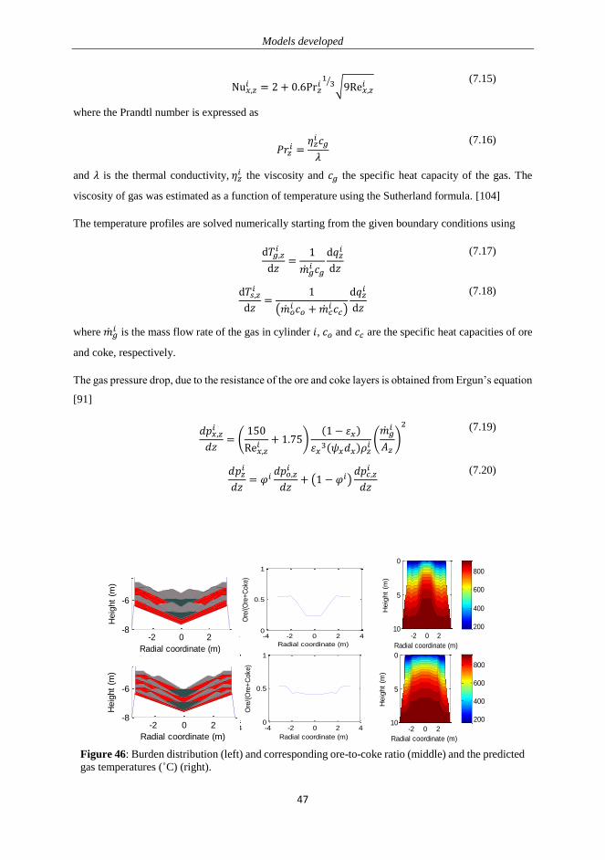
Models developed

47

Nu𝑥,𝑧

𝑖 = 2 + 0.6Pr𝑧𝑖1

3⁄ √9Re𝑥,𝑧𝑖

(7.15)

where the Prandtl number is expressed as

𝑃𝑟𝑧

𝑖 =𝜂𝑧

𝑖 𝑐𝑔

𝜆

(7.16)

and 𝜆 is the thermal conductivity, 𝜂𝑧𝑖 the viscosity and 𝑐𝑔 the specific heat capacity of the gas. The

viscosity of gas was estimated as a function of temperature using the Sutherland formula. [104]

The temperature profiles are solved numerically starting from the given boundary conditions using

d𝑇𝑔,𝑧𝑖

d𝑧=

1

��𝑔𝑖 𝑐𝑔

d𝑞𝑧𝑖

d𝑧

(7.17)

d𝑇𝑠,𝑧𝑖

d𝑧=

1

(��𝑜𝑖 𝑐𝑜 + ��𝑐

𝑖 𝑐𝑐)

d𝑞𝑧𝑖

d𝑧

(7.18)

where ��𝑔𝑖 is the mass flow rate of the gas in cylinder 𝑖, 𝑐𝑜 and 𝑐𝑐 are the specific heat capacities of ore

and coke, respectively.

The gas pressure drop, due to the resistance of the ore and coke layers is obtained from Ergun’s equation

[91]

𝑑𝑝𝑥,𝑧𝑖

𝑑𝑧= (

150

Re𝑥,𝑧𝑖

+ 1.75)(1 − 휀𝑥)

휀𝑥3(𝜓𝑥𝑑𝑥)𝜌𝑧

𝑖(��𝑔

𝑖

𝐴𝑧)

2

(7.19)

𝑑𝑝𝑧𝑖

𝑑𝑧= 𝜑𝑖

𝑑𝑝𝑜,𝑧𝑖

𝑑𝑧+ (1 − 𝜑𝑖)

𝑑𝑝𝑐,𝑧𝑖

𝑑𝑧

(7.20)

Figure 46: Burden distribution (left) and corresponding ore-to-coke ratio (middle) and the predicted

gas temperatures (˚C) (right).

-2 0 2-8

-6


Heig

ht

(m)

-2 0 2-8

-6


Heig

ht

(m)

-2 0 2-8

-6


Heig

ht

(m)

-2 0 2-8

-6


Heig

ht

(m)

-2 0 2-8

-6


Heig

ht

(m)

-2 0 2-8

-6


Heig

ht

(m)

-2 0 2-8

-6


Heig

ht

(m)

-2 0 2-8

-6


Heig

ht

(m)

-2 0 2-8

-6


Heig

ht

(m)

-2 0 2-8

-6


Heig

ht

(m)

-2 0 2-8

-6


Heig

ht

(m)

-2 0 2-8

-6


Heig

ht

(m)

-4 -2 0 2 40

0.5

1


Ore

/(O

re+

Cok

e)

-4 -2 0 2 40

0.5

1


Ore

/(O

re+

Cok

e)

-4 -2 0 2 40

0.5

1


Ore

/(O

re+

Cok

e)

-4 -2 0 2 40

0.5

1


Ore

/(O

re+

Cok

e)

-4 -2 0 2 40

0.5

1


Ore

/(O

re+

Cok

e)

-4 -2 0 2 40

0.5

1


Ore

/(O

re+

Cok

e)

-4 -2 0 2 40

0.5

1


Ore

/(O

re+

Coke)

-4 -2 0 2 40

0.5

1


Ore

/(O

re+

Coke)

-4 -2 0 2 40

0.5

1


Ore

/(O

re+

Coke)

-4 -2 0 2 40

0.5

1


Ore

/(O

re+

Coke)

-4 -2 0 2 40

0.5

1


Ore

/(O

re+

Coke)

-4 -2 0 2 40

0.5

1


Ore

/(O

re+

Coke)


Heig

ht

(m)

-2 0 2

0

5

10 200

400

600

800


Heig

ht

(m)

-2 0 2

0

5

10200

400

600

800


Heig

ht

(m)

-2 0 2

0

5

10 200

400

600

800


Heig

ht

(m)

-2 0 2

0

5

10 200

400

600

800


Heig

ht

(m)

-2 0 2

0

5

10 200

400

600

800


Heig

ht

(m)

-2 0 2

0

5

10 200

400

600

800


Heig

ht

(m)

-2 0 2

0

5

10 200

400

600

800


Heig

ht

(m)

-2 0 2

0

5

10200

400

600

800


Heig

ht

(m)

-2 0 2

0

5

10 200

400

600

800


Heig

ht

(m)

-2 0 2

0

5

10 200

400

600

800


Heig

ht

(m)

-2 0 2

0

5

10 200

400

600

800


Heig

ht

(m)

-2 0 2

0

5

10 200

400

600

800

47

Models developed

48

Thus, the effect of the main materials is considered whereas the possible effects of segregation of

particles is neglected. The temperature and pressure profiles are solved numerically by discretizing the

equations. At the beginning of the calculation a certain gas distribution is assumed for the concentric

rings. With the above assumption each of the concentric rings is solved individually using the above

equations for variation of pressure, gas and solid temperatures with height. The gas distribution is then

iterated until the pressure drop across all the concentric rings is the same. This gives a unique gas

distribution, which is considered to be the converged solution.

Figure 46 presents two different burden distributions in a blast furnace, which are evident from the

radial distribution of the ore-to-coke ratio. Therefore, the cases result in very different gas distributions

as simulated by the gas flow model and presented in the right part of the figure. Figure 47 presents a

schematic of how the gas flow model is integrated with the burden distribution and descent models.

48

Models developed

49

Start

Input simulation

parameters, charging

program, etc.

Insert first base layer into

the empty furnace

Are dumps left

for charging?

Is height

measured less

than required?

Descend the lowest layer, n, by a

differential amount

Descend the rest of the layers on top of the

layer below in the order n-1, n-2 ...1 such

that the volume of each layer is conserved

Solve the trajectory equation to get the

impact point on the burden surface

Solve for the burden surface to satisfy the

dump volume

Stop

Measure burden height at the

radar

Yes

Yes

No

No

Burden Charging model Burden Descent model

Display

results

Evaluate radial ore-to-coke ratio

distribution

Is end pressure

of concentric

rings equal?

Solve for the outlet temperature

and end pressure of the gas for

each concentric ring

individually

Change the gas distribution

among the rings

No

Gas Flow model

Assume gas distribution among

the concentric rings

Yes

Figure 47: Flowchart describing the burden distribution and the gas flow model

49

Models developed

50

7.4 Optimization using Genetic Algorithm (Paper II)

Blast furnace operators manipulate the charging program partly to target a particular gas flow

distribution inside the furnace, which is indirectly sensed through probe information (e.g., gas

temperatures and composition along a radius or diagonal). In bell-less top furnaces, the main means of

controlling the burden distribution is by changing the chute angle and the order of charges.

Mathematical models have been developed for predicting the burden distribution and gas flow inside

the furnace, however some strategy was required to systematically search through the innumerable

alternative parameter combinations. Such a problem is a non-linear and discontinuous function of the

parameters. Genetic Algorithm is very useful for tackling such optimization problems. In this study the

classical simple GA as proposed by Holland [42] was used for achieving required temperature profiles

at the in-burden probe levels by changing some parameters of a model charging program.

The model charging program consisted of four layers of pellet and coke each and one center coke layer,

which could be charged in one of the ways listed in Table 4. The coke dumps could be charged at chute

positions of 1-8 whereas the pellet dumps could be charged at positions 4-11 (cf. Table 3). Even for this

simplified case, the number of possibilities is enormous; more than 67 million (4 × 88 = 67,108,864)

charging programs exist.

Table 4 Different combinations for the charging order and respective bitwise representation. (P: Pellets;

C: Coke; CC: Center coke)

Charging order Bit representation

C C C C CC P P P P 00

C C P P CC C C P P 01

P P C C CC P P C C 10

P P P P CC C C C C 11

In the classical GA, the binary chromosome is used to represent a candidate solution. In this case the

chromosome was 26 bits long. The first two bits of it indicated the sequence of charging (Table 4) and

the subsequent bits in groups of three indicated the chute position for consecutive dumps. The three bits

indicate the position 1-8 or 4-11 depending on whether the dump is coke or pellet. Therefore, the

chromosome 01 101 011 011 101 111 100 111 110 is interpreted as the charging program

C6/C4/P7/P9/CC/C8/C5/P11/P10, where C represents coke, P pellet and the subscript indicates the chute

position. A set of 50 individual chromosomes were randomly generated to create the initial population,

which constituted the parent population. Two-point crossover was carried out between random pairs of

parent chromosomes and bitwise mutation was applied to create the offspring population. The crossover

and the mutation were carried out with 90% and 4% probability, respectively. The tournament selection

50

Models developed

51

method was used to select the surviving population which acts as the parent for the next generation.

This is repeated several times until the population converges to an optimum solution.

Six different targets were specified which represented some typical temperature profiles and the

optimization problem was set to minimize the root mean square error (𝐸) between the target (��𝑖) and

achieved (𝑇𝑖) temperatures. The achieved temperatures were calculated using the burden distribution

and gas flow models (Sec. 7.2 and 7.3)

𝐸 = √∑ (𝑇𝑖 − ��𝑖)2𝑁

𝑖=1

𝑁

(7.21)

Figure 48 presents the target and the achieved temperature profiles at the end of the search after 200

generations. There was a very good correspondence of the target and the achieved temperature profile,

especially for subplots A-D and F. For subplot E the fit is not so good; a possible reason is that it is

difficult to achieve a plateau of high temperature in the center of the furnace with the charging programs

available in the present setup.

The evaluation of one individual chromosome, i.e., the simulation of the burden distribution arising

from the charging program, followed by simulation of the gas distribution and calculation of the error

compared to the target, took slightly less than half a minute. Therefore, evolution of the individuals for

Figure 48 Target (dashed lines) and achieved (solid lines) temperature profiles for the best

individuals at the end of the evolution.

(A) (B) (C)

(D) (E) (F)

51

Models developed

52

200 generations, going through a search of about 24000 distinct individuals for each of the targets, took

about eight days. This is still acceptable compared to the estimated time of more than 63 years for an

exhaustive search among the 67 million possible candidates.

7.5 DEM model of burden distribution (Papers III, IV)

The burden distributions for different charging programs were simulated using EDEM, a commercial

software implementing the DEM. The simulation setup (Figure 49) consisted of a channel in which the

particles were generated at a rate so that the dump creates a complete ring. The particles fell on the

chute, rotating at a constant velocity (0.897 rad/s) around the ‘axis’ passing through the center of the

channel. After that the particle stream slid along the chute and distributed inside the furnace throat.

Initially, a conical surface with an angle mimicking the pellet repose angle constituted the lower

boundary for the first dump. Later dumps were formed on the layers generated by the previous dumps.

DEM simulation is computationally expensive because of a large number of particles and a maximum

time step in the order of 10-5 s. To reduce the computational burden, a 90˚ section of the throat was

simulated which reduced the number of particles considerably. However, this assumption introduced

artificial wall effects. Therefore, only a smaller section in the middle, an ‘angular slice’ of 30 of the

simulated region of the throat (Figure 49), was used to report the results. It should also be stressed that

because of this setup the particles have very limited space near the center of the furnace, so the results

in this region were mostly disregarded in the analysis. Uniform particle size distribution was assumed;

therefore size segregation was not considered.

channel

chute

rotational

axis

chute

angle

section angle throat

actual throat

circumference

direction of

rotation

cross section

for layer

formation

results repose angle of

pellet

section for

quantitative

calculations

Figure 49: (Left) Isometric view and (right) orthographic view of the simulated charging

system.

52

Models developed

53

Results from DEM simulation from a full scale setup and the experimental (small scale) setup were

compared. The distances were scaled as 1:10 and the particles were scaled as 1:4 for the two setups.

The charging program and some dimensions used for this comparison are shown in Table 5.

Table 5 Charging programs and some dimensions for comparison between experimental scale and full

scale simulations.

Material LC SC CC P P

Mass (kg)

Experimental scale 3.89 3.89 0.58 16.59 16.59

Full scale 3888 3888 580 16588 16588

Chute position 6 4 1 10 10

Max. particle

diameter (mm)

Experimental scale 12.5 7.5 18 3 3

Full scale 50 30 72 12 12

Throat

diameter (m)

Experimental scale 0.63

Full scale 6.3

Figure 50 shows the cross section for DEM simulations after charging each dump. The subfigures A-E

show the result for full scale simulation and subfigures 1-5 are the corresponding simulations using a

scaled model. It may be observed that the profiles are quite similar, but yet there are some differences

as the particles were not scaled according to the furnace dimension. It accounts for the distinct peak

which may be observed in coke dumps in full scale simulation unlike the small scale experiments

(subfigures A, B). The effect of pellets pushing the coke dump (subfigures C, D, E and 3, 4, 5) is much

more pronounced in full scale because the energy carried by pellet dumps is much higher.

53

Models developed

54

7.6 Mixed layer formulation (Paper III)

A mixed layer (Figure 51) is a layered volume occupied by multiple

particle types, often with a lower voidage than the other parts of the

bed. Formation of mixed layer in blast furnaces is important, as

some studies have reported it may account for 20-35% of the net

pressure drop across the furnace [92]. It is therefore important to

understand the formation of the mixed layer in burden distribution

calculations. Although the concept of mixed layer is easy to

understand, yet a computational definition of the mixed layer is

difficult as it requires proper definition of layer boundaries. This can

be a challenging task, particularly in three dimensions.

In this study, the simulation setup is divided into rectilinear grids of control volumes and each of these

volumes is assumed to be represented by a single value for the fraction of a particular particle type and

for the voidage. The mixed layer is defined as the collection of control volume units that contain more

than one particle type or are surrounded by mixed layer volumes. The control volumes surrounded by

mixed layer control volumes are also treated as part of the mixed layer to account for the case where a

control volume happens to lie in the space between two large particles. It is computationally difficult

Figure 50: DEM simulation of a charging program in experimental (1-5) and full (A-E)

scale.

(A) (B)

(C) (D)

(E)

(1) (2)

(3) (4)

(5)

Layer 1

Layer 2

Mixed layer

Figure 51: Mixed layer

54

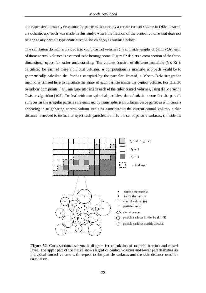
Models developed

55

and expensive to exactly determine the particles that occupy a certain control volume in DEM. Instead,

a stochastic approach was made in this study, where the fraction of the control volume that does not

belong to any particle type contributes to the voidage, as outlined below.

The simulation domain is divided into cubic control volumes (𝑣) with side lengths of 5 mm (∆ℎ): each

of these control volumes is assumed to be homogeneous. Figure 52 depicts a cross section of the three-

dimensional space for easier understanding. The volume fraction of different materials (𝑘 ∈ K) is

calculated for each of these individual volumes. A computationally intensive approach would be to

geometrically calculate the fraction occupied by the particles. Instead, a Monte-Carlo integration

method is utilized here to calculate the share of each particle inside the control volume. For this, 30

pseudorandom points, 𝑗 ∈ J, are generated inside each of the cubic control volumes, using the Mersenne

Twister algorithm [105]. To deal with non-spherical particles, the calculations consider the particle

surfaces, as the irregular particles are enclosed by many spherical surfaces. Since particles with centers

appearing in neighboring control volume can also contribute to the current control volume, a skin

distance is needed to include or reject such particles. Let I be the set of particle surfaces, 𝑖, inside the

outside the particle

inside the particle

control volume (𝑣)

particle center

skin distance

𝑟I,particle surfaces inside the skin (I)

particle surfaces outside the skin

𝑓1 > 0 ∩ 𝑓2 > 0

𝑓1 = 1

𝑓2 = 1

mixed layer

Figure 52: Cross-sectional schematic diagram for calculation of material fraction and mixed

layer. The upper part of the figure shows a grid of control volumes and lower part describes an

individual control volume with respect to the particle surfaces and the skin distance used for

calculation.

55

Models developed

56

region enclosed by another volume whose sides are within the skin distance 𝑟I,max from the control

volume sides as described in the lower part of Figure 52, with

𝑟I,max = max(𝑟𝑖) (7.22)

and where 𝑟𝑖 is the radius of the surface 𝑖, and 𝑑𝑗,𝑖 are the distances of the points 𝑗 from the center of

surface 𝑖. The material type for each of the 𝑖 surfaces is denoted by 𝜌𝑖 . The set of points in the control

volume 𝑣 which belong to a particular material type 𝑘 is now given by

Nk: {𝑗 ∈ 𝐽 | 𝑑𝑗,𝑖 ≤ 𝑟𝑖 | 𝜌𝑖 = 𝑘} (7.23)

The fraction of material type k in the control volume is the ratio of the cardinal numbers of set Nk and

N.

𝑓𝑘 =

|Nk|

|N|

(7.24)

The voidage of the control volume is, in turn, defined as

휀 = 1 − ∑𝑓𝑘𝑘

(7.25)

The simulation setup is enclosed within a mesh (𝑀 × 𝑁 × 𝑃) of such cubic control volumes, 𝑣𝑚,𝑛,𝑝,

where 𝑚, 𝑛, 𝑝 indicate the indices of the control volume in the three-dimensional space. Therefore,

𝑚 ∈ [1,𝑀], 𝑛 ∈ [1, 𝑁] and 𝑝 ∈ [1, 𝑃] and the indices increase along the direction of the axes. The

indices of the upper surface of any layer of material 𝑘 at horizontal indices (𝑚, 𝑛) are given by

𝑈𝑚,𝑛𝑘 = max{𝑝 | (𝑓𝑘)𝑚,𝑛,𝑝 ≥ 0} (7.26)

The lower surface control volumes are given by

𝐿𝑚,𝑛𝑘 = min{𝑝 | (𝑓𝑘)𝑚,𝑛,𝑝 ≥ 0} (7.27)

The layer height is therefore

ℎ𝑚,𝑛𝑘 = (𝑈𝑚,𝑛

𝑘 − 𝐿𝑚,𝑛𝑘 + 1)∆ℎ (7.28)

Likewise, for the mixed layer of material 𝑘 and 𝑘′, the upper surface (𝑈𝑚,𝑛𝑘,𝑘′

), lower surface (𝐿𝑚,𝑛𝑘,𝑘′

) and

the layer heights (ℎ𝑚,𝑛𝑘,𝑘′

) are given by

𝑈𝑚,𝑛𝑘,𝑘′

= max{𝑝 | (𝑓𝑘)𝑚,𝑛,𝑝 ≥ 0 ∩ (𝑓𝑘′)𝑚,𝑛,𝑝 ≥ 0} (7.29)

𝐿𝑚,𝑛𝑘,𝑘′

= min{𝑝 | (𝑓𝑘)𝑚,𝑛,𝑝 ≥ 0 ∩ (𝑓𝑘′)𝑚,𝑛,𝑝 ≥ 0} (7.30)

ℎ𝑚,𝑛𝑘,𝑘′

= (𝑈𝑚,𝑛𝑘,𝑘′

− 𝐿𝑚,𝑛𝑘,𝑘′

+ 1)∆ℎ (7.31)

56

Models developed

57

This formulation may be used to detect the extent and the voidage of mixed layers arising in simulation

by DEM, which can give interesting information for gas flow calculations. Figure 53 shows the analysis

based on the above formulation for the simulated layers of a full scale DEM simulation based on the

materials in Table 5. The first two subfigures show the thicknesses of the mixed layers formed by the

two coke sizes (small coke and large coke) and the coke and pellet layers. Each colored point in the

figure presents the highest point along the vertical

(z) axis of the mixed layer for a particular point on

the horizontal (x, y) plane (cf. Eq. 7.29). The color

of the point corresponds to the thickness of the

mixed layer at the (x, y) coordinate in question. The

mixed layer formed by the two different coke sizes

is bigger than that by pellet and coke, because the

participating particles have greater size.

Figure 54 shows the voidage distribution in a similar

manner for each of the individual layers and the

mixed layers. Yellow and blue show the regions of

high and low voidage respectively. The vertical axis

in the figure has been exaggerated for clarity. In

general, the coke particles have lower voidage than

the pellet particles as the combination of different

irregular shapes of the coke particles allows for

higher packing than for pellet particles.

Figure 53: Thickness of the mixed layer composed of two sizes of coke (left), as well as pellet

and coke (right).

x

y x

y

Figure 54: Voidage distribution for all the

layers charged into the furnace. (1: Pellet, 2:

Mixed, pellet and coke, 3: Center coke, 4:

Small coke, 5: Mixed, large coke and small

coke, 6: Large coke). The vertical axis is

exaggerated for clarity.

1

5

4 3

2

6

57

Models developed

58

7.7 Coke push formulation (Paper IV)

The burden distribution and descent models discussed in Sec. 7.2 did not consider the coke collapse but

assumed that the previous layers are stagnant at charging. The model was modified to calculate the

stability of a coke layer and to correct the layer structure accordingly using stability theory.

The stability of a slope may be

expressed as a ratio between the

available shear strength (𝑠) and the

shear stress (𝜏) along a failure plane,

referred to as a ‘factor of safety’

𝑓𝑠 =𝑠

𝜏

(7.32)

Theoretically the slope is unstable if

the factor of safety is less than unity.

However, studies have experimentally

identified the limit to be closer to 0.8

[53]. The shape of the failure plane

may vary but in this study it is assumed

to be circular (Figure 55, left), which is

a necessary condition for using the

‘Ordinary method of slices’ [106] for factor of safety calculation. The shear strength is defined in terms

of normal stress (𝜎) on the failure plane. Cohesion between the individual particles is neglected because

the particles are large enough. Therefore, the above equation may be written as

𝑓𝑠 =

𝜎 tan𝜙

𝜏

(7.33)

where 𝜙 is the developed friction angle of the material. As per many limit equilibrium methods [106]

for calculating the factor of safety for the slip surface, the region above the failure surface is divided

into a finite number of thin vertical slices, each with a base length of Δ𝑙𝑛 and of unit depth. Figure 55

shows the forces acting on such a slice, 𝑛 (right panel), located at a particular position on the failure

surface (left panel). 𝑊𝑛 is the weight and 𝐹𝑛 is the external force on the slice, and 𝛼𝑛 is the angle made

by the tangent on the failure surface to the horizontal. In the ordinary method of slices it is assumed that

the inter-slice forces acting in the horizontal direction cancel each other

𝐸𝑛−1 + 𝐸𝑛 = 0 (7.34)

Coke layer

Failure plane

R

𝛼𝑛

O

𝐹𝑛

𝑊𝑛 𝑁𝑛 𝛼𝑛

𝑆𝑛

𝐸𝑛−1

𝐸𝑛

Δ𝑙𝑛

Figure 55: Stability analysis using method of slices. Left:

The failure surface and the center of failure surface O. The

grid represents the different positions centers of rotation

used for evaluating the factor of safety. Right: Forces

acting on each slice.

58

Models developed

59

The shear force at the bottom of the slice (𝑆𝑛) is defined as

𝑆𝑛 = 𝜏𝑛Δ𝑙𝑛

(7.35)

where 𝜏𝑛 is the shear stress for slice 𝑛. Using Eq. (7.33) the above equation may be rewritten as

𝑆𝑛 =

𝜎𝑛 tan𝜙

𝑓𝑠Δ𝑙𝑛

(7.36)

where 𝜎𝑛 is the normal stress on slice 𝑛, while 𝑓𝑠 and 𝜙 are assumed to remain constant for all the slices.

The normal force on the slip surface is given by

𝑁𝑛 = 𝜎𝑛Δ𝑙𝑛 (7.37)

From the free body diagram (Figure 55, right), the normal force may also be expressed as

𝑁𝑛 = (𝑊𝑛 + 𝐹𝑛) cos𝛼𝑛

(7.38)

At the critical point of equilibrium, the clockwise and anti-clockwise moments around O, the center of

the slip surface, are equal, so

∑(𝑊𝑛 + 𝐹𝑛)𝑅 sin𝛼𝑛

𝑛

= ∑𝑆𝑛

𝑛

𝑅 (7.39)

where 𝑅 is the radius of curvature for the slip plane. Substituting the value of 𝑆𝑛 from Eq. (7.36) yields

∑(𝑊𝑛 + 𝐹𝑛)𝑅 sin 𝛼𝑛

𝑛

= ∑𝜎𝑛 tan𝜙

𝑓𝑠Δ𝑙𝑛

𝑛

𝑅 (7.40)

Using Eqs. (7.37), (7.38) and (7.40) we get

∑(𝑊𝑛 + 𝐹𝑛)𝑅 sin𝛼𝑛

𝑛

= ∑(𝑊𝑛 + 𝐹𝑛) cos𝛼𝑛 tan𝜙

Δ𝑙𝑛 𝑓𝑠𝑛

Δ𝑙𝑛 𝑅 (7.41)

Rearranging the equation, an expression for factor of safety is obtained as

𝑓𝑠 =

∑ (𝑊𝑛 + 𝐹𝑛) cos 𝛼𝑛 tan𝜙𝑛

∑ (𝑊𝑛 + 𝐹𝑛) sin 𝛼𝑛𝑛

(7.42)

Therefore, when an external force is applied on the heap formed by granular particles the stability of

the slope is a function of the magnitude and position of the force acting on the slope, density of the

material forming the slope and frictional resistance applied by the material.

This factor of safety is evaluated using different trial points as centers of curvature (intersections of the

grid in the left panel of Figure 55). The failure plane is assumed to pass through the intersection of the

wall and the layer surface. The minimum value of all the trial points corresponds to the critical factor

of safety and it also defines the stability of the layer surface.

59

Models developed

60

During the charging process there are three possibilities. Firstly, the slope does not change significantly

due to the incoming stream. Secondly, impact failure may occur when the pellet stream displaces the

coke particles but there is no collapse of the layer. Thirdly, gravity failure occurs when the slope is

unstable and the particles flow to the center of the furnace, in turn changing the slope of the layer. Each

of these three failure modes depend on the shape of the coke layer surface and the radial position of the

pellet stream. The factor of safety of a surface depends on these aspects, and a higher factor means a

stable slope. In this study the three possibilities are assessed by estimating the factor of safety of a slope:

if the value is high enough then the slope is stable, for a medium-level value impact failure is taken to

occur, while a low value of the safety factor corresponds to gravity failure. In practice, the impact failure

and gravity failure may occur in combination, but this was neglected in the present study to make the

model manageable.

Figure 56 shows a schematic diagram of the implementation of the failure modes in the mathematical

model. The factor of safety is evaluated for a particular coke surface against a pellet stream entering at

a particular position, and it is used to determine if the coke slope needs correction. If the value is lower

than a threshold value, impact failure is taken to occur and the coke apex is only moved towards the

furnace center but the surface would not collapse. For highly unstable slopes, i.e., very low values of

the safety factor, gravity failure is expected where part of the coke layer would break away and slide to

the center.

The lower part of Figure 56 schematically illustrates the correction scheme for a coke layer which

results in impact failure and gravity failure.

To correct the coke layer and to

accommodate the failure mechanisms, the

apex of the coke layer (𝑟, 𝑦) is moved

towards the center. The radial displacement,

Δ𝑟, results in a vertical displacement, Δ𝑦,

which is calculated from the constraint that

the volume of the coke layer before and after

the collapse is equal. Thus, no change in

voidage is taken to occur and the mixed layer

is neglected. In case of impact failure the

apex is displaced by a small amount and the

corresponding factor of safety for the

reconstructed layer is calculated. The factor

of safety increases as the apex is moved

towards the center. If the factor reaches the

limit of stability the displacement is stopped,

Base

Coke layer (before)

Coke layer (after)

Impact failure Gravity failure

(𝑟, 𝑦)

∆𝑟 ∆𝑦

𝑟 𝑦

Overflow

Figure 56: Top: Schematic diagram of two types of

coke collapse, impact failure and gravity failure.

Bottom: Corresponding implementation in the

present mathematical model.

60

Models developed

61

else it is displaced further towards the center and the factor of safety is recalculated. For gravity failure

the inner (𝛽i) and outer slopes (𝛽o) of the lines describing the upper surface of the coke layer are

decreased because of the collapse, where the decrease depends on the displacement of the apex. The

new slopes 𝛽i,new and 𝛽o,new are given by

𝛽i,new = 𝑘i∆𝑟 𝛽i (7.43)

𝛽o,new = 𝑘o∆𝑟 𝛽o (7.44)

where 𝑘i and 𝑘o are factors determined empirically and they depend on the dimensions of the furnace.

As the slopes of the lines are known and are less than the original slope, the layer overflows into the

center and the extent of overflow would depend on the degree of instability of the initial slope.

Five model charging programs consisting of a small coke dump, a large coke dump, a center coke dump

and two pellet dumps, were studied using DEM and small scale experiments. When the pellet dump

was charged over the coke layer, one of the charging programs showed impact failure and another

program showed gravity failure whereas, the rest were not affected. This theory was used to predict the

occurrence of the collapse and the layer structure after it had collapsed. The model showed good

correspondence with the DEM simulations and successfully predicted the collapse. The experiments

and the results are detailed in Paper IV.

This method may be utilized to study how prone a particular layer of a charging program is to collapse.

Figure 57 shows the mathematical simulation of a complicated charging program based on the

conditions in a real furnace with about 20 layers of pellets and coke at various charging positions,

repeated over a number of times. In general, it may be observed from the mathematical simulation that

the charging program creates two contiguous regions of coke (C1 and C2, consisting of grey and olive

layers in the figure) with pellet (P1

and P2, red) regions in between them.

One of the coke regions, C1, has an

overall slope which is steeper near the

furnace center, while the other coke

region, C2, has a less steep surface

because of a smaller coke dump near

the furnace center. Therefore it can be

reasoned that the C1 is more prone to

failure than C2. In this example, after

charging each coke dump, the factor

of safety of the layer was calculated if

the subsequent dump was pellet. The

layers which are prone to collapse are

Figure 57: Simulation for a complicated burden distribution

program. The slopes which are prone to collapse are marked

in yellow. Inset magnifies a portion of the simulation.

C1

C2 P1

P2

61

Models developed

62

marked in yellow in the figure. Thus, the coke collapse theory can help in identifying such regions and

also guide the operators in designing more stable programs.

Currently, the outlined procedure can only change the results of the burden distribution model to

account for a coke collapse in a limited number of dumps. In the future, the model should be

implemented to automatically adjust the burden distribution for layers showing coke collapse.

62

63

8. Conclusions

The efficiency of a blast furnace depends largely on the gas flow pattern inside it, as the gas phase is

central in the reduction reactions and in the heat transfer. The bed in a blast furnace consists of layers

of materials with different physical properties, including density, voidage, particle size and shape.

Therefore, controlling the burden distribution is the primary method for achieving a proper gas flow in

the furnace and practically the only means of directly controlling the radial distribution of variables in

the process. Thus, it is crucial for the furnace operator to understand the effect of the charging program

on the formation, shape and thickness of the burden layers. Modern charging equipment allows much

more precise charging, but this also increases the number of parameters the operator can modify to

achieve the required gas flow. This makes burden distribution optimization a complex problem with a

huge number of alternatives. Computational tools are therefore needed to help the operators understand

the effect of decisions concerning the choice of charging programs.

In this doctoral work a burden distribution model that can give a quick estimation of the layer structure

inside the furnace was developed. The model used simple equations and geometric representations of

the layers to achieve a fast model which can be run in less than half a minute. Small scale experiments

were used to verify the results from the mathematical model, which showed reasonable agreement with

the findings from the charging experiments.

The burden distribution model provided the distribution of materials in the furnace, which was used to

develop a model simulating the gas and solid temperature in the upper part of the furnace with

reasonable simplifications. A genetic algorithm was used to optimize the charging programs to attain a

particular gas temperature distribution at the vertical level of an in-burden (below burden) probe. The

search was efficient and the algorithm was found to be suitable for discontinuous and non-differentiable

problems like the problem at hand.

Particle methods like DEM are much more helpful for understanding the flow of bulk solids than

continuum methods. DEM was used in this thesis to gain an understanding of the burden formation

behavior for different charging programs. To account for the shape of coke particles a clumped sphere

model was used successfully. The simulation results were used to study mixed layers. In scaled

simulation the mixed layer was found to have around 12% lower voidage than the layers of individual

components. The formulation for calculating the voidage distribution in the furnace would be useful for

CFD calculations studying the gas flow in the blast furnace by continuum models.

In charging experiments and the DEM simulations, it was observed that for particular charging

programs the coke layer collapsed when heavier pellets were charged at higher charging positions.

Therefore, a model based on slope stability analysis was developed to classify the extent of coke

collapse and a scheme was outlined of how to change the layer structure to make it stable to the loading

63

Conclusions

64

condition. The simulations and the experimental results demonstrated that the scheme could capture the

behavior fairly well. A collapse may be avoided by charging the coke closer to the furnace center or at

least splitting the coke dump to partially charge it further off from the wall.

64

65

9. Future prospects

In this doctoral work, a mathematical model was developed for rapid simulation of burden distribution

in the blast furnace. A simplified gas distribution model was also developed using the results from the

burden distribution model. A genetic algorithm was used to find the right combination of charging

parameters for a target gas distribution. Additionally, DEM models and charging experiments were

applied to gain a deeper understanding of the phenomena at charging. Even though these models and

experiments have provided insight into the central factors and phenomena involved in the distribution

of the burden in the blast furnace, further work is still required.

The mathematical models may be optimized further to reduce the calculation overhead times. The coke

collapse model developed in this thesis should be fully integrated with the burden distribution model to

make the layer correction procedure robust enough for handling complicated charging programs. A

graphical user interface for the mathematical model has already been built to facilitate its interactive

use in steel industry, but in the future the model should also be connected to the industrial database to

allow for real time calculations.

The gas flow model has to be improved significantly to allow crossflows and accurate treatment of the

solid flow. The data from the gas flow model could then be matched with the temperature probe readings

from the plant, possibly in online use. This would make it possible to predict internal variables, such as

the cohesive zone shape in the furnace, which would give extremely useful information to the blast

furnace operator.

DEM provides a means of gaining insight into the flow behavior of particles in the furnace, but the

heavy computational burden still makes it impossible to simulate the whole furnace with true particle

sizes. However, as the computation technology improves, especially with the advent of GPU (Graphics

Processing Unit) accelerated computing, the computation times will decrease and it is likely that full-

scale simulation will be feasible in the near future. Meanwhile, there are several other phenomena

related to the behavior of bulk solids which need to be understood further, especially in context of blast

furnaces. The effect of particle shapes and particle size distribution on the burden distribution should

be studied further. The conditions inside the blast furnace are also particularly interesting, because the

gas flow affects the distribution of smaller particles (fines). Coupled CFD-DEM simulation can help in

understanding such phenomena in detail.

Finally, more research would be needed to fully understand the physical and chemical processes in the

blast furnace. Better understanding of the coupling of different processes can be used to improve the

efficiency of blast furnace charging. This will help in reducing the coke rates and thereby reduce the

production cost and carbon footprint of ironmaking process, paving the way to a more sustainable

future.

65

66

References

[1] D. R. Lide, Ed., CRC Handbook of Chemistry and Physics. New York: CRC Press, 1996.

[2] A. Ghosh and A. Chatterjee, Iron Making and Steelmaking: Theory and Practice. PHI Learning

Pvt. Ltd., 2008.

[3] (2016, Feb 16). Annual iron production archive. Available:

http://www.worldsteel.org/statistics/statistics-archive/iron-archive.html.

[4] A. Carpenter, "CO2 abatement in the iron and steel industry," IEA Clean Coal Centre, 2012.

[5] J. De Beer, "Future technologies for energy-efficient iron and steel making," in Potential for

Industrial Energy-Efficiency Improvement in the Long TermAnonymous Springer, 2000, pp. 93-

166.

[6] J. G. Peacey and W. G. (. G. Davenport, The Iron Blast Furnace : Theory and Practice. Oxford ;

New York : Pergamon Press, 1979.

[7] A. Rist and N. Meysson, "A Dual Graphic Representation of the Blast Furnace Mass and Heat

Balances," Journal of Metals, vol. 19, pp. 50-59, 1967.

[8] I. Muchi, "Mathematical Model of Blast Furnace," Transactions of the Iron and Steel Institute of

Japan, vol. 7, pp. 223-&, 1967.

[9] A. Kilpinen, "An on-line model for estimating the melting zone in a blast furnace," Chemical

Engineering Science, vol. 43, pp. 1813-1818, 1988.

[10] N. K. Nath, "Simulation of gas flow in blast furnace for different burden distribution and

cohesive zone shape," Materials and Manufacturing Processes, vol. 17, pp. 671-681, 2002.

[11] X. F. Dong, D. Pinson, S. J. Zhang, A. B. Yu and P. Zulli, "Gas-powder flow in blast furnace

with different shapes of cohesive zone," Applied Mathematical Modelling, vol. 30, pp. 1293-

1309, 11, 2006.

[12] M. Hatano and K. Kurita, "A Mathematical Model of Blast Furnace with Radial Distribution of

Gas Flow, Heat Transfer and Reactions Considered," Transactions of the Iron and Steel Institute

of Japan, vol. 22, pp. 448-456, 1982.

66

References

67

[13] Z. Zhou, H. Zhu, A. Yu, B. Wright, D. Pinson and P. Zulli, "Discrete particle simulation of solid

flow in a model blast furnace," ISIJ International, vol. 45, pp. 1828-1837, 2005.

[14] J. A. de Castro, H. Nogami and J. Yagi, "Three-dimensional Multiphase Mathematical Modeling

of the Blast Furnace Based on the Multifluid Model." ISIJ International, vol. 42, pp. 44-52,

2002.

[15] A. Adema, DEM-CFD Modelling of the Ironmaking Blast Furnace. TU Delft, Delft University of

Technology, 2014.

[16] H. Saxén and F. Pettersson, "Nonlinear prediction of the hot metal silicon content in the blast

furnace," ISIJ International, vol. 47, pp. 1732-1737, 2007.

[17] A. Agarwal, U. Tewary, F. Pettersson, S. Das, H. Saxén and N. Chakraborti, "Analysing blast

furnace data using evolutionary neural network and multiobjective genetic algorithms,"

Ironmaking & Steelmaking, vol. 37, pp. 353-359, 2010.

[18] A. Biswas, Principles of Blast Furnace Ironmaking : Theory and Practice. Brisbane Australia:

Cootha, 1981.

[19] J. J. Poveromo, "Burden distribution fundamentals," vol. 22-23, 1995-1996.

[20] H. Takahashi, H. Kawai, M. Kobayashi and T. Fukui, "Two dimensional cold model study on

unstable solid descending motion and control in blast furnace operation with low reducing agent

rate," ISIJ International, vol. 45, pp. 1386-1395, 2005.

[21] A. Murao, Y. Kashihara, N. Oyama, M. Sato, S. Watakabe, K. Yamamoto and Y. Fukumoto,

"Development of control techniques for mixing small coke at bell-less top blast furnace." ISIJ

International, vol. 55, pp. 1172-1180, 2015.

[22] P. K. Gupta, A. S. Rao, V. R. Sekhar, M. Ranjan and T. K. Naha, "Burden distribution control

and its optimisation under high pellet operation," Ironmaking & Steelmaking, vol. 37, pp. 235-

239, 2010.

[23] B. D. Pandey and U. S. Yadav, "Blast furnace performance as influenced by burden distribution,"

Ironmaking & Steelmaking, vol. 26, pp. 187-192, 1999.

[24] M. Riddle and P. Whitfield, "Design and operation of a Gimbal Top distribution system for

ironmaking plants," Revue De Métallurgie, vol. 104, pp. 113-119, 2007.

67

References

68

[25] B. Boranbaev, Y. Glazer, V. Vakulin and A. Sirkar, "Bell-less rotary charging unit–A perfect

burden loading technology," Metallurgist, vol. 53, pp. 395-403, 2009.

[26] R. Timmer, J. Droog, G. Flierman and A. Steeghs, "Radial gas distribution in the blast furnace

top," Steel Research, vol. 68, pp. 47-53, 1997.

[27] S. Nag, A. Gupta, S. Paul, D. J. Gavel and B. Aich, "Prediction of Heap Shape in Blast Furnace

Burden Distribution," ISIJ International, vol. 54, pp. 1517-1520, 2014.

[28] M. Naito, K. Takeda and Y. Matsui, "Ironmaking technology for the last 100 years: deployment

to advanced technologies from introduction of technological know-how, and evolution to next-

generation process," ISIJ International, vol. 55, pp. 7-35, 2015.

[29] H. P. Zhu, Z. Y. Zhou, R. Y. Yang and A. B. Yu, "Discrete particle simulation of particulate

systems: A review of major applications and findings," Chemical Engineering Science, vol. 63,

pp. 5728-5770, 12/1, 2008.

[30] DEM Solutions Ltd., "EDEM," vol. 2.3-2.7, 2010-2015.

[31] DEM Solutions Ltd., "EDEM 2.3 user guide," 2010.

[32] H. Hertz, "On the contact of elastic solids," Journal Für Die Reine Und Angewandte Mathematik,

vol. 92, pp. 156-171, 1881.

[33] P. A. Cundall and O. D. Strack, "A discrete numerical model for granular assemblies,"

Geotechnique, vol. 29, pp. 47-65, 1979.

[34] M. Kremmer and J. F. Favier, "A method for representing boundaries in discrete element

modelling—part II: Kinematics," International Journal for Numerical Methods in Engineering,

vol. 51, pp. 1423-1436, 2001.

[35] S. Ueda, S. Natsui, Z. Fan, H. Nogami, R. Soda, J. Kano, R. Inoue and T. Ariyama, "Influences

of physical properties of particle in discrete element method on descending phenomena and

stress distribution in blast furnace," ISIJ International, vol. 50, pp. 981-986, 2010.

[36] G. Defendi, A. Baltazar, P. F. Nogueira, A. G. Cornejo and D. S. Nasato, "Blast furnace charging

simulation using EDEM," in Proceedings EDEM Conference 2011, Edinburgh, Scotland, 2011,

pp. 291-311.

68

References

69

[37] Y. Yu and H. Saxen, "Flow of Pellet and Coke Particles in and from a Fixed Chute," Industrial &

Engineering Chemistry Research, vol. 51, pp. 7383-7397, 2012.

[38] H. Matuttis and J. Chen, Understanding the Discrete Element Method: Simulation of Non-

Spherical Particles for Granular and Multi-Body Systems. John Wiley & Sons, 2014.

[39] T. Pöschel and T. Schwager, Computational Granular Dynamics: Models and Algorithms.

Springer Science & Business Media, 2005.

[40] K. Deb, Multi-Objective Optimization using Evolutionary Algorithms. John Wiley & Sons, 2001.

[41] T. Mitra, H. Saxén and N. Chakraborti, "Evolutionary algorithms in ironmaking applications," in

Evolutionary Computation: Techniques and Applications, A. M. Gujrathi and B. V. Babu, Eds.

Ontario: Apple Academic Press, 2016, .

[42] J. H. Holland, Adaptation in Natural and Artificial Systems: An Introductory Analysis with

Applications to Biology, Control, and Artificial Intelligence. U Michigan Press, 1975.

[43] V. R. Radhakrishnan and K. M. Ram, "Mathematical model for predictive control of the bell-less

top charging system of a blast furnace," Journal of Process Control, vol. 11, pp. 565-586, 2001.

[44] R. Balevičius, R. Kačianauskas, Z. Mróz and I. Sielamowicz, "Analysis and DEM simulation of

granular material flow patterns in hopper models of different shapes," Advanced Powder

Technology, vol. 22, pp. 226-235, 3, 2011.

[45] A. W. Jenike, "Gravity flow of bulk solids," Bulletin no.108, Utah State University, 1961.

[46] S. Jung and W. Chung, "Improvement of Gas Flow through Analyzing Discharge Behavior in the

Bunker Used in Blast Furnace." ISIJ International, vol. 41, pp. 1324-1330, 2001.

[47] Y. Yu and H. Saxén, "Experimental and DEM study of segregation of ternary size particles in a

blast furnace top bunker model," Chemical Engineering Science, vol. 65, pp. 5237-5250, 2010.

[48] P. A. Langston, U. Tüzün and D. M. Heyes, "Discrete element simulation of granular flow in 2D

and 3D hoppers: Dependence of discharge rate and wall stress on particle interactions,"

Chemical Engineering Science, vol. 50, pp. 967-987, 3, 1995.

[49] P. W. Cleary and M. L. Sawley, "DEM modelling of industrial granular flows: 3D case studies

and the effect of particle shape on hopper discharge," Applied Mathematical Modelling, vol. 26,

pp. 89-111, 2, 2002.

69

References

70

[50] A. Anand, J. S. Curtis, C. R. Wassgren, B. C. Hancock and W. R. Ketterhagen, "Predicting

discharge dynamics from a rectangular hopper using the discrete element method (DEM),"

Chemical Engineering Science, vol. 63, pp. 5821-5830, 12, 2008.

[51] S. Watakabe, K. Takeda, H. Nishimura, S. Goto, N. Nishimura, T. Uchida and M. Kiguchi,

"Development of high ratio coke mixed charging technique to the blast furnace," ISIJ


[52] Y. Kashihara, Y. Morikawa, T. Sato, N. Ishiwata and M. Sato, "Development of Charging

Technique for Controlling Mixed Coke Distribution in Ore Layer," ISIJ International, vol. 55,

pp. 1165-1171, 2015.

[53] S. Nag and V. Koranne, "Development of material trajectory simulation model for blast furnace

compact bell-less top," Ironmaking & Steelmaking, vol. 36, pp. 371-378, 2009.

[54] T. Mitra and H. Saxén, "Model for fast evaluation of charging programs in the blast furnace,"

Metallurgical and Materials Transactions B, vol. 45, pp. 2382-2394, 2014.

[55] J. Park, H. Jung, M. Jo, H. Oh and J. Han, "Mathematical modeling of the burden distribution in

the blast furnace shaft," Metals and Materials International, vol. 17, pp. 485-496, 2011.

[56] Z. Teng, S. Cheng, P. Du and X. Guo, "Mathematical model of burden distribution for the bell-

less top of a blast furnace," International Journal of Minerals, Metallurgy, and Materials, vol.

20, pp. 620-626, 2013.

[57] Y. Yu and H. Saxén, "Analysis of rapid flow of particles down and from an inclined chute using

small scale experiments and discrete element simulation," Ironmaking & Steelmaking, vol. 38,

pp. 432-441, 2011.

[58] H. Mio, S. Komatsuki, M. Akashi, A. Shimosaka, Y. Shirakawa, J. Hidaka, M. Kadowaki, S.

Matsuzaki and K. Kunitomo, "Validation of particle size segregation of sintered ore during

flowing through laboratory-scale chute by discrete element method," ISIJ International, vol. 48,

pp. 1696-1703, 2008.

[59] J. Zhang, J. Qiu, H. Guo, S. Ren, H. Sun, G. Wang and Z. Gao, "Simulation of particle flow in a

bell-less type charging system of a blast furnace using the discrete element method,"

Particuology, vol. 16, pp. 167-177, 2014.

70

References

71

[60] H. Mio, S. Komatsuki, M. Akashi, A. Shimosaka, Y. Shirakawa, J. Hidaka, M. Kadowaki, S.

Matsuzaki and K. Kunitomo, "Effect of chute angle on charging behavior of sintered ore

particles at bell-less type charging system of blast furnace by discrete element method," ISIJ


[61] J. Jimenez, J. Mochon and J. S. d. Ayala, "Mathematical model of gas flow distribution in a scale

model of a blast furnace shaft," ISIJ International, vol. 44, pp. 518-526, 2004.

[62] H. Saxén, M. Nikus and J. Hinnelä, "Burden distribution estimation in the blast furnace from

stockrod and probe signals," Steel Research, vol. 69, 1998.

[63] H. Saxén and J. Hinnelä, "Model for burden distribution tracking in the blast furnace," Mineral

Processing and Extractive Metallurgy Review, vol. 25, pp. 1, 2004.

[64] Q. Zhu, C. Lu, Y. Yin and X. Chen, "Burden distribution calculation of bell-less top of blast

furnace based on multi-radar data," Journal of Iron and Steel Research, International, vol. 20,

pp. 33-37, 2013.

[65] S. Matsuzaki, "Estimation of stack profile of burden at peripheral zone of blast furnace top," ISIJ


[66] D. Fu, Y. Chen and C. Q. Zhou, "Mathematical modeling of blast furnace burden distribution

with non-uniform descending speed," Applied Mathematical Modelling, vol. 39, pp. 7554-7567,

12, 2015.

[67] P. Y. Shi, D. Fu, P. Zhou and C. Q. Zhou, "Evaluation of stock profile models for burden

distribution in blast furnace," Ironmaking and Steelmaking, 2015.

[68] J. Jimenez, J. Mochon, A. Formoso and J. S. d. Ayala, "Burden distribution analysis by digital

image processing in a scale model of a blast furnace shaft," ISIJ International, vol. 40, pp. 114-

120, 2000.

[69] J. Xu, S. Wu, M. Kou, L. Zhang and X. Yu, "Circumferential burden distribution behaviors at

bell-less top blast furnace with parallel type hoppers," Applied Mathematical Modelling, vol. 35,

pp. 1439-1455, 2011.

[70] Y. Kajiwara, T. Jimbo and T. Sakai, "Development of a simulation model for burden distribution

at blast furnace top." Transactions of the Iron and Steel Institute of Japan, vol. 23, pp. 1045-

1052, 1983.

71

References

72

[71] T. Mitra and H. Saxén, "Discrete element simulation of charging and mixed layer formation in

the ironmaking blast furnace," Computational Particle Mechanics, pp. 1-15, 2015.

[72] C. K. Ho, S. M. Wu, H. P. Zhu, A. B. Yu and S. T. Tsai, "Experimental and numerical

investigations of gouge formation related to blast furnace burden distribution," Minerals

Engineering, vol. 22, pp. 986-994, 2009.

[73] S. M. Wu, H. P. Zhu, A. B. Yu and P. Zulli, "Numerical investigation of crater phenomena in a

particle stream impact onto a granular bed," Granular Matter, vol. 9, pp. 7-17, 2007.

[74] S. Nag, S. Basu and A. B. Yu, "A static approach towards coke collapse modelling in blast

furnace," Ironmaking & Steelmaking, vol. 36, pp. 509-514, 2009.

[75] D. Tsai, C. Lo, J. Jeng and C. Ho, "A study on burden distribution of blast furnace with a bell‐

less top," Journal of the Chinese Institute of Engineers, vol. 11, pp. 199-205, 1988.

[76] S. Wu, C. Fu, C. Liu, X. Jian and M. Kou, "Coke collapse model and collapse profile variation

law for bell-less top BF," Journal of Iron and Steel Research, International, vol. 18, pp. 8-12,

2011.

[77] H. Nishio and T. Ariyama, "Analysis on formation processes of burden distribution in a blast

furnace," Tetsu-to-Hagane, vol. 68, pp. 2330-2337, 1982.

[78] M. Ichida, K. Nishihara, K. Tamura, M. Sugata and H. Ono, "Influence of ore/coke distribution

on descending and melting behavior of burden in blast furnace." ISIJ International, vol. 31, pp.

505-514, 1991.

[79] S. Natsui, S. Ueda, Z. Fan, N. Andersson, J. Kano, R. Inoue and T. Ariyama, "Characteristics of

solid flow and stress distribution including asymmetric phenomena in blast furnace analyzed by

discrete element method," ISIJ International, vol. 50, pp. 207-214, 2010.

[80] Z. Fan, S. Natsui, S. Ueda, T. Yang, J. Kano, R. Inoue and T. Ariyama, "Transient behavior of

burden descending and influence of cohesive zone shape on solid flow and stress distribution in

blast furnace by discrete element method," ISIJ International, vol. 50, pp. 946-953, 2010.

[81] Z. Fan, S. Igarashi, S. Natsui, S. Ueda, T. Yang, R. Inoue and T. Ariyama, "Influence of blast

furnace inner volume on solid flow and stress distribution by three dimensional discrete element

method," ISIJ International, vol. 50, pp. 1406-1412, 2010.

72

References

73

[82] Y. Yu, A. Westerlund, T. Paananen and H. Saxén, "Inter-particle percolation segregation during

burden descent in the blast furnace," ISIJ International, vol. 51, pp. 1050-1056, 2011.

[83] Y. Yu and H. Saxén, "Effect of DEM parameters on the simulated inter-particle percolation of

pellets into coke during burden descent in the blast furnace," ISIJ International, vol. 52, pp. 788-

796, 2012.

[84] J. Park, U. Baek, K. Jang, H. Oh and J. Han, "Development of the burden distribution and gas

flow model in the blast furnace shaft," ISIJ International, vol. 51, pp. 1617-1623, 2011.

[85] K. Yang, S. Choi, J. Chung and J. Yagi, "Numerical modeling of reaction and flow

characteristics in a blast furnace with consideration of layered burden," ISIJ International, vol.

50, pp. 972-980, 2010.

[86] D. Fu, Y. Chen, Y. Zhao, J. D'Alessio, K. J. Ferron and C. Q. Zhou, "CFD modeling of

multiphase reacting flow in blast furnace shaft with layered burden," Applied Thermal

Engineering, vol. 66, pp. 298-308, 5, 2014.

[87] X. Dong, A. Yu, S. Chew and P. Zulli, "Modeling of blast furnace with layered cohesive zone,"

Metallurgical and Materials Transactions B, vol. 41, pp. 330-349, 2010.

[88] Y. Shen, T. Shiozawa, P. Austin and A. Yu, "Model study of the effect of bird’s nest on transport

phenomena in the raceway of an ironmaking blast furnace," Minerals Engineering, vol. 63, pp.

91-99, 8, 2014.

[89] J. Szekely and J. Poveromo, "A mathematical and physical representation of the raceway region

in the iron blast furnace," Metallurgical and Materials Transactions B, vol. 6, pp. 119-130,

1975.

[90] Y. Feng, D. Pinson, A. Yu, S. J. Chew and P. Zulli, "Numerical study of gas-solid flow in the

raceway of a blast furnace," Steel Research International, vol. 74, pp. 523-530, 2003.

[91] S. Ergun, "Fluid flow through packed columns," Chemical Engineering Progress, vol. 48, pp. 89-

94, 1952.

[92] M. Guha, S. Nag, P. K. Swamy and R. V. Ramna, "Effect of Interface Resistance on Gas Flow in

Blast Furnace," ISIJ International, vol. 51, pp. 1795-1799, 2011.

73

References

74

[93] J. Liu, Q. Xue, X. She and J. Wang, "Investigation on interface resistance between alternating

layers in the upper of blast furnace," Powder Technology, vol. 246, pp. 73-81, 2013.

[94] Z. Qing-tian and C. Shu-sen, "“Redistribution” Effect of Lumpy Zone for Gas Flow in BF,"

Journal of Iron and Steel Research, International, vol. 14, pp. 1-7, 11, 2007.

[95] G. Qing, L. Ma, X. Zhang, J. Zhou and M. Kuwabara, "Numerical investigation of gas flow

through blast furnace shaft with designed layered structure of ore and coke burdens," Ironmaking

& Steelmaking, vol. 37, pp. 546-552, 2010.

[96] T. Mitra and H. Saxén, "Evolution of charging programs for achieving required gas temperature

profile in a blast furnace," Materials and Manufacturing Processes, vol. 30, pp. 474-487, 2015.

[97] Y. Shen, B. Guo, S. Chew, P. Austin and A. Yu, "Three-dimensional modeling of flow and

thermochemical behavior in a blast furnace," Metallurgical and Materials Transactions B, vol.

46, pp. 432-448, 2015.

[98] S. Natsui, H. Takai, R. Nashimoto, T. Kikuchi and R. O. Suzuki, "Model study of the effect of

particles structure on the heat and mass transfer through the packed bed in ironmaking blast

furnace," International Journal of Heat and Mass Transfer, vol. 91, pp. 1176-1186, DEC, 2015.

[99] J. Q. An, K. Peng, W. H. Cao and M. Wu, "Modeling of High Temperature Gas Flow 3D

Distribution in BF Throat Based on the Computational Fluid Dynamics," Journal of Advanced

Computational Intelligence and Intelligent Informatics, vol. 19, pp. 269-276, MAR, 2015.

[100] S. K. Kodukula and H. Saxén, "Model of radial distributions in the upper part of the blast

furnace shaft," Steel Research International, vol. 78, pp. 843-848, 2007.

[101] A. A. Kjellman, "Design, construction and testing of a pilot blast furnace bell-less top model,"

Åbo Akademi University, 2009.

[102] S. Natsui, H. Nogami, S. Ueda, J. Kano, R. Inoue and T. Ariyama, "Simultaneous three-

dimensional analysis of gas-solid flow in blast furnace by combining discrete element method

and computational fluid dynamics," ISIJ International, vol. 51, pp. 41-50, 2011.

[103] J. Yagi and I. Muchi, "Improved mathematical model for estimating process variables in blast

furnace," Transactions of the Iron and Steel Institute of Japan, vol. 10, pp. 181-187, 1970.

References

75

[104] A. J. Smits and J. Dussauge, Turbulent Shear Layers in Supersonic Flow. Springer Science &

Business Media, 2006.

[105] M. Matsumoto and T. Nishimura, "Mersenne twister: a 623-dimensionally equidistributed

uniform pseudo-random number generator," ACM Transactions on Modeling and Computer

Simulation (TOMACS), vol. 8, pp. 3-30, 1998.

[106] Anonymous "Slope stability," US Army Corps of Engineers, Tech. Rep. EM 1110-2-1902,

2003.

Tamoghna M

itra M

odeling of Burden Distribution in the Blast Furnace

2016

ISBN 978-952-12-3419-4Painosalama Oy

Turku/Åbo, Finland 2016


Tamoghna Mitra






modeling of burden distribution

Documents