Delft University of Technology

Modeling of a continuous physical vapor deposition processMass transfer limitations by evaporation rate and sonic chokingVesper, J. Elin; Obiji, Chibuikem S.; Westerwaal, Ruud; Boelsma, Christiaan; Kenjereš, Saša; Kleijn, ChrisR.DOI10.1016/j.applthermaleng.2021.117099Publication date2021Document VersionFinal published versionPublished inApplied Thermal Engineering

Citation (APA)Vesper, J. E., Obiji, C. S., Westerwaal, R., Boelsma, C., Kenjereš, S., & Kleijn, C. R. (2021). Modeling of acontinuous physical vapor deposition process: Mass transfer limitations by evaporation rate and sonicchoking. Applied Thermal Engineering, 195, [117099].https://doi.org/10.1016/j.applthermaleng.2021.117099Important noteTo cite this publication, please use the final published version (if applicable).Please check the document version above.

CopyrightOther than for strictly personal use, it is not permitted to download, forward or distribute the text or part of it, without the consentof the author(s) and/or copyright holder(s), unless the work is under an open content license such as Creative Commons.

Takedown policyPlease contact us and provide details if you believe this document breaches copyrights.We will remove access to the work immediately and investigate your claim.

This work is downloaded from Delft University of Technology.For technical reasons the number of authors shown on this cover page is limited to a maximum of 10.

Applied Thermal Engineering 195 (2021) 117099

Available online 28 May 20211359-4311/© 2021 The Author(s). Published by Elsevier Ltd. This is an open access article under the CC BY license (http://creativecommons.org/licenses/by/4.0/).

Modeling of a continuous physical vapor deposition process: Mass transfer limitations by evaporation rate and sonic choking

J. Elin Vesper a,c,*, Chibuikem S. Obiji a, Ruud Westerwaal b, Christiaan Boelsma b, Sasa Kenjeres a,c, Chris R. Kleijn a,c

a Transport Phenomena Section, Department of Chemical Engineering, Delft University of Technology, Van der Maasweg 9, 2629HZ Delft, the Netherlands b Tata Steel, R&D, PO Box 10000, 1970CA IJmuiden, the Netherlands c J.M. Burgerscentrum for Fluid Dynamics, Mekelweg 2, 2628 CD Delft, the Netherlands

A R T I C L E I N F O

Keywords: Viscous compressible flows Nozzle flow Discharge Isentropic efficiency Viscous losses Hertz-Knudsen condition Metal vapor evaporation CFD Modeling Physical Vapor Deposition

A B S T R A C T

In recent years, Physical Vapor Deposition has been advanced to a continuous process which makes it amenable for in-line, high-quality and energy-efficient galvanization. To achieve the high and uniform mass flow required for in-line production, a Vapor Distribution Box is used, in which the zinc is evaporated. The zinc fills the Vapor Distribution Box at a relatively high pressure and leaves into the coating chamber via nozzles. A reliable modeling approach that can be used in the design and optimization of Vapor Distribution Boxes is as yet not available in the literature. The present paper analyses which phenomena play a major role and therefore have to be included in a simulation model of continuous Physical Vapor Deposition processes, and identifies process parameters which have a significant impact on deposition rate and uniformity.

To this end, a model for the flow and heat transfer is developed based on the numerical solution of the compressible Navier–Stokes-Fourier equations in combination with the Launder and Sharma low-Reynolds k-∊ turbulence model, using the open-source CFD-library OpenFOAM. To account for the vapor mass flow to be limited by both evaporation and sonic choking, a novel inlet boundary condition is proposed based on the Hertz- Knudsen condition. Results from the CFD model are compared to those of analytical models based on isentropic flow, the influence of various modeling parameters is evaluated against experiments, and sensitivity of the process to various process parameters studied.

The proposed numerical model predicts mass flow rates with a much better accuracy than analytical models previously proposed in the literature. The latter overpredict the mass flow rate by a factor of 2.1–2.5, whereas the proposed numerical model overpredicts only by a factor of 1.3. Next to the novel Hertz-Knudsen boundary condition, the inclusion of viscous effects is found to be crucial to achieve this improvement, since viscous effects – especially in the boundary layer inside the nozzles – severely reduce the mass flow. The numerical model is shown to be only weakly sensitive to uncertainties in the evaporation coefficients and metal vapor viscosity. For the device studied, the mass flow discharge efficiency was found to be relatively low (≈ 40%). To increase this efficiency, viscous losses in the nozzle boundary layers have to be reduced, for instance by employing shorter or a bigger radius nozzles (possibly impairing nozzle-to-nozzle uniformity) or by employing a higher melt temper-ature and vapor pressure.

1. Introduction

Physical Vapor Deposition (PVD) is a coating technique commonly used in the automotive [1–3], turbomachinery [4,5], textile [6], elec-tronic [7] and solar energy industries [8,9]. The manufactured coatings may improve structural and optical properties [10], act as thermal

barriers [11] or protect steel from corrosion [12,13]. In the last two decades, PVD was adapted to coat steel in a continuous process [14–16]. Its advantage over commonly used hot-dip galvanization [17,18] and electro-galvanization processes [19] is that the heat impact which can change the steels structure is much lower [20]. In continuous PVD units, not only traditional zinc coatings can be applied, but also alloys such as zinc-magnesium-based coatings which provide a better protection

* Corresponding author at: Transport Phenomena Section, Department of Chemical Engineering, Delft University of Technology, Van der Maasweg 9, 2629HZ Delft, the Netherlands.

E-mail address: j.e.vesper@tudelft.nl (J.E. Vesper).

Contents lists available at ScienceDirect

Applied Thermal Engineering

journal homepage: www.elsevier.com/locate/apthermeng

https://doi.org/10.1016/j.applthermaleng.2021.117099 Received 30 November 2020; Received in revised form 4 April 2021; Accepted 10 May 2021

Applied Thermal Engineering 195 (2021) 117099

2

against corrosion [21–25]. However, a reliable modeling approach that can be used in the design and optimization of continuous PVD units is as yet not available in the literature.

Traditional PVD processes are operated in batch mode and use physical means such as electro-beams or sputtering to evaporate coating material in a vacuum. The spreading atoms (or molecules) deposit on any object placed inside the chamber – including the chamber walls which consequently require regular cleaning. As a result, this diffuse distribution involves regular shut-downs of the PVD station, which is not feasible for a continuous production line. Furthermore, the evaporation rates reached by electro-beams and sputtering are quite low. A high mass flow directed towards the coating surface is necessary to integrate PVD in a strip production line. To achieve this, a continuous process was proposed in recent years [26]: The coating material, here zinc, is heated in a crucible and evaporates. The zinc vapor fills a Vapor Distribution Box (VDB), which is connected to the coating chamber via several small nozzles. Due to the high pressure ratio between the VDB and the coating chamber, which is under moderate vacuum, the vapor is drawn through the nozzles into the coating chamber. The zinc spreads into the vacuum at supersonic speed and eventually deposits onto the steel strip.

To the authors’ knowledge, companies in South Korea, Belgium and the Netherlands are working on continuous PVD devices, but details are mostly not disclosed yet. A modification to the described setup was proposed by Banaszak et al. [27] who designed a VDB equipment with a longitudinal slot instead of nozzles and with a filter in front of the slot, which homogenizes flow speed and temperature before the vapor enters into the vacuum chamber. They also suggested using an induction heated filter consisting of a conductive material to avoid condensation. Zoestbergen et al. [15] heated the VDB wall to avoid condensation. While these measures are reasonable, the filter may hinder the flow and any heating inside the VDB decreases the metal vapor density which both lead to a decreased discharge.

While multiple shortcomings (e.g., stray deposition of coating ma-terial in the coating chamber and condensation at high mass flow rates) are yet to be remedied, this paper focuses on optimizing the process conditions to meet the most crucial requirement for continuous

production: to obtain the required coating thickness within given tol-erances at the typical speed of production lines, the mass flow has to be both high and uniform.

It is a major challenge to assess the effects of changes in design and process conditions. Measurements in high-temperature vacuum systems are difficult to perform and even simple geometry changes are costly. Theoretical predictions are complicated because the thermodynamic processes involved are highly non-linear and interwoven. Numerical simulation methods, e.g., continuum Computational Fluid Dynamics (CFD) or rarefied gas simulation techniques such as Direct Simulation Monte Carlo (DSMC), enable us to shed some light on the processes involved, as it allows to account for and distinguish between the influ-ence of non-ideal and non-linear phenomena.

The deposition rate and uniformity of batch PVD processes have been studied by using continuum CFD [28–31] or DSMC [32–37]. Some studies also compared both methods [38–40]. Schmitz [14] developed a theoretical model for a continuous PVD process, in which he estimated the mass transfer from the VDB to the coated surface on the basis of isentropic and empirical relations. He approximated the jet vapor deposition process through a slot opening by splitting the flow into two parts: first, a continuum flow inside the VDB; second, a collisionless expansion outside the vacuum chamber. In the first part, he assumed a perfect, adiabatic gas flow with friction losses at the slot entrance and exit. Numerical simulation of a continuous PVD setup has so far been reported only as a subsidiary support of experiments [26,27] to show the uniform velocity profile in a choking nozzle, but studies did not address the discharge efficiency or consider the limitation to the evaporation rate at the melt surface. The mass flow rate can be estimated by coupling the Hertz-Knudsen relation for evaporation with the isentropic relations for compressible flow, assuming choking in the nozzles. This estimate does not account for viscous effects. A reliable mass flow prediction to assess process modifications and optimize the process is missing.

A comprehensive numerical model of a continuous PVD process has to deal with various phenomena that complicate numerical simulations, such as evaporation at the melt surface, the rapid increase in the Mach number of the vapor flow ranging from incompressible to compressible

Nomenclature

Greek Symbols α Thermal conductivity kg m− 1s− 1

αt Turbulent thermal conductivity kg m− 1s− 1

γ Specific heat ratio – μ Dynamic viscosity kg m− 1s− 1

ν Kinematic viscosity m2s− 1

νt Turbulent viscosity m2s− 1

ψT Isothermal compressibility J kg− 1K− 1

ρ Density kgm− 3

Roman Symbols m mass flow rate kg s− 1

u Velocity m s− 1

A Surface area m2

a Speed of sound m s− 1

cp Specific heat at constant pressure J kg− 1 K− 1

cv Specific heat at constant volume J kg− 1 K− 1

Cdis Discharge coefficient – e Internal energy J kg− 1

f Evaporation coefficient – k Kinetic turbulent energy J kg− 1

ke Kinetic energy J kg− 1

M Molar mass kg mol− 1

p Pressure Pa

R Universal gas constant 8.314 J K− 1 mol t Time s

Superscripts * Quantity in critical section

Subscripts 0 Quantity at stagnation conditions g Gas HK Hertz-Knudsen relation in Inlet is isentropic relation m Melt n Nozzles S Sutherland law s Static quantity t Total quantity v Vapor VDB Vapor Distribution Box

Dimensionless Numbers Br Brinkmann number – Ma = u

a Mach number – Pr = ν

α Prandtl number – Prt = νt

αt Turbulent Prandtl number –

J.E. Vesper et al.

Applied Thermal Engineering 195 (2021) 117099

3

supersonic flow, the high pressure ratio between the VDB and the vac-uum chamber (up to O (106)) and the unknown thermodynamic, evap-oration and transport properties of metal vapors. Furthermore, such a model has to account for multiple viscous phenomena, i.e., (i) viscous dissipation including heat generation [41], (ii) Fanno [42] and (iii) Rayleigh flow [43]. All of these phenomena may affect the discharge: (i) The dramatic velocity changes from zero-slip at the wall to supersonic velocity in the core result in high viscous dissipation, decreasing the pressure and possibly generating heat; (ii) in compressible subsonic flow, the pressure drop lowers the density and subsequently increases the velocity, whereas in supersonic flow, the pressure drop increases the density and decreases the velocity. The stagnation pressure and hence the mass flow decrease; (iii) The heating of the nozzles itself may give rise to a Rayleigh effect in the boundary layer which decreases the stagnation pressure and thus also the mass flow. It is unknown in the literature, and difficult to estimate a priori which of these phenomena significantly affect the flow and which can be neglected.

The present paper proposes important steps towards the develop-ment of such a model. To the authors’ knowledge, it represents the first report on the development and assessment of a physically comprehen-sive numerical simulation model for continuous PVD coating processes that is validated against experimental data in an industrial setting. Various aspects of the numerical model discussed in this paper may not only benefit the emerging continuous Physical Vapor Deposition, but also other vacuum and turbomachinery technologies.

The present paper has two objectives: First, to evaluate which phe-nomena play a major role in the continuous PVD deposition process and have to be included in a numerical PVD model in order to capture all relevant physics. Second, to identify process modifications which have a significant impact on deposition rate and uniformity.

Gas flow and heat transfer in a pilot continuous PVD unit are modeled using the open-source CFD-library OpenFOAM [44]. To couple the limitation by the evaporation rate at the melt and the limitation the

choking inside the nozzles, a novel boundary condition is implemented based on the Hertz-Knudsen equation and the isentropic relation. The numerical simulation results are validated with experimental results. First, the experimental pilot case setup is described, the thermodynamics involved is summarized and the isentropic expressions are listed which are required to estimate the mass flow rate. Then, the numerical methods are presented with a focus on the boundary condition that we implemented to capture the evaporation process correctly. Subse-quently, the numerical method is verified and validated. In the results section, we present the flow field, mass flow rate and viscous losses. Finally, the results section discusses the applicability of isentropic equations to estimate the mass flow rate, the significance of the above- mentioned viscous phenomena and parameter uncertainties for nu-merical mass flow rate modeling and possible design improvements for a higher discharge efficiency.

2. Experiment

The studied equipment, its dimensions and the known process con-ditions are summarized in Fig. 1. Zinc is heated up in a crucible enclosed by induction coils to melt temperatures between 903K – 943K. The zinc vapor flows from the melt surface via an inlet pipe into the VDB, where a relatively high pressure builds up. The vapor leaves the VDB via 41 nozzles with a diameter of 2mm and a length of 9.5mm (nozzle-axis-to- nozzle-axis distance 6mm). In the nozzles, the vapor is rapidly acceler-ated due to the large pressure difference between the VDB and the vacuum chamber (which is held at a background pressure pb = 0.01Pa). Subsequently, the flow chokes (i.e., it is limited to Mach numbers around one) at the nozzle outlet. Rarefied metal vapor jets emerge from the nozzles directed towards the moving steel strip, where the vapor solid-ifies upon impingement. The steel strip has a width l = 0.3m and moves at a speed of 2 m min− 1 (the speed of real line production is about 50 times higher). To avoid recondensation in the process, the wall of the

Fig. 1. Sketch of Physical Vapor Deposition process. The simulated part of the Vapor Distribution Box is in gray. Brown denotes the modeling based on the Antoine vapor-pressure-equation and the isentropic relation, red the limitation of inlet pressure by the Hertz-Knudsen-equation, italic cyan the non-isentropic effects which require numerical modeling. (For interpretation of the references to color in this figure legend, the reader is referred to the web version of this article.)

J.E. Vesper et al.

Applied Thermal Engineering 195 (2021) 117099

4

VDB is kept at a temperature of about 1273K by multiple resistance heating wires. Three thermocouples are placed to monitor the process: at the bottom of the crucible, in its center, and above the melt in the vapor. The coating thickness was measured using an eddy current device. The specifications and sensitivities of the devices are listed in Table 1. For each melt temperature T = 903K,923K,943K, two separate runs were conducted. The mass flow was determined by weighing the crucible before and after the run. A stray deposition rate between 8% and 11% was derived from mass flow rate and deposited film thickness.

3. Model

3.1. Isentropic Approximation

Fig. 1 describes the thermodynamic relations and phenomena determining the flow. Neglecting all non-isentropic effects — such as flow separation, wall heating, viscous boundary layers — the mass flow rate can be estimated depending only on the melt temperature which is one of the few process conditions known from the experiment. Such an estimate is reasonable, (i) if the flow stays attached to the walls, which depends on geometry and Reynolds number, (ii) if the wall heat flux is not big enough to considerably heat the flow, and (iii) if the boundary layers are small compared with the bulk flow region. But even if this is not the case, an isentropic estimate is the best prediction available without a numerical simulation. In this section, we develop an ideal theoretical model assuming isentropic conditions. In addition, we as-sume that the pressure in the VDB is uniform, the gas inside the VDB is at stagnation conditions (i.e., the velocity is negligible) and the flow at the nozzle outlet is choked (i.e., Ma = 1) across the entire outlet cross section. All pressures used in this section are total pressures (i.e., static and dynamic pressure) and thus account for the flow dynamics. Fig. 1 shows the steps required for such a modeling. First, the saturation vapor pressure pv has to be determined using the empirical Antoine equation which describes the pressure–temperature relation along the vapor- pressure curve as

log10

(pv(Tm)

133.32

)

= −ATm

+B+Clog10Tm + 10− 3DTm, (1)

where Tm is the melt temperature in K; the coefficients for zinc are listed in Table 2.

In a first estimate it is assumed that the gas pressure pg inside the VDB is the same as the saturated vapor pressure pv. Isentropic relations can then be used to determine the mass flow rate as [43]

m*is = pg

γMRTg

√

A*n

(γ + 1

2

)− 12

γ+1γ− 1

, (2)

where A*n is the critical or sonic cross section of the nozzles (i.e., the

outlet area where Ma = 1). As we neglect the subsonic viscous boundary layer, the sonic section corresponds to the total cross section A*

n = An. However, as the evaporation does not occur in a closed system, the

actual gas pressure in the VDB adapts to a lower value than the vapor pressure used in Eq. (2). The actual vapor pressure pg in the VDB de-termines both the mass flux evaporated from the melt and the outflow mass flux at the nozzles. The actual evaporation rate is proportional to the difference between the vapor pressure and the gas pressure pg above the melt and is given by the Hertz-Knudsen equation [46,47]

mHK = fAm(pv(Tm)− pg

)

M2πRT

√

, (3)

where Am denotes the melt surface area and the evaporation coefficient is often assumed to be f = 1. However, multiple studies report values around f = 0.82 for metal melts [48–50] and the mean value derived from zinc evaporation experiments conducted by Clair and Spendlove [51] was f = 0.75 when neglecting negative value outliers, or f = 0.58 when neglecting both negative values and values above unity.

By balancing the two mass flow rates from Eqs. (3) and (2), we obtain the actual value for pg and from this the mass flow rate limited by the Hertz-Knudsen condition

m =

fAm

M

2πRT

√pv

(

Tm

)

1 +fAmAn

1

2πγ

√ (γ+1

2

)12

γ+1γ− 1

. (4)

For numerical modeling (as described in the next section) it is useful to rewrite this equation in a form which has the mass flow rate on both sides of the equation

m =

⎡

⎢⎢⎢⎣

pv(Tm) −m

fAm

2πRT

M

√

⏟ ⏞⏞ ⏟ limitation by HK

⎤

⎥⎥⎥⎦

⋅

γMRTg

√

An

(γ + 1

2

)− 12

γ+1γ− 1

.

(5)

While the mass flow rate can be calculated explicitly from Eq. (4), Eq. (5) clearly illustrates the limitation of the mass flow rate due to the Hertz- Knudsen equation which shows that the gas pressure in the VDB is not equal to the vapor pressure, but rather reduced by the mass flow leaving the VDB, which in a steady system is the same as the evaporated mass flow. The higher the mass flux (e.g., due to a high outlet area An), the higher the limitation. High availability of the evaporated metal (e.g., due to a high melt area Am or a high evaporation coefficient f) reduces the limitation.

In compressible flows through heated ducts, such as in the VDB nozzles, Rayleigh flow may occur which means that adding heat to the flow lowers the stagnation pressure [43]. Wall heating increases the thickness of the subsonic boundary layer and thus reduces the perfor-mance and mass flow rate of the nozzle. For a perfect one-dimensional flow this would reduce the stagnation pressure in the critical section, which would further decrease the mass flow rate to

mRayleigh,HK =1

γ + 1

(γ + 1

2

) γγ− 1

m (6)

and produce a discharge of mRayleigh,HK = 0.77m for monatomic gases (for which γ = 5/3). In the process under consideration, the Rayleigh effect is expected to be considerably lower, as the heating only occurs at the nozzle walls and the nozzles are not long enough to allow heat con-duction to the core.

Table 1 Specifications and sensitivities of used devices.

Device Specification Sensitivity

Thermocouple Mantel Thermocouple type K 5K Vacuum pump Pfeiffer Duo 125, oil diffusion, WKP

500 A -

Eddy current thickness measurement

Fischer Phascope PMP10 0.5μm

Table 2 Antoine equation coefficients for Zinc [45].

A [K] B C D [K− 1] Temperature range in K

6883 9.418 − 0.0503 − 0.33 473 − 692.5 6670 12.00 − 1.126 - 692.5 − 1000

J.E. Vesper et al.

Applied Thermal Engineering 195 (2021) 117099

5

3.2. Numerical Modeling

3.2.1. Governing Equations The compressible Navier–Stokes-Fourier equations describe the flow

by the conservation of mass, momentum and energy

∂ρ∂t

+∂(ρui)

∂xi= 0 ,

∂(ρui)

∂t+

∂(ρuiuj

)

∂xj= −

∂p∂xi

+∂

∂xj

[(

μ + μt

)(∂ui

∂xj+

∂uj

∂xi−

23

∂uk

∂xkδij

)]

⏟⏞⏞ ⏟=τij

,(7)

∂(ρe)∂t

+∂(ρuje

)

∂xj+

∂(ρke)

∂t+

∂(ρujke

)

∂xj=

−∂(puj)

∂xj+

∂∂xj

[(

α +μt

Prt

)∂e∂xj

]

+∂(τijui

)

∂xj,

(8)

where e is the internal energy and ke =12uiui is the kinetic energy.

Viscous effects dissipate momentum and generate heat. As the Brinkman number (i.e., the dimensionless ratio between heat generated by viscous dissipation and heat conducted away by thermal diffusion) was Br =O (1) in the nozzles, one simulation was run including heat generation due to viscous dissipation, which is the last term in the energy equation (Eq. (8)). However, the effect on temperature and the mass flow was negligible as the affected region was rather small. The difference in total mass flow rate was 0.3%. Therefore, heat generation by viscous dissi-pation was neglected in the simulations presented here. Modeling of compressible flows in similar geometries revealed that it may be important to consider turbulent losses as well [52]. After initial laminar simulations, Reynolds number calculations indicated that turbulence may have an effect on the flow field. The Reynolds number based on local velocity, local viscosity and VDB pipe diameter was Re =

2000–4000 in wide regions of the inlet pipe and in the VDB pipe. Consequently, an eddy viscosity model was added. For further simula-tions, the turbulent viscosity μt was modeled by the Launder and Sharma low-Reynolds k-∊ model [53] with a compression term based on rapid distortion theory (RDT) [54] (for brevity the turbulence model and corresponding boundary conditions are summarized in Appendix A.1). The turbulent Prandtl number was chosen as Prt = 1. Spontaneous nucleation and condensation may occur in the nozzle due to swift thermodynamic changes [55,56] and was reported for continuous PVD processes especially for high pressures inside the VDB [27,15]. Inspec-tion of the regions of saturation (i.e., where p > pv(T)) revealed, that supersaturation is reached inside the nozzles only and not to an extent which makes spontaneous nucleation probable [57]. Nor was conden-sation observed in the experiments which were run at moderate vapor pressures.

3.2.2. Numerical Solver A pressure-based compressible solver in the open-source library

OpenFOAM ®-v1806 (i.e., sonicFoam) is used to solve the governing equations [58]. For a description of a similar solver, the reader is referred to [59]. Our verification and validation of the solver can be found in Appendices B.1 and B.2. This solver is suitable in the transonic regime which is central to the flow we studied. Its limitations in su-personic flows, e.g., regarding exact shock location prediction and adiabatic expansion treatment, are not relevant for the flow region under consideration (i.e., inside the VDB). As the flow at the nozzle outlet is supersonic (except for a small subsonic region in the boundary layer), the flow inside the VDB is not affected by the flow in the vacuum chamber. The Navier–Stokes-Fourier and k-∊-equations were discretized on a hexagonal mesh of 2.3 million cells in total and with 27 cells across the diameter of each nozzle. For a grid independence study we refer to Appendix B.3. The time integration was conducted using an implicit Euler scheme. The gradients were discretized by central differencing,

the fluxes were discretized by a second-order Total Variation Dimin-ishing scheme (Sweby limiter [60]), only the k and ∊ fluxes in the tur-bulence model were discretized by a first-order upwind scheme to stabilize the simulation (a second-order scheme would be preferable, but turbulence did not affect the flow significantly anyhow). The allowable maximum final residuals for the linear algebra solvers were set to 10− 10

for pressure, turbulent kinetic energy and turbulent dissipation and 10− 8

for velocity and energy. The mass flow rates at inlet and outlet were monitored; a solution was considered converged when the relative de-viation of the two mass flow rates was below 0.5% (and no oscillations over time were observed).

3.2.3. Closure of Thermophysical Properties Since only the viscosity for alkali metal vapors has been reported in

the literature, other metal vapor viscosities have to be approximated. We used the inverse-power-law-based method described by Fan et al. [37] first to estimate the collisional variable-hard-sphere diameter to be σVHS = 5.684⋅10− 10 m at a reference temperature of Tref ,VHS = 2000K, and then we applied the inverse power law to derive the temperature- dependent viscosity which we fitted with the Sutherland equation

μ(

T)

=AS

T

√

1 + TS/T, (9)

which gives AS = 1.008⋅10− 6 Pas/K

√at a reference temperature TS =

400.9K. As temperature and pressure are far below the critical point, the ideal gas equation of state can be considered. The molecular weight of zinc is M = 65.38gmol− 1, the specific heat at constant pressure Cp =

317.901 JK− 1 kg− 1 and the Prandtl number Pr = 0.7.

Fig. 2. Boundaries of computational domain. The outlet boundary extends around the entire domain.

Table 3 Boundary conditions.

Boundary Pressure BC Velocity BC Temperature BC

Inlet Total pressure or Hertz- Knudsen condition based on p = pv(Tm)

Zero normal gradient

Total temperature based on Tm =

943K Outlet Wave transmissive pb =

0.01Pa at a distance of 0.01m

Outlet: zero normal gradient inlet: zero velocity convective

Constant temperature Tm

Wall Zero normal gradient No slip Wall temperature Tw = 1273K

Outlet Wall

Zero normal gradient No slip Zero normal gradient

J.E. Vesper et al.

Applied Thermal Engineering 195 (2021) 117099

6

3.2.4. Boundary Conditions The simulated domain and its boundaries are depicted in Fig. 2, the

boundary conditions applied are listed in Table 3. Based on the existing total pressure boundary condition in OpenFOAM [44], we implemented a Hertz-Knudsen pressure inlet boundary condition to obtain the correct mass flow. The total pressure pt above the melt is limited by the maximum evaporation rate described by the Hertz-Knudsen equation

(see Eq. (3)), where we set mfAm

= ρU and pt = pg to obtain

pt = pv

(

Tm

)

−ρ|U|

f

2πRT

M

√

, (10)

where the temperature in the second term is the static gas temperature at the inlet, which for the sake of simplicity was equated with the melt temperature (as in our simulations the gas temperature deviated less than 2 K from the melt temperature).

Furthermore, the computational domain does not start directly at the melt surface, but further downstream to reduce computational cost. The gap is bridged by assuming an isentropic acceleration of flow. Since it is in the incompressible flow regime (i.e., Ma < 0.3), the local static pressure ps,in evaluates depending on the calculated local inlet velocity U

as

ps,in = pt −12

ρU|

2. (11)

The isentropic total temperature inlet condition is given by

Ts,in =Tt

1 + γ− 12γ ψT

U|

2, (12)

where ψT =

(∂ρ∂p

)

T is the isothermal compressibility. The pressure

boundary condition which is limited by both the Hertz-Knudsen relation and the isentropic relation was implemented in OpenFOAM. 1 At the outlet, a wave-transmissive pressure boundary condition was used to avoid numerically reflected shocks in front of the boundary [61].

4. Results and Discussion

4.1. Flow Field Inside the VDB

Fig. 3 shows the contours of the simulated velocity, pressure and temperature fields in the short and long cross-sections of the VDB. The values are clipped to best visualize the VDB part so that the drastic changes inside the nozzles are not captured (which will be discussed in Section 4.3.4). The case shown applies to a melt temperature of 943K and a wall temperature of 1273K. In the simulation, a total pressure inlet boundary condition was used and the turbulence was modeled by means of the Launder and Sharma RDT-low-Reynolds k-∊ model (if not mentioned otherwise, the Results section refers to this case). The ve-locity at the inlet adjusts to approximately 28ms− 1 (Fig. 3a). At the wall of the inlet pipe, a boundary layer develops, while the core flow accel-erates. After the flow has entered the main part of the VDB, a shear layer forms between the jet and the surrounding vapor. On impinging onto the VDB wall, the flow stagnates, thus causing a local pressure rise. A wall jet emerges from the stagnation zone which is visible above the 4th to 6th nozzles from the left. The average static pressure at the inlet patch rises to 4171 Pa (Fig. 3b). This value remains similar in the entire VDB except for the stagnation region, where it is slightly higher, and the nozzle inlets where it drops dramatically (the pressure contours are clipped to values above 4100 Pa). The vapor temperature in the inlet

Fig. 3. Contours of the instantaneous velocity magnitude, pressure and tem-perature in the short and long cross section. Both the velocity magnitude and pressure are clipped to better visualize changes within the VDB.

Fig. 4. Streamlines colored by velocity magnitude, where values above 40 ms− 1 are clipped. (For interpretation of the references to color in this figure legend, the reader is referred to the web version of this article.)

1 The implemented inlet pressure boundary condition is available at https:// gitlab.tudelft.nl/evesper/HKLbc.

J.E. Vesper et al.

Applied Thermal Engineering 195 (2021) 117099

7

pipe and the emerging jet is close to the melt temperature of 943K (Fig. 3c). A thin thermal boundary layer forms at the pipe walls. In the rest of the VDB pipe, wall heating and the slow swirling motion result in a uniform temperature rise to approximately 1100K. An additional insight in the flow dynamics can be gained from the streamlines shown in Fig. 4. While the streamlines are aligned with the wall in the inlet pipe, most of them swirl inside the VDB pipe at a lower speed, before accelerating rapidly when leaving via the nozzles (up to supersonic velocities).

4.2. Validation and Modeling

4.2.1. Total Mass Flow Rate The total mass flow rate and the coating thickness over the strip

width are known from the experiments and used for validating the model. Fig. 5 shows the mass flow rate as a function of the melt tem-perature. Both experimental runs are in good agreement with each other

and show an increase in mass flow rate at higher melt temperatures. The analytic isentropic relation (Eq. (2)) overpredicts the mass flow by a factor of 2.5–3, the relation limited by the Hertz-Knudsen equation (Eq. (3)) by a factor of 2.1–2.5. The simulation with the total pressure boundary condition overpredicts the mass flow by a factor of 1.8, while that limited by the Hertz-Knudsen equation overestimates by a factor of 1.4 and after adding a turbulence model by a factor of 1.3. It should be noted that simulating half the domain instead of one quarter does not affect the mass flow rate. We also checked for the influence of applying a real gas model which, however, had no effect as most of the gas is not near the vapor pressure curve. To check the sensitivity to a wrongly predicted metal vapor viscosity, we ran one simulation with a viscosity increased by 50% which reduced the mass flow by only 8%.

4.2.2. Influence of Evaporation Coefficient As discussed above, considering the evaporation-limitation is crucial

for modeling the discharge. Limiting the possible mass flow from the

Fig. 5. Mass flow rate over melt temperature: solid lines analytic expression, dashed lines simulations, black points measurements.

Fig. 6. Influence of the evaporation coefficient on the mass flow rate modeling.

J.E. Vesper et al.

Applied Thermal Engineering 195 (2021) 117099

8

melt surface by the Hertz-Knudsen Equation (Eq. (3)), even when assuming an evaporation coefficient at the theoretical upper limit f = 1, results in a considerable (≈ 25%) drop in predicted mass flow rates. However, predicted mass flow rates are still 30–35% larger than experimental results. Assuming an evaporation coefficient f lower than 1 would further reduce the mass flow rate and could possibly explain the difference between experiments and simulations. In the literature, only few measurements of the evaporation coefficient were conducted for zinc [51] as well as for other metals [49,50,48]. The reported evapo-ration coefficients were in the range f ∈ [0.58 − 0.82]. We now discuss how the discharge depends on the evaporation coefficient. Before looking at the numerical results, we visualize in Fig. 6a, how the evap-oration coefficient affects the slope of the Hertz-Knudsen equation (Eq. (3)) and its intersection with the isentropic relation (Eq. (2)). The intersection point is given by Eq. (4). For the range of reported values of f, a small change of the mass flow rate at the intersection point was found. Reducing the value of the evaporation coefficient from f = 1 to the smallest reported experimental value f = 0.58 reduces the mass flow rate by 12% only, thus still not explaining the 30–35% difference to our experimental data.

In Fig. 6b, the simulated mass flow rates are compared with those predicted by the theoretical relation (Eq. (4)). While the simulations produce a lower total mass flow rate, the relative dependence of the mass flow rate as a function of f is very similar in the simulations and in the theory. We may therefore use the theoretical curve to estimate the required reduction in f to reach a 35% reduction in the mass flow rate. suggests that the evaporation coefficient f would have to be as low as f =0.33 in order for the numerical simulations to predict mass flow rates in agreement with the experimental data. Such an f = 0.33 value is much lower than reported experimental values. However, the experimental measurements of f were performed under process conditions (Tm =

730 − 810K and pg = 6 − 266Pa) that strongly deviate from those in the current PVD experiments. Moreover, the reported experimental values are for pure uncontaminated zinc. In the current experiments, dross was found to accumulate at the melt surface during the heat-up of the equipment and the run of the experiments. To further clarify this issue, an experimental evaluation under actual PVD process conditions may be required for a better estimate of f.

4.2.3. Uniformity of Mass Flow Fig. 7 shows the mass flow per nozzle. When connecting this to the

pressure contour (Fig. 3), it is apparent that the mass flow rate is higher for the stagnation zone with a high pressure and low temperature compared to the sides of the VDB, where the pressure is lower and the temperature is higher (thus decreasing the density). The deviation in mass flux for different nozzles is approximately 8% for all cases, which is roughly the coating thickness variation in the experiments of 8 − 10%. However, the latter is in the same range as the inaccuracy of the mea-surement device.

4.3. Optimization of Process Conditions

4.3.1. Isentropic Optimization For weak evaporation (i.e., small mass fluxes from the melt surface),

the second term of Eq. (5) is negligible and the mass flow rate is expected to vary proportionally to

m∝AnptTt

√ , (13)

where the total pressure pt is approximately an exponential function of the melt temperature Tm, which is almost equal to the total temperature Tt at the VDB inlet. (It should be noted that while we used pg and pv to denote the total pressure at certain locations in Section 3.1, here, we use the total pressure pt to distinguish from the static pressure p which is required for the discussion of the flow dynamics as the dynamic pressure has to be taken into account.) Consequently, a higher melt temperature increases the term pt

Tt√ . Considering only this isentropic approximation,

this leaves two options to increase the mass flow rate, a bigger critical nozzle outlet area An or a higher melt temperature Tm. However, both experiments and simulations show a much lower mass flow rate than the isentropic prediction. In the following subsection, we quantify the discharge efficiency and determine where the non-isentropic losses occur; we then describe the influence of the wall temperature and finally, explain why the discharge coefficient increases with the melt temperature.

4.3.2. Non-Isentropic Losses The discharge coefficient of the VDB, i.e. the ratio of the actual

(experimental or simulated) discharge mactual to the theoretical discharge mtheoretical (calculated by Eq. (5)

Cdis =mactual

mtheoretical,

is listed in Table 4. For higher melt temperatures, the discharge co-efficients increase for both the simulations and the experiments indi-cating a decline of non-isentropic effects. The total isentropic pressure pt, which is the driving force, drops in the real process due to viscous and non-adiabatic losses, such as flow separation, turbulence or heating. This directly reduces the mass flow rate as can be seen in Eq. (13). The local total pressure (i.e., the pressure obtained by isentropically decel-erating the flow to zero velocity) is calculated from the flow field as

pt = p(

1 +γ − 1

2Ma2

) γγ− 1

. (14)

In addition, increases in total temperature reduce efficiency, though the total temperature has much less influence than the total pressure (refer to Eq. (13)). The total temperature is calculated from the flow field as

Tt = T(

1 +γ − 1

2Ma2

)

. (15)

Table 5 shows total pressure and total temperature averaged across certain z-planes to permit an estimation of the impact by different re-gions. Total pressure decreases by 4% between the VDB inlet and the nozzle inlet plane, but drops dramatically inside the nozzles by 30%. Total temperature rises by approximately 200K between the VDB inlet

Fig. 7. Mass flow rate per nozzle from simulations for different melt temper-atures. The rate is given for the entire nozzle. The percentage on the right shows how much the maximum flow rate exceeds the minimum mass flow rate.

Table 4

Discharge coefficient Cdis =mactual

mtheoretical, where the theoretical mass flow rate

mtheoretical is from Eq. (4).

Tm 903K 923K 943K

Cdis,sim 0.43 0.50 0.54 Cdis,exp 0.33 0.37 0.40

J.E. Vesper et al.

Applied Thermal Engineering 195 (2021) 117099

9

and the inlet of the nozzles, inside the nozzles it only increases by approximately 100K. If we use the values to compare the ratio pt

Tt√ from

the approximation in Eq. (13) at the nozzle outlet plane with the one at the VDB inlet plane, the estimated efficiency is 0.58, which is close to the actual simulated discharge coefficient of 0.54 (Table 5).

The losses — either due to a reduction in total pressure or an increase in total temperature — can be broken down into different contributions: (1) flow separation or turbulence in the VDB, (2) the viscous boundary layer in the nozzles and (3) the wall heating. The first two impact on the total pressure; the wall heating impacts both the total temperature and the total pressure. Since the pressure drop between the VDB inlet and nozzle inlet is small, we will not discuss (1) any further, but rather focus first on wall heating and then on the boundary layer.

4.3.3. Wall Heating Wall heating is applied to prevent the metal vapor from condensing

at the VDB walls. At the same time wall heating in compressible flow causes Rayleigh flow. This increases total temperature and reduces total pressure, both of which in turn lower the discharge coefficient.

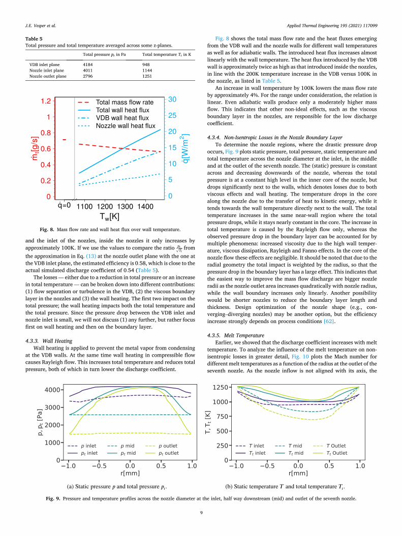
Fig. 8 shows the total mass flow rate and the heat fluxes emerging from the VDB wall and the nozzle walls for different wall temperatures as well as for adiabatic walls. The introduced heat flux increases almost linearly with the wall temperature. The heat flux introduced by the VDB wall is approximately twice as high as that introduced inside the nozzles, in line with the 200K temperature increase in the VDB versus 100K in the nozzle, as listed in Table 5.

An increase in wall temperature by 100K lowers the mass flow rate by approximately 4%. For the range under consideration, the relation is linear. Even adiabatic walls produce only a moderately higher mass flow. This indicates that other non-ideal effects, such as the viscous boundary layer in the nozzles, are responsible for the low discharge coefficient.

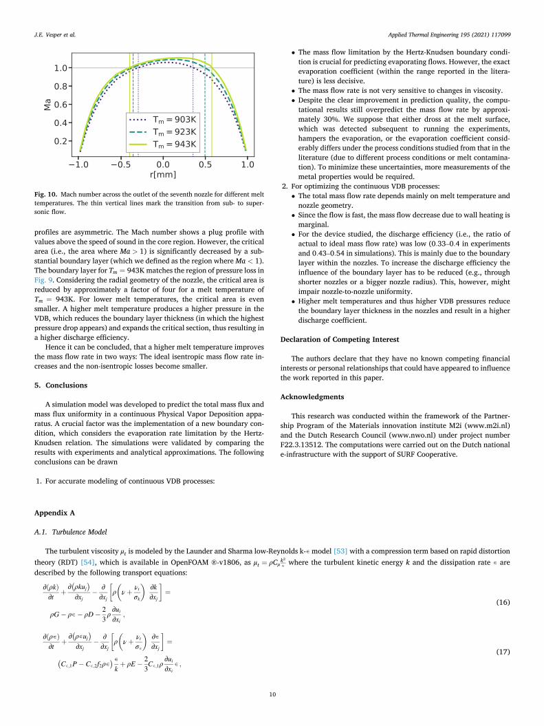
4.3.4. Non-Isentropic Losses in the Nozzle Boundary Layer To determine the nozzle regions, where the drastic pressure drop

occurs, Fig. 9 plots static pressure, total pressure, static temperature and total temperature across the nozzle diameter at the inlet, in the middle and at the outlet of the seventh nozzle. The (static) pressure is constant across and decreasing downwards of the nozzle, whereas the total pressure is at a constant high level in the inner core of the nozzle, but drops significantly next to the walls, which denotes losses due to both viscous effects and wall heating. The temperature drops in the core along the nozzle due to the transfer of heat to kinetic energy, while it tends towards the wall temperature directly next to the wall. The total temperature increases in the same near-wall region where the total pressure drops, while it stays nearly constant in the core. The increase in total temperature is caused by the Rayleigh flow only, whereas the observed pressure drop in the boundary layer can be accounted for by multiple phenomena: increased viscosity due to the high wall temper-ature, viscous dissipation, Rayleigh and Fanno effects. In the core of the nozzle flow these effects are negligible. It should be noted that due to the radial geometry the total impact is weighted by the radius, so that the pressure drop in the boundary layer has a large effect. This indicates that the easiest way to improve the mass flow discharge are bigger nozzle radii as the nozzle outlet area increases quadratically with nozzle radius, while the wall boundary increases only linearly. Another possibility would be shorter nozzles to reduce the boundary layer length and thickness. Design optimization of the nozzle shape (e.g., con-verging–diverging nozzles) may be another option, but the efficiency increase strongly depends on process conditions [62].

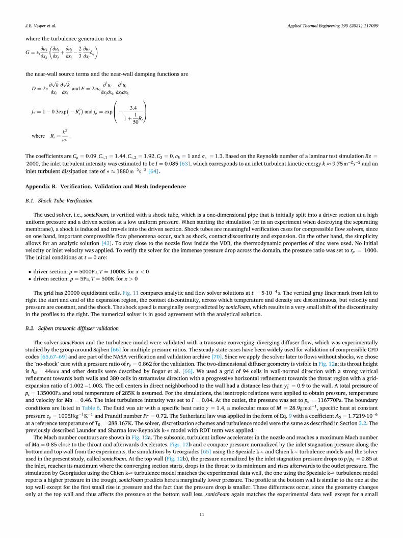
4.3.5. Melt Temperature Earlier, we showed that the discharge coefficient increases with melt

temperature. To analyze the influence of the melt temperature on non- isentropic losses in greater detail, Fig. 10 plots the Mach number for different melt temperatures as a function of the radius at the outlet of the seventh nozzle. As the nozzle inflow is not aligned with its axis, the

Fig. 9. Pressure and temperature profiles across the nozzle diameter at the inlet, half way downstream (mid) and outlet of the seventh nozzle.

Fig. 8. Mass flow rate and wall heat flux over wall temperature.

Table 5 Total pressure and total temperature averaged across some z-planes.

Total pressure pt in Pa Total temperature Tt in K

VDB inlet plane 4184 948 Nozzle inlet plane 4011 1144 Nozzle outlet plane 2796 1251

J.E. Vesper et al.

Applied Thermal Engineering 195 (2021) 117099

10

profiles are asymmetric. The Mach number shows a plug profile with values above the speed of sound in the core region. However, the critical area (i.e., the area where Ma > 1) is significantly decreased by a sub-stantial boundary layer (which we defined as the region where Ma < 1). The boundary layer for Tm = 943K matches the region of pressure loss in Fig. 9. Considering the radial geometry of the nozzle, the critical area is reduced by approximately a factor of four for a melt temperature of Tm = 943K. For lower melt temperatures, the critical area is even smaller. A higher melt temperature produces a higher pressure in the VDB, which reduces the boundary layer thickness (in which the highest pressure drop appears) and expands the critical section, thus resulting in a higher discharge efficiency.

Hence it can be concluded, that a higher melt temperature improves the mass flow rate in two ways: The ideal isentropic mass flow rate in-creases and the non-isentropic losses become smaller.

5. Conclusions

A simulation model was developed to predict the total mass flux and mass flux uniformity in a continuous Physical Vapor Deposition appa-ratus. A crucial factor was the implementation of a new boundary con-dition, which considers the evaporation rate limitation by the Hertz- Knudsen relation. The simulations were validated by comparing the results with experiments and analytical approximations. The following conclusions can be drawn

1. For accurate modeling of continuous VDB processes:

• The mass flow limitation by the Hertz-Knudsen boundary condi-tion is crucial for predicting evaporating flows. However, the exact evaporation coefficient (within the range reported in the litera-ture) is less decisive.

• The mass flow rate is not very sensitive to changes in viscosity. • Despite the clear improvement in prediction quality, the compu-

tational results still overpredict the mass flow rate by approxi-mately 30%. We suppose that either dross at the melt surface, which was detected subsequent to running the experiments, hampers the evaporation, or the evaporation coefficient consid-erably differs under the process conditions studied from that in the literature (due to different process conditions or melt contamina-tion). To minimize these uncertainties, more measurements of the metal properties would be required.

2. For optimizing the continuous VDB processes: • The total mass flow rate depends mainly on melt temperature and

nozzle geometry. • Since the flow is fast, the mass flow decrease due to wall heating is

marginal. • For the device studied, the discharge efficiency (i.e., the ratio of

actual to ideal mass flow rate) was low (0.33–0.4 in experiments and 0.43–0.54 in simulations). This is mainly due to the boundary layer within the nozzles. To increase the discharge efficiency the influence of the boundary layer has to be reduced (e.g., through shorter nozzles or a bigger nozzle radius). This, however, might impair nozzle-to-nozzle uniformity.

• Higher melt temperatures and thus higher VDB pressures reduce the boundary layer thickness in the nozzles and result in a higher discharge coefficient.

Declaration of Competing Interest

The authors declare that they have no known competing financial interests or personal relationships that could have appeared to influence the work reported in this paper.

Acknowledgments

This research was conducted within the framework of the Partner-ship Program of the Materials innovation institute M2i (www.m2i.nl) and the Dutch Research Council (www.nwo.nl) under project number F22.3.13512. The computations were carried out on the Dutch national e-infrastructure with the support of SURF Cooperative.

Appendix A

A.1. Turbulence Model

The turbulent viscosity μt is modeled by the Launder and Sharma low-Reynolds k-∊ model [53] with a compression term based on rapid distortion theory (RDT) [54], which is available in OpenFOAM ®-v1806, as μt = ρCμ

k2

∊ where the turbulent kinetic energy k and the dissipation rate ∊ are described by the following transport equations:

∂(ρk)∂t

+∂(ρkuj

)

∂xj−

∂∂xj

[

ρ(

ν +νt

σk

)∂k∂xj

]

=

ρG − ρ∊ − ρD −23

ρ ∂ui

∂xi,

(16)

∂(ρ∊)∂t

+∂(ρ∊uj

)

∂xj−

∂∂xj

[

ρ(

ν +νt

σ∊

)∂∊∂xj

]

=

(C∊,1P − C∊,2f2ρ∊

) ∊k+ ρE −

23C∊,1ρ ∂ui

∂xi∊ ,

(17)

Fig. 10. Mach number across the outlet of the seventh nozzle for different melt temperatures. The thin vertical lines mark the transition from sub- to super-sonic flow.

J.E. Vesper et al.

Applied Thermal Engineering 195 (2021) 117099

11

where the turbulence generation term is

G = νt∂uk

∂xk

(∂ui

∂xj+

∂uj

∂xi−

23

∂ul

∂xlδij

)

the near-wall source terms and the near-wall damping functions are

D = 2ν ∂k

√

∂xi

∂k

√

∂xiand E = 2ννt

∂2ui

∂xj∂xk

∂2ui

∂xj∂xk

f2 = 1 − 0.3exp(− R2

t

)and fμ = exp

⎛

⎜⎝ −

3.4

1 +1

50Rt

⎞

⎟⎠

where Rt =k2

ν∊.

The coefficients are Cμ = 0.09,C∊,1 = 1.44,C∊,2 = 1.92,C3 = 0, σk = 1 and σ∊ = 1.3. Based on the Reynolds number of a laminar test simulation Re =

2000, the inlet turbulent intensity was estimated to be I = 0.085 [63], which corresponds to an inlet turbulent kinetic energy k ≈ 9.75m− 2s− 2 and an inlet turbulent dissipation rate of ∊ ≈ 1880m− 2s− 3 [64].

Appendix B. Verification, Validation and Mesh Independence

B.1. Shock Tube Verification

The used solver, i.e., sonicFoam, is verified with a shock tube, which is a one-dimensional pipe that is initially split into a driver section at a high uniform pressure and a driven section at a low uniform pressure. When starting the simulation (or in an experiment when destroying the separating membrane), a shock is induced and travels into the driven section. Shock tubes are meaningful verification cases for compressible flow solvers, since on one hand, important compressible flow phenomena occur, such as shock, contact discontinuity and expansion. On the other hand, the simplicity allows for an analytic solution [43]. To stay close to the nozzle flow inside the VDB, the thermodynamic properties of zinc were used. No initial velocity or inlet velocity was applied. To verify the solver for the immense pressure drop across the domain, the pressure ratio was set to rp = 1000. The initial conditions at t = 0 are:

• driver section: p = 5000Pa,T = 1000K for x < 0 • driven section: p = 5Pa,T = 500K for x > 0

The grid has 20000 equidistant cells. Fig. 11 compares analytic and flow solver solutions at t = 5⋅10− 4 s. The vertical gray lines mark from left to right the start and end of the expansion region, the contact discontinuity, across which temperature and density are discontinuous, but velocity and pressure are constant, and the shock. The shock speed is marginally overpredicted by sonicFoam, which results in a very small shift of the discontinuity in the profiles to the right. The numerical solver is in good agreement with the analytical solution.

B.2. Sajben transonic diffuser validation

The solver sonicFoam and the turbulence model were validated with a transonic converging–diverging diffuser flow, which was experimentally studied by the group around Sajben [66] for multiple pressure ratios. The steady-state cases have been widely used for validation of compressible CFD codes [65,67–69] and are part of the NASA verification and validation archive [70]. Since we apply the solver later to flows without shocks, we chose the ’no-shock’ case with a pressure ratio of rp = 0.862 for the validation. The two-dimensional diffuser geometry is visible in Fig. 12a; its throat height is hth = 44mm and other details were described by Bogar et al. [66]. We used a grid of 94 cells in wall-normal direction with a strong vertical refinement towards both walls and 380 cells in streamwise direction with a progressive horizontal refinement towards the throat region with a grid- expansion ratio of 1.002 − 1.003. The cell centers in direct neighborhood to the wall had a distance less than y+1 = 0.9 to the wall. A total pressure of ps = 135000Pa and total temperature of 285K is assumed. For the simulations, the isentropic relations were applied to obtain pressure, temperature and velocity for Ma = 0.46. The inlet turbulence intensity was set to I = 0.04. At the outlet, the pressure was set to po = 116770Pa. The boundary conditions are listed in Table 6. The fluid was air with a specific heat ratio γ = 1.4, a molecular mass of M = 28.9gmol− 1, specific heat at constant pressure cp = 1005Jkg− 1K− 1 and Prandtl number Pr = 0.72. The Sutherland law was applied in the form of Eq. 9 with a coefficient AS = 1.7219⋅10− 6

at a reference temperature of T0 = 288.167K. The solver, discretization schemes and turbulence model were the same as described in Section 3.2. The previously described Launder and Sharma low-Reynolds k-∊ model with RDT term was applied.

The Mach number contours are shown in Fig. 12a. The subsonic, turbulent inflow accelerates in the nozzle and reaches a maximum Mach number of Ma = 0.85 close to the throat and afterwards decelerates. Figs. 12b and c compare pressure normalized by the inlet stagnation pressure along the bottom and top wall from the experiments, the simulations by Georgiades [65] using the Speziale k-∊ and Chien k-∊ turbulence models and the solver used in the present study, called sonicFoam. At the top wall (Fig. 12b), the pressure normalized by the inlet stagnation pressure drops to p/p0 = 0.85 at the inlet, reaches its maximum where the converging section starts, drops in the throat to its minimum and rises afterwards to the outlet pressure. The simulation by Georgiades using the Chien k-∊ turbulence model matches the experimental data well, the one using the Speziale k-∊ turbulence model reports a higher pressure in the trough, sonicFoam predicts here a marginally lower pressure. The profile at the bottom wall is similar to the one at the top wall except for the first small rise in pressure and the fact that the pressure drop is smaller. These differences occur, since the geometry changes only at the top wall and thus affects the pressure at the bottom wall less. sonicFoam again matches the experimental data well except for a small

J.E. Vesper et al.

Applied Thermal Engineering 195 (2021) 117099

12

underprediction in the throat. Overall, a reasonable agreement is reached between experiment and sonicFoam. B.3. Grid Independence Study

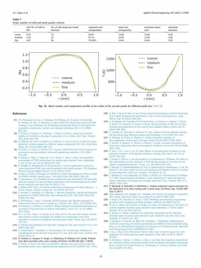
In compressible flows, adequate meshing is important for both the numerical stability and the accuracy of the result. The grid dependence of the solution was studied (for the standard case at a melt temperature of 943K) on three meshes listed in Table 7. As the gradients are expected to be highest within the nozzles, the resolution inside the nozzles is crucial. Fig. 13 shows the Mach number and temperature profile at the outlet of the second nozzle. While for the coarse mesh both Mach number and temperature deviate from the results of the finer meshes, the medium and fine mesh results are in good agreement. This is why we chose the medium mesh for further calculations.

To speed up the simulations, two symmetry planes were used and only a quarter of the VDB was simulated. This particularly constrains the swirling motion along the long extension of the VDB. To study the influence on the viscous losses, half of the VDB was also simulated for the standard case. Neither the total nor the local mass flow rate changed notably, which justifies the use of the quarter geometry.

Fig. 12. Sajben transonic diffuser validation case. Contours and pressure profiles along the walls from sonicFoam compared to experimental results (data from [65]) and simulations by Georgiades et al. [65].

Table 6 Boundary conditions for the Sajben transonic diffuser.

pressure velocity temperature kinetic energy turbulent dissipation

inlet static pressure pin = 116.77kPa 152.45ms− 1 (Ma = 0.46) static temperature 273.3K 54.4m2s− 2 21966m2s− 3

outlet static pressure 110.66kPa zero gradient zero gradient zero gradient zero gradient walls zero gradient no slip adiabatic wall function wall function

Fig. 11. Pressure, temperature and velocity in the shock tube at t = 0.0005s. Comparison of analytic and sonicFoam solutions. The thin vertical gray lines mark from left to right: the expansion head, the expansion tail, the slip surface and the shock.

J.E. Vesper et al.

Applied Thermal Engineering 195 (2021) 117099

13

References

[1] P.E. Hovsepian, Q. Luo, G. Robinson, M. Pittman, M. Howarth, D. Doerwald, R. Tietema, W. Sim, A. Deeming, T. Zeus, TiAlN/VN superlattice structured PVD coatings: a new alternative in machining of aluminium alloys for aerospace and automotive components, Surface and coatings technology 201 (1–2) (2006) 265–272.

[2] T. Prosek, A. Nazarov, F. Goodwin, J. Serak, D. Thierry, Improving corrosion stability of ZnAlMg by alloying for protection of car bodies, Surf. Coat. Technol. 306 (2016) 439–447.

[3] Q. Mehran, M. Fazal, A. Bushroa, S. Rubaiee, A critical review on physical vapor deposition coatings applied on different engine components, Crit. Rev. Solid State Mater. Sci. 43 (2) (2018) 158–175.

[4] M. Peters, C. Leyens, U. Schulz, W.A. Kaysser, EB-PVD thermal barrier coatings for aeroengines and gas turbines, Advanced engineering materials 3 (4) (2001) 193–204.

[5] X. Zhang, K. Zhou, C. Deng, M. Liu, Z. Deng, C. Deng, J. Song, Gas-deposition mechanisms of 7YSZ coating based on plasma spray-physical vapor deposition, J. Eur. Ceram. Soc. 36 (3) (2016) 697–703.

[6] S. Shahidi, B. Moazzenchi, M. Ghoranneviss, A review-application of physical vapor deposition (PVD) and related methods in the textile industry, The European Physical Journal Applied Physics 71 (3) (2015) 31302.

[7] H. Sun, K. Cooke, G. Eitzinger, P. Hamilton, B. Pollet, Development of PVD coatings for PEMFC metallic bipolar plates, Thin Solid Films 528 (2013) 199–204.

[8] N. Selvakumar, H.C. Barshilia, Review of physical vapor deposited (PVD) spectrally selective coatings for mid-and high-temperature solar thermal applications, Solar energy materials and solar cells 98 (2012) 1–23.

[9] S. Suman, M.K. Khan, M. Pathak, Performance enhancement of solar collectors – a review, Renew. Sustain. Energy Rev. 49 (2015) 192–210.

[10] N. Barreau, S. Marsillac, D. Albertini, J. Bernede, Structural, optical and electrical properties of β-In2S3-3xO3x thin films obtained by PVD, Thin Solid Films 403 (2002) 331–334.

[11] K. Matsumoto, Y. Itoh, T. Kameda, EB-PVD process and thermal properties of hafnia-based thermal barrier coating, Sci. Technol. Adv. Mater. 4 (2) (2003) 153.

[12] C.G. Soares, Y. Garbatov, A. Zayed, G. Wang, Influence of environmental factors on corrosion of ship structures in marine atmosphere, Corros. Sci. 51 (9) (2009) 2014–2026.

[13] M.-J. Li, S.-Z. Tang, F.-L. Wang, Q.-X. Zhao, W.-Q. Tao, Gas-side fouling, erosion and corrosion of heat exchangers for middle/low temperature waste heat utilization: A review on simulation and experiment, Appl. Therm. Eng. 126 (2017) 737–761.

[14] B. Schmitz, Development of Zn-Mg alloy coatings by JVD, steel research 72 (11–12) (2001) 522–527.

[15] E. Zoestbergen, T. Maalman, C. Commandeur, M. Goodenough, Influence of contamination on the thermal evaporation of a zinc melt, Surf. Coat. Technol. 218 (2013) 108–113.

[16] D. Chaleix, D. Jacques, P. Sergio, E. Silberberg, B. Schmitz, X.V. Eynde, Painted steel sheet provided with a zinc coating, US Patent 10,400,326 (Sep. 3 2019).

[17] S. Blakey, S. Beck, The effect of combined radiation and convection on hot dip galvanizing kettle wear, Applied thermal engineering 24 (8–9) (2004) 1301–1319.

[18] D. Mei, F. Xing, M. Wen, P. Lei, Z. Fang, Numerical simulation of mixed convection heat transfer of galvanized steel sheets in the vertical alloying furnace, Appl. Therm. Eng. 93 (2016) 500–508.

[19] A. El Hajjami, M. Gigandet, M. De Petris-Wery, J. Catonne, J. Duprat, L. Thiery, F. Raulin, N. Pommier, B. Starck, P. Remy, Characterization of thin Zn–Ni alloy coatings electrodeposited on low carbon steel, Applied surface science 254 (2) (2007) 480–489.

[20] R. Cresdee, W. Edwards, P. Thomas, G. Voss, Analysis of beam distortion during hot dip galvanising, Materials science and technology 9 (2) (1993) 161–162.

[21] N. Hosking, M. Strom, P. Shipway, C. Rudd, Corrosion resistance of zinc–magnesium coated steel, Corrosion science 49 (9) (2007) 3669–3695.

[22] T. Prosek, A. Nazarov, U. Bexell, D. Thierry, J. Serak, Corrosion mechanism of model zinc–magnesium alloys in atmospheric conditions, Corros. Sci. 50 (8) (2008) 2216–2231.

[23] K. Bae, J. La, I. Lee, S. Lee, K. Nam, Effects of annealing heat treatment on the corrosion resistance of Zn/Mg/Zn multilayer coatings, Met. Mater. Int. 23 (3) (2017) 481–487.

[24] J. Davies, C. Glover, J. Van de Langkruis, E. Zoestbergen, G. Williams, The effect of Mg concentration on the resistance of PVD Zn-Mg coatings to corrosion driven organic coating delamination, Corros. Sci. 100 (2015) 607–618.

[25] S. Sabooni, E. Galinmoghaddam, H. Cao, R. Westerwaal, E. Zoestbergen, J.T.M. De Hosson, Y. Pei, New insight into the loss of adhesion of ZnMgZn bi-layered coatings on steel substrates, Surf. Coat. Technol. 370 (2019) 35–43.

[26] L. Baptiste, N. van Landschoot, G. Gleijm, J. Priede, J.S. van Westrum, H. Velthuis, T.-Y. Kim, Electromagnetic levitation: A new technology for high rate physical vapour deposition of coatings onto metallic strip, Surf. Coat. Technol. 202 (4–7) (2007) 1189–1193.

[27] P. Banaszak, D. Marneffe, E. Silberberg, L. Vanhee, Industrial vapour generator for the deposition of an alloy coating onto a metal strip, US Patent App. 12/681,969 (Jan. 6 2011).

[28] J.M. Kapopara, A.R. Mengar, K.V. Chauhan, S.K. Rawal, Cfd analysis of sputtered TiN coating, Materials Today: Proceedings 4 (9) (2017) 9390–9393.

[29] L. Nastac, W. Hanusiak, H. Dong, F. Dax, Modeling and simulating engineering processes with computational fluid dynamics, JOM 56 (3) (2004), 43–43.

[30] W. He, G. Mauer, M. Gindrat, R. Wager, R. Vaßen, Investigations on the nature of ceramic deposits in plasma spray–physical vapor deposition, J. Therm. Spray Technol. 26 (1–2) (2017) 83–92.

[31] G. Mauer, R. Vaßen, Conditions for nucleation and growth in the substrate boundary layer at plasma spray-physical vapor deposition (ps-pvd), Surf. Coat. Technol. 371 (2019) 417–427.

[32] S. Upadhye, S. Ramesh, M. Shah, M. Tendolkar, J. Mukherjee, Application of multicore processing and volume parallelization in EBPVD process simulated using dsmc, in: in: International Conference on Advances in Thermal Systems, Materials and Design Engineering (ATSMDE2017), 2017.

[33] X. Lu, J. Chai, Direct Simulation Monte Carlo study of metal evaporation with collimator in e-beam physical vapor deposition, Chin. Phys. B 28 (7) (2019) 074702.

[34] R. Dorsman, C. Kleijn, J. Velthuis, J. Zijp, A. van Mol, Zinc deposition experiments for validation of Direct-Simulation Monte Carlo calculations of rarefied internal gas flows, Journal of Vacuum Science & Technology A: Vacuum, Surfaces, and Films 25 (3) (2007) 474–479.

Fig. 13. Mach number and temperature profile at the outlet of the second nozzle for different grids (see Table 7).

Table 7 Grids, number of cells and mesh quality criteria.

total No. of cells in Mio

No. of cells along one nozzle diameter

maximum non- orthogonality

mean non- orthogonality

maximum aspect ratio

maximum skewness

coarse 0.75 13 62.01 12.90 12.06 2.03 medium 2.32 27 67.10 12.50 13.02 2.26 fine 4.47 36 70.5921 14.69 52.64 2.52

J.E. Vesper et al.

Applied Thermal Engineering 195 (2021) 117099

14

[35] T.M. Rodgers, H. Zhao, H.N. Wadley, Thermal barrier coating deposition by rarefied gas jet assisted processes: Simulations of deposition on a stationary airfoil, Journal of Vacuum Science & Technology A: Vacuum, Surfaces, and Films 31 (6) (2013) 061509.

[36] J. Balakrishnan, I.D. Boyd, D.G. Braun, Monte carlo simulation of vapor transport in physical vapor deposition of titanium, Journal of Vacuum Science & Technology A: Vacuum, Surfaces, and Films 18 (3) (2000) 907–916.

[37] J. Fan, I.D. Boyd, C. Shelton, Monte carlo modeling of electron beam physical vapor deposition of yttrium, Journal of Vacuum Science & Technology A: Vacuum, Surfaces, and Films 18 (6) (2000) 2937–2945.

[38] K. Bobzin, R.P. Brinkmann, T. Mussenbrock, N. Bagcivan, R.H. Brugnara, M. Schafer, J. Trieschmann, Continuum and kinetic simulations of the neutral gas flow in an industrial physical vapor deposition reactor, Surf. Coat. Technol. 237 (2013) 176–181.

[39] D. Ivchenko, T. Zhang, G. Mariaux, A. Vardelle, S. Goutier, T.E. Itina, On the validity of continuum computational fluid dynamics approach under very low- pressure plasma spray conditions, J. Therm. Spray Technol. 27 (1–2) (2018) 3–13.

[40] D. Ivchenko, G. Mariaux, A. Vardelle, S. Goutier, T.E. Itina, P. Andre, Feasibility study of an adaptive-pressure plasma coating process — part 1: Model description, J. Therm. Spray Technol. (2019) 1–13.

[41] J.A. Morí nigo, J.H. Quesada, Analysis of viscous heating in a micro-rocket flow and performance, J. Therm. Sci. 17 (2) (2008) 116.

[42] N.S. Kumar, K.T. Ooi, One dimensional model of an ejector with special attention to fanno flow within the mixing chamber, Applied thermal engineering 65 (1–2) (2014) 226–235.

[43] J.D. Anderson, Modern Compressible Flow with Historical Perspective, McGraw- Hill, 2003.

[44] H. Jasak, A. Jemcov, Z. Tukovic, et al., OpenFOAM: A C++ library for complex physics simulations, in: International workshop on coupled methods in numerical dynamics, Vol. 1000, IUC Dubrovnik Croatia, 2007, pp. 1–20.

[45] C.J. Smithells, Metals reference book, Elsevier, 2013. [46] H. Hertz, Über den Druck des gesattigten Quecksilberdampfes, Ann. Phys. 253 (10)

(1882) 193–200. [47] M. Knudsen, Experimentelle Bestimmung des Druckes gesattigter

Quecksilberdampfe bei 0 und hoheren Temperaturen, Ann. Phys. 334 (6) (1909) 179–193.

[48] J. Safarian, T.A. Engh, Vacuum evaporation of pure metals, Metallurgical and Materials Transactions A 44 (2) (2013) 747–753.

[49] D. Labuntsov, A. Kryukov, Analysis of intensive evaporation and condensation, Int. J. Heat Mass Transf. 22 (7) (1979) 989–1002.

[50] T. Ytrehus, S. Østmo, Kinetic theory approach to interphase processes, International journal of multiphase flow 22 (1) (1996) 133–155.

[51] H.S. Clair, M. Spendlove, Rate of evaporation of zinc at low pressures, JOM 3 (12) (1951) 1192–1197.

[52] J. Song, X.-D. Ren, X.-S. Li, C.-W. Gu, M.-M. Zhang, One-dimensional model analysis and performance assessment of tesla turbine, Appl. Therm. Eng. 134 (2018) 546–554.

[53] B.E. Launder, B. Sharma, Application of the energy-dissipation model of turbulence to the calculation of flow near a spinning disc, Letters in heat and mass transfer 1 (2) (1974) 131–137.

[54] S. El Tahry, K-epsilon equation for compressible reciprocating engine flows, Journal of Energy 7 (4) (1983) 345–353.

[55] Y. Bayazitoglu, F. Brotzen, Y. Zhang, Metal vapor condensation in a converging nozzle, Nanostructured materials 7 (7) (1996) 789–803.

[56] J. Bian, X. Cao, W. Yang, D. Guo, C. Xiang, Prediction of supersonic condensation process of methane gas considering real gas effects, Appl. Therm. Eng. 164 (2020) 114508.

[57] Y. Yang, J.H. Walther, Y. Yan, C. Wen, CFD modeling of condensation process of water vapor in supersonic flows, Appl. Therm. Eng. 115 (2017) 1357–1362.

[58] OpenCFD Ltd, OpenFoam v1806, https://develop.openfoam.com/Development/ openfoam, commit: 71942d682 (2018).

[59] T. Uroic, H. Jasak, H. Rusche, Implicitly coupled pressure–velocity solver, in: OpenFOAM, Springer, 2019, pp. 249–267.

[60] P.K. Sweby, High resolution schemes using flux limiters for hyperbolic conservation laws, SIAM journal on numerical analysis 21 (5) (1984) 995–1011.

[61] T. Poinsot, S. Lelef, Boundary conditions for direct simulations of compressible viscous flows, Journal of computational physics 101 (1) (1992) 104–129.

[62] G.L. Martins, S.L. Braga, S.B. Ferreira, Design optimization of partial admission axial turbine for orc service, Appl. Therm. Eng. 96 (2016) 18–25.

[63] F. Russo, N.T. Basse, Scaling of turbulence intensity for low-speed flow in smooth pipes, Flow Meas. Instrum. 52 (2016) 101–114.

[64] ANSYS Inc., ANSYS Fluent User’s Guide, ANSYS Inc., release 19.0 Edition (2018). [65] N. Georgiadis, J. Drummond, B. Leonard, Evaluation of turbulence models in the

parc code for transonic diffuser flows, in: in: 32nd Aerospace Sciences Meeting and Exhibit, 1994, p. 582.

[66] T. Bogar, M. Sajben, J. Kroutil, Characteristic frequencies of transonic diffuser flow oscillations, AIAA journal 21 (9) (1983) 1232–1240.

[67] J.W. Slater, C. Towne, D. Yoder, S. Mohler, J. Dudek, Sajben Transonic Diffuser, https://www.grc.nasa.gov/www/wind/valid/transdif/transdif.html, [Online; accessed 04-February-2021] (198x–2017).

[68] B. Wüthrich, Simulation and validation of compressible flow in nozzle geometries and validation of openfoam for this application, Master’s thesis, ETH, Swiss Federal Institute of Technology Zurich, Institute of Fluid Dynamics (2007).

[69] J. Dudek, J.-R. Carlson, Evaluation of full Reynolds stress turbulence models in fun3d, in: in: 55th AIAA Aerospace Sciences Meeting, 2017, p. 0541.

[70] J.W. Slater, J.C. Dudek, K.E. Tatum, The NPARC alliance verification and validation archive, Proceedings of ASME FEDSM00.

J.E. Vesper et al.