lable at ScienceDirect

Renewable Energy 97 (2016) 849e859

Contents lists avai

Renewable Energy

journal homepage: www.elsevier .com/locate/renene

Modeling noise and lease soft costs improves wind farm design andcost-of-energy predictions

Le Chen a, Chris Harding b, Anupam Sharma c, Erin MacDonald d, *

a Mountain View, CA, USAb Department of Geological and Atmospheric Sciences, Iowa State University, Ames, IA, USAc Department of Aerospace Engineering, Iowa State University, Ames, IA, USAd Department of Mechanical Engineering, Stanford University, Stanford, CA, USA

a r t i c l e i n f o

Article history:Received 20 July 2015Received in revised form9 May 2016Accepted 11 May 2016Available online 23 June 2016

Keywords:Wind farm layout optimizationCost-of-energySoft costsOptimization under uncertaintyLand lease costNoise disturbance compensation

* Corresponding author.E-mail addresses: chenle86@gmail.com (L. C

(C. Harding), sharma@iastate.edu (A. Sharm(E. MacDonald).

http://dx.doi.org/10.1016/j.renene.2016.05.0450960-1481/© 2016 Published by Elsevier Ltd.

a b s t r a c t

The Department of Energy uses the metric Cost-of-Energy to assess the financial viability of wind farms.Non-hardware costs, termed soft costs, make up approximately 21% of total cost for a land-based farm,yet are only represented with general assumptions in models of Cost-of-Energy. This work replaces theseassumptions with a probabilistic model of the costs of land lease and noise disturbance compensation,which is incorporated into a wind-farm-layout-optimization-under-uncertainty model. These realisticrepresentations are applied to an Iowa land area with real land boundaries and house locations toaccentuate the challenges of accommodating landowners. The paper also investigates and removes acommon but unnecessary term that overestimates cost-savings from installing multiple turbines. Thesethree contributions combine to produce COE estimates in-line with industry data, replacing “soft” as-sumptions with specific parameters, identify noise and risk concerns prohibitive to the development ofprofitable wind farm. The model predicts COEs remarkably close to real-world costs. Wind energy policy-makers can use this model to promote new areas of soft-cost-focused research.

© 2016 Published by Elsevier Ltd.

1. Introduction

The Department of Energy (DOE) promotes research and pol-icies that investigate alternative renewable energy technologies toalleviate U.S. dependency on coal, oil, and natural gas [34]. Cost-Of-Energy (COE), or MWH of annualized cost divided by energy outputper year, offers a universal metric to compare the competitivenessof different power-generation approaches [43]. By far, the majorityof research in renewable energy technology focuses on decreasingCOE to a level comparable with traditional fuel sources, via im-provements in technology and/or hardware-related costs. COE isused as a metric in a variety of modeling studies, including hybridenergy systems, for example see Refs. [24,28]. Recently, the DOE hasinitiated programs that aim to reduce the soft costs of renewableenergy. For example, the SunShot Initiative [35], which aims tomake solar energy cost-competitive with other forms of energy by

hen), charding@iastate.edua), erinmacd@stanford.edu

the end of the decade, collaborates with industry and research in-stitutes to reduce soft costs for residential solar power installation.In just four years, this program has funded more than 350 projectsto make the solar energy resources more affordable and accessiblefor Americans.

The first contribution of this paper is a nuanced modelingapproach to wind energy soft costs which, even though theyamount to approximately 21% of a wind farm’s annualized costs,have received much less research attention. This 21% calculationcomes from the application of the enhanced cost model developedby the authors [8] which is based on the Wind Turbine Design Costand Scaling Model [16] by National Renewable Energy Laboratory(NREL) and the Turbine System Cost Report from Lawrence Ber-keley National Laboratory [4]. This paper enhances this existingwork with a detailed investigation and probabilistic modeling oftwo major soft costs in wind farm projects: the costs of landowneracquisition (land lease costs) as discussed in the authors’ previouswork [6,7,9], and noise disturbance compensationdan importantcontribution of this work, explained in detail in Section 2.4. Noisenot only annoys landowners, but may also induce health issues [11],which makes the consideration of noise disturbance compensationa necessity. The second contribution of this paper is the application

L. Chen et al. / Renewable Energy 97 (2016) 849e859850

of this work to a real plot of land in Story County, Iowa. The cleaningand coding of the GIS parcel data is explained in Section 2.1, andweblink is provided to the cleaned parcel data so that other re-searchers can use it in their modeling as well. The third contribu-tion of this paper is the investigation and subsequent removal ofthe economies-of-scale term used in previous research to modelthe reduction in turbine costs when more than one is installed,detailed in Section 2.3. In the early-development stages of com-mercial wind projects, developers approach landowners forpermission to build turbines on their land in exchange for mone-tary compensation. In a large-scale farmland project, developerscan approach over 100 individual landowners. Developers mustmake important and expensive decisions, such as placing equip-ment orders or obtaining funding from potential project backers,with limited and uncertain information of these factors. Much ofthis uncertainty stems from unknown landowner participation. Atthe same time, landowners must decide whether or not to partic-ipate in the project without knowing the turbine locations and thepotential impacts. Both stakeholders, developers and landowners,face high levels of risk.

It is customary for developers to offer all landowners in a projectthe same compensation structure. However, they make no profitguarantees to landowners. The contract offers a certain dollarcompensation per MW per year if developers install turbines, butthey may not install any. In this situation, the land is still undercontract with the developer, so landowners cannot work withanother developer or install their own turbines. Thus, landownerssign away the rights to their land without knowing if they willreceive compensation from wind energy produced. This is a largerisk. Developers offer particular riders for other disturbances, suchas dollar per decibel-level-range noise disturbance and dollar perunit of road built, but do not specify the level of noise or amount ofroad construction. The agreement also does not specify turbinelocation on land parcels, or number of turbines. Therefore, it isdifficult for landowners to assess compensation packages. Clearly,both stakeholders would benefit from increased information inearly-stage farm development. This could decrease both develop-ment time, via more-transparent negotiations, and COE, viaaddressing uncertainty in planning.

This paper uses an optimization-under-uncertainty frameworkdeveloped previously by the authors [6,7,9], to specifically addresstwo major soft-cost challenges: (a) determine land lease terms forall participating landowners and (b) determine noise disturbancecompensation. The robust design optimization problem has twoobjectives for the farm’s COE: minimize the normalized mean valueand standard deviation. The authors use probability theory tomodel the uncertain parameters, Latin Hypercube Sampling topropagate the uncertainty throughout the COE system model, andcompromise programming to solve the multi-objective optimiza-tion problem. The system model provided in this paper can helpdevelopers identify plots of land that are worth the extra invest-ment, and provide a robust wind farm design that is not onlyprofitable but also hasminimal noise disturbance for landowners. Itcan also give landowners an idea of where turbines are likely to beplaced on their land, and the likely auditory impacts.

2. Methods

2.1. Test case with real farmland and house locations

In previous related publications, we have used simulated landplots. However, to explore real noise issues and lease concerns, itwas necessary to use real land with real home locations, shown inFig. 1, which also shows potential turbine locations, discussed laterin Section 2.5.2. A portion of the Story County Wind Farm [45] in

central Iowa was selected as a realistic test case. The farm is oper-ated by NextEra Energy [41]. The land parcels within the 2-by-2mile test area are owned by 22 landowners, and most ownmultipleland parcels. Fig. 1 shows the test area; black lines outline the in-dividual land parcels, each parcel is labeled by landowner id(1e22), followed by a parcel counter. For example, 9-1 indicates thefirst parcel owned by landowner 9, 9-2 the second parcel owned bylandowner 9, etc. Note that all parcels owned by the same land-owner will have same acceptance profiles for compensation offersand noise disturbance. Note also that not all parcels owned by thesame landowner are adjacent to each other, for example see theparcels of landowners 13 and 14.

Note, in Fig.1, the house in the top-right area: it is surrounded byland owned by someone else. Such an intricacy would not beimagined in a hypothetic layout-scenario, but is a reality when landis bought, sold, and passed down through inheritances. There arealso several cases where parcels with the same owner are notadjacent, i.e. they are surrounded by non-owned parcels, as shownin Fig. 1. The complexity of the spatial arrangement of parcels andtheir ownership is a complicating, yet important factor in capturingthe complexities of modeling real world conditions. This is espe-cially important when adding a noise model, as noise preferenceswill be discontinuously (or discretely) identical for some non-adjacent plots of land.

A Geographic Information System (GIS) was used to convertpublic land information obtained from the Iowa Story County As-sessor’s office into the geospatial data required to run the model.ArcGIS 10 Desktop (ArcMap) was used to perform a spatial selectionof those parcel boundary polygons within the test area from themuch larger Story county data set. Coordinates were convertedfrom the feet-based Iowa State plane system used by the county,into a local, UTM (meter) based system as required by the modelingsoftware. The GIS was also used to set up the 10 � 10 and 24 � 24patterns of potential turbine locations. Satellite imagery (DigitalGlobe) was used to visually identify and digitize the coordinates ofthemain housewithin each homestead (which is assumed to be thelocation where owners live and experience the noise levelsmodeled). Extracting and anonymizing the names of the parcelowners into a number system while still retaining the spatial re-lationships required additional custom programming with theArcGIS Python API. Maps, combining the parcels, locations ofhouses and of potential wind turbine locations (Figs. 4, 6, and 8)were also designed in ArcMap. To facilitate communication withinthe team and with other project participants, a public online mapwas created in ArcMap Online: arcg.is/1gSC75q. This can be used byother researchers.

2.2. System model overview

Fig. 2 represents the overview of the COE system model used inthis work. Five models are used to calculate the COE: a noisepropagation model (introduced in detail in Section 2.4.4), anenhanced cost model developed based on theWind Turbine DesignCost and Scaling Model [16] by NREL and the Turbine System CostReport from Lawrence Berkeley National Laboratory [4], a windshear model [38], Jensen’s [23] wake loss model, and a powermodel for a GE 1.5sle turbine [2]. The authors’ previous work [6,7,9]discusses the latter four models. The NREL model includes all costsassociated with the construction of awind farm, including the costsof cabling, roads, and transportation, although these costs do notchange based on the locations of the turbines. The assumed landlease costs within the NRELmodel are removed and replaced by thework here. The cost model here has the additional constraint ofequal compensation structures for all participating landowners andeliminates the unnecessary economies-of-scale cost reduction

Fig. 1. Test area with parcels labels, home locations, and potential locations of turbines.

L. Chen et al. / Renewable Energy 97 (2016) 849e859 851

coefficient, as explained later in this section.The model includes four sources of uncertainty, indicated in

grey in Fig. 2. Wind condition is modeled as aleatory uncertaintyusing a wind rose, shown in detail in section 2.5.2. Three epistemicsources of uncertainty are modeled in this paper: wind shear, sameas in previous work [6,7,9]; landowner participation, with moredetail given in previous work [6,7,9] and Section 2.4.3; and mone-tary compensation required for a given noise disturbance, as rep-resented by aWillingness-to-Accept-Noise utility model, explainedbelow. There are multiple sources of uncertainty within the noisepropagation model, but they are self-contained and not detailedhere.

While this is useful for the conclusions drawn in previous work,it is not realistic enough for a detailed soft costs model. In reality,

Wind shear (Epistemic)

Wind condition at hub height

Locations of turbines (Design

variable X)

Wake Loss

Model

Wind speed at each turbine

Surface roughness

Parcels used

WTAs of each landowner for participation

(Epistemic)

Land lease cost

Noise Propagation

Model

Maximal source sound power level for each turbine

Maxisounlev

Wind Shear Model

Wind condition at anemometers

(Aleatory)

WTAs of each landowner fonoise (Epistemic)

Number of Turbines

Fig. 2. Overview of the COE m

instead of individual negotiations, which would increase the proj-ect timeline and cost, developers prefer to offer all landowners thesame compensation structure, namely a certain dollar per MWhwith riders to cover additional damage. Landowners with goodwind resource but more expensive compensation demands mayincrease compensation for all, as developers work to ensure theirparticipation. However, there is a breaking point at which evenwind-wealthy landowners are too expensive for the overall cost ofthe farm. To realistically model this behavior, the model uses anequality constraint of compensation per MWh per year for alllandowners that participate. For each Latin Hypercube draw ofWTAP, the highest WTAP among all participating landowners de-termines the final, shared compensation structure offered to each.The associated costs and wind resource benefits are captured in thecalculated COE, ensuring that only optimally cost-effective land-owners are included in the final design.

2.3. Economies-of-scale term determined unnecessary

Another improvement of the model in this paper is the elimi-nation of the economies-of-scale turbine cost reduction coefficient.This coefficient is included in many layout optimization studies[13,17,29,31], but underestimates costs. The optimal COE in theauthors’ previous work [6,7,9] ranged from USD 42e48 per MWh,about 10 USD lower than the real industry data. To investigate theimpact of the cost reduction coefficient on optimal COE, the authorsconducted an optimization analysis for a portion of the StoryCounty Wind Farm [45], varying the number of turbines and theinclusion of the cost reduction coefficient, as shown in Fig. 3. Theline indicates COE without the term, and the “X”s mark two ex-amples of the COE with the term. The authors conducted phoneinterviews with developers with farms in the area to establishCOEs, reported as ranging fromUSD 51e57 per MWh, and shown asa grey area in Fig. 3. There is no published reference for thesenumbers, they were collected via phone interview specifically forthis investigation. COEs are difficult to secure on-the-record fromdevelopers, as they are competitive information. The result shows

Power Model

Power output

Cost Model

Cost output

Cost of Energy

mal receiver d pressure

el for each house

Extra compensation for

noise level

r

Design Variable

System Output

Sub-Model

Parameter

Uncertain Parameter

Media ng Variable

odel with a noise model.

L. Chen et al. / Renewable Energy 97 (2016) 849e859852

optimal COEs are closer to the real industry data without the costreduction term. In addition, when the number of turbines in-creases, the advantage of removing cost reduction is more obvious.Therefore, the authors removed the cost reduction formulation inthe system model proposed in this paper.

2.4. Probabilistically modeling acceptance of noise

When placing wind turbines near residential locations, noiseimpact becomes a primary concern for landowners. The noise at aresidential home depends on the distance between the home andthe surrounding turbines. A qualitative analysis conducted byRef. [18] shows noise disturbance is one of the most commonly-stated negative perceptions of wind energy development. Peopledo not like to hear wind turbines, and different people havedifferent perceptions of it [37]. Developers receive complaints andlawsuits about excessive noise and its associated adverse healthimpacts [1]. For example, an Oregon landowner claimed he wassuffering “emotional distress, deteriorating physical and emotionalhealth, dizziness, inability to sleep, drowsiness, fatigue, headaches,difficulty thinking, irritation and lethargy” due to the wind turbinenoise [42] and recently filed a related $5million lawsuit. In practice,if the noise disturbance is above a certain decibel (dB) level,homeowners receive an annual compensation amount of up to$1500 in total from developers [32,33]. Landowners argue for saferguidelines in the siting of wind turbines, as they are uncertain ofthe associated health risks of noise disturbance [39].

If developers can guarantee the noise below a certain limit orgive landowners an idea of the likely auditory impact, the land-owners are more likely to accept the contract. Therefore, it isimportant to carefully model noise impact in the wind farm layoutoptimization problem. Current wind farm layout optimizationresearch sets noise disturbance as a constraint or an objectivefunction [15,26]. No existing research models monetary compen-sation for noise disturbance. This section addresses this limitationby modeling the landowners’ acceptance of noise probabilistically,in combination with a constraint on maximum noise disturbance.The model is built from existing research. Sections 2.4.1 and 2.4.2detail documentation on community reactions to noise that weused to create landowner acceptance profiles. The full Willingness-to-Accept-Noise model is developed in Section 2.4.3, while Section2.4.4 provides the Noise Propagation Model used in this paper.

Fig. 3. Relationship between the optima

2.4.1. Community reaction to different noise levels[1] summarized a variety of studies on the community reaction

to different noise levels. The results of these studies were plotted ina single chart to identify noise level ranges for different communityreactions, as show in Table 1. The chart indicates that people willnot react adversely to a noise level below 29 dB, but will stronglyoppose a noise level above 43 dB (about as loud as a refrigerator).Therefore, our optimization formulation sets 43 dB as a hardconstraint, i.e. the program guarantees that noise levels for allresidential locations are less than 43 dB. The model proposes: (1) ifthe noise level is below 29 dB, landowners will not receive anycompensation; and (2) if the noise level is between 29 dB and43 dB, landowners will receive compensation of up to $1500 peryearda typical amount offered by developers as compensation fornoise disturbance [32,33]. Note again that solution will not includenoise levels above 43 dB.

2.4.2. Landowner noise perception typesTo be able to model uncertainty, landowners are divided into

three theoretically possible types depending on their perception ofthe 43 dB turbine noise: (1) Type-1 landowners: do not notice theturbine noise of 43 dB and thus are not annoyed (10%); (2) Type-2landowners: notice the turbine noise of 43 dB, but do not feelannoyed (75%); and (3) Type-3 landowners: notice the turbinenoise of 43 dB and do feel annoyed (15%). The model’s represen-tation of perception of noise at levels lower than 43 dB is explainedin Section 2.4.3. Note that the landowner types for noise perceptionare distinct from the landowner land lease acceptance profiles, asdiscussed in the authors’ previous work [6,7,9] and later in Section2.4.3. Each landowner will have a different profile for noise andlease acceptance.

The percentage of each type is based on a cross-sectional studyconducted by Refs. [37]; which evaluated the perception andannoyance of wind turbine noise among people living near theturbines. 754 subjects completed a postal questionnaire regardingliving conditions, including response to wind turbine noise. Theoutdoor noise level for each respondent was calculated separately.Pedersen and Waye discovered that when turbine noise is around40 dB, 90% of respondents can notice the noise and 15% of re-spondents feel annoyed. Therefore, 75% of respondents can noticethe noise but do not feel annoyed. This result is in line withAmbrose and R. Rand’s study [1], which asserts that there are only

l COE and the number of turbines.

Table 2

L. Chen et al. / Renewable Energy 97 (2016) 849e859 853

complaints, not strong appeals, when the turbine noise is less than43 dB. As most of the landowners are not annoyed by turbine noisearound 40 dB, they do not make strong appeals to stop the noise.When the turbine noise is above 43 dB, more landowners feelannoyed. Community action might be initiated at this time. Morelandowners get together to discuss the adverse impacts of turbinenoise, which could influence the landowners who do not feelannoyed, which results in wider appeals to reduce the noise.

2.4.3. Willingness-to-Accept-Noise utility modelIn order for the landowners to be willing to accept noise

compensation, the utility of hearing noise plus the associatedcompensation must be greater than or equal to the utility of nothearing noise and not receiving compensation. We define WTAn,43as the minimum annual payment that a landowner is willing toaccept to compensate for the noise level of 43 dB:

U�m0 þWTAn;43;1

� � Uðm0;0Þ; (1)

where U is a landowner’s utility function, m0 is the landowner’sinitial wealth, WTAn,43 is the landowner’s minimum WTA dollaramount for a 43 dB noise, “1” represents the presence of a 43 dBturbine noise at the landowner’s house, and “0” represents theabsence of turbine noise at the landowner’s house.

In this paper, WTAn,43 is modeled as an epistemic uncertainty.The reasonable range of WTAn,43 is set to be between $0 and $1500per year, which is the typical compensation range offered by de-velopers [32,33]. Landowners are classified into three types, eachwith their own uncertain WTAn,43, as shown in Table 2. (1) Type-1landowners, as discussed above, cannot notice the turbine noiseof 43 dB. Therefore, the WTAn,43 per year is most likely to be be-tween $0 and $500 (probability ¼ 0.7) and between $500 and$1000 (probability ¼ 0.3); (2) Type-2 landowners can notice theturbine noise of 43 dB, but do not feel annoyed. Therefore, theWTAn,43 per year is equally likely to be between $0 and $500(probability ¼ 0.5) and between $500 and $1000(probability ¼ 0.5); (3) Type-3 landowners feel annoyed at turbinenoise of 43 dB. Therefore, the WTAn,43 per year is most likely to bebetween $1000 and $1500 (probability ¼ 0.7) and $500 and $1000(probability ¼ 0.3). These probabilities and other characteristics ofthe landowner profiles are determined by the authors from liter-ature, but in practice can be replaced with any numbers that de-velopers or researchers see fit.

Given the WTAn,43 amount ($/yr) of a landowner, the authorsassume that the landowner’s minimum WTA amount for a noiselevel of LAT follows a linear relationship:

WTAnðLAT Þ ¼

8>>>>>><>>>>>>:

0 LAT � 29 dB

ðLAT � 29Þ �WTAn;43

43� 2929 dB< LAT <43 dB

WTAn;43 LAT ¼ 43 dB

inf LAT >43 dB

:

(2)

Table 1Community reaction for different noise levels [1].

Community reaction Noise level (dB)

No Reaction (0, 29]Sporadic Complaints (29, 33.5]Widespread Complaints (33.5, 43]Strong Appeals to Stop Noise (43, 49.5]Vigorous Community Action (49.5, þ∞]

whereWTAn(LAT) is the landowner’s minimumWTA amount in $/yrfor a noise level of LAT; LAT is real receiver noise level in dB at thelandowner’s house, calculated using the Noise Propagation Modeldescribed in Section 2.4.4; WTAn,43 is the given WTA amount ($/yr)of the landowner for a 43 dB noise.

As discussed above, when the noise level is below 29 dB, land-owners will have no reaction according to [1]. Therefore,WTAn(LAT)is set to be 0 when LAT is below 29 dB, indicating landowners arewilling to accept a noise level below 29 dB without compensation.However, when the noise level is above 43 dB, landowners willhave strong appeals to stop noise [1]. Therefore, WTAn(LAT) is set tobe infinite when LAT is above 43 dB, indicating landowners are notwilling to accept a noise level above 43 dB no matter how muchcompensation they receive from developers.

Similar to the equal land lease compensation constraint, themodel has an equal compensation constraint for noise disturbance.After the optimization algorithm draws the noise acceptance pro-files for all landowners, it sets theWTAn for a 43 dB noise for all thelandowners to the value associated with the least-accepting (mostcostly) landowner that has been chosen to participate in the iter-ation’s design layout. For all landowners, the algorithm replaces theWTAn,43 in Equation (2) with this most-costly WTA, and calculatesthe final noise compensation for each landowner based on thenoise heard at their home.

2.4.4. Noise propagation modelThe noise propagation model used here is based on ISO 9613-2

[22]:

LAT ¼ 10lg

8<:

Xni¼1

24X8

j¼1

100:1½LfT ðijÞþAf ðjÞ�359=;; (3)

where LAT is the A-weighted downwind sound power level at areceiver location (landowner’s house), n is the number of noisesources (number of turbines), i is an index representing the noisesources, j is an index representing the eight standard octave-bandmidband frequencies, Af(j) is the standard A-weighting (IEC 651or IEC 61,672), and LfT(ij) is sound pressure level at a receiverlocation for noise source i and octave-band j:

LfT ðijÞ ¼ LW þ DC þ A (4)

here LW represents the octave-band sound power level for the noisesource (turbine), DC is the directivity correction, which is neglectedin this work, and the octave-band attenuationA is defined as thesum:

A ¼ Adiv þ Aatm þ Agr þ Abar þ Amisc (5)

where Adiv is the attenuation due to geometrical divergence(spreading of sound waves in 3D space), defined as

Intervals and probabilities, assumed for the WTAn,43.

WTAn,43 for Type-1 Landowners ($/yr)Intervals [0,500) [500,1000) [1000, 1500]Probabilities 0.7 0.3 0WTAn,43 for Type-2 Landowners ($/yr)Intervals [0,500) [500,1000) [1000, 1500]Probabilities 0.5 0.5 0WTAn,43 for Type-3 Landowners ($/yr)Intervals [0,500) [500,1000) [1000, 1500]Probabilities 0 0.3 0.7

L. Chen et al. / Renewable Energy 97 (2016) 849e859854

Adiv ¼ ½20lgðd=d0Þ þ 11� dB; (6)

where d is the distance from the source to receiver and d0 is thereference distance (1 m).

The attenuation due to atmospheric absorption (Aatm) is calcu-lated as:

Aatm ¼ acd=1000; (7)

where ac is the atmospheric attenuation coefficient. The yearlyaverage temperature and relative humidity for Ames in 2011 are 9.2deg C and 77% according to the real data obtained from the [21].Therefore, the value of ac for a temperature of 10 +C and relativehumidity of 70% is used for all computations in this research.

The attenuation due to the ground effect (Agr) is defined as

Agr ¼ As þ Ar þ Am: (8)

The detailed method for calculating attenuations with regard tosource region (As), receiver region (Ar), and middle region (Am) isdescribed in ISO 9613-2 [22]. The authors assume that the ground isporous for source region, middle region, and receiver region(G ¼ 1). The model assumes that entire noise radiation from aturbine can be approximated to be emanating from a single pointlocated at the turbine hub height. The turbine hub height is taken tobe 80 m, and the receiver height to be 2 m.

The model ignores attenuation due to screening obstacles (Abar)and from other miscellaneous barriers (Amisc); a reasonableapproach for wind farms in Iowa, which are typically installed infarming land with very few buildings or swaths of trees.

2.5. Problem formulation

2.5.1. Distribution of landowner types for lease acceptance andnoise perception

In the authors’ previous work [6,9], the authors summarizedwind project easement and lease data from published sources [46],and found out the compensation per MW installed per year forlandowners typically ranged from $1000 to $5000 with a meanvalue of $2757. To model the uncertainty associated with land leasecompensation, the authors took into account an uncertain WTAP inprevious work [6,7,9]. The range of WTAP was assumed to be from$1000 to $50000 per MW installed per year. The upper limit ofWTAP ($50000) approximates the entire property value, assumingthere are multiple turbines on the land. The higher the WTAP, themore reluctant the landowner, i.e. the reluctant landowner willonly participate in the project when the compensation is very high.In extreme situation, the most reluctant landowner will onlyparticipate when the compensation is equal to the value of his/herproperty.

The range of WTAP was split into three intervals: (1) interval[1000, 2500) indicates a low WTAP; (2) interval [2500, 5000) in-dicates a moderate WTAP; and (3) interval [5000, 50,000) indicatesa high WTAP. Four types of landowners are modeled with differentland lease acceptance profiles, each with their own uncertainWTAP.Table 3 provides the assumed WTAP for each landowner type: (1)Type-A landowners will accept low compensation. The WTAP isequally likely to be between $1000 and $2500 (probability ¼ 0.5)and between $2500 and $5000 (probability ¼ 0.5); (2) Type-Blandowners will accept moderate compensation. The WTAP ismore likely to be between $2500 and $5000 (probability ¼ 0.7); (3)Type-C landowners will accept high or moderate compensation.The WTAP is equally likely to be between $2500 and $5000(probability ¼ 0.5) and between $5000 and $50000(probability ¼ 0.5); and (4) Type-D landowners will only accept

high compensation. The WTAP is more likely to be between $5000and $50000 (probability ¼ 0.7). Here, the probabilities hypotheti-cal. In practice, developers will estimate probabilities and assigntypes based on interactions with landowners. All landowners wererandomly assigned a type, as shown in Table 4 and Fig. 4, as in theauthors’ previous work [6,7,9].

Fig. 4 shows the location of the twelve houses, owned by 9landowners, used as the noise receivers in this paper. In Fig. 4, thecentral location of each house is markedwith a small house symbol.Homeowners/landowners aremodeledwith three noise perceptionprofiles, i.e. uncertain WTAn,43 values range from $0 to $1500 peryear, shown previously in Table 2. Based on the study conducted byRefs. [37]; as discussed in Section 2.4.2, the percentages for Type-1,Type-2, and Type-3 landowners are 10%, 75%, and 15% respectively.Therefore, the formulation assumes one type-1 landowner, seventype-2 landowners, and one type-3 landowner. These types areassigned randomly, and the houses are shaded by type in Fig. 4.

2.5.2. Wind condition and potential turbine areasThe system model presented in this section allows for 100 po-

tential locations for turbines, as indicated by the white circles inFig. 1. The distance between any two potential locations is set to bemore than four rotor diameters to reduce wake interactions, atypical setting in wind farm layout optimization literature [25,36].The appendix modifies the formulation with more potential loca-tions to investigate a higher-resolution solution space.

Wind condition of the test area. The authors used the actual one-year wind data of 2011 from the [20] website to model the windcondition of the test area. Fig. 5 shows the wind rose plot down-loaded from the [21]. 10-meter-high anemometers were used tocollect the data, which range from 3 knots to 38 knots with a meanvalue of 9 knots.

The work used Weibull distribution to model the wind datashown in Fig. 5. More complicated wind models are available in theliterature. For example [14], proposed and compared seven bivar-iate wind distribution models [47]. used Kernel Density Estimationto construct a multivariate and multimodal wind model. Re-searchers, such as [30] and [5] conducted thorough reviews on avariety of wind models, and found out Weibull distribution wasable to fit most wind data well. The authors also proved in previouswork [6,7,9] that Weibull distribution can fit the wind data of Iowawell. Equation (9) provides the Probability Density Function (PDF)of Weibull Distribution [27], which defines wind speed v as afunction depending on the shape factor k and the scale factor l.More details of this wind model can be found in the authors’ pre-vious work [6,7,9].

PDFðvÞ ¼ kl

�vl

�k�1e��

vl

�k

: (9)

2.5.3. Objective functionThe objective for the deterministic system model is to minimize

the COE given the environmental parameters P and a fixed numberof turbines (16 turbines for the selected piece of land), defined as:

Minimize:

COEðX; PÞ ¼ CðX; PÞAEPtotðX; PÞ ; (10)

subject to:

Table 3Intervals and probabilities, assumed for the WTAP.

WTAP for Type-A Landowners ($/yr per MW installed)Intervals [1000,2500) [2500,5000) [5000, 50,000]Probabilities 0.5 0.5 0WTAP for Type-B Landowners ($/yr per MW installed)Intervals [1000,2500) [2500,5000) [5000, 50,000]Probabilities 0.3 0.7 0WTAP for Type-C Landowners ($/yr per MW installed)Intervals [1000,2500) [2500,5000) [5000, 50,000]Probabilities 0 0.5 0.5WTAP for Type-D Landowners ($/yr per MW installed)Intervals [1000,2500) [2500,5000) [5000, 50,000]Probabilities 0 0.3 0.7

L. Chen et al. / Renewable Energy 97 (2016) 849e859 855

hðXÞ ¼ NðXÞ ¼ 16; (11)

where COE(X,P) is the levelized cost of energy of the wind farm in$/MWh, as detailed in the authors’ previous work [6e9], C(X,P) isthe levelized cost per year of a wind farm in dollars, AEPtot(X,P) isthe farm’s total annual energy in MWh, h(X) is the equalityconstraint, and N(X) is the total number of turbines in the farm. X isa 100-bit binary string design variable representing the potentialturbine locations shown in Fig. 1. The equality constraint h(X) in-dicates that the total number of turbines selected by the optimi-zation programwill be fixed at 16. This number is selected based onthe actual number of turbines within the test area. In practice, it isstraightforward to modify this number to meet the developers’needs.

Fig. 4. Three noise perception types and four lease acceptance types are assignedrandomly in the test area.

3. Results and discussion

3.1. Results

GAlib, a library of genetic algorithms (GAs) developed byRefs. [44]; was used to solve the optimization problem in Cþþ. GAis awidely-used heuristic probabilistic search algorithm [17], whichdoes not require a differentiable objective function and are lesslikely to get trapped in a local optimum [12,19]. GAs are alsocommonly used as a stochastic heuristic algorithm to optimizewind farm layout [40]. The authors decided to use GA as: (1) thedesign variable in this work is a binary string; (2) the objectivefunction is non-differentiable; and (3) it is likely to have more thanone optimal layout (multi-modal).

The design variable was a binary vector of the turbine locations(¼1 with a turbine placed and 0without). This paper used a penaltyfunction for constraint violation, similar as in previous work [6e10],to address the equality constraint of Equation (11). The optimiza-tion program ran in three different scenarios: (1) minimize themean value of COE (mCOE); (2) minimize the standard deviation ofCOE (sCOE); and (3) compromise programming with two minimi-zation objectives: the normalized mean value of COE (mCOE

m*COE) and

standard deviation of COE (sCOEs*COE), where m*COE and s*COE are the

individually-optimized mean value and standard deviation of COE.For each scenario, the program ran over ten times with 10,000

Table 4Landowner type for lease acceptance, assumed for 22 landowners.

Landowner type forlease acceptance

Landowner ID

Type-A Landowners 4, 5, 12,15, 18, and 19Type-B Landowners 1, 3, 6, 9, 11, 14, 16, and 22Type-C Landowners 2, 7, 13, 17, and 21Type-D Landowners 8, 10, and 20

Fig. 5. Wind rose generated from the Iowa Environmental Mesonet website [21].

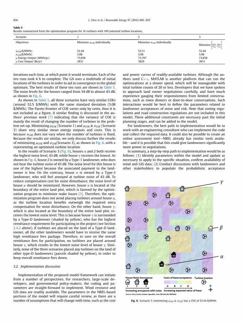
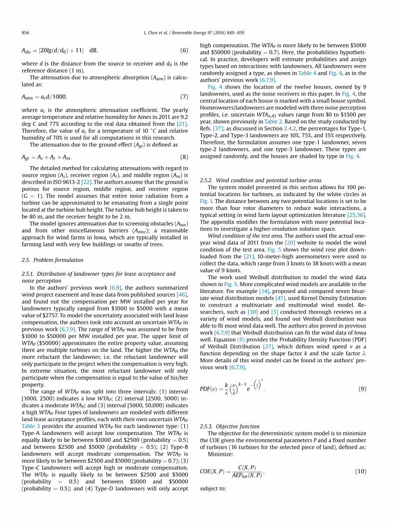
Table 5Results summarized from the optimization program for 16 turbines with 100 potential turbine locations.

Scenario 1 2 3

Objectives Minimize mCOE Individually Minimize sCOE IndividuallyMinimize

"mCOEm*COE; sCOEs*COE

#

mCOE($/MWh) 52.44 52.51 52.44sCOE($/MWh) 5.08 5.08 5.08m Energy Output (MWh/yr) 73,838 73,707 73,838m Cost Output ($k/yr) 3831 3829 3831

Fig. 6. Scenario 3 (minimizing mCOE & sCOE) has a COE of 52.44 $/MWh.

L. Chen et al. / Renewable Energy 97 (2016) 849e859856

iterations each time, at which point it would terminate. Each of theten runs took 4 h to complete. The GA uses a multitude of initiallocations of the turbines in order to aid in convergence to the globaloptimum. The best results of these ten runs are shown in Table 5.The noise levels for the houses ranged from 34 dB to almost 43 dB,as shown in Fig. 6.

As shown in Table 5, all three scenarios have very similar COEs(around 52.5 $/MWh) with the same standard deviation (5.08$/MWh). The Pareto frontier of COE varies only by cents, thus it isnot included as a figure. A similar finding is discussed in the au-thors’ previous work [7] indicating that the variance of COE ismainly the result of changing the number of turbines in the prob-lem set-up. Minimizing mCOE (Scenario 1) and mCOE & sCOE (Scenario3) share very similar mean energy outputs and costs. This isbecause sCOE does not vary when the number of turbines is fixed.Because the results are similar, we only discuss further the resultsof minimizing mCOE and sCOE(Scenario 3), as shown in Fig. 6, withrepresenting an optimized turbine location.

In the results of Scenario 3 (Fig. 6), houses a and b both receivethe highest noise level, 43 dB, while house g receives the lowest. Asshown in Fig. 6, house b is owned by a Type-1 landowner, who doesnot hear the turbine noise of 43 dB. The noise level for this house isone of the highest because the associated payment to the land-owner is low. On the contrary, house a is owned by a Type-3landowner, who will feel annoyed at turbine noise of 43 dB. Toreduce compensation cost for noise disturbance, the noise level ofhouse a should be minimized. However, house a is located at theboundary of the entire land plot, which is favored by the optimi-zation program to minimize wake losses [3]. Therefore, the opti-mization program does not avoid placing turbines around house a,as the turbine location benefits outweigh the required extracompensation for noise disturbance. On the other hand, house g,which is also located at the boundary of the entire land plot, re-ceives the lowest noise level. This is because house g is surroundedby a Type-D landowner (shaded by yellow), who has the highestremittance requirement for participating in the project (see Section2.4.2 above). If turbines are placed on the land of a Type-D land-owner, all the other landowners would have to receive the samehigh remittance fees package. Therefore, to save on the overallremittance fees for participation, no turbines are placed aroundhouse g, which results in the lowest noise level of house g. Simi-larly, none of the three scenarios placed any turbines on the land ofother type-D landowners (parcels shaded by yellow), in order tokeep overall remittance fees down.

3.2. Implementation discussion

Implementation of the proposed model framework can initiatefrom a number of perspectives. For researchers, large-scale de-velopers, and governmental policy-makers, the coding and pa-rameters are straight-forward to implement. Wind resource andGIS data are readily available. The parameters in the NREL-basedportions of the model will require careful review, as there are anumber of assumptions that will change with time, such as the cost

and power curves of readily-available turbines. Although the au-thors used Cþþ, MATLAB is another platform that can run theoptimizations at a slower speed, which will be manageable withtotal turbine counts of 20 or less. Developers that we have spokento approach land owner negotiations carefully, and have muchexperience gauging their responsiveness from limited conversa-tions, such as town dinners or door-to-door conversations. Suchinteractions would be best to define the parameters related tolandowner acceptances of noise and risk. Note that zoning regu-lations and road construction regulations are not included in thismodel. These additional constraints are necessary past the initialplanning stages, and can be added to the model.

For landowners, the best path to implementation would be towork with an engineering consultant who can implement the codeand collect the required data. It could also be possible to create anonline assessment tooldNREL already has similar tools availa-bledand it is possible that this could give landowners significantlymore power in negotiations.

In summary, a step-by-step path to implementationwould be asfollows: (1) Identify parameters within the model and update asnecessary to apply to the specific situation, confirm availability ofwind and GIS data; (2) Conduct discussions with landowners andother stakeholders to populate the probabilistic acceptance

L. Chen et al. / Renewable Energy 97 (2016) 849e859 857

parameters; (3) Code the model, check behavior with test sce-narios; (4) Optimize with a step-up/step-down count of turbines,such as 14-16-18; (5) With results, try moving turbine locationsslightly north/west/east/south to determine sensitivity of results toexact turbine positioning; (6) Share results with all stakeholders,update model constraints as necessary.

4. Conclusion and policy implications

This paper successfully improved the real-world validity andnuanced modeling of landowner concerns in WFLO. New contri-butions in this work included: (a) the use of real-world land parcelsand home locations, which lead to interesting findings on whichland parcels guided the cost of acquiring participation from land-owners; (b) the determination that the economy-of-scale costreduction coefficient used in previous work underestimated thecost of energy (and thus was not included in the optimization) and(c) the incorporation of a noise model and probabilistic compen-sation response of landowners, derived from a collection of real-world data sources. The new system model was tested withdifferent scenarios using realistic data from a 2 by 2 mile plot of anIowa windfarm containing 22 landowners and 12 noise receivers(houses). Initially using 100 potential turbine locations, the optimalmean COE value created by the model ranges from $52 to $53 perMWh (Table 5), which matches the observed COE industry data($51 to $57 per MWh).

Unlike the Wind Turbine Design Cost and Scaling Modeldeveloped by NREL [16], that use a single number to represent landlease cost, the model presented here predicts a realistic COEthrough the incorporation of landowners’ decisions, concerns, andprobabilistic models of associated soft costs. The NREL model es-timates a cost of 1.08 $/MWh for land lease costs, and our modeloffers a similar cost of 1.19 $/MWh for the farm with 16 turbines.This suggests that our model is a viable replacement for the single-number approach from NREL. It offers flexibility in design withrespect to land availability and noise concerns. It captures theimportant concept that if landowners find the potential noisegenerated by the farm unacceptable, or are not adequatelycompensated for hearing it, then the farm cannot be built as thelandowners will decline to participate. This important concept isnot captured in NREL’s approach, with its single $/MWh value andlack of noise impact valuation. The realistic COE predicted by thismodel could help the DOEmake better energy policy decisions thatare inclusive of all stakeholders’ concerns. In general, the workdemonstrates the potential impact of more research on landowner-related issues and the associated soft costs in wind projects, similarto the work that has been funded by the DOE’s SunShot Initiativethat targets reductions in solar energy soft costs [35].

While the model presented here offers reasonable compensa-tion values and provides useful design suggestions to landownersand developers during early-stage farm negotiations, it does have afew limitations that will require further input for it to be useful inthe field. In this paper, the estimations of uncertain parameters areall based on assumptions rather than on measured values, forexample, the dollar compensation values in the landowner noise-acceptance profiles. For implementation, it would be best toconduct interviews with developers and landowners to fine-tunethese parameters. Additionally, different types and sources of un-certainty could be added, such as those associated with turbinefailure. The noise propagation model used in the work [22] is theindustry standard, however it is fairly rudimentary. Higher-fidelitynoise models, such as CONCAWE, could be included in the future tofurther validate the results. Similarly, a higher-fidelity wake lossmodel could also be used.

The noise output and the optimal layout shown in Fig. 6

indicates that the importance of landowners to the outcome ofthe project depends on the wind resource their parcels provide,their lease-acceptance profile, and their noise-acceptance profile.Of these factors, lease acceptance (which has an uncertain rangefrom $1000 to $50000 per MW installed per year as shown inTable 3) plays a particularly important role - as can be seen in Fig. 6,all optimal layouts avoid placing turbines on parcels owned by thelandowners that demand themost compensation, type-D and type-C landowners. Noise acceptance plays a less important role indetermining crucial landowners, because the compensation fornoise annoyance has a much smaller impact on overall farm COE.For example, Fig. 6 shows that the noise level of house a is at thehighest level (43 dB), although it is owned by a landowner with ahigh noise compensation request, indicating that the locationbenefit of house a outweighs the required additional noisecompensation.

The results indicate that minimizing mCOE individually providesalmost identical COE when compared to minimizing mCOE and sCOEcombined, as sCOE is largely dependent on the number of turbines,which is fixed in this model. This finding can be beneficial for de-velopers; if the number of turbines for a farm is predetermined,running only the scenario to minimize the mean value of COE maybe sufficient to obtain a robust optimal farm layout. This savesconsiderable time and computing when planning a wind farmproject. Additionally, a higher-resolution solution space with 576potential turbine locations, instead of 100 locations, is investigatedin the Appendix. The optimal mCOE for 576 potential turbine loca-tions is only 0.7% better than that for 100 potential turbine loca-tions while requiring substantially more computing resources,suggesting it may serve a better role in fine turning locations laterin the project when geological concerns are included.

The implementation of the work is straightforward andextendable beyond the case study by combining existing datasources for wind, land, turbine, and cost parameters. Landowneracceptance probabilistic ranges and corresponding compensationvalues can be estimated with industry expertise and/or landownerparticipation. Thus, the approach here, with limitations notedabove, emphasizes that not only are soft costs an important anddeciding factor inwind-farm development, but also that these costsare not as “soft” as some models suggestdit is possible to put“hard” numbers behind them, with the aid of uncertainty.

Acknowledgments

The research reported in this manuscript was supported in-partby the Department of Energy Sciences under Contract No. DEAC02-07CH11358. The funding source had no involvement in thisresearch. The authors thank Dr. William Ross Morrow for his sup-port in this research.

Nomenclature

ac atmospheric attenuation coefficientA octave-band attenuationAatm attenuation due to atmospheric absorptionAbar attenuation due to screening obstaclesAdiv attenuation due to geometrical divergenceAf(j) standard A-weightingAm attenuation for the middle regionAmisc attenuation from other miscellaneous effects during

propagation through foliage or buildingsAr attenuation for the receiver regionAs attenuation for the source regionAEPtot(X,P) farm’s total annual energy in MWhC(X,P) levelized cost per year of a wind farm in dollars

L. Chen et al. / Renewable En858

COE(X,P) cost of energy of the farm in $/MWhCOE cost of energyd distance from the source to receiverd0 the reference distance (1 m)DC directivity correctionDOE Department of Energyh(X) equality constrainti an index representing the noise sourcesj an index representing the eight standard octave-band

midband frequenciesLAT a-weighted downwind sound power level at a receiver

locationk shaper factor for Weibull distributionLfT(ij) sound pressure level at a receiver location for source i and

octave-band jLW octave-band sound power level for the noise sourcem0 landowner’s initial wealthn number of noise sources (number of turbines)N(X) total number of turbines in the farmPDF(v) probability density function for Weibull distributionU landowner’s utility functionWTAp willingness-to-accept for participationWTAn,43 willingness-to-accept for a landowner at noise level of

43 dBX 100-bit binary string design variablemCOE mean value of Cost of Energym*COE optimal mean value if optimize mCOE individuallysCOE Standard deviation of Cost of Energys*COE optimal standard deviation if optimize sCOE individuallya house labelb house labelg house labelε previous turbine location shown in Fig. 8ε

0new turbine location shown in Fig. 8

l scale factor for Weibull distribution

Appendix

Improved results with higher resolution solution space

This appendix details our reinvestigation of Scenario 1, mini-mizing the mean COE, using a higher-resolution solution spacewith 576 (24 by 24) potential turbine locations (Fig. 7). The algo-rithm used the optimal turbine locations found in Section 3.1 as theinitial points for the GA. The improved optimal results are sum-marized in Table 6 and Fig. 8. Note that the optimal mCOE and energyoutput for 576 potential turbine locations are only 0.7% and 0.8%better than those for 100 potential turbine locations (52.08 $/MWhcompared to 52.44 $/MWh and 74407 MW h/yr compared to73838 MW h/yr), resulting in a total energy output difference of17070MWh over the lifetime of the farm (assumed to be 30 years).However, the computation time for 576 potential turbine locationsis almost five times longer than that for 100 potential turbinelocations.

Table 6Results summarized from the optimization program for 16 turbines with 576 po-tential turbine locations.

Scenarios 1

Objectives MinimizemCOE individually

mCOE ($/MWh) 52.08sCOE ($/MWh) 5.02m Energy Output (MWh/yr) 74,407m Cost Output ($k/yr) 3835

Fig. 7. Test area with 576 instead of 100 potential turbine locations.

The optimal layout in Fig. 8 (Scenario 1 with 576 potential tur-bine locations) is different from that in Fig. 6 (Scenario 3 with 100potential turbine locations). One major noticeable change is theshift of turbine from location ε to ε

0, as shown in Fig. 8. Note that the

new turbine location ε’ is located on plot 15-1 (the purple plot with

black borders), and plot 15-1 only has 3 potential turbine locationsfor the lower-resolution solution space, as shown in Fig.1. However,in this section, plot 15-1 has 12 potential turbine locations, asshown in Fig. 7. The higher-resolution solution space increases thepossibility of the optimization algorithm to select small land plotswith favorable wind resource and less acquiring cost, such as plot15-1.

Fig. 8. Scenario 1 (minimizing mCOE) with 576 potential turbine locations and Scenario3 (minimizing mCOE & sCOE) with 100 potential turbine locations have different optimallayouts.

References

[1] S. Ambrose, R. Rand, Wind Turbine Noise Complaint Predictions Made Easy,2013. Available at: http://www.windaction.org/documents/37241 (accessedon 26.03.15).

[2] C. Archer, M. Jacobson, Supplying baseload power and reducing transmissionrequirements by interconnecting wind farms, J. Appl. Meteorol. Climatol. 46(11) (2007) 1701e1717.

[3] J. Barthelmie, L. Folkerts, K. Rados, C. Larsen, C. Pryor, T. Frandsen, B. Lange,

ergy 97 (2016) 849e859

L. Chen et al. / Renewable Energy 97 (2016) 849e859 859

G. Schepers, Comparison of wake model simulations with offshore windturbine wake profiles measured by sodar, J. Atmos. Ocean. Technol. 23 (2006)888e901.

[4] M. Bolinger, R. Wiser, Understanding Trends in Wind Turbine Prices over thePast Decade. LBNL-5119E, Lawrence Berkeley National Laboratory, 2011.

[5] J. Carta, P. Ramίrez, S. vel�azquez, A review of wind speed probability distri-butions used in wind energy analysis case studies in the Canary Islands,Renew. Sustain. Energy Rev. 13 (2009) (2009) 933e955.

[6] L. Chen, Wind Farm Layout Optimization under Uncertainty with Landowners’Financial and Noise Concerns, Ph.D. Thesis, Iowa State University, Ames, IA,2013.

[7] L., Chen, E, MacDonald., 2015. Wind farm layout optimization under uncer-tainty with realistic landowner decisions. To be submitted to ASME J. EnergyResources Technol..

[8] L. Chen, E. MacDonald, A system-level cost-of-energy wind farm layoutoptimization with landowner modeling, Energy Convers. Manag. 77 (2014)484e494.

[9] L. Chen, E. MacDonald, Effects of uncertain land availability, wind shear, andcost on wind farm layout, in: Paper Presented at the ASME 2013 InternationalDesign Engineering Technical Conferences & Computers and Information inEngineering Conferences, Portland, Oregon, 2013.

[10] L. Chen, E. MacDonald, Considering landowner participation in wind farmlayout optimization, J. Mech. Des. 134 (8) (2012) 084506.

[11] K. Dai, A. Bergot, C. Liang, W.-N. Xiang, Z. Huang, Environmental issuesassociated with wind energy - a review, Renew. Energy 75 (2015) 911e921.

[12] L. Davis, Handbook of Genetic Algorithms, Van Nostrand Reinhold Co., NewYork, NY, 1991.

[13] B. DuPont, J. Cagan, An extended pattern search approach to wind farm layoutoptimization, J. Mech. Des. 134 (8) (2012) 081002e081018.

[14] E. Erdem, J. Shi, Comparison of bivariate distribution construction approachesfor analysing wind speed and direction data, Wind Energy 14 (2011) (2011)27e41.

[15] P. Fagerfj€all, Optimizing Wind Farm Layout: More Bang for the Buck UsingMixed Integer Linear Programming, Chalmers University of Technology andGothenburg University, 2010.

[16] L. Fingersh, M. Hand, A. Laxson, Wind Turbine Design Cost and Scaling Model,Technical Report: NREL/TP-500e40566, National Renewable Energy Labora-tory, 2006.

[17] S. Grady, M. Hussaini, M. Abdullah, Placement of wind turbines using geneticalgorithms, Renew. Energy 30 (2) (2005) 259e270.

[18] T.M. Groth, C. Vogt, Residents’ perceptions of wind turbines: an analysis oftwo townships in Michigan, Energy Policy 65 (0) (2014) 251e260.

[19] C. Houck, J. Joines, M. Kay, A Genetic Algorithm for Function Optimization: aMatlab Implementation, Technical Report: NCSU-IE-TR-95-09, North CarolinaState University, Raleigh, NC, 1995.

[20] Iowa Environmental Mesonet, Custom Wind Roses, Iowa State UniversityDepartment of Agronomy, 2013a available at: http://mesonet.agron.iastate.edu/sites/dyn_windrose.phtml?station¼AMW&network¼IA_ASOS (accessedon 28.10.13).

[21] Iowa Environmental Mesonet, ASOS/AWOS Data Download, Iowa State Uni-versity Department of Agronomy, 2013b available at: http://mesonet.agron.iastate.edu/request/download.phtml?network¼IA_ASOS (accessed on28.10.13).

[22] ISO 9613-2, Acoustics e Attenuation of Sound during Propagation OutdoorsePart 2: General Method of Calculation, 1996.

[23] N. Jensen, A Note on Wind Generator Interaction, Risø National Laboratory,DK-4000 Roskilde, Denmark, 1983.

[24] Y. Katsigiannis, P. Georgilakis, E. Karapidakis, Hybrid simulated annealing-tabu search method for optimal sizing of autonomous power systems withrenewables, IEEE Trans. Sustain. Energy 3 (3) (2012) 330e338.

[25] A. Kusiak, Z. Song, Design of wind farm layout for maximum wind energycapture, Renew. Energy 35 (3) (2010) 685e694.

[26] W. Kwong, P. Zhang, D. Romero, J. Moran, M. Morgenroth, C. Amon, Multi-objective optimization of wind farm layouts under energy generation andnoise propagation, in: Paper Presented at the ASME 2012 International Design

Engineering Technical Conferences & Computers and Information in Engi-neering Conference, Chicago, 2012.

[27] M. Lackner, C. Elkinton, An analytical framework for offshore wind farmlayout optimizaiton, Wind Eng. 31 (1) (2007) 17e31.

[28] T. Lambert, P. Gilman, P. Lilienthal, in: F.A. Farret, M.G. Sim~oes (Eds.), Micro-power System Modeling with HOMER,“ in Integration of Alternative Sourcesof Energy, Wiley, Hoboken, NJ, 2006, pp. 379e418.

[29] G. Marmidis, S. Lazarou, E. Pyrgioti, Optimal placement of wind turbines in awind park using monte carlo simulation, Renew. Energy 33 (7) (2008)1455e1460.

[30] E. Morgan, M. Lackner, R. Vogel, L. Baise, Probability distributions for offshorewind speeds, Energy Convers. Manag. 52 (2011) (2011) 15e26.

[31] G. Mosetti, C. Poloni, B. Diviacco, Optimization of wind turbine positioning inlarge windfarms by means of a genetic algorithm, J. Wind Eng. Ind. Aerodyn.51 (1) (1994) 105e116.

[32] K. Mosman, Wind Farm a Good Neighbor, 2015 available at: http://www.oleantimesherald.com/editorial/article_f74dc548-69ca-11e0-b1ae-00.1cc4c002e0.html (accessed on 26.03.15).

[33] K. Muschell, BP Good Neighbor Recruiting Letter, 2015 available at: http://pandorasboxofrocks.blogspot.com/2013/01/bp-good-neighbor-recruitment-letter.html (accessed on 26.03.15).

[34] Office of Energy Efficient and Renewable Energy, Renewable Energy Gener-ation, 2015 availble at: http://energy.gov/eere/renewables (accessed on26.03.15).

[35] Office of Energy Efficient and Renewable Energy, Soft Cost, 2015 available at:http://energy.gov/eere/sunshot/soft-costs (accessed on 26.03.15).

[36] U. Ozturk, B. Norman, Heuristic methods for wind energy conversion systempositioning, Electr. Power Syst. Res. 70 (3) (2004) 179e185.

[37] E. Pedersen, K. Waye, Wind turbine noise, annoyance and self-reported healthand well-being in different living environments, Occup. Environ. Med. 64 (7)(2007) 480e486.

[38] M. Ray, A. Rogers, J. McGowan, Analysis of wind shear models and trends indifferent terrain, in: Conference Proceeding: American Wind Energy Associ-ation Windpower. Pittsburgh, PA, June 2e7, 2006.

[39] E. Songsore, M. Buzzelli, Social responses to wind energy development inOntario: the influence of health risk perceptions and associated concerns,Energy Policy 69 (0) (2014) 285e296.

[40] S.Y.D. Sorkhabi, D.A. Romero, G.K. Yan, M.D. Gu, J. Moran, M. Morgenroth,C.H. Amon, The impact of land use constraints in multi-objective energy-noisewind farm layout optimization, Renew. Energy 85 (2016) 359e370.

[41] E. Takle, J. Lundquist, Research Experience for Undergraduates: Crop-wind-energy-Experiment (C-wex), 2011 available at: http://www.eol.ucar.edu/about/our-organization/fps/observing-facilities-assesment-panel-ofap/educational-facility-requests/edu_CWEX_2011_complete.pdf.

[42] The Associated Press, Oregon Man Files $5 Million Suit over Wind Farm Noise,2013 available at: http://www.oregonlive.com/pacific-northwest-news/index.ssf/2013/08/post_133.html (accessed on 26.03.15).

[43] U.S. Energy Information Administration, Levelized Cost and Levelized AvoidedCost of New Generation Resources in the Annual Energy Outlook 2014, 2014available at: http://www.eia.gov/forecasts/aeo/pdf/electricity_generation.pdf(accessed on 26.03.15).

[44] M. Wall, GAlib: a Cþþ Library for Genetic Algorithm Components, Massa-chusetts Institute of Technology, 1999 available at: http://lancet.mit.edu/ga/Copyright.html.

[45] Wikipedia, Story County Wind Farm, 2013. Available at: http://en.wikipedia.org/wiki/Story_County_Wind_Farm (accessed on 26.03.15).

[46] Windustry, Wind Energy Easement and Leases: Compensation Packages,Windustry Wind Easement Work Group, 2009 available at: http://saline.unl.edu/c/document_library/get_file?folderId¼294039&name¼DLFE-18538.pdf(accessed on 28.10.13).

[47] J. Zhang, S. Chowdhury, A. Messac, L. Castillo, Multivariate and multimodalwind distribution model based on kernel density estimation, in: ASME 20115th International Conference on Energy SustainabilityWashington, DC, USA,2011.