modeling in trnsys of a single effect evaporation...
TRANSCRIPT
Modeling in TRNSYS of a Single Effect Evaporation System
Powered by a Rankine Cycle
S. Casimiro
1, 2 , C. Ioakimidis
3, J. Mendes
4, M. Giestas
4
1 MIT|Portugal Program, Sustainable Energy Systems, Lisbon, Portugal
2 IN+, Instituto Superior Técnico, Lisbon, Portugal
3 DeustoTech, Energy Unit, University of Deusto, Bilbao, Spain
4 Laboratório Nacional de Energia e Geologia, UESEO, Lisbon, Portugal
Abstract
The paper presents an analysis of a Single Effect Evaporation (SEE) system as a pre-study to the
feasibility of concentrated solar power plants (CSP) powering desalination units for cogeneration of water
and electricity. An algorithm to model a SEE system in steady-state operation was made and is described
in this work. This algorithm was implemented in TRNSYS environment, and a simple analysis was
conducted of a SEE system powered by a Rankine cycle used in CSP plants.
Keywords: Desalination, Single Effect Evaporation, TRNSYS, simulation.
1. Introduction
Water scarcity has been a problem for many regions around the world, even if only during some critical
periods during the year. This has various economical, social and environmental impacts. Technological
developments, the need for clean water, and the growing concerns about water supply availability in
different areas of the world have justified investments in various types of desalination technologies
powered by different energy sources. As desalination processes require intense energy consumption,
energy security to power it and market fluctuations for fuel prices have made these important issues when
deciding whether or not to install a specific type of desalination system in a particular place.
Typically, areas with high levels of solar radiation also suffer a high instance of drought. The combination
of desalination and solar technologies in such areas can present an interesting investment, if these
regions are near sources of water (i.e., ocean or other bodies of non-drinkable water). Solar technologies
can be a reliable source of energy and can be partnered with desalination units in many such locations
(DLR, 2007).
This work is a pre-study on the feasibility of the usage of CSP technologies to power Desalination units
(CSP+D), and in it, it is presented a study on the performance of a SEE system coupled with a Rankine
cycle providing the necessary heat to power a desalination unit of this kind. The main part of this work
consisted in modeling the SEE system. The Rankine cycle is not evaluated in detail.
The SEE system has a very low efficiency when compared with other desalination methods (Ettouney,
2002). The only reason why it was chosen for this study is because it forms the basis to understand more
complex and efficient evaporation systems, such as the Multi Effect Desalination (MED) and the Multi
Stage Flash (MSF). A simple technical evaluation of the usage of the SEE system is presented at the
end of the work, along with a comparison of its performance with the other main desalination competing

technologies (Blanco, 2011): Thermal Vapor Compression (TVC)-MED, Low Temperature (LT) - MED and
Reverse Osmosis (RO).
For this, a transient systems simulation program with a modular structure called TRNSYS has been used.
This program has been used as a reference in the solar community for many years, including for the
simulation of CSP plants.
2. SEE system
The SEE system has very limited industrial applications. One of the measures for understanding the
performance of a desalination system is the thermal performance ratio (PR) (also called Gain Output
Ratio (GOR)), calculated by dividing the amount of distilled water produced by the mass of steam used
(Ettouney, 2002). PR values for the SEE normally are just below one. The PR values for the more
efficient evaporation technologies (LT-MED and TVC-MED namely) (Blanco, 2011), are roughly one order
of magnitude higher, comparing with a SEE.
Nomenclature:
Areas: Power: Ae - Area of Evaporator, [m
2] Qe - Evaporator heat transfer rate, [kJ/s]
Ac - Area of Condenser,[m2] Qc - Condenser heat transfer rate, [kJ/s]
Constants: Temperatures: Cp - Specific heat at constant pressure,
[kJ/kg ºC] Ts - Low Pressure Turbine steam temperature
input, [ºC] Tb - Boiling temperature, [ºC] Dimensionless: Tv - Temperature of the formed Vapor in the
condenser, [ºC] PR - Performance Ratio (or Gained Output Ratio, GOR) Tf - Temperature of the feed seawater, [ºC]
sMcw - Specific cooling water flow rate Tcw - Temperature of the cooling water, [ºC] BPE - Boiling point elevation, [ºC] Flow Rates: LMTDc - Logarithmic temperature difference, [ºC] Ms - Mass of steam, [kg/s] Md - Mass of Distillate produced, [kg/s] Salinity: Mt - Total Mass (Mf+Mcw), [kg/s] Xf - Salinity of the feed seawater [weight %] Mcw - Mass of cooling water, [kg/s] Xb - Salinity of the Brine [weight %] Mb - Mass of brine, [kg/s] Mf - Mass of feed seawater, [kg/s] Latent Heat: Mv - Mass of vapor formed in the
condenser, [kg/s] λs - Latent heat of input steam, [kJ/kg] λv - Latent heat of vapor formed in the
evaporator, [kJ/kg] Heat Transfer Coefficient: Ue - Evaporator heat transfer coefficient,
[kJ/s m2 ºC]
Uc - Condenser heat transfer coefficient, [kJ/s m
2 ºC]
2.1 Process description
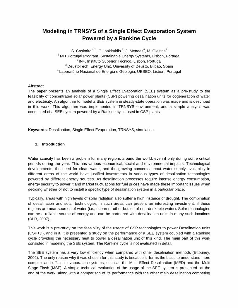
The main components of a SEE system are the evaporator and the condenser, as shown in Figure 1.
Each of these blocks consists of an enclosed vapor space, evaporator/condenser heat exchange tubes,
an un-evaporated water pool, a line for the removal of non-condensable gases, water distribution system,
and a mist eliminator (Ettouney, 2002). In each of these “blocks”, the two fluid systems are separated by
the heat exchange tubes. Only energy is exchanged, and no mass transfers occur.
Figure 1 – Single Effect Desalination process
A mass of seawater (Mt) enters the condenser at seawater temperature (Tcw). Here this water gets
preheated (Tf), due to the heat transfer (Qe) that occurs when the mass of vapor coming from the
Evaporator (Mv) is condensed. Not all of this preheated seawater is used to produce fresh water (Md),
and only part of it enters the evaporator after flowing through the condenser. A large quantity of energy is
wasted in this manner as most of the preheated water after leaving the condenser is discarded (Mcw). To
condense the entire vapor coming from the evaporator, more cold seawater is needed than the one
required to create it in the first place.
The part of the preheated seawater that enters the evaporator (Mf), receives an energy transfer from the
evaporator‟s main heat source (Qe) (in this simulation, the steam from the Rankine cycle Low Pressure
Turbine (LPT)). As the steam mass (Ms) coming from the LPT passes through the heat transfer tubes in
the evaporator, it condenses, releasing its latent heat energy (λs) to the preheated water mass (Mf) that
came from the condenser. Assuming that the steam from the LPT is saturated (100% vapor), after leaving
the evaporator, it will exit at the same temperature (Tcs) that it entered (Ts), but will be 100% liquid. In
reality steam outputs from LPT are not saturated, having a quality between 80 to 95%, but for the purpose
of this theoretical work it is assumed a quality of 100% for inlet vapor in the evaporator, and 0% for outlet.
Due to the energy transfer from the condensation of the LPT steam, the temperature of the preheated
water increases in the evaporator, reaching its maximum temperature (the boiling temperature (Tb)). To
avoid scaling problems, not all the preheated seawater entering the evaporated is vaporized. This would
cause the system to lose its efficiency as the heat transfer coefficients (Ue and Uc) would start suffering
and corrosion would seriously affect the materials. Because of this, part of the energy from the latent heat
is used for sensible heat increase of the water entering the evaporator (up to the boiling temperature) and
only the remaining is used to vaporize part of the evaporator‟s Mf. The preheated water which enters the

evaporator that is not vaporized is discarded as brine (Mb) back to the sea with a higher salt
concentration (Xb) than the seawater. Doing so leads to a big loss of energy as this water is warm.
The temperature of the vapor formed inside of the evaporator (Tv) is actually lower than the maximum
temperature that the seawater reaches as liquid state inside the evaporator. This is due to the salt
presence in seawater (Xf), causing the Boiling Point Elevation (BPE). The higher the concentration of salt
in the water, the lower the partial pressure of water is, resulting in the BPE. Salt molecules reduce the
total area of exposure of water molecules to the gaseous phase. The pressure that these water molecules
can produce in the presence of salt molecules is therefore reduced and the boiling temperature of the
solution is thus higher than if it was only pure water.
The vapor formed in the evaporator (Mv) is salt free. As it passes through the condenser, it releases its
latent heat (λv) preheating the incoming seawater (Mt) and closing the loop. A big loss of energy also
occurs at this point as the condensed distilled vapor (Md) leaves the system at a higher temperature than
Tcw.
The loss of energy with the brine and distilled water outputs at high temperature, plus the usage of only
part of the preheated water leaving the condenser justify the low performance ratio of the SEE system
(Ettouney, 2002).
2.2 Process Modeling under Steady-State operation
The evaporator and condenser created in TRNSYS for this work represent a SEE system in its basic
format, assuming a steady-state operation. The system can determine the equilibrium regarding operating
temperatures and mass balances for every moment. As steady-state operation was considered, this SEE
system ignores the values obtained in the previous time-step calculations as no thermal capacitance is
considered. For example, if from one second to the other a significant increase in temperatures or mass
occurs on the input, the simulation will not take into account the inertia of the system regarding these
changes. The equilibrium that it will be calculated will thus not be valid.
It has been taken into account that desalination plants and power plants operate within a small range of
temperatures and mass flows (apart from start-up and shut-down), and because of that it was decided
that for this initial study it would be considered a steady-state operation (Ettouney, 2006), (Mataix, 2000).
The steady-state formulation of the SEE process also means that the TRNSYS components would have
lower degree of complexity and it would be possible to compare results obtained with the literature
available (which for SEE systems the majority assumes steady-state formulations).
In the formulation of this SEE system, the aim was to make a system with the least amount of inputs
possible, so that it would be more flexible, and calculations for equilibriums would require less information
for a determined situation. To run it, the inputs needed are:
1. Seawater characteristics: Xf, Tcw, Cp (of water);
2. Heat transfer areas: Ae, Ac;
3. Maximum admissible salinity in the brine produced: Xb;
4. Heat source characteristics powering the evaporator: Ts, Ms (assuming always saturated vapor)
Having these inputs, the system obtains the equilibrium in steady-state conditions for the operational
temperatures and mass flow rates of water used and produced, being the most relevant: Mf, Md, Tv and
Tf. The other outputs are: Mv, Mb, Tb, BPE, λs, λv, Qe, Ue, PR, Mt, Mcw, Qc, Uc, sMcw.

Although Xb is a physical output of the SEE system, it was defined as an input when modeling for two
reasons. Firstly, it would reduce the number of unknown variables, making the calculations less complex.
Secondly, during the operation of a desalination plant, the brine has a negative impact in the ecosystems
when discarded back to the sea. Operators of these plants will have to limit the maximum brine salinity
they will accept a priori.
The equations considered to model the SEE system were (Ettouney, 2002):
Evaporator:
(1)
(2)
(3)
Condenser:
(4)
(5)
Auxiliary equations:
(6)
(7)
(8)
(9)
, where (10)
; ;
(11)
, for the ranges (1 ≤ X ≤ 16%) and (10 ≤ T ≤ 180ºC) (12)
(13)
(14)
(15)
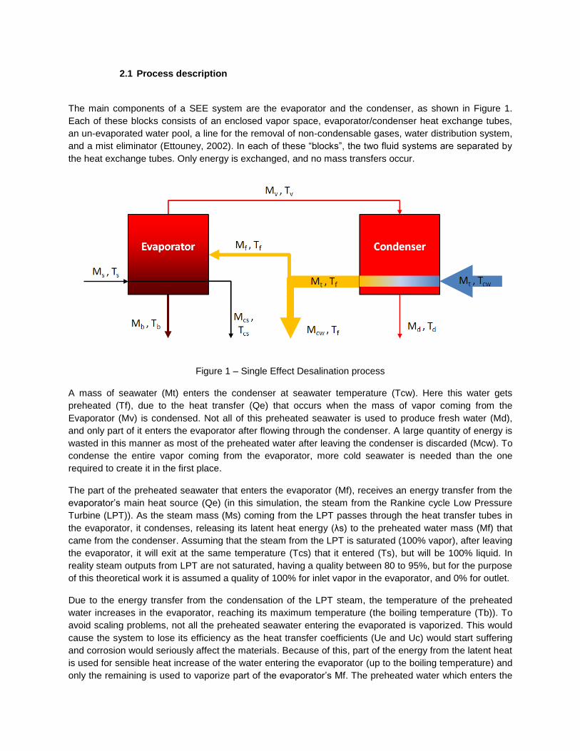
The key to understanding how the equilibrium for the SEE system was obtained in this work is to know
that only one possible value for Tf results in an equilibrium between the evaporator and the condenser
(given the eight necessary inputs mentioned before). As Figure 2 shows (for a particular SEE system
where only the Tf changes), increasing the Tf entering the evaporator increases Mv production. In
opposite, the more Mv enters the condenser, the lower the resulting Tf will be (if more water has to pass
through the condenser within the same amount of time, less energy will be absorbed per unit mass).
Figure 2 – Impact of Tf in the evaporator and condenser operation.
This means that only one value for Tf results in the correct amount of Mv produced to keep the system in
steady-state operation through time (if all conditions allow an equilibrium to be reached in the first place).
If a different value for Tf is used in the evaporator, a different amount of Mv will be produced. This will
unbalance the Tf output leaving the condenser (that feeds the evaporator) making impossible a steady-
state operation.
Using iterations it is possible to find the correct value for Tf since the maximum and minimum theoretical
values for it are known. The maximum is Ts, and the minimum is obtained by calculating the value of Tf
when (LMTD)c tends to zero.
By defining Xb as an input, the calculation for the equilibrium will always set an Md corresponding to the
maximum brine salinity. For the same Mf, the more Mv formed, the less Mb and higher Xb, as indicated
by equation (3).
Although Mf is a physical inlet for the evaporator, it was defined as an output as was with Xb, to reduce
the complexity of the mathematical system to be solved and make it more flexible. In this case the
flexibility was given by eliminating an input altogether instead of locking it (as it was done with Xb).
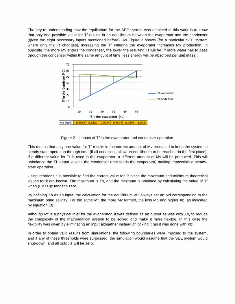
In order to obtain valid results from simulations, the following boundaries were imposed to the system,
and if any of these thresholds were surpassed, the simulation would assume that the SEE system would
shut-down, and all outputs will be zero:
Evaporator thresholds:
Condenser thresholds:
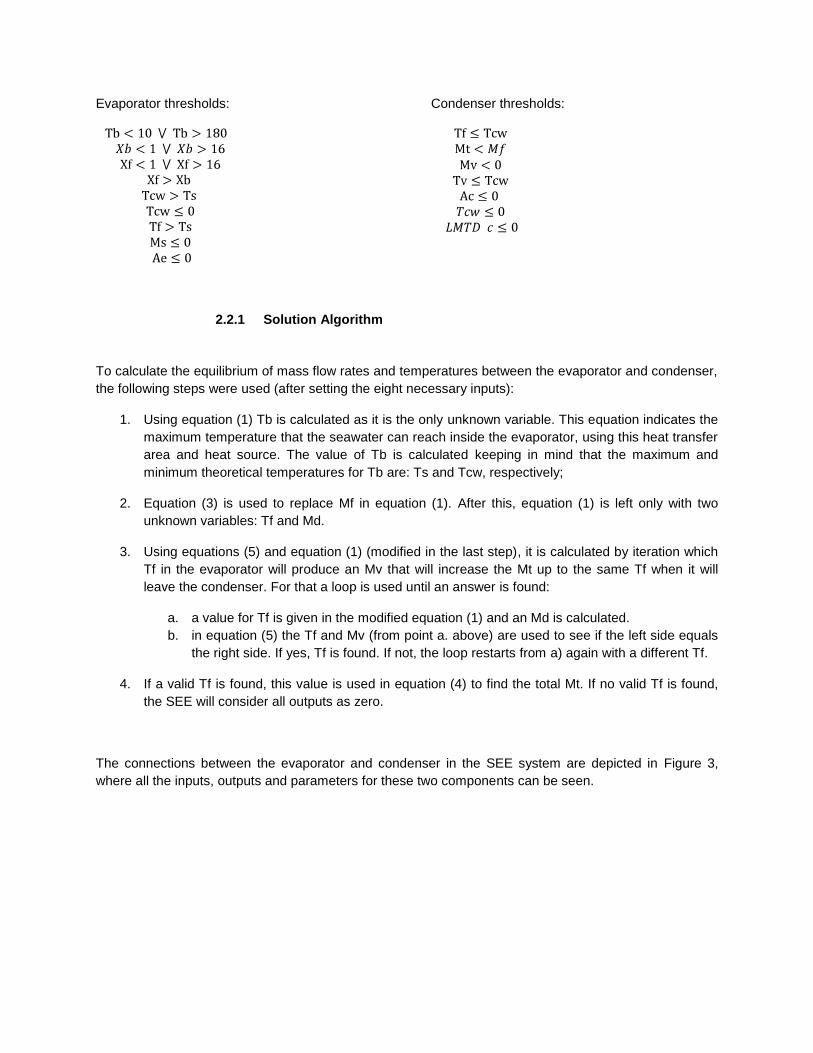
2.2.1 Solution Algorithm
To calculate the equilibrium of mass flow rates and temperatures between the evaporator and condenser,
the following steps were used (after setting the eight necessary inputs):
1. Using equation (1) Tb is calculated as it is the only unknown variable. This equation indicates the
maximum temperature that the seawater can reach inside the evaporator, using this heat transfer
area and heat source. The value of Tb is calculated keeping in mind that the maximum and
minimum theoretical temperatures for Tb are: Ts and Tcw, respectively;
2. Equation (3) is used to replace Mf in equation (1). After this, equation (1) is left only with two
unknown variables: Tf and Md.
3. Using equations (5) and equation (1) (modified in the last step), it is calculated by iteration which
Tf in the evaporator will produce an Mv that will increase the Mt up to the same Tf when it will
leave the condenser. For that a loop is used until an answer is found:
a. a value for Tf is given in the modified equation (1) and an Md is calculated.
b. in equation (5) the Tf and Mv (from point a. above) are used to see if the left side equals
the right side. If yes, Tf is found. If not, the loop restarts from a) again with a different Tf.
4. If a valid Tf is found, this value is used in equation (4) to find the total Mt. If no valid Tf is found,
the SEE will consider all outputs as zero.
The connections between the evaporator and condenser in the SEE system are depicted in Figure 3,
where all the inputs, outputs and parameters for these two components can be seen.
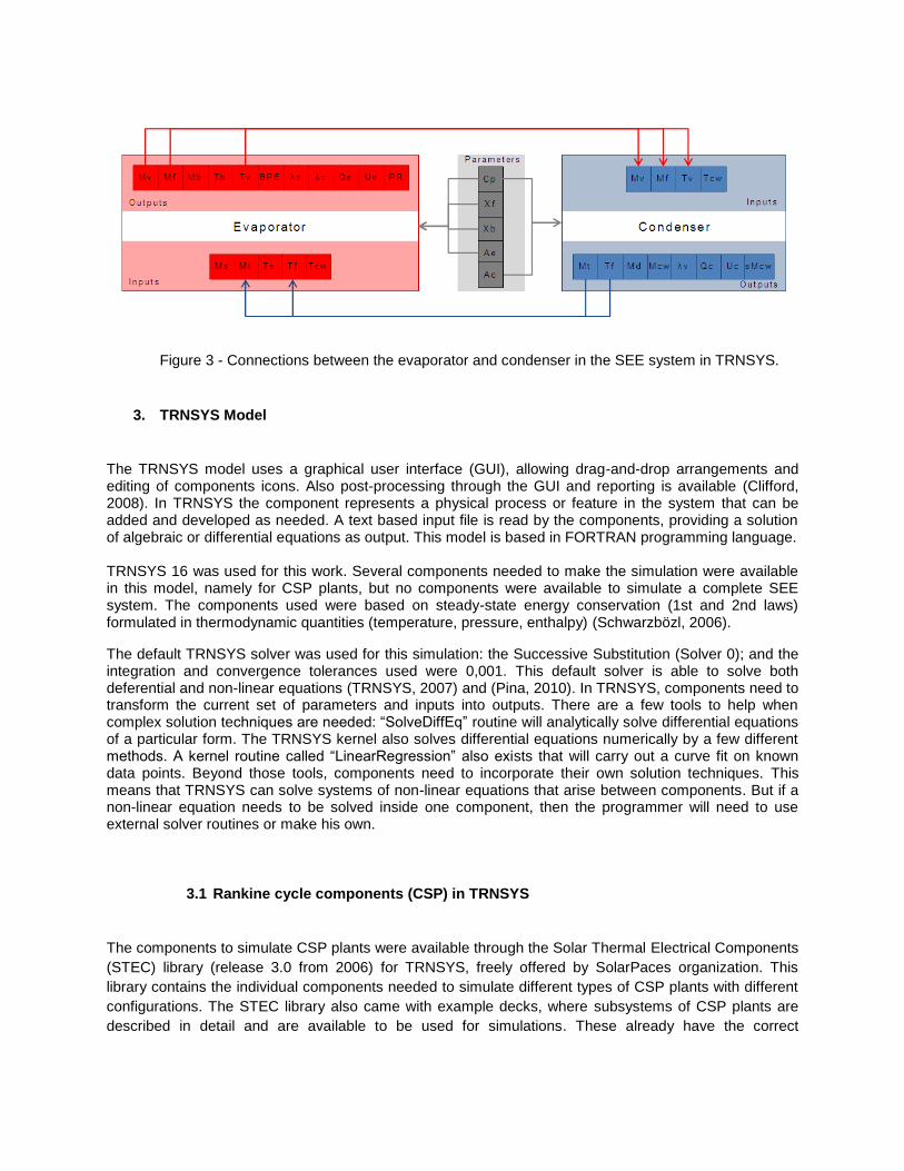
Figure 3 - Connections between the evaporator and condenser in the SEE system in TRNSYS.
3. TRNSYS Model
The TRNSYS model uses a graphical user interface (GUI), allowing drag-and-drop arrangements and editing of components icons. Also post-processing through the GUI and reporting is available (Clifford, 2008). In TRNSYS the component represents a physical process or feature in the system that can be added and developed as needed. A text based input file is read by the components, providing a solution of algebraic or differential equations as output. This model is based in FORTRAN programming language. TRNSYS 16 was used for this work. Several components needed to make the simulation were available in this model, namely for CSP plants, but no components were available to simulate a complete SEE system. The components used were based on steady-state energy conservation (1st and 2nd laws) formulated in thermodynamic quantities (temperature, pressure, enthalpy) (Schwarzbözl, 2006).
The default TRNSYS solver was used for this simulation: the Successive Substitution (Solver 0); and the integration and convergence tolerances used were 0,001. This default solver is able to solve both deferential and non-linear equations (TRNSYS, 2007) and (Pina, 2010). In TRNSYS, components need to transform the current set of parameters and inputs into outputs. There are a few tools to help when complex solution techniques are needed: “SolveDiffEq” routine will analytically solve differential equations of a particular form. The TRNSYS kernel also solves differential equations numerically by a few different methods. A kernel routine called “LinearRegression” also exists that will carry out a curve fit on known data points. Beyond those tools, components need to incorporate their own solution techniques. This means that TRNSYS can solve systems of non-linear equations that arise between components. But if a non-linear equation needs to be solved inside one component, then the programmer will need to use external solver routines or make his own.
3.1 Rankine cycle components (CSP) in TRNSYS
The components to simulate CSP plants were available through the Solar Thermal Electrical Components
(STEC) library (release 3.0 from 2006) for TRNSYS, freely offered by SolarPaces organization. This
library contains the individual components needed to simulate different types of CSP plants with different
configurations. The STEC library also came with example decks, where subsystems of CSP plants are
described in detail and are available to be used for simulations. These already have the correct
connections established between the individual components and the correct parameters. One of these
example decks describes a simple Rankine cycle, which was used in this work.
This Rankine cycle is composed by several components, namely (Schwarzbözl, 2006): a boiler section
(feedwater economizer and evaporator), turbine section (three turbines and two extraction lines),
condenser module, deaerator, condenser preheater and a subcooler, condenser pump and feed water
pump. The heat source for this Rankine cycle is simulated by a forcing function replicating a mass flow
rate of steam. The temperature at which this heat source enters the Rankine cycle is predefined at 573,8
ºC.
3.2 SEE components in TRNSYS
To simulate a simple SEE system, two basic components are needed: an evaporator and a condenser.
These are available in more than one TRNSYS component library though, none has been designed to
assume its operation with saltwater. To solve this, a new evaporator and a condenser were built in
TRNSYS using FORTRAN language in such a way that they could interact with other existing
components.
It is possible to program the evaporator and condenser in TRNSYS in two ways: 1) as a single
component (“combined-component”), or 2) as two individual components. The components were
programmed separately in order to increase component modularity and reduce complexity of the code
needed.
In this work, the equations describing the SEE system in steady-state are non-linear and they needed to
be solved inside the components. This meant that TRNSYS could not solve this part of the problem as
there are no internal subroutines that could be used for that inside the components (TRNSYS, 2007). To
work this out, a simple loop was made to solve the non-linear equation system of each component, acting
as a basic solver inside the condenser and the evaporator. The convergence tolerances used inside
these “home-made” solvers, started in 0.001, and decreased until 0.1 depending if a solution would be
found or not before the end of the loop. The evaporator follows step 1) and 2) and 3.a) from the solution
algorithm, and the condenser follows step 3.b).
By choosing to write two individual components, the TRNSYS solver calculates the equilibrium between
the evaporator and the condenser, and no extra programming is necessary to reach a balance between
the two components. Alternately, if just a single component was built for the SEE, another “home-made”
solver would need to be made just to connect the results between the evaporator and condenser blocks,
making probably the system slower during calculations.
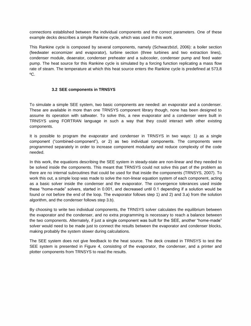
The SEE system does not give feedback to the heat source. The deck created in TRNSYS to test the
SEE system is presented in Figure 4, consisting of the evaporator, the condenser, and a printer and
plotter components from TRNSYS to read the results.
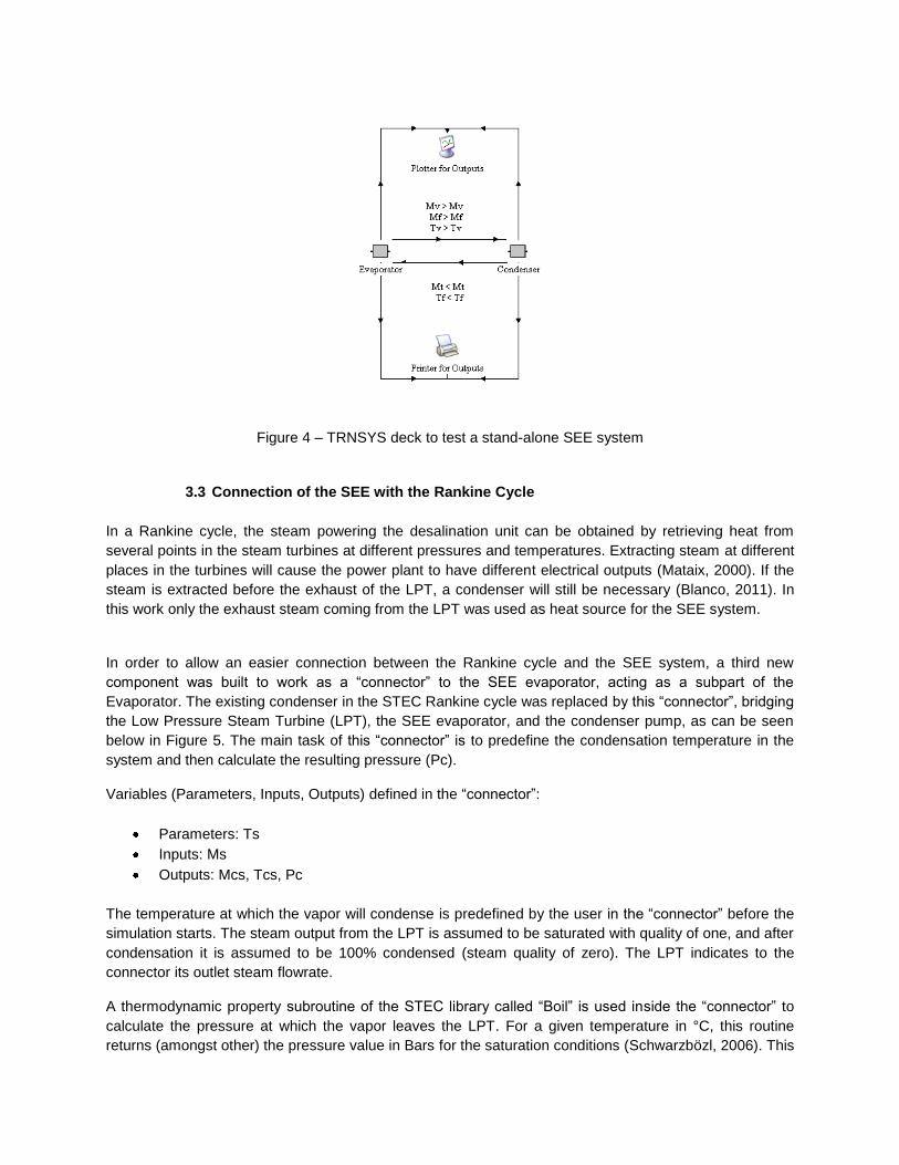
Figure 4 – TRNSYS deck to test a stand-alone SEE system
3.3 Connection of the SEE with the Rankine Cycle
In a Rankine cycle, the steam powering the desalination unit can be obtained by retrieving heat from
several points in the steam turbines at different pressures and temperatures. Extracting steam at different
places in the turbines will cause the power plant to have different electrical outputs (Mataix, 2000). If the
steam is extracted before the exhaust of the LPT, a condenser will still be necessary (Blanco, 2011). In
this work only the exhaust steam coming from the LPT was used as heat source for the SEE system.
In order to allow an easier connection between the Rankine cycle and the SEE system, a third new
component was built to work as a “connector” to the SEE evaporator, acting as a subpart of the
Evaporator. The existing condenser in the STEC Rankine cycle was replaced by this “connector”, bridging
the Low Pressure Steam Turbine (LPT), the SEE evaporator, and the condenser pump, as can be seen
below in Figure 5. The main task of this “connector” is to predefine the condensation temperature in the
system and then calculate the resulting pressure (Pc).
Variables (Parameters, Inputs, Outputs) defined in the “connector”:
Parameters: Ts
Inputs: Ms
Outputs: Mcs, Tcs, Pc
The temperature at which the vapor will condense is predefined by the user in the “connector” before the
simulation starts. The steam output from the LPT is assumed to be saturated with quality of one, and after
condensation it is assumed to be 100% condensed (steam quality of zero). The LPT indicates to the
connector its outlet steam flowrate.
A thermodynamic property subroutine of the STEC library called “Boil” is used inside the “connector” to
calculate the pressure at which the vapor leaves the LPT. For a given temperature in °C, this routine
returns (amongst other) the pressure value in Bars for the saturation conditions (Schwarzbözl, 2006). This

pressure information is provided to the LPT to act as its outlet steam pressure. Although the outlet
pressure is a physical output of the LPT, it is defined as an input to reduce the complexity of the system.
As can be seen in Figure 5, the outputs of the “connector” will inform the SEE evaporator of the Ms and
Ts that will be available to power it. No mass loss is assumed, and Ms equals Mcs. Ts is also equal to Tcs
as steam input in the “connector” is considered saturated, and only latent heat is transferred. In Figure 5
the Rankine cycle is not shown in detail and is represented as a Macro in the TRNSYS deck, as it is not
the main focus of this study. The connections between the components variables are indicated.
Figure 5 – TRNSYS deck with Rankine cycle + SEE system
The Mcs and Tcs outputs from the “connector” will also link with the inputs of the condenser pump in the
Rankine cycle. As this study is an initial analysis to desalination systems in TRNSYS, there is no
feedback from the SEE evaporator back to the Rankine cycle since the Ts is predefined in the “connector”
and the steam from the LPT is assumed saturated.
4. Scenarios
Three simulation decks were used for this work. The first was to test the SEE system and validate its
results with the reference data from the literature. The second, to simulate the performance of the
Rankine cycle without the SEE system coupled. The third, to simulate the Rankine cycle coupled with the
SEE system. Five scenarios were considered using decks two and three, as table 1 shows.
Table 1 – Scenarios description
Scenario Technologies used / TRNSYS deck Ts
(ºC) Tb
(ºC) Tf
(ºC) (Ae+Ac)
(m2)
1. Rankine cycle with no SEE - Business as Usual (BAU) (deck two)
- - - -
2.
Rankine cycle with SEE (deck three)
50 ~36 ~30 ~800
3. 60 ~44 ~36 ~600
4. 70 ~54 ~50 ~600
5. 70 ~54 ~43 ~500
Through a thermodynamic characterization, the overall efficiencies for CSP+D were assessed. For this
theoretical simulation, a 24 hour period was used with a time step of one hour.
5. Results and Discussion
5.1 SEE deck
The deck created in TRNSYS to validate the SEE system consisted only of the evaporator and the
condenser as can be seen in Figure 4. The inputs were predefined and did not vary over time so the
equilibrium was reached from the first time step. Components “Type65d” and “Type25a” were part of the
standard TRNSYS component library (TRNSYS, 2007) and were used to print and plot the outputs from
the SEE system.
From (Ettouney, 2002), examples one, two and three from „Chapter two - Single Effect Evaporation‟ were
used as reference data and the results obtained from the simulation, only an error less than 0.5%
presented when compared. The boundaries imposed on the system also gave the expected results,
shutting down the SEE system when it was supposed to. The results obtained were also verified using
the Visual basic computer package for thermal and membrane desalination processes (Ettouney, 2004),
obtaining similar results in both programs.
5.2 Rankine cycle deck (Scenario 1)
Scenario 1 represents the BAU case, where no cogeneration is done and only electric production occurs.
The simulation of the Rankine cycle as defined in the STEC deck, has an output of 103.9 MWh during a
simulation of 24 hours, reaching a peak power of 4,86 MWe and a minimum of 4,30 MWe (electrical
generator efficiency was set to 90%). The heat load available to the Rankine cycle varied through the 24
hours of the simulation as can be seen in Figure 6. The mass flow rate of steam ranged from a maximum
of 150 000 kg/h to a minimum of 129 600 kg/h and this is the reason for the oscillation in the power output
of the turbines.
Figure 6 – Profile of the heat load made available to the Rankine cycle during the 24 hours of the
simulation.

The condenser in the Rankine cycle had the following variables predetermined before the start of the
simulation: the exact temperatures for the Tcw, the cooling water outlet temperature (equivalent to Tf in
the SEE) and the condensing temperature of the steam from the LPT (equivalent to Ts in the SEE). Being
so, this component from STEC did not assume any values for heat transfer areas or coefficients.
5.3 Rankine cycle + SEE system deck (Scenario 2, 3, 4 and 5)
Scenario 2: In scenario two, the following parameters were predefined with these values:
SEE system:
Cp = 4,18 (kJ / kg.ºC);
Xf = 4,2 (salt weight % = 42 000 ppm);
Xb =7 (salt weight % = 70 000 ppm);
Ae = 304 (m2);
Ac = 564 (m2);
Tcw = 20 (ºC);
Rankine cycle :
Ts = 50 (ºC)
The heat transfer areas of the evaporator and condenser have been determined taking into account the
mass of steam coming from the LPT and the Ts predefined temperature. Having this information, it was
possible to define the Qe transferred to the SEE evaporator, using equation (7). By trial and error,
reasonable values for Tb, Tv and Md were assumed (~35ºC, ~34ºC and ~4kg/s, respectively) and an area
could be calculated for the evaporator (≈ 304 m2) and condenser (≈ 564 m
2) using equation (2) and (5)
respectively. A minimum area allowed for the evaporator and condenser for a determined value of
temperatures is already known to us. If the areas are smaller than this threshold value, even if a small
positive temperature difference between Tv and Tcw still exists and a massive amount of cooling water is
circulated, it will not be able to condense all the steam in the other side of the heat transfer tubes using
that heat transfer coefficient.
In scenario 2, when connecting the Rankine cycle to the SEE system by replacing the existing condenser
in the STEC deck, the modified Rankine cycle has an output of 99,28 MWh during a simulation of 24
hours, reaching a peak power of 4,64 MW and a minimum of 4,1 MW (electrical generator efficiency was
set to 90%). This represents less 4,4% of electricity produced (-4,62 MWh), compared with the operation
of the Rankine cycle without the SEE system. On the other hand it is now possible to produce fresh
water, obtaining ≈318 m3 in 24 hours.
The simple ratio between the kWh lost and the water production, gives a value of 25,16 kWh/m3 of water
produced, which is an order of magnitude higher than the competing technologies specific energy
consumption (SEC), namely LT-MED: 1.4-2.4 kWh/m3, TVC-MED: 1.2-2.2 kWh/m
3; RO: 3.5-5.5 kWh/m
3.
It should be noticed that the SEC values include not only the loss in energy production in the turbines, but
also the other main energy consumptions: the power required by the pumps, the desalination plant and
cooling system. If an evaluation is made for the SEE system in this scenario which also includes these
consumptions, the specific energy would be higher than 25,16 kWh/m3.
Changing only the parameters for the areas (Ae, Ac) and Ts from scenario 2 described above, the main
outputs for the remaining scenarios 3, 4 and 5 are shown in Table 2.
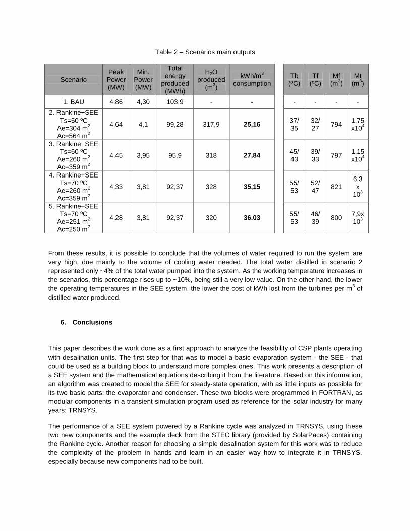
Table 2 – Scenarios main outputs
Scenario Peak Power (MW)
Min. Power (MW)
Total energy
produced (MWh)
H2O produced
(m3)
kWh/m3
consumption
Tb (ºC)
Tf (ºC)
Mf (m
3)
Mt (m
3)
1. BAU 4,86 4,30 103,9 - - - - - -
2. Rankine+SEE Ts=50 ºC
Ae=304 m2
Ac=564 m2
4,64 4,1 99,28 317,9 25,16 37/ 35
32/ 27
794 1,75x10
4
3. Rankine+SEE Ts=60 ºC
Ae=260 m2
Ac=359 m2
4,45 3,95 95,9 318 27,84 45/ 43
39/ 33
797 1,15x10
4
4. Rankine+SEE Ts=70 ºC
Ae=260 m2
Ac=359 m2
4,33 3,81 92,37 328 35,15 55/ 53
52/ 47
821 6,3 x
103
5. Rankine+SEE Ts=70 ºC
Ae=251 m2
Ac=250 m2
4,28 3,81 92,37 320 36.03 55/ 53
46/ 39
800 7,9x10
3
From these results, it is possible to conclude that the volumes of water required to run the system are
very high, due mainly to the volume of cooling water needed. The total water distilled in scenario 2
represented only ~4% of the total water pumped into the system. As the working temperature increases in
the scenarios, this percentage rises up to ~10%, being still a very low value. On the other hand, the lower
the operating temperatures in the SEE system, the lower the cost of kWh lost from the turbines per m3 of
distilled water produced.
6. Conclusions
This paper describes the work done as a first approach to analyze the feasibility of CSP plants operating
with desalination units. The first step for that was to model a basic evaporation system - the SEE - that
could be used as a building block to understand more complex ones. This work presents a description of
a SEE system and the mathematical equations describing it from the literature. Based on this information,
an algorithm was created to model the SEE for steady-state operation, with as little inputs as possible for
its two basic parts: the evaporator and condenser. These two blocks were programmed in FORTRAN, as
modular components in a transient simulation program used as reference for the solar industry for many
years: TRNSYS.
The performance of a SEE system powered by a Rankine cycle was analyzed in TRNSYS, using these
two new components and the example deck from the STEC library (provided by SolarPaces) containing
the Rankine cycle. Another reason for choosing a simple desalination system for this work was to reduce
the complexity of the problem in hands and learn in an easier way how to integrate it in TRNSYS,
especially because new components had to be built.
This work confirms that the usage of the SEE for desalination is not technically competitive, as indicated
by the literature. Though, this modeling and simulation experience will be important to evolve at a later
stage into the simulation in TRNSYS of more complex thermal desalination technologies with better
yields.
The output from the simulations show that: the lower the working temperatures are on the SEE system,
the lower the number of kWh lost per m3 of water produced when connected to a power plant. This gain is
offset by the increasing need for extra cooling water in the SEE as the working temperatures decrease.
7. Acknowledgments
This work was supported by SFRH/BD/44969/2008 PhD grant from Fundação para a Ciência e a Tecnologia (FCT), Portugal.
8. References
(Blanco, 2011) - J. Blanco, et al., 2011, „Thermodynamic characterization of combined parabolic-trough solar power
and desalination plants in Port Safaga (Egypt)‟, SolarPaces conference 2011, Granada.
(Pina, 2010) - H. Pina, Métodos Numéricos, 2010, Escolar Editora.
(Clifford, 2008) - Clifford, K., 2008, „Software and Codes for Analysis of Concentrating Solar Power Technologies‟,
Sandia National Laboratories, Albuquerque, New Mexico, USA.
(DLR, 2007) - 2007, AQUA-CSP Study Report, Concentrating Solar Power for Seawater Desalination – Final Report,
German Aerospace Center, Institute of Technical Thermodynamics, Section Systems Analysis and Technology
Assessment, Stuttgart, Germany.
(TRNSYS, 2007) - 2007, TRNSYS 16 Manual, 2007, Solar Energy Laboratory, University of Wisconsin-Madison.
(Schwarzbözl, 2006) - P. Schwarzbözl, 2006, A TRNSYS Model Library for Solar Thermal Electric Components
(STEC), Reference Manual, Release 3.0, SolarPaces, DLR, Germany.
(Ettouney, 2006) - H., Ettouney, 2006, „Design of single-effect mechanical vapor compression‟, Desalination 190
(2006) 1-15.
(Ettouney, 2004) - H., Ettouney, 2004, „Visual basic computer package for thermal and membrane desalination
processes‟, Desalination, 165 (2004) 393-408.
(Ettouney, 2002) - H., Ettouney, et.al, 2002, Fundamentals of Salt Water Desalination, Elsevier.
(Mataix, 2000) - C. Mataix, 2000, Turbomáquinas Térmicas, Tercera Edicíon, Inversiones Editoriales.