modeling hazard rates as functional data for the analysis
TRANSCRIPT
Modeling Hazard Rates as Functional Data for the Analysis of
Cohort Lifetables and Mortality Forecasting
October 2008
Jeng-Min Chiou
Institute of Statistical Science, Academia Sinica
128 Sec. 2 Academia Rd., Taipei 11529, Taiwan. E-mail: [email protected]
Hans-Georg Muller
Department of Statistics, University of California
One Shield Ave., Davis, CA 95616, USA. E-mail: [email protected]
Author’s Footnote:
Jeng-Min Chiou is Associate Research Fellow, Institute of Statistical Science, Academia Sinica,
Taipei 11529, Taiwan (E-mail: [email protected]). Hans-Georg Muller is Professor,
Department of Statistics, University of California, Davis, CA 95616 (E-mail:
[email protected]). We are extremely grateful to the Associate Editor for patience,
constructive feedback and detailed recommendations, and also wish to thank six anonymous
referees for careful reading and helpful suggestions that substantially improved the paper. This
research was supported in part by grants from National Science Council (NSC95-2118M001-
013MY3), and National Science Foundation (DMS-0354448, DMS-0505537 and DMS-086199).

Modeling Hazard Rates as Functional Data for the Analysis of
Cohort Lifetables and Mortality Forecasting
Abstract
As world populations age, the analysis of demographic mortality data and demographic
predictions of future mortality have met with increasing interest. The study of mortality
patterns and the forecasting of future mortality with its associated impacts on social
welfare, health care and societal planning has become a more pressing issue. An ideal set
of data to study patterns of change in long-term mortality is the well-known historical
Swedish cohort mortality data, due to its high quality and long span of more than two
centuries. We explore the use of functional data analysis to model these data and to derive
mortality forecasts. Specifically, we address the challenge of flexibly modeling these data
while including the effect of the birth year by regarding log-hazard functions, derived from
observed cohort lifetables, as random functions. A functional model for the analysis of
these cohort log hazard functions, extending functional principal component approaches by
introducing time-varying eigenfunctions, is found to adequately address these challenges.
The associated analysis of the dependency structure of the cohort log hazard functions
leads to the concept of time-varying principal components of mortality. We then extend
this analysis to mortality forecasting, by combining prediction of incompletely observed
log-hazard functions with functional local extrapolation, and demonstrate these functional
approaches for the Swedish cohort mortality data.
KEY WORDS: Eigenfunction; Force of mortality; Functional data analysis; Log haz-
ard function; Prediction; Principal component; Swedish mortality; Time-varying
modeling.
1

1. INTRODUCTION
Assessing demographic trends in mortality is of growing interest due to the demographic
impacts of aging and extended longevity on the future viability of social security and
retirement systems and the associated societal changes. Such trends not only raise basic
biodemographic questions about the nature and the limits of human lifespan (Oeppen
and Vaupel, 2002; Vaupel et al., 1998) but also about the demographic future of aging
societies. Two issues are of interest: the analysis of recurring mortality patterns and their
structure, and the prediction and forecasting of future cohort mortality.
The starting point of our mortality analysis are Swedish female mortality data for
year-of-birth cohorts, available from the Human Mortality Database
(www.mortality.org), see Glei, Lundstrom and Wilmoth (2006). Thanks to the exceptional
quality of official statistics and record keeping, the Swedish cohort mortality data are
thought to be among the most reliable long-term longitudinal cohort mortalities available.
To date, this data collection provides information on completely recorded mortalities for
longitudinally observed birth cohorts born in the years 1751 to 1975, spanning more than
200 years. For the domain of the log hazard trajectories we choose ages 0 to 80 for our
analysis, so as to include as many completely observed log hazard functions as possible.
Figure 1 displays estimated log-hazard functions for eight cohorts, over a wide range
of birth years. It is obvious that dramatic changes in mortality have occurred over historic
periods, a well-known phenomenon (Oeppen and Vaupel 2002, Vaupel and Canudas Romo
2003). The striking patterns of lifetable evolution with the overall lowering of mortality
from the past to the present and the fairly substantial variation in the shape of the log-
hazard functions pose two challenges: To model these data by viewing them as a sample of
log-hazard functions, and to include the birth year of the cohorts as an important covariate
in the modeling, as a successful model needs to flexibly adapt to the shape changes that
occur in the Swedish lifetables over the centuries. Due to its inherently nonparametric
2

nature, a functional data approach is expected to address these challenges.
To understand and model the complex shapes and shape changes of the cohort log haz-
ard functions for the Swedish mortality data, an assessment of the dependency structure
of mortality, e.g., through the covariance of mortality between different ages within the
same cohort, is of prime interest. Thus we are interested in a model for these data that
combines the influence of birth year with a model of intra-cohort mortality dependence,
allowing for a dependence structure that along with mean functions may change over time.
We refer to this concept as “time-varying principal components of mortality”. In addition
to modeling the Swedish cohort lifetables, we are also interested in taking advantage of
the specific features of this approach (a) to predict mortality for those cohorts that are
incompletely observed; and (b) to forecast mortality for cohorts born in the future. Mat-
lab code that implements the proposed procedures is available in an online Supplement
to this article.
In this article we pursue two main goals: To demonstrate a novel and useful analysis of
the mortality structure inherent in the completely observed cohorts of the Swedish cohort
lifetables; and to harness these approaches to predict and forecast cohort mortality. In
Section 2 we present the “moving windows approach”, devised to meet the first challenge,
while details on implementation of the moving-windows modeling approach and the data
analysis are provided in Section 3. What we can learn from these data for predicting cohort
log hazard functions from incompletely observed cohort mortalities and for forecasting
future mortality is the topic of Section 4, followed by concluding remarks (Section 5).
3

2. MODELING COHORT LOG HAZARD FUNCTIONS FOR SWEDISH
COHORT LIFETABLES AS FUNCTIONAL DATA
2.1 Lifetable Data and Hazard Functions
Several classical parametric models are available for modeling cohort log-hazard functions
on their entire domain or on suitable subdomains, usually implemented by maximum
likelihood. These include the Heligman-Pollard empirical method (Heligman and Pollard,
1980), the Gompertz model, and variants. We were unable to obtain good fits for the
Swedish mortality data with the relatively flexible Heligman-Pollard model. The large
heterogeneity of the hazard functions over the centuries (Figure 1) makes parametric
modeling with its inherent shape restrictions a difficult and unwieldy proposition. Thus
faced with the need for an alternative more flexible nonparametric approach for these
data, we first obtain a log hazard function nonparametrically from the lifetable data of
each cohort.
Demographic lifetable data can be represented by the pairs (Nj−1, dj), where Nj−1 is
the number of subjects alive (i.e., at risk) at the beginning of the jth lifetable interval
(defining N0 as the total number of subjects at risk in the beginning of the first lifetable
interval) and dj is the number of deaths occurring during the interval. These data are
collected for j = 1, 2, . . . until Nj−1 = 0 occurs, i.e., until all subjects in a cohort have died.
The corresponding jth time interval of the lifetable is assumed to be [(j − 1)∆, j∆]. The
interval length ∆ may vary. In the Swedish mortality lifetables it is one year. If tj denotes
the midpoint of the jth interval so that the jth lifetable interval is [tj −∆/2, tj + ∆/2],
the death rate q is q(tj) = dj/Nj−1, and the central death rate qc (also denoted as m in
some demographic and actuarial contexts, e.g., Elandt-Johnson and Johnson, 1980) is
qc(tj) = dj/{(Nj−1 +Nj)∆/2}.
4

When one targets the hazard function (force of mortality), defined as
h(t) = lim∆→0
1∆Pr(T ∈ [t, t+ ∆]|T > t), (1)
where T is a continuous random variable denoting age-at-death (survival time) for a sub-
ject, discretization biases arise due to the aggregated nature of the lifetable data. Wang,
Muller and Capra (1998) and Muller, Wang and Capra (1997) proposed a transformation
approach aimed at minimizing this discretization bias, which we adopt here. The goal is
to find a transformation ψ of the central death rate qc such that ψ(qc(t)) =∫ t+∆/2t−∆/2 h(t) dt
which provides the closest possible approximation to h(t), using aggregated information
about h in the interval [t−∆/2, t+ ∆/2], as ∆ → 0. This transformation turns out to be
ψ(x) =1∆
log2 + x∆2− x∆
.
Applying this transformation to the central death rate then leads to
Y (tj) = log{ψ(qc(tj))} = Z(tj) + εj (2)
as “observations at tj” of the underlying log-hazard function Z(t) = log{h(t)}, contami-
nated with zero mean observation errors, εj , that reflect deviations of the observed values
from the underlying hazard trajectories due to the discretization and random nature of
the counts in each lifetable interval of length ∆.
2.2 Functional Principal Components for Cohort Log Hazard Functions
The seminal work of Lee and Carter (1992) for modeling and forecasting long-term trends
in mortality rates demonstrates the importance of statistical approaches (see also Della-
portas, Smith and Stavropoulos, 2001; Renshaw and Haberman 2003; Currie, Durban and
Eilers, 2004; Li, Lee and Tuljapurkar, 2004; Wong-Fupuy and Haberman, 2004; Li and
Lee, 2005; Booth, 2006; Debon, Montes and Sala, 2006). To overcome the problems and
inherent limitations encountered with parametric modeling, we develop here a functional
5

data analysis (FDA) approach, where the functional data are the log hazard functions.
This approach is nonparametric and imposes only minimal assumptions on the data.
Ramsay and Silverman (2002, 2005) provide an excellent overview of the method-
ological foundations of FDA, with shorter reviews in Rice (2004) and Muller (2005). Our
approaches are motivated by response function models, with functional responses and vec-
tor predictors (Chiou, Muller and Wang, 2004). Other functional approaches relevant for
demographic data include Park, Choi and Kim (2006), who proposed to model with two
random processes, and Hyndman and Ullah (2007), who developed a functional approach
for forecasting mortality and fertility rates, combining FDA and time series techniques
with robustness features. A time-varying functional regression model for biodemographic
and general event-history data for which a longitudinal subject-specific covariate is avail-
able was developed in Muller and Zhang (2005), and conditional functional principal
component analysis closely related to our approach appeared recently in Cardot (2007).
Previous work along these lines also includes the modeling of mortality functions derived
from lifetable data as random functions in Capra and Muller (1997), the functional mod-
eling of density families in Kneip and Utikal (2001), and a smooth random-effects model
for random density functions (Chiou and Muller, 2001). Applications of FDA cover a vast
range from ergonomics (Faraway, 1997) to the analysis of gene expression data (Zhao,
Marron and Wells, 2004, Muller, Chiou and Leng, 2008).
Functional Principal Component Analysis (FPCA) provides a decomposition into a
systematic part that corresponds to the overall mean function, and a random part; it
is motivated by the Karhunen-Loeve expansion (Ash and Gardner, 1975) for stochastic
processes. Briefly, for the cohort-specific log hazard functions Z(t) = log{h(t)}, t ∈ [0, T ],
(see eq. (1),(2)), the Karhunen-Loeve representation for these random log hazard functions
6

is
Z(t) = µ(t) +∞∑
k=1
ξk ρk(t), (3)
where µ(t) is the overall mean function, and ρk(t) is the kth orthonormal eigenfunction of
the auto-covariance operator, a linear operator in the space of square integrable functions,
that is generated by the covariance kernel G(t1, t2) = cov(Z(t1), Z(t2)). The ξk are the
functional principal component scores, from now on referred to as principal components.
These are random variables ξk =∫ T0 (Z(t)−µ0(t)) ρk(t) dt, with Eξk = 0 and var(ξk) = λk.
Here λk is the eigenvalue corresponding to the eigenfunction ρk, k = 1, 2, . . . (see Ash and
Gardner, 1975). As a result, the covariance of the cohort log hazard functions at any two
ages t1 and t2 can be expressed as
G(t1, t2) =∞∑
k=1
λk ρk(t1) ρk(t2). (4)
It is easiest to understand FPCA as an extension of classical multivariate PCA, which
is defined in a Euclidean vector space of random vectors of a fixed dimension p ≥ 1,
to the case where the random vectors are replaced by random functions; in our case
this role is played by the cohort log hazard functions. The appropriate vector space is
then the infinite-dimensional Hilbert space of square integrable functions L2. In this
extension, vectors become functions, matrices become linear operators in Hilbert space,
and in a more formal approach one needs to define in which way the infinite sums that
one considers in (3) and (4) converge to their limits. Both representations (3) and (4)
have close analogues in the vector PCA case, where they are discussed in textbooks such
as Johnson and Wichern (2002, Sections 8.2, 8.3). We note that the interpretation of the
principal components ξk is essentially the same in functional and vector cases.
The cohort log-hazard functions (2) for n observed cohort lifetables i = 1, . . . , n are
then represented as
Yi(tj) = Zi(tj) + εij = µ(tj) +∞∑
k=1
ξki ρk(tj) + εij , 1 ≤ i ≤ n, 1 ≤ j ≤ m,
7

where m = [T/∆] and the random errors εij are uncorrelated and independent of ξki, with
E(εij) = 0, var(εij) = σ2ε . The covariances of the data (2) are
cov(Y (tj), Y (tl)) = cov(Zi(tj), Zi(tl)) + σ2ε δjl, (5)
where δjl = 1 if j = l and 0 otherwise. The above representations form the basis for the
proposed mortality modeling and forecasting. According to (5), the additional measure-
ment error is reflected in a non-smooth ridge that sits atop the diagonal of the covariance
surface; compare Staniswalis and Lee (1998).
2.3 Moving Windows Approach
A major challenge for modeling the Swedish cohort lifetables is how to appropriately
include the clearly discernible influence of the birth year of the cohort. Preliminary
analysis revealed that not only the mean of the cohort log hazard functions but also their
internal dependence structure depend on birth year, which is not surprising as the birth
years of the cohorts extend over more than two centuries. In light of (4), it is then plausible
that the eigenfunctions in the functional principal component expansion of the cohort log-
hazard functions not only are smooth but also depend smoothly on the covariate birth
year of the cohort.
To model the dependence of both mean and eigenfunctions on the birth year, we
consider a moving windows approach. A key feature is the inclusion of both time-varying
mean functions and time-varying eigenfunctions in the representation (3). The stochastic
(covariance and mean) structure of the cohort log hazard functions is assumed to change
smoothly and slowly as a function of cohort birth year X. This implies that this structure
is approximately constant for those log-hazard functions for which X falls into a window
around a specified level x0. Given such a window W(x0) around x0, we then aggregate
these cohort log hazard functions and treat them as an i.i.d. sample of random functions.
8

The mean and covariance structure of these random functions is determined by the window
W(x0).
Formally, assume x0 is a given birth year and ω > 0 is a window width. Define the
windows W(x0) = {xi : xi ∈ [max(x1, x0 − ω),min(xn, x0 + ω)]}, where we assume that
the covariate levels (birth years) are discrete and ordered by size, i.e., x1 ≤ x2 ≤ . . . ≤ xn.
In our application, x1 = 1751, . . ., and xn = 1914 for complete lifetables. Motivated
by (3), we consider a conditional version for the cohort log mortality functions Z, whose
covariate falls into the window W(x0), i.e.,
Zx0(t) = µx0(t) +∞∑
k=1
ξk,x0 ρk,x0(t), (6)
where µx0 and ρk,x0 are mean and covariance functions as in (3), however restricted to
the cohort log mortality functions Zi for which xi ∈ W0, and
ξk,x0 =∫ T
0(Zx0(t)− µx0(t)) ρk,x0(t) dt, E(ξk,x0) = 0, E(ξ2k,x0
) = λk,x0 . (7)
For the covariance function Gx0(s, t) = cov(Zx0(s), Zx0(t)) of log hazard functions Zx0 ,
we then have Gx0(s, t) =∑∞
k=1 λk,x0ρk,x0(s)ρk,x0(t).
Representation (6) provides a windowed version of FPCA that turns out to be quite
appropriate for modeling the Swedish cohort log hazard functions. This approach entails
the necessary flexibility to model these cohort lifetables and their changing patterns over
the centuries, without suffering from the drawbacks of parametric approaches. It ad-
dresses the two major modeling challenges posed by the Swedish lifetable data: Flexibly
modeling the sample of log-hazard functions corresponding to the cohort lifetables, and
incorporating the dependency on the birth year of the cohort for both eigenfunctions and
mean structure of the functions.
9

3. PRINCIPAL COMPONENTS OF MORTALITY FOR THE SWEDISH
COHORT LIFETABLES
3.1 Implementing the Moving Windows Approach
Model (6) is nonparametric, as no assumption is made on the shape of the hazard functions
or the eigenfunctions. The mean function µx0(t) is estimated for each single year of age
from 0 to 80, t denoting age of subjects in each cohort, and varies in dependence on the
birth year x0 of the cohort. The dependence on birth year is implemented by averaging
over the cohorts with birth year in the window around the birth year x0 of a given cohort.
The eigenfunctions ρk,x0(t) characterize the main directions of the deviations of the log
hazards of individual cohorts from the mean log hazard function within the window. These
random deviations are thus decomposed in these eigenfunctions and principal components
ξk,x0 , which vary according to the size of these deviations for specific cohorts, and play
the role of cohort-specific random effects. The principal components need to be estimated
separately for each cohort with birth year within the given window. The interpretation
of the eigenfunctions is analogous to that of eigenvectors in multivariate PCA. In our
model, the eigenfunctions vary in dependence on the birth year of the cohort, as they
are calculated only for the cohorts with birth year falling into the window around x0.
The essence of fitting this model is that one first obtains the mean log-hazard functions
by averaging over cohorts with similar birth years, and then the residuals between the
observed log-hazards for a specific cohort and this mean function are decomposed via a
functional version of principal component analysis.
Accordingly, estimation of the model component functions µx0 , ρk,x0 and of corre-
sponding cohort log hazard functions in model (6) is based on the data of cohorts with
birth years xi falling into the window W(x0). For estimation of the mean function µx0 ,
we use the locally weighted least squares smoothing method applied to the pooled mea-
surements made on all cohort log hazard functions of the cohorts within the window. The
10
necessary smoothing parameter can be chosen by various methods, e.g., cross-validation
(Rice and Silverman, 1991). Eigenfunctions ρk,x0 are obtained by first estimating the
auto-covariance function of Zx0 , for which we adopt the techniques proposed in Yao et
al. (2003), i.e., smoothing the empirical covariances with special handling for the diag-
onal which is removed in the initial smoothing steps as it may be contaminated by the
measurement errors. From smooth estimates of the covariance function cov(Z(s), Z(t)),
one then numerically derives estimates λk and ρk,x0 of eigenvalues and eigenfunctions
by discretizing and applying the corresponding procedures for matrices. Finally, fitted
covariance surfaces are obtained by
Gx0(s, t) =L∑
k=1
1{λk,x0>0}λk,x0 ρk,x0(s)ρk,x0(t); (8)
these are guaranteed to be symmetric and nonnegative definite. Fitted correlation surfaces
are an immediate consequence. Here L denotes the number of included components.
Once estimates for these fixed component functions have been found, the fitting of co-
hort log hazard functions requires one to predict the cohort-specific principal components
ξk,x0 , k ≥ 1 in model (6). Since lifetables correspond to the log hazard observations in eq.
(2) on a regular dense grid, one may obtain estimates by approximating integrals in eq.
(7) with sums,
ξk,x0 = ∆m∑
j=1
(Yx0(tj)− µx0(tj)) ρk,x0(tj), (9)
where ∆ is the length of the lifetable intervals with ∆ = 1 year for the Swedish lifetables,
and Yx0(tj) = Y (tj), as in eq. (2), for the cohort born at time x0. These estimates may
be further refined by a shrinkage step as in Yao et al. (2003) to adjust for measurement
errors, leading to
ξk,x0 =λk,x0
λk,x0 + θ/nx0
ξk,x0 , (10)
where nx0 is the number of available observations for the cohort, nx0 = m = 81 for all
11

x0 for the Swedish lifetable data. The estimate θ of the shrinkage parameter θ can be
obtained by leave-one-curve-out cross-validation, as explained in Yao et al. (2003).
These steps result in fitted cohort log hazard functions
Zx0(t) = µx0(t) +L∑
k=1
ξk,x0 ρk,x0(t), (11)
for some predetermined number L, reflecting the number of included components and
random effects. Results on the consistency of estimated functions Zx0 (11) are provided
in Appendix A.1. The fitted cohort log hazard functions in (11) depend on two auxiliary
parameters, namely, the size ω of the window W(x0) = W(x0;ω), and the dimension
L. For their selection, we adopt data-based choices described in Appendix A.2, which
worked well for the Swedish cohort lifetables. These selectors combine a “fraction of
variance explained” criterion for the choice of L with the quality of the approximation of
the local empirical covariances within the bins for the choice of ω. Too small as well as
too large bin sizes ω are associated with increased approximation errors. A plot of the
size of the deviation of fitted versus raw covariances, as quantified in (A.2), is displayed
in Figure 2, leading to the choices ω∗ = 11 and L∗ = 2.
3.2 Time-Varying Principal Components of Mortality
Analyzing the Swedish lifetable data with the moving windows approach, the time-varying
feature of the principal components of mortality for the Swedish log-hazard functions
over the centuries is confirmed by Figure 3, comparing the internal dependence structure
of the cohort log hazard functions for cohorts born in 1820 and in 1900. The upper
panels of Figure 3 illustrate the smoothed covariance functions. The covariances for the
1820 cohorts are generally lower, while the overall structure is similar although clearly
not the same. This becomes more obvious from the fitted correlation surfaces obtained
as corr(s, t) = Gx0(s, t)/{Gx0(s, s)Gx0(t, t)}1/2 derived from (8) which are shown in the
12

middle panels of Figure 3. We find nearly constant high correlation among all higher age
mortalities, and lower correlations for young age mortalities with older age mortalities.
Interestingly, the range of older ages among which mortality correlations are higher
is shorter for the 1820 cohort, where this range includes ages 20 and higher, than it is
for the 1900 cohort, where it includes ages 15 and above. This may point to a more
general phenomenon of increasing systematic influences and less randomness affecting
log-hazard functions of more recently born individual cohorts, and especially so for the
log-hazard functions at older ages. This interpretation is also supported by the eigenvalues
and the fractions of variance explained for the two selected components (1820: 0.2794
(89.73%), 0.0289 (9.28%); 1900: 2.5796 (98.17%), 0.0427 (1.63%)), meaning that more of
the observed variation in log-hazard functions is explained for the more recent cohorts,
and especially more of the variation is explained by the first eigenfunction. This points
to increasing stability of the more recent log-hazard functions.
The associated eigenfunctions for the 1820 and 1900 cohorts are shown in the bottom
panels. They display overall similar shapes but shifted trough and peak locations, as well
as changes in amplitude. A local peak is visible in the first eigenfunction, corresponding
to increased overall variability of mortality just before age 60 in the 1820 cohort and just
before age 40 in the 1900 cohort, so the area of maximum mortality variability has moved
earlier for adult mortality. The variability of infant mortality has declined from 1820 to
1900. These features can also be discerned in the covariance surfaces in the top panels. The
variability of mortality reflected in the second principal component and visualized in the
second eigenfunctions has not changed much from 1820 to 1900. Overall, we find smooth
time-variation of the eigenfunctions, supporting the concept of slowly evolving principal
components of mortality. This lends support to the assumption that eigenfunctions are
approximately constant within suitably chosen windows W(x0), but not constant over the
centuries.
13
The effect of time-varying principal components of mortality on the evolution of the
shapes of log-hazard functions over the 18th-19th centuries is illustrated further through
the fitted cohort log hazard functions (11) in Figure 4 for 1751-1880 (left panel) and 1881-
1910 (right panel). The curves at lower positions correspond to more recent calendar
years, respectively, for both plots. The curves in the right panel (1881-1910) correspond
to lower log-hazard functions as compared to those in the left panel (1751-1880). It
is interesting that before year 1880 the log-hazard functions display a single trough, at
around age 12, while there are dual troughs in the log-hazard functions after year 1880,
with a second trough of mortality becoming apparent at age 40. These troughs become
more pronounced for later birth years. This feature can be alternatively viewed as a
peak of mortality developing around age 20, the “mortality hump” which, for example,
motivated the Heligman-Pollard law. The biggest trend though is the universal decline in
mortality across all ages. Interestingly, the sizes of the overall changes between 1751 to
1880, a 130 year period, and between 1881 and 1910, a 20 year period, are comparable,
pointing towards a secular acceleration in the rate of change of mortality dynamics.
The moving windows approach naturally addresses the time-varying characteristics of
the principal components of mortality that we find for these log-hazard functions. The
relative performance when comparing moving windows with a global principal component
approach, where one would choose one set of eigenfunctions for the entire sample (full
window), irrespective of year of birth, can be quantified through the leave-one-curve-out
prediction errors,
∑xi∈IZ
m∑j=1
∆(Zxi(t)− Z(−i)xi
(tj))2, where Z(−i)xi
(t) = µ(−i)xi
(t) +L∑
k=1
ξ(−i)k,xi
ρ(−i)k,xi
(t),
and the estimates ρ(−i)k,xi
(t) and µ(−i)xi (t) are obtained by leaving out the ith mortality
trajectory, while ξ(−i)k,xi
= ∆∑m
j=1(Yxi(tj)− µ(−i)xi (tj)) ρ
(−i)k,xj
(tj), following (9), and we choose
IZ = [1760, 1900].
14

Table 1 presents the results for full window approaches with models including all
available lifetables in one analysis and the local window approach that includes data
within the moving window. Full window approaches include the model in (11) but with
the window stretching over all data, and the functional regression model with smooth
random effects (Chiou et al., 2003) where the functional principal component scores are
smooth function of the covariate (the calendar year). The local window approach is
based on model (13) with the optimal bin size chosen as 11. We found that increasing
the number of components beyond 5 or 6 does not further reduce the prediction errors,
which stay approximately constant. More importantly, the prediction errors using the
moving windows approach are always smaller then the global approaches, irrespective of
the number of components included in the models.
4. PREDICTING AND FORECASTING LOG-HAZARD FUNCTIONS
4.1 Overview
Forecasting future mortality is of major interest for demographic projections and societal
planning, affecting social security and health care providers, among many others. Us-
ing FDA approaches, Hyndman and Ullah (2007) proposed a two-step robust principal
component method of forecasting by predicting coefficients corresponding to the principal
components, through time series models such as the traditional ARIMA models and ex-
ponential smoothing time series models (Hyndman et al., 2002). Building on the moving
windows approach described above, we consider here a different, completely nonparamet-
ric approach. Notably, our approach does not rely on parametric time series structural
assumptions for the forecasts. A pertinent problem is that of predicting cohort log hazard
functions for cohorts for which complete log hazard functions have not been observed yet,
since the birth of the cohort members is too recent so that cohort members are still alive.
We will address this prediction problem by a conditional expectation method intro-
15

duced in Section 4.2. This approach combines the information available in all cohort log
mortality functions, whether they have been completely or partially observed, for the pur-
pose of obtaining both mean and covariance functions in windowsW(x0). Window-specific
eigenvalues and eigenfunctions can be obtained subsequently. While the conditional ap-
proach is suitable for the prediction of incompletely observed cohort log hazard functions,
our ultimate goal is to forecast log-hazard functions for cohorts that have not been born
yet, or have been born very recently, and for which the cohort log hazard functions are
essentially unobserved. We refer to this challenge as the forecasting problem and approach
it with a functional local linear extrapolation method, applied to the predicted mean and
eigenfunctions for the incompletely observed cohorts that were obtained in the prelimi-
nary prediction step. For the construction of associated prediction intervals we utilize the
bootstrap.
Throughout this section we use the following notation: x∗ denotes the birth year of
a cohort for which one intends to forecast or predict mortality. If the target year x∗ is
beyond the birth year of the last at least partially observed cohort which we denote by x∗n,
i.e., if x∗ > x∗n, then this is a forecasting problem. We denote a target year x∗ that leads
to a forecasting problem by x∗F . If x∗ ≤ x∗n, then x∗ is the birth year of an incompletely
observed cohort, leading to a prediction problem, for which we denote the target year x∗
by x∗P . From the Human Mortality Database as of 2006, all Swedish cohort mortalities
for cohorts born until 1975 are available until 2004. This means x∗n = 1975, and the
1975 cohort has been observed for 29 years and thus is incompletely observed, as are all
cohorts born after 1924, given the chosen domain of [0, 80]. Then, for all cohorts born
after 1975, we face a forecasting problem, while for cohorts born between 1925 and 1974
we have a prediction problem. The prediction problem is addressed in Section 4.2 and the
forecasting problem in Section 4.3.
16

4.2 Predicting Incompletely Observed Cohort Log Hazard Functions
The conditional method which we describe here borrows strength from all observed func-
tions in order to overcome the problem of incomplete data for a given cohort. The idea
is to combine and include all information available in the various log hazard functions
which fall into the windows W(x0), whether they have been completely or only partially
observed, for the purpose of obtaining both mean and covariance function estimates,
followed by the estimation of window-specific eigenvalues and eigenfunctions. The condi-
tional regression method then leads to predictions of the principal components for cohorts
with incompletely or partially observed log hazard functions. It is based on three assump-
tions: Gaussian measurement errors and Gaussian principal components, dense overall
designs when combining the available data from all available log hazard functions, and
independence of hazard functions and sampling designs. The second assumption is easily
seen to be satisfied for our data. As for the other two assumptions, normality is not
crucial and it has been shown in previous work that this method is robust to violations;
furthermore, normality is expected to be approximately satisfied for the transformed mor-
talities in eq. (2) on which we base our analysis, and additional transformations towards
normality can be easily implemented as needed. We note that the survival schedule itself
is not assumed to be Gaussian. Since log hazard functions are assumed to change only
slowly, as calendar time progresses, it is unlikely that one encounters severe violations of
the third assumption, although this assumption will not be strictly satisfied.
When the observations for each cohort are sparsely sampled or are incomplete, alterna-
tives to the integral approximations (7) are needed, as these require densely sampled data
over the entire domain (time, age). For cohorts with birth years within the last 80-100
years, their current and recent past mortality is not known, as mortality at older ages
(e.g. for centenarians) has not been observed yet. A conditional expectation method has
been developed in Yao et al. (2005) to address such situations of incompletely observed
17

log hazard functions.
Let Y x∗Pbe the vector of observations (assembling the individual transformed cen-
tral death rates as defined in eq. (2)) with the associated covariate value x∗P , Y x∗P=
(Yx∗P(t1), . . . , Yx∗P
(tnx∗P))>, where nx∗P
is the number of available observations for this
cohort. Let ρk,x∗Pbe the vector of the values of the kth eigenfunction, ρk,x∗P
=
(ρk,x∗P(t1), . . . , ρk,x∗P
(tnx∗P))>, ΣYx∗
Pbe the covariance matrix of Y x∗P
, corresponding to
the observed time points for the cohort, and µx∗P= EY x∗P
. For jointly Gaussian prin-
cipal components ξk,x∗Pand error terms εx∗P ,j , the conditional principal components are
E(ξk,x∗P|Y x∗P
) = λk,x∗Pρ>k,x∗P
Σ−1Yx∗
P
(Y x∗P− µx∗P
). The estimated conditional principal com-
ponents are then obtained by substituting the corresponding estimates, leading to
ξk,x∗P= λk,x∗P
ρ>k,x∗PΣ−1Yx∗
P
(Y x∗P− µx∗P
). (12)
These predicted principal components are then substituted into (11).
4.3 Forecasting of Future Cohort Log Hazard Functions
The proposed forecasting of mortality combines two principles: (a) Predicting incom-
pletely observed log hazard functions and their principal components by conditional ex-
pectation, pooling information from across all log hazard functions as in (12); and (b)
functional local linear extrapolation. For the latter, we adapt a proposal of Li and Heck-
man (2003) to obtain local linear extrapolation of the mean function, eigenfunctions, and
principal components.
Cohorts close to year x∗n will contain incomplete information about the cohort hazard
functions, due to the fact that members of such cohorts are still alive, so that their old-age
mortality has not yet been observed. Keeping in mind the notational convention to denote
target years for which prediction is needed by x∗P and target years for forecasting by x∗F ,
we define prediction windowsW(x∗P ) = [x∗P−ω,min(x∗P +ω, x∗n)], where x∗P is the covariate
18

of the trajectory to be predicted. Here, ω needs to be chosen large enough so that (a)
the set {tj , 1 ≤ i ≤ n, 1 ≤ j ≤ ni|xi ∈ W(x∗P )} is relatively dense in [0, T ]; i.e., there
are no “gaps”, and (b) the set of all pairs {(tj , tl), 1 ≤ i ≤ n, 1 ≤ j, l ≤ ni|xi ∈ W(x∗P )}
is relatively dense in [0, T ] × [0, T ]. These assumptions are typically satisfied for lifetime
data if (x∗P − ω) is small enough such that there is at least one i with xi ≥ x∗P − ω
for which a complete cohort mortality trajectory on [0, T ] is available. For the Swedish
cohort mortalities, we therefore chose ω = 51 years, such that for x∗n = 1975 we have
x∗n − ω = 1924, the last year for which completely observed cohort log hazard functions
up to age 80 were available.
Choosing L = L∗ as determined in (A.1) and (A.2), the predicted log hazard functions
over the entire domain [0, 80] for birth years x∗P are then given by
Zx∗P(t) = µx∗P
(t) +L∗∑
k=1
ξk,x∗Pρk,x∗P
(t). (13)
Here {ξk,x∗P}k=1,...,L∗ are the predicted principal components, obtained through the condi-
tional expectation approach (12), given incomplete cohort log hazard functions at x∗P , and
µk,x∗Pand ρk,x∗P
are obtained for incompletely observed log hazard functions as described
in Yao et al. (2005).
Next we consider forecasting log-hazard functions for cohorts born at a time x∗F , x∗F >
x∗n, i.e., born after the last observed cohort. Given a forecasting window width b > 0, the
proposed forecast is
Zx∗F(t; b) = µx∗F
(t; b) +L∗∑
k=1
αk(x∗F ; b) ρk,x∗F(t; b), (14)
where extrapolation estimates µx∗F(t; b), ρk,x∗F
(t; b) and αk(x∗F ; b) are obtained as described
in Appendix A.3. Discussion of the ideas underlying this forecasting approach can be found
in Section 5.
Choice of a reasonable forecasting window width b is important for the forecasting
step. Related issues regarding bandwidth selection with correlated errors for exponential
19
smoothing were discussed in detail by Gijbels, Pope and Wand (1999), where it was
concluded that the historical averaged squared prediction error provides a good choice.
We extend this idea of forward cross-validation in local linear extrapolation from the
scatterplot setting (Li and Heckman, 2003) to our forecasting problem. Details on this
are provided in Appendix A.4, along with a description of the construction of bootstrap
prediction intervals and the computational implementation of the procedures described in
this paper.
4.4 Predicting and Forecasting Swedish Cohort Log Hazard Functions
Assume we wish to construct the mortality forecast for the Swedish 2000 cohort. In
a preliminary prediction step we predict the log-hazard functions up to age 80 for the
1924-1975 cohorts which are only incompletely observed. For instance, we need to predict
log-hazard functions at age 29 and later for the 1975 cohort, at age 30 and later for
the 1974 year-of-birth cohort, and so on, using predictions (13). As an illustration, the
predicted log-hazard function up to age 80 for the year 1975 birth cohort is displayed in
Figure 5, superimposed on the observed raw log-hazard functions log(ψ(qc(t))), which for
this cohort are available up to age 29. The predicted 1975 trajectory is compared with
the estimated trajectory for 1910 for which raw mortalities are available throughout. To
obtain forecasts for log-hazard functions of more recent target years x∗F , we couple these
predictions with the proposed functional extrapolation (A.3) method described in Section
4.3 and Appendices A.3 and A.4.
The resulting forecasts for the functional components are illustrated in Figure 6 for
the target year x∗F = 2000. The cross-validation forecasting window width bFCV selected
by (A.4) is seven. The grey curves for the mean µx(t) and the eigenfunctions {ρk,x(t)},
x ∈ [1924, 1975], at later ages (in lighter grey) are obtained by prediction. The resulting
forecast for the log-hazard function of the 2000 cohort is demonstrated in Figure 7, and
20

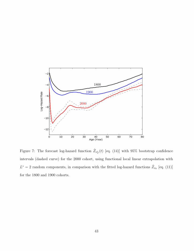
compared with the estimated log-hazard functions for the 1800 and 1900 cohorts. We find
that the forecast for the 2000 cohort implies an immediate sharp drop in the mortality
rate at early ages, with the lowest mortality rate occurring around age 3, followed by a
steep increase in mortality to age 20. Between ages 20 and 40, mortality rates stay more
or less constant, and then steadily rise after age 40.
Throughout, mortality rates of the 2000 cohort stay well below those of the 1800
and 1900 cohorts. This is supported by the 95% bootstrap prediction intervals that are
included in the figure. Interestingly, the right tails of the log-hazard functions are roughly
parallel and linear for all three cohorts, which suggests that the slope is invariant. Even
more remarkable is that in the right tail the average distance of the log-hazard functions
appears to be about the same between the three log-hazard functions. This suggests that
the size of the decreases in old-age log-hazards has been exponentially increasing since
1800.
5. DISCUSSION AND CONCLUDING REMARKS
The moving windows approach has proved suitable for modeling mortality trends in pop-
ulation lifetables for Swedish women for the age range 0 to 80. Birth year of the cohort
serves as covariate, and other covariates as available could be included analogously. Our
approach embodies the concept of time-varying principal components of mortality, and
adequately models long-term mortality time-dynamics and changes in longitudinal cohort
mortality as observed for the Swedish cohort lifetables. Extensions are proposed for the
prediction of cohort log hazard functions for which complete log hazard functions have
not been observed yet, and for the forecasting of future cohort mortality, when the target
year is beyond the last available birth cohort data. These demographic projections are
of central interest in demographic population studies, and of methodological interest in
statistical demography. They are furthermore useful beyond demographic applications,
whenever prediction and forecasting of partially observed log hazard functions, condition-
21

ing on a continuous increasing covariate, is of interest.
We note that a key feature of the proposed forecasting of future cohort mortality is
that it includes forecasting of both mean and random components. Accordingly, our fore-
cast for a log-mortality function is based on forecasts of mean functions, eigenfunctions
and principal components. Using extrapolation of the dependence structure in addition
to the extrapolation of the mean is natural when one aims at forecasting the conditional
expectation for a future log mortality function, given past observations on observed mor-
tality. Within a window, as used in the log mortality fitting for completely observed
cohort mortality, the log mortality functions are considered i.i.d. and the random compo-
nents have zero expectation. Thus the departure of one log mortality curve from the mean
does not contain information about nearby log mortality functions. However, this changes
when moving forward into the future and away from the last windows containing cohorts
with observed mortalities. Then the conditional expectation of the targeted future log
mortality trajectories is not equal to the forecasts of the mean structure alone but does
include random components. The evolution of the first eigenfunction, for example, pro-
vides information about the evolution of the conditional mean function, and it is prudent
to include this information in the forecast. We thus base our forecast on predicting the
overall stochastic structure (mean functions, eigenfunctions and principal components) of
log-mortality from previous structure.
To validate our forecasting method, we also investigated forecasts for historical cohorts
where the forecast is constructed assuming an analogous data situation as when forecasting
the mortality for the 2000 cohort. A good diagnostic whether the forecast will work is
provided by plots analogous to those provided in Figure 6, from which one can gauge
whether a linear extrapolation of past observed trends makes sense. This is clearly the
case for the year 2000, but is not the case for some years. Selecting as an example the
year 1850, judging from the plot analogous to Figure 6 (not shown), the situation is less
22

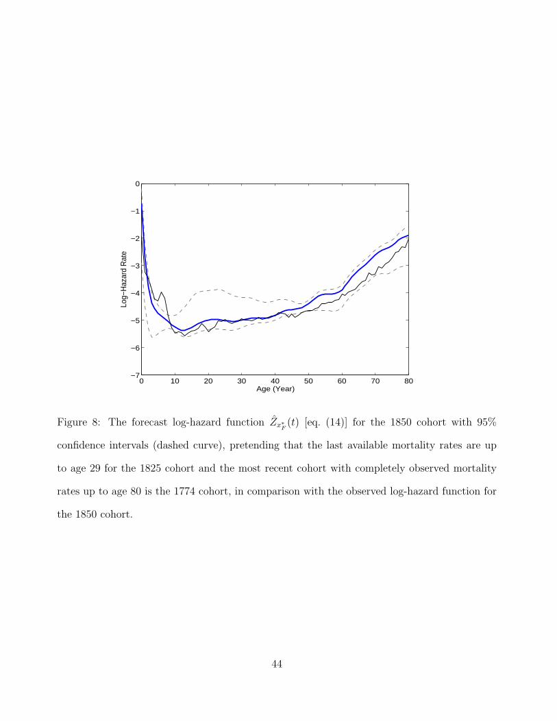
promising than for the year 2000 but the forecast still seems feasible. In the construction of
the 1850 forecast, one pretends that the last available mortality rates are up to age 29 for
the 1825 cohort and that the most recent cohort with completely observed mortality rates
up to age 80 is the 1774 cohort. The comparison of the 1850 cohort log mortality forecast
based on three components, including the 95% bootstrap confidence intervals, with the
actual raw and fitted log-hazards based on the actual observed mortality data for the
1850 cohort, can be found in Figure 8. Overall, the forecast seems reasonably accurate,
while it is also noteworthy that the reduction in older age mortality has accelerated and
is underestimated in the forecast.
While the cohorts from which the lifetables are formed consist of different individuals,
entire birth cohorts may be subject to period effects, which can appear as mortality shocks,
caused, e.g., by epidemics, famines or war, changes in socioeconomic environments, or
fluctuations in quality and availability of medical resources (for discussion of such period
effects we refer to Fienberg and Mason, 1985, Fu, 2000, Yang, Fu and Land, 2004, and
Yang et al., 2008). While each cohort will experience these effects at a different age range,
they may have similar impact on cohort mortality for adjacent cohorts. We assume that
in the model, these potential dependencies and period effects can be accounted for (a)
by the similarity and continuity of cohort mortality trajectories in adjacent birth years,
and (b) may be subsumed in measurement errors as included in model (2), and thus may
be viewed as nuisance effects that can be neglected in the analysis. In practice, sporadic
shocks will be averaged out during model fitting, while the longer-term slowly occurring
changes are accounted for by the changing mean log hazard functions and eigenfunctions.
Advantages of our approach are, first, its inherent flexibility to adjust to arbitrarily
shaped cohort log hazard functions, in contrast to popular parametric models which do
not go beyond reflecting preconceived shapes and thus are not flexible enough for many
demographic applications. Second, we propose extensions of this approach to the fore-
23

casting of future cohort log hazard functions, also retaining a large degree of flexibility.
Third, it provides novel insights into the covariance and correlation structure of mortality
and the changes of this structure over time. Fourth, it leads to the useful concept of
functional principal components of mortality which are also subject to change over time
and provide an adequate decomposition of mortality. Fifth, it does not require complex
iterative fitting algorithms and does not suffer from non-convergence as parametric models
do, especially in cases where their fit is at best marginal.
In the analysis of Swedish mortality lifetable data the observed smooth time-variation
of cohort log hazard functions, and of covariance and correlation surfaces of mortality,
indicates that the basic assumptions of our approach are satisfied. We distinguish pre-
diction of partially observed cohort log-hazard functions from forecasting of cohort log
hazard functions for cohorts for which no data are available. Prediction is therefore a
first step in the proposed forecasting method, which combines prediction with functional
linear extrapolation.
We demonstrate prediction of log-hazard functions for the pre-1975 birth cohorts and
forecasting for the more recent cohorts. Besides characteristic shape changes and sharp
drops in the mortality of infants and younger adults that are revealed by the proposed
approach, the forecast mortality is seen to uniformly decline at all ages, as birth year
increases. A noteworthy feature is that the various log-hazard functions are linear and
parallel at ages 60-80, suggesting exponentially increasing annual declines of log-hazards
in these older age ranges. As with all extrapolation methods, caution needs to be exercised
not to over-interpret the findings, as more fundamental changes in mortality may occur
in the future, rendering the extrapolation algorithm less appropriate as it reaches further
into the future.
In summary, functional data analysis methodology has much to offer for the study of
mortality. It is useful for predicting and forecasting cohort log hazard functions, as well
24

as for studying the internal dependence and covariance structure of log hazard functions
for human populations.
APPENDIX
A.1 Consistency of Estimated Cohort Log Hazard Functions
We consider the case with no shrinkage where θ = 0 in (10). We fix a bin center x0
and assume the bin size is ω, allowing for ω → 0 in the asymptotic setting where the
spacing of the measurements is getting denser. One has nω i.i.d. lifetables for which
xi ∈ [x0 − ω, x0 + ω], and for each of these lifetables, ni observations of mortality and
corresponding log hazards as in (2).
Further assumptions include nω →∞, m→∞ and, for the smoothing bandwidths bω
used for mean and covariance function estimation (as described in the second paragraph in
Section 2.2 and in more detail in Yao et al. (2003, 2005)), that bω = o(n−1/4ω ), mbωn−δ1 →
∞, m1−δ2bω →∞ for δ1, δ2 > 0. Under conditions (C) in Section 3.1 of Hall, Muller and
Wang (2006), slightly modifying the arguments in the proof of Theorem 3 of that paper
and omitting indices x0, one obtains that
|λk−λk| = Op(n−1/2ω ),
∫(ρk(t)−ρk(t))2 dt = Op(n−1
ω ),∫
(µ(t)−µ(t))2 dt = Op(n−1ω ).
Considering the case where L is known and fixed, using the representations (6) and (11),
and omitting indices x0, this leads to∫[Z(t)− Z(t)]2 dt
≤ C
{∫(µ(t)− µ(t))2 dt+
L∑k=1
{∫(ρk(t)− ρk(t))2 dt+ [ξk − ξk]2
∫ρk(t)2 dt
}}
for a suitable constant C > 0.
Working with the definitions (7) and (9), observing the smoothness assumptions and
that ξk = ξk in the situation considered here, we find (ξk − ξk)2 = Op(n−1ω + m−1) and
25

obtain the asymptotic consistency result∫{Zx0(t)− Zx0(t)}2 dt = Op(n−1
ω +m−1).
This result demonstrates that integrated squared error of the fitted log-hazard functions
converges to 0 asymptotically, with a rate of convergence that is determined by both
the number of cohorts with birth year falling into the window and by the number of
observations of mortality available per cohort.
A.2 Choice of Bin Size and Number of Components
We first determine a function L∗(ω) providing the optimal L for each given bin size ω.
We define L∗(ω) to be the smallest value of L such that when averaging over all bins, the
first L components explain 90% of the total variance. Formally,
L∗(ω) = min
L ≥ 1 :1|J |
∑x0∈J
∑Lk=1 λkx0∑Mk=1 λkx0
≥ 0.90
, (A.1)
where M is the largest number of components considered and the sum extends over all
available bins with window width ω, whose midpoints x0 form the set J , with |J | denoting
the count of its elements. This method is computationally fast and the 90% level worked
well in practice.
For each bin center x0 and given bin size ω, the empirical covariances are
cijl(x0, ω) = (Yi(tj)− µx0(tj))(Yi(tl)− µx0(tl)),
for all 1 ≤ j, l ≤ m and xi ∈ W(x0), which are compared with the fitted covariances
cjl(x0, ω) =L(ω)∑k=1
1{λk,x0>0}λk,x0(ω)ρk,x0(tj)ρk,x0(tl)
to determine the quality of the fit. The optimal bin size is then found by minimizing the
sum of squared distances,
ω∗ =arg minω
∑x0
∑i: xi∈W(x0,ω)
m∑j,l=1
(cijl(x0, ω)− cjl(x0, ω))2
. (A.2)
26

Combining this with (A.1) yields the choice L∗ = L∗(ω∗). In our application to Swedish
mortality data, we include birth years x0 = 1760, . . . , 1900 in this optimization.
A.3 Auxiliary Estimates for Mortality Forecasting
These are computed in the following two steps:
Step 1 Functional principal component analysis based on moving windows: For a given
bandwidth b > 0, and each x∗P ∈ W(x∗n) = [x∗n − b, x∗n], applying (12) and the steps
outlined before (13), obtain estimates {µx∗P(t), ρk,x∗P
(t), ξk,x∗P}, for all k = 1, . . . , L.
Step 2 Functional local linear extrapolation: Using the estimates from Step 1, obtain the
following locally weighted least squares estimates for both functions as well as first
derivatives, centering these estimates at x∗n,
(η(0)k , η
(1)k ) =arg min
(η0,η1)
∑x∗P∈W(x∗n)
K
(x∗P − x∗n
b
){ξk,x∗P
− η0 − η1(x∗P − x∗n)}2,
(γ(0)(t), γ(1)(t)) =arg min(γ0,γ1)
∑x∗P∈W(x∗n)
K
(x∗P − x∗n
b
){µx∗P
(t)− γ0 − γ1(x∗P − x∗n)}2,
(β(0)k (t), β(1)
k (t)) =arg min(β0,β1)
∑x∗P∈W(x∗n)
K
(x∗P − x∗n
b
){ρk,x∗P
(t)− β0 − β1(x∗P − x∗n)}2,
for each t = tj , where tj ∈ (0, 1, 2, . . . , 80), and for k = 1, . . . , L. The kernel function
K(·) is a symmetric density on domain [−1, 1], which we choose as 34(1 − x2) on
[−1, 1]. We obtain the predicted functions evaluated at time x∗F for each component
by (functional) local linear extrapolations:
αk(x∗F ; b) = η(0)k + (x∗F − x∗n) η(1)
k , (A.3)
µx∗F(t; b) = γ(0)(t) + (x∗F − x∗n) γ(1)(t),
ρk,x∗F(t; b) = β
(0)k (t) + (x∗F − x∗n) β(1)
k (t),
for all t ∈ [0, T ], where T = 80 in our example.
27

A.4 Choice of Forecasting Window Width, Bootstrap Prediction Intervals
and Computational Implementation
Let a = a(x∗n, δ), where δ = x∗F − x∗n. The observed cohort log hazard functions with
covariate values in [a, x∗n] are used as the cross-validation sample for selecting b. A rea-
sonable choice is a = x∗n − r δ, where we adopt the suggestion of Li and Heckman (2003)
to select r = 1. Let xj be a birth year in [a, x∗n] for which we desire the cross-validated
prediction error. The cross-validation forecast at xj is then solely based on data of cohorts
born prior to (xj − δ), leading to the forward cross-validation squared prediction error
FCV(b)
FCV(b) =1|I|
∑j∈I
∫ T
0(Zx∗jF
(t; b)− Zxj (t))2 dt. (A.4)
Here I = {j : xj ∈ [a, x∗n]}, |I| is the number of indices in I and Zx∗jF(t; b) is obtained in
the same way as in (14), except that x∗F = xj , i.e., the time frame is shifted back to xj
or, equivalently, from x∗n to (xj − δ), where Zxj may correspond to a fitted or predicted
trajectory, depending on the value of xj . In practice, FCV(b) is obtained via numerical
approximation of the integral in (A.4). The cross-validation forecasting window width
bFCV is selected as minimizer of the squared prediction errors FCV(b),
bFCV =arg minb
FCV(b).
Prediction intervals were constructed with a bootstrap procedure based on resampling
from suitable samples of cohort mortalities to form the bootstrap samples. The following
summarizes this approach for forecast log-hazard functions:
(B1) Resample with replacement from the cohorts with xi ∈ [x∗n − b, x∗n] to form a boot-
strap sample of the same size.
(B2) Use the bootstrap sample in (B1) to obtain the estimates µ∗x∗F (t), ρ∗k,x∗F(t; b) and
α∗k(x∗F ; b) by the forecasting procedure in Section 4.3, and obtain the bootstrap
28

forecast at the future point x∗F in the same way as (14) but from the bootstrap
sample.
(B3) Repeat steps (B1)-(B2) B times to obtain Y ∗x∗F(t). Construct the 95% pointwise
prediction limits by finding the 2.5% and 97.5% quantiles of {Y ∗x∗F (t)}.
Regarding the computational implementation of the procedures, it is broken down into
algorithmic modules (M1)-(M11) that are briefly described below. While the Matlab code
can be found in the online Supplement, Matlab routines HADES and PACE for modules
(M1), respectively (M2), which are basic for everything else, and are independently useful
for many other applications, can be downloaded from
http://anson.ucdavis.edu/ mueller/data/programs.html.
(A) Fitting and prediction of log-hazard functions: (M1) Compute nonparametric
cohort-specific hazard rates through the transformation ψ(qc); (M2) Compute mean func-
tion, eigenfunctions and functional principal components, and also fitted covariance ma-
trix, given a sample of functions (here applied to log hazard functions), and given the
number of components L to be included, both by the integration method (when the
task is fitting) and by the conditioning method (12) (when the task is prediction); (M3)
Construct windows W(x0) and determine the included cohorts for each window, for all
applicable x0, given bin widths ω; (M4) Call (M1)-(M3) repeatedly to find minimizers L∗,
ω∗ by iteratively solving (A.1) and (A.2); (M5) For fitting, use these minimizers for the
final fits. These are obtained by calling (M2) for the selected cohorts for each x0, applying
the integration method, and obtaining as output the mean function (providing the fitted
trajectory at x0), eigenfunctions and principal components, and also the fitted covari-
ance matrix; (M6) For prediction, assemble those cohorts falling into the (user-specified)
prediction window W(x∗P ), then use L∗ from (M4) and call (M2) for all applicable x∗P ,
applying the conditioning method.
29

(B) Mortality forecasting: (M7) Given a forecasting bandwidth b, obtain fits/predictions,
including the fitted/predicted mean functions, eigenfunctions and principal components,
using the procedures in (A), for each x∗P ∈ W(x∗n) (see Step 1 Appendix A.3); (M8)
Using the outputs from (M7), fit the locally weighted least squares estimates for each
age and obtain the local linear extrapolations (A.3) for mean functions, eigenfunctions
and principal components for each age t and each cohort birth year x∗F for which fore-
casting is desired. Use these to compute the forecast for the log-hazard function; (M9)
Assemble the fits/predictions obtained in (A) for all cohorts with birth years between
x∗n− (x∗F −x∗n) and xn, the forward cross-validation window, and then calculate mortality
forecasts for these same cohorts, using for the forecasting only cohorts with birth years
prior to x∗n − (x∗F − x∗n), by calling (M7) and (M8) with forecasting bandwidth b; (M10)
Find the optimal forecasting bandwidth bFCV by minimizing the discrepancy between the
forecasts and fits/predictions obtained in (M8), implementing (A.4) by numerical integra-
tion; (M11) Use bFCV for the final mortality forecast, calling (M8).
References
[1] Ash, R. B., and Gardner, M. F. (1975), Topics in Stochastic Processes, New York:
Academic Press, Inc.
[2] Booth, H. (2006), “Demographic Forecasting: 1980 to 2005 in Review,” International
Journal of Forecasting, 22, 547-581.
[3] Capra, W. B., and Muller, H. G. (1997), “An Accelerated-time Model for Response
Curves,” Journal of the American Statistical Association, 92, 72-83.
[4] Cardot, H. (2007), “Conditional Functional Principal Components Analysis,” Scan-
dinavian Journal of Statistics, 34, 317-335.
30

[5] Chiou, J. M. and Muller, H. G. (2001) Discussion of “Inference of Density Families
Using Functional Principal Component Analysis,” Journal of the American Statistical
Association, 96, 534-537.
[6] Chiou, J. M., Muller, H. G., and Wang, J. L. (2003), “Functional Quasi-likelihood
Regression Models with Smooth Random Effects,” Journal of the Royal Statistical
Society, Ser. B, 65, 405-423.
[7] −− (2004), “Functional Response Models,” Statistica Sinica, 14, 675-693.
[8] Congdon, P. (1993), “Statistical Graduation in Local Demographic Analysis and
Projection,” Journal of the Royal Statistical Society, Ser. A, 156, 237-270.
[9] Currie, I. D., Durban, M., and Eilers, P. HC (2004), “Smoothing and Forecasting
Mortality Rates,” Statistical Modelling, 4, 279-298.
[10] Debon, A., Montes, F., and Sala, R. (2006), “A Comparison of Models for Dynamic
Life Tables. Application to Mortality Data from the Valencia Region,” Lifetime Data
Analysis, 12, 223-244.
[11] Dellaportas, P., Smith, A. F.M. and Stavropoulos, P. (2001), “Bayesian Analysis of
Mortality Data,” Journal of the Royal Statistical Society, Ser. A, 164, 275-291.
[12] Elandt-Johnson, R. C., and Johnson, N. L. (1980), Survival Models and Data Anal-
ysis, New York: John Wiley & Sons.
[13] Faraway, J. J. (1997), “Regression Analysis for a Functional Response,” Technomet-
rics, 39, 254-262.
[14] Gijbels, I., Pope, A., and Wand, M. P. (1999), “Understanding Exponential Smooth-
ing via Kernel Regression,” Journal of the Royal Statistical Society, Ser. B, 61, 39-50.
[15] Glei, D., Lundstrom, H., and Wilmoth, J. (2006), “About Mortality Data for Swe-
den,” Technical Report. Available at www.mortality.org or www.humanmortality.de.
31

[16] Hall, P., Muller, H.-G., and Wang, J.-L. (2006), “Properties of Principal Component
Methods for Functional and Longitudinal Data Analysis,” The Annals of Statistics,
34, 1493-1517.
[17] Heligman, L., and Pollard, J. H. (1980), “The Age Pattern of Mortality,” Journal of
the Institute of Actuaries, 107, 49-80.
[18] Human Mortality Database. University of California, Berkeley (USA), and
Max Planck Institute for Demographic Research (Germany). Available at
www.mortality.org or www.humanmortality.de (data downloaded on 10 November,
2006).
[19] Fienberg, S. E. and Mason, W. M. (1985), “Specification and Implementation of Age,
Period, and Cohort Models,” in Cohort Analysis in Social Research, ed. W. M. Mason
and S. E. Fienberg, New York: Springer-Verlag, pp. 45-88.
[20] Fu, W. J. (2000), “Ridge Estimator in Singular Design with Application to Age-
Period-Cohort Analysis of Disease Rates,” Communications in Statistics, Part A-
Theory and Method, 29, 263-278.
[21] Hyndman, R. J., Koehler, A. B., Snyder, R. D., and Grose, S. (2002), “A State Space
Framework for Automatic Forecasting Using Exponential Smoothing Methods,” In-
ternational Journal of Forecasting, 18, 439-454.
[22] Hyndman, R. J., and Ullah, M. S. (2007), “Robust Forecasting of Mortality and
Fertility Rates: A Functional Data Approach,” Computational Statistics and Data
Analysis, 51, 4942-4956.
[23] Johnson, R.A., and Wichern, D.W. (2002),Applied Multivariate Statistical Analysis”,
New Jersey: Prentice Hall, Fifth Edition
32

[24] Kneip, A., and Utikal, K.J. (2001), “Inference for Density Families Using Functional
Principal Component Analysis,” Journal of the American Statistical Association, 96,
519-532.
[25] Lee, R. D., and Carter, R. C. (1992), “Modeling and Forecasting U.S. Mortality,”
Journal of the American Statistical Association, 87, 659-671.
[26] Li, N., and Lee, R. (2005), “Coherent Mortality Forecasts for a Group of Populations:
An Extension of the Lee-Carter Method,” Demography, 42, 575-594.
[27] Li, N., Lee R., and Tuljapurkar S. (2004), “Using the Lee-Carter Method to Forecast
Mortality for Populations with Limited Data,” International Statistical Review, 72,
19-36.
[28] Li, X., and Heckman, N. (2003), “Local Linear Extrapolation,” Journal of Nonpara-
metric Statistics, 15, 565-578.
[29] Muller, H. G. (2005), “Functional Modelling and Classification of Longitudinal Data
(with Discussion),” Scandinavian Journal of Statistics, 32, 223-246.
[30] Muller, H. G., Chiou, J. M. and Leng, X. (2008) “Inferring Gene Expression Dynamics
via Functional Regression,” BMC Bioinformatics, 9, 60.
[31] Muller, H. G., Wang, J. L., and Capra, W. B. (1997), “From Lifetables to Hazard
Rates: The Transformation Approach,” Biometrika, 84, 881-892.
[32] Muller, H. G., and Zhang, Y. (2005), “Time-Varying Functional Regression for Pre-
dicting Remaining Lifetime Distributions from Longitudinal Trajectories,” Biomet-
rics, 61, 1064-1075.
[33] Oeppen, J., and Vaupel, J. W. (2002), “Broken Limits to Life Expectancy,” Science,
296, 1029- 1031.
33

[34] Park, Y., Choi J. W., and Kim, H.-Y. (2006), “Forecasting Cause-Age Specific Mor-
tality Using Two Random Processes,” Journal of the American Statistical Associa-
tion, 101, 472-483.
[35] Ramsay, J., and Silverman, B. (2002), Applied Functional Data Analysis, New York:
Springer.
[36] −− (2005), Functional Data Analysis (2nd ed.), New York: Springer.
[37] Renshaw, A., and Haberman, S. (2003), “Lee-Carter Mortality Forecasting: A Par-
allel Generalized Linear Modelling Approach for England and Wales Mortality Pro-
jections,” Applied Statistics, 52, 119-137.
[38] Rice, J. (2004), “Functional and Longitudinal Data Analysis: Perspectives on
Smoothing,” Statistica Sinica, 14, 631-647.
[39] Rice, J., and Silverman, B. (1991), “Estimating The Mean and The Covariance Struc-
ture Nonparametrically When Data Are Curves,” Journal of the Royal Statistical
Society, Ser. B, 53, 233-243.
[40] Staniswalis, J. G., and Lee, J. J. (1998), “Nonparametric Regression Analysis of
Longitudinal Data,” Journal of the American Statistical Association, 93, 1403-1418.
[41] Vaupel, J. W., Carey, J. R., Christensen, K., Johnson T. E., Yashin, A. I., Holm,
N. V., Iachine, I. A., Kannisto, V., Khazaeli, A. A., Liedo, P., Longo, V. D., Zeng,Y.,
Manton, K. G., and Curtsinger, J. W. (1998), “Biodemographic Trajectories of
Longevity,” Science, 280, 855-860.
[42] Vaupel, J. W., and Canudas Romo, V. (2003), “Decomposing Change in Life Ex-
pectancy: A Bouquet of Formulas in Honor of Nathan Keyfitzs 90th Birthday,”
Demography, 40, 201-216.
[43] Wang, J. L., Muller, H. G., and Capra, W. B. (1998), “Analysis of Oldest-Old Mor-
tality: Lifetables Revisited,” The Annals of Statistics, 26, 126-163.
34

[44] Wong-Fupuy, C. and Haberman, S. (2004), “Projecting Mortality Trends: Recent
Developments in the United Kingdom and the United States,” Annals American
Actuarial Journal , 8, 56-83.
[45] Yang, Y., Fu, W. J., and Land, K. C. (2004), “A Methodological Comparison of
Age-Period-Cohort Models: Intrinsic Estimator and Conventional Generalized Linear
Models,” Sociological Methodology, 34, 75-110.
[46] Yang Y., Schulhofer-Wohl, S., Fu, W. J., and Land, K. C. (2008), “The Intrinsic
Estimator for Age-Period-Cohort Analysis: What It Is and How To Use It, American
Journal of Sociology, forthcoming.
[47] Yao, F., Muller, H. G., Clifford, A. J., Dueker, S. R., Follett, J. Lin, Y., Buch-
holz, B. A., and Vogel, J. S. (2003), “Shrinkage Estimation for Functional Principal
Component Scores With Application to The Population Kinetics of Plasma Folate,”
Biometrics, 59, 676-685.
[48] Yao, F., Muller, H. G., and Wang, J. L. (2005), “Functional Data Analysis for Sparse
Longitudinal Data,” Journal of the American Statistical Association, 100, 577-590.
[49] Zhao, X., Marron, J. S., and Wells, M. T. (2004), “The Functional Data Analysis
View of Longitudinal Data,” Statistica Sinica, 14, 789-808.
35

Table 1: Comparison of Leave-One-Curve-Out Prediction Errors Based On Global FPCA and
Moving-Windows FPCA, for Various Numbers of Included Components.
Number of components L
Model 0 1 2 3 4 5 ≥ 6
Full Window (Smooth)a .0998 .0282 .0266 .0256 .0244 .0239 .0239
Full Windowb .0998 .0351 .0349 .0346 .0347 .0359 .0358
Moving Windowsc .0232 .0230 .0228 .0227 .0227 .0227 .0227
aFunctional quasi-likelihood regression model with smooth random effects using full window.bModel (11) with the full window.cModel (11) with the moving windows using the optimal bin size ω∗ = 11.
36

0 10 20 30 40 50 60 70 80
−6
−5
−4
−3
−2
Age (Year)
Log−
Haz
ard
Rat
e
1760
1780
1860
1880
1900
Figure 1: “Observed” log-hazard rates Y (t) [eq. (2)] for cohorts born in 1760, 1780, 1800, 1820,
1840, 1860, 1880 and 1900, for Swedish lifetable data.
37

7 8 9 10 11 12 1354
54.5
55
55.5
56
56.5
57
Bin Size (Year)
Sum
of S
quar
ed D
ista
nce
Bet
wee
n C
ovar
ianc
es
Figure 2: Choice of the optimal bin size ω∗ [eq. (A.2)] for time-varying lifetable modeling:
Sum of squared distance between the raw and the fitted covariances versus bin size for Swedish
lifetable data.
38

020
4060
80
020
4060
800
0.01
0.02
0.03
Age (Year)Age (Year) 020
4060
80
020
4060
800
0.02
0.04
0.06
0.08
0.1
Age (Year)Age (Year)
020
4060
80
020
4060
800
0.2
0.4
0.6
0.8
1
Age (Year)Age (Year) 020
4060
80
020
4060
800
0.2
0.4
0.6
0.8
1
Age (Year)Age (Year)
0 20 40 60 800
0.05
0.1
0.15
0.2
0.25
0.3
0.35
Age (Year)
1820 (89.7%)1900 (98.2%)
0 20 40 60 80−0.2
−0.1
0
0.1
0.2
0.3
0.4
0.5
Age (Year)
1820 ( 9.3%)1900 ( 1.6%)
1820 1900
1820 1900
ρ1,x0(t) ρ2,x0(t)
Figure 3: Upper and Middle panels: Estimated smooth covariance and fitted correlation sur-
faces, respectively, for cohorts born in x0 = 1820 (left panel) and in x0 = 1900 (right panel),
using the moving windows approach with bin size ω∗ = 11. Lower panels: First (left panel)
and second (right panel) eigenfunctions, corresponding to the estimated covariance functions for
1820 and 1900. Percentages indicate fraction of variance explained by the respective component.
39

0 20 40 60 80
−6
−5
−4
−3
−2
−1
Age (Year)
Lo
g−
Ha
za
rd R
ate
1751−1880
0 20 40 60 80
−6
−5
−4
−3
−2
−1
Age (Year)
Lo
g−
Ha
za
rd R
ate
1881−1910
1751
1880
@@
@@R1881
1910
AAAAAU
Figure 4: Fitted log-hazard functions Zx0 [eq. (11)] for cohorts born in x0 ∈ [1751, 1880] (left
panel) and x0 ∈ [1881, 1910] (right panel).
40

0 10 20 30 40 50 60 70 80
−9
−8
−7
−6
−5
−4
−3
Age (Year)
Log−
Haz
ard
Rat
e
1910
1975
Figure 5: Predicted log-hazard function Zx∗P(t) [eq. (13)] for the 1975 cohort, where observed
hazard rates Y (t) are available up to age 29 only, in comparison with the fitted log-hazard
function Zx0(t) [eq. (11)] for the 1910 cohort, for which observed hazard rates Y (t) are available
throughout lifetime.
41

0 20 40 60 80
−0.4
−0.2
0
0.2
Age (Year)
1st E
igen
func
tion
0 20 40 60 80
−0.4
−0.2
0
0.2
Age (Year)
2nd
Eig
enfu
nctio
n
0 20 40 60 80−10
−8
−6
−4
−2
0
Ove
rall
Mea
n Lo
g−H
azar
d R
ate
Age (Year)1940 1960 1980 2000
−10
−8
−6
−4
−2
0
2
4
Calendar Year
FP
Cs
k=1k=2
µx∗(t) ξk,x∗
ρ1,x∗(t) ρ2,x∗(t)
1924
19752000
1975
2000
1924
1975
2000
1924
19752000
Figure 6: Predicted (for 1924-1975 cohorts) and forecast (for 2000 cohort) model components
when using functional local linear extrapolation. Upper left panel: Predicted log hazard func-
tions µx∗P(t) (gray) and forecast µx∗F
(t) for the log hazard function of the 2000 cohort (black).
Upper right panel: Predicted functional principal components {ξk,x∗P}, x∗P ∈ [1924, 1975], for
k = 1, 2 and forecast for the functional principal scores for the target year 2000 (rightmost
points). Lower left panel: First eigenfunctions for the 1924-1975 cohorts (gray) and forecast
ρ1,x∗F(t) of the first eigenfunction for the 2000 cohort (black). Lower right panel: Second eigen-
functions for the 1924-1975 cohorts (gray) and forecast ρ2,x∗F(t) of the second eigenfunction for
the 2000 cohort (black).42
0 10 20 30 40 50 60 70 80
−12
−10
−8
−6
−4
−2
Age (Year)
Log−
Haz
ard
Rat
e
1800
1900
2000
Figure 7: The forecast log-hazard function Zx∗F(t) [eq. (14)] with 95% bootstrap confidence
intervals (dashed curve) for the 2000 cohort, using functional local linear extrapolation with
L∗ = 2 random components, in comparison with the fitted log-hazard functions Zx0 [eq. (11)]
for the 1800 and 1900 cohorts.
43
0 10 20 30 40 50 60 70 80−7
−6
−5
−4
−3
−2
−1
0
Age (Year)
Log−
Haz
ard
Rat
e
Figure 8: The forecast log-hazard function Zx∗F(t) [eq. (14)] for the 1850 cohort with 95%
confidence intervals (dashed curve), pretending that the last available mortality rates are up
to age 29 for the 1825 cohort and the most recent cohort with completely observed mortality
rates up to age 80 is the 1774 cohort, in comparison with the observed log-hazard function for
the 1850 cohort.
44