modeling guidelines for health risk assessments · modeling guidelines for health risk assessments...
TRANSCRIPT

Modeling Guidelines for
Health Risk Assessments
May 2018
Form -15i

TABLE OF CONTENTS
1. INTRODUCTION..................................................................................................... 1
2. EMISSIONS .............................................................................................................. 1
2.1 POLLUTANTS ............................................................................................................... 1
2.2 EMISSION SOURCES .................................................................................................... 1
2.2.1 NSR HRA with Only New Equipment ............................................................ 1
2.2.2 NSR HRA with Existing Equipment ............................................................... 1
2.2.3 CEQA HRA ...................................................................................................... 2
2.2.4 AB 2588 Air Toxics “Hot Spots” Program HRA ........................................... 2
2.3 EMISSION CALCULATIONS ......................................................................................... 2
3. AIR DISPERSION MODEL .................................................................................... 2
3.1 CONTROL OPTIONS .................................................................................................... 3
3.2 DEFINING URBAN AND RURAL CONDITIONS ............................................................. 3
3.3 UTM COORDINATE SYSTEM ...................................................................................... 4
3.4 SOURCE PARAMETERS ............................................................................................... 4
3.4.1 Point Sources – POINT, POINTCAP, POINTHOR ...................................... 5
3.4.2 Area Sources – AREA, AREAPOLY, AREACIRC ........................................ 5
3.4.3 OPENPIT Sources ........................................................................................... 7
3.4.4 VOLUME Sources ........................................................................................... 7
3.4.5 LINE Sources .................................................................................................. 8
3.5 BUILDING IMPACTS .................................................................................................... 9
3.6 TERRAIN ..................................................................................................................... 9
3.7 METEOROLOGICAL DATA ........................................................................................ 10
3.8 RECEPTORS ............................................................................................................... 10
3.8.1 Pathway Receptors ......................................................................................... 10
3.8.2 Census Receptors ........................................................................................... 11
3.8.3 Cartesian Receptor Grids .............................................................................. 11
3.8.4 Property Boundary Receptors ....................................................................... 11
3.8.5 Residential Receptors .................................................................................... 12
3.8.6 Worker Receptors .......................................................................................... 12
3.8.7 Sensitive Receptors ........................................................................................ 12
3.8.8 Onsite Receptors ............................................................................................ 13
3.8.9 Vacant Land & Future Receptors: Building & Land Use Applications ..... 13

4. RISK ASSESSMENT ............................................................................................. 14
4.1 TIERED APPROACH TO RISK ASSESSMENT .............................................................. 14
4.2 RISK ANALYSIS ......................................................................................................... 14
4.2.1 Cancer Risk Scenarios ................................................................................... 14
4.2.2 Non-Cancer Risk Scenarios .......................................................................... 15
4.3 INHALATION PATHWAY ............................................................................................ 15
4.3.1 Fraction of Time at Home ............................................................................. 15
4.3.2 8-Hour Chronic Non-Cancer Risk ................................................................ 15
4.3.3 Worker Exposure – Adjustment Factor for Cancer Risk ............................. 16
4.4 MULTIPATHWAY ANALYSIS ..................................................................................... 18
4.4.1 Deposition Rate .............................................................................................. 19
4.4.2 Soil Ingestion ................................................................................................. 19
4.4.3 Dermal ............................................................................................................ 19
4.4.4 Mother’s Milk ................................................................................................ 19
4.4.5 Drinking Water .............................................................................................. 19
4.4.6 Fish ................................................................................................................ 19
4.4.7 Homegrown Produce ..................................................................................... 20
4.4.8 Beef & Dairy .................................................................................................. 20
4.4.9 Pig, Chicken & Egg ....................................................................................... 21
4.5 SPATIAL AVERAGING ............................................................................................... 22
4.6 REFINED ACUTE ANALYSIS ...................................................................................... 22
4.7 POPULATION EXPOSURE .......................................................................................... 23
4.8 SIGNIFICANT RISK THRESHOLDS ............................................................................. 23
5. HEALTH RISK ASSESSMENT REPORT ......................................................... 24
5.1 FACILITY INFORMATION .......................................................................................... 24
5.2 SOURCE AND EMISSION INVENTORY INFORMATION ............................................... 24
5.3 EMISSION QUANTIFICATION .................................................................................... 25
5.4 MODEL INFORMATION ............................................................................................. 25
5.5 RECEPTOR PLACEMENT ........................................................................................... 25
5.6 MULTIPATHWAY INFORMATION .............................................................................. 26
5.7 SUMMARY OF RESULTS ............................................................................................ 26
5.8 RISK DRIVER TABLES .............................................................................................. 28
5.9 MAPS AND AERIAL PHOTOS ..................................................................................... 31
5.10 ELECTRONIC FILES .................................................................................................. 32
6. REFERENCES ........................................................................................................ 33
7. CONTACTS ............................................................................................................ 35

APPENDIX A – VARIABLE EMISSIONS MODELING ..................................................... A1
A.1 Variable Emission Rates for Annual Emissions ......................................... A1
A.2 Variable Emission Rates for Maximum Hourly Emissions ........................ A2
APPENDIX B – MODELING SPECIFIC SOURCE TYPES ................................................ B1
B.1 Gasoline Dispensing Facilities ..................................................................... B1
B.2 Liquid Storage Tanks ................................................................................... B1
APPENDIX C – SPATIAL AVERAGING .............................................................................. C1
C.1 Nested Grid Size ............................................................................................ C1
C.2 Tilted Grids ................................................................................................... C2
C.3 Spatial Averaging Instructions .................................................................... C2
APPENDIX D – DEFAULT DICE STACK PARAMETERS ............................................... D1
APPENDIX E – HEALTH RISK CALCULATION AND ROUNDING POLICY .............. E1
APPENDIX F – DISTRICT-APPROVED EMISSION FACTORS ...................................... F1
APPENDIX G – SOURCE-RECEPTOR DISTANCE POLICY FOR ACUTE RISK ....... G1

LIST OF FIGURES
Figure 3.2-1: Auer Method for Determining Urban or Rural Dispersion ....................................... 3
LIST OF TABLES
Table 3.2-1: Urban Land Use .......................................................................................................... 4
Table 3.2-2: Population Data for Urban Dispersion Modeling ....................................................... 4
Table 3.4.4-1: Summary of Suggested Procedures for Estimating Initial Lateral Dimensions and
Initial Vertical Dimensions for Volume Sources ............................................................................ 8
Table 3.7-1: Meteorological Data Sets in Santa Barbara County ................................................. 10
Table 4.2.1-1: Required Cancer Risk Scenarios ........................................................................... 14
Table 4.4-1: Pathways to be Analyzed for Each Multipathway Pollutant ................................... 18
Table 4.4.7-1: Default Fractions of Human Diet from Contaminated Vegetables ....................... 20
Table 4.4.8-1: Default Fractions of Human Diet from Contaminated Beef and Dairy ................ 20
Table 4.4.9-1: Default Fractions of Human Diet from Contaminated Pig, Chicken and Egg ...... 21
Table 4.4.9-2: Default Fractions of Animal Diet from Contaminated Vegetables ....................... 22
Table 4.4.9-3: Default Fractions of Contaminated Animal Feed .................................................. 22
Table 5.6-1: Example Multipathway Receptor Analysis .............................................................. 26
Table 5.7-1: Summary of Cancer Health Risk Results ................................................................. 27
Table 5.7-2: Summary of Chronic Non-Cancer Health Risk Results ........................................... 27
Table 5.7-3: Summary of 8-Hour Chronic Non-Cancer Health Risk Results .............................. 27
Table 5.7-4: Summary of Acute Non-Cancer Health Risk Results .............................................. 28
Table 5.8-1: Cancer Risk by Pollutant at the MEIR ..................................................................... 28
Table 5.8-2: Cancer Risk by Source at the MEIR ........................................................................ 28
Table 5.8-3: Cancer Risk by Pollutant at the MEIW .................................................................... 28
Table 5.8-4: Cancer Risk by Source at the MEIW ....................................................................... 29
Table 5.8-5: Chronic Non-Cancer Risk by Pollutant at the MEIR ............................................... 29
Table 5.8-6: Chronic Non-Cancer Risk by Source at the MEIR .................................................. 29
Table 5.8-7: Chronic Non-Cancer Risk by Pollutant at the MEIW .............................................. 29
Table 5.8-8: Chronic Non-Cancer Risk by Source at the MEIW ................................................. 30
Table 5.8-9: 8-Hour Chronic Non-Cancer Risk by Pollutant at the MEIR .................................. 30

Table 5.8-10: 8-Hour Chronic Non-Cancer Risk by Source at the MEIR .................................... 30
Table 5.8-11: 8-Hour Chronic Non-Cancer Risk by Pollutant at the MEIW ............................... 30
Table 5.8-12: 8-Hour Chronic Non-Cancer Risk by Source at the MEIW ................................... 31
Table 5.8-13: Acute Non-Cancer Risk by Pollutant at the PMI ................................................... 31
Table 5.8-14: Acute Non-Cancer Risk by Source at the PMI ....................................................... 31
Table A.1-1: Example Variable Emission Scenario (Hour of Day) ............................................ A2
Table A.1-2: Variable Emission Options with Emission Rate Factors ........................................ A2
Table B.2.1-1: Stack Parameters for Modeling Tanks .................................................................. B1
Table D-1: Default Stationary DICE Stack Parameters ............................................................... D1
Table G-1: Example Data for Omitting Acute Receptors within the Minimum Source-Receptor
Distance........................................................................................................................................ G1

Page 1 May 2018
HRA Modeling Guidelines – Form-15i Santa Barbara County APCD
1. Introduction
This document explains the requirements for performing health risk assessments for the Santa Barbara
County Air Pollution Control District (District) using AERMOD and the Hotspots Analysis and
Reporting Program Version 2 (HARP 21). It is assumed that the reader has some modeling experience
with these programs; therefore, this document is not intended as a user’s guide for HARP 2 or AERMOD.
User’s guides for HARP 2 and AERMOD are noted in the References section of this document and
should be consulted for troubleshooting or when background information is needed.
A health risk assessment (HRA) must be completed for any of the following situations:
1. The District has determined that an HRA is necessary as part of the District’s New Source Review
(NSR) permitting program.
2. An HRA is necessary as part of the California Environmental Quality Act (CEQA) process.
3. The District has determined that an HRA is necessary as part of the District’s evaluation of the
facility in the AB 2588 Air Toxics “Hot Spots” Program.
2. Emissions
2.1 Pollutants
HRAs evaluate the health risk from emissions of toxic air contaminants (TACs). All TACs and their
corresponding health values can be found in the California Air Resources Board’s (CARB’s)
Consolidated Table of OEHHA/ARB Approved Risk Assessment Health Values, noted in the References
section of this document.
2.2 Emission Sources
Contact the District to confirm which emission sources should be included in the HRA. Sections 2.2.1
through 2.2.4 below explain the requirements for different types of HRAs.
2.2.1 NSR HRA with Only New Equipment
An HRA for an NSR project at a stationary source with no existing equipment must include all permitted
emitting equipment at its maximum potential to emit (PTE). Emissions from permit-exempt stationary
equipment are included in NSR HRAs consistent with the AB 2588 Air Toxics “Hot Spots” Program (see
Section 2.2.4).
2.2.2 NSR HRA with Existing Equipment
For an NSR project at a stationary source with existing equipment, both the newly-permitted equipment
emissions and the existing equipment emissions must be included in the HRA. Emissions from permit-
exempt stationary equipment are included in NSR HRAs consistent with the AB 2588 Air Toxics “Hot
Spots” Program (see Section 2.2.4). The newly-permitted equipment must be modeled at its maximum
PTE, and the existing equipment emissions must be modeled with emissions representative of historical
usage. However, if actual emissions for existing equipment will increase over the historical baseline
levels as a result of the project, that equipment must be modeled at its maximum PTE.
1 For the purpose of this document, HARP 2 refers to the California Air Resources Board’s HARP 2- Air Dispersion
& Risk Tool. Other modules of HARP 2 are available (e.g., Emission Inventory, Risk Assessment Standalone Tool),
but are not referenced in this document.

Page 2 May 2018
HRA Modeling Guidelines – Form-15i Santa Barbara County APCD
2.2.3 CEQA HRA
For CEQA HRAs, all emissions from the NSR HRA must be included. See Sections 2.2.1 and 2.2.2
above for the requirements for NSR HRAs. In addition, ongoing permit-exempt emissions (i.e., not
construction-related) from mobile and stationary equipment must be included. For example, combustion
emissions from vehicles, fugitive emissions from well workovers and combustion emissions from drill
rigs at oil and gas leases must be included in the CEQA HRA. All operational mobile emissions in a
1,000-foot line extending outside the property boundary must be modeled. An HRA for CEQA should
not include emissions from site grading, welding, vehicle combustion emissions, or other activities
associated with construction. Emissions from oil and gas well drilling must be included in the CEQA
analysis; the District does not consider drilling wells on an oil and gas lease to be a construction activity
because it occurs over the life of the project.
2.2.4 AB 2588 Air Toxics “Hot Spots” Program HRA
HRAs performed under AB 2588 are based on an inventory year. Therefore, all emissions calculated for
the HRA should reflect actual operations during the inventory year. All emissions from routine and
predictable operations (i.e., non-emergency usage) from both permitted and permit-exempt equipment
must be included in the HRA. ARB clarified that “the “Hot Spots” program “addresses all sources within
a subject facility that emit listed toxics during routine and predictable operations of the facility. Both
permitted and unpermitted sources located within the facility property boundary are included.”1
All AB 2588 HRAs must be performed after the District has approved the Air Toxics Emission Inventory
Plan and Report (ATEIP&R) for the stationary source. Contact the District to confirm the modeling and
ATEIP&R requirements for AB 2588 HRAs.
2.3 Emission Calculations
Detailed emission calculation spreadsheets, containing all calculation assumptions for both the average
annual and maximum hourly TAC emissions, must be submitted to the District with the HRA2. All
calculations within spreadsheets must contain formulas (i.e., spreadsheets showing only values in the cells
will be returned to the applicant for revision). It is recommended that the applicant contact the District
before performing the HRA to confirm the emission factors and emission calculation methodologies used
for the HRA will be accepted.
3. Air Dispersion Model
The District requires that USEPA’s AERMOD be used to perform the air dispersion modeling for HRAs.
The current version of AERMOD at the time of writing this document is dated 18081. Furthermore, the
District requires that the HRA be performed in CARB’s HARP 2. The current version of HARP 2 at the
time of writing this document is HARP 2- Air Dispersion & Risk Tool (17320), which incorporates the
following programs: AERMOD; AERMAP, USEPA’s terrain preprocessing program; and BPIP Prime,
USEPA’s program that applies the building downwash algorithms. HARP 2 is available for download at
CARB’s Air Dispersion Modeling and Risk Tool (ADMRT) webpage, noted in the References section of
this document.
1 This information was included in an enclosure to a letter sent by Linda C. Murchision (Chief of ARB’s Emission
Inventory Branch at the time) to Ed Romano (with the Glenn County Air Pollution Control District at the time) on
August 18, 1997. This letter is noted in the References section of this document. 2 This information is submitted in the Air Toxics Emission Inventory Plan and Report for AB 2588 HRAs.

Page 3 May 2018
HRA Modeling Guidelines – Form-15i Santa Barbara County APCD
HARP 2 can be used to complete both the air dispersion modeling and risk analysis; alternatively, the air
dispersion modeling can be run outside HARP 2 and the plotfiles imported into HARP 2 to complete the
risk analysis. Either method is acceptable, as long as all the files needed to run the HRA are submitted to
the District. The AERMOD executable is available for free from USEPA. There are also many software
options that incorporate AERMOD in a more user-friendly interface, such as Lakes Environmental’s
AERMOD View and Providence/Oris’ BEEST. While the District does not recommend any one
particular software product, the District primarily uses Lakes Environmental’s AERMOD View. The use
of Lakes Environmental’s AERMOD View by the applicant for any air dispersion modeling run outside
of HARP 2 may help with the ease of review and sharing of files.
3.1 Control Options
AERMOD contains several regulatory options, which are set by default, as well as non-regulatory
options. The District requires that the regulatory options are used. The use of any non-regulatory default
options must be justified with a discussion in the HRA report and approved by the District.
3.2 Defining Urban and Rural Conditions
The Auer method for classifying a site as urban or rural is specified in EPA’s 40 CFR Part 51, Appendix
W, noted in the References section of this document. Follow the Auer method, explained below, for the
selection of either urban or rural dispersion coefficients:
1. Draw a circle with a radius of 3 km from the center of the emission source or centroid of the
polygon formed by the facility emission sources.
2. If the industrial, commercial, dense single/multi-family, and multi-family, two-story land use
types account for 50% or more of the area within the circle, then the area is classified as urban;
otherwise, the area is classified as rural.
3. To verify if the area within the 3 km circle is predominantly rural or urban, overlay a grid on top
of the circle and identify each square as primarily urban or rural. If more than 50% of the total
number of squares is urban, then the area is classified as urban; otherwise, the area is rural. See
Figure 3.2-1 for an example of this grid method.
Figure 3.2-1: Auer Method for Determining Urban or Rural Dispersion
From the Auer method, areas typically defined as rural include:
Residences with large grass lawns and trees
Large estates
Metropolitan parks and golf courses

Page 4 May 2018
HRA Modeling Guidelines – Form-15i Santa Barbara County APCD
Agricultural areas
Undeveloped land
Water surfaces
Auer defines an area as urban if it has less than 35% vegetation coverage or if the area falls into one of the
land use types described in Table 3.2-1.
Table 3.2-1: Urban Land Use
Use and Structures Vegetation Coverage
Heavy industrial Less than 5%
Light/moderate industrial Less than 5%
Commercial Less than 15%
Dense single/multi-family Less than 30%
Multi-family two-story Less than 35%
After the site classification has been determined, apply it to all sources (i.e., do not model some sources as
rural and other sources as urban). If the urban option is selected, enter the population of the city where
the project is located. If the facility is located in an unincorporated area, use the closest city listed in
Table 3.2-2. The default value of 1 meter for urban surface roughness length is appropriate for most
urban sites. Use of any value other than 1 meter for the urban roughness length is considered a non-
regulatory option, and requires appropriate documentation and justification.
Table 3.2-2: Population Data for Urban Dispersion Modeling
City Name Population in 2010
Buellton 4,828
Carpinteria 13,040
Goleta 29,888
Guadalupe 7,080
Lompoc 42,434
New Cuyama 517
Santa Barbara 88,410
Santa Maria 99,553
Solvang 5,245
3.3 UTM Coordinate System
The coordinate system that should be used in HARP 2 is Universal Transverse Mercator (UTM).
Coordinates must be in entered in UTM WGS84 or UTM NAD83 format. Ensure all modeled sources,
buildings and receptors are defined in the correct datum. In the HRA report, state the datum used in the
model.
3.4 Source Parameters
The primary source types and their input requirements are outlined in Sections 3.4.1 through 3.4.5.
Detailed descriptions of the input fields are found in the AERMOD user’s guide, noted in the References
section of this document. All source parameter units specified in brackets are the default units in the
AERMOD executable and HARP 2.

Page 5 May 2018
HRA Modeling Guidelines – Form-15i Santa Barbara County APCD
After entering all the source information into AERMOD, the user should create a separate source group
for each source, as well as including a source group containing all the sources in the model. The source
group of all sources will allow the impact from all sources to be easily identified. The separate source
groups for each source will help identify the health risk driving devices.
3.4.1 Point Sources – POINT, POINTCAP, POINTHOR
A point source is the most common type of release and is characterized by a traditional stack or isolated
vent. Examples of point sources include combustion equipment with stacks and closed fixed roof tanks.
AERMOD includes three options for point sources: the POINT source is used for a non-capped vertical
stack; the POINTCAP source is used for a vertical stack with a rain cap; and the POINTHOR source is
used for a horizontal stack.
The point source parameter inputs are:
X Coordinate [m]: Easting UTM at the center of the point source.
Y Coordinate [m]: Northing UTM at the center of the point source.
Release Height [m]: Source release height (or stack height) above the ground.
Stack Diameter [m]: Inner diameter of the stack.
Exit Velocity [m/s]: Stack gas exit velocity.
Stack Temperature [K]: Stack gas exit temperature.
Emission Rate [g/s]: Pollutant emission rate.
3.4.2 Area Sources – AREA, AREAPOLY, AREACIRC
Area sources are used to model releases that occur over an area. Examples of area sources include
landfills, open tanks, slag dumps and lagoons. AERMOD includes three options for specifying the shape
of an area source: the AREA source is used to specify rectangular areas that may also have a rotation
angle specified relative to a north-south orientation; the AREAPOLY source is used to specify an area
source as an irregularly-shaped polygon; and the AREACIRC source is used to specify a circular-shaped
area source. All three of the area source types use the same calculations for estimating impacts from area
sources, and are merely different options for specifying the shape of the area source.
The source parameter inputs for each of the area source types are described in Sections 3.4.2.1 through
3.4.2.3 below.
3.4.2.1 AREA Sources Options
AERMOD accepts rectangular areas that may have a rotational angle specified relative to a north-south
orientation. The AREA source parameter inputs are:
X Coordinate [m]: Easting UTM for the southwest corner of the area source.
Y Coordinate [m]: Northing UTM for the southwest corner of the area source.
Release Height [m]: Release height above ground. For example, a tank open to the atmosphere
would have a release height equal to the tank height.
Xinit [m]: Length of X side of the area (in the east-west direction if Angle is 0 degrees).
Yinit [m]: Length of Y side of the area (in the north-south direction if Angle is 0 degrees). This
parameter is optional; if no value is entered, AERMOD sets Yinit equal to Xinit.

Page 6 May 2018
HRA Modeling Guidelines – Form-15i Santa Barbara County APCD
Szinit [m]: Initial vertical dimension of the area source plume. For more passive area source
emissions, such as evaporation or wind erosion, the Szinit parameter is typically omitted, which is
equivalent to using a Szinit of 0 meters.
Angle [degrees]: Orientation angle for the rectangular area from North, measured positive in the
clockwise direction.
Emission Rate [g/s/m2]: Pollutant emission rate. Note that the g/s emission rate must be divided
by the area of the area source to calculate the emission rate in units of g/s/m2.
The only option for defining the area is a rectangle or square. The maximum length/width aspect ratio for
area sources is 10 to 1. If the aspect ratio is greater than 10, use the AREAPOLY source type. See
Section 3.3.2.4, AREA source inputs, of the AERMOD user’s guide for more information on the AREA
source inputs.
3.4.2.2 AREAPOLY Sources Options
The AREAPOLY source type is used to specify an area source as an arbitrarily-shaped polygon with
between 3 and 20 sides. This source type option provides the user with flexibility for specifying the
shape of an area source. The AREAPOLY source parameter inputs are:
X Coordinate [m]: Easting UTM for the first vertex point of the area source.
Y Coordinate [m]: Northing UTM for the first vertex point of the area source.
Release Height [m]: Release height above ground. For example, a tank open to the atmosphere
would have a release height equal to the tank height.
Number of Vertices: Number of vertices (or sides) of the area source polygon.
Xv(1), Xv(2) … Xv(i) [m]: Easting UTM values of the vertices of the area source polygon.
Xv(1) must match the X coordinate identified for the source.
Yv(1), Yv(2) … Yv(i) [m]: Northing UTM values of the vertices of the area source polygon.
Yv(1) must match the Y coordinate identified for the source.
Szinit [m]: Initial vertical dimension of the area source plume. For more passive area source
emissions, such as evaporation or wind erosion, the Szinit parameter is typically omitted, which is
equivalent to using a Szinit of 0 meters.
Emission Rate [g/s/m2]: Pollutant emission rate. Note that the g/s emission rate must be divided
by the area of the area source to calculate the emission rate in units of g/s/m2.
3.4.2.3 AREACIRC Sources Options
The AREACIRC source type may be used to specify an area source as a circular shape. AERMOD will
automatically generate a regular polygon of up to 20 sides to approximate the circular area source. The
polygon will have the same area as that specified for the circle. The AREACIRC source parameter inputs
are:
X Coordinate [m]: Easting UTM at the center of the area source.
Y Coordinate [m]: Northing UTM at the center of the area source.
Release Height [m]: Release height above ground. For example, a tank open to the atmosphere
would have a release height equal to the tank height.
Radius [m]: Radius of the circular area source.

Page 7 May 2018
HRA Modeling Guidelines – Form-15i Santa Barbara County APCD
Number of Vertices: Number of vertices (or sides) of the area source polygon. This parameter is
optional; if no value is entered, AERMOD will generate a polygon with 20 sides.
Szinit [m]: Initial vertical dimension of the area source plume. For more passive area source
emissions, such as evaporation or wind erosion, the Szinit parameter is typically omitted, which is
equivalent to using a Szinit of 0 meters.
Emission Rate [g/s/m2]: Pollutant emission rate. Note that the g/s emission rate must be divided
by the area of the area source to calculate the emission rate in units of g/s/m2.
3.4.3 OPENPIT Sources
The OPENPIT algorithm uses an effective area for modeling emissions from open pits, based on
meteorological conditions. AERMOD then treats the effective area as an area source to determine the
impact of emissions. The OPENPIT source parameter inputs are:
X Coordinate [m]: Easting UTM for the southwest corner of the open pit.
Y Coordinate [m]: Northing UTM for the southwest corner of the open pit.
Release Height [m]: Average release height above the base of the pit. The release height cannot
exceed the effective depth of the pit, which is calculated by the model based on the length, width
and volume of the pit. A release height of 0 indicates emissions that are released from the base of
the pit. For example, an asphalt holding pit that is 1 meter in depth, filled with an average height
of 0.6 meters of asphalt, would have a release height of 0.6 m.
Xinit [m]: Length of X side of the open pit (in the east-west direction if Angle is 0 degrees).
Yinit [m]: Length of Y side of the open pit (in the north-south direction if Angle is 0 degrees).
Pitvol [m3]: Volume of the open pit.
Angle: Orientation angle for the rectangular area from North, measured positive in the clockwise
direction. If the Angle is not zero, the model will rotate the OPENPIT source clockwise around
the southwest corner.
Emission Rate [g/s/m2]: Pollutant emission rate. Note that the g/s emission rate must be divided
by the area of the open pit source to calculate the emission rate in units of g/s/m2.
The only option for defining the open pit is a rectangle or square. The maximum length/width aspect
ratio for open pit sources is 10 to 1. Because the open pit algorithm generates an effective area for
modeling emissions from the pit, and the size, shape and location of the effective area is a function of
wind direction, an open pit cannot be divided into a series of smaller sources. If the aspect ratio is greater
than 10, the user should model the pit as a rectangular shape of equal area. See Section 3.3.2.7,
OPENPIT source inputs, of the AERMOD user’s guide for more information on the OPENPIT source
inputs.
3.4.4 VOLUME Sources
The VOLUME source type is used to model releases that occur over a three-dimensional volume.
Examples of volume sources include fugitive leaks, multiple vents, sloped conveyor belts, wipe cleaning
and general solvent usage. The VOLUME source parameters inputs are:
X Coordinate [m]: Easting UTM at the center of the volume source.
Y Coordinate [m]: Northing UTM at the center of the volume source.

Page 8 May 2018
HRA Modeling Guidelines – Form-15i Santa Barbara County APCD
Release Height [m]: Release height above ground at the center of volume. For example, a
building with solvent releases from various open windows and doors should be modeled as a
volume source with a release height equal to half the building height.
Length of Side [m]: Length of the side of the volume source. The volume source cannot be
rotated, and the X side is equal to the Y side (i.e., a square surface area).
Syinit [m]: The initial lateral dimension is calculated by dividing the Length of Side in meters by
4.3.
Szinit [m]: The initial vertical dimension is calculated differently for different types of volume
sources, explained in Table 3.4.4-1.
Emission Rate [g/s]: Pollutant emission rate.
An irregularly-shaped volume can be represented by dividing the volume source into multiple smaller
volume sources. The user should create volume sources that cover approximately the same area where
the emissions actually occur.
Table 3.4.4-1: Summary of Suggested Procedures for Estimating Initial Lateral Dimensions and
Initial Vertical Dimensions for Volume Sources
Type of Source Procedure for Obtaining
Initial Vertical Dimension
Surface-Based Source
(he ~ 0) (vertical dimension of source in meters)
2.15
Elevated Source
(he > 0) on or adjacent to a building (building height in meters)
2.15
Elevated Source
(he > 0) NOT on or adjacent to a building (vertical dimension of source in meters)
4.3
3.4.5 LINE Sources
The LINE source type is used to model releases from a variety of sources, such as horizontal conveyor
belts, roads and rail lines. AERMOD allows a LINE source to be entered by specifying one line segment
with a start point, end point and width. AERMOD uses the same algorithms for LINE sources that are
used for AREA sources, and will give identical results for equivalent source parameter inputs. The LINE
source parameter inputs are:
X Coordinate [m]: Easting UTM for the start of the line source.
Y Coordinate [m]: Northing UTM for the start of the line source.
X End [m]: Easting UTM for the end of the line source.
Y End [m]: Northing UTM for the end of the line source.
Width [m]: Width of the source (minimum width is 1 m).
Szinit [m]: Initial vertical dimension of the line source.
Emission Rate [g/s/m2]: Pollutant emission rate. Note that the g/s emission rate must be divided
by the area of the line source to calculate the emission rate in units of g/s/m2.

Page 9 May 2018
HRA Modeling Guidelines – Form-15i Santa Barbara County APCD
UTM coordinates for the start and end points should reflect the center of the width of the line. The Szinit
parameter may be important for a line source that is meant to represent mechanically generated emission
sources, such as mobile sources. In these cases, the emissions may be turbulently mixed near the source
by the process that is generating the emissions, and therefore occupy some initial vertical depth. For
more passive line source emissions, such as a horizontal conveyor belt, the Szinit parameter is typically
omitted, which is equivalent to using a Szinit of 0 m.
3.5 Building Impacts
Buildings and other structures near a relatively short stack can have a substantial effect on plume
transport and dispersion, and on the resulting ground-level concentrations. Building downwash for point
sources that are within the area of influence of a building must be considered when running AERMOD.
A building is considered sufficiently close to a stack to cause wake effects when the distance between the
stack and the nearest part of the building is less than or equal to five times the lesser of the building height
or the projected width of the building (PBW), as described in Equation 3.5-1.
𝑫 ≤ 𝟓𝑳 Eq. 3.5-1
where: D = shortest distance from the exhaust stack to the building
L = lesser of the building height and projected building width (PBW)
PBW = maximum cross-sectional length of the building;
for rectangular buildings, PBW = √(𝑙𝑒𝑛𝑔𝑡ℎ2 +𝑤𝑖𝑑𝑡ℎ2)
The PBW is the maximum length of a building that could affect air flow around and over the structure.
For more information on building downwash and PBW, see EPA’s Guideline for Determination of Good
Engineering Practice Stack Height (Technical Support Document For the Stack Height Regulations),
noted in the References section of this document.
AERMOD requires the user to input the UTM coordinates for all building corners and the height of each
building. For buildings with more than one height or roofline, the UTM coordinates and height are
required for each building tier.
3.6 Terrain
All sources, buildings and receptors are required to have a base elevation, which is affected by the terrain
of the site. Terrain elevations can have a large impact on the air dispersion modeling results. Use the
default option (elevated terrain), with the appropriate digital elevation model (DEM) files. Elevation data
can be obtained from DEM files by running AERMAP in AERMOD or HARP 2. USGS DEM files are
available online at CARB’s Digital Elevation Model Files for HARP webpage, noted in the References
section of this document.
Alternatively, if the site will be graded and post-grading elevations are known, those elevations should be
entered when defining the source parameters and building information in AERMOD. Do not import
source and building elevation data from the DEM file(s) when running AERMAP if graded elevations are
used. Furthermore, the HRA report must clearly identify that graded elevations were used, and include a
spreadsheet with the graded elevations. The preferred format for submitting these graded elevations to
the District is the Lakes’ AERMOD View source file (*_Sources.xlsx) and the building file
(*_Buildings.xlsx) that are generated when the user exports the source data and the building data from
AERMOD View. If Lakes’ AERMOD View was not used for the HRA, spreadsheets should be
submitted to the District that show the graded elevations for each source and building with the
corresponding Source IDs and Building IDs.

Page 10 May 2018
HRA Modeling Guidelines – Form-15i Santa Barbara County APCD
3.7 Meteorological Data
District-processed AERMOD meteorological data should be used, and is available online at the District’s
Meteorological Data webpage, noted in the References section of this document, as well as in Table 3.7-1
below. All years of data should be used when running AERMOD. Please contact the District if you have
any questions about which meteorological data to use or if you wish to use alternative meteorological
data. For approval to use alternative meteorological data, submit a justification for the data use, including
information regarding representativeness and quality assurance, along with the meteorological data to the
District for review.
The PROFBASE parameter is used to specify the base elevation above mean sea level of the primary met
tower. The elevations of the Santa Barbara County sites are displayed in Table 3.7-1. All coordinates in
Table 3.7-1 are in the NAD83 datum.
Table 3.7-1: Meteorological Data Sets in Santa Barbara County
Met Data Set Name Latitude
(degrees)
Longitude
(degrees) Elevation (m) Met Data Files
Carpinteria 34.403 -119.459 137.0 Carp12-16.zip
El Capitan 34.462 -120.026 42.0 ElCap12-16.zip
Ellwood 34.430 -119.911 20.0 Ellwood12-16.zip
Goleta 34.446 -119.828 14.0 Goleta12-16.zip
Las Flores Canyon 34.490 -120.047 184.0 LFC12-16.zip
Lompoc H Street 34.638 -120.457 41.0 Lompoc12-16.zip
Nojoqui Pass 34.527 -120.196 303.0 Nojoqui12-16.zip
Paradise Road 34.542 -119.791 371.0 Paradise12-16.zip
Santa Barbara Airport 34.426 -119.842 4.0 SBA12-16.zip
SB National Guard 34.428 -119.691 20.0 SBNG12-16.zip
Santa Maria Airport 34.899 -120.448 79.6 SMX12-16.zip
Santa Maria Broadway 34.949 -120.438 76.0 SMBroadway12-16.zip
UCSB West Campus 34.415 -119.879 9.0 UCSB12-16.zip
VAFB South 34.596 -120.631 104.0 VAFB12-16.zip
3.8 Receptors
Receptor selection is critical to capturing the point of maximum impact (PMI), the maximally exposed
individual resident (MEIR) and the maximally exposed individual worker (MEIW). The receptor network
shall include a Cartesian grid, property boundary receptors, residential receptors (if any), worker receptors
(if any), sensitive receptors (if any), onsite receptors (if applicable), pathway receptors (if applicable) and
census receptors. The flagpole height shall be set to 1.5 meters for all receptors, except for pathway
receptors. Pathway receptors used for multipathway analysis (i.e., water bodies and pastures) shall have a
flagpole height of 0 meters.
3.8.1 Pathway Receptors
Pathway receptors are required for a multipathway analysis, explained in Section 4.4 of this document, if
there are beef or dairy grazing pastures, fishable ponds or lakes, open drinking water sources or
residences raising pigs or chickens near the facility. Sections 4.4.5 through 4.4.9 of this document discuss
the specific requirements for when these pathways must be evaluated.

Page 11 May 2018
HRA Modeling Guidelines – Form-15i Santa Barbara County APCD
Pathway receptors include pastures, fishable water bodies and drinking water bodies. The location and
elevation of the pathway receptors must be included in the air dispersion model. The beef and dairy cow
water source is assumed to be at the same location as the pasture, and the location of the surface water
source for pigs and chickens is assumed to be at the same location as the human water source in HARP 2.
Set the flagpole height of all pathway receptors to 0 meters. The locations of the pathway receptors may
be entered as a discrete location or as a grid for spatial averaging. If the pasture or water body is large,
spatial averaging is recommended. Spatial averaging is discussed in more detail in Section 4.5 and
Appendix C of this document.
When determining the concentrations for the pathway receptors in the Import/Calc GLCs tab of HARP 2,
select “Get average concentrations from NETID” if spatial averaging was used for the pathway receptors.
If a discrete location was used for the pathway receptors, select “Get concentrations from receptor index.”
3.8.2 Census Receptors
Census receptors are required for calculating the cancer burden and population exposure. Include census
receptors within 2 km of the facility boundary for the initial HRA. HARP 2 can import census receptors
based on the 2010 census data given a specific radius and origin. Census receptors are required to be
included over the entire 10 per million cancer risk isopleth and the hazard index of 1 for the chronic non-
cancer risk isopleth. If the significant risk isopleths extend beyond 2 km, additional census receptors will
be required to be added and the air dispersion model rerun.
3.8.3 Cartesian Receptor Grids
AERMOD and HARP 2 can create grids of Cartesian receptors that are defined by an origin with receptor
points in x and y directions. The grid spacing shall be no larger than 25 meters out to 200 meters from the
property boundary. Between 200 and 500 meters from the boundary, the spacing shall be no larger than
50 meters. Between 500 and 2000 meters from the boundary, the receptor spacing shall be no larger than
100 meters. If there are significant impacts near the edge of the grid, the grid must be extended farther.
For small properties like gas stations, the grid spacing must be no greater than 20 meters apart. For
efficiency, a small facility may want to use a grid spacing of 5 meters or less to avoid additional air
dispersion runs. This will allow the user to determine the PMI and immediately proceed to spatially
average the risk results in the Risk Analysis tab of HARP 2. See Section 4.5 and Appendix C of this
document for additional information on spatial averaging.
If it appears that the grid receptors are not close enough to capture the maximum pollutant concentrations,
the District may require the HRA to be rerun with a finer grid. For facilities with a large number of
emitting sources and a large property boundary, fine grid spacing will significantly impede the model run
time. It may be necessary to run the HRA with a coarse grid to determine the areas of highest risk and
then rerun the HRA with finer grids in those areas. If this method is used, finer grids shall be used for all
areas with high concentrations, not just the area around the PMI. AERMOD and HARP 2 allow for
multiple grids to be included in one dispersion run.
3.8.4 Property Boundary Receptors
Receptors shall be placed along the property boundary and may be used to determine the PMI. The
spacing of these receptors depends on the distance from the emission sources to the facility boundaries.
However, a maximum distance of 25 meters spacing along the property boundary is required. For
facilities with emissions only from short stacks or vents and a close property line, a receptor spacing of
10 to 25 meters may be required. For larger facilities, like oil and gas leases, a spacing of 25 meters is

Page 12 May 2018
HRA Modeling Guidelines – Form-15i Santa Barbara County APCD
more practical. A second run may be required with a finer spacing if the PMI is at or near the property
boundary.
3.8.5 Residential Receptors
Receptors shall be placed at each offsite location where a person lives or spends the majority of their day,
within 2 km of the proposed site, unless otherwise determined by the District. This may include indoor
and outdoor areas. Generally, one residential receptor is placed in the middle of each residential building.
However, if the Cartesian grid receptors show the potential for a significant risk, the District may require
that additional residential receptors be placed in other areas where people live including backyards,
garages, etc. In addition, the District may require that multiple residential receptors be placed for large
buildings. If multiple receptors are required for a building, they must be placed no greater than 20 meters
apart. Cartesian grid receptors may be used in lieu of placing discrete residential receptors, as long as a
Cartesian grid receptor is placed at every residential home/living area.
3.8.6 Worker Receptors
Receptors shall be placed at each offsite location where a person works, within 2 km of the proposed site,
unless otherwise determined by the District. This may include indoor and outdoor areas. Generally, one
worker receptor is placed in the middle of each building. However, if the Cartesian grid receptors show
the potential for a significant risk, the District may require that additional worker receptors be placed in
other areas where people work. Outside areas (e.g., parks, golf courses, agricultural fields, etc.) where a
worker may be exposed must be evaluated. However, locations that workers occasionally visit, but an
employee is not permanently stationed (e.g., cell towers), are not required to be evaluated for cancer risk,
chronic non-cancer risk or 8-hour chronic non-cancer risk. Please note that acute non-cancer risk must
still be evaluated in these locations. In addition, the District may require that multiple worker receptors
be placed for large buildings. If multiple receptors are required for a building, they must be placed no
greater than 20 meters apart. Cartesian grid receptors may be used in lieu of placing discrete worker
receptors, as long as a Cartesian grid receptor is placed in every work location.
3.8.7 Sensitive Receptors
All sensitive receptors within 2 km of the proposed site, unless otherwise determined by the District, shall
be included in any modeling runs. Sensitive receptors include any of the following:
Schools
Daycare facilities (this includes public and private childcare centers, and worksites with onsite
childcare facilities)
Hospitals
Care facilities (adult/elderly)
Generally, one sensitive receptor is placed in the middle of each building. However, if the Cartesian grid
receptors show the potential for a significant risk, the District may require that additional sensitive
receptors be placed in other areas, including outdoor areas. In addition, the District may require that
multiple sensitive receptors be placed for large buildings. If multiple receptors are required for a
building, they must be placed no greater than 20 meters apart. Cartesian grid receptors may be used in
lieu of placing discrete sensitive receptors, as long as a Cartesian grid receptor is placed at every area
where a sensitive receptor could be located.

Page 13 May 2018
HRA Modeling Guidelines – Form-15i Santa Barbara County APCD
3.8.8 Onsite Receptors
In some situations, receptors inside the facility boundary will need to be evaluated. Examples of these
situations include the following:
Residential receptors for each onsite building in which people sleep (e.g., dormitories at colleges
and housing on military bases).
Residential receptors for each onsite residential building if it is not owned by or monetarily tied
(e.g. mineral rights agreement, lease agreement, etc.) to the facility being evaluated.
Sensitive receptors for each onsite school, daycare, hospital or adult/elderly care facility where
people sleep or spend the majority of their day.
Worker receptors for each onsite area where a person works if they are not employed by or
monetarily tied to the facility being evaluated (e.g. agricultural workers on a field within an oil
lease, employees of restaurants located on military bases, etc.). Locations that workers
occasionally visit, but an employee is not permanently stationed, (e.g., cell towers) are not
required to be evaluated for cancer, chronic non-cancer or 8-hour chronic non-cancer risk.
Receptors for each onsite area where the public or a person not associated with the facility
operations has access (e.g. public access areas on military bases, agricultural fields on oil and gas
leases, public roadways within facility boundaries, cell tower at a university, public areas at
schools, public areas at hospitals, etc.), must be evaluated for acute non-cancer risk.
3.8.9 Vacant Land & Future Receptors: Building & Land Use Applications
In certain situations, evaluating long-term risk on vacant land1 may be required. If the District’s
significant risk thresholds are exceeded for cancer, chronic non-cancer or 8-hour chronic non-cancer risk
on vacant land, the applicable Planning Department (e.g., P&D for the County) must be contacted to
determine if there are any pending applications for this vacant land. If an application has been submitted
to the applicable Planning Department for the development of the vacant land or if the landowner is in
pre-application discussions to develop the property, the receptor(s) on the vacant land must be compared
to the District’s significant risk thresholds and used for risk management decisions. Written confirmation
must be obtained from the applicable Planning Department that the above criteria are not met (i.e., no
applications or pre-application discussions).
For example, an oil and gas facility is preparing an HRA for New Source Review. The owner of a rural
vacant parcel surrounding the oil and gas facility submitted an application to County P&D for a residence
with a guesthouse on land that is currently zoned agricultural. The County P&D application shows that
the area surrounding the proposed residences will be farmed. Residential receptors must be place at both
the proposed location of the primary residence and the proposed guesthouse. Worker receptors must be
placed throughout the proposed agricultural fields. Those residential or worker receptors must be
compared to the District’s significant risk thresholds and used for risk management decisions.
If your project includes rezoning of land for future use, receptors must be placed on the vacant land even
if no application has yet been submitted to P&D. For example, a gas station that is part of a new
shopping center submits a permit application to the District with an HRA. As part of the project for the
shopping center, nearby land is rezoned to residential and other parcels are rezoned to school. Even if no
building permits have been submitted for the residential development or the school, residential receptors
must be placed in the future residential area and sensitive receptors placed in the future school area.
1 Vacant land is defined as any unimproved or undeveloped land or parcel. Parking lots are not considered vacant
land.

Page 14 May 2018
HRA Modeling Guidelines – Form-15i Santa Barbara County APCD
Those residential and sensitive receptors must be compared to the District’s significant risk thresholds and
used for risk management decisions. Gridded receptors are recommended for rezoning if the exact
location of the future buildings are unknown.
4. Risk Assessment
4.1 Tiered Approach to Risk Assessment
The Office of Environmental Health Hazard Assessment (OEHHA) developed a tiered approach for
HRAs to accommodate consideration of site-specific data that may be more appropriate for a given
facility than the default values. The Tier 1 HRA is the first step and is the simplest point estimate
approach for estimating exposure to facility emissions. A Tier 1 HRA is always required in Santa
Barbara County. The defaults provided in this document and in HARP 2 are for a Tier 1 HRA.
Tier 2 allows use of site-specific point estimates of exposure variates as long as these estimates can be
justified. The risk assessor must supply the data and methods used for the site-specific estimates, and the
site-specific estimates must be reproducible and approved by the District. At the facility’s option, a Tier
2 risk assessment can be submitted in addition to the Tier 1 HRA described above. If the applicant
plans to conduct a Tier 2 HRA, it is highly recommended that they submit a modeling protocol for
District approval prior to running the HRA.
Tier 3 and 4 HRAs are for informational purposes only; risk management decisions are not made based
on the results of Tier 3 or Tier 4 analyses. Tier 3 risk assessment involves stochastic analysis of exposure
using data-based distributions for the key exposure variates compiled by OEHHA. A Tier 4 approach
uses distributions of exposure variates that may be more appropriate for a specific site. Additional
information on Tier 3 and Tier 4 stochastic analyses are found in Sections 1.4.3 and 1.4.4, respectively, of
OEHHA’s Air Toxics Hot Spots Program Risk Assessment Guidelines: Technical Support Document for
Exposure Assessment and Stochastic Analysis, noted in the References section of this document.
4.2 Risk Analysis
4.2.1 Cancer Risk Scenarios
The cancer risk for the maximally exposed individual resident (MEIR), the maximally exposed individual
worker (MEIW) and the point of maximum impact (PMI) shall be evaluated for the HRA. These risk
values shall be calculated using the methodology described in Table 4.2.1-1.
Table 4.2.1-1: Required Cancer Risk Scenarios
Receptor HARP 2
Receptor Type
HARP 2
Exposure Duration1 HARP 2 Intake Rate Percentile2
PMI Individual Resident 30 Year RMP using the Derived Method
Residential Individual Resident 30 Year RMP using the Derived Method
Worker Worker 25 Year (Worker) OEHHA Derived Method
Sensitive Individual Resident 30 Year RMP using the Derived Method 1 As a Tier 2 option, short term projects may be evaluated for shorter exposure durations upon District approval. 2 RMP refers to the ARB/CAPCOA Risk Management Policy breathing rates. This policy is presented in Appendix
D of ARB/CAPCOA’s Risk Management Guidance for Stationary Sources of Air Toxics, noted in the References
section of this document.

Page 15 May 2018
HRA Modeling Guidelines – Form-15i Santa Barbara County APCD
4.2.2 Non-Cancer Risk Scenarios
The OEHHA Derived Method shall be used to determine the PMI, MEIR, and MEIW for chronic non-
cancer risk. Acute non-cancer risk shall be evaluated for the PMI, MEIR, and MEIW. The 8-hour
chronic non-cancer risk must be evaluated for the MEIW, and if applicable, the MEIR (see Section 4.3.2
of this document for more information on the requirements of the 8-hour chronic non-cancer risk).
4.3 Inhalation Pathway
The inhalation pathway is always evaluated for HRAs. Sections 4.3.1 through 4.3.3 below describe the
District’s requirements for the inhalation pathway options.
4.3.1 Fraction of Time at Home
The fraction of time at home (FAH) options are used to adjust exposure duration to the facility’s
emissions, based on the assumption that exposure is not occurring when a person is away from home.
Run the initial HRA with all FAH options disabled in order to determine the 1 per million cancer risk
isopleth. If there are no schools or daycares within the 1 per million cancer risk isopleth, both FAH
options (i.e., ages less than 16 years and greater than or equal to 16 years) may be selected after the initial
HRA is done. If there is a school or daycare within the 1 per million cancer risk isopleth, the FAH option
for ages greater than or equal to 16 years may be selected, but the FAH option for ages less than 16 years
shall not be used.
4.3.2 8-Hour Chronic Non-Cancer Risk
The 8-hour non-cancer hazard index (8-hour chronic non-cancer risk) is a ratio of the predicted air toxic
exposure to the air concentrations at or below which health impacts would not be expected with repeated
daily 8-hour exposures over a significant fraction of a lifetime. The 8-hour non-cancer hazard index is
considered a chronic risk as it uses an 8-hour concentration that represents the long-term average of
repeated 8-hour daily averages that occur.
4.3.2.1 Continuous Facilities for 8-Hour Hazard Index
For facilities that operate continuously, the 8-hour hazard index (8-hour HI) is required to be calculated
for worker receptors and sensitive receptors, but not for residential receptors. The 8-hour chronic
non-cancer risk is based on the daily average 8-hour exposure; because the operations are continuous,
there is no worker adjustment factor (i.e., annual average concentration may equal the daily 8-hour
concentration). However, if significant diurnal-nocturnal meteorological differences are expected, use the
post-processing method in HARP 2, as described in Appendix M of OEHHA’s Air Toxics Hot Spots
Program Guidance Manual for Preparation of Health Risk Assessments (HRA Guidance Manual), noted
in the References section of this document.
4.3.2.2 Non-Continuous Facilities for 8-Hour Hazard Index
The 8-hour HI must be calculated for residential, sensitive and worker receptors for facilities that do not
operate continuously. The 8-hour chronic non-cancer risk is based on the daily average 8-hour exposure,
which can be determined by post-processing in HARP 2, as described in Appendix M of OEHHA’s HRA
Guidance Manual. This is the more refined method and is preferred. Alternatively, the daily average
8-hour exposure can be estimated adjusting the annual average air concentration in HARP 2, as described
in Equation 4.3.2.2-1.

Page 16 May 2018
HRA Modeling Guidelines – Form-15i Santa Barbara County APCD
𝑾𝑨𝑭𝟖−𝒉𝒐𝒖𝒓 =𝑯𝒓𝒆𝒔𝒊𝒅𝒆𝒏𝒕𝒊𝒂𝒍
𝑯𝒔𝒐𝒖𝒓𝒄𝒆∗𝑫𝒓𝒆𝒔𝒊𝒅𝒆𝒏𝒕𝒊𝒂𝒍
𝑫𝒔𝒐𝒖𝒓𝒄𝒆 Eq. 4.3.2.2-1
where: WAF8-hour = the worker adjustment factor for the 8-hour HI (although it is called the
worker adjustment factor, the WAF should also be applied when calculating the 8-hour
HI for residential and sensitive receptors, for a non-continuous facility)
Hresidential = the number of hours per day on which the long-term residential concentration
is based = 24 hours
Hsource = the number of hours per day that the source operates
Dresidential = the number of days per week on which the long-term residential concentration
is based = 7 days
Dsource = the number of days per week that the source operates
This method is similar to the cancer approximation adjustment method described below in Section 4.3.3.2
with one difference; there is no adjustment for partial overlap between the worker’s schedule and the
source’s emission schedule (i.e., no DF or Discount Factor).
4.3.3 Worker Exposure – Adjustment Factor for Cancer Risk
Modeled long-term averages are typically used for residential and worker cancer risk assessments. For an
inhalation cancer risk assessment for an offsite worker, the long-term average should represent what the
worker breathes during their work shift. However, the long-term averages calculated from AERMOD
typically represent exposures for receptors that are present 24 hours a day and seven days per week
(i.e., the schedule of a residential receptor). There are two approaches to estimate the offsite worker’s
concentration. The more refined, complex and time consuming approach is to post-process the hourly
raw dispersion model output and examine the hourly concentrations that fall within the offsite worker’s
shift. HARP 2 can simulate the long-term concentration for the offsite worker to estimate inhalation
cancer risk, as described in Appendix M of OEHHA’s HRA Guidance Manual.
The more typical approach is to obtain the long-term average concentration and approximate the worker’s
inhalation exposure using an adjustment factor. The factor that is used to adjust the concentration may
differ from the example in Section 4.3.3.2 of this document based on the specifics of the source and
worker receptor (e.g., work-shift overlap).
4.3.3.1 Continuous Facilities for Worker Cancer Risk
If the source is continuously emitting, then the worker is assumed to breathe the long-term annual average
concentration during their work shift and no concentration adjustments are necessary in this situation
when estimating the inhalation cancer risk. However, if an assessor does not wish to apply the
assumption that the worker breathes the long-term annual average concentration during the work shift
(e.g., significant diurnal-nocturnal meteorological differences are expected), then a refined concentration
can be post-processed in HARP 2, as described in Appendix M in OEHHA’s HRA Guidance Manual.
See Section 4.3.3.3 of this document for alternative assumption options.
4.3.3.2 Non-Continuous Facilities for Worker Cancer Risk
When modeling a non-continuously emitting source (e.g., operating for eight hours per day and five days
per week), the modeled long-term average concentrations are based on 24 hours a day and seven days per
week for the period of the meteorological data set, even if the emitting source is modeled using a non-
continuous emissions schedule. Thus, this long-term average concentration includes the hours when the
source was not operating. To address this discrepancy, the long-term concentration the worker is

Page 17 May 2018
HRA Modeling Guidelines – Form-15i Santa Barbara County APCD
breathing during their work shift must be determined to calculate the offsite worker inhalation risk.
Therefore, the long-term concentration needs to be adjusted so it is based only on the hours when the
worker is present. This can be accomplished by applying a worker adjustment factor (WAF) in HARP 2.
This WAF is for worker cancer risk only. The WAF does not apply to the worker chronic or acute
non-cancer risk, or to the residential risk. An adjustment factor for the 8-hour HI for non-continuous
facilities is discussed in Section 4.3.2.3 of this document.
𝑾𝑨𝑭𝒄𝒂𝒏𝒄𝒆𝒓 =𝑯𝒓𝒆𝒔𝒊𝒅𝒆𝒏𝒕𝒊𝒂𝒍
𝑯𝒔𝒐𝒖𝒓𝒄𝒆∗𝑫𝒓𝒆𝒔𝒊𝒅𝒆𝒏𝒕𝒊𝒂𝒍
𝑫𝒔𝒐𝒖𝒓𝒄𝒆∗ 𝑫𝑭 Eq. 4.3.2.3-1
where: WAFcancer = the worker adjustment factor for cancer risk
Hresidential = the number of hours per day on which the long-term residential concentration
is based = 24 hours
Hsource = the number of hours per day that the source operates
Dresidential = the number of days per week on which the long-term residential concentration
is based =7 days
Dsource = the number of days per week that the source operates
DF = the discount factor (default value is 1); see Section 4.3.3.3 of this document for the
requirements for using a DF less than 1
For example, assuming the emitting source and worker’s schedules are the same, the adjustment factor is
4.2 = (24 hours per day/8 hours per shift) * (7 days in a week/5 days in a work week). In this example,
the long term residential exposure is adjusted upward to represent the exposure to a worker. Alternative
concentration adjustments may be appropriate depending on the work shift overlap.
4.3.3.3 Tier 2 Adjustments for Worker
The following assumptions may be used for a Tier 2 analysis for worker risk. See Section 4.1 of this
document for more information on the four tiers in risk assessments.
1. Eight-hour breathing rate: Lower breathing rates of sedentary/passive and light intensity work
activities may be substituted in site-specific Tier 2 scenarios. Use of different breathing rates
requires a survey of the exposed workplace and approval by the District.
2. Exposure Frequency: The Tier 1 default for exposure frequency is 250 days/year, which is
equivalent to working 5 days/week, 50 weeks/year. Use of a different exposure frequency
requires a survey of the exposed workplace and approval by the District.
3. Discount Factor (DF): Use of a DF less than 1 (in the Worker Adjustment Factor equation)
requires a survey of the exposed workplace and approval by the District. The survey is required
to verify that some portion of the offsite worker shift is not exposed to the facility emissions. If
the offsite worker’s schedule partially overlaps with the source’s emission schedule, then
calculate the discount factor according to Equation 4.3.3.3-1.
𝑫𝑭 =𝑯𝒄𝒐𝒊𝒏𝒄𝒊𝒅𝒆𝒏𝒕
𝑯𝒘𝒐𝒓𝒌𝒆𝒓∗𝑫𝒄𝒐𝒊𝒏𝒄𝒊𝒅𝒆𝒏𝒕
𝑫𝒘𝒐𝒓𝒌𝒆𝒓 Eq. 4.3.3.3-1
where: DF = the discount factor
Hcoincident = the number of hours per day that the offsite worker’s schedule and the
source’s emission schedule overlap
Hworker = the number of hours per day that the offsite worker works

Page 18 May 2018
HRA Modeling Guidelines – Form-15i Santa Barbara County APCD
Dcoincident = the number of days per week that the offsite worker’s schedule and source’s
emission schedule overlap
Dworker = the number of days per week that the offsite worker works
4.4 Multipathway Analysis
A multipathway analysis considers exposure of airborne emissions not only by direct exposure through
the inhalation pathway, but also non-inhalation pathways. Significant exposure can occur for some
pollutants following deposition of airborne material onto soil, skin, surface water and plants and through
ingestion of meat, dairy, eggs and breast milk.
If the applicant’s facility emits any multipathway pollutants, a multipathway analysis is required. Use all
the pathways that are required as described in Sections 4.4.2 through 4.4.9 below. HARP 2 will
determine the appropriate pathway for each pollutant based on the pathways specified for the HRA. The
list of multipathway pollutants and the specific pathways that can be evaluated for those pollutants are
found in Table 5.1 of OEHHA’s HRA Guidance Manual and are reproduced in Table 4.4-1.
Table 4.4-1 Pathways to be Analyzed for Each Multipathway Pollutant
Pollutant
So
il I
ng
esti
on
Der
mal
Mea
t, M
ilk
& E
gg
Inges
tio
n
Fis
h I
nges
tion
Ex
po
sed V
eget
able
Inges
tio
n
Lea
fy V
eget
able
Inges
tio
n
Pro
tect
ed V
eget
able
Inges
tio
n
Roo
t V
eget
able
Inges
tio
n
Wat
er I
nges
tion
Bre
ast
Mil
k
Inges
tio
n
Arsenic & compounds X X X X X X X X X
Beryllium & compounds X X X X X X X X X
Cadmium & compounds X X X X X X X X X
Chromium VI & compounds X X X1 X X X X X X
Fluorides X X X X X X X X X
Lead & compounds X X X X X X X X X X
Mercury & compounds X X X X X X X X X
Nickel & compounds X X X X X X X X X
Selenium & compounds X X X X X X X X X
Creosotes X X X X X X X X
Diethylhexylphthalate X X X X X X X
Hexachlorobenzene X X X X X X X
Hexachlorocyclohexanes X X X X X X X
4,4’-Methylene dianiline X X X X X
Polychlorinated biphenyls X X X X X X X X
Polychlorinated dibenzo-p-dioxins
and dibenzofurans X X X X X X X X
Polycyclic aromatic hydrocarbons X X X X X X X X 1 Chromium VI & compounds are evaluated for the cow’s milk pathway, but not the egg or meat pathways.

Page 19 May 2018
HRA Modeling Guidelines – Form-15i Santa Barbara County APCD
4.4.1 Deposition Rate
A deposition rate must be chosen when determining potential multipathway health impacts. Use the
conservative deposition rate of 0.05 m/s for the risk assessment if any multipathway pollutant-emitting
(MPE) sources are uncontrolled. The deposition rate of 0.02 m/s may be used if all MPE sources have
verifiable particulate matter control devices. Any uncontrolled MPE sources must only emit particulate
matter that is less than 2.5 microns (e.g., internal combustion engines powered by compressed natural
gas) in order to use the deposition rate of 0.02 m/s. If a deposition rate of 0.02 m/s is used for an
uncontrolled device, documentation of the particle size must be submitted as part of the HRA report.
4.4.2 Soil Ingestion
Always include this pathway for all receptors. No default information is required.
4.4.3 Dermal
Always include this pathway for all receptors. Select “Warm” climate for all of Santa Barbara County.
4.4.4 Mother’s Milk
Always include this pathway for residential and sensitive receptors. No default information is required.
4.4.5 Drinking Water
Do not include this pathway for the initial HRA. Rerun the HRA with this pathway for residential and
sensitive receptors only if there is a pond or other water source that is used for human drinking water
within the isopleths of 1 per million for cancer risk or a hazard index of 0.1 for chronic non-cancer risk.
Municipal water sources should not be included. The fraction of drinking water consumed from the
contaminated water source and the location, surface area, volume and number of volume changes per year
of the water source are required information to use this pathway. Values for the surface area, water
volume and number of volume changes per year can be obtained from the Department of Water
Resources. The contact information for the office covering the region that includes Santa Barbara County
can be found at the Southern Region Office webpage, noted in the References section of this document.
While a site-survey is recommended, OEHHA allows a default fraction of 1.0 for drinking water
consumed from the contaminated source.
The location of the water body must be included in the air dispersion model. See Section 3.9.1 of this
document for additional information on modeling pathway receptors.
4.4.6 Fish
Do not include this pathway for the initial HRA. Rerun the HRA with this pathway for residential and
sensitive receptors only if there is a fish pond or lake within the isopleth of 1 per million for cancer risk or
a hazard index of 0.1 for chronic non-cancer risk. The fraction of human diet of fish consumed from the
contaminated water source and the location, surface area, volume and number of volume changes per year
of the pond/lake are required information to use this pathway. Values for the surface area, water volume
and number of volume changes per year can be obtained from the Department of Water Resources. The
contact information for the office covering the region that includes Santa Barbara County can be found at
the Southern Region Office webpage, noted in the References section of this document. While a site-
survey is recommended, OEHHA allows a default fraction of 1.0 for human diet of fish from the
contaminated source.

Page 20 May 2018
HRA Modeling Guidelines – Form-15i Santa Barbara County APCD
The location of the water body must be included in the air dispersion model. See Section 3.8.1 of this
document for additional information on modeling pathway receptors.
4.4.7 Homegrown Produce
Include this pathway for the initial HRA for residential and sensitive receptors. Select the HARP 2
default fractions, shown in Table 4.4.7-1, unless site-specific information is available. Choose the default
values for households that garden for receptors located in residential and urban areas. Choose the default
values for households that farm for residential receptors located in rural areas or on agricultural land.
Table 4.4.7-1: Default Fractions of Human Diet from Contaminated Vegetables
Type of Vegetable Households that Garden Households that Farm
Leafy 0.137 0.235
Exposed 0.137 0.235
Protected 0.137 0.235
Root 0.137 0.235
If the risk is significant, determine if the receptors of interest do not have fruit trees or a garden. If the
receptors of interest clearly do not have a garden or fruit trees (e.g., at a college dormitory or apartment
building), rerun the HRA without this pathway for the receptors of interest.
4.4.8 Beef & Dairy
Do not include these pathways for the initial HRA. Rerun the HRA with these pathways for residential
and sensitive receptors only if there is a pasture in the isopleths of 1 per million for cancer risk or a hazard
index of 0.1 for chronic non-cancer risk.
The location of the pasture must be included in the air dispersion model. The beef and dairy cow water
source is assumed to be at the same location as the pasture in HARP 2. See Section 3.8.1 of this
document for additional information on modeling pathway receptors.
Select the HARP 2 default fractions for the fraction of human diet from the contaminated source, shown
in Table 4.4.8-1, unless site-specific information is available. Choose the default values for households
that raise/hunt for residential receptors that are not engaged in farming. Choose the default values for
households that farm for residential receptors that farm. OEHHA’s default of 0.5 may be used for the
grazing fraction of beef and dairy cows from the contaminated source.
Table 4.4.8-1: Default Fractions of Human Diet from Contaminated Beef and Dairy
Pathway Households that Raise/Hunt Households that Farm
Beef 0.485 0.478
Dairy 0.207 0.254
Water ingestion is included for the beef and dairy pathways if there is a source of drinking water for the
animals, such as springs, ponds or lakes, which are exposed to airborne deposition of facility emissions.
Values for the surface area, water volume and number of volume changes per year can be obtained from
the Department of Water Resources. The contact information for the office covering the region that
includes Santa Barbara County can be found at the Southern Region Office webpage, noted in the
References section of this document. Due to the site-specific nature for this exposure pathway, OEHHA
recommends that the risk assessor conduct a survey at the site to estimate the fraction of contaminated

Page 21 May 2018
HRA Modeling Guidelines – Form-15i Santa Barbara County APCD
drinking water ingested by the animals, if such sources exist. Alternatively, the District allows a default
value of 1.0 for the fraction of animal drinking water from the contaminated source.
4.4.9 Pig, Chicken & Egg
Include only the chicken and egg pathways for the initial HRA for residential and sensitive receptors. If
the risk is significant, determine if the receptors of interest do not have chickens. If the receptors clearly
do not have chickens, rerun the HRA without the chicken and egg pathways. If it seems possible that the
receptors have chickens, the facility may have the opportunity to prove that there are no chickens in the
isopleths of 1 per million for cancer risk or a hazard index of 0.1 for chronic non-cancer risk (e.g., citing a
regulation/city ordinance that farm animals are not allowed in that area).
Do not include the pig pathway for the initial HRA. Rerun the HRA with this pathway for residential and
sensitive receptors only if there is a pig farm in the isopleths of 1 per million for cancer risk or a hazard
index of 0.1 for chronic non-cancer risk.
Select the HARP 2 default fractions for human diet from the contaminated source, shown in Table 4.4.9-
1, unless site-specific information is available. Choose the default values for households that raise/hunt
for receptors located in residential areas. Choose the default values for households that farm for
residential receptors located in rural areas or on agricultural land.
Table 4.4.9-1: Default Fractions of Human Diet from Contaminated Pig, Chicken and Egg
Pathway Households that Raise/Hunt Households that Farm
Pig 0.242 0.239
Chicken 0.156 0.151
Egg 0.146 0.214
The water ingestion pathway is applied if there are surface water sources of drinking water for the
animals, such as springs, ponds or lakes, which are exposed to airborne deposition of facility emissions.
Values for the surface area, water volume, and number of volume changes per year can be obtained from
the Department of Water Resources Southern Region Office. Due to the site-specific nature for this
exposure pathway, OEHHA recommends that the risk assessor conduct a survey at the site to estimate the
fraction of contaminated drinking water ingested by the animals, if such sources exist. Alternatively, the
District allows a default value of 1.0 for the fraction of animal drinking water from the contaminated
source.
The location of the drinking water source must be included in the air dispersion model. The surface water
source for pigs and chickens is assumed to be at the same location as the human drinking water source in
HARP 2, and therefore this location must be specified whether or not the drinking water pathway is
included. See Section 3.8.1 of this document for additional information on modeling pathway receptors.
Use the default fractions for animal diets that are recommended by OEHHA and shown in Tables 4.4.9-2
and 4.4.9-3, unless site-specific information is available.
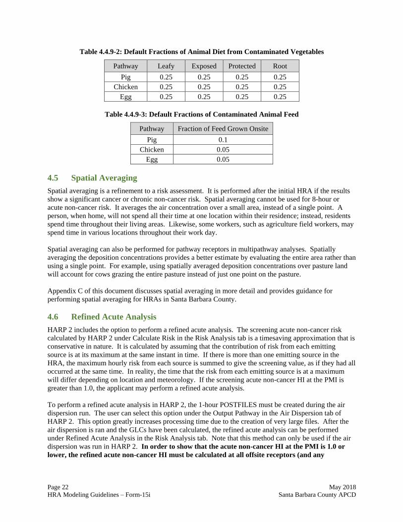
Page 22 May 2018
HRA Modeling Guidelines – Form-15i Santa Barbara County APCD
Table 4.4.9-2: Default Fractions of Animal Diet from Contaminated Vegetables
Pathway Leafy Exposed Protected Root
Pig 0.25 0.25 0.25 0.25
Chicken 0.25 0.25 0.25 0.25
Egg 0.25 0.25 0.25 0.25
Table 4.4.9-3: Default Fractions of Contaminated Animal Feed
Pathway Fraction of Feed Grown Onsite
Pig 0.1
Chicken 0.05
Egg 0.05
4.5 Spatial Averaging
Spatial averaging is a refinement to a risk assessment. It is performed after the initial HRA if the results
show a significant cancer or chronic non-cancer risk. Spatial averaging cannot be used for 8-hour or
acute non-cancer risk. It averages the air concentration over a small area, instead of a single point. A
person, when home, will not spend all their time at one location within their residence; instead, residents
spend time throughout their living areas. Likewise, some workers, such as agriculture field workers, may
spend time in various locations throughout their work day.
Spatial averaging can also be performed for pathway receptors in multipathway analyses. Spatially
averaging the deposition concentrations provides a better estimate by evaluating the entire area rather than
using a single point. For example, using spatially averaged deposition concentrations over pasture land
will account for cows grazing the entire pasture instead of just one point on the pasture.
Appendix C of this document discusses spatial averaging in more detail and provides guidance for
performing spatial averaging for HRAs in Santa Barbara County.
4.6 Refined Acute Analysis
HARP 2 includes the option to perform a refined acute analysis. The screening acute non-cancer risk
calculated by HARP 2 under Calculate Risk in the Risk Analysis tab is a timesaving approximation that is
conservative in nature. It is calculated by assuming that the contribution of risk from each emitting
source is at its maximum at the same instant in time. If there is more than one emitting source in the
HRA, the maximum hourly risk from each source is summed to give the screening value, as if they had all
occurred at the same time. In reality, the time that the risk from each emitting source is at a maximum
will differ depending on location and meteorology. If the screening acute non-cancer HI at the PMI is
greater than 1.0, the applicant may perform a refined acute analysis.
To perform a refined acute analysis in HARP 2, the 1-hour POSTFILES must be created during the air
dispersion run. The user can select this option under the Output Pathway in the Air Dispersion tab of
HARP 2. This option greatly increases processing time due to the creation of very large files. After the
air dispersion is ran and the GLCs have been calculated, the refined acute analysis can be performed
under Refined Acute Analysis in the Risk Analysis tab. Note that this method can only be used if the air
dispersion was run in HARP 2. In order to show that the acute non-cancer HI at the PMI is 1.0 or
lower, the refined acute non-cancer HI must be calculated at all offsite receptors (and any

Page 23 May 2018
HRA Modeling Guidelines – Form-15i Santa Barbara County APCD
applicable onsite receptors) that were calculated to have a screening acute non-cancer HI greater
than 1.0.
4.7 Population Exposure
In addition to estimating individual cancer risk at specific points such as the MEIR, determine the cancer
burden and the number of people exposed to a cancer risk of 10 per million or greater. For chronic
population evaluations, the number of people exposed to a hazard index greater than 1.0 must be reported.
HARP 2 can provide population exposure estimates as cancer burden and as the number of persons
exposed to a selected (user identified) health risk/impact level.
HARP 2 includes US census data and is recommended for performing population exposure estimates.
The census receptors must be imported in the air dispersion module, as discussed in Section 3.9.2 of this
document.
4.8 Significant Risk Thresholds
In June 1993, the Santa Barbara County Air Pollution Control Board of Directors (District’s Board)
adopted health risk notification levels. The risk notification levels were set at 10 per million for cancer
risk and a hazard index of greater than 1.0 for non-cancer risk. Risk reduction thresholds were adopted by
the District’s Board on September 17, 1998. These risk reduction thresholds were set at the same level as
the public notification thresholds. Use Appendix E, Health Risk Calculation and Rounding Policy, of this
document to properly round health risk values when comparing them to the significant risk thresholds for
risk management decisions.
Health risk assessment results shall be compared to the significant risk thresholds as follows:
Cancer Risk: The risk values for the MEIR, MEIW, sensitive receptors (if any), and onsite
residential and worker receptors (if any) are compared to the cancer significant risk threshold.
Chronic Non-Cancer Risk: The risk values for the MEIR, MEIW, sensitive receptors (if
any), and onsite residential and worker receptors (if any) are compared to the chronic non-
cancer significant risk threshold.
8-hour Chronic Non-Cancer Risk: The risk values for the MEIW, sensitive receptors (if
any) and onsite worker receptors (if any) are compared to the 8-hour chronic non-cancer
significant risk threshold. The MEIR and onsite residential receptors (if any) must be assessed
for the 8-hour HI and compared to the risk threshold only if the facility does not operate
continuously.
Acute Non-Cancer Risk: The risk values for the PMI, MEIR, MEIW, sensitive receptors (if
any), and onsite receptors (if any) are compared to the non-cancer significant risk threshold.
To further clarify, the acute non-cancer PMI can be at any boundary or offsite receptor (or
onsite receptors in specific situations), including the ocean. No residence or business is
required to occupy the offsite PMI. On a case-by case basis, certain receptors may be
excluded from the acute non-cancer analysis if the public cannot reasonably be expected to be
at that location (e.g., areas where fencing prevents public access). Please contact the District
to determine if any receptors may be excluded.
If any of the above significant risk thresholds are met or exceeded for an existing source, the District will
require public notification and risk reduction. If any of the above significant risk thresholds are met or
exceeded for a new project, the project will be denied or must be revised to include measures that reduce
the risk below the significance thresholds.

Page 24 May 2018
HRA Modeling Guidelines – Form-15i Santa Barbara County APCD
5. Health Risk Assessment Report
The applicant is required to perform the HRA and submit the HRA report and electronic files for the
District’s review. A $1500 non-refundable fee is required for the District to review the HRA.
Alternately, the District may assess fees for the HRA review on the cost reimbursement basis specified in
District Rule 210 section I.C. The District will notify the applicant if it is determined that the work will
be done on the cost reimbursement basis.
All HRAs must include the results of a Tier 1 exposure assessment. If the applicant would like to present
additional information (i.e., exposure duration adjustments or the inclusions of risk characterizations
using Tier 2 exposure data), then this information should be presented in separate, clearly titled sections,
tables and text. The required elements of the HRA report are discussed in Sections 5.1 through 5.10
below.
5.1 Facility Information
Report the following information regarding the facility and its surroundings:
Facility name
Stationary source identification number (SSID)
Location (street address and UTM coordinates, including datum)
Description of facility operations and a list identifying emitted substances, including a table of the
average annual and maximum hourly TAC emissions
5.2 Source and Emission Inventory Information
Report the following information for each emission source in table format:
Source (i,e., stack or release point) identification number
Source name
Source type (point, area, open pit, volume, line)
Device identification number(s) for any devices emitting at this source (use District device
identification numbers when available)
Source UTM coordinates
Source parameters
The description and operating schedule for each device should be reported in table format including the
following information:
Device name and identification number
Number of operating hours per day and per year, including which hours the device operates in a
24-hour day
Number of operating days per week, including which days the device operates in a 7-day week
Number of operating days or weeks per year
Source identification number(s) for the HARP 2 sources where emissions are released
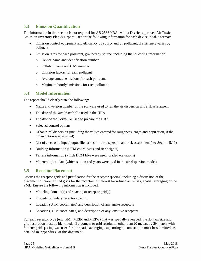
Page 25 May 2018
HRA Modeling Guidelines – Form-15i Santa Barbara County APCD
5.3 Emission Quantification
The information in this section is not required for AB 2588 HRAs with a District-approved Air Toxic
Emission Inventory Plan & Report. Report the following information for each device in table format:
Emission control equipment and efficiency by source and by pollutant, if efficiency varies by
pollutant
Emission rates for each pollutant, grouped by source, including the following information:
o Device name and identification number
o Pollutant name and CAS number
o Emission factors for each pollutant
o Average annual emissions for each pollutant
o Maximum hourly emissions for each pollutant
5.4 Model Information
The report should clearly state the following:
Name and version number of the software used to run the air dispersion and risk assessment
The date of the health.mdb file used in the HRA
The date of the Form-15i used to prepare the HRA
Selected control options
Urban/rural dispersion (including the values entered for roughness length and population, if the
urban option was selected)
List of electronic input/output file names for air dispersion and risk assessment (see Section 5.10)
Building information (UTM coordinates and tier heights)
Terrain information (which DEM files were used, graded elevations)
Meteorological data (which station and years were used in the air dispersion model)
5.5 Receptor Placement
Discuss the receptor grids and justification for the receptor spacing, including a discussion of the
placement of more refined grids for the receptors of interest for refined acute risk, spatial averaging or the
PMI. Ensure the following information is included:
Modeling domain(s) and spacing of receptor grid(s)
Property boundary receptor spacing
Location (UTM coordinates) and description of any onsite receptors
Location (UTM coordinates) and description of any sensitive receptors
For each receptor type (e.g., PMI, MEIR and MEIW) that was spatially averaged, the domain size and
grid resolution must be identified. If a domain or grid resolution other than 20 meters by 20 meters with
5-meter grid spacing was used for the spatial averaging, supporting documentation must be submitted, as
detailed in Appendix C of this document.

Page 26 May 2018
HRA Modeling Guidelines – Form-15i Santa Barbara County APCD
5.6 Multipathway Information
If multipathway substances are emitted, identify the exposure pathways analyzed for each receptor. If
receptor numbers at the same location vary for different dispersion runs, include the run name and/or
number and UTM coordinates for each receptor. An example multipathway receptor analysis table is
shown below (Table 5.6-1).
Table 5.6-1: Example Multipathway Receptor Analysis
Pathway
Residential
Rural Receptors
#1-333
Sensitive
Receptors
#334-346
Residential
Urban Receptors
#347-356
Worker
Receptors
#357-411
Soil X X X X
Dermal X X X X
Mother’s milk X X X
Drinking water
Fish
Homegrown produce X X X
Beef
Dairy
Pig X
Chicken X
Egg X
Also, provide a summary and discussion of the multipathway parameters used for each exposure pathway.
For example, Receptor #1-333 used the HARP 2 default fractions of human diet from the contaminated
source for households that farm, while Receptors #334-346 and 347-356 used the HARP 2 default
fractions of human diet from the contaminated source for households that garden.
Provide justification and documentation for any site-specific inputs (e.g., water intake or animal grazing
assumptions). If any multipathway parameters other than the HARP 2 defaults were used, then the
derivation and data used must be presented. The justification for using Tier 2 exposure parameters must
be clearly presented.
5.7 Summary of Results
Present the risk assessment results, including the information shown in Tables 5.7-1 through 5.7-4.

Page 27 May 2018
HRA Modeling Guidelines – Form-15i Santa Barbara County APCD
Table 5.7-1: Summary of Cancer Health Risk Results
Receptor
Type
Receptor
Number UTME (m) UTMN (m)
Cancer Risk
(in a million)
Significance
Threshold
(in a million)
Offsite PMI NA
Onsite PMI
(if present) NA
MEIR >10
MEIW >10
Sensitive
Receptor(s) >10
Table 5.7-2: Summary of Chronic Non-Cancer Health Risk Results
Receptor
Type
Receptor
Number UTME (m) UTMN (m) Chronic HI
Health
Endpoint(s)
Significance
Threshold (HI)
Offsite PMI NA
Onsite PMI
(if present) NA
MEIR >1
MEIW >1
Sensitive
Receptor(s) >1
Table 5.7-3: Summary of 8-Hour Chronic Non-Cancer Health Risk Results
Receptor
Type
Receptor
Number UTME (m) UTMN (m) 8-Hour HI
Health
Endpoint(s)
Significance
Threshold (HI)
Offsite PMI NA
Onsite PMI
(if present) NA
MEIR >1
MEIW >1
Sensitive
Receptor(s) >1

Page 28 May 2018
HRA Modeling Guidelines – Form-15i Santa Barbara County APCD
Table 5.7-4: Summary of Acute Non-Cancer Health Risk Results
Receptor
Type
Receptor
Number UTME (m) UTMN (m) Acute HI
Health
Endpoint(s)
Significance
Threshold (HI)
Offsite PMI >1
Onsite PMI
(if present) >1
MEIR >1
MEIW >1
Sensitive
Receptor(s) >1
5.8 Risk Driver Tables
Present the risk drivers, including the information shown in Tables 5.8-1 through 5.8-14. If a large
number of pollutants are emitted at the facility, and a large number of emitting sources are present, only
those that account for more than 5% of the health risk should be presented in the tables.
Table 5.8-1: Cancer Risk by Pollutant at the MEIR
Pollutant
Cancer Risk
Contribution at the
MEIR (in a million)
Percentage
Contribution to
Total Cancer Risk
Total 100%
Pollutant A
Pollutant B
Pollutant C
Table 5.8-2: Cancer Risk by Source at the MEIR
HARP 2
Source ID
Cancer Risk
Contribution at the
MEIR (in a million)
Percentage
Contribution to
Total Cancer Risk
Total 100%
Source X
Source Y
Source Z
Table 5.8-3: Cancer Risk by Pollutant at the MEIW
Pollutant
Cancer Risk
Contribution at the
MEIW (in a million)
Percentage
Contribution to
Total Cancer Risk
Total 100%
Pollutant A
Pollutant B
Pollutant C

Page 29 May 2018
HRA Modeling Guidelines – Form-15i Santa Barbara County APCD
Table 5.8-4: Cancer Risk by Source at the MEIW
HARP 2
Source ID
Cancer Risk
Contribution at the
MEIW (in a million)
Percentage
Contribution to
Total Cancer Risk
Total 100%
Source X
Source Y
Source Z
Table 5.8-5: Chronic Non-Cancer Risk by Pollutant at the MEIR
Pollutant
Chronic Non-Cancer
Risk Contribution at
the MEIR (HI)
Percentage Contribution
to Total Chronic Non-
Cancer Risk
Total 100%
Pollutant A
Pollutant B
Pollutant C
Table 5.8-6: Chronic Non-Cancer Risk by Source at the MEIR
HARP 2
Source ID
Chronic Non-Cancer
Risk Contribution at
the MEIR (HI)
Percentage Contribution
to Total Chronic Non-
Cancer Risk
Total 100%
Source X
Source Y
Source Z
Table 5.8-7: Chronic Non-Cancer Risk by Pollutant at the MEIW
Pollutant
Chronic Non-Cancer
Risk Contribution at
the MEIW (HI)
Percentage Contribution
to Total Chronic Non-
Cancer Risk
Total 100%
Pollutant A
Pollutant B
Pollutant C

Page 30 May 2018
HRA Modeling Guidelines – Form-15i Santa Barbara County APCD
Table 5.8-8: Chronic Non-Cancer Risk by Source at the MEIW
HARP 2
Source ID
Chronic Non-Cancer
Risk Contribution at
the MEIW (HI)
Percentage Contribution
to Total Chronic Non-
Cancer Risk
Total 100%
Source X
Source Y
Source Z
Table 5.8-9: 8-Hour Chronic Non-Cancer Risk by Pollutant at the MEIR
Pollutant
8-Hour Chronic Non-
Cancer Risk Contribution
at the MEIR (HI)
Percentage Contribution
to Total 8-Hour Chronic
Non-Cancer Risk
Total 100%
Pollutant A
Pollutant B
Pollutant C
Table 5.8-10: 8-Hour Chronic Non-Cancer Risk by Source at the MEIR
HARP 2
Source ID
8-Hour Chronic Non-
Cancer Risk Contribution
at the MEIR (HI)
Percentage Contribution
to Total 8-Hour Chronic
Non-Cancer Risk
Total 100%
Source X
Source Y
Source Z
Table 5.8-11: 8-Hour Chronic Non-Cancer Risk by Pollutant at the MEIW
Pollutant
8-Hour Chronic Non-
Cancer Risk Contribution
at the MEIW (HI)
Percentage Contribution
to Total 8-Hour Chronic
Non-Cancer Risk
Total 100%
Pollutant A
Pollutant B
Pollutant C
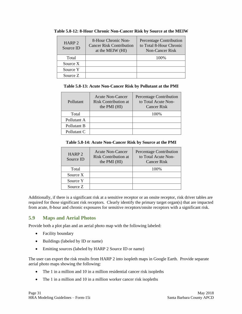
Page 31 May 2018
HRA Modeling Guidelines – Form-15i Santa Barbara County APCD
Table 5.8-12: 8-Hour Chronic Non-Cancer Risk by Source at the MEIW
HARP 2
Source ID
8-Hour Chronic Non-
Cancer Risk Contribution
at the MEIW (HI)
Percentage Contribution
to Total 8-Hour Chronic
Non-Cancer Risk
Total 100%
Source X
Source Y
Source Z
Table 5.8-13: Acute Non-Cancer Risk by Pollutant at the PMI
Pollutant
Acute Non-Cancer
Risk Contribution at
the PMI (HI)
Percentage Contribution
to Total Acute Non-
Cancer Risk
Total 100%
Pollutant A
Pollutant B
Pollutant C
Table 5.8-14: Acute Non-Cancer Risk by Source at the PMI
HARP 2
Source ID
Acute Non-Cancer
Risk Contribution at
the PMI (HI)
Percentage Contribution
to Total Acute Non-
Cancer Risk
Total 100%
Source X
Source Y
Source Z
Additionally, if there is a significant risk at a sensitive receptor or an onsite receptor, risk driver tables are
required for those significant risk receptors. Clearly identify the primary target organ(s) that are impacted
from acute, 8-hour and chronic exposures for sensitive receptors/onsite receptors with a significant risk.
5.9 Maps and Aerial Photos
Provide both a plot plan and an aerial photo map with the following labeled:
Facility boundary
Buildings (labeled by ID or name)
Emitting sources (labeled by HARP 2 Source ID or name)
The user can export the risk results from HARP 2 into isopleth maps in Google Earth. Provide separate
aerial photo maps showing the following:
The 1 in a million and 10 in a million residential cancer risk isopleths
The 1 in a million and 10 in a million worker cancer risk isopleths
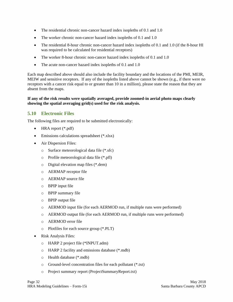
Page 32 May 2018
HRA Modeling Guidelines – Form-15i Santa Barbara County APCD
The residential chronic non-cancer hazard index isopleths of 0.1 and 1.0
The worker chronic non-cancer hazard index isopleths of 0.1 and 1.0
The residential 8-hour chronic non-cancer hazard index isopleths of 0.1 and 1.0 (if the 8-hour HI
was required to be calculated for residential receptors)
The worker 8-hour chronic non-cancer hazard index isopleths of 0.1 and 1.0
The acute non-cancer hazard index isopleths of 0.1 and 1.0
Each map described above should also include the facility boundary and the locations of the PMI, MEIR,
MEIW and sensitive receptors. If any of the isopleths listed above cannot be shown (e.g., if there were no
receptors with a cancer risk equal to or greater than 10 in a million), please state the reason that they are
absent from the maps.
If any of the risk results were spatially averaged, provide zoomed-in aerial photo maps clearly
showing the spatial averaging grid(s) used for the risk analysis.
5.10 Electronic Files
The following files are required to be submitted electronically:
HRA report (*.pdf)
Emissions calculations spreadsheet (*.xlsx)
Air Dispersion Files:
o Surface meteorological data file (*.sfc)
o Profile meteorological data file (*.pfl)
o Digital elevation map files (*.dem)
o AERMAP receptor file
o AERMAP source file
o BPIP input file
o BPIP summary file
o BPIP output file
o AERMOD input file (for each AERMOD run, if multiple runs were performed)
o AERMOD output file (for each AERMOD run, if multiple runs were performed)
o AERMOD error file
o Plotfiles for each source group (*.PLT)
Risk Analysis Files:
o HARP 2 project file (*INPUT.adm)
o HARP 2 facility and emissions database (*.mdb)
o Health database (*.mdb)
o Ground-level concentration files for each pollutant (*.txt)
o Project summary report (ProjectSummaryReport.txt)

Page 33 May 2018
HRA Modeling Guidelines – Form-15i Santa Barbara County APCD
o For each type of risk that was analyzed in the HRA (i.e., cancer risk and chronic, 8-hour and
acute non-cancer risks):
Input file with GLCs (*GLCList.csv)
HRA input file (*HRAInput.hra)
Output files with risk details (*Risk.csv, *RiskSumByRec.csv, and
*RiskSumByRecBySrc.csv)
Output log file (*Output.txt)
Pathway receptor information (*PathwayRec.csv)
Input file with health values (*PolDB.csv)
o Refined acute non-cancer risk file, if applicable (RefinedMaxHISummary.csv)
o Spatial averaging files, if applicable:
Plot files (*.PLT)
GLC files (*PER.txt)
Cancer input file with GLCs (CANCERSAGLCList.csv)
Cancer HRA input file (CANCERSAHRAInput.hra)
Cancer risk output files (CANCERSACancerRisk.csv,
CANCERSACancerRiskSumByRec.csv, CANCERSACancerRiskSumByRecBySrc.csv)
Cancer output log file (CANCERSAOutput.txt)
Chronic non-cancer input file with GLCs (CHRONICSAGLCList.csv)
Chronic non-cancer HRA input file (CHRONICSAHRAInput.hra)
Chronic non-cancer risk output files (CHRONICSACancerRisk.csv,
CHRONICSACancerRiskSumByRec.csv,
CHRONICSACancerRiskSumByRecBySrc.csv)
Chronic non-cancer output log file (CHRONICSAOutput.txt)
Google Earth files (*.kml, *.kmz)
If the HRA or HRA report fail to comply with these guidelines, the HRA and HRA report will be
returned, with District comments, to the applicant for revision.
6. References
California Air Resources Board. March 17, 2015. User Manual for the Hotspots Analysis and
Reporting Program Air Dispersion Modeling and Risk Assessment Tool Version 2.
https://www.arb.ca.gov/toxics/harp/docs2/harp2admrtuserguide.pdf.
California Air Resources Board. July 15, 2015. Digital Elevation Model Files for HARP.
https://www.arb.ca.gov/toxics/harp/dems.htm.
California Air Resources Board. April 25, 2016. AB 2588 Air Toxics “Hot Spots” Program.
https://www.arb.ca.gov/ab2588/ab2588.htm.

Page 34 May 2018
HRA Modeling Guidelines – Form-15i Santa Barbara County APCD
California Air Resources Board. February 22, 2017. Air Dispersion Modeling and Risk Tool
(ADMRT). https://www.arb.ca.gov/toxics/harp/admrt.htm.
California Air Resources Board. February 23, 2017. Table 1: Consolidated Table of
OEHHA/ARB Approved Risk Assessment Health Values.
https://www.arb.ca.gov/toxics/healthval/contable.pdf.
California Air Resources Board and California Air Pollution Control Officers Association.
July 23, 2015. Risk Management Guidance for Stationary Sources of Air Toxics.
https://www.arb.ca.gov/toxics/rma/rmgssat.pdf.
California Department of Water Resources. September 12, 2017. Southern Region Office.
http://wdl.water.ca.gov/irwm/resources/sro.cfm.
Murchision, Linda C. Letter received by Ed Romano on August 18, 1997.
https://www.arb.ca.gov/ab2588/portable.pdf.
Office of Environmental Health Hazard Assessment. August 2012. Air Toxics Hot Spots Program
Risk Assessment Guidelines: Technical Support Document for Exposure Assessment and
Stochastic Analysis. https://oehha.ca.gov/media/downloads/crnr/tsdportfolio2012.pdf.
Office of Environmental Health Hazard Assessment. February 2015. Air Toxics Hot Spots
Program Guidance Manual for Preparation of Health Risk Assessments: Risk Assessment
Guidelines. https://oehha.ca.gov/media/downloads/crnr/2015guidancemanual.pdf.
Office of Environmental Health Hazard Assessment. February 2015. Air Toxics Hot Spots
Program Guidance Manual for Preparation of Health Risk Assessments: Appendices.
https://oehha.ca.gov/media/downloads/crnr/2015gmappendices.pdf.
Santa Barbara County Air Pollution Control District. March 17, 2005. Rule 210.
https://www.ourair.org/wp-content/uploads/rule210.pdf.
Santa Barbara County Air Pollution Control District. 2018. Meteorological Data.
http://www.ourair.org/metdata/.
U.S. Environmental Protection Agency. June 1985. Guideline for Determination of Good
Engineering Practice Stack Height (Technical Support Document For the Stack Height
Regulations). https://www3.epa.gov/scram001/guidance/guide/gep.pdf.
U.S. Environmental Protection Agency. November 9, 2005. 40 CFR Part 51 Appendix W. Federal
Register. https://www3.epa.gov/ttn/scram/guidance/guide/appw_05.pdf.
U.S. Environmental Protection Agency. August 3, 2015. AERMOD Implementation Guide.
https://www3.epa.gov/ttn/scram/7thconf/aermod/aermod_implmtn_guide_3August2015.pdf.
U.S. Environmental Protection Agency. April 2018. User’s Guide for the AMS/EPA Regulatory
Model (AERMOD). https://www3.epa.gov/ttn/scram/models/aermod/aermod_userguide.pdf.
U.S. Environmental Protection Agency. April 24, 2018. Air Quality Dispersion Modeling –
Preferred and Recommended Models. https://www.epa.gov/scram/air-quality-dispersion-
modeling-preferred-and-recommended-models.

Page 35 May 2018
HRA Modeling Guidelines – Form-15i Santa Barbara County APCD
7. Contacts
For questions about the District’s requirements for modeling, contact the District at:
phone: 805-961-8800
email: [email protected]
The District does not provide technical support for AERMOD or HARP 2. For questions about HARP 2,
contact ARB at:
phone: 916-323-4327
email: [email protected]
web: http://www.arb.ca.gov/toxics/harp/harp.htm
For questions about AERMOD, contact USEPA’s Region IX Modeling Contact, Carol Bohnenkamp, at:
phone: 415-947-4130
email: [email protected]

Page A1 May 2018
HRA Modeling Guidelines – Form-15i Santa Barbara County APCD
Appendix A – Variable Emissions Modeling
During some air quality studies, modelers may encounter certain emitting scenarios that require the use of
variable emissions modeling. This appendix outlines modeling techniques to account for special
operating schedules.
Typically, the air dispersion is run with a unit emission rate of 1 g/s for 24 hours a days, 365 days a year
for an HRA. AERMOD includes options for modeling source emissions that fluctuate over time. With
the variable emissions option, the modeler can select the hours of operation and the emission rate for each
individual source. Emission variations can be characterized across many different periods, including
hourly, daily, monthly and seasonally. If variable emissions are used, the applicant must submit
documentation with the HRA that justifies using that variable emission scenario. The District may
require permit conditions to enforce the operating hours, days, months, etc. selected in the variable
emission scenario.
In order to maintain a consistent emissions inventory for dispersion modeling using HARP 2, certain rules
must be followed. Failure to adhere to the rules discussed in Section A.1 and A.2 below will result in
either generating or depleting inventory from your analysis. The same rules must be followed for air
dispersion runs modeled outside of HARP 2 (e.g., Lakes’ AERMOD View), if HARP 2 is used for
the risk assessment. (These rules do not apply to modeling performed for an Air Quality Impact
Assessment, which uses actual emission rates instead of the unit emission rate of 1 g/s.)
See Section 4.2.b, Variable Emissions, of ARB’s User Manual for the Hotspots Analysis and Reporting
program Air Dispersion Modeling and Risk Assessment Tool Version 2 for more information about the
variable emission requirements for HARP 2:
https://www.arb.ca.gov/toxics/harp/docs2/harp2admrtuserguide.pdf.
A.1 Variable Emission Rates for Annual Emissions
Air dispersion modeling for an HRA is typically run using the unit emission rate of 1 g/s for 24 hours a
day, 365 days a year (i.e., 8760 hr/yr). When emissions vary temporally, the annual emissions in
AERMOD are still required to sum to 31,536 kg/yr (i.e., 31,536 kg/yr = 1 g/s * 3600 s/hr * 8760 hr/yr).
Therefore, the emission rate in the variable emissions window must be adjusted accordingly. For
example, the HROFDY (Hour of Day) option allows the user to select the emission rate factor for certain
hours of the day. The total emission rate factor (n) for the entire day is equal to 24 for the Hour of Day
option. Therefore, for a source operating 12 hours a day (from 6AM to 6PM), 365 days a year, the user
should input a factor of 2 for each hour that the source operates; n = 2 * 12 = 24. The variable emission
rates for this source would be entered as shown in Table A.1-1.
It is important to note that the hours of the day displayed in AERMOD correspond to the hour ending at
the time displayed. Therefore, hour 7 corresponds to the hour from 6AM to 7AM, and hour 18
corresponds to the hour from 5PM to 6PM.

Page A2 May 2018
HRA Modeling Guidelines – Form-15i Santa Barbara County APCD
Table A.1-1: Example Variable Emission Scenario (Hour of Day)
Hour of Day Emission Rate Factor
by Hour Hour of Day
Emission Rate Factor
by Hour
1 0 13 2
2 0 14 2
3 0 15 2
4 0 16 2
5 0 17 2
6 0 18 2
7 2 19 0
8 2 20 0
9 2 21 0
10 2 22 0
11 2 23 0
12 2 24 0
Table A.1-2 shows the emission rate factor for each variable emission option.
Table A.1-2: Variable Emission Options with Emission Rate Factors
Variable
Emission Option Definition
Emission
Rate Factor
SEASON Seasons n = 4
MONTH Monthly n = 12
HROFDAY Hour-of-day n = 24
WSPEED Wind speed category n = 6
SEASHR Season-by-hour n = 96
SHRDOW Season by hour-of-day by day-of-week (M-F, Sat, Sun) n = 288
SHRDOW7 Season by hour-of-day by day-of-week (M, Tu, W, Th, F, Sat, Sun) n = 672
HRDOW Hour-of-day by day-of-week (M-F, Sat, Sun) n = 72
HRDOW7 Hour-of-day by day-of-week (M, Tu, W, Th, F, Sat, Sun) n = 168
MHRDOW Month by hour-of-day by day-of-week (M-F, Sat, Sun) n = 864
MHRODW7 Month by hour-of-day by day-of-week (M, Tu, W, Th, F, Sat, Sun) n = 2,016
A.2 Variable Emission Rates for Maximum Hourly Emissions
When emissions are allowed to vary temporally for any of the conditions described above, a second
dispersion modeling run is required for the maximum hourly emissions (i.e., for the acute non-cancer
risk). Specifically, the user must enter a value of 1 for the times during which the source is emitting and a
value of 0 for the times during which the source is not emitting. HARP 2 includes a checkbox that, if
selected, will create a second AERMOD input file with all variable emission rates set to the correct factor
of 1 for the acute non-cancer risk analysis. However, this option causes the first AERMOD input file for
the annual emissions to be overwritten by the second AERMOD input file created for the hourly
emissions. For this reason, the District prefers that the user manually creates two AERMOD input files
when using variable emission rates for ease of review.

Page B1 May 2018
HRA Modeling Guidelines – Form-15i Santa Barbara County APCD
Appendix B – Modeling Specific Source Types
This appendix will be updated with additional source types in the future.
B.1 Gasoline Dispensing Facilities
See District Form-25T (http://www.ourair.org/wp-content/uploads/apcd-25T.pdf) for specific modeling
instructions for gas stations.
B.2 Liquid Storage Tanks
Storage tanks are generally of two types—fixed roof tanks and floating roof tanks. In the case of fixed
roof tanks, most of the pollutant emissions escape from a vent, with some additional contribution from
hatches and other fittings. In the case of floating roof tanks, most of the pollutant emissions escape
through the seals between the roof and the wall and between the deck and the wall, with some additional
emissions from fittings, such as ports and hatches.
Approaches for modeling emission impacts from various types of storage tanks are outlined in Sections
B.2.1 and B.2.2 below.
B.2.1 Fixed Roof Tanks
Model a fixed roof tank as a point source (i.e., a stack). The point source location and release height
should represent the tank vent, which is usually in the center of the tank. The tank should also be
represented as a building for downwash modeling. Table B.2.1-1 shows the values that should be entered
for the velocity, diameter and temperature.
Table B.2.1-1: Stack Parameters for Modeling Tanks
Velocity Diameter Temperature
Near zero,
i.e., 0.001 m/s
Nero zero,
i.e., 0.001 m
Ambient – a value of 0 prompts the
model to use the ambient temperature
There is virtually no plume rise from tanks. Therefore, the stack parameters for the stack gas exit velocity
and stack diameter should be set to near zero for the stacks representing the emissions. In addition, stack
temperature should be set equal to the ambient temperature. This can be accomplished in AERMOD by
inputting a value of 0 for the stack gas temperature.
Note that it is very important for the diameter to be at or near zero. With low exit velocities and larger
diameters, stack tip downwash will be calculated. A very small stack diameter effectively eliminates the
stack tip downwash. Because all downwash effects are being modeled with the building downwash
algorithm, the additional stack tip downwash calculations would be inappropriate.
B.2.2 Floating Roof Tanks
Model a floating roof tank as an area source. The area source inputs should represent the diameter of the
tank and the height of the tank. The tank should also be represented as a building for downwash
modeling if there are nearby point sources that may be affected.

Page C1 May 2018
HRA Modeling Guidelines – Form-15i Santa Barbara County APCD
Appendix C – Spatial Averaging
Spatial averaging is a refinement to a risk assessment. OEHHA approves the use of the spatial averaging
method for risk management decisions; see Section 4.7.3 of OEHHA’s HRA Guidance Manual. It is
done after the initial risk assessment if the results show a significant cancer or chronic non-cancer risk.
Spatial averaging cannot be used for 8-hour or acute non-cancer risk. It averages the air concentration
over a small area, instead of a single point. This allows the risk assessor to base decisions on
concentrations over an entire residential living area, instead of a single point within the residence. A
person, when home, will not spend all their time at one location within their residence. Instead, residents
spend time throughout their living areas. Likewise, some workers, like agriculture field workers, may
spend time in various locations throughout their work day.
Spatial averaging may also be used for the pathway receptors in multipathway analyses. Spatially
averaging the deposition concentrations provides a better estimate by evaluating the entire area rather than
using a single point. For example, using spatially averaged deposition concentrations over pasture land
accounts for cows grazing the entire pasture instead of just one point on the pasture.
C.1 Nested Grid Size
C.1.1 Residential and Sensitive Receptors
Use a domain size of 20 meters by 20 meters with a grid spacing resolution of equal to or less than five
meters for a residential or sensitive receptor. This domain represents an area that is approximately the
size of a small urban lot.
If part of the domain is off of the receptor’s property boundary (e.g., domain covers part of two parcels),
the grid points outside of the receptor’s property must be omitted. If the risk with the omitted grid points
shows a significant risk, then the grid may be repositioned so that the full 20-meter by 20-meter domain is
only on the receptor’s property.
Although a domain size of 20 meters by 20 meters is generally appropriate for residential and sensitive
receptors, there may be cases where that size is considerably larger than the receptor’s actual living area.
If the District finds that the modeled domain size is not representative of the area where the receptor
spends time, the District may require a smaller domain size or not allow spatial averaging.
C.1.2 Worker Receptors
Worker locations (e.g., the MEIW) may also be a candidate for spatial averaging. However, spatial
averaging is not applicable for workers stationed at the same location during the majority of their daily
work shift (e.g., desk/office workers). In this situation, the traditional method of using a single location
and corresponding modeled concentration must be used. If the worker location is a candidate for spatial
averaging, submit documentation identifying that no workers are stationed at the same location during the
majority of their daily work shift.
A domain size of no larger than 20 meters by 20 meters with a grid spacing resolution of equal to or less
than five meters is recommended for a worker receptor. A larger grid size may be used for a worker
receptor if the workers routinely and continuously move throughout the worksite over a space greater than
20 meters by 20 meters. Documentation supporting the larger domain must be submitted to the District
for approval for any worker domain larger than 20 meters by 20 meters. This documentation must
include showing the area where each worker routinely performs their duties and the percentage of time
spent in those areas, for all workers. The final domain size should not be greater than the smallest area of

Page C2 May 2018
HRA Modeling Guidelines – Form-15i Santa Barbara County APCD
worker movement. Other considerations for determining domain size and grid spacing resolution may
include an evaluation of the concentration gradients across the worker area. A fine grid spacing (e.g. five
meters) must be used within the domain to obtain a representative concentration across the area of
interest.
C.1.3 Pasture and Waterbody Receptors
The District recommends using spatial averaging over a deposition area (e.g., a body of water used for
fishing, a pasture used for grazing) for a multipathway analysis. Alternatively, the simplified approach of
using the concentration at the centroid, a specific point of interest, or the PMI location for an area being
evaluated for non-inhalation exposures is acceptable for use in the HRA. However, evaluating deposition
concentrations over pasture land, or a water body for multipathway exposure scenarios using spatial
averaging could give more representative estimates of the overall deposition rate.
If spatial averaging will be done, follow the steps in Section C.3 below. When using spatial averaging
over the deposition area, care should be taken to determine the proper domain size to make sure it
includes all reasonable areas of potential deposition. The size of the area of interest (e.g., pasture or water
body) should be identified and used for the modeling domain.
A reasonably fine grid spacing must be used within the domain to obtain a representative concentration
across the area of interest. One way to determine the grid spacing resolution is to include an evaluation of
the concentration gradients across the deposition area. The HRA report shall support all assumptions
used, including, but not limited to, documentation of the deposition area (e.g., size of the pasture or water
body, maps, representative coordinates, grid spacing resolution, concentration gradients). The size of the
domain and grid spacing resolution is subject to approval by the District.
C.2 Tilted Grids
The dominant plume centerline is sometimes tilted from the cardinal directions. If the nested grids for
spatial averaging are placed along the cardinal directions, the results may underestimate a spatial average
centered on the dominant plume centerline. Tilting the nested grid to coincide with the dominant plume
centerline can provide a more accurate value of the spatial average. A tilted polar grid is easier to
implement than a tilted rectangular grid. The domain of the polar receptor field should be limited to a
15 meter radius.
See Appendix C-5 – Tilted Spatial Averaging, of OEHHA’s Technical Support Document for Exposure
Assessment and Stochastic Analysis dated August 2012 for guidance on creating tilted grids:
http://oehha.ca.gov/media/downloads/crnr/appendixc2012.pdf.
C.3 Spatial Averaging Instructions
OEHHA’s directions are available in Section 4.7.3.1 of OEHHA’s HRA Guidance Manual and are
included below, with modifications for use in our District:
1. Create an initial nested grid with 5 meter spacing centered on the receptor of interest (e.g., PMI,
MEIW, MEIR). The initial nested grid should extend out the length of the original grid spacing
in each of the cardinal directions. For example, if the original grid spacing was 100 meters, the
nested grid should extend 100 meters to the north, south, east and west from the center of the
receptor of interest.
2. After the initial nested grid is created, rerun the dispersion and risk modules. Determine the new
PMI of the nested grid. If necessary, create an additional nested grid(s) centered on the new PMI
with a finer grid spacing (i.e., less than 5 meters) to determine the final PMI. To achieve this, two

Page C3 May 2018
HRA Modeling Guidelines – Form-15i Santa Barbara County APCD
or more modeling runs with successively finer nested grid resolutions may be needed to find the
final location where the nested grid that will be used for spatial averaging will be placed.
3. Center the spatial average nested grid on each receptor’s location of interest (i.e., final PMI of
nested grid) determined in Step 1. Limit the nested grid to no larger than 20 meters by 20 meters
or 400 square meters for residential or sensitive receptors. Note if a portion of the centered and
nested grid falls within the facility boundary and the receptor location of interest is outside of the
boundary, then adjustments to the nested grid to obtain the spatially-averaged risk for the offsite
receptor are reasonable. This may be done by deleting any onsite grid points so that only the
offsite grid points surrounding the receptor are used in the spatially averaged concentration. If
additional risk refinement is required, reposition the nested grid to cover 400 square meters of
off-boundary area surrounding the residential or sensitive receptor. The grid resolution spacing
should be no greater than five meters for residential, sensitive, and work receptors. With a five
meter grid resolution, the 20 meter by 20 meter domain will result in 25 receptors. The size and
placement of the domain and the resolution of points are subject to approval by the District. See
Sections 4.7.3.1.2 and 4.7.3.1.3 of OEHHA’s HRA Guidance Manual for additional discussion on
domain sizing and grid spacing at worksites, pastures, and water bodies.
4. Some configurations of source activity and meteorological conditions result in a predominant
downwind plume center line that is significantly askew from one of the four cardinal directions.
In this case, a tilted nested grid may be necessary to coincide with the dominant plume centerline.
Section C.2 above has additional information on tilted grids.
5. After specifying the grid, AERMOD must be rerun. HARP 2 assists with creating the nested grid
and allows AERMOD to easily be rerun in the Risk Analysis tab.
6. While rerunning AERMOD in the Risk Analysis module, HARP 2 also calculates the risk at each
receptor in the nested grid. Report the Average Risk that is displayed at the bottom right-hand
corner of the Step 3. Calculate Risk & View Risk Results page of the Spatial Averaging Risk
(Optional) Tab.
7. Document and include all methods, assumptions, data, maps, and files used in the spatial
averaging analysis and clearly present this information in the risk assessment report.

Page D1 May 2018
HRA Modeling Guidelines – Form-15i Santa Barbara County APCD
Appendix D – Default DICE Stack Parameters
The table below contains default stack parameters for stationary diesel-fired internal combustion engines
(DICE). These parameters are based on a 2016 survey of the District’s permitted DICE. A total of 174
engines were included in the survey. These default stack parameters are only to be used when
engine-specific data is unknown.
Table D-1: Default Stationary DICE Stack Parameters
Engine Size
(bhp)
Stack Temp
(°F)
Stack Inner
Diameter (in)
Release Height
(ft)
Exhaust Flow
Rate (scfm)
<100 992 4.6 7.1 468
100-250 899 4.1 7.4 779
251-500 931 5.3 8.2 1829
501-750 799 8.0 7.6 2930
751-1000 886 7.3 10.1 3559
>1000 880 11.5 11.0 9894
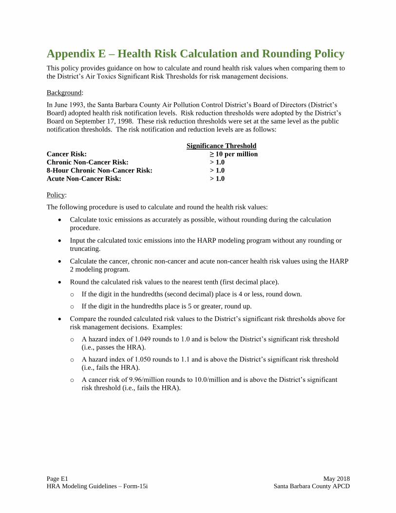
Page E1 May 2018
HRA Modeling Guidelines – Form-15i Santa Barbara County APCD
Appendix E – Health Risk Calculation and Rounding Policy
This policy provides guidance on how to calculate and round health risk values when comparing them to
the District’s Air Toxics Significant Risk Thresholds for risk management decisions.
Background:
In June 1993, the Santa Barbara County Air Pollution Control District’s Board of Directors (District’s
Board) adopted health risk notification levels. Risk reduction thresholds were adopted by the District’s
Board on September 17, 1998. These risk reduction thresholds were set at the same level as the public
notification thresholds. The risk notification and reduction levels are as follows:
Significance Threshold
Cancer Risk: ≥ 10 per million
Chronic Non-Cancer Risk: > 1.0
8-Hour Chronic Non-Cancer Risk: > 1.0
Acute Non-Cancer Risk: > 1.0
Policy:
The following procedure is used to calculate and round the health risk values:
Calculate toxic emissions as accurately as possible, without rounding during the calculation
procedure.
Input the calculated toxic emissions into the HARP modeling program without any rounding or
truncating.
Calculate the cancer, chronic non-cancer and acute non-cancer health risk values using the HARP
2 modeling program.
Round the calculated risk values to the nearest tenth (first decimal place).
o If the digit in the hundredths (second decimal) place is 4 or less, round down.
o If the digit in the hundredths place is 5 or greater, round up.
Compare the rounded calculated risk values to the District’s significant risk thresholds above for
risk management decisions. Examples:
o A hazard index of 1.049 rounds to 1.0 and is below the District’s significant risk threshold
(i.e., passes the HRA).
o A hazard index of 1.050 rounds to 1.1 and is above the District’s significant risk threshold
(i.e., fails the HRA).
o A cancer risk of 9.96/million rounds to 10.0/million and is above the District’s significant
risk threshold (i.e., fails the HRA).

Page F1 May 2018
HRA Modeling Guidelines – Form-15i Santa Barbara County APCD
Appendix F – District-Approved Emission Factors
This section is reserved for future use. The applicant should contact the District for approval of their
proposed emission factors prior to performing the HRA.

Page G1 May 2018
HRA Modeling Guidelines – Form-15i Santa Barbara County APCD
Appendix G – Source-Receptor Distance Policy for Acute Risk
When receptors are located at a close distance to an emitting source, the results of the air dispersion
model have a higher level of uncertainty. For that reason, the District allows a 20 meter minimum source-
receptor distance for acute non-cancer risk on a case-by-case basis. Receptors at locations where an
actual person is not expected to be located for at least an hour may be omitted from the HRA if the risk-
driving source is within 20 meters of the receptor. However, the District will not apply the minimum
source-receptor distance policy on any land parcels with a sensitive receptor (e.g., sidewalk of hospital,
school parking lot).
To request the use of this policy, use the following procedure:
1. Conduct the HRA or HRA screening without any minimum source-receptor distance (i.e., include
all receptors in the risk analysis).
2. If an offsite receptor has an acute HI greater than 1, determine if it is within 20 meters of the risk-
driving source. If it is within 20 meters of the risk-driving source, proceed to Step 3. Otherwise,
the receptor is not eligible for this policy.
3. In the HRA report, provide a list of proposed receptors to be omitted from the analysis along with
the information listed below.
Acute HI for each proposed receptor
UTM coordinates for each proposed receptor
Risk driving source and percent of contribution to acute HI
Distance from proposed receptor to risk driving source
Description of area surrounding each proposed receptor
Aerial photo showing the source location and the proposed receptor locations
An example of the required information is shown in Table G-1 below.
Table G-1: Example Data for Omitting Acute Receptors
within the Minimum Source-Receptor Distance
Proposed
Acute
Receptor No.
Acute
HI
UTM
Coordinates
(m)
Risk
Driving
Source
Percentage of
Contribution
to Risk
Distance to
Risk Driving
Source (m)
Description of
Surrounding
Area
1015 1.7 E 733054.3,
N 3850674
STCK1
(Boiler 1) 87.2% 6
Rugged steep
terrain
907 1.2 E 725597.0,
N 3846560
STCK5
(Tank 3) 76.5% 18
Driveway of
parking lot
After the District reviews your request along with the HRA report, the District will notify you if your
request was approved or denied. If your request is denied, a revised HRA report will be required. If your
request is approved, additional receptors may be required to be placed outside of the minimum
source-receptor distance at the District’s discretion.
Risk management decisions for long-term risk are based on actual residential and worker receptors, and
are therefore not affected by this policy.